mathematical programming - sas
TRANSCRIPT

SAS/OR® 9.1 User’s Guide:Mathematical Programming

The correct bibliographic citation for this manual is as follows: SAS Institute Inc. 2004. SAS/OR� 9.1 User’s Guide: Mathematical Programming. Cary, NC: SAS Institute Inc.
SAS/OR� 9.1 User’s Guide: Mathematical Programming
Copyright © 2004, SAS Institute Inc., Cary, NC, USA
ISBN 1-59047-239-X
All rights reserved. Produced in the United States of America. No part of this publication may be reproduced, stored in a retrieval system, or transmitted, in any form or by any means, electronic, mechanical, photocopying, or otherwise, without the prior written permission of the publisher, SAS Institute Inc.
U.S. Government Restricted Rights Notice: Use, duplication, or disclosure of this software and related documentation by the U.S. government is subject to the Agreement with SAS Institute and the restrictions set forth in FAR 52.227-19, Commercial Computer Software-Restricted Rights (June 1987).
SAS Institute Inc., SAS Campus Drive, Cary, North Carolina 27513.
1st printing, January 2004
SAS Publishing provides a complete selection of books and electronic products to help customers use SAS software to its fullest potential. For more information about our e-books, e-learning products, CDs, and hard-copy books, visit the SAS Publishing Web site at support.sas.com/pubs or call 1-800-727-3228.
SAS® and all other SAS Institute Inc. product or service names are registered trademarks or trademarks of SAS Institute Inc. in the USA and other countries. ® indicates USA registration.
Other brand and product names are trademarks of their respective companies.

Contents
What’s New in SAS/OR 9 and 9.1 . . . . . . . . . . . . . . . . . . . . . . . . . . . . . 1
Using This Book . . . . . . . . . . . . . . . . . . . . . . . . . . . . . . . . . . . . . . 7
Chapter 1. Introduction to Optimization . . . . . . . . . . . . . . . . . . . . . . . . . . 13
Chapter 2. The ASSIGN Procedure . . . . . . . . . . . . . . . . . . . . . . . . . . . . 47
Chapter 3. The INTPOINT Procedure . . . . . . . . . . . . . . . . . . . . . . . . . . . 63
Chapter 4. The LP Procedure . . . . . . . . . . . . . . . . . . . . . . . . . . . . . . . 185
Chapter 5. The NETFLOW Procedure . . . . . . . . . . . . . . . . . . . . . . . . . . . 313
Chapter 6. The NLP Procedure . . . . . . . . . . . . . . . . . . . . . . . . . . . . . . 507
Chapter 7. The QP Procedure . . . . . . . . . . . . . . . . . . . . . . . . . . . . . . . 651
Chapter 8. The TRANS Procedure . . . . . . . . . . . . . . . . . . . . . . . . . . . . 747
Subject Index . . . . . . . . . . . . . . . . . . . . . . . . . . . . . . . . . . . . . . . . 767
Syntax Index . . . . . . . . . . . . . . . . . . . . . . . . . . . . . . . . . . . . . . . . 777

iv

Acknowledgments
Credits
Documentation
Writing Trevor Kearney, Ben-Hao Wang
Editing Virginia Clark, Donna Sawyer
Documentation Support Tim Arnold, Michelle Opp
Technical Review Tao Huang, Edward P. Hughes, John Jasperse, Rob Pratt,Bengt Pederson, Charles B. Kelly, Donna Fulenwider, BillGjertsen
SoftwareThe procedures in SAS/OR software were implemented by the Operations Researchand Development Department. Substantial support was given to the project byother members of the Analytical Solutions Division. Core Development Division,Display Products Division, Graphics Division, and the Host Systems Division alsocontributed to this product.
In the following list, the name of the developer currently supporting the procedure islisted.
ASSIGN Ben-Hao Wang
INTPOINT Trevor Kearney
LP Ben-Hao Wang
NETFLOW Trevor Kearney
NLP Trevor Kearney
QP Dmitry V. Golovashkin
TRANS Trevor Kearney

Support Groups
Software Testing Tao Huang, Edward P. Hughes, John Jasperse, Charles B.Kelly, Rob Pratt, Bengt Pederson, Marcelo Bartroli
Technical Support Tonya Chapman
Acknowledgments
Many people have been instrumental in the development of SAS/OR software. Theindividuals acknowledged here have been especially helpful.
Richard Brockmeier Union Electric Company
Ken Cruthers Goodyear Tire & Rubber Company
Patricia Duffy Auburn University
Richard A. Ehrhardt University of North Carolina at Greensboro
Paul Hardy Babcock & Wilcox
Don Henderson ORI Consulting Group
Dave Jennings Lockheed Martin
Vidyadhar G. Kulkarni University of North Carolina at Chapel Hill
Wayne Maruska Basin Electric Power Cooperative
Roger Perala United Sugars Corporation
Bruce Reed Auburn University
Charles Rissmiller Lockheed Martin
David Rubin University of North Carolina at Chapel Hill
John Stone North Carolina State University
Keith R. Weiss ICI Americas Inc.
vi

The final responsibility for the SAS System lies with SAS Institute alone. We hopethat you will always let us know your opinions about the SAS System and its doc-umentation. It is through your participation that SAS software is continuously im-proved.
vii

viii � Acknowledgments

What’s New in SAS/OR 9 and 9.1
Contents
OVERVIEW . . . . . . . . . . . . . . . . . . . . . . . . . . . . . . . . . . . 3
THE BOM PROCEDURE . . . . . . . . . . . . . . . . . . . . . . . . . . . 3
THE CLP PROCEDURE (EXPERIMENTAL) . . . . . . . . . . . . . . . . 4
THE CPM PROCEDURE . . . . . . . . . . . . . . . . . . . . . . . . . . . . 4
THE GA PROCEDURE (EXPERIMENTAL) . . . . . . . . . . . . . . . . . 4
THE GANTT PROCEDURE . . . . . . . . . . . . . . . . . . . . . . . . . . 5
THE LP PROCEDURE . . . . . . . . . . . . . . . . . . . . . . . . . . . . . 5
THE PM PROCEDURE . . . . . . . . . . . . . . . . . . . . . . . . . . . . . 5
THE QP PROCEDURE (EXPERIMENTAL) . . . . . . . . . . . . . . . . . 5
BILL OF MATERIAL POST PROCESSING MACROS . . . . . . . . . . . 5

2 � What’s New in SAS/OR 9 and 9.1

What’s New in SAS/OR 9 and 9.1Overview
SAS/OR software contains several new and enhanced features since SAS 8.2. Briefdescriptions of the new features appear in the following sections. For more informa-tion, refer to the SAS/OR documentation, which is now available in the following sixvolumes:
• SAS/OR User’s Guide: Bills of Material Processing
• SAS/OR User’s Guide: Constraint Programming
• SAS/OR User’s Guide: Local Search Optimization
• SAS/OR User’s Guide: Mathematical Programming
• SAS/OR User’s Guide: Project Management
• SAS/OR User’s Guide: The QSIM Application
The online help can also be found under the corresponding classification.
The BOM Procedure
The BOM procedure in SAS/OR User’s Guide: Bills of Material Processing was in-troduced in Version 8.2 of the SAS System to perform bill of material processing.Several new features have been added to the procedure, enabling it to read all productstructure records from a product structure data file and all part “master” records froma part master file, and compose the combined information into indented bills of mate-rial. This data structure mirrors the most common method for storing bill-of-materialdata in enterprise settings; the part master file contains data on each part while theproduct structure file holds data describing the various part-component relationshipsrepresented in bills of material.
The PMDATA= option on the PROC BOM statement enables you to specify the nameof the Part Master data set. If you do not specify this option, PROC BOM uses theProduct Structure data set (as specified in the DATA= option) as the Part Masterdata set. The BOM procedure now looks up the Part, LeadTime, Requirement,QtyOnHand, and ID variables in the Part Master data set. On the other hand, theComponent and Quantity variables remain in the Product Structure data set.
You can use the NRELATIONSHIPS= (or NRELTS=) option to specify the numberof parent-component relationships in the Product Structure data set. You have greatercontrol over the handling of redundant relationships in the Product Structure data setusing the DUPLICATE= option.

4 � What’s New in SAS/OR 9 and 9.1
Several options have been added to the STRUCTURE statement enabling you to spec-ify information related to the parent-component relationships. In particular, the vari-able specified with the PARENT= option identifies the parent item, while the vari-ables listed in the LTOFFSET= option specify lead-time offset information. You canalso specify variables identifying scrap factor information for all parent-componentrelationships using the SFACTOR= option. The RID= option identifies all variablesin the Product Structure data set that are to be included in the Indented BOM outputdata set.
The CLP Procedure (Experimental)
The new CLP procedure in SAS/OR User’s Guide: Constraint Programming is an9.1experimental finite domain constraint programming solver for solving constraint sat-isfaction problems (CSPs) with linear, logical, global, and scheduling constraints.In addition to having an expressive syntax for representing CSPs, the solver fea-tures powerful built-in consistency routines and constraint propagation algorithms,a choice of nondeterministic search strategies, and controls for guiding the searchmechanism that enable you to solve a diverse array of combinatorial problems.
The CPM Procedure
The CPM procedure in SAS/OR User’s Guide: Project Management adds more op-tions for describing resource consumption by activities, enhancing its applicability toproduction scheduling models.
A new keyword, RESUSAGE, has been added to the list of values for the OBSTYPEvariable in the Resource data set. This keyword enables you to specify whether aresource is consumed at the beginning or at the end of a given activity.
The MILESTONERESOURCE option enables you to specify a nonzero usage ofconsumable resources for milestone activities. For example, this option is useful ifyou wish to designate specific milestones to be the points of payment for a subcon-tractor. The MILESTONENORESOURCE option is the current default behavior ofthe CPM procedure, which indicates that all resource requirements are to be ignoredfor milestone activities.
The GA Procedure (Experimental)
The new GA procedure in SAS/OR User’s Guide: Local Search Optimization fa-9.1cilitates the application of genetic algorithms to general optimization. Genetic al-gorithms adapt the biological processes of natural selection and evolution to searchfor optimal solutions. The procedure can be applied to optimize problems involv-ing integer, continuous, binary, or combinatorial variables. The GA procedure isespecially useful for finding optima for problems where the objective function mayhave discontinuities or may not otherwise be suitable for optimization by traditionalcalculus-based methods.

Bill of Material Post Processing Macros � 5
The GANTT Procedure
The GANTT procedure in SAS/OR User’s Guide: Project Management includes anew option for controlling the width of the Gantt chart. The CHARTWIDTH= optionspecifies the width of the axis area as a percentage of the total Gantt chart width.This option enables you to generate Gantt charts that are consistent in appearance,independent of the total time spanned by the project.
The LP Procedure
The performances of primal and dual simplex algorithms in the LP procedure(SAS/OR User’s Guide: Mathematical Programming) have been significantly im-proved on large scale linear or mixed integer programming problems.
The PM Procedure
The new options added to the CPM procedure are also available with PROC PM.
The QP Procedure (Experimental)
The new QP procedure in SAS/OR User’s Guide: Mathematical Programming im- 9.1plements a primal-dual predictor-corrector interior-point algorithm for large sparsequadratic programs. Depending on the distribution of the eigenvalues of the Hessianmatrix, H , two main classes of quadratic programs are distinguished (assuming min-imization):
• convex: H is positive semi-definite
• nonconvex: H has at least one negative eigenvalue
Diagonal and nonseparable Hessian matrices are recognized and handled automati-cally.
Bill of Material Post Processing Macros
Several macros enable users to generate miscellaneous reports using the IndentedBOM output data set from the BOM procedure in SAS/OR User’s Guide: Bills ofMaterial Processing. Other transactional macros perform specialized transactionsfor maintaining and updating the bills of material for a product, product line, plant,or company.

6 � What’s New in SAS/OR 9 and 9.1

Using This Book
Contents
PURPOSE . . . . . . . . . . . . . . . . . . . . . . . . . . . . . . . . . . . . 9
ORGANIZATION . . . . . . . . . . . . . . . . . . . . . . . . . . . . . . . . 9
TYPOGRAPHICAL CONVENTIONS . . . . . . . . . . . . . . . . . . . . 10
CONVENTIONS FOR EXAMPLES . . . . . . . . . . . . . . . . . . . . . . 11
ACCESSING THE SAS/OR SAMPLE LIBRARY . . . . . . . . . . . . . . 11
ONLINE HELP SYSTEM AND UPDATES . . . . . . . . . . . . . . . . . . 11
ADDITIONAL DOCUMENTATION FOR SAS/OR SOFTWARE . . . . . 12

8 � Using This Book

Using This Book
Purpose
SAS/OR User’s Guide: Mathematical Programming provides a complete referencefor the mathematical programming procedures in SAS/OR software. This bookserves as the primary documentation for the ASSIGN, INTPOINT, LP, NETFLOW,NLP, and TRANS procedures, in addition to the new QP procedure for solvingquadratic programming problems.
“Using This Book” describes the organization of this book and the conventions usedin the text and example code. To gain full benefit from using this book, you shouldfamiliarize yourself with the information presented in this section and refer to it whenneeded. “Additional Documentation” at the end of this section provides references toother books that contain information on related topics.
Organization
Chapter 1 contains a brief overview of the mathematical programming proceduresin SAS/OR software and provides an introduction to optimization and the use of theoptimization tools in the SAS System. The first chapter also describes the flow ofdata between the procedures and how the components of the SAS System fit together.
After the introductory chapter, the next seven chapters describe the ASSIGN,INTPOINT, LP, NETFLOW, NLP, QP, and TRANS procedures. Each procedure de-scription is self-contained; you need to be familiar with only the basic features ofthe SAS System and SAS terminology to use most procedures. The statements andsyntax necessary to run each procedure are presented in a uniform format throughoutthis book.
The following list summarizes the types of information provided for each procedure:
Overview provides a general description of what the procedure does.It outlines major capabilities of the procedure and lists allinput and output data sets that are used with it.
Getting Started illustrates simple uses of the procedure using a few shortexamples. It provides introductory hands-on informationfor the procedure.

10 � Using This Book
Syntax constitutes the major reference section for the syntax ofthe procedure. First, the statement syntax is summa-rized. Next, a functional summary table lists all the state-ments and options in the procedure, classified by function.In addition, the online version includes a Dictionary ofOptions, which provides an alphabetical list of all options.Following these tables, the PROC statement is described,and then all other statements are described in alphabeticalorder.
Details describes the features of the procedure, including algorith-mic details and computational methods. It also explainshow the various options interact with each other. This sec-tion describes input and output data sets in greater detail,with definitions of the output variables, and explains theformat of printed output, if any.
Examples consists of examples designed to illustrate the use of theprocedure. Each example includes a description of theproblem and lists the options highlighted by the exam-ple. The example shows the data and the SAS statementsneeded, and includes the output produced. You can du-plicate the examples by copying the statements and dataand running the SAS program. The SAS Sample Librarycontains the code used to run the examples shown in thisbook; consult your SAS Software representative for spe-cific information about the Sample Library.
References lists references that are relevant to the chapter.
Typographical Conventions
The printed version of SAS/OR User’s Guide: Mathematical Programming uses var-ious type styles, as explained by the following list:
roman is the standard type style used for most text.
UPPERCASE ROMAN is used for SAS statements, options, and other SAS lan-guage elements when they appear in the text. However,you can enter these elements in your own SAS code inlowercase, uppercase, or a mixture of the two. This styleis also used for identifying arguments and values (in theSyntax specifications) that are literals (for example, todenote valid keywords for a specific option).

Online Help System and Updates � 11
UPPERCASE BOLD is used in the “Syntax” section to identify SAS key-words, such as the names of procedures, statements, andoptions.
bold is used in the “Syntax” section to identify options.
helvetica is used for the names of SAS variables and data setswhen they appear in the text.
oblique is used for user-supplied values for options (for example,VARSELECT= rule).
italic is used for terms that are defined in the text, for empha-sis, and for references to publications.
monospace is used to show examples of SAS statements. In mostcases, this book uses lowercase type for SAS code. Youcan enter your own SAS code in lowercase, uppercase,or a mixture of the two. This style is also used for valuesof character variables when they appear in the text.
Conventions for Examples
Most of the output shown in this book is produced with the following SAS Systemoptions:
options linesize=80 pagesize=60 nonumber nodate;
Accessing the SAS/OR Sample Library
The SAS/OR sample library includes many examples that illustrate the use ofSAS/OR software, including the examples used in this documentation. To accessthese sample programs, select Learning to Use SAS->Sample SAS Programs fromthe SAS Help and Documentation window, and then select SAS/OR from the listof available topics.
Online Help System and Updates
You can access online help information about SAS/OR software in two ways, de-pending on whether you are using the SAS windowing environment in the commandline mode or the pull-down menu mode.
If you are using a command line, you can access the SAS/OR help menus by typinghelp or on the command line. If you are using the pull-down menus, you can selectSAS Help and Documentation->SAS Products from the Help pull-down menu, andthen select SAS/OR from the list of available topics.

12 � Using This Book
Additional Documentation for SAS/OR Software
In addition to SAS/OR User’s Guide: Mathematical Programming, you may findthese other documents helpful when using SAS/OR software:
SAS/OR User’s Guide: Bills of Material Processingprovides documentation for the BOM procedure and all bill-of-material post-processing SAS macros. The BOM procedure and SAS macros provide the ability togenerate different reports and to perform several transactions to maintain and updatebills of material.
SAS/OR User’s Guide: Constraint Programmingprovides documentation for the constraint programming procedure in SAS/OR soft-ware. This book serves as the primary documentation for the CLP procedure, anexperimental procedure new to SAS/OR software.
SAS/OR User’s Guide: Local Search Optimizationprovides documentation for the local search optimization procedure in SAS/OR soft-ware. This book serves as the primary documentation for the GA procedure, anexperimental procedure that uses genetic algorithms to solve optimization problems.
SAS/OR User’s Guide: Project Managementprovides documentation for the project management procedures in SAS/OR software.This book serves as the primary documentation for the CPM, DTREE, GANTT,NETDRAW, and PM procedures, as well as the PROJMAN Application, a graphi-cal user interface for project management.
SAS/OR User’s Guide: The QSIM Applicationprovides documentation for the QSIM Application, which is used to build and analyzemodels of queueing systems using discrete event simulation. This book shows youhow to build models using the simple point-and-click graphical user interface, howto run the models, and how to collect and analyze the sample data to give you insightinto the behavior of the system.
SAS/OR Software: Project Management Examples, Version 6contains a series of examples that illustrate how to use SAS/OR software to man-age projects. Each chapter contains a complete project management scenario anddescribes how to use PROC GANTT, PROC CPM, and PROC NETDRAW, in addi-tion to other reporting and graphing procedures in the SAS System, to perform thenecessary project management tasks.
SAS/IRP User’s Guide: Inventory Replenishment Planningprovides documentation for SAS/IRP software. This book serves as the primary doc-umentation for the IRP procedure for determining replenishment policies, as well asthe %IRPSIM SAS programming macro for simulating replenishment policies.

Chapter 1Introduction to Optimization
Chapter Contents
OVERVIEW . . . . . . . . . . . . . . . . . . . . . . . . . . . . . . . . . . . 15
DATA FLOW . . . . . . . . . . . . . . . . . . . . . . . . . . . . . . . . . . . 16PROC LP . . . . . . . . . . . . . . . . . . . . . . . . . . . . . . . . . . . 17PROC NETFLOW . . . . . . . . . . . . . . . . . . . . . . . . . . . . . . . 17PROC INTPOINT . . . . . . . . . . . . . . . . . . . . . . . . . . . . . . . 19PROC NLP . . . . . . . . . . . . . . . . . . . . . . . . . . . . . . . . . . 20PROC QP (Experimental) . . . . . . . . . . . . . . . . . . . . . . . . . . . 21PROC TRANS . . . . . . . . . . . . . . . . . . . . . . . . . . . . . . . . . 22PROC ASSIGN . . . . . . . . . . . . . . . . . . . . . . . . . . . . . . . . 22Model Formats: PROC LP and PROC NETFLOW . . . . . . . . . . . . . . 23Model Formats: PROC ASSIGN and PROC TRANS . . . . . . . . . . . . 33
MODEL BUILDING . . . . . . . . . . . . . . . . . . . . . . . . . . . . . . 34
MATRIX GENERATION . . . . . . . . . . . . . . . . . . . . . . . . . . . . 36Exploiting Model Structure . . . . . . . . . . . . . . . . . . . . . . . . . . 38
REPORT WRITING . . . . . . . . . . . . . . . . . . . . . . . . . . . . . . 41The DATA Step . . . . . . . . . . . . . . . . . . . . . . . . . . . . . . . . 41Other Reporting Procedures . . . . . . . . . . . . . . . . . . . . . . . . . . 43
DECISION SUPPORT SYSTEMS . . . . . . . . . . . . . . . . . . . . . . . 44The Full-Screen Interface . . . . . . . . . . . . . . . . . . . . . . . . . . . 44Communicating with the Optimization Procedures . . . . . . . . . . . . . . 45
REFERENCES . . . . . . . . . . . . . . . . . . . . . . . . . . . . . . . . . . 45

14 � Chapter 1. Introduction to Optimization

Chapter 1Introduction to Optimization
Overview
This chapter describes how to use SAS/OR software to solve a wide variety of opti-mization problems. The basic optimization problem is that of minimizing or maxi-mizing an objective function subject to constraints imposed on the variables of thatfunction. The objective function and constraints can be linear or nonlinear; the con-straints can be bound constraints, equality or inequality constraints, or integer con-straints.
Traditionally, optimization problems are divided into linear programming (LP; allfunctions are linear) and nonlinear programming (NLP). Variations of LP prob-lems are assignment problems, network flow problems, and transportation problems.Nonlinear regression (fitting a nonlinear model to a set of data and the subsequent sta-tistical analysis of the results) is a special NLP problem. Since these applications areso common, SAS/OR software has separate procedures or facilities within proceduresfor solving each type of these problems. Model data are supplied in a form suited forthe particular type of problem. Another benefit is that an optimization algorithm canbe specialized for the particular type of problem, reducing solution times. Optimizerscan exploit some structure in problems such as embedded networks, special orderedsets, least squares, and quadratic objective functions.
SAS/OR software has seven procedures used for optimization:
• PROC ASSIGN for solving assignment problems
• PROC INTPOINT for network programming problems with side constraints,and linear programming problems solved by an interior point algorithm
• PROC LP for solving linear and mixed integer programming problems
• PROC NETFLOW for solving network programming problems with side con-straints
• PROC NLP for solving nonlinear programming problems
• PROC QP for solving quadratic programming problems
• PROC TRANS for solving transportation problems
SAS/OR procedures use syntax that is similar to other SAS procedures. In particular,all SAS retrieval, data management, reporting, and analysis can be used with SAS/ORsoftware. Each optimizer is designed to integrate with the SAS System to simplifymodel building, maintenance, solution, and report writing.
Data for models are supplied to SAS/OR procedures in SAS data sets. These data setscan be saved and easily changed and the problem can be solved. Because the models

16 � Chapter 1. Introduction to Optimization
are in SAS data sets, problem data that can represent pieces of a larger model can beconcatenated and merged. The SAS/OR procedures output SAS data sets containingthe solutions. These can then be used to produce customized reports. This structureallows decision support systems to be constructed using SAS/OR procedures andother tools in the SAS System as building blocks.
The following list suggests application areas where decision support systems havebeen used. In practice, models often contain elements of several applications listedhere.
• Product-Mix problems find the mix of products that generates the largest re-turn when there are several products that compete for limited resources.
• Blending problems find the mix of ingredients to be used in a product so thatit meets minimum standards at minimum cost.
• Time-Staged problems are models whose structure repeats as a function oftime. Production and inventory models are classic examples of time-stagedproblems. In each period, production plus inventory minus current demandequals inventory carried to the next period.
• Scheduling problems assign people to times, places, or tasks so as to optimizepeople’s preferences while satisfying the demands of the schedule.
• Multiple objective problems have multiple conflicting objectives. Typically,the objectives are prioritized and the problems are solved sequentially in a pri-ority order.
• Capital budgeting and project selection problems ask for the project or setof projects that will yield the greatest return.
• Location problems seek the set of locations that meets the distribution needsat minimum cost.
• Cutting stock problems find the partition of raw material that minimizeswaste.
Data Flow
The LP, NETFLOW, INTPOINT, NLP, QP, TRANS, and ASSIGN procedures takea model that has been saved in one or more SAS data sets, solve it, and save thesolution in other SAS data sets. Most of the procedures define a SAS macro variablethat contains a character string indicating whether or not the procedure terminatedsuccessfully and the status of the optimizer (for example, whether the optimum wasfound). This information is useful when the procedure is one of the steps in a largerprogram.

PROC NETFLOW � 17
PROC LP
The LP procedure solves linear and mixed integer programs. It can perform severaltypes of post-optimality analysis, including range analysis, sensitivity analysis, andparametric programming. The procedure can also be used interactively.
PROC LP requires a problem data set that contains the model. In addition, a primaland active data set can be used for warm starting a problem that has been partiallysolved previously.
Figure 1.1 illustrates all the input and output data sets that are possible with PROCLP. It also shows the macro variable –ORLP– that PROC LP defines.
Problem data
Primal data
Active data
�
Primal data
Dual data
Active data
Tableau data
�
�
�
�
PROCLP
–ORLP–�
Figure 1.1. Data Flow in PROC LP
The problem data describing the model can be in one of two formats: a sparse or adense format. The dense format represents the model as a rectangular matrix. Thesparse format represents only the nonzero elements of a rectangular matrix. Thesparse and dense input formats are described in more detail later in this chapter.
PROC NETFLOW
The NETFLOW procedure solves network flow problems with linear side constraintsusing either the network simplex algorithm or the interior point algorithm. In addi-tion, it can solve linear programming (LP) problems using the interior point algo-rithm.
Networks and the Network Simplex Algorithm
PROC NETFLOW’s network simplex algorithm solves pure network flow problemsand network flow problems with linear side constraints. The procedure accepts thenetwork specification in a format that is particularly suited to networks. Althoughnetwork problems could be solved by PROC LP, the NETFLOW procedure generallysolves network flow problems more efficiently than PROC LP.
Network flow problems, such as finding the minimum cost flow in a network, requiremodel representation in a format that is simpler than PROC LP. The network is rep-resented in two data sets: a node data set that names the nodes in the network andgives supply and demand information at them, and an arc data set that defines the arcs

18 � Chapter 1. Introduction to Optimization
in the network using the node names and gives arc costs and capacities. In addition,a side-constraint data set is included that gives any side constraints that apply to theflow through the network. Examples of these are found later in this chapter.
The NETFLOW procedure saves solutions in four data sets. Two of these store so-lutions for the pure network model, ignoring the restrictions imposed by the sideconstraints. The remaining two data sets contain the solutions to the network flowproblem when the side constraints apply.
Figure 1.2 illustrates the input and output data sets that are possible with PROCNETFLOW when using the network simplex method. It also shows the macro vari-able –ORNETFL that PROC NETFLOW defines.
Arc data
Node data
Constraint data
�
Unconstrained solution:Arcs
Unconstrained solution:Nodes
Constrained solution:Arcs and Nonarcs
Constrained solution:Nodes and Rows
�
�
�
�
PROCNETFLOW
–ORNETFL�
Figure 1.2. Data Flow in PROC NETFLOW: Simplex Algorithm
The constraint data can be specified in either the sparse or dense input formats. This isthe same format that is used by PROC LP; therefore, any model-building techniquesthat apply to models for PROC LP also apply to network flow models having sideconstraints.
Linear and Network Programs Solved by the Interior Point Algorithm
The data required by PROC NETFLOW for a linear program resembles the data fornonarc variables and constraints for constrained network problems. It is similar tothe data required by PROC LP.
The LP representation requires a data set that defines the variables in the LP usingvariable names, and gives objective function coefficients and upper and lower bounds.In addition, a constraint data set can be included that specifies any constraints.
Figure 1.3 illustrates the input and output data sets that are possible with PROCNETFLOW for solving linear programs using the interior point algorithm. It alsoshows the macro variable –ORNETFL that PROC NETFLOW defines.

PROC INTPOINT � 19
Variables data
Constraint data
� LP solution: Variables�PROCNETFLOW
–ORNETFL�
Figure 1.3. Data Flow in PROC NETFLOW: LP Problems
When solving a constrained network problem, you can specify the INTPOINT optionto indicate that the interior point algorithm is to be used. The input data is the samewhether the simplex or interior point method is used. The interior point method isoften faster when problems have many side constraints.
Figure 1.4 illustrates the input and output data sets that are possible with PROCNETFLOW for solving network problems using the interior point algorithm. It alsoshows the macro variable –ORNETFL that PROC NETFLOW defines.
Arc data
Node data
Constraint data
� Solution:Arcs and Nonarcs
�PROCNETFLOW
–ORNETFL�
Figure 1.4. Data Flow in PROC NETFLOW: Interior Point Algorithm
The constraint data can be specified in either the sparse or dense input format. Thisis the same format that is used by PROC LP; therefore, any model-building tech-niques that apply to models for PROC LP also apply to LP models solved by PROCNETFLOW.
PROC INTPOINT
The INTPOINT procedure solves the Network Program with Side Constraints(NPSC) problem and the more general Linear Programming (LP) problem using theinterior point algorithm.
The data required by PROC INTPOINT is similar to the data required by PROCNETFLOW when solving network flow models using the interior point algorithm.

20 � Chapter 1. Introduction to Optimization
Figure 1.5 illustrates the input and output data sets that are possible with PROCINTPOINT.
Arc data
Node data
Constraint data
� Solution�PROCINTPOINT
Figure 1.5. Data Flow in PROC INTPOINT
The constraint data can be specified in either the sparse or dense input format. Thisis the same format that is used by PROC LP and PROC NETFLOW; therefore, anymodel-building techniques that apply to models for PROC LP or PROC NETFLOWalso apply to PROC INTPOINT.
PROC NLP
The NLP procedure (NonLinear Programming) offers a set of optimization tech-niques for minimizing or maximizing a continuous nonlinear function subject to lin-ear and nonlinear, equality and inequality, and lower and upper bound constraints.Problems of this type are found in many settings ranging from optimal control tomaximum likelihood estimation.
Nonlinear programs can be input into the procedure in various ways. The objective,constraint, and derivative functions are specified using the programming statementsof PROC NLP. In addition, information in SAS data sets can be used to define thestructure of objectives and constraints, and to specify constants used in objectives,constraints, and derivatives.
PROC NLP uses data sets to input various pieces of information:
• The DATA= data set enables you to specify data shared by all functions in-volved in a least squares problem.
• The INQUAD= data set contains the arrays appearing in a quadratic program-ming problem.
• The INEST= data set specifies initial values for the decision variables, the val-ues of constants that are referred to in the program statements, and simpleboundary and general linear constraints.
• The MODEL= data set specifies a model (functions, constraints, derivatives)saved at a previous execution of the NLP procedure.
PROC NLP uses data sets to output various results:
• The OUTEST= data set saves the values of the decision variables, the deriva-tives, the solution, and the covariance matrix at the solution.

PROC QP (Experimental) � 21
• The OUT= output data set contains variables generated in the program state-ments defining the objective function, as well as selected variables of theDATA= input data set, if available.
• The OUTMODEL= data set saves the programming statements. It can be usedto input a model in the MODEL= input data set.
Figure 1.6 illustrates all the input and output data sets that are possible with PROCNLP.
DATA
INQUAD
INEST
MODEL
� PROCNLP
OUT
OUTEST
OUTMODEL
�
�
�
Figure 1.6. Data Flow in PROC NLP
As an alternative to supplying data in SAS data sets, some or all data for the modelcan be specified using SAS programming statements. These are similar to those usedin the SAS DATA step.
PROC QP (Experimental)
The experimental QP procedure solves Quadratic Programming (QP) problems andQuadratic Network Problems with Side Constraints (QNPSC).
The data required by PROC QP is similar to the data required by PROC INTPOINT,with the addition of a Hessian matrix that must be specified in a data set. Figure 1.7illustrates the input and output data sets that are possible with PROC QP.
Variables (or Arc) data
Node data
Constraint data
Hessian data
� PROCQP
Solution�
Figure 1.7. Data Flow in PROC QP
The constraint data can be specified in either the sparse or dense input format. This isthe same format that is used by PROC LP, PROC NETFLOW, and PROC INTPOINT;therefore, any model-building techniques that apply to these models also apply toPROC QP.

22 � Chapter 1. Introduction to Optimization
PROC TRANS
Transportation networks are a special type of network, called bipartite networks, thathave only supply and demand nodes and arcs directed from supply nodes to demandnodes. For these networks, data can be given most efficiently in a rectangular ormatrix form. The TRANS procedure takes cost, capacity, and lower bound data inthis form. The observations in these data sets correspond to supply nodes, and thevariables correspond to demand nodes. The solution is saved in a single output dataset.
Figure 1.8 illustrates the input and output data sets that are possible with PROCTRANS. It also shows the macro variable –ORTRANS that PROC TRANS defines.
Cost data
Capacity data
Lower bound data
� Solution�PROCTRANS
–ORTRANS�
Figure 1.8. Data Flow in PROC TRANS
PROC ASSIGN
The assignment problem is a special type of transportation problem, one having sup-ply and demand values of one unit. As with the transportation problem, the cost datafor this type of problem are saved in a SAS data set in rectangular form. The ASSIGNprocedure saves the solution in a SAS data set.
Figure 1.9 illustrates the input and output data sets that are possible with PROCASSIGN. It also shows the macro variable –ORASSIG that PROC ASSIGN defines.
Cost data � Solution�PROCASSIGN
–ORASSIG�
Figure 1.9. Data Flow in PROC ASSIGN

Model Formats: PROC LP and PROC NETFLOW � 23
Model Formats: PROC LP and PROC NETFLOW
Model generation and maintenance are often difficult and expensive aspects of ap-plying mathematical programming techniques. The flexible input formats for theoptimization procedures in SAS/OR software simplify this task.
A small product mix problem serves as a starting point for a discussion of differenttypes of model formats supported in SAS/OR software.
A candy manufacturer makes two products: chocolates and toffee. What combinationof chocolates and toffee should be produced in a day in order to maximize the com-pany’s profit? Chocolates contribute $0.25 per pound to profit, and toffee contributes$0.75 per pound. The decision variables are chocolates and toffee.
Four processes are used to manufacture the candy:
1. Process 1 combines and cooks the basic ingredients for both chocolates andtoffee.
2. Process 2 adds colors and flavors to the toffee, then cools and shapes the con-fection.
3. Process 3 chops and mixes nuts and raisins, adds them to the chocolates, thencools and cuts the bars.
4. Process 4 is packaging: chocolates are placed in individual paper shells; toffeeare wrapped in cellophane packages.
During the day, there are 7.5 hours (27,000 seconds) available for each process.
Firm time standards have been established for each process. For Process 1, mixingand cooking take 15 seconds for each pound of chocolate, and 40 seconds for eachpound of toffee. Process 2 takes 56.25 seconds per pound of toffee. For Process 3,each pound of chocolate requires 18.75 seconds of processing. In packaging, a poundof chocolates can be wrapped in 12 seconds, whereas 50 seconds are required for apound of toffee. These data are summarized below:
Available Required per PoundTime chocolates toffee
Process (sec) (sec) (sec)1 Cooking 27,000 15 402 Color/Flavor 27,000 56.253 Condiments 27,000 18.754 Packaging 27,000 12 50
The objective is to
Maximize: 0.25(chocolates) + 0.75(toffee)
which is the company’s total profit.
The production of the candy is limited by the time available for each process. Thelimits placed on production by Process 1 are expressed by the following inequality.

24 � Chapter 1. Introduction to Optimization
Process 1: 15(chocolates) + 40(toffee)≤ 27,000
Process 1 can handle any combination of chocolates and toffee that satisfies this in-equality.
The limits on production by other processes generate constraints described by thefollowing inequalities.
Process 2: 56.25(toffee) ≤ 27,000
Process 3: 18.75(chocolates) ≤ 27,000
Process 4: 12(chocolates) + 50(toffee) ≤ 27,000
This linear program illustrates the type of problem known as a product mix example.The mix of products that maximizes the objective without violating the constraints isthe solution. Two formats — dense or sparse — can be used to represent this model.
Dense Format
The following DATA step creates a SAS data set for this product mix problem. Noticethat the values of CHOCO and TOFFEE in the data set are the coefficients of thosevariables in the equations corresponding to the objective function and constraints.The variable –id– contains a character string that names the rows in the data set. Thevariable –type– is a character variable that contains keywords that describes the typeof each row in the problem data set. The variable –rhs– contains the right-hand-sidevalues.
data factory;input _id_ $ CHOCO TOFFEE _type_ $ _rhs_;datalines;
object 0.25 0.75 MAX .process1 15.00 40.00 LE 27000process2 0.00 56.25 LE 27000process3 18.75 0.00 LE 27000process4 12.00 50.00 LE 27000;
To solve this problem using the interior point algorithm of PROC NETFLOW, specify
proc netflow arcdata=factory condata=factory;
However, this example will be solved by the LP procedure. Because the specialvariables –id– , –type– , and –rhs– are used in the problem data set, there is no needto identify them to the LP procedure. Therefore, the following statement is all that isneeded to solve this problem.
proc lp;
The output from the LP procedure is in four sections.

Model Formats: PROC LP and PROC NETFLOW � 25
Problem Summary
The first section of the output, the Problem Summary, describes the problem by iden-tifying the objective function (defined by the first observation in the data set used asinput), the right-hand-side variable, the type variable, and the density of the problem.The problem density describes the relative number of elements in the problem matrixthat are nonzero. The fewer zeros in the matrix, the higher the problem density. TheProblem Summary describes the problem, giving the number and type of variables inthe model and the number and type of constraints. The types of variables in the prob-lem are also identified. Variables are either structural or logical. Structural variablesare identified in the VAR statement when the dense format is used. They are the un-knowns in the equations defining the objective function and constraints. By default,PROC LP assumes that structural variables have the additional constraint that theymust be nonnegative. Upper and lower bounds to structural variables can be defined.
The LP Procedure
Problem Summary
Objective Function Max objectRhs Variable _rhs_Type Variable _type_Problem Density (%) 41.67
Variables Number
Non-negative 2Slack 4
Total 6
Constraints Number
LE 4Objective 1
Total 5
Figure 1.10. Problem Summary
The Problem Summary shows, for example, that there are two nonnegative decisionvariables, namely CHOCO and TOFFEE. It also shows that there are four con-straints of type LE.
After the procedure displays this information, it solves the problem and displays theSolution Summary.
Solution Summary
The Solution Summary (shown in Figure 1.11) gives information about the solu-tion that was found, including whether the optimizer terminated successfully, havingfound the optimum.
When PROC LP solves a problem, an iterative process is used. First, the procedurefinds a feasible solution that satisfies the constraints. The second phase finds the

26 � Chapter 1. Introduction to Optimization
optimal solution from the set of feasible solutions. The Solution Summary lists thenumber of iterations in each of these phases, the number of variables in the initialfeasible solution, the time the procedure used to solve the problem, and the numberof matrix inversions necessary.
The LP Procedure
Solution Summary
Terminated Successfully
Objective Value 475
Phase 1 Iterations 0Phase 2 Iterations 3Phase 3 Iterations 0Integer Iterations 0Integer Solutions 0Initial Basic Feasible Variables 6Time Used (seconds) 0Number of Inversions 3
Epsilon 1E-8Infinity 1.797693E308Maximum Phase 1 Iterations 100Maximum Phase 2 Iterations 100Maximum Phase 3 Iterations 99999999Maximum Integer Iterations 100Time Limit (seconds) 120
Figure 1.11. Solution Summary
After performing three Phase 2 iterations, the procedure terminated successfully withoptimal objective value of 475.
Variable Summary
The next section of the output is the Variable Summary, as shown in Figure 1.12. Foreach variable, the Variable Summary gives the value, objective function coefficient,status in the solution, and reduced cost.
The LP Procedure
Variable Summary
Variable ReducedCol Name Status Type Price Activity Cost
1 CHOCO BASIC NON-NEG 0.25 1000 02 TOFFEE BASIC NON-NEG 0.75 300 03 process1 SLACK 0 0 -0.0129634 process2 BASIC SLACK 0 10125 05 process3 BASIC SLACK 0 8250 06 process4 SLACK 0 0 -0.00463
Figure 1.12. Variable Summary

Model Formats: PROC LP and PROC NETFLOW � 27
The Variable Summary contains details about each variable in the solution. TheActivity variable shows that optimum profitability is achieved when 1000 poundsof chocolate and 300 pounds of toffee are produced. The variables process1,process2, process3, and process4 correspond to the four slack variables in theProcess 1, Process 2, Process 3, and Process 4 constraints, respectively. Producing1000 pounds of chocolate and 300 pounds of toffee a day leaves 10,125 seconds ofslack time in Process 2 (where colors and flavors are added to the toffee), and 8,250seconds of slack time in Process 3 (where nuts and raisins are mixed and added to thechocolate).
Constraint Summary
The last section of the output is the Constraint Summary, as shown in Figure 1.13.The Constraint Summary gives the value of the objective function, the value of eachconstraint, and the dual activities.
The Activity variable gives the value of the right-hand side of each equation when theproblem is solved using the information given in the Variable Summary.
The Dual Activity variable reveals that each second in Process 1 (mixing-cooking)is worth approximately $.013, and each second in Process 4 (Packaging) is worthapproximately $.005. These figures (called shadow prices) can be used to decidewhether the total available time for Process 1 and Process 4 should be increased. If asecond can be added to the total production time in Process 1 for less than $.013, itwould be profitable to do so. The dual activities for Process 2 and Process 3 are zero,since adding time to those processes does not increase profits. Keep in mind that thedual activity gives the marginal improvement to the objective, and that adding timeto Process 1 changes the original problem and solution.
The LP Procedure
Constraint Summary
Constraint S/S DualRow Name Type Col Rhs Activity Activity
1 object OBJECTVE . 0 475 .2 process1 LE 3 27000 27000 0.0129633 process2 LE 4 27000 16875 04 process3 LE 5 27000 18750 05 process4 LE 6 27000 27000 0.0046296
Figure 1.13. Constraint Summary
For a complete description of the output from PROC LP, see Chapter 4, “The LPProcedure.”
Sparse Format
Typically, mathematical programming models are sparse. That is, few of the coef-ficients in the constraint matrix are nonzero. The dense problem format shown inthe previous section is an inefficient way to represent sparse models. The LP proce-dure also accepts data in a sparse input format. Only the nonzero coefficients must

28 � Chapter 1. Introduction to Optimization
be specified. It is consistent with the standard MPS sparse format, and much moreflexible; models using the MPS format can be easily converted to the LP format.
Although the factory example of the last section is not sparse, an example of thesparse input format for that problem is illustrated here. The sparse data set has fourvariables: a row type identifying variable (–type–), a row name variable (–row–), acolumn name variable (–col–), and a coefficient variable (–coef–).
data factory;format _type_ $8. _row_ $10. _col_ $10.;input _type_ $_row_ $ _col_ $ _coef_ ;datalines;
max object . .. object chocolate .25. object toffee .75le process1 . .. process1 chocolate 15. process1 toffee 40. process1 _RHS_ 27000le process2 . .. process2 toffee 56.25. process2 _RHS_ 27000le process3 . .. process3 chocolate 18.75. process3 _RHS_ 27000le process4 . .. process4 chocolate 12. process4 toffee 50. process4 _RHS_ 27000;
To solve this problem using the interior point algorithm of PROC NETFLOW, specify
proc netflow sparsecondata arcdata=factory condata=factory;
However, this example will be solved by the LP procedure.
Notice that the –type– variable contains keywords as for the dense format, the
–row– variable contains the row names in the model, the –col– variable containsthe column names in the model, and the –coef– variable contains the coefficients forthat particular row and column. Since the row and column names are the values ofvariables in a SAS data set, they are not limited to eight characters. This feature, aswell as the order independence of the format, simplifies matrix generation.
The SPARSEDATA option in the PROC LP statement tells the LP procedure that themodel in the problem data set is in the sparse format. This example also illustrateshow the solution of the linear program is saved in two output data sets: the primaldata set and the dual data set.

Model Formats: PROC LP and PROC NETFLOW � 29
proc lpdata=factory sparsedataprimalout=primal dualout=dual;run;
The primal data set (shown in Figure 1.14) contains the information that is displayedin the Variable Summary, plus additional information about the bounds on the vari-ables.
Obs _OBJ_ID_ _RHS_ID_ _VAR_ _TYPE_ _STATUS_
1 object _RHS_ chocolate NON-NEG _BASIC_2 object _RHS_ toffee NON-NEG _BASIC_3 object _RHS_ process1 SLACK4 object _RHS_ process2 SLACK _BASIC_5 object _RHS_ process3 SLACK _BASIC_6 object _RHS_ process4 SLACK7 object _RHS_ PHASE_1_OBJECTIV OBJECT _DEGEN_8 object _RHS_ object OBJECT _BASIC_
Obs _LBOUND_ _VALUE_ _UBOUND_ _PRICE_ _R_COST_
1 0 1000 1.7977E308 0.25 0.0000002 0 300 1.7977E308 0.75 0.0000003 0 0 1.7977E308 0.00 -0.0129634 0 10125 1.7977E308 0.00 0.0000005 0 8250 1.7977E308 0.00 0.0000006 0 0 1.7977E308 0.00 -0.0046307 0 0 0 0.00 0.0000008 0 475 1.7977E308 0.00 0.000000
Figure 1.14. Primal Data Set
The dual data set (shown in Figure 1.15) contains the information that is displayedin the Constraint Summary, plus additional information about bounds on the rows.
Obs _OBJ_ID_ _RHS_ID_ _ROW_ID_ _TYPE_ _RHS_ _L_RHS_ _VALUE_ _U_RHS_ _DUAL_
1 object _RHS_ object OBJECT 475 475 475 475 .2 object _RHS_ process1 LE 27000 -1.7977E308 27000 27000 0.0129633 object _RHS_ process2 LE 27000 -1.7977E308 16875 27000 0.0000004 object _RHS_ process3 LE 27000 -1.7977E308 18750 27000 0.0000005 object _RHS_ process4 LE 27000 -1.7977E308 27000 27000 0.004630
Figure 1.15. Dual Data Set
Network Format
Network flow problems can be described by specifying the nodes in the network andtheir supplies and demands, and the arcs in the network and their costs, capacities,and lower flow bounds. Consider the simple transshipment problem in Figure 1.16 asan illustration.

30 � Chapter 1. Introduction to Optimization
�
�
�
�factory–2
�
�
�
�factory–1
�
�
�
�warehouse–2
�
�
�
�warehouse–1
�
�
�
�customer–3
�
�
�
�customer–2
�
�
�
�customer–1
�
���
��
��
�����
��
��
���
���������
��������
�
��
��
��
��
��
�
���������
��������
500
500
−50
−200
−100
Figure 1.16. Transshipment Problem
Suppose the candy manufacturing company has two factories, two warehouses, andthree customers for chocolate. The two factories each have a production capacity of500 pounds per day. The three customers have demands of 100, 200, and 50 poundsper day, respectively.
The following data set describes the supplies (positive values for the supdem vari-able) and the demands (negative values for the supdem variable) for each of thecustomers and factories.
data nodes;format node $10. ;input node $ supdem;datalines;
customer_1 -100customer_2 -200customer_3 -50factory_1 500factory_2 500;
Suppose that there are two warehouses that are used to store the chocolate beforeshipment to the customers, and that there are different costs for shipping between eachfactory, warehouse, and customer. What is the minimum cost routing for supplyingthe customers?
Arcs are described in another data set. Each observation defines a new arc in thenetwork and gives data about the arc. For example, there is an arc between thenode factory–1 and the node warehouse–1. Each unit of flow on that arc costs 10.

Model Formats: PROC LP and PROC NETFLOW � 31
Although this example does not include it, lower and upper bounds on the flow acrossthat arc can be listed here.
data network;format from $12. to $12.;input from $ to $ cost ;datalines;
factory_1 warehouse_1 10factory_2 warehouse_1 5factory_1 warehouse_2 7factory_2 warehouse_2 9warehouse_1 customer_1 3warehouse_1 customer_2 4warehouse_1 customer_3 4warehouse_2 customer_1 5warehouse_2 customer_2 5warehouse_2 customer_3 6;
You can use PROC NETFLOW to find the minimum cost routing. This proceduretakes the model as defined in the network and nodes data sets and finds the minimumcost flow.
proc netflow arcout=arc_savarcdata=network nodedata=nodes;
node node; /* node data set information */supdem supdem;tail from; /* arc data set information */head to;cost cost;run;
proc print;var from to cost _capac_ _lo_ _supply_ _demand_
_flow_ _fcost_ _rcost_;sum _fcost_;run;
PROC NETFLOW produces the following messages on the SAS log:
NOTE: Number of nodes= 7 .NOTE: Number of supply nodes= 2 .NOTE: Number of demand nodes= 3 .NOTE: Total supply= 1000 , total demand= 350 .NOTE: Number of arcs= 10 .NOTE: Number of iterations performed (neglecting
any constraints)= 7 .NOTE: Of these, 2 were degenerate.NOTE: Optimum (neglecting any constraints) found.NOTE: Minimal total cost= 3050 .NOTE: The data set WORK.ARC_SAV has 10 observations
and 13 variables.

32 � Chapter 1. Introduction to Optimization
The solution (Figure 1.17) saved in the arc–sav data set shows the optimal amountof chocolate to send across each arc (the amount to ship from each factory to eachwarehouse and from each warehouse to each customer) in the network per day.
_ __ S D _ _C U E _ F RA P M F C C
f c P _ P A L O OO r o A L L N O S Sb o t s C O Y D W T Ts m o t _ _ _ _ _ _ _
1 warehouse_1 customer_1 3 99999999 0 . 100 100 300 .2 warehouse_2 customer_1 5 99999999 0 . 100 0 0 43 warehouse_1 customer_2 4 99999999 0 . 200 200 800 .4 warehouse_2 customer_2 5 99999999 0 . 200 0 0 35 warehouse_1 customer_3 4 99999999 0 . 50 50 200 .6 warehouse_2 customer_3 6 99999999 0 . 50 0 0 47 factory_1 warehouse_1 10 99999999 0 500 . 0 0 58 factory_2 warehouse_1 5 99999999 0 500 . 350 1750 .9 factory_1 warehouse_2 7 99999999 0 500 . 0 0 .10 factory_2 warehouse_2 9 99999999 0 500 . 0 0 2
====3050
Figure 1.17. ARCOUT Data Set
Notice which arcs have positive flow (–FLOW– is greater than 0). These arcs indi-cate the amount of chocolate that should be sent from factory–2 to warehouse–1 andfrom there on to the three customers. The model indicates no production at factory–1and no use of warehouse–2.
�
�
�
�factory–2
�
�
�
�factory–1
�
�
�
�warehouse–2
�
�
�
�warehouse–1
�
�
�
�customer–3
�
�
�
�customer–2
�
�
�
�customer–1
�
���
��
��
�����
��
��
���
���������
��������
�
��
��
��
��
��
�
���������
��������
500
500
−50
−200
−100
350 50
100
200
Figure 1.18. Optimal Solution for the Transshipment Problem
Model Formats: PROC ASSIGN and PROC TRANS � 33
Model Formats: PROC ASSIGN and PROC TRANS
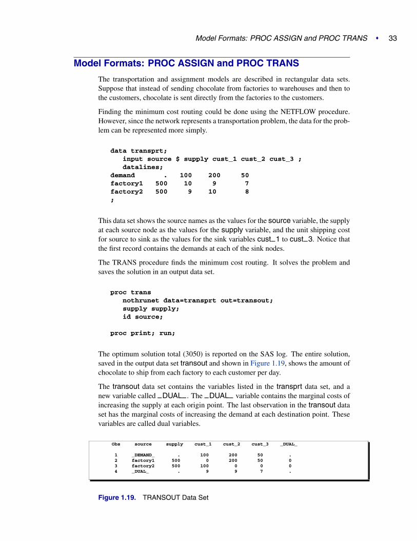
The transportation and assignment models are described in rectangular data sets.Suppose that instead of sending chocolate from factories to warehouses and then tothe customers, chocolate is sent directly from the factories to the customers.
Finding the minimum cost routing could be done using the NETFLOW procedure.However, since the network represents a transportation problem, the data for the prob-lem can be represented more simply.
data transprt;input source $ supply cust_1 cust_2 cust_3 ;datalines;
demand . 100 200 50factory1 500 10 9 7factory2 500 9 10 8;
This data set shows the source names as the values for the source variable, the supplyat each source node as the values for the supply variable, and the unit shipping costfor source to sink as the values for the sink variables cust–1 to cust–3. Notice thatthe first record contains the demands at each of the sink nodes.
The TRANS procedure finds the minimum cost routing. It solves the problem andsaves the solution in an output data set.
proc transnothrunet data=transprt out=transout;supply supply;id source;
proc print; run;
The optimum solution total (3050) is reported on the SAS log. The entire solution,saved in the output data set transout and shown in Figure 1.19, shows the amount ofchocolate to ship from each factory to each customer per day.
The transout data set contains the variables listed in the transprt data set, and anew variable called –DUAL– . The –DUAL– variable contains the marginal costs ofincreasing the supply at each origin point. The last observation in the transout dataset has the marginal costs of increasing the demand at each destination point. Thesevariables are called dual variables.
Obs source supply cust_1 cust_2 cust_3 _DUAL_
1 _DEMAND_ . 100 200 50 .2 factory1 500 0 200 50 03 factory2 500 100 0 0 04 _DUAL_ . 9 9 7 .
Figure 1.19. TRANSOUT Data Set

34 � Chapter 1. Introduction to Optimization
Model Building
It is often desirable to keep the data separate from the structure of the model. Thisis useful for large models with numerous identifiable components. The data are bestorganized in rectangular tables that can be easily examined and modified. Then,before the problem is solved, the model is built using the stored data. This process ofmodel building is known as matrix generation. In conjunction with the sparse format,the SAS DATA step provides a good matrix generation language.
For example, consider the candy manufacturing example introduced previously.Suppose that, for the user interface, it is more convenient to organize the data sothat each record describes the information related to each product (namely, the con-tribution to the objective function and the unit amount needed for each process). ADATA step for saving the data might look like this:
data manfg;format product $12.;input product $ object process1 - process4 ;datalines;
chocolate .25 15 0.00 18.75 12toffee .75 40 56.25 0.00 50licorice 1.00 29 30.00 20.00 20jelly_beans .85 10 0.00 30.00 10_RHS_ . 27000 27000 27000 27000;
Notice that there is a special record at the end having product –RHS–. This recordgives the amounts of time available for each of the processes. This information couldhave been stored in another data set. The next example illustrates a model where thedata are stored in separate data sets.
Building the model involves adding the data to the structure. There are as many waysto do this as there are programmers and problems. The following DATA step showsone way to use the candy data to build a sparse format model to solve the productmix problem.
data model;array process object process1-process4;format _type_ $8. _row_ $12. _col_ $12. ;keep _type_ _row_ _col_ _coef_;
set manfg; /* read the manufacturing data */
/* build the object function */
if _n_=1 then do;_type_=’max’; _row_=’object’; _col_=’ ’; _coef_=.;output;
end;
/* build the constraints */

Model Building � 35
do over process;if _i_>1 then do;
_type_=’le’; _row_=’process’||put(_i_-1,1.);end;else _row_=’object’;_col_=product; _coef_=process;output;
end;run;
The sparse format data set is shown in Figure 1.20.
Obs _type_ _row_ _col_ _coef_
1 max object .2 max object chocolate 0.253 le process1 chocolate 15.004 le process2 chocolate 0.005 le process3 chocolate 18.756 le process4 chocolate 12.007 object toffee 0.758 le process1 toffee 40.009 le process2 toffee 56.2510 le process3 toffee 0.0011 le process4 toffee 50.0012 object licorice 1.0013 le process1 licorice 29.0014 le process2 licorice 30.0015 le process3 licorice 20.0016 le process4 licorice 20.0017 object jelly_beans 0.8518 le process1 jelly_beans 10.0019 le process2 jelly_beans 0.0020 le process3 jelly_beans 30.0021 le process4 jelly_beans 10.0022 object _RHS_ .23 le process1 _RHS_ 27000.0024 le process2 _RHS_ 27000.0025 le process3 _RHS_ 27000.0026 le process4 _RHS_ 27000.00
Figure 1.20. Sparse Data Format
The model data set looks a little different from the sparse representation of thecandy model shown earlier. It not only includes additional products (licorice andjelly–beans), but it also defines the model in a different order. Since the sparse for-mat is robust, the model can be generated in ways that are convenient for the DATAstep program.
If the problem had more products, you could increase the size of the manfg data setto include the new product data. Also, if the problem had more than four processes,you could add the new process variables to the manfg data set and increase the sizeof the process array in the model data set. With these two simple changes andadditional data, a product mix problem having hundreds of processes and productscan be solved.

36 � Chapter 1. Introduction to Optimization
Matrix Generation
It is desirable to keep data in separate tables, then automate model building andreporting. This example illustrates a problem that has elements of a product mixproblem and a blending problem. Suppose four kinds of ties are made; all silk, allpolyester, a 50-50 polyester-cotton blend, and a 70-30 cotton-polyester blend.
The data includes cost and supplies of raw material, selling price, minimum con-tract sales, maximum demand of the finished products, and the proportions of rawmaterials that go into each product. The product mix that maximizes profit is to befound.
The data are saved in three SAS data sets. The program that follows demonstrates oneway for these data to be saved. Alternatively, the full-screen editor PROC FSEDITcan be used to store and edit these data.
data material;format descpt $20.;input descpt $ cost supply;datalines;
silk_material .21 25.8polyester_material .6 22.0cotton_material .9 13.6;
data tie;format descpt $20.;input descpt $ price contract demand;datalines;
all_silk 6.70 6.0 7.00all_polyester 3.55 10.0 14.00poly_cotton_blend 4.31 13.0 16.00cotton_poly_blend 4.81 6.0 8.50;
data manfg;format descpt $20.;input descpt $ silk poly cotton;datalines;
all_silk 100 0 0all_polyester 0 100 0poly_cotton_blend 0 50 50cotton_poly_blend 0 30 70;
The following program takes the raw data from the three data sets and builds a linearprogram model in the data set called model. Although it is designed for the three-resource, four-product problem described here, it can be easily extended to includemore resources and products. The model-building DATA step remains essentially thesame; all that changes are the dimensions of loops and arrays. Of course, the datatables must increase to accommodate the new data.
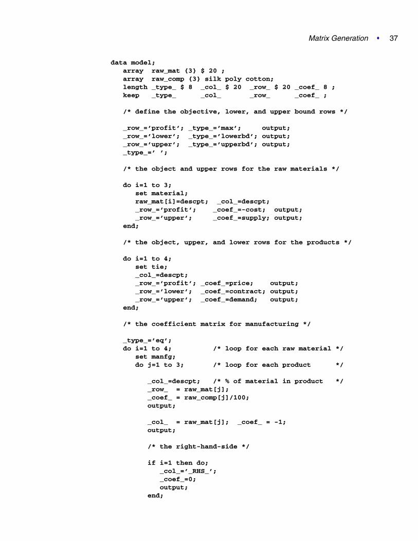
Matrix Generation � 37
data model;array raw_mat {3} $ 20 ;array raw_comp {3} silk poly cotton;length _type_ $ 8 _col_ $ 20 _row_ $ 20 _coef_ 8 ;keep _type_ _col_ _row_ _coef_ ;
/* define the objective, lower, and upper bound rows */
_row_=’profit’; _type_=’max’; output;_row_=’lower’; _type_=’lowerbd’; output;_row_=’upper’; _type_=’upperbd’; output;_type_=’ ’;
/* the object and upper rows for the raw materials */
do i=1 to 3;set material;raw_mat[i]=descpt; _col_=descpt;_row_=’profit’; _coef_=-cost; output;_row_=’upper’; _coef_=supply; output;
end;
/* the object, upper, and lower rows for the products */
do i=1 to 4;set tie;_col_=descpt;_row_=’profit’; _coef_=price; output;_row_=’lower’; _coef_=contract; output;_row_=’upper’; _coef_=demand; output;
end;
/* the coefficient matrix for manufacturing */
_type_=’eq’;do i=1 to 4; /* loop for each raw material */
set manfg;do j=1 to 3; /* loop for each product */
_col_=descpt; /* % of material in product */_row_ = raw_mat[j];_coef_ = raw_comp[j]/100;output;
_col_ = raw_mat[j]; _coef_ = -1;output;
/* the right-hand-side */
if i=1 then do;_col_=’_RHS_’;_coef_=0;output;
end;

38 � Chapter 1. Introduction to Optimization
end;_type_=’ ’;
end;stop;
run;
The model is solved using PROC LP, which saves the solution in the PRIMALOUTdata set named solution. PROC PRINT displays the solution, shown in Figure 1.21.
proc lp sparsedata primalout=solution;
proc print ;id _var_;var _lbound_--_r_cost_;
run;
_VAR_ _LBOUND_ _VALUE_ _UBOUND_ _PRICE_ _R_COST_
all_polyester 10 11.800 14.0 3.55 0.000all_silk 6 7.000 7.0 6.70 6.490cotton_material 0 13.600 13.6 -0.90 4.170cotton_poly_blend 6 8.500 8.5 4.81 0.196polyester_material 0 22.000 22.0 -0.60 2.950poly_cotton_blend 13 15.300 16.0 4.31 0.000silk_material 0 7.000 25.8 -0.21 0.000PHASE_1_OBJECTIVE 0 0.000 0.0 0.00 0.000profit 0 168.708 1.7977E308 0.00 0.000
Figure 1.21. Solution Data Set
The solution shows that 11.8 units of polyester ties, 7 units of silk ties, 8.5 units ofthe cotton-polyester blend, and 15.3 units of the polyester-cotton blend should beproduced. It also shows the amounts of raw materials that go into this product mix togenerate a total profit of 168.708.
Exploiting Model Structure
Another example helps to illustrate how the model can be simplified by exploitingthe structure in the model when using the NETFLOW procedure.
Recall the chocolate transshipment problem discussed previously. The solution re-quired no production at factory–1 and no storage at warehouse–2. Suppose thissolution, although optimal, is unacceptable. An additional constraint requiring theproduction at the two factories to be balanced is required. Now, the production at thetwo factories can differ by, at most, 100 units. Such a constraint might look like
-100 <= (factory_1_warehouse_1 + factory_1_warehouse_2 -factory_2_warehouse_1 - factory_2_warehouse_2) <= 100
The network and supply and demand information are saved in two data sets.

Exploiting Model Structure � 39
data network;format from $12. to $12.;input from $ to $ cost ;datalines;
factory_1 warehouse_1 10factory_2 warehouse_1 5factory_1 warehouse_2 7factory_2 warehouse_2 9warehouse_1 customer_1 3warehouse_1 customer_2 4warehouse_1 customer_3 4warehouse_2 customer_1 5warehouse_2 customer_2 5warehouse_2 customer_3 6;
data nodes;format node $12. ;input node $ supdem;datalines;
customer_1 -100customer_2 -200customer_3 -50factory_1 500factory_2 500;
The factory-balancing constraint is not a part of the network. It is represented in thesparse format in a data set for side constraints.
data side_con;format _type_ $8. _row_ $8. _col_ $21. ;input _type_ _row_ _col_ _coef_ ;datalines;
eq balance . .. balance factory_1_warehouse_1 1. balance factory_1_warehouse_2 1. balance factory_2_warehouse_1 -1. balance factory_2_warehouse_2 -1. balance diff -1lo lowerbd diff -100up upperbd diff 100;
This data set contains an equality constraint that sets the value of DIFF to be theamount that factory 1 production exceeds factory 2 production. It also contains im-plicit bounds on the DIFF variable. Note that the DIFF variable is a nonarc variable.

40 � Chapter 1. Introduction to Optimization
proc netflowconout=con_savarcdata=network nodedata=nodes condata=side_consparsecondata ;node node;supdem supdem;tail from;head to;cost cost;run;
proc print;var from to _name_ cost _capac_ _lo_ _supply_ _demand_
_flow_ _fcost_ _rcost_;sum _fcost_;run;
The solution is saved in the con–sav data set (Figure 1.22).
_ __ S D _ _
_ C U E _ F RN A P M F C C
f A c P _ P A L O OO r M o A L L N O S Sb o t E s C O Y D W T Ts m o _ t _ _ _ _ _ _ _
1 warehouse_1 customer_1 3 99999999 0 . 100 100 300 .2 warehouse_2 customer_1 5 99999999 0 . 100 0 0 1.03 warehouse_1 customer_2 4 99999999 0 . 200 75 300 .4 warehouse_2 customer_2 5 99999999 0 . 200 125 625 .5 warehouse_1 customer_3 4 99999999 0 . 50 50 200 .6 warehouse_2 customer_3 6 99999999 0 . 50 0 0 1.07 factory_1 warehouse_1 10 99999999 0 500 . 0 0 2.08 factory_2 warehouse_1 5 99999999 0 500 . 225 1125 .9 factory_1 warehouse_2 7 99999999 0 500 . 125 875 .10 factory_2 warehouse_2 9 99999999 0 500 . 0 0 5.011 diff 0 100 -100 . . -100 0 1.5
====3425
Figure 1.22. CON–SAV Data Set
Notice that the solution now has production balanced across the factories; the pro-duction at factory 2 exceeds that at factory 1 by 100 units.

The DATA Step � 41
�
�
�
�factory–2
�
�
�
�factory–1
�
�
�
�warehouse–2
�
�
�
�warehouse–1
�
�
�
�customer–3
�
�
�
�customer–2
�
�
�
�customer–1
�
���
��
��
�����
��
��
���
���������
��������
�
��
��
��
��
��
�
���������
��������
500
500
−50
−200
−100
225
125
50
100
75
125
Figure 1.23. Constrained Optimum for the Transshipment Problem
Report Writing
The reporting of the solution is also an important aspect of modeling. Since theoptimization procedures save the solution in one or more SAS data sets, report writingcan be written using any of the tools in the SAS language.
The DATA Step
Use of the DATA step and PROC PRINT is the most general way to produce reports.For example, a table showing the revenue generated from the production and a tableof the cost of material can be produced with the following program.
data product(keep= _var_ _value_ _price_ revenue)material(keep=_var_ _value_ _price_ cost);
set solution;if _price_>0 then do;
revenue=_price_*_value_; output product;end;else if _price_<0 then do;
_price_=-_price_;cost = _price_*_value_; output material;
end;run;

42 � Chapter 1. Introduction to Optimization
/* display the product report */
proc print data=product;id _var_;var _value_ _price_ revenue ;sum revenue;title ’Revenue Generated from Tie Sales’;
run;
/* display the materials report */
proc print data=material;id _var_;var _value_ _price_ cost;sum cost;title ’Cost of Raw Materials’;
run;
This DATA step reads the solution data set saved by PROC LP and segregates therecords based on whether they correspond to materials or products, namely whetherthe contribution to profit is positive or negative. Each of these is then displayed toproduce Figure 1.24.
Revenue Generated from Tie Sales
_VAR_ _VALUE_ _PRICE_ revenue
all_polyester 11.8 3.55 41.890all_silk 7.0 6.70 46.900cotton_poly_blend 8.5 4.81 40.885poly_cotton_blend 15.3 4.31 65.943
=======195.618
Cost of Raw Materials
_VAR_ _VALUE_ _PRICE_ cost
cotton_material 13.6 0.90 12.24polyester_material 22.0 0.60 13.20silk_material 7.0 0.21 1.47
=====26.91
Figure 1.24. Tie Problem: Revenues and Costs

Other Reporting Procedures � 43
Other Reporting Procedures
The GCHART procedure can be a useful tool for displaying the solution to mathe-matical programming models. The con–solv data set that contains the solution to thebalanced transshipment problem can be effectively displayed using PROC GCHART.In Figure 1.25, the amount that is shipped from each factory and warehouse can beseen by submitting the following.
title;proc gchart data=con_sav;
hbar from / sumvar=_flow_;run;
Figure 1.25. Tie Problem: Throughputs
The horizontal bar chart is just one way of displaying the solution to a mathematicalprogram. The solution to the Tie Product Mix problem that was solved using PROCLP can also be illustrated using PROC GCHART. Here, a pie chart shows the relativecontribution of each product to total revenues.
proc gchart data=product;pie _var_ / sumvar=revenue;
title ’Projected Tie Sales Revenue’;run;

44 � Chapter 1. Introduction to Optimization
Figure 1.26. Tie Problem: Projected Tie Sales Revenue
The TABULATE procedure is another procedure that can help automate solution re-porting. Several examples in Chapter 4, “The LP Procedure,” illustrate its use.
Decision Support Systems
The close relationship between a SAS data set and the representation of the mathe-matical model makes it easy to build decision support systems.
The Full-Screen Interface
The ability to manipulate data using the full-screen tools in the SAS language fur-ther enhances the decision support capabilities. The several data set pieces that arecomponents of a decision support model can be edited using the full-screen editingprocedures FSEDIT and FSPRINT. The screen control language SCL directs dataediting, model building, and solution reporting through its menuing capabilities.
The compatibility of each of these pieces in the SAS System makes construction ofa full-screen decision support system based on mathematical programming an easytask.

References � 45
Communicating with the Optimization Procedures
The optimization procedures communicate with any decision support system throughthe various problem and solution data sets. However, there is a need for the systemto have a more intimate knowledge of the status of the optimization procedures. Thisis achieved through the use of macro variables defined by each of the optimizationprocedures.
References
Rosenbrock, H. H. (1960), “An Automatic Method for Finding the Greatest or LeastValue of a Function,” Computer Journal, 3, 175–184.

46 � Chapter 1. Introduction to Optimization

Chapter 2The ASSIGN Procedure
Chapter Contents
OVERVIEW . . . . . . . . . . . . . . . . . . . . . . . . . . . . . . . . . . . 49
GETTING STARTED . . . . . . . . . . . . . . . . . . . . . . . . . . . . . . 50Introductory Example . . . . . . . . . . . . . . . . . . . . . . . . . . . . . 50
SYNTAX . . . . . . . . . . . . . . . . . . . . . . . . . . . . . . . . . . . . . 52Functional Summary . . . . . . . . . . . . . . . . . . . . . . . . . . . . . . 52PROC ASSIGN Statement . . . . . . . . . . . . . . . . . . . . . . . . . . 52BY Statement . . . . . . . . . . . . . . . . . . . . . . . . . . . . . . . . . 53COST Statement . . . . . . . . . . . . . . . . . . . . . . . . . . . . . . . . 53ID Statement . . . . . . . . . . . . . . . . . . . . . . . . . . . . . . . . . . 54
DETAILS . . . . . . . . . . . . . . . . . . . . . . . . . . . . . . . . . . . . . 54Missing Values . . . . . . . . . . . . . . . . . . . . . . . . . . . . . . . . . 54Output Data Set . . . . . . . . . . . . . . . . . . . . . . . . . . . . . . . . 54The Objective Value . . . . . . . . . . . . . . . . . . . . . . . . . . . . . . 54Macro Variable –ORASSIG . . . . . . . . . . . . . . . . . . . . . . . . . . 55Scaling . . . . . . . . . . . . . . . . . . . . . . . . . . . . . . . . . . . . . 55
EXAMPLES . . . . . . . . . . . . . . . . . . . . . . . . . . . . . . . . . . . 56Example 2.1. Assigning Subcontractors to Construction Jobs . . . . . . . . 56Example 2.2. Assigning Construction Jobs to Subcontractors . . . . . . . . 58Example 2.3. Minimizing Swim Times . . . . . . . . . . . . . . . . . . . . 59Example 2.4. Using PROC ASSIGN with a BY Statement . . . . . . . . . . 61

48 � Chapter 2. The ASSIGN Procedure

Chapter 2The ASSIGN ProcedureOverview
The ASSIGN procedure finds the minimum or maximum cost assignment of m sinknodes to n source nodes. The procedure can handle problems where m =, <, > n.
When n = m, the number of source nodes equals the number of sink nodes and theprocedure solves
min (max)∑m
j=1
∑ni=1 cijxij
subject to∑m
j=1 xij = 1 for i = 1, . . . , n
∑ni=1 xij = 1 for j = 1, . . . ,m
where x = 0 or 1 for i = 1, . . . , n and j = 1, . . . ,m.
When n < m, the number of source nodes is less than the number of sink nodes andthe procedure solves
min (max)∑m
j=1
∑ni=1 cijxij
subject to∑m
j=1 xij = 1 for i = 1, . . . , n
∑ni=1 xij ≤ 1 for j = 1, . . . ,m
where x = 0 or 1 for i = 1, . . . , n and j = 1, . . . ,m.
When n > m, the number of source nodes is greater than the number of sink nodesand the procedure solves
min (max)∑m
j=1
∑ni=1 cijxij
subject to∑m
j=1 xij ≤ 1 for i = 1, . . . , n
∑ni=1 xij = 1 for j = 1, . . . ,m
where x = 0 or 1 for i = 1, . . . , n and j = 1, . . . ,m.

50 � Chapter 2. The ASSIGN Procedure
Getting Started
The ASSIGN procedure finds the minimum or maximum cost assignment of sinknodes to source nodes. Many practical problems can be formulated in a way that issolvable by PROC ASSIGN.
Introductory Example
Consider assigning five programmers to five programming jobs. Each programmerprefers specific programming jobs over others. You can use PROC ASSIGN to as-sign jobs to programmers in such a way that the total preferences of the group aremaximized. Suppose you ask each programmer to rank the jobs according to pref-erence (using 1 for the most preferred job and 5 for the least preferred job). PROCASSIGN maximizes the total preference of the group by minimizing the sum of thepreferences. In the matrix that follows, each row of the matrix represents a program-mer and each column represents a programming job. Each entry in the matrix is apreference ranking that each programmer has given to each job.
PRGMER JOB1 JOB2 JOB3 JOB4 JOB5
PRGMER1 4 1 3 5 2PRGMER2 2 1 3 4 5PRGMER3 3 2 4 1 5PRGMER4 2 3 4 5 1PRGMER5 4 2 3 1 5
To solve this problem using PROC ASSIGN, the data must be in a SAS data set; thesolution is output to a SAS data set and no output is produced. Each observationcorresponds to a programmer and contains the programming job assigned to it. Inthis way, the procedure identifies the assignment of the five jobs to the five program-mers. To solve this assignment problem, place the preference data into a SAS dataset (PREFER). Then, call PROC ASSIGN, identifying the cost variables in the inputdata set. The solution is output by PROC ASSIGN to a SAS data set (PREFER1)and displayed with the PRINT procedure. The following statements produce Figure2.1:
title ’Assigning Programming Jobs to Programmers’;
data prefer;input prgmer $ job1-job5;datalines;
PRGMER1 4 1 3 5 2PRGMER2 2 1 3 4 5PRGMER3 3 2 4 1 5PRGMER4 2 3 4 5 1PRGMER5 4 2 3 1 5;

Introductory Example � 51
proc assign data=prefer out=prefer1;cost job1-job5;id prgmer;
run;
proc print data=prefer1;sum _fcost_;
run;
The following note is written to the SAS log:
NOTE: The minimum cost assignment costs 8.
Assigning Programming Jobs to Programmers
Obs prgmer job1 job2 job3 job4 job5 _ASSIGN_ _FCOST_
1 PRGMER1 4 1 3 5 2 job2 12 PRGMER2 2 1 3 4 5 job1 23 PRGMER3 3 2 4 1 5 job4 14 PRGMER4 2 3 4 5 1 job5 15 PRGMER5 4 2 3 1 5 job3 3
=======8
Figure 2.1. Assigning Programming Jobs to Programmers
The solution, given in column –ASSIGN– , shows how each programming jobshould be assigned to each worker in order to minimize the assignment cost, which isequivalent to maximizing the worker preferences. The –FCOST– column expressesin units of preference the cost of the assignment. The SUM statement in the PRINTprocedure is used to total the assignment cost.

52 � Chapter 2. The ASSIGN Procedure
Syntax
PROC ASSIGN options ;BY variables ;COST variables ;ID variable ;
The statements and options available on PROC ASSIGN are discussed in the order inwhich they appear in the preceding list of syntax elements.
Functional Summary
The options available with PROC ASSIGN and its statements are summarized bypurpose in the following table.
Table 2.1. Functional Summary
Description Statement Option
Data Set Options:input data set PROC ASSIGN DATA=output data set containing the solution PROC ASSIGN OUT=
Optimization Control Options:scaling factor for input cost data PROC ASSIGN DEC=find maximum cost assignment PROC ASSIGN MAXIMUM
Variable Lists:process data in groups BYcost variables COSTsource node names ID
PROC ASSIGN Statement
PROC ASSIGN options ;
The PROC ASSIGN statement invokes the procedure. The following options canappear in the PROC ASSIGN statement.
Data Set Options
DATA=SAS-data-setnames the SAS data set that contains the network specification. If the DATA= optionis omitted, the most recently created SAS data set is used.

COST Statement � 53
OUT=SAS-data-setspecifies a name for the output data set. If the OUT= option is omitted, the SASSystem creates a data set and names it according to the DATAn convention. Refer tobase SAS documentation for more information.
Optimization Control Options
DEC=nspecifies a scaling factor for the input cost data. The input data are scaled by 10n.The default value of n is 3. For more information, see the discussion on scaling inthe “Details” section on page 54.
MAXIMUMspecifies that the objective is to find an assignment that maximizes the sum of thecosts. By default, PROC ASSIGN minimizes the sum of the costs.
BY Statement
BY variables ;
A BY statement can be used with PROC ASSIGN to obtain separate solutions onproblems in groups defined by the BY variables. When you use a BY statement, theprocedure expects the input data to be sorted in ascending order of the BY variables.If your input data set is not sorted, use the SORT procedure with a similar BY state-ment to sort the data, or, if appropriate, use the BY statement option NOTSORTED orDESCENDING. See Example 2.4 in the “Examples” section. For more information,refer to the discussion of the BY statement in base SAS documentation.
COST Statement
COST variables ;
The COST statement identifies the variables to be interpreted as sink nodes in theinput DATA= data set. The values of a COST variable are the costs (or preferences)of assigning each source node (named in the ID variable) to the sink node identifiedwith the COST variable.
If the value of a COST variable is missing, then that particular assignment betweensource and sink node is infeasible. If you do not use a COST statement, then allnumeric variables not specified in the ID or BY statement are assumed to be costvariables.
To find an assignment that maximizes profit instead of minimizing cost, include theMAXIMUM option in the PROC ASSIGN statement and let the COST variablesrepresent profit instead of cost. The COST variables must be numeric. See Example2.1 for an illustration of the COST statement.

54 � Chapter 2. The ASSIGN Procedure
ID Statement
ID variable ;
The ID statement identifies a variable in the input DATA= data set that gives thenames of the source nodes. The ID variable can be character or numeric.
Details
Missing Values
Because the value of a cost variable is interpreted as the cost of an assignment, a miss-ing value for a cost variable is assumed to mean that the assignment is not allowed.Refer to Example 2.1 for an illustration of a data set with missing values.
Output Data Set
The output data set contains the m cost variables in the input data set, any vari-ables identified in the ID statement, and two new variables named –ASSIGN– and
–FCOST– . The variable named –ASSIGN– is a character variable containing thenames of the sink nodes (names of COST variables) assigned to the source nodes(values of the ID variable). The variable named –FCOST– is a numeric variablecontaining the costs of assigning the sink nodes to the source nodes. Note that thevalues of the m cost variables in the output data set reflect any effects of scalingperformed by PROC ASSIGN.
The Objective Value
If the problem is infeasible, an error message is written to the SAS log. Otherwise,the value of the objective function
m∑j=1
n∑i=1
cijxij
under the optimal assignment is reported on the SAS log.

Scaling � 55
Macro Variable –ORASSIG
On termination, the ASSIGN procedure defines a macro variable named –ORASSIG.This variable contains a character string that indicates the status of the procedure ontermination and gives the objective value at termination. The form of the –ORASSIGcharacter string is
STATUS=charstr OBJECTIVE=objective
where charstr can be any one of the following:
• SUCCESSFUL
• INFEASIBLE
• MEMORY–ERROR
• IO–ERROR
• SYNTAX–ERROR
• SEMANTIC–ERROR
• BADDATA–ERROR
• UNKNOWN–ERROR
This information is useful when PROC ASSIGN comprises one step in a larger pro-gram that needs to identify just how the ASSIGN procedure terminated. Because
–ORASSIG is a standard SAS macro variable, it can be used in the ways that allmacro variables can be used. See the SAS Guide to Macro Processing for more infor-mation. Example 2.2 illustrates the method to write the –ORASSIG variable to thelog.
Scaling
PROC ASSIGN uses a variant of the out-of-kilter algorithm. Integral cost data areimportant for maintaining a rapid rate of convergence with this algorithm. To assureintegrality, the cost data are automatically scaled by DEC= decimal places on inputto PROC ASSIGN. If this scaling can result in loss of accuracy in the input data, awarning is written to the log indicating a nonzero fractional component in the dataafter scaling. The output data set produced by PROC ASSIGN contains the scaledinput cost data rescaled to its original order of magnitude. Since the input cost dataand the output cost data may differ because of scaling, you can use this difference asa measure of how poorly the input cost data were scaled.

56 � Chapter 2. The ASSIGN Procedure
Examples
The following examples illustrate some of the capabilities of PROC ASSIGN. Theseexamples, together with the other SAS/OR examples, can be found in the SAS samplelibrary.
Example 2.1. Assigning Subcontractors to Construction Jobs
This example shows how PROC ASSIGN can be used to maximize an objective func-tion. Consider a construction project that consists of nine jobs. Because of the natureof the project, each job must be performed by a different subcontractor. Each job isbid upon by twelve subcontractors. The matrix that follows shows the expected profitto the contractor if each job is given to each subcontractor. Each row in the matrixrepresents a different job, and each column represents a different subcontractor.
SUBCONTRACTOR 1 2 3 4 5 6 7 8 9 10 11 12________________________________________________
JOB1 | 79 24 13 53 47 66 85 17 92 47 46 13JOB2 | 43 59 33 95 55 97 34 55 84 94 26 56JOB3 | 29 52 0 27 13 33 0 11 71 86 6 76JOB4 | 88 83 64 72 0 67 27 47 83 62 35 38JOB5 | 65 90 56 62 53 91 48 23 6 89 49 33JOB6 | 44 79 86 93 71 7 86 59 0 56 45 59JOB7 | 35 51 -9 91 39 32 3 12 79 25 79 81JOB8 | 50 12 59 32 23 64 20 94 97 14 11 97JOB9 | 25 17 39 . 38 63 87 14 4 18 11 45
The negative profit in the third column means that if job 7 is awarded to subcontractor3, the contractor loses money. The missing value in the fourth column means thatsubcontractor 4 did not bid on job 9. PROC ASSIGN treats a missing value differentlyfrom the way it treats a 0. While it is possible that an optimal assignment couldinclude a 0 (or even a negative) contribution to profit, the missing value is neverincluded in an assignment. In this case, subcontractor 4 is never awarded job 9,regardless of the profit structure.
You can use PROC ASSIGN to find how the contractor should award the jobs to thesubcontractors to maximize his profit. First, put the data in a SAS data set. Then, callPROC ASSIGN using the MAXIMUM option.
The following statements produce Output 2.1.1:
title ’Assigning Subcontractors to Construction Jobs’;
data profit;input job $ subcon1-subcon12;datalines;
JOB1 79 24 13 53 47 66 85 17 92 47 46 13JOB2 43 59 33 95 55 97 34 55 84 94 26 56JOB3 29 52 0 27 13 33 0 11 71 86 6 76JOB4 88 83 64 72 0 67 27 47 83 62 35 38

Example 2.1. Assigning Subcontractors to Construction Jobs � 57
JOB5 65 90 56 62 53 91 48 23 6 89 49 33JOB6 44 79 86 93 71 7 86 59 0 56 45 59JOB7 35 51 -9 91 39 32 3 12 79 25 79 81JOB8 50 12 59 32 23 64 20 94 97 14 11 97JOB9 25 17 39 . 38 63 87 14 4 18 11 45;
proc assign maximum data=profit;cost subcon1-subcon12;id job;
run;
proc print;sum _fcost_;
run;
The cost of the optimal assignment is written to the SAS log:
NOTE: The maximum return assignment yields 814.
This means that the contractor can expect a profit of $814 if he follows the optimalassignment.
Output 2.1.1. Assigning Subcontractors to Construction Jobs
Assigning Subcontractors to Construction Jobs
s s s _s s s s s s s s s u u u A _u u u u u u u u u b b b S Fb b b b b b b b b c c c S Cc c c c c c c c c o o o I O
O j o o o o o o o o o n n n G Sb o n n n n n n n n n 1 1 1 N Ts b 1 2 3 4 5 6 7 8 9 0 1 2 _ _
1 JOB1 79 24 13 53 47 66 85 17 92 47 46 13 subcon9 922 JOB2 43 59 33 95 55 97 34 55 84 94 26 56 subcon6 973 JOB3 29 52 0 27 13 33 0 11 71 86 6 76 subcon10 864 JOB4 88 83 64 72 0 67 27 47 83 62 35 38 subcon1 885 JOB5 65 90 56 62 53 91 48 23 6 89 49 33 subcon2 906 JOB6 44 79 86 93 71 7 86 59 0 56 45 59 subcon3 867 JOB7 35 51 -9 91 39 32 3 12 79 25 79 81 subcon4 918 JOB8 50 12 59 32 23 64 20 94 97 14 11 97 subcon12 979 JOB9 25 17 39 . 38 63 87 14 4 18 11 45 subcon7 87
===814
Note that three subcontractors, SUBCON5, SUBCON8, and SUBCON11, are notassigned to any jobs.

58 � Chapter 2. The ASSIGN Procedure
Example 2.2. Assigning Construction Jobs to Subcontractors
Suppose that the data from Example 2.1 are transposed so that the variables are jobs.Then each observation contains the profit from awarding each job to a single subcon-tractor. The following program finds the maximum profit assignment and producesOutput 2.2.1.
title ’Assigning Construction Jobs to Subcontractors’;
data profit;input subcont $ job1-job9;datalines;
SUBCON1 79 43 29 88 65 44 35 50 25SUBCON2 24 59 52 83 90 79 51 12 17SUBCON3 13 33 0 64 56 86 -9 59 39SUBCON4 53 95 27 72 62 93 91 32 .SUBCON5 47 55 13 0 53 71 39 23 38SUBCON6 66 97 33 67 91 7 32 64 63SUBCON7 85 34 0 27 48 86 32 0 87SUBCON8 17 55 11 47 23 59 12 94 14SUBCON9 92 84 71 83 6 0 79 97 4SUBCON10 47 94 86 62 89 56 25 14 18SUBCON11 46 26 6 35 49 45 79 11 11SUBCON12 13 56 76 38 33 59 81 97 45;
proc assign maximum data=profit;cost job1-job9;id subcont;
run;
proc print;sum _fcost_;
run;
The cost of the optimal assignment is written to the SAS log:
NOTE: The maximum return assignment yields 814.
This means that the contractor can expect a profit of $814 if the optimal assignmentis followed.

Example 2.3. Minimizing Swim Times � 59
Output 2.2.1. Assigning Construction Jobs to Subcontractors
Assigning Construction Jobs to Subcontractors
Obs subcont job1 job2 job3 job4 job5 job6 job7 job8 job9 _ASSIGN_ _FCOST_
1 SUBCON1 79 43 29 88 65 44 35 50 25 job4 882 SUBCON2 24 59 52 83 90 79 51 12 17 job5 903 SUBCON3 13 33 0 64 56 86 -9 59 39 job6 864 SUBCON4 53 95 27 72 62 93 91 32 . job7 915 SUBCON5 47 55 13 0 53 71 39 23 38 06 SUBCON6 66 97 33 67 91 7 32 64 63 job2 977 SUBCON7 85 34 0 27 48 86 32 0 87 job9 878 SUBCON8 17 55 11 47 23 59 12 94 14 09 SUBCON9 92 84 71 83 6 0 79 97 4 job1 9210 SUBCON10 47 94 86 62 89 56 25 14 18 job3 8611 SUBCON11 46 26 6 35 49 45 79 11 11 012 SUBCON12 13 56 76 38 33 59 81 97 45 job8 97
=======814
The macro variable –ORASSIG defined by PROC ASSIGN contains informationregarding the termination of the procedure.
This information can be useful when you use PROC ASSIGN as part of a larger SASprogram. For example, information can be written to the SAS log with the statement
%put &_orassig;
On the log the following appears:
STATUS=SUCCESSFUL OBJECTIVE=814.
Example 2.3. Minimizing Swim Times
A swimming coach needs to assign male and female swimmers to each stroke of amedley relay team. The swimmers’ best times for each stroke are stored in a SAS dataset. The ASSIGN procedure is used to evaluate the times and to match strokes andswimmers to minimize the total relay swim time. The following statements produceOutput 2.3.1:
title ’Assigning Strokes Using the BY Statement’;
data relay;input name $ sex $ back breast fly free;datalines;
SUE F 35.1 36.7 28.3 36.1KAREN F 34.6 32.6 26.9 26.2JAN F 31.3 33.9 27.1 31.2ANDREA F 28.6 34.1 29.1 30.3CAROL F 32.9 32.2 26.6 24.0ELLEN F 27.8 32.5 27.8 27.0JIM M 26.3 27.6 23.5 22.4

60 � Chapter 2. The ASSIGN Procedure
MIKE M 29.0 24.0 27.9 25.4SAM M 27.2 33.8 25.2 24.1CLAYTON M 27.0 29.2 23.0 21.9;
proc assign out=fast;cost back--free;id name;by sex;
proc print;by sex;sum _fcost_;
run;
Output 2.3.1. Assigning Strokes Using the BY StatementAssigning Strokes Using the BY Statement
------------------------------------ sex=F -------------------------------------
Obs name back breast fly free _ASSIGN_ _FCOST_
1 SUE 35.1 36.7 28.3 36.1 0.02 KAREN 34.6 32.6 26.9 26.2 breast 32.63 JAN 31.3 33.9 27.1 31.2 fly 27.14 ANDREA 28.6 34.1 29.1 30.3 0.05 CAROL 32.9 32.2 26.6 24.0 free 24.06 ELLEN 27.8 32.5 27.8 27.0 back 27.8
--- -------sex 111.5
------------------------------------ sex=M -------------------------------------
Obs name back breast fly free _ASSIGN_ _FCOST_
7 JIM 26.3 27.6 23.5 22.4 free 22.48 MIKE 29.0 24.0 27.9 25.4 breast 24.09 SAM 27.2 33.8 25.2 24.1 back 27.210 CLAYTON 27.0 29.2 23.0 21.9 fly 23.0--- -------sex 96.6
=======208.1
On the basis of this solution, Jim will swim freestyle, Mike will swim breast stroke,Sam will swim back stroke, and Clayton will swim butterfly. For the women’s team,Karen will swim breast stroke, Jan will swim butterfly, Carol will swim freestyle, andEllen will swim back stroke.

Example 2.4. Using PROC ASSIGN with a BY Statement � 61
Example 2.4. Using PROC ASSIGN with a BY Statement
A major beverage company wants to assign TV commercials to television commercialtime slot openings in a way that maximizes the overall effectiveness of its televisionadvertising. The time slots in this example begin at 7:00 on a Saturday morningand run hourly through 3:00 p.m. A combination of Nielsen TV ratings and marketresearch testing produces an effectiveness rating for each time slot and commercialcombination. The commercials are of three types: children, lifestyle, and sports. Thecompany is willing to show up to three commercials in each time slot as long as thecommercials are of different types. Which commercials should be assigned to whichtime slots in order to maximize the total effectiveness of its television advertisingcampaign? Data are missing for those time slots where certain programs are notavailable; for instance, no sports shows are presented during the 7:00 a.m. time slot.
The following statements produce Output 2.4.1:
title ’Assigning Television Commercials Using the BY Statement’;
data beverage;input commercl $ type $ slot1-slot9;datalines;
COMM1 KIDS 27.2 32.8 30.4 31.5 20.9 19.8 . . .COMM2 KIDS 37.4 33.5 38.4 32.4 25.6 27.2 . . .COMM3 KIDS 32.5 31.9 34.6 34.5 26.7 28.3 . . .COMM4 LIFEST . 22.6 25.9 25.3 26.4 28.3 29.1 22.2 20.2COMM5 LIFEST . 25.1 36.6 36.8 38.2 33.5 33.2 33.1 30.1COMM6 LIFEST . 20.2 31.3 29.3 24.6 25.1 20.0 22.4 23.1COMM7 SPORTS . . 25.1 26.1 28.3 36.1 29.4 31.7 34.5COMM8 SPORTS . . 24.7 27.2 36.4 31.2 28.7 33.2 33.1COMM9 SPORTS . 20.2 20.4 20.2 25.6 37.8 35.6 32.4 34.3;
proc assign maximum out=newslots;cost slot1-slot9;id commercl;by type;
run;
proc print;by type;sum _fcost_;
run;

62 � Chapter 2. The ASSIGN Procedure
Output 2.4.1. Assigning Television Commercials using the BY StatementAssigning Television Commercials Using the BY Statement
---------------------------------- type=KIDS -----------------------------------
c _o A _m S Fm s s s s s s s s s S Ce l l l l l l l l l I O
O r o o o o o o o o o G Sb c t t t t t t t t t N Ts l 1 2 3 4 5 6 7 8 9 _ _
1 COMM1 27.2 32.8 30.4 31.5 20.9 19.8 . . . slot2 32.82 COMM2 37.4 33.5 38.4 32.4 25.6 27.2 . . . slot3 38.43 COMM3 32.5 31.9 34.6 34.5 26.7 28.3 . . . slot4 34.5
---- -----type 105.7
--------------------------------- type=LIFEST ----------------------------------
c _o A _m S Fm s s s s s s s s s S Ce l l l l l l l l l I O
O r o o o o o o o o o G Sb c t t t t t t t t t N Ts l 1 2 3 4 5 6 7 8 9 _ _
4 COMM4 . 22.6 25.9 25.3 26.4 28.3 29.1 22.2 20.2 slot7 29.15 COMM5 . 25.1 36.6 36.8 38.2 33.5 33.2 33.1 30.1 slot5 38.26 COMM6 . 20.2 31.3 29.3 24.6 25.1 20.0 22.4 23.1 slot3 31.3
---- ----type 98.6
--------------------------------- type=SPORTS ----------------------------------
c _o A _m S Fm s s s s s s s s s S Ce l l l l l l l l l I O
O r o o o o o o o o o G Sb c t t t t t t t t t N Ts l 1 2 3 4 5 6 7 8 9 _ _
7 COMM7 . . 25.1 26.1 28.3 36.1 29.4 31.7 34.5 slot9 34.58 COMM8 . . 24.7 27.2 36.4 31.2 28.7 33.2 33.1 slot5 36.49 COMM9 . 20.2 20.4 20.2 25.6 37.8 35.6 32.4 34.3 slot6 37.8
---- -----type 108.7
=====313.0
On the basis of this survey, this company has decided to drop commercial advertisingfrom the 7:00 a.m. (slot1) and 2:00 p.m. (slot8) time slots.

Chapter 3The INTPOINT Procedure
Chapter Contents
OVERVIEW . . . . . . . . . . . . . . . . . . . . . . . . . . . . . . . . . . . 65Mathematical Description of NPSC . . . . . . . . . . . . . . . . . . . . . . 66Mathematical Description of LP . . . . . . . . . . . . . . . . . . . . . . . . 67The Interior Point Algorithm . . . . . . . . . . . . . . . . . . . . . . . . . 68Network Models . . . . . . . . . . . . . . . . . . . . . . . . . . . . . . . . 76
INTRODUCTION . . . . . . . . . . . . . . . . . . . . . . . . . . . . . . . . 84Getting Started: NPSC Problems . . . . . . . . . . . . . . . . . . . . . . . 84Getting Started: LP Problems . . . . . . . . . . . . . . . . . . . . . . . . . 91Typical PROC INTPOINT Run . . . . . . . . . . . . . . . . . . . . . . . . 99
SYNTAX . . . . . . . . . . . . . . . . . . . . . . . . . . . . . . . . . . . . . 100Functional Summary . . . . . . . . . . . . . . . . . . . . . . . . . . . . . . 100PROC INTPOINT Statement . . . . . . . . . . . . . . . . . . . . . . . . . 103CAPACITY Statement . . . . . . . . . . . . . . . . . . . . . . . . . . . . . 123COEF Statement . . . . . . . . . . . . . . . . . . . . . . . . . . . . . . . . 123COLUMN Statement . . . . . . . . . . . . . . . . . . . . . . . . . . . . . 124COST Statement . . . . . . . . . . . . . . . . . . . . . . . . . . . . . . . . 124DEMAND Statement . . . . . . . . . . . . . . . . . . . . . . . . . . . . . 124HEADNODE Statement . . . . . . . . . . . . . . . . . . . . . . . . . . . . 125ID Statement . . . . . . . . . . . . . . . . . . . . . . . . . . . . . . . . . . 125LO Statement . . . . . . . . . . . . . . . . . . . . . . . . . . . . . . . . . 125NAME Statement . . . . . . . . . . . . . . . . . . . . . . . . . . . . . . . 126NODE Statement . . . . . . . . . . . . . . . . . . . . . . . . . . . . . . . 126QUIT Statement . . . . . . . . . . . . . . . . . . . . . . . . . . . . . . . . 126RHS Statement . . . . . . . . . . . . . . . . . . . . . . . . . . . . . . . . 126ROW Statement . . . . . . . . . . . . . . . . . . . . . . . . . . . . . . . . 126RUN Statement . . . . . . . . . . . . . . . . . . . . . . . . . . . . . . . . 127SUPDEM Statement . . . . . . . . . . . . . . . . . . . . . . . . . . . . . . 127SUPPLY Statement . . . . . . . . . . . . . . . . . . . . . . . . . . . . . . 127TAILNODE Statement . . . . . . . . . . . . . . . . . . . . . . . . . . . . 128TYPE Statement . . . . . . . . . . . . . . . . . . . . . . . . . . . . . . . . 128VAR Statement . . . . . . . . . . . . . . . . . . . . . . . . . . . . . . . . 130
DETAILS . . . . . . . . . . . . . . . . . . . . . . . . . . . . . . . . . . . . . 130Input Data Sets . . . . . . . . . . . . . . . . . . . . . . . . . . . . . . . . . 130Output Data Set . . . . . . . . . . . . . . . . . . . . . . . . . . . . . . . . 140

64 � Chapter 3. The INTPOINT Procedure
Case Sensitivity . . . . . . . . . . . . . . . . . . . . . . . . . . . . . . . . 141Loop Arcs . . . . . . . . . . . . . . . . . . . . . . . . . . . . . . . . . . . 142Multiple Arcs . . . . . . . . . . . . . . . . . . . . . . . . . . . . . . . . . 142Flow and Value Bounds . . . . . . . . . . . . . . . . . . . . . . . . . . . . 142Tightening Bounds and Side Constraints . . . . . . . . . . . . . . . . . . . 143Reasons for Infeasibility . . . . . . . . . . . . . . . . . . . . . . . . . . . . 143Missing S Supply and Missing D Demand Values . . . . . . . . . . . . . . 144Balancing Total Supply and Total Demand . . . . . . . . . . . . . . . . . . 149How to Make the Data Read of PROC INTPOINT More Efficient . . . . . . 150Stopping Criteria . . . . . . . . . . . . . . . . . . . . . . . . . . . . . . . . 155
EXAMPLES . . . . . . . . . . . . . . . . . . . . . . . . . . . . . . . . . . . 159Example 3.1. Production, Inventory, Distribution Problem . . . . . . . . . . 160Example 3.2. Altering Arc Data . . . . . . . . . . . . . . . . . . . . . . . . 165Example 3.3. Adding Side Constraints . . . . . . . . . . . . . . . . . . . . 169Example 3.4. Using Constraints and More Alteration to Arc Data . . . . . . 174Example 3.5. Nonarc Variables in the Side Constraints . . . . . . . . . . . . 178Example 3.6. Solving an LP Problem with Data in MPS Format . . . . . . . 183
REFERENCES . . . . . . . . . . . . . . . . . . . . . . . . . . . . . . . . . . 184

Chapter 3The INTPOINT ProcedureOverview
The INTPOINT procedure solves the Network Program with Side Constraints(NPSC) problem (defined in the “Mathematical Description of NPSC” section onpage 66) and the more general Linear Programming (LP) problem (defined in the“Mathematical Description of LP” section on page 67). NPSC and LP models can beused to describe a wide variety of real-world applications ranging from production,inventory, and distribution problems to financial applications.
Whether your problem is NPSC or LP, PROC INTPOINT uses the same optimizationalgorithm, the interior point algorithm. This algorithm is outlined in the “The InteriorPoint Algorithm” section on page 68.
While many of your problems may best be formulated as LP problems, there may beother instances when your problems are better formulated as NPSC problems. The“Network Models” section on page 76 describes typical models that have a networkcomponent and suggests reasons why NPSC may be preferable to LP. The “GettingStarted: NPSC Problems” section on page 84 outlines how you supply data of anyNPSC problem to PROC INTPOINT and call the procedure. After it reads the NPSCdata, PROC INTPOINT converts the problem into an equivalent LP problem, per-forms interior point optimization, then converts the solution it finds back into a formyou can use as the optimum to the original NPSC model.
If your model is an LP problem, the way you supply the data to PROC INTPOINTand run the procedure is described in the “Getting Started: LP Problems” section onpage 91.
The remainder of this chapter is organized as follows:
• The “Typical PROC INTPOINT Run” section on page 99 describes how to usethis procedure.
• The “Syntax” section on page 100 describes all the statements and options ofPROC INTPOINT.
• The “Functional Summary” section on page 100 lists the statements and op-tions that can be used to control PROC INTPOINT.
• The “Details” section on page 130 contains detailed explanations, descriptions,and advice on the use and behavior of the procedure.
• PROC INTPOINT is demonstrated by solving several examples in the“Examples” section on page 159.

66 � Chapter 3. The INTPOINT Procedure
Mathematical Description of NPSC
A network consists of a collection of nodes joined by a collection of arcs. The arcsconnect nodes and convey flow of one or more commodities that are supplied atsupply nodes and demanded at demand nodes in the network. Each arc has a costper unit of flow, a flow capacity, and a lower flow bound associated with it. Animportant concept in network modeling is conservation of flow. Conservation of flowmeans that the total flow in arcs directed toward a node, plus the supply at the node,minus the demand at the node, equals the total flow in arcs directed away from thenode.
Often all the details of a problem cannot be specified in a network model alone. Inmany of these cases, these details can be represented by the addition of side con-straints to the model. Side constraints are linear functions of arc variables (variablescontaining flow through an arc) and nonarc variables (variables that are not part of thenetwork). The data for a side constraint consist of coefficients of arcs and coefficientsof nonarc variables, a constraint type (that is, ≤, =, or ≥) and a right-hand-side value(rhs). A nonarc variable has a name, an objective function coefficient analogous to anarc cost, an upper bound analogous to an arc capacity, and a lower bound analogousto an arc lower flow bound.
If a network component of NPSC is removed by merging arcs and nonarc variablesinto a single set of variables, and if the flow conservation constraints and side con-straints are merged into a single set of constraints, the result is an LP problem. PROCINTPOINT will automatically transform an NPSC problem into an equivalent LPproblem, perform the optimization, then transform the problem back into its originalform. By doing this, PROC INTPOINT finds the flow through the network and thevalues of any nonarc variables that minimize the total cost of the solution. Flow con-servation is met, flow through each arc is on or between the arc’s lower flow boundand capacity, the value of each nonarc variable is on or between the nonarc’s lowerand upper bounds, and the side constraints are satisfied.
Note that, since many LPs have large embedded networks, PROC INTPOINT is anattractive alternative to the LP procedure in many cases. Rather than formulating allproblems as LPs, network models remain conceptually easy since they are based onnetwork diagrams that represent the problem pictorially. PROC INTPOINT acceptsthe network specification in a format that is particularly suited to networks. This notonly simplifies problem description but also aids in the interpretation of the solution.The conversion to and from the equivalent LP is done “behind the scenes” by theprocedure.
If a network programming problem with side constraints has n nodes, a arcs, g nonarcvariables, and k side constraints, then the formal statement of the problem solved byPROC INTPOINT is
minimize cT x + dT zsubject to Fx = b
Hx + Qz {≥, =,≤} rl ≤ x ≤ um ≤ z ≤ v

Mathematical Description of LP � 67
where
• c is the a× 1 arc variable objective function coefficient vector (the cost vector)
• x is the a × 1 arc variable value vector (the flow vector)
• d is the g × 1 nonarc variable objective function coefficient vector
• z is the g × 1 nonarc variable value vector
• F is the n × a node-arc incidence matrix of the network, where
Fi,j =
−1, if arc j is directed from node i1, if arc j is directed toward node i0, otherwise
• b is the n × 1 node supply/demand vector, where
bi =
s, if node i has supply capability of s units of flow−d, if node i has demand of d units of flow
0, if node i is a transshipment node
• H is the k × a side constraint coefficient matrix for arc variables, where Hi,j
is the coefficient of arc j in the ith side constraint
• Q is the k × g side constraint coefficient matrix for nonarc variables, whereQi,j is the coefficient of nonarc j in the ith side constraint
• r is the k × 1 side constraint right-hand-side vector
• l is the a × 1 arc lower flow bound vector
• u is the a × 1 arc capacity vector
• m is the g × 1 nonarc variable lower bound vector
• v is the g × 1 nonarc variable upper bound vector
The INTPOINT procedure can also be used to solve an unconstrained network prob-lem, that is, one in which H , Q, d, r, and z do not exist. It can also be used to solvea network problem with side constraints but no nonarc variables, in which case Q, d,and z do not exist.
Mathematical Description of LP
A linear programming (LP) problem has a linear objective function and a collection oflinear constraints. PROC INTPOINT finds the values of variables that minimize thetotal cost of the solution. The value of each variable is on or between the variable’slower and upper bounds, and the constraints are satisfied.
If an LP has g variables and k constraints, then the formal statement of the problemsolved by PROC INTPOINT is
minimize dT zsubject to Qz {≥, =,≤} r
m ≤ z ≤ v

68 � Chapter 3. The INTPOINT Procedure
where
• d is the g × 1 variable objective function coefficient vector
• z is the g × 1 variable value vector
• Q is the k × g constraint coefficient matrix for the variables, where Qi,j is thecoefficient of variable j in the ith constraint
• r is the k × 1 side constraint right-hand-side vector
• m is the g × 1 variable lower bound vector
• v is the g × 1 variable upper bound vector
The Interior Point Algorithm
The simplex algorithm, developed shortly after World War II, was for many years themain method used to solve linear programming problems. Over the last fifteen years,however, the interior point algorithm has been developed. This algorithm also solveslinear programming problems. From the start it showed great theoretical promise, andconsiderable research in the area resulted in practical implementations that performedcompetitively with the simplex algorithm. More recently, interior point algorithmshave evolved to become superior to the simplex algorithm, in general, especiallywhen the problems are large.
There are many variations of interior point algorithms. PROC INTPOINT uses thePrimal-Dual with Predictor-Corrector algorithm. More information on this particularalgorithm and related theory can be found in the texts by Roos, Terlaky, and Vial(1997), Wright (1996), and Ye (1996).
Interior Point Algorithmic Details
After preprocessing, the linear program to be solved is
minimize cT xsubject to Ax = b
x ≥ 0
This is the primal problem. The matrices d, z, and Q of NPSC have been renamedc, x, and A, respectively, as these symbols are by convention used more, the problemto be solved is different from the original because of preprocessing, and there hasbeen a change of primal variable to transform the LP into one whose variables havezero lower bounds. To simplify the algebra here, assume that variables have infiniteupper bounds, and constraints are equalities. (Interior point algorithms do efficientlyhandle finite upper bounds, and it is easy to introduce primal slack variables to changeinequalities into equalities.) The problem has n variables; i is a variable number; k isan iteration number, and if used as a subscript or superscript it denotes “of iterationk”.

The Interior Point Algorithm � 69
There exists an equivalent problem, the dual problem, stated as
maximize bT ysubject to AT y + s = c
s ≥ 0
where y are dual variables, and s are dual constraint slacks.
The interior point algorithm solves the system of equations to satisfy the Karush-Kuhn-Tucker (KKT) conditions for optimality:
Ax = b
AT y + s = c
XSe = 0
x ≥ 0
s ≥ 0
where
S = diag(s) (that is, Si,j = si if i = j, Si,j = 0 otherwise)
X = diag(x)
ei = 1 ∀i
These are the conditions for feasibility, with the complementarity condition XSe = 0added. Complementarity forces the optimal objectives of the primal and dual to beequal, cT xopt = bT yopt, as
0 = xToptsopt = sT
optxopt = (c − AT yopt)T xopt =
cT xopt − yTopt(Axopt) = cT xopt − bT yopt
Before the optimum is reached, a solution (x, y, s) may not satisfy the KKT condi-tions:
• Primal constraints may be violated, infeasc = b − Ax �= 0.
• Dual constraints may be violated, infeasd = c − AT y − s �= 0.
• Complementarity may not be satisfied, xT s = cT x − bT y �= 0. This is calledthe duality gap.
The interior point algorithm works by using Newton’s method to find a direction tomove (∆xk, ∆yk, ∆sk) from the current solution (xk, yk, sk) toward a better solu-tion:
(xk+1, yk+1, sk+1) = (xk, yk, sk) + α(∆xk, ∆yk, ∆sk)

70 � Chapter 3. The INTPOINT Procedure
where α is the step length and is assigned a value as large as possible but not so largethat an xk+1
i or sk+1i is “too close” to zero. The direction in which to move is found
using
A∆xk = infeasc
AT ∆yk + ∆sk = infeasd
Sk∆xk + Xk∆sk = −XkSke
To greatly improve performance, the third equation is changed to
Sk∆xk + Xk∆sk = −XkSke + σkµke
where µk = (xk)T sk/n, the average complementarity, and 0 ≤ σk ≤ 1.
The effect now is to find a direction in which to move to reduce infeasibilities andto reduce the complementarity toward zero, but if any xk
i ski is too close to zero, it is
“nudged out” to µ, and any xki s
ki that is larger than µ is “nudged into” µ. A σk close
to or equal to 0.0 biases a direction toward the optimum, and a value of σk closeto or equal to 1.0 “centers” the direction toward a point where all pairwise productsxk
i ski = µ. Such points make up the central path in the interior. Although centering
directions make little, if any, progress in reducing µ and moving the solution closerto the optimum, substantial progress toward the optimum can usually be made in thenext iteration.
The central path is crucial to why the interior point algorithm is so efficient. As µis decreased, this path “guides” the algorithm to the optimum through the interior offeasible space. Without centering, the algorithm would find a series of solutions neareach other close to the boundary of feasible space. Step lengths along the directionwould be small and many more iterations would probably be required to reach theoptimum.
That in a nutshell is the primal-dual interior point algorithm. Varieties of the algo-rithm differ in the way α and σk are chosen and the direction adjusted during eachiteration. A wealth of information can be found in the texts by Roos, Terlaky, andVial (1997), Wright (1996), and Ye (1996).
The calculation of the direction is the most time-consuming step of the interior pointalgorithm. Assume the kth iteration is being performed, so the subscript and super-script k can be dropped from the algebra:
A∆x = infeasc
AT ∆y + ∆s = infeasd
S∆x + X∆s = −XSe + σµe

The Interior Point Algorithm � 71
Rearranging the second equation,
∆s = infeasd − AT ∆y
Rearranging the third equation,
∆s = X−1(−S∆x − XSe + σµe)
∆s = −Θ∆x − Se + X−1σµe
where Θ = SX−1.
Equating these two expressions for ∆s and rearranging,
−Θ∆x − Se + X−1σµe = infeasd − AT ∆y
−Θ∆x = Se − X−1σµe + infeasd − AT ∆y
∆x = Θ−1(−Se + X−1σµe − infeasd + AT ∆y)
∆x = ρ + Θ−1AT ∆y
where ρ = Θ−1(−Se + X−1σµe − infeasd).
Substituting into the first direction equation,
A∆x = infeasc
A(ρ + Θ−1AT ∆y) = infeasc
AΘ−1AT ∆y = infeasc − Aρ
∆y = (AΘ−1AT )−1(infeasc − Aρ)
Θ, ρ, ∆y, ∆x, and ∆s are calculated in that order. The hardest term is the factoriza-tion of the (AΘ−1AT ) matrix to determine ∆y. Fortunately, although the values of(AΘ−1AT ) are different for each iteration, the locations of the nonzeros in this ma-trix remain fixed; the nonzero locations are the same as those in the matrix (AAT ).This is because Θ−1 = XS−1 is a diagonal matrix that has the effect of merelyscaling the columns of (AAT ).
The fact that the nonzeros in AΘ−1AT have a constant pattern is exploited by all in-terior point algorithms and is a major reason for their excellent performance. Beforeiterations begin, AAT is examined and its rows and columns are symmetrically per-muted so that during Cholesky factorization, the number of fill-ins created is smaller.A list of arithmetic operations to perform the factorization is saved in concise com-puter data structures (working with memory locations rather than actual numericalvalues). This is called symbolic factorization. During iterations, when memory hasbeen initialized with numerical values, the operations list is performed sequentially.Determining how the factorization should be performed again and again is unneces-sary.
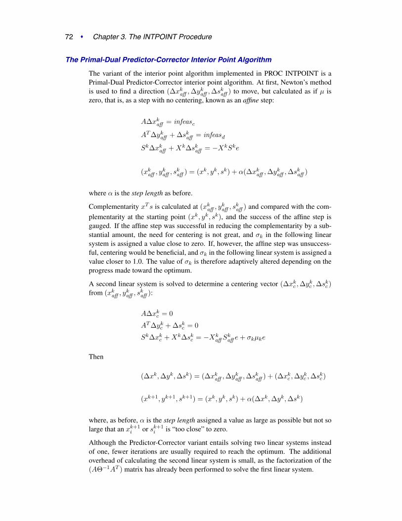
72 � Chapter 3. The INTPOINT Procedure
The Primal-Dual Predictor-Corrector Interior Point Algorithm
The variant of the interior point algorithm implemented in PROC INTPOINT is aPrimal-Dual Predictor-Corrector interior point algorithm. At first, Newton’s methodis used to find a direction (∆xk
aff , ∆ykaff , ∆sk
aff ) to move, but calculated as if µ iszero, that is, as a step with no centering, known as an affine step:
A∆xkaff = infeasc
AT ∆ykaff + ∆sk
aff = infeasd
Sk∆xkaff + Xk∆sk
aff = −XkSke
(xkaff , yk
aff , skaff ) = (xk, yk, sk) + α(∆xk
aff , ∆ykaff , ∆sk
aff )
where α is the step length as before.
Complementarity xT s is calculated at (xkaff , yk
aff , skaff ) and compared with the com-
plementarity at the starting point (xk, yk, sk), and the success of the affine step isgauged. If the affine step was successful in reducing the complementarity by a sub-stantial amount, the need for centering is not great, and σk in the following linearsystem is assigned a value close to zero. If, however, the affine step was unsuccess-ful, centering would be beneficial, and σk in the following linear system is assigned avalue closer to 1.0. The value of σk is therefore adaptively altered depending on theprogress made toward the optimum.
A second linear system is solved to determine a centering vector (∆xkc , ∆yk
c , ∆skc )
from (xkaff , yk
aff , skaff ):
A∆xkc = 0
AT ∆ykc + ∆sk
c = 0
Sk∆xkc + Xk∆sk
c = −Xkaff Sk
aff e + σkµke
Then
(∆xk, ∆yk, ∆sk) = (∆xkaff , ∆yk
aff , ∆skaff ) + (∆xk
c , ∆ykc , ∆sk
c )
(xk+1, yk+1, sk+1) = (xk, yk, sk) + α(∆xk, ∆yk, ∆sk)
where, as before, α is the step length assigned a value as large as possible but not solarge that an xk+1
i or sk+1i is “too close” to zero.
Although the Predictor-Corrector variant entails solving two linear systems insteadof one, fewer iterations are usually required to reach the optimum. The additionaloverhead of calculating the second linear system is small, as the factorization of the(AΘ−1AT ) matrix has already been performed to solve the first linear system.

The Interior Point Algorithm � 73
Interior Point: Upper Bounds
If the LP had upper bounds (0 ≤ x ≤ u where u is the upper bound vector), then theprimal and dual problems, the duality gap, and the KKT conditions would have to beexpanded.
The primal linear program to be solved is
minimize cT xsubject to Ax = b
0 ≤ x ≤ u
where 0 ≤ x ≤ u is split into x ≥ 0 and x ≤ u. Let z be primal slack so thatx + z = u, and associate dual variables w with these constraints. The interior pointalgorithm solves the system of equations to satisfy the Karush-Kuhn-Tucker (KKT)conditions for optimality:
Ax = b
x + z = u
AT y + s − w = c
XSe = 0
ZWe = 0
x, s, z, w ≥ 0
These are the conditions for feasibility, with the complementarity conditions XSe =0 and ZWe = 0 added. Complementarity forces the optimal objectives of the primaland dual to be equal, cT xopt = bT yopt − uT wopt, as
0 = zToptwopt = (u − xopt)T wopt = uT wopt − xT
optwopt
0 = xToptsopt = sT
optxopt = (c − AT yopt + wopt)T xopt =
cT xopt − yTopt(Axopt) + wT
optxopt = cT xopt − bT yopt + uT wopt
Before the optimum is reached, a solution (x, y, s, z, w) might not satisfy the KKTconditions:
• Primal bound constraints may be violated, infeasb = u − x − z �= 0.
• Primal constraints may be violated, infeasc = b − Ax �= 0.
• Dual constraints may be violated, infeasd = c − AT y − s + w �= 0.
• Complementarity conditions may not be satisfied, xT s �= 0 or zT w �= 0.
The calculations of the interior point algorithm can easily be derived in a fashionsimilar to calculations for when an LP has no upper bounds. See the paper by Lustig,Marsten, and Shanno (1992).

74 � Chapter 3. The INTPOINT Procedure
In some iteration k, the affine step system that must be solved is
∆xaff + ∆zaff = infeasb
A∆xaff = infeasc
AT ∆yaff + ∆saff − ∆waff = infeasd
S∆xaff + X∆saff = −XSe
Z∆waff + W∆zaff = −ZWe
Therefore, the computations involved in solving the affine step are
Θ = SX−1 + WZ−1
ρ = Θ−1(infeasd + (S − W )e − Z−1W infeasb)
∆yaff = (AΘ−1AT )−1(infeasc + Aρ)
∆xaff = Θ−1AT ∆yaff − ρ
∆zaff = infeasb − ∆xaff
∆waff = −We − Z−1W∆zaff
∆saff = −Se − X−1S∆xaff
(xaff , yaff , saff , zaff , waff ) = (x, y, s, z, w)+
α(∆xaff , ∆yaff , ∆saff , ∆zaff , ∆waff )
and α is the step length as before.
A second linear system is solved to determine a centering vector(∆xc, ∆yc, ∆sc, ∆zc, ∆wc) from (xaff , yaff , saff , zaff , waff ):
∆xc + ∆zc = 0
A∆xc = 0
AT ∆yc + ∆sc − ∆wc = 0
S∆xc + X∆sc = −Xaff Saff e + σµe
Z∆wc + W∆zc = −Zaff Waff e + σµe
where
ζstart = xT s + zT w, complementarity at the start of the iteration
ζaff = xTaff saff + zT
aff waff , the affine complementarity
µ = ζaff /2n, the average complementarity
σ = (ζaff /ζstart)3

The Interior Point Algorithm � 75
Therefore, the computations involved in solving the centering step are
ρ = Θ−1(σµ(X−1 − Z−1)e − X−1Xaff Saff e + Z−1Zaff Waff e)
∆yc = (AΘ−1AT )−1Aρ
∆xc = Θ−1AT ∆yc − ρ
∆zc = −∆xc
∆wc = σµZ−1e − Z−1Zaff Waff e − Z−1Waff ∆zc
∆sc = σµX−1e − X−1Xaff Saff e − X−1Saff ∆xc
Then
(∆x,∆y, ∆s,∆z, ∆w) =
(∆xaff , ∆yaff , ∆saff , ∆zaff , ∆waff )
+(∆xc, ∆yc, ∆sc, ∆zc, ∆wc)
(xk+1, yk+1, sk+1, zk+1, wk+1) =
(xk, yk, sk, zk, wk)
+α(∆x,∆y, ∆s,∆z, ∆w)
where, as before, α is the step length assigned a value as large as possible but not solarge that an xk+1
i , sk+1i , zk+1
i , or wk+1i is “too close” to zero.
The algebra in this section has been simplified by assuming that all variables havefinite upper bounds. If the number of variables with finite upper bounds nu < n,you need to change the algebra to reflect that the Z and W matrices have dimensionnu × 1 or nu × nu. Other computations need slight modification. For example, theaverage complementarity is
µ = xTaff saff /n + zT
aff waff /nu
An important point is that any upper bounds can be handled by specializing the al-gorithm and not by generating the constraints x ≤ u and adding these to the mainprimal constraints Ax = b.

76 � Chapter 3. The INTPOINT Procedure
Network Models
The following are descriptions of some typical NPSC models.
Production, Inventory, and Distribution (Supply Chain) Problems
One common class of network models is the production-inventory-distribution orsupply-chain problem. The diagram in Figure 3.1 illustrates this problem. The sub-scripts on the Production, Inventory, and Sales nodes indicate the time period. Byreplicating sections of the model, the notion of time can be included.
�
�
�
�Salesi−1
�
�
�
�Salesi
�
�
�
�Salesi+1
�
�
�
�Inventoryi−1
�
�
�
�Inventoryi
�
�
�
�Inventoryi+1
�
�
�
�Productioni−1
�
�
�
�Productioni
�
�
�
�Productioni+1
�
�
�
�Stock on hand
�
�
�
�Stock at end
� � � �� �
� � �
� � �
Figure 3.1. Production-Inventory-Distribution Problem
In this type of model, the nodes can represent a wide variety of facilities. Severalexamples are suppliers, spot markets, importers, farmers, manufacturers, factories,parts of a plant, production lines, waste disposal facilities, workstations, warehouses,coolstores, depots, wholesalers, export markets, ports, rail junctions, airports, roadintersections, cities, regions, shops, customers, and consumers. The diversity of thisselection demonstrates how rich the potential applications of this model are.
Depending upon the interpretation of the nodes, the objectives of the modeling exer-cise can vary widely. Some common types of objectives are
• to reduce collection or purchase costs of raw materials
• to reduce inventory holding or backorder costs. Warehouses and other storagefacilities sometimes have capacities, and there can be limits on the amount ofgoods that can be placed on backorder.
• to decide where facilities should be located and what the capacity of theseshould be. Network models have been used to help decide where factories,hospitals, ambulance and fire stations, oil and water wells, and schools shouldbe sited.

Network Models � 77
• to determine the assignment of resources (machines, production capability,workforce) to tasks, schedules, classes, or files
• to determine the optimal distribution of goods or services. This usually meansminimizing transportation costs and reducing transit time or distances covered.
• to find the shortest path from one location to another
• to ensure that demands (for example, production requirements, market de-mands, contractual obligations) are met
• to maximize profits from the sale of products or the charge for services
• to maximize production by identifying bottlenecks
Some specific applications are
• car distribution models. These help determine which models and numbers ofcars should be manufactured in which factories and where to distribute carsfrom these factories to zones in the United States in order to meet customerdemand at least cost.
• models in the timber industry. These help determine when to plant and millforests, schedule production of pulp, paper, and wood products, and distributeproducts for sale or export.
• military applications. The nodes can be theaters, bases, ammunition dumps,logistical suppliers, or radar installations. Some models are used to find thebest ways to mobilize personnel and supplies and to evacuate the wounded inthe least amount of time.
• communications applications. The nodes can be telephone exchanges, trans-mission lines, satellite links, and consumers. In a model of an electrical grid,the nodes can be transformers, powerstations, watersheds, reservoirs, dams,and consumers. The effect of high loads or outages might be of concern.
Proportionality Constraints
In many models, you have the characteristic that a flow through an arc must be pro-portional to the flow through another arc. Side constraints are often necessary tomodel that situation. Such constraints are called proportionality constraints and areuseful in models where production is subject to refining or modification into differentmaterials. The amount of each output, or any waste, evaporation, or reduction can bespecified as a proportion of input.
Typically, the arcs near the supply nodes carry raw materials and the arcs near thedemand nodes carry refined products. For example, in a model of the milling industry,the flow through some arcs may represent quantities of wheat. After the wheat isprocessed, the flow through other arcs might be flour. For others it might be bran. Theside constraints model the relationship between the amount of flour or bran producedas a proportion of the amount of wheat milled. Some of the wheat can end up asneither flour, bran, nor any useful product, so this waste is drained away via arcs to awaste node.

78 � Chapter 3. The INTPOINT Procedure
�
�
�
�Wheat
�
�
�
�Mill
�
�
�
�Flour
�
�
�
�Bran
�
�
�
�Other
� ��
��
��
��
���
��
��
��
��
����
1.0 0.2
0.3
0.5
Figure 3.2. Proportionality Constraints
In order for arcs to be specified in side constraints, they must be named. By default,PROC INTPOINT names arcs using the names of the nodes at the head and tail of thearc. An arc is named with its tail node name followed by an underscore and its headnode name. For example, an arc from node from to node to is called from–to.
Consider the network fragment in Figure 3.2. The arc Wheat–Mill conveys the wheatmilled. The cost of flow on this arc is the milling cost. The capacity of this arc is thecapacity of the mill. The lower flow bound on this arc is the minimum quantity thatmust be milled for the mill to operate economically. The constraints
0.3 Wheat–Mill − Mill–Flour = 0.00.2 Wheat–Mill − Mill–Bran = 0.0
force every unit of wheat that is milled to produce 0.3 units of flour and 0.2 units ofbran. Note that it is not necessary to specify the constraint
0.5 Wheat–Mill − Mill–Other = 0.0
since flow conservation implies that any flow that does not traverse throughMill–Flour or Mill–Bran must be conveyed through Mill–Other. And, computation-ally, it is better if this constraint is not specified, since there is one less side constraintand fewer problems with numerical precision. Notice that the sum of the proportionsmust equal 1.0 exactly; otherwise, flow conservation is violated.
Blending Constraints
Blending or quality constraints can also influence the recipes or proportions of in-gredients that are mixed. For example, different raw materials can have differentproperties. In an application of the oil industry, the amount of products that are ob-tained could be different for each type of crude oil. Furthermore, fuel might have aminimum octane requirement or limited sulphur or lead content, so that a blending ofcrudes is needed to produce the product.

Network Models � 79
The network fragment in Figure 3.3 shows an example of this.
�
�
�
�USA
�
�
�
�MidEast
�
�
�
�Port
�
�
�
�Refinery
�
�
�
�Gasoline
�
�
�
�Diesel
�
�
�
�Other�
��
���
��
��
��
� ��
��
����
��
��
��
���
5 units/liter
4 units/liter
4.75 units/liter
Figure 3.3. Blending Constraints
The arcs MidEast–Port and USA–Port convey crude oil from the two sources.The arc Port–Refinery represents refining while the arcs Refinery–Gasoline andRefinery–Diesel carry the gas and diesel produced. The proportionality constraints
0.4 Port–Refinery − Refinery–Gasoline = 0.00.2 Port–Refinery − Refinery–Diesel = 0.0
capture the restrictions for producing gasoline and diesel from crude. Suppose thatonly crude from the Middle East is used, then the resulting diesel would contain 5units of sulphur per liter. If only crude from the U.S.A. is used, the resulting dieselwould contain 4 units of sulphur per liter. Diesel can have at most 4.75 units ofsulphur per liter. Some crude from the U.S.A. must be used if Middle East crude isused in order to meet the 4.75 sulphur per liter limit. The side constraint to modelthis requirement is
5 MidEast–Port +4 USA–Port −4.75 Port–Refinery ≤ 0.0
Since Port–Refinery = MidEast–Port + USA–Port, flow conservation allows thisconstraint to be simplified to
1 MidEast–Port −3 USA–Port ≤ 0.0
If, for example, 120 units of crude from the Middle East is used, then at least 40units of crude from the U.S.A. must be used. The preceding constraint is simplifiedbecause you assume that the sulphur concentration of diesel is proportional to thesulphur concentration of the crude mix. If this is not the case, the relation
0.2 Port–Refinery = Refinery–Diesel
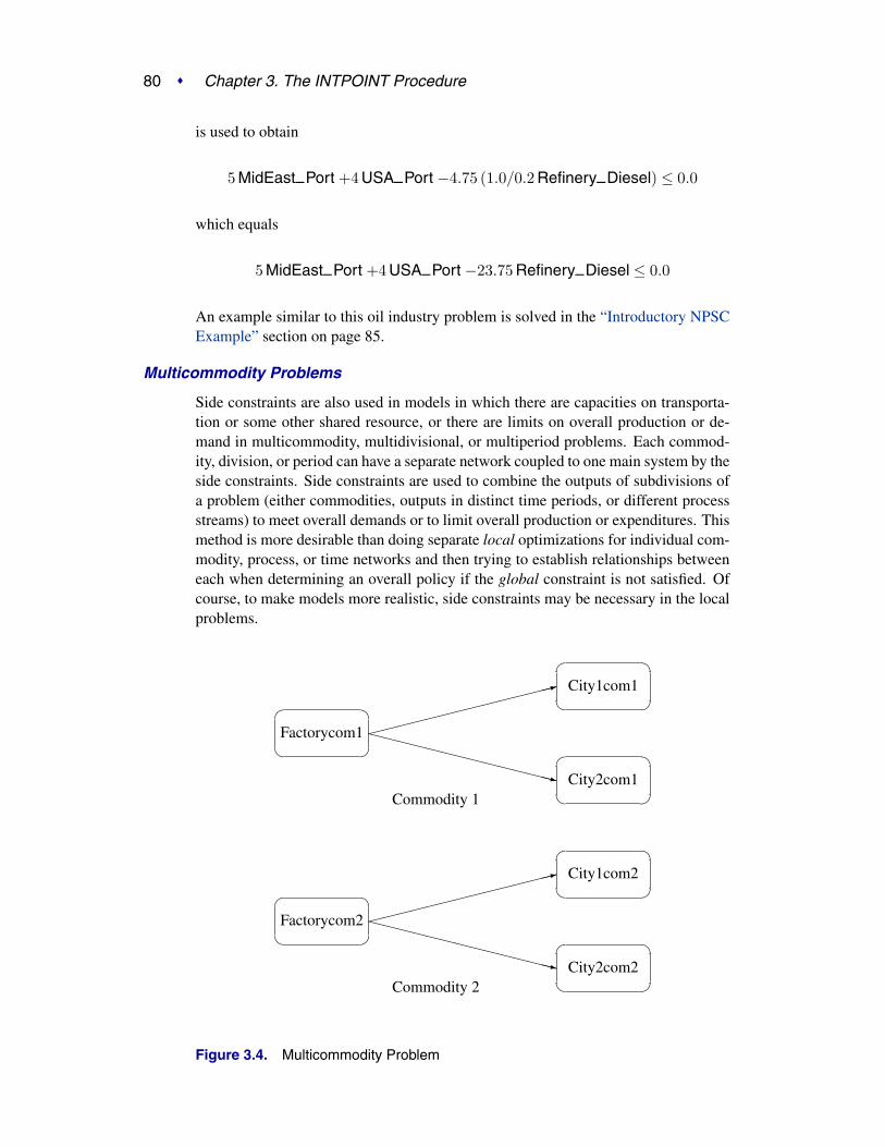
80 � Chapter 3. The INTPOINT Procedure
is used to obtain
5 MidEast–Port +4 USA–Port −4.75 (1.0/0.2 Refinery–Diesel) ≤ 0.0
which equals
5 MidEast–Port +4 USA–Port −23.75 Refinery–Diesel ≤ 0.0
An example similar to this oil industry problem is solved in the “Introductory NPSCExample” section on page 85.
Multicommodity Problems
Side constraints are also used in models in which there are capacities on transporta-tion or some other shared resource, or there are limits on overall production or de-mand in multicommodity, multidivisional, or multiperiod problems. Each commod-ity, division, or period can have a separate network coupled to one main system by theside constraints. Side constraints are used to combine the outputs of subdivisions ofa problem (either commodities, outputs in distinct time periods, or different processstreams) to meet overall demands or to limit overall production or expenditures. Thismethod is more desirable than doing separate local optimizations for individual com-modity, process, or time networks and then trying to establish relationships betweeneach when determining an overall policy if the global constraint is not satisfied. Ofcourse, to make models more realistic, side constraints may be necessary in the localproblems.
�
�
�
�Factorycom2
�
�
�
�Factorycom1
�
�
�
�City2com2
�
�
�
�City1com2
�
�
�
�City2com1
�
�
�
�City1com1
���������������
���������������
���������������
���������������
Commodity 1
Commodity 2
Figure 3.4. Multicommodity Problem

Network Models � 81
Figure 3.4 shows two network fragments. They represent identical production anddistribution sites of two different commodities. Suffix com1 represents commod-ity 1 and suffix com2 represents commodity 2. The nodes Factorycom1 andFactorycom2 model the same factory, and nodes City1com1 and City1com2 modelthe same location, city 1. Similarly, City2com1 and City2com2 are the same loca-tion, city 2. Suppose that commodity 1 occupies 2 cubic meters, commodity 2 occu-pies 3 cubic meters, the truck dispatched to city 1 has a capacity of 200 cubic meters,and the truck dispatched to city 2 has a capacity of 250 cubic meters. How much ofeach commodity can be loaded onto each truck? The side constraints for this case are
2 Factorycom1–City1com1 +3 Factorycom2–City1com2 ≤ 2002 Factorycom1–City2com1 +3 Factorycom2–City2com2 ≤ 250
Large Modeling Strategy
In many cases, the flow through an arc might actually represent the flow or movementof a commodity from place to place or from time period to time period. However,sometimes an arc is included in the network as a method of capturing some aspect ofthe problem that you would not normally think of as part of a network model. Thereis no commodity movement associated with that arc. For example, in a multiprocess,multiproduct model (Figure 3.5), there might be subnetworks for each process andeach product. The subnetworks can be joined together by a set of arcs that have flowsthat represent the amount of product j produced by process i. To model an upper-limit constraint on the total amount of product j that can be produced, direct all arcscarrying product j to a single node and from there through a single arc. The capacityof this arc is the upper limit of product j production. It is preferable to model thisstructure in the network rather than to include it in the side constraints because theefficiency of the optimizer may be less affected by a reasonable increase in the sizeof the network rather than increasing the number or complicating side constraints.
�
�
�
�
��
��
����
���
���
���
Capacity ofProcess 2
Process 2 subnetwork
�
�
�
�
��
��
����
���
���
���
Capacity ofProcess 1
Process 1 subnetwork
�
�
�
�
��
��
����
���
���
���
Capacity is upper limit ofProduct 2 production
Product 2 subnetwork
�
�
�
�
��
��
����
���
���
���
Capacity is upper limit ofProduct 1 production
Product 1 subnetwork
�
�
��
��
�����
��
���
Figure 3.5. Multiprocess, Multiproduct Example
When starting a project, it is often a good strategy to use a small network formulationand then use that model as a framework upon which to add detail. For example, inthe multiprocess, multiproduct model, you might start with the network depicted in

82 � Chapter 3. The INTPOINT Procedure
Figure 3.5. Then, for example, the process subnetwork can be enhanced to includethe distribution of products. Other phases of the operation could be included byadding more subnetworks. Initially, these subnetworks can be single nodes, but insubsequent studies they can be expanded to include greater detail.
Advantages of Network Models over LP Models
Many linear programming problems have large embedded network structures. Suchproblems often result when modeling manufacturing processes, transportation or dis-tribution networks, or resource allocation, or when deciding where to locate facilities.Often, some commodity is to be moved from place to place, so the more natural for-mulation in many applications is that of a constrained network rather than a linearprogram.
Using a network diagram to visualize a problem makes it possible to capture theimportant relationships in an easily understood picture form. The network diagramaids the communication between model builder and model user, making it easier tocomprehend how the model is structured, how it can be changed, and how results canbe interpreted.
If a network structure is embedded in a linear program, the problem is an NPSC (seethe “Mathematical Description of NPSC” section on page 66). When the networkpart of the problem is large compared to the nonnetwork part, especially if the numberof side constraints is small, it is worthwhile to exploit this structure to describe themodel. Rather than generating the data for the flow conservation constraints, generateinstead the data for the nodes and arcs of the network.
Flow Conservation Constraints
The constraints Fx = b in NPSC (see the “Mathematical Description of NPSC” sec-tion on page 66) are referred to as the nodal flow conservation constraints. Theseconstraints algebraically state that the sum of the flow through arcs directed towarda node plus that node’s supply, if any, equals the sum of the flow through arcs di-rected away from that node plus that node’s demand, if any. The flow conservationconstraints are implicit in the network model and should not be specified explicitly inside constraint data when using PROC INTPOINT to solve NPSC problems.
Nonarc Variables
Nonarc variables can be used to simplify side constraints. For example, if a sum offlows appears in many constraints, it may be worthwhile to equate this expressionwith a nonarc variable and use this in the other constraints. This keeps the constraintcoefficient matrix sparse. By assigning a nonarc variable a nonzero objective func-tion, it is then possible to incur a cost for using resources above some lowest feasiblelimit. Similarly, a profit (a negative objective function coefficient value) can be madeif all available resources are not used.
In some models, nonarc variables are used in constraints to absorb excess resources orsupply needed resources. Then, either the excess resource can be used or the neededresource can be supplied to another component of the model.

Network Models � 83
For example, consider a multicommodity problem of making television sets that haveeither 19- or 25-inch screens. In their manufacture, three and four chips, respectively,are used. Production occurs at two factories during March and April. The supplierof chips can supply only 2,600 chips to factory 1 and 3,750 chips to factory 2 eachmonth. The names of arcs are in the form Prodn–s–m, where n is the factory number,s is the screen size, and m is the month. For example, Prod1–25–Apr is the arc thatconveys the number of 25-inch TVs produced in factory 1 during April. You mighthave to determine similar systematic naming schemes for your application.
As described, the constraints are
3 Prod1–19–Mar +4 Prod1–25–Mar ≤ 26003 Prod2–19–Mar +4 Prod2–25–Mar ≤ 37503 Prod1–19–Apr +4 Prod1–25–Apr ≤ 26003 Prod2–19–Apr +4 Prod2–25–Apr ≤ 3750
If there are chips that could be obtained for use in March but not used for productionin March, why not keep these unused chips until April? Furthermore, if the Marchexcess chips at factory 1 could be used either at factory 1 or factory 2 in April, themodel becomes
3 Prod1–19–Mar +4 Prod1–25–Mar + F1–Unused–Mar = 26003 Prod2–19–Mar +4 Prod2–25–Mar + F2–Unused–Mar = 3750
3 Prod1–19–Apr +4 Prod1–25–Apr −F1–Kept–Since–Mar = 26003 Prod2–19–Apr +4 Prod2–25–Apr −F2–Kept–Since–Mar = 3750
F1–Unused–Mar + F2–Unused–Mar (continued)− F1–Kept–Since–Mar − F2–Kept–Since–Mar ≥ 0.0
where F1–Kept–Since–Mar is the number of chips used during April atfactory 1 that were obtained in March at either factory 1 or factory 2, andF2–Kept–Since–Mar is the number of chips used during April at factory 2 thatwere obtained in March. The last constraint ensures that the number of chips usedduring April that were obtained in March does not exceed the number of chipsnot used in March. There may be a cost to hold chips in inventory. This can bemodeled having a positive objective function coefficient for the nonarc variablesF1–Kept–Since–Mar and F2–Kept–Since–Mar. Moreover, nonarc variableupper bounds represent an upper limit on the number of chips that can be held ininventory between March and April.
See Example 3.1 through Example 3.5, which use this TV problem. The use of nonarcvariables as described previously is illustrated.

84 � Chapter 3. The INTPOINT Procedure
Introduction
Getting Started: NPSC Problems
To solve NPSC problems using PROC INTPOINT, you save a representation of thenetwork and the side constraints in three SAS data sets. These data sets are thenpassed to PROC INTPOINT for solution. There are various forms that a problem’sdata can take. You can use any one or a combination of several of these forms.
The NODEDATA= data set contains the names of the supply and demand nodes andthe supply or demand associated with each. These are the elements in the columnvector b in the NPSC problem (see the “Mathematical Description of NPSC” sectionon page 66).
The ARCDATA= data set contains information about the variables of the problem.Usually these are arcs, but there can be data related to nonarc variables in theARCDATA= data set as well.
An arc is identified by the names of its tail node (where it originates) and head node(where it is directed). Each observation can be used to identify an arc in the networkand, optionally, the cost per flow unit across the arc, the arc’s capacity, lower flowbound, and name. These data are associated with the matrix F and the vectors c, l,and u in the NPSC problem (see the “Mathematical Description of NPSC” section onpage 66).
Note: Although F is a node-arc incidence matrix, it is specified in the ARCDATA=data set by arc definitions. Do not explicitly specify these flow conservation con-straints as constraints of the problem.
In addition, the ARCDATA= data set can be used to specify information about nonarcvariables, including objective function coefficients, lower and upper value bounds,and names. These data are the elements of the vectors d, m, and v in the NPSCproblem (see the “Mathematical Description of NPSC” section on page 66). Data foran arc or nonarc variable can be given in more than one observation.
Supply and demand data also can be specified in the ARCDATA= data set. In such acase, the NODEDATA= data set may not be needed.
The CONDATA= data set describes the side constraints and their right-hand sides.These data are elements of the matrices H and Q and the vector r. Constraint typesare also specified in the CONDATA= data set. You can include in this data set up-per bound values or capacities, lower flow or value bounds, and costs or objectivefunction coefficients. It is possible to give all information about some or all nonarcvariables in the CONDATA= data set.
An arc is identified in this data set by its name. If you specify an arc’s name in theARCDATA= data set, then this name is used to associate data in the CONDATA=data set with that arc. Each arc also has a default name that is the name of the tail andhead node of the arc concatenated together and separated by an underscore character;tail–head, for example.

Getting Started: NPSC Problems � 85
If you use the dense side constraint input format (described in the “CONDATA= DataSet” section on page 131), and want to use the default arc names, these arc names arenames of SAS variables in the VAR list of the CONDATA= data set.
If you use the sparse side constraint input format (see the “CONDATA= Data Set”section on page 131) and want to use the default arc names, these arc names arevalues of the COLUMN list variable of the CONDATA= data set.
PROC INTPOINT reads the data from the NODEDATA= data set, the ARCDATA=data set, and the CONDATA= data set. Error checking is performed, and the modelis converted into an equivalent LP. This LP is preprocessed. Preprocessing is op-tional but highly recommended. Preprocessing analyzes the model and tries to de-termine before optimization whether variables can be “fixed” to their optimal values.Knowing that, the model can be modified and these variables dropped out. It can bedetermined that some constraints are redundant. Sometimes, preprocessing succeedsin reducing the size of the problem, thereby making the subsequent optimization eas-ier and faster.
The optimal solution to the equivalent LP is then found. This LP is converted back tothe original NPSC problem, and the optimum for this is derived from the optimum ofthe equivalent LP. If the problem was preprocessed, the model is now post-processed,where fixed variables are reintroduced. The solution can be saved in the CONOUT=data set.
Introductory NPSC Example
Consider the following transshipment problem for an oil company. Crude oil isshipped to refineries where it is processed into gasoline and diesel fuel. The gaso-line and diesel fuel are then distributed to service stations. At each stage, there areshipping, processing, and distribution costs. Also, there are lower flow bounds andcapacities.
In addition, there are two sets of side constraints. The first set is that two times thecrude from the Middle East cannot exceed the throughput of a refinery plus 15 units.(The phrase “plus 15 units” that finishes the last sentence is used to enable some sideconstraints in this example to have a nonzero rhs.) The second set of constraints arenecessary to model the situation that one unit of crude mix processed at a refineryyields three-fourths of a unit of gasoline and one-fourth of a unit of diesel fuel.
Because there are two products that are not independent in the way in which they flowthrough the network, an NPSC is an appropriate model for this example (see Figure3.6). The side constraints are used to model the limitations on the amount of MiddleEastern crude that can be processed by each refinery and the conversion proportionsof crude to gasoline and diesel fuel.

86 � Chapter 3. The INTPOINT Procedure
�
�
�
�u.s.a.
�
�
�
�refinery2
�
�
�
�middle east
�
�
�
�refinery1
�
�
�
�r2
�
�
�
�r1
�
�
�
�ref2 diesel
�
�
�
�ref2 gas
�
�
�
�ref1 diesel
�
�
�
�ref1 gas
�
�
�
�servstn2
diesel
�
�
�
�servstn2
gas
�
�
�
�servstn1
diesel
�
�
�
�servstn1
gas
�
�
�
�
�
�
�
�
������������������
���������������
��
��
���
��
��
���
��
��
���
��
��
���
!!!!!!!!!!!!!!!!"
!!!!!!!!!!!!!!!!"
################$
################$
Figure 3.6. Oil Industry Example
To solve this problem with PROC INTPOINT, save a representation of the model inthree SAS data sets. In the NODEDATA= data set, you name the supply and demandnodes and give the associated supplies and demands. To distinguish demand nodesfrom supply nodes, specify demands as negative quantities. For the oil example, theNODEDATA= data set can be saved as follows:
title ’Oil Industry Example’;title3 ’Setting Up Nodedata = Noded For PROC INTPOINT’;data noded;
input _node_&$15. _sd_;datalines;
middle east 100u.s.a. 80servstn1 gas -95servstn1 diesel -30servstn2 gas -40servstn2 diesel -15;
The ARCDATA= data set contains the rest of the information about the network.Each observation in the data set identifies an arc in the network and gives the cost perflow unit across the arc, the capacities of the arc, the lower bound on flow across thearc, and the name of the arc.

Getting Started: NPSC Problems � 87
title3 ’Setting Up Arcdata = Arcd1 For PROC INTPOINT’;data arcd1;
input _from_&$11. _to_&$15. _cost_ _capac_ _lo_ _name_ $;datalines;
middle east refinery 1 63 95 20 m_e_ref1middle east refinery 2 81 80 10 m_e_ref2u.s.a. refinery 1 55 . . .u.s.a. refinery 2 49 . . .refinery 1 r1 200 175 50 thruput1refinery 2 r2 220 100 35 thruput2r1 ref1 gas . 140 . r1_gasr1 ref1 diesel . 75 . .r2 ref2 gas . 100 . r2_gasr2 ref2 diesel . 75 . .ref1 gas servstn1 gas 15 70 . .ref1 gas servstn2 gas 22 60 . .ref1 diesel servstn1 diesel 18 . . .ref1 diesel servstn2 diesel 17 . . .ref2 gas servstn1 gas 17 35 5 .ref2 gas servstn2 gas 31 . . .ref2 diesel servstn1 diesel 36 . . .ref2 diesel servstn2 diesel 23 . . .;
Finally, the CONDATA= data set contains the side constraints for the model:
title3 ’Setting Up Condata = Cond1 For PROC INTPOINT’;data cond1;
input m_e_ref1 m_e_ref2 thruput1 r1_gas thruput2 r2_gas_type_ $ _rhs_;
datalines;-2 . 1 . . . >= -15. -2 . . 1 . GE -15. . -3 4 . . EQ 0. . . . -3 4 = 0;
Note that the SAS variable names in the CONDATA= data set are the names of arcsgiven in the ARCDATA= data set. These are the arcs that have nonzero constraintcoefficients in side constraints. For example, the proportionality constraint that spec-ifies that one unit of crude at each refinery yields three-fourths of a unit of gasolineand one-fourth of a unit of diesel fuel is given for refinery 1 in the third observa-tion and for refinery 2 in the last observation. The third observation requires thateach unit of flow on the arc thruput1 equals three-fourths of a unit of flow on thearc r1–gas. Because all crude processed at refinery 1 flows through thruput1 andall gasoline produced at refinery 1 flows through r1–gas, the constraint models thesituation. It proceeds similarly for refinery 2 in the last observation.

88 � Chapter 3. The INTPOINT Procedure
To find the minimum cost flow through the network that satisfies the supplies, de-mands, and side constraints, invoke PROC INTPOINT as follows:
proc intpointbytes=1000000nodedata=noded /* the supply and demand data */arcdata=arcd1 /* the arc descriptions */condata=cond1 /* the side constraints */conout=solution; /* the solution data set */run;
The following messages, which appear on the SAS log, summarize the model as readby PROC INTPOINT and note the progress toward a solution.
NOTE: Number of nodes= 14 .NOTE: Number of supply nodes= 2 .NOTE: Number of demand nodes= 4 .NOTE: Total supply= 180 , total demand= 180 .NOTE: Number of arcs= 18 .NOTE: Number of <= side constraints= 0 .NOTE: Number of == side constraints= 2 .NOTE: Number of >= side constraints= 2 .NOTE: Number of side constraint coefficients= 8 .NOTE: The following messages relate to the equivalent
Linear Programming problem solved by the InteriorPoint algorithm.
NOTE: Number of <= constraints= 0 .NOTE: Number of == constraints= 16 .NOTE: Number of >= constraints= 2 .NOTE: Number of constraint coefficients= 44 .NOTE: Number of variables= 18 .NOTE: After preprocessing, number of <= constraints= 0.NOTE: After preprocessing, number of == constraints= 5.NOTE: After preprocessing, number of >= constraints= 2.NOTE: The preprocessor eliminated 11 constraints from the
problem.NOTE: The preprocessor eliminated 25 constraint
coefficients from the problem.NOTE: After preprocessing, number of variables= 8.NOTE: The preprocessor eliminated 10 variables from the
problem.NOTE: 2 columns, 0 rows and 2 coefficients were added to
the problem to handle unrestricted variables,variables that are split, and constraint slack orsurplus variables.
NOTE: There are 13 nonzero elements in A * A transpose.NOTE: Of the 7 rows and columns, 2 are sparse.NOTE: There are 6 nonzero superdiagonal elements in the
sparse rows of the factored A * A transpose. Thisincludes fill-in.
NOTE: There are 2 operations of the formu[i,j]=u[i,j]-u[q,j]*u[q,i]/u[q,q] to factorize the

Getting Started: NPSC Problems � 89
sparse rows of A * A transpose.NOTE: Bound feasibility attained by iteration 1.NOTE: Dual feasibility attained by iteration 1.NOTE: Constraint feasibility attained by iteration 2.NOTE: The Primal-Dual Predictor-Corrector Interior Point
algorithm performed 7 iterations.NOTE: Objective = 50875.01279.NOTE: The data set WORK.SOLUTION has 18 observations and
10 variables.NOTE: There were 18 observations read from the data set
WORK.ARCD1.NOTE: There were 6 observations read from the data set
WORK.NODED.NOTE: There were 4 observations read from the data set
WORK.COND1.
The first set of messages shows the size of the problem. The next set of messagesprovides statistics on the size of the equivalent LP problem. The number of variablesmay not equal the number of arcs if the problem has nonarc variables. This examplehas none. To convert a network to the equivalent LP problem, a flow conservationconstraint must be created for each node (including an excess or bypass node, ifrequired). This explains why the number of equality constraints and the number ofconstraint coefficients differ from the number of equality side constraints and thenumber of coefficients in all side constraints.
If the preprocessor was successful in decreasing the problem size, some messageswill report how well it did. In this example, the model size was cut approximately inhalf!
The next set of messages describes aspects of the interior point algorithm. Of partic-ular interest are those concerned with the Cholesky factorization of AAT where A isthe coefficient matrix of the final LP. It is crucial to preorder the rows and columnsof this matrix to prevent fill-in and reduce the number of row operations to undertakethe factorization. See the “Interior Point Algorithmic Details” section on page 68 fora more extensive explanation.
Unlike PROC LP, which displays the solution and other information as output, PROCINTPOINT saves the optimum in the output SAS data set that you specify. For thisexample, the solution is saved in the SOLUTION data set. It can be displayed withthe PRINT procedure as
title3 ’Optimum’;proc print data=solution;
var _from_ _to_ _cost_ _capac_ _lo_ _name__supply_ _demand_ _flow_ _fcost_;
sum _fcost_;run;

90 � Chapter 3. The INTPOINT Procedure
Oil Industry Example
Optimum
_ __ S D _
_ _ c _ U E _ Ff c a n P M F Cr _ o p _ a P A L O
O o t s a l m L N O Sb m o t c o e Y D W Ts _ _ _ _ _ _ _ _ _ _
1 refinery 1 r1 200 175 50 thruput1 . . 145.000 28999.982 refinery 2 r2 220 100 35 thruput2 . . 35.000 7700.023 r1 ref1 diesel 0 75 0 . . 36.250 0.004 r1 ref1 gas 0 140 0 r1_gas . . 108.750 0.005 r2 ref2 diesel 0 75 0 . . 8.750 0.006 r2 ref2 gas 0 100 0 r2_gas . . 26.250 0.007 middle east refinery 1 63 95 20 m_e_ref1 100 . 80.000 5039.998 u.s.a. refinery 1 55 99999999 0 80 . 65.000 3575.009 middle east refinery 2 81 80 10 m_e_ref2 100 . 20.000 1620.0210 u.s.a. refinery 2 49 99999999 0 80 . 15.000 735.0011 ref1 diesel servstn1 diesel 18 99999999 0 . 30 30.000 540.0012 ref2 diesel servstn1 diesel 36 99999999 0 . 30 0.000 0.0113 ref1 gas servstn1 gas 15 70 0 . 95 68.750 1031.2614 ref2 gas servstn1 gas 17 35 5 . 95 26.250 446.2415 ref1 diesel servstn2 diesel 17 99999999 0 . 15 6.250 106.2516 ref2 diesel servstn2 diesel 23 99999999 0 . 15 8.750 201.2417 ref1 gas servstn2 gas 22 60 0 . 40 40.000 879.9918 ref2 gas servstn2 gas 31 99999999 0 . 40 0.000 0.01
========50875.01
Figure 3.7. CONOUT=SOLUTION
Notice that, in CONOUT=SOLUTION (Figure 3.7), the optimal flow through eacharc in the network is given in the variable named –FLOW– , and the cost of flowthrough each arc is given in the variable –FCOST– .

Getting Started: LP Problems � 91
�
�
�
�u.s.a.
�
�
�
�refinery2
�
�
�
�middle east
�
�
�
�refinery1
�
�
�
�r2
�
�
�
�r1
�
�
�
�ref2 diesel
�
�
�
�ref2 gas
�
�
�
�ref1 diesel
�
�
�
�ref1 gas
�
�
�
�servstn2
diesel
�
�
�
�servstn2
gas
�
�
�
�servstn1
diesel
�
�
�
�servstn1
gas
�
�
�
�
�
�
�
�
������������������
���������������
��
��
���
��
��
���
��
��
���
��
��
���
!!!!!!!!!!!!!!!!"
!!!!!!!!!!!!!!!!"
################$
################$
80
100
15
80
20
65
35
145
8.75
26.25
36.25
108.7568.75
8.75
30
40 26.25
6.25
−95
−30
−40
−15
Figure 3.8. Oil Industry Solution
Getting Started: LP Problems
Data for an LP problem resembles the data for side constraints and nonarc variablessupplied to PROC INTPOINT when solving an NPSC problem. It is also very similarto the data required by the LP procedure.
To solve LP problems using PROC INTPOINT, you save a representation of the LPvariables and the constraints in one or two SAS data sets. These data sets are thenpassed to PROC INTPOINT for solution. There are various forms that a problem’sdata can take. You can use any one or a combination of several of these forms.
The ARCDATA= data set contains information about the LP variables of the problem.Although this data set is called ARCDATA, it contains data for no arcs. Instead, alldata in this data set are related to LP variables. This data set has no SAS variablescontaining values that are node names.
The ARCDATA= data set can be used to specify information about LP variables,including objective function coefficients, lower and upper value bounds, and names.These data are the elements of the vectors d, m, and v in problem (LP). Data for anLP variable can be given in more than one observation.
The CONDATA= data set describes the constraints and their right-hand sides. Thesedata are elements of the matrix Q and the vector r.

92 � Chapter 3. The INTPOINT Procedure
Constraint types are also specified in the CONDATA= data set. You can include inthis data set LP variable data such as upper bound values, lower value bounds, andobjective function coefficients. It is possible to give all information about some or allLP variables in the CONDATA= data set.
Because PROC INTPOINT evolved from PROC NETFLOW, another procedure inSAS/OR software that was originally designed to solve models with networks, theARCDATA= data set is always expected. If the ARCDATA= data set is not specified,by default the last data set created before PROC INTPOINT is invoked is assumed tobe the ARCDATA= data set. However, these characteristics of PROC INTPOINT arenot helpful when an LP problem is being solved and all data is provided in a singledata set specified by the CONDATA= data set, and that data set is not the last dataset created before PROC INTPOINT starts. In this case, you must specify that theARCDATA= data set and the CONDATA= data set are both equal to the input dataset. PROC INTPOINT then knows that an LP problem is to be solved and that thedata reside in one data set.
An LP variable is identified in this data set by its name. If you specify an LP variable’sname in the ARCDATA= data set, then this name is used to associate data in theCONDATA= data set with that LP variable.
If you use the dense constraint input format (described in the “CONDATA= DataSet” section on page 131), these LP variable names are names of SAS variables inthe VAR list of the CONDATA= data set.
If you use the sparse constraint input format (described in the “CONDATA= DataSet” section on page 131), these LP variable names are values of the SAS variablesin the COLUMN list of the CONDATA= data set.
PROC INTPOINT reads the data from the ARCDATA= data set (if there is one) andthe CONDATA= data set. Error checking is performed, and the LP is preprocessed.Preprocessing is optional but highly recommended. The preprocessor analyzes themodel and tries to determine before optimization whether LP variables can be “fixed”to their optimal values. Knowing that, the model can be modified and these LP vari-ables dropped out. Some constraints may be found to be redundant. Sometimes,preprocessing succeeds in reducing the size of the problem, thereby making the sub-sequent optimization easier and faster.
The optimal solution is then found for the resulting LP. If the problem was prepro-cessed, the model is now post-processed, where fixed LP variables are reintroduced.The solution can be saved in the CONOUT= data set.
Introductory LP Example
Consider the linear programming problem in the section “An Introductory Example”on page 190. The SAS data set in that section is created the same way here:

Getting Started: LP Problems � 93
title ’Linear Programming Example’;title3 ’Setting Up Condata = dcon1 For PROC INTPOINT’;data dcon1;
input _id_ $17.a_light a_heavy brega naphthal naphthaiheatingo jet_1 jet_2_type_ $ _rhs_;
datalines;profit -175 -165 -205 0 0 0 300 300 max .naphtha_l_conv .035 .030 .045 -1 0 0 0 0 eq 0naphtha_i_conv .100 .075 .135 0 -1 0 0 0 eq 0heating_o_conv .390 .300 .430 0 0 -1 0 0 eq 0recipe_1 0 0 0 0 .3 .7 -1 0 eq 0recipe_2 0 0 0 .2 0 .8 0 -1 eq 0available 110 165 80 . . . . . upperbd .;
To solve this problem, use
proc intpointbytes=1000000condata=dcon1conout=solutn1;run;
Note how it is possible to use an input SAS data set of PROC LP and, without requir-ing any changes to be made to the data set, to use that as an input data set for PROCINTPOINT.
The following messages that appear on the SAS log summarize the model as read byPROC INTPOINT and note the progress toward a solution
NOTE: Number of variables= 8 .NOTE: Number of <= constraints= 0 .NOTE: Number of == constraints= 5 .NOTE: Number of >= constraints= 0 .NOTE: Number of constraint coefficients= 18 .NOTE: After preprocessing, number of <= constraints= 0.NOTE: After preprocessing, number of == constraints= 0.NOTE: After preprocessing, number of >= constraints= 0.NOTE: The preprocessor eliminated 5 constraints from the
problem.NOTE: The preprocessor eliminated 18 constraint
coefficients from the problem.NOTE: After preprocessing, number of variables= 0.NOTE: The preprocessor eliminated 8 variables from the
problem.WARNING: Optimization is unnecessary as the problem no
longer has any variables and rows.NOTE: Preprocessing could have caused that.NOTE: Objective = 1544.NOTE: The data set WORK.SOLUTN1 has 8 observations and 6
variables.

94 � Chapter 3. The INTPOINT Procedure
NOTE: There were 7 observations read from the data setWORK.DCON1.
Notice that the preprocessor succeeded in fixing all LP variables to their optimalvalues, eliminating the need to do any actual optimization.
Unlike PROC LP, which displays the solution and other information as output, PROCINTPOINT saves the optimum in the output SAS data set you specify. For this exam-ple, the solution is saved in the SOLUTION data set. It can be displayed with PROCPRINT as
title3 ’LP Optimum’;proc print data=solutn1;
var _name_ _objfn_ _upperbd _lowerbd _value_ _fcost_;sum _fcost_;run;
Notice that in the CONOUT=SOLUTION (Figure 3.9) the optimal value througheach variable in the LP is given in the variable named –VALUE– , and that the costof value for each variable is given in the variable –FCOST– .
Linear Programming Example
LP Optimum
Obs _NAME_ _OBJFN_ _UPPERBD _LOWERBD _VALUE_ _FCOST_
1 a_heavy -165 165 0 0.00 02 a_light -175 110 0 110.00 -192503 brega -205 80 0 80.00 -164004 heatingo 0 99999999 0 77.30 05 jet_1 300 99999999 0 60.65 181956 jet_2 300 99999999 0 63.33 189997 naphthai 0 99999999 0 21.80 08 naphthal 0 99999999 0 7.45 0
=======1544
Figure 3.9. CONOUT=SOLUTN1
The same model can be specified in the sparse format as in the following scon2 dataset. This format enables you to omit the zero coefficients.
title3 ’Setting Up Condata = scon2 For PROC INTPOINT’;data scon2;
format _type_ $8. _col_ $8. _row_ $16.;input _type_ $ _col_ $ _row_ $ _coef_;datalines;
max . profit .eq . napha_l_conv .eq . napha_i_conv .eq . heating_oil_conv .eq . recipe_1 .eq . recipe_2 .upperbd . available .. a_light profit -175

Getting Started: LP Problems � 95
. a_light napha_l_conv .035
. a_light napha_i_conv .100
. a_light heating_oil_conv .390
. a_light available 110
. a_heavy profit -165
. a_heavy napha_l_conv .030
. a_heavy napha_i_conv .075
. a_heavy heating_oil_conv .300
. a_heavy available 165
. brega profit -205
. brega napha_l_conv .045
. brega napha_i_conv .135
. brega heating_oil_conv .430
. brega available 80
. naphthal napha_l_conv -1
. naphthal recipe_2 .2
. naphthai napha_i_conv -1
. naphthai recipe_1 .3
. heatingo heating_oil_conv -1
. heatingo recipe_1 .7
. heatingo recipe_2 .8
. jet_1 profit 300
. jet_1 recipe_1 -1
. jet_2 profit 300
. jet_2 recipe_2 -1;
To find the minimum cost solution, invoke PROC INTPOINT (note theSPARSECONDATA option which must be specified) as follows:
proc intpointbytes=1000000sparsecondatacondata=scon2conout=solutn2;run;
A data set that can be used as the ARCDATA= data set can be initialized as follows:
data vars3;input _name_ $ profit available;datalines;
a_heavy -165 165a_light -175 110brega -205 80heatingo 0 .jet_1 300 .jet_2 300 .naphthai 0 .naphthal 0 .;

96 � Chapter 3. The INTPOINT Procedure
The following CONDATA= data set is the original dense format CONDATA= dcon1data set after the LP variable’s nonconstraint information has been removed. (Youcould have left some or all of that information in CONDATA as PROC INTPOINT“merges” data, but doing that and checking for consistency takes time.)
data dcon3;input _id_ $17.
a_light a_heavy brega naphthal naphthaiheatingo jet_1 jet_2_type_ $ _rhs_;
datalines;naphtha_l_conv .035 .030 .045 -1 0 0 0 0 eq 0naphtha_i_conv .100 .075 .135 0 -1 0 0 0 eq 0heating_o_conv .390 .300 .430 0 0 -1 0 0 eq 0recipe_1 0 0 0 0 .3 .7 -1 0 eq 0recipe_2 0 0 0 .2 0 .8 0 -1 eq 0;
Note: You must now specify the MAXIMIZE option; otherwise, PROC INTPOINTwill optimize to the minimum (which, incidentally, has a total objective = -3539.25).You must indicate that the SAS variable profit in the ARCDATA=vars3 data set hasvalues that are objective function coefficients, by specifying the OBJFN statement.The UPPERBD must be specified as the SAS variable available that has as valuesupper bounds:
proc intpointmaximize /* ***** necessary ***** */bytes=1000000arcdata=vars3condata=dcon3conout=solutn3;
objfn profit;upperbd available;run;
The ARCDATA=vars3 data set can become more concise by noting that the modelvariables heatingo, naphthai, and naphthal have zero objective function coeffi-cients (the default) and default upper bounds, so those observations need not bepresent:
data vars4;input _name_ $ profit available;datalines;
a_heavy -165 165a_light -175 110brega -205 80jet_1 300 .jet_2 300 .;

Getting Started: LP Problems � 97
The CONDATA=dcon3 data set can become more concise by noting that all the con-straints have the same type (eq) and zero (the default) rhs values. This model is agood candidate for using the DEFCONTYPE= option.
The DEFCONTYPE= option can be useful not only when all constraints have thesame type as is the case here, but also when most constraints have the same type andyou want to change the default type from ≤ to = or ≥. The essential constraint typedata in the CONDATA= data set is that which overrides the DEFCONTYPE= typeyou specified.
data dcon4;input _id_ $17.
a_light a_heavy brega naphthal naphthaiheatingo jet_1 jet_2;
datalines;naphtha_l_conv .035 .030 .045 -1 0 0 0 0naphtha_i_conv .100 .075 .135 0 -1 0 0 0heating_o_conv .390 .300 .430 0 0 -1 0 0recipe_1 0 0 0 0 .3 .7 -1 0recipe_2 0 0 0 .2 0 .8 0 -1;
proc intpointmaximize defcontype=eqarcdata=vars3condata=dcon3conout=solutn3;
objfn profit;upperbd available;run;
Here are several different ways of using the ARCDATA= data set and a sparse for-mat CONDATA= data set for this LP. The following CONDATA= data set is theresult of removing the profit and available data from the original sparse formatCONDATA=scon2 data set.
data scon5;format _type_ $8. _col_ $8. _row_ $16. ;input _type_ $ _col_ $ _row_ $ _coef_;datalines;
eq . napha_l_conv .eq . napha_i_conv .eq . heating_oil_conv .eq . recipe_1 .eq . recipe_2 .. a_light napha_l_conv .035. a_light napha_i_conv .100. a_light heating_oil_conv .390. a_heavy napha_l_conv .030. a_heavy napha_i_conv .075. a_heavy heating_oil_conv .300
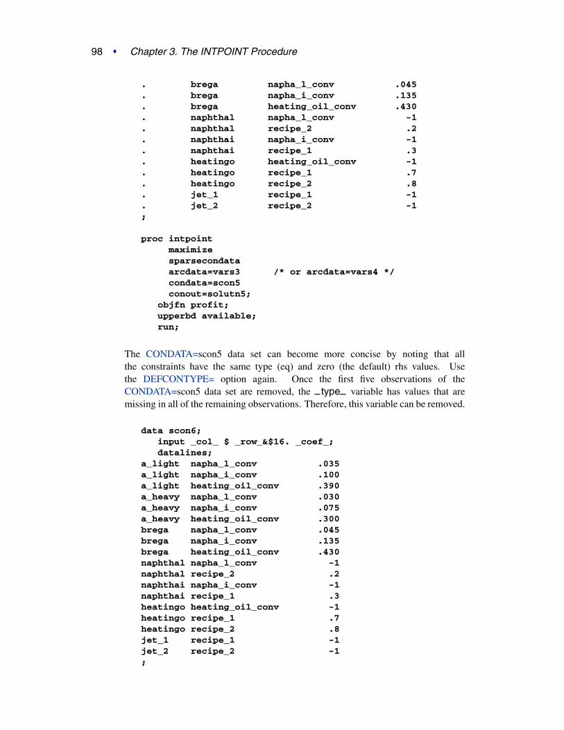
98 � Chapter 3. The INTPOINT Procedure
. brega napha_l_conv .045
. brega napha_i_conv .135
. brega heating_oil_conv .430
. naphthal napha_l_conv -1
. naphthal recipe_2 .2
. naphthai napha_i_conv -1
. naphthai recipe_1 .3
. heatingo heating_oil_conv -1
. heatingo recipe_1 .7
. heatingo recipe_2 .8
. jet_1 recipe_1 -1
. jet_2 recipe_2 -1;
proc intpointmaximizesparsecondataarcdata=vars3 /* or arcdata=vars4 */condata=scon5conout=solutn5;
objfn profit;upperbd available;run;
The CONDATA=scon5 data set can become more concise by noting that allthe constraints have the same type (eq) and zero (the default) rhs values. Usethe DEFCONTYPE= option again. Once the first five observations of theCONDATA=scon5 data set are removed, the –type– variable has values that aremissing in all of the remaining observations. Therefore, this variable can be removed.
data scon6;input _col_ $ _row_&$16. _coef_;datalines;
a_light napha_l_conv .035a_light napha_i_conv .100a_light heating_oil_conv .390a_heavy napha_l_conv .030a_heavy napha_i_conv .075a_heavy heating_oil_conv .300brega napha_l_conv .045brega napha_i_conv .135brega heating_oil_conv .430naphthal napha_l_conv -1naphthal recipe_2 .2naphthai napha_i_conv -1naphthai recipe_1 .3heatingo heating_oil_conv -1heatingo recipe_1 .7heatingo recipe_2 .8jet_1 recipe_1 -1jet_2 recipe_2 -1;

Typical PROC INTPOINT Run � 99
proc intpointmaximizedefcontype=eqsparsecondataarcdata=vars4condata=scon6conout=solutn6;
objfn profit;upperbd available;run;
Typical PROC INTPOINT Run
You start PROC INTPOINT by giving the PROC INTPOINT statement. You canspecify many options in the PROC INTPOINT statement to control the procedure,or you can rely on default settings and specify very few options. However, there aresome options you must specify:
• You must specify the BYTES= parameter indicating the size of the workingmemory that the procedure is allowed to use. This option has no default.
• In many instances (and certainly when solving NPSC problems), you need tospecify the ARCDATA= data set. This option has a default (which is the SASdata set that was created last before PROC INTPOINT began running), but thatmay need to be overridden.
• The CONDATA= data set must also be specified if the problem is NPSC andhas side constraints, or if it is an LP problem.
• When solving a network problem, you have to specify the NODEDATA= dataset, if some model data is given in such a data set.
Some options, while optional, are frequently required. To have the optimal solutionoutput to a SAS data set, you have to specify the CONOUT= data set. You maywant to indicate reasons why optimization should stop (for example, you can indicatethe maximum number of iterations that can be performed), or you might want to alterstopping criteria so that optimization does not stop prematurely. Some options enableyou to control other aspects of the interior point algorithm. Specifying certain valuesfor these options can reduce the time it takes to solve a problem.
The SAS variable lists should be given next. If you have SAS variables in the inputdata sets that have special names (for example, a SAS variable in the ARCDATA=data set named –TAIL– that has tail nodes of arcs as values), it may not be necessaryto have many or any variable lists. If you do not specify a TAIL variable list, PROCINTPOINT will search the ARCDATA= data set for a SAS variable named –TAIL–.
What usually follows is a RUN statement, which indicates that all information thatyou, the user, need to supply to PROC INTPOINT has been given, and the procedureis to start running. This also happens if you specify a statement in your SAS programthat PROC INTPOINT does not recognize as one of its own, the next DATA step orprocedure.

100 � Chapter 3. The INTPOINT Procedure
The QUIT statement indicates that PROC INTPOINT must immediately finish.
For example, a PROC INTPOINT run might look something like this:
proc intpointbytes= /* working memory size */arcdata= /* data set */condata= /* data set *//* other options */
;variable list specifications; /* if necessary */run; /* start running, read data, */
/* and do the optimization. */
Syntax
Below are statements used in PROC INTPOINT, listed in alphabetical order as theyappear in the text that follows.
PROC INTPOINT options ;CAPACITY variable ;COEF variables ;COLUMN variable ;COST variable ;DEMAND variable ;HEADNODE variable ;ID variables ;LO variable ;NAME variable ;NODE variable ;QUIT;RHS variable ;ROW variables ;RUN;SUPDEM variable ;SUPPLY variable ;TAILNODE variable ;TYPE variable ;VAR variables ;
Functional Summary
Table 3.1 outlines the options that can be specified in the INTPOINT procedure. Alloptions are specified in the PROC INTPOINT statement.

Functional Summary � 101
Table 3.1. Functional Summary
Description Statement Option
Input Data Set Options:arcs input data set PROC INTPOINT ARCDATA=nodes input data set PROC INTPOINT NODEDATA=constraint input data set PROC INTPOINT CONDATA=
Output Data Set Option:constrained solution data set PROC INTPOINT CONOUT=
Data Set Read Options:CONDATA has sparse data format PROC INTPOINT SPARSECONDATAdefault constraint type PROC INTPOINT DEFCONTYPE=special COLUMN variable value PROC INTPOINT TYPEOBS=special COLUMN variable value PROC INTPOINT RHSOBS=used to interpret arc and variable names PROC INTPOINT NAMECTRL=no nonarc data in ARCDATA PROC INTPOINT ARCS–ONLY–ARCDATAdata for an arc found once in ARCDATA PROC INTPOINT ARC–SINGLE–OBSdata for a constraint found once in CONDATA PROC INTPOINT CON–SINGLE–OBSdata for a coefficient found once in CONDATA PROC INTPOINT NON–REPLIC=data is grouped, exploited during data read PROC INTPOINT GROUPED=
Problem Size Specification Options:approximate number of nodes PROC INTPOINT NNODES=approximate number of arcs PROC INTPOINT NARCS=approximate number of variables PROC INTPOINT NNAS=approximate number of coefficients PROC INTPOINT NCOEFS=approximate number of constraints PROC INTPOINT NCONS=
Network Options:default arc cost, objective function coefficient PROC INTPOINT DEFCOST=default arc capacity, variable upper bound PROC INTPOINT DEFCAPACITY=default arc flow and variable lower bound PROC INTPOINT DEFMINFLOW=network’s only supply node PROC INTPOINT SOURCE=SOURCE’s supply capability PROC INTPOINT SUPPLY=network’s only demand node PROC INTPOINT SINK=SINK’s demand PROC INTPOINT DEMAND=convey excess supply/demand through network PROC INTPOINT THRUNETfind max flow between SOURCE and SINK PROC INTPOINT MAXFLOWcost of bypass arc, MAXFLOW problem PROC INTPOINT BYPASSDIVIDE=find shortest path from SOURCE to SINK PROC INTPOINT SHORTPATH
Interior Point Algorithm Options:allowed amount of dual infeasibility PROC INTPOINT TOLDINF=allowed amount of primal infeasibility PROC INTPOINT TOLPINF=allowed total amount of dual infeasibility PROC INTPOINT TOLTOTDINF=

102 � Chapter 3. The INTPOINT Procedure
Description Statement Option
allowed total amount of primal infeasibility PROC INTPOINT TOLTOTPINF=cut-off tolerance for Cholesky factorization PROC INTPOINT CHOLTINYTOL=density threshold for Cholesky processing PROC INTPOINT DENSETHR=step-length multiplier PROC INTPOINT PDSTEPMULT=preprocessing type PROC INTPOINT PRSLTYPE=print optimization progress on SAS log PROC INTPOINT PRINTLEVEL2=ratio test zero tolerance PROC INTPOINT RTTOL=
Interior Point Algorithm Stopping Criteria:maximum number of interior point iterations PROC INTPOINT MAXITERB=primal-dual (duality) gap tolerance PROC INTPOINT PDGAPTOL=stop because of complementarity PROC INTPOINT STOP–C=stop because of duality gap PROC INTPOINT STOP–DG=stop because of infeasb PROC INTPOINT STOP–IB=stop because of infeasc PROC INTPOINT STOP–IC=stop because of infeasd PROC INTPOINT STOP–ID=stop because of complementarity PROC INTPOINT AND–STOP–C=stop because of duality gap PROC INTPOINT AND–STOP–DG=stop because of infeasb PROC INTPOINT AND–STOP–IB=stop because of infeasc PROC INTPOINT AND–STOP–IC=stop because of infeasd PROC INTPOINT AND–STOP–ID=stop because of complementarity PROC INTPOINT KEEPGOING–C=stop because of duality gap PROC INTPOINT KEEPGOING–DG=stop because of infeasb PROC INTPOINT KEEPGOING–IB=stop because of infeasc PROC INTPOINT KEEPGOING–IC=stop because of infeasd PROC INTPOINT KEEPGOING–ID=stop because of complementarity PROC INTPOINT AND–KEEPGOING–C=stop because of duality gap PROC INTPOINT AND–KEEPGOING–DG=stop because of infeasb PROC INTPOINT AND–KEEPGOING–IB=stop because of infeasc PROC INTPOINT AND–KEEPGOING–IC=stop because of infeasd PROC INTPOINT AND–KEEPGOING–ID=
Memory Control Options:issue memory usage messages to SAS log PROC INTPOINT MEMREPnumber of bytes to use for main memory PROC INTPOINT BYTES=
Miscellaneous Options:infinity value PROC INTPOINT INFINITY=maximization instead of minimization PROC INTPOINT MAXIMIZEzero tolerance - optimization PROC INTPOINT ZERO2=zero tolerance - real number comparisons PROC INTPOINT ZEROTOL=suppress similar SAS log messages PROC INTPOINT VERBOSE=scale constraint row, nonarc variable columncoefficients, or both
PROC INTPOINT SCALE=

PROC INTPOINT Statement � 103
PROC INTPOINT Statement
PROC INTPOINT options ;
This statement invokes the procedure. The following options can be specified in thePROC INTPOINT statement.
Data Set Options
This section briefly describes all the input and output data sets used by PROCINTPOINT. The ARCDATA= data set, the NODEDATA= data set, and theCONDATA= data set can contain SAS variables that have special names, for instance
–CAPAC– , –COST– , and –HEAD– . PROC INTPOINT looks for such variablesif you do not give explicit variable list specifications. If a SAS variable with a specialname is found and that SAS variable is not in another variable list specification,PROC INTPOINT determines that values of the SAS variable are to be interpretedin a special way. By using SAS variables that have special names, you may not needto have any variable list specifications.
ARCDATA=SAS-data-setnames the data set that contains arc and, optionally, nonarc variable information andnodal supply/demand data. The ARCDATA= data set must be specified in all PROCINTPOINT statements when solving NPSC problems.
If your problem is an LP, the ARCDATA= data set is optional. You can specifyLP variable information such as objective function coefficients, and lower and upperbounds.
CONDATA=SAS-data-setnames the data set that contains the side constraint data. The data set can also containother data such as arc costs, capacities, lower flow bounds, nonarc variable upperand lower bounds, and objective function coefficients. PROC INTPOINT needs aCONDATA= data set to solve a constrained problem. See the “CONDATA= DataSet” section on page 131 for more information.
If your problem is an LP, this data set contains the constraint data, and can also containother data such as objective function coefficients, and lower and upper bounds. PROCINTPOINT needs a CONDATA= data set to solve an LP.
CONOUT=SAS-data-setCOUT=SAS-data-set
names the output data set that receives an optimal solution. See the “CONOUT= DataSet” section on page 140 for more information.
If PROC INTPOINT is outputting observations to the output data set and you wantthis to stop, press the keys used to stop SAS procedures.
NODEDATA=SAS-data-setnames the data set that contains the node supply and demand specifications. Youdo not need observations in the NODEDATA= data set for transshipment nodes.(Transshipment nodes neither supply nor demand flow.) All nodes are assumed to

104 � Chapter 3. The INTPOINT Procedure
be transshipment nodes unless supply or demand data indicate otherwise. It is ac-ceptable for some arcs to be directed toward supply nodes or away from demandnodes.
This data set is used only when you are solving network problems (not when solv-ing LP problems), in which case the use of the NODEDATA= data set is optionalprovided that, if the NODEDATA= data set is not used, supply and demand de-tails are specified by other means. Other means include using the MAXFLOWor SHORTPATH option, SUPPLY or DEMAND variable list (or both) in theARCDATA= data set, and the SOURCE=, SUPPLY=, SINK=, or DEMAND= op-tion in the PROC INTPOINT statement.
General Options
The following is a list of options you can use with PROC INTPOINT. The optionsare listed in alphabetical order.
ARCS–ONLY–ARCDATAindicates that data for arcs only are in the ARCDATA= data set. When PROCINTPOINT reads the data in the ARCDATA= data set, memory would not be wastedto receive data for nonarc variables. The read might then be performed faster. See thesection “How to Make the Data Read of PROC INTPOINT More Efficient” on page150.
ARC–SINGLE–OBSindicates that for all arcs and nonarc variables, data for each arc or nonarc variable isfound in only one observation of the ARCDATA= data set. When reading the data inthe ARCDATA= data set, PROC INTPOINT knows that the data in an observation isfor an arc or a nonarc variable that has not had data previously read and that needs tobe checked for consistency. The read might then be performed faster.
When solving an LP, specifying the ARC–SINGLE–OBS option indicates that forall LP variables, data for each LP variable is found in only one observation of theARCDATA= data set. When reading the data in the ARCDATA= data set, PROCINTPOINT knows that the data in an observation is for an LP variable that has nothad data previously read and that needs to be checked for consistency. The read mightthen be performed faster.
If you specify ARC–SINGLE–OBS, PROC INTPOINT automatically works as ifGROUPED=ARCDATA is also specified.
See the section “How to Make the Data Read of PROC INTPOINT More Efficient”on page 150.
BYPASSDIVIDE=bBYPASSDIV=bBPD=b
should be used only when the MAXFLOW option has been specified; that is, PROCINTPOINT is solving a maximal flow problem. PROC INTPOINT prepares to solvemaximal flow problems by setting up a bypass arc. This arc is directed from theSOURCE= to the SINK= and will eventually convey flow equal to INFINITY minusthe maximal flow through the network. The cost of the bypass arc must be great

PROC INTPOINT Statement � 105
enough to drive flow through the network, rather than through the bypass arc. Also,the cost of the bypass arc must be greater than the eventual total cost of the maxi-mal flow, which can be nonzero if some network arcs have nonzero costs. The costof the bypass is set to the value of the INFINITY= option. Valid values for theBYPASSDIVIDE= option must be greater than or equal to 1.1.
If there are no nonzero costs of arcs in the MAXFLOW problem, the cost of the by-pass arc is set to 1.0 (-1.0 if maximizing) if you do not specify the BYPASSDIVIDE=option. The default value for the BYPASSDIVIDE= option (in the presence ofnonzero arc costs) is 100.0.
BYTES=bindicates the size of the main working memory (in bytes) that PROC INTPOINTwill allocate. Specifying this option is mandatory. The working memory is usedto store all the arrays and buffers used by PROC INTPOINT. If this memory has asize smaller than what is required to store all arrays and buffers, PROC INTPOINTuses various schemes that page information between auxiliary memory (often yourmachine’s disk) and RAM.
For small problems, specify BYTES=100000. For large problems (those with hun-dreds of thousands or millions of variables), BYTES=1000000 might do. For solvingproblems of that size, if you are running on a machine with an inadequate amount ofRAM, PROC INTPOINT’s performance will suffer since it will be forced to page orto rely on virtual memory.
If you specify the MEMREP option, PROC INTPOINT will issue messages on theSAS log informing you of its memory usage; that is, how much memory is requiredto prevent paging, and details about the amount of paging that must be performed, ifapplicable.
CON–SINGLE–OBSimproves how the CONDATA= data set is read. How it works depends on whetherthe CONDATA has a dense or sparse format.
If the CONDATA= data set has the dense format, specifying CON–SINGLE–OBSindicates that, for each constraint, data for each can be found in only one observationof the CONDATA= data set.
If the CONDATA= data set has a sparse format, and data for each arc, nonarc variable,or LP variable can be found in only one observation of the CONDATA, then specifythe CON–SINGLE–OBS option. If there are n SAS variables in the ROW and COEFlist, then each arc or nonarc can have at most n constraint coefficients in the model.See the section “How to Make the Data Read of PROC INTPOINT More Efficient”on page 150.
DEFCAPACITY=cDC=c
requests that the default arc capacity and the default nonarc variable value upperbound (or for LP problems, the default LP variable value upper bound) be c. If thisoption is not specified, then DEFCAPACITY=INFINITY.

106 � Chapter 3. The INTPOINT Procedure
DEFCONTYPE=cDEFTYPE=cDCT=c
specifies the default constraint type. This default constraint type is either less than orequal to or is the type indicated by DEFCONTYPE=c. Valid values for this optionare
LE, le, or <= for less than or equal to
EQ, eq, or = for equal to
GE, ge, or >= for greater than or equal to
The values do not need to be enclosed in quotes.
DEFCOST=crequests that the default arc cost and the default nonarc variable objective functioncoefficient (or for an LP, the default LP variable objective function coefficient) be c.If this option is not specified, then DEFCOST=0.0.
DEFMINFLOW=mDMF=m
requests that the default lower flow bound through arcs and the default lower valuebound of nonarc variables (or for an LP, the default lower value bound of LP vari-ables) be m. If a value is not specified, then DEFMINFLOW=0.0.
DEMAND=dspecifies the demand at the SINK node specified by the SINK= option. TheDEMAND= option should be used only if the SINK= option is given in the PROCINTPOINT statement and neither the SHORTPATH option nor the MAXFLOW op-tion is specified. If you are solving a minimum cost network problem and the SINK=option is used to identify the sink node, and the DEMAND= option is not specified,then the demand at the sink node is made equal to the network’s total supply.
GROUPED=groupedPROC INTPOINT can take a much shorter time to read data if the data have beengrouped prior to the PROC INTPOINT call. This enables PROC INTPOINT to con-clude that, for instance, a new NAME list variable value seen in the ARCDATA=data set grouped by the values of the NAME list variable before PROC INTPOINTwas called is new. PROC INTPOINT does not need to check that the NAME hasbeen read in a previous observation. See the section “How to Make the Data Read ofPROC INTPOINT More Efficient” on page 150.
• GROUPED=ARCDATA indicates that the ARCDATA= data set has beengrouped by values of the NAME list variable. If –NAME– is the name ofthe NAME list variable, you could use
proc sort data=arcdata; by _name_;
prior to calling PROC INTPOINT. Technically, you do not have to sort thedata, only to ensure that all similar values of the NAME list variable are

PROC INTPOINT Statement � 107
grouped together. If you specify the ARCS–ONLY–ARCDATA option, PROCINTPOINT automatically works as if GROUPED=ARCDATA is also speci-fied.
• GROUPED=CONDATA indicates that the CONDATA= data set has beengrouped.
If the CONDATA= data set has a dense format, GROUPED=CONDATA indi-cates that the CONDATA= data set has been grouped by values of the ROWlist variable. If –ROW– is the name of the ROW list variable, you could use
proc sort data=condata; by _row_;
prior to calling PROC INTPOINT. Technically, you do not have to sort thedata, only to ensure that all similar values of the ROW list variable aregrouped together. If you specify the CON–SINGLE–OBS option, or ifthere is no ROW list variable, PROC INTPOINT automatically works as ifGROUPED=CONDATA has been specified.
If the CONDATA= data set has the sparse format, GROUPED=CONDATAindicates that CONDATA has been grouped by values of the COLUMN listvariable. If –COL– is the name of the COLUMN list variable, you could use
proc sort data=condata; by _col_;
prior to calling PROC INTPOINT. Technically, you do not have to sort the data,only to ensure that all similar values of the COLUMN list variable are groupedtogether.
• GROUPED=BOTH indicates that both GROUPED=ARCDATA andGROUPED=CONDATA are TRUE.
• GROUPED=NONE indicates that the data sets have not been grouped, thatis, neither GROUPED=ARCDATA nor GROUPED=CONDATA is TRUE.This is the default, but it is much better if GROUPED=ARCDATA, orGROUPED=CONDATA, or GROUPED=BOTH.
A data set like
... _XXXXX_ ....bbbbbbaaacccccc
is a candidate for the GROUPED= option. Similar values are grouped together. WhenPROC INTPOINT is reading the ith observation, either the value of the –XXXXX–variable is the same as the (i − 1)st (that is, the previous observation’s) –XXXXX–value, or it is a new –XXXXX– value not seen in any previous observation. This alsomeans that if the ith –XXXXX– value is different from the (i−1)st –XXXXX– value,the value of the (i − 1)st –XXXXX– variable will not be seen in any observationsi, i + 1, . . . .

108 � Chapter 3. The INTPOINT Procedure
INFINITY=iINF=i
is the largest number used by PROC INTPOINT in computations. A number too smallcan adversely affect the solution process. You should avoid specifying an enormousvalue for the INFINITY= option because numerical roundoff errors can result. If avalue is not specified, then INFINITY=999999. The INFINITY= option cannot beassigned a value less than 9999.
MAXFLOWMF
specifies that PROC INTPOINT solve a maximum flow problem. In this case, thePROC INTPOINT procedure finds the maximum flow from the node specified by theSOURCE= option to the node specified by the SINK= option. PROC INTPOINTautomatically assigns an INFINITY= option supply to the SOURCE= option nodeand the SINK= option is assigned the INFINITY= option demand. In this way, theMAXFLOW option sets up a maximum flow problem as an equivalent minimum costproblem.
You can use the MAXFLOW option when solving any flow problem (not necessar-ily a maximum flow problem) when the network has one supply node (with infinitesupply) and one demand node (with infinite demand). The MAXFLOW option canbe used in conjunction with all other options (except SHORTPATH, SUPPLY=, andDEMAND=) and capabilities of PROC INTPOINT.
MAXIMIZEMAX
specifies that PROC INTPOINT find the maximum cost flow through the network.If both the MAXIMIZE and the SHORTPATH options are specified, the solutionobtained is the longest path between the SOURCE= and SINK= nodes. Similarly,MAXIMIZE and MAXFLOW together cause PROC INTPOINT to find the minimumflow between these two nodes; this is zero if there are no nonzero lower flow bounds.If solving an LP, specifying the MAXIMIZE option is necessary if you want themaximal optimal solution found instead of the minimal optimum.
MEMREPindicates that information on the memory usage and paging schemes (if necessary) isreported by PROC INTPOINT on the SAS log.
NAMECTRL=iis used to interpret arc and nonarc variable names in the CONDATA= data set. In theARCDATA= data set, an arc is identified by its tail and head node. In the CONDATA=data set, arcs are identified by names. You can give a name to an arc by having aNAME list specification that indicates a SAS variable in the ARCDATA= data setthat has names of arcs as values.
PROC INTPOINT requires that arcs that have information about them in theCONDATA= data set have names, but arcs that do not have information about themin the CONDATA= data set can also have names. Unlike a nonarc variable whosename uniquely identifies it, an arc can have several different names. An arc has adefault name in the form tail–head, that is, the name of the arc’s tail node followed

PROC INTPOINT Statement � 109
by an underscore and the name of the arc’s head node.
In the CONDATA= data set, if the dense data format is used (described in the“CONDATA= Data Set” section on page 131), a name of an arc or a nonarc vari-able is the name of a SAS variable listed in the VAR list specification. If the sparsedata format of the CONDATA= data set is used, a name of an arc or a nonarc variableis a value of the SAS variable listed in the COLUMN list specification.
The NAMECTRL= option is used when a name of an arc or a nonarc variable in theCONDATA= data set (either a VAR list variable name or a value of the COLUMNlist variable) is in the form tail–head and there exists an arc with these end nodes. Iftail–head has not already been tagged as belonging to an arc or nonarc variable inthe ARCDATA= data set, PROC INTPOINT needs to know whether tail–head is thename of the arc or the name of a nonarc variable.
If you specify NAMECTRL=1, a name that is not defined in the ARCDATA= data setis assumed to be the name of a nonarc variable. NAMECTRL=2 treats tail–head asthe name of the arc with these endnodes, provided no other name is used to associatedata in the CONDATA= data set with this arc. If the arc does have other names thatappear in the CONDATA= data set, tail–head is assumed to be the name of a nonarcvariable. If you specify NAMECTRL=3, tail–head is assumed to be a name of thearc with these end nodes, whether the arc has other names or not. The default valueof NAMECTRL is 3.
If the dense format is used for the CONDATA= data set, there are two circumstancesthat affect how this data set is read:
1. if you are running SAS Version 6, or a previous version to that, or if you arerunning SAS Version 7 onward and you specify
options validvarname=v6;
in your SAS session. Let’s refer to this as case 1.
2. if you are running SAS Version 7 onward and you do not specify
options validvarname=v6;
in your SAS session. Let’s refer to this as case 2.
For case 1, the SAS System converts SAS variable names in a SAS program touppercase. The VAR list variable names are uppercased. Because of this, PROCINTPOINT automatically uppercases names of arcs and nonarc variables or LP vari-ables (the values of the NAME list variable) in the ARCDATA= data set. The namesof arcs and nonarc variables or LP variables (the values of the NAME list variable)appear uppercased in the CONOUT= data set.
Also, if the dense format is used for the CONDATA= data set, be careful with defaultarc names (names in the form tailnode–headnode). Node names (values in theTAILNODE and HEADNODE list variables) in the ARCDATA= data set are notautomatically uppercased by PROC INTPOINT. Consider the following code.

110 � Chapter 3. The INTPOINT Procedure
data arcdata;input _from_ $ _to_ $ _name $ ;datalines;
from to1 .from to2 arc2TAIL TO3 .;data densecon;
input from_to1 from_to2 arc2 tail_to3;datalines;
2 3 3 5;proc intpoint
arcdata=arcdata condata=densecon;run;
The SAS System does not uppercase character string values within SAS data sets.PROC INTPOINT never uppercases node names, so the arcs in observations 1, 2, and3 in the preceding ARCDATA= data set have the default names from–to1, from–to2,and TAIL–TO3, respectively. When the dense format of the CONDATA= data set isused, PROC INTPOINT does uppercase values of the NAME list variable, so thename of the arc in the second observation of the ARCDATA= data set is ARC2.Thus, the second arc has two names: its default from–to2 and the other that wasspecified ARC2.
As the SAS System uppercases program code, you must think of the input statement
input from_to1 from_to2 arc2 tail_to3;
as really being
INPUT FROM_TO1 FROM_TO2 ARC2 TAIL_TO3;
The SAS variables named FROM–TO1 and FROM–TO2 are not associated withany of the arcs in the preceding ARCDATA= data set. The values FROM–TO1and FROM–TO2 are different from all of the arc names from–to1, from–to2,TAIL–TO3, and ARC2. FROM–TO1 and FROM–TO2 could end up being thenames of two nonarc variables.
The SAS variable named ARC2 is the name of the second arc in the ARCDATA=data set, even though the name specified in the ARCDATA= data set looks likearc2. The SAS variable named TAIL–TO3 is the default name of the third arc inthe ARCDATA= data set.
For case 2, the SAS System does not convert SAS variable names in a SAS program touppercase. The VAR list variable names are not uppercased. PROC INTPOINT doesnot automatically uppercase names of arcs and nonarc variables or LP variables (thevalues of the NAME list variable) in the ARCDATA= data set. PROC INTPOINTdoes not uppercase any SAS variable names, data set values, or indeed anything.Therefore, PROC INTPOINT respects case, and characters in the data if compared

PROC INTPOINT Statement � 111
must have the right case if you mean them to be the same. Note how the inputstatement in the data step that initialized the data set densecon below is specified inthe following code:
data arcdata;input _from_ $ _to_ $ _name $ ;datalines;
from to1 .from to2 arc2TAIL TO3 .;data densecon;
input from_to1 from_to2 arc2 TAIL_TO3;datalines;
2 3 3 5;proc intpoint
arcdata=arcdata condata=densecon;run;
NARCS=nspecifies the approximate number of arcs. See the section “How to Make the DataRead of PROC INTPOINT More Efficient” on page 150.
NCOEFS=nspecifies the approximate number of constraint coefficients. See the section “How toMake the Data Read of PROC INTPOINT More Efficient” on page 150.
NCONS=nspecifies the approximate number of constraints. See the section “How to Make theData Read of PROC INTPOINT More Efficient” on page 150.
NNAS=nspecifies the approximate number of nonarc variables. See the section “How to Makethe Data Read of PROC INTPOINT More Efficient” on page 150.
NNODES=nspecifies the approximate number of nodes. See the section “How to Make the DataRead of PROC INTPOINT More Efficient” on page 150.
NON–REPLIC=non–replicprevents PROC INTPOINT from doing unnecessary checks of data previously read.
• NON–REPLIC=COEFS indicates that each constraint coefficient is specifiedonce in the CONDATA= data set.
• NON–REPLIC=NONE indicates that constraint coefficients can be specifiedmore than once in the CONDATA= data set. NON–REPLIC=NONE is thedefault.
See the section “How to Make the Data Read of PROC INTPOINT More Efficient”on page 150.

112 � Chapter 3. The INTPOINT Procedure
RHSOBS=charstrspecifies the keyword that identifies a right-hand-side observation when using thesparse format for data in the CONDATA= data set. The keyword is expected as avalue of the SAS variable in the CONDATA= data set named in the COLUMN listspecification. The default value of the RHSOBS= option is –RHS– or –rhs–. Ifcharstr is not a valid SAS variable name, enclose it in quotes.
SCALE=scaleindicates that the NPSC side constraints or the LP constraints are to be scaled. Scalingis useful when some coefficients are either much larger or much smaller than other co-efficients. Scaling might make all coefficients have values that have a smaller range,and this can make computations more stable numerically. Try the SCALE= optionif PROC INTPOINT is unable to solve a problem because of numerical instability.Specify
• SCALE=ROW, SCALE=CON, or SCALE=CONSTRAINT if you want thelargest absolute value of coefficients in each constraint to be about 1.0
• SCALE=COL, SCALE=COLUMN, or SCALE=NONARC if you want NPSCnonarc variable columns or LP variable columns to be scaled so that the abso-lute value of the largest constraint coefficient of that variable is near to 1
• SCALE=BOTH if you want the largest absolute value of coefficients in eachconstraint, and the absolute value of the largest constraint coefficient of anNPSC nonarc variable or LP variable to be near to 1. This is the default.
• SCALE=NONE if no scaling should be done
SHORTPATHSP
specifies that PROC INTPOINT solve a shortest path problem. The INTPOINT pro-cedure finds the shortest path between the nodes specified in the SOURCE= optionand the SINK= option. The costs of arcs are their lengths. PROC INTPOINT auto-matically assigns a supply of one flow unit to the SOURCE= node, and the SINK=node is assigned to have a one flow unit demand. In this way, the SHORTPATHoption sets up a shortest path problem as an equivalent minimum cost problem.
If a network has one supply node (with supply of one unit) and one demand node(with demand of one unit), you could specify the SHORTPATH option, with theSOURCE= and SINK= nodes, even if the problem is not a shortest path problem.You then should not provide any supply or demand data in the NODEDATA= data setor the ARCDATA= data set.
SINK=sinknameSINKNODE=sinkname
identifies the demand node. The SINK= option is useful when you specify theMAXFLOW option or the SHORTPATH option and you need to specify towardwhich node the shortest path or maximum flow is directed. The SINK= option alsocan be used when a minimum cost problem has only one demand node. Rather thanhaving this information in the ARCDATA= data set or the NODEDATA= data set,use the SINK= option with an accompanying DEMAND= specification for this node.

PROC INTPOINT Statement � 113
The SINK= option must be the name of a head node of at least one arc; thus, it musthave a character value. If the value of the SINK= option is not a valid SAS charactervariable name (if, for example, it contains embedded blanks), it must be enclosed inquotes.
SOURCE=sourcenameSOURCENODE=sourcename
identifies a supply node. The SOURCE= option is useful when you specify theMAXFLOW or the SHORTPATH option and need to specify from which node theshortest path or maximum flow originates. The SOURCE= option also can be usedwhen a minimum cost problem has only one supply node. Rather than havingthis information in the ARCDATA= data set or the NODEDATA= data set, use theSOURCE= option with an accompanying SUPPLY= amount of supply at this node.The SOURCE= option must be the name of a tail node of at least one arc; thus, itmust have a character value. If the value of the SOURCE= option is not a valid SAScharacter variable name (if, for example, it contains embedded blanks), it must beenclosed in quotes.
SPARSECONDATASCDATA
indicates that the CONDATA= data set has data in the sparse data format. Otherwise,it is assumed that the data are in the dense format.
Note: If the SPARSECONDATA option is not specified, and you are running SASsoftware Version 6 or you have specified
options validvarname=v6;
all NAME list variable values in the ARCDATA= data set are uppercased. See the“Case Sensitivity” section on page 141.
SUPPLY=sspecifies the supply at the source node specified by the SOURCE= option. TheSUPPLY= option should be used only if the SOURCE= option is given in the PROCINTPOINT statement and neither the SHORTPATH option nor the MAXFLOW op-tion is specified. If you are solving a minimum cost network problem and theSOURCE= option is used to identify the source node and the SUPPLY= option isnot specified, then by default the supply at the source node is made equal to the net-work’s total demand.
THRUNETtells PROC INTPOINT to force through the network any excess supply (the amountby which total supply exceeds total demand) or any excess demand (the amount bywhich total demand exceeds total supply) as is required. If a network problem hasunequal total supply and total demand and the THRUNET option is not specified,PROC INTPOINT drains away the excess supply or excess demand in an optimalmanner. The consequences of specifying or not specifying THRUNET are discussedin the “Balancing Total Supply and Total Demand” section on page 149.

114 � Chapter 3. The INTPOINT Procedure
TYPEOBS=charstrspecifies the keyword that identifies a type observation when using the sparse formatfor data in the CONDATA= data set. The keyword is expected as a value of the SASvariable in the CONDATA= data set named in the COLUMN list specification. Thedefault value of the TYPEOBS= option is –TYPE– or –type–. If charstr is not avalid SAS variable name, enclose it in quotes.
VERBOSE=vlimits the number of similar messages that are displayed on the SAS log.
For example, when reading the ARCDATA= data set, PROC INTPOINT might havecause to issue the following message many times:
ERROR: The HEAD list variable value in obs i in ARCDATA ismissing and the TAIL list variable value of this obsis nonmissing. This is an incomplete arc specification.
If there are many observations that have this fault, messages that are similar are issuedfor only the first VERBOSE= such observations. After the ARCDATA= data set hasbeen read, PROC INTPOINT will issue the message
NOTE: More messages similar to the ones immediately abovecould have been issued but were suppressed asVERBOSE=v.
If observations in the ARCDATA= data set have this error, PROC INTPOINT stopsand you have to fix the data. Imagine that this error is only a warning and PROCINTPOINT proceeded to other operations such as reading the CONDATA= data set.If PROC INTPOINT finds there are numerous errors when reading that data set, thenumber of messages issued to the SAS log are also limited by the VERBOSE= option.
When PROC INTPOINT finishes and messages have been suppressed, the message
NOTE: To see all messages, specify VERBOSE=vmin.
is issued. The value of vmin is the smallest value that should be specified for theVERBOSE= option so that all messages are displayed if PROC INTPOINT is runagain with the same data and everything else (except VERBOSE=vmin) unchanged.
The default value for the VERBOSE= option is 12.
ZERO2=zZ2=z
specifies the zero tolerance level used when determining whether the final solu-tion has been reached. ZERO2= is also used when outputting the solution to theCONOUT= data set. Values within z of zero are set to 0.0, where z is the value ofthe ZERO2= option. Flows close to the lower flow bound or capacity of arcs are re-assigned those exact values. If there are nonarc variables, values close to the lower orupper value bound of nonarc variables are reassigned those exact values. When solv-ing an LP problem, values close to the lower or upper value bound of LP variablesare reassigned those exact values.

PROC INTPOINT Statement � 115
The ZERO2= option works when determining whether optimality has been reachedor whether an element in the vector (∆xk, ∆yk, ∆sk) is less than or greater than zero.It is crucial to know that when determining the maximal value for the step length αin the formula
(xk+1, yk+1, sk+1) = (xk, yk, sk) + α(∆xk, ∆yk, ∆sk)
See the description of the PDSTEPMULT= option for more details on this computa-tion.
Two values are deemed to be close if one is within z of the other. The default valuefor the ZERO2= option is 0.000001. Any value specified for the ZERO2= option thatis < 0.0 or > 0.0001 is not valid.
ZEROTOL=zspecifies the zero tolerance used when PROC INTPOINT must compare any realnumber with another real number, or zero. For example, if x and y are real numbers,then for x to be considered greater than y, x must be at least y + z. The ZEROTOL=option is used throughout any PROC INTPOINT run.
ZEROTOL=z controls the way PROC INTPOINT performs all double precision com-parisons; that is, whether a double precision number is equal to, not equal to, greaterthan (or equal to), or less than (or equal to) zero or some other double precision num-ber. A double precision number is deemed to be the same as another such value if theabsolute difference between them is less than or equal to the value of the ZEROTOL=option.
The default value for the ZEROTOL= option is 1.0E−14. You can specify theZEROTOL= option in the INTPOINT statement. Valid values for the ZEROTOL=option must be > 0.0 and < 0.0001. Do not specify a value too close to zero as thisdefeats the purpose of the ZEROTOL= option. Neither should the value be too large,as comparisons might be incorrectly performed.
Interior Point Algorithm Options
TOLDINF=tRTOLDINF=t
specifies the allowed amount of dual infeasibility. In the “Interior Point AlgorithmicDetails” section on page 68, the vector infeasd is defined. If all elements of thisvector are ≤ t, the solution is considered dual feasible. infeasd is replaced by azero vector, making computations faster. This option is the dual equivalent to theTOLPINF= option. Increasing the value of the TOLDINF= option too much canlead to instability, but a modest increase can give the algorithm added flexibility anddecrease the iteration count. Valid values for t are greater than 1.0E−12. The defaultis 1.0E−7.

116 � Chapter 3. The INTPOINT Procedure
TOLPINF=tRTOLPINF=t
specifies the allowed amount of primal infeasibility. This option is the primal equiv-alent to the TOLDINF= option. In the “Interior Point: Upper Bounds” section onpage 73, the vector infeasb is defined. In the “Interior Point Algorithmic Details”section on page 68, the vector infeasc is defined. If all elements in these vectorsare ≤ t, the solution is considered primal feasible. infeasb and infeasc are replacedby zero vectors, making computations faster. Increasing the value of the TOLPINF=option too much can lead to instability, but a modest increase can give the algorithmadded flexibility and decrease the iteration count. Valid values for t are greater than1.0E−12. The default is 1.0E−7.
TOLTOTDINF=tRTOLTOTDINF=t
specifies the allowed total amount of dual infeasibility. In the “Interior PointAlgorithmic Details” section on page 68, the vector infeasd is defined. If∑n
i=1 infeasdi ≤ t, the solution is considered dual feasible. infeasd is replaced bya zero vector, making computations faster. This option is the dual equivalent to theTOLTOTPINF= option. Increasing the value of the TOLTOTDINF= option too muchcan lead to instability, but a modest increase can give the algorithm added flexibilityand decrease the iteration count. Valid values for t are greater than 1.0E−12. Thedefault is 1.0E−7.
TOLTOTPINF=tRTOLTOTPINF=t
specifies the allowed total amount of primal infeasibility. This option is the primalequivalent to the TOLTOTDINF= option. In the “Interior Point: Upper Bounds”section on page 73, the vector infeasb is defined. In the “Interior Point AlgorithmicDetails” section on page 68, the vector infeasc is defined. If
∑ni=1 infeasbi ≤ t and∑m
i=1 infeasci ≤ t, the solution is considered primal feasible. infeasb and infeasc
are replaced by zero vectors, making computations faster. Increasing the value of theTOLTOTPINF= option too much can lead to instability, but a modest increase cangive the algorithm added flexibility and decrease the iteration count. Valid values fort are greater than 1.0E−12. The default is 1.0E−7.
CHOLTINYTOL=cRCHOLTINYTOL=c
specifies the cut-off tolerance for Cholesky factorization of the AΘA−1. If a diagonalvalue drops below c, the row is essentially treated as dependent and is ignored in thefactorization. Valid values for c are between 1.0E−30 and 1.0E−6. The default valueis 1.0E−8.
DENSETHR=dRDENSETHR=d
specifies the density threshold for Cholesky factorization. When the symbolic factor-ization encounters a column of L (where L is the remaining unfactorized submatrix)that has DENSETHR= proportion of nonzeros and the remaining part of L is at least12 × 12, the remainder of L is treated as dense. In practice, the lower right part ofthe Cholesky triangular factor L is quite dense and it can be computationally more

PROC INTPOINT Statement � 117
efficient to treat it as 100% dense. The default value for d is 0.7. A specification ofd ≤ 0.0 causes all dense processing; d ≥ 1.0 causes all sparse processing.
PDSTEPMULT=pRPDSTEPMULT=p
specifies the step-length multiplier. The maximum feasible step-length chosen by theinterior point algorithm is multiplied by the value of the PDSTEPMULT= option.This number must be less than 1 to avoid moving beyond the barrier. An actual step-length greater than 1 indicates numerical difficulties. Valid values for p are between0.01 and 0.999999. The default value is 0.99995.
In the “Interior Point Algorithmic Details” section on page 68, the solution of the nextiteration is obtained by moving along a direction from the current iteration’s solution:
(xk+1, yk+1, sk+1) = (xk, yk, sk) + α(∆xk, ∆yk, ∆sk)
where α is the maximum feasible step-length chosen by the interior point algorithm.If α ≤ 1, then α is reduced slightly by multiplying it by p. α is a value as large aspossible but ≤ 1.0 and not so large that an xk+1
i or sk+1i of some variable i is “too
close” to zero.
PRSLTYPE=pIPRSLTYPE=p
Preprocessing the linear programming problem often succeeds in allowing some vari-ables and constraints to be temporarily eliminated from the resulting LP that must besolved. This reduces the solution time and possibly also the chance that the optimizerwill run into numerical difficulties. The task of preprocessing is inexpensive to do.
You control how much preprocessing to do by specifying PRSLTYPE=p, where pcan be -1, 0, 1, 2, or 3:
-1 Do not perform preprocessing. For most problems, specifyingPRSLTYPE=-1 is not recommended.
0 Given upper and lower bounds on each variable, the greatest and least con-tribution to the row activity of each variable is computed. If these arewithin the limits set by the upper and lower bounds on the row activity,then the row is redundant and can be discarded. Otherwise, whenever pos-sible, the bounds on any of the variables are tightened. For example, if allcoefficients in a constraint are positive and all variables have zero lowerbounds, then the row’s smallest contribution is zero. If the rhs value of thisconstraint is zero, then if the constraint type is = or ≤, all the variablesin that constraint are fixed to zero. These variables and the constraint areremoved. If the constraint type is ≥, the constraint is redundant. If therhs is negative and the constraint is ≤, the problem is infeasible. If justone variable in a row is not fixed, the row to used to impose an implicitupper or lower bound on the variable and then this row is eliminated. Thepreprocessor also tries to tighten the bounds on constraint right-hand sides.

118 � Chapter 3. The INTPOINT Procedure
1 When there are exactly two unfixed variables with coefficients in an equal-ity constraint, one variable is solved in terms of the other. The problem willhave one less variable. The new matrix will have at least two fewer coef-ficients and one less constraint. In other constraints where both variablesappear, two coefficients are combined into one. PRSLTYPE=0 reductionsare also done.
2 It may be possible to determine that an equality constraint is not constrain-ing a variable. That is, if all variables are nonnegative, then x−∑
i yi = 0does not constrain x, since it must be nonnegative if all the yi’s are non-negative. In this case, x is eliminated by subtracting this equation from allothers containing x. This is useful when the only other entry for x is inthe objective function. This reduction is performed if there is at most oneother nonobjective coefficient. PRSLTYPE=0 reductions are also done.
3 All possible reductions are performed. PRSLTYPE=3 is the default.
Preprocessing is iterative. As variables are fixed and eliminated, and constraints arefound to be redundant and they too are eliminated, and as variable bounds and con-straint right-hand sides are tightened, the LP to be optimized is modified to reflectthese changes. Another iteration of preprocessing of the modified LP may revealmore variables and constraints that are eliminated, or tightened.
PRINTLEVEL2=pis used when you want to see PROC INTPOINT’s progress to the optimum. PROCINTPOINT will produce a table on the SAS log. A row of the table is generatedduring each iteration and may consist of values of
• the affine step complementarity
• the complementarity of the solution for the next iteration
• the total bound infeasibility∑n
i=1 infeasbi (see the infeasb array in the“Interior Point: Upper Bounds” section on page 73)
• the total constraint infeasibility∑m
i=1 infeasci (see the infeasc array in the“Interior Point Algorithmic Details” section on page 68)
• the total dual infeasibility∑n
i=1 infeasdi (see the infeasd array in the “InteriorPoint Algorithmic Details” section on page 68)
As optimization progresses, the values in all columns should converge to zero.If you specify PRINTLEVEL2=2, all columns will appear in the table. IfPRINTLEVEL2=1 is specified, only the affine step complementarity and the com-plementarity of the solution for the next iteration will appear. Some time is saved bynot calculating the infeasibility values.
PRINTLEVEL2=2 is specified in all PROC INTPOINT runs in the “Examples” sec-tion on page 159.

PROC INTPOINT Statement � 119
RTTOL=rspecifies the zero tolerance used during the ratio test of the interior point algorithm.The ratio test determines α, the maximum feasible step length.
Valid values for r are greater than 1.0E−14. The default value is 1.0E−10.
In the “Interior Point Algorithmic Details” section on page 68, the solution of the nextiteration is obtained by moving along a direction from the current iteration’s solution:
(xk+1, yk+1, sk+1) = (xk, yk, sk) + α(∆xk, ∆yk, ∆sk)
where α is the maximum feasible step-length chosen by the interior point algo-rithm. If α ≤ 1, then α is reduced slightly by multiplying it by the value of thePDSTEPMULT= option. α is a value as large as possible but ≤ 1.0 and not so largethat an xk+1
i or sk+1i of some variable i is negative. When determining α, only nega-
tive elements of ∆x and ∆s are important.
RTTOL=r indicates a number close to zero so that another number n is consideredtruly negative if n ≤ −r. Even though n < 0, if n > −r, n may be too close to zeroand may have the wrong sign due to rounding error.
Interior Point Algorithm Options: Stopping Criteria
MAXITERB=mIMAXITERB=m
specifies the maximum number of iterations that the interior point algorithm can per-form. The default value for m is 100. One of the most remarkable aspects of theinterior point algorithm is that for most problems, it usually needs to do a small num-ber of iterations, no matter the size of the problem.
PDGAPTOL=pRPDGAPTOL=p
specifies the primal-dual gap or duality gap tolerance. Duality gap is defined inthe “Interior Point Algorithmic Details” section on page 68. If the relative gap(duality gap/(cT x)) between the primal and dual objectives is smaller than the valueof the PDGAPTOL= option and both the primal and dual problems are feasible, thenPROC INTPOINT stops optimization with a solution that is deemed optimal. Validvalues for p are between 1.0E−12 and 1.0E−1. The default is 1.0E−7.
STOP–C=sis used to determine whether optimization should stop. At the beginning of each iter-ation, if complementarity (the value of the Complem-ity column in the table producedwhen you specify PRINTLEVEL2=1 or PRINTLEVEL2=2) is <= s, optimizationwill stop. This option is discussed in the “Stopping Criteria” section on page 155.
STOP–DG=sis used to determine whether optimization should stop. At the beginning of eachiteration, if the duality gap (the value of the Duality–gap column in the table producedwhen you specify PRINTLEVEL2=1 or PRINTLEVEL2=2) is <= s, optimizationwill stop. This option is discussed in the “Stopping Criteria” section on page 155.

120 � Chapter 3. The INTPOINT Procedure
STOP–IB=sis used to determine whether optimization should stop. At the beginning of eachiteration, if total bound infeasibility
∑ni=1 infeasbi (see the infeasb array in the
“Interior Point: Upper Bounds” section on page 73; this value appears in theTot–infeasb column in the table produced when you specify PRINTLEVEL2=1 orPRINTLEVEL2=2) is <= s, optimization will stop. This option is discussed in the“Stopping Criteria” section on page 155.
STOP–IC=sis used to determine whether optimization should stop. At the beginning of eachiteration, if total constraint infeasibility
∑mi=1 infeasci (see the infeasc array in the
“Interior Point Algorithmic Details” section on page 68; this value appears in theTot–infeasc column in the table produced when you specify PRINTLEVEL2=2)is <= s, optimization will stop. This option is discussed in the “Stopping Criteria”section on page 155.
STOP–ID=sis used to determine whether optimization should stop. At the beginning of each iter-ation, if total dual infeasibility
∑ni=1 infeasdi (see the infeasd array in the “Interior
Point Algorithmic Details” section on page 68; this value appears in the Tot–infeasdcolumn in the table produced when you specify PRINTLEVEL2=2) is <= s, opti-mization will stop. This option is discussed in the “Stopping Criteria” section onpage 155.
AND–STOP–C=sis used to determine whether optimization should stop. At the beginning of each iter-ation, if complementarity (the value of the Complem-ity column in the table producedwhen you specify PRINTLEVEL2=1 or PRINTLEVEL2=2) is <= s, and the otherconditions related to other AND–STOP parameters are also satisfied, optimizationwill stop. This option is discussed in the “Stopping Criteria” section on page 155.
AND–STOP–DG=sis used to determine whether optimization should stop. At the beginning of eachiteration, if the duality gap (the value of the Duality–gap column in the table producedwhen you specify PRINTLEVEL2=1 or PRINTLEVEL2=2) is <= s, and the otherconditions related to other AND–STOP parameters are also satisfied, optimizationwill stop. This option is discussed in the “Stopping Criteria” section on page 155.
AND–STOP–IB=sis used to determine whether optimization should stop. At the beginning of eachiteration, if total bound infeasibility
∑ni=1 infeasbi (see the infeasb array in the
“Interior Point: Upper Bounds” section on page 73; this value appears in theTot–infeasb column in the table produced when you specify PRINTLEVEL2=1 orPRINTLEVEL2=2) is <= s, and the other conditions related to other AND–STOPparameters are also satisfied, optimization will stop. This option is discussed in the“Stopping Criteria” section on page 155.

PROC INTPOINT Statement � 121
AND–STOP–IC=sis used to determine whether optimization should stop. At the beginning of eachiteration, if total constraint infeasibility
∑mi=1 infeasci (see the infeasc array in the
“Interior Point Algorithmic Details” section on page 68; this value appears in theTot–infeasc column in the table produced when you specify PRINTLEVEL2=2)is <= s, and the other conditions related to other AND–STOP parameters are alsosatisfied, optimization will stop. This option is discussed in the “Stopping Criteria”section on page 155.
AND–STOP–ID=sis used to determine whether optimization should stop. At the beginning of each iter-ation, if total dual infeasibility
∑ni=1 infeasdi (see the infeasd array in the “Interior
Point Algorithmic Details” section on page 68; this value appears in the Tot–infeasdcolumn in the table produced when you specify PRINTLEVEL2=2) is <= s, and theother conditions related to other AND–STOP parameters are also satisfied, optimiza-tion will stop. This option is discussed in the “Stopping Criteria” section on page155.
KEEPGOING–C=sis used to determine whether optimization should stop. When a stopping condition ismet, if complementarity (the value of the Complem-ity column in the table producedwhen you specify PRINTLEVEL2=1 or PRINTLEVEL2=2) is > s, optimization willcontinue. This option is discussed in the “Stopping Criteria” section on page 155.
KEEPGOING–DG=sis used to determine whether optimization should stop. When a stopping conditionis met, if the duality gap (the value of the Duality–gap column in the table producedwhen you specify PRINTLEVEL2=1 or PRINTLEVEL2=2) is > s, optimization willcontinue. This option is discussed in the “Stopping Criteria” section on page 155.
KEEPGOING–IB=sis used to determine whether optimization should stop. When a stopping con-dition is met, if total bound infeasibility
∑ni=1 infeasbi (see the infeasb array in
the “Interior Point: Upper Bounds” section on page 73; this value appears in theTot–infeasb column in the table produced when you specify PRINTLEVEL2=1 orPRINTLEVEL2=2) is > s, optimization will continue. This option is discussed inthe “Stopping Criteria” section on page 155.
KEEPGOING–IC=sis used to determine whether optimization should stop. When a stopping condi-tion is met, if total constraint infeasibility
∑mi=1 infeasci (see the infeasc array in
the “Interior Point Algorithmic Details” section on page 68; this value appears inthe Tot–infeasc column in the table produced when you specify PRINTLEVEL2=2)is > s, optimization will continue. This option is discussed in the “Stopping Criteria”section on page 155.
KEEPGOING–ID=sis used to determine whether optimization should stop. When a stopping conditionis met, if total dual infeasibility
∑ni=1 infeasdi (see the infeasd array in the “Interior
Point Algorithmic Details” section on page 68; this value appears in the Tot–infeasd
122 � Chapter 3. The INTPOINT Procedure
column in the table produced when you specify PRINTLEVEL2=2) is > s, optimiza-tion will continue. This option is discussed in the “Stopping Criteria” section on page155.
AND–KEEPGOING–C=sis used to determine whether optimization should stop. When a stopping condition ismet, if complementarity (the value of the Complem-ity column in the table producedwhen you specify PRINTLEVEL2=1 or PRINTLEVEL2=2) is > s, and the otherconditions related to other AND–KEEPGOING parameters are also satisfied, opti-mization will continue. This option is discussed in the “Stopping Criteria” section onpage 155.
AND–KEEPGOING–DG=sis used to determine whether optimization should stop. When a stopping conditionis met, if the duality gap (the value of the Duality–gap column in the table producedwhen you specify PRINTLEVEL2=1 or PRINTLEVEL2=2) is > s, and the otherconditions related to other AND–KEEPGOING parameters are also satisfied, opti-mization will continue. This option is discussed in the “Stopping Criteria” section onpage 155.
AND–KEEPGOING–IB=sis used to determine whether optimization should stop. When a stopping condition ismet, if total bound infeasibility
∑ni=1 infeasbi (see the infeasb array in the “Interior
Point: Upper Bounds” section on page 73; this value appears in the Tot–infeasbcolumn in the table produced when you specify PRINTLEVEL2=2) is > s, and theother conditions related to other AND–KEEPGOING parameters are also satisfied,optimization will continue. This option is discussed in the “Stopping Criteria” sectionon page 155.
AND–KEEPGOING–IC=sis used to determine whether optimization should stop. When a stopping condi-tion is met, if total constraint infeasibility
∑mi=1 infeasci (see the infeasc array in
the “Interior Point Algorithmic Details” section on page 68; this value appears inthe Tot–infeasc column in the table produced when you specify PRINTLEVEL2=2)is > s, and the other conditions related to other AND–KEEPGOING parameters arealso satisfied, optimization will continue. This option is discussed in the “StoppingCriteria” section on page 155.
AND–KEEPGOING–ID=sis used to determine whether optimization should stop. When a stopping conditionis met, if total dual infeasibility
∑ni=1 infeasdi (see the infeasd array in the “Interior
Point Algorithmic Details” section on page 68; this value appears in the Tot–infeasdcolumn in the table produced when you specify PRINTLEVEL2=2) is > s, and theother conditions related to other AND–KEEPGOING parameters are also satisfied,optimization will continue. This option is discussed in the “Stopping Criteria” sectionon page 155.

COEF Statement � 123
CAPACITY Statement
CAPACITY variable ;
CAPAC variable ;
UPPERBD variable ;
The CAPACITY statement identifies the SAS variable in the ARCDATA= data setthat contains the maximum feasible flow or capacity of the network arcs. If an ob-servation contains nonarc variable information, the CAPACITY list variable is theupper value bound for the nonarc variable named in the NAME list variable in thatobservation.
When solving an LP, the CAPACITY statement identifies the SAS variable in theARCDATA= data set that contains the maximum feasible value of the LP variables.
The CAPACITY list variable must have numeric values. It is not necessary to havea CAPACITY statement if the name of the SAS variable is –CAPAC– , –UPPER– ,
–UPPERBD, or –HI– .
COEF Statement
COEF variables ;
The COEF list is used with the sparse input format of the CONDATA= data set. TheCOEF list can contain more than one SAS variable, each of which must have numericvalues. If the COEF statement is not specified, the CONDATA= data set is searchedand SAS variables with names beginning with –COE are used. The number of SASvariables in the COEF list must be no greater than the number of SAS variables inthe ROW list.
The values of the COEF list variables in an observation can be interpreted differentlythan these variables’ values in other observations. The values can be coefficients inthe side constraints, costs and objective function coefficients, bound data, constrainttype data, or rhs data. If the COLUMN list variable has a value that is a name of anarc or a nonarc variable, the ith COEF list variable is associated with the constraintor special row name named in the ith ROW list variable. Otherwise, the COEF listvariables indicate type values, rhs values, or missing values.
When solving an LP, the values of the COEF list variables in an observation can beinterpreted differently than these variables’ values in other observations. The val-ues can be coefficients in the constraints, objective function coefficients, bound data,constraint type data, or rhs data. If the COLUMN list variable has a value that is aname of an LP variable, the ith COEF list variable is associated with the constraintor special row name named in the ith ROW list variable. Otherwise, the COEF listvariables indicate type values, rhs values, or missing values.

124 � Chapter 3. The INTPOINT Procedure
COLUMN Statement
COLUMN variable ;
The COLUMN list is used with the sparse input format of the CONDATA= data set.
This list consists of one SAS variable in the CONDATA= data set that has as valuesthe names of arc variables, nonarc variables, or missing values. When solving an LP,this list consists of one SAS variable in the CONDATA= data set that has as valuesthe names of LP variables, or missing values. Some, if not all, of these values alsocan be values of the NAME list variables of the ARCDATA= data set. The COLUMNlist variable can have other special values (Refer to the TYPEOBS= and RHSOBS=options). If the COLUMN list is not specified after the PROC INTPOINT statement,the CONDATA= data set is searched and a SAS variable named –COLUMN– isused. The COLUMN list variable must have character values.
COST Statement
COST variable ;
OBJFN variable ;
The COST statement identifies the SAS variable in the ARCDATA= data set thatcontains the per unit flow cost through an arc. If an observation contains nonarcvariable information, the value of the COST list variable is the objective functioncoefficient of the nonarc variable named in the NAME list variable in that observation.
If solving an LP, the COST statement identifies the SAS variable in the ARCDATA=data set that contains the per unit objective function coefficient of an LP variablenamed in the NAME list variable in that observation.
The COST list variable must have numeric values. It is not necessary to specify aCOST statement if the name of the SAS variable is –COST– or –LENGTH– .
DEMAND Statement
DEMAND variable ;
The DEMAND statement identifies the SAS variable in the ARCDATA= data setthat contains the demand at the node named in the corresponding HEADNODE listvariable. The DEMAND list variable must have numeric values. It is not necessaryto have a DEMAND statement if the name of this SAS variable is –DEMAND– . Seethe “Missing S Supply and Missing D Demand Values” section on page 144 for caseswhen the SUPDEM list variable values can have other values. There should be noDEMAND statement if you are solving an LP.

LO Statement � 125
HEADNODE Statement
HEADNODE variable ;
HEAD variable ;
TONODE variable ;
TO variable ;
The HEADNODE statement specifies the SAS variable that must be present in theARCDATA= data set that contains the names of nodes toward which arcs are directed.It is not necessary to have a HEADNODE statement if the name of the SAS variableis –HEAD– or –TO– . The HEADNODE variable must have character values.
There should be no HEAD statement if you are solving an LP.
ID Statement
ID variables ;
The ID statement specifies SAS variables containing values for pre- and post-optimalprocessing and analysis. These variables are not processed by PROC INTPOINTbut are read by the procedure and written in the CONOUT= data set. For example,imagine a network used to model a distribution system. The SAS variables listed onthe ID statement can contain information on the type of vehicle, the transportationmode, the condition of the road, the time to complete the journey, the name of thedriver, or other ancillary information useful for report writing or describing facets ofthe operation that do not have bearing on the optimization. The ID variables can becharacter, numeric, or both.
If no ID list is specified, the procedure forms an ID list of all SAS variables notincluded in any other implicit or explicit list specification. If the ID list is specified,any SAS variables in the ARCDATA= data set not in any list are dropped and do notappear in the CONOUT= data set.
LO Statement
LO variable ;
LOWERBD variable ;
MINFLOW variable ;
The LO statement identifies the SAS variable in the ARCDATA= data set that con-tains the minimum feasible flow or lower flow bound for arcs in the network. If anobservation contains nonarc variable information, the LO list variable has the valueof the lower bound for the nonarc variable named in the NAME list variable. If solv-ing an LP, the LO statement identifies the SAS variable in the ARCDATA= data setthat contains the lower value bound for LP variables. The LO list variables must havenumeric values. It is not necessary to have a LO statement if the name of this SASvariable is –LOWER– , –LO– , –LOWERBD, or –MINFLOW.

126 � Chapter 3. The INTPOINT Procedure
NAME Statement
NAME variable ;
ARCNAME variable ;
VARNAME variable ;
Each arc and nonarc variable in an NPSC, or each variable in an LP, that has datain the CONDATA= data set must have a unique name. This name is a value ofthe NAME list variable. The NAME list variable must have character values (seethe NAMECTRL= option in the PROC INTPOINT statement for more information).It is not necessary to have a NAME statement if the name of this SAS variable is
–NAME– .
NODE Statement
NODE variable ;
The NODE list variable, which must be present in the NODEDATA= data set, hasnames of nodes as values. These values must also be values of the TAILNODE listvariable, the HEADNODE list variable, or both. If this list is not explicitly specified,the NODEDATA= data set is searched for a SAS variable with the name –NODE– .The NODE list variable must have character values.
QUIT Statement
QUIT ;
The QUIT statement indicates that PROC INTPOINT is to stop immediately. Thesolution is not saved in the CONOUT= data set. The QUIT statement has no options.
RHS Statement
RHS variable ;
The RHS variable list is used when the dense format of the CONDATA= data set isused. The values of the SAS variable specified in the RHS list are constraint right-hand-side values. If the RHS list is not specified, the CONDATA= data set is searchedand a SAS variable with the name –RHS– is used. The RHS list variable must havenumeric values. If there is no RHS list and no SAS variable named –RHS– , allconstraints are assumed to have zero right-hand-side values.
ROW Statement
ROW variables ;
The ROW list is used when either the sparse or the dense format of the CONDATA=data set is being used. SAS variables in the ROW list have values that are constraintor special row names. The SAS variables in the ROW list must have character values.
If the dense data format is used, there must be only one SAS variable in this list. Inthis case, if a ROW list is not specified, the CONDATA= data set is searched and the

SUPPLY Statement � 127
SAS variable with the name –ROW– or –CON– is used. If that search fails to finda suitable SAS variable, data for each constraint must reside in only one observation.
If the sparse data format is used and the ROW statement is not specified, theCONDATA= data set is searched and SAS variables with names beginning with
–ROW or –CON are used. The number of SAS variables in the ROW list mustnot be less than the number of SAS variables in the COEF list. The ith ROW listvariable is paired with the ith COEF list variable. If the number of ROW list vari-ables is greater than the number of COEF list variables, the last ROW list variableshave no COEF partner. These ROW list variables that have no corresponding COEFlist variable are used in observations that have a TYPE list variable value. All ROWlist variable values are tagged as having the type indicated. If there is no TYPE listvariable, all ROW list variable values are constraint names.
RUN Statement
RUN ;
The RUN statement causes optimization to be started. The RUN statement has nooptions. If PROC INTPOINT is called and is not terminated because of an erroror a QUIT statement, and you have not used a RUN statement, a RUN statementis assumed implicitly as the last statement of PROC INTPOINT. Therefore, PROCINTPOINT reads that data, performs optimization, and saves the optimal solution inthe CONOUT= data set.
SUPDEM Statement
SUPDEM variable ;
The SAS variable in this list, which must be present in the NODEDATA= data set,contains supply and demand information for the nodes in the NODE list. A positiveSUPDEM list variable value s (s > 0) denotes that the node named in the NODE listvariable can supply s units of flow. A negative SUPDEM list variable value −d (d >0) means that this node demands d units of flow. If a SAS variable is not explicitlyspecified, a SAS variable with the name –SUPDEM– or –SD– in the NODEDATA=data set is used as the SUPDEM variable. If a node is a transshipment node (neithera supply nor a demand node), an observation associated with this node need not bepresent in the NODEDATA= data set. If present, the SUPDEM list variable valuemust be zero or a missing value. See the “Missing S Supply and Missing D DemandValues” section on page 144 for cases when the SUPDEM list variable values canhave other values.
SUPPLY Statement
SUPPLY variable ;
The SUPPLY statement identifies the SAS variable in the ARCDATA= data set thatcontains the supply at the node named in that observation’s TAILNODE list variable.If a tail node does not supply flow, use zero or a missing value for the observation’sSUPPLY list variable value. If a tail node has supply capability, a missing valueindicates that the supply quantity is given in another observation. It is not necessary

128 � Chapter 3. The INTPOINT Procedure
to have a SUPPLY statement if the name of this SAS variable is –SUPPLY– . Seethe “Missing S Supply and Missing D Demand Values” section on page 144 for caseswhen the SUPDEM list variable values can have other values. There should be noSUPPLY statement if you are solving an LP.
TAILNODE Statement
TAILNODE variable ;
TAIL variable ;
FROMNODE variable ;
FROM variable ;
The TAILNODE statement specifies the SAS variable that must (when solving anNPSC problem) be present in the ARCDATA= data set that has as values the namesof tail nodes of arcs. The TAILNODE variable must have character values. It is notnecessary to have a TAILNODE statement if the name of the SAS variable is –TAIL–or –FROM– . If the TAILNODE list variable value is missing, it is assumed that theobservation of the ARCDATA= data set contains information concerning a nonarcvariable. There should be no TAILNODE statement if you are solving an LP.
TYPE Statement
TYPE variable ;
CONTYPE variable ;
The TYPE list, which is optional, names the SAS variable that has as values keywordsthat indicate either the constraint type for each constraint or the type of special rowsin the CONDATA= data set. The values of the TYPE list variable also indicate, ineach observation of the CONDATA= data set, how values of the VAR or COEF listvariables are to be interpreted and how the type of each constraint or special rowname is determined. If the TYPE list is not specified, the CONDATA= data set issearched and a SAS variable with the name –TYPE– is used. Valid keywords for theTYPE variable are given below. If there is no TYPE statement and no other methodis used to furnish type information (see the DEFCONTYPE= option), all constraintsare assumed to be of the type “less than or equal to” and no special rows are used.The TYPE list variable must have character values and can be used when the data inthe CONDATA= data set is in either the sparse or the dense format. If the TYPE listvariable value has a * as its first character, the observation is ignored because it is acomment observation.
TYPE List Variable Values
The following are valid TYPE list variable values. The letters in boldface denote thecharacters that PROC INTPOINT uses to determine what type the value suggests.You need to have at least these characters. In the following list, the minimal TYPElist variable values have additional characters to aid you in remembering these values.

TYPE Statement � 129
< less than or equal to (≤)= equal to (=)> greater than or equal to (≥)CAPAC capacityCOST costEQ equal toFREE free row (used only for linear programs solved by interior point)GE greater than or equal toLE less than or equal toLOWERBD lower flow or value boundLOWblank lower flow or value boundMAXIMIZE maximize (opposite of cost)MINIMIZE minimize (same as cost)OBJECTIVE objective function (same as cost)RHS rhs of constraintTYPE type of constraintUPPCOST reserved for future useUNREST unrestricted variable (used only for linear programs solved by in-
terior point)UPPER upper value bound or capacity; second letter must not be N
The valid TYPE list variable values in function order are
• LE less than or equal to (≤)
• EQ equal to (=)
• GE greater than or equal to (≥)
• COSTMINIMIZEMAXIMIZEOBJECTIVEcost or objective function coefficient
• CAPACUPPERcapacity or upper value bound
• LOWERBDLOWblanklower flow or value bound
• RHS rhs of constraint
• TYPE type of constraint
A TYPE list variable value that has the first character ∗ causes the observation to betreated as a comment. If the first character is a negative sign, then ≤ is the type. If thefirst character is a zero, then = is the type. If the first character is a positive number,then ≥ is the type.

130 � Chapter 3. The INTPOINT Procedure
VAR Statement
VAR variables ;
The VAR variable list is used when the dense data format is used for the CONDATA=data set. The names of these SAS variables are also names of the arc and nonarcvariables that have data in the CONDATA= data set. If solving an LP, the namesof these SAS variables are also names of the LP variables. If no explicit VAR listis specified, all numeric SAS variables in the CONDATA= data set that are not inother SAS variable lists are put onto the VAR list. The VAR list variables must havenumeric values. The values of the VAR list variables in some observations can beinterpreted differently than in other observations. The values can be coefficients inthe side constraints, costs and objective function coefficients, or bound data. Whensolving an LP, the values of the SAS variables in the VAR list can be constraintcoefficients, objective function coefficients, or bound data. How these numeric valuesare interpreted depends on the value of each observation’s TYPE or ROW list variablevalue. If there are no TYPE list variables, the VAR list variable values are all assumedto be side constraint coefficients.
Details
Input Data Sets
PROC INTPOINT is designed so that there are as few rules as possible that youmust obey when inputting a problem’s data. Raw data are acceptable. This shouldcut the amount of processing required to groom the data before it is input to PROCINTPOINT. Data formats are so flexible that, due to space restrictions, all possibleforms for a problem’s data are not shown here. Try any reasonable form for yourproblem’s data; it should be acceptable. PROC INTPOINT will outline its objections.
You can supply the same piece of data several ways. You do not have to restrictyourself to using any particular one. If you use several ways, PROC INTPOINTchecks that the data are consistent each time that the data are encountered. Afterall input data sets have been read, data are merged so that the problem is describedcompletely. The observations can be in any order.
ARCDATA= Data Set
See the “Getting Started: NPSC Problems” section on page 84 and the “IntroductoryNPSC Example” section on page 85 for a description of this input data set.
Note: Information for an arc or nonarc variable can be specified in more than oneobservation. For example, consider an arc directed from node A toward node B thathas a cost of 50, capacity of 100, and lower flow bound of 10 flow units. Somepossible observations in the ARCDATA= data set are as follows:

Input Data Sets � 131
_tail_ _head_ _cost_ _capac_ _lo_A B 50 . .A B . 100 .A B . . 10A B 50 100 .A B . 100 10A B 50 . 10A B 50 100 10
Similarly, for a nonarc variable that has an upper bound of 100, a lower bound of10, and an objective function coefficient of 50, the –TAIL– and –HEAD– values aremissing.
When solving an LP that has an LP variable named my–var with an upper bound of100, a lower bound of 10, and an objective function coefficient of 50, some possibleobservations in the ARCDATA= data set are
_name_ _cost_ _capac_ _lo_my_var 50 . .my_var . 100 .my_var . . 10my_var 50 100 .my_var . 100 10my_var 50 . 10my_var 50 100 10
CONDATA= Data Set
Regardless of whether the data in the CONDATA= data set is in the sparse or denseformat, you will receive a warning if PROC INTPOINT finds a constraint row thathas no coefficients. You will also be warned if any nonarc or LP variable has noconstraint coefficients.
Dense Input Format
If the dense format is used, most SAS variables in the CONDATA= data set belongto the VAR list. The names of the SAS variables belonging to this list have namesof arc and nonarc variables or, if solving an LP, names of the LP variables. Thesenames can be values of the SAS variables in the ARCDATA= data set that belongto the NAME list, or names of nonarc variables, or names in the form tail–head, orany combination of these three forms. Names in the form tail–head are default arcnames, and if you use them, you must specify node names in the ARCDATA= dataset (values of the TAILNODE and HEADNODE list variables).
The CONDATA= data set can have three other SAS variables belonging, respectively,to the ROW, the TYPE, and the RHS lists. The CONDATA= data set of the oilindustry example in the “Introductory NPSC Example” section on page 85 uses thedense data format.
Consider the SAS code that creates a dense format CONDATA= data set that has datafor three constraints. This data set was used in the “Introductory NPSC Example”section on page 85.

132 � Chapter 3. The INTPOINT Procedure
data cond1;input m_e_ref1 m_e_ref2 thruput1 r1_gas thruput2 r2_gas
_type_ $ _rhs_;datalines;
-2 . 1 . . . >= -15. -2 . . 1 . GE -15. . -3 4 . . EQ 0. . . . -3 4 = 0;
You can use nonconstraint type values to furnish data on costs, capacities, lowerflow bounds (and, if there are nonarc or LP variables, objective function coefficientsand upper and lower bounds). You need not have such (or as much) data in theARCDATA= data set. The first three observations in the following data set are exam-ples of observations that provide cost, capacity, and lower bound data.
data cond1b;input m_e_ref1 m_e_ref2 thruput1 r1_gas thruput2 r2_gas
_type_ $ _rhs_;datalines;
63 81 200 . 220 . cost .95 80 175 140 100 100 capac .20 10 50 . 35 . lo .-2 . 1 . . . >= -15. -2 . . 1 . GE -15. . -3 4 . . EQ 0. . . . -3 4 = 0;
If a ROW list variable is used, the data for a constraint can be spread over morethan one observation. To illustrate, the data for the first constraint (which is calledcon1) and the cost and capacity data (in special rows called costrow and caprow,respectively) are spread over more than one observation in the following data set.
data cond1c;input _row_ $
m_e_ref1 m_e_ref2 thruput1 r1_gas thruput2 r2_gas_type_ $ _rhs_;
datalines;costrow 63 . . . . . . .costrow . 81 200 . . . cost .. . . . . 220 . cost .caprow . . . . . . capac .caprow 95 . 175 . 100 100 . .caprow . 80 175 140 . . . .lorow 20 10 50 . 35 . lo .con1 -2 . 1 . . . . .con1 . . . . . . >= -15con2 . -2 . . 1 . GE -15con3 . . -3 4 . . EQ 0con4 . . . . -3 4 = 0;

Input Data Sets � 133
Using both ROW and TYPE lists, you can use special row names. Examples of theseare costrow and caprow in the last data set. It should be restated that in any of theinput data sets of PROC INTPOINT, the order of the observations does not matter.However, the CONDATA= data set can be read more quickly if PROC INTPOINTknows what type of constraint or special row a ROW list variable value is. For ex-ample, when the first observation is read, PROC INTPOINT does not know whethercostrow is a constraint or special row and how to interpret the value 63 for the arcwith the name m–e–ref1. When PROC INTPOINT reads the second observation,it learns that costrow has cost type and that the values 81 and 200 are costs. Whenthe entire CONDATA= data set has been read, PROC INTPOINT knows the type ofall special rows and constraints. Data that PROC INTPOINT had to set aside (suchas the first observation 63 value and the costrow ROW list variable value, which atthe time had unknown type, but is subsequently known to be a cost special row) isreprocessed. During this second pass, if a ROW list variable value has unassignedconstraint or special row type, it is treated as a constraint with DEFCONTYPE= (orDEFCONTYPE= default) type. Associated VAR list variable values are coefficientsof that constraint.
Sparse Input Format
The side constraints usually become sparse as the problem size increases. Whenthe sparse data format of the CONDATA= data set is used, only nonzero constraintcoefficients must be specified. Remember to specify the SPARSECONDATA optionin the PROC INTPOINT statement. With the sparse method of specifying constraintinformation, the names of arc and nonarc variables or, if solving an LP, the names ofLP variables do not have to be valid SAS variable names.
A sparse format CONDATA= data set for the oil industry example in the“Introductory NPSC Example” section on page 85 is displayed below.
title ’Setting Up Condata = Cond2 for PROC INTPOINT’;data cond2;
input _column_ $ _row1 $ _coef1 _row2 $ _coef2 ;datalines;
m_e_ref1 con1 -2 . .m_e_ref2 con2 -2 . .thruput1 con1 1 con3 -3r1_gas . . con3 4thruput2 con2 1 con4 -3r2_gas . . con4 4_type_ con1 1 con2 1_type_ con3 0 con4 0_rhs_ con1 -15 con2 -15;
Recall that the COLUMN list variable values –type– and –rhs– are the defaultvalues of the TYPEOBS= and RHSOBS= options. Also, the default rhs value ofconstraints (con3 and con4) is zero. The third to last observation has the value
–type– for the COLUMN list variable. The –ROW1 variable value is con1, andthe –COEF1– variable has the value 1. This indicates that the constraint con1 isgreater than or equal to type (because the value 1 is greater than zero). Similarly,

134 � Chapter 3. The INTPOINT Procedure
the data in the second to last observation’s –ROW2 and –COEF2 variables indicatethat con2 is an equality constraint (0 equals zero).
An alternative, using a TYPE list variable, is
title ’Setting Up Condata = Cond3 for PROC INTPOINT’;data cond3;
input _column_ $ _row1 $ _coef1 _row2 $ _coef2 _type_ $ ;datalines;
m_e_ref1 con1 -2 . . >=m_e_ref2 con2 -2 . . .thruput1 con1 1 con3 -3 .r1_gas . . con3 4 .thruput2 con2 1 con4 -3 .r2_gas . . con4 4 .. con3 . con4 . eq. con1 -15 con2 -15 ge;
If the COLUMN list variable is missing in a particular observation (the last 2 obser-vations in the data set cond3, for instance), the constraints named in the ROW listvariables all have the constraint type indicated by the value in the TYPE list variable.It is for this type of observation that you are allowed more ROW list variables thanCOEF list variables. If corresponding COEF list variables are not missing (for ex-ample, the last observation in the data set cond3), these values are the rhs values ofthose constraints. Therefore, you can specify both constraint type and rhs in the sameobservation.
As in the previous CONDATA= data set, if the COLUMN list variable is an arc ornonarc variable, the COEF list variable values are coefficient values for that arc ornonarc variable in the constraints indicated in the corresponding ROW list variables.If in this same observation the TYPE list variable contains a constraint type, all con-straints named in the ROW list variables in that observation have this constraint type(for example, the first observation in the data set cond3). Therefore, you can specifyboth constraint type and coefficient information in the same observation.
Also note that DEFCONTYPE=EQ could have been specified, saving you from hav-ing to include in the data that con3 and con4 are of this type.
In the oil industry example, arc costs, capacities, and lower flow bounds are presentedin the ARCDATA= data set. Alternatively, you could have used the following inputdata sets. The arcd2 data set has only two SAS variables. For each arc, there is anobservation in which the arc’s tail and head node are specified.
title3 ’Setting Up Arcdata = Arcd2 for PROC INTPOINT’;data arcd2;
input _from_&$11. _to_&$15. ;datalines;
middle east refinery 1middle east refinery 2u.s.a. refinery 1u.s.a. refinery 2

Input Data Sets � 135
refinery 1 r1refinery 2 r2r1 ref1 gasr1 ref1 dieselr2 ref2 gasr2 ref2 dieselref1 gas servstn1 gasref1 gas servstn2 gasref1 diesel servstn1 dieselref1 diesel servstn2 dieselref2 gas servstn1 gasref2 gas servstn2 gasref2 diesel servstn1 dieselref2 diesel servstn2 diesel;
title ’Setting Up Condata = Cond4 for PROC INTPOINT’;data cond4;
input _column_&$27. _row1 $ _coef1 _row2 $ _coef2 _type_ $ ;datalines;
. con1 -15 con2 -15 ge
. costrow . . . cost
. . . caprow . capacmiddle east_refinery 1 con1 -2 . . .middle east_refinery 2 con2 -2 . . .refinery 1_r1 con1 1 con3 -3 .r1_ref1 gas . . con3 4 =refinery 2_r2 con2 1 con4 -3 .r2_ref2 gas . . con4 4 eqmiddle east_refinery 1 costrow 63 caprow 95 .middle east_refinery 2 costrow 81 caprow 80 .u.s.a._refinery 1 costrow 55 . . .u.s.a._refinery 2 costrow 49 . . .refinery 1_r1 costrow 200 caprow 175 .refinery 2_r2 costrow 220 caprow 100 .r1_ref1 gas . . caprow 140 .r1_ref1 diesel . . caprow 75 .r2_ref2 gas . . caprow 100 .r2_ref2 diesel . . caprow 75 .ref1 gas_servstn1 gas costrow 15 caprow 70 .ref1 gas_servstn2 gas costrow 22 caprow 60 .ref1 diesel_servstn1 diesel costrow 18 . . .ref1 diesel_servstn2 diesel costrow 17 . . .ref2 gas_servstn1 gas costrow 17 caprow 35 .ref2 gas_servstn2 gas costrow 31 . . .ref2 diesel_servstn1 diesel costrow 36 . . .ref2 diesel_servstn2 diesel costrow 23 . . .middle east_refinery 1 . 20 . . lomiddle east_refinery 2 . 10 . . lorefinery 1_r1 . 50 . . lorefinery 2_r2 . 35 . . loref2 gas_servstn1 gas . 5 . . lo;

136 � Chapter 3. The INTPOINT Procedure
The first observation in the cond4 data set defines con1 and con2 as greater thanor equal to (≥) constraints that both (by coincidence) have rhs values of -15. Thesecond observation defines the special row costrow as a cost row. When costrowis a ROW list variable value, the associated COEF list variable value is interpretedas a cost or objective function coefficient. PROC INTPOINT has to do less workif constraint names and special rows are defined in observations near the top of adata set, but this is not a strict requirement. The fourth to ninth observations containconstraint coefficient data. Observations seven and nine have TYPE list variablevalues that indicate that constraints con3 and con4 are equality constraints. The lastfive observations contain lower flow bound data. Observations that have an arc ornonarc variable name in the COLUMN list variable, a nonconstraint type TYPE listvariable value, and a value in (one of) the COEF list variables are valid.
The following data set is equivalent to the cond4 data set.
title ’Setting Up Condata = Cond5 for PROC INTPOINT’;data cond5;
input _column_&$27. _row1 $ _coef1 _row2 $ _coef2 _type_ $ ;datalines;
middle east_refinery 1 con1 -2 costrow 63 .middle east_refinery 2 con2 -2 lorow 10 .refinery 1_r1 . . con3 -3 =r1_ref1 gas caprow 140 con3 4 .refinery 2_r2 con2 1 con4 -3 .r2_ref2 gas . . con4 4 eq. CON1 -15 CON2 -15 GEref2 diesel_servstn1 diesel . 36 costrow . cost. . . caprow . capac. lorow . . . lomiddle east_refinery 1 caprow 95 lorow 20 .middle east_refinery 2 caprow 80 costrow 81 .u.s.a._refinery 1 . . . 55 costu.s.a._refinery 2 costrow 49 . . .refinery 1_r1 con1 1 caprow 175 .refinery 1_r1 lorow 50 costrow 200 .refinery 2_r2 costrow 220 caprow 100 .refinery 2_r2 . 35 . . lor1_ref1 diesel caprow2 75 . . capacr2_ref2 gas . . caprow 100 .r2_ref2 diesel caprow2 75 . . .ref1 gas_servstn1 gas costrow 15 caprow 70 .ref1 gas_servstn2 gas caprow2 60 costrow 22 .ref1 diesel_servstn1 diesel . . costrow 18 .ref1 diesel_servstn2 diesel costrow 17 . . .ref2 gas_servstn1 gas costrow 17 lorow 5 .ref2 gas_servstn1 gas . . caprow2 35 .ref2 gas_servstn2 gas . 31 . . costref2 diesel_servstn2 diesel . . costrow 23 .;

Input Data Sets � 137
Converting from an NPSC to an LP Problem
If you have data for a linear programming program that has an embedded network, thesteps required to change that data into a form that is acceptable by PROC INTPOINTare
1. Identify the nodal flow conservation constraints. The coefficient matrix of theseconstraints (a submatrix of the LP’s constraint coefficient matrix) has only twononzero elements in each column, -1 and 1.
2. Assign a node to each nodal flow conservation constraint.
3. The rhs values of conservation constraints are the corresponding node’s sup-plies and demands. Use this information to create the NODEDATA= data set.
4. Assign an arc to each column of the flow conservation constraint coefficientmatrix. The arc is directed from the node associated with the row that hasthe 1 element in it and directed toward to the node associated with the rowthat has the −1 element in it. Set up the ARCDATA= data set that has twoSAS variables. This data set could resemble ARCDATA=arcd2. These willeventually be the TAILNODE and HEADNODE list variables when PROCINTPOINT is used. Each observation consists of the tail and head node ofeach arc.
5. Remove from the data of the linear program all data concerning the nodal flowconservation constraints.
6. Put the remaining data into a CONDATA= data set. This data set will probablyresemble CONDATA=cond4 or CONDATA=cond5.
The Sparse Format Summary
The following list illustrates possible CONDATA= data set observation sparse for-mats. a1, b1, b2, b3 and c1 have as a –COLUMN– variable value either the name ofan arc (possibly in the form tail–head) or the name of a nonarc variable (if you aresolving an NPSC), or the name of the LP variable (if you are solving an LP). Theseare collectively referred to as variable in the tables that follow.

138 � Chapter 3. The INTPOINT Procedure
• If there is no TYPE list variable in the CONDATA= data set, the problem mustbe constrained and there is no nonconstraint data in the CONDATA= data set:
_COLUMN_ _ROWx_ _COEFx_ _ROWy_(no _COEFy_)(may not bein CONDATA)
a1 variable constraint lhs coef +------------+a2 _TYPE_ or constraint -1 0 1 | |
TYPEOBS= | |a3 _RHS_ or constraint rhs value | constraint |
RHSOBS= or | or |missing | missing |
a4 _TYPE_ or constraint missing | |TYPEOBS= | |
a5 _RHS_ or constraint missing | |RHSOBS= or +------------+missing
Observations of the form a4 and a5 serve no useful purpose but are still allowedto make problem generation easier.
• If there are no ROW list variables in the data set, the problem has no constraintsand the information is nonconstraint data. There must be a TYPE list variableand only one COEF list variable in this case. The COLUMN list variable has asvalues the names of arcs or nonarc variables and must not have missing valuesor special row names as values:
_COLUMN_ _TYPE_ _COEFx_
b1 variable UPPERBD capacityb2 variable LOWERBD lower flowb3 variable COST cost
• Using a TYPE list variable for constraint data implies the following:
_COLUMN_ _TYPE_ _ROWx_ _COEFx_ _ROWy_(no _COEFy_)(may not bein CONDATA)
c1 variable missing +-----+ lhs coef +------------+c2 _TYPE_ or missing | c | -1 0 1 | |
TYPEOBS= | o | | |c3 _RHS_ or missing | n | rhs value | constraint |
missing | s | | or |or RHSOBS= | t | | missing |
c4 variable con type | r | lhs coef | |c5 _RHS_ or con type | a | rhs value | |
missing | i | | |or RHSOBS= | n | | |
c6 missing TYPE | t | -1 0 1 | |c7 missing RHS +-----+ rhs value +------------+
If the observation is in form c4 or c5, and the –COEFx– values are missing,the constraint is assigned the type data specified in the –TYPE– variable.

Input Data Sets � 139
• Using a TYPE list variable for arc and nonarc variable data implies the follow-ing:
_COLUMN_ _TYPE_ _ROWx_ _COEFx_ _ROWy_(no _COEFy_)(may not bein CONDATA)
+---------+ +---------+ +---------+d1 variable | UPPERBD | | missing | capacity | missing |d2 variable | LOWERBD | | or | lowerflow | or |d3 variable | COST | | special | cost | special |
| | | row | | row || | | name | | name || | +---------+ | |
d4 missing | | | special | | || | | row | | |+---------+ | name | +---------+
d5 variable missing | | value that missing| |is interpreted| |according to+---------+ _ROWx_
The observations of the form d1 to d5 can have ROW list variable values.Observation d4 must have ROW list variable values. The ROW value is putinto the ROW name tree so that when dealing with observation d4 or d5, theCOEF list variable value is interpreted according to the type of ROW list vari-able value. For example, the following three observations define the –ROWx–variable values up–row, lo–row, and co–row as being an upper value boundrow, lower value bound row, and cost row, respectively:
_COLUMN_ _TYPE_ _ROWx_ _COEFx_
. UPPERBD up_row .variable_a LOWERBD lo_row lower flowvariable_b COST co_row cost
PROC INTPOINT is now able to correctly interpret the following observation:
_COLUMN_ _TYPE_ _ROW1_ _COEF1_ _ROW2_ _COEF2_ _ROW3_ _COEF3_
var_c . up_row upval lo_row loval co_row cost
If the TYPE list variable value is a constraint type and the value of theCOLUMN list variable equals the value of the TYPEOBS= option or the de-fault value –TYPE– , the TYPE list variable value is ignored.
NODEDATA= Data Set
See the “Getting Started: NPSC Problems” section on page 84 and the “IntroductoryNPSC Example” section on page 85 for a description of this input data set.

140 � Chapter 3. The INTPOINT Procedure
Output Data Set
For NPSC problems, the procedure determines the flow that should pass through eacharc as well as the value that should be assigned to each nonarc variable. The goal isthat the minimum flow bounds, capacities, lower and upper value bounds, and sideconstraints are not violated. This goal is reached when total cost incurred by such aflow pattern and value assignment is feasible and optimal. The solution found mustalso conserve flow at each node.
For LP problems, the procedure determines the value that should be assigned to eachvariable. The goal is that the lower and upper value bounds and the constraints are notviolated. This goal is reached when the total cost incurred by such a value assignmentis feasible and optimal.
The CONOUT= data set can be produced and contains a solution obtained after per-forming optimization.
CONOUT= Data Set
The variables in the CONOUT= data set depend on whether or not the problem has anetwork component. If the problem has a network component, the variables and theirpossible values in an observation are as follows:
–FROM– a tail node of an arc. This is a missing value if an observation hasinformation about a nonarc variable.
–TO– a head node of an arc. This is a missing value if an observationhas information about a nonarc variable.
–COST– the cost of an arc or the objective function coefficient of a nonarcvariable
–CAPAC– the capacity of an arc or upper value bound of a nonarc variable
–LO– the lower flow bound of an arc or lower value bound of a nonarcvariable
–NAME– a name of an arc or nonarc variable
–SUPPLY– the supply of the tail node of the arc in the observation. This isa missing value if an observation has information about a nonarcvariable.
–DEMAND– the demand of the head node of the arc in the observation. This isa missing value if an observation has information about a nonarcvariable.
–FLOW– the flow through the arc or value of the nonarc variable
–FCOST– flow cost, the product of –COST– and –FLOW––RCOST– the reduced cost of the arc or nonarc variable
–ANUMB– the number of the arc (positive) or nonarc variable (nonpositive);used for warm starting PROC NETFLOW
–TNUMB– the number of the tail node in the network basis spanning tree;used for warm starting PROC NETFLOW
–STATUS– the status of the arc or nonarc variable

Case Sensitivity � 141
If the problem does not have a network component, the variables and their possiblevalues in an observation are as follows:
–OBJFN– the objective function coefficient of a variable
–UPPERBD the upper value bound of a variable
–LOWERBD the lower value bound of a variable
–NAME– the name of a variable
–VALUE– the value of the variable
–FCOST– objective function value for that variable; the product of
–OBJFN– and –VALUE–
The variables present in the ARCDATA= data set are present in a CONOUT= dataset. For example, if there is a variable called tail in the ARCDATA= data set and youspecified the SAS variable list
from tail;
then tail is a variable in the CONOUT= data sets instead of –FROM– . Any ID listvariables also appear in the CONOUT= data sets.
Case Sensitivity
Whenever the INTPOINT procedure has to compare character strings, whether theyare node names, arc names, nonarc names, LP variable names, or constraint names,if the two strings have different lengths, or on a character by character basis thecharacter is different or has different cases, PROC INTPOINT judges the characterstrings to be different.
Not only is this rule enforced when one or both character strings are obtained asvalues of SAS variables in PROC INTPOINT’s input data sets, it also should beobeyed if one or both character strings were originally SAS variable names, or wereobtained as the values of options or statements parsed to PROC INTPOINT. For ex-ample, if the network has only one node that has supply capability, or if you aresolving a MAXFLOW or SHORTPATH problem, you can indicate that node usingthe SOURCE= option. If you specify
proc intpoint source=NotableNode
then PROC INTPOINT looks for a value of the TAILNODE list variable that isNotableNode.
Version 6 of the SAS System converts text that makes up statements into uppercase.The name of the node searched for would be NOTABLENODE, even if this was yourSAS code:
proc intpoint source=NotableNode

142 � Chapter 3. The INTPOINT Procedure
If you want PROC INTPOINT to behave as it did in Version 6, specify
options validvarname=v6;
If the SPARSECONDATA option is not specified, and you are running SAS softwareVersion 6, or you are running SAS software Version 7 onward and have specified
options validvarname=v6;
all values of the SAS variables that belong to the NAME list are uppercased. This isbecause the SAS System has uppercased all SAS variable names, particularly thosein the VAR list of the CONDATA= data set.
Entities that contain blanks must be enclosed in quotes.
Loop Arcs
Loop arcs (which are arcs directed toward nodes from which they originate) are pro-hibited. Rather, introduce a dummy intermediate node in loop arcs. For example,replace arc (A,A) with (A,B) and (B,A); B is the name of a new node, and it must bedistinct for each loop arc.
Multiple Arcs
Multiple arcs with the same tail and head nodes are prohibited. PROC INTPOINTchecks to ensure there are no such arcs before proceeding with the optimization.Introduce a new dummy intermediate node in multiple arcs. This node must be dis-tinct for each multiple arc. For example, if some network has three arcs directedfrom node A toward node B, then replace one of these three with arcs (A,C) and(C,B) and replace another one with (A,D) and (D,B). C and D are new nodes addedto the network.
Flow and Value Bounds
The capacity and lower flow bound of an arc can be equal. Negative arc capacitiesand lower flow bounds are permitted. If both arc capacities and lower flow boundsare negative, the lower flow bound must be at least as negative as the capacity. An arc(A,B) that has a negative flow of −f units can be interpreted as an arc that conveys funits of flow from node B to node A.
The upper and lower value bound of a nonarc variable can be equal. Negative upperand lower bounds are permitted. If both are negative, the lower bound must be at leastas negative as the upper bound.
When solving an LP, the upper and lower value bounds of an LP variable can be equal.Negative upper and lower bounds are permitted. If both are negative, the lower boundmust be at least as negative as the upper bound.
In short, for any problem to be feasible, a lower bound must be ≤ the associatedupper bound.

Reasons for Infeasibility � 143
Tightening Bounds and Side Constraints
If any piece of data is furnished to PROC INTPOINT more than once, PROCINTPOINT checks for consistency so that no conflict exists concerning the data val-ues. For example, if the cost of some arc is seen to be one value and as more data areread, the cost of the same arc is seen to be another value, PROC INTPOINT issuesan error message on the SAS log and stops. There are two exceptions to this:
• The bounds of arcs and nonarc variables, or the bounds of LP variables, aremade as tight as possible. If several different values are given for the lowerflow bound of an arc, the greatest value is used. If several different values aregiven for the lower bound of a nonarc or LP variable, the greatest value is used.If several different values are given for the capacity of an arc, the smallest valueis used. If several different values are given for the upper bound of a nonarc orLP variable, the smallest value is used.
• Several values can be given for inequality constraint right-hand sides. For aparticular constraint, the lowest rhs value is used for the rhs if the constraint isof less than or equal to type. For a particular constraint, the greatest rhs valueis used for the rhs if the constraint is of greater than or equal to type.
Reasons for Infeasibility
Before optimization commences, PROC INTPOINT tests to ensure that the problemis not infeasible by ensuring that, with respect to supplies, demands, and arc flowbounds, flow conservation can be obeyed at each node:
• Let IN be the sum of lower flow bounds of arcs directed toward a node plusthe node’s supply. Let OUT be the sum of capacities of arcs directed from thatnode plus the node’s demand. If IN exceeds OUT, not enough flow can leavethe node.
• Let OUT be the sum of lower flow bounds of arcs directed from a node plus thenode’s demand. Let IN be the total capacity of arcs directed toward the nodeplus the node’s supply. If OUT exceeds IN, not enough flow can arrive at thenode.
Reasons why a network problem can be infeasible are similar to those previouslymentioned but apply to a set of nodes rather than for an individual node.
Consider the network illustrated in Figure 3.10.

144 � Chapter 3. The INTPOINT Procedure
NODE_1----------------->NODE_2/ capac=55 \/ lo=50 \/ \/ \/ \
NODE_3 NODE_4supply=100 \ / demand=120
\ /\ /\ capac=62 /\ lo=60 /NODE_5----------------->NODE_6
Figure 3.10. An Infeasible Network
The demand of NODE–4 is 120. That can never be satisfied because the maximalflow through arcs (NODE–1, NODE–2) and (NODE–5, NODE–6) is 117. Morespecifically, the implicit supply of NODE–2 and NODE–6 is only 117, which isinsufficient to satisfy the demand of other nodes (real or implicit) in the network.
Furthermore, the lower flow bounds of arcs (NODE–1, NODE–2) and (NODE–5,NODE–6) are greater than the flow that can reach the tail nodes of these arcs, that,by coincidence, is the total supply of the network. The implicit demand of nodesNODE–1 and NODE–5 is 110, which is greater than the amount of flow that canreach these nodes.
Missing S Supply and Missing D Demand Values
In some models, you may want a node to be either a supply or demand node but youwant the node to supply or demand the optimal number of flow units. To indicatethat a node is such a supply node, use a missing S value in the SUPPLY list variablein the ARCDATA= data set or the SUPDEM list variable in the NODEDATA= dataset. To indicate that a node is such a demand node, use a missing D value in theDEMAND list variable in the ARCDATA= data set or the SUPDEM list variable inthe NODEDATA= data set.
Suppose the oil example in the “Introductory NPSC Example” section on page 85 ischanged so that crude oil can be obtained from either the Middle East or U.S.A. inany amounts. You should specify that the node middle east is a supply node, but youdo not want to stipulate that it supplies 100 units, as before. The node u.s.a. shouldalso remain a supply node, but you do not want to stipulate that it supplies 80 units.You must specify that these nodes have missing S supply capabilities:
title ’Oil Industry Example’;title3 ’Crude Oil can come from anywhere’;data miss_s;
missing S;input _node_&$15. _sd_;datalines;
middle east Su.s.a. S

Missing S Supply and Missing D Demand Values � 145
servstn1 gas -95servstn1 diesel -30servstn2 gas -40servstn2 diesel -15;
The following PROC INTPOINT run uses the same ARCDATA= and CONDATA=data sets used in the “Introductory NPSC Example” section on page 85:
proc intpointbytes=100000nodedata=miss_s /* the supply (missing S) and */
/* demand data */arcdata=arcd1 /* the arc descriptions */condata=cond1 /* the side constraints */conout=solution; /* the solution data set */run;
proc print;var _from_ _to_ _cost_ _capac_ _lo_ _flow_ _fcost_;sum _fcost_;run;
The following messages appear on the SAS log:
NOTE: Number of nodes= 14 .NOTE: Number of supply nodes= 2 .NOTE: Of these, 2 have unspecified (.S) supply capability.NOTE: Number of demand nodes= 4 .NOTE: Total supply= 0 , total demand= 180 .NOTE: Number of arcs= 18 .NOTE: Number of <= side constraints= 0 .NOTE: Number of == side constraints= 2 .NOTE: Number of >= side constraints= 2 .NOTE: Number of side constraint coefficients= 8 .NOTE: The following messages relate to the equivalent
Linear Programming problem solved by the InteriorPoint algorithm.
NOTE: Number of <= constraints= 0 .NOTE: Number of == constraints= 17 .NOTE: Number of >= constraints= 2 .NOTE: Number of constraint coefficients= 48 .NOTE: Number of variables= 20 .NOTE: After preprocessing, number of <= constraints= 0.NOTE: After preprocessing, number of == constraints= 7.NOTE: After preprocessing, number of >= constraints= 2.NOTE: The preprocessor eliminated 10 constraints from the
problem.NOTE: The preprocessor eliminated 23 constraint
coefficients from the problem.NOTE: After preprocessing, number of variables= 11.

146 � Chapter 3. The INTPOINT Procedure
NOTE: The preprocessor eliminated 9 variables from theproblem.
NOTE: 2 columns, 0 rows and 2 coefficients were added tothe problem to handle unrestricted variables,variables that are split, and constraint slack orsurplus variables.
NOTE: There are 16 nonzero elements in A * A transpose.NOTE: Of the 9 rows and columns, 4 are sparse.NOTE: There are 11 nonzero superdiagonal elements in the
sparse rows of the factored A * A transpose. Thisincludes fill-in.
NOTE: There are 5 operations of the formu[i,j]=u[i,j]-u[q,j]*u[q,i]/u[q,q] to factorize thesparse rows of A * A transpose.
NOTE: Bound feasibility attained by iteration 1.NOTE: Dual feasibility attained by iteration 1.NOTE: Constraint feasibility attained by iteration 2.NOTE: The Primal-Dual Predictor-Corrector Interior Point
algorithm performed 7 iterations.NOTE: Objective = 50075.NOTE: The data set WORK.SOLUTION has 18 observations and
10 variables.NOTE: There were 18 observations read from the data set
WORK.ARCD1.NOTE: There were 6 observations read from the data set
WORK.MISS_S.NOTE: There were 4 observations read from the data set
WORK.COND1.
The CONOUT= data set is shown in Figure 3.11.
Oil Industry Example
Crude Oil can come from anywhere
Obs _from_ _to_ _cost_ _capac_ _lo_ _FLOW_ _FCOST_
1 refinery 1 r1 200 175 50 145.00 29000.002 refinery 2 r2 220 100 35 35.00 7700.003 r1 ref1 diesel 0 75 0 36.25 0.004 r1 ref1 gas 0 140 0 108.75 0.005 r2 ref2 diesel 0 75 0 8.75 0.006 r2 ref2 gas 0 100 0 26.25 0.007 middle east refinery 1 63 95 20 20.00 1260.008 u.s.a. refinery 1 55 99999999 0 125.00 6875.009 middle east refinery 2 81 80 10 10.00 810.0010 u.s.a. refinery 2 49 99999999 0 25.00 1225.0011 ref1 diesel servstn1 diesel 18 99999999 0 30.00 540.0012 ref2 diesel servstn1 diesel 36 99999999 0 0.00 0.0013 ref1 gas servstn1 gas 15 70 0 68.75 1031.2514 ref2 gas servstn1 gas 17 35 5 26.25 446.2515 ref1 diesel servstn2 diesel 17 99999999 0 6.25 106.2516 ref2 diesel servstn2 diesel 23 99999999 0 8.75 201.2517 ref1 gas servstn2 gas 22 60 0 40.00 880.0018 ref2 gas servstn2 gas 31 99999999 0 0.00 0.00
========50075.00
Figure 3.11. Missing S SUPDEM values in NODEDATA

Missing S Supply and Missing D Demand Values � 147
The optimal supplies of nodes middle east and u.s.a. are 30 and 150 units, re-spectively. For this example, the same optimal solution is obtained if these nodes hadsupplies less than these values (each supplies 1 unit, for example) and the THRUNEToption was specified in the PROC INTPOINT statement. With the THRUNET optionactive, when total supply exceeds total demand, the specified nonmissing demandvalues are the lowest number of flow units that must be absorbed by the correspond-ing node. This is demonstrated in the following PROC INTPOINT run. The missingS is most useful when nodes are to supply optimal numbers of flow units and it turnsout that for some nodes, the optimal supply is 0.
data miss_s_x;missing S;input _node_&$15. _sd_;datalines;
middle east 1u.s.a. 1servstn1 gas -95servstn1 diesel -30servstn2 gas -40servstn2 diesel -15;
proc intpointbytes=100000thrunetnodedata=miss_s_x /* No supply (missing S) */arcdata=arcd1 /* the arc descriptions */condata=cond1 /* the side constraints */conout=solution; /* the solution data set */run;
proc print;var _from_ _to_ _cost_ _capac_ _lo_ _flow_ _fcost_;sum _fcost_;run;
The following messages appear on the SAS log. Note that the Total supply= 2, not 0as in the last run:
NOTE: Number of nodes= 14 .NOTE: Number of supply nodes= 2 .NOTE: Number of demand nodes= 4 .NOTE: Total supply= 2 , total demand= 180 .NOTE: Number of arcs= 18 .NOTE: Number of <= side constraints= 0 .NOTE: Number of == side constraints= 2 .NOTE: Number of >= side constraints= 2 .NOTE: Number of side constraint coefficients= 8 .NOTE: The following messages relate to the equivalent
Linear Programming problem solved by the InteriorPoint algorithm.
NOTE: Number of <= constraints= 0 .

148 � Chapter 3. The INTPOINT Procedure
NOTE: Number of == constraints= 17 .NOTE: Number of >= constraints= 2 .NOTE: Number of constraint coefficients= 48 .NOTE: Number of variables= 20 .NOTE: After preprocessing, number of <= constraints= 0.NOTE: After preprocessing, number of == constraints= 7.NOTE: After preprocessing, number of >= constraints= 2.NOTE: The preprocessor eliminated 10 constraints from the
problem.NOTE: The preprocessor eliminated 23 constraint
coefficients from the problem.NOTE: After preprocessing, number of variables= 11.NOTE: The preprocessor eliminated 9 variables from the
problem.NOTE: 2 columns, 0 rows and 2 coefficients were added to
the problem to handle unrestricted variables,variables that are split, and constraint slack orsurplus variables.
NOTE: There are 16 nonzero elements in A * A transpose.NOTE: Of the 9 rows and columns, 4 are sparse.NOTE: There are 11 nonzero superdiagonal elements in the
sparse rows of the factored A * A transpose. Thisincludes fill-in.
NOTE: There are 5 operations of the formu[i,j]=u[i,j]-u[q,j]*u[q,i]/u[q,q] to factorize thesparse rows of A * A transpose.
NOTE: Bound feasibility attained by iteration 1.NOTE: Dual feasibility attained by iteration 1.NOTE: Constraint feasibility attained by iteration 2.NOTE: The Primal-Dual Predictor-Corrector Interior Point
algorithm performed 7 iterations.NOTE: Objective = 50075.NOTE: The data set WORK.SOLUTION has 18 observations and
10 variables.NOTE: There were 18 observations read from the data set
WORK.ARCD1.NOTE: There were 6 observations read from the data set
WORK.MISS_S_X.NOTE: There were 4 observations read from the data set
WORK.COND1.
If total supply exceeds total demand, any missing S values are ignored. If total de-mand exceeds total supply, any missing D values are ignored.

Balancing Total Supply and Total Demand � 149
Balancing Total Supply and Total Demand
When Total Supply Exceeds Total Demand
When total supply of a network problem exceeds total demand, PROC INTPOINTadds an extra node (called the excess node) to the problem and sets the demand atthat node equal to the difference between total supply and total demand. There arethree ways that this excess node can be joined to the network. All three ways entailPROC INTPOINT generating a set of arcs (henceforth referred to as the generatedarcs) that are directed toward the excess node. The total amount of flow in generatedarcs equals the demand of the excess node. The generated arcs originate from one ofthree sets of nodes.
When you specify the THRUNET option, the set of nodes that generated arcs origi-nate from are all demand nodes, even those demand nodes with unspecified demandcapability. You indicate that a node has unspecified demand capability by using amissing D value instead of an actual value for demand data (discussed in the “MissingS Supply and Missing D Demand Values” section on page 144). The value specifiedas the demand of a demand node is in effect a lower bound of the number of flowunits that node can actually demand. For missing D demand nodes, this lower boundis zero.
If you do not specify the THRUNET option, the way in which the excess node isjoined to the network depends on whether there are demand nodes with unspecifieddemand capability (nodes with missing D demand) or not.
If there are missing D demand nodes, these nodes are the set of nodes that generatedarcs originate from. The value specified as the demand of a demand node, if notmissing D, is the number of flow units that node can actually demand. For a missingD demand node, the actual demand of that node may be zero or greater.
If there are no missing D demand nodes, the set of nodes that generated arcs originatefrom are the set of supply nodes. The value specified as the supply of a supply node isin effect an upper bound of the number of flow units that node can actually supply. Formissing S supply nodes (discussed in the “Missing S Supply and Missing D DemandValues” section on page 144), this upper bound is zero, so missing S nodes whentotal supply exceeds total demand are transshipment nodes, that is, nodes that neithersupply nor demand flow.
When Total Supply Is Less Than Total Demand
When total supply of a network problem is less than total demand, PROC INTPOINTadds an extra node (called the excess node) to the problem and sets the supply at thatnode equal to the difference between total demand and total supply. There are threeways that this excess node can be joined to the network. All three ways entail PROCINTPOINT generating a set of arcs (henceforth referred to as the generated arcs) thatoriginate from the excess node. The total amount of flow in generated arcs equals thesupply of the excess node. The generated arcs are directed toward one of three setsof nodes.
When you specify the THRUNET option, the set of nodes that generated arcs aredirected toward are all supply nodes, even those supply nodes with unspecified supply

150 � Chapter 3. The INTPOINT Procedure
capability. You indicate that a node has unspecified supply capability by using amissing S value instead of an actual value for supply data (discussed in the “MissingS Supply and Missing D Demand Values” section on page 144). The value specifiedas the supply of a supply node is in effect a lower bound of the number of flow unitsthat the node can actually supply. For missing S supply nodes, this lower bound iszero.
If you do not specify the THRUNET option, the way in which the excess node isjoined to the network depends on whether there are supply nodes with unspecifiedsupply capability (nodes with missing S supply) or not.
If there are missing S supply nodes, these nodes are the set of nodes that generatedarcs are directed toward. The value specified as the supply of a supply node, if notmissing S, is the number of flow units that the node can actually supply. For a missingS supply node, the actual supply of that node may be zero or greater.
If there are no missing S supply nodes, the set of nodes that generated arcs are directedtoward are the set of demand nodes. The value specified as the demand of a demandnode is in effect an upper bound of the number of flow units that node can actuallydemand. For missing D demand nodes (discussed in the “Missing S Supply andMissing D Demand Values” section on page 144), this upper bound is zero, so missingD nodes when total supply is less than total demand are transshipment nodes, that is,nodes that neither supply nor demand flow.
How to Make the Data Read of PROC INTPOINT More Efficient
This section contains information that is useful when you want to solve largeconstrained network problems. However, much of this information is also use-ful if you have a large linear programming problem. All of the options de-scribed in this section that are not directly applicable to networks (options such asARCS–ONLY–ARCDATA, ARC–SINGLE–OBS, NNODES=, and NARCS=) canbe specified to improve the speed at which LP data is read.
Large Constrained Network Problems
Many of the models presented to PROC INTPOINT are enormous. They can beconsidered large by linear programming standards; problems with thousands, evenmillions, of variables and constraints. When dealing with side constrained networkprogramming problems, models can have not only a linear programming componentof that magnitude, but also a larger, possibly much larger, network component.
The majority of network problem’s decision variables are arcs. Like an LP decisionvariable, an arc has an objective function coefficient, upper and lower value bounds,and a name. Arcs can have coefficients in constraints. Therefore, an arc is quitesimilar to an LP variable and places the same memory demands on optimizationsoftware as an LP variable. But a typical network model has many more arcs andnonarc variables than the typical LP model has variables. And arcs have tail and headnodes. Storing and processing node names require huge amounts of memory. Tomake matters worse, node names occupy memory at times when a large amount ofother data should reside in memory as well.

How to Make the Data Read of PROC INTPOINT More Efficient � 151
While memory requirements are lower for a model with embedded network compo-nent compared with the equivalent LP once optimization starts, the same is usuallynot true during the data read. Even though nodal flow conservation constraints inthe LP should not be specified in the constrained network formulation, the memoryrequirements to read the latter are greater because each arc (unlike an LP variable)originates at one node and is directed toward another.
Paging
PROC INTPOINT has facilities to read data when the available memory is insufficientto store all the data at once. PROC INTPOINT does this by allocating memory fordifferent purposes; for example, to store an array or receive data read from an inputSAS data set. After that memory has filled, the information is written to disk andPROC INTPOINT can resume filling that memory with new information. Often,information must be retrieved from disk so that data previously read can be examinedor checked for consistency. Sometimes, to prevent any data from being lost, or toretain any changes made to the information in memory, the contents of the memorymust be sent to disk before other information can take its place. This process ofswapping information to and from disk is called paging. Paging can be very time-consuming, so it is crucial to minimize the amount of paging performed.
There are several steps you can take to make PROC INTPOINT read the data ofnetwork and linear programming models more efficiently, particularly when memoryis scarce and the amount of paging must be reduced. PROC INTPOINT will then beable to tackle large problems in what can be considered reasonable amounts of time.
The Order of Observations
PROC INTPOINT is quite flexible in the ways data can be supplied to it. Data canbe given by any reasonable means. PROC INTPOINT has convenient defaults thatcan save you work when generating the data. There can be several ways to supplythe same piece of data, and some pieces of data can be given more than once. PROCINTPOINT reads everything, then merges it all together. However, this flexibility andconvenience come at a price; PROC INTPOINT may not assume the data has a char-acteristic that, if possessed by the data, could save time and memory during the dataread. Several options can indicate that the data has some exploitable characteristic.
For example, an arc cost can be specified once or several times in the ARCDATA=data set or the CONDATA= data set, or both. Every time it is given in the ARCDATA=data set, a check is made to ensure that the new value is the same as any correspond-ing value read in a previous observation of the ARCDATA= data set. Every time itis given in the CONDATA= data set, a check is made to ensure that the new value isthe same as the value read in a previous observation of the CONDATA= data set, orpreviously in the ARCDATA= data set. PROC INTPOINT would save time if it knewthat arc cost data would be encountered only once while reading the ARCDATA= dataset, so performing the time-consuming check for consistency would not be necessary.Also, if you indicate that the CONDATA= data set contains data for constraints only,PROC INTPOINT will not expect any arc information, so memory will not be allo-cated to receive such data while reading the CONDATA= data set. This memory isused for other purposes and this might lead to a reduction in paging. If applicable,

152 � Chapter 3. The INTPOINT Procedure
use the ARC–SINGLE–OBS or the CON–SINGLE–OBS option, or both, and theNON–REPLIC=COEFS specification to improve how the ARCDATA= data set andthe CONDATA= data set are read.
PROC INTPOINT allows the observations in input data sets to be in any order.However, major time savings can result if you are prepared to order observationsin particular ways. Time spent by the SORT procedure to sort the input data sets,particularly the CONDATA= data set, may be more than made up for when PROCINTPOINT reads them, because PROC INTPOINT has in memory information pos-sibly used when the previous observation was read. PROC INTPOINT can assume apiece of data is either similar to that of the last observation read or is new. In the firstcase, valuable information such as an arc or a nonarc variable number or a constraintnumber is retained from the previous observation. In the last case, checking the datawith what has been read previously is not necessary.
Even if you do not sort the CONDATA= data set, grouping observations that containdata for the same arc or nonarc variable or the same row pays off. PROC INTPOINTestablishes whether an observation being read is similar to the observation just read.
In practice, many input data sets for PROC INTPOINT have this characteristic, be-cause it is natural for data for each constraint to be grouped together (when usingthe dense format of the CONDATA= data set) or data for each column to be groupedtogether (when using the sparse format of the CONDATA= data set). If data for eacharc or nonarc is spread over more than one observation of the ARCDATA= data set,it is natural to group these observations together.
Use the GROUPED= option to indicate whether observations of the ARCDATA=data set, the CONDATA= data set, or both, are grouped in a way that can be exploitedduring data read.
You can save time if the type data for each row appears near the top of theCONDATA= data set, especially if it has the sparse format. Otherwise, when read-ing an observation, if PROC INTPOINT does not know if a row is a constraint orspecial row, the data is set aside. Once the data set has been completely read, PROCINTPOINT must reprocess the data it set aside. By then, it knows the type of eachconstraint or row or, if its type was not provided, it is assumed to have a default type.
Better Memory Utilization
In order for PROC INTPOINT to make better utilization of available memory,you can specify options that indicate the approximate size of the model. PROCINTPOINT then knows what to expect. For example, if you indicate that the problemhas no nonarc variables, PROC INTPOINT will not allocate memory to store nonarcdata. That memory is better utilized for other purposes. Memory is often allocatedto receive or store data of some type. If you indicate that the model does not havemuch data of a particular type, the memory that would otherwise have been allocatedto receive or store that data can be used to receive or store data of another type.

How to Make the Data Read of PROC INTPOINT More Efficient � 153
The problem size options are as follows:
• NNODES= approximate number of nodes
• NARCS= approximate number of arcs
• NNAS= approximate number of nonarc variables or LP variables
• NCONS= approximate number of NPSC side constraints or LP constraints
• NCOEFS= approximate number of NPSC side constraint coefficients or LPconstraint coefficients
These options will sometimes be referred to as Nxxxx= options.
You do not need to specify all these options for the model, but the more you do,the better. If you do not specify some or all of these options, PROC INTPOINTguesses the size of the problem by using what it already knows about the model.Sometimes PROC INTPOINT guesses the size of the model by looking at the numberof observations in the ARCDATA= and the CONDATA= data sets. However, PROCINTPOINT uses rough rules of thumb, that typical models are proportioned in certainways (for example, if there are constraints, then arcs, nonarc variables, or LP variablesusually have about five constraint coefficients). If your model has an unusual shapeor structure, you are encouraged to use these options.
If you do use the options and you do not know the exact values to specify, overesti-mate the values. For example, if you specify NARCS=10000 but the model has 10100arcs, when dealing with the last 100 arcs, PROC INTPOINT might have to page outdata for 10000 arcs each time one of the last arcs must be dealt with. Memory couldhave been allocated for all 10100 arcs without affecting (much) the rest of the dataread, so NARCS=10000 could be more of a hindrance than a help.
The point of these Nxxxx= options is to indicate the model size when PROCINTPOINT does not know it. When PROC INTPOINT knows the “real” value, thatvalue is used instead of Nxxxx= .
ARCS–ONLY–ARCDATA indicates that data for only arcs are in the ARCDATA=data set. Memory would not be wasted to receive data for nonarc variables.
Use the memory usage options:
• The BYTES= option specifies the size of PROC INTPOINT main workingmemory in number of bytes.
• The MEMREP option indicates that memory usage report is to be displayed onthe SAS log.
Specifying an appropriate value for the BYTES= parameter is particularly important.Specify as large a number as possible, but not so large a number that will cause PROCINTPOINT (that is, the SAS System running underneath PROC INTPOINT) to runout of memory.
PROC INTPOINT reports its memory requirements on the SAS log if you specify theMEMREP option.

154 � Chapter 3. The INTPOINT Procedure
Use Defaults to Reduce the Amount of Data
Use the parameters that specify default values as much as possible. For example,if there are many arcs with the same cost value c, use DEFCOST=c for arcs thathave that cost. Use missing values in the COST variable in the ARCDATA= data setinstead of c. PROC INTPOINT ignores missing values, but must read, store, and pro-cess nonmissing values, even if they are equal to a default option or could have beenequal to a default parameter had it been specified. Sometimes, using default parame-ters makes the need for some SAS variables in the ARCDATA= and the CONDATA=data sets no longer necessary, or reduces the quantity of data that must be read. Thedefault options are
• DEFCOST= default cost of arcs, objective function of nonarc variables or LPvariables
• DEFMINFLOW= default lower flow bound of arcs, lower bound of nonarcvariables or LP variables
• DEFCAPACITY= default capacity of arcs, upper bound of nonarc variables orLP variables
• DEFCONTYPE= LE or DEFCONTYPE= <=DEFCONTYPE= EQ or DEFCONTYPE= =DEFCONTYPE= GE or DEFCONTYPE= >=
DEFCONTYPE=LE is the default.
The default options themselves have defaults. For example, you do not need to spec-ify DEFCOST=0 in the PROC INTPOINT statement. You should still have missingvalues in the COST variable in the ARCDATA= data set for arcs that have zero costs.
If the network has only one supply node, one demand node, or both, use
• SOURCE= name of single node that has supply capability
• SUPPLY= the amount of supply at SOURCE
• SINK= name of single node that demands flow
• DEMAND= the amount of flow SINK demands
Do not specify that a constraint has zero right-hand-side values. That is the default.The only time it might be practical to specify a zero rhs is in observations of theCONDATA= data set read early so that PROC INTPOINT can infer that a row is aconstraint. This could prevent coefficient data from being put aside because PROCINTPOINT did not know the row was a constraint.
Names of Things
To cut data read time and memory requirements, reduce the number of bytes in thelongest node name, the longest arc name, the longest nonarc variable name, thelongest LP variable name, and the longest constraint name to 8 bytes or less. Thelonger a name, the more bytes must be stored and compared with other names.
If an arc has no constraint coefficients, do not give it a name in the NAME list variablein the ARCDATA= data set. Names for such arcs serve no purpose.

Stopping Criteria � 155
PROC INTPOINT can have a default name for each arc. If an arc is directedfrom node tailname toward node headname, the default name for that arc istailname–headname. If you do not want PROC INTPOINT to use these default arcnames, specify NAMECTRL=1. Otherwise, PROC INTPOINT must use memory forstoring node names and these node names must be searched often.
If you want to use the default tailname–headname name, that is, NAMECTRL=2or NAMECTRL=3, do not use underscores in node names. If the CONDATA hasa dense format and has a variable in the VAR list A–B–C–D, or if the valueA–B–C–D is encountered as a value of the COLUMN list variable when readingthe CONDATA= data set that has the sparse format, PROC INTPOINT first looksfor a node named A. If it finds it, it looks for a node called B–C–D. It then looksfor a node with the name A–B and possibly a node with name C–D. A search isthen conducted for a node named A–B–C and possibly a node named D is done.Underscores could have caused PROC INTPOINT to look unnecessarily for nonexis-tent nodes. Searching for node names can be expensive, and the amount of memory tostore node names is often large. It might be better to assign the arc name A–B–C–Ddirectly to an arc by having that value as a NAME list variable value for that arc inthe ARCDATA= data set and specify NAMECTRL=1.
Other Ways to Speed-up Data Reads
Arcs and nonarc variables, or LP variables, can have associated with them values orquantities that have no bearing on the optimization. This information is given in theARCDATA= data set in the ID list variables. For example, in a distribution problem,information such as truck number and driver’s name can be associated with each arc.This is useful when the optimal solution saved in the CONOUT= data set is analyzed.However, PROC INTPOINT needs to reserve memory to process this informationwhen data is being read. For large problems when memory is scarce, it might bebetter to remove ancillary data from the ARCDATA. After PROC INTPOINT runs,use SAS software to merge this information into the CONOUT= data set that containsthe optimal solution.
Stopping Criteria
There are several reasons why PROC INTPOINT stops interior point optimization.Optimization stops when
• the number of iteration equals MAXITERB=m
• the relative gap (duality gap/(cT x)) between the primal and dual objectivesis smaller than the value of the PDGAPTOL= option, and both the primaland dual problems are feasible. Duality gap is defined in the “Interior PointAlgorithmic Details” section on page 68.
PROC INTPOINT may stop optimization when it detects that the rate at which thecomplementarity or duality gap is being reduced is too slow; that is, that there areconsecutive iterations when the complementarity or duality gap has stopped gettingsmaller and the infeasibilities, if nonzero, have also stalled. Sometimes this indicatesthat the problem is infeasible.

156 � Chapter 3. The INTPOINT Procedure
The reasons to stop optimization outlined in the previous paragraph will be termedthe usual stopping conditions in the following explanation.
However, when solving some problems, especially if the problems are large, the usualstopping criteria are inappropriate. PROC INTPOINT might stop optimizing prema-turely. If it were allowed to perform additional optimization, a better solution wouldbe found. On other occasions, PROC INTPOINT might do too much work. A suf-ficiently good solution might be reached several iterations before PROC INTPOINTeventually stops.
You can see PROC INTPOINT’s progress to the optimum by specifyingPRINTLEVEL2=2. PROC INTPOINT will produce a table on the SAS log.A row of the table is generated during each iteration and consists of values ofthe affine step complementarity, the complementarity of the solution for the nextiteration, the total bound infeasibility
∑ni=1 infeasbi (see the infeasb array in the
“Interior Point: Upper Bounds” section on page 73), the total constraint infeasibility∑mi=1 infeasci (see the infeasc array in the “Interior Point Algorithmic Details”
section on page 68), and the total dual infeasibility∑n
i=1 infeasdi (see the infeasd
array in the “Interior Point Algorithmic Details” section on page 68). As optimizationprogresses, the values in all columns should converge to zero.
To tailor stopping criteria to your problem, you can use two sets of parameters: theSTOP–x and the KEEPGOING–x parameters. The STOP–x parameters (STOP–C,STOP–DG, STOP–IB, STOP–IC, and STOP–ID) are used to test for some con-dition at the beginning of each iteration and if met, to stop optimizing imme-diately. The KEEPGOING–x parameters (KEEPGOING–C, KEEPGOING–DG,KEEPGOING–IB, KEEPGOING–IC, and KEEPGOING–ID) are used when PROCINTPOINT would ordinarily stop optimizing but does not if some conditions are notmet.
For the sake of conciseness, a set of options might be referred to as the part of theoption name they have in common followed by the suffix x. For example, STOP–C,STOP–DG, STOP–IB, STOP–IC, and STOP–ID will collectively be referred to asSTOP–x.
At the beginning of each iteration, PROC INTPOINT will test whether complemen-tarity is <= STOP–C (provided you have specified a STOP–C parameter) and ifit is, PROC INTPOINT will stop optimizing. If the duality gap is <= STOP–DG(provided you have specified a STOP–DG parameter), PROC INTPOINT will stopoptimizing immediately. This is true as well for the other STOP–x parameters thatare related to infeasibilities, STOP–IB, STOP–IC, and STOP–ID.
For example, if you want PROC INTPOINT to stop optimizing for the usual stoppingconditions, plus the additional condition, complementarity ≤ 100 or duality gap ≤0.001, then use
proc intpoint stop_c=100 stop_dg=0.001
If you want PROC INTPOINT to stop optimizing for the usual stopping conditions,plus the additional condition, complementarity ≤ 1000 and duality gap ≤ 0.001 andconstraint infeasibility ≤ 0.0001, then use

Stopping Criteria � 157
proc intpointand_stop_c=1000 and_stop_dg=0.01 and_stop_ic=0.0001
Unlike the STOP–x parameters that cause PROC INTPOINT to stop optimiz-ing when any one of them is satisfied, the corresponding AND–STOP–x param-eters (AND–STOP–C, AND–STOP–DG, AND–STOP–IB, AND–STOP–IC, andAND–STOP–ID) cause PROC INTPOINT to stop only if all (more precisely, all thatare specified) options are satisfied. For example, if PROC INTPOINT should stopoptimizing when
• complementarity ≤ 100 or duality gap ≤ 0.001 or
• complementarity ≤ 1000 and duality gap ≤ 0.001 and constraint infeasibility≤ 0.000
then use
proc intpointstop_c=100 stop_dg=0.001and_stop_c=1000 and_stop_dg=0.01 and_stop_ic=0.0001
Just as the STOP–x parameters have AND–STOP–x partners, the KEEPGOING–xparameters have AND–KEEPGOING–x partners. The role of the KEEPGOING–xand AND–KEEPGOING–x parameters is to prevent optimization from stopping tooearly, even though a usual stopping criteria is met.
When PROC INTPOINT detects that it should stop optimizing for a usual stoppingcondition, it will perform the following tests:
• It will test whether complementarity is > KEEPGOING–C (provided you havespecified a KEEPGOING–C parameter), and if it is, PROC INTPOINT willperform more optimization.
• Otherwise, PROC INTPOINT will then test whether the primal-dual gap is >KEEPGOING–DG (provided you have specified a KEEPGOING–DG param-eter), and if it is, PROC INTPOINT will perform more optimization.
• Otherwise, PROC INTPOINT will then test whether the total bound infea-sibility
∑ni=1 infeasbi > KEEPGOING–IB (provided you have specified a
KEEPGOING–IB parameter), and if it is, PROC INTPOINT will performmore optimization.
• Otherwise, PROC INTPOINT will then test whether the total constraint in-feasibility
∑mi=1 infeasci > KEEPGOING–IC (provided you have specified
a KEEPGOING–IC parameter), and if it is, PROC INTPOINT will performmore optimization.
• Otherwise, PROC INTPOINT will then test whether the total dual infeasi-bility
∑ni=1 infeasdi > KEEPGOING–ID (provided you have specified a
KEEPGOING–ID parameter), and if it is, PROC INTPOINT will performmore optimization.

158 � Chapter 3. The INTPOINT Procedure
• Otherwise it will test whether complementarity is > AND–KEEPGOING–C(provided you have specified an AND–KEEPGOING–C parameter), and theprimal-dual gap is > AND–KEEPGOING–DG (provided you have speci-fied an AND–KEEPGOING–DG parameter), and the total bound infeasi-bility
∑ni=1 infeasbi > AND–KEEPGOING–IB (provided you have speci-
fied an AND–KEEPGOING–IB parameter), and the total constraint infeasi-bility
∑mi=1 infeasci > AND–KEEPGOING–IC (provided you have speci-
fied an AND–KEEPGOING–IC parameter), and the total dual infeasibility∑ni=1 infeasdi > AND–KEEPGOING–ID (provided you have specified an
AND–KEEPGOING–ID parameter), and if it is, PROC INTPOINT will per-form more optimization.
If all these tests to decide whether more optimization should be performed are false,optimization is stopped.
The following PROC INTPOINT example is used to illustrate how several stoppingcriteria options can be used together:
proc intpointstop_c=1000and_stop_c=2000 and_stop_dg=0.01and_stop_ib=1 and_stop_ic=1 and_stop_id=1keepgoing_c=1500and_keepgoing_c=2500 and_keepgoing_dg=0.05and_keepgoing_ib=1 and_keepgoing_ic=1 and_keepgoing_id=1
At the beginning of each iteration, PROC INTPOINT will stop optimizing if
• complementarity ≤ 1000 or
• complementarity ≤ 2000 and duality gap ≤ 0.01 and the total bound, con-straint, and dual infeasibilities are each ≤ 1
When PROC INTPOINT determines it should stop optimizing because a usual stop-ping condition is met, it will stop optimizing only if
• complementarity ≤ 1500 or
• complementarity ≤ 2500 and duality gap ≤ 0.05 and the total bound, con-straint, and dual infeasibilities are each ≤ 1

Examples � 159
Examples
The following examples illustrate some of the capabilities of PROC INTPOINT.These examples, together with the other SAS/OR examples, can be found in the SASsample library.
In order to illustrate variations in the use of the INTPOINT procedure, Example 3.1through Example 3.5 use data from a company that produces two sizes of televisions.The company makes televisions with a diagonal screen measurement of either 19inches or 25 inches. These televisions are made between March and May at bothof the company’s two factories. Each factory has a limit on the total number oftelevisions of each screen dimension that can be made during those months.
The televisions are distributed to one of two shops, stored at the factory where theywere made, and sold later or shipped to the other factory. Some sets can be used tofill backorders from the previous months. Each shop demands a number of each typeof TV for the months of March through May. The following network in Figure 3.12illustrates the model. Arc costs can be interpreted as production costs, storage costs,backorder penalty costs, inter-factory transportation costs, and sales profits. The arcscan have capacities and lower flow bounds.
Production
Inventory andBackorders
Inter-factory
Distribution
fact2
f2–may
f2–apl
f2–mar
fact1
f1–may
f1–apl
f1–mar
%%%%%%
%%%%%%%%%&%
%%
%%
%%
%%
%%
%%
%%'
%%%%%%
%%%%%%%%%&%
%%
%%
%%
%%
%%
%%
%%'
%%%%%%
%%%%%%%%%&%
%%
%%
%%
%%
%%
%%
%%'
shop2
shop1(
((
(()
�
**
**
*+
,,,,,,,,,,,,,,,-
�.............../ �
��
���
��
���
00
00
00�
���
11
11
11
11
1
#############$
22
22
222
############$
������
##########$
333333
**
**
**
**
**
**+
�����������**
**
**
**
**
**
*+
33333333333*
**
**
**
**
**
**
**+
����������
��
��
��
��
��
��
����,,,,,,,,,,,,,,
��
����
44
44
44
44
44
44
444
�
�
�
�
�
�
�
�
Figure 3.12. TV Problem

160 � Chapter 3. The INTPOINT Procedure
There are two similarly structured networks, one for the 19-inch televisions and theother for the 25-inch screen TVs. The minimum cost production, inventory, anddistribution plan for both TV types can be determined in the same run of PROCINTPOINT. To ensure that node names are unambiguous, the names of nodes in the19-inch network have suffix –1, and the node names in the 25-inch network havesuffix –2.
Example 3.1. Production, Inventory, Distribution Problem
The following code shows how to save a specific problem’s data in data sets and solvethe model with PROC INTPOINT.
title ’Production Planning/Inventory/Distribution’;title2 ’Minimum Cost Flow problem’;title3;
data node0;input _node_ $ _supdem_ ;datalines;
fact1_1 1000fact2_1 850fact1_2 1000fact2_2 1500shop1_1 -900shop2_1 -900shop1_2 -900shop2_2 -1450;
data arc0;input _tail_ $ _head_ $ _cost_ _capac_ _lo_ diagonal factory
key_id $10. mth_made $ _name_&$17. ;datalines;
fact1_1 f1_mar_1 127.9 500 50 19 1 production March prod f1 19 marfact1_1 f1_apr_1 78.6 600 50 19 1 production April prod f1 19 aplfact1_1 f1_may_1 95.1 400 50 19 1 production May .f1_mar_1 f1_apr_1 15 50 . 19 1 storage March .f1_apr_1 f1_may_1 12 50 . 19 1 storage April .f1_apr_1 f1_mar_1 28 20 . 19 1 backorder April back f1 19 aplf1_may_1 f1_apr_1 28 20 . 19 1 backorder May back f1 19 mayf1_mar_1 f2_mar_1 11 . . 19 . f1_to_2 March .f1_apr_1 f2_apr_1 11 . . 19 . f1_to_2 April .f1_may_1 f2_may_1 16 . . 19 . f1_to_2 May .f1_mar_1 shop1_1 -327.65 250 . 19 1 sales March .f1_apr_1 shop1_1 -300 250 . 19 1 sales April .f1_may_1 shop1_1 -285 250 . 19 1 sales May .f1_mar_1 shop2_1 -362.74 250 . 19 1 sales March .f1_apr_1 shop2_1 -300 250 . 19 1 sales April .f1_may_1 shop2_1 -245 250 . 19 1 sales May .fact2_1 f2_mar_1 88.0 450 35 19 2 production March prod f2 19 marfact2_1 f2_apr_1 62.4 480 35 19 2 production April prod f2 19 aplfact2_1 f2_may_1 133.8 250 35 19 2 production May .f2_mar_1 f2_apr_1 18 30 . 19 2 storage March .f2_apr_1 f2_may_1 20 30 . 19 2 storage April .f2_apr_1 f2_mar_1 17 15 . 19 2 backorder April back f2 19 aplf2_may_1 f2_apr_1 25 15 . 19 2 backorder May back f2 19 may

Example 3.1. Production, Inventory, Distribution Problem � 161
f2_mar_1 f1_mar_1 10 40 . 19 . f2_to_1 March .f2_apr_1 f1_apr_1 11 40 . 19 . f2_to_1 April .f2_may_1 f1_may_1 13 40 . 19 . f2_to_1 May .f2_mar_1 shop1_1 -297.4 250 . 19 2 sales March .f2_apr_1 shop1_1 -290 250 . 19 2 sales April .f2_may_1 shop1_1 -292 250 . 19 2 sales May .f2_mar_1 shop2_1 -272.7 250 . 19 2 sales March .f2_apr_1 shop2_1 -312 250 . 19 2 sales April .f2_may_1 shop2_1 -299 250 . 19 2 sales May .fact1_2 f1_mar_2 217.9 400 40 25 1 production March prod f1 25 marfact1_2 f1_apr_2 174.5 550 50 25 1 production April prod f1 25 aplfact1_2 f1_may_2 133.3 350 40 25 1 production May .f1_mar_2 f1_apr_2 20 40 . 25 1 storage March .f1_apr_2 f1_may_2 18 40 . 25 1 storage April .f1_apr_2 f1_mar_2 32 30 . 25 1 backorder April back f1 25 aplf1_may_2 f1_apr_2 41 15 . 25 1 backorder May back f1 25 mayf1_mar_2 f2_mar_2 23 . . 25 . f1_to_2 March .f1_apr_2 f2_apr_2 23 . . 25 . f1_to_2 April .f1_may_2 f2_may_2 26 . . 25 . f1_to_2 May .f1_mar_2 shop1_2 -559.76 . . 25 1 sales March .f1_apr_2 shop1_2 -524.28 . . 25 1 sales April .f1_may_2 shop1_2 -475.02 . . 25 1 sales May .f1_mar_2 shop2_2 -623.89 . . 25 1 sales March .f1_apr_2 shop2_2 -549.68 . . 25 1 sales April .f1_may_2 shop2_2 -460.00 . . 25 1 sales May .fact2_2 f2_mar_2 182.0 650 35 25 2 production March prod f2 25 marfact2_2 f2_apr_2 196.7 680 35 25 2 production April prod f2 25 aplfact2_2 f2_may_2 201.4 550 35 25 2 production May .f2_mar_2 f2_apr_2 28 50 . 25 2 storage March .f2_apr_2 f2_may_2 38 50 . 25 2 storage April .f2_apr_2 f2_mar_2 31 15 . 25 2 backorder April back f2 25 aplf2_may_2 f2_apr_2 54 15 . 25 2 backorder May back f2 25 mayf2_mar_2 f1_mar_2 20 25 . 25 . f2_to_1 March .f2_apr_2 f1_apr_2 21 25 . 25 . f2_to_1 April .f2_may_2 f1_may_2 43 25 . 25 . f2_to_1 May .f2_mar_2 shop1_2 -567.83 500 . 25 2 sales March .f2_apr_2 shop1_2 -542.19 500 . 25 2 sales April .f2_may_2 shop1_2 -461.56 500 . 25 2 sales May .f2_mar_2 shop2_2 -542.83 500 . 25 2 sales March .f2_apr_2 shop2_2 -559.19 500 . 25 2 sales April .f2_may_2 shop2_2 -489.06 500 . 25 2 sales May .;
proc intpointbytes=1000000printlevel2=2nodedata=node0arcdata=arc0conout=arc1;run;
proc print data=arc1;var _tail_ _head_ _cost_ _capac_ _lo_ _flow_ _fcost_
diagonal factory key_id mth_made;sum _fcost_;run;

162 � Chapter 3. The INTPOINT Procedure
The following notes appear on the SAS log:
NOTE: Number of nodes= 20 .NOTE: Number of supply nodes= 4 .NOTE: Number of demand nodes= 4 .NOTE: Total supply= 4350 , total demand= 4150 .NOTE: Number of arcs= 64 .NOTE: The following messages relate to the equivalent
Linear Programming problem solved by the InteriorPoint algorithm.
NOTE: Number of <= constraints= 0 .NOTE: Number of == constraints= 21 .NOTE: Number of >= constraints= 0 .NOTE: Number of constraint coefficients= 136 .NOTE: Number of variables= 68 .NOTE: After preprocessing, number of <= constraints= 0.NOTE: After preprocessing, number of == constraints= 20.NOTE: After preprocessing, number of >= constraints= 0.NOTE: The preprocessor eliminated 1 constraints from the
problem.NOTE: The preprocessor elimiated 9 constraint coefficients
from the problem.NOTE: 0 columns, 0 rows and 0 coefficients were added to
the problem to handle unrestricted variables,variables that are split, and constraint slack orsurplus variables.
NOTE: There are 48 nonzero elements in A * A transpose.NOTE: Of the 20 rows and columns, 11 are sparse.NOTE: There are 40 nonzero superdiagonal elements in the
sparse rows of the factored A * A transpose. Thisincludes fill-in.
NOTE: There are 49 operations of the formu[i,j]=u[i,j]-u[q,j]*u[q,i]/u[q,q] to factorize thesparse rows of A * A transpose.
Iter Complem_aff Complem-ity Duality_gap Tot_infeasb Tot_infeasc Tot_infeasd0 -1.000000 169009903 0.835362 52835 25664 380051 36984291 17566249 0.914108 1649.363089 801.164462 02 1982553 866890 0.413012 0 1.461734E-12 03 542347 234381 0.153440 0 0 04 129900 52560 0.038044 0 0 05 25835 18168 0.013343 0 0 06 8923.214994 2976.020480 0.002203 0 0 07 928.231932 624.792307 0.000463 0 0 08 218.771392 74.386900 0.000055131 0 0 09 11.639195 2.197862 0.000001629 0 0 010 0.089160 0.000399 2.958631E-10 0 0 0NOTE: The Primal-Dual Predictor-Corrector Interior Point
algorithm performed 10 iterations.NOTE: Objective = -1281110.35.NOTE: The data set WORK.ARC1 has 64 observations and 14
variables.NOTE: There were 64 observations read from the data set
WORK.ARC0.NOTE: There were 8 observations read from the data set
WORK.NODE0.

Example 3.1. Production, Inventory, Distribution Problem � 163
The solution is given in the CONOUT=arc1 data sets. In the CONOUT= data set,shown in Output 3.1.1, the variables diagonal, factory, key–id, and mth–madeform an implicit ID list. The diagonal variable has one of two values, 19 or 25.factory also has one of two values, 1 or 2, to denote the factory where either pro-duction or storage occurs, from where TVs are either sold to shops or used to satisfybackorders. production, storage, sales, and backorder are values of the key–idvariable.
Other values of this variable, f1–to–2 and f2–to–1, are used when flow througharcs represents the transportation of TVs between factories. The mth–made variablehas values March, April, and May, the months when TVs that are modeled as flowthrough an arc were made (assuming that no televisions are stored for more than onemonth and none manufactured in May are used to fill March backorders).
These ID variables can be used after the PROC INTPOINT run to produce reports andperform analysis on particular parts of the company’s operation. For example, reportscan be generated for production numbers for each factory; optimal sales figures foreach shop; and how many TVs should be stored, used to fill backorders, sent to theother factory, or any combination of these, for TVs with a particular screen, thoseproduced in a particular month, or both.

164 � Chapter 3. The INTPOINT Procedure
Output 3.1.1. CONOUT=ARC1
Production Planning/Inventory/DistributionMinimum Cost Flow problem
Obs _tail_ _head_ _cost_ _capac_ _lo_ _FLOW_ _FCOST_ diagonal factory key_id mth_made
1 fact1_1 f1_apr_1 78.60 600 50 600.000 47160.00 19 1 production April2 f1_mar_1 f1_apr_1 15.00 50 0 0.000 0.00 19 1 storage March3 f1_may_1 f1_apr_1 28.00 20 0 0.000 0.00 19 1 backorder May4 f2_apr_1 f1_apr_1 11.00 40 0 0.000 0.00 19 . f2_to_1 April5 fact1_2 f1_apr_2 174.50 550 50 550.000 95975.00 25 1 production April6 f1_mar_2 f1_apr_2 20.00 40 0 0.000 0.00 25 1 storage March7 f1_may_2 f1_apr_2 41.00 15 0 15.000 615.00 25 1 backorder May8 f2_apr_2 f1_apr_2 21.00 25 0 0.000 0.00 25 . f2_to_1 April9 fact1_1 f1_mar_1 127.90 500 50 345.000 44125.49 19 1 production March
10 f1_apr_1 f1_mar_1 28.00 20 0 20.000 560.00 19 1 backorder April11 f2_mar_1 f1_mar_1 10.00 40 0 40.000 400.00 19 . f2_to_1 March12 fact1_2 f1_mar_2 217.90 400 40 400.000 87160.00 25 1 production March13 f1_apr_2 f1_mar_2 32.00 30 0 30.000 960.00 25 1 backorder April14 f2_mar_2 f1_mar_2 20.00 25 0 25.000 500.00 25 . f2_to_1 March15 fact1_1 f1_may_1 95.10 400 50 50.000 4755.00 19 1 production May16 f1_apr_1 f1_may_1 12.00 50 0 50.000 600.00 19 1 storage April17 f2_may_1 f1_may_1 13.00 40 0 0.000 0.00 19 . f2_to_1 May18 fact1_2 f1_may_2 133.30 350 40 40.000 5332.00 25 1 production May19 f1_apr_2 f1_may_2 18.00 40 0 0.000 0.00 25 1 storage April20 f2_may_2 f1_may_2 43.00 25 0 0.000 0.00 25 . f2_to_1 May21 f1_apr_1 f2_apr_1 11.00 99999999 0 30.000 330.00 19 . f1_to_2 April22 fact2_1 f2_apr_1 62.40 480 35 480.000 29952.00 19 2 production April23 f2_mar_1 f2_apr_1 18.00 30 0 0.000 0.00 19 2 storage March24 f2_may_1 f2_apr_1 25.00 15 0 0.000 0.00 19 2 backorder May25 f1_apr_2 f2_apr_2 23.00 99999999 0 0.000 0.00 25 . f1_to_2 April26 fact2_2 f2_apr_2 196.70 680 35 680.000 133756.00 25 2 production April27 f2_mar_2 f2_apr_2 28.00 50 0 0.000 0.00 25 2 storage March28 f2_may_2 f2_apr_2 54.00 15 0 15.000 810.00 25 2 backorder May29 f1_mar_1 f2_mar_1 11.00 99999999 0 0.000 0.00 19 . f1_to_2 March30 fact2_1 f2_mar_1 88.00 450 35 290.000 25520.00 19 2 production March31 f2_apr_1 f2_mar_1 17.00 15 0 0.000 0.00 19 2 backorder April32 f1_mar_2 f2_mar_2 23.00 99999999 0 0.000 0.00 25 . f1_to_2 March33 fact2_2 f2_mar_2 182.00 650 35 645.000 117390.00 25 2 production March34 f2_apr_2 f2_mar_2 31.00 15 0 0.000 0.00 25 2 backorder April35 f1_may_1 f2_may_1 16.00 99999999 0 100.000 1600.00 19 . f1_to_2 May36 fact2_1 f2_may_1 133.80 250 35 35.000 4683.00 19 2 production May37 f2_apr_1 f2_may_1 20.00 30 0 15.000 300.00 19 2 storage April38 f1_may_2 f2_may_2 26.00 99999999 0 0.000 0.00 25 . f1_to_2 May39 fact2_2 f2_may_2 201.40 550 35 35.000 7049.00 25 2 production May40 f2_apr_2 f2_may_2 38.00 50 0 0.000 0.00 25 2 storage April41 f1_mar_1 shop1_1 -327.65 250 0 155.000 -50785.73 19 1 sales March42 f1_apr_1 shop1_1 -300.00 250 0 250.000 -75000.00 19 1 sales April43 f1_may_1 shop1_1 -285.00 250 0 0.000 0.00 19 1 sales May44 f2_mar_1 shop1_1 -297.40 250 0 250.000 -74350.00 19 2 sales March45 f2_apr_1 shop1_1 -290.00 250 0 245.000 -71050.01 19 2 sales April46 f2_may_1 shop1_1 -292.00 250 0 0.000 0.00 19 2 sales May47 f1_mar_2 shop1_2 -559.76 99999999 0 0.000 0.00 25 1 sales March48 f1_apr_2 shop1_2 -524.28 99999999 0 0.000 0.00 25 1 sales April49 f1_may_2 shop1_2 -475.02 99999999 0 25.000 -11875.50 25 1 sales May50 f2_mar_2 shop1_2 -567.83 500 0 500.000 -283915.00 25 2 sales March51 f2_apr_2 shop1_2 -542.19 500 0 375.000 -203321.25 25 2 sales April52 f2_may_2 shop1_2 -461.56 500 0 0.000 0.00 25 2 sales May53 f1_mar_1 shop2_1 -362.74 250 0 250.000 -90685.00 19 1 sales March54 f1_apr_1 shop2_1 -300.00 250 0 250.000 -75000.00 19 1 sales April55 f1_may_1 shop2_1 -245.00 250 0 0.000 0.00 19 1 sales May56 f2_mar_1 shop2_1 -272.70 250 0 0.000 0.00 19 2 sales March57 f2_apr_1 shop2_1 -312.00 250 0 250.000 -78000.00 19 2 sales April58 f2_may_1 shop2_1 -299.00 250 0 150.000 -44850.00 19 2 sales May59 f1_mar_2 shop2_2 -623.89 99999999 0 455.000 -283869.95 25 1 sales March60 f1_apr_2 shop2_2 -549.68 99999999 0 535.000 -294078.80 25 1 sales April61 f1_may_2 shop2_2 -460.00 99999999 0 0.000 0.00 25 1 sales May62 f2_mar_2 shop2_2 -542.83 500 0 120.000 -65139.60 25 2 sales March63 f2_apr_2 shop2_2 -559.19 500 0 320.000 -178940.80 25 2 sales April64 f2_may_2 shop2_2 -489.06 500 0 20.000 -9781.20 25 2 sales May
===========-1281110.35

Example 3.2. Altering Arc Data � 165
Example 3.2. Altering Arc Data
This example examines the effect of changing some of the arc costs. The backorderpenalty costs are increased by 20 percent. The sales profit of 25-inch TVs sent to theshops in May is increased by 30 units. The backorder penalty costs of 25-inch TVsmanufactured in May for April consumption is decreased by 30 units. The produc-tion cost of 19-inch and 25-inch TVs made in May are decreased by 5 units and 20units, respectively. How does the optimal solution of the network after these arc costalterations compare with the optimum of the original network?
These SAS statements produce the new NODEDATA= and ARCDATA= data sets:
title2 ’Minimum Cost Flow problem- Altered Arc Data’;data arc2;
set arc1;oldcost=_cost_;oldfc=_fcost_;oldflow=_flow_;if key_id=’backorder’
then _cost_=_cost_*1.2;else if _tail_=’f2_may_2’ then _cost_=_cost_-30;
if key_id=’production’ & mth_made=’May’ thenif diagonal=19 then _cost_=_cost_-5;
else _cost_=_cost_-20;run;
proc intpointbytes=100000printlevel2=2nodedata=node0arcdata=arc2conout=arc3;run;
proc print data=arc3;var _tail_ _head_ _capac_ _lo_ _supply_ _demand_ _name_
_cost_ _flow_ _fcost_ oldcost oldflow oldfcdiagonal factory key_id mth_made;/* to get this variable order */
sum oldfc _fcost_;run;

166 � Chapter 3. The INTPOINT Procedure
The following notes appear on the SAS log:
NOTE: Number of nodes= 20 .NOTE: Number of supply nodes= 4 .NOTE: Number of demand nodes= 4 .NOTE: Total supply= 4350 , total demand= 4150 .NOTE: Number of arcs= 64 .NOTE: The following messages relate to the equivalent Linear
Programming problem solved by the Interior Point algorithm.NOTE: Number of <= constraints= 0 .NOTE: Number of == constraints= 21 .NOTE: Number of >= constraints= 0 .NOTE: Number of constraint coefficients= 136 .NOTE: Number of variables= 68 .NOTE: After preprocessing, number of <= constraints= 0.NOTE: After preprocessing, number of == constraints= 20.NOTE: After preprocessing, number of >= constraints= 0.NOTE: The preprocessor eliminated 1 constraints from the
problem.NOTE: The preprocessor eliminated 9 constraint coefficients
from the problem.NOTE: 0 columns, 0 rows and 0 coefficients were added to
the problem to handle unrestricted variables,variables that are split, and constraint slack orsurplus variables.
NOTE: There are 48 nonzero elements in A * A transpose.NOTE: Of the 20 rows and columns, 11 are sparse.NOTE: There are 40 nonzero superdiagonal elements in the
sparse rows of the factored A * A transpose. Thisincludes fill-in.
NOTE: There are 49 operations of the formu[i,j]=u[i,j]-u[q,j]*u[q,i]/u[q,q] to factorize thesparse rows of A * A transpose.
Iter Complem_aff Complem-ity Duality_gap Tot_infeasb Tot_infeasc Tot_infeasd0 -1.000000 169822194 0.834344 52835 25664 381741 37113367 17651592 0.912723 1650.135100 801.539460 02 1990318 739344 0.369751 0 1.363097E-12 03 358794 186448 0.125234 0 0 04 116081 45454 0.033002 0 0 05 26298 16467 0.012077 0 0 06 8963.676317 3893.499547 0.002875 0 0 07 1615.258886 718.590270 0.000532 0 0 08 178.225920 47.380105 0.000035062 0 0 09 6.698353 0.020987 1.5531175E-8 0 0 0NOTE: The Primal-Dual Predictor-Corrector Interior Point algorithm
performed 9 iterations.NOTE: Objective = -1285086.46.NOTE: The data set WORK.ARC3 has 64 observations and 17
variables.NOTE: There were 64 observations read from the data set
WORK.ARC2.NOTE: There were 8 observations read from the data set
WORK.NODE0.
The solution is displayed in Output 3.2.1.

Example 3.2. Altering Arc Data � 167
Output 3.2.1. CONOUT=ARC3
Minimum Cost Flow problem- Altered arc data
Obs _tail_ _head_ _capac_ _lo_ _SUPPLY_ _DEMAND_ _name_ _cost_ _FLOW_
1 fact1_1 f1_apr_1 600 50 1000 . prod f1 19 apl 78.60 540.0012 f1_mar_1 f1_apr_1 50 0 . . 15.00 0.0003 f1_may_1 f1_apr_1 20 0 . . back f1 19 may 33.60 0.0004 f2_apr_1 f1_apr_1 40 0 . . 11.00 0.0005 fact1_2 f1_apr_2 550 50 1000 . prod f1 25 apl 174.50 250.0006 f1_mar_2 f1_apr_2 40 0 . . 20.00 0.0007 f1_may_2 f1_apr_2 15 0 . . back f1 25 may 49.20 15.0008 f2_apr_2 f1_apr_2 25 0 . . 21.00 0.0009 fact1_1 f1_mar_1 500 50 1000 . prod f1 19 mar 127.90 340.000
10 f1_apr_1 f1_mar_1 20 0 . . back f1 19 apl 33.60 20.00011 f2_mar_1 f1_mar_1 40 0 . . 10.00 40.00012 fact1_2 f1_mar_2 400 40 1000 . prod f1 25 mar 217.90 400.00013 f1_apr_2 f1_mar_2 30 0 . . back f1 25 apl 38.40 30.00014 f2_mar_2 f1_mar_2 25 0 . . 20.00 25.00015 fact1_1 f1_may_1 400 50 1000 . 90.10 114.99916 f1_apr_1 f1_may_1 50 0 . . 12.00 0.00117 f2_may_1 f1_may_1 40 0 . . 13.00 0.00018 fact1_2 f1_may_2 350 40 1000 . 113.30 350.00019 f1_apr_2 f1_may_2 40 0 . . 18.00 0.00020 f2_may_2 f1_may_2 25 0 . . 13.00 0.00021 f1_apr_1 f2_apr_1 99999999 0 . . 11.00 20.00022 fact2_1 f2_apr_1 480 35 850 . prod f2 19 apl 62.40 480.00023 f2_mar_1 f2_apr_1 30 0 . . 18.00 0.00024 f2_may_1 f2_apr_1 15 0 . . back f2 19 may 30.00 0.00025 f1_apr_2 f2_apr_2 99999999 0 . . 23.00 0.00026 fact2_2 f2_apr_2 680 35 1500 . prod f2 25 apl 196.70 680.00027 f2_mar_2 f2_apr_2 50 0 . . 28.00 0.00028 f2_may_2 f2_apr_2 15 0 . . back f2 25 may 64.80 0.00029 f1_mar_1 f2_mar_1 99999999 0 . . 11.00 0.00030 fact2_1 f2_mar_1 450 35 850 . prod f2 19 mar 88.00 290.00031 f2_apr_1 f2_mar_1 15 0 . . back f2 19 apl 20.40 0.00032 f1_mar_2 f2_mar_2 99999999 0 . . 23.00 0.00033 fact2_2 f2_mar_2 650 35 1500 . prod f2 25 mar 182.00 635.00034 f2_apr_2 f2_mar_2 15 0 . . back f2 25 apl 37.20 0.00035 f1_may_1 f2_may_1 99999999 0 . . 16.00 115.00036 fact2_1 f2_may_1 250 35 850 . 128.80 35.00037 f2_apr_1 f2_may_1 30 0 . . 20.00 0.00038 f1_may_2 f2_may_2 99999999 0 . . 26.00 335.00039 fact2_2 f2_may_2 550 35 1500 . 181.40 35.00040 f2_apr_2 f2_may_2 50 0 . . 38.00 0.00041 f1_mar_1 shop1_1 250 0 . 900 -327.65 150.00042 f1_apr_1 shop1_1 250 0 . 900 -300.00 250.00043 f1_may_1 shop1_1 250 0 . 900 -285.00 0.00044 f2_mar_1 shop1_1 250 0 . 900 -297.40 250.00045 f2_apr_1 shop1_1 250 0 . 900 -290.00 250.00046 f2_may_1 shop1_1 250 0 . 900 -292.00 0.00047 f1_mar_2 shop1_2 99999999 0 . 900 -559.76 0.00048 f1_apr_2 shop1_2 99999999 0 . 900 -524.28 0.00049 f1_may_2 shop1_2 99999999 0 . 900 -475.02 0.00050 f2_mar_2 shop1_2 500 0 . 900 -567.83 500.00051 f2_apr_2 shop1_2 500 0 . 900 -542.19 400.00052 f2_may_2 shop1_2 500 0 . 900 -491.56 0.00053 f1_mar_1 shop2_1 250 0 . 900 -362.74 250.00054 f1_apr_1 shop2_1 250 0 . 900 -300.00 250.00055 f1_may_1 shop2_1 250 0 . 900 -245.00 0.00056 f2_mar_1 shop2_1 250 0 . 900 -272.70 0.00057 f2_apr_1 shop2_1 250 0 . 900 -312.00 250.00058 f2_may_1 shop2_1 250 0 . 900 -299.00 150.00059 f1_mar_2 shop2_2 99999999 0 . 1450 -623.89 455.00060 f1_apr_2 shop2_2 99999999 0 . 1450 -549.68 235.00061 f1_may_2 shop2_2 99999999 0 . 1450 -460.00 0.00062 f2_mar_2 shop2_2 500 0 . 1450 -542.83 110.00063 f2_apr_2 shop2_2 500 0 . 1450 -559.19 280.00064 f2_may_2 shop2_2 500 0 . 1450 -519.06 370.000

168 � Chapter 3. The INTPOINT Procedure
Obs _FCOST_ oldcost oldflow oldfc diagonal factory key_id mth_made
1 42444.05 78.60 600.000 47160.00 19 1 production April2 0.00 15.00 0.000 0.00 19 1 storage March3 0.00 28.00 0.000 0.00 19 1 backorder May4 0.00 11.00 0.000 0.00 19 . f2_to_1 April5 43625.01 174.50 550.000 95975.00 25 1 production April6 0.00 20.00 0.000 0.00 25 1 storage March7 738.00 41.00 15.000 615.00 25 1 backorder May8 0.00 21.00 0.000 0.00 25 . f2_to_1 April9 43486.02 127.90 345.000 44125.49 19 1 production March10 672.00 28.00 20.000 560.00 19 1 backorder April11 400.00 10.00 40.000 400.00 19 . f2_to_1 March12 87160.00 217.90 400.000 87160.00 25 1 production March13 1152.00 32.00 30.000 960.00 25 1 backorder April14 500.00 20.00 25.000 500.00 25 . f2_to_1 March15 10361.42 95.10 50.000 4755.00 19 1 production May16 0.01 12.00 50.000 600.00 19 1 storage April17 0.00 13.00 0.000 0.00 19 . f2_to_1 May18 39655.00 133.30 40.000 5332.00 25 1 production May19 0.00 18.00 0.000 0.00 25 1 storage April20 0.00 43.00 0.000 0.00 25 . f2_to_1 May21 220.00 11.00 30.000 330.00 19 . f1_to_2 April22 29952.00 62.40 480.000 29952.00 19 2 production April23 0.00 18.00 0.000 0.00 19 2 storage March24 0.00 25.00 0.000 0.00 19 2 backorder May25 0.00 23.00 0.000 0.00 25 . f1_to_2 April26 133755.98 196.70 680.000 133756.00 25 2 production April27 0.00 28.00 0.000 0.00 25 2 storage March28 0.00 54.00 15.000 810.00 25 2 backorder May29 0.00 11.00 0.000 0.00 19 . f1_to_2 March30 25520.00 88.00 290.000 25520.00 19 2 production March31 0.00 17.00 0.000 0.00 19 2 backorder April32 0.00 23.00 0.000 0.00 25 . f1_to_2 March33 115570.02 182.00 645.000 117390.00 25 2 production March34 0.00 31.00 0.000 0.00 25 2 backorder April35 1840.00 16.00 100.000 1600.00 19 . f1_to_2 May36 4508.00 133.80 35.000 4683.00 19 2 production May37 0.00 20.00 15.000 300.00 19 2 storage April38 8710.00 26.00 0.000 0.00 25 . f1_to_2 May39 6349.00 201.40 35.000 7049.00 25 2 production May40 0.00 38.00 0.000 0.00 25 2 storage April41 -49147.54 -327.65 155.000 -50785.73 19 1 sales March42 -75000.00 -300.00 250.000 -75000.00 19 1 sales April43 -0.01 -285.00 0.000 0.00 19 1 sales May44 -74349.99 -297.40 250.000 -74350.00 19 2 sales March45 -72499.96 -290.00 245.000 -71050.01 19 2 sales April46 -0.00 -292.00 0.000 0.00 19 2 sales May47 0.00 -559.76 0.000 0.00 25 1 sales March48 -0.01 -524.28 0.000 0.00 25 1 sales April49 -0.08 -475.02 25.000 -11875.50 25 1 sales May50 -283915.00 -567.83 500.000 -283915.00 25 2 sales March51 -216875.89 -542.19 375.000 -203321.25 25 2 sales April52 -0.01 -461.56 0.000 0.00 25 2 sales May53 -90685.00 -362.74 250.000 -90685.00 19 1 sales March54 -75000.00 -300.00 250.000 -75000.00 19 1 sales April55 0.00 -245.00 0.000 0.00 19 1 sales May56 -0.01 -272.70 0.000 0.00 19 2 sales March57 -78000.00 -312.00 250.000 -78000.00 19 2 sales April58 -44850.00 -299.00 150.000 -44850.00 19 2 sales May59 -283869.95 -623.89 455.000 -283869.95 25 1 sales March60 -129174.79 -549.68 535.000 -294078.80 25 1 sales April61 0.00 -460.00 0.000 0.00 25 1 sales May62 -59711.36 -542.83 120.000 -65139.60 25 2 sales March63 -156573.27 -559.19 320.000 -178940.80 25 2 sales April64 -192052.10 -489.06 20.000 -9781.20 25 2 sales May
=========== ===========-1285086.46 -1281110.35

Example 3.3. Adding Side Constraints � 169
Example 3.3. Adding Side Constraints
The manufacturer of Gizmo chips, which are parts needed to make televisions, cansupply only 2,600 chips to factory 1 and 3,750 chips to factory 2 in time for produc-tion in each of the months of March and April. However, Gizmo chips will not be inshort supply in May. Three chips are required to make each 19-inch TV while the 25-inch TVs require four chips each. To limit the production of televisions produced atfactory 1 in March so that the TVs have the correct number of chips, a side constraintcalled FACT1 MAR GIZMO is used. The form of this constraint is
3 * prod f1 19 mar + 4 * prod f1 25 mar <= 2600
prod f1 19 mar is the name of the arc directed from the node fact1–1 towardnode f1–mar–1 and, in the previous constraint, designates the flow assigned to thisarc. The ARCDATA= and CONOUT= data sets have arc names in a variable called
–name– .
The other side constraints (shown below) are called FACT2 MAR GIZMO, FACT1APL GIZMO, and FACT2 APL GIZMO.
3 * prod f2 19 mar + 4 * prod f2 25 mar <= 37503 * prod f1 19 apl + 4 * prod f1 25 apl <= 26003 * prod f2 19 apl + 4 * prod f2 25 apl <= 3750
To maintain customer goodwill, the total number of backorders is not to exceed 50sets. The side constraint TOTAL BACKORDER that models this restriction is
back f1 19 apl + back f1 25 apl +back f2 19 apl + back f2 25 apl +back f1 19 may + back f1 25 may +back f2 19 may + back f2 25 may <= 50
The sparse CONDATA= data set format is used. All side constraints are of less thanor equal type. Because this is the default type value for the DEFCONTYPE= op-tion, type information is not necessary in the following CONDATA=con3. Also,DEFCONTYPE= <= does not have to be specified in the PROC INTPOINT state-ment that follows. Notice that the –column– variable value CHIP/BO LIMIT indi-cates that an observation of the con3 data set contains rhs information. Therefore,specify RHSOBS=‘CHIP/BO LIMIT’.
title2 ’Adding Side Constraints’;data con3;
input _column_ &$14. _row_ &$15. _coef_ ;datalines;
prod f1 19 mar FACT1 MAR GIZMO 3prod f1 25 mar FACT1 MAR GIZMO 4CHIP/BO LIMIT FACT1 MAR GIZMO 2600prod f2 19 mar FACT2 MAR GIZMO 3prod f2 25 mar FACT2 MAR GIZMO 4CHIP/BO LIMIT FACT2 MAR GIZMO 3750prod f1 19 apl FACT1 APL GIZMO 3

170 � Chapter 3. The INTPOINT Procedure
prod f1 25 apl FACT1 APL GIZMO 4CHIP/BO LIMIT FACT1 APL GIZMO 2600prod f2 19 apl FACT2 APL GIZMO 3prod f2 25 apl FACT2 APL GIZMO 4CHIP/BO LIMIT FACT2 APL GIZMO 3750back f1 19 apl TOTAL BACKORDER 1back f1 25 apl TOTAL BACKORDER 1back f2 19 apl TOTAL BACKORDER 1back f2 25 apl TOTAL BACKORDER 1back f1 19 may TOTAL BACKORDER 1back f1 25 may TOTAL BACKORDER 1back f2 19 may TOTAL BACKORDER 1back f2 25 may TOTAL BACKORDER 1CHIP/BO LIMIT TOTAL BACKORDER 50;
The four pairs of data sets that follow can be used as ARCDATA= and NODEDATA=data sets in the following PROC INTPOINT run. The set used depends on which costinformation the arcs are to have.
ARCDATA=arc0 NODEDATA=node0ARCDATA=arc1 NODEDATA=node0ARCDATA=arc2 NODEDATA=node0ARCDATA=arc3 NODEDATA=node0
arc0, node0, and arc1 were created in Example 3.1. The first two data sets are theoriginal input data sets.
In the previous example, arc2 was created by modifying arc1 to reflect different arccosts. arc2 and node0 can also be used as the ARCDATA= and NODEDATA= datasets in a PROC INTPOINT run.
If you are going to continue optimization using the changed arc costs, it is probablybest to use arc3 and node0 as the ARCDATA= and NODEDATA= data sets.
PROC INTPOINT is used to find the changed cost network solution that obeys thechip limit and backorder side constraints. An explicit ID list has also been specifiedso that the variables oldcost, oldfc, and oldflow do not appear in the subsequentoutput data sets:
proc intpointbytes=1000000printlevel2=2nodedata=node0 arcdata=arc3condata=con3 sparsecondata rhsobs=’CHIP/BO LIMIT’conout=arc4;id diagonal factory key_id mth_made;run;

Example 3.3. Adding Side Constraints � 171
proc print data=arc4;var _tail_ _head_ _cost_ _capac_ _lo_ _flow_ _fcost_;
/* to get this variable order */sum _fcost_;run;
The following messages appear on the SAS log:
NOTE: The following variables in ARCDATA do not belong to anySAS variable list. These will be ignored._FLOW__FCOST_oldcostoldfcoldflow
NOTE: Number of nodes= 20 .NOTE: Number of supply nodes= 4 .NOTE: Number of demand nodes= 4 .NOTE: Total supply= 4350 , total demand= 4150 .NOTE: Number of arcs= 64 .NOTE: Number of <= side constraints= 5 .NOTE: Number of == side constraints= 0 .NOTE: Number of >= side constraints= 0 .NOTE: Number of side constraint coefficients= 16 .NOTE: The following messages relate to the equivalent
Linear Programming problem solved by the InteriorPoint algorithm.
NOTE: Number of <= constraints= 5 .NOTE: Number of == constraints= 21 .NOTE: Number of >= constraints= 0 .NOTE: Number of constraint coefficients= 152 .NOTE: Number of variables= 68 .NOTE: After preprocessing, number of <= constraints= 5.NOTE: After preprocessing, number of == constraints= 20.NOTE: After preprocessing, number of >= constraints= 0.NOTE: The preprocessor eliminated 1 constraints from the
problem.NOTE: The preprocessor eliminated 9 constraint coefficients
from the problem.NOTE: 5 columns, 0 rows and 5 coefficients were added to
the problem to handle unrestricted variables,variables that are split, and constraint slack orsurplus variables.
NOTE: There are 74 nonzero elements in A * A transpose.NOTE: Of the 25 rows and columns, 14 are sparse.NOTE: There are 74 nonzero superdiagonal elements in the
sparse rows of the factored A * A transpose. Thisincludes fill-in.
NOTE: There are 65 operations of the formu[i,j]=u[i,j]-u[q,j]*u[q,i]/u[q,q] to factorize thesparse rows of A * A transpose.
Iter Complem_aff Complem-ity Duality_gap Tot_infeasb Tot_infeasc Tot_infeasd0 -1.000000 176663849 0.834344 52835 39643 491401 51289701 21890177 0.912033 2958.813395 2220.091192 2621.6472232 4297808 1359558 0.517260 0 7.06244E-11 42.6148363 341918 246210 0.159762 0 0 7.7230544 124303 68295 0.049237 0 0 1.1155125 46970 29876 0.021786 0 0 0.482224

172 � Chapter 3. The INTPOINT Procedure
6 9976.439552 6294.587840 0.004647 0 0 0.0947647 3266.423958 1984.437170 0.001468 0 0 0.0227408 472.139836 257.075141 0.000190 0 0 0.0030629 24.953361 6.458585 0.000004781 0 0 0.00011410 0.007991 0.000361 2.671196E-10 0 0 0NOTE: The Primal-Dual Predictor-Corrector Interior Point algorithm
performed 10 iterations.NOTE: Objective = -1282708.625.NOTE: The data set WORK.ARC4 has 64 observations and 14
variables.NOTE: There were 64 observations read from the data set
WORK.ARC3.NOTE: There were 8 observations read from the data set
WORK.NODE0.NOTE: There were 21 observations read from the data set
WORK.CON3.
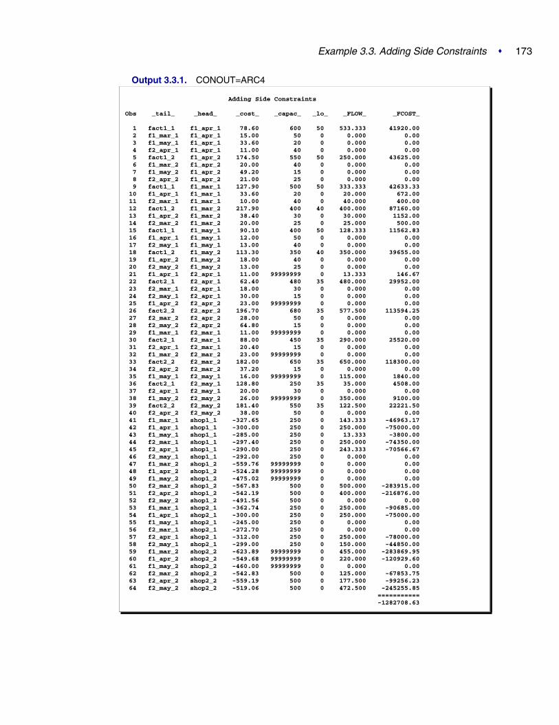
Example 3.3. Adding Side Constraints � 173
Output 3.3.1. CONOUT=ARC4
Adding Side Constraints
Obs _tail_ _head_ _cost_ _capac_ _lo_ _FLOW_ _FCOST_
1 fact1_1 f1_apr_1 78.60 600 50 533.333 41920.002 f1_mar_1 f1_apr_1 15.00 50 0 0.000 0.003 f1_may_1 f1_apr_1 33.60 20 0 0.000 0.004 f2_apr_1 f1_apr_1 11.00 40 0 0.000 0.005 fact1_2 f1_apr_2 174.50 550 50 250.000 43625.006 f1_mar_2 f1_apr_2 20.00 40 0 0.000 0.007 f1_may_2 f1_apr_2 49.20 15 0 0.000 0.008 f2_apr_2 f1_apr_2 21.00 25 0 0.000 0.009 fact1_1 f1_mar_1 127.90 500 50 333.333 42633.3310 f1_apr_1 f1_mar_1 33.60 20 0 20.000 672.0011 f2_mar_1 f1_mar_1 10.00 40 0 40.000 400.0012 fact1_2 f1_mar_2 217.90 400 40 400.000 87160.0013 f1_apr_2 f1_mar_2 38.40 30 0 30.000 1152.0014 f2_mar_2 f1_mar_2 20.00 25 0 25.000 500.0015 fact1_1 f1_may_1 90.10 400 50 128.333 11562.8316 f1_apr_1 f1_may_1 12.00 50 0 0.000 0.0017 f2_may_1 f1_may_1 13.00 40 0 0.000 0.0018 fact1_2 f1_may_2 113.30 350 40 350.000 39655.0019 f1_apr_2 f1_may_2 18.00 40 0 0.000 0.0020 f2_may_2 f1_may_2 13.00 25 0 0.000 0.0021 f1_apr_1 f2_apr_1 11.00 99999999 0 13.333 146.6722 fact2_1 f2_apr_1 62.40 480 35 480.000 29952.0023 f2_mar_1 f2_apr_1 18.00 30 0 0.000 0.0024 f2_may_1 f2_apr_1 30.00 15 0 0.000 0.0025 f1_apr_2 f2_apr_2 23.00 99999999 0 0.000 0.0026 fact2_2 f2_apr_2 196.70 680 35 577.500 113594.2527 f2_mar_2 f2_apr_2 28.00 50 0 0.000 0.0028 f2_may_2 f2_apr_2 64.80 15 0 0.000 0.0029 f1_mar_1 f2_mar_1 11.00 99999999 0 0.000 0.0030 fact2_1 f2_mar_1 88.00 450 35 290.000 25520.0031 f2_apr_1 f2_mar_1 20.40 15 0 0.000 0.0032 f1_mar_2 f2_mar_2 23.00 99999999 0 0.000 0.0033 fact2_2 f2_mar_2 182.00 650 35 650.000 118300.0034 f2_apr_2 f2_mar_2 37.20 15 0 0.000 0.0035 f1_may_1 f2_may_1 16.00 99999999 0 115.000 1840.0036 fact2_1 f2_may_1 128.80 250 35 35.000 4508.0037 f2_apr_1 f2_may_1 20.00 30 0 0.000 0.0038 f1_may_2 f2_may_2 26.00 99999999 0 350.000 9100.0039 fact2_2 f2_may_2 181.40 550 35 122.500 22221.5040 f2_apr_2 f2_may_2 38.00 50 0 0.000 0.0041 f1_mar_1 shop1_1 -327.65 250 0 143.333 -46963.1742 f1_apr_1 shop1_1 -300.00 250 0 250.000 -75000.0043 f1_may_1 shop1_1 -285.00 250 0 13.333 -3800.0044 f2_mar_1 shop1_1 -297.40 250 0 250.000 -74350.0045 f2_apr_1 shop1_1 -290.00 250 0 243.333 -70566.6746 f2_may_1 shop1_1 -292.00 250 0 0.000 0.0047 f1_mar_2 shop1_2 -559.76 99999999 0 0.000 0.0048 f1_apr_2 shop1_2 -524.28 99999999 0 0.000 0.0049 f1_may_2 shop1_2 -475.02 99999999 0 0.000 0.0050 f2_mar_2 shop1_2 -567.83 500 0 500.000 -283915.0051 f2_apr_2 shop1_2 -542.19 500 0 400.000 -216876.0052 f2_may_2 shop1_2 -491.56 500 0 0.000 0.0053 f1_mar_1 shop2_1 -362.74 250 0 250.000 -90685.0054 f1_apr_1 shop2_1 -300.00 250 0 250.000 -75000.0055 f1_may_1 shop2_1 -245.00 250 0 0.000 0.0056 f2_mar_1 shop2_1 -272.70 250 0 0.000 0.0057 f2_apr_1 shop2_1 -312.00 250 0 250.000 -78000.0058 f2_may_1 shop2_1 -299.00 250 0 150.000 -44850.0059 f1_mar_2 shop2_2 -623.89 99999999 0 455.000 -283869.9560 f1_apr_2 shop2_2 -549.68 99999999 0 220.000 -120929.6061 f1_may_2 shop2_2 -460.00 99999999 0 0.000 0.0062 f2_mar_2 shop2_2 -542.83 500 0 125.000 -67853.7563 f2_apr_2 shop2_2 -559.19 500 0 177.500 -99256.2364 f2_may_2 shop2_2 -519.06 500 0 472.500 -245255.85
===========-1282708.63

174 � Chapter 3. The INTPOINT Procedure
Example 3.4. Using Constraints and More Alteration to ArcData
Suppose the 25-inch screen TVs produced at factory 1 in May can be sold at eithershop with an increased profit of 40 dollars each. What is the new optimal solution?
title2 ’Using Constraints and Altering arc data’;data new_arc4;
set arc4;oldcost=_cost_;oldflow=_flow_;oldfc=_fcost_;if _tail_=’f1_may_2’ & (_head_=’shop1_2’ | _head_=’shop2_2’)
then _cost_=_cost_-40;run;
proc intpointbytes=1000000printlevel2=2arcdata=new_arc4 nodedata=node0condata=con3 sparsecondata rhsobs=’CHIP/BO LIMIT’conout=arc5;run;
proc print data=arc5;var _tail_ _head_ _cost_ _capac_ _lo_
_supply_ _demand_ _name__flow_ _fcost_ oldflow oldfc;
/* to get this variable order */sum oldfc _fcost_;run;
The following messages appear on the SAS log:
NOTE: Number of nodes= 20 .NOTE: Number of supply nodes= 4 .NOTE: Number of demand nodes= 4 .NOTE: Total supply= 4350 , total demand= 4150 .NOTE: Number of arcs= 64 .NOTE: Number of <= side constraints= 5 .NOTE: Number of == side constraints= 0 .NOTE: Number of >= side constraints= 0 .NOTE: Number of side constraint coefficients= 16 .NOTE: The following messages relate to the equivalent
Linear Programming problem solved by the InteriorPoint algorithm.
NOTE: Number of <= constraints= 5 .NOTE: Number of == constraints= 21 .NOTE: Number of >= constraints= 0 .NOTE: Number of constraint coefficients= 152 .NOTE: Number of variables= 68 .NOTE: After preprocessing, number of <= constraints= 5.NOTE: After preprocessing, number of == constraints= 20.NOTE: After preprocessing, number of >= constraints= 0.NOTE: The preprocessor eliminated 1 constraints from the
problem.NOTE: The preprocessor eliminated 9 constraint coefficients

Example 3.4. Using Constraints and More Alteration to Arc Data � 175
from the problem.NOTE: 5 columns, 0 rows and 5 coefficients were added to
the problem to handle unrestricted variables,variables that are split, and constraint slack orsurplus variables.
NOTE: There are 74 nonzero elements in A * A transpose.NOTE: Of the 25 rows and columns, 14 are sparse.NOTE: There are 74 nonzero superdiagonal elements in the
sparse rows of the factored A * A transpose. Thisincludes fill-in.
NOTE: There are 65 operations of the formu[i,j]=u[i,j]-u[q,j]*u[q,i]/u[q,q] to factorize thesparse rows of A * A transpose.
Iter Complem_aff Complem-ity Duality_gap Tot_infeasb Tot_infeasc Tot_infeasd0 -1.000000 178045680 0.833846 52835 39643 495921 51679271 22114244 0.911781 2979.752508 2235.802470 2678.0444872 4360227 1397064 0.521965 0 2.084022E-11 46.9647603 337615 239843 0.155358 0 0 8.0679074 119497 59613 0.042674 0 0 1.2630355 30689 20758 0.015076 0 0 0.4306386 9107.182114 7099.343072 0.005192 0 0 0.1094137 3406.632390 1496.513249 0.001098 0 0 0.0039358 616.222707 155.883444 0.000114 0 0 0.0004809 23.880446 1.372116 0.000001007 0 0 010 0.000755 0.000068819 -4.28512E-10 0 0 0NOTE: The Primal-Dual Predictor-Corrector Interior Point algorithm
performed 10 iterations.NOTE: Objective = -1295661.8.NOTE: The data set WORK.ARC5 has 64 observations and 17
variables.NOTE: There were 64 observations read from the data set
WORK.NEW_ARC4.NOTE: There were 8 observations read from the data set
WORK.NODE0.NOTE: There were 21 observations read from the data set
WORK.CON3.

176 � Chapter 3. The INTPOINT Procedure
Output 3.4.1. CONOUT=ARC5
Using Constraints and Altering arc data
Obs _tail_ _head_ _cost_ _capac_ _lo_ _SUPPLY_ _DEMAND_
1 fact1_1 f1_apr_1 78.60 600 50 1000 .2 f1_mar_1 f1_apr_1 15.00 50 0 . .3 f1_may_1 f1_apr_1 33.60 20 0 . .4 f2_apr_1 f1_apr_1 11.00 40 0 . .5 fact1_2 f1_apr_2 174.50 550 50 1000 .6 f1_mar_2 f1_apr_2 20.00 40 0 . .7 f1_may_2 f1_apr_2 49.20 15 0 . .8 f2_apr_2 f1_apr_2 21.00 25 0 . .9 fact1_1 f1_mar_1 127.90 500 50 1000 .10 f1_apr_1 f1_mar_1 33.60 20 0 . .11 f2_mar_1 f1_mar_1 10.00 40 0 . .12 fact1_2 f1_mar_2 217.90 400 40 1000 .13 f1_apr_2 f1_mar_2 38.40 30 0 . .14 f2_mar_2 f1_mar_2 20.00 25 0 . .15 fact1_1 f1_may_1 90.10 400 50 1000 .16 f1_apr_1 f1_may_1 12.00 50 0 . .17 f2_may_1 f1_may_1 13.00 40 0 . .18 fact1_2 f1_may_2 113.30 350 40 1000 .19 f1_apr_2 f1_may_2 18.00 40 0 . .20 f2_may_2 f1_may_2 13.00 25 0 . .21 f1_apr_1 f2_apr_1 11.00 99999999 0 . .22 fact2_1 f2_apr_1 62.40 480 35 850 .23 f2_mar_1 f2_apr_1 18.00 30 0 . .24 f2_may_1 f2_apr_1 30.00 15 0 . .25 f1_apr_2 f2_apr_2 23.00 99999999 0 . .26 fact2_2 f2_apr_2 196.70 680 35 1500 .27 f2_mar_2 f2_apr_2 28.00 50 0 . .28 f2_may_2 f2_apr_2 64.80 15 0 . .29 f1_mar_1 f2_mar_1 11.00 99999999 0 . .30 fact2_1 f2_mar_1 88.00 450 35 850 .31 f2_apr_1 f2_mar_1 20.40 15 0 . .32 f1_mar_2 f2_mar_2 23.00 99999999 0 . .33 fact2_2 f2_mar_2 182.00 650 35 1500 .34 f2_apr_2 f2_mar_2 37.20 15 0 . .35 f1_may_1 f2_may_1 16.00 99999999 0 . .36 fact2_1 f2_may_1 128.80 250 35 850 .37 f2_apr_1 f2_may_1 20.00 30 0 . .38 f1_may_2 f2_may_2 26.00 99999999 0 . .39 fact2_2 f2_may_2 181.40 550 35 1500 .40 f2_apr_2 f2_may_2 38.00 50 0 . .41 f1_mar_1 shop1_1 -327.65 250 0 . 90042 f1_apr_1 shop1_1 -300.00 250 0 . 90043 f1_may_1 shop1_1 -285.00 250 0 . 90044 f2_mar_1 shop1_1 -297.40 250 0 . 90045 f2_apr_1 shop1_1 -290.00 250 0 . 90046 f2_may_1 shop1_1 -292.00 250 0 . 90047 f1_mar_2 shop1_2 -559.76 99999999 0 . 90048 f1_apr_2 shop1_2 -524.28 99999999 0 . 90049 f1_may_2 shop1_2 -515.02 99999999 0 . 90050 f2_mar_2 shop1_2 -567.83 500 0 . 90051 f2_apr_2 shop1_2 -542.19 500 0 . 90052 f2_may_2 shop1_2 -491.56 500 0 . 90053 f1_mar_1 shop2_1 -362.74 250 0 . 90054 f1_apr_1 shop2_1 -300.00 250 0 . 90055 f1_may_1 shop2_1 -245.00 250 0 . 90056 f2_mar_1 shop2_1 -272.70 250 0 . 90057 f2_apr_1 shop2_1 -312.00 250 0 . 90058 f2_may_1 shop2_1 -299.00 250 0 . 90059 f1_mar_2 shop2_2 -623.89 99999999 0 . 145060 f1_apr_2 shop2_2 -549.68 99999999 0 . 145061 f1_may_2 shop2_2 -500.00 99999999 0 . 145062 f2_mar_2 shop2_2 -542.83 500 0 . 145063 f2_apr_2 shop2_2 -559.19 500 0 . 145064 f2_may_2 shop2_2 -519.06 500 0 . 1450

Example 3.4. Using Constraints and More Alteration to Arc Data � 177
Obs _name_ _FLOW_ _FCOST_ oldflow oldfc
1 prod f1 19 apl 533.333 41920.00 533.333 41920.002 0.000 0.00 0.000 0.003 back f1 19 may 0.000 0.00 0.000 0.004 0.000 0.00 0.000 0.005 prod f1 25 apl 250.000 43625.00 250.000 43625.006 0.000 0.00 0.000 0.007 back f1 25 may 0.000 0.00 0.000 0.008 0.000 0.00 0.000 0.009 prod f1 19 mar 333.333 42633.33 333.333 42633.3310 back f1 19 apl 20.000 672.00 20.000 672.0011 40.000 400.00 40.000 400.0012 prod f1 25 mar 400.000 87160.00 400.000 87160.0013 back f1 25 apl 30.000 1152.00 30.000 1152.0014 25.000 500.00 25.000 500.0015 128.333 11562.83 128.333 11562.8316 0.000 0.00 0.000 0.0017 0.000 0.00 0.000 0.0018 350.000 39655.00 350.000 39655.0019 0.000 0.00 0.000 0.0020 0.000 0.00 0.000 0.0021 13.333 146.67 13.333 146.6722 prod f2 19 apl 480.000 29952.00 480.000 29952.0023 0.000 0.00 0.000 0.0024 back f2 19 may 0.000 0.00 0.000 0.0025 0.000 0.00 0.000 0.0026 prod f2 25 apl 550.000 108185.00 577.500 113594.2527 0.000 0.00 0.000 0.0028 back f2 25 may 0.000 0.00 0.000 0.0029 0.000 0.00 0.000 0.0030 prod f2 19 mar 290.000 25520.00 290.000 25520.0031 back f2 19 apl 0.000 0.00 0.000 0.0032 0.000 0.00 0.000 0.0033 prod f2 25 mar 650.000 118300.00 650.000 118300.0034 back f2 25 apl 0.000 0.00 0.000 0.0035 115.000 1840.00 115.000 1840.0036 35.000 4508.00 35.000 4508.0037 0.000 0.00 0.000 0.0038 0.000 0.00 350.000 9100.0039 150.000 27210.00 122.500 22221.5040 0.000 0.00 0.000 0.0041 143.333 -46963.17 143.333 -46963.1742 250.000 -75000.00 250.000 -75000.0043 13.333 -3800.00 13.333 -3800.0044 250.000 -74350.00 250.000 -74350.0045 243.333 -70566.67 243.333 -70566.6746 0.000 0.00 0.000 0.0047 0.000 0.00 0.000 0.0048 0.000 0.00 0.000 0.0049 350.000 -180257.00 0.000 0.0050 500.000 -283915.00 500.000 -283915.0051 50.000 -27109.50 400.000 -216876.0052 0.000 0.00 0.000 0.0053 250.000 -90685.00 250.000 -90685.0054 250.000 -75000.00 250.000 -75000.0055 0.000 0.00 0.000 0.0056 0.000 0.00 0.000 0.0057 250.000 -78000.00 250.000 -78000.0058 150.000 -44850.00 150.000 -44850.0059 455.000 -283869.95 455.000 -283869.9560 220.000 -120929.60 220.000 -120929.6061 0.000 0.00 0.000 0.0062 125.000 -67853.75 125.000 -67853.7563 500.000 -279595.00 177.500 -99256.2364 150.000 -77859.00 472.500 -245255.85
=========== ===========-1295661.80 -1282708.63

178 � Chapter 3. The INTPOINT Procedure
Example 3.5. Nonarc Variables in the Side Constraints
You can verify that the FACT2 MAR GIZMO constraint has a left-hand-side activityof 3,470, which is not equal to the –RHS– of this constraint. Not all of the 3,750chips that can be supplied to factory 2 for March production are used. It is suggestedthat all the possible chips be obtained in March and those not used be saved for Aprilproduction. Because chips must be kept in an air-controlled environment, it costs onedollar to store each chip purchased in March until April. The maximum number ofchips that can be stored in this environment at each factory is 150. In addition, asearch of the parts inventory at factory 1 turned up 15 chips available for their Marchproduction.
Nonarc variables are used in the side constraints that handle the limitations of supplyof Gizmo chips. A nonarc variable called f1 unused chips has as a value the numberof chips that are not used at factory 1 in March. Another nonarc variable, f2 unusedchips, has as a value the number of chips that are not used at factory 2 in March.f1 chips from mar has as a value the number of chips left over from March usedfor production at factory 1 in April. Similarly, f2 chips from mar has as a valuethe number of chips left over from March used for April production at factory 2 inApril. The last two nonarc variables have objective function coefficients of 1 andupper bounds of 150. The Gizmo side constraints are
3*prod f1 19 mar + 4*prod f1 25 mar + f1 unused chips = 26153*prod f2 19 apl + 4*prod f2 25 apl + f2 unused chips = 37503*prod f1 19 apl + 4*prod f1 25 apl - f1 chips from mar = 26003*prod f2 19 apl + 4*prod f2 25 apl - f2 chips from mar = 3750f1 unused chips + f2 unused chips -f1 chips from mar - f2 chips from mar >= 0
The last side constraint states that the number of chips not used in March is not lessthan the number of chips left over from March and used in April. Here, this constraintis called CHIP LEFTOVER.
The following SAS code creates a new data set containing constraint data. It seemsthat most of the constraints are now equalities, so you specify DEFCONTYPE=EQin the PROC INTPOINT statement from now on and provide constraint type data forconstraints that are not “equal to” type, using the default TYPEOBS value –TYPE–as the –COLUMN– variable value to indicate observations that contain constrainttype data. Also, from now on, the default RHSOBS value is used.
title2 ’Nonarc Variables in the Side Constraints’;data con6;
input _column_ &$17. _row_ &$15. _coef_ ;datalines;
prod f1 19 mar FACT1 MAR GIZMO 3prod f1 25 mar FACT1 MAR GIZMO 4f1 unused chips FACT1 MAR GIZMO 1_RHS_ FACT1 MAR GIZMO 2615prod f2 19 mar FACT2 MAR GIZMO 3prod f2 25 mar FACT2 MAR GIZMO 4f2 unused chips FACT2 MAR GIZMO 1_RHS_ FACT2 MAR GIZMO 3750

Example 3.5. Nonarc Variables in the Side Constraints � 179
prod f1 19 apl FACT1 APL GIZMO 3prod f1 25 apl FACT1 APL GIZMO 4f1 chips from mar FACT1 APL GIZMO -1_RHS_ FACT1 APL GIZMO 2600prod f2 19 apl FACT2 APL GIZMO 3prod f2 25 apl FACT2 APL GIZMO 4f2 chips from mar FACT2 APL GIZMO -1_RHS_ FACT2 APL GIZMO 3750f1 unused chips CHIP LEFTOVER 1f2 unused chips CHIP LEFTOVER 1f1 chips from mar CHIP LEFTOVER -1f2 chips from mar CHIP LEFTOVER -1_TYPE_ CHIP LEFTOVER 1back f1 19 apl TOTAL BACKORDER 1back f1 25 apl TOTAL BACKORDER 1back f2 19 apl TOTAL BACKORDER 1back f2 25 apl TOTAL BACKORDER 1back f1 19 may TOTAL BACKORDER 1back f1 25 may TOTAL BACKORDER 1back f2 19 may TOTAL BACKORDER 1back f2 25 may TOTAL BACKORDER 1_TYPE_ TOTAL BACKORDER -1_RHS_ TOTAL BACKORDER 50;
The nonarc variables f1 chips from mar and f2 chips from mar have objectivefunction coefficients of 1 and upper bounds of 150. There are various ways in whichthis information can be furnished to PROC INTPOINT. If there were a TYPE listvariable in the CONDATA= data set, observations could be in the form
_COLUMN_ _TYPE_ _ROW_ _COEF_f1 chips from mar objfn . 1f1 chips from mar upperbd . 150f2 chips from mar objfn . 1f2 chips from mar upperbd . 150
It is desirable to assign ID list variable values to all the nonarc variables:
data arc6;set arc5;drop oldcost oldfc oldflow _flow_ _fcost_ ;run;
data arc6_b;input _name_ &$17. _cost_ _capac_ factory key_id $ ;datalines;
f1 unused chips . . 1 chipsf2 unused chips . . 2 chipsf1 chips from mar 1 150 1 chipsf2 chips from mar 1 150 2 chips;

180 � Chapter 3. The INTPOINT Procedure
proc append forcebase=arc6 data=arc6_b;run;
proc intpointbytes=1000000printlevel2=2nodedata=node0 arcdata=arc6condata=con6 defcontype=eq sparsecondataconout=arc7;run;
The following messages appear on the SAS log:
NOTE: Number of nodes= 20 .NOTE: Number of supply nodes= 4 .NOTE: Number of demand nodes= 4 .NOTE: Total supply= 4350 , total demand= 4150 .NOTE: Number of arcs= 64 .NOTE: Number of nonarc variables= 4 .NOTE: Number of <= side constraints= 1 .NOTE: Number of == side constraints= 4 .NOTE: Number of >= side constraints= 1 .NOTE: Number of side constraint coefficients= 24 .NOTE: The following messages relate to the equivalent
Linear Programming problem solved by the InteriorPoint algorithm.
NOTE: Number of <= constraints= 1 .NOTE: Number of == constraints= 25 .NOTE: Number of >= constraints= 1 .NOTE: Number of constraint coefficients= 160 .NOTE: Number of variables= 72 .NOTE: After preprocessing, number of <= constraints= 1.NOTE: After preprocessing, number of == constraints= 24.NOTE: After preprocessing, number of >= constraints= 1.NOTE: The preprocessor eliminated 1 constraints from the
problem.NOTE: The preprocessor eliminated 9 constraint coefficients
from the problem.NOTE: 2 columns, 0 rows and 2 coefficients were added to
the problem to handle unrestricted variables,variables that are split, and constraint slack orsurplus variables.
NOTE: There are 78 nonzero elements in A * A transpose.NOTE: Of the 26 rows and columns, 15 are sparse.NOTE: There are 87 nonzero superdiagonal elements in the
sparse rows of the factored A * A transpose. Thisincludes fill-in.
NOTE: There are 104 operations of the formu[i,j]=u[i,j]-u[q,j]*u[q,i]/u[q,q] to factorize thesparse rows of A * A transpose.
Iter Complem_aff Complem-ity Duality_gap Tot_infeasb Tot_infeasc Tot_infeasd0 -1.000000 182185121 0.837584 55030 37757 473821 56730833 28510760 0.910015 5004.066395 3433.344938 6917.1399282 9604878 2589633 0.665677 0 1.309672E-10 226.0472233 328091 309636 0.191136 0 0 26.9432974 135892 89815 0.063031 0 0 6.3899045 62039 31604 0.022877 0 0 0

Example 3.5. Nonarc Variables in the Side Constraints � 181
6 16881 7606.584128 0.005568 0 0 07 3753.426021 1918.980183 0.001408 0 0 08 709.549939 330.027670 0.000242 0 0 09 155.181759 36.697802 0.000026949 0 0 010 3.865957 0.421161 0.000000309 0 0 011 0.001557 0.000021177 1.557982E-11 0 0 0NOTE: The Primal-Dual Predictor-Corrector Interior Point algorithm
performed 11 iterations.NOTE: Objective = -1295542.742.NOTE: The data set WORK.ARC7 has 68 observations and 14
variables.NOTE: There were 68 observations read from the data set
WORK.ARC6.NOTE: There were 8 observations read from the data set
WORK.NODE0.NOTE: There were 31 observations read from the data set
WORK.CON6.
The optimal solution data set, CONOUT=ARC7, is given in Output 3.5.1.
proc print data=arc7;var _tail_ _head_ _name_ _cost_ _capac_ _lo_
_flow_ _fcost_;sum _fcost_;run;
The optimal value of the nonarc variable f2 unused chips is 280. This means thatalthough there are 3,750 chips that can be used at factory 2 in March, only 3,470are used. As the optimal value of f1 unused chips is zero, all chips available forproduction in March at factory 1 are used. The nonarc variable f2 chips from maralso has zero optimal value. This means that the April production at factory 2 doesnot need any chips that could have been held in inventory since March. However,the nonarc variable f1 chips from mar has value of 20. Thus, 3,490 chips should beordered for factory 2 in March. Twenty of these chips should be held in inventoryuntil April, then sent to factory 1.

182 � Chapter 3. The INTPOINT Procedure
Output 3.5.1. CONOUT=ARC7
Nonarc Variables in the Side Constraints
Obs _tail_ _head_ _name_ _cost_ _capac_ _lo_ _FLOW_ _FCOST_
1 fact1_1 f1_apr_1 prod f1 19 apl 78.60 600 50 540.000 42444.002 f1_mar_1 f1_apr_1 15.00 50 0 0.000 0.003 f1_may_1 f1_apr_1 back f1 19 may 33.60 20 0 0.000 0.004 f2_apr_1 f1_apr_1 11.00 40 0 0.000 0.005 fact1_2 f1_apr_2 prod f1 25 apl 174.50 550 50 250.000 43625.006 f1_mar_2 f1_apr_2 20.00 40 0 0.000 0.007 f1_may_2 f1_apr_2 back f1 25 may 49.20 15 0 0.000 0.008 f2_apr_2 f1_apr_2 21.00 25 0 25.000 525.009 fact1_1 f1_mar_1 prod f1 19 mar 127.90 500 50 338.333 43272.8310 f1_apr_1 f1_mar_1 back f1 19 apl 33.60 20 0 20.000 672.0011 f2_mar_1 f1_mar_1 10.00 40 0 40.000 400.0012 fact1_2 f1_mar_2 prod f1 25 mar 217.90 400 40 400.000 87160.0013 f1_apr_2 f1_mar_2 back f1 25 apl 38.40 30 0 30.000 1152.0014 f2_mar_2 f1_mar_2 20.00 25 0 25.000 500.0015 fact1_1 f1_may_1 90.10 400 50 116.667 10511.6716 f1_apr_1 f1_may_1 12.00 50 0 0.000 0.0017 f2_may_1 f1_may_1 13.00 40 0 0.000 0.0018 fact1_2 f1_may_2 113.30 350 40 350.000 39655.0019 f1_apr_2 f1_may_2 18.00 40 0 0.000 0.0020 f2_may_2 f1_may_2 13.00 25 0 0.000 0.0021 f1_apr_1 f2_apr_1 11.00 99999999 0 20.000 220.0022 fact2_1 f2_apr_1 prod f2 19 apl 62.40 480 35 480.000 29952.0023 f2_mar_1 f2_apr_1 18.00 30 0 0.000 0.0024 f2_may_1 f2_apr_1 back f2 19 may 30.00 15 0 0.000 0.0025 f1_apr_2 f2_apr_2 23.00 99999999 0 0.000 0.0026 fact2_2 f2_apr_2 prod f2 25 apl 196.70 680 35 577.500 113594.2527 f2_mar_2 f2_apr_2 28.00 50 0 0.000 0.0028 f2_may_2 f2_apr_2 back f2 25 may 64.80 15 0 0.000 0.0029 f1_mar_1 f2_mar_1 11.00 99999999 0 0.000 0.0030 fact2_1 f2_mar_1 prod f2 19 mar 88.00 450 35 290.000 25520.0031 f2_apr_1 f2_mar_1 back f2 19 apl 20.40 15 0 0.000 0.0032 f1_mar_2 f2_mar_2 23.00 99999999 0 0.000 0.0033 fact2_2 f2_mar_2 prod f2 25 mar 182.00 650 35 650.000 118300.0034 f2_apr_2 f2_mar_2 back f2 25 apl 37.20 15 0 0.000 0.0035 f1_may_1 f2_may_1 16.00 99999999 0 115.000 1840.0036 fact2_1 f2_may_1 128.80 250 35 35.000 4508.0037 f2_apr_1 f2_may_1 20.00 30 0 0.000 0.0038 f1_may_2 f2_may_2 26.00 99999999 0 0.000 0.0039 fact2_2 f2_may_2 181.40 550 35 122.500 22221.5040 f2_apr_2 f2_may_2 38.00 50 0 0.000 0.0041 f1_mar_1 shop1_1 -327.65 250 0 148.333 -48601.4242 f1_apr_1 shop1_1 -300.00 250 0 250.000 -75000.0043 f1_may_1 shop1_1 -285.00 250 0 1.667 -475.0044 f2_mar_1 shop1_1 -297.40 250 0 250.000 -74350.0045 f2_apr_1 shop1_1 -290.00 250 0 250.000 -72500.0046 f2_may_1 shop1_1 -292.00 250 0 0.000 0.0047 f1_mar_2 shop1_2 -559.76 99999999 0 0.000 0.0048 f1_apr_2 shop1_2 -524.28 99999999 0 0.000 0.0049 f1_may_2 shop1_2 -515.02 99999999 0 347.500 -178969.4550 f2_mar_2 shop1_2 -567.83 500 0 500.000 -283915.0051 f2_apr_2 shop1_2 -542.19 500 0 52.500 -28464.9852 f2_may_2 shop1_2 -491.56 500 0 0.000 0.0053 f1_mar_1 shop2_1 -362.74 250 0 250.000 -90685.0054 f1_apr_1 shop2_1 -300.00 250 0 250.000 -75000.0055 f1_may_1 shop2_1 -245.00 250 0 0.000 0.0056 f2_mar_1 shop2_1 -272.70 250 0 0.000 0.0057 f2_apr_1 shop2_1 -312.00 250 0 250.000 -78000.0058 f2_may_1 shop2_1 -299.00 250 0 150.000 -44850.0059 f1_mar_2 shop2_2 -623.89 99999999 0 455.000 -283869.9560 f1_apr_2 shop2_2 -549.68 99999999 0 245.000 -134671.6061 f1_may_2 shop2_2 -500.00 99999999 0 2.500 -1250.0062 f2_mar_2 shop2_2 -542.83 500 0 125.000 -67853.7563 f2_apr_2 shop2_2 -559.19 500 0 500.000 -279595.0064 f2_may_2 shop2_2 -519.06 500 0 122.500 -63584.8565 f1 chips from mar 1.00 150 0 20.000 20.0066 f1 unused chips 0.00 99999999 0 0.000 0.0067 f2 chips from mar 1.00 150 0 0.000 0.0068 f2 unused chips 0.00 99999999 0 280.000 0.00
===========-1295542.74

Example 3.6. Solving an LP Problem with Data in MPS Format � 183
Example 3.6. Solving an LP Problem with Data in MPS Format
In this example, PROC INTPOINT is ultimately used to solve an LP. But prior tothat, there is SAS code that is used to read a MPS format file and initialize an in-put SAS data set. MPS was an optimization package developed for IBM computersmany years ago and the format by which data had to be supplied to that system be-came the industry standard for other optimization software packages, including thosedeveloped recently. The MPS format is described in Murtagh (1981). If you have anLP which has data in MPS format in a file /your-directory/your-filename.dat, then thefollowing SAS code should be run:
filename w ’/your-directorys/your-filename.dat’;data raw;
infile w lrecl=80 pad;input field1 $ 2-3 field2 $ 5-12 field3 $ 15-22
field4 25-36 field5 $ 40-47 field6 50-61;run;
%sasmpsxs;
data lp;set;if _type_="FREE" then _type_="MIN";if lag(_type_)="*HS" then _type_="RHS";run;
proc sort data=lp;by _col_;run;
proc intpointarcdata=lpcondata=lp sparsecondata rhsobs=rhs grouped=condataconout=solutn /* SAS data set for the optimal solution */bytes=20000000nnas=1700 ncoefs=4000 ncons=700printlevel2=2 memrep;run;
proc lpdata=lp sparsedataendpause time=3600 maxit1=100000 maxit2=100000;run;show status;quit;
You will have to specify the appropriate path and file name in which your MPS formatdata resides.
SASMPSXS is a SAS macro provided within SAS/OR software. The MPS formatresembles the sparse format of the CONDATA= data set for PROC INTPOINT. TheSAS macro SASMPSXS examines the MPS data and transfers it into a SAS data setwhile automatically taking into account how the MPS format differs slightly fromPROC INTPOINT’s sparse format.

184 � Chapter 3. The INTPOINT Procedure
The parameters NNAS=1700, NCOEFS=4000, and NCONS=700 indicate the ap-proximate (overestimated) number of variables, coefficients and constraints thismodel has. You must change these to your problems dimensions. Knowing these,PROC INTPOINT is able to utilize memory better and read the data faster. Theseparameters are optional.
The PROC SORT preceding PROC INTPOINT is not necessary, but sorting the SASdata set can speed up PROC INTPOINT when it reads the data. After the sort, datafor each column is grouped together. GROUPED=condata can be specified.
For small problems, presorting and specifying those additional options is not going togreatly influence PROC INTPOINT’s run time. However, when problems are large,presorting and specifying those additional options can be very worthwhile.
If you generate the model yourself, you will be familiar enough with it to knowwhat to specify for the RHSOBS= parameter. If the value of the SAS variable in theCOLUMN list is equal to the character string specified as the RHSOBS= option, thedata in that observation is interpreted as right-hand-side data as opposed to coefficientdata. If you do not know what to specify for the RHSOBS= option, you should firstrun PROC LP and optionally set MAXIT1=1 and MAXIT2=1. PROC LP will outputa Problem Summary that includes the line
Rhs Variable rhs-charstr
BYTES=20000000 is the size of working memory PROC INTPOINT is allowed.
The options PRINTLEVEL2=2 and MEMREP indicate that you want to see an iter-ation log and messages about memory usage. Specifying these options is optional.
References
Lustig, I. J., Marsten, R. E., and Shanno, D. F. (1992), “On ImplementingMehrotra’s Predictor-Corrector Interior-Point Method for Linear Programming,”SIAM Journal of Optimization, 2, 435–449.
Murtagh, B. A. (1981), Advanced Linear Programming, Computation and Practice,McGraw-Hill Inc.
Reid, J. K. (1975), “A Sparsity-Exploiting Variant of the Bartels-GolubDecomposition for Linear Programming Bases,” Harwell Report CSS 20.
Roos, C., Terlaky, T., and Vial, J. (1997), Theory and Algorithms for LinearOptimization, Chichester, England: John Wiley & Sons.
Wright, S. J. (1996), Primal-Dual Interior Point Algorithms, Philadelphia: SIAM.
Ye, Y. (1996), Interior Point Algorithms: Theory and Analysis, New York: JohnWiley & Sons.

Chapter 4The LP Procedure
Chapter Contents
OVERVIEW . . . . . . . . . . . . . . . . . . . . . . . . . . . . . . . . . . . 187
GETTING STARTED . . . . . . . . . . . . . . . . . . . . . . . . . . . . . . 189An Introductory Example . . . . . . . . . . . . . . . . . . . . . . . . . . . 190An Integer Programming Example . . . . . . . . . . . . . . . . . . . . . . 194An MPS Format Conversion Example . . . . . . . . . . . . . . . . . . . . 196
SYNTAX . . . . . . . . . . . . . . . . . . . . . . . . . . . . . . . . . . . . . 197Functional Summary . . . . . . . . . . . . . . . . . . . . . . . . . . . . . . 198PROC LP Statement . . . . . . . . . . . . . . . . . . . . . . . . . . . . . . 202COEF Statement . . . . . . . . . . . . . . . . . . . . . . . . . . . . . . . . 212COL Statement . . . . . . . . . . . . . . . . . . . . . . . . . . . . . . . . 212ID Statement . . . . . . . . . . . . . . . . . . . . . . . . . . . . . . . . . . 212IPIVOT Statement . . . . . . . . . . . . . . . . . . . . . . . . . . . . . . . 213PIVOT Statement . . . . . . . . . . . . . . . . . . . . . . . . . . . . . . . 213PRINT Statement . . . . . . . . . . . . . . . . . . . . . . . . . . . . . . . 213QUIT Statement . . . . . . . . . . . . . . . . . . . . . . . . . . . . . . . . 215RANGE Statement . . . . . . . . . . . . . . . . . . . . . . . . . . . . . . 215RESET Statement . . . . . . . . . . . . . . . . . . . . . . . . . . . . . . . 216RHS Statement . . . . . . . . . . . . . . . . . . . . . . . . . . . . . . . . 216RHSSEN Statement . . . . . . . . . . . . . . . . . . . . . . . . . . . . . . 217ROW Statement . . . . . . . . . . . . . . . . . . . . . . . . . . . . . . . . 217RUN Statement . . . . . . . . . . . . . . . . . . . . . . . . . . . . . . . . 218SHOW Statement . . . . . . . . . . . . . . . . . . . . . . . . . . . . . . . 218TYPE Statement . . . . . . . . . . . . . . . . . . . . . . . . . . . . . . . . 218VAR Statement . . . . . . . . . . . . . . . . . . . . . . . . . . . . . . . . 220
DETAILS . . . . . . . . . . . . . . . . . . . . . . . . . . . . . . . . . . . . . 221Missing Values . . . . . . . . . . . . . . . . . . . . . . . . . . . . . . . . . 221Dense Data Input Format . . . . . . . . . . . . . . . . . . . . . . . . . . . 221Sparse Data Input Format . . . . . . . . . . . . . . . . . . . . . . . . . . . 222Converting MPS Format . . . . . . . . . . . . . . . . . . . . . . . . . . . . 224The Reduced Costs, Dual Activities, and Current Tableau . . . . . . . . . . 227Macro Variable –ORLP– . . . . . . . . . . . . . . . . . . . . . . . . . . . 227Pricing . . . . . . . . . . . . . . . . . . . . . . . . . . . . . . . . . . . . . 229Scaling . . . . . . . . . . . . . . . . . . . . . . . . . . . . . . . . . . . . . 230Preprocessing . . . . . . . . . . . . . . . . . . . . . . . . . . . . . . . . . 230

186 � Chapter 4. The LP Procedure
Integer Programming . . . . . . . . . . . . . . . . . . . . . . . . . . . . . 231Sensitivity Analysis . . . . . . . . . . . . . . . . . . . . . . . . . . . . . . 239Range Analysis . . . . . . . . . . . . . . . . . . . . . . . . . . . . . . . . 242Parametric Programming . . . . . . . . . . . . . . . . . . . . . . . . . . . 242Interactive Facilities . . . . . . . . . . . . . . . . . . . . . . . . . . . . . . 244Memory Management . . . . . . . . . . . . . . . . . . . . . . . . . . . . . 245Output Data Sets . . . . . . . . . . . . . . . . . . . . . . . . . . . . . . . . 246Input Data Sets . . . . . . . . . . . . . . . . . . . . . . . . . . . . . . . . . 248Displayed Output . . . . . . . . . . . . . . . . . . . . . . . . . . . . . . . 249ODS Table and Variable Names . . . . . . . . . . . . . . . . . . . . . . . . 252
EXAMPLES . . . . . . . . . . . . . . . . . . . . . . . . . . . . . . . . . . . 254Example 4.1. An Oil Blending Problem . . . . . . . . . . . . . . . . . . . . 254Example 4.2. A Sparse View of the Oil Blending Problem . . . . . . . . . . 259Example 4.3. Analyzing the Sensitivity of the Solution to Changes in the
Objective Coefficients . . . . . . . . . . . . . . . . . . . . . . . . . 263Example 4.4. Additional Analysis of the Sensitivity of the Solution to Changes
in the Objective Coefficients . . . . . . . . . . . . . . . . . . . . . 265Example 4.5. Price Parametric Programming for the Oil Blending Problem . 267Example 4.6. Special Ordered Sets and the Oil Blending Problem . . . . . . 269Example 4.7. Goal-Programming a Product Mix Problem . . . . . . . . . . 272Example 4.8. A Simple Integer Program . . . . . . . . . . . . . . . . . . . 278Example 4.9. An Infeasible Problem . . . . . . . . . . . . . . . . . . . . . 281Example 4.10. Restarting an Integer Program . . . . . . . . . . . . . . . . . 284Example 4.11. Alternative Search of the Branch-and-Bound Tree . . . . . . 289Example 4.12. An Assignment Problem . . . . . . . . . . . . . . . . . . . 293Example 4.13. A Scheduling Problem . . . . . . . . . . . . . . . . . . . . . 300Example 4.14. A Multicommodity Transshipment Problem with Fixed Charges307
REFERENCES . . . . . . . . . . . . . . . . . . . . . . . . . . . . . . . . . . 310

Chapter 4The LP ProcedureOverview
The LP procedure solves linear programs, integer programs, and mixed-integer pro-grams. It also performs parametric programming, range analysis, and reports onsolution sensitivity to changes in the right-hand-side constants and price coefficients.
The LP procedure provides various control options and solution strategies. It alsoprovides the functionality to produce various kinds of intermediate and final solutioninformation. The procedure’s interactive features enable you to take control of theproblem solving process. During linear or integer iterations, for example, you canstop the procedure at intermediate stages and examine current results. If necessary,you can change options or strategies and resume the execution of the procedure.
The LP procedure is used to optimize a linear function subject to linear and integerconstraints. Specifically, the LP procedure solves the general mixed-integer programof the form
minimize cT x
subject to Ax {≥, =,≤} b� ≤ x ≤ uxi is integer, i ∈ S
where
• A is an m × n matrix of technological coefficients
• b is an m × 1 matrix of right-hand-side (RHS) constants
• c is an n × 1 matrix of objective function coefficients
• x is an n × 1 matrix of structural variables
• l is an n × 1 matrix of lower bounds on x
• u is an n × 1 matrix of upper bounds on x
• S is a subset of the set of indices {1, . . . , n}
Linear programs (when S is empty) are denoted by (LP). For these problems, theprocedure employs the two-phase revised simplex method, which uses the Bartels-Golub update of the LU decomposed basis matrix to pivot between feasible solutions(Bartels 1971). In phase 1, PROC LP finds a basic feasible solution to (LP), while inphase 2, PROC LP finds an optimal solution, xopt. The procedure implicitly handlesunrestricted variables, lower-bounded variables, upper-bounded variables, and rangeson constraints. When no explicit lower bounds are specified, PROC LP assumes thatall variables are bounded below by zero.

188 � Chapter 4. The LP Procedure
When a variable is specified as an integer variable, S has at least one element. Theprocedure then uses the branch-and-bound technique for optimization.
The relaxed problem (the problem with no integer constraints) is solved initially us-ing the primal algorithm described previously. Constraints are added in defining thesubsequent descendant problems in the branch-and-bound tree. These problems arethen solved using the dual simplex algorithm. Dual pivots are referred to as phase 3pivots.
The preprocessing option enables the procedure to identify redundant and infeasibleconstraints, fix variables, and reduce the feasible region before solving a problem.For linear programs, the option often can reduce the number of constraints and vari-ables, leading to a quicker elapsed solution time and improved reliability. For integerprograms, it often reduces the gap between an integer program and its relaxed linearprogram, which will likely lead to a reduced branch-and-bound tree and a quickerCPU time. In general, it provides users an alternative to solving large, complicatedoperations research problems.
The LP procedure can also analyze the sensitivity of the solution xopt to changes inboth the objective function and the right-hand-side constants. There are three tech-niques available for this analysis: sensitivity analysis, parametric programming, andrange analysis. Sensitivity analysis enables you to examine the size of a perturbationto the right-hand-side or objective vector by an arbitrary change vector for which thebasis of the current optimal solution remains optimal.
Parametric programming, on the other hand, enables you to specify the size of theperturbation beforehand and examine how the optimal solution changes as the de-sired perturbation is realized. With this technique, the procedure pivots to maintainoptimality as the right-hand-side or objective vector is perturbed beyond the range forwhich the current solution is optimal. Range analysis is used to examine the range ofeach right-hand-side value or objective coefficient for which the basis of the currentoptimal solution remains optimal.
The LP procedure can also save both primal and dual solutions, the current tableau,and the branch-and-bound tree in SAS data sets. This enables you to generate solutionreports and perform additional analyses with the SAS System. Although PROC LPreports solutions, this feature is particularly useful for reporting solutions in formatstailored to your specific needs. Saving computational results in a data set also enablesyou to continue executing a problem not solved because of insufficient time or othercomputational problems.
The LP procedure uses the Output Delivery System (ODS), a SAS subsystem thatprovides capabilities for displaying and controlling the output from SAS procedures.ODS enables you to modify the headers, column names, data formats, and layouts ofthe output tables in PROC LP.
There are no restrictions on the problem size in the LP procedure. The number ofconstraints and variables in a problem that PROC LP can solve depends on the hostplatform, the available memory, and the available disk space for utility data sets.

Getting Started � 189
Getting Started
PROC LP expects the definition of one or more linear, integer, or mixed-integer pro-grams in an input data set. There are two formats, a dense format and a sparse format,for this data set.
In the dense format, a model is expressed in a similar way as it is formulated. EachSAS variable corresponds to a model’s column, and each SAS observation corre-sponds to a model’s row. A SAS variable in the input data set is one of the following:
• a type variable
• an id variable
• a structural variable
• a right-hand-side variable
• a right-hand-side sensitivity analysis variable or
• a range variable
The type variable tells PROC LP how to interpret the observation as a part of themathematical programming problem. It identifies and classifies objectives, con-straints, and the rows that contain information of variables like types, bounds, andso on. PROC LP recognizes the following keywords as values for the type variable:MIN, MAX, EQ, LE, GE, SOSEQ, SOSLE, UNRSTRCT, LOWERBD, UPPERBD,FIXED, INTEGER, BINARY, BASIC, PRICESEN, and FREE. The values of the idvariable are the names of the rows in the model. The other variables identify andclassify the columns with numerical values.
The sparse format to PROC LP is designed to enable you to specify only the nonzerocoefficients in the description of linear programs, integer programs, and mixed-integer programs. The SAS data set that describes the sparse model must containat least four SAS variables:
• a type variable
• a column variable
• a row variable and
• a coefficient variable
Each observation in the data set associates a type with a row or a column, or definesa coefficient or a numerical value in the model, or both. In addition to the keywordsin the dense format, PROC LP also recognizes the keywords RHS, RHSSEN, andRANGE as values of the type variable. The values of the row and column variablesare the names of the rows and columns in the model. The values of the coefficientvariables give the coefficients or other numerical data. The SAS data set can containmultiple pairs of row and coefficient variables. In this way, more information aboutthe model can be specified in each observation in the data set. See the “Sparse DataInput Format” section on page 222 for further discussion.

190 � Chapter 4. The LP Procedure
With both the dense and sparse formats for model specification, the observation orderis not important. This feature is particularly useful when using the sparse modelinput.
An Introductory Example
A simple blending problem illustrates the dense and sparse input formats and theuse of PROC LP. A step in refining crude oil into finished oil products involves adistillation process that splits crude into various streams. Suppose there are threetypes of crude available: Arabian light, Arabian heavy, and Brega. These types ofcrude are distilled into light naphtha, intermediate naphtha, and heating oil. These inturn are blended into jet fuel using one of two recipes. What amounts of the threecrudes maximize the profit from producing jet fuel? A formulation to answer thisquestion is as follows:
max − 175 a– light − 165 a–heavy − 205 brega + 300 jet–1 + 300 jet–2
subject to .035 a– light + .03 a–heavy + .045 brega = naphthal.1 a– light + .075 a–heavy + .135 brega = naphthai
.39 a– light + .3 a–heavy + .43 brega = heatingo.3 naphthai + .7 heatingo = jet–1.2 naphthal + .8 heatingo = jet–2
a– light ≤ 110a–heavy ≤ 165
brega ≤ 80a– light, a–heavy, brega, naphthai,
naphthal, heatingo, jet–1, jet–2 ≥ 0
The following data set gives the representation of this formulation. Notice that thevariable names are the structural variables, the rows are the constraints, and the coef-ficients are given as the values for the structural variables.
data;input _id_ $17.
a_light a_heavy brega naphthal naphthaiheatingo jet_1 jet_2_type_ $ _rhs_;
datalines;profit -175 -165 -205 0 0 0 300 300 max .naphtha_l_conv .035 .030 .045 -1 0 0 0 0 eq 0naphtha_i_conv .100 .075 .135 0 -1 0 0 0 eq 0heating_o_conv .390 .300 .430 0 0 -1 0 0 eq 0recipe_1 0 0 0 0 .3 .7 -1 0 eq 0recipe_2 0 0 0 .2 0 .8 0 -1 eq 0available 110 165 80 . . . . . upperbd .;

An Introductory Example � 191
The same model can be specified in the sparse format, as follows. This format enablesyou to omit the zero coefficients.
data;format _type_ $8. _col_ $8. _row_ $16. ;input _type_ $ _col_ $ _row_ $ _coef_ ;datalines;
max . profit .eq . napha_l_conv .eq . napha_i_conv .eq . heating_oil_conv .eq . recipe_1 .eq . recipe_2 .upperbd . available .. a_light profit -175. a_light napha_l_conv .035. a_light napha_i_conv .100. a_light heating_oil_conv .390. a_light available 110. a_heavy profit -165. a_heavy napha_l_conv .030. a_heavy napha_i_conv .075. a_heavy heating_oil_conv .300. a_heavy available 165. brega profit -205. brega napha_l_conv .045. brega napha_i_conv .135. brega heating_oil_conv .430. brega available 80. naphthal napha_l_conv -1. naphthal recipe_2 .2. naphthai napha_i_conv -1. naphthai recipe_1 .3. heatingo heating_oil_conv -1. heatingo recipe_1 .7. heatingo recipe_2 .8. jet_1 profit 300. jet_1 recipe_1 -1. jet_2 profit 300. jet_2 recipe_2 -1. _rhs_ recipe_1 0;
Because the input order of the model into PROC LP is unimportant, this model canbe specified in sparse input in arbitrary row order. Example 4.2 in the “Examples”section demonstrates this.
The dense and sparse forms of model input give you flexibility to generate modelsusing the SAS language. The dense form of the model is solved with the statements
proc lp;run;

192 � Chapter 4. The LP Procedure
The sparse form is solved with the statements
proc lp sparsedata;run;
Example 4.1 and Example 4.2 in the “Examples” section continue with this problem.
Problem Input
As default, PROC LP uses the most recently created SAS data set as the probleminput data set. However, if you want to input the problem from a specific SAS dataset, use the DATA= option. For example, if the previous dense form data set has thename DENSE, the PROC LP statements can be written as
proc lp data=dense;run;
Problem Definition Statements
In the previous dense form data set, the –ID– , –TYPE– , and –RHS– variablesare special variables in PROC LP. They stand for id variable, type variable, andright-hand-side variable. If you replace those variable names with, for example,ROWNAME, TYPE, and RHS, you need the problem definition statements (ID,TYPE and RHS) in PROC LP:
proc lp;id rowname;type type;rhs rhs;
run;
Other special variables for the dense format are –RHSSEN– and –RANGE– , whichidentify the vectors for the right-hand-side sensitivity and range analyses. The corre-sponding statements are the RHSSEN and RANGE statements. (Notice that a vari-able name can be identical to a statement name.)
In the same way, if you replace the variables –COL– , –ROW– , –TYPE– , and
–COEF– in the previous sparse form data set by COLUMN, ROW, TYPE, andCOEF, you need the problem definition statements (COL, ROW, TYPE, and COEF)in PROC LP.
proc lp sparsedata;col column;row row;type type;coef coef;
run;

An Introductory Example � 193
In the sparse form data set, the value ‘–RHS–’ under the variable –COL– is a specialcolumn name, which represents the model’s right-hand-side column. If you replaceit by a value ‘R’, the PROC LP statements would be
proc lp sparsedata;rhs r;
run;
Other special column names for the sparse format are ‘–RHSSEN–’ and‘–RANGE–’. The corresponding statements are the RHSSEN and RANGEstatements.
PROC LP is case insensitive to variable names and all character values, includingthe row and column names in the sparse format. The order of the problem definitionstatements is not important.
For the dense format, a model’s row names appear as character values in a SAS dataset. For the sparse format, both the row and the column names of the model appear ascharacter values in the data set. Thus, you can put spaces or other special charactersin the names. When referring to these names in the problem definition statement orother LP statements, you must use single or double quotes around them. For example,if you replace ‘–RHS–’ by ‘R H S’ in the previous sparse form data set, the PROCLP statements would become
proc lp sparsedata;rhs "r h s";
run;
LP Options
The specifications SPARSEDATA and DATA= in the previous examples are PROCLP options. PROC LP options include
• data set options
• display control options
• interactive control options
• preprocessing options
• branch-and-bound control options
• sensitivity/parametric/ranging control options
• simplex options
Interactive Processing
Interactive control options include READPAUSE, ENDPAUSE, and so forth. Youcan run PROC LP interactively using those options. For example, for the blendingproblem example in the dense form, you can first pause the procedure before itera-tions start with the READPAUSE option. The PROC LP statements are

194 � Chapter 4. The LP Procedure
proc lp readpause;run;
When the procedure pauses, you run the PRINT statement to display the initial tech-nological matrix and see if the input is correct. Then you run the PIVOT statement todo one simplex pivot and pause. After that you use the SHOW statement to check thecurrent solution status. Then you apply the RESET statement to tell the procedureto stop as soon as it finds a solution. Now you use the RUN statement to continuethe execution. When the procedure stops, you run the PRINT statement again to do aprice range analysis and QUIT the procedure. Use a SAS %PUT statement to displaythe contents of PROC LP’s macro variable, –ORLP–, which contains iterations andsolution information. What follows are the complete statements in batch mode:
proc lp readpause;run;print matrix(,); /* display all rows and columns. */pivot;show status;reset endpause;run;print rangeprice;quit;%put &_orlp_;
Note: You can force PROC LP to pause during iterations by using the CTRL-BREAKkey.
An Integer Programming Example
The following is a simple mixed-integer programming problem. Details can be foundin Example 4.8 in the “Examples” section.
data;format _row_ $10.;input _row_ $ choco gumdr ichoco igumdr _type_ $ _rhs_;datalines;
object .25 .75 -100 -75 max .cooking 15 40 0 0 le 27000color 0 56.25 0 0 le 27000package 18.75 0 0 0 le 27000condiments 12 50 0 0 le 27000chocolate 1 0 -10000 0 le 0gum 0 1 0 -10000 le 0only_one 0 0 1 1 eq 1binary . . 1 2 binary .;
The row with ‘binary’ type indicates that this problem is a mixed-integer programand all the integer variables are binary. The integer values of the row set an ordering

An Integer Programming Example � 195
for PROC LP to pick the branching variable when VARSELECT=PRIOR is chosen.Smaller values will have higher priorities. The –ROW– variable here is an alias ofthe –ID– variable.
This problem can be solved with the following statements:
proc lp canselect=lifo backtrack=obj varselect=far endpause;run;quit;%put &_orlp_;
The options CANSELECT=, BACKTRACK=, and VARSELECT= specify the rulesfor picking the next active problem and the rule to choose the branching variable. Inthis example, the values LIFO, OBJ and FAR serve as the default values, so the threeoptions can be omitted from the PROC LP statement. The following is the outputfrom the %PUT statement:
STATUS=SUCCESSFUL PHASE=3 OBJECTIVE=285 P_FEAS=YES D_FEAS=YES INT_ITER=3INT_FEAS=2 ACTIVE=0 INT_BEST=285 PHASE1_ITER=0 PHASE2_ITER=5PHASE3_ITER=5
Figure 4.1. The Output of –ORLP–
PreprocessingUsing the PREPROCESS= option, you can apply the preprocessing techniques topre-solve and then solve the preceding mixed-integer program:
proc lp preprocess=1 endpause;run;quit;%put &_orlp_;
The preprocessing statistics are written to the SAS log file as follows:
NOTE: Preprocessing 1 ...NOTE: 2 upper bounds decreased.NOTE: 2 coefficients reduced.NOTE: Preprocessing 2 ...NOTE: 2 constraints eliminated.NOTE: Preprocessing done.
The new output –ORLP– is as follows:
STATUS=SUCCESSFUL PHASE=3 OBJECTIVE=285 P_FEAS=YES D_FEAS=YES INT_ITER=0INT_FEAS=1 ACTIVE=0 INT_BEST=285 PHASE1_ITER=0 PHASE2_ITER=5PHASE3_ITER=0
Figure 4.2. The Output of –ORLP– with Preprocessing Option On
In this example, the number of integer iterations (INT–ITER=) is zero, which meansthat the preprocessing has reduced the gap between the relaxed linear problem andthe mixed-integer program to zero.

196 � Chapter 4. The LP Procedure
An MPS Format Conversion Example
If your model input is in MPS input format, you can convert it to the sparse inputformat of PROC LP using the SAS macro function SASMPSXS. For example, ifyour have an MPS file called MODEL.MPS and it is stored in the directory C:\OR ona PC, the following program can help you to convert the file and solve the problem.
%sasmpsxs(mpsfile="c:\or\model.mps",lpdata=lp);
data;set lp;retain i=1;if _type_="FREE" and i=1 then
do;_type_="MIN";i=0;
end;run;
proc lp sparsedata;run;
In the MPS input format, all objective functions, price change rows, and free rowshave the type ‘N’. The SASMPSXS macro marks them as ‘FREE’ rows. After theconversion, you must run a DATA step to identify the objective rows and price changerows. In this example, assume that the problem is one of minimization and the first‘FREE’ row is an objective row.

Syntax � 197
SyntaxBelow are statements used in PROC LP, listed in alphabetical order as they appear inthe text that follows.
PROC LP options ;COEF variables ;COL variable ;ID variable(s) ;IPIVOT;PIVOT;PRINT options ;QUIT options ;RANGE variable ;RESET options ;RHS variables ;RHSSEN variables ;ROW variable(s) ;RUN;SHOW options ;TYPE variable ;VAR variables ;
The TYPE, ID (or ROW), VAR, RHS, RHSSEN, and RANGE statements are usedfor identifying variables in the problem data set when the model is in the dense inputformat. In the dense input format, a model’s variables appear as variables in theproblem data set. The TYPE, ID (or ROW), and RHS statements can be omitted ifthe input data set contains variables –TYPE– , –ID– (or –ROW–), and –RHS– ;otherwise, they must be used. The VAR statement is optional. When it is omitted,PROC LP treats all numeric variables that are not explicitly or implicitly includedin RHS, RHSSEN, and RANGE statements as structural variables. The RHSSENand RANGE statements are optional statements for sensitivity and range analyses.They can be omitted if the input data set contains the –RHSSEN– and –RANGE–variables.
The TYPE, COL, ROW (or ID), COEF, RHS, RHSSEN, and RANGE statementsare used for identifying variables in the problem data set when the model is in thesparse input format. In the sparse input format, a model’s rows and columns ap-pear as observations in the problem data set. The TYPE, COL, ROW (or ID), andCOEF statements can be omitted if the input data set contains the –TYPE– and
–COL– variables, as well as variables beginning with the prefixes –ROW (or –ID)and –COEF. Otherwise, they must be used. The RHS, RHSSEN, and RANGE state-ments identify the corresponding columns in the model. These statements can beomitted if there are observations that contain the RHS, RHSSEN, and RANGE typesor the –RHS–, –RHSSEN–, and –RANGE– column values.
The SHOW, RESET, PRINT, QUIT, PIVOT, IPIVOT, and RUN statements are espe-cially useful when executing PROC LP interactively. However, they can also be usedin batch mode.

198 � Chapter 4. The LP Procedure
Functional Summary
The statements and options available with PROC LP are summarized by purpose inthe following table.
Table 4.1. Functional Summary
Description Statement Option
Interactive Statements:perform one integer pivot and pause IPIVOTperform one simplex pivot and pause PIVOTdisplay information at current iteration PRINTterminate processing immediately QUITreset options specified RESETstart or resume optimization RUNshow settings of options SHOW
Variable Lists:variables containing coefficients (sparse) COEFvariable containing column names (sparse) COLalias for the ROW statement IDvariable (column) containing the range constantfor the dense (sparse) format
RANGE
variables (columns) containing RHS constants forthe dense (sparse) format
RHS
variables (columns) defining RHS change vectorsfor the dense (sparse) format
RHSSEN
variable containing names of constraints and ob-jective functions (names of rows) for the dense(sparse) format
ROW
variable containing the type of each observation TYPEstructural variables (dense) VAR
Data Set Options:active nodes input data set PROC LP ACTIVEIN=active nodes output data set PROC LP ACTIVEOUT=input data set PROC LP DATA=dual output data set PROC LP DUALOUT=primal input data set PROC LP PRIMALIN=primal output data set PROC LP PRIMALOUT=sparse format data input flag PROC LP SPARSEDATAtableau output data set PROC LP TABLEAUOUT=
Display Control Options:display iteration log PROC LP FLOWnonzero tolerance displaying PROC LP FUZZ=inverse of FLOW option PROC LP NOFLOWinverse of PARAPRINT option PROC LP NOPARAPRINT

Functional Summary � 199
Description Statement Option
omit some displaying PROC LP NOPRINTinverse of TABLEAUPRINT PROC LP NOTABLEAUPRINTparametric programming displaying PROC LP PARAPRINTinverse of NOPRINT PROC LP PRINTiteration frequency of display PROC LP PRINTFREQ=level of display desired PROC LP PRINTLEVEL=display the final tableau PROC LP TABLEAUPRINT
Interactive Control Options:pause before displaying the solution PROC LP ENDPAUSEpause after first feasible solution PROC LP FEASIBLEPAUSEpause frequency of integer solutions PROC LP IFEASIBLEPAUSE=pause frequency of integer iterations PROC LP IPAUSE=inverse of ENDPAUSE PROC LP NOENDPAUSEinverse of FEASIBLEPAUSE PROC LP NOFEASIBLEPAUSEpause frequency of iterations PROC LP PAUSE=pause if within specified proximity PROC LP PROXIMITYPAUSE=pause after data is read PROC LP READPAUSE
Preprocessing Options:do not perform preprocessing PROC LP NOPREPROCESSpreprocessing error tolerance PROC LP PEPSILON=limit preprocessing iterations PROC LP PMAXIT=perform preprocessing techniques PROC LP PREPROCESS
Branch-and-Bound (BB) Control Options:perform automatic node selection technique PROC LP AUTObacktrack strategy to be used PROC LP BACKTRACK=branch on binary variables first PROC LP BINFSTactive node selection strategy PROC LP CANSELECT=comprehensive node selection control parameter PROC LP CONTROL=backtrack related technique PROC LP DELTAIT=measure for pruning BB tree PROC LP DOBJECTIVE=integer tolerance PROC LP IEPSILON=limit integer iterations PROC LP IMAXIT=measure for pruning BB tree PROC LP IOBJECTIVE=order of two branched nodes in adding to BB tree PROC LP LIFOTYPE=inverse of AUTO PROC LP NOAUTOinverse of BINFST PROC LP NOBINFSTinverse of POSTPROCESS PROC LP NOPOSTPROCESSlimit number of branching variables PROC LP PENALTYDEPTH=measure for pruning BB tree PROC LP POBJECTIVE=perform variables fixing technique PROC LP POSTPROCESSpercentage used in updating WOBJECTIVE PROC LP PWOBJECTIVE=compression algorithm for storing active nodes PROC LP TREETYPE=

200 � Chapter 4. The LP Procedure
Description Statement Option
branching variable selection strategy PROC LP VARSELECT=delay examination of some active nodes PROC LP WOBJECTIVE=
Sensitivity/Parametric/Ranging Control Options:inverse of RANGEPRICE PROC LP NORANGEPRICEinverse of RANGERHS PROC LP NORANGERHSlimit perturbation of the price vector PROC LP PRICEPHI=range analysis on the price coefficients PROC LP RANGEPRICErange analysis on the RHS vector PROC LP RANGERHSlimit perturbation of the RHS vector PROC LP RHSPHI=
Simplex Algorithm Control Options:use devex method PROC LP DEVEXgeneral error tolerance PROC LP EPSILON=perform goal programming PROC LP GOALPROGRAMlargest number used in computation PROC LP INFINITY=reinversion frequency PROC LP INVFREQ=reinversion tolerance PROC LP INVTOL=simultaneously set MAXIT1, MAXIT2, MAXIT3and IMAXIT values
PROC LP MAXIT=
limit phase 1 iterations PROC LP MAXIT1=limit phase 2 iterations PROC LP MAXIT2=limit phase 3 iterations PROC LP MAXIT3=inverse of devex PROC LP NODEVEXrestore basis after parametric programming PROC LP PARARESTOREweight of the phase 2 objective function in phase 1 PROC LP PHASEMIX=multiple pricing strategy PROC LP PRICETYPE=number of columns to subset in multiple pricing PROC LP PRICE=limit the number of iterations randomly selectingeach entering variable during phase 1
PROC LP RANDOMPRICEMULT=
zero tolerance in ratio test PROC LP REPSILON=scaling type to be performed PROC LP SCALE=zero tolerance in LU decomposition PROC LP SMALL=time pause limit PROC LP TIME=control pivoting during LU decomposition PROC LP U=
RESET Statement Options:The RESET statement supports the same options as the PROC LP statement except forthe DATA=, PRIMALIN=, and ACTIVEIN= options, and supports the following additionaloptions:
new variable lower bound during phase 3 RESET LOWER=new variable upper bound during phase 3 RESET UPPER=

Functional Summary � 201
Description Statement Option
PRINT Statement Options:display the best integer solution PRINT BESTdisplay variable summary for specified columns PRINT COLUMNdisplay variable summary and price sensitivityanalysis for specified columns
PRINT COLUMN / SENSITIVITY
display variable summary for integer variables PRINT INTEGERdisplay variable summary for nonzero integervariables
PRINT INTEGER–NONZEROS
display variable summary for integer variableswith zero activity
PRINT INTEGER–ZEROS
display submatrix for specified rows and columns PRINT MATRIXdisplay formatted submatrix for specified rowsand columns
PRINT MATRIX / PICTURE
display variable summary for continuous vari-ables
PRINT NONINTEGER
display variable summary for nonzero continuousvariables
PRINT NONINTEGER–NONZEROS
display variable summary for variables withnonzero activity
PRINT NONZEROS
display price sensitivity analysis or price paramet-ric programming
PRINT PRICESEN
display price range analysis PRINT RANGEPRICEdisplay RHS range analysis PRINT RANGERHSdisplay RHS sensitivity analysis or RHS paramet-ric programming
PRINT RHSSEN
display constraint summary for specified rows PRINT ROWdisplay constraint summary and RHS sensitivityanalysis for specified rows
PRINT ROW / SENSITIVITY
display solution, variable, and constraint sum-maries
PRINT SOLUTION
display current tableau PRINT TABLEAUdisplay variables with zero activity PRINT ZEROS
SHOW Statement Options:display options applied SHOW OPTIONSdisplay status of the current solution SHOW STATUS
QUIT Statement Option:save the defined output data sets and then termi-nate PROC LP
QUIT / SAVE

202 � Chapter 4. The LP Procedure
PROC LP Statement
PROC LP options ;
This statement invokes the procedure. The following options can appear in the PROCLP statement.
Data Set Options
ACTIVEIN=SAS-data-setnames the SAS data set containing the active nodes in a branch-and-bound tree thatis to be used to restart an integer program.
ACTIVEOUT=SAS-data-setnames the SAS data set in which to save the current branch-and-bound tree of activenodes.
DATA=SAS-data-setnames the SAS data set containing the problem data. If the DATA= option is notspecified, PROC LP uses the most recently created SAS data set.
DUALOUT=SAS-data-setnames the SAS data set that contains the current dual solution (shadow prices) on ter-mination of PROC LP. This data set contains the current dual solution only if PROCLP terminates successfully.
PRIMALIN=SAS-data-setnames the SAS data set that contains a feasible solution to the problem defined bythe DATA= data set. The data set specified in the PRIMALIN= option should havethe same format as a data set saved using the PRIMALOUT= option. Specifying thePRIMALIN= option is particularly useful for continuing iteration on a problem pre-viously attempted. It is also useful for performing sensitivity analysis on a previouslysolved problem.
PRIMALOUT=SAS-data-setnames the SAS data set that contains the current primal solution when PROC LPterminates.
SPARSEDATAtells PROC LP that the data are in the sparse input format. If this option is notspecified, PROC LP assumes that the data are in the dense input format. See the“Sparse Data Input Format” section on page 222 for information about the sparseinput format.
TABLEAUOUT=SAS-data-setnames the SAS data set in which to save the final tableau.

PROC LP Statement � 203
Display Control Options
FLOWrequests that a journal of pivot information (the Iteration Log) be displayed afterevery PRINTFREQ= iterations. This includes the names of the variables entering andleaving the basis, the reduced cost of the entering variable, and the current objectivevalue.
FUZZ=edisplays all numbers within e of zero as zeros. The default value is 1.0E−10.
NOFLOWis the inverse of the FLOW option.
NOPARAPRINTis the inverse of the PARAPRINT option.
NOPRINTsuppresses the display of the Variable, Constraint, and Sensitivity Analysis sum-maries. This option is equivalent to the PRINTLEVEL=0 option.
NOTABLEAUPRINTis the inverse of the TABLEAUPRINT option.
PARAPRINTindicates that the solution be displayed at each pivot when performing parametricprogramming.
PRINTis the inverse of the NOPRINT option.
PRINTFREQ=mindicates that after every mth iteration, a line in the (Integer) Iteration Log be dis-played. The default value is 1.
PRINTLEVEL=iindicates the amount of displaying that the procedure should perform.
PRINTLEVEL=-2 only messages to the SAS log are displayed
PRINTLEVEL=-1 is equivalent to NOPRINT unless the problem is infeasi-ble. If it is infeasible, the infeasible rows are displayedin the Constraint Summary along with the InfeasibleInformation Summary.
PRINTLEVEL=0 is identical to NOPRINT
PRINTLEVEL=1 all output is displayed
The default value is 1.

204 � Chapter 4. The LP Procedure
TABLEAUPRINTindicates that the final tableau be displayed.
Interactive Control Options
ENDPAUSErequests that PROC LP pause before displaying the solution. When this pause occurs,you can enter the RESET, SHOW, PRINT, RUN, and QUIT statements.
FEASIBLEPAUSErequests that PROC LP pause after a feasible (not necessarily integer feasible) solu-tion has been found. At a pause, you can enter the RESET, SHOW, PRINT, PIVOT,RUN, and QUIT statements.
IFEASIBLEPAUSE=nrequests that PROC LP pause after every n integer feasible solutions. At a pause, youcan enter the RESET, SHOW, PRINT, IPIVOT, PIVOT, RUN, and QUIT statements.The default value is 99999999.
IPAUSE=nrequests that PROC LP pause after every n integer iterations. At a pause, you canenter RESET, SHOW, PRINT, IPIVOT, PIVOT, RUN, and QUIT statements. Thedefault value is 99999999.
NOENDPAUSEis the inverse of the ENDPAUSE option.
NOFEASIBLEPAUSEis the inverse of the FEASIBLEPAUSE option.
PAUSE=nrequests that PROC LP pause after every n iterations. At a pause, you can enter theRESET, SHOW, PRINT, IPIVOT, PIVOT, RUN, and QUIT statements. The defaultvalue is 99999999.
PROXIMITYPAUSE=rcauses the procedure to pause if at least one integer feasible solution has been foundand the objective value of the current best integer solution can be determined to bewithin r units of the optimal integer solution. This distance, called proximity, is alsodisplayed on the Integer Iteration Log. Note that the proximity is calculated usingthe minimum (maximum if the problem is maximization) objective value among thenodes that remain to be explored in the branch-and-bound tree as a bound on the valueof the optimal integer solution. Following the first PROXIMITYPAUSE= pause, inorder to avoid a pause at every iteration thereafter, it is recommended that you reducethis measure through the use of a RESET statement. Otherwise, if any other option orstatement that causes the procedure to pause is used while the PROXIMITYPAUSE=option is in effect, pause interferences may occur. When this pause occurs, you canenter the RESET, SHOW, PRINT, IPIVOT, PIVOT, RUN, and QUIT statements. Thedefault value is 0.

PROC LP Statement � 205
READPAUSErequests that PROC LP pause after the data have been read and the initial basis in-verted. When this pause occurs, you can enter the RESET, SHOW, PRINT, IPIVOT,PIVOT, RUN, and QUIT statements.
Preprocessing Control Options
NOPREPROCESSis the inverse of the PREPROCESS option.
PEPSILON=especifies a positive number close to zero. This value is an error tolerance in thepreprocessing. If the value is too small, any marginal changes may cause the prepro-cessing to repeat itself. However, if the value is too large, it may alter the optimalsolution or falsely claim that the problem is infeasible. The default value is 1.0E−8.
PMAXIT=nperforms at most n preprocessings. Preprocessing repeats itself if it improves somebounds or fixes some variables. However when a problem is large and dense, eachpreprocessing may take a significant amount of CPU time. This option limits thenumber of preprocessings PROC LP performs. It can also reduce the build-up ofround-off errors. The default value is 100.
PREPROCESSperforms preprocessing techniques. See the “Preprocessing” section on page 230 forfurther discussion.
Branch-and-Bound Algorithm Control Options
AUTO, AUTO(m,n)automatically sets and adjusts the value of the CONTROL= option. Initially, it setsCONTROL=0.70, concentrating on finding an integer feasible solution or an upperbound. When an upper bound is found, it sets CONTROL=0.5, concentrating onefficiency and lower bound improvement. When the number of active problems ex-ceeds m, it starts to gradually increase the value of the CONTROL= option to keepthe size of active problems under control. When total active problems exceed n,CONTROL=1 will keep the active problems from growing further. You can alter theautomatic process by resetting the value of the CONTROL= option interactively.
The default values of m and n are 20000 and 250000, respectively. You can changethe two values according to your computer’s space and memory capacities.
BACKTRACK=rulespecifies the rule used to choose the next active problem when backtracking is re-quired. One of the following can be specified:
• BACKTRACK=LIFO
• BACKTRACK=FIFO
• BACKTRACK=OBJ
• BACKTRACK=PROJECT

206 � Chapter 4. The LP Procedure
• BACKTRACK=PSEUDOC
• BACKTRACK=ERROR
The default value is OBJ. See the “Integer Programming” section on page 231 forfurther discussion.
BINFSTrequests that PROC LP branch on binary variables first when integer and binary vari-ables are present. The reasoning behind this is that a subproblem will usually be fath-omed or found integer feasible after less than 20% of its variables have been fixed.Considering binary variables first attempts to reduce the size of the branch-and-boundtree. It is a heuristic technique.
CANSELECT=rulespecifies the rule used to choose the next active problem when backtracking is notrequired or used. One of the following can be specified:
• CANSELECT=LIFO
• CANSELECT=FIFO
• CANSELECT=OBJ
• CANSELECT=PROJECT
• CANSELECT=PSEUDOC
• CANSELECT=ERROR
The default value is LIFO. See the “Integer Programming” section on page 231 forfurther discussion.
CONTROL=rspecifies a number between 0 and 1. This option combines CANSELECT= and otherrules to choose the next active problem. It takes into consideration three factors:efficiency, improving lower bounds, and improving upper bounds. When r is closeto 0, PROC LP concentrates on improving lower bounds (upper bounds for maxi-mization). However, the efficiency per integer iteration is usually the worst. Whenr is close to 1, PROC LP concentrates on improving upper bounds (lower boundsfor maximization). In addition, the growth of active problems will be controlled andstopped at r = 1. When its value is around 0.5, PROC LP will be in the most efficientstate in terms of CPU time and integer number of iterations. The CONTROL= optionwill be automatically adjusted when the AUTO option is applied.
DELTAIT=ris used to modify the exploration of the branch-and-bound tree. If more than r integeriterations have occurred since the last integer solution was found, then the procedureuses the backtrack strategy in choosing the next node to be explored. The defaultvalue is 3 times the number of integer variables.

PROC LP Statement � 207
DOBJECTIVE=rspecifies that PROC LP should discard active nodes that cannot lead to an integersolution with the objective at least as small (or as large for maximizations) as theobjective of the relaxed problem plus (minus) r. The default value is +∞.
IEPSILON=erequests that PROC LP consider an integer variable as having an integer value if itsvalue is within e units of an integer. The default value is 1.0E−7.
IMAXIT=nperforms at most n integer iterations. The default value is 100.
IOBJECTIVE=rspecifies that PROC LP should discard active nodes unless the node could lead to aninteger solution with the objective smaller (or larger for maximizations) than r. Thedefault value is +∞ for minimization (−∞ for maximization).
LIFOTYPE=cspecifies the order in which to add the two newly branched active nodes to the LIFOlist.
LIFOTYPE=0 add the node with minimum penalty first
LIFOTYPE=1 add the node with maximum penalty first
LIFOTYPE=2 add the node resulting from adding xi ≥ �xopt(k)i first
LIFOTYPE=3 add the node resulting from adding xi ≤ xopt(k)i� first
The default value is 0.
NOAUTOis the inverse of the AUTO option.
NOBINFSTis the inverse of the BINFST option.
NOPOSTPROCESSis the inverse of the POSTPROCESS option.
PENALTYDEPTH=mrequests that PROC LP examine m variables as branching candidates whenVARSELECT=PENALTY. If the PENALTYDEPTH= option is not specified whenVARSELECT=PENALTY, then all of the variables are considered branchingcandidates. The default value is the number of integer variables. See the “IntegerProgramming” section on page 231 for further discussion.
POBJECTIVE=rspecifies that PROC LP should discard active nodes that cannot lead to an integersolution with objective at least as small as o+ | o |×r (at least as large as o − | o | × rfor maximizations) where o is the objective of the relaxed noninteger constrainedproblem. The default value is +∞.

208 � Chapter 4. The LP Procedure
POSTPROCESSattempts to fix binary variables globally based on the relationships among the reducedcost and objective value of the relaxed problem and the objective value of the currentbest integer feasible solution.
PWOBJECTIVE=rspecifies a percentage for use in the automatic update of the WOBJECTIVE= option.If the WOBJECTIVE= option is not specified in PROC LP, then when an integerfeasible solution is found, the value of the option is updated to be b + q× r whereb is the best bound on the value of the optimal integer solution and q is the currentproximity. Note that for maximizations, b - q× r is used. The default value is 0.95.
TREETYPE=ispecifies a data compression algorithm.
TREETYPE=0 no data compression
TREETYPE=1 Huffman coding compression routines
TREETYPE=2 adaptive Huffman coding compression routines
TREETYPE=3 adaptive arithmetic coding compression routines
For IP or MIP problems, the basis and bounds information of each active node issaved to a utility file. When the number of active nodes increases, the size of theutility file becomes larger and larger. If PROC LP runs into a disk problem, like “diskfull ...” or “writing failure ...”, you can use this option to compress the utility file.For more information on the data compression routines, refer to Nelson (1992). Thedefault value is 0.
VARSELECT=rulespecifies the rule used to choose the branching variable on an integer iteration.
• VARSELECT=CLOSE
• VARSELECT=PRIOR
• VARSELECT=PSEUDOC
• VARSELECT=FAR
• VARSELECT=PRICE
• VARSELECT=PENALTY
The default value is FAR. See the “Integer Programming” section on page 231 forfurther discussion.
WOBJECTIVE=rspecifies that PROC LP should delay examination of active nodes that cannot leadto an integer solution with objective at least as small (as large for maximizations)as r, until all other active nodes have been explored. The default value is +∞ forminimization (−∞ for maximization).

PROC LP Statement � 209
Sensitivity/Parametric/Ranging Control Options
NORANGEPRICEis the inverse of the RANGEPRICE option.
NORANGERHSis the inverse of the RANGERHS option.
PRICEPHI=Φspecifies the limit for parametric programming when perturbing the price vector.See the “Parametric Programming” section on page 242 for further discussion. SeeExample 4.5 for an illustration of this option.
RANGEPRICEindicates that range analysis is to be performed on the price coefficients. See the“Range Analysis” section on page 242 for further discussion.
RANGERHSindicates that range analysis is to be performed on the right-hand-side vector. See the“Range Analysis” section on page 242 for further discussion.
RHSPHI=Φspecifies the limit for parametric programming when perturbing the right-hand-sidevector. See the “Parametric Programming” section on page 242 for further discussion.
Simplex Algorithm Control Options
DEVEXindicates that the devex method of weighting the reduced costs be used in pricing(Harris 1975).
EPSILON=especifies a positive number close to zero. It is used in the following instances:
During phase 1, if the sum of the basic artificial variables is within e of zero, thecurrent solution is considered feasible. If this sum is not exactly zero, then thereare artificial variables within e of zero in the current solution. In this case, a note isdisplayed on the SAS log.
During phase 1, if all reduced costs are ≤ e for nonbasic variables at their lowerbounds and ≥ e for nonbasic variables at their upper bounds and the sum of infeasi-bilities is greater than e, then the problem is considered infeasible. If the maximumreduced cost is within e of zero, a note is displayed on the SAS log.
During phase 2, if all reduced costs are ≤ e for nonbasic variables at their lowerbounds and ≥ e for nonbasic variables at their upper bounds, then the current solutionis considered optimal.
During phases 1, 2, and 3, the EPSILON= option is also used to test if the denomi-nator is different from zero before performing the ratio test to determine which basicvariable should leave the basis.
The default value is 1.0E−8.

210 � Chapter 4. The LP Procedure
GOALPROGRAMspecifies that multiple objectives in the input data set are to be treated as sequentialobjectives in a goal-programming model. The value of the right-hand-side variablein the objective row gives the priority of the objective. Lower numbers have higherpriority.
INFINITY=rspecifies the largest number PROC LP uses in computation. The INFINITY= optionis used to determine when a problem has an unbounded variable value. The defaultvalue is the largest double precision number. ∗
INVFREQ=mreinverts the current basis matrix after m major and minor iterations. The defaultvalue is 100.
INVTOL=rreinverts the current basis matrix if the largest element in absolute value in the de-composed basis matrix is greater than r. If after reinversion this condition still holds,then the value of the INVTOL= option is increased by a factor of 10 and a note indi-cating this modification is displayed on the SAS log. When r is frequently exceeded,this may be an indication of a numerically unstable problem. The default value is1000.
MAXIT=nsimultaneously sets the values of the MAXIT1=, MAXIT2=, MAXIT3=, andIMAXIT= options.
MAXIT1=nperforms at most n ≥ 0 phase 1 iterations. The default value is 100.
MAXIT2=nperforms at most n ≥ 0 phase 2 iterations. If MAXIT2=0, then only phase 1 isentered so that on successful termination PROC LP will have found a feasible, butnot necessarily optimal, solution. The default value is 100.
MAXIT3=nperforms at most n ≥ 0 phase 3 iterations. All dual pivots are counted as phase 3pivots. The default value is 99999999.
NODEVEXis the inverse of the DEVEX option.
PARARESTOREindicates that following a parametric programming analysis, PROC LP should restorethe basis.
PHASEMIX=rspecifies a number between 0 and 1. When the number is positive, PROC LP tries toimprove the objective function of phase 2 during phase 1. The PHASEMIX= optionis a weight factor of the phase 2 objective function in phase 1. The default value is 0.
∗This value is system dependent.

PROC LP Statement � 211
PRICE=mspecifies the number of columns to subset when multiple pricing is used in selectingthe column to enter the basis (Greenberg 1978). The type of suboptimization used isdetermined by the PRICETYPE= option. See the “Pricing” section on page 229 for adescription of this process.
PRICETYPE=pricetypespecifies the type of multiple pricing to be performed. If this option is specified andthe PRICE= option is not specified, then PRICE= is assumed to be 10. Valid valuesfor the PRICETYPE= option are
• PRICETYPE=COMPLETE
• PRICETYPE=DYNAMIC
• PRICETYPE=NONE
• PRICETYPE=PARTIAL
The default value is PARTIAL. See the “Pricing” section on page 229 for a descrip-tion of this process.
RANDOMPRICEMULT=rspecifies a number between 0 and 1. This option sets a limit, in phase 1, on thenumber of iterations when PROC LP will randomly pick the entering variables. Thelimit equals r times the number of nonbasic variables, or the number of basic vari-ables, whichever is smaller. The default value of the RANDOMPRICEMULT= op-tion is 0.01.
REPSILON=especifies a positive number close to zero. The REPSILON= option is used in theratio test to determine which basic variable is to leave the basis. The default value is1.0E−10.
SCALE=scalespecifies the type of scaling to be used. Valid values for the SCALE= option are
• SCALE=BOTH
• SCALE=COLUMN
• SCALE=NONE
• SCALE=ROW
The default value is BOTH. See the “Scaling” section on page 230 for further discus-sion.
SMALL=especifies a positive number close to zero. Any element in a matrix with a value lessthan e is set to zero. The default value is machine dependent.

212 � Chapter 4. The LP Procedure
TIME=tchecks at each iteration to see if t seconds have elapsed since PROC LP began. If morethan t seconds have elapsed, the procedure pauses and displays the current solution.The default value is 120 seconds.
U=renables PROC LP to control the choice of pivots during LU decomposition and up-dating the basis matrix. The variable r should take values between EPSILON and1.0 because small values of r bias the algorithm toward maintaining sparsity at theexpense of numerical stability and vice versa. The more sparse the decomposed basisis, the less time each iteration takes. The default value is 0.1.
COEF Statement
COEF variables ;
For the sparse input format, the COEF statement specifies the numeric variables inthe problem data set that contain the coefficients in the model. The value of thecoefficient variable in a given observation is the value of the coefficient in the columnand row specified in the COLUMN and ROW variables in that observation. Formultiple ROW variables, the LP procedure maps the ROW variables to the COEFvariables on the basis of their order in the COEF and ROW statements. There mustbe the same number of COEF variables as ROW variables. If the COEF statementis omitted, the procedure looks for the default variable names that have the prefix
–COEF.
COL Statement
COL variable ;
For the sparse input format, the COL statement specifies a character variable in theproblem data set that contains the names of the columns in the model. Columns in themodel are either structural variables, right-hand-side vectors, right-hand-side changevectors, or a range vector. The COL variable must be a character variable. If the COLstatement is omitted, the LP procedure looks for the default variable name –COL– .
ID Statement
ID variable(s) ;
For the dense input format, the ID statement specifies a character variable in theproblem data set that contains a name for each constraint coefficients row, objectivecoefficients row, and variable definition row. If the ID statement is omitted, the LPprocedure looks for the default variable name, –ID– . If this variable is not in theproblem data set, the procedure assigns the default name –OBSxx– to each row,where xx specifies the observation number in the problem data set.
For the sparse input format, the ID statement specifies the character variables in theproblem data set that contain the names of the rows in the model. Rows in the modelare one of the following types: constraints, objective functions, bounding rows, orvariable describing rows. The ID variables must be character variables. There must

PRINT Statement � 213
be the same number of ID variables as variables specified in the COEF statement. Ifthe ID statement is omitted, the LP procedure looks for the default variable nameshaving the prefix –ID.
Note: The ID statement is an alias for the ROW statement.
IPIVOT Statement
IPIVOT ;
The IPIVOT statement causes the LP procedure to execute one integer branch-and-bound pivot and pause. If you use the IPIVOT statement while thePROXIMITYPAUSE= option is in effect, pause interferences may occur. Toavoid such interferences, you must either reset the PROXIMITYPAUSE value orsubmit IPIVOT; RUN; instead of IPIVOT;.
PIVOT Statement
PIVOT ;
The PIVOT statement causes the LP procedure to execute one simplex pivot andpause.
PRINT Statement
PRINT options ;
The PRINT statement is useful for displaying part of a solution summary, examiningintermediate tableaus, performing sensitivity analysis, and using parametric program-ming. In the options, the colnames and rownames lists can be empty, in which casethe LP procedure displays tables with all columns or rows, or both. If a column nameor a row name has spaces or other special characters in it, the name must be enclosedin single or double quotes when it appears in the argument. The options that can beused with this statement are as follows.
BESTdisplays a Solution, Variable, and Constraint Summary for the best integer solutionfound.
COLUMN(colnames) / SENSITIVITYdisplays a Variable Summary containing the logical and structural variables listed inthe colnames list. If the / SENSITIVITY option is included, then sensitivity analysisis performed on the price coefficients for the listed colnames structural variables.
INTEGERdisplays a Variable Summary containing only the integer variables.
INTEGER–NONZEROSdisplays a Variable Summary containing only the integer variables with nonzero ac-tivity.

214 � Chapter 4. The LP Procedure
INTEGER–ZEROSdisplays a Variable Summary containing only the integer variables with zero activity.
MATRIX(rownames,colnames) / PICTUREdisplays the submatrix of the matrix of constraint coefficients defined by the row-names and colnames lists. If the / PICTURE option is included, then the formattedsubmatrix is displayed. The format used is summarized in Table 4.2.
Table 4.2. Format SummaryCondition on the Coefficient x Symbols Printed
abs(x) = 0 “ ”0 < abs(x) < .000001 sgn(x) “Z”
.000001 ≤ abs(x) < .00001 sgn(x) “Y”
.00001 ≤ abs(x) < .0001 sgn(x) “X”
.0001 ≤ abs(x) < .001 sgn(x) “W”
.001 ≤ abs(x) < .01 sgn(x) “V”
.01 ≤ abs(x) < .1 sgn(x) “U”
.1 ≤ abs(x) < 1 sgn(x) “T”abs(x) = 1 sgn(x) “1”
1 < abs(x) < 10 sgn(x) “A”10 ≤ abs(x) < 100 sgn(x) “B”
100 ≤ abs(x) < 1000 sgn(x) “C”1000 ≤ abs(x) < 10000 sgn(x) “D”
10000 ≤ abs(x) < 100000 sgn(x) “E”100000 ≤ abs(x) < 1.0E06 sgn(x) “F”
NONINTEGERdisplays a Variable Summary containing only the continuous variables.
NONINTEGER–NONZEROSdisplays a Variable Summary containing only the continuous variables with nonzeroactivity.
NONZEROSdisplays a Variable Summary containing only the variables with nonzero activity.
PRICESENdisplays the results of parametric programming for the current value of thePRICEPHI= option, the price coefficients, and all of the price change vectors.
RANGEPRICEperforms range analysis on the price coefficients.
RANGERHSperforms range analysis on the right-hand-side vector.
RHSSENdisplays the results of parametric programming for the current value of the RHSPHI=option, the right-hand-side coefficients, and all of the right-hand-side change vectors.

RANGE Statement � 215
ROW(rownames) / SENSITIVITYdisplays a constraint summary containing the rows listed in the rowname list. Ifthe / SENSITIVITY option is included, then sensitivity analysis is performed on theright-hand-side coefficients for the listed rownames.
SOLUTIONdisplays the Solution Summary, including the Variable Summary and the ConstraintSummary.
TABLEAUdisplays the current tableau.
ZEROSdisplays a Variable Summary containing only the variables with zero activity. Thismay be useful in the analysis of ON/OFF, ZERO/ONE, scheduling, and assignmentapplications.
QUIT StatementQUIT options ;
The QUIT statement causes the LP procedure to terminate processing immediately.No further displaying is performed and no output data sets are created.
The QUIT/SAVE statement causes the LP procedure to save the output data sets,defined in the PROC LP statement or in the RESET statement, and then terminate theprocedure.
RANGE StatementRANGE variable ;
For the dense input format, the RANGE statement identifies the variable in the prob-lem data set that contains the range coefficients. These coefficients enable you tospecify the feasible range of a row. For example, if the ith row is
aT x ≤ bi
and the range coefficient for this row is ri > 0, then all values of x that satisfy
bi − ri ≤ aT x ≤ bi
are feasible for this row. Table 4.3 shows the bounds on a row as a function of therow type and the sign on a nonmissing range coefficient r.
Table 4.3. Interpretation of the Range Coefficient
Boundsr –TYPE– Lower Upper
�= 0 LE b − |r| b�= 0 GE b b + |r|> 0 EQ b b + r< 0 EQ b + r b

216 � Chapter 4. The LP Procedure
If you include a range variable in the model and have a missing value or zero for itin a constraint row, then that constraint is treated as if no range variable had beenincluded.
If the RANGE statement is omitted, the LP procedure assumes that the variablenamed –RANGE– contains the range coefficients.
For the sparse input format, the RANGE statement gives the name of a column inthe problem data set that contains the range constants. If the RANGE statementis omitted, then the LP procedure assumes that the column named –RANGE– orthe column with the ‘RANGE’ keyword in the problem data set contains the rangeconstants.
RESET Statement
RESET options ;
The RESET statement is used to change options after the LP procedure has startedexecution. All of the options that can be set in the PROC LP statement can alsobe reset with the RESET statement, except for the DATA=, the PRIMALIN=, andthe ACTIVEIN= options. In addition to the options available with the PROC LPstatement, the following two options can be used.
LOWER(colnames)=n;During phase 3, this sets the lower bound on all of the structural variables listed inthe colnames list to an integer value n. This may contaminate the branch-and-boundtree. All nodes that descend from the current problem have lower bounds that may bedifferent from those input in the problem data set.
UPPER(colnames)=n;During phase 3, this sets the upper bound on all of the structural variables listed inthe colnames list to an integer value n. This may contaminate the branch-and-boundtree. All nodes that descend from the current problem have upper bounds that maybe different from those input in the problem data set.
Note that the LOWER= and UPPER= options only apply to phase 3 for integer prob-lems. Therefore, they should only be applied once the integer iterations have started;if they are applied before then, they will be ignored.
RHS Statement
RHS variables ;
For the dense input format, the RHS statement identifies variables in the problem dataset that contain the right-hand-side constants of the linear program. Only numericvariables can be specified. If more than one variable is included in the RHS statement,the LP procedure assumes that problems for several linear programs are defined in theproblem data set. A new linear program is defined for each variable in the RHS list. Ifthe RHS statement is omitted, the procedure assumes that a variable named –RHS–contains the right-hand-side constants.

ROW Statement � 217
For the sparse input format, the RHS statement gives the names of one or morecolumns in the problem data set that are to be considered as right-hand-side con-stants. If the RHS statement is omitted, then the LP procedure assumes that thecolumn named –RHS– or columns with the ‘RHS’ keyword in the problem data setcontain the right-hand-side constants. See the “Sparse Data Input Format” section onpage 222 for further discussion.
As default, the LP procedure assumes that the RHS constant is a zero vector for thedense and sparse input formats.
RHSSEN Statement
RHSSEN variables ;
For the dense input format, the RHSSEN statement identifies variables in the problemdata set that define change vectors for examining the sensitivity of the optimal solu-tion to changes in the RHS constants. If the RHSSEN statement is omitted, then theLP procedure assumes that a variable named –RHSSEN– contains a right-hand-sidechange vector.
For the sparse input format, the RHSSEN statement gives the names of one or morecolumns in the problem data set that are to be considered as change vectors. If theRHSSEN statement is omitted, then the LP procedure assumes that the column named
–RHSSEN– or columns with the ‘RHSSEN’ keyword in the problem data set con-tain the right-hand-side change vectors. For further information, see the “SparseData Input Format”, “Right-Hand-Side Sensitivity Analysis”, and “Right-Hand-SideParametric Programming” sections.
ROW Statement
ROW variable(s) ;
For the dense input format, the ROW statement specifies a character variable in theproblem data set that contains a name for each row of constraint coefficients, eachrow of objective coefficients and each variable describing row. If the ROW statementis omitted, the LP procedure looks for the default variable name, –ROW– . If thereis no such variable in the problem data set, the procedure assigns the default name
–OBSxx– to each row, where xx specifies the observation number in the problemdata set.
For the sparse input format, the ROW statement specifies the character variablesin the problem data set that contain the names of the rows in the model. Rows inthe model are one of the following types: constraints, objective functions, boundingrows, or variable describing rows. The ROW variables must be character variables.There must be the same number of ROW variables as variables specified in the COEFstatement. If the ROW statement is omitted, the LP procedure looks for the defaultvariable names having the prefix –ROW.

218 � Chapter 4. The LP Procedure
RUN Statement
RUN ;
The RUN statement causes optimization to be started or resumed. The TITLE orOPTIONS statement should not appear between PROC LP and RUN statements.
SHOW Statement
SHOW options ;
The SHOW statement specifies that the LP procedure display either the current op-tions or the current solution status on the SAS log.
OPTIONSrequests that the current options be displayed on the SAS log.
STATUSrequests that the status of the current solution be displayed on the SAS log.
TYPE Statement
TYPE variable ;
The TYPE statement specifies a character variable in the problem data set that con-tains the type identifier for each observation. This variable has keyword values thatspecify how the LP procedure should interpret the observation. If the TYPE state-ment is omitted, the procedure assumes that a variable named –TYPE– contains thetype keywords.
For the dense input format, the type variable identifies the constraint and objectiverows and rows that contain information about the variables. The type variable shouldhave nonmissing values in all observations.
For the sparse input format, the type variable identifies a model’s rows and columns.In an observation, a nonmissing type is associated with either a row or a column. Ifthere are many columns sharing the same type, you can define a row of that type.Then, any nonmissing values in that row set the types of the corresponding columns.
The following are valid values for the TYPE variable in an observation:
MIN contains the price coefficients of an objective row, for example,c in the problem (MIP), to be minimized.
MAX contains the price coefficients of an objective row, for example,c, to be maximized.
EQ (=) contains coefficients of an equality constrained row.LE (≤) contains coefficients of an inequality, less than or equal to, con-
strained row.GE (≥) contains coefficients of an inequality, greater than or equal to,
constrained row.

TYPE Statement � 219
SOSEQ identifies the row as specifying a special ordered set. The vari-ables flagged in this row are members of a set exactly one ofwhich must be above its lower bound in the optimal solution.Note that variables in this type of special ordered set must beinteger.
SOSLE identifies the row as specifying a special ordered set. The vari-ables flagged in this row are members of a set in which only onecan be above its lower bound in the optimal solution.
UNRSTRCT identifies those structural variables to be considered as unre-stricted variables. These are variables for which �i = −∞ andui = +∞. Any variable that has a 1 in this observation is con-sidered an unrestricted variable.
LOWERBD identifies lower bounds on the structural variables. If all struc-tural variables are to be nonnegative, that is, �i = 0, then you donot need to include an observation with the ‘LOWERBD’ key-word in a variable specified in the TYPE statement. Missing val-ues for variables in a lower-bound row indicate that the variablehas lower bound equal to zero.Note: A variable with lower or upper bounds cannot be identifiedas unrestricted.
UPPERBD identifies upper bounds ui on the structural variables. For eachstructural variable that is to have an upper bound ui = +∞, theobservation must contain a missing value or the current valueof INFINITY. All other values are interpreted as upper bounds,including 0.
FIXED identifies variables that have fixed values. A nonmissing valuein a row with ‘FIXED’ type keyword gives the constant value ofthat variable.
INTEGER identifies variables that are integer-constrained. In a feasible so-lution, these variables must have integer values. A missing valuein a row with ‘INTEGER’ type keyword indicates that the vari-able is not integer-constrained. The value of variables in the‘INTEGER’ row gives an ordering to the integer-constrainedvariables that is used when the VARSELECT= option equalsPRIOR.Note: Every integer-constrained variable must have an up-per bound defined in a row with type ‘UPPERBD’. See the“Controlling the Branch-and-Bound Search” section on page 234for further discussion.
BINARY identifies variables that are constrained to be either 0 or 1. Thisis equivalent to specifying that the variable is an integer vari-able and has a lower bound of 0 and an upper bound of 1. Amissing value in a row with ‘BINARY’ type keyword indicatesthat the variable is not constrained to be 0 or 1. The value ofvariables in the ‘BINARY’ row gives an ordering to the integer-constrained variables that is used when the VARSELECT= op-tion equals PRIOR. See the “Controlling the Branch-and-BoundSearch” section on page 234 for further discussion.

220 � Chapter 4. The LP Procedure
BASIC identifies variables that form an initial basic feasible solution.A missing value in a row with ‘BASIC’ type indicates that thevariable is not basic.
PRICESEN identifies a vector that is used to evaluate the sensitivity of the op-timal solution to changes in the objective function. See the “PriceSensitivity Analysis” and “Price Parametric Programming” sec-tions for further discussion.
FREE identifies a nonbinding constraint. Any number of FREE con-straints can appear in a problem data set.
RHS identifies a right-hand-side column in the sparse input format.This replaces the RHS statement. It is useful when convertingthe MPS format into the sparse format of PROC LP. See the“Converting MPS Format” section on page 224 for more infor-mation.
RHSSEN identifies a right-hand-side sensitivity analysis vector in thesparse input format. This replaces the RHSSEN statement. Itis useful when converting the MPS format into the sparse formatof PROC LP. See the “Converting MPS Format” section on page224 for more information.
RANGE identifies a range vector in the sparse input format. This replacesthe RANGE statement. It is useful when converting the MPSformat into the sparse format of PROC LP. See the “ConvertingMPS Format” section on page 224 for more information.
VAR Statement
VAR variables ;
For the dense input format, the VAR statement identifies variables in the problem dataset that are to be interpreted as structural variables in the linear program. Only nu-meric variables can be specified. If no VAR statement is specified, the LP procedureuses all numeric variables not included in an RHS or RHSSEN statement as structuralvariables.

Dense Data Input Format � 221
Details
Missing Values
The LP procedure treats missing values as missing in all rows except those that iden-tify either upper or lower bounds on structural variables. If the row is an upper-boundrow, then the type identifier is ‘UPPERBD’ and the LP procedure treats missing val-ues as +∞. If the row is a lower-bound row, then the type identifier is ‘LOWERBD’and the LP procedure treats missing values as 0, except for the variables that areidentified as ‘UNRSTRCT’.
Dense Data Input Format
In the dense format, a model is expressed in a similar way as it is formulated. EachSAS variable corresponds to a model’s column and each SAS observation corre-sponds to a model’s row. A SAS variable in the input data set is one of the following:
• a type variable
• an id variable
• a structural variable
• a right-hand-side variable
• a right-hand-side sensitivity analysis variable
• a range variable
The type variable tells PROC LP how to interpret the observation as a part of themathematical programming problem. It identifies and classifies objectives, con-straints, and the rows that contain information of variables like types, bounds, andso on. PROC LP recognizes the following keywords as values for the type variable:MIN, MAX, EQ, LE, GE, SOSEQ, SOSLE, UNRSTRCT, LOWERBD, UPPERBD,FIXED, INTEGER, BINARY, BASIC, PRICESEN, and FREE. The values of the idvariable are the names of the rows in the model. The other variables identify andclassify the columns with numerical values.
The TYPE, ID (or ROW), and RHS statements can be omitted if the input data setcontains variables –TYPE– , –ID– (or –ROW–), and –RHS– ; otherwise, they mustbe used. The VAR statement is optional. When it is not specified, PROC LP usesas structural variables all numeric variables not explicitly or implicitly included instatement lists. The RHSSEN and RANGE statements are optional statements forsensitivity and range analyses. They can be omitted if the input data set contains the
–RHSSEN– and –RANGE– variables.

222 � Chapter 4. The LP Procedure
Sparse Data Input Format
The sparse format to PROC LP is designed to enable you to specify only the nonzerocoefficients in the description of linear programs, integer programs, and mixed-integer programs. The SAS data set that describes the sparse model must containat least four SAS variables:
• a type variable
• a column variable
• a row variable
• a coefficient variable
Each observation in the data set associates a type with a row or column, and definesa coefficient or numerical value in the model. The value of the type variable is akeyword that tells PROC LP how to interpret the observation. In addition to the key-words in the dense format, PROC LP also recognizes the keywords RHS, RHSSEN,and RANGE as values of the type variable. Table 4.4 shows the keywords that arerecognized by PROC LP and in which variables can appear in the problem data set.
The values of the row and column variables are the names of the rows and columnsin the model. The values of the coefficient variables define basic coefficients andlower and upper bounds, and identify model variables with types BASIC, FIXED,BINARY, and INTEGER. All character values in the sparse data input format arecase insensitive.
The SAS data set can contain multiple pairs of rows and coefficient variables. In thisway, more information about the model can be specified in each observation in thedata set. See Example 4.2 for details.

Sparse Data Input Format � 223
Table 4.4. Variable Keywords Used in the Problem Data Set
TYPE (–TYPE–) COL (–COL–)MINMAXEQLEGESOSEQSOSLEUNRSTRCTLOWERBDUPPERBDFIXEDINTEGERBINARYBASICPRICESENFREERHS –RHS–RHSSEN –RHSSEN–RANGE –RANGE–∗xxxxxxx
Follow these rules for sparse data input:
• The order of the observations is unimportant.
• Each unique column name appearing in the COL variable defines a uniquecolumn in the model.
• Each unique row name appearing in the ROW variable defines a unique row inthe model.
• The type of the row is identified when an observation in which the row name ap-pears (in a ROW variable) has type MIN, MAX, LE, GE, EQ, SOSLE, SOSEQ,LOWERBD, UPPERBD, UNRSTRCT, FIXED, BINARY, INTEGER, BASIC,FREE, or PRICESEN.
• The type of each row must be identified at least once. If a row is given a typemore than once, the multiple definitions must be identical.
• When there are multiple rows named in an observation (that is, when there aremultiple ROW variables), the TYPE variable applies to each row named in theobservation.
• The type of a column is identified when an observation in which the col-umn name but no row name appears has the type LOWERBD, UPPERBD,UNRSTRCT, FIXED, BINARY, INTEGER, BASIC, RHS, RHSSEN, orRANGE. A column type can also be identified in an observation in which both

224 � Chapter 4. The LP Procedure
column and row names appear and the row name has one of the precedingtypes.
• Each column is assumed to be a structural column in the model unless the col-umn is identified as a right-hand-side vector, a right-hand-side change vector,or a range vector. A column can be identified as one of these types using eitherthe keywords RHS, RHSSEN, or RANGE in the TYPE variable, the specialcolumn names –RHS– , –RHSSEN– , or –RANGE– , or the RHS, RHSSEN,or RANGE statements following the PROC LP statement.
• A TYPE variable beginning with the character ∗ causes the observation to beinterpreted as a comment.
When the column names appear in the Variable Summary in the PROC LP output,they are listed in alphabetical order. The row names appear in the order in which theyappear in the problem data set.
Converting MPS Format
MPS input format was introduced by IBM. It has been a way of creating inputs forlinear and integer programs. SASMPSXS is a SAS macro function that converts thestandard MPS format to the sparse format of the LP procedure. The following is anexample of the MPS format:
NAME EXAMPLE* THIS IS DATA FOR THE PRODUCT MIX PROBLEM.ROWSN PROFITL STAMPL ASSEMBL FINISHN CHNROWN PRICECOLUMNS
DESK STAMP 3.00000 ASSEMB 10.00000DESK FINISH 10.00000 PROFIT 95.00000DESK PRICE 175.00000CHAIR STAMP 1.50000 ASSEMB 6.00000CHAIR FINISH 8.00000 PROFIT 41.00000CHAIR PRICE 95.00000CABINET STAMP 2.00000 ASSEMB 8.00000CABINET FINISH 8.00000 PROFIT 84.00000CABINET PRICE 145.00000BOOKCSE STAMP 2.00000 ASSEMB 7.00000BOOKCSE FINISH 7.00000 PROFIT 76.00000BOOKCSE PRICE 130.00000 CHNROW 1.00000
RHSTIME STAMP 800.00000 ASSEMB 1200.0000TIME FINISH 800.00000
RANGEST1 ASSEMB 900.00000
BOUNDS

Converting MPS Format � 225
UP CHAIR 75.00000LO BOOKCSE 50.00000
ENDATA
In this example, the company tries to find an optimal product mix of four items:a DESK, a CHAIR, a CABINET, and a BOOKCASE. Each item is processed in astamping department (STAMP), an assembly department (ASSEMB), and a finishingdepartment (FINISH). The time each item requires in each department is given inthe input data. Because of resource limitations, each department has an upper limiton the time available for processing. Furthermore, because of labor constraints, theassembly department must work at least 300 hours. Finally, marketing tells you notto make more than 75 chairs, to make at least 50 bookcases, and to find the range overwhich the selling price of a bookcase can vary without changing the optimal productmix.
The SASMPSXS macro function uses MPSFILE=‘FILENAME’ as an argument toread an MPS input file. It then converts the file and saves the conversion to a defaultSAS data set, PROB. The FILENAME should include the path.
Running the following statements on the preceding example
%sasmpsxs(mpsfile=’filename’);
proc print data=prob;run;
produces the sparse input form of the LP procedure:
OBS _TYPE_ _COL_ _ROW1_ _COEF1_ _ROW2_ _COEF2_
1 *OW . .2 FREE PROFIT . .3 LE STAMP . .4 LE ASSEMB . .5 LE FINISH . .6 FREE CHNROW . .7 FREE PRICE . .8 *OL MNS . .9 DESK STAMP 3.0 ASSEMB 1010 DESK FINISH 10.0 PROFIT 9511 DESK PRICE 175.0 .12 CHAIR STAMP 1.5 ASSEMB 613 CHAIR FINISH 8.0 PROFIT 4114 CHAIR PRICE 95.0 .15 CABINET STAMP 2.0 ASSEMB 816 CABINET FINISH 8.0 PROFIT 8417 CABINET PRICE 145.0 .18 BOOKCSE STAMP 2 ASSEMB 719 BOOKCSE FINISH 7 PROFIT 7620 BOOKCSE PRICE 130 CHNROW 121 *HS . .

226 � Chapter 4. The LP Procedure
22 RHS TIME STAMP 800 ASSEMB 120023 RHS TIME FINISH 800 .24 *AN ES . .25 RANGE T1 ASSEMB 900 .26 *OU DS . .27 UPPERBDD CHAIR UP 75 .28 LOWERBDD BOOKCSE LO 50 .
SASMPSXS recognizes four MPS row types: E, L, G, and N. It converts them intotypes EQ, LE, GE, and FREE. Since objective rows, price change rows and free rowsall share the same type N in the MPS format, you need a DATA step to assign propertypes to the objective rows and price change rows.
data;set prob;if _type_=’free’ and _row1_=’profit’ then _type_=’max’;if _type_=’free’ and _row1_=’chnrow’ then _type_=’pricesen’;
run;
proc lp sparsedata;run;
In the MPS format, the variable types include LO, UP, FX, FR, MI, and BV.The SASMPSXS macro converts them into types LOWERBD, UPPERBD, FIXED,UNRESTRICTED, -INFINITY, and BINARY, respectively. Occasionally, you mayneed to define your own variable types, in which case, you must add correspondingtype handling entries in the SASMPSXS.SAS program and use the SAS %INCLUDEmacro to include the file at the beginning of your program. The SASMPSXS macrofunction can be found in the SAS sample library. Information on the MPS format canbe obtained from Murtagh (1981).
SASMPSXS can take no arguments, or it can take one or two arguments. If no argu-ments are present, SASMPSXS assumes that the MPS input file has been saved to aSAS data set named RAW. The macro then takes information from that data set andconverts it into the sparse form of the LP procedure. The RAW data set should havethe following six variables:
data RAW;infile ...;input field1 $ 2-3 field2 $ 5-12
field3 $ 15-22 field4 25-36field5 $ 40-47 field6 50-61;
...run;
If the preceding MPS input data set has a name other than RAW, you can useMPSDATA=SAS-data-set as an argument in the SASMPSXS macro function. Ifyou want the converted sparse form data set to have a name other than PROB, youcan use LPDATA=SAS-data-set as an argument. The order of the arguments in theSASMPSXS macro function is not important.

Macro Variable –ORLP– � 227
The Reduced Costs, Dual Activities, and Current Tableau
The evaluation of reduced costs and the dual activities is independent of problemstructure. For a basic solution, let B be the matrix composed of the basic columns ofA and let N be the matrix composed of the nonbasic columns of A. The reduced costassociated with the ith variable is
(cT − cTBB−1A)i
and the dual activity of the jth row is
(cTBB−1)j
The Current Tableau is a section displayed when you specify either theTABLEAUPRINT option in the PROC LP statement or the TABLEAU optionin the PRINT statement. The output contains a row for each basic variable and acolumn for each nonbasic variable. In addition, there is a row for the reduced costsand a column for the product
B−1b
This column is labeled INV(B)*R. The body of the tableau contains the matrix
B−1N
Macro Variable –ORLP–The LP procedure defines a macro variable named –ORLP–. This variable con-tains a character string that indicates the status of the procedure. It is set when-ever the user gets control, at breakpoints, and at procedure termination. The formof the –ORLP– character string is STATUS= PHASE= OBJECTIVE= P–FEAS=D–FEAS= INT–ITER= INT–FEAS= ACTIVE= INT–BEST= PHASE1–ITER=PHASE2–ITER= PHASE3–ITER=. The terms are interpreted as follows:
STATUS= the status of the current solution
PHASE= the phase the procedure is in (1, 2, or 3)
OBJECTIVE= the current objective value
P–FEAS= whether the current solution is primal feasible
D–FEAS= whether the current solution is dual feasible
INT–ITER= the number of integer iterations performed
INT–FEAS= the number of integer feasible solutions found
ACTIVE= the number of active nodes in the current branch-and-boundtree

228 � Chapter 4. The LP Procedure
INT–BEST= the best integer objective value found
PHASE1–ITER= the number of iterations performed in phase 1
PHASE2–ITER= the number of iterations performed in phase 2
PHASE3–ITER= the number of iterations performed in phase 3
Table 4.5 shows the possible values for the nonnumeric terms in the string.
Table 4.5. Possible Values for Nonnumeric Terms
STATUS= P–FEAS= D–FEAS=SUCCESSFUL YES YESUNBOUNDED NO NOINFEASIBLEMAX–TIMEMAX–ITERPIVOTBREAKINT–FEASIBLEINT–INFEASIBLEINT–MAX–ITERPAUSEFEASIBLEPAUSEIPAUSEPROXIMITYPAUSEACTIVERELAXEDFATHOMEDIPIVOTUNSTABLESINGULARMEMORY–ERRORIO–ERRORSYNTAX–ERRORSEMANTIC–ERRORBADDATA–ERRORUNKNOWN–ERROR
This information can be used when PROC LP is one step in a larger program thatneeds to identify how the LP procedure terminated. Because –ORLP– is a standardSAS macro variable, it can be used in the ways that all macro variables can be used(see the SAS Guide to Macro Processing).

Pricing � 229
Pricing
PROC LP performs multiple pricing when determining which variable will enter thebasis at each pivot (Greenberg 1978). This heuristic can shorten execution time inmany problems. The specifics of the multiple pricing algorithm depend on the valueof the PRICETYPE= option. However, in general, when some form of multiple pric-ing is used, during the first iteration PROC LP places the PRICE= nonbasic columnsyielding the greatest marginal improvement to the objective function in a candidatelist. This list identifies a subproblem of the original. On subsequent iterations, onlythe reduced costs for the nonbasic variables in the candidate list are calculated. Thisaccounts for the potential time savings. When either the candidate list is empty or thesubproblem is optimal, a new candidate list must be identified and the process repeats.Because identification of the subproblem requires pricing the complete problem, aniteration in which this occurs is called a major iteration. A minor iteration is aniteration in which only the subproblem is to be priced.
The value of the PRICETYPE= option determines the type of multiple pricingthat is to be used. The types of multiple pricing include partial suboptimization(PRICETYPE=PARTIAL), complete suboptimization (PRICETYPE=COMPLETE),and complete suboptimization with dynamically varying the value of the PRICE=option (PRICETYPE=DYNAMIC).
When partial suboptimization is used, in each minor iteration the nonbasic columnin the subproblem yielding the greatest marginal improvement to the objective isbrought into the basis and removed from the candidate list. The candidate list nowhas one less entry. At each subsequent iteration, another column from the subproblemis brought into the basis and removed from the candidate list. When there are eitherno remaining candidates or the remaining candidates do not improve the objective,the subproblem is abandoned and a major iteration is performed. If the objectivecannot be improved on a major iteration, the current solution is optimal and PROCLP terminates.
Complete suboptimization is identical to partial suboptimization with one exception.When a nonbasic column from the subproblem is brought into the basis, it is replacedin the candidate list by the basic column that is leaving the basis. As a result, thecandidate list does not diminish at each iteration.
When PRICETYPE=DYNAMIC, complete suboptimization is performed, but thevalue of the PRICE= option changes so that the ratio of minor to major iterationsis within two units of the PRICE= option.
These heuristics can shorten execution time for small values of the PRICE= option.Care should be exercised in choosing a value from the PRICE= option because toolarge a value can use more time than if pricing were not used.

230 � Chapter 4. The LP Procedure
Scaling
Based on the SCALE= option specified, the procedure scales the coefficientsof both the constraints and objective rows before iterating. This technique canimprove the numerical stability of an ill-conditioned problem. If you wantto modify the default matrix scaling used, which is SCALE=BOTH, use theSCALE=COLUMN, SCALE=ROW, or SCALE=NONE option in the PROC LPstatement. If SCALE=BOTH, the matrix coefficients are scaled so that the largest el-ement in absolute value in each row or column equals 1. They are scaled by columnsfirst and then by rows. If SCALE=COLUMN (ROW), the matrix coefficients arescaled so that the largest element in absolute value in each column (row) equals 1. IfSCALE=NONE, no scaling is performed.
Preprocessing
With the preprocessing option, you can identify redundant and infeasible constraints,improve lower and upper bounds of variables, fix variable values and improve coeffi-cients and RHS values before solving a problem. Preprocessing can be applied to LP,IP and MIP problems. For an LP problem, it may significantly reduce the problemsize. For an IP or MIP problem, it can often reduce the gap between the optimal so-lution and the solution of the relaxed problem, which could lead to a smaller searchtree in the branch-and-bound algorithm. As a result, the CPU time may be reducedon many problems. Although there is no guarantee that preprocessing will alwaysyield a faster solution, it does provide a highly effective approach to solving largeand difficult problems.
Preprocessing is especially useful when the original problem causes numerical dif-ficulties to PROC LP. Since preprocessing could identify redundant constraints andtighten lower and upper bounds of variables, the reformulated problem may eliminatethe numerical difficulties in practice.
When a constraint is identified as redundant, its type is marked as ‘FREE’ in theConstraint Summary. If a variable is fixed, its type is marked as ‘FIXED’ in theVariables Summary. If a constraint is identified as infeasible, PROC LP stops imme-diately and displays the constraint name in the SAS log file. This capability some-times gives valuable insight into the model or the formulation and helps establish ifthe model is reasonable and the formulation is correct.
For a large and dense problem, preprocessing may take a longer time for each itera-tion. To limit the number of preprocessings, use the PMAXIT= option. To stop anyfurther preprocessings during the preprocessing stage, press the CTRL-BREAK key.PROC LP will enter phase 1 at the end of the current iteration.

Integer Programming � 231
Integer Programming
Formulations of mathematical programs often require that some of the decision vari-ables take only integer values. Consider the formulation
minimize cT x
subject to Ax {≥, =,≤} b� ≤ x ≤ uxi is integer, i ∈ S
The set of indices S identifies those variables that must take only integer values.When S does not contain all of the integers between 1 and n, inclusive, this problem iscalled a mixed-integer program (MIP). Otherwise, it is known as an integer program.Let xopt(MIP) denote an optimal solution to (MIP). An integer variable with boundsbetween 0 and 1 is also called a binary variable.
Specifying the Problem
An integer or mixed-integer problem can be solved with PROC LP. To solve thisproblem, you must identify the integer variables. You can do this with a row in theinput data set that has the keyword ‘INTEGER’ for the type variable. Any variablethat has a nonmissing and nonzero value for this row is interpreted as an integer vari-able. It is important to note that integer variables must have upper bounds explicitlydefined using the ‘UPPERBD’ keyword. The values in the ‘INTEGER’ row not onlyidentify those variables that must be integral, but they also give an ordering to theinteger variables that can be used in the solution technique.
You can follow the same steps to identify binary variables. For the binary variables,there is no need to supply any upper bounds.
Following the rules of sparse data input format, you can also identify individual inte-ger or binary variables.
The Branch-and-Bound Technique
The branch-and-bound approach is used to solve integer and mixed-integer problems.The following discussion outlines the approach and explains how to use several op-tions to control the procedure.
The branch-and-bound technique solves an integer program by solving a sequence oflinear programs. The sequence can be represented by a tree, with each node in thetree being identified with a linear program that is derived from the problems on thepath leading to the root of the tree. The root of the tree is identified with a linearprogram that is identical to (MIP), except that S is empty. This relaxed version of(MIP), called (LP(0)), can be written as
xopt(0) = min cT x
subject to Ax {≥, =,≤} b� ≤ x ≤ u

232 � Chapter 4. The LP Procedure
The branch-and-bound approach generates linear programs along the nodes of thetree using the following scheme. Consider xopt(0), the optimal solution to (LP(0)). Ifxopt(0)i is integer for all i ∈ S, then xopt(0) is optimal in (MIP). Suppose for somei ∈ S, xopt(0)i is nonintegral. In that case, define two new problems (LP(1)) and(LP(2)), descendants of the parent problem (LP(0)). The problem (LP(1)) is identicalto (LP(0)) except for the additional constraint
xi ≤ xopt(0)i�
and the problem (LP(2)) is identical to (LP(0)) except for the additional constraint
xi ≥ �xopt(0)i
The notation �y means the smallest integer greater than or equal to y, and the no-tation y� means the largest integer less than or equal to y. Note that the two newproblems do not have xopt(0) as a feasible solution, but because the solution to (MIP)must satisfy one of the preceding constraints, xopt
i (MIP) must satisfy one of the newconstraints. The two problems thus defined are called active nodes in the branch-and-bound tree, and the variable xi is called the branching variable.
Next, the algorithm chooses one of the problems associated with an active node andattempts to solve it using the dual simplex algorithm. The problem may be infeasible,in which case the problem is dropped. If it can be solved, and it in turn does not havean integer solution (that is, a solution for which xi is integer for all i ∈ S), then itdefines two new problems. These new problems each contain all of the constraints ofthe parent problems plus the appropriate additional one.
Branching continues in this manner until either there are no active nodes or an integersolution is found. When an integer solution is found, its objective value provides abound for the objective of (MIP). In particular, if z is the objective value of the currentbest integer solution, then any active problems whose parent problem has objectivevalue ≥ z can be discarded (assuming that the problem is a minimization). This canbe done because all problems that descend from this parent will also have objectivevalue ≥ z. This technique is known as fathoming. When there are no active nodesremaining to be solved, the current integer solution is optimal in (MIP). If no integersolution has been found, then (MIP) is (integer) infeasible.
It is important to realize that integer programs are NP-complete. Roughly speaking,this means that the effort required to solve them grows exponentially with the sizeof the problem. For example, a problem with 10 binary variables can, in the worstcase, generate 210 = 1024 nodes in the branch-and-bound tree. A problem with 20binary variables can, in the worst case, generate 220 = 1048576 nodes in the branch-and-bound tree. Although the algorithm is unlikely to have to generate every singlepossible node, the need to explore even a small fraction of the potential number ofnodes for a large problem can be resource intensive.

Integer Programming � 233
The Integer Iteration Log
To help monitor the growth of the branch-and-bound tree, the LP procedure reportson the status of each problem that is solved. The report, displayed in the IntegerIteration Log, can be used to reconstruct the branch-and-bound tree. Each row in thereport describes the results of the attempted solution of the linear program at a nodein the tree. In the following discussion, a problem on a given line in the log is calledthe current problem. The following columns are displayed in the report:
Iter identifies the number of the branch-and-bound iteration.
Problem identifies how the current problem fits in the branch-and-bound tree.
Condition reports the result of the attempted solution of the currentproblem. Values for Condition are:
• ACTIVE: The current problem was solved success-fully.
• INFEASIBLE: The current problem is infeasible.
• FATHOMED: The current problem cannot lead to animproved integer solution and therefore it is dropped.
• SINGULAR: A singular basis was encountered in at-tempting to solve the current problem. Solution of thisrelaxed problem is suspended and will be attemptedlater if necessary.
• SUBOPTIMAL: The current problem has an integerfeasible solution.
Objective reports the objective value of the current problem.
Branched names the variable that is branched in subtrees defined by thedescendants of this problem.
Value gives the current value of the variable named in the columnlabeled Branched.
Sinfeas gives the sum of the integer infeasibilities in the optimal so-lution to the current problem.
Active reports the total number of nodes currently active in thebranch-and-bound tree.
Proximity reports the gap between the best integer solution and thecurrent lower (upper for maximizations) bound of all activenodes.
To reconstruct the branch-and-bound tree from this report, consider the interpretationof iteration j. If Iter=j and Problem=k, then the problem solved on iteration j isidentical to the problem solved on iteration | k | with an additional constraint. If
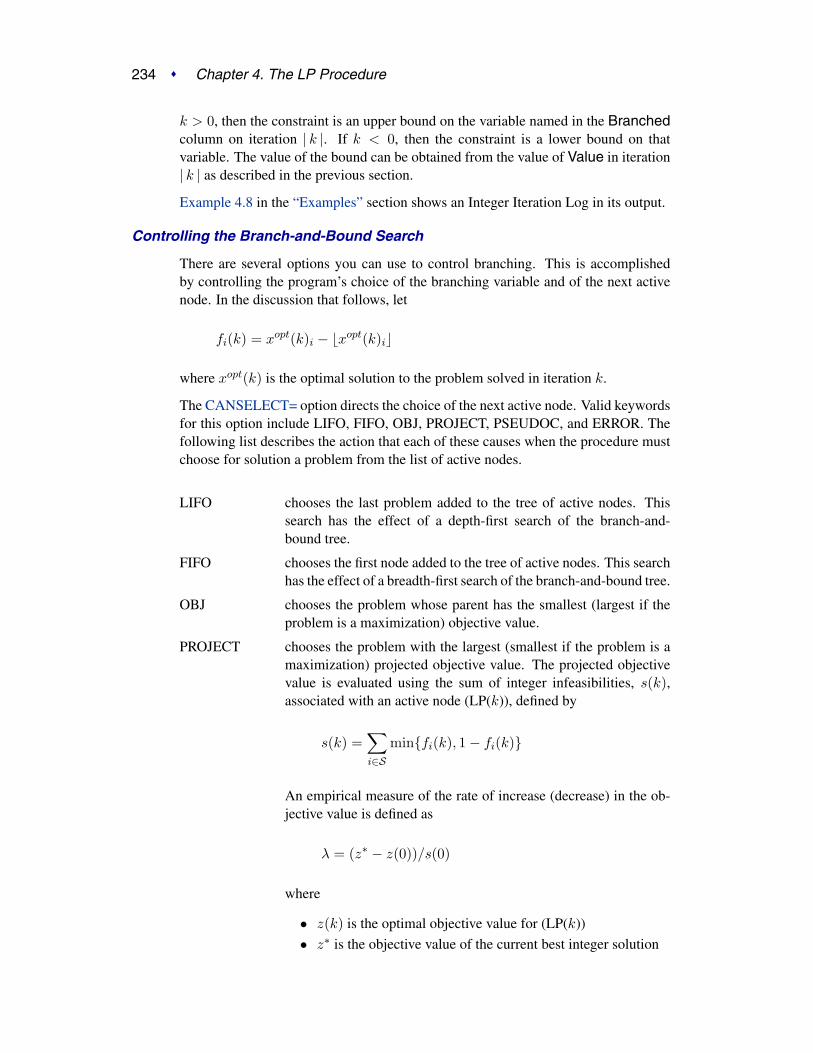
234 � Chapter 4. The LP Procedure
k > 0, then the constraint is an upper bound on the variable named in the Branchedcolumn on iteration | k |. If k < 0, then the constraint is a lower bound on thatvariable. The value of the bound can be obtained from the value of Value in iteration| k | as described in the previous section.
Example 4.8 in the “Examples” section shows an Integer Iteration Log in its output.
Controlling the Branch-and-Bound Search
There are several options you can use to control branching. This is accomplishedby controlling the program’s choice of the branching variable and of the next activenode. In the discussion that follows, let
fi(k) = xopt(k)i − xopt(k)i�
where xopt(k) is the optimal solution to the problem solved in iteration k.
The CANSELECT= option directs the choice of the next active node. Valid keywordsfor this option include LIFO, FIFO, OBJ, PROJECT, PSEUDOC, and ERROR. Thefollowing list describes the action that each of these causes when the procedure mustchoose for solution a problem from the list of active nodes.
LIFO chooses the last problem added to the tree of active nodes. Thissearch has the effect of a depth-first search of the branch-and-bound tree.
FIFO chooses the first node added to the tree of active nodes. This searchhas the effect of a breadth-first search of the branch-and-bound tree.
OBJ chooses the problem whose parent has the smallest (largest if theproblem is a maximization) objective value.
PROJECT chooses the problem with the largest (smallest if the problem is amaximization) projected objective value. The projected objectivevalue is evaluated using the sum of integer infeasibilities, s(k),associated with an active node (LP(k)), defined by
s(k) =∑i∈S
min{fi(k), 1 − fi(k)}
An empirical measure of the rate of increase (decrease) in the ob-jective value is defined as
λ = (z∗ − z(0))/s(0)
where
• z(k) is the optimal objective value for (LP(k))
• z∗ is the objective value of the current best integer solution

Integer Programming � 235
The projected objective value for problems (LP(k + 1)) and(LP(k + 2)) is defined as
z(k) + λs(k)
PSEUDOC chooses the problem with the largest (least if the problem is a max-imization) projected pseudocost. The projected pseudocost is eval-uated using the weighted sum of infeasibilities sw(k) associatedwith an active problem (LP(k)), defined by
sw(k) =∑i∈S
min{di(k)fi(k), ui(k)(1 − fi(k))}
The weights ui and di are initially equal to the absolute value of theith objective coefficient and are updated at each integer iteration.They are modified by examining the empirical marginal change inthe objective as additional constraints are placed on the variablesin S along the path from (LP(0)) to a node associated with an in-teger feasible solution. In particular, if the definition of problems(LP(k+1)) and (LP(k+2)) from parent (LP(k)) involve the additionof constraints xi ≤ xopt(k)i� and xi ≥ �xopt(k)i, respectively,and one of them is on a path to an integer feasible solution, thenonly one of the following is true:
di(k) = (z(k + 1) − z(k))/fi(k)
ui(k) = (z(k + 2) − z(k))/(1 − fi(k))
Note the similarity between sw(k) and s(k). The weighted quantitysw(k) accounts to some extent for the influence of the objectivefunction. The projected pseudocost for problems (LP(k + 1)) and(LP(k + 2)) is defined as
zw(k) ≡ z(k) + sw(k)
ERROR chooses the problem with the largest error. The error associatedwith problems (LP(k + 1)) and (LP(k + 2)) is defined as
(z∗ − zw(k))/(z∗ − z(k))
The BACKTRACK= option controls the search for the next problem. This optioncan take the same values as the CANSELECT= option. In addition to the case out-lined under the DELTAIT= option, backtracking is required as follows based on theCANSELECT= option in effect:

236 � Chapter 4. The LP Procedure
• If CANSELECT=LIFO and there is no active node in the portion of the ac-tive tree currently under exploration with a bound better than the value ofWOBJECTIVE=, then the procedure must backtrack.
• If CANSELECT=FIFO, PROJECT, PSEUDOC, or ERROR and the boundcorresponding to the node under consideration is not better than the value ofWOBJECTIVE=, then the procedure must backtrack.
The default value is OBJ.
The VARSELECT= option directs the choice of branching variable. Valid keywordsfor this option include CLOSE, FAR, PRIOR, PSEUDOC, PRICE, and PENALTY.The following list describes the action that each of these causes when xopt(k), anoptimal solution of problem (LP(k)), is used to define active problems (LP(k + 1))and (LP(k + 2)).
CLOSE chooses as branching variable the variable xi such that i minimizes
{min{fi(k), 1 − fi(k)} | i ∈ S and
IEPSILON ≤ fi(k) ≤ 1 − IEPSILON}
FAR chooses as branching variable the variable xi such that i maximizes
{min{fi(k), 1 − fi(k)} | i ∈ S and
IEPSILON ≤ fi(k) ≤ 1 − IEPSILON}
PRIOR chooses as branching variable xi such that i ∈ S, xopt(k)i is non-integral, and variable xi has the minimum value in the INTEGERrow in the input data set. This choice for the VARSELECT= optionis recommended when you have enough insight into the model toidentify those integer variables that have the most significant effecton the objective value.
PENALTY chooses as branching variable xi such that i ∈ S and a bound onthe increase in the objective of (LP(k)) (penalty) resulting fromadding the constraint
xi ≤ xopt(k)i� or xi ≥ �xopt(k)i
is maximized. The bound is calculated without pivoting usingtechniques of sensitivity analysis (Garfinkel and Nemhauser 1972).Because the cost of calculating the maximum penalty can be largeif S is large, you may want to limit the number of variables in Sfor which the penalty is calculated. The penalty is calculated forPENALTYDEPTH= variables in S.

Integer Programming � 237
PRICE chooses as branching variable xi such that i ∈ S, xopt(k)i is non-integral, and variable xi has the minimum price coefficient (maxi-mum for maximization).
PSEUDOC chooses as branching variable the variable xi such that i maximizes
{min{difi(k), ui(1 − fi(k))} | i ∈ S and
IEPSILON ≤ fi(k) ≤ 1 − IEPSILON}
The weights ui and di are initially equal to the absolute valueof the ith objective coefficient and are updated whenever an in-teger feasible solution is encountered. See the discussion on theCANSELECT= option for details on the method of updating theweights.
Customizing Search Heuristics
Often a good heuristic for searching the branch-and-bound tree of a problem canbe found. You are tempted to continue using this heuristic when the problem datachanges but the problem structure remains constant. The ability to reset procedureoptions interactively enables you to experiment with search techniques in an attemptto identify approaches that perform well. Then you can easily reapply these tech-niques to subsequent problems.
For example, the PIP branch-and-bound strategy (Crowder, Johnson, and Padberg1983) describes one such heuristic. The following program uses a similar strategy.Here, the OBJ rule (choose the active node with least parent objective function in thecase of a minimization problem) is used for selecting the next active node to be solveduntil an integer feasible solution is found. Once such a solution is found, the searchprocedure is changed to the LIFO rule: choose the problem most recently placed inthe list of active nodes.
proc lp canselect=obj ifeasiblepause=1;run;
reset canselect=lifo ifeasiblepause=9999999;run;
Further Discussion on AUTO and CONTROL= options
Consider a minimization problem. At each integer iteration, PROC LP will se-lect a node to solve from a pool of active nodes. The best bound strategy(CANSELECT=OBJ) will pick the node with the smallest projected objective value.This strategy improves the lower bound of the integer program and usually takesfewer integer iterations. One disadvantage is that PROC LP must recalculate theinverse of the basis matrix at almost every integer iteration; such recalculation is rel-atively expensive. Another disadvantage is that this strategy does not pay attention toimproving the upper bound of the integer program. Thus the number of active nodestends to grow rapidly if PROC LP cannot quickly find an optimal integer solution.

238 � Chapter 4. The LP Procedure
On the other hand, the LIFO strategy is very efficient and does not need to calculatethe inverse of the basis matrix unless the previous node is fathomed. It is a depth-firststrategy so it tends to find an integer feasible solution quickly. However, this strategywill pick nodes locally and usually will take longer integer iterations than the bestbound strategy.
There is another strategy that is often overlooked. Here it is called the best upperbound strategy. With this strategy, each time you select an active node, instead ofpicking the node with the smallest projected objective value, you select the one withthe largest projected objective value. This strategy is as efficient as the LIFO strategy.Moreover, it selects active nodes globally. This strategy tries to improve the upperbound of the integer program by searching for new integer feasible solutions. It alsofathoms active nodes quickly and keeps the total number of active nodes below thecurrent level. A disadvantage is that this strategy may evaluate more nodes that donot have any potential in finding an optimal integer solution.
The best bound strategy has the advantage of improving the lower bound. The LIFOstrategy has the advantages of efficiency and finding a local integer feasible solution.The best upper bound strategy has the advantages of keeping the size of active nodesunder control and at the same time trying to identify any potential integer feasiblesolution globally.
Although the best bound strategy is generally preferred, in some instances otherstrategies may be more effective. For example, if you have found an integer opti-mal solution but you do not know it, you still have to enumerate all possible activenodes. Then the three strategies will basically take the same number of integer itera-tions after an optimal solution is found but not yet identified. Since the LIFO and bestupper bound strategies are very efficient per integer iteration, both will outperformthe best bound strategy.
Since no one strategy suits all situations, a hybrid strategy has been developed toincrease applicability. The CONTROL= option combines the above three strategiesnaturally and provides a simple control parameter in [0, 1] dealing with differentinteger programming problems and different solution situations. The AUTO optionautomatically sets and adjusts the CONTROL= parameter so that you do not need toknow any problem structure or decide a node selection strategy in advance.
Since the LIFO strategy is less costly, you should use it as much as possible in thecombinations. The following process is called a diving process. Starting from anactive node, apply the LIFO strategy as much as you can until the current node be-comes feasible or is fathomed, or exceeds a preset limit. During this process, thereis no inverse matrix calculation involved except for the first node. When the divingprocess is over, apply one of the three strategies to select the next starting node. Oneset of combinations is called a cycle.
The control parameter r controls the frequency of the three strategies being appliedand the depth of the diving process in a cycle. It starts with a pure best bound strategyat r = 0, and then gradually increases the frequency of the diving processes and theirdepths as r increases. At r = 0.5, one cycle contains a best bound strategy plus afull diving process. After r = 0.5, the number of the diving processes will gradually

Sensitivity Analysis � 239
increase in a cycle. In addition, the best upper bound strategy will join the cycle. Asr continues to increase, the frequency of the best upper bound strategy will increase.At r = 1, it becomes a pure best upper bound strategy.
The AUTO option will automatically adjust the value of the CONTROL= option. Atthe start, it sets CONTROL=0.7, which emphasizes finding an upper bound. Afteran integer feasible solution is found, it sets CONTROL=0.5, which emphasizes effi-ciency and lower bound improvement. When the number of active nodes grows overthe default or user defined limit m, the number indicates that a better upper bound isneeded. The AUTO option will start to increase the value of CONTROL= from 0.5.If the size of the active nodes continues to grow, so will the value of the CONTROL=option. When the size of active nodes reaches to the default or user-defined limit n,CONTROL= will be set to 1. At this moment, the growth of active nodes is stopped.When the size of active nodes reduces, AUTO will decrease the value of CONTROL=option.
You can use other strategies to improve the lower bound by setting CANSELECT=to other options.
Saving and Restoring the List of Active Nodes
The list of active nodes can be saved in a SAS data set for use at a subsequent in-vocation of PROC LP. The ACTIVEOUT= option in the PROC LP statement namesthe data set into which the current list of active nodes is saved when the procedureterminates due to an error termination condition. Examples of such conditions aretime limit exceeded, integer iterations exceeded, and phase 3 iterations exceeded.The ACTIVEIN= option in the PROC LP statement names a data set that can beused to initialize the list of active nodes. To achieve the greatest benefit when restart-ing PROC LP, use the PRIMALOUT= and PRIMALIN= options in conjunction withthe ACTIVEOUT= and ACTIVEIN= options. See Example 4.10 in the “Examples”section for an illustration.
Sensitivity Analysis
Sensitivity analysis is a technique for examining the effects of changes in modelparameters on the optimal solution. The analysis enables you to examine the size ofa perturbation to the right-hand-side or objective vector by an arbitrary change vectorfor which the basis of the current optimal solution remains optimal.
Note: When sensitivity analysis is performed on integer-constrained problems, theinteger variables are fixed at the value they obtained in the integer optimal solution.Therefore, care must be used when interpreting the results of such analyses. Caremust also be taken when preprocessing is enabled, because preprocessing usuallyalters the original formulation.

240 � Chapter 4. The LP Procedure
Right-Hand-Side Sensitivity Analysis
Consider the problem (lpr(φ)):
xopt(φ) = min cT x
subject to Ax {≥, =,≤} b + φr� ≤ x ≤ u
where r is a right-hand-side change vector.
Let xopt(φ) denote an optimal basic feasible solution to (lpr(φ)). PROC LP canbe used to examine the effects of changes in φ on the solution xopt(0) of problem(lpr(0)) . For the basic solution xopt(0), let B be the matrix composed of the basiccolumns of A and let N be the matrix composed of the nonbasic columns of A. Forthe basis matrix B, the basic components of xopt(0), written as xopt(0)B , can beexpressed as
xopt(0)B = B−1(b − Nxopt(0)N )
Furthermore, because xopt(0) is feasible,
�B ≤ B−1(b − Nxopt(0)N ) ≤ uB
where �B is a column vector of the lower bounds on the structural basic variables,and uB is a column vector of the upper bounds on the structural basic variables. Foreach right-hand-side change vector r identified in the RHSSEN statement, PROC LPfinds an interval [φmin, φmax] such that
�B ≤ B−1(b + φr − Nxopt(0)N ) ≤ uB
for φ ∈ [φmin, φmax]. Furthermore, because changes in the right-hand side do notaffect the reduced costs, for φ ∈ [φmin, φmax],
xopt(φ)T = ((B−1(b + φr − Nxopt(0)N ))T , xopt(0)TN )
is optimal in (lpr(φ)).
For φ = φmin and φ = φmax, PROC LP reports the following:
• the names of the leaving variables
• the value of the optimal objective in the modified problems
• the RHS values in the modified problems
• the solution status, reduced costs and activities in the modified problems
The leaving variable identifies the basic variable xi that first reaches either the lowerbound �i or the upper bound ui as φ reaches φmin or φmax. This is the basic variablethat would leave the basis to maintain primal feasibility. Multiple RHSSEN variablescan appear in a problem data set.

Sensitivity Analysis � 241
Price Sensitivity Analysis
Consider the problem (lpp(φ)):
xopt(φ) = min(c + φr)T x
subject to Ax {≥, =,≤} b� ≤ x ≤ u
where r is a price change vector.
Let xopt(φ) denote an optimal basic feasible solution to (lpp(φ)). PROC LP canbe used to examine the effects of changes in φ on the solution xopt(0) of problem(lpp(0)). For the basic solution xopt(0), let B be the matrix composed of the basiccolumns of A and let N be the matrix composed of the nonbasic columns of A. Forbasis matrix B, the reduced cost associated with the ith variable can be written as
rci(φ) = ((c + φr)TN − (c + φr)T
BB−1N)i
where (c + φr)N and (c + φr)B is a partition of the vector of price coefficients intononbasic and basic components. Because xopt(0) is optimal in (lpp(0)), the reducedcosts satisfy
rci(φ) ≥ 0
if the nonbasic variable in column i is at its lower bound, and
rci(φ) ≤ 0
if the nonbasic variable in column i is at its upper bound.
For each price coefficient change vector r identified with the keyword PRICESENin the TYPE variable, PROC LP finds an interval [φmin, φmax] such that forφ ∈ [φmin, φmax],
rci(φ) ≥ 0
if the nonbasic variable in column i is at its lower bound, and
rci(φ) ≤ 0
if the nonbasic variable in column i is at its upper bound. Because changes in theprice coefficients do not affect feasibility, for φ ∈ [φmin, φmax], xopt(φ) is optimal in(lpp(φ)). For φ = φmin and φ = φmax, PROC LP reports the following:
• the names of entering variables
• the value of the optimal objective in the modified problems

242 � Chapter 4. The LP Procedure
• the price coefficients in the modified problems
• the solution status, reduced costs, and activities in the modified problems
The entering variable identifies the variable whose reduced cost first goes to zero asφ reaches φmin or φmax. This is the nonbasic variable that would enter the basis tomaintain optimality (dual feasibility). Multiple PRICESEN variables may appear ina problem data set.
Range Analysis
Range analysis is sensitivity analysis for specific change vectors. As with the sen-sitivity analysis case, care must be used in interpreting the results of range analysiswhen the problem has integers or the preprocessing option is enabled.
Right-Hand-Side Range Analysis
The effects on the optimal solution of changes in each right-hand-side value can bestudied using the RANGERHS option in the PROC LP or RESET statement. This op-tion results in sensitivity analysis for the m right-hand-side change vectors specifiedby the columns of the m × m identity matrix.
Price Range Analysis
The effects on the optimal solution of changes in each price coefficient can be studiedusing the RANGEPRICE option in the PROC LP or RESET statement. This optionresults in sensitivity analysis for the n price change vectors specified by the rows ofthe n × n identity matrix.
Parametric Programming
Sensitivity analysis and range analysis examine how the optimal solution behaveswith respect to perturbations of model parameter values. These approaches assumethat the basis at optimality is not allowed to change. When greater flexibility is de-sired and a change of basis is acceptable, parametric programming can be used.
As with the sensitivity analysis case, care must be used in interpreting the results ofparametric programming when the problem has integers or the preprocessing optionis enabled.
Right-Hand-Side Parametric Programming
As discussed in the “Right-Hand-Side Sensitivity Analysis” section on page 240, foreach right-hand-side change vector r, PROC LP finds an interval [φmin, φmax] suchthat for φ ∈ [φmin, φmax],
xopt(φ)T = ((B−1(b + φr − Nxopt(0)N ))T , xopt(0)TN )
is optimal in (lpr(φ)) for the fixed basis B. Leaving variables that inhibit furtherchanges in φ without a change in the basis B are associated with the quantities φmin
and φmax. By specifying RHSPHI=Φ in either the PROC LP statement or the RESET

Parametric Programming � 243
statement, you can examine the solution xopt(φ) as φ increases or decreases from 0to Φ.
When RHSPHI=Φ is specified, the procedure first finds the interval [φmin, φmax] asdescribed previously. Then, if Φ ∈ [φmin, φmax], no further investigation is needed.However, if Φ > φmax or Φ < φmin, then the procedure attempts to solve the newproblem (lpr(Φ)). To accomplish this, it pivots the leaving variable out of the basiswhile maintaining dual feasibility. If this new solution is primal feasible in (lpr(Φ)),no further investigation is needed; otherwise, the procedure identifies the new leavingvariable and pivots it out of the basis, again maintaining dual feasibility. Dual piv-oting continues in this manner until a solution that is primal feasible in (lpr(Φ)) isidentified. Because dual feasibility is maintained at each pivot, the (lpr(Φ)) primalfeasible solution is optimal.
At each pivot, the procedure reports on the variables that enter and leave the basis, thecurrent range of φ , and the objective value. When xopt(Φ) is found, it is displayed.If you want the solution xopt(φ) at each pivot, then specify the PARAPRINT optionin either the PROC LP or the RESET statement.
Price Parametric Programming
As discussed in the “Price Sensitivity Analysis” section on page 241, for eachprice change vector r, PROC LP finds an interval [φmin, φmax] such that for eachφ ∈ [φmin, φmax],
rci(φ) = ((c + φr)TN − (c + φr)T
BB−1N)i
satisfies the conditions for optimality in (lpp(φ)) for the fixed basis B. Entering vari-ables that inhibit further changes in φ without a change in the basis B are associatedwith the quantities φmin and φmax. By specifying PRICEPHI=Φ in either the PROCLP statement or the RESET statement, you can examine the solution xopt(φ) as φincreases or decreases from 0 to Φ.
When PRICEPHI=Φ is specified, the procedure first finds the interval [φmin, φmax],as described previously. Then, if Φ ∈ [φmin, φmax], no further investigation isneeded. However, if Φ > φmax or Φ < φmin, the procedure attempts to solvethe new problem (lpp(Φ)). To accomplish this, it pivots the entering variable intothe basis while maintaining primal feasibility. If this new solution is dual feasible in(lpp(Φ)), no further investigation is needed; otherwise, the procedure identifies thenew entering variable and pivots it into the basis, again maintaining primal feasibility.Pivoting continues in this manner until a solution that is dual feasible in (lpp(Φ)) isidentified. Because primal feasibility is maintained at each pivot, the (lpp(Φ)) dualfeasible solution is optimal.
At each pivot, the procedure reports on the variables that enter and leave the basis, thecurrent range of φ , and the objective value. When xopt(Φ) is found, it is displayed.If you want the solution xopt(φ) at each pivot, then specify the PARAPRINT optionin either the PROC LP or the RESET statement.

244 � Chapter 4. The LP Procedure
Interactive Facilities
The interactive features of the LP procedure enable you to examine intermediate re-sults, perform sensitivity analysis, parametric programming, and range analysis, andcontrol the solution process.
Controlling Interactive Features
You can gain control of the LP procedure for interactive processing by setting a break-point or pressing the CTRL-BREAK key combination, or when certain error condi-tions are encountered:
• when a feasible solution is found
• at each pivot of the simplex algorithm
• when an integer feasible solution is found
• at each integer pivot of the branch-and-bound algorithm
• after the data are read but before iteration begins
• after at least one integer feasible solution has been found which is within de-sirable proximity of optimality
• after the problem has been solved but before results are displayed
When the LP procedure pauses, you can enter any of the interactive statementsRESET, PIVOT, IPIVOT, PRINT, SHOW, QUIT, and RUN.
Breakpoints are set using the FEASIBLEPAUSE, PAUSE=, IFEASIBLEPAUSE=,IPAUSE=, PROXIMITYPAUSE=, READPAUSE, and ENDPAUSE options. The LPprocedure displays a message on the SAS log when it gives you control because ofencountering one of these breakpoints.
During phase 1, 2, or 3, the CTRL-BREAK key pauses the LP procedure and releasesthe control at the beginning of the next iteration.
The error conditions, which usually cause the LP procedure to pause, include timelimit exceeded, phase 1 iterations exceeded, phase 2 iterations exceeded, phase 3 it-erations exceeded, and integer iterations exceeded. You can use the RESET statementto reset the option that caused the error condition.
The PIVOT and IPIVOT statements result in control being returned to you after a sin-gle simplex algorithm pivot and an integer pivot. The PRINT and SHOW statementsdisplay current solution information and return control to you. On the other hand, theQUIT statement requests that you leave the LP procedure immediately. If you wantto quit but save output data sets, then type QUIT/SAVE. The RUN statement requeststhe LP procedure to continue its execution immediately.

Memory Management � 245
Displaying Intermediate Results
Once you have control of the procedure, you can examine the current values of theoptions and the status of the problem being solved using the SHOW statement. Alldisplaying done by the SHOW statement goes to the SAS log.
Details about the current status of the solution are obtained using the PRINT state-ment. The various display options enable you to examine parts of the variable andconstraint summaries, display the current tableau, perform sensitivity analysis on thecurrent solution, and perform range analysis.
Interactive Facilities in Batch Mode
All of the interactive statements can be used when processing in batch mode. This isparticularly convenient when the interactive facilities are used to combine differentsearch strategies in solving integer problems.
Sensitivity Analysis
Two features that enhance the ability to perform sensitivity analysis need furtherexplanation. When you specify /SENSITIVITY in a PRINT COLUMN(colnames)statement, the LP procedure defines a new change row to use in sensitivity analysisand parametric programming. This new change row has a +1 entry for each variablelisted in the PRINT statement. This enables you to define new change rows interac-tively.
When you specify /SENSITIVITY in a PRINT ROW (rownames) statement, the LPprocedure defines a new change column to use in sensitivity analysis and parametricprogramming. This new change column has a +1 entry for each right-hand-side coef-ficient listed in the PRINT statement. This enables you to define new change columnsinteractively.
In addition, you can interactively change the RHSPHI= and PRICEPHI= options us-ing the RESET statement. This enables you to perform parametric programminginteractively.
Memory Management
There are no restrictions on the problem size in the LP procedure. The number ofconstraints and variables in a problem that PROC LP can solve depends on the hostplatform, the available memory, and the available disk space for utility data sets.
Memory usage is affected by a great many factors including the density of the tech-nological coefficient matrix, the model structure, and the density of the decomposedbasis matrix. The algorithm requires that the decomposed basis fit completely inmemory. Any additional memory is used for nonbasic columns. The partition be-tween the decomposed basis and the nonbasic columns is dynamic so that as theinverse grows, which typically happens as iterations proceed, more memory is avail-able to it and less is available for the nonbasic columns.
The LP procedure determines the initial size of the decomposed basis matrix. If thearea used is too small, PROC LP must spend time compressing this matrix, which de-grades performance. If PROC LP must compress the decomposed basis matrix on the

246 � Chapter 4. The LP Procedure
average more than 15 times per iteration, then the size of the memory devoted to thebasis is increased. If the work area cannot be made large enough to invert the basis,an error return occurs. On the other hand, if PROC LP compresses the decomposedbasis matrix on the average once every other iteration, then memory devoted to thedecomposed basis is decreased, freeing memory for the nonbasic columns.
For many models, memory constraints are not a problem because both the decom-posed basis and all the nonbasic columns will have no problem fitting. However,when the models become large relative to the available memory, the algorithm triesto adjust memory distribution in order to solve the problem. In the worst cases, onlyone nonbasic column fits in memory with the decomposed basis matrix.
Problems involving memory use can occur when solving mixed-integer problems.Data associated with each node in the branch-and-bound tree must be kept in mem-ory. As the tree grows, competition for memory by the decomposed basis, the non-basic columns, and the branch-and-bound tree may become critical. If the situationbecomes critical, the procedure automatically switches to branching strategies thatuse less memory. However, it is possible to reach a point where no further processingis possible. In this case, PROC LP terminates on a memory error.
Output Data Sets
The LP procedure can optionally produce four output data sets. These are theACTIVEOUT=, PRIMALOUT=, DUALOUT=, and TABLEAUOUT= data sets.Each contains two variables that identify the particular problem in the input dataset. These variables are
–OBJ–ID– identifies the objective function ID.
–RHS–ID– identifies the right-hand-side variable.
Additionally, each data set contains other variables, which are discussed below.
ACTIVEOUT= Data Set
The ACTIVEOUT= data set contains a representation of the current active branch-and-bound tree. You can use this data set to initialize the branch-and-bound tree tocontinue iterations on an incompletely solved problem. Each active node in the treegenerates two observations in this data set. The first is a ‘LOWERBD’ observationthat is used to reconstruct the lower-bound constraints on the currently describedactive node. The second is an ‘UPPERBD’ observation that is used to reconstruct theupper-bound constraints on the currently described active node. In addition to these,an observation that describes the current best integer solution is included. The dataset contains the following variables:
–STATUS– contains the keywords LOWERBD, UPPERBD, and INTBEST foridentifying the type of observation.
–PROB– contains the problem number for the current observation.
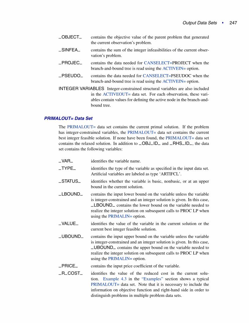
Output Data Sets � 247
–OBJECT– contains the objective value of the parent problem that generatedthe current observation’s problem.
–SINFEA– contains the sum of the integer infeasibilities of the current obser-vation’s problem.
–PROJEC– contains the data needed for CANSELECT=PROJECT when thebranch-and-bound tree is read using the ACTIVEIN= option.
–PSEUDO– contains the data needed for CANSELECT=PSEUDOC when thebranch-and-bound tree is read using the ACTIVEIN= option.
INTEGER VARIABLES Integer-constrained structural variables are also includedin the ACTIVEOUT= data set. For each observation, these vari-ables contain values for defining the active node in the branch-and-bound tree.
PRIMALOUT= Data Set
The PRIMALOUT= data set contains the current primal solution. If the problemhas integer-constrained variables, the PRIMALOUT= data set contains the currentbest integer feasible solution. If none have been found, the PRIMALOUT= data setcontains the relaxed solution. In addition to –OBJ–ID– and –RHS–ID– , the dataset contains the following variables:
–VAR– identifies the variable name.
–TYPE– identifies the type of the variable as specified in the input data set.Artificial variables are labeled as type ‘ARTIFCL’.
–STATUS– identifies whether the variable is basic, nonbasic, or at an upperbound in the current solution.
–LBOUND– contains the input lower bound on the variable unless the variableis integer-constrained and an integer solution is given. In this case,
–LBOUND– contains the lower bound on the variable needed torealize the integer solution on subsequent calls to PROC LP whenusing the PRIMALIN= option.
–VALUE– identifies the value of the variable in the current solution or thecurrent best integer feasible solution.
–UBOUND– contains the input upper bound on the variable unless the variableis integer-constrained and an integer solution is given. In this case,
–UBOUND– contains the upper bound on the variable needed torealize the integer solution on subsequent calls to PROC LP whenusing the PRIMALIN= option.
–PRICE– contains the input price coefficient of the variable.
–R–COST– identifies the value of the reduced cost in the current solu-tion. Example 4.3 in the “Examples” section shows a typicalPRIMALOUT= data set. Note that it is necessary to include theinformation on objective function and right-hand side in order todistinguish problems in multiple problem data sets.

248 � Chapter 4. The LP Procedure
DUALOUT= Data Set
The DUALOUT= data set contains the dual solution for the current solution. If theproblem has integer-constrained variables, the DUALOUT= data set contains the dualfor the current best integer solution, if any. Otherwise it contains the dual for the re-laxed solution. In addition to –OBJ–ID– and –RHS–ID– , it contains the followingvariables:
–ROW–ID– identifies the row or constraint name.
–TYPE– identifies the type of the row as specified in the input data set.
–RHS– gives the value of the right-hand side on input.
–L–RHS– gives the lower bound for the row evaluated from the input right-hand-side value, the TYPE of the row, and the value of the RANGEvariable for the row.
–VALUE– gives the value of the row, at optimality, excluding logical vari-ables.
–U–RHS– gives the upper bound for the row evaluated from the input right-hand-side value, the TYPE of the row, and the value of the RANGEvariable for the row.
–DUAL– gives the value of the dual variable associated with the row.
TABLEAUOUT= Data Set
The TABLEAUOUT= data set contains the current tableau. Each observation, exceptfor the first, corresponds to a basic variable in the solution. The observation labeledR–COSTS contains the reduced costs cT
N − cTBB−1N . In addition to –OBJ–ID–
and –RHS–ID– , it contains the following variables:
–BASIC– gives the names of the basic variables in the solution.
INVB–R gives the values of B−1r , where r is the right-hand-sidevector.
STRUCTURAL VARIABLES give the values in the tableau, namely B−1A .
Input Data Sets
In addition to the DATA= input data set, PROC LP recognizes the ACTIVEIN= andthe PRIMALIN= data sets.
ACTIVEIN= Data Set
The ACTIVEIN= data set contains a representation of the current active tree. Theformat is identical to that of the ACTIVEOUT= data set.

Displayed Output � 249
PRIMALIN= Data Set
The format of the PRIMALIN= data set is identical to the PRIMALOUT= data set.PROC LP uses the PRIMALIN= data set to identify variables at their upper boundsin the current solution and variables that are basic in the current solution.
You can add observations to the end of the problem data set if they define cost (right-hand-side) sensitivity change vectors and have PRICESEN (RHSSEN) types. Thisenables you to solve a problem, save the solution in a SAS data set, and perform sen-sitivity analysis later. You can also use the PRIMALIN= data set to restart problemsthat have not been completely solved or to which new variables have been added.
Displayed Output
The output from the LP procedure is discussed in the following six sections:
• Problem Summary
• Solution Summary including a Variable Summary and a Constraint Summary
• Infeasible Information Summary
• RHS Sensitivity Analysis Summary (the RHS Range Analysis Summary is notdiscussed)
• Price Sensitivity Analysis Summary (the Price Range Analysis Summary is notdiscussed)
• Iteration Log
For integer-constrained problems, the procedure also displays an Integer IterationLog. The description of this Log can be found in the “Integer Programming” sectionon page 231. When you request that the tableau be displayed, the procedure displaysthe Current Tableau. The description of this can be found in the “The Reduced Costs,Dual Activities, and Current Tableau” section on page 227.
A problem data set can contain a set of constraints with several right-hand sides andseveral objective functions. PROC LP considers each combination of right-hand sideand objective function as defining a new linear programming problem and solveseach, performing all specified sensitivity analysis on each problem. For each problemdefined, PROC LP displays a new sequence of output sections. Example 4.1 in the“Examples” section on page 254 discusses each of these elements.
The LP procedure produces the following displayed output by default.
The Problem Summary
The problem summary includes the
• type of optimization and the name of the objective row (as identified by the IDor ROW variable)
• name of the SAS variable that contains the right-hand-side constants
• name of the SAS variable that contains the type keywords

250 � Chapter 4. The LP Procedure
• density of the coefficient matrix (the ratio of the number of nonzero elementsto the number of total elements) after the slack and surplus variables have beenappended
• number of each type of variable in the mathematical program
• number of each type of constraint in the mathematical program
The Solution Summary
The solution summary includes the
• termination status of the procedure
• objective value of the current solution
• number of phase 1 iterations that were completed
• number of phase 2 iterations that were completed
• number of phase 3 iterations that were completed
• number of integer iterations that were completed
• number of integer feasible solutions that were found
• number of initial basic feasible variables identified
• time used in solving the problem excluding reading the data and displaying thesolution
• number of inversions of the basis matrix
• current value of several of the options
The Variable Summary
The variable summary includes the
• column number associated with each structural or logical variable in the prob-lem
• name of each structural or logical variable in the problem. (PROC LP gives thelogical variables the name of the constraint ID. If no ID variable is specified,the procedure names the logical variable –OBSn– , where n is the observationthat describes the constraint.)
• variable’s status in the current solution. The status can be BASIC, DEGEN,ALTER, blank, LOWBD, or UPPBD, depending upon whether the variable isa basic variable, a degenerate variable (that is, a basic variable whose activityis at its input lower bound), a nonbasic variable that can be brought into thebasis to define an alternate optimal solution, a nonbasic variable at its defaultlower bound 0, a nonbasic variable at its lower bound, or a nonbasic variable atits upper bound.
• type of variable (whether it is logical or structural, and, if structural, its boundtype, or other value restriction). See Example 4.1 for a list of possible types inthe variable summary.

Displayed Output � 251
• value of the objective coefficient associated with each variable
• activity of the variable in the current solution
• variable’s reduced cost in the current solution
The Constraint SummaryThe constraint summary includes the
• constraint row number and its ID
• kind of constraint (whether it is an OBJECTIVE, LE, EQ, GE, RANGELE,RANGEEQ, RANGEGE, or FREE row)
• number of the slack or surplus variable associated with the constraint row
• value of the right-hand-side constant associated with the constraint row
• current activity of the row (excluding logical variables)
• current activity of the dual variable (shadow price) associated with the con-straint row
The Infeasible Information SummaryThe infeasible information summary includes the
• name of the infeasible row or variable
• current activity for the row or variable
• type of the row or variable
• value of right-hand-side constant
• name of each nonzero and nonmissing variable in the row
• activity and upper and lower bounds for the variable
The RHS Sensitivity Analysis SummaryThe RHS sensitivity analysis summary includes the
• value of φmin
• leaving variable when φ = φmin
• objective value when φ = φmin
• value of φmax
• leaving variable when φ = φmax
• objective value when φ = φmax
• column number and name of each logical and structural variable
• variable’s status when φ ∈ [φmin, φmax]
• variable’s reduced cost when φ ∈ [φmin, φmax]
• value of right-hand-side constant when φ = φmin
• activity of the variable when φ = φmin
• value of right-hand-side constant when φ = φmax
• activity of the variable when φ = φmax

252 � Chapter 4. The LP Procedure
The Price Sensitivity Analysis Summary
The price sensitivity analysis summary includes the
• value of φmin
• entering variable when φ = φmin
• objective value when φ = φmin
• value of φmax
• entering variable when φ = φmax
• objective value when φ = φmax
• column number and name of each logical and structural variable
• variable’s status when φ ∈ [φmin, φmax]
• activity of the variable when φ ∈ [φmin, φmax]
• price of the variable when φ = φmin
• variable’s reduced cost when φ = φmin
• price of the variable when φ = φmax
• variable’s reduced cost when φ = φmax
The Iteration Log
The iteration log includes the
• phase number
• iteration number in each phase
• name of the leaving variable
• name of the entering variable
• variable’s reduced cost
• objective value
ODS Table and Variable Names
PROC LP assigns a name to each table it creates. You can use these names to selectoutput tables when using the Output Delivery System (ODS).
Table 4.6. ODS Tables Produced in PROC LP
Table Name Description Statement/OptionProblemSummary Problem summary defaultSolutionSummary Solution summary defaultVariableSummary Variable summary defaultConstraintSummary Constraint summary defaultIterationLog Iteration log FLOWIntegerIterationLog Integer iteration log default

ODS Table and Variable Names � 253
Table 4.6. (continued)
Table Name Description Statement/OptionPriceSensitivitySummary Price sensitivity analysis
summarydefault, PRINT PRICESEN, or PRINTCOLUMN/SENSITIVITY
PriceActivities Price activities at φmin andφmax
default, PRINT PRICESEN, or PRINTCOLUMN/SENSITIVITY
PriceActivity Price activity at φmin or φmax PRICEPHI= and PARAPRINTPriceParametricLog Price parametric program-
ming logPRICEPHI=
PriceRangeSummary Price range analysis RANGEPRICE or PRINT RANGEPRICERhsSensitivitySummary RHS sensitivity analysis sum-
marydefault, PRINT RHSSEN, or PRINTROW/SENSITIVITY
RhsActivities RHS activities at φmin andφmax
default, PRINT RHSSEN, or PRINTROW/SENSITIVITY
RhsActivity RHS activity at φmin or φmax RHSPHI= and PARAPRINTRhsParametricLog RHS parametric program-
ming logRHSPHI=
RhsRangeSummary RHS range analysis RANGERHS or PRINT RANGERHSInfeasibilitySummary Infeasible row or variable
summarydefault
InfeasibilityActivity Variable activity in an infeasi-ble row
default
CurrentTableau Current tableau TABLEAUPRINT or PRINT TABLEAUMatrix Technological matrix PRINT MATRIXMatrixPicture Technological matrix picture PRINT MATRIX/PICTUREMatrixPictureLegend Technological matrix picture
legendPRINT MATRIX/PICTURE
The following table lists the variable names of the preceding tables used in the ODStemplate of the LP procedure.
Table 4.7. Variable Names for the ODS Tables Produced in PROC LP
Table Name VariablesVariableSummary VarName, Status, Type, Price, Activity, ReducedCostConstraintSummary Row, RowName, Type, SSCol, Rhs, Activity, DualIterationLog Phase, Iteration, EnterVar, EnterCol, LeaveVar, LeaveCol, ReducedCost,
ObjValueIntegerIterationLog Iteration, Problem, Condition, Objective, Branch, Value, SumOfInfeas, Active,
ProximityPriceActivities Col, VarName, Status, Activity, MinPrice, MinReducedCost, MaxPrice,
MaxReducedCostPriceActivity Col, VarName, Status, Activity, Price, ReducedCostPriceParametricLog LeaveVar, LeaveCol, EnterVar, EnterCol, ObjValue, CurrentPhiPriceRangeSummary Col, VarName, MinPrice, MinEnterVar, MinObj, MaxPrice, MaxEnterVar,
MaxObjRhsActivities Col, VarName, Status, ReducedCost, MinRhs, MinActivity, MaxRhs,
MaxActivity

254 � Chapter 4. The LP Procedure
Table 4.7. (continued)
Table Name VariablesRhsActivity Col, VarName, Status, ReducedCost, Rhs, Activity,RhsParametricLog LeaveVar, LeaveCol, EnterVar, EnterCol, ObjValue, CurrentPhiRhsRangeSummary RowName, MinRhs, MinLeaveVar, MinObj, MaxRhs, MaxLeaveVar, MaxObjInfeasibilityActivity VarName, Coefficient, Activity, Lower, Upper
Examples
The following fourteen examples illustrate some of the capabilities of PROC LP.These examples, together with the other SAS/OR examples, can be found in the SASsample library. A description of the features of PROC LP as shown in the examplesare
Example 4.1 dense input format
Example 4.2 sparse input format
Example 4.3 the RANGEPRICE option to show you the range over which eachobjective coefficient can vary without changing the variables in thebasis
Example 4.4 more sensitivity analysis and restarting a problem
Example 4.5 parametric programming
Example 4.6 special ordered sets
Example 4.7 goal programming
Example 4.8 integer programming
Example 4.9 an infeasible problem
Example 4.10 restarting integer programs
Example 4.11 controlling the search of the branch-and-bound tree
Example 4.12 matrix generation and report writing for an assignment problem
Example 4.13 matrix generation and report writing for a scheduling problem
Example 4.14 a multicommodity transshipment problem
Example 4.1. An Oil Blending Problem
The blending problem presented in the introduction is a good example for demon-strating some of the features of the LP procedure. Recall that a step in refining crudeoil into finished oil products involves a distillation process that splits crude into var-ious streams. Suppose that there are three types of crude available: Arabian light,Arabian heavy, and Brega. These are distilled into light naphtha, intermediate naph-tha, and heating oil. Using one of two recipes, these in turn are blended into jetfuel.
Assume that you can sell as much fuel as is produced. What production strategymaximizes the profit from jet fuel sales? The following SAS code demonstrates a

Example 4.1. An Oil Blending Problem � 255
way of answering this question using linear programming. The SAS data set is arepresentation of the formulation for this model given in the introductory section.
data;input _row_ $17.
a_light a_heavy brega naphthal naphthai heatingo jet_1jet_2 _type_ $ _rhs_;
datalines;profit -175 -165 -205 0 0 0 300 300 max .naphtha_l_conv .035 .030 .045 -1 0 0 0 0 eq 0naphtha_i_conv .100 .075 .135 0 -1 0 0 0 eq 0heating_o_conv .390 .300 .430 0 0 -1 0 0 eq 0recipe_1 0 0 0 0 .3 .7 -1 0 eq 0recipe_2 0 0 0 .2 0 .8 0 -1 eq 0available 110 165 80 . . . . . upperbd .;
proc lp;run;
The –ROW– variable contains the names of the rows in the model; the variablesA–LIGHT to JET–2 are the names of the structural variables in the model; the
–TYPE– variable contains the keywords that tell the LP procedure how to interpreteach row in the model; and the –RHS– variable gives the value of the right-hand-sideconstants.
The structural variables are interpreted as the quantity of each type of constituentor finished product. For example, the value of A–HEAVY in the solution is theamount of Arabian heavy crude to buy while the value of JET–1 in the solution isthe amount of recipe 1 jet fuel that is produced. As discussed previously, the valuesgiven in the model data set are the technological coefficients whose interpretationdepends on the model. In this example, the coefficient -175 in the PROFIT row for thevariable A–LIGHT gives a cost coefficient (because the row with –ROW–=PROFIThas –TYPE–=MAX) for the structural variable A–LIGHT. This means that for eachunit of Arabian heavy crude purchased, a cost of 175 units is incurred.
The coefficients 0.035, 0.100, and 0.390 for the A–LIGHT variable give the per-centages of each unit of Arabian light crude that is distilled into the light naph-tha, intermediate naphtha, and heating oil components. The 110 value in the row
–ROW–=AVAILABLE gives the quantity of Arabian light that is available.
PROC LP produces the following Problem Summary output. Included in the sum-mary is an identification of the objective, defined by the first observation of theproblem data set; the right-hand-side variable, defined by the variable –RHS– ;and the type identifier, defined by the variable –TYPE– . See Output 4.1.1.

256 � Chapter 4. The LP Procedure
Output 4.1.1. Problem Summary for the Oil Blending ProblemThe LP Procedure
Problem Summary
Objective Function Max profitRhs Variable _rhs_Type Variable _type_Problem Density (%) 45.00
Variables Number
Non-negative 5Upper Bounded 3
Total 8
Constraints Number
EQ 5Objective 1
Total 6
The next section of output (Output 4.1.2) contains the Solution Summary, which in-dicates whether or not an optimal solution was found. In this example, the procedureterminates successfully (with an optimal solution), with 1544 as the value of the ob-jective function. Also included in this section of output is the number of phase 1 andphase 2 iterations, the number of variables used in the initial basic feasible solution,and the time used to solve the problem. For several options specified in the PROC LPstatement, the current option values are also displayed.
Output 4.1.2. Solution Summary for the Oil Blending Problem
The LP Procedure
Solution Summary
Terminated Successfully
Objective Value 1544
Phase 1 Iterations 0Phase 2 Iterations 4Phase 3 Iterations 0Integer Iterations 0Integer Solutions 0Initial Basic Feasible Variables 5Time Used (seconds) 0Number of Inversions 3
Epsilon 1E-8Infinity 1.797693E308Maximum Phase 1 Iterations 100Maximum Phase 2 Iterations 100Maximum Phase 3 Iterations 99999999Maximum Integer Iterations 100Time Limit (seconds) 120

Example 4.1. An Oil Blending Problem � 257
The next section of output (Output 4.1.3) contains the Variable Summary. A lineis displayed for each variable in the mathematical program with the variable name,the status of the variable in the solution, the type of variable, the variable’s pricecoefficient, the activity of the variable in the solution, and the reduced cost for thevariable. The status of a variable can be
BASIC if the variable is a basic variable in the solution.
DEGEN if the variable is a basic variable whose activity is at its inputlower bound.
ALTER if the variable is nonbasic and is basic in an alternate optimalsolution.
LOWBD if the variable is nonbasic and is at its lower bound.
UPPBD if the variable is nonbasic and is at its upper bound.
The TYPE column shows how PROC LP interprets the variable in the problem dataset. Types include the following:
NON-NEG if the variable is a nonnegative variable with lower bound 0and upper bound +∞.
LOWERBD if the variable has a lower bound specified in a LOWERBDobservation and upper bound +∞.
UPPERBD if the variable has an upper bound that is less than +∞and lower bound 0. This upper bound is specified in anUPPERBD observation.
UPLOWBD if the variable has a lower bound specified in a LOWERBDobservation and an upper bound specified in an UPPERBDobservation.
INTEGER if the variable is constrained to take integer values. If this isthe case, then it must also be upper and lower bounded.
BINARY if the variable is constrained to take value 0 or 1.
UNRSTRCT if the variable is an unrestricted variable having bounds of−∞ and +∞.
SLACK if the variable is a slack variable that PROC LP has appendedto a LE constraint. For variables of this type, the variablename is the same as the name of the constraint (given inthe ROW variable) for which this variable is the slack. Anonzero slack variable indicates that the constraint is nottight. The slack is the amount by which the right-hand sideof the constraint exceeds the left-hand side.

258 � Chapter 4. The LP Procedure
SURPLUS if the variable is a surplus variable that PROC LP has ap-pended to a GE constraint. For variables of this type, thevariable name is the same as the name of the constraint(given in the ROW variable) for which this variable is thesurplus. A nonzero surplus variable indicates that the con-straint is not tight. The surplus is the amount by which theleft-hand side of the constraint exceeds the right-hand side.
The Variable Summary gives the value of the structural variables at optimality. Inthis example, it tells you how to produce the jet fuel to maximize your profit. Youshould buy 110 units of A–LIGHT and 80 units of BREGA. These are used to make7.45 units of NAPHTHAL, 21.8 units of NAPHTHAI, and 77.3 units of HEATINGO.These in turn are used to make 60.65 units of JET–1 using recipe 1 and 63.33 unitsof JET–2 using recipe 2.
Output 4.1.3. Variable Summary for the Oil Blending Problem
The LP Procedure
Variable Summary
ReducedCol Variable Name Status Type Price Activity Cost
1 a_light UPPBD UPPERBD -175 110 11.62 a_heavy UPPERBD -165 0 -21.453 brega UPPBD UPPERBD -205 80 3.354 naphthal BASIC NON-NEG 0 7.45 05 naphthai BASIC NON-NEG 0 21.8 06 heatingo BASIC NON-NEG 0 77.3 07 jet_1 BASIC NON-NEG 300 60.65 08 jet_2 BASIC NON-NEG 300 63.33 0
The reduced cost associated with each nonbasic variable is the marginal value ofthat variable if it is brought into the basis. In other words, the objective functionvalue would (assuming no constraints were violated) increase by the reduced cost ofa nonbasic variable if that variable’s value increased by one. Similarly, the objectivefunction value would (assuming no constraints were violated) decrease by the reducedcost of a nonbasic variable if that variable’s value were decreased by one. Basicvariables always have a zero reduced cost. At optimality, for a maximization problem,nonbasic variables that are not at an upper bound have nonpositive reduced costs (forexample, A–HEAVY has a reduced cost of -21.45). The objective would decreaseif they were to increase beyond their optimal values. Nonbasic variables at upperbounds have nonnegative reduced costs, showing that increasing the upper bound (ifthe reduced cost is not zero) does not decrease the objective. For a nonbasic variableat its upper bound, the reduced cost is the marginal value of increasing its upperbound, often called its shadow price.
For minimization problems, the definition of reduced costs remains the same but theconditions for optimality change. For example, at optimality the reduced costs ofall non-upper-bounded variables are nonnegative, and the reduced costs of upper-bounded variables at their upper bound are nonpositive.

Example 4.2. A Sparse View of the Oil Blending Problem � 259
The next section of output (Output 4.1.4) contains the Constraint Summary. Foreach constraint row, free row, and objective row, a line is displayed in the ConstraintSummary. Included on the line are the constraint name, the row type, the slack orsurplus variable associated with the row, the right-hand-side constant associated withthe row, the activity of the row (not including the activity of the slack and surplusvariables), and the dual activity (shadow prices).
A dual variable is associated with each constraint row. At optimality, the value of thisvariable, the dual activity, tells you the marginal value of the right-hand-side constant.For each unit increase in the right-hand-side constant, the objective changes by thisamount. This quantity is also known as the shadow price. For example, the marginalvalue for the right-hand-side constant of constraint HEATING–O–CONV is -450.
Output 4.1.4. Constraint Summary for the Oil Blending Problem
The LP Procedure
Constraint Summary
Constraint S/S DualRow Name Type Col Rhs Activity Activity
1 profit OBJECTVE . 0 1544 .2 naphtha_l_conv EQ . 0 0 -603 naphtha_i_conv EQ . 0 0 -904 heating_o_conv EQ . 0 0 -4505 recipe_1 EQ . 0 0 -3006 recipe_2 EQ . 0 0 -300
Example 4.2. A Sparse View of the Oil Blending Problem
Typically, mathematical programming models are very sparse. This means that onlya small percentage of the coefficients are nonzero. The sparse problem input is idealfor these models. The oil blending problem in the “An Introductory Example” sectionon page 190 has a sparse form. This example shows the same problem in a sparseform with the data given in a different order. In addition to representing the problemin a concise form, the sparse format
• allows long column names
• enables easy matrix generation (see Example 4.12, Example 4.13, and Example4.14)
• is compatible with MPS sparse format
The model in the sparse format is solved by invoking PROC LP with theSPARSEDATA option as follows.

260 � Chapter 4. The LP Procedure
data oil;format _type_ $8. _col_ $14. _row_ $16. ;input _type_ $ _col_ $ _row_ $ _coef_ ;datalines;
max . profit .. arabian_light profit -175. arabian_heavy profit -165. brega profit -205. jet_1 profit 300. jet_2 profit 300eq . napha_l_conv .. arabian_light napha_l_conv .035. arabian_heavy napha_l_conv .030. brega napha_l_conv .045. naphtha_light napha_l_conv -1eq . napha_i_conv .. arabian_light napha_i_conv .100. arabian_heavy napha_i_conv .075. brega napha_i_conv .135. naphtha_inter napha_i_conv -1eq . heating_oil_conv .. arabian_light heating_oil_conv .390. arabian_heavy heating_oil_conv .300. brega heating_oil_conv .430. heating_oil heating_oil_conv -1eq . recipe_1 .. naphtha_inter recipe_1 .3. heating_oil recipe_1 .7eq . recipe_2 .. jet_1 recipe_1 -1. naphtha_light recipe_2 .2. heating_oil recipe_2 .8. jet_2 recipe_2 -1upperbd . available .. arabian_light available 110. arabian_heavy available 165. brega available 80;
proc lp data=oil sparsedata;run;
The output from PROC LP follows.

Example 4.2. A Sparse View of the Oil Blending Problem � 261
Output 4.2.1. Output for the Sparse Oil Blending Problem
The LP Procedure
Problem Summary
Objective Function Max profitRhs Variable _rhs_Type Variable _type_Problem Density (%) 45.00
Variables Number
Non-negative 5Upper Bounded 3
Total 8
Constraints Number
EQ 5Objective 1
Total 6
The LP Procedure
Solution Summary
Terminated Successfully
Objective Value 1544
Phase 1 Iterations 0Phase 2 Iterations 5Phase 3 Iterations 0Integer Iterations 0Integer Solutions 0Initial Basic Feasible Variables 5Time Used (seconds) 0Number of Inversions 3
Epsilon 1E-8Infinity 1.797693E308Maximum Phase 1 Iterations 100Maximum Phase 2 Iterations 100Maximum Phase 3 Iterations 99999999Maximum Integer Iterations 100Time Limit (seconds) 120

262 � Chapter 4. The LP Procedure
The LP Procedure
Variable Summary
ReducedCol Variable Name Status Type Price Activity Cost
1 arabian_heavy UPPERBD -165 0 -21.452 arabian_light UPPBD UPPERBD -175 110 11.63 brega UPPBD UPPERBD -205 80 3.354 heating_oil BASIC NON-NEG 0 77.3 05 jet_1 BASIC NON-NEG 300 60.65 06 jet_2 BASIC NON-NEG 300 63.33 07 naphtha_inter BASIC NON-NEG 0 21.8 08 naphtha_light BASIC NON-NEG 0 7.45 0
The LP Procedure
Constraint Summary
S/S DualRow Constraint Name Type Col Rhs Activity Activity
1 profit OBJECTVE . 0 1544 .2 napha_l_conv EQ . 0 0 -603 napha_i_conv EQ . 0 0 -904 heating_oil_conv EQ . 0 0 -4505 recipe_1 EQ . 0 0 -3006 recipe_2 EQ . 0 0 -300

Example 4.3. Analyzing the Sensitivity of the Solution to Changes in the ObjectiveCoefficients � 263
Example 4.3. Analyzing the Sensitivity of the Solution toChanges in the Objective Coefficients
Simple solution of a linear program is often not enough. A manager needs to evaluatehow sensitive the solution is to changing assumptions. The LP procedure providesseveral tools that are useful for “what if,” or sensitivity, analysis. One tool studies theeffects of changes in the objective coefficients.
For example, in the oil blending problem, the cost of crude and the selling priceof jet fuel can be highly variable. If you want to know the range over which eachobjective coefficient can vary without changing the variables in the basis, you canuse the RANGEPRICE option in the PROC LP statement.
proc lp data=oil sparsedatarangeprice primalout=solution;
run;
In addition to the Problem and Solution summaries, the LP procedure produces aPrice Range Summary, shown in Output 4.3.1.
For each structural variable, the upper and lower ranges of the price (objective func-tion coefficient) and the objective value are shown. The blocking variables, thosevariables that would enter the basis if the objective coefficient were perturbed further,are also given. For example, the output shows that if the cost of ARABIAN–LIGHTcrude were to increase from 175 to 186.6 per unit (remember that you are maximiz-ing profit so the ARABIAN–LIGHT objective coefficient would decrease from -175to -186.6), then it would become optimal to use less of this crude for any fractionalincrease in its cost. Increasing the unit cost to 186.6 would drive its reduced costto zero. Any additional increase would drive its reduced cost negative and woulddestroy the optimality conditions; thus, you would want to use less of it in your pro-cessing. The output shows that, at the point where the reduced cost is zero, you wouldonly be realizing a profit of 268 = 1544 - (110 × 11.6) and that ARABIAN–LIGHTenters the basis, that is, leaves its upper bound. On the other hand, if the cost ofARABIAN–HEAVY were to decrease to 143.55, you would want to stop using theformulation of 110 units of ARABIAN–LIGHT and 80 units of BREGA and switchto a production scheme that included ARABIAN–HEAVY, in which case the profitwould increase from the 1544 level.

264 � Chapter 4. The LP Procedure
Output 4.3.1. Price Range Summary for the Oil Blending Problem
The LP Procedure
Price Range Analysis
-------------Minimum Phi-------------Col Variable Name Price Entering Objective
1 arabian_heavy -INFINITY . 15442 arabian_light -186.6 arabian_light 2683 brega -208.35 brega 12764 heating_oil -7.790698 brega 941.779075 jet_1 290.19034 brega 949.043926 jet_2 290.50992 brega 942.992927 naphtha_inter -24.81481 brega 1003.0378 naphtha_light -74.44444 brega 989.38889
Price Range Analysis
-------------Maximum Phi-------------Col Price Entering Objective
1 -143.55 arabian_heavy 15442 INFINITY . INFINITY3 INFINITY . INFINITY4 71.5 arabian_heavy 7070.955 392.25806 arabian_heavy 7139.45166 387.19512 arabian_heavy 7066.06717 286 arabian_heavy 7778.88 715 arabian_heavy 6870.75
Note that in the PROC LP statement, the PRIMALOUT=SOLUTION option wasgiven. This caused the procedure to save the optimal solution in a SAS data setnamed SOLUTION. This data set can be used to perform further analysis on theproblem without having to restart the solution process. Example 4.4 shows how thisis done. A display of the data follows in Output 4.3.2.
Output 4.3.2. The PRIMALOUT= Data Set for the Oil Blending Problem_ _ _ _ _ _O R S L _ U _ RB H _ T B V B P _J S _ T A O A O R C_ _ V Y T U L U I O
O I I A P U N U N C Sb D D R E S D E D E Ts _ _ _ _ _ _ _ _ _ _
1 profit _rhs_ arabian_heavy UPPERBD 0 0.00 165 -165 -21.452 profit _rhs_ arabian_light UPPERBD _UPPER_ 0 110.00 110 -175 11.603 profit _rhs_ brega UPPERBD _UPPER_ 0 80.00 80 -205 3.354 profit _rhs_ heating_oil NON-NEG _BASIC_ 0 77.30 1.7977E308 0 0.005 profit _rhs_ jet_1 NON-NEG _BASIC_ 0 60.65 1.7977E308 300 0.006 profit _rhs_ jet_2 NON-NEG _BASIC_ 0 63.33 1.7977E308 300 0.007 profit _rhs_ naphtha_inter NON-NEG _BASIC_ 0 21.80 1.7977E308 0 -0.008 profit _rhs_ naphtha_light NON-NEG _BASIC_ 0 7.45 1.7977E308 0 0.009 profit _rhs_ PHASE_1_OBJECTIVE OBJECT _DEGEN_ 0 0.00 0 0 0.00
10 profit _rhs_ profit OBJECT _BASIC_ 0 1544.00 1.7977E308 0 0.00

Example 4.4. Additional Analysis of the Sensitivity of the Solution to Changes in theObjective Coefficients � 265
Example 4.4. Additional Analysis of the Sensitivity ofthe Solution to Changes in the ObjectiveCoefficients
The objective coefficient ranging analysis, discussed in the last example, is useful forassessing the effects of changing costs and returns on the optimal solution if eachobjective function coefficient is modified in isolation. However, this is often not thecase.
Suppose you anticipate that the cost of crude will be increasing and you want toexamine how that will affect your optimal production plans. Furthermore, you es-timate that if the price of ARABIAN–LIGHT goes up by 1 unit, then the price ofARABIAN–HEAVY will rise by 1.2 units and the price of BREGA will increase by1.5 units. However, you plan on passing some of your increased overhead on to yourjet fuel customers, and you decide to increase the price of jet fuel 1 unit for each unitof increased cost of ARABIAN–LIGHT.
An examination of the solution sensitivity to changes in the cost of crude is a two-step process. First, add the information on the proportional rates of change in thecrude costs and the jet fuel price to the problem data set. Then, invoke the LP pro-cedure. The following program accomplishes this. First, it adds a new row, namedCHANGE, to the model. It gives this row a type of PRICESEN. That tells PROC LPto perform objective function coefficient sensitivity analysis using the given rates ofchange. The program then invokes PROC LP to perform the analysis. Notice thatthe PRIMALIN=SOLUTION option is used in the PROC LP statement. This tellsthe LP procedure to use the saved solution. Although it is not necessary to do this, itwill eliminate the need for PROC LP to re-solve the problem and can save computingtime.
data sen;format _type_ $8. _col_ $14. _row_ $6.;input _type_ $ _col_ $ _row_ $ _coef_;datalines;
pricesen . change .. arabian_light change 1. arabian_heavy change 1.2. brega change 1.5. jet_1 change -1. jet_2 change -1;
data;set oil sen;
run;
proc lp sparsedata primalin=solution;run;
Output 4.4.1 shows the range over which the current basic solution remains opti-mal so that the current production plan need not change. The objective coefficientsare modified by adding φ times the change vector given in the SEN data set, where

266 � Chapter 4. The LP Procedure
φ ranges from a minimum of -4.15891 to a maximum of 29.72973. At the mini-mum value of φ, the profit decreases to 1103.073. This value of φ corresponds toan increase in the cost of ARABIAN–HEAVY to 169.99 (namely, −175 + φ× 1.2),ARABIAN–LIGHT to 179.16 (= −175 + φ× 1), and BREGA to 211.24 (= −205 +φ× 1.5), and corresponds to an increase in the price of JET–1 and JET–2 to 304.16(= 300 + φ× (-1)). These values can be found in the Price column under the sectionlabeled Minimum Phi.
Output 4.4.1. The Price Sensitivity Analysis Summary for the Oil BlendingProblem
The LP Procedure
Price Sensitivity Analysis SummarySensitivity Vector change
Minimum Phi -4.158907511Entering Variable bregaOptimal Objective 1103.0726257
Maximum Phi 29.72972973Entering Variable arabian_heavyOptimal Objective 4695.9459459
----Minimum Phi---- ----Maximum Phi----Reduced Reduced
Col Variable Name Status Activity Price Cost Price Cost
1 arabian_heavy 0 -169.9907 -24.45065 -129.3243 02 arabian_light UPPBD 110 -179.1589 10.027933 -145.2703 22.8378383 brega UPPBD 80 -211.2384 0 -160.4054 27.2972974 heating_oil BASIC 77.3 0 0 0 05 jet_1 BASIC 60.65 304.15891 0 270.27027 06 jet_2 BASIC 63.33 304.15891 0 270.27027 07 naphtha_inter BASIC 21.8 0 0 0 08 naphtha_light BASIC 7.45 0 0 0 0
The Price Sensitivity Analysis Summary also shows the effects of lowering the cost ofcrude and lowering the price of jet fuel. In particular, at the maximum φ of 29.72973,the current optimal production plan yields a profit of 4695.95. Any increase or de-crease in φ beyond the limits given results in a change in the production plan. Moreprecisely, the columns that constitute the basis change.

Example 4.5. Price Parametric Programming for the Oil Blending Problem � 267
Example 4.5. Price Parametric Programming for the OilBlending Problem
This example continues to examine the effects of a change in the cost of crude andthe selling price of jet fuel. Suppose that you know the cost of ARABIAN–LIGHTcrude is likely to increase 30 units, with the effects on oil and fuel prices as describedin Example 4.4. The analysis in the last example only accounted for an increase ofa little over 4 units (because the minimum φ was -4.15891). Because an increasein the cost of ARABIAN–LIGHT beyond 4.15891 units requires a change in theoptimal basis, it may require a change in the optimal production strategy as well.This type of analysis, where you want to find how the solution changes with changesin the objective function coefficients or right-hand-side vector, is called parametricprogramming.
You can answer this question by using the PRICEPHI= option in the PROC LP state-ment. The following program instructs PROC LP to continually increase the cost ofthe crudes and the return from jet fuel using the ratios given previously, until the costof ARABIAN–LIGHT increases at least 30 units.
proc lp sparsedata primalin=solution pricephi=-30;run;
The PRICEPHI= option in the PROC LP statement tells PROC LP to perform para-metric programming on any price change vectors specified in the problem data set.The value of the PRICEPHI= option tells PROC LP how far to change the value of φand in what direction. A specification of PRICEPHI=-30 tells PROC LP to continuepivoting until the problem has objective function equal to (original objective functionvalue) − 30 × (change vector).
Output 4.5.1 shows the result of this analysis. The first page is the Price SensitivityAnalysis Summary, as discussed in Example 4.4. The next page is an accountingfor the change in basis as a result of decreasing φ beyond -4.1589. It shows thatBREGA left the basis at an upper bound and entered the basis at a lower bound. Theinterpretation of these basis changes can be difficult (Hadley 1962; Dantzig 1963).
The last page of output shows the optimal solution at the displayed value of φ, namely-30.6878. At an increase of 30.6878 units in the cost of ARABIAN–LIGHT andthe related changes to the other crudes and the jet fuel, it is optimal to modify theproduction of jet fuel as shown in the activity column. Although this plan is optimal,it results in a profit of 0. This may suggest that the ratio of a unit increase in the priceof jet fuel per unit increase in the cost of ARABIAN–LIGHT is lower than desirable.

268 � Chapter 4. The LP Procedure
Output 4.5.1. Price Parametric Programming for the Oil Blending Problem
The LP Procedure
Price Sensitivity Analysis SummarySensitivity Vector change
Minimum Phi -4.158907511Entering Variable bregaOptimal Objective 1103.0726257
Maximum Phi 29.72972973Entering Variable arabian_heavyOptimal Objective 4695.9459459
----Minimum Phi---- ----Maximum Phi----Reduced Reduced
Col Variable Name Status Activity Price Cost Price Cost
1 arabian_heavy 0 -169.9907 -24.45065 -129.3243 02 arabian_light UPPBD 110 -179.1589 10.027933 -145.2703 22.8378383 brega UPPBD 80 -211.2384 0 -160.4054 27.2972974 heating_oil BASIC 77.3 0 0 0 05 jet_1 BASIC 60.65 304.15891 0 270.27027 06 jet_2 BASIC 63.33 304.15891 0 270.27027 07 naphtha_inter BASIC 21.8 0 0 0 08 naphtha_light BASIC 7.45 0 0 0 0
The LP Procedure
Price Parametric Programming LogSensitivity Vector change
CurrentLeaving Variable Entering Variable Objective Phi
brega brega 1103.0726 -4.158908
The LP Procedure
Price Sensitivity Analysis SummarySensitivity Vector change
Minimum Phi -30.68783069Entering Variable arabian_lightOptimal Objective 0
----Minimum Phi----Reduced
Col Variable Name Status Activity Price Cost
1 arabian_heavy 0 -201.8254 -43.591272 arabian_light ALTER 110 -205.6878 03 brega 0 -251.0317 -21.369054 heating_oil BASIC 42.9 0 05 jet_1 BASIC 33.33 330.68783 06 jet_2 BASIC 35.09 330.68783 07 naphtha_inter BASIC 11 0 08 naphtha_light BASIC 3.85 0 0

Example 4.6. Special Ordered Sets and the Oil Blending Problem � 269
What is the optimal return if φ is exactly -30? Because the change in the objective islinear as a function of φ, you can calculate the objective for any value of φ betweenthose given by linear interpolation. For example, for any φ between -4.1589 and-30.6878, the optimal objective value is
φ × (1103.0726 − 0)/(−4.1589 − 30.6878) + b
where
b = 30.6878 × (1103.0726 − 0)/(−4.1589 − 30.6878)
For φ =-30, this is 28.5988.
Example 4.6. Special Ordered Sets and the Oil BlendingProblem
Often managers want to evaluate the cost of making a choice among alternatives.In particular, they want to make the most profitable choice. Suppose that only oneoil crude can be used in the production process. This identifies a set of variablesof which only one can be above its lower bound. This additional restriction couldbe included in the model by adding a binary integer variable for each of the threecrudes. Constraints would be needed that would drive the appropriate binary variableto 1 whenever the corresponding crude is used in the production process. Then aconstraint limiting the total of these variables to only one would be added. A similarformulation for a fixed charge problem is shown in Example 4.8.
The SOSLE type implicitly does this. The following DATA step adds a row to themodel that identifies which variables are in the set. The SOSLE type tells the LPprocedure that only one of the variables in this set can be above its lower bound. Ifyou use the SOSEQ type, it tells PROC LP that exactly one of the variables in the setmust be above its lower bound. Only integer variables can be in an SOSEQ set.
data special;format _type_ $6. _col_ $14. _row_ $8. ;input _type_ $ _col_ $ _row_ $ _coef_;datalines;
SOSLE . special .. arabian_light special 1. arabian_heavy special 1. brega special 1;
data;set oil special;
run;
proc lp sparsedata;run;

270 � Chapter 4. The LP Procedure
Output 4.6.1 includes an Integer Iteration Log. This log shows the progress thatPROC LP is making in solving the problem. This is discussed in some detail inExample 4.8.
Output 4.6.1. The Oil Blending Problem with a Special Ordered Set
The LP Procedure
Problem Summary
Objective Function Max profitRhs Variable _rhs_Type Variable _type_Problem Density (%) 45.00
Variables Number
Non-negative 5Upper Bounded 3
Total 8
Constraints Number
EQ 5Objective 1
Total 6
The LP Procedure
Integer Iteration Log
Iter Problem Condition Objective Branched Value Sinfeas Active Proximity
1 0 ACTIVE 1544 arabian_light 110 0 2 .2 -1 SUBOPTIMAL 1276 . . . 1 2683 1 FATHOMED 268 . . . 0 .

Example 4.6. Special Ordered Sets and the Oil Blending Problem � 271
The LP Procedure
Solution Summary
Integer Optimal Solution
Objective Value 1276
Phase 1 Iterations 0Phase 2 Iterations 5Phase 3 Iterations 0Integer Iterations 3Integer Solutions 1Initial Basic Feasible Variables 5Time Used (seconds) 0Number of Inversions 5
Epsilon 1E-8Infinity 1.797693E308Maximum Phase 1 Iterations 100Maximum Phase 2 Iterations 100Maximum Phase 3 Iterations 99999999Maximum Integer Iterations 100Time Limit (seconds) 120
The LP Procedure
Variable Summary
ReducedCol Variable Name Status Type Price Activity Cost
1 arabian_heavy UPPERBD -165 0 -21.452 arabian_light UPPBD UPPERBD -175 110 11.63 brega UPPERBD -205 0 3.354 heating_oil BASIC NON-NEG 0 42.9 05 jet_1 BASIC NON-NEG 300 33.33 06 jet_2 BASIC NON-NEG 300 35.09 07 naphtha_inter BASIC NON-NEG 0 11 08 naphtha_light BASIC NON-NEG 0 3.85 0
The LP Procedure
Constraint Summary
S/S DualRow Constraint Name Type Col Rhs Activity Activity
1 profit OBJECTVE . 0 1276 .2 napha_l_conv EQ . 0 0 -603 napha_i_conv EQ . 0 0 -904 heating_oil_conv EQ . 0 0 -4505 recipe_1 EQ . 0 0 -3006 recipe_2 EQ . 0 0 -300
The solution shows that only the ARABIAN–LIGHT crude is purchased. The re-quirement that only one crude be used in the production is met, and the profit is 1276.This tells you that the value of purchasing crude from an additional source, namelyBREGA, is worth 1544 − 1276 = 268.

272 � Chapter 4. The LP Procedure
Example 4.7. Goal-Programming a Product Mix Problem
This example shows how to use PROC LP to solve a linear goal-programming prob-lem. PROC LP has the ability to solve a series of linear programs, each with a newobjective function. These objective functions are ordered by priority. The first step isto solve a linear program with the highest priority objective function constrained onlyby the formal constraints in the model. Then, the problem with the next highest pri-ority objective function is solved, constrained by the formal constraints in the modeland by the value that the highest priority objective function realized. That is, thesecond problem optimizes the second highest priority objective function among thealternate optimal solutions to the first optimization problem. The process continuesuntil a linear program is solved for each of the objectives.
This technique is useful for differentiating among alternate optimal solutions to alinear program. It also fits into the formal paradigm presented in goal programming.In goal programming, the objective functions typically take on the role of driving alinear function of the structural variables to meet a target level as closely as possible.The details of this can be found in many books on the subject, including Ignizio(1976).
Consider the following problem taken from Ignizio (1976). A small paint companymanufactures two types of paint, latex and enamel. In production, the company uses10 hours of labor to produce 100 gallons of latex and 15 hours of labor to produce 100gallons of enamel. Without hiring outside help or requiring overtime, the companyhas 40 hours of labor available each week. Furthermore, each paint generates a profitat the rate of $1.00 per gallon. The company has the following objectives listed indecreasing priority:
• avoid the use of overtime
• achieve a weekly profit of $1000
• produce at least 700 gallons of enamel paint each week
The program to solve this problem follows.
data object;input _row_ $ latex enamel n1 n2 n3 p1 p2 p3 _type_ $ _rhs_;datalines;
overtime . . . . . 1 . . min 1profit . . . 1 . . . . min 2enamel . . . . 1 . . . min 3overtime 10 15 1 . . -1 . . eq 40profit 100 100 . 1 . . -1 . eq 1000enamel . 1 . . 1 . . -1 eq 7;
proc lp data=object goalprogram;run;

Example 4.7. Goal-Programming a Product Mix Problem � 273
The data set called OBJECT contains the model. Its first three observations are theobjective rows, and the next three observations are the constraints. The values in theright-hand-side variable –RHS– in the objective rows give the priority of the ob-jectives. The objective in the first observation with –ROW–=‘OVERTIME’ has thehighest priority, the objective named PROFIT has the next highest, and the objectivenamed ENAMEL has the lowest. Note that the value of the right-hand-side variabledetermines the priority, not the order, in the data set.
Because this example is set in the formal goal-programming scheme, the model hasstructural variables representing negative (n1, n2, and n3) and positive (p1, p2, andp3) deviations from target levels. For example, n1+p1 is the deviation from the ob-jective of avoiding the use of overtime and underusing the normal work time, namelyusing exactly 40 work hours. The other objectives are handled similarly.
Notice that the PROC LP statement includes the GOALPROGRAM option. Withoutthis option, the procedure would solve three separate problems: one for each of thethree objective functions. In that case, however, the procedure would not constrainthe second and third programs using the results of the preceding programs; also, thevalues 1, 2, and 3 for –RHS– in the objective rows would have no effect.
Output 4.7.1 shows the solution of the goal program, apparently as three linear pro-gram outputs. However, examination of the constraint summaries in the second andthird problems shows that the constraints labeled by the objectives OVERTIME andPROFIT have type FIXEDOBJ. This indicates that these objective rows have becomeconstraints in the subsequent problems.
Output 4.7.1. Goal Programming
The LP Procedure
Problem Summary
Objective Function Min overtimeRhs Variable _rhs_Type Variable _type_Problem Density (%) 45.83
Variables Number
Non-negative 8
Total 8
Constraints Number
EQ 3Objective 3
Total 6

274 � Chapter 4. The LP Procedure
The LP Procedure
Solution Summary
Terminated Successfully
Objective Value 0
Phase 1 Iterations 2Phase 2 Iterations 0Phase 3 Iterations 0Integer Iterations 0Integer Solutions 0Initial Basic Feasible Variables 7Time Used (seconds) 0Number of Inversions 2
Epsilon 1E-8Infinity 1.797693E308Maximum Phase 1 Iterations 100Maximum Phase 2 Iterations 100Maximum Phase 3 Iterations 99999999Maximum Integer Iterations 100Time Limit (seconds) 120
The LP Procedure
Variable Summary
Variable ReducedCol Name Status Type Price Activity Cost
1 latex ALTER NON-NEG 0 0 02 enamel ALTER NON-NEG 0 0 03 n1 BASIC NON-NEG 0 40 04 n2 BASIC NON-NEG 0 1000 05 n3 BASIC NON-NEG 0 7 06 p1 NON-NEG 1 0 17 p2 ALTER NON-NEG 0 0 08 p3 ALTER NON-NEG 0 0 0
The LP Procedure
Constraint Summary
Constraint S/S DualRow Name Type Col Rhs Activity Activity
1 overtime OBJECTVE . 0 0 .2 profit FREE_OBJ . 0 1000 .3 enamel FREE_OBJ . 0 7 .4 overtime EQ . 40 40 05 profit EQ . 1000 1000 06 enamel EQ . 7 7 0

Example 4.7. Goal-Programming a Product Mix Problem � 275
The LP Procedure
Problem Summary
Objective Function Min profitRhs Variable _rhs_Type Variable _type_Problem Density (%) 45.83
Variables Number
Non-negative 8
Total 8
Constraints Number
EQ 3Objective 3
Total 6
The LP Procedure
Solution Summary
Terminated Successfully
Objective Value 600
Phase 1 Iterations 0Phase 2 Iterations 3Phase 3 Iterations 0Integer Iterations 0Integer Solutions 0Initial Basic Feasible Variables 7Time Used (seconds) 0Number of Inversions 5
Epsilon 1E-8Infinity 1.797693E308Maximum Phase 1 Iterations 100Maximum Phase 2 Iterations 100Maximum Phase 3 Iterations 99999999Maximum Integer Iterations 100Time Limit (seconds) 120

276 � Chapter 4. The LP Procedure
The LP Procedure
Variable Summary
Variable ReducedCol Name Status Type Price Activity Cost
1 latex BASIC NON-NEG 0 4 02 enamel NON-NEG 0 0 503 n1 NON-NEG 0 0 104 n2 BASIC NON-NEG 1 600 05 n3 BASIC NON-NEG 0 7 06 p1 DEGEN NON-NEG 0 0 07 p2 NON-NEG 0 0 18 p3 ALTER NON-NEG 0 0 0
The LP Procedure
Constraint Summary
Constraint S/S DualRow Name Type Col Rhs Activity Activity
1 overtime FIXEDOBJ . 0 0 .2 profit OBJECTVE . 0 600 .3 enamel FREE_OBJ . 0 7 .4 overtime EQ . 40 40 -105 profit EQ . 1000 1000 16 enamel EQ . 7 7 0
The LP Procedure
Problem Summary
Objective Function Min enamelRhs Variable _rhs_Type Variable _type_Problem Density (%) 45.83
Variables Number
Non-negative 8
Total 8
Constraints Number
EQ 3Objective 3
Total 6

Example 4.7. Goal-Programming a Product Mix Problem � 277
The LP Procedure
Solution Summary
Terminated Successfully
Objective Value 7
Phase 1 Iterations 0Phase 2 Iterations 1Phase 3 Iterations 0Integer Iterations 0Integer Solutions 0Initial Basic Feasible Variables 7Time Used (seconds) 0Number of Inversions 8
Epsilon 1E-8Infinity 1.797693E308Maximum Phase 1 Iterations 100Maximum Phase 2 Iterations 100Maximum Phase 3 Iterations 99999999Maximum Integer Iterations 100Time Limit (seconds) 120
The LP Procedure
Variable Summary
Variable ReducedCol Name Status Type Price Activity Cost
1 latex BASIC NON-NEG 0 4 02 enamel DEGEN NON-NEG 0 0 03 n1 NON-NEG 0 0 0.24 n2 BASIC NON-NEG 0 600 05 n3 BASIC NON-NEG 1 7 06 p1 DEGEN NON-NEG 0 0 07 p2 NON-NEG 0 0 0.028 p3 NON-NEG 0 0 1
The LP Procedure
Constraint Summary
Constraint S/S DualRow Name Type Col Rhs Activity Activity
1 overtime FIXEDOBJ . 0 0 .2 profit FIXEDOBJ . 0 600 .3 enamel OBJECTVE . 0 7 .4 overtime EQ . 40 40 -0.25 profit EQ . 1000 1000 0.026 enamel EQ . 7 7 1

278 � Chapter 4. The LP Procedure
The solution to the last linear program shows a value of 4 for the variable LATEX anda value of 0 for the variable ENAMEL. This tells you that the solution to the lineargoal program is to produce 400 gallons of latex and no enamel paint.
The values of the objective functions in the three linear programs tell you whether youcan achieve the three objectives. The activities of the constraints labeled OVERTIME,PROFIT, and ENAMEL tell you values of the three linear program objectives.Because the first linear programming objective OVERTIME is 0, the highest pri-ority objective, which is to avoid using additional labor, is accomplished. However,because the second and third objectives are nonzero, the second and third priorityobjectives are not satisfied completely. The PROFIT objective is 600. Because thePROFIT objective is to minimize the negative deviation from the profit constraint, thismeans that a profit of only 400 = 1000 − 600 is realized. Similarly, the ENAMELobjective is 7, indicating that there is a negative deviation from the ENAMEL targetof 7 units.
Example 4.8. A Simple Integer Program
Recall the linear programming problem presented in Chapter 1, “Introduction toOptimization.” In that problem, a firm produces two products, chocolates and gum-drops, that are processed by four processes: cooking, color/flavor, condiments, andpackaging. The objective is to determine the product mix that maximizes the profitto the firm while not exceeding manufacturing capacities. The problem is extendedto demonstrate a use of integer-constrained variables.
Suppose that you must manufacture only one of the two products. In addition, thereis a setup cost of 100 if you make the chocolates and 75 if you make the gum-drops. To identify which product will maximize profit, you define two zero-one in-teger variables, ICHOCO and IGUMDR, and you also define two new constraints,CHOCOLATE and GUM. The constraint labeled CHOCOLATE forces ICHOCOto equal one when chocolates are manufactured. Similarly, the constraint labeledGUM forces IGUMDR to equal 1 when gumdrops are manufactured. Also, youshould include a constraint labeled ONLY–ONE that requires the sum of ICHOCOand IGUMDR to equal 1. (Note that this could be accomplished more simply byincluding ICHOCO and IGUMDR in a SOSEQ set.) Since ICHOCO and IGUMDRare integer variables, this constraint eliminates the possibility of both products beingmanufactured. Notice the coefficients -10000, which are used to force ICHOCO orIGUMDR to 1 whenever CHOCO and GUMDR are nonzero. This technique, whichis often used in integer programming, can cause severe numerical problems. If thisdriving coefficient is too large, then arithmetic overflows and underflow may result.If the driving coefficient is too small, then the integer variable may not be driven to 1as desired by the modeler.
The objective coefficients of the integer variables ICHOCO and IGUMDR are thenegatives of the setup costs for the two products. The following is the data set thatdescribes this problem and the call to PROC LP to solve it:

Example 4.8. A Simple Integer Program � 279
data;format _row_ $10. ;input _row_ $ choco gumdr ichoco igumdr _type_ $ _rhs_;datalines;
object .25 .75 -100 -75 max .cooking 15 40 0 0 le 27000color 0 56.25 0 0 le 27000package 18.75 0 0 0 le 27000condiments 12 50 0 0 le 27000chocolate 1 0 -10000 0 le 0gum 0 1 0 -10000 le 0only_one 0 0 1 1 eq 1binary . . 1 2 binary .;
proc lp;run;
The solution shows that gumdrops are produced. See Output 4.8.1.
Output 4.8.1. Summaries and an Integer Programming Iteration Log
The LP Procedure
Problem Summary
Objective Function Max objectRhs Variable _rhs_Type Variable _type_Problem Density (%) 25.71
Variables Number
Non-negative 2Binary 2Slack 6
Total 10
Constraints Number
LE 6EQ 1Objective 1
Total 8
The LP Procedure
Integer Iteration Log
Iter Problem Condition Objective Branched Value Sinfeas Active Proximity
1 0 ACTIVE 397.5 ichoco 0.1 0.2 2 .2 -1 SUBOPTIMAL 260 . . . 1 703 1 SUBOPTIMAL 285 . . . 0 .

280 � Chapter 4. The LP Procedure
The LP Procedure
Solution Summary
Integer Optimal Solution
Objective Value 285
Phase 1 Iterations 0Phase 2 Iterations 5Phase 3 Iterations 5Integer Iterations 3Integer Solutions 2Initial Basic Feasible Variables 9Time Used (seconds) 0Number of Inversions 5
Epsilon 1E-8Infinity 1.797693E308Maximum Phase 1 Iterations 100Maximum Phase 2 Iterations 100Maximum Phase 3 Iterations 99999999Maximum Integer Iterations 100Time Limit (seconds) 120
The LP Procedure
Variable Summary
Variable ReducedCol Name Status Type Price Activity Cost
1 choco DEGEN NON-NEG 0.25 0 02 gumdr BASIC NON-NEG 0.75 480 03 ichoco BINARY -100 0 24754 igumdr BASIC BINARY -75 1 05 cooking BASIC SLACK 0 7800 06 color SLACK 0 0 -0.0133337 package BASIC SLACK 0 27000 08 condiments BASIC SLACK 0 3000 09 chocolate SLACK 0 0 -0.2510 gum BASIC SLACK 0 9520 0
The LP Procedure
Constraint Summary
Constraint S/S DualRow Name Type Col Rhs Activity Activity
1 object OBJECTVE . 0 285 .2 cooking LE 5 27000 19200 03 color LE 6 27000 27000 0.01333334 package LE 7 27000 0 05 condiments LE 8 27000 24000 06 chocolate LE 9 0 0 0.257 gum LE 10 0 -9520 08 only_one EQ . 1 1 -75

Example 4.9. An Infeasible Problem � 281
The branch-and-bound tree can be reconstructed from the information contained inthe integer iteration log. The column labeled Iter numbers the integer iterations. Thecolumn labeled Problem identifies the Iter number of the parent problem from whichthe current problem is defined. For example, Iter=2 has Problem=-1. This meansthat problem 2 is a direct descendant of problem 1. Furthermore, because problem1 branched on ICHOCO, you know that problem 2 is identical to problem 1 withan additional constraint on variable ICHOCO. The minus sign in the Problem=-1in Iter=2 tells you that the new constraint on variable ICHOCO is a lower bound.Moreover, because Value=0.1 in Iter=1, you know that ICHOCO=0.1 in Iter=1 sothat the added constraint in Iter=2 is ICHOCO ≥ �0.1. In this way, the informationin the log can be used to reconstruct the branch-and-bound tree. In fact, when yousave an ACTIVEOUT= data set, it contains information in this format that is used toreconstruct the tree when you restart a problem using the ACTIVEIN= data set. SeeExample 4.10.
Note that if you defined a SOSEQ special ordered set containing the variablesCHOCO and GUMDR, the integer variables ICHOCO and IGUMDR and the threeassociated constraints would not have been needed.
Example 4.9. An Infeasible Problem
This is an example of the Infeasible Information Summary that is displayed when aninfeasible problem is encountered. Consider the following problem:
max x + y + z + wsubject to x + 3y + 2z + 4w ≤ 5
3x + y + 2z + w ≤ 45x + 3y + 3z + 3w = 9x, y, z, w ≥ 0
Examination of this problem reveals that it is unsolvable. Consequently, PROC LPidentifies it as infeasible. The following program attempts to solve it.
data infeas;format _id_ $6.;input _id_ $ x1-x4 _type_ $ _rhs_;datalines;
profit 1 1 1 1 max .const1 1 3 2 4 le 5const2 3 1 2 1 le 4const3 5 3 3 3 eq 9;
proc lp;run;
The results are shown in Output 4.9.1.

282 � Chapter 4. The LP Procedure
Output 4.9.1. The Solution of an Infeasible Problem
The LP Procedure
Problem Summary
Objective Function Max profitRhs Variable _rhs_Type Variable _type_Problem Density (%) 77.78
Variables Number
Non-negative 4Slack 2
Total 6
Constraints Number
LE 2EQ 1Objective 1
Total 4
ERROR: Infeasible problem. Note the constraints in the constraint summarythat are identified as infeasible. If none of the constraints areflagged then check the implicit bounds on the variables.
The LP Procedure
Solution Summary
Infeasible Problem
Objective Value 2.5
Phase 1 Iterations 2Phase 2 Iterations 0Phase 3 Iterations 0Integer Iterations 0Integer Solutions 0Initial Basic Feasible Variables 5Time Used (seconds) 0Number of Inversions 2
Epsilon 1E-8Infinity 1.797693E308Maximum Phase 1 Iterations 100Maximum Phase 2 Iterations 100Maximum Phase 3 Iterations 99999999Maximum Integer Iterations 100Time Limit (seconds) 120

Example 4.9. An Infeasible Problem � 283
The LP Procedure
Variable Summary
Variable ReducedCol Name Status Type Price Activity Cost
1 x1 BASIC NON-NEG 1 0.75 02 x2 BASIC NON-NEG 1 1.75 03 x3 NON-NEG 1 0 0.54 x4 NON-NEG 1 0 0
*INF* const1 BASIC SLACK 0 -1 06 const2 SLACK 0 0 0.5
The LP Procedure
Constraint Summary
Constraint S/S DualRow Name Type Col Rhs Activity Activity
1 profit OBJECTVE . 0 2.5 .*INF* const1 LE 5 5 6 0
3 const2 LE 6 4 4 -0.54 const3 EQ . 9 9 0.5
The LP Procedure
Infeasible Information Summary
Infeasible Row const1Constraint Activity 6Row Type LERhs Data 5
Lower UpperVariable Coefficient Activity Bound Bound
x1 1 0.75 0 INFINITYx2 3 1.75 0 INFINITYx3 2 0 0 INFINITYx4 4 0 0 INFINITY
Note the information given in the Infeasible Information Summary for the infeasiblerow CONST1. It shows that the inequality row CONST1 with right-hand side 5 wasfound to be infeasible with activity 6. The summary also shows each variable that hasa nonzero coefficient in that row and its activity level at the infeasibility. Examinationof these model parameters might give you a clue as to the cause of infeasibility, suchas an incorrectly entered coefficient or right-hand-side value.

284 � Chapter 4. The LP Procedure
Example 4.10. Restarting an Integer Program
The following example is attributed to Haldi (Garfinkel and Nemhauser 1972) andis used in the literature as a test problem. Notice that the ACTIVEOUT= and thePRIMALOUT= options are used when invoking PROC LP. These cause the LP pro-cedure to save the primal solution in the data set named P and the active tree in thedata set named A. If the procedure fails to find an optimal integer solution on theinitial call, it can be called later using the A and P data sets as starting information.
data haldi10;input x1-x12 _type_ $ _rhs_;datalines;0 0 0 0 0 0 1 1 1 1 1 1 MAX .9 7 16 8 24 5 3 7 8 4 6 5 LE 11012 6 6 2 20 8 4 6 3 1 5 8 LE 9515 5 12 4 4 5 5 5 6 2 1 5 LE 8018 4 4 18 28 1 6 4 2 9 7 1 LE 100-12 0 0 0 0 0 1 0 0 0 0 0 LE 00 -15 0 0 0 0 0 1 0 0 0 0 LE 00 0 -12 0 0 0 0 0 1 0 0 0 LE 00 0 0 -10 0 0 0 0 0 1 0 0 LE 00 0 0 0 -11 0 0 0 0 0 1 0 LE 00 0 0 0 0 -11 0 0 0 0 0 1 LE 01 1 1 1 1 1 1000 1000 1000 1000 1000 1000 UPPERBD .1 2 3 4 5 6 7 8 9 10 11 12 INTEGER .;
proc lp data=haldi10 activeout=a primalout=p;run;
The ACTIVEOUT= data set contains a representation of the current active problemsin the branch-and-bound tree. The PRIMALOUT= data set contains a representationof the solution to the current problem. These two can be used to restore the procedureto an equivalent state to the one it was in when it stopped.
The results from the call to PROC LP is shown in Output 4.10.1. Notice that the pro-cedure performed 100 iterations and then terminated on maximum integer iterations.This is because, by default, IMAXIT=100. The procedure reports the current bestinteger solution.

Example 4.10. Restarting an Integer Program � 285
Output 4.10.1. Output from the HALDI10 Problem
The LP Procedure
Problem Summary
Objective Function Max _OBS1_Rhs Variable _rhs_Type Variable _type_Problem Density (%) 31.82
Variables Number
Integer 6Binary 6Slack 10
Total 22
Constraints Number
LE 10Objective 1
Total 11

286 � Chapter 4. The LP Procedure
The LP Procedure
Integer Iteration Log
Iter Problem Condition Objective Branched Value Sinfeas Active Proximity
1 0 ACTIVE 18.709524 x9 1.543 1.11905 2 .2 1 ACTIVE 18.467723 x12 9.371 0.88948 3 .3 2 ACTIVE 18.460133 x8 0.539 1.04883 4 .4 -3 ACTIVE 18.453638 x12 8.683 1.12993 5 .5 4 ACTIVE 18.439678 x10 7.448 1.20125 6 .6 5 ACTIVE 18.403728 x6 0.645 1.3643 7 .7 -6 ACTIVE 18.048289 x4 0.7 1.18395 8 .8 -7 ACTIVE 17.679087 x8 1.833 0.52644 9 .9 8 ACTIVE 17.52 x10 6.667 0.70111 10 .10 9 ACTIVE 17.190085 x12 7.551 1.37615 11 .11 -10 ACTIVE 17.02 x1 0.085 0.255 12 .12 11 ACTIVE 16.748 x11 0.748 0.47 13 .13 -12 ACTIVE 16.509091 x9 0.509 0.69091 14 .14 13 ACTIVE 16.261333 x11 1.261 0.44267 15 .15 14 ACTIVE 16 x3 0.297 0.45455 16 .16 15 ACTIVE 16 x5 0.091 0.15758 16 .17 -16 INFEASIBLE -0.4 . . . 15 .18 -15 ACTIVE 11.781818 x10 1.782 0.37576 15 .19 18 ACTIVE 11 x5 0.091 0.15758 15 .20 -19 INFEASIBLE -6.4 . . . 14 .21 -14 ACTIVE 11.963636 x5 0.182 0.28485 14 .22 -21 INFEASIBLE -4.4 . . . 13 .23 -13 ACTIVE 15.281818 x10 4.282 0.52273 13 .24 23 ACTIVE 15.041333 x5 0.095 0.286 14 .25 -24 INFEASIBLE -2.9 . . . 13 .26 24 INFEASIBLE 14 . . . 12 .27 12 ACTIVE 16 x3 0.083 0.15 13 .28 -27 ACTIVE 15.277778 x9 0.278 0.34444 14 .29 -28 ACTIVE 13.833333 x10 3.833 0.23333 14 .30 29 ACTIVE 13 x2 0.4 0.4 15 .31 30 INFEASIBLE 12 . . . 14 .32 -30 SUBOPTIMAL 10 . . . 13 833 28 ACTIVE 15 x2 0.067 0.06667 13 834 -33 SUBOPTIMAL 12 . . . 12 635 27 ACTIVE 15 x2 0.067 0.06667 12 636 -35 SUBOPTIMAL 15 . . . 11 337 -11 FATHOMED 14.275 . . . 10 338 10 ACTIVE 16.804848 x1 0.158 0.50313 11 339 -38 FATHOMED 14.784 . . . 10 340 38 ACTIVE 16.40381 x11 1.404 0.68143 11 341 -40 ACTIVE 16.367677 x10 5.368 0.69949 12 342 41 ACTIVE 16.113203 x11 2.374 1.00059 12 343 42 ACTIVE 16 x5 0.182 0.33182 12 344 -43 FATHOMED 13.822222 . . . 11 345 -41 FATHOMED 12.642424 . . . 10 346 40 ACTIVE 16 x5 0.229 0.37857 10 347 46 FATHOMED 15 . . . 9 348 -9 ACTIVE 17.453333 x7 0.453 0.64111 10 349 48 ACTIVE 17.35619 x11 0.356 0.53857 11 350 49 ACTIVE 17 x5 0.121 0.27143 12 3

Example 4.10. Restarting an Integer Program � 287
51 50 ACTIVE 17 x3 0.083 0.15 13 352 -51 FATHOMED 15.933333 . . . 12 353 51 ACTIVE 16 x2 0.067 0.06667 12 354 -53 SUBOPTIMAL 16 . . . 8 255 -8 ACTIVE 17.655399 x12 7.721 0.56127 9 256 55 ACTIVE 17.519375 x10 6.56 0.76125 10 257 56 ACTIVE 17.256874 x2 0.265 0.67388 11 258 57 INFEASIBLE 17.167622 . . . 10 259 -57 FATHOMED 16.521755 . . . 9 260 -56 FATHOMED 17.03125 . . . 8 261 -55 ACTIVE 17.342857 x9 0.343 0.50476 8 262 61 ACTIVE 17.2225 x7 0.16 0.37333 9 263 62 ACTIVE 17.1875 x8 2.188 0.33333 9 264 63 ACTIVE 17.153651 x11 0.154 0.30095 10 265 -64 FATHOMED 12.381818 . . . 9 266 64 ACTIVE 17 x2 0.133 0.18571 9 267 -66 FATHOMED 13 . . . 8 268 -62 FATHOMED 14.2 . . . 7 269 7 FATHOMED 15.428583 . . . 6 270 6 FATHOMED 16.75599 . . . 5 271 -5 ACTIVE 17.25974 x6 0.727 0.82078 5 272 -71 FATHOMED 17.142857 . . . 4 273 -4 ACTIVE 18.078095 x4 0.792 0.70511 5 274 -73 ACTIVE 17.662338 x10 7.505 0.91299 5 275 74 ACTIVE 17.301299 x9 0.301 0.57489 5 276 75 ACTIVE 17.210909 x7 0.211 0.47697 5 277 76 FATHOMED 17.164773 . . . 4 278 73 FATHOMED 12.872727 . . . 3 279 3 ACTIVE 18.368316 x10 7.602 1.20052 4 280 79 ACTIVE 18.198323 x7 1.506 1.85351 5 281 80 ACTIVE 18.069847 x12 8.517 1.67277 6 282 -81 ACTIVE 17.910909 x4 0.7 0.73015 7 283 -82 ACTIVE 17.790909 x7 0.791 0.54015 8 284 -83 ACTIVE 17.701299 x9 0.701 0.62229 8 285 84 ACTIVE 17.17619 x6 0.818 0.45736 8 286 -85 ACTIVE 17.146667 x11 0.147 0.24333 8 287 86 ACTIVE 17 x1 0.167 0.16667 8 288 87 INFEASIBLE 16 . . . 7 289 83 ACTIVE 17.58 x11 0.58 0.73788 8 290 -89 FATHOMED 17.114286 . . . 7 291 -80 ACTIVE 18.044048 x12 8.542 1.71158 8 292 91 ACTIVE 17.954536 x11 0.477 1.90457 9 293 92 ACTIVE 17.875084 x4 0.678 1.16624 10 294 93 FATHOMED 13.818182 . . . 9 295 -93 ACTIVE 17.231221 x6 0.727 0.76182 9 296 -95 FATHOMED 17.085714 . . . 8 297 -92 FATHOMED 17.723058 . . . 7 298 -91 FATHOMED 16.378788 . . . 6 299 89 ACTIVE 17 x6 0.818 0.26515 6 2100 -99 ACTIVE 17 x3 0.083 0.08333 6 2
WARNING: The maximum number of integer iterations has been exceeded. Increasethis limit with the ’IMAXIT=’ option on the RESET statement.

288 � Chapter 4. The LP Procedure
The LP Procedure
Solution Summary
Terminated on Maximum Integer IterationsInteger Feasible Solution
Objective Value 16
Phase 1 Iterations 0Phase 2 Iterations 13Phase 3 Iterations 161Integer Iterations 100Integer Solutions 4Initial Basic Feasible Variables 12Time Used (seconds) 0Number of Inversions 37
Epsilon 1E-8Infinity 1.797693E308Maximum Phase 1 Iterations 100Maximum Phase 2 Iterations 100Maximum Phase 3 Iterations 99999999Maximum Integer Iterations 100Time Limit (seconds) 120
The LP Procedure
Variable Summary
Variable ReducedCol Name Status Type Price Activity Cost
1 x1 DEGEN BINARY 0 0 02 x2 ALTER BINARY 0 1 03 x3 BINARY 0 0 124 x4 ALTER BINARY 0 1 05 x5 ALTER BINARY 0 0 06 x6 ALTER BINARY 0 1 07 x7 INTEGER 1 0 18 x8 INTEGER 1 1 19 x9 DEGEN INTEGER 1 0 010 x10 INTEGER 1 7 111 x11 INTEGER 1 0 112 x12 INTEGER 1 8 113 _OBS2_ BASIC SLACK 0 15 014 _OBS3_ BASIC SLACK 0 2 015 _OBS4_ BASIC SLACK 0 7 016 _OBS5_ BASIC SLACK 0 2 017 _OBS6_ ALTER SLACK 0 0 018 _OBS7_ BASIC SLACK 0 14 019 _OBS8_ SLACK 0 0 -120 _OBS9_ BASIC SLACK 0 3 021 _OBS10_ DEGEN SLACK 0 0 022 _OBS11_ BASIC SLACK 0 3 0

Example 4.11. Alternative Search of the Branch-and-Bound Tree � 289
The LP Procedure
Constraint Summary
Constraint S/S DualRow Name Type Col Rhs Activity Activity
1 _OBS1_ OBJECTVE . 0 16 .2 _OBS2_ LE 13 110 95 03 _OBS3_ LE 14 95 93 04 _OBS4_ LE 15 80 73 05 _OBS5_ LE 16 100 98 06 _OBS6_ LE 17 0 0 07 _OBS7_ LE 18 0 -14 08 _OBS8_ LE 19 0 0 19 _OBS9_ LE 20 0 -3 010 _OBS10_ LE 21 0 0 011 _OBS11_ LE 22 0 -3 0
To continue with the solution of this problem, invoke PROC LP with the ACTIVEIN=and PRIMALIN= options and reset the IMAXIT= option. This restores the branch-and-bound tree and simplifies calculating a basic feasible solution from which to startprocessing.
proc lp data=haldi10 activein=a primalin=p imaxit=250;run;
The procedure picks up iterating from a equivalent state to where it left off. Theproblem will still not be solved when IMAXIT=250 occurs.
Example 4.11. Alternative Search of the Branch-and-BoundTree
In this example, the HALDI10 problem from Example 4.10 is solved. However,here the default strategy for searching the branch-and-bound tree is modified. Bydefault, the search strategy has VARSELECT=FAR. This means that when searchingfor an integer variable on which to branch, the procedure uses the one that has a valuefarthest from an integer value. An alternative strategy has VARSELECT=PENALTY.This strategy causes PROC LP to look at the cost, in terms of the objective function,of branching on an integer variable. The procedure looks at PENALTYDEPTH=integer variables before choosing the one with the largest cost. This is a much moreexpensive strategy (in terms of execution time) than the VARSELECT=FAR strategy,but it can be beneficial if fewer integer iterations must be done to find an optimalsolution.
proc lp data=haldi10 varselect=penalty;run;
Compare the number of integer iterations needed to solve the problem using thisheuristic with the default strategy used in Example 4.10. In this example, the dif-ference is profound; in general, solution times can vary significantly with the searchtechnique. See Output 4.11.1.

290 � Chapter 4. The LP Procedure
Output 4.11.1. Summaries and an Integer Programming Iteration Log: UsingVARSELECT=PENALTY
The LP Procedure
Problem Summary
Objective Function Max _OBS1_Rhs Variable _rhs_Type Variable _type_Problem Density (%) 31.82
Variables Number
Integer 6Binary 6Slack 10
Total 22
Constraints Number
LE 10Objective 1
Total 11

Example 4.11. Alternative Search of the Branch-and-Bound Tree � 291
The LP Procedure
Integer Iteration Log
Iter Problem Condition Objective Branched Value Sinfeas Active Proximity
1 0 ACTIVE 18.709524 x4 0.8 1.11905 2 .2 1 ACTIVE 16.585187 x1 0.447 2.33824 3 .3 2 ACTIVE 14.86157 x5 0.221 2.09584 4 .4 3 ACTIVE 14.807195 x2 0.897 1.31729 5 .5 -4 ACTIVE 14.753205 x8 14.58 0.61538 6 .6 5 ACTIVE 14.730078 x6 0.043 0.79446 7 .7 -6 ACTIVE 13.755102 x3 0.051 0.58163 8 .8 -7 ACTIVE 11.6 x8 11.6 0.4 9 .9 8 ACTIVE 11.6 x12 0.6 0.4 10 .10 -9 ACTIVE 11.6 x8 10.6 0.4 11 .11 10 ACTIVE 11.6 x12 1.6 0.4 12 .12 -11 ACTIVE 11.6 x8 9.6 0.4 13 .13 12 ACTIVE 11.6 x12 2.6 0.4 14 .14 -13 ACTIVE 11.571429 x9 0.143 0.57143 15 .15 14 ACTIVE 11.5 x8 8.5 0.5 16 .16 -15 INFEASIBLE 9 . . . 15 .17 15 ACTIVE 11.375 x12 3.375 0.375 16 .18 -17 ACTIVE 11.166667 x8 7.167 0.16667 17 .19 18 ACTIVE 11.125 x12 4.125 0.125 18 .20 19 SUBOPTIMAL 11 . . . 7 721 7 ACTIVE 13.5 x8 13.5 0.5 8 722 -21 INFEASIBLE 11 . . . 7 723 21 ACTIVE 13.375 x12 0.375 0.375 8 724 -23 ACTIVE 13.166667 x8 12.17 0.16667 9 725 24 ACTIVE 13.125 x12 1.125 0.125 10 726 25 SUBOPTIMAL 13 . . . 4 527 6 ACTIVE 14.535714 x3 0.045 0.50893 5 528 -27 FATHOMED 12.625 . . . 4 529 27 SUBOPTIMAL 14 . . . 1 430 -1 ACTIVE 18.309524 x3 0.129 1.31905 2 431 30 ACTIVE 17.67723 x6 0.886 0.43662 3 432 31 ACTIVE 15.485156 x2 0.777 1.50833 4 433 -32 ACTIVE 15.2625 x1 0.121 1.38333 4 434 33 ACTIVE 15.085106 x10 3.532 0.91489 4 435 34 FATHOMED 14.857143 . . . 3 436 32 FATHOMED 11.212121 . . . 2 437 -31 ACTIVE 17.56338 x10 7.93 0.43662 3 438 37 ACTIVE 17.225962 x8 2.38 0.69231 4 439 38 ACTIVE 17.221818 x1 0.016 0.37111 5 440 -39 FATHOMED 14.43662 . . . 4 441 39 ACTIVE 17.172375 x2 0.133 0.31948 5 442 41 ACTIVE 16.890196 x5 0.086 0.19608 6 443 42 ACTIVE 16.75 x12 9.75 0.25 7 444 -43 SUBOPTIMAL 15 . . . 6 345 43 SUBOPTIMAL 16 . . . 3 246 -38 FATHOMED 17.138028 . . . 2 247 -37 SUBOPTIMAL 17 . . . 1 148 -30 FATHOMED 16.566667 . . . 0 .

292 � Chapter 4. The LP Procedure
The LP Procedure
Solution Summary
Integer Optimal Solution
Objective Value 17
Phase 1 Iterations 0Phase 2 Iterations 13Phase 3 Iterations 79Integer Iterations 48Integer Solutions 6Initial Basic Feasible Variables 12Time Used (seconds) 0Number of Inversions 17
Epsilon 1E-8Infinity 1.797693E308Maximum Phase 1 Iterations 100Maximum Phase 2 Iterations 100Maximum Phase 3 Iterations 99999999Maximum Integer Iterations 100Time Limit (seconds) 120
The LP Procedure
Variable Summary
Variable ReducedCol Name Status Type Price Activity Cost
1 x1 DEGEN BINARY 0 0 02 x2 BINARY 0 0 -43 x3 BINARY 0 0 -44 x4 BINARY 0 1 -185 x5 DEGEN BINARY 0 0 06 x6 BINARY 0 1 -17 x7 INTEGER 1 0 -6.58 x8 INTEGER 1 0 -39 x9 INTEGER 1 0 -110 x10 INTEGER 1 8 -811 x11 INTEGER 1 0 -8.54545512 x12 BASIC INTEGER 1 9 013 _OBS2_ BASIC SLACK 0 20 014 _OBS3_ BASIC SLACK 0 5 015 _OBS4_ BASIC SLACK 0 10 016 _OBS5_ SLACK 0 0 -117 _OBS6_ SLACK 0 0 -1.518 _OBS7_ DEGEN SLACK 0 0 019 _OBS8_ DEGEN SLACK 0 0 020 _OBS9_ BASIC SLACK 0 2 021 _OBS10_ SLACK 0 0 -2.54545522 _OBS11_ BASIC SLACK 0 2 0

Example 4.12. An Assignment Problem � 293
The LP Procedure
Constraint Summary
Constraint S/S DualRow Name Type Col Rhs Activity Activity
1 _OBS1_ OBJECTVE . 0 17 .2 _OBS2_ LE 13 110 90 03 _OBS3_ LE 14 95 90 04 _OBS4_ LE 15 80 70 05 _OBS5_ LE 16 100 100 16 _OBS6_ LE 17 0 0 1.57 _OBS7_ LE 18 0 0 08 _OBS8_ LE 19 0 0 09 _OBS9_ LE 20 0 -2 010 _OBS10_ LE 21 0 0 2.545454511 _OBS11_ LE 22 0 -2 0
Although the VARSELECT=PENALTY strategy works well in this example, there isno guarantee that it will work well with your model. Experimentation with variousstrategies is necessary to find the one that works well with your model and data,particularly if a model is solved repeatedly with few changes to either the structureor the data.
Example 4.12. An Assignment Problem
This example departs somewhat from the emphasis of previous ones. Typically, linearprogramming models are large, have considerable structure, and are solved with someregularity. Some form of automatic model building, or matrix generation as it iscommonly called, is a useful aid. The sparse input format provides a great deal offlexibility in model specification so that, in many cases, the DATA step can be usedto generate the matrix.
The following assignment problem illustrates some techniques in matrix generation.In this example, you have four machines that can produce any of six grades of cloth,and you have five customers that demand various amounts of each grade of cloth. Thereturn from supplying a customer with a demanded grade depends on the machine onwhich the cloth was made. In addition, the machine capacity depends both upon thespecific machine used and the grade of cloth made.
To formulate this problem, let i denote customer, j denote grade, and k denote ma-chine. Then let xijk denote the amount of cloth of grade j made on machine k forcustomer i; let rijk denote the return from selling one unit of grade j cloth made onmachine k to customer i; let dij denote the demand for grade j cloth by customer i;let cjk denote the number of units of machine k required to produce one unit of gradej cloth; and let ak denote the number of units of machine k available. Then, you get
max∑
ijk rijkxijk
subject to∑
k xijk = dij for all i and j∑ij cjkxijk ≤ ak for all k
xijk ≥ 0 for all i, j and k

294 � Chapter 4. The LP Procedure
The data are saved in three data sets. The OBJECT data set contains the returns forsatisfying demand, the DEMAND data set contains the amounts demanded, and theRESOURCE data set contains the conversion factors for each grade and the totalamounts of machine resources available.
title ’An Assignment Problem’;
data object;input machine customer
grade1 grade2 grade3 grade4 grade5 grade6;datalines;
1 1 102 140 105 105 125 1481 2 115 133 118 118 143 1661 3 70 108 83 83 88 861 4 79 117 87 87 107 1051 5 77 115 90 90 105 1482 1 123 150 125 124 154 .2 2 130 157 132 131 166 .2 3 103 130 115 114 129 .2 4 101 128 108 107 137 .2 5 118 145 130 129 154 .3 1 83 . . 97 122 1473 2 119 . . 133 163 1803 3 67 . . 91 101 1013 4 85 . . 104 129 1293 5 90 . . 114 134 1794 1 108 121 79 . 112 1324 2 121 132 92 . 130 1504 3 78 91 59 . 77 724 4 100 113 76 . 109 1044 5 96 109 77 . 105 145;
data demand;input customer
grade1 grade2 grade3 grade4 grade5 grade6;datalines;
1 100 100 150 150 175 2502 300 125 300 275 310 3253 400 0 400 500 340 04 250 0 750 750 0 05 0 600 300 0 210 360;
data resource;input machine
grade1 grade2 grade3 grade4 grade5 grade6 avail;datalines;
1 .250 .275 .300 .350 .310 .295 7442 .300 .300 .305 .315 .320 . 2443 .350 . . .320 .315 .300 7904 .280 .275 .260 . .250 .295 672;

Example 4.12. An Assignment Problem � 295
The linear program is built using the DATA step. The model is saved in a SAS dataset in the sparse input format for PROC LP. Each section of the following DATA stepgenerates a piece of the linear program. The first section generates the objective func-tion; the next section generates the demand constraints; and the last section generatesthe machine resource availability constraints.
/* build the linear programming model */
data model;array grade{6} grade1-grade6;length _type_ $ 8 _row_ $ 8 _col_ $ 8;keep _type_ _row_ _col_ _coef_;
ncust=5;nmach=4;ngrade=6;
/* generate the objective function */
_type_=’MAX’;_row_=’OBJ’;do k=1 to nmach;
do i=1 to ncust;link readobj; /* read the objective coefficient data */do j=1 to ngrade;
if grade{j}^=. then do;_col_=’X’||put(i,1.)||put(j,1.)||put(k,1.);_coef_=grade{j};output;
end;end;
end;end;
/* generate the demand constraints */
do i=1 to ncust;link readdmd; /* read the demand data */do j=1 to ngrade;
if grade{j}^=. then do;_type_=’EQ’;_row_=’DEMAND’||put(i,1.)||put(j,1.);_col_=’_RHS_’;_coef_=grade{j};output;_type_=’ ’;do k=1 to nmach;
_col_=’X’||put(i,1.)||put(j,1.)||put(k,1.);_coef_=1.0;output;
end;end;

296 � Chapter 4. The LP Procedure
end;end;
/* generate the machine constraints */
do k=1 to nmach;link readres; /* read the machine data */_type_=’LE’;_row_=’MACHINE’||put(k,1.);_col_=’_RHS_’;_coef_=avail;output;_type_=’ ’;do i=1 to ncust;
do j=1 to ngrade;if grade{j}^=. then do;
_col_=’X’||put(i,1.)||put(j,1.)||put(k,1.);_coef_=grade{j};output;end;
end;end;
end;
readobj: set object;return;readdmd: set demand;return;readres: set resource;return;run;
With the model built and saved in a data set, it is ready for solution using PROC LP.The following program solves the model and saves the solution in the data set calledPRIMAL:
/* solve the linear program */
proc lp data=model sparsedata noprint primalout=primal;run;
The following output is produced by PROC LP.

Example 4.12. An Assignment Problem � 297
Output 4.12.1. An Assignment Problem
An Assignment Problem
The LP Procedure
Problem Summary
Objective Function Max OBJRhs Variable _RHS_Type Variable _type_Problem Density (%) 5.31
Variables Number
Non-negative 120Slack 4
Total 124
Constraints Number
LE 4EQ 30Objective 1
Total 35
The LP Procedure
Solution Summary
Terminated Successfully
Objective Value 871426.03763
Phase 1 Iterations 0Phase 2 Iterations 40Phase 3 Iterations 0Integer Iterations 0Integer Solutions 0Initial Basic Feasible Variables 36Time Used (seconds) 0Number of Inversions 3
Epsilon 1E-8Infinity 1.797693E308Maximum Phase 1 Iterations 100Maximum Phase 2 Iterations 100Maximum Phase 3 Iterations 99999999Maximum Integer Iterations 100Time Limit (seconds) 120
The solution is prepared for reporting using the DATA step, and a report is writtenusing PROC TABULATE.

298 � Chapter 4. The LP Procedure
/* report the solution */
data solution;set primal;keep customer grade machine amount;if substr(_var_,1,1)=’X’ then do;if _value_^=0 then do;customer = substr(_var_,2,1);grade = substr(_var_,3,1);machine = substr(_var_,4,1);amount = _value_;output;
end;end;
run;
proc tabulate data=solution;class customer grade machine;var amount;table (machine*customer), (grade*amount);
run;
The report shown in Output 4.12.2 gives the assignment of customer, grade of cloth,and machine that maximizes the return and does not violate the machine resourceavailability.

Example 4.12. An Assignment Problem � 299
Output 4.12.2. An Assignment Problem-------------------------------------------------------------------------| | grade || |---------------------------------------------------|| | 1 | 2 | 3 | 4 || |------------+------------+------------+------------|| | amount | amount | amount | amount || |------------+------------+------------+------------|| | Sum | Sum | Sum | Sum ||-------------------+------------+------------+------------+------------||machine |customer | | | | ||---------+---------| | | | ||1 |1 | .| 100.00| 150.00| 150.00|| |---------+------------+------------+------------+------------|| |2 | .| .| 300.00| .|| |---------+------------+------------+------------+------------|| |3 | .| .| 256.72| 210.31|| |---------+------------+------------+------------+------------|| |4 | .| .| 750.00| .|| |---------+------------+------------+------------+------------|| |5 | .| 92.27| .| .||---------+---------+------------+------------+------------+------------||2 |3 | .| .| 143.28| .|| |---------+------------+------------+------------+------------|| |5 | .| .| 300.00| .||---------+---------+------------+------------+------------+------------||3 |2 | .| .| .| 275.00|| |---------+------------+------------+------------+------------|| |3 | .| .| .| 289.69|| |---------+------------+------------+------------+------------|| |4 | .| .| .| 750.00|| |---------+------------+------------+------------+------------|| |5 | .| .| .| .||---------+---------+------------+------------+------------+------------||4 |1 | 100.00| .| .| .|| |---------+------------+------------+------------+------------|| |2 | 300.00| 125.00| .| .|| |---------+------------+------------+------------+------------|| |3 | 400.00| .| .| .|| |---------+------------+------------+------------+------------|| |4 | 250.00| .| .| .|| |---------+------------+------------+------------+------------|| |5 | .| 507.73| .| .|-------------------------------------------------------------------------
(Continued)

300 � Chapter 4. The LP Procedure
-----------------------------------------------| | grade || |-------------------------|| | 5 | 6 || |------------+------------|| | amount | amount || |------------+------------|| | Sum | Sum ||-------------------+------------+------------||machine |customer | | ||---------+---------| | ||1 |1 | 175.00| 250.00|| |---------+------------+------------|| |2 | .| .|| |---------+------------+------------|| |3 | .| .|| |---------+------------+------------|| |4 | .| .|| |---------+------------+------------|| |5 | .| .||---------+---------+------------+------------||2 |3 | 340.00| .|| |---------+------------+------------|| |5 | .| .||---------+---------+------------+------------||3 |2 | 310.00| 325.00|| |---------+------------+------------|| |3 | .| .|| |---------+------------+------------|| |4 | .| .|| |---------+------------+------------|| |5 | 210.00| 360.00||---------+---------+------------+------------||4 |1 | .| .|| |---------+------------+------------|| |2 | .| .|| |---------+------------+------------|| |3 | .| .|| |---------+------------+------------|| |4 | .| .|| |---------+------------+------------|| |5 | .| .|-----------------------------------------------
Example 4.13. A Scheduling Problem
Scheduling is an application area where techniques in model generation can be valu-able. Problems involving scheduling are often solved with integer programming andare similar to assignment problems. In this example, you have eight one-hour timeslots in each of five days. You have to assign four people to these time slots so thateach slot is covered on every day. You allow the people to specify preference data foreach slot on each day. In addition, there are constraints that must be satisfied:
• Each person has some slots for which they are unavailable.
• Each person must have either slot 4 or 5 off for lunch.
• Each person can work only two time slots in a row.
• Each person can work only a specified number of hours in the week.
To formulate this problem, let i denote person, j denote time slot, and k denote day.Then, let xijk = 1 if person i is assigned to time slot j on day k, and 0 otherwise;

Example 4.13. A Scheduling Problem � 301
let pijk denote the preference of person i for slot j on day k; and let hi denote thenumber of hours in a week that person i will work. Then, you get
max∑
ijk pijkxijk
subject to∑
i xijk = 1 for all j and kxi4k + xi5k ≤ 1 for all i and kxi,�,k + xi,�+1,k + xi,�+2,k ≤ 2 for all i and k, and � = 1, . . . , 6∑
jk xijk ≤ hi for all i
xijk = 0 or 1 for all i and k such that pijk > 0,otherwise xijk = 0
To solve this problem, create a data set that has the hours and preference data for eachindividual, time slot, and day. A 10 represents the most desirable time slot, and a 1represents the least desirable time slot. In addition, a 0 indicates that the time slot isnot available.
data raw;input name $ hour slot mon tue wed thu fri;datalines;
marc 20 1 10 10 10 10 10marc 20 2 9 9 9 9 9marc 20 3 8 8 8 8 8marc 20 4 1 1 1 1 1marc 20 5 1 1 1 1 1marc 20 6 1 1 1 1 1marc 20 7 1 1 1 1 1marc 20 8 1 1 1 1 1mike 20 1 10 9 8 7 6mike 20 2 10 9 8 7 6mike 20 3 10 9 8 7 6mike 20 4 10 3 3 3 3mike 20 5 1 1 1 1 1mike 20 6 1 2 3 4 5mike 20 7 1 2 3 4 5mike 20 8 1 2 3 4 5bill 20 1 10 10 10 10 10bill 20 2 9 9 9 9 9bill 20 3 8 8 8 8 8bill 20 4 0 0 0 0 0bill 20 5 1 1 1 1 1bill 20 6 1 1 1 1 1bill 20 7 1 1 1 1 1bill 20 8 1 1 1 1 1bob 20 1 10 9 8 7 6bob 20 2 10 9 8 7 6bob 20 3 10 9 8 7 6bob 20 4 10 3 3 3 3bob 20 5 1 1 1 1 1bob 20 6 1 2 3 4 5bob 20 7 1 2 3 4 5bob 20 8 1 2 3 4 5;

302 � Chapter 4. The LP Procedure
These data are read by the following DATA step, and an integer program is builtto solve the problem. The model is saved in the data set named MODEL. First,the objective function is built using the data saved in the RAW data set. Then, theconstraints requiring a person to be working in each time slot are built. Next, theconstraints allowing each person time for lunch are added. Then, the constraintsrestricting people to only two consecutive hours are added. Next, the constraints lim-iting the time that any one person works in a week are added. Finally, the constraintsallowing a person to be assigned only to a time slot for which he is available areadded. The code to build each of these constraints follows the formulation closely.
data model;array workweek{5} mon tue wed thu fri;array hours{4} hours1 hours2 hours3 hours4;retain hours1-hours4;
set raw end=eof;
length _row_ $ 8 _col_ $ 8 _type_ $ 8;keep _type_ _col_ _row_ _coef_;
if name=’marc’ then i=1;else if name=’mike’ then i=2;else if name=’bill’ then i=3;else if name=’bob’ then i=4;
hours{i}=hour;
/* build the objective function */
do k=1 to 5;_col_=’x’||put(i,1.)||put(slot,1.)||put(k,1.);
_row_=’object’;_coef_=workweek{k} * 1000;output;_row_=’upper’;if workweek{k}^=0 then _coef_=1;output;_row_=’integer’;_coef_=1;output;
end;
/* build the rest of the model */
if eof then do;_coef_=.;_col_=’ ’;_type_=’upper’;_row_=’upper’;output;

Example 4.13. A Scheduling Problem � 303
_type_=’max’;_row_=’object’;output;_type_=’int’;_row_=’integer’;output;
/* every hour 1 person working */
do j=1 to 8;do k=1 to 5;
_row_=’work’||put(j,1.)||put(k,1.);_type_=’eq’;_col_=’_RHS_’;_coef_=1;output;_coef_=1;_type_=’ ’;do i=1 to 4;
_col_=’x’||put(i,1.)||put(j,1.)||put(k,1.);output;
end;end;
end;
/* each person has a lunch */
do i=1 to 4;do k=1 to 5;
_row_=’lunch’||put(i,1.)||put(k,1.);_type_=’le’;_col_=’_RHS_’;_coef_=1;output;_coef_=1;_type_=’ ’;_col_=’x’||put(i,1.)||’4’||put(k,1.);output;_col_=’x’||put(i,1.)||’5’||put(k,1.);output;
end;end;
/* work at most 2 slots in a row */
do i=1 to 4;do k=1 to 5;
do l=1 to 6;_row_=’seq’||put(i,1.)||put(k,1.)||put(l,1.);_type_=’le’;_col_=’_RHS_’;_coef_=2;output;

304 � Chapter 4. The LP Procedure
_coef_=1;_type_=’ ’;
do j=0 to 2;_col_=’x’||put(i,1.)||put(l+j,1.)||put(k,1.);output;
end;end;
end;end;
/* work at most n hours in a week */
do i=1 to 4;_row_=’capacit’||put(i,1.);_type_=’le’;_col_=’_RHS_’;_coef_=hours{i};output;_coef_=1;_type_=’ ’;do j=1 to 8;
do k=1 to 5;_col_=’x’||put(i,1.)||put(j,1.)||put(k,1.);output;
end;end;
end;end;
run;
The model saved in the data set named MODEL is in the sparse format. The con-straint that requires one person to work in time slot 1 on day 2 is named WORK12; itis
∑i xi12 = 1.
The following model is saved in the MODEL data set (which has 1387 observations).
_TYPE_ _COL_ _ROW_ _COEF_
eq _RHS_ work12 1x112 work12 1x212 work12 1x312 work12 1x412 work12 1
The model is solved using the LP procedure. The option PRIMALOUT=SOLUTIONcauses PROC LP to save the primal solution in the data set named SOLUTION.
/* solve the linear program */
proc lp sparsedata noprint primalout=solutiontime=1000 maxit1=1000 maxit2=1000;
run;

Example 4.13. A Scheduling Problem � 305
The following DATA step below takes the solution data set SOLUTION and gener-ates a report data set named REPORT. It translates the variable names xijk so thata more meaningful report can be written. Then, the PROC TABULATE procedure isused to display a schedule showing how the eight time slots are covered for the week.
/* report the solution */title ’Reported Solution’;
data report;set solution;keep name slot mon tue wed thu fri;if substr(_var_,1,1)=’x’ then do;if _value_>0 then do;
n=substr(_var_,2,1);slot=substr(_var_,3,1);d=substr(_var_,4,1);if n=’1’ then name=’marc’;else if n=’2’ then name=’mike’;else if n=’3’ then name=’bill’;else name=’bob’;if d=’1’ then mon=1;else if d=’2’ then tue=1;else if d=’3’ then wed=1;else if d=’4’ then thu=1;else fri=1;output;
end;end;
run;
proc format;value xfmt 1=’ xxx ’;
run;
proc tabulate data=report;class name slot;var mon--fri;table (slot * name), (mon tue wed thu fri)*sum=’ ’*f=xfmt.
/misstext=’ ’;run;
Output 4.13.1 from PROC TABULATE summarizes the schedule. Notice that theconstraint requiring that a person be assigned to each possible time slot on each dayis satisfied.

306 � Chapter 4. The LP Procedure
Output 4.13.1. A Scheduling ProblemReported Solution
------------------------------------------------------------------| | mon | tue | wed | thu | fri ||-------------------+--------+--------+--------+--------+--------||slot |name | | | | | ||---------+---------| | | | | ||1 |bill | xxx | xxx | xxx | xxx | xxx ||---------+---------+--------+--------+--------+--------+--------||2 |bob | xxx | | | | || |---------+--------+--------+--------+--------+--------|| |marc | | xxx | xxx | xxx | xxx ||---------+---------+--------+--------+--------+--------+--------||3 |marc | | | xxx | xxx | xxx || |---------+--------+--------+--------+--------+--------|| |mike | xxx | xxx | | | ||---------+---------+--------+--------+--------+--------+--------||4 |mike | xxx | xxx | xxx | xxx | xxx ||---------+---------+--------+--------+--------+--------+--------||5 |bob | xxx | xxx | xxx | xxx | xxx ||---------+---------+--------+--------+--------+--------+--------||6 |bob | | xxx | | | xxx || |---------+--------+--------+--------+--------+--------|| |marc | xxx | | | | || |---------+--------+--------+--------+--------+--------|| |mike | | | xxx | xxx | ||---------+---------+--------+--------+--------+--------+--------||7 |bill | xxx | | | | || |---------+--------+--------+--------+--------+--------|| |bob | | | xxx | xxx | || |---------+--------+--------+--------+--------+--------|| |mike | | xxx | | | xxx ||---------+---------+--------+--------+--------+--------+--------||8 |bill | xxx | | | | || |---------+--------+--------+--------+--------+--------|| |mike | | xxx | xxx | xxx | xxx |------------------------------------------------------------------
Recall that PROC LP puts a character string in the macro variable –ORLP– thatdescribes the characteristics of the solution on termination. This string can be parsedusing macro functions and the information obtained can be used in report writing.The variable can be written to the log with the command
%put &_orlp_;
which produces Output 4.13.2.
Output 4.13.2. –ORLP– Macro Variable
STATUS=SUCCESSFUL PHASE=3 OBJECTIVE=211000 P_FEAS=YES D_FEAS=YESINT_ITER=0 INT_FEAS=1 ACTIVE=0 INT_BEST=211000 PHASE1_ITER=34PHASE2_ITER=49 PHASE3_ITER=0
From this you learn, for example, that at termination the solution is integer optimaland has an objective value of 211000.

Example 4.14. A Multicommodity Transshipment Problem with Fixed Charges �
307
Example 4.14. A Multicommodity Transshipment Problemwith Fixed Charges
The following example illustrates a DATA step program for generating a linear pro-gram to solve a multicommodity network flow model that has fixed charges. Considera network consisting of the following nodes: farm-a, farm-b, farm-c, Chicago, St.Louis, and New York. You can ship four commodities from each farm to Chicago orSt. Louis and from Chicago or St. Louis to New York. The following table showsthe unit shipping cost for each of the four commodities across each of the arcs. Thetable also shows the supply (positive numbers) at each of the from nodes and the de-mand (negative numbers) at each of the to nodes. The fixed charge is a fixed cost forshipping any nonzero amount across an arc. For example, if any amount of any of thefour commodities is sent from farm-c to St. Louis, then a fixed charge of 75 units isadded to the shipping cost.
Table 4.8. Farms to cities network problem
Unit Shipping Supply and Demand FixedFrom To Cost ChargeNode Node 1 2 3 4 1 2 3 4
farm-a Chicago 20 15 17 22 100 100 40 . 100farm-b Chicago 15 15 15 30 100 200 50 50 75farm-c Chicago 30 30 10 10 40 100 75 100 100farm-a StLouis 30 25 27 22 . . . . 150farm-c StLouis 10 9 11 10 . . . . 75Chicago NY 75 75 75 75 -150 -200 -50 -75 200StLouis NY 80 80 80 80 . . . . 200
The following program is designed to take the data in the form given in the precedingtable. It builds the node arc incidence matrix for a network given in this form and addsinteger variables to capture the fixed charge using the type of constraints discussedin Example 4.8. The program solves the model using PROC LP, saves the solutionin the PRIMALOUT= data set named SOLUTION, and displays the solution. TheDATA step can be easily modified to handle larger problems with similar structure.
title ’Multi-commodity Transshipment Problem with Fixed Charges’;
data network;retain M 1.0e6;length _col_ $ 22 _row_ $ 22;keep _type_ _col_ _row_ _coef_;array sd sd1-sd4;array c c1-c4;format arc $10.;input arc $ from $ to $ c1 c2 c3 c4 sd1 sd2 sd3 sd4 fx;
/* for the first observation define some of the rows */
if _n_=1 then do;_type_=’upperbd’;

308 � Chapter 4. The LP Procedure
_row_=’upper’;output;_type_=’lowerbd’;_row_=’lower’;output;_type_=’min’;_row_=’obj’;output;_type_=’integer’;_row_=’int’;output;end;
_col_=’_rhs_’;_type_=’le’;
do over sd; /* loop for each commodity */_coef_=sd;if sd>0 then do; /* the node is a supply node */
_row_=from||’ commodity’||put(_i_,2.);if from^=’ ’ then output;
end;else if sd<0 then do; /* the node is a demand node */
_row_=to||’ commodity’||put(_i_,2.);if to^=’ ’ then output;
end;else if from^=’ ’ & to^=’ ’ then do; /* a transshipment node */
_coef_=0;_row_=from||’ commodity’||put(_i_,2.);output;_row_=to ||’ commodity’||put(_i_,2.);output;
end;end;
do over c; /* loop for each commodity */_col_=arc||’ commodity’||put(_i_,2.);if from^=’ ’ & to^=’ ’ then do;
/* add node arc incidence matrix*/_type_=’le’;_row_=from||’ commodity’||put(_i_,2.);_coef_=1;output;_row_=to ||’ commodity’||put(_i_,2.);_coef_=-1;output;_type_=’ ’;_row_=’obj’;_coef_=c;output;
/* add fixed charge variables */_type_=’le’;_row_=arc;_coef_=1;output;

Example 4.14. A Multicommodity Transshipment Problem with Fixed Charges �
309
_col_=’_rhs_’;_type_=’ ’;_coef_=0;output;_col_=arc||’fx’;_coef_=-M;output;_row_=’int’;_coef_=1;output;_row_=’obj’;_coef_=fx;output;_row_=’upper’;_coef_=1;output;
end;end;
datalines;a-Chicago farm-a Chicago 20 15 17 22 100 100 40 . 100b-Chicago farm-b Chicago 15 15 15 30 100 200 50 50 75c-Chicago farm-c Chicago 30 30 10 10 40 100 75 100 100a-StLouis farm-a StLouis 30 25 27 22 . . . . 150c-StLouis farm-c StLouis 10 9 11 10 . . . . 75Chicago-NY Chicago NY 75 75 75 75 -150 -200 -50 -75 200StLous-NY StLouis NY 80 80 80 80 . . . . 200;
/* solve the model */
proc lp sparsedata pout=solution noprint;run;
/* print the solution */
data;set solution;rename _var_=arc _value_=amount;if _value_^=0 & _type_=’NON-NEG’;
run;
proc print;id arc;var amount;
run;
The results from this example are shown in Output 4.14.1. The NOPRINT option inthe PROC LP statement suppresses the Variable and Constraint Summary sections.This is useful when solving large models for which a report program is available.Here, the solution is saved in data set SOLUTION and reported using PROC PRINT.The solution shows the amount that is shipped over each arc.

310 � Chapter 4. The LP Procedure
Output 4.14.1. Multicommodity Transshipment Problem with Fixed Charges
Multi-commodity Transshipment Problem with Fixed Charges
arc amount
a-Chicago commodity 1 10b-Chicago commodity 1 100b-Chicago commodity 2 100c-Chicago commodity 3 50c-Chicago commodity 4 75c-StLouis commodity 1 40c-StLouis commodity 2 100Chicago-NY commodity 1 110Chicago-NY commodity 2 100Chicago-NY commodity 3 50Chicago-NY commodity 4 75StLous-NY commodity 1 40StLous-NY commodity 2 100
References
Bartels, R. (1971), “A Stabilization of the Simplex Method,” Numerical Mathematics,16, 414–434.
Bland, R. G. (1977), “New Finite Pivoting Rules for the Simplex Method,”Mathematics of Operations Research, 2, 103–107.
Breau, R. and Burdet, C. A. (1974), “Branch and Bound Experiments in Zero-OneProgramming,” Mathematical Programming Study, 2, 1–50.
Crowder, H., Johnson, E. L., and Padberg, M. W. (1983), “Solving Large-Scale Zero-One Linear Programming Problems,” Operations Research, 31, 803–834.
Dantzig, G. B. (1963), Linear Programming and Extensions, Princeton: PrincetonUniversity Press.
Garfinkel, R. S. and Nemhauser, G. L. (1972), Integer Programming, New York: JohnWiley & Sons.
Greenberg, H. J. (1978), “Pivot Selection Tactics,” in H. J. Greenberg, ed., “Designand Implementation of Optimization Software,” 143–174, Netherlands: Sijthoff &Noordhoff.
Hadley, G. (1962), Linear Programming, Reading, MA: Addison-Wesley PublishingCompany, Inc.
Harris, P. (1975), “Pivot Selection Methods of the Devex LP Code,” MathematicalProgramming Study, 4, 30–57.
Ignizio, J. P. (1976), Goal Programming and Extensions, Lexington, MA: D.C. Heathand Company.
Murtagh, B. A. (1981), Advanced Linear Programming, Computation and Practice,McGraw-Hill Inc.

References � 311
Nelson, M. (1992), The Data Compression Book, M&T Books.
Reid, J. K. (1975), “A Sparsity-Exploiting Variant of the Bartels-GolubDecomposition for Linear Programming Bases,” Harwell Report CSS 20.
Reid, J. K. (1976), “Fortran Subroutines for Handling Sparse Linear ProgrammingBases,” Harwell Report R 8269.
Savelsbergh, M. W. (1996), “Preprocessing and Probing Techniques for MixedInteger Programming Problems,” ORSA J. on Computing, 6, 445–454.
Taha, H. A. (1975), Integer Programming, New York: Academic Press.

312 � Chapter 4. The LP Procedure

Chapter 5The NETFLOW Procedure
Chapter Contents
OVERVIEW . . . . . . . . . . . . . . . . . . . . . . . . . . . . . . . . . . . 315Introduction . . . . . . . . . . . . . . . . . . . . . . . . . . . . . . . . . . 315Network Models . . . . . . . . . . . . . . . . . . . . . . . . . . . . . . . . 315Side Constraints . . . . . . . . . . . . . . . . . . . . . . . . . . . . . . . . 317Advantages of Network Models over LP Models . . . . . . . . . . . . . . . 322Mathematical Description of NPSC . . . . . . . . . . . . . . . . . . . . . . 323Flow Conservation Constraints . . . . . . . . . . . . . . . . . . . . . . . . 324Nonarc Variables . . . . . . . . . . . . . . . . . . . . . . . . . . . . . . . . 324Warm Starts . . . . . . . . . . . . . . . . . . . . . . . . . . . . . . . . . . 325
GETTING STARTED . . . . . . . . . . . . . . . . . . . . . . . . . . . . . . 326Introductory Example . . . . . . . . . . . . . . . . . . . . . . . . . . . . . 327
SYNTAX . . . . . . . . . . . . . . . . . . . . . . . . . . . . . . . . . . . . . 333Functional Summary . . . . . . . . . . . . . . . . . . . . . . . . . . . . . . 333Interactivity . . . . . . . . . . . . . . . . . . . . . . . . . . . . . . . . . . 338PROC NETFLOW Statement . . . . . . . . . . . . . . . . . . . . . . . . . 340CAPACITY Statement . . . . . . . . . . . . . . . . . . . . . . . . . . . . . 354COEF Statement . . . . . . . . . . . . . . . . . . . . . . . . . . . . . . . . 354COLUMN Statement . . . . . . . . . . . . . . . . . . . . . . . . . . . . . 354CONOPT Statement . . . . . . . . . . . . . . . . . . . . . . . . . . . . . . 355COST Statement . . . . . . . . . . . . . . . . . . . . . . . . . . . . . . . . 355DEMAND Statement . . . . . . . . . . . . . . . . . . . . . . . . . . . . . 355HEADNODE Statement . . . . . . . . . . . . . . . . . . . . . . . . . . . . 355ID Statement . . . . . . . . . . . . . . . . . . . . . . . . . . . . . . . . . . 356LO Statement . . . . . . . . . . . . . . . . . . . . . . . . . . . . . . . . . 356NAME Statement . . . . . . . . . . . . . . . . . . . . . . . . . . . . . . . 356NODE Statement . . . . . . . . . . . . . . . . . . . . . . . . . . . . . . . 357PIVOT Statement . . . . . . . . . . . . . . . . . . . . . . . . . . . . . . . 357PRINT Statement . . . . . . . . . . . . . . . . . . . . . . . . . . . . . . . 357QUIT Statement . . . . . . . . . . . . . . . . . . . . . . . . . . . . . . . . 364RESET Statement . . . . . . . . . . . . . . . . . . . . . . . . . . . . . . . 364RHS Statement . . . . . . . . . . . . . . . . . . . . . . . . . . . . . . . . 385ROW Statement . . . . . . . . . . . . . . . . . . . . . . . . . . . . . . . . 385RUN Statement . . . . . . . . . . . . . . . . . . . . . . . . . . . . . . . . 386SAVE Statement . . . . . . . . . . . . . . . . . . . . . . . . . . . . . . . . 386

314 � Chapter 5. The NETFLOW Procedure
SHOW Statement . . . . . . . . . . . . . . . . . . . . . . . . . . . . . . . 388SUPDEM Statement . . . . . . . . . . . . . . . . . . . . . . . . . . . . . . 392SUPPLY Statement . . . . . . . . . . . . . . . . . . . . . . . . . . . . . . 392TAILNODE Statement . . . . . . . . . . . . . . . . . . . . . . . . . . . . 393TYPE Statement . . . . . . . . . . . . . . . . . . . . . . . . . . . . . . . . 393VAR Statement . . . . . . . . . . . . . . . . . . . . . . . . . . . . . . . . 395
DETAILS . . . . . . . . . . . . . . . . . . . . . . . . . . . . . . . . . . . . . 395Input Data Sets . . . . . . . . . . . . . . . . . . . . . . . . . . . . . . . . . 395Output Data Sets . . . . . . . . . . . . . . . . . . . . . . . . . . . . . . . . 404Case Sensitivity . . . . . . . . . . . . . . . . . . . . . . . . . . . . . . . . 407Loop Arcs . . . . . . . . . . . . . . . . . . . . . . . . . . . . . . . . . . . 408Multiple Arcs . . . . . . . . . . . . . . . . . . . . . . . . . . . . . . . . . 408Pricing Strategies . . . . . . . . . . . . . . . . . . . . . . . . . . . . . . . 408Dual Variables, Reduced Costs, and Status . . . . . . . . . . . . . . . . . . 412The Working Basis Matrix . . . . . . . . . . . . . . . . . . . . . . . . . . . 413Flow and Value Bounds . . . . . . . . . . . . . . . . . . . . . . . . . . . . 415Tightening Bounds and Side Constraints . . . . . . . . . . . . . . . . . . . 415Reasons for Infeasibility . . . . . . . . . . . . . . . . . . . . . . . . . . . . 415Missing S Supply and Missing D Demand Values . . . . . . . . . . . . . . 417Balancing Total Supply and Total Demand . . . . . . . . . . . . . . . . . . 421Warm Starts . . . . . . . . . . . . . . . . . . . . . . . . . . . . . . . . . . 422How to Make the Data Read of PROC NETFLOW More Efficient . . . . . . 426Macro Variable –ORNETFL . . . . . . . . . . . . . . . . . . . . . . . . . 432
THE INTERIOR POINT ALGORITHM . . . . . . . . . . . . . . . . . . . 434Introduction . . . . . . . . . . . . . . . . . . . . . . . . . . . . . . . . . . 434Network Models: Interior Point Algorithm . . . . . . . . . . . . . . . . . . 435Linear Programming Models: Interior Point Algorithm . . . . . . . . . . . 446
EXAMPLES . . . . . . . . . . . . . . . . . . . . . . . . . . . . . . . . . . . 469Example 5.1. Shortest Path Problem . . . . . . . . . . . . . . . . . . . . . 469Example 5.2. Minimum Cost Flow Problem . . . . . . . . . . . . . . . . . 472Example 5.3. Using a Warm Start . . . . . . . . . . . . . . . . . . . . . . . 475Example 5.4. Production, Inventory, Distribution Problem . . . . . . . . . . 476Example 5.5. Using an Unconstrained Solution Warm Start . . . . . . . . . 483Example 5.6. Adding Side Constraints, Using a Warm Start . . . . . . . . . 487Example 5.7. Using a Constrained Solution Warm Start . . . . . . . . . . . 494Example 5.8. Nonarc Variables in the Side Constraints . . . . . . . . . . . . 498
REFERENCES . . . . . . . . . . . . . . . . . . . . . . . . . . . . . . . . . . 505

Chapter 5The NETFLOW ProcedureOverview
Introduction
Constrained network models can be used to describe a wide variety of real-world ap-plications ranging from production, inventory, and distribution problems to financialapplications. These problems can be solved with the NETFLOW procedure.
These models are conceptually easy since they are based on network diagrams thatrepresent the problem pictorially. PROC NETFLOW accepts the network specifi-cation in a format that is particularly suited to networks. This not only simplifiesproblem description but also aids in the interpretation of the solution.
Certain algebraic features of networks are exploited by a specialized version of thesimplex method so that solution times are reduced. Another optimization algorithm,the interior point algorithm, has been implemented in PROC NETFLOW and can beused as an alternative to the simplex algorithm to solve network problems.
Should PROC NETFLOW detect there are no arcs and nodes in the model’s data, (thatis, there is no network component), it assumes it is dealing with a linear programming(LP) problem. The interior point algorithm is automatically selected to perform theoptimization.
Network Models
A network consists of a collection of nodes joined by a collection of arcs. The arcsconnect nodes and convey flow of one or more commodities that are supplied atsupply nodes and demanded at demand nodes in the network. Each arc has a costper unit of flow, a flow capacity, and a lower flow bound associated with it. Animportant concept in network modeling is conservation of flow. Conservation of flowmeans that the total flow in arcs directed toward a node, plus the supply at the node,minus the demand at the node, equals the total flow in arcs directed away from thenode.
A network and its associated data can be described in SAS data sets. PROCNETFLOW uses this description and finds the flow through each arc in the networkthat minimizes the total cost of flow, meets the demand at demand nodes using thesupply at supply nodes so that the flow through each arc is on or between the arc’slower flow bound and its capacity, and satisfies the conservation of flow.
One class of network models is the production-inventory-distribution problem. Thediagram in Figure 5.1 illustrates this problem. The subscripts on the Production,Inventory, and Sales nodes indicate the time period. Notice that if you replicatesections of the model, the notion of time can be included.

316 � Chapter 5. The NETFLOW Procedure
�
�
�
�Salesi−1
�
�
�
�Salesi
�
�
�
�Salesi+1
�
�
�
�Inventoryi−1
�
�
�
�Inventoryi
�
�
�
�Inventoryi+1
�
�
�
�Productioni−1
�
�
�
�Productioni
�
�
�
�Productioni+1
�
�
�
�Stock on hand
�
�
�
�Stock at end
� � � �� �
� � �
� � �
Figure 5.1. Production-Inventory-Distribution Problem
In this type of model, the nodes can represent a wide variety of facilities. Severalexamples are suppliers, spot markets, importers, farmers, manufacturers, factories,parts of a plant, production lines, waste disposal facilities, workstations, warehouses,coolstores, depots, wholesalers, export markets, ports, rail junctions, airports, roadintersections, cities, regions, shops, customers, and consumers. The diversity of thisselection demonstrates the richness of potential applications of this model.
Depending upon the interpretation of the nodes, the objectives of the modeling exer-cise can vary widely. Some common types of objectives are
• to reduce collection or purchase costs of raw materials
• to reduce inventory holding or backorder costs. Warehouses and other storagefacilities sometimes have capacities, and there can be limits on the amount ofgoods that can be placed on backorder.
• to decide where facilities should be located and what the capacity of theseshould be. Network models have been used to help decide where factories,hospitals, ambulance and fire stations, oil and water wells, and schools shouldbe sited.
• to determine the assignment of resources (machines, production capability,workforce) to tasks, schedules, classes, or files
• to determine the optimal distribution of goods or services. This usually meansminimizing transportation costs, and reducing time in transit or distances cov-ered.
• to find the shortest path from one location to another
• to ensure that demands (for example, production requirements, market de-mands, contractual obligations) are met
• to maximize profits from the sale of products or the charge for services
• to maximize production by identifying bottlenecks

Side Constraints � 317
Some specific applications are
• car distribution models. These help determine which models and numbers ofcars should be manufactured in which factories and where to distribute carsfrom these factories to zones in the United States in order to meet customerdemand at least cost.
• models in the timber industry. These help determine when to plant and millforests, schedule production of pulp, paper and wood products, and distributeproducts for sale or export.
• military applications. The nodes can be theatres, bases, ammunition dumps,logistical suppliers, or radar installations. Some models are used to find thebest ways to mobilize personnel and supplies and to evacuate the wounded inthe least amount of time.
• communications applications. The nodes can be telephone exchanges, trans-mission lines, satellite links, and consumers. In a model of an electrical grid,the nodes can be transformers, powerstations, watersheds, reservoirs, dams,and consumers. Of concern might be the effect of high loads or outages.
Side Constraints
Often all the details of a problem cannot be specified in a network model alone. Inmany of these cases, these details can be represented by the addition of side con-straints to the model. Side constraints are a linear function of arc variables (variablescontaining flow through an arc) and nonarc variables (variables that are not part ofthe network). This enhancement to the basic network model allows for very generalproblems. In fact, any linear program can be represented with network models havingthese types of side constraints. The examples that follow help to clarify the notionof side constraints.
PROC NETFLOW enables you to specify side constraints. The data for a side con-straint consist of coefficients of arcs and coefficients of nonarc variables, a constrainttype (that is, ≤, =, or ≥) and a right-hand-side value (rhs). A nonarc variable has aname, an objective function coefficient analogous to an arc cost, an upper bound anal-ogous to an arc capacity, and a lower bound analogous to an arc lower flow bound.PROC NETFLOW finds the flow through the network and the values of any nonarcvariables that minimize the total cost of the solution. Flow conservation is met, flowthrough each arc is on or between the arc’s lower flow bound and capacity, the valueof each nonarc variable is on or between the nonarc’s lower and upper bounds, and theside constraints are satisfied. Note that, since many linear programs have large em-bedded networks, PROC NETFLOW is an attractive alternative to the LP procedurein many cases.
In order for arcs to be specified in side constraints, they must be named. By default,PROC NETFLOW names arcs using the names of the nodes at the head and tail ofthe arc. An arc is named with its tail node name followed by an underscore and itshead node name. For example, an arc from node from to node to is called from–to.

318 � Chapter 5. The NETFLOW Procedure
Proportionality Constraints
Side constraints in network models fall into several categories that have special struc-ture. They are frequently used when the flow through an arc must be proportional tothe flow through another arc. Such constraints are called proportionality constraintsand are useful in models where production is subject to refining or modification intodifferent materials. The amount of each output, or any waste, evaporation, or reduc-tion can be specified as a proportion of input.
Typically the arcs near the supply nodes carry raw materials and the arcs near thedemand nodes carry refined products. For example, in a model of the milling industry,the flow through some arcs may represent quantities of wheat. After the wheat isprocessed, the flow through other arcs might be flour. For others it might be bran. Theside constraints model the relationship between the amount of flour or bran producedas a proportion of the amount of wheat milled. Some of the wheat can end up asneither flour, bran, nor any useful product, so this waste is drained away via arcs to awaste node.
�
�
�
�Wheat
�
�
�
�Mill
�
�
�
�Flour
�
�
�
�Bran
�
�
�
�Other
� ��
��
��
��
���
��
��
��
��
����
1.0 0.2
0.3
0.5
Figure 5.2. Proportionality Constraints
Consider the network fragment in Figure 5.2. The arc Wheat–Mill conveys the wheatmilled. The cost of flow on this arc is the milling cost. The capacity of this arc is thecapacity of the mill. The lower flow bound on this arc is the minimum quantity thatmust be milled for the mill to operate economically. The constraints
0.3 Wheat–Mill − Mill–Flour = 0.00.2 Wheat–Mill − Mill–Bran = 0.0
force every unit of wheat that is milled to produce 0.3 units of flour and 0.2 units ofbran. Note that it is not necessary to specify the constraint
0.5 Wheat–Mill − Mill–Other = 0.0
since flow conservation implies that any flow that does not traverse throughMill–Flour or Mill–Bran must be conveyed through Mill–Other. And, computation-ally, it is better if this constraint is not specified, since there is one less side constraint

Side Constraints � 319
and fewer problems with numerical precision. Notice that the sum of the proportionsmust equal 1.0 exactly; otherwise, flow conservation is violated.
Blending Constraints
Blending or quality constraints can also influence the recipes or proportions of in-gredients that are mixed. For example, different raw materials can have differentproperties. In an application of the oil industry, the amount of products that are ob-tained could be different for each type of crude oil. Furthermore, fuel might have aminimum octane requirement or limited sulphur or lead content, so that a blending ofcrudes is needed to produce the product.
The network fragment in Figure 5.3 shows an example of this.
�
�
�
�USA
�
�
�
�MidEast
�
�
�
�Port
�
�
�
�Refinery
�
�
�
�Gasoline
�
�
�
�Diesel
�
�
�
�Other�
��
���
��
��
��
� ��
��
����
��
��
��
���
5 units/liter
4 units/liter
4.75 units/liter
Figure 5.3. Blending Constraints
The arcs MidEast–Port and USA–Port convey crude oil from the two sources.The arc Port–Refinery represents refining while the arcs Refinery–Gasoline andRefinery–Diesel carry the gas and diesel produced. The proportionality constraints
0.4 Port–Refinery − Refinery–Gasoline = 0.00.2 Port–Refinery − Refinery–Diesel = 0.0
capture the restrictions for producing gasoline and diesel from crude. Suppose that,if only crude from the Middle East is used, the resulting diesel would contain 5 unitsof sulphur per liter. If only crude from the USA is used, the resulting diesel wouldcontain 4 units of sulphur per liter. Diesel can have at most 4.75 units of sulphur perliter. Some crude from the USA must be used if Middle East crude is used in order tomeet the 4.75 sulphur per liter limit. The side constraint to model this requirement is
5 MidEast–Port +4 USA–Port −4.75 Port–Refinery ≤ 0.0
Since Port–Refinery = MidEast–Port + USA–Port, flow conservation allows thisconstraint to be simplified to

320 � Chapter 5. The NETFLOW Procedure
1 MidEast–Port −3 USA–Port ≤ 0.0
If, for example, 120 units of crude from the Middle East is used, then at least 40 unitsof crude from the USA must be used. The preceding constraint is simplified becauseyou assume that the sulphur concentration of diesel is proportional to the sulphurconcentration of the crude mix. If this is not the case, the relation
0.2 Port–Refinery = Refinery–Diesel
is used to obtain
5 MidEast–Port +4 USA–Port −4.75 (1.0/0.2 Refinery–Diesel) ≤ 0.0
which equals
5 MidEast–Port +4 USA–Port −23.75 Refinery–Diesel ≤ 0.0
An example similar to this Oil Industry problem is solved in the “IntroductoryExample” section on page 327.
Multicommodity Problems
Side constraints are also used in models in which there are capacities on transporta-tion or some other shared resource, or there are limits on overall production or de-mand in multicommodity, multidivisional or multiperiod problems. Each commod-ity, division or period can have a separate network coupled to one main system by theside constraints. Side constraints are used to combine the outputs of subdivisions ofa problem (either commodities, outputs in distinct time periods, or different processstreams) to meet overall demands or to limit overall production or expenditures. Thismethod is more desirable than doing separate local optimizations for individual com-modity, process, or time networks and then trying to establish relationships betweeneach when determining an overall policy if the global constraint is not satisfied. Ofcourse, to make models more realistic, side constraints may be necessary in the localproblems.

Side Constraints � 321
�
�
�
�Factorycom2
�
�
�
�Factorycom1
�
�
�
�City2com2
�
�
�
�City1com2
�
�
�
�City2com1
�
�
�
�City1com1
���������������
���������������
���������������
���������������
Commodity 1
Commodity 2
Figure 5.4. Multicommodity Problem
Figure 5.4 shows two network fragments. They represent identical production anddistribution sites of two different commodities. Suffix com1 represents commod-ity 1 and suffix com2 represents commodity 2. The nodes Factorycom1 andFactorycom2 model the same factory, and nodes City1com1 and City1com2 modelthe same location, city 1. Similarly, City2com1 and City2com2 are the same loca-tion, city 2. Suppose that commodity 1 occupies 2 cubic meters, commodity 2 occu-pies 3 cubic meters, the truck dispatched to city 1 has a capacity of 200 cubic meters,and the truck dispatched to city 2 has a capacity of 250 cubic meters. How much ofeach commodity can be loaded onto each truck? The side constraints for this case are
2 Factorycom1–City1com1 +3 Factorycom2–City1com2 ≤ 2002 Factorycom1–City2com1 +3 Factorycom2–City2com2 ≤ 250
Large Modeling Strategy
In many cases, the flow through an arc might actually represent the flow or movementof a commodity from place to place or from time period to time period. However,sometimes an arc is included in the network as a method of capturing some aspect ofthe problem that you would not normally think of as part of a network model. Forexample, in a multiprocess, multiproduct model (Figure 5.5), there might be subnet-works for each process and each product. The subnetworks can be joined together bya set of arcs that have flows that represent the amount of product j produced by pro-cess i. To model an upper limit constraint on the total amount of product j that can beproduced, direct all arcs carrying product j to a single node and from there througha single arc. The capacity of this arc is the upper limit of product j production. It ispreferable to model this structure in the network rather than to include it in the sideconstraints because the efficiency of the optimizer is affected less by a reasonableincrease in the size of the network.

322 � Chapter 5. The NETFLOW Procedure
�
�
�
�
��
��
����
���
���
���
Capacity ofProcess 2
Process 2 subnetwork
�
�
�
�
��
��
����
���
���
���
Capacity ofProcess 1
Process 1 subnetwork
�
�
�
�
��
��
����
���
���
���
Capacity is upper limit ofProduct 2 production
Product 2 subnetwork
�
�
�
�
��
��
����
���
���
���
Capacity is upper limit ofProduct 1 production
Product 1 subnetwork
�
�
��
��
�����
��
���
Figure 5.5. Multiprocess, Multiproduct Example
It is often a good strategy when starting a project to use a small network formulationand then use that model as a framework upon which to add detail. For example, inthe multiprocess, multiproduct model, you might start with the network depicted inFigure 5.5. Then, for example, the process subnetwork can be enhanced to includethe distribution of products. Other phases of the operation could be included byadding more subnetworks. Initially, these subnetworks can be single nodes, but insubsequent studies they can be expanded to include greater detail.
The NETFLOW procedure accepts the side constraints in the same dense and sparseformats that the LP procedure provides. Although PROC LP can solve network prob-lems, the NETFLOW procedure generally solves network flow problems more effi-ciently than PROC LP.
Advantages of Network Models over LP Models
Many linear programming problems have large embedded network structures. Suchproblems often result when modeling manufacturing processes, transportation or dis-tribution networks, or resource allocation, or when deciding where to locate facilities.Often, some commodity is to be moved from place to place, so the more natural for-mulation in many applications is that of a constrained network rather than a linearprogram.
Using a network diagram to visualize a problem makes it possible to capture theimportant relationships in an easily understood picture form. The network diagramaids the communication between model builder and model user, making it easier tocomprehend how the model is structured, how it can be changed, and how results canbe interpreted.
If a network structure is embedded in a linear program, the problem is a networkprogramming problem with side constraints (NPSC). When the network part of theproblem is large compared to the nonnetwork part, especially if the number of sideconstraints is small, it is worthwhile to exploit this structure in the solution process.This is what PROC NETFLOW does. It uses a variant of the revised primal simplexalgorithm that exploits the network structure to reduce solution time.

Mathematical Description of NPSC � 323
Mathematical Description of NPSC
If a network programming problem with side constraints has n nodes, a arcs, g nonarcvariables, and k side constraints, then the formal statement of the problem solved byPROC NETFLOW is
minimize cT x + dT zsubject to Fx = b
Hx + Qz ≥, =,≤ rl ≤ x ≤ um ≤ z ≤ v
where
• c is the a× 1 arc variable objective function coefficient vector (the cost vector)
• x is the a × 1 arc variable value vector (the flow vector)
• d is the g × 1 nonarc variable objective function coefficient vector
• z is the g × 1 nonarc variable value vector
• F is the n × a node-arc incidence matrix of the network, where
Fi,j =
−1, if arc j is directed from node i1, if arc j is directed toward node i0, otherwise
• b is the n × 1 node supply/demand vector, where
bi =
s, if node i has supply capability of s units of flow−d, if node i has demand of d units of flow
0, if node i is a transshipment node
• H is the k × a side constraint coefficient matrix for arc variables, where Hi,j
is the coefficient of arc j in the ith side constraint
• Q is the k × g side constraint coefficient matrix for nonarc variables, whereQi,j is the coefficient of nonarc j in the ith side constraint
• r is the k × 1 side constraint right-hand-side vector
• l is the a × 1 arc lower flow bound vector
• u is the a × 1 arc capacity vector
• m is the g × 1 nonarc variable lower bound vector
• v is the g × 1 nonarc variable upper bound vector

324 � Chapter 5. The NETFLOW Procedure
Flow Conservation Constraints
The constraints Fx = b are referred to as the nodal flow conservation constraints.These constraints algebraically state that the sum of the flow through arcs directedtoward a node plus that node’s supply, if any, equals the sum of the flow through arcsdirected away from that node plus that node’s demand, if any. The flow conservationconstraints are implicit in the network model and should not be specified explic-itly in side constraint data when using PROC NETFLOW. The constrained problemsmost amenable to being solved by the NETFLOW procedure are those that, afterthe removal of the flow conservation constraints, have very few constraints. PROCNETFLOW is superior to linear programming optimizers when the network part ofthe problem is significantly larger than the nonnetwork part.
The NETFLOW procedure can also be used to solve an unconstrained network prob-lem, that is, one in which H , Q, d, r, and z do not exist.
Nonarc Variables
If the constrained problem to be solved has no nonarc variables, then Q, d, and z donot exist. However, nonarc variables can be used to simplify side constraints. Forexample, if a sum of flows appears in many constraints, it may be worthwhile toequate this expression with a nonarc variable and use this in the other constraints. Byassigning a nonarc variable a nonzero objective function, it is then possible to incura cost for using resources above some lowest feasible limit. Similarly, a profit (anegative objective function coefficient value) can be made if all available resourcesare not used.
In some models, nonarc variables are used in constraints to absorb excess resources orsupply needed resources. Then, either the excess resource can be used or the neededresource can be supplied to another component of the model.
For example, consider a multicommodity problem of making television sets that haveeither 19- or 25-inch screens. In their manufacture, 3 and 4 chips, respectively, areused. Production occurs at 2 factories during March and April. The supplier of chipscan supply only 2600 chips to factory 1 and 3750 chips to factory 2 each month. Thenames of arcs are in the form Prodn–s–m , where n is the factory number, s is thescreen size, and m is the month. For example, Prod1–25–Apr is the arc that conveysthe number of 25-inch TVs produced in factory 1 during April. You might have todetermine similar systematic naming schemes for your application.
As described, the constraints are
3 Prod1–19–Mar +4 Prod1–25–Mar ≤ 26003 Prod2–19–Mar +4 Prod2–25–Mar ≤ 37503 Prod1–19–Apr +4 Prod1–25–Apr ≤ 26003 Prod2–19–Apr +4 Prod2–25–Apr ≤ 3750
If there are chips that could be obtained for use in March but not used for productionin March, why not keep these unused chips until April? Furthermore, if the March

Warm Starts � 325
excess chips at factory 1 could be used either at factory 1 or factory 2 in April, themodel becomes
3 Prod1–19–Mar +4 Prod1–25–Mar + F1–Unused–Mar = 26003 Prod2–19–Mar +4 Prod2–25–Mar + F2–Unused–Mar = 3750
3 Prod1–19–Apr +4 Prod1–25–Apr −F1–Kept–Since–Mar = 26003 Prod2–19–Apr +4 Prod2–25–Apr −F2–Kept–Since–Mar = 3750
F1–Unused–Mar + F2–Unused–Mar (continued)− F1–Kept–Since–Mar − F2–Kept–Since–Mar ≥ 0.0
where F1–Kept–Since–Mar is the number of chips used during April atfactory 1 that were obtained in March at either factory 1 or factory 2 andF2–Kept–Since–Mar is the number of chips used during April at factory 2 thatwere obtained in March. The last constraint ensures that the number of chips usedduring April that were obtained in March does not exceed the number of chipsnot used in March. There may be a cost to hold chips in inventory. This can bemodeled having a positive objective function coefficient for the nonarc variablesF1–Kept–Since–Mar and F2–Kept–Since–Mar. Moreover, nonarc variableupper bounds represent an upper limit on the number of chips that can be held ininventory between March and April.
See Example 5.4 through Example 5.8 for a series of examples that use this TVproblem. The use of nonarc variables as described previously is illustrated.
Warm Starts
If you have a problem that has already been partially solved and is to be solved furtherto obtain a better, optimal solution, information describing the solution now availablemay be used as an initial solution. This is called warm starting the optimization, andthe supplied solution data are called the warm start.
Some data can be changed between the time when a warm start is created and whenit is used as a warm start for a subsequent PROC NETFLOW run. Elements in thearc variable cost vector, the nonarc variable objective function coefficient vector, andsometimes capacities, upper value bounds, and side constraint data can be changedbetween PROC NETFLOW calls. See the “Warm Starts” section on page 422. Also,see Example 5.4 through Example 5.8 (the TV problem) for a series of examples thatshow the use of warm starts.

326 � Chapter 5. The NETFLOW Procedure
Getting Started
To solve network programming problems with side constraints using PROCNETFLOW, you save a representation of the network and the side constraints in threeSAS data sets. These data sets are then passed to PROC NETFLOW for solution.There are various forms that a problem’s data can take. You can use any one or acombination of several of these forms.
The NODEDATA= data set contains the names of the supply and demand nodes andthe supply or demand associated with each. These are the elements in the columnvector b in problem (NPSC).
The ARCDATA= data set contains information about the variables of the problem.Usually these are arcs, but there can be data related to nonarc variables in theARCDATA= data set as well.
An arc is identified by the names of its tail node (where it originates) and head node(where it is directed). Each observation can be used to identify an arc in the networkand, optionally, the cost per flow unit across the arc, the arc’s capacity, lower flowbound, and name. These data are associated with the matrix F and the vectors c, l,and u in problem (NPSC).
Note: Although F is a node-arc incidence matrix, it is specified in the ARCDATA=data set by arc definitions.
In addition, the ARCDATA= data set can be used to specify information about nonarcvariables, including objective function coefficients, lower and upper value bounds,and names. These data are the elements of the vectors d, m, and v in problem (NPSC).Data for an arc or nonarc variable can be given in more than one observation.
Supply and demand data also can be specified in the ARCDATA= data set. In such acase, the NODEDATA= data set may not be needed.
The CONDATA= data set describes the side constraints and their right-hand sides.These data are elements of the matrices H and Q and the vector r. Constraint typesare also specified in the CONDATA= data set. You can include in this data set up-per bound values or capacities, lower flow or value bounds, and costs or objectivefunction coefficients. It is possible to give all information about some or all nonarcvariables in the CONDATA= data set.
An arc is identified in this data set by its name. If you specify an arc’s name in theARCDATA= data set, then this name is used to associate data in the CONDATA=data set with that arc. Each arc also has a default name that is the name of the tail andhead node of the arc concatenated together and separated by an underscore character;tail–head, for example.
If you use the dense side constraint input format (described in the “CONDATA= DataSet” section on page 396) and want to use the default arc names, these arc names arenames of SAS variables in the VAR list of the CONDATA= data set.
Introductory Example � 327
If you use the sparse side constraint input format (see the “CONDATA= Data Set”section on page 396) and want to use the default arc names, these arc names arevalues of the COLUMN list SAS variable of the CONDATA= data set.
The execution of PROC NETFLOW has three stages. In the preliminary (zeroth)stage, the data are read from the NODEDATA= data set, the ARCDATA= data set, andthe CONDATA= data set. Error checking is performed, and an initial basic feasiblesolution is found. If an unconstrained solution warm start is being used, then aninitial basic feasible solution is obtained by reading additional data containing thatinformation in the NODEDATA= data set and the ARCDATA= data set. In this case,only constraint data and nonarc variable data are read from the CONDATA= data set.
In the first stage, an optimal solution to the network flow problem neglecting any sideconstraints is found. The primal and dual solutions for this relaxed problem can besaved in the ARCOUT= data set and the NODEOUT= data set, respectively. Thesedata sets are named in the PROC NETFLOW, RESET, and SAVE statements.
In the second stage, an optimal solution to the network flow problem with side con-straints is found. The primal and dual solutions for this side constrained problem aresaved in the CONOUT= data set and the DUALOUT= data set, respectively. Thesedata sets are also named in the PROC NETFLOW, RESET, and SAVE statements.
If a constrained solution warm start is being used, PROC NETFLOW does not per-form the zeroth and first stages. This warm start can be obtained by reading basisdata containing additional information in the NODEDATA= data set (also called theDUALIN= data set) and the ARCDATA= data set.
If warm starts are to be used in future optimizations, the FUTURE1 and FUTURE2options must be used in addition to specifying names for the data sets that containthe primal and dual solutions in stages one and two. Then, most of the informationnecessary for restarting problems is available in the output data sets containing theprimal and dual solutions of both the relaxed and side constrained network programs.
Introductory Example
Consider the following transshipment problem for an oil company. Crude oil isshipped to refineries where it is processed into gasoline and diesel fuel. The gaso-line and diesel fuel are then distributed to service stations. At each stage, there areshipping, processing, and distribution costs. Also, there are lower flow bounds andcapacities.
In addition, there are two sets of side constraints. The first set is that two times thecrude from the Middle East cannot exceed the throughput of a refinery plus 15 units.(The phrase “plus 15 units” that finishes the last sentence is used to enable some sideconstraints in this example to have a nonzero rhs.) The second set of constraints arenecessary to model the situation that one unit of crude mix processed at a refineryyields three-fourths of a unit of gasoline and one-fourth of a unit of diesel fuel.

328 � Chapter 5. The NETFLOW Procedure
Because there are two products that are not independent in the way in which theyflow through the network, a network programming problem with side constraints isan appropriate model for this example (see Figure 5.6). The side constraints are usedto model the limitations on the amount of Middle Eastern crude that can be processedby each refinery and the conversion proportions of crude to gasoline and diesel fuel.
�
�
�
�u.s.a.
�
�
�
�refinery2
�
�
�
�middle east
�
�
�
�refinery1
�
�
�
�r2
�
�
�
�r1
�
�
�
�ref2 diesel
�
�
�
�ref2 gas
�
�
�
�ref1 diesel
�
�
�
�ref1 gas
�
�
�
�servstn2
diesel
�
�
�
�servstn2
gas
�
�
�
�servstn1
diesel
�
�
�
�servstn1
gas
�
�
�
�
�
�
�
�
������������������
���������������
��
��
���
��
��
���
��
��
���
��
��
���
!!!!!!!!!!!!!!!!"
!!!!!!!!!!!!!!!!"
################$
################$
Figure 5.6. Oil Industry Example
To solve this problem with PROC NETFLOW, save a representation of the model inthree SAS data sets. In the NODEDATA= data set, you name the supply and demandnodes and give the associated supplies and demands. To distinguish demand nodesfrom supply nodes, specify demands as negative quantities. For the oil example, theNODEDATA= data set can be saved as follows:
title ’Oil Industry Example’;title3 ’Setting Up Nodedata = Noded For Proc Netflow’;data noded;
input _node_&$15. _sd_;datalines;
middle east 100u.s.a. 80servstn1 gas -95servstn1 diesel -30servstn2 gas -40servstn2 diesel -15;

Introductory Example � 329
The ARCDATA= data set contains the rest of the information about the network.Each observation in the data set identifies an arc in the network and gives the cost perflow unit across the arc, the capacities of the arc, the lower bound on flow across thearc, and the name of the arc.
title3 ’Setting Up Arcdata = Arcd1 For Proc Netflow’;data arcd1;
input _from_&$11. _to_&$15. _cost_ _capac_ _lo_ _name_ $;datalines;
middle east refinery 1 63 95 20 m_e_ref1middle east refinery 2 81 80 10 m_e_ref2u.s.a. refinery 1 55 . . .u.s.a. refinery 2 49 . . .refinery 1 r1 200 175 50 thruput1refinery 2 r2 220 100 35 thruput2r1 ref1 gas . 140 . r1_gasr1 ref1 diesel . 75 . .r2 ref2 gas . 100 . r2_gasr2 ref2 diesel . 75 . .ref1 gas servstn1 gas 15 70 . .ref1 gas servstn2 gas 22 60 . .ref1 diesel servstn1 diesel 18 . . .ref1 diesel servstn2 diesel 17 . . .ref2 gas servstn1 gas 17 35 5 .ref2 gas servstn2 gas 31 . . .ref2 diesel servstn1 diesel 36 . . .ref2 diesel servstn2 diesel 23 . . .;
Finally, the CONDATA= data set contains the side constraints for the model.
title3 ’Setting Up Condata = Cond1 For Proc Netflow’;data cond1;
input m_e_ref1 m_e_ref2 thruput1 r1_gas thruput2 r2_gas_type_ $ _rhs_;
datalines;-2 . 1 . . . >= -15. -2 . . 1 . GE -15. . -3 4 . . EQ 0. . . . -3 4 = 0;
Note that the SAS variable names in the CONDATA= data set are the names of arcsgiven in the ARCDATA= data set. These are the arcs that have nonzero constraintcoefficients in side constraints. For example, the proportionality constraint that spec-ifies that one unit of crude at each refinery yields three-fourths of a unit of gasolineand one-fourth of a unit of diesel fuel is given for REFINERY 1 in the third obser-vation and for REFINERY 2 in the last observation. The third observation requiresthat each unit of flow on arc THRUPUT1 equals three-fourths of a unit of flow on arcR1–GAS. Because all crude processed at REFINERY 1 flows through THRUPUT1and all gasoline produced at REFINERY 1 flows through R1–GAS, the constraintmodels the situation. It proceeds similarly for REFINERY 2 in the last observation.

330 � Chapter 5. The NETFLOW Procedure
To find the minimum cost flow through the network that satisfies the supplies, de-mands, and side constraints, invoke PROC NETFLOW as follows:
proc netflownodedata=noded /* the supply and demand data */arcdata=arcd1 /* the arc descriptions */condata=cond1 /* the side constraints */conout=solution; /* the solution data set */run;
The following messages, which appear on the SAS log, summarize the model as readby PROC NETFLOW and note the progress toward a solution:
NOTE: Number of nodes= 14 .NOTE: Number of supply nodes= 2 .NOTE: Number of demand nodes= 4 .NOTE: Total supply= 180 , total demand= 180 .NOTE: Number of arcs= 18 .NOTE: Number of iterations performed (neglecting any
constraints)= 8 .NOTE: Of these, 0 were degenerate.NOTE: Optimum (neglecting any constraints) found.NOTE: Minimal total cost= 50600 .NOTE: Number of <= side constraints= 0 .NOTE: Number of == side constraints= 2 .NOTE: Number of >= side constraints= 2 .NOTE: Number of arc and nonarc variable side constraint
coefficients= 8 .NOTE: Number of iterations, optimizing with constraints= 4 .NOTE: Of these, 0 were degenerate.NOTE: Optimum reached.NOTE: Minimal total cost= 50875 .NOTE: The data set WORK.SOLUTION has 18 observations and 14
variables.
Unlike PROC LP, which displays the solution and other information as output, PROCNETFLOW saves the optimum in output SAS data sets that you specify. For thisexample, the solution is saved in the SOLUTION data set. It can be displayed withthe PRINT procedure as
proc print data=solution;var _from_ _to_ _cost_ _capac_ _lo_ _name_
_supply_ _demand_ _flow_ _fcost_ _rcost_;sum _fcost_;title3 ’Constrained Optimum’;run;

Introductory Example � 331
Constrained Optimum
Obs _from_ _to_ _cost_ _capac_ _lo_ _name_
1 refinery 1 r1 200 175 50 thruput12 refinery 2 r2 220 100 35 thruput23 r1 ref1 diesel 0 75 04 r1 ref1 gas 0 140 0 r1_gas5 r2 ref2 diesel 0 75 06 r2 ref2 gas 0 100 0 r2_gas7 middle east refinery 1 63 95 20 m_e_ref18 u.s.a. refinery 1 55 99999999 09 middle east refinery 2 81 80 10 m_e_ref210 u.s.a. refinery 2 49 99999999 011 ref1 diesel servstn1 diesel 18 99999999 012 ref2 diesel servstn1 diesel 36 99999999 013 ref1 gas servstn1 gas 15 70 014 ref2 gas servstn1 gas 17 35 515 ref1 diesel servstn2 diesel 17 99999999 016 ref2 diesel servstn2 diesel 23 99999999 017 ref1 gas servstn2 gas 22 60 018 ref2 gas servstn2 gas 31 99999999 0
Obs _SUPPLY_ _DEMAND_ _FLOW_ _FCOST_ _RCOST_
1 . . 145.00 29000.00 .2 . . 35.00 7700.00 293 . . 36.25 0.00 .4 . . 108.75 0.00 .5 . . 8.75 0.00 .6 . . 26.25 0.00 .7 100 . 80.00 5040.00 .8 80 . 65.00 3575.00 .9 100 . 20.00 1620.00 .10 80 . 15.00 735.00 .11 . 30 30.00 540.00 .12 . 30 0.00 0.00 1213 . 95 68.75 1031.25 .14 . 95 26.25 446.25 .15 . 15 6.25 106.25 .16 . 15 8.75 201.25 .17 . 40 40.00 880.00 .18 . 40 0.00 0.00 7
========50875.00
Figure 5.7. CONOUT=SOLUTION
Notice that, in CONOUT=SOLUTION (Figure 5.7), the optimal flow through eacharc in the network is given in the variable named –FLOW– , and the cost of flowthrough each arc is given in the variable –FCOST– .

332 � Chapter 5. The NETFLOW Procedure
�
�
�
�u.s.a.
�
�
�
�refinery2
�
�
�
�middle east
�
�
�
�refinery1
�
�
�
�r2
�
�
�
�r1
�
�
�
�ref2 diesel
�
�
�
�ref2 gas
�
�
�
�ref1 diesel
�
�
�
�ref1 gas
�
�
�
�servstn2
diesel
�
�
�
�servstn2
gas
�
�
�
�servstn1
diesel
�
�
�
�servstn1
gas
�
�
�
�
�
�
�
�
������������������
���������������
��
��
���
��
��
���
��
��
���
��
��
���
!!!!!!!!!!!!!!!!"
!!!!!!!!!!!!!!!!"
################$
################$
80
100
15
80
20
65
35
145
8.75
26.25
36.25
108.7568.75
8.75
30
40 26.25
6.25
−95
−30
−40
−15
Figure 5.8. Oil Industry Solution

Functional Summary � 333
Syntax
Below are statements used in PROC NETFLOW, listed in alphabetical order as theyappear in the text that follows.
PROC NETFLOW options ;CAPACITY variable ;COEF variables ;COLUMN variable ;CONOPT;COST variable ;DEMAND variable ;HEADNODE variable ;ID variables ;LO variable ;NAME variable ;NODE variable ;PIVOT;PRINT options ;QUIT;RESET options ;RHS variables ;ROW variables ;RUN;SAVE options ;SHOW options ;SUPDEM variable ;SUPPLY variable ;TAILNODE variable ;TYPE variable ;VAR variables ;
Functional Summary
The following table outlines the options available for the NETFLOW procedure clas-sified by function.
Table 5.1. Functional Summary
Description Statement Option
Input Data Set Options:arcs input data set PROC NETFLOW ARCDATA=nodes input data set PROC NETFLOW NODEDATA=constraint input data set PROC NETFLOW CONDATA=
Output Data Set Options:unconstrained primal solution data set PROC NETFLOW ARCOUT=

334 � Chapter 5. The NETFLOW Procedure
Description Statement Option
unconstrained dual solution data set PROC NETFLOW NODEOUT=constrained primal solution data set PROC NETFLOW CONOUT=constrained dual solution data set PROC NETFLOW DUALOUT=
Data Set Read Options:CONDATA has sparse data format PROC NETFLOW SPARSECONDATAdefault constraint type PROC NETFLOW DEFCONTYPE=special COLUMN variable value PROC NETFLOW TYPEOBS=special COLUMN variable value PROC NETFLOW RHSOBS=used to interpret arc and nonarc variable names PROC NETFLOW NAMECTRL=no new nonarc variables PROC NETFLOW SAME–NONARC–DATAno nonarc data in ARCDATA PROC NETFLOW ARCS–ONLY–ARCDATAdata for an arc found once in ARCDATA PROC NETFLOW ARC–SINGLE–OBSdata for a constraint found once in CONDATA PROC NETFLOW CON–SINGLE–OBSdata for a coefficient found once in CONDATA PROC NETFLOW NON–REPLIC=data is grouped, exploited during data read PROC NETFLOW GROUPED=
Problem Size Specification Options:approximate number of nodes PROC NETFLOW NNODES=approximate number of arcs PROC NETFLOW NARCS=approximate number of nonarc variables PROC NETFLOW NNAS=approximate number of coefficients PROC NETFLOW NCOEFS=approximate number of constraints PROC NETFLOW NCONS=
Network Options:default arc cost PROC NETFLOW DEFCOST=default arc capacity PROC NETFLOW DEFCAPACITY=default arc lower flow bound PROC NETFLOW DEFMINFLOW=network’s only supply node PROC NETFLOW SOURCE=SOURCE’s supply capability PROC NETFLOW SUPPLY=network’s only demand node PROC NETFLOW SINK=SINK’s demand PROC NETFLOW DEMAND=convey excess supply/demand through network PROC NETFLOW THRUNETfind maximal flow between SOURCE and SINK PROC NETFLOW MAXFLOWcost of bypass arc for MAXFLOW problem PROC NETFLOW BYPASSDIVIDE=find shortest path from SOURCE to SINK PROC NETFLOW SHORTPATH
Memory Control Options:issue memory usage messages to SAS log PROC NETFLOW MEMREPnumber of bytes to use for main memory PROC NETFLOW BYTES=proportion of memory for arrays PROC NETFLOW COREFACTOR=memory allocated for LU factors PROC NETFLOW DWIA=linked list for updated column PROC NETFLOW SPARSEP2use 2-dimensional array for basis matrix PROC NETFLOW INVD–2Dmaximum bytes for a single array PROC NETFLOW MAXARRAYBYTES=

Functional Summary � 335
Description Statement Option
Simplex Options:use big-M instead of two-phase method, stage 1 RESET BIGM1use Big-M instead of two-phase method, stage 2 RESET BIGM2anti-cycling option RESET CYCLEMULT1=interchange first nonkey with leaving key arc RESET INTFIRSTcontrols working basis matrix inversions RESET INVFREQ=maximum number of L row operations allowedbefore refactorization
RESET MAXL=
maximum number of LU factor column updates RESET MAXLUUPDATES=anti-cycling option RESET MINBLOCK1=use first eligible leaving variable, stage 1 RESET LRATIO1use first eligible leaving variable, stage 2 RESET LRATIO2negates INTFIRST RESET NOINTFIRSTnegates LRATIO1 RESET NOLRATIO1negates LRATIO2 RESET NOLRATIO2negates PERTURB1 RESET NOPERTURB1anti-cycling option RESET PERTURB1controls working basis matrix refactorization RESET REFACTFREQ=use two-phase instead of big-M method, stage 1 RESET TWOPHASE1use two-phase instead of big-M method, stage 2 RESET TWOPHASE2pivot element selection parameter RESET U=zero tolerance, stage 1 RESET ZERO1=zero tolerance, stage 2 RESET ZERO2=zero tolerance, real number comparisons RESET ZEROTOL=
Pricing Options:frequency of dual value calculation RESET DUALFREQ=pricing strategy, stage 1 RESET PRICETYPE1=pricing strategy, stage 2 RESET PRICETYPE2=used when P1SCAN=PARTIAL RESET P1NPARTIAL=controls search for entering candidate, stage 1 RESET P1SCAN=used when P2SCAN=PARTIAL RESET P2NPARTIAL=controls search for entering candidate, stage 2 RESET P2SCAN=initial queue size, stage 1 RESET QSIZE1=initial queue size, stage 2 RESET QSIZE2=used when Q1FILLSCAN=PARTIAL RESET Q1FILLNPARTIAL=controls scan when filling queue, stage 1 RESET Q1FILLSCAN=used when Q2FILLSCAN=PARTIAL RESET Q2FILLNPARTIAL=controls scan when filling queue, stage 2 RESET Q2FILLSCAN=queue size reduction factor, stage 1 RESET REDUCEQSIZE1=queue size reduction factor, stage 2 RESET REDUCEQSIZE2=frequency of refreshing queue, stage 1 RESET REFRESHQ1=frequency of refreshing queue, stage 2 RESET REFRESHQ2=

336 � Chapter 5. The NETFLOW Procedure
Description Statement Option
Optimization Termination Options:pause after stage 1; don’t start stage 2 RESET ENDPAUSE1pause when feasible, stage 1 RESET FEASIBLEPAUSE1pause when feasible, stage 2 RESET FEASIBLEPAUSE2maximum number of iterations, stage 1 RESET MAXIT1=maximum number of iterations, stage 2 RESET MAXIT2=negates ENDPAUSE1 RESET NOENDPAUSE1negates FEASIBLEPAUSE1 RESET NOFEASIBLEPAUSE1negates FEASIBLEPAUSE2 RESET NOFEASIBLEPAUSE2pause every PAUSE1 iterations, stage 1 RESET PAUSE1=pause every PAUSE2 iterations, stage 2 RESET PAUSE2=
Interior Point Algorithm Options:use interior point algorithm PROC NETFLOW INTPOINTallowed amount of dual infeasibility RESET TOLDINF=allowed amount of primal infeasibility RESET TOLPINF=allowed total amount of dual infeasibility RESET TOLTOTDINF=allowed total amount of primal infeasibility RESET TOLTOTPINF=cut-off tolerance for Cholesky factorization RESET CHOLTINYTOL=density threshold for Cholesky processing RESET DENSETHR=step-length multiplier RESET PDSTEPMULT=preprocessing type RESET PRSLTYPE=print optimization progress on SAS log RESET PRINTLEVEL2=
Interior Point Stopping Criteria Options:maximum number of interior point iterations RESET MAXITERB=primal-dual (duality) gap tolerance RESET PDGAPTOL=stop because of complementarity RESET STOP–C=stop because of duality gap RESET STOP–DG=stop because of infeasb RESET STOP–IB=stop because of infeasc RESET STOP–IC=stop because of infeasd RESET STOP–ID=stop because of complementarity RESET AND–STOP–C=stop because of duality gap RESET AND–STOP–DG=stop because of infeasb RESET AND–STOP–IB=stop because of infeasc RESET AND–STOP–IC=stop because of infeasd RESET AND–STOP–ID=stop because of complementarity RESET KEEPGOING–C=stop because of duality gap RESET KEEPGOING–DG=stop because of infeasb RESET KEEPGOING–IB=stop because of infeasc RESET KEEPGOING–IC=stop because of infeasd RESET KEEPGOING–ID=stop because of complementarity RESET AND–KEEPGOING–C=stop because of duality gap RESET AND–KEEPGOING–DG=stop because of infeasb RESET AND–KEEPGOING–IB=

Functional Summary � 337
Description Statement Option
stop because of infeasc RESET AND–KEEPGOING–IC=stop because of infeasd RESET AND–KEEPGOING–ID=
PRINT Statement Options:display everything PRINT PROBLEMdisplay arc information PRINT ARCSdisplay nonarc variable information PRINT NONARCSdisplay variable information PRINT VARIABLESdisplay constraint information PRINT CONSTRAINTSdisplay information for some arcs PRINT SOME–ARCSdisplay information for some nonarc variables PRINT SOME–NONARCSdisplay information for some variables PRINT SOME–VARIABLESdisplay information for some constraints PRINT SOME–CONSdisplay information for some constraints associ-ated with some arcs
PRINT CON–ARCS
display information for some constraints associ-ated with some nonarc variables
PRINT CON–NONARCS
display information for some constraints associ-ated with some variables
PRINT CON–VARIABLES
PRINT Statement Qualifiers:produce a short report PRINT / SHORTproduce a long report PRINT / LONGdisplay arcs/variables with zero flow/value PRINT / ZEROdisplay arcs/variables with nonzero flow/value PRINT / NONZEROdisplay basic arcs/variables PRINT / BASICdisplay nonbasic arcs/variables PRINT / NONBASIC
SHOW Statement Options:show problem, optimization status SHOW STATUSshow network model parameters SHOW NETSTMTshow data sets that have been or will be created SHOW DATASETSshow options that pause optimization SHOW PAUSEshow simplex algorithm options SHOW SIMPLEXshow pricing strategy options SHOW PRICINGshow miscellaneous options SHOW MISC
SHOW Statement Qualifiers:display information only on relevant options SHOW / RELEVANTdisplay options for current stage only SHOW / STAGE
Miscellaneous Options:infinity value PROC NETFLOW INFINITY=scale constraint row, nonarc variable column co-efficients, or both
PROC NETFLOW SCALE=

338 � Chapter 5. The NETFLOW Procedure
Description Statement Option
maximization instead of minimization PROC NETFLOW MAXIMIZEuse warm start solution PROC NETFLOW WARMall-artificial starting solution PROC NETFLOW ALLARToutput complete basis information to ARCOUT=and NODEOUT= data sets
RESET FUTURE1
output complete basis information to CONOUT=and DUALOUT= data sets
RESET FUTURE2
turn off infeasibility or optimality flags RESET MOREOPTnegates FUTURE1 RESET NOFUTURE1negates FUTURE2 RESET NOFUTURE2negates SCRATCH RESET NOSCRATCHnegates ZTOL1 RESET NOZTOL1negates ZTOL2 RESET NOZTOL2no stage 1 optimization; do stage 2 optimization RESET SCRATCHsuppress similar SAS log messages RESET VERBOSE=use zero tolerance, stage 1 RESET ZTOL1use zero tolerance, stage 2 RESET ZTOL2
Interactivity
PROC NETFLOW can be used interactively. You begin by giving the PROCNETFLOW statement, and you must specify the ARCDATA= data set. TheCONDATA= data set must also be specified if the problem has side constraints. Ifnecessary, specify the NODEDATA= data set.
The variable lists should be given next. If you have variables in the input data setsthat have special names (for example, a variable in the ARCDATA= data set named
–TAIL– that has tail nodes of arcs as values), it may not be necessary to have manyor any variable lists.
The CONOPT, PIVOT, PRINT, QUIT, SAVE, SHOW, RESET, and RUN statementsfollow and can be listed in any order. The CONOPT and QUIT statements can beused only once. The others can be used as many times as needed.
Use the RESET or SAVE statement to change the names of the output data sets.With RESET, you can also indicate the reasons why optimization should stop (forexample, you can indicate the maximum number of stage 1 or stage 2 iterations thatcan be performed). PROC NETFLOW then has a chance to either execute the nextstatement, or, if the next statement is one that PROC NETFLOW does not recognize(the next PROC or DATA step in the SAS session), do any allowed optimization andfinish. If no new statement has been submitted, you are prompted for one. Someoptions of the RESET statement enable you to control aspects of the primal simplexalgorithm. Specifying certain values for these options can reduce the time it takes tosolve a problem. Note that any of the RESET options can be specified in the PROCNETFLOW statement.

Interactivity � 339
The RUN statement starts or resumes optimization. The PIVOT statement makesPROC NETFLOW perform one simplex iteration. The QUIT statement immediatelystops PROC NETFLOW. The CONOPT statement forces PROC NETFLOW to con-sider constraints when it next performs optimization. The SAVE statement has op-tions that enable you to name output data sets; information about the current solutionis put in these output data sets. Use the SHOW statement if you want to examine thevalues of options of other statements. Information about the amount of optimizationthat has been done and the STATUS of the current solution can also be displayedusing the SHOW statement.
The PRINT statement instructs PROC NETFLOW to display parts of the problem.PRINT ARCS produces information on all arcs. PRINT SOME–ARCS limits thisoutput to a subset of arcs. There are similar PRINT statements for nonarc variablesand constraints:
print nonarcs;print some_nonarcs;print constraints;print some_cons;
PRINT CON–ARCS enables you to limit constraint information that is obtained tomembers of a set of arcs that have nonzero constraint coefficients in a set of con-straints. PRINT CON–NONARCS is the corresponding statement for nonarc vari-ables.
For example, an interactive PROC NETFLOW run might look something like this:
proc netflow arcdata=data setother options;
variable list specifications; /* if necessary */reset options;print options; /* look at problem */run; /* do some optimization *//* suppose that optimization stopped for *//* some reason or you manually stopped it */print options; /* look at the current solution */save options; /* keep current solution */show options; /* look at settings */reset options; /* change some settings, those that */
/* caused optimization to stop */run; /* do more optimization */print options; /* look at the optimal solution */save options; /* keep optimal solution */
If you are interested only in finding the optimal solution, have used SAS variablesthat have special names in the input data sets, and want to use default settings foreverything, then the following statement is all you need:
PROC NETFLOW ARCDATA= data set ;

340 � Chapter 5. The NETFLOW Procedure
PROC NETFLOW Statement
PROC NETFLOW options ;
This statement invokes the procedure. The following options and the options listedwith the RESET statement can appear in the PROC NETFLOW statement.
Data Set Options
This section briefly describes all the input and output data sets used by PROCNETFLOW. The ARCDATA= data set, NODEDATA= data set, and CONDATA=data set can contain SAS variables that have special names, for instance –CAPAC– ,
–COST– , and –HEAD– . PROC NETFLOW looks for such variables if you donot give explicit variable list specifications. If a SAS variable with a special nameis found and that SAS variable is not in another variable list specification, PROCNETFLOW determines that values of the SAS variable are to be interpreted in a spe-cial way. By using SAS variables that have special names, you may not need to haveany variable list specifications.
ARCDATA=SAS-data-setnames the data set that contains arc and, optionally, nonarc variable information andnodal supply/demand data. The ARCDATA= data set must be specified in all PROCNETFLOW statements.
ARCOUT=SAS-data-setAOUT=SAS-data-set
names the output data set that receives all arc and nonarc variable data, includingflows or values, and other information concerning the unconstrained optimal solu-tion. The supply and demand information can also be found in the ARCOUT= dataset. Once optimization that considers side constraints starts, you are not able to ob-tain an ARCOUT= data set. Instead, use the CONOUT= data set to get the currentsolution. See the “ARCOUT= and CONOUT= Data Sets” section on page 404 formore information.
CONDATA=SAS-data-setnames the data set that contains the side constraint data. The data set can also con-tain other data such as arc costs, capacities, lower flow bounds, nonarc variable upperand lower bounds, and objective function coefficients. PROC NETFLOW needs aCONDATA= data set to solve a constrained problem or a linear programming prob-lem. See the “CONDATA= Data Set” section on page 396 for more information.
CONOUT=SAS-data-setCOUT=SAS-data-set
names the output data set that receives an optimal primal solution to the problemobtained by performing optimization that considers the side constraints. See the“ARCOUT= and CONOUT= Data Sets” section on page 404 for more information.
DUALOUT=SAS-data-setDOUT=SAS-data-set
names the output data set that receives an optimal dual solution to the problemobtained by performing optimization that considers the side constraints. See the

PROC NETFLOW Statement � 341
“NODEOUT= and DUALOUT= Data Sets” section on page 406 for more informa-tion.
NODEDATA=SAS-data-setDUALIN=SAS-data-set
names the data set that contains the node supply and demand specifications. Youdo not need observations in the NODEDATA= data set for transshipment nodes.(Transshipment nodes neither supply nor demand flow.) All nodes are assumed tobe transshipment nodes unless supply or demand data indicate otherwise. It is ac-ceptable for some arcs to be directed toward supply nodes or away from demandnodes.
The use of the NODEDATA= data set is optional in the PROC NETFLOW state-ment provided that, if the NODEDATA= data set is not used, supply and demanddetails are specified by other means. Other means include using the MAXFLOWor SHORTPATH option, SUPPLY or DEMAND list variables (or both) in theARCDATA= data set, and the SOURCE=, SUPPLY=, SINK=, or DEMAND= op-tion in the PROC NETFLOW statement.
NODEOUT=SAS-data-setnames the output data set that receives all information about nodes (supply and de-mand and nodal dual variable values) and other information concerning the optimalsolution found by the optimizer when neglecting side constraints. Once optimizationthat considers side constraints starts, you are not able to obtain a NODEOUT= dataset. Instead, use the DUALOUT= data set to get the current solution dual informa-tion. See the “NODEOUT= and DUALOUT= Data Sets” section on page 406 for amore complete description.
General Options
The following is a list of options you can use with PROC NETFLOW. The optionsare listed in alphabetical order.
ALLARTindicates that PROC NETFLOW uses an all artificial initial solution (Kenningtonand Helgason 1980, p. 68) instead of the default good path method for determiningan initial solution (Kennington and Helgason 1980, p. 245). The ALLART initialsolution is generally not as good; more iterations are usually required before theoptimal solution is obtained. However, because less time is used when setting up anALLART start, it can offset the added expenditure of CPU time in later computations.
ARCS–ONLY–ARCDATAindicates that data for only arcs are in the ARCDATA= data set. When PROCNETFLOW reads the data in ARCDATA= data set, memory would not be wastedto receive data for nonarc variables. The read might then be performed faster. See thesection “How to Make the Data Read of PROC NETFLOW More Efficient” on page426.

342 � Chapter 5. The NETFLOW Procedure
ARC–SINGLE–OBSindicates that for all arcs and nonarc variables, data for each arc or nonarc variable isfound in only one observation of the ARCDATA= data set. When reading the data inthe ARCDATA= data set, PROC NETFLOW knows that the data in an observation isfor an arc or a nonarc variable that has not had data previously read that needs to bechecked for consistency. The read might then be performed faster.
If you specify ARC–SINGLE–OBS, PROC NETFLOW automatically works as ifGROUPED=ARCDATA is also specified.
See the section “How to Make the Data Read of PROC NETFLOW More Efficient”on page 426.
BYPASSDIVIDE=bBYPASSDIV=bBPD=b
should be used only when the MAXFLOW option has been specified; that is, PROCNETFLOW is solving a maximal flow problem. PROC NETFLOW prepares to solvemaximal flow problems by setting up a bypass arc. This arc is directed from theSOURCE to the SINK and will eventually convey flow equal to INFINITY minusthe maximal flow through the network. The cost of the bypass arc must be expen-sive enough to drive flow through the network, rather than through the bypass arc.However, the cost of the bypass arc must be less than the cost of artificial variables(otherwise these might have nonzero optimal value and a false infeasibility error willresult). Also, the cost of the bypass arc must be greater than the eventual total costof the maximal flow, which can be nonzero if some network arcs have nonzero costs.The cost of the bypass is set to the value of the INFINITY= option. Valid values forthe BYPASSDIVIDE= option must be greater than or equal to 1.1.
If there are no nonzero costs of arcs in the MAXFLOW problem, the cost of the by-pass arc is set to 1.0 (-1.0 if maximizing) if you do not specify the BYPASSDIVIDE=option. The reduced costs in the ARCOUT= data set and the CONOUT= data set willcorrectly reflect the value that would be added to the maximal flow if the capacity ofthe arc is increased by one unit. If there are nonzero costs, or if you specify theBYPASSDIVIDE= option, the reduced costs may be contaminated by the cost of thebypass arc and no economic interpretation can be given to reduced cost values. Thedefault value for the BYPASSDIVIDE= option (in the presence of nonzero arc costs)is 100.0.
BYTES=bindicates the size of the main working memory (in bytes) that PROC NETFLOW willallocate. The default value for the BYTES= option is near to the number of bytes ofthe largest contiguous memory that can be allocated for this purpose. The workingmemory is used to store all the arrays and buffers used by PROC NETFLOW. If thismemory has a size smaller than what is required to store all arrays and buffers, PROCNETFLOW uses various schemes that page information between memory and disk.
PROC NETFLOW uses more memory than the main working memory. The addi-tional memory requirements cannot be determined at the time when the main work-ing memory is allocated. For example, every time an output data set is created, some

PROC NETFLOW Statement � 343
additional memory is required. Do not specify a value for the BYTES= option equalto the size of available memory.
CON–SINGLE–OBSimproves how the CONDATA= data set is read. How it works depends on whetherthe CONDATA has a dense or sparse format.
If CONDATA has the dense format, specifying CON–SINGLE–OBS indicates that,for each constraint, data can be found in only one observation of CONDATA.
If CONDATA has a sparse format, and data for each arc and nonarc variable can befound in only one observation of CONDATA, then specify the CON–SINGLE–OBSoption. If there are n SAS variables in the ROW and COEF list, then each arc ornonarc can have at most n constraint coefficients in the model. See the section “Howto Make the Data Read of PROC NETFLOW More Efficient” on page 426.
COREFACTOR=cCF=c
enables you to specify the maximum proportion of memory to be used by the arraysfrequently accessed by PROC NETFLOW. PROC NETFLOW strives to maintain allinformation required during optimization in core. If the amount of available mem-ory is not great enough to store the arrays completely in core, either initially or asmemory requirements grow, PROC NETFLOW can change the memory manage-ment scheme it uses. Large problems can still be solved. When necessary, PROCNETFLOW transfers data from random access memory (RAM) or core that can beaccessed quickly but is of limited size to slower access large capacity disk memory.This is called paging.
Some of the arrays and buffers used during constrained optimization either vary insize, are not required as frequently as other arrays, or are not required throughoutthe simplex iteration. Let a be the amount of memory in bytes required to storefrequently accessed arrays of nonvarying size. Specify the MEMREP option in thePROC NETFLOW statement to get the value for a and a report of memory usage. Ifthe size of the main working memory BYTES=b multiplied by COREFACTOR=c isgreater than a, PROC NETFLOW keeps the frequently accessed arrays of nonvaryingsize resident in core throughout the optimization. If the other arrays cannot fit intocore, they are paged in and out of the remaining part of the main working memory.
If b multiplied by c is less than a, PROC NETFLOW uses a different memory scheme.The working memory is used to store only the arrays needed in the part of the algo-rithm being executed. If necessary, these arrays are read from disk into the mainworking area. Paging, if required, is done for all these arrays, and sometimes infor-mation is written back to disk at the end of that part of the algorithm. This memoryscheme is not as fast as the other memory schemes. However, problems can be solvedwith memory that is too small to store every array.
PROC NETFLOW is capable of solving very large problems in a modest amount ofavailable memory. However, as more time is spent doing input/output operations,the speed of PROC NETFLOW decreases. It is important to choose the value of theCOREFACTOR= option carefully. If the value is too small, the memory scheme thatneeds to be used might not be as efficient as another that could have been used had a

344 � Chapter 5. The NETFLOW Procedure
larger value been specified. If the value is too large, too much of the main workingmemory is occupied by the frequently accessed, nonvarying sized arrays, leaving toolittle for the other arrays. The amount of input/output operations for these other arrayscan be so high that another memory scheme might have been used more beneficially.
The valid values of COREFACTOR=c are between 0.0 and 0.95, inclusive. The de-fault value for c is 0.75 when there are over 200 side constraints, and 0.9 when thereis only one side constraint. When the problem has between 2 and 200 constraints, thevalue of c lies between the two points (1, 0.9) and (201, 0.75).
DEFCAPACITY=cDC=c
requests that the default arc capacity and the default nonarc variable value upperbound be c. If this option is not specified, then DEFCAPACITY= INFINITY.
DEFCONTYPE=cDEFTYPE=cDCT=c
specifies the default constraint type. This default constraint type is either less than orequal to or is the type indicated by DEFCONTYPE=c. Valid values for this optionare
LE, le, <= for less than or equal to
EQ, eq, = for equal to
GE, ge, >= for greater than or equal to
The values do not need to be enclosed in quotes.
DEFCOST=crequests that the default arc cost and the default nonarc variable objective functioncoefficient be c. If this option is not specified, then DEFCOST=0.0.
DEFMINFLOW=mDMF=m
requests that the default lower flow bound through arcs and the default lower valuebound of nonarc variables be m. If a value is not specified, then DEFMINFLOW=0.0.
DEMAND=dspecifies the demand at the SINK node specified by the SINK= option. TheDEMAND= option should be used only if the SINK= option is given in the PROCNETFLOW statement and neither the SHORTPATH option nor the MAXFLOW op-tion is specified. If you are solving a minimum cost network problem and the SINK=option is used to identify the sink node, but the DEMAND= option is not specified,then the demand at the sink node is made equal to the network’s total supply.
DWIA=icontrols the initial amount of memory to be allocated to store the LU factors of theworking basis matrix. DWIA stands for DW initial allocation and i is the numberof nonzeros and matrix row operations in the LU factors that can be stored in thismemory. Due to fill-in in the U factor and the growth in the number of row operations,

PROC NETFLOW Statement � 345
it is often necessary to move information about elements of a particular row or columnto another location in the memory allocated for the LU factors. This process leavessome memory temporarily unoccupied. Therefore, DWIA=i must be greater than thememory required to store only the LU factors.
Occasionally, it is necessary to compress the U factor so that it again occupies con-tiguous memory. Specifying too large a value for DWIA means that more memoryis required by PROC NETFLOW. This might cause more expensive memory mecha-nisms to be used than if a smaller but adequate value had been specified for DWIA=.Specifying too small a value for the DWIA= option can make time-consuming com-pressions more numerous. The default value for the DWIA= option is eight times thenumber of side constraints.
GROUPED=groupedPROC NETFLOW can take a much shorter time to read data if the data have beengrouped prior to the PROC NETFLOW call. This enables PROC NETFLOW toconclude that, for instance, a new NAME list variable value seen in an ARCDATA=data set grouped by the values of the NAME list variable before PROC NETFLOWwas called is new. PROC NETFLOW does not need to check that the NAME hasbeen read in a previous observation. See the section “How to Make the Data Read ofPROC NETFLOW More Efficient” on page 426.
• GROUPED=ARCDATA indicates that the ARCDATA= data set has beengrouped by values of the NAME list variable. If –NAME– is the name ofthe NAME list variable, you could use PROC SORT DATA=ARCDATA; BY
–NAME–; prior to calling PROC NETFLOW. Technically, you do not haveto sort the data, only ensure that all similar values of the NAME list variableare grouped together. If you specify the ARCS–ONLY–ARCDATA option,PROC NETFLOW automatically works as if GROUPED=ARCDATA is alsospecified.
• GROUPED=CONDATA indicates that the CONDATA= data set has beengrouped.
If the CONDATA= data set has a dense format, GROUPED=CONDATA indi-cates that the CONDATA= data set has been grouped by values of the ROWlist variable. If –ROW– is the name of the ROW list variable, you coulduse PROC SORT DATA=CONDATA; BY –ROW–; prior to calling PROCNETFLOW. Technically, you do not have to sort the data, only ensure thatall similar values of the ROW list variable are grouped together. If you specifythe CON–SINGLE–OBS option, or if there is no ROW list variable, PROCNETFLOW automatically works as if GROUPED=CONDATA has been spec-ified.
If the CONDATA= data set has the sparse format, GROUPED=CONDATAindicates that the CONDATA= data set has been grouped by values of theCOLUMN list variable. If –COL– is the name of the COLUMN list variable,you could use PROC SORT DATA=CONDATA; BY –COL–; prior to callingPROC NETFLOW. Technically, you do not have to sort the data, only ensurethat all similar values of the COLUMN list variable are grouped together.

346 � Chapter 5. The NETFLOW Procedure
• GROUPED=BOTH indicates that both GROUPED=ARCDATA andGROUPED=CONDATA are TRUE.
• GROUPED=NONE indicates that the data sets have not been grouped, thatis, neither GROUPED=ARCDATA nor GROUPED=CONDATA is TRUE.This is the default, but it is much better if GROUPED=ARCDATA, orGROUPED=CONDATA, or GROUPED=BOTH.
A data set like
... _XXXXX_ ....bbbbbbaaacccccc
is a candidate for the GROUPED= option. Similar values are grouped together. WhenPROC NETFLOW is reading the ith observation, either the value of the –XXXXX–variable is the same as the (i − 1)st (that is, the previous observation’s) –XXXXX–value, or it is a new –XXXXX– value not seen in any previous observation. This alsomeans that if the ith –XXXXX– value is different from the (i−1)st –XXXXX– value,the value of the (i − 1)st –XXXXX– variable will not be seen in any observationsi, i + 1, . . ..
INFINITY=iINF=i
is the largest number used by PROC NETFLOW in computations. A number toosmall can adversely affect the solution process. You should avoid specifying an enor-mous value for the INFINITY= option because numerical roundoff errors can result.If a value is not specified, then INFINITY=999999. The INFINITY= option cannotbe assigned a value less than 9999.
INVD–2Dcontrols the way in which the inverse of the working basis matrix is stored. How thismatrix is stored affects computations as well as how the working basis or its inverseis updated. The working basis matrix is defined in the “Details” section on page395. If INVD–2D is specified, the working basis matrix inverse is stored as a matrix.Typically, this memory scheme is best when there are few side constraints or whenthe working basis is dense.
If INVD–2D is not specified, lower (L) and upper (U) factors of the working basismatrix are used. U is an upper triangular matrix and L is a lower triangular ma-trix corresponding to a sequence of elementary matrix row operations. The sparsity-exploiting variant of the Bartels-Golub decomposition is used to update the LU fac-tors. This scheme works well when the side constraint coefficient matrix is sparse orwhen many side constraints are nonbinding.

PROC NETFLOW Statement � 347
MAXARRAYBYTES=mspecifies the maximum number of bytes an individual array can occupy. This optionis of most use when solving large problems and the amount of available memory isinsufficient to store all arrays at once. Specifying the MAXARRAYBYTES= optionensures that arrays that need a large amount of memory do not consume too muchmemory at the expense of other arrays.
There is one array that contains information about nodes and the network basisspanning tree description. This tree description enables computations involvingthe network part of the basis to be performed very quickly and is the reason whyPROC NETFLOW is more suited to solving constrained network problems thanPROC LP. It is beneficial that this array be stored in core when possible, other-wise this array must be paged, slowing down the computations. Try not to specify aMAXARRAYBYTES=m value smaller than the amount of memory needed to storethe main node array. You are told what this memory amount is on the SAS log if youspecify the MEMREP option in the PROC NETFLOW statement.
MAXFLOWMF
specifies that PROC NETFLOW solve a maximum flow problem. In this case, thePROC NETFLOW procedure finds the maximum flow from the node specified by theSOURCE= option to the node specified by the SINK= option. PROC NETFLOWautomatically assigns an INFINITY= option supply to the SOURCE= option nodeand the SINK= option is assigned the INFINITY= option demand. In this way, theMAXFLOW option sets up a maximum flow problem as an equivalent minimum costproblem.
You can use the MAXFLOW option when solving any flow problem (not necessar-ily a maximum flow problem) when the network has one supply node (with infinitesupply) and one demand node (with infinite demand). The MAXFLOW option canbe used in conjunction with all other options (except SHORTPATH, SUPPLY=, andDEMAND=) and capabilities of PROC NETFLOW.
MAXIMIZEMAX
specifies that PROC NETFLOW find the maximum cost flow through the network.If both the MAXIMIZE and the SHORTPATH options are specified, the solutionobtained is the longest path between the SOURCE= and SINK= nodes. Similarly,MAXIMIZE and MAXFLOW together cause PROC NETFLOW to find the mini-mum flow between these two nodes; this is zero if there are no nonzero lower flowbounds.
MEMREPindicates that information on the memory usage and paging schemes (if necessary) isreported by PROC NETFLOW on the SAS log. As optimization proceeds, you areinformed of any changes in the memory requirements and schemes used by PROCNETFLOW.

348 � Chapter 5. The NETFLOW Procedure
NAMECTRL=iis used to interpret arc and nonarc variable names in the CONDATA= data set.
In the ARCDATA= data set, an arc is identified by its tail and head node. In theCONDATA= data set, arcs are identified by names. You can give a name to an arc byhaving a NAME list specification that indicates a SAS variable in the ARCDATA=data set that has names of arcs as values.
PROC NETFLOW requires arcs that have information about them in the CONDATA=data set to have names, but arcs that do not have information about them in theCONDATA= data set can also have names. Unlike a nonarc variable whose nameuniquely identifies it, an arc can have several different names. An arc has a defaultname in the form tail–head, that is, the name of the arc’s tail node followed by anunderscore and the name of the arc’s head node.
In the CONDATA= data set, if the dense data format is used, (described in the“CONDATA= Data Set” section on page 396) a name of an arc or a nonarc vari-able is the name of a SAS variable listed in the VAR list specification. If the sparsedata format of the CONDATA= data set is used, a name of an arc or a nonarc variableis a value of the SAS variable listed in the COLUMN list specification.
The NAMECTRL= option is used when a name of an arc or nonarc variable in theCONDATA= data set (either a VAR list SAS variable name or value of the COLUMNlist SAS variable) is in the form tail–head and there exists an arc with these endnodes. If tail–head has not already been tagged as belonging to an arc or nonarc vari-able in the ARCDATA= data set, PROC NETFLOW needs to know whether tail–headis the name of the arc or the name of a nonarc variable.
If you specify NAMECTRL=1, a name that is not defined in the ARCDATA= data setis assumed to be the name of a nonarc variable. NAMECTRL=2 treats tail–head asthe name of the arc with these endnodes, provided no other name is used to associatedata in the CONDATA= data set with this arc. If the arc does have other names thatappear in the CONDATA= data set, tail–head is assumed to be the name of a nonarcvariable. If you specify NAMECTRL=3, tail–head is assumed to be a name of thearc with these end nodes, whether the arc has other names or not. The default valueof NAMECTRL is 3. Note that if you use the dense side constraint input format, thedefault arc name tail–head is not recognized (regardless of the NAMECTRL value)unless the head node and tail node names contain no lowercase letters.
If the dense format is used for the CONDATA= data set, the SAS System convertsSAS variable names in a SAS program to uppercase. The VAR list variable names areuppercased. Because of this, PROC NETFLOW automatically uppercases names ofarcs and nonarc variables (the values of the NAME list variable) in the ARCDATA=data set. The names of arcs and nonarc variables (the values of the NAME list vari-able) appear uppercased in the ARCOUT= data set and the CONOUT= data set, andin the PRINT statement output.
Also, if the dense format is used for the CONDATA= data set, be careful with defaultarc names (names in the form tailnode–headnode). Node names (values in theTAILNODE and HEADNODE list variables) in the ARCDATA= data set are notuppercased by PROC NETFLOW. Consider the following code:

PROC NETFLOW Statement � 349
data arcdata;input _from_ $ _to_ $ _name $ ;datalines;
from to1 .from to2 arc2TAIL TO3 .;
data densecon;input from_to1 from_to2 arc2 tail_to3;datalines;
2 3 3 5;
proc netflowarcdata=arcdata condata=densecon;run;
The SAS System does not uppercase character string values. PROC NETFLOWnever uppercases node names, so the arcs in observations 1, 2, and 3 in the pre-ceding ARCDATA= data set have the default names “from–to1”, “from–to2”, and“TAIL–TO3”, respectively. When the dense format of the CONDATA= data set isused, PROC NETFLOW does uppercase values of the NAME list variable, so thename of the arc in the second observation of the ARCDATA= data set is “ARC2”.Thus, the second arc has two names: its default “from–to2” and the other that wasspecified “ARC2”.
As the SAS System does uppercase program code, you must think of the input state-ment
input from_to1 from_to2 arc2 tail_to3;
as really being
INPUT FROM_TO1 FROM_TO2 ARC2 TAIL_TO3;
The SAS variables named “FROM–TO1” and “FROM–TO2” are not associated withany of the arcs in the preceding ARCDATA= data set. The values “FROM–TO1”and “FROM–TO2” are different from all of the arc names “from–to1”, “from–to2”,“TAIL–TO3”, and “ARC2”. “FROM–TO1” and “FROM–TO2” could end up be-ing the names of two nonarc variables. It is sometimes useful to specify PRINTNONARCS; before commencing optimization to ensure that the model is correct(has the right set of nonarc variables).
The SAS variable named “ARC2” is the name of the second arc in the ARCDATA=data set, even though the name specified in the ARCDATA= data set looks like “arc2”.The SAS variable named “TAIL–TO3” is the default name of the third arc in theARCDATA= data set.

350 � Chapter 5. The NETFLOW Procedure
NARCS=nspecifies the approximate number of arcs. See the section “How to Make the DataRead of PROC NETFLOW More Efficient” on page 426.
NCOEFS=nspecifies the approximate number of constraint coefficients. See the section “How toMake the Data Read of PROC NETFLOW More Efficient” on page 426.
NCONS=nspecifies the approximate number of constraints. See the section “How to Make theData Read of PROC NETFLOW More Efficient” on page 426.
NNAS=nspecifies the approximate number of nonarc variables. See the section “How to Makethe Data Read of PROC NETFLOW More Efficient” on page 426.
NNODES=nspecifies the approximate number of nodes. See the section “How to Make the DataRead of PROC NETFLOW More Efficient” on page 426.
NON–REPLIC=non–replicprevents PROC NETFLOW from doing unnecessary checks of data previously read.
• NON–REPLIC=COEFS indicates that each constraint coefficient is specifiedonce in the CONDATA= data set.
• NON–REPLIC=NONE indicates that constraint coefficients can be specifiedmore than once in the CONDATA= data set. NON–REPLIC=NONE is thedefault.
See the section “How to Make the Data Read of PROC NETFLOW More Efficient”on page 426.
RHSOBS=charstrspecifies the keyword that identifies a right-hand-side observation when using thesparse format for data in the CONDATA= data set. The keyword is expected as avalue of the SAS variable in the CONDATA= data set named in the COLUMN listspecification. The default value of the RHSOBS= option is –RHS– or –rhs–. Ifcharstr is not a valid SAS variable name, enclose it in single quotes.
SAME–NONARC–DATASND
If all nonarc variable data are given in the ARCDATA= data set, or if the problem hasno nonarc variables, the unconstrained warm start can be read more quickly if the op-tion SAME–NONARC–DATA is specified. SAME–NONARC–DATA indicates thatany nonconstraint nonarc variable data in the CONDATA= data set is to be ignored.Only side constraint data in the CONDATA= data set are read.
If you use an unconstrained warm start and SAME–NONARC–DATA is not speci-fied, any nonarc variable objective function coefficient, upper bound, or lower boundcan be changed. Any nonarc variable data in the CONDATA= data set overrides(without warning messages) corresponding data in the ARCDATA= data set. You

PROC NETFLOW Statement � 351
can possibly introduce new nonarc variables to the problem, that is, nonarc variablesthat were not in the problem when the warm start was generated.
SAME–NONARC–DATA should be specified if nonarc variable data in theCONDATA= data set are to be deliberately ignored. Consider
proc netflow options arcdata=arc0 nodedata=node0condata=con0
/* this data set has nonarc variable *//* objective function coefficient data */
future1 arcout=arc1 nodeout=node1;run;
data arc2;reset arc1; /* this data set has nonarc variable obs */if _cost_<50.0 then _cost_=_cost_*1.25;
/* some objective coefficients of nonarc *//* variable might be changed */
proc netflow optionswarm arcdata=arc2 nodedata=node1condata=con0 same_nonarc_data
/* This data set has old nonarc variable *//* obj, fn. coefficients. same_nonarc_data *//* indicates that the "new" coefs in the *//* arcdata=arc2 are to be used. */
run;
SCALE=scaleindicates that the side constraints are to be scaled. Scaling is useful when some coef-ficients of a constraint or nonarc variable are either much larger or much smaller thanother coefficients. Scaling might make all coefficients have values that have a smallerrange, and this can make computations more stable numerically. Try the SCALE=option if PROC NETFLOW is unable to solve a problem because of numerical insta-bility. Specify
• SCALE=ROW, SCALE=CON, or SCALE=CONSTRAINT if the largest abso-lute value of coefficients in each constraint is about 1.0
• SCALE=COL, SCALE=COLUMN, or SCALE=NONARC if nonarc variablecolumns are scaled so that the absolute value of the largest constraint coefficientof a nonarc variable is near to 1
• SCALE=BOTH if the largest absolute value of coefficients in each constraint,and the absolute value of the largest constraint coefficient of a nonarc variableis near to 1. This is the default.
• SCALE=NONE if no scaling should be done

352 � Chapter 5. The NETFLOW Procedure
SHORTPATHSP
specifies that PROC NETFLOW solve a shortest path problem. The NETFLOW pro-cedure finds the shortest path between the nodes specified in the SOURCE= optionand the SINK= option. The costs of arcs are their lengths. PROC NETFLOW auto-matically assigns a supply of one flow unit to the SOURCE= node, and the SINK=node is assigned to have a one flow unit demand. In this way, the SHORTPATHoption sets up a shortest path problem as an equivalent minimum cost problem.
If a network has one supply node (with supply of one unit) and one demand node(with demand of one unit), you could specify the SHORTPATH option, with theSOURCE= and SINK= nodes, even if the problem is not a shortest path problem.You then should not provide any supply or demand data in the NODEDATA= data setor the ARCDATA= data set.
SINK=sinknameSINKNODE=sinkname
identifies the demand node. The SINK= option is useful when you specify theMAXFLOW option or the SHORTPATH option and need to specify toward whichnode the shortest path or maximum flow is directed. The SINK= option also can beused when a minimum cost problem has only one demand node. Rather than havingthis information in the ARCDATA= data set or the NODEDATA= data set, use theSINK= option with an accompanying DEMAND= specification for this node. TheSINK= option must be the name of a head node of at least one arc; thus, it must havea character value. If the the value of the SINK= option is not a valid SAS charactervariable name, it must be enclosed in single quotes and can contain embedded blanks.
SOURCE=sourcenameSOURCENODE=sourcename
identifies a supply node. The SOURCE= option is useful when you specify theMAXFLOW or the SHORTPATH option and need to specify from which node theshortest path or maximum flow originates. The SOURCE= option also can be usedwhen a minimum cost problem has only one supply node. Rather than having thisinformation in the the ARCDATA= data set or the NODEDATA= data set, use theSOURCE= option with an accompanying SUPPLY= amount of supply at this node.The SOURCE= option must be the name of a tail node of at least one arc; thus, it musthave a character value. If the value of the SOURCE= option is not a valid SAS char-acter variable name, it must be enclosed in single quotes and can contain embeddedblanks.
SPARSECONDATASCDATA
indicates that the CONDATA= data set has data in the sparse data format. Otherwise,it is assumed that the data are in the dense format.
Note: If the SPARSECONDATA option is not specified, and you are running SASsoftware Version 6 or you have specified options validvarname=v6;, all NAME listvariable values in the ARCDATA= data set are uppercased. See the “Case Sensitivity”section on page 407.

PROC NETFLOW Statement � 353
SPARSEP2SP2
indicates that the new column of the working basis matrix that replaces anothercolumn be held in a linked list. If the SPARSEP2 option is not specified, a one-dimensional array is used to store this column’s information, that can contain ele-ments that are 0.0 and use more memory than the linked list. The linked list mech-anism requires more work if the column has numerous nonzero elements in manyiterations. Otherwise, it is superior. Sometimes, specifying SPARSEP2 is beneficialwhen the side constrained coefficient matrix is very sparse or when some paging isnecessary.
SUPPLY=sspecifies the supply at the source node specified by the SOURCE= option. TheSUPPLY= option should be used only if the SOURCE= option is given in the PROCNETFLOW statement and neither the SHORTPATH option nor the MAXFLOWoption is specified. If you are solving a minimum cost network problem and theSOURCE= option is used to identify the source node and the SUPPLY= option is notspecified, then by default the supply at the source node is made equal to the network’stotal demand.
THRUNETtells PROC NETFLOW to force through the network any excess supply (the amountby which total supply exceeds total demand) or any excess demand (the amount bywhich total demand exceeds total supply) as is required. If a network problem hasunequal total supply and total demand and the THRUNET option is not specified,PROC NETFLOW drains away the excess supply or excess demand in an optimalmanner. The consequences of specifying or not specifying THRUNET are discussedin the “Balancing Total Supply and Total Demand” section on page 421.
TYPEOBS=charstrspecifies the keyword that identifies a type observation when using the sparse formatfor data in the CONDATA= data set. The keyword is expected as a value of the SASvariable in the CONDATA= data set named in the COLUMN list specification. Thedefault value of the TYPEOBS= option is –TYPE– or –type–. If charstr is not avalid SAS variable name, enclose it in single quotes.
WARMindicates that the NODEDATA= data set or the DUALIN= data set and the theARCDATA= data set contain extra information of a warm start to be used by PROCNETFLOW. See the “Warm Starts” section on page 422.

354 � Chapter 5. The NETFLOW Procedure
CAPACITY Statement
CAPACITY variable ;
CAPAC variable ;
UPPERBD variable ;
The CAPACITY statement identifies the SAS variable in the ARCDATA= data setthat contains the maximum feasible flow or capacity of the network arcs. If an ob-servation contains nonarc variable information, the CAPACITY list variable is theupper value bound for the nonarc variable named in the NAME list variable in thatobservation. The CAPACITY list variable must have numeric values. It is not neces-sary to have a CAPACITY statement if the name of the SAS variable is –CAPAC– ,
–UPPER– , –UPPERBD, or –HI– .
COEF Statement
COEF variables ;
The COEF list is used with the sparse input format of the CONDATA= data set. TheCOEF list can contain more than one SAS variable, each of which must have numericvalues. If the COEF statement is not specified, the CONDATA= data set is searchedand SAS variables with names beginning with –COE are used. The number of SASvariables in the COEF list must be no greater than the number of SAS variables inthe ROW list.
The values of the COEF list variables in an observation can be interpreted differentlythan these variables’ values in other observations. The values can be coefficients inthe side constraints, costs and objective function coefficients, bound data, constrainttype data, or rhs data. If the COLUMN list variable has a value that is a name ofan arc or nonarc variable, the ith COEF list variable is associated with the constraintor special row name named in the ith ROW list variable. Otherwise, the COEF listvariables indicate type values, rhs values, or missing values.
COLUMN Statement
COLUMN variable ;
The COLUMN list is used with the sparse input format of side constraints. Thislist consists of one SAS variable in the CONDATA= data set that has as valuesthe names of arc variables, nonarc variables, or missing values. Some, if not allof these values, also can be values of the NAME list variables of the ARCDATA=data set. The COLUMN list variable can have other special values (refer to theTYPEOBS= and RHSOBS= options). If the COLUMN list is not specified after thePROC NETFLOW statement, the CONDATA= data set is searched and a SAS vari-able named –COLUMN– is used. The COLUMN list variable must have charactervalues.

HEADNODE Statement � 355
CONOPT StatementCONOPT ;
The CONOPT statement has no options. It is equivalent to specifying RESETSCRATCH;. The CONOPT statement should be used before stage 2 optimizationcommences. It indicates that the optimization performed next should consider theside constraints.
Usually, the optimal unconstrained network solution is used as a starting solution forconstrained optimization. Finding the unconstrained optimum usually reduces theamount of stage 2 optimization. Furthermore, the unconstrained optimum is almostalways “closer” to the constrained optimum than the initial basic solution determinedbefore any optimization is performed. However, as the optimum is approached duringstage 1 optimization, the flow change candidates become scarcer and a solution goodenough to start stage 2 optimization may already be at hand. You should then specifythe CONOPT statement.
COST StatementCOST variable ;
OBJFN variable ;
The COST statement identifies the SAS variable in the ARCDATA= data set thatcontains the per unit flow cost through an arc. If an observation contains nonarcvariable information, the value of the COST list variable is the objective functioncoefficient of the nonarc variable named in the NAME list variable in that observation.The COST list variable must have numeric values. It is not necessary to specify aCOST statement if the name of the SAS variable is –COST– or –LENGTH– .
DEMAND StatementDEMAND variable ;
The DEMAND statement identifies the SAS variable in the ARCDATA= data setthat contains the demand at the node named in the corresponding HEADNODE listvariable. The DEMAND list variable must have numeric values. It is not necessaryto have a DEMAND statement if the name of this SAS variable is –DEMAND– .
HEADNODE StatementHEADNODE variable ;
HEAD variable ;
TONODE variable ;
TO variable ;
The HEADNODE statement specifies the SAS variable that must be present in theARCDATA= data set that contains the names of nodes toward which arcs are directed.It is not necessary to have a HEADNODE statement if the name of the SAS variableis –HEAD– or –TO– . The HEADNODE variable must have character values.

356 � Chapter 5. The NETFLOW Procedure
ID Statement
ID variables ;
The ID statement specifies SAS variables containing values for pre- and post-optimalprocessing and analysis. These variables are not processed by PROC NETFLOW butare read by the procedure and written in the ARCOUT= and CONOUT= data setsand the output of PRINT statements. For example, imagine a network used to modela distribution system. The SAS variables listed on the ID statement can contain infor-mation on type of vehicle, transportation mode, condition of road, time to completejourney, name of driver, or other ancillary information useful for report writing ordescribing facets of the operation that do not have bearing on the optimization. TheID variables can be character, numeric, or both.
If no ID list is specified, the procedure forms an ID list of all SAS variables notincluded in any other implicit or explicit list specification. If the ID list is specified,any SAS variables in the ARCDATA= data set not in any list are dropped and do notappear in the ARCOUT= or CONOUT= data sets, or in the PRINT statement output.
LO Statement
LO variable ;
LOWERBD variable ;
MINFLOW variable ;
The LO statement identifies the SAS variable in the ARCDATA= data set that con-tains the minimum feasible flow or lower flow bound for arcs in the network. If anobservation contains nonarc variable information, the LO list variable has the value ofthe lower bound for the nonarc variable named in the NAME list variable. The LO listvariables must have numeric values. It is not necessary to have a LO statement if thename of this SAS variable is –LOWER– , –LO– , –LOWERBD, or –MINFLOW.
NAME Statement
NAME variable ;
ARCNAME variable ;
VARNAME variable ;
Each arc and nonarc variable that has data in the CONDATA= data set must havea unique name. This name is a value of the NAME list variable. The NAME listvariable must have character values (see the NAMECTRL= option in the PROCNETFLOW statement for more information). It is not necessary to have a NAMEstatement if the name of this SAS variable is –NAME– .

PRINT Statement � 357
NODE Statement
NODE variable ;
The NODE list variable, which must be present in the NODEDATA= data set, hasnames of nodes as values. These values must also be values of the TAILNODE listvariable, the HEADNODE list variable, or both. If this list is not explicitly specified,the NODEDATA= data set is searched for a SAS variable with the name –NODE– .The NODE list variable must have character values.
PIVOT Statement
PIVOT ;
The PIVOT statement has no options. It indicates that one simplex iteration is tobe performed. The PIVOT statement forces a simplex iteration to be performed inspite of the continued presence of any reasons or solution conditions that causedoptimization to be halted. For example, if the number of iterations performed exceedsthe value of the MAXIT1= or MAXIT2= option and you issue a PIVOT statement,the iteration is performed even though the MAXIT1= or MAXIT2= value has not yetbeen changed using a RESET statement.
PRINT Statement
PRINT options / qualifiers ;
The options available with the PRINT statement of PROC NETFLOW are summa-rized by purpose in the following table.
Table 5.2. Functional Summary, PRINT statement
Description Statement Option
PRINT Statement Options:display everything PRINT PROBLEMdisplay arc information PRINT ARCSdisplay nonarc variable information PRINT NONARCSdisplay variable information PRINT VARIABLESdisplay constraint information PRINT CONSTRAINTSdisplay information for some arcs PRINT SOME–ARCSdisplay information for some nonarc variables PRINT SOME–NONARCSdisplay information for some variables PRINT SOME–VARIABLESdisplay information for some constraints PRINT SOME–CONSdisplay information for some constraints associ-ated with some arcs
PRINT CON–ARCS
display information for some constraints associ-ated with some nonarc variables
PRINT CON–NONARCS
display information for some constraints associ-ated with some variables
PRINT CON–VARIABLES

358 � Chapter 5. The NETFLOW Procedure
Description Statement Option
PRINT Statement Qualifiers:produce a short report PRINT / SHORTproduce a long report PRINT / LONGdisplay arcs/variables with zero flow/value PRINT / ZEROdisplay arcs/variables with nonzero flow/value PRINT / NONZEROdisplay basic arcs/variables PRINT / BASICdisplay nonbasic arcs/variables PRINT / NONBASIC
The PRINT statement enables you to examine part or all of the problem. You canlimit the amount of information displayed when a PRINT statement is processedby specifying PRINT statement options. The name of the PRINT option indicateswhat part of the problem is to be examined. If no options are specified, or PRINTPROBLEM is specified, information about the entire problem is produced.
The amount of displayed information can be limited further by following any PRINTstatement options with a slash (/) and one or more of the qualifiers SHORT or LONG,ZERO or NONZERO, BASIC or NONBASIC.
Some of the PRINT statement options require you to specify a list of some type ofentity, thereby enabling you to indicate what entities are of interest. The entities ofinterest are the ones you want to display. These entities might be tail node names,head node names, nonarc variable names, or constraint names. The entity list is madeup of one or more of the following constructs. Each construct can add none, one, ormore entities to the set of entities to be displayed.
• –ALL–Display all entities in the required list.
• entityDisplay the named entity that is interesting.
• entity1 - entity2 (one hyphen)entity1 -- entity2 (two hyphens)entity1 - CHARACTER - entity2 orentity1 - CHAR - entity2Both entity1 and entity2 have names made up of the same character string pre-fix followed by a numeric suffix. The suffixes of both entity1 and entity2 havethe same number of numerals but can have different values. A specificationof entity1 - entity2 indicates that all entities with the same prefix and suffixeswith values on or between the suffixes of entity1 and entity2 are to be put in theset of entities to be displayed. The numeric suffix of both entity1 and entity2can be followed by a character string. For example, –OBS07– - –OBS13– is avalid construct of the forms entity1 - entity2.
• part–of–entity–name:Display all entities in the required list that have names beginning with the char-acter string preceding the colon.

PRINT Statement � 359
The following options can appear in the PRINT statement:
• ARCSindicates that you want to have displayed information about all arcs.
• SOME–ARCS (taillist, headlist)is similar to the statement PRINT ARCS except that, instead of displayinginformation about all arcs, only arcs directed from nodes in a specified set oftail nodes to nodes in a specified set of head nodes are included. The nodes ornode constructs belonging to the taillist list are separated by blanks. The nodesor node constructs belonging to the headlist list are also separated by blanks.The lists are separated by a comma.
• NONARCSindicates that information is to be displayed about all nonarc variables.
• SOME–NONARCS (nonarclist)is similar to the PRINT NONARCS statement except that, instead of displayinginformation about all nonarc variables, only those belonging to a specified setof nonarc variables have information displayed. The nonarc variables or nonarcvariable constructs belonging to the nonarclist list are separated by blanks.
• CONSTRAINTSindicates that you want to have displayed information about all constraint co-efficients.
• SOME–CONS (conlist)displays information for coefficients in a specified set of constraints. The con-straints or constraint constructs belonging to the conlist list are separated byblanks.
• CON–ARCS (conlist, taillist, headlist)is similar to the PRINT SOME–CONS (conlist) statement except that, insteadof displaying information about all coefficients in specified constraints, infor-mation about only those coefficients that are associated with arcs directed froma set of specified tail nodes toward a set of specified head nodes is displayed.The constraints or constraint constructs belonging to the conlist list are sepa-rated by blanks; so too are the nodes or node constructs belonging to the taillistlist and the nodes or node constructs belonging to the headlist list. The lists areseparated by commas.
• CON–NONARCS (conlist, nonarclist)is similar to the PRINT SOME–CONS (conlist) statement except that, insteadof displaying information about all coefficients in specified constraints, infor-mation about only those coefficients that are associated with nonarc variablesin a specified set is displayed. The constraints or constraint constructs belong-ing to the conlist list are separated by blanks. The nonarc variables or nonarcvariable constructs belonging to the nonarclist list are separated by blanks. Thelists are separated by a comma.
• PROBLEMis equivalent to the statement PRINT ARCS NONARCS CONSTRAINTS.

360 � Chapter 5. The NETFLOW Procedure
Following a slash (/), the qualifiers SHORT or LONG, ZERO or NONZERO, BASICor NONBASIC can appear in any PRINT statement. These qualifiers are describedbelow.
• BASICOnly rows that are associated with arcs or nonarc variables that are basicare displayed. The –STATUS– column values are KEY–ARC BASIC orNONKEY ARC BASIC for arcs, and NONKEY–BASIC for nonarc variables.
• LONGAll table columns are displayed (the default when no qualifier is used).
• NONBASICOnly rows that are associated with arcs or nonarc variables that are nonbasicare displayed. The –STATUS– column values are LOWERBD NONBASICor UPPERBD NONBASIC.
• NONZEROOnly rows that have nonzero –FLOW– column values (nonzero arc flows,nonzero nonarc variable values) are displayed.
• SHORTThe table columns are –N– , –FROM– , –TO– , –COST– , –CAPAC– ,
–LO– , –NAME– , and –FLOW– , or the names of the SAS variables spec-ified in the corresponding variable lists (TAILNODE, HEADNODE, COST,CAPACITY, LO, and NAME lists). –COEF– or the name of the SAS vari-able in the COEF list specification will head a column when the SHORTqualifier is used in PRINT CONSTRAINTS, SOME–CONS, CON–ARCS, orCON–NONARCS.
• ZEROOnly rows that have zero –FLOW– column values (zero arc flows, zero nonarcvariable values) are displayed.
The default qualifiers are BASIC, NONBASIC, ZERO, NONZERO, and LONG.
Displaying Information On All Constraints
In the oil refinery problem, if you had entered
print constraints;
after the RUN statement, the output in Figure 5.9 would have been produced.
Displaying Information About Selected Arcs
In the oil refinery problem, if you had entered
print some_arcs(refin:,_all_)/short;
after the RUN statement, the output in Figure 5.10 would have been produced.

PRINT Statement � 361
Oil Industry Example
Setting Up Condata = Cond1 For Proc Netflow
The NETFLOW Procedure
_N_ _CON_ _type_ _rhs_ _name_ _from_ _to_
1 _OBS1_ GE -15 m_e_ref1 middle east refinery 12 _OBS1_ GE -15 thruput1 refinery 1 r13 _OBS2_ GE -15 m_e_ref2 middle east refinery 24 _OBS2_ GE -15 thruput2 refinery 2 r25 _OBS3_ EQ 0 thruput1 refinery 1 r16 _OBS3_ EQ 0 r1_gas r1 ref1 gas7 _OBS4_ EQ 0 thruput2 refinery 2 r28 _OBS4_ EQ 0 r2_gas r2 ref2 gas
_N_ _cost_ _capac_ _lo_ _SUPPLY_ _DEMAND_ _FLOW_ _COEF_
1 63 95 20 100 . 80 -22 200 175 50 . . 145 13 81 80 10 100 . 20 -24 220 100 35 . . 35 15 200 175 50 . . 145 -36 0 140 0 . . 108.75 47 220 100 35 . . 35 -38 0 100 0 . . 26.25 4
_N_ _FCOST_ _RCOST_ _STATUS_
1 5040 . KEY_ARC BASIC2 29000 . KEY_ARC BASIC3 1620 . NONKEY ARC BASIC4 7700 29 LOWERBD NONBASIC5 29000 . KEY_ARC BASIC6 0 . KEY_ARC BASIC7 7700 29 LOWERBD NONBASIC8 0 . KEY_ARC BASIC
Figure 5.9. print constraints
The NETFLOW Procedure
_N_ _from_ _to_ _cost_ _capac_ _lo_ _name_
1 refinery 1 r1 200 175 50 thruput12 refinery 2 r2 220 100 35 thruput2
_N_ _FLOW_
1 1452 35
Figure 5.10. print some–arcs

362 � Chapter 5. The NETFLOW Procedure
Displaying Information About Selected Constraints
In the oil refinery problem, if you had entered
print some_cons(_obs3_-_obs4_)/nonzero short;
after the RUN statement, the output in Figure 5.11 would have been produced.
The NETFLOW Procedure
_N_ _CON_ _type_ _rhs_ _name_ _from_ _to_
1 _OBS3_ EQ 0 thruput1 refinery 1 r12 _OBS3_ EQ 0 r1_gas r1 ref1 gas3 _OBS4_ EQ 0 thruput2 refinery 2 r24 _OBS4_ EQ 0 r2_gas r2 ref2 gas
_N_ _cost_ _capac_ _lo_ _FLOW_ _COEF_
1 200 175 50 145 -32 0 140 0 108.75 43 220 100 35 35 -34 0 100 0 26.25 4
Figure 5.11. print some–cons
If you had entered
print con_arcs(_all_,r1 r2,_all_)/short;
after the RUN statement, the output in Figure 5.12 would have been produced.Constraint information about arcs directed from selected tail nodes is displayed.
The NETFLOW Procedure
_N_ _CON_ _type_ _rhs_ _name_ _from_ _to_
1 _OBS3_ EQ 0 r1_gas r1 ref1 gas2 _OBS4_ EQ 0 r2_gas r2 ref2 gas
_N_ _cost_ _capac_ _lo_ _FLOW_ _COEF_
1 0 140 0 108.75 42 0 100 0 26.25 4
Figure 5.12. print con–arcs
Cautions
This subsection has two parts; the first part is applicable if you are running Version7 or later of the SAS System, and the second part is applicable if you are runningVersion 6. You can get later versions to “act” like Version 6 by specifying
options validvarname=v6;

PRINT Statement � 363
For Version 7 onward, PROC NETFLOW strictly respects case sensitivity. ThePRINT statements of PROC NETFLOW that require lists of entities will work prop-erly only if the entities have the same case as in the input data sets. Entities thatcontain blanks must be enclosed in single or double quotes. For example,
print some_arcs (_all_,"Ref1 Gas");
In this example, a head node of an arc in the model is “Ref1 Gas” (without the quotes).If you omit the quotes, PROC NETFLOW issues a message on the SAS log:
WARNING: The node Ref1 in the list of head nodes in the PRINTSOME_ARCS or PRINT CON_ARCS is not a node in theproblem. This statement will be ignored.
If you had specified
print some_arcs (_all_,"ref1 Gas");
(note the small r), you would have been warned
WARNING: The node ref1 Gas in the list of head nodes in the PRINTSOME_ARCS or PRINT CON_ARCS is not a node in theproblem. This statement will be ignored.
If you are running Version 6, or if you are running a later version and you havespecified
options validvarname=v6;
when information is parsed to procedures, the SAS System converts the text thatmakes up statements into uppercase. The PRINT statements of PROC NETFLOWthat require lists of entities will work properly only if the entities are uppercase in theinput data sets. If you do not want this uppercasing to occur, you must enclose theentity in single or double quotes.
print some_arcs(’lowercase tail’,’lowercase head’);print some_cons(’factory07’-’factory12’);print some_cons(’_factory07_’-’_factory12_’);print some_nonarcs("CO2 content":);
Entities that contain blanks must be enclosed in single or double quotes.

364 � Chapter 5. The NETFLOW Procedure
QUIT Statement
QUIT ;
The QUIT statement indicates that PROC NETFLOW is to be terminated immedi-ately. The solution is not saved in the current output data sets. The QUIT statementhas no options.
RESET Statement
RESET options ;
SET options ;
The RESET statement is used to change options after PROC NETFLOW has startedexecution. Any of the following options can appear in the PROC NETFLOW state-ment.
Another name for the RESET statement is SET. You can use RESET when you areresetting options and SET when you are setting options for the first time.
The following options fall roughly into five categories:
• output data set specifications
• options that indicate conditions under which optimization is to be halted tem-porarily, giving you an opportunity to use PROC NETFLOW interactively
• options that control aspects of the operation of the network primal simplexoptimization
• options that control the pricing strategies of the network simplex optimizer
• miscellaneous options
If you want to examine the setting of any options, use the SHOW statement. If youare interested in looking at only those options that fall into a particular category, theSHOW statement has options that enable you to do this.
The execution of PROC NETFLOW has three stages. In stage zero the problem dataare read from the NODEDATA=, ARCDATA=, and CONDATA= data sets. If a warmstart is not available, an initial basic feasible solution is found. Some options of thePROC NETFLOW statement control what occurs in stage zero. By the time the firstRESET statement is processed, stage zero has already been completed.
In the first stage, an optimal solution to the network flow problem neglecting any sideconstraints is found. The primal and dual solutions for this relaxed problem can besaved in the ARCOUT= data set and the NODEOUT= data set, respectively.
In the second stage, the side constraints are examined and some initializations occur.Some preliminary work is also needed to commence optimization that considers theconstraints. An optimal solution to the network flow problem with side constraints isfound. The primal and dual solutions for this side-constrained problem are saved inthe CONOUT= data set and the DUALOUT= data set, respectively.

RESET Statement � 365
Many options in the RESET statement have the same name except that they have asa suffix the numeral 1 or 2. Such options have much the same purpose, but option1controls what occurs during the first stage when optimizing the network neglectingany side constraints and option2 controls what occurs in the second stage when PROCNETFLOW is performing constrained optimization.
Some options can be turned off by the option prefixed by the word NO. For exam-ple, FEASIBLEPAUSE1 may have been specified in a RESET statement and in alater RESET statement, you can specify NOFEASIBLEPAUSE1. In a later RESETstatement, you can respecify FEASIBLEPAUSE1 and, in this way, toggle this option.
The options available with the RESET statement are summarized by purpose in thefollowing table.
Table 5.3. Functional Summary, RESET statement
Description Statement Option
Output Data Set Options:unconstrained primal solution data set RESET ARCOUT=unconstrained dual solution data set RESET NODEOUT=constrained primal solution data set RESET CONOUT=constrained dual solution data set RESET DUALOUT=
Simplex Options:use big-M instead of two-phase method, stage 1 RESET BIGM1use Big-M instead of two-phase method, stage 2 RESET BIGM2anti-cycling option RESET CYCLEMULT1=interchange first nonkey with leaving key arc RESET INTFIRSTcontrols working basis matrix inversions RESET INVFREQ=maximum number of L row operations allowedbefore refactorization
RESET MAXL=
maximum number of LU factor column updates RESET MAXLUUPDATES=anti-cycling option RESET MINBLOCK1=use first eligible leaving variable, stage 1 RESET LRATIO1use first eligible leaving variable, stage 2 RESET LRATIO2negates INTFIRST RESET NOINTFIRSTnegates LRATIO1 RESET NOLRATIO1negates LRATIO2 RESET NOLRATIO2negates PERTURB1 RESET NOPERTURB1anti-cycling option RESET PERTURB1controls working basis matrix refactorization RESET REFACTFREQ=use two-phase instead of big-M method, stage 1 RESET TWOPHASE1use two-phase instead of big-M method, stage 2 RESET TWOPHASE2pivot element selection parameter RESET U=zero tolerance, stage 1 RESET ZERO1=zero tolerance, stage 2 RESET ZERO2=zero tolerance, real number comparisons RESET ZEROTOL=

366 � Chapter 5. The NETFLOW Procedure
Description Statement Option
Pricing Options:frequency of dual value calculation RESET DUALFREQ=pricing strategy, stage 1 RESET PRICETYPE1=pricing strategy, stage 2 RESET PRICETYPE2=used when P1SCAN=PARTIAL RESET P1NPARTIAL=controls search for entering candidate, stage 1 RESET P1SCAN=used when P2SCAN=PARTIAL RESET P2NPARTIAL=controls search for entering candidate, stage 2 RESET P2SCAN=initial queue size, stage 1 RESET QSIZE1=initial queue size, stage 2 RESET QSIZE2=used when Q1FILLSCAN=PARTIAL RESET Q1FILLNPARTIAL=controls scan when filling queue, stage 1 RESET Q1FILLSCAN=used when Q2FILLSCAN=PARTIAL RESET Q2FILLNPARTIAL=controls scan when filling queue, stage 2 RESET Q2FILLSCAN=queue size reduction factor, stage 1 RESET REDUCEQSIZE1=queue size reduction factor, stage 2 RESET REDUCEQSIZE2=frequency of refreshing queue, stage 1 RESET REFRESHQ1=frequency of refreshing queue, stage 2 RESET REFRESHQ2=
Optimization Termination Options:pause after stage 1; don’t start stage 2 RESET ENDPAUSE1pause when feasible, stage 1 RESET FEASIBLEPAUSE1pause when feasible, stage 2 RESET FEASIBLEPAUSE2maximum number of iterations, stage 1 RESET MAXIT1=maximum number of iterations, stage 2 RESET MAXIT2=negates ENDPAUSE1 RESET NOENDPAUSE1negates FEASIBLEPAUSE1 RESET NOFEASIBLEPAUSE1negates FEASIBLEPAUSE2 RESET NOFEASIBLEPAUSE2pause every PAUSE1 iterations, stage 1 RESET PAUSE1=pause every PAUSE2 iterations, stage 2 RESET PAUSE2=
Interior Point Algorithm Options:allowed amount of dual infeasibility RESET TOLDINF=allowed amount of primal infeasibility RESET TOLPINF=allowed total amount of dual infeasibility RESET TOLTOTDINF=allowed total amount of primal infeasibility RESET TOLTOTPINF=cut-off tolerance for Cholesky factorization RESET CHOLTINYTOL=density threshold for Cholesky processing RESET DENSETHR=step-length multiplier RESET PDSTEPMULT=preprocessing type RESET PRSLTYPE=print optimization progress on SAS log RESET PRINTLEVEL2=
Interior Point Stopping Criteria Options:maximum number of interior point iterations RESET MAXITERB=primal-dual (duality) gap tolerance RESET PDGAPTOL=

RESET Statement � 367
Description Statement Option
stop because of complementarity RESET STOP–C=stop because of duality gap RESET STOP–DG=stop because of infeasb RESET STOP–IB=stop because of infeasc RESET STOP–IC=stop because of infeasd RESET STOP–ID=stop because of complementarity RESET AND–STOP–C=stop because of duality gap RESET AND–STOP–DG=stop because of infeasb RESET AND–STOP–IB=stop because of infeasc RESET AND–STOP–IC=stop because of infeasd RESET AND–STOP–ID=stop because of complementarity RESET KEEPGOING–C=stop because of duality gap RESET KEEPGOING–DG=stop because of infeasb RESET KEEPGOING–IB=stop because of infeasc RESET KEEPGOING–IC=stop because of infeasd RESET KEEPGOING–ID=stop because of complementarity RESET AND–KEEPGOING–C=stop because of duality gap RESET AND–KEEPGOING–DG=stop because of infeasb RESET AND–KEEPGOING–IB=stop because of infeasc RESET AND–KEEPGOING–IC=stop because of infeasd RESET AND–KEEPGOING–ID=
Miscellaneous Options:output complete basis information to ARCOUT=and NODEOUT= data sets
RESET FUTURE1
output complete basis information to CONOUT=and DUALOUT= data sets
RESET FUTURE2
turn off infeasibility or optimality flags RESET MOREOPTnegates FUTURE1 RESET NOFUTURE1negates FUTURE2 RESET NOFUTURE2negates SCRATCH RESET NOSCRATCHnegates ZTOL1 RESET NOZTOL1negates ZTOL2 RESET NOZTOL2no stage 1 optimization; do stage 2 optimization RESET SCRATCHsuppress similar SAS log messages RESET VERBOSE=use zero tolerance, stage 1 RESET ZTOL1use zero tolerance, stage 2 RESET ZTOL2
Output Data Set Specifications
In a RESET statement, you can specify an ARCOUT= data set, a NODEOUT= dataset, a CONOUT= data set, or a DUALOUT= data set. You are advised to specifythese output data sets early because if you make a syntax error when using PROCNETFLOW interactively or, for some other reason, PROC NETFLOW encountersor does something unexpected, these data sets will contain information about the

368 � Chapter 5. The NETFLOW Procedure
solution that was reached. If you had specified the FUTURE1 or FUTURE2 optionin a RESET statement, PROC NETFLOW may be able to resume optimization in asubsequent run.
You can turn off these current output data set specifications by specifyingARCOUT=NULL, NODEOUT=NULL, CONOUT=NULL, or DUALOUT=NULL.
If PROC NETFLOW is outputting observations to an output data set and you wantthis to stop, press the keys used to stop SAS procedures. PROC NETFLOW waits, ifnecessary, and then executes the next statement.
ARCOUT=SAS-data-setAOUT=SAS-data-set
names the output data set that receives all information concerning arc and nonarcvariables, including flows and and other information concerning the current solutionand the supply and demand information. The current solution is the latest solutionfound by the optimizer when the optimization neglecting side constraints is halted orthe unconstrained optimum is reached.
You can specify an ARCOUT= data set in any RESET statement before the un-constrained optimum is found (even at commencement). Once the unconstrainedoptimum has been reached, use the SAVE statement to produce observations in anARCOUT= data set. Once optimization that considers constraints starts, you will beunable to obtain an ARCOUT= data set. Instead, use a CONOUT= data set to get thecurrent solution. See the “ARCOUT= and CONOUT= Data Sets” section on page404 for more information.
CONOUT=SAS-data-setCOUT=SAS-data-set
names the output data set that contains the primal solution obtained after optimiza-tion considering side constraints reaches the optimal solution. You can specify aCONOUT= data set in any RESET statement before the constrained optimum isfound (even at commencement or while optimizing neglecting constraints). Once theconstrained optimum has been reached, or during stage 2 optimization, use the SAVEstatement to produce observations in a CONOUT= data set. See the “ARCOUT= andCONOUT= Data Sets” section on page 404 for more information.
DUALOUT=SAS-data-setDOUT=SAS-data-set
names the output data set that contains the dual solution obtained after doing opti-mization that considers side constraints reaches the optimal solution. You can specifya DUALOUT= data set in any RESET statement before the constrained optimum isfound (even at commencement or while optimizing neglecting constraints). Once theconstrained optimum has been reached, or during stage 2 optimization, use the SAVEstatement to produce observations in a DUALOUT= data set. See the “NODEOUT=and DUALOUT= Data Sets” section on page 406 for more information.

RESET Statement � 369
NODEOUT=SAS-data-setNOUT=SAS-data-set
names the output data set that receives all information about nodes (supply/demandand nodal dual variable values) and other information concerning the unconstrainedoptimal solution.
You can specify a NODEOUT= data set in any RESET statement before the uncon-strained optimum is found (even at commencement). Once the unconstrained opti-mum has been reached, or during stage 1 optimization, use the SAVE statement toproduce observations in a NODEOUT= data set. Once optimization that considersconstraints starts, you will not be able to obtain a NODEOUT= data set. Insteaduse a DUALOUT= data set to get the current solution. See the “NODEOUT= andDUALOUT= Data Sets” section on page 406 for more information.
Options to Halt Optimization
The following options indicate conditions when optimization is to be halted. You thenhave a chance to use PROC NETFLOW interactively. If the NETFLOW procedure isoptimizing and you want optimization to halt immediately, press the CTRL-BREAKkey combination used to stop SAS procedures. Doing this is equivalent to PROCNETFLOW finding that some prespecified condition of the current solution underwhich optimization should stop has occurred.
If optimization does halt, you may need to change the conditions for when optimiza-tion should stop again. For example, if the number of iterations exceeded MAXIT2,use the RESET statement to specify a larger value for the MAXIT2= option beforethe next RUN statement. Otherwise, PROC NETFLOW will immediately find thatthe number of iterations still exceeds MAXIT2 and halt without doing any additionaloptimization.
ENDPAUSE1indicates that PROC NETFLOW will pause after the unconstrained optimal solutionhas been obtained and information about this solution has been output to the currentARCOUT= data set, NODEOUT= data set, or both. The procedure then executes thenext statement, or waits if no subsequent statement has been specified.
FEASIBLEPAUSE1FP1
indicates that unconstrained optimization should stop once a feasible solution isreached. PROC NETFLOW checks for feasibility every 10 iterations. A solutionis feasible if there are no artificial arcs having nonzero flow assigned to be conveyedthrough them. The presence of artificial arcs with nonzero flows means that the cur-rent solution does not satisfy all the nodal flow conservation constraints implicit innetwork problems.
MAXIT1=mspecifies the maximum number of primal simplex iterations PROC NETFLOW isto perform in stage 1. The default value for the MAXIT1= option is 1000. IfMAXIT1=m iterations are performed and you want to continue unconstrained op-timization, reset MAXIT1= to a number larger than the number of iterations alreadyperformed and issue another RUN statement.

370 � Chapter 5. The NETFLOW Procedure
NOENDPAUSE1NOEP1
negates the ENDPAUSE1 option.
NOFEASIBLEPAUSE1NOFP1
negates the FEASIBLEPAUSE1 option.
PAUSE1=pindicates that PROC NETFLOW will halt unconstrained optimization and pausewhen the remainder of the number of stage 1 iterations divided by the value of thePAUSE1= option is zero. If present, the next statement is executed; if not, the proce-dure waits for the next statement to be specified. The default value for PAUSE1= is999999.
FEASIBLEPAUSE2FP2NOFEASIBLEPAUSE2NOFP2PAUSE2=pMAXIT2=m
are the stage 2 constrained optimization counterparts of the options described previ-ously and having as a suffix the numeral 1.
Options Controlling the Network Simplex Optimization
BIGM1NOTWOPHASE1TWOPHASE1NOBIGM1
BIGM1 indicates that the “big-M” approach to optimization is used. Artificial vari-ables are treated like real arcs, slacks, surpluses and nonarc variables. Artificials havevery expensive costs. BIGM1 is the default.
TWOPHASE1 indicates that the two-phase approach is used instead of the big-Mapproach. At first, artificial variables are the only variables to have nonzero objectivefunction coefficients. An artificial variable’s objective function coefficient is tem-porarily set to 1 and PROC NETFLOW minimizes. When all artificial variables havezero value, PROC NETFLOW has found a feasible solution, and phase 2 commences.Arcs and nonarc variables have their real costs and objective function coefficients.
Before all artificial variables are driven to have zero value, you can toggle betweenthe big-M and the two-phase approaches by specifying BIGM1 or TWOPHASE1 ina RESET statement. The option NOTWOPHASE1 is synonymous with BIGM1, andNOBIGM1 is synonymous with TWOPHASE1.
CYCLEMULT1=cMINBLOCK1=mNOPERTURB1PERTURB1
In an effort to reduce the number of iterations performed when the problem is highly

RESET Statement � 371
degenerate, PROC NETFLOW has in stage 1 optimization adopted an algorithm out-lined in Ryan and Osborne (1988).
If the number of consecutive degenerate pivots (those with no progress toward theoptimum) performed equals the value of the CYCLEMULT1= option times the num-ber of nodes, the arcs that were “blocking” (can leave the basis) are added to a list.In subsequent iterations, of the arcs that now can leave the basis, the one chosen toleave is an arc on the list of arcs that could have left in the previous iteration. Inother words, perference is given to arcs that “block” many iterations. After severaliterations, the list is cleared.
If the number of blocking arcs is less than the value of the MINBLOCK1= option, alist is not kept. Otherwise, if PERTURB1 is specified, the arc flows are perturbed by arandom quantity, so that arcs on the list that block subsequent iterations are chosen toleave the basis randomly. Although perturbation often pays off, it is computationallyexpensive. Periodically, PROC NETFLOW has to clear out the lists and un-perturbthe solution. You can specify NOPERTURB1 to prevent perturbation.
Defaults are CYCLEMULT1=0.15, MINBLOCK1=2, and NOPERTURB1.
LRATIO1specifies the type of ratio test to use in determining which arc leaves the basis in stage1. In some iterations, more than one arc is eligible to leave the basis. Of those arcsthat can leave the basis, the leaving arc is the first encountered by the algorithm ifthe LRATIO1 option is specified. Specifying the LRATIO1 option can decrease thechance of cycling but can increase solution times. The alternative to the LRATIO1option is the NOLRATIO1 option, which is the default.
LRATIO2specifies the type of ratio test to use in determining what leaves the basis in stage 2.In some iterations, more than one arc, constraint slack, surplus, or nonarc variableis eligible to leave the basis. If the LRATIO2 option is specified, the leaving arc,constraint slack, surplus, or nonarc variable is the one that is eligible to leave the basisfirst encountered by the algorithm. Specifying the LRATIO2 option can decrease thechance of cycling but can increase solution times. The alternative to the LRATIO2option is the NOLRATIO2 option, which is the default.
NOLRATIO1specifies the type of ratio test to use in determining which arc leaves the basis instage 1. If the NOLRATIO1 option is specified, of those arcs that can leave thebasis, the leaving arc has the minimum (maximum) cost if the leaving arc is to benonbasic with flow capacity equal to its capacity (lower flow bound). If more than onepossible leaving arc has the minimum (maximum) cost, the first such arc encounteredis chosen. Specifying the NOLRATIO1 option can decrease solution times, but canincrease the chance of cycling. The alternative to the NOLRATIO1 option is theLRATIO1 option. The NOLRATIO1 option is the default.

372 � Chapter 5. The NETFLOW Procedure
NOLRATIO2specifies the type of ratio test to use in determining which arc leaves the basis instage 2. If the NOLRATIO2 option is specified, the leaving arc, constraint slack,surplus, or nonarc variable is the one eligible to leave the basis with the minimum(maximum) cost or objective function coefficient if the leaving arc, constraint slackor nonarc variable is to be nonbasic with flow or value equal to its capacity or uppervalue bound (lower flow or value bound), respectively. If several possible leavingarcs, constraint slacks, surpluses, or nonarc variables have the minimum (maximum)cost or objective function coefficient, then the first encountered is chosen. Specifyingthe NOLRATIO2 option can decrease solution times, but can increase the chance ofcycling. The alternative to the NOLRATIO2 option is the LRATIO2 option. TheNOLRATIO2 option is the default.
Options Applicable to Constrained Optimization
The INVFREQ= option is relevant only if INVD–2D is specified in the PROCNETFLOW statement; that is, the inverse of the working basis matrix is be-ing stored and processed as a two-dimensional array. The REFACTFREQ=, U=,MAXLUUPDATES=, and MAXL= options are relevant if the INVD–2D option isnot specified in the PROC NETFLOW statement; that is, if the working basis matrixis LU factored.
BIGM2NOTWOPHASE2TWOPHASE2NOBIGM2
are the stage 2 constrained optimization counterparts of the options BIGM1,NOTWOPHASE1, TWOPHASE1, and NOBIGM1.
The TWOPHASE2 option is often better than the BIGM2 option when the problemhas many side constraints.
INVFREQ=nrecalculates the working basis matrix inverse whenever n iterations have been per-formed where n is the value of the INVFREQ= option. Although a relatively expen-sive task, it is prudent to do as roundoff errors accumulate, especially affecting theelements of this matrix inverse. The default is INVFREQ=50. The INVFREQ= op-tion should be used only if the INVD–2D option is specified in the PROC NETFLOWstatement.
INTFIRSTIn some iterations, it is found that what must leave the basis is an arc that is partof the spanning tree representation of the network part of the basis (called a keyarc). It is necessary to interchange another basic arc not part of the tree (called anonkey arc) with the tree arc that leaves to permit the basis update to be performedefficiently. Specifying the INTFIRST option indicates that of the nonkey arcs eligibleto be swapped with the leaving key arc, the one chosen to do so is the first encounteredby the algorithm. If the INTFIRST option is not specified, all such arcs are examinedand the one with the best cost is chosen.

RESET Statement � 373
The terms key and nonkey are used because the algorithm used by PROC NETFLOWfor network optimization considering side constraints (GUB-based, PrimalPartitioning, or Factorization) is a variant of an algorithm originally developed tosolve linear programming problems with generalized upper bounding constraints.The terms key and nonkey were coined then. The STATUS SAS variable in theARCOUT= and CONOUT= data sets and the STATUS column in tables producedwhen PRINT statements are processed indicate whether basic arcs are key or nonkey.Basic nonarc variables are always nonkey.
MAXL=mIf the working basis matrix is LU factored, U is an upper triangular matrix and Lis a lower triangular matrix corresponding to a sequence of elementary matrix rowoperations required to change the working basis matrix into U. L and U enable sub-stitution techniques to be used to solve the linear systems of the simplex algorithm.Among other things, the LU processing strives to keep the number of L elementarymatrix row operation matrices small. A buildup in the number of these could indicatethat fill-in is becoming excessive and the computations involving L and U will behampered. Refactorization should be performed to restore U sparsity and reduce Linformation. When the number of L matrix row operations exceeds the value of theMAXL= option, a refactorization is done rather than one or more updates. The defaultvalue for MAXL= is 10 times the number of side constraints. The MAXL= optionshould not be used if INVD–2D is specified in the PROC NETFLOW statement.
MAXLUUPDATES=mMLUU=m
In some iterations, PROC NETFLOW must either perform a series of single columnupdates or a complete refactorization of the working basis matrix. More than onecolumn of the working basis matrix must change before the next simplex iterationcan begin. The single column updates can often be done faster than a complete refac-torization, especially if few updates are necessary, the working basis matrix is sparse,or a refactorization has been performed recently. If the number of columns that mustchange is less than the value specified in the MAXLUUPDATES= option, the up-dates are attempted; otherwise, a refactorization is done. Refactorization also occursif the sum of the number of columns that must be changed and the number of LUupdates done since the last refactorization exceeds the value of the REFACTFREQ=option. The MAXLUUPDATES= option should not be used if the INVD–2D optionis specified in the PROC NETFLOW statement.
In some iterations, a series of single column updates are not able to complete thechanges required for a working basis matrix because, ideally, all columns shouldchange at once. If the update cannot be completed, PROC NETFLOW performs arefactorization. The default value is 5.
NOINTFIRSTindicates that of the arcs eligible to be swapped with the leaving arc, the one chosento do so has the best cost. See the INTFIRST option.

374 � Chapter 5. The NETFLOW Procedure
REFACTFREQ=rRFF=r
specifies the maximum number of L and U updates between refactorization of theworking basis matrix to reinitialize LU factors. In most iterations, one or severalBartels-Golub updates can be performed. An update is performed more quickly thana complete refactorization. However, after a series of updates, the sparsity of theU factor is degraded. A refactorization is necessary to regain sparsity and to makesubsequent computations and updates more efficient. The default value is 50. TheREFACTFREQ= option should not be used if INVD–2D is specified in the PROCNETFLOW statement.
U=ucontrols the choice of pivot during LU decomposition or Bartels-Golub update. Whensearching for a pivot, any element less than the value of the U= option times thelargest element in its matrix row is excluded, or matrix rows are interchanged to im-prove numerical stability. The U= option should have values on or between ZERO2and 1.0. Decreasing the value of the U= option biases the algorithm toward main-taining sparsity at the expense of numerical stability and vice-versa. Reid (1975)suggests that the value of 0.01 is acceptable and this is the default for the U= option.This option should not be used if INVD–2D is specified in the PROC NETFLOWstatement.
Pricing Strategy Options
There are three main types of pricing strategies:
• PRICETYPEx=NOQ
• PRICETYPEx=BLAND
• PRICETYPEx=Q
The one that usually performs better than the others is PRICETYPEx=Q, so this isthe default.
Because the pricing strategy takes a lot of computational time, you should experi-ment with the following options to find the optimum specification. These optionsinfluence how the pricing step of the simplex iteration is performed. See the “PricingStrategies” section on page 408 for further information.
PRICETYPEx=BLAND or PTYPEx=BLAND
PRICETYPEx=NOQ or PTYPEx=NOQ
• PxSCAN=BEST
• PxSCAN=FIRST
• PxSCAN=PARTIAL and PxNPARTIAL=p

RESET Statement � 375
PRICETYPEx=Q or PTYPEx=QQSIZEx=q or Qx=qREFRESHQx=rREDUCEQSIZEx=rREDUCEQx=r
• PxSCAN=BEST
• PxSCAN=FIRST
• PxSCAN=PARTIAL and PxNPARTIAL=p
• QxFILLSCAN=BEST
• QxFILLSCAN=FIRST
• QxFILLSCAN=PARTIAL and QxFILLNPARTIAL=q
For stage 2 optimization, you can specify P2SCAN=ANY, which is used in conjunc-tion with the DUALFREQ= option.
Miscellaneous Options
FUTURE1signals that PROC NETFLOW must output extra observations to the NODEOUT=and ARCOUT= data sets. These observations contain information about the solutionfound by doing optimization neglecting any side constraints. These two data setsthen can be used as the NODEDATA= and ARCDATA= data sets, respectively, insubsequent PROC NETFLOW runs with the WARM option specified. See the “WarmStarts” section on page 422.
FUTURE2signals that PROC NETFLOW must output extra observations to the DUALOUT=and CONOUT= data sets. These observations contain information about the solutionfound by optimization that considers side constraints. These two data sets can thenbe used as the NODEDATA= data set (also called the DUALIN= data set) and theARCDATA= data sets, respectively, in subsequent PROC NETFLOW runs with theWARM option specified. See the “Warm Starts” section on page 422.
MOREOPTThe MOREOPT option turns off all optimality and infeasibility flags that may havebeen raised. Unless this is done, PROC NETFLOW will not do any optimizationwhen a RUN statement is specified.
If PROC NETFLOW determines that the problem is infeasible, it will not do anymore optimization unless you specify MOREOPT in a RESET statement. At thesame time, you can try resetting options (particularly zero tolerances) in the hopethat the infeasibility was raised incorrectly.

376 � Chapter 5. The NETFLOW Procedure
Consider the following example:
proc netflownodedata=noded /* supply and demand data */arcdata=arcd1 /* the arc descriptions */condata=cond1 /* the side constraints */conout=solution; /* output the solution */run;
/* Netflow states that the problem is infeasible. *//* You suspect that the zero tolerance is too large */
reset zero2=1.0e-10 moreopt;run;
/* Netflow will attempt more optimization. *//* After this, if it reports that the problem is *//* infeasible, the problem really might be infeasible */
If PROC NETFLOW finds an optimal solution, you might want to do additional opti-mization to confirm that an optimum has really been reached. Specify the MOREOPToption in a RESET statement. Reset options, but in this case tighten zero tolerances.
NOFUTURE1negates the FUTURE1 option.
NOFUTURE2negates the FUTURE2 option.
NOSCRATCHnegates the SCRATCH option.
NOZTOL1indicates that the majority of tests for roundoff error should not be done. Specifyingthe NOZTOL1 option and obtaining the same optimal solution as when the theNOZTOL1 option is not specified in the PROC NETFLOW statement (or the ZTOL1option is specified), verifies that the zero tolerances were not too high. Roundofferror checks that are critical to the successful functioning of PROC NETFLOW andany related readjustments are always done.
NOZTOL2indicates that the majority of tests for roundoff error are not to be done during an op-timization that considers side constraints. The reasons for specifying the NOZTOL2option are the same as those for specifying the NOZTOL1 option for stage 1 opti-mization (see the NOZTOL1 option).
SCRATCHspecifies that you do not want PROC NETFLOW to enter or continue stage 1 ofthe algorithm. Rather than specify RESET SCRATCH, you can use the CONOPTstatement.

RESET Statement � 377
VERBOSE=vlimits the number of similar messages that are displayed on the SAS log.
For example, when reading the ARCDATA= data set, PROC NETFLOW might havecause to issue the following message many times:
ERROR: The HEAD list variable value in obs i in ARCDATA ismissing and the TAIL list variable value of this obsis nonmissing. This is an incomplete arc specification.
If there are many observations that have this fault, messages that are similar are issuedfor only the first VERBOSE= such observations. After the ARCDATA= data set hasbeen read, PROC NETFLOW will issue the message
NOTE: More messages similar to the ones immediately abovecould have been issued but were suppressed asVERBOSE=v.
If observations in the ARCDATA= data set have this error, PROC NETFLOW stopsand you have to fix the data. Imagine that this error is only a warning and PROCNETFLOW proceeded to other operations such as reading the CONDATA= data set.If PROC NETFLOW finds there are numerous errors when reading that data set, thenumber of messages issued to the SAS log are also limited by the VERBOSE= option.
If you have a problem with a large number of side constraints and for some reasonyou stop stage 2 optimization early, PROC NETFLOW indicates that constraints areviolated by the current solution. Specifying VERBOSE=v allows at most v violatedconstraints to be written to the log. If there are more, these are not displayed.
When PROC NETFLOW finishes and messages have been suppressed, the message
NOTE: To see all messages, specify VERBOSE=vmin.
is issued. The value of vmin is the smallest value that should be specified for theVERBOSE= option so that all messages are displayed if PROC NETFLOW is runagain with the same data and everything else (except the VERBOSE= option) un-changed. No messages are suppressed.
The default value for the VERBOSE= option is 12.
ZERO1=zZ1=z
specifies the zero tolerance level in stage 1. If the NOZTOL1 option is not specified,values within z of zero are set to 0.0, where z is the value of the ZERO1= option.Flows close to the lower flow bound or capacity of arcs are reassigned those exactvalues. Two values are deemed to be close if one is within z of the other. The defaultvalue for the ZERO1= option is 0.000001. Any value specified for the ZERO1=option that is < 0.0 or > 0.0001 is invalid.

378 � Chapter 5. The NETFLOW Procedure
ZERO2=zZ2=z
specifies the zero tolerance level in stage 2. If the NOZTOL2 option is not specified,values within z of zero are set to 0.0, where z is the value of the ZERO2= option.Flows close to the lower flow bound or capacity of arcs are reassigned those exactvalues. If there are nonarc variables, values close to the lower or upper value boundof nonarc variables are reassigned those exact values. Two values are deemed to beclose if one is within z of the other. The default value for the ZERO2= option is0.000001. Any value specified for the ZERO2= option that is < 0.0 or > 0.0001 isinvalid.
ZEROTOL=zspecifies the zero tolerance used when PROC NETFLOW must compare any realnumber with another real number, or zero. For example, if x and y are real numbers,then for x to be considered greater than y, x must be at least y + z. The ZEROTOL=option is used throughout any PROC NETFLOW run.
ZEROTOL=z controls the way PROC NETFLOW performs all double precisioncomparisons; that is, whether a double precision number is equal to, not equal to,greater than (or equal to), or less than (or equal to) zero or some other double preci-sion number. A double precision number is deemed to be the same as another suchvalue if the absolute difference between them is less than or equal to the value of theZEROTOL= option.
The default value for the ZEROTOL= option is 1.0E−14. You can specify theZEROTOL= option in the NETFLOW or RESET statement. Valid values for theZEROTOL= option must be > 0.0 and < 0.0001. Do not specify a value too close tozero as this defeats the purpose of the ZEROTOL= option. Neither should the valuebe too large, as comparisons might be incorrectly performed.
The ZEROTOL= option is different from the ZERO1= and ZERO2= options in thatZERO1= and ZERO2= options work when determining whether optimality has beenreached, whether an entry in the updated column in the ratio test of the simplexmethod is zero, whether a flow is the same as the arc’s capacity or lower bound,or whether the value of a nonarc variable is at a bound. The ZEROTOL= option isused in all other general double precision number comparisons.
ZTOL1indicates that all tests for roundoff error are performed during stage 1 optimization.Any alterations are carried out. The opposite of the ZTOL1 option is the NOZTOL1option.
ZTOL2indicates that all tests for roundoff error are performed during stage 2 optimization.Any alterations are carried out. The opposite of the ZTOL2 option is the NOZTOL2option.

RESET Statement � 379
Interior Point Algorithm Options
INTPOINTindicates that the interior point algorithm is to be used. The INTPOINT option mustbe specified if you want the interior point algorithm to be used for solving networkproblems, otherwise the simplex algorithm is used instead. For linear programmingproblems (problems with no network component), PROC NETFLOW must use theinterior point algorithm, so you need not specify the INTPOINT option.
TOLDINF=tRTOLDINF=t
specifies the allowed amount of dual infeasibility. In the “Interior Point AlgorithmicDetails” section on page 446, the vector infeasd is defined. If all elements of thisvector are ≤ t, the solution is deemed feasible. infeasd is replaced by a zero vector,making computations faster. This option is the dual equivalent to the TOLPINF=option. Valid values for t are greater than 1.0E−12. The default is 1.0E−7.
TOLPINF=tRTOLPINF=t
specifies the allowed amount of primal infeasibility. This option is the primal equiva-lent to the TOLDINF= option. In the “Interior Point: Upper Bounds” section on page454, the vector infeasb is defined. In the “Interior Point Algorithmic Details” sectionon page 446, the vector infeasc is defined. If all elements in these vectors are ≤ t,the solution is deemed feasible. infeasb and infeasc are replaced by zero vectors,making computations faster. Increasing the value of the TOLPINF= option too muchcan lead to instability, but a modest increase can give the algorithm added flexibilityand decrease the iteration count. Valid values for t are greater than 1.0E−12. Thedefault is 1.0E−7.
TOLTOTDINF=tRTOLTOTDINF=t
specifies the allowed total amount of dual infeasibility. In the “Interior PointAlgorithmic Details” section on page 446, the vector infeasd is defined. If∑n
i=1 infeasdi ≤ t, the solution is deemed feasible. infeasd is replaced by azero vector, making computations faster. This option is the dual equivalent to theTOLTOTPINF= option. Valid values for t are greater than 1.0E−12. The default is1.0E−7.
TOLTOTPINF=tRTOLTOTPINF=t
specifies the allowed total amount of primal infeasibility. This option is the primalequivalent to the TOLTOTDINF= option. In the “Interior Point: Upper Bounds”section on page 454, the vector infeasb is defined. In the “Interior Point AlgorithmicDetails” section on page 446, the vector infeasc is defined. If
∑ni=1 infeasbi ≤ t
and∑m
i=1 infeasci ≤ t, the solution is deemed feasible. infeasb and infeasc arereplaced by zero vectors, making computations faster. Increasing the value of theTOLTOTPINF= option too much can lead to instability, but a modest increase cangive the algorithm added flexibility and decrease the iteration count. Valid values fort are greater than 1.0E−12. The default is 1.0E−7.

380 � Chapter 5. The NETFLOW Procedure
CHOLTINYTOL=cRCHOLTINYTOL=c
specifies the cut-off tolerance for Cholesky factorization of the AΘA−1. If a diagonalvalue drops below c, the row is essentially treated as dependent and is ignored in thefactorization. Valid values for c are between 1.0E−30 and 1.0E−6. The default valueis 1.0E−8.
DENSETHR=dRDENSETHR=d
specifies the density threshold for Cholesky processing. When the symbolic factor-ization encounters a column of L that has DENSETHR= proportion of nonzeros andthe remaining part of L is at least 12 × 12, the remainder of L is treated as dense. Inpractice, the lower right part of the Cholesky triangular factor L is quite dense and itcan be computationally more efficient to treat it as 100% dense. The default value ford is 0.7. A specification of d ≤ 0.0 causes all dense processing; d ≥ 1.0 causes allsparse processing.
PDSTEPMULT=pRPDSTEPMULT=p
specifies the step-length multiplier. The maximum feasible step-length chosen bythe Primal-Dual with Predictor-Corrector algorithm is multiplied by the value of thePDSTEPMULT= option. This number must be less than 1 to avoid moving beyondthe barrier. An actual step length greater than 1 indicates numerical difficulties. Validvalues for p are between 0.01 and 0.999999. The default value is 0.99995.
In the “Interior Point Algorithmic Details” section on page 446, the solution of thenext iteration is obtained by moving along a direction from the current iteration’ssolution:
(xk+1, yk+1, sk+1) = (xk, yk, sk) + α(∆xk, ∆yk, ∆sk)
where α is the maximum feasible step-length chosen by the interior point algorithm.If α ≤ 1, then α is reduced slightly by multiplying it by p. α is a value as large aspossible but ≤ 1.0 and not so large that an xk+1
i or sk+1i of some variable i is “too
close” to zero.
PRSLTYPE=pIPRSLTYPE=p
Preprocessing the linear programming problem often succeeds in allowing some vari-ables and constraints to be temporarily eliminated from the LP that must be solved.This reduces the solution time and possibly also the chance that the optimizer willrun into numerical difficulties. The task of preprocessing is inexpensive to do.
You control how much preprocessing to do by specifying PRSLTYPE=p, where pcan be -1, 0, 1, 2, or 3.
-1 Do not perform preprocessing. For most problems, specifyingPRSLTYPE=-1 is not recommended.

RESET Statement � 381
0 Given upper and lower bounds on each variable, the greatest and least con-tribution to the row activity of each variable is computed. If these arewithin the limits set by the upper and lower bounds on the row activity,then the row is redundant and can be discarded. Try to tighten the boundson any of the variables it can. For example, if all coefficients in a con-straint are positive and all variables have zero lower bounds, then the row’ssmallest contribution is zero. If the rhs value of this constraint is zero, thenif the constraint type is = or ≤, all the variables in that constraint can befixed to zero. These variables and the constraint can be removed. If theconstraint type is ≥, the constraint is redundant. If the rhs is negative andthe constraint is ≤, the problem is infeasible. If just one variable in a rowis not fixed, use the row to impose an implicit upper or lower bound on thevariable and then eliminate the row. The preprocessor also tries to tightenthe bounds on constraint right-hand sides.
1 When there are exactly two unfixed variables with coefficients in an equal-ity constraint, solve for one in terms of the other. The problem will haveone less variable. The new matrix will have at least two fewer coefficientsand one less constraint. In other constraints where both variables appear,two coefs are combined into one. PRSLTYPE=0 reductions are also done.
2 It may be possible to determine that an equality constraint is not constrain-ing a variable. That is, if all variables are nonnegative, then x−∑
i yi = 0does not constrain x, since it must be nonnegative if all the yi’s are non-negative. In this case, eliminate x by subtracting this equation from allothers containing x. This is useful when the only other entry for x is inthe objective function. Perform this reduction if there is at most one othernonobjective coefficient. PRSLTYPE=0 reductions are also done.
3 All possible reductions are performed. PRSLTYPE=3 is the default.
Preprocessing is iterative. As variables are fixed and eliminated, and constraints arefound to be redundant and they too are eliminated, and as variable bounds and con-straint right-hand sides are tightened, the LP to be optimized is modified to reflectthese changes. Another iteration of preprocessing of the modified LP may revealmore variables and constraints that can be eliminated.
PRINTLEVEL2=pis used when you want to see PROC NETFLOW’s progress to the optimum. PROCNETFLOW will produce a table on the SAS log. A row of the table is generatedduring each iteration and may consist of values of
• the affine step complementarity
• the complementarity of the solution for the next iteration
• the total bound infeasibility∑n
i=1 infeasbi (see the infeasb array in the“Interior Point: Upper Bounds” section on page 454)
• the total constraint infeasibility∑m
i=1 infeasci (see the infeasc array in the“Interior Point Algorithmic Details” section on page 446)
• the total dual infeasibility∑n
i=1 infeasdi (see the infeasd array in the “InteriorPoint Algorithmic Details” section on page 446)

382 � Chapter 5. The NETFLOW Procedure
As optimization progresses, the values in all columns should converge to zero.If you specify PRINTLEVEL2=2, all columns will appear in the table. IfPRINTLEVEL2=1 is specified, only the affine step complementarity and the com-plementarity of the solution for the next iteration will appear. Some time is saved bynot calculating the infeasibility values.
Interior Point Algorithm Options: Stopping Criteria
MAXITERB=mIMAXITERB=m
specifies the maximum number of iterations of the interior point algorithm that canbe performed. The default value for m is 100. One of the most remarkable aspects ofthe interior point algorithm is that for most problems, it usually needs to do a smallnumber of iterations, no matter the size of the problem.
PDGAPTOL=pRPDGAPTOL=p
specifies the primal-dual gap or duality gap tolerance. Duality gap is defined inthe “Interior Point Algorithmic Details” section on page 446. If the relative gap(duality gap/(cT x)) between the primal and dual objectives is smaller than the valueof the PDGAPTOL= option and both the primal and dual problems are feasible, thenPROC NETFLOW stops optimization with a solution that is deemed optimal. Validvalues for p are between 1.0E−12 and 1.0E−1. The default is 1.0E−7.
STOP–C=sis used to determine whether optimization should stop. At the beginning of each iter-ation, if complementarity (the value of the Complem-ity column in the table producedwhen you specify PRINTLEVEL2=1 or PRINTLEVEL2=2) is ≤ s, optimization willstop. This option is discussed in the “Stopping Criteria” section on page 451.
STOP–DG=sis used to determine whether optimization should stop. At the beginning of eachiteration, if the duality gap (the value of the Duality–gap column in the table producedwhen you specify PRINTLEVEL2=1 or PRINTLEVEL2=2) is ≤ s, optimization willstop. This option is discussed in the “Stopping Criteria” section on page 451.
STOP–IB=sis used to determine whether optimization should stop. At the beginning of eachiteration, if total bound infeasibility
∑ni=1 infeasbi (see the infeasb array in the
“Interior Point: Upper Bounds” section on page 454; this value appears in theTot–infeasb column in the table produced when you specify PRINTLEVEL2=1 orPRINTLEVEL2=2) is ≤ s, optimization will stop. This option is discussed in the“Stopping Criteria” section on page 451.
STOP–IC=sis used to determine whether optimization should stop. At the beginning of eachiteration, if total constraint infeasibility
∑mi=1 infeasci (see the infeasc array in the
“Interior Point Algorithmic Details” section on page 446; this value appears in theTot–infeasc column in the table produced when you specify PRINTLEVEL2=2)is ≤ s, optimization will stop. This option is discussed in the “Stopping Criteria”section on page 451.

RESET Statement � 383
STOP–ID=sis used to determine whether optimization should stop. At the beginning of each iter-ation, if total dual infeasibility
∑ni=1 infeasdi (see the infeasd array in the “Interior
Point Algorithmic Details” section on page 446; this value appears in the Tot–infeasdcolumn in the table produced when you specify PRINTLEVEL2=2) is ≤ s, optimiza-tion will stop. This option is discussed in the “Stopping Criteria” section on page451.
AND–STOP–C=sis used to determine whether optimization should stop. At the beginning of eachiteration, if complementarity (the value of the Complem-ity column in the table pro-duced when you specify PRINTLEVEL2=1 or PRINTLEVEL2=2) is ≤ s, and theconditions related to other AND–STOP parameters are also satisfied, optimizationwill stop. This option is discussed in the “Stopping Criteria” section on page 451.
AND–STOP–DG=sis used to determine whether optimization should stop. At the beginning of eachiteration, if the duality gap (the value of the Duality–gap column in the table pro-duced when you specify PRINTLEVEL2=1 or PRINTLEVEL2=2) is ≤ s, and theconditions related to other AND–STOP parameters are also satisfied, optimizationwill stop. This option is discussed in the “Stopping Criteria” section on page 451.
AND–STOP–IB=sis used to determine whether optimization should stop. At the beginning of eachiteration, if total bound infeasibility
∑ni=1 infeasbi (see the infeasb array in the
“Interior Point: Upper Bounds” section on page 454; this value appears in theTot–infeasb column in the table produced when you specify PRINTLEVEL2=1 orPRINTLEVEL2=2) is ≤ s, and the conditions related to other AND–STOP parame-ters are also satisfied, optimization will stop. This option is discussed in the “StoppingCriteria” section on page 451.
AND–STOP–IC=sis used to determine whether optimization should stop. At the beginning of eachiteration, if total constraint infeasibility
∑mi=1 infeasci (see the infeasc array in the
“Interior Point Algorithmic Details” section on page 446; this value appears in theTot–infeasc column in the table produced when you specify PRINTLEVEL2=2)is ≤ s, and the conditions related to other AND–STOP parameters are also satisfied,optimization will stop. This option is discussed in the “Stopping Criteria” section onpage 451.
AND–STOP–ID=sis used to determine whether optimization should stop. At the beginning of each iter-ation, if total dual infeasibility
∑ni=1 infeasdi (see the infeasd array in the “Interior
Point Algorithmic Details” section on page 446; this value appears in the Tot–infeasdcolumn in the table produced when you specify PRINTLEVEL2=2) is ≤ s, and theconditions related to other AND–STOP parameters are also satisfied, optimizationwill stop. This option is discussed in the “Stopping Criteria” section on page 451.

384 � Chapter 5. The NETFLOW Procedure
KEEPGOING–C=sis used to determine whether optimization should stop. If a stopping condition ismet, if complementarity (the value of the Complem-ity column in the table producedwhen you specify PRINTLEVEL2=1 or PRINTLEVEL2=2) is > s, optimization willcontinue. This option is discussed in the “Stopping Criteria” section on page 451.
KEEPGOING–DG=sis used to determine whether optimization should stop. If a stopping condition ismet, if the duality gap (the value of the Duality–gap column in the table producedwhen you specify PRINTLEVEL2=1 or PRINTLEVEL2=2) is > s, optimization willcontinue. This option is discussed in the “Stopping Criteria” section on page 451.
KEEPGOING–IB=sis used to determine whether optimization should stop. If a stopping condition is met,if total bound infeasibility
∑ni=1 infeasbi (see the infeasb array in the “Interior Point:
Upper Bounds” section on page 454; this value appears in the Tot–infeasb columnin the table produced when you specify PRINTLEVEL2=1 or PRINTLEVEL2=2)is > s, optimization will continue. This option is discussed in the “Stopping Criteria”section on page 451.
KEEPGOING–IC=sis used to determine whether optimization should stop. If a stopping condition is met,if total constraint infeasibility
∑mi=1 infeasci (see the infeasc array in the “Interior
Point Algorithmic Details” section on page 446; this value appears in the Tot–infeasccolumn in the table produced when you specify PRINTLEVEL2=2) is > s, optimiza-tion will continue. This option is discussed in the “Stopping Criteria” section on page451.
KEEPGOING–ID=sis used to determine whether optimization should stop. If a stopping condition is met,if total dual infeasibility
∑ni=1 infeasdi (see the infeasd array in the “Interior Point
Algorithmic Details” section on page 446; this value appears in the Tot–infeasd col-umn in the table produced when you specify PRINTLEVEL2=2) is > s, optimizationwill continue. This option is discussed in the “Stopping Criteria” section on page451.
AND–KEEPGOING–C=sis used to determine whether optimization should stop. If a stopping condition is met,if complementarity (the value of the Complem-ity column in the table produced whenyou specify PRINTLEVEL2=1 or PRINTLEVEL2=2) is > s, and the conditionsrelated to other AND–KEEPGOING parameters are also satisfied, optimization willcontinue. This option is discussed in the “Stopping Criteria” section on page 451.
AND–KEEPGOING–DG=sis used to determine whether optimization should stop. If a stopping condition is met,if the duality gap (the value of the Duality–gap column in the table produced whenyou specify PRINTLEVEL2=1 or PRINTLEVEL2=2) is > s, and the conditionsrelated to other AND–KEEPGOING parameters are also satisfied, optimization willcontinue. This option is discussed in the “Stopping Criteria” section on page 451.

ROW Statement � 385
AND–KEEPGOING–IB=sis used to determine whether optimization should stop. If a stopping condition is met,if total bound infeasibility
∑ni=1 infeasbi (see the infeasb array in the “Interior Point:
Upper Bounds” section on page 454; this value appears in the Tot–infeasb column inthe table produced when you specify PRINTLEVEL2=2) is > s, and the conditionsrelated to other AND–KEEPGOING parameters are also satisfied, optimization willcontinue. This option is discussed in the “Stopping Criteria” section on page 451.
AND–KEEPGOING–IC=sis used to determine whether optimization should stop. If a stopping condition is met,if total constraint infeasibility
∑mi=1 infeasci (see the infeasc array in the “Interior
Point Algorithmic Details” section on page 446; this value appears in the Tot–infeasccolumn in the table produced when you specify PRINTLEVEL2=2) is > s, and theconditions related to other AND–KEEPGOING parameters are also satisfied, opti-mization will continue. This option is discussed in the “Stopping Criteria” section onpage 451.
AND–KEEPGOING–ID=sis used to determine whether optimization should stop. If a stopping condition is met,if total dual infeasibility
∑ni=1 infeasdi (see the infeasd array in the “Interior Point
Algorithmic Details” section on page 446; this value appears in the Tot–infeasd col-umn in the table produced when you specify PRINTLEVEL2=2) is > s, and theconditions related to other AND–KEEPGOING parameters are also satisfied, opti-mization will continue. This option is discussed in the “Stopping Criteria” section onpage 451.
RHS Statement
RHS variable ;
The RHS variable list is used when the dense format of the CONDATA= data set isused. The values of the SAS variable specified in the RHS list are constraint right-hand-side values. If the RHS list is not specified, the CONDATA= data set is searchedand a SAS variable with the name –RHS– is used. If there is no RHS list and noSAS variable named –RHS– , all constraints are assumed to have zero right-hand-side values. The RHS list variable must have numeric values.
ROW Statement
ROW variables ;
The ROW list is used when either the sparse or the dense format of side constraints isbeing used. SAS variables in the ROW list have values that are constraint or specialrow names. The SAS variables in the ROW list must have character values.
If the dense data format is used, there must be only one SAS variable in this list. Inthis case, if a ROW list is not specified, the CONDATA= data set is searched and theSAS variable with the name –ROW– or –CON– is used.
If the sparse data format is used and the ROW statement is not specified, theCONDATA= data set is searched and SAS variables with names beginning with

386 � Chapter 5. The NETFLOW Procedure
–ROW or –CON are used. The number of SAS variables in the ROW list mustnot be less than the number of SAS variables in the COEF list. The ith ROW listvariable is paired with the ith COEF list variable. If the number of ROW list vari-ables is greater than the number of COEF list variables, the last ROW list variableshave no COEF partner. These ROW list variables that have no corresponding COEFlist variable are used in observations that have a TYPE list variable value. All ROWlist variable values are tagged as having the type indicated. If there is no TYPE listvariable, all ROW list variable values are constraint names.
RUN Statement
RUN ;
The RUN statement causes optimization to be started or resumed. The RUN statementhas no options. If PROC NETFLOW is called and is not terminated because of anerror or a QUIT statement, and you have not used a RUN statement, a RUN statementis assumed implicitly as the last statement of PROC NETFLOW. Therefore, PROCNETFLOW always performs optimization and saves the obtained (optimal) solutionin the current output data sets.
SAVE Statement
SAVE options ;
The options available with the SAVE statement of PROC NETFLOW are summarizedby purpose in the following table.
Table 5.4. Functional Summary, SAVE statement
Description Statement Option
Output Data Set Options:unconstrained primal solution data set SAVE ARCOUT=unconstrained dual solution data set SAVE NODEOUT=constrained primal solution data set SAVE CONOUT=constrained dual solution data set SAVE DUALOUT=
The SAVE statement can be used to specify output data sets and create observationsin these data sets. Use the SAVE statement if no optimization is to be performedbefore these output data sets are created.
The SAVE statement must be used to save solutions in data sets if there is no moreoptimization to do. If more optimization is to be performed, after which you want tosave the solution, then do one of the following:
• Submit a RUN statement followed by a SAVE statement.
• Use the PROC NETFLOW or RESET statement to specify current output datasets. After optimization, output data sets are created and observations are au-tomatically sent to the current output data sets.

SAVE Statement � 387
Consider the following example:
proc netflow options; lists;reset maxit1=10 maxit2=25
arcout=arcout0 nodeout=nodeout0conout=conout0 dualout=dualout0;
run;/* Stage 1 optimization stops after iteration 10. *//* No output data sets are created yet. */save arcout=arcout1 nodeout=nodeout1;/* arcout1 and nodeout1 are created. */reset arcout=arcout2 maxit1=999999;run;/* The stage 1 optimum is reached. *//* Arcout2 and nodeout0 are created. *//* Arcout0 is not created as arcout=arcout2 over- *//* rides the arcout=arcout0 specified earlier. *//* Stage 2 optimization stops after 25 iterations *//* as MAXIT2=25 was specified. */save conout=conout1;/* Conout1 is created. */reset maxit2=999999 dualout=null;run;/* The stage 2 optimum is reached. *//* Conout0 is created. *//* No dualout is created as the last NETFLOW or *//* reset statements dualout=data set specification*//* was dualout=null. */
The data sets specified in the PROC NETFLOW and RESET statements are createdwhen an optimal solution is found. The data sets specified in SAVE statements arecreated immediately.
The data sets in the preceding example are all distinct, but this need not be the case.The only exception to this is that the ARCOUT= data set and the NODEOUT= dataset (or the CONOUT= data set and the DUALOUT= data set) that are being createdat the same time must be distinct. Use the SHOW DATASETS statement to examinewhat data sets are current and when they were created.
The following options can appear in the SAVE statement:
ARCOUT= SAS-data-set (or AOUT= SAS-data-set)
NODEOUT= SAS-data-set (or NOUT= SAS-data-set)
CONOUT= SAS-data-set (or COUT= SAS-data-set)
DUALOUT= SAS-data-set (or DOUT= SAS-data-set)

388 � Chapter 5. The NETFLOW Procedure
SHOW Statement
SHOW options / qualifiers ;
The options available with the SHOW statement of PROC NETFLOW are summa-rized by purpose in the following table.
Table 5.5. Functional Summary, SHOW statement
Description Statement Option
SHOW Statement Options:show problem, optimization status SHOW STATUSshow network model parameters SHOW NETSTMTshow data sets that have been or will be created SHOW DATASETSshow options that pause optimization SHOW PAUSEshow simplex algorithm options SHOW SIMPLEXshow pricing strategy options SHOW PRICINGshow miscellaneous options SHOW MISC
SHOW Statement Qualifiers:display information only on relevant options SHOW / RELEVANTdisplay options for current stage only SHOW / STAGE
The SHOW statement enables you to examine the status of the problem and values ofthe RESET statement options. All output of the SHOW statement appears on the SASlog. The amount of information displayed when a SHOW statement is processed canbe limited if some of the options of the SHOW statement are specified. These optionsindicate whether the problem status or a specific category of the RESET options isof interest. If no options are specified, the problem status and information on allRESET statement options in every category is displayed. The amount of displayedinformation can be limited further by following any SHOW statement options with aslash (/) and one or both qualifiers, RELEVANT and STAGE.
STATUSproduces one of the following optimization status reports, whichever is applicable.The warning messages are issued only if the network or entire problem is infeasible.
NOTE: Optimization Status.Optimization has not started yet.
NOTE: Optimization Status.Optimizing network (ignoring any side constraints).Number of iterations=17Of these, 3 were degenerate
WARNING: This optimization has detected that the network isinfeasible.

SHOW Statement � 389
NOTE: Optimization Status.Found network optimum (ignoring side constraints)Number of iterations=23Of these, 8 were degenerate
NOTE: Optimization Status.Optimizing side constrained network.Number of iterations=27Of these, 9 were degenerate
WARNING: This optimization has detected that the problem isinfeasible.
NOTE: Optimization Status.Found side constrained network optimumNumber of iterations=6Of these, 0 were degenerate
DATASETSproduces a report on output data sets.
NOTE: Current output SAS data setsNo output data sets have been specified
NOTE: Current output SAS data setsARCOUT=libname.memnameNODEOUT=libname.memnameCONOUT=libname.memnameDUALOUT=libname.memname
NOTE: Other SAS data sets specified in previous ARCOUT=, NODEOUT=,CONOUT=, or DUALOUT=.libname.memname
.
.
.
NOTE: Current output SAS data sets (SHOW DATASETS)libname.memname
.
.
.NOTE: SAS data sets specified as ARCOUT= NODEOUT= CONOUT= or
DUALOUT= data sets in previous PROC NETFLOW, SET, RESETand SAVE statements.The number following the data set specification was theiteration number when observations were placed into thedata set.libname.memname iteration_number
. .
. .
. .

390 � Chapter 5. The NETFLOW Procedure
PAUSEproduces a report on the current settings of options used to make optimization pause.
NOTE: Options and parameters that stop optimization for reasonsother than infeasibility or optimality (SHOW PAUSE)FEASIBLEPAUSE1=FALSEENDPAUSE1=FALSEPAUSE1=999999MAXIT1=1000FEASIBLEPAUSE2=FALSEPAUSE2=999999MAXIT2=999999
SIMPLEXproduces the following:
NOTE: Options and parameters that control the primal simplexnetwork algorithm (excluding those that affect thepricing strategies) (SHOW SIMPLEX)LRATIO1=FALSEBIGM1=NOTWOPHASE1=TRUE, TWOPHASE1=NOBIGM1=FALSECYCLEMULT1=0.15PERTURB1=FALSEMINBLOCK1=2INTFIRST=TRUELRATIO2=FALSEBIGM2=NOTWOPHASE2=TRUE, TWOPHASE2=NOBIGM2=FALSEREFACTFREQ=50U=0.1MAXLUUPDATES=6MAXL=40
PRICINGproduces the following:
NOTE: Options and parameters that control the primal simplexnetwork algorithm pricing strategies (SHOW PRICING)PRICETYPE1=QP1SCAN=FIRSTP1NPARTIAL=10Q1FILLSCAN=FIRSTQSIZE1=24REFRESHQ1=0.75REDUCEQSIZE1=1Q1FILLNPARTIAL=10PRICETYPE2=QP2SCAN=FIRSTP2NPARTIAL=10DUALFREQ=4Q2FILLSCAN=FIRSTQSIZE2=24REFRESHQ2=0.75

SHOW Statement � 391
REDUCEQSIZE2=1Q2FILLNPARTIAL=10
MISCproduces the following:
NOTE: Miscellaneous options and parameters (SHOW MISC)VERBOSE=12ZTOL1=TRUEZERO1=1E-6FUTURE1=FALSEZTOL2=TRUEZERO2=1E-6FUTURE2=FALSE
Following a slash (/), the qualifiers below can appear in any SHOW statement.
RELEVANTindicates that you want information only on relevant options of the RESET statement.The following will not be displayed if / RELEVANT is specified:
• information on noncurrent data sets
• the options that control the reasons why stage 1 optimization should be haltedand the options that control the simplex algorithm during stage 1 optimization,if the unconstrained optimum has been reached or constrained optimization hasbeen performed
• if P1SCAN=BEST or P1SCAN=FIRST, the P1NPARTIAL= option is irrele-vant
• if PRICETYPE1=BLAND or PRICETYPE1=NOQ, the options QSIZE1=,Q1FILLSCAN=, REFRESHQ1=, and REDUCEQSIZE1= are irrelevant
• if Q1FILLSCAN=BEST or Q1FILLSCAN=FIRST, the Q1FILLNPARTIAL=option is irrelevant
• the options that control the reasons stage 2 optimization should be halted, theoptions that control the simplex algorithm during stage 2 optimization, if theconstrained optimum has been reached
• if P2SCAN=BEST or P2SCAN=FIRST, the P2NPARTIAL= option is irrele-vant
• if PRICETYPE2=BLAND or PRICETYPE2=NOQ, the options QSIZE2=,Q2FILLSCAN=, REFRESHQ2=, and REDUCEQSIZE2= are irrelevant
• if Q2FILLSCAN=BEST or Q2FILLSCAN=FIRST, the Q2FILLNPARTIAL=option is irrelevant

392 � Chapter 5. The NETFLOW Procedure
STAGEindicates that you want to examine only the options that affect the optimization thatis performed if a RUN statement is executed next. Before any optimization has beendone, only stage 2 options are displayed if the problem has side constraints and theSCRATCH option is used, or if the CONOPT statement is specified. Otherwise, stage1 options are displayed. If still optimizing neglecting constraints, only stage 1 optionswill be displayed. If the unconstrained optimum has been reached and optimizationthat considers constraints has not been performed, stage 1 options are displayed. Ifthe problem has constraints, stage 2 options are displayed. If any optimization thatconsiders constraints has been performed, only stage 2 options are displayed.
SUPDEM Statement
SUPDEM variable ;
The SAS variable in this list, which must be present in the NODEDATA= data set,contains supply and demand information for the nodes in the NODE list. A positiveSUPDEM list variable value s (s > 0) denotes that the node named in the NODE listvariable can supply s units of flow. A negative SUPDEM list variable value −d (d >0) means that this node demands d units of flow. If a SAS variable is not explicitlyspecified, a SAS variable with the name –SUPDEM– or –SD– in the NODEDATA=data set is used as the SUPDEM variable. If a node is a transshipment node (neithera supply nor a demand node), an observation associated with this node need not bepresent in the NODEDATA= data set. If present, the SUPDEM list variable valuemust be zero or a missing value.
SUPPLY Statement
SUPPLY variable ;
The SUPPLY statement identifies the SAS variable in the ARCDATA= data set thatcontains the supply at the node named in that observation’s TAILNODE list variable.If a tail node does not supply flow, use zero or a missing value for the observation’sSUPPLY list variable value. If a tail node has supply capability, a missing valueindicates that the supply quantity is given in another observation. It is not necessaryto have a SUPPLY statement if the name of this SAS variable is –SUPPLY– .

TYPE Statement � 393
TAILNODE Statement
TAILNODE variable ;
TAIL variable ;
FROMNODE variable ;
FROM variable ;
The TAILNODE statement specifies the SAS variable that must be present in theARCDATA= data set that has as values the names of tail nodes of arcs. TheTAILNODE variable must have character values. It is not necessary to have aTAILNODE statement if the name of the SAS variable is –TAIL– or –FROM– .If the TAILNODE list variable value is missing, it is assumed that the observation ofARCDATA= data set contains information concerning a nonarc variable.
TYPE Statement
TYPE variable ;
CONTYPE variable ;
The TYPE list, which is optional, names the variable that has as values keywordsthat indicate either the constraint type for each constraint or the type of special rowsin the CONDATA= data set. The values of the TYPE list variable also indicate, ineach observation of the CONDATA= data set, how values of the VAR or COEF listvariables are to be interpreted and how the type of each constraint or special rowname is determined. If the TYPE list is not specified, the CONDATA= data set issearched and a SAS variable with the name –TYPE– is used. Valid keywords for theTYPE variable are given below. If there is no TYPE statement and no other methodis used to furnish type information (see the DEFCONTYPE= option), all constraintsare assumed to be of the type “less than or equal to” and no special rows are used.The TYPE list variable must have character values and can be used when the data inthe CONDATA= data set is in either the sparse or the dense format. If the TYPE listvariable value has a * as its first character, the observation is ignored because it is acomment observation.
TYPE List Variable Values
The following are valid TYPE list variable values. The letters in boldface denote thecharacters that PROC NETFLOW uses to determine what type the value suggests.You need to have at least these characters. In the following list, the minimal TYPElist variable values have additional characters to aid you in remembering these values.

394 � Chapter 5. The NETFLOW Procedure
< less than or equal to (≤)= equal to (=)> greater than or equal to (≥)CAPAC capacityCOST costEQ equal toFREE free row (used only for linear programs solved by interior point)GE greater than or equal toLE less than or equal toLOWERBD lower flow or value boundLOWblank lower flow or value boundMAXIMIZE maximize (opposite of cost)MINIMIZE minimize (same as cost)OBJECTIVE objective function (same as cost)RHS rhs of constraintTYPE type of constraintUPPCOST reserved for future useUNREST unrestricted variable (used only for linear programs solved by in-
terior point)UPPER upper value bound or capacity; second letter must not be N
The valid TYPE list variable values in function order are
• LE less than or equal to (≤)
• EQ equal to (=)
• GE greater than or equal to (≥)
• COSTMINIMIZEMAXIMIZEOBJECTIVEcost or objective function coefficient
• CAPACUPPERcapacity or upper value bound
• LOWERBDLOWblanklower flow or value bound
• RHS rhs of constraint
• TYPE type of constraint
A TYPE list variable value that has the first character ∗ causes the observation to betreated as a comment. If the first character is a negative sign, then ≤ is the type. If thefirst character is a zero, then = is the type. If the first character is a positive number,then ≥ is the type.

Input Data Sets � 395
VAR Statement
VAR variables ;
The VAR variable list is used when the dense data format is used. The names of theseSAS variables are also names of the arc and nonarc variables that have data in theCONDATA= data set. If no explicit VAR list is specified, all numeric variables noton other lists are put onto the VAR list. The VAR list variables must have numericvalues. The values of the VAR list variables in some observations can be interpreteddifferently than in other observations. The values can be coefficients in the side con-straints, costs and objective function coefficients, or bound data. How these numericvalues are interpreted depends on the value of each observation’s TYPE or ROW listvariable value. If there are no TYPE list variables, the VAR list variable values areall assumed to be side constraint coefficients.
Details
Input Data Sets
PROC NETFLOW is designed so that there are as few rules as possible that youmust obey when inputting a problem’s data. Raw data are acceptable. This shouldcut the amount of processing required to groom the data before it is input to PROCNETFLOW. Data formats are so flexible that, due to space restrictions, all possibleforms for a problem’s data are not shown here. Try any reasonable form for yourproblem’s data; it should be acceptable. PROC NETFLOW will outline its objections.
There are several ways to supply the same piece of data. You do not have to restrictyourself to using any particular one. If you use several ways, PROC NETFLOWchecks that the data are consistent each time the data are encountered. After all inputdata sets have been read, data are merged so that the problem is described completely.The order of the observations is not important in any of the input data sets.
ARCDATA= Data Set
See the “Getting Started” section on page 326 and the “Introductory Example” sec-tion on page 327 for a description of this input data set.
Note: Information for an arc or nonarc variable can be specified in more than oneobservation. For example, consider an arc directed from node A toward node B thathas a cost of 50, capacity of 100, and lower flow bound of 10 flow units. Somepossible observations in the ARCDATA= data set may be
_TAIL_ _HEAD_ _COST_ _CAPAC_ _LO_A B 50 . .A B . 100 .A B . . 10A B 50 100 .A B . 100 10A B 50 . 10A B 50 100 10

396 � Chapter 5. The NETFLOW Procedure
Similarly, for a nonarc variable with upperbd=100, lowerbd=10, and objective func-tion coefficient=50, the –TAIL– and –HEAD– values are missing.
CONDATA= Data Set
Regardless of whether the data in the CONDATA= data set is in the sparse or denseformat, you will receive a warning if PROC NETFLOW finds a constraint row thathas no coefficients. You will also be warned if any nonarc variable has no constraintcoefficients.
Dense Input Format
If the dense format is used, most SAS variables in the CONDATA= data set belongto the VAR list and have names of arc and nonarc variables. These names can bevalues of the NAME list SAS variables in the ARCDATA= data set, or names ofnonarc variables, or names in the form tail–head, or any combination of these threeforms. Names in the form tail–head are default arc names, and if you use them, youmust specify node names in the ARCDATA= data set (values of the TAILNODE andHEADNODE list SAS variables) using no lowercase letters.
There can be three other variables in the CONDATA= data set, belonging, respec-tively, to the ROW, TYPE, and RHS lists. The CONDATA= data set of the oilindustry example in the “Introductory Example” section on page 327 uses the densedata format.
Consider the SAS code that creates a dense format CONDATA= data set that has datafor three constraints. This data set was used in the “Introductory Example” sectionon page 327.
data cond1;input m_e_ref1 m_e_ref2 thruput1 r1_gas thruput2 r2_gas
_type_ $ _rhs_;datalines;
-2 . 1 . . . >= -15. -2 . . 1 . GE -15. . -3 4 . . EQ 0. . . . -3 4 = 0;
You can use nonconstraint type values to furnish data on costs, capacities, lower flowbounds (and, if there are nonarc variables, objective function coefficients and upperand lower bounds). You need not have such (or as much) data in the ARCDATA= dataset. The first three observations in the following data set are examples of observationsthat provide cost, capacity and lower bound data.

Input Data Sets � 397
data cond1b;input m_e_ref1 m_e_ref2 thruput1 r1_gas thruput2 r2_gas
_type_ $ _rhs_;datalines;
63 81 200 . 220 . cost .95 80 175 140 100 100 capac .20 10 50 . 35 . lo .-2 . 1 . . . >= -15. -2 . . 1 . GE -15. . -3 4 . . EQ 0. . . . -3 4 = 0;
If a ROW list variable is used, the data for a constraint can be spread over morethan one observation. To illustrate, the data for the first constraint, (which is calledcon1), and the cost and capacity data (in special rows called costrow and caprow,respectively) are spread over more than one observation in the following data set.
data cond1c;input _row_ $
m_e_ref1 m_e_ref2 thruput1 r1_gas thruput2 r2_gas_type_ $ _rhs_;
datalines;costrow 63 . . . . . . .costrow . 81 200 . . . cost .. . . . . 220 . cost .caprow . . . . . . capac .caprow 95 . 175 . 100 100 . .caprow . 80 175 140 . . . .lorow 20 10 50 . 35 . lo .con1 -2 . 1 . . . . .con1 . . . . . . >= -15con2 . -2 . . 1 . GE -15con3 . . -3 4 . . EQ 0con4 . . . . -3 4 = 0;
Using both ROW and TYPE lists, you can use special row names. Examples ofthese are “costrow” and “caprow” in the last data set. It should be restated that inany of the input data sets of PROC NETFLOW, the order of the observations doesnot matter. However, the CONDATA= data set can be read more quickly if PROCNETFLOW knows what type of constraint or special row a ROW list variable valueis. For example, when the first observation is read, PROC NETFLOW does not knowwhether costrow is a constraint or special row and how to interpret the value 63 for thearc with the name m–e–ref1. When PROC NETFLOW reads the second observation,it learns that costrow has type cost and that the values 81 and 200 are costs. When theentire CONDATA= data set has been read, PROC NETFLOW knows the type of allspecial rows and constraints. Data that PROC NETFLOW had to set aside (such as thefirst observation 63 value and the costrow ROW list variable value, which at the timehad unknown type, but is then known to be a cost special row) is reprocessed. During

398 � Chapter 5. The NETFLOW Procedure
this second pass, if a ROW list variable value has unassigned constraint or special rowtype, it is treated as a constraint with DEFCONTYPE= (or DEFCONTYPE= default)type. Associated VAR list variable values as coefficients of that constraint.
Sparse Input Format
The side constraints usually become sparse as the problem size increases. Whenthe sparse data format of the CONDATA= data set is used, only nonzero constraintcoefficients must be specified. Remember to specify the SPARSECONDATA optionin the PROC NETFLOW statement. With the sparse method of specifying constraintinformation, the names of arc and nonarc variables do not have to be valid SASvariable names.
A sparse format CONDATA= data set for the oil industry example in the“Introductory Example” section on page 327 is displayed in the following code.
title ’Setting Up Condata = Cond2 for PROC NETFLOW’;data cond2;
input _column_ $ _row1 $ _coef1 _row2 $ _coef2 ;datalines;
m_e_ref1 con1 -2 . .m_e_ref2 con2 -2 . .thruput1 con1 1 con3 -3r1_gas . . con3 4thruput2 con2 1 con4 -3r2_gas . . con4 4_type_ con1 1 con2 1_type_ con3 0 con4 0_rhs_ con1 -15 con2 -15;
Recall that the COLUMN list variable values “–type–” and “–rhs–” are the defaultvalues of the TYPEOBS= and RHSOBS= options. Also, the default rhs value ofconstraints (con3 and con4) is zero. The third to last observation has the value“–type–” for the COLUMN list variable. The –ROW1 variable value is con1, andthe –COEF1– variable has the value 1. This indicates that the constraint con1 isgreater than or equal to type (because the value 1 is greater than zero). Similarly,the data in the second to last observation’s –ROW2 and –COEF2 variables indicatethat con2 is an equality constraint (0 equals zero).
An alternative, using a TYPE list variable is as follows:
title ’Setting Up Condata = Cond3 for PROC NETFLOW’;data cond3;
input _column_ $ _row1 $ _coef1 _row2 $ _coef2 _type_ $ ;datalines;
m_e_ref1 con1 -2 . . >=m_e_ref2 con2 -2 . . .thruput1 con1 1 con3 -3 .r1_gas . . con3 4 .thruput2 con2 1 con4 -3 .r2_gas . . con4 4 .

Input Data Sets � 399
. con3 . con4 . eq
. con1 -15 con2 -15 ge;
If the COLUMN list variable is missing in a particular observation (the last two ob-servations in the data set cond3, for instance), the constraints named in the ROW listvariables all have the constraint type indicated by the value in the TYPE list variable.It is for this type of observation that you are allowed more ROW list variables thanCOEF list variables. If corresponding COEF list variables are not missing (for ex-ample, the last observation in the data set cond3), these values are the rhs values ofthose constraints. Therefore, you can specify both constraint type and rhs in the sameobservation.
As in the previous CONDATA= data set, if the COLUMN list variable is an arc ornonarc variable, the COEF list variable values are coefficient values for that arc ornonarc variable in the constraints indicated in the corresponding ROW list variables.If in this same observation, the TYPE list variable contains a constraint type, allconstraints named in the ROW list variables in that observation have this constrainttype (for example, the first observation in the data set cond3). Therefore, you canspecify both constraint type and coefficient information in the same observation.
Also note that DEFCONTYPE=EQ could have been specified, saving you from hav-ing to include in the data that CON3 and CON4 are of this type.
In the oil industry example, arc costs, capacities, and lower flow bounds are presentedin the ARCDATA= data set. Alternatively, you could have used the following inputdata sets.
title3 ’Setting Up Arcdata = Arcd2 for PROC NETFLOW’;data arcd2;
input _from_&$11. _to_&$15. ;datalines;
middle east refinery 1middle east refinery 2u.s.a. refinery 1u.s.a. refinery 2refinery 1 r1refinery 2 r2r1 ref1 gasr1 ref1 dieselr2 ref2 gasr2 ref2 dieselref1 gas servstn1 gasref1 gas servstn2 gasref1 diesel servstn1 dieselref1 diesel servstn2 dieselref2 gas servstn1 gasref2 gas servstn2 gasref2 diesel servstn1 dieselref2 diesel servstn2 diesel;

400 � Chapter 5. The NETFLOW Procedure
title ’Setting Up Condata = Cond4 for PROC NETFLOW’;data cond4;
input _column_&$27. _row1 $ _coef1 _row2 $ _coef2 _type_ $ ;datalines;
. con1 -15 con2 -15 ge
. costrow . . . cost
. . . caprow . capacmiddle east_refinery 1 con1 -2 . . .middle east_refinery 2 con2 -2 . . .refinery 1_r1 con1 1 con3 -3 .r1_ref1 gas . . con3 4 =refinery 2_r2 con2 1 con4 -3 .r2_ref2 gas . . con4 4 eqmiddle east_refinery 1 costrow 63 caprow 95 .middle east_refinery 2 costrow 81 caprow 80 .u.s.a._refinery 1 costrow 55 . . .u.s.a._refinery 2 costrow 49 . . .refinery 1_r1 costrow 200 caprow 175 .refinery 2_r2 costrow 220 caprow 100 .r1_ref1 gas . . caprow 140 .r1_ref1 diesel . . caprow 75 .r2_ref2 gas . . caprow 100 .r2_ref2 diesel . . caprow 75 .ref1 gas_servstn1 gas costrow 15 caprow 70 .ref1 gas_servstn2 gas costrow 22 caprow 60 .ref1 diesel_servstn1 diesel costrow 18 . . .ref1 diesel_servstn2 diesel costrow 17 . . .ref2 gas_servstn1 gas costrow 17 caprow 35 .ref2 gas_servstn2 gas costrow 31 . . .ref2 diesel_servstn1 diesel costrow 36 . . .ref2 diesel_servstn2 diesel costrow 23 . . .middle east_refinery 1 . 20 . . lomiddle east_refinery 2 . 10 . . lorefinery 1_r1 . 50 . . lorefinery 2_r2 . 35 . . loref2 gas_servstn1 gas . 5 . . lo;
The first observation in the cond4 data set defines con1 and con2 as greater than orequal to (≥) constraints that both (by coincidence) have rhs values of -15. The secondobservation defines the special row costrow as a cost row. When costrow is a ROWlist variable value, the associated COEF list variable value is interpreted as a cost orobjective function coefficient. PROC NETFLOW has to do less work if constraintnames and special rows are defined in observations near the top of a data set, butthis is not a strict requirement. The fourth to ninth observations contain constraintcoefficient data. Observations 7 and 9 have TYPE list variable values that indicatethat constraints con3 and con4 are equality constraints. The last five observationscontain lower flow bound data. Observations that have an arc or nonarc variablename in the COLUMN list variable, a nonconstraint type TYPE list variable value,and a value in (one of) the COEF list variables are valid.
The following data set is equivalent to the cond4 data set.

Input Data Sets � 401
title ’Setting Up Condata = Cond5 for PROC NETFLOW’;data cond5;
input _column_&$27. _row1 $ _coef1 _row2 $ _coef2 _type_ $ ;datalines;
middle east_refinery 1 con1 -2 costrow 63 .middle east_refinery 2 con2 -2 lorow 10 .refinery 1_r1 . . con3 -3 =r1_ref1 gas caprow 140 con3 4 .refinery 2_r2 con2 1 con4 -3 .r2_ref2 gas . . con4 4 eq. CON1 -15 CON2 -15 GEref2 diesel_servstn1 diesel . 36 costrow . cost. . . caprow . capac. lorow . . . lomiddle east_refinery 1 caprow 95 lorow 20 .middle east_refinery 2 caprow 80 costrow 81 .u.s.a._refinery 1 . . . 55 costu.s.a._refinery 2 costrow 49 . . .refinery 1_r1 con1 1 caprow 175 .refinery 1_r1 lorow 50 costrow 200 .refinery 2_r2 costrow 220 caprow 100 .refinery 2_r2 . 35 . . lor1_ref1 diesel caprow2 75 . . capacr2_ref2 gas . . caprow 100 .r2_ref2 diesel caprow2 75 . . .ref1 gas_servstn1 gas costrow 15 caprow 70 .ref1 gas_servstn2 gas caprow2 60 costrow 22 .ref1 diesel_servstn1 diesel . . costrow 18 .ref1 diesel_servstn2 diesel costrow 17 . . .ref2 gas_servstn1 gas costrow 17 lorow 5 .ref2 gas_servstn1 gas . . caprow2 35 .ref2 gas_servstn2 gas . 31 . . costref2 diesel_servstn2 diesel . . costrow 23 .;
If you have data for a linear programming program that has an embedded network, thesteps required to change that data into a form that is acceptable by PROC NETFLOWare
1. Identify the nodal flow conservation constraints. The coefficient matrix of theseconstraints (a submatrix of the LP’s constraint coefficient matrix) has only twononzero elements in each column, -1 and 1.
2. Assign a node to each nodal flow conservation constraint.
3. The rhs values of conservation constraints are the corresponding node’s sup-plies and demands. Use this information to create a NODEDATA= data set.
4. Assign an arc to each column of the flow conservation constraint coefficientmatrix. The arc is directed from the node associated with the row that hasthe 1 element in it and directed toward to the node associated with the rowthat has the −1 element in it. Set up an ARCDATA= data set that has twoSAS variables. This data set could resemble ARCDATA=arcd2. These willeventually be the TAILNODE and HEADNODE list variables when PROC

402 � Chapter 5. The NETFLOW Procedure
NETFLOW is used. Each observation consists of the tail and head node ofeach arc.
5. Remove from the data of the linear program all data concerning the nodal flowconservation constraints.
6. Put the remaining data into a CONDATA= data set. This data set will probablyresemble CONDATA=cond4 or CONDATA=cond5.
The Sparse Format Summary
The following list illustrates possible CONDATA= data set observation sparse for-mats. a1, b1, b2, b3 and c1 have as a –COLUMN– variable value either the name ofan arc (possibly in the form tail–head) or the name of a nonarc variable.
• If there is no TYPE list variable in the CONDATA= data set, the problem mustbe constrained and there is no nonconstraint data in the CONDATA= data set.
_COLUMN_ _ROWx_ _COEFx_ _ROWy_(no _COEFy_)(may not bein CONDATA)
a1 variable constraint lhs coef +------------+a2 _TYPE_ or constraint -1 0 1 | |
TYPEOBS= | |a3 _RHS_ or constraint rhs value | constraint |
RHSOBS= or | or |missing | missing |
a4 _TYPE_ or constraint missing | |TYPEOBS= | |
a5 _RHS_ or constraint missing | |RHSOBS= or +------------+missing
Observations of the form a4 and a5 serve no useful purpose but are still allowedto make problem generation easier.
• If there are no ROW list variables in the data set, the problem has no constraintsand the information is nonconstraint data. There must be a TYPE list variableand only one COEF list variable in this case. The COLUMN list variable has asvalues the names of arcs or nonarc variables and must not have missing valuesor special row names as values.
_COLUMN_ _TYPE_ _COEFx_
b1 variable UPPERBD capacityb2 variable LOWERBD lower flowb3 variable COST cost

Input Data Sets � 403
• Using a TYPE list variable for constraint data implies the following:
_COLUMN_ _TYPE_ _ROWx_ _COEFx_ _ROWy_(no _COEFy_)(may not bein CONDATA)
c1 variable missing +-----+ lhs coef +------------+c2 _TYPE_ or missing | c | -1 0 1 | |
TYPEOBS= | o | | |c3 _RHS_ or missing | n | rhs value | constraint |
missing | s | | or |or RHSOBS= | t | | missing |
c4 variable con type | r | lhs coef | |c5 _RHS_ or con type | a | rhs value | |
missing | i | | |or RHSOBS= | n | | |
c6 missing TYPE | t | -1 0 1 | |c7 missing RHS +-----+ rhs value +------------+
If the observation is of the form c4 or c5, and the –COEFx– values are miss-ing, the constraint is assigned the type data specified in the –TYPE– variable.
• Using a TYPE list variable for arc and nonarc variable data implies the follow-ing:
_COLUMN_ _TYPE_ _ROWx_ _COEFx_ _ROWy_(no _COEFy_)(may not bein CONDATA)
+---------+ +---------+ +---------+d1 variable | UPPERBD | | missing | capacity | missing |d2 variable | LOWERBD | | or | lowerflow | or |d3 variable | COST | | special | cost | special |
| | | row | | row || | | name | | name || | +---------+ | |
d4 missing | | | special | | || | | row | | |+---------+ | name | +---------+
d5 variable missing | | value that missing| |is interpreted| |according to+---------+ _ROWx_
Observations with form d1 to d5 can have ROW list variable values.Observation d4 must have ROW list variable values. The ROW value is putinto the ROW name tree so that when dealing with observation d4 or d5,the COEF list variable value is interpreted according to the type of ROWlist variable value. For example, the following three observations define the
–ROWx– variable values up–row, lo–row and co–row as being an uppervalue bound row, lower value bound row, and cost row, respectively.

404 � Chapter 5. The NETFLOW Procedure
_COLUMN_ _TYPE_ _ROWx_ _COEFx_
. UPPERBD up_row .variable_a LOWERBD lo_row lower flowvariable_b COST co_row cost
PROC NETFLOW is now able to correctly interpret the following observation:
_COLUMN_ _TYPE_ _ROW1_ _COEF1_ _ROW2_ _COEF2_ _ROW3_ _COEF3_
var_c . up_row upval lo_row loval co_row cost
If the TYPE list variable value is a constraint type and the value of theCOLUMN list variable equals the value of the TYPEOBS= option or the de-fault value –TYPE– , the TYPE list variable value is ignored.
NODEDATA= Data Set
See the “Getting Started” section on page 326 and the “Introductory Example” sec-tion on page 327 for a description of this input data set.
Output Data Sets
The procedure determines the flow that should pass through each arc as well as thevalue assigned to each nonarc variable. The goal is that the minimum flow bounds,capacities, lower and upper value bounds, and side constraints are not violated. Thisgoal is reached when total cost incurred by such a flow pattern and value assignmentis feasible and optimal. The solution found must also conserve flow at each node.
The ARCOUT= data set contains a solution obtained when performing optimizationthat does not consider any constraints. The NODEOUT= data set contains nodaldual variable information for this type of solution. You can choose to have PROCNETFLOW create the ARCOUT= data set and the NODEOUT= data set and savethe optimum of the network or the nodal dual variable values before any optimizationthat considers the side constraints is performed.
If there are side constraints, the CONOUT= data set can be produced and containsa solution obtained after performing optimization that considers constraints. TheDUALOUT= data set contains dual variable information for nodes and side con-straints from the solution obtained after optimization that considers the constraints.The CONOUT= data set and DUALOUT= data set can be used to save the constrainedoptimal solution.
ARCOUT= and CONOUT= Data Sets
The ARCOUT= and CONOUT= data sets contain the same variables. Furthermore,the variables in the output data sets depend on whether or not the problem has anetwork component.

Output Data Sets � 405
If the problem has a network component, the variables and their possible values in anobservation are as follows:
–FROM– a tail node of an arc. This is a missing value if an observation hasinformation about a nonarc variable.
–TO– a head node of an arc. This is a missing value if an observationhas information about a nonarc variable.
–COST– the cost of an arc or the objective function coefficient of a nonarcvariable
–CAPAC– the capacity of an arc or upper value bound of a nonarc variable
–LO– the lower flow bound of an arc or lower value bound of a nonarcvariable
–NAME– a name of an arc or nonarc variable
–SUPPLY– the supply of the tail node of the arc in the observation. This isa missing value if an observation has information about a nonarcvariable.
–DEMAND– the demand of the head node of the arc in the observation. This isa missing value if an observation has information about a nonarcvariable.
–FLOW– the flow through the arc or value of the nonarc variable
–FCOST– flow cost, the product of –COST– and –FLOW––RCOST– the reduced cost of the arc or nonarc variable
–ANUMB– the number of the arc (positive) or nonarc variable (nonpositive);used for warm starting PROC NETFLOW
–TNUMB– the number of the tail node in the network basis spanning tree;used for warm starting PROC NETFLOW
–STATUS– the status of the arc or nonarc variable
If the problem does not have a network component, the variables and their possiblevalues in an observation are as follows:
–OBJFN– the objective function coefficient of a variable
–UPPERBD the upper value bound of a variable
–LOWERBD the lower value bound of a variable
–NAME– the name of a variable
–VALUE– the value of the variable
–FCOST– objective function value for that variable; the product of
–OBJFN– and –VALUE–
The variables present in the ARCDATA= data set are present in an ARCOUT= dataset or a CONOUT= data set. For example, if there is a variable called tail in theARCDATA= data set and you specified the SAS variable list
from tail;
then tail is a variable in the ARCOUT= and CONOUT= data sets instead of
–FROM– . Any ID list variables also appear in the ARCOUT= and CONOUT=data sets.

406 � Chapter 5. The NETFLOW Procedure
NODEOUT= and DUALOUT= Data Sets
There are two types of observations in the NODEOUT= and DUALOUT= data sets.One type of observation contains information about a node. These are called type Nobservations. There is one such observation of this type for each node. The –NODE–variable has a name of a node, and the –CON– variable values in these observationsare missing values.
The other type of observation contains information about constraints. These arecalled the type C observations. There is one such observation for each constraint.The –CON– variable has a name of a constraint, and the –NODE– variable valuesin these observations are missing values.
Many of the variables in the NODEOUT= and DUALOUT= data sets contain in-formation used to warm start PROC NETFLOW. The variables –NODE– , –SD– ,
–DUAL– , –VALUE– , –RHS– , –TYPE– , and –CON– contain information thatmight be of interest to you.
The NODEOUT= and DUALOUT= data sets look similar, as the same variables arein both. These variables and their values in an observation of each type are
–NODE– Type N: the node nameType C: a missing value
–SD– Type N: the supply (positive) or demand (negative) of the nodeType C: a missing value
–DUAL– Type N: the dual variable value of the node in –NODE–Type C: the dual variable value of the constraint named in
–CON––NNUMB– Type N: the number of the node named in –NODE–
Type C: the number of the constraint named in –CON––PRED– Type N: the predecessor in the network basis spanning tree of the
node named in –NODE–Type C: the number of the node toward which the arc with num-ber in –ARCID– is directed, or the constraint number associatedwith the slack, surplus, or artificial variable basic in this row
–TRAV– Type N: the traversal thread label of the node named in
–NODE–Type C: a missing value
–SCESS– Type N: the number of successors (including itself) in the net-work basis spanning tree of the node named in –NODE–Type C: a missing value
–ARCID– Type N: if –ARCID– is nonnegative, –ARCID– is the numberof the network basis spanning tree arc directed from the nodewith number –PRED– to the node named in –NODE– . If
–ARCID– is negative, minus –ARCID– is the number of thenetwork basis spanning tree arc directed from the node named in
–NODE– to the node with number –PRED– .Type C: if –ARCID– is positive, –ARCID– is the number of thearc basic in a constraint row. If nonpositive, minus –ARCID– isthe number of the nonarc variable basic in a constraint row.

Case Sensitivity � 407
–FLOW– Type N: the flow minus the lower flow bound of the arc
–ARCID–Type C: the flow minus lower flow bound of the arc –ARCID– orvalue lower bound of the nonarc variable value minus –ARCID–
–FBQ– Type N: If –FBQ– is positive, then –FBQ– is the subscript inarc length arrays of the first arc directed toward the node namedin –NODE– . PROC NETFLOW’s arc length arrays are sortedso that data of arcs directed toward the same head node are to-gether. If –FBQ– is negative, no arcs are directed toward thenode named in –NODE– . Arcs directed toward node i havesubscripts in the arc length arrays between observations FBQ(i)and (FBQ(i + 1))−1, inclusive.Type C: a missing value
–VALUE– Type N: a missing valueType C: the lhs value (the sum of the products of coefficient andflows or values) of the constraint named in –CON–
–RHS– Type N: a missing valueType C: the rhs value of the constraint named in –CON–
–TYPE– Type N: a missing valueType C: the type of the constraint named in –CON–
–CON– Type N: a missing valueType C: the name of the constraint
If specified in variable lists, the variables in the input data sets are used insteadof some of the previous variables. These variables are specified in the NODE,SUPDEM, RHS, TYPE, and ROW (if there is only one variable in the ROW list)lists and are used instead of –NODE– , –SD– , –RHS– , –TYPE– , and –CON– ,respectively.
Case Sensitivity
Whenever the NETFLOW procedure has to compare character strings, whether theyare node names, arc names, nonarc names, or constraint names, if the two stringshave different lengths, or on a character by character basis the character is differentor has different cases, PROC NETFLOW judges the character strings to be different.
Not only is this rule enforced when one or both character strings are obtained asvalues of SAS variables in PROC NETFLOW’s input data sets, it also should beobeyed if one or both character strings were originally SAS variable names, or wereobtained as the values of options or statements parsed to PROC NETFLOW. Forexample, if the network has only one node that has supply capability, or if you aresolving a MAXFLOW or SHORTPATH problem, you can indicate that node usingthe SOURCE= option. If you specify
proc netflow source=NotableNode
then PROC NETFLOW looks for a value of the TAILNODE list variable that isNotableNode.

408 � Chapter 5. The NETFLOW Procedure
Version 6 of the SAS System converts text that makes up statements into uppercase.The name of the node searched for would be NOTABLENODE, even if this was yourSAS code:
proc netflow source=NotableNode
If you want PROC NETFLOW to behave as it did in Version 6, specify
options validvarname=v6;
If the SPARSECONDATA option is not specified, and you are running SAS softwareVersion 6 or have specified options validvarname=v6; using a later version, all NAMElist variable values in the ARCDATA= data set are uppercased. This is because theSAS System has uppercased all SAS variable names, particularly those in the VARlist of the CONDATA= data set.
Entities that contain blanks must be enclosed in single or double quotes.
See the “Cautions” section on page 362 for additional discussion of case sensitivity.
Loop Arcs
When using the primal simplex network algorithm, loop arcs (arcs directed towardnodes from which they originate) are prohibited. Rather, introduce a dummy inter-mediate node in loop arcs. For example, replace arc (A,A) with (A,B) and (B,A). Bis the name of a new node, and it must be distinct for each loop arc.
Multiple Arcs
Multiple arcs with the same tail and head nodes are prohibited. PROC NETFLOWchecks to ensure there are no such arcs before proceeding with the optimization.Introduce a new dummy intermediate node in multiple arcs. This node must be dis-tinct for each multiple arc. For example, if some network has three arcs directedfrom node A toward node B, then replace one of these three with arcs (A,C) and(C,B) and replace another one with (A,D) and (D,B). C and D are new nodes addedto the network.
Pricing Strategies
The pricing strategy is the part of the simplex iteration that selects the nonbasic arc,constraint slack, surplus, or nonarc variable that should have a flow or value change,and perhaps enter the basis so that the total cost incurred is improved.
The pricing mechanism takes a large amount of computational effort, so it is impor-tant to use the appropriate pricing strategy for the problem under study. As in otherlarge scale mathematical programming software, network codes can spend more thanhalf of their execution time performing simplex iterations in the pricing step. Somecompromise must be made between using a fast strategy and improving the quality ofthe flow or value change candidate selection, although more simplex iterations mayneed to be executed.

Pricing Strategies � 409
The configuration of the problem to be optimized has a great effect on the choice ofstrategy. If a problem is to be run repeatedly, experimentation on that problem todetermine which scheme is best may prove worthwhile. The best pricing strategy touse when there is a large amount of work to do (for example, when a cold start isused) may not be appropriate when there is little work required to reach the optimum(such as when a warm start is used). If paging is necessary, then a pricing strategythat reduces the number of simplex iterations performed might have the advantage.The proportion of time spent doing the pricing step during stage 1 optimization isusually less than the same proportion when doing stage 2 optimization. Therefore,it is more important to choose a stage 2 pricing strategy that causes fewer, but notnecessarily the fewest, iterations to be executed.
There are many similarities between the pricing strategies for optimizing an uncon-strained problem (or when constraints are temporarily ignored) and the pricing mech-anisms for optimizing considering constraints. To prevent repetition, options have asuffix or embedded x . Replace x with 1 for optimization without constraint consid-eration and 2 for optimization with constraint consideration.
There are three main types of pricing strategies:
• PRICETYPEx=NOQ
• PRICETYPEx=BLAND
• PRICETYPEx=Q
The pricing strategy that usually performs better than the others is PRICETYPEx=Q.For this reason, PRICETYPEx=Q is the default.
PRICETYPEx=NOQ
PRICETYPEx=NOQ is the least complex pricing strategy, but it is nevertheless quiteefficient. In contrast to the specification of PRICETYPEx=Q, a candidate queue isnot set up.
The PxSCAN= option controls the amount of additional candidate selection workdone to find a better candidate after an eligible candidate has been found.
If PxSCAN=FIRST is specified, the search for candidates finishes when the firsteligible candidate is found, with this exception: if a node has more than one eligiblearc directed toward it, the best such arc is chosen.
If PxSCAN=BEST is specified, everything that is nonbasic is examined, and the bestcandidate of all is chosen.
If PxSCAN=PARTIAL is specified, once an eligible candidate is found, the scancontinues for another PxNPARTIAL= cycles in the hope that during the additionalscan, a better candidate is found. Examining all nonbasic arcs directed toward asingle node is counted as only one cycle.
If PxSCAN=FIRST or PxSCAN=PARTIAL is specified, the scan for entering candi-dates starts where the last iteration’s search left off. For example, if the last iteration’sscan terminated after examining arcs that are directed toward the node with internal

410 � Chapter 5. The NETFLOW Procedure
number i, the next iteration’s scan starts by examining arcs directed toward the nodewith internal number i+1. If i is the largest node number, next iterations scan beginsby scanning arcs directed toward node 1 (during stage 1) or scanning constraint slackor surplus variables, if any, or nonarc variables, if any, (during stage 2). During stage2, if the scan terminated after examining the slack or surplus of constraint i, next iter-ations scan starts by examining the slack or surplus of the constraint with the internalnumber greater than i that has such a logical variable. If the scan terminated after ex-amining the nonarc variable i, the next iterations scan starts by examining the nonarcvariable with internal number i + 1, (or arcs directed to the node with the smallestinternal number if the nonarc variable with the greatest number has been examined).This is termed a wraparound search.
PRICETYPEx=Q
If PRICETYPEx=Q, a queue is set up. Candidates currently on the queue are testedat each iteration and either enter the basis or are removed from the queue. The sizeof the queue can be specified by using the QSIZEx= option. The default value forQSIZE1= is
QSIZE1=number of arcs/200if (QSIZE1<24) QSIZE1=24else if (QSIZE1>100) QSIZE1=100
The default value for QSIZE2= is
QSIZE2=(number of arcs+number of nonarc variables)/200if (QSIZE2<24) QSIZE2=24else if (QSIZE2>100) QSIZE2=100
controls the amount of additional candidate selection work done to find a better can-didate after an eligible candidate has been found in the queue.
If you specify PxSCAN=BEST, the best eligible candidate found is removed fromthe queue. It can sustain a flow or value change and possibly enter the basis.
If you specify PxSCAN=FIRST, the first eligible candidate found is removed fromthe queue, and possibly sustains a flow or value change and enters the basis.
If you specify PxSCAN=PARTIAL, PxNPARTIAL= can then be specified as well.After an eligible candidate has been found, PxNPARTIAL= more queue members areexamined and the best of the eligible candidates found is chosen.
When PxSCAN=FIRST or PxSCAN=PARTIAL, the scan of the queue iswraparound. When the member last added to the queue has been examined, the scancontinues from the member that was first added to the queue.
When the queue is empty, or after QSIZEx= times REFRESHQx= iterations havebeen executed since the queue was last refreshed, new candidates are found and putonto the queue. Valid values for the REFRESHQx= options are greater than 0.0and less than or equal to 1.0. The default for REFRESHQx is 0.75. If the scancannot find enough candidates to fill the queue, the procedure reduces the value of

Pricing Strategies � 411
QSIZEx=. If qfound is the number of candidates found, the new QSIZEx= valueis qfound + ((old QSIZEx − qfound) × REDUCEQSIZEx ). Valid values ofthe REDUCEQSIZEx= option are between 0.0 and 1.0, inclusive. The default forREDUCEQSIZEx= is 1.0.
The QxFILLSCAN= option controls the amount of additional candidate selectionwork performed to find better candidates to put into the queue after the queue hasbeen filled.
If you specify QxFILLSCAN=FIRST, the nonbasic arcs, and during stage 2 opti-mization, nonbasic constraint slack and surplus variables, and nonbasic nonarc vari-ables are scanned; the scan stops when the queue is filled. If a node has morethan one eligible arc directed toward it, the best such arc is put onto the queue.QxFILLSCAN=FIRST is the default.
If QxFILLSCAN=BEST is specified, everything that is nonbasic is scanned and thebest eligible candidates are used to fill the queue.
If QxFILLSCAN=PARTIAL is specified, after the queue is full, the scan contin-ues for another QxFILLNPARTIAL= cycles in the hope that during the additionalscan, better candidates are found to replace other candidates previously put ontothe queue. QxFILLNPARTIAL=10 is the default. If QxFILLSCAN=FIRST orQxFILLSCAN=PARTIAL, the scan starts where the previous iteration ended; thatis, it is wraparound.
In the following section, dual variables and reduced costs are explained. These helpPROC NETFLOW determine whether an arc, constraint slack, surplus, or nonarcvariable should have a flow or value change. P2SCAN=ANY and the DUALFREQ=option can be specified to control stage 2 pricing, and how often dual variables andreduced costs are calculated.
What usually happens when PRICETYPE2=Q is specified is that before the first it-eration, the queue is filled with nonbasic variables that are eligible to enter the basis.At the start of each iteration, a candidate on the queue is examined and its reducedcost is calculated to ensure that it is still eligible to enter the basis. If it is ineligibleto enter the basis, it is removed from the queue and another candidate on the queueis examined, until a candidate on the queue is found that can enter the basis. Whenthis happens, a minor iteration occurs. If there are no candidates left on the queue,or several iterations have been performed since the queue was refreshed, new non-basic variables that are eligible to enter the basis are found and are placed on thequeue. When this occurs, the iteration is termed a major iteration. Dual variables arecalculated or maintained every iteration.
During most optimizations, if a variable is put onto the queue during a major itera-tion, it usually remains eligible to enter the basis in later minor iterations. SpecifyingP2SCAN=ANY indicates that PROC NETFLOW should choose any candidate onthe queue and use that as the entering variable. Reduced costs are not calculated.It is simply hoped that the chosen candidate is eligible. Sometimes, a candidate onthe queue is chosen that has become ineligible and the optimization takes “a stepbackward” rather than “a step forward” toward the optimum. However, the disad-vantages of incurring an occasional step backwards and the possible danger of never

412 � Chapter 5. The NETFLOW Procedure
converging to the optimum are offset by not having to calculate reduced costs and,more importantly, not having to maintain dual variable values. The calculation ofdual variables is one of two large linear equation systems that must be solved eachiteration in the simplex iteration.
If P2SCAN=ANY is specified, dual variables are calculated after DUALFREQ= it-erations have been performed since they were last calculated. These are used to cal-culate the reduced costs of all the candidates currently on the queue. Any candidatefound to be ineligible to enter the basis is removed from the queue. DUALFREQ=4is the default.
Once again, the practice of not maintaining correct dual variable values is dangerousbecause backward steps are allowed, so the optimization is not guaranteed to con-verge to the optimum. However, if PROC NETFLOW does not run forever, it canfind the optimum much more quickly than when the P2SCAN= option is not ANY.Before concluding that any solution is optimal, PROC NETFLOW calculates truedual variable values and reduced costs and uses these to verify that the optimum isreally at hand.
Whether P2SCAN=ANY is specified or not, dual variables are always calculated atthe start of major iterations.
PRICETYPEx=BLAND
PRICETYPEx=BLAND is equivalent to specifying in the PROC NETFLOW orRESET statement all three options PRICETYPEx=NOQ, PxSCAN=FIRST, andLRATIOx, and the scans are not wraparound. Bland (1977) proved that this pivotrule prevents the simplex algorithm from cycling. However, because the pivots con-centrate on the lower indexed arcs, constraint slack, surplus, and nonarc variables, op-timization with PRICETYPEx=BLAND can make the optimization execute slowly.
Dual Variables, Reduced Costs, and Status
During optimization, dual variables and reduced costs are used to determine whetheran arc, constraint slack, surplus, or nonarc variable should have a flow or valuechange. The ARCOUT= and CONOUT= data sets each have a variable called
–RCOST– that contains reduced cost values. In the CONOUT= data set, this vari-able also has the reduced costs of nonarc variables. For an arc, the reduced cost isthe amount that would be added to the total cost if that arc were made to convey onemore unit of flow. For a nonarc variable, the reduced cost is the amount that wouldbe added to the total cost if the value currently assigned to that nonarc variable wereincreased by one.
During the optimization of a minimization problem, if an arc has a positive reducedcost, PROC NETFLOW takes steps to decrease the flow through it. If an arc has anegative reduced cost, PROC NETFLOW takes steps to increase the flow through it.At optimality, the reduced costs of arcs with flow at their respective lower bounds arenonnegative; otherwise, the optimizer would have tried to increase the flow, therebydecreasing the total cost. The –STATUS– of each such nonbasic arc is LOWERBDNONBASIC. The reduced costs of arcs with flow at capacity are nonpositive. The

The Working Basis Matrix � 413
–STATUS– of each such nonbasic arc is UPPERBD NONBASIC. Even though itwould decrease total cost, the optimizer cannot increase the flows through such arcsbecause of the capacity bound. Similar arguments apply for nonarc variables.
The reduced cost is also the amount that would be subtracted from the total cost ifthat arc was made to convey one less unit of flow. Similarly, a reduced cost is theamount subtracted from the total cost if the value currently assigned to that nonarcvariable is decreased by one.
The dual variables and reduced costs can be used to detect whether multiple optimalsolutions exist. A zero reduced cost of a nonbasic arc indicates the existence ofmultiple optimal solutions. A zero reduced cost indicates, by definition, that the flowthrough such arcs can be changed with zero change to the total cost. (Basic arcs andbasic nonarc variables technically have zero reduced costs. A missing value is usedfor these so that reduced costs of nonbasic arcs and nonbasic nonarc variables thatare zero are highlighted.)
The range over which costs can vary before the present solution becomes nonoptimalcan be determined through examination of the reduced costs. For any nonbasic arcwith assigned flow equal to its lower bound, the amount by which the cost must bedecreased before it becomes profitable for this arc to convey additional flow is thevalue of its reduced cost. The cost reduction necessary for a nonbasic arc currentlyassigned capacity flow to undergo a worthwhile flow decrease is the absolute valueof its reduced cost. In both cases, this minimum cost reduction changes the reducedcost to zero. Any further reduction promotes a possible basis change.
The reduced cost of an arc (t, h) is rct,h = ct,h − πt + πh where πi is the dual valuefor node i and ct,h is the cost of the arc with tail node t and head node h.
If the problem has side constraints and arc (t, h) has nonzero lhs coefficients, thenthe following term must be subtracted from rct,h :
∑i
condual iHi,(t,h)
where condual i is the dual variable of constraint i, and Hi,(t,h) is the coefficient ofarc (t, h) in constraint i.
If dn is the objective function coefficient of nonarc variable n, the reduced cost isrcn = dn − ∑
i condual iQi,n, where Qi,n is the coefficient of nonarc variable n inconstraint i.
The Working Basis Matrix
Let T be the basis matrix of NPSC. The following partitioning is done:
T =[
A BC D
]

414 � Chapter 5. The NETFLOW Procedure
where
• n is the number of nodes.
• k is the number of side constraints.
• A (n × n) is the network component of the basis. Most of the columns ofthis matrix are columns of the problem’s node-arc incidence matrix. The arcsassociated with columns of A, called key basic variables or key arcs, form aspanning tree. The data structures of the spanning tree of this submatrix of thebasis T enable the computations involving T and the manner in which T isupdated to be very efficient, especially those dealing with A (or A−1).
• C (k × n) are the key arcs’ side constraint coefficient columns.
• B (n × k) are the node-arc incidence matrix columns of the nontree arcs. Thecolumns of B having nonzero elements are associated with basic nonspanningtree arcs.
• D (k × k) are the constraint coefficient columns of nonkey basic variables.Nonkey basic variables not only include nontree basic arcs but also basic slack,surplus, artificial, or nonarc variables.
It is more convenient to factor T by block triangular matrices P and M , such thatP = TM. The matrices P and M are used instead of T because they are lessburdensome to work with. You can perform block substitution when solving thesimplex iteration linear systems of equations
P =[
A 0C Dw
]
M =[
I −A−1B0 I
]
where Dw = D − CA−1B and is called the working basis matrix.
To perform block substitution, you need the tree data structure of the A matrix, andalso the C, B, and Dw matrices. Because the C matrix consists of columns of theconstraint coefficient matrix, the maintenance of C from iteration to iteration simplyentails changing information specifying which columns of the constraint coefficientmatrix compose C.
The A−1B matrix is usually very sparse. Fortunately, the information in A−1B canbe initialized easily using the tree structures. In most iterations, only one column isreplaced by a new one. The values of the elements of the new column may alreadybe known from preceding steps of the simplex iteration.
The working basis matrix is the submatrix that presents the most computational com-plexity. However, PROC NETFLOW usually can use classical simplex pivot tech-niques. In many iterations, only one column of Dw changes. Sometimes it is notnecessary to update Dw or its inverse at all.

Reasons for Infeasibility � 415
If INVD–2D is specified in the PROC NETFLOW statement, only one row and onecolumn may need to be changed in the D−1
w before the next simplex iteration can be-gin. The new contents of the changed column are already known. The new elementsof the row that changes are influenced by the contents of a row of A−1B that is verysparse.
If INVD–2D is not specified in the PROC NETFLOW statement, the Bartels-Golubupdate can be used to update the LU factors of Dw. The choice must be madewhether to perform a series of updates (how many depends on the number of nonzerosin a row of A−1B), or refactorization.
Flow and Value Bounds
The capacity and lower flow bound of an arc can be equal. Negative arc capacitiesand lower flow bounds are permitted. If both arc capacities and lower flow boundsare negative, the lower flow bound must be at least as negative as the capacity. An arc(A,B) that has a negative flow of −f units can be interpreted as an arc that conveys funits of flow from node B to node A.
The upper and lower value bounds of a nonarc variable can be equal. Negative upperand lower bounds are permitted. If both are negative, the lower bound must be at leastas negative as the upper bound.
Tightening Bounds and Side Constraints
If any piece of data is furnished to PROC NETFLOW more than once, PROCNETFLOW checks for consistency so that no conflict exists concerning the data val-ues. For example, if the cost of some arc is seen to be one value and as more data areread, the cost of the same arc is seen to be another value, PROC NETFLOW issuesan error message on the SAS log and stops. There are two exceptions:
• The bounds of arcs and nonarc variables are made as tight as possible. If severaldifferent values are given for the lower flow bound of an arc, the greatest valueis used. If several different values are given for the lower bound of a nonarcvariable, the greatest value is used. If several different values are given for thecapacity of an arc, the smallest value is used. If several different values aregiven for the upper bound of a nonarc variable, the smallest value is used.
• Several values can be given for inequality constraint right-hand sides. For aparticular constraint, the lowest rhs value is used for the rhs if the constraint isof less than or equal to type. For a particular constraint, the greatest rhs valueis used for the rhs if the constraint is of greater than or equal to type.
Reasons for Infeasibility
Before optimization commences, PROC NETFLOW tests to ensure that the problemis not infeasible by ensuring that, with respect to supplies, demands, and arc flowbounds, flow conservation can be obeyed at each node.

416 � Chapter 5. The NETFLOW Procedure
• Let IN be the sum of lower flow bounds of arcs directed toward a node plusthe node’s supply. Let OUT be the sum of capacities of arcs directed from thatnode plus the node’s demand. If IN exceeds OUT, not enough flow can leavethe node.
• Let OUT be the sum of lower flow bounds of arcs directed from a node plus thenode’s demand. Let IN be the total capacity of arcs directed toward the nodeplus the node’s supply. If OUT exceeds IN, not enough flow can arrive at thenode.
Reasons why a network problem can be infeasible are similar to those previouslymentioned but apply to a set of nodes rather than for an individual node.
Consider the network illustrated in Figure 5.13.
NODE_1----------------->NODE_2/ capac=55 \/ lo=50 \/ \/ \/ \
NODE_3 NODE_4supply=100 \ / demand=120
\ /\ /\ capac=62 /\ lo=60 /NODE_5----------------->NODE_6
Figure 5.13. An infeasible network
The demand of NODE–4 is 120. That can never be satisfied because the maximalflow through arcs (NODE–1, NODE–2) and (NODE–5, NODE–6) is 117. Morespecifically, the implicit supply of NODE–2 and NODE–6 is only 117, which isinsufficient to satisfy the demand of other nodes (real or implicit) in the network.
Furthermore, the lower flow bounds of arcs (NODE–1, NODE–2) and (NODE–5,NODE–6) are greater than the flow that can reach the tail nodes of these arcs, that,by coincidence, is the total supply of the network. The implicit demand of nodesNODE–1 and NODE–5 is 110, which is greater than the amount of flow that canreach these nodes.
When PROC NETFLOW detects that the problem is infeasible, it indicates why thesolution, obtained after optimization stopped, is infeasible. It can report that the so-lution cannot obey flow conservation constraints and which nodes these conservationconstraints are associated with. If applicable, the side constraints that the solutionviolates are also output.
If stage 1 optimization obtains a feasible solution to the network, stage 2 optimiza-tion can determine that the problem is infeasible and note that some flow conservationconstraint is broken while all side constraints are satisfied. The infeasibility messagesissued by PROC NETFLOW pertain to why the current solution is infeasible, not

Missing S Supply and Missing D Demand Values � 417
quite the same as the reasons why the problem is infeasible. However, the messageshighlight areas in the problem where the infeasibility can be tracked down. If theproblem is infeasible, make PROC NETFLOW do a stage 1 unconstrained optimiza-tion by removing the CONDATA= data set specification in the PROC NETFLOWstatement. If a feasible network solution is found, then the side constraints are thesource of the infeasibility in the problem.
Missing S Supply and Missing D Demand Values
In some models, you may want a node to be either a supply or demand node but youwant the node to supply or demand the optimal number of flow units. To indicatethat a node is such a supply node, use a missing S value in the SUPPLY list variablein the ARCDATA= data set or the SUPDEM list variable in the NODEDATA= dataset. To indicate that a node is such a demand node, use a missing D value in theDEMAND list variable in the ARCDATA= data set or the SUPDEM list variable inthe NODEDATA= data set.
Suppose the oil example in the “Introductory Example” section on page 327 ischanged so that crude oil can be obtained from either the Middle East or U.S.A.in any amounts. You should specify that the node “middle east” is a supply node, butyou do not want to stipulate that it supplies 100 units, as before. The node “u.s.a.”should also remain a supply node, but you do not want to stipulate that it supplies 80units. You must specify that these nodes have missing S supply capabilities.
title ’Oil Industry Example’;title3 ’Crude Oil can come from anywhere’;data miss_s;
missing S;input _node_&$15. _sd_;datalines;
middle east Su.s.a. Sservstn1 gas -95servstn1 diesel -30servstn2 gas -40servstn2 diesel -15;
The following PROC NETFLOW run uses the same ARCDATA= and CONDATA=data sets used in the “Introductory Example” section on page 327.
proc netflownodedata=miss_s /* the supply (missing S) and */
/* demand data */arcdata=arcd1 /* the arc descriptions */condata=cond1 /* the side constraints */conout=solution; /* the solution data set */run;
print some_arcs(’middle east’ ’u.s.a.’,_all_)/short;

418 � Chapter 5. The NETFLOW Procedure
proc print;sum _fcost_;run;
The following messages appear on the SAS log:
NOTE: Number of nodes= 14 .NOTE: Number of supply nodes= 2 .NOTE: Of these, 2 have unspecified (.S) supply capability.NOTE: Number of demand nodes= 4 .NOTE: Total supply= 0 , total demand= 180 .NOTE: Number of arcs= 18 .NOTE: Number of iterations performed (neglecting any
constraints)= 9 .NOTE: Of these, 0 were degenerate.NOTE: Optimum (neglecting any constraints) found.NOTE: Minimal total cost= 50040 .NOTE: Number of <= side constraints= 0 .NOTE: Number of == side constraints= 2 .NOTE: Number of >= side constraints= 2 .NOTE: Number of arc and nonarc variable side
constraint coefficients= 8 .NOTE: Number of iterations, optimizing with
constraints= 3 .NOTE: Of these, 0 were degenerate.NOTE: Optimum reached.NOTE: Minimal total cost= 50075 .
The PRINT statement reports the arcs directed away from the supply nodes, shownin Figure 5.14. The amount of crude obtained from the Middle East and U.S.A. is 30and 150 units, respectively.
Oil Industry Example
Crude Oil can come from anywhere
The NETFLOW Procedure
_N_ _from_ _to_ _cost_ _capac_ _lo_ _name_
1 middle east refinery 1 63 95 20 m_e_ref12 u.s.a. refinery 1 55 99999999 03 middle east refinery 2 81 80 10 m_e_ref24 u.s.a. refinery 2 49 99999999 0
_N_ _FLOW_
1 202 1253 104 25
Figure 5.14. Print statement, Oil example, missing S supplies.

Missing S Supply and Missing D Demand Values � 419
The CONOUT= data set is shown in Figure 5.15.
Obs _from_ _to_ _cost_ _capac_ _lo_ _name_ _SUPPLY_
1 refinery 1 r1 200 175 50 thruput1 .2 refinery 2 r2 220 100 35 thruput2 .3 r1 ref1 diesel 0 75 0 .4 r1 ref1 gas 0 140 0 r1_gas .5 r2 ref2 diesel 0 75 0 .6 r2 ref2 gas 0 100 0 r2_gas .7 middle east refinery 1 63 95 20 m_e_ref1 S8 u.s.a. refinery 1 55 99999999 0 S9 middle east refinery 2 81 80 10 m_e_ref2 S10 u.s.a. refinery 2 49 99999999 0 S11 ref1 diesel servstn1 diesel 18 99999999 0 .12 ref2 diesel servstn1 diesel 36 99999999 0 .13 ref1 gas servstn1 gas 15 70 0 .14 ref2 gas servstn1 gas 17 35 5 .15 ref1 diesel servstn2 diesel 17 99999999 0 .16 ref2 diesel servstn2 diesel 23 99999999 0 .17 ref1 gas servstn2 gas 22 60 0 .18 ref2 gas servstn2 gas 31 99999999 0 .
Obs _DEMAND_ _FLOW_ _FCOST_ _RCOST_ _ANUMB_ _TNUMB_ _STATUS_
1 . 145.00 29000.00 . 7 2 KEY_ARC BASIC2 . 35.00 7700.00 17 8 3 LOWERBD NONBASIC3 . 36.25 0.00 . 10 5 KEY_ARC BASIC4 . 108.75 0.00 . 9 5 KEY_ARC BASIC5 . 8.75 0.00 . 12 6 KEY_ARC BASIC6 . 26.25 0.00 . 11 6 KEY_ARC BASIC7 . 20.00 1260.00 8 2 1 LOWERBD NONBASIC8 . 125.00 6875.00 . 3 4 KEY_ARC BASIC9 . 10.00 810.00 32 4 1 LOWERBD NONBASIC10 . 25.00 1225.00 . 5 4 KEY_ARC BASIC11 30 30.00 540.00 . 17 8 KEY_ARC BASIC12 30 0.00 0.00 12 18 10 LOWERBD NONBASIC13 95 68.75 1031.25 . 13 7 KEY_ARC BASIC14 95 26.25 446.25 . 14 9 NONKEY ARC BASIC15 15 6.25 106.25 . 19 8 KEY_ARC BASIC16 15 8.75 201.25 . 20 10 KEY_ARC BASIC17 40 40.00 880.00 . 15 7 KEY_ARC BASIC18 40 0.00 0.00 7 16 9 LOWERBD NONBASIC
========50075.00
Figure 5.15. Missing S SUPDEM values in NODEDATA
The optimal supplies of nodes “middle east” and “u.s.a.” are 30 and 150 units, re-spectively. For this example, the same optimal solution is obtained if these nodes hadsupplies less than these values (each supplies 1 unit, for example) and the THRUNEToption was specified in the PROC NETFLOW statement. With the THRUNET optionactive, when total supply exceeds total demand, the specified nonmissing demand val-ues are the lowest number of flow units that must be absorbed by the correspondingnode. This is demonstrated in the following PROC NETFLOW run. The missing S ismost useful when nodes are to supply optimal numbers of flow units and it turns outthat for some nodes, the optimal supply is 0.

420 � Chapter 5. The NETFLOW Procedure
data miss_s_x;missing S;input _node_&$15. _sd_;datalines;
middle east 1u.s.a. 1servstn1 gas -95servstn1 diesel -30servstn2 gas -40servstn2 diesel -15;
proc netflowthrunetnodedata=miss_s_x /* No supply (missing S) */arcdata=arcd1 /* the arc descriptions */condata=cond1 /* the side constraints */conout=solution; /* the solution data set */run;
print some_arcs(’middle east’ ’u.s.a.’,_all_)/short;
proc print;sum _fcost_;run;
The following messages appear on the SAS log. Note that the Total supply= 2, not 0as in the last run.
NOTE: Number of nodes= 14 .NOTE: Number of supply nodes= 2 .NOTE: Number of demand nodes= 4 .NOTE: Total supply= 2 , total demand= 180 .NOTE: Number of arcs= 18 .NOTE: Number of iterations performed (neglecting any
constraints)= 13 .NOTE: Of these, 0 were degenerate.NOTE: Optimum (neglecting any constraints) found.NOTE: Minimal total cost= 50040 .NOTE: Number of <= side constraints= 0 .NOTE: Number of == side constraints= 2 .NOTE: Number of >= side constraints= 2 .NOTE: Number of arc and nonarc variable side
constraint coefficients= 8 .NOTE: Number of iterations, optimizing with
constraints= 3 .NOTE: Of these, 0 were degenerate.NOTE: Optimum reached.NOTE: Minimal total cost= 50075 .
The PRINT statement and the CONDATA= data set are very similar; the supplies ofthe supply nodes are 1, not missing S. Otherwise, the solutions are identical.
If total supply exceeds total demand, any missing S values are ignored. If total de-mand exceeds total supply, any missing D values are ignored.

Balancing Total Supply and Total Demand � 421
Balancing Total Supply and Total Demand
When Total Supply Exceeds Total Demand
When total supply of a network problem exceeds total demand, PROC NETFLOWcan add an extra node (called the excess node) to the problem and set the demand atthat node equal to the difference between total supply and total demand. There arethree ways that this excess node can be joined to the network. All three ways entailPROC NETFLOW generating a set of arcs (henceforth referred to as the generatedarcs) that are directed toward the excess node. The total amount of flow in generatedarcs equals the demand of the excess node. The generated arcs originate from one ofthree sets of nodes.
When you specify the THRUNET option, the set of nodes that generated arcs origi-nate from are all demand nodes, even those demand nodes with unspecified demandcapability. You indicate that a node has unspecified demand capability by using amissing D value instead of an actual value for demand data (discussed in the “MissingS Supply and Missing D Demand Values” section on page 417). The value specifiedas the demand of a demand node is in effect a lower bound of the number of flowunits that node can actually demand. For missing D demand nodes, this lower boundis zero.
If you do not specify the THRUNET option, the way in which the excess node isjoined to the network depends on whether there are demand nodes with unspecifieddemand capability (nodes with missing D demand).
If there are missing D demand nodes, these nodes are the set of nodes that generatedarcs originate from. The value specified as the demand of a demand node, if notmissing D, is the number of flow units that node actually demands. For a missing Ddemand node, the actual demand of that node may be zero or greater.
If there are no missing D demand nodes, the set of nodes that generated arcs originatefrom are the set of supply nodes. The value specified as the supply of a supply node isin effect an upper bound of the number of flow units that node can actually supply. Formissing S supply nodes (discussed in the “Missing S Supply and Missing D DemandValues” section on page 417), this upper bound is zero, so missing S nodes when totalsupply exceeds total demand are transshipment nodes, nodes that neither supply nordemand flow.
When Total Supply Is Less Than Total Demand
When total supply of a network problem is less than total demand, PROC NETFLOWcan add an extra node (called the excess node) to the problem and set the supply atthat node equal to the difference between total demand and total supply. There arethree ways that this excess node can be joined to the network. All three ways entailPROC NETFLOW generating a set of arcs (henceforth referred to as the generatedarcs) that originate from the excess node. The total amount of flow in generated arcsequals the supply of the excess node. The generated arcs are directed toward one ofthree sets of nodes.
When you specify the THRUNET option, the set of nodes that generated arcs aredirected toward are all supply nodes, even those supply nodes with unspecified supply

422 � Chapter 5. The NETFLOW Procedure
capability. You indicate that a node has unspecified supply capability by using amissing S value instead of an actual value for supply data (discussed in the “MissingS Supply and Missing D Demand Values” section on page 417). The value specifiedas the supply of a supply node is in effect a lower bound of the number of flow unitsthat node can actually supply. For missing S supply nodes, this lower bound is zero.
If you do not specify the THRUNET option, the way in which the excess node isjoined to the network depends on whether there are supply nodes with unspecifiedsupply capability (nodes with missing S supply).
If there are missing S supply nodes, these nodes are the set of nodes that generatedarcs are directed toward. The value specified as the supply of a supply node, if notmissing S, is the number of flow units that node actually supplys. For a missing Ssupply node, the actual supply of that node may be zero or greater.
If there are no missing S supply nodes, the set of nodes that generated arcs are directedtoward are the set of demand nodes. The value specified as the demand of a demandnode is in effect an upper bound of the number of flow units that node can actuallydemand. For missing D demand nodes, (discussed in the “Missing S Supply andMissing D Demand Values” section on page 417), this upper bound is zero, so missingD nodes when total supply is less than total demand are transshipment nodes, nodesthat neither supply nor demand flow.
Warm Starts
Using a warm start can increase the overall speed of PROC NETFLOW when it isused repetitively on problems with similar structure. It is most beneficial when asolution of a previous optimization is close to the optimum of the same networkwith some of its parameters, for example, arc costs, changed. Whether a problem ischanged or not, a nonoptimal solution resulting from a previous optimization can beused to restart optimization, thereby saving PROC NETFLOW from having to repeatwork to reach the warm start already available.
Time also is saved in the data structure initialization part of the NETFLOW proce-dure’s execution. Information about the previous optimal solution, particularly con-cerning the size of the problem, a description of the basis spanning tree structure,and what is basic in constraint rows, is known. Information about which nonbasicarcs have capacity flow and which nonbasic nonarc variables are at their respectiveupper bounds also makes up part of the warm start. The procedure can place arc datainto the internal arc length arrays in precisely defined locations, in order of ascendinghead node internal number. It is not necessary to have multiple passes through thedata because literals such as node, nonarc variable, arc, constraint, and special rownames are defined and meaning is attached to each. This saves a considerable amountof memory as well. None of the pre-optimization feasibility checks need be repeated.
Warm starts also are useful if you want to determine the effect of arcs being closedto carrying flow. The costs of these arcs are set high enough to ensure that the nextoptimal solution never has flow through them. Similarly, the effect of opening arcscan be determined by changing the cost of such arcs from an extreme to a reasonablevalue.

Warm Starts � 423
Specify the FUTURE1 or FUTURE2 option to ensure that additional data about asolution to be used as a warm start are output to output data sets. If the FUTURE1option is specified, extra observations with information on what is to be the warm startare set up for the NODEOUT= and ARCOUT= data sets. The warm start solutionin these data sets is a solution obtained after optimization neglecting side constraints.Any cost list variable value in the ARCOUT= data set (and, if there are side con-straints, any constraint data in the CONDATA= data set) can be changed before thesolution is used as a warm start in a subsequent PROC NETFLOW run. Any nonarcvariable data in the CONDATA= data set can be changed at this time as well. Newnonarc variables not present in the original problem when the warm start was gen-erated can also be added to the CONDATA= data set before the problem is warmstarted.
If the FUTURE2 option is specified, extra variables containing information on whatwill be the warm start solution are set up for the DUALOUT= and CONOUT= datasets. The warm start solution in these data sets is obtained after optimization thatconsiders side constraints has been performed. Part of the warm start is concernedwith the constraint part of the basis. Only cost list variable values in the CONOUT=data set can be changed before the solution is used as a warm start in a subsequentPROC NETFLOW run.
If a primal simplex optimization is to use a warm start, the WARM option must bespecified in the PROC NETFLOW statement. Otherwise, the primal simplex networkalgorithm processes the data for a cold start and the extra information is not used.
The ARCDATA= data set is either the ARCOUT= data set from a previous run ofPROC NETFLOW with the FUTURE1 option specified (if an unconstrained warmstart is used) or the CONOUT= data set from a previous run of PROC NETFLOWwith the FUTURE2 option specified (if the warm start was obtained after optimizationthat considers side constraints was used).
The NODEDATA= data set is the NODEOUT= data set from a previous run of PROCNETFLOW with FUTURE1 specified if an unconstrained warm start is being used.Otherwise, the DUALIN= is the DUALOUT= data sets from a previous run of PROCNETFLOW with FUTURE2 specified, if the warm start was obtained after optimiza-tion that considers side constraints was used.
You never need to alter the NODEOUT= data set or the DUALOUT= data set betweenthe time they are generated and when they are used as a warm start. The resultswould be unpredictable if incorrect changes were made to these data sets, or if aNODEDATA= or a DUALIN= data set were used with an ARCDATA= data set of adifferent solution.
It is possible, and often useful, to specify WARM and either FUTURE1 orFUTURE2, or both, in the same PROC NETFLOW statement if a new warm startis to be generated from the present warm start.
The extent of the changes allowed to a primal simplex warm start between the timeit is generated and when it is used depends on whether the warm start describes anunconstrained or constrained solution. The following list describes parts of a con-strained or an unconstrained warm start that can be altered:

424 � Chapter 5. The NETFLOW Procedure
• COST list variable values
• the value of an arc’s capacity, as long as the new capacity value is not less thanthe lower flow bound or the flow through the arc
• any nonarc variable information, in an unconstrained warm start
• for an unconstrained warm start, any side constraint data
The changes that can be made in constraint data for a constrained warm start are morerestrictive than those for an unconstrained warm start. The lhs coefficients, type, andrhs value of a constraint can be changed as long as that constraint’s slack, surplus, orartificial variable is basic. The constraint name cannot be changed.
Example of a Warm Start
The following sample SAS session demonstrates how the warm start facilities areused to obtain optimal solutions to an unconstrained network where some arc costchanges occur or optimization is halted before the optimum is found.
/* data already in data sets node0 and arc0 */proc netflow
nodedata=node0 /* if supply_demand information *//* is in this SAS data set */
arcdata=arc0;/* variable list specifications go here *//* assume that they are not necessary here *//* if they are, they must be included in *//* all the PROC NETFLOW calls that follow */
resetfuture1nodeout=node2 /* nodeout and arcout are necessary */
/* when FUTURE1 is used */arcout=arc1;
proc printdata=arc1; /* display the optimal solution */
proc fseditdata=arc1; /* change some arc costs */
data arc2;reset arc1;
oldflow=_flow_;oldfc=_fcost_;
/* make duplicates of the flow and flowcost*//* variables. If a id list was explicitly *//* specified, add oldflow and oldfc to this*//* list so that they appear in subsequently*//* created arcout= data sets */
The following PROC NETFLOW uses the warm start created previously, performs250 stage 2 iterations and saves that solution, which (as FUTURE1, ARCOUT=, andNODEOUT= are specified) can be used as a warm start in another PROC NETFLOWrun.

Warm Starts � 425
proc netflowwarmnodedata=node2arcdata=arc2;
resetmaxit1=250future1;
run;savenodeout=savelib.node3arcout=savelib.arc3;
/* optimization halted because 250 iterations *//* were performed to resume optimization, *//* possibly in another session (the output *//* data sets were saved in a SAS library *//* called savelib) */
Using the latest warm start, PROC NETFLOW is re-invoked to find the optimal so-lution.
proc netflowwarmnodedata=savelib.node3arcdata=savelib.arc3;
resetfuture1nodeout=node4arcout=arc4;
run;
If this problem has constraints with data in a data set called CON0, then in each of theprevious PROC NETFLOW statements, specify CONDATA=CON0. Between PROCNETFLOW runs, you can change constraint data. In each of the RESET statements,you could specify the CONOUT= data set to save the last (possibly optimal) solutionreached by the optimizer if it reaches stage 2. You could specify FUTURE2 and theDUALOUT= data set to generate a constrained warm start.
proc netflowwarmnodedata=node4arcdata=arc4condata=con0;
resetmaxit2=125 /* optional, here as a reason why */
/* optimum will not be obtained */scratch /* optional, but warm start might be good */
/* enough to start stage 2 optimization */future2
run;/* optimization halted after 125 stage 2 iterations */
save dualout=dual1 conout=conout1;

426 � Chapter 5. The NETFLOW Procedure
Stage 2 optimization halted before optimum was reached. Now you can make costand nonarc variable objective function coefficient changes. Then to restart optimiza-tion, use
proc netflowwarmcondata=con0
/* NB. NETFLOW reads constraint data only */dualin=dual1arcdata=con1;
resetfuture2dualout=dual2conout=con2;
run;
How to Make the Data Read of PROC NETFLOW MoreEfficient
This section contains information useful when you want to solve large constrainednetwork problems. However, much of this information is also useful if you have alarge linear programming problem. All of the options described in this section thatare not directly applicable to networks (options such as ARCS–ONLY–ARCDATA,ARC–SINGLE–OBS, NNODES=, and NARCS=) can be specified to improve thespeed at which LP data is read.
Large Constrained Network Problems
Many of the models presented to PROC NETFLOW are enormous. They can be con-sidered large by linear programming standards; problems with thousands of variablesand constraints. When dealing with side constrained network programming prob-lems, models can have not only a linear programming component of that magnitude,but also a larger, possibly much larger, network component.
The majority of a network problem’s decision variables are arcs. Like an LP decisionvariable, an arc has an objective function coefficient, upper and lower value bounds,and a name. Arcs can have coefficients in constraints. Therefore, an arc is quitesimilar to an LP variable and places the same memory demands on optimizationsoftware as an LP variable. But a typical network model has many more arcs andnonarc variables than the typical LP model has variables. And arcs have tail and headnodes. Storing and processing node names require huge amounts of memory. Tomake matters worse, node names occupy memory at times when a large amount ofother data should reside in memory as well.
While memory requirements are lower for a model with embedded network compo-nent compared with the equivalent LP once optimization starts, the same is usuallynot true during the data read. Even though nodal flow conservation constraints inthe LP should not be specified in the constrained network formulation, the memoryrequirements to read the latter are greater because each arc (unlike an LP variable)originates at one node, and is directed toward another.

How to Make the Data Read of PROC NETFLOW More Efficient � 427
Paging
PROC NETFLOW has facilities to read data when the available memory is insuffi-cient to store all the data at once. PROC NETFLOW does this by allocating memoryfor different purposes, for example, to store an array or receive data read from aninput SAS data set. After that memory has filled, the information is sent to disk andPROC NETFLOW can resume filling that memory with new information. Often, in-formation must be retrieved from disk so that data previously read can be examined orchecked for consistency. Sometimes, to prevent any data from being lost, or to retainany changes made to the information in memory, the contents of the memory mustbe sent to disk before other information can take its place. This process of swappinginformation to and from disk is called paging. Paging can be very time-consuming,so it is crucial to minimize the amount of paging performed.
There are several steps you can take to make PROC NETFLOW read the data ofnetwork and linear programming models more efficiently, particularly when memoryis scarce and the amount of paging must be reduced. PROC NETFLOW will then beable to tackle large problems in what can be considered reasonable amounts of time.
The Order of Observations
PROC NETFLOW is quite flexible in the ways data can be supplied to it. Data canbe given by any reasonable means. PROC NETFLOW has convenient defaults thatcan save you work when generating the data. There can be several ways to supplythe same piece of data, and some pieces of data can be given more than once. PROCNETFLOW reads everything, then merges it all together. However, this flexibilityand convenience come at a price; PROC NETFLOW may not assume the data hasa characteristic that, if possessed by the data, could save time and memory duringthe data read. There are several options that indicate the data has some exploitablecharacteristic.
For example, an arc cost can be specified once or several times in the ARCDATA= orCONDATA= data set, or both. Every time it is given in ARCDATA, a check is madeto ensure that the new value is the same as any corresponding value read in a previousobservation of ARCDATA. Every time it is given in CONDATA, a check is made toensure that the new value is the same as the value read in a previous observation ofCONDATA, or previously in ARCDATA. It would save PROC NETFLOW time if itknew that arc cost data would be encountered only once while reading ARCDATA, soperforming the time-consuming check for consistency would not be necessary. Also,if you indicate that CONDATA contains data for constraints only, PROC NETFLOWwill not expect any arc information, so memory will not be allocated to receive suchdata while reading CONDATA. This memory is used for other purposes and thismight lead to a reduction in paging. If applicable, use the ARC–SINGLE–OBS or theCON–SINGLE–OBS option, or both, and the NON–REPLIC=COEFS specificationto improve how ARCDATA and CONDATA are read.
PROC NETFLOW allows the observations in input data sets to be in any order.However, major time savings can result if you are prepared to order observationsin particular ways. Time spent by the SORT procedure to sort the input data sets,particularly the CONDATA= data set, may be more than made up for when PROC

428 � Chapter 5. The NETFLOW Procedure
NETFLOW reads them, because PROC NETFLOW has in memory information pos-sibly used when the previous observation was read. PROC NETFLOW can assume apiece of data is either similar to that of the last observation read or is new. In the firstcase, valuable information such as an arc or a nonarc variable number or a constraintnumber is retained from the previous observation. In the last case, checking the datawith what has been read previously is not necessary.
Even if you do not sort the CONDATA= data set, grouping observations that containdata for the same arc or nonarc variable or the same row pays off. PROC NETFLOWestablishes whether an observation being read is similar to the observation just read.
Practically, several input data sets for PROC NETFLOW might have this character-istic, because it is natural for data for each constraint to be grouped together (denseformat of CONDATA) or data for each column to be grouped together (sparse formatof CONDATA). If data for each arc or nonarc is spread over more than one observa-tion of the ARCDATA= data set, it is natural to group these observations together.
Use the GROUPED= option to indicate whether observations of the ARCDATA= dataset, CONDATA= data set, or both are grouped in a way that can be exploited duringdata read.
Time is saved if the type data for each row appears near the top of the CONDATA=data set, especially if it has the sparse format. Otherwise, when reading an observa-tion, if PROC NETFLOW does not know if a row is a constraint or special row, thedata is set aside. Once the data set has been completely read, PROC NETFLOW mustreprocess the data it set aside. By then, it knows the type of each constraint or rowor, if its type was not provided, it is assumed to have a default type.
Better Memory Utilization
In order for PROC NETFLOW to make better utilization of available memory, youcan now specify options that indicate the approximate size of the model. PROCNETFLOW then knows what to expect. For example, if you indicate that the problemhas no nonarc variables, PROC NETFLOW will not allocate memory to store nonarcdata. That memory is utilized better for other purposes. Memory is often allocatedto receive or store data of some type. If you indicate that the model does not havemuch data of a particular type, the memory that would otherwise have been allocatedto receive or store that data can be used to receive or store data of another type.
• NNODES= approximate number of nodes
• NARCS= approximate number of arcs
• NNAS= approximate number of nonarc variables or LP variables
• NCONS= approximate number of constraints
• NCOEFS= approximate number of constraint coefficients
These options will sometimes be referred to as Nxxxx= options.
You do not need to specify all these options for the model, but the more you do,the better. If you do not specify some or all of these options, PROC NETFLOW

How to Make the Data Read of PROC NETFLOW More Efficient � 429
guesses the size of the problem by using what it already knows about the model.Sometimes PROC NETFLOW guesses the size of the model by looking at the numberof observations in the ARCDATA= and CONDATA= data sets. However, PROCNETFLOW uses rough rules of thumb; that typical models are proportioned in certainways (for example, if there are constraints, then arcs and nonarcs usually have 5constraint coefficients). If your model has an unusual shape or structure, you areencouraged to use these options.
If you do use the options and you do not know the exact values to specify, overesti-mate the values. For example, if you specify NARCS=10000 but the model has 10100arcs, when dealing with the last 100 arcs, PROC NETFLOW might have to page outdata for 10000 arcs each time one of the last arcs must be dealt with. Memory couldhave been allocated for all 10100 arcs without affecting (much) the rest of the dataread, so NARCS=10000 could be more of a hindrance than a help.
The point of these Nxxxx= options is to indicate the model size when PROCNETFLOW does not know it. When PROC NETFLOW knows the “real” value,that value is used instead of Nxxxx= .
When PROC NETFLOW is given a constrained solution warm start, PROCNETFLOW knows from the warm start information all model size parameters, soNxxxx= options are not used. When an unconstrained warm start is used and theSAME–NONARC–DATA is specified, PROC NETFLOW knows the number ofnonarc variables, so that is used instead of the value of the NNAS= option.
ARCS–ONLY–ARCDATA indicates that data for only arcs are in the ARCDATA=data set. Memory would not be wasted to receive data for nonarc and LP variables.
Use the memory usage parameters:
• The BYTES= option specifies the size of PROC NETFLOW main workingmemory in number of bytes.
• The MAXARRAYBYTES= option specifies the maximum number of bytesthat an array can occupy.
• The MEMREP option indicates that memory usage report is to be displayed onthe SAS log.
Specifying the BYTES= parameter is particularly important. Specify as large anumber as possible, but not such a large number of bytes that will cause PROCNETFLOW (rather, the SAS System running underneath PROC NETFLOW) to runout of memory. Use the MAXARRAYBYTES= option if the model is very large or“disproportionate.” Try increasing or decreasing the MAXARRAYBYTES= option.Limiting the amount of memory for use by big arrays is good if they would takeup too much memory to the detriment of smaller arrays, buffers, and other thingsthat require memory. However, too small a value of the MAXARRAYBYTES= op-tion might cause PROC NETFLOW to page a big array excessively. Never specify avalue for the MAXARRAYBYTES= option that is smaller than the main node lengtharray. PROC NETFLOW reports the size of this array on the SAS log if you spec-ify the MEMREP option. The MAXARRAYBYTES= option influences paging not

430 � Chapter 5. The NETFLOW Procedure
only in the data read, but also during optimization. It is often better if optimization isperformed as fast as possible, even if the read is made slower as a consequence.
Use Defaults to Reduce the Amount of Data
Use as much as possible the parameters that specify default values. For example, ifthere are several arcs with the same cost value c, use DEFCOST=c for arcs that havethat cost. Use missing values in the COST variable in ARCDATA instead of c. PROCNETFLOW ignores missing values, but must read, store, and process nonmissingvalues, even if they are equal to a default option or could have been equal to a defaultparameter had it been specified. Sometimes, using default parameters makes the needfor some SAS variables in the ARCDATA= and CONDATA= data sets no longernecessary, or reduces the quantity of data that must be read. The default options are
• DEFCOST= default cost of arcs, objective function of nonarc variables or LPvariables
• DEFMINFLOW= default lower flow bound of arcs, lower bound of nonarcvariables or LP variables
• DEFCAPACITY= default capacity of arcs, upper bound of nonarc variables orLP variables
• DEFCONTYPE=LE DEFCONTYPE= <=DEFCONTYPE=EQ DEFCONTYPE= =DEFCONTYPE=GE DEFCONTYPE= >= (default constraint type)
The default options themselves have defaults. For example, you do not need to spec-ify DEFCOST=0 in the PROC NETFLOW statement. You should still have missingvalues in the COST variable in ARCDATA for arcs that have zero costs.
If the network has only one supply node, one demand node, or both, use
• SOURCE= name of single node that has supply capability
• SUPPLY= the amount of supply at SOURCE
• SINK= name of single node that demands flow
• DEMAND= the amount of flow SINK demands
Do not specify that a constraint has zero right-hand-side values. That is the de-fault. The only time it might be practical to specify a zero rhs is in observations ofCONDATA read early so that PROC NETFLOW can infer that a row is a constraint.This could prevent coefficient data from being put aside because PROC NETFLOWdid not know the row was a constraint.
Names of Things
To cut data read time and memory requirements, reduce the number of bytes in thelongest node name, longest arc name, and longest constraint name to 8 bytes or less.The longer a name, the more bytes must be stored and compared with other names.

How to Make the Data Read of PROC NETFLOW More Efficient � 431
If an arc has no constraint coefficients, do not give it a name in the NAME list variablein the ARCDATA= data set. Names for such arcs serve no purpose.
PROC NETFLOW can have a default name for each arc. If an arc is directedfrom node tailname toward node headname, the default name for that arc istailname–headname. If you do not want PROC NETFLOW to use these default arcnames, specify NAMECTRL=1. Otherwise, PROC NETFLOW must use memoryfor storing node names and these node names must be searched often.
If you want to use the default tailname–headname name, that is, NAMECTRL=2 orNAMECTRL=3, do not use underscores in node names. If a CONDATA has a denseformat and has a variable in the VAR list A–B–C–D, or if the value A–B–C–D isencountered as a value of the COLUMN list variable when reading CONDATA thathas the sparse format, PROC NETFLOW first looks for a node named A. If it finds it,it looks for a node called B–C–D. It then looks for a node with the name A–B andpossibly a node with name C–D. A search for a node named A–B–C and possiblya node named D is done. Underscores could have caused PROC NETFLOW to lookunnecessarily for nonexistant nodes. Searching for node names can be expensive,and the amount of memory to store node names large. It might be better to assign thearc name A–B–C–D directly to an arc by having that value as a NAME list variablevalue for that arc in ARCDATA and specify NAMECTRL=1.
Other Ways to Speed-up Data Reads
Use warm starts as much as possible.
• WARM indicates that the input SAS data sets contain a warm start.
The data read of a warm start is much faster than a cold start data read. The model sizeis known before the read starts. The observations of the NODEDATA= or DUALIN=data sets have observations ordered by node name and constraint name. Informationis stored directly in the data structures used by PROC NETFLOW. For a cold start,much of preprocessing must be performed before the information can be stored in thesame way. And using a warm start can greatly reduce the time PROC NETFLOWspends doing optimization.
• SAME–NONARC–DATA is an option that excludes data from processing.
This option indicates that the warm start nonarc variable data in ARCDATA is readand any nonarc variable data in CONDATA is to be ignored. Use this option if it is ap-plicable, or when CONDATA has no nonarc variable data, or such data is duplicatedin ARCDATA. ARCDATA is always read before CONDATA.
Arcs and nonarc variables can have associated with them values or quantities thathave no bearing with the optimization. This information is given in ARCDATA in theID list variables. For example, in a distribution problem, information such as trucknumber and driver’s name can be associated with each arc. This is useful when asolution is saved in an output SAS data set. However, PROC NETFLOW needs to re-serve memory to process this information when data is being read. For large problems
432 � Chapter 5. The NETFLOW Procedure
when memory is scarce, it might be better to remove ancillary data from ARCDATA.After PROC NETFLOW runs, use SAS software to merge this information into theoutput data sets that contain the optimal solution.
Macro Variable –ORNETFL
The NETFLOW procedure always creates and initializes a SAS macro called
–ORNETFL . After each PROC NETFLOW run, you can examine this macro byspecifying %put –ORNETFL; and see whether PROC NETFLOW ran correctly orwhat error or difficulty it encountered.
The value of –ORNETFL consists of four parts:
• ERROR–STATUS, indicating the existence or absence of any errors
• OPT–STATUS, the stage of the optimization, or what solution has been found
• OBJECTIVE=objective, the total cost or profit of the current solution. If PROCNETFLOW is solving a maximal flow problem, MAXFLOW=maxflow, theamount of the current solution’s maximal flow, will follow. If solving a mini-mal flow problem (MAXFLOW and MAXIMIZE specified at the same time),MINFLOW=minflow, the amount of the current solution’s mimimal flow, willfollow instead.
• SOLUTION, describing the nature of the current solution
The value of –ORNETFL is of the form
ERROR–STATUS=charstr OPT–STATUS=charstr OBJECTIVE=objectiveSOLUTION=charstr
Nontrailing blank characters that are unnecessary are removed. Ideally, at the end aPROC NETFLOW run, –ORNETFL would have the value
ERROR_STATUS=OK OPT_STATUS=OPTIMAL OBJECTIVE=xSOLUTION=OPTIMAL
Table 5.6 lists alternate values for the –ORNETFL value parts.

Macro Variable –ORNETFL � 433
Table 5.6. PROC NETFLOW –ORNETFL macro values
Keyword Value Meaning
ERROR–STATUS OK no errorsMEMORY memory request failedIO input-output errorDATA error in the dataBUG error with PROC NETFLOWSEMANTIC semantic errorSYNTAX syntax errorUNKNOWN unknown error
OPT–STATUS START no optimization has been doneSTAGE–1 performing stage 1 optimizationUNCON–OPT reached unconstrained optimum,
but there are side constraintsSTAGE–2 performing stage 2 optimizationOPTIMAL reached the optimum
OBJECTIVE objective total cost or profitMINFLOW minflow if MAXFLOW MAXIMIZE is specifiedMAXFLOW maxflow if MAXFLOW is specifiedSOLUTION NONOPTIMAL more optimization is required
STAGE–2–REQUIRED reached unconstrained optimum,stage 2 optimization is required
OPTIMAL have determined the optimumINFEASIBLE infeasible; no solution exists

434 � Chapter 5. The NETFLOW Procedure
The Interior Point Algorithm
Introduction
The simplex algorithm, developed shortly after World War II, was the main methodused to solve linear programming problems. Over the last fifteen years, the interiorpoint algorithm has been developed to also solve linear programming problems. Fromthe start it showed great theoretical promise, and considerable research in the arearesulted in practical implementations that performed competitively with the simplexalgorithm. More recently, interior point algorithms have evolved to become superiorto the simplex algorithm, in general, especially when the problems are large.
The interior point algorithm has been implemented in PROC NETFLOW. This al-gorithm can be used to solve linear programs as well as network problems. WhenPROC NETFLOW detects that the problem has no network component, it automati-cally invokes the interior point algorithm to solve the problem. The data required byPROC NETFLOW for a linear program resembles the data for nonarc variables andconstraints for constrained network problems.
If PROC NETFLOW does detect a network component to the problem (the problemhas arcs), you must specify the option INTPOINT in the PROC NETFLOW state-ment if you want to use the interior point algorithm. PROC NETFLOW first convertsthe constrained network model into an equivalent linear programming formulation,solves that, then converts the LP back to the network model. These models remainconceptually easy since they are based on network diagrams that represent the prob-lem pictorially. This procedure accepts the network specification in a format that isparticularly suited to networks. This not only simplifies problem description but alsoaids in the interpretation of the solution. The conversions to and from the equivalentLP are done “behind the scenes.”
There are many variations of interior point algorithms. PROC NETFLOW uses thePrimal-Dual with Predictor-Corrector algorithm. This algorithm and related theorycan be found in the texts by Roos, Terlaky, and Vial (1997), Wright (1996), and Ye(1996).
The remainder of this section is split into two parts. In the first part, how you usePROC NETFLOW’s interior point algorithm to solve network problems is described.In the second part, using PROC NETFLOW to solve linear programming problems(its interior point algorithm must be used) is described. Both parts are organizedsimilarly:
• The way data are supplied to PROC NETFLOW is outlined in a “GettingStarted” subsection.
• An “Introductory Example” is solved to demonstrate how the data is set up,how PROC NETFLOW is used to compute the solution, and how the optimumis saved.
• More sophisticated ways to use PROC NETFLOW interactively are detailed inan “Interactivity” subsection.

Network Models: Interior Point Algorithm � 435
• A “Functional Summary” lists the statements and options that can be used tocontrol PROC NETFLOW. Of particular interest are the options used to controlthe optimizer, and the way the solution is saved into output data sets or isdisplayed.
The Linear Programs section has additional subsections:
• “Mathematical Description of LP”
• “Interior Point Algorithmic Details,” a brief theory of the algorithm containinginformation about the options that can be specified to control the interior pointalgorithm.
• “Syntax” subsection, which is a subset of the syntax when the simplex algo-rithm is used. Gone are the statements and lists relevant only when the simplexalgorithm is used.
Network Models: Interior Point Algorithm
The data required by PROC NETFLOW for a network problem is identical whetherthe simplex algorithm or the interior point algorithm is used as the optimizer. Bydefault, the simplex algorithm is used for problems with a network component. Touse the interior point algorithm, all you need to do is specify the INTPOINT optionin the PROC NETFLOW statement. You can optionally specify some options thatcontrol the interior point algorithm, of which there are only a few. The interior pointalgorithm is remarkedly robust when reasonable choices are made during the designand implementation, so it does not need to be tuned to the same extent as the simplexalgorithm.
When to Use INTPOINT: Network Models: Interior Point Algorithm
PROC NETFLOW uses the primal simplex network algorithm and the primal parti-tioning algorithm to solve constrained network problems. These algorithms are fast,since they take advantage of algebraic properties of the network component of theproblem.
If the network component of the model is large compared to the side constraint com-ponent, PROC NETFLOW’s optimizer can store what would otherwise be a largematrix as a spanning tree computer data structure. Computations involving the span-ning tree data structure can be performed much faster than those using matrices. Onlythe nonnetwork part of the problem, hopefully quite small, needs to be manipulatedby PROC NETFLOW as matrices.
In contrast, LP optimizers must contend with matrices that can be large for largeproblems. Arithmetic operations on matrices often accumulate rounding errors thatcause difficulties for the algorithm. So in addition to the performance improvements,network optimization is generally more numerically stable than LP optimization.
The nodal flow conservation constraints do not need to be specified in the networkmodel. They are implied by the network structure. However, flow conservation con-straints do make up the data for the equivalent LP model. If you have an LP that is

436 � Chapter 5. The NETFLOW Procedure
small after the flow conservation constraints are removed, that problem is a definitecandidate for solution by PROC NETFLOW’s specialized simplex method.
However, some constrained network problems are solved more quickly by the interiorpoint algorithm than the network optimizer in PROC NETFLOW. Usually, they havea large number of side constraints or nonarc variables. These models are more likeLPs than network problems. The network component of the problem is so smallthat PROC NETFLOW’s network simplex method cannot recoup the effort to exploitthat component rather than treat the whole problem as an LP. If this is the case, itis worthwhile to get PROC NETFLOW to convert a constrained network problem tothe equivalent LP and use its interior point algorithm. This conversion must be donebefore any optimization has been performed (specify the INTPOINT option in thePROC NETFLOW statement).
Even though some network problems are better solved by converting them to an LP,the input data and the output solution are more conveniently maintained as networks.You retain the advantages of casting problems as networks: ease of problem gener-ation and expansion when more detail is required. The model and optimal solutionsare easy to understand, as a network can be drawn.
Getting Started: Network Models: Interior Point Algorithm
To solve network programming problems with side constraints using PROCNETFLOW, you save a representation of the network and the side constraints in threeSAS data sets. These data sets are then passed to PROC NETFLOW for solution.There are various forms that a problem’s data can take. You can use any one or acombination of several of these forms.
The NODEDATA= data set contains the names of the supply and demand nodes andthe supply or demand associated with each. These are the elements in the columnvector b in problem (NPSC).
The ARCDATA= data set contains information about the variables of the prob-lem. Usually these are arcs, but there can be data related to nonarc variables inthe ARCDATA= data set as well. If there are no arcs, this is a linear programmingproblem.
An arc is identified by the names of its tail node (where it originates) and head node(where it is directed). Each observation can be used to identify an arc in the networkand, optionally, the cost per flow unit across the arc, the arc’s lower flow bound,capacity, and name. These data are associated with the matrix F and the vectors c, l,and u in problem (NPSC).
Note: Although F is a node-arc incidence matrix, it is specified in the ARCDATA=data set by arc definitions. Do not explicitly specify these flow conservation con-straints as constraints of the problem.
In addition, the ARCDATA= data set can be used to specify information about nonarcvariables, including objective function coefficients, lower and upper value bounds,and names. These data are the elements of the vectors d, m, and v in problem (NPSC).Data for an arc or nonarc variable can be given in more than one observation.

Network Models: Interior Point Algorithm � 437
Supply and demand data also can be specified in the ARCDATA= data set. In such acase, the NODEDATA= data set may not be needed.
The CONDATA= data set describes the side constraints and their right-hand sides.These data are elements of the matrices H and Q and the vector r. Constraint typesare also specified in the CONDATA= data set. You can include in this data set up-per bound values or capacities, lower flow or value bounds, and costs or objectivefunction coefficients. It is possible to give all information about some or all nonarcvariables in the CONDATA= data set.
An arc or nonarc variable is identified in this data set by its name. If you specify anarc’s name in the ARCDATA= data set, then this name is used to associate data inthe CONDATA= data set with that arc. Each arc also has a default name that is thename of the tail and head node of the arc concatenated together and separated by anunderscore character; tail–head, for example.
If you use the dense side constraint input format and want to use the default arc names,these arc names are names of SAS variables in the VAR list of the CONDATA= dataset.
If you use the sparse side constraint input format (described later as well) and wantto use the default arc names, these arc names are values of the COLUMN list SASvariable of the CONDATA= data set.
When using the interior point algorithm, the execution of PROC NETFLOW has twostages. In the preliminary (zeroth) stage, the data are read from the NODEDATA=data set, the ARCDATA= data set, and the CONDATA= data set. Error checking isperformed. The model is converted into an equivalent linear program.
In the next stage, the linear program is preprocessed. This is optional but highlyrecommended. Preprocessing analyzes the model and tries to determine before opti-mization whether variables can be “fixed” to their optimal values. Knowing that, themodel can be modified and these variables dropped out. It can be determined thatsome constraints are redundant. Sometimes, preprocessing succeeds in reducing thesize of the problem, thereby making the subsequent optimization easier and faster.
The optimal solution to the linear program is then found. The linear program is con-verted back to the original constrained network problem, and the optimum for this isderived from the optimum of the equivalent linear program. If the problem was pre-processed, the model is now post-processed, where fixed variables are reintroduced.The solution can be saved in the CONOUT= data set. This data set is also named inthe PROC NETFLOW, RESET, and SAVE statements.
The interior point algorithm cannot efficiently be warm started, so options such asFUTURE1 and FUTURE2 options are irrelevant.
Introductory Example: Network Models: Interior Point Algorithm
Consider the following transshipment problem for an oil company in the“Introductory Example” section on page 327. Recall that crude oil is shippedto refineries where it is processed into gasoline and diesel fuel. The gasoline anddiesel fuel are then distributed to service stations. At each stage there are shipping,

438 � Chapter 5. The NETFLOW Procedure
processing, and distribution costs. Also, there are lower flow bounds and capacities.In addition, there are side constraints to model crude mix stipulations, and model thelimitations on the amount of Middle Eastern crude that can be processed by eachrefinery and the conversion proportions of crude to gasoline and diesel fuel. Thenetwork diagram is reproduced in Figure 5.16.
�
�
�
�u.s.a.
�
�
�
�refinery2
�
�
�
�middle east
�
�
�
�refinery1
�
�
�
�r2
�
�
�
�r1
�
�
�
�ref2 diesel
�
�
�
�ref2 gas
�
�
�
�ref1 diesel
�
�
�
�ref1 gas
�
�
�
�servstn2
diesel
�
�
�
�servstn2
gas
�
�
�
�servstn1
diesel
�
�
�
�servstn1
gas
�
�
�
�
�
�
�
�
������������������
���������������
��
��
���
��
��
���
��
��
���
��
��
���
!!!!!!!!!!!!!!!!"
!!!!!!!!!!!!!!!!"
################$
################$
Figure 5.16. Oil Industry Example
To solve this problem with PROC NETFLOW, a representation of the model is savedin three SAS data sets that are identical to the data sets supplied to PROC NETFLOWwhen the simplex algorithm was used.
To find the minimum cost flow through the network that satisfies the supplies, de-mands, and side constraints, invoke PROC NETFLOW as follows:
proc netflowintpoint /* <<<--- Interior Point used */nodedata=noded /* the supply and demand data */arcdata=arcd1 /* the arc descriptions */condata=cond1 /* the side constraints */conout=solution; /* the solution data set */run;
The following messages, which appear on the SAS log, summarize the model as readby PROC NETFLOW and note the progress toward a solution:

Network Models: Interior Point Algorithm � 439
NOTE: Number of nodes= 14 .NOTE: Number of supply nodes= 2 .NOTE: Number of demand nodes= 4 .NOTE: Total supply= 180 , total demand= 180 .NOTE: Number of arcs= 18 .NOTE: Number of <= side constraints= 0 .NOTE: Number of == side constraints= 2 .NOTE: Number of >= side constraints= 2 .NOTE: Number of side constraint coefficients= 8 .NOTE: The following messages relate to the equivalent Linear
Programming problem solved by the Interior Pointalgorithm.
NOTE: Number of <= constraints= 0 .NOTE: Number of == constraints= 16 .NOTE: Number of >= constraints= 2 .NOTE: Number of constraint coefficients= 44 .NOTE: Number of variables= 18 .NOTE: After preprocessing, number of <= constraints= 0.NOTE: After preprocessing, number of == constraints= 5.NOTE: After preprocessing, number of >= constraints= 2.NOTE: The preprocessor eliminated 11 constraints from the
problem.NOTE: The preprocessor eliminated 25 constraint coefficients
from the problem.NOTE: After preprocessing, number of variables= 8.NOTE: The preprocessor eliminated 10 variables from the
problem.NOTE: 2 columns, 0 rows and 2 coefficients were added to the
problem to handle unrestricted variables, variables thatare split, and constraint slack or surplus variables.
NOTE: There are 13 nonzero elements in A * A transpose.NOTE: Of the 7 rows and columns, 2 are sparse.NOTE: There are 6 nonzero superdiagonal elements in the
sparse rows of the factored A * A transpose. Thisincludes fill-in.
NOTE: There are 2 operations of the formu[i,j]=u[i,j]-u[q,j]*u[q,i]/u[q,q] to factorize thesparse rows of A * A transpose.
NOTE: Bound feasibility attained by iteration 1.NOTE: Dual feasibility attained by iteration 1.NOTE: Constraint feasibility attained by iteration 2.NOTE: The Primal-Dual Predictor-Corrector Interior Point
algorithm performed 7 iterations.NOTE: Objective= 50875.01279.NOTE: The data set WORK.SOLUTION has 18 observations and
10 variables.
The first set of messages provide statistics on the size of the equivalent linear pro-gramming problem. The number of variables may not equal the number of arcs if theproblem has nonarc variables. This example has none. To convert a network to anequivalent LP problem, a flow conservation constraint must be created for each node(including an excess or bypass node, if required). This explains why the number ofequality side constraints and the number of constraint coefficients change when the

440 � Chapter 5. The NETFLOW Procedure
interior point algorithm is used.
If the preprocessor was successful in decreasing the problem size, some messageswill report how well it did. In this example, the model size was cut in half!
The following set of messages describe aspects of the interior point algorithm. Of par-ticular interest are those concerned with the Cholesky factorization of AAT where Ais the coefficient matrix of the final LP. It is crucial to preorder the rows and columnsof this matrix to prevent fill-in and reduce the number of row operations to undertakethe factorization. See the “Interior Point Algorithmic Details” section on page 446for more explanation.
Unlike PROC LP, which displays the solution and other information as output, PROCNETFLOW saves the optimum in output SAS data sets you specify. For this example,the solution is saved in the SOLUTION data set. It can be displayed with PROCPRINT as
proc print data=solution;var _from_ _to_ _cost_ _capac_ _lo_ _name_
_supply_ _demand_ _flow_ _fcost_ ;sum _fcost_;title3 ’Constrained Optimum’;run;
Constrained Optimum
_ __ S D _
_ _ c _ U E _ Ff c a n P M F Cr _ o p _ a P A L O
O o t s a l m L N O Sb m o t c o e Y D W Ts _ _ _ _ _ _ _ _ _ _
1 refinery 1 r1 200 175 50 thruput1 . . 145.000 28999.982 refinery 2 r2 220 100 35 thruput2 . . 35.000 7700.023 r1 ref1 diesel 0 75 0 . . 36.250 0.004 r1 ref1 gas 0 140 0 r1_gas . . 108.750 0.005 r2 ref2 diesel 0 75 0 . . 8.750 0.006 r2 ref2 gas 0 100 0 r2_gas . . 26.250 0.007 middle east refinery 1 63 95 20 m_e_ref1 100 . 80.000 5039.998 u.s.a. refinery 1 55 99999999 0 80 . 65.000 3575.009 middle east refinery 2 81 80 10 m_e_ref2 100 . 20.000 1620.0210 u.s.a. refinery 2 49 99999999 0 80 . 15.000 735.0011 ref1 diesel servstn1 diesel 18 99999999 0 . 30 30.000 540.0012 ref2 diesel servstn1 diesel 36 99999999 0 . 30 0.000 0.0113 ref1 gas servstn1 gas 15 70 0 . 95 68.750 1031.2614 ref2 gas servstn1 gas 17 35 5 . 95 26.250 446.2415 ref1 diesel servstn2 diesel 17 99999999 0 . 15 6.250 106.2516 ref2 diesel servstn2 diesel 23 99999999 0 . 15 8.750 201.2417 ref1 gas servstn2 gas 22 60 0 . 40 40.000 879.9918 ref2 gas servstn2 gas 31 99999999 0 . 40 0.000 0.01
========50875.01
Figure 5.17. conout=solution
Notice that, in the solution data set (Figure 5.17), the optimal flow through each arcin the network is given in the variable named –FLOW– , and the cost of flow througheach arc is given in the variable –FCOST– . As expected, the miminal total cost of

Network Models: Interior Point Algorithm � 441
the solution found by the interior point algorithm is equal to miminal total cost of thesolution found by the simplex algorithm. In this example, the solutions are the same(within several significant digits), but sometimes the solutions can be different.
�
�
�
�u.s.a.
�
�
�
�refinery2
�
�
�
�middle east
�
�
�
�refinery1
�
�
�
�r2
�
�
�
�r1
�
�
�
�ref2 diesel
�
�
�
�ref2 gas
�
�
�
�ref1 diesel
�
�
�
�ref1 gas
�
�
�
�servstn2
diesel
�
�
�
�servstn2
gas
�
�
�
�servstn1
diesel
�
�
�
�servstn1
gas
�
�
�
�
�
�
�
�
������������������
���������������
��
��
���
��
��
���
��
��
���
��
��
���
!!!!!!!!!!!!!!!!"
!!!!!!!!!!!!!!!!"
################$
################$
80
100
15
80
20
65
35
145
8.75
26.25
36.25
108.7568.75
8.75
30
40 26.25
6.25
−95
−30
−40
−15
Figure 5.18. Oil Industry Solution
Interactivity: Network Models: Interior Point Algorithm
PROC NETFLOW can be used interactively. You begin by giving the PROCNETFLOW statement with INTPOINT specified, and you must specify theARCDATA= data set. The CONDATA= data set must also be specified if theproblem has side constraints. If necessary, specify the NODEDATA= data set.
The variable lists should be given next. If you have variables in the input data setsthat have special names (for example, a variable in the ARCDATA= data set named
–TAIL– that has tail nodes of arcs as values), it may not be necessary to have manyor any variable lists.
So far, this is the same as when the simplex algorithm is used, except the INTPOINToption is specified in the PROC NETFLOW statement. The PRINT, QUIT, SAVE,SHOW, RESET, and RUN statements follow and can be listed in any order. TheQUIT statements can be used only once. The others can be used as many times asneeded.
The CONOPT and PIVOT statements are not relevant to the interior point algorithmand should not be used.

442 � Chapter 5. The NETFLOW Procedure
Use the RESET or SAVE statement to change the name of the output data set. There isonly one output data set, the CONOUT= data set. With the RESET statement, you canalso indicate the reasons why optimization should stop (for example, you can indicatethe maximum number of iterations that can be performed). PROC NETFLOW thenhas a chance to either execute the next statement, or, if the next statement is onethat PROC NETFLOW does not recognize (the next PROC or DATA step in theSAS session), do any allowed optimization and finish. If no new statement has beensubmitted, you are prompted for one. Some options of the RESET statement enableyou to control aspects of the interior point algorithm. Specifying certain values forthese options can reduce the time it takes to solve a problem. Note that any of theRESET options can be specified in the PROC NETFLOW statement.
The RUN statement starts optimization. Once the optimization has started, it runsuntil the optimum is reached. The RUN statement should be specified at most once.
The QUIT statement immediately stops PROC NETFLOW. The SAVE statement hasoptions that allow you to name the output data set; information about the current so-lution is put in this output data set. Use the SHOW statement if you want to examinethe values of options of other statements. Information about the amount of optimiza-tion that has been done and the STATUS of the current solution can also be displayedusing the SHOW statement.
The PRINT statement makes PROC NETFLOW display parts of the problem. Theway the PRINT statements are specified are identical whether the interior point algo-rithm or the simplex algorithm is used, however there are minor differences in whatis displayed for each arc, nonarc variable or constraint coefficient.
PRINT ARCS produces information on all arcs. PRINT SOME–ARCS limits thisoutput to a subset of arcs. There are similar PRINT statements for nonarc variablesand constraints:
PRINT NONARCS;PRINT SOME_NONARCS;PRINT CONSTRAINTS;PRINT SOME_CONS;
PRINT CON–ARCS enables you to limit constraint information that is obtained tomembers of a set of arcs and that have nonzero constraint coefficients in a set of con-straints. PRINT CON–NONARCS is the corresponding statement for nonarc vari-ables.
For example, an interactive PROC NETFLOW run might look something like this:
proc netflowintpoint /* use the Interior Point algorithm */arcdata=data setother options;
variable list specifications; /* if necessary */reset options;print options; /* look at problem */
run; /* do the optimization */

Network Models: Interior Point Algorithm � 443
print options; /* look at the optimal solution */save options; /* keep optimal solution */
If you are interested only in finding the optimal solution, have used SAS variablesthat have special names in the input data sets, and want to use default settings foreverything, then the following statement is all you need.
proc netflow intpoint arcdata= data set ;
Functional Summary: Network Models, Interior Point Algorithm
The following table outlines the options available for the NETFLOW procedure whenthe interior point algorithm is being used, classified by function.
Table 5.7. Functional Summary, Network Models
Description Statement Option
Input Data Set Options:arcs input data set PROC NETFLOW ARCDATA=nodes input data set PROC NETFLOW NODEDATA=constraint input data set PROC NETFLOW CONDATA=
Output Data Set Option:constrained solution data set PROC NETFLOW CONOUT=
Data Set Read Options:CONDATA has sparse data format PROC NETFLOW SPARSECONDATAdefault constraint type PROC NETFLOW DEFCONTYPE=special COLUMN variable value PROC NETFLOW TYPEOBS=special COLUMN variable value PROC NETFLOW RHSOBS=used to interpret arc and nonarc variable names PROC NETFLOW NAMECTRL=no new nonarc variables PROC NETFLOW SAME–NONARC–DATAno nonarc data in ARCDATA PROC NETFLOW ARCS–ONLY–ARCDATAdata for an arc found once in ARCDATA PROC NETFLOW ARC–SINGLE–OBSdata for a constraint found once in CONDATA PROC NETFLOW CON–SINGLE–OBSdata for a coefficient found once in CONDATA PROC NETFLOW NON–REPLIC=data is grouped, exploited during data read PROC NETFLOW GROUPED=
Problem Size Specification Options:approximate number of nodes PROC NETFLOW NNODES=approximate number of arcs PROC NETFLOW NARCS=approximate number of nonarc variables PROC NETFLOW NNAS=approximate number of coefficients PROC NETFLOW NCOEFS=approximate number of constraints PROC NETFLOW NCONS=
Network Options:default arc cost PROC NETFLOW DEFCOST=default arc capacity PROC NETFLOW DEFCAPACITY=

444 � Chapter 5. The NETFLOW Procedure
Description Statement Option
default arc lower flow bound PROC NETFLOW DEFMINFLOW=network’s only supply node PROC NETFLOW SOURCE=SOURCE’s supply capability PROC NETFLOW SUPPLY=network’s only demand node PROC NETFLOW SINK=SINK’s demand PROC NETFLOW DEMAND=convey excess supply/demand through network PROC NETFLOW THRUNETfind maximal flow between SOURCE and SINK PROC NETFLOW MAXFLOWcost of bypass arc for MAXFLOW problem PROC NETFLOW BYPASSDIVIDE=find shortest path from SOURCE to SINK PROC NETFLOW SHORTPATH
Memory Control Options:issue memory usage messages to SAS log PROC NETFLOW MEMREPnumber of bytes to use for main memory PROC NETFLOW BYTES=proportion of memory for arrays PROC NETFLOW COREFACTOR=maximum bytes for a single array PROC NETFLOW MAXARRAYBYTES=
Interior Point Algorithm Options:use interior point algorithm PROC NETFLOW INTPOINTallowed amount of dual infeasibility RESET TOLDINF=allowed amount of primal infeasibility RESET TOLPINF=allowed total amount of dual infeasibility RESET TOLTOTDINF=allowed total amount of primal infeasibility RESET TOLTOTPINF=cut-off tolerance for Cholesky factorization RESET CHOLTINYTOL=density threshold for Cholesky processing RESET DENSETHR=step-length multiplier RESET PDSTEPMULT=preprocessing type RESET PRSLTYPE=print optimization progress on SAS log RESET PRINTLEVEL2=
Interior Point Stopping Criteria Options:maximum number of interior point iterations RESET MAXITERB=primal-dual (duality) gap tolerance RESET PDGAPTOL=stop because of complementarity RESET STOP–C=stop because of duality gap RESET STOP–DG=stop because of infeasb RESET STOP–IB=stop because of infeasc RESET STOP–IC=stop because of infeasd RESET STOP–ID=stop because of complementarity RESET AND–STOP–C=stop because of duality gap RESET AND–STOP–DG=stop because of infeasb RESET AND–STOP–IB=stop because of infeasc RESET AND–STOP–IC=stop because of infeasd RESET AND–STOP–ID=stop because of complementarity RESET KEEPGOING–C=stop because of duality gap RESET KEEPGOING–DG=stop because of infeasb RESET KEEPGOING–IB=stop because of infeasc RESET KEEPGOING–IC=

Network Models: Interior Point Algorithm � 445
Description Statement Option
stop because of infeasd RESET KEEPGOING–ID=stop because of complementarity RESET AND–KEEPGOING–C=stop because of duality gap RESET AND–KEEPGOING–DG=stop because of infeasb RESET AND–KEEPGOING–IB=stop because of infeasc RESET AND–KEEPGOING–IC=stop because of infeasd RESET AND–KEEPGOING–ID=
PRINT Statement Options:display everything PRINT PROBLEMdisplay arc information PRINT ARCSdisplay nonarc variable information PRINT NONARCSdisplay variable information PRINT VARIABLESdisplay constraint information PRINT CONSTRAINTSdisplay information for some arcs PRINT SOME–ARCSdisplay information for some nonarc variables PRINT SOME–NONARCSdisplay information for some variables PRINT SOME–VARIABLESdisplay information for some constraints PRINT SOME–CONSdisplay information for some constraints associ-ated with some arcs
PRINT CON–ARCS
display information for some constraints associ-ated with some nonarc variables
PRINT CON–NONARCS
display information for some constraints associ-ated with some variables
PRINT CON–VARIABLES
PRINT Statement Qualifiers:produce a short report PRINT / SHORTproduce a long report PRINT / LONGdisplay arcs/variables with zero flow/value PRINT / ZEROdisplay arcs/variables with nonzero flow/value PRINT / NONZERO
SHOW Statement Options:show problem, optimization status SHOW STATUSshow network model parameters SHOW NETSTMTshow data sets that have been or will be created SHOW DATASETS
Miscellaneous Options:infinity value PROC NETFLOW INFINITY=scale constraint row, nonarc variable column co-efficients, or both
PROC NETFLOW SCALE=
maximization instead of minimization PROC NETFLOW MAXIMIZE

446 � Chapter 5. The NETFLOW Procedure
Linear Programming Models: Interior Point Algorithm
By default, the interior point algorithm is used for problems without a network com-ponent, that is, a linear programming problem. You do not need to specify theINTPOINT option in the PROC NETFLOW statement (although you will do no harmif you do).
Data for a linear programming problem resembles the data for side constraints andnonarc variables supplied to PROC NETFLOW when solving a constrained networkproblem. It is also very similar to the data required by the LP procedure.
Mathematical Description of LP
If the network component of NPSC is removed, the result is the mathematical descrip-tion of the linear programming problem. If an LP has g variables, and k constraints,then the formal statement of the problem solved by PROC NETFLOW is
minimize dT zsubject to Qz {≥, =,≤} r
m ≤ z ≤ v
where
• d is the g × 1 objective function coefficient vector
• z is the g × 1 variable value vector
• Q is the k × g constraint coefficient matrix for variables, where Qi,j is thecoefficient of variable j in the ith constraint
• r is the k × 1 side constraint right-hand-side vector
• m is the g × 1 variable value lower bound vector
• v is the g × 1 variable value upper bound vector
Interior Point Algorithmic Details
After preprocessing, the linear program to be solved is
minimize cT xsubject to Ax = b
x ≥ 0
This is the primal problem. The matrices d, z, and Q of NPSC have been renamedc, x, and A respectively, as these symbols are by convention used more, the problemto be solved is different from the original because of preprocessing, and there hasbeen a change of primal variable to transform the LP into one whose variables havezero lower bounds. To simplify the algebra here, assume that variables have infinitebounds, and constraints are equalities. (Interior point algorithms do efficiently handlefinite bounds, and it is easy to introduce primal slack variables to change inequalitiesinto equalities.) The problem has n variables; i is a variable number, k is an iterationnumber, and if used as a subscript or superscript it denotes “of iteration k”.

Linear Programming Models: Interior Point Algorithm � 447
There exists an equivalent problem, the dual problem, stated as
maximize bT ysubject to AT y + s = c
s ≥ 0
where y are dual variables, and s are dual constraint slacks.
The interior point algorithm solves the system of equations to satisfy the Karush-Kuhn-Tucker (KKT) conditions for optimality:
Ax = b
AT y + s = c
xT s = 0
x ≥ 0
s ≥ 0
These are the conditions for feasibility, with the complementarity condition xT s = 0added. Complementarity forces the optimal objectives of the primal and dual to beequal, cT xopt = bT yopt, as
0 = xToptsopt = sT
optxopt = (c − AT yopt)T xopt =
cT xopt − yTopt(Axopt) = cT xopt − bT yopt
Before the optimum is reached, a solution (x, y, s) may not satisfy the KKT condi-tions:
• Primal constraints may be violated, infeasc = b − Ax �= 0.
• Dual constraints may be violated, infeasd = c − AT y − s �= 0.
• Complementarity may not be satisfied, xT s = cT x − bT y �= 0. This is calledthe duality gap.
The interior point algorithm works by using Newton’s method to find a direction tomove (∆xk, ∆yk, ∆sk) from the current solution (xk, yk, sk) toward a better solu-tion:
(xk+1, yk+1, sk+1) = (xk, yk, sk) + α(∆xk, ∆yk, ∆sk)
where α is the step length and is assigned a value as large as possible but ≤ 1.0 andnot so large that an xk+1
i or sk+1i is “too close” to zero. The direction in which to
move is found using the following:

448 � Chapter 5. The NETFLOW Procedure
A∆xk = −infeasc
AT ∆yk + ∆sk = −infeasd
Sk∆xk + Xk∆sk = −XkSke
where S = diag(s), X = diag(x), and e is a vector with all elements equal to 1.
To greatly improve performance, the third equation is changed to
Sk∆xk + Xk∆sk = −XkSke + σkµke
where µk = 1/nXkSke, the average complementarity, and 0 ≤ σk ≤ 1.
The effect now is to find a direction in which to move to reduce infeasibilities andto reduce the complementarity toward zero, but if any xk
i ski is too close to zero, it is
“nudged out” to µ, and any xki s
ki that is larger than µ is “nudged into” µ. A σk close
to or equal to 0.0 biases a direction toward the optimum, and a value for σk closeto or equal to 1.0 “centers” the direction toward a point where all pairwise productsxk
i ski = µ. Such points make up the central path in the interior. Although centering
directions make little, if any, progress in reducing µ and moving the solution closerto the optimum, substantial progress toward the optimum can usually be made in thenext iteration.
The central path is crucial to why the interior point algorithm is so efficient. This path“guides” the algorithm to the optimum through the interior of feasible space. Withoutcentering, the algorithm would find a series of solutions near each other close to theboundary of feasible space. Step lengths along the direction would be small and manymore iterations would probably be required to reach the optimum.
That in a nutshell is the primal-dual interior point algorithm. Varieties of the algo-rithm differ in the way α and σk are chosen and the direction adjusted during eachiteration. A wealth of information can be found in the texts by Roos, Terlaky, andVial (1997), Wright (1996), and Ye (1996).
The calculation of the direction is the most time-consuming step of the interior pointalgorithm. Assume the kth iteration is being performed, so the subscript and super-script k can be dropped from the algebra:
A∆x = −infeasc
AT ∆y + ∆s = −infeasd
S∆x + X∆s = −XSe + σµe
Rearranging the second equation,
∆s = −infeasd − AT ∆y

Linear Programming Models: Interior Point Algorithm � 449
Rearranging the third equation,
∆s = X−1(−S∆x − XSe + σµe)
∆s = −Θ∆x − Se + X−1σµe
where Θ = SX−1.
Equating these two expressions for ∆s and rearranging,
−Θ∆x − Se + X−1σµe = −infeasd − AT ∆y
−Θ∆x = Se − X−1σµe − infeasd − AT ∆y
∆x = Θ−1(−Se + X−1σµe + infeasd + AT ∆y)
∆x = ρ + Θ−1AT ∆y
where ρ = Θ−1(−Se + X−1σµe + infeasd).
Substituting into the first direction equation,
A∆x = −infeasc
A(ρ + Θ−1AT ∆y) = −infeasc
AΘ−1AT ∆y = −infeasc − Aρ
∆y = (AΘ−1AT )−1(−infeasc − Aρ)
Θ, ρ, ∆y, ∆x and ∆s are calculated in that order. The hardest term is the factoriza-tion of the (AΘ−1AT ) matrix to determine ∆y. Fortunately, although the values of(AΘ−1AT ) are different for each iteration, the locations of the nonzeros in this ma-trix remain fixed; the nonzero locations are the same as those in the matrix (AAT ).This is due to Θ−1 = XS−1 being a diagonal matrix, which has the effect of merelyscaling the columns of (AAT ).
The fact that the nonzeros in AΘ−1AT have a constant pattern is exploited by all in-terior point algorithms, and is a major reason for their excellent performance. Beforeiterations begin, AAT is examined and its rows and columns are permuted so thatduring Cholesky Factorization, the number of fill-ins created is smaller. A list ofarithmetic operations to perform the factorization is saved in concise computer datastructures (working with memory locations rather than actual numerical values). Thisis called symbolic factorization. During iterations, when memory has been initializedwith numerical values, the operations list is performed sequentially. Determininghow the factorization should be performed again and again is unnecessary.

450 � Chapter 5. The NETFLOW Procedure
The Primal-Dual Predictor-Corrector Interior Point Algorithm
The variant of the interior point algorithm implemented in PROC NETFLOW is aPrimal-Dual Predictor-Corrector interior point algorithm. At first, Newton’s methodis used to find a direction to move (∆xk
aff , ∆ykaff , ∆sk
aff ), but calculated as if µ iszero, that is, a step with no centering, known as an affine step:
A∆xkaff = −infeasc
AT ∆ykaff + ∆sk
aff = −infeasd
Sk∆xkaff + Xk∆sk
aff = −XkSke
(xkaff , yk
aff , skaff ) = (xk, yk, sk) + α(∆xk
aff , ∆ykaff , ∆sk
aff )
where α is the step length as before.
Complementarity xT s is calculated at (xkaff , yk
aff , skaff ) and compared with the com-
plementarity at the starting point (xk, yk, sk), and the success of the affine step isgauged. If the affine step was successful in reducing the complementarity by a sub-stantial amount, the need for centering is not great, and the value of σk in the fol-lowing linear system is assigned a value close to zero. If, however, the affine stepwas unsuccessful, centering would be beneficial, and the value of σk in the followinglinear system is assigned a value closer to 1.0. The value of σk is therefore adaptivelyaltered depending on the progress made toward the optimum.
A second linear system is solved to determine a centering vector (∆xkc , ∆yk
c , ∆skc )
from (xkaff , yk
aff , skaff ) :
A∆xkc = 0
AT ∆ykc + ∆sk
c = 0
Sk∆xkc + Xk∆sk
c = −XkSke
Sk∆xk + Xk∆sk = −Xkaff Sk
aff e + σkµke
Then
(∆xk, ∆yk, ∆sk) = (∆xkaff , ∆yk
aff , ∆skaff ) + (∆xk
c , ∆ykc , ∆sk
c )
(xk+1, yk+1, sk+1) = (xk, yk, sk) + α(∆xk, ∆yk, ∆sk)
where, as before, α is the step length assigned a value as large as possible but not solarge that an xk+1
i or sk+1i is “too close” to zero.
Although the Predictor-Corrector variant entails solving two linear system insteadof one, fewer iterations are usually required to reach the optimum. The additionaloverhead of calculating the second linear system is small, as the factorization of the(AΘ−1AT ) matrix has already been performed to solve the first linear system.

Linear Programming Models: Interior Point Algorithm � 451
Stopping Criteria
There are several reasons why PROC NETFLOW stops interior point optimization.Optimization stops when
• the number of iteration equals MAXITERB=m
• the relative gap (duality gap/(cT x)) between the primal and dual objectivesis smaller than the value of the PDGAPTOL= option, and both the primaland dual problems are feasible. Duality gap is defined in the “Interior PointAlgorithmic Details” section on page 446.
PROC NETFLOW may stop optimization when it detects that the rate at which thecomplementarity or duality gap is being reduced is too slow, that is, there are consec-utive iterations when the complementarity or duality gap has stopped getting smallerand the infeasibilities, if nonzero, have also stalled. Sometimes, this indicates theproblem is infeasible.
The reasons to stop optimization outlined in the previous paragraph will be termedthe usual stopping conditions in the following explanation.
However, when solving some problems, especially if the problems are large, the usualstopping criteria are inappropriate. PROC NETFLOW might stop prematurely. If itwere allowed to perform additional optimization, a better solution would be found.On other occasions, PROC NETFLOW might do too much work. A sufficientlygood solution might be reached several iterations before PROC NETFLOW eventu-ally stops.
You can see PROC NETFLOW’s progress to the optimum by specifyingPRINTLEVEL2=2. PROC NETFLOW will produce a table on the SAS log.A row of the table is generated during each iteration and consists of values ofthe affine step complementarity, the complementarity of the solution for the nextiteration, the total bound infeasibility
∑ni=1 infeasbi (see the infeasb array in
the “Interior Point: Upper Bounds” section on page 454), the total constraintinfeasibility
∑mi=1 infeasci (see the infeasc array in the “Interior Point Algorithmic
Details” section on page 446), and the total dual infeasibility∑n
i=1 infeasdi (see theinfeasd array in the “Interior Point Algorithmic Details” section on page 446). Asoptimization progresses, the values in all columns should converge to zero.
To tailor stopping criteria to your problem, you can use two sets of parame-ters: the STOP–x and the KEEPGOING–x parameters. The STOP–x parame-ters (STOP–C, STOP–DG, STOP–IB, STOP–IC, and STOP–ID) are used to testfor some condition at the beginning of each iteration and if met, to stop imme-diately. The KEEPGOING–x parameters (KEEPGOING–C, KEEPGOING–DG,KEEPGOING–IB, KEEPGOING–IC, and KEEPGOING–ID) are used when PROCNETFLOW would ordinarily stop but does not if some conditions are not met.
For the sake of conciseness, a set of options will be referred to as the part of theoption name they have in common followed by the suffix x. For example, STOP–C,STOP–DG, STOP–IB, STOP–IC, and STOP–ID will collectively be referred to asSTOP–x.

452 � Chapter 5. The NETFLOW Procedure
At the beginning of each iteration, PROC NETFLOW will test whether complemen-tarity is ≤ STOP–C (provided you have specified a STOP–C parameter) and if it is,PROC NETFLOW will stop. If the duality gap is ≤ STOP–DG (provided you havespecified a STOP–DG parameter), PROC NETFLOW will stop immediately. Thisis true as well for the other STOP–x parameters that are related to infeasibilities,STOP–IB, STOP–IC, and STOP–ID.
For example, if you want PROC NETFLOW to stop optimizing for the usual stoppingconditions, plus the additional condition, complementarity ≤ 100 or duality gap ≤0.001, then use
proc netflow stop_c=100 stop_dg=0.001
If you want PROC NETFLOW to stop optimizing for the usual stopping conditions,plus the additional condition, complementarity ≤ 1000 and duality gap ≤ 0.001 andconstraint infeasibility ≤ 0.0001, then use
proc netflowand_stop_c=1000 and_stop_dg=0.01 and_stop_ic=0.0001
Unlike the STOP–x parameters that cause PROC NETFLOW to stop when any oneof them is satisfied, the corresponding AND–STOP–x parameters (AND–STOP–C,AND–STOP–DG, AND–STOP–IB, AND–STOP–IC, and AND–STOP–ID) causePROC NETFLOW to stop only if all (more precisely, all that are specified) optionsare satisfied. For example, if PROC NETFLOW should stop when
• complementarity ≤ 100 or duality gap ≤ 0.001 or
• complementarity ≤ 1000 and duality gap ≤ 0.001 and constraint infeasibility≤ 0.000
then use
proc netflowstop_c=100 stop_dg=0.001and_stop_c=1000 and_stop_dg=0.01 and_stop_ic=0.0001
Just as the STOP–x parameters have AND–STOP–x partners, the KEEPGOING–xparameters have AND–KEEPGOING–x partners. The role of the KEEPGOING–xand AND–KEEPGOING–x parameters is to prevent optimization from stopping tooearly, even though a usual stopping criterion is met.
When PROC NETFLOW detects that it should stop for a usual stopping condition, itperforms the following tests:
• It will test whether complementarity is > KEEPGOING–C (provided you havespecified a KEEPGOING–C parameter), and if it is, PROC NETFLOW willperform more optimization.

Linear Programming Models: Interior Point Algorithm � 453
• Otherwise, PROC NETFLOW will then test whether the primal-dual gap is >KEEPGOING–DG (provided you have specified a KEEPGOING–DG param-eter), and if it is, PROC NETFLOW will perform more optimization.
• Otherwise, PROC NETFLOW will then test whether the total bound infea-sibility
∑ni=1 infeasbi > KEEPGOING–IB (provided you have specified a
KEEPGOING–IB parameter), and if it is, PROC NETFLOW will performmore optimization.
• Otherwise, PROC NETFLOW will then test whether the total constraint in-feasibility
∑mi=1 infeasci > KEEPGOING–IC (provided you have specified
a KEEPGOING–IC parameter), and if it is, PROC NETFLOW will performmore optimization.
• Otherwise, PROC NETFLOW will then test whether the total dual infea-sibility
∑ni=1 infeasdi > KEEPGOING–ID (provided you have specified a
KEEPGOING–ID parameter), and if it is, PROC NETFLOW will performmore optimization.
• Otherwise it will test whether complementarity is > AND–KEEPGOING–C(provided you have specified an AND–KEEPGOING–C parameter), and theprimal-dual gap is > AND–KEEPGOING–DG (provided you have speci-fied an AND–KEEPGOING–DG parameter), and the total bound infeasi-bility
∑ni=1 infeasbi > AND–KEEPGOING–IB (provided you have speci-
fied an AND–KEEPGOING–IB parameter), and the total constraint infea-sibility
∑mi=1 infeasci > AND–KEEPGOING–IC (provided you have spec-
ified an AND–KEEPGOING–IC parameter) and the total dual infeasibility∑ni=1 infeasdi > AND–KEEPGOING–ID (provided you have specified an
AND–KEEPGOING–ID parameter), and if it is, PROC NETFLOW will per-form more optimization.
If all these tests to decide whether more optimization should be performed are false,optimization is stopped.
For example,
proc netflowstop_c=1000and_stop_c=2000 and_stop_dg=0.01and_stop_ib=1 and_stop_ic=1 and_stop_id=1keepgoing_c=1500and_keepgoing_c=2500 and_keepgoing_dg=0.05and_keepgoing_ib=1 and_keepgoing_ic=1 and_keepgoing_id=1
At the beginning of each iteration, PROC NETFLOW will stop if
• complementarity ≤ 1000 or
• complementarity ≤ 2000 and duality gap ≤ 0.01 and the total bound, con-straint, and dual infeasibilities are each ≤ 1

454 � Chapter 5. The NETFLOW Procedure
When PROC NETFLOW determines it should stop because a usual stopping condi-tion is met, it will stop only if
• complementarity ≤ 1500 or
• complementarity ≤ 2500 and duality gap ≤ 0.05 and the total bound, con-straint, and dual infeasibilities are each ≤ 1
Interior Point: Upper Bounds
If the LP model had upper bounds (0 ≤ x ≤ u where u is the upper bound vector),then the primal and dual problems, the duality gap, and the KKT conditions wouldhave to be expanded.
The primal linear program to be solved is
minimize cT xsubject to Ax = b
0 ≤ x ≤ u
where 0 ≤ x ≤ u is split into x ≥ 0 and x ≤ u. Let z be primal slack so thatx + z = u, and associate dual variables w with these constraints. The interior pointalgorithm solves the system of equations to satisfy the Karush-Kuhn-Tucker (KKT)conditions for optimality:
Ax = b
x + z = u
AT y + s − w = c
xT s = 0
zT w = 0
x, s, z, w ≥ 0
These are the conditions for feasibility, with the complementarity conditions xT s = 0and zT w = 0 added. Complementarity forces the optimal objectives of the primaland dual to be equal, cT xopt = bT yopt − uT wopt, as
0 = zToptwopt = (u − xopt)T wopt = uT wopt − xT
optwopt
0 = xToptsopt = sT
optxopt = (c − AT yopt + wopt)T xopt =
cT xopt − yTopt(Axopt) + wopt)T xopt = cT xopt − bT yopt + uT wopt

Linear Programming Models: Interior Point Algorithm � 455
Before the optimum is reached, a solution (x, y, s, z, w) might not satisfy the KKTconditions:
• Primal bound constraints may be violated, infeasb = u − x − z �= 0.
• Primal constraints may be violated, infeasc = b − Ax �= 0.
• Dual constraints may be violated, infeasd = c − AT y − s + w �= 0.
• Complementarity conditions may not be satisfied, xT s �= 0 and zT w �= 0.
The calculations of the interior point algorithm can easily be derived in a fashionsimilar to calculations for when an LP has no upper bounds. See the paper by Lustig,Marsten, and Shanno (1992). An important point is that upper bounds can be handledby specializing the algorithm and not by generating the constraints x + z = u andadding these to the main primal constraints Ax = b.
Getting Started: Linear Programming Models: Interior Point Algorithm
To solve linear programming problem using PROC NETFLOW, you save a represen-tation of the variables and the constraints in one or two SAS data sets. These datasets are then passed to PROC NETFLOW for solution. There are various forms thata problem’s data can take. You can use any one or a combination of several of theseforms.
The ARCDATA= data set contains information about the variables of the problem.Although this data set is called ARCDATA, it contains data for no arcs. Instead, alldata in this data set are related to variables.
The ARCDATA= data set can be used to specify information about variables, in-cluding objective function coefficients, lower and upper value bounds, and names.These data are the elements of the vectors d, m, and v in problem (NPSC). Data fora variable can be given in more than one observation.
When the data for a constrained network problem is being provided, the ARCDATA=data set always contains information necessary for arcs, their tail and head nodes, andoptionally the supply and demand information of these nodes. When the data for alinear programming problem is being provided, none of this information is present,as the model has no arcs. This is the way PROC NETFLOW decides which type ofproblem it is to solve.
PROC NETFLOW was originally designed to solve models with networks, so anARCDATA= data set is always expected. If an ARCDATA= data set is not specified,by default the last data set created before PROC NETFLOW is invoked is assumedto be an ARCDATA= data set. However, these characteristics of PROC NETFLOWare not helpful when a linear programming problem is being solved and all data isprovided in a single data set specified by the CONDATA= data set, and that data setis not the last data set created before PROC NETFLOW starts. In this case, you mustspecify that an ARCDATA= data set and a CONDATA= data set are both equal to theinput data set. PROC NETFLOW then knows that a linear programming problem isto be solved, and the data reside in one data set.

456 � Chapter 5. The NETFLOW Procedure
The CONDATA= data set describes the constraints and their right-hand sides. Thesedata are elements of the matrix Q and the vector r.
Constraint types are also specified in the CONDATA= data set. You can includein this data set variable data such as upper bound values, lower value bounds, andobjective function coefficients. It is possible to give all information about some or allvariables in the CONDATA= data set.
A variable is identified in this data set by its name. If you specify a variable’s name inthe ARCDATA= data set, then this name is used to associate data in the CONDATA=data set with that variable.
If you use the dense constraint input format, these variable names are names of SASvariables in the VAR list of the CONDATA= data set.
If you use the sparse constraint input format, these variable names are values of theCOLUMN list SAS variable of CONDATA= data set.
When using the interior point algorithm, the execution of PROC NETFLOW has twostages. In the preliminary (zeroth) stage, the data are read from the ARCDATA= dataset (if used) and the CONDATA= data set. Error checking is performed. In the nextstage, the linear program is preprocessed, then the optimal optimal solution to thelinear program is found. The solution is saved in the CONOUT= data set. This dataset is also named in the PROC NETFLOW, RESET, and SAVE statements.
See the “Getting Started: Network Models: Interior Point Algorithm” section on page436 for a fuller description of the stages of the interior point algorithm.
Introductory Example: Linear Programming Models: Interior Point Algorithm
Consider the linear programming problem in the section “An Introductory Example”on page 190 in the chapter on the LP procedure.
data dcon1;input _id_ $17.
a_light a_heavy brega naphthal naphthaiheatingo jet_1 jet_2_type_ $ _rhs_;
datalines;profit -175 -165 -205 0 0 0 300 300 max .naphtha_l_conv .035 .030 .045 -1 0 0 0 0 eq 0naphtha_i_conv .100 .075 .135 0 -1 0 0 0 eq 0heating_o_conv .390 .300 .430 0 0 -1 0 0 eq 0recipe_1 0 0 0 0 .3 .7 -1 0 eq 0recipe_2 0 0 0 .2 0 .8 0 -1 eq 0available 110 165 80 . . . . . upperbd .;
To find the minimum cost solution and to examine all or parts of the optimum, youuse PRINT statements.

Linear Programming Models: Interior Point Algorithm � 457
• print problem/short; outputs information for all variables and all constraintcoefficients. See Figure 5.19 and Figure 5.20.
• print some–variables(j:)/short; is information about a set of variables, (inthis case, those with names that start with the character string preceding thecolon). See Figure 5.21.
• print some–cons(recipe–1)/short; is information about a set of constraints(here, that set only has one member, the constraint called recipe–1). See Figure5.22.
• print con–variables(–all–,brega)/short; lists the constraint information for aset of variables (here, that set only has one member, the variable called brega).See Figure 5.23.
• print con–variables(recipe:,n: jet–1)/short; coefficient information forthose in a set of constraints belonging to a set of variables. See Figure 5.24.
proc netflowcondata=dcon1conout=solutn1;
run;print problem/short;print some_variables(j:)/short;print some_cons(recipe_1)/short;print con_variables(_all_,brega)/short;print con_variables(recipe:,n: jet_1)/short;
The following messages, which appear on the SAS log, summarize the model as readby PROC NETFLOW and note the progress toward a solution:
NOTE: Number of variables= 8 .NOTE: Number of <= constraints= 0 .NOTE: Number of == constraints= 5 .NOTE: Number of >= constraints= 0 .NOTE: Number of constraint coefficients= 18 .NOTE: After preprocessing, number of <= constraints= 0.NOTE: After preprocessing, number of == constraints= 0.NOTE: After preprocessing, number of >= constraints= 0.NOTE: The preprocessor eliminated 5 constraints from the
problem.NOTE: The preprocessor eliminated 18 constraint
coefficients from the problem.NOTE: After preprocessing, number of variables= 0.NOTE: The preprocessor eliminated 8 variables from the
problem.WARNING: Optimization is unnecessary as the problem no
longer has any variables and rows.NOTE: Preprocessing could have caused that.NOTE: Objective= 1544.NOTE: The data set WORK.SOLUTN1 has 8 observations and
6 variables.

458 � Chapter 5. The NETFLOW Procedure
The NETFLOW Procedure
_N_ _NAME_ _OBJFN_ _UPPERBD _LOWERBD _VALUE_
1 a_heavy -165 165 0 02 a_light -175 110 0 1103 brega -205 80 0 804 heatingo 0 99999999 0 77.35 jet_1 300 99999999 0 60.656 jet_2 300 99999999 0 63.337 naphthai 0 99999999 0 21.88 naphthal 0 99999999 0 7.45
Figure 5.19. print problem/short;
The NETFLOW Procedure
_N_ _id_ _type_ _rhs_ _NAME_ _OBJFN_ _UPPERBD
1 heating_o_conv EQ 0 a_light -175 1102 heating_o_conv EQ 0 a_heavy -165 1653 heating_o_conv EQ 0 brega -205 804 heating_o_conv EQ 0 heatingo 0 999999995 naphtha_i_conv EQ 0 a_light -175 1106 naphtha_i_conv EQ 0 a_heavy -165 1657 naphtha_i_conv EQ 0 brega -205 808 naphtha_i_conv EQ 0 naphthai 0 999999999 naphtha_l_conv EQ 0 a_light -175 11010 naphtha_l_conv EQ 0 a_heavy -165 16511 naphtha_l_conv EQ 0 brega -205 8012 naphtha_l_conv EQ 0 naphthal 0 9999999913 recipe_1 EQ 0 naphthai 0 9999999914 recipe_1 EQ 0 heatingo 0 9999999915 recipe_1 EQ 0 jet_1 300 9999999916 recipe_2 EQ 0 naphthal 0 9999999917 recipe_2 EQ 0 heatingo 0 9999999918 recipe_2 EQ 0 jet_2 300 99999999
_N_ _LOWERBD _VALUE_ _COEF_
1 0 110 0.392 0 0 0.33 0 80 0.434 0 77.3 -15 0 110 0.16 0 0 0.0757 0 80 0.1358 0 21.8 -19 0 110 0.03510 0 0 0.0311 0 80 0.04512 0 7.45 -113 0 21.8 0.314 0 77.3 0.715 0 60.65 -116 0 7.45 0.217 0 77.3 0.818 0 63.33 -1
Figure 5.20. print problem/short; (continued)
The NETFLOW Procedure
_N_ _NAME_ _OBJFN_ _UPPERBD _LOWERBD _VALUE_
1 jet_1 300 99999999 0 60.652 jet_2 300 99999999 0 63.33

Linear Programming Models: Interior Point Algorithm � 459
Figure 5.21. print some–variables(j:)/short;
The NETFLOW Procedure
_N_ _id_ _type_ _rhs_ _NAME_ _OBJFN_ _UPPERBD
1 recipe_1 EQ 0 naphthai 0 999999992 recipe_1 EQ 0 heatingo 0 999999993 recipe_1 EQ 0 jet_1 300 99999999
_N_ _LOWERBD _VALUE_ _COEF_
1 0 21.8 0.32 0 77.3 0.73 0 60.65 -1
Figure 5.22. print some–cons(recipe–1)/short;
The NETFLOW Procedure
_N_ _id_ _type_ _rhs_ _NAME_ _OBJFN_ _UPPERBD
1 heating_o_conv EQ 0 brega -205 802 naphtha_i_conv EQ 0 brega -205 803 naphtha_l_conv EQ 0 brega -205 80
_N_ _LOWERBD _VALUE_ _COEF_
1 0 80 0.432 0 80 0.1353 0 80 0.045
Figure 5.23. print con–variables(–all–,brega)/short;

460 � Chapter 5. The NETFLOW Procedure
The NETFLOW Procedure
_N_ _id_ _type_ _rhs_ _NAME_ _OBJFN_ _UPPERBD
1 recipe_1 EQ 0 naphthai 0 999999992 recipe_1 EQ 0 jet_1 300 999999993 recipe_2 EQ 0 naphthal 0 99999999
_N_ _LOWERBD _VALUE_ _COEF_
1 0 21.8 0.32 0 60.65 -13 0 7.45 0.2
Figure 5.24. print con–variables(recipe:,n: jet–1)/short;
Unlike PROC LP, which displays the solution and other information as output, PROCNETFLOW saves the optimum in output SAS data sets you specify. For this example,the solution is saved in the SOLUTN1 data set. It can be displayed with PROC PRINTas
proc print data=solutn1;var _name_ _objfn_ _upperbd _lowerbd _value_ _fcost_;sum _fcost_;title3 ’LP Optimum’;run;
Notice, in the CONOUT=SOLUTN1 (Figure 5.25), the optimal value through eachvariable in the linear program is given in the variable named –VALUE– , and the costof value for each variable is given in the variable –FCOST– .
LP Optimum
Obs _NAME_ _OBJFN_ _UPPERBD _LOWERBD _VALUE_ _FCOST_
1 a_heavy -165 165 0 0.00 02 a_light -175 110 0 110.00 -192503 brega -205 80 0 80.00 -164004 heatingo 0 99999999 0 77.30 05 jet_1 300 99999999 0 60.65 181956 jet_2 300 99999999 0 63.33 189997 naphthai 0 99999999 0 21.80 08 naphthal 0 99999999 0 7.45 0
=======1544
Figure 5.25. CONOUT=SOLUTN1

Linear Programming Models: Interior Point Algorithm � 461
The same model can be specified in the sparse format as in the following scon2dataset. This format enables you to omit the zero coefficients.
data scon2;format _type_ $8. _col_ $8. _row_ $16. ;input _type_ $ _col_ $ _row_ $ _coef_;datalines;
max . profit .eq . napha_l_conv .eq . napha_i_conv .eq . heating_oil_conv .eq . recipe_1 .eq . recipe_2 .upperbd . available .. a_light profit -175. a_light napha_l_conv .035. a_light napha_i_conv .100. a_light heating_oil_conv .390. a_light available 110. a_heavy profit -165. a_heavy napha_l_conv .030. a_heavy napha_i_conv .075. a_heavy heating_oil_conv .300. a_heavy available 165. brega profit -205. brega napha_l_conv .045. brega napha_i_conv .135. brega heating_oil_conv .430. brega available 80. naphthal napha_l_conv -1. naphthal recipe_2 .2. naphthai napha_i_conv -1. naphthai recipe_1 .3. heatingo heating_oil_conv -1. heatingo recipe_1 .7. heatingo recipe_2 .8. jet_1 profit 300. jet_1 recipe_1 -1. jet_2 profit 300. jet_2 recipe_2 -1;
To find the minimum cost solution, invoke PROC NETFLOW (note theSPARSECONDATA option which must be specified) as follows:
proc netflowsparsecondatacondata=scon2conout=solutn2;run;

462 � Chapter 5. The NETFLOW Procedure
A data set that is used as an ARCDATA= data set can be initialized as follows:
data vars3;input _name_ $ profit available;datalines;
a_heavy -165 165a_light -175 110brega -205 80heatingo 0 .jet_1 300 .jet_2 300 .naphthai 0 .naphthal 0 .;
The following CONDATA= data set is the original dense format CONDATA= dcon1data set with the variable information removed. (You could have left some or all ofthat information in CONDATA as PROC NETFLOW “merges” data, but doing thatand checking for consistency uses time.)
data dcon3;input _id_ $17.
a_light a_heavy brega naphthal naphthaiheatingo jet_1 jet_2_type_ $ _rhs_;
datalines;naphtha_l_conv .035 .030 .045 -1 0 0 0 0 eq 0naphtha_i_conv .100 .075 .135 0 -1 0 0 0 eq 0heating_o_conv .390 .300 .430 0 0 -1 0 0 eq 0recipe_1 0 0 0 0 .3 .7 -1 0 eq 0recipe_2 0 0 0 .2 0 .8 0 -1 eq 0;
It is important to note that it is now necessary to specify the MAXIMIZE option;otherwise, PROC NETFLOW will optimize to the minimum (which, incidently, hasa total objective = -3539.25). You must indicate that the SAS variable profit in theARCDATA=vars3 data set has values that are objective function coefficients, by spec-ifying the OBJFN statement. The UPPERBD must be specified as the SAS variableavailable that has as values upper bounds.
proc netflowmaximize /* ***** necessary ***** */arcdata=vars3condata=dcon3conout=solutn3;
objfn profit;upperbd available;run;
The ARCDATA=vars3 data set can become more concise by noting that the modelvariables heatingo, naphthai, and naphthal have zero objective function coefficients(the default) and default upper bounds, so those observations need not be present.

Linear Programming Models: Interior Point Algorithm � 463
data vars4;input _name_ $ profit available;datalines;
a_heavy -165 165a_light -175 110brega -205 80jet_1 300 .jet_2 300 .;
The CONDATA=dcon3 data set can become more concise by noting that all the con-straints have the same type (eq) and zero (the default) rhs values. This model is agood candidate for using the DEFCONTYPE= option.
The DEFCONTYPE= option can be useful not only when all constraints have thesame type as is the case here, but also when most constraints have the same type, orif you prefer to change the default type from ≤ to = or ≥. The essential constrainttype data in CONDATA= data set is that which overrides the DEFCONTYPE= typeyou specified.
data dcon4;input _id_ $17.
a_light a_heavy brega naphthal naphthaiheatingo jet_1 jet_2;
datalines;naphtha_l_conv .035 .030 .045 -1 0 0 0 0naphtha_i_conv .100 .075 .135 0 -1 0 0 0heating_o_conv .390 .300 .430 0 0 -1 0 0recipe_1 0 0 0 0 .3 .7 -1 0recipe_2 0 0 0 .2 0 .8 0 -1;
proc netflowmaximize defcontype=eqarcdata=vars3condata=dcon3conout=solutn3;
objfn profit;upperbd available;run;
Several different ways of using an ARCDATA= data set and a sparse formatCONDATA= data set for this linear program follow. The following CONDATA=data set is the result of removing the profit and available data from the original sparseformat CONDATA=scon2 data set.

464 � Chapter 5. The NETFLOW Procedure
data scon5;format _type_ $8. _col_ $8. _row_ $16. ;input _type_ $ _col_ $ _row_ $ _coef_;datalines;
eq . napha_l_conv .eq . napha_i_conv .eq . heating_oil_conv .eq . recipe_1 .eq . recipe_2 .. a_light napha_l_conv .035. a_light napha_i_conv .100. a_light heating_oil_conv .390. a_heavy napha_l_conv .030. a_heavy napha_i_conv .075. a_heavy heating_oil_conv .300. brega napha_l_conv .045. brega napha_i_conv .135. brega heating_oil_conv .430. naphthal napha_l_conv -1. naphthal recipe_2 .2. naphthai napha_i_conv -1. naphthai recipe_1 .3. heatingo heating_oil_conv -1. heatingo recipe_1 .7. heatingo recipe_2 .8. jet_1 recipe_1 -1. jet_2 recipe_2 -1;
proc netflowmaximizesparsecondataarcdata=vars3 /* or arcdata=vars4 */condata=scon5conout=solutn5;
objfn profit;upperbd available;run;
The CONDATA=scon5 data set can become more concise by noting that allthe constraints have the same type (eq) and zero (the default) rhs values.Use the DEFCONTYPE= option again. Once the first 5 observations of theCONDATA=scon5 data set are removed, the –type– SAS variable has values thatare missing in the remaining observations. Therefore, this SAS variable can beremoved.

Linear Programming Models: Interior Point Algorithm � 465
data scon6;input _col_ $ _row_&$16. _coef_;datalines;
a_light napha_l_conv .035a_light napha_i_conv .100a_light heating_oil_conv .390a_heavy napha_l_conv .030a_heavy napha_i_conv .075a_heavy heating_oil_conv .300brega napha_l_conv .045brega napha_i_conv .135brega heating_oil_conv .430naphthal napha_l_conv -1naphthal recipe_2 .2naphthai napha_i_conv -1naphthai recipe_1 .3heatingo heating_oil_conv -1heatingo recipe_1 .7heatingo recipe_2 .8jet_1 recipe_1 -1jet_2 recipe_2 -1;
proc netflowmaximizedefcontype=eqsparsecondataarcdata=vars3 /* or arcdata=vars4 */condata=scon6conout=solutn6;
objfn profit;upperbd available;run;
Interactivity: Linear Programming Models: Interior Point algorithm
PROC NETFLOW can be used interactively. You begin by giving the PROCNETFLOW statement, and you must specify the CONDATA= data set. If necessary,specify the ARCDATA= data set.
The variable lists should be given next. If you have variables in the input data setsthat have special names (for example, a variable in the ARCDATA= data set named
–COST– that has objective function coefficients as values), it may not be necessaryto have many or any variable lists.
The PRINT, QUIT, SAVE, SHOW, RESET, and RUN statements follow and can belisted in any order. The QUIT statements can be used only once. The others can beused as many times as needed.
The CONOPT and PIVOT are not relevant to the interior point algorithm and shouldnot be used.
Use the RESET or SAVE statement to change the name of the output data set. Thereis only one output data set, the CONOUT= data set. With the RESET statement, you

466 � Chapter 5. The NETFLOW Procedure
can also indicate the reasons why optimization should stop, (for example, you can in-dicate the maximum number of iterations that can be performed). PROC NETFLOWthen has a chance to either execute the next statement or, if the next statement is onethat PROC NETFLOW does not recognize (the next PROC or DATA step in the SASsession), do any allowed optimization and finish. If no new statement has been sub-mitted, you are prompted for one. Some options of the RESET statement enable youto control aspects of the interior point algorithm. Specifying certain values for theseoptions can reduce the time it takes to solve a problem. Note that any of the RESEToptions can be specified in the PROC NETFLOW statement.
The RUN statement starts optimization. Once the optimization has started, it runsuntil the optimum is reached. The RUN statement should be specified at most once.
The QUIT statement immediately stops PROC NETFLOW. The SAVE statement hasoptions that enable you to name the output data set; information about the currentsolution is saved in this output data set. Use the SHOW statement if you want toexamine the values of options of other statements. Information about the amount ofoptimization that has been done and the STATUS of the current solution can also bedisplayed using the SHOW statement.
The PRINT statement instructs PROC NETFLOW to display parts of the problem.The ways the PRINT statements are specified are identical whether the interior pointalgorithm or the simplex algorithm is used; however, there are minor differences inwhat is displayed for each variable or constraint coefficient.
PRINT VARIABLES produces information on all arcs. PRINTSOME–VARIABLES limits this output to a subset of variables. There aresimilar PRINT statements for constraints:
PRINT CONSTRAINTS;PRINT SOME_CONS;
PRINT CON–VARIABLES enables you to limit constraint information that is ob-tained to members of a set of variables that have nonzero constraint coefficients in aset of constraints.
For example, an interactive PROC NETFLOW run might look something like this:
proc netflowcondata=data setother options;
variable list specifications; /* if necessary */reset options;print options; /* look at problem */
run; /* do some optimization */print options; /* look at the optimal solution */save options; /* keep optimal solution */

Linear Programming Models: Interior Point Algorithm � 467
If you are interested only in finding the optimal solution, have used SAS variablesthat have special names in the input data sets, and want to use default setting foreverything, then the following statement is all you need:
proc netflow condata= data set ;
Functional Summary: Linear Programming Models: Interior Point Algorithm
The following table outlines the options available for the NETFLOW procedure whenthe interior point algorithm is being used to solve a linear programming problem,classified by function.
Table 5.8. Functional Summary, Linear Programming Models
Description Statement Option
Input Data Set Options:arcs input data set PROC NETFLOW ARCDATA=constraint input data set PROC NETFLOW CONDATA=
Output Data Set Option:solution data set PROC NETFLOW CONOUT=
Data Set Read Options:CONDATA has sparse data format PROC NETFLOW SPARSECONDATAdefault constraint type PROC NETFLOW DEFCONTYPE=special COLUMN variable value PROC NETFLOW TYPEOBS=special COLUMN variable value PROC NETFLOW RHSOBS=data for a constraint found once in CONDATA PROC NETFLOW CON–SINGLE–OBSdata for a coefficient found once in CONDATA PROC NETFLOW NON–REPLIC=data is grouped, exploited during data read PROC NETFLOW GROUPED=
Problem Size Specification Options:approximate number of variables PROC NETFLOW NNAS=approximate number of coefficients PROC NETFLOW NCOEFS=approximate number of constraints PROC NETFLOW NCONS=
Network Options:default variable objective function coefficient PROC NETFLOW DEFCOST=default variable upper bound PROC NETFLOW DEFCAPACITY=default variable lower bound PROC NETFLOW DEFMINFLOW=
Memory Control Options:issue memory usage messages to SAS log PROC NETFLOW MEMREPnumber of bytes to use for main memory PROC NETFLOW BYTES=proportion of memory for arrays PROC NETFLOW COREFACTOR=maximum bytes for a single array PROC NETFLOW MAXARRAYBYTES=

468 � Chapter 5. The NETFLOW Procedure
Description Statement Option
Interior Point Algorithm Options:use interior point algorithm PROC NETFLOW INTPOINTallowed amount of dual infeasibility RESET TOLDINF=allowed amount of primal infeasibility RESET TOLPINF=allowed total amount of dual infeasibility RESET TOLTOTDINF=allowed total amount of primal infeasibility RESET TOLTOTPINF=cut-off tolerance for Cholesky factorization RESET CHOLTINYTOL=density threshold for Cholesky processing RESET DENSETHR=step-length multiplier RESET PDSTEPMULT=preprocessing type RESET PRSLTYPE=print optimization progress on SAS log RESET PRINTLEVEL2=
Interior Point Stopping Criteria Options:maximum number of interior point iterations RESET MAXITERB=primal-dual (duality) gap tolerance RESET PDGAPTOL=stop because of complementarity RESET STOP–C=stop because of duality gap RESET STOP–DG=stop because of infeasb RESET STOP–IB=stop because of infeasc RESET STOP–IC=stop because of infeasd RESET STOP–ID=stop because of complementarity RESET AND–STOP–C=stop because of duality gap RESET AND–STOP–DG=stop because of infeasb RESET AND–STOP–IB=stop because of infeasc RESET AND–STOP–IC=stop because of infeasd RESET AND–STOP–ID=stop because of complementarity RESET KEEPGOING–C=stop because of duality gap RESET KEEPGOING–DG=stop because of infeasb RESET KEEPGOING–IB=stop because of infeasc RESET KEEPGOING–IC=stop because of infeasd RESET KEEPGOING–ID=stop because of complementarity RESET AND–KEEPGOING–C=stop because of duality gap RESET AND–KEEPGOING–DG=stop because of infeasb RESET AND–KEEPGOING–IB=stop because of infeasc RESET AND–KEEPGOING–IC=stop because of infeasd RESET AND–KEEPGOING–ID=
PRINT Statement Options:display everything PRINT PROBLEMdisplay variable information PRINT VARIABLESdisplay constraint information PRINT CONSTRAINTSdisplay information for some variables PRINT SOME–VARIABLESdisplay information for some constraints PRINT SOME–CONSdisplay information for some constraints associ-ated with some variables
PRINT CON–VARIABLES

Example 5.1. Shortest Path Problem � 469
Description Statement Option
PRINT Statement Qualifiers:produce a short report PRINT / SHORTproduce a long report PRINT / LONGdisplay arcs/variables with zero flow/value PRINT / ZEROdisplay arcs/variables with nonzero flow/value PRINT / NONZERO
SHOW Statement Options:show problem, optimization status SHOW STATUSshow LP model parameters SHOW NETSTMTshow data sets that have been or will be created SHOW DATASETS
Miscellaneous Options:infinity value PROC NETFLOW INFINITY=scale constraint row, variable column coefficients,or both
PROC NETFLOW SCALE=
maximization instead of minimization PROC NETFLOW MAXIMIZE
Examples
The following examples illustrate some of the capabilities of PROC NETFLOW.These examples, together with the other SAS/OR examples, can be found in the SASsample library.
Example 5.1. Shortest Path Problem
Whole pineapples are served in a restaurant in London. To ensure freshness, thepineapples are purchased in Hawaii and air freighted from Honolulu to Heathrow inLondon. The network diagram in Figure 5.26 outlines the different routes that thepineapples could take.
The cost to freight a pineapple is known for each arc. You can use PROC NETFLOWto determine what routes should be used to minimize total shipping cost. The shortestpath is the least cost path that all pineapples should use. The SHORTPATH optionindicates this type of network problem.

470 � Chapter 5. The NETFLOW Procedure
�
�
�
�Honolulu
�
�
�
�Los Angeles
�
�
�
�San Francisco
�
�
�
�Chicago
�
�
�
�Atlanta
�
�
�
�New York
�
�
�
�Boston
�
�
�
�Heathrow
London��
��
��
��
��
�
�
�
���
��
��
��
��
�
���
��
��
��
��
�
��
��
��
��
��
��
105
75
65
45
56 71
48
63 44
57
88
65
76
Figure 5.26. Pineapple Routes: Shortest Path Problem
The SINK= option value HEATHROW LONDON is not a valid SAS variable nameso it must be enclosed in single quotes. The TAILNODE list variable is FFROM.Because the name of this variable is not –TAIL– or –FROM– , the TAILNODE listmust be specified in the PROC NETFLOW statement. The HEADNODE list mustalso be explicitly specified because the variable that belongs to this list does not havethe name –HEAD– or –TO– , but is TTO.
title ’Shortest Path Problem’;title2 ’How to get Hawaiian Pineapples to a London Restaurant’;data aircost1;
input ffrom&$13. tto&$15. _cost_ ;datalines;
Honolulu Chicago 105Honolulu San Francisco 75Honolulu Los Angeles 68Chicago Boston 45Chicago New York 56San Francisco Boston 71San Francisco New York 48San Francisco Atlanta 63Los Angeles New York 44Los Angeles Atlanta 57Boston Heathrow London 88New York Heathrow London 65Atlanta Heathrow London 76;
proc netflowshortpathsourcenode=Honolulusinknode=’Heathrow London’ /* Quotes for embedded blank */

Example 5.1. Shortest Path Problem � 471
ARCDATA=aircost1arcout=spath;tail ffrom;head tto;run;
proc print data=spath;sum _fcost_;run;
The length at optimality is written to the SAS log as
NOTE: Number of nodes= 8 .NOTE: Number of arcs= 13 .NOTE: Number of iterations performed (neglecting any
constraints)= 5 .NOTE: Of these, 4 were degenerate.NOTE: Optimum (neglecting any constraints) found.NOTE: Shortest path= 177 .NOTE: The data set WORK.SPATH has 13 observations and 13
variables.
The output data set ARCOUT=SPATH in Output 5.1.1 shows that the best route forthe pineapples is from Honolulu to Los Angeles to New York to Heathrow London.
Output 5.1.1. ARCOUT=SPATH
Shortest Path ProblemHow to get Hawaiian Pineapples to a London Restaurant
Obs ffrom tto _cost_ _CAPAC_ _LO_ _SUPPLY_ _DEMAND_
1 San Francisco Atlanta 63 99999999 0 . .2 Los Angeles Atlanta 57 99999999 0 . .3 Chicago Boston 45 99999999 0 . .4 San Francisco Boston 71 99999999 0 . .5 Honolulu Chicago 105 99999999 0 1 .6 Boston Heathrow London 88 99999999 0 . 17 New York Heathrow London 65 99999999 0 . 18 Atlanta Heathrow London 76 99999999 0 . 19 Honolulu Los Angeles 68 99999999 0 1 .
10 Chicago New York 56 99999999 0 . .11 San Francisco New York 48 99999999 0 . .12 Los Angeles New York 44 99999999 0 . .13 Honolulu San Francisco 75 99999999 0 1 .
Obs _FLOW_ _FCOST_ _RCOST_ _ANUMB_ _TNUMB_ _STATUS_
1 0 0 13 9 3 LOWERBD NONBASIC2 0 0 . 10 4 KEY_ARC BASIC3 0 0 4 4 2 LOWERBD NONBASIC4 0 0 . 5 3 KEY_ARC BASIC5 0 0 . 1 1 KEY_ARC BASIC6 0 0 57 11 5 LOWERBD NONBASIC7 1 65 . 12 6 KEY_ARC BASIC8 0 0 24 13 7 LOWERBD NONBASIC9 1 68 . 3 1 KEY_ARC BASIC
10 0 0 49 6 2 LOWERBD NONBASIC11 0 0 11 7 3 LOWERBD NONBASIC12 1 44 . 8 4 KEY_ARC BASIC13 0 0 . 2 1 KEY_ARC BASIC
=======177

472 � Chapter 5. The NETFLOW Procedure
Example 5.2. Minimum Cost Flow Problem
You can continue to use the pineapple example in Example 5.1 by supposing that theairlines now stipulate that no more than 350 pineapples per week can be handled inany single leg of the journey. The restaurant uses 500 pineapples each week. Howmany pineapples should take each route between Hawaii and London?
You will probably have more minimum cost flow problems because they are moregeneral than maximal flow and shortest path problems. A shortest path formulationis no longer valid because the sink node does not demand one flow unit.
All arcs have the same capacity of 350 pineapples. Because of this, theDEFCAPACITY= option can be specified in the PROC NETFLOW statement,rather than having a CAPACITY list variable in ARCDATA=aircost1. You canhave a CAPACITY list variable, but the value of this variable would be 350 in allobservations, so using the DEFCAPACITY= option is more convenient. You wouldhave to use the CAPACITY list variable if arcs had differing capacities. You can useboth the DEFCAPACITY= option and a CAPACITY list variable.
There is only one supply node and one demand node. These can be named in theSOURCE= and SINK= options. DEMAND=500 is specified for the restaurant de-mand. There is no need to specify SUPPLY=500, as this is assumed.
title ’Minimum Cost Flow Problem’;title2 ’How to get Hawaiian Pineapples to a London Restaurant’;proc netflow
defcapacity=350sourcenode=’Honolulu’sinknode=’Heathrow London’ /* Quotes for embedded blank */demand=500
arcdata=aircost1arcout=arcout1nodeout=nodeout1;
tail ffrom;head tto;
set future1;proc print data=arcout1; sum _fcost_;proc print data=nodeout1;run;

Example 5.2. Minimum Cost Flow Problem � 473
The following notes appear on the SAS log:
NOTE: SOURCENODE was assigned supply of the totalnetwork demand= 500 .
NOTE: Number of nodes= 8 .NOTE: Number of supply nodes= 1 .NOTE: Number of demand nodes= 1 .NOTE: Total supply= 500 , total demand= 500 .NOTE: Number of arcs= 13 .NOTE: Number of iterations performed (neglecting any
constraints)= 6 .NOTE: Of these, 4 were degenerate.NOTE: Optimum (neglecting any constraints) found.NOTE: Minimal total cost= 93750 .NOTE: The data set WORK.ARCOUT1 has 13 observations and
13 variables.NOTE: The data set WORK.NODEOUT1 has 9 observations and
10 variables.
�
�
�
�Honolulu
�
�
�
�Los Angeles
�
�
�
�San Francisco
�
�
�
�Chicago
�
�
�
�Atlanta
�
�
�
�New York
�
�
�
�Boston
�
�
�
�Heathrow
London��
��
��
��
��
�
�
�
���
��
��
��
��
�
���
��
��
��
��
�
��
��
��
��
��
��
150
350
150
200
150
350
150
Figure 5.27. Pineapple Routes: Minimum Cost Flow Solution
The routes and numbers of pineapples in each arc can be seen in the output data setARCOUT=arcout1 in Output 5.2.1. NODEOUT=NODEOUT1 is shown in Output5.2.2.

474 � Chapter 5. The NETFLOW Procedure
Output 5.2.1. ARCOUT=ARCOUT1
Minimum Cost Flow ProblemHow to get Hawaiian Pineapples to a London Restaurant
Obs ffrom tto _cost_ _CAPAC_ _LO_ _SUPPLY_ _DEMAND_
1 San Francisco Atlanta 63 350 0 . .2 Los Angeles Atlanta 57 350 0 . .3 Chicago Boston 45 350 0 . .4 San Francisco Boston 71 350 0 . .5 Honolulu Chicago 105 350 0 500 .6 Boston Heathrow London 88 350 0 . 5007 New York Heathrow London 65 350 0 . 5008 Atlanta Heathrow London 76 350 0 . 5009 Honolulu Los Angeles 68 350 0 500 .10 Chicago New York 56 350 0 . .11 San Francisco New York 48 350 0 . .12 Los Angeles New York 44 350 0 . .13 Honolulu San Francisco 75 350 0 500 .
Obs _FLOW_ _FCOST_ _RCOST_ _ANUMB_ _TNUMB_ _STATUS_
1 0 0 2 9 3 LOWERBD NONBASIC2 150 8550 . 10 4 KEY_ARC BASIC3 0 0 4 4 2 LOWERBD NONBASIC4 0 0 . 5 3 KEY_ARC BASIC5 0 0 . 1 1 KEY_ARC BASIC6 0 0 22 11 5 LOWERBD NONBASIC7 350 22750 -24 12 6 UPPERBD NONBASIC8 150 11400 . 13 7 KEY_ARC BASIC9 350 23800 -11 3 1 UPPERBD NONBASIC10 0 0 38 6 2 LOWERBD NONBASIC11 150 7200 . 7 3 KEY_ARC BASIC12 200 8800 . 8 4 KEY_ARC BASIC13 150 11250 . 2 1 KEY_ARC BASIC
=======93750
Output 5.2.2. NODEOUT=NODEOUT1
Minimum Cost Flow ProblemHow to get Hawaiian Pineapples to a London Restaurant
_S _ _ _
_ U _ N _ _ S A _N P D N P T C R F _O D U U R R E C L F
O D E A M E A S I O Bb E M L B D V S D W Qs _ _ _ _ _ _ _ _ _ _
1 _ROOT_ 0 0 9 0 1 0 -1 81 -142 Atlanta . -136 7 4 8 2 10 150 93 Boston . -146 5 3 9 1 5 0 44 Chicago . -105 2 1 3 1 1 0 15 Heathrow London -500 -212 8 7 5 1 13 150 116 Honolulu 500 0 1 9 2 8 -14 0 -17 Los Angeles . -79 4 6 7 3 -8 200 38 New York . -123 6 3 4 4 7 150 69 San Francisco . -75 3 1 6 6 2 150 2

Example 5.3. Using a Warm Start � 475
Example 5.3. Using a Warm StartSuppose that the airlines state that the freight cost per pineapple in flights that leaveChicago has been reduced by 30. How many pineapples should take each route be-tween Hawaii and London? This example illustrates how PROC NETFLOW uses awarm start.
In Example 5.2, the RESET statement of PROC NETFLOW is used to specifyFUTURE1. A NODEOUT= data set is also specified. The warm start information issaved in the arcout1 and nodeout1 data sets.
In the following DATA step, the costs, reduced costs, and flows in the arcout1data set are saved in variables called oldcost, oldflow, and oldfc. These variablesform an implicit ID list in the following PROC NETFLOW run and will appear inARCOUT=arcout2. Thus, it is easy to compare the previous optimum and the newoptimum.
title ’Minimum Cost Flow Problem - Warm Start’;title2 ’How to get Hawaiian Pineapples to a London Restaurant’;data aircost2;
set arcout1;oldcost=_cost_;oldflow=_flow_;oldfc=_fcost_;if ffrom=’Chicago’ then _cost_=_cost_-30;
proc netflowwarm
arcdata=aircost2nodedata=nodeout1arcout=arcout2;
tail ffrom;head tto;
proc print data=arcout2;var ffrom tto _cost_ oldcost _capac_ _lo_
_flow_ oldflow _fcost_ oldfc;sum _fcost_ oldfc;
run;
The following notes appear on the SAS log:
NOTE: Number of nodes= 8 .NOTE: Number of supply nodes= 1 .NOTE: Number of demand nodes= 1 .NOTE: Total supply= 500 , total demand= 500 .NOTE: Number of iterations performed (neglecting any
constraints)= 3 .NOTE: Of these, 1 were degenerate.NOTE: Optimum (neglecting any constraints) found.NOTE: Minimal total cost= 93150 .NOTE: The data set WORK.ARCOUT2 has 13 observations
and 16 variables.
ARCOUT=arcout2 is shown in Output 5.3.1.

476 � Chapter 5. The NETFLOW Procedure
Output 5.3.1. ARCOUT=ARCOUT2
Minimum Cost Flow Problem - Warm StartHow to get Hawaiian Pineapples to a London Restaurant
o _ o __ l C _ l F
f c d A F d C of o c P _ L f O l
O r t s o A L O l S db o t t s C O W o T fs m o _ t _ _ _ w _ c
1 San Francisco Atlanta 63 63 350 0 0 0 0 02 Los Angeles Atlanta 57 57 350 0 0 150 0 85503 Chicago Boston 15 45 350 0 150 0 2250 04 San Francisco Boston 71 71 350 0 0 0 0 05 Honolulu Chicago 105 105 350 0 150 0 15750 06 Boston Heathrow London 88 88 350 0 150 0 13200 07 New York Heathrow London 65 65 350 0 350 350 22750 227508 Atlanta Heathrow London 76 76 350 0 0 150 0 114009 Honolulu Los Angeles 68 68 350 0 350 350 23800 2380010 Chicago New York 26 56 350 0 0 0 0 011 San Francisco New York 48 48 350 0 0 150 0 720012 Los Angeles New York 44 44 350 0 350 200 15400 880013 Honolulu San Francisco 75 75 350 0 0 150 0 11250
===== =====93150 93750
Example 5.4. Production, Inventory, Distribution Problem
Example 5.4 through Example 5.8 use data from a company that produces two sizes oftelevisions in order to illustrate variations in the use the NETFLOW procedure. Thecompany makes televisions with a diagonal screen measurement of either 19 inchesor 25 inches. These televisions are made between March and May at both of thecompany’s two factories. Each factory has a limit on the total number of televisionsof each screen dimension that can be made during those months.
The televisions are distributed to one of two shops, stored at the factory where theywere made and sold later, or shipped to the other factory. Some sets can be used tofill backorders from the previous months. Each shop demands a number of each typeof TV for the months of March through May. The following network in Figure 5.28illustrates the model. Arc costs can be interpreted as production costs, storage costs,backorder penalty costs, inter-factory transportation costs, and sales profits. The arcscan have capacities and lower flow bounds.

Example 5.4. Production, Inventory, Distribution Problem � 477
Production
Inventory andBackorders
Inter-factory
Distribution
fact2
f2–may
f2–apl
f2–mar
fact1
f1–may
f1–apl
f1–mar
%%%%%%%%%%%%
%%%&%
%%
%%
%%
%%
%%
%%
%%'
%%%%%%%%%%%%
%%%&%
%%
%%
%%
%%
%%
%%
%%'
%%%%%%%%%%%%
%%%&%
%%
%%
%%
%%
%%
%%
%%'
shop2
shop1(
((
(()
�
**
**
*+
,,,,,,,,,,,,,,,-
�.............../ �
��
���
��
���
00
00
00�
���
11
11
11
11
1
#############$
22
22
222
############$
������
##########$
333333
**
**
**
**
**
**+
�����������**
**
**
**
**
**
*+
33333333333*
**
**
**
**
**
**
**+
����������
��
��
��
��
��
��
����,,,,,,,,,,,,,,
��
����
44
44
44
44
44
44
444
�
�
�
�
�
�
�
�
Figure 5.28. TV problem
There are two similarly structured networks, one for the 19-inch televisions and theother for the 25-inch screen TVs. The minimum cost production, inventory, anddistribution plan for both TV types can be determined in the same run of PROCNETFLOW. To ensure that node names are unambiguous, the names of nodes in the19-inch network have suffix –1, and the node names in the 25-inch network havesuffix –2.
The FUTURE1 option is specified because further processing could be required.Information concerning an optimal solution is retained so it can be used towarm start later optimizations. Warm start information is mostly in variablesnamed –NNUMB– , –PRED– , –TRAV– , –SCESS– , –ARCID– , and –FBQ–and in observations for nodes named –EXCESS– and –ROOT–, that are in theNODEOUT=NODE2 output data set. (PROC NETFLOW uses similar devices tostore warm start information in the DUALOUT= data set when the FUTURE2 op-tion is specified.) Variables –ANUMB– and –TNUMB– and observations for arcsdirected from or toward a node called –EXCESS– are present in ARCOUT=arc1.(PROC NETFLOW uses similar devices to store warm start information in theCONOUT= data set when the FUTURE2 option is specified.)

478 � Chapter 5. The NETFLOW Procedure
The following code shows how to save the problem data in data sets and solve themodel with PROC NETFLOW.
title ’Minimum Cost Flow problem’;title2 ’Production Planning/Inventory/Distribution’;data node0;
input _node_ $ _supdem_ ;datalines;
fact1_1 1000fact2_1 850fact1_2 1000fact2_2 1500shop1_1 -900shop2_1 -900shop1_2 -900shop2_2 -1450;
data arc0;input _tail_ $ _head_ $ _cost_ _capac_ _lo_ diagonal factory
key_id $10. mth_made $ _name_&$17. ;datalines;
fact1_1 f1_mar_1 127.9 500 50 19 1 production March prod f1 19 marfact1_1 f1_apr_1 78.6 600 50 19 1 production April prod f1 19 aplfact1_1 f1_may_1 95.1 400 50 19 1 production May .f1_mar_1 f1_apr_1 15 50 . 19 1 storage March .f1_apr_1 f1_may_1 12 50 . 19 1 storage April .f1_apr_1 f1_mar_1 28 20 . 19 1 backorder April back f1 19 aplf1_may_1 f1_apr_1 28 20 . 19 1 backorder May back f1 19 mayf1_mar_1 f2_mar_1 11 . . 19 . f1_to_2 March .f1_apr_1 f2_apr_1 11 . . 19 . f1_to_2 April .f1_may_1 f2_may_1 16 . . 19 . f1_to_2 May .f1_mar_1 shop1_1 -327.65 250 . 19 1 sales March .f1_apr_1 shop1_1 -300 250 . 19 1 sales April .f1_may_1 shop1_1 -285 250 . 19 1 sales May .f1_mar_1 shop2_1 -362.74 250 . 19 1 sales March .f1_apr_1 shop2_1 -300 250 . 19 1 sales April .f1_may_1 shop2_1 -245 250 . 19 1 sales May .fact2_1 f2_mar_1 88.0 450 35 19 2 production March prod f2 19 marfact2_1 f2_apr_1 62.4 480 35 19 2 production April prod f2 19 aplfact2_1 f2_may_1 133.8 250 35 19 2 production May .f2_mar_1 f2_apr_1 18 30 . 19 2 storage March .f2_apr_1 f2_may_1 20 30 . 19 2 storage April .f2_apr_1 f2_mar_1 17 15 . 19 2 backorder April back f2 19 aplf2_may_1 f2_apr_1 25 15 . 19 2 backorder May back f2 19 mayf2_mar_1 f1_mar_1 10 40 . 19 . f2_to_1 March .f2_apr_1 f1_apr_1 11 40 . 19 . f2_to_1 April .f2_may_1 f1_may_1 13 40 . 19 . f2_to_1 May .f2_mar_1 shop1_1 -297.4 250 . 19 2 sales March .f2_apr_1 shop1_1 -290 250 . 19 2 sales April .f2_may_1 shop1_1 -292 250 . 19 2 sales May .f2_mar_1 shop2_1 -272.7 250 . 19 2 sales March .f2_apr_1 shop2_1 -312 250 . 19 2 sales April .f2_may_1 shop2_1 -299 250 . 19 2 sales May .fact1_2 f1_mar_2 217.9 400 40 25 1 production March prod f1 25 marfact1_2 f1_apr_2 174.5 550 50 25 1 production April prod f1 25 aplfact1_2 f1_may_2 133.3 350 40 25 1 production May .f1_mar_2 f1_apr_2 20 40 . 25 1 storage March .
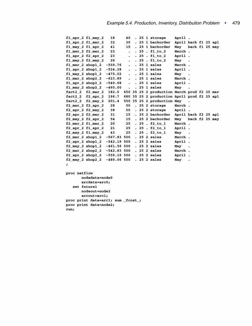
Example 5.4. Production, Inventory, Distribution Problem � 479
f1_apr_2 f1_may_2 18 40 . 25 1 storage April .f1_apr_2 f1_mar_2 32 30 . 25 1 backorder April back f1 25 aplf1_may_2 f1_apr_2 41 15 . 25 1 backorder May back f1 25 mayf1_mar_2 f2_mar_2 23 . . 25 . f1_to_2 March .f1_apr_2 f2_apr_2 23 . . 25 . f1_to_2 April .f1_may_2 f2_may_2 26 . . 25 . f1_to_2 May .f1_mar_2 shop1_2 -559.76 . . 25 1 sales March .f1_apr_2 shop1_2 -524.28 . . 25 1 sales April .f1_may_2 shop1_2 -475.02 . . 25 1 sales May .f1_mar_2 shop2_2 -623.89 . . 25 1 sales March .f1_apr_2 shop2_2 -549.68 . . 25 1 sales April .f1_may_2 shop2_2 -460.00 . . 25 1 sales May .fact2_2 f2_mar_2 182.0 650 35 25 2 production March prod f2 25 marfact2_2 f2_apr_2 196.7 680 35 25 2 production April prod f2 25 aplfact2_2 f2_may_2 201.4 550 35 25 2 production May .f2_mar_2 f2_apr_2 28 50 . 25 2 storage March .f2_apr_2 f2_may_2 38 50 . 25 2 storage April .f2_apr_2 f2_mar_2 31 15 . 25 2 backorder April back f2 25 aplf2_may_2 f2_apr_2 54 15 . 25 2 backorder May back f2 25 mayf2_mar_2 f1_mar_2 20 25 . 25 . f2_to_1 March .f2_apr_2 f1_apr_2 21 25 . 25 . f2_to_1 April .f2_may_2 f1_may_2 43 25 . 25 . f2_to_1 May .f2_mar_2 shop1_2 -567.83 500 . 25 2 sales March .f2_apr_2 shop1_2 -542.19 500 . 25 2 sales April .f2_may_2 shop1_2 -461.56 500 . 25 2 sales May .f2_mar_2 shop2_2 -542.83 500 . 25 2 sales March .f2_apr_2 shop2_2 -559.19 500 . 25 2 sales April .f2_may_2 shop2_2 -489.06 500 . 25 2 sales May .;
proc netflownodedata=node0arcdata=arc0;
set future1nodeout=node2arcout=arc1;
proc print data=arc1; sum _fcost_;proc print data=node2;run;

480 � Chapter 5. The NETFLOW Procedure
The following notes appear on the SAS log:
NOTE: Number of nodes= 20 .NOTE: Number of supply nodes= 4 .NOTE: Number of demand nodes= 4 .NOTE: Total supply= 4350 , total demand= 4150 .NOTE: Number of arcs= 64 .NOTE: Number of iterations performed (neglecting any
constraints)= 74 .NOTE: Of these, 1 were degenerate.NOTE: Optimum (neglecting any constraints) found.NOTE: Minimal total cost= -1281110.35 .NOTE: The data set WORK.ARC1 has 68 observations and
18 variables.NOTE: The data set WORK.NODE2 has 22 observations and
10 variables.
The solution is given in the NODEOUT=node2 and ARCOUT=arc1 data sets. In theARCOUT= data set, shown in Output 5.4.1 and Output 5.4.2, the variables diagonal,factory, key–id, and mth–made form an implicit ID list. The diagonal variablehas one of two values, 19 or 25. factory also has one of two values, 1 or 2, todenote the factory where either production or storage occurs, from where TVs areeither sold to shops or satisfy backorders. PRODUCTION, STORAGE, SALES, andBACKORDER are values of the key–id variable.
Other values of this variable, F1–TO–2 and F2–TO–1, are used when flow througharcs represents the transportation of TVs between factories. The mth–made variablehas values MARCH, APRIL, and MAY, the months when TVs that are modeled asflow through an arc were made (assuming that no televisions are stored for more thanone month and none manufactured in May are used to fill March backorders).
These ID variables can be used after the PROC NETFLOW run to produce reports andperform analysis on particular parts of the company’s operation. For example, reportscan be generated for production numbers for each factory; optimal sales figures foreach shop; and how many TVs should be stored, used to fill backorders, sent to theother factory, or any combination of these, for TVs with a particular screen, thoseproduced in a particular month, or both.

Example 5.4. Production, Inventory, Distribution Problem � 481
Output 5.4.1. ARCOUT=ARC1
Minimum Cost Flow problemProduction Planning/Inventory/Distribution
Obs _tail_ _head_ _cost_ _capac_ _lo_ _name_ _SUPPLY_ _DEMAND_ _FLOW_ _FCOST_
1 fact1_1 _EXCESS_ 0.00 99999999 0 1000 200 5 0.002 fact2_1 _EXCESS_ 0.00 99999999 0 850 200 45 0.003 fact1_2 _EXCESS_ 0.00 99999999 0 1000 200 10 0.004 fact2_2 _EXCESS_ 0.00 99999999 0 1500 200 140 0.005 fact1_1 f1_apr_1 78.60 600 50 prod f1 19 apl 1000 . 600 47160.006 f1_mar_1 f1_apr_1 15.00 50 0 . . 0 0.007 f1_may_1 f1_apr_1 28.00 20 0 back f1 19 may . . 0 0.008 f2_apr_1 f1_apr_1 11.00 40 0 . . 0 0.009 fact1_2 f1_apr_2 174.50 550 50 prod f1 25 apl 1000 . 550 95975.0010 f1_mar_2 f1_apr_2 20.00 40 0 . . 0 0.0011 f1_may_2 f1_apr_2 41.00 15 0 back f1 25 may . . 15 615.0012 f2_apr_2 f1_apr_2 21.00 25 0 . . 0 0.0013 fact1_1 f1_mar_1 127.90 500 50 prod f1 19 mar 1000 . 345 44125.5014 f1_apr_1 f1_mar_1 28.00 20 0 back f1 19 apl . . 20 560.0015 f2_mar_1 f1_mar_1 10.00 40 0 . . 40 400.0016 fact1_2 f1_mar_2 217.90 400 40 prod f1 25 mar 1000 . 400 87160.0017 f1_apr_2 f1_mar_2 32.00 30 0 back f1 25 apl . . 30 960.0018 f2_mar_2 f1_mar_2 20.00 25 0 . . 25 500.0019 fact1_1 f1_may_1 95.10 400 50 1000 . 50 4755.0020 f1_apr_1 f1_may_1 12.00 50 0 . . 50 600.0021 f2_may_1 f1_may_1 13.00 40 0 . . 0 0.0022 fact1_2 f1_may_2 133.30 350 40 1000 . 40 5332.0023 f1_apr_2 f1_may_2 18.00 40 0 . . 0 0.0024 f2_may_2 f1_may_2 43.00 25 0 . . 0 0.0025 f1_apr_1 f2_apr_1 11.00 99999999 0 . . 30 330.0026 fact2_1 f2_apr_1 62.40 480 35 prod f2 19 apl 850 . 480 29952.0027 f2_mar_1 f2_apr_1 18.00 30 0 . . 0 0.0028 f2_may_1 f2_apr_1 25.00 15 0 back f2 19 may . . 0 0.0029 f1_apr_2 f2_apr_2 23.00 99999999 0 . . 0 0.0030 fact2_2 f2_apr_2 196.70 680 35 prod f2 25 apl 1500 . 680 133756.0031 f2_mar_2 f2_apr_2 28.00 50 0 . . 0 0.0032 f2_may_2 f2_apr_2 54.00 15 0 back f2 25 may . . 15 810.0033 f1_mar_1 f2_mar_1 11.00 99999999 0 . . 0 0.0034 fact2_1 f2_mar_1 88.00 450 35 prod f2 19 mar 850 . 290 25520.0035 f2_apr_1 f2_mar_1 17.00 15 0 back f2 19 apl . . 0 0.0036 f1_mar_2 f2_mar_2 23.00 99999999 0 . . 0 0.0037 fact2_2 f2_mar_2 182.00 650 35 prod f2 25 mar 1500 . 645 117390.0038 f2_apr_2 f2_mar_2 31.00 15 0 back f2 25 apl . . 0 0.0039 f1_may_1 f2_may_1 16.00 99999999 0 . . 100 1600.0040 fact2_1 f2_may_1 133.80 250 35 850 . 35 4683.0041 f2_apr_1 f2_may_1 20.00 30 0 . . 15 300.0042 f1_may_2 f2_may_2 26.00 99999999 0 . . 0 0.0043 fact2_2 f2_may_2 201.40 550 35 1500 . 35 7049.0044 f2_apr_2 f2_may_2 38.00 50 0 . . 0 0.0045 f1_mar_1 shop1_1 -327.65 250 0 . 900 155 -50785.7546 f1_apr_1 shop1_1 -300.00 250 0 . 900 250 -75000.0047 f1_may_1 shop1_1 -285.00 250 0 . 900 0 0.0048 f2_mar_1 shop1_1 -297.40 250 0 . 900 250 -74350.0049 f2_apr_1 shop1_1 -290.00 250 0 . 900 245 -71050.0050 f2_may_1 shop1_1 -292.00 250 0 . 900 0 0.0051 f1_mar_2 shop1_2 -559.76 99999999 0 . 900 0 0.0052 f1_apr_2 shop1_2 -524.28 99999999 0 . 900 0 0.0053 f1_may_2 shop1_2 -475.02 99999999 0 . 900 25 -11875.5054 f2_mar_2 shop1_2 -567.83 500 0 . 900 500 -283915.0055 f2_apr_2 shop1_2 -542.19 500 0 . 900 375 -203321.2556 f2_may_2 shop1_2 -461.56 500 0 . 900 0 0.0057 f1_mar_1 shop2_1 -362.74 250 0 . 900 250 -90685.0058 f1_apr_1 shop2_1 -300.00 250 0 . 900 250 -75000.0059 f1_may_1 shop2_1 -245.00 250 0 . 900 0 0.0060 f2_mar_1 shop2_1 -272.70 250 0 . 900 0 0.0061 f2_apr_1 shop2_1 -312.00 250 0 . 900 250 -78000.0062 f2_may_1 shop2_1 -299.00 250 0 . 900 150 -44850.0063 f1_mar_2 shop2_2 -623.89 99999999 0 . 1450 455 -283869.9564 f1_apr_2 shop2_2 -549.68 99999999 0 . 1450 535 -294078.8065 f1_may_2 shop2_2 -460.00 99999999 0 . 1450 0 0.0066 f2_mar_2 shop2_2 -542.83 500 0 . 1450 120 -65139.6067 f2_apr_2 shop2_2 -559.19 500 0 . 1450 320 -178940.8068 f2_may_2 shop2_2 -489.06 500 0 . 1450 20 -9781.20
===========-1281110.35

482 � Chapter 5. The NETFLOW Procedure
Output 5.4.2. ARCOUT=ARC1 (continued)
Obs _RCOST_ _ANUMB_ _TNUMB_ _STATUS_ diagonal factory key_id mth_made
1 . 65 1 KEY_ARC BASIC . .2 . 66 10 KEY_ARC BASIC . .3 . 67 11 KEY_ARC BASIC . .4 . 68 20 KEY_ARC BASIC . .5 -0.650 4 1 UPPERBD NONBASIC 19 1 production April6 63.650 5 2 LOWERBD NONBASIC 19 1 storage March7 43.000 6 4 LOWERBD NONBASIC 19 1 backorder May8 22.000 7 6 LOWERBD NONBASIC 19 . f2_to_1 April9 -14.350 36 11 UPPERBD NONBASIC 25 1 production April10 94.210 37 12 LOWERBD NONBASIC 25 1 storage March11 -16.660 38 14 UPPERBD NONBASIC 25 1 backorder May12 30.510 39 16 LOWERBD NONBASIC 25 . f2_to_1 April13 . 1 1 KEY_ARC BASIC 19 1 production March14 -20.650 2 3 UPPERBD NONBASIC 19 1 backorder April15 -29.900 3 5 UPPERBD NONBASIC 19 . f2_to_1 March16 -45.160 33 11 UPPERBD NONBASIC 25 1 production March17 -42.210 34 13 UPPERBD NONBASIC 25 1 backorder April18 -61.060 35 15 UPPERBD NONBASIC 25 . f2_to_1 March19 0.850 8 1 LOWERBD NONBASIC 19 1 production May20 -3.000 9 3 UPPERBD NONBASIC 19 1 storage April21 29.000 10 7 LOWERBD NONBASIC 19 . f2_to_1 May22 2.110 40 11 LOWERBD NONBASIC 25 1 production May23 75.660 41 13 LOWERBD NONBASIC 25 1 storage April24 40.040 42 17 LOWERBD NONBASIC 25 . f2_to_1 May25 . 14 3 KEY_ARC BASIC 19 . f1_to_2 April26 -27.850 15 10 UPPERBD NONBASIC 19 2 production April27 15.750 16 5 LOWERBD NONBASIC 19 2 storage March28 45.000 17 7 LOWERBD NONBASIC 19 2 backorder May29 13.490 46 13 LOWERBD NONBASIC 25 . f1_to_2 April30 -1.660 47 20 UPPERBD NONBASIC 25 2 production April31 11.640 48 15 LOWERBD NONBASIC 25 2 storage March32 -16.130 49 17 UPPERBD NONBASIC 25 2 backorder May33 50.900 11 2 LOWERBD NONBASIC 19 . f1_to_2 March34 . 12 10 KEY_ARC BASIC 19 2 production March35 19.250 13 6 LOWERBD NONBASIC 19 2 backorder April36 104.060 43 12 LOWERBD NONBASIC 25 . f1_to_2 March37 . 44 20 KEY_ARC BASIC 25 2 production March38 47.360 45 16 LOWERBD NONBASIC 25 2 backorder April39 . 18 4 KEY_ARC BASIC 19 . f1_to_2 May40 23.550 19 10 LOWERBD NONBASIC 19 2 production May41 . 20 6 KEY_ARC BASIC 19 2 storage April42 28.960 50 14 LOWERBD NONBASIC 25 . f1_to_2 May43 73.170 51 20 LOWERBD NONBASIC 25 2 production May44 108.130 52 16 LOWERBD NONBASIC 25 2 storage April45 . 21 2 KEY_ARC BASIC 19 1 sales March46 -21.000 22 3 UPPERBD NONBASIC 19 1 sales April47 9.000 23 4 LOWERBD NONBASIC 19 1 sales May48 -9.650 24 5 UPPERBD NONBASIC 19 2 sales March49 . 25 6 KEY_ARC BASIC 19 2 sales April50 18.000 26 7 LOWERBD NONBASIC 19 2 sales May51 47.130 53 12 LOWERBD NONBASIC 25 1 sales March52 8.400 54 13 LOWERBD NONBASIC 25 1 sales April53 . 55 14 KEY_ARC BASIC 25 1 sales May54 -42.000 56 15 UPPERBD NONBASIC 25 2 sales March55 . 57 16 KEY_ARC BASIC 25 2 sales April56 10.500 58 17 LOWERBD NONBASIC 25 2 sales May57 -46.090 27 2 UPPERBD NONBASIC 19 1 sales March58 -32.000 28 3 UPPERBD NONBASIC 19 1 sales April59 38.000 29 4 LOWERBD NONBASIC 19 1 sales May60 4.050 30 5 LOWERBD NONBASIC 19 2 sales March61 -33.000 31 6 UPPERBD NONBASIC 19 2 sales April62 . 32 7 KEY_ARC BASIC 19 2 sales May63 . 59 12 KEY_ARC BASIC 25 1 sales March64 . 60 13 KEY_ARC BASIC 25 1 sales April65 32.020 61 14 LOWERBD NONBASIC 25 1 sales May66 . 62 15 KEY_ARC BASIC 25 2 sales March67 . 63 16 KEY_ARC BASIC 25 2 sales April68 . 64 17 KEY_ARC BASIC 25 2 sales May

Example 5.5. Using an Unconstrained Solution Warm Start � 483
Output 5.4.3. NODEOUT=NODE2
Minimum Cost Flow problemProduction Planning/Inventory/Distribution
_s _ _ _
_ u _ N _ _ S A _n p D N P T C R F _o d U U R R E C L F
O d e A M E A S I O Bb e m L B D V S D W Qs _ _ _ _ _ _ _ _ _ _
1 _ROOT_ 238 0.00 22 0 8 0 3 166 -692 _EXCESS_ -200 -100000198.75 21 1 11 13 65 5 653 f1_apr_1 . -100000278.00 3 6 7 1 -14 30 44 f1_apr_2 . -100000387.60 13 19 17 1 -60 535 365 f1_mar_1 . -100000326.65 2 8 1 15 -21 155 16 f1_mar_2 . -100000461.81 12 19 13 1 -59 455 337 f1_may_1 . -100000293.00 4 7 2 1 -18 100 88 f1_may_2 . -100000329.94 14 18 12 1 -55 25 409 f2_apr_1 . -100000289.00 6 8 3 5 -25 245 14
10 f2_apr_2 . -100000397.11 16 19 18 3 -63 320 4611 f2_mar_1 . -100000286.75 5 10 22 1 12 255 1112 f2_mar_2 . -100000380.75 15 20 19 8 44 610 4313 f2_may_1 . -100000309.00 7 6 9 3 20 15 1814 f2_may_2 . -100000326.98 17 19 10 1 -64 20 5015 fact1_1 1000 -100000198.75 1 2 21 14 -1 295 -116 fact1_2 1000 -100000198.75 11 21 20 1 -67 10 -3317 fact2_1 850 -100000198.75 10 21 5 2 -66 45 -3318 fact2_2 1500 -100000198.75 20 21 15 9 -68 140 -6519 shop1_1 -900 -99999999.00 8 22 6 21 0 0 2120 shop1_2 -900 -99999854.92 18 16 14 2 57 375 5321 shop2_1 -900 -100000010.00 9 7 4 1 32 150 2722 shop2_2 -1450 -99999837.92 19 15 16 7 62 120 59
Example 5.5. Using an Unconstrained Solution Warm Start
This example examines the effect of changing some of the arc costs. The backorderpenalty costs are increased by twenty percent. The sales profit of 25-inch TVs sent tothe shops in May is increased by thirty units. The backorder penalty costs of 25-inchTVs manufactured in May for April consumption is decreased by thirty units. Theproduction cost of 19- and 25-inch TVs made in May are decreased by five units andtwenty units, respectively. How does the optimal solution of the network after thesearc cost alterations compare with the optimum of the original network? If you wantto use the warm start facilities of PROC NETFLOW to solve this undefined problem,specify the WARM option. Notice that the FUTURE1 option was specified in the lastPROC NETFLOW run.

484 � Chapter 5. The NETFLOW Procedure
The following SAS statements produce the new NODEOUT= and ARCOUT= datasets.
title ’Minimum Cost Flow problem- Unconstrained Warm Start’;title2 ’Production Planning/Inventory/Distribution’;data arc2;
set arc1;oldcost=_cost_;oldfc=_fcost_;oldflow=_flow_;if key_id=’backorder’
then _cost_=_cost_*1.2;else if _tail_=’f2_may_2’ then _cost_=_cost_-30;
if key_id=’production’ & mth_made=’May’ thenif diagonal=19 then _cost_=_cost_-5;
else _cost_=_cost_-20;
proc netflowwarm future1nodedata=node2arcdata=arc2nodeout=node3arcout=arc3;
proc print data=arc3 (drop = _status_ _rcost_);var _tail_ _head_ _capac_ _lo_ _supply_ _demand_ _name_
_cost_ _flow_ _fcost_ oldcost oldflow oldfcdiagonal factory key_id mth_made _anumb_ _tnumb_;/* to get this variable order */
sum oldfc _fcost_;proc print data=node3;
run;
The following notes appear on the SAS log:
NOTE: Number of nodes= 21 .NOTE: Number of supply nodes= 4 .NOTE: Number of demand nodes= 5 .NOTE: The greater of total supply and total
demand= 4350 .NOTE: Number of iterations performed (neglecting any
constraints)= 8 .NOTE: Of these, 0 were degenerate.NOTE: Optimum (neglecting any constraints) found.NOTE: Minimal total cost= -1285086.45 .NOTE: The data set WORK.ARC3 has 68 observations and
21 variables.NOTE: The data set WORK.NODE3 has 22 observations and
10 variables.
The solution is displayed in Output 5.5.1 and Output 5.5.2. The associatedNODEOUT data set is in Output 5.5.3.

Example 5.5. Using an Unconstrained Solution Warm Start � 485
Output 5.5.1. ARCOUT=ARC3
Minimum Cost Flow problem- Unconstrained Warm StartProduction Planning/Inventory/Distribution
Obs _tail_ _head_ _capac_ _lo_ _SUPPLY_ _DEMAND_ _name_ _cost_ _FLOW_ _FCOST_
1 fact1_1 _EXCESS_ 99999999 0 1000 200 0.00 5 0.002 fact2_1 _EXCESS_ 99999999 0 850 200 0.00 45 0.003 fact1_2 _EXCESS_ 99999999 0 1000 200 0.00 0 0.004 fact2_2 _EXCESS_ 99999999 0 1500 200 0.00 150 0.005 fact1_1 f1_apr_1 600 50 1000 . prod f1 19 apl 78.60 540 42444.006 f1_mar_1 f1_apr_1 50 0 . . 15.00 0 0.007 f1_may_1 f1_apr_1 20 0 . . back f1 19 may 33.60 0 0.008 f2_apr_1 f1_apr_1 40 0 . . 11.00 0 0.009 fact1_2 f1_apr_2 550 50 1000 . prod f1 25 apl 174.50 250 43625.0010 f1_mar_2 f1_apr_2 40 0 . . 20.00 0 0.0011 f1_may_2 f1_apr_2 15 0 . . back f1 25 may 49.20 15 738.0012 f2_apr_2 f1_apr_2 25 0 . . 21.00 0 0.0013 fact1_1 f1_mar_1 500 50 1000 . prod f1 19 mar 127.90 340 43486.0014 f1_apr_1 f1_mar_1 20 0 . . back f1 19 apl 33.60 20 672.0015 f2_mar_1 f1_mar_1 40 0 . . 10.00 40 400.0016 fact1_2 f1_mar_2 400 40 1000 . prod f1 25 mar 217.90 400 87160.0017 f1_apr_2 f1_mar_2 30 0 . . back f1 25 apl 38.40 30 1152.0018 f2_mar_2 f1_mar_2 25 0 . . 20.00 25 500.0019 fact1_1 f1_may_1 400 50 1000 . 90.10 115 10361.5020 f1_apr_1 f1_may_1 50 0 . . 12.00 0 0.0021 f2_may_1 f1_may_1 40 0 . . 13.00 0 0.0022 fact1_2 f1_may_2 350 40 1000 . 113.30 350 39655.0023 f1_apr_2 f1_may_2 40 0 . . 18.00 0 0.0024 f2_may_2 f1_may_2 25 0 . . 13.00 0 0.0025 f1_apr_1 f2_apr_1 99999999 0 . . 11.00 20 220.0026 fact2_1 f2_apr_1 480 35 850 . prod f2 19 apl 62.40 480 29952.0027 f2_mar_1 f2_apr_1 30 0 . . 18.00 0 0.0028 f2_may_1 f2_apr_1 15 0 . . back f2 19 may 30.00 0 0.0029 f1_apr_2 f2_apr_2 99999999 0 . . 23.00 0 0.0030 fact2_2 f2_apr_2 680 35 1500 . prod f2 25 apl 196.70 680 133756.0031 f2_mar_2 f2_apr_2 50 0 . . 28.00 0 0.0032 f2_may_2 f2_apr_2 15 0 . . back f2 25 may 64.80 0 0.0033 f1_mar_1 f2_mar_1 99999999 0 . . 11.00 0 0.0034 fact2_1 f2_mar_1 450 35 850 . prod f2 19 mar 88.00 290 25520.0035 f2_apr_1 f2_mar_1 15 0 . . back f2 19 apl 20.40 0 0.0036 f1_mar_2 f2_mar_2 99999999 0 . . 23.00 0 0.0037 fact2_2 f2_mar_2 650 35 1500 . prod f2 25 mar 182.00 635 115570.0038 f2_apr_2 f2_mar_2 15 0 . . back f2 25 apl 37.20 0 0.0039 f1_may_1 f2_may_1 99999999 0 . . 16.00 115 1840.0040 fact2_1 f2_may_1 250 35 850 . 128.80 35 4508.0041 f2_apr_1 f2_may_1 30 0 . . 20.00 0 0.0042 f1_may_2 f2_may_2 99999999 0 . . 26.00 335 8710.0043 fact2_2 f2_may_2 550 35 1500 . 181.40 35 6349.0044 f2_apr_2 f2_may_2 50 0 . . 38.00 0 0.0045 f1_mar_1 shop1_1 250 0 . 900 -327.65 150 -49147.5046 f1_apr_1 shop1_1 250 0 . 900 -300.00 250 -75000.0047 f1_may_1 shop1_1 250 0 . 900 -285.00 0 0.0048 f2_mar_1 shop1_1 250 0 . 900 -297.40 250 -74350.0049 f2_apr_1 shop1_1 250 0 . 900 -290.00 250 -72500.0050 f2_may_1 shop1_1 250 0 . 900 -292.00 0 0.0051 f1_mar_2 shop1_2 99999999 0 . 900 -559.76 0 0.0052 f1_apr_2 shop1_2 99999999 0 . 900 -524.28 0 0.0053 f1_may_2 shop1_2 99999999 0 . 900 -475.02 0 0.0054 f2_mar_2 shop1_2 500 0 . 900 -567.83 500 -283915.0055 f2_apr_2 shop1_2 500 0 . 900 -542.19 400 -216876.0056 f2_may_2 shop1_2 500 0 . 900 -491.56 0 0.0057 f1_mar_1 shop2_1 250 0 . 900 -362.74 250 -90685.0058 f1_apr_1 shop2_1 250 0 . 900 -300.00 250 -75000.0059 f1_may_1 shop2_1 250 0 . 900 -245.00 0 0.0060 f2_mar_1 shop2_1 250 0 . 900 -272.70 0 0.0061 f2_apr_1 shop2_1 250 0 . 900 -312.00 250 -78000.0062 f2_may_1 shop2_1 250 0 . 900 -299.00 150 -44850.0063 f1_mar_2 shop2_2 99999999 0 . 1450 -623.89 455 -283869.9564 f1_apr_2 shop2_2 99999999 0 . 1450 -549.68 235 -129174.8065 f1_may_2 shop2_2 99999999 0 . 1450 -460.00 0 0.0066 f2_mar_2 shop2_2 500 0 . 1450 -542.83 110 -59711.3067 f2_apr_2 shop2_2 500 0 . 1450 -559.19 280 -156573.2068 f2_may_2 shop2_2 500 0 . 1450 -519.06 370 -192052.20
===========-1285086.45

486 � Chapter 5. The NETFLOW Procedure
Output 5.5.2. ARCOUT=ARC3 (continued)
Obs oldcost oldflow oldfc diagonal factory key_id mth_made _ANUMB_ _TNUMB_
1 0.00 5 0.00 . . 65 12 0.00 45 0.00 . . 66 103 0.00 10 0.00 . . 67 114 0.00 140 0.00 . . 68 205 78.60 600 47160.00 19 1 production April 4 16 15.00 0 0.00 19 1 storage March 5 27 28.00 0 0.00 19 1 backorder May 6 48 11.00 0 0.00 19 . f2_to_1 April 7 69 174.50 550 95975.00 25 1 production April 36 11
10 20.00 0 0.00 25 1 storage March 37 1211 41.00 15 615.00 25 1 backorder May 38 1412 21.00 0 0.00 25 . f2_to_1 April 39 1613 127.90 345 44125.50 19 1 production March 1 114 28.00 20 560.00 19 1 backorder April 2 315 10.00 40 400.00 19 . f2_to_1 March 3 516 217.90 400 87160.00 25 1 production March 33 1117 32.00 30 960.00 25 1 backorder April 34 1318 20.00 25 500.00 25 . f2_to_1 March 35 1519 95.10 50 4755.00 19 1 production May 8 120 12.00 50 600.00 19 1 storage April 9 321 13.00 0 0.00 19 . f2_to_1 May 10 722 133.30 40 5332.00 25 1 production May 40 1123 18.00 0 0.00 25 1 storage April 41 1324 43.00 0 0.00 25 . f2_to_1 May 42 1725 11.00 30 330.00 19 . f1_to_2 April 14 326 62.40 480 29952.00 19 2 production April 15 1027 18.00 0 0.00 19 2 storage March 16 528 25.00 0 0.00 19 2 backorder May 17 729 23.00 0 0.00 25 . f1_to_2 April 46 1330 196.70 680 133756.00 25 2 production April 47 2031 28.00 0 0.00 25 2 storage March 48 1532 54.00 15 810.00 25 2 backorder May 49 1733 11.00 0 0.00 19 . f1_to_2 March 11 234 88.00 290 25520.00 19 2 production March 12 1035 17.00 0 0.00 19 2 backorder April 13 636 23.00 0 0.00 25 . f1_to_2 March 43 1237 182.00 645 117390.00 25 2 production March 44 2038 31.00 0 0.00 25 2 backorder April 45 1639 16.00 100 1600.00 19 . f1_to_2 May 18 440 133.80 35 4683.00 19 2 production May 19 1041 20.00 15 300.00 19 2 storage April 20 642 26.00 0 0.00 25 . f1_to_2 May 50 1443 201.40 35 7049.00 25 2 production May 51 2044 38.00 0 0.00 25 2 storage April 52 1645 -327.65 155 -50785.75 19 1 sales March 21 246 -300.00 250 -75000.00 19 1 sales April 22 347 -285.00 0 0.00 19 1 sales May 23 448 -297.40 250 -74350.00 19 2 sales March 24 549 -290.00 245 -71050.00 19 2 sales April 25 650 -292.00 0 0.00 19 2 sales May 26 751 -559.76 0 0.00 25 1 sales March 53 1252 -524.28 0 0.00 25 1 sales April 54 1353 -475.02 25 -11875.50 25 1 sales May 55 1454 -567.83 500 -283915.00 25 2 sales March 56 1555 -542.19 375 -203321.25 25 2 sales April 57 1656 -461.56 0 0.00 25 2 sales May 58 1757 -362.74 250 -90685.00 19 1 sales March 27 258 -300.00 250 -75000.00 19 1 sales April 28 359 -245.00 0 0.00 19 1 sales May 29 460 -272.70 0 0.00 19 2 sales March 30 561 -312.00 250 -78000.00 19 2 sales April 31 662 -299.00 150 -44850.00 19 2 sales May 32 763 -623.89 455 -283869.95 25 1 sales March 59 1264 -549.68 535 -294078.80 25 1 sales April 60 1365 -460.00 0 0.00 25 1 sales May 61 1466 -542.83 120 -65139.60 25 2 sales March 62 1567 -559.19 320 -178940.80 25 2 sales April 63 1668 -489.06 20 -9781.20 25 2 sales May 64 17
===========-1281110.35

Example 5.6. Adding Side Constraints, Using a Warm Start � 487
Output 5.5.3. NODEOUT=NODE3
Minimum Cost Flow problem- Unconstrained Warm StartProduction Planning/Inventory/Distribution
_s _ _ _
_ u _ N _ _ S A _n p D N P T C R F _o d U U R R E C L F
O d e A M E A S I O Bb e m L B D V S D W Qs _ _ _ _ _ _ _ _ _ _
1 _ROOT_ 238 0.00 22 0 8 0 3 166 -692 _EXCESS_ -200 -100000198.75 21 1 20 13 65 5 653 f1_apr_1 . -100000277.35 3 1 6 2 4 490 44 f1_apr_2 . -100000387.60 13 19 11 2 -60 235 365 f1_mar_1 . -100000326.65 2 8 1 20 -21 150 16 f1_mar_2 . -100000461.81 12 19 13 1 -59 455 337 f1_may_1 . -100000288.85 4 1 7 3 8 65 88 f1_may_2 . -100000330.98 14 17 10 1 -50 335 409 f2_apr_1 . -100000288.35 6 3 4 1 14 20 14
10 f2_apr_2 . -100000397.11 16 19 18 2 -63 280 4611 f2_mar_1 . -100000286.75 5 10 22 1 12 255 1112 f2_mar_2 . -100000380.75 15 20 19 9 44 600 4313 f2_may_1 . -100000304.85 7 4 9 2 18 115 1814 f2_may_2 . -100000356.98 17 19 14 2 -64 370 5015 fact1_1 1000 -100000198.75 1 2 3 19 -1 290 -116 fact1_2 1000 -100000213.10 11 13 17 1 -36 200 -3317 fact2_1 850 -100000198.75 10 21 5 2 -66 45 -3318 fact2_2 1500 -100000198.75 20 21 15 10 -68 150 -6519 shop1_1 -900 -99999999.00 8 22 2 21 0 0 2120 shop1_2 -900 -99999854.92 18 16 12 1 57 400 5321 shop2_1 -900 -100000005.85 9 7 21 1 32 150 2722 shop2_2 -1450 -99999837.92 19 15 16 8 62 110 59
Example 5.6. Adding Side Constraints, Using a Warm Start
The manufacturer of Gizmo chips, which are parts needed to make televisions, cansupply only 2600 chips to factory 1 and 3750 chips to factory 2 in time for productionin each of the months of March and April. However, Gizmo chips will not be in shortsupply in May. Three chips are required to make each 19-inch TV while the 25-inch TVs require four chips each. To limit the production of televisions produced atfactory 1 in March so that the TVs have the correct number of chips, a side constraintcalled FACT1 MAR GIZMO is used. The form of this constraint is
3 * prod f1 19 mar + 4 * prod f1 25 mar <= 2600
“prod f1 19 mar” is the name of the arc directed from the node fact1–1 toward nodef1–mar–1 and, in the previous constraint, designates the flow assigned to this arc. TheARCDATA= and ARCOUT= data sets have arc names in a variable called –name– .
The other side constraints (shown below) are called FACT2 MAR GIZMO , FACT1APL GIZMO, and FACT2 APL GIZMO.

488 � Chapter 5. The NETFLOW Procedure
3 * prod f2 19 mar + 4 * prod f2 25 mar <= 37503 * prod f1 19 apl + 4 * prod f1 25 apl <= 26003 * prod f2 19 apl + 4 * prod f2 25 apl <= 3750
To maintain customer goodwill, the total number of backorders is not to exceed 50sets. The side constraint TOTAL BACKORDER that models this restriction is:
back f1 19 apl + back f1 25 apl +back f2 19 apl + back f2 25 apl +back f1 19 may + back f1 25 may +back f2 19 may + back f2 25 may <= 50
The sparse CONDATA= data set format is used. All side constraints are less thanor equal type. Because this is the default type value for the DEFCONTYPE= op-tion, type information is not necessary in the following CONDATA=CON3. Also,DEFCONTYPE= <= does not have to be specified in the PROC NETFLOW state-ment that follows. Notice that the –column– variable value CHIP/BO LIMIT indi-cates that an observation of the CON3 data set contains rhs information. Therefore,specify RHSOBS=‘CHIP/BO LIMIT’.
title ’Adding Side Constraints and Using a Warm Start’;title2 ’Production Planning/Inventory/Distribution’;data con3;
input _column_ &$14. _row_ &$15. _coef_ ;datalines;
prod f1 19 mar FACT1 MAR GIZMO 3prod f1 25 mar FACT1 MAR GIZMO 4CHIP/BO LIMIT FACT1 MAR GIZMO 2600prod f2 19 mar FACT2 MAR GIZMO 3prod f2 25 mar FACT2 MAR GIZMO 4CHIP/BO LIMIT FACT2 MAR GIZMO 3750prod f1 19 apl FACT1 APL GIZMO 3prod f1 25 apl FACT1 APL GIZMO 4CHIP/BO LIMIT FACT1 APL GIZMO 2600prod f2 19 apl FACT2 APL GIZMO 3prod f2 25 apl FACT2 APL GIZMO 4CHIP/BO LIMIT FACT2 APL GIZMO 3750back f1 19 apl TOTAL BACKORDER 1back f1 25 apl TOTAL BACKORDER 1back f2 19 apl TOTAL BACKORDER 1back f2 25 apl TOTAL BACKORDER 1back f1 19 may TOTAL BACKORDER 1back f1 25 may TOTAL BACKORDER 1back f2 19 may TOTAL BACKORDER 1back f2 25 may TOTAL BACKORDER 1CHIP/BO LIMIT TOTAL BACKORDER 50;
The four pairs of data sets that follow can be used as ARCDATA= and NODEDATA=data sets in the following PROC NETFLOW run. The set used depends on whichcost information the arcs are to have and whether a warm start is to be used.

Example 5.6. Adding Side Constraints, Using a Warm Start � 489
ARCDATA=arc0 NODEDATA=node0ARCDATA=arc1 NODEDATA=node2ARCDATA=arc2 NODEDATA=node2ARCDATA=arc3 NODEDATA=node3
arc0, node0, arc1, and node2 were created in Example 5.4. The first two datasets are the original input data sets. arc1 and node2 were the ARCOUT= andNODEOUT= data sets of a PROC NETFLOW run with FUTURE1 specified. Now, ifyou use arc1 and node2 as the ARCDATA= data set and NODEDATA= data set in aPROC NETFLOW run, you can specify WARM, as these data sets contain additionalinformation describing a warm start.
In Example 5.5, arc2 was created by modifying arc1 to reflect different arc costs.arc2 and node2 can also be used as the ARCDATA= and NODEDATA= data sets ina PROC NETFLOW run. Again, specify WARM, as these data sets contain additionalinformation describing a warm start. This start, however, contains the optimal basisusing the original costs.
If you are going to continue optimization using the changed arc costs, it is probablybest to use arc3 and node3 as the ARCDATA= and NODEDATA= data sets. Thesedata sets, created in Example 5.6 by PROC NETFLOW when the FUTURE1 optionwas specified, contain an optimal basis that can be used as a warm start.
PROC NETFLOW is used to find the changed cost network solution that obeys thechip limit and backorder side constraints. The FUTURE2 option is specified in casefurther processing is required. An explicit ID list has also been specified so that thevariables oldcost, oldfc and oldflow do not appear in the subsequent output data sets.
proc netflownodedata=node3 arcdata=arc3 warmcondata=con3 sparsecondata rhsobs=’CHIP/BO LIMIT’future2 dualout=dual4 conout=con4;
id diagonal factory key_id mth_made;proc print data=con4;
sum _fcost_;proc print data=dual4;
run;

490 � Chapter 5. The NETFLOW Procedure
The following messages appear on the SAS log:
NOTE: The following 3 variables in ARCDATA do not belong toany SAS variable list. These will be ignored.oldcostoldfcoldflow
NOTE: Number of nodes= 21 .NOTE: Number of supply nodes= 4 .NOTE: Number of demand nodes= 5 .NOTE: The greater of total supply and total demand= 4350 .NOTE: Number of iterations performed (neglecting any
constraints)= 1 .NOTE: Of these, 0 were degenerate.NOTE: Optimum (neglecting any constraints) found.NOTE: Minimal total cost= -1285086.45 .NOTE: Number of <= side constraints= 5 .NOTE: Number of == side constraints= 0 .NOTE: Number of >= side constraints= 0 .NOTE: Number of arc and nonarc variable side constraint
coefficients= 16 .NOTE: Number of iterations, optimizing with constraints= 10 .NOTE: Of these, 0 were degenerate.NOTE: Optimum reached.NOTE: Minimal total cost= -1282708.625 .NOTE: The data set WORK.CON4 has 68 observations and 18
variables.NOTE: The data set WORK.DUAL4 has 27 observations and 14
variables.

Example 5.6. Adding Side Constraints, Using a Warm Start � 491
Output 5.6.1. CONOUT=CON4
Adding Side Constraints and Using a Warm StartProduction Planning/Inventory/Distribution
Obs _tail_ _head_ _cost_ _capac_ _lo_ _name_ _SUPPLY_ _DEMAND_ _FLOW_ _FCOST_
1 fact1_1 _EXCESS_ 0.00 99999999 0 1000 200 5.000 0.002 fact2_1 _EXCESS_ 0.00 99999999 0 850 200 45.000 0.003 fact1_2 _EXCESS_ 0.00 99999999 0 1000 200 0.000 0.004 fact2_2 _EXCESS_ 0.00 99999999 0 1500 200 150.000 0.005 fact1_1 f1_apr_1 78.60 600 50 prod f1 19 apl 1000 . 533.333 41920.006 f1_mar_1 f1_apr_1 15.00 50 0 . . 0.000 0.007 f1_may_1 f1_apr_1 33.60 20 0 back f1 19 may . . 0.000 0.008 f2_apr_1 f1_apr_1 11.00 40 0 . . 0.000 0.009 fact1_2 f1_apr_2 174.50 550 50 prod f1 25 apl 1000 . 250.000 43625.0010 f1_mar_2 f1_apr_2 20.00 40 0 . . 0.000 0.0011 f1_may_2 f1_apr_2 49.20 15 0 back f1 25 may . . 0.000 0.0012 f2_apr_2 f1_apr_2 21.00 25 0 . . 0.000 0.0013 fact1_1 f1_mar_1 127.90 500 50 prod f1 19 mar 1000 . 333.333 42633.3314 f1_apr_1 f1_mar_1 33.60 20 0 back f1 19 apl . . 20.000 672.0015 f2_mar_1 f1_mar_1 10.00 40 0 . . 40.000 400.0016 fact1_2 f1_mar_2 217.90 400 40 prod f1 25 mar 1000 . 400.000 87160.0017 f1_apr_2 f1_mar_2 38.40 30 0 back f1 25 apl . . 30.000 1152.0018 f2_mar_2 f1_mar_2 20.00 25 0 . . 25.000 500.0019 fact1_1 f1_may_1 90.10 400 50 1000 . 128.333 11562.8320 f1_apr_1 f1_may_1 12.00 50 0 . . 0.000 0.0021 f2_may_1 f1_may_1 13.00 40 0 . . 0.000 0.0022 fact1_2 f1_may_2 113.30 350 40 1000 . 350.000 39655.0023 f1_apr_2 f1_may_2 18.00 40 0 . . 0.000 0.0024 f2_may_2 f1_may_2 13.00 25 0 . . 0.000 0.0025 f1_apr_1 f2_apr_1 11.00 99999999 0 . . 13.333 146.6726 fact2_1 f2_apr_1 62.40 480 35 prod f2 19 apl 850 . 480.000 29952.0027 f2_mar_1 f2_apr_1 18.00 30 0 . . 0.000 0.0028 f2_may_1 f2_apr_1 30.00 15 0 back f2 19 may . . 0.000 0.0029 f1_apr_2 f2_apr_2 23.00 99999999 0 . . 0.000 0.0030 fact2_2 f2_apr_2 196.70 680 35 prod f2 25 apl 1500 . 577.500 113594.2531 f2_mar_2 f2_apr_2 28.00 50 0 . . 0.000 0.0032 f2_may_2 f2_apr_2 64.80 15 0 back f2 25 may . . 0.000 0.0033 f1_mar_1 f2_mar_1 11.00 99999999 0 . . 0.000 0.0034 fact2_1 f2_mar_1 88.00 450 35 prod f2 19 mar 850 . 290.000 25520.0035 f2_apr_1 f2_mar_1 20.40 15 0 back f2 19 apl . . 0.000 0.0036 f1_mar_2 f2_mar_2 23.00 99999999 0 . . 0.000 0.0037 fact2_2 f2_mar_2 182.00 650 35 prod f2 25 mar 1500 . 650.000 118300.0038 f2_apr_2 f2_mar_2 37.20 15 0 back f2 25 apl . . 0.000 0.0039 f1_may_1 f2_may_1 16.00 99999999 0 . . 115.000 1840.0040 fact2_1 f2_may_1 128.80 250 35 850 . 35.000 4508.0041 f2_apr_1 f2_may_1 20.00 30 0 . . 0.000 0.0042 f1_may_2 f2_may_2 26.00 99999999 0 . . 350.000 9100.0043 fact2_2 f2_may_2 181.40 550 35 1500 . 122.500 22221.5044 f2_apr_2 f2_may_2 38.00 50 0 . . 0.000 0.0045 f1_mar_1 shop1_1 -327.65 250 0 . 900 143.333 -46963.1746 f1_apr_1 shop1_1 -300.00 250 0 . 900 250.000 -75000.0047 f1_may_1 shop1_1 -285.00 250 0 . 900 13.333 -3800.0048 f2_mar_1 shop1_1 -297.40 250 0 . 900 250.000 -74350.0049 f2_apr_1 shop1_1 -290.00 250 0 . 900 243.333 -70566.6750 f2_may_1 shop1_1 -292.00 250 0 . 900 0.000 0.0051 f1_mar_2 shop1_2 -559.76 99999999 0 . 900 0.000 0.0052 f1_apr_2 shop1_2 -524.28 99999999 0 . 900 0.000 0.0053 f1_may_2 shop1_2 -475.02 99999999 0 . 900 0.000 0.0054 f2_mar_2 shop1_2 -567.83 500 0 . 900 500.000 -283915.0055 f2_apr_2 shop1_2 -542.19 500 0 . 900 400.000 -216876.0056 f2_may_2 shop1_2 -491.56 500 0 . 900 0.000 0.0057 f1_mar_1 shop2_1 -362.74 250 0 . 900 250.000 -90685.0058 f1_apr_1 shop2_1 -300.00 250 0 . 900 250.000 -75000.0059 f1_may_1 shop2_1 -245.00 250 0 . 900 0.000 0.0060 f2_mar_1 shop2_1 -272.70 250 0 . 900 0.000 0.0061 f2_apr_1 shop2_1 -312.00 250 0 . 900 250.000 -78000.0062 f2_may_1 shop2_1 -299.00 250 0 . 900 150.000 -44850.0063 f1_mar_2 shop2_2 -623.89 99999999 0 . 1450 455.000 -283869.9564 f1_apr_2 shop2_2 -549.68 99999999 0 . 1450 220.000 -120929.6065 f1_may_2 shop2_2 -460.00 99999999 0 . 1450 0.000 0.0066 f2_mar_2 shop2_2 -542.83 500 0 . 1450 125.000 -67853.7567 f2_apr_2 shop2_2 -559.19 500 0 . 1450 177.500 -99256.2368 f2_may_2 shop2_2 -519.06 500 0 . 1450 472.500 -245255.85
===========-1282708.63

492 � Chapter 5. The NETFLOW Procedure
Output 5.6.2. CONOUT=CON4 (continued)
Obs _RCOST_ _ANUMB_ _TNUMB_ _STATUS_ diagonal factory key_id mth_made
1 . 65 1 KEY_ARC BASIC . .2 . 66 10 KEY_ARC BASIC . .3 30.187 67 11 LOWERBD NONBASIC . .4 . 68 20 KEY_ARC BASIC . .5 . 4 1 KEY_ARC BASIC 19 1 production April6 63.650 5 2 LOWERBD NONBASIC 19 1 storage March7 47.020 6 4 LOWERBD NONBASIC 19 1 backorder May8 22.000 7 6 LOWERBD NONBASIC 19 . f2_to_1 April9 . 36 11 KEY_ARC BASIC 25 1 production April10 94.210 37 12 LOWERBD NONBASIC 25 1 storage March11 . 38 14 NONKEY ARC BASIC 25 1 backorder May12 30.510 39 16 LOWERBD NONBASIC 25 . f2_to_1 April13 . 1 1 KEY_ARC BASIC 19 1 production March14 -7.630 2 3 UPPERBD NONBASIC 19 1 backorder April15 -34.750 3 5 UPPERBD NONBASIC 19 . f2_to_1 March16 -31.677 33 11 UPPERBD NONBASIC 25 1 production March17 -28.390 34 13 UPPERBD NONBASIC 25 1 backorder April18 -61.060 35 15 UPPERBD NONBASIC 25 . f2_to_1 March19 . 8 1 KEY_ARC BASIC 19 1 production May20 6.000 9 3 LOWERBD NONBASIC 19 1 storage April21 29.000 10 7 LOWERBD NONBASIC 19 . f2_to_1 May22 -11.913 40 11 UPPERBD NONBASIC 25 1 production May23 74.620 41 13 LOWERBD NONBASIC 25 1 storage April24 39.000 42 17 LOWERBD NONBASIC 25 . f2_to_1 May25 . 14 3 KEY_ARC BASIC 19 . f1_to_2 April26 -14.077 15 10 UPPERBD NONBASIC 19 2 production April27 10.900 16 5 LOWERBD NONBASIC 19 2 storage March28 48.420 17 7 LOWERBD NONBASIC 19 2 backorder May29 13.490 46 13 LOWERBD NONBASIC 25 . f1_to_2 April30 . 47 20 KEY_ARC BASIC 25 2 production April31 11.640 48 15 LOWERBD NONBASIC 25 2 storage March32 32.090 49 17 LOWERBD NONBASIC 25 2 backorder May33 55.750 11 2 LOWERBD NONBASIC 19 . f1_to_2 March34 . 12 10 KEY_ARC BASIC 19 2 production March35 34.920 13 6 LOWERBD NONBASIC 19 2 backorder April36 104.060 43 12 LOWERBD NONBASIC 25 . f1_to_2 March37 -23.170 44 20 UPPERBD NONBASIC 25 2 production March38 60.980 45 16 LOWERBD NONBASIC 25 2 backorder April39 . 18 4 KEY_ARC BASIC 19 . f1_to_2 May40 22.700 19 10 LOWERBD NONBASIC 19 2 production May41 9.000 20 6 LOWERBD NONBASIC 19 2 storage April42 . 50 14 KEY_ARC BASIC 25 . f1_to_2 May43 . 51 20 NONKEY ARC BASIC 25 2 production May44 78.130 52 16 LOWERBD NONBASIC 25 2 storage April45 . 21 2 KEY_ARC BASIC 19 1 sales March46 -21.000 22 3 UPPERBD NONBASIC 19 1 sales April47 . 23 4 NONKEY ARC BASIC 19 1 sales May48 -14.500 24 5 UPPERBD NONBASIC 19 2 sales March49 . 25 6 NONKEY ARC BASIC 19 2 sales April50 9.000 26 7 LOWERBD NONBASIC 19 2 sales May51 47.130 53 12 LOWERBD NONBASIC 25 1 sales March52 8.400 54 13 LOWERBD NONBASIC 25 1 sales April53 1.040 55 14 LOWERBD NONBASIC 25 1 sales May54 -42.000 56 15 UPPERBD NONBASIC 25 2 sales March55 . 57 16 KEY_ARC BASIC 25 2 sales April56 10.500 58 17 LOWERBD NONBASIC 25 2 sales May57 -37.090 27 2 UPPERBD NONBASIC 19 1 sales March58 -23.000 28 3 UPPERBD NONBASIC 19 1 sales April59 38.000 29 4 LOWERBD NONBASIC 19 1 sales May60 8.200 30 5 LOWERBD NONBASIC 19 2 sales March61 -24.000 31 6 UPPERBD NONBASIC 19 2 sales April62 . 32 7 KEY_ARC BASIC 19 2 sales May63 . 59 12 KEY_ARC BASIC 25 1 sales March64 . 60 13 KEY_ARC BASIC 25 1 sales April65 33.060 61 14 LOWERBD NONBASIC 25 1 sales May66 . 62 15 KEY_ARC BASIC 25 2 sales March67 . 63 16 KEY_ARC BASIC 25 2 sales April68 . 64 17 KEY_ARC BASIC 25 2 sales May

Example 5.6. Adding Side Constraints, Using a Warm Start � 493
Output 5.6.3. DUALOUT=DUAL4
Adding Side Constraints and Using a Warm StartProduction Planning/Inventory/Distribution
Obs _node_ _supdem_ _DUAL_ _NNUMB_ _PRED_ _TRAV_ _SCESS_
1 _ROOT_ 238 0.00 22 0 8 52 _EXCESS_ -200 -100000193.90 21 1 20 133 f1_apr_1 . -100000278.00 3 1 6 24 f1_apr_2 . -100000405.92 13 19 11 25 f1_mar_1 . -100000326.65 2 8 1 206 f1_mar_2 . -100000480.13 12 19 13 17 f1_may_1 . -100000284.00 4 1 7 38 f1_may_2 . -100000349.30 14 17 15 19 f2_apr_1 . -100000289.00 6 3 4 110 f2_apr_2 . -100000415.43 16 20 18 911 f2_mar_1 . -100000281.90 5 10 3 112 f2_mar_2 . -100000399.07 15 19 10 113 f2_may_1 . -100000300.00 7 4 9 214 f2_may_2 . -100000375.30 17 19 14 215 fact1_1 1000 -100000193.90 1 2 21 1916 fact1_2 1000 -100000224.09 11 13 17 117 fact2_1 850 -100000193.90 10 21 5 218 fact2_2 1500 -100000193.90 20 21 16 1019 shop1_1 -900 -99999999.00 8 22 2 2120 shop1_2 -900 -99999873.24 18 16 19 121 shop2_1 -900 -100000001.00 9 7 22 122 shop2_2 -1450 -99999856.24 19 16 12 723 . -1.83 2 8 . .24 . -1.62 0 8 . .25 . -6.21 3 17 . .26 . 0.00 1 1 . 127 . -7.42 4 13 . .
Obs _ARCID_ _FLOW_ _FBQ_ _VALUE_ _RHS_ _TYPE_ _row_
1 3 166.000 -69 0 752 65 5.000 65 . .3 4 483.333 4 . .4 -60 220.000 36 . .5 -21 143.333 1 . .6 -59 455.000 33 . .7 8 78.333 8 . .8 -50 350.000 40 . .9 14 13.333 14 . .10 47 542.500 46 . .11 12 255.000 11 . .12 -62 125.000 43 . .13 18 115.000 18 . .14 -64 472.500 50 . .15 -1 283.333 -1 . .16 -36 200.000 -33 . .17 -66 45.000 -33 . .18 -68 150.000 -65 . .19 0 0.000 21 . .20 57 400.000 53 . .21 32 150.000 27 . .22 63 177.500 59 . .23 25 243.333 . 2600 2600 LE FACT1 APL GIZMO24 23 13.333 . 2600 2600 LE FACT1 MAR GIZMO25 51 87.500 . 3750 3750 LE FACT2 APL GIZMO26 . 280.000 . 3470 3750 LE FACT2 MAR GIZMO27 38 0.000 . 50 50 LE TOTAL BACKORDER

494 � Chapter 5. The NETFLOW Procedure
Example 5.7. Using a Constrained Solution Warm Start
Suppose the 25-inch screen TVs produced at factory 1 in May can be sold at eithershop with an increased profit of 40 dollars each. What is the new optimal solu-tion? Because only arc costs have been changed, information about the present so-lution in DUALOUT=dual4 and CONOUT=con4 can be used as a warm start in thefollowing PROC NETFLOW run. It is still necessary to specify CONDATA=con3SPARSECONDATA RHSOBS=‘CHIP/BO LIMIT’, since the CONDATA= data setis always read.
title ’Using a Constrained Solution Warm Start’;title2 ’Production Planning/Inventory/Distribution’;data new_con4;
set con4;oldcost=_cost_;oldflow=_flow_;oldfc=_fcost_;if _tail_=’f1_may_2’
& (_head_=’shop1_2’ | _head_=’shop2_2’)then _cost_=_cost_-40;
run;
proc netflowwarmarcdata=new_con4dualin=dual4condata=con3sparsecondatarhsobs=’CHIP/BO LIMIT’dualout=dual5conout=con5;run;
proc print data=con5 (drop = _status_ _rcost_);var _tail_ _head_ _capac_ _lo_ _supply_ _demand_ _name_
_cost_ _flow_ _fcost_ oldcost oldflow oldfcdiagonal factory key_id mth_made _anumb_ _tnumb_;
/* to get this variable order */sum oldfc _fcost_;
run;
proc print data=dual5;run;

Example 5.7. Using a Constrained Solution Warm Start � 495
The following messages appear on the SAS log:
NOTE: The following 1 variables in NODEDATA do not belong toany SAS variable list. These will be ignored._VALUE_
NOTE: Number of nodes= 21 .NOTE: Number of supply nodes= 4 .NOTE: Number of demand nodes= 5 .NOTE: The greater of total supply and total demand= 4350 .NOTE: Number of <= side constraints= 5 .NOTE: Number of == side constraints= 0 .NOTE: Number of >= side constraints= 0 .NOTE: Number of arc and nonarc variable side constraint
coefficients= 16 .NOTE: Number of iterations, optimizing with constraints= 7 .NOTE: Of these, 1 were degenerate.NOTE: Optimum reached.NOTE: Minimal total cost= -1295661.8 .NOTE: The data set WORK.CON5 has 64 observations and 21
variables.NOTE: The data set WORK.DUAL5 has 25 observations and 14
variables.

496 � Chapter 5. The NETFLOW Procedure
Output 5.7.1. CONOUT=CON5
Using a Constrained Solution Warm StartProduction Planning/Inventory/Distribution
Obs _tail_ _head_ _capac_ _lo_ _SUPPLY_ _DEMAND_ _name_ _cost_ _FLOW_ _FCOST_
1 fact1_1 f1_apr_1 600 50 1000 . prod f1 19 apl 78.60 533.333 41920.002 f1_mar_1 f1_apr_1 50 0 . . 15.00 0.000 0.003 f1_may_1 f1_apr_1 20 0 . . back f1 19 may 33.60 0.000 0.004 f2_apr_1 f1_apr_1 40 0 . . 11.00 0.000 0.005 fact1_2 f1_apr_2 550 50 1000 . prod f1 25 apl 174.50 250.000 43625.006 f1_mar_2 f1_apr_2 40 0 . . 20.00 0.000 0.007 f1_may_2 f1_apr_2 15 0 . . back f1 25 may 49.20 0.000 0.008 f2_apr_2 f1_apr_2 25 0 . . 21.00 0.000 0.009 fact1_1 f1_mar_1 500 50 1000 . prod f1 19 mar 127.90 333.333 42633.3310 f1_apr_1 f1_mar_1 20 0 . . back f1 19 apl 33.60 20.000 672.0011 f2_mar_1 f1_mar_1 40 0 . . 10.00 40.000 400.0012 fact1_2 f1_mar_2 400 40 1000 . prod f1 25 mar 217.90 400.000 87160.0013 f1_apr_2 f1_mar_2 30 0 . . back f1 25 apl 38.40 30.000 1152.0014 f2_mar_2 f1_mar_2 25 0 . . 20.00 25.000 500.0015 fact1_1 f1_may_1 400 50 1000 . 90.10 128.333 11562.8316 f1_apr_1 f1_may_1 50 0 . . 12.00 0.000 0.0017 f2_may_1 f1_may_1 40 0 . . 13.00 0.000 0.0018 fact1_2 f1_may_2 350 40 1000 . 113.30 350.000 39655.0019 f1_apr_2 f1_may_2 40 0 . . 18.00 0.000 0.0020 f2_may_2 f1_may_2 25 0 . . 13.00 0.000 0.0021 f1_apr_1 f2_apr_1 99999999 0 . . 11.00 13.333 146.6722 fact2_1 f2_apr_1 480 35 850 . prod f2 19 apl 62.40 480.000 29952.0023 f2_mar_1 f2_apr_1 30 0 . . 18.00 0.000 0.0024 f2_may_1 f2_apr_1 15 0 . . back f2 19 may 30.00 0.000 0.0025 f1_apr_2 f2_apr_2 99999999 0 . . 23.00 0.000 0.0026 fact2_2 f2_apr_2 680 35 1500 . prod f2 25 apl 196.70 550.000 108185.0027 f2_mar_2 f2_apr_2 50 0 . . 28.00 0.000 0.0028 f2_may_2 f2_apr_2 15 0 . . back f2 25 may 64.80 0.000 0.0029 f1_mar_1 f2_mar_1 99999999 0 . . 11.00 0.000 0.0030 fact2_1 f2_mar_1 450 35 850 . prod f2 19 mar 88.00 290.000 25520.0031 f2_apr_1 f2_mar_1 15 0 . . back f2 19 apl 20.40 0.000 0.0032 f1_mar_2 f2_mar_2 99999999 0 . . 23.00 0.000 0.0033 fact2_2 f2_mar_2 650 35 1500 . prod f2 25 mar 182.00 650.000 118300.0034 f2_apr_2 f2_mar_2 15 0 . . back f2 25 apl 37.20 0.000 0.0035 f1_may_1 f2_may_1 99999999 0 . . 16.00 115.000 1840.0036 fact2_1 f2_may_1 250 35 850 . 128.80 35.000 4508.0037 f2_apr_1 f2_may_1 30 0 . . 20.00 0.000 0.0038 f1_may_2 f2_may_2 99999999 0 . . 26.00 0.000 0.0039 fact2_2 f2_may_2 550 35 1500 . 181.40 150.000 27210.0040 f2_apr_2 f2_may_2 50 0 . . 38.00 0.000 0.0041 f1_mar_1 shop1_1 250 0 . 900 -327.65 143.333 -46963.1742 f1_apr_1 shop1_1 250 0 . 900 -300.00 250.000 -75000.0043 f1_may_1 shop1_1 250 0 . 900 -285.00 13.333 -3800.0044 f2_mar_1 shop1_1 250 0 . 900 -297.40 250.000 -74350.0045 f2_apr_1 shop1_1 250 0 . 900 -290.00 243.333 -70566.6746 f2_may_1 shop1_1 250 0 . 900 -292.00 0.000 0.0047 f1_mar_2 shop1_2 99999999 0 . 900 -559.76 0.000 0.0048 f1_apr_2 shop1_2 99999999 0 . 900 -524.28 0.000 0.0049 f1_may_2 shop1_2 99999999 0 . 900 -515.02 350.000 -180257.0050 f2_mar_2 shop1_2 500 0 . 900 -567.83 500.000 -283915.0051 f2_apr_2 shop1_2 500 0 . 900 -542.19 50.000 -27109.5052 f2_may_2 shop1_2 500 0 . 900 -491.56 0.000 0.0053 f1_mar_1 shop2_1 250 0 . 900 -362.74 250.000 -90685.0054 f1_apr_1 shop2_1 250 0 . 900 -300.00 250.000 -75000.0055 f1_may_1 shop2_1 250 0 . 900 -245.00 0.000 0.0056 f2_mar_1 shop2_1 250 0 . 900 -272.70 0.000 0.0057 f2_apr_1 shop2_1 250 0 . 900 -312.00 250.000 -78000.0058 f2_may_1 shop2_1 250 0 . 900 -299.00 150.000 -44850.0059 f1_mar_2 shop2_2 99999999 0 . 1450 -623.89 455.000 -283869.9560 f1_apr_2 shop2_2 99999999 0 . 1450 -549.68 220.000 -120929.6061 f1_may_2 shop2_2 99999999 0 . 1450 -500.00 0.000 0.0062 f2_mar_2 shop2_2 500 0 . 1450 -542.83 125.000 -67853.7563 f2_apr_2 shop2_2 500 0 . 1450 -559.19 500.000 -279595.0064 f2_may_2 shop2_2 500 0 . 1450 -519.06 150.000 -77859.00
===========-1295661.80

Example 5.7. Using a Constrained Solution Warm Start � 497
Output 5.7.2. CONOUT=CON5 (continued)
Obs oldcost oldflow oldfc diagonal factory key_id mth_made _ANUMB_ _TNUMB_
1 78.60 533.333 41920.00 19 1 production April 4 12 15.00 0.000 0.00 19 1 storage March 5 23 33.60 0.000 0.00 19 1 backorder May 6 44 11.00 0.000 0.00 19 . f2_to_1 April 7 65 174.50 250.000 43625.00 25 1 production April 36 116 20.00 0.000 0.00 25 1 storage March 37 127 49.20 0.000 0.00 25 1 backorder May 38 148 21.00 0.000 0.00 25 . f2_to_1 April 39 169 127.90 333.333 42633.33 19 1 production March 1 1
10 33.60 20.000 672.00 19 1 backorder April 2 311 10.00 40.000 400.00 19 . f2_to_1 March 3 512 217.90 400.000 87160.00 25 1 production March 33 1113 38.40 30.000 1152.00 25 1 backorder April 34 1314 20.00 25.000 500.00 25 . f2_to_1 March 35 1515 90.10 128.333 11562.83 19 1 production May 8 116 12.00 0.000 0.00 19 1 storage April 9 317 13.00 0.000 0.00 19 . f2_to_1 May 10 718 113.30 350.000 39655.00 25 1 production May 40 1119 18.00 0.000 0.00 25 1 storage April 41 1320 13.00 0.000 0.00 25 . f2_to_1 May 42 1721 11.00 13.333 146.67 19 . f1_to_2 April 14 322 62.40 480.000 29952.00 19 2 production April 15 1023 18.00 0.000 0.00 19 2 storage March 16 524 30.00 0.000 0.00 19 2 backorder May 17 725 23.00 0.000 0.00 25 . f1_to_2 April 46 1326 196.70 577.500 113594.25 25 2 production April 47 2027 28.00 0.000 0.00 25 2 storage March 48 1528 64.80 0.000 0.00 25 2 backorder May 49 1729 11.00 0.000 0.00 19 . f1_to_2 March 11 230 88.00 290.000 25520.00 19 2 production March 12 1031 20.40 0.000 0.00 19 2 backorder April 13 632 23.00 0.000 0.00 25 . f1_to_2 March 43 1233 182.00 650.000 118300.00 25 2 production March 44 2034 37.20 0.000 0.00 25 2 backorder April 45 1635 16.00 115.000 1840.00 19 . f1_to_2 May 18 436 128.80 35.000 4508.00 19 2 production May 19 1037 20.00 0.000 0.00 19 2 storage April 20 638 26.00 350.000 9100.00 25 . f1_to_2 May 50 1439 181.40 122.500 22221.50 25 2 production May 51 2040 38.00 0.000 0.00 25 2 storage April 52 1641 -327.65 143.333 -46963.17 19 1 sales March 21 242 -300.00 250.000 -75000.00 19 1 sales April 22 343 -285.00 13.333 -3800.00 19 1 sales May 23 444 -297.40 250.000 -74350.00 19 2 sales March 24 545 -290.00 243.333 -70566.67 19 2 sales April 25 646 -292.00 0.000 0.00 19 2 sales May 26 747 -559.76 0.000 0.00 25 1 sales March 53 1248 -524.28 0.000 0.00 25 1 sales April 54 1349 -475.02 0.000 0.00 25 1 sales May 55 1450 -567.83 500.000 -283915.00 25 2 sales March 56 1551 -542.19 400.000 -216876.00 25 2 sales April 57 1652 -491.56 0.000 0.00 25 2 sales May 58 1753 -362.74 250.000 -90685.00 19 1 sales March 27 254 -300.00 250.000 -75000.00 19 1 sales April 28 355 -245.00 0.000 0.00 19 1 sales May 29 456 -272.70 0.000 0.00 19 2 sales March 30 557 -312.00 250.000 -78000.00 19 2 sales April 31 658 -299.00 150.000 -44850.00 19 2 sales May 32 759 -623.89 455.000 -283869.95 25 1 sales March 59 1260 -549.68 220.000 -120929.60 25 1 sales April 60 1361 -460.00 0.000 0.00 25 1 sales May 61 1462 -542.83 125.000 -67853.75 25 2 sales March 62 1563 -559.19 177.500 -99256.23 25 2 sales April 63 1664 -519.06 472.500 -245255.85 25 2 sales May 64 17
===========-1282708.63

498 � Chapter 5. The NETFLOW Procedure
Output 5.7.3. DUALOUT=DUAL5
Using a Constrained Solution Warm StartProduction Planning/Inventory/Distribution
Obs _node_ _supdem_ _DUAL_ _NNUMB_ _PRED_ _TRAV_ _SCESS_
1 f1_apr_1 . -100000278.00 3 1 6 22 f1_apr_2 . -100000405.92 13 19 11 23 f1_mar_1 . -100000326.65 2 8 1 204 f1_mar_2 . -100000480.13 12 19 13 15 f1_may_1 . -100000284.00 4 1 7 36 f1_may_2 . -100000363.43 14 18 10 17 f2_apr_1 . -100000289.00 6 3 4 18 f2_apr_2 . -100000390.60 16 20 18 39 f2_mar_1 . -100000281.90 5 10 3 1
10 f2_mar_2 . -100000399.07 15 19 16 111 f2_may_1 . -100000300.00 7 4 9 212 f2_may_2 . -100000375.30 17 20 19 613 fact1_1 1000 -100000193.90 1 2 21 1914 fact1_2 1000 -100000224.09 11 13 15 115 fact2_1 850 -100000193.90 10 21 5 216 fact2_2 1500 -100000193.90 20 21 17 1017 shop1_1 -900 -99999999.00 8 22 2 2118 shop1_2 -900 -99999848.41 18 16 14 219 shop2_1 -900 -100000001.00 9 7 22 120 shop2_2 -1450 -99999856.24 19 17 12 521 . -1.83 2 8 . .22 . -1.62 0 8 . .23 . 0.00 3 3 . 324 . 0.00 1 1 . 125 . 0.00 4 4 . 4
Obs _ARCID_ _FLOW_ _FBQ_ _VALUE_ _RHS_ _TYPE_ _row_
1 4 483.333 4 . .2 -60 220.000 36 . .3 -21 143.333 1 . .4 -59 455.000 33 . .5 8 78.333 8 . .6 -55 350.000 40 . .7 14 13.333 14 . .8 47 515.000 46 . .9 12 255.000 11 . .
10 -62 125.000 43 . .11 18 115.000 18 . .12 51 115.000 50 . .13 -1 283.333 -1 . .14 -36 200.000 -33 . .15 -66 45.000 -33 . .16 -68 150.000 -65 . .17 0 0.000 21 . .18 57 50.000 53 . .19 32 150.000 27 . .20 64 150.000 59 . .21 25 243.333 . 2600 2600 LE FACT1 APL GIZMO22 23 13.333 . 2600 2600 LE FACT1 MAR GIZMO23 . 110.000 . 3640 3750 LE FACT2 APL GIZMO24 . 280.000 . 3470 3750 LE FACT2 MAR GIZMO25 . 0.000 . 50 50 LE TOTAL BACKORDER
Example 5.8. Nonarc Variables in the Side Constraints
Notice in DUALOUT=dual5 from Example 5.7 the FACT2 MAR GIZMO constraint(observation 24) has a –VALUE– of 3470, which is not equal to the –RHS– of thisconstraint. Not all of the 3750 chips that can be supplied to factory 2 for Marchproduction are used. It is suggested that all the possible chips be obtained in Marchand those not used be saved for April production. Because chips must be kept in anair-controlled environment, it costs 1 dollar to store each chip purchased in Marchuntil April. The maximum number of chips that can be stored in this environment at

Example 5.8. Nonarc Variables in the Side Constraints � 499
each factory is 150. In addition, a search of the parts inventory at factory 1 turned up15 chips available for their March production.
Nonarc variables are used in the side constraints that handle the limitations of supplyof Gizmo chips. A nonarc variable called “f1 unused chips” has as a value the numberof chips that are not used at factory 1 in March. Another nonarc variable, “f2 unusedchips”, has as a value the number of chips that are not used at factory 2 in March.“f1 chips from mar” has as a value the number of chips left over from March usedfor production at factory 1 in April. Similarly, “f2 chips from mar” has as a valuethe number of chips left over from March used for April production at factory 2 inApril. The last two nonarc variables have objective function coefficients of 1 andupper bounds of 150. The Gizmo side constraints are
3*prod f1 19 mar + 4*prod f1 25 mar + f1 unused chips = 26153*prod f2 19 apl + 4*prod f2 25 apl + f2 unused chips = 37503*prod f1 19 apl + 4*prod f1 25 apl - f1 chips from mar = 26003*prod f2 19 apl + 4*prod f2 25 apl - f2 chips from mar = 3750f1 unused chips + f2 unused chips -f1 chips from mar - f2 chips from mar >= 0
The last side constraint states that the number of chips not used in March is not lessthan the number of chips left over from March and used in April. Here, this constraintis called CHIP LEFTOVER.
The following SAS code creates a new data set containing constraint data. It seemsthat most of the constraints are now equalities, so you specify DEFCONTYPE=EQ inthe PROC NETFLOW statements from now on and provide constraint type data forconstraints that are not “equal to” type, using the default TYPEOBS value –TYPE–as the –COLUMN– variable value to indicate observations that contain constrainttype data. Also, from now on, the default RHSOBS value is used.
title ’Nonarc Variables in the Side Constraints’;title2 ’Production Planning/Inventory/Distribution’;data con6;
input _column_ &$17. _row_ &$15. _coef_ ;datalines;
prod f1 19 mar FACT1 MAR GIZMO 3prod f1 25 mar FACT1 MAR GIZMO 4f1 unused chips FACT1 MAR GIZMO 1_RHS_ FACT1 MAR GIZMO 2615prod f2 19 mar FACT2 MAR GIZMO 3prod f2 25 mar FACT2 MAR GIZMO 4f2 unused chips FACT2 MAR GIZMO 1_RHS_ FACT2 MAR GIZMO 3750prod f1 19 apl FACT1 APL GIZMO 3prod f1 25 apl FACT1 APL GIZMO 4f1 chips from mar FACT1 APL GIZMO -1_RHS_ FACT1 APL GIZMO 2600prod f2 19 apl FACT2 APL GIZMO 3prod f2 25 apl FACT2 APL GIZMO 4f2 chips from mar FACT2 APL GIZMO -1

500 � Chapter 5. The NETFLOW Procedure
_RHS_ FACT2 APL GIZMO 3750f1 unused chips CHIP LEFTOVER 1f2 unused chips CHIP LEFTOVER 1f1 chips from mar CHIP LEFTOVER -1f2 chips from mar CHIP LEFTOVER -1_TYPE_ CHIP LEFTOVER 1back f1 19 apl TOTAL BACKORDER 1back f1 25 apl TOTAL BACKORDER 1back f2 19 apl TOTAL BACKORDER 1back f2 25 apl TOTAL BACKORDER 1back f1 19 may TOTAL BACKORDER 1back f1 25 may TOTAL BACKORDER 1back f2 19 may TOTAL BACKORDER 1back f2 25 may TOTAL BACKORDER 1_TYPE_ TOTAL BACKORDER -1_RHS_ TOTAL BACKORDER 50;
The nonarc variables “f1 chips from mar” and “f2 chips from mar” have objectivefunction coefficients of 1 and upper bounds of 150. There are various ways in whichthis information can be furnished to PROC NETFLOW. If there were a TYPE listvariable in the CONDATA= data set, observations could be in the form
_COLUMN_ _TYPE_ _ROW_ _COEF_f1 chips from mar objfn . 1f1 chips from mar upperbd . 150f2 chips from mar objfn . 1f2 chips from mar upperbd . 150
It is desirable to assign ID list variable values to all the nonarc variables:
data arc6;set con5;drop oldcost oldfc oldflow _flow_ _fcost_ _status_ _rcost_;
data arc6_b;input _name_ &$17. _cost_ _capac_ factory key_id $ ;datalines;
f1 unused chips . . 1 chipsf2 unused chips . . 2 chipsf1 chips from mar 1 150 1 chipsf2 chips from mar 1 150 2 chips;
proc appendbase=arc6 data=arc6_b;
proc netflownodedata=node0 arcdata=arc6condata=con6 defcontype=eq sparsecondatadualout=dual7 conout=con7;run;
print nonarcs/short;

Example 5.8. Nonarc Variables in the Side Constraints � 501
The following messages appear on the SAS log:
NOTE: Number of nodes= 20 .NOTE: Number of supply nodes= 4 .NOTE: Number of demand nodes= 4 .NOTE: Total supply= 4350 , total demand= 4150 .NOTE: Number of arcs= 64 .NOTE: Number of nonarc variables= 4 .NOTE: Number of iterations performed (neglecting any
constraints)= 70 .NOTE: Of these, 1 were degenerate.NOTE: Optimum (neglecting any constraints) found.NOTE: Minimal total cost= -1295730.8 .NOTE: Number of <= side constraints= 1 .NOTE: Number of == side constraints= 4 .NOTE: Number of >= side constraints= 1 .NOTE: Number of arc and nonarc variable side constraint
coefficients= 24 .NOTE: Number of iterations, optimizing with constraints= 13 .NOTE: Of these, 3 were degenerate.NOTE: Optimum reached.NOTE: Minimal total cost= -1295542.742 .NOTE: The data set WORK.CON7 has 68 observations and 18
variables.NOTE: The data set WORK.DUAL7 has 26 observations and 14
variables.
The output in Output 5.8.1 is produced by
print nonarcs/short;
Output 5.8.1. Output of PRINT NONARCS/SHORT;
Nonarc Variables in the Side ConstraintsProduction Planning/Inventory/Distribution
The NETFLOW Procedure
_N_ _name_ _cost_ _capac_ _lo_ _VALUE_
1 f1 chips from mar 1 150 0 202 f1 unused chips 0 99999999 0 03 f2 chips from mar 1 150 0 04 f2 unused chips 0 99999999 0 280
The optimal solution data sets, CONOUT=CON7 in Output 5.8.2 and Output 5.8.3and DUALOUT=DUAL7 in Output 5.8.4 follow.
proc print data=con7;sum _fcost_;
proc print data=dual7;

502 � Chapter 5. The NETFLOW Procedure
Output 5.8.2. CONOUT=CON7
Nonarc Variables in the Side ConstraintsProduction Planning/Inventory/Distribution
Obs _tail_ _head_ _cost_ _capac_ _lo_ _name_ _SUPPLY_ _DEMAND_ _FLOW_ _FCOST_
1 fact1_1 f1_apr_1 78.60 600 50 prod f1 19 apl 1000 . 540.000 42444.002 f1_mar_1 f1_apr_1 15.00 50 0 . . 0.000 0.003 f1_may_1 f1_apr_1 33.60 20 0 back f1 19 may . . 0.000 0.004 f2_apr_1 f1_apr_1 11.00 40 0 . . 0.000 0.005 fact1_2 f1_apr_2 174.50 550 50 prod f1 25 apl 1000 . 250.000 43625.006 f1_mar_2 f1_apr_2 20.00 40 0 . . 0.000 0.007 f1_may_2 f1_apr_2 49.20 15 0 back f1 25 may . . 0.000 0.008 f2_apr_2 f1_apr_2 21.00 25 0 . . 25.000 525.009 fact1_1 f1_mar_1 127.90 500 50 prod f1 19 mar 1000 . 338.333 43272.83
10 f1_apr_1 f1_mar_1 33.60 20 0 back f1 19 apl . . 20.000 672.0011 f2_mar_1 f1_mar_1 10.00 40 0 . . 40.000 400.0012 fact1_2 f1_mar_2 217.90 400 40 prod f1 25 mar 1000 . 400.000 87160.0013 f1_apr_2 f1_mar_2 38.40 30 0 back f1 25 apl . . 30.000 1152.0014 f2_mar_2 f1_mar_2 20.00 25 0 . . 25.000 500.0015 fact1_1 f1_may_1 90.10 400 50 1000 . 116.667 10511.6716 f1_apr_1 f1_may_1 12.00 50 0 . . 0.000 0.0017 f2_may_1 f1_may_1 13.00 40 0 . . 0.000 0.0018 fact1_2 f1_may_2 113.30 350 40 1000 . 350.000 39655.0019 f1_apr_2 f1_may_2 18.00 40 0 . . 0.000 0.0020 f2_may_2 f1_may_2 13.00 25 0 . . 0.000 0.0021 f1_apr_1 f2_apr_1 11.00 99999999 0 . . 20.000 220.0022 fact2_1 f2_apr_1 62.40 480 35 prod f2 19 apl 850 . 480.000 29952.0023 f2_mar_1 f2_apr_1 18.00 30 0 . . 0.000 0.0024 f2_may_1 f2_apr_1 30.00 15 0 back f2 19 may . . 0.000 0.0025 f1_apr_2 f2_apr_2 23.00 99999999 0 . . 0.000 0.0026 fact2_2 f2_apr_2 196.70 680 35 prod f2 25 apl 1500 . 577.500 113594.2527 f2_mar_2 f2_apr_2 28.00 50 0 . . 0.000 0.0028 f2_may_2 f2_apr_2 64.80 15 0 back f2 25 may . . 0.000 0.0029 f1_mar_1 f2_mar_1 11.00 99999999 0 . . 0.000 0.0030 fact2_1 f2_mar_1 88.00 450 35 prod f2 19 mar 850 . 290.000 25520.0031 f2_apr_1 f2_mar_1 20.40 15 0 back f2 19 apl . . 0.000 0.0032 f1_mar_2 f2_mar_2 23.00 99999999 0 . . 0.000 0.0033 fact2_2 f2_mar_2 182.00 650 35 prod f2 25 mar 1500 . 650.000 118300.0034 f2_apr_2 f2_mar_2 37.20 15 0 back f2 25 apl . . 0.000 0.0035 f1_may_1 f2_may_1 16.00 99999999 0 . . 115.000 1840.0036 fact2_1 f2_may_1 128.80 250 35 850 . 35.000 4508.0037 f2_apr_1 f2_may_1 20.00 30 0 . . 0.000 0.0038 f1_may_2 f2_may_2 26.00 99999999 0 . . 0.000 0.0039 fact2_2 f2_may_2 181.40 550 35 1500 . 122.500 22221.5040 f2_apr_2 f2_may_2 38.00 50 0 . . 0.000 0.0041 f1_mar_1 shop1_1 -327.65 250 0 . 900 148.333 -48601.4242 f1_apr_1 shop1_1 -300.00 250 0 . 900 250.000 -75000.0043 f1_may_1 shop1_1 -285.00 250 0 . 900 1.667 -475.0044 f2_mar_1 shop1_1 -297.40 250 0 . 900 250.000 -74350.0045 f2_apr_1 shop1_1 -290.00 250 0 . 900 250.000 -72500.0046 f2_may_1 shop1_1 -292.00 250 0 . 900 0.000 0.0047 f1_mar_2 shop1_2 -559.76 99999999 0 . 900 0.000 0.0048 f1_apr_2 shop1_2 -524.28 99999999 0 . 900 0.000 0.0049 f1_may_2 shop1_2 -515.02 99999999 0 . 900 347.500 -178969.4550 f2_mar_2 shop1_2 -567.83 500 0 . 900 500.000 -283915.0051 f2_apr_2 shop1_2 -542.19 500 0 . 900 52.500 -28464.9852 f2_may_2 shop1_2 -491.56 500 0 . 900 0.000 0.0053 f1_mar_1 shop2_1 -362.74 250 0 . 900 250.000 -90685.0054 f1_apr_1 shop2_1 -300.00 250 0 . 900 250.000 -75000.0055 f1_may_1 shop2_1 -245.00 250 0 . 900 0.000 0.0056 f2_mar_1 shop2_1 -272.70 250 0 . 900 0.000 0.0057 f2_apr_1 shop2_1 -312.00 250 0 . 900 250.000 -78000.0058 f2_may_1 shop2_1 -299.00 250 0 . 900 150.000 -44850.0059 f1_mar_2 shop2_2 -623.89 99999999 0 . 1450 455.000 -283869.9560 f1_apr_2 shop2_2 -549.68 99999999 0 . 1450 245.000 -134671.6061 f1_may_2 shop2_2 -500.00 99999999 0 . 1450 2.500 -1250.0062 f2_mar_2 shop2_2 -542.83 500 0 . 1450 125.000 -67853.7563 f2_apr_2 shop2_2 -559.19 500 0 . 1450 500.000 -279595.0064 f2_may_2 shop2_2 -519.06 500 0 . 1450 122.500 -63584.8565 1.00 150 0 f1 chips from mar . . 20.000 20.0066 0.00 99999999 0 f1 unused chips . . 0.000 0.0067 1.00 150 0 f2 chips from mar . . 0.000 0.0068 0.00 99999999 0 f2 unused chips . . 280.000 0.00
===========-1295542.74

Example 5.8. Nonarc Variables in the Side Constraints � 503
Output 5.8.3. CONOUT=CON7 (continued)
Obs _RCOST_ _ANUMB_ _TNUMB_ _STATUS_ diagonal factory key_id mth_made
1 . 1 1 KEY_ARC BASIC 19 1 production April2 66.150 2 3 LOWERBD NONBASIC 19 1 storage March3 42.580 3 4 LOWERBD NONBASIC 19 1 backorder May4 22.000 4 5 LOWERBD NONBASIC 19 . f2_to_1 April5 . 15 6 KEY_ARC BASIC 25 1 production April6 94.210 16 8 LOWERBD NONBASIC 25 1 storage March7 . 17 9 NONKEY ARC BASIC 25 1 backorder May8 -1.510 18 10 UPPERBD NONBASIC 25 . f2_to_1 April9 . 5 1 KEY_ARC BASIC 19 1 production March10 -17.070 6 2 UPPERBD NONBASIC 19 1 backorder April11 -34.750 7 11 UPPERBD NONBASIC 19 . f2_to_1 March12 -28.343 19 6 UPPERBD NONBASIC 25 1 production March13 -35.330 20 7 UPPERBD NONBASIC 25 1 backorder April14 -61.060 21 12 UPPERBD NONBASIC 25 . f2_to_1 March15 . 8 1 KEY_ARC BASIC 19 1 production May16 3.500 9 2 LOWERBD NONBASIC 19 1 storage April17 29.000 10 13 LOWERBD NONBASIC 19 . f2_to_1 May18 -15.520 22 6 UPPERBD NONBASIC 25 1 production May19 67.680 23 7 LOWERBD NONBASIC 25 1 storage April20 32.060 24 14 LOWERBD NONBASIC 25 . f2_to_1 May21 . 11 2 KEY_ARC BASIC 19 . f1_to_2 April22 -35.592 12 15 UPPERBD NONBASIC 19 2 production April23 13.400 13 11 LOWERBD NONBASIC 19 2 storage March24 43.980 14 13 LOWERBD NONBASIC 19 2 backorder May25 45.510 25 7 LOWERBD NONBASIC 25 . f1_to_2 April26 . 26 16 KEY_ARC BASIC 25 2 production April27 43.660 27 12 LOWERBD NONBASIC 25 2 storage March28 57.170 28 14 LOWERBD NONBASIC 25 2 backorder May29 55.750 29 3 LOWERBD NONBASIC 19 . f1_to_2 March30 . 30 15 KEY_ARC BASIC 19 2 production March31 25.480 31 5 LOWERBD NONBASIC 19 2 backorder April32 104.060 32 8 LOWERBD NONBASIC 25 . f1_to_2 March33 -23.170 33 16 UPPERBD NONBASIC 25 2 production March34 22.020 34 10 LOWERBD NONBASIC 25 2 backorder April35 . 35 4 KEY_ARC BASIC 19 . f1_to_2 May36 22.700 36 15 LOWERBD NONBASIC 19 2 production May37 6.500 37 5 LOWERBD NONBASIC 19 2 storage April38 6.940 38 9 LOWERBD NONBASIC 25 . f1_to_2 May39 . 39 16 KEY_ARC BASIC 25 2 production May40 46.110 40 10 LOWERBD NONBASIC 25 2 storage April41 . 41 3 KEY_ARC BASIC 19 1 sales March42 -23.500 42 2 UPPERBD NONBASIC 19 1 sales April43 . 43 4 NONKEY ARC BASIC 19 1 sales May44 -14.500 44 11 UPPERBD NONBASIC 19 2 sales March45 -2.500 45 5 UPPERBD NONBASIC 19 2 sales April46 9.000 46 13 LOWERBD NONBASIC 19 2 sales May47 79.150 47 8 LOWERBD NONBASIC 25 1 sales March48 40.420 48 7 LOWERBD NONBASIC 25 1 sales April49 . 49 9 KEY_ARC BASIC 25 1 sales May50 -9.980 50 12 UPPERBD NONBASIC 25 2 sales March51 . 51 10 KEY_ARC BASIC 25 2 sales April52 42.520 52 14 LOWERBD NONBASIC 25 2 sales May53 -37.090 53 3 UPPERBD NONBASIC 19 1 sales March54 -25.500 54 2 UPPERBD NONBASIC 19 1 sales April55 38.000 55 4 LOWERBD NONBASIC 19 1 sales May56 8.200 56 11 LOWERBD NONBASIC 19 2 sales March57 -26.500 57 5 UPPERBD NONBASIC 19 2 sales April58 . 58 13 KEY_ARC BASIC 19 2 sales May59 . 59 8 KEY_ARC BASIC 25 1 sales March60 . 60 7 KEY_ARC BASIC 25 1 sales April61 . 61 9 NONKEY ARC BASIC 25 1 sales May62 . 62 12 KEY_ARC BASIC 25 2 sales March63 -32.020 63 10 UPPERBD NONBASIC 25 2 sales April64 . 64 14 KEY_ARC BASIC 25 2 sales May65 . -2 . NONKEY BASIC . 1 chips66 1.617 0 . LOWERBD NONBASIC . 1 chips67 2.797 -3 . LOWERBD NONBASIC . 2 chips68 . -1 . NONKEY BASIC . 2 chips

504 � Chapter 5. The NETFLOW Procedure
Output 5.8.4. DUALOUT=DUAL7
Nonarc Variables in the Side ConstraintsProduction Planning/Inventory/Distribution
Obs _node_ _supdem_ _DUAL_ _NNUMB_ _PRED_ _TRAV_ _SCESS_
1 f1_apr_1 . -100000275.50 2 1 5 22 f1_apr_2 . -100000405.92 7 20 6 23 f1_mar_1 . -100000326.65 3 17 1 204 f1_mar_2 . -100000480.13 8 20 7 15 f1_may_1 . -100000284.00 4 1 13 36 f1_may_2 . -100000356.24 9 18 2 17 f2_apr_1 . -100000286.50 5 2 4 18 f2_apr_2 . -100000383.41 10 16 18 39 f2_mar_1 . -100000281.90 11 15 16 1
10 f2_mar_2 . -100000399.07 12 20 10 111 f2_may_1 . -100000300.00 13 4 19 212 f2_may_2 . -100000375.30 14 16 20 613 fact1_1 1000 -100000193.90 1 3 21 1914 fact1_2 1000 -100000227.42 6 7 12 115 fact2_1 850 -100000193.90 15 21 11 216 fact2_2 1500 -100000193.90 16 21 14 1017 shop1_1 -900 -99999999.00 17 22 3 2118 shop1_2 -900 -99999841.22 18 10 9 219 shop2_1 -900 -100000001.00 19 13 22 120 shop2_2 -1450 -99999856.24 20 14 8 521 . 0.00 4 4 . 422 . -1.00 2 2 . .23 . -1.62 0 17 . .24 . 1.80 3 20 . .25 . 0.00 1 1 . .26 . -0.48 5 7 . .
Obs _ARCID_ _FLOW_ _FBQ_ _VALUE_ _RHS_ _TYPE_ _row_
1 1 490.000 1 . .2 -60 245.000 15 . .3 -41 148.333 5 . .4 -59 455.000 19 . .5 8 66.667 8 . .6 -49 347.500 22 . .7 11 20.000 11 . .8 26 542.500 25 . .9 30 255.000 29 . .
10 -62 125.000 32 . .11 35 115.000 35 . .12 39 87.500 38 . .13 -5 288.333 -1 . .14 -15 200.000 -15 . .15 -67 45.000 -41 . .16 -68 150.000 -41 . .17 0 0.000 41 . .18 51 52.500 47 . .19 58 150.000 53 . .20 64 122.500 59 . .21 . 260.000 . 260 0 GE CHIP LEFTOVER22 -2 20.000 . 2600 2600 EQ FACT1 APL GIZMO23 43 1.667 . 2615 2615 EQ FACT1 MAR GIZMO24 61 2.500 . 3750 3750 EQ FACT2 APL GIZMO25 -1 280.000 . 3750 3750 EQ FACT2 MAR GIZMO26 17 0.000 . 50 50 LE TOTAL BACKORDER
The optimal value of the nonarc variable “f2 unused chips” is 280. This means thatalthough there are 3750 chips that can be used at factory 2 in March, only 3470are used. As the optimal value of “f1 unused chips” is zero, all chips available forproduction in March at factory 1 are used. The nonarc variable “f2 chips from mar”also has zero optimal value. This means that the April production at factory 2 doesnot need any chips that could have been held in inventory since March. However,the nonarc variable “f1 chips from mar” has value of 20. Thus, 3490 chips shouldbe ordered for factory 2 in March. Twenty of these chips should be held in inventoryuntil April, then sent to factory 1.

References � 505
References
Bland, R. G. (1977), “New Finite Pivoting Rules for the Simplex Method,”Mathematics of Operations Research, 2, 103–107.
Kearney, T. D. (1990), “A Tutorial on the NETFLOW Procedure in SAS/OR,”Proceedings of the Fifteenth Annual SAS Users Group International Conference,97–108.
Kennington, J. L. and Helgason, R. V. (1980), Algorithms for NetworkingProgramming, New York: Wiley Interscience, John Wiley & Sons.
Lustig, I. J., Marsten, R. E., and Shanno, D. F. (1992), “On ImplementingMehrotra’s Predictor-Corrector Interior-Point Method for Linear Programming,”SIAM Journal of Optimization, 2, 435–449.
Reid, J. K. (1975), “A Sparsity-Exploiting Variant of the Bartels-GolubDecomposition for Linear Programming Bases,” Harwell Report CSS 20.
Roos, C., Terlaky, T., and Vial, J. (1997), Theory and Algorithms for LinearOptimization, Chichester, England: John Wiley & Sons.
Ryan, D. M. and Osborne, M. R. (1988), “On the Solution of Highly DegenerateLinear Programmes,” Mathematical Programming, 41, 385–392.
Wright, S. J. (1996), Primal-Dual Interior Point Algorithms, Philadelphia: SIAM.
Ye, Y. (1996), Interior Point Algorithms: Theory and Analysis, New York: JohnWiley & Sons.

506 � Chapter 5. The NETFLOW Procedure

Chapter 6The NLP Procedure
Chapter Contents
OVERVIEW . . . . . . . . . . . . . . . . . . . . . . . . . . . . . . . . . . . 509
GETTING STARTED . . . . . . . . . . . . . . . . . . . . . . . . . . . . . . 511Introductory Examples . . . . . . . . . . . . . . . . . . . . . . . . . . . . 511
SYNTAX . . . . . . . . . . . . . . . . . . . . . . . . . . . . . . . . . . . . . 522Functional Summary . . . . . . . . . . . . . . . . . . . . . . . . . . . . . . 522PROC NLP Statement . . . . . . . . . . . . . . . . . . . . . . . . . . . . . 525ARRAY Statement . . . . . . . . . . . . . . . . . . . . . . . . . . . . . . . 544BOUNDS Statement . . . . . . . . . . . . . . . . . . . . . . . . . . . . . . 545BY Statement . . . . . . . . . . . . . . . . . . . . . . . . . . . . . . . . . 546CRPJAC Statement . . . . . . . . . . . . . . . . . . . . . . . . . . . . . . 546DECVAR Statement . . . . . . . . . . . . . . . . . . . . . . . . . . . . . . 547GRADIENT Statement . . . . . . . . . . . . . . . . . . . . . . . . . . . . 548HESSIAN Statement . . . . . . . . . . . . . . . . . . . . . . . . . . . . . 548INCLUDE Statement . . . . . . . . . . . . . . . . . . . . . . . . . . . . . 549JACNLC Statement . . . . . . . . . . . . . . . . . . . . . . . . . . . . . . 549JACOBIAN Statement . . . . . . . . . . . . . . . . . . . . . . . . . . . . . 550LABEL Statement . . . . . . . . . . . . . . . . . . . . . . . . . . . . . . . 551LINCON Statement . . . . . . . . . . . . . . . . . . . . . . . . . . . . . . 551MATRIX Statement . . . . . . . . . . . . . . . . . . . . . . . . . . . . . . 552MIN, MAX, and LSQ Statements . . . . . . . . . . . . . . . . . . . . . . . 554MINQUAD and MAXQUAD Statements . . . . . . . . . . . . . . . . . . . 554NLINCON Statement . . . . . . . . . . . . . . . . . . . . . . . . . . . . . 556PROFILE Statement . . . . . . . . . . . . . . . . . . . . . . . . . . . . . . 557Program Statements . . . . . . . . . . . . . . . . . . . . . . . . . . . . . . 558
DETAILS . . . . . . . . . . . . . . . . . . . . . . . . . . . . . . . . . . . . . 563Criteria for Optimality . . . . . . . . . . . . . . . . . . . . . . . . . . . . . 563Optimization Algorithms . . . . . . . . . . . . . . . . . . . . . . . . . . . 566Finite-Difference Approximations of Derivatives . . . . . . . . . . . . . . . 577Hessian and CRP Jacobian Scaling . . . . . . . . . . . . . . . . . . . . . . 580Testing the Gradient Specification . . . . . . . . . . . . . . . . . . . . . . . 580Termination Criteria . . . . . . . . . . . . . . . . . . . . . . . . . . . . . . 581Active Set Methods . . . . . . . . . . . . . . . . . . . . . . . . . . . . . . 582Feasible Starting Point . . . . . . . . . . . . . . . . . . . . . . . . . . . . . 585Line-Search Methods . . . . . . . . . . . . . . . . . . . . . . . . . . . . . 585

508 � Chapter 6. The NLP Procedure
Restricting the Step Length . . . . . . . . . . . . . . . . . . . . . . . . . . 586Computational Problems . . . . . . . . . . . . . . . . . . . . . . . . . . . 587Covariance Matrix . . . . . . . . . . . . . . . . . . . . . . . . . . . . . . . 590Input and Output Data Sets . . . . . . . . . . . . . . . . . . . . . . . . . . 593Displayed Output . . . . . . . . . . . . . . . . . . . . . . . . . . . . . . . 602Missing Values . . . . . . . . . . . . . . . . . . . . . . . . . . . . . . . . . 604Computational Resources . . . . . . . . . . . . . . . . . . . . . . . . . . . 605
EXAMPLES . . . . . . . . . . . . . . . . . . . . . . . . . . . . . . . . . . . 609Example 6.1. Using the DATA= Option . . . . . . . . . . . . . . . . . . . . 609Example 6.2. Using the INQUAD= Option . . . . . . . . . . . . . . . . . . 611Example 6.3. Using the INEST=Option . . . . . . . . . . . . . . . . . . . . 612Example 6.4. Restarting an Optimization . . . . . . . . . . . . . . . . . . . 614Example 6.5. Approximate Standard Errors . . . . . . . . . . . . . . . . . . 615Example 6.6. Maximum Likelihood Weibull Estimation . . . . . . . . . . . 622Example 6.7. Simple Pooling Problem . . . . . . . . . . . . . . . . . . . . 629Example 6.8. Chemical Equilibrium . . . . . . . . . . . . . . . . . . . . . 637Example 6.9. Minimize Total Delay in a Network . . . . . . . . . . . . . . 642
REFERENCES . . . . . . . . . . . . . . . . . . . . . . . . . . . . . . . . . . 647

Chapter 6The NLP ProcedureOverview
The NLP procedure (NonLinear Programming) offers a set of optimization tech-niques for minimizing or maximizing a continuous nonlinear function f(x) of n deci-sion variables, x = (x1, . . . , xn)T with lower and upper bound, linear and nonlinear,equality and inequality constraints. This can be expressed as solving
minx∈Rn f(x)subject to ci(x) = 0, i = 1, . . . ,me
ci(x) ≥ 0, i = me + 1, . . . ,mli ≤ xi ≤ ui, i = 1, . . . , n
where f is the objective function, the ci’s are the nonlinear functions, and the li’s andui’s are the lower and upper bounds. Problems of this type are found in many settingsranging from optimal control to maximum likelihood estimation.
The NLP procedure provides a number of algorithms for solving this problem thattake advantage of special structure on the objective function and constraints. Oneexample is the quadratic programming problem:
min (max) f(x) = 12xT Gx + gT x + b
subject to ci(x) = 0, i = 1, . . . ,me
where G is an n × n symmetric matrix, g = (g1, . . . , gn)T is a vector, b is a scalar,and the ci(x)’s are linear functions.
Another example is the least-squares problem:
min f(x) = 12{f2
1 (x) + · · · + f2l (x)}
subject to ci(x) = 0, i = 1, . . . ,me
where the ci(x)’s are linear functions, and f1(x), ..., fl(x) are nonlinear functions ofx.
The following problems are handled by PROC NLP:
• quadratic programming with an option for sparse problems
• unconstrained minimization/maximization
• constrained minimization/maximization
• linear complementarity problem

510 � Chapter 6. The NLP Procedure
The following optimization techniques are supported in PROC NLP:
• Quadratic Active Set Technique
• Trust Region Method
• Newton-Raphson Method with Line Search
• Newton-Raphson Method with Ridging
• Quasi-Newton Methods
• Double Dogleg Method
• Conjugate Gradient Methods
• Nelder-Mead Simplex Method
• Levenberg-Marquardt Method
• Hybrid Quasi-Newton Methods
These optimization techniques require a continuous objective function f , and all butone (NMSIMP) require continuous first-order derivatives of the objective function f .Some of the techniques also require continuous second-order derivatives. There arethree ways to compute derivatives in PROC NLP:
• analytically (using a special derivative compiler), the default method
• via finite-difference approximations
• via user-supplied exact or approximate numerical functions
Nonlinear programs can be input into the procedure in various ways. The objective,constraint, and derivative functions are specified using the programming statementsof PROC NLP. In addition, information in SAS data sets can be used to define thestructure of objectives and constraints as well as specify constants used in objectives,constraints and derivatives.
PROC NLP uses data sets to input various pieces of information:
• The DATA= data set enables you to specify data shared by all functions in-volved in a least-squares problem.
• The INQUAD= data set contains the arrays appearing in a quadratic program-ming problem.
• The INEST= data set specifies initial values for the decision variables, the val-ues of constants that are referred to in the program statements, and simpleboundary and general linear constraints.
• The MODEL= data set specifies a model (functions, constraints, derivatives)saved at a previous execution of the NLP procedure.
PROC NLP uses data sets to output various results:
• The OUTEST= data set saves the values of the decision variables, the deriva-tives, the solution, and the covariance matrix at the solution.

Introductory Examples � 511
• The OUT= output data set contains variables generated in the program state-ments defining the objective function as well as selected variables of theDATA= input data set, if available.
• The OUTMODEL= data set saves the programming statements. It can be usedto input a model in the MODEL= input data set.
Getting Started
The NLP procedure solves general nonlinear programs. It has several optimizers thatare tuned to best perform on a particular class of problems. Guidelines for choosing aparticular optimizer for a problem can be found in the the “Optimization Algorithms”section on page 566.
Regardless of the selected optimizer, it is necessary to specify an objective functionand constraints that the optimal solution must satisfy. In PROC NLP, the objectivefunction and the constraints are specified using SAS programming statements that aresimilar to those used in the SAS DATA step. Some of the differences are discussedin the “Program Statements” section on page 558 and in the “ARRAY Statement”section on page 544. As with any programming language, there are many differentways to specify the same problem. Some are more economical than others.
Introductory Examples
The following introductory examples illustrate how to get started using the NLP pro-cedure.
An Unconstrained Problem
Consider the simple example of minimizing the Rosenbrock function (Rosenbrock1960):
f(x) =12{100(x2 − x2
1)2 + (1 − x1)2}
=12{f2
1 (x) + f22 (x)}, x = (x1, x2)
The minimum function value is f(x∗) = 0 at x∗ = (1, 1). This problem does nothave any constraints.
The following statements can be used to solve this problem:
proc nlp;min f;decvar x1 x2;f1 = 10 * (x2 - x1 * x1);f2 = 1 - x1;f = .5 * (f1 * f1 + f2 * f2);
run;

512 � Chapter 6. The NLP Procedure
The MIN statement identifies the symbol f that characterizes the objective functionin terms of f1 and f2, and the DECVAR statement names the decision variables x1and x2. Because there is no explicit optimizing algorithm option specified (TECH=),PROC NLP uses the Newton-Raphson method with ridging, the default algorithmwhen there are no constraints.
A better way to solve this problem is to take advantage of the fact that f is a sumof squares of f1 and f2 and to treat it as a least-squares problem. Using the LSQstatement instead of the MIN statement tells the procedure that this is a least-squaresproblem, which results in the use of one of the specialized algorithms for solvingleast-squares problems (for example, Levenberg-Marquardt).
proc nlp;lsq f1 f2;decvar x1 x2;f1 = 10 * (x2 - x1 * x1);f2 = 1 - x1;
run;
The LSQ statement results in the minimization of a function that is the sum of squaresof functions that appear in the LSQ statement. The least-squares specification ispreferred because it enables the procedure to exploit the structure in the problem fornumerical stability and performance.
PROC NLP displays the iteration history and the solution to this least-squares prob-lem as shown in Figure 6.1. It shows that the solution has x1 = 1 and x2 = 1. Asexpected in an unconstrained problem, the gradient at the solution is very close to 0.

Introductory Examples � 513
PROC NLP: Least Squares Minimization
Levenberg-Marquardt Optimization
Scaling Update of More (1978)
Parameter Estimates 2Functions (Observations) 2
Optimization Start
Active Constraints 0 Objective Function 47.40627029Max Abs Gradient Element 96.895634353 Radius 969.01382828
ActualMax Abs Over
Rest Func Act Objective Obj Fun Gradient PredIter arts Calls Con Function Change Element Lambda Change
1 0 2 0 42.77209 4.6342 185.0 0 0.09782 0 3 0 1.7971E-29 42.7721 6E-15 0 1.000
Optimization Results
Iterations 2 Function Calls 4Jacobian Calls 3 Active Constraints 0Objective Function 1.797124E-29 Max Abs Gradient Element 5.995204E-15Lambda 0 Actual Over Pred Change 1Radius 18.49802027
ABSGCONV convergence criterion satisfied.
PROC NLP: Least Squares Minimization
Optimization ResultsParameter Estimates
GradientObjective
N Parameter Estimate Function
1 x1 1.000000 5.995204E-152 x2 1.000000 0
Value of Objective Function = 1.797124E-29
Figure 6.1. Least-Squares Minimization
Boundary Constraints on the Decision Variables
Bounds on the decision variables can be used. Suppose, for example, that it is nec-essary to constrain the decision variables in the previous example to be less than 0.5.That can be done by adding a BOUNDS statement.

514 � Chapter 6. The NLP Procedure
proc nlp;lsq f1 f2;decvar x1 x2;bounds x1-x2 <= .5;f1 = 10 * (x2 - x1 * x1);f2 = 1 - x1;
run;
The solution in Figure 6.2 shows that the decision variables meet the constraintbounds.
PROC NLP: Least Squares Minimization
Optimization ResultsParameter Estimates
Gradient ActiveObjective Bound
N Parameter Estimate Function Constraint
1 x1 0.500000 -0.500000 Upper BC2 x2 0.250000 0
Value of Objective Function = 0.125
Figure 6.2. Least-Squares with Bounds Solution
Linear Constraints on the Decision Variables
More general linear equality or inequality constraints of the form
n∑j=1
aijxj {≤ | = | ≥} bi for i = 1, . . . ,m
can be specified in a LINCON statement. For example, suppose that in addition tothe bounds constraints on the decision variables it is necessary to guarantee that thesum x1 + x2 is less than or equal to 0.6. That can be achieved by adding a LINCONstatement:
proc nlp;lsq f1 f2;decvar x1 x2;bounds x1-x2 <= .5;lincon x1 + x2 <= .6;f1 = 10 * (x2 - x1 * x1);f2 = 1 - x1;
run;
The output in Figure 6.3 displays the iteration history and the convergence criterion.

Introductory Examples � 515
PROC NLP: Least Squares Minimization
Levenberg-Marquardt Optimization
Scaling Update of More (1978)
Parameter Estimates 2Functions (Observations) 2Lower Bounds 0Upper Bounds 2Linear Constraints 1
ActualMax Abs Over
Rest Func Act Objective Obj Fun Gradient PredIter arts Calls Con Function Change Element Lambda Change
1 0 3 0 8.19877 21.0512 39.5420 0.0170 0.7292 0 4 0 1.05752 7.1412 13.6170 0.0105 0.8853 0 5 1 1.04396 0.0136 18.6337 0 0.01284 0 6 1 0.16747 0.8765 0.5552 0 0.9975 0 7 1 0.16658 0.000895 0.000324 0 0.9986 0 8 1 0.16658 3.06E-10 5.911E-7 0 0.998
Optimization Results
Iterations 6 Function Calls 9Jacobian Calls 7 Active Constraints 1Objective Function 0.1665792899 Max Abs Gradient Element 5.9108825E-7Lambda 0 Actual Over Pred Change 0.9981769215Radius 0.0000532357
GCONV convergence criterion satisfied.
Figure 6.3. Least-Squares with Bounds and Linear Constraints Iteration History
Figure 6.4 shows that the solution satisfies the linear constraint. Note that the proce-dure displays the active constraints (the constraints that are tight) at optimality.

516 � Chapter 6. The NLP Procedure
PROC NLP: Least Squares Minimization
Optimization ResultsParameter Estimates
GradientObjective
N Parameter Estimate Function
1 x1 0.423645 -0.3120002 x2 0.176355 -0.312001
Value of Objective Function = 0.1665792899
Linear Constraints Evaluated at Solution
1 ACT 0 = 0.6000 - 1.0000 * x1 - 1.0000 * x2
Figure 6.4. Least-Squares with Bounds and Linear Constraints Solution
Nonlinear Constraints on the Decision Variables
More general nonlinear equality or inequality constraints can be specified using anNLINCON statement. Consider the least-squares problem with the additional con-straint
x21 − 2x2 ≥ 0
This constraint is specified by a new function c1 constrained to be greater than orequal to 0 in the NLINCON statement. The function c1 is defined in the programmingstatements.
proc nlp tech=QUANEW;min f;decvar x1 x2;bounds x1-x2 <= .5;lincon x1 + x2 <= .6;nlincon c1 >= 0;
c1 = x1 * x1 - 2 * x2;
f1 = 10 * (x2 - x1 * x1);f2 = 1 - x1;
f = .5 * (f1 * f1 + f2 * f2);run;
Figure 6.5 shows the iteration history, and Figure 6.6 shows the solution to this prob-lem.

Introductory Examples � 517
PROC NLP: Nonlinear Minimization
Dual Quasi-Newton Optimization
Modified VMCWD Algorithm of Powell (1978, 1982)
Dual Broyden - Fletcher - Goldfarb - Shanno Update (DBFGS)Lagrange Multiplier Update of Powell(1982)
Parameter Estimates 2Lower Bounds 0Upper Bounds 2Linear Constraints 1Nonlinear Constraints 1
Optimization Start
Objective Function 29.25 Maximum Constraint 0Violation
Maximum Gradient of the 76.5Lagran Func
MaximumGradientElement
Maximum Predicted of theFunction Objective Constraint Function Step Lagrange
Iter Restarts Calls Function Violation Reduction Size Function
1 0 4 2.88501 0 2.9362 1.000 20.9612 0 5 0.91110 0 0.5601 1.000 6.7773 0 6 0.61803 0 0.00743 1.000 1.1484’ 0 7 0.61090 0 0.0709 1.000 1.1945’ 0 8 0.54427 0 0.6015 1.000 0.9886 0 10 0.49223 0 0.3369 0.100 0.9707 0 12 0.45729 0 0.1848 0.114 1.3328 0 14 0.40786 0 0.0749 0.355 2.3909 0 15 0.36176 0 0.0556 1.000 1.12910 0 16 0.33086 0 0.00178 1.000 0.13911 0 17 0.33017 0 0.000290 1.000 0.052112 0 18 0.33004 0 0.000012 1.000 0.0022213 0 19 0.33003 0 2.963E-8 1.000 0.00004
Optimization Results
Iterations 13 Function Calls 20Gradient Calls 16 Active Constraints 1Objective Function 0.3300307304 Maximum Constraint 0
ViolationMaximum Projected Gradient 0.0000142688 Value Lagrange Function 0.3300307155Maximum Gradient of the 0.0000138527 Slope of Search Direction -2.962973E-8Lagran Func
Figure 6.5. Least-Squares with Bounds, Linear and Nonlinear Constraints,Iteration History

518 � Chapter 6. The NLP Procedure
PROC NLP: Nonlinear Minimization
Optimization ResultsParameter Estimates
Gradient GradientObjective Lagrange
N Parameter Estimate Function Function
1 x1 0.246953 0.753018 -0.0000138532 x2 0.030493 -3.049292 -0.000003421
Value of Objective Function = 0.3300307304
Value of Lagrange Function = 0.3300307155
Linear Constraints Evaluated at Solution
1 0.32255 = 0.6000 - 1.0000 * x1 - 1.0000 * x2
Values of Nonlinear Constraints
LagrangeConstraint Value Residual Multiplier
[ 2 ] c1_G 9.71E-9 9.71E-9 1.5246 Active NLIC
Figure 6.6. Least-Squares with Bounds, Linear and Nonlinear Constraints,Solution
Not all of the optimization methods support nonlinear constraints. In particularthe Levenberg-Marquardt method, the default for LSQ, does not support nonlin-ear constraints. (For more information about the particular algorithms, see the“Optimization Algorithms” section on page 566.) The Quasi-Newton method is theprime choice for solving nonlinear programs with nonlinear constraints. The optionTECH=QUANEW in the PROC NLP statement causes the Quasi-Newton method tobe used.
A Simple Maximum Likelihood Example
The following is a very simple example of a maximum likelihood estimation problemwith the log likelihood function:
l(µ, σ) = − log(σ) − 12
(x − µ
σ
)2
The maximum likelihood estimates of the parameters µ and σ form the solution to
maxµ,σ>0
∑i
li(µ, σ)

Introductory Examples � 519
where
li(µ, σ) = − log(σ) − 12
(xi − µ
σ
)2
In the following DATA step, values for x are input into SAS data set X; this data setprovides the values of xi.
data x;input x @@;
datalines;1 3 4 5 7;
In the following statements, the DATA=X specification drives the building of the ob-jective function. When each observation in the DATA=X data set is read, a new termli(µ, σ) using the value of xi is added to the objective function LOGLIK specified inthe MAX statement.
proc nlp data=x vardef=n covariance=h pcov phes;profile mean sigma / alpha=.5 .1 .05 .01;max loglik;parms mean=0, sigma=1;bounds sigma > 1e-12;loglik=-0.5*((x-mean)/sigma)**2-log(sigma);
run;
After a few iterations of the default Newton-Raphson optimization algorithm, PROCNLP produces the results shown in Figure 6.7.
PROC NLP: Nonlinear Maximization
Optimization ResultsParameter Estimates
Approx ApproxN Parameter Estimate Std Err t Value Pr > |t|
1 mean 4.000000 0.894427 4.472136 0.0065662 sigma 2.000000 0.632456 3.162278 0.025031
Optimization ResultsParameter Estimates
GradientObjectiveFunction
-1.33149E-105.6064147E-9
Value of Objective Function = -5.965735903
Figure 6.7. Maximum Likelihood Estimates

520 � Chapter 6. The NLP Procedure
In unconstrained maximization, the gradient (that is, the vector of first derivatives) atthe solution must be very close to zero and the Hessian matrix at the solution (thatis, the matrix of second derivatives) must have nonpositive eigenvalues. The Hessianmatrix is displayed in Figure 6.8.
Hessian Matrix
mean sigma
mean -1.250000003 1.331489E-10sigma 1.331489E-10 -2.500000014
Determinant = 3.1250000245
Matrix has Only Negative Eigenvalues
Figure 6.8. Hessian Matrix
Under reasonable assumptions, the approximate standard errors of the estimates arethe square roots of the diagonal elements of the covariance matrix of the parameterestimates, which (because of the COV=H specification) is the same as the inverse ofthe Hessian matrix. The covariance matrix is shown in Figure 6.9.
Covariance Matrix 2: H = (NOBS/d) inv(G)
mean sigma
mean 0.7999999982 4.260766E-11sigma 4.260766E-11 0.3999999978
Factor sigm = 1
Determinant = 0.3199999975
Matrix has 2 Positive Eigenvalue(s)
Figure 6.9. Covariance Matrix
The PROFILE statement computes the values of the profile likelihood confidencelimits on SIGMA and MEAN, as shown in Figure 6.10.

Introductory Examples � 521
PROC NLP: Nonlinear Maximization
Wald and PL Confidence Limits
Profile LikelihoodN Parameter Estimate Alpha Confidence Limits
1 mean 4.000000 0.500000 3.384431 4.6155691 mean . 0.100000 2.305716 5.6942841 mean . 0.050000 1.849538 6.1504621 mean . 0.010000 0.670351 7.3296492 sigma 2.000000 0.500000 1.638972 2.5160782 sigma . 0.100000 1.283506 3.7486332 sigma . 0.050000 1.195936 4.3583212 sigma . 0.010000 1.052584 6.064107
Wald and PL Confidence Limits
Wald Confidence Limits
3.396718 4.6032822.528798 5.4712022.246955 5.7530451.696108 6.3038921.573415 2.4265850.959703 3.0402970.760410 3.2395900.370903 3.629097
Figure 6.10. Confidence Limits

522 � Chapter 6. The NLP Procedure
Syntax
Below are statements used in PROC NLP, listed in alphabetical order as they appearin the text that follows.
PROC NLP options ;ARRAY function names ;BOUNDS boundary constraints ;BY variables ;CRPJAC variables ;DECVAR function names ;GRADIENT variables ;HESSIAN variables ;INCLUDE model files ;JACNLC variables ;JACOBIAN function names ;LABEL decision variable labels ;LINCON linear constraints ;MATRIX matrix specification ;MIN, MAX, or LSQ function names ;MINQUAD or MAXQUAD matrix, vector, or number ;NLINCON nonlinear constraints ;PROFILE profile specification ;Program Statements ;
Functional Summary
The following table outlines the options in PROC NLP classified by function.
Table 6.1. Functional Summary
Description Statement Option
Input Data Set Options:input data set PROC NLP DATA=initial values and constraints PROC NLP INEST=quadratic objective function PROC NLP INQUAD=program statements PROC NLP MODEL=skip missing value observations PROC NLP NOMISS
Output Data Set Options:variables and derivatives PROC NLP OUT=result parameter values PROC NLP OUTEST=program statements PROC NLP OUTMODEL=combine various OUT... statements PROC NLP OUTALLCRP Jacobian in the OUTEST= data set PROC NLP OUTCRPJACderivatives in the OUT= data set PROC NLP OUTDER=

Functional Summary � 523
Description Statement Option
grid in the OUTEST= data set PROC NLP OUTGRIDHessian in the OUTEST= data set PROC NLP OUTHESSIANiterative output in the OUTEST= data set PROC NLP OUTITERJacobian in the OUTEST= data set PROC NLP OUTJACNLC Jacobian in the OUTEST= data set PROC NLP OUTNLCJACtime in the OUTEST= data set PROC NLP OUTTIME
Optimization Options:minimization method PROC NLP TECH=update technique PROC NLP UPDATE=version of optimization technique PROC NLP VERSION=line-search method PROC NLP LINESEARCH=line-search precision PROC NLP LSPRECISION=type of Hessian scaling PROC NLP HESCAL=start for approximated Hessian PROC NLP INHESSIAN=iteration number for update restart PROC NLP RESTART=
Initial Value Options:produce best grid points PROC NLP BEST=infeasible points in grid search PROC NLP INFEASIBLEpseudorandom initial values PROC NLP RANDOM=constant initial values PROC NLP INITIAL=
Derivative Options:finite-difference derivatives PROC NLP FD=finite-difference derivatives PROC NLP FDHESSIAN=compute finite-difference interval PROC NLP FDINT=use only diagonal of Hessian PROC NLP DIAHEStest gradient specification PROC NLP GRADCHECK=
Constraint Options:range for active constraints PROC NLP LCEPSILON=LM tolerance for deactivating PROC NLP LCDEACT=tolerance for dependent constraints PROC NLP LCSINGULAR=sum all observations for continuous functions NLINCON / SUMOBSevaluate each observation for continuous func-tions
NLINCON / EVERYOBS
Termination Criteria Options:maximum number of function calls PROC NLP MAXFUNC=maximum number of iterations PROC NLP MAXITER=minimum number of iterations PROC NLP MINITER=upper limit on CPU time PROC NLP MAXTIME=absolute function convergence criterion PROC NLP ABSCONV=absolute function convergence criterion PROC NLP ABSFCONV=

524 � Chapter 6. The NLP Procedure
Description Statement Option
absolute gradient convergence criterion PROC NLP ABSGCONV=absolute parameter convergence criterion PROC NLP ABSXCONV=relative function convergence criterion PROC NLP FCONV=relative function convergence criterion PROC NLP FCONV2=relative gradient convergence criterion PROC NLP GCONV=relative gradient convergence criterion PROC NLP GCONV2=relative parameter convergence criterion PROC NLP XCONV=used in FCONV, GCONV criterion PROC NLP FSIZE=used in XCONV criterion PROC NLP XSIZE=
Covariance Matrix Options:type of covariance matrix PROC NLP COV=σ2 factor of COV matrix PROC NLP SIGSQ=determine factor of COV matrix PROC NLP VARDEF=absolute singularity for inertia PROC NLP ASINGULAR=relative M singularity for inertia PROC NLP MSINGULAR=relative V singularity for inertia PROC NLP VSINGULAR=threshold for Moore-Penrose inverse PROC NLP G4=tolerance for singular COV matrix PROC NLP COVSING=profile confidence limits PROC NLP CLPARM=
Printed Output Options:display (almost) all printed output PROC NLP PALLsuppress all printed output PROC NLP NOPRINTreduce some default output PROC NLP PSHORTreduce most default output PROC NLP PSUMMARYdisplay initial values and gradients PROC NLP PINITdisplay optimization history PROC NLP PHISTORYdisplay Jacobian matrix PROC NLP PJACOBIdisplay crossproduct Jacobian matrix PROC NLP PCRPJACdisplay Hessian matrix PROC NLP PHESSIANdisplay Jacobian of nonlinear constraints PROC NLP PNLCJACdisplay values of grid points PROC NLP PGRIDdisplay values of functions in LSQ, MIN, MAX PROC NLP PFUNCTIONdisplay approximate standard errors PROC NLP PSTDERRdisplay covariance matrix PROC NLP PCOVdisplay eigenvalues for covariance matrix PROC NLP PEIGVALprint code evaluation problems PROC NLP PERRORprint measures of CPU time PROC NLP PTIMEdisplay model program, variables PROC NLP LISTdisplay compiled model program PROC NLP LISTCODE
Step Length Options:damped steps in line search PROC NLP DAMPSTEP=maximum trust region radius PROC NLP MAXSTEP=

PROC NLP Statement � 525
Description Statement Option
initial trust region radius PROC NLP INSTEP=
Profile Point and Confidence Interval Options:factor relating discrepancy function to χ2 quantile PROFILE FFACTOR=scale for y values written to OUTEST= data set PROFILE FORCHI=upper bound for confidence limit search PROFILE FEASRATIO=write all confidence limit parameter estimates toOUTEST= data set
PROFILE OUTTABLE
Miscellaneous Options:number of accurate digits in objective function PROC NLP FDIGITS=number of accurate digits in nonlinear constraints PROC NLP CDIGITS=general singularity criterion PROC NLP SINGULAR=do not compute inertia of matrices PROC NLP NOEIGNUMcheck optimality in neighborhood PROC NLP OPTCHECK=
PROC NLP Statement
PROC NLP options ;
This statement invokes the NLP procedure. The following options are used with thePROC NLP statement.
ABSCONV=rABSTOL=r
specifies an absolute function convergence criterion. For minimization (maximiza-tion), termination requires f(x(k)) ≤ (≥) r. The default value of ABSCONV is thenegative (positive) square root of the largest double precision value.
ABSFCONV=r[n]ABSFTOL=r[n]
specifies an absolute function convergence criterion. For all techniques exceptNMSIMP, termination requires a small change of the function value in successiveiterations:
|f(x(k−1)) − f(x(k))| ≤ r
For the NMSIMP technique the same formula is used, but x(k) is defined as the vertexwith the lowest function value, and x(k−1) is defined as the vertex with the highestfunction value in the simplex. The default value is r = 0. The optional integervalue n specifies the number of successive iterations for which the criterion must besatisfied before the process can be terminated.

526 � Chapter 6. The NLP Procedure
ABSGCONV=r[n]ABSGTOL=r[n]
specifies the absolute gradient convergence criterion. Termination requires the maxi-mum absolute gradient element to be small:
maxj
|gj(x(k))| ≤ r
This criterion is not used by the NMSIMP technique. The default value is r = 1E−5.The optional integer value n specifies the number of successive iterations for whichthe criterion must be satisfied before the process can be terminated.
ABSXCONV=r[n]ABSXTOL=r[n]
specifies the absolute parameter convergence criterion. For all techniques exceptNMSIMP, termination requires a small Euclidean distance between successive pa-rameter vectors:
‖ x(k) − x(k−1) ‖2≤ r
For the NMSIMP technique, termination requires either a small length α(k) of thevertices of a restart simplex
α(k) ≤ r
or a small simplex sizeδ(k) ≤ r
where the simplex size δ(k) is defined as the L1 distance of the simplex vertex y(k)
with the smallest function value to the other n simplex points x(k)l �= y(k):
δ(k) =∑xl �=y
‖ x(k)l − y(k) ‖1
The default value is r = 1E−4 for the COBYLA NMSIMP technique, r = 1E−8 forthe standard NMSIMP technique, and r = 0 otherwise. The optional integer value nspecifies the number of successive iterations for which the criterion must be satisfiedbefore the process can be terminated.
ASINGULAR=rASING=r
specifies an absolute singularity criterion for measuring singularity of Hessian andcrossproduct Jacobian and their projected forms, which may have to be converted tocompute the covariance matrix. The default is the square root of the smallest positivedouble precision value. For more information, see the “Covariance Matrix” sectionon page 590.
BEST=iproduces the i best grid points only. This option not only restricts the output, italso can significantly reduce the computation time needed for sorting the grid pointinformation.

PROC NLP Statement � 527
CDIGITS=rspecifies the number of accurate digits in nonlinear constraint evaluations. Fractionalvalues such as CDIGITS=4.7 are allowed. The default value is r = − log10(ε), whereε is the machine precision. The value of r is used to compute the interval length hfor the computation of finite-difference approximations of the Jacobian matrix ofnonlinear constraints.
CLPARM= PL | WALD | BOTHis similar to but not the same as that used by other SAS procedures. UsingCLPARM=BOTH is equivalent to specifying
PROFILE / ALPHA=0.5 0.1 0.05 0.01 OUTTABLE;
The CLPARM=BOTH option specifies that profile confidence limits (PL CLs) for allparameters and for α = .5, .1, .05, .01 are computed and displayed or written to theOUTEST= data set. Computing the profile confidence limits for all parameters canbe very expensive and should be avoided when a difficult optimization problem orone with many parameters is solved. The OUTTABLE option is valid only when anOUTEST= data set is specified in the PROC NLP statement. For CLPARM=BOTH,the table of displayed output contains the Wald confidence limits computed from thestandard errors as well as the PL CLs. The Wald confidence limits are not computed(displayed or written to the OUTEST= data set) unless the approximate covariancematrix of parameters is computed.
COV= 1 | 2 | 3 | 4 | 5 | 6 | M | H | J | B | E | UCOVARIANCE= 1 | 2 | 3 | 4 | 5 | 6 | M | H | J | B | E | U
specifies one of six formulas for computing the covariance matrix. For more infor-mation, see the “Covariance Matrix” section on page 590.
COVSING=rspecifies a threshold r > 0 that determines whether the eigenvalues of a singularHessian matrix or crossproduct Jacobian matrix are considered to be zero. For moreinformation, see the “Covariance Matrix” section on page 590.
DAMPSTEP[=r]DS[=r]
specifies that the initial step length value α(0) for each line search (used by theQUANEW, HYQUAN, CONGRA, or NEWRAP technique) cannot be larger thanr times the step length value used in the former iteration. If the DAMPSTEP optionis specified but r is not specified, the default is r = 2. The DAMPSTEP=r option canprevent the line-search algorithm from repeatedly stepping into regions where someobjective functions are difficult to compute or where they could lead to floating pointoverflows during the computation of objective functions and their derivatives. TheDAMPSTEP=r option can save time-costly function calls during the line searchesof objective functions that result in very small steps. For more information, see thesection “Restricting the Step Length” on page 586.

528 � Chapter 6. The NLP Procedure
DATA=SAS-data-setallows variables from the specified data set to be used in the specification of theobjective function f . For more information, see the “DATA= Input Data Set” sectionon page 593.
DIAHESspecifies that only the diagonal of the Hessian or crossproduct Jacobian is used. Thissaves function evaluations but may slow the convergence process considerably. Notethat the DIAHES option refers to both the Hessian and the crossproduct Jacobianwhen using the LSQ statement. When derivatives are specified using the HESSIANor CRPJAC statement, these statements must refer only to the n diagonal derivativeelements (otherwise, the n(n + 1)/2 derivatives of the lower triangle must be spec-ified). The DIAHES option is ignored if a quadratic programming with a constantHessian is specified by TECH=QUADAS or TECH=LICOMP.
FCONV=r[n]FTOL=r[n]
specifies the relative function convergence criterion. For all techniques exceptNMSIMP, termination requires a small relative change of the function value in suc-cessive iterations:
|f(x(k)) − f(x(k−1))|max(|f(x(k−1))|,FSIZE )
≤ r
where FSIZE is defined by the FSIZE= option. For the NMSIMP technique, the sameformula is used, but x(k) is defined as the vertex with the lowest function value, andx(k−1) is defined as the vertex with the highest function value in the simplex. Thedefault value is r = 10−FDIGITS where FDIGITS is the value of the FDIGITS=option. The optional integer value n specifies the number of successive iterations forwhich the criterion must be satisfied before the process can be terminated.
FCONV2=r[n]FTOL2=r[n]
specifies another function convergence criterion. For least-squares problems and alltechniques except NMSIMP, termination requires a small predicted reduction
df (k) ≈ f(x(k)) − f(x(k) + s(k))
of the objective function. The predicted reduction
df (k) = −g(k)T s(k) − 12s(k)T G(k)s(k)
= −12s(k)T g(k)
≤ r
is based on approximating the objective function f by the first two terms of the Taylorseries and substituting the Newton step
s(k) = −G(k)−1g(k)

PROC NLP Statement � 529
For the NMSIMP technique, termination requires a small standard deviation of the
function values of the n + 1 simplex vertices x(k)l , l = 0, . . . , n,
√1
n + 1
∑l
(f(x(k)l ) − f(x(k)))2 ≤ r
where f(x(k)) = 1n+1
∑l f(x(k)
l ). If there are nact boundary constraints active at
x(k), the mean and standard deviation are computed only for the n + 1−nact uncon-strained vertices. The default value is r = 1E−6 for the NMSIMP technique and theQUANEW technique with nonlinear constraints, and r = 0 otherwise. The optionalinteger value n specifies the number of successive iterations for which the criterionmust be satisfied before the process can be terminated.
FD[=FORWARD | CENTRAL | number]specifies that all derivatives be computed using finite-difference approximations. Thefollowing specifications are permitted:
FD=FORWARD uses forward differences.
FD=CENTRAL uses central differences.
FD=number uses central differences for the initial and final evaluations of thegradient, Jacobian, and Hessian. During iteration, start with for-ward differences and switch to a corresponding central-differenceformula during the iteration process when one of the following twocriteria is satisfied:
• The absolute maximum gradient element is less than or equalto number times the ABSGCONV threshold.
• The term left of the GCONV criterion is less than or equal tomax(1.0E − 6,number× GCONV threshold). The 1.0E−6ensures that the switch is done, even if you set the GCONVthreshold to zero.
FD is equivalent to FD=100.
Note that the FD and FDHESSIAN options cannot apply at the same time. TheFDHESSIAN option is ignored when only first-order derivatives are used, for ex-ample, when the LSQ statement is used and the HESSIAN is not explicitly needed(displayed or written to a data set). For more information, see the “Finite-DifferenceApproximations of Derivatives” section on page 577.
FDHESSIAN[=FORWARD | CENTRAL]FDHES[=FORWARD | CENTRAL]FDH[=FORWARD | CENTRAL]
specifies that second-order derivatives be computed using finite-difference approxi-mations based on evaluations of the gradients.

530 � Chapter 6. The NLP Procedure
FDHESSIAN=FORWARD uses forward differences.FDHESSIAN=CENTRAL uses central differences.FDHESSIAN uses forward differences for the Hessian except
for the initial and final output.
Note that the FD and FDHESSIAN options cannot apply at the same time. For moreinformation, see the “Finite-Difference Approximations of Derivatives” section onpage 577
FDIGITS=rspecifies the number of accurate digits in evaluations of the objective func-tion. Fractional values such as FDIGITS=4.7 are allowed. The default value isr = − log10(ε), where ε is the machine precision. The value of r is used to computethe interval length h for the computation of finite-difference approximations of thederivatives of the objective function and for the default value of the FCONV= option.
FDINT= OBJ | CON | ALLspecifies how the finite-difference intervals h should be computed. For FDINT=OBJ,the interval h is based on the behavior of the objective function; for FDINT=CON,the interval h is based on the behavior of the nonlinear constraints functions; and forFDINT=ALL, the interval h is based on the behavior of the objective function andthe nonlinear constraints functions. For more information, see the “Finite-DifferenceApproximations of Derivatives” section on page 577.
FSIZE=rspecifies the FSIZE parameter of the relative function and relative gradient termina-tion criteria. The default value is r = 0. For more details, refer to the FCONV= andGCONV= options.
G4=nis used when the covariance matrix is singular. The value n > 0 determines whichgeneralized inverse is computed. The default value of n is 60. For more information,see the “Covariance Matrix” section on page 590.
GCONV=r[n]GTOL=r[n]
specifies the relative gradient convergence criterion. For all techniques except theCONGRA and NMSIMP techniques, termination requires that the normalized pre-dicted function reduction is small:
g(x(k))T [G(k)]−1g(x(k))max(|f(x(k))|,FSIZE )
≤ r
where FSIZE is defined by the FSIZE= option. For the CONGRA technique (wherea reliable Hessian estimate G is not available),
‖ g(x(k)) ‖22 ‖ s(x(k)) ‖2
‖ g(x(k)) − g(x(k−1)) ‖2 max(|f(x(k))|, FSIZE)≤ r
is used. This criterion is not used by the NMSIMP technique. The default value is r= 1E−8. The optional integer value n specifies the number of successive iterationsfor which the criterion must be satisfied before the process can be terminated.

PROC NLP Statement � 531
GCONV2=r[n]GTOL2=r[n]
specifies another relative gradient convergence criterion,
maxj
|gj(x(k))|√f(x(k))G(k)
j,j
≤ r
This option is valid only when using the TRUREG, LEVMAR, NRRIDG, andNEWRAP techniques on least-squares problems. The default value is r = 0. Theoptional integer value n specifies the number of successive iterations for which thecriterion must be satisfied before the process can be terminated.
GRADCHECK[= NONE | FAST | DETAIL]GC[= NONE | FAST | DETAIL]
Specifying GRADCHECK=DETAIL computes a test vector and test matrix to checkwhether the gradient g specified by a GRADIENT statement (or indirectly by aJACOBIAN statement) is appropriate for the function f computed by the programstatements. If the specification of the first derivatives is correct, the elements of thetest vector and test matrix should be relatively small. For very large optimizationproblems, the algorithm can be too expensive in terms of computer time and mem-ory. If the GRADCHECK option is not specified, a fast derivative test identical tothe GRADCHECK=FAST specification is performed by default. It is possible tosuppress the default derivative test by specifying GRADCHECK=NONE. For moreinformation, see the “Testing the Gradient Specification” section on page 580.
HESCAL= 0 | 1 | 2 | 3HS= 0 | 1 | 2 | 3
specifies the scaling version of the Hessian or crossproduct Jacobian matrix usedin NRRIDG, TRUREG, LEVMAR, NEWRAP, or DBLDOG optimization. If thevalue of the HESCAL= option is not equal to zero, the first iteration and each restart
iteration sets the diagonal scaling matrix D(0) = diag(d(0)i ):
d(0)i =
√max(|G(0)
i,i |, ε)
where G(0)i,i are the diagonal elements of the Hessian or crossproduct Jacobian ma-
trix. In all other iterations, the diagonal scaling matrix D(0) = diag(d(0)i ) is updated
depending on the HESCAL= option:
HESCAL=0 specifies that no scaling is done
HESCAL=1 specifies the Moré (1978) scaling update:
d(k+1)i = max
(d
(k)i ,
√max(|G(k)
i,i |, ε))
HESCAL=2 specifies the Dennis, Gay, and Welsch (1981) scaling update:
d(k+1)i = max
(0.6d
(k)i ,
√max(|G(k)
i,i |, ε))

532 � Chapter 6. The NLP Procedure
HESCAL=3 specifies that di is reset in each iteration:
d(k+1)i =
√max(|G(k)
i,i |, ε)
where ε is the relative machine precision. The default value is HESCAL=1 forLEVMAR minimization and HESCAL=0 otherwise. Scaling of the Hessian orcrossproduct Jacobian matrix can be time-consuming in the case where general linearconstraints are active.
INEST=SAS-data-setINVAR=SAS-data-setESTDATA=SAS-data-set
can be used to specify the initial values of the parameters defined in a DECVARstatement as well as simple boundary constraints and general linear constraints. TheINEST= data set can contain additional variables with names corresponding to con-stants used in the program statements. At the beginning of each run of PROC NLP,the values of the constants are read from the PARMS observation, initializing theconstants in the program statements. For more information, see the “INEST= InputData Set” section on page 594.
INFEASIBLEIFP
specifies that the function values of both feasible and infeasible grid points are to becomputed, displayed, and written to the OUTEST= data set, although only the feasi-ble grid points are candidates for the starting point x(0). This option enables you toexplore the shape of the objective function of points surrounding the feasible region.For the output, the grid points are sorted first with decreasing values of the maximumconstraint violation. Points with the same value of the maximum constraint violationare then sorted with increasing (minimization) or decreasing (maximization) valueof the objective function. Using the BEST= option restricts only the number of bestgrid points in the displayed output, not those in the data set. The INFEASIBLE op-tion affects both the displayed output and the output saved to the OUTEST= data set.The OUTGRID option can be used to write the grid points and their function valuesto an OUTEST= data set. After small modifications (deleting unneeded informa-tion), this data set can be used with the G3D procedure of SAS/GRAPH to generatea three-dimensional surface plot of the objective function depending on two selectedparameters. For more information on grids, see the “DECVAR Statement” section onpage 547.
INHESSIAN[=r]INHESS[=r]
specifies how the initial estimate of the approximate Hessian is defined for the quasi-Newton techniques QUANEW, DBLDOG, and HYQUAN. There are two alterna-tives:
• The = r specification is not used: the initial estimate of the approximateHessian is set to the true Hessian or crossproduct Jacobian at x(0).
• The = r specification is used: the initial estimate of the approximate Hessianis set to the multiple of the identity matrix rI .

PROC NLP Statement � 533
By default, if INHESSIAN=r is not specified, the initial estimate of the approximateHessian is set to the multiple of the identity matrix rI , where the scalar r is computedfrom the magnitude of the initial gradient. For most applications, this is a sufficientlygood first approximation.
INITIAL=rspecifies a value r as the common initial value for all parameters for which no otherinitial value assignments by the DECVAR statement or an INEST= data set are made.
INQUAD=SAS-data-setcan be used to specify (the nonzero elements of) the matrix H , the vector g, and thescalar c of a quadratic programming problem, f(x) = 1
2xT Hx + gT x + c. Thisoption cannot be used together with the NLINCON statement. Two forms (denseand sparse) of the INQUAD= data set can be used. For more information, see the“INQUAD= Input Data Set” section on page 595.
INSTEP=rFor highly nonlinear objective functions, such as the EXP function, the default ini-tial radius of the trust region algorithms TRUREG, DBLDOG, or LEVMAR orthe default step length of the line-search algorithms can result in arithmetic over-flows. If this occurs, decreasing values of 0 < r < 1 should be specified, such asINSTEP=1E−1, INSTEP=1E−2, INSTEP=1E−4, and so on, until the iteration startssuccessfully.
• For trust region algorithms (TRUREG, DBLDOG, LEVMAR), the INSTEP=option specifies a factor r > 0 for the initial radius ∆(0) of the trust region.The default initial trust region radius is the length of the scaled gradient. Thisstep corresponds to the default radius factor of r = 1.
• For line-search algorithms (NEWRAP, CONGRA, QUANEW, HYQUAN), theINSTEP= option specifies an upper bound for the initial step length for the linesearch during the first five iterations. The default initial step length is r = 1.
• For the Nelder-Mead simplex algorithm (NMSIMP), the INSTEP=r option de-fines the size of the initial simplex.
For more details, see the “Computational Problems” section on page 587.
LCDEACT=rLCD=r
specifies a threshold r for the Lagrange multiplier that decides whether an activeinequality constraint remains active or can be deactivated. For a maximization (min-imization), an active inequality constraint can be deactivated only if its Lagrangemultiplier is greater (less) than the threshold value r. For maximization, r must begreater than zero; for minimization, r must be smaller than zero. The default value is
r = ±min(0.01, max(0.1 × ABSGCONV , 0.001 × gmax(k)))
where the + stands for maximization, the − for minimization, ABSGCONV is thevalue of the absolute gradient criterion, and gmax(k) is the maximum absolute ele-ment of the (projected) gradient g(k) or ZT g(k).

534 � Chapter 6. The NLP Procedure
LCEPSILON=rLCEPS=rLCE=r
specifies the range r > 0 for active and violated boundary and linear constraints.During the optimization process, the introduction of rounding errors can force PROCNLP to increase the value of r by a factor of 10, 100, . . .. If this happens it is in-dicated by a message written to the log. For more information, see the “LinearComplementarity (LICOMP)” section on page 570.
LCSINGULAR=rLCSING=rLCS=r
specifies a criterion r > 0 used in the update of the QR decomposition that decideswhether an active constraint is linearly dependent on a set of other active constraints.The default value is r = 1E−8. The larger r becomes, the more the active constraintsare recognized as being linearly dependent. If the value of r is larger than 0.1, it isreset to 0.1.
LINESEARCH=iLIS=i
specifies the line-search method for the CONGRA, QUANEW, HYQUAN, andNEWRAP optimization techniques. Refer to Fletcher (1987) for an introduction toline-search techniques. The value of i can be 1, . . . , 8. For CONGRA, QUANEW,and NEWRAP, the default value is i = 2. A special line-search method is the defaultfor the least-squares technique HYQUAN that is based on an algorithm developedby Lindström and Wedin (1984). Although it needs more memory, this default line-search method sometimes works better with large least-squares problems. However,by specifying LIS=i, i = 1, . . . , 8, it is possible to use one of the standard techniqueswith HYQUAN.
LIS=1 specifies a line-search method that needs the same number of func-tion and gradient calls for cubic interpolation and cubic extrapola-tion.
LIS=2 specifies a line-search method that needs more function than gra-dient calls for quadratic and cubic interpolation and cubic ex-trapolation; this method is implemented as shown in Fletcher(1987) and can be modified to an exact line search by using theLSPRECISION= option.
LIS=3 specifies a line-search method that needs the same number offunction and gradient calls for cubic interpolation and cubic ex-trapolation; this method is implemented as shown in Fletcher(1987) and can be modified to an exact line search by using theLSPRECISION= option.
LIS=4 specifies a line-search method that needs the same number of func-tion and gradient calls for stepwise extrapolation and cubic inter-polation.
LIS=5 specifies a line-search method that is a modified version of LIS=4.

PROC NLP Statement � 535
LIS=6 specifies golden section line search (Polak 1971), which uses onlyfunction values for linear approximation.
LIS=7 specifies bisection line search (Polak 1971), which uses only func-tion values for linear approximation.
LIS=8 specifies the Armijo line-search technique (Polak 1971), whichuses only function values for linear approximation.
LISTdisplays the model program and variable lists. The LIST option is a debugging featureand is not normally needed. This output is not included in either the default output orthe output specified by the PALL option.
LISTCODEdisplays the derivative tables and the compiled program code. The LISTCODE optionis a debugging feature and is not normally needed. This output is not included ineither the default output or the output specified by the PALL option. The option issimilar to that used in MODEL procedure in SAS/ETS software.
LSPRECISION=rLSP=r
specifies the degree of accuracy that should be obtained by the line-search algorithmsLIS=2 and LIS=3. Usually an imprecise line search is inexpensive and sufficient forconvergence to the optimum. For difficult optimization problems, a more preciseand expensive line search may be necessary (Fletcher 1987). The second (default forNEWRAP, QUANEW, and CONGRA) and third line-search methods approach exactline search for small LSPRECISION= values. In the presence of numerical problems,it is advised to decrease the LSPRECISION= value to obtain a more precise linesearch. The default values are as follows:
TECH= UPDATE= LSP defaultQUANEW DBFGS, BFGS r = 0.4QUANEW DDFP, DFP r = 0.06HYQUAN DBFGS r = 0.1HYQUAN DDFP r = 0.06CONGRA all r = 0.1NEWRAP no update r = 0.9
For more details, refer to Fletcher (1987).
MAXFUNC=iMAXFU=i
specifies the maximum number i of function calls in the optimization process. Thedefault values are
• TRUREG, LEVMAR, NRRIDG, NEWRAP: 125
• QUANEW, HYQUAN, DBLDOG: 500

536 � Chapter 6. The NLP Procedure
• CONGRA, QUADAS: 1000
• NMSIMP: 3000
Note that the optimization can be terminated only after completing a full iteration.Therefore, the number of function calls that are actually performed can exceed thenumber that is specified by the MAXFUNC= option.
MAXITER=i[n]MAXIT=i[n]
specifies the maximum number i of iterations in the optimization process. The defaultvalues are:
• TRUREG, LEVMAR, NRRIDG, NEWRAP: 50
• QUANEW, HYQUAN, DBLDOG: 200
• CONGRA, QUADAS: 400
• NMSIMP: 1000
This default value is valid also when i is specified as a missing value. The optionalsecond value n is valid only for TECH=QUANEW with nonlinear constraints. Itspecifies an upper bound n for the number of iterations of an algorithm used to reducethe violation of nonlinear constraints at a starting point. The default value is n = 20.
MAXSTEP=r[n]specifies an upper bound for the step length of the line-search algorithms during thefirst n iterations. By default, r is the largest double precision value and n is thelargest integer available. Setting this option can increase the speed of convergence forTECH=CONGRA, TECH=QUANEW, TECH=HYQUAN, and TECH=NEWRAP.
MAXTIME=rspecifies an upper limit of r seconds of CPU time for the optimization process. Thedefault value is the largest floating point double representation of the computer. Notethat the time specified by the MAXTIME= option is checked only once at the endof each iteration. Therefore, the actual running time of the PROC NLP job maybe longer than that specified by the MAXTIME= option. The actual running timeincludes the rest of the time needed to finish the iteration, time for the output of the(temporary) results, and (if required) the time for saving the results in an OUTEST=data set. Using the MAXTIME= option with a permanent OUTEST= data set enablesyou to separate large optimization problems into a series of smaller problems thatneed smaller amounts of CPU time.
MINITER=iMINIT=i
specifies the minimum number of iterations. The default value is zero. If more itera-tions than are actually needed are requested for convergence to a stationary point, theoptimization algorithms can behave strangely. For example, the effect of rounding er-rors can prevent the algorithm from continuing for the required number of iterations.

PROC NLP Statement � 537
MODEL=model-name, model-listMOD=model-name, model-listMODFILE=model-name, model-list
reads the program statements from one or more input model files created by previousPROC NLP steps using the OUTMODEL= option. If it is necessary to include theprogram code at a special location in newly written code, the INCLUDE statementcan be used instead of using the MODEL= option. Using both the MODEL= optionand the INCLUDE statement with the same model file will include the same modeltwice, which can produce different results than including it once. The MODEL=option is similar to the option used in PROC MODEL in SAS/ETS software.
MSINGULAR=rMSING=r
specifies a relative singularity criterion r > 0 for measuring singularity of Hessianand crossproduct Jacobian and their projected forms. The default value is 1E−12 ifthe SINGULAR= option is not specified and max(10 × ε, 1E − 4 × SINGULAR)otherwise. For more information, see the “Covariance Matrix” section on page 590.
NOEIGNUMsuppresses the computation and output of the determinant and the inertia of theHessian, crossproduct Jacobian, and covariance matrices. The inertia of a symmetricmatrix are the numbers of negative, positive, and zero eigenvalues. For large applica-tions, the NOEIGNUM option can save computer time.
NOMISSis valid only for those variables of the DATA= data set that are referred to in programstatements. If the NOMISS option is specified, observations with any missing valuefor those variables are skipped. If the NOMISS option is not specified, the miss-ing value may result in a missing value of the objective function, implying that thecorresponding BY group of data is not processed.
NOPRINTNOP
suppresses the output.
OPTCHECK[=r]computes the function values f(xl) of a grid of points xl in a small neighborhood ofx∗. The xl are located in a ball of radius r about x∗. If the OPTCHECK option isspecified without r, the default value is r = 0.1 at the starting point and r = 0.01at the terminating point. If a point x∗
l is found with a better function value thanf(x∗), then optimization is restarted at x∗
l . For more information on grids, see the“DECVAR Statement” section on page 547.
OUT=SAS-data-setcreates an output data set that contains those variables of a DATA= input data setreferred to in the program statements plus additional variables computed by perform-ing the program statements of the objective function, derivatives, and nonlinear con-straints. The OUT= data set can also contain first- and second-order derivatives ofthese variables if the OUTDER= option is specified. The variables and derivativesare evaluated at x∗; for TECH=NONE, they are evaluated at x0.

538 � Chapter 6. The NLP Procedure
OUTALLIf an OUTEST= data set is specified, this option sets the OUTHESSIAN option ifthe MIN or MAX statement is used. If the LSQ statement is used, the OUTALLoption sets the OUTCRPJAC option. If nonlinear constraints are specified using theNLINCON statement, the OUTALL option sets the OUTNLCJAC option.
OUTCRPJACIf an OUTEST= data set is specified, the crossproduct Jacobian matrix of the mfunctions composing the least-squares function is written to the OUTEST= data set.
OUTDER= 0 | 1 | 2specifies whether or not derivatives are written to the OUT= data set. ForOUTDER=2, first- and second-order derivatives are written to the data set; forOUTDER=1, only first-order derivatives are written; for OUTDER=0, no deriva-tives are written to the data set. The default value is OUTDER=0. Derivatives areevaluated at x∗.
OUTEST=SAS-data-setOUTVAR=SAS-data-set
creates an output data set that contains the results of the optimization. This is usefulfor reporting and for restarting the optimization in a subsequent execution of the pro-cedure. Information in the data set can include parameter estimates, gradient values,constraint information, Lagrangian values, Hessian values, Jacobian values, covari-ance, standard errors, and confidence intervals.
OUTGRIDwrites the grid points and their function values to the OUTEST= data set. By de-fault, only the feasible grid points are saved; however, if the INFEASIBLE optionis specified, all feasible and infeasible grid points are saved. Note that the BEST=option does not affect the output of grid points to the OUTEST= data set. For moreinformation on grids, see the “DECVAR Statement” section on page 547.
OUTHESSIANOUTHES
writes the Hessian matrix of the objective function to the OUTEST= data set. If theHessian matrix is computed for some other reason (if, for example, the PHESSIANoption is specified), the OUTHESSIAN option is set by default.
OUTITERwrites during each iteration the parameter estimates, the value of the objective func-tion, the gradient (if available), and (if OUTTIME is specified) the time in secondsfrom the start of the optimization to the OUTEST= data set.
OUTJACwrites the Jacobian matrix of the m functions composing the least-squares functionto the OUTEST= data set. If the PJACOBI option is specified, the OUTJAC option isset by default.

PROC NLP Statement � 539
OUTMODEL=model-nameOUTMOD=model-nameOUTM=model-name
specifies the name of an output model file to which the program statements are to bewritten. The program statements of this file can be included into the program state-ments of a succeeding PROC NLP run using the MODEL= option or the INCLUDEprogram statement. The OUTMODEL= option is similar to the option used in PROCMODEL in SAS/ETS software. Note that the following statements are not partof the program code that is written to an OUTMODEL= data set: MIN, MAX,LSQ, MINQUAD, MAXQUAD, DECVAR, BOUNDS, BY, CRPJAC, GRADIENT,HESSIAN, JACNLC, JACOBIAN, LABEL, LINCON, MATRIX, and NLINCON.
OUTNLCJACIf an OUTEST= data set is specified, the Jacobian matrix of the nonlinear constraintfunctions specified by the NLINCON statement is written to the OUTEST= data set.If the Jacobian matrix of the nonlinear constraint functions is computed for someother reason (if, for example, the PNLCJAC option is specified), the OUTNLCJACoption is set by default.
OUTTIMEis used if an OUTEST= data set is specified and if the OUTITER option is specified.If OUTTIME is specified, the time in seconds from the start of the optimization tothe start of each iteration is written to the OUTEST= data set.
PALLALL
displays all optional output except the output generated by the PSTDERR, PCOV,LIST, or LISTCODE option.
PCOVdisplays the covariance matrix specified by the COV= option. The PCOV option isset automatically if the PALL and COV= options are set.
PCRPJACPJTJ
displays the n×n crossproduct Jacobian matrix JT J . If the PALL option is specifiedand the LSQ statement is used, this option is set automatically. If general linearconstraints are active at the solution, the projected crossproduct Jacobian matrix isalso displayed.
PEIGVALdisplays the distribution of eigenvalues if a G4 inverse is computed for the covariancematrix. The PEIGVAL option is useful for observing which eigenvalues of the matrixare recognized as zero eigenvalues when the generalized inverse is computed, and itis the basis for setting the COVSING= option in a subsequent execution of PROCNLP. For more information, see the “Covariance Matrix” section on page 590.

540 � Chapter 6. The NLP Procedure
PERRORspecifies additional output for such applications where the program code for objectivefunction or nonlinear constraints cannot be evaluated during the iteration process.The PERROR option is set by default during the evaluations at the starting point butnot during the optimization process.
PFUNCTIONdisplays the values of all functions specified in a LSQ, MIN, or MAX statement foreach observation read fom the DATA= input data set. The PALL option sets thePFUNCTION option automatically.
PGRIDdisplays the function values from the grid search. For more information on grids, seethe “DECVAR Statement” section on page 547.
PHESSIANPHES
displays the n× n Hessian matrix G. If the PALL option is specified and the MIN orMAX statement is used, this option is set automatically. If general linear constraintsare active at the solution, the projected Hessian matrix is also displayed.
PHISTORYPHIS
displays the optimization history. No optimization history is displayed forTECH=LICOMP. This output is included in both the default output and the outputspecified by the PALL option.
PINITPIN
displays the initial values and derivatives (if available). This output is included inboth the default output and the output specified by the PALL option.
PJACOBIPJAC
displays the m× n Jacobian matrix J . Because of the memory requirement for largeleast-squares problems, this option is not invoked when using the PALL option.
PNLCJACdisplays the Jacobian matrix of nonlinear constraints specified by the NLINCONstatement. The PNLCJAC option is set automatically if the PALL option is specified.
PSHORTSHORTPSH
restricts the amount of default output. If PSHORT is specified, then
• The initial values are not displayed.
• The listing of constraints is not displayed.
• If there is more than one function in the MIN, MAX, or LSQ statement, theirvalues are not displayed.

PROC NLP Statement � 541
• If the GRADCHECK[=DETAIL] option is used, only the test vector is dis-played.
PSTDERRSTDERRSE
computes standard errors that are defined as square roots of the diagonal elementsof the covariance matrix. The t values and probabilities > |t| are displayed togetherwith the approximate standard errors. The type of covariance matrix must be specifiedusing the COV= option. The SIGSQ= option, the VARDEF= option, and the specialvariables –NOBS– and –DF– defined in the program statements can be used to definea scalar factor σ2 of the covariance matrix and the approximate standard errors. Formore information, see the “Covariance Matrix” section on page 590.
PSUMMARYSUMMARYSUM
restricts the amount of default displayed output to a short form of iteration historyand notes, warnings, and errors.
PTIMEspecifies the output of four different but partially overlapping differences of CPUtime:
• total running time
• total time for the evaluation of objective function, nonlinear constraints, andderivatives: shows the total time spent executing the programming statementsspecifying the objective function, derivatives, and nonlinear constraints, and(if necessary) their first- and second-order derivatives. This is the total timeneeded for code evaluation before, during, and after iterating.
• total time for optimization: shows the total time spent iterating.
• time for some CMP parsing: shows the time needed for parsing the programstatements and its derivatives. In most applications this is a negligible num-ber, but for applications that contain ARRAY statements or DO loops or use anoptimization technique with analytic second-order derivatives, it can be con-siderable.
RANDOM=ispecifies a positive integer as a seed value for the pseudorandom number generator.Pseudorandom numbers are used as the initial value x(0).
RESTART=iREST=i
specifies that the QUANEW, HYQUAN, or CONGRA algorithm is restarted with asteepest descent/ascent search direction after at most i > 0 iterations. Default valuesare as follows:
• CONGRA with UPDATE=PB: restart is done automatically so specification ofi is not used

542 � Chapter 6. The NLP Procedure
• CONGRA with UPDATE�=PB: i = min(10n, 80), where n is the number ofparameters
• QUANEW, HYQUAN: i is the largest integer available
SIGSQ=sqspecifies a scalar factor sq > 0 for computing the covariance matrix. If the SIGSQ=option is specified, VARDEF=N is the default. For more information, see the“Covariance Matrix” section on page 590.
SINGULAR=rSING=r
specifies the singularity criterion r > 0 for the inversion of the Hessian matrix andcrossproduct Jacobian. The default value is 1E−8. For more information, refer to theMSINGULAR= and VSINGULAR= options.
TECH=nameTECHNIQUE=name
specifies the optimization technique. Valid values for it are as follows:
• CONGRAchooses one of four different conjugate gradient optimization algorithms,which can be more precisely specified with the UPDATE= option and modifiedwith the LINESEARCH= option. When this option is selected, UPDATE=PBby default. For n ≥ 400, CONGRA is the default optimization technique.
• DBLDOGperforms a version of double dogleg optimization, which can be more pre-cisely specified with the UPDATE= option. When this option is selected,UPDATE=DBFGS by default.
• HYQUANchooses one of three different hybrid quasi-Newton optimization algorithmswhich can be more precisely defined with the VERSION= option andmodified with the LINESEARCH= option. By default, VERSION=2 andUPDATE=DBFGS.
• LEVMARperforms the Levenberg-Marquardt minimization. For n < 40, this is the de-fault minimization technique for least-squares problems.
• LICOMPsolves a quadratic program as a linear complementarity problem.
• NMSIMPperforms the Nelder-Mead simplex optimization method.
• NONEdoes not perform any optimization. This option can be used
– to do grid search without optimization
– to compute and display derivatives and covariance matrices which cannotbe obtained efficiently with any of the optimization techniques

PROC NLP Statement � 543
• NEWRAPperforms the Newton-Raphson optimization technique. The algorithmcombines a line-search algorithm with ridging. The line-search algorithmLINESEARCH=2 is the default.
• NRRIDGperforms the Newton-Raphson optimization technique. For n ≤ 40 and non-linear least-squares, this is the default.
• QUADASperforms a special quadratic version of the active set strategy.
• QUANEWchooses one of four quasi-Newton optimization algorithms which can bedefined more precisely with the UPDATE= option and modified with theLINESEARCH= option. This is the default for 40 < n < 400 or if thereare nonlinear constraints.
• TRUREGperforms the trust region optimization technique.
UPDATE=methodUPD=method
specifies the update method for the (dual) quasi-Newton, double dogleg, hybrid quasi-Newton, or conjugate gradient optimization technique. Not every update methodcan be used with each optimizer. For more information, see the “OptimizationAlgorithms” section on page 566. Valid values for method are as follows:
BFGS performs the original BFGS (Broyden, Fletcher, Goldfarb, & Shanno)update of the inverse Hessian matrix.
DBFGS performs the dual BFGS (Broyden, Fletcher, Goldfarb, & Shanno) updateof the Cholesky factor of the Hessian matrix.
DDFP performs the dual DFP (Davidon, Fletcher, & Powell) update of theCholesky factor of the Hessian matrix.
DFP performs the original DFP (Davidon, Fletcher, & Powell) update of theinverse Hessian matrix.
PB performs the automatic restart update method of Powell (1977) and Beale(1972).
FR performs the Fletcher-Reeves update (Fletcher 1987).
PR performs the Polak-Ribiere update (Fletcher 1987).
CD performs a conjugate-descent update of Fletcher (1987).
VARDEF= DF | Nspecifies the divisor d used in the calculation of the covariance matrix and approx-imate standard errors. If the SIGSQ= option is not specified, the default value isVARDEF=DF; otherwise, VARDEF=N is the default. For more information, see the“Covariance Matrix” section on page 590.

544 � Chapter 6. The NLP Procedure
VERSION= 1 | 2 | 3VS= 1 | 2 | 3
specifies the version of the hybrid quasi-Newton optimization technique or the ver-sion of the quasi-Newton optimization technique with nonlinear constraints.
For the hybrid quasi-Newton optimization technique,
VS=1 specifies version HY1 of Fletcher and Xu (1987).
VS=2 specifies version HY2 of Fletcher and Xu (1987).
VS=3 specifies version HY3 of Fletcher and Xu (1987).
For the quasi-Newton optimization technique with nonlinear constraints,
VS=1 specifies update of the µ vector like Powell (1978a;b) (update like VF02AD).
VS=2 specifies update of the µ vector like Powell (1982b) (update like VMCWD).
In both cases, the default value is VS=2.
VSINGULAR=rVSING=r
specifies a relative singularity criterion r > 0 for measuring singularity of Hessianand crossproduct Jacobian and their projected forms, which may have to be convertedto compute the covariance matrix. The default value is 1E−8 if the SINGULAR=option is not specified and the value of SINGULAR otherwise. For more information,see the “Covariance Matrix” section on page 590.
XCONV=r[n]XTOL=r[n]
specifies the relative parameter convergence criterion. For all techniques exceptNMSIMP, termination requires a small relative parameter change in subsequent it-erations:
maxj |x(k)j − x
(k−1)j |
max(|x(k)j |, |x(k−1)
j |, XSIZE)≤ r
For the NMSIMP technique, the same formula is used, but x(k)j is defined as the vertex
with the lowest function value and x(k−1)j is defined as the vertex with the highest
function value in the simplex. The default value is r = 1E−8 for the NMSIMPtechnique and r = 0 otherwise. The optional integer value n specifies the number ofsuccessive iterations for which the criterion must be satisfied before the process canbe terminated.
XSIZE=rspecifies the parameter r > 0 of the relative parameter termination criterion. Thedefault value is r = 0. For more details, see the XCONV= option.

BOUNDS Statement � 545
ARRAY Statement
ARRAY arrayname [{ dimensions }] [$] [variables and constants] ;
The ARRAY statement is similar to, but not the same as, the ARRAY statement inthe SAS DATA step. The ARRAY statement is used to associate a name (of no morethan eight characters) with a list of variables and constants. The array name is usedwith subscripts in the program to refer to the array elements. The following codeillustrates this:
array r[8] r1-r8;
do i = 1 to 8;r[i] = 0;end;
The ARRAY statement does not support all the features of the DATA step ARRAYstatement. It cannot be used to give initial values to array elements. Implicit indexingof variables cannot be used; all array references must have explicit subscript expres-sions. Only exact array dimensions are allowed; lower-bound specifications are notsupported and a maximum of six dimensions is allowed.
On the other hand, the ARRAY statement does allow both variables and constants tobe used as array elements. (Constant array elements cannot have values assigned tothem.) Both dimension specification and the list of elements are optional, but at leastone must be given. When the list of elements is not given or fewer elements than thesize of the array are listed, array variables are created by suffixing element numbersto the array name to complete the element list.
BOUNDS Statement
BOUNDS b–con [ , b–con... ] ;
where b–con is given in one of the following formats:
• number operator parameter–list operator number
• number operator parameter–list
• parameter–list operator number
and operator is ≤, <,≥, >, or =.
Boundary constraints are specified with a BOUNDS statement. One- or two-sidedboundary constraints are allowed. The list of boundary constraints are separated bycommas. For example,
bounds 0 <= a1-a9 X <= 1, -1 <= c2-c5;bounds b1-b10 y >= 0;

546 � Chapter 6. The NLP Procedure
More than one BOUNDS statement can be used. If more than one lower (upper)bound for the same parameter is specified, the maximum (minimum) of these istaken. If the maximum lj of all lower bounds is larger than the minimum of allupper bounds uj for the same variable xj , the boundary constraint is replaced byxj = lj = min(uj) defined by the minimum of all upper bounds specified for xj .
BY Statement
BY variables ;
A BY statement can be used with PROC NLP to obtain separate analyses on DATA=data set observations in groups defined by the BY variables. That means, for valuesof the TECH= option other than NONE, an optimization problem is solved for eachBY group separately. When a BY statement appears, the procedure expects the inputDATA= data set to be sorted in order of the BY variables. If the input data set is notsorted in ascending order, it is necessary to use one of the following alternatives:
• Use the SORT procedure with a similar BY statement to sort the data.
• Use the BY statement option NOTSORTED or DESCENDING in the BY state-ment for the NLP procedure. As a cautionary note, the NOTSORTED optiondoes not mean that the data are unsorted but rather that the data are arranged ingroups (according to values of the BY variables) and that these groups are notnecessarily in alphabetical or increasing numeric order.
• Use the DATASETS procedure (in Base SAS software) to create an index onthe BY variables.
For more information on the BY statement, refer to the discussion in SAS LanguageReference: Concepts. For more information on the DATASETS procedure, refer tothe SAS Procedures Guide.
CRPJAC Statement
CRPJAC variables ;
The CRPJAC statement defines the crossproduct Jacobian matrix JT J used in solvingleast-squares problems. For more information, see the “Derivatives” section on page564. If the DIAHES option is not specified, the CRPJAC statement lists n(n + 1)/2variable names, which correspond to the elements (JT J)j,k, j ≥ k of the lowertriangle of the symmetric crossproduct Jacobian matrix listed by rows. For example,the statements
lsq f1-f3;decvar x1-x3;crpjac jj1-jj6;
correspond to the crossproduct Jacobian matrix
JT J =
JJ1 JJ2 JJ4
JJ2 JJ3 JJ5JJ4 JJ5 JJ6

DECVAR Statement � 547
If the DIAHES option is specified, only the n diagonal elements must be listed inthe CRPJAC statement. The n rows and n columns of the crossproduct Jacobianmatrix must be in the same order as the n corresponding parameter names listed inthe DECVAR statement. To specify the values of nonzero derivatives, the variablesspecified in the CRPJAC statement have to be defined at the left-hand side of alge-braic expressions in programming statements. For example, consider the Rosenbrockfunction:
proc nlp tech=levmar;lsq f1 f2;decvar x1 x2;gradient g1 g2;crpjac cpj1-cpj3;
f1 = 10 * (x2 - x1 * x1);f2 = 1 - x1;g1 = -200 * x1 * (x2 - x1 * x1) - (1 - x1);g2 = 100 * (x2 - x1 * x1);
cpj1 = 400 * x1 * x1 + 1 ;cpj2 = -200 * x1;cpj3 = 100;
run;
DECVAR Statement
DECVAR name–list [=numbers] [, name–list [=numbers] ...] ;
VAR name–list [=numbers] [, name–list [=numbers] ...] ;
PARMS name–list [=numbers] [, name–list [=numbers] ...] ;
PARAMETERS name–list [=numbers] [, name–list [=numbers] ...] ;
The DECVAR statement lists the names of the n > 0 decision variables and speci-fies grid search and initial values for an iterative optimization process. The decisionvariables listed in the DECVAR statement cannot also be used in the MIN, MAX,MINQUAD, MAXQUAD, LSQ, GRADIENT, HESSIAN, JACOBIAN, CRPJAC, orNLINCON statement.
The DECVAR statement contains a list of decision variable names (not separatedby commas) optionally followed by an equals sign and a list of numbers. If thenumber list consists of only one number, this number defines the initial value for allthe decision variables listed to the left of the equals sign.
If the number list consists of more than one number, these numbers specify the gridlocations for each of the decision variables listed left of the equals sign. The TOand BY keywords can be used to specify a number list for a grid search. Whena grid of points is specified with a DECVAR statement, PROC NLP computes theobjective function value at each grid point and chooses the best (feasible) grid pointas a starting point for the optimization process. The use of the BEST= option isrecommended to save computing time and memory for the storing and sorting of all

548 � Chapter 6. The NLP Procedure
grid point information. Usually only feasible grid points are included in the gridsearch. If the specified grid contains points located outside the feasible region andyou are interested in the function values at those points, it is possible to use theINFEASIBLE option to compute (and display) their function values as well.
GRADIENT Statement
GRADIENT variables ;
The GRADIENT statement defines the gradient vector which contains the first-orderderivatives of the objective function f with respect to x1, . . . , xn. For more infor-mation, see the “Derivatives” section on page 564. To specify the values of nonzeroderivatives, the variables specified in the GRADIENT statement must be defined onthe left-hand side of algebraic expressions in programming statements. For example,consider the Rosenbrock function:
proc nlp tech=congra;min y;decvar x1 x2;gradient g1 g2;
y1 = 10 * (x2 - x1 * x1);y2 = 1 - x1;
y = .5 * (y1 * y1 + y2 * y2);
g1 = -200 * x1 * (x2 - x1 * x1) - (1 - x1);g2 = 100 * (x2 - x1 * x1);
run;
HESSIAN Statement
HESSIAN variables ;
The HESSIAN statement defines the Hessian matrix G containing the second-orderderivatives of the objective function f with respect to x1, . . . , xn. For more informa-tion, see the “Derivatives” section on page 564.
If the DIAHES option is not specified, the HESSIAN statement lists n(n + 1)/2variable names which correspond to the elements Gj,k, j ≥ k, of the lower triangleof the symmetric Hessian matrix listed by rows. For example, the statements
min f;decvar x1 - x3;hessian g1-g6;
correspond to the Hessian matrix
G =
G1 G2 G4
G2 G3 G5G4 G5 G6
=
∂2f/∂x2
1 ∂2f/∂x1∂x2 ∂2f/∂x1∂x3
∂2f/∂x2∂x1 ∂2f/∂x22 ∂2f/∂x2∂x3
∂2f/∂x3∂x1 ∂2f/∂x3∂x2 ∂2f/∂x23

JACNLC Statement � 549
If the DIAHES option is specified, only the n diagonal elements must be listed inthe HESSIAN statement. The n rows and n columns of the Hessian matrix G mustcorrespond to the order of the n parameter names listed in the DECVAR statement.To specify the values of nonzero derivatives, the variables specified in the HESSIANstatement must be defined on the left-hand side of algebraic expressions in the pro-gramming statements. For example, consider the Rosenbrock function:
proc nlp tech=nrridg;min f;decvar x1 x2;gradient g1 g2;hessian h1-h3;
f1 = 10 * (x2 - x1 * x1);f2 = 1 - x1;
f = .5 * (f1 * f1 + f2 * f2);
g1 = -200 * x1 * (x2 - x1 * x1) - (1 - x1);g2 = 100 * (x2 - x1 * x1);
h1 = -200 * (x2 - 3 * x1 * x1) + 1;h2 = -200 * x1;h3 = 100;
run;
INCLUDE Statement
INCLUDE model files ;
The INCLUDE statement can be used to append model code to the current modelcode. The contents of included model files, created using the OUTMODEL= option,are inserted into the model program at the position in which the INCLUDE statementappears.
JACNLC Statement
JACNLC variables ;
The JACNLC statement defines the Jacobian matrix for the system of constraint func-tions c1(x), . . . , cmc(x). The statements list the mc ×n variable names which corre-spond to the elements CJi,j , i = 1, . . . ,mc; j = 1, . . . , n, of the Jacobian matrix byrows.
For example, the statements
nlincon c1-c3;decvar x1-x2;jacnlc cj1-cj6;

550 � Chapter 6. The NLP Procedure
correspond to the Jacobian matrix
CJ =
CJ1 CJ2
CJ3 CJ4CJ5 CJ6
=
∂c1/∂x1 ∂c1/∂x2
∂c2/∂x1 ∂c2/∂x2
∂c3/∂x1 ∂c3/∂x2
The mc rows of the Jacobian matrix must be in the same order as the mc correspond-ing names of nonlinear constraints listed in the NLINCON statement. The n columnsof the Jacobian matrix must be in the same order as the n corresponding parameternames listed in the DECVAR statement. To specify the values of nonzero derivatives,the variables specified in the JACNLC statement must be defined on the left-handside of algebraic expressions in programming statements.
For example,
array cd[3,4] cd1-cd12;nlincon c1-c3 >= 0;jacnlc cd1-cd12;
c1 = 8 - x1 * x1 - x2 * x2 - x3 * x3 - x4 * x4 -x1 + x2 - x3 + x4;
c2 = 10 - x1 * x1 - 2 * x2 * x2 - x3 * x3 - 2 * x4 * x4 +x1 + x4;
c3 = 5 - 2 * x1 * x2 - x2 * x2 - x3 * x3 - 2 * x1 + x2 + x4;
cd[1,1]= -1 - 2 * x1; cd[1,2]= 1 - 2 * x2;cd[1,3]= -1 - 2 * x3; cd[1,4]= 1 - 2 * x4;cd[2,1]= 1 - 2 * x1; cd[2,2]= -4 * x2;cd[2,3]= -2 * x3; cd[2,4]= 1 - 4 * x4;cd[3,1]= -2 - 4 * x1; cd[3,2]= 1 - 2 * x2;cd[3,3]= -2 * x3; cd[3,4]= 1;
JACOBIAN Statement
JACOBIAN variables ;
The JACOBIAN statement defines the JACOBIAN matrix J for a system of objectivefunctions. For more information, see the “Derivatives” section on page 564.
The JACOBIAN statement lists m×n variable names that correspond to the elementsJi,j , i = 1, . . . ,m; j = 1, . . . , n, of the Jacobian matrix listed by rows.
For example, the statements
lsq f1-f3;decvar x1 x2;jacobian j1-j6;
correspond to the Jacobian matrix
J =
J1 J2
J3 J4J5 J6
=
∂f1/∂x1 ∂f1/∂x2
∂f2/∂x1 ∂f2/∂x2
∂f3/∂x1 ∂f3/∂x2

LINCON Statement � 551
The m rows of the Jacobian matrix must correspond to the order of the m functionnames listed in the MIN, MAX, or LSQ statement. The n columns of the Jacobianmatrix must correspond to the order of the n decision variables listed in the DECVARstatement. To specify the values of nonzero derivatives, the variables specified in theJACOBIAN statement must be defined on the left-hand side of algebraic expressionsin programming statements.
For example, consider the Rosenbrock function:
proc nlp tech=levmar;array j[2,2] j1-j4;lsq f1 f2;decvar x1 x2;jacobian j1-j4;
f1 = 10 * (x2 - x1 * x1);f2 = 1 - x1;
j[1,1] = -20 * x1;j[1,2] = 10;j[2,1] = -1;j[2,2] = 0; /* is not needed */
run;
The JACOBIAN statement is useful only if more than one objective function is givenin the MIN, MAX, or LSQ statement, or if a DATA= input data set specifies morethan one function. If the MIN, MAX, or LSQ statement contains only one objectivefunction and no DATA= input data set is used, the JACOBIAN and GRADIENTstatements are equivalent. In the case of least-squares minimization, the crossproductJacobian is used as an approximate Hessian matrix.
LABEL Statement
LABEL variable=‘label’ [ ,variable=‘label’... ] ;
The LABEL statement can be used to assign labels (up to 40 chararcters) to the deci-sion variables listed in the DECVAR statement. The INEST= data set can also be usedto assign labels. The labels are attached to the output and are used in an OUTEST=data set.
LINCON Statement
LINCON l–con [ , l–con ... ] ;
where l–con is given in one of the following formats:
• linear–term operator number
• number operator linear–term
and linear–term is of the following form:
< +|− >< number∗ > variable < +|− < number∗ > variable . . . >

552 � Chapter 6. The NLP Procedure
The value of operator can be one of the following: ≤, <,≥, >, or =.
The LINCON statement specifies equality or inequality constraints
n∑j=1
aijxj {≤ | = | ≥} bi for i = 1, . . . ,m
separated by commas. For example, the constraint 4x1 − 3x2 = 0 is expressed as
decvar x1 x2;lincon 4 * x1 - 3 * x2 = 0;
and the constraints10x1 − x2 ≥ 10
x1 + 5x2 ≥ 15
are expressed as
decvar x1 x2;lincon 10 <= 10 * x1 - x2,
x1 + 5 * x2 >= 15;
MATRIX Statement
MATRIX M–name pattern–definitions ;
The MATRIX statement defines a matrix H and the vector g, which can be given inthe MINQUAD or MAXQUAD statement. The matrix H and vector g are initializedto zero, so that only the nonzero elements are given. The five different forms of theMATRIX statement are illustrated with the following example:
H =
100 10 1 010 100 10 11 10 100 100 1 10 100
g =
1234
c = 0
Each MATRIX statement first names the matrix or vector and then lists its elements.If more than one MATRIX statement is given for the same matrix, the later definitionsoverride the earlier ones.
The rows and columns in matrix H and vector g correspond to the order of decisionvariables in the DECVAR statement.
• Full Matrix Definition: The MATRIX statement consists of H–name org–name followed by an equals sign and all (nonredundant) numerical valuesof the matrix H or vector g. Assuming symmetry, only the elements of thelower triangular part of the matrix H must be listed. This specification shouldbe used mainly for small problems with almost dense H matrices.

MATRIX Statement � 553
MATRIX H= 10010 1001 10 1000 1 10 100;
MATRIX G= 1 2 3 4;
• Band-diagonal Matrix Definition: This form of pattern definition is usefulif the H matrix has (almost) constant band-diagonal structure. The MATRIXstatement consists of H–name followed by empty brackets [, ], an equals sign,and a list of numbers to be assigned to the diagonal and successive subdiago-nals.
MATRIX H[,]= 100 10 1;MATRIX G= 1 2 3 4;
• Sparse Matrix Definitions: In each of the following three specification types,the H–name or g–name is followed by a list of pattern definitions separated bycommas. Each pattern definition consists of a location specification in bracketson the left side of an equals sign that is followed by a list of numbers.
– (Sub)Diagonalwise: This form of pattern definition is useful if the Hmatrix contains nonzero elements along diagonals or subdiagonals. Thestarting location is specified by an index pair in brackets [i, j]. The ex-pression k ∗num on the right-hand side specifies that num is assigned tothe elements [i, j], . . . , [i+k−1, j +k−1] in a diagonal direction of theH matrix. The special case k = 1 can be used to assign values to singlenonzero element locations in H .
MATRIX H [1,1]= 4 * 100,[2,1]= 3 * 10,[3,1]= 2 * 1;
MATRIX G [1,1]= 1 2 3 4;
– Columnwise Starting in Diagonal: This form of pattern definition isuseful if the H matrix contains nonzero elements columnwise starting inthe diagonal. The starting location is specified by only one index j inbrackets [, j]. The k numbers at the right-hand side are assigned to theelements [j, j], . . . , [min(j + k − 1, n), j].
MATRIX H [,1]= 100 10 1,[,2]= 100 10 1,[,3]= 100 10,[,4]= 100;
MATRIX G [,1]= 1 2 3 4;
– Rowwise Starting in First Column: This form of pattern definition isuseful if the H matrix contains nonzero elements rowwise ending in thediagonal. The starting location is specified by only one index i in brackets[i, ]. The k numbers at the right-hand side are assigned to the elements[i, 1], . . . , [i, min(k, i)].
MATRIX H [1,]= 100,[2,]= 10 100,[3,]= 1 10 100,[4,]= 0 1 10 100;
MATRIX G [1,]= 1 2 3 4;

554 � Chapter 6. The NLP Procedure
MIN, MAX, and LSQ StatementsMIN variables ;
MAX variables ;
LSQ variables ;
The MIN, MAX, or LSQ statement specifies the objective functions. Only one of thethree statements can be used at a time and at least one must be given. The MIN andLSQ statements are for minimizing the objective function, and the MAX statement isfor maximizing the objective function. The MIN, MAX, or LSQ statement lists oneor more variables naming the objective functions fi, i = 1, . . . ,m (later defined bySAS program code).
• If the MIN or MAX statement lists m function names f1, . . . , fm, the objectivefunction f is
f(x) =m∑
i=1
fi
• If the LSQ statement lists m function names f1, . . . , fm, the objective functionf is
f(x) =12
m∑i=1
f2i (x)
Note that the LSQ statement can be used only if TECH=LEVMAR orTECH=HYQUAN.
MINQUAD and MAXQUAD StatementsMINQUAD H–name [ , g–name [ , c–number ] ] ;
MAXQUAD H–name [ , g–name [ , c–number ] ] ;
The MINQUAD and MAXQUAD statements specify the matrix H , vector g, andscalar c that define a quadratic objective function. The MINQUAD statement is forminimizing the objective function and the MAXQUAD statement is for maximizingthe objective function.
The rows and columns in H and g correspond to the order of decision variables givenin the DECVAR statement. Specifying the objective function with a MINQUAD orMAXQUAD statement indirectly defines the analytic derivatives for the objectivefunction. Therefore, statements specifying derivatives are not valid in these cases.Also, only use these statements when TECH=LICOMP or TECH=QUADAS and nononlinear constraints are imposed.
There are three ways of using the MINQUAD or MAXQUAD statement:
• Using ARRAY Statements:The names H–name and g–name specified in the MINQUAD or MAXQUADstatement can be used in ARRAY statements. This specification is mainly forsmall problems with almost dense H matrices.

MINQUAD and MAXQUAD Statements � 555
proc nlp pall;array h[2,2] .4 0
0 4;minquad h, -100;decvar x1 x2 = -1;bounds 2 <= x1 <= 50,
-50 <= x2 <= 50;lincon 10 <= 10 * x1 - x2;
run;
• Using Elementwise Setting:The names H–name and g–name specified in the MINQUAD or MAXQUADstatement can be followed directly by one-dimensional indices specifying thecorresponding elements of the matrix H and vector g. These element namescan be used on the left side of numerical assignments. The one-dimensionalindex value l following H–name, which corresponds to the element Hij , iscomputed by l = (i−1)n+ j, i ≥ j. The matrix H and vector g are initializedto zero, so that only the nonzero elements must be given. This specification isefficient for small problems with sparse H matrices.
proc nlp pall;minquad h, -100;decvar x1 x2;bounds 2 <= x1 <= 50,
-50 <= x2 <= 50;lincon 10 <= 10 * x1 - x2;h1 = .4; h4 = 4;
run;
• Using MATRIX Statements:The names H–name and g–name specified in the MINQUAD or MAXQUADstatement can be used in MATRIX statements. There are different ways tospecify the nonzero elements of the matrix H and vector g by MATRIX state-ments. The following example illustrates one way to use the MATRIX state-ment.
proc nlp all;matrix h[1,1] = .4 4;minquad h, -100;decvar x1 x2 = -1;bounds 2 <= x1 <= 50;
-50 <= x2 <= 50;lincon 10 <= 10 * x1 - x2;
run;

556 � Chapter 6. The NLP Procedure
NLINCON Statement
NLINCON nlcon [ , nlcon ...] [ / option ] ;
NLC nlcon [ , nlcon ...] [ / option ] ;
where nlcon is given in one of the following formats:
• number operator variable–list operator number
• -number operator variable–list
• variable–list operator number
and operator is ≤, <,≥, >, or =. The value of option can be SUMOBS orEVERYOBS.
General nonlinear equality and inequality constraints are specified with theNLINCON statement. The syntax of the NLINCON statement is similar to that ofthe BOUNDS statement with two small additions:
• The BOUNDS statement can contain only the names of decision variables.The NLINCON statement can also contain the names of continuous functionsof the decision variables. These functions must be computed in the programstatements, and since they can depend on the values of some of the variables inthe DATA= data set, there are two possibilities:
– If the continuous functions should be summed across all observationsread from the DATA= data set, the NLINCON statement must be termi-nated by the / SUMOBS option.
– If the continuous functions should be evaluated separately for each obser-vation in the data set, the NLINCON statement must be terminated by the/ EVERYOBS option. One constraint is generated for each observationin the data set.
• If the continuous function should be evaluated only once for the entire data set,the NLINCON statement has the same form as the BOUNDS statement. If thisconstraint does depend on the values of variables in the DATA= data set, it isevaluated using the data of the first observation.
One- or two-sided constraints can be specified in the NLINCON statement. However,equality constraints must be one-sided. The pairs of operators (<,<=) and (>,>=)are treated in the same way.
These three statements require the values of the three functions v1, v2, v3 to be be-tween zero and ten, and they are equivalent:
nlincon 0 <= v1-v3,v1-v3 <= 10;
nlincon 0 <= v1-v3 <= 10;
nlincon 10 >= v1-v3 >= 0;

PROFILE Statement � 557
Also, consider the Rosen-Suzuki problem. It has three nonlinear inequality con-straints:
8 − x21 − x2
2 − x23 − x2
4 − x1 + x2 − x3 + x4 ≥ 0
10 − x21 − 2x2
2 − x23 − 2x2
4 + x1 + x4 ≥ 0
5 − 2x21 − x2
2 − x23 − 2x1 + x2 + x4 ≥ 0
These are specified as
nlincon c1-c3 >= 0;
c1 = 8 - x1 * x1 - x2 * x2 - x3 * x3 - x4 * x4 -x1 + x2 - x3 + x4;
c2 = 10 - x1 * x1 - 2 * x2 * x2 - x3 * x3 - 2 * x4 * x4 +x1 + x4;
c3 = 5 - 2 * x1 * x1 - x2 * x2 - x3 * x3 - 2 * x1 + x2 + x4;
Note: QUANEW and NMSIMP are the only optimization subroutines that supportthe NLINCON statement.
PROFILE Statement
PROFILE parms [ / [ ALPHA= values ] [ options ] ] ;
where parms is given in the format pnam–1 pnam–2 ... pnam–n, and values is thelist of α values in (0,1).
The PROFILE statement
• writes the (x, y) coordinates of profile points for each of the listed parametersto the OUTEST= data set
• displays, or writes to the OUTEST= data set, the profile likelihood confidencelimits (PL CLs) for the listed parameters for the specified α values. If theapproximate standard errors are available, the corresponding Wald confidencelimits can be computed.
When computing the profile points or likelihood profile confidence intervals, PROCNLP assumes that a maximization of the log likelihood function is desired. Each pointof the profile and each endpoint of the confidence interval is computed by solvingcorresponding nonlinear optimization problems.
The keyword PROFILE must be followed by the names of parameters for which theprofile or the PL CLs should be computed. If the parameter name list is empty, theprofiles and PL CLs for all parameters are computed. Then, optionally, the α valuesfollow. The list of α values may contain TO and BY keywords. Each element mustsatisfy 0 < α < 1. The following is an example:
profile l11-l15 u1-u5 c /alpha= .9 to .1 by -.1 .09 to .01 by -.01;

558 � Chapter 6. The NLP Procedure
Duplicate α values or values outside (0, 1) are automatically eliminated from the list.
A number of additional options can be specified.
FFACTOR=r specifies the factor relating the discrepancy function f(θ) to theχ2 quantile. The default value is r = 2.
FORCHI= F | CHI defines the scale for the y values written to the OUTEST= dataset. For FORCHI=F, the y values are scaled to the values of thelog likelihood function f = f(θ); for FORCHI=CHI, the y val-ues are scaled so that y = χ2. The default value is FORCHI=F.
FEASRATIO=r specifies a factor of the Wald confidence limit (or an approx-imation of it if standard errors are not computed) defining anupper bound for the search for confidence limits. In general,the range of x values in the profile graph is between r = 1 andr = 2 times the length of the corresponding Wald interval. Formany examples, the χ2 quantiles corresponding to small α val-ues define a y level y − 1
2q1(1−α), which is too far away fromy to be reached by y(x) for x within the range of twice the Waldconfidence limit. The search for an intersection with such a ylevel at a practically infinite value of x can be computationallyexpensive. A smaller value for r can speed up computation timeby restricting the search for confidence limits to a region closerto x. The default value of r = 1000 practically disables theFEASRATIO= option.
OUTTABLE specifies that the complete set θ of parameter estimates ratherthan only x = θj for each confidence limit is written to theOUTEST= data set. This output can be helpful for further anal-yses on how small changes in x = θj affect the changes in theθi, i �= j.
For some applications, it may be computationally less expensive to compute thePL confidence limits for a few parameters than to compute the approximate covari-ance matrix of many parameters, which is the basis for the Wald confidence limits.However, the computation of the profile of the discrepancy function and the corre-sponding CLs in general will be much more time-consuming than that of the WaldCLs.
Program Statements
This section lists the program statements used to code the objective function andnonlinear constraints and their derivatives, and it documents the differences betweenprogram statements in the NLP procedure and program statements in the DATA step.The syntax of program statements used in PROC NLP is identical to that used in theCALIS, GENMOD, and MODEL procedures (refer to the SAS/ETS User’s Guide).
Most of the program statements which can be used in the SAS DATA step can also beused in the NLP procedure. See the SAS Language Guide or base SAS documentationfor a description of the SAS program statements.

Program Statements � 559
ABORT;CALL name [ ( expression [, expression ... ] ) ];DELETE;DO [ variable = expression
[ TO expression ] [ BY expression ][, expression [ TO expression ] [ BY expression ] ... ]
][ WHILE expression ] [ UNTIL expression ];
END;GOTO statement–label;IF expression;IF expression THEN program–statement;
ELSE program–statement;variable = expression;variable + expression;LINK statement–label;PUT [ variable] [=] [...] ;RETURN;SELECT [( expression )];STOP;SUBSTR( variable, index, length ) = expression;WHEN ( expression) program–statement;
OTHERWISE program–statement;
For the most part, the SAS program statements work as they do in the SAS DATA stepas documented in the SAS Language Guide. However, there are several differencesthat should be noted.
• The ABORT statement does not allow any arguments.
• The DO statement does not allow a character index variable. Thus
do i = 1,2,3;
is supported; however,
do i = ’A’,’B’,’C’;
is not.
• The PUT statement, used mostly for program debugging in PROC NLP, sup-ports only some of the features of the DATA step PUT statement, and has somenew features that the DATA step PUT statement does not:
– The PROC NLP PUT statement does not support line pointers, factoredlists, iteration factors, overprinting, –INFILE–, the colon (:) format mod-ifier, or “$”.
– The PROC NLP PUT statement does support expressions, but the expres-sion must be enclosed inside of parentheses. For example, the followingstatement displays the square root of x: put (sqrt(x));

560 � Chapter 6. The NLP Procedure
– The PROC NLP PUT statement supports the print item –PDV– to print aformatted listing of all variables in the program. For example, the follow-ing statement displays a more readable listing of the variables than the
–all– print item: put -pdv-;
• The WHEN and OTHERWISE statements allow more than one target state-ment. That is, DO/END groups are not necessary for multiple statementWHENs. For example, the following syntax is valid:
SELECT;WHEN ( exp1 ) stmt1;
stmt2;WHEN ( exp2 ) stmt3;
stmt4;END;
It is recommended to keep some kind of order in the input of NLP, that is, betweenthe statements that define decision variables and constraints and the program codeused to specify objective functions and derivatives.
Use of Special Variables in Program Code
Except for the quadratic programming techniques (QUADAS and LICOMP) that donot execute program statements during the iteration process, several special variablesin the program code can be used to communicate with PROC NLP in special situa-tions:
• –OBS– If a DATA= input data set is used, it is possible to access a variable
–OBS– which contains the number of the observation processed from thedata set. You should not change the content of the –OBS– variable. Thisvariable enables you to modify the programming statements depending on theobservation number processed in the DATA= input data set. For example, toset variable A to 1 when observation 10 is processed, and otherwise to 2, it ispossible to specify
IF _OBS_ = 10 THEN A=1; ELSE A=2;
• –ITER– This variable is set by PROC NLP, and it contains the number ofthe current iteration of the optimization technique as it is displayed in theoptimization history. You should not change the content of the –ITER–variable. It is possible to read the value of this variable in order to modify theprogramming statements depending on the iteration number processed. Forexample, to display the content of the variables A, B, and C when there aremore than 100 iterations processed, it is possible to use
IF _ITER_ > 100 THEN PUT A B C;

Program Statements � 561
• –DPROC– This variable is set by PROC NLP to indicate whether the code iscalled only to obtain the values of the m objective functions fi (–DPROC–=0)or whether specified derivatives (defined by the GRADIENT, JACOBIAN,CRPJAC, or HESSIAN statement) also have to be computed (–DPROC–=1).You should not change the content of the –DPROC– variable. Checking the
–DPROC– variable makes it possible to save computer time by not perform-ing derivative code that is not needed by the current call. In particular, whena DATA= input data set is used, the code is processed many times to computeonly the function values. If the programming statements in the program containthe specification of computationally expensive first- and second-order deriva-tives, you can put the derivative code in an IF statement that is processed onlyif –DPROC– is not zero.
• –INDF– The –INDF– variable is set by PROC NLP to inform you of thesource of calls to the function or derivative programming.
–INDF–=0 indicates the first function call in a grid search. This is also thefirst call evaluating the programming statements if there is a grid searchdefined by grid values in the DECVAR statement.
–INDF–=1 indicates further function calls in a grid search.
–INDF–=2 indicates the call for the feasible starting point. This is also thefirst call evaluating the programming statements if there is no grid searchdefined.
–INDF–=3 indicates calls from a gradient-checking algorithm.
–INDF–=4 indicates calls from the minimization algorithm. The –ITER–variable contains the iteration number.
–INDF–=5 If the active set algorithm leaves the feasible region (due torounding errors), an algorithm tries to return it into the feasible region;
–INDF–=5 indicates a call that is done when such a step is successful.
–INDF–=6 indicates calls from a factorial test subroutine that tests the neigh-borhood of a point x for optimality.
–INDF–=7, 8 indicates calls from subroutines needed to compute finite-difference derivatives using only values of the objective function. Nononlinear constraints are evaluated.
–INDF–=9 indicates calls from subroutines needed to compute second-orderfinite-difference derivatives using analytic (specified) first-order deriva-tives. No nonlinear constraints are evaluated.
–INDF–=10 indicates calls where only the nonlinear constraints but no objec-tive function are needed. The analytic derivatives of the nonlinear con-straints are computed.
–INDF–=11 indicates calls where only the nonlinear constraints but no objec-tive function are needed. The analytic derivatives of the nonlinear con-straints are not computed.
–INDF–=-1 indicates the last call at the final solution.
You should not change the content of the –INDF– variable.

562 � Chapter 6. The NLP Procedure
• –LIST– You can set the –LIST– variable to control the output during the iter-ation process:
–LIST–=0 is equivalent to the NOPRINT option. It suppresses all output.
–LIST–=1 is equivalent to the PSUMMARY but not the PHISTORY option.The optimization start and termination messages are displayed. However,the PSUMMARY option suppresses the output of the iteration history.
–LIST–=2 is equivalent to the PSHORT option or to a combination of thePSUMMARY and PHISTORY options. The optimization start informa-tion, the iteration history, and termination message are displayed.
–LIST–=3 is equivalent to not PSUMMARY, not PSHORT, and not PALL.The optimization start information, the iteration history, and the termina-tion message are displayed.
–LIST–=4 is equivalent to the PALL option. The extended optimization startinformation (also containing settings of termination criteria and othercontrol parameters) is displayed.
–LIST–=5 In addition to the iteration history, the vector x(k) of parameterestimates is displayed for each iteration k.
–LIST–=6 In addition to the iteration history, the vector x(k) of parameterestimates and the gradient g(k) (if available) of the objective function aredisplayed for each iteration k.
It is possible to set the –LIST– variable in the program code to obtain more orless output in each iteration of the optimization process. For example,
IF _ITER_ = 11 THEN _LIST_=5;ELSE IF _ITER_ > 11 THEN _LIST_=1;
ELSE _LIST_=3;
• –TOOBIG– The value of –TOOBIG– is initialized to 0 by PROC NLP, butyou can set it to 1 during the iteration, indicating problems evaluating the pro-gram statements. The objective function and derivatives must be computableat the starting point. However, during the iteration it is possible to set the
–TOOBIG– variable to 1, indicating that the programming statements (com-puting the value of the objective function or the specified derivatives) cannotbe performed for the current value of xk. Some of the optimization techniquescheck the value of –TOOBIG– and try to modify the parameter estimates sothat the objective function (or derivatives) can be computed in a following trial.
• –NOBS– The value of the –NOBS– variable is initialized by PROC NLP tothe product of the number of functions mfun specified in the MIN, MAX orLSQ statement and the number of valid observations nobs in the current BYgroup of the DATA= input data set. The value of the –NOBS– variable isused for computing the scalar factor of the covariance matrix (see the COV=,VARDEF=, and SIGSQ= options). If you reset the value of the –NOBS– vari-able, the value that is available at the end of the iteration is used by PROC NLPto compute the scalar factor of the covariance matrix.

Criteria for Optimality � 563
• –DF– The value of the –DF– variable is initialized by PROC NLP to the num-ber n of parameters specified in the DECVAR statement. The value of the
–DF– variable is used for computing the scalar factor d of the covariance ma-trix (see the COV=, VARDEF=, and SIGSQ= options). If you reset the valueof the –DF– variable, the value that is available at the end of the iteration isused by PROC NLP to compute the scalar factor of the covariance matrix.
• –LASTF– In each iteration (except the first one), the value of the –LASTF–variable is set by PROC NLP to the final value of the objective function thatwas achieved during the last iteration. This value should agree with the valuethat is displayed in the iteration history and that is written in the OUTEST=data set when the OUTITER option is specified.
Details
Criteria for Optimality
PROC NLP solves
minx∈Rn f(x)subject to ci(x) = 0, i = 1, . . . ,me
ci(x) ≥ 0, i = me + 1, . . . ,m
where f is the objective function and the ci’s are the constraint functions.
A point x is feasible if it satisfies all the constraints. The feasible region G is the setof all the feasible points. A feasible point x∗ is a global solution of the precedingproblem if no point in G has a smaller function value than f(x∗). A feasible point x∗
is a local solution of the problem if there exists some open neighborhood surroundingx∗ in that no point has a smaller function value than f(x∗). Nonlinear programmingalgorithms cannot consistently find global minima. All the algorithms in PROC NLPfind a local minimum for this problem. If you need to check whether the obtainedsolution is a global minimum, you may have to run PROC NLP with different startingpoints obtained either at random or by selecting a point on a grid that contains G.
Every local minimizer x∗ of this problem satisfies the following local optimality con-ditions:
• The gradient (vector of first derivatives) g(x∗) = ∇f(x∗) of the objectivefunction f (projected toward the feasible region if the problem is constrained)at the point x∗ is zero.
• The Hessian (matrix of second derivatives) G(x∗) = ∇2f(x∗) of the objectivefunction f (projected toward the feasible region G in the constrained case) atthe point x∗ is positive definite.
Most of the optimization algorithms in PROC NLP use iterative techniques that resultin a sequence of points x0, ..., xn, ..., that converges to a local solution x∗. At thesolution, PROC NLP performs tests to confirm that the (projected) gradient is closeto zero and that the (projected) Hessian matrix is positive definite.

564 � Chapter 6. The NLP Procedure
Karush-Kuhn-Tucker Conditions
An important tool in the analysis and design of algorithms in constrained optimizationis the Lagrangian function, a linear combination of the objective function and theconstraints:
L(x, λ) = f(x) −m∑
i=1
λici(x)
The coefficients λi are called Lagrange multipliers. This tool makes it possible tostate necessary and sufficient conditions for a local minimum. The various algorithmsin PROC NLP create sequences of points, each of which is closer than the previousone to satisfying these conditions.
Assuming that the functions f and ci are twice continuously differentiable, the pointx∗ is a local minimum of the nonlinear programming problem, if there exists a vectorλ∗ = (λ∗
1, . . . , λ∗m) that meets the following conditions.
1. First-order Karush-Kuhn-Tucker conditions:
ci(x∗) = 0, i = 1, . . . ,me
ci(x∗) ≥ 0, λ∗i ≥ 0, λ∗
i ci(x∗) = 0, i = me + 1, . . . ,m∇xL(x∗, λ∗) = 0
2. Second-order conditions: Each nonzero vector y ∈ Rn that satisfies
yT∇xci(x∗) = 0{
i = 1, . . . ,me
∀i ∈ {me + 1, . . . ,m : λ∗i > 0}
also satisfies
yT∇2xL(x∗, λ∗)y > 0
Most of the algorithms to solve this problem attempt to find a combination of vectorsx and λ for which the gradient of the Lagrangian function with respect to x is zero.
Derivatives
The first- and second-order conditions of optimality are based on first and secondderivatives of the objective function f and the constraints ci.
The gradient vector contains the first derivatives of the objective function f withrespect to the parameters x1, . . . , xn, as follows:
g(x) = ∇f(x) =(
∂f
∂xj
)

Criteria for Optimality � 565
The n×n symmetric Hessian matrix contains the second derivatives of the objectivefunction f with respect to the parameters x1, . . . , xn, as follows:
G(x) = ∇2f(x) =(
∂2f
∂xj∂xk
)
For least-squares problems, the m×n Jacobian matrix contains the first-order deriva-tives of the m objective functions fi(x) with respect to the parameters x1, . . . , xn, asfollows:
J(x) = (∇f1, . . . ,∇fm) =(
∂fi
∂xj
)
In the case of least-squares problems, the crossproduct Jacobian
JT J =
(m∑
i=1
∂fi
∂xj
∂fi
∂xk
)
is used as an approximate Hessian matrix. It is a very good approximation of theHessian if the residuals at the solution are “small.” (If the residuals are not suffi-ciently small at the solution, this approach may result in slow convergence.) Thefact that it is possible to obtain Hessian approximations for this problem that do notrequire any computation of second derivatives means that least-squares algorithmsare more efficient than unconstrained optimization algorithms. Using the vectorf(x) = (f1(x), . . . , fm(x))T of function values, PROC NLP computes the gradi-ent g(x) by
g(x) = JT (x)f(x)
The mc × n Jacobian matrix contains the first-order derivatives of the mc nonlinearconstraint functions ci(x), i = 1, . . . ,mc, with respect to the parameters x1, . . . , xn,as follows:
CJ(x) = (∇c1, . . . ,∇cmc) =(
∂ci
∂xj
)
PROC NLP provides three ways to compute derivatives:
• It computes analytical first- and second-order derivatives of the objective func-tion f with respect to the n variables xj .
• It computes first- and second-order finite-difference approximations tothe derivatives. For more information, see the section “Finite-DifferenceApproximations of Derivatives” on page 577.
• The user supplies formulas for analytical or numerical first- and second-orderderivatives of the objective function in the GRADIENT, JACOBIAN, CRPJAC,and HESSIAN statements. The JACNLC statement can be used to specify thederivatives for the nonlinear constraints.

566 � Chapter 6. The NLP Procedure
Optimization Algorithms
There are three groups of optimization techniques available in PROC NLP. A partic-ular optimizer can be selected with the TECH= option in the PROC NLP statement.
Algorithm TECH=Linear Complementarity Problem LICOMPQuadratic Active Set Technique QUADASTrust-Region Method TRUREGNewton-Raphson Method with Line Search NEWRAPNewton-Raphson Method with Ridging NRRIDGQuasi-Newton Methods (DBFGS, DDFP, BFGS, DFP) QUANEWDouble Dogleg Method (DBFGS, DDFP) DBLDOGConjugate Gradient Methods (PB, FR, PR, CD) CONGRANelder-Mead Simplex Method NMSIMPLevenberg-Marquardt Method LEVMARHybrid Quasi-Newton Methods (DBFGS, DDFP) HYQUAN
Since no single optimization technique is invariably superior to others, PROC NLPprovides a variety of optimization techniques that work well in various circumstances.However, it is possible to devise problems for which none of the techniques in PROCNLP can find the correct solution. Moreover, nonlinear optimization can be com-putationally expensive in terms of time and memory, so care must be taken whenmatching an algorithm to a problem.
All optimization techniques in PROC NLP use O(n2) memory except the conjugategradient methods, which use only O(n) memory and are designed to optimize prob-lems with many variables. Since the techniques are iterative, they require the repeatedcomputation of
• the function value (optimization criterion)
• the gradient vector (first-order partial derivatives)
• for some techniques, the (approximate) Hessian matrix (second-order partialderivatives)
• values of linear and nonlinear constraints
• the first-order partial derivatives (Jacobian) of nonlinear constraints
However, since each of the optimizers requires different derivatives and supports dif-ferent types of constraints, some computational efficiencies can be gained. The fol-lowing table shows, for each optimization technique, which derivatives are needed(FOD: first-order derivatives; SOD: second-order derivatives) and what kinds of con-straints (BC: boundary constraints; LIC: linear constraints; NLC: nonlinear con-straints) are supported.

Optimization Algorithms � 567
Algorithm FOD SOD BC LIC NLCLICOMP - - x x -QUADAS - - x x -TRUREG x x x x -NEWRAP x x x x -NRRIDG x x x x -
QUANEW x - x x xDBLDOG x - x x -CONGRA x - x x -NMSIMP - - x x xLEVMAR x - x x -HYQUAN x - x x -
Preparation for Using Optimization Algorithms
It is rare that a problem is submitted to an optimization algorithm “as is.” By makinga few changes in your problem, you can reduce its complexity, which would increasethe chance of convergence and save execution time.
• Whenever possible, use linear functions instead of nonlinear functions. PROCNLP will reward you with faster and more accurate solutions.
• Most optimization algorithms are based on quadratic approximations to non-linear functions. You should try to avoid the use of functions that cannot beproperly approximated by quadratic functions. Try to avoid the use of rationalfunctions.
For example, the constraint
sin(x)x + 1
> 0
should be replaced by the equivalent constraint
sin(x)(x + 1) > 0
and the constraint
sin(x)x + 1
= 1
should be replaced by the equivalent constraint
sin(x) − (x + 1) = 0
• Try to avoid the use of exponential functions, if possible.
• If you can reduce the complexity of your function by the addition of a smallnumber of variables, it may help the algorithm avoid stationary points.

568 � Chapter 6. The NLP Procedure
• Provide the best starting point you can. A good starting point leads to betterquadratic approximations and faster convergence.
Choosing an Optimization Algorithm
The factors that go into choosing a particular optimizer for a particular problem arecomplex and may involve trial and error. Several things must be taken into account.First, the structure of the problem has to be considered: Is it quadratic? least-squares?Does it have linear or nonlinear constraints? Next, it is important to consider thetype of derivatives of the objective function and the constraints that are needed andwhether these are analytically tractable or not. This section provides some guidelinesfor making the right choices.
For many optimization problems, computing the gradient takes more computer timethan computing the function value, and computing the Hessian sometimes takes muchmore computer time and memory than computing the gradient, especially when thereare many decision variables. Optimization techniques that do not use the Hessianusually require more iterations than techniques that do use Hessian approximations(such as finite differences or BFGS update) and so are often slower. Techniques thatdo not use Hessians at all tend to be slow and less reliable.
The derivative compiler is not efficient in the computation of second-order deriva-tives. For large problems, memory and computer time can be saved by programmingyour own derivatives using the GRADIENT, JACOBIAN, CRPJAC, HESSIAN, andJACNLC statements. If you are not able to specify first- and second-order derivativesof the objective function, you can rely on finite-difference gradients and Hessian up-date formulas. This combination is frequently used and works very well for small andmedium problems. For large problems, you are advised not to use an optimizationtechnique that requires the computation of second derivatives.
The following provides some guidance for matching an algorithm to a particular prob-lem.
• Quadratic Programming
– QUADAS– LICOMP
• General Nonlinear Optimization
– Nonlinear Constraints
∗ Small Problems: NMSIMPNot suitable for highly nonlinear problems or for problems withn > 20.
∗ Medium Problems: QUANEW
– Only Linear Constraints
∗ Small Problems: TRUREG (NEWRAP, NRRIDG)(n ≤ 40) where the Hessian matrix is not expensive to compute.

Optimization Algorithms � 569
Sometimes NRRIDG can be faster than TRUREG, but TRUREG canbe more stable. NRRIDG needs only one matrix with n(n + 1)/2double words; TRUREG and NEWRAP need two such matrices.
∗ Medium Problems: QUANEW (DBLDOG)(n ≤ 200) where the objective function and the gradient are muchfaster to evaluate than the Hessian. QUANEW and DBLDOGin general need more iterations than TRUREG, NRRIDG, andNEWRAP, but each iteration can be much faster. QUANEW andDBLDOG need only the gradient to update an approximate Hessian.QUANEW and DBLDOG need slightly less memory than TRUREGor NEWRAP (essentially one matrix with n(n+1)/2 double words).
∗ Large Problems: CONGRA(n > 200) where the objective function and the gradient can be com-puted much faster than the Hessian and where too much memoryis needed to store the (approximate) Hessian. CONGRA in generalneeds more iterations than QUANEW or DBLDOG, but each itera-tion can be much faster. Since CONGRA needs only a factor of ndouble-word memory, many large applications of PROC NLP can besolved only by CONGRA.
∗ No Derivatives: NMSIMP(n ≤ 20) where derivatives are not continuous or are very difficult tocompute.
• Least-Squares Minimization
– Small Problems: LEVMAR (HYQUAN)(n ≤ 60) where the crossproduct Jacobian matrix is inexpensive to com-pute. In general, LEVMAR is more reliable, but there are problems withhigh residuals where HYQUAN can be faster than LEVMAR.
– Medium Problems: QUANEW (DBLDOG)(n ≤ 200) where the objective function and the gradient are much fasterto evaluate than the crossproduct Jacobian. QUANEW and DBLDOGin general need more iterations than LEVMAR or HYQUAN, but eachiteration can be much faster.
– Large Problems: CONGRA– No Derivatives: NMSIMP
Quadratic Programming Method
The QUADAS and LICOMP algorithms can be used to minimize or maximize aquadratic objective function,
f(x) =12xT Gx + gT x + c, with GT = G
subject to linear or boundary constraints
Ax ≥ b or lj ≤ xj ≤ uj

570 � Chapter 6. The NLP Procedure
where x = (x1, . . . , xn)T , g = (g1, . . . , gn)T , G is an n × n symmetric matrix, Ais an m × n matrix of general linear constraints, and b = (b1, . . . , bm)T . The valueof c modifies only the value of the objective function, not its derivatives, and thelocation of the optimizer x∗ does not depend on the value of the constant term c. ForQUADAS or LICOMP, the objective function must be specified using the MINQUADor MAXQUAD statement or using an INQUAD= data set. In this case, derivatives donot need to be specified because the gradient vector
∇f(x) = Gx + g
and the n × n Hessian matrix
∇2f(x) = G
are easily obtained from the data input.
Simple boundary and general linear constraints can be specified using the BOUNDSor LINCON statement or an INQUAD= or INEST= data set.
General Quadratic Programming (QUADAS)
The QUADAS algorithm is an active set method that iteratively updates the QT de-composition of the matrix Ak of active linear constraints and the Cholesky factorof the projected Hessian ZT
k GZk simultaneously. The update of active boundaryand linear constraints is done separately; refer to Gill et al. (1984). Here Q is annfree ×nfree orthogonal matrix composed of vectors spanning the null space Z of Ak
in its first nfree − nalc columns and range space Y in its last nalc columns; T is annalc ×nalc triangular matrix of special form, tij = 0 for i < n− j, where nfree is thenumber of free parameters (n minus the number of active boundary constraints), andnalc is the number of active linear constraints. The Cholesky factor of the projectedHessian matrix ZT
k GZk and the QT decomposition are updated simultaneously whenthe active set changes.
Linear Complementarity (LICOMP)
The LICOMP technique solves a quadratic problem as a linear complementarity prob-lem. It can be used only if G is positive (negative) semidefinite for minimization(maximization) and if the parameters are restricted to be positive.
This technique finds a point that meets the Karush-Kuhn-Tucker conditions by solv-ing the linear complementary problem
w = Mz + q
with constraints
wT z ≥ 0, w ≥ 0, z ≥ 0,
where
z =[
xλ
]M =
[G −AT
A 0
]q =
[g−b
]

Optimization Algorithms � 571
Only the LCEPSILON= option can be used to specify a tolerance used in computa-tions.
General Nonlinear Optimization
Trust-Region Optimization (TRUREG)
The trust region method uses the gradient g(x(k)) and Hessian matrix G(x(k)) andthus requires that the objective function f(x) have continuous first- and second-orderderivatives inside the feasible region.
The trust region method iteratively optimizes a quadratic approximation to the nonlin-ear objective function within a hyperelliptic trust region with radius ∆ that constrainsthe step length corresponding to the quality of the quadratic approximation. The trustregion method is implemented using Dennis, Gay, and Welsch (1981), Gay (1983).
The trust region method performs well for small to medium problems and does notrequire many function, gradient, and Hessian calls. If the computation of the Hessianmatrix is computationally expensive, use the UPDATE= option for update formulas(that gradually build the second-order information in the Hessian). For larger prob-lems, the conjugate gradient algorithm may be more appropriate.
Newton-Raphson Optimization With Line-Search (NEWRAP)
The NEWRAP technique uses the gradient g(x(k)) and Hessian matrix G(x(k)) andthus requires that the objective function have continuous first- and second-orderderivatives inside the feasible region. If second-order derivatives are computed ef-ficiently and precisely, the NEWRAP method may perform well for medium to largeproblems, and it does not need many function, gradient, and Hessian calls.
This algorithm uses a pure Newton step when the Hessian is positive definite andwhen the Newton step reduces the value of the objective function successfully.Otherwise, a combination of ridging and line search is done to compute success-ful steps. If the Hessian is not positive definite, a multiple of the identity matrix isadded to the Hessian matrix to make it positive definite (Eskow and Schnabel 1991).
In each iteration, a line search is done along the search direction to find an ap-proximate optimum of the objective function. The default line-search method usesquadratic interpolation and cubic extrapolation (LIS=2).
Newton-Raphson Ridge Optimization (NRRIDG)
The NRRIDG technique uses the gradient g(x(k)) and Hessian matrix G(x(k)) andthus requires that the objective function have continuous first- and second-orderderivatives inside the feasible region.
This algorithm uses a pure Newton step when the Hessian is positive definite andwhen the Newton step reduces the value of the objective function successfully. If atleast one of these two conditions is not satisfied, a multiple of the identity matrix isadded to the Hessian matrix. If this algorithm is used for least-squares problems, itperforms a ridged Gauss-Newton minimization.
The NRRIDG method performs well for small to medium problems and does notneed many function, gradient, and Hessian calls. However, if the computation of

572 � Chapter 6. The NLP Procedure
the Hessian matrix is computationally expensive, one of the (dual) quasi-Newton orconjugate gradient algorithms may be more efficient.
Since NRRIDG uses an orthogonal decomposition of the approximate Hessian, eachiteration of NRRIDG can be slower than that of NEWRAP, which works withCholesky decomposition. However, usually NRRIDG needs fewer iterations thanNEWRAP.
Quasi-Newton Optimization (QUANEW)
The (dual) quasi-Newton method uses the gradient g(x(k)) and does not need to com-pute second-order derivatives since they are approximated. It works well for mediumto moderately large optimization problems where the objective function and the gra-dient are much faster to compute than the Hessian, but in general it requires moreiterations than the techniques TRUREG, NEWRAP, and NRRIDG, which computesecond-order derivatives.
The QUANEW algorithm depends on whether or not there are nonlinear constraints.
Unconstrained or Linearly Constrained Problems
If there are no nonlinear constraints, QUANEW is either
• the original quasi-Newton algorithm that updates an approximation of the in-verse Hessian, or
• the dual quasi-Newton algorithm that updates the Cholesky factor of an ap-proximate Hessian (default),
depending on the value of the UPDATE= option. For problems with general linearinequality constraints, the dual quasi-Newton methods can be more efficient than theoriginal ones.
Four update formulas can be specified with the UPDATE= option:
DBFGS performs the dual BFGS (Broyden, Fletcher, Goldfarb, & Shanno)update of the Cholesky factor of the Hessian matrix. This is thedefault.
DDFP performs the dual DFP (Davidon, Fletcher, & Powell) update of theCholesky factor of the Hessian matrix.
BFGS performs the original BFGS (Broyden, Fletcher, Goldfarb, &Shanno) update of the inverse Hessian matrix.
DFP performs the original DFP (Davidon, Fletcher, & Powell) updateof the inverse Hessian matrix.
In each iteration, a line search is done along the search direction to find an approxi-mate optimum. The default line-search method uses quadratic interpolation and cubicextrapolation to obtain a step length α satisfying the Goldstein conditions. One of theGoldstein conditions can be violated if the feasible region defines an upper limit ofthe step length. Violating the left-side Goldstein condition can affect the positive

Optimization Algorithms � 573
definiteness of the quasi-Newton update. In those cases, either the update is skippedor the iterations are restarted with an identity matrix resulting in the steepest descentor ascent search direction. Line-search algorithms other than the default one can bespecified with the LINESEARCH= option.
Nonlinearly Constrained Problems
The algorithm used for nonlinearly constrained quasi-Newton optimization is anefficient modification of Powell’s (1978a, 1982b) Variable Metric ConstrainedWatchDog (VMCWD) algorithm. A similar but older algorithm (VF02AD) is partof the Harwell library. Both VMCWD and VF02AD use Fletcher’s VE02AD algo-rithm (part of the Harwell library) for positive-definite quadratic programming. ThePROC NLP QUANEW implementation uses a quadratic programming subroutinethat updates and downdates the approximation of the Cholesky factor when the activeset changes. The nonlinear QUANEW algorithm is not a feasible-point algorithm,and the value of the objective function need not decrease (minimization) or increase(maximization) monotonically. Instead, the algorithm tries to reduce a linear combi-nation of the objective function and constraint violations, called the merit function.
The following are similarities and differences between this algorithm and theVMCWD algorithm:
• A modification of this algorithm can be performed by specifying VERSION=1,which replaces the update of the Lagrange vector µ with the original updateof Powell (1978a;b) that is used in VF02AD. This can be helpful for someapplications with linearly dependent active constraints.
• If the VERSION option is not specified or if VERSION=2 is specified, theevaluation of the Lagrange vector µ is performed in the same way as Powell(1982b) describes.
• Instead of updating an approximate Hessian matrix, this algorithm uses thedual BFGS (or DFP) update that updates the Cholesky factor of an approximateHessian. If the condition of the updated matrix gets too bad, a restart is donewith a positive diagonal matrix. At the end of the first iteration after eachrestart, the Cholesky factor is scaled.
• The Cholesky factor is loaded into the quadratic programming subroutine,automatically ensuring positive definiteness of the problem. During thequadratic programming step, the Cholesky factor of the projected Hessian ma-trix ZT
k GZk and the QT decomposition are updated simultaneously when theactive set changes. Refer to Gill et al. (1984) for more information.
• The line-search strategy is very similar to that of Powell (1982b). However,this algorithm does not call for derivatives during the line search, so the al-gorithm generally needs fewer derivative calls than function calls. VMCWDalways requires the same number of derivative and function calls. SometimesPowell’s line-search method uses steps that are too long. In these cases, use theINSTEP= option to restrict the step length α.
• The watchdog strategy is similar to that of Powell (1982b); however, it doesn’treturn automatically after a fixed number of iterations to a former better point.

574 � Chapter 6. The NLP Procedure
A return here is further delayed if the observed function reduction is close tothe expected function reduction of the quadratic model.
• The Powell termination criterion still is used (as FCONV2) but the QUANEWimplementation uses two additional termination criteria (GCONV andABSGCONV).
The nonlinear QUANEW algorithm needs the Jacobian matrix of the first-orderderivatives (constraints normals) of the constraints CJ(x).
You can specify two update formulas with the UPDATE= option:
DBFGS performs the dual BFGS update of the Cholesky factor of theHessian matrix. This is the default.
DDFP performs the dual DFP update of the Cholesky factor of the Hessianmatrix.
This algorithm uses its own line-search technique. No options or parameters (ex-cept the INSTEP= option) controlling the line search in the other algorithms applyhere. In several applications, large steps in the first iterations were troublesome. Youcan use the INSTEP= option to impose an upper bound for the step length α dur-ing the first five iterations. You may also use the INHESSIAN= option to specify adifferent starting approximation for the Hessian. Choosing simply the INHESSIANoption will use the Cholesky factor of a (possibly ridged) finite-difference approxi-mation of the Hessian to initialize the quasi-Newton update process. The values ofthe LCSINGULAR=, LCEPSILON=, and LCDEACT= options, which control theprocessing of linear and boundary constraints, are valid only for the quadratic pro-gramming subroutine used in each iteration of the nonlinear constraints QUANEWalgorithm.
Double Dogleg Optimization (DBLDOG)
The double dogleg optimization method combines the ideas of the quasi-Newton andtrust region methods. The double dogleg algorithm computes in each iteration thestep s(k) as a linear combination of the steepest descent or ascent search direction
s(k)1 and a quasi-Newton search direction s
(k)2 :
s(k) = α1s(k)1 + α2s
(k)2
The step is requested to remain within a prespecified trust region radius; refer toFletcher (1987, p. 107). Thus, the DBLDOG subroutine uses the dual quasi-Newtonupdate but does not perform a line search. Two update formulas can be specified withthe UPDATE= option:
DBFGS performs the dual BFGS (Broyden, Fletcher, Goldfarb, & Shanno)update of the Cholesky factor of the Hessian matrix. This is thedefault.
DDFP performs the dual DFP (Davidon, Fletcher, & Powell) update of theCholesky factor of the Hessian matrix.

Optimization Algorithms � 575
The double dogleg optimization technique works well for medium to moderatelylarge optimization problems where the objective function and the gradient are muchfaster to compute than the Hessian. The implementation is based on Dennis and Mei(1979) and Gay (1983) but is extended for dealing with boundary and linear con-straints. DBLDOG generally needs more iterations than the techniques TRUREG,NEWRAP, or NRRIDG that need second-order derivatives, but each of the DBLDOGiterations is computationally cheap. Furthermore, DBLDOG needs only gradientcalls for the update of the Cholesky factor of an approximate Hessian.
Conjugate Gradient Optimization (CONGRA)
Second-order derivatives are not used by CONGRA. The CONGRA algorithm canbe expensive in function and gradient calls but needs only O(n) memory for un-constrained optimization. In general, many iterations are needed to obtain a precisesolution, but each of the CONGRA iterations is computationally cheap. Four differ-ent update formulas for generating the conjugate directions can be specified using theUPDATE= option:
PB performs the automatic restart update method of Powell (1977) andBeale (1972). This is the default.
FR performs the Fletcher-Reeves update (Fletcher 1987).
PR performs the Polak-Ribiere update (Fletcher 1987).
CD performs a conjugate-descent update of Fletcher (1987).
The default value is UPDATE=PB, since it behaved best in most test examples. Youare advised to avoid the option UPDATE=CD, a it behaved worst in most test exam-ples.
The CONGRA subroutine should be used for optimization problems with large n. Forthe unconstrained or boundary constrained case, CONGRA needs only O(n) bytesof working memory, whereas all other optimization methods require order O(n2)bytes of working memory. During n successive iterations, uninterrupted by restartsor changes in the working set, the conjugate gradient algorithm computes a cycle ofn conjugate search directions. In each iteration, a line search is done along the searchdirection to find an approximate optimum of the objective function. The default line-search method uses quadratic interpolation and cubic extrapolation to obtain a steplength α satisfying the Goldstein conditions. One of the Goldstein conditions canbe violated if the feasible region defines an upper limit for the step length. Otherline-search algorithms can be specified with the LINESEARCH= option.
Nelder-Mead Simplex Optimization (NMSIMP)
The Nelder-Mead simplex method does not use any derivatives and does not assumethat the objective function has continuous derivatives. The objective function itselfneeds to be continuous. This technique requires a large number of function evalua-tions. It is unlikely to give accurate results for n � 40.

576 � Chapter 6. The NLP Procedure
Depending on the kind of constraints, one of the following Nelder-Mead simplexalgorithms is used:
• unconstrained or only boundary constrained problems
The original Nelder-Mead simplex algorithm is implemented and extended toboundary constraints. This algorithm does not compute the objective for in-feasible points. This algorithm is automatically invoked if the LINCON orNLINCON statement is not specified.
• general linearly constrained or nonlinearly constrained problems
A slightly modified version of Powell’s (1992) COBYLA (ConstrainedOptimization BY Linear Approximations) implementation is used. Thisalgorithm is automatically invoked if either the LINCON or the NLINCONstatement is specified.
The original Nelder-Mead algorithm cannot be used for general linear or nonlinearconstraints but can be faster for the unconstrained or boundary constrained case. Theoriginal Nelder-Mead algorithm changes the shape of the simplex adapting the non-linearities of the objective function which contributes to an increased speed of con-vergence. The two NMSIMP subroutines use special sets of termination criteria. Formore details, refer to the “Termination Criteria” section on page 581.
Powell’s COBYLA Algorithm (COBYLA)
Powell’s COBYLA algorithm is a sequential trust region algorithm (originally witha monotonically decreasing radius ρ of a spheric trust region) that tries to maintaina regular-shaped simplex over the iterations. A small modification was made to theoriginal algorithm that permits an increase of the trust region radius ρ in special situa-tions. A sequence of iterations is performed with a constant trust region radius ρ untilthe computed objective function reduction is much less than the predicted reduction.Then, the trust region radius ρ is reduced. The trust region radius is increased only ifthe computed function reduction is relatively close to the predicted reduction and thesimplex is well-shaped. The start radius ρbeg and the final radius ρend can be specifiedusing ρbeg=INSTEP and ρend=ABSXTOL. The convergence to small values of ρend
(high precision) may take many calls of the function and constraint modules and mayresult in numerical problems. There are two main reasons for the slow convergenceof the COBYLA algorithm:
• Only linear approximations of the objective and constraint functions are usedlocally.
• Maintaining the regular-shaped simplex and not adapting its shape to nonlin-earities yields very small simplices for highly nonlinear functions (for example,fourth-order polynomials).
Nonlinear Least-Squares Optimization
Levenberg-Marquardt Least-Squares Method (LEVMAR)
The Levenberg-Marquardt method is a modification of the trust region method fornonlinear least-squares problems and is implemented as in Moré (1978).

Finite-Difference Approximations of Derivatives � 577
This is the recommended algorithm for small to medium least-squares problems.Large least-squares problems can be transformed into minimization problems, whichcan be processed with conjugate gradient or (dual) quasi-Newton techniques. In eachiteration, LEVMAR solves a quadratically constrained quadratic minimization prob-lem that restricts the step to stay at the surface of or inside an n- dimensional ellip-tical (or spherical) trust region. In each iteration, LEVMAR uses the crossproductJacobian matrix JT J as an approximate Hessian matrix.
Hybrid Quasi-Newton Least-Squares Methods (HYQUAN)
In each iteration of one of the Fletcher and Xu (1987) (refer also to Al-Baali andFletcher (1985,1986)) hybrid quasi-Newton methods, a criterion is used to decidewhether a Gauss-Newton or a dual quasi-Newton search direction is appropriate. TheVERSION= option can be used to choose one of three criteria (HY1, HY2, HY3)proposed by Fletcher and Xu (1987). The default is VERSION=2; that is, HY2. Ineach iteration, HYQUAN computes the crossproduct Jacobian (used for the Gauss-Newton step), updates the Cholesky factor of an approximate Hessian (used for thequasi-Newton step), and does a line search to compute an approximate minimumalong the search direction. The default line-search technique used by HYQUAN isespecially designed for least-squares problems (refer to Lindström and Wedin (1984)and Al-Baali and Fletcher (1986)). Using the LINESEARCH= option you can choosea different line-search algorithm than the default one.
Two update formulas can be specified with the UPDATE= option:
DBFGS performs the dual BFGS (Broyden, Fletcher, Goldfarb, andShanno) update of the Cholesky factor of the Hessian matrix. Thisis the default.
DDFP performs the dual DFP (Davidon, Fletcher, and Powell) update ofthe Cholesky factor of the Hessian matrix.
The HYQUAN subroutine needs about the same amount of working memory asthe LEVMAR algorithm. In most applications, LEVMAR seems to be superior toHYQUAN, and using HYQUAN is recommended only when problems are experi-enced with the performance of LEVMAR.
Finite-Difference Approximations of Derivatives
The FD= and FDHESSIAN= options specify the use of finite-difference approxi-mations of the derivatives. The FD= option specifies that all derivatives are ap-proximated using function evaluations, and the FDHESSIAN= option specifies thatsecond-order derivatives are approximated using gradient evaluations.
Computing derivatives by finite-difference approximations can be very time-consuming, especially for second-order derivatives based only on values of theobjective function (FD= option). If analytical derivatives are difficult to obtain (forexample, if a function is computed by an iterative process), you might consider one ofthe optimization techniques that uses first-order derivatives only (TECH=QUANEW,TECH=DBLDOG, or TECH=CONGRA).

578 � Chapter 6. The NLP Procedure
Forward-Difference Approximations
The forward-difference derivative approximations consume less computer time butare usually not as precise as those using central-difference formulas.
• First-order derivatives: n additional function calls are needed:
gi =∂f
∂xi=
f(x + hiei) − f(x)hi
• Second-order derivatives based on function calls only (Dennis and Schnabel1983, p. 80, 104): for dense Hessian, n(n + 3)/2 additional function calls areneeded:
∂2f
∂xi∂xj=
f(x + hiei + hjej) − f(x + hiei) − f(x + hjej) + f(x)hj
• Second-order derivatives based on gradient calls (Dennis and Schnabel 1983,p. 103): n additional gradient calls are needed:
∂2f
∂xi∂xj=
gi(x + hjej) − gi(x)2hj
+gj(x + hiei) − gj(x)
2hi
Central-Difference Approximations
• First-order derivatives: 2n additional function calls are needed:
gi =∂f
∂xi=
f(x + hiei) − f(x − hiei)2hi
• Second-order derivatives based on function calls only (Abramowitz and Stegun1972, p. 884): for dense Hessian, 2n(n + 1) additional function calls areneeded:
∂2f
∂x2i
=−f(x + 2hiei) + 16f(x + hiei) − 30f(x) + 16f(x − hiei) − f(x − 2hiei)
12h2i
∂2f
∂xi∂xj=
f(x + hiei + hjej) − f(x + hiei − hjej) − f(x − hiei + hjej) + f(x − hiei − hjej)4hihj
• Second-order derivatives based on gradient: 2n additional gradient calls areneeded:
∂2f
∂xi∂xj=
gi(x + hjej) − gi(x − hjej)4hj
+gj(x + hiei) − gj(x − hiei)
4hi

Finite-Difference Approximations of Derivatives � 579
The FDIGITS= and CDIGITS= options can be used for specifying the number of ac-curate digits in the evaluation of objective function and nonlinear constraints. Thesespecifications are helpful in determining an appropriate interval length h to be usedin the finite-difference formulas.
The FDINT= option specifies whether the finite-difference intervals h should be com-puted using an algorithm of Gill, Murray, Saunders, and Wright (1983) or based onlyon the information of the FDIGITS= and CDIGITS= options. For FDINT=OBJ, theinterval h is based on the behavior of the objective function; for FDINT=CON, theinterval h is based on the behavior of the nonlinear constraints functions; and forFDINT=ALL, the interval h is based on the behaviors of both the objective func-tion and the nonlinear constraints functions. Note that the algorithm of Gill, Murray,Saunders, and Wright (1983) to compute the finite-difference intervals hj can be veryexpensive in the number of function calls. If the FDINT= option is specified, it is cur-rently performed twice, the first time before the optimization process starts and thesecond time after the optimization terminates.
If FDINT= is not specified, the step lengths hj , j = 1, . . . , n, are defined as follows:
• for the forward-difference approximation of first-order derivatives us-ing function calls and second-order derivatives using gradient calls:hj = 2
√ηj(1 + |xj |),
• for the forward-difference approximation of second-order derivatives that useonly function calls and all central-difference formulas: hj = 3
√ηj(1 + |xj |),
where η is defined using the FDIGITS= option:
• If the number of accurate digits is specified with FDIGITS=r, η is set to 10−r.
• If FDIGITS= is not specified, η is set to the machine precision ε.
For FDINT=OBJ and FDINT=ALL, the FDIGITS= specification is used in comput-ing the forward and central finite-difference intervals.
If the problem has nonlinear constraints and the FD= option is specified, the first-order formulas are used to compute finite-difference approximations of the Jacobianmatrix JC(x). You can use the CDIGITS= option to specify the number of accuratedigits in the constraint evaluations to define the step lengths hj , j = 1, . . . , n. ForFDINT=CON and FDINT=ALL, the CDIGITS= specification is used in computingthe forward and central finite-difference intervals.
Note: If you are unable to specify analytic derivatives and the finite-difference ap-proximations provided by PROC NLP are not good enough to solve your problem,you may program better finite-difference approximations using the GRADIENT,JACOBIAN, CRPJAC, or HESSIAN statement and the program statements.

580 � Chapter 6. The NLP Procedure
Hessian and CRP Jacobian Scaling
The rows and columns of the Hessian and crossproduct Jacobian matrix can bescaled when using the trust region, Newton-Raphson, double dogleg, and Levenberg-Marquardt optimization techniques. Each element Gi,j , i, j = 1, . . . , n, is dividedby the scaling factor di × dj , where the scaling vector d = (d1, . . . , dn) is iterativelyupdated in a way specified by the HESCAL=i option, as follows:
i = 0 No scaling is done (equivalent to di = 1).
i �= 0 First iteration and each restart iteration:
d(0)i =
√max(|G(0)
i,i |, ε)
i = 1 refer to Moré (1978):
d(k+1)i = max
(d
(k)i ,
√max(|G(k)
i,i |, ε))
i = 2 refer to Dennis, Gay, and Welsch (1981):
d(k+1)i = max
(0.6d
(k)i ,
√max(|G(k)
i,i |, ε))
i = 3 di is reset in each iteration:
d(k+1)i =
√max(|G(k)
i,i |, ε)
where ε is the relative machine precision or, equivalently, the largest double precisionvalue that when added to 1 results in 1.
Testing the Gradient Specification
There are three main ways to check the correctness of derivative specifications:
• Specify the FD= or FDHESSIAN= option in the PROC NLP statement to com-pute finite-difference approximations of first- and second-order derivatives.In many applications, the finite-difference approximations are computed withhigh precision and do not differ too much from the derivatives that are com-puted by specified formulas.
• Specify the GRADCHECK[=DETAIL] option in the PROC NLP statementto compute and display a test vector and a test matrix of the gradient val-ues at the starting point x(0) by the method of Wolfe (1982). If you donot specify the GRADCHECK option, a fast derivative test identical to theGRADCHECK=FAST specification is done by default.

Termination Criteria � 581
• If the default analytical derivative compiler is used or if derivatives are speci-fied using the GRADIENT or JACOBIAN statement, the gradient or Jacobiancomputed at the initial point x(0) is tested by default using finite-differenceapproximations. In some examples, the relative test can show significant dif-ferences between the two forms of derivatives, resulting in a warning messageindicating that the specified derivatives could be wrong, even if they are cor-rect. This happens especially in cases where the magnitude of the gradient atthe starting point x(0) is small.
The algorithm of Wolfe (1982) is used to check whether the gradient g(x) specifiedby a GRADIENT statement (or indirectly by a JACOBIAN statement) is appropriatefor the objective function f(x) specified by the program statements.
Using function and gradient evaluations in the neighborhood of the starting pointx(0), second derivatives are approximated by finite-difference formulas. Forwarddifferences of gradient values are used to approximate the Hessian element Gjk,
Gjk ≈ Hjk =gj(x + δek) − gj(x)
δ
where δ is a small step length and ek = (0, . . . , 0, 1, 0, . . . , 0)T is the unit vectoralong the kth coordinate axis. The test vector s, with
sj = Hjj − 2δ
{f(x + δej) − f(x)
δ− gj(x)
}
contains the differences between two sets of finite-difference approximations for thediagonal elements of the Hessian matrix
Gjj = ∂2f(x(0))/∂x2j , j = 1, . . . , n
The test matrix ∆H contains the absolute differences of symmetric elements in theapproximate Hessian |Hjk −Hkj |, j, k = 1, . . . , n, generated by forward differencesof the gradient elements.
If the specification of the first derivatives is correct, the elements of the test vectorand test matrix should be relatively small. The location of large elements in the testmatrix points to erroneous coordinates in the gradient specification. For very largeoptimization problems, this algorithm can be too expensive in terms of computer timeand memory.
Termination Criteria
All optimization techniques stop iterating at x(k) if at least one of a set of terminationcriteria is satisfied. PROC NLP also terminates if the point x(k) is fully constrainedby n linearly independent active linear or boundary constraints, and all Lagrangemultiplier estimates of active inequality constraints are greater than a small negativetolerance.

582 � Chapter 6. The NLP Procedure
Since the Nelder-Mead simplex algorithm does not use derivatives, no termina-tion criterion is available based on the gradient of the objective function. Powell’sCOBYLA algorithm uses only one more termination criterion. COBYLA is a trustregion algorithm that sequentially reduces the radius ρ of a spherical trust regionfrom a start radius ρbeg = INSTEP to the final radius ρend = ABSXTOL. The defaultvalue is ρend = 1e−4. The convergence to small values of ρend (high precision) maytake many calls of the function and constraint modules and may result in numericalproblems.
In some applications, the small default value of the ABSGCONV= criterion is toodifficult to satisfy for some of the optimization techniques. This occurs most oftenwhen finite-difference approximations of derivatives are used.
The default setting for the GCONV= option sometimes leads to early termination farfrom the location of the optimum. This is especially true for the special form of thiscriterion used in the CONGRA optimization.
The QUANEW algorithm for nonlinearly constrained optimization does not mono-tonically reduce the value of either the objective function or some kind of merit func-tion which combines objective and constraint functions. Furthermore, the algorithmuses the watchdog technique with backtracking (Chamberlain et al. 1982). Therefore,no termination criteria were implemented that are based on the values (x or f ) of suc-cessive iterations. In addition to the criteria used by all optimization techniques,three more termination criteria are currently available. They are based on satisfyingthe Karush-Kuhn-Tucker conditions, which require that the gradient of the Lagrangefunction is zero at the optimal point (x∗, λ∗):
∇xL(x∗, λ∗) = 0
For more information, refer to the “Criteria for Optimality” section on page 563.
Active Set Methods
The parameter vector x ∈ Rn may be subject to a set of m linear equality andinequality constraints:
n∑j=1
aijxj = bi, i = 1, . . . ,me
n∑j=1
aijxj ≥ bi, i = me + 1, . . . ,m
The coefficients aij and right-hand sides bi of the equality and inequality constraintsare collected in the m × n matrix A and the m−vector b.
The m linear constraints define a feasible region G in Rn that must contain the pointx∗ that minimizes the problem. If the feasible region G is empty, no solution to theoptimization problem exists.
All optimization techniques in PROC NLP (except those processing nonlinear con-straints) are active set methods. The iteration starts with a feasible point x(0), which

Active Set Methods � 583
either is provided by the user or can be computed by the Schittkowski and Stoer(1979) algorithm implemented in PROC NLP. The algorithm then moves from onefeasible point x(k−1) to a better feasible point x(k) along a feasible search directions(k):
x(k) = x(k−1) + α(k)s(k) , α(k) > 0
Theoretically, the path of points x(k) never leaves the feasible region G of the opti-mization problem, but it can hit its boundaries. The active set A(k) of point x(k) isdefined as the index set of all linear equality constraints and those inequality con-straints that are satisfied at x(k). If no constraint is active for x(k), the point is locatedin the interior of G, and the active set A(k) is empty. If the point x(k) in iteration khits the boundary of inequality constraint i, this constraint i becomes active and isadded to A(k). Each equality or active inequality constraint reduces the dimension(degrees of freedom) of the optimization problem.
In practice, the active constraints can be satisfied only with finite precision. TheLCEPSILON=r option specifies the range for active and violated linear constraints.If the point x(k) satisfies the condition
∣∣∣∣∣∣n∑
j=1
aijx(k)j − bi
∣∣∣∣∣∣ ≤ t
where t = r × (|bi| + 1), the constraint i is recognized as an active constraint.Otherwise, the constraint i is either an inactive inequality or a violated inequalityor equality constraint. Due to rounding errors in computing the projected searchdirection, error can be accumulated so that an iterate x(k) steps out of the feasibleregion. In those cases, PROC NLP may try to pull the iterate x(k) into the feasibleregion. However, in some cases the algorithm needs to increase the feasible regionby increasing the LCEPSILON=r value. If this happens it is indicated by a messagedisplayed in the log output.
If you cannot expect an improvement in the value of the objective function by movingfrom an active constraint back into the interior of the feasible region, you use thisinequality constraint as an equality constraint in the next iteration. That means theactive set A(k+1) still contains the constraint i. Otherwise you release the activeinequality constraint and increase the dimension of the optimization problem in thenext iteration.
A serious numerical problem can arise when some of the active constraints become(nearly) linearly dependent. Linearly dependent equality constraints are removedbefore entering the optimization. You can use the LCSINGULAR= option to specifya criterion r used in the update of the QR decomposition that decides whether anactive constraint is linearly dependent relative to a set of other active constraints.
If the final parameter set x∗ is subjected to nact linear equality or active inequalityconstraints, the QR decomposition of the n×nact matrix AT of the linear constraintsis computed by AT = QR, where Q is an n × n orthogonal matrix and R is ann × nact upper triangular matrix. The n columns of matrix Q can be separated intotwo matrices, Q = [Y, Z], where Y contains the first nact orthogonal columns of

584 � Chapter 6. The NLP Procedure
Q and Z contains the last n − nact orthogonal columns of Q. The n × (n − nact)column-orthogonal matrix Z is also called the nullspace matrix of the active linearconstraints AT . The n − nact columns of the n × (n − nact) matrix Z form a basisorthogonal to the rows of the nact × n matrix A.
At the end of the iteration process, the PROC NLP can display the projected gradient
gZ = ZT g
In the case of boundary constrained optimization, the elements of the projected gradi-ent correspond to the gradient elements of the free parameters. A necessary conditionfor x∗ to be a local minimum of the optimization problem is
gZ(x∗) = ZT g(x∗) = 0
The symmetric nact × nact matrix
GZ = ZT GZ
is called a projected Hessian matrix. A second-order necessary condition for x∗ to bea local minimizer requires that the projected Hessian matrix is positive semidefinite.If available, the projected gradient and projected Hessian matrix can be displayed andwritten in an OUTEST= data set.
Those elements of the nact vector of first-order estimates of Lagrange multipliers
λ = (AAT )−1AZZT g
which correspond to active inequality constraints indicate whether an improvementof the objective function can be obtained by releasing this active constraint. For min-imization (maximization), a significant negative (positive) Lagrange multiplier indi-cates that a possible reduction (increase) of the objective function can be obtainedby releasing this active linear constraint. The LCDEACT=r option can be used tospecify a threshold r for the Lagrange multiplier that decides whether an active in-equality constraint remains active or can be deactivated. The Lagrange multipliers aredisplayed (and written in an OUTEST= data set) only if linear constraints are activeat the solution x∗. (In the case of boundary-constrained optimization, the Lagrangemultipliers for active lower (upper) constraints are the negative (positive) gradientelements corresponding to the active parameters.)

Line-Search Methods � 585
Feasible Starting Point
Two algorithms are used to obtain a feasible starting point.
• When only boundary constraints are specified:
– If the parameter xj , 1 ≤ j ≤ n, violates a two-sided boundary constraint(or an equality constraint) lj ≤ xj ≤ uj , the parameter is given a newvalue inside the feasible interval, as follows:
xj =
lj , if uj ≤ lj
lj + 12(uj − lj), if uj − lj < 4
lj + 110(uj − lj), if uj − lj ≥ 4
– If the parameter xj , 1 ≤ j ≤ n, violates a one-sided boundary constraintlj ≤ xj or xj ≤ uj , the parameter is given a new value near the violatedboundary, as follows:
xj =
{lj + max(1, 1
10 lj), if xj < lj
uj − max(1, 110uj), if xj > uj
• When general linear constraints are specified, the algorithm of Schittkowskiand Stoer (1979) computes a feasible point, which may be quite far from auser-specified infeasible point.
Line-Search Methods
In each iteration k, the (dual) quasi-Newton, hybrid quasi-Newton, conjugate gra-dient, and Newton-Raphson minimization techniques use iterative line-search algo-rithms that try to optimize a linear, quadratic, or cubic approximation of f along afeasible descent search direction s(k)
x(k+1) = x(k) + α(k)s(k), α(k) > 0
by computing an approximately optimal scalar α(k).
Therefore, a line-search algorithm is an iterative process that optimizes a nonlinearfunction f = f(α) of one parameter (α) within each iteration k of the optimizationtechnique, which itself tries to optimize a linear or quadratic approximation of thenonlinear objective function f = f(x) of n parameters x. Since the outside iterationprocess is based only on the approximation of the objective function, the inside it-eration of the line-search algorithm does not have to be perfect. Usually, the choiceof α significantly reduces (in a minimization) the objective function. Criteria oftenused for termination of line-search algorithms are the Goldstein conditions (refer toFletcher (1987)).
Various line-search algorithms can be selected using the LINESEARCH= option. Theline-search method LINESEARCH=2 seems to be superior when function evaluationconsumes significantly less computation time than gradient evaluation. Therefore,

586 � Chapter 6. The NLP Procedure
LINESEARCH=2 is the default value for Newton-Raphson, (dual) quasi-Newton,and conjugate gradient optimizations.
A special default line-search algorithm for TECH=HYQUAN is useful only for least-squares problems and cannot be chosen by the LINESEARCH= option. This methoduses three columns of the m × n Jacobian matrix, which for large m can requiremore memory than using the algorithms designated by LINESEARCH=1 throughLINESEARCH=8.
The line-search methods LINESEARCH=2 and LINESEARCH=3 can be modifiedto exact line search by using the LSPRECISION= option (specifying the σ parameterin Fletcher (1987)). The line-search methods LINESEARCH=1, LINESEARCH=2,and LINESEARCH=3 satisfy the left-hand-side and right-hand-side Goldstein condi-tions (refer to Fletcher (1987)). When derivatives are available, the line-search meth-ods LINESEARCH=6, LINESEARCH=7, and LINESEARCH=8 try to satisfy theright-hand-side Goldstein condition; if derivatives are not available, these line-searchalgorithms use only function calls.
Restricting the Step Length
Almost all line-search algorithms use iterative extrapolation techniques which caneasily lead them to (feasible) points where the objective function f is no longer de-fined. (e.g., resulting in indefinite matrices for ML estimation) or difficult to compute(e.g., resulting in floating point overflows). Therefore, PROC NLP provides optionsrestricting the step length α or trust region radius ∆, especially during the first mainiterations.
The inner product gT s of the gradient g and the search direction s is the slopeof f(α) = f(x + αs) along the search direction s. The default starting valueα(0) = α(k,0) in each line-search algorithm (minα>0 f(x + αs)) during the mainiteration k is computed in three steps:
1. The first step uses either the difference df = |f (k) − f (k−1)| of the functionvalues during the last two consecutive iterations or the final step length value
α– of the last iteration k − 1 to compute a first value of α(0)1 .
• Not using the DAMPSTEP=r option:
α(0)1 =
step, if 0.1 ≤ step ≤ 10
10, if step > 10
0.1, if step < 0.1
with
step =
{df/|gT s|, if |gT s| ≥ ε max(100df , 1)
1, otherwise
This value of α(0)1 can be too large and lead to a difficult or impossible
function evaluation, especially for highly nonlinear functions such as theEXP function.

Computational Problems � 587
• Using the DAMPSTEP=r option:
α(0)1 = min(1, rα– )
The initial value for the new step length can be no larger than r times thefinal step length α– of the previous iteration. The default value is r = 2.
2. During the first five iterations, the second step enables you to reduce α(0)1 to a
smaller starting value α(0)2 using the INSTEP=r option:
α(0)2 = min(α(0)
1 , r)
After more than five iterations, α(0)2 is set to α
(0)1 .
3. The third step can further reduce the step length by
α(0)3 = min(α(0)
2 , min(10, u))
where u is the maximum length of a step inside the feasible region.
The INSTEP=r option lets you specify a smaller or larger radius ∆ of the trust regionused in the first iteration of the trust region, double dogleg, and Levenberg-Marquardtalgorithms. The default initial trust region radius ∆(0) is the length of the scaled gra-dient (Moré 1978). This step corresponds to the default radius factor of r = 1. Inmost practical applications of the TRUREG, DBLDOG, and LEVMAR algorithms,this choice is successful. However, for bad initial values and highly nonlinear ob-jective functions (such as the EXP function), the default start radius can result inarithmetic overflows. If this happens, you may try decreasing values of INSTEP=r,0 < r < 1, until the iteration starts successfully. A small factor r also affects thetrust region radius ∆(k+1) of the next steps because the radius is changed in eachiteration by a factor 0 < c ≤ 4, depending on the ratio ρ expressing the goodnessof quadratic function approximation. Reducing the radius ∆ corresponds to increas-ing the ridge parameter λ, producing smaller steps directed more closely toward the(negative) gradient direction.
Computational Problems
First Iteration Overflows
If you use bad initial values for the parameters, the computation of the value of theobjective function (and its derivatives) can lead to arithmetic overflows in the firstiteration. The line-search algorithms that work with cubic extrapolation are espe-cially sensitive to arithmetic overflows. If an overflow occurs with an optimiza-tion technique that uses line search, you can use the INSTEP= option to reducethe length of the first trial step during the line search of the first five iterations oruse the DAMPSTEP or MAXSTEP= option to restrict the step length of the initialα in subsequent iterations. If an arithmetic overflow occurs in the first iteration ofthe trust region, double dogleg, or Levenberg-Marquardt algorithm, you can use theINSTEP= option to reduce the default trust region radius of the first iteration. Youcan also change the minimization technique or the line-search method. If none ofthese methods helps, consider the following actions:

588 � Chapter 6. The NLP Procedure
• scale the parameters
• provide better initial values
• use boundary constraints to avoid the region where overflows may happen
• change the algorithm (specified in program statements) which computes theobjective function
Problems in Evaluating the Objective Function
The starting point x(0) must be a point that can be evaluated by all the functionsinvolved in your problem. However, during optimization the optimizer may iterate toa point x(k) where the objective function or nonlinear constraint functions and theirderivatives cannot be evaluated. If you can identify the problematic region, you canprevent the algorithm from reaching it by adding another constraint to the problem.Another possibility is a modification of the objective function that will produce alarge, undesired function value. As a result, the optimization algorithm reduces thestep length and stays closer to the point that has been evaluated successfully in theprevious iteration. For more information, refer to the section “Missing Values inProgram Statements” on page 604.
Problems with Quasi-Newton Methods for Nonlinear Constraints
The sequential quadratic programming algorithm in QUANEW, which is used forsolving nonlinearly constrained problems, can have problems updating the Lagrangemultiplier vector µ. This usually results in very high values of the Lagrangian func-tion and in watchdog restarts indicated in the iteration history. If this happens, thereare three actions you can try:
• By default, the Lagrange vector µ is evaluated in the same way as Powell(1982b) describes. This corresponds to VERSION=2. By specifyingVERSION=1, a modification of this algorithm replaces the update of theLagrange vector µ with the original update of Powell (1978a;b), which is usedin VF02AD.
• You can use the INSTEP= option to impose an upper bound for the step lengthα during the first five iterations.
• You can use the INHESSIAN= option to specify a different starting approxi-mation for the Hessian. Choosing only the INHESSIAN option will use theCholesky factor of a (possibly ridged) finite-difference approximation of theHessian to initialize the quasi-Newton update process.
Other Convergence Difficulties
There are a number of things to try if the optimizer fails to converge.
• Check the derivative specification:If derivatives are specified by using the GRADIENT, HESSIAN, JACOBIAN,CRPJAC, or JACNLC statement, you can compare the specified derivativeswith those computed by finite-difference approximations (specifying the FD

Computational Problems � 589
and FDHESSIAN option). Use the GRADCHECK option to check if the gra-dient g is correct. For more information, refer to the “Testing the GradientSpecification” section on page 580.
• Forward-difference derivatives specified with the FD= or FDHESSIAN= op-tion may not be precise enough to satisfy strong gradient termination criteria.You may need to specify the more expensive central-difference formulas or useanalytical derivatives. The finite-difference intervals may be too small or toobig and the finite-difference derivatives may be erroneous. You can specify theFDINT= option to compute better finite-difference intervals.
• Change the optimization technique:For example, if you use the default TECH=LEVMAR, you can
– change to TECH=QUANEW or to TECH=NRRIDG
– run some iterations with TECH=CONGRA, write the results in anOUTEST= data set, and use them as initial values specified by an INEST=data set in a second run with a different TECH= technique
• Change or modify the update technique and the line-search algorithm:This method applies only to TECH=QUANEW, TECH=HYQUAN, orTECH=CONGRA. For example, if you use the default update formula and thedefault line-search algorithm, you can
– change the update formula with the UPDATE= option
– change the line-search algorithm with the LINESEARCH= option
– specify a more precise line search with the LSPRECISION= option, ifyou use LINESEARCH=2 or LINESEARCH=3
• Change the initial values by using a grid search specification to obtain a set ofgood feasible starting values.
Convergence to Stationary Point
The (projected) gradient at a stationary point is zero and that results in a zero steplength. The stopping criteria are satisfied.
There are two ways to avoid this situation:
• Use the DECVAR statement to specify a grid of feasible starting points.
• Use the OPTCHECK= option to avoid terminating at the stationary point.
The signs of the eigenvalues of the (reduced) Hessian matrix contain informationregarding a stationary point:
• If all eigenvalues are positive, the Hessian matrix is positive definite and thepoint is a minimum point.
• If some of the eigenvalues are positive and all remaining eigenvalues are zero,the Hessian matrix is positive semidefinite and the point is a minimum or saddlepoint.

590 � Chapter 6. The NLP Procedure
• If all eigenvalues are negative, the Hessian matrix is negative definite and thepoint is a maximum point.
• If some of the eigenvalues are negative and all remaining eigenvalues are zero,the Hessian matrix is negative semidefinite and the point is a maximum orsaddle point.
• If all eigenvalues are zero, the point can be a minimum, maximum, or saddlepoint.
Precision of Solution
In some applications, PROC NLP may result in parameter estimates that are not pre-cise enough. Usually this means that the procedure terminated too early at a point toofar from the optimal point. The termination criteria define the size of the terminationregion around the optimal point. Any point inside this region can be accepted for ter-minating the optimization process. The default values of the termination criteria areset to satisfy a reasonable compromise between the computational effort (computertime) and the precision of the computed estimates for the most common applications.However, there are a number of circumstances where the default values of the termi-nation criteria specify a region that is either too large or too small. If the terminationregion is too large, it can contain points with low precision. In such cases, you shouldinspect the log or list output to find the message stating which termination criterionterminated the optimization process. In many applications, you can obtain a solutionwith higher precision by simply using the old parameter estimates as starting valuesin a subsequent run where you specify a smaller value for the termination criterionthat was satisfied at the previous run.
If the termination region is too small, the optimization process may take longer to finda point inside such a region or may not even find such a point due to rounding errors infunction values and derivatives. This can easily happen in applications where finite-difference approximations of derivatives are used and the GCONV and ABSGCONVtermination criteria are too small to respect rounding errors in the gradient values.
Covariance Matrix
The COV= option must be specified to compute an approximate covariance matrixfor the parameter estimates under asymptotic theory for least-squares, maximum-likelihood, or Bayesian estimation, with or without corrections for degrees of freedomas specified by the VARDEF= option.
Two groups of six different forms of covariance matrices (and therefore approximatestandard errors) can be computed corresponding to the following two situations:
• The LSQ statement is specified, which means that least-squares estimates arebeing computed:
min f(x) =m∑
i=1
f2i (x)
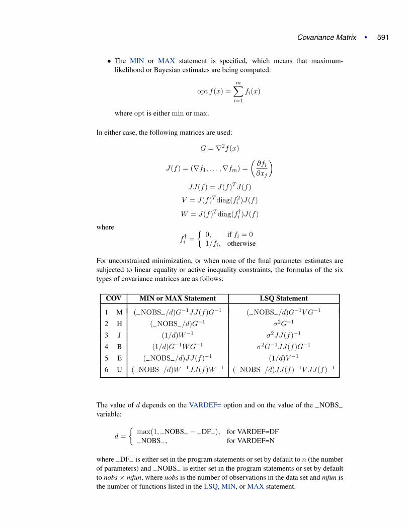
Covariance Matrix � 591
• The MIN or MAX statement is specified, which means that maximum-likelihood or Bayesian estimates are being computed:
opt f(x) =m∑
i=1
fi(x)
where opt is either min or max.
In either case, the following matrices are used:
G = ∇2f(x)
J(f) = (∇f1, . . . ,∇fm) =(
∂fi
∂xj
)
JJ(f) = J(f)T J(f)
V = J(f)T diag(f2i )J(f)
W = J(f)T diag(f †i )J(f)
where
f †i =
{0, if fi = 01/fi, otherwise
For unconstrained minimization, or when none of the final parameter estimates aresubjected to linear equality or active inequality constraints, the formulas of the sixtypes of covariance matrices are as follows:
COV MIN or MAX Statement LSQ Statement
1 M (–NOBS–/d)G−1JJ(f)G−1 (–NOBS–/d)G−1V G−1
2 H (–NOBS–/d)G−1 σ2G−1
3 J (1/d)W−1 σ2JJ(f)−1
4 B (1/d)G−1WG−1 σ2G−1JJ(f)G−1
5 E (–NOBS–/d)JJ(f)−1 (1/d)V −1
6 U (–NOBS–/d)W−1JJ(f)W−1 (–NOBS–/d)JJ(f)−1V JJ(f)−1
The value of d depends on the VARDEF= option and on the value of the –NOBS–variable:
d ={
max(1, –NOBS– − –DF–), for VARDEF=DF
–NOBS– , for VARDEF=N
where –DF– is either set in the program statements or set by default to n (the numberof parameters) and –NOBS– is either set in the program statements or set by defaultto nobs × mfun, where nobs is the number of observations in the data set and mfun isthe number of functions listed in the LSQ, MIN, or MAX statement.

592 � Chapter 6. The NLP Procedure
The value σ2 depends on the specification of the SIGSQ= option and on the value ofd:
σ2 ={
sq × –NOBS–/d, if SIGSQ=sq is specified2f(x∗)/d, if SIGSQ= is not specified
where f(x∗) is the value of the objective function at the optimal parameter estimatesx∗.
The two groups of formulas distinguish between two situations:
• For least-squares estimates, the error variance can be estimated from the objec-tive function value and is used in three of the six different forms of covariancematrices. If you have an independent estimate of the error variance, you canspecify it with the SIGSQ= option.
• For maximum-likelihood or Bayesian estimates, the objective function shouldbe the logarithm of the likelihood or of the posterior density when using theMAX statement.
For minimization, the inversion of the matrices in these formulas is done so thatnegative eigenvalues are considered zero, resulting always in a positive semidefinitecovariance matrix.
In small samples, estimates of the covariance matrix based on asymptotic theory areoften too small and should be used with caution.
If the final parameter estimates are subjected to nact > 0 linear equality or activelinear inequality constraints, the formulas of the covariance matrices are modifiedsimilar to Gallant (1987) and Cramer (1986, p. 38) and additionally generalized forapplications with singular matrices. In the constrained case, the value of d used inthe scalar factor σ2 is defined by
d ={
max(1, –NOBS– − –DF– + nact), for VARDEF=DF
–NOBS– , for VARDEF=N
where nact is the number of active constraints and –NOBS– is set as in the uncon-strained case.
For minimization, the covariance matrix should be positive definite; for maximizationit should be negative definite. There are several options available to check for a rankdeficiency of the covariance matrix:
• The ASINGULAR=, MSINGULAR=, and VSINGULAR= options can beused to set three singularity criteria for the inversion of the matrix A neededto compute the covariance matrix, when A is either the Hessian or one of thecrossproduct Jacobian matrices. The singularity criterion used for the inversionis
|dj,j | ≤ max(ASING ,VSING × |Aj,j |,MSING × max(|A1,1|, . . . , |An,n|))

Covariance Matrix � 593
where dj,j is the diagonal pivot of the matrix A, and ASING, VSING andMSING are the specified values of the ASINGULAR=, VSINGULAR=, andMSINGULAR= options. The default values are
– ASING: the square root of the smallest positive double precision value
– MSING: 1E−12 if the SINGULAR= option is not specified andmax(10 × ε, 1E − 4 × SINGULAR) otherwise, where ε is the machineprecision
– VSING: 1E−8 if the SINGULAR= option is not specified and the valueof SINGULAR otherwise
Note: In many cases, a normalized matrix D−1AD−1 is decomposed and thesingularity criteria are modified correspondingly.
• If the matrix A is found singular in the first step, a generalized inverse is com-puted. Depending on the G4= option, a generalized inverse is computed thatsatisfies either all four or only two Moore-Penrose conditions. If the numberof parameters n of the application is less than or equal to G4=i, a G4 inverse iscomputed; otherwise only a G2 inverse is computed. The G4 inverse is com-puted by (the computationally very expensive but numerically stable) eigen-value decomposition; the G2 inverse is computed by Gauss transformation.The G4 inverse is computed using the eigenvalue decomposition A = ZΛZT ,where Z is the orthogonal matrix of eigenvectors and Λ is the diagonal matrixof eigenvalues, Λ = diag(λ1, ..., λn). If the PEIGVAL option is specified, theeigenvalues λi are displayed. The G4 inverse of A is set to
A− = ZΛ−ZT
where the diagonal matrix Λ− = diag(λ−1 , ..., λ−
n ) is defined using theCOVSING= option:
λ−i =
{1/λi, if |λi| > COVSING0, if |λi| ≤ COVSING
If the COVSING= option is not specified, the nr smallest eigenvalues are setto zero, where nr is the number of rank deficiencies found in the first step.
For optimization techniques that do not use second-order derivatives, the covariancematrix is usually computed using finite-difference approximations of the derivatives.By specifying TECH=NONE, any of the covariance matrices can be computed usinganalytical derivatives. The covariance matrix specified by the COV= option can bedisplayed (using the PCOV option) and is written to the OUTEST= data set.
594 � Chapter 6. The NLP Procedure
Input and Output Data Sets
DATA= Input Data Set
The DATA= data set is used only to specify an objective function f that is a combi-nation of m other functions fi. For each function fi, i = 1, . . . ,m, listed in a MAX,MIN, or LSQ statement, each observation l, l = 1, . . . ,nobs , in the DATA= data setdefines a specific function fil that is evaluated by substituting the values of the vari-ables of this observation into the program statements. If the MAX or MIN statementis used, the m×nobs specific functions fil are added to a single objective function f .If the LSQ statement is used, the sum-of-squares f of the m×nobs specific functionsfil is minimized. The NOMISS option causes observations with missing values to beskipped.
INEST= Input Data Set
The INEST= (or INVAR=, or ESTDATA=) input data set can be used to specify theinitial values of the parameters defined in a DECVAR statement as well as boundaryconstraints and the more general linear constraints which could be imposed on theseparameters. This form of input is similar to the dense format input used in PROC LP.
The variables of the INEST= data set are
• a character variable –TYPE– that indicates the type of the observation
• n numeric variables with the parameter names used in the DECVAR statement
• the BY variables that are used in a DATA= input data set
• a numeric variable –RHS– specifying the right-hand-side constants (neededonly if linear constraints are used)
• additional variables with names corresponding to constants used in the programstatements
The content of the –TYPE– variable defines the meaning of the observation of theINEST= data set. PROC NLP recognizes the following –TYPE– values:
• PARMS, which specifies initial values for parameters. Additional variables cancontain the values of constants that are referred to in program statements. Thevalues of the constants in the PARMS observation initialize the constants in theprogram statements.
• UPPERBD | UB, which specifies upper bounds. A missing value indicates thatno upper bound is specified for the parameter.
• LOWERBD | LB, which specifies lower bounds. A missing value indicates thatno lower bound is specified for the parameter.
• LE | <= | <, which specifies linear constraint∑
j aijxj ≤ bi. The n parametervalues contain the coefficients aij , and the –RHS– variable contains the right-hand side bi. Missing values indicate zeros.

Input and Output Data Sets � 595
• GE | >= | >, which specifies linear constraint∑
j aijxj ≥ bi. The n parametervalues contain the coefficients aij , and the –RHS– variable contains the right-hand side bi. Missing values indicate zeros.
• EQ | =, which specifies linear constraint∑
j aijxj = bi. The n parametervalues contain the coefficients aij , and the –RHS– variable contains the right-hand side bi. Missing values indicate zeros.
The constraints specified in an INEST= data set are added to the constraints specifiedin the BOUNDS and LINCON statements. You can use an OUTEST= data set asan INEST= data set in a subsequent run of PROC NLP. However, be aware that theOUTEST= data set also contains the boundary and general linear constraints spec-ified in the previous run of PROC NLP. When you are using this OUTEST= dataset without changes as an INEST= data set, PROC NLP adds the constraints from thedata set to the constraints specified by a BOUNDS and LINCON statement. AlthoughPROC NLP automatically eliminates multiple identical constraints you should avoidspecifying the same constraint twice.
INQUAD= Input Data Set
Two types of INQUAD= data sets can be used to specify the objective function of aquadratic programming problem for TECH=QUADAS or TECH=LICOMP,
f(x) =12xT Gx + gT x + c, with GT = G
The dense INQUAD= data set must contain all numerical values of the symmetricmatrix G, the vector g, and the scalar c. Using the sparse INQUAD= data set allowsyou to specify only the nonzero positions in matrix G and vector g. Those locationsthat are not set by the sparse INQUAD= data set are assumed to be zero.
Dense INQUAD= Data Set
A dense INQUAD= data set must contain two character variables, –TYPE– and
–NAME–, and at least n numeric variables whose names are the parameter names.The –TYPE– variable takes the following values:
• QUAD lists the n values of the row of the G matrix that is defined by theparameter name used in the –NAME– variable.
• LINEAR lists the n values of the g vector.
• CONST sets the the value of the scalar c and cannot contain different numericalvalues; however, it could contain up to n − 1 missing values.
• PARMS specifies initial values for parameters.
• UPPERBD | UB specifies upper bounds. A missing value indicates that noupper bound is specified.
• LOWERBD | LB specifies lower bounds. A missing value indicates that nolower bound is specified.

596 � Chapter 6. The NLP Procedure
• LE | <= | < specifies linear constraint∑
j aijxj ≤ bi. The n parameter valuescontain the coefficients aij , and the –RHS– variable contains the right-handside bi. Missing values indicate zeros.
• GE | >= | > specifies linear constraint∑
j aijxj ≥ bi. The n parameter valuescontain the coefficients aij , and the –RHS– variable contains the right-handside bi. Missing values indicate zeros.
• EQ | = specifies linear constraint∑
j aijxj = bi. The n parameter valuescontain the coefficients aij , and the –RHS– variable contains the right-handside bi. Missing values indicate zeros.
Constraints specified in a dense INQUAD= data set are added to the constraints spec-ified in BOUNDS and LINCON statements.
Sparse INQUAD= Data Set
A sparse INQUAD= data set must contain three character variables –TYPE–,
–ROW–, and –COL–, and one numeric variable –VALUE–. The –TYPE– variablecan assume two values:
• QUAD specifies that the –ROW– and –COL– variables define the row andcolumn locations of the values in the G matrix.
• LINEAR specifies that the –ROW– variable defines the row locations of thevalues in the g vector. The –COL– variable is not used.
Using both the MODEL= option and the INCLUDE statement with the same modelfile will include the file twice (erroneous in most cases).
OUT= Output Data Set
The OUT= data set contains those variables of a DATA= input data set that are re-ferred to in the program statements and additional variables computed by the programstatements for the objective function. Specifying the NOMISS option enables you toskip observations with missing values in variables used in the program statements.The OUT= data set can also contain first- and second-order derivatives of these vari-ables if the OUTDER= option is specified. The variables and derivatives are the finalparameter estimates x∗ or (for TECH=NONE) the initial value x0.
The variables of the OUT= data set are
• the BY variables and all other variables that are used in a DATA= input data setand referred to in the program code
• a variable –OBS– containing the number of observations read from a DATA=input data set, where the counting is restarted with the start of each BY group.If there is no DATA= input data set, then –OBS–=1.
• a character variable –TYPE– naming the type of the observation
• the parameter variables listed in the DECVAR statement
• the function variables listed in the the MIN, MAX, or LSQ statement

Input and Output Data Sets � 597
• all other variables computed in the program statements
• the character variable –WRT– (if OUTDER=1) containing the with respect tovariable for which the first-order derivatives are written in the function vari-ables
• the two character variables –WRT1– and –WRT2– (if OUTDER=2) contain-ing the two with respect to variables for which the first- and second-orderderivatives are written in the function variables
OUTEST= Output Data Set
The OUTEST= or OUTVAR= output data set saves the optimization solution ofPROC NLP. You can use the OUTEST= or OUTVAR= data set as follows:
• to save the values of the objective function on grid points to examine, for ex-ample, surface plots using PROC G3D (use the OUTGRID option)
• to avoid any costly computation of analytical (first- or second-order) derivativesduring optimization when they are needed only upon termination. In this casea two-step approach is recommended:
1. In a first execution, the optimization is done; that is, optimal parameterestimates are computed, and the results are saved in an OUTEST= dataset.
2. In a subsequent execution, the optimal parameter estimates in the pre-vious OUTEST= data set are read in an INEST= data set and used withTECH=NONE to compute further results, such as analytical second-orderderivatives or some kind of covariance matrix.
• to restart the procedure using parameter estimates as initial values
• to split a time-consuming optimization problem into a series of smaller prob-lems using intermediate results as initial values in subsequent runs. (Refer tothe MAXTIME=, MAXIT=, and MAXFUNC= options to trigger stopping.)
• to write the value of the objective function, the parameter estimates, the time inseconds starting at the beginning of the optimization process and (if available)the gradient to the OUTEST= data set during the iterations. After the PROCNLP run is completed, the convergence progress can be inspected by graphi-cally displaying the iterative information. (Refer to the OUTITER option.)
The variables of the OUTEST= data set are
• the BY variables that are used in a DATA= input data set
• a character variable –TECH– naming the optimization technique used
• a character variable –TYPE– specifying the type of the observation
• a character variable –NAME– naming the observation. For a linear constraint,the –NAME– variable indicates whether the constraint is active at the solution.For the initial observations, the –NAME– variable indicates if the number inthe –RHS– variable corresponds to the number of positive, negative, or zeroeigenvalues.

598 � Chapter 6. The NLP Procedure
• n numeric variables with the parameter names used in the DECVAR statement.These variables contain a point x of the parameter space, lower or upper boundconstraints, or the coefficients of linear constraints.
• a numeric variable –RHS– (right-hand side) that is used for the right-hand-side value bi of a linear constraint or for the value f = f(x) of the objectivefunction at a point x of the parameter space
• a numeric variable –ITER– that is zero for initial values, equal to the iterationnumber for the OUTITER output, and missing for the result output
The –TYPE– variable identifies how to interpret the observation. If –TYPE– is
• PARMS then parameter-named variables contain the coordinates of the result-ing point x∗. The –RHS– variable contains f(x∗).
• INITIAL then parameter-named variables contain the feasible starting pointx(0). The –RHS– variable contains f(x(0)).
• GRIDPNT then (if the OUTGRID option is specified) parameter-named vari-ables contain the coordinates of any point x(k) used in the grid search. The
–RHS– variable contains f(x(k)).
• GRAD then parameter-named variables contain the gradient at the initial orfinal estimates.
• STDERR then parameter-named variables contain the approximate standarderrors (square roots of the diagonal elements of the covariance matrix) if theCOV= option is specified.
• –NOBS– then (if the COV= option is specified) all parameter variables containthe value of –NOBS– used in computing the σ2 value in the formula of thecovariance matrix.
• UPPERBD | UB then (if there are boundary constraints) the parameter variablescontain the upper bounds.
• LOWERBD | LB then (if there are boundary constraints) the parameter vari-ables contain the lower bounds.
• NACTBC then all parameter variables contain the number nabc of activeboundary constraints at the solution x∗.
• ACTBC then (if there are active boundary constraints) the observation indicatewhich parameters are actively constrained, as follows:
–NAME–=GE the active lower bounds
–NAME–=LE the active upper bounds
–NAME–=EQ the active equality constraints
• NACTLC then all parameter variables contain the number nalc of active linearconstraints that are recognized as linearly independent.
• NLDACTLC then all parameter variables contain the number of active linearconstraints that are recognized as linearly dependent.

Input and Output Data Sets � 599
• LE then (if there are linear constraints) the observation contains the ith linearconstraint
∑j aijxj ≤ bi. The parameter variables contain the coefficients aij ,
j = 1, . . . , n, and the –RHS– variable contains bi. If the constraint i is activeat the solution x∗, then –NAME–=ACTLC or –NAME–=LDACTLC.
• GE then (if there are linear constraints) the observation contains the ith linearconstraint
∑j aijxj ≥ bi. The parameter variables contain the coefficients aij ,
j = 1, . . . , n, and the –RHS– variable contains bi. If the constraint i is activeat the solution x∗, then –NAME–=ACTLC or –NAME–=LDACTLC.
• EQ then (if there are linear constraints) the observation contains the ith linearconstraint
∑j aijxj = bi. The parameter variables contain the coefficients
aij , j = 1, . . . , n, the –RHS– variable contains bi, and –NAME–=ACTLC or
–NAME–=LDACTLC.
• LAGRANGE then (if at least one of the linear constraints is an equality con-straint or an active inequality constraint) the observation contains the vector ofLagrange multipliers. The Lagrange multipliers of active boundary constraintsare listed first followed by those of active linear constraints and those of activenonlinear constraints. Lagrange multipliers are available only for the set oflinearly independent active constraints.
• PROJGRAD then (if there are linear constraints) the observation contains then − nact values of the projected gradient gZ = ZT g in the variables corre-sponding to the first n − nact parameters.
• JACOBIAN then (if the PJACOBI or OUTJAC option is specified) the m ob-servations contain the m rows of the m × n Jacobian matrix. The –RHS–variable contains the row number l, l = 1, . . . ,m.
• HESSIAN then the first n observations contain the n rows of the (symmetric)Hessian matrix. The –RHS– variable contains the row number j, j = 1, . . . , n,and the –NAME– variable contains the corresponding parameter name.
• PROJHESS then the first n − nact observations contain the n − nact rows ofthe projected Hessian matrix ZT GZ. The –RHS– variable contains the rownumber j, j = 1, . . . , n − nact , and the –NAME– variable is blank.
• CRPJAC then the first n observations contain the n rows of the (symmetric)crossproduct Jacobian matrix at the solution. The –RHS– variable containsthe row number j, j = 1, . . . , n, and the –NAME– variable contains the cor-responding parameter name.
• PROJCRPJ then the first n − nact observations contain the n − nact rows ofthe projected crossproduct Jacobian matrix ZT (JT J)Z. The –RHS– variablecontains the row number j, j = 1, . . . , n − nact, and the –NAME– variable isblank.
• COV1, COV2, COV3, COV4, COV5, or COV6 then (depending on the COV=option) the first n observations contain the n rows of the (symmetric) covari-ance matrix of the parameter estimates. The –RHS– variable contains the rownumber j, j = 1, . . . , n, and the –NAME– variable contains the correspondingparameter name.

600 � Chapter 6. The NLP Procedure
• DETERMIN contains the determinant det = a × 10b of the matrix specifiedby the value of the –NAME– variable where a is the value of the first variablein the DECVAR statement and b is in –RHS–.
• NEIGPOS, NEIGNEG, or NEIGZER then the –RHS– variable contains thenumber of positive, negative, or zero eigenvalues of the matrix specified by thevalue of the –NAME– variable.
• COVRANK then the –RHS– variable contains the rank of the covariance ma-trix.
• SIGSQ then the –RHS– variable contains the scalar factor of the covariancematrix.
• –TIME– then (if the OUTITER option is specified) the –RHS– variable con-tains the number of seconds passed since the start of the optimization.
• TERMINAT then if optimization terminated at a point satisfying one of thetermination criteria, an abbreviation of the corresponding criteria is given tothe –NAME– variable. Otherwise –NAME–=PROBLEMS.
If for some reason the procedure does not terminate successfully (for example, nofeasible initial values can be computed or the function value or derivatives at thestarting point cannot be computed), the OUTEST= data set may contain only part ofthe observations (usually only the PARMS and GRAD observation).
Note: Generally you can use an OUTEST= data set as an INEST= data set in a furtherrun of PROC NLP. However, be aware that the OUTEST= data set also contains theboundary and general linear constraints specified in the previous run of PROC NLP.When you are using this OUTEST= data set without changes as an INEST= dataset, PROC NLP adds the constraints from the data set to the constraints specified bya BOUNDS or LINCON statement. Although PROC NLP automatically eliminatesmultiple identical constraints you should avoid specifying the same constraint twice.
Output of Profiles
The following observations are written to the OUTEST= data set only when thePROFILE statement or CLPARM option is specified.
–TYPE– –NAME– –RHS– Meaning of ObservationPLC–LOW parname y value coordinates of lower CL for αPLC–UPP parname y value coordinates of upper CL for α
WALD–CL LOWER y value lower Wald CL for α in –ALPHA–WALD–CL UPPER y value upper Wald CL for α in –ALPHA–
PL–CL LOWER y value lower PL CL for α in –ALPHA–PL–CL UPPER y value upper PL CL for α in –ALPHA–
PROFILE L(THETA) missing y value corresponding to xin following –NAME–=THETA
PROFILE THETA missing x value corresponding to yin previous –NAME–=L(THETA)

Input and Output Data Sets � 601
Assume that the PROFILE statement specifies np parameters and nα confidence lev-els. For CLPARM, np = n and nα = 4.
• –TYPE–=PLC–LOW and –TYPE–=PLC–UPP:If the CLPARM= option or the PROFILE statement with the OUTTABLE op-tion is specified, then the complete set θ of parameter estimates (rather thanonly the confidence limit x = θj) is written to the OUTEST= data set for eachside of the confidence interval. This output may be helpful for further analyseson how small changes in x = θj affect the changes in the other θi, i �= j. The
–ALPHA– variable contains the corresponding value of α. There should beno more than 2nαnp observations. If the confidence limit cannot be computed,the corresponding observation is not available.
• –TYPE–=WALD–CL:If CLPARM=WALD, CLPARM=BOTH, or the PROFILE statement withα values is specified, then the Wald confidence limits are written to theOUTEST= data set for each of the default or specified values of α. The
–ALPHA– variable contains the corresponding value of α. There should be2nα observations.
• –TYPE–=PL–CL:If CLPARM=PL, CLPARM=BOTH, or the PROFILE statement with α valuesis specified, then the PL confidence limits are written to the OUTEST= dataset for each of the default or specified values of α. The –ALPHA– variablecontains the corresponding values of α. There should be 2nα observations;some observations may have missing values.
• –TYPE–=PROFILE:If CLPARM=PL, CLPARM=BOTH, or the CLPARM= statement with or with-out α values is specified, then a set of (x, y) point coordinates in two adjacentobservations with –NAME–=L(THETA) (y value) and –NAME–=THETA (xvalue) is written to the OUTEST= data set. The –RHS– and –ALPHA– vari-ables are not used (are set to missing). The number of observations depends onthe difficulty of the optimization problems.
OUTMODEL= Output Data Set
The program statements for objective functions, nonlinear constraints, and derivativescan be saved into an OUTMODEL= output data set. This data set can be used in anINCLUDE program statement or as a MODEL= input data set in subsequent callsof PROC NLP. The OUTMODEL= option is similar to the option used in PROCMODEL in SAS/ETS software.
Storing Programs in Model Files
Models can be saved to and recalled from SAS catalog files. SAS catalogs are specialfiles which can store many kinds of data structures as separate units in one SAS file.Each separate unit is called an entry, and each entry has an entry type that identifiesits structure to the SAS system.
In general, to save a model, use the OUTMODEL=name option in the PROC NLPstatement, where name is specified as libref.catalog.entry, libref.entry, or entry. The

602 � Chapter 6. The NLP Procedure
libref, catalog, and entry names must be valid SAS names no more than 8 characterslong. The catalog name is restricted to 7 characters on the CMS operating system. Ifnot given, the catalog name defaults to MODELS, and the libref defaults to WORK.The entry type is always MODEL. Thus, OUTMODEL=X writes the model to thefile WORK.MODELS.X.MODEL.
The MODEL= option is used to read in a model. A list of model files can be specifiedin the MODEL= option, and a range of names with numeric suffixes can be given, asin MODEL=(MODEL1-MODEL10). When more than one model file is given, thelist must be placed in parentheses, as in MODEL=(A B C). If more than one modelfile is specified, the files are combined in the order listed in the MODEL= option.
When the MODEL= option is specified in the PROC NLP statement and model defi-nition statements are also given later in the PROC NLP step, the model files are readin first, in the order listed, and the model program specified in the PROC NLP step isappended after the model program read from the MODEL= files.
The INCLUDE statement can be used to append model code to the current modelcode. The contents of the model files are inserted into the current model at the posi-tion where the INCLUDE statement appears.
Note that the following statements are not part of the program code that is written toan OUTMODEL= data set: MIN, MAX, LSQ, MINQUAD, MAXQUAD, DECVAR,BOUNDS, BY, CRPJAC, GRADIENT, HESSIAN, JACNLC, JACOBIAN, LABEL,LINCON, MATRIX, and NLINCON.
Displayed Output
Procedure Initialization
After the procedure has processed the problem, it displays summary informationabout the problem and the options that you have selected. It may also display alist of linearly dependent constraints and other information about the constraints andparameters.
Optimization Start
At the start of optimization the procedure displays
• the number of constraints that are active at the starting point, or more precisely,the number of constraints that are currently members of the working set. Ifthis number is followed by a plus sign, there are more active constraints, ofwhich at least one is temporarily released from the working set due to negativeLagrange multipliers.
• the value of the objective function at the starting point
• if the (projected) gradient is available, the value of the largest absolute (pro-jected) gradient element
• for the TRUREG and LEVMAR subroutines, the initial radius of the trust re-gion around the starting point

Displayed Output � 603
Iteration History
In general, the iteration history consists of one line of output containing the most im-portant information for each iteration. The iteration-extensive Nelder-Mead simplexmethod, however, displays only one line for several internal iterations. This techniqueskips the output for some iterations because
• some of the termination tests (size and standard deviation) are rather time-consuming compared to the simplex operations and are done once every fivesimplex operations
• the resulting history output is smaller
The –LIST– variable (refer to the “Program Statements” section on page 558) alsoenables you to display the parameter estimates x(k) and the gradient g(k) in all orsome selected iterations k.
The iteration history always includes the following (the words in parentheses indicatethe column header output):
• the iteration number (iter)
• the number of iteration restarts (nrest)
• the number of function calls (nfun)
• the number of active constraints (act)
• the value of the optimization criterion (optcrit)
• the difference between adjacent function values (difcrit)
• the maximum of the absolute (projected) gradient components (maxgrad)
An apostrophe trailing the number of active constraints indicates that at least one ofthe active constraints was released from the active set due to a significant Lagrangemultiplier.
The optimization history is displayed by default because it is important to check forpossible convergence problems.
Optimization Termination
The output of the optimization history ends with a short output of information con-cerning the optimization result:
• the number of constraints that are active at the final point, or more precisely,the number of constraints that are currently members of the working set. Whenthis number is followed by a plus sign, it indicates that there are more activeconstraints of which at least one is temporarily released from the working setdue to negative Lagrange multipliers.
• the value of the objective function at the final point

604 � Chapter 6. The NLP Procedure
• if the (projected) gradient is available, the value of the largest absolute (pro-jected) gradient element
• other information that is specific for the optimization technique
The NOPRINT option suppresses all output to the list file and only errors, warnings,and notes are displayed to the log file. The PALL option sets a large group of someof the commonly used specific displaying options, the PSHORT option suppressessome, and the PSUMMARY option suppresses almost all of the default output. Thefollowing table summarizes the correspondence between the general and the specificprint options.
Output Options PALL default PSHORT PSUMMARYy y y y summary of optimizationy y y n parameter estimatesy y y n gradient of objective func
PHISTORY y y y n iteration historyPINIT y y n n setting of initial values
y y n n listing of constraintsPGRID y n n n results of grid searchPNLCJAC y n n n Jacobian nonlin. constr.PFUNCTION y n n n values of functionsPEIGVAL y n n n eigenvalue distributionPCRPJAC y n n n crossproduct JacobianPHESSIAN y n n n Hessian matrixPSTDERR y n n n approx. standard errorsPCOV y n n n covariance matricesPJACOBI n n n n JacobianLIST n n n n model program, variablesLISTCODE n n n n compiled model program
Missing Values
Missing Values in Program Statements
There is one very important reason for using missing values in program statementsspecifying the values of the objective functions and derivatives: it may not be pos-sible to evaluate the program statements for a particular point x. For example, theextrapolation formula of one of the line-search algorithms may generate large x val-ues for which the EXP function cannot be evaluated without floating point overflow.The compiler of the program statements may check for such situations automatically,but it would be safer if you check the feasibility of your program statements. In somecases, the specification of boundary or linear constraints for parameters can avoidsuch situations. In many other cases, you can indicate that x is a bad point simply byreturning a missing value for the objective function. In such cases the optimizationalgorithms in PROC NLP shorten the step length α or reduce the trust region radiusso that the next point will be closer to the point that was already successfully evalu-

Computational Resources � 605
ated at the last iteration. Note that the starting point x(0) must be a point for whichthe program statements can be evaluated.
Missing Values in Input Data Sets
Observations with missing values in the DATA= data set for variables used in theobjective function can lead to a missing value of the objective function implying thatthe corresponding BY group of data is not processed. The NOMISS option can beused to skip those observations of the DATA= data set for which relevant variableshave missing values. Relevant variables are those that are referred to in programstatements.
There can be different reasons to include observations with missing values in theINEST= data set. The value of the –RHS– variable is not used in some cases andcan be missing. Missing values for the variables corresponding to parameters in the
–TYPE– variable are as follows:
• PARMS observations cause those parameters to have initial values assigned bythe DECVAR statement or by the RANDOM= or INITIAL= option.
• UPPERBD or LOWERBD observations cause those parameters to be uncon-strained by upper or lower bounds.
• LE, GE, or EQ observations cause those parameters to have zero values in theconstraint.
In general, missing values are treated as zeros.
Computational Resources
Since nonlinear optimization is an iterative process that depends on many factors, itis difficult to estimate how much computer time is necessary to compute an optimalsolution satisfying one of the termination criteria. The MAXTIME=, MAXITER=,and MAXFUNC= options can be used to restrict the amount of CPU time, the numberof iterations, and the number of function calls in a single run of PROC NLP.
In each iteration k, the NRRIDG and LEVMAR techniques use symmetricHouseholder transformations to decompose the n × n Hessian (crossproductJacobian) matrix G,
G = V T TV , V orthogonal, T tridiagonal
to compute the (Newton) search direction s:
s(k) = −G(k−1)g(k) , k = 1, 2, 3, . . .
The QUADAS, TRUREG, NEWRAP, and HYQUAN techniques use the Choleskydecomposition to solve the same linear system while computing the search direction.The QUANEW, DBLDOG, CONGRA, and NMSIMP techniques do not need to in-vert or decompose a Hessian or crossproduct Jacobian matrix and thus require fewercomputational resources then the first group of techniques.

606 � Chapter 6. The NLP Procedure
The larger the problem, the more time is spent computing function values and deriva-tives. Therefore, many researchers compare optimization techniques by counting andcomparing the respective numbers of function, gradient, and Hessian (crossproductJacobian) evaluations. You can save computer time and memory by specifying deriva-tives (using the GRADIENT, JACOBIAN, CRPJAC, or HESSIAN statement) sinceyou will typically produce a more efficient representation than the internal derivativecompiler.
Finite-difference approximations of the derivatives are expensive since they requireadditional function or gradient calls.
• Forward-difference formulas:
– First-order derivatives: n additional function calls are needed.
– Second-order derivatives based on function calls only: for a denseHessian, n(n + 3)/2 additional function calls are needed.
– Second-order derivatives based on gradient calls: n additional gradientcalls are needed.
• Central-difference formulas:
– First-order derivatives: 2n additional function calls are needed.
– Second-order derivatives based on function calls only: for a denseHessian, 2n(n + 1) additional function calls are needed.
– Second-order derivatives based on gradient: 2n additional gradient callsare needed.
Many applications need considerably more time for computing second-order deriva-tives (Hessian matrix) than for first-order derivatives (gradient). In such cases, a(dual) quasi-Newton or conjugate gradient technique is recommended, which doesnot require second-order derivatives.
The following table shows for each optimization technique which derivatives areneeded (FOD: first-order derivatives; SOD: second-order derivatives), what kinds ofconstraints are supported (BC: boundary constraints; LIC: linear constraints), and theminimal memory (number of double floating point numbers) required. For variousreasons, there are additionally about 7n + m double floating point numbers needed.

Computational Resources � 607
Quadratic Programming FOD SOD BC LIC MemoryLICOMP - - x x 18n + 3nnQUADAS - - x x 1n + 2nn/2General Optimization FOD SOD BC LIC MemoryTRUREG x x x x 4n + 2nn/2NEWRAP x x x x 2n + 2nn/2NRRIDG x x x x 6n + nn/2QUANEW x - x x 1n + nn/2DBLDOG x - x x 7n + nn/2CONGRA x - x x 3nNMSIMP - - x x 4n + nn
Least-Squares FOD SOD BC LIC MemoryLEVMAR x - x x 6n + nn/2HYQUAN x - x x 2n + nn/2 + 3m
Notes:
• Here, n denotes the number of parameters, nn the squared number of parame-ters, and nn/2 := n(n + 1)/2.
• The value of m is the product of the number of functions specified in the MIN,MAX, or LSQ statement and the maximum number of observations in each BYgroup of a DATA= input data set. The following table also contains the numberv of variables in the DATA= data set that are used in the program statements.
• For a diagonal Hessian matrix, the nn/2 term in QUADAS, TRUREG,NEWRAP, and NRRIDG is replaced by n.
• If the TRUREG, NRRIDG, or NEWRAP method is used to minimize a least-squares problem, the second derivatives are replaced by the crossproductJacobian matrix.
• The memory needed by the TECH=NONE specification depends on the outputspecifications (typically, it needs 3n+nn/2 double floating point numbers andan additional mn if the Jacobian matrix is required).
The total amount of memory needed to run an optimization technique consists ofthe technique-specific memory listed in the preceding table, plus additional blocks ofmemory as shown in the following table.

608 � Chapter 6. The NLP Procedure
double int long 8byteBasic Requirement 7n + m n 3n n + mDATA= data set v - - vJACOBIAN statement m(n + 2) - - -CRPJAC statement nn/2 - - -HESSIAN statement nn/2 - - -COV= option (2∗)nn/2 + n - - -Scaling vector n - - -BOUNDS statement 2n n - -Bounds in INEST= 2n - - -LINCON and TRUREG c(n + 1) + nn + nn/2 + 4n 3c - -LINCON and other c(n + 1) + nn + 2nn/2 + 4n 3c - -
Notes:
• For TECH=LICOMP, the total amount of memory needed for the linear orboundary constrained case is 18(n + c) + 3(n + c)(n + c), where c is thenumber of constraints.
• The amount of memory needed to specify derivatives with a GRADIENT,JACOBIAN, CRPJAC, or HESSIAN statement (shown in this table) is smallcompared to that needed for using the internal function compiler to computethe derivatives. This is especially so for second-order derivatives.
• If the CONGRA technique is used, specifying the GRADCHECK=DETAILoption requires an additional nn/2 double floating point numbers to store thefinite-difference Hessian matrix.

Example 6.1. Using the DATA= Option � 609
Examples
Example 6.1. Using the DATA= Option
This example illustrates the use of the DATA= option. The Bard function (refer toMoré et al. (1981)) is a least-squares problem with n = 3 parameters and m = 15functions fk:
f(x) =12
15∑k=1
f2k (x), x = (x1, x2, x3)
where
fk(x) = yk −(
x1 +uk
vkx2 + wkx3
)
with uk = k, vk = 16 − k, wk = min(uk, vk), and
y = (.14, .18, .22, .25, .29, .32, .35, .39, .37, .58, .73, .96, 1.34, 2.10, 4.39)
The minimum function value f(x∗) = 4.107E−3 is at the point (0.08, 1.13, 2.34).The starting point x0 = (1, 1, 1) is used.
The following is the naive way of specifying the objective function.
proc nlp tech=levmar;lsq y1-y15;parms x1-x3 = 1;tmp1 = 15 * x2 + min(1,15) * x3;y1 = 0.14 - (x1 + 1 / tmp1);tmp1 = 14 * x2 + min(2,14) * x3;y2 = 0.18 - (x1 + 2 / tmp1);tmp1 = 13 * x2 + min(3,13) * x3;y3 = 0.22 - (x1 + 3 / tmp1);tmp1 = 12 * x2 + min(4,12) * x3;y4 = 0.25 - (x1 + 4 / tmp1);tmp1 = 11 * x2 + min(5,11) * x3;y5 = 0.29 - (x1 + 5 / tmp1);tmp1 = 10 * x2 + min(6,10) * x3;y6 = 0.32 - (x1 + 6 / tmp1);tmp1 = 9 * x2 + min(7,9) * x3;y7 = 0.35 - (x1 + 7 / tmp1);tmp1 = 8 * x2 + min(8,8) * x3;y8 = 0.39 - (x1 + 8 / tmp1);tmp1 = 7 * x2 + min(9,7) * x3;y9 = 0.37 - (x1 + 9 / tmp1);tmp1 = 6 * x2 + min(10,6) * x3;y10 = 0.58 - (x1 + 10 / tmp1);tmp1 = 5 * x2 + min(11,5) * x3;y11 = 0.73 - (x1 + 11 / tmp1);

610 � Chapter 6. The NLP Procedure
tmp1 = 4 * x2 + min(12,4) * x3;y12 = 0.96 - (x1 + 12 / tmp1);tmp1 = 3 * x2 + min(13,3) * x3;y13 = 1.34 - (x1 + 13 / tmp1);tmp1 = 2 * x2 + min(14,2) * x3;y14 = 2.10 - (x1 + 14 / tmp1);tmp1 = 1 * x2 + min(15,1) * x3;y15 = 4.39 - (x1 + 15 / tmp1);
run;
A more economical way to program this problem uses the DATA= option to input the15 terms in f(x).
data bard;input r @@;
w1 = 16. - _n_;w2 = min(_n_ , 16. - _n_);datalines;
.14 .18 .22 .25 .29 .32 .35 .39
.37 .58 .73 .96 1.34 2.10 4.39;
proc nlp data=bard tech=levmar;lsq y;parms x1-x3 = 1.;y = r - (x1 + _obs_ / (w1 * x2 + w2 * x3));
run;
Another way you can specify the objective function uses the ARRAY statement andan explicit do loop, as in the following code.
proc nlp tech=levmar;array r[15] .14 .18 .22 .25 .29 .32 .35 .39 .37 .58
.73 .96 1.34 2.10 4.39 ;array y[15] y1-y15;lsq y1-y15;parms x1-x3 = 1.;do i = 1 to 15;
w1 = 16. - i;w2 = min(i , w1);w3 = w1 * x2 + w2 * x3;y[i] = r[i] - (x1 + i / w3);
end;run;

Example 6.2. Using the INQUAD= Option � 611
Example 6.2. Using the INQUAD= Option
This example illustrates the INQUAD= option for specifying a quadratic program-ming problem:
min f(x) =12xT Gx + gT x + c, with GT = G
Suppose that c = −100, G = diag(.4, 4) and 2 ≤ x1 ≤ 50, −50 ≤ x2 ≤ 50, and10 ≤ 10x1 − x2.
You specify the constant c and the Hessian G in the data set QUAD1. Notice thatthe –TYPE– variable contains the keywords that identify how the procedure shouldinterpret the observations.
data quad1;input _type_ $ _name_ $ x1 x2;datalines;
const . -100 -100quad x1 0.4 0quad x2 0 4;
You specify the QUAD1 data set with the INQUAD= option. Notice that the namesof the variables in the QUAD1 data set and the –NAME– variable match the namesof the parameters in the PARMS statement.
proc nlp inquad=quad1 all;min ;parms x1 x2 = -1;bounds 2 <= x1 <= 50,
-50 <= x2 <= 50;lincon 10 <= 10 * x1 - x2;
run;
Alternatively, you can use a sparse format for specifying the G matrix, eliminatingthe zeros. You use the special variables –ROW–, –COL–, and –VALUE– to give thenonzero row and column names and value.
data quad2;input _type_ $ _row_ $ _col_ $ _value_;datalines;
const . . -100quad x1 x1 0.4quad x2 x2 4;
You can also include the constraints in the QUAD data set. Notice how the –TYPE–variable contains keywords that identify how the procedure is to interpret the valuesin each observation.

612 � Chapter 6. The NLP Procedure
data quad3;input _type_ $ _name_ $ x1 x2 _rhs_;datalines;
const . -100 -100 .quad x1 0.02 0 .quad x2 0.00 2 .parms . -1 -1 .lowerbd . 2 -50 .upperbd . 50 50 .ge . 10 -1 10;
proc nlp inquad=quad3;min ;parms x1 x2;
run;
Example 6.3. Using the INEST=OptionThis example illustrates the use of the INEST= option for specifying a starting pointand linear constraints. You name a data set with the INEST= option. The format ofthis data set is similar to the format of the QUAD data set described in the previousexample.
Consider the Hock and Schittkowski (1981) Problem # 24:
min f(x) =((x1 − 3)2 − 9)x3
2
27√
3
subject to:
0 ≤ x1, x2
0 ≤ .57735x1 − x2
0 ≤ x1 + 1.732x2
6 ≥ x1 + 1.732x2
with minimum function value f(x∗) = −1 at x∗ = (3,√
3). The feasible startingpoint is x0 = (1, .5).
You can specify this model in PROC NLP as follows:
proc nlp tech=trureg outest=res;min y;parms x1 = 1,
x2 = .5;bounds 0 <= x1-x2;lincon .57735 * x1 - x2 >= 0,
x1 + 1.732 * x2 >= 0,-x1 - 1.732 * x2 >= -6;
y = (((x1 - 3)**2 - 9.) * x2**3) / (27 * sqrt(3));run;

Example 6.3. Using the INEST=Option � 613
Note that none of the data for this model are in a data set. Alternatively, you cansave the starting point (1, .5) and the linear constraints in a data set. Notice that the
–TYPE– variable contains keywords that identify how the procedure is to interpreteach of the observations and that the parameters in the problems X1 and X2 arevariables in the data set. The observation with –TYPE–=LOWERBD gives the lowerbounds on the parameters. The observation with –TYPE–=GE gives the coefficientsfor the first constraint. Similarly, the subsequent observations contain specificationsfor the other constraints. Also notice that the special variable –RHS– contains theright-hand-side values.
data betts1(type=est);input _type_ $ x1 x2 _rhs_;datalines;
parms 1 .5 .lowerbd 0 0 .ge .57735 -1 .ge 1 1.732 .le 1 1.732 6;
Now you can solve this problem with the following code. Notice that you specify theobjective function and the parameters.
proc nlp inest=betts1 tech=trureg;min y;parms x1 x2;y = (((x1 - 3)**2 - 9) * x2**3) / (27 * sqrt(3));
run;
You can even include any constants used in the program statements in the INEST=data set. In the following code the variables A, B, C, and D contain some of theconstants used in calculating the objective function Y.
data betts2(type=est);input _type_ $ x1 x2 _rhs_ a b c d;datalines;
parms 1 .5 . 3 9 27 3lowerbd 0 0 . . . . .ge .57735 -1 0 . . . .ge 1 1.732 0 . . . .le 1 1.732 6 . . . .;
Notice that in the program statement for calculating Y, the constants are replaced bythe A, B, C, and D variables.
proc nlp inest=betts2 tech=trureg;min y;parms x1 x2;y = (((x1 - a)**2 - b) * x2**3) / (c * sqrt(d));
run;

614 � Chapter 6. The NLP Procedure
Example 6.4. Restarting an Optimization
This example shows how you can restart an optimization problem using theOUTEST=, INEST=, OUTMODEL=, and MODEL= options and how to save out-put into an OUT= data set. The least-squares solution of the Rosenbrock functionusing the trust region method is used.
The following code solves the problem and saves the model in the MODEL data setand the solution in the EST and OUT1 data sets.
proc nlp tech=trureg outmodel=model outest=est out=out1;lsq y1 y2;parms x1 = -1.2 ,
x2 = 1.;y1 = 10. * (x2 - x1 * x1);y2 = 1. - x1;
run;
proc print data=out1;run;
The final parameter estimates x∗ = (1, 1) and the values of the functions f1 =Y1 andf2 =Y2 are written into an OUT= data set, shown in Output 6.4.1. Since OUTDER=0is the default, the OUT= data set does not contain the Jacobian matrix.
Output 6.4.1. Solution in an OUT= Data Set
Obs _OBS_ _TYPE_ y1 y2 x2 x1
1 1 0 0 1 1
Next, the procedure reads the optimal parameter estimates from the EST dataset and the model from the MODEL data set. It does not do any optimization(TECH=NONE), but it saves the Jacobian matrix to the OUT=OUT2 data set be-cause of the option OUTDER=1. It also displays the Jacobian matrix because of theoption PJAC; the Jacobian matrix is shown in Output 6.4.2. Output 6.4.3 shows thecontents of the OUT2 data set, which also contains the Jacobian matrix.
proc nlp tech=none model=model inest=est out=out2 outder=1 pjac;lsq y1 y2;parms x1 x2;
run;
proc print data=out2;run;

Example 6.5. Approximate Standard Errors � 615
Output 6.4.2. Jacobian Matrix Output
PROC NLP: Least Squares Minimization
Jacobian Matrix
x1 x2
-20 10-1 0
Output 6.4.3. Jacobian Matrix in an OUT= Data Set
Obs _OBS_ _TYPE_ y1 y2 _WRT_ x2 x1
1 1 0 0 1 12 1 ANALYTIC 10 0 x2 1 13 1 ANALYTIC -20 -1 x1 1 1
Example 6.5. Approximate Standard Errors
The NLP procedure provides a variety of ways for estimating parameters in nonlin-ear statistical models and for obtaining approximate standard errors and covariancematrices for the estimators. These methods are illustrated by estimating the meanof a random sample from a normal distribution with mean µ and standard deviationσ. The simplicity of the example makes it easy to compare the results of differentmethods in NLP with the usual estimator, the sample mean.
The following data step is used:
data x;input x @@;
datalines;1 3 4 5 7;
The standard error of the mean, computed with n − 1 degrees of freedom, is 1. Theusual maximum-likelihood approximation to the standard error of the mean, using avariance divisor of n rather than n − 1, is 0.894427.
The sample mean is a least-squares estimator, so it can be computed using an LSQstatement. Moreover, since this model is linear, the Hessian matrix and crossprod-uct Jacobian matrix are identical, and all three versions of the COV= option yieldthe same variance and standard error of the mean. Note that COV=j means that thecrossproduct Jacobian is used. This is chosen because it requires the least computa-tion.

616 � Chapter 6. The NLP Procedure
proc nlp data=x cov=j pstderr pshort;lsq resid;parms mean=0;resid=x-mean;
run;
The results are the same as the usual estimates.
Output 6.5.1. Parameter Estimates
PROC NLP: Least Squares Minimization
Optimization ResultsParameter Estimates
Approx ApproxN Parameter Estimate Std Err t Value Pr > |t|
1 mean 4.000000 1.000000 4.000000 0.016130
Optimization ResultsParameter Estimates
GradientObjectiveFunction
0
Value of Objective Function = 10
PROC NLP can also compute maximum-likelihood estimates of µ and σ. In this caseit is convenient to minimize the negative log likelihood. To get correct standard errorsfor maximum-likelihood estimators, the SIGSQ=1 option is required. The followingprogram shows COV=1 but the output that follows has COV=2 and COV=3.
proc nlp data=x cov=1 sigsq=1 pstderr phes pcov pshort;min nloglik;parms mean=0, sigma=1;bounds 1e-12 < sigma;nloglik=.5*((x-mean)/sigma)**2 + log(sigma);
run;
The variance divisor is n instead of n − 1, so the standard error of the mean is0.894427 instead of 1. The standard error of the mean is the same with all six typesof covariance matrix, but the standard error of the standard deviation varies. Thesampling distribution of the standard deviation depends on the higher moments ofthe population distribution, so different methods of estimation can produce markedlydifferent estimates of the standard error of the standard deviation.
Output 6.5.2 shows the output when COV=1, Output 6.5.3 shows the output whenCOV=2, and Output 6.5.4 shows the output when COV=3.

Example 6.5. Approximate Standard Errors � 617
Output 6.5.2. Solution for COV=1
PROC NLP: Nonlinear Minimization
Optimization ResultsParameter Estimates
Approx ApproxN Parameter Estimate Std Err t Value Pr > |t|
1 mean 4.000000 0.894427 4.472136 0.0065662 sigma 2.000000 0.458258 4.364358 0.007260
Optimization ResultsParameter Estimates
GradientObjectiveFunction
1.33149E-10-5.606415E-9
Value of Objective Function = 5.9657359028
Hessian Matrix
mean sigma
mean 1.2500000028 -1.33149E-10sigma -1.33149E-10 2.500000014
Determinant = 3.1250000245
Matrix has Only Positive Eigenvalues
Covariance Matrix 1: M = (NOBS/d)inv(G) JJ(f) inv(G)
mean sigma
mean 0.8 1.980107E-11sigma 1.980107E-11 0.2099999991
Factor sigm = 1
Determinant = 0.1679999993
Matrix has Only Positive Eigenvalues

618 � Chapter 6. The NLP Procedure
Output 6.5.3. Solution for COV=2
PROC NLP: Nonlinear Minimization
Optimization ResultsParameter Estimates
Approx ApproxN Parameter Estimate Std Err t Value Pr > |t|
1 mean 4.000000 0.894427 4.472136 0.0065662 sigma 2.000000 0.632456 3.162278 0.025031
Optimization ResultsParameter Estimates
GradientObjectiveFunction
1.33149E-10-5.606415E-9
Value of Objective Function = 5.9657359028
Hessian Matrix
mean sigma
mean 1.2500000028 -1.33149E-10sigma -1.33149E-10 2.500000014
Determinant = 3.1250000245
Matrix has Only Positive Eigenvalues
Covariance Matrix 2: H = (NOBS/d) inv(G)
mean sigma
mean 0.7999999982 4.260766E-11sigma 4.260766E-11 0.3999999978
Factor sigm = 1
Determinant = 0.3199999975
Matrix has Only Positive Eigenvalues

Example 6.5. Approximate Standard Errors � 619
Output 6.5.4. Solution for COV=3
PROC NLP: Nonlinear Minimization
Optimization ResultsParameter Estimates
Approx ApproxN Parameter Estimate Std Err t Value Pr > |t|
1 mean 4.000000 0.509136 7.856442 0.0005372 sigma 2.000000 0.419936 4.762634 0.005048
Optimization ResultsParameter Estimates
GradientObjectiveFunction
1.301733E-10-5.940302E-9
Value of Objective Function = 5.9657359028
Hessian Matrix
mean sigma
mean 1.2500000028 -1.33149E-10sigma -1.33149E-10 2.500000014
Determinant = 3.1250000245
Matrix has Only Positive Eigenvalues
Covariance Matrix 3: J = (1/d) inv(W)
mean sigma
mean 0.2592197879 1.062283E-11sigma 1.062283E-11 0.1763460041
Factor sigm = 0.2
Determinant = 0.0457123738
Matrix has Only Positive Eigenvalues
Under normality, the maximum-likelihood estimators of µ and σ are independent,as indicated by the diagonal Hessian matrix in the previous example. Hence, themaximum-likelihood estimate of µ can be obtained by using any fixed value forσ, such as 1. However, if the fixed value of σ differs from the actual maximum-likelihood estimate (in this case 2), the model is misspecified and the standard er-rors obtained with COV=2 or COV=3 are incorrect. It is therefore necessary to useCOV=1, which yields consistent estimates of the standard errors under a variety offorms of misspecification of the error distribution.

620 � Chapter 6. The NLP Procedure
proc nlp data=x cov=1 sigsq=1 pstderr pcov pshort;min sqresid;parms mean=0;sqresid=.5*(x-mean)**2;
run;
This formulation produces the same standard error of the mean, 0.894427 (see Output6.5.5).
Output 6.5.5. Solution for fixed σ and COV=1
PROC NLP: Nonlinear Minimization
Optimization ResultsParameter Estimates
Approx ApproxN Parameter Estimate Std Err t Value Pr > |t|
1 mean 4.000000 0.894427 4.472136 0.006566
Optimization ResultsParameter Estimates
GradientObjectiveFunction
0
Value of Objective Function = 10
Covariance Matrix1: M = (NOBS/d) inv(G)
JJ(f) inv(G)
mean
mean 0.8
Factor sigm = 1
The maximum-likelihood formulation with fixed σ is actually a least-squares prob-lem. The objective function, parameter estimates, and Hessian matrix are the sameas those in the first example in this section using the LSQ statement. However, theJacobian matrix is different, each row being multiplied by twice the residual. To treatthis formulation as a least-squares problem, the SIGSQ=1 option can be omitted. Butsince the Jacobian is not the same as in the formulation using the LSQ statement,the COV=1 | M and COV=3 | J options, which use the Jacobian, do not yield correctstandard errors. The correct standard error is obtained with COV=2 | H, which usesonly the Hessian matrix:
proc nlp data=x cov=2 pstderr pcov pshort;min sqresid;parms mean=0;sqresid=.5*(x-mean)**2;
run;

Example 6.5. Approximate Standard Errors � 621
The results are the same as in the first example.
Output 6.5.6. Solution for Fixed σ and COV=2
PROC NLP: Nonlinear Minimization
Optimization ResultsParameter Estimates
Approx ApproxN Parameter Estimate Std Err t Value Pr > |t|
1 mean 4.000000 0.500000 8.000000 0.001324
Optimization ResultsParameter Estimates
GradientObjectiveFunction
0
Value of Objective Function = 10
Covariance Matrix 2:H = (NOBS/d) inv(G)
mean
mean 0.25
Factor sigm = 1.25
In summary, to obtain appropriate standard errors for least-squares estimates, you canuse the LSQ statement with any of the COV= options, or you can use the MIN state-ment with COV=2. To obtain appropriate standard errors for maximum-likelihood es-timates, you can use the MIN statement with the negative log likelihood or the MAXstatement with the log likelihood, and in either case you can use any of the COV=options provided that you specify SIGSQ=1. You can also use a log-likelihood func-tion with a misspecified scale parameter provided that you use SIGSQ=1 and COV=1.For nonlinear models, all of these methods yield approximations based on asymptotictheory, and should therefore be interpreted cautiously.

622 � Chapter 6. The NLP Procedure
Example 6.6. Maximum Likelihood Weibull Estimation
Two-Parameter Weibull Estimation
The following data are taken from Lawless (1982, p. 193) and represent the numberof days it took rats painted with a carcinogen to develop carcinoma. The last twoobservations are censored data from a group of 19 rats:
data pike;input days cens @@;datalines;
143 0 164 0 188 0 188 0190 0 192 0 206 0 209 0213 0 216 0 220 0 227 0230 0 234 0 246 0 265 0304 0 216 1 244 1;
Suppose that you want to show how to compute the maximum likelihood estimatesof the scale parameter σ (α in Lawless), the shape parameter c (β in Lawless), andthe location parameter θ (µ in Lawless). The observed likelihood function of thethree-parameter Weibull transformation (Lawless 1982, p. 191) is
L(θ, σ, c) =cm
σm
∏i∈D
(ti − θ
σ
)c−1 p∏i=1
exp(−
(ti − θ
σ
)c)
and the log likelihood is
l(θ, σ, c) = m log c − mc log σ + (c − 1)∑i∈D
log(ti − θ) −p∑
i=1
(ti − θ
σ
)c
The log likelihood function can be evaluated only for σ > 0, c > 0, and θ < mini ti.In the estimation process, you must enforce these conditions using lower and upperboundary constraints. The three-parameter Weibull estimation can be numericallydifficult, and it usually pays off to provide good initial estimates. Therefore, you firstestimate σ and c of the two-parameter Weibull distribution for constant θ = 0. Youthen use the optimal parameters σ and c as starting values for the three-parameterWeibull estimation.
Although the use of an INEST= data set is not really necessary for this simple ex-ample, it illustrates how it is used to specify starting values and lower boundary con-straints:

Example 6.6. Maximum Likelihood Weibull Estimation � 623
data par1(type=est);keep _type_ sig c theta;_type_=’parms’; sig = .5;
c = .5; theta = 0; output;_type_=’lb’; sig = 1.0e-6;
c = 1.0e-6; theta = .; output;run;
The following PROC NLP call specifies the maximization of the log likelihood func-tion for the two-parameter Weibull estimation for constant θ = 0:
proc nlp data=pike tech=tr inest=par1 outest=opar1outmodel=model cov=2 vardef=n pcov phes;
max logf;parms sig c;profile sig c / alpha = .9 to .1 by -.1 .09 to .01 by -.01;
x_th = days - theta;s = - (x_th / sig)**c;if cens=0 then s + log(c) - c*log(sig) + (c-1)*log(x_th);logf = s;
run;
After a few iterations you obtain the solution given in Output 6.6.1.
Output 6.6.1. Optimization Results
PROC NLP: Nonlinear Maximization
Optimization ResultsParameter Estimates
Approx ApproxN Parameter Estimate Std Err t Value Pr > |t|
1 sig 234.318611 9.645908 24.292021 9.050475E-162 c 6.083147 1.068229 5.694611 0.000017269
Optimization ResultsParameter Estimates
GradientObjectiveFunction
1.3372183E-9-7.859311E-9
Value of Objective Function = -88.23273515
Since the gradient has only small elements and the Hessian (shown in Output 6.6.2)is negative definite (has only negative eigenvalues), the solution defines an isolatedmaximum point.

624 � Chapter 6. The NLP Procedure
Output 6.6.2. Hessian Matrix at x∗
Hessian Matrix
sig c
sig -0.011457556 0.0257527577c 0.0257527577 -0.934221388
Determinant = 0.0100406894
Matrix has Only Negative Eigenvalues
The square roots of the diagonal elements of the approximate covariance matrix ofparameter estimates are the approximate standard errors (ASE’s). The covariancematrix is given in Output 6.6.3.
Output 6.6.3. Covariance Matrix
Covariance Matrix 2:H = (NOBS/d) inv(G)
sig c
sig 93.043549863 2.5648395794c 2.5648395794 1.141112488
Factor sigm = 1
Determinant = 99.594754608
Matrix has 2 Positive Eigenvalue(s)
The confidence limits in Output 6.6.4 correspond to the α values in the PROFILEstatement.

Example 6.6. Maximum Likelihood Weibull Estimation � 625
Output 6.6.4. Confidence Limits
PROC NLP: Nonlinear Maximization
Wald and PL Confidence Limits
Profile LikelihoodN Parameter Estimate Alpha Confidence Limits
1 sig 234.318611 0.900000 233.111324 235.5326951 sig . 0.800000 231.886549 236.7728761 sig . 0.700000 230.623280 238.0638241 sig . 0.600000 229.292797 239.4366391 sig . 0.500000 227.855829 240.9352901 sig . 0.400000 226.251597 242.6292011 sig . 0.300000 224.372260 244.6433921 sig . 0.200000 221.984557 247.2784231 sig . 0.100000 218.390824 251.3941021 sig . 0.090000 217.884162 251.9874891 sig . 0.080000 217.326988 252.6452781 sig . 0.070000 216.708814 253.3835461 sig . 0.060000 216.008815 254.2280341 sig . 0.050000 215.199301 255.2154961 sig . 0.040000 214.230116 256.4110411 sig . 0.030000 213.020874 257.9356861 sig . 0.020000 211.369067 260.0661281 sig . 0.010000 208.671091 263.6871742 c 6.083147 0.900000 5.950029 6.2177522 c . 0.800000 5.815559 6.3555762 c . 0.700000 5.677909 6.4991872 c . 0.600000 5.534275 6.6517892 c . 0.500000 5.380952 6.8178802 c . 0.400000 5.212344 7.0044852 c . 0.300000 5.018784 7.2257332 c . 0.200000 4.776379 7.5061662 c . 0.100000 4.431310 7.9316692 c . 0.090000 4.382687 7.9914572 c . 0.080000 4.327815 8.0566282 c . 0.070000 4.270773 8.1292382 c . 0.060000 4.207130 8.2112212 c . 0.050000 4.134675 8.3062182 c . 0.040000 4.049531 8.4187822 c . 0.030000 3.945037 8.5596772 c . 0.020000 3.805759 8.7491302 c . 0.010000 3.588814 9.056751
Three-Parameter Weibull Estimation
You now prepare for the three-parameter Weibull estimation by using PROCUNIVARIATE to obtain the smallest data value for the upper boundary constraintfor θ. For this small problem, you can do this much more simply by just using avalue slightly smaller than the minimum data value 143.
/* Calculate upper bound for theta parameter */proc univariate data=pike noprint;
var days;output out=stats n=nobs min=minx range=range;
run;

626 � Chapter 6. The NLP Procedure
data stats;set stats;keep _type_ theta;
/* 1. write parms observation */theta = minx - .1 * range;if theta < 0 then theta = 0;_type_ = ’parms’;output;
/* 2. write ub observation */theta = minx * (1 - 1e-4);_type_ = ’ub’;output;
run;
The data set PAR2 specifies the starting values and the lower and upper bounds forthe three-parameter Weibull problem:
proc sort data=opar1;by _type_;
run;
data par2(type=est);merge opar1(drop=theta) stats;by _type_;keep _type_ sig c theta;if _type_ in (’parms’ ’lowerbd’ ’ub’);
run;
The following PROC NLP call uses the MODEL= input data set containing the loglikelihood function that was saved during the two-parameter Weibull estimation:
proc nlp data=pike tech=tr inest=par2 outest=opar2model=model cov=2 vardef=n pcov phes;
max logf;parms sig c theta;profile sig c theta / alpha = .5 .1 .05 .01;
run;
After a few iterations, you obtain the solution given in Output 6.6.5.

Example 6.6. Maximum Likelihood Weibull Estimation � 627
Output 6.6.5. Optimization Results
PROC NLP: Nonlinear Maximization
Optimization ResultsParameter Estimates
Approx ApproxN Parameter Estimate Std Err t Value Pr > |t|
1 sig 108.382732 32.573396 3.327339 0.0035402 c 2.711477 1.058759 2.560995 0.0191083 theta 122.025942 28.692439 4.252895 0.000430
Optimization ResultsParameter Estimates
GradientObjectiveFunction
-8.91765E-12-1.406349E-9-1.93916E-10
Value of Objective Function = -87.32424712
From inspecting the first- and second-order derivatives at the optimal solution, youcan verify that you have obtained an isolated maximum point. The Hessian matrix isshown in Output 6.6.6.
Output 6.6.6. Hessian Matrix
Hessian Matrix
sig c theta
sig -0.010639974 0.0453887849 -0.010033749c 0.0453887849 -4.078687939 -0.083026333theta -0.010033749 -0.083026333 -0.014752091
Determinant = 0.0000502116
Matrix has Only Negative Eigenvalues
The square roots of the diagonal elements of the approximate covariance matrix ofparameter estimates are the approximate standard errors. The covariance matrix isgiven in Output 6.6.7.

628 � Chapter 6. The NLP Procedure
Output 6.6.7. Covariance Matrix
Covariance Matrix 2: H = (NOBS/d) inv(G)
sig c theta
sig 1061.02613 29.926259613 -890.093361c 29.926259613 1.1209710432 -26.66352284theta -890.093361 -26.66352284 823.2560786
Factor sigm = 1
Determinant = 19915.723162
Matrix has 3 Positive Eigenvalue(s)
The difference between the Wald and profile CLs for parameter PHI2 are remarkable,especially for the upper 95% and 99% limits, as shown in Output 6.6.8.
Output 6.6.8. Confidence Limits
Wald and PL Confidence Limits
Profile LikelihoodN Parameter Estimate Alpha Confidence Limits
1 sig 108.382732 0.500000 91.811562 141.5646051 sig . 0.100000 76.502373 .1 sig . 0.050000 72.215845 .1 sig . 0.010000 64.262384 .2 c 2.711477 0.500000 2.139297 3.7040522 c . 0.100000 1.574162 9.2500722 c . 0.050000 1.424853 19.5161662 c . 0.010000 1.163096 19.5406813 theta 122.025942 0.500000 91.027144 135.0954543 theta . 0.100000 . 141.8337693 theta . 0.050000 . 142.5126033 theta . 0.010000 . 142.967407
Wald and PL Confidence Limits
Wald Confidence Limits
86.412310 130.35315454.804263 161.96120144.540049 172.22541524.479224 192.2862401.997355 3.4255990.969973 4.4529810.636347 4.786607
-0.015706 5.438660102.673186 141.37869874.831079 142.98570065.789794 142.98570048.119116 142.985700

Example 6.7. Simple Pooling Problem � 629
Example 6.7. Simple Pooling Problem
The following optimization problem is discussed in Haverly (1978) and in Liebmanet al. (1986, pp. 127–128). Two liquid chemicals, X and Y , are produced by thepooling and blending of three input liquid chemicals, A, B, and C. You know thesulfur impurity amounts of the input chemicals, and you have to respect upper limitsof the sulfur impurity amounts of the output chemicals. The sulfur concentrationsand the prices of the input and output chemicals are:
• Chemical A: Concentration = 3%, Price= $6
• Chemical B: Concentration = 1%, Price= $16
• Chemical C: Concentration = 2%, Price= $10
• Chemical X: Concentration ≤ 2.5%, Price= $9
• Chemical Y : Concentration ≤ 1.5%, Price= $15
The problem is complicated by the fact that the two input chemicals A and B areavailable only as a mixture (they are either shipped together or stored together).Because the amounts of A and B are unknown, the sulfur concentration of the mix-ture is also unknown.
C
B
A �3% Sfor $ 6
�1% Sfor $ 16
Pool Blend X �≤ 2.5 % Sfor $ 9
X ≤ 100
�Pool to X
Pool to Y
�
Blend Y �≤ 1.5 % Sfor $ 15
Y ≤ 200�2% Sfor $ 10
�C to Y
�C to X
You know customers will buy no more than 100 units of X and 200 units of Y. Theproblem is determining how to operate the pooling and blending of the chemicals tomaximize the profit. The objective function for the profit is
profit = cost(x) × amount(x) + cost(y) × amount(y)− cost(a) × amount(a) − cost(b) × amount(b) − cost(c) × amount(c)

630 � Chapter 6. The NLP Procedure
There are three groups of constraints:
1. The first group of constraint functions is the mass balance restrictions illus-trated by the graph. These are four linear equality constraints:
• amount(a) + amount(b) = pool–to–x + pool–to–y• pool–to–x + c–to–x = amount(x)• pool–to–y + c–to–y = amount(y)• amount(c) = c–to–x + c–to–y
2. You introduce a new variable, pool–s, that represents the sulfur concentrationof the pool. Using pool–s and the sulfur concentration of C (2%), you obtaintwo nonlinear inequality constraints for the sulfur concentrations of X andY , one linear equality constraint for the sulfur balance, and lower and upperboundary restrictions for pool–s:
• pool–s × pool–to–x + 2 c–to–x ≤ 2.5 amount(x)• pool–s × pool–to–y + 2 c–to–y ≤ 1.5 amount(y)• 3 amount(a) + 1 amount(b) = pool–s × (amount(a) + amount(b))• 1 ≤ pool–s ≤ 3
3. The last group assembles the remaining boundary constraints. First, you donot want to produce more than you can sell; and finally, all variables must benonnegative:
• amount(x) ≤ 100, amount(y) ≤ 200• amount(a), amount(b), amount(c), amount(x), amount(y) ≥ 0• pool–to–x , pool–to–y , c–to–x , c–to–y ≥ 0
There exist several local optima to this problem that can be found by specifying dif-ferent starting points. Using the starting point with all variables equal to 1 (specifiedwith a PARMS statement), PROC NLP finds a solution with profit = 400:
proc nlp all;parms amountx amounty amounta amountb amountc
pooltox pooltoy ctox ctoy pools = 1;bounds 0 <= amountx amounty amounta amountb amountc,
amountx <= 100,amounty <= 200,
0 <= pooltox pooltoy ctox ctoy,1 <= pools <= 3;
lincon amounta + amountb = pooltox + pooltoy,pooltox + ctox = amountx,pooltoy + ctoy = amounty,ctox + ctoy = amountc;
nlincon nlc1-nlc2 >= 0.,nlc3 = 0.;
max f;costa = 6; costb = 16; costc = 10;costx = 9; costy = 15;

Example 6.7. Simple Pooling Problem � 631
f = costx * amountx + costy * amounty- costa * amounta - costb * amountb - costc * amountc;
nlc1 = 2.5 * amountx - pools * pooltox - 2. * ctox;nlc2 = 1.5 * amounty - pools * pooltoy - 2. * ctoy;nlc3 = 3 * amounta + amountb - pools * (amounta + amountb);
run;
The specified starting point was not feasible with respect to the linear equality con-straints; therefore, a starting point is generated that satisfies linear and boundary con-straints. Output 6.7.1 gives the starting parameter estimates.
Output 6.7.1. Starting Estimates
PROC NLP: Nonlinear Maximization
Optimization StartParameter Estimates
Gradient Gradient LowerObjective Lagrange Bound
N Parameter Estimate Function Function Constraint
1 amountx 1.363636 9.000000 -0.843698 02 amounty 1.363636 15.000000 -0.111882 03 amounta 0.818182 -6.000000 -0.430733 04 amountb 0.818182 -16.000000 -0.542615 05 amountc 1.090909 -10.000000 0.017768 06 pooltox 0.818182 0 -0.669628 07 pooltoy 0.818182 0 -0.303720 08 ctox 0.545455 0 -0.174070 09 ctoy 0.545455 0 0.191838 010 pools 2.000000 0 0.068372 1.000000
Optimization StartParameter Estimates
UpperBound
Constraint
100.000000200.000000
.
.
.
.
.
.
.3.000000
Value of Objective Function = 3.8181818182
Value of Lagrange Function = -2.866739915
The starting point satisfies the four equality constraints, as shown in Output 6.7.2.The nonlinear constraints are given in Output 6.7.3.

632 � Chapter 6. The NLP Procedure
Output 6.7.2. Linear Constraints
Linear Constraints
1 -5.551E-16 : ACT 0 == + 1.0000 * amounta + 1.0000 * amountb- 1.0000 * pooltox - 1.0000 * pooltoy
2 -2.22E-16 : ACT 0 == - 1.0000 * amountx + 1.0000 * pooltox+ 1.0000 * ctox
3 1.1102E-16 : ACT 0 == - 1.0000 * amounty + 1.0000 * pooltoy+ 1.0000 * ctoy
4 0 : ACT 0 == - 1.0000 * amountc + 1.0000 * ctox+ 1.0000 * ctoy
Output 6.7.3. Nonlinear Constraints
Values of Nonlinear Constraints
LagrangeConstraint Value Residual Multiplier
[ 5 ] nlc3 0 0 4.9441 Active NLEC[ 6 ] nlc1_G 0.6818 0.6818 .[ 7 ] nlc2_G -0.6818 -0.6818 -9.8046 Violat. NLIC
Output 6.7.4 shows the settings of some important PROC NLP options.
Output 6.7.4. Options
PROC NLP: Nonlinear Maximization
Minimum Iterations 0Maximum Iterations 200Maximum Function Calls 500Iterations Reducing Constraint Violation 20ABSGCONV Gradient Criterion 0.00001GCONV Gradient Criterion 1E-8ABSFCONV Function Criterion 0FCONV Function Criterion 2.220446E-16FCONV2 Function Criterion 1E-6FSIZE Parameter 0ABSXCONV Parameter Change Criterion 0XCONV Parameter Change Criterion 0XSIZE Parameter 0ABSCONV Function Criterion 1.340781E154Line Search Method 2Starting Alpha for Line Search 1Line Search Precision LSPRECISION 0.4DAMPSTEP Parameter for Line Search .FD Derivatives: Accurate Digits in Obj.F 15.653559775FD Derivatives: Accurate Digits in NLCon 15.653559775Singularity Tolerance (SINGULAR) 1E-8Constraint Precision (LCEPS) 1E-8Linearly Dependent Constraints (LCSING) 1E-8Releasing Active Constraints (LCDEACT) .
The iteration history, given in Output 6.7.5, does not show any problems.

Example 6.7. Simple Pooling Problem � 633
Output 6.7.5. Iteration History
PROC NLP: Nonlinear Maximization
Dual Quasi-Newton OptimizationModified VMCWD Algorithm of Powell (1978, 1982)
Dual Broyden - Fletcher - Goldfarb - Shanno Update (DBFGS)Lagrange Multiplier Update of Powell(1982)
MaximumGradientElement
Maximum Predicted of theFunction Objective Constraint Function Step Lagrange
Iter Restarts Calls Function Violation Reduction Size Function
1 0 19 -1.42400 0.00962 6.9131 1.000 0.7832’ 0 20 2.77026 0.0166 5.3770 1.000 2.6293 0 21 7.08706 0.1409 7.1965 1.000 9.4524’ 0 22 11.41264 0.0583 15.5771 1.000 23.3905’ 0 23 24.84630 1.78E-15 496.1 1.000 147.66 0 24 378.22995 147.4 3316.6 1.000 840.47’ 0 25 307.56908 50.9348 607.9 1.000 27.1438’ 0 26 347.24557 1.8330 21.9896 1.000 28.4839’ 0 27 349.49342 0.00915 7.1838 1.000 28.29110’ 0 28 356.58483 0.1084 50.2539 1.000 27.48011’ 0 29 388.70516 2.4275 24.7951 1.000 21.11412’ 0 30 389.29922 0.0157 10.0489 1.000 18.64813’ 0 31 399.19185 0.7999 11.1897 1.000 0.41614’ 0 32 400.00000 0.0128 0.1535 1.000 0.0008715’ 0 33 400.00000 7.38E-11 2.43E-10 1.000 366E-12
Optimization Results
Iterations 15 Function Calls 34Gradient Calls 18 Active Constraints 10Objective Function 400 Maximum Constraint 7.381118E-11
ViolationMaximum Projected Gradient 0 Value Lagrange Function -400Maximum Gradient of the 3.552714E-14 Slope of Search Direction -2.43495E-10Lagran Func
FCONV2 convergence criterion satisfied.
The optimal solution in Output 6.7.6 shows that to obtain the maximum profit of$400, you need only to produce the maximum 200 units of blending Y and no unitsof blending X .

634 � Chapter 6. The NLP Procedure
Output 6.7.6. Optimization Solution
Optimization ResultsParameter Estimates
Gradient Gradient ActiveObjective Lagrange Bound
N Parameter Estimate Function Function Constraint
1 amountx -1.40483E-11 9.000000 0 Lower BC2 amounty 200.000000 15.000000 8.881784E-16 Upper BC3 amounta 5.484612E-16 -6.000000 0 Lower BC4 amountb 100.000000 -16.000000 -5.32907E-155 amountc 100.000000 -10.000000 -1.77636E-156 pooltox 7.024625E-12 0 0 Lower BC7 pooltoy 100.000000 0 -1.42109E-148 ctox -2.10729E-11 0 0 Lower BC LinDep9 ctoy 100.000000 0 -1.77636E-1510 pools 1.000000 0 3.552714E-14 Lower BC LinDep
Value of Objective Function = 400
Value of Lagrange Function = 400
The constraints are satisfied at the solution, as shown in Output 6.7.7
Output 6.7.7. Linear and Nonlinear Constraints at the Solution
Linear Constraints Evaluated at Solution
1 ACT 0 = 0 + 1.0000 * amounta + 1.0000 * amountb- 1.0000 * pooltox - 1.0000 * pooltoy
2 ACT 2.6603E-17 = 0 - 1.0000 * amountx + 1.0000 * pooltox+ 1.0000 * ctox
3 ACT 0 = 0 - 1.0000 * amounty + 1.0000 * pooltoy+ 1.0000 * ctoy
4 ACT 0 = 0 - 1.0000 * amountc + 1.0000 * ctox+ 1.0000 * ctoy
Values of Nonlinear Constraints
LagrangeConstraint Value Residual Multiplier
[ 5 ] nlc3 1.1E-15 1.1E-15 6.0000 Active NLEC[ 6 ] nlc1_G 4.18E-16 4.18E-16 . Active NLIC LinDep[ 7 ] nlc2_G 0 0 -6.0000 Active NLIC
Linearly Dependent Active Boundary Constraints
Parameter N Kind
ctox 8 Lower BCpools 10 Lower BC
Linearly Dependent Gradients of Active Nonlinear Constraints
Parameter N
nlc3 6

Example 6.7. Simple Pooling Problem � 635
The same problem can be specified in many different ways. For example, the follow-ing specification uses an INEST= data set containing the values of the starting pointand of the constants COST, COSTB, COSTC, COSTX, COSTY, CA, CB, CC, andCD:
data init1(type=est);input _type_ $ amountx amounty amounta amountb
amountc pooltox pooltoy ctox ctoy pools_rhs_ costa costb costc costx costyca cb cc cd;
datalines;parms 1 1 1 1 1 1 1 1 1 1
. 6 16 10 9 15 2.5 1.5 2. 3.;
proc nlp inest=init1 all;parms amountx amounty amounta amountb amountc
pooltox pooltoy ctox ctoy pools;bounds 0 <= amountx amounty amounta amountb amountc,
amountx <= 100,amounty <= 200,
0 <= pooltox pooltoy ctox ctoy,1 <= pools <= 3;
lincon amounta + amountb = pooltox + pooltoy,pooltox + ctox = amountx,pooltoy + ctoy = amounty,ctox + ctoy = amountc;
nlincon nlc1-nlc2 >= 0.,nlc3 = 0.;
max f;f = costx * amountx + costy * amounty
- costa * amounta - costb * amountb - costc * amountc;nlc1 = ca * amountx - pools * pooltox - cc * ctox;nlc2 = cb * amounty - pools * pooltoy - cc * ctoy;nlc3 = cd * amounta + amountb - pools * (amounta + amountb);
run;
The third specification uses an INEST= data set containing the boundary and linearconstraints in addition to the values of the starting point and of the constants. Thisspecification also writes the model specification into an OUTMOD= data set:
data init2(type=est);input _type_ $ amountx amounty amounta amountb amountc
pooltox pooltoy ctox ctoy pools_rhs_ costa costb costc costx costy;
datalines;parms 1 1 1 1 1 1 1 1 1 1
. 6 16 10 9 15 2.5 1.5 2 3lowerbd 0 0 0 0 0 0 0 0 0 1
. . . . . . . . . .upperbd 100 200 . . . . . . . 3
. . . . . . . . . .

636 � Chapter 6. The NLP Procedure
eq . . 1 1 . -1 -1 . . .0 . . . . . . . . .
eq 1 . . . . -1 . -1 . .0 . . . . . . . . .
eq . 1 . . . . -1 . -1 .0 . . . . . . . . .
eq . . . . 1 . . -1 -1 .0 . . . . . . . . .
;
proc nlp inest=init2 outmod=model all;parms amountx amounty amounta amountb amountc
pooltox pooltoy ctox ctoy pools;nlincon nlc1-nlc2 >= 0.,
nlc3 = 0.;max f;f = costx * amountx + costy * amounty
- costa * amounta - costb * amountb - costc * amountc;nlc1 = 2.5 * amountx - pools * pooltox - 2. * ctox;nlc2 = 1.5 * amounty - pools * pooltoy - 2. * ctoy;nlc3 = 3 * amounta + amountb - pools * (amounta + amountb);
run;
The fourth specification not only reads the INEST=INIT2 data set, it also uses themodel specification from the MODEL data set that was generated in the last specifi-cation. The PROC NLP call now contains only the defining variable statements:
proc nlp inest=init2 model=model all;parms amountx amounty amounta amountb amountc
pooltox pooltoy ctox ctoy pools;nlincon nlc1-nlc2 >= 0.,
nlc3 = 0.;max f;
run;
All four specifications start with the same starting point of all variables equal to 1 andgenerate the same results. However, there exist several local optima to this problem,as is pointed out in Liebman et al. (1986, p. 130).
proc nlp inest=init2 model=model all;parms amountx amounty amounta amountb amountc
pooltox pooltoy ctox ctoy = 0,pools = 2;
nlincon nlc1-nlc2 >= 0.,nlc3 = 0.;
max f;run;
This starting point with all variables equal to 0 is accepted as a local solution withprofit = 0, which minimizes rather than maximizes the profit.

Example 6.8. Chemical Equilibrium � 637
Example 6.8. Chemical Equilibrium
The following example is used in many test libraries for nonlinear programming andwas taken originally from Bracken and McCormick (1968).
The problem is to determine the composition of a mixture of various chemicals sat-isfying its chemical equilibrium state. The second law of thermodynamics impliesthat a mixture of chemicals satisfies its chemical equilibrium state (at a constant tem-perature and pressure) when the free energy of the mixture is reduced to a minimum.Therefore the composition of the chemicals satisfying its chemical equilibrium statecan be found by minimizing the function of the free energy of the mixture.
Notation:
m number of chemical elements in the mixturen number of compounds in the mixturexj number of moles for compound j, j = 1, . . . , ns total number of moles in the mixture (s =
∑ni=1 xj)
aij number of atoms of element i in a molecule of compound jbi atomic weight of element i in the mixture
Constraints for the Mixture:
• The number of moles must be positive:
xj > 0, j = 1, . . . , n
• There are m mass balance relationships,
n∑j=1
aijxj = bi, i = 1, . . . ,m
Objective Function: Total Free Energy of Mixture
f(x) =n∑
j=1
xj
[cj + ln
(xj
s
)]
with
cj =(
F ◦
RT
)j
+ lnP
where F ◦/RT is the model standard free energy function for the jth compound(found in tables) and P is the total pressure in atmospheres.

638 � Chapter 6. The NLP Procedure
Minimization Problem:
Determine the parameters xj that minimize the objective function f(x) subject to thenonnegativity and linear balance constraints.
Numeric Example:
Determine the equilibrium composition of compound 12N2H4 + 1
2O2 at temperatureT = 3500◦K and pressure P = 750psi.
aij
i = 1 i = 2 i = 3j Compound (F ◦/RT )j cj H N O
1 H -10.021 -6.089 12 H2 -21.096 -17.164 23 H2O -37.986 -34.054 2 14 N -9.846 -5.914 15 N2 -28.653 -24.721 26 NH -18.918 -14.986 1 17 NO -28.032 -24.100 1 18 O -14.640 -10.708 19 O2 -30.594 -26.662 2
10 OH -26.111 -22.179 1 1
Example Specification:
proc nlp tech=tr pall;array c[10] -6.089 -17.164 -34.054 -5.914 -24.721
-14.986 -24.100 -10.708 -26.662 -22.179;array x[10] x1-x10;min y;parms x1-x10 = .1;bounds 1.e-6 <= x1-x10;lincon 2. = x1 + 2. * x2 + 2. * x3 + x6 + x10,
1. = x4 + 2. * x5 + x6 + x7,1. = x3 + x7 + x8 + 2. * x9 + x10;
s = x1 + x2 + x3 + x4 + x5 + x6 + x7 + x8 + x9 + x10;y = 0.;do j = 1 to 10;
y = y + x[j] * (c[j] + log(x[j] / s));end;
run;
Displayed Output:
The iteration history given in Output 6.8.1 does not show any problems.

Example 6.8. Chemical Equilibrium � 639
Output 6.8.1. Iteration History
Trust Region Optimization
Without Parameter Scaling
Max Abs TrustRest Func Act Objective Obj Fun Gradient Region
Iter arts Calls Con Function Change Element Lambda Radius
1 0 2 3’ -47.33412 2.2790 6.0765 2.456 1.0002 0 3 3’ -47.70043 0.3663 8.5592 0.908 0.4183 0 4 3 -47.73074 0.0303 6.4942 0 0.3594 0 5 3 -47.73275 0.00201 4.7606 0 0.1185 0 6 3 -47.73554 0.00279 3.2125 0 0.01686 0 7 3 -47.74223 0.00669 1.9552 110.6 0.002717 0 8 3 -47.75048 0.00825 1.1157 102.9 0.005638 0 9 3 -47.75876 0.00828 0.4165 3.787 0.01169 0 10 3 -47.76101 0.00224 0.0716 0 0.012110 0 11 3 -47.76109 0.000083 0.00238 0 0.011111 0 12 3 -47.76109 9.609E-8 2.733E-6 0 0.00248
Optimization Results
Iterations 11 Function Calls 13Hessian Calls 12 Active Constraints 3Objective Function -47.76109086 Max Abs Gradient Element 1.8637498E-6Lambda 0 Actual Over Pred Change 0Radius 0.0024776027
GCONV convergence criterion satisfied.
Output 6.8.2 lists the optimal parameters with the gradient.
Output 6.8.2. Optimization Results
PROC NLP: Nonlinear Minimization
Optimization ResultsParameter Estimates
GradientObjective
N Parameter Estimate Function
1 x1 0.040668 -9.7850552 x2 0.147730 -19.5701103 x3 0.783153 -34.7921704 x4 0.001414 -12.9689215 x5 0.485247 -25.9378416 x6 0.000693 -22.7539767 x7 0.027399 -28.1909848 x8 0.017947 -15.2220609 x9 0.037314 -30.44412010 x10 0.096871 -25.007115
Value of Objective Function = -47.76109086
The three equality constraints are satisfied at the solution, as shown in Output 6.8.3.

640 � Chapter 6. The NLP Procedure
Output 6.8.3. Linear Constraints at Solution
PROC NLP: Nonlinear Minimization
Linear Constraints Evaluated at Solution
1 ACT 6.9389E-17 = 2.0000 - 1.0000 * x1 - 2.0000 * x2 -2.0000 * x3 - 1.0000 * x6 - 1.0000 * x10
2 ACT -4.337E-16 = 1.0000 - 1.0000 * x4 - 2.0000 * x5 -1.0000 * x6 - 1.0000 * x7
3 ACT -4.163E-17 = 1.0000 - 1.0000 * x3 - 1.0000 * x7 -1.0000 * x8 - 2.0000 * x9 - 1.0000 * x10
The Lagrange multipliers are given in Output 6.8.4.
Output 6.8.4. Lagrange Multipliers
PROC NLP: Nonlinear Minimization
First Order Lagrange Multipliers
LagrangeActive Constraint Multiplier
Linear EC [1] 9.785055Linear EC [2] 12.968921Linear EC [3] 15.222060
The elements of the projected gradient must be small to satisfy a necessary first-orderoptimality condition. The projected gradient is given in Output 6.8.5
Output 6.8.5. Projected Gradient
PROC NLP: Nonlinear Minimization
Projected Gradient
Free ProjectedDimension Gradient
1 4.577009E-92 6.86833E-103 -7.283021E-94 -0.0000018645 -0.0000014346 -0.0000013617 -0.000000294
The projected Hessian matrix shown in Output 6.8.6 is positive definite, satisfyingthe second-order optimality condition.

Example 6.8. Chemical Equilibrium � 641
Output 6.8.6. Projected Hessian Matrix
Projected Hessian Matrix
X1 X2 X3 X4
X1 20.903196985 -0.122067474 2.6480263467 3.3439156526X2 -0.122067474 565.97299938 106.54631863 -83.7084843X3 2.6480263467 106.54631863 1052.3567179 -115.230587X4 3.3439156526 -83.7084843 -115.230587 37.529977667X5 -1.373829641 -37.43971036 182.89278895 -4.621642366X6 -1.491808185 -36.20703737 175.97949593 -4.574152161X7 1.1462413516 -16.635529 -57.04158208 10.306551561
Projected Hessian Matrix
X5 X6 X7
X1 -1.373829641 -1.491808185 1.1462413516X2 -37.43971036 -36.20703737 -16.635529X3 182.89278895 175.97949593 -57.04158208X4 -4.621642366 -4.574152161 10.306551561X5 79.326057844 22.960487404 -12.69831637X6 22.960487404 66.669897023 -8.121228758X7 -12.69831637 -8.121228758 14.690478023
The following PROC NLP call uses a specified analytical gradient and the Hessianmatrix is computed by finite-difference approximations based on the analytic gradi-ent:
proc nlp tech=tr fdhessian all;array c[10] -6.089 -17.164 -34.054 -5.914 -24.721
-14.986 -24.100 -10.708 -26.662 -22.179;array x[10] x1-x10;array g[10] g1-g10;min y;parms x1-x10 = .1;bounds 1.e-6 <= x1-x10;lincon 2. = x1 + 2. * x2 + 2. * x3 + x6 + x10,
1. = x4 + 2. * x5 + x6 + x7,1. = x3 + x7 + x8 + 2. * x9 + x10;
s = x1 + x2 + x3 + x4 + x5 + x6 + x7 + x8 + x9 + x10;y = 0.;do j = 1 to 10;
y = y + x[j] * (c[j] + log(x[j] / s));g[j] = c[j] + log(x[j] / s);
end;run;
The results are almost identical to those of the previous run.

642 � Chapter 6. The NLP Procedure
Example 6.9. Minimize Total Delay in a Network
The following example is taken from the user’s guide of GINO (Liebman et al. 1986).A simple network of five roads (arcs) can be illustrated by the path diagram:
1
2
3
4F � ��
���
��
���
�
��
���
��
��� � F
Figure 6.11. Simple Road Network
The five roads connect four intersections illustrated by numbered nodes. Each minuteF vehicles enter and leave the network. Arc (i, j) refers to the road from intersectioni to intersection j, and the parameter xij refers to the flow from i to j. The law thattraffic flowing into each intersection j must also flow out is described by the linearequality constraint ∑
i
xij =∑
i
xji , j = 1, . . . , n
In general, roads also have an upper capacity, which is the number of vehicles whichcan be handled per minute. The upper limits cij can be enforced by boundary con-straints
0 ≤ xij ≤ cij , i, j = 1, . . . , n
Finding the maximum flow through a network is equivalent to solving a simple linearoptimization problem, and for large problems, PROC LP or PROC NETFLOW canbe used. The objective function is
max f = x24 + x34
and the constraints are0 ≤ x12, x32, x34 ≤ 10
0 ≤ x13, x24 ≤ 30
x13 = x32 + x34
x12 + x32 = x24
x12 + x13 = x24 + x34

Example 6.9. Minimize Total Delay in a Network � 643
The three linear equality constraints are linearly dependent. One of them is deletedautomatically by the PROC NLP subroutines. Even though the default technique isused for this small example, any optimization subroutine can be used.
proc nlp all initial=.5;max y;parms x12 x13 x32 x24 x34;bounds x12 <= 10,
x13 <= 30,x32 <= 10,x24 <= 30,x34 <= 10;
/* what flows into an intersection must flow out */lincon x13 = x32 + x34,
x12 + x32 = x24,x24 + x34 = x12 + x13;
y = x24 + x34 + 0*x12 + 0*x13 + 0*x32;run;
The iteration history is given in Output 6.9.1, and the optimal solution is given inOutput 6.9.2.
Output 6.9.1. Iteration History
Newton-Raphson Ridge Optimization
Without Parameter Scaling
ActualMax Abs Over
Rest Func Act Objective Obj Fun Gradient PredIter arts Calls Con Function Change Element Ridge Change
1* 0 2 4 20.25000 19.2500 0.5774 0.0313 0.8602* 0 3 5 30.00000 9.7500 0 0.0313 1.683
Optimization Results
Iterations 2 Function Calls 4Hessian Calls 3 Active Constraints 5Objective Function 30 Max Abs Gradient Element 0Ridge 0 Actual Over Pred Change 1.6834532374
All parameters are actively constrained. Optimization cannot proceed.

644 � Chapter 6. The NLP Procedure
Output 6.9.2. Optimization Results
PROC NLP: Nonlinear Maximization
Optimization ResultsParameter Estimates
Gradient ActiveObjective Bound
N Parameter Estimate Function Constraint
1 x12 10.000000 0 Upper BC2 x13 20.000000 03 x32 10.000000 0 Upper BC4 x24 20.000000 1.0000005 x34 10.000000 1.000000 Upper BC
Value of Objective Function = 30
Finding a traffic pattern that minimizes the total delay to move F vehicles per minutefrom node 1 to node 4 introduces nonlinearities that, in turn, demand nonlinear op-timization techniques. As traffic volume increases, speed decreases. Let tij be thetravel time on arc (i, j) and assume that the following formulas describe the traveltime as decreasing functions of the amount of traffic:
t12 = 5 + 0.1x12/(1 − x12/10)
t13 = x13/(1 − x13/30)
t32 = 1 + x32/(1 − x32/10)
t24 = x24/(1 − x24/30)
t34 = 5 + .1x34/(1 − x34/10)
These formulas use the road capacities (upper bounds), assuming F = 5 vehicles perminute have to be moved through the network. The objective function is now
min f = t12x12 + t13x13 + t32x32 + t24x24 + t34x34
and the constraints are0 ≤ x12, x32, x34 ≤ 10
0 ≤ x13, x24 ≤ 30
x13 = x32 + x34
x12 + x32 = x24
x24 + x34 = F = 5
Again, the default algorithm is used:
proc nlp all initial=.5;min y;parms x12 x13 x32 x24 x34;bounds x12 x13 x32 x24 x34 >= 0;lincon x13 = x32 + x34, /* flow in = flow out */

Example 6.9. Minimize Total Delay in a Network � 645
x12 + x32 = x24,x24 + x34 = 5; /* = f = desired flow */
t12 = 5 + .1 * x12 / (1 - x12 / 10);t13 = x13 / (1 - x13 / 30);t32 = 1 + x32 / (1 - x32 / 10);t24 = x24 / (1 - x24 / 30);t34 = 5 + .1 * x34 / (1 - x34 / 10);y = t12*x12 + t13*x13 + t32*x32 + t24*x24 + t34*x34;
run;
The iteration history is given in Output 6.9.3, and the optimal solution is given inOutput 6.9.4.
Output 6.9.3. Iteration History
Newton-Raphson Ridge Optimization
Without Parameter Scaling
ActualMax Abs Over
Rest Func Act Objective Obj Fun Gradient PredIter arts Calls Con Function Change Element Ridge Change
1 0 2 4 40.30303 0.3433 1.23E-16 0 0.508
Optimization Results
Iterations 1 Function Calls 3Hessian Calls 2 Active Constraints 4Objective Function 40.303030303 Max Abs Gradient Element 1.233822E-16Ridge 0 Actual Over Pred Change 0.5083585587
ABSGCONV convergence criterion satisfied.
Output 6.9.4. Opimization Results
PROC NLP: Nonlinear Minimization
Optimization ResultsParameter Estimates
Gradient ActiveObjective Bound
N Parameter Estimate Function Constraint
1 x12 2.500000 5.7777782 x13 2.500000 5.7024793 x32 2.036945E-17 1.000000 Lower BC4 x24 2.500000 5.7024795 x34 2.500000 5.777778
Value of Objective Function = 40.303030303
The active constraints and corresponding Lagrange multiplier estimates (costs) aregiven in Output 6.9.5 and Output 6.9.6, respectively.

646 � Chapter 6. The NLP Procedure
Output 6.9.5. Linear Constraints at Solution
PROC NLP: Nonlinear Minimization
Linear Constraints Evaluated at Solution
1 ACT -8.882E-16 = 0 + 1.0000 * x13 - 1.0000 * x32 -1.0000 * x34
2 ACT 0 = 0 + 1.0000 * x12 + 1.0000 * x32 -1.0000 * x24
3 ACT 1.7764E-15 = -5.0000 + 1.0000 * x24 + 1.0000 * x34
Output 6.9.6. Lagrange Multipliers at Solution
First Order Lagrange Multipliers
LagrangeActive Constraint Multiplier
Lower BC x32 0.924702Linear EC [1] 5.702479Linear EC [2] 5.777778Linear EC [3] 11.480257
Output 6.9.7 shows that the projected gradient is very small, satisfying the first-orderoptimality criterion.
Output 6.9.7. Projected Gradient at Solution
Projected Gradient
Free ProjectedDimension Gradient
1 1.233822E-16
The projected Hessian matrix (shown in Output 6.9.8) is positive definite, satisfyingthe second-order optimality criterion.
Output 6.9.8. Projected Hessian at Solution
Projected HessianMatrix
X1
X1 1.535309013

References � 647
References
Abramowitz, M. and Stegun, I. A. (1972), Handbook of Mathematical Functions,New York: Dover Publications, Inc.
Al-Baali, M. and Fletcher, R. (1985), “Variational Methods for Nonlinear LeastSquares,” Journal of the Operations Research Society, 36, 405–421.
Al-Baali, M. and Fletcher, R. (1986), “An Efficient Line Search for Nonlinear LeastSquares,” Journal of Optimization Theory and Applications, 48, 359–377.
Bard, Y. (1974), Nonlinear Parameter Estimation, New York: Academic Press, Inc.
Beale, E. M. L. (1972), “A Derivation of Conjugate Gradients,” in F. A. Lootsma, ed.,“Numerical Methods for Nonlinear Optimization,” London: Academic Press.
Betts, J. T. (1977), “An Accelerated Multiplier Method for Nonlinear Programming,”Journal of Optimization Theory and Applications, 21, 137–174.
Bracken, J. and McCormick, G. P. (1968), Selected Applications of NonlinearProgramming, New York: John Wiley & Sons, Inc.
Chamberlain, R. M., Powell, M. J. D., Lemarechal, C., and Pedersen, H. C. (1982),“The Watchdog Technique for Forcing Convergence in Algorithms for ConstrainedOptimization,” Mathematical Programming, 16, 1–17.
Cramer, J. S. (1986), Econometric Applications of Maximum Likelihood Methods,Cambridge, England: Cambridge University Press.
Dennis, J. E., Gay, D. M., and Welsch, R. E. (1981), “An Adaptive Nonlinear Least-Squares Algorithm,” ACM Transactions on Mathematical Software, 7, 348–368.
Dennis, J. E. and Mei, H. H. W. (1979), “Two New Unconstrained OptimizationAlgorithms which Use Function and Gradient Values,” Journal of OptimizationTheory Applications, 28, 453–482.
Dennis, J. E. and Schnabel, R. B. (1983), Numerical Methods for UnconstrainedOptimization and Nonlinear Equations, Englewood, New Jersey: Prentice-Hall.
Eskow, E. and Schnabel, R. B. (1991), “Algorithm 695: Software for a NewModified Cholesky Factorization,” ACM Transactions on Mathematical Software,17, 306–312.
Fletcher, R. (1987), Practical Methods of Optimization, Second Edition, Chichester:John Wiley & Sons, Inc.
Fletcher, R. and Powell, M. J. D. (1963), “A Rapidly Convergent Descent Method forMinimization,” Computer Journal, 6, 163–168.
Fletcher, R. and Xu, C. (1987), “Hybrid Methods for Nonlinear Least Squares,”Journal of Numerical Analysis, 7, 371–389.

648 � Chapter 6. The NLP Procedure
Gallant, A. R. (1987), Nonlinear Statistical Models, New York: John Wiley and Sons,Inc.
Gay, D. M. (1983), “Subroutines for Unconstrained Minimization,” ACMTransactions on Mathematical Software, 9, 503–524.
George, J. A. and Liu, J. W. (1981), Computer Solutions of Large Sparse PositiveDefinite Systems, Englewood Cliffs, NJ: Prentice-Hall.
Gill, E. P., Murray, W., Saunders, M. A., and Wright, M. H. (1983), “ComputingForward-Difference Intervals for Numerical Optimization,” SIAM J. Sci. Stat.Comput., 4, 310–321.
Gill, E. P., Murray, W., Saunders, M. A., and Wright, M. H. (1984), “Procedures forOptimization Problems with a Mixture of Bounds and General Linear Constraints,”ACM Transactions on Mathematical Software, 10, 282–298.
Gill, E. P., Murray, W., and Wright, M. H. (1981), Practical Optimization, New York:Academic Press Inc.
Goldfeld, S. M., Quandt, R. E., and Trotter, H. F. (1966), “Maximisation by QuadraticHill-Climbing,” Econometrica, 34, 541–551.
Hambleton, R. K., Swaminathan, H., and Rogers, H. J. (1991), Fundamentals of ItemResponse Theory, Newbury Park, CA: Sage Publications.
Hartmann, W. (1992a), “Applications of Nonlinear Optimization with PROC NLPand SAS/IML Software,” Technical report, SAS Institute Inc, Cary, N.C.
Hartmann, W. (1992b), “Nonlinear Optimization in IML, Releases 6.08, 6.09, 6.10,”Technical report, SAS Institute Inc, Cary, N.C.
Haverly, C. A. (1978), “Studies of the Behavior of Recursion for the PoolingProblem,” SIGMAP Bulletin, Association for Computing Machinery.
Hock, W. and Schittkowski, K. (1981), Test Examples for Nonlinear ProgrammingCodes, Lecture Notes in Economics and Mathematical Systems 187, Berlin-Heidelberg-New York: Springer-Verlag.
Jennrich, R. I. and Sampson, P. F. (1968), “Application of Stepwise Regression toNonlinear Estimation,” Technometrics, 10, 63–72.
Lawless, J. F. (1982), Statistical Methods and Methods for Lifetime Data, New York:John Wiley & Sons, Inc.
Liebman, J., Lasdon, L., Schrage, L., and Waren, A. (1986), Modeling andOptimization with GINO, California: The Scientific Press.
Lindström, P. and Wedin, P. A. (1984), “A New Line-Search Algorithm for NonlinearLeast-Squares Problems,” Mathematical Programming, 29, 268–296.
Moré, J. J. (1978), “The Levenberg-Marquardt Algorithm: Implementation andTheory,” in G. A. Watson, ed., “Lecture Notes in Mathematics,” volume 30,105–116, Berlin-Heidelberg-New York: Springer-Verlag.

References � 649
Moré, J. J., Garbow, B. S., and Hillstrom, K. E. (1981), “Testing UnconstrainedOptimization Software,” ACM Trans. Math. Software, 7, 17–41.
Moré, J. J. and Sorensen, D. C. (1983), “Computing a Trust-Region Step,” SIAM J.Sci. Stat. Comput., 4, 553–572.
Moré, J. J. and Wright, S. J. (1993), Optimization Software Guide, Philadelphia:SIAM.
Murtagh, B. A. and Saunders, M. A. (1983), MINOS 5.0 User’s Guide, TechnicalReport SOL 83-20, Stanford University.
Nelder, J. A. and Mead, R. (1965), “A Simplex Method for Function Minimization,”Computer Journal, 7, 308–313.
Polak, E. (1971), Computational Methods in Optimization, New York - San Francisco- London: Academic Press.
Powell, M. J. D. (1977), “Restart Procedures for the Conjugate Gradient Method,”Mathematical Programming, 12, 241–254.
Powell, M. J. D. (1978a), “Algorithms for Nonlinear Constraints that use LagrangianFunctions,” Mathematical Programming, 14, 224–248.
Powell, M. J. D. (1978b), “A Fast Algorithm for Nonlinearly ConstrainedOptimization Calculations,” in G. A. Watson, ed., “Lecture Notes in Mathematics,”volume 630, 144–175, Berlin-Heidelberg-New York: Springer-Verlag.
Powell, M. J. D. (1982a), “Extensions to Subroutine VF02AD,” in R. F. Drenick andF. Kozin, eds., “Systems Modeling and Optimization, Lecture Notes in Controland Information Sciences,” volume 38, 529–538, Berlin-Heidelberg-New York:Springer-Verlag.
Powell, M. J. D. (1982b), “VMCWD: A Fortran Subroutine for ConstrainedOptimization,” DAMTP 1982/NA4, Cambridge, England.
Powell, M. J. D. (1992), “A Direct Search Optimization Method that Modelsthe Objective and Constraint Functions by Linear Interpolation,” DAMTP/NA5,Cambridge, England.
Rosenbrock, H. H. (1960), “An Automatic Method for Finding the Greatest or LeastValue of a Function,” Computer Journal, 3, 175–184.
Schittkowski, K. (1980), “Nonlinear Programming Codes - Information, Tests,Performance,” Lecture Notes in Economics and Mathematical Systems, 183,Berlin–Heidelberg–New York: Springer Verlag.
Schittkowski, K. (1987), “More Test Examples for Nonlinear Programming Codes,”Lecture Notes in Economics and Mathematical Systems, 282, Berlin–Heidelberg–New York: Springer Verlag.
Schittkowski, K. and Stoer, J. (1979), “A Factorization Method for the Solution ofConstrained Linear Least Squares Problems Allowing Subsequent Data Changes,”Numer. Math., 31, 431–463.

650 � Chapter 6. The NLP Procedure
Stewart, G. W. (1967), “A Modification of Davidon’s Minimization Method to AcceptDifference Approximations of Derivatives,” J. Assoc. Comput. Mach., 14, 72–83.
Wedin, P. A. and Lindström, P. (1987), Methods and Software for Nonlinear LeastSquares Problems, University of Umea, Report No. UMINF 133.87.
Whitaker, D., Triggs, C. M., and John, J. A. (1990), “Construction of Block Designsusing Mathematical Programming,” J. R. Statist. Soc. B, 52, 497–503.
Wolfe, P. (1982), “Checking the Calculation of Gradients,” ACM Transactions onMathematical Software, 8, 337–343.

Chapter 7The QP Procedure (Experimental)
Chapter Contents
OVERVIEW . . . . . . . . . . . . . . . . . . . . . . . . . . . . . . . . . . . 653
QUADRATIC PROGRAMMING PROBLEMS . . . . . . . . . . . . . . . . 654The Interior Point Algorithm . . . . . . . . . . . . . . . . . . . . . . . . . 655Getting Started: QP Problems . . . . . . . . . . . . . . . . . . . . . . . . . 656Introductory QP Example . . . . . . . . . . . . . . . . . . . . . . . . . . . 657Typical PROC QP Run: QP Problems . . . . . . . . . . . . . . . . . . . . . 664Syntax: QP Problems . . . . . . . . . . . . . . . . . . . . . . . . . . . . . 665Functional Summary: QP Problems . . . . . . . . . . . . . . . . . . . . . . 666PROC QP Statement: QP Problems . . . . . . . . . . . . . . . . . . . . . . 667COEF Statement: QP Problems . . . . . . . . . . . . . . . . . . . . . . . . 673COLUMN Statement: QP Problems . . . . . . . . . . . . . . . . . . . . . 673HESSIANCOEF Statement . . . . . . . . . . . . . . . . . . . . . . . . . . 674HESSIANCOLUMN Statement . . . . . . . . . . . . . . . . . . . . . . . . 674HESSIANROW Statement . . . . . . . . . . . . . . . . . . . . . . . . . . 674ID Statement: QP Problems . . . . . . . . . . . . . . . . . . . . . . . . . . 675LO Statement: QP Problems . . . . . . . . . . . . . . . . . . . . . . . . . 675NAME Statement: QP Problems . . . . . . . . . . . . . . . . . . . . . . . 675OBJFN Statement . . . . . . . . . . . . . . . . . . . . . . . . . . . . . . . 676QUIT Statement . . . . . . . . . . . . . . . . . . . . . . . . . . . . . . . . 676RHS Statement . . . . . . . . . . . . . . . . . . . . . . . . . . . . . . . . 676ROW Statement . . . . . . . . . . . . . . . . . . . . . . . . . . . . . . . . 676RUN Statement . . . . . . . . . . . . . . . . . . . . . . . . . . . . . . . . 677TYPE Statement . . . . . . . . . . . . . . . . . . . . . . . . . . . . . . . . 677UPPERBD Statement . . . . . . . . . . . . . . . . . . . . . . . . . . . . . 678VAR Statement . . . . . . . . . . . . . . . . . . . . . . . . . . . . . . . . 679
QUADRATIC NETWORK PROBLEMS WITH SIDE CONSTRAINTS . . 679Network Models . . . . . . . . . . . . . . . . . . . . . . . . . . . . . . . . 681Getting Started: QNPSC Problems . . . . . . . . . . . . . . . . . . . . . . 688Introductory QNPSC Example . . . . . . . . . . . . . . . . . . . . . . . . 690Typical PROC QP Run: QNPSC Problems . . . . . . . . . . . . . . . . . . 695Syntax: QNPSC Problems . . . . . . . . . . . . . . . . . . . . . . . . . . . 697Functional Summary: QNPSC Problems . . . . . . . . . . . . . . . . . . . 698PROC QP Statement: QNPSC Problems . . . . . . . . . . . . . . . . . . . 699CAPACITY Statement . . . . . . . . . . . . . . . . . . . . . . . . . . . . . 707

652 � Chapter 7. The QP Procedure (Experimental)
COEF Statement: QNPSC Problems . . . . . . . . . . . . . . . . . . . . . 707COLUMN Statement: QNPSC Problems . . . . . . . . . . . . . . . . . . . 707COST Statement . . . . . . . . . . . . . . . . . . . . . . . . . . . . . . . . 708DEMAND Statement . . . . . . . . . . . . . . . . . . . . . . . . . . . . . 708HEADNODE Statement . . . . . . . . . . . . . . . . . . . . . . . . . . . . 708ID Statement: QNPSC Problems . . . . . . . . . . . . . . . . . . . . . . . 709LO Statement: QNPSC Problems . . . . . . . . . . . . . . . . . . . . . . . 709NAME Statement: QNPSC Problems . . . . . . . . . . . . . . . . . . . . . 709NODE Statement . . . . . . . . . . . . . . . . . . . . . . . . . . . . . . . 710SUPDEM Statement . . . . . . . . . . . . . . . . . . . . . . . . . . . . . . 710SUPPLY Statement . . . . . . . . . . . . . . . . . . . . . . . . . . . . . . 710TAILNODE Statement . . . . . . . . . . . . . . . . . . . . . . . . . . . . 711
DETAILS . . . . . . . . . . . . . . . . . . . . . . . . . . . . . . . . . . . . . 711Input Data Sets . . . . . . . . . . . . . . . . . . . . . . . . . . . . . . . . . 711Output Data Set . . . . . . . . . . . . . . . . . . . . . . . . . . . . . . . . 721Case Sensitivity . . . . . . . . . . . . . . . . . . . . . . . . . . . . . . . . 722Loop Arcs . . . . . . . . . . . . . . . . . . . . . . . . . . . . . . . . . . . 723Multiple Arcs . . . . . . . . . . . . . . . . . . . . . . . . . . . . . . . . . 723Flow and Value Bounds . . . . . . . . . . . . . . . . . . . . . . . . . . . . 723Tightening Bounds and Side Constraints . . . . . . . . . . . . . . . . . . . 724Reasons for Infeasibility . . . . . . . . . . . . . . . . . . . . . . . . . . . . 724Missing S Supply and Missing D Demand Values . . . . . . . . . . . . . . 725Balancing Total Supply and Total Demand . . . . . . . . . . . . . . . . . . 729How to Make the Data Read of PROC QP More Efficient . . . . . . . . . . 730
EXAMPLES . . . . . . . . . . . . . . . . . . . . . . . . . . . . . . . . . . . 736Example 7.1. Dense Format in CONDATA . . . . . . . . . . . . . . . . . . 736Example 7.2. Dense Format in CONDATA and a VARDATA Is Used . . . . 738Example 7.3. Sparse Format in CONDATA . . . . . . . . . . . . . . . . . . 739Example 7.4. Another Sparse Format in CONDATA and a VARDATA Is Used740Example 7.5. A QP Problem with a Network Component . . . . . . . . . . 741Example 7.6. Equivalent Nonnetwork QP Problem . . . . . . . . . . . . . . 743Example 7.7. An Unnamed Arc Has Data in the Hessian . . . . . . . . . . . 744Example 7.8. A Named Arc Has Data in the Hessian . . . . . . . . . . . . . 745
REFERENCES . . . . . . . . . . . . . . . . . . . . . . . . . . . . . . . . . . 746

Chapter 7The QP Procedure (Experimental)
OverviewThe QP procedure solves the Quadratic Programming (QP) problem, defined in the“Quadratic Programming Problems” section on page 654, and the Quadratic NetworkProblem with Side Constraints (QNPSC), defined in the “Quadratic NetworkProblems with Side Constraints” section on page 679. This chapter is therefore di-vided into two parts:
1. Using the QP procedure to solve QP problems.
2. Using the QP procedure to solve QNPSC problems. While many of your prob-lems may be best formulated as QP problems, there may be other instanceswhen your problems are better formulated as QNPSC problems. After it readsthe QNPSC data, PROC QP converts the problem into an equivalent QP prob-lem, performs interior point optimization, and converts the solution back into aform you can use as the optimum to the original QNPSC model.
QP and QNPSC models can be used to describe a wide variety of real-world prob-lems, ranging from production, inventory, and distribution problems to financial ap-plications.
If you are already familiar with using PROC INTPOINT to solve linear NPSC andLP problems, using PROC QP to solve QNPSC and QP problems is similar; the onlydifference in the required data is that data for a Hessian matrix is supplied in anadditional input SAS data set.
Whether your problem is QP or QNPSC, PROC QP uses the same optimization al-gorithm, the interior point algorithm. This algorithm is outlined in the section “TheInterior Point Algorithm” beginning on page 655.
The remainder of this chapter is organized as follows:
• When using PROC QP to solve QP problems:
– The “Quadratic Programming Problems” section on page 654 defines aQP problem. The section “The Interior Point Algorithm” on page 655gives brief details about the interior point algorithm used in PROC QP.
– The “Getting Started: QP Problems” section on page 656 describes thedata required by PROC QP to specify a QP problem. The “IntroductoryQP Example” section on page 657 illustrates the SAS code to set up thedata and solve a sample QP problem.
– The “Typical PROC QP Run: QP Problems” section on page 664 de-scribes more generally how to use the QP procedure to solve QP prob-lems.

654 � Chapter 7. The QP Procedure (Experimental)
– The “Syntax: QP Problems” section beginning on page 665 describes allthe statements and options of PROC QP when solving QP problems.
• When using PROC QP to solve QNPSC problems:
– The “Quadratic Network Problems with Side Constraints” section onpage 679 defines a QNPSC problem.
– The “Network Models” section on page 681 describes several networkmodels, such as Production, Inventory, and Distribution (Supply Chain)Problems, network models with flows through arcs that must be insome proportion to flow through other arcs, network models with blend-ing constraints, and multicommodity problems. The “Large ModelingStrategies” section on page 686 gives hints about how large modelsshould be constructed. Advantages of QNPSC problems are describedin the “Advantages of Network Models over QP Models” section on page687, and flow conservation constraints and nonarc variables are also de-scribed.
– The “Getting Started: QNPSC Problems” section on page 688 describesthe data required by PROC QP to specify a QNPSC problem. The“Introductory QNPSC Example” section on page 690 illustrates the SAScode to set up the data and solve a sample QNPSC problem.
– The “Typical PROC QP Run: QNPSC Problems” section on page 695describes more generally how to use the QP procedure to solve QNPSCproblems.
– The “Syntax: QNPSC Problems” section beginning on page 697 de-scribes all the statements and options of PROC QP when solving QNPSCproblems.
• The “Details” section on page 711 contains detailed explanations, descriptions,and advice on the use and behavior of the procedure.
• PROC QP is demonstrated by solving several examples in the “Examples” sec-tion beginning on page 736.
For the most recent updates to the documentation for this experimental pro-cedure, see the Statistics and Operations Research Documentation page athttp://support.sas.com/rnd/app/doc.html.
Quadratic Programming Problems
A quadratic programming (QP) problem has a quadratic objective function and acollection of linear constraints. PROC QP finds the values of variables that minimizethe total cost of the solution. The value of each variable is at or between the variable’slower and upper bounds, and the constraints are satisfied.

The Interior Point Algorithm � 655
If a QP has g variables and k constraints, then the formal statement of the problemsolved by PROC QP is
minimize 12xT Hx + cT x
subject to Qx {≥, =,≤} r (QP)l ≤ x ≤ u
where
• H is the g × g Hessian matrix (positive semi-definite)
• c is the g × 1 variable objective function coefficient vector
• x is the g × 1 variable value vector
• Q is the k × g constraint coefficient matrix for the variables, where Qi,j is thecoefficient of variable j in the ith constraint
• r is the k × 1 constraint right-hand-side vector
• l is the g × 1 variable lower bound vector
• u is the g × 1 variable upper bound vector
The Interior Point Algorithm
There are many variations of interior point algorithms. PROC QP uses the Primal-Dual with Predictor-Corrector algorithm. More information on this particular algo-rithm and related theory can be found in the texts by Roos, Terlaky, and Vial (1997),Wright (1996), and Ye (1996).
The quadratic program to be solved is
minimize 12xT Hx + cT x
subject to A1x ≥ b1
A2x = b2
0 ≤ x ≤ u
This is the primal problem. The matrix Q has been separated into two matrices, A1
and A2, and the vector r has been separated into the corresponding vectors b1 andb2. There has been a change of primal variable to transform the QP into one whosevariables have zero lower bounds.
There exists an equivalent problem, the dual problem, stated as
maximize −12xT Hx + yT
1 b1 + yT2 b2 − zT
2 u
subject to Hx + c − AT1 y1 − AT
2 y2 − z1 + z2 = 0y1, z1, z2 ≥ 0
where y1 and y2 are dual variables, and z1 and z2 handle dual constraint slack.

656 � Chapter 7. The QP Procedure (Experimental)
The interior point algorithm used by PROC QP utilizes Newton’s method, an iterativeprocess based on successive linearization of the quadratic system. At each iteration,an indefinite system
[H + D1 −AT
−AT D2
] [xy
]=
[αβ
]
or a positive-definite system of linear equations is solved.
The stopping criterion for the interior point method can be either an elimination ofthe duality gap, or the following infeasibility measures:
• Primal infeasibility:
‖Ax − b‖1 + ‖b‖
• Dual infeasibility:
‖Hx + c − AT y − z1 + z2‖1 + ‖Hx + c‖
Getting Started: QP Problems
To solve QP problems using PROC QP, you save a representation of the QP variablesand the constraints in either two or three SAS data sets. These data sets are thenpassed to PROC QP for solution. A problem’s data can take various forms. You canuse any one or a combination of several of these forms.
The VARDATA= data set can be used to specify information about QP variables,including names, objective function coefficients, and lower and upper value bounds.These data are the elements of the vectors c, l, and u in problem (QP). Data for a QPvariable can be given in more than one observation.
The CONDATA= data set describes the constraints and their right-hand sides. Thesedata are elements of the matrix Q and the vector r.
Constraint types are also specified in the CONDATA= data set. This data set caninclude QP variable data such as upper bound values, lower value bounds, and objec-tive function coefficients. It is possible to give all information about some or all QPvariables in the CONDATA= data set.
A QP variable is identified in this data set by its name. If you specify a QP variable’sname in the VARDATA= data set, then this name is used to associate data in theCONDATA= data set with that QP variable.
If you use the dense constraint input format (described in the “CONDATA= DataSet” section on page 712), these QP variable names are names of SAS variables inthe VAR list of the CONDATA= data set.

Introductory QP Example � 657
If you use the sparse constraint input format (described in the “CONDATA= DataSet” section on page 712), these QP variable names are values of the SAS variablesin the COLUMN list of the CONDATA= data set.
The HESSIAN= data set describes the Hessian matrix. These data are elements ofthe H matrix. Each observation of the HESSIAN= data set provides data for anelement of the Hessian matrix. If there is a term 6xvar7xvar5 in the objective function,then Hvar7,var5 = 6, and there will be an observation in the HESSIAN= data setthat has the value ‘var7’ for the HESSIANROW variable, the value ‘var5’ for theHESSIANCOLUMN variable, and the value 6 for the HESSIANCOEF variable. TheHessian matrix is symmetric so Hvar5,var7 = 6 also, and another observation of theHESSIAN= data set could have values ‘var5’, ‘var7’, and 6 for the HESSIANROW,HESSIANCOLUMN, and HESSIANCOEF variables, respectively. However, youneed only one of these observations; PROC QP will assume the existence of theelement’s symmetric pair.
Note that while data for a nondiagonal element of the H matrix corresponds ex-actly to the term in the objective function, data for diagonal elements of H are dou-bled. For the term 6xvar7xvar5 in the objective function, the nondiagonal elementHvar7,var5 = Hvar5,var7 = 6, and the value 6 is used in the corresponding observa-tion of the HESSIAN= data set. If there is a term 5x2
var4 in the objective function,the diagonal element Hvar4,var4 = 10, and the value 10 is used in the correspondingobservation of the HESSIAN= data set. In that observation, both the HESSIANROWand the HESSIANCOLUMN variables would have the value ‘var4’.
PROC QP reads the data from the VARDATA= data set (if there is one), theCONDATA= data set, and the HESSIAN= data set, and error checking is performed.The optimal solution is then found for the resulting QP. The solution can be saved inthe CONOUT= data set.
Data for a QP problem resembles the data for side constraints and nonarc variablessupplied to PROC QP when solving a QNPSC problem (see the “Quadratic NetworkProblems with Side Constraints” section on page 679). It is also very similar to thedata required by the NETFLOW, INTPOINT, and LP procedures.
Introductory QP Example
Consider the linear programming problem in the section “An Introductory Example”on page 190 of Chapter 4, “The LP Procedure.” The SAS data set in that section iscreated the same way here:
title3 ’Setting Up Condata = dcon1 For PROC QP’;data dcon1;
input _id_ $17.a_light a_heavy brega naphthal naphthaiheatingo jet_1 jet_2_type_ $ _rhs_;
datalines;profit -175 -165 -205 0 0 0 300 300 max .naphtha_l_conv .035 .030 .045 -1 0 0 0 0 eq 0naphtha_i_conv .100 .075 .135 0 -1 0 0 0 eq 0heating_o_conv .390 .300 .430 0 0 -1 0 0 eq 0

658 � Chapter 7. The QP Procedure (Experimental)
recipe_1 0 0 0 0 .3 .7 -1 0 eq 0recipe_2 0 0 0 .2 0 .8 0 -1 eq 0available 110 165 80 . . . . . upperbd .;
Suppose the objective function is extended to contain the quadratic terms 4x2naphthal+
3x2naphthai + xnaphthalxnaphthai. Data for these terms are created with the following
data set:
data hessian;format _hessrow $8. _hesscol $8.;input _hessrow & _hesscol & _hescoef;datalines;
naphthal naphthal 8.0naphthai naphthai 6.0naphthal naphthai 1.0;
To solve this problem, use the following call to PROC QP.
proc qpbytes=1000000stop_dg=1e-6condata=dcon1hessian=hessianconout=solutn1;run;
Note how it is possible to use an input SAS data set of PROC LP along with aHESSIAN= data set as input data sets for PROC QP.
The following messages that appear on the SAS log summarize the model as read byPROC QP and note the progress toward a solution.
NOTE: Number of variables= 8 .NOTE: Number of <= constraints= 0 .NOTE: Number of == constraints= 5 .NOTE: Number of >= constraints= 0 .NOTE: Number of constraint coefficients= 18 .NOTE: There are 3 diagonal and superdiagonal
elements in the Hessian matrix.NOTE: Objective= 3354.1386111.NOTE: The data set WORK.SOLUTN1 has 8 observations
and 5 variables.NOTE: There were 3 observations read from the data
set WORK.HESSIAN.NOTE: There were 7 observations read from the data
set WORK.DCON1.
Unlike PROC LP, which displays the solution and other information as output, PROCQP saves the optimum in the output data set you specify. For this example, the so-lution is saved in the SOLUTN1 data set. It can be displayed with PROC PRINT asfollows:

Introductory QP Example � 659
title3 ’QP Optimum’;proc print data=solutn1;
run;
Notice that in the CONOUT=SOLUTN1 data set (Figure 7.1), the optimal value ofeach variable in the QP is given in the variable named –VALUE– .
QP Optimum
Obs _NAME_ _OBJFN_ _UPPERBD _LOWERBD _VALUE_
1 a_heavy 165 165 0 0.0002 a_light 175 110 0 110.0003 brega 205 80 0 80.0004 heatingo 0 99999999 0 77.3005 jet_1 -300 99999999 0 60.6506 jet_2 -300 99999999 0 63.3307 naphthai 0 99999999 0 21.8008 naphthal 0 99999999 0 7.450
Figure 7.1. CONOUT=SOLUTN1
The same model can be specified in the sparse format as in the following scon2 dataset. This format enables you to omit the zero coefficients.
title3 ’Setting Up Condata = scon2 For PROC QP’;data scon2;
format _type_ $8. _col_ $8. _row_ $16.;input _type_ $ _col_ $ _row_ $ _coef_;datalines;
max . profit .eq . napha_l_conv .eq . napha_i_conv .eq . heating_oil_conv .eq . recipe_1 .eq . recipe_2 .upperbd . available .. a_light profit -175. a_light napha_l_conv .035. a_light napha_i_conv .100. a_light heating_oil_conv .390. a_light available 110. a_heavy profit -165. a_heavy napha_l_conv .030. a_heavy napha_i_conv .075. a_heavy heating_oil_conv .300. a_heavy available 165. brega profit -205. brega napha_l_conv .045. brega napha_i_conv .135. brega heating_oil_conv .430. brega available 80. naphthal napha_l_conv -1

660 � Chapter 7. The QP Procedure (Experimental)
. naphthal recipe_2 .2
. naphthai napha_i_conv -1
. naphthai recipe_1 .3
. heatingo heating_oil_conv -1
. heatingo recipe_1 .7
. heatingo recipe_2 .8
. jet_1 profit 300
. jet_1 recipe_1 -1
. jet_2 profit 300
. jet_2 recipe_2 -1;
To find the maximum profit solution, invoke PROC QP with the following code. Notethat the SPARSECONDATA option must be specified.
proc qpbytes=1000000stop_dg=1e-6sparsecondatacondata=scon2hessian=hessianconout=solutn2;run;
You can also use PROC QP with a VARDATA= data set; for this example, theVARDATA= is initialized as follows:
data vars3;input _name_ $ profit available;datalines;
a_heavy -165 165a_light -175 110brega -205 80heatingo 0 .jet_1 300 .jet_2 300 .naphthai 0 .naphthal 0 .;
The following CONDATA= data set is similar to the original dense formatCONDATA=dcon1 data set, but the QP variables’ nonconstraint information hasbeen removed, since this information is now present in the VARDATA=vars3data set. Note that you could have left some or all of this information in theCONDATA=dcon3 data set, as PROC QP merges data, but doing that and checkingfor consistency takes time.

Introductory QP Example � 661
data dcon3;input _id_ $17.
a_light a_heavy brega naphthal naphthaiheatingo jet_1 jet_2_type_ $ _rhs_;
datalines;naphtha_l_conv .035 .030 .045 -1 0 0 0 0 eq 0naphtha_i_conv .100 .075 .135 0 -1 0 0 0 eq 0heating_o_conv .390 .300 .430 0 0 -1 0 0 eq 0recipe_1 0 0 0 0 .3 .7 -1 0 eq 0recipe_2 0 0 0 .2 0 .8 0 -1 eq 0;
Note: Because the objective function information has been removed from theCONDATA=dcon3 data set, you must specify the MAXIMIZE option; otherwise,PROC QP will optimize to the minimum. You must also specify the OBJFN state-ment to indicate that the objective function coefficients are stored in the variable profitin the VARDATA=vars3 data set. The UPPERBD statement is used to specify thatthe upper bounds are stored in the variable available.
proc qpmaximize /****** necessary ******/bytes=1000000stop_dg=1e-6arcdata=vars3condata=dcon3hessian=hessianconout=solutn3;
objfn profit;upperbd available;run;
The VARDATA=vars3 data set can be specified more concisely, because the modelvariables heatingo, naphthai, and naphthal have zero objective function coefficients(the default), and default upper bounds; therefore, these observations can be removed.
data vars4;input _name_ $ profit available;datalines;
a_heavy -165 165a_light -175 110brega -205 80jet_1 300 .jet_2 300 .;
The CONDATA=dcon3 data can be specified more concisely, because all the con-straints have the same type (eq) and zero (the default) right-hand-side values. Thismodel is a good candidate for the DEFCONTYPE= option.
The DEFCONTYPE= option can be useful not only when all constraints have thesame type, as is the case here, but also when most constraints have the same type and

662 � Chapter 7. The QP Procedure (Experimental)
you want to change the default type from ≤ to = or ≥. Any constraint type specifiedin the CONDATA= data set overrides the DEFCONTYPE= type you have specified.
data dcon4;input _id_ $17.
a_light a_heavy brega naphthal naphthaiheatingo jet_1 jet_2;
datalines;naphtha_l_conv .035 .030 .045 -1 0 0 0 0naphtha_i_conv .100 .075 .135 0 -1 0 0 0heating_o_conv .390 .300 .430 0 0 -1 0 0recipe_1 0 0 0 0 .3 .7 -1 0recipe_2 0 0 0 .2 0 .8 0 -1;
proc qpmaximizebytes=1000000stop_dg=1e-6defcontype=eqarcdata=vars3condata=dcon3hessian=hessianconout=solutn3;
objfn profit;upperbd available;run;
There are several different ways of using the VARDATA= data set and a sparse formatCONDATA= data set for this QP. The following CONDATA= data set is the resultof removing the profit and availability (upper bound) data from the original sparseformat CONDATA=scon2 data set.
data scon5;format _type_ $8. _col_ $8. _row_ $16. ;input _type_ $ _col_ $ _row_ $ _coef_;datalines;
eq . napha_l_conv .eq . napha_i_conv .eq . heating_oil_conv .eq . recipe_1 .eq . recipe_2 .. a_light napha_l_conv .035. a_light napha_i_conv .100. a_light heating_oil_conv .390. a_heavy napha_l_conv .030. a_heavy napha_i_conv .075. a_heavy heating_oil_conv .300. brega napha_l_conv .045. brega napha_i_conv .135. brega heating_oil_conv .430

Introductory QP Example � 663
. naphthal napha_l_conv -1
. naphthal recipe_2 .2
. naphthai napha_i_conv -1
. naphthai recipe_1 .3
. heatingo heating_oil_conv -1
. heatingo recipe_1 .7
. heatingo recipe_2 .8
. jet_1 recipe_1 -1
. jet_2 recipe_2 -1;
proc qpmaximizebytes=1000000stop_dg=1e-6sparsecondatavardata=vars3 /* or vardata=vars4 */condata=scon5hessian=hessianconout=solutn5;
objfn profit;upperbd available;run;
The CONDATA=scon5 data set can be specified more concisely, because all the con-straints have the same type (eq) and zero (the default) right-hand-side values. Onceagain, the DEFCONTYPE= option is used. After the first five observations of theCONDATA=scon5 data set are removed, the –type– variable has values that aremissing in all of the remaining observations. Therefore, this variable can be removed,resulting in the data set CONDATA=scon6.
data scon6;input _col_ $ _row_&$16. _coef_;datalines;
a_light napha_l_conv .035a_light napha_i_conv .100a_light heating_oil_conv .390a_heavy napha_l_conv .030a_heavy napha_i_conv .075a_heavy heating_oil_conv .300brega napha_l_conv .045brega napha_i_conv .135brega heating_oil_conv .430naphthal napha_l_conv -1naphthal recipe_2 .2naphthai napha_i_conv -1naphthai recipe_1 .3heatingo heating_oil_conv -1heatingo recipe_1 .7heatingo recipe_2 .8jet_1 recipe_1 -1jet_2 recipe_2 -1;

664 � Chapter 7. The QP Procedure (Experimental)
proc qpmaximizebytes=1000000stop_dg=1e-6defcontype=eqsparsecondatavardata=vars4condata=scon6hessian=hessianconout=solutn6;
objfn profit;upperbd available;run;
Typical PROC QP Run: QP Problems
You start PROC QP by giving the PROC QP statement. You can specify many optionsin the PROC QP statement to control the procedure, or you can rely on default settingsand specify very few options. However, there are some options you must specify:
• You must specify the BYTES= parameter to indicate the size of the workingmemory that the procedure is allowed to use. This option has no default.
• You must specify the VARDATA= data set if you are providing data in thisdata set. This option has a default (the SAS data set that was created last beforePROC QP began running), but that may need to be overridden. If there is noVARDATA= data set, and if the CONDATA= data set is not the data set createdlast before calling PROC QP, then you must specify the VARDATA= data setas the same data set that you specify with the CONDATA= option.
• The CONDATA= data set must be specified.
• The HESSIAN= data set must be specified. Note that the Hessian must bepositive semi-definite for minimization problems, and negative semi-definitefor maximization problems.
Some options are frequently required. To output the optimal solution to a SAS dataset, you must specify the CONOUT= option. You may want to indicate reasons whyoptimization should stop (for example, you can indicate the maximum number ofiterations that can be performed), or you may want to alter stopping criteria so thatoptimization does not stop prematurely. Some options enable you to control otheraspects of the interior point algorithm. Specifying certain values for these optionscan reduce the time it takes to solve a problem.
The SAS variable lists should be given next. If you have variables in the input datasets that have special names (for example, a variable in the VARDATA= data setnamed –OBJFN– that has the linear component objective function coefficients asvalues), it may not be necessary to have many or any variable lists. If you do notspecify an OBJFN variable list, PROC QP will search the VARDATA= data set for avariable named –OBJFN– .

Syntax: QP Problems � 665
What usually follows is a RUN statement, which indicates that all information neededby PROC QP has been given, and the procedure is to start running. This also happensif you specify a statement in your SAS program that PROC QP does not recognize asone of its own, or the next DATA step or procedure.
The QUIT statement indicates that PROC QP must immediately finish.
For example, a PROC QP run might look something like this:
proc qpbytes= /* working memory size */vardata= /* data set */condata= /* data set */hessian= /* data set *//* other options */
;variable list specifications; /* if necessary */run; /* start running, read data, */
/* and do the optimization */
Syntax: QP Problems
The following statements are used in PROC QP when solving a QP problem, listedin alphabetical order as they appear in the text that follows.
PROC QP options ;COEF variables ;COLUMN variable ;HESSIANCOEF variable ;HESSIANCOLUMN variable ;HESSIANROW variable ;ID variables ;LO variable ;NAME variable ;OBJFN variable ;QUIT;RHS variable ;ROW variables ;RUN;TYPE variable ;UPPERBD variable ;VAR variables ;

666 � Chapter 7. The QP Procedure (Experimental)
Functional Summary: QP Problems
Table 7.1 outlines the options that can be specified in the QP procedure when solvinga QP problem. All options are specified in the PROC QP statement.
Table 7.1. Functional Summary
Description Statement Option
Input Data Set Options:variables input data set PROC QP VARDATA=constraint input data set PROC QP CONDATA=Hessian input data set PROC QP HESSIAN=
Output Data Set Option:solution data set PROC QP CONOUT=
Data Set Read Options:CONDATA has sparse data format PROC QP SPARSECONDATAdefault constraint type PROC QP DEFCONTYPE=special COLUMN variable value PROC QP TYPEOBS=special COLUMN variable value PROC QP RHSOBS=data for a constraint found once in CONDATA PROC QP CON–SINGLE–OBSdata for a coefficient found once in CONDATA PROC QP NON–REPLIC=data for a variable found once in VARDATA PROC QP ARC–SINGLE–OBSdata is grouped, exploited during data read PROC QP GROUPED=
Problem Size Specification Options:approximate number of variables PROC QP NNAS=approximate number of coefficients PROC QP NCOEFS=approximate number of constraints PROC QP NCONS=
Network Options:default objective function coefficient PROC QP DEFCOST=default QP variable upper bound PROC QP DEFCAPACITY=default QP variable lower bound PROC QP DEFMINFLOW=
Memory Control Options:issue memory usage messages to SAS log PROC QP MEMREPnumber of bytes to use for main memory PROC QP BYTES=
Miscellaneous Options:infinity value PROC QP INFINITY=maximization instead of minimization PROC QP MAXIMIZEzero tolerance, real number comparisons PROC QP ZEROTOL=suppress similar SAS log messages PROC QP VERBOSE=duality gap stopping criterion PROC QP STOP–DG=

PROC QP Statement: QP Problems � 667
PROC QP Statement: QP Problems
PROC QP options ;
This statement invokes the procedure. The following options can be specified in thePROC QP statement. Details about the PROC QP statement for solving a QNPSCproblem are found in the “PROC QP Statement: QNPSC Problems” section on page699.
Data Set Options: QP Problems
This section briefly describes all the input and output data sets used by PROC QPwhen solving QP problems without a network component. The VARDATA= data set,the CONDATA= data set, and the HESSIAN= data set can contain SAS variables thathave special names, for instance –UPPERBD, –OBJFN– , and –COLUMN– . PROCQP looks for such variables if you do not give explicit variable list specifications. Ifa SAS variable with a special name is found, and that SAS variable is not in anothervariable list specification, PROC QP determines that values of the SAS variable areto be interpreted in a special way. By using SAS variables that have special names,you may not need to have any variable list specifications.
VARDATA=SAS-data-setnames the data set that contains QP variable information. When solving QP problems,the VARDATA= data set is optional. You can specify QP variable information suchas objective function coefficients, and lower and upper bounds.
CONDATA=SAS-data-setnames the required data set that contains the constraint data. The data set can alsocontain other data, such as QP variable upper and lower bounds and objective func-tion coefficients. See the “CONDATA= Data Set” section on page 712 for moreinformation. Specific details about this option for QNPSC problems are given in the“Data Set Options: QNPSC Problems” section on page 699.
CONOUT=SAS-data-setCOUT=SAS-data-set
names the output data set that receives an optimal solution. See the “CONOUT= DataSet” section on page 721 for more information.
HESSIAN=SAS-data-setnames the data set that describes the Hessian matrix. These data are elements of theH matrix. See the “HESSIAN= Data Set” section on page 720 for more information.
General Options: QP Problems
The following is a list of options you can use with PROC QP when solving QP prob-lems. The options are listed in alphabetical order.
ARC–SINGLE–OBSindicates that for all QP variables, data for each QP variable is found in only oneobservation of the VARDATA= data set. When reading the data in the VARDATA=data set, PROC QP knows that the data in an observation is for a QP variable thathas not had data previously read and that needs to be checked for consistency. The

668 � Chapter 7. The QP Procedure (Experimental)
read might then be performed faster. See the section “How to Make the Data Read ofPROC QP More Efficient” on page 730 for details.
If you specify ARC–SINGLE–OBS, PROC QP automatically works as ifGROUPED=VARDATA is also specified.
Specific details about this option for QNPSC problems are given in the “GeneralOptions: QNPSC Problems” section beginning on page 700.
BYTES=bindicates the size of the main working memory (in bytes) that PROC QP will allocate.This option is required; there is no default value. The working memory is used tostore all the arrays and buffers used by PROC QP. If this memory has a size smallerthan what is required to store all arrays and buffers, PROC QP uses various schemesthat page information between auxiliary memory (often your machine’s disk) andRAM.
For small problems, specify BYTES=100000. For large problems (those with hun-dreds of thousands or millions of variables), BYTES=1000000 might do. For solvingproblems of that size, if you are running on a machine with an inadequate amount ofRAM, PROC QP’s performance will suffer since it will be forced to page or to relyon virtual memory.
If you specify the MEMREP option, PROC QP will issue messages on the SAS loginforming you of its memory usage; that is, how much memory is required to preventpaging, and details about the amount of paging that must be performed, if applicable.
CON–SINGLE–OBSimproves how the CONDATA= data set is read. How it works depends on whetherthe CONDATA has a dense or sparse format.
If the CONDATA= data set has a dense format, specifying CON–SINGLE–OBS indi-cates that, for each constraint, data for the constraint is found in only one observationof the CONDATA= data set.
If the CONDATA= data set has a sparse format, and data for each QP variablecan be found in only one observation of the CONDATA= data set, then specify theCON–SINGLE–OBS option. If there are n SAS variables in the ROW and COEFvariable lists, then each QP variable can have at most n constraint coefficients in themodel. See the section “How to Make the Data Read of PROC QP More Efficient”on page 730 for details.
Specific details about this option for QNPSC problems are given in the “GeneralOptions: QNPSC Problems” section beginning on page 700.
DEFCAPACITY=cDC=c
requests that the default QP variable value upper bound be c. If this option is notspecified, then DEFCAPACITY=INFINITY.
Specific details about this option for QNPSC problems are given in the “GeneralOptions: QNPSC Problems” section beginning on page 700.

PROC QP Statement: QP Problems � 669
DEFCONTYPE=cDEFTYPE=cDCT=c
specifies the default constraint type. This default constraint type is either less than orequal to or is the type indicated by DEFCONTYPE=c. Valid values for this optionare as follows:
LE, le, or <= for less than or equal to
EQ, eq, or = for equal to
GE, ge, or >= for greater than or equal to
The values do not need to be enclosed in quotes.
DEFCOST=crequests that the default QP variable objective function coefficient be c. If this optionis not specified, then DEFCOST=0.0. Specific details about this option for QNPSCproblems are given in the “General Options: QNPSC Problems” section beginningon page 700.
DEFMINFLOW=mDMF=m
requests that the default lower bound value of QP variables be m. If this option is notspecified, then DEFMINFLOW=0.0. Specific details about this option for QNPSCproblems are given in the “General Options: QNPSC Problems” section beginningon page 700.
GROUPED=groupedPROC QP can take a much shorter time to read data if the data have been groupedprior to the PROC QP call. This enables PROC QP to conclude that, for instance, anew NAME list variable value seen in the VARDATA= data set is new. PROC QPdoes not need to check that the NAME has been read in a previous observation. Seethe section “How to Make the Data Read of PROC QP More Efficient” on page 730for details.
• GROUPED=VARDATA indicates that the VARDATA= data set has beengrouped by values of the NAME list variable. If –name– is the name of theNAME list variable, you could use
proc sort data=vardata; by _name_;
prior to calling PROC QP. Technically, you do not have to sort the data, only toensure that all similar values of the NAME list variable are grouped together. Ifyou specify the ARC–SINGLE–OBS option, PROC QP automatically worksas if GROUPED=VARDATA is also specified.
• GROUPED=CONDATA indicates that the CONDATA= data set has beengrouped.
If the CONDATA= data set has a dense format, GROUPED=CONDATA indi-cates that the CONDATA= data set has been grouped by values of the ROWlist variable. If –row– is the name of the ROW list variable, you could use

670 � Chapter 7. The QP Procedure (Experimental)
proc sort data=condata; by _row_;
prior to calling PROC QP. Technically, you do not have to sort the data, onlyto ensure that all similar values of the ROW list variable are grouped together.If you specify the CON–SINGLE–OBS option, or if there is no ROW list vari-able, PROC QP automatically works as if GROUPED=CONDATA has beenspecified.
If the CONDATA= data set has a sparse format, GROUPED=CONDATA indi-cates that CONDATA has been grouped by values of the COLUMN list vari-able. If –col– is the name of the COLUMN list variable, you could use
proc sort data=condata; by _col_;
prior to calling PROC QP. Technically, you do not have to sort the data, onlyto ensure that all similar values of the COLUMN list variable are grouped to-gether.
• GROUPED=BOTH indicates that both GROUPED=VARDATA andGROUPED=CONDATA are TRUE.
• GROUPED=NONE indicates that the data sets have not been grouped,that is, neither GROUPED=VARDATA nor GROUPED=CONDATA isTRUE. This is the default, but it is much better if GROUPED=VARDATA,GROUPED=CONDATA, or GROUPED=BOTH.
A data set like
... _XXXXX_ ....bbbbbbaaacccccc
is a candidate for the GROUPED= option. Similar values are grouped together. WhenPROC QP is reading the ith observation, either the value of the –XXXXX– variable isthe same as the (i− 1)st (that is, the previous observation’s) –XXXXX– value, or it isa new –XXXXX– value not seen in any previous observation. This also means that ifthe ith –XXXXX– value is different from the (i − 1)st –XXXXX– value, the value ofthe (i − 1)st –XXXXX– variable will not be seen in any observations i, i + 1, . . . .
INFINITY=iINF=i
specifies the largest number used by PROC QP in computations. A number too smallcan adversely affect the solution process. You should avoid specifying an enormousvalue for the INFINITY= option because numerical roundoff errors can result. If avalue is not specified, then INFINITY=999999. The INFINITY= option cannot beassigned a value less than 9999.

PROC QP Statement: QP Problems � 671
MAXIMIZEMAX
specifies that PROC QP find the maximum optimal solution. For a maximizationproblem, the Hessian must be negative semi-definite.
MEMREPindicates that information on the memory usage and paging schemes (if necessary) isreported by PROC QP on the SAS log.
NCOEFS=nspecifies the approximate number of constraint coefficients. See the section “How toMake the Data Read of PROC QP More Efficient” on page 730 for details.
NCONS=nspecifies the approximate number of constraints. See the section “How to Make theData Read of PROC QP More Efficient” on page 730 for details.
NNAS=nspecifies the approximate number of nonarc variables. See the section “How to Makethe Data Read of PROC QP More Efficient” on page 730 for details.
NON–REPLIC=non–replicprevents PROC QP from doing unnecessary checks of data previously read.
• NON–REPLIC=COEFS indicates that each constraint coefficient is specifiedonce in the CONDATA= data set.
• NON–REPLIC=NONE indicates that constraint coefficients can be specifiedmore than once in the CONDATA= data set. NON–REPLIC=NONE is thedefault.
See the section “How to Make the Data Read of PROC QP More Efficient” on page730 for details.
RHSOBS=charstrspecifies the keyword that identifies a right-hand-side observation when using thesparse format for data in the CONDATA= data set. The keyword is expected as avalue of the SAS variable in the CONDATA= data set named in the COLUMN listspecification. The default value of the RHSOBS= option is –RHS– or –rhs–. Ifcharstr is not a valid SAS variable name, it must be enclosed in quotes.
SPARSECONDATASCDATA
indicates that the CONDATA= data set has data in the sparse data format. Otherwise,it is assumed that the data are in the dense format.
Note: If the SPARSECONDATA option is not specified, and you have specified
options validvarname=v6;
all NAME list variable values in the VARDATA= data set are uppercased. See the“Case Sensitivity” section on page 722.

672 � Chapter 7. The QP Procedure (Experimental)
STOP–DG=sis used to determine whether optimization should stop. At the beginning of eachiteration, if the duality gap is ≤ s, optimization stops. The default value of s is1.0E−5.
TYPEOBS=charstrspecifies the keyword that identifies a type observation when using the sparse formatfor data in the CONDATA= data set. The keyword is expected as a value of the SASvariable in the CONDATA= data set named in the COLUMN list specification. Thedefault value of the TYPEOBS= option is –TYPE– or –type–. If charstr is not avalid SAS variable name, it must be enclosed in quotes.
VERBOSE=vlimits the number of similar messages that are displayed on the SAS log.
For example, when reading the VARDATA= data set, PROC QP might have cause toissue the following message many times:
ERROR: The HEAD list variable value in obs i in VARDATA ismissing and the TAIL list variable value of this obsis nonmissing. This is an incomplete arc specification.
If there are many observations that have this fault, messages that are similar are issuedfor only the first VERBOSE= such observations. After the VARDATA= data set hasbeen read, PROC QP will issue the message
NOTE: More messages similar to the ones immediately abovecould have been issued but were suppressed asVERBOSE=v.
If observations in the VARDATA= data set have this error, PROC QP stops and youwill need to fix the data. However, if the VARDATA= data set has no errors, and onlywarning messages are issued to the SAS log, PROC QP proceeds to other operationssuch as reading the CONDATA= data set. If PROC QP finds there are numerouswarnings and errors when reading that data set, the number of messages issued to theSAS log is also limited by the VERBOSE= option.
When PROC QP finishes and messages have been suppressed, the following messageis issued:
NOTE: To see all messages, specify VERBOSE=vmin.
The value of vmin is the smallest value that should be specified for the VERBOSE=option so that all messages are displayed if PROC QP is run again with the same dataand everything else (except VERBOSE=vmin) unchanged.
The default value for the VERBOSE= option is 12.

COLUMN Statement: QP Problems � 673
ZEROTOL=zspecifies the zero tolerance used when PROC QP must compare any real number withanother real number, or zero. For example, if x and y are real numbers, then for xto be considered greater than y, x must be at least y + z. The ZEROTOL= option isused throughout any PROC QP run.
ZEROTOL=z controls the way PROC QP performs all double precision comparisons;that is, whether a double precision number is equal to, not equal to, greater than (orequal to), or less than (or equal to) zero or some other double precision number.A double precision number is deemed to be the same as another such value if theabsolute difference between them is less than or equal to the value of the ZEROTOL=option.
The default value for the ZEROTOL= option is 1.0E−14. You can specify theZEROTOL= option in the QP statement. Valid values for the ZEROTOL= optionmust be > 0.0 and < 0.0001. Do not specify a value too close to zero, as this de-feats the purpose of the ZEROTOL= option. Neither should the value be too large, ascomparisons might be incorrectly evaluated.
COEF Statement: QP Problems
COEF variables ;
The COEF variable list is used with the sparse input format of the CONDATA= dataset. The COEF list can contain more than one SAS variable, each of which musthave numeric values. If the COEF statement is not specified, the CONDATA= dataset is searched and SAS variables with names beginning with –COE are used. Thenumber of SAS variables in the COEF list must be no greater than the number of SASvariables in the ROW variable list.
The values of the COEF list variables in an observation can be interpreted differentlyfrom these variables’ values in other observations. The values can be coefficients inthe constraints, objective function coefficients, bound data, constraint type data, orright-hand-side data. If the COLUMN list variable has a value that is a name of a QPvariable, the ith COEF list variable is associated with the constraint or special rowname given in the ith ROW list variable. Otherwise, the COEF list variables indicatetype values, right-hand-side (rhs) values, or missing values.
Specific details about this statement for QNPSC problems are given in the “COEFStatement: QNPSC Problems” section on page 707.
COLUMN Statement: QP Problems
COLUMN variable ;
The COLUMN variable list is used with the sparse input format of the CONDATA=data set. This list consists of one SAS variable in the CONDATA= data set that hasas values the names of QP variables, or missing values. Some, if not all, of thesevalues can also be values of the NAME list variables of the VARDATA= data set.The COLUMN list variable can have other special values (see the TYPEOBS= and

674 � Chapter 7. The QP Procedure (Experimental)
RHSOBS= options). If the COLUMN list is not specified after the PROC QP state-ment, the CONDATA= data set is searched and a SAS variable named –COLUMN–is used. The COLUMN list variable must have character values.
Specific details about this statement for QNPSC problems are given in the“COLUMN Statement: QNPSC Problems” section on page 707.
HESSIANCOEF Statement
HESSIANCOEF variable ;
HESSCOEF variable ;
The HESSIANCOEF statement identifies the SAS variable in the HESSIAN= data setthat contains the values of the elements of the Hessian matrix. The HESSIANCOEFvariable must have numeric values. The HESSIANCOEF statement is not required ifthe name of the SAS variable is –COEF– or –HESCOEF.
HESSIANCOLUMN Statement
HESSIANCOLUMN variable ;
HESSIANCOL variable ;
HESSCOLUMN variable ;
HESSCOL variable ;
The HESSIANCOLUMN statement identifies the SAS variable in the HESSIAN=data set that contains the QP variable name associated with the column of the associ-ated Hessian matrix element. The HESSIANCOLUMN variable must have charactervalues. The HESSIANCOLUMN statement is not required if the name of the SASvariable is –COL– , –HESSCOL, or –COLUMN– .
HESSIANROW Statement
HESSIANROW variable ;
HESSROW variable ;
The HESSIANROW statement identifies the SAS variable in the HESSIAN= dataset that contains the QP variable name associated with the row of the associatedHessian matrix element. The HESSIANROW variable must have character values.The HESSIANROW statement is not required if the name of the SAS variable is
–ROW– or –HESSROW.

NAME Statement: QP Problems � 675
ID Statement: QP Problems
ID variables ;
The ID statement specifies SAS variables containing values for pre- and post-optimalprocessing and analysis. These variables are not processed by PROC QP, but are readby the procedure and written to the CONOUT= data set. For example, imagine amodel of a distribution system. The SAS variables listed on the ID statement cancontain information on the type of vehicle, the transportation mode, the condition ofthe road, the time to complete the journey, the name of the driver, or other ancillaryinformation useful for writing reports or describing facets of the operation that do notaffect the optimization. The ID variables can be character, numeric, or both.
If no ID list is specified, the procedure forms an ID list of all SAS variables notincluded in any other implicit or explicit list specification. If the ID list is specified,any SAS variables in the VARDATA= data set not in any list are dropped and do notappear in the CONOUT= data set.
LO Statement: QP Problems
LO variable ;
LOWERBD variable ;
The LO statement identifies the SAS variable in the VARDATA= data set that containsthe lower bound for the QP variable named in the NAME list variable. The LO listvariable must have numeric values. It is not necessary to have a LO statement if thename of this SAS variable is –LOWER– , –LO– , or –LOWERBD.
Specific details about this statement for QNPSC problems are given in the “LOStatement: QNPSC Problems” section on page 709.
NAME Statement: QP Problems
NAME variable ;
VARNAME variable ;
Each QP variable that has data in the CONDATA= data set must have a unique name.This name is a value of the NAME list variable. The NAME list variable must havecharacter values. It is not necessary to have a NAME statement if the name of thisSAS variable is –NAME– .
Specific details about this statement for QNPSC problems are given in the “NAMEStatement: QNPSC Problems” section on page 709.

676 � Chapter 7. The QP Procedure (Experimental)
OBJFN Statement
OBJFN variable ;
The OBJFN statement identifies the SAS variable in the VARDATA= data set thatcontains the per unit objective function coefficient of a QP variable named in theNAME list variable in that observation. The OBJFN list variable must have numericvalues. It is not necessary to specify an OBJFN statement if the name of the SASvariable is –OBJFN– .
When solving a QNPSC problem, the corresponding statement is the COST state-ment; see the “COST Statement” section on page 708 for details about this statement.
QUIT Statement
QUIT ;
The QUIT statement indicates that PROC QP is to stop immediately. The solution isnot saved in the CONOUT= data set. The QUIT statement has no options.
RHS Statement
RHS variable ;
The RHS variable list is used when the dense format of the CONDATA= data set isused. The values of the SAS variable specified in the RHS list are constraint right-hand-side values. If the RHS list is not specified, the CONDATA= data set is searchedand a SAS variable with the name –RHS– is used. The RHS list variable must havenumeric values. If there is no RHS list and no SAS variable named –RHS– , allconstraints are assumed to have zero right-hand-side values.
ROW Statement
ROW variables ;
The ROW list is used when either the sparse or the dense format of the CONDATA=data set is being used. SAS variables in the ROW list have values that are constraintor special row names. The SAS variables in the ROW list must have character values.
If the dense data format is used, there must be only one SAS variable in this list. Inthis case, if a ROW list is not specified, the CONDATA= data set is searched and theSAS variable with the name –ROW– or –CON– is used. If that search fails to find asuitable SAS variable, data for each constraint must reside in only one observation.
If the sparse data format is used and the ROW statement is not specified, theCONDATA= data set is searched and SAS variables with names beginning with
–ROW or –CON are used. The number of SAS variables in the ROW list must not beless than the number of SAS variables in the COEF list. The ith ROW list variable ispaired with the ith COEF list variable. If the number of ROW list variables is greaterthan the number of COEF list variables, the last ROW list variables have no COEFpartner. These ROW list variables that have no corresponding COEF list variableare used in observations that have a TYPE list variable value. All ROW list variable

TYPE Statement � 677
values are tagged as having the type indicated. If there is no TYPE list variable, allROW list variable values are constraint names.
RUN Statement
RUN ;
The RUN statement starts the optimization; this statement has no options. If PROCQP is called and is not terminated because of an error or a QUIT statement, and youhave not used a RUN statement, a RUN statement is assumed implicitly as the laststatement of PROC QP. Therefore, PROC QP reads the data, performs optimization,and saves the optimal solution in the CONOUT= data set.
TYPE Statement
TYPE variable ;
CONTYPE variable ;
The TYPE list, which is optional, names the SAS variable that has as values keywordsthat indicate either the constraint type for each constraint, or the type of special rowsin the CONDATA= data set. The values of the TYPE list variable also indicate, ineach observation of the CONDATA= data set, how values of the VAR or COEF listvariables are to be interpreted and how the type of each constraint or special rowname is determined. If the TYPE list is not specified, the CONDATA= data set issearched and a SAS variable with the name –TYPE– is used. Valid keywords for theTYPE variable are given below. If there is no TYPE statement and no other methodis used to furnish type information (see the DEFCONTYPE= option), all constraintsare assumed to be of the type “less than or equal to,” and no special rows are used.The TYPE list variable must have character values and can be used when the data inthe CONDATA= data set is in either the sparse or the dense format. If the TYPE listvariable value has a * as its first character, the observation is ignored because it is acomment observation.
TYPE List Variable Values
The following are valid TYPE list variable values. The letters in boldface denote thecharacters that PROC QP uses to determine what type the value suggests. You needto have at least these characters. Below, the minimal TYPE list variable values haveadditional characters to aid you in remembering these values.
The valid TYPE list variable values are as follows:
< less than or equal to (≤)= equal to (=)> greater than or equal to (≥)CAPAC capacityCOST costEQ equal toFREE free rowGE greater than or equal to

678 � Chapter 7. The QP Procedure (Experimental)
LE less than or equal toLOWERBD lower flow or value boundLOWblank lower flow or value boundMAXIMIZE maximize (opposite of cost)MINIMIZE minimize (same as cost)OBJECTIVE objective function (same as cost)RHS rhs of constraintTYPE type of constraintUPPCOST reserved for future useUNREST unrestricted variableUPPER upper value bound or capacity; second letter must not be N
The valid TYPE list variable values in function order are
• LE less than or equal to (≤)
• EQ equal to (=)
• GE greater than or equal to (≥)
• COSTMINIMIZEMAXIMIZEOBJECTIVEcost or objective function coefficient
• CAPACUPPERcapacity or upper value bound
• LOWERBDLOWblanklower flow or value bound
• RHS rhs of constraint
• TYPE type of constraint
A TYPE list variable value that has the first character ∗ causes the observation to betreated as a comment. If the first character is a negative sign, then ≤ is the type. If thefirst character is a zero, then = is the type. If the first character is a positive number,then ≥ is the type.
UPPERBD Statement
UPPERBD variable ;
The UPPERBD statement identifies the SAS variable in the VARDATA= data setthat contains the maximum feasible value of the QP variables. The UPPERBD listvariable must have numeric values. It is not necessary to have a UPPERBD statementif the name of the SAS variable is –CAPAC– , –UPPER– , –UPPERBD, or –HI– .

Quadratic Network Problems with Side Constraints � 679
VAR StatementVAR variables ;
The VAR variable list is used when the dense data format is used for the CONDATA=data set. When solving a QP, the names of these SAS variables are also names of theQP variables. If no explicit VAR list is specified, all numeric SAS variables in theCONDATA= data set that are not in other SAS variable lists are put onto the VAR list.The VAR list variables must have numeric values. The values of the VAR list vari-ables in some observations can be interpreted differently than in other observations.When solving a QP, the values of the SAS variables in the VAR list can be constraintcoefficients, objective function coefficients, or bound data. How these numeric val-ues are interpreted depends on the value of each observation’s TYPE or ROW listvariable value. If there are no TYPE list variables, the VAR list variable values areall assumed to be side constraint coefficients.
Quadratic Network Problems with SideConstraintsA network consists of a collection of nodes joined by a collection of arcs. The arcsconnect nodes and convey flow of one or more commodities that are supplied atsupply nodes and demanded at demand nodes in the network. Each arc has a costper unit of flow, a flow capacity, and a lower flow bound associated with it. Animportant concept in network modeling is conservation of flow: the total flow in arcsdirected toward a node, plus the supply at the node, minus the demand at the node,equals the total flow in arcs directed away from the node.
Often all the details of a problem cannot be specified in a network model alone. Inmany of these cases, these details can be represented by the addition of side con-straints to the model. Side constraints are linear functions of arc variables (variablescontaining flow through an arc) and nonarc variables (variables that are not part of thenetwork). The data for a side constraint consist of coefficients of arcs and coefficientsof nonarc variables, a constraint type (that is, ≤, =, or ≥), and a right-hand-side value(rhs). A nonarc variable has a name, an objective function coefficient analogous to anarc cost, an upper bound analogous to an arc capacity, and a lower bound analogousto an arc lower flow bound.
If a network component of QNPSC is removed by merging arcs and nonarc variablesinto a single set of variables, and if the flow conservation constraints and side con-straints are merged into a single set of constraints, the result is a QP problem. PROCQP automatically transforms a QNPSC problem into an equivalent QP problem, per-forms the optimization, and transforms the problem back into its original form. Bydoing this, PROC QP finds the flow through the network and the values of any nonarcvariables that minimize the total cost of the solution. Flow conservation is met, flowthrough each arc is on or between the arc’s lower flow bound and capacity, the valueof each nonarc variable is on or between its lower and upper bounds, and the sideconstraints are satisfied.
Note that, since many QPs have large embedded networks, using PROC QP to solvea QNPSC is an attractive option in many cases. Network models remain conceptually

680 � Chapter 7. The QP Procedure (Experimental)
easy since they are based on network diagrams that represent the problem pictorially.PROC QP accepts the network specification in a format that is particularly suitedto networks. This not only simplifies the problem description but also aids in theinterpretation of the solution. The conversion to and from the equivalent QP is done“behind the scenes” by the procedure.
If a network programming problem with side constraints has n nodes, a arcs, g nonarcvariables, and k side constraints, then the formal statement of the problem solved byPROC QP is
minimize12
[xT zT
]H
[x
z
]+ cT x + dT z
subject to Fx = bGx + Qz {≥, =,≤} rl ≤ x ≤ um ≤ z ≤ v
where
• H is the (a+g)×(a+g) Hessian matrix (symmetric and positive semi-definite)
• c is the a× 1 arc variable objective function coefficient vector (the cost vector)
• x is the a × 1 arc variable value vector (the flow vector)
• d is the g × 1 nonarc variable objective function coefficient vector
• z is the g × 1 nonarc variable value vector
• F is the n × a node-arc incidence matrix of the network, where
Fi,j =
−1, if arc j is directed from node i1, if arc j is directed toward node i0, otherwise
• b is the n × 1 node supply/demand vector, where
bi =
s, if node i has supply capability of s units of flow−d, if node i has demand of d units of flow
0, if node i is a transshipment node
• G is the k× a side constraint coefficient matrix for arc variables, where Gi,j isthe coefficient of arc j in the ith side constraint
• Q is the k × g side constraint coefficient matrix for nonarc variables, whereQi,j is the coefficient of nonarc variable j in the ith side constraint
• r is the k × 1 side constraint right-hand-side vector
• l is the a × 1 arc lower flow bound vector
• u is the a × 1 arc capacity vector
• m is the g × 1 nonarc variable lower bound vector
• v is the g × 1 nonarc variable upper bound vector
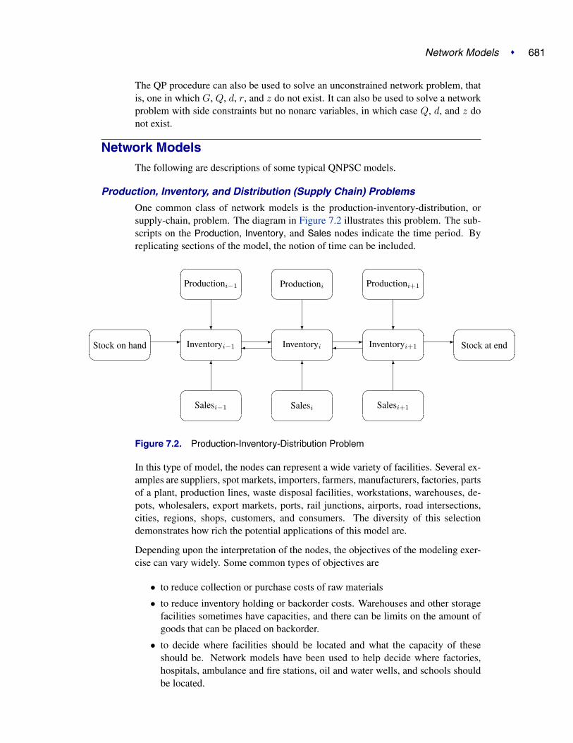
Network Models � 681
The QP procedure can also be used to solve an unconstrained network problem, thatis, one in which G, Q, d, r, and z do not exist. It can also be used to solve a networkproblem with side constraints but no nonarc variables, in which case Q, d, and z donot exist.
Network ModelsThe following are descriptions of some typical QNPSC models.
Production, Inventory, and Distribution (Supply Chain) Problems
One common class of network models is the production-inventory-distribution, orsupply-chain, problem. The diagram in Figure 7.2 illustrates this problem. The sub-scripts on the Production, Inventory, and Sales nodes indicate the time period. Byreplicating sections of the model, the notion of time can be included.
�
�
�
�Salesi−1
�
�
�
�Salesi
�
�
�
�Salesi+1
�
�
�
�Inventoryi−1
�
�
�
�Inventoryi
�
�
�
�Inventoryi+1
�
�
�
�Productioni−1
�
�
�
�Productioni
�
�
�
�Productioni+1
�
�
�
�Stock on hand
�
�
�
�Stock at end
� � � �� �
� � �
� � �
Figure 7.2. Production-Inventory-Distribution Problem
In this type of model, the nodes can represent a wide variety of facilities. Several ex-amples are suppliers, spot markets, importers, farmers, manufacturers, factories, partsof a plant, production lines, waste disposal facilities, workstations, warehouses, de-pots, wholesalers, export markets, ports, rail junctions, airports, road intersections,cities, regions, shops, customers, and consumers. The diversity of this selectiondemonstrates how rich the potential applications of this model are.
Depending upon the interpretation of the nodes, the objectives of the modeling exer-cise can vary widely. Some common types of objectives are
• to reduce collection or purchase costs of raw materials
• to reduce inventory holding or backorder costs. Warehouses and other storagefacilities sometimes have capacities, and there can be limits on the amount ofgoods that can be placed on backorder.
• to decide where facilities should be located and what the capacity of theseshould be. Network models have been used to help decide where factories,hospitals, ambulance and fire stations, oil and water wells, and schools shouldbe located.

682 � Chapter 7. The QP Procedure (Experimental)
• to determine the assignment of resources (machines, production capability,workforce) to tasks, schedules, classes, or files
• to determine the optimal distribution of goods or services. This usually meansminimizing transportation costs and reducing transit time or distance covered.
• to find the shortest path from one location to another
• to ensure that demands (for example, production requirements, market de-mands, contractual obligations) are met
• to maximize profits from the sale of products or the charge for services
• to maximize production by identifying bottlenecks
Some specific applications are
• car distribution models. These help determine which models and numbers ofcars should be manufactured in which factories, and where to distribute carsfrom these factories to zones in the United States in order to meet customerdemand at least cost.
• models in the timber industry. These help determine when to plant and millforests, schedule production of pulp, paper, and wood products, and distributeproducts for sale or export.
• military applications. The nodes can be theaters, bases, ammunition dumps,logistical suppliers, or radar installations. Some models are used to find thebest ways to mobilize personnel and supplies and to evacuate the wounded inthe least amount of time.
• communications applications. The nodes can be telephone exchanges, trans-mission lines, satellite links, and consumers. In a model of an electrical grid,the nodes can be transformers, power stations, watersheds, reservoirs, dams,and consumers. The effect of high loads or outages might be of concern.
Proportionality Constraints
In many models, you have the characteristic that a flow through an arc must be pro-portional to the flow through another arc. Side constraints are often necessary tomodel this situation. Such constraints are called proportionality constraints and areuseful in models where production is subject to refining or modification into differentmaterials. The amount of each output, or any waste, evaporation, or reduction can bespecified as a proportion of input.
Typically, the arcs near the supply nodes carry raw materials and the arcs near thedemand nodes carry refined products. For example, in a model of the milling industry,the flow through some arcs may represent quantities of wheat. After the wheat isprocessed, the flow through other arcs might be flour. For others it might be bran. Theside constraints model the relationship between the amount of flour or bran producedas a proportion of the amount of wheat milled. Some of the wheat can end up asneither flour, bran, nor any useful product, so this waste is drained away through arcsto a waste node.

Network Models � 683
�
�
�
�Wheat
�
�
�
�Mill
�
�
�
�Flour
�
�
�
�Bran
�
�
�
�Other
� ��
��
��
��
���
��
��
��
��
����
1.0 0.2
0.3
0.5
Figure 7.3. Proportionality Constraints
In order for arcs to be specified in side constraints, they must be named. By default,PROC QP names arcs using the names of the nodes at the head and tail of the arc.An arc is named with its tail node name followed by an underscore and its head nodename. For example, an arc from node from to node to is called from–to.
Consider the network fragment in Figure 7.3. The arc Wheat–Mill conveys the wheatmilled. The cost of flow on this arc is the milling cost. The capacity of this arc is thecapacity of the mill. The lower flow bound on this arc is the minimum quantity thatmust be milled for the mill to operate economically. The constraints
0.3 Wheat–Mill − Mill–Flour = 0.00.2 Wheat–Mill − Mill–Bran = 0.0
force every unit of wheat that is milled to produce 0.3 units of flour and 0.2 units ofbran. Note that it is not necessary to specify the constraint
0.5 Wheat–Mill − Mill–Other = 0.0
since flow conservation implies that any flow that does not traverse through Mill–Flouror Mill–Bran must be conveyed through Mill–Other. Computationally, it is better ifthis constraint is not specified, since there is one less side constraint and fewer prob-lems with numerical precision. Notice that the sum of the proportions must equal 1.0exactly; otherwise, flow conservation is violated.
Blending Constraints
Blending or quality constraints can also influence the recipes or proportions of in-gredients that are mixed. For example, different raw materials can have differentproperties. In an application of the oil industry, the amount of products that are ob-tained could be different for each type of crude oil. Furthermore, fuel might have aminimum octane requirement or limited sulphur or lead content, so that a blending ofcrude oils is needed to produce the product.

684 � Chapter 7. The QP Procedure (Experimental)
The network fragment in Figure 7.4 shows an example of this.
�
�
�
�USA
�
�
�
�MidEast
�
�
�
�Port
�
�
�
�Refinery
�
�
�
�Gasoline
�
�
�
�Diesel
�
�
�
�Other�
��
���
��
��
��
� ��
��
����
��
��
��
���
5 units/liter
4 units/liter
4.75 units/liter
Figure 7.4. Blending Constraints
The arcs MidEast–Port and USA–Port convey crude oil from the two sources.The arc Port–Refinery represents refining, while the arcs Refinery–Gasoline andRefinery–Diesel carry the gas and diesel produced. The proportionality constraints
0.4 Port–Refinery − Refinery–Gasoline = 0.00.2 Port–Refinery − Refinery–Diesel = 0.0
capture the restrictions for producing gasoline and diesel from crude oil. Suppose thatonly crude oil from the Middle East is used, then the resulting diesel would contain5 units of sulphur per liter. If only crude oil from the U.S.A. is used, the resultingdiesel would contain 4 units of sulphur per liter. Diesel can have at most 4.75 units ofsulphur per liter. Some crude oil from the U.S.A. must be used if Middle East crudeoil is used in order to meet the 4.75 sulphur per liter limit. The side constraint tomodel this requirement is
5 MidEast–Port +4 USA–Port −4.75 Port–Refinery ≤ 0.0
Since Port–Refinery = MidEast–Port + USA–Port, flow conservation allows thisconstraint to be simplified to
1 MidEast–Port −3 USA–Port ≤ 0.0
If, for example, 120 units of crude oil from the Middle East are used, then at least40 units of crude oil from the U.S.A. must be used. The preceding constraint issimplified because you assume that the sulphur concentration of diesel is proportionalto the sulphur concentration of the crude oil mix. If this is not the case, the relation
0.2 Port–Refinery = Refinery–Diesel

Network Models � 685
is used to obtain
5 MidEast–Port +4 USA–Port −4.75 (1.0/0.2 Refinery–Diesel) ≤ 0.0
which equals
5 MidEast–Port +4 USA–Port −23.75 Refinery–Diesel ≤ 0.0
An example similar to this oil industry problem is solved in the “Introductory QNPSCExample” section on page 690.
Multicommodity Problems
Side constraints are also used in models in which there are capacities on transporta-tion or some other shared resource, or there are limits on overall production or de-mand in multicommodity, multidivisional, or multiperiod problems. Each commod-ity, division, or period can have a separate network coupled to one main system by theside constraints. Side constraints are used to combine the outputs of subdivisions ofa problem (either commodities, outputs in distinct time periods, or different processstreams) to meet overall demands or to limit overall production or expenditures. Thismethod is more desirable than doing separate local optimizations for individual com-modity, process, or time networks and then trying to establish relationships betweeneach when determining an overall policy if the global constraint is not satisfied. Ofcourse, to make models more realistic, side constraints may be necessary in the localproblems.
�
�
�
�Factorycom2
�
�
�
�Factorycom1
�
�
�
�City2com2
�
�
�
�City1com2
�
�
�
�City2com1
�
�
�
�City1com1
���������������
���������������
���������������
���������������
Commodity 1
Commodity 2
Figure 7.5. Multicommodity Problem

686 � Chapter 7. The QP Procedure (Experimental)
Figure 7.5 shows two network fragments. They represent identical production anddistribution sites of two different commodities. The suffix com1 represents com-modity 1 and the suffix com2 represents commodity 2. The nodes Factorycom1 andFactorycom2 model the same factory, and nodes City1com1 and City1com2 modelthe same location, city 1. Similarly, City2com1 and City2com2 are the same location,city 2. Suppose that commodity 1 occupies 2 cubic meters, commodity 2 occupies 3cubic meters, the truck dispatched to city 1 has a capacity of 200 cubic meters, andthe truck dispatched to city 2 has a capacity of 250 cubic meters. How much of eachcommodity can be loaded onto each truck? The side constraints for this case are
2 Factorycom1–City1com1 +3 Factorycom2–City1com2 ≤ 2002 Factorycom1–City2com1 +3 Factorycom2–City2com2 ≤ 250
Large Modeling Strategies
In many cases, the flow through an arc might actually represent the flow or movementof a commodity from place to place or from time period to time period. However,sometimes an arc is included in the network as a method of capturing some aspect ofthe problem that you would not normally think of as part of a network model. Thereis no commodity movement associated with that arc. For example, in a multiprocess,multiproduct model (Figure 7.6), there might be subnetworks for each process andeach product. The subnetworks can be joined together by a set of arcs that have flowsthat represent the amount of product j produced by process i. To model an upper-limit constraint on the total amount of product j that can be produced, direct all arcscarrying product j to a single node, and from there through a single arc. The capacityof this arc is the upper limit of product j production. It is preferable to model thisstructure in the network rather than to include it in the side constraints because theefficiency of the optimizer may be less affected by a reasonable increase in the sizeof the network rather than increasing the number of complicating side constraints.
�
�
�
�
��
��
����
���
���
���
Capacity ofProcess 2
Process 2 subnetwork
�
�
�
�
��
��
����
���
���
���
Capacity ofProcess 1
Process 1 subnetwork
�
�
�
�
��
��
����
���
���
���
Capacity is upper limit ofProduct 2 production
Product 2 subnetwork
�
�
�
�
��
��
����
���
���
���
Capacity is upper limit ofProduct 1 production
Product 1 subnetwork
�
�
��
��
�����
��
���
Figure 7.6. Multiprocess, Multiproduct Example
When starting a project, it is often a good strategy to use a small network formulationand then use that model as a framework upon which to add detail. For example, inthe multiprocess, multiproduct model, you might start with the network depicted in

Network Models � 687
Figure 7.6. Then, for example, the process subnetwork can be enhanced to includethe distribution of products. Other phases of the operation could be included byadding more subnetworks. Initially, these subnetworks can be single nodes, but insubsequent studies they can be expanded to include greater detail.
Advantages of Network Models over QP Models
Many quadratic programming problems have large embedded network structures.Such problems often result when modeling manufacturing processes, transportationor distribution networks, or resource allocation, or when deciding where to locatefacilities. Often, some commodity is to be moved from place to place, so the morenatural formulation in many applications is that of a constrained network rather thana quadratic program.
Using a network diagram to visualize a problem makes it possible to capture theimportant relationships in an easily understood picture form. The network diagramaids the communication between model builder and model user, making it easier tocomprehend how the model is structured, how it can be changed, and how results canbe interpreted.
If a network structure is embedded in a quadratic program, the problem is a QNPSC(see the “Quadratic Network Problems with Side Constraints” section on page 679).When the network part of the problem is large compared to the nonnetwork part,especially if the number of side constraints is small, it is worthwhile to exploit thisstructure to describe the model. Rather than generating the data for the flow conser-vation constraints, generate instead the data for the nodes and arcs of the network.
Flow Conservation Constraints
The constraints Fx = b in QNPSC (see the “Quadratic Network Problems withSide Constraints” section on page 679) are referred to as the nodal flow conservationconstraints. These constraints algebraically state that the sum of the flow througharcs directed toward a node plus that node’s supply, if any, equals the sum of the flowthrough arcs directed away from that node plus that node’s demand, if any. The flowconservation constraints are implicit in the network model and should not be specifiedexplicitly in side constraint data when using PROC QP to solve QNPSC problems.
Nonarc Variables
Nonarc variables can be used to simplify side constraints. For example, if a sum offlows appears in many constraints, it may be worthwhile to equate this expressionwith a nonarc variable and use this in the other constraints. This keeps the constraintcoefficient matrix sparse. By assigning a nonarc variable a nonzero objective functioncoefficient, it is then possible to incur a cost for using resources above some lowestfeasible limit. Similarly, a profit (a negative objective function coefficient value) canbe made if all available resources are not used.
In some models, nonarc variables are used in constraints to absorb excess resources orsupply needed resources. Then, either the excess resource can be used or the neededresource can be supplied to another component of the model.

688 � Chapter 7. The QP Procedure (Experimental)
For example, consider a multicommodity problem of making television sets that haveeither 19- or 25-inch screens. In their manufacture, three and four chips, respectively,are used. Production occurs at two factories during March and April. The supplierof chips can supply only 2,600 chips to factory 1 and 3,750 chips to factory 2 eachmonth. The names of arcs are in the form Prodn–s–m, where n is the factory number,s is the screen size, and m is the month. For example, Prod1–25–Apr is the arc thatconveys the number of 25-inch TVs produced in factory 1 during April.
As described, the constraints are
3 Prod1–19–Mar +4 Prod1–25–Mar ≤ 26003 Prod2–19–Mar +4 Prod2–25–Mar ≤ 37503 Prod1–19–Apr +4 Prod1–25–Apr ≤ 26003 Prod2–19–Apr +4 Prod2–25–Apr ≤ 3750
If there are chips that could be obtained for use in March but not used for productionin March, why not keep these unused chips until April? Furthermore, if the Marchexcess chips at factory 1 could be used either at factory 1 or factory 2 in April, themodel becomes
3 Prod1–19–Mar +4 Prod1–25–Mar + F1–Unused–Mar = 26003 Prod2–19–Mar +4 Prod2–25–Mar + F2–Unused–Mar = 3750
3 Prod1–19–Apr +4 Prod1–25–Apr −F1–Kept–Since–Mar = 26003 Prod2–19–Apr +4 Prod2–25–Apr −F2–Kept–Since–Mar = 3750
F1–Unused–Mar + F2–Unused–Mar (continued)− F1–Kept–Since–Mar − F2–Kept–Since–Mar ≥ 0.0
where F1–Kept–Since–Mar is the number of chips used during April at factory 1 thatwere obtained in March at either factory 1 or factory 2, and F2–Kept–Since–Mar isthe number of chips used during April at factory 2 that were obtained in March. Thelast constraint ensures that the number of chips used during April that were obtainedin March does not exceed the number of chips not used in March. There may be acost to hold chips in inventory. This can be modeled by a positive objective functioncoefficient for the nonarc variables F1–Kept–Since–Mar and F2–Kept–Since–Mar.Moreover, nonarc variable upper bounds represent an upper limit on the number ofchips that can be held in inventory between March and April.
Getting Started: QNPSC Problems
To solve QNPSC problems using PROC QP, you save a representation of the networkand the side constraints in four SAS data sets. These data sets are then passed toPROC QP for solution. There are various forms that a problem’s data can take. Youcan use any one or a combination of several of these forms.
The NODEDATA= data set contains the names of the supply and demand nodes andthe supply or demand associated with each. These are the elements in the columnvector b in the QNPSC problem (see the “Quadratic Network Problems with SideConstraints” section on page 679).

Getting Started: QNPSC Problems � 689
The ARCDATA= data set contains information about the variables of the problem.Usually these are arcs, but there can be data related to nonarc variables in theARCDATA= data set as well.
An arc is identified by the names of its tail node (where it originates) and head node(where it is directed). Each observation can be used to identify an arc in the networkand, optionally, the cost per unit flow across the arc, the arc’s capacity, lower flowbound, and name. These data are associated with the matrix F and the vectors c,l, and u in the QNPSC problem (see the “Quadratic Network Problems with SideConstraints” section on page 679).
Note: Although F is a node-arc incidence matrix, it is specified in the ARCDATA=data set by arc definitions. Do not explicitly specify these flow conservation con-straints as constraints of the problem.
In addition, the ARCDATA= data set can be used to specify information about nonarcvariables, including linear objective function coefficients, lower and upper valuebounds, and names. These data are the elements of the vectors d, m, and v in theQNPSC problem (see the “Quadratic Network Problems with Side Constraints” sec-tion on page 679). Data for an arc or nonarc variable can be given in more than oneobservation.
Supply and demand data can also be specified in the ARCDATA= data set. In such acase, the NODEDATA= data set may not be needed.
The CONDATA= data set describes the side constraints and their right-hand sides.These data are elements of the matrices G and Q and the vector r. Constraint typesare also specified in the CONDATA= data set. This data set can include upper boundvalues or capacities, lower flow or value bounds, and costs or objective function co-efficients. It is possible to give all information about some or all nonarc variables inthe CONDATA= data set.
An arc is identified in this data set by its name. If you specify an arc’s name in theARCDATA= data set, then this name is used to associate data in the CONDATA=data set with that arc. Each arc also has a default name that is the name of the tail andhead node of the arc concatenated together and separated by an underscore character;tail–head, for example.
If you use the dense side constraint input format (described in the “CONDATA= DataSet” section on page 712), and want to use the default arc names, these arc names arenames of SAS variables in the VAR list of the CONDATA= data set.
If you use the sparse side constraint input format (see the “CONDATA= Data Set”section on page 712) and want to use the default arc names, these arc names arevalues of the COLUMN list variable of the CONDATA= data set.
The HESSIAN= data set describes the Hessian matrix. These data are elements ofthe H matrix in the QNPSC problem (see the “Quadratic Network Problems withSide Constraints” section on page 679). Each observation of the HESSIAN= data setprovides data for an element of the Hessian matrix. If there is a term 6xarc3xnonarc5
in the objective function, then Harc3,nonarc5 = 6, and there will be an observationin the HESSIAN= data set that has the value ‘arc3’ for the HESSIANROW variable,

690 � Chapter 7. The QP Procedure (Experimental)
the value ‘nonarc5’ for the HESSIANCOLUMN variable, and the value 6 for theHESSIANCOEF variable. The Hessian matrix is symmetric so Hnonarc5,arc3 = 6also, and another observation of the HESSIAN= data set could have values ‘nonarc5’,‘arc3’, and 6 for the HESSIANROW, HESSIANCOLUMN, and HESSIANCOEFvariables, respectively. However, you need only one of these observations; PROC QPwill assume the existence of the element’s symmetric pair.
Note that while data for a nondiagonal element of the H matrix corresponds ex-actly to the term in the objective function, data for diagonal elements of H are dou-bled. For the term 6xarc3xnonarc5 in the objective function, the nondiagonal elementHarc3,nonarc5 = Hnonarc5,arc3 = 6 and the value 6 is used in the corresponding obser-vation of the HESSIAN= data set. If there is a term 5x2
arc4 in the objective function,the diagonal element Harc4,arc4 = 10 and the value 10 is used in the correspondingobservation of the HESSIAN= data set. In that observation, both the HESSIANROWand the HESSIANCOLUMN variables would have the value ‘arc4’.
PROC QP reads the data from the NODEDATA= data set, the ARCDATA= data set,the CONDATA= data set, and the HESSIAN= data set. Error checking is performed,and the model is converted into an equivalent QP. The optimal solution to the equiv-alent QP is then found. This QP is converted back to the original QNPSC problem,and the optimum for this is derived from the optimum of the equivalent QP. If theproblem was preprocessed, the model is now post-processed, where fixed variablesare reintroduced. The solution can be saved in the CONOUT= data set.
Introductory QNPSC Example
Consider the following transshipment problem for an oil company. Crude oil isshipped to refineries where it is processed into gasoline and diesel fuel. The gaso-line and diesel fuel are then distributed to service stations. At each stage, there areshipping, processing, and distribution costs. Also, there are lower flow bounds andcapacities.
In addition, there are two sets of side constraints. The first set is that two times thecrude oil from the Middle East cannot exceed the throughput of a refinery plus 15units. (The phrase “plus 15 units” that finishes the last sentence is used to enablesome side constraints in this example to have a nonzero right-hand side.) The secondset of constraints is necessary to model the situation that one unit of crude oil mixprocessed at a refinery yields three-fourths of a unit of gasoline and one-fourth of aunit of diesel fuel.
Because there are two products that are not independent in the way in which theyflow through the network, a QNPSC is an appropriate model for this example (seeFigure 7.7). The side constraints are used to model the limitations on the amount ofMiddle Eastern crude oil that can be processed by each refinery, and the conversionproportions of crude oil to gasoline and diesel fuel.

Introductory QNPSC Example � 691
�
�
�
�u.s.a.
�
�
�
�refinery2
�
�
�
�middle east
�
�
�
�refinery1
�
�
�
�r2
�
�
�
�r1
�
�
�
�ref2 diesel
�
�
�
�ref2 gas
�
�
�
�ref1 diesel
�
�
�
�ref1 gas
�
�
�
�servstn2
diesel
�
�
�
�servstn2
gas
�
�
�
�servstn1
diesel
�
�
�
�servstn1
gas
�
�
�
�
�
�
�
�
������������������
���������������
��
��
���
��
��
���
��
��
���
��
��
���
!!!!!!!!!!!!!!!!"
!!!!!!!!!!!!!!!!"
################$
################$
Figure 7.7. Oil Industry Example
To solve this problem with PROC QP, you first save a representation of the model infour SAS data sets. In the NODEDATA= data set, you name the supply and demandnodes and give the associated supplies and demands. To distinguish demand nodesfrom supply nodes, specify demands as negative quantities. For the oil example, theNODEDATA= data set can be saved as follows:
title ’Oil Industry Example’;title3 ’Setting Up Nodedata = Noded For PROC QP’;data noded;
input _node_&$15. _sd_;datalines;
middle east 100u.s.a. 80servstn1 gas -95servstn1 diesel -30servstn2 gas -40servstn2 diesel -15;
The ARCDATA= data set contains the rest of the information about the network.Each observation in the data set identifies an arc in the network and gives the cost perflow unit across the arc, the capacity of the arc, the lower bound on flow across thearc, and the name of the arc.
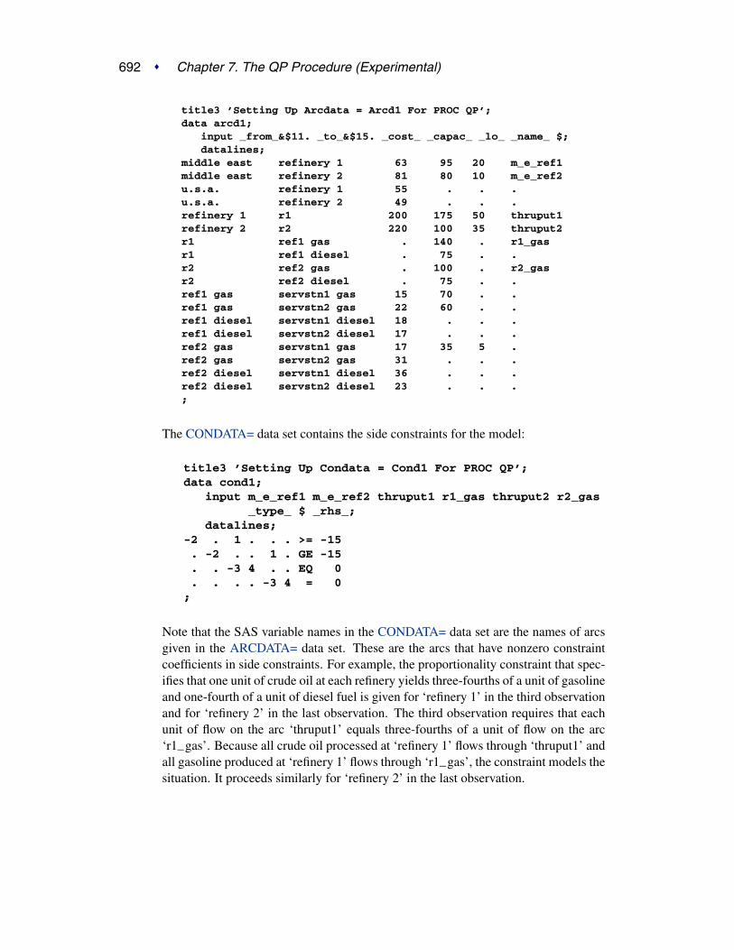
692 � Chapter 7. The QP Procedure (Experimental)
title3 ’Setting Up Arcdata = Arcd1 For PROC QP’;data arcd1;
input _from_&$11. _to_&$15. _cost_ _capac_ _lo_ _name_ $;datalines;
middle east refinery 1 63 95 20 m_e_ref1middle east refinery 2 81 80 10 m_e_ref2u.s.a. refinery 1 55 . . .u.s.a. refinery 2 49 . . .refinery 1 r1 200 175 50 thruput1refinery 2 r2 220 100 35 thruput2r1 ref1 gas . 140 . r1_gasr1 ref1 diesel . 75 . .r2 ref2 gas . 100 . r2_gasr2 ref2 diesel . 75 . .ref1 gas servstn1 gas 15 70 . .ref1 gas servstn2 gas 22 60 . .ref1 diesel servstn1 diesel 18 . . .ref1 diesel servstn2 diesel 17 . . .ref2 gas servstn1 gas 17 35 5 .ref2 gas servstn2 gas 31 . . .ref2 diesel servstn1 diesel 36 . . .ref2 diesel servstn2 diesel 23 . . .;
The CONDATA= data set contains the side constraints for the model:
title3 ’Setting Up Condata = Cond1 For PROC QP’;data cond1;
input m_e_ref1 m_e_ref2 thruput1 r1_gas thruput2 r2_gas_type_ $ _rhs_;
datalines;-2 . 1 . . . >= -15. -2 . . 1 . GE -15. . -3 4 . . EQ 0. . . . -3 4 = 0;
Note that the SAS variable names in the CONDATA= data set are the names of arcsgiven in the ARCDATA= data set. These are the arcs that have nonzero constraintcoefficients in side constraints. For example, the proportionality constraint that spec-ifies that one unit of crude oil at each refinery yields three-fourths of a unit of gasolineand one-fourth of a unit of diesel fuel is given for ‘refinery 1’ in the third observationand for ‘refinery 2’ in the last observation. The third observation requires that eachunit of flow on the arc ‘thruput1’ equals three-fourths of a unit of flow on the arc‘r1–gas’. Because all crude oil processed at ‘refinery 1’ flows through ‘thruput1’ andall gasoline produced at ‘refinery 1’ flows through ‘r1–gas’, the constraint models thesituation. It proceeds similarly for ‘refinery 2’ in the last observation.

Introductory QNPSC Example � 693
Finally, the HESSIAN= data set for this example can be generated using the followingcode. Note that the names of arcs also appear in this data set.
title3 ’Setting Up Hessian For PROC QP’;data hessian1;
input _row_&$27. _col_&$27. _coef_;datalines;
middle east_refinery 1 ref1 gas_servstn1 gas .0010u.s.a._refinery 1 ref1 diesel_servstn1 diesel .00021u.s.a._refinery 2 ref1 diesel_servstn2 diesel .00002ref1 diesel_servstn2 diesel ref1 diesel_servstn2 diesel 358.2u.s.a._refinery 1 u.s.a._refinery 1 10.4u.s.a._refinery 2 u.s.a._refinery 2 50.4r1_ref1 gas r1_ref1 gas 200r2_ref2 gas r2_ref2 gas 10;
To find the minimum cost flow through the network that satisfies the supplies, de-mands, and side constraints, invoke PROC QP as follows:
proc qpbytes=1000000stop_dg=1e-6nodedata=noded /* the supply and demand data */arcdata=arcd1 /* the arc descriptions */condata=cond1 /* the side constraints */hessian=hessian1 /* the hessian matrix */conout=solution; /* the solution data set */run;
The following messages, which appear on the SAS log, summarize the model as readby PROC QP and note the progress toward a solution.
NOTE: Number of nodes= 14 .NOTE: Number of supply nodes= 2 .NOTE: Number of demand nodes= 4 .NOTE: Total supply= 180 , total demand= 180 .NOTE: Number of arcs= 18 .NOTE: Number of <= side constraints= 0 .NOTE: Number of == side constraints= 2 .NOTE: Number of >= side constraints= 2 .NOTE: Number of side constraint coefficients= 8 .NOTE: The following messages relate to the equivalent
Quadratic Programming problem solved by theInterior Point algorithm.
NOTE: Number of <= constraints= 0 .NOTE: Number of == constraints= 16 .NOTE: Number of >= constraints= 2 .NOTE: Number of constraint coefficients= 44 .NOTE: Number of variables= 18 .NOTE: There are 8 diagonal and superdiagonal elements
in the Hessian matrix.NOTE: Objective= 494237.75987.

694 � Chapter 7. The QP Procedure (Experimental)
NOTE: The data set WORK.SOLUTION has 18 observationsand 9 variables.
NOTE: There were 18 observations read from the dataset WORK.ARCD1.
NOTE: There were 6 observations read from the dataset WORK.NODED.
NOTE: There were 8 observations read from the dataset WORK.HESSIAN1.
NOTE: There were 4 observations read from the dataset WORK.COND1.
The first set of messages shows the size of the problem. The next set of messagesprovides statistics on the size of the equivalent QP problem. The number of variablesmay not equal the number of arcs if the problem has nonarc variables. This examplehas none. To convert a network to the equivalent QP problem, a flow conservationconstraint must be created for each node (including an excess or bypass node, ifrequired). This explains why the number of equality constraints and the number ofconstraint coefficients differ from the number of equality side constraints and thenumber of coefficients in all side constraints.
Unlike PROC LP, which displays the solution and other information as output, PROCQP saves the optimum in the output SAS data set that you specify. For this example,the solution is saved in the SOLUTION data set. It can be displayed with the PRINTprocedure as follows:
title3 ’Optimum’;proc print data=solution;
format _name_ $12.;run;

Typical PROC QP Run: QNPSC Problems � 695
Oil Industry Example
Optimum
_ __ S D
_ _ c _ U E _f c a n P M Fr _ o p _ a P A L
O o t s a l m L N Ob m o t c o e Y D Ws _ _ _ _ _ _ _ _ _
1 refinery 1 r1 200 175 50 thruput1 . . 80.00002 refinery 2 r2 220 100 35 thruput2 . . 100.0003 r1 ref1 diesel 0 75 0 . . 20.00004 r1 ref1 gas 0 140 0 r1_gas . . 60.00005 r2 ref2 diesel 0 75 0 . . 25.00006 r2 ref2 gas 0 100 0 r2_gas . . 75.00007 middle east refinery 1 63 95 20 m_e_ref1 100 . 42.50008 u.s.a. refinery 1 55 99999999 0 u.s.a._refin 80 . 37.50009 middle east refinery 2 81 80 10 m_e_ref2 100 . 57.500010 u.s.a. refinery 2 49 99999999 0 u.s.a._refin 80 . 42.500011 ref1 diesel servstn1 diesel 18 99999999 0 ref1 diesel_ . 30 19.999212 ref2 diesel servstn1 diesel 36 99999999 0 . 30 10.000813 ref1 gas servstn1 gas 15 70 0 ref1 gas_ser . 95 60.000014 ref2 gas servstn1 gas 17 35 5 . 95 35.000015 ref1 diesel servstn2 diesel 17 99999999 0 ref1 diesel_ . 15 0.000816 ref2 diesel servstn2 diesel 23 99999999 0 . 15 14.999217 ref1 gas servstn2 gas 22 60 0 . 40 0.000018 ref2 gas servstn2 gas 31 99999999 0 . 40 40.0000
Figure 7.8. CONOUT=SOLUTION
Notice that, in CONOUT=SOLUTION (Figure 7.8), the optimal flow through eacharc in the network is given in the variable named –FLOW– .
Typical PROC QP Run: QNPSC Problems
You start PROC QP by giving the PROC QP statement. You can specify many optionsin the PROC QP statement to control the procedure, or you can rely on default settingsand specify very few options. However, there are some options you must specify:
• You must specify the BYTES= parameter to indicate the size of the workingmemory that the procedure is allowed to use. This option has no default.
• When solving QNPSC problems, you must specify the ARCDATA= data set.This option has a default (the SAS data set that was created last before PROCQP began running), but that may need to be overridden.
• The CONDATA= data set must also be specified if the problem is QNPSC andhas side constraints, or if it is a QP problem.
• The HESSIAN= data set must be specified. Note that the Hessian must bepositive semi-definite for minimization problems, and negative semi-definitefor maximization problems.

696 � Chapter 7. The QP Procedure (Experimental)
• When solving a network problem, you must specify the NODEDATA= data setif the model data is given in such a data set.
Some options are frequently required. To output the optimal solution to a SAS dataset, you must specify the CONOUT= option. You may want to indicate reasons whyoptimization should stop (for example, you can indicate the maximum number ofiterations that can be performed), or you may want to alter stopping criteria so thatoptimization does not stop prematurely. Some options enable you to control otheraspects of the interior point algorithm. Specifying certain values for these optionscan reduce the time it takes to solve a problem.
The SAS variable lists should be given next. If you have variables in the input datasets that have special names (for example, a variable in the ARCDATA= data setnamed –TAIL– that has tail nodes of arcs as values), it may not be necessary to havemany or any variable lists. If you do not specify a TAIL variable list, PROC QP willsearch the ARCDATA= data set for a variable named –TAIL– .
What usually follows is a RUN statement, which indicates that all information neededby PROC QP has been given, and the procedure is to start running. This also happensif you specify a statement in your SAS program that PROC QP does not recognize asone of its own, or the next DATA step or procedure.
The QUIT statement indicates that PROC QP must immediately finish.
For example, a PROC QP run might look something like this:
proc qpbytes= /* working memory size */arcdata= /* data set */condata= /* data set */hessian= /* data set *//* other options */
;variable list specifications; /* if necessary */run; /* start running, read data, */
/* and do the optimization */

Syntax: QNPSC Problems � 697
Syntax: QNPSC Problems
Below are statements used in PROC QP when solving a QNPSC problem, listed inalphabetical order as they appear in the text that follows.
PROC QP options ;CAPACITY variable ;COEF variables ;COLUMN variable ;COST variable ;DEMAND variable ;HEADNODE variable ;HESSIANCOEF variable ;HESSIANCOLUMN variable ;HESSIANROW variable ;ID variables ;LO variable ;NAME variable ;NODE variable ;QUIT;RHS variable ;ROW variables ;RUN;SUPDEM variable ;SUPPLY variable ;TAILNODE variable ;TYPE variable ;VAR variables ;
The information related to most of the statements and variable lists are the samewhether you are solving a QP problem or a QNPSC problem. However, there aresome exceptions, as listed in the following table.
Solving QP Problems Solving QNPSC ProblemsPROC QP PROC QPUPPERBD CAPACITYCOEF COEFCOLUMN COLUMNOBJFN COSTID IDLO LONAME NAME
The following statements and variable lists are relevant only when solving a QNPSCproblem: DEMAND, HEADNODE, NODE, SUPDEM, SUPPLY, TAILNODE.

698 � Chapter 7. The QP Procedure (Experimental)
Functional Summary: QNPSC Problems
Table 7.2 outlines the options that can be specified in the QP procedure when solvinga QNPSC problem. All options are specified in the PROC QP statement.
Table 7.2. Functional Summary
Description Statement Option
Input Data Set Options:arcs input data set PROC QP ARCDATA=nodes input data set PROC QP NODEDATA=constraint input data set PROC QP CONDATA=Hessian input data set PROC QP HESSIAN=
Output Data Set Option:solution data set PROC QP CONOUT=
Data Set Read Options:CONDATA has sparse data format PROC QP SPARSECONDATAdefault constraint type PROC QP DEFCONTYPE=special COLUMN variable value PROC QP TYPEOBS=special COLUMN variable value PROC QP RHSOBS=used to interpret arc and variable names PROC QP NAMECTRL=no nonarc data in ARCDATA PROC QP ARCS–ONLY–ARCDATAdata for an arc found once in ARCDATA PROC QP ARC–SINGLE–OBSdata for a constraint found once in CONDATA PROC QP CON–SINGLE–OBSdata for a coefficient found once in CONDATA PROC QP NON–REPLIC=data is grouped, exploited during data read PROC QP GROUPED=
Problem Size Specification Options:approximate number of nodes PROC QP NNODES=approximate number of arcs PROC QP NARCS=approximate number of variables PROC QP NNAS=approximate number of coefficients PROC QP NCOEFS=approximate number of constraints PROC QP NCONS=
Network Options:default arc cost, objective function coefficient PROC QP DEFCOST=default arc capacity, variable upper bound PROC QP DEFCAPACITY=default arc flow, variable lower bound PROC QP DEFMINFLOW=network’s only supply node PROC QP SOURCE=SOURCE’s supply capability PROC QP SUPPLY=network’s only demand node PROC QP SINK=SINK’s demand PROC QP DEMAND=convey excess supply/demand through network PROC QP THRUNETfind max flow between SOURCE and SINK PROC QP MAXFLOWcost of bypass arc, MAXFLOW problem PROC QP BYPASSDIVIDE=find shortest path from SOURCE to SINK PROC QP SHORTPATH

PROC QP Statement: QNPSC Problems � 699
Description Statement Option
Memory Control Options:issue memory usage messages to SAS log PROC QP MEMREPnumber of bytes to use for main memory PROC QP BYTES=
Miscellaneous Options:infinity value PROC QP INFINITY=maximization instead of minimization PROC QP MAXIMIZEzero tolerance, real number comparisons PROC QP ZEROTOL=suppress similar SAS log messages PROC QP VERBOSE=duality gap stopping criterion PROC QP STOP–DG=
PROC QP Statement: QNPSC Problems
PROC QP options ;
This statement invokes the procedure. The following options can be specified in thePROC QP statement. Details about the PROC QP statement for solving a QP problemwithout a network component are found in the “PROC QP Statement: QP Problems”section on page 667.
Data Set Options: QNPSC Problems
This section briefly describes all the input and output data sets used by PROC QPwhen solving QNPSC problems. The ARCDATA= data set, the NODEDATA= dataset, the CONDATA= data set, and the HESSIAN= data set can contain SAS variablesthat have special names, for instance –UPPERBD, –OBJFN– , and –HEAD– . PROCQP looks for such variables if you do not give explicit variable list specifications. Ifa SAS variable with a special name is found, and that SAS variable is not in anothervariable list specification, PROC QP determines that values of the SAS variable areto be interpreted in a special way. By using SAS variables that have special names,you may not need to have any variable list specifications.
ARCDATA=SAS-data-setnames the data set that contains arc and, optionally, nonarc variable information andnodal supply/demand data. The ARCDATA= data set must be specified in all PROCQP statements when solving QNPSC problems.
If your problem is a QP without a network component, the ARCDATA= data set isoptional. You can specify QP variable information such as objective function coeffi-cients, and lower and upper bounds.
CONDATA=SAS-data-setnames the data set that contains the side constraint data. The data set can also containother data such as arc costs, capacities, lower flow bounds, nonarc variable upperand lower bounds, and objective function coefficients. The CONDATA= data set is

700 � Chapter 7. The QP Procedure (Experimental)
required in order for PROC QP to solve a constrained problem. See the “CONDATA=Data Set” section on page 712 for more information.
Specific details about this option for QP problems are given in the “Data Set Options:QP Problems” section beginning on page 667.
CONOUT=SAS-data-setCOUT=SAS-data-set
names the output data set that receives an optimal solution. See the “CONOUT= DataSet” section on page 721 for more information.
HESSIAN=SAS-data-setnames the data set that describes the Hessian matrix. These data are elements of theH matrix. See the “HESSIAN= Data Set” section on page 720 for more information.
NODEDATA=SAS-data-setnames the data set that contains the node supply and demand specifications. Youdo not need observations in the NODEDATA= data set for transshipment nodes.(Transshipment nodes neither supply nor demand flow.) All nodes are assumed tobe transshipment nodes unless supply or demand data indicate otherwise. It is ac-ceptable for some arcs to be directed toward supply nodes or away from demandnodes.
This data set is used only when you are solving network problems, in which case theuse of the NODEDATA= data set is optional provided that, if the NODEDATA= dataset is not used, supply and demand details are specified by other means. Other meansinclude using the MAXFLOW or SHORTPATH option, SUPPLY or DEMAND vari-able list (or both) in the ARCDATA= data set, and the SOURCE=, SUPPLY=,SINK=, or DEMAND= option in the PROC QP statement.
General Options: QNPSC Problems
The following is a list of options you can use with PROC QP when solving QNPSCproblems. The options are listed in alphabetical order.
ARCS–ONLY–ARCDATAindicates that the data in the ARCDATA= data set are for arcs only. When PROC QPreads the data in the ARCDATA= data set, memory will not be wasted to receive datafor nonarc variables. The read might then be performed faster. See the section “Howto Make the Data Read of PROC QP More Efficient” on page 730 for details.
ARC–SINGLE–OBSindicates that for all arcs and nonarc variables, data for each arc or nonarc variableis found in only one observation of the ARCDATA= data set. When reading the datain the ARCDATA= data set, PROC QP knows that the data in an observation is foran arc or a nonarc variable that has not had data previously read and that needs to bechecked for consistency. The read might then be performed faster. See the section“How to Make the Data Read of PROC QP More Efficient” on page 730 for details.
If you specify ARC–SINGLE–OBS, PROC QP automatically works as ifGROUPED=ARCDATA is also specified.

PROC QP Statement: QNPSC Problems � 701
Specific details about this option for QP problems are given in the “General Options:QP Problems” section beginning on page 667.
BYPASSDIVIDE=bBYPASSDIV=bBPD=b
should be used only when the MAXFLOW option has been specified; that is, PROCQP is solving a maximal flow problem. PROC QP prepares to solve maximal flowproblems by setting up a bypass arc. This arc is directed from the SOURCE nodeto the SINK node and will eventually convey flow equal to INFINITY minus themaximal flow through the network. The cost of the bypass arc must be great enoughto drive flow through the network, rather than through the bypass arc. Also, the cost ofthe bypass arc must be greater than the eventual total cost of the maximal flow, whichcan be nonzero if some network arcs have nonzero costs. The cost of the bypass isset to the value of the INFINITY= option. Valid values for the BYPASSDIVIDE=option must be greater than or equal to 1.1.
If there are no nonzero costs of arcs in the MAXFLOW problem, the cost ofthe bypass arc is set to 1.0 (-1.0 if maximizing) if you do not specify theBYPASSDIVIDE= option. In the presence of nonzero arc costs, the default valuefor the BYPASSDIVIDE= option is 100.0.
CON–SINGLE–OBSimproves how the CONDATA= data set is read. How it works depends on whetherthe CONDATA has a dense or sparse format.
If the CONDATA= data set has a dense format, specifying CON–SINGLE–OBSindicates that, for each constraint, data for the constraint can be found in only oneobservation of the CONDATA= data set.
If the CONDATA= data set has a sparse format, and data for each arc, nonarc variable,or QP variable can be found in only one observation of the CONDATA= data set,then specify the CON–SINGLE–OBS option. If there are n SAS variables in theROW and COEF variable lists, then each arc or nonarc can have at most n constraintcoefficients in the model. See the section “How to Make the Data Read of PROC QPMore Efficient” on page 730 for details.
Specific details about this option for QP problems are given in the “General Options:QP Problems” section beginning on page 667.
DEFCAPACITY=cDC=c
requests that the default arc capacity and the default nonarc variable value upperbound be c. If this option is not specified, then DEFCAPACITY=INFINITY. Specificdetails about this option for QP problems are given in the “General Options: QPProblems” section beginning on page 667.
DEFCOST=crequests that the default arc cost and the default nonarc variable objective functioncoefficient be c. If this option is not specified, then DEFCOST=0.0. Specific details

702 � Chapter 7. The QP Procedure (Experimental)
about this option for QP problems are given in the “General Options: QP Problems”section beginning on page 667.
DEFMINFLOW=mDMF=m
requests that the default lower flow bound through arcs and the default lowervalue bound of nonarc variables be m. If this option is not specified, thenDEFMINFLOW=0.0. Specific details about this option for QP problems are givenin the “General Options: QP Problems” section beginning on page 667.
DEMAND=dspecifies the demand at the sink node given by the SINK= option. The DEMAND=option should be used only if the SINK= option is given in the PROC QP statementand neither the SHORTPATH option nor the MAXFLOW option is specified. If youare solving a minimum cost network problem and the SINK= option is used to iden-tify the sink node, and the DEMAND= option is not specified, then the demand at thesink node is made equal to the network’s total supply.
MAXFLOWMF
specifies that PROC QP solve a maximum flow problem. In this case, PROC QPfinds the maximum flow from the node specified by the SOURCE= option to thenode specified by the SINK= option. PROC QP automatically assigns an INFINITYsupply to the SOURCE node, and the SINK node is assigned INFINITY demand. Inthis way, the MAXFLOW option sets up a maximum flow problem as an equivalentminimum cost problem.
You can use the MAXFLOW option when solving any flow problem (not necessar-ily a maximum flow problem) when the network has one supply node (with infinitesupply) and one demand node (with infinite demand). The MAXFLOW option canbe used in conjunction with all other options (except SHORTPATH, SUPPLY=, andDEMAND=) and capabilities of PROC QP.
NAMECTRL=iis used to interpret arc and nonarc variable names in the CONDATA= data set. In theARCDATA= data set, an arc is identified by its tail and head node. In the CONDATA=data set, arcs are identified by names. You can give a name to an arc by having aNAME list specification that indicates a SAS variable in the ARCDATA= data setthat has names of arcs as values.
PROC QP requires that arcs that have information about them in the CONDATA= dataset have names, but arcs that do not have information about them in the CONDATA=data set can also have names. Unlike a nonarc variable whose name uniquely identi-fies it, an arc can have several different names. An arc has a default name in the formtail–head, that is, the name of the arc’s tail node followed by an underscore and thename of the arc’s head node.
In the CONDATA= data set, if the dense data format is used (described in the“CONDATA= Data Set” section on page 712), a name of an arc or a nonarc vari-able is the name of a SAS variable listed in the VAR list specification. If the sparse

PROC QP Statement: QNPSC Problems � 703
data format of the CONDATA= data set is used, a name of an arc or a nonarc variableis a value of the SAS variable listed in the COLUMN list specification.
The NAMECTRL= option is used when a name of an arc or a nonarc variable in theCONDATA= data set (either a VAR list variable name or a value of the COLUMNlist variable) is in the form tail–head and there exists an arc with these end nodes. Iftail–head has not already been tagged as belonging to an arc or nonarc variable in theARCDATA= data set, PROC QP needs to know whether tail–head is the name of thearc or the name of a nonarc variable.
If you specify NAMECTRL=1, a name that is not defined in the ARCDATA= data setis assumed to be the name of a nonarc variable. NAMECTRL=2 treats tail–head asthe name of the arc with these end nodes, provided no other name is used to associatedata in the CONDATA= data set with this arc. If the arc does have other names thatappear in the CONDATA= data set, tail–head is assumed to be the name of a nonarcvariable. If you specify NAMECTRL=3, tail–head is assumed to be a name of thearc with these end nodes, whether the arc has other names or not. The default valueis NAMECTRL=3.
If the dense format is used for the CONDATA= data set, there are two circumstancesthat affect how this data set is read:
• Case 1: You specify
options validvarname=v6;
in your SAS session.
• Case 2: You do not specify
options validvarname=v6;
in your SAS session.
For case 1, the SAS System converts SAS variable names in a SAS program to up-percase. The VAR list variable names are uppercased. Because of this, PROC QPautomatically uppercases names of arcs and nonarc variables or QP variables (thevalues of the NAME list variable) in the ARCDATA= data set. The names of arcsand nonarc variables or QP variables (the values of the NAME list variable) appearuppercased in the CONOUT= data set.
Also, if the dense format is used for the CONDATA= data set, be careful with de-fault arc names (names in the form tailnode–headnode). Node names (values inthe TAILNODE and HEADNODE list variables) in the ARCDATA= data set are notautomatically uppercased by PROC QP. Consider the following code.
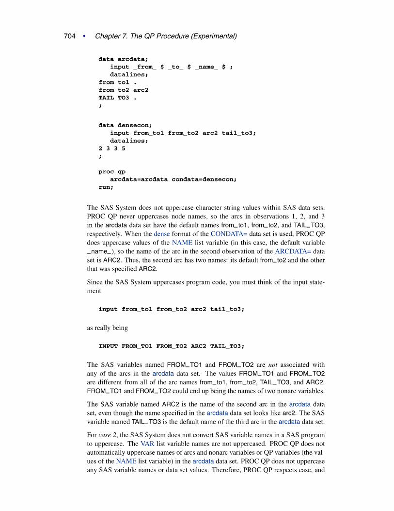
704 � Chapter 7. The QP Procedure (Experimental)
data arcdata;input _from_ $ _to_ $ _name_ $ ;datalines;
from to1 .from to2 arc2TAIL TO3 .;
data densecon;input from_to1 from_to2 arc2 tail_to3;datalines;
2 3 3 5;
proc qparcdata=arcdata condata=densecon;
run;
The SAS System does not uppercase character string values within SAS data sets.PROC QP never uppercases node names, so the arcs in observations 1, 2, and 3in the arcdata data set have the default names from–to1, from–to2, and TAIL–TO3,respectively. When the dense format of the CONDATA= data set is used, PROC QPdoes uppercase values of the NAME list variable (in this case, the default variable
–name–), so the name of the arc in the second observation of the ARCDATA= dataset is ARC2. Thus, the second arc has two names: its default from–to2 and the otherthat was specified ARC2.
Since the SAS System uppercases program code, you must think of the input state-ment
input from_to1 from_to2 arc2 tail_to3;
as really being
INPUT FROM_TO1 FROM_TO2 ARC2 TAIL_TO3;
The SAS variables named FROM–TO1 and FROM–TO2 are not associated withany of the arcs in the arcdata data set. The values FROM–TO1 and FROM–TO2are different from all of the arc names from–to1, from–to2, TAIL–TO3, and ARC2.FROM–TO1 and FROM–TO2 could end up being the names of two nonarc variables.
The SAS variable named ARC2 is the name of the second arc in the arcdata dataset, even though the name specified in the arcdata data set looks like arc2. The SASvariable named TAIL–TO3 is the default name of the third arc in the arcdata data set.
For case 2, the SAS System does not convert SAS variable names in a SAS programto uppercase. The VAR list variable names are not uppercased. PROC QP does notautomatically uppercase names of arcs and nonarc variables or QP variables (the val-ues of the NAME list variable) in the arcdata data set. PROC QP does not uppercaseany SAS variable names or data set values. Therefore, PROC QP respects case, and

PROC QP Statement: QNPSC Problems � 705
characters in the data must have the same case if you mean them to be the same. Notehow the input statement in the DATA step that initialized the data set densecon belowis specified in the following code:
data arcdata;input _from_ $ _to_ $ _name_ $ ;datalines;
from to1 .from to2 arc2TAIL TO3 .;
data densecon;input from_to1 from_to2 arc2 TAIL_TO3;datalines;
2 3 3 5;
proc qparcdata=arcdata condata=densecon;
run;
NARCS=nspecifies the approximate number of arcs. See the section “How to Make the DataRead of PROC QP More Efficient” on page 730 for details.
NNAS=nspecifies the approximate number of nonarc variables. See the section “How to Makethe Data Read of PROC QP More Efficient” on page 730 for details.
NNODES=nspecifies the approximate number of nodes. See the section “How to Make the DataRead of PROC QP More Efficient” on page 730 for details.
SHORTPATHSP
specifies that PROC QP solve a shortest path problem. The QP procedure finds theshortest path between the nodes specified in the SOURCE= option and the SINK=option. The costs of arcs are their lengths. PROC QP automatically assigns a supplyof one flow unit to the SOURCE node and a demand of one flow unit to the SINKnode. In this way, the SHORTPATH option sets up a shortest path problem as anequivalent minimum cost problem.
If a network has one supply node (with supply of one unit) and one demand node(with demand of one unit), you could specify the SHORTPATH option, with theSOURCE= and SINK= nodes, even if the problem is not a shortest path problem.You then should not provide any supply or demand data in the NODEDATA= data setor the ARCDATA= data set.

706 � Chapter 7. The QP Procedure (Experimental)
SINK=sinknameSINKNODE=sinkname
identifies the demand node. The SINK= option is useful when you specify theMAXFLOW option or the SHORTPATH option and you need to specify towardwhich node the maximum flow or shortest path is directed. The SINK= option alsocan be used when a minimum cost problem has only one demand node. Rather thanhaving this information in the ARCDATA= data set or the NODEDATA= data set,you can use the SINK= option with an accompanying DEMAND= specification forthis node. The SINK= option must be the name of a head node of at least one arc;thus, it must have a character value. If the value of the SINK= option is not a validSAS character variable name (if, for example, it contains embedded blanks), it mustbe enclosed in quotes.
SOURCE=sourcenameSOURCENODE=sourcename
identifies a supply node. The SOURCE= option is useful when you specify theMAXFLOW or the SHORTPATH option and need to specify from which node themaximum flow or shortest path originates. The SOURCE= option also can be usedwhen a minimum cost problem has only one supply node. Rather than having this in-formation in the ARCDATA= data set or the NODEDATA= data set, you can use theSOURCE= option with an accompanying SUPPLY= amount of supply at this node.The SOURCE= option must be the name of a tail node of at least one arc; thus, itmust have a character value. If the value of the SOURCE= option is not a valid SAScharacter variable name (if, for example, it contains embedded blanks), it must beenclosed in quotes.
SUPPLY=sspecifies the supply at the source node specified by the SOURCE= option. TheSUPPLY= option should be used only if the SOURCE= option is given in the PROCQP statement and neither the SHORTPATH option nor the MAXFLOW option isspecified. If you are solving a minimum cost network problem and the SOURCE=option is used to identify the source node, and the SUPPLY= option is not specified,then by default the supply at the source node is made equal to the network’s totaldemand.
THRUNETtells PROC QP to force through the network any excess supply (the amount by whichtotal supply exceeds total demand) or any excess demand (the amount by which totaldemand exceeds total supply) as is required. If a network problem has unequal totalsupply and total demand and the THRUNET option is not specified, PROC QP drainsaway the excess supply or excess demand in an optimal manner. The consequencesof specifying or not specifying THRUNET are discussed in the “Balancing TotalSupply and Total Demand” section on page 729.

COLUMN Statement: QNPSC Problems � 707
CAPACITY Statement
CAPACITY variable ;
CAPAC variable ;
UPPERBD variable ;
The CAPACITY statement identifies the SAS variable in the ARCDATA= dataset that contains the capacity of the network arcs and the maximum feasible flowof nonarc variables. If an observation contains nonarc variable information, theCAPACITY list variable is the upper value bound for the nonarc variable named inthe NAME list variable in that observation.
The CAPACITY list variable must have numeric values. It is not necessary to havea CAPACITY statement if the name of the SAS variable is –CAPAC– , –UPPER– ,
–UPPERBD, or –HI– .
COEF Statement: QNPSC Problems
COEF variables ;
The COEF variable list is used with the sparse input format of the CONDATA= dataset. The COEF list can contain more than one SAS variable, each of which musthave numeric values. If the COEF statement is not specified, the CONDATA= dataset is searched and SAS variables with names beginning with –COE are used. Thenumber of SAS variables in the COEF list must be no greater than the number of SASvariables in the ROW variable list.
The values of the COEF list variables in an observation can be interpreted differentlythan these variables’ values in other observations. The values can be coefficients inthe side constraints, costs and objective function coefficients, bound data, constrainttype data, or rhs data. If the COLUMN list variable has a value that is a name of anarc or a nonarc variable, the ith COEF list variable is associated with the constraintor special row name named in the ith ROW list variable. Otherwise, the COEF listvariables indicate type values, rhs values, or missing values.
Specific details about this statement for QP problems are given in the “COEFStatement: QP Problems” section on page 673.
COLUMN Statement: QNPSC Problems
COLUMN variable ;
The COLUMN list is used with the sparse input format of the CONDATA= dataset. This list consists of one SAS variable in the CONDATA= data set that hasas values the names of arc variables, nonarc variables, or missing values. Some,if not all, of these values can also be values of the NAME list variables of theARCDATA= data set. The COLUMN list variable can have other special values (seethe TYPEOBS= and RHSOBS= options). If the COLUMN list is not specified afterthe PROC QP statement, the CONDATA= data set is searched and a SAS variablenamed –COLUMN– is used. The COLUMN list variable must have character values.

708 � Chapter 7. The QP Procedure (Experimental)
Specific details about this statement for QP problems are given in the “COLUMNStatement: QP Problems” section on page 673.
COST Statement
COST variable ;
OBJFN variable ;
The COST statement identifies the SAS variable in the ARCDATA= data set thatcontains the per unit flow cost through an arc. If an observation contains nonarcvariable information, the value of the COST list variable is the objective functioncoefficient of the nonarc variable named in the NAME list variable in that observation.The COST list variable must have numeric values. It is not necessary to specify aCOST statement if the name of the SAS variable is –COST– or –LENGTH– .
When solving a QP problem, the corresponding statement is the OBJFN statement;see the “OBJFN Statement” section on page 676 for details about this statement.
DEMAND Statement
DEMAND variable ;
The DEMAND statement identifies the SAS variable in the ARCDATA= data setthat contains the demand at the node named in the corresponding HEADNODE listvariable. The DEMAND list variable must have numeric values. It is not necessaryto have a DEMAND statement if the name of this SAS variable is –DEMAND– . Seethe “Missing S Supply and Missing D Demand Values” section on page 725 for caseswhen the SUPDEM list variable values can have other values. There should be noDEMAND statement if you are solving a QP without a network component.
HEADNODE Statement
HEADNODE variable ;
HEAD variable ;
TONODE variable ;
TO variable ;
The HEADNODE statement specifies the SAS variable that must be present in theARCDATA= data set that contains the names of nodes toward which arcs are directed.It is not necessary to have a HEADNODE statement if the name of the SAS variableis –HEAD– or –TO– . The HEADNODE variable must have character values. Thereshould be no HEAD statement if you are solving a QP without a network component.

NAME Statement: QNPSC Problems � 709
ID Statement: QNPSC Problems
ID variables ;
The ID statement specifies SAS variables containing values for pre- and post-optimalprocessing and analysis. These variables are not processed by PROC QP, but areread by the procedure and written in the CONOUT= data set. For example, imaginea network used to model a distribution system. The SAS variables listed on the IDstatement can contain information on the type of vehicle, the transportation mode, thecondition of the road, the time to complete the journey, the name of the driver, or otherancillary information useful for writing reports or describing facets of the operationthat do not affect the optimization. The ID variables can be character, numeric, orboth.
If no ID list is specified, the procedure forms an ID list of all SAS variables notincluded in any other implicit or explicit list specification. If the ID list is specified,any SAS variables in the ARCDATA= data set not in any list are dropped and do notappear in the CONOUT= data set.
LO Statement: QNPSC Problems
LO variable ;
LOWERBD variable ;
MINFLOW variable ;
The LO statement identifies the SAS variable in the ARCDATA= data set that con-tains the minimum feasible flow or lower flow bound for arcs in the network. If anobservation contains nonarc variable information, the LO list variable has the valueof the lower bound for the nonarc variable named in the NAME list variable. The LOlist variable must have numeric values. It is not necessary to have a LO statement ifthe name of this SAS variable is –LOWER– , –LO– , –LOWERBD, or –MINFLOW.
Specific details about this statement for QP problems are given in the “LO Statement:QP Problems” section on page 675.
NAME Statement: QNPSC Problems
NAME variable ;
ARCNAME variable ;
VARNAME variable ;
Each arc and nonarc variable in a QNPSC that has data in the CONDATA= data setmust have a unique name. This name is a value of the NAME list variable. TheNAME list variable must have character values (see the NAMECTRL= option in thePROC QP statement for more information). It is not necessary to have a NAMEstatement if the name of this SAS variable is –NAME– .
Specific details about this statement for QP problems are given in the “NAMEStatement: QP Problems” section on page 675.

710 � Chapter 7. The QP Procedure (Experimental)
NODE Statement
NODE variable ;
The NODE list variable, which must be present in the NODEDATA= data set, hasnames of nodes as values. These values must also be values of the TAILNODE listvariable, the HEADNODE list variable, or both. If this list is not explicitly specified,the NODEDATA= data set is searched for a SAS variable with the name –NODE– .The NODE list variable must have character values.
SUPDEM Statement
SUPDEM variable ;
The SAS variable in this list, which must be present in the NODEDATA= data set,contains supply and demand information for the nodes in the NODE list. A positiveSUPDEM list variable value s (s > 0) denotes that the node named in the NODE listvariable can supply s units of flow. A negative SUPDEM list variable value −d (d >0) means that this node demands d units of flow. If a SAS variable is not explicitlyspecified, a SAS variable with the name –SUPDEM– or –SD– in the NODEDATA=data set is used as the SUPDEM variable. If a node is a transshipment node (neithera supply nor a demand node), an observation associated with this node need not bepresent in the NODEDATA= data set. If present, the SUPDEM list variable valuemust be zero or a missing value. See the “Missing S Supply and Missing D DemandValues” section on page 725 for cases when the SUPDEM list variable values canhave other values.
SUPPLY Statement
SUPPLY variable ;
The SUPPLY statement identifies the SAS variable in the ARCDATA= data set thatcontains the supply at the node named in that observation’s TAILNODE list variable.If a tail node does not supply flow, use zero or a missing value for the observation’sSUPPLY list variable value. If a tail node has supply capability, a missing valueindicates that the supply quantity is given in another observation. It is not necessaryto have a SUPPLY statement if the name of this SAS variable is –SUPPLY– . See the“Missing S Supply and Missing D Demand Values” section on page 725 for caseswhen the SUPDEM list variable values can have other values. There should be noSUPPLY statement if you are solving a QP without a network component.

Input Data Sets � 711
TAILNODE Statement
TAILNODE variable ;
TAIL variable ;
FROMNODE variable ;
FROM variable ;
The TAILNODE statement specifies the SAS variable in the ARCDATA= data setthat has as its values the names of tail nodes of arcs. The TAILNODE variable musthave character values. It is not necessary to have a TAILNODE statement if the nameof the SAS variable is –TAIL– or –FROM– . If the value of the TAILNODE list vari-able value is missing, it is assumed that the observation of the ARCDATA= data setcontains information concerning a nonarc variable. There should be no TAILNODEstatement if you are solving a QP without a network component.
Details
Input Data Sets
PROC QP is designed so that there are as few rules as possible that you must obeywhen inputting a problem’s data. Raw data are acceptable. This reduces the amountof processing required to groom the data before it is input to PROC QP. Data formatsare so flexible that, due to space restrictions, all possible forms for a problem’s dataare not described here. Try any reasonable form for your problem’s data; it should beacceptable. PROC QP will outline its objections.
You can supply the same piece of data in several ways; you do not have to restrictyourself to using any particular one. If you use several ways, PROC QP checks thatthe data are consistent each time that the data are encountered. After all input datasets have been read, data are merged so that the problem is described completely. Theobservations can be in any order.
ARCDATA= Data Set
See the “Getting Started: QNPSC Problems” section on page 688 and the“Introductory QNPSC Example” section on page 690 for a description of this inputdata set.
Note: Information for an arc or nonarc variable can be specified in more than oneobservation. For example, consider an arc directed from node A toward node B thathas a cost of 50, capacity of 100, and lower flow bound of 10 flow units. Somepossible observations in the ARCDATA= data set are as follows:

712 � Chapter 7. The QP Procedure (Experimental)
_tail_ _head_ _cost_ _capac_ _lo_A B 50 . .A B . 100 .A B . . 10A B 50 100 .A B . 100 10A B 50 . 10A B 50 100 10
Similarly, for a nonarc variable that has an upper bound of 100, a lower bound of10, and an objective function coefficient of 50, the –TAIL– and –HEAD– values aremissing values.
When solving a QP that has a QP variable named my–var with an upper bound of100, a lower bound of 10, and an objective function coefficient of 50, some possibleobservations in the ARCDATA= data set are
_name_ _cost_ _capac_ _lo_my_var 50 . .my_var . 100 .my_var . . 10my_var 50 100 .my_var . 100 10my_var 50 . 10my_var 50 100 10
CONDATA= Data Set
Regardless of whether the data in the CONDATA= data set is in the sparse or denseformat, you will receive a warning if PROC QP finds a constraint row that has nocoefficients. You will also be warned if any nonarc or QP variable has no constraintcoefficients.
Dense Input Format
If the dense format is used, most SAS variables in the CONDATA= data set belong tothe VAR list. The names of the SAS variables belonging to this list have names of arcand nonarc variables or, if solving a QP, names of the QP variables. These names canbe values of the SAS variables in the ARCDATA= data set that belong to the NAMElist, names of nonarc variables, names in the form tail–head, or any combination ofthese three forms. Names in the form tail–head are default arc names, and if youuse them, you must specify node names in the ARCDATA= data set (values of theTAILNODE and HEADNODE list variables).
The CONDATA= data set can have three other SAS variables belonging to the ROWlist, the TYPE list, and the RHS list, respectively. The CONDATA= data set of theoil industry example in the “Introductory QNPSC Example” section on page 690 usesthe dense data format.
Consider the SAS code that creates a dense format CONDATA= data set that has datafor three constraints. This data set was used in the “Introductory QNPSC Example”section on page 690.

Input Data Sets � 713
data cond1;input m_e_ref1 m_e_ref2 thruput1 r1_gas thruput2 r2_gas
_type_ $ _rhs_;datalines;
-2 . 1 . . . >= -15. -2 . . 1 . GE -15. . -3 4 . . EQ 0. . . . -3 4 = 0;
You can use nonconstraint type values to furnish data on costs, capacities, lowerflow bounds (and, if there are nonarc or QP variables, objective function coefficientsand upper and lower bounds). You need not have such (or as much) data in theARCDATA= data set. The first three observations in the following data set are exam-ples of observations that provide cost, capacity, and lower bound data.
data cond1b;input m_e_ref1 m_e_ref2 thruput1 r1_gas thruput2 r2_gas
_type_ $ _rhs_;datalines;
63 81 200 . 220 . cost .95 80 175 140 100 100 capac .20 10 50 . 35 . lo .-2 . 1 . . . >= -15. -2 . . 1 . GE -15. . -3 4 . . EQ 0. . . . -3 4 = 0;
If a ROW list variable is used, the data for a constraint can be spread over morethan one observation. To illustrate, the data for the first constraint (which is calledcon1) and the cost and capacity data (in special rows called costrow and caprow,respectively) are spread over more than one observation in the following data set.
data cond1c;input _row_ $
m_e_ref1 m_e_ref2 thruput1 r1_gas thruput2 r2_gas_type_ $ _rhs_;
datalines;costrow 63 . . . . . . .costrow . 81 200 . . . cost .. . . . . 220 . cost .caprow . . . . . . capac .caprow 95 . 175 . 100 100 . .caprow . 80 175 140 . . . .lorow 20 10 50 . 35 . lo .con1 -2 . 1 . . . . .con1 . . . . . . >= -15con2 . -2 . . 1 . GE -15con3 . . -3 4 . . EQ 0con4 . . . . -3 4 = 0;

714 � Chapter 7. The QP Procedure (Experimental)
Using both ROW and TYPE lists, you can use special row names. Examples of theseare costrow and caprow in the last data set. Note that in any of the input data sets ofPROC QP, the order of the observations does not matter. However, the CONDATA=data set can be read more quickly if PROC QP knows what type of constraint orspecial row a ROW list variable value is. For example, when the first observation isread, PROC QP does not know whether costrow is a constraint or special row, andit does not know how to interpret the value 63 for the arc with the name m–e–ref1.When PROC QP reads the second observation, it learns that costrow has cost typeand that the values 81 and 200 are costs. When the entire CONDATA= data sethas been read, PROC QP knows the type of all special rows and constraints. Datathat PROC QP had to set aside (such as the value 63 in the first observation andthe costrow ROW list variable value, which at the time had unknown type, but wassubsequently known to be a cost special row) is reprocessed. During this second pass,if a ROW list variable value has unassigned constraint or special row type, it is treatedas a constraint with DEFCONTYPE= type. Associated VAR list variable values arecoefficients of that constraint.
Sparse Input Format
The side constraints usually become sparse as the problem size increases. When thesparse data format of the CONDATA= data set is used, only nonzero constraint coeffi-cients must be specified. Remember to specify the SPARSECONDATA option in thePROC QP statement. With the sparse method of specifying constraint information,the names of arc and nonarc variables or, if solving a QP, the names of QP variables,do not have to be valid SAS variable names.
A sparse format CONDATA= data set for the oil industry example in the“Introductory QNPSC Example” section on page 690 is displayed below.
title ’Setting Up Condata = Cond2 for PROC QP’;data cond2;
input _column_ $ _row1 $ _coef1 _row2 $ _coef2 ;datalines;
m_e_ref1 con1 -2 . .m_e_ref2 con2 -2 . .thruput1 con1 1 con3 -3r1_gas . . con3 4thruput2 con2 1 con4 -3r2_gas . . con4 4_type_ con1 1 con2 1_type_ con3 0 con4 0_rhs_ con1 -15 con2 -15;
Recall that the COLUMN list variable values –type– and –rhs– are the default val-ues of the TYPEOBS= and RHSOBS= options. Also, the default rhs value of con-straints (con3 and con4) is zero. The seventh observation has the value –type– forthe COLUMN list variable. The –ROW1 variable value is con1, and the –COEF1–variable has the value 1. This indicates that the constraint con1 has type greaterthan or equal to (because the value 1 is greater than zero). Similarly, the data in the

Input Data Sets � 715
eighth observation’s –ROW2 and –COEF2 variables indicate that con2 is an equalityconstraint (0 equals zero).
An alternative, using a TYPE list variable, is as follows:
title ’Setting Up Condata = Cond3 for PROC QP’;data cond3;
input _column_ $ _row1 $ _coef1 _row2 $ _coef2 _type_ $ ;datalines;
m_e_ref1 con1 -2 . . >=m_e_ref2 con2 -2 . . .thruput1 con1 1 con3 -3 .r1_gas . . con3 4 .thruput2 con2 1 con4 -3 .r2_gas . . con4 4 .. con3 . con4 . eq. con1 -15 con2 -15 ge;
If the COLUMN list variable is missing in a particular observation (the last two ob-servations in the data set cond3, for instance), the constraints named in the ROW listvariables all have the constraint type indicated by the value in the TYPE list variable.It is for this type of observation that you are allowed more ROW list variables thanCOEF list variables. If corresponding COEF list variables are not missing (for ex-ample, the last observation in the data set cond3), these values are the rhs values ofthose constraints. Therefore, you can specify both constraint type and rhs in the sameobservation.
As in the previous CONDATA= data set, if the COLUMN list variable is an arc ornonarc variable, the COEF list variable values are coefficient values for that arc ornonarc variable in the constraints indicated in the corresponding ROW list variables.If, in this same observation, the TYPE list variable contains a constraint type, allconstraints named in the ROW list variables in that observation have this constrainttype (for example, the first observation in the data set cond3). Therefore, you canspecify both constraint type and coefficient information in the same observation.
Also note that DEFCONTYPE=EQ could have been specified, saving you from hav-ing to include in the data that con3 and con4 are of this type.
In the oil industry example, arc costs, capacities, and lower flow bounds are givenin the ARCDATA= data set. Alternatively, you could have used the following inputdata sets. The arcd2 data set has only two SAS variables. For each arc, there is anobservation in which the arc’s tail and head node are specified.
title3 ’Setting Up Arcdata = Arcd2 for PROC QP’;data arcd2;
input _from_&$11. _to_&$15. ;datalines;
middle east refinery 1middle east refinery 2u.s.a. refinery 1u.s.a. refinery 2

716 � Chapter 7. The QP Procedure (Experimental)
refinery 1 r1refinery 2 r2r1 ref1 gasr1 ref1 dieselr2 ref2 gasr2 ref2 dieselref1 gas servstn1 gasref1 gas servstn2 gasref1 diesel servstn1 dieselref1 diesel servstn2 dieselref2 gas servstn1 gasref2 gas servstn2 gasref2 diesel servstn1 dieselref2 diesel servstn2 diesel;
title ’Setting Up Condata = Cond4 for PROC QP’;data cond4;
input _column_&$27. _row1 $ _coef1 _row2 $ _coef2 _type_ $ ;datalines;
. con1 -15 con2 -15 ge
. costrow . . . cost
. . . caprow . capacmiddle east_refinery 1 con1 -2 . . .middle east_refinery 2 con2 -2 . . .refinery 1_r1 con1 1 con3 -3 .r1_ref1 gas . . con3 4 =refinery 2_r2 con2 1 con4 -3 .r2_ref2 gas . . con4 4 eqmiddle east_refinery 1 costrow 63 caprow 95 .middle east_refinery 2 costrow 81 caprow 80 .u.s.a._refinery 1 costrow 55 . . .u.s.a._refinery 2 costrow 49 . . .refinery 1_r1 costrow 200 caprow 175 .refinery 2_r2 costrow 220 caprow 100 .r1_ref1 gas . . caprow 140 .r1_ref1 diesel . . caprow 75 .r2_ref2 gas . . caprow 100 .r2_ref2 diesel . . caprow 75 .ref1 gas_servstn1 gas costrow 15 caprow 70 .ref1 gas_servstn2 gas costrow 22 caprow 60 .ref1 diesel_servstn1 diesel costrow 18 . . .ref1 diesel_servstn2 diesel costrow 17 . . .ref2 gas_servstn1 gas costrow 17 caprow 35 .ref2 gas_servstn2 gas costrow 31 . . .ref2 diesel_servstn1 diesel costrow 36 . . .ref2 diesel_servstn2 diesel costrow 23 . . .middle east_refinery 1 . 20 . . lomiddle east_refinery 2 . 10 . . lorefinery 1_r1 . 50 . . lorefinery 2_r2 . 35 . . loref2 gas_servstn1 gas . 5 . . lo;

Input Data Sets � 717
The first observation in the cond4 data set defines con1 and con2 as greater than orequal to (≥) constraints that both (by coincidence) have rhs values of -15. The secondobservation defines the special row costrow as a cost row. When costrow is a ROWlist variable value, the associated COEF list variable value is interpreted as a costor objective function coefficient. PROC QP has to do less work if constraint namesand special rows are defined in observations near the top of a data set, but this is nota strict requirement. The fourth to ninth observations contain constraint coefficientdata. Observations seven and nine have TYPE list variable values that indicate thatconstraints con3 and con4 are equality constraints. The last five observations containlower flow bound data. Observations that have an arc or nonarc variable name in theCOLUMN list variable, a nonconstraint type TYPE list variable value, and a value in(one of) the COEF list variables are valid.
The following data set is equivalent to the cond4 data set.
title ’Setting Up Condata = Cond5 for PROC QP’;data cond5;
input _column_&$27. _row1 $ _coef1 _row2 $ _coef2 _type_ $ ;datalines;
middle east_refinery 1 con1 -2 costrow 63 .middle east_refinery 2 con2 -2 lorow 10 .refinery 1_r1 . . con3 -3 =r1_ref1 gas caprow 140 con3 4 .refinery 2_r2 con2 1 con4 -3 .r2_ref2 gas . . con4 4 eq. CON1 -15 CON2 -15 GEref2 diesel_servstn1 diesel . 36 costrow . cost. . . caprow . capac. lorow . . . lomiddle east_refinery 1 caprow 95 lorow 20 .middle east_refinery 2 caprow 80 costrow 81 .u.s.a._refinery 1 . . . 55 costu.s.a._refinery 2 costrow 49 . . .refinery 1_r1 con1 1 caprow 175 .refinery 1_r1 lorow 50 costrow 200 .refinery 2_r2 costrow 220 caprow 100 .refinery 2_r2 . 35 . . lor1_ref1 diesel caprow2 75 . . capacr2_ref2 gas . . caprow 100 .r2_ref2 diesel caprow2 75 . . .ref1 gas_servstn1 gas costrow 15 caprow 70 .ref1 gas_servstn2 gas caprow2 60 costrow 22 .ref1 diesel_servstn1 diesel . . costrow 18 .ref1 diesel_servstn2 diesel costrow 17 . . .ref2 gas_servstn1 gas costrow 17 lorow 5 .ref2 gas_servstn1 gas . . caprow2 35 .ref2 gas_servstn2 gas . 31 . . costref2 diesel_servstn2 diesel . . costrow 23 .;

718 � Chapter 7. The QP Procedure (Experimental)
Converting from a QNPSC to a QP Problem
If you have data for a quadratic programming problem that has an embedded network,the steps required to change that data into a form that is acceptable by PROC QP areas follows:
1. Identify the nodal flow conservation constraints. The coefficient matrix of theseconstraints (a submatrix of the QP’s constraint coefficient matrix) has only twononzero elements in each column, -1 and 1.
2. Assign a node to each nodal flow conservation constraint.
3. The rhs values of conservation constraints are the corresponding node’s sup-plies and demands. Use this information to create the NODEDATA= data set.
4. Assign an arc to each column of the flow conservation constraint coefficientmatrix. The arc is directed from the node associated with the row that hasthe 1 element in it, and directed toward to the node associated with the rowthat has the −1 element in it. Set up the ARCDATA= data set that has twoSAS variables. This data set could resemble ARCDATA=arcd2. These willeventually be the TAILNODE and HEADNODE list variables when PROC QPis used. Each observation consists of the tail and head node of each arc.
5. Remove from the data of the quadratic program all data concerning the nodalflow conservation constraints.
6. Put the remaining data into a CONDATA= data set. This data set will probablyresemble CONDATA=cond4 or CONDATA=cond5.
The Sparse Format Summary
The following list illustrates possible CONDATA= data set sparse formats.Observations a1, b1, b2, b3, and c1 have as a –COLUMN– variable value either thename of an arc (possibly in the form tail–head), the name of a nonarc variable (ifyou are solving a QNPSC), or the name of a QP variable (if you are solving a QP).These are collectively referred to as variable in the tables that follow.

Input Data Sets � 719
• If there is no TYPE list variable in the CONDATA= data set, the problem mustbe constrained, and there is no nonconstraint data in the CONDATA= data set:
_COLUMN_ _ROWx_ _COEFx_ _ROWy_(no _COEFy_)(may not bein CONDATA)
a1 variable constraint lhs coef +------------+a2 _TYPE_ or constraint -1 0 1 | |
TYPEOBS= | |a3 _RHS_ or constraint rhs value | constraint |
RHSOBS= or | or |missing | missing |
a4 _TYPE_ or constraint missing | |TYPEOBS= | |
a5 _RHS_ or constraint missing | |RHSOBS= or +------------+missing
Observations of the form a4 and a5 serve no useful purpose but are still allowedto make problem generation easier.
• If there are no ROW list variables in the data set, the problem has no constraintsand the information is nonconstraint data. There must be a TYPE list variableand only one COEF list variable in this case. The COLUMN list variable has asvalues the names of arcs or nonarc variables, and must not have missing valuesor special row names as values:
_COLUMN_ _TYPE_ _COEFx_
b1 variable UPPERBD capacityb2 variable LOWERBD lower flowb3 variable COST cost
• Using a TYPE list variable for constraint data implies the following:
_COLUMN_ _TYPE_ _ROWx_ _COEFx_ _ROWy_(no _COEFy_)(may not bein CONDATA)
c1 variable missing +-----+ lhs coef +------------+c2 _TYPE_ or missing | c | -1 0 1 | |
TYPEOBS= | o | | |c3 _RHS_ or missing | n | rhs value | constraint |
missing | s | | or |or RHSOBS= | t | | missing |
c4 variable con type | r | lhs coef | |c5 _RHS_ or con type | a | rhs value | |
missing | i | | |or RHSOBS= | n | | |
c6 missing TYPE | t | -1 0 1 | |c7 missing RHS +-----+ rhs value +------------+
If the observation is in form c4 or c5, and the –COEFx– values are missing,the constraint is assigned the type data specified in the –TYPE– variable.

720 � Chapter 7. The QP Procedure (Experimental)
• Using a TYPE list variable for arc and nonarc variable data implies the follow-ing:
_COLUMN_ _TYPE_ _ROWx_ _COEFx_ _ROWy_(no _COEFy_)(may not bein CONDATA)
+---------+ +---------+ +---------+d1 variable | UPPERBD | | missing | capacity | missing |d2 variable | LOWERBD | | or | lowerflow | or |d3 variable | COST | | special | cost | special |
| | | row | | row || | | name | | name || | +---------+ | |
d4 missing | | | special | | || | | row | | |+---------+ | name | +---------+
d5 variable missing | | value that missing| |is interpreted| |according to+---------+ _ROWx_
The observations of the form d1 to d5 can have ROW list variable values.Observation d4 must have ROW list variable values. The ROW value is put intothe ROW name tree so that when dealing with observation d4 or d5, the COEFlist variable value is interpreted according to the type of ROW list variablevalue. For example, the following three observations define the –ROWx– vari-able values ‘up–row’, ‘lo–row’, and ‘co–row’ as being an upper value boundrow, lower value bound row, and cost row, respectively:
_COLUMN_ _TYPE_ _ROWx_ _COEFx_
. UPPERBD up_row .variable_a LOWERBD lo_row lower flowvariable_b COST co_row cost
PROC QP is now able to correctly interpret the following observation:
_COLUMN_ _TYPE_ _ROW1_ _COEF1_ _ROW2_ _COEF2_ _ROW3_ _COEF3_
var_c . up_row upval lo_row loval co_row cost
If the TYPE list variable value is a constraint type and the value of theCOLUMN list variable equals the value of the TYPEOBS= option or the de-fault value –TYPE– , the TYPE list variable value is ignored.
HESSIAN= Data Set
Each observation of the HESSIAN= data set provides data for an element of theHessian matrix. If there is a term 6xarc3xnonarc5 in the objective function, thenHarc3,nonarc5 = 6, and there will be an observation in the HESSIAN= data setthat has the value ‘arc3’ for the HESSIANROW variable, the value ‘nonarc5’ forthe HESSIANCOLUMN variable, and the value 6 for the HESSIANCOEF variable.

Output Data Set � 721
The Hessian matrix is symmetric, so Hnonarc5,arc3 = 6 also, and another observa-tion of the HESSIAN= data set could have values ‘nonarc5’, ‘arc3’, and 6 for theHESSIANROW, HESSIANCOLUMN, and HESSIANCOEF variables, respectively.However, you need only one of these observations; PROC QP will assume the exis-tence of the element’s symmetric pair.
Note that while data for a nondiagonal element of the H matrix corresponds ex-actly to the term in the objective function, data for diagonal elements of H are dou-bled. For the term 6xarc3xnonarc5 in the objective function, the nondiagonal elementHarc3,nonarc5 = Hnonarc5,arc3 = 6, and the value 6 is used in the correspondingobservation of the HESSIAN= data set. If there is a term 5x2
arc4 in the objectivefunction, then the diagonal element Harc4,arc4 = 10 and the value 10 is used in thecorresponding observation of the HESSIAN= data set. In that observation, both theHESSIANROW and the HESSIANCOLUMN variables would have the value ‘arc4’.
For minimization problems, the Hessian matrix must be positive semi-definite; formaximization problems, it must be negative semi-definite.
NODEDATA= Data Set
See the “Getting Started: QNPSC Problems” section on page 688 and the“Introductory QNPSC Example” section on page 690 for a description of this inputdata set.
Output Data Set
For QNPSC problems, the procedure determines the flow that should pass througheach arc, as well as the value that should be assigned to each nonarc variable. Thegoal is that the minimum flow bounds, capacities, lower and upper value bounds, andside constraints are not violated. This goal is reached when total cost incurred bysuch a flow pattern and value assignment is feasible and optimal. The solution foundmust also conserve flow at each node.
For QP problems, the procedure determines the value that should be assigned to eachvariable. The goal is that the lower and upper value bounds and the constraints are notviolated. This goal is reached when the total cost incurred by such a value assignmentis feasible and optimal.
The CONOUT= data set can be produced and contains a solution obtained after per-forming optimization.
CONOUT= Data Set
The variables in the CONOUT= data set depend on whether PROC QP solved a QPproblem or a QNPSC problem. When solving a QP problem (see the “QuadraticProgramming Problems” section beginning on page 654), the CONOUT= data setcontains the following variables:
–NAME– the name of a QP variable
–OBJFN– the objective function coefficient of a QP variable
–UPPERBD the upper value bound of a QP variable
–LOWERBD the lower value bound of a QP variable
–VALUE– the value of a QP variable in the optimal solution

722 � Chapter 7. The QP Procedure (Experimental)
When solving a QNPSC problem (see the “Quadratic Network Problems with SideConstraints” section beginning on page 679), the CONOUT= data set contains thefollowing variables:
–FROM– a tail node of an arc. This is a missing value if an observation hasinformation about a nonarc variable.
–TO– a head node of an arc. This is a missing value if an observationhas information about a nonarc variable.
–COST– the cost of an arc or the objective function coefficient of a nonarcvariable
–CAPAC– the capacity of an arc or upper value bound of a nonarc variable
–LO– the lower flow bound of an arc or lower value bound of a nonarcvariable
–NAME– the name of an arc or nonarc variable
–SUPPLY– the supply of the tail node of the arc in the observation. This isa missing value if an observation has information about a nonarcvariable.
–DEMAND– the demand of the head node of the arc in the observation. This isa missing value if an observation has information about a nonarcvariable.
–FLOW– the optimal flow through the arc or the optimal value of a nonarcvariable
The variables present in the ARCDATA= data set are present in a CONOUT= dataset. For example, if there is a variable called tail in the ARCDATA= data set and youspecified the SAS variable list
from tail;
then tail replaces the variable –FROM– in the CONOUT= data set. Any ID list vari-ables also appear in the CONOUT= data sets.
Case Sensitivity
Whenever the QP procedure has to compare character strings, whether they are nodenames, arc names, nonarc names, QP variable names, or constraint names, PROC QPjudges the character strings to be different if the two strings have different lengths,or if on a character-by-character basis, the characters are different or have differentcases.
Not only is this rule enforced when one or both character strings are obtained asvalues of SAS variables in PROC QP’s input data sets, it should also be obeyed if oneor both character strings were originally SAS variable names, or were obtained asthe values of options or statements parsed to PROC QP. For example, if the networkhas only one node with supply capability, or if you are solving a MAXFLOW orSHORTPATH problem, you can indicate that node using the SOURCE= option. Ifyou specify
proc qp source=NotableNode

Flow and Value Bounds � 723
then PROC QP looks for a value of the TAILNODE list variable that is NotableNode.
Version 6 of the SAS System converts text that makes up statements into uppercase.The name of the node searched for would be NOTABLENODE, even if this was yourSAS code:
proc qp source=NotableNode
If you want PROC QP to behave as it did in Version 6, specify
options validvarname=v6;
If the SPARSECONDATA option is not specified and you have specified
options validvarname=v6;
all values of the SAS variables that belong to the NAME list are uppercased. This isbecause the SAS System has uppercased all SAS variable names, particularly thosein the VAR list of the CONDATA= data set. Variable names that contain blanks mustbe enclosed in quotes.
Loop Arcs
Loop arcs (arcs directed toward nodes from which they originate) are prohibited.Rather, introduce a dummy intermediate node in loop arcs. For example, replace arc(A,A) with (A,B) and (B,A). B is the name of a new node, and it must be distinct foreach loop arc.
Multiple Arcs
Multiple arcs with the same tail and head nodes are prohibited. PROC QP checks toensure that there are no such arcs before proceeding with the optimization. You caninclude multiple arcs in your model by introducing a new dummy intermediate node.This node must be distinct for each multiple arc. For example, if some network hasthree arcs directed from node A toward node B, then replace one of these three witharcs (A,C) and (C,B), and replace another one with (A,D) and (D,B). The nodes C andD are new nodes added to the network.
Flow and Value Bounds
The capacity and lower flow bound of an arc can be equal. Negative arc capacitiesand lower flow bounds are permitted. If both the arc capacity and the lower flowbound are negative, the lower flow bound must be at least as negative as the capacity.An arc (A,B) that has a negative flow of −f units can be interpreted as an arc thatconveys f units of flow from node B to node A.
The upper and lower value bound of a nonarc variable can be equal. Negative upperand lower bounds are permitted. If both are negative, the lower bound must be at leastas negative as the upper bound.

724 � Chapter 7. The QP Procedure (Experimental)
When solving a QP, the upper and lower value bounds of a QP variable can be equal.Negative upper and lower bounds are permitted. If both are negative, the lower boundmust be at least as negative as the upper bound.
In short, for any problem to be feasible, a lower bound must be less than or equal tothe associated upper bound.
Tightening Bounds and Side Constraints
If any piece of data is furnished to PROC QP more than once, PROC QP checks forconsistency so that no conflict exists concerning the data values. For example, if thecost of some arc is seen to be one value, and as more data are read, the cost of thesame arc is seen to be another value, PROC QP issues an error message on the SASlog and stops. There are two exceptions to this:
• The bounds of arcs and nonarc variables, or the bounds of QP variables, aremade as tight as possible. If several different values are given for the lowerflow bound of an arc, the greatest value is used. If several different values aregiven for the lower bound of a nonarc or QP variable, the greatest value is used.If several different values are given for the capacity of an arc, the smallest valueis used. If several different values are given for the upper bound of a nonarc orQP variable, the smallest value is used.
• Several values can be given for inequality constraint right-hand sides. For aparticular constraint, the lowest rhs value is used for the rhs if the constraint isof less than or equal to type. For a particular constraint, the greatest rhs valueis used for the rhs if the constraint is of greater than or equal to type.
Reasons for Infeasibility
Before optimization begins, PROC QP tests to ensure that the problem is not infea-sible by ensuring that, with respect to supplies, demands, and arc flow bounds, flowconservation can be obeyed at each node:
• Let IN be the sum of lower flow bounds of arcs directed toward a node, plusthe node’s supply. Let OUT be the sum of capacities of arcs directed from thatnode, plus the node’s demand. If IN exceeds OUT, not enough flow can leavethe node.
• Let OUT be the sum of lower flow bounds of arcs directed from a node, plusthe node’s demand. Let IN be the total capacity of arcs directed toward thenode, plus the node’s supply. If OUT exceeds IN, not enough flow can arrive atthe node.
Reasons why a network problem can be infeasible are similar to those previouslymentioned, but apply to a set of nodes rather than to an individual node.
Consider the network illustrated in Figure 7.9.

Missing S Supply and Missing D Demand Values � 725
NODE_1----------------->NODE_2/ capac=55 \/ lo=50 \/ \/ \/ \
NODE_3 NODE_4supply=100 \ / demand=120
\ /\ /\ capac=62 /\ lo=60 /NODE_5----------------->NODE_6
Figure 7.9. An Infeasible Network
The demand of NODE–4 is 120. That can never be satisfied because the maximalflow through arcs (NODE–1, NODE–2) and (NODE–5, NODE–6) is 117. Morespecifically, the implicit supply of NODE–2 and NODE–6 is only 117, which isinsufficient to satisfy the demand of other nodes (real or implicit) in the network.
Furthermore, the lower flow bounds of arcs (NODE–1, NODE–2) and (NODE–5,NODE–6) are greater than the flow that can reach the tail nodes of these arcs, that,by coincidence, is the total supply of the network. The implicit demand of nodesNODE–1 and NODE–5 is 110, which is greater than the amount of flow that canreach these nodes.
Missing S Supply and Missing D Demand Values
In some models, you may want a node to be either a supply or demand node, but youwant the node to supply or demand the optimal number of flow units. To indicatethat a node is such a supply node, use a missing S value in the SUPPLY list variablein the ARCDATA= data set, or the SUPDEM list variable in the NODEDATA= dataset. To indicate that a node is such a demand node, use a missing D value in theDEMAND list variable in the ARCDATA= data set, or the SUPDEM list variable inthe NODEDATA= data set.
Suppose the oil example in the “Introductory QNPSC Example” section on page 690is changed so that crude oil can be obtained from either the Middle East or U.S.A. inany amounts. You should specify that the node middle east is a supply node, but youdo not want to stipulate that it supplies 100 units, as before. The node u.s.a. shouldalso remain a supply node, but you do not want to stipulate that it supplies 80 units.You must specify that these nodes have missing S supply capabilities:
title ’Oil Industry Example’;title3 ’Crude Oil can come from anywhere’;data miss_s;
missing S;input _node_&$15. _sd_;datalines;
middle east Su.s.a. S

726 � Chapter 7. The QP Procedure (Experimental)
servstn1 gas -95servstn1 diesel -30servstn2 gas -40servstn2 diesel -15;
The following PROC QP run uses the same ARCDATA=, CONDATA=, andHESSIAN= data sets used in the “Introductory QNPSC Example” section on page690:
proc qpbytes=100000stop_dg=1e-6nodedata=miss_s /* the supply (missing S) and */
/* demand data */arcdata=arcd1 /* the arc descriptions */condata=cond1 /* the side constraints */hessian=hessian1 /* the hessian matrix */conout=solution; /* the solution data set */run;
proc print data=solution;format _name_ $12.;run;
The following messages appear on the SAS log:
NOTE: Number of nodes= 14 .NOTE: Number of supply nodes= 2 .NOTE: Of these, 2 have unspecified (.S) supply capability.NOTE: Number of demand nodes= 4 .NOTE: Total supply= 0 , total demand= 180 .NOTE: Number of arcs= 18 .NOTE: Number of <= side constraints= 0 .NOTE: Number of == side constraints= 2 .NOTE: Number of >= side constraints= 2 .NOTE: Number of side constraint coefficients= 8 .NOTE: The following messages relate to the equivalent
Quadratic Programming Problem solved by theInterior Point algorithm.
NOTE: Number of <= constraints= 0 .NOTE: Number of == constraints= 17 .NOTE: Number of >= constraints= 2 .NOTE: Number of constraint coefficients= 48 .NOTE: Number of variables= 20 .NOTE: There are 8 diagonal and superdiagonal elements of
the Hessian matrix.NOTE: Objective = 492458.06949.NOTE: The data set WORK.SOLUTION has 18 observations and
9 variables.NOTE: There were 18 observations read from the data set
WORK.ARCD1.

Missing S Supply and Missing D Demand Values � 727
NOTE: There were 6 observations read from the data setWORK.MISS_S.
NOTE: There were 8 observations read from the data setWORK.HESSIAN1.
NOTE: There were 4 observations read from the data setWORK.COND1.
The CONOUT= data set is shown in Figure 7.10.
Oil Industry Example
Crude Oil can come from anywhere
_ __ S D
_ _ c _ U E _f c a n P M Fr _ o p _ a P A L
O o t s a l m L N Ob m o t c o e Y D Ws _ _ _ _ _ _ _ _ _
1 refinery 1 r1 200 175 50 thruput1 . . 80.00002 refinery 2 r2 220 100 35 thruput2 . . 100.0003 r1 ref1 diesel 0 75 0 . . 20.00004 r1 ref1 gas 0 140 0 r1_gas . . 60.00005 r2 ref2 diesel 0 75 0 . . 25.00006 r2 ref2 gas 0 100 0 r2_gas . . 75.00007 middle east refinery 1 63 95 20 m_e_ref1 S . 47.50008 u.s.a. refinery 1 55 99999999 0 u.s.a._refin S . 32.50009 middle east refinery 2 81 80 10 m_e_ref2 S . 57.500010 u.s.a. refinery 2 49 99999999 0 u.s.a._refin S . 42.500011 ref1 diesel servstn1 diesel 18 99999999 0 ref1 diesel_ . 30 19.994112 ref2 diesel servstn1 diesel 36 99999999 0 . 30 10.005913 ref1 gas servstn1 gas 15 70 0 ref1 gas_ser . 95 60.000014 ref2 gas servstn1 gas 17 35 5 . 95 35.000015 ref1 diesel servstn2 diesel 17 99999999 0 ref1 diesel_ . 15 0.005916 ref2 diesel servstn2 diesel 23 99999999 0 . 15 14.994117 ref1 gas servstn2 gas 22 60 0 . 40 0.000018 ref2 gas servstn2 gas 31 99999999 0 . 40 40.0000
Figure 7.10. Missing S SUPDEM Values in NODEDATA
The optimal supplies of nodes middle east and u.s.a. are 105 and 75 units, respec-tively. For this example, the same optimal solution is obtained if these nodes hadsupplies less than these values (each supplies 1 unit, for example) and the THRUNEToption was specified in the PROC QP statement. With the THRUNET option active,when total supply exceeds total demand, the specified nonmissing demand values arethe lowest number of flow units that must be absorbed by the corresponding node.This is demonstrated in the following PROC QP run. The missing S is most usefulwhen nodes are to supply optimal numbers of flow units, and it turns out that for somenodes, the optimal supply is 0.

728 � Chapter 7. The QP Procedure (Experimental)
data miss_s_x;missing S;input _node_&$15. _sd_;datalines;
middle east 1u.s.a. 1servstn1 gas -95servstn1 diesel -30servstn2 gas -40servstn2 diesel -15;
proc qpbytes=100000stop_dg=1e-6thrunetnodedata=miss_s_x /* No supply (missing S) */arcdata=arcd1 /* the arc descriptions */condata=cond1 /* the side constraints */hessian=hessian1 /* the hessian matrix */conout=solution; /* the solution data set */run;
proc print;run;
The following messages appear on the SAS log. Note that the Total supply= 2, not 0as in the last run:
NOTE: Number of nodes= 14 .NOTE: Number of supply nodes= 2 .NOTE: Number of demand nodes= 4 .NOTE: Total supply= 2 , total demand= 180 .NOTE: Number of arcs= 18 .NOTE: Number of <= side constraints= 0 .NOTE: Number of == side constraints= 2 .NOTE: Number of >= side constraints= 2 .NOTE: Number of side constraint coefficients= 8 .NOTE: The following messages relate to the equivalent
Quadratic Programming problem solved by theInterior Point algorithm.
NOTE: Number of <= constraints= 0 .NOTE: Number of == constraints= 17 .NOTE: Number of >= constraints= 2 .NOTE: Number of constraint coefficients= 48 .NOTE: Number of variables= 20 .NOTE: There are 8 diagonal and superdiagonal elements
in the Hessian matrix.NOTE: Objective= 492458.08064.NOTE: The data set WORK.SOLUTION has 18 observations
and 9 variables.NOTE: There were 18 observations read from the data set

Balancing Total Supply and Total Demand � 729
WORK.ARCD1.NOTE: There were 6 observations read from the data set
WORK.MISS_S_X.NOTE: There were 8 observations read from the data set
WORK.HESSIAN1.NOTE: There were 4 observations read from the data set
WORK.COND1.
If total supply exceeds total demand, any missing S values are ignored. If total de-mand exceeds total supply, any missing D values are ignored.
Balancing Total Supply and Total Demand
When Total Supply Exceeds Total Demand
When total supply of a network problem exceeds total demand, PROC QP adds anextra node (called the excess node) to the problem and sets the demand at that nodeequal to the difference between total supply and total demand. There are three waysthat this excess node can be joined to the network. All three ways entail PROC QPgenerating a set of arcs (henceforth referred to as the generated arcs) that are directedtoward the excess node. The total amount of flow in generated arcs equals the demandof the excess node. The generated arcs originate from one of three sets of nodes.
When you specify the THRUNET option, the set of nodes that generated arcs orig-inate from are all demand nodes, including those demand nodes with unspecifieddemand capability. You indicate that a node has unspecified demand capability byusing a missing D value instead of an actual value for demand data (discussed in the“Missing S Supply and Missing D Demand Values” section on page 725). The valuespecified as the demand of a demand node is in effect a lower bound of the numberof flow units that node can actually demand. For missing D demand nodes, this lowerbound is zero.
If you do not specify the THRUNET option, the way in which the excess node isjoined to the network depends on whether or not there are demand nodes with un-specified demand capability (nodes with missing D demand).
If there are missing D demand nodes, these nodes are the set of nodes from which thegenerated arcs originate. The value specified as the demand of a demand node, if notmissing D, is the number of flow units that node can actually demand. For a missingD demand node, the actual demand of that node may be zero or greater.
If there are no missing D demand nodes, the set of nodes from which the generatedarcs originate is the set of supply nodes. The value specified as the supply of a supplynode is, in effect, an upper bound of the number of flow units that node can actuallysupply. For missing S supply nodes (discussed in the “Missing S Supply and MissingD Demand Values” section on page 725), this upper bound is zero, so missing S nodeswhen total supply exceeds total demand are transshipment nodes (that is, nodes thatneither supply nor demand flow).

730 � Chapter 7. The QP Procedure (Experimental)
When Total Supply Is Less Than Total DemandWhen total supply of a network problem is less than total demand, PROC QP addsan extra node (called the excess node) to the problem and sets the supply at that nodeequal to the difference between total demand and total supply. There are three waysthat this excess node can be joined to the network. All three ways entail PROC QPgenerating a set of arcs (henceforth referred to as the generated arcs) that originatefrom the excess node. The total amount of flow in generated arcs equals the supplyof the excess node. The generated arcs are directed toward one of three sets of nodes.
When you specify the THRUNET option, the set of nodes that generated arcs aredirected toward are all supply nodes, including those supply nodes with unspecifiedsupply capability. You indicate that a node has unspecified supply capability by usinga missing S value instead of an actual value for supply data (discussed in the “MissingS Supply and Missing D Demand Values” section on page 725). The value specifiedas the supply of a supply node is, in effect, a lower bound of the number of flow unitsthat the node can actually supply. For missing S supply nodes, this lower bound iszero.
If you do not specify the THRUNET option, the way in which the excess node isjoined to the network depends on whether or not there are supply nodes with unspec-ified supply capability (nodes with missing S supply).
If there are missing S supply nodes, these nodes are the set of nodes that generatedarcs are directed toward. The value specified as the supply of a supply node, if notmissing S, is the number of flow units that the node can actually supply. For a missingS supply node, the actual supply of that node may be zero or greater.
If there are no missing S supply nodes, the set of nodes that generated arcs are directedtoward is the set of demand nodes. The value specified as the demand of a demandnode is, in effect, an upper bound of the number of flow units that node can actuallydemand. For missing D demand nodes (discussed in the “Missing S Supply andMissing D Demand Values” section on page 725), this upper bound is zero, so missingD nodes when total supply is less than total demand are transshipment nodes (that is,nodes that neither supply nor demand flow).
How to Make the Data Read of PROC QP More EfficientThis section contains information that is useful when you want to solve largeconstrained network problems. However, much of this information is also use-ful if you have a large quadratic programming problem. All of the options de-scribed in this section that are not directly applicable to networks (options such asARCS–ONLY–ARCDATA, ARC–SINGLE–OBS, NNODES=, and NARCS=) canbe specified to improve the speed at which QP data is read.
Large Constrained Network ProblemsMany of the models presented to PROC QP are enormous. They can be consideredlarge by quadratic programming standards; problems with thousands, even millions,of variables and constraints. When dealing with side-constrained network program-ming problems, models can have not only a quadratic programming component ofthat magnitude, but also a larger (possibly much larger) network component.

How to Make the Data Read of PROC QP More Efficient � 731
The majority of a network problem’s decision variables are arcs. Like a QP decisionvariable, an arc has an objective function coefficient, upper and lower value bounds,and a name. Arcs can have coefficients in constraints. Therefore, an arc is quitesimilar to a QP variable, and places the same memory demands on optimization asa QP variable. But a typical network model has many more arcs and nonarc vari-ables than the typical QP model has variables. In addition, arcs have tail and headnodes. Storing and processing node names require huge amounts of memory. Tomake matters even more complicated, node names occupy memory at times when alarge amount of other data should reside in memory as well.
While memory requirements are lower for a model with an embedded network com-ponent compared with the equivalent QP once optimization starts, the same is usuallynot true during the data read. Even though nodal flow conservation constraints inthe QP should not be specified in the constrained network formulation, the memoryrequirements to read the latter are greater because each arc (unlike a QP variable)originates at one node and is directed toward another.
Paging
PROC QP has facilities to read data when the available memory is insufficient tostore all the data at once. PROC QP does this by allocating memory for differentpurposes; for example, to store an array or receive data read from an input SASdata set. After that memory has filled, the information is written to disk and PROCQP can resume filling that memory with new information. Often, information mustbe retrieved from disk so that data previously read can be examined or checked forconsistency. Sometimes, to prevent any data from being lost, or to retain any changesmade to the information in memory, the contents of the memory must be sent to diskbefore other information can take its place. This process of swapping information toand from disk is called paging. Paging can be very time-consuming, so it is crucialto minimize the amount of paging performed.
There are several steps you can take to make PROC QP read the data of network andquadratic programming models more efficiently, particularly when memory is scarceand the amount of paging must be reduced. PROC QP will then be able to tacklelarge problems in what can be considered reasonable amounts of time.
The Order of Observations
PROC QP is quite flexible in the ways data can be supplied to it. Data can be givenby any reasonable means. PROC QP has convenient defaults that can save you workwhen generating the data. There can be several ways to supply the same piece of data,and some pieces of data can be given more than once. PROC QP reads everything,then merges it all together. However, this flexibility and convenience come at a price;PROC QP may not assume the data has a characteristic that, if possessed by the data,could save time and memory during the data read. Several options can indicate thatthe data has some exploitable characteristic.
For example, an arc cost can be specified once or several times in the ARCDATA=data set or the CONDATA= data set, or both. Every time it is given in the ARCDATA=data set, a check is made to ensure that the new value is the same as any correspond-ing value read in a previous observation of the ARCDATA= data set. Every time it

732 � Chapter 7. The QP Procedure (Experimental)
is given in the CONDATA= data set, a check is made to ensure that the new value isthe same as the value read in a previous observation of the CONDATA= data set, orpreviously in the ARCDATA= data set. PROC QP would save time if it knew thatarc cost data would be encountered only once while reading the ARCDATA= dataset, so performing the time-consuming check for consistency would not be neces-sary. Also, if you indicate that the CONDATA= data set contains data for constraintsonly, PROC QP will not expect any arc information, so memory will not be allo-cated to receive such data while reading the CONDATA= data set. This memory isused for other purposes, and this might lead to a reduction in paging. If applicable,use the ARC–SINGLE–OBS or the CON–SINGLE–OBS option, or both, and theNON–REPLIC=COEFS specification to improve how the ARCDATA= data set andthe CONDATA= data set are read.
PROC QP allows the observations in input data sets to be in any order. However,major time savings can result if the observations are ordered in particular ways. Timespent by the SORT procedure to sort the input data sets, particularly the CONDATA=data set, may be more than made up for when PROC QP reads them, because PROCQP has in memory information possibly used when the previous observation wasread. PROC QP can assume a piece of data is either similar to that of the last ob-servation read or is new. In the first case, valuable information, such as an arc or anonarc variable number or a constraint number, is retained from the previous obser-vation. In the last case, checking the data with what has been read previously is notnecessary.
Even if you do not sort the CONDATA= data set, grouping observations that con-tain data for the same arc or nonarc variable or the same row pays off. PROC QPestablishes whether an observation being read is similar to the observation just read.
In practice, many input data sets for PROC QP have this characteristic, because itis natural for data for each constraint to be grouped together (when using the denseformat of the CONDATA= data set) or data for each column to be grouped together(when using the sparse format of the CONDATA= data set). If data for each arc ornonarc is spread over more than one observation of the ARCDATA= data set, it isnatural to group these observations together.
You can use the GROUPED= option to indicate whether observations of theARCDATA= data set, the CONDATA= data set, or both, are grouped in a way thatcan be exploited during data read.
You can save time if the type data for each row appears near the top of theCONDATA= data set, especially if it has the sparse format. Otherwise, when readingan observation, if PROC QP does not know if a row is a constraint or special row,the data is set aside. Once the data set has been completely read, PROC QP mustreprocess the data it set aside. By then, it knows the type of each constraint or rowor, if its type was not provided, it is assumed to have a default type.
Better Memory Utilization
In order for PROC QP to make better utilization of available memory, you can specifyoptions that indicate the approximate size of the model. PROC QP then knows whatto expect. For example, if you indicate that the problem has no nonarc variables,

How to Make the Data Read of PROC QP More Efficient � 733
PROC QP will not allocate memory to store nonarc data. That memory is betterutilized for other purposes. Memory is often allocated to receive or store data ofsome type. If you indicate that the model does not have much data of a particulartype, the memory that would otherwise have been allocated to receive or store thatdata can be used to receive or store data of another type.
The problem size options are as follows:
• NNODES= approximate number of nodes
• NARCS= approximate number of arcs
• NNAS= approximate number of nonarc variables or QP variables
• NCONS= approximate number of QNPSC side constraints or QP constraints
• NCOEFS= approximate number of QNPSC side constraint coefficients or QPconstraint coefficients
These options will sometimes be referred to as Nxxxx= options.
You do not need to specify all these options for the model, but the more you do, thebetter. If you do not specify some or all of these options, PROC QP guesses the sizeof the problem by using what it already knows about the model. Sometimes PROCQP guesses the size of the model by looking at the number of observations in theARCDATA= and the CONDATA= data sets. However, PROC QP uses rough rulesof thumb, that typical models are proportioned in certain ways (for example, if thereare constraints, then arcs, nonarc variables, or QP variables usually have about fiveconstraint coefficients). If your model has an unusual shape or structure, you areencouraged to use these options.
If you do use the options and you do not know the exact values to specify, it is best tooverestimate the values. For example, if you specify NARCS=10000 but the modelhas 10100 arcs, when dealing with the last 100 arcs, PROC QP might have to pageout data for 10000 arcs each time one of the last arcs must be dealt with. Memorycould have been allocated for all 10100 arcs without affecting (much) the rest of thedata read, so NARCS=10000 could be more of a hindrance than a help.
The point of these Nxxxx= options is to indicate the model size when PROC QP doesnot know it. When PROC QP knows the real value, that value is used instead ofNxxxx= .
ARCS–ONLY–ARCDATA indicates that the data in the ARCDATA= data set are forarcs only. Memory will not be wasted to receive data for nonarc variables.
You can use the memory usage options to make the data read more efficient:
• The BYTES= option specifies the size of PROC QP main working memory innumber of bytes.
• The MEMREP option indicates that memory usage report is to be displayed onthe SAS log.

734 � Chapter 7. The QP Procedure (Experimental)
Specifying an appropriate value for the BYTES= parameter is particularly important.Specify as large a number as possible, but not so large a number that will cause PROCQP (that is, the SAS System running underneath PROC QP) to run out of memory.
PROC QP reports its memory requirements on the SAS log if you specify theMEMREP option.
Use Defaults to Reduce the Amount of Data
You should use the parameters that specify default values as much as possible. Forexample, if there are many arcs with the same cost value c, use DEFCOST=c for arcsthat have that cost. Use missing values in the COST variable in the ARCDATA= dataset instead of c. PROC QP ignores missing values, but must read, store, and processnonmissing values, even if they are equal to a default option or could have been equalto a default parameter had it been specified. Using default parameters sometimes-makes the need for some SAS variables in the ARCDATA= and the CONDATA=data sets no longer necessary, or reduces the quantity of data that must be read. Thedefault options are
• DEFCOST= default cost of arcs, objective function of nonarc variables or QPvariables
• DEFMINFLOW= default lower flow bound of arcs, lower bound of nonarcvariables or QP variables
• DEFCAPACITY= default capacity of arcs, upper bound of nonarc variables orQP variables
• DEFCONTYPE= LE or DEFCONTYPE= <=DEFCONTYPE= EQ or DEFCONTYPE= =DEFCONTYPE= GE or DEFCONTYPE= >=
DEFCONTYPE=LE is the default.
The default options themselves have defaults. For example, you do not need to spec-ify DEFCOST=0 in the PROC QP statement. You should still have missing values inthe COST variable in the ARCDATA= data set for arcs that have zero costs.
If the network has only one supply node, one demand node, or both, use
• SOURCE= name of single node that has supply capability
• SUPPLY= the amount of supply at SOURCE
• SINK= name of single node that demands flow
• DEMAND= the amount of flow that SINK demands
Do not specify that a constraint has zero right-hand-side values. That is the default.The only time it might be practical to specify a zero rhs is in observations of theCONDATA= data set read early so that PROC QP can infer that a row is a constraint.This could prevent coefficient data from being put aside because PROC QP did notknow the row was a constraint.

How to Make the Data Read of PROC QP More Efficient � 735
Names of Things
To cut data read time and memory requirements, you should reduce the number ofbytes in the longest node name, the longest arc name, the longest nonarc variablename, the longest QP variable name, and the longest constraint name to 8 bytes orless. The longer a name, the more bytes must be stored and compared with othernames.
If an arc has no constraint coefficients, do not give it a name in the NAME list variablein the ARCDATA= data set. Names for such arcs serve no purpose.
PROC QP has a default name for each arc. If an arc is directed from node tail-name toward node headname, the default name for that arc is tailname–headname. Ifyou do not want PROC QP to use these default arc names, specify NAMECTRL=1.Otherwise, PROC QP must use memory for storing node names and these node namesmust be searched often.
If you want to use the default tailname–headname name, that is, NAMECTRL=2 orNAMECTRL=3, do not use underscores in node names. If the CONDATA= data sethas a dense format and has a variable in the VAR list named A–B–C–D, or if the valueA–B–C–D is encountered as a value of the COLUMN list variable when reading theCONDATA= data set that has the sparse format, PROC QP first looks for a nodenamed A. If it finds it, it looks for a node called B–C–D. It then looks for a node withthe name A–B and possibly a node with name C–D. A search is then conducted fora node named A–B–C and possibly a node named D. Underscores could have causedPROC QP to look unnecessarily for nonexistent nodes. Searching for node names canbe expensive, and the amount of memory to store node names is often large. It mightbe better to assign the arc name A–B–C–D directly to an arc by having that value asa NAME list variable value for that arc in the ARCDATA= data set and specifyingNAMECTRL=1.
Other Ways to Speed-up Data Reads
Arcs and nonarc variables, or QP variables, can have associated with them valuesor quantities that have no bearing on the optimization. This information is givenin the ARCDATA= data set in the ID list variables. For example, in a distributionproblem, information such as truck number and driver’s name can be associated witheach arc. This is useful when the optimal solution saved in the CONOUT= data set isanalyzed. However, PROC QP needs to reserve memory to process this informationwhen data is being read. For large problems when memory is scarce, it might bebetter to remove ancillary data from the ARCDATA= data set. After PROC QP runs,you can use SAS software to merge this information into the CONOUT= data set thatcontains the optimal solution.

736 � Chapter 7. The QP Procedure (Experimental)
Examples
The following examples illustrate some of the capabilities of PROC QP. These ex-amples, together with the other SAS/OR examples, can be found in the SAS samplelibrary.
In order to illustrate variations in the use of the QP procedure, Example 7.1 throughExample 7.8 use data for the following QP problem:
minimize 10x21 + 10x2
2 + 10x23 + 2x1x2 + 4x1x3 + 10x2 + 10x3
subject to x1 + x2 = 44x1 + x2 + x3 ≥ 5x1 − 3x3 = 40 ≤ x1 ≤ 10010 ≤ x2 ≤ 10010 ≤ x3 ≤ 100
The QP procedure can solve problems that have an embedded network. To demon-strate this, a simple two-node, one-arc network is added to the QP instance above.For such problems, an optimal solution is comprised of the optimal flows througharcs, and the optimal values of the nonarc variables. Example 7.5 demonstrates howthe QP procedure is used, and Example 7.6 confirms that the solution is correct bysolving the equivalent QP problem when the network specification is included withthe data for the remainder of the problem. Example 7.7 and Example 7.8 show howarc Hessian data is specified.
Example 7.1. Dense Format in CONDATA
The HESSIAN=HESS data set is initialized with the quadratic part of the objectivefunction. Remember that the term 10x2
1 in the objective function is really 12(20x2
1)when matrix multiplication is performed in the term 1
2xT Hx; therefore, diagonal el-ements in H must be doubled. The term 4x1x3 is really 1
2(4x1x3 + 4x3x1), so theoff-diagonal elements of the Hessian should not be doubled. The HESSIAN=HESSdata set is initialized with SAS variables row, col, and val, which are not the de-fault names of SAS variables used for the HESSIANCOEF, HESSIANROW, andHESSIANCOLUMN SAS variable lists, so these variable lists must be specified af-ter the QP statement.
/*-- Dense format in condata --*/data HESS;
input row $ col $ val;datalines;
X1 X1 20X2 X2 20X3 X3 20X2 X1 2X3 X1 4;

Example 7.1. Dense Format in CONDATA � 737
data DENDATA;input X1-X3 _type_ $ _rhs_;datalines;
1 1 . eq 441 1 1 ge 51 . -3 eq 40 10 10 min .0 10 10 lo .100 100 100 up .;
proc qpcondata=DENDATA hessian=HESSbytes=100000stop_dg=1e-6conout=soln1;hessiancoef val;hessianrow row;hessiancolumn col;run;
The following messages are written to the SAS log.
NOTE: Number of variables= 3 .NOTE: Number of <= constraints= 0 .NOTE: Number of == constraints= 2 .NOTE: Number of >= constraints= 1 .NOTE: Number of constraint coefficients= 7 .NOTE: There are 5 diagonal and superdiagonal
elements in the Hessian matrix.NOTE: Objective= 15799.998723.NOTE: The data set WORK.SOLN has 3 observations
and 5 variables.NOTE: There were 5 observations read from the
data set WORK.HESS.NOTE: There were 6 observations read from the
data set WORK.DENDATA.
The optimal solution data set, CONOUT=SOLN1, is given in Output 7.1.1.
Output 7.1.1. CONOUT=SOLN1
Obs _NAME_ _OBJFN_ _UPPERBD _LOWERBD _VALUE_
1 X1 0 100 0 34.00002 X2 10 100 10 10.00003 X3 10 100 10 10.0000

738 � Chapter 7. The QP Procedure (Experimental)
Example 7.2. Dense Format in CONDATA and a VARDATA IsUsed
You can provide data for the same problem in other ways. In this example, anotherHESSIAN= data set is created using SAS variable names suitable to be automati-cally used in the HESSIANCOEF, HESSIANROW, and HESSIANCOLUMN vari-able lists. This saves you from having to specify these lists. Also, the nonconstraintdata (that is, the data corresponding to each variable’s linear component of the objec-tive function, and upper and lower bounds) are provided in a VARDATA= data set.The CONDATA= data set is reduced to providing only constraint data.
These data sets are used to solve the QP problem. The QP procedure issues messagesto the SAS log that are the same as for Example 7.1. The data set SOLN2 differs fromSOLN1 in that the names of variables in VARDATA1 assumed to be in the NAME,OBJFN, LO, and UPPERBD variable lists are used.
/*-- Dense format in condata and a vardata is used --*/data HESS2;
input _row_ $ _col_ $ _coef_;datalines;
X1 X1 20X2 X2 20X3 X3 20X2 X1 2X3 X1 4;
data DENDATA2;input X1-X3 _type_ $ _rhs_;datalines;
1 1 . eq 441 1 1 ge 51 . -3 eq 4;
data VARDATA1;input _name_ $ _objfn_ _lo_ _upper_;datalines;
X1 0 0 100X2 10 10 100X3 10 10 100;
proc qpcondata=DENDATA2 hessian=HESS2vardata=VARDATA1bytes=100000stop_dg=1e-6conout=soln2;run;

Example 7.3. Sparse Format in CONDATA � 739
The optimal solution data set, CONOUT=SOLN2, is given in Output 7.2.1.
Output 7.2.1. CONOUT=SOLN2
Obs _name_ _objfn_ _upper_ _lo_ _VALUE_
1 X1 0 100 0 34.00002 X2 10 100 10 10.00003 X3 10 100 10 10.0000
Example 7.3. Sparse Format in CONDATAThe same QP problem is now solved by providing a sparse format CONDATA= dataset to the QP procedure. The output data set SOLN3 is identical to SOLN1 of Example7.1.
/*-- Sparse format in condata --*/data SPDATA;
input _column_ $ _type_ $ _row_ $ _coef_;datalines;
. eq row1 44X1 . row1 1X2 . row1 1. ge row2 5X1 . row2 1X2 . row2 1X3 . row2 1. eg row3 4X1 . row3 1X3 . row3 -3. min obj .X2 . obj 10X3 . obj 10. lo lovect .X2 . lovect 10X3 . lovect 10X1 upp . 100X2 upp . 100X3 upp . 100;
proc qpcondata=SPDATA sparsecondatahessian=HESSbytes=100000stop_dg=1e-6conout=soln3;hessiancoef val;hessianrow row;hessiancolumn col;run;

740 � Chapter 7. The QP Procedure (Experimental)
Example 7.4. Another Sparse Format in CONDATA and aVARDATA Is Used
This example demonstrates another way to use the sparse format of CONDATA= toprovide the same data. Two SAS variables are assumed to be in the ROW Statementand COEF Statement SAS variable lists. The variable –row1– is paired with –coef1– ,and –row2– is paired with –coef2– .
/*-- Another sparse format in condata --*/data SPDATA2;
input _column_ $ _type_ $ _row1_ $ _coef1__row2_ $ _coef2_;
datalines;. eq row1 44 row3 4. ge row2 5 . .. min obj . . .. lo lovect . . .. up upvect . . .X1 . row1 1 row2 1X1 . row3 1 upvect 100X2 . row1 1 row2 1X2 . obj 10 lovect 10X2 . upvect 100 . .X3 . row2 1 row3 -3X3 . obj 10 lovect 10X3 . upvect 100 . .;
proc qpcondata=SPDATA2 sparsecondatahessian=HESS2bytes=100000stop_dg=1e-6conout=soln4;run;
The output SAS data set SOLN4 is the same as SOLN1 of Example 7.1.
You could also remove the nonconstraint data from SPDATA2 and use the resultingSPDATA3, along with VARDATA1 and either HESS1 or HESS2 to solve this problem.
data SPDATA3;input _column_ $ _type_ $ _row1_ $ _coef1_
_row2_ $ _coef2_;datalines;
. eq row1 44 row3 4
. ge row2 5 . .X1 . row1 1 row2 1X1 . row3 1 . .X2 . row1 1 row2 1X3 . row2 1 row3 -3;

Example 7.5. A QP Problem with a Network Component � 741
Example 7.5. A QP Problem with a Network Component
The QP procedure solves not only ordinary QP problems, but also problems that haveembedded network structures. The remaining examples demonstrate how this is done.The design of QP allows data for problems to be conveniently specified.
Suppose that the QP problem has a network added to it. This network is simply onearc directed from a node n1 toward another node n2. The arc does not appear at allin the objective function, and has default capacity and lower flow bound. Node n1supplies one unit of flow, and node n2 demands one unit of flow. The data is providedin the ARCDATA= and NODEDATA= data sets.
Obviously, the optimal flow through this arc is 1 flow unit, which is what is deter-mined by the following optimization.
data NODEDATA;input _node_ $ _supdem_;datalines;
n1 1n2 -1;
data ARCDATA;input _from_ $ _to_ $ ;datalines;
n1 n2;
proc qpcondata=DENDATA hessian=HESSarcdata=ARCDATA nodedata=NODEDATAbytes=100000stop_dg=1e-6conout=soln5;hessiancoef val;hessianrow row;hessiancolumn col;run;
The following messages are written to the SAS log.
NOTE: Number of nodes= 2 .NOTE: Number of supply nodes= 1 .NOTE: Number of demand nodes= 1 .NOTE: Total supply= 1 , total demand= 1 .NOTE: Number of arcs= 1 .NOTE: There are 3 variables in CONDATA which are
not the names of arcs or nonarc variables inARCDATA or in the form tailnode_headnode. WasNAMECTRL=1 specified. If not specified, shouldSPARSECONDATA have been specified.

742 � Chapter 7. The QP Procedure (Experimental)
NOTE: It is assumed that these are nonarc variableswhich have all information relating to them inCONDATA.
NOTE: Number of nonarc variables= 3 .NOTE: Number of <= side constraints= 0 .NOTE: Number of == side constraints= 2 .NOTE: Number of >= side constraints= 1 .NOTE: Number of side constraint coefficients= 7 .NOTE: The following messages relate to the equivalent
Quadratic Programming problem solved by theInterior Point algorithm.
NOTE: Number of <= constraints= 0 .NOTE: Number of == constraints= 4 .NOTE: Number of >= constraints= 1 .NOTE: Number of constraint coefficients= 9 .NOTE: Number of variables= 4 .NOTE: There are 5 diagonal and superdiagonal elements
in the Hessian matrix.NOTE: Objective= 16399.999374.NOTE: The data set WORK.SOLN5 has 4 observations and
9 variables.NOTE: There were 1 observations read from the data
set WORK.ARCDATA.NOTE: There were 2 observations read from the data
set WORK.NODEDATA.NOTE: There were 5 observations read from the data
set WORK.HESS.NOTE: There were 6 observations read from the data
set WORK.DENDATA.
The optimal solution data set, CONOUT=SOLN5, is given in Output 7.5.1.
Output 7.5.1. CONOUT=SOLN5
Obs _from_ _to_ _COST_ _CAPAC_ _LO_ _NAME_ _SUPPLY_ _DEMAND_ _FLOW_
1 n1 n2 0 99999999 0 1 1 1.00002 0 100 0 X1 . . 34.00003 10 100 10 X2 . . 10.00004 10 100 10 X3 . . 10.0000
Notice that observation 1 contains the arc information. As this problem has a networkcomponent (and as it is more typical to have many more arcs than nonarc variables),coefficients of problem variables for the linear part of the objective function are givenin the variable –COST– , upper bounds are given in the variable –CAPAC– , and lowerbounds are given in the variable –LO– .

Example 7.6. Equivalent Nonnetwork QP Problem � 743
Example 7.6. Equivalent Nonnetwork QP Problem
You can verify that PROC QP has indeed found the correct solution by adding theflow conservation constraints for each node to the constraint data and solving theequivalent QP problem as if it had no embedded network. This example demonstratesthis verification technique.
data DENDATA9;input ARC1 X1-X3 _type_ $ _rhs_;datalines;
1 . . . eq 1-1 . . . eq -1. 1 1 . eq 44. 1 1 1 ge 5. 1 . -3 eq 4. 0 10 10 min .. 0 10 10 lo .. 100 100 100 up .;
proc qpcondata=DENDATA9 hessian=HESSbytes=100000stop_dg=1e-6conout=soln6;hessiancoef val;hessianrow row;hessiancolumn col;run;
The following messages are written to the SAS log.
NOTE: Number of variables= 4 .NOTE: Number of <= constraints= 0 .NOTE: Number of == constraints= 4 .NOTE: Number of >= constraints= 1 .NOTE: Number of constraint coefficients= 9 .NOTE: There are 5 diagonal and superdiagonal
elements in the Hessian matrix.NOTE: Objective= 16399.999374.NOTE: The data set WORK.SOLN6 has 4 observations
and 5 variables.NOTE: There were 5 observations read from the
data set WORK.HESS.NOTE: There were 8 observations read from the
data set WORK.DENDATA9.
The optimal solution data set, CONOUT=SOLN6, is given in Output 7.6.1. Notethat the solution is the same as that given in Output 7.5.1. However, providing net-work data in the specialized manner as is done in Example 7.5 saves you from having

744 � Chapter 7. The QP Procedure (Experimental)
to manually generate the equivalent QP problem, and to interpret the solution forgeneral problem variables as flows through arcs and values of nonarc variables. Forinstance, in the SOLN6 data set shown in Output 7.6.1, there is no information re-garding the –from– node or –to– node of arcs; in fact, there is nothing to distinguisheach observation as an arc or a nonarc variable.
Output 7.6.1. CONOUT=SOLN6
Obs _NAME_ _OBJFN_ _UPPERBD _LOWERBD _VALUE_
1 ARC1 0 99999999 0 1.00002 X1 0 100 0 34.00003 X2 10 100 10 10.00004 X3 10 100 10 10.0000
Example 7.7. An Unnamed Arc Has Data in the HessianWhat if the arc has data in the Hessian? Suppose the term 6x1xarc is added to theobjective function. When reading data for the Hessian, the QP procedure uses asimilar mechanism as when the CONDATA= data set is read. An arc may have adefault name comprised of the arc’s –from– node and –to– node, separated by anunderscore character (the case in this example), or may be given a name of yourchoosing by having a NAME list variable in the ARCDATA= data set (see Example7.8).
data HESSARC;input row $ col $ val;datalines;
X1 X1 20X2 X2 20X3 X3 20X2 X1 2X3 X1 4X1 n1_n2 6n1_n2 n1_n2 20;
proc qpcondata=DENDATA hessian=HESSARCarcdata=ARCDATA nodedata=NODEDATAbytes=100000stop_dg=1e-6conout=soln7;hessiancoef val;hessianrow row;hessiancolumn col;run;
The output SAS data set SOLN7 is the same as SOLN6 of Example 7.6.

Example 7.8. A Named Arc Has Data in the Hessian � 745
Example 7.8. A Named Arc Has Data in the Hessian
This example is similar to Example 7.7, except that the arc is specified by a name(‘the–arc’), rather than by its –from– node and –to– node.
data ARCDATA2;input _name_ $ _from_ $ _to_ $ _cost_ _capac_ _lo_ ;datalines;
the_arc n1 n2 . . .X1 . . 0 100 0X2 . . 10 100 10X3 . . 10 100 10;
data HESSARC2;input _row_ $ _col_ $ _coef_;datalines;
X1 X1 20X2 X2 20X3 X3 20X2 X1 2X3 X1 4X1 the_arc 6the_arc the_arc 20;
proc qpcondata=DENDATA2 hessian=HESSARC2arcdata=ARCDATA2 nodedata=NODEDATAbytes=100000stop_dg=1e-6conout=soln8;run;
The optimal solution data set, CONOUT=SOLN8, is given in Output 7.8.1. Note thepresence of the NAME list variable, –name– .
Output 7.8.1. CONOUT=SOLN8
Obs _from_ _to_ _cost_ _capac_ _lo_ _name_ _SUPPLY_ _DEMAND_ _FLOW_
1 n1 n2 0 99999999 0 the_arc 1 1 0.99992 0 100 0 X1 . . 33.99983 10 100 10 X2 . . 10.00004 10 100 10 X3 . . 10.0000

746 � Chapter 7. The QP Procedure (Experimental)
References
Reid, J. K. (1975), “A Sparsity-Exploiting Variant of the Bartels-GolubDecomposition for Linear Programming Bases,” Harwell Report CSS 20.
Roos, C., Terlaky, T., and Vial, J. (1997), Theory and Algorithms for LinearOptimization, Chichester, England: John Wiley & Sons.
Wright, S. J. (1996), Primal-Dual Interior Point Algorithms, Philadelphia: SIAM.
Ye, Y. (1996), Interior Point Algorithms: Theory and Analysis, New York: JohnWiley & Sons.

Chapter 8The TRANS Procedure
Chapter Contents
OVERVIEW . . . . . . . . . . . . . . . . . . . . . . . . . . . . . . . . . . . 749
GETTING STARTED . . . . . . . . . . . . . . . . . . . . . . . . . . . . . . 750Introductory Example . . . . . . . . . . . . . . . . . . . . . . . . . . . . . 750
SYNTAX . . . . . . . . . . . . . . . . . . . . . . . . . . . . . . . . . . . . . 751Functional Summary . . . . . . . . . . . . . . . . . . . . . . . . . . . . . . 751PROC TRANS Statement . . . . . . . . . . . . . . . . . . . . . . . . . . . 752HEADNODE Statement . . . . . . . . . . . . . . . . . . . . . . . . . . . . 753SUPPLY Statement . . . . . . . . . . . . . . . . . . . . . . . . . . . . . . 753TAILNODE Statement . . . . . . . . . . . . . . . . . . . . . . . . . . . . 754
DETAILS . . . . . . . . . . . . . . . . . . . . . . . . . . . . . . . . . . . . . 754Missing Values . . . . . . . . . . . . . . . . . . . . . . . . . . . . . . . . . 754Output Data Set . . . . . . . . . . . . . . . . . . . . . . . . . . . . . . . . 754Objective Value . . . . . . . . . . . . . . . . . . . . . . . . . . . . . . . . 754Demand . . . . . . . . . . . . . . . . . . . . . . . . . . . . . . . . . . . . 755Dual Variables . . . . . . . . . . . . . . . . . . . . . . . . . . . . . . . . . 755Macro Variable –ORTRANS . . . . . . . . . . . . . . . . . . . . . . . . . 755Reasons for Infeasibility . . . . . . . . . . . . . . . . . . . . . . . . . . . . 756Balancing Total Supply and Total Demand . . . . . . . . . . . . . . . . . . 756
EXAMPLES . . . . . . . . . . . . . . . . . . . . . . . . . . . . . . . . . . . 759Example 8.1. Uncapacitated Transportation Network . . . . . . . . . . . . . 759Example 8.2. Capacitated Transportation Network . . . . . . . . . . . . . . 761Example 8.3. Capacitated Transportation Network with MINFLOW . . . . . 762Example 8.4. An Infeasible Problem . . . . . . . . . . . . . . . . . . . . . 764

748 � Chapter 8. The TRANS Procedure

Chapter 8The TRANS ProcedureOverview
The TRANS procedure is used to solve the transportation problem, which is a typeof network flow problem. A node of a transportation problem is either a source nodeor a destination node. Each source node is able to supply a specified number offlow units; each destination node has a demand for a specified number of flow units.Each arc of a transportation problem originates at a source node and terminates ata destination node. Some arcs can have capacities (the maximum amount of flowthat they can convey) and lower flow bounds (the minimum amount of flow that thearc can convey). Arcs also have per unit traversal costs, simply referred to as costs(for example, the cost incurred when one unit of flow is conveyed through an arc).Figure 8.1 shows a transportation problem network having three source nodes andtwo destination nodes.
����
sourcenodes
����������
��
��
��
��
��
����
����������
����
����������
����
destinationnodes
����
Figure 8.1. A Transportation Problem

750 � Chapter 8. The TRANS Procedure
Getting Started
The TRANS procedure accepts information about the transportation problem as dataand produces a SAS data set that contains the flows that should be conveyed by eacharc (the flow between each source and destination node) that minimizes the total costof flow.
Introductory Example
Consider the SAS data set in Figure 8.2. The SAS code used to create the data setcan be found in Example 8.1.
Uncapacitated Transportation Network
L N S WA C H o e a S at h D o s w n e s sl i e u _ M _ _ a h ua c n s A i Y F t i p c
O n a v t n a o r t n p ib t g e o g m r a l g l ts a o r n e i k n e t y y
1 50 75 89 8 27 39 64 100 50 8 .2 20 58 121 70 193 60 74 213 218 54 10 Atlanta3 58 20 92 94 174 118 71 185 173 57 150 Chicago4 121 92 20 87 83 172 163 94 102 149 90 Denver5 70 94 87 20 137 96 142 154 189 122 27 Houston6 193 174 83 137 20 223 245 34 95 230 80 Los_Ange7 60 118 172 96 233 20 109 259 273 92 26 Miami8 74 71 163 142 245 109 20 257 240 20 80 New_York9 213 185 94 164 34 259 257 20 67 244 25 San_Fran10 218 173 102 189 95 273 240 67 20 232 7 Seattle11 54 59 149 122 230 92 20 244 232 20 15 Washingt
Figure 8.2. Introductory Example Input Data Set
The first observation provides the number of units demanded at each destination node.The supply variable provides the number of units supplied at each source node. Ifyou exclude the first observation and the supply variable, the remaining values are thecost of shipping one unit between nodes. For example, the per unit transportation costbetween Miami and Houston is 96. The transportation problem is solved when theminimum total cost flow between supply points and destination points that satisfiesthe demand is found. PROC TRANS solves this problem and produces a SAS dataset containing the number of units to ship between each supply point and demandpoint. It does not produce any output but does report the minimum cost on the log.See Example 8.1 for the results.

Functional Summary � 751
Syntax
PROC TRANS options ;HEADNODE variables ;SUPPLY variable ;TAILNODE variable ;
The PROC TRANS statement invokes the procedure. The TAILNODE and SUPPLYstatements are required.
Functional Summary
The following table outlines the options available for the TRANS procedure classifiedby function.
Table 8.1. Functional Summary
Description Statement Option
Input Data Set Options:data set containing arc capacities PROC TRANS CAPACITY=data set containing cost, supply, and demand data PROC TRANS COST=data set containing arc minimum flows PROC TRANS MINFLOW=
Output Data Set Options:data set containing the solution PROC TRANS OUT=
General Options:default arc capacities PROC TRANS DEFCAPACITY=default arc lower flow bounds PROC TRANS DEFMINFLOW=observation number containing demands PROC TRANS DEMAND=find maximum transportation cost PROC TRANS MAXIMUMdiscard any excess supply or demand PROC TRANS NOTHRUNETforce excess supply or demand through the network PROC TRANS THRUNET
The statements and options available in PROC TRANS are discussed in the order inwhich they appear in the preceding list of syntax elements.

752 � Chapter 8. The TRANS Procedure
PROC TRANS Statement
PROC TRANS options ;
Input Data Set Options
CAPACITY=SAS-data-setnames the SAS data set that contains the capacity on each arc in the transportationnetwork. These data specify the maximum allowable flow on each network arc. Ifthe CAPACITY= option is omitted, then the value of the DEFCAPACITY= option isused for each arc in the network.
COST=SAS-data-setnames the SAS data set that contains the cost, supply, and demand data for the trans-portation network. If the COST= option is omitted, the most recently created SASdata set is used.
MINFLOW=SAS-data-setnames the SAS data set that contains the minimum flow data for the transportationnetwork. These data specify the minimum required flow on each arc in the network.If the MINFLOW= option is omitted, then the value of the DEFMINFLOW= optionis used for each arc in the network.
Output Data Set Options
OUT=SAS-data-setspecifies a name for the output data set. If the OUT= option is omitted, the SASSystem creates a data set and names it according to the DATAn convention. Refer tobase SAS documentation for more information.
General Options
DEFCAPACITY=cspecifies the default capacity for the arcs in the network. The default value of c is+∞.
DEFMINFLOW=sspecifies the default minimum flow for the arcs in the network. The default value ofs is 0.
DEMAND=dgives the number of the observation that contains the number of units demanded ateach destination node. The default value of d is 1.0. See the “Demand” section onpage 755.
MAXIMUMtells the procedure to maximize rather than minimize the objective function.
NOTHRUNETtells PROC TRANS to drain away any excess supply (the amount that total supplyexceeds total demand) or excess demand (the amount that total demand exceeds totalsupply). If total supply exceeds total demand and if a destination node demands dunits of flow, then at least d units and maybe more will flow to that node. Similarly,

SUPPLY Statement � 753
if total demand exceeds total supply and if a source node supplies s units of flow,then at least s units and possibly more will flow from that node. If a transportationproblem has unequal total supply and total demand, and you do not specify either theTHRUNET or NOTHRUNET option, then PROC TRANS assumes that the problemis infeasible and does not proceed with the optimization. See the “Balancing TotalSupply and Total Demand” section on page 756 for more information.
THRUNETADDSUPPLY
tells the procedure to force through the network any excess supply (the amountthat total supply exceeds total demand) or any excess demand (the amount that to-tal demand exceeds total supply), as is required. If a transportation problem hasunequal total supply and total demand, and you do not specify either THRUNETor NOTHRUNET, then PROC TRANS assumes that the problem is infeasible anddoes not proceed with the optimization. See the “Balancing Total Supply and TotalDemand” section on page 756 for more information.
HEADNODE Statement
HEADNODE variables ;
The HEADNODE statement is a list of SAS variables in the COST= data set. Someor all of these variables are in the CAPACITY= data set and the MINFLOW= dataset. The names of these SAS variables are also the names of the destination nodes inthe transportation problem.
In the COST= data set, the value of a HEADNODE list variable in an observationthat does not contain demand data is the cost of transporting a unit of flow fromthe source node named in that observation’s TAILNODE list to the destination nodeassociated with the name of the HEADNODE list variable. HEADNODE variablesin the MINFLOW= data set and CAPACITY= data set are similarly associated withdestination nodes. In these data sets, the HEADNODE list variables have as valuesthe upper and lower bounds on arc flows.
If the HEADNODE statement is not specified, PROC TRANS forms a HEADNODElist of all numeric variables in the COST= data set not included in the explicit orimplicit list specifications.
SUPPLY Statement
SUPPLY variable ;
The SUPPLY statement identifies the variable in the COST= data set that contains thenumber of units of supply at each supply node. The SUPPLY statement is required.Values of the SUPPLY variable must be numeric.

754 � Chapter 8. The TRANS Procedure
TAILNODE Statement
TAILNODE variable ;
The TAILNODE statement identifies the variable in all input data sets that names eachof the source nodes. This variable is included in the output data set. The TAILNODEstatement is required, and the values of the TAILNODE variable must be character.
Details
Missing Values
A missing value in a HEADNODE list variable in the COST= data set indicates thatthe arc from that observation’s TAILNODE list source node to the correspondingdestination node does not exist. A missing supply or demand value is interpreted aszero.
A missing value in the MINFLOW= data set and CAPACITY= data set causes theprocedure to assign the default capacity or default minimum flow to the correspond-ing arc, if it exists.
A missing value in the OUT= data set is used when the arc does not exist.
Output Data Set
The output data set contains the variables listed in the HEADNODE, TAILNODE,and SUPPLY statements, and an additional variable named –DUAL–. See the “DualVariables” section on page 755. For each observation in the COST= data set that isassociated with a source node, the output data set tells you
• the optimal flow between the source and destination nodes
• the name of the source node as given in the TAILNODE variable
• the value of the dual variable associated with that source node
The demand data specified in the COST= data set are also included in the same ob-servation as they are in the COST= data set. The TAILNODE variable has the value
–DEMAND– in this observation. An observation labeled with the TAILNODE vari-able taking the value –DUAL– contains the dual variables at the destination nodes.
Objective Value
If the problem is infeasible (see the “Reasons for Infeasibility” section on page 756),a note to that effect is written to the SAS log. Otherwise, the value of the objec-tive function, the total cost (the multiple of flow and cost, summed for all arcs) atoptimality, is reported on the SAS log.

Macro Variable –ORTRANS � 755
Demand
The demand at each destination node must be specified. Because there are the samenumber of destination nodes as there are HEADNODE statement variables, PROCTRANS assumes that the values of the first observation contain the number of unitsdemanded at each destination node. If DEMAND=d is specified in the PROC TRANSstatement, then observation d is assumed to contain the number of units demanded ateach destination node.
Dual Variables
Let πi, i = 1, . . . , n be the dual variable values of the source nodes, πj , j = 1, . . . ,mbe the dual variable values of the destination nodes, and cij be the cost of unit flowon the arc between source i and destination j. Then
rij = πi − πj − cij
is the reduced cost of the arc between nodes i and j. This is the amount by which thetotal cost increases if flow through arc (i, j) is increased by one unit. The total costdecreases by rij if the flow through arc (i, j) is decreased by one unit. Dual variablesare saved in the OUT= data set.
Macro Variable –ORTRANS
On termination, the TRANS procedure defines a macro variable named –ORTRANS.This variable contains a character string that indicates the status of the proce-dure on termination and gives the objective value at termination. The form of the
–ORTRANS character string is
STATUS=xxx OBJECTIVE=total-cost-of-the-solution
where xxx can be one of the following:
• SUCCESSFUL
• INFEASIBLE
• INFEASIBLE–SUPPLY>DEMAND
• INFEASIBLE–SUPPLY<DEMAND
• MEMORY–ERROR
• IO–ERROR
• SYNTAX–ERROR
• SEMANTIC–ERROR
• BADDATA–ERROR
• UNKNOWN–ERROR

756 � Chapter 8. The TRANS Procedure
This information can be used when PROC TRANS is one step in a larger programthat needs to identify how the TRANS procedure terminated. Because –ORTRANSis a standard SAS macro variable, it can be used in the ways that all macro variablescan be used (refer to the SAS Guide to Macro Processing). One way to write the
–ORTRANS variable to the log is illustrated in Example 8.1.
Reasons for Infeasibility
By default, PROC TRANS assumes that all transportation problems have total supplyequal to total demand. The THRUNET and NOTHRUNET options enable you torelax this assumption.
A transportation problem is infeasible if nodal flow conservation constraints cannotbe met so that the flow into a node plus its supply does not equal the flow out of thenode plus its demand. Instances of this type of infeasibility occur when
• the supply of a source node exceeds the total capacities of arcs leading out of it
• the supply of a source node does not meet the total lower flow bounds of arcsleading out of it
• the demand of a destination node exceeds the total capacities of arcs leadinginto it
• the demand of a destination node does not meet the total lower flow bounds ofarcs leading into it
If a solution does not exist where all arcs have flow on or between their lower flowbounds or capacities, the problem is infeasible.
Balancing Total Supply and Total Demand
When Total Supply Exceeds Total Demand
When total supply of a transportation problem exceeds total demand, PROC TRANScan add an extra destination node (called the excess node) to the problem and set thedemand at that node equal to the difference between total supply and total demand.There are two ways that this extra destination node can be added to the transportationnetwork.
Figure 8.3 shows a network in which the NOTHRUNET option is specified. The sumof flows that reach the destination nodes equals the total demand of the transportationproblem. For some source nodes, supply can be conveyed through real arcs but canalso be drained away to the excess node. The supply of each source node is really anupper bound of the number of flow units such a node can actually supply.

Balancing Total Supply and Total Demand � 757
����
sourcenodes
��
��
��
����
����������
��
��
��
��
��
����
����������
����
��
��
��
����
����������
����
excess
����
destinationnodes
����
Figure 8.3. Using the NOTHRUNET Option when Total Supply Exceeds TotalDemand
Figure 8.4 illustrates a network in which the THRUNET option is used. The sumof flows that reach the destination nodes equals the total supply of the transportationproblem.
����
sourcenodes
����������
��
��
��
��
��
����
����������
����
����������
����
����������
destinationnodes
����
����������
����
excess
Figure 8.4. Using the THRUNET Option when Total Supply Exceeds TotalDemand
For some destination nodes, the amount of flow can exceed that node’s demand. Thedemand of destination nodes is a lower bound of the number of flow units a destina-tion node can demand.

758 � Chapter 8. The TRANS Procedure
When Total Demand Exceeds Total Supply
When total demand exceeds total supply, PROC TRANS can add an extra sourcenode (the excess node) to the problem. This node is able to supply to the networkthe difference between total demand and total supply. There are two ways this extrasource node can be added to the transportation network.
Figure 8.5 shows a network in which the NOTHRUNET option is specified. Thesum of flows that leave the source nodes equals the total supply of the transportationproblem. For some destination nodes, demand will be satisfied by flow through realarcs and can be satisfied by flows through arcs directed from the excess node. Thedemand of each destination node is really an upper bound of the number of flow unitssuch a node can actually receive.
����
sourcenodes
����������
��
��
��
��
��
����
����������
����
����������
����
destinationnodes
����
����
excess
����������
����������
Figure 8.5. Using the NOTHRUNET Option when Total Demand Exceeds TotalSupply
Figure 8.6 illustrates a network in which the THRUNET option is specified. The sumof flows that leave the source nodes equals the total demand of the transportationproblem. For some source nodes, the sum of flow that is conveyed through arcsoriginating at that node can exceed the node’s supply capability. The supply of sourcenodes is a lower bound of the number of flow units a source node is able to supply tothe network.

Example 8.1. Uncapacitated Transportation Network � 759
����
sourcenodes
����������
��
��
��
��
��
����
����������
����
����������
����
excess�
��
��
��
���
���
��
��
����
����
destinationnodes
����
Figure 8.6. Using the THRUNET Option when Total Demand Exceeds TotalSupply
If total supply does not equal total demand and either the THRUNET orNOTHRUNET option is specified, PROC TRANS automatically creates theexcess node and the arcs incident to it. When the optimization is complete, theseancillary parts of the network are erased. Information about these parts will not befound in the OUT= data set.
Examples
Example 8.1. Uncapacitated Transportation Network
The transportation problem described in the “Getting Started” section on page 750 issolved next. The cost data are stored in the following SAS data set. The solution isstored in a SAS data set as shown in Output 8.1.1 and displayed with PROC PRINT.
title ’Uncapacitated Transportation Network’;
data cst;input Atlanta Chicago Denver Houston Los_Ange Miami
New_York San_Fran Seattle Washingt supply city$;datalines;
50 75 89 8 27 39 64 100 50 8 . .20 58 121 70 193 60 74 213 218 54 10 Atlanta58 20 92 94 174 118 71 185 173 57 150 Chicago121 92 20 87 83 172 163 94 102 149 90 Denver70 94 87 20 137 96 142 154 189 122 27 Houston193 174 83 137 20 223 245 34 95 230 80 Los_Ange60 118 172 96 233 20 109 259 273 92 26 Miami74 71 163 142 245 109 20 257 240 20 80 New_York213 185 94 164 34 259 257 20 67 244 25 San_Fran218 173 102 189 95 273 240 67 20 232 7 Seattle54 59 149 122 230 92 20 244 232 20 15 Washingt;

760 � Chapter 8. The TRANS Procedure
proc trans cost=cst;TAILNODE city;HEADNODE Atlanta--Washingt;SUPPLY supply;
run;
proc print;run;
After this program executes, the following message is written to the SAS log:
NOTE: Optimal Solution total = 22928.
Output 8.1.1. Uncapacitated Transportation Network Solution
L N S WA C H o e a S a
s t h D o s w n e s _u l i e u _ M _ _ a h D
c p a c n s A i Y F t i UO i p n a v t n a o r t n Ab t l t g e o g m r a l g Ls y y a o r n e i k n e t _
1 _DEMAND_ . 50 75 89 8 27 39 64 100 50 8 .2 Atlanta 10 10 0 0 0 0 0 0 0 0 0 -513 Chicago 150 30 75 2 0 0 0 0 0 43 0 -134 Denver 90 0 0 87 0 0 0 0 3 0 0 -855 Houston 27 0 0 0 8 19 0 0 0 0 0 -286 Los_Ange 80 0 0 0 0 8 0 0 72 0 0 -1457 Miami 26 0 0 0 0 0 26 0 0 0 0 -898 New_York 80 0 0 0 0 0 8 64 0 0 8 09 San_Fran 25 0 0 0 0 0 0 0 25 0 0 -15910 Seattle 7 0 0 0 0 0 0 0 0 7 0 -16611 Washingt 15 10 0 0 0 0 5 0 0 0 0 -1712 _DUAL_ . 71 33 105 48 165 109 20 179 186 20 .
Because the first observation is associated with the demands, the TAILNODE valueis –DEMAND–. If you had specified DEMAND=d, the dth observation would havecontained demand information. The last observation has a TAILNODE value of
–DUAL–, and the values of the HEADNODE variables are the dual variables at thedestination nodes, or the marginal costs of increasing demand at a destination node.
The other observations in the OUT= data set contain the optimal flows. For exam-ple, the third observation contains information associated with the Chicago sourcenode. The values of the HEADNODE variables in this observation give the optimalflow between Chicago and each destination node. To achieve the minimum cost, theChicago supply must be sent to four destinations: 30 units to Atlanta, 75 units toChicago, 2 units to Denver, and 43 units to Seattle. The SUPPLY variable has thesupply capability of this source node (150 units).
The –DUAL– variable value (-13) for Chicago is the amount the total solution costwould increase (because of the negative sign, in this case, the total cost would de-crease by $13) if Chicago supplies an extra unit of flow. (If you were to increase the

Example 8.2. Capacitated Transportation Network � 761
supply of Chicago to 151 and rerun PROC TRANS, specifying the NOTHRUNEToption, the total cost would change from 22928 to 22915.)
The macro variable –ORTRANS, defined by PROC TRANS, contains informationregarding the termination of the procedure. This information can be useful whenPROC TRANS is part of a larger SAS program. This information can be written tothe log using the macro language with the statement
%put &_ORTRANS;
The following message is written to the SAS log:
STATUS=SUCCESSFUL OBJECTIVE=22928
Example 8.2. Capacitated Transportation Network
In this example, the optimal flow is found on a capacitated transportation network.Suppose that there are upper bounds on the amount that can be shipped within eachcity. The following SAS program and output show how this capacity constraint isincluded in the model:
title ’Capacitated Transportation Network’;
data capcty;input Atlanta Chicago Denver Houston Los_Ange Miami
New_York San_Fran Seattle Washingt city$;datalines;
10 . . . . . . . . . Atlanta. 60 . . . . . . . . Chicago. . 100 . . . . . . . Denver. . . 10 . . . . . . Houston. . . . 30 . . . . . Los_Ange. . . . . 20 . . . . Miami. . . . . . 75 . . . New_York. . . . . . . 25 . . San_Fran. . . . . . . . 10 . Seattle. . . . . . . . . 10 Washingt;
proc trans cost=cst capacity=capcty;HEADNODE Atlanta--Washingt;TAILNODE city;supply supply;
run;
proc print;run;

762 � Chapter 8. The TRANS Procedure
After this program executes, the following message is written to the SAS log:
NOTE: Optimal Solution Total = 24036.
The preceding statements produce the SAS data set in Output 8.2.1.
Output 8.2.1. Capacitated Transportation Network Solution
Capacitated Transportation Network with MINFLOW
L N S WA C H o e a S a
s t h D o s w n e s _u l i e u _ M _ _ a h D
c p a c n s A i Y F t i UO i p n a v t n a o r t n Ab t l t g e o g m r a l g Ls y y a o r n e i k n e t _
1 _DEMAND_ . 50 75 89 8 27 39 64 100 50 8 .2 Atlanta 10 0 0 0 0 0 10 0 0 0 0 -533 Chicago 150 44 60 3 0 0 0 0 0 43 0 -24 Denver 90 0 0 86 0 0 0 0 4 0 0 -745 Houston 27 0 0 0 8 18 1 0 0 0 0 -176 Los_Ange 80 0 0 0 0 9 0 0 71 0 0 -1347 Miami 26 6 0 0 0 0 20 0 0 0 0 08 New_York 80 0 8 0 0 0 0 64 0 0 8 -99 San_Fran 25 0 0 0 0 0 0 0 25 0 0 -14810 Seattle 7 0 0 0 0 0 0 0 0 7 0 -15511 Washingt 15 0 7 0 0 0 8 0 0 0 0 -2112 _DUAL_ . 60 80 94 37 154 113 29 168 175 29 .
Note that the optimal objective value is greater in the capacitated network (24036)than in the uncapacitated network (22928). Additional constraints can never decreasethe objective value of a minimization problem at optimality. Also observe that theflow within Chicago, Miami, and San–Fran are at their limits. The rerouting of flowwithin these cities accounts for the increase in cost.
Example 8.3. Capacitated Transportation Network withMINFLOW
Suppose you place a minimum on the flow within each city. Just as capacity restric-tions can be interpreted as limits on available transportation, minimum flow restric-tions can be interpreted as requirements to ship minimum quantities on certain routes,perhaps as a result of contractual agreements. The following program adds minimumflow requirements on four routes. Because the MINFLOW= data set contains manymissing values, named input mode is used to input the data. The solution is displayedfollowing the program in Output 8.3.1.

Example 8.3. Capacitated Transportation Network with MINFLOW � 763
title ’Capacitated Transportation Network with MINFLOW’;
data minflw;input Chicago= Denver= San_Fran= Seattle= city= $;datalines;
city=Chicago Chicago=30 San_Fran=40 Seattle=50city=Denver Denver=40;
proc trans cost=cst capacity=capcty minflow=minflw;HEADNODE Atlanta--Washingt;TAILNODE city;supply supply;
run;
proc print;run;
The SAS log contains the following message:
NOTE: Optimal Solution Total = 31458.
Output 8.3.1. Capacitated Transportation Network Solution with MINFLOW
L N S WA C H o e a S a
s t h D o s w n e s _u l i e u _ M _ _ a h D
c p a c n s A i Y F t i UO i p n a v t n a o r t n Ab t l t g e o g m r a l g Ls y y a o r n e i k n e t _
1 _DEMAND_ . 50 75 89 8 27 39 64 100 50 8 .2 Atlanta 10 10 0 0 0 0 0 0 0 0 0 -1383 Chicago 150 0 60 0 0 0 0 0 40 50 0 -1004 Denver 90 11 8 71 0 0 0 0 0 0 0 -375 Houston 27 0 0 0 8 0 19 0 0 0 0 -916 Los_Ange 80 0 0 18 0 27 0 0 35 0 0 267 Miami 26 6 0 0 0 0 20 0 0 0 0 -988 New_York 80 8 0 0 0 0 0 64 0 0 8 -849 San_Fran 25 0 0 0 0 0 0 0 25 0 0 12
10 Seattle 7 0 7 0 0 0 0 0 0 0 0 4411 Washingt 15 15 0 0 0 0 0 0 0 0 0 -10412 _DUAL_ . 158 129 57 111 -6 187 104 8 -24 104 .
Note that the optimal objective value is greater in the minimum flow capacitatednetwork than in the capacitated network. Additional constraints can never decreasethe objective value of a minimization problem at optimality.

764 � Chapter 8. The TRANS Procedure
Example 8.4. An Infeasible Problem
This example shows what happens when the total demand exceeds the total supply.The data from Example 8.1 are used with the demand at Atlanta increased to 100units. Consequently, the demand exceeds the supply by 50 units. When the state-ments
proc trans cost=cst;TAILNODE city;HEADNODE Atlanta--Washingt;supply supply;
run;
are executed, the following message is written to the SAS log:
ERROR: Infeasible network. Total supply 510 does not equaltotal demand 560.Use either the THRUNET or the NOTHRUNET optionon the PROC TRANS statement.
However, if the THRUNET option is specified in the PROC TRANS statement, theprocedure distributes the supply optimally among the source nodes. In that case, thestatements
title ’Using the THRUNET Option’;
proc trans data=cst THRUNET;TAILNODE city;HEADNODE Atlanta--Washingt;supply supply;
run;
proc print;run;
produce the following message on the SAS log and display the solution in Output8.4.1.
NOTE: Optimal Solution Total = 18302.

Example 8.4. An Infeasible Problem � 765
Output 8.4.1. Using the THRUNET Option
Using the THRUNET Option
L N S WA C H o e a S a
s t h D o s w n e s _u l i e u _ M _ _ a h D
c p a c n s A i Y F t i UO i p n a v t n a o r t n Ab t l t g e o g m r a l g Ls y y a o r n e i k n e t _
1 _DEMAND_ . 100 75 89 8 27 39 64 100 50 8 .2 Atlanta 10 10 0 0 0 0 0 0 0 0 0 903 Chicago 150 75 75 0 0 0 0 0 0 0 0 1284 Denver 90 0 0 89 0 0 0 0 1 0 0 745 Houston 27 0 0 0 8 14 5 0 0 0 0 1316 Los_Ange 80 0 0 0 0 13 0 0 67 0 0 147 Miami 26 0 0 0 0 0 26 0 0 0 0 558 New_York 80 0 0 0 0 0 8 64 0 0 8 1449 San_Fran 25 0 0 0 0 0 0 0 32 0 0 010 Seattle 7 0 0 0 0 0 0 0 0 50 0 011 Washingt 15 15 0 0 0 0 0 0 0 0 0 12412 _DUAL_ . -70 -108 -54 -111 6 -35 -124 20 20 -124 .

766 � Chapter 8. The TRANS Procedure

Subject Index
Aactive set methods, 582
quadratic programming, 543, 570affine step, 72, 74arc capacity
INTPOINT procedure, 123NETFLOW procedure, 354QP procedure, 707
arc namesINTPOINT procedure, 84, 108, 154NETFLOW procedure, 348, 356QP procedure, 689, 702, 735
ASSIGN examples, 56BY statement, 61maximizing profit, 56, 58minimizing total time, 59
ASSIGN procedurecosts, 53data flow, 22data set options, 52, 53details, 54functional summary, 52input data set, 52introductory example, 50macro variable –ORASSIG, 55missing values, 54network specification, 52objective function, 54optimization control options, 53options classified by function, 52out-of-kilter algorithm, 55output data set, 53, 54overview, 49profit, 53scaling input data, 53, 55separate solutions on grouped problems, 53syntax skeleton, 52table of syntax elements, 52
assignment problem, 50data format, 33definition of, 49
Bbacktracking rules
LP procedure, 205, 235balancing network problems
INTPOINT procedure, 113NETFLOW procedure, 353QP procedure, 706
Bard function, 609Bartels-Golub decomposition, 346, 374, 415BFGS update method, 543big-M method, 370bipartite network, 22blending constraints
INTPOINT procedure, 78NETFLOW procedure, 319QP procedure, 683
boundary constraintsNLP procedure, 545
branch-and-bound, 231branching variable, 236, 237breadth-first search, 234control options, 205, 234depth-first search, 234
bypass arcINTPOINT procedure, 104NETFLOW procedure, 342QP procedure, 701
Ccase sensitivity
INTPOINT procedure, 109, 110, 141NETFLOW procedure, 348, 362, 407QP procedure, 703, 704, 722
centering step, 72, 74central path
INTPOINT procedure, 70NETFLOW procedure, 448
Cholesky factor, 573COBYLA algorithm, 576, 582coefficients
INTPOINT procedure, 123LP procedure, 212NETFLOW procedure, 354QP procedure, 673, 707
columnsINTPOINT procedure, 124LP procedure, 212NETFLOW procedure, 354QP procedure, 673, 707
complementarityINTPOINT procedure, 69, 73, 156NETFLOW procedure, 447
complete pricingLP procedure, 211
computational problems

768 � Subject Index
NLP procedure, 587–589computational resources,
See also memory requirementsNLP procedure, 605–607
confidence intervals, 557output options, 600profile confidence limits, 527
conjugate-descent update method, 543conjugate gradient methods, 542, 575constraint summary
LP procedure, 27, 251, 259converting NPSC to LP
INTPOINT procedure, 137converting QNPSC to QP
QP procedure, 718costs
ASSIGN procedure, 53INTPOINT procedure, 124NETFLOW procedure, 355QP procedure, 676, 708
covariance matrix, 527, 590, 599displaying, 539
crossproduct Jacobian matrix, 546, 599definition, 565displaying, 539saving, 538
current tableauLP procedure, 227
cyclingNETFLOW procedure, 370–372, 412
Ddata compression
LP procedure, 208data flow
ASSIGN procedure, 22INTPOINT procedure, 20LP procedure, 17NETFLOW procedure, 18, 19NLP procedure, 20, 21QP procedure, 21TRANS procedure, 22
data sets,See also input data setsSee also output data sets
demandsINTPOINT procedure, 124NETFLOW procedure, 355QP procedure, 708TRANS procedure, 755
dense input formatINTPOINT procedure, 85, 92, 126, 130, 131LP procedure, 189NETFLOW procedure, 326, 395, 396, 428, 431QP procedure, 656, 676, 679, 689, 712
derivatives, 564computing, 510, 565finite differences, 577
devex method, 209
DFP update method, 543displayed output
LP procedure, 203, 213, 249–252NETFLOW procedure, 357NLP procedure, 602, 603
distribution problem, 76, 681double dogleg method, 542, 574dual activities
LP procedure, 227dual BFGS update method, 543dual DFP update method, 543dual problem
INTPOINT procedure, 69NETFLOW procedure, 447QP procedure, 655
dual variablesINTPOINT procedure, 69NETFLOW procedure, 412, 447QP procedure, 655TRANS procedure, 755
duality gapINTPOINT procedure, 69, 156NETFLOW procedure, 447
dynamic pricingLP procedure, 211
Eefficiency
INTPOINT procedure, 150–155NETFLOW procedure, 426–431QP procedure, 730–735
embedded networksINTPOINT procedure, 137NETFLOW procedure, 401QP procedure, 718
examples,See also ASSIGN examplesSee also INTPOINT examplesSee also LP examplesSee also NETFLOW examplesSee also NLP examplesSee also QP examplesSee also TRANS examplesSee also ASSIGN examples, 56
excess nodeINTPOINT procedure, 149NETFLOW procedure, 421QP procedure, 729, 730
Ffeasible region, 563feasible solution, 563finite-difference approximations
central differences, 578computation of, 530forward differences, 578NLP procedure, 529second-order derivatives, 529
first-order conditions

Subject Index � 769
local minimum, 564Fletcher-Reeves update method, 543flow conservation constraints
INTPOINT procedure, 66, 79, 82NETFLOW procedure, 315, 324, 435QP procedure, 679, 684, 687
full-screen interface, 44function convergence
NLP procedure, 525functional summary
ASSIGN procedure, 52INTPOINT procedure, 100LP procedure, 198NETFLOW procedure, 333NLP procedure, 522QP procedure, 666, 698TRANS procedure, 751
Gglobal solution, 563goal-programming model, 210Goldstein conditions, 572, 575, 585gradient vector
checking correctness, 580convergence, 526definition, 564local optimality conditions, 563projected gradient, 584specifying, 548
grid points, 526, 537, 538
HHessian matrix, 599
definition, 565displaying, 540finite-difference approximations, 529, 577initial estimate, 532local optimality conditions, 563projected, 584saving, 538scaling, 531, 580specifying, 548update method, 543
hybrid quasi-Newton methods, 542, 543, 577
Iinfeasibility
INTPOINT procedure, 69, 73, 143LP procedure, 203, 230, 251NETFLOW procedure, 415QP procedure, 724TRANS procedure, 756
infeasible information summaryLP procedure, 251
infinityINTPOINT procedure, 108LP procedure, 210NETFLOW procedure, 346QP procedure, 670
initial basic feasible solutionNETFLOW procedure, 341
input data setsASSIGN procedure, 52INTPOINT procedure, 103, 130LP procedure, 202, 248, 249NETFLOW procedure, 340, 395NLP procedure, 510, 593–595QP procedure, 667, 699, 711TRANS procedure, 752
integer iteration log, 233integer programs, 187, 231interactive processing
LP procedure, 193, 204, 244, 245NETFLOW procedure, 338
interior point algorithm, 18, 19, 21INTPOINT procedure, 68network problems, 435options (NETFLOW), 379QP procedure, 655
INTPOINT examples, 159altering arc data, 165, 174linear program, 183MPS format, 183nonarc variables, 178production, inventory, distribution problem, 160side constraints, 169, 174, 178
INTPOINT procedureaffine step, 72, 74arc names, 108, 154balancing supply and demand, 113, 149blending constraints, 78bypass arc, 104case sensitivity, 109, 110, 113, 141centering step, 72, 74central path, 70coefficients, 123columns, 124complementarity, 69, 73, 156converting NPSC to LP, 137costs, 124data flow, 20data set options, 103default arc capacity, 105default arc cost, 106default constraint type, 106default lower bound, 106default objective function, 106default options, 154default upper bounds, 105demands, 124dense format, 85, 92, 126, 130, 131details, 130distribution problem, 76dual problem, 69dual variables, 69duality gap, 69, 156efficiency, 150–155embedded networks, 82, 137

770 � Subject Index
excess node, 149flow conservation constraints, 66, 79, 82functional summary, 100general options, 104infeasibility, 69, 73, 143input data sets, 103, 130interior point algorithm, 68introductory LP example, 92introductory NPSC example, 85inventory problem, 76Karush-Kuhn-Tucker conditions, 69, 73linear programming problems, 67, 91loop arcs, 142maximum cost flow, 108maximum flow problem, 108memory requirements, 99, 105, 108, 150–155missing supply and missing demand, 144missing values, 144MPS file conversion, 183multicommodity problems, 80multiple arcs, 142multiprocess, multiproduct example, 81network problems, 76nonarc variables, 82NPSC, 66options classified by function, 100output data sets, 103, 140overview, 65preprocessing, 68, 85, 92, 117Primal-Dual with Predictor-Corrector algorithm,
68, 72primal problem, 68production-inventory-distribution problem, 76proportionality constraints, 77scaling input data, 112shortest path problem, 112side constraints, 66, 82sparse format, 85, 92, 124, 133, 137step length, 70stopping criteria, 119, 155supply-chain problem, 76symbolic factorization, 71syntax skeleton, 100table of syntax elements, 100termination criteria, 119, 155TYPE variable, 128upper bounds, 73
inventory problem, 76, 681iteration log
integer iteration log (LP), 233LP procedure, 203, 252
JJacobian matrix, 599
constraint functions, 549definition, 565displaying, 540objective functions, 550saving, 538, 539
scaling, 580
KKarush-Kuhn-Tucker conditions, 564, 582
INTPOINT procedure, 69, 73NETFLOW procedure, 454
Kuhn-Tucker conditions,See Karush-Kuhn-Tucker conditions
Llabels
assigning to decision variables, 551Lagrange multipliers, 564, 584, 598Lagrangian function, 564least-squares problems
definition of, 509optimization algorithms, 569
Levenberg-Marquardt minimization, 542least-squares method, 576
line-search methods, 534, 585step length, 527, 536
linear complementarity problem, 542quadratic programming, 570
linear constraintsNLP procedure, 551
linear programming problems, 187Bartels-Golub update, 187INTPOINT procedure, 67, 91NETFLOW procedure, 322
linearly constrained optimization, 572local minimum
first-order conditions, 564second-order conditions, 564
local solution, 563loop arcs
INTPOINT procedure, 142NETFLOW procedure, 408QP procedure, 723
lower boundsNETFLOW procedure, 356
LP examples, 254assignment problem, 293blending problem, 190, 254branch-and-bound search, 289fixed charges, 307goal programming, 272infeasibilities, 281integer program, 278introductory example, 190mixed-integer program, 194MPS file conversion, 196multicommodity transshipment problem, 307preprocessing, 195price parametric programming, 267price sensitivity analysis, 263product mix problem, 272range analysis, 265restarting a problem, 265restarting an integer program, 284

Subject Index � 771
scheduling problem, 300sparse data format, 259special ordered sets, 269
LP procedurebacktracking rules, 205, 235branch-and-bound, 205, 231, 234coefficients, 212columns, 212complete pricing, 211constraint summary, 27, 251, 259current tableau, 227customizing search heuristics, 237data compression, 208data flow, 17data set options, 202dense format, 189details, 221devex method, 209displayed output, 203, 213, 249–252dual activities, 227dynamic pricing, 211functional summary, 198infeasible information summary, 251input data sets, 202, 248, 249integer iteration log, 233integer programs, 231interactive processing, 193, 204, 244, 245introductory example, 190iteration log, 203, 252memory requirements, 245missing values, 221mixed-integer programs, 231MPS file conversion, 196, 224multiple pricing, 211, 229ODS table names, 252ODS variable names, 252, 253options classified by function, 198
–ORLP– macro variable, 227output data sets, 202, 246–248Output Delivery System (ODS), 252overview, 187parametric programming, 209, 242, 245partial pricing, 211pause processing, 204, 205preprocessing, 195, 205, 230price parametric programming, 243price sensitivity analysis, 241, 252pricing strategies, 229problem definition statements, 192problem input, 192problem summary, 25, 249, 255projected objective value, 234projected pseudocost, 235range analysis, 209, 242range coefficient, 215reduced costs, 227reset options, 216right-hand-side constants, 216right-hand-side parametric programming, 242
right-hand-side sensitivity analysis, 240, 251rows, 212, 217scaling input data, 211, 230sensitivity analysis, 209, 239, 245simplex algorithm control options, 209solution summary, 25, 250, 256sparse format, 189, 202, 222suppress printing, 203syntax skeleton, 197table of syntax elements, 198terminate processing, 215tolerance, 203, 205, 207, 209–211TYPE variable, 218, 223, 257variable summary, 26variables, 189, 220, 246–248, 250, 257
Mmacro variable
–ORASSIG, 55
–ORLP–, 227
–ORNETFL, 432
–ORTRANS, 755matrix
definition (NLP), 552, 553generation, 36
maximum flow problemINTPOINT procedure, 108NETFLOW procedure, 347QP procedure, 702
memory requirementsINTPOINT procedure, 99, 105, 108, 150–155LP procedure, 245NETFLOW procedure, 342–344, 347, 426–431QP procedure, 664, 668, 671, 695, 730–735
merit function, 573missing values
ASSIGN procedure, 54INTPOINT procedure, 144LP procedure, 221NETFLOW procedure, 417NLP procedure, 537, 604, 605QP procedure, 725TRANS procedure, 754
mixed-integer programs, 187form of, 187LP procedure, 231
model building, 34Moore-Penrose conditions, 593MPS file conversion
INTPOINT procedure, 183LP procedure, 196, 224
multicommodity problemsINTPOINT procedure, 80NETFLOW procedure, 320QP procedure, 685
multiple arcsINTPOINT procedure, 142NETFLOW procedure, 408QP procedure, 723

772 � Subject Index
multiple pricingLP procedure, 211, 229
NNelder-Mead simplex method, 542, 575NETFLOW examples, 469
constrained solution, 494distribution problem, 476inventory problem, 476minimum cost flow, 472nonarc variables, 498production problem, 476shortest path problem, 469side constraints, 487, 498unconstrained solution, 483warm start, 475, 483, 487, 494
NETFLOW procedurearc capacity, 354arc names, 326, 329, 348, 356balancing supply and demand, 353, 421Bartels-Golub decomposition, 346, 374, 415big-M method, 370blending constraints, 319bypass arc, 342case sensitivity, 348, 362, 407central path, 448coefficients, 354columns, 354complementarity, 447costs, 355cycling, 370–372, 412data flow, 18, 19data set options, 340default arc capacity, 344default arc cost, 344default constraint type, 344default lower flow bound, 344default options, 430demands, 344, 355dense format, 322, 326, 395, 396, 428, 431details, 395dual variables, 412, 447duality gap, 447efficiency, 426–431embedded networks, 401excess node, 421flow conservation constraints, 315, 324, 435functional summary, 333infeasibility, 415infinity, 346initial basic feasible solution, 341input data sets, 340, 395interactive processing, 338interior point algorithm, 434interior point options, 379introductory example, 327Karush-Kuhn-Tucker conditions, 454key arc, 372linear programming, 322
loop arcs, 408lower bounds, 356macro variable –ORNETFL, 432major iteration, 411maximum cost flow, 347maximum flow problem, 347memory requirements, 342–344, 347, 426–431minor iteration, 411missing supply and missing demand, 417multicommodity problems, 320multiple arcs, 408network models, 315network problems, 435nonarc variables, 324nonkey arc, 372NPSC, 323options classified by function, 333output data sets, 340, 367, 404overview, 315pivot, 357preprocessing, 380pricing strategies, 374, 408printing cautions, 362printing options, 357production-inventory-distribution problem, 315proportionality constraints, 318ratio test, 371, 372reduced costs, 412scaling input data, 351shortest path problem, 352side constraints, 317, 323, 415sink nodes, 352source nodes, 352sparse format, 322, 327, 352, 398, 402, 428, 431stages, 364status, 412stopping criteria, 451supplies, 353syntax skeleton, 333table of syntax elements, 333termination criteria, 382, 451tightening bounds, 415TYPE variable, 393warm starts, 325, 353, 422, 424, 431working basis matrix, 344, 346, 353, 372, 413wraparound search, 410
network models, 315network problems, 17
format, 29interior point algorithm, 435INTPOINT procedure, 76QP procedure, 681specification (ASSIGN), 52
Newton-Raphson method, 542, 543with line search, 571with ridging, 571
NLP examples, 609approximate standard errors, 615Bard function, 609

Subject Index � 773
blending problem, 629boundary constraints, 513chemical equilibrium, 637covariance matrix, 615Hock and Schittkowski problem, 612introductory examples, 511–514, 516, 518least-squares problem, 512, 609linear constraints, 514, 612maximum likelihood Weibull estimation, 622maximum-likelihood estimates, 518, 616nonlinear constraints, 516nonlinear network problem, 642quadratic programming problem, 611restarting an optimization, 614Rosenbrock function, 614starting point, 612statistical analysis, 615trust region method, 614unconstrained optimization, 511
NLP procedureactive set methods, 570, 582boundary constraints, 545choosing an optimization algorithm, 568computational problems, 587–589computational resources, 605–607conjugate gradient methods, 575convergence difficulties, 588, 589covariance matrix, 527, 539, 590, 592, 599crossproduct Jacobian, 565, 599data flow, 20, 21debugging options, 535, 559derivatives, 564display function values, 539, 540displayed output, 539, 602, 603double dogleg method, 574eigenvalue tolerance, 527feasible region, 563feasible solution, 563feasible starting point, 585finite-difference approximations, 529, 577first-order conditions, 564function convergence, 525, 528functional summary, 522global solution, 563Goldstein conditions, 572, 575, 585gradient, 531, 564gradient convergence, 526, 530, 531grid points, 526Hessian, 532, 565, 577, 599Hessian scaling, 531, 580Hessian update method, 543initial values, 533, 540, 594input data sets, 510, 593–595iteration history, 602Jacobian, 565, 599Karush-Kuhn-Tucker conditions, 564Lagrange multipliers, 564, 598Lagrangian function, 564least-squares problems, 569
Levenberg-Marquardt method, 576limiting function calls, 535limiting number of iterations, 536line-search methods, 534, 585linear complementarity, 570linear constraints, 551, 572local optimality conditions, 563local solution, 563memory requirements, 566missing values, 537, 604, 605Nelder-Mead simplex method, 575Newton-Raphson method, 571nonlinear constraints, 547, 573optimality criteria, 563optimization algorithms, 542, 566optimization history, 540options classified by function, 522output data sets, 510, 537, 538, 596, 601overview, 509parameter convergence, 526, 544precision, 527, 530, 579, 590predicted reduction convergence, 528profile confidence limits, 527program statements, 558projected gradient, 599projected Hessian matrix, 599quadratic programming, 568, 569, 573quasi-Newton methods, 572, 577rank of covariance matrix, 599restricting output, 540, 541restricting step length, 586second-order conditions, 564singularity criterion, 526, 537, 544stationary point, 589step length, 527storing model files, 601suppress printing, 537table of syntax elements, 522termination criteria, 581time limit, 536trust region method, 571TYPE variable, 594, 595, 597, 600, 601unconstrained optimization, 572variables, 594
nonarc variablesINTPOINT procedure, 82NETFLOW procedure, 324QP procedure, 687
nonlinear optimization, 509,See also NLP procedurealgorithms, 566computational problems, 587conjugate gradient methods, 575feasible starting point, 585hybrid quasi-Newton methods, 577Levenberg-Marquardt method, 576Nelder-Mead simplex method, 575Newton-Raphson method with line search, 571Newton-Raphson method with ridging, 571

774 � Subject Index
nonlinear constraints, 547, 556, 573optimization algorithms, 568quasi-Newton method, 572trust region method, 571
NPSCINTPOINT procedure, 66NETFLOW procedure, 323
Oobjective function
ASSIGN procedure, 54INTPOINT procedure, 67, 68, 124LP procedure, 187NETFLOW procedure, 323, 446NLP procedure, 509, 519, 554QP procedure, 655, 676, 680, 708TRANS procedure, 754
ODS variable namesLP procedure, 253
optimality criteria, 563optimization
double dogleg method, 574introduction, 15linear constraints, 572nonlinear constraints, 573unconstrained, 572
optimization algorithmsleast-squares problems, 569NLP procedure, 542, 566nonlinear optimization, 568quadratic programming, 568, 569
optimization control optionsASSIGN procedure, 53
options classified by function,See functional summary
–ORASSIG macro variable, 55
–ORLP– macro variable, 227
–ORNETFL macro variable, 432
–ORTRANS macro variable, 755out-of-kilter algorithm, 55output data sets
ASSIGN procedure, 53, 54INTPOINT procedure, 103, 140LP procedure, 202, 246–248NETFLOW procedure, 340, 367, 404NLP procedure, 510, 537, 538, 596, 601QP procedure, 667, 699, 721TRANS procedure, 752, 754
Output Delivery System (ODS)LP procedure, 252
overviewASSIGN procedure, 49INTPOINT procedure, 65LP procedure, 187NETFLOW procedure, 315NLP procedure, 509optimization, 15QP procedure, 653TRANS procedure, 749
Pparametric control options
LP procedure, 209parametric programming, 209, 242, 245partial pricing
LP procedure, 211pause processing
LP procedure, 204, 205Polak-Ribiere update method, 543Powell-Beale update method, 543precision
nonlinear constraints, 527, 579objective function, 530, 579
preprocessingINTPOINT procedure, 68, 85, 92, 117LP procedure, 195, 205, 230NETFLOW procedure, 380
price parametric programming, 243price sensitivity analysis, 241, 252pricing strategies
LP procedure, 229NETFLOW procedure, 374, 408
Primal-Dual with Predictor-Corrector algorithmINTPOINT procedure, 68, 72QP procedure, 655
problem definition statementsLP procedure, 192
problem specificationassignment format, 33dense format, 24network format, 29sparse format, 27transportation format, 33
problem summaryLP procedure, 25, 249, 255
production-inventory-distribution problem, 315INTPOINT procedure, 76QP procedure, 681
profile confidence limits, 557parameters for, 527
profitASSIGN procedure, 53
program statementsNLP procedure, 558
projected gradient, 584, 599projected Hessian matrix, 584, 599projected objective value
LP procedure, 234projected pseudocost
LP procedure, 235proportionality constraints
INTPOINT procedure, 77NETFLOW procedure, 318QP procedure, 682
QQNPSC
QP procedure, 679QP examples, 736

Subject Index � 775
QP procedurearc names, 702, 735balancing supply and demand, 706, 729, 730blending constraints, 683bypass arc, 701case sensitivity, 671, 703, 704, 722coefficients, 673, 707columns, 673, 707converting QNPSC to QP, 718costs, 676, 708data flow, 21data set options, 667, 699default arc capacity, 701default arc cost, 701default constraint type, 669default lower bound, 669, 702default objective function, 669, 701default options, 734default upper bounds, 668, 701demands, 708dense format, 656, 676, 679, 689, 712details, 711distribution problem, 681dual problem, 655dual variables, 655efficiency, 730–735embedded networks, 687, 718excess node, 729, 730flow conservation constraints, 679, 684, 687functional summary, 666, 698general options, 667, 700infeasibility, 724input data sets, 667, 699, 711interior point algorithm, 655introductory QNPSC example, 690introductory QP example, 657inventory problem, 681loop arcs, 723maximum flow problem, 702memory requirements, 664, 668, 671, 695, 730–
735missing supply and missing demand, 725missing values, 725multicommodity problems, 685multiple arcs, 723multiprocess, multiproduct example, 686network problems, 681nonarc variables, 687options classified by function, 666, 698output data sets, 667, 699, 721overview, 653Primal-Dual with Predictor-Corrector algorithm,
655primal problem, 655production-inventory-distribution problem, 681proportionality constraints, 682QNPSC, 679quadratic programming problems, 654, 656shortest path problem, 705
side constraints, 679, 687sparse format, 657, 673, 689, 707, 714, 718supply-chain problem, 681syntax skeleton, 665, 697table of syntax elements, 666, 698TYPE variable, 677
quadratic programming, 533, 573active set methods, 570definition, 509linear complementarity problem, 570optimization algorithms, 568, 569specifying the objective function, 554
quadratic programming problemsQP procedure, 654, 656
quasi-Newton methods, 543, 572
Rrandom numbers
seed, 541range analysis, 209, 242range coefficient
LP procedure, 215ranging control options
LP procedure, 209ratio test
NETFLOW procedure, 371, 372reduced costs
LP procedure, 227NETFLOW procedure, 412
report writing, 41, 43right-hand-side constants
LP procedure, 216right-hand-side parametric programming, 242right-hand-side sensitivity analysis, 240, 251Rosenbrock function, 511, 547, 548, 550Rosen-Suzuki problem, 557rows
LP procedure, 212, 217
Sscaling input data
ASSIGN procedure, 53, 55INTPOINT procedure, 112LP procedure, 211, 230NETFLOW procedure, 351
second-order conditionslocal minimum, 564
second-order derivativesfinite-difference approximations, 529
sensitivity analysis, 239, 245sensitivity control options
LP procedure, 209shortest path problem
INTPOINT procedure, 112NETFLOW procedure, 352QP procedure, 705
side constraintsINTPOINT procedure, 66, 82NETFLOW procedure, 317, 323

776 � Subject Index
QP procedure, 679, 687simplex algorithm control options
LP procedure, 209singularity, 542, 592
absolute singularity criterion, 526relative singularity criterion, 537, 544
sink nodesNETFLOW procedure, 352
solution summaryLP procedure, 25, 250, 256
source nodesNETFLOW procedure, 352
sparse input formatINTPOINT procedure, 85, 92, 124, 133LP procedure, 189, 202, 222NETFLOW procedure, 327, 352, 398, 428, 431QP procedure, 657, 673, 689, 707, 714summary (INTPOINT), 137summary (NETFLOW), 402summary (QP), 718
special ordered set, 219standard errors
computing, 540step length, 586
INTPOINT procedure, 70supplies
NETFLOW procedure, 353supply-chain problem, 76, 681symbolic factorization
INTPOINT procedure, 71syntax skeleton
ASSIGN procedure, 52INTPOINT procedure, 100LP procedure, 197NETFLOW procedure, 333NLP procedure, 522QP procedure, 665, 697TRANS procedure, 751
Ttable of syntax elements,
See functional summarytableau
display current, 227termination criteria, 581
absolute function convergence, 525absolute gradient convergence, 526absolute parameter convergence, 526INTPOINT procedure, 119, 155NETFLOW procedure, 382, 451number of function calls, 535number of iterations, 536predicted reduction convergence, 528relative function convergence, 528relative gradient convergence, 530, 531relative parameter convergence, 544time limit, 536
toleranceLP procedure, 203, 205, 207, 209–211
TRANS examples, 759capacitated transportation network, 761, 762infeasibilities, 764introductory example, 750minimum flow restrictions, 762uncapacitated transportation network, 759
TRANS proceduredata flow, 22demands, 755details, 754dual variables, 755functional summary, 751infeasibility, 756input data sets, 752missing values, 754objective function, 754options classified by function, 751
–ORTRANS macro variable, 755output data set, 752, 754overview, 749syntax skeleton, 751table of syntax elements, 751
transportation problem, 22, 749balancing, 756–758data format, 33
trust region methods, 543TYPE variable
INTPOINT procedure, 128LP procedure, 218, 223, 257NETFLOW procedure, 393NLP procedure, 594, 595, 597, 600, 601QP procedure, 677
Uunconstrained optimization, 572upper bounds
INTPOINT procedure, 73QP procedure, 678
Vvariable summary
LP procedure, 26variables
LP procedure, 220, 246–248, 250, 257VF02AD algorithm, 573VMCWD algorithm, 573
WWald confidence limits, 557, 558warm starts
NETFLOW procedure, 325, 353, 422, 424, 431working basis matrix
NETFLOW procedure, 344, 346, 353, 372, 413wraparound search
NETFLOW procedure, 410

Syntax Index
AABORT statement
NLP program statements, 559ABSCONV= option
PROC NLP statement, 525ABSFCONV= option
PROC NLP statement, 525ABSFTOL= option,
See ABSFCONV= optionABSGCONV= option
PROC NLP statement, 526, 574, 582, 590ABSGTOL= option,
See ABSGCONV= optionABSTOL= option,
See ABSCONV= optionABSXCONV= option
PROC NLP statement, 526ABSXTOL= option,
See ABSXCONV= optionACTBC keyword
TYPE variable (NLP), 598ACTIVEIN= option
PROC LP statement, 202, 239, 248ACTIVEOUT= option
PROC LP statement, 202, 239, 246ADDSUPPLY option
PROC TRANS statement, 753ALL keyword
FDINT= option (NLP), 530ALL option,
See PALL optionALLART option
PROC NETFLOW statement, 341AND–KEEPGOING–C= option
PROC INTPOINT statement, 122, 158RESET statement (NETFLOW), 384
AND–KEEPGOING–DG= optionPROC INTPOINT statement, 122, 158RESET statement (NETFLOW), 384
AND–KEEPGOING–IB= optionPROC INTPOINT statement, 122, 158RESET statement (NETFLOW), 385
AND–KEEPGOING–IC= optionPROC INTPOINT statement, 122, 158RESET statement (NETFLOW), 385
AND–KEEPGOING–ID= optionPROC INTPOINT statement, 122, 158RESET statement (NETFLOW), 385
AND–STOP–C= optionPROC INTPOINT statement, 120, 157RESET statement (NETFLOW), 383
AND–STOP–DG= optionPROC INTPOINT statement, 120, 157RESET statement (NETFLOW), 383
AND–STOP–IB= optionPROC INTPOINT statement, 120, 157RESET statement (NETFLOW), 383
AND–STOP–IC= optionPROC INTPOINT statement, 121, 157RESET statement (NETFLOW), 383
AND–STOP–ID= optionPROC INTPOINT statement, 121, 157RESET statement (NETFLOW), 383
ANY keywordPxSCAN= option (NETFLOW), 411
AOUT= option,See ARCOUT= option
ARCDATA keywordGROUPED= option (INTPOINT), 106GROUPED= option (NETFLOW), 345
ARCDATA= optionPROC INTPOINT statement, 84, 85, 91, 92, 99,
103, 130PROC NETFLOW statement, 326, 327, 340, 395PROC QP statement, 688, 690, 695, 699, 711
ARCNAME statement,See NAME statement
ARCOUT= optionPROC NETFLOW statement, 327, 340, 404RESET statement (NETFLOW), 368
ARCS optionPRINT statement (NETFLOW), 359
ARC–SINGLE–OBS optionPROC INTPOINT statement, 104PROC NETFLOW statement, 342PROC QP statement, 667, 700
ARCS–ONLY–ARCDATA optionPROC INTPOINT statement, 104, 153PROC NETFLOW statement, 341, 429PROC QP statement, 700, 733
ARRAY statementNLP procedure, 544
ASING= option,See ASINGULAR= option
ASINGULAR= optionPROC NLP statement, 526, 592

778 � Syntax Index
ASSIGN procedure, 52BY statement, 53COST statement, 53ID statement, 54PROC ASSIGN statement, 52
AUTO optionPROC LP statement, 205, 237–239
BBACKTRACK= option
PROC LP statement, 205, 235BASIC keyword
TYPE variable (LP), 220BASIC option
PRINT statement (NETFLOW), 360BEST keyword
PxSCAN= option (NETFLOW), 374, 409, 410QxFILLSCAN= option (NETFLOW), 375, 411
BEST optionPRINT statement (LP), 213
BEST= optionPROC NLP statement, 526, 547
BFGS keywordUPDATE= option (NLP), 543, 572, 573
BIGM1 optionRESET statement (NETFLOW), 370
BIGM2 optionRESET statement (NETFLOW), 372
BINARY keywordTYPE variable (LP), 219
BINFST optionPROC LP statement, 206
BLAND keywordPRICETYPEx= option (NETFLOW), 374, 409,
412BOTH keyword
CLPARM= option (NLP), 527GROUPED= option (INTPOINT), 107GROUPED= option (NETFLOW), 346GROUPED= option (QP), 670SCALE= option (INTPOINT), 112SCALE= option (LP), 211, 230SCALE= option (NETFLOW), 351
BOUNDS statementNLP procedure, 545, 556, 570
BPD= option,See BYPASSDIVIDE= option
BY statementASSIGN procedure, 53NLP procedure, 546
BYPASSDIV= option,See BYPASSDIVIDE= option
BYPASSDIVIDE= optionPROC INTPOINT statement, 104PROC NETFLOW statement, 342PROC QP statement, 701
BYTES= optionPROC INTPOINT statement, 99, 105, 153PROC NETFLOW statement, 342, 429
PROC QP statement, 664, 668, 695, 733
CCANSELECT= option
PROC LP statement, 206, 234, 237, 239CAPAC keyword
TYPE variable (INTPOINT), 129TYPE variable (NETFLOW), 394TYPE variable (QP), 677
CAPAC statement,See CAPACITY statement
CAPACITY statementINTPOINT procedure, 123NETFLOW procedure, 354QP procedure, 707
CAPACITY= optionPROC TRANS statement, 752
CD keywordUPDATE= option (NLP), 543, 575
CDIGITS= optionPROC NLP statement, 527, 579
CENTRAL keywordFD= option (NLP), 529FDHESSIAN= option (NLP), 529
CF= option,See COREFACTOR= option
CHI keywordFORCHI= option (NLP), 558
CHOLTINYTOL= optionPROC INTPOINT statement, 116RESET statement (NETFLOW), 380
CLOSE keywordVARSELECT= option (LP), 208, 236
CLPARM= optionPROC NLP statement, 527, 600
COEF statementINTPOINT procedure, 123LP procedure, 212NETFLOW procedure, 354QP procedure, 673, 707
COEFS keywordNON–REPLIC= option (INTPOINT), 111NON–REPLIC= option (NETFLOW), 350NON–REPLIC= option (QP), 671
COL keywordSCALE= option (INTPOINT), 112SCALE= option (NETFLOW), 351
COL statementLP procedure, 212
COLUMN keywordSCALE= option (INTPOINT), 112SCALE= option (LP), 211, 230SCALE= option (NETFLOW), 351
COLUMN optionPRINT statement (LP), 213
COLUMN statementINTPOINT procedure, 124NETFLOW procedure, 354QP procedure, 673, 707

Syntax Index � 779
COMPLETE keywordPRICETYPE= option (LP), 211, 229
CON keywordFDINT= option (NLP), 530SCALE= option (INTPOINT), 112SCALE= option (NETFLOW), 351
CON–ARCS optionPRINT statement (NETFLOW), 359
CONDATA keywordGROUPED= option (INTPOINT), 107GROUPED= option (NETFLOW), 345GROUPED= option (QP), 669
CONDATA= optionPROC INTPOINT statement, 84, 85, 91, 92, 99,
103, 131PROC NETFLOW statement, 326, 327, 340, 396PROC QP statement, 656, 657, 664, 667, 689,
690, 695, 699, 712CONGRA keyword
TECH= option (NLP), 542, 569, 575, 582CON–NONARCS option
PRINT statement (NETFLOW), 359CONOPT statement
NETFLOW procedure, 355CONOUT= option
PROC INTPOINT statement, 85, 92, 99, 103,140
PROC NETFLOW statement, 327, 340, 404PROC QP statement, 657, 664, 667, 690, 696,
700, 721RESET statement (NETFLOW), 368
CON–SINGLE–OBS optionPROC INTPOINT statement, 105PROC NETFLOW statement, 343PROC QP statement, 668, 701
CONST keywordTYPE variable (NLP), 595
CONSTRAINT keywordSCALE= option (INTPOINT), 112SCALE= option (NETFLOW), 351
CONSTRAINTS optionPRINT statement (NETFLOW), 359
CONTROL= optionPROC LP statement, 205, 206, 238, 239
CONTYPE statement,See TYPE statement
COREFACTOR= optionPROC NETFLOW statement, 343
COST keywordTYPE variable (INTPOINT), 129TYPE variable (NETFLOW), 394TYPE variable (QP), 677
COST statementASSIGN procedure, 53INTPOINT procedure, 124NETFLOW procedure, 355QP procedure, 708
COST= optionPROC TRANS statement, 752
COUT= option,See CONOUT= option
COVx keywordTYPE variable (NLP), 599
COV= optionPROC NLP statement, 527, 590
COVARIANCE= option,See COV= option
COVRANK keywordTYPE variable (NLP), 599
COVSING= optionPROC NLP statement, 527, 593
CRPJAC keywordTYPE variable (NLP), 599
CRPJAC statementNLP procedure, 546, 568, 579
CYCLEMULT1= optionRESET statement (NETFLOW), 370
DDAMPSTEP= option
PROC NLP statement, 527, 586, 587DATA= option
PROC ASSIGN statement, 52PROC LP statement, 202PROC NLP statement, 528, 593
DATASETS optionSHOW statement (NETFLOW), 389
DBFGS keywordUPDATE= option (NLP), 543, 572, 574, 577
DBLDOG keywordTECH= option (NLP), 542, 569, 574, 587
DC= option,See DEFCAPACITY= option
DCT= option,See DEFCONTYPE= option
DDFP keywordUPDATE= option (NLP), 543, 572, 574, 577
DEC= optionPROC ASSIGN statement, 53, 55
DECVAR statementNLP procedure, 547, 589
DEFCAPACITY= optionPROC INTPOINT statement, 105, 154PROC NETFLOW statement, 344, 430PROC QP statement, 668, 701, 734PROC TRANS statement, 752
DEFCONTYPE= optionPROC INTPOINT statement, 106, 154PROC NETFLOW statement, 344, 430PROC QP statement, 669, 734
DEFCOST= optionPROC INTPOINT statement, 106, 154PROC NETFLOW statement, 344, 430PROC QP statement, 669, 701, 734
DEFMINFLOW= optionPROC INTPOINT statement, 106, 154PROC NETFLOW statement, 344, 430PROC QP statement, 669, 702, 734

780 � Syntax Index
PROC TRANS statement, 752DEFTYPE= option,
See DEFCONTYPE= optionDELTAIT= option
PROC LP statement, 206DEMAND statement
INTPOINT procedure, 124NETFLOW procedure, 355QP procedure, 708
DEMAND= optionPROC INTPOINT statement, 106, 154PROC NETFLOW statement, 344, 430PROC QP statement, 702, 734PROC TRANS statement, 752, 755
DENSETHR= optionPROC INTPOINT statement, 116RESET statement (NETFLOW), 380
DESCENDING optionBY statement (ASSIGN), 53BY statement (NLP), 546
DETAIL keywordGRADCHECK= option (NLP), 531, 580
DETERMIN keywordTYPE variable (NLP), 599
DEVEX optionPROC LP statement, 209
DF keywordVARDEF= option (NLP), 543
DFP keywordUPDATE= option (NLP), 543, 572, 573
DIAHES optionPROC NLP statement, 528, 546, 548
DMF= option,See DEFMINFLOW= option
DO statementNLP program statements, 559
DOBJECTIVE= optionPROC LP statement, 207
DOUT= option,See DUALOUT= option
DS=option,See DAMPSTEP= option
DUALFREQ= optionRESET statement (NETFLOW), 411
DUALIN= option,See NODEDATA= option
DUALOUT= optionPROC LP statement, 202, 248PROC NETFLOW statement, 327, 340, 406RESET statement (NETFLOW), 368
DWIA= optionPROC NETFLOW statement, 344
DYNAMIC keywordPRICETYPE= option (LP), 211, 229
EENDPAUSE option
PROC LP statement, 204, 244ENDPAUSE1 option
RESET statement (NETFLOW), 369EPSILON= option
PROC LP statement, 209EQ keyword
TYPE variable (INTPOINT), 129TYPE variable (LP), 218TYPE variable (NETFLOW), 394TYPE variable (NLP), 594, 595, 598TYPE variable (QP), 677
ERROR keywordBACKTRACK= option (LP), 206CANSELECT= option (LP), 206, 235
ESTDATA= option,See INEST= option
EVERYOBS optionNLINCON statement (NLP), 556
FF keyword
FORCHI= option (NLP), 558FAR keyword
VARSELECT= option (LP), 208, 236FAST keyword
GRADCHECK= option (NLP), 531, 580FCONV= option
PROC NLP statement, 528FCONV2= option
PROC NLP statement, 528, 574FD= option
PROC NLP statement, 529, 577, 580FDH= option,
See FDHESSIAN= optionFDHES= option,
See FDHESSIAN= optionFDHESSIAN= option
PROC NLP statement, 529, 577, 580FDIGITS= option
PROC NLP statement, 530, 579FDINT= option
PROC NLP statement, 530, 579, 589FEASIBLEPAUSE option
PROC LP statement, 204, 244FEASIBLEPAUSE1 option
RESET statement (NETFLOW), 369FEASIBLEPAUSE2 option
RESET statement (NETFLOW), 370FEASRATIO= option
PROFILE statement (NLP), 558FFACTOR= option
PROFILE statement (NLP), 558FIFO keyword
BACKTRACK= option (LP), 205CANSELECT= option (LP), 206, 234
FIRST keywordPxSCAN= option (NETFLOW), 374, 409, 410QxFILLSCAN= option (NETFLOW), 375, 411
FIXED keywordTYPE variable (LP), 219, 230
FLOW option

Syntax Index � 781
PROC LP statement, 203FORCHI= option
PROFILE statement (NLP), 558FORWARD keyword
FD= option (NLP), 529FDHESSIAN= option (NLP), 529
FP1 option,See FEASIBLEPAUSE1 option
FP2 option,See FEASIBLEPAUSE2 option
FR keywordUPDATE= option (NLP), 543, 575
FREE keywordTYPE variable (INTPOINT), 129TYPE variable (LP), 220, 230TYPE variable (NETFLOW), 394TYPE variable (QP), 677
FROM statement,See TAILNODE statement
FROMNODE statement,See TAILNODE statement
FSIZE= optionPROC NLP statement, 530
FTOL= option,See FCONV= option
FTOL2= option,See FCONV2= option
FUTURE1 optionPROC NETFLOW statement, 423RESET statement (NETFLOW), 375
FUTURE2 optionPROC NETFLOW statement, 423RESET statement (NETFLOW), 375
FUZZ= optionPROC LP statement, 203
GG4= option
PROC NLP statement, 530, 593GC= option,
See GRADCHECK= optionGCONV= option
PROC NLP statement, 530, 574, 582, 590GCONV2= option
PROC NLP statement, 531GE keyword
TYPE variable (INTPOINT), 129TYPE variable (LP), 218TYPE variable (NETFLOW), 394TYPE variable (NLP), 594, 595, 598TYPE variable (QP), 678
GOALPROGRAM optionPROC LP statement, 210
GRAD keywordTYPE variable (NLP), 598
GRADCHECK= optionPROC NLP statement, 531, 580
GRADIENT statementNLP procedure, 548, 551, 568, 579, 581
GRIDPNT keywordTYPE variable (NLP), 598
GROUPED= optionPROC INTPOINT statement, 106, 152PROC NETFLOW statement, 345, 428PROC QP statement, 669, 732
GTOL= option,See GCONV= option
GTOL2= option,See GCONV2= option
HHEAD statement,
See HEADNODE statementHEADNODE statement
INTPOINT procedure, 125NETFLOW procedure, 355QP procedure, 708TRANS procedure, 753
HESCAL= optionPROC NLP statement, 531, 580
HESSCOEF statement,See HESSIANCOEF statement
HESSCOL statement,See HESSIANCOLUMN statement
HESSCOLUMN statement,See HESSIANCOLUMN statement
HESSIAN keywordTYPE variable (NLP), 599
HESSIAN statementNLP procedure, 548, 568, 579
HESSIAN= optionPROC INTPOINT statement, 689PROC QP statement, 657, 667, 690, 700
HESSIANCOEF statementQP procedure, 674
HESSIANCOL statement,See HESSIANCOLUMN statement
HESSIANCOLUMN statementQP procedure, 674
HESSIANROW statementQP procedure, 674
HESSROW statement,See HESSIANROW statement
HS= option,See HESCAL= option
HYQUAN keywordTECH= option (NLP), 542, 569, 577, 586
IID statement
ASSIGN procedure, 54INTPOINT procedure, 125LP procedure, 212NETFLOW procedure, 356QP procedure, 675, 709
IEPSILON= optionPROC LP statement, 207
IFEASIBLEPAUSE= option

782 � Syntax Index
PROC LP statement, 204, 244IFP option,
See INFEASIBLE optionIMAXIT= option
PROC LP statement, 207IMAXITERB= option,
See MAXITERB= optionINCLUDE statement
NLP procedure, 537, 549, 602INEST= option
PROC NLP statement, 532, 551, 570, 594, 600INF= option,
See INFINITY= optionINFEASIBLE option
PROC NLP statement, 532, 547INFINITY= option
PROC INTPOINT statement, 108PROC LP statement, 210PROC NETFLOW statement, 346PROC QP statement, 670
INHESS= option,See INHESSIAN= option
INHESSIAN= optionPROC NLP statement, 532, 574, 588
INITIAL keywordTYPE variable (NLP), 597
INITIAL= optionPROC NLP statement, 533
INQUAD= optionPROC NLP statement, 533, 570, 595
INSTEP= optionPROC NLP statement, 533, 573, 587, 588
INTEGER keywordTYPE variable (LP), 219, 231
INTEGER–NONZEROS optionPRINT statement (LP), 213
INTEGER optionPRINT statement (LP), 213
INTEGER–ZEROS optionPRINT statement (LP), 214
INTFIRST optionRESET statement (NETFLOW), 372
INTPOINT optionPROC NETFLOW statement, 435, 436RESET statement (NETFLOW), 379
INTPOINT procedure, 100CAPACITY statement, 123COEF statement, 123COLUMN statement, 124COST statement, 124DEMAND statement, 124HEADNODE statement, 125ID statement, 125LO statement, 125NAME statement, 126NODE statement, 126PROC INTPOINT statement, 103QUIT statement, 126RHS statement, 126
ROW statement, 126RUN statement, 127SUPDEM statement, 127SUPPLY statement, 127TAILNODE statement, 128TYPE statement, 128VAR statement, 130
INVAR= option,See INEST= option
INVD–2D optionPROC NETFLOW statement, 346, 415
INVFREQ= optionPROC LP statement, 210RESET statement (NETFLOW), 372
INVTOL= optionPROC LP statement, 210
IOBJECTIVE= optionPROC LP statement, 207
IPAUSE= optionPROC LP statement, 204, 244
IPIVOT statementLP procedure, 213, 244
IPRSLTYPE= option,See PRSLTYPE= option
JJACNLC statement
NLP procedure, 549, 568JACOBIAN keyword
TYPE variable (NLP), 599JACOBIAN statement
NLP procedure, 550, 568, 579, 581
KKEEPGOING–C= option
PROC INTPOINT statement, 121, 156RESET statement (NETFLOW), 384
KEEPGOING–DG= optionPROC INTPOINT statement, 121, 156RESET statement (NETFLOW), 384
KEEPGOING–IB= optionPROC INTPOINT statement, 121, 156RESET statement (NETFLOW), 384
KEEPGOING–IC= optionPROC INTPOINT statement, 121, 156RESET statement (NETFLOW), 384
KEEPGOING–ID= optionPROC INTPOINT statement, 121, 156RESET statement (NETFLOW), 384
LLABEL statement
NLP procedure, 551LAGRANGE keyword
TYPE variable (NLP), 598LB keyword
TYPE variable (NLP), 594, 595, 598LCD= option,
See LCDEACT= option

Syntax Index � 783
LCDEACT= optionPROC NLP statement, 533, 574, 584
LCE= option,See LCEPSILON= option
LCEPS= option,See LCEPSILON= option
LCEPSILON= optionPROC NLP statement, 534, 571, 574, 583
LCS= option,See LCSINGULAR= option
LCSING= option,See LCSINGULAR= option
LCSINGULAR= optionPROC NLP statement, 534, 574, 583
LE keywordTYPE variable (INTPOINT), 129TYPE variable (LP), 218TYPE variable (NETFLOW), 394TYPE variable (NLP), 594, 595, 598TYPE variable (QP), 678
LEVMAR keywordTECH= option (NLP), 542, 569, 576, 587
LICOMP keywordTECH= option (NLP), 542, 568, 570, 595
LIFO keywordBACKTRACK= option (LP), 205CANSELECT= option (LP), 206, 234, 238
LIFOTYPE= optionPROC LP statement, 207
LINCON statementNLP procedure, 570, 576
LINEAR keywordTYPE variable (NLP), 595, 596
LINESEARCH= optionPROC NLP statement, 534, 575, 577, 585
LIS= option,See LINESEARCH= option
LIST optionPROC NLP statement, 535, 604
LISTCODE optionPROC NLP statement, 535, 604
LO statementINTPOINT procedure, 125NETFLOW procedure, 356QP procedure, 675, 709
LONG optionPRINT statement (NETFLOW), 360
LOW keywordTYPE variable (INTPOINT), 129TYPE variable (NETFLOW), 394TYPE variable (QP), 678
LOWER= optionRESET statement (LP), 216
LOWERBD keywordTYPE variable (INTPOINT), 129TYPE variable (LP), 219TYPE variable (NETFLOW), 394TYPE variable (NLP), 594, 595, 598TYPE variable (QP), 678
LOWERBD statement,See LO statement
LP procedure, 197COEF statement, 212COL statement, 212ID statement, 212IPIVOT statement, 213PIVOT statement, 213PRINT statement, 213PROC LP statement, 202QUIT statement, 215RANGE statement, 215RESET statement, 216RHS statement, 216RHSSEN statement, 217ROW statement, 217RUN statement, 218SHOW statement, 218TYPE statement, 218VAR statement, 220
LRATIO1 optionRESET statement (NETFLOW), 371
LRATIO2 optionRESET statement (NETFLOW), 371
LSP= option,See LSPRECISION= option
LSPRECISION= optionPROC NLP statement, 535, 586
LSQ statementNLP procedure, 554
MMATRIX option
PRINT statement (LP), 214MATRIX statement
NLP procedure, 552MAX keyword
TYPE variable (LP), 218MAX option,
See MAXIMIZE optionMAX statement
NLP procedure, 554MAXARRAYBYTES= option
PROC NETFLOW statement, 347, 429MAXFLOW option
PROC INTPOINT statement, 108PROC NETFLOW statement, 347PROC QP statement, 702
MAXFU= option,See MAXFUNC= option
MAXFUNC= optionPROC NLP statement, 535, 605
MAXIMIZE keywordTYPE variable (NETFLOW), 394
MAXIMIZE optionPROC INTPOINT statement, 108PROC NETFLOW statement, 347PROC QP statement, 671
MAXIMUM option

784 � Syntax Index
PROC ASSIGN statement, 53PROC TRANS statement, 752
MAXIT1= optionPROC LP statement, 210RESET statement (NETFLOW), 369
MAXIT2= optionPROC LP statement, 210RESET statement (NETFLOW), 370
MAXIT3= optionPROC LP statement, 210
MAXIT= option,NLP procedure, See MAXITER= optionPROC LP statement, 210
MAXITER= optionPROC NLP statement, 536, 605
MAXITERB= optionPROC INTPOINT statement, 119, 155PROC NETFLOW statement, 451RESET statement (NETFLOW), 382
MAXL= optionRESET statement (NETFLOW), 373
MAXLUUPDATES= optionRESET statement (NETFLOW), 373
MAXQUAD statementNLP procedure, 554, 570
MAXSTEP= optionPROC NLP statement, 536, 587
MAXTIME= optionPROC NLP statement, 536, 605
MAZIMIZE keywordTYPE variable (INTPOINT), 129TYPE variable (QP), 678
MEMREP optionPROC INTPOINT statement, 108, 153PROC NETFLOW statement, 347, 429PROC QP statement, 671, 733
MF option,See MAXFLOW option
MIN keywordTYPE variable (LP), 218
MIN statementNLP procedure, 554
MINBLOCK1= optionRESET statement (NETFLOW), 370
MINFLOW statement,See LO statement
MINFLOW= optionPROC TRANS statement, 752
MINIMIZE keywordTYPE variable (INTPOINT), 129TYPE variable (NETFLOW), 394TYPE variable (QP), 678
MINIT= option,See MINITER= option
MINITER= optionPROC NLP statement, 536
MINQUAD statementNLP procedure, 554, 570
MISC option
SHOW statement (NETFLOW), 391MLUU= option,
See MAXLUUPDATES= optionMOD= option,
See MODEL= optionMODEL= option
PROC NLP statement, 536, 601MODFILE= option,
See MODEL= optionMOREOPT option
RESET statement (NETFLOW), 375MSING= option,
See MSINGULAR= optionMSINGULAR= option
PROC NLP statement, 537, 592
NN keyword
VARDEF= option (NLP), 543NACTBC keyword
TYPE variable (NLP), 598NACTLC keyword
TYPE variable (NLP), 598NAME statement
INTPOINT procedure, 126NETFLOW procedure, 356QP procedure, 675, 709
NAMECTRL= optionPROC INTPOINT statement, 108PROC NETFLOW statement, 348PROC QP statement, 702
NARCS= optionPROC INTPOINT statement, 111, 153PROC NETFLOW statement, 350, 428PROC QP statement, 705, 733
NCOEFS= optionPROC INTPOINT statement, 111, 153PROC NETFLOW statement, 350, 428PROC QP statement, 671, 733
NCONS= optionPROC INTPOINT statement, 111, 153PROC NETFLOW statement, 350, 428PROC QP statement, 671, 733
NEIGNEG keywordTYPE variable (NLP), 599
NEIGPOS keywordTYPE variable (NLP), 599
NEIGZER keywordTYPE variable (NLP), 599
NETFLOW procedure, 333CAPACITY statement, 354COEF statement, 354PROC NETFLOW statement, 340RESET statement, 364RHS statement, 385ROW statement, 385RUN statement, 386SAVE statement, 386SHOW statement, 388

Syntax Index � 785
SUPDEM statement, 392SUPPLY statement, 392TAILNODE statement, 393TYPE statement, 393VAR statement, 395
NEWRAP keywordTECH= option (NLP), 542, 568, 571
NLC statement,See NLINCON statement
NLDACTLC keywordTYPE variable (NLP), 598
NLINCON statementNLP procedure, 556, 576
NLP procedureARRAY statement, 544BOUNDS statement, 545, 556, 570BY statement, 546CRPJAC statement, 546, 568, 579DECVAR statement, 547GRADIENT statement, 548, 551, 568, 579, 581HESSIAN statement, 548, 568, 579INCLUDE statement, 537, 549, 602JACNLC statement, 549, 568JACOBIAN statement, 550, 568, 579, 581LABEL statement, 551LINCON statement, 551, 570, 576LSQ statement, 554MATRIX statement, 552MAX statement, 554MAXQUAD statement, 554, 570MIN statement, 554MINQUAD statement, 554, 570NLINCON statement, 556, 576PROC NLP statement, 525PROFILE statement, 557, 600
NMSIMP keywordTECH= option, 575TECH= option (NLP), 542, 568, 569
NNAS= optionPROC INTPOINT statement, 111, 153PROC NETFLOW statement, 350, 428PROC QP statement, 671, 705, 733
NNODES= optionPROC INTPOINT statement, 111, 153PROC NETFLOW statement, 350, 428PROC QP statement, 705, 733
NOAUTO optionPROC LP statement, 207
NOBIGM1 option,See TWOPHASE1 option
NOBIGM2 option,See TWOPHASE2 option
NOBINFST optionPROC LP statement, 207
–NOBS– keywordTYPE variable (NLP), 598
NODE statementINTPOINT procedure, 126NETFLOW procedure, 357
QP procedure, 710NODEDATA= option
PROC INTPOINT statement, 84, 85, 99, 103PROC NETFLOW statement, 326, 327, 341PROC QP statement, 688, 690, 696, 700
NODEOUT= optionPROC NETFLOW statement, 327, 341, 406RESET statement (NETFLOW), 369
NODEVEX optionPROC LP statement, 210
NOEIGNUM optionPROC NLP statement, 537
NOENDPAUSE optionPROC LP statement, 204
NOENDPAUSE1 optionRESET statement (NETFLOW), 370
NOEP1 option,See NOENDPAUSE1 option
NOFEASIBLEPAUSE optionPROC LP statement, 204
NOFEASIBLEPAUSE1 optionRESET statement (NETFLOW), 370
NOFEASIBLEPAUSE2 optionRESET statement (NETFLOW), 370
NOFLOW optionPROC LP statement, 203
NOFP1 option,See NOFEASIBLEPAUSE1 option
NOFP2 option,See NOFEASIBLEPAUSE2 option
NOFUTURE1 optionRESET statement (NETFLOW), 376
NOFUTURE2 optionRESET statement (NETFLOW), 376
NOINTFIRST optionRESET statement (NETFLOW), 373
NOLRATIO1 optionRESET statement (NETFLOW), 371
NOLRATIO2 optionRESET statement (NETFLOW), 372
NOMISS optionPROC NLP statement, 537, 593, 605
NONARC keywordSCALE= option (INTPOINT), 112SCALE= option (NETFLOW), 351
NONARCS optionPRINT statement (NETFLOW), 359
NONBASIC optionPRINT statement (NETFLOW), 360
NONE keywordGRADCHECK= option (NLP), 531GROUPED= option (INTPOINT), 107GROUPED= option (NETFLOW), 346GROUPED= option (QP), 670NON–REPLIC= option (INTPOINT), 111NON–REPLIC= option (NETFLOW), 350NON–REPLIC= option (QP), 671PRICETYPE= option (LP), 211SCALE= option (INTPOINT), 112

786 � Syntax Index
SCALE= option (LP), 211, 230SCALE= option (NETFLOW), 351TECH= option (NLP), 542
NONINTEGER–NONZEROS optionPRINT statement (LP), 214
NONINTEGER optionPRINT statement (LP), 214
NON–REPLIC= optionPROC INTPOINT statement, 111PROC NETFLOW statement, 350PROC QP statement, 671
NONZERO optionPRINT statement (NETFLOW), 360
NONZEROS optionPRINT statement (LP), 214
NOP option,See NOPRINT option
NOPARAPRINT optionPROC LP statement, 203
NOPERTURB1 optionRESET statement (NETFLOW), 370
NOPOSTPROCESS optionPROC LP statement, 207
NOPREPROCESS optionPROC LP statement, 205
NOPRINT optionPROC LP statement, 203PROC NLP statement, 537, 604
NOQ keywordPRICETYPEx= option (NETFLOW), 374, 409
NORANGEPRICE optionPROC LP statement, 209
NORANGERHS optionPROC LP statement, 209
NOSCRATCH optionRESET statement (NETFLOW), 376
NOTABLEAUPRINT optionPROC LP statement, 203
NOTHRUNET optionPROC TRANS statement, 752, 756, 758, 759
NOTSORTED optionBY statement (ASSIGN), 53BY statement (NLP), 546
NOTWOPHASE1 option,See BIGM1 option
NOTWOPHASE2 option,See BIGM2 option
NOUT= option,See NODEOUT= option
NOZTOL1 optionRESET statement (NETFLOW), 376
NOZTOL2 optionRESET statement (NETFLOW), 376
NRRIDG keywordTECH= option (NLP), 543, 568, 571
OOBJ keyword
BACKTRACK= option (LP), 205
CANSELECT= option (LP), 206, 234, 237FDINT= option (NLP), 530
OBJECTIVE keywordTYPE variable (INTPOINT), 129TYPE variable (NETFLOW), 394TYPE variable (QP), 678
OBJFN statement,See COST statementQP procedure, 676
OPTCHECK= optionPROC NLP statement, 537, 589
OPTIONS optionSHOW statement (LP), 218
ORMP, ivOTHERWISE statement
NLP program statements, 560OUT= option
PROC ASSIGN statement, 53PROC NLP statement, 537, 596PROC TRANS statement, 752
OUTALL optionPROC NLP statement, 537
OUTCRPJAC optionPROC NLP statement, 538
OUTDER= optionPROC NLP statement, 538, 596
OUTEST= optionPROC NLP statement, 538, 551, 596, 600
OUTGRID optionPROC NLP statement, 538
OUTHES option,See OUTHESSIAN option
OUTHESSIAN optionPROC NLP statement, 538
OUTITER optionPROC NLP statement, 538
OUTJAC optionPROC NLP statement, 538
OUTM= option,See OUTMODEL= option
OUTMOD= option,See OUTMODEL= option
OUTMODEL= optionPROC NLP statement, 538, 549, 601
OUTNCJAC optionPROC NLP statement, 539
OUTTABLE optionPROFILE statement (NLP), 558
OUTTIME optionPROC NLP statement, 539
OUTVAR= option,See OUTEST= option
PPxNPARTIAL= option
RESET statement (NETFLOW), 374, 391, 409,410
PxSCAN= optionPROC NETFLOW statement, 409

Syntax Index � 787
RESET statement (NETFLOW), 374, 391, 410,411
PALL optionPROC NLP statement, 539, 604
PARAMETERS statement,See DECVAR statement
PARAPRINT optionPROC LP statement, 203, 243
PARARESTORE optionPROC LP statement, 210
PARMS keywordTYPE variable (NLP), 594, 595, 597
PARMS statement,See DECVAR statement
PARTIAL keywordPxSCAN= option (NETFLOW), 374, 409, 410PRICETYPE= option (LP), 211, 229QxFILLSCAN= option (NETFLOW), 375, 411
PAUSE optionSHOW statement (NETFLOW), 390
PAUSE1= optionRESET statement (NETFLOW), 370
PAUSE2= optionRESET statement (NETFLOW), 370
PAUSE= optionPROC LP statement, 204, 244
PB keywordUPDATE= option (NLP), 543, 575
PCOV optionPROC NLP statement, 539, 604
PCRPJAC optionPROC NLP statement, 539, 604
PDGAPTOL= optionPROC INTPOINT statement, 119, 155PROC NETFLOW statement, 451RESET statement (NETFLOW), 382
PDSTEPMULT= optionPROC INTPOINT statement, 117RESET statement (NETFLOW), 380
PEIGVAL optionPROC NLP statement, 539, 593, 604
PENALTY keywordVARSELECT= option (LP), 207, 208, 236
PENALTYDEPTH= optionPROC LP statement, 207, 236
PEPSILON= optionPROC LP statement, 205
PERROR optionPROC NLP statement, 539
PERTURB1 optionRESET statement (NETFLOW), 370
PFUNCTION optionPROC NLP statement, 539, 604
PGRID optionPROC NLP statement, 540, 604
PHASEMIX= optionPROC LP statement, 210
PHES option,See PHESSIAN option
PHESSIAN optionPROC NLP statement, 540, 604
PHIS option,See PHISTORY option
PHISTORY optionPROC NLP statement, 540, 604
PICTURE optionPRINT statement (LP), 214
PIN option,See PINIT option
PINIT optionPROC NLP statement, 540, 604
PIVOT statementLP procedure, 213, 244NETFLOW procedure, 357
PJAC option,See PJACOBI option
PJACOBI optionPROC NLP statement, 540, 604
PJTJ option,See PCRPJAC option
PL keywordCLPARM= option (NLP), 527
PL–CL keywordTYPE variable (NLP), 601
PLC–LOW keywordTYPE variable (NLP), 600
PLC–UPP keywordTYPE variable (NLP), 600
PMAXIT= optionPROC LP statement, 205, 230
PNLCJAC optionPROC NLP statement, 540, 604
POBJECTIVE= optionPROC LP statement, 207
POSTPROCESS optionPROC LP statement, 208
PR keywordUPDATE= option (NLP), 543, 575
PREPROCESS optionPROC LP statement, 205
PRICE keywordVARSELECT= option (LP), 208, 237
PRICE= optionPROC LP statement, 211, 229
PRICEPHI= optionPROC LP statement, 209, 214, 243, 245
PRICESEN keywordTYPE variable (LP), 220, 241
PRICESEN optionPRINT statement (LP), 214
PRICETYPEx= optionRESET statement (NETFLOW), 374, 391, 409,
410, 412PRICETYPE= option
PROC LP statement, 211, 229PRICING option
SHOW statement (NETFLOW), 390PRIMALIN= option
788 � Syntax Index
PROC LP statement, 202, 239, 249PRIMALOUT= option
PROC LP statement, 202, 239, 247PRINT option
PROC LP statement, 203PRINT statement
LP procedure, 213, 244NETFLOW procedure, 357
PRINTFREQ= optionPROC LP statement, 203
PRINTLEVEL= optionPROC LP statement, 203
PRINTLEVEL2= optionPROC INTPOINT statement, 118, 156PROC NETFLOW statement, 451RESET statement (NETFLOW), 381
PRIOR keywordVARSELECT= option (LP), 208, 236
PROBLEM optionPRINT statement (NETFLOW), 359
PROC ASSIGN statementSee also ASSIGN procedure, 52statement options, 52
PROC INTPOINT statement,See also INTPOINT proceduredata set options, 103general options, 104
PROC LP statement,See also LP procedurebranch-and-bound control options, 205data set options, 202display control options, 203interactive control options, 204parametric control options, 209preprocessing control options, 205ranging control options, 209sensitivity control options, 209simplex algorithm control options, 209
PROC NETFLOW statement,See also NETFLOW proceduredata set options, 340general options, 341
PROC NLP statement,See also NLP procedurestatement options, 525
PROC QP statement,See also QP proceduredata set options, 667, 699general options, 667, 700
PROC TRANS statement,See also TRANS procedureinput data set options, 752output data set options, 752statement options, 752
PROFILE keywordTYPE variable (NLP), 601
PROFILE statementNLP procedure, 557, 600
PROJCRPJ keyword
TYPE variable (NLP), 599PROJECT keyword
BACKTRACK= option (LP), 205CANSELECT= option (LP), 206, 234
PROJGRAD keywordTYPE variable (NLP), 599
PROJHESS keywordTYPE variable (NLP), 599
PROXIMITYPAUSE= optionPROC LP statement, 204, 213, 244
PRSLTYPE= optionINTPOINT procedure, 117RESET statement (NETFLOW), 380
PSEUDOC keywordBACKTRACK= option (LP), 206CANSELECT= option (LP), 206, 235VARSELECT= option (LP), 208, 237
PSH option,See PSHORT option
PSHORT optionPROC NLP statement, 540, 604
PSTDERR optionPROC NLP statement, 540, 604
PSUMMARY optionPROC NLP statement, 541, 604
PTIME optionPROC NLP statement, 541
PTYPEx= option,See PRICETYPEx= option
PUT statementNLP program statements, 559
PWOBJECTIVE= optionPROC LP statement, 208
QQ keyword
PRICETYPEx= option (NETFLOW), 374, 409,410
Qx= option,See QSIZEx= option
QxFILLNPARTIAL= optionRESET statement (NETFLOW), 375, 391, 411
QxFILLSCAN= optionRESET statement (NETFLOW), 375, 391, 411
QP procedure, 665, 697CAPACITY statement, 707COEF statement, 673, 707COLUMN statement, 673, 707COST statement, 708DEMAND statement, 708HEADNODE statement, 708HESSIANCOEF statement, 674HESSIANCOLUMN statement, 674HESSIANROW statement, 674ID statement, 675, 709LO statement, 675, 709NAME statement, 675, 709NODE statement, 710OBJFN statement, 676

Syntax Index � 789
PROC QP statement, 667, 699QUIT statement, 676RHS statement, 676ROW statement, 676RUN statement, 677SUPDEM statement, 710SUPPLY statement, 710TAILNODE statement, 711TYPE statement, 677UPPERBD statement, 678VAR statement, 679
QSIZEx= optionRESET statement (NETFLOW), 375, 391, 410
QUAD keywordTYPE variable (NLP), 595, 596
QUADAS keywordTECH= option (NLP), 543, 568, 570, 595
QUANEW keywordTECH= option (NLP), 543, 568, 569, 572–574,
582, 588QUIT statement
INTPOINT procedure, 126LP procedure, 215, 244NETFLOW procedure, 364QP procedure, 676
RRANDOM= option
PROC NLP statement, 541RANDOMPRICEMULT= option
PROC LP statement, 211RANGE keyword
TYPE variable (LP), 220RANGE statement
LP procedure, 215RANGEPRICE option
PRINT statement (LP), 214PROC LP statement, 209, 242
RANGERHS optionPRINT statement (LP), 214PROC LP statement, 209, 242
RCHOLTINYTOL= option,See CHOLTINYTOL= option
RDENSETHR= option,See DENSETHR= option
READPAUSE optionPROC LP statement, 205, 244
REDUCEQx= optionRESET statement (NETFLOW), 375
REDUCEQSIZEx= optionRESET statement (NETFLOW), 375, 391, 411
REFACTFREQ= optionRESET statement (NETFLOW), 374
REFRESHQx= optionRESET statement (NETFLOW), 375, 391, 410
RELEVANT optionSHOW statement (NETFLOW), 391
REPSILON= optionPROC LP statement, 211
RESET statementLP procedure, 216, 244NETFLOW procedure, 364
REST= option,See RESTART= option
RESTART= optionPROC NLP statement, 541
RFF= option,See REFACTFREQ= option
RHS keywordTYPE variable (INTPOINT), 129TYPE variable (LP), 220TYPE variable (NETFLOW), 394TYPE variable (QP), 678
RHS statementINTPOINT procedure, 126LP procedure, 216NETFLOW procedure, 385QP procedure, 676
RHSOBS= optionPROC INTPOINT statement, 112PROC NETFLOW statement, 350PROC QP statement, 671
RHSPHI= optionPROC LP statement, 209, 214, 242, 245
RHSSEN keywordTYPE variable (LP), 220
RHSSEN optionPRINT statement (LP), 214
RHSSEN statementLP procedure, 217, 240
ROW keywordSCALE= option (INTPOINT), 112SCALE= option (LP), 211, 230SCALE= option (NETFLOW), 351
ROW optionPRINT statement (LP), 215
ROW statementINTPOINT procedure, 126LP procedure, 217NETFLOW procedure, 385QP procedure, 676
RPDGAPTOL= option,See PDGAPTOL= option
RPDSTEPMULT= option,See PDSTEPMULT= option
RTOLDINF= option,See TOLDINF= option
RTOLPINF= option,See TOLPINF= option
RTOLTOTDINF= option,See TOLTOTDINF= option
RTOLTOTPINF= option,See TOLTOTPINF= option
RTTOL= optionPROC INTPOINT statement, 119
RUN statementINTPOINT procedure, 127LP procedure, 218, 244

790 � Syntax Index
NETFLOW procedure, 386QP procedure, 677
SSAME–NONARC–DATA option
PROC NETFLOW statement, 350, 429, 431SAS/ORMP, ivSASMPSXS macro function, 196, 224SAVE option
QUIT statement (LP), 215SAVE statement
NETFLOW procedure, 386SCALE= option
PROC INTPOINT statement, 112PROC LP statement, 211, 230PROC NETFLOW statement, 351
SCDATA option,See SPARSECONDATA option
SCRATCH optionRESET statement (NETFLOW), 376
SE option,See PSTDERR option
SELECT statementNLP program statements, 560
SENSITIVITY optionPRINT statement (LP), 213, 215, 245
SET statement,See RESET statement
SHORT option,NLP procedure, See PSHORT optionPRINT statement (NETFLOW), 360
SHORTPATH optionPROC INTPOINT statement, 112PROC NETFLOW statement, 352PROC QP statement, 705
SHOW statementLP procedure, 218, 244NETFLOW procedure, 388
SIGSQ keywordTYPE variable (NLP), 599
SIGSQ= optionPROC NLP statement, 542, 591
SIMPLEX optionSHOW statement (NETFLOW), 390
SING= option,See SINGULAR= option
SINGULAR= optionPROC NLP statement, 542
SINK= optionPROC INTPOINT statement, 112, 154PROC NETFLOW statement, 352, 430PROC QP statement, 706, 734
SINKNODE= option,See SINK= option
SMALL= optionPROC LP statement, 211
SND option,See SAME–NONARC–DATA option
SOLUTION option
PRINT statement (LP), 215SOME–ARCS option
PRINT statement (NETFLOW), 359SOME–CONS option
PRINT statement (NETFLOW), 359SOME–NONARCS option
PRINT statement (NETFLOW), 359SOSEQ keyword
TYPE variable (LP), 219SOSLE keyword
TYPE variable (LP), 219SOURCE= option
PROC INTPOINT statement, 113, 154PROC NETFLOW statement, 352, 430PROC QP statement, 706, 734
SOURCENODE= option,See SOURCE= option
SP option,See SHORTPATH option
SP2 option,See SPARSEP2 option
SPARSECONDATA optionPROC INTPOINT statement, 113, 133PROC NETFLOW statement, 352, 398PROC QP statement, 671, 714
SPARSEDATA optionPROC LP statement, 202
SPARSEP2 optionPROC NETFLOW statement, 353
STAGE optionSHOW statement (NETFLOW), 392
STATUS optionSHOW statement (LP), 218SHOW statement (NETFLOW), 388
STDERR keywordTYPE variable (NLP), 598
STDERR option,See PSTDERR option
STOP–DG= optionPROC QP statement, 672
STOP–C= optionPROC INTPOINT statement, 119, 156RESET statement (NETFLOW), 382
STOP–DG= optionPROC INTPOINT statement, 119, 156RESET statement (NETFLOW), 382
STOP–IB= optionPROC INTPOINT statement, 120, 156RESET statement (NETFLOW), 382
STOP–IC= optionPROC INTPOINT statement, 120, 156RESET statement (NETFLOW), 382
STOP–ID= optionPROC INTPOINT statement, 120, 156RESET statement (NETFLOW), 383
SUM optionSee PSUMMARY option, 541
SUMMARY option,See PSUMMARY option

Syntax Index � 791
SUMOBS optionNLINCON statement (NLP), 556
SUPDEM statementINTPOINT procedure, 127NETFLOW procedure, 392QP procedure, 710
SUPPLY statementINTPOINT procedure, 127NETFLOW procedure, 392QP procedure, 710TRANS procedure, 753
SUPPLY= optionPROC INTPOINT statement, 113, 154PROC NETFLOW statement, 353, 430PROC QP statement, 706, 734
TTABLEAU option
PRINT statement (LP), 215, 227TABLEAUOUT= option
PROC LP statement, 202, 248TABLEAUPRINT option
PROC LP statement, 204, 227TAIL statement,
See TAILNODE statementTAILNODE statement
INTPOINT procedure, 128NETFLOW procedure, 393QP procedure, 711TRANS procedure, 754
TECH= optionPROC NLP statement, 542, 589
TECHNIQUE= option,See TECH= option
TERMINAT keywordTYPE variable (NLP), 599
THRUNET optionPROC INTPOINT statement, 113, 149PROC NETFLOW statement, 353, 421PROC QP statement, 706, 729, 730PROC TRANS statement, 753, 756–759
–TIME– keywordTYPE variable (NLP), 599
TIME= optionPROC LP statement, 212
TO statement,See HEADNODE statement
TOLDINF= optionPROC INTPOINT statement, 115RESET statement (NETFLOW), 379
TOLPINF= optionPROC INTPOINT statement, 116RESET statement (NETFLOW), 379
TOLTOTDINF= optionPROC INTPOINT statement, 116RESET statement (NETFLOW), 379
TOLTOTPINF= optionPROC INTPOINT statement, 116RESET statement (NETFLOW), 379
TONODE statement,See HEADNODE statement
TRANS procedure, 751HEADNODE statement, 753PROC TRANS statement, 751SUPPLY statement, 753TAILNODE statement, 754
TREETYPE= optionPROC LP statement, 208
TRUREG keywordTECH= option (NLP), 543, 568, 571, 587
TWOPHASE1 optionRESET statement (NETFLOW), 370
TWOPHASE2 optionRESET statement (NETFLOW), 372
TYPE keywordTYPE variable (INTPOINT), 129TYPE variable (NETFLOW), 394TYPE variable (QP), 678
TYPE statementINTPOINT procedure, 128LP procedure, 218NETFLOW procedure, 393QP procedure, 677
TYPEOBS= optionPROC INTPOINT statement, 114PROC NETFLOW statement, 353PROC QP statement, 672
UU= option
PROC LP statement, 212RESET statement (NETFLOW), 374
UB keywordTYPE variable (NLP), 594, 595, 598
UNREST keywordTYPE variable (INTPOINT), 129TYPE variable (NETFLOW), 394TYPE variable (QP), 678
UNRSTRCT keywordTYPE variable (LP), 219
UPD= option,See UPDATE= option
UPDATE= optionPROC NLP statement, 543, 571, 572
UPPCOST keywordTYPE variable (INTPOINT), 129TYPE variable (NETFLOW), 394TYPE variable (QP), 678
UPPER keywordTYPE variable (INTPOINT), 129TYPE variable (NETFLOW), 394TYPE variable (QP), 678
UPPER= optionRESET statement (LP), 216
UPPERBD keywordTYPE variable (LP), 219, 231TYPE variable (NLP), 594, 595, 598
UPPERBD statement,

792 � Syntax Index
See CAPACITY statementQP procedure, 678
VVAR statement,
NLP procedure, See DECVAR statementINTPOINT procedure, 130LP procedure, 220NETFLOW procedure, 395QP procedure, 679
VARDATA keywordGROUPED= option (QP), 669
VARDATA= optionPROC QP statement, 656, 657, 664, 667
VARDEF= optionPROC NLP statement, 543, 590
VARNAME statement,See NAME statement
VARSELECT= optionPROC LP statement, 207, 208, 236
VERBOSE= optionPROC INTPOINT statement, 114PROC QP statement, 672RESET statement (NETFLOW), 377
VERSION= optionPROC NLP statement, 543, 573, 577, 588
VS= option,See VERSION= option
VSING= option,See VSINGULAR= option
VSINGULAR= optionPROC NLP statement, 544, 592
WWALD keyword
CLPARM= option (NLP), 527WALD–CL keyword
TYPE variable (NLP), 600WARM option
PROC NETFLOW statement, 353, 423, 431WHEN statement
NLP program statements, 560WOBJECTIVE= option
PROC LP statement, 208
XXCONV= option
PROC NLP statement, 544XSIZE= option
PROC NLP statement, 544XTOL= option,
See XCONV= option
ZZ1= option,
See ZERO1= optionZ2= option,
See ZERO2= optionZERO option
PRINT statement (NETFLOW), 360ZERO1= option
RESET statement (NETFLOW), 377ZERO2= option
PROC INTPOINT statement, 114RESET statement (NETFLOW), 378
ZEROS optionPRINT statement (LP), 215
ZEROTOL= optionPROC INTPOINT statement, 115PROC QP statement, 673RESET statement (NETFLOW), 378
ZTOL1 optionRESET statement (NETFLOW), 378
ZTOL2 optionRESET statement (NETFLOW), 378


Your Turn
If you have comments or suggestions about SAS/OR� 9.1 User’s Guide: Mathematical Programming, please send them to us on a photocopy of this page or send us electronic mail.
For comments about this book, please return the photocopy to
SAS Publishing SAS Campus Drive Cary, NC 27513 E-mail: [email protected]
For suggestions about the software, please return the photocopy to
SAS Institute Inc. Technical Support Division SAS Campus Drive Cary, NC 27513 E-mail: [email protected]

