mathematical programming methods for large-scale...
TRANSCRIPT

General rights Copyright and moral rights for the publications made accessible in the public portal are retained by the authors and/or other copyright owners and it is a condition of accessing publications that users recognise and abide by the legal requirements associated with these rights.
• Users may download and print one copy of any publication from the public portal for the purpose of private study or research. • You may not further distribute the material or use it for any profit-making activity or commercial gain • You may freely distribute the URL identifying the publication in the public portal
If you believe that this document breaches copyright please contact us providing details, and we will remove access to the work immediately and investigate your claim.
Downloaded from orbit.dtu.dk on: Apr 30, 2018
Mathematical programming methods for large-scale topology optimization problems
Rojas Labanda, Susana; Stolpe, Mathias; Sigmund, Ole
Publication date:2015
Document VersionPublisher's PDF, also known as Version of record
Link back to DTU Orbit
Citation (APA):Rojas Labanda, S., Stolpe, M., & Sigmund, O. (2015). Mathematical programming methods for large-scaletopology optimization problems. DTU Wind Energy.

Mathematical programming methods for large-scaletopology optimization problems
Ph
DT
hes
is
Susana Rojas LabandaDTU Wind EnergyAugust 2015


Mathematical programming methods forlarge-scale topology optimization problems
Susana Rojas Labanda
PhD Thesis
Department of Wind Energy, DTUAugust 2015

Author: Susana Rojas LabandaTitle: Mathematical programming methods for large-scale topology optimization problemsDivision: Department of Wind Energy
The thesis is submitted to the Danish Technical Uni-versity in partial fulfillment of the requirements for thePhD degree. The PhD project was carried out in theyears 2012-2015 at the Wind Turbine Structures sectionof the Department of Wind Energy. The dissertationwas submitted in August 2015.
August 2015
Project Period:2012-2015
Degree:PhD
Supervisor:Mathias StolpeOle Sigmund
Sponsorship:Villum Foun-dation through the researchproject "Topology Optimiza-tion, the Next Generation(NextTop)".
Technical University of Den-mark,Department of Wind EnergyFrederiksborgvej 399Building 1184000 RoskildeDenmarkTelephone: (+45)20683230Email: [email protected]

"Life is not about waiting for the storm to pass.It’s about learning how to dance in the rain."
Vivian Greene.


Acknowledgements
During the PhD I have had the great privilege of working and sharing these three yearswith a lot of wonderful people.
I would firstly like to thank my supervisor, Mathias Stolpe, for his extraordinary helpand support, and for the initiation into this amazing field. I will always be grateful forthe amount of time he has dedicated me, for his guidance and advise. Thanks for pushingand demanding but at the same time for being so positive and close.
I would like to acknowledge Professor Michael Saunders from Stanford University forhis help and advice during my external stay. I would also want to thank all the people Imet in San Francisco, special thanks to Rikel and the firehouse.
Thanks to my office colleagues and Risø friends, to make these three years very easy-going, for all the moments in the Friday bar, for the moral support, the coffee breaks andfor the good times in the office. Special thanks to Juan.
I would also like to thank for all the support to my "Danish family". Thanks Britta,Felix, Jorge and Cristina for all the great moments, all the conversations and for theevery day life. It was very comforting to have you there.
Special mention must go to my family and friends back home. I am really grateful tohave them in my lives. Without them this will never be done, and they are the reasonwhy I am here right now. Last but not least, many many thanks to Jaime. Thanks forbeing always there.
Gracias a todos y a todas por hacer que la distancia no sea un obstáculo. Por todaslas risas, la cercanía, las visitas, las escapadas y los skypes. Os quiero!
Especial gracias a mis padres por la ejemplar educación que me habéis dado. Porquesin vosotros no estaría hoy aquí. Gracias por la confianza, la exigencia y el amor quesiempre me dais. Gracias a mis hermanas, Cristina y Elena, por ser a la vez tan distintasy tan iguales a mí. Por enseñarme algo cada día y por ser ejemplo. Y por último millonesde gracias a tí, Jaime. Por ser mi compañero de viaje, por ser bastón, por hacerlo todomás fácil, por tu optimismo, tu infinita paciencia y por tu cariño. Gracias por ser mi víade escape, por hacerme reír y por enseñarme a relativizar.
i

ii

Abstract
This thesis investigates new optimization methods for structural topology optimizationproblems. The aim of topology optimization is finding the optimal design of a structure.The physical problem is modelled as a nonlinear optimization problem. This powerfultool was initially developed for mechanical problems, but has rapidly extended to manyother disciplines, such as fluid dynamics and biomechanical problems. However, thenovelty and improvements of optimization methods has been very limited. It is, indeed,necessary to develop of new optimization methods to improve the final designs, and at thesame time, reduce the number of function evaluations. Nonlinear optimization methods,such as sequential quadratic programming and interior point solvers, have almost notbeen embraced by the topology optimization community. Thus, this work is focused onthe introduction of this kind of second-order solvers to drive the field forward.
The first part of the thesis introduces, for the first time, an extensive benchmarkingstudy of different optimization methods in structural topology optimization. This com-parison uses a large test set of instance problems and three different structural topologyoptimization problems.
The thesis additionally investigates, based on the continuation approach, an alterna-tive formulation of the problem to reduce the chances of ending in local minima, and atthe same time, decrease the number of iterations.
The last part is focused on special purpose methods for the classical minimum compli-ance problem. Two of the state-of-the-art optimization algorithms are investigated andimplemented for this structural topology optimization problem. A Sequential QuadraticProgramming (TopSQP) and an interior point method (TopIP) are developed exploitingthe specific mathematical structure of the problem. In both solvers, information of theexact Hessian is considered. A robust iterative method is implemented to efficiently solvelarge-scale linear systems. Both TopSQP and TopIP have successful results in terms ofconvergence, number of iterations, and objective function values. Thanks to the use ofthe iterative method implemented, TopIP is able to solve large-scale problems with morethan three millions degrees of freedom.
iii

iv
Resumé (In Danish)
Denne afhandling undersøger nye optimeringsmetoder for strukturelle topologiske opti-meringsproblemer. Målet med topologisk optimering er at finde det optimale design afen struktur. Det fysiske problem er modelleret som et ikke-lineært optimeringsproblem.Dette stærke værktøj var oprindeligt udviklet til mekaniske problemer, men har sidenudviklet sig hastigt til andre discipliner såsom strømningsmekanik (fluid dynamics) ogbiomekaniske problemer. Ikke desto mindre har nytænkningen og forbedringerne af opti-mieringsmetoderne været meget begrænset. Det er i den grad nødvendigt at udvikle nyeoptimeringsmetoder til at forbedre det endelige design og på samme tid reducere antalletaf funktionsevalueringer. Ikke-lineære optimeringsmetoder, såsom sekvensiel kvadratiskprogramming og indre punkts metoder, har næsten ikke fået opmærksomhed af det topol-ogiske optimeringsfaglige fællesskab. Derfor fokuserer dette arbejde på at introduceredisse anden-ordens løsningsmetoder for at drive feltet fremad.
Den første del af afhandlingen introducerer, for første gang, et omfattende bench-mark studie af forskellige optimeringsmetoder indenfor strukturel topologisk optimering.Denne sammenligning anvender et stort testsæt og tre forskellige strukturelle optimer-ingsproblemer.
Afhandlingen undersøger desuden, baseret på kontinuerte tilgange, en alternativ for-mulering af problemet for at reducere risikoen for at ende i et lokalt minimum, og samtidigmindske antallet af iterationer.
Den sidste del fokuserer på skrædersyede metoder til det klassiske minimum com-pliance problem. To af de mest velansete optimeringsalgoritmer er undersøgt og im-plementeret for dette struturalle optimeringsproblem. En sekvensiel kvadratisk pro-grammerings (TopSQP) og en indre punks metode (TopIP) er udviklet til at udnytteproblemets specielle matematiske struktur. I begge løserer bruger vi eksakt Hessianinformation. En robust iterativ metode er implementeret til effektivt at løse lineæresystemer i stor skala. Både TopSQP og TopIP opnår successfulde resultater, både hvadangår konvergens, antallet af iterationer og objektivværdien. Takket været den imple-menterede iterative metode, kan TopIP løse problemer i stor skala med mere end tremillioner frihedsgrader.
v

vi

Preface
This thesis was submitted in partial fulfillment of the requirements for obtaining the PhDdegree at the Technical University of Denmark. The PhD project was carried out fromSeptember 2012 till August 2015 at the Wind Turbine Structures section of the Depart-ment of Wind Energy. The project has been supervised by Professor Mathias Stolpe andProfessor Ole Sigmund. The PhD project was funded by the Villum Foundation throughthe research project Topology Optimization - the Next Generation (NextTop).
The dissertation is organized as a collection of papers. The first part of the thesis givesan overview of the background needed for the investigation. The second part contains acollection of four articles.
During the PhD studies, part of the work was presented at the 11th World Congress onComputational Mechanics (WCCM XI), Barcelona, July, 2014, the 11th World Congresson Structural and Multidisciplinary Optimization (WCSMO-11), Sydney, June 2015,and the DCAMM Internal Symposium in March 2013 and in 2015. From October toDecember 2014, I visited Professor Michael Saunders at Stanford University (California,USA) as part of the external research stay.
A list of attended conferences and publications is collected below.
List of publications
• Rojas-Labanda, S. and Stolpe, M.: Benchmarking optimization solvers for struc-tural topology optimization. Structural and Multidisciplinary Optimization (2015).Published online. DOI : 10.1007/s00158-015-1250-z.
• Rojas-Labanda, S. and Stolpe, M.: Automatic penalty continuation in structuraltopology optimization. Structural and Multidisciplinary Optimization (2015). Pub-lished online. DOI : 10.1007/s00158-015-1277-1.
• Rojas-Labanda, S. and Stolpe, M.: An efficient second-order SQP method for struc-tural topology optimization. Structural and Multidisciplinary Optimization (2015).In review.
• Rojas-Labanda, S. and Stolpe, M.: Solving large-scale structural topology opti-mization problems using a second-order interior point method. To be submitted.
vii

Presentation and conferences
• 14th DCAMM Symposium, March 2013, Nyborg, Denmark. Rojas-Labanda S. andStolpe, M.: Mathematical programming methods for large-scale topology optimiza-tion problems. Poster presentation.
• 11thWorld Congress on Computational Mechanics (WCCMXI), July 2014, Barcelona,Spain. Rojas-Labanda S. and Stolpe, M.: Benchmarking optimization methods forstructural topology optimization problems. Oral presentation.
• Linear Algebra and Optimization Seminar, ICME Stanford University, October2014, California, USA. Rojas-Labanda S. and Stolpe, M.: Mathematical program-ming methods for large-scale structural topology optimization. Oral presentation.
• 15th DCAMM Symposium, March 2015, Horsens, Denmark. Rojas-Labanda S. andStolpe, M.: The use of second-order information in structural topology optimiza-tion. Oral presentation.
• 11th World Congress of Structural and Multidisciplinary Optimization (WCSMO11), June 2015, Sydney, Australia. Rojas-Labanda S. and Stolpe, M.: An efficientsecond-order SQP method for structural topology optimization. Oral presentation.
Roskilde, August 2015
Susana Rojas Labanda
viii

List of Acronyms
AMG Algebraic MultigridBFGS Broyden Fletcher Godfarb ShannoCG Conjugate GradientCQ Constraint QualificationCONLIN Convex LinearizationESO Evolutionary Structural OptimizationFEM Finite Element MethodGCMMA Globally Convergent Method of Moving AsymptotesGMRES Generalized Minimal ResidualKKT Karush Kuhn TuckerLICQ Linear Independence Constraint QualificationMBB Messerschmitt Bölkow BlohmMFCQ Mangasarian Fromowitz Constraint QualificationMINRES Minimal ResidualMMA Method of Moving AsymptotesOC Optimality CriteriaPCG Preconditioner Conjugate GradientPDE Partial Differential EquationQP Quadratic ProgrammingRAMP Rational Approximation of Material PropertiesSAND Simultaneous Analysis and DesignSCP Separable Convex ProgrammingSIMP Solid Isotropic Material with PenalizationSQP Sequential Quadratic Programming
ix

x

Contents
I Background 1
1 Introduction 3
2 Structural topology optimization 72.1 Problem formulation . . . . . . . . . . . . . . . . . . . . . . . . . . . . . . 82.2 Density penalization and regularization techniques . . . . . . . . . . . . . 122.3 Topology optimization methods . . . . . . . . . . . . . . . . . . . . . . . . 162.4 Benchmark test problems and numerical experiments in structural topol-
ogy optimization . . . . . . . . . . . . . . . . . . . . . . . . . . . . . . . . 18
3 Numerical Optimization 213.1 Numerical Optimization . . . . . . . . . . . . . . . . . . . . . . . . . . . . 223.2 Methods for nonlinear constrained problems . . . . . . . . . . . . . . . . . 26
3.2.1 Strategies for determining the step . . . . . . . . . . . . . . . . . . 283.2.2 Existence of solution of saddle-point problems . . . . . . . . . . . . 323.2.3 Dealing with nonconvex problems . . . . . . . . . . . . . . . . . . . 333.2.4 Other implementation techniques . . . . . . . . . . . . . . . . . . . 35
4 Iterative methods for solving linear systems 374.1 Stationary iterative methods . . . . . . . . . . . . . . . . . . . . . . . . . 384.2 Krylov sub-space methods . . . . . . . . . . . . . . . . . . . . . . . . . . . 394.3 Multigrid methods . . . . . . . . . . . . . . . . . . . . . . . . . . . . . . . 39
5 Contributions and conclusions 455.1 Contributions and conclusions . . . . . . . . . . . . . . . . . . . . . . . . . 465.2 Future work . . . . . . . . . . . . . . . . . . . . . . . . . . . . . . . . . . . 50
xi
Contents
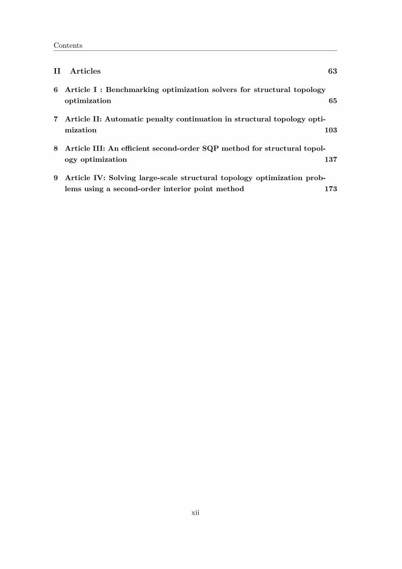
II Articles 63
6 Article I : Benchmarking optimization solvers for structural topologyoptimization 65
7 Article II: Automatic penalty continuation in structural topology opti-mization 103
8 Article III: An efficient second-order SQP method for structural topol-ogy optimization 137
9 Article IV: Solving large-scale structural topology optimization prob-lems using a second-order interior point method 173
xii

Part I
Background
1


1Introduction
Structural topology optimization [74] is a relatively mature field that has rapidly ex-panded due to its interesting theoretical implications in mathematics, mechanics, andcomputer science. It has, additionally, important practical applications in the manufac-turing, automotive, and aerospace industries [34]. This discipline is focused on findingthe optimal distribution of material in a prescribed design domain given some boundaryconditions and external loads. Topology optimization is commonly used in the concep-tual design phase presenting new and innovative structures. Classical structural topologyoptimization problems are, for instance, maximization of the stiffness (minimize the com-pliance) or minimization of the total weight (volume) of the structure, subject to someconstraints on the total volume, total stiffness, maximum displacements, or stresses [10].The design domain is often discretized using finite elements, where the variables representthe density of each element.
Topology optimization was first initiated in the 1960s, with the introduction of trusstopology design in [39]. The continuum approach appeared in the late 1980s [8]. Topologyoptimization can be regarded as an extension of sizing and shape optimization. The goalof sizing optimization consists of finding the thickness of the structure for a fixed designdomain, whereas shape optimization finds the optimal shape of a domain. Topologyoptimization is now well-establish and can be applied in many different research areassuch as fluid dynamics, electromagnetic problems, nuclear physics, and biomechanicalproblems, among others [10]. However, the discussion in this thesis is limited to structuraltopology design problems.
3

Figure 1.1 shows some of the practical applications of structural topology optimiza-tion. In the last decade plenty of new applications have emerged in this field [34]. Onthe other hand, very few improvements and insights are done regarding the optimizationtechniques. The development of novel mathematical optimization methods to accuratelysolve large-scale topology optimization problems, is crucial to improve the final designsin these and in many other applications ([103]).
(a) Aerospace applications (b) Architecture applica-tions
(c) Medical applications (d) Micromachineapplications
(e) Automotive ap-plications
Figure 1.1: Examples of some practical structural topology optimization applications (from[76], [111], [110], [97], and [88], respectively).
First of all, the physical problem needs to be suitably formulated in a mathematicalproblem. Then, it is discretized and optimized. Figure 1.2 shows the general flow used inthis work for obtaining an optimized design using a mathematical programming method.In particular, standard finite element analysis and classical formulations of the topologyoptimization problem are considered. This thesis concerns with the optimization steprather than the pre-processing, the post-processing, and the structural analysis. Newtechniques are implemented and developed to improve the performance of the "black-box" that is usually considered the optimization solver.
4

CHAPTER 1. INTRODUCTION
Initialization
Sensitivity AnalysisOptimization
Post processing
Structural Analysis
Problem formulation
Figure 1.2: Flow chart of topology optimization design using mathematical programmingmethods. The research presented here is focused on the optimization step.
While a variety of large-scale nonlinear solvers could be applied, structural topologyoptimization problems are usually solved by sequential convex approximation methodssuch as the Method of Moving Asymptotes (MMA) [112] and [131], and the ConvexLinearization (CONLIN) method [48], or by using Optimality Criteria (OC) methods,see e.g. [93], [130], and [4]. These methods were specially designed for optimal designpurposes and are now extensively used in commercial optimal design software as wellas academic research codes. However, they are first-order methods with slow conver-gence rates. In addition, methods such as the original CONLIN and MMA have lack ofconvergence proof.
Throughout this thesis, different alternatives to the classical structural topology op-timization solvers based on second-order information are presented. It is well-known inthe mathematical optimization community, that second-order methods converge in feweriterations and produce more accurate solutions than first-order solvers [38]. Althoughsecond-order methods have not been embraced by the topology optimization community,this thesis will show that the introduction of this kind of solvers is necessary to drive thefield forward. The use of second-order information is essential to obtain good optimizeddesigns in few iterations.
The problem is frequently defined in its nested form, meaning that the state (nodaldisplacement) variables are related to the design (density) variables through the equi-librium equations [10]. When second-order solvers are applied to this formulation, thecomputational effort is dominated by both, the solution of the equilibrium equations andthe computation of the Hessian. In such cases, efficient approaches to reduce the compu-tational time and memory usage are needed. Thus, the implementation of the methods
5
presented in this thesis exploits the specific mathematical structure of the problem.Ultimately, new techniques for large-scale problems will enable the solution of real
structural topology optimization problems. More specifically, the use of iterative methodsfor solving large-scale linear systems such as multigrid techniques and Krylov sub-spacemethods is necessary to apply general nonlinear solvers to this type of problems [103].
This thesis concerns with the comparison, research, and implementation of numeri-cal optimization methods for structural topology optimization problems, such as interiorpoint methods [52], and Sequential Quadratic Programming (SQP) methods [15]. Thediscussion is almost restricted to the minimum compliance problem. Further investiga-tions regarding different topology optimization problems or finite element analysis areout of the scope in this work.
This thesis consists of four separate journal papers related to numerical optimizationprogramming in topology optimization problems. Part I regards with the general back-ground of topology optimization problems (Chapter 2), numerical optimization (Chapter3), and linear algebra methods (Chapter 4). This covers the essentials needed to fullyunderstand the rest of the thesis. Chapter 5 includes a brief summary of the differentpapers collected in the thesis, with the main results and contributions. In the secondpart of the thesis the four research articles are included. Chapter 6 collects "Benchmark-ing optimization solvers for structural topology optimization", Chapter 7 presents "Anautomatic penalty continuation in structural topology optimization problems", Chapter8 gathers "An efficient second-order SQP method for structural topology optimizationproblems". Finally, Chapter 9 deals with "Solving large-scale structural topology opti-mization problems using a second-order interior point method".
6
2Structural topology optimization
Structural topology optimization obtains an optimal material distribution in a prescribeddesign domain for some boundary conditions and loads. This optimized design is found byminimizing an objective function subject to some constraints modelling technical specifi-cations. Structural topology optimization has become a multidisciplinary field of researchand has been very active since 1988 with the publication of [7] and [8]. It is also consid-ered a very powerful tool for industrial applications, such as the construction of aircraftsand automobiles [34]. These applications require, for instance, a light structure but atthe same time as stiff as possible. In topology optimization, there are no assumptions inthe final design of the structure, and ideally, the goal is to decide whether to put materialamong all the points in the design domain. The choice of the topology of the structurein this conceptual phase gives innovative and novel designs. In general, the structure isdiscretized using finite element method (FEM) for design parametrization and structuralanalysis.
The main purpose of this chapter is to give a brief introduction and a literature reviewof structural topology optimization problems. Firstly, the topology optimization problemformulation considered throughout the thesis is introduced. Then, an overview of someoptimization methods commonly used in this field is presented. Finally, the standard setof benchmark problems is discussed.
7

2.1 Problem formulation
The classical structural topology optimization problem consists of maximizing the stiff-ness of the structure (or minimizing the compliance) with a constraint on the total volumeor weight [10]. This problem, without any type of regularization, is well-known to beill-posed, see e.g. [18], [42], and [9]. This means, the problem lacks existence of solu-tions in the original design domain. To simplify the notation, the variational problemformulation is presented without regularization techniques. Thus, the problem as statedin this section is ill-posed. For the complete and correct description of the problem, seee.g. [18]. The variational problem is defined as in [10], [107], and [18].
Let Ω ∈ Rdim describes the bounded domain, with a Lipschitz boundary Γ [33].For notation purposes, the Sobolev space W k,p for k = 1 and p= 2 is defined as
H1(Ω) = f ∈ L2(Ω), s.t. ∇f ∈ L2(Ω),
withLp(Ω) = f :Ω→ R, s.t. ||f ||Lp(Ω) <∞,
||f ||Lp(Ω) =
(∫
Ω|f(x)|pdx
)1/p1≤ p <∞,
infα : |f(x)| ≤ α for almost every point x ∈Ω p=∞.
The standard notation H1(Ω)dim will be used for the Sobolev space of function f :Ω→Rdim. More details on Sobolev spaces can be found in [33].
In the following formulation, the term U refers to the space of kinematically admissibledisplacements, and H to the set of feasible designs [18], i.e.,
U = u ∈H1(Ω)dim, such that u = 0 on Γu,
H= t ∈ L∞(Ω)∩L1(Ω) : 0< t≤ t≤ 1 on Ω, and∫
ΩtdΩ ≤ V . (2.1)
For any given t > 0 and maximum volume V > 0. For convenience, the boundary ispartitioned, Γ = Γu∪Γt such that Γu∩Γt = ∅. Γt refers to the part of the boundary withnon-fixed displacements, i.e., where the tractions are assigned [10].
The minimum compliance problem is stated as
minimizeu∈U ,t∈H
l(u)
subject to a(u,v) = l(v) ∀v ∈ U .
The problem minimizes the load linear form [10], described as
l(u) =∫
Ωfb ·udΩ+
∫
Γt
ft ·uds,
8

CHAPTER 2. STRUCTURAL TOPOLOGY OPTIMIZATION
Here, the variable fb ∈L2(Ω)dim represents the body forces and ft ∈L2(Γt)dim the bound-ary tractions. For a fixed and admissible design t ∈ H, the displacement u ∈ U satisfiesthe state equation in its variational form [107],
a(u,v) =∫
Ωfb ·vdΩ+
∫
Γt
ft ·vds ∀v ∈ U ,
with the energy bilinear form defined as
a(u,v) =∫
Ωt E ε(u) ·ε(v)dΩ.
The term ε(u) refers to the strain tensor and E is the elasticity tensor. Existence ofsolutions to the state equations are ensured, see for instance [18]. Assuming, smalldisplacements, the linearized strain is
ε(u) = 12(∇u+∇uT
).
For computational purposes, the space U (and H) is usually discretized. Let Vh ⊂U (Qh ⊂ H) be any finite dimensional sub-space. Here, h refers to the discretizationparameter. Then, the finite dimensional problem finds the approximated solution uh ∈Vh
(and th ∈Qh) such thata(uh,vh) = l(uh) ∀vh ∈Vh.
In particular, the domain Ω is discretized using finite elements. In the following, thefinite element method is presented for a 2D domain (assuming constant thickness andplane stress condition). More details of the finite element method (FEM) can be foundin [31] and [30].
The strain-displacement relationship on the element e is
εe = ∂uhe .
In order to keep only the necessary information, the strain tensor is transformed in a vec-tor with independent components ([31]). Here, the partial derivatives of the coordinatesare gathered in ∂
∂ =
∂∂x 00 ∂
∂y∂∂y
∂∂x
.
The displacement on a finite element can be written as
uhe = Ned,
where d is the vector with all nodal displacements (global level) and Ne is the shapefunctions (interpolation functions).
9

The strain tensor can be redefined as
εe = ∂uhe = ∂Ned = Bed,
with Be, the strain-displacement matrix (element level). The principle of virtual workis applied to obtain the element stiffness matrix and forces expressions, similar to [31].Notice that the state equations can be written as the summation of integrals over theelements. Let v=Ned define a virtual displacement (small perturbation of the displace-ment), then the discretized bilinear energy form becomes
∑
e
dT∫
Ωe
theBTe EBedΩd =
∑
e
dT(∫
Ωe
NTe fhb dΩ+
∫
(Γt)e
NTe fht ds
). (2.2)
Here, the represents the material of the element e. The discretized problem is defined onan element level. The vector of nodal loads applied to the element e is
fe =∫
Ωe
NTe fhb dΩ+
∫
(Γt)e
NTe fht ds,
andKe =
∫
Ωe
teBTe EBedΩ, (2.3)
the element stiffness matrix. The isotropic stiffness tensor E is defined based on theHooke’s law as follows [31]
E = E
1−ν2
1 ν 0ν 1 00 0 (1−ν)/2
,
with ν the Poisson’s ratio of the material, and E the Young’s modulus constant. Fromnow on, the global density, displacement (state variable), and force vectors are definedwith the terms t ∈Rn, u ∈Rd (instead of d) and f ∈Rd, respectively, with n the numberof elements and d the total number of degrees of freedom. Then, the global equilibriumequations are obtained by the assembly of all elements,
Ku = f,
withK =
n∑
e=1Ke.
The summation symbol refers to the expansion to the element terms to the global vector(or matrix), i.e. K : Rn→∈ Rd×d.For more information about the finite element methodand its expressions, see [30] and [31].
Throughout the rest of the thesis the problem is always formulated in its discretizedversion. Isotropic materials and a regular grid with a constant density throughout each
10

CHAPTER 2. STRUCTURAL TOPOLOGY OPTIMIZATION
element are considered. In particular, bilinear quadrilateral elements are considered. Inthis scenario, the element stiffness matrix is assumed to be the same for all elements.Additionally, the integral (2.3) is evaluated using 2×2 Gauss-point quadrature. Finally,only design-independent loads are considered. Along the thesis, the isotropic stiffnesstensor is defined based on the density of the element, i.e. E(te) (see Section 2.2). Thus,the equilibrium equations are defined as in [10],
K(t)u = f
K(t) =n∑
e=1E(te)Ke.
Finally, throughout the rest of the thesis, the stiffness matrix is assumed to be positivedefinite to avoid singularity. In other words, E(ti)> 0 (see Section 2.2).
The discretized minimum compliance problem is formulated as
minimizet∈Rn,u∈Rd
fTu
subject to K(t)u− f = 0vT t≤ V0≤ t≤ 1.
(P cS)
The volume constraint is defined as a linear inequality with v = (v1, . . . ,vn)T ∈ Rn therelative volume of each element and 0 < V < 1 the maximum volume fraction allowed.The discretized equilibrium equations are described as explicit constraints.
In its original formulation (2.1), the density variable specifies the design of the struc-ture, taking either ti = 1, if the ith element contains material (solid), or ti = 0, if theelement remains void. However, in practice, the integer variables are replaced by contin-uous variables. The solid and void topology optimization problem is modified, so thatthe density variables can take any value between 0 (void) and 1 (solid) (see Section 2.2).
The minimum compliance formulation described in (P cS) is the so-called SimultaneousAnalysis and Design (SAND) [5], since both, design and state variables, are simultane-ously optimized. The main advantage of this formulation is the ease of the objectivefunction, which is linear. On the other hand, optimization algorithms need to deal witha large number of nonlinear equality constraints and infeasible iterations.
The problem is frequently defined in a nested form, where the equilibrium equationsare implicit in the objective function. Therefore, only the design variables are optimized,while the state variables are computed by solving the equilibrium equations at eachobjective function evaluation. The nested formulation is described as in (P cN ).
minimizet∈Rn
uT (t)K(t)u(t) (or fTK−1(t)f)
subject to vT t≤ V0≤ t≤ 1,
(P cN )
11
with u(t) =K−1(t)f. Although the objective function of the nested form is highly nonlin-ear (and typically nonconvex), it has the advantage of containing only linear constraints.Thus, the development and implementation of nonlinear optimization methods for thisspecific formulation (see Chapters 8 and 9) are focused on dealing with the nonconvexityand the computational effort of the objective function, rather than incorporating differenttechniques to cope with the infeasibility and unboundedness of the problem.
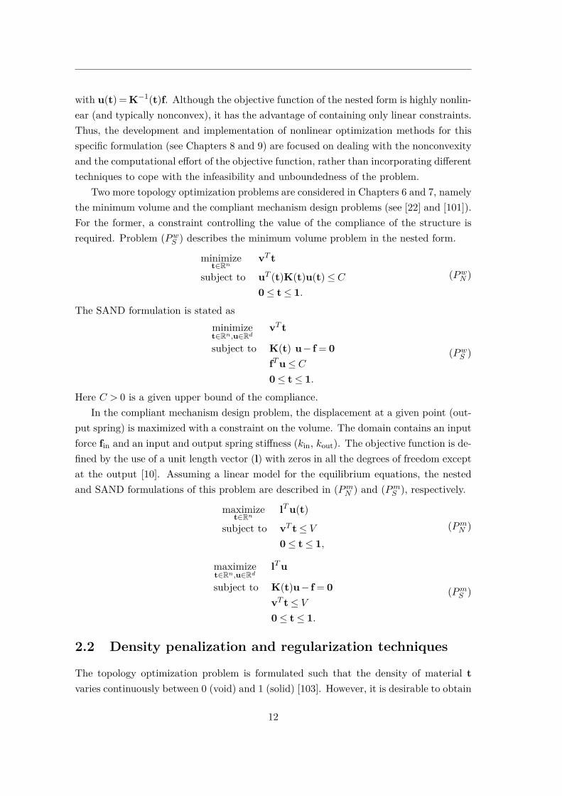
Two more topology optimization problems are considered in Chapters 6 and 7, namelythe minimum volume and the compliant mechanism design problems (see [22] and [101]).For the former, a constraint controlling the value of the compliance of the structure isrequired. Problem (PwS ) describes the minimum volume problem in the nested form.
minimizet∈Rn
vT t
subject to uT (t)K(t)u(t)≤ C0≤ t≤ 1.
(PwN )
The SAND formulation is stated asminimizet∈Rn,u∈Rd
vT t
subject to K(t) u− f = 0fTu≤ C0≤ t≤ 1.
(PwS )
Here C > 0 is a given upper bound of the compliance.In the compliant mechanism design problem, the displacement at a given point (out-
put spring) is maximized with a constraint on the volume. The domain contains an inputforce fin and an input and output spring stiffness (kin, kout). The objective function is de-fined by the use of a unit length vector (l) with zeros in all the degrees of freedom exceptat the output [10]. Assuming a linear model for the equilibrium equations, the nestedand SAND formulations of this problem are described in (PmN ) and (PmS ), respectively.
maximizet∈Rn
lTu(t)
subject to vT t≤ V0≤ t≤ 1,
(PmN )
maximizet∈Rn,u∈Rd
lTu
subject to K(t)u− f = 0vT t≤ V0≤ t≤ 1.
(PmS )
2.2 Density penalization and regularization techniques
The topology optimization problem is formulated such that the density of material tvaries continuously between 0 (void) and 1 (solid) [103]. However, it is desirable to obtain
12

CHAPTER 2. STRUCTURAL TOPOLOGY OPTIMIZATION
designs close to a 0-1 solution. A material interpolation scheme is included to penalizeintermediate density values. These artificial densities are typically called grey regions [9].Two of the most popular approaches to penalize these densities are the Solid IsotropicMaterial with Penalization (SIMP) [7] and [130], and the Rational Approximation ofMaterial Properties (RAMP) [109]. These approaches use interpolation schemes to forcethe density values go to the bounds. The Young’s modulus E is defined as
E(ti) =
Ev +(E1−Ev)tpi SIMP scheme
Ev +(E1−Ev) ti1+q(1−ti) RAMP scheme.
(2.4)
Here, Ev > 0 and E1 ≫ Ev are the Young’s modulus for the "void" and solid materialrespectively. In practice, the material penalization parameter is generally set to p= 3 andq = 6, for the SIMP and RAMP approaches, respectively [71]. For values of p= 1 (q = 0),the structural topology optimization problems described in Section 2.1 are convex, but,in general, the problem becomes nonconvex for values of p > 1 (q > 0). In particular, thefour articles included in this thesis consider the penalization parameter greater than 1.Chapters 6, 8, and 9 use the SIMP approach with p= 3, while Chapter 7 uses both theSIMP (with p= 3) and the RAMP (with q = 6) approaches.
(a) No penalization parameter, p= 1. (b) Penalization parameter p= 3.
Figure 2.1: Example of a cantilever beam design using different penalization parametervalues. This figure illustrates how the material interpolation approaches affect the opti-mized design. A density filter technique was used to obtain the design presented in Figure2.1b.
Figure 2.1 shows an illustrative example where the design of a cantilever beam isoptimized with no penalization scheme, i.e. p = 1 (Figure 2.1a), and with the SIMPapproach using p= 3 (Figure 2.1b). In the latter, the grey regions (intermediate designs)disappear. Throughout the rest of the thesis, terms such as almost solid-and-void and
13
0 0.1 0.2 0.3 0.4 0.5 0.6 0.7 0.8 0.9 10
0.1
0.2
0.3
0.4
0.5
0.6
0.7
0.8
0.9
1
You
ng’s
mod
ulus
density variable
p = 1p = 2p = 3p = 10
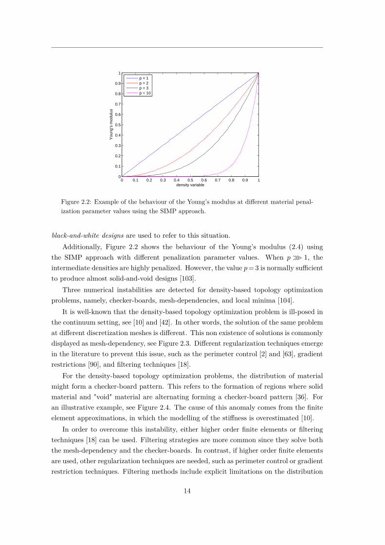
Figure 2.2: Example of the behaviour of the Young’s modulus at different material penal-ization parameter values using the SIMP approach.
black-and-white designs are used to refer to this situation.Additionally, Figure 2.2 shows the behaviour of the Young’s modulus (2.4) using
the SIMP approach with different penalization parameter values. When p ≫ 1, theintermediate densities are highly penalized. However, the value p= 3 is normally sufficientto produce almost solid-and-void designs [103].
Three numerical instabilities are detected for density-based topology optimizationproblems, namely, checker-boards, mesh-dependencies, and local minima [104].
It is well-known that the density-based topology optimization problem is ill-posed inthe continuum setting, see [10] and [42]. In other words, the solution of the same problemat different discretization meshes is different. This non existence of solutions is commonlydisplayed as mesh-dependency, see Figure 2.3. Different regularization techniques emergein the literature to prevent this issue, such as the perimeter control [2] and [63], gradientrestrictions [90], and filtering techniques [18].
For the density-based topology optimization problems, the distribution of materialmight form a checker-board pattern. This refers to the formation of regions where solidmaterial and "void" material are alternating forming a checker-board pattern [36]. Foran illustrative example, see Figure 2.4. The cause of this anomaly comes from the finiteelement approximations, in which the modelling of the stiffness is overestimated [10].
In order to overcome this instability, either higher order finite elements or filteringtechniques [18] can be used. Filtering strategies are more common since they solve boththe mesh-dependency and the checker-boards. In contrast, if higher order finite elementsare used, other regularization techniques are needed, such as perimeter control or gradientrestriction techniques. Filtering methods include explicit limitations on the distribution
14

CHAPTER 2. STRUCTURAL TOPOLOGY OPTIMIZATION
Figure 2.3: Example of mesh-dependency in a MBB beam. Different optimized designsresult for different discretizations. Figure taken from [104].
Figure 2.4: Example of a checker-board pattern in a cantilever beam.
of the density. The sensitivity filter [10], the density filter [18], and the PDE filter [77]are, nowadays, some of the most popular choices, see e.g. [100] and [104].
In particular, only the density filter is considered to ensure regularity and existenceof solution [18]. It is implemented based on [4]. For a given element e, its filtered densityvariable te depends on a weighted average over the neighbours in a radius rmin.
te = 1∑i∈Ne
Hei
∑
i∈Ne
Heiti
Hei = max(0, rmin−∆(e, i))
Here, Ne the set of elements for which the distance to element i (defined by ∆(e, i)) is
15
smaller than the filter radius rmin.Finally, the third numerical and theoretical challenge is the so-called local minima
[104]. Since topology optimization problems are generally defined as nonlinear and non-convex problems, a global solution cannot be guaranteed. Different optimization methodscan produce different local solutions for the same problem (and the same discretization).To avoid this issue, [104] suggests the use of continuation techniques. In these meth-ods, either the radius of the filter or the material penalization parameter is graduallydecreasing or increasing (respectively) to reduce the chances of ending in local minima.Thus, the continuation approach solves a sequence of optimization problems. A specificcontinuation in the penalization parameter strategy is implemented in Chapter 7. In thisarticle, the performance of this method is compared with the classical formulation. Theresults suggest that, indeed, continuation methods help to avoid local minima. Moreover,the article proposes a new alternative to overcome this numerical issue.
In this section, the classical density-based topology optimization formulation has beenintroduced. Yet, other alternative formulations are emerging in this field and becomingvery popular. For instance, in the review [103], topology optimization methods are princi-pally classified in (i) density-based methods ([130] and [7]), (ii) evolutionary approaches(such as Evolutionary Structural Optimization (ESO) [127] and [128]), (iii) level setmethods ([37] and [121]), (iv) phase field methods ([19] and [24]), and (v) topologicalderivatives [106].
2.3 Topology optimization methods
Since topology optimization problems can be described as a 0-1 discrete problem, it isindeed natural to solve them using discrete optimization methods [108]. Even so, thesolution of the discrete problem is very difficult to obtain, and large-scale problems arenowadays impossible to solve [103]. Heuristic approaches, such as Genetic Algorithms,can estimate an optimized design of the problem without any information of the gra-dients, see for instance [122] and [6]. However, the computational effort of these non-gradient methods is extremely large for large-scale problems and they are not practicalfor real topology optimization problems [92] and [103]. Therefore, this thesis is focusedon gradient-based mathematical programming methods.
The Optimality Criteria (OC) method [93], [130], and [4], and the Method of Mov-ing Asymptotes (MMA) [112], [113], and [131], are two of the most classical first-orderoptimization solvers in structural topology optimization, see e.g. [8], [114], [3], and [102]among others. With the sake of completeness, their principal ideas are briefly introduced.
Ultimately, several studies investigate second-order solvers for this type of problems.Newton’s type and SQP methods are implemented for structural topology optimizationproblems in the SAND formulation in, for instance, [70], [69], [68], and [40].
16

CHAPTER 2. STRUCTURAL TOPOLOGY OPTIMIZATION
Optimality Criteria
The origins of the Optimality Criteria method go back to the 1960-70s [91] and [10]. TheOC method updates the design variables of each point based on an estimation of theoptimality conditions. The method updates the designs independently, adding materialin those elements in which the estimation of the strain energy is high. For more detailsof this method, see e.g. the text book [10], where the OC method is explained for theminimum compliance and mechanism design problems.
The OC method used in Chapter 6 is based on 88-lines code implemented in MATLAB[4]. Note that this optimization method, in contrast to the rest of the solvers developedand used in this thesis, does not estimate the Lagrangian multipliers, and therefore,there is no knowledge of the Karush-Kuhn-Tucker (KKT) conditions (see Chapter 3).The KKT conditions are typically used to determine the convergence of the solvers.Thus, the stopping criterion of this method depends only on the difference between twoconsecutive iterate points.
The Method of Moving Asymptotes
The development of the first-order Convex Linearization (CONLIN) method [48] was thebasis for the Method of Moving Asymptotes. MMA was originally developed in 1987[112], and was specifically implemented for structural optimization problems. It is stillone of the most popular solvers in the structural optimization community. MMA approx-imates the objective and the constraint functions with convex and separable functions.These local approximations appear from the Taylor expansion in the reciprocate andshifted variables, and they only require one objective and gradient function evaluationper iteration [107].
f(x)k = rk +n∑
i=1
(pki
Uki −xi+ qkixi−Lki
),
with
rk = f(xk)−n∑
i=1
(pki
Uki −xki+ qkixki −Lki
),
pki =
(Uki −xki
)2 ∂f∂xi
(xk) if ∂f∂xi
(xk)> 0,0 otherwise.
qki =
0 if ∂f∂xi
(xk)≥ 0,−(xki −Lki
)2 ∂f∂xi
(xk) otherwise.
The variable Ui and Li are the asymptotes of the convex approximations. The valuesof these variables depend on the previous iterations. They move apart if the iteratesare going in the same direction (the solver is making progress), and move closer (more
17

conservative approximations) if the iterates display oscillatory behaviour. The updatingscheme of these variables is as follows
Lki −xki = γki (Lk−1i −xk−1
i ),Uki −xki = γki (Uk−1
i −xk−1i ).
Here,
γki =
1.2 if (xki −xk−1i )(xk−1
i −xk−2i )> 0,
0.7 if (xki −xk−1i )(xk−1
i −xk−2i )< 0,
1.0 if (xki −xk−1i )(xk−1
i −xk−2i ) = 0.
Similar to other mathematical programming methods, MMA solves a sequence ofeasier sub-problems until the KKT conditions (see Chapter 3) are satisfied. Although astopping criterion based only on the change between design variables is commonly usedin the literature (see for instance [3] and [1]), the stopping criterion of MMA in this thesisis based on the first-order optimality conditions.
MMA is an inexpensive method in the sense that the sub-problems are normallyeasily solvable. However, it does not have globally convergent properties. In contrast,the globally convergent version, GCMMA, introduces conservative approximations of thefunctions to ensure convergence at the expense of becoming potentially slower [113].
There is plenty of literature concerning extensions of MMA and separable convexprogramming (SCP) methods, see for instance, [132], [131], [23], [120], and [129]. Ad-ditionally, several articles, such as [50], [43], [49], and [13], are focused on MMA-typesolvers based on second-order approximations.
Both solvers are compared with other general nonlinear optimization methods inChapter 6. GCMMA is also used for the comparison of the continuation strategy studiedin Chapter 7. Since MMA and GCMMA use the Taylor expansion in the reciprocate vari-ables, these methods cannot be applied in the automatic continuation strategy proposedin Chapter 71.
2.4 Benchmark test problems and numerical experimentsin structural topology optimization
The numerical experiments in the topology optimization community are generally doneusing very few examples, see for instance [35], [16], [3], and [63]. When only two or threeproblems are used to compare different solvers, the results can be misleading. To illustratethis fact, the minimum compliance problem in the nested formulation is considered. Table2.1 shows the objective function value of three different design domains optimized withGCMMA and IPOPT (interior point software) [117].
1This approach requires solvers in which the constraints are linearized (see Chapter 3 and Chapter 7).
18

CHAPTER 2. STRUCTURAL TOPOLOGY OPTIMIZATION
Table 2.1: Comparison of the objective function value between GCMMA and IPOPT usingthree examples. These results are taken from the numerical experiments of Chapter 6.
Problem 1: Problem 2: Problem 3:Solver Michell 40×40, V = 0.2 Michell 40×20, V = 0.5 Michell 40×20, V = 0.1
GCMMA f(t) = 43.54 f(t) = 73.72 f(t) = 2137IPOPT f(t) = 43.74 f(t) = 73.73 f(t) = 1618
It is clear that if only the results of the first two problems are shown, GCMMAis a better solver choice2. In contrast, if the third problem is under consideration, theconclusion will be completely different. Additionally, the difference between the objectivefunction values is very important. In problems 1 and 2, IPOPT and GCMMA obtainvery similar designs, while in the third problem, the optimized design of GCMMA has anobjective function value noticeably worse than the one obtained with IPOPT. Thus, it isnot enough to show which solver obtains the best objective function values, but also howbig the difference between the results are. IPOPT might not obtain the best designs, butit might produce good results for larger number of problems. Furthermore, there is noavailable big test set of problems in which the results can be based on.
The possibility of improving the comparison of formulations and optimization solversin topology optimization motivates the introduction of performance profiles in this field.For the description of this approach, see [38] and Chapter 6. Performance profiles arenowadays the only acceptable tool used in the numerical optimization community tofairly compare different optimization methods and choices of problem formulations. As aresult, a large benchmark library needs to be defined. Some of the well-known and well-establish test problems for benchmarking the minimum compliance problem are cited in[103]. In contrast, there is no standardization for compliant mechanism design problems.Chapter 6 collects for the very first time a large benchmarking test set of problemsfor minimum compliance, minimum volume, and compliant mechanism design problems.As an illustrative example, Figures 2.5, 2.6 and 2.7 show some of these problems. Onthe left side of the figures, their boundary conditions and external loads are defined.A possible optimized design is included on the right side. Note that this final designdepends on the mesh discretization, length ratios, volume fraction, problem formulation,and optimization solver, among other factors.
2Chapter 6 will refute this statement.
19

Figure 2.5: Michell 2D domain with an example of a possible optimized design.
Figure 2.6: MBB 2D domain with an example of a possible optimized design.
Figure 2.7: Compliant gripper 2D domain with an example of a possible optimized design.
20

3Numerical Optimization
The thesis addresses numerical optimization methods for solving structural topologyoptimization problems efficiently. In particular, two of the state-of-the-art second-orderoptimization methods are developed and implemented. An efficient Sequential QuadraticProgramming (TopSQP) method is implemented in Chapter 8. Chapter 9 is focused onan interior point method (TopIP). In the latter, special emphasis is given on investigat-ing efficient linear algebraic solvers for obtaining the search direction, since large-scaleproblems are considered.
This chapter provides the necessary background regarding mathematical optimizationtheory and some optimization methods. First, some preliminary definitions and theoremsare introduced. Afterwards, general nonlinear gradient-based programming techniquesare discussed. More details of general numerical optimization theory can be found inthe text books [87], [78], and [57]. A general review of some iterative methods for linearsystems is covered in Chapter 4.
21
3.1 Numerical Optimization
The considered nonlinear optimization problem can be stated as
minimizex
f(x)subject to gi(x) = 0 i ∈ E ,
gi(x)≤ 0 i ∈ I,li ≤ xi ≤ ui i= 1, . . . ,n,
(NLP)
with x = (x1, . . . ,xn)T ∈ Rn, f : Rn −→ R and gi : Rn −→ R (with i = 1, . . . ,m) beingcontinuously differentiable functions. The terms li and ui are the lower and the upperbounds of the variable xi, respectively. The set I contains the indices i such as theconstraint gi(x) is an inequality. The term E refers to the equality constraints. Fornotational convenience, both general and bound constraints are gathered in ci(x), i.e.,
ci(x) =
(gj(x))j=1,...,m i= 1, . . . ,m(xj−uj)j=1,...,n i=m+1, . . . ,m+n
(lj−xj)j=1,...,n i=m+n+1, . . . ,m+2n.
For this generalization, the indices i such that the constraint ci(x) is an inequality aregathered in I (I ⊂ I). Thus, E ∪I = 1, . . . ,m+2n and E ∩I = ∅.
This section only outlines some theoretical aspects needed. The proofs of the theoremscan be found in [87], [20], and [78].
Definition 3.1. (from [87]) A feasible set Ω is the set of all points x for an optimizationproblem that satisfy all the constraints.
Ω = x ∈ Rn |ci(x)≤ 0, i ∈ I and ci(x) = 0, i ∈ E.
A vector x ∈ Rn is a feasible point if x ∈Ω.
A set is a convex set [20] if it contains a line segment joining any two points x andy in the set, i.e.,
x,y ∈Ω, θ ∈ [0,1]⇒ θx+(1−θ)y ∈Ω.
Examples of convex sets are, for instance, hyperplanes, halfspaces, Euclidean balls, andpolyhedra [20]. The feasible set of a nonlinear optimization problem must be non-emptyin order for the problem to admit a solution.
The constrained optimization problem (NLP) is described using inequality constraints.In general, nonlinear optimization solvers can be categorized based on how the inequali-ties are dealt with. With the aim of distinguishing whether these constraints are exactlyheld or not, the active set is defined as follows.
22
CHAPTER 3. NUMERICAL OPTIMIZATION
Definition 3.2. (from [87]) The active set of the optimization problem (NLP) at apoint x is defined as
A(x) = i ∈ 1, . . . ,2n+m such that ci(x) = 0.
The active constraints restrict the possible directions from a feasible point x. Onthe other hand, if a constraint is inactive in a feasible point, then any small enoughperturbation will end up in another feasible point.
Convex analysis
Convex optimization is a special case of mathematical optimization. One of the greatadvantages of convex problems is that any local solution is a global solution. Thus, mostof the nonlinear optimization solvers, approximate (NLP) by convex sub-problems. Letsome preliminary concepts be introduced.
Definition 3.3. (from [20]) A function f :Rn−→R is a convex function if the domainof f (dom f) is a convex set and
f(θx+(1−θ)y)≤ θf(x)+(1−θ)f(y)∀x, y ∈ domf θ ∈ [0,1].
Here, the dom f specifies the subset of Rn of points x for which f(x) is defined.
Definition 3.4. (from [20]) A problem such as (NLP) is a convex optimization prob-lem if f(x) and ci(x) with i ∈ I are convex functions, and ci(x) with i ∈ E are affinefunctions.
Here, the term affine refers to functions with the form f(x) =Ax+b. It is importantto note that the feasible set of a convex problem is convex.
Theorem 3.1 relates the convexity property with the second-order information of thefunction.
Theorem 3.1. (from [20]) Let be f a twice differentiable function with convex domain.
f is convex ⇐⇒∇2f(x) 0 for all x ∈ dom f.
Here, (∇2f(x))ij = ∂2f(x)∂xi∂xj
i, j = 1, . . . ,n is the Hessian of the function f . If ∇2f(x) 0,then f is strictly convex.
The expression "A B" ("A B") means that A−B is a positive semi-definite(positive definite) matrix.
A vector x ∈Ω is a global solution of (NLP) if ∀ x ∈Ω, f(x)≤ f(x). In addition,it is said a local solution of (NLP) if x ∈ Ω, and there is a neighbourhood N ⊂ Ω of xsuch that f(x)≥ f(x) for x ∈N .
23

Theorem 3.2 states one of the most important properties of convex optimization. Fornonconvex problems, implications in only one direction are satisfied, from the top to thebottom. The proof of this theorem can be found in [20]. Definition 3.5 is included tocomplete the theorem.
Definition 3.5. (from [20]) A vector d ∈ Rn is
• A feasible direction at x∈Ω if there exists a real number ε1 > 0 such that x+td ∈Ω for all t ∈ (0, ε1).
• A descent direction at x ∈Ω if there exists a real number ε2 > 0 such that f(x+td)< f(x) for all t ∈ (0, ε2).
• A feasible descent direction at x∈Ω if d is both feasible direction and a descentdirection at x.
Theorem 3.2. (from [20]) Suppose that (NLP) is a convex problem, and that x ∈ Ω.Then the following are equivalent:
x is a global solution.m
x is a local solution.m
At x there is no feasible descent direction d.
Optimality conditions
The optimality conditions are some necessary and sufficient expressions to check if agiven point x is indeed a local solution. Nonlinear optimization solvers generally stopwhen the first-order optimality conditions are satisfied for a given tolerance.
Constraint Qualifications (CQ) are regularity conditions in the constraints to ensurethat they do not show degenerate behaviour at the Karush-Kuhn-Tucker (KKT) point x(cf. below). There are plenty of CQ. Here, two of the most popular ones are cited.
Definition 3.6 (Linear independence constraint qualification (LICQ) [87]). TheLICQ holds at x if the gradients ∇ci(x), i ∈ A(x) are linearly independent.
Definition 3.7 (Mangasarian-Fromovitz constraint qualification (MFCQ) [87]).The MFCQ holds at x if there exists a vector d ∈ Rn such that
∇ci(x)Td< 0 i ∈ A(x)∩I∇ci(x)Td = 0 i ∈ E
and the set of equality constraint gradients ∇ci(x) : i ∈ E is linearly independent.
24

CHAPTER 3. NUMERICAL OPTIMIZATION
In particular, if the feasible region is formed by only linear constraints, then theconstraint qualifications are met (see [87]). Therefore, in Chapter 8 and 9, the CQ aresatisfied for all feasible points since the minimum compliance problem is formulated inthe nested form (P cN ) (only linear constraints, see Chapter 2).
Definition 3.8. (from [87]) The Lagrangian function of (NLP) is defined as
L(x,λ) = f(x)+m+2n∑
i=1λici(x).
Here λ= (λ1, . . . ,λm+2n)T are the Lagrangian multipliers of all general constraints.
The first-order conditions for a point x to be a local solution of the problem (NLP),are gathered Theorem 3.3.
Theorem 3.3 (First-order necessary conditions [87]). Suppose that x is a localsolution of (NLP) and that a CQ holds at x. Then, there is a Lagrangian multipliervector λ such that the following conditions are satisfied at (x,λ).
∇L(x,λ) =∇f(x)+J(x)Tλ= 0, (3.1)ci(x)≤ 0 i ∈ I, (3.2)ci(x) = 0 i ∈ E , (3.3)λi ≥ 0 i ∈ I, (3.4)
ci(x)λi = 0 i ∈ I, (3.5)
where J(x) = [∇ci(x)T ]i=1,...,m+2n : Rn 7→ Rm+2n×n is the Jacobian matrix of the con-straints. Equation (3.1) refers to the stationarity condition, equations (3.2)-(3.3) are theprimal feasibility conditions, and equation (3.5)) is the complementarity condition.
Finally, the second-order condition gathers how the second derivatives affect the op-timality condition. The second-order conditions are assumed in some theoretical conver-gence proofs for second-order methods (see Chapter 8).
Theorem 3.4 (Second-order sufficient conditions [87]). Suppose that for some fea-sible point x there is a Lagrangian multiplier vector for which the KKT conditions aresatisfied. Suppose also that
pT∇2L(x,λ)p> 0 ∀p such that J(x)Tp = 0, with p 6= 0.
Then x is a strict local solution of (NLP).
25

Duality Theory
This section outlines the duality theory which consists of defining the general nonlinearoptimization problem (NLP) alternatively. This new dual problem is defined using dualvariables λ instead of the primal variable x, as in the original problem (NLP). In somecases the dual problem is much easier to solve, and computationally less expensive. Thepurpose of this sub-section is to outline some theoretical details assumed in Chapter 81.
Definition 3.9. (from [20]) For a given optimization problem such as (NLP), the La-grangian dual function ρ is defined as the minimum value the Lagrangian primalfunction L can take over the primal variable x.
ρ(λ) = infxL(x,λ).
The Lagrangian dual function is the infimum of a family of affine functions (linearfunction of λ). Thus, ρ(λ) is always concave for any general problem (NLP). Let theLagrangian dual problem (NLPd) be defined as
maximizeλ
ρ(λ)
subject to λ≥ 0.(NLPd)
One important property, called weak duality (see for instance [20] for the proof), is thatthe Lagrangian dual function gives a lower bound of the optimal value of f(x), i.e.,
ρ(λ)≤ f(x).
The strong duality ([20]) holds when ρ(λ) = f(x), i.e. when there is no gap between thesetwo optimal values. When (NLP) is convex, the strong duality generally holds, howeversome constraint qualification conditions are needed to ensure it.
3.2 Methods for nonlinear constrained problems
In this section, general aspects and characteristics of some existing nonlinear optimizationalgorithms are described. Nonlinear optimization methods can be categorized as follows[87].
• Penalty methods: The constrained optimization problem is replaced by a se-quence of sub-problems in which the constraints are included in the objective func-tion using a penalty function.
1In the proposed TopSQP (Chapter 8) the inequality quadratic problem (IQP) is reformulated into itsdual to avoid the storage and computation of the Hessian, and thus, to reduce memory and time demand.
26

CHAPTER 3. NUMERICAL OPTIMIZATION
The resulting unconstrained sub-problem is, for instance,
minimizex
f(x)+µ
(∑
i∈E|ci(x)|+
∑
i∈I[ci(x)]+
),
orminimize
xf(x)+ µ
2
(∑
i∈Eci(x)2 +
∑
i∈I([ci(x)]+)2
),
where the penalty parameter is µ> 0, and the operation [ci(x)]+ denotes max(ci(x),0).
The aim is to solve the unconstrained minimization problem for a sequence ofincreasing values of µ ↑∞.
• Augmented Lagrangian methods: In this type of methods, the Lagrangianmultipliers are explicitly included in the objective function. The Augmented La-grangian method combines properties of the Lagrangian function and the quadraticpenalization introduced above [28]. The inequality constraints are reformulated asequality constraints using slack variables, and thus, the approximate sub-problemto solve at each outer iteration is
minimizex,s
f(x)−∑
i∈Iλi(ci(x)+si)−
∑
i∈Eλici(x)+ µ
2
(∑
i∈I(ci(x)+si)2 +
∑
i∈Eci(x)2
)
subject to si ≥ 0 i ∈ I.The sub-problem is solved for fixed values of λ and µ. Then, both parameters areupdated until the KKT conditions are satisfied.
MINOS [84], LANCELOT [29], and PENNON [75], are examples of nonlinear soft-ware based on Augmented Lagrangian methods.
• Sequential Quadratic Programming: This nonlinear method obtains the searchdirection d by minimizing a quadratic programming problem where the objectivefunction is normally a convex and quadratic approximation of the Lagrangian andthe constraints are linearized [15].
minimized
∇f(x)Td+ 12d
T∇2L(x,λ)d
subject to ci(x)+∇ci(x)Td≤ 0 i ∈ I,ci(x)+∇ci(x)Td = 0 i ∈ E ,
SQP methods solve a sequence of Quadratic Programming (QP) problems. Moredetails of QP problems can be found in [87]. Once the search direction is estimated,the primal variable x and the estimates of the Lagrangian multipliers are updateduntil a KKT point is found.
Examples of existing SQP algorithms are SNOPT [55], NPSOL [56], FILTERSQP[46], and KNITRO/ACTIVE [26]. Chapter 8 explains in more detail a SQP-typemethod.
27

• Interior point methods: Slack variables are introduced to transform the inequal-ities to equality constraints. In addition, the objective function is defined with abarrier function to deal with the bound constraints. For a given value of the barrierparameter µ > 0, the algorithm solves the following sub-problem
minimizex,s
f(x)−µ∑
i∈Ilnsi+
n∑
i=1ln(xi− li)+
n∑
i=1ln(ui−xi)
subject to gi(x)+si = 0, i ∈ I,gi(x) = 0, i ∈ E .
For a fixed µ, the goal is to obtain a local solution of the barrier problem usinga Newton’s method [41]. The search direction is obtained by solving the so-calledKKT system2. Generally, these sub-problems are not solved to optimality.
Then, the barrier parameter is decreased µ→ 0 until convergence, so that xµ→ x.
Examples of nonlinear interior point methods available in the community are LOQO[116], IPOPT [117], KNITRO/DIRECT, and KNITRO/CG [26]. Chapter 9 gathersmore implementation details of an interior point method.
Interior point methods together with SQP methods are considered the most powerfulsolvers nowadays [59], [38], and [11]. Therefore, both algorithms are implemented forthe minimum compliance problem in Chapters 8 and 9. Additionally, these methodssolve sequence of sub-problems in which the constraints are linearized. The topologyoptimization formulation proposed in Chapter 7 is based on this property. Thus, bothSQP and interior point methods are suitable for this automatic continuation approach.
Nonlinear solvers need to deal with several challenges, such as how to solve the sub-problems, how to deal with nonconvexity, how to deal with infeasible and unbounded sub-problems, and how to ensure progress towards a KKT point, among others. Throughoutthe rest of the section, some techniques and methods commonly used to solve thesechallenges are introduced.
3.2.1 Strategies for determining the step
There exist two different techniques to ensure the progress of the solvers to a KKT point,namely line search [82] and trust region [27] strategies. These strategies require the useof either merit functions [14] or filters [47] to measure the progress. In particular, aline search combined with a merit function is implemented in both the SQP in TopSQP(Chapter 8) and the interior point method in TopIP (Chapter 9).
2Special saddle-point system appeared from a Newton’s method [83] iteration, with the form ∇F∆ =−F, with F the KKT conditions. Here, ∆ is the search direction.
28

CHAPTER 3. NUMERICAL OPTIMIZATION
Line search methods
Line search is a technique to decide how far the algorithm should move along the givensearch direction dk. The new iterate solution is then xk+1 = xk+αkdk, where 0<αk ≤ 1is the step length chosen by the line search at the kth iteration.
The aim of line search strategies is to find a step length α to give a substantialreduction of f(x) [82]. Ideally, the goal is to find the minimizer of φ(α) = f(xk +αdk)with 1 ≥ α > 0. However, this is computationally expensive. In practice, the algorithmtries a sequence of candidates of α enforcing some sufficient decrease conditions. Forinstance, to ensure the Wolfe conditions [87],
f(xk +αdk)≤ f(xk)+ c1α∇f(xk)Tdk∇f(xk +αdk)Tdk ≥ c2∇f(xk)Tdk,
for some constants c1 ∈ (0,1), c2 ∈ (c1,1). The first condition is commonly called Armijocondition [87]. Algorithm 1 outlines one of the most popular line search strategies basedon a backtracking search satisfying the Armijo condition. Nevertheless, there are otherconditions that a line search can follow to force a sufficient decrease, such as the Goldsteinconditions [87], the 1D-Gamma, and 2D-Gamma conditions [72]. Other more sophisti-cated and complicated line search strategies based on finding the minimum of φ(α) canbe applied, for example interpolation techniques [87]. Finally, new approaches to extendthe search from line to curve using arc search strategies are found in the literature, seee.g. [115] and [65].
Algorithm 1 Line search Backtracking algorithm [87].Input: Choose τ ∈ (0,1) and c ∈ (0,1).1: Initialize α= 1.2: repeat3: if f(xk+αdk)≤ f(xk)+ cα∇f(xk)Tdk then4: sufficient decrease = true5: else6: α= τα.7: end if8: until sufficient decrease9: return
For constrained optimization problems, a sufficient decrease in the objective functionis not enough. There is a need of balance between minimizing the objective function andsatisfying the constraints [87]. Then, the objective function in Algorithm 1 is replacedwith a merit function or with the use of filters (cf. below).
Line search strategies are used in some nonlinear software such as LOQO, KNI-TRO/DIRECT, IPOPT, and SNOPT.
29

Trust region methods
Trust region strategies are the alternative of line search methods. The main idea is todefine a region around the current iterate point xk such that a selected model fits ade-quately with the real objective function, and thus, the method can trust the approximatemodel in this area. The model is minimized in this region to be able to choose the stepfor the current iterate [27].
The main difference between line search strategies and trust region methods is thatthe latter finds αk and dk simultaneously. At every iteration, the size of the trust regionis modified depending on the performance of the step selected. Trust region methodschoose a suitable ∆k, such that the descent direction is inside the ball of radius ∆k, i.e.,
||dk|| ≤∆k.
This inequality is included as an extra constraint in the optimization problem. At a giveniteration, a ratio ρk is defined based on a model function mk and the original objectivefunction [87],
ρk = actual reductionpredicted reduction = f(xk)−f(xk +dk)
mk(0)−mk(dk).
Algorithm 2 Outline of a trust region method [87].Input: Choose ∆max > 0, ∆0 ∈ (0,∆max) and κ ∈ [0, 1
4 ).1: repeat2: Obtain dk such that the model function mk(dk) is minimized and ||dk|| ≤∆k is satisfied.3: Evaluate ratio ρk.4: if ρk < 1
4 then5: ∆k+1 = 1
4∆k.6: else7: if ρk > 3
4 and ||dk||=∆k then8: ∆k+1 = min(2∆k,∆max).9: else
10: ∆k+1 =∆k.11: end if12: end if13: if ρk > κ then14: xk+1 = xk+dk.15: else16: xk+1 = xk.17: end if18: k = k+1.19: until convergence20: return
30

CHAPTER 3. NUMERICAL OPTIMIZATION
Depending on the ratio value, the size of the region will increase, decrease, or remainthe same (see Algorithm 2). Typically, the model function is a quadratic approximationof the objective function. For nonlinear constraint problems, merit functions or filtersare used instead (cf. below).
Nowadays, there are several nonlinear optimization methods that are based on trustregions strategies, such as KNITRO/CG, LANCELOT, and FILTERSQP.
Merit function
A merit function balances the conflicting goal of reducing the objective function andsatisfying the constraints. It is defined using a penalty parameter π > 0 which representsthe weight assigned to the satisfaction of the constraints [14]. Several alternative functionsto use as merit function are [87]:
• l1 merit function:
φ(x,π) = f(x)+π
(∑
i∈E|ci(x)|+
∑
i∈I[ci(x)]+
).
• Sum-of-squares merit function:
φ(x,π) = f(x)+ π
2
(∑
i∈Eci(x)2 +
∑
i∈I([ci(x)]+)2
).
• Fletcher’s augmented Lagrangian merit function:
φ(x,π) = f(x)−∑
i∈Eλici(x)−
∑
i∈Iλi[ci(x)]+ + π
2
(∑
i∈Eci(x)2 +
∑
i∈I([ci(x)]+)2
).
The merit function is in charge of controlling the step length αk in line search methods,and the ratio ρk in trust region methods. The penalty parameter is updated at everyiteration and it plays an important role in the convergence rate of the algorithm. Fordifferent updating schemes, see for instance [119] and [32]. SNOPT and LOQO areexamples of nonlinear optimization software that use merit functions.
In particular, the implementation of both, TopSQP (Chapter 8) and TopIP (Chapter9), are based on the l1-merit function with a very simple update rule for the penaltyparameter [87],
π = ||λ||∞.
Filters
The second mechanism to control the acceptance or rejection of the step is the use offilters. It is based on multi-objective function since the idea is to minimize the objective
31

function, but at the same time, satisfy the constraints [47]. In other words, both f(x)and h(x) must be minimized, where
h(x) =∑
i∈E|ci(x)|+
∑
i∈I[ci(x)]+.
Filters will accept a trial step depending on the value of the pair (fk,hk).
Definition 3.10. (from [87])
• A pair (fk,hk) is said to dominate another pair (fl,hl) if both fk ≤ fl andhk ≤ hl.
• A filter is a list of pairs (fl,hl) such that no pair dominates any other.
• An iterate xk is said to be acceptable to the filter if (fk,hk) is not dominated by anyother pair in the filter.
Examples of nonlinear solvers with filter techniques are IPOPT and FILTERSQP.
3.2.2 Existence of solution of saddle-point problems
Some mathematical programming algorithms, such as interior point methods and someQP solvers, require the solution of saddle-point systems. The saddle-point problem isdefined as the following linear system
W∆= F (3.6)
with
W =[A BT
1B2 −C
].
Here, A and C are square matrices. The saddle-point must satisfy at least one of thefollowing conditions [12]:
• A is symmetric.
• 12(A+AT ) (symmetric part) is positive semi-definite.
• B1 = B2 = B.
• C is symmetric and positive definite.
• C = 0.
32

CHAPTER 3. NUMERICAL OPTIMIZATION
The most typical scenario is when all the conditions are satisfied [12]. Examples of theseproblems arise in Chapters 8 and 9.
For simplicity, let assume that A = H ∈ Rn×n is the Hessian of the Lagrangian func-tion, C = 0 ∈ Rm×m, and B = J ∈ Rm×n is the Jacobian of the active constraints. Inthis case, the matrix W is called the Karush-Kuhn-Tucker matrix. The next theoremscontain the requirements for a KKT matrix to ensure existence of solution of (3.6).
Theorem 3.5. (from [87]) Let J have a full row rank, and assume that the reduced-Hessian matrix ZTHZ is positive definite. Then the KKT matrix W is nonsingular, andhence there is a unique vector satisfying the linear system (3.6).
Here, Z ∈ Rn×n−m is a matrix which columns are a basis for the null-space of J [87].
Definition 3.11. (from [61]) The inertia of a symmetric matrix W is the triple (i+, i−, i0),where i0, i+ and i− be the number of zero, positive and negative eigenvalues of W, re-spectively.
Theorem 3.6. (from [87]) Suppose W is defined as (3.6) with A = H, C = 0, and B = Jthe Jacobian of the constraints (full rank). Then
inertia(W) = inertia(ZTHZ)+(m,m,0).
Therefore, if ZTHZ is positive definite, inertia(W) = (n,m,0) [87].
In order to ensure the existence of solution of the saddle-point problem, the matrixW must have the correct inertia. In the next sub-section, some methods available in theliterature to correct the inertia of these systems are cited. Nevertheless, in Chapters 8 and9 the existence of solution of the KKT systems is assumed. The Hessian is approximatedusing a positive definite matrix, thus, the reduced-Hessian is also positive definite, andthe inertia is always correct.
Saddle-point systems can be solved using direct methods [87], such as Schur comple-ment, null-space methods, and LDL factorization, or using iterative methods (see Section4). For more details of saddle-point problems and some existing techniques available tosolve them see the review article [12].
3.2.3 Dealing with nonconvex problems
In the previous sub-section, the importance of the inertia in a saddle-point problem hasbeen introduced. If the inertia of the KKT system in interior point methods is not correct,the search direction may not be a descent direction (of a merit function, for instance).Thus, the solver could end in a local maximum or a stationary point. Algorithms dealingwith nonconvex problems, such as interior point methods, need to modify or perturb thesaddle-point system to ensure the existence of solution. In addition, the QP sub-problems
33

of SQP methods should generally be convex. There are many different ways of handlingthe nonconvexity of the problems.
The easiest technique consists of adding a constant diagonal matrix to the Hessianof the Lagrangian, big enough, such that the eigenvalues of the reduced-Hessian becomepositive, i.e.,
H = H+γIwithγ = max(0,−λmin(ZTHZ)+ ε).
Here, λmin refers to the minimum eigenvalue, I the identity matrix, and 1 ε > 0. Moredetails of this inertia correction strategy can be found in [87].
In the mid 1950s, a new algorithm was implemented to accelerate the iteration ofNewton’s method. This quasi-Newton’s method was proven to be more reliable andfast than the classical Newton’s method. In particular, the BFGS (Broyden-Fletcher-Godfarb-Shanno) method is one of the most popular quasi-Newton’s algorithms [85].This method is nowadays commonly used to approximate the Hessian when there is noavailable second-order information (or is computationally expensive). Software such asIPOPT and SNOPT, use a limited memory BFGS approach to estimate the Hessian[117] and [55]. Equation (3.7) outlines the general iterative process for obtaining a BFGSapproximation [87].
Bk+1 = Bk−BksksTkBk
sTkBksk+ ykyTkyTk sk
withsk = xk+1−xk,yk =∇f(xk+1)−∇f(xk).
(3.7)
Inertia controlling methods are included in some algorithms where the linear systemhas an incorrect inertia. Plenty of literature can be found in this regard, for instance[45], [54], [53], [52], and [51], where LDL factorization techniques are detailed. Addi-tionally, some modifications and perturbations to the KKT matrix are discussed in [67]and in the implementation of the interior point method in IPOPT [117]. Finally, someconvexification strategies to obtain convex problems are explained in [58] and [60].
Nevertheless, Chapters 8 and 9 do not include any of the techniques mentioned above.Instead, a convex approximation of the Hessian based on its specific mathematical struc-ture is proposed. Part of the information of the exact Hessian is lost at the expense ofreducing computational effort.
34

CHAPTER 3. NUMERICAL OPTIMIZATION
3.2.4 Other implementation techniques
Some features are often added to improve the practical performance of the algorithms.For instance, it is common to include a corrector step in interior point algorithms [80].The idea is to compensate the errors made due to the linearization by including twosteps namely, predictor and corrector steps [87]. It has been proved very effective forlinear and convex quadratic problems. The adaptive barrier parameter update strategyin Chapter 9 is based on [86]. Here, the Mehrotra’s predictor-corrector method [80] is notimplemented since [86] states that it is not robust for nonlinear programming. Thus, theproposed algorithm does not introduce it either.
The Maratos effect [79] is the phenomenon where the algorithm fails to converge fastbecause it rejects steps that make progress towards the solution. The implementationof general nonlinear solvers also needs the incorporation of some techniques to avoidthis issue. Examples of these strategies are, the use of second-order correction, theuse of different merit functions, and the flexibility of increasing the merit function in afixed number of iterations (called watchdog strategy) [87]. However, since the consideredproblem formulation (P cN ) contains only linear constraints, this effect does not occur inpractice, see [25].
Finally, the algorithms need to deal with infeasibility and unboundedness of problems.Some techniques to detect infeasible or unbounded problems are explained in the com-parison study [11]. SNOPT software, for instance, forces a feasible starting point whilethe interior point algorithms in KNITRO, LOQO, and IPOPT allow infeasible iteratesand detect infeasibility through line search, filters, or feasibility restoration phases, [116]and [117]. Nevertheless, the proposed solvers in Chapter 8 and 9 assumed feasible andbounded problems.
Some practical implementation details are included in Chapters 8 and 9 to producefast convergence. For instance, in TopSQP, the KKT conditions of some problems stallin a value close to the optimal. To promote convergence in those cases, the maximumpossible step direction is taken without the backtracking (see Chapter 8). Furthermore,the scaling of the problem plays an extremely important role in the efficiency of thesolvers. For more details of practical implementation in optimization, the text book [57]is recommended.
35

36

4Iterative methods for solving linear systems
The computational effort of some optimization solvers, such as interior point methods, re-lies on the solution of large-scale linear systems. The different existing techniques to solvethese systems can be classified in two main groups, namely direct and iterative methods[57]. Direct methods are characterized for their robustness, but they have difficulties insolving large-scale linear systems due to the amount of memory and time required. Onthe other side, for this type of problems, iterative methods are particularly interestingsince they have lower storage need and are easier to parallelize [73]. Structural topologyoptimization problems are characterized as large-scale problems involving millions of de-grees of freedom. Thus, the performance of optimization methods is highly dependent onthe solution of very large-scale systems. This chapter outlines different iterative methodsavailable in the literature. More details of these techniques can be found in [12], [95], and[73]. This introductory chapter serves as a lead to Chapter 9, where an efficient iterativemethod to solve the KKT system of an interior point solver is proposed for the minimumcompliance problem.
Let us consider the linear system Ax = b. Iterative methods produce a sequenceof xk that is expected to converge to x = A−1b. Depending on how this sequenceof iterate points is defined, different techniques emerge, such as stationary iterations,Krylov sub-space, and multigrid methods [73]. These approaches can be defined for bothpositive definite and indefinite linear systems.
Most of these techniques terminate when the residual r= b−Ax is sufficiently small.
37

In practice, the Euclidean-norm of the relative residual error is used, i.e.,
||r||2 = ||b−Ax||2||b||2
≤ ε,
for some tolerance 1 ε > 0.
4.1 Stationary iterative methods
The Richardson [98] or stationary iteration is one of the simplest iterative techniques inwhich the linear system Ax = b is modified into a linear fixed-point iteration as
x = (I−A)x+b.
In particular, these methods solve the more general iteration
xi+1 = Mxi+c. (4.1)
A common technique to obtain the above iteration, consists of splitting the matrix asA = A1 +A2. Here, A1 is nonsingular, and the system A1y = q is easy to solve. Then,the iteration matrix is defined as M =−A−1
1 A2 and c = A−11 b. This technique is called
preconditioned Richardson iteration [73].Two of the most common and popular matrix splitting techniques are Jacobi and
Gauss-Seidel methods [73]. The matrix A is partitioned in three parts; the diagonal partD, the upper triangular part U, and the lower triangular part L. In the first method,the matrices are defined as A1 =D and A2 = L+U, while in Gauss-Seidel the partitionis A1 = U+D and A2 = L. Thus, Jacobi and Gauss-Seidel iterations are defined as
xi+1 =−D−1(L+U)xi+D−1b,
andxi+1 =−(U+D)−1Lxi+(U+D)−1b,
respectively. These stationary methods are commonly used as preconditioner of othermore efficient iterative methods, such as Krylov sub-space methods, or as smootherfunctions in multigrid cycles (cf. below) [105] and [73].
The convergence rate of stationary iterative methods depends on the condition num-ber1 of the matrix A [73]. Preconditioner matrices will help to reduce the conditionnumber and, therefore, decrease the number of iterations needed to converge [73].
1(from [95]) The condition number κ of a matrix A with respect to a norm is given by
κ(A) = ||A||||A−1||.
38

CHAPTER 4. ITERATIVE METHODS FOR SOLVING LINEAR SYSTEMS
In particular, a stationary iteration method for structural topology optimization prob-lems has been implemented in [68] and [69]. Here, the so-called right-transforming iter-ation (see e.g. [99] and [126]) is applied to solve Newton’s systems in a SAND form oftopology optimization problems.
4.2 Krylov sub-space methods
Unlike the stationary iteration, Krylov sub-space methods [123] do not normally haveaccess to the whole matrix. They obtain the sequence of iterates from the history ofthe previous iterations. These methods minimize the residual error over the affine spacex0 +Kk, where x0 is the initial iterate, r0 = b−Ax0 is the initial residual, and Kk =span(r0,Ar0, . . . ,Ak−1r0) is the Krylov sub-space. The speed of convergence of Krylovsub-space methods improves with respect to classical stationary iterations, although itstill depends on the condition number of the matrix [95]. Details of these algorithms,implementation, and theoretical properties can be found in [73].
Examples of this type of iterative methods are the Conjugate Gradient (CG) method[66] and the Generalized Minimal Residual (GMRES) method [96], among others. Theconjugate gradient method was developed in 1952, and is one of the most efficient meth-ods for linear systems when the matrix is symmetric and positive definite. The basicalgorithm is described in Algorithm 3, where the matrix P is a preconditioner.
In contrast, GMRES can also be applied to non-symmetric and indefinite systems. Itis a generalization of the minimal residual algorithm (MINRES) [89] based on the Arnoldiprocess to obtain the orthonormal vectors. Algorithm 4 outlines the GMRES method.
For large-scale structural topology optimization problems, PCG (Preconditioner Con-jugate Gradient) is commonly used to solve the equilibrium equations, see for instance[3]. In addition, Chapter 9 uses flexible GMRES (FGMRES, [94]) in combination withefficient preconditioners. In this article, an indefinite linear system needs to be efficientlysolved at each interior point iteration.
4.3 Multigrid methods
Multigrid methods have been developed since 1964 [44], with a huge growth in the lastdecades. In contrast to other methods, the number of iterations does not depend onthe condition of the matrix. Thus, these methods are characterized for their great effi-ciency [124]. They are considered numerically scalable since the computational cost islinearly dependent on the number of variables [3]. Multigrid methods are successfullyused in plenty of different applications, such as shape optimization of turbine blades [40],computational fluid dynamics [125], and optimal control [105], among others.
39

Algorithm 3 Conjugate Gradient using a general preconditioner [73].Input: A,b,x0, tolerance ω, and max iter.1: Initialization. r = b−Ax0, k = 1.2: Preconditioner z = P−1r.3: p = z.4: repeat5: w = Ap.6: γ = rT z.7: α= γ
wT p .8: x = x+αp.9: r = r−αw.
10: z = P−1r.11: β = rT z
γ .12: p = z+βp.13: k = k+1.14: rn= ||b−Ax||2/||b||215: if rn < ω then16: convergence = true17: end if18: until convergence or k ≥ max iter.19: return
In this section, a basic overview of geometric multigrid methods is presented, in whichhierarchical meshes with their corresponding discretizations are required. The theoreticalproperties and convergence proofs are detailed in the monographs [21], [124], and [64].Another type of multigrid methods, namely Algebraic Multigrid (AMG) methods, arebecoming very popular since unstructured meshes can efficiently be solved. More detailsof this technique can be found in [81], [62], and [118].
The multigrid strategy combines two key parts, the smoothing and the coarse-gridcorrection steps. The smoothing step reduces the high frequency error. The smoothresidual is used to obtain the solution of the system in a coarse grid. This estimationis then prolonged to a finer mesh where the low frequencies are corrected again with asmoother. Smoothing methods in multigrid algorithms are usually some kind of station-ary iterative methods, such as Gauss-Seidel and Jacobi [124], [105], and [133]. However,if the matrix A at level l is indefinite, the construction of an appropriate smoother is notobvious and very problem dependent [12].
For the coarse-grid correction, some mappings are required to go from the coarse tothe fine grids. Let us consider l hierarchy meshes with the corresponding finite elementspaces V0 ⊂ V1 ⊂ . . .⊂ Vl and mesh sizes h0 ≥ h1 ≥ . . .≥ hl, respectively. The restrictionand prolongation operators are defined as follows,
40

CHAPTER 4. ITERATIVE METHODS FOR SOLVING LINEAR SYSTEMS
Algorithm 4 Generalized Minimal Residual method [73].Input: A,b,x0, tolerance ω, max restart iter and max iter.1: Initialization r = b−Ax0, e1 = (1,0, . . . ,0), and m= 1.2: v1 = r
||r||2 and β = ||r||2.3: repeat4: vm+1 = Avm.5: j = 16: repeat7: hj,m = vTm+1vj .8: vm+1 = vm+1−hj,mvj .9: j = j+1.
10: until j ==m
11: hm+1,m = ||vm+1||2.12: vm+1 = vm+1
hm+1,m.
13: minimize ||βe1−Hmy|| to obtain ym.14: Form the approximate solution xm = x0 +Vmym15: r = b−Axm16: rn= ||b−Axm||2/||b||217: if rn < ω then18: convergence = true19: end if20: m=m+1.21: if m=max restart iter then22: Restart: x0 = xm, and v1 = r
||r||2 .23: end if24: until convergence or m≥max iter25: return
Definition 4.1. (from [105]) The coarse-to-fine operator, called prolongation is
Ill−1 : Vl−1 −→ Vl.
The fine-to-coarse operator, called restriction is
Il−1l : Vl −→ Vl−1.
One of the simplest ways to define the prolongation operation is through a linearinterpolation. The restriction is the inverse operation. Examples of these operatorscan be found in [95] and [3]. Figure 4.1 represents both operators more visually witha hierarchical discretization in 2D. The linear system to be solved at a given level l isdefined as
Alxl = bl.
Thus, the methods requires the matrix A at each level of discretization. This can begenerated either by assembling the matrix A for all the levels, or by using the Galerkin’s
41
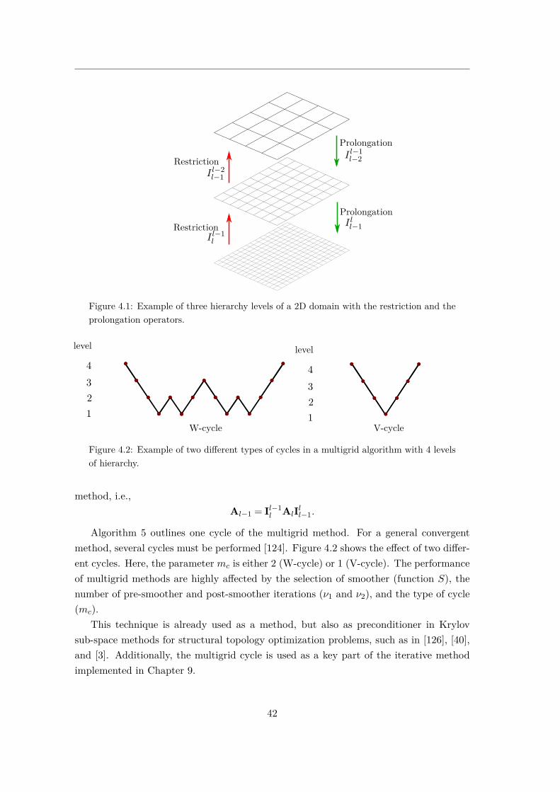
Restriction
RestrictionProlongation
ProlongationI l−1l−2
I l−1l
I l−2l−1
I ll−1
Figure 4.1: Example of three hierarchy levels of a 2D domain with the restriction and theprolongation operators.
level
4321
level
4321
W-cycle V-cycle
Figure 4.2: Example of two different types of cycles in a multigrid algorithm with 4 levelsof hierarchy.
method, i.e.,Al−1 = Il−1
l AlIll−1.
Algorithm 5 outlines one cycle of the multigrid method. For a general convergentmethod, several cycles must be performed [124]. Figure 4.2 shows the effect of two differ-ent cycles. Here, the parameter mc is either 2 (W-cycle) or 1 (V-cycle). The performanceof multigrid methods are highly affected by the selection of smoother (function S), thenumber of pre-smoother and post-smoother iterations (ν1 and ν2), and the type of cycle(mc).
This technique is already used as a method, but also as preconditioner in Krylovsub-space methods for structural topology optimization problems, such as in [126], [40],and [3]. Additionally, the multigrid cycle is used as a key part of the iterative methodimplemented in Chapter 9.
42

CHAPTER 4. ITERATIVE METHODS FOR SOLVING LINEAR SYSTEMS
Algorithm 5 Multigrid cycle [17].Input: x = MC(Al,bl,xl, l, ν1, ν2, mc)1: if l == 0 then2: Solve the problem: x0 = A−1
0 b0.3: return4: end if5: Pre-smoothing step: xl = S(Al,bl,xl, ν1).6: Grid correction: rl = Alxl−bl.7: Restriction step: rl−1 = Il−1
l rl.8: Al−1 = Il−1
l AlIll−1 .9: Initialize c= 1, xl−1 = 0.
10: repeat11: xl−1 = MC(Al−1,rl−1, xl−1, l−1,ν1, ν2, mc).12: c= c+1.13: until c=mc
14: Prolongation step: xl = xl− Ill−1xl−1.15: Post-smoothing step: xl = S(Al,bl,xl, ν2).16: return
43

44

5Contributions and conclusions
This thesis thoroughly investigates some state-of-the-art nonlinear optimization algo-rithms for structural topology optimization problems. First of all, an extensive bench-marking study is carried out in order to establish whether general nonlinear algorithmsoutperform classical structural topology optimization methods. The results presentedin Chapter 6 motivate the work of this thesis. The benchmarking study strongly rec-ommends the use of the exact Hessian to produce designs with good objective functionvalues and to reduce the number of iterations. The benchmarking also reinforces theinitial belief, in which general nonlinear optimization methods can be at least as efficientand robust as classical structural optimization solvers.
Based on these results, a Sequential Quadratic Programming method, namely Top-SQP, is implemented for the minimum compliance problem (Chapter 8). In order topromote fast convergence and reduce the objective function value, second-order informa-tion is used. The Hessian of the compliance is approximated with a positive and semi-definite matrix based on its structure. This approximation is used to properly definethe sub-problems. In addition, the mathematical structure of the Hessian is exploited toreduce both computational time and memory usage. The proposed TopSQP is a robustmethod that obtains optimized designs using few iterations. However, its main draw-back is the computational time spent in solving the inequality quadratic sub-problem.These sub-problems can be solved using several algorithms, for instance, interior pointmethods. Interior point algorithms solve a sequence of large-scale saddle-point systemsin which they spend most of the computational effort. Chapter 9 investigates efficient
45

iterative methods to solve the saddle-point problem arising in interior point methods forthe minimum compliance problem. Particularly, Krylov sub-space methods are combinedwith different preconditioners such as multigrid cycles, to develop an efficient and robustlarge-scale method for the KKT system. The interior point method presented in Chapter9, namely TopIP, solves large-scale 3D minimum compliance problems.
In parallel with the implementation of state-of-the-art nonlinear optimization solvers,a comparative study of continuation methods is performed. Continuation methods areconsidered one of the best alternatives to decrease the chances of ending in a local mini-mum. Chapter 7 assesses the effectiveness of the continuation technique. This techniqueimproves the final designs, but the computational time considerably increases. Thus,a new alternative to be able to produce better designs without consuming so much it-erations (and therefore computational time) is proposed. The automatic penalty con-tinuation approach includes the material penalization parameter as an extra variable inthe optimization problem. This new formulation of the problem reduces not only theobjective function value, but also the number of iterations.
The remainder of the chapter elaborates in more detail the main conclusions andcontributions of the articles collected in the thesis. Furthermore, some recommendationsfor future work are gathered at the end of the chapter.
5.1 Contributions and conclusions
Benchmarking optimization solvers for structural topology optimization
Methods such as MMA and OC were specially implemented to be used in optimal design.They are extensively used in commercial software and in academic research codes. Sincetopology optimization problems are defined as nonlinear problems, we strongly believethat the use of the state-of-the-art optimization software could (and should) outperformthese classical and first-order structural optimization solvers.
The goal of this paper is to perform extensive numerical tests and compare structuralsolvers such as MMA, GCMMA, and the OC method, with existing general purpose non-linear optimization methods, such as the interior point methods in IPOPT and MAT-LAB, and the sequential quadratic programming method in SNOPT. For the first timein this field, general nonlinear solvers are compared with the classical structural topologyoptimization solvers on a large test set of benchmark problems.
Extensive numerical results are presented using performance profiles. In the numericaloptimization field, performance profiles are used to illustratively compare optimizationmethods and formulations. This tool shows the results "at-a-glance" by comparing therelative ratio of performance for a certain criterion. The criteria considered to evalu-ate the solvers are the number of iterations, the objective function value, the number
46

CHAPTER 5. CONTRIBUTIONS AND CONCLUSIONS
of stiffness matrix assemblies, and the computational time. With the aim of producingrepresentative and fair results, a large test set is defined, gathering 225 minimum com-pliance and minimum volume problems, and 150 compliance mechanism design probleminstances.
The numerical experiments show that the interior point solver IPOPT applied to theSAND formulation (in which the exact second-order information is used), outperformsMMA and GCMMA both in terms of the objective function value and the number of func-tion evaluations. In addition, SNOPT (SQP solver) in the nested formulation requiresvery few iterations.
The article motivates the investigation of general nonlinear solvers such as interiorpoint and sequential quadratic programming methods for specific topology optimizationpurposes. These results emphasize the need of using second-order information to reducethe objective function values and improve the convergence rate.
Automatic penalty continuation in structural topology optimization
Structural topology optimization problems are commonly defined based on material in-terpolation schemes. The design variables of the discretized problem can take any valuebetween zero and one. The topology optimization problem becomes nonconvex when theintermediate densities are penalized with techniques such as SIMP and RAMP. A con-tinuation strategy in the material penalization parameter is often used to avoid endingin a poor local optimum. This approach solves a sequence of optimization problems withdifferent material penalization parameter values. The value of the parameter is graduallyincreasing, and the solution of the optimization solver is used as starting point for thenext optimization problem.
The purpose of this article can be divided in two. Firstly, a benchmarking study ofrepresentative continuation methods and the classical formulation in topology optimiza-tion problems is performed. Based on the previous article, the results are collected usingperformance profiles and the test set of 225 minimum compliance and 150 compliantmechanism design problems. Indeed, the numerical experiments reflect better perfor-mance of continuation methods for the objective function value. However, the numberof iterations and the computational time are remarkably large.
Based on these results, the second part of the article proposes an automatic contin-uation method. Instead of solving a sequence of optimization problems, the automaticcontinuation approach solves one problem in which the penalization parameter is consid-ered as a new variable. Thus, the design and the penalization parameter simultaneouslychange. This new formulation includes only one extra nonlinear constraint to enforce theincrease of the penalization parameter.
Since both the objective function and the number of iterations decrease compared
47

to classical formulations, the automatic continuation approach is considered a very goodalternative to continuation methods.
An efficient second-order SQP method for structural topology optimiza-tion
The use of second-order optimization solvers such as interior point and sequential quadraticprogramming methods has not been commonly adopted by the structural optimizationcommunity. Nevertheless, the results of the first article motivate the introduction ofsecond-order optimization methods in the field.
A special-purpose SQP method, namely TopSQP, is proposed for the minimum com-pliance problem. It contains two phases, an inequality and an equality quadratic phase.The inequality constrained convex quadratic sub-problem estimates the set of active con-straints. The equality constrained quadratic sub-problem promotes fast convergence. Inboth phases, the TopSQP uses second-order information.
Since the Hessian of the compliance is dense, and for some designs indefinite, anapproximate positive semi-definite Hessian is defined. It is obtained by removing thepotentially nonconvex part from the exact Hessian. Moreover, the sub-problems arereformulated based on their specific mathematical structure, avoiding the storage of theHessian and consequently, significantly improving the efficiency of the method.
The performance of the proposed TopSQPmethod is compared with GCMMA, SNOPT,and IPOPT using the same test set of 225 medium-sized topology optimization probleminstances defined in Chapter 6. Performance profiles confirm that the use of informationbased on the exact Hessian is decisive to produce good optimized designs (with low KKTerror). TopSQP obtains better objective function values and uses fewer iterations thanclassical first-order structural optimization solvers. On the other hand, the proposedmethod demands a lot of computational time. In particular, most of the time is spent inthe solution of the inequality quadratic sub-problem. Efficient solvers must be developedfor solving this type of large-scale problems.
Solving large-scale structural topology optimization problems using asecond-order interior point method
Based on the previous studies, we conclude that the use of second-order informationreduces the number of function evaluations at the expense of increasing the computationaltime. The computational effort of some of these methods is principally focused on thesolution of large-scale indefinite linear systems. Thus, the cost of second-order methodscan be reduced to the cost of solving linear systems.
This article implements and develops an efficient iterative method integrated in aninterior point method for large-scale minimum compliance problems. The proposed inte-
48

CHAPTER 5. CONTRIBUTIONS AND CONCLUSIONS
rior point method, namely TopIP, is based on an adaptive strategy, in which the barrierparameter is updated every iteration. The most expensive step in interior point meth-ods is the computation of the search direction. The proposed iterative method solvesthe KKT system by combining some of the state-of-the-art iterative strategies, such asKrylov sub-space methods, block preconditioners, and multigrid methods. The KKT sys-tem contains the Hessian of the compliance. The same approximation and reformulationas in Chapter 8 is done to formulate the saddle-point problem with only sparse matrices.
Large-scale 3D minimum compliance problems are presented in the numerical experi-ments. The results show the robustness of the proposed iterative method. The number ofiterative iterations remains constant along the optimization process. Additionally, TopIPconverges to good designs using, in general, less than 100 iterations. Problems with morethan three million degrees of freedom can now be solved using second-order methods.
General contributions and impact of the thesis
The most important contributions from our point of view, are gathered in the followingpoints:
• Introduction of performance profiles in the topology optimization field.
• Extensive benchmarking study of the performance of classical structural optimiza-tion solvers and general nonlinear optimization methods in structural topologyoptimization problems.
• Reliable results concluding that second-order information is decisive to produceaccurate and good designs and improve the convergence rate.
• Introduction, implementation, and benchmarking of an automatic continuation ap-proach to reduce the chances of ending in local minima. It improves the optimizeddesigns and at the same time reduces the number of function evaluations.
• Definition of a positive semi-definite approximate Hessian of the compliance basedon its specific mathematical structure.
• Implementation and benchmarking of an efficient sequential quadratic program-ming method for the minimum compliance problem.
• Reformulation of quadratic sub-problems in the TopSQP method to reduce thecomputational effort based on the specific mathematical structure of the problem.
• Implementation and benchmarking of an interior point method for the minimumcompliance problem.
• Implementation and benchmarking of an efficient and robust iterative method forsolving large-scale structural topology optimization problems.
49

5.2 Future work
As far as solving topology optimization problems with second-order methods concerns,there are several challenges to deal with. In this dissemination we discuss how to approx-imate the Hessian and how to efficiently solve QP problems and saddle-point systems.The thesis thus provides a step towards the introduction and development of second-ordermethods in the field. There is, however, plenty of room to investigate new methods andapproximations for many other problems and formulations. For instance, the methodscan be implemented to handle more and possibly nonlinear constraints, such as stressconstraints, or to efficiently solve SAND formulations, among other possibilities. Thissection presents several topics for possible future research.
The discussion is limited to the minimum compliance problem in the nested formu-lation. Future work must be done to answer the above questions for other topologyoptimization problems, such as compliant mechanism design problems in which the Hes-sian is more complicated to approximate.
The proposed formulation uses the SIMP material penalization approach and a den-sity filter as regularization technique. In addition, the domain is discretized using astandard finite element model, generally used for academic purposes. The final imple-mentation of both TopSQP and TopIP must be able to handle more general meshes aswell as different regularization techniques, such as PDE filters and projection filters. Forinstance, the proposed solvers could handle ABAQUS or ANSYS (finite element analysissoftware) input files to solve more complex and industrial problems.
Regarding the benchmarking study, the solvers are compared using a medium-sizetest set of problems. Further investigations need to be done to assess the performanceof the optimization methods in a large-scale test set in order to obtain more reliableresults for practical applications. The size of the problems may significantly affect theperformance of the solvers. In addition, this work could answer the question of whichis the best formulation of the problem (SAND or nested) for very large-scale problems.Moreover, the methods can be tested for difficult starting points and design domains tostudy their robustness and convergence rate.
It seems particularly interesting to extend the solvers to be able to handle nonlinearconstraints, and thus, to apply the proposed methods to real and practical applications.However, infeasibility control techniques are needed since the considered problem (mini-mum compliance in the nested form) is bounded and feasible, and neither TopSQP norTopIP study how to deal with infeasible and unbounded problems. Moreover, there isplenty of room to improve the line search strategy implemented in the solvers, as wellas the choice of a merit function, the penalty parameter update method, and the barrierparameter update scheme (for TopIP). In addition, the mentioned nonlinear methods canbe tested for structural topology optimization problems using also trust region methods
50

CHAPTER 5. CONTRIBUTIONS AND CONCLUSIONS
and filter techniques.Issues with the scaling of the problem were observed throughout the four articles.
The scaling of the problem was controlled with the Young’s modulus parameters E1 andEv. However, the Young’s modulus contrast (E1/Ev) established in the thesis is smallerthan the commonly observed in the literature. Further investigation should be done toallow different Young’s moduli values.
Hopefully, the promising results presented in the thesis can stimulate further researchtowards the development of more efficient and fast iterative methods that can facilitatethe solution of very large-scale problems. For instance, the investigation of inexpensiveand robust smoother functions may be interesting to develop a multigrid method forsolving the saddle-point system in interior point methods, and thus, reduce the compu-tational time of TopIP. Moreover, the iterative method needs to be extended to handleunstructured meshes. Therefore, the geometric multigrid cycle must be replaced by al-gebraic multigrid methods.
Additionally, TopSQP and TopIP are written in MATLAB without the use of parallellinear algebra libraries such as PETSc or ScaLAPACK. The code must be improved andparallelized in order to solve very large-scale problem efficiently. Moreover, an easyand user-friendly interface should be prepared to be able to use them for research andcommercial purposes.
In parallel with these improvements, the solvers should be extended to include theautomatic continuation approach, to reduce the objective function value even more. Ul-timately, TopIP can be introduced in TopSQP for solving the IQP sub-problem. Thiscombination might help to produce good and fast 3D large-scale optimized designs.
Based on the numerical experiments in this thesis, and extending the code with thementioned suggestions, we are hopeful that the proposed methods can be accepted in thestructural topology optimization community.
51

52

Bibliography
[1] N. Aage, E. Andreassen, and B. S. Lazarov. Topology optimization using PETSc:An easy-to-use, fully parallel, open source topology optimization framework. Struc-tural and Multidisciplinary Optimization, 51(3):565–572, 2014.
[2] L. Ambrosio and G. Buttazzo. An optimal design problem with perimeter pe-nalization. Calculus of Variations and Partial Differential Equations, 1(1):55–69,1993.
[3] O. Amir, N. Aage, and B. S. Lazarov. On multigrid-CG for efficient topologyoptimization. Structural and Multidisciplinary Optimization, 49(5):815–829, 2014.
[4] E. Andreassen, A. Clausen, M. Schevenels, B. S. Lazarov, and O. Sigmund. Ef-ficient topology optimization in MATLAB using 88 lines of code. Structural andMultidisciplinary Optimization, 43(1):1–16, 2011.
[5] J. S. Arora and Q. Wang. Review of formulations for structural and mechanicalsystem optimization. Structural and Multidisciplinary Optimization, 30(4):251–272,2005.
[6] R. Balamurugan, C. V. Ramakrishnan, and N. Singh. Performance evaluation of atwo stage adaptive genetic algorithm (TSAGA) in structural topology optimization.Applied Soft Computing, 8(4):1607–1624, 2008.
[7] M. P. Bendsøe. Optimal shape design as a material distribution problem. StructuralOptimization, 1(4):192–202, 1989.
[8] M. P. Bendsøe and N. Kikuchi. Generating optimal topologies in structural designusing a homogenization method. Computer Methods in Applied Mechanics andEngineering, 71(2):197–224, 1988.
[9] M. P. Bendsøe and O. Sigmund. Material interpolation schemes in topology opti-mization. Archive of Applied Mechanics, 69(9–10):635–654, 1999.
[10] M. P. Bendsøe and O. Sigmund. Topology optimization: Theory, methods andapplications. Springer, 2003.
53

[11] H. Y. Benson, D. F. Shanno, and R. J. Vanderbei. A comparative study of large-scale nonlinear optimization algorithms. Technical Report ORFE-01-04, OperationsResearch and Financial Engineering, Princeton University, 2002.
[12] M. Benzi, G . H. Golub, and J. Liesen. Numerical solution of saddle point problems.Acta Numerica, 14:1–137, 2004.
[13] K. U. Bletzinger. Extended method of moving asymptotes based on second-orderinformation. Structural Optimization, 5(3):175–183, 1993.
[14] P. T. Boggs and J. W. Tolle. A family of descent functions for constrained opti-mization. SIAM Journal on Numerical Analysis, 21(6):1146–1161, 1984.
[15] P. T. Boggs and J. W. Tolle. Sequential Quadratic Programming. Acta Numerica,4:1–51, 1995.
[16] T. Borrvall and J. Petersson. Large-scale topology optimization in 3D using parallelcomputing. Computer Methods in Applied Mechanics and Engineering, 190(46-47):6201–6229, 2001.
[17] A. Borzì and V. Schulz. Multigrid methods for PDE optimization. SIAM Review,51(2):361–395, 2009.
[18] B. Bourdin. Filters in topology optimization. International Journal for NumericalMethods in Engineering, 50(9):2143–2158, 2001.
[19] B. Bourdin and A. Chambolle. Design-dependent loads in topology optimization.ESAIM: Control, Optimization and Calculus of Variations, 9:19–48, 2003.
[20] S. Boyd and L. Vandenberghe. Convex Optimization. Cambridge University Press,2010.
[21] W. L. Briggs, V. E. Henson, and S. F. McCormick. A multigrid tutorial. SIAM,3rd edition, 2000.
[22] M. Bruggi and P. Duysinx. Topology optimization for minimum weight withcompliance and stress constraints. Structural and Multidisciplinary Optimization,46(3):369–384, 2012.
[23] M. Bruyneel, P. Duysinx, and C. Fleury. A family of MMA approximations forstructural optimization. Structural and Multidisciplinary Optimization, 24(4):263–276, 2002.
[24] M. Burger and R. Stainko. Phase-field relaxation of topology optimization withlocal stress constraints. SIAM Journal on Control and Optimization, 45(4):1447–1466, 2006.
54

BIBLIOGRAPHY
[25] R. H. Byrd, M. E. Hribar, and J. Nocedal. An interior point algorithm for large-scale nonlinear programming. SIAM Journal on Optimization, 9(4):877–900, 1999.
[26] R. H. Byrd, J. Nocedal, and R. A. Waltz. KNITRO : An Integrated Package forNonlinear Optimization. In Large Scale Nonlinear Optimization, volume 83, pages35–59. Springer, 2006.
[27] A. R. Conn, N. I. M. Gould, and P. L. Toint. Trust Region Methods. Society forIndustrial and Applied Mathematics, 1987.
[28] A. R. Conn, N. I. M. Gould, and P. L. Toint. A globally convergent AugmentedLagrangian algorithm for optimization with general constraints and simple bounds.SIAM Journal on Numerical Analysis, 28(2):545–572, 1991.
[29] A. R Conn, N. I. M Gould, and P. L. Toint. Lancelot: A FORTRAN Package forLarge-Scale Nonlinear Optimization (Release A). Springer-Verlag, 1992.
[30] R. D. Cook. Finite element modelling for stress analysis. John Wiley & Sons, 1995.
[31] R. D. Cook, D. S. Malkus, M. E. Plesha, and R. J. Witt. Concepts and applicationsof finite element analysis. John Wiley & Sons, 4th Edition, 2002.
[32] F. E. Curtis and J. Nocedal. Flexible penalty functions for nonlinear constrainedoptimization. IMA Journal of Numerical Analysis, 25(4):749–769, 2008.
[33] B. Dacorogna. Introduction to the calculus of variations. Imperial College Press,2004.
[34] J. D. Deaton and R. V. Grandhi. A survey of structural and multidisciplinarycontinuum topology optimization: post 2000. Structural and Multidisciplinary Op-timization, 49(1):1–38, 2014.
[35] S. R. Deepak, M. Dinesh, D. K. Sahu, and G. K. Ananthasuresh. A comparativestudy of the formulations and benchmark problems for the topology optimizationof compliant mechanisms. Journal of Mechanisms and Robotics, 1(1):1–8, 2009.
[36] A. Diaz and O. Sigmund. Checkerboard patterns in layout optimization. StructuralOptimization, 10(1):40–45, 1995.
[37] N. P. Dijk, K. Maute, M. Langelaar, and F. Keulen. Level set methods for structuraltopology optimization: A review. Structural and Multidisciplinary Optimization,48(3):437–472, 2013.
[38] E. D. Dolan and J. J. Moré. Benchmarking optimization software with performanceprofiles. Mathematical Programming, 91(2):201–213, 2002.
55

[39] W. S. Dorn, R. E. Gomory, and H. J. Greenberg. Automatic design of optimalstructures. Journal De Mecanique, 3(1):25–52, 1964.
[40] T. Dreyer, B. Maar, and V. Schulz. Multigrid optimization in applications. Journalof Computational and Applied Mathematics, 120(1-2):67–84, 2000.
[41] A. S. El-Bakry, R. A. Tapia, T. Tsuchiya, and Y. Zhang. On the formulation andtheory of the Newton interior-point method for nonlinear programming. Journalof Optimization Theory and Applications, 89(3):507–541, 1996.
[42] H. A. Eschenauer and N. Olhoff. Topology optimization of continuum structures:A review. Applied Mechanics Reviews, 54(4):331–390, 2001.
[43] L. F. Etman, A. A. Groenwold, and J. E. Rooda. First-order sequential convexprogramming using approximate diagonal QP subproblems. Structural and Multi-disciplinary Optimization, 45(4):479–488, 2012.
[44] R. P. Fedorenko. The speed of convergence of one iterative process. USSR Com-putational Mathematics and Mathematical Physics, 4(3):227–235, 1964.
[45] R. Fletcher. A general quadratic programming algorithm. Journal of the Instituteof Mathematics and Its Applications, 6(4):76–91, 1970.
[46] R. Fletcher and S. Leyffer. User manual for filterSQP. Technical Report NA/181,University of Dundee Numerical Analysis Report, 1998.
[47] R. Fletcher and S. Leyffer. Nonlinear programming without a penalty function.Mathematical Programming, 91(2):239–269, 2002.
[48] C. Fleury. CONLIN: An efficient dual optimizer based on convex approximationconcepts. Structural Optimization, 1(2):81–89, 1989.
[49] C. Fleury. Efficient approximation concepts using second order information. Inter-national Journal for Numerical Methods in Engineering, 28(9):2041–2058, 1989.
[50] C. Fleury. First and second order convex approximation strategies in structuraloptimization. Structural Optimization, 1(1):3–10, 1989.
[51] A. Forsgren. Inertia-controlling factorizations for optimization algorithms. AppliedNumerical Mathematics, 43(1-2):91–107, 2002.
[52] A. Forsgren and P. E. Gill. Primal-dual interior methods for nonconvex nonlinearprogramming. SIAM Journal on Optimization, 8(4):1132–1152, 1998.
[53] A. Forsgren and W. Murray. Newton methods for large-scale linear inequality-constrained minimization. SIAM Journal on Optimization, 7(1):162–176, 1997.
56

BIBLIOGRAPHY
[54] P. E. Gill and W. Murray. Numerically stable methods for quadratic programming.Mathematical Programming, 14(3):349 – 372.
[55] P. E. Gill, W. Murray, and M. A. Saunders. SNOPT: An SQP Algorithm for Large-Scale Constrained Optimization. SIAM Journal on Optimization, 47(4):99–131,2005.
[56] P. E. Gill, W. Murray, M. A. Saunders, and M. H. Wright. User’s guide for NPSOL5.0: A fortran package for nonlinear programming. Technical Report SOL 86-1,Systems Optimization Laboratory, Department of Opertations Research, StanfordUniversity, 1998.
[57] P. E. Gill, W. Murray, and M. H. Wright. Practical optimization. Academic Press,1981.
[58] P. E. Gill and D. P. Robinson. A globally convergent stabilized SQP method. SIAMJournal on Optimization, 23(4):1983–2010, 2013.
[59] P. E. Gill, M. A. Saunders, and E. Wong. On the performance of SQP methods fornonlinear optimization. Technical Report CCoM 15-1, Department of Mathematics,University of California, San Diego, 2015.
[60] P. E. Gill and E. L. Wong. Convexification schemes for SQP methods. TechnicalReport CCoM 14-6, Center for Computational Mathematics, University of Califor-nia, San Diego, 2014.
[61] N. I. M. Gould. On practical conditions for the existence and uniqueness of so-lutions to the general equality quadratic programming problem. MathematicalProgramming, 32(1):90–99, 1985.
[62] M. Griebel, D. Oeltz, and M. A. Schweitzer. An Algebraic Multigrid Method forLinear Elasticity. SIAM Journal on Scientific Computing, 25(2):385–407, 2003.
[63] R. B. Haber, C. S. Jog, and M. P. Bendsøe. A new approach to variable-topologyshape design using a constraint on perimeter. Structural optimization, 11(1–2):1–12, 1996.
[64] W. Hackbusch. Multigrid Methods and Applications. Springer, 1985.
[65] N. W. Henderson. Arc Search Methods for Linearly Constrained Optimization. PhDthesis, Stanford University, 2012.
[66] M. R. Hestenes and E. Stiefel. Methods of conjugate gradients for solving linearsystems. Journal of Research of the National Bureau of Standards, 49(6):409–436,1952.
57

[67] N. J. Higham and S. H. Cheng. Modifying the inertia of matrices arising in opti-mization. Linear Algebra and its Applications, 275–276:261–279, 1998.
[68] R. H. W. Hoppe, C. Linsenmann, and S. I. Petrova. Primal-dual Newton methodsin structural optimization. Computing and Visualization in Science, 9(2):71–87,2006.
[69] R. H. W. Hoppe and S. I. Petrova. Primal-dual Newton interior point methodsin shape and topology optimization. Numerical Linear Algebra with Applications,11(56):413–429, 2004.
[70] R. H. W. Hoppe, S. I. Petrova, and V. Schulz. Primal-dual Newton-type interior-point method for topology optimization. Journal of Optimization Theory and Ap-plication, 114(3):545–571, 2002.
[71] C. F. Hvejsel and E. Lund. Material interpolation schemes for unified topologyand multi-material optimization. Structural and Multidisciplinary Optimization,43(6):811–825, 2011.
[72] Kaustuv. IPSOL: An Interior Point Solver for Nonconvex Optimization Problems.PhD thesis, Stanford University, 2009.
[73] C. T. Kelley. Iterative Methods for Linear and Nonlinear Equations. Society forIndustrial and Applied Mathematics, Philadelphia, 1995.
[74] U. Kirsch. Structural Optimization. Fundamentals and Applications. Springer,1993.
[75] M. Kočvara and M. Stingl. PENNON: A code for convex nonlinear and semidefiniteprogramming. Optimization Methods and Software, 18(3):317–333, 2003.
[76] L. Krog, A. Tucker, and G. Rollema. Application of topology, sizing and shapeoptimization methods to optimal design of aircraft components. Technical ReportBS99 7AR, Altair Engineering, Airbus. Advanced numerical simulation depart-ment, Bristol, 2011.
[77] B. S. Lazarov and O. Sigmund. Filters in topology optimization based onHelmholtz-type differential equations. International Journal for Numerical methodsin engineering, 86(6):765–781, 2011.
[78] D. G. Luenberger and Y. Ye. Linear and Nonlinear Programming. Springer, 2008.
[79] N. Maratos. Exact penalty function algorithms for finite dimensional and controloptimization problems. PhD thesis, University of London, 1978.
58

BIBLIOGRAPHY
[80] S. Mehrotra. On the implementation of a primal-dual interior point method. SIAMJournal Optimization, 2(4):575–601, 1992.
[81] B. Metsch. Algebraic multigrid (AMG) for saddle point systems. PhD thesis, PhDin Mathematics, Faculty of Natural Sciences of Rheinischen Friedrich-Wilhelms-Universität Bonn, 2013.
[82] J. J. Moré and D. J. Thuente. Line search algorithms with guaranteed sufficientdecrease. ACM Transactions on Mathematical Software, 20(3):286–307, 1994.
[83] W. Murray. Newton-type Methods. Technical report, Deparment of ManagementScience and Engineering, Stanford University, Stanford, CA, 2010.
[84] B. A. Murtagh and M. A. Saunders. MINOS 5.5 User’s Guide. Technical ReportSOL 83-20R, Stanford University Systems Optimization Laboratory, Departmentof Operations Research, 1998.
[85] J. Nocedal. Updating Quasi-Newton matrices with limited storage. Mathematicsof Computation, 35(151):773–782, 1980.
[86] J. Nocedal, R. Wächter, and R. A. Waltz. Adaptive barrier update strategies fornonlinear interior methods. SIAM Journal on Optimization, 19(4):1674–1693, 2009.
[87] J. Nocedal and S. J. Wright. Numerical Optimization. Springer, 1999.
[88] E. Norberg and S. Lövgren. Topology optimization of vehicle body structure forimproved ride and handling. Technical Report SRN LIu-IEI-TEK-A-11/01158-SE,Deparment of Management and Engineering, Linköpings universitet, 2011.
[89] C. C. Paige and M. A. Saunders. Solution of sparse indefinite systems of linearequations. SIAM Journal on Numerical Analysis, 12(4):617–629, 1975.
[90] J. Petersson and O. Sigmund. Slope constrained topology optimization. Interna-tional Journal for Numerical Methods in Engineering, 41(8):1417–1434, 1998.
[91] W. Prager and J. E. Taylor. Problems of optimal structural design. Applied Me-chanics, 35(1):102–106, 1968.
[92] G. I. N. Rozvany. A critical review of established methods of structural topologyoptimization. Structural and Multidisciplinary Optimization, 37(3):217–237, 2008.
[93] G. I. N. Rozvany and M. Zhou. The COC algorithm, part I: Cross-section op-timization or sizing. Computer Methods in Applied Mechanics and Engineering,89(1–3):281–308, 1991.
59

[94] Y. Saad. A flexible inner-outer preconditioned GMRES algorithm. SIAM Journalon Scientific Computing, 14(2):461–469, 1993.
[95] Y. Saad. Iterative Methods for Sparse Linear Systems. SIAM, 2003.
[96] Y. Saad and M. H. Schultz. GMRES: A generalized minimal residual algorithm forsolving nonsymmetric linear systems. SIAM Journal on Scientific and StatisticalComputing, 7(3):856–869, 1986.
[97] O. Sardan, V. Eichhorn, D. H. Petersen, S. Fatikow, O. Sigmund, and P. Bøggild.Rapid prototyping of nanotube-based devices using topology-optimized microgrip-pers. Nanotechnology, 19(49):1–9, 2008.
[98] P. E. Saylor and D. C. Smolarski. Implementation of an adaptive algorithm forRichardson’s method. Linear Algebra and its Applications, 154-156:615–646, 1991.
[99] V. Schulz and G. Wittum. Transforming smoothers for PDE constrained optimiza-tion problems. Computing and Visualization in Science, 11(4–6):207–219, 2008.
[100] O. Sigmund. Design of material structures using topology optimization. PhD thesis,Department of Solid Mechanics, Technical University of Denmark, 1994.
[101] O. Sigmund. On the design of compliant mechanisms using topology optimization.Journal of Structural Mechanics, 25(4):492–526, 1997.
[102] O. Sigmund. Manufacturing tolerant topology optimization. Acta MechanicaSinica, 25(2):227–239, 2009.
[103] O. Sigmund and K. Maute. Topology optimization approaches. Structural andMultidisciplinary Optimization, 48(6):1031–1055, 2013.
[104] O. Sigmund and J. Petersson. Numerical instabilities in topology optimization:A survey on procedures dealing with checkerboards, mesh-dependencies and localminima. Structural Optimization, 16(2):68–75, 1998.
[105] R. Simon. Multigrid solvers for saddle point problems in PDE-constrained opti-mization. PhD thesis, Johannes Kepler Universität, 2008.
[106] J. Sokolowski and A. Zochowski. On the topological derivative in shape optimiza-tion. SIAM Journal on Control Optimization, 37(4):1251–1272, 1999.
[107] R. Stainko. Advanced multilevel techniques to topology optimization. PhD thesis,Johannes Kepler Universität, 2006.
[108] M. Stolpe and M. P. Bendsøe. Global optima for the Zhou-Rozvany problem.Structural and Multidisciplinary Optimization, 43(2):151–164, 2011.
60

BIBLIOGRAPHY
[109] M. Stolpe and K. Svanberg. An alternative interpolation scheme for minimumcompliance topology optimization. Structural and Multidisciplinary Optimization,22(2):116–124, 2001.
[110] L. L. Stromberg, A. Beghini, W. F. Baker, and G. H. Paulino. Application oflayout and topology optimization using pattern gradation for the conceptual designof buildings. Structural and Multidisciplinary Optimization, 43(2):165–180, 2011.
[111] A. Sutradhar, G. H. Paulino, M. J. Miller, and T. H. Nguyen. Topological optimiza-tion for designing patient-specific large craniofacial segmental bone replacements.PNAS, 107(30):13222 – 13227, 2010.
[112] K. Svanberg. The method of moving asymptotes - A new method for structural opti-mization. International Journal for Numerical Methods in Engineering, 24(2):359–373, 1987.
[113] K. Svanberg. A class of globally convergent optimization methods based onconservative convex separable approximations. SIAM Journal on Optimization,12(2):555–573, 2002.
[114] J. E. Taylor and M. P. Rossow. Optimal truss design based on an algorithm usingoptimality criteria. International Journal of Solids and Structures, 13(10):913 –923, 1977.
[115] A. L. Tits, A. Wächter, and S. Bakhtiari. A primal-dual interior-point method fornonlinear programming with strong global and local convergence properties. SIAMJournal on Optimization, 14(1):173–199, 2003.
[116] R. J. Vanderbei and D. F. Shanno. An interior-point algorithm for nonconvex non-linear programming. Computational Optimization and Applications, 13(1-3):231–252, 1999.
[117] A. Wächter and L. T. Biegler. On the implementation of an interior point filterline-search algorithm for large-scale nonlinear programming. Mathematical Pro-gramming, 106(1):25–57, 2006.
[118] C. Wagner. Introduction to algebraic multigrid. Technical Reporthttp://perso.uclouvain.be/alphonse.magnus/num2/amg.pdf, Course notes of an al-gebraic multigrid course at the University of Heidelberg, 1998/99, 1998.
[119] B. Wang and D. Pu. Flexible penalty functions for SQP algorithm with additionalequality constrained phase. Technical report, Proceedings of the 2013 InternationalConference on Advance Mechanic System, China, September 25-27, 2013.
61
[120] H. Wang, Q. Ni, and H. Liu. A new method of moving asymptotes for large-scalelinearly equality-constrained minimization. Acta Mathematicae Applicatae Sinica,27(2):317–328, 2011.
[121] M. Y. Wang, X. Wang, and D. Guo. A level set method for structural topologyoptimization. Computer Methods in Applied Mechanics and Engineering, 192(1-2):227–246, 2003.
[122] S. Wang, K. Tai, and M. Y. Wang. An enhanced genetic algorithm for structuraltopology optimization. International Journal for Numerical Methods in Engineer-ing, 65(1):18–44, 2006.
[123] R. Weiss. A theoretical overview of Krylov subspace methods. Applied NumericalMathematics, 9(1):207–233, 1995.
[124] P. Wesseling. An introduction to multigrid methods. John Wiley & Sons, 1992.
[125] P. Wesseling and C. W. Oosterlee. Geometric multigrid with applications to com-putational fluid dynamics. Journal of Computational and Applied Mathematics,128:311–334, 2001.
[126] G. Wittum. On the convergence of multi-grid methods with transformingsmoothers. Numerische Mathematik, 57(3):15–38, 1990.
[127] Y. M. Xie and G. P. Steven. A simple evolutionary procedure for structural opti-mization. Computers and Structures, 49(5):885 – 896, 1993.
[128] Y. M. Xie and G. P. Steven. Evolutionary structural optimization. Springer, 1997.
[129] W. H. Zhang, C. Fleury, P. Duysinx, V. H. Nguyen, and I. Laschet. A generalizedmethod of moving asymptotes (GMMA) including equality constraints. Structuraloptimization, 12(2-3):143–146, 1996.
[130] M. Zhou and G. I. N. Rozvany. The COC algorithm, Part II: Topological, geomet-rical and generalized shape optimization. Computer Methods in Applied Mechanicsand Engineering, 89(1–3):309–336, 1991.
[131] C. Zillober. A globally convergent version of the method of moving asymptotes.Structural optimization, 6(3):166–174, 1993.
[132] C. Zillober, K. Schittkowski, and K. Moritzen. Very large scale optimization bysequential convex programming. Optimization Methods and Sofware, 19(1):103–120, 2004.
[133] W. Zulehner. A Class of Smoothers for Saddle Point Problems. Computing,65(3):227–246, 2000.
62

Part II
Articles
63


6Article I : Benchmarking optimization solvers for
structural topology optimization
Published online the 17 May 2015:Rojas-Labanda, S. and Stolpe, M.: Benchmarking optimization solvers for structuraltopology optimization. Structural and Multidisciplinary Optimization (2015). DOI :10.1007/s00158-015-1250-z.
65

66

Benchmarking optimization solvers for structural topologyoptimization∗
Susana Rojas-Labanda+ and Mathias Stolpe+
+DTU Wind Energy, Technical University of Denmark, Frederiksborgvej 399, 4000 Roskilde,Denmark. E-mail: [email protected] , [email protected]
Abstract
The purpose of this article is to benchmark different optimization solvers whenapplied to various finite element based structural topology optimization problems.An extensive and representative library of minimum compliance, minimum volume,and mechanism design problem instances for different sizes is developed for thisbenchmarking. The problems are based on a material interpolation scheme combinedwith a density filter.
Different optimization solvers including Optimality Criteria (OC), the Methodof Moving Asymptotes (MMA) and its globally convergent version GCMMA, theinterior point solvers in IPOPT and FMINCON, and the sequential quadraticprogramming method in SNOPT, are benchmarked on the library usingperformance profiles. Whenever possible the methods are applied to both thenested and the Simultaneous Analysis and Design (SAND) formulations of theproblem.
The performance profiles conclude that general solvers are as efficient andreliable as classical structural topology optimization solvers. Moreover, the use ofthe exact Hessians in SAND formulations, generally produce designs with betterobjective function values. However, with the benchmarked implementations,solving SAND formulations consumes more computational time than solving thecorresponding nested formulations.
Keywords: Topology optimization, Benchmarking, Nonlinear optimization,Optimization methodsMathematics Subject Classification 2010: 74P05, 74P15, 90C30, and 90C90
∗This research is funded by the Villum Foundation through the research project Topology Optimization- The Next Generation (NextTop).
1

1 Introduction
Structural topology optimization problems determine the optimal distribution of materialin a given design domain that minimizes an objective function under certain constraints.The continuum design problem is often discretized using finite elements and a designvariable is associated with each finite element. A detailed description of this approachfor topology optimization problems can be found in e.g [6]. Since topology optimizationproblems are examples of large-scale nonlinear optimization problems, it is possible tosolve them using a large variety of different numerical optimization methods.
Some first-order methods which are well-established in the topology optimizationcommunity are the Method of Moving Asymptotes (MMA) [43] and [54], its globallyconvergent version GCMMA [44], and the Convex Linearization (CONLIN) method[22]. However, general methods such as primal-dual interior point [23] and SequentialQuadratic Programming (SQP) [8] methods, are also applicable to these optimizationproblems.
The main purpose of this article is to assess combinations of optimization methodsand formulations in topology optimization problems to see their performance and studyif they are efficient and reliable for this class of problems. The interior point methodsimplemented in IPOPT [47] and MATLAB’s FMINCON [45], and the SQP method inSNOPT [24], are compared with the commonly used topology optimization methodsOptimality Criteria (OC) [37], [53], and [2], MMA, and GCMMA.
Three classes of structural topology optimization problems, which often appear in theliterature, are taken into account. We study minimum compliance, minimum volume,and compliant mechanism design problems as described in e.g. [6]. It is suggested in[41] that in order to generalize the results and have reliable conclusions, an algorithmmust be tested using several problems. It is expected to obtain differences between theformulations of the problem as well as differences in the performance of the methods forthe three classes of problems.
In order to generalize the results, several equivalent problem formulations areevaluated. Both the nested approach in which the displacements are functions of thedesign variables, and the Simultaneous Analysis and Design (SAND) approach in whichthe displacements and design are independent variables, are used. SAND formulationshave the advantages that both gradients and Hessians of the objective and constraintsfunctions are easily computed without the need of solving the equilibrium equationsand adjoint equations. Furthermore, the Hessian of the Lagrangian is, in general, asparse matrix. The apparent disadvantage is the potentially significant increase in thesize of the problems, both in terms of variables and constraints. Nested formulationshave the advantage of reduced size at the expense of more complicated and moreexpensive sensitivity analysis. Moreover, second-order information is, in general,
2

1 INTRODUCTION
computationally and memory wise much too expensive, and can thus, disqualify fastsecond-order methods. More details of the advantages and disadvantages of these twoapproaches are listed in the review [3].
Between all possible alternatives to define the discretized topology optimizationproblem, we formulate it using continuous design variables. The Solid IsotropicMaterial with Penalization (SIMP) material interpolation scheme is chosen to penalizeintermediate densities values [5]. The RAMP (Rational Approximation of MaterialProperties) interpolation scheme [42] was also considered and implemented but it wasremoved in the final benchmark since the results were very similar. Finally, the densityfilter technique described in e.g. [12] is used to ensure existence of solutions and toavoid checker-board patterns in the final design.
We are aware of the limitations of this benchmark. Only one approach to parametrizethe topology and one material interpolation scheme with a density filter is used for thematerial modelling and regularization. Other possibilities are the use of level sets see e.g.[50], or other mesh-independence techniques such as perimeter control [26]. We decidedto focus on the performance of the solvers using one classic approach and deepen theinvestigation in the behaviour of the solvers in a large test set, rather than study theperformance for different topology optimization formulations.
Therefore, one of the most important targets of this article, is to produce useful, clear,and fair results. The state-of-art technique for benchmarking optimization solvers, calledperformance profiles [19], is used on an illustrative and large set of topology optimizationproblems. A specific benchmark library has created for this study. Moreover, in Section4.4 this library is defined in detail. In this test set, some typical 2D test examples arecollected from the literature, gathering over different problem instances for minimumcompliance, minimum volume and for mechanism design problems. The design domains,boundary conditions and external loads are taken from the literature such as [40] [4],[13], [2], [14], [6], [48], [39], [18], and [38].
Performance profiles have already been extensively used in [7] for a comparativestudy of different large-scale nonlinear optimization algorithms such as the interiorpoint algorithm LOQO [46] and KNITRO [16], and the SQP method SNOPT. The testset used for this benchmarking came from CUTE [10] and COPS [9], two generalbenchmark libraries with equality and inequality constrained nonlinear problems.Performance profiles were also used in [19] where LANCELOT [17], MINOS [34],SNOPT, and LOQO are compared on the COPS benchmarking library.
Finally, this article is focused on medium-size problems since our implementation isin MATLAB and some of the solvers require, due to their particular implementations,large amounts of memory. Several articles develop techniques for solving large-scaletopology optimization problems focused mostly on 3D design domains. Thecomputational bottleneck of these problems is the computation of the solution of
3

large-scale linear systems such as the equilibrium equations in the nested formulationand the saddle-point system in the SAND formulations. Techniques capable of solvinglarge-scale problems are presented in e.g. [51], [21], and [11].
The paper is organized as follows. Section 2 presents the fundamentals of thetopology optimization problems and the different formulations. Section 3 reports theimplementation and methods used in the benchmarking. Section 4 introduces the testset of topology optimization problems, explains the performance profiles as well asdescribes some aspects to consider before the benchmark. Section 5 reports thenumerical results. Finally, Sections 6 and 7 conclude with the limitations of ourbenchmark and collect the main results, our final recommendations, and topics forfuture research.
2 Problem formulations
Structural topology design problems consist of obtaining a material distribution in a fixeddesign domain with boundary conditions and external loads.
The classical formulation of the problem is minimizing the compliance of thestructure, considering a volume constraint, see e.g. [6]. However, it is also possible, andsometimes desirable, to formulate topology optimization problems as minimizing thestructural volume (or mass) subject to a compliance constraint [13]. In addition,compliant mechanism design problems are included in this benchmarking study. Theseproblems are considered in e.g. [39]. In practice, these problems are modelled bydiscretizing the design domain using finite elements and coupling one design variable toeach element. This section describes the mathematical formulation for theseoptimization problems.
2.1 Minimum compliance problems
Minimizing the compliance is equivalent to maximizing the global stiffness of the structurefor the given external load. The linear elastic equilibrium equation obtained by applyingthe finite element method to the underlying partial differential equation must be satisfiedin the final design. The equilibrium equations are modelled as
K(t)u− f = 0, (1)
where u∈Rd is the state variable (nodal displacements) and t∈Rn is the design variable.Throughout this article the design variables represent relative density of the material ineach finite element. Furthermore, f ∈ Rd is the design independent external load, d thedegrees of freedom, and n the number of elements. The stiffness matrix is K(t) : Rn→Rd×d, and we assume it is positive definite for all designs satisfying the variable box
4

2 PROBLEM FORMULATIONS
constraints in order to avoid ill-conditioning i.e. K(t) 0 for all t such that 0≤ t≤ 1. Asmall positive value is included in the definition of the stiffness matrix to avoid singularityfor those densities equal to zero (cf. below).
There are different ways of modelling the optimization problem. In the firstapproach, the compliance is minimized over the design variables (density) and the statevariables (displacements). They are considered as independent variables. In addition,the equilibrium equations are explicitly included as equality constraints. Thus, theformulation (P c
S) is commonly called SAND (Simultaneous Analysis and Design), seee.g [3]. The discrete form of the problem is
minimizet,u
fTu
subject to K(t)u− f = 0aT t≤ V0≤ t≤ 1.
(P cS)
The relative volume of the elements is defined with a ∈ Rn with ai > 0. Finally,0< V ≤ 1 is the volume fraction upper limit. The problem (P c
S) is defined with a linearobjective function, nonlinear equality constraints and a linear inequality constraint.Topology optimization problems, such as (P c
S) are generally characterized as nonconvexproblems.
An alternative approach is to model the objective as a nonlinear function. Theexternal load f is defined as K(t)u, by the equilibrium equation (1). This formulation,which is equivalent to (P c
SNL), is called SAND nonlinear (SANDNL),
minimizet,u
uTK(t)u
subject to K(t)u− f = 0aT t≤ V0≤ t≤ 1.
(P cSNL)
The name is given since the objective function is nonlinear and nonconvex, in general,due to the definition of the stiffness matrix. In the numerical experiments we do notinclude this formulation. The performance of the solvers is very similar to the SANDformulation (see Section 5).
The number of constraints and variables can be reduced if the problem is formulatedusing only the design variable. The displacement caused by the force is determined bythe equilibrium equation (1),
u(t) = K−1(t)f. (2)
5

The state problem is thus solved during the objective function evaluation, and theminimum compliance problem can equivalently be written in the nested formulation
minimizet
uT (t)K(t)u(t) (or fTK−1(t)f)subject to aT t≤ V
0≤ t≤ 1,(P c
N )
The formulation (P cN ) has only linear inequality constraints with a nonlinear, and
generally nonconvex, objective function, and it is the classic formulation in the topologyoptimization field, see e.g. [6].
The main advantage of the nested approach is that the number of variables andconstraints are much smaller than in the SAND approach. However, the evaluation ofthe objective, gradient, and Hessian functions, is more costly. In these functions, theinverse of the stiffness matrix is involved which is computational expensive.
2.2 Minimum volume problems
Structural topology optimization problems can also be formulated as the minimizationof the volume of the structure with a restriction on the compliance [13]. Similar to theminimum compliance problem (P c
S), the SAND formulation for minimum volume (PwS )
isminimize
t,uaT t
subject to K(t) u− f = 0fTu≤ C0≤ t≤ 1,
(PwS )
where C > 0 is a given upper bound of the compliance. In the nested formulation (PwN ),
the equilibrium equation is satisfied in the nonlinear inequality constraint (complianceconstraint)
minimizet
aT tsubject to uT (t)K(t)u(t)≤ C
0≤ t≤ 1.(Pw
N )
Finally, the SANDNL formulation (PwSNL) has nonlinear equality and inequality
constraints.minimize
t,uaT t
subject to K(t)u− f = 0uTK(t)u≤ C0≤ t≤ 1.
(PwSNL)
For minimum volume problems, the objective function is linear and the nonlinearityappears in the constraints.
6
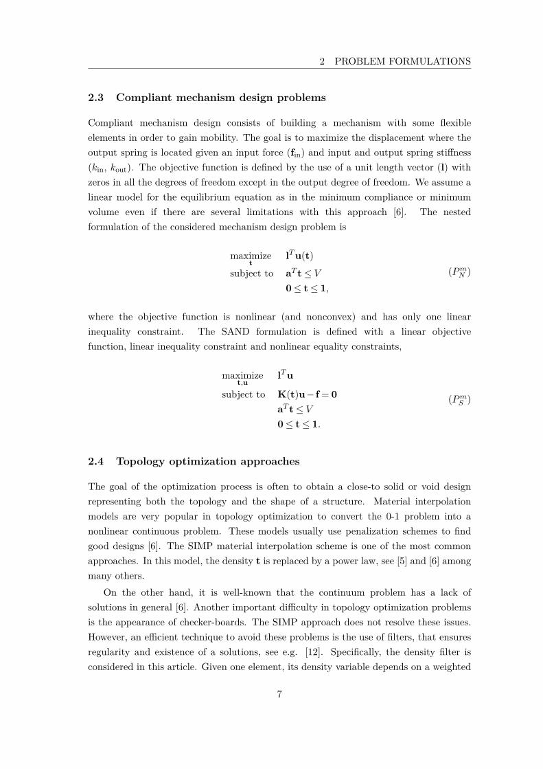
2 PROBLEM FORMULATIONS
2.3 Compliant mechanism design problems
Compliant mechanism design consists of building a mechanism with some flexibleelements in order to gain mobility. The goal is to maximize the displacement where theoutput spring is located given an input force (fin) and input and output spring stiffness(kin, kout). The objective function is defined by the use of a unit length vector (l) withzeros in all the degrees of freedom except in the output degree of freedom. We assume alinear model for the equilibrium equation as in the minimum compliance or minimumvolume even if there are several limitations with this approach [6]. The nestedformulation of the considered mechanism design problem is
maximizet
lTu(t)subject to aT t≤ V
0≤ t≤ 1,(Pm
N )
where the objective function is nonlinear (and nonconvex) and has only one linearinequality constraint. The SAND formulation is defined with a linear objectivefunction, linear inequality constraint and nonlinear equality constraints,
maximizet,u
lTu
subject to K(t)u− f = 0aT t≤ V0≤ t≤ 1.
(PmS )
2.4 Topology optimization approaches
The goal of the optimization process is often to obtain a close-to solid or void designrepresenting both the topology and the shape of a structure. Material interpolationmodels are very popular in topology optimization to convert the 0-1 problem into anonlinear continuous problem. These models usually use penalization schemes to findgood designs [6]. The SIMP material interpolation scheme is one of the most commonapproaches. In this model, the density t is replaced by a power law, see [5] and [6] amongmany others.
On the other hand, it is well-known that the continuum problem has a lack ofsolutions in general [6]. Another important difficulty in topology optimization problemsis the appearance of checker-boards. The SIMP approach does not resolve these issues.However, an efficient technique to avoid these problems is the use of filters, that ensuresregularity and existence of a solutions, see e.g. [12]. Specifically, the density filter isconsidered in this article. Given one element, its density variable depends on a weighted
7

average over the neighbours in a radius rmin.
te = 1∑
i∈NeHei
∑
i∈Ne
Heiti
Hei = max(0, rmin−∆(e, i))(3)
Here, te is the transformed density variable of element e, Ne the set of elements for whichthe distance to element i (defined by ∆(e, i)) is smaller than the filter radius rmin. Inpractice, this concrete value is taken from [2], rmin = 0.04Lx, where Lx is the length ofthe design domain in the x direction.
The modified stiffness matrix using density filter and SIMP penalization is
K(t) =n∑
e=1(Ev +(E1−Ev)tpe)Ke (4)
where p ≥ 1 and Ev > 0 and E1 Ev are Young’s modulus of the "void" and solidmaterial, respectively. The parameter Ev is included to avoid ill-conditioning when thedensity variable is equal to zero, as previously mentioned. This formulation has provenparticularly efficient in many cases [6]. More details about this interpolation is given in[4]. In practice, SIMP typically has a penalization parameter value chosen to be p = 3,see e.g [2] and [6]. This value is used in the numerical experiments (cf. below).
3 Implementation
This section contains all relevant information required to reproduce the numerical results.It includes a brief description of the solvers used in the benchmarking as well as the detailsof the implementation such as the finite elements, the stopping criteria, and the settingof the parameters.
3.1 Chosen optimization methods
Structural topology optimization problems are usually solved using sequential convexapproximation methods such as the Method of Moving Asymptotes (MMA) [43] or theGlobally Convergent Method of Moving Asymptotes (GCMMA) [44]. These methodswere used for structural topology optimization in e.g. [41], [48], and [18], among manyothers.
These methods generally require one evaluation of the objective and constraintfunctions and their derivatives at each iteration. GCMMA includes inner iterations,making the approximations more conservative, to force global convergence to a KKT(Karush-Kuhn-Tucker) point. These methods are only applicable for optimization
8

3 IMPLEMENTATION
problems with inequality constraints1, which means that only the nested formulationscan be solved with them.
In addition, the nested formulations can also be solved using the Optimality Criteria(OC) method [37], [53], and [6] among others. It is valid only when the gradient of theobjective function is negative, thus it is not possible to implement it for minimum volumeproblems. In particular, we use the 88-lines code from [2] and the 104-lines code from [6]for the OC method for minimum compliance and compliant mechanism design problems,respectively.
However, since topology optimization are nonlinear optimization problems, it ispossible to use state-of-the-art second-order solvers to solve them. Twoimplementations of primal-dual interior point solvers, IPOPT [47] and FMINCON [45],and a sequential quadratic programming solver SNOPT [24] version 7, are tested fortopology optimization problems. IPOPT is a primal-dual interior point software libraryfor large-scale nonlinear optimization problems that uses a line-search based on filtermethods. SNOPT is also a general large-scale optimization solver that uses a sequentialquadratic programming algorithm. Finally, FMINCON is a set of nonlinearoptimization algorithms in MATLAB. These three optimization methods all haveMATLAB interfaces, are popular, and have been extensively benchmarked in theoptimization community, see e.g. [7] and [32]. Moreover, IPOPT and SNOPT havealready used for certain topology optimization problems in e.g. [15] and [28]. Thesesolvers accept both equality and inequality constraints, hence it is possible tobenchmark the SAND formulation. For those solvers that can use exact Hessian(IPOPT and FMINCON), it is much simpler and cheaper to compute it in the SANDthan in the nested approach. For the nested formulation, the default linear solverMUMPS [1] is used in IPOPT to compute the search direction while for the SANDformulation, MA27 is used [20]. The IPOPT version used is 3.11.1.
3.2 Finite element analysis
The design domains of the benchmark library created for this study (cf. below), are all2D and discretized by square finite elements. It is assumed that the domain is rectangularand each element has four nodes with two degrees of freedom per node. A 2 by 2 Gaussianintegration rule is used in the computation of the stiffness matrix. This Q4 interpolationof displacements is identical to that implemented in [2].
1There are implementations of these methods which do allow equality constraints see e.g. [52] and[49]. However, to the best of our knowledge there are no numerical results suggesting that these methodscan be used to solve SAND formulation of topology optimization problems.
9

3.3 Stopping criteria
For a general nonlinear optimization problem
minimizex
f(x)subject to hi(x) = 0 i= 1, . . . ,m
gi(x)≤ 0 i= 1, . . . , t,(5)
the Lagrangian function is
L(x,λ,µ) = f(x)+m∑
i
λihi(x)+t∑
i
µigi(x), (6)
where λ and µ are the Lagrangian multipliers of the equality and inequality constraints,respectively. A primal-dual solution (x,λ,µ) of problem (5), should satisfy the Karush-Kuhn-Tucker (KKT) optimality conditions [33].
∇L(x∗,λ∗,µ∗) = 0 (7)hi(x∗) = 0 i= 1, . . . ,m (8)gi(x∗)≤ 0 i= 1, . . . , t (9)
µ∗i ≥ 0 i= 1, . . . , t (10)µ∗i gi(x∗) = 0 i= 1, . . . , t. (11)
Equation (7) is the stationary condition, (8) and (9) are the primal feasibility condition,(10) is the dual feasibility condition, and (11) contains the complementarity condition.In practice, we assume that the KKT conditions are numerically satisfied if the Euclideannorm of the equations is lower than a given positive tolerance ω. In the same way, theprimal feasibility conditions are satisfied if the Euclidean norm is lower than some givenpositive tolerance η. These tolerances will significantly affect the final design.
The solvers MMA, GCMMA, IPOPT, SNOPT and FMINCON have differentimplementations of the optimality conditions (different scalings and norms).Nevertheless, at the end of the optimization process the KKT error is measured for allof them using (7)-(11) to be consistent in the future comparison of the solvers.
The solvers will try to obtain a design until the feasibility error and the optimalityconditions are lower than certain specified tolerances (ω and η, respectively). The valueof ω is, in this benchmark, set differently for the first- and second-order methods2,respectively. IPOPT, FMINCON and SNOPT are generally able to satisfy the KKT
2MMA and GCMMA are considered as first-order methods. IPOPT, SNOPT and FMINCON areconsidered as second-order methods even though for certain problem formulations, limited memory BFGS(Broyden-Fletcher-Goldfarb-Shanno) is used to approximate the Hessian of the Lagrangian.
10
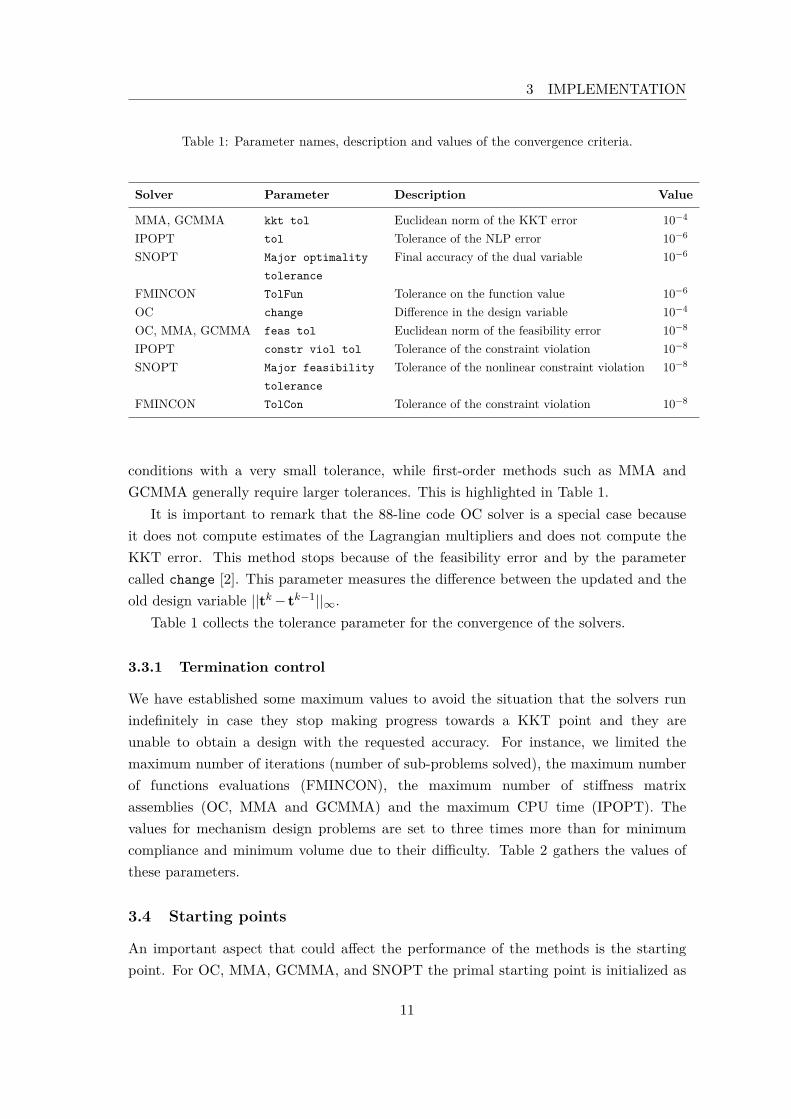
3 IMPLEMENTATION
Table 1: Parameter names, description and values of the convergence criteria.
Solver Parameter Description Value
MMA, GCMMA kkt tol Euclidean norm of the KKT error 10−4
IPOPT tol Tolerance of the NLP error 10−6
SNOPT Major optimality Final accuracy of the dual variable 10−6
toleranceFMINCON TolFun Tolerance on the function value 10−6
OC change Difference in the design variable 10−4
OC, MMA, GCMMA feas tol Euclidean norm of the feasibility error 10−8
IPOPT constr viol tol Tolerance of the constraint violation 10−8
SNOPT Major feasibility Tolerance of the nonlinear constraint violation 10−8
toleranceFMINCON TolCon Tolerance of the constraint violation 10−8
conditions with a very small tolerance, while first-order methods such as MMA andGCMMA generally require larger tolerances. This is highlighted in Table 1.
It is important to remark that the 88-line code OC solver is a special case becauseit does not compute estimates of the Lagrangian multipliers and does not compute theKKT error. This method stops because of the feasibility error and by the parametercalled change [2]. This parameter measures the difference between the updated and theold design variable ||tk− tk−1||∞.
Table 1 collects the tolerance parameter for the convergence of the solvers.
3.3.1 Termination control
We have established some maximum values to avoid the situation that the solvers runindefinitely in case they stop making progress towards a KKT point and they areunable to obtain a design with the requested accuracy. For instance, we limited themaximum number of iterations (number of sub-problems solved), the maximum numberof functions evaluations (FMINCON), the maximum number of stiffness matrixassemblies (OC, MMA and GCMMA) and the maximum CPU time (IPOPT). Thevalues for mechanism design problems are set to three times more than for minimumcompliance and minimum volume due to their difficulty. Table 2 gathers the values ofthese parameters.
3.4 Starting points
An important aspect that could affect the performance of the methods is the startingpoint. For OC, MMA, GCMMA, and SNOPT the primal starting point is initialized as
11

Table 2: Parameter names, description and values of the other termination criteria.
Solver Parameter Description Value
OC loop Maximum number of iterations 1,000MMA, GCMMA max outer itn Maximum number iterations 1,000IPOPT max iter Maximum number of iterations 1,000SNOPT Major iterations limit Maximum number of iterations 1,000FMINCON MaxIter Maximum number of iterations 1,000OC, MMA, GCMMA max assemblies Maximum number of stiffness 10,000
matrix assembliesIPOPT max cpu time Maximum CPU time 48hFMINCON MaxFunEvals Maximum number of 10,000
function evaluations
an homogeneous design with t0 = V e where e is a vector of all ones. The displacementsare set to u0 = 0 for the minimum compliance and compliant mechanism design problems.However, the starting points in IPOPT and FMINCON are always initialized in betweenthe lower and upper bounds on the density variables, i.e t0 = 0.5e and u0 = 0. Otherstarting points could be a disadvantage due to the use of interior point algorithms. Forminimum volume problems the starting point is chosen as t0 = 0.5e and u0 = 0. Otherstarting points for the displacements were examined but did not give better results.For instance, our numerical experiments did not indicate any difference between theinitialization u0 = K−1(t0)f to the initialization u0 = 0.
3.5 Computation of compliance upper limit
For minimum compliance and compliant mechanism design problems, the volumeconstraint is limited by an upper bound given by a scalar value between 0 and 1, toindicate the percentage of material the user wants in the final design. For minimumvolume problems the upper limit in the compliance constraint is chosen as
C = k(fT (K−1(t0)f)), (12)
for some user defined constant k ≥ 1.
3.6 Setting of the parameters
In general, it is desirable to tune the solver parameters as little as possible. However, theperformance of the solvers for topology optimization problems can be improved if somedefault parameters are modified. The automatic scaling of the problem is turned off inboth IPOPT and FMINCON solvers. Depending on the problem and the formulation
12
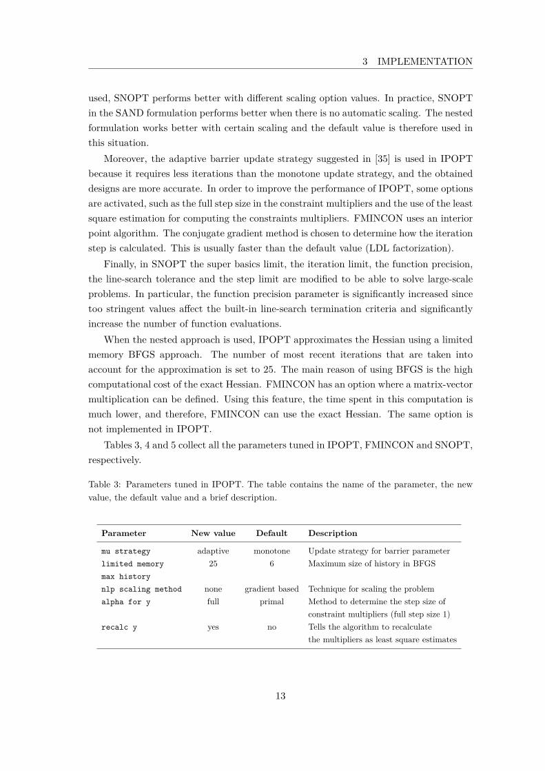
3 IMPLEMENTATION
used, SNOPT performs better with different scaling option values. In practice, SNOPTin the SAND formulation performs better when there is no automatic scaling. The nestedformulation works better with certain scaling and the default value is therefore used inthis situation.
Moreover, the adaptive barrier update strategy suggested in [35] is used in IPOPTbecause it requires less iterations than the monotone update strategy, and the obtaineddesigns are more accurate. In order to improve the performance of IPOPT, some optionsare activated, such as the full step size in the constraint multipliers and the use of the leastsquare estimation for computing the constraints multipliers. FMINCON uses an interiorpoint algorithm. The conjugate gradient method is chosen to determine how the iterationstep is calculated. This is usually faster than the default value (LDL factorization).
Finally, in SNOPT the super basics limit, the iteration limit, the function precision,the line-search tolerance and the step limit are modified to be able to solve large-scaleproblems. In particular, the function precision parameter is significantly increased sincetoo stringent values affect the built-in line-search termination criteria and significantlyincrease the number of function evaluations.
When the nested approach is used, IPOPT approximates the Hessian using a limitedmemory BFGS approach. The number of most recent iterations that are taken intoaccount for the approximation is set to 25. The main reason of using BFGS is the highcomputational cost of the exact Hessian. FMINCON has an option where a matrix-vectormultiplication can be defined. Using this feature, the time spent in this computation ismuch lower, and therefore, FMINCON can use the exact Hessian. The same option isnot implemented in IPOPT.
Tables 3, 4 and 5 collect all the parameters tuned in IPOPT, FMINCON and SNOPT,respectively.
Table 3: Parameters tuned in IPOPT. The table contains the name of the parameter, the newvalue, the default value and a brief description.
Parameter New value Default Description
mu strategy adaptive monotone Update strategy for barrier parameterlimited memory 25 6 Maximum size of history in BFGSmax historynlp scaling method none gradient based Technique for scaling the problemalpha for y full primal Method to determine the step size of
constraint multipliers (full step size 1)recalc y yes no Tells the algorithm to recalculate
the multipliers as least square estimates
13

Table 4: Parameters tuned in FMINCON. The table contains the name of the parameter, thenew value, the default value and a brief description.
Parameter New value Default Description
Algorithm interior point trust region reflective Determine the optimization algorithmSubproblem cg ldl factorization Determines how the iteration step is calculatedAlgorithm
Table 5: Parameters tuned in SNOPT. The table contains the name of the parameter, the newvalue, the default value and a brief description.
Parameter New value Default Description
scale option 0(SAND) 2 Scaling of the problem(2 LP, 0 no scale)
Iteration limit 106 104 Maximum number of minor iterations allowedin QP su-bproblem
Major step limit 10 2 Limits the change in x during the line-searchLine search tolerance .99999 .9 Accuracy which a step length will be located
along the search directionNew superbasics limit 104 99 Early termination of QP sub-problem if the
number of free variables has increasedsince the first feasibility iteration
Function precision 10−4 3.7×10⁻¹¹ Relative function precision
3.7 Scaling of the problems
Regarding the Young’s modulus parameters, the benchmark library instances defined inSection 4.4, considers rather small contrast between the solid (E1) and the void (Ev)values. The main reason is that the final design is similar to the results for largecontrast but the time and iterations required to satisfy the stopping criteria issignificantly reduced. Since the scope of interest in this article is the comparison of thesolvers, this contrast is fixed to E1/Ev = 103 for minimum compliance and minimumvolume problems, and to E1/Ev = 102 for compliant mechanism design problems. Ourexperience is that compliant mechanism design problems, in general, are more difficultto solve.
Moreover, the choices of void and solid Young’s modulus values considerably modifythe computational performances of all solvers. In particular, the number of iterationsand the obtained accuracy are affected. Table 6 gathers the values of Ev and E1 for eachsolver and class of problem.
14

3 IMPLEMENTATION
Table 6: Young modulus’s values for each solver and topology optimization problem.
Solver Problem E1 E0
IPOPT/SNOPT Minimum compliance 103 1FMINCON Minimum compliance 102 10−1
IPOPT/SNOPT Minimum volume 104 10FMINCON Minimum volume 10 10−2
MMA/GCMMA Minimum compliance/volume 10 10−2
OC Minimum compliance 1 10−3
All Mechanism design 1 10−2
Finally, the Poisson’s ratio parameter is set to ν = 0.3 as in [2]. The numericalbehaviour of the solvers (except OC) is better if the inequality constraint is scaled bya factor of 1√
nfor minimum compliance and minimum volume problems. Additionally,
for IPOPT, FMINCON and SNOPT in the compliant mechanism design problems, it isscaled by 1
n , while in MMA and GCMMA is by 1√n.
3.8 Code modifications
Some parts of the code for GCMMA and OC have been modified to obtain betterresults and to improve the performance. First of all, the maximum number of inneriterations in GCMMA is reduced from 50 to two. The main reason is to be lessrestrictive with the convex approximation of the problems. This means that thetheoretical global convergence results from [44] are no longer certain to hold, but ournumerical results indicate that this is a good compromise between robustness andefficiency.
In OC, the stopping criteria has been slightly changed to satisfy either the changeparameter and the feasibility tolerance, or the maximum number of iterations orassemblies, with values given in Tables 1 and 2. Moreover, the inner OC loop, i.e.estimation of the Lagrange multiplier for the volume constraint by bisection, ismodified such as that the difference of limits has to be lower than 10−6. Previous valueswere 10−3 for minimum compliance problems and 10−4 for mechanism design problems.Finally, it is important to remark that the OC method in the 88-line code from [2] hasbeen modified to mechanism design problems following instructions for earlier codes in[6].
15

4 Benchmarking
A method called performance profiles was proposed in [19] to compare differentoptimization solvers on a set of problem instances. This tool was also used in e.g [7] tocompare large-scale nonlinear optimization algorithms.
One of the benefits of this tool of comparison is that it is possible to obtain a globalidea of how the solvers perform.
4.1 Performance profiles
Performance profiles show the general performance of all the solvers in 2D plots. The x-axis represents the parameter τ that indicates how far a solver is from being the winner(regarding a specific criterion such as objective function or number of iterations), i.e.it describes the relative ratio of performance. The y-axis represents the percentage ofproblems that each solver is able to obtain a solution by a factor τ to the best solverfor a concrete measure of performance. In the case where we are only interested in thenumber of problems where the solver is the best, the scope of interest is τ = 1.
When τ is small, the performance profile shows the amount of problems the solver hasperformed similar to the best solver at each problem. While τ increases, the percentageof problems increases because the solver has more chances to obtain a solution. It isdesirable to observe a high increase of percentage of problems for small variations of τ .Those solvers with fast growth are the most suitable because, in general, the performanceof this solver for the whole test set is very close to the best solver for each concreteproblem, for the specific criterion. When τ is large, it shows the chances of a solver to beable to solve any problem. Performance profiles, as explained in [19], are based on a setP of problem instances. The performance of a set of solvers S is evaluated and comparedusing the set. A measure of performance, m, such as the number of iterations, is definedfor a given problem p and a solver s as
mp,s = iterp,s = number of iterations required to solve the problem p by a solver s.(13)
The ratio of performance rp,s is the specific measure compared with the bestperformance of all the solvers.
rp,s = mp,s
minmp,s : s ∈ S . (14)
Moreover, the maximum value of the ratio, rM , is defined such as rM > rp,s for all p ands, and rM = rp,s if and only if there is a failure of the solver. Then, the performance ofthe solver is defined by
ρs(τ) = 1np
sizep ∈ P : rp,s ≤ τ (15)
16

4 BENCHMARKING
which represents the probability that the performance ratio for solver s is at most, a factorof τ of the best possible ratio. The term np represents the total number of problems inthe test set.
The performance of a solver can also be defined by
ρs(τ) = 1np
sizep ∈ P : log(rp,s)≤ τ (16)
This logarithmic scale is considered in order to observe all the performance of the solveruntil τ = rM .
4.2 Performance evaluation
Before presenting the results of the benchmark, it is necessary to establish which measuresare the most suitable to compare the optimization methods. It is, for example, importantto use few function evaluations. For topology optimization problems on nested form, thisis equivalent to the assembly of the stiffness matrix. An efficient method should, thus,assemble the matrix as few times as possible.
Moreover, the performance of a solver should be evaluated for the number of iterations(one iteration is equivalent to the solution of one sub-problem), the CPU time, and theobtained objective function value. The comparison of the objective function value isfocused on the behaviour for small values of τ . This first performance will be decisive forour final recommendation, since hopefully, most the methods will achieve good designsin a small range of τ .
4.3 Penalization of inaccurate designs
It is important to be consistent and clarify under which circumstances the final designof a solver is not considered adequate and is penalized in the performance profiles.
It could happen that for some problems, a method is unable to obtain an accuratedesign, i.e. to sufficiently accurately satisfy the optimality conditions. In those cases,the solver fails and must be penalized in the performance profiles. We establish that themethod obtains an incorrect design when some of the following conditions occurs:
• Infeasibility. If the feasibility error, i.e the Euclidean norm of equations (8) and(9), is greater than a threshold chosen to ηmax = 10−4.
• KKT conditions unsatisfied. If the KKT error, i.e the Euclidean norm of equations(7)-(11), is greater than ωmax = 10−3 (cf. below).
• Incorrect sign of the objective function. If the objective function value is greaterthan zero for compliant mechanism design problems and smaller than zero forminimum compliance and minimum volume problems.
17

In those cases, the ratio for this concrete solver s for the problem p must be rp,s = rM
for all the ratio criteria.However, there are some problems that have to be removed from the test set either
for computational time or for problems with the available memory. Each solver is allowedto run for 48 hours. If it cannot find a design, if MATLAB produces an exception or ifIPOPT and SNOPT stop with flag of memory/time problems, the problem is removedfrom the final test set. If one solver is unable to solve an instance for these reasons, thisproblem is not solved for any solver. When these errors happen, it is not possible toconsider that the solver is unable to obtain a good design because it is simply, it cannotsolve such a large problem. It is not a problem of the underlying method by itself, it isan issue related to the particular choices in the implementation and the properties of thecomputer.
4.4 Test set of topology optimization problems
It is important to produce a large and representative test set of topology optimizationproblems in order to be able to conclude and state recommendations from theperformance profiles. The election of which problems should be selected to obtain a fairbenchmark is always a source of disagreements. The test set should be heterogeneous,interesting and difficult to solve.
Some of the most typical test sets of problems considered in the literature for linearand nonlinear optimization methods are CUTE [10], CUTEr [25], MIPLIB [29], COPS[9] and Vanderbei among others (used in [7], [19] and [47]). In contrast, in the topologyoptimization field, there is no publicly available big test set of problems. In general, thenumerical results in research articles are made using only three or four examples, see e.g.[18], and [48].
In [41] it is noted that there are several test problems well-known for benchmarkingminimum compliance problems, however, there is no standardization regarding compliantmechanism design problems. In this section we present a test set of problems in twodimensions and with a rectangular design domain. Moreover, the static external loadis a single nonzero vector with value equal to one (fi = 1, fj = 0 ∀j 6= i). Finally, forsimplicity, the volume is identical for all the elements, i.e. ai = aj ∀i, j = 1, . . . ,n.
4.4.1 Minimum compliance and minimum volume test problems
Three different types of design domains and loads are considered (see Figure 1) forminimum compliance and minimum volume problems. These examples are considered inplenty of articles related to topology optimization such as [40], [4], [13], [2], [14], and [6].For each domain we consider different length ratios. We experience that the methodshave difficulties in solving problems with large difference between lengths.
18

4 BENCHMARKING
(a) Michell problem (b) Cantilever problem
(c) MBB problem
Figure 1: Michell, Cantilever, and MBB design domains, boundary conditions and external loaddefinitions that are collected and used to define the benchmarking library.
Moreover, for each length, different size of discretization, Nl, are defined. Nl refersto the number of elements in the finite element analysis defined for unit of length. Wedecided to build a test set with a relatively low number of elements to be able to test allthe solvers. Since several of the implementations are general purpose codes, which arenot designed for simulation based problems, larger numbers of elements will eventuallyresult in problems of memory. The memory usage could be an important factor whendifferent solvers are compared. However, since each solver is implemented in differentlanguages, the interfaces between MATLAB and these programs increase memory usagesignificantly. Therefore, it is not possible to produce any fair study of memory usage.
Finally, for each design domain in the minimum compliance test set, 5 different volumefraction upper bounds are considered. The volume bound is chosen from the values 0.1,0.2, 0.3, 0.4, and 0.5. Solving problems with small volume bounds is, in our experience,generally more difficult and should give some issues. In general, when the amount ofmaterial available is reduced, the solvers have more difficulties in distributing the materialso that the structure satisfies the constraints and minimizes the objective function. Forminimum volume problems, three different instances, with upper bound in the complianceproportional to k = 1, 1.2, and 1.5 (see (12)) are generated.
A brief description of the test set is outlined in Tables 7, 9, and 8. The test set ofminimum compliance problems contains 5 different problems for each characteristic’s row(one for each volume bound) with a total number of problems of 225, while the minimumvolume test set contains 135 problems.
19

Table 7: Test set of problems for the Michelldesign domain, see Figure 1a. Lx and Ly
denote the length ratio on the x and y
direction, respectively. Nl denotes the sizeof the discretization per unit of length, nthe number of elements and d the numberof degrees of freedom.
Domain Lx Ly Nl n d
Michell
1 1
20 400 88240 1600 336260 3600 744280 6400 13122100 10000 20402
2 1
20 800 172240 3200 664260 7200 1476280 12800 26082100 20000 40602
3 1
20 1200 256240 4800 992260 10800 2208280 19200 39042100 30000 60802
Table 8: Test set of problems for the MBBdesign domain, see Figure 1c.
Domain Lx Ly Nl n d
MBB
1 2
20 800 172240 3200 664260 7200 1476280 12800 26082100 20000 40602
1 4
20 1600 340240 6400 1320260 14400 2940280 25600 52002100 40000 81002
2 1
20 800 172240 3200 664260 7200 1476280 12800 26082100 20000 40602
4 1
20 1600 340240 6400 1320260 14400 2940280 25600 52002100 40000 81002
Table 9: Test set of problems for theCantilever design domain, see Figure 1b.
Domain Lx Ly Nl n d
Cantilever
2 1
20 800 172240 3200 664260 7200 1476280 12800 26082100 20000 40602
4 1
20 1600 340240 6400 1320260 14400 2940280 25600 52002100 40000 81002
Table 10: Test set of 150 compliantmechanism design problems, see Figure 2.
Domain Lx Ly Nl n d
Inverter/Gripper/Amplifier/CompliantLever/Crimper
1 1
20 400 88240 1600 336260 3600 744280 6400 13122100 10000 20402
2 1
20 800 172240 3200 664260 7200 1476280 12800 26082100 20000 40602
20

5 NUMERICAL EXPERIMENTS
4.4.2 Compliant mechanism design problem
The most typical problem used to test the methods in the literature is the force inverter,shown in Figure 2a, see e.g. [41]. Furthermore, another typical compliant mechanism,called the compliance gripper, is included in the benchmark library, see Figure 2b. Threemore examples denoted the amplifier, the compliant lever, and the crimper, shown inFigure 2c, 2d, and 2e, respectively, complete the mechanism design test set. Theseproblems can be found in different publications such as [6], [48], [40], [14], [39], [18], [31],and [38].
For each design domain, 5 different discretizations, and three different volumefractions: 0.2, 0.3, 0.4, are considered resulting in a a final test set of 150 problemsgathered in Table 10.
5 Numerical experiments
The benchmark library is based on 225 minimum compliance problems, 135 minimumvolume problems and 150 mechanism design problems. However, the final benchmarklibrary is made of a subset using 121, 64 and 124 examples respectively. For the rest ofthe problem instances, either IPOPT, SNOPT or FMINCON in the SAND formulationhave memory problems or the computational time required is more than the maximumallowed (which is 48h). The need of research in efficient and fast large-scale methods tobe able to solve large saddle-points systems is evident from this fact.
Furthermore, as the objective function value of the compliant mechanism designproblems is negative, large values of ratios represent better performance than smallvalues of ratios. In order to observe the same scale and behaviour in the profiles forcompliant mechanism design problems, the ratio of the objective function value iscomputed as the inverse of equation (14).
All computations were done on an Intel Xeon X5650 6-core CPUs, running at 2.66GHz and with 4 GB Memory for each core.
It is important to highlight that the computation time is highly affected by theamount of work assigned to the nodes in the cluster. The time for the same problemusing the same solver at different moments in time can vary significantly. Therefore,we do not recommend that the performance profiles for computational time are trustedunconditionally.
Finally, some restrictions have been made during the numerical experiments. Boththe SAND and the SANDNL formulations require a lot of memory, and, for largeproblems, the solvers are unable to run. In a reduced test set of small problems, theperformance of both formulations is compared. The results are not reported here, butboth formulations obtain similar results in function objective value, number of
21

(a) Force inverter example with kin = 1 andkout = 0.001
(b) Compliant gripper example with kin = 1and kout = 0.005
(c) Amplifier example with kin = 1 andkout = 0.005
(d) Compliant lever example with kin = 1and kout = 0.005
(e) Crimper example with kin = 1 andkout = 0.05
Figure 2: Compliant mechanism design domains, with boundary conditions and external loadsdefinition.
iterations and also computational time. The performance of SNOPT and FMINCONon the SAND/SANDNL formulation is not competitive. In order to save time,represent more problems and produce clearer results we have decided to remove theSANDNL formulation. The SAND formulation for SNOPT and FMINCON are alsoexcluded from the minimum volume benchmark.
22
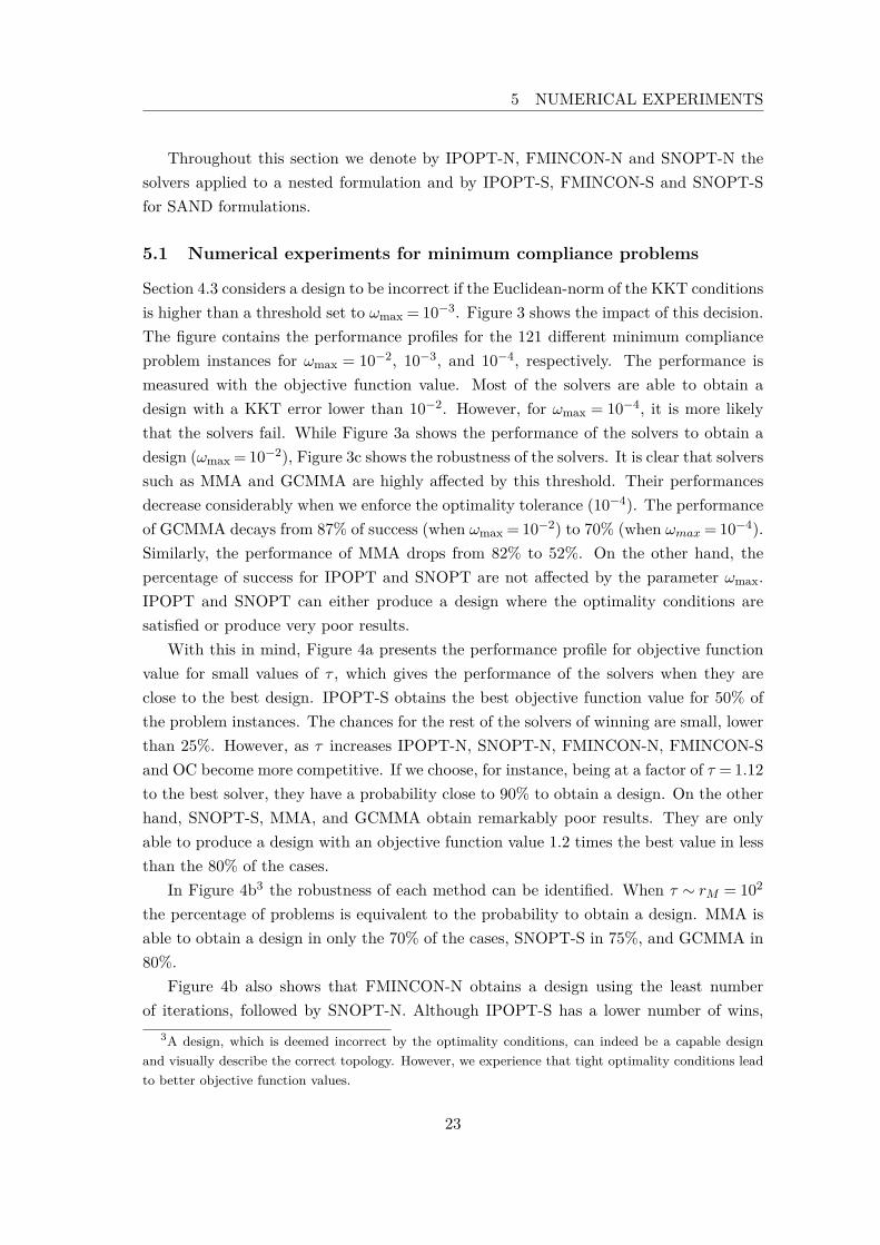
5 NUMERICAL EXPERIMENTS
Throughout this section we denote by IPOPT-N, FMINCON-N and SNOPT-N thesolvers applied to a nested formulation and by IPOPT-S, FMINCON-S and SNOPT-Sfor SAND formulations.
5.1 Numerical experiments for minimum compliance problems
Section 4.3 considers a design to be incorrect if the Euclidean-norm of the KKT conditionsis higher than a threshold set to ωmax = 10−3. Figure 3 shows the impact of this decision.The figure contains the performance profiles for the 121 different minimum complianceproblem instances for ωmax = 10−2, 10−3, and 10−4, respectively. The performance ismeasured with the objective function value. Most of the solvers are able to obtain adesign with a KKT error lower than 10−2. However, for ωmax = 10−4, it is more likelythat the solvers fail. While Figure 3a shows the performance of the solvers to obtain adesign (ωmax = 10−2), Figure 3c shows the robustness of the solvers. It is clear that solverssuch as MMA and GCMMA are highly affected by this threshold. Their performancesdecrease considerably when we enforce the optimality tolerance (10−4). The performanceof GCMMA decays from 87% of success (when ωmax = 10−2) to 70% (when ωmax = 10−4).Similarly, the performance of MMA drops from 82% to 52%. On the other hand, thepercentage of success for IPOPT and SNOPT are not affected by the parameter ωmax.IPOPT and SNOPT can either produce a design where the optimality conditions aresatisfied or produce very poor results.
With this in mind, Figure 4a presents the performance profile for objective functionvalue for small values of τ , which gives the performance of the solvers when they areclose to the best design. IPOPT-S obtains the best objective function value for 50% ofthe problem instances. The chances for the rest of the solvers of winning are small, lowerthan 25%. However, as τ increases IPOPT-N, SNOPT-N, FMINCON-N, FMINCON-Sand OC become more competitive. If we choose, for instance, being at a factor of τ = 1.12to the best solver, they have a probability close to 90% to obtain a design. On the otherhand, SNOPT-S, MMA, and GCMMA obtain remarkably poor results. They are onlyable to produce a design with an objective function value 1.2 times the best value in lessthan the 80% of the cases.
In Figure 4b3 the robustness of each method can be identified. When τ ∼ rM = 102
the percentage of problems is equivalent to the probability to obtain a design. MMA isable to obtain a design in only the 70% of the cases, SNOPT-S in 75%, and GCMMA in80%.
Figure 4b also shows that FMINCON-N obtains a design using the least numberof iterations, followed by SNOPT-N. Although IPOPT-S has a lower number of wins,
3A design, which is deemed incorrect by the optimality conditions, can indeed be a capable designand visually describe the correct topology. However, we experience that tight optimality conditions leadto better objective function values.
23

1 1.02 1.04 1.06 1.08 1.1 1.12 1.14 1.16 1.18 1.20
10
20
30
40
50
60
70
80
90
100
τ
%problems
OCMMAGCMMAIPOPT NIPOPT SFMINCON NFMINCON SSNOPT NSNOPT S
(a) Penalization of problems with ωmax = 10−2
1 1.02 1.04 1.06 1.08 1.1 1.12 1.14 1.16 1.18 1.20
10
20
30
40
50
60
70
80
90
100
τ
%problems
OCMMAGCMMAIPOPT NIPOPT SFMINCON NFMINCON SSNOPT NSNOPT S
(b) Penalization of problems with ωmax = 10−3
1 1.02 1.04 1.06 1.08 1.1 1.12 1.14 1.16 1.18 1.20
10
20
30
40
50
60
70
80
90
100
τ
%problems
OCMMAGCMMAIPOPT NIPOPT SFMINCON NFMINCON SSNOPT NSNOPT S
(c) Penalization of problems with ωmax = 10−4
Figure 3: Performance profiles for the (reduced) test set of 121 minimum compliance problems(P c
N ) and (P cS). The performance is measured for objective function value. A problem is penalized
in the performance profiles if the KKT error is higher than 10−2 (3a), 10−3 (3b) or 10−4 (3c),respectively.
24

5 NUMERICAL EXPERIMENTS
1 1.02 1.04 1.06 1.08 1.1 1.12 1.14 1.16 1.18 1.20
10
20
30
40
50
60
70
80
90
100
τ
%problems
OCMMAGCMMAIPOPT NIPOPT SFMINCON NFMINCON SSNOPT NSNOPT S
(a) Objective function value
0 0.2 0.4 0.6 0.8 1 1.2 1.4 1.6 1.8 20
10
20
30
40
50
60
70
80
90
100
τ (log10)
%problems
OCMMAGCMMAIPOPT NIPOPT SFMINCON NFMINCON SSNOPT NSNOPT S
(b) Number of iterations
0 0.5 1 1.5 2 2.5 3 3.50
10
20
30
40
50
60
70
80
90
100
τ (log10)
%problems
OCMMAGCMMAIPOPT NIPOPT SFMINCON NFMINCON SSNOPT NSNOPT S
(c) Number of stiffness matrix assemblies
0 0.5 1 1.5 2 2.5 3 3.5 40
10
20
30
40
50
60
70
80
90
100
τ (log10)
%problems
OCMMAGCMMAIPOPT NIPOPT SFMINCON NFMINCON SSNOPT NSNOPT S
(d) Computational time
Figure 4: Performance profiles for the (reduced) test set of 121 minimum compliance problems(P c
N ) and (P cS) described in Tables 7, 9 and 8. The performance is measured by objective
function value (4a), number of iterations (4b), number of stiffness matrix assemblies (4c), andcomputational time (4d).
25

it becomes a strong rival when τ increases. FMINCON-N, SNOPT-N and IPOPT-Sperform at a factor of 10 to the best solver in around 85-100% of the instances. Ingeneral, the rest of the solvers require substantial numbers of iterations to obtain adesign (the performance is lower than 80%).
The performance of the solvers for the number of stiffness matrix assemblies (Figure4c) is very similar to for the number of iterations.
Finally, Figure 4d shows the performance profile for the computational time. Itsuggests that SNOPT-N or OC are the best solvers for minimum compliance problems.The rest of the solvers consume more than 102 times, even 103 times more, to achievesimilar percentage of success. It is also clear that the SAND formulation requires a lotof time. However, this study is done using small-scale problems.
We observe that IPOPT-S (which uses an exact Hessian of the Lagrangian)outperforms IPOPT-N (which uses a limited memory BFGS approximation of theHessian) with respect to the objective function value, the number of iterations, and thenumber of assemblies. In contrast, it is clear that the SAND formulation consumesmore time. This could be either for the increase of the number of variables andconstraints or because of the use of exact Hessian. On the other hand, if thecomputational time for FMINCON (both formulations compute the exact Hessian) orSNOPT (both formulations use limited memory BFGS approximations) is compared,we conclude that the increment of time is due to the increment of variables andconstraint but not the use of second order information.
5.2 Numerical experiments for minimum volume problems
Figure 5 shows the performance profiles for the 64 minimum volume problems. This testsect is a sub-set of the problems listed in Tables 7, 9 and 8.
It is clear that IPOPT-S outperforms the rest of the solvers with respect to theobtained objective function value, see Figure 5a. The probability for IPOPT-S of winningis higher than 55%. In addition, it has at least 10% more chances than any other solverto obtain a final design with an objective function value at a factor of τ = 1.2. Unlikethe minimum compliance problems, FMINCON is unable to solve more than the 70% ofthe problems. MMA shows similar performance.
However, IPOPT-S also has the problem that it consumes more iterations andassemblies of the stiffness matrix than SNOPT or FMINCON. Nevertheless, IPOPT-Simproves really fast as τ increases. If we are interested in a solver that can solve morethan the 80% of the problems with the greatest efficiency as possible (for the number ofiterations), then the election should be either IPOPT-S or SNOPT. Their performancefor this 80% is at a factor of τ = 5.6.
The performance of the solvers with respect to the number of assemblies is represented
26

5 NUMERICAL EXPERIMENTS
1 1.02 1.04 1.06 1.08 1.1 1.12 1.14 1.16 1.18 1.20
10
20
30
40
50
60
70
80
90
100
τ
%problems
MMAGCMMAIPOPT NIPOPT SFMINCON NSNOPT N
(a) Objective function value
0 0.2 0.4 0.6 0.8 1 1.2 1.4 1.6 1.80
10
20
30
40
50
60
70
80
90
100
τ (log10)
%problems
MMAGCMMAIPOPT NIPOPT SFMINCON NSNOPT N
(b) Number of iterations
0 0.2 0.4 0.6 0.8 1 1.2 1.4 1.6 1.80
10
20
30
40
50
60
70
80
90
100
τ (log10)
%problems
MMAGCMMAIPOPT NIPOPT SFMINCON NSNOPT N
(c) Number of stiffness matrix assemblies
0 0.5 1 1.5 2 2.5 3 3.50
10
20
30
40
50
60
70
80
90
100
τ (log10)
%problems
MMAGCMMAIPOPT NIPOPT SFMINCON NSNOPT N
(d) Computational time
Figure 5: Performance profiles for the (reduced) test set of 64 minimum volume problems (PwN )
and (PwS ) described in Tables 7, 9 and 8. The performance is measured by objective function value
(5a), number of iterations (5b), number of stiffness matrix assemblies (5c), and computationaltime (5d).
27

in Figure 5c. The robustness of IPOPT-S is again demonstrated since it can solve almost100% of the problems. In contrast, the rest of the solvers have between 75 to 85% ofchances to solve a problem. It is remarkable that MMA and GCMMA require moreiterations and more stiffness matrix assemblies than the general nonlinear solvers.
The performance of the solvers, for computational time, is similar to the results forminimum compliance problems as observed in Figure 5d.
5.3 Numerical experiments for compliant mechanism design problems
Figure 6 shows the performance profiles for the 124 compliant mechanism designproblems listed in Table 10. Our experience is that these problems, in general, are moredifficult to solve than minimum compliance and volume problems. This is reflected inthe performance profiles. One more time, IPOPT-S highlights from the rest of thesolvers. Although, OC has the best performance in 25% of the problems, its probabilityto obtain a design with an objective function value between the best one and 1.2 times,is not higher than 80%. The rest of the solvers have a very poor performance.
Figure 6b shows the performance of the solvers for the number of iterations. AlthoughSNOPT-N obtains the best percentage of winners, IPOPT-S has a 100% of chancesto obtain a design in at most 10 times more iterations than the best solver. At thisfactor, only SNOPT-N is able to obtain a success in more than the 70% of the instances.Indeed, SNOPT-S and MMA have very low performance. They solve less than 65% of theproblems. Although OC has the 100% of probability to obtain a design, the performancefor any value of τ is very poor. In general, OC stops because it reaches the maximumnumber of allowed iterations and not because the change parameter is satisfied (whichis not penalized in these performance profiles).
The behaviour of the solvers for number of stiffness matrix assemblies is very similar tothe number of iterations. For mechanism design problems, GCMMA stands out comparedto FMINCON. This is unlike the situation for minimum compliance and minimum volumeproblems.
5.4 Conclusions from the numerical experiments
After the detailed explanation of the performance profiles for the different type ofproblems, we can generalize that IPOPT-S obtains good designs, it is very robust, andthe performance does not depend on the problem under consideration. With more than95% of probability, IPOPT-S is able to obtain a design satisfying the requiredoptimality conditions. The use of second order information helps IPOPT to producebetter designs using less iterations. On the other hand, it requires a lot ofcomputational time.
28

5 NUMERICAL EXPERIMENTS
1 1.02 1.04 1.06 1.08 1.1 1.12 1.14 1.16 1.18 1.20
10
20
30
40
50
60
70
80
90
100
τ
%problems
OCMMAGCMMAIPOPT NIPOPT SFMINCON NFMINCON SSNOPT NSNOPT S
(a) Objective function value
0 0.5 1 1.5 2 2.50
10
20
30
40
50
60
70
80
90
100
τ (log10)
%problems
OCMMAGCMMAIPOPT NIPOPT SFMINCON NFMINCON SSNOPT NSNOPT S
(b) Number of iterations
0 0.5 1 1.5 2 2.5 30
10
20
30
40
50
60
70
80
90
100
τ (log10)
%problems
OCMMAGCMMAIPOPT NIPOPT SFMINCON NFMINCON SSNOPT NSNOPT S
(c) Number of stiffness matrix assemblies
0 0.5 1 1.5 2 2.5 3 3.5 40
10
20
30
40
50
60
70
80
90
100
τ (log10)
%problems
OCMMAGCMMAIPOPT NIPOPT SFMINCON NFMINCON SSNOPT NSNOPT S
(d) Computational time
Figure 6: Performance profiles for the (reduced) test set of 124 compliant mechanism designproblems (Pm
N ) and (PmS ) described in Table 10. The performance is measured by objective
function value (6a), number of iterations (6b), number of stiffness matrix assemblies (6c), andcomputational time (6d).
29

In contrast, SNOPT-N produces poor designs (bad objective function value) but usingvery few number of iterations and computational time.
In general, the SAND formulation requires a lot of time. There is a need ofimprovements in the computation of the saddle-point system in order to reduce thiscomputational time to be able to obtain a competitive solver when the SANDformulation is used.
Finally, it is curious to observe that the structural optimization methods, MMA andGCMMA, do not outperform the other solvers in neither objective function value nornumber of iterations. Moreover, the performance profiles reveal that GCMMA in generalobtains better designs and requires less iterations than MMA. The additional measuresimplemented in GCMMA compared to MMA to ensure the theoretical global convergenceresults in [44] apparently also have a positive effect on the numerical performance.
6 Limitations of the benchmark
We are aware of the many limitations of this benchmarking study. However, it iscomputationally too demanding to benchmark all possible combinations of optimizationmethods and problem formulations. We therefore decided to focus on a small, butrelevant, range of combinations of problem formulations and methods and develop arepresentative and meticulous benchmark. Further research must be done in order tocontemplate other alternatives to the problems.
First of all, only one topology optimization approach, namely combining the SIMPmaterial interpolation scheme with a density filter, has been used. The RAMP materialinterpolation [42] and [36] has been numerically tested, giving similar results to the SIMPscheme. It could be interesting to observe the performance of the solvers when otherpenalizations schemes or regularization approach are used, such as for example perimetercontrol [26]. The problems, furthermore, only include a few mechanical requirements.Important constraints such as displacement and stress constraints, are not modelled andincluded in the benchmark problems.
Moreover, there are limitations regarding the choice of solvers used for thebenchmarking. There is room for testing several other general nonlinear optimizationsolvers. This includes those implemented in the KNITRO package [16], the interiorpoint method in LOQO [46], the sequential augmented Lagrangian algorithms inLANCELOT [17], or MINOS [34], the generalized augmented Lagrangian method inPENNON [30], and the feasible direction method in FAIPA [27], among others.
The scaling of the problems as well as different parameter values such as the Young’smodulus, the magnitude of the external loads, the penalty parameter p in the SIMPpenalization, and the filter radius rmin of the density filter have been set to only onevalue. It is likely that the performance of the solvers is affected by them.
30
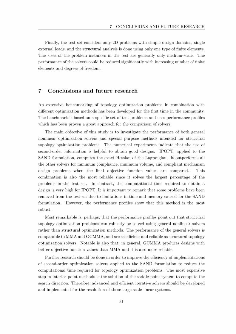
7 CONCLUSIONS AND FUTURE RESEARCH
Finally, the test set considers only 2D problems with simple design domains, singleexternal loads, and the structural analysis is done using only one type of finite elements.The sizes of the problem instances in the test are generally only medium-scale. Theperformance of the solvers could be reduced significantly with increasing number of finiteelements and degrees of freedom.
7 Conclusions and future research
An extensive benchmarking of topology optimization problems in combination withdifferent optimization methods has been developed for the first time in the community.The benchmark is based on a specific set of test problems and uses performance profileswhich has been proven a great approach for the comparison of solvers.
The main objective of this study is to investigate the performance of both generalnonlinear optimization solvers and special purpose methods intended for structuraltopology optimization problems. The numerical experiments indicate that the use ofsecond-order information is helpful to obtain good designs. IPOPT, applied to theSAND formulation, computes the exact Hessian of the Lagrangian. It outperforms allthe other solvers for minimum compliance, minimum volume, and compliant mechanismdesign problems when the final objective function values are compared. Thiscombination is also the most reliable since it solves the largest percentage of theproblems in the test set. In contrast, the computational time required to obtain adesign is very high for IPOPT. It is important to remark that some problems have beenremoved from the test set due to limitations in time and memory caused for the SANDformulation. However, the performance profiles show that this method is the mostrobust.
Most remarkable is, perhaps, that the performance profiles point out that structuraltopology optimization problems can robustly be solved using general nonlinear solversrather than structural optimization methods. The performance of the general solvers iscomparable to MMA and GCMMA, and are as efficient and reliable as structural topologyoptimization solvers. Notable is also that, in general, GCMMA produces designs withbetter objective function values than MMA and it is also more reliable.
Further research should be done in order to improve the efficiency of implementationsof second-order optimization solvers applied to the SAND formulation to reduce thecomputational time required for topology optimization problems. The most expensivestep in interior point methods is the solution of the saddle-point system to compute thesearch direction. Therefore, advanced and efficient iterative solvers should be developedand implemented for the resolution of these large-scale linear systems.
31

Acknowledgements
We would like to thank Professor Krister Svanberg at KTH in Stockholm for providingthe implementations of both MMA and GCMMA.
References
[1] P. R. Amestoy, I. S. Duff, and J. Y. L’Excellent. Multifrontal parallel distributedsymmetric and unsymmetric solvers. Computer Methods in Applied Mechanics andEngineering, 184(2–4):501–520, 2000.
[2] E. Andreassen, A. Clausen, M. Schevenels, B. S. Lazarov, and O. Sigmund.Efficient topology optimization in MATLAB using 88 lines of code. Structural andMultidisciplinary Optimization, 43(1):1–16, 2011.
[3] J. S. Arora and Q. Wang. Review of formulations for structural and mechanicalsystem optimization. Structural and Multidisciplinary Optimization, 30(4):251–272,2005.
[4] M. P. Bendsøe. Optimal shape design as a material distribution problem. StructuralOptimization, 1(4):192–202, 1989.
[5] M. P. Bendsøe and O. Sigmund. Material interpolation schemes in topologyoptimization. Archive of Applied Mechanics, 69(9–10):635–654, 1999.
[6] M. P. Bendsøe and O. Sigmund. Topology optimization: Theory, methods andapplications. Springer, 2003.
[7] H. Y. Benson, D. F. Shanno, and R. J. Vanderbei. A comparative study of large-scale nonlinear optimization algorithms. Technical report, Operations Research andFinancial Engineering, Princeton University, 2002.
[8] P. T. Boggs and J. W. Tolle. Sequential Quadratic Programming. Acta Numerica,4:1–51, 1995.
[9] A. S. Bondarenko, D. M. Bortz, and J. J. Moré. COPS: Large-scalenonlinearly constrained optimization problems. Technical Report ANL/MCS-TM-237, Mathematics and Computer Science Division, Argonne National Laboratory,1999.
[10] I. Bongartz, A. R. Conn, N. I. M. Gould, and P. L. Toint. CUTE: Constrained andunconstrained testing environment. ACM Transactions on Mathematical Software,21(1):123–160, 1995.
32

REFERENCES
[11] T. Borrvall and J. Petersson. Large-scale topology optimization in 3D using parallelcomputing. Computer Methods in Applied Mechanics and Engineering, 190(46-47):6201–6229, 2001.
[12] B. Bourdin. Filters in topology optimization. International Journal for NumericalMethods in Engineering, 50(9):2143–2158, 2001.
[13] M. Bruggi and P. Duysinx. Topology optimization for minimum weight withcompliance and stress constraints. Structural and Multidisciplinary Optimization,46(3):369–384, 2012.
[14] T. E. Bruns. A reevaluation of the SIMP method with filtering and an alternativeformulation for solid void topology optimization. Structural and MultidisciplinaryOptimization, 30(6):428–436, 2005.
[15] M. Burger and R. Stainko. Phase-field relaxation of topology optimization withlocal stress constraints. SIAM Journal on Control and Optimization, 45(4):1447–1466, 2006.
[16] R. H. Byrd, J. Nocedal, and R. A. Waltz. KNITRO : An Integrated Package forNonlinear Optimization. In Large Scale Nonlinear Optimization, volume 83, pages35–59. Springer, 2006.
[17] A. R Conn, N. I. M. Gould, and P. L. Toint. Lancelot: A FORTRAN Package forLarge-Scale Nonlinear Optimization (Release A). Springer-Verlag, 1992.
[18] S. R. Deepak, M. Dinesh, D. K. Sahu, and G. K. Ananthasuresh. A comparativestudy of the formulations and benchmark problems for the topology optimization ofcompliant mechanisms. Journal of Mechanisms and Robotics, 1(1), 2009.
[19] E. D. Dolan and J. J. Moré. Benchmarking optimization software with performanceprofiles. Mathematical Programming, 91(2):201–213, 2002.
[20] I. S. Duff and J. K. Reid. The multifrontal solution of indefinite sparse symmetriclinear. ACM Transactions on Mathematical Software, 9(3):302–325, 1983.
[21] A. Evgrafov, C. J. Rupp, K. Maute, and M. L. Dunn. Large-scale paralleltopology optimization using a dual-primal substructuring solver. Structural andMultidisciplinary Optimization, 36(4):329–345, 2008.
[22] C. Fleury. Efficient approximation concepts using second order information.International Journal for Numerical Methods in Engineering, 28(9):2041–2058, 1989.
[23] A. Forsgren and P. E. Gill. Primal-dual interior methods for nonconvex nonlinearprogramming. SIAM Journal on Optimization, 8(4):1132–1152, 1998.
33

[24] P. E. Gill, W. Murray, and M. A. Saunders. SNOPT: An SQP Algorithm for Large-Scale Constrained Optimization. SIAM Journal on Optimization, 47(4):99–131,2005.
[25] N. I. M. Gould, D. Orban, and P. L. Toint. CUTEr and SifDec: A constrained andunconstrained testing environment, revisited. ACM Transactions on MathematicalSoftware, 29(4):373–394, 2003.
[26] R. B. Haber, C. S. Jog, and M. P. Bendsøe. A new approach to variable-topologyshape design using a constraint on perimeter. Structural optimization, 11(1–2):1–12,1996.
[27] J. Herskovits. A feasible directions interior-point technique for nonlinearoptimization. Journal of Optimization Theory and Applications, 99(1):121–146,1998.
[28] C. F. Hvejsel and E. Lund. Material interpolation schemes for unified topologyand multi-material optimization. Structural and Multidisciplinary Optimization,43(6):811–825, 2011.
[29] T. Koch, T. Achterberg, E. Andersen, O. Bastert, T. Berthold, R. E. Bixby,E. Danna, G. Gamrath, A. M. Gleixner, S. Heinz, A. Lodi, H. Mittelmann,T. Ralphs, D. Salvagnin, D. E. Steffy, and K. Wolter. MIPLIB 2010. MathematicalProgramming Computation, 3(2):103–163, 2011.
[30] M. Kočvara and M. Stingl. PENNON: A code for convex nonlinear and semidefiniteprogramming. Optimization Methods and Software, 18(3):317–333, 2003.
[31] G. K. Lau, H. Du, and M. K. Lim. Use of functional specifications as objectivefunctions in topological optimization of compliant mechanism. Computer Methodsin Applied Mechanics and Engineering, 190(34):4421–4433, 2001.
[32] S. Leyffer and A. Mahajan. Software for Nonlinearly Constrained Optimization.Technical Report ANS/MCS-P1768-0610, Mathematics and Computer ScienceDivision, Argonne National Laboratory, 2010.
[33] D. G. Luenberger and Y. Ye. Linear and Nonlinear Programming. Springer, 2008.
[34] B. A. Murtagh and M. A. Saunders. MINOS 5.5 User’s Guide. Technical ReportSOL 83-20R, Stanford University Systems Optimization Laboratory, Department ofOperations Research, 1998.
[35] J. Nocedal, R. Wächter, and R. A. Waltz. Adaptive barrier update strategies fornonlinear interior methods. SIAM Journal on Optimization, 19(4):1674–1693, 2009.
34

REFERENCES
[36] A. Rietz. Sufficiency of a finite exponent in SIMP (power law) methods. Structuraland Multidisciplinary Optimization, 21(2):159–163, 2001.
[37] G. I. N. Rozvany and M. Zhou. The COC algorithm, part I: Cross-sectionoptimization or sizing. Computer Methods in Applied Mechanics and Engineering,89(1–3):281–308, 1991.
[38] A. Saxena and G. K. Ananthasuresh. Topology synthesis of compliant mechanismsfor nonlinear force-deflection and curved path specifications. Journal of MechanicalDesign, 123(1):33–42, 2001.
[39] O. Sigmund. On the design of compliant mechanisms using topology optimization.Journal of Structural Mechanics, 25(4):492–526, 1997.
[40] O. Sigmund. Manufacturing tolerant topology optimization. Acta Mechanica Sinica,25(2):227–239, 2009.
[41] O. Sigmund and K. Maute. Topology optimization approaches. Structural andMultidisciplinary Optimization, 48(6):1031–1055, 2013.
[42] M. Stolpe and K. Svanberg. An alternative interpolation scheme for minimumcompliance topology optimization. Structural and Multidisciplinary Optimization,22(2):116–124, 2001.
[43] K. Svanberg. The method of moving asymptotes - A new method for structuraloptimization. International Journal for Numerical Methods in Engineering,24(2):359–373, 1987.
[44] K. Svanberg. A class of globally convergent optimization methods based onconservative convex separable approximations. SIAM Journal on Optimization,12(2):555–573, 2002.
[45] Inc. The MathWorks. Optimization Toolbox User’s Guide R release 2014a, 2014.
[46] R. J. Vanderbei. LOQO User’s Manual. Version 4.05. Technical report, OperationsResearch and Financial Engineering Princeton University, 2006.
[47] A. Wächter and L. T. Biegler. On the implementation of an interior point filter line-search algorithm for large-scale nonlinear programming. Mathematical Programming,106(1):25–57, 2006.
[48] F. Wang, B. S. Lazarov, and O. Sigmund. On projection methods, convergenceand robust formulations in topology optimization. Structural and MultidisciplinaryOptimization, 43(6):767–784, 2011.
35

[49] H. Wang, Q. Ni, and H. Liu. A new method of moving asymptotes for large-scalelinearly equality-constrained minimization. Acta Mathematicae Applicatae Sinica,27(2):317–328, 2011.
[50] M. Y. Wang, X. Wang, and D. Guo. A level set method for structural topologyoptimization. Computer Methods in Applied Mechanics and Engineering, 192(1-2):227–246, 2003.
[51] S. Wang, E. Sturler, and G. H. Paulino. Large scale topology optimization usingpreconditioned Krylov subspace methods with recycling. International Journal forNumerical Methods in Engineering, 69:2441–2468, 2007.
[52] W. H. Zhang, C. Fleury, P. Duysinx, V. H. Nguyen, and I. Laschet. A generalizedmethod of moving asymptotes (GMMA) including equality constraints. Structuraloptimization, 12(2-3):143–146, 1996.
[53] M. Zhou and G. I. N. Rozvany. The COC algorithm, Part II: Topological, geometricaland generalized shape optimization. Computer Methods in Applied Mechanics andEngineering, 89(1–3):309–336, 1991.
[54] C. Zillober. A globally convergent version of the method of moving asymptotes.Structural optimization, 6(3):166–174, 1993.
36

7Article II: Automatic penalty continuation in
structural topology optimization
Published online the 28 July 2015:Rojas-Labanda, S. and Stolpe, M.: Automatic penalty continuation in structural topologyoptimization. Structural and Multidisciplinary Optimization (2015). DOI : 10.1007/s00158-015-1277-1.
103

104

Automatic penalty continuation in structural topologyoptimization∗
Susana Rojas-Labanda+ and Mathias Stolpe+
+DTU Wind Energy, Technical University of Denmark, Frederiksborgvej 399, 4000 Roskilde,Denmark. E-mail: [email protected], [email protected]
Abstract
Structural topology optimization problems are often modelled using materialinterpolation schemes to produce almost solid-and-void designs. The problemsbecome nonconvex due to the use of these techniques. Several articles introducecontinuation approaches in the material penalization parameter to reduce the risksof ending in local minima. However, the numerical performance of continuationmethods has not been studied in detail.
The first purpose of this article is to benchmark existing continuation methodsand the classical formulation with fixed penalty parameter in structural topologyoptimization. This is done using performance profiles on 225 minimum complianceand 150 compliant mechanism design problems.
The results show that continuation methods, generally, find better designs. Onthe other hand, they typically require a larger number of iterations. In the secondpart of the article this issue is addressed. We propose an automatic continuationmethod, where the material penalization parameter is included as a new variable inthe problem and a constraint guarantees that the requested penalty is eventuallyreached. The numerical results suggest that this approach is an appealingalternative to continuation methods. Automatic continuation also generally obtainsbetter designs than the classical formulation using a reduced number of iterations.
Keywords: Topology optimization, Continuation methods, Benchmarking, Mechanismdesign, Minimum complianceMathematics Subject Classification 2010: 74P05, 74P15, and 90C90
∗This research is funded by the Villum Foundation through the research project Topology Optimization- The Next Generation (NextTop).
1

1 Introduction
Structural topology optimization distributes the material in a design domain to minimizean objective function under certain constraints [6]. In the most common formulation, thedesign variable is chosen as the density t, which is defined as a continuous variablewith values between 0 (void) and 1 (solid). The design domain is discretized using finiteelements and a design variable is associated with each element. The aim is often to obtaina final design which is almost solid-and-void. In order to penalize intermediate values,different interpolation schemes such as the Solid Isotropic Material with Penalization(SIMP), see e.g. [4], [25], and [38], or the Rational Approximation of Material Properties(RAMP) [30] are used. These approaches principally modify the stiffness matrix in thefollowing ways,
K(t) =
n∑
e=1tpeKe in the SIMP scheme
n∑
e=1
te1+(p−1)(1− te)
Ke in the RAMP scheme.
(1)
Here, Ke is the element stiffness matrix of unit density, the stiffness matrix is K(t) :Rn → Rd×d, n is the number of elements, and d is the number of degrees of freedom.The density variable is defined with t∈Rn and the material penalization parameter withp≥ 1 for both the SIMP and the RAMPainterpolation schemes.
For values of the parameter p > 1, the topology optimization problem generallybecomes nonconvex. Thus, numerical optimization solvers could end in a localminimum. However, it is common to use a continuation method to avoid local minima,see e.g. [22]. This technique consists of obtaining a solution of the problem withoutpenalization (p = 1), where the optimal design generally has grey regions (intermediatedensity values). Then, the value of the material penalization parameter is graduallyincreased in small steps and the problem is resolved. This is continued until the desiredvalue is reached, which should be large enough to produce (almost) solid-and-voiddesigns. For each new value of the material penalization parameter, the optimizationproblem is normally solved using the solution of the previous problem as starting point.
Continuation methods are introduced in e.g. [2] and [1] among others. In addition,[6] and [11] suggest to use them as a standard procedure.
Particularly, as the review article [24] explains, one starts from a global optimum andafter some steps, the grey regions change into black-and-white regions. It is expectedthat the final design does not move too far from the solution of the convex problem.
aThe material penalization parameter in the RAMP approach is commonly defined as q = p−1 in theliterature, see e.g. [30], [28], and [17].
2

1 INTRODUCTION
Nevertheless, one of the major drawbacks of these methods is the increase in the numberof iterations required for convergence, see e.g. [22] and [10].
Many articles use the technique of solving a sequence of problems with increasingvalue of p, such as [19], [37], [29], [22], [36], [10], and [14] among others. These articlesclaim this method helps to avoid ending in a local minimum. We find in [29]: “Based onexperience, it seems that continuation methods must be applied because, by construction,they take also "global" information into account and are thus more likely to ensure "global"convergence (or at least convergence to better designs)". The review [24] states, "Onthe basis of many years experience, one should start with p=1, use small increments ofp...". Moreover, it is mentioned in [10] that: "Using this approach we experience thatthe "optimal" designs can be reproduced with a high accuracy and as the examples willshow, it makes it possible to compare the objective functions of different designs withseveral digits of accuracy". In addition, the review [11] reports: "...continuation methodsare frequently used in the literature to increase the chance of obtaining a global optimalsolution." and "...they nonetheless perform very well in practical applications, especiallywhen used with a regularization scheme".
In contrast, [31] shows some examples where the continuation approach in thematerial penalization parameter fails. The article concludes that "...although thecontinuation approach combined with some penalization techniques may be a very goodheuristic in many cases, it is not possible to prove any convergence results".Furthermore, [36] concludes that: "The global optimal solution cannot always beobtained by continuation with respect to the penalization parameter...." However, theyassert that "... a good approximate solution is found in the numerical examples".
One of the purposes of this article is to study if existing continuation methods forstructural topology optimization problems help to obtain, in general, good designs. Wealso study if these methods are more robustb than the classical approach, where nocontinuation techniques are applied. Moreover, we give a new alternative tocontinuation methods, namely automatic continuation. This new approach includes thematerial penalization parameter as a variable in the definition of the optimizationproblem. Additionally, an extra constraint is added to force the material penalizationvariable towards the requested final value during the optimization process. In contrastto other continuation methods, our proposed automatic continuation approach solvesonly one optimization problem. In our numerical experiments, the final designsobtained by automatic continuation approach, are generally better than those providedby the classical approach. Additionally, automatic continuation uses fewer iterationsand therefore, less computational time than existing continuation approaches.
Specifically, we define the topology optimization problem with a materialbBy robustness we mean the capability to find points that satisfy first-order optimality conditions to
requested accuracy within stated iteration and time limitations.
3

interpolation scheme combined with a density filter, see e.g. [29], and [8]. Bothtechniques together penalize the intermediate densities, ensure the existence of asolution, and avoid checker-boards. Two structural topology optimization problems areconsidered; minimum compliance and compliant mechanism design problems. Bothclasses of problems are often included in the literature to benchmark topologyoptimization solvers, see e.g. [28].
Structural topology optimization problems are commonly solved using sequentialconvex approximations methods such as the Method of Moving Asymptotes (MMA)[32] and its globally convergent version GCMMA [33]. In particular, in thebenchmarking of our continuation methods we use GCMMA for solving the problemsfor each value of p. The choice of GCMMA over MMA is based on our previousexperience which is reported in the extensive solver benchmarking [23]. Thebenchmarking study shows that GCMMA generally produces better designs thanMMA.
The automatic continuation formulation is based on linearization of the constraints(cf. Section 6.2). Linearization of constraints is a very common technique and it isused in Sequential Quadratic Programming (SQP) [7], interior point methods [15], andsequential linearly constrained Lagrangian methods [21], among others. We expect agood performance using solvers such as the interior point algorithm in IPOPT [34] orthe sequential quadratic programming method SNOPT [16]. It is presumed that thistechnique helps to obtain good designs since the material penalization variable p increasesgradually. Moreover, as automatic continuation solves only one problem instead of asequence of problems, we expect that the number of optimization iterations is reduced.
The continuation approaches and the automatic continuation method are comparedto the classical formulation where the material penalization parameter is kept fixed.This comparative study is done using performance profiles as introduced in [13].Performance profile is a state-of-the-art technique commonly chosen for comparing theperformance of numerical optimization solvers and problem formulations. A test libraryof 2D examples are collected from the literature. The library consists of 225 minimumcompliance problem instances and 150 compliant mechanism design problems.
The paper is organized as follows. Section 2 formulates the considered topologyoptimization problems. The implementation details of the continuation methods arecollected in Section 3. Section 4 introduces the performance profiles and describes thetest set used for this study. Section 5 reports the performance profiles of the continuationmethods and the classical formulation. The automatic continuation approach and thedetails of its implementation are explained in Section 6. The numerical experiments ofthis approach are included in Section 7. Finally, Section 8 gathers the main conclusionsof the numerical experiments.
4

2 PROBLEM FORMULATION
2 Problem formulation
The classical formulation of structural topology optimization problems consists ofmaximizing the stiffness with a constraint on the volume of the structure [6]. Thisformulation is equivalent to minimizing the compliance of the structure. The topologyoptimization problems are stated in nested forms where the displacements u (statevariables) depend on the density t (design variables). The linear elastic equilibriumequations in their discretized form relate these variables through,
f = K(t)uu(t) = K−1(t)f.
(2)
Here, f ∈ Rd is the (design independent) static external load, and u ∈ Rd thedisplacements. The minimum compliance problem (P c) consists of
minimizet∈Rn
uT (t)K(t)u(t)
subject to vT t≤ V0≤ t≤ 1,
(P c)
where v= (v1, . . . ,vn)T ∈Rn is the relative volume of the elements with vi > 0 i= 1, . . . ,nand 0< V ≤ 1 the maximum total volume fraction of the structure.
The considered compliant mechanism problem (Pm) consists of maximizing an outputdisplacement of a flexible structure under a volume restriction,
maximizet∈Rn
lTu(t)
subject to vT t≤ V0≤ t≤ 1.
(Pm)
Here, l ∈ Rd is a vector with zeros in all entries except the output degree of freedomwhere the displacement must be maximized. More details of compliant mechanism designproblems are included in e.g. [6] and [26].
For simplicity, it is assumed that:
• In order to avoid singularity, the stiffness matrix K(t) is modified to be positivedefinite (see (4)) for all design variables satisfying 0≤ t≤ 1.
• All the elements have the same volume.
5

3 Continuation methods
In this section we describe a class of continuation methods which is similar to thosedescribed and used in the literature. Three different variants are obtained by choosingcertain parameters.
Several articles suggest to apply continuation methods in the material penalizationparameter to obtain better designs. Classical continuation methods consist of increasingthe material penalization parameter p in small steps. For a fixed value of the penaltyparameter pk at continuation iteration k, an optimization problem is solved for a givenoptimality tolerance ωk > 0. Our continuation method solves sequence of sub-problemswhere the optimality tolerance decreases using a parameter defined with 0 < θ < 1, i.e.ωk+1 ≈ θωk. This parameter helps to reduce the number of optimization iterations.Problems with material penalization parameter below the requested value, are mainlyused to estimate a good starting point for the next problem. Thus, they can be solvedwith lower accuracy.
The outline of the continuation method proposed in this article is explained inAlgorithm 1. The obtained design variable at continuation iteration k, tk, is chosen asthe starting point for the next sub-problem. The continuation method solves oneoptimization problem at each iteration k. The parameter ∆p > 0 is the step incrementof the material penalization parameter. The initial value p0 = 1 ensures the convexity ofthe problem (P c) in the first continuation iteration.
Algorithm 1 Basic continuation method.Input: Starting point t0, optimality tolerance ω0, initial material penalization parameter p0 = 1.1: Set 0< θ < 1 and ∆p > 0.2: Define ωmin as the minimum optimality tolerance and pmax the maximum material penalization
parameter.3: Initialize the continuation iteration counter k = 04: repeat5: Find a KKT point of the problem (P c) or (Pm) with tk as starting point, for a given pk and ωk.
6: Update the penalty parameter pk+1 = pk +∆p
7: Update the optimality tolerance ωk+1 = max(ωkθ,ωmin).8: Update the iteration counter k = k+ 19: until pk+1 = pmax10: return
Although it is not commonly used in continuation methods, the material penalizationparameter can be increased using a nonlinear updating scheme. Step 6 in Algorithm 1 canbe modified to pk+1 = pkγ with γ > 1. In this case, the step increment at the beginningof the algorithm is small, and pk remains closer to p0. However, when pk approachespmax, the step increments becomes larger than the linear step increment ∆p.
6

3 CONTINUATION METHODS
3.1 Implementation
The well-known structural optimization solver the Globally Convergent Method ofMoving Asymptotes (GCMMA) [33] is selected for solving the problems in Step 5 ofAlgorithm 1. The problem is, for the purpose of benchmarking continuation methods,described using the SIMP material interpolation scheme (see e.g. [4], and [5]) combinedwith a density filter [8]. Thus, the density variable of one element depends on aweighted average of the neighbours in a radius rmin. The filtered density in the ethelement is denoted by te. It is defined by
te = 1∑i∈Ne
Hei
∑
i∈Ne
Heiti
Hei = max(0, rmin−dist(e, i)).(3)
Here, the term dist refers to the Euclidean distance between the centers of elements eand i. The set Ne contains the elements such as the distance to element i is smaller thanthe filter radius rmin. In our implementation, we define rmin = 0.04Lx where Lx is thelength of the design domain in the x direction. This is identical to the filter radius usedin e.g. [3].
The SIMP scheme interpolates the density with a power law. The modified stiffnessmatrix for this density filter and the SIMP penalization is
K(t) =n∑
e=1(Ev +(E1−Ev)tpe)Ke
p≥ 1.(4)
Here, Ev > 0 and E1 Ev are the Young’s modulus of the "void" and solid materials,respectively. The SIMP penalization attempts to force the design variables to the limitst = 0 (void) or t = 1 (solid) producing a close to 0-1 design. GCMMA combined withthe SIMP scheme is selected for this benchmarking study since it is one of the mostpopular combinations of optimization methods and material interpolation schemes in thestructural topology optimization community.
It is common to set the material penalization parameter in the SIMP interpolation top= 3, see e.g. [3] and [6]. This value is, in general, large enough to produce almost solid-and-void designs. Hence, the maximum value of the material penalization parameter isequal to pmax = 3 which is also suggested in [10]. However, other maximum values aresuggested in the literature. The value pmax = 5 is used in [22] and pmax = 10 is used in[14]. Several articles state that the increment step ∆p should be sufficiently small, withvalues between ∆p= 0.1 and ∆p= 0.5, see e.g [10], [14], and [22]. Three versions of thecontinuation approach with different increments of the material penalization parameterare implemented and benchmarked in this article. This allows us to study whether theperformance of the continuation methods are highly affected by the increment ∆p or not.
7

The three variants are
• Continuation method 1. C1-GCMMA:
– Updating pk+1 = pk +∆p with ∆p= 0.1.
– Updating ωk+1 = ωkθ with θ = 0.7.
– Total number of sub-problems solved = 21.
• Continuation method 2. C2-GCMMA:
– Updating pk+1 = pkγ with γ = 1.09.
– Updating ωk+1 = ωkθ with θ = 0.7.
– Total number of sub-problems solved = 14.
• Continuation method 3. C3-GCMMA:
– Updating pk+1 = pk +∆p with ∆p= 0.3.
– Updating ωk+1 = ωkθ with θ = 0.5.
– Total number of sub-problems solved = 8.
Here, the total number of continuation iterations refers to the number of sub-problemssolved in the continuation method to reach pmax. Continuation method 3 solves only8 problems, and thus the reduction factor θ for the optimality tolerance is higher thanfor methods 1 and 2 to be able to reduce ωk from ω0 to ωmin in the correct number ofiterations. This term does, in our experience, not significantly affect the performance ofthe method.
The values of the parameters set in our implementation of the continuation methodusing GCMMA are collected in Table 1.
For intermediate material penalization parameter values (pk < pmax), two stoppingcriteria are implemented in GCMMA for minimum compliance problems. Either themaximum number of optimization iterations equal to max interm iter = 100 is reachedor a KKT point satisfying the optimality tolerance ωk is found. When pk = pmax, thestopping criteria is modified to be the same as for the classical formulation (with fixedp). In this case, the stopping criteria of GCMMA are based on the optimality tolerancetol = ωmin = 10−4 and the optimization iteration limit max iter = 1000.
We experience that compliant mechanism design problems are more difficult to solvethan minimum compliance problems. In order to obtain accurate designs, we increase the
cHere, e refers to a vector of all ones.dWe consider relatively small gaps between the solid and void Young’s modulus values (i.e. E1/Ev)
since we are mostly interested in the comparison of the solvers rather than the final design. Small gapsreduce the computational time and the number of iterations (see [23] for more details.)
8

4 BENCHMARKING
Table 1: Values of the parameters used in the continuation method for minimum compliance andcompliant mechanism design problems when the sub-problems are solved by GCMMA.
Parameter Description Value
t0 Density vector of the initial design V ec
p0 Initial value of the material penalization parameter 1pmax Final value of the material penalization parameter 3ω0 Initial optimality tolerance 10−2
ωmin Final optimality tolerance 10−4
∆p Step increment of the material penalization parameter -θ Factor for reducing the optimality tolerance -
max interm Maximum number of opt. iterations 100iter in the intermediate steps (P c)
max interm Maximum number of opt. iterations 300iter in the intermediate steps (Pm)
max iter Maximum number of opt. iterations for (P c) 1000max iter Maximum number of opt. iterations for (Pm) 3000
E1 Solid Young’s modulus (P c) 10E1 Solid Young’s modulus (Pm) 1Ev Void Young’s modulus (P c) and (Pm) 10−2d
ν Poisson’s ratio 0.3
maximum number of optimization iterations to 3000 and in the intermediate steps to 300optimization iterations. The Young’s modulus gap is decreased compared to minimumcompliance problems to reduce the computational time.
The accumulated number of optimization iterations required for the continuationmethods to obtain the final design is the sum of all GCMMA iterations required to solvethe sequence of sub-problems.
Finally, the inequality constraint is scaled in both minimum compliance and compliantmechanism design problems with a factor of 1√
nwith n the number of elements [23].
4 Benchmarking
This section contains a brief description of performance profiles and the benchmarklibrary. These are the tools used to evaluate and compare the performance of thecontinuation methods in Algorithm 1 and the classical formulation with fixed penaltyparameter. Performance profiles ensure a fair conclusion whether continuation methodsare a good alternative to the classical approach. The test set built for thebenchmarking consists of 225 minimum compliance problems and 150 compliantmechanism design problems extracted from the literature. The large problem libraryensures general and representative benchmarking results.
9

4.1 Performance profiles
Performance profiles are an effective tool to produce fair and representative results whencomparing optimization solvers and problem formulations, see [13]. Performance profilesevaluate the overall performance of the solvers using a ratio of the performance of thesolver s versus the best solver, for a given metric such as the objective function value.The goal is to represent the non-decreasing function ρs(τ) that shows the percentage ofproblems that the solver s performs at a factor of τ to the best solver for the specificmetric. The factor τ represents the distance between the solver and the best one. In themathematical formulation, the performance profiles visually represent the function
ρs(τ) = 1N
sizep ∈ P : rp,s ≤ τ, (5)
where N is the total number of problems in the set P . In addition, the ratio ofperformance of a solver s for a given problem p is
rp,s = mp,s
minmp,s : s ∈ S (6)
The set S contains all the solvers of the benchmarking study. Here, the performanceis measured with a specific criterion defined by m. For these numerical experiments, theperformance of the solvers are measured with the number of iterations and the objectivefunction value, i.e.
mp,s = iterp,s = number of optimization iterations required to solvethe problem p by solver s.
(7)
or
mp,s = fp,s = objective function value of problem p obtained by solver s. (8)
Performance profiles are often represented using a logarithmic scale. This makes iteasier to observe the general performance. The function ρs(τ) is then defined by
ρs(τ) = 1N
sizep ∈ P : log10(rp,s)≤ τ. (9)
Finally, since the objective function value of our compliant mechanism designs problemsis negative, the ratio of performance for this criterion is defined as the inverse of equation(6), i.e.
rp,s = minmp,s : s ∈ Smp,s
. (10)
Moreover, in our numerical experiments, we consider that a problem is not accuratelysolved if the Euclidean norm of the KKT conditions [20] is higher than a maximumtolerance defined with ωmax = 10−3. In those cases, the ratio of performance is set to a
10

5 NUMERICAL EXPERIMENTS WITH CONTINUATION METHODS
value higher than the maximum possible. This way we can identify the percentage ofproblems where the solver is unable to produce accurate designs. More details about theimpact of this threshold can be found in [23].
There are three main aspects to consider in performance profiles:
1. The probability of being the best solver is read at τ = 1 (or τ = 0 for logarithmicscales).
2. The performance of any good solver must increase for ratio values close to 1. Thefunction ρs is expected to grow fast for these solvers.
3. When τ is large enough, performance profiles represent the percentage of problemswhere the solver is able to obtain solutions. Thus, the ability of a solver to producedesigns with a KKT error lower or equal to ωmax is represented at large values ofτ . Throughout this article, this probability of success is defined as robustness.
We refer to [13] and [23] for details on performance profiles in numerical optimizationin general and structural topology optimization in particular, respectively.
4.2 Test set
Performance profiles require an illustrative and large test set of problem instances inorder to produce clear and fair results. The test set consists of 225 different instancesfor minimum compliance problems and 150 for compliant mechanism design problems.The design domains are represented in Figures 1 and 2, for minimum compliance andcompliant mechanism design problems, respectively. These design domains and load casesare found in numerous articles related to structural optimization such as [6], [3], [9], [12],[18], [27], [35], [27], and [26] among many others. Moreover, this test set is described indetail in [23].
The upper volume fraction V in (P c) takes the values 0.1, 0.2, 0.3, 0.4, or 0.5,respectively. For the mechanism design problem (Pm) these values are set to 0.2, 0.3, or0.4, respectively. Moreover, we define 5 different mesh sizes (with 20, 40, 60, 80, and 100elements per length ratio). Our numerical experiments thus only consider medium-sizeproblem instances. The largest minimum compliance problem contains 40,000 elements,the largest mechanism design problem contains 20,000 design variables.
5 Numerical experiments with continuation methods
This section contains the performance profiles for the three different implementations ofthe continuation method (denoted C1-GCMMA, C2-GCMMA, and C3-GCMMA)together with the classical formulation of topology optimization problems solved usingGCMMA. In the numerical experiments we refer to this formulation as NC-GCMMA,
11

(a) Michell problem (with 1 × 1,2 × 1, 3 × 1 length ratios)
(b) Cantilever problem (with 2×1, 4 × 1 length ratios)
(c) MBB problem (with 2 × 1,4 × 1, 1 × 2, 1 × 4 length ratios)
Figure 1: Michell, Cantilever, and MBB design domains, boundary conditions and external loaddefinitions that are collected in the benchmark library for minimum compliance problems (from[23]).
i.e. no continuation with the problem solved by GCMMA. The numerical experimentswere computed on an Intel Xeon 10-core CPUs running at 2.8 GHz and with 64 GBmemory.
It is expected, due to the implementation and the choices of parameters, that thenumber of iterations for C1-GCMMA will be larger than for C2-GCMMA. In turn, thiswill be larger than for C3-GCMMA. However, we would like to observe how theyperform in terms of objective function values since C1-GCMMA uses small incrementsof the penalization parameter, C2-GCMMA uses a nonlinear updating strategy, andC3-GCMMA uses large increment step (∆p= 0.3).
Figure 3 shows the performance profiles for the test set of 225 minimum complianceproblem instances. The three continuation implementations obtain very similar objectivefunction values, see Figure 3a. For instance, at a factor of τ = 1.05 there is a differenceof only 2% between them, and the percentage of success is higher than 70%. In contrast,the NC-GCMMA curve falls below all the continuation approaches. NC-GCMMA is alsoless robust. It has about a 5% less chances to obtain a design with a tolerance loweror equal to ωmax than any of the continuation methods. Figure 3b shows that there arelarge differences between the performances of the solvers with respect to the number of
12

5 NUMERICAL EXPERIMENTS WITH CONTINUATION METHODS
(a) Force inverter problem with kin = 1 andkout = 0.001.
(b) Compliant gripper problem with kin = 1and kout = 0.005.
(c) Amplifier problem with kin = 1 andkout = 0.005.
(d) Compliant lever problem with kin = 1and kout = 0.005.
(e) Crimper problem with kin = 1 and kout =0.05
Figure 2: Design domains with boundary conditions and external loads definition for thebenchmark library of compliant mechanism design problems with 1× 1 and 2× 1 length ratios(from [23]).
13

τ
1 1.05 1.1 1.15 1.2 1.25 1.3 1.35 1.4 1.45 1.5
%problems
0
10
20
30
40
50
60
70
80
90
100
C1 GCMMA
C2 GCMMA
C3 GCMMA
NC GCMMA
(a) Objective function valueτ (log10)
0 0.2 0.4 0.6 0.8 1 1.2 1.4 1.6
%problems
0
10
20
30
40
50
60
70
80
90
100
C1 GCMMA
C2 GCMMA
C3 GCMMA
NC GCMMA
(b) Number of iterations
Figure 3: Performance profiles for various continuation methods combined with GCMMA anda classical formulation of GCMMA on a test set of 225 of minimum compliance problems (P c).The performance is measured by the objective function value (3a) and the accumulated numberof GCMMA iterations (3b).
τ
1 1.02 1.04 1.06 1.08 1.1 1.12 1.14 1.16 1.18 1.2
%problems
0
10
20
30
40
50
60
70
80
90
100
C1 GCMMA
C2 GCMMA
C3 GCMMA
NC GCMMA
(a) Objective function valueτ (log10)
0 0.2 0.4 0.6 0.8 1 1.2 1.4 1.6 1.8 2
%problems
0
10
20
30
40
50
60
70
80
90
100
C1 GCMMA
C2 GCMMA
C3 GCMMA
NC GCMMA
(b) Number of iterations
Figure 4: Performance profiles for the continuation methods combined with GCMMA and aclassical formulation of GCMMA on a test set of 150 compliant mechanism design problems(Pm). The performance is measured by the objective function value (4a) and the accumulatednumber of GCMMA iterations (4b). Note that Figure 4a represents a small range of the parameterτ .
14

6 A NEW APPROACH TO CONTINUATION METHODS
optimization iterations, as expected. In some cases it would be impractical to use one ofour continuation methods due to the large amount of iterations required.
Correspondingly, Figure 4 shows the performance profiles for the test set of 150compliant mechanism design problems. Similar to the minimum compliance problems,the three schemes of the continuation method performs better than the classical NC-GCMMA. At τ = 1.02 the chances to find a KKT point for all the continuation approachesare higher than 85% while for NC-GCMMA the chance is lower than 70%. Additionally,the performance measured in the number of optimization iterations is much worse forcontinuation methods than for the classical approach.
Note that since the maximum number of iterations in the compliant mechanism designproblem is set to 3000, GCMMA is able to produce more designs with KKT error lowerthan or equal to ωmax than for minimum compliance problems where the maximumnumber of optimization iterations is 1000.
Balancing the obtained objective function values and the required number ofiterations, C3-GCMMA (with large increments) can be considered as the winnerimplementation of the three suggested continuation methods.
Finally, from the study of the performance of continuation methods for minimumcompliance and mechanism design problems, we conclude the following.
1. The use of continuation methods help to obtain a design with better objectivefunction value. However, it is (of course) still possible to end in local minima.
2. The suggested continuation methods require a large number of optimizationiterations and therefore, large computational time.
3. The implementation of the continuation method does not require very smallincrement. The experiments reflect that ∆p = 0.3 produce similar results as∆p= 0.1.
6 A new approach to continuation methods
The previous numerical experiments evidence that solving a sequence of problems wherethe material penalization parameter is increasing from pmin to pmax helps to producebetter designs. However, the main drawback of our continuation method is the largenumber of iterations required. In some situations this makes continuation intractable inpractice.
We propose an automatic continuation method where the material penalizationparameter p is considered as an additional variable of the optimization problem. Thus,the solver simultaneously finds the design and increases the material penalizationvariable from the initial value to pmax. In contrast to continuation methods, the
15

automatic continuation approach only needs to solve one optimization problem. Thisgives the potential of possible reductions in the total number of iterations requiredwhile retaining some of the positive effects of continuation.
The variable p is initialized as pmin, and then an additional nonlinear constraintg(p) = 0 ensures that the problem is feasible only when p = pmax, i.e. the constraint isviolated for any values in [pmin,pmax). Thus, we force the material penalization variableto increase from the initial value to pmax.
6.1 Formulation of the automatic continuation problem
The new automatic continuation formulation for minimum compliance (P cac) and forcompliant mechanism design (Pmac ) problems in nested formulations are
minimizet∈Rn,p∈R
uT (t,p)K(t,p)u(t,p)
subject to vT t≤ Vg(p) = 00≤ t≤ 1pmin ≤ p≤ pmax,
(P cac)
andmaximizet∈Rn,p∈R
lTu(t,p)
subject to vT t≤ Vg(p) = 00≤ t≤ 1pmin ≤ p≤ pmax.
(Pmac )
Here, p now refers to the material penalization variable, u(t,p) = K−1(t,p)f, pmin = 1and g(p) is the automatic penalization constraint (cf. below).
In this new formulation, the sensitivities are affected by the variable p, which isinvolved in the stiffness matrix. For any material interpolation scheme, the stiffnessmatrix can be defined as
K(t,p) =n∑
e=1E(t,p)Ke. (11)
It follows that (∂K∂p
)
i
=(∂E
∂p
)
i
Ke. (12)
More specifically,
(∂E(t,p)∂p
)
i
=
(E1−Ev)tpi ln(ti) for ti > 00 for ti = 0
(SIMP)
(E1−Ev)(ti−1)ti
(1+(p−1)(1− ti))2 (RAMP).
(13)
16

6 A NEW APPROACH TO CONTINUATION METHODS
Equation (13) for the SIMP approach is defined using the L’Hôpital rule.It is important to highlight that the automatic continuation method only introduces
one additional variable and one additional nonlinear and univariate constraint. Thus, thecomputational cost of the method is not significantly increased compared to the classicalformulation. In contrast, the number of iterations and the final designs can potentiallybe improved.
6.2 Obtaining an adequate automatic penalization constraint
Our proposed automatic continuation formulation contains a nonlinear equalityconstraint g(p) = 0 to force the material penalization variable to increase from p0 = pmin
to pmax. The constraint must satisfy that
g(p) = 0⇐⇒ p= pmax. (14)
In addition, for any value of p < pmax the constraint must be infeasible, i.e.
g(p)> 0 ∀p < pmax.
It is preferable that the solver uses some iterations until the constraint is satisfied.Methods such as the primal dual interior point solver [15] in IPOPT [34] or theSequential Quadratic Programming [7] in SNOPT [16], linearize the constraints as
g(pk)+g′(pk)(p−pk) = 0. (15)
We now assume a linearization of the constraint as in (15), and that a line-search strategyis used in the update of the iterates. The variable p for any iteration k of the solver isupdated using the search direction ∆pk and the step length 0< αk ≤ 1 as
pk+1 = pk +αk∆pk,
with
∆pk = (p−pk) =− g(pk)g′(pk)
> 0.
(16)
Hence, the gradient of the automatic penalization constraint must be negative, since
∀ p ∈ [pmin,pmax), g(p)> 0⇒ g′(p)< 0. (17)
Finally, the constraint should be nonlinear in order to use some iterations until p= pmax.There are many possibilities to define a function g(p) satisfying the requirements
outlined in (14) and (17). Some of them are
• g1(p) = e−µ(p−pmax)−1
• g2(p) = eµ(p/pmax−1)2−1
17

• g3(p) = eµ(p/pmax−1)2− ppmax
• g4(p) = eµ(p/pmax−1)2− ( ppmax
)2
• g5(p) = ( ppmax
)−q−1.
Here, the parameters µ≥ 1 and q ≥ 1 are given by the user. The main difference betweenthese possibilities is how the variable p is increased, by the solver, until p= pmax.
As an illustrative example, Figure 5 shows how the idealized iterates for the materialpenalization variable behaves for different automatic penalization constraint functions.The underlying assumptions for the figure are (i) the step length α is one for all iterates,and (ii) the linearization of the automatic penalization constraint is the only thing thatdetermines the step length and the search direction. These requirements do, in practice,normally not occur. The figure thus, shows the minimum number of iterates required toreach the requested value of the material penalization parameter, if the constraints arelinearized. The scheme is thus, both solver dependent and problem dependent, and thematerial penalization sequence is not pre-determined.
We observe that g1(p) increases p almost linearly. Moreover as µ increases, it requiresmore iterations to reach pmax. The opposite behaviour is observed in g2(p). Whenµ increases, fewer iterations are required. It also needs many iterations to change forvalues of p close to pmax. In contrast, in g5(p) the parameter p remains closer to 1 formany iterations and then it increases rapidly to pmax. Finally, the behaviour of g3(p) issimilar to g4(p) and is also closely related to g2(p).
The automatic penalization constraint should require some iterations to increase pfrom p= pmin to p= pmax, but at the same time, it is important not to spend too manyiterations such that the performance of the solver is deteriorated. A good compromisebetween these requirements could be g2(p) with µ= 2 or g5(p) with q = 10.
6.3 Implementation
The choice of the automatic penalization constraint is based on the linearization of theconstraints. In order to ensure a good behaviour, we decided to use a solver thatlinearizes the constraints. GCMMA, in its current implementation, is not a goodcandidate since the constraints are dealt with using convex and separableapproximations. The interior point method in IPOPT [34] is chosen for ourimplementation. We experienced better performance with IPOPT than with the SQPmethod in SNOPT while benchmarking solvers for structural topology optimizationproblems in [23]. In the implementation, the automatic continuation constraint istreated as an inequality constraint, i.e. g(p) ≤ 0. This inequality, together with thebounds on p, is equivalent to the equality constraint while it gives more freedom to thesolver. In addition, both the SIMP and the RAMP material interpolation schemes are
18

6 A NEW APPROACH TO CONTINUATION METHODS
0 10 20 30 40 50 60 70 800
1
2
3
4
5
6
number of iterations
valueofpenaltyparameter
g1 µ = 2g1 µ = 5g2 µ = 2g2 µ = 5g3 µ = 5g4 µ = 5g5 q = 2g5 q = 10
Figure 5: Example of an idealized behaviour of the material penalization variable for differentconstraint function assuming a fix step length α= 1. The figure thus shows the minimum numberof iterations to reach the requested value.
studied. Throughout this paper we denote by AC-IPOPT the automatic continuationformulation with the sub-problems solved by IPOPT. Similarly, as Section 5 describes,NC-IPOPT and C3-IPOPT refer to the classical formulation and the continuationapproach solved by IPOPT, respectively.
Moreover, different constraints for the automatic continuation were numericallytested using IPOPT to select the parameters for this specific solver. The best resultswere obtained with g2(p) with µ= 5 for the SIMP interpolation scheme, and g5(p) withq = 15 for the RAMP scheme. A small computational study suggested that IPOPTperforms better with an automatic penalization constraint that requires severaliterations to achieve p ≈ pmax. Differences between SIMP and RAMP are expectedsince the range of possible values and the initial value of p are different.
Section 7 shows the comparative study of an automatic continuation approach (AC-IPOPT), the classic formulation (NC-IPOPT), and a continuation method (C3-IPOPT).For this numerical experiment, the topology optimization problem is formulated in thesame way as in the previous section, i.e. we use the SIMP interpolation scheme togetherwith a density filter. Moreover, we also include results using the RAMP scheme [30] withpmax = 7, which visually gives similar results as the SIMP interpolation with pmax = 3,see e.g. [17].
Although it is preferable to tune as few parameters as possible, we experiencedbetter performance of IPOPT with some parameters set differently from the defaultvalues. Table 2 collects the information of these parameters tuned for the threeapproaches (NC-IPOPT, AC-IPOPT and C3-IPOPT). The Hessian of the Lagrangian
19

Table 2: Parameters tuned in IPOPT. The table contains the name of the parameter, the defaultvalue, and the new value used in the numerical experiments.
Parameter Default New value
mu strategy monotone adaptivelimited memory max history 6 25max iter 3,000 1,000/3,000tol 10−8 10−6
constr viol tol 10−4 10−8
nlp scaling method gradient based noneobj scaling factor 1 104 (Pmac )
for the nested formulation of both the minimum compliance (P c), (P cac) and thecompliant mechanism design (Pm), (Pmac ) problems is computational expensive. Thus, alimited memory BFGS is used to approximate the Hessian in IPOPT for all approaches.The parameter limited memory max history determines the number of the mostrecent iterations that are taken into account for the BFGS approximation. Weexperience that with more history information than the default value (6), IPOPTperforms better. A reasonable number to avoid too many iterations is 25.
It is well known in the optimization community that the performance of the solversis highly affected by the scaling of the problems. Particularly, for topology optimization,IPOPT performs better without scaling the problem (see e.g. [23]). Thus, the parameternlp scaling method is set to none. However, the performance of IPOPT for compliantmechanism design problems improves if the objective function is scaled by a factor givenby the parameter obj scaling factor. The objective function value of these problemsis negative and close to zero, thus, a scaling of 104 helps IPOPT to produce faster andmore accurate results.
Moreover, in a preliminary study of the performance of IPOPT for different valuesof parameters, we observe that IPOPT is highly affected by the election of strategy forupdating the barrier parameter (mu strategy). The adaptive strategy performs betterthan the monotone strategy for topology optimization problems, see e.g. [23].
Additionally, for IPOPT, the volume constraint is scaled in both minimum complianceand compliant mechanism design problems with a factor of 1√
nand 1
n , respectively [23].Finally, Table 3 gathers the values of some characteristic parameters involved in
structural topology optimization problems as well as the parameters defined for thecontinuation approach. Section 5 revealed that continuation methods work well with∆p = 0.3 and θ = 0.5 (continuation method type 3). In contrast with theimplementation of the continuation approach in Section 3.1, and as IPOPT is able toproduce designs with better accuracy (lower optimality tolerance) than GCMMA (see[23]), both the ω0 and ωmin tolerances, are set to smaller values than before.
20

7 NUMERICAL EXPERIMENTS WITH AUTOMATIC CONTINUATION
Table 3: Values of some characteristic parameters of topology optimization problems.
Parameter Description Value
t0 Starting point 0.5eE1 Solid Young’s modulus (P c), (P cac) 103e
E1 Solid Young’s modulus (Pm), (Pmac ) 1Ev Void Young’s modulus (P c), (P cac) 1Ev Void Young’s modulus (Pm), (Pmac ) 10−2
ν Poisson’s ratio 0.3p0 Initial penalization parameter value 1pmax Final penalization parameter value 3/7∆pk Step increment of penalization parameter 0.3θ Factor of reducing the tolerance at each step 0.5ω0 Initial tolerance for optimality (tol) 10−4
ωmin Final tolerance for optimality (tol) 10−6
7 Numerical experiments with automatic continuation
This section is focused on the numerical experiments with automatic continuation. Theperformance of AC-IPOPT is compared to the classical formulation of the problem (NC-IPOPT) and the continuation method C3-IPOPT.
The computational time is an important aspect when comparing different solvers.However, our experiments are run on a multi-core processor in a cluster and thecomputational time required for the solvers may vary with the load on the cluster.Nevertheless, in structural topology optimization, one of the most expensive steps is theassembly of the stiffness matrix. Thus, the computational time required for the solversshould be proportional to the number of stiffness matrix assemblies. In this section, theperformance of the solvers is compared not only with the objective function value andthe number of iterations, but also with the number of stiffness matrix assemblies andthe computational time.
The section is divided into two parts with the numerical results for the SIMP and theRAMP material interpolation schemes, respectively.
7.1 SIMP material interpolation scheme
Figure 6 shows the performance profiles for minimum compliance problems based on theSIMP material interpolation scheme on a test set of 225 problem instances. The use ofp as a new variable helps to produce designs with better objective function values than
eThe choices of Ev and E1 have changed compared to Table 1 since the performance of the solvers ishighly affected by these values. The Young’s modulus contrast E1/Ev remains the same, but the scalingof the problem has changed, see [23] for more details.
21

τ
1 1.02 1.04 1.06 1.08 1.1 1.12 1.14 1.16 1.18 1.2
%problems
0
10
20
30
40
50
60
70
80
90
100
NC IPOPT
AC IPOPT
C3 IPOPT
(a) Objective function valueτ (log10)
0 0.2 0.4 0.6 0.8 1 1.2 1.4
%problems
0
10
20
30
40
50
60
70
80
90
100
NC IPOPT
AC IPOPT
C3 IPOPT
(b) Number of iterations
τ (log10)0 0.5 1 1.5 2 2.5
%problems
0
10
20
30
40
50
60
70
80
90
100
NC IPOPT
AC IPOPT
C3 IPOPT
(c) Stiffness matrix assembliesτ (log10)
0 0.5 1 1.5 2
%problems
0
10
20
30
40
50
60
70
80
90
100
NC IPOPT
AC IPOPT
C3 IPOPT
(d) Computational time
Figure 6: Performance profiles for NC-IPOPT, C3-IPOPT and AC-IPOPT on a test set of 225of minimum compliance problems using SIMP. The performance is measured by the objectivefunction value (6a), the (accumulated) number of IPOPT iterations (6b), the number of stiffnessmatrix assemblies (6c), and the computational time (6d).
22

7 NUMERICAL EXPERIMENTS WITH AUTOMATIC CONTINUATION
τ
1 1.02 1.04 1.06 1.08 1.1 1.12 1.14 1.16 1.18 1.2
%problems
0
10
20
30
40
50
60
70
80
90
100
NC IPOPT
AC IPOPT
C3 IPOPT
(a) Objective function valueτ (log10)
0 0.2 0.4 0.6 0.8 1 1.2 1.4 1.6
%problems
0
10
20
30
40
50
60
70
80
90
100
NC IPOPT
AC IPOPT
C3 IPOPT
(b) Number of iterations
τ (log10)0 0.5 1 1.5 2 2.5 3
%problems
0
10
20
30
40
50
60
70
80
90
100
NC IPOPT
AC IPOPT
C3 IPOPT
(c) Stiffness matrix assembliesτ (log10)
0 0.5 1 1.5 2 2.5
%problems
0
10
20
30
40
50
60
70
80
90
100
NC IPOPT
AC IPOPT
C3 IPOPT
(d) Computational time
Figure 7: Performance profiles for NC-IPOPT, C3-IPOPT and AC-IPOPT on a test set of 150compliant mechanism design problems using SIMP. The performance is measured by the objectivefunction value (7a), the (accumulated) number of IPOPT iterations (7b), the number of stiffnessmatrix assemblies (7c), and the computational time (7d).
23
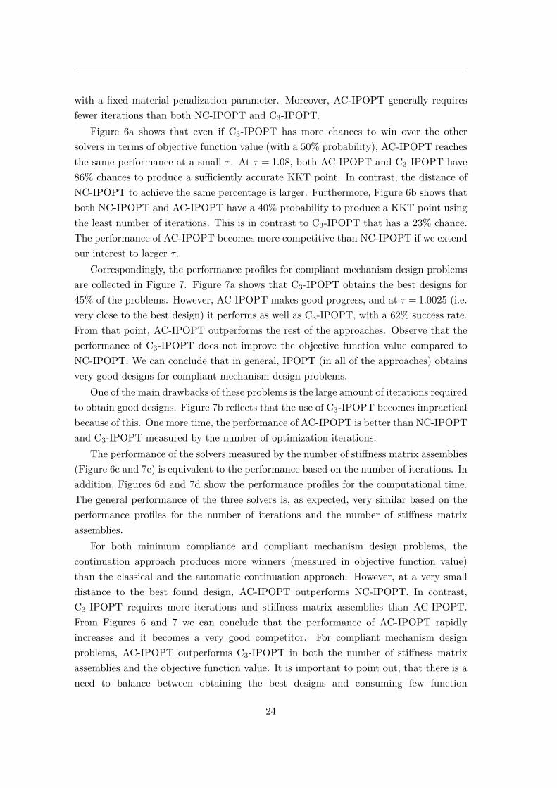
with a fixed material penalization parameter. Moreover, AC-IPOPT generally requiresfewer iterations than both NC-IPOPT and C3-IPOPT.
Figure 6a shows that even if C3-IPOPT has more chances to win over the othersolvers in terms of objective function value (with a 50% probability), AC-IPOPT reachesthe same performance at a small τ . At τ = 1.08, both AC-IPOPT and C3-IPOPT have86% chances to produce a sufficiently accurate KKT point. In contrast, the distance ofNC-IPOPT to achieve the same percentage is larger. Furthermore, Figure 6b shows thatboth NC-IPOPT and AC-IPOPT have a 40% probability to produce a KKT point usingthe least number of iterations. This is in contrast to C3-IPOPT that has a 23% chance.The performance of AC-IPOPT becomes more competitive than NC-IPOPT if we extendour interest to larger τ .
Correspondingly, the performance profiles for compliant mechanism design problemsare collected in Figure 7. Figure 7a shows that C3-IPOPT obtains the best designs for45% of the problems. However, AC-IPOPT makes good progress, and at τ = 1.0025 (i.e.very close to the best design) it performs as well as C3-IPOPT, with a 62% success rate.From that point, AC-IPOPT outperforms the rest of the approaches. Observe that theperformance of C3-IPOPT does not improve the objective function value compared toNC-IPOPT. We can conclude that in general, IPOPT (in all of the approaches) obtainsvery good designs for compliant mechanism design problems.
One of the main drawbacks of these problems is the large amount of iterations requiredto obtain good designs. Figure 7b reflects that the use of C3-IPOPT becomes impracticalbecause of this. One more time, the performance of AC-IPOPT is better than NC-IPOPTand C3-IPOPT measured by the number of optimization iterations.
The performance of the solvers measured by the number of stiffness matrix assemblies(Figure 6c and 7c) is equivalent to the performance based on the number of iterations. Inaddition, Figures 6d and 7d show the performance profiles for the computational time.The general performance of the three solvers is, as expected, very similar based on theperformance profiles for the number of iterations and the number of stiffness matrixassemblies.
For both minimum compliance and compliant mechanism design problems, thecontinuation approach produces more winners (measured in objective function value)than the classical and the automatic continuation approach. However, at a very smalldistance to the best found design, AC-IPOPT outperforms NC-IPOPT. In contrast,C3-IPOPT requires more iterations and stiffness matrix assemblies than AC-IPOPT.From Figures 6 and 7 we can conclude that the performance of AC-IPOPT rapidlyincreases and it becomes a very good competitor. For compliant mechanism designproblems, AC-IPOPT outperforms C3-IPOPT in both the number of stiffness matrixassemblies and the objective function value. It is important to point out, that there is aneed to balance between obtaining the best designs and consuming few function
24

8 CONCLUSIONS
evaluations. Thus, AC-IPOPT is a very good alternative to C3-IPOPT. Moreover, wesuggest a new way of solving topology optimization problems where the final design isconsiderable better and it converges faster than with a fixed penalization parameter.
7.2 RAMP material interpolation scheme
We also briefly examine the performance of automatic continuation coupled with theRAMP interpolation scheme for both minimum compliance and compliant mechanismdesign problems. The results are shown in Figure 8 and Figure 9, respectively.
In this case, the performance of AC-IPOPT measured by the objective function valueis more prominent for minimum compliance problems (as illustrated in Figure 8a) than forcompliant mechanism design (see Figure 9a) where it performs similar to NC-IPOPT.Nevertheless, for the latter problems, the improvements compared to NC-IPOPT andC3-IPOPT in the number of iterations make AC-IPOPT a very good alternative. Forcompliant mechanism design problems, it is more important to reduce the computationaltime and the number of iterations required than producing good designs, since IPOPTgenerally obtains very good designs for all approaches.
Similarly to the previous section, the performance of the methods measured in stiffnessmatrix assemblies and computational time is comparable to the number of iterations.
8 Conclusions
In structural topology optimization, it is common to use continuation methods in thepenalization parameter of the material interpolation scheme to produce better designs.These continuation methods solve sequences of problems with increasing values of thematerial penalization parameter p. In this article, we presented a benchmarking studyof continuation methods using GCMMA on a test set of 225 minimum compliance and150 compliant mechanism design problems, in order to assess the general performance ofthis approach.
The numerical results clearly indicate that the continuation methods implemented inthis article generally (but not always) obtain better designs than using a fixed materialpenalization parameter value. Moreover, the performance of our continuation methodsis not highly affected by the increment step selected. The latter result is preliminary andrequires additional investigations. However, the suggested continuation approaches arecomputationally expensive, and for large-scale problems or for industrial applications, ourimplementation of continuation methods is impractical. We present a new alternative,called automatic continuation, where the parameter of the material interpolation schemeis an explicit variable of the problem. In contrast to other continuation methods, theproposed automatic continuation approach only solves one optimization problem.
25
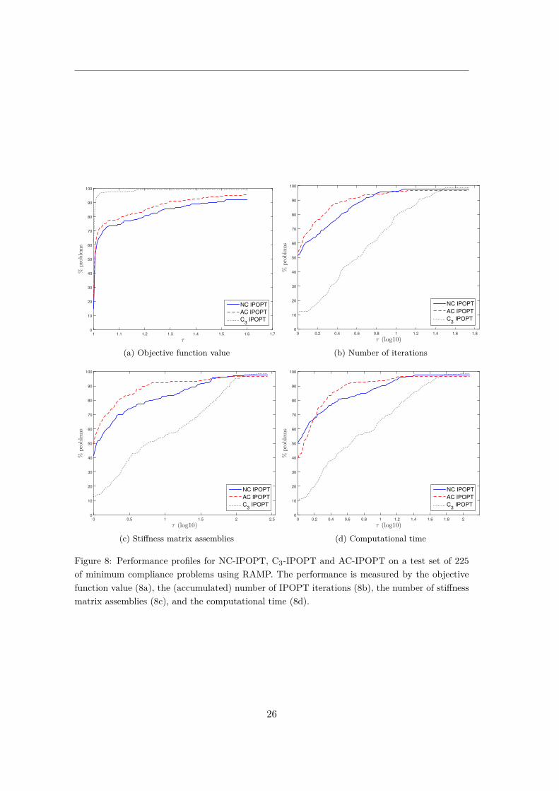
τ
1 1.1 1.2 1.3 1.4 1.5 1.6 1.7
%problems
0
10
20
30
40
50
60
70
80
90
100
NC IPOPT
AC IPOPT
C3 IPOPT
(a) Objective function valueτ (log10)
0 0.2 0.4 0.6 0.8 1 1.2 1.4 1.6 1.8
%problems
0
10
20
30
40
50
60
70
80
90
100
NC IPOPT
AC IPOPT
C3 IPOPT
(b) Number of iterations
τ (log10)0 0.5 1 1.5 2 2.5
%problems
0
10
20
30
40
50
60
70
80
90
100
NC IPOPT
AC IPOPT
C3 IPOPT
(c) Stiffness matrix assembliesτ (log10)
0 0.2 0.4 0.6 0.8 1 1.2 1.4 1.6 1.8 2
%problems
0
10
20
30
40
50
60
70
80
90
100
NC IPOPT
AC IPOPT
C3 IPOPT
(d) Computational time
Figure 8: Performance profiles for NC-IPOPT, C3-IPOPT and AC-IPOPT on a test set of 225of minimum compliance problems using RAMP. The performance is measured by the objectivefunction value (8a), the (accumulated) number of IPOPT iterations (8b), the number of stiffnessmatrix assemblies (8c), and the computational time (8d).
26

8 CONCLUSIONS
τ
1 1.1 1.2 1.3 1.4 1.5 1.6 1.7
%problems
0
10
20
30
40
50
60
70
80
90
100
NC IPOPT
AC IPOPT
C3 IPOPT
(a) Objective function valueτ (log10)
0 0.2 0.4 0.6 0.8 1 1.2 1.4 1.6 1.8
%problems
0
10
20
30
40
50
60
70
80
90
100
NC IPOPT
AC IPOPT
C3 IPOPT
(b) Number of iterations
τ (log10)0 0.5 1 1.5 2 2.5 3
%problems
0
10
20
30
40
50
60
70
80
90
100
NC IPOPT
AC IPOPT
C3 IPOPT
(c) Stiffness matrix assembliesτ (log10)
0 0.5 1 1.5 2 2.5
%problems
0
10
20
30
40
50
60
70
80
90
100
NC IPOPT
AC IPOPT
C3 IPOPT
(d) Computational time
Figure 9: Performance profiles for NC-IPOPT, C3-IPOPT and AC-IPOPT on a test set of150 compliant mechanism design problems using RAMP. The performance is measured by theobjective function value (9a), the (accumulated) number of IPOPT iterations (9b), the numberof stiffness matrix assemblies (9c), and the computational time (9d).
27

The automatic continuation approach is a good alternative to the outlinedcontinuation methods both in terms of quality of designs and the computational effort.Even though the suggested continuation approach obtains better designs for someproblems, the computational time required is high in comparison to the automaticcontinuation approach. Additionally, both the objective function value and the numberof iterations are reduced compared to the classical formulation with fixed penaltyparameter. Thus, this new formulation is a good replacement of both continuationmethods and the classical formulation.
This study opens many possibilities for further research and developments of newimplementations of continuation methods and new alternatives.
Acknowledgements
We would like to thank Professor Krister Svanberg at KTH in Stockholm for providingus with the MATLAB implementation of GCMMA. We extend our sincere thanks to tworeviewers and the editor for providing many comments and suggestions that improvedthe quality of this article.
References
[1] G. Allaire and G. A. Francfort. A numerical algorithm for topology and shapeoptimization. In Topology design of structures, pages 239–248. Kluwer AcademicPublishers, 1993.
[2] G. Allaire and R. V. Kohn. Topology optimization and optimal shape design usinghomogenization. In Topology design of structures, pages 207–218. Kluwer AcademicPublishers, 1993.
[3] E. Andreassen, A. Clausen, M. Schevenels, B. S. Lazarov, and O. Sigmund.Efficient topology optimization in MATLAB using 88 lines of code. Structural andMultidisciplinary Optimization, 43(1):1–16, 2011.
[4] M. P. Bendsøe. Optimal shape design as a material distribution problem. StructuralOptimization, 1(4):192–202, 1989.
[5] M. P. Bendsøe and O. Sigmund. Material interpolation schemes in topologyoptimization. Archive of Applied Mechanics, 69(9–10):635–654, 1999.
[6] M. P. Bendsøe and O. Sigmund. Topology optimization: Theory, methods andapplications. Springer, 2003.
28

REFERENCES
[7] P. T. Boggs and J. W. Tolle. Sequential Quadratic Programming. Acta Numerica,4:1–51, 1995.
[8] B. Bourdin. Filters in topology optimization. International Journal for NumericalMethods in Engineering, 50(9):2143–2158, 2001.
[9] T. E. Bruns. A reevaluation of the SIMP method with filtering and an alternativeformulation for solid void topology optimization. Structural and MultidisciplinaryOptimization, 30(6):428–436, 2005.
[10] T. Buhl, C. B. W. Pedersen, and O. Sigmund. Stiffness design of geometricallynonlinear structures using topology optimization. Structural and MultidisciplinaryOptimization, 19(2):93–104, 2000.
[11] J. D. Deaton and R. V. Grandhi. A survey of structural and multidisciplinarycontinuum topology optimization: post 2000. Structural and MultidisciplinaryOptimization, 49(1):1–38, 2014.
[12] S. R. Deepak, M. Dinesh, D. K. Sahu, and G. K. Ananthasuresh. A comparativestudy of the formulations and benchmark problems for the topology optimization ofcompliant mechanisms. Journal of Mechanisms and Robotics, 1(1), 2009.
[13] E. D. Dolan and J. J. Moré. Benchmarking optimization software with performanceprofiles. Mathematical Programming, 91(2):201–213, 2002.
[14] C. S. Edwards, H. A. Kim, and C. J. Budd. An evaluative study on ESO and SIMPfor optimising a cantilever tie beam. Structural and Multidisciplinary Optimization,34(5):403–414, 2007.
[15] A. Forsgren and P. E. Gill. Primal-dual interior methods for nonconvex nonlinearprogramming. SIAM Journal on Optimization, 8(4):1132–1152, 1998.
[16] P. E. Gill, W. Murray, and M. A. Saunders. SNOPT: An SQP Algorithm for Large-Scale Constrained Optimization. SIAM Journal on Optimization, 47(4):99–131,2005.
[17] C. F. Hvejsel and E. Lund. Material interpolation schemes for unified topologyand multi-material optimization. Structural and Multidisciplinary Optimization,43(6):811–825, 2011.
[18] G. K. Lau, H. Du, and M. K. Lim. Use of functional specifications as objectivefunctions in topological optimization of compliant mechanism. Computer Methodsin Applied Mechanics and Engineering, 190(34):4421–4433, 2001.
29

[19] L. Li and K. Khandelwal. Volume preserving projection filters and continuationmethods in topology optimization. Engineering Structures, 85:144–161, 2015.
[20] D. G. Luenberger and Y. Ye. Linear and Nonlinear Programming. Springer, 2008.
[21] B. A. Murtagh and M. A. Saunders. Large-scale linearly constrained optimization.Mathematical programming, 14(1):41–72, 1978.
[22] J. Petersson and O. Sigmund. Slope constrained topology optimization.International Journal for Numerical Methods in Engineering, 41(8):1417–1434, 1998.
[23] S. Rojas-Labanda and M. Stolpe. Benchmarking optimization solvers for structuraltopology optimization. Structural and Multidisciplinary Optimization, In print,2015. DOI: 10.1007/s00158-015-1250-z.
[24] G. I. N. Rozvany. A critical review of established methods of structural topologyoptimization. Structural and Multidisciplinary Optimization, 37(3):217–237, 2008.
[25] G. I. N. Rozvany, M. Zhou, and T. Birker. Generalized shape optimization withouthomogenization. Structural Optimization, 4(3–4):250–252, 1992.
[26] O. Sigmund. On the design of compliant mechanisms using topology optimization.Journal of Structural Mechanics, 25(4):492–526, 1997.
[27] O. Sigmund. Manufacturing tolerant topology optimization. Acta Mechanica Sinica,25(2):227–239, 2009.
[28] O. Sigmund and K. Maute. Topology optimization approaches. Structural andMultidisciplinary Optimization, 48(6):1031–1055, 2013.
[29] O. Sigmund and J. Petersson. Numerical instabilities in topology optimization:A survey on procedures dealing with checkerboards, mesh-dependencies and localminima. Structural Optimization, 16(2):68–75, 1998.
[30] M. Stolpe and K. Svanberg. An alternative interpolation scheme for minimumcompliance topology optimization. Structural and Multidisciplinary Optimization,22(2):116–124, 2001.
[31] M. Stolpe and K. Svanberg. On the trajectories of penalization methods for topologyoptimization. Structural and Multidisciplinary Optimization, 21(2):128–139, 2001.
[32] K. Svanberg. The method of moving asymptotes - A new method for structuraloptimization. International Journal for Numerical Methods in Engineering,24(2):359–373, 1987.
30

REFERENCES
[33] K. Svanberg. A class of globally convergent optimization methods based onconservative convex separable approximations. SIAM Journal on Optimization,12(2):555–573, 2002.
[34] A. Wächter and L. T. Biegler. On the implementation of an interior point filter line-search algorithm for large-scale nonlinear programming. Mathematical Programming,106(1):25–57, 2006.
[35] F. Wang, B. S. Lazarov, and O. Sigmund. On projection methods, convergenceand robust formulations in topology optimization. Structural and MultidisciplinaryOptimization, 43(6):767–784, 2011.
[36] R. Watada and M. Ohsaki. Continuation approach for investigation of non-uniqueness of optimal topology for minimum compliance. In Proceedings of 8thWorld Congress on Structural and Multidisciplinary Optimization, June 1–5, Lisbon,Portugal, 2009.
[37] R. Watada, M. Ohsaki, and Y. Kanno. Non-uniqueness and symmetry of optimaltopology of a shell for minimum compliance. Structural and MultidisciplinaryOptimization, 43(4):459–471, 2011.
[38] M. Zhou and G. I. N. Rozvany. The COC algorithm, Part II: Topological, geometricaland generalized shape optimization. Computer Methods in Applied Mechanics andEngineering, 89(1–3):309–336, 1991.
31

136

8Article III: An efficient second-order SQP method
for structural topology optimization
In review:Rojas-Labanda, S. and Stolpe, M.: An efficient second-order SQP method for structuraltopology optimization
137

138

An efficient second-order SQP method for structuraltopology optimization∗
Susana Rojas-Labanda+ and Mathias Stolpe+
+DTU Wind Energy, Technical University of Denmark, Frederiksborgvej 399, 4000 Roskilde,Denmark. E-mail: [email protected], [email protected]
Abstract
This article presents a Sequential Quadratic Programming (SQP) solver forstructural topology optimization problems (TopSQP). The implementation is basedon the general SQP method proposed in [40] called SQP+. The topologyoptimization problem is based on a density approach and thus, is classified as anonconvex problem. More specifically, the method is designed for the classicalminimum compliance problem with a constraint on the volume of the structure.The sub-problems are defined using exact second-order information and they arereformulated based on the specific mathematical properties of the problem tosignificantly improve the efficiency of the solver.
The performance of the TopSQP solver is compared to the special-purposestructural optimization method, the Globally Convergent Method of MovingAsymptotes (GCMMA) and the two general nonlinear solvers IPOPT and SNOPT.Numerical experiments on a large set of benchmark problems show greatperformance of TopSQP in terms of number of function evaluations. In addition,the use of exact second-order information helps to decrease the objective functionvalue.
Keywords: Topology optimization, Sequential Quadratic Programming, Minimumcompliance, Second-order method, Hessian approximationMathematics Subject Classification 2010: 74P05, 74P15, 90C30, 90C46, and90C90
∗This research is funded by the Villum Foundation through the research project Topology Optimization- The Next Generation (NextTop).
1

1 Introduction
Structural topology optimization determines the design in a domain by minimizing anobjective function under certain constraints, for a given set of boundary conditions andloads. It is common to minimize compliance or volume subject to limitations on thedisplacements, volume, or stresses. Topology optimization is a mathematical approachwhere the design domain is often discretized using finite elements for designparametrization and structural analysis. More details of these problems can be found inthe monograph [5].
Several special purpose methods have been implemented to solve structuraltopology optimization problems. Examples include the Method of Moving Asymptotes,(MMA) [52], its globally convergent version, (GCMMA) [53], and the ConvexLinearization (CONLIN) method [21]. These first-order methods solve a sequence ofconvex sub-problems based on separable approximations of the objective and constraintfunctions. Different variations of MMA using the diagonal of the second-orderderivatives are proposed in [22] and [23], evaluating the benefits of using partialsecond-order information.
Although it is not very commonly reported in the literature, general nonlinearoptimization solvers are also applicable to topology optimization problems. Thenumerical experiments in [46] show that general purpose solvers, such as interior-pointand sequential quadratic programming methods, can be used for solving these type ofproblems. In these numerical experiments, SNOPT (an SQP method) [27] requires veryfew iterations to converge to a Karush-Kuhn-Tucker (KKT) point. In addition,second-order information helps to produce accurate results (optimized designs with lowobjective function value) as demonstrated by the interior-point method IPOPT [55].The results of the benchmarking study in [46] have motivated the implementation of thesecond-order SQP method for structural topology optimization problems (TopSQP).Due to the use of second-order information, TopSQP is expected to converge faster thanfirst-order methods. In addition, the objective function values might be reduced too.
In the SQP family of methods, there are numerous variations of algorithms, but all ofthem are characterized by the same idea. They find approximate solutions to a sequenceof normally convex sub-problems. A quadratic objective function models the Lagrangianwhile the original constraints are linearized. For general information of SQP see e.g. [7]and [30].
One of the main properties of SQP methods is the fast convergence when close to thesolution. However, the performance of SQP depends, in general, on the starting point.It is quite difficult to use second-order information (see Section 2) when the problems arenonconvex. In practice, most of the SQP algorithms use quasi-Newton approximationsof the Hessian in order to obtain a convex sub-problem, see e.g. [30].
2

1 INTRODUCTION
The main differences between SQP algorithms are how the search direction iscomputed, how the search direction is accepted or rejected, and how inequalityconstraints are dealt with. Both line search [41] and trust region strategies [12] can beapplied in SQP solvers. Additionally, to ensure convergence, merit functions [6] or filtermethods [20] are used. Regarding how the method obtains the active inequalityconstraints, SQP is classified as equality constrained quadratic programming (EQP) orinequality constrained quadratic programming (IQP), see e.g. [33]. Finally, there aredifferent ways to approximate the Hessian of the Lagrangian, using eitherlimited-memory approximations like BFGS (Broyden - Fletcher - Goldfarb - Shanno)[15] or some information of the Hessian. Examples of different SQP algorithms can befound in [30], [29], [33], [40], [35], [13], and [49], among others.
There are several software in the optimization community based on SQP methods.For instance, SNOPT [27], NLPQLP solver [48], and NPSOL [28], where a line searchis combined with different penalty functions, the trust region with a filter method inFilterSQP [19], or the new SQP implemented in KNITRO, see e.g. [11] among others.More details of nonlinear solvers can be found in e.g. [38]. Nevertheless, the use of SQPmethods in topology optimization is seemingly not very popular, and very few referenceshave been found in this regard, see e.g. [44], [17], and [18].
This article contains a detailed description of an efficient sequential quadraticprogramming method for maximum stiffness structural topology optimization problems.The SQP+ method introduced in [40] is implemented using second-order informationbased on the exact Hessian. SQP+ contains two phases, the inequality quadratic phase(IQP), where an inequality constrained convex quadratic sub-problem is solved. Then,an equality constrained quadratic phase (EQP), where the active constraints found forthe IQP are used. The step generation is done using a line search strategy inconjunction with a reduction in a merit function. In the special-purposeimplementation TopSQP, the IQP phase uses a convex approximation of the exactHessian instead of the traditional BFGS. Based on the specific structure of the problemformulation, both phases are efficiently reformulated to reduce computational cost. Thereformulations avoid one of the most expensive steps in topology optimizationproblems, which is the computation of the inverse of the stiffness matrix (involved inthe Hessian of compliance).
The performance of the proposed TopSQP is compared to the specific purposeGCMMA and with two of the state-of-the-art software in numerical optimization;SNOPT and IPOPT. The comparative study is done using performance profiles [16] ona test set of 225 medium-size minimum compliance problem instances described in [46].
The paper is organized as follows. Section 2 introduces the SQP+ algorithm for ageneral nonlinear problem and Section 3 briefly defines the topology optimization problemunder consideration. Then, the Hessian of the Lagrangian function and some possible
3
convex approximations are proposed in Section 4. The efficient reformulations of theIQP and EQP phases of TopSQP are gathered in Section 5 and Section 6, respectively.Some implementation details are collected in Section 7. The comparative study of theperformance of TopSQP is reported in Section 8, followed by a list of the main limitationsthis new algorithm may have for topology optimization problems, in Section 9. Finally,Section 10 draws the main conclusions from the results and outlines recommendationsfor the future work.
2 Sequential Quadratic Programming with an additionalequality constrained phase
A general sequential quadratic programming method generates approximate solutionsusing a quadratic model of the Lagrangian function and a linearization of the constraints.
The general nonlinear constrained problem under consideration is
minimizex∈Rn
f(x)
subject to gi(x)≤ 0 i= 1, . . . ,m,li ≤ xi ≤ ui i= 1, . . . ,n,
(NLP)
where f(x) : Rn −→ R and gi(x) : Rn −→ R are assumed to be twice continuouslydifferentiable functions.
A conventional SQP method approximates (NLP) at a given iterate xk, and usesthe solution of the sub-problem to produce a search direction dk. The solver ensuresconvergence to a KKT point by enforcing, for instance, an improvement in a meritfunction. This class of methods has shown fast local convergence (see e.g. [43] and [40]),however, the theoretical properties do not hold when the Hessian is indefinite, producingsome difficulties to the solver. Since nonconvex problems are NP-hard problems [42], aminimizer of the sub-problem does not guarantee the convergence of the algorithm, seee.g. [45].
The sequential quadratic programming method proposed in this article is based onthe algorithm SQP+ in [40]. SQP+ tries to improve the convergence rate by includingtwo phases. First, an inequality quadratic convex constrained sub-problem is solved.Second, the set of active constraints is estimated, and with them, an EQP sub-problemis defined and solved, ignoring the rest of the constraints. The EQP estimated solutionrefines the search direction, producing fast convergence. Additionally, the IQP iterateof the proposed TopSQP is expected to be more precise than in [40] since a positivedefinite approximation of the indefinite Hessian is used instead of the BFGS approach.The approximation is based on the exact second-order information (see Section 4).
Throughout this section, the SQP+ method, summarized in Algorithm 1, is outlinedfor the general nonlinear problem (NLP).
4

2 SEQUENTIAL QUADRATIC PROGRAMMING WITH AN ADDITIONALEQUALITY CONSTRAINED PHASE
Algorithm 1 SQP+ algorithm from [40].Input: Define the starting point x0, the initial Lagrangian multipliers λ0, ξ0 η0 and the optimality
tolerance ω.1: Set σ = 10−4, κ= 0.5, k = 1, π = 1.2: repeat3: Define an approximation of the Hessian of the Lagrangian function, Bk 0 such as Bk ≈
∇2L(xk,λk).4: Solve the IQP sub-problem as explained in Section 2.2 where the solution is (diqk ,λ
iqk ,ξ
iqk ,η
iqk ).
5: Determine the working set of active constraints, Wk, defined in Section 2.3.6: Solve the EQP sub-problem as explained in Section 2.3 where the solution is (deqk ,λ
eqk ,ξ
eqk ,η
eqk ).
7: Compute the contraction parameter β ∈ (0,1] such as the linearized contraints of the IQP sub-problem are feasible at the iterate point xk + diqk +βdeqk .
8: Acceptance/rejection step. Use of line search strategy:9: if φπ(xk + diqk +βdeqk )≤ φπ(xk)−σqredπ(diqk ) then10: dk = diqk +βdeqk .11: else12: Find α= 1,κ,κ2, ... such that φπ(xk +αdiqk )≤ φπ(xk)−σαqredπ(diqk ).13: dk = αdiqk .14: end if15: Update the primal iterate xk+1 = xk + dk.16: Update the Lagrangian multiplier estimates λk+1, ξk+1, ηk+1 with the strategy explained in
Section 2.5.17: Update the penalty parameter π.18: Compute the ∞-norm of KKT conditions of the original problem (NLP).19: Set k← k+ 1.20: until convergence21: return
2.1 Optimality conditions
The Lagrangian function of (NLP) is defined as
L(x,λ,ξ,η) = f(x)+m∑
i=1λigi(x)+
n∑
i=1ξi(xi−ui)+
n∑
i=1ηi(li−xi).
Here λ = (λ1, . . . ,λm)T , ξ = (ξ1, . . . , ξn)T , and η = (η1, . . . ,ηn)T are the Lagrangianmultipliers of the inequality, the upper bound, and the lower bound constraints,respectively.
The first-order necessary conditions for a primal-dual point (x,λ,ξ,η) to be a localoptimal solution of the problem (NLP) are gathered in the Karush-Kuhn-Tucker (KKT)conditions (1)-(9), see e.g. [43].
5
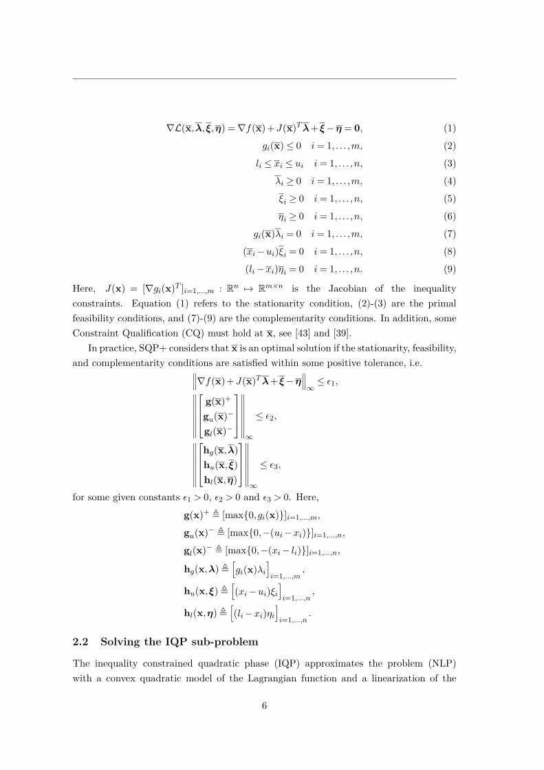
∇L(x,λ,ξ,η) =∇f(x)+J(x)Tλ+ξ−η = 0, (1)gi(x)≤ 0 i= 1, . . . ,m, (2)li ≤ xi ≤ ui i= 1, . . . ,n, (3)
λi ≥ 0 i= 1, . . . ,m, (4)ξi ≥ 0 i= 1, . . . ,n, (5)ηi ≥ 0 i= 1, . . . ,n, (6)
gi(x)λi = 0 i= 1, . . . ,m, (7)(xi−ui)ξi = 0 i= 1, . . . ,n, (8)(li−xi)ηi = 0 i= 1, . . . ,n. (9)
Here, J(x) = [∇gi(x)T ]i=1,...,m : Rn 7→ Rm×n is the Jacobian of the inequalityconstraints. Equation (1) refers to the stationarity condition, (2)-(3) are the primalfeasibility conditions, and (7)-(9) are the complementarity conditions. In addition, someConstraint Qualification (CQ) must hold at x, see [43] and [39].
In practice, SQP+ considers that x is an optimal solution if the stationarity, feasibility,and complementarity conditions are satisfied within some positive tolerance, i.e.
∥∥∥∇f(x)+J(x)Tλ+ξ−η∥∥∥∞≤ ε1,
∥∥∥∥∥∥∥∥
g(x)+
gu(x)−
gl(x)−
∥∥∥∥∥∥∥∥∞
≤ ε2,
∥∥∥∥∥∥∥∥
hg(x,λ)hu(x,ξ)hl(x,η)
∥∥∥∥∥∥∥∥∞
≤ ε3,
for some given constants ε1 > 0, ε2 > 0 and ε3 > 0. Here,
g(x)+ , [max0,gi(x)]i=1,...,m,
gu(x)− , [max0,−(ui−xi)]i=1,...,n,
gl(x)− , [max0,−(xi− li)]i=1,...,n,
hg(x,λ) ,[gi(x)λi
]i=1,...,m
,
hu(x,ξ) ,[(xi−ui)ξi
]i=1,...,n
,
hl(x,η) ,[(li−xi)ηi
]i=1,...,n
.
2.2 Solving the IQP sub-problem
The inequality constrained quadratic phase (IQP) approximates the problem (NLP)with a convex quadratic model of the Lagrangian function and a linearization of the
6

2 SEQUENTIAL QUADRATIC PROGRAMMING WITH AN ADDITIONALEQUALITY CONSTRAINED PHASE
constraints. Thus, a positive definite matrix, Bk, computed in Step 3 of Algorithm 1 iscrucial to define the IQP problem.
minimized∈Rn
∇f(xk)Td+ 12d
TBkd
subject to g(xk)+J(xk)d≤ 0,li ≤ di ≤ ui i= 1, . . . ,n.
(IQP)
The lower and the upper bounds of di are defined with li = li− (xk)i and ui = ui− (xk)i,i= 1, . . . ,n, respectively.
From now on, the linearization of the constraints in (IQP) is assumed to result in afeasible problem (see Section 3). The primal-dual solution of the sub-problem (diqk , λ
iqk ,
ξiqk , ηiqk ), is used to estimate first, the set of active constraints and second, the search
direction.The most important characteristic of this IQP phase is the convexity of the
optimization problem. Any local optimal solution of a convex problem is a globalsolution. Furthermore, for the IQP in this work, existence of solution is ensured (seeSection 4). In addition, the problem always has a descent direction until convergence(see e.g. [9]).
An important aspect for large-scale problems is to solve this sub-problem as fastas possible. In this context, it is solved using fast commercial solvers for large-scalequadratic problems, such as Gurobi [34] or CPLEX [37].
2.3 Solving EQP sub-problem
The working set Wk (Step 5 of Algorithm 1) contains all the indices of the constraintswhere their linearization in the sub-problem (IQP) are active at diqk , i.e,
Wk = Wgk ∪Wu
k ∪W lk,
withWgk = i | gi(xk)+∇gi(xk)Tdiqk = 0, i= 1, . . . ,m,Wuk = i | (diqk )i− ui = 0, i= 1, . . . ,n,W lk = i | (diqk )i− li = 0, i= 1, . . . ,n.
For those active constraints, the following equality constrained sub-problem (EQP) isdefined. The explanation of its final formulation can be found in [10].
minimized∈Rn
(∇f(xk)+Hkdiqk )Td +12d
THkd
subject to JWgk(xk)d = 0,
di = 0 i ∈ Wuk ∪W l
k.(EQP)
The matrix Hk refers to the exact Hessian of the Lagrangian function i.e. Hk =∇2L(xk,λiqk ) and JWg
k(xk) represents the matrix whose rows are the active constraint
7

gradients (i.e. the Wgk rows of the Jacobian). Applying Newton’s method to the first-
order optimality conditions of (EQP), this optimization problem is equivalent to solvethe KKT system
Hk JWgk(xk)T IWu
k−IWl
k
JWgk(xk) 0 0 0
ITWuk
0 0 0−ITWl
k0 0 0
deqkλeqkξeqkηeqk
=−
∇f(xk)+Hkdiqk000
(10)
where IWuk∈ Rn×|Wu
k | and IWlk∈ Rn×|Wl
k| are pseudo-identity matrices. The Lagrangianmultipliers (λeqk ,ξ
eqk ,η
eqk ) refer to the active constraints. The size of the system (10) can
be easily reduced sinceITWu
kdeqk = 0,
ITWlkdeqk = 0.
Therefore, only a system taking into account the nonzero direction ((deqk )i 6= 0) need tobe solved.
Hk,Wb
k,cJWg
k,Wb
k,c(xk)T
JWgk,Wb
k,c(xk) 0
[deqkλeqk
]=−
(∇f(xk)+Hkdiqk )Wb
k,c
0
. (11)
Here, Wbk,c = 1, . . . ,n \ Wu
k ∪W lk is the complementarity set of the active bounds
(upper and lower), Hk,Wbk,c
refers to the Wbk,c columns and rows of Hk, and JWg
k,Wb
k,c(xk)
refers to the Wgk rows and Wb
k,c columns of the Jacobian. In this case, the term deqkrepresents the Wb
k,c rows of deqk . The Lagrangian multipliers of the active bounds areobtained afterwards1 by
zeqk =−∇f(xk)−Hkdiqk −Hkdeqk −JWgk(xk)Tλeqk ,
ξeqk = zeqk,Wuk,
ηeqk =−zeqk,Wl
k
.
The computation of the EQP search direction is, generally, much faster than the IQPsolution. The EQP sub-problem not only helps to produce a more accurate searchdirection, but also reduces the number of IQP phases (the number of iterations isdecreased) (see Section 7). A direct consequence is a reduction of the totalcomputational time.
2.3.1 Existence of solutions of the equality quadratic constraint problem
The equality constrained quadratic problem (EQP) is equivalent to solving the systemof equations (11). The matrix of this system is commonly defined like
K =[H AT
A 0
],
1Note that Wuk and Wl
k are disjoint sets by definition.
8

2 SEQUENTIAL QUADRATIC PROGRAMMING WITH AN ADDITIONALEQUALITY CONSTRAINED PHASE
where H ∈ Rn×n is symmetric and A ∈ Rm×n is the Jacobian of the linearized activeconstraints. It is assumed that A has full row rank. The matrix K is called a Karush-Kuhn-Tucker matrix. There are conditions under which the system has solution.
Theorem 1. (from [43]) Let A have a full row rank, and assume that the reduced-Hessianmatrix ZTHZ is positive definite. Then the KKT matrix K is nonsingular, and hencethere is a unique vector that satisfied the linear system and is the unique global solution.
Where Z ∈Rn×(n−m) is a matrix whose columns are the basis of the null-space of A.
Thus, in order to obtain a solution of the EQP sub-problem, the reduced-Hessianmust be positive definite, and the matrix A must have full rank.
Definition 1. (from [32]) Suppose a matrix K. Let i0, i+ and i− be the number ofzero, positive and negative eigenvalues of K, respectively. The trial (i+, i−, i0) is calledinertia.
Theorem 2. Gould Theorem ([36]). Suppose that A has full rank m. The conditionpTHp> 0, ∀p 6= 0, such that ATp = 0 holds if and only if
inertia(K) = (n,m,0).
In addition,inertia(K) = inertia( ZTHZ)+(m,m,0).
Therefore, if ZTHZ is positive definite, inertia(K) = (n,m,0).
An option to compute the inertia of a KKT matrix is by the LDL factorization, seee.g. [26] and [43]. If the inertia is not correct, it is necessary to modify the KKT matrixto ensure the existence of solution. There are many different alternatives to modifythe nonconvex sub-problem into a local convex approximation, such as using differentinertia correction based on LDL factorizations, see e.g. [26], [25], and [24], or usingother techniques such as in [36] and [55]. In addition, it is possible to apply differentconvexification approaches proposed in [29] and [31].
When the computation of the reduced-Hessian is computationally cheap, the systemcan be easily modified to guarantee a positive definite reduced-Hessian, see [43]. Forinstance, Hz = ZTkHkZk is perturbed using its eigenvalues, so that Hz = Hz + γI 0,with γ = min(|λeig(Hz)|) + ε, where λeig refers the the eigenvalues of the matrix. Thisperturbation is then used for the KKT matrix,
[H+γI AT
A 0
].
The EQP sub-problem in [40] is solved only in those cases where the inertia of thesystem is correct. However, TopSQP modifies the KKT matrix to guarantee a correct
9

inertia. If the same approach as in [40] is used, TopSQP would essentially be a classicalSQP with only an IQP step since the indefiniteness of the Hessian of the compliance (seeSection 3) usually produces an incorrect inertia.
2.4 Acceptance/rejection of the step
Once the IQP and EQP search directions are computed, it is necessary to verify whetherthese estimates improve the iterate xk. First of all, a contraction parameter β (Step 7)secures that the linearization of all the constraints (active and inactive) are satisfied atthe point with maximum search direction d =diqk +βdeqk . In other words, the constraintsof the IQP phase must remain feasible.
The largest value of β ∈ (0,1] is computed such that
gi(xk)+∇gi(xk)Td≤ 0 i ∈Wgk,c,
di ≤ ui i ∈Wuk,c,
li ≤ di i ∈W lk,c.
Here,Wgk,c = 1, . . . ,m\Wg
k ,
Wuk,c = 1, . . . ,n\Wu
k ,
W lk,c = 1, . . . ,n\W l
k,
are the complementarity working set. Once the contraction parameter is determined,a line search estimates the step length α for the new step direction (Step 9 and 12 inAlgorithm 1). The TopSQP line search is implemented as [40], Section 5. The linesearch procedure is slightly modified compared to the theoretical procedure used for thetheoretical results. The acceptance criterion is based on the merit function (12) and themodel reduction from xk to xk +d (13) of the original problem (NLP). These functionsare defined as
φπ(x) = f(x)+π(||g(x)+||1 + ||gl(x)−||1 + ||gu(x)−||1) (12)
qredπ(d) = −(∇f(xk)Td+ 12d
TBkd)+π(||g(xk)+||1+||gl(xk)−||1 + ||gu(xk)−||1).
(13)
If the sufficient decrease condition (14) is satisfied, then the iterate xk+1 = xk+diqk +βdeqk is accepted.
φπ(xk +diqk +βdeqk )≤ φπ(xk)−σqredπ(diqk ). (14)
Otherwise, α ∈ 1,κ,κ2, . . . is found such that condition (15) is satisfied. In this case,the new iterate is defined as xk+1 = xk +αdiqk .
φπ(xk +αdiqk )≤ φπ(xk)−σαqredπ(diqk ). (15)
10

2 SEQUENTIAL QUADRATIC PROGRAMMING WITH AN ADDITIONALEQUALITY CONSTRAINED PHASE
There are several techniques to update the penalty parameter π in order to improvethe convergence rate, for instance, the strategy explained in e.g. [56] and [14]. In practice,due to the feasibility of the sub-problems (see Section 3), the term affected by π is alwaysclose to 0. The penalty parameter π is updated very simple by just using the Lagrangianmultipliers, i.e. π = ||λ||∞. Finally, the parameters σ = 10−4 and κ= 0.5 are taken from[40].
2.5 Updating the Lagrangian multipliers
The SQP+ algorithm in [40] updates the estimates of the Lagrangian multipliersdepending on the final step direction. The updating scheme of the SQP+ is
λk+1 =
max(0,λeqk ) if dk = diqk +βdeqk(1−α)λk +αλiqk if dk = αdiqk .
Although [40] suggest that both the equality and the inequality Lagrangian multiplierscan be good candidates, the former is considered since a BFGS is used in the IQP phase.Nevertheless, the proposed IQP, detailed in Section 5, gives also accurate Lagrangianestimates due to the use of part of the exact Hessian (see Section 4). In addition, theworking set of active constraints is numerically approximated (see Section 7), and theEQP might be defined with constraints that are inactive. A preliminary study wasperformed to investigate how the election of the Lagrangian multipliers was affectingthe convergence. The performance was slightly better when the inequality Lagrangianmultipliers were used, i.e.,
λk+1 = αλiqk +(1−α)λk,ξk+1 = αξiqk +(1−α)ξk,ηk+1 = αηiqk +(1−α)ηk.
2.6 Convergence properties
In [40] the global and local convergence properties of SQP+ are explained in detail.The IQP phase gives the global convergence while the EQP phase helps to producefast local convergence, when the active set is correct. For the theoretical proof, someassumptions are established. In addition, the quadratic convergence proof relies on thesecond-order sufficient conditions,2 at xk sufficiently close to the optimal point. A fullstep (dk = diqk +deqk ) is also assumed at those points [40]. Even, if it is not the goal ofthis article to demonstrate the convergence of the solver, it is important to point outthat some of the assumptions made in [40] are easily proven for our specific problem,
2(from [43]) For a given feasible point x, there are some Lagrangian multipliers (λ,ξ,η) such that theKKT conditions are satisfied. Suppose that pTHp> 0, such that ATp = 0, with A the Jacobian of theactive constraints. Then, x is a strict local solution.
11

such as the convexity of the feasible set, the feasibility of the IQP sub-problem andthe Lipschitz continuous property of the objective and constraint functions. On theother hand, there are several assumptions that cannot be proven for general topologyoptimization problems, such as the strict complementarity assumption. In general, theseassumptions are quite strict and they exist to prove general global and local convergence.
However, TopSQP lost the theoretical quadratic convergence property. Due tonumerical tolerances, the optimization method, at iterates close to the optimal solution,does not take the full step, i.e. β < 1. The strict complementarity is not satisfied, andat some of these iterations, the second-order sufficient conditions are not satisfied.Thus, Theorem 4.3 in [40] cannot be applied. Nevertheless, the numerical experimentsin Section 8 will show that the proposed implementation has a great robustness.
3 Problem formulation
The minimum compliance problem is considered as one of the most typical structuraltopology optimization problems. The classical formulation consists of maximizing thestiffness of the structure (minimizing compliance) subject to a volume constraint, see moredetails in e.g. [5]. This article considers the nested approach, where the displacements(state variables, u) depend on the design variables (t), related with the linear elasticequilibrium equations in their discretized form
K(t)u = f,u(t) = K−1(t)f.
Here t ∈ Rn is the density variable, n is the number of elements, K(t) : Rn → Rd×d isthe stiffness matrix, with d the number of degrees of freedom, and f ∈ Rd the staticdesign-independent force vector.
In particular, the density-based approach is used to penalize intermediate densitiesto produce an almost solid-and-void design. More specifically, the Solid Isotropic ofMaterial Penalization (SIMP) approach is chosen (see e.g. [4], [47], and [57]). For thisinterpolation, the stiffness matrix is defined as
K(t) =n∑
e=1E(te)Ke,
withE(te) = Ev +(E1−Ev)tpe,where the SIMP penalty parameter is p≥ 1.
Here, Ev > 0 and E1Ev are the "void" and solid Young’s modulus, respectively, andKe
the element stiffness matrix. The stiffness matrix is assumed to be positive definite for alldesign vectors satisfying the bound constraints to avoid singularity. Finally, the variable
12

4 APPROXIMATION OF THE HESSIAN OF THE LAGRANGIAN
te refers to the design variable with a density filter [8], and [51], defined analogous to[46].
The minimum compliance problem in its discrete version is
minimizet∈Rn
u(t)TK(t)u(t)
subject to aT t≤ V,0≤ t≤ 1.
(P c)
Here a= (a1, . . . ,an)T ∈Rn with ai > 0 i= 1, . . . ,n the relative element volume, andV > 0 the total volume fraction. For simplicity, ai = aj ∀i, j.
The nonlinear optimization problem (P c) contains only one linear inequalityconstraint and bound constraints. Denote the feasible set of (P c) by
Ω = ti ∈ [0,1] i= 1, . . . ,n,n∑
i=1aiti ≤ V . (16)
The set Ω (16) is convex, nonempty under natural assumptions, closed, bounded andthus compact, [9].
Both Ω and the constraint functions are convex. However, the optimization problemis, in general, nonconvex [9], since the Hessian of the Lagrangian function ∇2L(t,λ) =∇2f(x) is not positive semi-definite (cf. below). The feasible set is nonempty, i.e. thereis, at least, one local solution for (NLP). Certain CQs hold at every point due to thelinearity of the constraints. The authors emphasize the importance of the CQ because,in general, the numerical optimization theory assumes that they are satisfied (see e.g.[43] and [39]).
4 Approximation of the Hessian of the Lagrangian
The Hessian is defined by using sensitivity analysis on the objective function,
∇2L(t,λ) = 2F(t)TK−1(t)F(t)−Q(t)
withQ(t) = diag(uT (t)∂
2Ki(ti)∂t2i
u(t)) : Rn −→ Rn×n
F(t) =(∂K1(t1)∂t1
u(t) · · · ∂Kn(tn)∂tn
u(t))
: Rn −→ Rd×n.
For p= 1 (SIMP penalization parameter), the term Q(t) is zero, and the problem isconvex with
∇2L(t,λ) = 2F(t)TK−1(t)F(t) 0.
The problem generally becomes nonconvex for p > 1.The IQP phase requires a positive definite approximation of the Hessian, Bk (step 3
Algorithm 1). Instead of using a BFGS approximation as in [40], the exact second-order
13
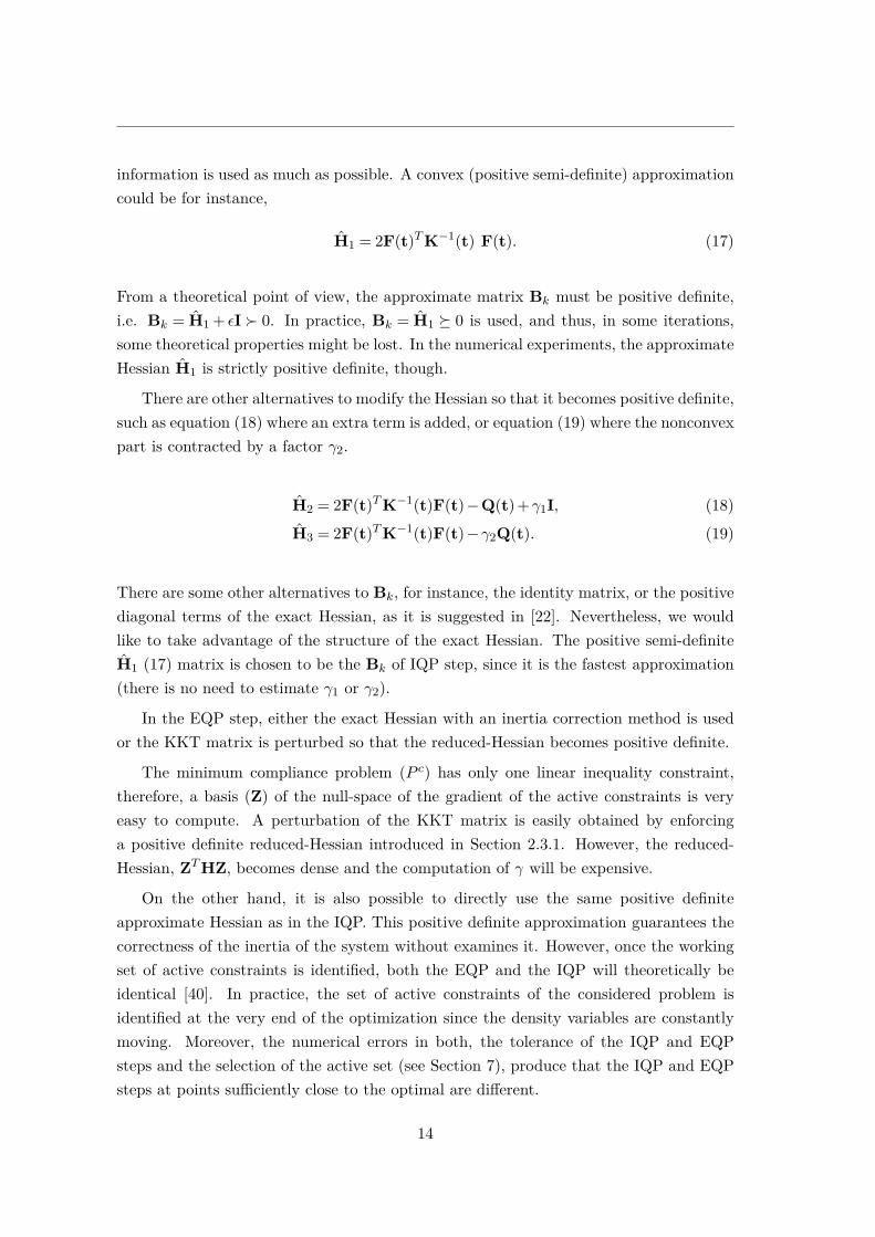
information is used as much as possible. A convex (positive semi-definite) approximationcould be for instance,
H1 = 2F(t)TK−1(t) F(t). (17)
From a theoretical point of view, the approximate matrix Bk must be positive definite,i.e. Bk = H1 + εI 0. In practice, Bk = H1 0 is used, and thus, in some iterations,some theoretical properties might be lost. In the numerical experiments, the approximateHessian H1 is strictly positive definite, though.
There are other alternatives to modify the Hessian so that it becomes positive definite,such as equation (18) where an extra term is added, or equation (19) where the nonconvexpart is contracted by a factor γ2.
H2 = 2F(t)TK−1(t)F(t)−Q(t)+γ1I, (18)H3 = 2F(t)TK−1(t)F(t)−γ2Q(t). (19)
There are some other alternatives to Bk, for instance, the identity matrix, or the positivediagonal terms of the exact Hessian, as it is suggested in [22]. Nevertheless, we wouldlike to take advantage of the structure of the exact Hessian. The positive semi-definiteH1 (17) matrix is chosen to be the Bk of IQP step, since it is the fastest approximation(there is no need to estimate γ1 or γ2).
In the EQP step, either the exact Hessian with an inertia correction method is usedor the KKT matrix is perturbed so that the reduced-Hessian becomes positive definite.
The minimum compliance problem (P c) has only one linear inequality constraint,therefore, a basis (Z) of the null-space of the gradient of the active constraints is veryeasy to compute. A perturbation of the KKT matrix is easily obtained by enforcinga positive definite reduced-Hessian introduced in Section 2.3.1. However, the reduced-Hessian, ZTHZ, becomes dense and the computation of γ will be expensive.
On the other hand, it is also possible to directly use the same positive definiteapproximate Hessian as in the IQP. This positive definite approximation guarantees thecorrectness of the inertia of the system without examines it. However, once the workingset of active constraints is identified, both the EQP and the IQP will theoretically beidentical [40]. In practice, the set of active constraints of the considered problem isidentified at the very end of the optimization since the density variables are constantlymoving. Moreover, the numerical errors in both, the tolerance of the IQP and EQPsteps and the selection of the active set (see Section 7), produce that the IQP and EQPsteps at points sufficiently close to the optimal are different.
14

5 ALTERNATIVES TO THE PRIMAL IQP FORMULATION
5 Alternatives to the primal IQP formulation
The IQP sub-problem of (P c) is formulated using an approximate Hessian Bk defined in(17) as
minimized∈Rn
f(d) =−(FTk uk)Td+dTFTkK−1k Fkd
subject to aT tk−V +aTd≤ 0−tk ≤ d≤ 1− tk.
(IQPp)
For simplicity, any function or matrix with the form A(tk) is represented by Ak.The feasible set of (IQPp) is convex (hyperplanes), nonempty, closed, and bounded.
By construction the (IQPp) is convex. Moreover some CQs hold. Thus, this sub-problemhas an optimal solution and any local solution that satisfies the KKT condition is also aglobal minimizer.
5.1 Reformulation of the primal IQP formulation
TopSQP spends most of the computational time in the IQP phase. In addition, (IQPp)is extremely expensive since the inverse of the stiffness matrix is involved, and the matrixBk is dense.
However, it is possible to reformulate the inequality sub-problem such that thecomputation and the storage of the approximate Hessian are no longer required. Firstof all, a Cholesky factorization is used for the stiffness matrix. Then, a new variablez = (RT
k )−1Fkd ∈ Rd is included to rename some terms of the problem so that anyinverse matrix is removed from the objective function of (IQPp).
f(d) =−(FTk uk)Td+dTFTk (RTkRk)−1Fkd,
f(d, z) =−(FTk uk)Td+ zT z.
The introduction of the new variable z leads to an enlargement of the number ofconstraints. The alternative IQP formulation is
minimized∈Rn,z∈Rd
−(FTk uk)Td+ zT z
subject to RTk z−Fkd = 0,
Akd≤ bk,
(IQPp−2)
where the linear inequality constraints are condensed into a system Akd≤bk, to simplifythe notation. Here, m= 2n+1, and
Ak =
aT
I−I
∈ Rm×n,
bk =
−(aT tk−V )1− tktk
∈ Rm.
15

Using this new formulation, the number of variables and linear constraints areincreased. In contrast, the computational time can, due to sparsity, significantly bereduced.
5.2 Dual problem of the IQP formulation
Using Lagrangian duality theory (see e.g. [9]), an optimization problem can bereformulated using the dual variables (λ,ξ,η). In some cases this new dual problem ismuch easier to solve and computationally less expensive than the primal problem.Thus, the problem (IQPp) can also be formulated in its dual problem.
A new variable z ∈ Rd is introduced to rename some terms of the objective function.Let
z = Fkd, (20)
then, the (IQPp) problem is equivalent to
minimized∈Rn,z∈Rd
−(FTk uk)Td+zTK−1k z
subject to Akd≤ bk,z = Fkd.
(21)
The Lagrangian function of the IQP sub-problem (21) is described in terms of theprimal variables d and z, and the dual variables ν = (λ,ξ,η) ∈ Rm (for the inequalityand bound constraints) and θ ∈ Rd (for the new equality constraints).
Lp(d,z,ν,θ) = −(FTk uk)Td+zTK−1k z+
νT (Akd−bk)+θT (z−Fkd).
The dual problem consists of maximizing
ϕ(ν,θ) = infd,zLp(d,z,ν,θ)
respect to the dual variables ν,θ [9]. The formulation of the dual problem is obtainedby satisfying the optimality conditions of (21),
∇dLp(d,z,ν,θ) =−FTk uk +ATk ν−FTk θ = 0,
∇zLp(d,z,ν,θ) = 2K−1k z+θ = 0.
Then, the solution of the dual problem must satisfy:
z =−12Kkθ, (22)
−FTk uk +ATk ν−FTk θ = 0. (23)
16

5 ALTERNATIVES TO THE PRIMAL IQP FORMULATION
Based on the above equations, the primal Lagrangian function at (d,z,ν,θ) is
Lp(d,z,ν,θ) =−(FTk uk)Td+zTK−1k z+νT (Akd−bk)+
θT (z−Fkd)
= (−FTk uk +ATk ν−FTk θ)Td−
14θ
TKkθ−νTbk.
(24)
Thus, the dual IQP problem is defined by merging (23) and (24) resulting in the quadraticproblem
maximizeν∈Rm,θ∈Rd
ϕ(ν,θ) =−14θ
TKkθ−νTbk
subject to ATk ν−FTk θ = FTk uk,
ν ≥ 0,which is equivalent to
minimizeν,θ
14θ
TKkθ+νTbksubject to AT
k ν−FTk θ = FTk uk,ν ≥ 0.
(IQPd)
The dual problem (IQPd) is defined with a quadratic convex objective function, nlinear equality constraints andm= 2n+1 bound constraints. The strong duality propertyfor convex problems ensures that ϕ(ν,θ) = f(d) see e.g. [9].
In order to recover the primal variables, the optimality conditions of the dual problem(IQPd) are explicitly obtained. Given the dual Lagrangian function
Ld(ν,θ,χ,ζ) = 14θ
TKkθ+νTbk+χT (−FTk uk +AT
k ν−FTk θ)−ζTν,
the optimality conditions are satisfied at (ν,θ,χ,ζ)
∇νLd(ν,θ,χ,ζ) = bk +Akχ−ζ = 0∇θLd(ν,θ,χ,ζ) = 1
2Kkθ−Fkχ = 0.(25)
Here, χ ∈ Rn and ζ ∈ Rm are the Lagrangian multipliers of the equality and the boundconstraints of (IQPd), respectively.
From Equation (25), θ = 2K−1k Fkχ is obtained. In addition, the primal variable z is
related with the dual variable θ by equation (22). Thus, z=−Fkχ. At the same time, zwas previously defined as z=Fkd (20), then, the optimal primal variable d is equivalentto the negative value of the optimal dual variable of (IQPd), i.e. d
iqk =−χ.
The variable ν collects the inequality, the upper bound, and the lower boundLagrangian multipliers, i.e. ν = (λiqk ,ξ
iqk ,η
iqk ) with λiqk ∈ R, and ξiqk ,η
iqk ∈ Rn.
The main advantage of solving the IQP sub-problem using the dual formulation is theelimination of the inverse of the stiffness matrix. This new formulation is expected to befaster than the alternative primal formulation since there are fewer number of variablesand constraints. Therefore, it is chosen for the implementation of TopSQP.
17

6 Alternative to the EQP system
Analogous to the IQP, the KKT system for the minimum compliance problem isimpractical since to the computation of the Hessian is needed. Throughout this section,and with the aim of simplifying the notation, the sub-indices referring to the workingset or the complementary working set are omitted, see Section 2.3 for the sake ofcompleteness.
The original EQP system for minimum compliance problem is[Hk aaT 0
][deqkλeqk
]=−
[−FTk uk +Hkdiqk
0
](EQP0)
With Hk =∇2L(xk,λiqk ), and Hk an approximation of the Hessian such that the inertiaof the system (EQP0) is correct.
Let assume Hk = 2FTkK−1k Fk− Qk for any Qk such that Hk 0.
The first system of equations for the minimum compliance problem is
Hkdeqk +aλeqk =−(−FTk uk +Hkdiqk ),⇓
2FTkK−1k Fkdeqk −Qkd
eqk +aλeqk =−(−FTk uk +Hkdiqk ).
(26)
In order to reduce the computational cost caused for the dense Hessian, the systemis expanded. A new variable vk = 2K−1
k Fkdeqk is included to split equation (26) in two,
12Kkvk−Fkdeqk = 0,FTk vk− Qkd
eqk +aλeqk =−(−FTk uk +Hkdiqk ).
It enables to define an expanded EQP symmetric system
−Qk FTk aFk −1/2Kk 0aT 0 0
deqkvkλeqk
=−
−FTk uk +Hkdiqk00
. (EQPe)
Although the size of the system is increased from |Wbk,c|+ |W
gk | to d+ |Wb
k,c|+ |Wgk |, it is
much faster to solve than (EQP0) since there are only sparse matrices.The system can be solved using direct methods such as the null-space method [43].
The computation of a matrix Z with columns are the basis of the null-space of theJacobian is cheap, easy, and fast. However, as there is only one constraint, the timereduction is negligible. In addition, the computational cost of the EQP step is notsignificant for the overall algorithm due to the sparsity of the KKT matrix. Moreover,the density variables tend fast to the bounds, and most of the bound constraints will beactive. This produces a meaningful reduction of the size of the system (EQPe), see (11).
18

7 IMPLEMENTATION
Table 1: Study of the number of iterations required for TopSQP to converge using both EQP+IQPand using only the IQP phase on a test set of 10 small-size problems. The table contains thedescription of the problem (design domain, length ratios, discretization, and volume fraction) andthe number of iterations required for both approaches.
Domain Length ratio Discretization Volume TopIQP iterations TopSQP iterations
Michell 1×1 20×20 0.1 63 36Michell 1×1 40×40 0.3 85 74Michell 2×1 40×20 0.1 256 151Michell 2×1 80×40 0.5 37 30Michell 3×1 60×20 0.4 137 114MBB 1×2 40×80 0.3 88 59MBB 1×4 40×160 0.5 124 113MBB 2×1 80×40 0.2 169 141Cantilever 2×1 120×60 0.5 81 78Cantilever 4×1 80×20 0.2 131 92
7 Implementation
The same approximate Hessian is used for both, the IQP and the EQP phase (see (17)),since preliminary results show that the performance of H1 in the EQP was very similarto H2 and H3. However, the computational time required for H2 and H3 is higher thanH1 due to the estimation of γ1 and γ2. In addition any inertia correction in the originalsystem will increase the computational time of the algorithm considerably.
The implementation of the proposed algorithm is written in MATLAB [54], and theIQP sub-problem is solved using Gurobi optimizer software [34]. The default method inGurobi is used in which the QP problem is solved with a barrier algorithm. Althoughthe Gurobi software is very efficient, the IQP phase makes the method expensive. TheEQP is, thus, very important to reduce the number of IQP iterations.
The numerical experiments in [40] show the benefits of the EQP in terms of numberof iterations. Since the proposed IQP is defined with the same approximate Hessian asthe EQP phase, a small preliminary study was performed to study the effects of theEQP step. Table 1 shows the number of iterations needed for TopSQP using only theIQP (namely TopIQP) and using both phases. Although, only ten small problems areconsidered, similar behaviour was observed for the whole test set of problems. The EQPreduces the total number of iterations. In addition, the cost of the EQP phase is negligiblecompared to the IQP.
19

For the estimation of the working set, the linearized constraint g(x) are consideredactive if:
−ε4 < g(xk)+∇g(xk)Tdiqk < ε4,
with ε4 = 10−4. In the same way, the line search is, in practice, more flexible. First of all,a smaller reduction in the merit function than in the original SQP+ algorithm is allowed,using the parameter ε5 = 10−6.
φπ(xk +diqk +βdeqk )≤ φπ(xk)−σqredπ(diqk )− ε5.
Secondly, in those cases where the previous condition is not satisfied (Step 9 Algorithm1), instead of doing a line search with only diqk , up to 5 consecutive times the full IQPstep (α = 1) is allowed. In practice, the algorithm will take in most of the iterations astep direction involving both phases: dk = diqk +βdeqk . However, in very few examples,this descent direction does not reduce the merit function and it stalls in a local minimumwith a small KKT error but not sufficiently small for convergence. In those situationsthe KKT conditions are satisfied when a full inequality step is forced.
Regarding the finite element analysis, the design domain is discretized using the samesize of plane stress elements (with 4 nodes per element), and then the element stiffnessmatrix is the same for all elements. The code of the finite element analysis is based on[2].
8 Numerical Experiments
The specific purpose TopSQP solver is compared to the first-order structural topologyoptimization solver, GCMMA [53], and two general purpose solvers, SNOPT [27] andIPOPT [55]. These last two solvers (namely SNOPT and IPOPT-N) use limited memoryBFGS approximation of the Hessian. Moreover, the best solver (in terms of objectivefunction value) according to [46], IPOPT-S, is under consideration. IPOPT-S3 solvesthe SAND (Simultaneous Analysis and Design, see e.g. [3]) formulation using the exactHessian. More information about these solvers and their specific parameter settings canbe found in [46]. The parameter values set for the TopSQP and Gurobi are gatheredin Tables 2 and 3, respectively. In addition, Table 4 contains the parameter values ofthe minimum compliance problem used for TopSQP. Since IPOPT and SNOPT are alsosecond-order methods, the optimality conditions are set as in TopSQP, i.e. feas norm= 10−8 and kkt norm = 10−6. More details of how the KKT norm is obtained in thesesolvers can be found in [55] and [27]. The stopping criterion of GCMMA is kkt norm =10−4 and feas norm = 10−8 (first-order method). The maximum number of iterationsfor all the solvers is set to max iter = 1,000. See more details in [46].
3For simplicity, the default linear algebra package MUMPS [1] is used in both nested (IPOPT-N) andSAND (IPOPT-S) formulation.
20

8 NUMERICAL EXPERIMENTS
All the computations were done on a Intel Xeon e5-2680v2 ten-core processor, runningat 2.8GHz with 64 GB RAM. Only Gurobi (IQP phase) runs in parallel using four threads.TopSQP, IPOPT, SNOPT, and GCMMA all run in serial.
Table 2: Parameter setting for TopSQP. The table contains the name of the parameter, a briefdescription and the value.
Parameter Description Value
t0 Starting point V e4
stat tol Stationarity error ε1 (see 2.1) 10−6
feas tol Feasibility error ε2 (see 2.1) 10−8
comp tol Complementarity error ε3 (see 2.1) 10−6
max iter Maximum number of iterations 1,000
Table 3: Parameter setting for Gurobi for solving the IQP sub-problem. The table contains thename of the parameter, a brief description and the value.
Parameter Description Value
OptimalityTol Optimality tolerance 10−9
FeasibilityTol Feasibility tolerance 10−9
threads Number of OMP threads 4presolve Presolve level 0 (off)
Table 4: Values of charateristic parameters of topology optimization problems solve by TopSQP.
Parameter Description Value
Ev Young’s modulus value for void material 10−1
E1 Young’s modulus value for solid material5 102
p SIMP penalization parameter 3rmin radius for the density filter 0.04Lx
(Lx is the length in the x direction)
4Here, e refers to a vector of all ones.5A small contrast of E1/Ev is considered since we are mostly interested in the behaviour of the solvers.
In addition, the values of Ev and E1 are chosen to well-scaled problems for the solvers (see [46] for moredetails).
21

[0:4] [4:8] [8:12] [12:16] [16:20] [20:24] [24:28] [28:32] [32:36] [36:40]0
10
20
30
40
50
60
70
80
number of elements ×103
numberofproblem
instances
Figure 1: Distribution of the number of instances of the test set for different number of elementsranges.
The numerical experiments to assess the performance of TopSQP are presented usingperformance profiles, see [16]. The specific minimum compliance test set consists of 2252D medium-size instances (with 400-40,000 finite elements) as defined in [46]. Figure 1shows how the problem instances are distributed with regards to the number of elements(size of the problem). Since a time limit is set to 300 hours, the execution of TopSQP(MATLAB general purpose implementation) is not finished6 for 18 problem instances.In addition, IPOPT-S (SAND formulation) has some issues in the linear algebra7 for 12problem instances. Nevertheless, the last intermediate design obtained in these instancesis considered as the final design in the benchmarking study.
The performance profiles show the percentage of problems (in the test set) where asolver s obtains different relative ratios of performance (defined with the parameter τ).In other words, for a given solver s, the function ρs defined is represented as
ρs(τ) = 1N
sizep ∈ P : rp,s ≤ τ,
or
ρs(τ) = 1N
sizep ∈ P : log10(rp,s)≤ τ.
Here, P is the set of problems with p ∈ P and N the size of P . The ratio of performancefor a solver s for each problem p is defined as
rp,s = mp,s
minmp,s : s ∈ S ,
6The computational time required for the solver is highly dependent on the number of processors, themethod, as well as the number of threads used during the execution.
7IPOPT needs to reallocate memory and thus, it has difficulties to converge.
22

8 NUMERICAL EXPERIMENTS
1 1.02 1.04 1.06 1.08 1.1 1.12 1.14 1.16 1.18 1.20
10
20
30
40
50
60
70
80
90
100
τ
%problems
TopSQPIPOPT NIPOPT SSNOPTGCMMA
(a) Objective function value (ωmax = 10−3).
1 1.02 1.04 1.06 1.08 1.1 1.12 1.14 1.16 1.18 1.20
10
20
30
40
50
60
70
80
90
100
τ
%problems
TopSQPIPOPT NIPOPT SSNOPTGCMMA
(b) Objective function value (ωmax 0).
Figure 2: Performance profile for a test set of 225 minimum compliance problems. Theperformance is measured by the objective function value. Figure 2a shows the performance whendesigns with KKT error higher than ωmax = 10−3 are penalized. Figure 2b shows the performancewithout any penalization measured, i.e., with ωmax 0.
with m a measure of performance, such as
mp,s = iterp,s = number of iterations required to solve the problem p by a solver s.
In these numerical experiments, the solvers are compared using four different criteria:the objective function value, the number of iterations (outer iterations), the number ofstiffness matrix assemblies, and the computational time.
Furthermore, at the maximum value ratio rM the performance profiles reflect therobustness of the solvers. In these numerical experiments, a solver fails if the KKTerror is larger than ωmax = 10−3. Thus, the term robustness refers to the capability ofobtaining a design with a KKT accuracy lower than or equal to 10−3. More details aboutthe impact of this threshold can be found in [46].
Figure 2a shows the performance profile for the objective function value. IPOPT-Sstill has the highest number of problems where the designs have the minimum objectivefunction value (70% of the cases). Nevertheless, when τ is relatively small, (τ = 1.05),the performance of TopSQP is the same as IPOPT-S with a success of 81%. TopSQPoutperforms the other solvers in terms of objective function value for τ close to 1. Someof the methods presented in the study produce feasible iterates. Although thefirst-order optimality conditions are not satisfied (KKT error higher than ωmax), theobjective function values of feasible designs might still be acceptable. Figure 2b showsthe performance profile (for objective function value) when no penalization is applied.The difference is meaningful for GCMMA. In general, its feasible iterates producereasonably good approximations. Although, the performance of IPOPT-S and TopSQP
23

1 1.05 1.1 1.15 1.2 1.25 1.3 1.35 1.4 1.450
10
20
30
40
50
60
70
80
90
100
τ
%problems
TopSQPIPOPT NIPOPT SSNOPTGCMMA
(a) Objective function value (V = 0.1)
1 1.05 1.1 1.15 1.2 1.25 1.3 1.35 1.4 1.450
10
20
30
40
50
60
70
80
90
100
τ
%problems
TopSQPIPOPT NIPOPT SSNOPTGCMMA
(b) Objective function value (V = 0.2)
1 1.05 1.1 1.15 1.2 1.25 1.30
10
20
30
40
50
60
70
80
90
100
τ
%problems
TopSQPIPOPT NIPOPT SSNOPTGCMMA
(c) Objective function value (V = 0.3)
1 1.05 1.1 1.15 1.2 1.25 1.30
10
20
30
40
50
60
70
80
90
100
τ
%problems
TopSQPIPOPT NIPOPT SSNOPTGCMMA
(d) Objective function value (V = 0.4)
1 1.05 1.1 1.15 1.2 1.25 1.30
10
20
30
40
50
60
70
80
90
100
τ
%problems
TopSQPIPOPT NIPOPT SSNOPTGCMMA
(e) Objective function value (V = 0.5)
Figure 3: Performance profiles for five different subsets of the minimum compliance problems (45instances each). The problems are divided depending on their volume fraction. The performanceis measured by the objective function value.
24

8 NUMERICAL EXPERIMENTS
0 0.2 0.4 0.6 0.8 1 1.2 1.4 1.6 1.80
10
20
30
40
50
60
70
80
90
100
τ (log10)
%problems
TopSQPIPOPT NIPOPT SSNOPTGCMMA
(a) Number of iterations
0 0.5 1 1.5 20
10
20
30
40
50
60
70
80
90
100
τ (log10)
%problems
TopSQPIPOPT NIPOPT SSNOPTGCMMA
(b) Stiffness matrix assemblies
0 0.5 1 1.5 2 2.5 3 3.50
10
20
30
40
50
60
70
80
90
100
τ (log10)
%problems
TopSQPIPOPT NIPOPT SSNOPTGCMMA
(c) Computational time
Figure 4: Performance profiles for a test set of 225 minimum compliance problems. Theperformance is measured by the objective function value (2a), the number of iterations (4a),the number of stiffness matrix assemblies (4b) and the computational time (4c).
25

is still better, in general all the solvers produce designs with similar objective functionvalues. In 80% of the problems, the difference of objective function values is smallerthan 12% (i.e. τ = 1.12).
In almost the 30% of the problems solved with GCMMA, the KKT error is higherthan 10−3. Before analysing the performance of the methods for different criteria, it isimportant to study in detail why GCMMA has difficulties to converge. Figure 3 showsthe performance profiles (for objective function value) for smaller test sets of problems.The original test set is partitioned into five. Each subset gathers 45 problems in whichthe volume fraction is the same (V = 0.1, 0.2, 0.3, 0.4, and 0.5). It seems clear thatGCMMA has difficulties on solving problems with low volume fractions, see Figures 3aand 3b in which the test set collects problems with V = 0.1 and V = 0.2, respectively.
Regarding the performance for the number of iterations (Figure 4a), TopSQPproduces designs using the smallest number of iterations, with a very similarperformance to SNOPT. However, the designs for the latter solver have large objectivefunction values (see Figure 2a). Since TopSQP has two phases, it is also important tocompare the performance using other criteria to check the cost of every major iteration.Figure 4b shows the performance profiles when the solvers are compared with thenumber of stiffness matrix assemblies, which is equivalent to the number of functionevaluations. It is outstanding the few number of stiffness matrix assembled for TopSQP.In contrast to SNOPT or IPOPT-S, TopSQP usually evaluates the stiffness matrix onceper iteration. This is due to the definition of the line search.
A very important aspect in the comparison of solvers is the computational timerequired for obtaining a solution. On the other hand, we need to be cautious sincethe solvers have different interfaces, they are programmed in different languages, andcan be linked to different linear algebra packages. The computational time could behighly affected by this. Although it is preferable to compare the computational costof the solvers using a more objective criterion such as the number of iterations or thenumber of stiffness matrix assemblies, it is remarkable the amount of time required forTopSQP (Figure 4c). It performs slightly worse than IPOPT-S (SAND formulation). Themajor amount of time in the proposed method is spent in the IQP sub-problem. Moresophisticated and advanced convex quadratic methods must be developed to solve thissub-problem in order to produce an efficient and fast method. Nevertheless, TopSQPis considered a good compromise between accurate and good designs (good objectivefunction values) and computational time.
Finally, TopSQP, IPOPT-N, and SNOPT have excellent robustness properties, i.e.the KKT error is lower than 10−3 in about the 96% of the test set. In contrast, therobustness of GCMMA is highly dependent on the problems. GCMMA performs verywell with respect to the objective function value when the volume fraction is large, witha robustness of 100% (see Figure 3e). On the other hand, the robustness of GCMMA
26
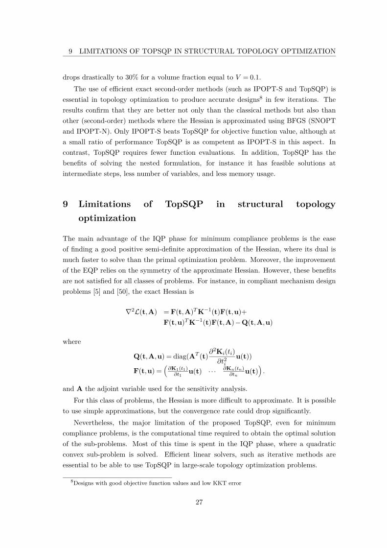
9 LIMITATIONS OF TOPSQP IN STRUCTURAL TOPOLOGY OPTIMIZATION
drops drastically to 30% for a volume fraction equal to V = 0.1.The use of efficient exact second-order methods (such as IPOPT-S and TopSQP) is
essential in topology optimization to produce accurate designs8 in few iterations. Theresults confirm that they are better not only than the classical methods but also thanother (second-order) methods where the Hessian is approximated using BFGS (SNOPTand IPOPT-N). Only IPOPT-S beats TopSQP for objective function value, although ata small ratio of performance TopSQP is as competent as IPOPT-S in this aspect. Incontrast, TopSQP requires fewer function evaluations. In addition, TopSQP has thebenefits of solving the nested formulation, for instance it has feasible solutions atintermediate steps, less number of variables, and less memory usage.
9 Limitations of TopSQP in structural topologyoptimization
The main advantage of the IQP phase for minimum compliance problems is the easeof finding a good positive semi-definite approximation of the Hessian, where its dual ismuch faster to solve than the primal optimization problem. Moreover, the improvementof the EQP relies on the symmetry of the approximate Hessian. However, these benefitsare not satisfied for all classes of problems. For instance, in compliant mechanism designproblems [5] and [50], the exact Hessian is
∇2L(t,A) = F(t,A)TK−1(t)F(t,u)+F(t,u)TK−1(t)F(t,A)−Q(t,A,u)
where
Q(t,A,u) = diag(AT (t)∂2Ki(ti)∂t2i
u(t))
F(t,u) =(∂K1(t1)∂t1
u(t) · · · ∂Kn(tn)∂tn
u(t)).
and A the adjoint variable used for the sensitivity analysis.For this class of problems, the Hessian is more difficult to approximate. It is possible
to use simple approximations, but the convergence rate could drop significantly.Nevertheless, the major limitation of the proposed TopSQP, even for minimum
compliance problems, is the computational time required to obtain the optimal solutionof the sub-problems. Most of this time is spent in the IQP phase, where a quadraticconvex sub-problem is solved. Efficient linear solvers, such as iterative methods areessential to be able to use TopSQP in large-scale topology optimization problems.
8Designs with good objective function values and low KKT error
27

10 Conclusions and further research
An efficient second-order sequential quadratic programming method based on SQP+ from[40] is presented for topology optimization problems (TopSQP). More specifically, theminimum compliance problem is solved using exact information of the Hessian in both,the IQP and EQP phases. An efficient approximate Hessian is used in both phases,producing very accurate estimations of the search direction. These sub-problems areefficiently improved, since they are reformulated taking advantages of the structure ofthe problem.
The numerical experiments confirm the benefits of using second-order information notonly for reducing the number of iterations but also for decreasing the objective functionvalues. IPOPT-S and TopSQP are the most competent methods to produce designs withgood objective function value. The comparison of the performance between IPOPT-S andTopSQP (exact Hessian) and SNOPT and IPOPT-N (BFGS approximation), reinforcesthat the use of information based on the exact Hessian is important to obtain gooddesigns.
Additionally, TopSQP outperforms GCMMA not only in the objective function valuebut also in the number of iterations, the number of stiffness matrix assemblies, and theoverall robustness.
Although IPOPT-S outperforms the other solvers when measuring the objectivefunction value, all the solvers are able to produce similar results. Indeed the objectivefunction value of TopSQP is very close to the minimum possible. In contrast, IPOPT-Srequires more iterations and function evaluations than TopSQP. Finally, TopSQP solvesthe nested formulation with all the advantages that brings with it.
Further work must be done in order to extend and generalize the proposed TopSQPmethod to solve more general topology optimization problems such as compliantmechanism design problems. Additional investigations are needed to extend the code tobe able to solve large-scale problems.
Acknowledgements
We would like to thank Professor Krister Svanberg at KTH in Stockholm for providingthe implementation of GCMMA. We extend our sincere thanks to two reviewers and theeditor for providing many comments and suggestions that improved the quality of thisarticle.
28
REFERENCES
References
[1] P. R. Amestoy, I. S. Duff, and J. Y. L’Excellent. Multifrontal parallel distributedsymmetric and unsymmetric solvers. Computer Methods in Applied Mechanics andEngineering, 184(2–4):501–520, 2000.
[2] E. Andreassen, A. Clausen, M. Schevenels, B. S. Lazarov, and O. Sigmund.Efficient topology optimization in MATLAB using 88 lines of code. Structural andMultidisciplinary Optimization, 43(1):1–16, 2011.
[3] J. S. Arora and Q. Wang. Review of formulations for structural and mechanicalsystem optimization. Structural and Multidisciplinary Optimization, 30(4):251–272,2005.
[4] M. P. Bendsøe. Optimal shape design as a material distribution problem. StructuralOptimization, 1(4):192–202, 1989.
[5] M. P. Bendsøe and O. Sigmund. Topology optimization: Theory, methods andapplications. Springer, 2003.
[6] P. T. Boggs and J. W. Tolle. A family of descent functions for constrainedoptimization. SIAM Journal on Numerical Analysis, 21(6):1146–1161, 1984.
[7] P. T. Boggs and J. W. Tolle. Sequential Quadratic Programming. Acta Numerica,4:1–51, 1995.
[8] B. Bourdin. Filters in topology optimization. International Journal for NumericalMethods in Engineering, 50(9):2143–2158, 2001.
[9] S. Boyd and L. Vandenberghe. Convex Optimization. Cambridge University Press,2010.
[10] R. H. Byrd, N. I. M. Gould, J. Nocedal, and R. A. Waltz. An algorithm for nonlinearoptimization using linear programming and equality constrained subproblems.Mathematical Programming, 48:27–48, 2004.
[11] R. H. Byrd, J. Nocedal, and R. A. Waltz. KNITRO : An Integrated Package forNonlinear Optimization. In Large Scale Nonlinear Optimization, volume 83, pages35–59. Springer, 2006.
[12] A. R. Conn, N. I. M. Gould, and P. L. Toint. Trust Region Methods. Society forIndustrial and Applied Mathematics, 1987.
[13] F. E. Curtis, T. C. Johnson, D. P. Robinson, and A. Wächter. An inexact sequentialquadratic optimization algorithm for nonlinear optimization. SIAM Journal onOptimization, 24(3):1041–1074, 2014.
29

[14] F. E. Curtis and J. Nocedal. Flexible penalty functions for nonlinear constrainedoptimization. IMA Journal of Numerical Analysis, 25(4):749–769, 2008.
[15] J. E. Dennis and J. J. Moré. Quasi-Newton Methods, Motivation and Theory. SIAMReview, 19(1):46–89, 1977.
[16] E. D. Dolan and J. J. Moré. Benchmarking optimization software with performanceprofiles. Mathematical Programming, 91(2):201–213, 2002.
[17] T. Dreyer, B. Maar, and V. Schulz. Multigrid optimization in applications. Journalof Computational and Applied Mathematics, 120(1-2):67–84, 2000.
[18] L. F. Etman, A. A. Groenwold, and J. E. Rooda. First-order sequentialconvex programming using approximate diagonal QP subproblems. Structural andMultidisciplinary Optimization, 45(4):479–488, 2012.
[19] R. Fletcher and S. Leyffer. User manual for filterSQP. Technical Report NA/181,University of Dundee Numerical Analysis, 1998.
[20] R. Fletcher and S. Leyffer. Nonlinear programming without a penalty function.Mathematical Programming, 91(2):239–269, 2002.
[21] C. Fleury. CONLIN: An efficient dual optimizer based on convex approximationconcepts. Structural Optimization, 1(2):81–89, 1989.
[22] C. Fleury. Efficient approximation concepts using second order information.International Journal for Numerical Methods in Engineering, 28(9):2041–2058, 1989.
[23] C. Fleury. First and second order convex approximation strategies in structuraloptimization. Structural Optimization, 1(1):3–10, 1989.
[24] A. Forsgren. Inertia-controlling factorizations for optimization algorithms. AppliedNumerical Mathematics, 43(1-2):91–107, 2002.
[25] A. Forsgren and P. E. Gill. Primal-dual interior methods for nonconvex nonlinearprogramming. SIAM Journal on Optimization, 8(4):1132–1152, 1998.
[26] A. Forsgren and W. Murray. Newton methods for large-scale linear inequality-constrained minimization. SIAM Journal on Optimization, 7(1):162–176, 1997.
[27] P. E. Gill, W. Murray, and M. A. Saunders. SNOPT: An SQP Algorithm for Large-Scale Constrained Optimization. SIAM Journal on Optimization, 47(4):99–131,2005.
30

REFERENCES
[28] P. E. Gill, W. Murray, M. A. Saunders, and M. H. Wright. User’s guide for NPSOL5.0: A fortran package for nonlinear programming. Technical report, SystemsOptimization Laboratory, Department of Opertations Research, Stanford University,1998.
[29] P. E. Gill and D. P. Robinson. A globally convergent stabilized SQP method. SIAMJournal on Optimization, 23(4):1983–2010, 2013.
[30] P. E. Gill and E. L. Wong. Sequential quadratic programming methods. MixedInteger Nonlinear Programming, in the IMA Volumes in Mathematics and itsApplications, 154:147–224, 2012.
[31] P. E Gill and E. L. Wong. Convexification schemes for SQP methods.Technical Report CCoM 14-6, Center for Computational Mathematics, Universityof California, San Diego, 2014.
[32] N. I. M. Gould. On practical conditions for the existence and uniqueness ofsolutions to the general equality quadratic programming problem. MathematicalProgramming, 32(1):90–99, 1985.
[33] N. I. M. Gould and D. P. Robinson. A second derivative SQP method: Globalconvergence. SIAM Journal on Optimization, 20(4):2023–2048, 2010.
[34] Inc. Gurobi Optimization. Gurobi 12.6.0 Reference Manual, 2010.
[35] W. W. Hager. Stabilized sequential quadratic programming. In ComputationalOptimization, pages 253–273. Springer, 1999.
[36] N. J. Higham and S. H. Cheng. Modifying the inertia of matrices arising inoptimization. Linear Algebra and its Applications, 275–276:261–279, 1998.
[37] IBM. ILOG. ILOG CPLEX, Reference Manual, 2007.
[38] S. Leyffer and A. Mahajan. Software for Nonlinearly Constrained Optimization.Technical Report ANS/MCS-P1768-0610, Mathematics and Computer ScienceDivision, Argonne National Laboratory, 2010.
[39] D. G. Luenberger and Y. Ye. Linear and Nonlinear Programming. Springer, 2008.
[40] J. L. Morales, J. Nocedal, and Y. Wu. A sequential quadratic programmingalgorithm with an additional equality constrained phase. Journal of NumericalAnalysis, 32(2):553–579, 2010.
[41] J. J. Moré and D. J. Thuente. Line search algorithms with guaranteed sufficientdecrease. ACM Transactions on Mathematical Software, 20(3):286–307, 1994.
31

[42] K. G. Murty and S. N. Kabadi. Some NP-complete problems in quadratic andnonlinear programming. Mathematical Programming, 39:117 – 129, 1987.
[43] J. Nocedal and S. J. Wright. Numerical Optimization. Springer, 1999.
[44] C. E. Orozco and O. N. Ghattas. A reduced SAND method for optimal design ofnonlinear structures. International Journal for Numerical Methods in Engineering,40(15):2759–2774, 1997.
[45] F. J. Prieto. Sequential quadratic programming algorithms for optimization.Technical Report SOL 89-7, Systems Optimization Laboratory, Department ofOperations Research, Stanford University, 1989.
[46] S. Rojas-Labanda and M. Stolpe. Benchmarking optimization solvers for structuraltopology optimization. Structural and Multidisciplinary Optimization, In print,2015. DOI: 10.1007/s00158-015-1250-z.
[47] G. I. N. Rozvany, M. Zhou, and T. Birker. Generalized shape optimization withouthomogenization. Structural Optimization, 4(3–4):250–252, 1992.
[48] K. Schittkowski. NLPQLP : A new fortran implementation of a Sequential QuadraticProgramming algorithm. Technical report, Department of Mathematics, Universityof Bayreuth, 2002.
[49] C. Shen, W. Xue, and X. Chen. Global convergence of a robust filter SQP algorithm.European Journal of Operational Research, 206(1):34–45, 2010.
[50] O. Sigmund. On the design of compliant mechanisms using topology optimization.Journal of Structural Mechanics, 25(4):492–526, 1997.
[51] O. Sigmund and J. Petersson. Numerical instabilities in topology optimization:A survey on procedures dealing with checkerboards, mesh-dependencies and localminima. Structural Optimization, 16(2):68–75, 1998.
[52] K. Svanberg. The method of moving asymptotes - A new method for structuraloptimization. International Journal for Numerical Methods in Engineering,24(2):359–373, 1987.
[53] K. Svanberg. A class of globally convergent optimization methods based onconservative convex separable approximations. SIAM Journal on Optimization,12(2):555–573, 2002.
[54] Inc. The MathWorks. Optimization Toolbox User’s Guide R 2013 b, 2013.
32

REFERENCES
[55] A. Wächter and L. T. Biegler. On the implementation of an interior point filter line-search algorithm for large-scale nonlinear programming. Mathematical Programming,106(1):25–57, 2006.
[56] B. Wang and D. Pu. Flexible penalty functions for SQP algorithm with additionalequality constrained phase. Technical report, Proceedings of the 2013 InternationalConference on Advance Mechanic System, China, September 25-27, 2013.
[57] M. Zhou and G. I. N. Rozvany. The COC algorithm, Part II: Topological, geometricaland generalized shape optimization. Computer Methods in Applied Mechanics andEngineering, 89(1–3):309–336, 1991.
33

172
9Article IV: Solving large-scale structural topology
optimization problems using a second-orderinterior point method
To be submitted:Rojas-Labanda, S. and Stolpe, M.: Solving large-scale structural topology optimizationproblems using a second-order interior point method
173

174

Solving large-scale structural topology optimizationproblems using a second-order interior point method∗
Susana Rojas-Labanda+ and Mathias Stolpe+
+DTU Wind Energy, Technical University of Denmark, Frederiksborgvej 399, 4000 Roskilde,Denmark. E-mail: [email protected], [email protected]
Abstract
The article presents an efficient iterative method for the indefinite saddle-pointsystems that arise in optimization methods when solving structural topologyoptimization problems. In particular, the density-based minimum complianceproblem is solved with an interior point method based on an adaptive barrierparameter scheme.
Interior point methods are one of the most powerful nonlinear solvers, but forlarge-scale problems, the computational bottleneck is the solution of the saddle-point system. The proposed interior point method TopIP reduces the computationaltime by solving this system with an specific purpose iterative method that combinesKrylov sub-space methods and multigrid cycles for preconditioners.
TopIP is numerically tested on a test set of large-scale 3D topology optimizationproblems. The results show good convergence and robustness properties. Theperformance of TopIP is comparable to GCMMA in objective function values witha better convergence rate. The proposed iterative method allows TopIP to solveproblems with more than three million degrees of freedom.
Keywords: Topology optimization, Minimum compliance, Interior point methods,Saddle-point systems, Iterative methodsMathematics Subject Classification 2010: 74P05, 74P15, 90C30, 90C46, and90C90
∗This research is funded by the Villum Foundation through the research project Topology Optimization- The Next Generation (NextTop).
1

1 Introduction
Structural topology optimization finds an optimal distribution of the material in adesign domain by minimizing an objective function under certain constraints. Thedesign domain is usually discretized using finite elements and a design variable isassociated with each element. For more details of topology optimization problems seee.g. the text book [10].
More specifically, this study is focused on the minimum compliance problem with aconstraint on the total volume of the structure. The topology optimization problem issolved in the nested formulation based on the Solid Isotropic Material with Penalization(SIMP) approach (see e.g. [8], [59], and [80]) combined with a density filter forregularization [19] and [64]. This article develops and benchmarks iterative methods forsolving the saddle-point problems arising in interior point methods for structuraltopology optimization. A primal dual line search interior point method is implementedin which an approximate positive semi-definite Hessian is used to ensure descentdirections for a merit function [56].
General purpose nonlinear optimization methods such as Sequential QuadraticProgramming (SQP) [16] and interior point methods [31], can be used to solve topologyoptimization problems, see for instance the benchmarking study in [57]. Here, the SQPmethod in SNOPT [32] and the interior point method in IPOPT [72] produce betterresults than the classical structural topology optimization methods in terms of numberof iterations and objective function values, respectively. The numerical results obtainedby a special-purpose SQP method in [56] conclude that the use of second-orderinformation indeed reduces the number of optimization iterations compared tofirst-order methods. The objective function value is lower but the computational timeis, in general, very large (compared to first-order methods).
Both interior point and SQP methods solve sequences of sub-problems where thesecond-order information is involved. In fact, the solution of the sub-problem in interiorpoint methods is equivalent to the solution of saddle-point systems1. This is the maincomputational bottleneck of the algorithm. Topology optimization problems typically
1Saddle-point systems are a particular type of indefinite linear systems. They are commonlyformulated as a 2×2 block linear systems like
[A BT
1B2 −C
][xy
]=[
fg
],
where the matrices A, B1, B2, and C satisfy at least one of these conditions [13]:
• A is symmetric or 12 (A + AT ) is positive definite.
• B1 = B2 = B.
• C is symmetric and positive semi-definite or C = 0.
2

1 INTRODUCTION
contain a large number of variables. Therefore, efficient techniques must be developed tosolve these indefinite linear systems. Theory and numerical methods to solve saddle-pointproblems are reviewed in [13].
Direct and iterative methods can be used to solve linear systems. Although theformer are still preferable in optimization due to their robustness, iterative methods havebecome very popular [61]. Large-scale problems provide challenges to direct methodsbecause of memory and time demands. In contrast, iterative methods have a lower storageneed and are parallelizable. For more details of iterative solvers, see for instance [42]and [61]. An important development was the combination of Krylov sub-space methodsand preconditioners, providing efficient techniques comparable to direct solvers, see e.g.[15], [61], and [68]. Classical examples of preconditioning are the incomplete Choleskyfactorization [43], sparse approximate inverse [14], and Richardson iteration type methodssuch as Jacobi or Gauss-Seidel [42] and [13]. Nowadays, multigrid methods are becomingvery popular. Their theoretical convergence rate is asymptotically linearly to the numberof unknowns and does not depend on the mesh discretization (conditioning of the matrix)[61], [76], [18], and [65].
Several articles present new alternatives to reduce the computational time intopology optimization problems, see for instance [5], [75], [4], and [1]. In all thesearticles, the topology optimization problem is solved in the nested formulation usingfirst-order methods such as the Optimality Criteria (OC) method (see e.g. [58] and [6])or the Method of Moving Asymptotes (MMA) [66]. Most of them are focused onreducing the computational time spent in the solution of the equilibrium equations(which are implicitly used in the objective function) since this is the most expensivestep in those algorithms. Krylov sub-space methods, such as the Conjugate Gradient(CG) method [37], the Minimal Residual (MINRES) method [55], and the GeneralizedMinimal Residual (GMRES) method [62], are presented for topology optimization. Inaddition, several articles discuss the use of parallel computing in combination withdomain decomposition for solving these equations, see e.g. [71], [17], [48], [29], and [2].
However, very few articles investigate the reduction of the computational timerequired in the saddle-point systems arising in interior point or SQP methods intopology optimization. . For instance, [47] and [26] present multigrid strategies to solvethe Simultaneous Analysis and Design (SAND) formulation ([7] and [54]).
The article is organized as follows. The topology optimization problem is described inSection 2. Section 3 contains a brief description of the implemented interior point methodwhile Sections 4 and 5 are focused on the iterative methods developed for the saddle-point problem. Section 6 collects all the implementation details needed to reproducethe numerical experiments gathered in Section 7. Finally, Section 8 contains the mainconclusions and a brief description of future work.
3

Notation
Throughout this article, matrices are denoted with capital bold letter such as H and A.Lower case bold letters represent vectors, for instance u, v, and λ. Correspondingly,scalars are denoted with lower case letters. For convenience, matrices and vectorssometimes depend on other vectors, for instance, J(x) and g(x). I and e denote theidentity matrix and a vector of all ones of suitable size, respectively. The expression"A B" ("A B") means that A−B is positive definite (or semi-definite) matrix.Finally, the diagonal matrix formed by placing the elements of a given vector on thediagonal is denoted by diag(x).
2 Problem formulation
Topology optimization determines the optimal distribution of material in a prescribeddesign domain given a set of loads and boundary conditions. Topology optimizationproblems are generally defined as nonlinear constrained optimization problems. Theyare in applications often characterized as large-scale optimization problems. A detaileddescription of topology optimization problems and associated applications can be foundin [10].
The design domain is usually discretized using finite element analysis. The designvariables are related to the finite elements as thickness, densities, or materialproperties. Thus, the elements describe the topology and are also used to evaluate theobjective function and the constraints. In particular, this article is focused on theminimum compliance problem with a limitation on the total volume of the structure.For simplicity, distribution of an isotropic material, linear elasticity, and a constantYoung’s modulus and Poisson’s ratio values in each element, are assumed.
A material interpolation approach [9] is used to penalize intermediate densities toproduce an almost solid-and-void design. The SIMP approach is chosen in combinationwith a density filter to avoid numerical instabilities such as mesh-dependency and checker-boards [64]. Thus, the stiffness matrix is defined as
K(t) =n∑
e=1E(te)Ke,
withE(te) = Ev +(E1−Ev)tpe,
and p≥ 1 is the SIMP penalty parameter.Here, n is the number of elements, Ev > 0, and E1Ev represent the "void" and solid
Young’s modulus, respectively, andKe is the element stiffness matrix of unit density. Thedensity variable is represented with t ∈Rn and te refers to the filtered density of the ethelement (see e.g. [57], [6], and [45]). The stiffness matrix K(t) : Rn 7→Rd×d is assumed to
4
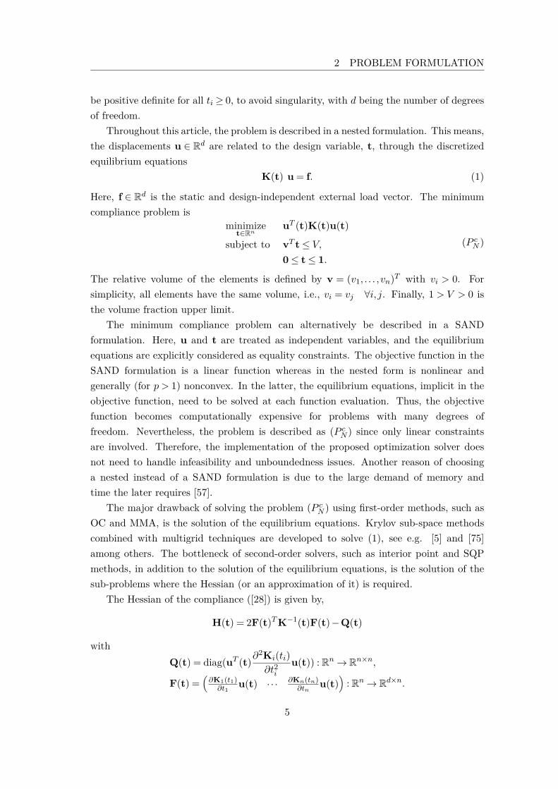
2 PROBLEM FORMULATION
be positive definite for all ti ≥ 0, to avoid singularity, with d being the number of degreesof freedom.
Throughout this article, the problem is described in a nested formulation. This means,the displacements u ∈ Rd are related to the design variable, t, through the discretizedequilibrium equations
K(t) u = f. (1)
Here, f ∈ Rd is the static and design-independent external load vector. The minimumcompliance problem is
minimizet∈Rn
uT (t)K(t)u(t)
subject to vT t≤ V,0≤ t≤ 1.
(P cN )
The relative volume of the elements is defined by v = (v1, . . . ,vn)T with vi > 0. Forsimplicity, all elements have the same volume, i.e., vi = vj ∀i, j. Finally, 1 > V > 0 isthe volume fraction upper limit.
The minimum compliance problem can alternatively be described in a SANDformulation. Here, u and t are treated as independent variables, and the equilibriumequations are explicitly considered as equality constraints. The objective function in theSAND formulation is a linear function whereas in the nested form is nonlinear andgenerally (for p > 1) nonconvex. In the latter, the equilibrium equations, implicit in theobjective function, need to be solved at each function evaluation. Thus, the objectivefunction becomes computationally expensive for problems with many degrees offreedom. Nevertheless, the problem is described as (P cN ) since only linear constraintsare involved. Therefore, the implementation of the proposed optimization solver doesnot need to handle infeasibility and unboundedness issues. Another reason of choosinga nested instead of a SAND formulation is due to the large demand of memory andtime the later requires [57].
The major drawback of solving the problem (P cN ) using first-order methods, such asOC and MMA, is the solution of the equilibrium equations. Krylov sub-space methodscombined with multigrid techniques are developed to solve (1), see e.g. [5] and [75]among others. The bottleneck of second-order solvers, such as interior point and SQPmethods, in addition to the solution of the equilibrium equations, is the solution of thesub-problems where the Hessian (or an approximation of it) is required.
The Hessian of the compliance ([28]) is given by,
H(t) = 2F(t)TK−1(t)F(t)−Q(t)
withQ(t) = diag(uT (t)∂
2Ki(ti)∂t2i
u(t)) : Rn→ Rn×n,
F(t) =(∂K1(t1)∂t1
u(t) · · · ∂Kn(tn)∂tn
u(t))
: Rn→ Rd×n.
5
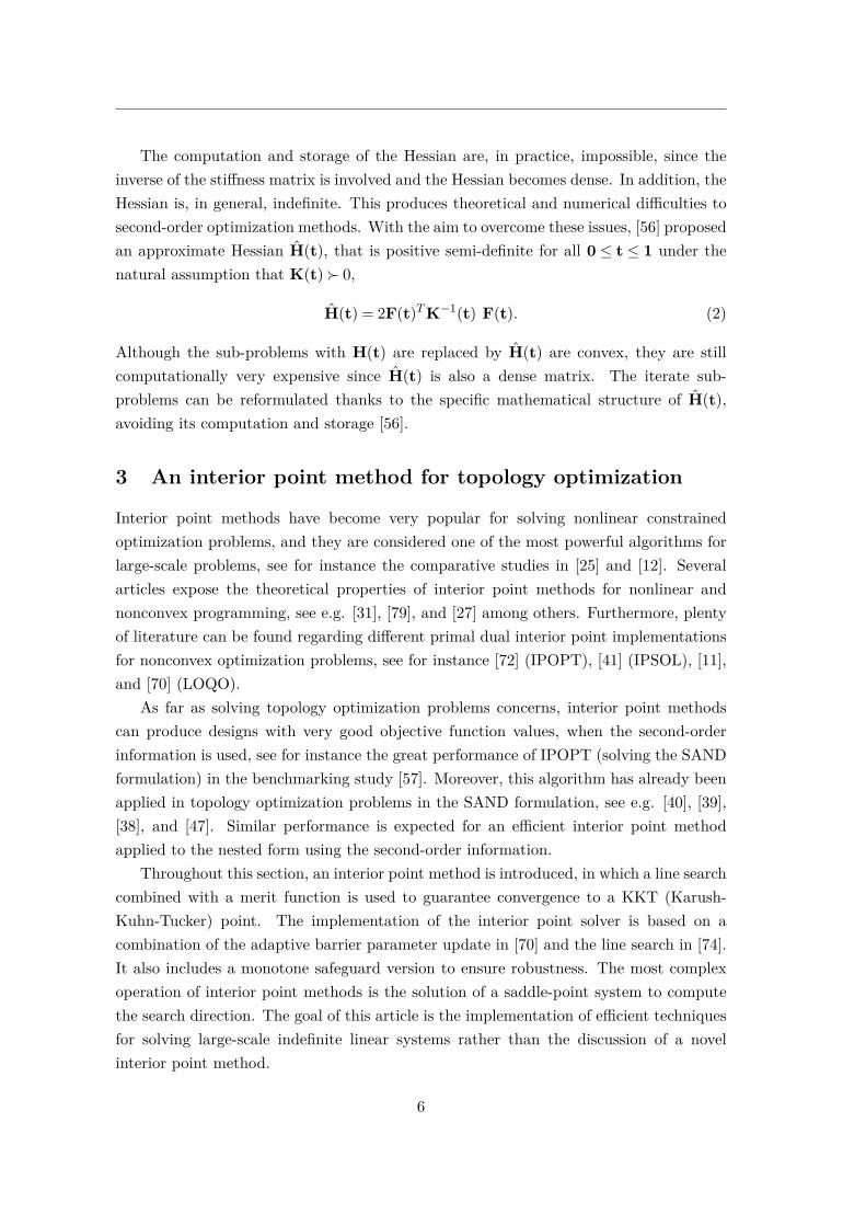
The computation and storage of the Hessian are, in practice, impossible, since theinverse of the stiffness matrix is involved and the Hessian becomes dense. In addition, theHessian is, in general, indefinite. This produces theoretical and numerical difficulties tosecond-order optimization methods. With the aim to overcome these issues, [56] proposedan approximate Hessian H(t), that is positive semi-definite for all 0 ≤ t ≤ 1 under thenatural assumption that K(t) 0,
H(t) = 2F(t)TK−1(t) F(t). (2)
Although the sub-problems with H(t) are replaced by H(t) are convex, they are stillcomputationally very expensive since H(t) is also a dense matrix. The iterate sub-problems can be reformulated thanks to the specific mathematical structure of H(t),avoiding its computation and storage [56].
3 An interior point method for topology optimization
Interior point methods have become very popular for solving nonlinear constrainedoptimization problems, and they are considered one of the most powerful algorithms forlarge-scale problems, see for instance the comparative studies in [25] and [12]. Severalarticles expose the theoretical properties of interior point methods for nonlinear andnonconvex programming, see e.g. [31], [79], and [27] among others. Furthermore, plentyof literature can be found regarding different primal dual interior point implementationsfor nonconvex optimization problems, see for instance [72] (IPOPT), [41] (IPSOL), [11],and [70] (LOQO).
As far as solving topology optimization problems concerns, interior point methodscan produce designs with very good objective function values, when the second-orderinformation is used, see for instance the great performance of IPOPT (solving the SANDformulation) in the benchmarking study [57]. Moreover, this algorithm has already beenapplied in topology optimization problems in the SAND formulation, see e.g. [40], [39],[38], and [47]. Similar performance is expected for an efficient interior point methodapplied to the nested form using the second-order information.
Throughout this section, an interior point method is introduced, in which a line searchcombined with a merit function is used to guarantee convergence to a KKT (Karush-Kuhn-Tucker) point. The implementation of the interior point solver is based on acombination of the adaptive barrier parameter update in [70] and the line search in [74].It also includes a monotone safeguard version to ensure robustness. The most complexoperation of interior point methods is the solution of a saddle-point system to computethe search direction. The goal of this article is the implementation of efficient techniquesfor solving large-scale indefinite linear systems rather than the discussion of a novelinterior point method.
6

3 AN INTERIOR POINT METHOD FOR TOPOLOGY OPTIMIZATION
The performance of the interior point method in terms of time, number of iterations,and accuracy is expected to be good since (i) the saddle-point system is solved fast andwith low memory requirements due to the use of iterative methods, (ii) an adaptivebarrier parameter updated scheme is implemented improving the convergence rate of thealgorithm, and (iii) second-order information of the Hessian is used.
3.1 Interior point approach
Consider the general optimization problem
minimizex∈Rn
f(x)
subject to gi(x)≤ 0 i= 1, . . . ,m,li ≤ xi ≤ ui i= 1, . . . ,n.
(3)
Here, the objective function f : Rn→ R and the inequality constraints gi : Rn→ R areassumed to be smooth. The terms li > −∞ and ui < +∞ represent the lower and theupper bounds of the variables, respectively. The formulation of the problem assumesbound constraints on all variables to resemble the particular problem under consideration,i.e., the minimum compliance problem (P cN ) in which the design variables are bounded.
Slack variables s ≥ 0 ∈ Rm are introduced to transform the inequality constraintsgi(x)≤ 0 to equality constraints gi(x) + si = 0. The barrier problem associated with theproblem is
minimizex∈Rn,s∈Rm
f(x)+µφ(x,s)
subject to gi(x)+si = 0 i= 1, . . . ,m.(4)
Here, µ > 0 is the barrier parameter, and
φ(x,s) =−m∑
i=1ln(si)−
n∑
i=1ln(ui−xi)−
n∑
i=1ln(xi− li)
the barrier function (with ln the natural logarithm).There are (at least) three main aspects to take into account for a globally convergent
interior point method; how to treat nonconvexity, how to update the barrier parameter,and how to ensure progress towards a KKT point. The first aspect is dealt with inSection 5, where the solution of the saddle-point system is discussed for the minimumcompliance problem. The remaining questions are detailed throughout this section.
Algorithm 1 describes the interior point strategy based on the adaptive barrierparameter updated scheme from [52]. Since bounded variables and feasible problemsare assumed, the algorithm does not need to include control techniques as in othergeneral frameworks, such as [72]. Adaptive schemes allow some flexibility in both, thebarrier parameter sequence and the reduction in the merit function. This approachupdates the barrier parameter every iteration, allowing µ to both increase and decrease.
7

Algorithm 1 Adaptive interior point algorithm [52].Input: Define starting point (x0,s0,λ0,ξ0,η0), µmin = 10−7, τ = 0.995,τa = 0.9999, ρ = 10−8,
θ = 0.5, γ = 0.2, δ = 1.5, lmax = 15, κ= 1, and the tolerances ε1, ε2 and ε3.1: repeat2: *Adaptive scheme*3: Compute µk as in (15).4: Solve the linear system (10) to compute the primal dual search direction ∆.5: Determine the maximum step size αmax
p and αmaxd as in (11).
6: Compute ϕk+1; the Euclidean norm of the KKT conditions of the sub-problem.7: Obtain Mk = maxϕk−lmax , . . . ,ϕk.8: if ϕk+1 ≤ τaMk then9: Accept the new iterate (xk+1,sk+1,λk+1,ξk+1,ηk+1).
10: Check convergence of the problem as in (18).11: Include ϕk+1 in Mk+1.12: else13: *Monotone scheme*14: Define starting point as (xk+1,sk+1,λk+1,ξk+1,ηk+1), and initialize i, j = 0.15: Define µi as in (17).16: repeat17: repeat18: Solve the linear system (10) to compute the primal dual search direction ∆.19: Determine the maximum step size αmax
p and αmaxd as in (11).
20: Perform a backtracking line search to compute the final steps αp and αd as in (12).
21: Accept the new iterate (xj+1,sj+1,λj+1,ξj+1,ηj+1).22: Compute ϕj+1; the Euclidean norm of the KKT conditions of the sub-problem.23: Check convergence of sub-problem for εµ1 , εµ2 , and εµ3 as in (18).24: if ϕj+1 ≤ τaMk then25: go-to-adaptive = true.26: end if27: j = j+1.28: until convergence sub-problem or go-to-adaptive29: Decrease µi+1 as in (16).30: i= i+1.31: Check convergence of the problem as in (18).32: until convergence or go-to-adaptive33: Include ϕj+1 in Mk+1.34: end if35: k = k+1.36: until convergence
8

3 AN INTERIOR POINT METHOD FOR TOPOLOGY OPTIMIZATION
They are usually more efficient than the monotone version (faster convergence rate).The main drawback of these strategies is that they do not ensure global convergence.On the other hand, the monotone approach solves the sub-problem (4) for a fixed µ,and then monotonically, the barrier parameter is decreased until convergence. Thepresented interior point method combines an adaptive and a monotone barrierparameter update. Once the adaptive approach does not accept a point, the monotoneversion is used to guarantee global convergence. It is similarly defined as in [52] with aline search strategy inspired by [74].
3.2 Obtaining the search direction
The Lagrangian function associated with problem (4) is
L(x,s,λ;µ) = f(x)+µφ(x,s)+m∑
i=1λi(gi(x)+si).
Here, λ = (λ1, . . . ,λm)T are the Lagrangian multipliers of the constraints. The perturbedfirst-order KKT conditions (5)-(9) gather the first-order necessary conditions for a primaldual point (x, s, λ, ξ, η) to be an optimal solution of (4) for a given µ, [53] and [46].
∇xL=∇f(x)+ξ−η+J(x)Tλ = 0, (5)∇sL= D(s)λ−µe = 0, (6)
g(x)+ s = 0, (7)U(x)ξ−µe = 0, (8)L(x)η−µe = 0. (9)
Here, ξ = (ξ1, . . . , ξn)T ≥ 0, η = (η1, . . . ,ηn)T ≥ 0 are the Lagrangian multipliers of theupper and the lower bounds respectively, and g(x) = [gi(x)]i=1,...,m. The Jacobian of theinequality constraints is denoted with J(x) = [∇gi(x)T ]i=1,...,m : Rn 7−→ Rm×n, and theremaining of the matrices are defined as D(s) = diag(s), U(x) = diag(u), and L(x) =diag(l), with ui = ui− xi and li = xi− li. A point satisfying the KKT conditions iscommonly called a KKT point.
The sub-problem (4) is solved by applying Newton’s method to the first-orderoptimality conditions (5)-(9) for a given value of µ. The search direction ∆, at the kthinterior point iteration, is obtained by solving a KKT system2 evaluated at the iterate(xk,sk,λk, ξk,ηk). For notational convenience, the sub-index kth has been removed.
2Saddle-point problem ∇F∆ =−F, where F represents the KKT conditions.
9

The KKT system to be solved is condensed to a symmetric matrix resulting in
H(x)+Σu+Σl 0 J(x)T
0 Σs IJ(x) I 0
∆x∆s∆λ
=−
∇f(x)+J(x)Tλ+µU(x)−1e−µL(x)−1eλ−µD(s)−1e
g(x)+ s
.
(10)Here, Σs = D(s)−1λ, Σu = U(x)−1ξ, Σl = L(x)−1η, and H(x) the Hessian of theLagrangian (which for this problem coincides with the Hessian of the objectivefunction). After solving (10), the search direction of the bound Lagrangian multipliersare obtained,
∆ξ =−ξ+µU(x)−1e+Σu∆x,∆η =−η+µL(x)−1e−Σl∆x.
The computational time of an interior point iteration is dominated by the solution ofthe system (10). Section 4 is focused on presenting an efficient iterative method to solveit.
3.3 Updating the iterates
Line search [51] or trust region [23] methods are generally included in nonlinearoptimization solvers to guarantee convergence to a KKT point [53]. In particular, theproposed interior point method is based on a line search strategy combined with areduction in a merit function. Once the search direction ∆ is determined, the primaland dual step lengths, αp and αd, are estimated in order to obtain the new iterate(xk+1,sk+1, λk+1, ξk+1, ηk+1). First, the maximum step lengths are computed, αmax
p
and αmaxd , such that the new iterate remains feasible. The fraction to the boundary rule
(11) is used for estimating these values in order to prevent that the primal and dualvariables approach their bounds too quickly [53]. The step lengths are determined from
αmaxp = maxα ∈ (0,1] : z+α∆z≥ (1− τ)zαmaxd = maxα ∈ (0,1] : χ+α∆χ≥ (1− τ)χ,
(11)
with τ ∈ (0,1). The maximum operator is defined as component-wise, the dual variablesare gathered in χ = (λ,ξ,η), and z denotes z = (s, u, l).
Additionally, the Armijo condition (see e.g. [53] and [41]) must be satisfied for thevalues αp and αd obtained within the interval
αp ∈ (0,αmaxp ] αd ∈ (0,αmax
d ].
A backtracking line search is performed to compute the αp and αd such that a meritfunction ψ is reduced. The line search strategy is based on [74]. A maximum possible
10

3 AN INTERIOR POINT METHOD FOR TOPOLOGY OPTIMIZATION
value of αT = 1,θ,θ2... with θ ∈ (0,1) is selected such that the following inequality issatisfied,
ψπ(z+αTαmaxp ∆z)≤ ψπ(z)+ραTα
maxp Dψπ(z,∆z), (12)
with z = (x,s) the primal variables. Here, ρ ∈ (0,1), and Dψπ(z,∆z) is the directionalderivative of the merit function with respect to the direction ∆z. After the backtracking,αp = αTα
maxp and αd = αTα
maxd are defined.
A popular choice of merit function is the l1-penalty function (see e.g. [53], [74], and[24])
ψπ(x) = f(x)+µφ(x,s)+π(m∑
i=1|gi(x)+si|).
The penalty parameter π > 0 is updated every iteration. There are several approachesto update this parameter so that the convergence is accelerated, see for instance [21].Nevertheless, the penalty parameter is updated following a simple rule described in [53]as
π = ||λ||∞.
This rule was successfully used for minimum compliance problems in [56]. A majordrawback of this merit function is the lack of differentiability and thus, the potentiallyMaratos effect [49]. This can be avoided either with a watchdog strategy or with asecond-order correction step, see for instance [53], [74], and [31]. However, since theproblem (P cN ) has only linear constraints, the Maratos effect cannot occur [20].
The adaptive interior point scheme is more flexible than the monotone version inregards to the reduction of the merit function. The algorithm allows the merit functionto increase some iterations, i.e. the Armijo condition is not imposed. The methodforces a reduction in the optimality conditions of the sub-problem within the lmax
previous iterations [52]. Before an iterate is accepted, the interior point method verifiesthe following condition
ϕk+1 ≤ τaMk, (13)
with ϕk+1 the Euclidean norm of the KKT conditions of the sub-problem, and
Mk = maxϕk−lmax , . . . ,ϕk.
In addition, the algorithm switches from monotone to adaptive strategy when thiscondition is satisfied for a given iterate. Finally, the new primal and dual iterates aregiven by
zk+1 = zk +αp∆z,χk+1 = χk +αd∆χ.
(14)
11

3.4 Updating the barrier parameter
The sequence of the barrier parameter values µk must converge to zero through theoptimization process. The Fiacco and McCormick strategy [30], or monotone strategy,consists of fixing the barrier parameter to one value until the sub-problem convergesfor a given tolerance εµk
(see Section 3.5). Then, the barrier parameter is decreased.It provides global convergence. On the other hand, the adaptive strategy consists ofupdating the barrier parameter at each iteration. The adaptive barrier parameter updatescheme is based on [70] and described by
µk+1 = σkzTkχknz
. (15)
Here, nz is the number of element in z (nz = 2n+m), and σk is
σk = 0.1min(
0.051−ββ
,2)3,
with
β =mini
((zk)i(χk)i)
zTkχk/nz.
State-of-the-art software such as IPOPT and LOQO, already use this adaptive updatingscheme. Finally, the barrier update strategy in the monotone scheme is inspired by [72].The barrier parameter is decreased based on the previous value of µi and some constants,γ ∈ (0,1) and δ ∈ (1,2),
µi+1 = min(γµi,µδi ). (16)
Here, the index i refers to the outer loop of the monotone version (see Algorithm 1).Before the monotone strategy starts, the initial barrier parameter is estimated as in [52],i.e.,
µ0 = 0.8 zTkχknz
. (17)
3.5 Stopping criteria
In practice, the KKT conditions of the sub-problem converge to the original problemwhen µ is close to zero. Thus, the algorithm stops and reports to have found a KKTpoint, when the following inequalities are satisfied,
||∇f(x)+ξ−η+J(x)Tλ||2 ≤ ε1,||g(x)+ s||2 ≤ ε2,∣∣∣∣∣∣∣∣
∣∣∣∣∣∣∣∣
D(s)λ−µeU(x)ξ−µeL(x)η−µe
∣∣∣∣∣∣∣∣
∣∣∣∣∣∣∣∣2
≤ ε3.(18)
12
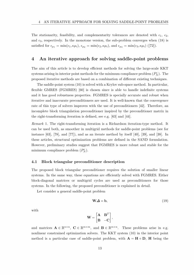
4 AN ITERATIVE APPROACH FOR SOLVING SADDLE-POINT PROBLEMS
The stationarity, feasibility, and complementarity tolerances are denoted with ε1, ε2,and ε3, respectively. In the monotone version, the sub-problem converges when (18) issatisfied for εµ1 = min(ε1,κµi), εµ2 = min(ε2,κµi), and εµ3 = min(ε3,κµi) ([72]).
4 An iterative approach for solving saddle-point problems
The aim of this article is to develop efficient methods for solving the large-scale KKTsystems arising in interior point methods for the minimum compliance problem (P cN ). Theproposed iterative methods are based on a combination of different existing techniques.
The saddle-point system (10) is solved with a Krylov sub-space method. In particular,flexible GMRES (FGMRES) [60] is chosen since is able to handle indefinite systemsand it has good robustness properties. FGMRES is specially accurate and robust wheniterative and inaccurate preconditioners are used. It is well-known that the convergencerate of this type of solvers improves with the use of preconditioners [42]. Therefore, anincomplete block triangulation preconditioner inspired by the preconditioner matrix inthe right-transforming iteration is defined, see e.g. [63] and [44].
Remark 1. The right-transforming iteration is a Richardson iteration-type method. Itcan be used both, as smoother in multigrid methods for saddle-point problems (see forinstance [63], [78], and [77]), and as an iterate method by itself [40], [39], and [38]. Inthese articles, structural optimization problems are defined in the SAND formulation.However, preliminary studies suggest that FGMRES is more robust and stable for theminimum compliance problem (P cN ).
4.1 Block triangular preconditioner description
The proposed block triangular preconditioner requires the solution of smaller linearsystems. In the same way, these equations are efficiently solved with FGMRES. Eitherblock-diagonal matrices or multigrid cycles are used as preconditioners for thosesystems. In the following, the proposed preconditioner is explained in detail.
Let consider a general saddle-point problem
W∆ = b, (19)
with
W =[A BT
B −C
],
and matrices A ∈ Rn×n, C ∈ Rm×m, and B ∈ Rm×n. These problems arise in e.g.nonlinear constrained optimization solvers. The KKT system (10) in the interior pointmethod is a particular case of saddle-point problem, with A = H+D, H being the
13

Hessian of the Lagrangian function and D a diagonal matrix. In our application, C= 0,and B is the Jacobian of the constraints.
Theorems 1, 2, and 3 give some conditions under which existence of solution of thesystem (19) can be proved.
Theorem 1. (from [13]) Assuming A nonsingular, W is nonsingular if and only ifS =−(C+BA−1B) is.
Theorem 2. (from [13]) Assume A symmetric positive definite and C symmetric positivesemi-definite. If kerC∩kerBT = 0 then the saddle-point matrix W is nonsingular.In particular W is invertible if B has full rank.
Theorem 3. (from [53]) For simplicity, let assume C = 0, A = H. Let B = J have afull row rank (Jacobian of the constraints), and assume that the reduced-Hessian matrixZTHZ is positive definite. Then the KKT matrix W is nonsingular, and hence there isa unique vector satisfying the linear system (19).
The matrix W is partitioned in two nonsingular matrices, M and N, using right-transformation, WR, and left-transformation, WL, matrices. Here, M is relatively easyto invert and N' 0.
WLWWR = M−N.
The right-transformation iteration is defined when WL = I [44]. Since a goodpreconditioner should approximate the matrix as much as possible, PW is defined asfollows
W = WWRW−R 'MW−R
PW 'WP−1
W ≡ (MW−R)−1 = WRM−1.
In particular, the right-transformation matrix is
WR =[I −A−1BT
0 I
].
Here, A is assumed to be a good approximation of A. Then, from a regular splitting
M =[A 0B S
],
with S=−(C+BA−1BT ) an approximation of the Schur complement (see [63] for moredetails). Based on block triangular matrix theory, the inverse of M is
M−1 =
A−1 0−S−1BA−1 S−1
. (20)
14

4 AN ITERATIVE APPROACH FOR SOLVING SADDLE-POINT PROBLEMS
Then, the preconditioner matrix is
P−1W = WRM−1 =
[I −A−1BT
0 I
] A−1 0−S−1BA−1 S−1
=
A−1 + A−1BT S−1BA−1 −A−1BT S−1
−S−1BA−1 S−1
.
For the rest of the article, the term b refers to a general known vector. Here, b1 ∈ Rn
and b2 ∈ Rm are defined such that
b =[b1
b2
].
To reduce the computational cost of the preconditioner operation, a matrix-vectormultiplication is defined as
P−1W b =
A−1b1 + A−1(BT S−1(BA−1b1− b2))
−S−1(BA−1b1− b2)
. (21)
The preconditioner operator (21) requires the solution of three linear systems where Aor S appear.
Remark 2. PW is chosen as preconditioner matrix instead of classical block diagonalpreconditioners since, in preliminary numerical studies, it showed better robustnessproperties.
Figure 1 illustrates the procedure for solving the saddle-point system (19) with theproposed iterative method. FGMRES needs two operations; a matrix-vectormultiplication (Wb) and the preconditioner operator (P−1
W b). These functions arerepresented as branches in Figure 1. The preconditioner, in turn, is detailed in fivesteps.
4.2 Using a multigrid cycle as preconditioner of Krylov sub-spacemethods
The solution of PWx= b needs the solution of systems with the form Ax= b and Sx= b.Direct methods can be used, although for large enough systems, iterative methods, suchas Krylov sub-space methods, are recommended. In these solvers, the choice of a goodpreconditioner that does not increase the computational effort is essential. In this article,a multigrid cycle (MC) is defined as preconditioner of Krylov sub-space methods inpositive definite linear systems due to its great properties [4], [36], and [76].
Multigrid methods solve the problem on a coarse mesh. Then, the solution isinterpolated from coarse to fine meshes until the original discretization is achieved.
15

Solve W∆ = bUse FGMRES
Multiplication Wb
Solve PWx = b
Split b into b1 and b2
Solve AxA = b1
Solve SxS = BxA− b2
Solve AxAB = BTxS
x =[xA+xAB−xS
]
(1)
(2)
(3)
(4)
(5)
Figure 1: Iterative scheme for solving a saddle-point system with the form (19).
The good performance of the multigrid cycle is due to the use of smoother functionsto remove the high frequency of the errors, and the coarse-grid correction to transfer theresiduals from coarse to fine and from fine to coarse mesh [18].
The computational effort (memory and time) is significantly reduced and, unlike otheriterative methods, the convergence rate does not depend on the condition number of thematrix [4]. Typically, the condition of the matrix increases with the discretization of themesh, thus, it is considered a very powerful technique due to its scalability3 properties.For more details of multigrid techniques, the text books [76] and [35] are recommended.
Algorithm 2 outlines the general scheme of a multigrid cycle (MC) for solving a linearsystem with the form Wx = b. Matrices R and P correspond to the restriction andprolongation operators to move from the fine to the coarse mesh, and from the coarseto the fine mesh, respectively. Depending on the number of mc cycles the multigridmethod computes V-cycles, W-cycles, or other different variations [65] and [76]. Theperformance of the method is affected by the number of pre-smoothers (ν1), the typeof cycle (mc), the number of post-smoothers (ν2), but most importantly, the smoothing
3A solver is numerically scalable if the complexity of the method grows asymptotically linearly withthe size of the problem [29].
16

5 ON THE SOLUTION OF A KKT SYSTEM IN STRUCTURAL TOPOLOGYOPTIMIZATION
Algorithm 2 Multigrid cycle [18].Input: x = MC(W,b,x, level, ν1, ν2, mc)1: if level = coarsest-level then2: Solve the problem: x = W−1b.3: return4: end if5: Pre-smoothing step: x = S(W,b,x, ν1).6: Grid correction: r = Wx−b.7: Restriction step: r = Rr.8: W = RWRT .9: Initialize mc= 1, xmc = 0.
10: repeat11: xmc = MC(W,r, xmc, level-1,ν1, ν2, mc).12: mc=mc+1.13: until mc=mc
14: Prolongation step: x = x−Pxmc.15: Post-smoothing step: x = S(W,b,x, ν2).16: return
method selected. This is the computationally most expensive step in the multigrid cycle.Moreover, it is the most expensive step in terms of time and memory of the proposediterative method. For positive definite linear systems, methods such as Jacobi and Gauss-Seidel are typically used as smoothers. In preliminary studies, better performance androbustness were achieved with Gauss-Seidel than with damped Jacobi (suggested in [4]).Multigrid methods can be also applied to indefinite systems, although the selection of asmoother function is more complicated and problem dependent [13].
5 On the solution of a KKT system in structural topologyoptimization
Throughout this section, different techniques are introduced to reproduce each step of theiterative method presented in Section 4 (Figure 1) for the specific minimum complianceproblem. In particular, two different iterative approaches are presented. They differ inthe choice of the stiffness matrix preconditioner (see Section 5.1). The iterative methodimplemented in this article solves, at each interior point iteration, the KKT systemdescribed as
2F(t)TK−1(t) F(t)+Σu+Σl 0 v0 Σs 1vT 1 0
∆t∆s
∆λ
=−
∇f(t)+λv+µU(t)−1e−µL(t)−1eλ− µ
s
vT t−V +s
.
(22)
17

Here, the approximate positive semi-definite Hessian of the compliance (2) is used.With this H(t), the existence of solution of (22) is ensured. Theorem 3 is satisfied forC = 0, B = [vT 1] and
H =[H(t)+Σu+Σl 0
0 Σs
].
The reduced-Hessian ZTHZ is positive definite (H(t) 0 and Σu+Σl 0 and Σs 0)and B has full row rank, then, the KKT system has a unique solution and is a descentdirection of the merit function [56], [53], and [46]. Thus, the inertia4 of the KKT matrixis correct in all the iterations and there is no need to perturb or modify the system asin, for instance IPOPT [72]. Due to the symmetry of H(t), the system is expanded toget rid of the dense Hessian [56].
Σu+Σl F(t)T 0 vF(t) −1
2K(t) 0 00 0 Σs 1vT 0 1 0
∆t∆w∆s
∆λ
=−
∇f(t)+λv+µU(t)−1e−µL(t)−1e0
λ− µs
vT t−V +s
. (23)
Here, ∆w is an auxiliary variable. Moreover, the KKT matrix in (23) is modified tosimplify the construction of PW. The matrix W is regrouped as follows
W =
−12K(t) 0 F(t) 00 Σs 0 1
F(t)T 0 Σu+Σl v0 1 vT 0
. (24)
Identification and approximation give the block matrices
A =[−1
2K(t) 00 Σs
],
B =[F(t) 00 1
],
C =−[Σu+Σl v
vT 0
],
and the approximate Schur complement
S =−(C+BA−1BT ) =[Σu+Σl+2FT (t)K−1(t)F(t) v
vT −Σ−1s
].
4For a given matrix W, the trial (i+, i−, i0) is called inertia, where i0, i+, and i− are the number ofzeros, positive and negative eigenvalues, respectively.
18

5 ON THE SOLUTION OF A KKT SYSTEM IN STRUCTURAL TOPOLOGYOPTIMIZATION
Remark 3. Based on Theorem 1, the saddle-point problem (23) is well defined and solvablesince A and S are nonsingular. For this particular matrix (24), S is a saddle-pointproblem satisfying Theorem 2;
S =[AS BT
SBS −CS
],
with AS = Σu +Σl + 2FT (t)K−1(t)F(t) 0, CS = Σ−1s 0, and BS = vT is linearly
independent (full rank). Therefore, S is nonsingular.
Remark 4. Both WR and M−1 are well defined due to the nonsingularity of A and S.
Since W is regrouped, the vector b (Figure 1 Step 1) and the output vector x (Step5 in Figure 1) need to be reorganized in the same way.
Two linear systems with the form
Ax = b ∈ Rd+1 (25)
are needed for PW (Steps 2 and 4 in Figure 1). This system of equations is relativelyeasy to solve because A is block diagonal. Nevertheless, it requires the solution of
− 12K(t)x = b1 ∈ Rd. (26)
Here, b1 is another general known vector. In this case, b1 is part of the b in (25). InSection 5.1, different alternatives for solving this system of equations are detailed.
On the other hand, the solution of the linear system (Step 3 in Figure 1),
Sx = a ∈ Rn+1 (27)
is more expensive, and the use of an iterative solver (FGMRES) is needed.Figure 2 shows the scheme to solve (27). Another general known vector is denoted
with a to emphasize that a 6= b. In the matrix-vector multiplication operation (Sb),a system like (26) is involved. In addition, the following block diagonal preconditionermatrix of S is defined,
PS =[AS 00 SS
].
WithAS = Σu+Σl+2FT (t)K(t)F(t) 0 ∈ Rn,
andSS =−Σ−1
s −vT A−1S v ∈ R.
Here, the preconditioner of the stiffness matrix is just the inverse of its diagonal terms,
K(t) = diag(
1Ki,i(t)
)
i=1,...,d.
19

Solve Sx = a
Solve K(t)x = F(t)b1
Use FGMRES
Multiplication Sb
Solve PSx = b
Solve ASx1 = b1
Solve SSx2 = b2
Use FGMRES
Multiplication ASb
Multigrid cycle(AS, b,x)
Figure 2: Iterative scheme for solving the indefinite linear system (27).
This fast and cheap preconditioner of the stiffness matrix is used since K(t) is just partof PS. More advanced stiffness matrix preconditioners are detailed in Section 5.1. Thepreconditioner operation of S consists of solving
PSx = b,
such that
ASx1 = b1, (28)SSx2 = b2, (29)
with
b =[b1
b2
], x =
[x1
x2
].
The system of equations (28) is still expensive (the dimension of the matrix is n). Thecomputational cost of the iterative solver will be highly dependent on the efficiency ofthe method used to solve it5. Since the matrix AS is positive definite, a multigrid cycle(MC) is chosen as preconditioner of FGMRES.
5This system is solved one time per FGMRES preconditioner iteration for solving (27). At the sametime, (27) is solved one per FGMRES preconditioner iteration for (23).
20

5 ON THE SOLUTION OF A KKT SYSTEM IN STRUCTURAL TOPOLOGYOPTIMIZATION
Solve Ax = b
Solve K(t)x1 = b1Use FGMRES
Multigrid cycle(K(t), b,x)
Solve Σsx2 = b2
Multiplication K(t)b
Figure 3: Iterative scheme for solving the positive definite system (25) using the first approach.
5.1 Good preconditioners for the stiffness matrix
The iterative method needs, at two different steps, the solution of the linear system (26)in which the stiffness matrix is involved. Additionally, the equilibrium equations aresolved every optimization iteration. Plenty of literature can be found regarding iterativemethods for the equilibrium equations (1), see e.g. [75], [5], [4], and [1] among others.Based on [4], the equilibrium equations are solved with a Krylov sub-space method anda multigrid cycle as preconditioner. However, FGMRES is chosen since, in preliminarystudies, it seems more robust and requires less iterations than PCG.
The same technique can be used for (26) to obtain the solution of Ax = b and Sb.In this case, the exact matrix K(t) is used (and thus, A and S). For this approach, thesolution of (25) (Steps 2 and 4 in Figure 1) is illustrated in Figure 3. Another alternativepreconditioner consists of using the Separate Displacement Component (SDC) as in [34].The stiffness matrix K(t) is reorganized and approximated using block diagonal sub-matrices as
K(t) =
Kxx(t) 0 00 Kyy(t) 00 0 Kzz(t)
. (30)
Here, Kxx(t), Kyy(t), and Kzz(t) are sub-matrices of the degrees of freedom componentsin the x-direction, y-direction, and z-direction, respectively.
Remark 5. The approximation (30) ofK(t)∼ K(t) is well-defined and it remains positivedefinite, see [34].
Remark 6. Preliminary numerical experiments have proven that preconditioners such asthe diagonal matrix and the incomplete Cholesky factorization for (26), are not good
21

enough to produce a robust and convergent iterative method.
In this second approach (SDC), Ax = b and Sb are solved exactly (direct solvers)using a simplified approximation of the stiffness matrix, K(t).
These two possible preconditioners are tested and compared in the numericalexperiments. In the following the first approach denotes the use of FGMRES+MC tosolve (26). The second approach refers to the use of SDC.
Both preconditioners have advantages and disadvantages. In the first case(FGMRES+MC), the preconditioner of the KKT matrix, P−1
W , is exactly the inverse ofW. However, (21) is approximately obtained (concatenation of several iterativemethods with different tolerances). Errors arising from the iterative methods mayproduce a failure. Nevertheless, in practice, this approach is robust and efficient (seeSection 7). On the other hand, the second preconditioner has all the mathematicalproperties to ensure convergence (see [44] and [34]) but the computational effort andmemory storage are higher. The stiffness matrix approximation (30) requires threeCholesky factorizations, the storage of several matrices, and the solution of three smallsystems.
6 Implementation
Section 7 shows the numerical experiments on examples where the 3D design domain isdiscretized using brick elements. Each rectangular solid element contains 8 nodes (24degrees of freedom) and the scaled element stiffness matrix is assumed to be the samefor all elements in the examples. The code is written in MATLAB release 2014a [69].
Regarding the pre-processing required for the multigrid cycle, two differentrestriction matrices, Rt and Ru, are built before the optimization process takes place.The restriction matrix Rt refers to the full weight average of the elements, while Ru
refers to the nodes, i.e.,(Rt)Hh : Rnh −→ Rnh×nH ,
(Ru)Hh : Rdh −→ Rdh×dH .
Here, h and H refer to the mesh size of the fine and the coarse mesh, respectively.Similarly, nh and nH refer to the number of elements and dh and dH are the degrees offreedom at each mesh. The restriction matrix Rt is used in the multigrid cycle in (28)and Ru is applied in (1) and in (26) (first approach). The prolongation matrix is justthe transpose of the restriction matrix [4] and [76].
In particular, the restriction matrix for the density variables collects the parent-children relationship. Given a coarse mesh with nH elements, the next level containsnh = 23nH elements. Thus, given an element i in a coarse level, Rt contains the valueof 1/8 in those positions corresponding with its children, i.e., the elements from the
22

6 IMPLEMENTATION
fine mesh that are "inside" the coarse element. The restriction matrix for the nodes isbuilt based on the shape functions. Each node of the fine mesh gives the correspondingcontribution to the nodes of the coarse mesh. For more details see [36].
Step 8 of Algorithm 2 is, in practice, omitted to save time. In addition, since MCis chosen as preconditioner at several steps of the proposed iterative method, all thematrices needed in Gauss-Seidel are stored to reduce the computational time. Althoughit will lead to an increment in memory usage, it is preferable to focus on reducing thecomputational time as much as possible. Every time a new stiffness matrix is assembled,Galerkin’s method is used to store the stiffness matrices of each level,
K(t)H = (Ru)Hh K(t)h((Ru)Hh )T .
Moreover, the upper triangular (with the diagonal) and the lower triangular matrices ofeach K(t)H are stored (using triu and tril MATLAB functions). Similarly, before theiterative method starts, AS, the upper triangular (and diagonal), and the lower triangularmatrices for every level are stored,
(AS)H = (Rt)Hh (AS)h((Rt)Hh )T .
If the second approach (SDC) is used, the block matrices Kxx, Kyy, and Kzz areneeded. More precisely, their Cholesky factorizations and the transposes of them arestored to reduce the computational time of the direct solver. The MATLAB functionsymamd [3] is used to permute the order of the matrices and create sparser Choleskyfactorizations (using chol [22]).
Tables 1, 2, and 3 contain the name, description, and value of every parameterinvolved in the interior point method for topology optimization problems. Throughoutthe rest of the article, due to brevity reasons, the optimization method is cited asTopIP. The parameters needed in the interior point method detailed in Algorithm 1 arecollected in Table 1.
Preliminary studies suggest that multigrid cycles perform very accurately with aW-type cycle. In TopIP, depending on the linear system solved, FGMRES+MC hasdifferent parameters. It is important to obtain an accurate solution in the equilibriumequations (1). Thus, a W-type with ν1 = ν2 = 2 is set for the multigrid. The stoppingcriteria for FGMRES are a relative residual error equal to ωe = 10−8 and a maximumnumber of iterations equal to 200. In contrast, (28) and (26) (first approach) are partof the preconditioner, and then, it is possible to be less strict. A simple V-cycle, withν1 = ν2 = 1 and ωs = 10−2 is used. The number of smoother iterations is chosen so thatthere is a balance between accuracy of solutions and computational effort. The multigridcycle is built with 4 levels of discretizations.
23

Table 1: Parameter setting for the interior point method. The table contains the name of theparameter, a brief description, and the value.
Parameter Description Value
t0 Starting point 0.5es0 Starting slack variable max(V −vT t0,10−5)ε1 Stationarity tolerance 10−6
ε2 Feasibility tolerance 10−8
ε3 Complementarity tolerance 10−6
κ Factor parameter for convergence of sub-problem 1(monotone version)
max iter Maximum number of interior point iterations 1,000τ Fraction to the boundary factor [74] 0.995ρ Backtracking factor (monotone version) [74] 10−8
θ Backtracking reduction factor (monotone version) [74] 0.5γ Factor parameter to update µ (monotone version) [72] 0.2δ Power parameter to update µ (monotone version) [72] 1.5τa Factor parameter to accept the iterate (adaptive version) [52] 0.9999lmax Number of previous iterations to take into account 15
to accept iterate (adaptive version)µmin Minimum barrier parameter value 10−7
Remark 7. The Krylov sub-space methods presented in this article stop when theEuclidean norm of the relative residual error is lower than a tolerance ω, i.e.
||r||2 = ||b−W∆||2||b||2
≤ ω.
The principal (top level) FGMRES method, which solves the KKT system (23), andthe intermediates (second and third level) FGMRES to solve (27), (28), and (26) (firstapproach), are differentiated in regards to the maximum number of iterations. For theformer, it is set to 300, for the second level it is set to 100 and finally, for the last levelit is set to 30.
Nonlinear optimization methods require some practical implementation details toimprove their efficiency. In particular, the scaling of the problem will significantly affectthe performance of TopIP. Therefore, the Young’s modulus are set to Ev = 1 and E1 = 104.Moreover, the objective function is scaled as
f(t) = f(t)||∇f(t0)||2
.
24

6 IMPLEMENTATION
Table 2: Parameter setting for the iterative method. The table contains the name of theparameter, a brief description, and the value.
Parameter Description Value
ω Norm of the relative residual error in FGMRES 10−6
for the top levelωe Norm of the relative residual error in FGMRES 10−8
for the equilibrium equationsωs Norm of the relative residual error in FGMRES 10−2
for the second and third levelmax iterative iter Maximum number of iterations of FGMRES in the top level 300
max gmres1 iter Maximum number of iterations of FGMRES in the second level 100max gmres2 iter Maximum number of iterations of FGMRES in the third level 30
max eq iter Maximum number of iterations of FGMRES 200for the equilibrium equations
restart step Number of FGMRES restart iterations 20mc Multigrid cycle type for the equilibrium equations 2 (W-cycle)mc Multigrid cycle type for the iterative method 1 (V-cycle)ν1, ν2 Number of pre-smoothing/post smoothing iterations in MC 2
for the equilibrium equationsν1, ν2 Number of pre-smoothing/post-smoothing iterations in MC 1
for the iterative methodelement coarse Number of elements (per unit of length) in the coarsest mesh 2
level Number of levels in MC 4
Table 3: Values of characteristic parameters of topology optimization problems.
Parameter Description Value
Ev Young’s modulus value for "void" material (TopIP) 10E1 Young’s modulus value for solid material (TopIP) 104
Ev Young’s modulus value for "void" material (GCMMA) 10−2
E1 Young’s modulus value for solid material (GCMMA) 10p SIMP penalization parameter 3rmin Radius for the density filter 0.04Lx
(Lx is the length in the x direction od the design domain)υ Poisson’s ratio 0.3vi Relative volume of element 1√
n
25

Finally, the relative volume of the elements is set to vi = 1√n. In the numerical
experiments, the performance of TopIP is compared to GCMMA. The settings of theparameters for GCMMA are slightly different to appropiately scale the problem (seeTable 3 and [57]). In particular, Ev = 10−2, E1 = 10, and the optimality tolerance isω = 10−4 (first-order method). The starting point is initialized with a homogeneousdesign, t0 = 0.5e (middle value) for TopIP and t0 = V e for GCMMA.
7 Numerical experiments
All the computations were done on Intel Xeon E5-2680v2 ten-core CPUs, running at2.8GHz with 128 GB RAM.
Figure 4 contains the six different boundary conditions and external load definitionsused for the numerical experiments. The domain is either fully clamped on one side (D1,D2, and D3) or clamped at the corners (D4, D5, and D6). Regarding the loads, threedifferent possibilities are collected. On the free face, the force is defined either as a pointload in the middle of an edge (D1 and D4), a point load on the center (D2 and D5), ora distributed load on an edge (D3 and D6). Some of these design domains are optimizedin, for instance, [4], [5], [75], and [45]. The length ratios will vary as well as the meshsize and the volume fraction.
A test set of 13 large-scale 3D problems is gathered for the numerical experiments.Table 4 collects the description of the optimized designs, such as the length ratio, thevolume fraction, the type of domain, the discretization of the mesh, the number ofelements (n), and the number of degrees of freedom (d). It also gathers the objectivefunction value obtained by TopIP (f(t)), the number of optimization (outer) iterationsrequired to find a KKT point (Iter), and the computational time consumed by thesolver. For convenience, the problems are denoted with a number (N) from 1 to 13. Thefinal designs and the performance (except computational time) of TopIP areindependent of the preconditioner chosen for the stiffness matrix in the iterativemethod. Thus, the table shows the results using the first approach (FGMRES+MC).The computational time for the second approach (SDC) is presented in parenthesis.The biggest problem in this test set contains more than one million elements (morethan three million degrees of freedom). Larger problems are not included due to timerestrictions on the cluster.
During the numerical experiments, the execution of some instances is not finisheddue to problems of memory or time limitation. For the former, the time is marked witha dash. When the problems are not finished due to the time limitation, the time is setto infinite. The remaining of the problems in the test set are run until the Euclideannorm of the KKT conditions is lower or equal to 10−6 or until the maximum number ofiterations is reached (max iter = 1,000).
26

7 NUMERICAL EXPERIMENTS
(a) Type D1 (b) Type D2
(c) Type D3 (d) Type D4
(e) Type D5 (f) Type D6
Figure 4: Collection of six 3D design domains with different boundary conditions and externalloads.
27

Table 4: Results of the optimized design obtained with TopIP for 13 3D minimum complianceproblems. The table contains the number of the problem (N), its description (length ratio, volumefraction, and domain type), the mesh discretization, the number of elements, and the numberof degrees of freedom. In addition, the objective function value, the number of optimizationiterations, and the computational time (first approach) obtained with TopIP are collected. Thecomputational time for the second approach is included in parenthesis. In some problems, thetime is marked with a dash (-) or with infinite (Inf) to indicate two possible types of error.
N Description Mesh n d f(t) Iter Time[hh:mm:ss]
1 1×1×2, v = 0.4, D1 16×16×32 8192 28611 1.296e+02 36 00:10:04 (00:10:47)2 2×2×2, v = 0.2, D3 32×32×32 32768 107811 2.760e+04 425 07:16:05 (65:13:37)3 2×2×4, v = 0.4, D1 32×32×64 65536 212355 9.998e+01 78 01:54:45 (07:58:35)4 3×3×3, v = 0.3, D2 48×48×48 110592 352947 3.233e+01 48 01:55:37 (04:58:52)5 2×4×6, v = 0.3, D5 32×64×96 196608 624195 2.935e+02 94 12:48:47 (96:54:17)6 3×3×6, v = 0.4, D1 48×48×96 221184 698691 9.301e+01 70 05:40:37 (44:55:48)7 4×4×4, v = 0.2, D5 64×64×64 262144 823875 1.406e+02 78 17:29:22 (133:45:58)8 4×5×5, v = 0.3, D4 64×80×80 409600 1279395 1.767e+02 51 30:48:47 (235:15:29)9 5×5×5, v = 0.4, D6 80×80×80 512000 1594323 7.423e+05 37 69:15:50 (Inf)10 4×4×8, v = 0.4, D1 64×64×128 524288 1635075 9.041e+01 64 50:39:41 (242:05:32)11 4×6×6, v = 0.2, D2 64×96×96 589824 1834755 3.690e+01 77 33:25:49 (Inf)12 6×6×6, v = 0.4, D1 96×96×96 884736 2738019 6.917e+01 40 76:23:04 (-)13 4×8×8, v = 0.3, D4 64×128×128 1048576 3244995 1.845e+02 51 74:20:51 (-)
28

7 NUMERICAL EXPERIMENTS
Indeed, Table 4 gives some hints to differentiate between the first and the secondapproach. Since the SDC (second approach) needs three Cholesky factorization (andtheir transposes), problems number 12 and 13 (problems bigger than 1,834,755 degreesof freedom) cannot be solved. Moreover, due to time limitations, the execution ofproblems number 9 and 11, for the same approach, is not finished. In these problems,one optimization iteration requires at least 27 hours.
The modest number of iterations that TopIP needs for finding a KKT point isremarkable. Most of the problems, in this numerical experiment, are solved using lessthan 100 iterations. However, it seems that TopIP has more difficulties in finding anoptimal design on problems with design domain D3. In fact, problem 2 requires 425iterations. For this problem, the convergence rate of TopIP has decreased because itswitches to the monotone approach. Thus, further investigations need to be done toimprove the monotone version.
The optimized designs of some problems of the test set are represented in Figure 5.The density value of the isosurface displayed is 0.8.
The rest of the section deals with an extensive study of the performance of TopIP.First of all, the relation between the number of TopIP iterations and the size of theproblem (number of elements) is represented in Figure 6a. It points out, more visually,that the convergence of TopIP is not affected by the size of the problem.
Similarly, Figure 6b shows a comparative study of the computational time of TopIPwith respect to the number of elements, using the two approaches. The dotted black lineis included as a reference to the linear behaviour. The computational effort of the secondapproach (SDC) is noticeably larger than the first approach (FGMRES+MC), but moreimportant, it increases more than linearly. In contrast, the growth of the computationaltime of the first approach is very slow with respect to the number of elements.
Since the number of optimization iterations is independent of the size of the problem,it is important to study the effort of each iteration. In other words, the number ofiterative iterations required at every TopIP iteration. Figure 7 shows the number ofFGMRES iterations (top level) at each interior point iteration for some problems. In thefirst approach, the iterations remain constant between two and 7 (Figure 7a). In contrast,the second approach needs slightly more iterations as the optimization advances (Figure7b). In addition, the number of FGMRES goes up to 250. Ultimately, there is almost norelation between the number of iterations and the size of the problem. This observationis clearer in Figure 8.
The average number of iterations and computational time of FGMRES over theTopIP iterations at different problem sizes are represented in Figures 8 and 9. Figures8a and 8b represent the mean (and standard deviation) of the number of iterationsneeded to solve one KKT system, for the first and the second approaches, respectively.The average of FGMRES iterations is not affected by the size of the problem. In the
29

(a) Domain D3, 2×2×2 mesh, with V = 0.2 (b) Domain D2, 3×3×3 mesh, with V = 0.3
(c) Domain D5, 2×4×6 mesh, with V = 0.3 (d) Domain D4, 4×5×5 mesh, with V = 0.3
(e) Domain D6, 5×5×5 mesh, with V = 0.4 (f) Domain D1, 4×4×8 mesh, with V = 0.4
Figure 5: Optimized designs examples of some problems in the test set.
30

7 NUMERICAL EXPERIMENTS
number of elements ×105
0 2 4 6 8 10 12
TopIP
iteration
0
50
100
150
200
250
300
350
400
450
(a) Number of TopIP iterations versus the size of theproblem.
number of elements ×105
0 2 4 6 8 10 12
Top
IPtime(s)
×105
0
2
4
6
8
10
12
Linear asymptoteFirst approach (FGMRES+MC)Second approach (SDC)
(b) Computational time of TopIP versus the size of theproblem
Figure 6: Number of optimization iterations (6a) and computational time of TopIP (6b) versusthe size of the problem (number of elements). Figure 6b shows the total time of TopIP usingboth, the first (blue line) and the second (red line) iterative approaches. The black line representsa linear behaviour for reference.
0 10 20 30 40 50 60 70 80 90 1001
2
3
4
5
6
7
8
9
10
TopIP iterations
FGMRESiterations
Problem01Problem05Problem07Problem10
(a) Iterative method using the first approach
0 10 20 30 40 50 60 70 80 90 1000
50
100
150
200
250
300
TopIP iterations
FGMRESiterations
Problem01Problem05Problem07Problem10
(b) Iterative method using the second approach
Figure 7: Number of FGMRES iterations required to solve the KKT system at each TopIPiteration. Figures 7a and 7b show the results for the first and second iterative approach,respectively for some of the problems in the test set.
31

number of elements ×105
0 2 4 6 8 10 12
AverageFGMRESiterationper
TopIP
iteration
1
2
3
4
5
6
7
8
9
10
(a) Iterative method using the first approachnumber of elements ×10
5
0 1 2 3 4 5 6
AverageFGMRESiterationper
TopIP
iteration
20
40
60
80
100
120
140
160
180
200
(b) Iterative method using the second approach
Figure 8: Comparative study between the FGMRES iterations required to solve one KKT system(on average) versus the size of the problem (number of elements), for the first (Figure 8a) andsecond (8b) approaches.
number of elements ×105
0 1 2 3 4 5 6
Average
timeper
Top
IPiteration
0
2000
4000
6000
8000
10000
12000
14000
16000
18000
First approach (FGMRES+MC)Second approach (SDC)
Figure 9: Comparative study between the computational time required to solve one KKT system(on average) versus the size of the problem (number of elements). The blue line represents thefirst approach (FGMRES+MC) and the red line represents the second approach (SDC). Thefigure shows the results for the subset test of problems solved using the second approach.
32

7 NUMERICAL EXPERIMENTS
first approach, the iterations remain constant (average of 5-6), while the range ofiterations in the second approach is substantially large, between 25 to 150 (on average).Additionally, the standard deviation is also greater, i.e., the number of iterations variesa lot between optimization iterations. In other words, the second approach is moresensitive to the optimization process. These fluctuations in the number of iterationsmake this approach more unstable and less robust than the first approach. Figure 9shows that the computational time spent in solving one KKT system (on average) usingSDC is also larger than using FGMRES+MC. This is due to the computational effortneeded in the factorization of Kxx, Kyy, and Kzz, and the solution of linear systemswith them.
Since the second approach needs more memory and time, the use of FGMRES+MCas preconditioner of the stiffness matrix in the iterative method is highly recommended.
Finally, the performance of TopIP (first approach) is compared with the first-orderstructural optimization method GCMMA (Global Convergent Method of MovingAsymptotes) [67]. The performance of both solvers is evaluated using the objectivefunction values, the number of iterations, and the total computational time. Thiscomparative study is done using performance profiles ([25]) similar to [57] and [56]. Thetest set used for this comparison is the 13 problems detailed in Table 4. Those problemswith a KKT error higher than ωmax = 10−4 are penalized since the final design isconsidered incorrect (the problem is not solved). For this numerical study, only oneproblem solved with GCMMA has a KKT error higher than ωmax. All details aboutperformance profiles in topology optimization problems can be found in [57].
Figure 10 shows that the second-order (TopIP) method clearly needs less iterationsthan the first-order (GCMMA) method. Although, the computational time of TopIP isstill higher than GCMMA, the maximum difference between cpu times is τmax = 6.02.More importantly, the 30% of TopIP winners refers to the biggest problems in the testset. Figure 11 shows the computational time of both GCMMA and TopIP, for varyingsize of the problem. The computational time of TopIP grows slower than GCMMA. Thus,for larger problems, TopIP is expected to outperform first-order methods with respectto time. The computational time can be reduced, even more, if the implementation isparallelized. Ultimately, the objective function value obtained with TopIP is not as goodas it was expected for second-order solvers [57]. In fact, GCMMA produces designs withlower objective function values than TopIP. Nevertheless, the results show the efficiencyand robustness of the proposed iterative method. TopIP will not be able to solve problemswith more than three million degrees of freedom without iterative solvers.
In general, the performance of nonlinear optimization methods is highly affectedby the selection of the parameters. The scaling of the problem may cause TopIP toconverge to local minima. Another possible reason might be the excessive flexibility ofthe adaptive strategy. Moreover, the tolerance in the iterative method is quite large,
33

τ
1 1.02 1.04 1.06 1.08 1.1 1.12 1.14 1.16 1.18 1.2
%problems
0
10
20
30
40
50
60
70
80
90
100
GCMMA
TopIP
(a) Objective function valueτ (log10)
0 0.2 0.4 0.6 0.8 1
%problems
0
10
20
30
40
50
60
70
80
90
100
GCMMA
TopIP
(b) Number of iterations
τ (log10)0 0.1 0.2 0.3 0.4 0.5 0.6 0.7 0.8
%problems
0
10
20
30
40
50
60
70
80
90
100
GCMMA
TopIP
(c) Computational time
Figure 10: Performance profiles for a test set of 13 3D minimum compliance problems. Theperformance is measured by the objective function value (10a), the number of iterations (10b),and the computational time (10c).
34

7 NUMERICAL EXPERIMENTS
number of elements ×105
0 2 4 6 8 10 12
Tim
e(s)
×105
0
0.5
1
1.5
2
2.5
3
3.5
4
4.5
TopIP (first approach)GCMMA
Figure 11: Comparative study of the computational time required to solve the problem usingTopIP and GCMMA with respect to the number of elements.
ω = 10−6, producing some errors in the descent direction that may be significant to thefinal objective function value. The stopping criterion of TopIP is measured with theKKT conditions of the sub-problem, thus, the high value of µmin = 10−7 is the mostlikely reason of these large objective function values. TopIP could stop without actuallyconverging. In order to obtain good results, TopIP is run again with µmin = 10−9, E0 = 10,and Emin = 10−2, showing promising results gathered in Figure 12.
With these new parameter settings, the objective function value of TopIP hassignificantly improved, outperforming GCMMA for a very small τ (τ = 1.0018). Incontrast, the computational effort and the number of iterations have slightly increased,but not critically. For instance, TopIP still converges, generally, in about 100 iterations,with 78% chances of winning and a maximum ratio value of τmax = 11. However, thepercentage of success with respect to computational time has decreased from 30% to22%. In addition, the behaviour of Figure 11 is no longer observed for this parameterselection (see Figure 13). Thus, the parallelization of the code is important tooutperform GCMMA with respect to time.
Table 5 shows the results for this new TopIP configuration. The study of theperformance of the two iterative approaches does not change. The number of iterativeiterations (and computational time) is almost identical for µmin = 10−7 and forµmin = 10−9.
This result encourages further investigation to obtain an even better and moreaccurate implementation of the interior point method. The previous results evidencethat the performance of TopIP is sensitive to the parameter selection, and thus, furtherwork can be done to obtain an optimal parameter setting.
35

τ
1 1.02 1.04 1.06 1.08 1.1 1.12
%problems
0
10
20
30
40
50
60
70
80
90
100
GCMMA
TopIP
(a) Objective function valueτ (log10)
0 0.1 0.2 0.3 0.4 0.5 0.6 0.7 0.8 0.9 1
%problems
0
10
20
30
40
50
60
70
80
90
100
GCMMA
TopIP
(b) Number of iterations
τ (log10)0 0.1 0.2 0.3 0.4 0.5 0.6 0.7 0.8 0.9 1
%problems
0
10
20
30
40
50
60
70
80
90
100
GCMMA
TopIP
(c) Computational time
Figure 12: Performance profiles for a test set of 13 3D minimum compliance problems. Theperformance is measured by the objective function value (12a), the number of iterations (12b),and the computational time (12c) (with µmin = 10−9, E0 = 10, and Emin = 10−2).
36

7 NUMERICAL EXPERIMENTS
number of elements ×105
0 2 4 6 8 10 12
Tim
e(s)
×105
0
0.5
1
1.5
2
2.5
3
3.5
4
4.5
5
TopIP (first approach)GCMMA
Figure 13: Comparative study of the computational time required to solve the problem usingTopIP and GCMMA with respect to the number of elements (with µmin = 10−9, E0 = 10, andEmin = 10−2).
Table 5: Results of the optimized design obtained with TopIP for 13 3D minimum complianceproblems. The table contains the number of the problem (N), its description (length ratio, volumefraction, and domain type), the mesh discretization, the number of elements, and the numberof degrees of freedom. In addition, the objective function value, the number of optimizationiterations, and the computational time obtained with TopIP (first approach) are collected, forµmin = 10−9 (E0 = 10 and Emin = 10−2).
N Description Mesh n d f(t) Iter Time[hh:mm:ss]
1 1×1×2, v = 0.4, D1 16×16×32 8192 28611 1.269e+02 95 00:14:322 2×2×2, v = 0.2, D3 32×32×32 32768 107811 2.757e+04 616 11:02:193 2×2×4, v = 0.4, D1 32×32×64 65536 212355 9.469e+01 91 01:46:434 3×3×3, v = 0.3, D2 48×48×48 110592 352947 3.057e+01 77 02:16:595 2×4×6, v = 0.3, D5 32×64×96 196608 624195 2.714e+02 76 09:20:206 3×3×6, v = 0.4, D1 48×48×96 221184 698691 8.370e+01 94 07:04:577 4×4×4, v = 0.2, D5 64×64×64 262144 823875 1.338e+02 70 14:24:168 4×5×5, v = 0.3, D4 64×80×80 409600 1279395 1.676e+02 62 43:21:489 5×5×5, v = 0.4, D6 80×80×80 512000 1594323 7.041e+05 47 73:09:5910 4×4×8, v = 0.4, D1 64×64×128 524288 1635075 7.813e+01 114 43:49:5511 4×6×6, v = 0.2, D2 64×96×96 589824 1834755 3.187e+01 132 39:36:4712 6×6×6 v = 0.4 D1 96×96×96 884736 2738019 6.314e+01 54 96:21:0413 4×8×8, v = 0.3, D4 64×128×128 1048576 3244995 1.686e+02 83 133:16:10
37

8 Conclusion
The article presents a robust and efficient iterative method for solving the large-scaleindefinite linear systems arising in interior point methods for structural topologyoptimization problems. The proposed iterative method solves the most expensive stepin interior point algorithms (the solution of a KKT system), reducing, significantly, theamount of time and memory required to direct solvers. The saddle-point system issolved using a combination of the state-of-the-art iterative methods, exploiting thestructure of the problem. In particular, the interior point method (TopIP) isimplemented for the minimum compliance problem based on a density-based approachin the nested form. TopIP approximates the Hessian using part of the exactsecond-order information.
Both adaptive and monotone barrier parameter updates are part of TopIP toguarantee global convergence. The iterative method is based on flexible GMRES withan incomplete block preconditioner matrix. This preconditioner needs the solution ofsmaller systems where different techniques such as FGMRES, multigrid cycles, andblock diagonal preconditioners are used.
The numerical results show the robustness and efficiency of TopIP, where large 3Dtopology optimization problems are solved. TopIP is able to optimize designs with morethan three million degrees of freedom.
The number of TopIP iterations is constant, independently on the size of theproblem. Moreover, TopIP requires fewer iterations than GCMMA, in general. Thenumber of iterative iterations remains also constant through the optimization processand at different problem sizes. Finally, the computational time of TopIP (firstapproach) increases slowly (lower than linearly) with respect to the size of the problem,outperforming even GCMMA for the largest problems. All these characteristics give toTopIP excellent properties for solving very large-scale problems.
At every preconditioner operation, several systems are solved where only the rightside vector is modified. Thus, additional investigations should be done to develop efficientsolvers to reduce the computational time even more. Future work should be also doneregarding the extension of the geometric multigrid to algebraic multigrid (AMG) [50], [33],and [73], to be able to apply this interior point method to unstructured meshes. Finally,further research in regards to the adaptive strategy and to the parameter selection arerecommended to speed up the convergence rate and the accuracy of TopIP.
Acknowledgements
We would like to thank Professor Krister Svanberg at KTH in Stockholm for providingthe MATLAB implementation of GCMMA.
38

REFERENCES
References
[1] N. Aage, E. Andreassen, and B. S. Lazarov. Topology optimization using PETSc: Aneasy-to-use, fully parallel, open source topology optimization framework. Structuraland Multidisciplinary Optimization, 51(3):565–572, 2014.
[2] N. Aage and B. S. Lazarov. Parallel framework for topology optimization usingthe method of moving asymptotes. Structural and Multidisciplinary Optimization,47(4):493–505, 2013.
[3] P. R. Amestoy, T. A. Davis, and I. S. Duff. Algorithm 837: AMD, an ApproximateMinimum Degree Ordering Algorithm. ACM Transactions on MathematicalSoftware, 30(3):381–388, 2004.
[4] O. Amir, N. Aage, and B. S. Lazarov. On multigrid-CG for efficient topologyoptimization. Structural and Multidisciplinary Optimization, 49(5):815–829, 2014.
[5] O. Amir, M. Stolpe, and O. Sigmund. Efficient use of iterative solvers in nestedtopology optimization. Structural and Multidisciplinary Optimization, 42(1):55–72,2009.
[6] E. Andreassen, A. Clausen, M. Schevenels, B. S. Lazarov, and O. Sigmund.Efficient topology optimization in MATLAB using 88 lines of code. Structural andMultidisciplinary Optimization, 43(1):1–16, 2011.
[7] J. S. Arora and Q. Wang. Review of formulations for structural and mechanicalsystem optimization. Structural and Multidisciplinary Optimization, 30(4):251–272,2005.
[8] M. P. Bendsøe. Optimal shape design as a material distribution problem. StructuralOptimization, 1(4):192–202, 1989.
[9] M. P. Bendsøe and O. Sigmund. Material interpolation schemes in topologyoptimization. Archive of Applied Mechanics, 69(9–10):635–654, 1999.
[10] M. P. Bendsøe and O. Sigmund. Topology optimization: Theory, methods andapplications. Springer, 2003.
[11] H. Y. Benson and D. F. Shanno. Interior-point methods for nonconvex nonlinearprogramming: cubic regularization. Computational Optimization and Applications,58(2):323–346, 2013.
[12] H. Y. Benson, D. F. Shanno, and R. J. Vanderbei. A comparative study of large-scale nonlinear optimization algorithms. Technical Report ORFE-01-04, OperationsResearch and Financial Engineering, Princeton University, 2002.
39

[13] M. Benzi, G . H. Golub, and J. Liesen. Numerical solution of saddle point problems.Acta Numerica, 14:1–137, 2004.
[14] M. Benzi and M. Tuma. A comparative study of sparse approximate inversepreconditioners. Applied Numerical Mathematics, 30(2):305–340, 1999.
[15] M. Benzi and A. J. Wathen. Some preconditioning techniques for saddle pointproblems. In Model Order Reduction: Theory, Research Aspects and Applications,volume 13 of Mathematics in Industry, pages 195–211. Springer, 2008.
[16] P. T. Boggs and J. W. Tolle. Sequential Quadratic Programming. Acta Numerica,4:1–51, 1995.
[17] T. Borrvall and J. Petersson. Large-scale topology optimization in 3D using parallelcomputing. Computer Methods in Applied Mechanics and Engineering, 190(46-47):6201–6229, 2001.
[18] A. Borzì and V. Schulz. Multigrid methods for PDE optimization. SIAM Review,51(2):361–395, 2009.
[19] B. Bourdin. Filters in topology optimization. International Journal for NumericalMethods in Engineering, 50(9):2143–2158, 2001.
[20] R. H. Byrd, M. E. Hribar, and J. Nocedal. An interior point algorithm for large-scalenonlinear programming. SIAM Journal on Optimization, 9(4):877–900, 1999.
[21] R. H. Byrd, G. Lopez-Calva, and J. Nocedal. A line search exact penalty methodusing steering rules. Mathematical Programming, 133(1-2):39–73, 2012.
[22] Y. Chen, T. A. Davis, W. W. Hager, and S. Rajamanickam. Algorithm 887:CHOLMOD, Supernodal Sparse Cholesky Factorization and Update/Downdate.ACM Transactions on Mathematical Software, 35(3):22:1–22:14, 2008.
[23] A. R. Conn, N. I. M. Gould, and P. L. Toint. Trust Region Methods. Society forIndustrial and Applied Mathematics, 1987.
[24] F. E. Curtis, O. Schenk, and A. Wächter. An interior-point algorithm for large-scalenonlinear optimization with inexact step computations. SIAM Journal on ScientificComputing, 32(6):3447–3475, 2010.
[25] E. D. Dolan and J. J. Moré. Benchmarking optimization software with performanceprofiles. Mathematical Programming, 91(2):201–213, 2002.
[26] T. Dreyer, B. Maar, and V. Schulz. Multigrid optimization in applications. Journalof Computational and Applied Mathematics, 120(1-2):67–84, 2000.
40

REFERENCES
[27] A. S. El-Bakry, R. A. Tapia, T. Tsuchiya, and Y. Zhang. On the formulation andtheory of the Newton interior-point method for nonlinear programming. Journal ofOptimization Theory and Applications, 89(3):507–541, 1996.
[28] A. Evgrafov. On the reduced Hessian of the compliance. Structural andMultidisciplinary Optimization, 50(5):1197–1199, 2014.
[29] A. Evgrafov, C. J. Rupp, K. Maute, and M. L. Dunn. Large-scale paralleltopology optimization using a dual-primal substructuring solver. Structural andMultidisciplinary Optimization, 36(4):329–345, 2008.
[30] A. V. Fiacco and G. P. McCormick. Nonlinear Programming: SequentialUnconstrained Minimization Techniques. John Wiley and Sons. Reprinted by SIAMPublications, 1990.
[31] A. Forsgren and P. E. Gill. Primal-dual interior methods for nonconvex nonlinearprogramming. SIAM Journal on Optimization, 8(4):1132–1152, 1998.
[32] P. E. Gill, W. Murray, and M. A. Saunders. SNOPT: An SQP Algorithm for LargeScale Constrained Optimization. SIAM Journal on Optimization, 47(4):99–131,2005.
[33] M. Griebel, D. Oeltz, and M. A. Schweitzer. An Algebraic Multigrid Method forLinear Elasticity. SIAM Journal on Scientific Computing, 25(2):385–407, 2003.
[34] I. Gustafsson and G. Lindskog. On Parallel Solution of Linear Elasticity Problems.Part I : Theory. Numerical Linear Algebra with Applications, 5:123–139, 1998.
[35] W. Hackbusch. Multigrid Methods and Applications. Springer, 1985.
[36] S. Häfner and C. Könke. Multigrid preconditioned conjugate gradient methodin the mechanical analysis of heterogeneous solids. Technical report, 17thInternational Conference on the Application of Computer Science and Mathematicsin Architecture and Civil Engineering, Germany, 2006.
[37] M. R. Hestenes and E. Stiefel. Methods of conjugate gradients for solving linearsystems. Journal of Research of the National Bureau of Standards, 49(6):409–436,1952.
[38] R. H. W. Hoppe, C. Linsenmann, and S. I. Petrova. Primal-dual Newton methods instructural optimization. Computing and Visualization in Science, 9(2):71–87, 2006.
[39] R. H. W. Hoppe and S. I. Petrova. Primal-dual Newton interior point methodsin shape and topology optimization. Numerical Linear Algebra with Applications,11(56):413–429, 2004.
41

[40] R. H. W. Hoppe, S. I. Petrova, and V. Schulz. Primal-dual Newton-type interior-point method for topology optimization. Journal of Optimization Theory andApplication, 114(3):545–571, 2002.
[41] Kaustuv. IPSOL: An Interior Point Solver for Nonconvex Optimization Problems.PhD thesis, Stanford University, 2009.
[42] C. T. Kelley. Iterative Methods for Linear and Nonlinear Equations. Society forIndustrial and Applied Mathematics, 1995.
[43] C. J. Lin and J. J. Moré. Incomplete Cholesky Factorizations with limited memory.SIAM Journal on Scientific Computing, 21(1):24–45, 2006.
[44] C. Linsenmann. On the convergence of right transforming iterations for thenumerical solution of PDE constrained optimization problems. Numerical LinearAlgebra with Applications, 19(4):621–638, 2012.
[45] K. Liu and A. Tovar. An efficient 3D topology optimization code written in Matlab.Structural and Multidisciplinary Optimization, 5(6):1175–1196, 2014.
[46] D. G. Luenberger and Y. Ye. Linear and Nonlinear Programming. Springer, 2008.
[47] B. Maar and V. Schulz. Interior point multigrid methods for topology optimization.Structural and Multidisciplinary Optimization, 19(3):214–224, 2000.
[48] A. Mahdavi, R. Balaji, M. Frecker, and E. M. Mockensturm. Topology optimizationof 2D continua for minimum compliance using parallel computing. Structural andMultidisciplinary Optimization, 32(2):121–132, 2006.
[49] N. Maratos. Exact penalty function algorithms for finite dimensional and controloptimization problems. PhD thesis, University of London, 1978.
[50] B. Metsch. Algebraic multigrid (AMG) for saddle point systems. PhD thesis, PhDin Mathematics, Faculty of Natural Sciences of Rheinischen Friedrich-Wilhelms-Universität Bonn, 2013.
[51] J. J. Moré and D. J. Thuente. Line search algorithms with guaranteed sufficientdecrease. ACM Transactions on Mathematical Software, 20(3):286–307, 1994.
[52] J. Nocedal, R. Wächter, and R. A. Waltz. Adaptive barrier update strategies fornonlinear interior methods. SIAM Journal on Optimization, 19(4):1674–1693, 2009.
[53] J. Nocedal and S. J. Wright. Numerical Optimization. Springer, 1999.
42

REFERENCES
[54] C. E. Orozco and O. N. Ghattas. A reduced SAND method for optimal design ofnonlinear structures. International Journal for Numerical Methods in Engineering,40(15):2759–2774, 1997.
[55] C. C. Paige and M. A. Saunders. Solution of sparse indefinite systems of linearequations. SIAM Journal on Numerical Analysis, 12(4):617–629, 1975.
[56] S. Rojas-Labanda and M. Stolpe. An efficient second-order SQP method forstructural topology optimization. Technical report, Technical University ofDenmark, Department of Wind Energy. Submitted, 2015.
[57] S. Rojas-Labanda and M. Stolpe. Benchmarking optimization solvers for structuraltopology optimization. Structural and Multidisciplinary Optimization, In print,2015. DOI: 10.1007/s00158-015-1250-z.
[58] G. I. N. Rozvany and M. Zhou. The COC algorithm, part I: Cross-sectionoptimization or sizing. Computer Methods in Applied Mechanics and Engineering,89(1–3):281–308, 1991.
[59] G. I. N. Rozvany, M. Zhou, and T. Birker. Generalized shape optimization withouthomogenization. Structural Optimization, 4(3–4):250–252, 1992.
[60] Y. Saad. A flexible inner-outer preconditioned GMRES algorithm. SIAM Journalon Scientific Computing, 14(2):461–469, 1993.
[61] Y. Saad. Iterative Methods for Sparse Linear Systems. SIAM, 2003.
[62] Y. Saad and M. H. Schultz. GMRES: A generalized minimal residual algorithm forsolving nonsymmetric linear systems. SIAM Journal on Scientific and StatisticalComputing, 7(3):856–869, 1986.
[63] V. Schulz and G. Wittum. Transforming smoothers for PDE constrainedoptimization problems. Computing and Visualization in Science, 11(4–6):207–219,2008.
[64] O. Sigmund and J. Petersson. Numerical instabilities in topology optimization:A survey on procedures dealing with checkerboards, mesh-dependencies and localminima. Structural Optimization, 16(2):68–75, 1998.
[65] R. Simon. Multigrid solvers for saddle point problems in PDE-constrainedoptimization. PhD thesis, Johannes Kepler Universität, 2008.
[66] K. Svanberg. The method of moving asymptotes - A new method for structuraloptimization. International Journal for Numerical Methods in Engineering,24(2):359–373, 1987.
43

[67] K. Svanberg. A class of globally convergent optimization methods based onconservative convex separable approximations. SIAM Journal on Optimization,12(2):555–573, 2002.
[68] O. Tatebe. The multigrid preconditioned conjugate gradient method. Technicalreport, 6th Copper Mountain Conference on Multigrid Methods, 1993.
[69] Inc. The MathWorks. Optimization Toolbox User’s Guide R release 2014a, 2014.
[70] R. J. Vanderbei and D. F. Shanno. An interior-point algorithm for nonconvexnonlinear programming. Computational Optimization and Applications, 13(1-3):231–252, 1999.
[71] K. Vemaganti and W. E. Lawrence. Parallel methods for optimality criteria-basedtopology optimization. Computer Methods in Applied Mechanics and Engineering,194(34-35):3637–3667, 2005.
[72] A. Wächter and L. T. Biegler. On the implementation of an interior point filter line-search algorithm for large-scale nonlinear programming. Mathematical Programming,106(1):25–57, 2006.
[73] C. Wagner. Introduction to algebraic multigrid. Technical Reporthttp://perso.uclouvain.be/alphonse.magnus/num2/amg.pdf, Course notes of analgebraic multigrid course at the University of Heidelberg, 1998/99, 1998.
[74] R. A. Waltz, J. L. Morales, J. Nocedal, and D. Orban. An interior algorithmfor nonlinear optimization that combines line search and trust region steps.Mathematical Programming, 107(3):391–408, 2006.
[75] S. Wang, E. Sturler, and G. H. Paulino. Large scale topology optimization usingpreconditioned Krylov subspace methods with recycling. International Journal forNumerical Methods in Engineering, 69:2441–2468, 2007.
[76] P. Wesseling. An introduction to multigrid methods. John Wiley & Sons, 1992.
[77] G. Wittum. Multigrid methods for Stokes and Navier-Stokes equations. NumerischeMathematik, 54(5):543–563, 1989.
[78] G. Wittum. On the convergence of multi-grid methods with transforming smoothers.Numerische Mathematik, 57(3):15–38, 1990.
[79] H. Yamashita. A globally convergent primal-dual interior point method forconstrained optimization. Optimization Methods and Software, 10(2):2–4, 1998.
44

REFERENCES
[80] M. Zhou and G. I. N. Rozvany. The COC algorithm, Part II: Topological, geometricaland generalized shape optimization. Computer Methods in Applied Mechanics andEngineering, 89(1–3):309–336, 1991.
45

220

DTU Wind Energy
Department of Wind Energy
Technical University of Denmark
Frederiksborgvej 399
4000 Roskilde
www.vindenergi.dtu.dk