Mathematical Prediction of Boomerang Flight Paths using a Simplified

Aerodynamic Model and Finite Difference Methods -Martin Laslett

Abstract Competitive boomerang throwing events seek to obtain certain flight characteristics of

boomerangs, beyond the requirement for it to simply return approximately to the thrower.

In order to better understand the flight dynamics of boomerangs, mathematically simulated

boomerang trajectories are calculated using a simplified aerodynamic model and a finite

difference method. The aerodynamic forces of lift and drag are calculated in a simplified

form from the motion of the boomerang. The arms / wings of the boomerang are broken

down into any number of small elements (foil elements) and their position and speed

vectors are calculated during the rotation of a boomerang around its axis. The angles of

orientation and motion through the air are combined with velocity and other properties

(area, position, stall angle, etc) of the foil elements to calculate lift and drag forces and

torques on the boomerang. The resultant forces and torques are then applied to a

mathematical model of boomerang dynamics developed by Hess [1] in the 1970s and

integrated forwards in time by finite difference methods. The resultant trajectory and

orientation of the boomerang is then plotted in 3D space. Simulations are run with different

initial starting conditions and also with modifications to the shape and mass of model

boomerangs

Introduction Boomerang competitions and the desire to understand boomerang trajectories

The competitive boomerang sports scene consists of approximately 1000 individuals

worldwide and a few dozen makers of boomerangs. Boomerang throwing events are held

throughout the World and broadly organized by national boomerangs associations under

the International Federation of Boomerang Associations (IFBA) rules.

In competitive sports boomerang throwing boomerang design, manufacture and throwing

parameters strive to produce the most desirable trajectories to meet a certain set of criteria

required by a particular competition event. The events require such characteristics as

accuracy of return, catching, distance, speed of return, time of flight (maximum time aloft or

MTA) and distance travelled (long distance or LD) , in different combinations for different

events. All events require the boomerang to make some sort of returning flight due to

aerodynamic forces and gyroscopic motion caused by the spinning of the boomerang about

its own axis [2]. Most competitive throwing is done outside under the wind conditions

prevailing at the time.

Boomerang trajectories in these competitions have an outward range of between 20 metres

(20m) and 50 m for most events, although Long Distance throwing requires a maximum

outbound distance before returning across a specified line from where it was thrown. Long

distance throws are typically 80m to 160m although the maximum recorded was 238m [3].

Competition boomerangs have a mass of between approximately 15 grams (15g) and 80g

and most could be drawn around on a piece of A4 paper. Typical thickness is 2-6mm and

materials include plywood, carbon / glass fibre reinforced composites, and other plastics

such as phenolic resin, polypropylene, polythene. Very few if any competition boomerangs

are shaped in the traditional ‘banana’ plan form or right angle stick, and are often 3 armed

for 20m events.

Practical experience has led boomerang throwers and makers to adjust the plan form,

section, size, bending, twisting and mass distribution of boomerangs to achieve desired

flight paths. On the competition field adjustments known as ‘tuning’ modify all parameters

except plan form, size and section to suit the wind conditions. There is an incomplete

scientific understanding of how the manufacture and tuning of boomerangs lead to more or

less desirable flight paths, but some boomerangs are clearly better than others.

Unfortunately it is almost impossible to recreate an exact repetition of the throwing

conditions (launch angles, spin, speed) as very few (if any) accurate throwing machines have

been produced [4] [4a]. Even if an accurate throwing machine existed, the range of

competition boomerangs would most likely require an outdoor test area where wind

conditions are often variable.

The flight of a boomerang

To a very rough first approximation, the path of a boomerangs flight is level and circular.

This flight is due to aerodynamic force of lift producing centripetal acceleration and

balancing the forces of gravity. The orientation of the boomerang’s spin axis changes during

flight so that more of the aerodynamic lift is directed in an upward direction, balancing the

reduction of the speed and spin of the boomerang due to drag forces. This is termed ‘laying

over’. Eventually drag forces and gravity prevail and the boomerang falls to earth or is

caught by the thrower. The interaction of the lift, drag and gravity forces on the boomerang

determine its flight path for a given mass, moment of inertia, throw and wind strength.

The aim of this work

The aim of the mathematical model is to optimise the changes in the flight of a boomerang

by changes in boomerang design and on the field tuning. It is also to enhance the scientific

approach to design, and tuning of boomerangs and to formalise the approximate

understanding and rules of thumb that are used with a more accurate understanding. The

use of a simplified aerodynamic model is intended to reduce computation times of

boomerang trajectories, so that a model boomerang may be rapidly produced and adjusted

to emulate a physical boomerang. The model boomerang can then be quickly tested with

emulated throws to see the effect of these adjustments and tuning.

An analytical solution to fully describe the flight path of boomerangs does not currently exist

but approximate solutions that make simplifications (such as to ignore the effect of gravity)

do exist to predict the range of a boomerang [5] and predict that it may be independent of

the strength of throw so long as speed and spin are in a certain ratio. However, it is well

known in practice that the launch spin and speed do affect the range of boomerangs in

practice, hence the existence of long distance competitions.

Numerical integration methods have been used before by Hess [1] for 4 real and 2 modelled

boomerangs, and also by Kuleshov [6] for model boomerangs. Methods using a fuller

computational fluid dynamics (CFD) approach on model boomerangs have been undertaken

by Vassberg [7] and [8], but such models so far have been so computationally expensive that

only a few flights of model boomerangs can be undertaken in a reasonable time and access

to specialised computing equipment may be required.

A simplified aerodynamic model should allow approximate flight paths to be quickly

simulated for different boomerangs, throws and tuning adjustments using a simplified

theory of model boomerangs and simplified aerodynamics

Simplified Model of a Boomerang

Rather than consider the complete description of the surfaces of a boomerang, a model

boomerang is considered as any number of small ‘foil elements’ which have a particular

orientation with a ‘leading’ and ‘trailing’ edge. (Note: the combination of spin and ‘forward’

motion of the boomerang means that the air does not always meet the leading edge in a

forwards direction or perpendicular to the chord length)

fig.0

Each element has a configurable density and volume which can be calculated from its

approximate cross section. The model boomerang is edited in graphical interface, which

requires no specialist knowledge. The position and calculated mass of each foil element can

be used to find the overall mass and moments of inertia of the whole boomerang. The

boomerang is then aligned with its principal axes I1, I2, I3, such that I3 = I1 + I2. Screen shots

of the model boomerang editor (before alignment of axes) are shown in fig. 0a. Note the 3D

model right is to give a visual impression of the boomerang’s twist and dihedral, the air flow

is not modelled over the 3D surface.

fig. 0a

Each foil element can be set at angles to the plane of the boomerang to model the twist and bends that boomerang makers and throwers use to adjust the flight of a boomerang. (Bending the arms of a boomerang up from its plane gives the boomerang arm ‘positive

dihedral’. The dihedral angle is labelled d in later equations)

Aerodynamic Model The size of the lift force

The lift and drag forces on a thin foil are given by the lift equation [9]

L = ½ ρ V 2 A CL [eqn. 1], where:

L is lift force,

ρ is air density

V is airspeed2

A is wing area

CL is the 'Lift coefficient' at a given angle of attack

Thin airfoils theory [9] gives CL = 2where is the angle of attack in radians, and is 3.142.. . Substituting this into eqn.1 gives:

L = ρ V 2 A [eqn. 3]

(The above expression is also applicable to a cambered airfoil where is the angle of attack

measured relative to the zero-lift line instead of the chord line.)

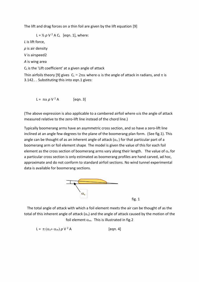
Typically boomerang arms have an asymmetric cross section, and so have a zero-lift line

inclined at an angle few degrees to the plane of the boomerang plan form. (See fig.1). This

angle can be thought of as an inherent angle of attack (s ) for that particular part of a

boomerang arm or foil element shape. The model is given the value of this for each foil

element as the cross section of boomerang arms vary along their length. The value of s for

a particular cross section is only estimated as boomerang profiles are hand carved, ad hoc,

approximate and do not conform to standard airfoil sections. No wind tunnel experimental

data is available for boomerang sections.

fig. 1

The total angle of attack with which a foil element meets the air can be thought of as the

total of this inherent angle of attack (s) and the angle of attack caused by the motion of the

foil element m. This is illustrated in fig.2

L = sm ρ V 2 A [eqn. 4]

fig.2

The arrow labelled ‘Motion V’ shows the direction of the motion of a particular foil element

at an instant in time relative to the plane of the boomerang.

Position and direction of the lift

The aerodynamic centre is given by thin airfoil theory as being at the quarter-chord point

[10]. This position changes for different airfoil sections and also different flow conditions.

The simulation allows a fixed value to be entered for each foil element, but does not alter

for different flow conditions, so is simulated as acting in the centre of the foil element chord

length but at a fixed percentage of the chord width. Thus it is at a different position from

the centre of the foil element. By definition lift force is a vector perpendicular to the

motion of the foil element through the air.

fig.3

Stall Angle(stall)

Stall of the airfoil usually occurs at an angle of attack between 10° and 15° for typical airfoils

[11]. Stalls depend primarily on angle of attack, not air speed [11] but can change with

Reynolds number. As the speed of the foil element through the air may vary between 0

and its maximum (the maximum is typically twice the linear speed of COM boomerang) the

Reynolds number may vary considerably, however for simplicity stall angle is set as a fixed

property of each foil element. As an approximation lift is assumed to be proportional to AOA

from 0 to the stall angle, and then decrease linearly with increasing AOA, down to zero at

twice the stall angle. See fig.4.

fig 4

The model has a configurable stall angle for each foil element. The model assumes that for

negative angles of attack a similar function operates but the lift will be in the opposite

direction, so a negative value is given to the force. The lift is then calculated by a saw tooth

function applied to the total angle of attack as in eqn. 5

L = sawtooth sm, stall .ρ V 2 A . [eqn. 5]

The size and direction of the drag force

For simplicity drag force is calculated as follows with a drag factor which is configurable for each foil element separately for motion parallel and perpendicular to the foil element chord length direction. This is to simulate the fact that boomerang throwers add flaps of tape either aligned with or across the wing to reduce spin and speed of the boomerang differently.

D = sm .ρ V 2 A . Drag factor [eqn. 6]

The direction of the drag force is parallel and opposite to the motion of the foil element.

The position and motion of the foil elements

The motion of each foil element is calculated as a 3d vector relative to the air. A constant wind can also be simulated for each throw.

Frames of reference

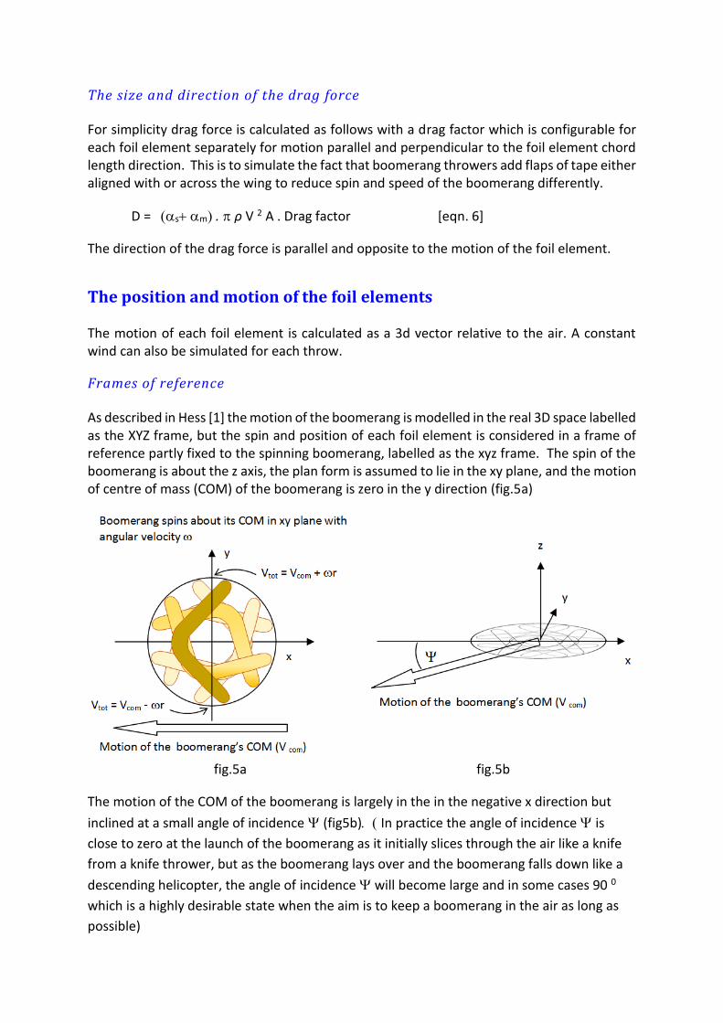
As described in Hess [1] the motion of the boomerang is modelled in the real 3D space labelled as the XYZ frame, but the spin and position of each foil element is considered in a frame of reference partly fixed to the spinning boomerang, labelled as the xyz frame. The spin of the boomerang is about the z axis, the plan form is assumed to lie in the xy plane, and the motion of centre of mass (COM) of the boomerang is zero in the y direction (fig.5a)

fig.5a fig.5b

The motion of the COM of the boomerang is largely in the in the negative x direction but

inclined at a small angle of incidence (fig5b) In practice the angle of incidence is

close to zero at the launch of the boomerang as it initially slices through the air like a knife

from a knife thrower, but as the boomerang lays over and the boomerang falls down like a

descending helicopter, the angle of incidence will become large and in some cases 90 0

which is a highly desirable state when the aim is to keep a boomerang in the air as long as

possible)

The spinning disc of the boomerang in the xyz frame is related to the XYZ frame (of the

thrower and the grass field in which they are likely to be standing) by Euler angles as given

in Hess [1]. (See fig. 6 )

fig.6

The transformation matrix for xyz vectors into XYZ vectors is used as quoted by Hess [1] as the following matrix:

fig. 7

Note: the angle of incidence of the boomerang disc to the –x direction is an upper case

whilst the angle of the x axis to its projection on the X Y plane is a lower case . These are not the same angle, although they look similar dependant on the font used for Greek letters

Spinning the boomerang

The boomerang rotates around its center of mass with angular velocity The boomerang as a collection of foil elements at radius r from the COM is step-wise rotated around any fraction of a full spin rotation (the user interface allows the number of steps per complete spin to be specified). The number of steps in a complete rotation is N See fig.8, in which for example N = 12 steps

fig. 8

The rotational velocity of each foil element ( X r) in the xyz frame is combined with the ‘forward’ velocity of the centre of mass in the XYZ frame (V com) translated into the xyz frame for each part of a complete spin. The velocity of the wind (if present) is also translated from the XYZ to the xyz frame and added to the velocity.

The Precession of the Boomerang

In the xyz frames of reference it is expected that a positive torque about the boomerang’s x axis will create a rotation about the y axis due to gyroscopic motion. This is the ‘main precession of the boomerang’ causing it to turn left and is caused by the greater combined

speed Vtot = Vcom + R in when y is positive (the top half of the xy plane in fig. 5a and fig.8) for a particular foil element.

A positive torque about the y axis will produce a negative turn about the x axis, causing the

stand up angle of the boomerang to decrease (the boomerang will layover). This effect is

virtually always observed in reality and is thought to be due to greater lift at eh ‘front’ of the

boomerang’s spin circle (the left half of the xy plane in fig. 5a and fig.8)

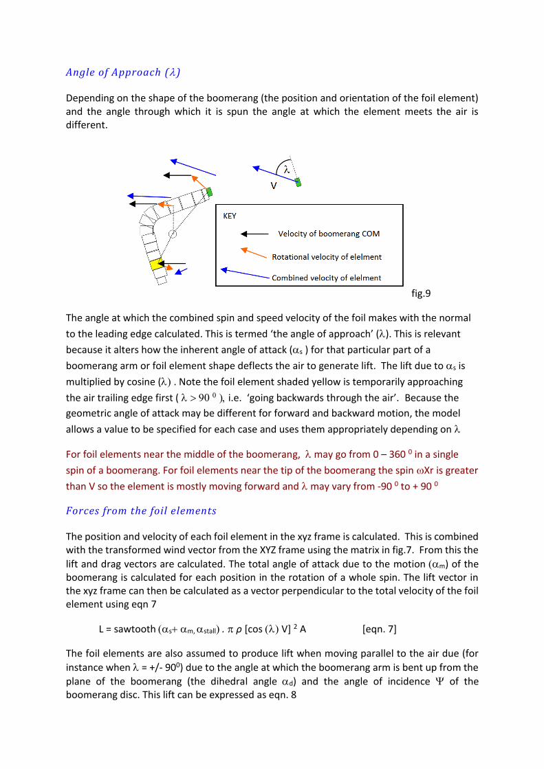
Angle of Approach ()

Depending on the shape of the boomerang (the position and orientation of the foil element) and the angle through which it is spun the angle at which the element meets the air is different.

fig.9

The angle at which the combined spin and speed velocity of the foil makes with the normal

to the leading edge calculated. This is termed ‘the angle of approach’ (). This is relevant

because it alters how the inherent angle of attack (s ) for that particular part of a

boomerang arm or foil element shape deflects the air to generate lift. The lift due to s is

multiplied by cosine (. Note the foil element shaded yellow is temporarily approaching

the air trailing edge first ( i.e. ‘going backwards through the air’.Because the

geometric angle of attack may be different for forward and backward motion, the model

allows a value to be specified for each case and uses them appropriately depending on

For foil elements near the middle of the boomerang, may go from 0 – 360 0 in a single

spin of a boomerang. For foil elements near the tip of the boomerang the spin Xr is greater

than V so the element is mostly moving forward and may vary from -90 0 to + 90 0

Forces from the foil elements

The position and velocity of each foil element in the xyz frame is calculated. This is combined with the transformed wind vector from the XYZ frame using the matrix in fig.7. From this the

lift and drag vectors are calculated. The total angle of attack due to the motion m) of the boomerang is calculated for each position in the rotation of a whole spin. The lift vector in the xyz frame can then be calculated as a vector perpendicular to the total velocity of the foil element using eqn 7

L = sawtooth sm, stall .ρ [cosV] 2 A [eqn. 7]

The foil elements are also assumed to produce lift when moving parallel to the air due (for

instance when = +/- 900) due to the angle at which the boomerang arm is bent up from the

plane of the boomerang (the dihedral angle d) and the angle of incidence of the boomerang disc. This lift can be expressed as eqn. 8

L = sawtooth dm, stall .ρ [sinV] 2 A [eqn. 8]

A configurable fraction of this lift due to the total lift (K) for each foil element is then calculated added to the total lift. K is configurable in the user interface because not much data is available for an airfoils moving parallel to their chord length.

LTotal = [cos2K sin2sawtooth sm, stall .ρ V 2 A [eqn. 9]

By a similar approach drag is calculated from eqn.6 as

DTotal = [cos2K sin2sm .ρ V 2 A . Drag factor [eqn. 10]

The lift and drag force vectors are averaged for each foil element for a complete spin rotation and a configurable gravitational force g translated as a downward force in the XYZ frame into a vector in the xyz frame as g xyz.

The total force on the boomerang for one spin rotation is then

F = 1/N (1 spin rotation LTotal + DTotal ) + M g xyz [eqn. 11]

where M is the total mass of the boomerang

The model stores the total force F as a 3D vector [Fx, Fy, Fz]

Torques from the foil elements

The torque on the boomerang is calculated as the sum of the lift and drag torque vectors.

The lift torque vector is calculated throughout each step of the spin rotation as a vector that

is perpendicular to the total velocity vector of each foil element, multiplied by the radius (r)

of the foil element form the COM of the boomerang. Similarly the drag torque vector is

calculated in a direction opposite to the velocity vector of each foil element. This is

expressed in eqns. 12 and 13

TL = LTotal X V direction [eqn.12]

TD = DTotal . V direction [eqn.13]

The lift and drag torque vectors are combined and averaged over a spin cycle. No torque is added due to gravity as this is assumed to be zero if the boomerang is spinning around its COM. The model stores the total torque T as a 3D vector [Tx, Ty, Tz]

T= 1/N (1 spin rotation [TL + TD ] [eqn.14]

Modelling a throw

The model boomerang is then thrown with a configurable set of parameters to describe its

initial motion. These parameters are editable in the user interface and describe the initial

angles of orientation as the Euler angles andthe initial incidence angle . The

strength of the wind is variable but always at a set angle so the model allows the

thrower to aim the boomerang left and right of the wind by editing The angles are

described in more ‘user friendly terms’ in degrees. The speed of the boomerang (Vcom) and

the spin () are also edited in the user interface. A screen shot of the throw editor is given

in fig.11. The computational tool MATLAB was used to produce all the user interfaces and

code for all the simulations.

fig.11

The editor also calculates a value for the ratio of R/Vcom = for a particular throw of a

boomerang.

Equations of motion

The equations of motion developed by Hess [1] are then applied to the vectors describing

the position and orientation of the boomerang, using the lift and torque vectors from the

simplified aerodynamic model. A different set of equations of motion could be used with a

different aerodynamic model if required. Note the difference between and

t ( = Tz / I3

t (V com) = 1/M . (-Fx cos – Fz sin )

t () = 1/(M V com) . (Fx sin – Fz cos ) + Tx/(I3

t ( = 1/(I3 -Ty cos – Tx sin

t ( = 1/(I3 sin -Ty sin – Tx cos

t ( = -Fy / ( M Vcom cos ) – tan .( Ty / I3 ) – cos . t (

t (X = Vcom [ -cos (cos cossin sin cossinsinsin ]

t (Y = Vcom [ -cos (cos sinsin cos cos+ sin cos sin ]

t (Z = Vcom [-cos sin sin – sin cos ] [eqns.15]

The angles , Vcom and are then step-wise integrated in time using eqns. 15 and

stored as arrays for later plotting. The position of the boomerang XYZ is plotted as soon as

it is calculated. A configurable number of iterations are possible before recalculating the

aerodynamic forces to allow quick approximate simulations with little computational cost

The model allows a number of iterations of these equations of motion before re-calculating

the force and torque vectors. The 3D XYZ trajectory is plotted on a background marked with

range circles at the same distances as the real lines on a field marked out for a boomerang

competition with a 1.8m figure of a thrower for perspective.

Simulations A sample flight

Fig.12 shows the results of a typical simulated throw from the model with the path of the

boomerang in yellow and its ‘shadow’ projected onto the XY plane in black.

fig12a

fig.12b

For the flight in Fig. 12 the details are as follows

Boomerang details. Fig.13 shows the boomerang plan form for model boomerang

‘classic2d’

fig.13

M (g) I3 (gcm2) Atot (cm2) Rg (cm) R(cm) Number of Foil elements s (deg)

48 5475 132 10.68 16.17 11 0 - 4

Throw details (angles in degrees)

Spin

(Hz)

Speed

(m/s) R/Vcom

t wind

Wind

speed

(m/s)

K

21 15 1.42 89 50 10 0 1.8 0.4

Simulation parameters

t N Iterations of position before recalculating Forces and torques

0.01 12 10

The Euler angles (fig.6) are defined in such a way that aiming above the horizon (i.e. aiming

upwards) gives a negative value of so is given in the above table. (t wind) is the

launch of the throw to the wind, is the ‘stand up angle’ of the boomerang which is what

boomerang throwers usually refer to as the ‘layover angle’ subtracted from 900. All angles

are given in degrees. In other words: the boomerang was thrown at 900 to the oncoming

wind, with a layover angle of 400 (900 - 500). = 0 indicating that the boomerang was

thrown with a perfect ‘slice’, so that the motion of the boomerang was parallel to the plane

of rotation. The throw has been adjusted to provide an accurate return – this is not always

the case.

Analysis

General Characteristics

At first inspection it is very similar to the flight of a real boomerang. The flight is slightly

elliptical, reaching a maximum height of 6.05 m and a range of just over 20.2m after 2.5

seconds (shown with a red star of the plot) with a total flight time of 7.5 seconds as the

boomerang decelerates and looses spin.

Speed and Spin

Fig. 14 shows a steady decrease in the spin rate to 66% of its original value whilst the value

of the speed generally decreases with fluctuation due to the boomerang going up and

down hill. This reduction in spin equates to a reduction in rotational kinetic energy to 43%

of its original value which is indicates a much higher retention that reported by Pomeroy

and Uhlig [4a] for a small indoor boomerang who results indicate only about 25% of in

rotational kinetic energy is retained. The throw required producing an accurate return and

‘realistic’ flight pattern has a much greater spin rate (and hence ) than likely to be

required in reality.

fig. 14

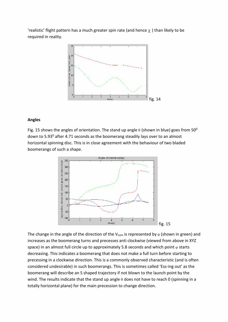
Angles

Fig. 15 shows the angles of orientation. The stand up angle (shown in blue)goes from 500

down to 5.930 after 4.71 seconds as the boomerang steadily lays over to an almost

horizontal spinning disc. This is in close agreement with the behaviour of two bladed

boomerangs of such a shape.

fig. 15

The change in the angle of the direction of the Vcom is represented by (shown in green) and

increases as the boomerang turns and precesses anti clockwise (viewed from above in XYZ

space) in an almost full circle up to approximately 5.8 seconds and which point starts

decreasing. This indicates a boomerang that does not make a full turn before starting to

precessing in a clockwise direction. This is a commonly observed characteristic (and is often

considered undesirable) in such boomerangs. This is sometimes called ‘Ess-ing out’ as the

boomerang will describe an S shaped trajectory if not blown to the launch point by the

wind. The results indicate that the stand up angle does not have to reach 0 (spinning in a

totally horizontal plane) for the main precession to change direction.

The elevation angle (), (shown in red) wavers up and down as the boomerang climbs and

falls up until 4.5 seconds after which it becomes difficult to visualise in reality.

The incidence angle of the whole disc increase from 00 to 90 after 0.86 seconds which

agrees with values calculated by Hess [1] and measured for an indoor boomerang by

Pomeroy and Uhlig [4a]. After this, it decreases and even becomes negative between 1.98

and 3.86 seconds which is not expected behaviour. then increases steadily until 89.40

after 6.5 seconds where the boomerang is falling out of the air in an almost vertical

descent.(t Z= approx. -1.2 m/s) This is the desirable state of a ‘hover’ at the end of the

flight where the thrower has a good opportunity to catch the slowly descending boomerang.

Adjusting the model parameters Using the above boomerang and throw, the flight simulation on desktop PC with a 2 GHz

processor took 19.48 seconds for a flight time of 7.5 seconds. Repeating the simulation with

the following simulation parameters produced a slightly different flight path but took 305.2

seconds on the same PC.

t (seconds) N Iterations of position before recalculating Forces and torques

0.005 32 3

Fig. 27

The resultant flight path is similar up until about 6 seconds of flight time as shown in fig. 27.

After 6 seconds there is a difference in the trajectory as the boomerang in the continues in a

circular. (Releasing from a greater height does produce an S shaped trajectory, but after a

greater time (about 7 seconds – not shown). Arguably the finer simulation is less likely to

produce more realistic simulations by avoiding discontinuities that world not happen in

reality.

Adjusting the Throw The following descriptions are of the effect of changing one parameter at a time from those

listed in the tables describing the first modelled throw. The term ‘range’ is used to describe

the maximum out bound distance of the boomerang onto the xy plane as this is how it is

measured in boomerang competitions

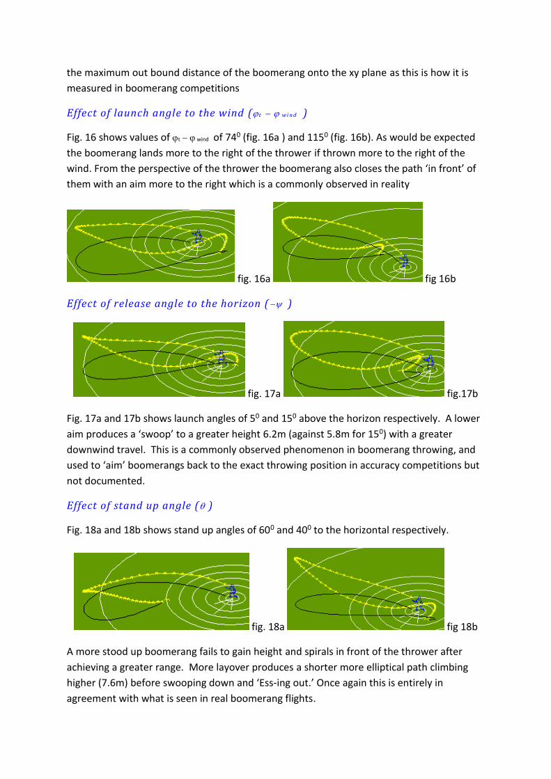
Effect of launch angle to the wind ( t wi n d )

Fig. 16 shows values of t windof 740 (fig. 16a ) and 1150 (fig. 16b). As would be expected

the boomerang lands more to the right of the thrower if thrown more to the right of the

wind. From the perspective of the thrower the boomerang also closes the path ‘in front’ of

them with an aim more to the right which is a commonly observed in reality

fig. 16a fig 16b

Effect of release angle to the horizon ( )

fig. 17a fig.17b

Fig. 17a and 17b shows launch angles of 50 and 150 above the horizon respectively. A lower

aim produces a ‘swoop’ to a greater height 6.2m (against 5.8m for 150) with a greater

downwind travel. This is a commonly observed phenomenon in boomerang throwing, and

used to ‘aim’ boomerangs back to the exact throwing position in accuracy competitions but

not documented.

Effect of stand up angle ( )

Fig. 18a and 18b shows stand up angles of 600 and 400 to the horizontal respectively.

fig. 18a fig 18b

A more stood up boomerang fails to gain height and spirals in front of the thrower after

achieving a greater range. More layover produces a shorter more elliptical path climbing

higher (7.6m) before swooping down and ‘Ess-ing out.’ Once again this is entirely in

agreement with what is seen in real boomerang flights.

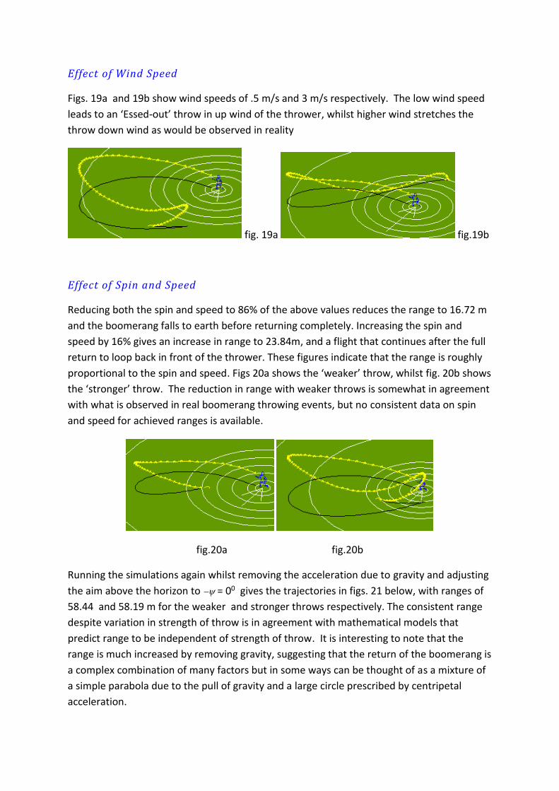
Effect of Wind Speed

Figs. 19a and 19b show wind speeds of .5 m/s and 3 m/s respectively. The low wind speed

leads to an ‘Essed-out’ throw in up wind of the thrower, whilst higher wind stretches the

throw down wind as would be observed in reality

fig. 19a fig.19b

Effect of Spin and Speed

Reducing both the spin and speed to 86% of the above values reduces the range to 16.72 m

and the boomerang falls to earth before returning completely. Increasing the spin and

speed by 16% gives an increase in range to 23.84m, and a flight that continues after the full

return to loop back in front of the thrower. These figures indicate that the range is roughly

proportional to the spin and speed. Figs 20a shows the ‘weaker’ throw, whilst fig. 20b shows

the ‘stronger’ throw. The reduction in range with weaker throws is somewhat in agreement

with what is observed in real boomerang throwing events, but no consistent data on spin

and speed for achieved ranges is available.

fig.20a fig.20b

Running the simulations again whilst removing the acceleration due to gravity and adjusting

the aim above the horizon to = 00 gives the trajectories in figs. 21 below, with ranges of

58.44 and 58.19 m for the weaker and stronger throws respectively. The consistent range

despite variation in strength of throw is in agreement with mathematical models that

predict range to be independent of strength of throw. It is interesting to note that the

range is much increased by removing gravity, suggesting that the return of the boomerang is

a complex combination of many factors but in some ways can be thought of as a mixture of

a simple parabola due to the pull of gravity and a large circle prescribed by centripetal

acceleration.

fig. 21a fig. 21b

Boomerangs have been throw in micro gravity environments a number of times [12] and

found to return if a sufficiently dense atmosphere is also present. Sadly no data is available

on the effect of the conditions on their range compared with under more usual conditions.

Note: the above simulations were stopped after a limited number of iterations, but letting it

run on produces fig 22a. Releasing the boomerang from a height of 50m but with the

presence of normal gravity shows the boomerang continues to spiral downwards (fig. 22b)

but has changed the direction of its precession to clockwise when viewed from above.

Behaviour similar to this is observed in maximum time aloft boomerangs that climb very

high but fail to reach as stable descent and instead go into what boomerang throwers term

a ‘death spiral’ . Hess [1] predicted a similar phenomenon but in his simulations the

clockwise circles were smaller in size than the anti-clockwise part of the path.

fig. 22a fig. 22b

Adjusting the Boomerang Adding Mass

Figs. 21a and 21b show the effect of adding mass to the lifting and dingle arms (see fig. 0 for

the positions of the arms known as lift and dingle) respectively by increasing the mass of foil

elements 11 and 12 respectively from fig. 13.

Adding 3 grams mass to the lift arm increased the range from 20.2m to 23.1 m (an increase

of approx 14%) but reduced the maximum height to 4.61 m, whilst adding the same mass to

the dingle arm to increased the maximum range 22.4m and increased the maximum height

to 6.27m. Adding mass to the lift and dingle arms produced an increase in I3 from 5475 g

cm2 to 6214 g cm2 and 6198 g cm2 respectively (approx a 13% increase). These figures are

roughly in accordance with predictions that range is proportional to I3 [5] More mass on

the dingle arm produced a more elliptical flight path.

fig.21a fig.21b

Adjusting the Plan Shape of the Boomerang

Fig.22b shows a new model boomerang next to the ‘original’ model used for all previous

test flights. The last element of the lift arm has been turned clockwise or ‘swept frward.’

This also changes the position of the COM slightly and increases I3 slightly (0.04%) from 5475

g cm2 to 5496 g cm2

fig.22a fig.22b

fig.23a fig.23b

The resulting flight path is lower (max Z= 4.6m), less elliptical and does not show a tendency

to produce an ‘S’ path or end up spinning in such a horizontal plane at the end of the flight.

This can be seen from the decreasing later. Throwing the same boomerang from a height

of 50m reveals that the path would do this, but later in time (about 7.3 seconds). The

primary cause of this behaviour is the reduced

fig. 24a fig. 24b

The primary reason for the change in flight path is thought to be that decreases less, that

is to say that the boomerang stays more ‘stood up’ and less laid over. The stand up angles

() for the original and adjusted model boomerangs are shown in figs. 25a and 25b

respectively. Boomerang throwers refer to the angle of layover from a vertical plane of

rotation and thus the sweeping forward of the wing modification produces what boomerang

throwers would describe as the boomerang ‘laying over less rapidly.’ This effect is generally

accepted in the boomerang competition community [13]

fig.25a fig.25b

3 Bladed Boomerang

In competitions 3 bladed are often used, so a simple model with 3 blades was produced and

tested. The plan shape and a flight path is given below in fig. 26

fig. 26

M (g) I3 (gcm2) Atot (cm2) Rg (cm) R(cm) Number of Foil elements s (deg)

44.4 3980 108 9.5 13.3 9 0 - 4

Throw details (angles in degrees)

Spin

(Hz)

Speed

(m/s) R/Vcom

t wind

Wind

speed

(m/s)

K

27 17 1.3 80 50 9 0 2 0.4

The flight path is slightly lower (max Z= 5.27m) more circular, and less blown back by the

wind. This is a similar path to those achieved in boomerang events with 3 bladed and is

broadly similar in shape to the indoor boomerang flight paths produced by Pomery and

Uhlig [4a]

A 6 Bladed Boomerang

fig. 28 fig. 29

Producing a 6 bladed boomerang by ‘doubling’ the 3 bladed boomerang produces a model

boomerang with twice the mass, twice the area and twice the moments of inertia. Not

surprisingly the modelled trajectory of this boomerang is similar for the same launch

conditions as the forces, torques, masses and inertias are all in balance. In practice similar

behaviour is not seen in practice by producing such a 6 blade boomerang, even if the

thrower has twice the strength to match the spin and speed with the larger boomerang.

Simple tests with indoor cardboard or plastic boomerangs have shown a greatly different

flight path by attaching a pair of similar 3 bladed boomerangs in the centre. In this case the

boomerang lays over much more rapidly and does produce a pleasing return curve but may

even veer to the right. This change in behaviour is thought to be due to the arms flying

through air that is already disturbed by preceding arms [14]. This effect is always present to

some extent in real boomerangs, but is greatly increased in boomerangs with 5 or 6 arms.

The model simple aerodynamic model does not take this effect into account at all.

Conclusions The simulated flights are in broad agreement with what has been observed in the throwing

of real boomerangs for a classic 2 bladed boomerang shape and simple 3 bladed shape. The

simplified aerodynamic model allows approximate flight paths to be quickly simulated on a

desktop PC for different boomerangs, throws and tuning adjustments. It is also possible to

test hypothetical situations such as the behaviour of boomerangs in the absence of gravity

and release from great heights. A coarse simulation produces similar trajectories to a

simulation with finer time intervals and more steps in the boomerangs spin (N). The

resultant flight paths show many similarities with those observed in reality, although

accurate data on real outdoor flights is rare apart from Hess [1] and Vassberg [7].

In general the required spin rate to speed ration () for simulations to produce returning

flight was about twice what has been observed [7]. The range of the boomerangs is also

dependant on the ‘strength’ of the throw (i.e. speed and spin rate) to a greater extent than

is likely to be the case in reality, although the range does not depend on strength of throw

when the force of gravity is removed.

The absence of any modelling of the disturbance of the air by preceding wings produces

noticeable discrepancies with reality in many bladed boomerangs, and is also a weakness of

the model in general.

As a boomerang thrower with real experience of what can be estimated as about 50,000 –

100,000 throws of about 1000 - 1500 different boomerangs over 20 years, I consider the

simulations to have some merit and similarity to reality, but it is still not sufficiently accurate

to answer the questions that can make a difference to boomerang design in the more

challenging areas of time of flight (maximum time aloft or MTA) and distance travelled (long

distance or LD) boomerangs.

Further work Wind tunnel of airfoil sections

Rigidity / vibration

Self tuning – micro comp om board

optimisation

Symbols

Symbol Description

I Moment of inertia of the boomerang

I1, I2, I3 Moments of inertia about the principal axes of the boomerang such that:

I3 = I1 + I2.

d Angle at which the boomerang arm is bent upwards from the plane of the

boomerang. (Dihedral angle)

L Lift force

D Drag force

ρ Density

COM Centre of Mass

V Airspeed

Vcom Speed of the COM of boomerang

A Wing area

Atot Total wing area of a boomerang

CL Lift coefficient at a given angle of attack

The angle of attack in radians, measured relative to the chord line

3.142….

s Inherent angle of attack of foil shape

m The angle of attack caused by the motion of a foil element

stall The stall angle of a given foil element airfoil section

XYZ Real 3D space

xyz A frame of reference partly fixed to the spinning boomerang

Angular velocity of a foil element about the z axis

r Radius of a foil element from the COM of the boomerang

A Area of a foil element

R Radius of the most distant foil element from the COM of the boomerang

(~=maximum radius of the boomerang)

Angle of incidence of xy plane to the motion of the boomerang’s COM

Euler angles between XYZ and xyz

Angle of approach between a lie parallel to the chord width and the

motion of a foil element to the air

Ratio of R/Vcom = 1/U

g Acceleration due to gravity

N Number of steps modelled in rotating a model boomerang through a

complete spin

t Rate of change of a value with respect to time

M Mass of a boomerang

Rg Radius of gyration

References [1] Hess papers and thesis

[2] International federation of Boomerang Associations (IFBA) rule book

[3] Records of Manu’s LD throw

[4] Musgrove, P.J The return flight of boomerangs – can’t find it but

videhttps://www.youtube.com/watch?v=OxzOr_SgmhA

[4a] B. Pomeroy and D. Uhlig Boomerang flight tests

[5] Hugh Hunt

[6] A.S. Kuleshov / Procedia Engineering 2 (2010) 3335–3341 -

[7] Vassberg

[8] Those other jokers doing CFD stuff

[9] Abbott, Ira H., and Von Doenhoff, Albert E. (1959), Theory of Wing Sections, Section 4.2,

Dover Publications Inc., New York, Standard Book Number 486-60586-8

[10] Benson, Tom (2006). "Aerodynamic Center (ac)". The Beginner's Guide to Aeronautics.

NASA Glenn Research Center. Retrieved 2006-04-01.

[11] "Pilot's Handbook of Aeronautical Knowledge – Chapter 4" (PDF). Federal Aviation

Administration. Retrieved 2014-03-13.

[12] http://www.flight-toys.com/boomerang/boomnews/spacebooms.html

[13] The British Boomerang Society Journal No.23 Summer 2004

Cross

[14] Laslett, M. The Essential Boomerang Book