mathematical optimization ima s c /semidefinite o · pdf filemathematical optimization ima...

Mathematical OptimizationIMA SUMMER COURSE:

CONIC/SEMIDEFINITE OPTIMIZATION

Shuzhong Zhang

Department of Industrial & Systems EngineeringUniversity of Minnesota

[email protected]

August 3, 2016

Shuzhong Zhang (ISyE@UMN) Mathematical Optimization August 3, 2016 1 / 43

Let us start by considering the rationalized preferences choices. In thetraditional economics theory, the rationality of the preferences lies inthe fact that they pass the following consistency test:

1. Any commodity is always considered to be preferred over itself.2. If commodity A is preferred over commodity B, while B is preferred

over A at the same time, then the decision-maker is clearlyindifferent between A and B, i.e., they are identical to thedecision-maker.

3. If commodity A is preferred over commodity B, then any positivemultiple of A should also be preferred over the same amount ofmultiple of B.

4. If commodity A is preferred over commodity B, while commodity Bis preferred over commodity C, then the decision-maker wouldprefer A over C.


In mathematical terms, the analog is an object known as the pointedconvex cone. We shall confine ourself to a finite dimensional Euclideanspace here, to be denoted by Rn. A subset K of Rn is called a pointedconvex cone in Rn if the following conditions are satisfied:

1. The origin of the space – vector 0 – belongs to K .2. If x P K and ´x P K then x “ 0.3. If x P K then tx P K for all t ą 0.4. If x P K and y P K then x` y P K .


If the objects in question reside in Rn, then a preference ordering isrational if and only if there is a convex cone K , such that x is preferredover y is signified by x´ y P K . In this context, the order-definingconvex cone may not be a closed set. Consider the lexicographicordering in R2. That is, for any two points in R2, the preferred choice isthe one with greater first coordinate; in case a tie occurs then the pointwith larger second coordinate is preferred; in case the secondcoordinate is also a tie, then the two points are identical. Now, theunderlying order-defining cone can be explicitly written as

K “

"ˆ

x1x2

˙ ˇ

ˇ

ˇ

ˇ

x1 ą 0*

ď

ˆ

R`ˆ

01

˙˙

.


In general, the preference ordering may not necessarily be complete:there can be incomparable objects. For convenience, from now on weshall consider closed pointed convex cones, i.e., clK “ K andK X p´Kq “ 0. The ordering defined by a closed pointed convex coneis necessarily partial.

Cone K is called proper if

§ K is convex;§ K is solid;§ K is pointed.


Many decision problems can be formulated using a chosen propercone as a preference ordering.

A most famous example is linear programming:

minimize cJxsubject to Ax “ b

x ě 0,

where A is a matrix, and b and c are vectors. The last constraint x ě 0is understood to be a componentwise relation, which can as well bewritten as x P Rn

`.


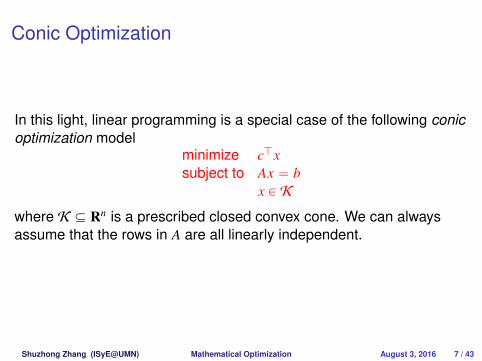
Conic Optimization

In this light, linear programming is a special case of the following conicoptimization model

minimize cJxsubject to Ax “ b

x P K

where K Ď Rn is a prescribed closed convex cone. We can alwaysassume that the rows in A are all linearly independent.


In practice, the following three convex cones are most popular in conicoptimization:

‚ K “ Rn`.

‚ K is a Cartesian product of Lorentz cones; that is,

K “

"ˆ

t1x1

˙ ˇ

ˇ

ˇ

ˇ

t1 P R, x1 P Rd1 , t1 ě }x1}

*

ˆ ¨ ¨ ¨ ˆ

"ˆ

tmxm

˙ˇ

ˇ

ˇ

ˇ

tm P R, xm P Rdm , tm ě }xm}

*

.


For convenience, let us denote the standard Lorentz cone as follows:

SOCpn` 1q “"ˆ

tx

˙ ˇ

ˇ

ˇ

ˇ

t P R, x P Rn, t ě }x}*

.

In this notation, the previous cone is

K “ SOCpd1 ` 1q ˆ ¨ ¨ ¨ ˆ SOCpdm ` 1q


Semidefinite Programming

‚ K is the cone of positive semidefinite matrices either in Snˆn (n by nreal symmetric matrices) or in Hnˆn (n by n complex Hermitianmatrices); that is, K “ Snˆn

` or K “ Hnˆn` .

Specifically, the standard conic optimization model in this case is:

minimize C ‚ Xsubject to Ai ‚ X “ bi, i “ 1, ...,m

X ľ 0

whereX ‚ Y ” xX,Yy ”

ÿ

i, j

Xi jYi j ” Tr XY.


The first choice of the cone is also known as polyhedral cone and thecorresponding optimization problem is Linear Programming (LP);

The second choice of the cone corresponds to Second Order ConeProgramming (SOCP);

The third choice of the cone corresponds to Semidefinite Programming(SDP).

As an appetizer we shall introduce some examples leading to SOCPand SDP.


Example 1: The Weber problem

The first traceable problem of SOCP is perhaps the following problemposed by Pierre de Fermat in the 17th century. Given three points a, band c on the plane, find the point in the plane that minimizes the totaldistance to the three given points. The solution was found by Torricelli,hence known as the Torricelli point, and the method was published byViviani, a pupil of Torricelli, in 1659. The problem can be formulated asSOCP:

minimize t1 ` t2 ` t3subject to u “ x´ a, v “ x´ b, w “ x´ c

ˆ

t1u

˙

P SOCp3q,ˆ

t2v

˙

P SOCp3q,ˆ

t3w

˙

P SOCp3q.


Problems of such type later had gained a renewed interest inmanagement science. In 1909 the German economist Alfred Weberintroduced the problem of finding a best location for the warehouse ofa company, in such a way that the total transportation cost to serve thecustomers is minimum. This is known as the Weber problem. Again,the problem can be formulated as SOCP. Suppose that there are mcustomers needing to be served. Let the location of customer i be ai,i “ 1, ...,m. Suppose that customers may have different demands, to betranslated as weight wi for customer i, i “ 1, ...,m. Denote the desiredlocation of the warehouse to be x. Then, the optimization problem is

minimizemÿ

i“1

witi

subject toˆ

tix´ ai

˙

P SOCp3q, i “ 1, ...,m.


Example 2: Convex Quadratic Programming

The popularity of SOCP is also due to that it is a generalized form ofconvex QCQP (Quadratically Constrained Quadratic Programming). Tobe precise, consider the following QCQP:

minimize xJQ0x` 2bJ0 x

subject to xJQix` 2bJi x` ci ď 0, i “ 1, ...,m,(1)

where Qi ľ 0, i “ 0, 1, ...,m.


Observe that t ě xJx ðñ›

›

›

›

ˆ t´12x

˙›

›

›

›

ď t`12 . Therefore, (1) can be

equivalently written as

minimize x0

subject to

¨

˚

˚

˝

´2bJ0 x`x0`1

2´2bJ

0 x`x0´12

Q120 x

˛

‹

‹

‚

P SOCpn` 2q

¨

˚

˚

˝

´2bJi x´ci`1

2´2bJ

i x´ci´12

Q12i x

˛

‹

‹

‚

P SOCpn` 2q, i “ 1, ...,m.


The versatility of the SOCP modelling goes beyond quadratic models.For the illustrating purpose, let us consider an example of stochasticqueue location problem.

Suppose that there are m potential customers to serve in the region.Customers’ demands are random, and once a customer calls forservice, then the server in the service center will need to go to thecustomer to provide the required service. In case the server isoccupied, then the customer will have to wait. The goal is to find agood location for the service center so as to minimize the expectedwaiting time of the service.


Suppose that the service calls from the customers are i.i.d., and thedemand process follows the Poisson distribution with overall arrivalrate λ, and the probability that the lth service call is from customer i isassumed to be pi, where l “ 1, 2, ... and i “ 1, ...,m. The queueingprinciple is First Come First Serve, and there is only one server in theservice center. This model can be regarded as M/G/1 queue, and theexpected service time, including waiting and travelling, can be explicitlycomputed. To this end, denote the velocity of the server to be v, andthe location of customer i to be ai, i “ 1, ...,m, and the location of theservice center to be x.


The expected waiting time for customer i is given by

wipxq :“

p2λ{v2q

mÿ

i“1

pi}x´ ai}2

1´ p2λ{vqmÿ

i“1

pi}x´ ai}

`1v}x´ ai}, (2)

where the first term is the expected waiting time for the server to befree, and the second term is the waiting time for the server to show upat the door, after his departure at the service center.


A first glance at (2) may not suggest that it can be modelled by SOCP,due to the fractional term. One can find the connection, however, byobserving the fact that }x}2{s ď t, s ě 0 is equivalent to›

›

›

›

ˆ t´s2x

˙›

›

›

›

ď t`s2 . In view of (2), to minimize the total waiting time the

optimal location of the service center is formulated as

minimizex

p2mλ{v2q

mÿ

i“1

pi}x´ ai}2

1´ p2λ{vqmÿ

i“1

pi}x´ ai}

` p1{vqmÿ

i“1

}x´ ai}


or, equivalently,

minimize p2mλ{v2q

mÿ

i“1

piti ` p1{vqmÿ

i“1

t0i

subject toˆ

t0i

x´ ai

˙

P SOCp3q, i “ 1, ...,m

¨

˝

ti`s2

ti´s2

x´ ai

˛

‚P SOCp4q, i “ 1, ...,m

s ď 1´ p2λ{vqmÿ

i“1

pisi

ˆ

si

x´ ai

˙

P SOCp3q, i “ 1, ...,m.


If the objective is to minimize the worst response time, i.e. minimizingmax1ďiďm wipxq, then the problem can be formulated as

minimize t0

subject to t0 ě p2λ{v2q

mÿ

i“1

piti ` t0i{v, i “ 1, ...,mˆ

t0i

x´ ai

˙

P SOCp3q, i “ 1, ...,m

¨

˝

ti`s2

ti´s2

x´ ai

˛

‚P SOCp4q, i “ 1, ...,m

s ď 1´ p2λ{vqmÿ

i“1

pisi

ˆ

si

x´ ai

˙

P SOCp3q, i “ 1, ...,m.


Departure from Linear Programming

All is fine and familiar, just like in the case of LP. But is that so? Let usconsider some serious discrepancy between SOCP and LP.

A famous result regarding linear programming asserts that a linearprogramming problem can only be in one of the three states: (1) theproblem is infeasible, and any slight perturbation of the problem datawill keep the problem infeasible; (2) the problem is feasible but there isno finite optimal value; (3) the problem is feasible and has an optimalsolution. Does the same hold true for SOCP? The answer is a definiteNo!


Considerminimize x1 ` x2 ` x3subject to x1 ´ x2 “ 0

x3 “ 1¨

˝

x1x2x3

˛

‚P SOCp3q.

The conic constraint requires that x1 ě

b

x22 ` x2

3. The above problemis clearly infeasible.


For any positive ε ą 0 the following perturbed version is howeveralways feasible

minimize x1 ` x2 ` x3subject to x1 ´ x2 “ ε

x3 “ 1¨

˝

x1x2x3

˛

‚P SOCp3q,

with a feasible solution e.g. px1, x2, x3q “ p12ε ` ε, 1

2ε , 1q.


In the same vein, it is possible for SOCP to be not infeasible, notunbounded in the objective value, yet there is no optimal solution.Consider

minimize x1 ´ x2subject to x3 “ 1

¨

˝

x1x2x3

˛

‚P SOCp3q.

In this example, for any ε ą 0 the solution px1, x2, x3q “ p12ε ` ε, 1

2ε , 1qyields an objective value ε. However, there is no attainable solutionwith value exactly equal to 0. In this sense, it is a bit of abuse to usethe term ‘minimize’ in the objective. It might be more appropriate toreplace ‘minimize’ by ‘infimum’. In order not to create too many newsymbols, we will still use the old notation, as a suboptimal compromise.


The choice of K being the cone of positive matrices leads to manyinteresting consequences. Later, we will focus on a number of selectedapplications for SDP. As an appetizer, here we shall introduce SDPand consider a few examples. First of all, the second order cone canbe easily embedded into the cone of positive matrices, by observingthe fact that

ˆ

tx

˙

P SOCpn` 1q ðñ„

t, xJ

x, tIn

P Spn`1qˆpn`1q` .


In SDP, the decision variables are in the matrix form. In the realdomain, the standard SDP is

minimizeřn

i, j“1 Ci jXi j

subject tořn

i, j“1 Apkqi j Xi j “ bk, k “ 1, ...,mX P Snˆn

` ,

where, as problem data, C, Apkq P Snˆn, for k “ 1, ...,m, and b P Rm.Observe that Tr pCXq “

řni, j“1 Ci jXi j, which is an inner product between

the two matrices. To unify the notation, we use xx, yy to denote theinner product between x and y, which can be either in the vector formor in the matrix form. In case of SDP, it is often convenient to denoteX ‚ Y as the inner-product between X and Y.


Example 3: the Eigenvalue Problems

The most obvious application of SDP is perhaps the problem of findingthe largest eigenvalue of a given n by n symmetric matrix A, which canbe cast as

minimize tsubject to tI ´ A P Snˆn

` .

If the matrix A itself is a result of design, say A “ A0 `řm

j“1 x jA j, thendesigning the matrix so as to yield the smallest eigenvalue is again anSDP problem:

minimize tsubject to tI ´ A0 ´

řmj“1 x jA j P S

nˆn` .


Moreover, the sum (or the weighted sum) of the first k largesteigenvalues of a matrix can also be expressed by Linear MatrixInequalities. Let λ1pAq ě λ2pAq ě ¨ ¨ ¨ ě λnpAq be the n eigenvalues ofthe symmetric matrix A in descending order of the symmetric matrix A,and let fkpAq “

řki“1 λipAq. Then,

t ě fkpAq ðñ Ds P R, Z P Snˆn : t´ks´Tr pZq ě 0, Z ľ 0, Z´A` sI ľ 0.

Hence, the problem of designing a matrix so as to minimize the sum ofthe k largest eigenvalues can be cast as SDP:

minimize tsubject to t ´ ks´ Tr pZq ě 0

Z ` sI ´ A0 ´řm

j“1 x jA j P Snˆn`

Z P Snˆn` .


Example 4: Polynomial Optimization

Consider the problem of finding the minimum of a univariatepolynomial of degree 2n:

minimizex x2n ` a1x2n´1 ` ¨ ¨ ¨ ` a2n´1x` a2n.

The problem can be cast equivalently as

maximize tsubject to x2n ` a1x2n´1 ` ¨ ¨ ¨ ` a2n´1x` a2n ´ t ě 0 for all x P R.

(3)


It is well known that a univariate polynomial is nonnegative over thereal domain if and only if it can be written as a sum of squares (SOS),which is equivalent to saying that there must be a positive semidefinitematrix Z P Spn`1qˆpn`1q

` such that

x2nà1x2n´1`¨ ¨ ¨à2n´1xà2n´ t “ p1, x, x2, ¨ ¨ ¨ , xnqZp1, x, x2, ¨ ¨ ¨ , xnqJ.

Thus, (3) can be equivalently written as

maximize tsubject to a2n ´ t “ Z1,1

a2n´k “ÿ

i` j“k`2

Zi, j, k “ 1, ..., 2n´ 1

Zpn`1q,pn`1q “ 1Z P Spn`1qˆpn`1q

` .


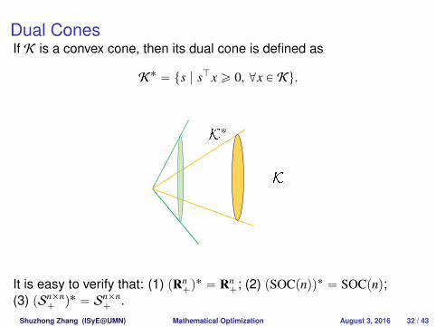
Dual ConesIf K is a convex cone, then its dual cone is defined as

K˚ “ ts | sJx ě 0, @x P Ku.

It is easy to verify that: (1) pRn`q˚ “ Rn

`; (2) pSOCpnqq˚ “ SOCpnq;(3) pSnˆn

` q˚ “ Snˆn` .


Duality in Conic Optimization

Recall the conic optimization

pPq minimize cJxsubject to Ax “ b

x P K .

Upper bounding the optimal value yields its dual

pDq maximize bJysubject to AJy` s “ c

s P K˚.

Theorem 1

(Weak duality theorem) vpDq ď vpPq.


The Strong Duality Theorem

Theorem 2

If the primal conic program and its dual conic program both satisfy theSlater condition, then the optimal solution sets for both problems arenon-empty and compact. Moreover, the optimal solutions arecomplementary to each other with zero duality gap.


Barrier FunctionConsider a convex barrier function Fpxq for K :

§ Fpxq ă 8 for all x P int K ;§ Fpxkq Ñ 8 as xk Ñ x where x is on the boundary of K .

Definition 3

Let K Ď Rn be a given solid, closed, convex cone, and F be a barrierfunction defined in int K . We call F to be a self-concordant function iffor any x P int K and any direction h P Rn the following two propertiesare satisfied:

§ |∇3Fpxqrh, h, hs| ď 2p∇2Fpxqrh, hsq3{2;§ |∇Fpxqrhs| ď θp∇2Fpxqrh, hsq1{2.

Then, F is called a self-concordant barrier function for the cone K withθ as the complexity value.


Self-Concordant Barrier for SDP

ConsiderFpXq “ ´ log det X.

For any direction H P Snˆn we have

∇FpXqrHs “ ´Tr pX´1Hq

and∇2FpXqrH,Hs “ Tr pX´1Hq2

and∇3FpXqrH,H,Hs “ ´2Tr pX´1Hq3.

One can easily show that it is self-concordant with θ “?

n.


Local Geometry

A geometry is associated with a local inner product system. Supposethat Fpxq is a strictly convex barrier function for the cone K . Consider

xu, vy “ uJ∇2Fpxqv.

The above inner product is coordinate-free, i.e., if we let y “ A´1x thenthe inner product remains invariant.

To be specific about the locality of the inner product, let us denote

xu, vyx :“ uJ∇2Fpxqv.

The norm induced by the inner product is }u}x :“a

xu, uyx.


Penalized ProblemFor

pPq minimize cJxsubject to x P a`L

x P K ,

where L “ tx P Rn | Ax “ 0u, let

Fµpxq “1µ

cJx` Fpxq.

Obviously, Fµpxq is also a barrier function for pPq.

For any 0 ă µ1 ă µ, we have

∇2Fµ1pxq “ ∇2Fµpxq “ ∇2Fpxq

∇Fµ1pxq “µ

µ1∇Fµpxq `

µ1 ´ µ

µ1∇Fpxq.


Short-step central path followingLet

npµ; xq “ ´p∇2Fµpxqq´1∇Fµpxq,

andppµ; xq :“ }npµ; xq}x,

namely, the local norm of Newton direction of Fµ.

Newton step. Let xi`1 “ xi ` npµi; xiq.Target shifting. Let µi`1 be so that ppµi`1; xi`1q “ 1{4.

Theorem 4

Suppose that µ0 “ Op1q. Then, in Opθ log 1ε q Newton steps we will

reach a point x with µ ă ε and ppµ; xq ď 1{4.


Long-step central path following

Newton step.

§ Let y “ xi.§ While ppµi; yq ě 1{8, find the Newton

direction npµi; yq and do line minimization

t :“ argmin Fµipy` tnpµi; yqq,

andy :“ y` tnpµi; yq

and return to while.§ Update the iterate: Let xi`1 “ y.

Target shifting. Let µi`1 “ µi{2.


By construction, in the while loop, it holds that ppµi; yq ě 1{8 andppµi; xi`1q ă 1{8.

Theorem 5

Suppose that µ0 “ Op1q. Then, in Oplog 1ε q number of target shifting we

will reach a point x with µ ă ε and ppµ; xq ď 1{8. Between each targetshifting it takes at most Opθ2q numbers of Newton steps.


References

Software tools:

§ CVX for disciplined convex optimization, developed by MichaelGrant and Stephen Boyd:

http://cvxr.com/cvx/

§ YALMIP, developed by Johan Löfberg:http://users.isy.liu.se/johanl/yalmip/


http://cvxr.com/cvx/

http://users.isy.liu.se/johanl/yalmip/

More materials for general reading:

§ S. Boyd and L. Vandenberghe, Convex Optimization, CambridgeUniversity Press, 2004.

§ A. Ben-Tal and A. Nemirovski, Lectures on Modern ConvexOptimization, MPS-SIAM Series on Optimization, SIAM,Philadelphia, 2001.

§ J.F. Sturm, Theory and Algorithms for Semidefinite Programming.In High Performance Optimization, eds. H. Frenk, K. Roos, T.Terlaky, and S. Zhang, Kluwer Academic Publishers, 1999.

§ Yu. Nesterov and A. Nemirovski, Interior-Point PolynomialAlgorithms in Convex Programming, SIAM Studies in AppliedMathematics, 13, 1994.

§ J. Renegar, A Mathematical View of Interior Point Methods inConvex Optimization, MPS-SIAM Series on Optimization, 2001.

§ Yu. Nesterov, Introductory Lectures on Convex Optimization,Kluwer Academic Publishers, 2004.


mathematical optimization ima s c /semidefinite o · pdf filemathematical optimization ima...

Documents