Mathematical models for angiogenic, metabolic and

apoptotic processes in tumours

by

Colin Phipps

A thesis

presented to the University of Waterloo

in fulfillment of the

thesis requirements for the degree of

Doctor of Philosophy

in

Applied Mathematics

Waterloo, Ontario, Canada, 2014

c© Colin Phipps 2014

Author’s Declaration

I hereby declare that I am the sole author of this thesis. This is a true copy of the thesis,

including any required final revisions, as accepted by my examiners.

I understand that my thesis may be made electronically available to the public.

ii

Abstract

This doctoral thesis outlines a body of research within the field of mathematical oncologythat focusses on the inclusion of microenvironmental factors in mathematical models forsolid tumour behaviour. These models primarily address tumour angiogenesis signalling,tumour metabolism and inducing apoptosis via novel treatment combinations.

After a brief introduction in Chapter 1, background material pertinent to cancer biologyand treatment is provided in Chapter 2. This chapter details tumour angiogenesis, tumourmetabolism and various cancer treatments. This is followed in Chapter 3 by a survey ofmathematical models that directly influence my work including summaries of models forrelevant tumour entities such as angiogenic growth factors, interstitial fluid pressure, tu-mour metabolism and acidosis. The progression of topics in these two preliminary chaptersemulate the ordering of the original research presented in Chapters 4–6.

Chapter 4 presents an angiogenic growth factor (AGF) model used to study the impactof transport processes on tumour angiogenic behaviour. The study focusses on a coupledsystem of diffusion-convection-reaction equations that establish the role of convection indetermining relative concentrations of proangiogenic and antiangiogenic growth factors,and hence the angiogenic behaviour, in solid tumours. The effect of various cancer treat-ments, such as chemotherapy and antiangiogenic drugs, that can alter tumour propertiesare considered through parameter analyses. The angiogenesis that results from angiogenicstimulation provides tumours with an oxygen and nutrient supply required for metabolism.

Chapter 5 quantifies the benefit of metabolic symbiosis on tumour ATP production.A diffusion-reaction model of cell metabolism in the hypoxic tissue surrounding a leakytumour blood vessel is developed that includes both lactate and glucose fuelled respirationalong with glycolysis. We can then study the energetic effects of cancer cells’ metabolicbehaviour, such as the Warburg effect and metabolic symbiosis. A model coupling thesemetabolic behaviours with acidosis is also analyzed that includes the effects of extracel-lular buffers. These models can be used to investigate metabolic inhibitor treatments byknocking out specific model parameters and buffering therapies.

While treatment effects are considered in the previous chapters via parameter alter-ation, Chapter 6 explicitly models concentrations of molecular inhibitors and chemotherapynanoparticles. These treatments are coupled to a model for apoptotic protein expression toevaluate strategies for counteracting chemoresistance in triple-negative breast cancer. Theprotein model is then used to predict cell viability, which indicates the efficacy of schedulesfor treatment combinations. The model prediction of post-chemotherapy inhibitor outper-forming pre-chemotherapy and simultaneous application is verified by further experiments.

Finally, a summary of the contributions to the field of mathematical oncology andsuggested future directions are indicated in the final chapter.

iii

Acknowledgements

Firstly, I would like to thank my supervisor Dr. Mohammad Kohandel for his research

guidance and scientific insight. The other professors in the Applied Mathematics Biomed-

ical Research Group were also integral to my graduate studies: I thank Dr. Siv Sival-

oganathan (also on my thesis defence committee) for his advice and support and Dr.

Giuseppe Tenti for his wisdom and notes on biophysics and continuum mechanics. I also

owe a debt of gratitude to the other members of my Ph.D. committee for their time and

useful feedback: Dr. Matthew Scott (Applied Mathematics, University of Waterloo), Dr.

Maud Gorbet (internal-external: Systems Design Engineering, University of Waterloo) and

Dr. Philip K. Maini (external examiner: Oxford University). I acknowledge my many re-

search colleagues who were integral to my success, especially Dr. Hamid Molavian, Dr.

(Venkata) Satya Manem, Dr. Gibin Powathil and Dr. Kathleen Wilkie. Many of these

projects could not be accomplished without wonderful collaborators including Dr. Am-

barish Pandey, Dr. Aaron Goldman and Dr. Shiladitya Sengupta. Finally, thanks to my

friends and my very supportive family for their love and support.

iv

Dedication

This thesis is dedicated to my mother, Diana (1955–1995).

v

Table of Contents

List of Tables x

List of Figures xii

List of Acronyms xv

1 Introduction 1

2 Biological and Medical Background 4

2.1 Cancer . . . . . . . . . . . . . . . . . . . . . . . . . . . . . . . . . . . . . . 4

2.1.1 Tumour angiogenesis . . . . . . . . . . . . . . . . . . . . . . . . . . 5

2.1.2 Cell metabolism . . . . . . . . . . . . . . . . . . . . . . . . . . . . . 6

2.1.3 Tumour metabolism and acidosis . . . . . . . . . . . . . . . . . . . 8

2.2 Cancer treatments . . . . . . . . . . . . . . . . . . . . . . . . . . . . . . . 11

2.2.1 Chemotherapy . . . . . . . . . . . . . . . . . . . . . . . . . . . . . . 12

2.2.2 Antiangiogenic agents . . . . . . . . . . . . . . . . . . . . . . . . . 13

2.2.3 Molecular inhibitors . . . . . . . . . . . . . . . . . . . . . . . . . . 15

2.2.4 Other treatments . . . . . . . . . . . . . . . . . . . . . . . . . . . . 15

2.3 Drug delivery vehicles . . . . . . . . . . . . . . . . . . . . . . . . . . . . . 16

2.4 Treatment strategies and combinations . . . . . . . . . . . . . . . . . . . . 19

2.5 Summary . . . . . . . . . . . . . . . . . . . . . . . . . . . . . . . . . . . . 20

3 Mathematical Modelling Background 23

3.1 Interstitial fluid pressure . . . . . . . . . . . . . . . . . . . . . . . . . . . . 24

vi

3.1.1 Microscopic pressure . . . . . . . . . . . . . . . . . . . . . . . . . . 24

3.1.2 Macroscopic pressure . . . . . . . . . . . . . . . . . . . . . . . . . . 28

3.2 General solute transport equations . . . . . . . . . . . . . . . . . . . . . . 33

3.2.1 Charge migration . . . . . . . . . . . . . . . . . . . . . . . . . . . . 34

3.2.2 Microscopic solute transport . . . . . . . . . . . . . . . . . . . . . . 37

3.2.3 Macroscopic solute transport . . . . . . . . . . . . . . . . . . . . . . 38

3.3 Angiogenic growth factor model . . . . . . . . . . . . . . . . . . . . . . . . 39

3.3.1 Angiogenic activity . . . . . . . . . . . . . . . . . . . . . . . . . . . 44

3.4 Models for cancer cell metabolism and pH . . . . . . . . . . . . . . . . . . 45

3.4.1 Macroscopic tumour model . . . . . . . . . . . . . . . . . . . . . . . 45

3.4.2 Microvessel model . . . . . . . . . . . . . . . . . . . . . . . . . . . . 49

3.4.3 Metabolite consumption rates . . . . . . . . . . . . . . . . . . . . . 52

3.4.4 Parameter estimation . . . . . . . . . . . . . . . . . . . . . . . . . . 59

3.5 Summary . . . . . . . . . . . . . . . . . . . . . . . . . . . . . . . . . . . . 61

4 The Effect of Convective Transport on Angiogenic Activity 65

4.1 Introduction . . . . . . . . . . . . . . . . . . . . . . . . . . . . . . . . . . . 65

4.2 Mathematical model . . . . . . . . . . . . . . . . . . . . . . . . . . . . . . 67

4.2.1 Angiogenic growth factor model . . . . . . . . . . . . . . . . . . . . 67

4.2.2 Angiogenic activity . . . . . . . . . . . . . . . . . . . . . . . . . . . 70

4.2.3 Parameters . . . . . . . . . . . . . . . . . . . . . . . . . . . . . . . 72

4.2.4 Solution method . . . . . . . . . . . . . . . . . . . . . . . . . . . . 73

4.3 Results . . . . . . . . . . . . . . . . . . . . . . . . . . . . . . . . . . . . . . 74

4.4 Discussion . . . . . . . . . . . . . . . . . . . . . . . . . . . . . . . . . . . . 79

4.5 Conclusions . . . . . . . . . . . . . . . . . . . . . . . . . . . . . . . . . . . 83

5 Microvessel Models for Cell Metabolism and pH 84

5.1 Introduction . . . . . . . . . . . . . . . . . . . . . . . . . . . . . . . . . . . 84

5.2 Mathematical model . . . . . . . . . . . . . . . . . . . . . . . . . . . . . . 87

5.2.1 Parameter estimation . . . . . . . . . . . . . . . . . . . . . . . . . . 94

vii

5.3 Results and discussion . . . . . . . . . . . . . . . . . . . . . . . . . . . . . 96

5.3.1 Base case . . . . . . . . . . . . . . . . . . . . . . . . . . . . . . . . 96

5.3.2 Warburg effect . . . . . . . . . . . . . . . . . . . . . . . . . . . . . 98

5.3.3 Optimal metabolic behaviour . . . . . . . . . . . . . . . . . . . . . 99

5.3.4 Cancer treatment effects . . . . . . . . . . . . . . . . . . . . . . . . 100

5.4 A model for metabolism and acidity . . . . . . . . . . . . . . . . . . . . . . 104

5.4.1 Parameters . . . . . . . . . . . . . . . . . . . . . . . . . . . . . . . 106

5.4.2 Analytical observations . . . . . . . . . . . . . . . . . . . . . . . . . 107

5.5 Convective transport in a metabolism model . . . . . . . . . . . . . . . . . 109

5.6 Conclusions . . . . . . . . . . . . . . . . . . . . . . . . . . . . . . . . . . . 112

6 Mathematical Model for the Sequential Application of a Cytotoxic Nanopar-

ticle and a PI3K Inhibitor 114

6.1 Medical motivation . . . . . . . . . . . . . . . . . . . . . . . . . . . . . . . 115

6.2 Mathematical model . . . . . . . . . . . . . . . . . . . . . . . . . . . . . . 116

6.2.1 Protein expression model . . . . . . . . . . . . . . . . . . . . . . . . 117

6.2.2 Treatment effects . . . . . . . . . . . . . . . . . . . . . . . . . . . . 119

6.2.3 Nanoparticle release . . . . . . . . . . . . . . . . . . . . . . . . . . 120

6.2.4 Cellular chemotherapy concentrations . . . . . . . . . . . . . . . . . 121

6.2.5 Cell viability . . . . . . . . . . . . . . . . . . . . . . . . . . . . . . 123

6.3 Parameter estimation . . . . . . . . . . . . . . . . . . . . . . . . . . . . . . 123

6.4 Results . . . . . . . . . . . . . . . . . . . . . . . . . . . . . . . . . . . . . . 124

6.4.1 Cisplatin nanoparticle release . . . . . . . . . . . . . . . . . . . . . 124

6.4.2 Protein expression . . . . . . . . . . . . . . . . . . . . . . . . . . . 126

6.4.3 Cell viability . . . . . . . . . . . . . . . . . . . . . . . . . . . . . . 126

6.5 Conclusions . . . . . . . . . . . . . . . . . . . . . . . . . . . . . . . . . . . 130

7 Contributions and Future Work 132

7.1 Minor contributions . . . . . . . . . . . . . . . . . . . . . . . . . . . . . . . 132

7.2 Major contributions . . . . . . . . . . . . . . . . . . . . . . . . . . . . . . . 133

7.3 Future work . . . . . . . . . . . . . . . . . . . . . . . . . . . . . . . . . . . 134

viii

APPENDICES 137

A Mixture Theory 138

B Parameter values for mathematical models 141

B.1 Homogeneous AGFs parameters . . . . . . . . . . . . . . . . . . . . . . . . 141

B.2 Interstitial fluid pressure parameters . . . . . . . . . . . . . . . . . . . . . 142

B.3 Microvessel model for pH . . . . . . . . . . . . . . . . . . . . . . . . . . . . 142

C Metabolism model details 144

C.1 Boundary conditions . . . . . . . . . . . . . . . . . . . . . . . . . . . . . . 144

C.2 Generalized analytical derivation . . . . . . . . . . . . . . . . . . . . . . . 145

C.3 Numerical methods . . . . . . . . . . . . . . . . . . . . . . . . . . . . . . . 146

C.4 Biochemical Summary . . . . . . . . . . . . . . . . . . . . . . . . . . . . . 149

C.5 Metabolism reaction details . . . . . . . . . . . . . . . . . . . . . . . . . . 156

C.6 The effect of respiratory ATP yield on the results . . . . . . . . . . . . . . 163

D Additional nanoparticle release and protein expression work 168

D.1 Preliminary nanoparticle models . . . . . . . . . . . . . . . . . . . . . . . . 168

D.1.1 Liposomal model . . . . . . . . . . . . . . . . . . . . . . . . . . . . 170

D.2 Additional protein expression experiments . . . . . . . . . . . . . . . . . . 172

E Reactive oxygen species and antioxidant model 175

E.1 Introduction . . . . . . . . . . . . . . . . . . . . . . . . . . . . . . . . . . . 175

E.2 Mathematical model . . . . . . . . . . . . . . . . . . . . . . . . . . . . . . 176

E.3 Results . . . . . . . . . . . . . . . . . . . . . . . . . . . . . . . . . . . . . . 178

References 180

ix

List of Tables

3.1 Parameter values for calculating diffusion coefficients of bicarbonate and

carbon dioxide in water. . . . . . . . . . . . . . . . . . . . . . . . . . . . . 59

3.2 Molecular masses and diffusion coefficients DwX of molecules in water. . . . 60

3.3 Apparent diffusion coefficients for various molecules in tissues. . . . . . . . 63

3.4 Parameters used in metabolic models. . . . . . . . . . . . . . . . . . . . . . 64

4.1 Molecular weights of proangiogenic and antiangiogenic growth factors. . . . 67

4.2 AGF model parameters . . . . . . . . . . . . . . . . . . . . . . . . . . . . . 68

4.3 Angiogenic activity resulting from cytotoxic therapy . . . . . . . . . . . . . 79

5.1 Fixed parameter values for the ‘base case’ simulation. . . . . . . . . . . . . 95

6.1 Nanoparticle release parameters in (6.7)–(6.8). . . . . . . . . . . . . . . . . 125

6.2 Protein expression parameters. . . . . . . . . . . . . . . . . . . . . . . . . . 126

6.3 Experimental scaling factors for protein expression . . . . . . . . . . . . . . 126

6.4 Cell viability parameters. . . . . . . . . . . . . . . . . . . . . . . . . . . . . 130

B.1 Angiogenic growth factor parameters from [1]. . . . . . . . . . . . . . . . . 141

B.2 Pressure parameters from [2]. . . . . . . . . . . . . . . . . . . . . . . . . . 142

B.3 Notation conversion from the works of Casciari et al. [3, 4]. . . . . . . . . . 142

B.4 Consumption rates and parameters for acidity-metabolism model. . . . . . 143

B.5 Molecular parameters for metabolism model. . . . . . . . . . . . . . . . . . 143

C.1 Molecular formulae for the central molecules involved in metabolic reactions. 157

C.2 Molecular formulae for glycolytic intermediaries. . . . . . . . . . . . . . . . 159

x

C.3 Molecular formulae for citric acid cycle intermediates. . . . . . . . . . . . . 162

C.4 Molecular formulae for other molecules involved in the metabolic reactions. 164

D.1 Parameters for the preliminary release profile experiments. . . . . . . . . . 170

E.1 Rate constants for the GPx system. . . . . . . . . . . . . . . . . . . . . . . 177

xi

List of Figures

2.1 The process of glycolysis. . . . . . . . . . . . . . . . . . . . . . . . . . . . . 7

2.2 The process of cellular respiration. . . . . . . . . . . . . . . . . . . . . . . 9

2.3 Simplified view of the mitochondrial electron transport chain, ATP synthase

and ATP hydrolysis. . . . . . . . . . . . . . . . . . . . . . . . . . . . . . . 10

2.4 Average pH profile surrounding a single microvessel [5]. . . . . . . . . . . . 11

2.5 Folate receptor level comparisons. . . . . . . . . . . . . . . . . . . . . . . . 16

2.6 Nanocell and nanoparticles sizes relative to pore sizes. . . . . . . . . . . . . 17

2.7 The effect of nanocells on drug distribution and tumour vasculature. . . . . 19

2.8 Interactions between the major components of cancer biology and treatments. 21

3.1 The effect of the parameter α on IFP and IFV. . . . . . . . . . . . . . . . 33

3.2 Radial profile of AGF concentrations. . . . . . . . . . . . . . . . . . . . . . 41

3.3 Radial profile of angiogenic activity. . . . . . . . . . . . . . . . . . . . . . . 44

3.4 pH and oxygen concentration in the tissue surrounding a single microvessel. 51

3.5 Hill functions. . . . . . . . . . . . . . . . . . . . . . . . . . . . . . . . . . . 54

4.1 The nondimensional parameters in the tumour and host tissues are shown

in the context of the model geometry. . . . . . . . . . . . . . . . . . . . . . 71

4.2 The balance between proangiogenic and antiangiogenic factors. . . . . . . . 73

4.3 The effect of adding convective transport to a model for AGF concentrations. 75

4.4 The effect of changing the nondimensional pressure parameter α. . . . . . . 75

4.5 Nondimensional AGF concentrations fj and corresponding angiogenic ac-

tivity a under parameter changes. . . . . . . . . . . . . . . . . . . . . . . . 78

xii

4.6 Sensitivity to AGF production parameters. . . . . . . . . . . . . . . . . . . 80

4.7 The effects of treatment on angiogenic behaviour of tumours. . . . . . . . . 82

5.1 The spatial relationship between the cell populations in the model. . . . . 86

5.2 The summary reactions included in the metabolism model. . . . . . . . . . 89

5.3 Solution to base case boundary value problem. . . . . . . . . . . . . . . . . 97

5.4 Consumption rates of oxygen, lactate and glucose. . . . . . . . . . . . . . . 98

5.5 The base case for ATP turnover (consumption/production) rates. . . . . . 99

5.6 ATP turnover rates for cells exhibiting the Warburg effect. . . . . . . . . . 100

5.7 An optimal metabolism on the microscale. . . . . . . . . . . . . . . . . . . 101

5.8 The ATP turnover contributions of the pathways in a unit annulus of tissue. 102

5.9 The metabolism and pH model diagram. . . . . . . . . . . . . . . . . . . . 105

5.10 pH profiles. . . . . . . . . . . . . . . . . . . . . . . . . . . . . . . . . . . . 111

5.11 pH profiles. Inset: Glucose and oxygen consumption rates. . . . . . . . . . 112

6.1 A detailed pathway of cell apoptosis. . . . . . . . . . . . . . . . . . . . . . 116

6.2 A diagram summary of the protein expression and cell viability model. . . 117

6.3 Depiction of the drug model for nanoparticle release. . . . . . . . . . . . . 122

6.4 Flowchart showing the computational algorithm used to fit parameters in

the mathematical model. . . . . . . . . . . . . . . . . . . . . . . . . . . . . 124

6.5 Release profiles of cisplatin nanoparticles in acidic and neutral microenvi-

ronments. . . . . . . . . . . . . . . . . . . . . . . . . . . . . . . . . . . . . 125

6.6 Mathematical predicted expression of caspase, pAkt and XIAP in the pres-

ence of different concentrations of SACN alone. . . . . . . . . . . . . . . . 127

6.7 The inhibition of pAkt and increase of caspase by PI828 alone. . . . . . . . 128

6.8 The inhibition of pAkt by PI828 post treatment with SACN and the increase

in caspase expression as compared to SACN alone-treated controls. . . . . 128

6.9 Mathematical model-based prediction of cell viability using different dosing

schedules of SACNs and PI828. . . . . . . . . . . . . . . . . . . . . . . . . 129

C.1 Solution to oxygen boundary value problem fit to radial oxygen profile data

from [5]. Inset: scaled oxygen consumption rate. . . . . . . . . . . . . . . . 148

xiii

C.2 The Cartesian and cylindrical solutions to the oxygen boundary value problem.149

C.3 The base case for ATP turnover (consumption/production) rates corre-

sponding to consumption rates given in Figure 5.4 with altered respiratory

ATP parameters. . . . . . . . . . . . . . . . . . . . . . . . . . . . . . . . . 165

C.4 ATP turnover (consumption/production) rates for cells exhibiting the War-

burg effect with altered respiratory ATP parameters. . . . . . . . . . . . . 166

C.5 The contributions of the pathways are bounded by the total ATP turnover

rate Φ in a unit annulus of tissue with altered respiratory ATP parameters. 167

D.1 Depiction of drug model for biexponential nano particle release. . . . . . . 171

D.2 Release profile kinetics. . . . . . . . . . . . . . . . . . . . . . . . . . . . . . 172

D.3 Attempting to fit the release profile of cisplatin from liposomes in acidic and

neutral environments using a single exponential. . . . . . . . . . . . . . . . 173

D.4 Fitting the release profile of cisplatin from liposomes in acidic and neutral

environments using a liposomal release model. . . . . . . . . . . . . . . . . 174

D.5 The inhibition of pAkt by PI828 post treatment with SACN and the increase

in caspase expression as compared to SACN alone-treated controls. . . . . 174

xiv

List of AcronymsAGF angiogenic growth factor

ADP adenosine diphosphate

AMP adenosine monophosphate

ATP adenosine triphosphate

CAC citric acid cycle

DCM directed cell movement

DNA deoxyribonucleic acid

ECM extracellular matrix

EPR enhanced permeability and retention

FGF fibroblast growth factor

HIF hypoxia-inducible factor

IFP interstitial fluid pressure

IFV interstitial fluid velocity

LDH lactate dehydrogenase

mAb monoclonal antibody

MTD maximum-tolerated dose

NAD nicotinamide adenine dinucleotide

NP nanoparticle

ODE ordinary differential equation

PDE partial differential equation

PI3K phosphatidylinositol-4,5-bisphosphate 3-kinase

xv

pH power of hydrogen

ROS reactive oxygen species

SACN self-assembling cis-platinum nanoparticles

TNBC triple negative breast cancer

TSP thrombospondin

VEGF vascular endothelial growth factor

XIAP X-linked inhibitor of apoptosis protein

xvi

Chapter 1

Introduction

This doctoral thesis outlines my body of research within the field of mathematical on-

cology, an area that utilizes mathematical tools to address problems in cancer research.

The overarching goal is to develop mathematical models that provide insight into cancer

processes with a focus on cancer treatment, which fosters collaboration with clinicians and

leads to meaningful contributions in the medical community. Repeated calls to bridge

the gap between the fields of experimental and mathematical oncology [6, 7] have been

met with many success collaborative efforts and my research has been strongly enriched

and occasionally guided by direct collaboration with biologists and clinicians [8]. Mathe-

matical oncology encompasses the modelling of many cancer processes, including genetic

mutational events, tumour growth, cell signalling, among many others; for an overview, see

[9]. These models can occur on multiple length scales, ranging from molecular modelling

all the way up to tissue modelling, and can even address problems on multiple scales,

referred to as multiscale models [10]. These models can be developed within numerous

mathematical frameworks ranging from continuous partial differential equations (PDEs)

to discrete models [11], and can be combinations of these methodologies, termed hybrid

models [12]. The models that I use will be formulated as PDEs on the microscale (single

blood vessel) or on the macroscale (whole tumour) and then analyzed in steady state, thus

reducing their complexity to ordinary differential equations (ODEs) in Chapters 4 and 5,

or be formulated as strictly time-dependent ODEs in Chapter 6.

From a public health perspective, encouraging non-medical scientists to research cancer,

and indeed other diseases, is becoming a favourable and increasingly common phenomenon

amongst mathematicians, computer scientists, physicists, statisticians, chemists and, un-

1

surprisingly, biologists. This serves as a boon to cancer research as cancer continues to

be a global threat that is one of the leading causes of death in both the developed and

developing world, causing an estimated 7.6 millions deaths in 2008 [13]. In Canada the

incidence rate for all cancers has increased by 0.9% per year in males and 0.8% in females,

however, the mortality rates dropped 0.3% for males and 0.2% for females over the same

time period [14]. Some of the seemingly bloated rates of incidence can be explained by im-

proved screening methods and diagnosis, while the decrease in mortality can be attributed

to improved treatments and earlier detection [14]. Mathematical oncology has much to

contribute to the further improvement of cancer treatments, including the optimization of

treatment scheduling and dosages, especially in the complex scenarios encountered when

considering combinations of multiple treatment modalities. This can be achieved by pre-

dicting tumour progression, cell signalling, metabolic and angiogenic behaviours as well as

cancer cell evolution, all of which can be addressed with mathematical models and have

crucial bearing on the efficacy of cancer treatments.

My research focusses on the incorporation of microenvironmental factors unique to

cancerous tissues into mathematical models that govern tumour behaviour. To facilitate

the discussion of these medically motivated models, a brief background of cancer biology

and treatment is provided in Chapter 2. This contains pertinent information on tumour

angiogenesis, tumour metabolism and various therapies. This is followed by a survey of

mathematical models that directly influence my work in Chapter 3. This chapter contains

summaries of models for relevant tumour entities such as angiogenic growth factors, in-

terstitial fluid pressure, tumour metabolism and acidosis. The progression through these

two preliminary background chapters mirror the sequence of original research content in

Chapters 4–6.

Chapter 4 presents an angiogenic growth factor (AGF) model to study the impact of

transport processes on tumour angiogenic behaviour. The study focusses on a coupled

system of diffusion-convection-reaction equations that elucidate the role of convective fluid

flow on local imbalances of proangiogenic and antiangiogenic factors in solid tumours.

These cell signalling factors promote or suppress angiogenesis and hence have a significant

influence on determining a tumour’s oxygen and nutrient supply. The effect of various

cancer treatments, such as chemotherapy and antiangiogenic drugs, that can alter tumour

properties are considered through parameter analyses.

Chapter 5 investigates a diffusion-reaction model of cell metabolism in the hypoxic

tissue surrounding a leaky tumour blood vessel. The model includes both lactate and glu-

2

cose fuelled respiration along with glycolysis, to study the effects of cancer cells’ metabolic

behaviour, such as the Warburg effect and metabolic symbiosis, on ATP production. A

model coupling metabolic behaviour and acidosis is also analyzed that includes the effects

of extracellular buffer and blood vessel properties. These models can be used to investigate

metabolic inhibitor treatments by knocking out specific model parameters.

While effects of treatment are included in the previous models by altering model pa-

rameters, Chapter 6 explicitly studies drug concentrations in a data-driven study of com-

binations of molecular inhibitors and chemotherapy nanoparticles. A model for apoptotic

protein expression is coupled to models for nanoparticle release in an acidic microenviron-

ment and cellular treatment concentrations to investigate counteracting chemoresistance

in triple-negative breast cancer. These protein expressions are then used in a cell viability

model in an attempt to predict the optimal scheduling of nanoparticles in combination

with a molecular inhibitor. The model prediction of post-chemotherapy inhibitor per-

forming better than pre-chemotherapy or simultaneous application is verified by further

experiments.

The major contributions to the field of mathematical oncology include the following,

contained in Chapters 4, 5 and 6 respectively:

(i) Establishing the role of convective transport in angiogenesis signalling: This model

is used to classify angiogenic tumour behaviours and to predict the effects of various treat-

ments via physiological parameter changes. This finding is generalizable to other cell

signalling pathways in tumours.

(ii) Metabolism model that includes lactate-fuelled and glucose-fuelled respiration along

with oxygen-repressible glycolysis: This was the first model to spatially consider the opti-

mal ATP production in a tumour on the microscale and could be used to analyze metabolic

inhibitors.

(iii) The optimal sequence of chemotherapy nanoparticles and molecular inhibitors:

Utilizing nanoparticle release models in conjunction with protein expression models can

yield cell viability estimates for treatment optimization. This contribution has the most

significant medical and clinical relevance.

3

Chapter 2

Biological and Medical Background

2.1 Cancer

Cancer is the result of genetic mutations that accumulate through the generations of a cell’s

progeny. These mutations lead to abnormal cells, typically characterized by unregulated

proliferation, that are detrimental to an organism’s survival. A cell population is considered

cancerous when these mutations lead to their uncontrolled proliferation and intrusion into

nearby tissues. In humans these cancer cells can interfere with the normal functioning

of the body and if left untreated can metastasize to other tissues and lead to death.

While some forms of cancer do not form a solid mass, such as leukaemia (cancer of the

blood/bone marrow), our focus will be on solid tumours that possess most or all of the

following capabilities: avoidance of apoptosis (the natural cell death trigger), self-sufficient

growth signalling, antigrowth signal insensitivity and unlimited replicative potential [15].

Along with these traits, solid tumours promote angiogenesis, the growth of new vessels from

pre-existing vessels. They facilitate this by upregulating the production of proangiogenic

growth factors and developing insensitivity to antiangiogenic growth factors, leading to

tumour vasculature [16] (see Section 2.1.1). In light of recent evidence it has become

increasingly clear that cancer cells also reprogram their energy metabolism pathways and

can evade the immune system [17]. Most lethal is their invasive nature, a result of decreased

cell-cell adhesion due to disruption of the normal production of integrins that tether cells to

the extracellular matrix (ECM). In addition, they can often degrade the surrounding ECM

in order to facilitate their movement within the tissue. The invasiveness of cancer cells poses

4

a threat to the viability of normal cell populations as they become crowded and attempt

to create space by triggering their own death or those of surrounding normal cells. The

normal cells are also deprived of oxygen and nutrients as these invaders use their resources

to fuel their movements and proliferation. This invasion is often not limited to those tissues

that are directly adjacent to the tumour. Tumour cells often metastasize, making their

way into blood vessels or the lymphatic system, using the vasculature for transport to

other parts of the body. This process is very complex and includes the original event of

entering the vasculature, the process of eventually extravasating into tissue, adapting to

this new microenvironment and finally the development of another cancer cell colony that

could lead to a secondary tumour. Pioneering attempts by cancer cells commonly fail, but

the ones that do succeed will themselves have the potential to colonize further.

Each of these cancer cell traits must be taken into consideration when attempting

to treat a tumour (and when attempting to model their behaviour). Their ability to

avoid apoptosis and senescence implies that natural cell death is relatively rare and must

therefore be triggered (directly or indirectly) by an agent. Their accelerated proliferation

can be exploited by using drugs that target rapidly dividing cells. The promotion of

angiogenesis can be countered by antiangiogenic agents that target endothelial cells or

inhibit proangiogenic factors. The invasive nature of cancer implies that in many tissues,

the surrounding area must also be treated in case cancer cells have migrated to these areas.

While metastasis continues to be the most consistent indicator of negative prognosis, this

is countered primarily by expedient treatment and early detection efforts.

2.1.1 Tumour angiogenesis

Ever since the extremely important connection between angiogenesis and tumour growth

was established in [16], the field of oncology has been revitalized by the advent of antian-

giogenic treatments. When a tumour begins to form, the survival of the cell colony is

completely dependent on the diffusion of oxygen and nutrients in its immediate vicinity.

However, after it reaches a certain size, approximately 2–3 mm in diameter, the center of

this cell cluster can no longer be sustained by the inadequate amount of oxygen attain-

able via simple diffusion, a condition known as hypoxia. In response to this, the effected

cells begin to release hypoxia-inducible factors (HIFs). These HIFs are responsible for

triggering the production of proangiogenic factors in nearby cells, most prominently (and

heavily-studied) among them being those in the vascular endothelial growth factor (VEGF)

5

family. These factors initiate signalling cascades that begin the complex process of tumour

vascularization. Typically there is a balance between the action of proangiogenic and

antiangiogenic factors which leads to vessel maintenance in normal tissues. However, the

increased proangiogenic factor production in tumours disrupts the delicate balance between

angiogenic inducers and inhibitors [18].

These processes are very effective in causing blood vessels to sprout from nearby ex-

isting vasculature, however, the development of the vessels is hasty and unregulated. The

balance between proangiogenic and antiangiogenic factors is disrupted to the point that

vessel construction and network structure are sacrificed. Tumour vasculature is often highly

tortuous and inefficiently assembled, with the vessels typically exhibiting large fenestra-

tions and poor pericyte coverage (pericytes are cells that wrap around endothelial cells

and regulate blood flow among many other vessel processes) [19]. These factors lead to

both spatially and temporally heterogeneous blood flow. The vessel leakiness results in

compromised nutrient and oxygen delivery and contributes to high interstitial fluid pres-

sure (IFP). The cancer cells that originally triggered the angiogenic switch rarely see the

benefit of their efforts since these incoming vessels usually penetrate only the tumour rim,

leaving the bulk of the tumour with an inadequate oxygen supply. As a result, regions

near the center of a tumour often develop into a necrotic core and the hypoxic cells that

surround this core maintain constant angiogenic signalling. As the tumour grows, the very

dense blood vessels and tumour cells become compacted leading to restricted blood flow

and collapsed blood vessels.

2.1.2 Cell metabolism

Cell metabolism can be broadly lumped into two categories, those that are catabolic, break-

ing down molecules to derive energy, and those that are anabolic, constructing molecules

using this energy. Anabolic processes, such as cellular proliferation and motility, are pri-

marily fuelled by adenosine triphosphate (ATP) whilst catabolic processes, such as gly-

colysis and cellular respiration, are primarily employed to manufacture ATP. Thus ATP

is the fundamental carrier of chemical energy in cells. In what follows we will focus on

catabolism, specifically the consumption of glucose and the subsequent generation of ATP

molecules. While anabolism is certainly central to cancer research as it is responsible for

cell growth, division and movement, the models that comprise the bulk of this thesis are

concerned with processes that occur on a much faster time scale than tumour growth, and

6

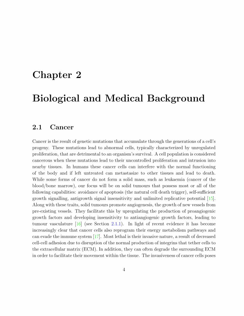
Figure 2.1: A simplified view of glycolysis. The top row contains the molecules requiredfor the ten constitutive steps of glycolysis that convert glucose to pyruvate; see C.5 for theintermediary steps and enzymes. Glycolysis yields two ATP and one NADH. If respirationcannot proceed due to hypoxia, or glucose upregulation then the pyruvate is converted tolactate by lactate dehydrogenase (LDH). Once the ATP is consumed the net reaction is:glucose→2 lactate+2H+.

thus we generally assume static tumour tissues. As such we will only consider anabolism

via the inclusion of ATP hydrolysis in the cytosol.

Before relating how genetic mutations and the tumour microenvironment affect cancer

cell metabolism, we will present a highly simplified view of normal cell respiration includ-

ing glycolysis, the citric acid cycle (CAC) and the electron transport chain (ETC). As

mentioned above, the primary goal of these processes is to produce ATP, either directly

via substrate-level phosphorylation or indirectly via the reduction of cofactors, specifically

nicotinamide adenine dinucleotide (NAD) and coenzyme Q10 (Q), that will be used by the

ETC to fuel ATP synthesis.

In normal adequately oxygenated tissues the primary source of ATP is the process of

cellular respiration. The complete conversion of glucose to carbon dioxide and water has

an ideal yield of approximately 29 ATP [20] (my calculations, which are the result of the

7

reactions contained in C.4, purport that this theoretical yield is an overestimate). The

preliminary stage of cellular respiration is glycolysis, the conversion of glucose to pyruvate.

This process consists of ten enzyme-catalysed steps (given in C.5) and directly produces two

ATP and two reduced NAD (NADH). In hypoxic conditions this pyruvate is converted into

lactate by the enzyme lactate dehydrogenase (LDH) to regenerate the essential oxidized

cofactor NAD+. This process, including ATP hydrolysis, which regenerates adenosine

diphosphate (ADP) and phosphate (Pi), is shown in Figure 2.1. The net reaction for

glycolysis is then: glucose→2 lactate+2 H+.

In oxygenated conditions the pyruvate is transported across the inner mitochondrial

matrix and the malate-aspartate shuttle enables the NADH in the cytosol to reduce a

NAD+ in the mitochondrion. The pyruvate is decarboxylated and then enters the citric

acid cycle. The citric acid cycle directly generates 1 more ATP per pyruvate (2 per glucose).

One pyruvate molecule’s pathway can also produce four NADH and one reduced Q (QH2).

A pictorial summary of this process is provided in Figure 2.2 and the details are found in

C.5.

The primary energy payoff is a result of cofactor oxidization that enables the electron

transport chain (ETC) to establish a proton gradient across the inner mitochondrial matrix.

Ten H+ are deposited in the intermembrane space per NADH, and 6 per QH2. ATP

synthase then utilizes the electrochemical gradient across the mitochondrial matrix to

drive the phosphorylation of ADP at a cost ratio of 10 H+ for 3 ATP [21]. The simplified

version of the reactions involved with the ETC are given in C.5 and the net effect on

intermembrane space protons is shown in Figure 2.3.

The summary given above is a highly simplified version of metabolic biochemistry. A

more in-depth view of the reactions is given in C.4 where the impacts of transport across

the cell membrane and the inner mitochondrial membrane are detailed along with summary

reactions of the above processes.

2.1.3 Tumour metabolism and acidosis

The metabolic scenario described above corresponds to the case of a tissue that has ac-

cess to sufficient nutrients and oxygen. There are a number of factors, including increased

metabolic requirements to support uncontrolled proliferation, tumour blood vessel proper-

ties and acidosis that compound to create a much altered metabolic landscape in tumours.

8

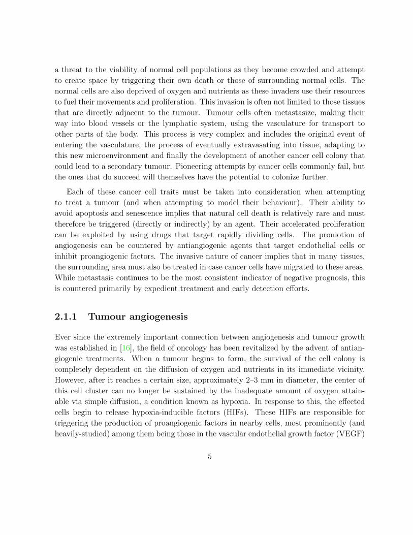
Figure 2.2: The components of cellular respiration excluding the electron transport chainare presented here. The first step is the conversion of glucose to pyruvate via glycolysisfollowed by transport of the pyruvate into the mitochondrion. The pyruvate is decarboxy-lated to acetyl-CoA, reducing a NAD and fuelling the CAC. The CAC intermediaries aredenoted with their first letter. One full ‘revolution’ of the CAC directly produces threemore NADH, one ATP and one reduced Q (QH2).

The inefficient structure of the tumour vasculature network is directly responsible for high

interstitial fluid pressure and the lack of oxygen and nutrients that most tumours expe-

rience. In addition to releasing HIFs that trigger tumour angiogenesis, tumour cells can

also alter their metabolic pathways. Typically, in the presence of sufficient oxygen, cells

prefer to use respiration to produce energy. However, in the tumour microenvironment

there are typically regions experiencing hypoxia or anoxia, leaving them unable to perform

aerobic respiration. Instead, they must rely on the consumption of glucose via the process

9

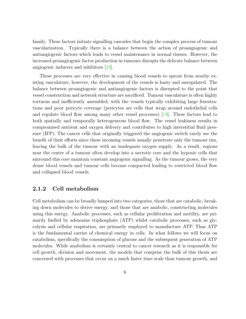
Figure 2.3: Ten H+ are deposited in the intermembrane space per NADH, and 6 per QH2.ATP synthase then utilizes the electrochemical gradient across the mitochondrial matrixto drive the phosphorylation of ADP at a ratio of 10 H+ per 3 ATP [21]. ATP generatedin the mitochondrion can be consumed by cellular processes in the cytosol. The acidicstatuses of mitochondrion components are also shown.

of glycolysis for their energy needs. The drawback of utilizing predominantly glycolysis

is the resulting acidification of the microenvironment. The net byproducts produced by

this metabolism are more acidic than those from respiration. The issue is compounded

by the fact that even in the presence of sufficient oxygen, cancer cells continue to rely on

glycolysis as their primary metabolism. There is still no consensus as to the cause of this

phenomenon, known as the Warburg effect [22], although by not requiring oxygen, it could

give tumour cells a proliferative advantage [23]. The resulting acidosis from upregulated

glycolysis is considered to be a key factor in the invasiveness and metastatic activity of

cancer cells as they try to escape the toxic microenvironment [24].

Some very interesting experimental results, reported in [5] show that cancer cell metabolism

and acidosis may be more complicated than originally suspected. They took measurements

of pH and oxygen concentration around single microvessels, the first time this had been

done, to give average radial profiles of these quantities. Perhaps surprisingly, there was

a plateau observed in the pH measurements, located approximately 100 to 170 µm away

10

0 100 200 300 4006.6

6.7

6.8

6.9

7

7.1

7.2

7.3

7.4

Distance (µm)

pH

Figure 2.4: The average pH profile surrounding a single microvessel [5]. The smooth curveis a simple functional fit to the data.

from the vessel as can be seen in Figure 2.4. It was surmised to be a consequence of the

tumour cells performing respiration even in anoxic conditions or a lack of glucose prevent-

ing glycolysis. An alternative explanation of this is provided by a mathematical model [25]

and will be revisited in Sections 3.4.2 and Chapter 5.

There is also an emerging metabolic story in tumours of a symbiosis existing between

lactate-producing glycolytic cells and lactate-consuming respiratory cells whereby lactate

is converted back into pyruvate via LDH and fed into respiration. This has been observed

since the 80s [26] but rekindled interest due to successful cancer treatment that blocked lac-

tate transport [27]. The phenomenon of metabolic symbiosis (and the effects of metabolic

inhibition) will also be investigated in Chaper 5.

2.2 Cancer treatments

Prior to the seminal work of Folkman [16], and the subsequent development and integration

of antiangiogenic therapy into mainstream clinical use, the focus in oncology had always

11

been on surgical techniques and cytotoxic therapies aimed at directly removing or killing

cancer cells. Here, I will omit discussions of two very important and common treatment

strategies, surgery and radiotherapy, and focus on those that will be the topic of the

mathematical modelling to follow: chemotherapy, antiangiogenic agents and molecular

inhibitors. Drug delivery vehicles such as nanoparticles, and treatment combinations will

also be discussed.

2.2.1 Chemotherapy

Chemotherapy involves the administration of drugs that directly kill cancer cells. Unfor-

tunately, this cytotoxicity is rarely specific to tumour cells alone leading to the death of

normal cells as well. Most often, these drugs damage the DNA or inhibit microtubule

formation which kills rapidly dividing cells. This results in a wide array of side effects that

limit both the size of the dosage and the frequency of administrations. Initially, chemother-

apy agents were used primarily on those tumours that were beyond the physical limitations

of the surgical and radiotherapy techniques of the time. However, they are now frequently

used, targeting many different cellular pathways. For example, one of the more commonly

used agents, doxorubicin, discovered and shown to have anti-tumour effects by DiMarco

et al. [28], induces apoptosis by essentially wedging itself between the two DNA strands

(intercalation) inhibiting transcription and replication. The chemotherapy drug that will

be of most interest to us here, is cisplatin, a platinum-containing drug that is capable of

binding to DNA bases and can cause crosslinking of DNA strands [29]. When the cell

attempts to repair this DNA damage, apoptosis is triggered once it is deemed impossible.

This cell-killing mechanism is widely effective and thus used in the treatment of testicular,

ovarian, cervical, lung and breast cancer among others [30, 31, 32].

The combination of chemotherapy agents with other treatments presented a major leap

forward in oncology, starting with adjuvant therapy, the administration of chemotherapy

agents after surgery to kill the remaining cells. The next step was combination chemother-

apy which employed different cytotoxic agents administered concurrently. These met with

success in certain forms of leukaemia and lymphoma and these types of drug cocktails are

still researched extensively today. Today, chemotherapy is often combined with antiangio-

genic agents, that target tumour vasculature, and molecular inhibitors, that can prevent

chemoresistance, leading to questions of optimal scheduling; the latter case will be ad-

dressed in Chapter 6. Also of concern in chemotherapy research is the efficient delivery of

12

chemotherapy agents and their ability to preferentially target cancer cells. These concerns

will be described shortly when drug delivery vehicles are introduced.

2.2.2 Antiangiogenic agents

In recent years the focus of cancer treatments has shifted, with the realization that tumours

are dependent on angiogenesis for sustained growth and metastasis, to the development of

antiangiogenic treatments. Originally, the rationale was that destroying all tumour vascu-

lature would starve the tumour of essential nutrients and oxygen leading to tumour cell

death. When endothelial cell killing drugs such as combretastatin were first injected into

a tumour, the antiangiogenic effects were deemed to be significant and fast-acting [33], yet

the majority of tumour cells remained unaffected. This outcome is due to a number of

factors but most importantly, many types of cancer cells can survive under hypoxic condi-

tions until vasculature is re-established. Not only does the tumour survive, it also leaves

the source of angiogenic signalling intact ensuring the recurrence of tumour angiogenesis.

Moreover, with no functioning vasculature in the tumour, the delivery of chemotherapy

drugs to the tumour is highly compromised, severely reducing treatment efficacy [34]. An

alternative to this approach, coined vascular normalization [35], involves applying enough

antiangiogenic drugs to prune underdeveloped or unnecessary vessels and remodel the net-

work. This would theoretically lead to a more regular blood vessel structure that could

provide a means of effectively delivering chemotherapy drugs in a more homogeneous fash-

ion to the tumour. While this could also lead to the improved delivery of oxygen and

nutrients to the tumour, this effect would hopefully be inconsequential. Some successes

have been documented [36], but the main limitation remains: this state of normalized vas-

culature lasts for a brief period of time, referred to as the normalization window, followed

by either a return to an irregular, dense system or, on the other hand, an overkill of the

endothelial cells.

While the efficacy of antiangiogenic treatment strategies remains far from established,

there have been a number of different angiogenic mechanisms successfully exploited for

antiangiogenic treatments. There are many types of drugs which target endothelial cell

proliferation in various ways, some similar to regular chemotherapy drugs. While not

specifically antiangiogenic, standard chemotherapy agents have been shown to have an-

tiangiogenic effects even before they begin to kill tumour cells [37]. There are a few that

do attack endothelial cells directly such as combretastatin, angiostatin and endostatin.

13

Combretastatin disrupts the cytoskeletal structure of the endothelial cells causing them to

change into a balloon-shape resulting in vasculature breakdown [38]. Others inhibit the

migration or adhesion of endothelial cells. The other key area of antiangiogenic therapy

are those that indirectly target the endothelial cells by instead targeting various signalling

integrins and factors.

Naturally, due to its large role in tumour angiogenesis and consistent overexpression

by cancer cells, VEGF is a prime target of antiangiogenic therapy. The two most com-

mon ways to prevent the angiogenic action of VEGF are by blocking its receptors or

directly inhibiting it. In the former case, a small molecule which blocks tyrosine kinase

receptors is administered, preventing the binding of VEGF. Two of these drugs are now

commercially available, sunitinib (Sutent) and sorafenib (Nexavar) while there are a hand-

ful more in clinical trials. The side effects of these treatments are rarely serious but due

to their nonspecific receptor targeting there is a wide array of possible side effects. Factor

inhibiting agents were the first type of anti-VEGF drug developed and the monoclonal an-

tibody bevacizumab was the first anti-angiogenesis drug to be successfully combined with

chemotherapy in a Phase III trial [39] and has now been used in various clinical scenarios

[40]. Bevacizumab recognizes all of the VEGF isoforms and has widespread clinical appli-

cations. The most serious side effects include the impairment of wound healing and the

suspension of the body’s natural blood vessel maintenance which has made the research

focus turn toward drug localization. Large fenestrations in the tumour vasculature lead

to some natural targeting of the areas around the tumour but drug delivery vehicles (see

Section 2.3) will improve targeting capabilities. Both forms of anti-VEGF treatments are

now primarily used in combination with chemotherapy drugs or radiotherapy.

Other forms of antiangiogenic treatment have been proposed, some even the result

of mathematical models that show a specific mechanism to be a worthwhile target. For

instance, the blockade of the coupling between VEGFR-2 and its co-receptor NRP1 was

shown to be a good strategy in [41] yet such an inhibitor has not yet been developed.

Various aspects of antiangiogenic drug treatments will be investigated in Chapter 4

including the augmentation of antiangiogenic factors and the inhibition of proangiogenic

factors.

14

2.2.3 Molecular inhibitors

With ever-increasing knowledge of cell signalling pathways, automated molecular discovery

algorithms and the emergence of systems biology, the list of potential cellular targets and

corresponding potential cancer treatments grows by the day. However, there is still hope

that the very potent cytotoxic agents already developed can be made to be more effective

by overcoming their main drawbacks: side effects and resistance. The side effects can

be reduced by improved targeting and delivery techniques which will be described below.

Chemoresistance on the other hand can be counteracted by targeting specific molecules

of signalling networks that elicit an anti-apoptotic response [42]. Here, we will discuss a

specific instance of this phenomenon that will be the focus of the study in Chapter 6.

In previous studies, a chemotherapy drug described above, cisplatin, has been shown

to upregulate PI3K signalling, which can reduce the cytotoxic effects of cisplatin and thus

cause the cells to display chemoresistance [43]. This suggests the application of a PI3K

inhibitor in combination with cisplatin could increase the anti-tumour effect. The question

of the scheduling of molecular inhibitors with chemotherapy is the primary concern of

Chapter 6.

2.2.4 Other treatments

While some of the most popular forms of treatment have been outlined, there are many oth-

ers which will not be included in the mathematical models to follow but those with potential

for significant clinical benefits could be considered in future modelling attempts. Various

hormonal therapies have gained prominence across genders since breast and prostate can-

cers rely heavily on specific hormones for tumour growth. Immunotherapy is a treatment

that relies on the patient’s immune system to fight the cancer. This can be achieved by

giving monoclonal antibodies that can identify antigens specific to the tumour cells. In

fact, the antiangiogenic drug bevacizumab can be thought of as a form of immunother-

apy against tumour vasculature. The developing field of radioimmunotherapy which uses

radioactively conjugated antibodies to target tumour antigens holds promise in treating

radio-sensitive tumours (such as lymphomas [44]). Along with gene therapy and photo-

dynamic therapy, there are countless other biological mechanisms that are targeted by

current cancer treatments and as more viable targets are found, additional molecules will

be fashioned to exploit them.

15

Brain Ovary Uterus10

−2

10−1

100

101

102

fola

te r

ece

pto

r co

nce

ntr

atio

n(p

mo

le/m

g p

rote

in)

Normal

Tumour

Figure 2.5: Comparing the levels of folate receptors on the cell membrane of normal tissueswith medium or high grade tumours. Adapted from [48] using data from [49].

2.3 Drug delivery vehicles

By administering drugs in nanoparticles, many advantages over direct administrations of

free agents have been observed [45]. Improved tumour cell specificity can be achieved by

natural and engineered tumour targeting, longer circulation times are obtained by avoiding

the immune system and slowly eroding layers lead to sustained drug release.

Natural tumour targeting is exhibited by most nanoparticles larger than 100 nm since

the typical pore size in normal blood vessels is approximately 50 nm while the size of

tumour vasculature pores can be upwards of 500 nm. Due to their size, the nanoparticles

cannot escape the tight gap junctions of normal blood vessels leading to their extravasation

primarily in the tumour vicinity. Once they exit the blood vessel, they are trapped in the

tumour tissue. This increases the efficiency of the contained agents and decreases the

severity of side effects in the normal tissue. Exploitation of this natural targeting process,

known as the enhanced permeability and retention (EPR) effect and coined in [46], is a

critical consideration for reducing side effects and successful delivery of therapeutics to

tumours [47].

In addition to this natural targeting, nanoparticles also enable bioengineered attempts

at increasing cancer cell targeting capabilities. Most commonly, a ligand is attached to the

nanoparticle surface whose corresponding receptor is overexpressed on the cancer cell mem-

brane. The prime example of this technique is folate targeting since folate receptors are

overexpressed on the cell membrane of many different cancers. Due to the comparatively

16

Figure 2.6: Approximate sizes of nanocell and nanoparticle core in relation to normal andtumour pores. Data from [53].

low concentration of folate receptors on most types of healthy cells, this was identified as a

possible marker that could be targeted, see Figure 2.5. By attaching folic acid to both lipo-

somal [50] and polymer nanoparticle surfaces, these nanoparticles would be preferentially

taken up by the tumour cells, leaving normal cells mostly unaffected [51].Many other cell

surface receptors have been exploited for cancer treatment targeting. Tumour vasculature

has also been targeted, commonly using the αvβ3 integrin as a target for antiangiogenic

therapies [52].

The immune system is a large obstacle to overcome for successful drug delivery. As soon

as a foreign substance is detected in our bloodstream, our immune system tags them for

removal (opsonization) and then macrophages remove them. Therefore, the drug delivery

system must attempt to avoid this natural process. By attaching certain polymers to the

surface of the nanoparticle envelope, the tagging proteins are prevented from binding to

the nanoparticle. A concern that must be kept in mind is that in order to successfully

target cancer cells via receptor-ligand binding, the density of these polymers cannot be so

high as to interfere with this process.

17

Nanoparticles are typically either lipid-based or polymer-based. Lipid-based nanopar-

ticles can be lumped into two categories based on the number of phospholipid layers they

contain: single-layered micelles and double-layered liposomes. Micelles are good for carry-

ing hydrophobic agents and are relatively straightforward to create. However, they have

relatively short release times since after injection they are rapidly dissolved to below the

minimum micelle concentration. Liposomes have the advantage of being able to carry

both hydrophobic and hydrophilic drug in a single delivery vehicle and have longer circu-

lation times due to the increased stability of the structure. They can also fuse with other

lipid bilayers such as the cell membrane, aiding in drug delivery. The main disadvantage of

these lipid-based vehicles is their surfaces are not easily modifiable for targeting or immune

system avoidance [45].

Polymer-based nanoparticles, usually forming a nanocapsule or nanosphere, are typi-

cally upwards of 100 nm in diameter in order to take advantage of the EPR effect. The

major advantage of polymer-based nanoparticles over lipid-based nanoparticles is their sta-

ble surface structure. This allows for various surface modifications that can dissuade the

immune system and preferentially target cancer cells as described above. However, as we

shall discuss below, a combination of lipid and polymer-based delivery may be advanta-

geous.

Nanocells

Pioneered by Shiladitya Sengupta at the labs of MIT, nanocells are delivery vehicles that

have the ability to trap different agents in separate layers of lipids and polymers. Nanocells

can target cancer cells, in much the same way as nanoparticles, by attaching ligands cor-

responding to overexpressed receptors to their surface. They are approximately 150 nm in

diameter, allowing them to take advantage of the EPR effect. Initial trials were reported

in [53] and used a nanoparticle core (nanocore) loaded with doxorubicin (chemotherapy)

inside of a lipid envelope containing the antiangiogenic drug combretastatin. The nanopar-

ticles were heterogeneous in size, so they were filtered and only those between 80–120 nm

were covered in lipids to form nanocells; see Figure 2.6 for the comparative average (de-

sired) sizes of the nanoparticle and the nanocell complete with lipid layer. This delivery

vehicle enables the controlled temporal release of two separate drugs in a single administra-

tion. First, the outer lipid-bound antiangiogenic agents are released and destroy or prune

the surrounding vasculature. The chemotherapy nanoparticles are now captured inside the

18

Figure 2.7: The antiangiogenic agent in nanocells leads to tumour vasculature normaliza-tion and the trapping of chemotherapy agents in the tumour [55].

tumour, liberating cytotoxic agents as they erode (this process is illustrated in Figure 2.7).

This research area has ‘taken off’ with many centers investigating the concept of a nanocell

with recent attempts at improving folate-targeted nanocells reported in [54].

2.4 Treatment strategies and combinations

The maximum-tolerated dose (MTD) method was a popular treatment technique amongst

oncologists during the 1950’s and 60’s. Since typical chemotherapy drugs have serious side

effects due to their toxicity to normal cells as well as cancer cells, there is an upper limit

on the drug dosage that can be administered to an individual in a single administration

without risking the patient’s life. This amount is referred to as the MTD and anything

above this amount is potentially lethal. The MTD requires a break of weeks between

administrations allowing the patient to recover from the treatment and effected healthy

cells to repair. Unfortunately this also gives the cancer cells time to reproduce. While this

method has fallen out of favour, the MTD is still often explored during experiments and

considered at certain points during a patient’s treatment.

The metronomic technique, coined in [56], is different from MTD in both the scheduling

and dosage of treatments. Dosages much lower than the MTD are used and thus less

recovery time is needed between treatments. These treatments are applied more frequently,

even daily and have been shown to cause less side effects and improved tumour response.

This technique has been shown to provide increased antiangiogenic effects (reviewed in

[57]) since the tumour vasculature does not have time to repair during breaks in treatment

[58]. These two extremes of cancer treatment scheduling can be viewed as a spectrum with

19

continuous low dose at one end of the spectrum and an infrequent MTD at the opposite

end.

A more complicated question than individual drug dosing is how to schedule the treat-

ments of multiple methodologies to optimize the anti-tumour effect. My Master’s thesis

[59] focussed primarily on the optimal scheduling of antiangiogenic drugs and chemother-

apy, using a mathematical model to predict the benefits of tumour vessel normalization.

Here, we will not look at this specific combination but instead at a combination of cisplatin-

nanoparticles and the molecular inhibitor described above (PI3K inhibitor) that has been

demonstrated to aid in overcoming chemoresistance.

2.5 Summary

The understanding of cancer biology has expanded exponentially over the past couple of

decades; historically one of the largest threats to life with no known cure, advanced treat-

ment techniques greatly improve chances of survival. The discovery of the importance of

tumour angiogenesis led to the development of antiangiogenic treatments which in combi-

nation with traditional chemotherapy agents have improved clinical outcomes. Improved

targeting and increased circulation time of these agents have been achieved due to drug

delivery vehicles such as nanoparticles. The surface of nanoparticles can be manipulated to

target specific cancer cell receptors and to degrade in a controlled way. The recent advent

of nanocells that have the aforementioned advantages along with the ability to carry mul-

tiple agents could be the next leap forward for efficient delivery and tumour eradication.

The diagrammatic summary contained in Figure 2.8 and explained below will outline the

topics that will be of importance in this thesis. These areas span a wide breadth of cancer

research but still comprise only a minute niche of the field.

A diagram containing the most relevant interactions and causal relationships between

tumour microenvironmental factors, treatment effects, treatment targets and tumour be-

haviour is presented in Figure 2.8. The entries contained in the leftmost column, with

the exception of cell survival, are not explicitly included in the models that follow but

are the tumour responses to the tumour traits and microenvironmental conditions listed

in the second column. These omitted phenomena include tumour invasion in response

to hypoxic or acidic conditions, metastases enabled by tumour blood vessels and cellular

proliferation fuelled by metabolism. The tumour properties in the second column include

20

Figure 2.8: Interactions and relationships between the major components of cancer bi-ology and treatments that are the focus of the models contained in this thesis. Theleftmost column are tumour responses to microenvironmental factors that, with the ex-ception of cell survival, are not the focus of the models to follow. Tumour propertiesare linked as follows: Hypoxia leads to AGF production that initiates angiogenesis; an-giogenesis provides oxygen to the tumour; this angiogenesis also provides nutrients forcell metabolism, which produces energy for angiogenesis and cell proliferation. Tumourmetabolism is predominantly glycolysis which acidifies the environment; this acidity canimpede metabolic enzymes. Cancer cells can also avoid apoptosis by ignoring apoptoticsignals. These properties affect the outcome of cancer therapies. Hypoxia decreases theefficacy of chemotherapy and radiotherapy; angiogenesis enables drug delivery while theleaky walls of tumour vessels lead to convection of drugs and AGFs; acidity causes rapiddrug release from delivery vehicles; pro-survival signalling also increases chemoresistance.These properties can be exploited by therapies: angiogenesis is targeted by antiangiogenicagents, metabolic inhibitors can halt ATP production, buffer therapies could normalizeacidity, and molecular inhibitors can overcome chemoresistance.

21

the most substantial links between them. Hypoxic microenvironmental conditions lead to

AGF production (via HIFs) that initiates angiogenesis. The resulting angiogenesis provides

oxygen to some cells but hypoxic populations typically remain at all times. Angiogenesis

also provides nutrients for cell metabolism, which produces energy for angiogenesis, cell

proliferation and many other cellular processes. Tumour metabolism relies predominantly

on glycolysis, a process which acidifies the environment. The resulting acidosis can re-

duce enzyme functionality and further alter metabolic pathways (e.g. increased reliance

on glutaminolysis). In addition to these interconnected properties cancer cells can also

avoid apoptosis by ignoring anti-growth signals and producing pro-survival signals. This

cell survival is typically the result of genetic mutations (as is much of the altered cell

metabolism).

The aforementioned tumour characteristics also affect the outcome of cancer therapies

and are shown in Figure 2.8 under ‘Treatment effects’. Hypoxia decreases the efficacy of

chemotherapy (since these cells proliferate less) and radiotherapy. Angiogenesis enables

drug delivery and the blood vessel structure enables the EPR effect. These leaky walls

of tumour vessels lead to elevated interstitial fluid pressure. The resulting pressure gra-

dient leads to convective flow that can dramatically impair drug delivery and alter AGF

concentrations. Acidity promotes more rapid drug release from delivery vehicles due to

accelerated erosion. Upregulated pro-survival signalling, and other cellular adaptations,

result in decreased chemotherapy efficacy, known as chemoresistance. However, all of these

properties can be exploited as shown in the rightmost column under ‘Treatment targets’.

Tumour angiogenesis suggests the application of antiangiogenic agents to eradicate vessels

or normalize the vessels. Metabolic inhibitors could be applied to impede glycolysis or

respiration while buffer therapies could normalize acidity, thus reducing invasion. Finally,

molecular inhibitors could be applied to encourage cell apoptosis to occur upon adminis-

tration of cytotoxic agents.

Our attention will now turn to modelling the entities that affect the tumour microenvi-

ronment and cancer treatments described above. Previous models will be reviewed in the

next chapter in order to lay the foundation for the mathematical models contained in the

original research discussed in Chapters 4–6.

22

Chapter 3

Mathematical Modelling Background

The development of mathematical models that accurately predict tumour growth has been

an ongoing field of research for over fifty years. The first models were simple ordinary

differential equations (ODEs) typically borrowed from ecology. The parameters in the

models were estimated from limited experimental data. The evolution of these model sys-

tems exhibits ever-increasing complexity as more aspects of the tumour microenvironment

and the effects of cancer treatments are included. Mathematical models can be simplified

by assuming spatial homogeneity and symmetry, strict time-dependence, which does not

take into account spatial effects, or steady state. These models are now complemented by

ones with more complex formalisms that include tumour heterogeneity, a defining charac-

teristic that determines, among many others, local growth rates [60], metabolic behaviours

and treatment response. For continuous spatio-temporal models, we use partial differen-

tial equations (PDEs) that have enabled modellers to simulate heterogeneity by adding

tumour vasculature, growth factor concentrations, and drug distributions [59]. Tumour

metabolic behaviour and the resulting acidosis have also been modelled, whereby the tu-

mour growth and invasive capability are linked by the development of hypoxia resistant

and acidity resistant populations of cancer cells [24, 61]. Efforts continue to develop spa-

tial models that include accurate tumour vasculature and concentrations of metabolites,

signalling factors and various treatment types. Developing a model of this type has been

the focus of my previous work while the focus of this thesis is the development of three

interconnected mathematical models spanning the processes of angiogenesis, metabolism

and chemoresistance.

The predominant mathematical oncology models that have guided my work will be pre-

23

sented in this chapter. First, a mathematical model of interstitial fluid pressure and velocity

developed by Jain et al. [62] will be considered on both the microscale (∼ 10−4 m=100 µm)

and the macroscale (∼ 10−2 m=1 cm). This model is critical to developing models for the

convective transport of solutes including AGFs. General solute transport equations includ-

ing convection, diffusion and ion migration are also developed on these spatial scales. We

will then formulate specific applications of these equations. The first application, modelling

of angiogenic growth factors (AGFs), will be outlined, where diffusion-reaction equations

are used to predict angiogenic activity. This model will be extended in Chapter 4 to in-

clude the well-established and prevalent convective transport in solid tumours. We will

then turn our attention to models of tumour metabolism including the work of Casciari et

al. [3, 4], which links metabolism and acidity on the macroscale and Molavian et al. [25],

which does this on the microscale. Other models of cell metabolism that contribute to the

development of functional forms for metabolite consumption, e.g. [63, 64, 65] will also be

touched upon. These will all contribute to the modelling contained in Chapter 5, which

consider metabolite consumption on the microscale and their effect on acidosis. The novel

nanoparticle release, protein expression and cell viability model contained in Chapter 6

remain independent of the mathematical background given below.

3.1 Interstitial fluid pressure

Based on studies of fluid and molecule movement in tumours through interstitial space [66]

and through the blood vessel wall [19], a series of papers developed models for fluid and

macromolecule transport ([67, 68, 69, 70]) and were used to explain various phenomenon

such as the heterogenous distribution of monoclonal antibodies (mAbs) in tumours [62].

The fluid transport models are rigorously derived in [71] and a simplified formulation

will be outlined here for predicting IFP. This will be followed in the next section by its

effect on macromolecule distribution. This will be needed to formulate the PDEs for

macromolecules, such as AGFs and large metabolites.

3.1.1 Microscopic pressure

We adapt the derivation from [71] to calculate the pressure profile in the interstitial matrix

surrounding a single blood vessel. The radial distance under consideration is restricted to

24

some value Ω known as the penetration depth; small enough to ensure limited interactions

with neighbouring vessels but large enough to ensure that this local pressure profile, p,

approaches the average macroscopic pressure p∗ at this distance. We assume this vessel

is a rigid cylinder of constant radius ω with negligible changes in the local axial pressure

gradient. It is also assumed that this vessel experiences constant vascular pressure pv(mmHg), the vessel wall has constant hydraulic conductivity Lp (cm/mmHg-s) while the

blood plasma has constant osmotic pressure πv and the osmotic reflection coefficient for

plasma proteins is σv (the fraction of solute filtered through a membrane if there is zero

concentration difference with high filtration rate). This vessel is surrounded by tissue which

is treated as a homogeneous poroelastic medium with constant hydraulic conductivity K

(cm2/mmHg-s) and osmotic pressure πi.

We consider the interstitial fluid on a length scale such that the assumption of it being a

continuous entity is appropriate. From the conservation of mass equation, once can derive

the formula∂ρ

∂t= −∇ · J

where J is the mass flux and ρ is the density of the fluid. The flux of the fluid is given by

J = ρv where v is the interstitial fluid velocity. This give a differential equation

∂ρ

∂t+∇ · (ρv) = 0,

referred to as the continuity equation for fluids. Expanding the second term using the

product rule gives:∂ρ

∂t+∇ρ · v = −ρ∇ · v. (3.1)

For incompressible flow, it is assumed that ρ is constant within an infinitesimal volume

dV that moves at the velocity v of the fluid. This is equivalent to assuming that the

material derivative of the fluid, denoted Dρ/Dt, and given by

Dρ

Dt=∂ρ

∂t+∇ρ · v,

is equal to zero. This expression can be identified as the left-hand side of (3.1). Putting

this together with the fact that Dρ/Dt = 0 for incompressible flow, we must have

∇ · v = 0. (3.2)

25

It should be noted that (3.2) can also be reached by making a stronger assumption: that

the fluid itself is homogeneous and incompressible, and thus of constant density. This

would mean ∂ρ∂t

= 0 and ∇ρ = 0 in (3.1) giving (3.2) without discussion of the material

derivative. The relationship between these two derivations can be summarized by noting

that homogeneous, incompressible fluids always lead to an incompressible flow while those

fluids undergoing incompressible flow are not necessarily incompressible.

For the geometry we are currently considering, a rigid cylinder with axial and angular

symmetry, the interstitial fluid velocity (IFV) in the interstitial space is given by v =

(u(r), 0, 0). Thus, (3.2) becomesd

dr(ru) = 0.

where u is interstitial fluid velocity in the radial direction. The IFV of this fluid is related

to the IFP by Darcy’s Law in a porous medium [72]:

u = −Kdp

dr. (3.3)

Substituting this into the continuity equation gives

d

dr

(rdp

dr

)= 0. (3.4)

Before moving on, we should note that the above derivation of (3.4) corresponds to

incompressible fluid flow, however it ignores the fact that tissue is in fact comprised of

multiple non-fluid phases, most notably the extracellular matrix and various cell types,

whose behaviours are not strictly fluid and are better treated as deformable solids. Many

physical models of tumour tissues consider biphasic [73] or even triphasic (separate com-

partment for vasculature) [74]. These problems can be addressed using mixture theory,

which fundamentally assumes that the phases simultaneously exist at each point in space,

among other simplifying assumptions which make the equations tractable (e.g. complete

saturation, small deformations, etc.). However, despite the complexity invoked by consid-

ering multiple phases, if one assumes that the fluid exchange between phases is small [75],

that the fluid is experiencing incompressible flow and that the solid is incompressible, then

one once again obtains (3.2), see Appendix A for a brief derivation.

For the boundary condition at the vessel wall, we must balance the IFV with the fluid

velocity across the vessel wall Jf/S, where Jf is the flux across the vessel wall and S is

26

the surface area of the vessel wall. This fluid flux was observed to be proportional to the

difference between the hydrostatic pressure change, ∆p = pv− p, and the osmotic pressure

change, ∆π = πv − πi, across the vessel wall by Starling [76]. This was later altered to

account for the vessel permeability of those molecules that contribute to maintaining the

osmotic pressure difference, predominantly albumin, via the osmotic reflection coefficient

σv, which is set to one if the vessel wall is completely impermeable to plasma proteins, and

approaches zero as the vessel becomes leakier [77]. Thus, the net fluid loss from a single

vessel, Jf (mL/s), is then given by Starling’s Law

Jf = LpS[pv − p− σv(πv − πi)]. (3.5)

This gives us the boundary condition,

−Kdp

dr= Lp(pe − p) at r = ω (3.6)

where pe is the effective pressure, pe = pv − σv(πv − πi). The other boundary condition

ensures that the macroscopic pressure is reached as we move far away from the vessel

p = p∗ at r = Ω. (3.7)

With these boundary conditions, (3.4) can be solved for p from which the IFV u can be

obtained via Darcy’s Law (3.3). Before solving we will nondimensionalize the problem as

described below.

Nondimensionalizing (3.4) and the corresponding boundary conditions by setting p =

pep and r = ωr and rescaling p∗ = pep∗ and Ω = ωr0 gives the identical nondimensional

equivalent of (3.4) and the boundary conditions

dp

dr= −α(1− p) at r = 1

p = p∗ at r = r0,

where the nondimensional parameter α is given by α = Lpω/K. Solving (3.4) yields the

solution p(r) = A ln r + B where A and B are constants. Using the boundary conditions

27

to solve for the constants yields

A = −α(

1− p∗1 + α ln r0

)and B =

p∗ + α ln r0

1 + α ln r0

.

With some algebraic manipulation, once can find that

p(r) =α(1− p∗)

1 + α ln(r0)ln

(r0

r

)+ p∗. (3.8)

Applying Darcy’s Law, and nondimensionalizing the IFV by the characteristic velocity of

Kpe/ω gives

u(r) =α(1− p∗)

1 + α ln(r0)

1

r. (3.9)

This implies that the fluid velocity at the vessel wall is

u(1) =α(1− p∗)

1 + α ln(Ω).

3.1.2 Macroscopic pressure

Similar to the derivation above, we will now consider an entire spherical tumour of radius R

embedded in a host tissue, both of which are considered to be homogeneous and poroelastic

media. The average flow across the vessel wall is again given by Starling’s Law (3.5) where

now the parameters correspond to average values in the entirety of the tissue rather than

corresponding to any one specific vessel. In normal tissues, the excess fluid flux by normal

vessels Jf would be counteracted by absorption by the lymphatic system. However, in

tumours the fluid can either leak toward the core of the tumour, or toward the periphery

[62]. Inward flow would lead to increased IFP until the effective pressure, pe = pv−σv(πv−πi), is reached at which point Jf = 0. Outward flow would lead to excess fluid entering

the interstitium. The interstitial velocity of this fluid, u, is related to the IFP by Darcy’s

Law (3.3) where now r is the macroscopic distance from the tumour core.

Considering the conservation of mass between the fluid filtered from the vessels with

the fluid moving toward the periphery gives

1

r2

d(r2u)

dr=JfV. (3.10)

28

Substituting equations Darcy’s Law (3.3) and Starling’s Law (3.5) into (3.10) yields

1

r2

d

dr

(r2dp

dr

)= −Lp

K

S

V[pv − p− σv(πv − πi)], (3.11)

which is typically rewritten as

1

r2

d

dr

(r2dp

dr

)= −α

2

R2(pe − p), (3.12)

where

α = R

√LpS

KV

is a nondimensional parameter that measures the ratio of the flow resistance in the intersti-

tial space to the resistance in the microvessel wall. With appropriate boundary conditions

(3.12) can also be solved analytically. Below we will present a different derivation than that

typically found in the literature [67, 2] since the nondimensionalization implicitly assumes

the same effective pressure in both tumour and host tissues, involves a far-field bound-

ary condition that fixes the pressure at some value or shifts the solutions by this far-field

pressure. Here, we assume far-field zero flux conditions and include the generalization to

nonzero effective pressures in the host tissue for the embedded tumour case.

Isolated

Considering the case of an isolated tumour, we can nondimensionalize (3.12) by setting

p = pep and r = Rr, which gives

1

r2

d

dr

(r2dp

dr

)= −α2(1− p). (3.13)

To achieve spherical symmetry at the tumour core a no-flux boundary condition is enforced

dp

dr

∣∣∣∣r=0

= 0. (3.14)

Note that the form of (3.13) is very similar to the diffusion-reaction equations that will be

considered below for AGF concentrations (3.35) discussed in Section 3.3, so the derivation

to follow will be referred to later.

29

To solve this system we will consider a Dirichlet boundary condition, where at the

tumour boundary, we set the pressure to the pressure found in the host tissue, ph and

hence take p(1) = ph.

The nondimensional equation for the equation (3.13) can be transformed into a modified

Bessel function in z(u) of order n = 1/2 via the substitutions u = αr, z =√r(p− 1) [78].

This modified Bessel function is

u2 d2z

du2+ u

dz

du− z

(1

4+ u2

)= 0,

which has the general solution

z(u) = C1I1/2(u) + C2K1/2(u),

where In and Kn are the modified Bessel functions of the first and second kind, respectively.

For n = 1/2, these functions reduce to the elementary functions:

I1/2(u) =

√2

πusinh(u), K1/2(u) =

√π

2ue−u.

Thus, reverting back to our original variables, the solution of (3.35) is of the form

p(r) = Asinh(αr)

r+B

e−αr

r+ 1, 0 ≤ r ≤ 1, (3.15)

where the constants A and B will be determined by enforcing boundary conditions.

Considering boundary conditions, the symmetry condition at the tumour core (3.14)

can only hold if B = 0 eliminating the second term in the general solution. Enforcing the

tumour boundary condition gives A = (ph − 1)/ sinh(α) and so the solution is

p(r) = 1− 1− phsinh(α)

sinh(αr)

r.

If ph is set to zero, then the solution typically found in the literature (e.g. [2]) is recaptured.

Applying Darcy’s Law and nondimensionalizing u by again setting u = Kpeu/R gives

u(r) =1− phsinh(α)

(αr cosh(αr)− sinh(αr)

r2

).

30

Embedded

We now consider the case of a tumour embedded in host tissue. This boils down to the

consideration of an infinite spatial domain instead of the finite one considered for the

isolated case, where the various parameters change value at the tumour boundary. We

differentiate between tumour and host tissue parameters with subscripts (or superscripts

for effective pressures) t and h, i.e.

α =

αt, 0 ≤ r ≤ R,

αh, r > R.

We will once again nondimensionalize (3.12) by setting p = pte p and r = Rr, to obtain

the equation

1

r2

d

dr

(r2dp

dr

)=

α2t (p− 1), 0 ≤ r ≤ 1,

α2h(p− pe), 1 < r <∞,

(3.16)

where pe = phe/pte.

The boundary conditions for this case, in addition to the symmetry condition (3.14),

are:

p|r=1− = p|r=1+ ,

−Ktdp

dr

∣∣∣∣r=1−

= −Khdp

dr

∣∣∣∣r=1+

,

limr→∞

dp

dr= 0.

Performing an analogous procedure to the one outlined above, the nondimensional equa-

tion for the system (3.16) can once again be transformed into a modified Bessel function.

Thus, reverting back to our original variables, solutions to (3.35) are of the form

p(r) =

At

sinh(αt r)

r+Bt

e−αt r

r+ 1, 0 ≤ r ≤ 1,

Ahsinh(αh r)

r+Bh

e−αh r

r+ pe, 1 < r <∞,

(3.17)

where the constants Ae and Be, e = t, h will be determined by enforcing the boundary

31

conditions above.

The tumour core and far-field conditions immediately yield Bt = 0 and Ah = 0 re-

spectively. Enforcing the conditions at the tumour boundary yields two equations for the

unknowns At and Bh, which can be solved to give

At =(pe − 1)(1 + αh)

(1 + αh −K) sinh(αt) +Kαt cosh(αt),

Bh =(pe − 1)K[sinh(αt)− αt cosh(αt)]e

αh

(1 + αh −K) sinh(αt) +Kαt cosh(αt),

where the relative hydraulic permeability K is given by Kt/Kh; for simplicity we typically

assume K ≈ 1. This gives the analytical solution,

p(r) =

1− (1− pe)(1 + αh)

φ+ θ

sinh(αtr)

r, 0 ≤ r ≤ 1

pe +(1− pe)θφ+ θ

e−αh(r−1)

r, r > 1

(3.18)

where θ = K[αt cosh(αt) − sinh(αt)] and φ = (1 + αh) sinh(αt). A typical solution in

the literature corresponds to the case where pe = 0, i.e. pte phe . The nondimensional

interstitial fluid velocity is then given by

u(r) =

(1− pe)(αh + 1)

φ+ θ

[αtr cosh(αtr)− sinh(αtr)]

r2, 0 ≤ r ≤ 1

(1− pe)θK(φ+ θ)

(αhr + 1)e−αh(r−1)

r2, r > 1.

(3.19)

The nondimensional pressure and velocity profiles are given in Figure 3.1. As the pa-

rameter αt increases, the pressure reduction at the tumour rim becomes more drastic, it

also leads to higher IFP inside the tumour. Equivalently, as αt increases, the interstitial

fluid velocity reaches a higher and sharper peak at the tumour rim. Note that the pa-

rameter choices for αt inside the tumour of 2, 6, and 14 correspond roughly to parameters

associated with normal tissue, normalized tumour tissue, and nonnormalized tumour tis-

sue, respectively [2]; the choice for αh outside the tumour remains a constant value of 2 in

Figures 3.1a and 3.1b [2].

These analytical solutions were first presented in [62] but were not experimentally

32

r

p

0

0.2

0.4

0.6

0.8

1

0 0.5 1 1.5 2

αt=2αt=6αt=14

(a) Nondimensional interstitial fluid pressure.

r

u

0

0.5

1

1.5

2

2.5

0 0.5 1 1.5 2

αt=2αt=6αt=14

(b) Nondimensional interstitial fluid velocity.

Figure 3.1: The effect of changing the parameter α on IFP and IFV in an embeddedtumour. These analytical solutions are given in (3.18) and (3.18) respectively and are froma model developed and analytically solved by Baxter and Jain [62, 67].

confirmed until direct measurements of interstitial fluid pressure were made in [79]. It

was found that indeed the isolated tumour solution fit the IFP data of various tumours,

including mammary adenocarcinoma using the parameter values of α2 = 1210 and pe =

10.2 mmHg [79, Figure 8], which was in good agreement with the estimated parameters

from [62].

3.2 General solute transport equations

Considering the conservation of mass equation for concentrations of a solute in solution X,

results in the continuity equation,

∂X

∂t= −∇ · JX + PX (3.20)

where JX is the flux of the solute and PX is the production rate (related to source and

sink densities). This solute flux through the interstitium is governed by some combination

of transport processes, including diffusion, convection and charge migration, each of which

we will address below. Letting Jd be the diffusive flux, Jc be the convective flux and Jibe the charge migratory flux, we seek an expression for JX of the form JX = Jd + Jc + Ji,

33

where depending on the relative contributions of each process, in specific scenarios one or

more of these fluxes can be omitted for simplicity.

Diffusion is driven by thermal energy which results in the random movement of molecules.

The macroscopic effect of this random movement is the movement of molecules down their

concentration gradient, i.e. in the direction of −∇X. This can be intuitively understood

as the movement from areas of higher concentration to those of lower concentrations. The

diffusive flux is assumed to be proportional to −∇X, known as Fick’s Law, with propor-

tionality constant, called the diffusion coefficient DX . In a biological context this constant

is more accurately referred to as the interstitial effective diffusion coefficient and we will

typically assume that it is constant throughout each tissue.

Convection is the transport of molecules in the direction of a bulk fluid flow. In tissue

this flow is typically due to leaky blood vessels. The convective flux is proportional to

the product of the concentration and the interstitial fluid velocity u with proportionality

constant rX known as the retardation factor, the ratio of solute velocity to fluid velocity.

Thus the convective flux is given by Jc = rXu, where analytical solutions for the IFV u have

already been derived in cylindrical (microscopic) and spherical (macroscopic) geometries

above.

Finally, the flux due to the electric potential φ is proportional to the product of the

concentration and the ion migration velocity vX . The derivation of a functional form for

vX is more in depth so we will address this in the next section. Taking all of the previous

form for fluxes into consideration this gives the total interstitial flux as

JX = −DX∇X + (rXu+ vX)X. (3.21)

We will now address vX before explicitly writing down the corresponding microscopic and

macroscopic tumour equations.

3.2.1 Charge migration

For charged particles, we must calculate a form for the velocity vX , here we will adapt a

derivation from [3] to include convection and diffusion.

The force F (N) exerted on a unit charge within an electric field E (N/C) is given by

F = qE where q ≈ 1.602 × 10−19 C is the elementary charge. The force exerted on an

34

ion with valence zX is then FX = qXE, where qX = zXq is the charge of the particle.

The velocity of ion migration is then this force divided by a frictional coefficient fX (kg/s)

giving

vX =qXfX

E;

fX (kg/s) is sometimes called the Stokes drag coefficient and is related to the commonly

used parameter electrical mobility µX = qX/fX . Before simplifying this expression, note

that the ionic current, Jion associated with this velocity is

Jion =qXX

fXE,

which is Ohm’s Law with conductivity σ = qXX/fX .

Assuming a quasi-steady state, there is no magnetic contribution to the electric field

and E = −∇φ where φ (V) is the electric potential, which gives

vX = −qXfX∇φ.

The Stokes-Einstein equation gives the relationship between the diffusion coefficient DX

and the drag coefficient fX (for low Reynolds number) as

DX =kBT

fX,

where kB ≈ 1.380× 10−23 J/K and T (K) is the absolute temperature. Thus,

vX = −DXqXkBT∇φ,

or using different universal constants

vX = −DXzXF

RT∇φ,

since Faraday’s constant, F = qNA ≈ 96485C/mol and the gas constant R = kBNA ≈ 8.314

J/K/mol, where the Avogadro constant NA ≈ 6.022 × 1023 /mol, share the same ratio as

35

q/kB. The flux granted by the ionic current is then

Jion = −DXzXF

RTX∇φ. (3.22)

If a system is comprised of multiple species X with charges zX , then the charge density of

the system is

Q = F∑X

zXX,

while the total charge flux is

I = F∑X

zXJX

where JX is given in (3.21). When Q = 0 this represents electroneutrality in the system;

this is a commonly justified modelling assumption. A stronger simplifying assumption, is

the condition that there is no net current, equivalent to I = 0, gives

∑X

zX

(−DX∇X + rXuX −DXX

zXF

RT∇φ)

= 0,

or

∇φ =RT

F

∑X zX(−DX∇X + rXuX)∑

X DXz2XX

.

This expression for the electric field can now be substituted back into (3.22) and subse-

quently into (4.2) to give

∂X

∂t= −∇ ·

(rXuX −DX

(∇X + zXX

∑Y zY (−DY∇Y + rY uY )∑

Y DY z2Y Y

)). (3.23)

If transport is diffusion-dominated, implying the contribution of convection is relatively

negligible, we can write

∂X

∂t= −DX

(∇2X − zX∇ ·

(XS1,1

S2,0

)), (3.24)

where Si,j =∑

X DxziX∇jX, and we define ∇0X = X. Distributing the divergence over

36

the ionic flux gives the tractable form

∂X

∂t= −DX

(∇2X − zXS1,1

S2,0

(X

(S1,2

S1,1

− S2,1

S2,0

)+∇X

)). (3.25)

This previous equation, or the more general (3.23), could be adapted for microscopic and

macroscopic applications, but to simplify the equations in what follows, we will limit the

discussion to uncharged particles and thus take vX = 0 (since zX = 0).

3.2.2 Microscopic solute transport

Making similar assumptions on the blood vessel and interstitial space as was done when

deriving equations for microscopic pressure in Section 3.1.1, we arrive at the equation

∂X

∂t=DX

r

∂

∂r

(r∂X

∂r

)− 1

r

∂

∂rr(rXu+ vX)X + PX . (3.26)

Further, noting that the fluid is assumed to be incompressible, (3.26) simplifies to

∂X

∂t=DX

r

∂

∂r

(r∂X

∂r

)− rXu

∂X

∂r+ PX , (3.27)

for an uncharged molecule; the case of vX > 0 would require the use of (3.25).

Following the process above, we determine the vessel boundary condition by considering

the transport of solute molecules Js due to extravasation from blood vessels. There are

many variations on the formula for this transport, such as the Kedem-Katchalsky equation

[77], but the most useful to us is written as a sum of its diffusive and convective parts.

This diffusion is proportional to the difference between the plasma concentration VX and

the interstitial concentration X, and convection is proportional to the fluid leakage Jf in

(3.5). Known as the Patlak equation [80], it gives the rate of solute transport as,

Js = µXS(VX −X)PeX

ePeX − 1+ Jf (1− σX)VX , (3.28)

37

where PeX is the Peclet number defined by

PeX =Jf (1− σX)

µXS,

µX is the vascular permeability coefficient and σX is the osmotic reflection coefficient for

the solute. For large molecules the first term can be ignored since they do not diffuse

very much, instead their primary means of movement is convection while the opposite is

true for small molecules dominated by diffusion. Now, balancing the solute extravasation

from blood vessels in (3.28) with the solute moving in the interstitial space (3.21) gives the

boundary condition at the vessel wall for a microscopic model:

rfuX −DXdX

dr= µ(VX −X)

PeXePeX − 1

+JfS

(1− σX)VX at r = ω. (3.29)

We also require the concentrations to reach a steady state as we move away from the vessel

and takedX

dr= 0 at r = Ω, (3.30)

where Ω is the penetration depth [71], a distance far enough from the microvessel to

justify the assumption that the system has reached steady state but close enough to ensure

minimal contributions from other nearby vessels.

3.2.3 Macroscopic solute transport

As in the above discussion on interstitial fluid pressure, this can be readily expanded into a

macroscopic convection-diffusion equation for the entire tumour by taking the blood vessels

as an averaged source term giving,

∂X

∂t=DX

r2

∂

∂r

(r2∂X

∂r

)− 1

r2

∂

∂r[r2(rXu+ vX)X] + PX +

JsV. (3.31)

Once again assuming that interstitial fluid is incompressible and the particle is uncharged

yields∂X

∂t=D

r2

∂

∂r

(r2∂X

∂r

)− rXu

∂X

∂r+ PX +

JsV. (3.32)

38

The boundary conditions ensure continuity of concentrations and equality of fluxes at the

tumour boundary. The above equation can be useful when considering the extravasation

of drug delivery vehicles from tumour vasculature and the release of the agents contained

therein and could be easily expanded to a non-radially symmetric case.

3.3 Angiogenic growth factor model

This section will outline a model developed by Ramanujan et al. [1] that considers the con-

centrations of proangiogenic and antiangiogenic growth factors in a solid spherical tumour

of radius R. This will be followed by consideration of measures of angiogenic activity, es-

sentially functions that summarize whether angiogenic activity is being locally stimulated

or suppressed. The notation used in this section is consistent with the simplified notation

used in my work [81], i.e. instead of cfe to denote the concentration of factor f (proangio-

genic: +, antiangiogenic: -) in environment e (malignant: m, host: h) [1], we will use fjfor concentration of factor j (proangiogenic: p, antiangiogenic a) where it is understood

that for 0 < r < R we are inside the tumour and for R > 0 we are in the host tissue;

when necessary tumour (t) and host (h) parameters are differentiated with the appropriate

superscript.

Following [1] for this preliminary modelling, let fj denote the concentration of factor

j where the factor can either be considered to be proangiogenic (j = p) or antiangiogenic

(j = a). This tumour is assumed to be a homogeneous sphere of radius R. Proangiogenic

growth factors are those responsible for encouraging and stimulating angiogenesis while

antiangiogenic growth factors are those that discourage or counteract vascularization. The

factors are assumed to be produced at constant rates gj, degrade exponentially at rates kjand diffuse with diffusion constants Dj, j = p, a, all of which can differ between tumour

(superscript t) and host (superscript h) tissues. These assumptions lead to the PDEs

∂fj∂t

= Dj∇2fj − kjfj + gj, j = p, a. (3.33)

Now by making a pseudo-steady-state assumption, it is assumed that local changes in factor

concentration are relatively small, i.e. ∂fj/∂t = 0, compared to the cellular responses such

39

as proliferation. Assuming spherical symmetry, solutions of the equation

Dj1

r2

∂

∂r

(r2∂fj∂r

)− kjfj + gj = 0 (3.34)

with suitable boundary conditions can be derived. First we nondimensionalize (3.34),

which is not only a useful process for parameter reduction in this case, but also crucial

to subsequently defining angiogenic activity. This can be achieved by setting r = Rr,

fj = f sj fj, and by defining the rescaled parameters κj =√kjR2/Dj and γj = gjR

2/Djfsj

where

f sj := limr→∞

fj(r) =ghjkhj

is the steady state factor concentration in host tissue. This process yields the equations

1

r2

d

dr

(r2dfjdr

)− (κj)

2fj + γj = 0. (3.35)

Note that the derivatives are no longer denoted as partial derivatives to reinforce that the

concentration fj is a function of the single variable r with no time dependence and that

γhj = (κhj )2. To be explicit about the spatial dependence and since the solutions to follow

require their consideration, we could rewrite (3.35) as

1

r2

d

dr

(r2dfjdr

)=

(κtj)

2fj − γtj, 0 ≤ r ≤ 1,

(κhj )2(fj − 1), 1 < r <∞.

(3.36)

Solutions to (3.35) with appropriate boundary conditions can be found and the details are

presented below since only partial ([82]) or erroneous ([1, 59]) solutions in this context exist

in the literature. The solution process is very similar to the process whereby the analytical

pressure solution in an embedded tumour geometry was derived above in Section 3.1.2.

The nondimensional equation for the system (3.35) can be transformed into a modified

Bessel function in z(u) of order n = 1/2 via the substitutions u = κj r, z =√r(fj − γj/κ2

j)

[78]. This modified Bessel function is

u2 d2z

du2+ u

dz

du− z

(1

4+ u2

)= 0,

40

0 0.5 1 1.5 21

1.5

2

2.5

3

3.5

4

4.5

5

5.5

6

r

fj

fp

fa

Figure 3.2: The nondimensional concentrations of antiangiogenic, fa, and proangiogenic,fp, growth factors [1]. At the tumour core fp > fa, at the rim (r = 1) fp < fa and in thehost tissue they are approximately equal.

41

which has the general solution

z(u) = C1I1/2(u) + C2K1/2(u),

where In and Kn are the modified Bessel functions of the first and second kind, respectively.

For n = 1/2, these functions reduce to the elementary functions:

I1/2(u) =

√2

πusinh(u), K1/2(u) =

√π

2ue−u.

Thus, reverting back to our original variables, solutions to (3.35) are of the form

fj(r) =

Atj

sinh(κtj r)

r+Bt

j

e−κtj r

r+ Ωj, 0 ≤ r ≤ 1,

Ahjsinh(κhj r)

r+Bh

j

e−κhj r

r+ 1, 1 < r <∞,

(3.37)

where Ωj = γtj/(κtj)

2 and the constants Aej and Bej (j = p, a; e = t, h) will be determined

by enforcing boundary conditions.

Considering boundary conditions, we require symmetry at the tumour core, continuity

of concentrations and fluxes at that the tumour boundary, and the concentrations approach

steady state value as we move into the host tissue. These correspond to the following

conditions:

dfjdr

∣∣∣∣∣r=0

= 0,

fj

∣∣∣r=1−

= fj

∣∣∣r=1+

,

−Dtj

dfjdr

∣∣∣∣∣r=1−

= −Dhj

dfjdr

∣∣∣∣∣r=1+

,

limr→∞

dfjdr

= 0.

The first (tumour core) and last (far-field) conditions immediately yield Btj = 0 and

Ahj = 0. This gives the factor concentrations fj(0) = Amj κmj + Ωj at the tumour core and

42

fj = 1 as r →∞. Enforcing the conditions at the tumour boundary yields two equations

for the unknowns Atj and Bhj , which can be solved to give

Atj =(1− Ωj)(1 + κhj )

(1 + κhj − βj) sinh(κtj) + βjκtj cosh(κtj),

Bhj =

(1− Ωj)βj[sinh(κtj)− κtj cosh(κtj)]eκhj

(1 + κhj − βj) sinh(κtj) + βjκtj cosh(κtj),

where βj = Dtj/D

hj . Thus, the final solution is given by

fj =

Ωj −

(Ωj − 1)(κhj + 1)

θj + φj

sinh(κtj r)

r, 0 ≤ r ≤ 1

1 +(Ωj − 1)θjθj + φj

e−κhj (r−1)

r, 1 < r <∞,

(3.38)

where θj = βj[κtj cosh(κtj)− sinh(κtj)] and φj = (1+κhj ) sinh(κtj). This solution is analogous

to the solution form of IFP in an embedded tumour (3.16). A plot of the solutions using

the parameters from [1], given in Table B.1 for your reference, is shown in Figure 3.2.

Angiogenic growth factor models have been used in my previous work [59], where it is

assumed that these angiogenic factors slide along the tumour cell density gradient toward

the periphery. The equation for these factors was given by

∂fj∂t

= Dj∇2fj − kjfj + gj + Pjn+ γj∇ · (fj∇n), (3.39)

where n is tumour cell density and Pj is the rate of production by tumour cells. The

last term is a proxy for the omission of a model for interstitial fluid pressure which is

typically required in order to add convective transport. This directed movement term is

a convenient addition to the equation but could be made more precise by adding a true

convection term as will be done in Chapter 4. However, this modelling will not be coupled

to tumour growth in what follows.

43

0 0.5 1 1.5 2−0.03

−0.02

−0.01

0

0.01

0.02

0.03

0.04

0.05

0.06

0.07

r

a

Figure 3.3: Areas of angiogenic suppression near the tumour core (r = 0) fall below thedashed line while areas of stimulation near the rim (r = 1) are above the line. The measurea depicted here corresponds to the AGF concentrations from Figure 3.2 [1].

3.3.1 Angiogenic activity

The balance between proangiogenic and antiangiogenic factors is the primary determinant

of whether angiogenesis is suppressed or initiated. This was represented in [82] by the

parameter a defined by

a =

fp

fa− 1 fp > fa

1− fa

fpfp < fa

(3.40)

where fp and fa correspond to the nondimensional concentrations of proangiogenic and

antiangiogenic factors respectively. This definition makes a an indicator of angiogenic

activity where a > 0 corresponds to angiogenesis being initiated, a = 0 when angiogenesis is

stable and a < 0 implies vessels are regressing. This measure of angiogenic activity has been

incorporated into blood vessel development models based on the previous observations [82].

A typical scenario of an angiogenic activity radial profile displaying angiogenic repression

at the tumour core and angiogenic stimulation around the rim is shown in Figure 3.3.

44

3.4 Models for cancer cell metabolism and pH

We will now briefly review a model developed for tumour cell metabolism and acidity in an

entire tumour [3] before showing how this model was adapted to model metabolic and acid-

ity on the microscale. This will be followed by a more general discussion of consumption

rates for glucose, oxygen and other metabolites that are present in the literature. Finally,

we will present many of the estimated parameters for diffusion coefficients, vessel concen-

trations and metabolic parameters for cancerous tissues that appear in the literature.

3.4.1 Macroscopic tumour model

Following a model developed by Casciari et al. [3], a model to describe the concentrations

of the major players in the metabolic pathways of respiration and glycolysis, along with a

pH buffering system, will be outlined here.

Respiration requires oxygen (O2) and glucose (C6H12O6) molecules to produce a total

of approximately 29 ATP molecules [20], with carbon dioxide (CO2) and water (H2O) as

the only byproducts. Denoting glucose by G, the simplified chemical reaction is

G + 6O2 → 6CO2 + 6H2O. (3.41)

In hypoxic and anoxic conditions, cells must partially or exclusively rely on metabolic

pathways, such as glycolysis, that do not require oxygen. In glycolysis, a single glucose

molecule yields 2 ATP with the byproducts of the anion lactate (C3H5O−3 ) and a single

hydrogen ion (H+). Denoting lactate by L−, we consider the net reaction to be

G→ 2L− + 2H+. (3.42)

The accumulation of these hydrogen ions in a solid tumour is one of the primary causes

of tumour acidosis, quantified by the usual measure of acidity, pH. The precise definition

and measurement techniques of pH will not be addressed here, and are rarely discussed in

mathematical models that consider tumour acidosis, e.g. [3], [83]. Suffice it to say, in the

tumour microenvironment we will calculate pH with the approximate relationship

pH = − log10(H), (3.43)

45

where H denotes the concentration of hydrogen ions measured in mol/L, a unit which we

will denote with M, the commonly used molar concentration. A seemingly pedantic point

of clarification in this approximation is that we must normalize H with a standard state H0

(M). This eliminates the units of concentration allowing the application of the logarithm

to this dimensionless value. In practice, this standard state is always set to H0 = 1 M thus

recovering the approximation above, although other non-arbitrary choices for this state

could yield more biochemically relevant measures of acidity.

In addition to the chemical species in the metabolic pathways in (3.41) and (3.42), they

included the primary biological buffering system due to bicarbonate, whereby bicarbonate

(HCO−3 ) neutralizes a hydrogen ion by combining into carbonic acid (H2CO3) which rapidly

disassociates into water and carbon dioxide. This reaction is reversible and summarized

by

CO2 + H2Okf

GGGGGGBFGGGGGG

krHCO−3 + H+, (3.44)

where kf and kr are the forward and reverse rate (taken to be kr = 58 /mM/s and

kf = 7.4×10−7 /s [84]). In order to ensure charge neutrality, chloride ions (Cl−) and sodium

cations (Na+) must be included in the model, however, they do not play an active role in the

production or consumption rates of the other molecules, so they are considered extraneous

and are not explicitly considered in what follows. The presence of water molecules in (3.41)

and (3.44) is also non-consequential to the modelling since they comprise the bulk of the

fluid in the cytosol and interstitial fluid.

We denote the concentrations of H+, lactate−, bicarbonate−, CO2, glucose and oxygen

in the extracellular space by X = H, L, B, C, G, O, respectively, and in the intracellular

space by X∗; their consumption rates are denoted by QX , and when appropriate their

production rate is denoted by PX = −QX . These extracellular concentrations are modelled

by conservation equations of the form

∂X

∂t+∇ · JX +QX = 0,

where JX is the flux of species X. Assuming this flux is given by Fick’s law JX = −DX∇X,

where DX is the constant diffusion coefficient, gives

∂X

∂t−DX∇2X +QX = 0. (3.45)

46

Steady state solutions in a spherical tumour are sought and so (3.45) becomes

DX1

r2

∂

∂r

(r2∂X

∂t

)= QX . (3.46)

The boundary condition to ensure symmetry at the tumour core is:

dX

dr

∣∣∣∣r=0

= 0

while at the tumour rim, we must have equality of the flux inside the tumour and outside.

Inside the tumour,we have JX = −DXdX/dr while just outside the flux will be assumed

to be a linear function of the concentration difference between the medium outside the

tumour Xo and at the tumour rim X(R−) giving the boundary condition

DXdX

dr= µX

(Xo −X(R−)

).

The consumption rates of glucose and oxygen are empirically formulated and will be

addressed below but relationships between the production rates of the molecules involved

in cell metabolism can be gleamed. Since CO2 and H+ are present in the buffering reaction

along with a metabolic pathway, it will be convenient to denote the production of CO2

by respiration alone by PY and the production of H+ by glycolysis alone by PZ . It is

immediately clear from reaction 3.41 that PY = QO and from 3.42 that PZ = −QL.

Considering both reactions, it can be observed that the consumption of glucose is given by

QG = 16PY + 1

2PZ . Putting these three observations together yields, QL = 1

3QO − 2QG, a

relation between the three production rates that are not explicitly involved in the buffering

reaction 3.44.

The following production rates follow from the metabolic and buffering reactions above:

PC = kr(εBH + (1− ε)B∗H∗)− kf (εC + (1− ε)C∗) +QO, (3.47)

PB = kf (εC + (1− ε)C∗)− kr(εBH + (1− ε)B∗H∗), (3.48)

PH = kf (εC + (1− ε)C∗)− kr(εBH + (1− ε)B∗H∗)−QL, (3.49)

where ε denotes the volume fraction of extracellular space and 1−ε is the volume fraction of

the intracellular space. The only species that will be assumed to have the same extracellular

47

and intracellular concentrations, are oxygen and CO2 which can freely diffuse across the

cell membrane whereas the others have to rely on the action of cell membrane transporters

and other forms of active transport.

We now present a modified argument (modified from [3]) for eliminating the product

B∗H∗ in (3.47)-(3.49) to obtain a system with extracellular concentrations only. We utilize

the assumption C = C∗ to perform this crucial simplification of the model. We use XC to

denote the left hand side of (3.46) for CO2, the total mass transport in the radial direction

per unit volume of tumour. Considering only the extracellular transport, the following

equation must be satisfied

βXC = −kfεC + krεBH

where β is the fraction of transport that occurs outside the cells. Since it has already been

assumed that C = C∗, this implies that β = ε and therefore,

XC = −kfC + krBH. (3.50)

Now, considering just the intracellular production of CO2, we must also have

γXC = QO − kf (1− ε)C∗ + kr(1− ε)B∗H∗

where γ = 1 − ε is the fraction of transport that occurs through the cells and once again

C = C∗. This gives

XC =QO

1− ε − kfC + krB∗H∗. (3.51)

Equating (3.50) and (3.51) yields

B∗H∗ = BH − QO

kr(1− ε)(3.52)

which upon substituting into (3.47)-(3.49) yields

PC = krBH − kfC, (3.53)

PB = kfC − krBH +QO, (3.54)

PH = kfC − krBH −QL +QO. (3.55)

The issue of what functional forms to utilize for glucose and oxygen consumption was

48

broached in [4] and applied in [3] in tandem with the buffering model described above.

They suggest a simple form for glucose and oxygen production rates given by

QO =

(AO +

BO

G

)(O

kO +O

)QG =

(AG +

BG

O

)(G

kG +G

).

They also present a more complicated version that incorporates the decreasing consumption

of oxygen and glucose in the presence of hydrogen ions due to the acidic breakdown of

proteins critical to metabolism:

QO =

(AO +

BO

GHn

)(O

kO +O

)QG =

(AG +

BG

O

)1

Hm

(G

kG +G

)where n and m are phenomenological constants. Other possible functional forms for these

consumption rates will be addressed below.

3.4.2 Microvessel model

Microvessel scale models of coupled glucose and oxygen concentrations exist in the litera-

ture [85], but do not analyze the implications for tumour acidity. Of note, they proposed

oxygen and glucose consumption rates of the form:

QO = KOOG

(kO +O)(kG +G)

QG = KGOG

(kO +O)(kG +G)−KGly

G

kGly +G

where KO and KG are the maximum consumption rates than can be achieved by respiration

while KGly is the maximum rate of glycolysis. These consumption rates will make an

appearance in the next section where we discuss the development of these functional forms.

In [25], a mathematical model was developed to describe the concentrations of various

molecules important to cell metabolism in order to study pH profiles in a two-dimensional

49

region outside of a single microvessel. This corresponds with the experimental setup used

in [5], a transparent dorsal window chamber implanted in a mouse. This was partly under-

taken to explain the observed pH plateau in [5] and to incorporate the role of an alternative

metabolic pathway, glutaminolysis.

Diffusion-reaction equations were used to describe concentrations of the major players

in respiration and glycolysis: H+, Cl−, Na+, lactate−, bicarbonate−, CO2, glucose and

oxygen, given by (3.45) where the consumption rate of species X, QX , is a function of the

other chemical species (provided in Table B.4, detailed below). We are not concerned with

the time evolution of these concentrations, and so assume that all species have reached

steady state by setting ∂X/∂t = 0. Thus, we must solve the equations:

Did2X

dr2= QX , (3.56)

similar to (3.46) except now we are using a Cartesian Laplacian rather than a spherical one.

Since we are considering a single micro vessel rather than an entire tumour, the boundary

conditions must change as well. The boundary condition at the vessel wall must ensure

that the diffusive flux in the interstitial space outside of the vessel is equal to the fluid flux

across the vessel wall:

−DXdX

dr= µX(VX −X). (3.57)

We also use a far field assumption that as r grows large the system approaches steady

state.

The production rates of bicarbonate, hydrogen ions and carbon dioxide are from [3]

and are given in (3.53)-(3.55). The glucose and oxygen consumption rates for this model

are given by QG = KGG/(G + kG)f1(O) and QO = RQGO/(O + kO)f2(O) respectively,

where 0 ≤ R ≤ 6 is the ratio of respiration to glycolysis and the functions f1 and f2 are

given by

fi(O) = 1− aiO0.02 exp(−100(O − 0.01)4), i = 1, 2,

where a1 = 2/3 and a2 = 1/2. These consumption rates are depicted in (the inset) of

Figure 3.4. These forms of the consumption rates assume that respiration is the dominant

metabolism near the vessel (in well-oxygenated regions), glycolysis and oxygen are both

reduced at intermediary distances (in hypoxic regions) and glycolysis is dominant distant

from the vessel (in anoxic regions).

First, the coupled system of oxygen and glucose can be solved. Using these we can then

50

0 50 100 150 200 250 300 350 4006.7

6.8

6.9

7

7.1

7.2

7.3

pH

Distance (µm)0 50 100 150 200 250 300 350 400

0

0.01

0.02

0.03

0.04

0.05

0.06

O(m

M)

0 100 200 300 4000

0.002

0.004

0.006

0.008

0.01

Distance (µm)

Con

sum

ptio

n R

ate

(mM

/s)

oxygenglucose

Figure 3.4: Profiles of pH (red) and oxygen concentration (blue) in the tissue surroundinga single microvessel with the base case of parameters [25]. Inset: glucose and oxygenconsumption rates.

51

solve for the system governing bicarbonate, carbon dioxide and hydrogen ions. Finally,

acidity is determined using the relation pH=− log10(H). As can be seen in Figure 3.4

these assumptions produce a pH plateau experimentally observed in [5] (see Figure 2.4).

We delay a discussion of any results gleamed from this paper as they will be expanded

upon in Chapter 5. Here, in order to build upon previous work, we will outline the

nondimensionalization and numerical methods used to solve the system outlined above.

Nondimensionalizing X by setting x = X/VX and formally nondimensionalizing space

by dividing the spatial variable r by a characteristic length 1µm (but not changing its

notation), gives the equationsd2x

dr2= Qx, (3.58)

where Qx = QX/(DXVX) and the boundary conditions are

− dx

dr= µx(1− x), at r = ω (3.59)

where µx = µX l/DX anddx

dr= 0, at r = Ω. (3.60)

Nondimensionalization is a useful process for computational and analytical reasons. When

attempting to understand model behaviour and performing sensitivity analyses, it is usu-

ally enlightening and convenient to consider nondimensional groups of parameters rather

than individual parameters. Additionally, computational and numerical methods could be

rescued from errors by scaling variables by a characteristic value.

3.4.3 Metabolite consumption rates

The most straightforward place to start our discussion about proposing functional forms

for consumption rates is with consideration of the oxygen consumption rate, In models

that do not include lactate-fuelled respiration, oxygen is consumed at six times the rate

of glucose-fuelled respiration, i.e. QO = 6kO, see (C.34). Assuming for now that there is

sufficient glucose to ensure that this rate is not glucose-limited, i.e. independent of G, then

a reasonable starting point, would be to require that (i) QO = 0 when O = 0 and (ii) QO is

bounded and approaches some constant value, say BO, as O grows large. The simplest form

for this rate would be some constant rate QO = BO for O > 0. This supposition forms the

basis of the Krogh model [86] whose work with Erlang helped form the foundation for the

52

disciplinary nature of the field of mathematical biology. This model is limited by the fact

that once all the oxygen is consumed the solutions dip into negative concentration values

unless the spatial domain is truncated when O = 0, or if the consumption rate is piecewise

defined so that no consumption occurs once the oxygen supply is depleted. The simplest

form for a continuous function that satisfies the aforementioned conditions is given by a

Michaelis-Menten formulation, which has been rigorously formulated for certain enzyme

kinetics, and is given by

kO(O) = BOO

O +KO

,

where KO is the concentration at which the consumption is half the maximum rate, i.e.

kO(KO) = BO/2. This was first proposed and analyzed in the context of oxygen consump-

tion by Blum [87]; he also analyzed constant (the correct solution in this case was derived

later [88]) and linear consumption rates. The latter will be neglected here due to its un-

bounded nature although it could be used as an approximation to the Michaelis-Menten

rate for small oxygen concentrations (only applicable in hypoxic conditions).

One generalization of a Michaelis-Menten function is the Hill equation,

kO(O) = BOOn

On +KnO

,

where n > 0 is the Hill coefficient which recaptures Michaelis-Menten kinetics when n = 1.

This form can also be derived in a biological context to describe cooperative (or noncoop-

erative) binding, but here we mention it only because of its sigmoidal properties. A sample

of these functions is shown in Figure 3.5 showing that as n increases, the function exhibits

more switch-like behaviour. Using these functions with larger values of n than unity can

have numerical advantages for low concentrations as their derivatives are equal to 1/KnO as

the concentration approaches zero. So for large n, the derivative at the origin approaches

zero.

The Michaelis-Menten formulation formed the basis of more complicated versions that

included dependencies on other species concentrations. For instance, if the rate is limited

by glucose availability then the maximal rate BO should also show some dependance on

G. An appropriate form for kO that continues to satisfy the minimal requirements above

was proposed by Kirkpatrick et al. [85] and is given by

kO(O,G) = BOG

G+ ΓG

O

O +KO

.

53

0 k 0

p/2

p

C

pC

n/(

Cn+

kn)

n=1

n=2

n=10

Figure 3.5: Michaelis-Menten function (n = 1) and Hill functions (n = 2, 10) of concen-tration C with maximum rate p and half-maximal concentration k. As the exponent nincreases the function becomes more switch-like.

In [4], a seemingly opposite approach was taken with the maximal rate approaching a

constant as G increases, but approaching infinity as G approaches zero

kO(O,G) = BO

(1 +

AOG

)O

O +KO

.

This functional form captures the so-called Crabtree effect, which is the observation that

oxygen consumption will actually decrease as glucose increases, as cells tend to rely more

on glycolysis in hyperglycaemic conditions. However this form certainly does not hold for

small glucose values, as the rate rapidly increases. When they attempted to implement

this form numerically, they had to modify the expression for low glucose values, so that

when G < 0.27 mM,

kO(O,G) = αO(1− βOG2)G2

G2 + Γ2G

O2

O2 +K2O

,

forced to use both a Hill coefficient of 2, and bounding the maximal rate. While more

complicated forms for oxygen consumption certainly exist, we will hold off their discussion

54

since they must be broached in tandem with glucose, lactate or pyruvate consumption

rates.

Similarly for our discussion of glucose consumption QG, as a starting point for proposing

a functional form, we require as a bare minimum that QG = 0 when G = 0 and that QG is

bounded and preferably approaches some constant value, say BG, as G grows large. The

simplest form for this is once again given by a Michealis-Menten formulation,

QG(G) = BGG

G+KG

.

This formalism for glucose consumption has been used in previous tumour spheroid models

[65, 63, 89] that similarly consider diffusion-reaction equations albeit in a larger spherical

tissue with boundary conditions appropriate for that scenario. Unfortunately this form

does not account for the Pasteur effect, i.e. the decreased glucose consumption as oxygen

increases, or conversely the increased glucose consumption as oxygen decreases. The lat-

ter interpretation can be understood by the cell’s adaptation to the lower ATP yield of

glycolysis experienced by hypoxic cells. This could be achieved by making the maximal

achievable consumption rate, previously denoted by BG, a decreasing function of O. This

one again was attempted in [4] by introducing a variable maximum rate which we will

denote by BG(O), which gives a consumption rate of

QG(G,O) = BG(O)QG(G) = BG

(1 +

AGO

)G

G+KG

,

where BG is the consumption rate at high oxygen concentrations and AG determines the

inhibitory sensitivity to oxygen. This expression cannot be applied globally since BG(O)→∞ as O → 0, so in [3] they modify the expression and use BG(O) = BG(1 − AOO2) and

similarly switch to a Hill coefficient of 2 for O < 0.01 mM. In [25], a complicated form of

BG(O) was proposed, namely,

BG(O) = 1− 23O0.02 exp(−100(O − 0.01)4).

Its main drawbacks are the introduction of many parameters, a very sharp upward spike for

low oxygen values and lower glucose consumption values for hypoxic conditions. However, it

is a bounded functional form that can be easily interpreted as a maximal rate. This glucose

consumption rate was coupled to oxygen consumption with the form QO = RQGO/(O +

55

kO)f(O), where 0 ≤ R ≤ 6 is the ratio of respiration to glycolysis [25] and the functions f

is very similar to the form of BG(O) given above and is given

f(O) = 1− 12O0.02 exp(−100(O − 0.01)4).

These forms of the consumption rates ensure that respiration is the dominant metabolism

near the vessel (in well-oxygenated regions), glycolysis and respiration are both active yet

reduced at intermediary distances (in hypoxic regions) and glycolysis is dominant distant

from the vessel (in anoxic regions). The consumption rates above include a total of 14

parameters and manage to produce a pH plateau.

Another tactic for proposing glucose consumption rates is to formally separate the

two processes of respiration (in the presence of oxygen) and glycolysis (ending in lactate

production) by proposing functions for the glycolytic rate kG and the respiration rate kOand taking their sum, giving QG = kO + kG. This is the approach taken in [85], where

QG = BOG

G+ ΓG

O

O +KO

+BGG

G+KG

.

This is also the approach taken in [90], discussed below, where the phenomenon of metabolic

symbiosis was included in their model. The lactate produced by glycolytic cells can be con-

sumed during respiration by cells with access to oxygen. This is captured via a competition

term, where lactate inhibits glucose consumption via respiration and vice versa,

QG = BOαGG

αGG+ αLL+ ΓG+BG

G

G+KG

.

In addition to glucose and oxygen, lactate consumption is also a key consideration since

it can be used as fuel for cells performing respiration. In [65], the transmembrane transport

of glucose, oxygen and lactate are given by Michaelis-Menten rates QX,m (the m subscript

denotes transmembrane rates),

QX,m = BXX

X +KX

and serve as the maxima for the corresponding metabolic rates. The model is more com-

plicated than this but was criticized in [63] for a lack of lactate production when lactate

concentrations drop to zero in normoxic conditions. To remedy this Bertuzzi et al. formu-

56

lated a series of models originating in [63], and being revised in[89] that propose forms for

glucose, lactate and pyruvate consumption

QG = BGG

KG +G,

QP = −2QG +BPP

Kp + P

O

KO +O+ φ,

QL = −φ− h(L− L∗),

where BP is the maximal rate of oxidative phosphorylation, φ is the rate of interconversion

between lactate and pyruvate, and h is the rate constant for lactate transmembrane trans-

port which is proportional to the difference between extracellular and intracellular con-

centration (L− L∗). This uses the facts that pyruvate is produced at twice the glycolytic

rate, consumed in the presence of oxygen, and that pyruvate and lactate are reversibly

interchanged by the enzyme lactate dehydrogenase (LDH). They derive their oxygen con-

sumption based on the intracellular equations for pyruvate and lactate which ends up

being the solution to a quadratic equation. This approach differs from those above be-

cause they consider glycolysis and respiration to be inextricably linked processes, instead

of two distinct fates of glucose. This requires the introduction of pyruvate, but since its

intracellular concentration can be found in steady state, it is readily eliminated. However,

their functional form for QG leaves something to be desired since hypoxic conditions are

often prevalent in tumours and cells compensate for the lowered rate of respiration (and

thus ATP production) by dramatically increasing their glycolytic flux. This approach also

leads to a very complicated function form for QO which will not be reproduced here.

A key step was taken by Mendoza-Juez et al. [90] when they explicitly included the

symbiotic nature of glycolytic and respiration fuelled cells (without including pyruvate).

They used ODEs of the form dX/dt = −QX where their functional forms for glucose and

lactate consumption by respiration assume that glucose inhibits lactate consumption and

vice versa and are given by

QG = BOαGG

αGG+ αLL+N∗+BG

G

G+G∗

QL = BLαLL

αGG+ αLL+M∗− 2BG

G

G+G∗,

where BX , X = O,L,G have been redefined from [90] for simplicity and comparison, by

57

BO = βoPo, BG = βgPg, BL = βLPo to absorb the aerobic and glycolytic cell population

proportions, denoted by Po and Pg respectively. Equations that govern these population

proportions are omitted but it should be noted that they switch metabolism when lactate

reaches a threshold level L∗. These equations were extended to include oxygen concen-

trations and spatial effects (by including diffusion), but were not investigated [90]. These

proposed rates are

QG = BOαGG

αGG+ αLL+ ΓG

O

O +KO

+BGG

G+KG

,

QL = BLαLL

αGG+ αLL+ ΓL

O

O +KO

− 2BGG

G+KG

,

QO = 6BOαGG

αGG+ αLL+ ΓG

O

O +KO

+ 3BLαLL

αGG+ αLL+ ΓL

O

O +KO

.

As summarized above, the issue of what functional forms to utilize for glucose and

oxygen consumption was broached in [4] and applied in [3] in tandem with a bicarbonate

buffering model. In [4] they suggest a simple form for glucose and oxygen production rates

given by

QO =

(AO +

BO

G

)(O

O +KO

)QG =

(AG +

BG

O

)(G

G+KG

).

The choice of modification from standard Michaelis-Menten kinetics is to compensate for

a Pasteur-like and Crabtree-like effect explained above. They also present a more compli-

cated version that incorporates the decreasing consumption of oxygen and glucose in the

presence of hydrogen ions due to the acidic breakdown of proteins critical to metabolism:

QO =

(AO +

BO

GHn

)(O

O +KO

)QG =

(AG +

BG

O

)1

Hm

(G

G+KG

)where n and m are phenomenological constants, and the choice of the pH dependencies

are based on experimental observations. An equivalently generalized model could raise O

and G to some powers in these consumption rates as well (as they were forced to do for

58

low concentrations).

3.4.4 Parameter estimation

Diffusion coefficients

There is no single study that has measured the apparent diffusion coefficients of all of the

molecules of interest, which include but are not limited to glucose, lactate, oxygen, carbon

dioxide, bicarbonate and hydronium, in the same type of tissue. In fact, our references for

these parameter values have not measured any more than two of the diffusion parameters of

interest. In general, these apparent diffusion coefficients may exhibit spatial-dependence

due to changes in temperature, tissue properties and molecular concentrations but for

simplicity, we will assume that they are constant in the tissue surrounding a blood vessel.

As a starting point, we will consider these diffusion coefficients in water and then move to

measurements in various normal and tumour tissues to observe their changes.

A detailed study on the estimation of the diffusion coefficients of dissolved carbon diox-

ide and bicarbonate was performed by R. Zeebe [91]; we will only use the functional fit to

his simulation results, namely, DwX = D0

X [(T/TX)−1]pX , where the applicable temperature

range is 273 < T < 373 and the parameters are given in Table 3.1. These functions give a

reasonable fit to carbon dioxide diffusion coefficients [92, 93, 94], and bicarbonate diffusion

coefficients [94, 95] in the literature. We will fix the temperature at a value slightly higher

than body temperature (≈310 K) due to hyperthermia exhibited by many solid tumours

[96]. Temperature differences can even differentiate between malignant and benign growths

with malignant tumours, exhibiting a temperature more than 0.7 K higher than normal

tissue [97]. We will take T=311 K which would yield DC=2745 µm2/s and DB=1495 µm2/s

in water. Approximate diffusion coefficients of other molecules in water are given in Table

3.2.

X D0X (µm2/s) TX pX

C 14 683.6 217.2056 1.9970B 7015.8 204.0282 2.3942

Table 3.1: Parameter values for calculating diffusion coefficients of bicarbonate and carbondioxide in water, adapted from [91].

59

Most mathematical models of tumour metabolism that include diffusive transport use

values calculated in various tissues; some common choices are listed in Table 3.3. However,

the self-consistency of these values is rather suspect. In some cases, the diffusion coefficients

of uncharged molecules are not even inversely related to their molecular mass, i.e. some

particle A with lower molecular weight than particle B (MA < MB) is assumed to have a

lower diffusion coefficient than particle B (DA < DB). Here, we will ensure this does not

occur by first taking a very loose assumption, by simply ensuring that MA < MB implies

DA > DB.

X MX (g/mol) DwX (µm2/s) Reference

G 180.16 940 [98]925 [99], used in [100, 89]

L 89.07 1230 [101]1200 [75] used in [102, 89]

O 32.00 3240 interpolated [103]B 61.02 1495 [91]C 44.01 2745 [91]H 1.01 >10 000 extrapolated [95]

Table 3.2: Molecular masses and diffusion coefficients DwX of molecules in water.

Diffusion coefficients vary depending on the tissue under study but the ratio between

the diffusion coefficients of different species remains relatively constant. For two neutral

molecules, A and B, with molecular weights MA and MB respectively, their diffusion coef-

ficients satisfy the (very) approximate relation

DX

DY

=

(MY

MX

)nwhere n = 1/2 in water and n ≈ 3/4 for molecules in 37 tissue [75] (specifically DX =

17780/M3/4X µm2/s, 32 < M < 69000, [75]). The latter is used to estimate the lactate

diffusion coefficient in [3] from the glucose diffusion coefficient measured in [105].

Vessel concentrations

Typical ranges for normal lactate, glucose and oxygen concentration in the blood are VL:

0.5–2 mM, VG: 4–6 mM, and VO: 0.04–0.08 mM. The range of glucose to include extreme

60

hyperglycaemic and hypoglycaemic conditions that could arise locally in a tumour would

encompass VG: 1–10 mM; similarly, for oxygen, including severely hypoxic conditions would

allow VO: 0.01–0.08 mM.

As an example of tumour blood vessel concentrations, the experiments performed by [5]

represent the first micrometer scale measurements of the partial pressure of oxygen (pO2)

and interstitial pH adjacent to tumour blood vessels. We will focus on their measurements

of average pO2 provided as functions of distance from a single blood vessel. In their exper-

iment the individual measurements were taken from multiple blood vessels in 7 tumours.

When averaged, these measurements were only considered up to a distance D/3 from the

vessel, where D is the distance to the nearest neighbouring vessel, in order to ensure that

the contribution was predominantly from the local effects of a single vessel. The corre-

sponding average pO2 profile gives even more information, specifically that certainly the

oxygen concentration drops to zero well before the penetration depth, in fact here near

anoxic conditions are encountered less than 200 µm away from the vessels, and the average

partial pressure of oxygen in the tumour vessel is 13.5 mmHg [5]. Henry’s Law relates this

partial pressure, pO2, to the molar concentration, O, via the solubility coefficient, SO, i.e.

O = SOpO2. At 37 C the solubility of oxygen of DS-carcinosarcoma in the rat kidney is

SO = 1.05× 10−3 mM/mmHg [117]; this yields VO ≈ 1.43× 10−2 mM.

Metabolic parameters

Parameters determining Michaelis-Menten consumption rates and half-maximal concen-

trations have been estimated in a number of tissues. Some representative values and their

previous model usage are summarized in Table 3.4.

3.5 Summary

The mathematical models presented in this chapter will form the basis on which the models

to follow will be built. The general solute transport equation derived in Section 3.2 are

utilized in the models that consider the concentrations of specific entities in tumours. The

models for interstitial fluid pressure and velocity, along with those that govern angiogenic

growth factor concentrations in Sections 3.1.2 and 3.3 respectively will both be utilized to

formulate the system in Chapter 4. Similarly the metabolic models developed in Section

61

3.4, especially the microscale model, and the consumption rates discussed have influenced

the symbiosis model and the metabolism-acidity model presented in Chapter 5.

62

X DX (µm2/s) Medium

G

11.5 V79-171B tumour spheroid [104]∗

23–55 human cell spheroids [105], upper bound used in [106]42.1 EMT6/Ro tumour spheroid [104]∗, used in [107]105 EMT6/Ro tumour spheroid [105], used in [64, 25]∗∗,[108, 109, 65, 63, 89]

126/139 rat brain (with/without glucose infusion) [110]150 9L rat brain tumours[99]362 Swabb relation [75]500 EMT6/Ro tumour spheroid [111], used in [85] (they cited [75])560 used in [112]

700, 770 blood plasma [113], [114]

L

59 used in [107]176 rat brain [110]177 molecular weight correlation with DG [105] [3], used in [65, 63, 89]350 used in [102]608 Swabb relation [75]

820, 887 blood plasma [114], [113]900 [112]

O

1321 Swabb relation [75]1460 EMT6/Ro tumour spheroid [115] (25 C), used in [25]1500 used in [85]1650 used in [107]1690 V79-171B tumour spheroid [116]1750 DS-carcinosarcoma (rat kidney) [117], used in [108, 109]1820 EMT6/Ro tumour spheroid [116] (37 C), used in [3, 65, 64, 63, 89]1980 [112]2000 [118] used in [119, 120, 106, 121]

B22 mammalian corneal epithelium (310 K) [122]

140 100% hemolysate [123]150 mammalian corneal stroma (310 K) [122]

C 340 100% hemolysate [123]

H190 mammalian corneal epithelium (310 K) [122]

1180 mammalian corneal stroma (310 K) [122]

Table 3.3: Apparent diffusion coefficients reported in the literature for various moleculesin tissues. Those for bicarbonate, carbon dioxide and hydrogen ions are sparsely reportedwhereas those for metabolites have been frequently measured in tumour tissues.* value calculated using molecular weight correlation with inulin.**value rounded to 110 as in the abstract of [105]

63

Parameter Value ReferenceKO 2×10−4 used in [25]KO 4.640×10−3 mM [3], used in [64, 65, 63, 89]KG 4.0×10−2 mM [4] cites [99], used in [3, 64, 65, 63, 89]KG 5.0×10−2 mM used in [25]KG 0.58 mM 9L rat brain tumours[99], cited by [4]βO 1.43916×10−2 mM/s [3], used in [64]βG 0.04 mM/s [3], used in [64]

Table 3.4: Parameters used in metabolic models.

64

Chapter 4

The Effect of Convective Transport

on Angiogenic Activity

In this chapter, the effect of convective transport on angiogenic factors concentrations

and consequently the overall angiogenic behaviour is investigated. The majority of results

presented here are reported in [81]. This work shows that altering physiological parameters

of a tumour, such as hydraulic conductivity of the tissue, vessel permeability and vascular

pressure, all of which alter macromolecule transport, can alter the spatial distribution of

angiogenic growth factors (AGF) concentrations. The imbalance between proangiogenic

and antiangiogenic factors can subsequently suppress or initiate angiogenesis in a tumour.

While the process of tumour angiogenesis and interstitial fluid pressure were outlined in

Chapter 2 and models for AGFs and interstitial fluid pressure (IFP) were given in Chapter

3, we will first give a brief introduction for the modelling to follow.

4.1 Introduction

The process of angiogenesis, the development of new blood vessels from preexisting vascu-

lature, is governed by the net balance between proangiogenic and antiangiogenic growth

factors [124]. Multiple regulatory factors are involved in this process, including the vascu-

lar endothelial growth factor (VEGF) family and its receptors, the fibroblast growth factor

(FGF) family, angiostatin, and endostatin [124]. During tumour progression, this delicate

65

balance is heavily skewed in favour of angiogenesis at the tumour rim, resulting in an

abnormal tumour vasculature and microenvironment [35, 125]. The tumour core remains

relatively devoid of nutrient-providing blood vessels and thus maintain highly upregulated

AGF production.

The tumour vascular network in solid tumours is spatially and temporally heteroge-

neous, resulting in a harsh microenvironment characterized by hypoxia, acidosis, and el-

evated interstitial fluid pressure. While all three of these traits play critical roles in the

activity and upregulation of angiogenic growth factors, the relationships between these

features and tumour angiogenesis are complex and not fully understood. The most promi-

nent and widely studied AGF is VEGF, a potent proangiogenic agent that is independently

upregulated by both hypoxia and acidosis [126]. While angiogenesis is commonly triggered

as a result of hypoxia, it is also the case that acidic pH induces the production of several

other angiogenic molecules including basic FGF [127] and nitric oxide [128]. Although the

effects of hypoxia and acidosis on angiogenic factors have been investigated experimentally,

the effects of elevated IFP are less clearly understood. Here, we seek to explore the effect

of IFP gradients on proangiogenic and antiangiogenic factor concentrations, with a focus

on extrapolating a tumour’s spatial angiogenic tendency induced by the local imbalance of

these factor concentrations.

Two compounding factors that contribute to elevated IFP in solid tumours are the

increased permeability of blood vessels and the absence of functional lymphatics [125, 129].

It has been hypothesized that the normalization of tumour vessels, by the application of

antiangiogenic therapies such as antibodies inhibiting VEGF or blocking VEGFR-2, would

lead to lowered tumour IFP [35, 130]. Baxter and Jain [67] developed a mathematical

model to study the transport of fluid and macromolecules in tumours. Recently, Jain et al.

[2] revisited their model to investigate the effect of vascular normalization by antiangiogenic

therapy on IFP, as well as to determine the parameters that could lead to a reduction of

IFP.

In other work, Ramanujan et al. [1] used a mathematical framework to study the local

imbalance of pro- and antiangiogenic factors. Their model contained production, diffusion,

and degradation of these factors, and was used to explain focal necrosis and dormancy

in tumours. The details of their work is contained in Section 3.3. Here, we expand and

generalize their model to include the effect of interstitial convection on proangiogenic and

antiangiogenic factor concentrations, which is supported by the fact that convection can

contribute significantly to the transport of molecules of the typical size of AGFs (see

66

Table 4.1). It has also been noted that convection plays an important role, not only

in determining local concentrations, but also in the functionality and activity of AGFs,

particularly VEGF [131]. This effect is added via a convection term in the equations that

govern the concentrations of AGFs (see following section). The mathematical model is then

used to study the changes in a tumours angiogenic behaviour as a result of altering tissue

or blood vessel properties (e.g. hydraulic conductivity of tissue, hydraulic permeability of

vessels).

Molecule Angiogenic category Size (kDa) ReferenceVEGF165 dimer Proangiogenic 45 [132]FGF family Proangiogenic 17–34 [133]TSP-1 Antiangiogenic 140 [134]Angiostatin Antiangiogenic 38 [135]Endostatin Antiangiogenic 20 [136]

Table 4.1: Molecular weights of common proangiogenic and antiangiogenic growth factors.

4.2 Mathematical model

4.2.1 Angiogenic growth factor model

We first assume that angiogenic growth factors can be considered to initiate either proan-

giogenic (stimulatory) or antiangiogenic (inhibitory) activity [1, 78]. Although some of

these factors may behave in either a proangiogenic or antiangiogenic manner depending

on the state of the system, we consider this effect to be negligible. While different cellular

mechanisms and signaling cascades activated by specific (and possibly multiple) factors

have greater effects on the level of angiogenic activity than others, we simply consider the

pro- and antiangiogenic factor concentrations to be representative of the angiogenic ef-

fect enabled by these two categories. The proangiogenic (p) and antiangiogenic (a) factor

concentrations will be denoted by fp and fa (µg/mm3), respectively. These factors are as-

sumed to diffuse with constant diffusion coefficients Dj (mm2/s), j = p, a, to degrade under

first-order kinetics with constant deactivation rates kj (s−1) and to be produced indepen-

dently with constant production rates gj (µg/mm3/s). Since the aforementioned diffusion,

deactivation, and production parameters are used to describe entire families of factors with

67

Parameter Units Host Tumour NormalizedR mm – 4 4K mm2/s/mm Hg 2.5×10−5 2.5×10−5 2.5×10−5

Angiogenic growth factorsDp mm2/s 4.0×10−5 5.5×10−5 5.5×10−5

Da mm2/s 3.25×10−5 4.0×10−5 4.0×10−5

kp s−1 2.0×10−4 1.99×10−4 1.99×10−4

ka s−1 1.5×10−4 1.1×10−4 1.1×10−4

gp µg/mm3/s 2.0×10−4 12.0×10−4 12.0×10−4

ga µg/mm3/s 1.5 ×10−4 7.0×10−4 7.0×10−4

kp – 80 57.9 57.9

ka – 73.8 44 44gp – 80 349 349ga – 73.8 280 280

Kp – 12.5 9.1 9.1

Ka – 15.4 12.5 12.5Interstitial fluid pressureLp mm/s/mm Hg 3.6×10−7 1.86×10−5 3.7×10−6

Φ = S/V mm22/mm3 17.4 16.5 15.2pv mmHg 20 20 20σ – 0.91 8.7×10−5 2.1×10−3

πv mmHg 20 19.8 19.2πi mmHg 10 17.3 15.1pe mmHg 10.9 20 20α – 2 14 6

Table 4.2: AGF model parameters primarily from [1] and [2]. See Tables B.1 and B.2 forfurther information.

68

varying molecular weights and kinetic rates, they are assumed to be representative of their

respective angiogenic categories. However, each of these parameters can differ in host and

tumour tissue, both of which are assumed to be homogeneous and isotropic, so that when

appropriate, we will distinguish between these values with superscripts for host (h) and

tumour (t) tissues, explicitly, e.g.

Dj =

Dtj, 0 ≤ r ≤ R,

Dhj , r > R.

As indicated earlier, we also include the convection of these factors since interstitial fluid ve-

locity (IFV) in the tumour plays a role in determining the concentration of macromolecules

including AGFs in the tumour. Assuming the velocity of these molecules is equal to the in-

terstitial fluid velocity u (mm/s) [75] (this is equivalent to setting the retardation coefficient

to 1), we arrive at the equation

∂fj∂t

= Dj∇2fj − kjfj + gj −∇ · (ufj), j = p, a, (4.1)

where the IFV, u, is given by Darcy’s Law u = −K∇p, where K (mm2/s/mm Hg) is the

hydraulic conductivity of the interstitium and p (mm Hg) is the IFP [62, 137]. The IFP is

modelled utilizing Starling’s Law; see Section 3.1.2 for the derivation, specifically (3.12).

In addition, the analytical pressure solutions are given in Equation(3.18) and plotted in

Figure 3.1a for a tumour embedded in host tissue.

By adding convection to this equation, we can study larger tumours since the model

was previously restricted to those where convection was not a factor (usually those tumours

with radii less than 2 mm). It is worthwhile reemphasizing that interstitial convection also

plays a vital role in the activity of AGFs and the process of tumour angiogenesis [131].

Convective effects have been incorporated in previous models of drug distribution and

other macromolecules in tumours [62, 67], and thus it seems natural to include it in this

case. The parameters for the diffusion, production, and degradation of AGFs inside the

host and tumour tissues are those assumed based on the conditions stated in Ramanujan

et al. [1] and these are presented in Table 4.2.

To facilitate solving (4.1), we assume that the tumour is a sphere of radius R (mm),

and since the dynamics of growth factor distribution occur on a much faster time scale

than tumour growth, we consider the system to be in quasi-steady-state. This results in

69

the equationDj

r2

d

dr

(r2dfjdr

)− kjfj + gj +

K

r2

d

dr

(r2dp

drfj

)= 0. (4.2)

Equation (3.34) can be nondimensionalized by setting r = r/R and fj = fj/fsj where

f sj = ghj /khj is the steady-state AGF concentration in host tissue. Dividing by Dj elim-

inates the diffusion coefficient and gives the nondimensional parameters kj = kjR2/Dj,

gj = gjR2/(Djf

sj ) and Kj = Kpe/Dj where pe (mm Hg) is the effective pressure used to

nondimensionalize the equation for pressure (the nondimensional pressure is defined to be

p = p/pe, refer to Equation (3.13)). This nondimensionalization yields the equation

1

r2

d

dr

(r2dfjdr

)− kj fj + gj +

Kj

r2

d

dr

(r2dp

drfj

)= 0. (4.3)

This step is essential to the model since the nondimensional quantities are used to define

a measure of angiogenic activity below in (4.4).

The nondimensional parameters in the tumour and host tissues are shown in the context

of the model geometry in Figure 4.1 with tumour parameters shown inside the spherical

tumour and host parameters outside. Note that in the host tissue, the normalization by

the steady state factor concentrations simplifies the degradation rate so that ghj = khj . The

system has been reduced to a system with seven nondimensional parameters.

In the absence of the convection term, that is, eliminating the last term in (4.3), an

analytical solution can be obtained with appropriate boundary conditions [1] (see Section

3.3). However, in this work, we also consider the scenario where diffusion and convection

could play a significant role in factor transport, and hence we rely on numerical integration

schemes to solve (4.3).

4.2.2 Angiogenic activity

While we are interested in the qualitative effects of IFP on AGF concentrations, we are not

specifically interested in the quantitative concentrations of these two factor groups. The

relationship between the proangiogenic and antiangiogenic forces is of greater importance,

since the balance between these factors is the determinant of whether angiogenesis will

be locally suppressed or initiated. Following Stoll et al. [82], we introduce a measure of

70

Figure 4.1: The nondimensional parameters in the tumour and host tissues are shown in thecontext of the model geometry. Tumour parameters are shown inside the spherical tumourwhile host parameters are shown outside. These parameters include the nondimensional-ized production, degradation and transport parameters for AGFs and the nondimensionalpressure parameter.

71

angiogenic activity a defined by

a =

fp

fa− 1, if fp ≥ fa,

1− fa

fp, if fp < fa,

(4.4)

where a > 0 corresponds to angiogenesis being initiated, a = 0 indicates a stable vascu-

lature network, and a < 0 implies that no angiogenesis is taking place, and vessels could

be regressing. These scenarios are depicted in Figure 4.2 where the scale of AGFs can be

tilted toward suppression or initiation of angiogeniesis. While other forms of this function

for a are viable, we choose this form due to its symmetry and the apparent inclusion of

the balance between these nondimensionalized factor concentrations.

A typical angiogenic activity scenario in a solid tumour maintains angiogenic repression

at the tumour core where heightened levels of angiogenic inhibitors override the effect of

elevated proangiogenic factor production. They also exhibit angiogenic stimulation near

the tumour boundary where the angiogenic balance leans toward a proangiogenic tendency.

This typically leads to the development of both an oxygen-deprived core consisting of

hypoxic and necrotic cells along with a heavily vascularized and rapidly proliferating outer

rim [138].

We use the angiogenic activity measure a to classify the model output into one of

three cases: focal suppression, global suppression, and global angiogenesis [1]. The typical

focally suppressive behaviour described above is characterized by a transition from negative

to positive values of a as we move from the core to the rim part of the tumour. Global

suppression and angiogenesis are defined by a < 0 and a > 0, respectively, everywhere

inside the tumour (i.e., for all r ∈ [0, R]).

4.2.3 Parameters

Parameters governing AGF production, degradation and diffusion are taken from [1] while

those that govern the pressure and therefore convection in the model are taken from [2,

Table 3]; these are all given in Table 4.2. Those that differ between host (superscript h)

and tumour (superscript t) tissues along with those for tumours whose vascular structure

has been normalized using antiangiogenic agents are given in separate columns. While

72

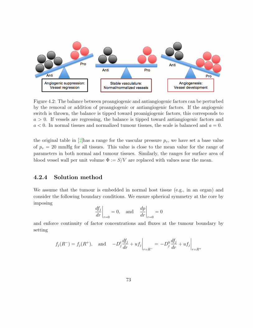
Figure 4.2: The balance between proangiogenic and antiangiogenic factors can be perturbedby the removal or addition of proangiogenic or antiangiogenic factors. If the angiogenicswitch is thrown, the balance is tipped toward proanigiogenic factors, this corresponds toa > 0. If vessels are regressing, the balance is tipped toward antiangiogenic factors anda < 0. In normal tissues and normalized tumour tissues, the scale is balanced and a = 0.

the original table in [2]has a range for the vascular pressure pv, we have set a base value

of pv = 20 mmHg for all tissues. This value is close to the mean value for the range of

parameters in both normal and tumour tissues. Similarly, the ranges for surface area of

blood vessel wall per unit volume Φ := S/V are replaced with values near the mean.

4.2.4 Solution method

We assume that the tumour is embedded in normal host tissue (e.g., in an organ) and

consider the following boundary conditions. We ensure spherical symmetry at the core by

imposingdfjdr

∣∣∣∣r=0

= 0, anddp

dr

∣∣∣∣r=0

= 0

and enforce continuity of factor concentrations and fluxes at the tumour boundary by

setting

fj(R−) = fj(R

+), and −Dtj

dfjdr

+ ufj

∣∣∣∣r=R−

= −Dhj

dfjdr

+ ufj

∣∣∣∣r=R+

73

along with continuity of IFP and IFV by setting

p(R−) = p(R+), and u(R−) = u(R+).

The latter condition is equivalent to

−Khdp

dr

∣∣∣∣r=R−

= −Ktdp

dr

∣∣∣∣r=R+

,

where typically Kh = Kt (based on [2, Table 3]). We also require that factor concentrations

and the pressure reach steady state as we move away from the tumour and so impose

limr→∞

dfjdr

= 0, limr→∞

dp

dr= 0.

This ensures that the factor concentration reaches steady state f sj and that p(r) → 0 for

large r (achieved by setting phe = 0).

The analytical solution for nondimensionalized pressure, p, can be obtained by solving

(3.13). This along with the solution for nondimensional IFV, u = uR/(Ktpe), was derived

by Jain et al. [67] (see Section 3.1.2). The radial profile for p is then used to numerically

solve for the factor concentrations in (4.3). Due to the non-linearity of (4.3), we could no

longer rely on the analytical technique shown in 3.3, instead we had to develop a numerical

scheme to approximate their solutions. The corresponding matrix inversion problem was

performed using a second-order finite difference scheme in MATLAB [139].

4.3 Results

Interstitial pressure and velocity profiles are obtained from solving (3.13); these profiles

can be viewed in Figures 3.1a and 3.1b, respectively. Most notably, as the parameter αtincreases, the pressure reduction at the tumour rim becomes more drastic and the IFP

inside the tumour increases. Equivalently, as αt increases, the interstitial fluid velocity

reaches a higher and sharper peak at the tumour rim while remaining zero at the core.

We solve (4.3), with the boundary conditions given in the previous section and the ana-

lytical pressure profiles, to determine AGF concentrations and subsequently the imbalance

factor in (4.4). First, we compare the results of our model with those of the model without

74

r

fj

1

2

3

4

5

6

0 0.5 1 1.5 2

no convectionconvection

(a) Nondimensional AGF concentrations fj .

r

a

−0.1

0

0.1

0.2

0.3

0.4

0 0.5 1 1.5 2

no convectionconvection

(b) Angiogenic activity a.

Figure 4.3: Comparing 4.3a nondimensionalized proangiogenic (solid) and antiangiogenic(dashed) growth factor concentrations and 4.3b angiogenic activity for the model withoutconvection (u = 0) and with convection (αt = 14, αh = 2). With the addition of convection,the area of angiogenic stimulation is larger and more pronounced

r

fj

1

2

3

4

5

6

0 0.5 1 1.5 2

αt = 2αt = 6αt = 14

(a) Nondimensional AGF concentrations fj .

r

a

−0.1

0

0.1

0.2

0.3

0.4

0 0.5 1 1.5 2

αt = 2αt = 6αt = 14

(b) Angiogenic activity a.

Figure 4.4: Effect of varying the vascular hydraulic permeability, Lp (mm/s/mm Hg), inthe tumour tissue on 4.4a AGF concentrations and 4.4b angiogenic activity. The valuesof αt=2, 6, 14 correspond to Lp=3.6×10−7, 3.7×10−6, 1.86×10−5 mm/s/mm Hg. Theparameter for host tissue was fixed at αh = 2. This changes the shape of the resultingpressure profile and thus the interstitial fluid velocity.

75

convection [1]; the only difference between the curves corresponding to no convection in

Figure 4.3a and the original results of [1] is that we consider a tumour radius of 4mm

(up from 2.5mm) in order to remain consistent with the parameter estimates from [2] that

are used for the pressure model. For our model with convection, the angiogenic activity

still reaches a maximum at the tumour boundary, and the region of angiogenic suppres-

sion persists at the tumour core. However, we now observe a higher peak of angiogenic

tendency at the rim and a larger area of angiogenic stimulation, see Figure 4.3b. This is

due to the larger difference between the proangiogenic and antiangiogenic growth factor

concentrations near the boundary, a result of these factors being pushed out of the tumour

core into the surrounding normal tissue as can be seen in Figure 4.3a. However, as we will

see, the transition from a system without convection to a system with convection is not

straightforward.

By changing the values of αt, we can see the effect of varying only the contribution

of the pressure profile on the model. This can be achieved by modifying Lp, Φ, or R.

However, we wish to consider a fixed tumour radius and surface to volume ratio, so we

will consider changes in αt to correspond to changes in the values of Lp only. Note that

we cannot analyze the contribution of IFP alone by modifying K since this would also

change the value of the nondimensional convection parameter in (4.3). Similarly, we can

look at the contribution of the nondimensional convection parameter alone by modifying

pe. Finally, we will consider the effect of changing the hydraulic conductivity K which

simultaneously decreases αt and increases Kj affecting the pressure profile and the rate of

convection.

We consider first the effects of varying only the pressure parameter αt (for fixed αh = 2),

which, as stated above, we will assume is achieved by changing Lp, leaving the rest of the

parameters fixed as in Table 4.2. As can be seen in Figures 4.4a and 4.4b, the results

suggest that altering the pressure parameter leads to different angiogenic behaviour in the

tumour. Indeed, the region of angiogenic suppression (a < 0) at the core is not conserved

for all values of αt between the cases of negligible convection (αt ≈ 0) and non-normalized

tumour tissue (αt = 14). Thus, the behaviour is more complicated than that observed by

modifying the convection parameter via pe or both pressure and convection parameters via

K (see Figures 4.5a and 4.5b and the Discussion below). For values of αt close to zero,

there is a region of angiogenic suppression (a < 0) at the core and stimulation (a > 0) at

the rim (similar to the no convection case in Figure 4.3b). For midrange values of αt the

tumour can experience global angiogenesis (i.e., a > 0 for all r ∈ [0, R]). That is, instead

76

of the proangiogenic and antiangiogenic concentrations balancing inside the tumour, the

antiangiogenic factor concentration lies entirely below that of the proangiogenic factor

concentration. Considering αt = 2, this assumes that the tumour tissue has the same

value of Lp as normal tissue. Indeed, the angiogenic activity in this case remains constant

inside the tumour due to a consistent difference between the two factor concentrations

leading to global angiogenesis. For the parameters corresponding to normalized tumour

tissue (αt = 6), we see an intermediate behaviour where global angiogenesis occurs, but

the activity at the core is much lower than at the tumour rim. For high values of αt(e.g., αt = 14), the core once again becomes a region of suppression but with higher levels

of angiogenic activity occurring close to the tumour rim as previously observed in the

convection case in Figure 4.3b. While different angiogenic profiles are obtained, it remains

true that the angiogenic activity at the tumour rim increases with αt.

As expected, fixing αt = 14 and increasing pe, thereby increasing the convection of

factors leads to higher concentrations outside the tumour (see Figure 4.5b) and larger

concentration differences at the rim. This coincides with an increase of angiogenic activity

at the tumour rim. For the parameters considered and a reasonable range of pe, the tumour

exhibits only focal suppression. Other activities can be achieved but require a modification

of the AGF parameters (see the sensitivity analysis in Figures 4.6a–4.6c).

Finally, we consider varying K, an increase in this parameter value leads to decreased

αt and αh along with increased values of the convection parameters Kj. This essentially

compounds the effects observed in Figures 4.4a, 4.4b and 4.5a leading to elevated levels of

angiogenesis inside the tumour (from decreasing αt) and at the tumour rim (from increasing

pe); refer to Figure 4.5b.

Following Ramanujan et al. [1], we performed a sensitivity analysis on AGF production;

see Figures 4.6a–4.6c. We generalize their results by fixing one of the parameters of interest

(αt, pe, and K) and analyze results over a large range of tumour production values (gtp and

gta). Focal suppression occurs between lines of the same colour, global suppression occurs

above this region (high gta, low gtp), and global angiogenesis occurs above (low gta, high

gtp). The results indicate that focal suppression is observed only for a narrow sliver of the

parameter space. This is realistic since one would assume that the behaviour is sensitive

to the balance of these factors production rates. As expected, the behaviour is not as

sensitive to varying the host production parameters as it is to tumour production (results

are not shown).

Figure 4.6a shows how this sensitivity changes when varying αt. As αt increases, the

77

r

fj

1

2

3

4

5

6

0 0.5 1 1.5 2

pe = 5pe = 15pe = 35

r

a

−0.1

0

0.1

0.2

0.3

0.4

0.5

0 0.5 1 1.5 2

(a) The effect of varying pe (mmHg) on nondi-mensional AGF concentrations fj and angio-genic activity a (inset) for fixed Lp = 1.86 ×10−5 mm/s/mm Hg. This alters the value ofthe convection parameters Kj .

r

fj

1

2

3

4

5

6

0 0.5 1 1.5 2

K = 8 × 10−6

K = 2.5 × 10−5

K = 8 × 10−5

r

a

−0.1

0

0.1

0.2

0.3

0.4

0.5

0 0.5 1 1.5 2

r

fj

1

2

3

4

5

6

0 0.5 1 1.5 2

K = 8 × 10−6

K = 2.5 × 10−5

K = 8 × 10−5

r

a

−0.1

0

0.1

0.2

0.3

0.4

0.5

0 0.5 1 1.5 2

(b) The effect of increasing K (mm2/s/mmHg)on nondimensional AGF concentrations fj andangiogenic activity a (inset) for fixed Lp =1.86 × 10−5 mm/s/mm Hg and pe = 10.9 mmHg. This simultaneously decreases αt and in-creases Kj leading to altered IFP and elevatedconvective transport.

Figure 4.5: Nondimensional AGF concentrations fj under parameter changes. Inset: An-giogenic activity a.

78

region of focal suppression widens from a very narrow region to encompass more of the

parameter space above and below this region. For different values of pe, we notice little

movement in the boundary between focal suppression and global angiogenesis while the

boundary between focal suppression and global suppression increases with pe (see Figure

4.6b). Finally, for K, we see a combination of these effects; the region where focal suppres-

sion and peripheral stimulation occur is widening and drifting towards the top left corner

of Figure 4.6c (high gta, low gtp). Parameter values that correspond to focal suppression

switch to values corresponding to globally angiogenic behaviour when the convection term

is added. Also shown in these graphs are the precise points in parameter space correspond-

ing to the tumour production values gtp = 349 and gtp = 279; this will be discussed further

in the following section.

4.4 Discussion

αt gtp = 349 (no treatment) gtp = 279

2 Global angiogenesis Global suppression6 Global angiogenesis Focal suppression14 Focal suppression Focal suppression

Table 4.3: Angiogenic activity resulting from cytotoxic therapy (see Figure 4.7a).

We have presented a mathematical model to study the effects of interstitial convection

on proangiogenic and antiangiogenic factor concentrations in tumour and surrounding host

tissue, and from this determined the overall angiogenic activity of the tumour. The re-

sulting AGF concentration profiles agree qualitatively with experimental observations that

show the highest concentrations in the core of the tumour, decreasing as one approaches

the tumour rim [126]. Also, the resulting angiogenic behaviours, including suppression at

the tumour core and maximal angiogenic stimulation near the tumour rim, correspond with

experimental observations such as tumour perfusion [140]. The imbalance between proan-

giogenic and antiangiogenic factors provides an empirical explanation for observed angio-

genic activity and could be correlated with resulting tumour necrosis or growth. While the

precise effects of IFP and factor convection on the angiogenic activity of tumours have not

been experimentally verified, our results indicate that an IFP gradient could significantly

influence suppression and stimulation of angiogenesis in a tumour.

79

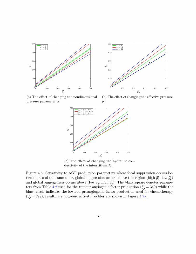
g tp

gt a

0

100

200

300

400

500

0 100 200 300 400 500

αt = 2αt = 6αt = 14

(a) The effect of changing the nondimensionalpressure parameter α.

g tp

gt a

0

100

200

300

400

500

0 100 200 300 400 500

pe = 5pe = 15pe = 35

(b) The effect of changing the effective pressurepe.

g tp

gt a

0

100

200

300

400

500

0 100 200 300 400 500

K = 8 × 10−6

K = 2.5 × 10−5

K = 8 × 10−5

(c) The effect of changing the hydraulic con-ductivity of the interstitium K.

Figure 4.6: Sensitivity to AGF production parameters where focal suppression occurs be-tween lines of the same color, global suppression occurs above this region (high gta, low gtp)and global angiogenesis occurs above (low gta, high gtp). The black square denotes parame-ters from Table 4.2 used for the tumour angiogenic factor production (gtp = 349) while theblack circle indicates the lowered proangiogenic factor production used for chemotherapy(gtp = 279); resulting angiogenic activity profiles are shown in Figure 4.7a.

80

While not explicitly included, the effect of antiangiogenic treatments can be ascertained

in this model since it has been shown that the value of αt decreases when the vasculature

is normalized due to the application of, for instance, anti-VEGFR-2 [130]. The value of αtcan decrease through any combination of decreasing Φ, Lp, or R, all of which could occur

as a result of antiangiogenic therapy. Φ decreases as blood vessels are destroyed and/or

remodelled due to the administration of an antiangiogenic drugs (in this case, there is

less area of vessel wall per unit of tumour volume). The radius R decreases indirectly;

as tumour vessels regress, tumour cells are deprived of oxygen and consequently become

hypoxic or necrotic. Moreover, the vessel permeability Lp could decrease due to judicious

application of antiangiogenic agents (vessel normalization, [35]). The pressure parameter

αt could also be decreased by increasing the hydraulic conductivity K, an effect that would

be somewhat counterbalanced by the corresponding increase in the convection parameter

(refer to Figure 4.5b). However, K could be increased by administering enzymes that

degrade the extracellular matrix (ECM), which subsequently decreases the flow resistance

in the interstitium [137]. Overall, strategies that lead to the reduction of the parameter αtresult in decreased IFP, which influences tumour angiogenesis activity. As shown in Figure

4.4b and discussed in the previous section, the changes in the interstitial fluid velocity from

decreasing αt reduces the angiogenic activity at the rim and produces a more constant level

of angiogenic activity inside the tumour. On the other hand, one could also consider the

administration of antiangiogenic agents by decreasing the concentration of proangiogenic

factors through an increase of their degradation (or deactivation) constant (see Figure

4.7b). This increase in deactivation should take into account that most antiangiogenic

treatments only affect a single factor or a family of growth factors.

One can consider the effect of cytotoxic therapies by noting that the application of

either chemotherapy or radiotherapy reduces the number of tumour cells leading to less

proangiogenic factor production (Figure 4.7a); this is achieved by lowering the parameter

gtp. We considered the reduction of this production rate and the movement through param-

eter space is shown in the sensitivity diagrams (Figures 4.6a–4.6c). In Figure 4.7a, we can

observe that the resulting angiogenic behaviour depends on the value of αt as summarized

in Table 4.3. The effect of cytotoxic therapies either on tumour cells or blood vessels could

also reduce the pressure due to increased interstitial space; this could be included in our

model by, for instance, increasing K (Figure 4.5b). The effects of cytotoxic treatments

could also be included by reducing the tumour radius R. Combinations of antiangiogenic

therapy and chemotherapy could be considered by performing the aforementioned param-

81

r

a

−0.3

−0.2

−0.1

0

0.1

0 0.5 1 1.5 2

αt = 2αt = 6αt = 14

(a) Applying chemotherapy leads to cell deathand hence decreased tumour proangiogenicproduction (from gtp = 349 to gtp = 279).

r

a

−0.3

−0.2

−0.1

0

0.1

0.2

0.3

0 0.5 1 1.5 2

αt = 2αt = 6αt = 14

(b) Applying antiangiogenic therapy inacti-vates proangiogenic factors leading to in-creased tumour proangiogenic deactivation(from ktp = 58 to ktp = 70).

Figure 4.7: The effects of treatment on angiogenic behaviour of tumours.

eter changes simultaneously; these changes compound the effects leading to even further

reduced angiogenic tendency.

Decreasing the IFP prior to or simultaneously with other therapies is an important

concern in cancer treatment since the flow of interstitial fluid out of the tumour prevents

drugs from penetrating the tumour bulk. While the various effects of antiangiogenic treat-

ments (decreasing Φ, Lp, or R) or ECM-degrading enzymes (increasing K) all reduce αtand hence pressure, there are other independent mechanisms that could also elicit reduc-

tions in pressure. For instance, reducing pe would reduce IFP. This could be achieved by

reducing the vascular pressure pv, which can be readily accomplished by decreasing the

resistance of blood. Clinically, decreasing the viscosity of the blood or normalizing the tu-

mour vasculature would accomplish the goal of less resistance [137]. The effects of changing

pe are shown in Figure 4.5a as decreasing the effective pressure leads to diminishing levels

of angiogenic activity at the rim.

82

4.5 Conclusions

By taking into consideration the different angiogenic behaviours exhibited by modifying

any of the key parameters involved in the pressure model, we can establish an alternate

(or more likely, complementary) mechanism for these changes. Whereas it was previously

hypothesized [1] that the production, degradation, and diffusion of the AGFs were primar-

ily responsible for the overall angiogenic behaviour, we have exhibited that changes in the

tumour tissue physiology could also elicit these changes. The interplay between the two

groups of parameters, those related to AGF properties that determine AGF concentrations

and those corresponding to the tumour physiology that determine interstitial fluid pres-

sure, should be further investigated with more detailed modelling and experimental work.

We emphasize that it was never the goal of this work to quantitatively predict concen-

trations of specific AGFs or to model the process of angiogenesis but rather to emphasize

the importance of tumour tissue properties and macromolecule convection on angiogenic

behaviour.

One should note that there are limitations to our mathematical model, many of which

have been mentioned during the model development. These include the existence of two

distinct groups of AGFs, the specific functional form of our angiogenic activity measure and

the distributed fluid source terms. Most prominent among these various assumptions are

those of spherical symmetry and homogeneity of tissues and environment [1]. The other

main limitation is the assumption of constant parameter values both inside the tumour

and in the host tissue, or even the constant values assumed across this boundary. These

assumptions make the modelling and computation tractable especially since physiological

parameters as functions of radial distance are uncommon in the literature. However, our

computational approach can readily be extended to include aspects of the heterogeneous

tumour microenvironment upon availability of relevant experimental data. Finally, we

propose that an experimental study measuring both interstitial fluid pressure and quanti-

ties associated with AGF concentrations or angiogenic activity (such as vessel density or

perfusion) would help to validate our qualitative model predictions.

83

Chapter 5

Microvessel Models for Cell

Metabolism and pH

This chapter analyzes microvessel models for cell metabolism and pH. Cell metabolism in a

tumour is enabled by angiogenesis that brings the oxygen, glucose, and other metabolites

necessary to cell survival. First, we will propose a model for metabolic symbiosis that

includes glucose, lactate and oxygen concentrations in a tissue that utilizes glucose-fuelled

and lactate-fuelled respiration along with glycolysis. The ATP production in tissue un-

der various metabolic inhibitor treatments are considered and the importance of glycolysis

shutdown is emphasized. A simpler version of this metabolic model that includes oxygen-

fuelled respiration and glycolysis is coupled to a cellular buffering model that requires the

addition of carbon dioxide, bicarbonate and H+ to the model. The effects of hypoxia and

cell permeability are observed in this context. We also show results for adding convec-

tive transport, which show that unlike the macroscopic model considered in the previous

chapter, this is a diffusion-dominated system.

5.1 Introduction

The extensive metabolic requirements for cancer cell proliferation coupled with the harsh

microenvironment in solid tumours culminates in a highly adaptive and complex network

for cellular energy production. The genetically altered metabolic behaviour of cancer cells

84

has led to a number of emerging metabolic paradigms, in addition to those that are uni-

versally exhibited in both cancerous and normal cells. We will investigate this complex

metabolic behaviour by formulating a minimal mathematical model that includes the es-

sential metabolites of glucose, lactate and oxygen in the tissue surrounding a microvessel.

This model will enable the quantification of various behaviours, such as the symbiotic

relationship that exists between lactate-producing glycolytic cells and lactate-consuming

respiratory cells, and the analysis of metabolic dependence on various physiological con-

ditions such as hypoxia and induced metabolic inhibition. Metabolic inhibition including

glycolytic inhibitors among many others targets could be very important for cancer treat-

ment since an ATP deficit can induce apoptosis [141]. The key consideration for addressing

this problem with mathematics is the formulation of nutrient consumption rates that en-

compass the various primary facets of cancer cell metabolism and their corresponding ATP

yields.

In normal well-oxygenated tissues the primary source of ATP is the process of cellular

respiration. The complete conversion of glucose to carbon dioxide and water has an ideal

yield of at most 29 ATP [20] (although the reactions contained in C.4 suggest a yield as

low as 24.25). The preliminary stage of cellular respiration is glycolysis, the conversion

of glucose to pyruvate; this process directly produces 2 ATP. In hypoxic conditions this

pyruvate is preferentially converted into lactate via the enzyme lactate dehydrogenase

(LDH) to regenerate the essential cofactor NAD+. In oxygenated conditions this pyruvate

is transported across the inner mitochondrial matrix where it is decarboxylated and enters

the citric acid cycle; the citric acid cycle directly generates 2 more ATP per glucose. The

primary energy payoff is a result of cofactor oxidization that enables the electron transport

chain to establish a proton gradient across the inner mitochondrial matrix. ATP synthase

utilizes this electrochemical gradient to drive the phosphorylation of approximately 25

additional ATP per glucose molecule.

The aforementioned universal traits that cancer cells and normal cells share include

cellular responses to various levels of oxygen, lactate or glucose. Examples include a

Crabtree-like effect and a Pasteur-like effect [4]. The Crabtree-like effect is when oxygen

consumption decreases as glucose concentration increases. This can be explained by an

increasing reliance on glycolysis for ATP when hyperglycaemic conditions are encountered.

The Pasteur-like effect is decreased glucose consumption as oxygen increases. This is due

primarily to the inhibition of various metabolic steps by the presence of elevated ATP and

other intermediaries. However, cancer cells are unique in that they preferentially utilize

85

Figure 5.1: The spatial relationship between the cell populations in the model. When theglucose and oxygen concentrations are highest near the vessel wall, the cells preferentiallyutilize glucose-fuelled respiration. When the oxygen supply is depleted far from the vessel,the cells rely on glycolysis. The glycolytic cells produce large quantities of lactate which areconsumed by cells at intermediary distances. These cells are participating in a behaviourthat we will refer to as metabolic symbiosis.

glycolysis, even in the presence of oxygen, coined aerobic glycolysis. This phenomenon

is generally referred to as the Warburg effect whereby cells rely primarily on glycolysis

even in the presence of sufficient oxygen to perform respiration [22]. There is a perceived

inefficiency of this metabolic strategy, namely the dramatically reduced ATP yield, just

2 per glucose instead of 29, however, it has the benefits of faster ATP production and

it is likely that much of this glucose is being consumed for proliferative [23] (e.g. by the

pentose phosphate pathway) purposes. In addition to the typical glycolytic phenotype

exhibited in many cancers, there is also a developing story of a co-operative relationship

existing between aerobic and anaerobic cancer cells. The lactate necessarily produced

by glycolytic cells is being pushed back into the respiratory cycle by being converted

into pyruvate (summarized in [142, 143]); this spatial relationship is shown in Figure 5.1.

Lactate consumption has been observed in vitro in various models [144, 145] as well as in

vivo as early as the early 80s [26]. However, a renewed interest in the topic was piqued when

Sonveaux et al. [27] showed that reducing lactate uptake by cancer cells led to hypoxic cell

death, a particularly difficult subpopulation to target using traditional methods.

Metabolic phenomena have been studied in great detail by mathematical models, but

models of tumour metabolism rarely include the interaction of the transport mechanisms

86

of microvessels with the localized metabolic behaviour of cells. In the section to follow,

we will develop a mathematical model that describes the concentrations of molecules that

are important to cellular metabolism in the tissue around a single three-dimensional vessel

that exhibits diffusion-dominated interstitial transport. We will then use this model to

demonstrate how the properties of the tumour cell population, such as glucose, lactate

and oxygen consumption rates, affect hypoxia and ATP production around a single vessel.

The effects of metabolic inhibitors will be investigated by parameter changes that could be

elicited by the application of glycolysis inhibitors, lactate dehydrogenase (LDH) inhibitors

or respiratory inhibitors. We are interested in those metabolic inhibitors that could cripple

the cells’ ability to produce ATP. Furthermore, these micrometer scale predictions give an

indication of local shifts in cell metabolism, which could aid in developing combination

treatments that can simultaneously hinder multiple metabolic pathways in tumours. Our

simulations show that treatments targeting glycolysis via glycolytic enzyme inhibition or

LDH inhibition, which have been thoroughly investigated [146, 147, 148], could be the

most successful metabolic suppression strategy.

5.2 Mathematical model

A model to describe the concentrations of the major players in the metabolic pathways

of respiration and glycolysis, will be outlined here. Its origins lie in a metabolic model

developed by Casciari et al. [3] that was subsequently applied on the microscale by [25].

The functional forms for the production rates are similar to those proposed by Mendoza

et al. [90].

In hypoxic and anoxic conditions, cells must partially or exclusively rely on metabolic

pathways, such as glycolysis, that do not require oxygen for ATP production. In glycolysis,

the preliminary stage of respiration, a single glucose molecule (C6H12O6) yields 2 ATP,

which we will denote under the reaction arrow with a boxed ATP yield number, with the

byproducts of lactate and a proton. Denoting glucose by G and lactate by L−(C3H5O−3 ),

the net reaction is

GkG

GGGGGGA

22L− + 2H+, (5.1)

where kG (mM/s) is the rate of glucose consumption by glycolysis that results in lac-

tate formation. The accumulation of these hydrogen ions in a solid tumour is a primary

87

contributor to tumour acidosis.

In the presence of oxygen (O2), glycolysis is typically followed by the rest of the respi-

ratory process with an ideal energy yield of approximately 29 ATP molecules with carbon

dioxide (CO2) and water (H2O) as the only byproducts. The constituent reactions can be

found in C.4 and the simplified summary reaction is

G + 6O2

kOGGGGGGA

296CO2 + 6H2O, (5.2)

where kO is the rate of glucose consumption that results in cellular respiration.

To represent the metabolic symbiosis between cells primarily producing energy via

glycolysis and those consuming lactate in well-oxygenated areas, we will link the above

two reactions with the lactate-consuming net reaction

L− + H+ + 3O2

kLGGGGGGA

13.53CO2 + 3H2O, (5.3)

where kL is the rate of lactate consumption. This summarizes the re-entry of lactate, via

conversion to pyruvate, into aerobic respiration that yields 13.5 ATP per lactate molecule.

The relationships between the summary reactions included in the model are given in Figure

5.2. For details on the omitted intermediary steps and derivations of these summary

reactions and ATP yields, see C.4.

Under the strictest assumptions, the only chemical species required for a mathematical

model are the three substrates required for the metabolic pathways in (5.1), (5.2) and (5.3).

We denote the concentrations of oxygen, lactate− and glucose in the extracellular space

by X = O, L, G, respectively, and their consumption rates per unit volume are denoted

by QX . These extracellular concentrations are modelled by conservation equations of the

form∂X

∂t+∇ · JX +QX = 0,

where JX is the flux of species X. In general, the flux can be given as a sum of convective,

migratory and diffusive elements. Due to the small molecular sizes of the molecules consid-

ered here, their transvascular and interstitial transport are diffusion-dominated. On larger

spatial scales, convection becomes an important transport mechanism for large molecules

88

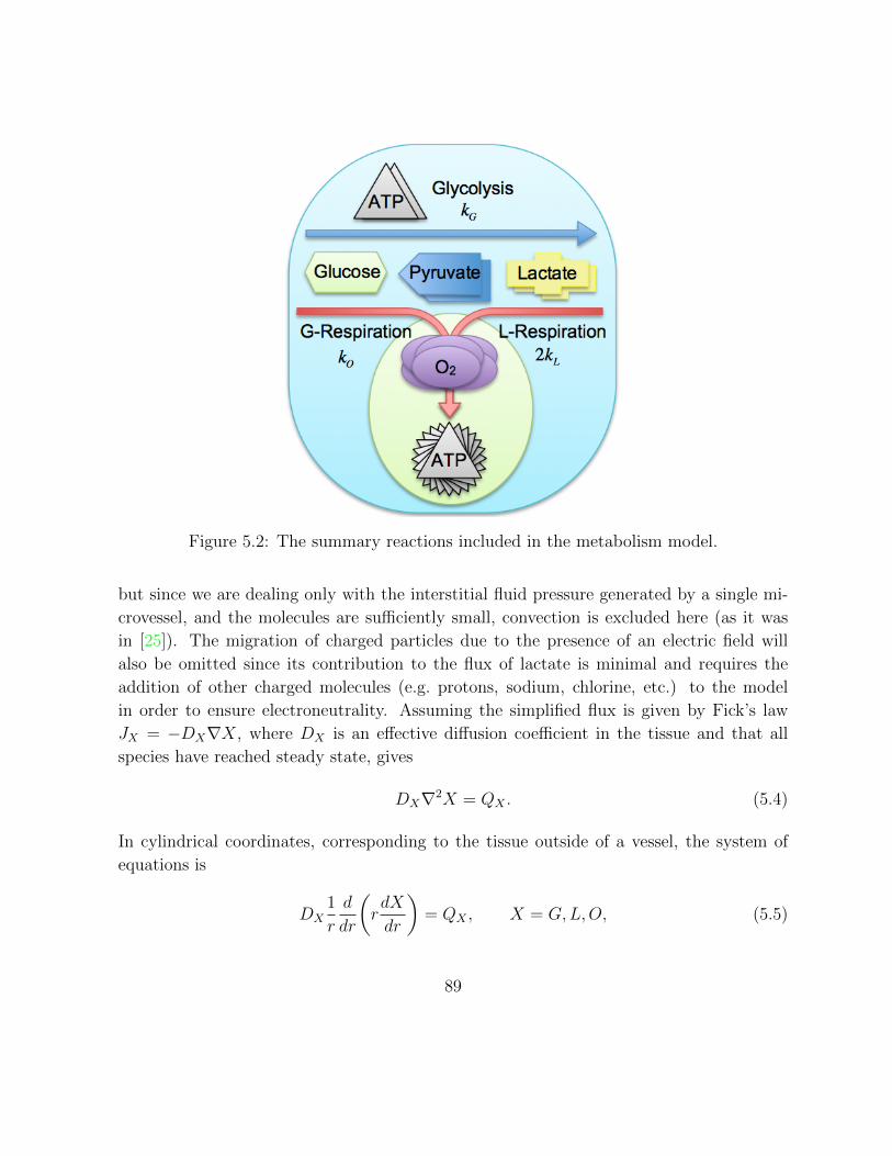
Figure 5.2: The summary reactions included in the metabolism model.

but since we are dealing only with the interstitial fluid pressure generated by a single mi-

crovessel, and the molecules are sufficiently small, convection is excluded here (as it was

in [25]). The migration of charged particles due to the presence of an electric field will

also be omitted since its contribution to the flux of lactate is minimal and requires the

addition of other charged molecules (e.g. protons, sodium, chlorine, etc.) to the model

in order to ensure electroneutrality. Assuming the simplified flux is given by Fick’s law

JX = −DX∇X, where DX is an effective diffusion coefficient in the tissue and that all

species have reached steady state, gives

DX∇2X = QX . (5.4)

In cylindrical coordinates, corresponding to the tissue outside of a vessel, the system of

equations is

DX1

r

d

dr

(rdX

dr

)= QX , X = G,L,O, (5.5)

89

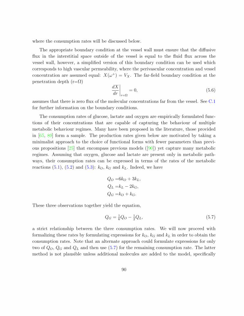
where the consumption rates will be discussed below.

The appropriate boundary condition at the vessel wall must ensure that the diffusive

flux in the interstitial space outside of the vessel is equal to the fluid flux across the

vessel wall, however, a simplified version of this boundary condition can be used which

corresponds to high vascular permeability, where the perivascular concentration and vessel

concentration are assumed equal: X(ω+) = VX . The far-field boundary condition at the

penetration depth (r=Ω)dX

dr

∣∣∣∣r=Ω

= 0, (5.6)

assumes that there is zero flux of the molecular concentrations far from the vessel. See C.1

for further information on the boundary conditions.

The consumption rates of glucose, lactate and oxygen are empirically formulated func-

tions of their concentrations that are capable of capturing the behaviour of multiple

metabolic behaviour regimes. Many have been proposed in the literature, those provided

in [65, 89] form a sample. The production rates given below are motivated by taking a

minimalist approach to the choice of functional forms with fewer parameters than previ-

ous propositions [25] that encompass previous models ([90]) yet capture many metabolic

regimes. Assuming that oxygen, glucose and lactate are present only in metabolic path-

ways, their consumption rates can be expressed in terms of the rates of the metabolic

reactions (5.1), (5.2) and (5.3): kO, kG and kL. Indeed, we have

QO =6kO + 3kL,

QL =kL − 2kG,

QG =kO + kG.

These three observations together yield the equation,

QG = 16QO − 1

2QL, (5.7)

a strict relationship between the three consumption rates. We will now proceed with

formalizing these rates by formulating expressions for kO, kG and kL in order to obtain the

consumption rates. Note that an alternate approach could formulate expressions for only

two of QO, QG and QL and then use (5.7) for the remaining consumption rate. The latter

method is not plausible unless additional molecules are added to the model, specifically

90

pyruvate, the molecular hub of these rates.

To establish kG, the rate of glycolysis that results in lactate production, above and

beyond the rate required as the pyruvate-producing preliminary step of respiration, we

must consider encompassing both normal cell behaviour and cancer cell behaviour. One

of the noted key differences between these cell types is the well-known Warburg effect

whereby cancer cells consume much more glucose, and preferentially utilize glycolysis even

in the presence of sufficient oxygen for respiration, a process dubbed aerobic glycolysis.

We propose the form

kG = BGG

G+ ΛOO +KG

,

where BG is the maximal rate, KG is the half-maximal concentration (in the absence of

oxygen) and ΛO is a novel parameter that can inhibit superfluous glycolysis in the pres-

ence of sufficient oxygen to produce ATP. In cancer cells exhibiting the Warburg effect

this parameter would be relatively small, as the glycolytic flux would be highly elevated

regardless of oxygen concentration, while in normal cells or cancer cells that do not prefer-

entially utilize aerobic glycolysis this parameter value would be relatively large, effectively

inhibiting glycolysis until hypoxic conditions are encountered.

For glucose and lactate-fuelled respiration we use a basic Michaelis-Menten expression

to express the dependence on oxygen concentration and a competitive expression to include

the proportion that is glucose-fuelled and lactate-fuelled. These rates are

kO = BO

(ΛGG

ΛGG+ ΛLL+ ΓG

)O

O +KO

, (5.8)

kL = BL

(ΛLL

ΛGG+ ΛLL+ ΓL

)O

O +KO

, (5.9)

respectively. The Michaelis-Menten half-maximal concentration for oxygen is KO, the

maximal rates for glucose and lactate consuming cells are BO and BL respectively, the

preference of cells to utilize glucose or lactate in respiration is parameterized by ΛG and

ΛL, and to ensure that these expression are defined near (L,G) = (0, 0), ΓG and ΓL are

constants that correspond to half-maximal rates in the absence of the other fuel (these will

be set to zero later but for generality are included here).

91

In summary, the consumption rates of the species in the model are:

QO =

(6BO

ΛGG

ΛGG+ ΛLL+ ΓG+ 3BL

ΛLL

ΛGG+ ΛLL+ ΓL

)O

O +KO

, (5.10)

QL = BL

(ΛLL

ΛGG+ ΛLL+ ΓL

)O

O +KO

− 2BGG

G+ ΛOO +KG

, (5.11)

QG = BO

(ΛGG

ΛGG+ ΛLL+ ΓG

)O

O +KO

+BGG

G+ ΛOO +KG

. (5.12)

Clearly these rates satisfy the aforementioned relation (5.7): QG = QO/6−QL/2.

In order to utilize the model, we require estimates of the diffusion coefficients and

vessel concentrations of the aforementioned molecular species along with the parameter

values contained in the functional forms for oxygen consumption (respiration) and lactate

production (glycolysis). The sheer volume of necessary parameters can be dramatically

reduced by first nondimensionalizing the system. This is a useful process for computational

and analytical reasons.

We can also rewrite the system of equations in a way more conducive to gaining some

analytical traction and simpler parameter estimation. Since the production rates of oxygen,

glucose and lactate satisfy the relation QG = QO/6 − QL/2, we can replace one of the

equations for these individual species with this relation, which we will evolve into a simpler

formula below. For concreteness we will omit the diffusion-reaction equation for glucose

and retain the equations for oxygen and lactate in the nondimensionalization below.

Nondimensionalizing concentrations by their vessel concentration VX , i.e. setting X =

VXx, and nondimensionalizing space by dividing the spatial variable r by a characteristic

length of r = 1 µm (but not changing its notation), gives the nondimensional system:

1

r

d

dr

(rdo

dr

)=

(6βo

g

g + λ`+ γg+ 3

β`α`αo

`

g/λ+ `+ γ`

)o

o+ κo, (5.13)

1

r

d

dr

(rd`

dr

)= β`

(`

g/λ+ `+ γ`

)o

o+ κo− 2βg

α`

g

g + δo+ κg, (5.14)

1

r

d

dr

(rdg

dr

)=αo6

1

r

d

dr

(rdo

dr

)− α`

2

1

r

d

dr

(rd`

dr

), (5.15)

where αx = dxvx (dx = DX/DG, vx = VX/VG), βx = BX/(DXVX), λ = Λv` (Λ = ΛL/ΛG),

δ = ΛOvo, κx = KX/VX and γx = ΓX/(VXΛX). In addition to these equations, we also

92

require the nondimensional version of the vessel boundary conditions, namely, x(ρ) = 1,

where ρ = ω/r; the far-field boundary condition is essentially the same:

dx

dr

∣∣∣∣r=P

= 0, (5.16)

where P = Ω/r.

First, integrating (5.15) over (r, P ) and enforcing the far-field boundary condition (5.16)

givesdg

dr=αo6

do

dr− α`

2

d`

dr. (5.17)

Now integrating the equations once more, this time over (ρ, r), and using the vessel bound-

ary condition gives

g(r) = 1− αo6

(1− o(r)

)+α`2

(1− `(r)

). (5.18)

This expression for glucose enables a simpler system to solve numerically for `(r) and o(r).

These solutions also hold in a Cartesian geometry, as was considered by Molvian et al. [25]

to correspond to the geometry of window chambers used by Helm et al. [5]. See C.2 for

additional details.

To calculate the ATP turnover rate, an analysis of the stoichometry of all the involved

processes at physiological pH is required. For glycolysis, 2 ATP are produced while for the

full process of respiration including glycolysis, approximately 29 ATP are produced [20],

see C.4 for summary biochemical reactions. This ATP yield is less than the yield assumed

by previous models, e.g. [65] assumed the classical 38, [25] assumed an intermediary 36,

while [63] assumed 32; these are all more than the accepted ideal yield of approximately

29 [20]. While this accepted value will be used to generate the results that follow, I have

also calculated a novel estimate of 24.25 ATP/glucose based on the reactions contained in

C.4. The discrepancy arises from the uncertainty associated with the efficiency of ADP

phosphorylation and processes such as ATP and pyruvate transport that effect the elec-

trochemical gradient across the inner mitochondrial membrane. Most significantly, the

multiple protonated states of phosphate, which is critical to intercellular buffering is in-

cluded in the summary reaction for phosphate transport across the inner mitochondrial

wall. The results calculated below have all been recalculated using this novel estimate in

C.6.

In terms of the reaction rates for the processes considered here for glycolysis (kG),

93

glucose-fuelled respiration (kO) and lactate-fuelled respiration (kL), the production rate of

ATP PATP is given by:

PATP = 2kG + 29kO + 13.5kL. (5.19)

The total production rate in the tissue space is characterized by the normalized value

Φ =

∫ P

ρ

PATP rdr. (5.20)

The total production rate is the triple integral over a unit of tissue defined by a uniform

cylindrical annulus of height ∆z with inner radius ρ and outer radius P , so the parameter

of interest is normalized by 2π∆z. This value is used to indicate the relative contributions

of the metabolic pathways.

5.2.1 Parameter estimation

There is no single study that has measured the apparent diffusion coefficients of oxygen,

glucose and lactate in the same type of tissue. In general, these apparent diffusion coef-

ficients may exhibit spatial-dependence due to changes in temperature, tissue properties

and molecular concentrations but for simplicity, we have assumed that they are constant

in the tissue surrounding a blood vessel. The diffusion coefficients will remain fixed for

the simulations presented here and were chosen for consistency with previous modelling

attempts (e.g. [64, 3, 25, 65, 63, 89]); they are given in Table 5.1 along with the other

model parameters.

The base case for vessel concentrations considers a slightly hypoglycaemic condition of

2 mM since glucose consumption is highly upregulated in tumours. For reference, a normal

fasting concentration of glucose is approximately 5 mM. It would be reasonable to consider

hyperglycaemic conditions that could arise locally in a tumour but for simplicity we will

neglect this consideration in the present study. For lactate we consider an elevated level of

2mM since cancer cells are performing increased glycolysis. If it is being consumed as the

primary respiratory fuel, it could be lower. A normal resting level is 1 mM of lactate. The

oxygen concentration will be taken to be consistent with the hypoxic conditions measured

by Helmlinger et al. [5]. They found the average partial pressure of oxygen in the tumour

vessel to be 13.5 mmHg [5]. Henry’s Law relates this partial pressure to the molar concen-

tration via a proportionality constant, known as the solubility coefficient, denoted by SO

94

Parameter Value Units Referenceω 11.5 µm [149]Ω 401.5 µm [25]a

VO 1.43×10−2 mM [5]VL 2 mM [25]VG 2 mM this workDO 1820 µm2/s [116]DL 177 µm2/s [3]DG 105 µm2/s [105]KO 2×10−4 mM [25]KG 5.0×10−2 mM [25]BO 2.32×10−4 mM/s this workb

BL 4.63×10−4 mM/s this workb

BG 2.8×10−3 mM/s this workc

ΛO 4×103 - this workΛ 1 - [90]

ΓL 0 mM this workΓG 0 mM this work

Table 5.1: Fixed parameter values for physiological, molecular and metabolic parametersfor the ‘base case’ simulation.a 401.5 is chosen for numerical convenience (400 was used in [25]). Evidence for steadystate achieved at this distance is given in [5] where oxygen and pH have reached steadystate.b Numerical fit based on data from [5]. Details in C.3. These values satisfy 6BO = 3BL =pO.c This maximum glucose consumption rate is assumed to be approximately 3 × pO, themaximum oxygen consumption rate. This is similar to the relationship that exists betweenconsumption rates in [4].

(mM/mmHg). At 37 C the solubility of oxygen of DS-carcinosarcoma in the rat kidney

is SO = 1.05× 10−3 mM/mmHg [117]; this yields VO ≈ 1.43× 10−2 mM.

The consumption and production rate parameters are typically varied over large ranges

as is commonly done since these can vary widely depending on the tumour type, e.g. [90].

However, we will enforce one condition to remain consistent with the oxygen profiles in [5].

Performing a least squares fitting to this spatial data, the maximum oxygen consumption

rate is approximately pO = 1.39 × 10−3 mM/s, the details are outlined in C.3. We will

95

utilize this value to fix BO and BL, the maximum consumption rates of glucose-fuelled and

lactate-fuelled respiration respectively. We will ensureQO ≤ pO by taking pO = 6BO = 3BL

which implies that the maximal oxygen consumption rate is the same regardless of whether

lactate or glucose is the respiratory fuel. There are cancer cell lines, namely SiHa cervix

cancer cells [27] and C6 glioma cells [150], which have been shown to temporally obey the

relation 2BO = BL [90]; there are others where BO ≈ BL (e.g. WiDr colon cancer cells

[27]) or 3BO ≈ BL (e.g. LN18 and LN229 glioblastoma cells [151]) [90].

While the system given above is widely applicable, it can be argued that in the interest

of further parameter reduction, the constants γg and γ` are superfluous in this scenario

where ` never approaches zero. Thus, we will take γg = γ` = 0. This reduces our nondi-

mensional parameters to a total of 10.

5.3 Results and discussion

5.3.1 Base case

We will first examine how our model captures the behaviour of metabolic symbiosis in tu-

mours. Using the parameters given in Table 5.1, we numerically solve the nondimensional

system given by (5.13) and (5.14). The corresponding glucose concentration is found by

using the explicit formula (5.18). The solutions for the nondimensional oxygen, lactate

and glucose concentrations are given in Figure 5.3. The oxygen concentration decreases

to anoxic values approximately 100 µm away from the vessel as expected. The glucose

concentration also decreases as it is consumed by respiratory cells near the vessel and then

predominantly consumed by glycolytic cells further from the vessel. The lactate concen-

tration increases over double its vessel concentration as it is produced by glycolytic cells

at a much higher rate than it is consumed by lactate-fuelled cells. These observations are

complemented by consideration of their consumption rates shown in Figure 5.4. Oxygen

is consumed for the first 150 µm outside of the vessel and as it decreases you can clearly

see the glucose consumption rate ramp up in response to increased glycolytic activity. The

lactate consumption rate is negative (implying production) everywhere except for directly

adjacent to the vessel where there is very little glycolysis occurring. The positive contribu-

tion of lactate consumption to the total consumption rate is washed out as the glycolytic

production rate is much higher. The energetic landscape of the base case considered here

96

0 50 100 150 200 250 3000

0.5

1

1.5

2

2.5

r (µm)

No

nd

ime

nsio

na

l co

nce

ntr

atio

n

oℓg

Figure 5.3: Solution to base case boundary value problem. Nondimensional oxygen andglucose concentrations decrease due to consumption. Lactate increases to almost double itsvessel concentration since it is produced by glycolysis at a higher rate than it is consumedby respiration due to a limiting oxygen concentration. This image has been spatiallytruncated to 300 µm since the concentrations are approximately constant after this point.

are given in Figure 5.5 where the contributions of the three cell populations’ metabolic

pathways are given as areas under the total ATP turnover rate. Glycolysis dominates

the total ATP production in hypoxic and anoxic regions while glucose-fuelled respiration

occurs sparingly near the blood vessel. The lactate-fuelled cell population, sandwiched

between these glucose consuming cells are utilizing the byproduct of the glycolytic cells

while there is still sufficient oxygen. Before analyzing the effects of parameter changes we

will note that the ATP production profile just described is a function of radial distance.

When considering the total ATP turnover rate of the whole tissue, those regions further

away from the vessel contribute much more than those close to the vessel. This is reflected

in the first bar of the graph given in Figure 5.8 where the total amount of ATP turnover

by respiratory cells is more accurately represented after integrating over the whole tissue.

97

0 50 100 150 200 250 300 350 400−4

−3

−2

−1

0

1

2x 10

−3

r (µm)

Co

nsu

mp

tio

n r

ate

s (

mM

/s)

QO

QL

QG

Figure 5.4: Consumption rates of oxygen, lactate and glucose for the concentrations givenin Figure 5.3. The glucose and oxygen consumption rates are strictly positive while theconsumption rate of lactate is predominantly negative. This indicates that even in regionswhere lactate is being consumed, it is being produced at a higher rate by glycolysis.

5.3.2 Warburg effect

In the base case considered above glycolysis is inhibited until the oxygen consumption

drops to values that prevent the production of sufficient ATP to maintain cell survival.

However, cancer cells will commonly utilize glycolysis as a primary energy source even

when there is enough oxygen to ensure cell survival. In the model we characterize the

cell’s ability to hold off on utilizing glycolysis in oxygenated areas by the parameter ΛO.

Reducing it 400-fold from the base case above (from 4000 to 100) results in spatial ATP

turnover rate as given in Figure 5.6. Cells near the vessel greedily consume the available

resources leaving cells further from the vessel to die from insufficient ATP supply. The

ATP production breakdown corresponds to the second bar in Figure 5.8 and is slightly

higher than the whole tissue considered in the base case above.

98

0 50 100 150 200 250 300 350 4000

1

2

3

4

5

6

7 x 10−3

r (µm)

ATP

prod

uctio

n (m

M/s

)

GlycolysisL−respirationG−respiration

Figure 5.5: The base case for ATP turnover (consumption/production) rates correspondingto consumption rates given in Figure 5.4. The contributions of the pathways are boundedby the total ATP turnover rate PATP . Glycolysis dominates in hypoxic/anoxic regionswhile glucose-fuelled respiration occurs sparingly near the blood vessel. Lactate-fuelledcells are consuming the byproduct of the glycolytic cells where there is oxygen present.

5.3.3 Optimal metabolic behaviour

Instead of fixing all of the parameters to the values given in Table 5.1, we could leave some of

the parameters free and optimize the amount of ATP generated from the given metabolites

by imposing a maximum constraint on ATP production. For instance, setting all of the

parameters initially to those given in Table 5.1, and then minimizing some function of

Z = PATP − θ where θ is the maximum allowed ATP turnover rate. Allowing cells to

alter their consumption rates βo, βg and β`, along with the glycolytic trigger parameter

δ gives the results shown in Figure 5.7. In this simulation θ was set to 7 × 10−3 mM/s

and the minimized function was f(Z) = Z2. While there was still enough constraint that

the system still exhibited a non-constant ATP turnover where it could, this reinforces the

suggested optimal strategy of glucose-fuelled respiration near the vessel, glycolysis far from

99

0 50 100 150 200 250 300 350 4000

1

2

3

4

5

6

7

8

9

x 10−3

r (µm)

ATP

prod

uctio

n (m

M/s

)

GlycolysisL−respirationG−respiration

Figure 5.6: ATP turnover (consumption/production) rates for cells exhibiting the Warburgeffect (differs from base case because ΛO = 100 instead of 4000). The contributions of thepathways are bounded by the total ATP turnover rate PATP . Glycolysis is dominant in allregions of the tumour. Glucose-fuelled respiration occurs sparingly near the blood vessel.Lactate-fuelled cells are consuming the byproduct of the glycolytic cells where there isoxygen present.

the vessel and a lactate-consuming population in between these two.

5.3.4 Cancer treatment effects

The mathematical model presented here can give insight into the effects of blocking various

metabolic pathways. The three metabolic pathways that we have considered, namely

(i) glucose-fuelled respiration, (ii) lactate-fuelled respiration and (iii) glycolysis, could be

inhibited by various agents, and the effects on ATP production will be outlined below.

Entirely knocking out lactate metabolism could be achieved by inhibiting lactate dehy-

drogenase (LDH) which is responsible for the reentry of lactate into respiratory pathways

100

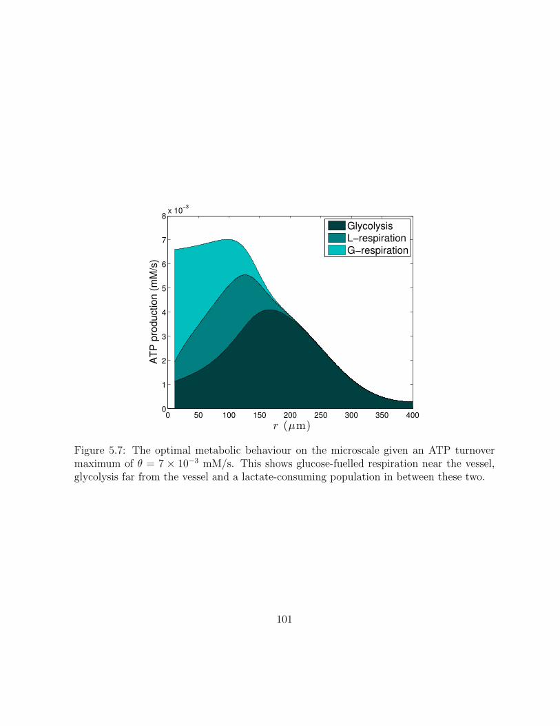
0 50 100 150 200 250 300 350 4000

1

2

3

4

5

6

7

8x 10

−3

r (µm)

AT

P p

rod

uctio

n (

mM

/s)

Glycolysis

L−respiration

G−respiration

Figure 5.7: The optimal metabolic behaviour on the microscale given an ATP turnovermaximum of θ = 7 × 10−3 mM/s. This shows glucose-fuelled respiration near the vessel,glycolysis far from the vessel and a lactate-consuming population in between these two.

101

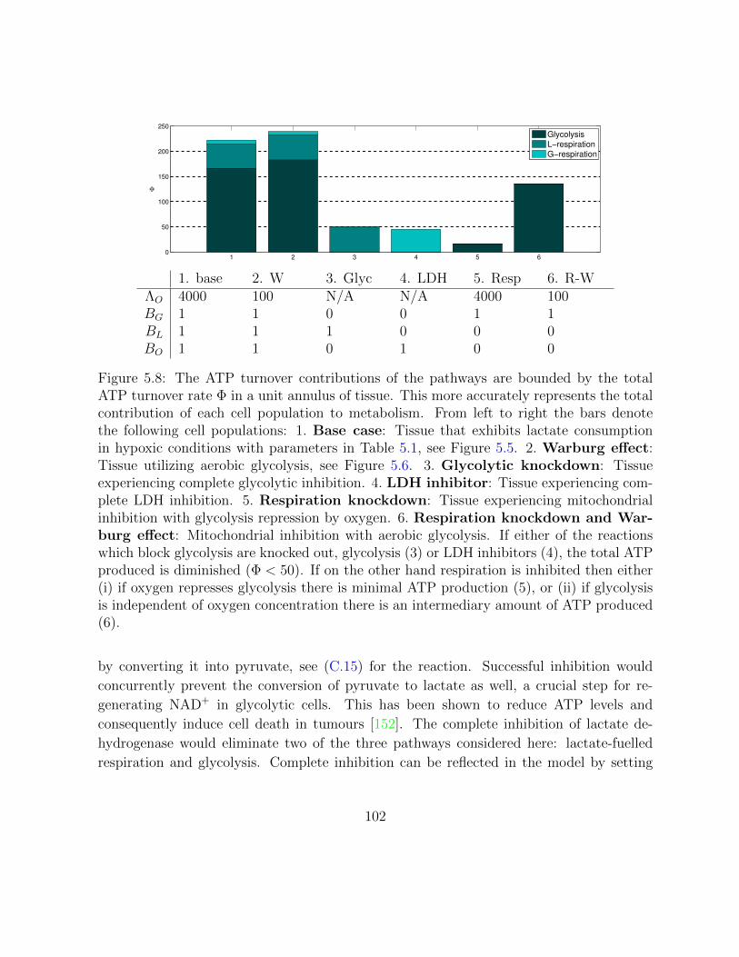
1 2 3 4 5 60

50

100

150

200

250

Φ

Glycolysis

L−respiration

G−respiration

1. base 2. W 3. Glyc 4. LDH 5. Resp 6. R-WΛO 4000 100 N/A N/A 4000 100BG 1 1 0 0 1 1BL 1 1 1 0 0 0BO 1 1 0 1 0 0

Figure 5.8: The ATP turnover contributions of the pathways are bounded by the totalATP turnover rate Φ in a unit annulus of tissue. This more accurately represents the totalcontribution of each cell population to metabolism. From left to right the bars denotethe following cell populations: 1. Base case: Tissue that exhibits lactate consumptionin hypoxic conditions with parameters in Table 5.1, see Figure 5.5. 2. Warburg effect:Tissue utilizing aerobic glycolysis, see Figure 5.6. 3. Glycolytic knockdown: Tissueexperiencing complete glycolytic inhibition. 4. LDH inhibitor: Tissue experiencing com-plete LDH inhibition. 5. Respiration knockdown: Tissue experiencing mitochondrialinhibition with glycolysis repression by oxygen. 6. Respiration knockdown and War-burg effect: Mitochondrial inhibition with aerobic glycolysis. If either of the reactionswhich block glycolysis are knocked out, glycolysis (3) or LDH inhibitors (4), the total ATPproduced is diminished (Φ < 50). If on the other hand respiration is inhibited then either(i) if oxygen represses glycolysis there is minimal ATP production (5), or (ii) if glycolysisis independent of oxygen concentration there is an intermediary amount of ATP produced(6).

by converting it into pyruvate, see (C.15) for the reaction. Successful inhibition would

concurrently prevent the conversion of pyruvate to lactate as well, a crucial step for re-

generating NAD+ in glycolytic cells. This has been shown to reduce ATP levels and

consequently induce cell death in tumours [152]. The complete inhibition of lactate de-

hydrogenase would eliminate two of the three pathways considered here: lactate-fuelled

respiration and glycolysis. Complete inhibition can be reflected in the model by setting

102

BL = 0 and BG = 0, leaving only glucose-fuelled respiration to produce ATP, a physiolog-

ically normal condition. However, the hypoxic and hypoglycaemic conditions considered

here do not leave enough fuel for cell survival. This scenario corresponds to the third bar

in Figure 5.8.

We could also target glucose transport into the cell, an intermediary of glycolysis or

one of the critical enzymes responsible for converting glucose to pyruvate. This is distinct

from the strategy noted above of inhibiting LDH which prevents the conversion of lactate

to pyruvate and vice versa. This has also been noted as a prime target for cancer therapy

[146, 147] and there are currently many potential targets [148]. Here we will consider the

shutdown of glycolysis as preventing both glucose-fuelled respiration and glycolysis since

both of these require glucose to be converted into pyruvate. However, it leaves the lactate-

fuelled respiratory pathway intact. This could be considered in the model by taking BO = 0

and BG = 0. Similar to the case of LDH inhibition this leads to a significant decrease in

ATP production as shown in the fourth bar of Figure 5.8.

The final scenario that we consider corresponds to full inhibition of respiration some-

where along the chain between pyruvate transport into the mitochondria and the electron

transport chain. There are numerous potential targets in the mitochondria [153] and we

will consider the complete shutdown of respiration by setting BL = 0 and BO = 0. This

would result in negligible oxygen consumption and with our base case of ΛO = 400 this

would lead to repressed glycolysis in the tissue. This is likely a non-physiological scenario

since glycolysis would attempt to compensate for a lack of ATP production but it would

lead to heavily reduced ATP production. If glycolysis was able to compensate for the lack

of respiration, represented in the model by reducing ΛO to 100, then the tissue could still

produce a significant amount of ATP. This indicates that in a hypoxic microenvironment,

commonly found in tumour tissue, the complete inhibition of respiration would still allow

the tumour energy supply to be maintained by glycolysis alone.

We could also consider the effects of theoretical single knockdowns in the model by

setting one of the parameters to zero at a time (results not shown). Inhibiting just one

of the respiratory pathways had negligible effect on the total ATP production (in both

the base case and Warburg case) since the other fuel compensated. If glycolysis alone is

inhibited, the respiration is split between lactate and glucose-fuelled and the total ATP is

similar to the amount produced during LDH inhibition or glycolytic inhibition (bars 4 and

5 respectively).

103

5.4 A model for metabolism and acidity

Here we will utilize the model for interstitial fluid pressure formulated for a single vessel

in [71] (see Section 3.1.1 for a summary) to add convective transport to a pH microvessel

model [25] (see Section 3.4.2). This model assumed a two-dimensional region in Cartesian

coordinates to correspond with the experimental setup in [5], namely transparent dorsal

window chambers implanted in mice that contained human colon adenocarcinmoa. Firstly,

we see if the predicted plateau is robust enough to occur in a more appropriate geometry

corresponding to an in vivo tissue: a three-dimensional cylindrical vessel with diffusive

and convective transvascular transport. We also want to consider effects that could be

induced by cancer treatments, such as decreased vessel permeability and increased oxygen

concentration by the application of antiangiogenic agents or increased ratio of respiration

to glycolysis caused by glycolysis inhibitors.

Before adding convection we will first consider the model with glucose-fuelled respiration

and glycolysis (production rates given in Table B.4) are the included metabolisms and they

are coupled to the bicarbonate buffering system [3]. A diagram of the model is provided

in Figure 5.9, showing the extracellular species included in the model and the direction of

their diffusive transport. Also shown are the intracellular metabolism reactions and ATP

yields.

Collecting the system of steady-state equations for the pertinent molecular species

derived in Section 3.4.1, we have

DOd2O

dr2= QO, (5.21)

DGd2G

dr2= QG, (5.22)

DLd2L

dr2= QL, (5.23)

DCd2C

dr2= −krBH + kfC, (5.24)

DBd2B

dr2= krBH − kfC −QO, (5.25)

DHd2H

dr2= krBH − kfC −QO +QL, (5.26)

where QL = QO/3− 2QG, and QG and QO are empirical formulas relating the concentra-

104

Figure 5.9: The metabolism and pH model diagram showing extracellular species directionof diffusive transport and buffering, along with the intracellular metabolism, ATP yieldsand buffering.

105

tions of glucose and oxygen (and possibly pH) to their consumption rates. The boundary

condition at the vessel wall (r = ω) is

−DXdX

dr

∣∣∣∣r=ω

= µX(VX −X0), (5.27)

where X0 = X(ω) ensuring equality of fluxes at the interface between blood and tissue,

while at the penetration depth (r = Ω)

dX

dr

∣∣∣∣r=Ω

= 0, (5.28)

which assumes that the concentrations have reached a steady state equilibrium concentra-

tion.

5.4.1 Parameters

We require estimates of the diffusion coefficients, vessel concentrations, vessel permeabili-

ties and buffering reaction rates of all the molecular species mentioned above along with

functional forms and parameter values for oxygen consumption (respiration) and lactate

production (glycolysis). The values for oxygen, glucose and lactate diffusion coefficients are

provided above in Table 5.1. Those for the molecules necessary for including bicarbonate

buffers along with vessel concentrations and permeabilities are found in Table B.5 and the

metabolic parameters are found in Table B.4.

For blood vessel concentrations, we assume that the concentrations of the molecules

involved in the primary buffering reaction (3.44) are in equilibrium and thus,

VBVHVC

=kfkr

= K.

Based on a pK of 6.12 [154], this gives K ≈ 7.6 × 10−4 mM. In normal vessels pH typi-

cally ranges from 7.35–7.45 with the higher end of this range usually occurring in arteries

while the lower end is observed in veins. pH values above this range imply alkalosis has

set in while values below this indicate acidosis, a characteristic commonly observed in

tumour vessels, e.g. tumour pH near a microvessel of approximately 7.25 [5]. The vessel

measurement corresponds to VH ≈ 4 × 10−5 mM, so we must have VB/VC ≈ 20. Vessel

106

concentrations of bicarbonate typically lie in the range of 18–23 mM , and thus carbon

dioxide lies in the range of 0.75–1.25 mM. As noted above these blood vessel observations

along with these species diffusion coefficients are given in Table B.5.

5.4.2 Analytical observations

Before considering the effects of altering geometries and molecular transport, I will consider

some analytical ramifications of the model in its present form.

I will know rewrite the system (5.21)-(5.26) in a way more conducive to eliminate one of

the diffusion-reaction equations in a similar fashion to the three species system above. Since

the consumption rates of oxygen, glucose and lactate satisfy the relation QL = QO/3−2QG,

we can replace one of (5.21)-(5.23) with this relation; for simplicity we omit (5.22) since

QL and/or QO are present in (5.25) and (5.26). Assuming that we know O(r) and thus

QO, along with L(r) and thus QL, allows us to derive some useful relations in terms of

these concentrations.

Adding (5.24) and (5.25) gives

DCd2C

dr2+DB

d2B

dr2+DO

d2O

dr2= 0,

while subtracting (5.25) and (5.26) gives

DBd2B

dr2−DH

d2H

dr2+DL

d2L

dr2= 0,

both useful relations since we can simply integrate over the spatial variable twice to elim-

inate derivatives in this equation. Finally, we retain (5.26) to close the system for reasons

that will become evident in what follows. Nondimensionalizing concentrations by their

vessel concentration VX , i.e. setting X = VXx and formally nondimensionalizing space by

dividing the spatial variable r by a characteristic length of 1 µm (but not changing its

107

notation), gives the non dimensional system:

d2o

dr2= Qo, (5.29)

d2`

dr2= Q`, (5.30)

d2`

dr2=αo`3

d2o

dr2− 2αg`

d2g

dr2, (5.31)

d2b

dr2= αhb

d2h

dr2− α`b

d2`

dr2, (5.32)

d2c

dr2= −αbc

d2b

dr2− αoc

d2o

dr2, (5.33)

d2h

dr2=krVBDH

bh− kfVCDHVH

c− αohQo + α`hQ`, (5.34)

where αyx = dyxvyx, d

yx = DY /DX , vyx = VY /VX and Qx = QX/(DXVX). In addition to

this system, we also require the non dimensional version of the vessel boundary condition

(5.27), namely,

−dxdr

∣∣∣∣r=ω

= µx(1− x0), (5.35)

where x0 = x(ρ) and µx = µX/DX ; the far-field boundary condition is essentially the same:

dx

dr

∣∣∣∣r=Ω

= 0. (5.36)

First, integrating (5.31)-(5.33) over (r,Ω) and enforcing the far-field boundary condition

(5.36) gives

d`

dr=αo`3

do

dr− 2αg`

dg

dr, (5.37)

db

dr= αhb

dh

dr− α`b

d`

dr, (5.38)

dc

dr= αbc

db

dr− αoc

do

dr. (5.39)

Before integrating again, it is worth noting that by applying (5.35) and rearranging the

108

previous equalities at r = ω yields

`0 =1− βo`3

(1− o0) + 2βg` (1− g0), (5.40)

b0 =1− βhb (1− h0) + β`b(1− `0), (5.41)

c0 =1 + βbc(1− b0) + βoc (1− o0). (5.42)

where βyx = µyxVyx and µyx = µY /µX . Now integrating the equations once more, this time

over (ω, r), gives

`(r) = `0 −αo`3

(o0 − o(r)

)+ 2αg`

(g0 − g(r)

), (5.43)

b(r) = b0 + αhb (h(r)− h0)− α`b(`(r)− `0), (5.44)

c(r) = c0 + αbc(b0 − b(r)

)+ αoc

(o0 − o(r)

)(5.45)

= c0 − αhc (h(r)− h0) + α`c(`(r)− `0) + αoc(o0 − o(r)

).

As a consequence of (5.36), the steady state concentrations satisfy h(Ω)b(Ω)/c(Ω) = 1.

Thus in order to achieve a steady state concentration of h(Ω) = h∞ we must have,

h∞ =c0 − αhc (h∞ − h0) + α`c(`∞ − `0) + αoco0

b0 + αhb (h∞ − h0)− α`b(`∞ − `0),

where `∞ = `0 − αo`o0/3 + 2αg`g0. This expression gives the far-field acidity for the system

as a function of vessel concentrations and diffusion coefficients .

5.5 Convective transport in a metabolism model

Adding convective transport to (3.56) gives the equation

∂X

∂t=DX

r

∂

∂r

(r∂X

∂r

)− ri

1

r

∂

∂r(ruX) + PX . (5.46)

where ri is the retardation coefficient of species i. Typically, we assume that each solute

travels at the same velocity as the fluid and thus take ri = 1 [75]. Again, the production

rates PX are given in Table B.4 while the diffusion coefficients DX are given in Table B.5.

The analytical solution for IFV u is given in 3.9. Expanding the convection term and

109

noting that du/dr = −u/r yields

DX

r

d

dr

(rdX

dr

)− riu

dX

dr+ PX = 0.

The boundary condition at the blood vessel wall ensures the equality of the flux of

solute through the vessel wall (3.28) with the flux through the interstitial space (3.21)

giving

rfuX −DXdX

dr= µ(VX −X)

PeXePeX − 1

+JfS

(1− σi)VX at r = ω. (5.47)

We also require the concentrations to reach a steady state as we move away from the vessel

and takedX

dr= 0 at r = Ω, (5.48)

where Ω is the penetration depth [71], a distance far enough from the microvessel to

justify the assumption that the system has reached steady state but close enough to ensure

minimal contributions from other nearby vessels. This is more practical than the ‘far field’

boundary condition in (3.60) [25] since numerically we will be forced to consider a finite

spatial domain

Given the fluid flux Jf (determining the solute flux (3.5)), we can solve the coupled

system of oxygen and glucose. Using these we can then solve for the system governing

bicarbonate, carbon dioxide and hydrogen ions. Finally we determine the acidity using the

relation pH=− log10(H).

First, we notice that the plateau is still observed in this three-dimensional geometry

and as presented in Figure 5.10a the addition of convection has some effect on the pH but

does not exhibit a drastic change due to the relatively low magnitude of the interstitial

fluid velocity of a single blood vessel (see the inset of Figure 5.10a) indicating that diffusion

is the dominant form of transport for such small molecules on the microscale.

As mentioned in Chapter 2, the acidic microenvironment is caused by upregulated

glycolysis. In this model the ratio of oxygen to glucose consumption is determined by the

parameter R where R = 6 corresponds to purely respiration (where 6 oxygen are consumed

and 1 glucose molecule) or all the way down to 1 which indicates that far more glycolysis is

occurring than respiration. If cells performed only respiration, the plateau in pH would be

even more pronounced since all of the oxygen is being consumed close to the vessel leading

to a sudden switch to glycolysis close to the vessel (see Figure 5.10b). As R decreases

110

Distance (µm)

pH

6.6

6.7

6.8

6.9

7

7.1

7.2

7.3

0 50 100 150 200 250 300

no convectionconvection

Distance (µm)

IFV

(µm

/s)

0

0.02

0.04

0.06

0.08

0 100 200 300

(a) The effect of adding convection to themodel. Inset: IFV, u, outside the vessel.

Distance (µm)

pH

6.6

6.7

6.8

6.9

7

7.1

7.2

7.3

0 50 100 150 200 250 300

Z = 6R= 4R= 2

Distance (µm)

Consu

mpti

on

(mm

ol/

L/s)

0

0.002

0.004

0.006

0.008

0.01

0.012

0 100 200 300

oxygenglucose

Distance (µm)

pH

6.6

6.7

6.8

6.9

7

7.1

7.2

7.3

0 50 100 150 200 250 300

R= 6R= 4R= 2

Distance (µm)

Consu

mpti

on

(mm

ol/

L/s)

0

0.002

0.004

0.006

0.008

0.01

0.012

0 100 200 300

oxygenglucose

(b) The effect of altering the metabolism ratioR. Inset: Consumption rates.

Figure 5.10: pH profiles.

the transition is less pronounced as cells near the vessel do not consume all of the limited

oxygen supply leaving some for cells at intermediary distances.

Vessel permeability varies drastically from normal vessels to tumour vessels and as it

increases the convective and diffusive transport of molecules are enhanced. As shown in

Figure 5.11a, high permeabilities (the tumour base case µ0) have enough oxygen crossing

the vessel wall to ensure that glycolysis does not have to take over close to the vessel while

for low values (e.g. µ0/50), there is no plateau observed since the anoxic environment

causes glycolysis to take over immediately outside the vessel. Note, that despite this latter

case corresponding to a permeability closer to a normal vessel than a tumour vessel, we are

still dealing with a tumour vessel with a very limited oxygen supply. This is reflected by

the consumption rates that decrease to the repressed metabolic phase due to intermediate

oxygen concentrations right outside the vessel wall.

Finally, we observe the effects of hypoxia and anoxia by varying the vessel concentration

of oxygen. For very low values of oxygen (e.g. VO/10), we observe the same phenomenon

as when we considered low permeability. The switch to glycolysis happens very near the

vessel whereas for our base case oxygen concentration we observe the plateau; this is shown

in Figure 5.11b. For a high oxygen concentration found in a normal tissue (e.g. 3VO) we

notice the smooth pH curve expected from a sufficient oxygen supply since the switch to a

glycolysis-dominated metabolism occurs after the steady state of pH is reached.

111

Distance (µm)

pH

6.6

6.7

6.8

6.9

7

7.1

7.2

7.3

0 50 100 150 200 250 300

µ = µ0/50µ = µ0/10µ = µ0

Distance (µm)

Consu

mpti

on

(mm

ol/

L/s)

0

0.002

0.004

0.006

0.008

0.01

0 100 200 300

oxygenglucose

(a) The effect of altering the microvessel per-meability, from base case values denoted by µ0

to lower values corresponding to normal or nor-malized vessels.

Distance (µm)

pH

6.6

6.7

6.8

6.9

7

7.1

7.2

7.3

0 50 100 150 200 250 300

V O/10V O10V O

Distance (µm)

Consu

mpti

on

(mm

ol/

L/s)

0

0.002

0.004

0.006

0.008

0.01

0 100 200 300

oxygenglucose

Distance (µm)

pH

6.6

6.7

6.8

6.9

7

7.1

7.2

7.3

0 50 100 150 200 250 300

V O/10V O3V O

Distance (µm)

Consu

mpti

on

(mm

ol/

L/s)

0

0.002

0.004

0.006

0.008

0.01

0 100 200 300

oxygenglucose

(b) The effect of changing the oxygen concen-tration in the microvessel from the base casehypoxic value VO to higher and lower values.

Figure 5.11: pH profiles. Inset: Glucose and oxygen consumption rates.

5.6 Conclusions

The mathematical models formulated and analyzed above can give insight into the metabolic

behaviours of cancer cells on the microscale. The tumour microenvironment characterized

by hypoxia and nutrient depravation leads to the utilization of highly unregulated gly-

colytic pathways and the consumption by respiring cells of the lactate produced by these

cells. These metabolic scenarios are encompassed by the functional forms proposed for

glucose, lactate and oxygen consumption.

To consider the effect of altering parameters in the model to the efficiency of energy

production we must also consider the rate of ATP turnover in the tissue. To this end

a detailed biochemical summary was performed in order to calculate novel estimates for

ATP yields. These energetic landscapes were considered in tissues that utilize anaerobic

glycolysis, thus keeping more cells alive, and those that experience the Warburg effect,

performing glycolysis in oxygenated areas. The analysis shows that the latter does confer

a proliferative advantage by producing more ATP.

The effects of metabolic inhibition was taken into account by knocking out the path-

ways considered in our model. Glycolytic inhibition blocked glycolysis and glucose-fuelled

112

respiration, LDH inhibition blocked glycolysis and lactate-fuelled respiration while respi-

ration inhibition blocked both forms of respiration. Both strategies that block glycolysis

lead to significant decreases in total ATP production while those that block respiration

still allow sufficient ATP for cell survival.

Of the many biochemical reactions stated above, some are tissue-dependent, pH-dependent

or are not well established in the literature. Tissue-dependency of these models has been

considered in [90], while the coupling of buffering and reactions has been considered on the

microscale and temporal models [25, 155]. The uncertainty with the reactions above is pri-

marily associated with the transmembrane transport of glucose across the cell membrane

of glucose (C.12), pyruvate and phosphate transport into the mitochondria (C.18) and

other processes that consume the electrochemical gradient in the mitochondrion. These

transport processes may be very important to accurately modelling the efficiency of tumour

metabolism.

Model extensions, including the addition of acidity and buffering mechanisms along

with convective transport in the interstitial space and across the blood vessel wall have

also been indicated. The work presented here should lead to a reconsideration of the bio-

chemical reactions that constitute metabolic mathematical models and provide a minimally

parameterized and straightforward basis for future metabolite consumption models.

113

Chapter 6

Mathematical Model for the

Sequential Application of a Cytotoxic

Nanoparticle and a PI3K Inhibitor

The previous two chapters detailed models of a solid tumour’s macroscale angiogenic re-

sponse to hypoxia and the subsequent microscale metabolism that a tumour performs.

Treatment effects were analyzed by parameter variations that corresponded to treatments.

Here, we address treatment concentrations and combinations in a specific type of solid

tumour, breast cancer. This chapter details a mathematical model that describes drug

concentrations, subsequent effects on protein expression and finally cell viability. The

model was formulated based on data obtained via close collaboration with experimental-

ists at Dr. S. Sengupta’s Laboratory for Nanomedicine at Havard Medical School. This

experimental work was the first time that the combination of nanomedicine and a molec-

ular targeted therapy was tested in vivo. The primarily goal of the mathematical model

was to establish the optimal schedule of these two therapies which was determined by min-

imizing cell viability. The majority of the results contained in this chapter were published

in Cancer Research [8].

Before launching into the layers of the mathematical models, we will summarize the

necessary medical background and specifics of the study that were not already addressed

in Chapter 2.

114

6.1 Medical motivation

Paralleling the question of optimal scheduling of chemotherapy and antiangiogenic agents

to optimize treatment effects [35, 59] is the problem of optimal scheduling chemotherapy

and molecular inhibitors. In both cases the complementary therapy is attempting to max-

imize the cytotoxic effects of chemotherapy. In the work considered here, a mathematical

model was developed for a novel combination of anticancer treatments: a chemotherapy

drug encapsulated in a nanoparticle delivery vehicle and a molecular inhibitor. Combi-

nations of cytotoxic agents and molecular inhibitors have been previously considered in

leukaemia and breast cancer [156, 157] but never with the effective delivery rendered by

a nanodelivery device. These nanomedicines have many advantages over traditional deliv-

ery including preferential accumulation in the tumour via the enhanced permeability and

retention (EPR) effect [46] and their ability to spatially and temporally control their drug

release [53].

In this study, the impact of sequencing of a cisplatin-based supramolecular nanopar-

ticle with an inhibitor of phosphoinositide 3-kinase (PI3K) was studied in a cell model

that is particularly difficult to treat: triple negative breast cancer (TNBC). TNBC is

characterized by the absence of estrogen receptors, progesterone receptors and Her2/neu.

These entities are typical targets for hormonal and chemotherapy treatments. Cisplatin

has shown some success in treating TNBC [32] but the dosage is highly limited due to

toxicity, particularly of the kidneys. To counteract this the group of our collaborators

engineered a polymeric cisplatinum (II) nanoparticle, which displayed preferential tumour

accumulation, bypassed the kidney, and exhibited an enhanced antitumour efficacy com-

pared to free cisplatin [158]. However, cisplatin has another drawback, it can upregulate

PI3K signalling, which reduces the apoptotic response of cells [43]. This outcome suggests

that a rational combination of PI3K inhibitor and cisplatin nanoparticles could further

improve treatment efficacy. Indeed, experiments showed that treatment with a novel (self-

assembling) cisplatin nanoparticle (SACN) results in activation of PI3K signalling. The

motivation now is to use a mathematical model to predict the optimal treatment schedul-

ing of SACNs combined with a PI3K inhibitor called PI8282. The model will be outlined

below before showing and the validation of the results were obtained both in vitro and in

vivo. Our results reveal the treatment with SACNs followed by the administration of PI828

results in better results than pre-treatment with PI8282 or simultaneous administration.

These results indicate the appropriate sequencing of this cytotoxic nanomedicine and a

115

Figure 6.1: A detailed pathway of cell apoptosis showing the interactions between themajor players in this process. Image courtesy of Dr. M. Kohandel.

molecular targeted therapeutic to achieve optimal therapeutic efficiency.

6.2 Mathematical model

The mathematical model developed here is broken up into three parts. The first part

will describe the protein expression levels of pAkt, caspase-3 and XIAP. The next will

include the treatment effects of cisplatin-NP and PI828 on protein expression. Then a

nanoparticle release model will be used to describe the release profile of the nanoparticles

measured in this study. Finally, we will propose a simple model for predicting cell viability.

The consideration of parameter estimation will come in the next section.

In addition to the three proteins mentioned above, there are many more proteins and cell

signalling pathways that encourage cell survival or cell apoptosis, summarized succinctly

in Figure 6.1. Among all of them, we only consider a select few that are critical indicators

of cell viability: pAkt, caspase-3 and XIAP. pAkt and XIAP are key cell survival factor

while caspase-3 is widely considered to be the primary indicator of imminent cell apoptosis.

The expression of these proteins can be determined experimentally by Western blotting

techniques.

116

Figure 6.2: A diagram summary of the protein expression and cell viability model. (A)The simplified apoptosis pathway including the interactions of pAkt, XIAP and caspase-3. (B) The cell viability model where tumour cells proliferate at a rate proportional topAkt concentration and the death rate is proportional to caspase-3 concentration. Imagecourtesy of Dr. M. Kohandel.

6.2.1 Protein expression model

Several mathematical models of varying complexity have been developed to study intrinsic

and extrinsic apoptosis [159, 160, 161]; see [162] for a review. Here, we consider a simple

model containing three critical proteins: pAkt, XIAP, and capsase-3. The effects of com-

binations of liposomal cisplatin and PI828 treatments are investigated. The basic reaction

pathways are shown in Figure 6.2.

Akt phosphorylation is induced by activated PI3K. Once activated, Akt negatively reg-

ulates apoptotic pathways at a pre-mitochondrial level by blocking the actions of proteins

such as Bad and Bax, which in turn inhibits the release of cytochrome c into the cytosol. It

has also been reported that Akt directly phosphorylates and inactivates cell death protease

caspase-9 [163]. For simplicity and to keep the number of parameters manageable, these

multiple pro-survival initiatives are considered to have the net effect of inhibiting capsase-3

production, see (1) in Figure 6.2.

It has been also reported that active caspase-3 cleaves Akt in vitro, and inhibiting

caspase-3 can block this effect [164]. Thus, a negative feedback is assumed to represent the

cleavage of Akt by caspase-3, (2) in Figure 6.2. In addition, activated Akt interacts with

117

and phosphorylates XIAP, protecting it from autoubiquitination [165], (3) in Figure 6.2.

XIAP inhibits caspase-3 by the degradation of caspase-3 ((4) in Figure 6.2), and

caspase-3 inhibits XIAP through ubiquitination and degradation [166, 159, 160, 167], (5) in

Figure 6.2(A). Caspase-3 can also inhibit XIAP by inactivating XIAP through formation

of a complex [159].

To include the effect of treatment, we first note that based on our experimental data

and other studies [164, 168], cisplatin increases the production of pAkt. This activation

might be mediated through EGFR and PI3K. Similar to previous studies [164], our data

shows an increase in caspase-3 due to cisplatin. This increase could be due to activation

of FasL, which in turn activates caspase-8 and subsequently caspase-3 [169, 170]. Another

possible pathway is the release of cytochrome c, which subsequently activates caspase-9

and caspase-3 [171, 170].

In addition, phosphorylation of XIAP by Akt protects ubiquitination and degradation

of XIAP in response to cisplatin. Since we have only considered the active form of XIAP in

our model, we assume that cisplatin reduces XIAP, as observed in the experimental data.

The reduction in XIAP could be also due to increase in caspase-3. Finally, we assume that

PI828 inhibits phosphorylation of Akt by binding to P13K.

Here, we will consider the effects of the chemotherapy agent cisplatin in nanoparticles in

combination with the P13K inhibitor PI828. Cisplatin is known to increase concentrations

of caspase-3 triggering cell death but unfortunately, it simultaneously increases pAkt which

commonly leads to anti-apoptotic effects and thus lowered efficacy of cisplatin treatment

and overall chemoresistance. To counter this resistance, PI828 can be administered which

inhibits PI3K, rapidly preventing the production of pAkt. The primary goal of this mod-

elling is to determine the optimal combination of these two drugs to minimize cell viability

for appropriate ranges of treatment dosages.

We consider the effects of the aforementioned treatments, liposomal cisplatin and PI828

along with their combinations, on the select group of proteins critical to apoptosis described

above: pAkt, caspase-3 and XIAP. Denoting the dimensionless concentrations of the pro-

teins by P=[pAkt]/P0, C=[caspase-3]/C0 and X=[XIAP]/X0, where P0, C0 and X0 are

experiment-dependent scaling factors. The system of equations for the protein expression

that we will use includes the indirect mutual inhibition of pAkt and caspase-3, the di-

rect mutual inhibition of caspase-3 and XIAP, along with production, natural decay and

118

treatment effects, and is given by:

dP

dt=

kp + λpfp(t)

1 + αpC + γpgi(t)− δpP (6.1)

dC

dt=kc + λcfc(t)

1 + αcP− βcXC − δcC (6.2)

dX

dt= kx + λxPX − βcCX − δxX, (6.3)

where the concentration of PI828 is denoted by g(t) and the effects of cisplatin on pAkt

and caspase-3 production are denoted by fp(t) and fc(t) respectively. The models for these

treatment effects will be addressed below.

6.2.2 Treatment effects

We will first consider the effect of PI828, a potent inhibitor of Akt phosphorylation. It

performs this inhibition by blocking the activity of the enzyme P13K which is responsible

for phosphorylating Akt, creating pAkt. There are no release kinetics to consider for this

treatment. A reasonable approach would be to consider extracellular and intracellular con-

centrations, denoted by ge and gi respectively, that follow mass transport and exponential

decay of the effect giving

dgedt

= −rggedgidt

= rgge − dggi.

However, even this simplistic approach introduces an unnecessary parameter and variable

since the effect of PI828 is very rapid (compared to the time scale of the experiments:

hours). Thus, it is sufficient to simply take

dg

dt= −dgg. (6.4)

119

The treatment effects of cisplatin on pAkt and caspase-3 are modeled by

dfpdt

= rcci(t− Ti)− dpfp(t), (6.5)

dfcdt

= rcci(t− Ti)− dcfc(t), (6.6)

where ci(t) is the intracellular cisplatin concentration which will be modelled below. Since

protein expression increase occurs on a similar time scale, and in the interest of parameter

reduction, we assume that the effect of the drug has the same activation constant rc and

time delay Ti, after the release of cisplatin nanoparticles, that accounts for intracellular

diffusion to active sites and the delayed impact of cisplatin on the apoptosis pathway.

This delay is attributed to the translational and transcriptional events that occur prior to

changes in the expression of the proteins of interest. However, to facilitate the fitting to

follow this model development, the delay in the equations above is not a strict time delay.

Instead, a linear chain of reactions is used where the delay of a signal is approximated by

N steps with equal reaction rates k [172]. Thus, the value of Ti is not explicitly included

in parameter fitting and can be shown to have mean T = N/k and standard deviation

σT = T /√N [173]. The number of intermediary reactions, N , which is suggested to be

set somewhere between 5 and 15, is set to 10 here since anything larger would promote

stiffness in the system and impede the proficiency of the fitting algorithms. The treatment

effects do exhibit different decay rates dp and dc since the cisplatin-induced production of

pAkt is sustained longer than the increased production of caspase (i.e. dp < dc).

6.2.3 Nanoparticle release

For nanoparticle release, many models were investigated. Preliminary data suggested that

out of all the candidates, a biexponential (or a biexponential with decay) release profile

was appropriate while a monoexponential yielded an unsatisfactory fit. Subsequent exper-

iments showed a simple erosion model fit well while even the simplest monoexponential

model was sufficient. Here we will only present the final published results utilizing the

monoexponential decay model while unpublished release profile results are found in D.

To determine the rate of cisplatin release from the liposome nanoparticles, release ex-

periments were performed over 120 hours in acidic and neutral conditions. In an acidic

environment these release profiles can be accurately determined by a one-parameter ex-

120

ponential release profile. We can motivate the functional form by considering a simple

ordinary differential equation (ODE) that includes both the constant and sustained re-

lease of drug due to encapsulation in the liposome. To facilitate this, we assume that

the administered liposomes initially consists of a fixed fraction of cisplatin, θu, that will

be subsequently released upon administration at rate ru and a fixed fraction of cisplatin,

θi = 1−θu, that remains inert and is omitted from the modelling that follows. The fraction

of the total amount of contained cisplatin that is released depends primarily on the acidity

of the environment. In an acidic environment, just over 60% of the cisplatin is eventually

released from the liposome, as opposed to the approximately 40% that is released in a

neutral environment (this can be seen in Figure 6.5). This helps to preferentially target

tissues exhibiting an acidic microenvironment as found in solid tumours. The concentra-

tion of the cisplatin that is released from the nanoparticle is denoted by c(t) while the

unreleased cisplatin concentration remains to be released is denoted by u(t). The initial

conditions are u(t0) = θucT and c(t0) = 0 where t0 is the time of administration and cT is

the administered dosage (µM). The system of ODEs is then:

du

dt= −ruu(t), (6.7)

dc

dt= ruu(t), (6.8)

with the solution of interest being c(t).

6.2.4 Cellular chemotherapy concentrations

The model given above for the release profile experiments must be extended for the in

vitro experiments where expression of proteins are measured. The previous model will

now correspond to extracellular concentrations of cisplatin (denoted with subscript e) that

will now be transported inside the cell where the intracellular concentration (denoted with

subscript i) can then have an effect on the protein pathways. To facilitate this we add a

term to these extracellular concentrations to include the mass transport of cisplatin into

the cells, a process with some rate constant rc and time delay Te. This time delay accounts

for the effects of extracellular diffusion and transmembrane transport. In the interest

of avoiding extraneous parameters, and since the computational process to include delay

parameters introduces significant stiffness, we will make the assumption that this transport

delay (and the rate constant) is the same for nanoparticles and free cisplatin. Similar to

121

Figure 6.3: Depiction of the drug model in Equations (6.9)–(6.12) for nanoparticle re-lease and delayed transmembrane transport of self-assembling cis-platinum nanoparticles(SACNs) and free cisplatin in an acidic environment.

122

the time delay Ti in the treatment effects equations, we assume a linear chain of reactions

to obtain a distributed delay for the data fitting procedure. These drug-related reactions

are shown schematically in Figure 6.3. This leads to the extended system:

duedt

= −ruue(t)− φcue(t), (6.9)

dcedt

= ruue(t)− φcce(t), (6.10)

duidt

= −ruui(t) + φcue(t− Te), (6.11)

dcidt

= ruui(t) + φcce(t− Te). (6.12)

6.2.5 Cell viability

With the model for protein expression and therapeutic concentrations established, we

now propose a model to predict cell viability. Making the simple assumptions that cell

survival is proportional to pAkt expression and cell death is proportional to caspase-3

expression proves to be a sufficient model for this prediction (see Figure 6.9a). The resulting

differential equation for cell viability is then given by

dN

dt= (λNP − δNC)N. (6.13)

6.3 Parameter estimation

All of the parameter estimation to follow was performed using the MATLAB toolbox

PottersWheel (http://www.potterswheel.de) [139, 173]. This toolbox is capable of loading

multiple experimental data files and then estimating local and global parameters in the

ODE model. The parameter values were not determined simultaneously. The data fitting

process was done step-by-step as shown schematically in Figure 6.4. While the best fit

for release parameters is likely the unique global minimum of the chi-square error, those

determined for protein expression are not guaranteed to be a global minimum due to the

lack of experimental estimates of most of the parameters (aside from the decay rates) and

123

Figure 6.4: Flowchart showing the computational algorithm used to fit parameters in themathematical model.

the sheer number of parameters to be estimated. The cell viability parameters are likely

the best estimate based on the given set of protein expression parameters.

6.4 Results

6.4.1 Cisplatin nanoparticle release

Fitting the parameters of the nanoparticle release model in Equations (6.7)–(6.8) to the

release profile data yields a suitable fit for the acidic environment (χ2red = 0.54, N = 15,

p = 2) and a mediocre one for the neutral environment (χ2red = 1.66, N = 15, p = 2),

see Figure 6.5 for these profiles and D for discussion of the reduced chi-squared statistic

χ2red. The release parameters for these fits are given in Table 6.1. Only those determined

for acidic environments are utilized in the calculations to follow so we will not present

a detailed model for neutral release properties; however, the release profile for a neutral

environment could be suitably fit by the addition of a single parameter that accounts for

liposomal erosion (χ2red = 0.61, N = 15, p = 3); this would have negligible effect on the

acidic release (χ2red = 0.58, N = 15, p = 3).

124

0 20 40 60 80 100 1200

10

20

30

40

50

60

70

time (hours)

% re

leas

e

AcidicNeutral

Figure 6.5: (Data points) The release profile of cisplatin liposomes was evaluated at 37Cin neutral and acidic (tumour-like) pH in triplicates. 500 mwco dialysis bags packed with16198665 ng liposome were stirred in 30 mL of acidic and neutral pH. 500 µL samples weretaken out at predetermined time points from the outer chamber and analyzed by AAS byserial dilution. (Solid lines) Release profiles of cisplatin nanoparticles in acidic (χ2

red=0.54,N=15, p=2) and neutral (χ2

red=1.66, N=15, p=2) microenvironments determined by fittingsolutions of Equations (6.7)–(6.8).

Parameter Neutral Acidicru 0.0471 [1/h] 0.0171 [1/h]θu 0.499 0.614

Table 6.1: Nanoparticle release parameters in (6.7)–(6.8).

125

6.4.2 Protein expression

The data from the in vitro protein expression experiments in 4T1 breast cancer cells are

used to determine the parameters in the model above; these parameters are given in Table

6.2. The only parameters present in the literature are those that determine decay rates

of the proteins [159]. Each experiment is considered to have a scaling factor for each

protein which are given in Table 6.3. This takes into account that the value used to

non-dimensionalize the protein concentrations is different for each experiment.

Parameter Value Parameter Value Parameter Valuekp 1.86 [1/h] αp 0.13 dg 0.001* [1/h]kc 11.56 [1/h] αc 0.56 γp 6.42 [1/µM]kx 0.29 [1/h] λx 0.01 [1/h] φc 0.26 [1/h]δp 0.36 [1/h] βc 2.30 [1/h] rc 0.47 [1/h]δc 0.48 [1/h] βx 0.040 [1/h] dp 0.030 [1/h]δx 0.57 [1/h] λp 0.34 [1/h·nM] dc 0.28 [1/h]

λc 11.9 [1/h·nM]

Table 6.2: Protein expression parameters in (6.1)–(6.3).*Parameter reached minimum allowable value. Indicates PI828 decay is not detected inexperiments on this time scale. This is evident from the continued inhibition exhibited inFigure 6.7b.

Figure(s) P0 C0 X0

Figure 6.6a–6.6c (3 µM) 0.514 1.18 1.06Figure 6.6a–6.6c (5 M) 0.381 1.36 0.770Figure 6.7b 0.812 1.32 0.1*Figure 6.8a-6.8b (Post) 0.510 0.834 1.29Figure 6.8a-6.8b (Control) 0.511 0.529 1.29

Table 6.3: Experimental scaling factors for protein expression in (6.7)–(6.8).

6.4.3 Cell viability

Finally, with the release parameters and protein expression parameters approximated from

the data, we can introduce two parameters that predict cell viability. For this step of the fit-

ting we must have the same scaling parameters for each experiment. Fitting to the existing

126

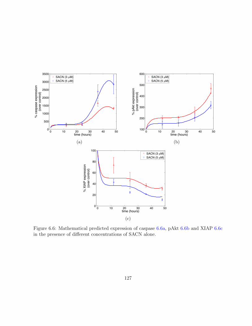
0 10 20 30 40 500

500

1000

1500

2000

2500

3000

3500

time (hours)

% c

aspa

se e

xpre

ssio

n(o

ver c

ontro

l)

SACN (3 µM)SACN (5 µM)

(a)

0 10 20 30 40 50100

200

300

400

500

600

time (hours)%

pAk

t exp

ress

ion

(ove

r con

trol)

SACN (3 µM)SACN (5 µM)

(b)

0 10 20 30 40 500

20

40

60

80

100

time (hours)

% X

IAP

expr

essi

on(o

ver c

ontro

l)

SACN (3 µM)SACN (5 µM)

(c)

Figure 6.6: Mathematical predicted expression of caspase 6.6a, pAkt 6.6b and XIAP 6.6cin the presence of different concentrations of SACN alone.

127

0 10 20 30 400

0.5

1

1.5

2

2.5

3 x 104

time (hours)

% c

aspa

se e

xpre

ssio

n(o

ver c

ontro

l)

(a)

0 10 20 30 400

20

40

60

80

100

time (hours)

% p

Akt expre

ssio

n(o

ver

contr

ol)

(b)

Figure 6.7: The inhibition of pAkt and increase of caspase by PI828 alone 6.7b.

0 5 10 15 20 250

1000

2000

3000

4000

5000

time (hours)

% c

aspase e

xpre

ssio

n(o

ver

contr

ol)

PI828

Control

(a)

0 5 10 15 20 250

20

40

60

80

100

120

time (hours)

% p

Akt expre

ssio

n(o

ver

contr

ol)

PI828

Control

(b)

Figure 6.8: The inhibition of pAkt by PI828 post treatment with SACN 6.8b and thesynergistic increase in caspase expression as compared to SACN alone-treated controls6.8a.

128

0 0.5 1 5 10 20 500

50

100

150

Cisplatin concentration (µM)

Cel

l via

bilit

y (%

of c

ontro

l)

SACN (36 h)PI828 (12 h):SACN (36 h)SACN (36 h):PI828 (12 h)

(a)

0 0.5 1 5 10 20 500

10

20

30

40

50

60

70

80

90

100

110

Cisplatin concentration (µM)

Cel

l via

bilit

y (%

of c

ontro

l)

SACN (36 h):PI828 (12 h)SACN (24 h):PI828 (12 h)SACN (12 h):PI828 (12 h)

(b)

Figure 6.9: (a) Mathematical model-based prediction of cell viability using different dosingschedules of SACNs and PI828. (Data points) In vitro measurements where the effect ofdifferent drug combinations on 4T1 cell viability was quantified using MTS assay. SACN-treated: cells were incubated with SACN containing media in an increasing concentrationgradient (0.5–50 µM) for 36 hours, after which it was replaced with control media for12 hours. PI828 pretreatment: cells were pretreated with 5 µM PI828 for 12 hours, afterwhich the culture media were removed and cells were incubated with SACN in an increasingconcentration gradient (0.5–50 µM) for 36 hours. PI828 posttreatment: cells were incu-bated with SACN-containing media in increasing concentration gradient (0.5–50 µM) for36 hours, after which it was replaced with PI828-containing media at 5 µM concentrationfor 12 hours. All readings were taken at 48 hours (data shown are mean ± SEM, n = 3).(Lines) The cell viability data was used to fit (6.13) for increasing SACN concentrationsyielding the parameters in Table 6.4. For the purpose of plotting, the model predictionsat each SACN concentration were interpolated using cubic splines. (b) The mathemati-cal model solution for cell viability for various post-SACN PI828 treatments: 36 hours ofSACN followed by 12 hours of PI828, 24 hours of SACN followed by 12 hours of PI828,and 12 hours of SACN followed by 12 hours of PI828. Minimal cell viability was exhibitedin the case where PI828 was administered 24 hours after SACN. Once again each cell vi-ability prediction was taken at 48 hours and the prediction for each SACN concentrationwas interpolated with a cubic spline.

129

cell viability data at the 48 hour time point, (data points in Figure 6.9a) gives the param-

eters in Table 6.4 and the model fit at the 48 hour time point shown in Figure 6.9a. Using

these parameters in the model, the cell viability associated with other treatment combina-

tions can now be determined. Since the data already displays that PI828 posttreatment

outperforming pretreatment, we will only investigate the posttreatment scenario. The cell

viability associated with administering PI828 12, 24 and 36 hours after SACN treatment

is shown in Figure 6.9b where once again the cell viability prediction is after 48 hours have

elapsed since the start of treatment. The 24 hour mark represents a superior treatment

option to both the earlier and later dosing regimens of molecular inhibitor, as in the early

administration (12 hours) the cisplatin has not had enough time to take effect whilst in

the later administration (36 hours) the treatment effects have begun to wear off by the

time PI828 is administered. This reinforces the importance of precise timing, on the or-

der of hours, in order to maximize the synergistic effects of these drugs and minimize cell

viability.

Parameter ValueλN 2.7×10−3 [1/h]δN 1.5×10−3 [1/h]

Table 6.4: Cell viability parameters in (6.13).

6.5 Conclusions

Our mathematical model captured the rising cleaved caspase-3 and p-Akt levels, as can

be seen by the accurate fits in Figures 6.6a and 6.6b along with decreasing XIAP levels

after treatment with cisplatin nanoparticle (Figure 6.6c). The potent inhibition of pAkt

after PI828 administration was also facilitated by the model (Figure 6.7b). On the basis

of our assumptions and the above data, the model predicted the desired synergistic effects

of the combination treatments. Relative to the control case, the mathematical model

predicted synergistic increase in caspase-3 due to treatment with SACNs along with the

p-Akt inhibition provided by PI828 (Figures 6.8a and 4H respectively). In addition, as

shown in Figure 6.9a, PI828 administered after SACN treatment was predicted to result in

lower cell viability compared with pretreatment with PI828 followed by SACNs treatment

or with SACNs alone. We then sought to find the most efficient time for the administration

130

of PI828 after cisplatin nanoparticle treatment. It was determined that administration of

PI828 approximately 24 hours after cisplatin would yield lower cell viability as compared

to 36 hours or earlier times (Figure 6.9b).

131

Chapter 7

Contributions and Future Work

In this concluding chapter, I will first outline the minor contributions to research that I

have made during my Ph.D., which do not comprise the bulk of my thesis in Chapters 4–6.

These include collaborative projects and unpublished results. This will be followed by brief

summaries of the major contributions made to the field of mathematical oncology including

evidence of scientific impact in the literature. Finally, a selection of future directions that

these mathematicals could take will be suggested.

7.1 Minor contributions

I will briefly outline a couple minor contributions that pertain to the material disseminated

in Chapter 5 along with a collaborative research project on antioxidant systems that has

led to a number of co-authored manuscripts.

A minor contribution that has some potential of evolving into substantially more is a

reconsideration of phosphate transport’s effect on ATP yield. The effects of this prelim-

inary parameter alteration was included in the supplementary material of the metabolic

symbiosis study in C.6. Phosphate transport, among other mitochondrial transport pro-

cesses, remains relatively unestablished in the literature. The role of the pH differences

between the cytosol, intermembrane space and mitochondrial matrix could be significant

to modelling the proton gradient across the mitochondrial membrane. In fact, if one makes

strong simplifying assumptions, the ATP yield from a single glucose molecule may be re-

duced from approximately 29 [20], to approximately 24. The truth may lie somewhere

132

in between these two values, or even below that threshold, if pyruvate transport or other

molecular transport reduces the proton gradient further. Regardless, it remains pertinent

that these transport processes, along with ATP transport and subsequent utilization should

be compensated for in any model that makes steady state, or flux balance, assumptions.

An incremental generalization of the single vessel results in Chapter 5 is the two vessel

model equivalent that is a more appropriate simplified model of tissue and has been used

in previous models e.g. [83]. This introduces a well-defined parameter of intercapillary

distance and can be used to analyze asymmetrical situations as well. This still represents a

highly constrained geometry but represents the first generalization to a multi-vessel system.

Another project, which relates to the metabolism models is the development of mod-

els for antioxidant systems including the glutathione peroxide system. These counteract

reactive oxygen species (ROS) that are produced by cellular respiration and by growth

factors in tumours, among other processes. While essential to cell metabolism, at high

concentrations ROS become detrimental to normal cell function and in extreme conditions

can trigger apoptosis (cell death). To safeguard cells from ROS, there are various antiox-

idant enzymes that remove ROS or render them harmless. The ROS that is produced at

the highest rate is typically hydrogen peroxide (H2O2), a molecule that can be reduced by

various enzymes including catalase and those in the glutathione peroxides (GPx) family.

A mathematical model that considers the effects of these antioxidants in detoxifying hy-

drogen peroxidase is summarized in E. Interestingly we discovered that there is a synergy

between catalase and glutathione-peroxidase-1 which amplifies the detoxification power of

glutathione peroxidase-1. Hence any change (upregulation or downregulation) in the cata-

lase concentration has a direct affect on the glutathione peroxidase-1 activity and has to

be included in understanding any related phenomena. Also we propose that the activity

of glutathione peroxidase-1 could be regulated by changing the concentration of catalase.

The synergistic relationship between these antioxidants is reported in [174]. This work

was expanded to include the effects of cell permeability, especially the role of aquaporin

expression. This has important consequences for the efficacy of ascorbic acid for cancer

treatment and has also been submitted [175].

7.2 Major contributions

The major contributions to the field of mathematical oncology include the following:

133

(i) Establishing the role of convective transport in angiogenesis signalling:

This model could be used in tumour growth models or to predict the effects of various

treatments. The alteration of biochemical signalling by convection could be generalizable

to other cell signalling pathways in tumours, and has been investigated in the context of

tumour invasion [176].This model has been used in the literature as inspiration for including

convective transport of AGFs in a tumour growth model [177] and has been quoted in [178]

for the observation that, “Angiogenic behaviours were suppressed when closer to the core of

the tumour and maximal angiogenic stimulation was detected towards the [outer] rim of the

tumor.” It has also been cited as an example of convection-based models [179, 180]. The

angiogenic effect of altering physiological parameters in tumours is the focus of Chapter 4.

(ii) Mathematical model for metabolic symbiosis in solid tumours: This

metabolism model includes lactate-fuelled and glucose-fuelled respiration along with oxygen-

repressible glycolysis. This was the first model to spatially consider the optimal ATP pro-

duction strategy in a tumour on the microscale and could be used to analyze metabolic

inhibitors. This may lead to a significant contribution to the study of metabolism in

biochemistry. This forms the majority of Chapter 5.

(iii) The link between metabolism and acidity: Using acidity models in tumours,

the effects of blood vessel permeability (antiangiogenic agents), hypoxia and metabolic

behaviour on acidosis are investigated. This research is contained in the latter half of

Chapter 5.

(iv) The optimal sequence of chemotherapy nanoparticles and molecular in-

hibitors: Utilizing nanoparticle release models in conjunction with protein expression

models can yield cell viability estimates for treatment optimization. The experimentally

confirmed prediction of inhibitor application after chemotherapy nanoparticles could guide

optimal scheduling models in this context. This contribution has the most medical and

clinical relevance and is outlined in Chapter 6.

7.3 Future work

Each of these aforementioned models could be extended or utilized in alternate systems. I

will indicate a sample of what I estimate to be the most fruitful endeavours.

For Chapter 4, the most obvious extension is to a non-symmetrical geometry that

could model more complex tumour shapes than the spherical one considered. However,

134

this extension only warrants consideration if relevant experimental data is generated that

confirms the role of convection in angiogenic signalling. In terms of qualitative modelling

of angiogenesis, the distinct roles of various AGFs could be included by introducing sep-

arate equations for the different factors and explicitly including the inhibitory effects of

antiangiogenic factors and the stimulatory effects of proangiogenic factors via appropriate

terms in differential equations. The appeal of the model considered here is the utilization

of effective parameters for the two groups of AGFs that dramatically reduce the number

of parameters. By expanding the model to include multiple factors, diffusion coefficients,

degradation and production rates must also be estimated. A less dramatic model improve-

ment would be including continuous parameter values over the spatial domain of interest,

rather than the piecewise constant parameters considered, i.e. instead of of having one value

inside the tumour and one value outside the tumour (for diffusion, production and decay)

these values could be smoothly interpolated. The same could be said for the pressure

parameters as well, since the effective pressures, hydraulic conductivities, vessel perme-

abilities, etc. are all considered to be piecewise constant as well. This model also holds

promise for inclusion in more complicated models, including tumour growth models (I have

some preliminary results in this area), and more directly, models of tumour angiogenesis.

In Chapter 5 there are many possible areas for expansion include radially-dependent

parameters (diffusion coefficients, cell densities that modify metabolic parameters), axially-

dependent parameters (vessel concentrations, vessel permeability) and more generalized

functional forms for the consumption rates (e.g. ATP-dependent or pH-dependent). Ad-

ditional details of cellular metabolic pathways including other glycolytic and respiratory

intermediaries within the pathways or alternative metabolic pathways such as glutaminol-

ysis, could be adapted on a tumour-dependent basis. The most significant extension would

be to include non-symmetrical three-dimensional geometries. While relatively straightfor-

ward to formalize and even solve numerically, a complicated spatial domain would only be

clinically relevant once pertinent clinical data is generated. The details of the metabolic

reactions that are used to derive the summary metabolic reactions given by (5.1), (5.2)

and (5.3) are contained in C.4. An inherent assumption of these reactions is that all

ATP produced in these processes are subsequently consumed at the same rate. While

not tightly coupled, in steady state this is not an overly strict simplifying assumption.

However if there is significant overcompensation or underconsumption of ATP, it may be

worth adding ATP (and therefore ADP, phosphate and possible AMP) concentrations to

a time-dependent model.

135

The model developed in Chapter 6 has multiple layers including nanoparticle release,

protein expression and cell viability. The most rudimentary of the three is the cell via-

bility model, which was proposed to be as simple as possible, in an attempt to predict

cell viability from only the expression of two proteins. Since this endeavour achieved the

research purpose, it was deemed inappropriate to propose a more complicated model for

this application, however a more comprehensive protein expression model could lead to

a more accurate cell viability model. The protein expression model could also be signifi-

cantly extended to include more of the apoptotic signalling pathways, however, we limited

ourselves to the inclusion of only those proteins for which expression was measured by our

experimental collaborators. There are many nanoparticle release models that exist in the

literature, and model selection here was motivated primarily by parameter minimization

and satisfactory fit to data.

These models could also be coalesced into a single entity that includes many microen-

vironmental features including IFP, AGFs, metabolites, acidity and multiple treatments

(and ROS). Certainly each of these processes are connected, as demonstrated in Chapter 2

and graphically summarized in Figure 2.8. While mathematically and computationally at-

tractive this would rely heavily on experimental verification that simultaneously measures

many different quantities. Mathematical modelling of the many interconnected processes

and phenomena in solid tumours will continue to progress in terms of biological, chemical

and physical relevance but most importantly in clinical and medical impact. This field is a

rich area for collaboration between multiple disciplines and I hope that this thesis can serve

as a launching point for others who want to investigate these fertile areas of mathematical

oncology.

136

APPENDICES

137

Appendix A

Mixture Theory

The derivation of the equations for IFP and IFV in Section 3.1 consider a highly simplified

derivation of a tissue treated as a fluid. However, the resulting equations are identical to

those obtained through more rigorous and complicated formulations. As an example, we

will present a brief argument for a biphasic tissue, adapted from [71] that considers the

tissue as a mixture of solid and fluid phases. The preliminary details of mixture theory,

not contained in [71], are adapted from unpublished notes from Dr. G. Tenti (provided in

personal communication) whose origins lie in the work of Biot [181].

Considering a biphasic material, for concreteness assume that there is a fluid phase and

a solid phase, which comprise volumes ∆Vf and ∆Vs respectively, in the volume element

∆V , where we assume saturation, so ∆Vf+∆Vs = ∆V . Within ∆Vf there is only fluid with

mass ∆Mf and within ∆Vs there is only solid with mass ∆Ms. We have two notions of mass

density that we could use, the apparent (partial, or bulk) mass density ρi = ∆Mi/∆V ,

i = f,m or the true (realistic, or material) mass density ρi = ∆Mi/∆Vi, i = f,m. The

proportionality between these two mass densities is the volume fraction φi = ∆Vi/∆V ,

i = f,m, so that ρi = ρiφi, i = f,m. Since φf + φs = 1 due to the saturation condition,

we will take φf = ε, and thus φs = 1− ε.By considering the conservation of mass, with no sources or sinks, we have the continuity

138

equations

∂ρf∂t

+∇ · (ρfvf ) = 0,

∂ρs∂t

+∇ · (ρsvs) = 0,

where vf and vs are the velocities of the fluid and solid phases respectively. These equations

can be rewritten in terms of their true mass densities by using the relations ρf = ερf and

ρs = (1− ε)ρs to give

∂ερf∂t

+∇ · (ερfvf ) = 0,

∂(1− ε)ρs∂t

+∇ · ((1− ε)ρsvs) = 0.

Expanding these expressions give

εDρfDt

+ ρf

(∇ · (εvf ) +

∂ε

∂t

)= 0,

(1− ε)DρsDt

+ ρs

(∇ · ((1− ε)vs) +

∂(1− ε)∂t

)= 0,

where the material derivative Dρi/Dt is given by

DρiDt

=∂ρi∂t

+∇ρi · vi, i = f,m.

Assuming the fluid and solid phases are undergoing incompressible flow (or even stronger

that the solid, and possibly the fluid, is incompressible) sets this material derivative to

zero and gives

∇ · (εvf ) +∂ε

∂t= 0,

∇ · ((1− ε)vs) +∂(1− ε)∂t

= 0.

Adding these two equations gives

∇ · (εvf + (1− ε)vs) = 0. (A.1)

139

The expression that relates these velocities to the interstitial fluid pressure p is given

by a generalized Darcy’s Law

ε(vf − vs) = −K∇p,where K is the average tissue hydraulic conductivity; the derivation will be omitted, see

[182] for a clear generalized derivation of this equation in soft tissues. Substituting this

into (A.1) gives

∇ · (−K∇p+ vs) = 0.

Here we will simply assume that ∇ · vs = 0, equivalent to assuming that the matrix

dilatation of the elastic solid is in steady state. This finally gives

∇2p = 0,

which in cylindrical coordinates is simply (3.4).

A similar derivation for the macroscopic case with a distributed vessel source, mirroring

that given in Section 3.1.2, also leads to the same result in (3.12).

140

Appendix B

Parameter values for mathematical

models

B.1 Homogeneous AGFs parameters

The angiogenic growth factor parameters given in [1] and used in Section 3.3 to plot the

AGFs in Figure 3.2 and the angiogenic activity in Figure 3.3 are given here in Table B.1.

These form the basis for the host and tumour parameters used in Chapter 4 and presented

in Table 4.2 for adding convection to an angiogenic factor model [81].

Parameter Units Host TumourDp mm2/s 4.0×10−5 5.5×10−5

Da mm2/s 3.25×10−5 4.0×10−5

kp s−1 2.0×10−4 1.99×10−4

ka s−1 1.5×10−4 1.1×10−4

gp µ/mm3/s 2.0×10−4 12.0×10−4

ga µ/mm3/s 1.5×10−4 7.0×10−4

Table B.1: Angiogenic growth factor parameters from [1]. They use a tumour radius of 2.5mm.

141

B.2 Interstitial fluid pressure parameters

The pressure parameters given in [2] and used in Section 3.1.2 to plot the nondimension-

alized IFP and IFV are given in Table B.2. These form the basis for host, tumour and

normalized tumour parameters used in Chapter 4 and presented in Table 4.2.

Parameter Units Host TumourLp mm/s/mmHg 3.6×10−7 1.86×10−5

K mm2/s/mmHg 2.5×10−5 2.5×10−5

S/V mm2/mm3 17.4 16.5pv mmHg 20 20σv - 0.91 8.7×10−5

πv mmHg 20 19.8πi mmHg 10 17.3pe mmHg 10.9 20α – 2 14

Table B.2: Pressure parameters from [2].

B.3 Microvessel model for pH

To convert between the notation used by Casciari et al. in their papers [3, 4] to the notation

used in this thesis, please consult Table B.3.

The production rates and parameters used in Section 3.4.2 are given in Tables B.4 and

B.5 respectively.

i a b c d e f g hX O G L C B Cl− H Na+

Table B.3: Conversion of concentration notation Ci from [3, 4] to notation standardizedin this thesis X. Note that the ions Cl− and Na+ are omitted in [25] since they areextraneous charge-maintaining variables when a model does not include charge migration.If these concentrations exhibited interesting spatial patterns outside tumour vessels, thenthey would be worth including in a simple model.

142

Compound X QX (10−2mM/s)Cl− Cl 0Na+ Na -

Glucose G pGG

G+ kGf1(O)

O2 O RPGO

O + kOf2(O)

Lactate− L −2QG + 13QO

CO2 C −krHB + kfCBicarbonate− B −kfC + krHB −QO

H+ H −kfC + krHB −QO +QL

Table B.4: Consumption rates and parameters for acidity-metabolism model from [25],where fi(O) = 1 − aiO0.02 exp(−100(O − 0.01)4), i = 1, 2 where a1 = 2/3 and a2 = 1/2.Other reaction parameters are pG = 1.8 × 10−3 mM/s, kO = 2 × 10−4mM, kG = 5 × 10−2

mM, kr = 58 /mM/s and kf = 7.4× 10−7 /s.

X DX (cm2/s) µX (cm/s) VX (mM) σXCl 2.26×10−7 1.20×10−4 1.05×102 0.99Na 3.14×10−7 1.20×10−4 1.22×102 0.99G 1.10×10−6 3.0×10−5 2 0.95O 1.82×10−5 3.0×10−5 1.43×10−2 0.99L 1.8×10−6 1.20×10−4 2 0.99C 8.9×10−7 3.0×10−5 1 0.99B 2.2×10−7 1.7×10−5 20 0.99H 1.9×10−6 1.20×10−4 4×10−5 0.99

Table B.5: Molecular parameters for metabolism model from [25]: diffusion coefficientsDX , vessel permeability µX , vessel concentration VX and osmotic reflection coefficient σXestimated from [62].

143

Appendix C

Metabolism model details

This appendix serves as supplementary material for Chapter 5.

C.1 Boundary conditions

The interstitial flux in the interstitial space of the tissue is assumed to be given by Fick’s

Law JX = −DX∇X, where DX is an effective diffusion coefficient in the tissue. This form

assumes that diffusion is the dominant transport mechanism for oxygen, glucose and lactate

on the microscale. This expression could be generalized to include convective transport

and charge migration effects.

In this case the transvascular transport is also assumed to be diffusion-dominated and

is given by Js = µXS(VX −X), where µX is the vessel permeability to solute X, VX is the

blood vessel concentration and X1 = X(ω+) is the perivascular concentration; the super-

script ‘+’ denotes the exterior surface of the vessel. Once again this diffusive expression

could be extended to include convective transport (e.g. the Patlak equation [80]).

At the vessel wall the solute flux in the interstitium should be equal to the solute flux

across the vessel wall. Equating the above expressions for JX and Js gives the appropriate

boundary condition:

−DXdX

dr

∣∣∣∣r=ω+

= µX(VX −X1). (C.1)

144

This would me appropriate for any blood vessel that exhibits a difference in concentration

between the blood inside and the tissue outside. In many tumour blood vessels, the vessel

walls are poorly constructed, exhibiting large fenestrations and thus highly elevated perme-

ability. In the limit of large µX , we obtain the simplified version of the boundary condition

X(ω+) = VX , which assumes that the perivascular concentration and vessel concentration

are equal. This is the one we have used in our analysis.

We also require the concentrations to reach a steady state as we move away from the

vessel and takedX

dr= 0 at r = Ω, (C.2)

where Ω is the penetration depth [71], a distance far enough from the microvessel to

justify the assumption that the system has reached steady state but close enough to ensure

minimal contributions from other nearby vessels.

C.2 Generalized analytical derivation

In this paper the system was integrated twice in cylindrical co-ordinates to replace one of

the differential equations with a formula. Here we will generalize that result by showing the

calculation in Cartesian coordinates with the more widely applicable boundary condition

given in (C.1). The dimensional system is given by:

DXd2X

dr2= QX , X = O,L,G, (C.3)

where QX are the consumption rates of species X (given by (5.10)–(5.12)) and they satisfy

the relation QG = QO/6−QL/2.

The nondimensional system is given by

d2o

dr2= Qo, (C.4)

d2`

dr2= Q`, (C.5)

d2g

dr2− αo

6

d2o

dr2+α`2

d2`

dr2= 0, (C.6)

145

where αx = dxvx (dx = DX/DG, vx = VX/VG), and Qx = QX/(DXVX). These are subject

to the nondimensional boundary conditions

−dxdr

∣∣∣∣r=ρ

= µx(1− x1), (C.7)

where x1 = x(ρ) and µx = µX/DX ; the far-field boundary condition is

dx

dr

∣∣∣∣r=P

= 0. (C.8)

First, integrating (C.6) over (r, P ) and enforcing the far-field boundary condition (C.8)

givesdg

dr− αo

6

do

dr+α`2

d`

dr= 0, (C.9)

the identical expression to that found in cylindrical coordinates (5.17). Before integrating

again, it is worth noting that by applying the more general vessel boundary condition (C.7)

and rearranging the previous equality at r = ρ yields

g1 = 1− βo6

(1− o1) +β`2

(1− `1), (C.10)

where βx = µxvx (µx = µX/µG). Now integrating the equation (C.9) once more, this time

over (ρ, r), gives

g(r) = g1 −αo6

(o1 − o(r)

)+α`2

(`1 − `(r)

), (C.11)

an analogous expression to (5.18) with modified perivascular concentrations.

C.3 Numerical methods

For estimation of the maximum consumption rate of oxygen pO (mM/s), we use parame-

ter fitting and boundary value problem (BVP) solving functions in MATLAB[139]. This

algorithm imposes a constraint on the system that limits the rate of ATP production by

lactate or glucose fuelled respiration, proportional to the rate of oxygen consumption. The

data we use to fit the model are from experiments performed by [5] that represent the first

micrometer scale measurements of the partial pressure of oxygen (pO2) and interstitial

146

pH adjacent to tumour blood vessels. We will utilize their measurements of average pO2

provided as a function of distance from a single blood vessel to estimate this oxygen con-

sumption rate in the model. In their experiment the individual measurements were taken

from multiple blood vessels in 7 tumours. When averaged, these measurements were only

considered up to a distance D/3 from the vessel, where D is the distance to the nearest

neighbouring vessel, in order to ensure that the contribution was predominantly from the

local effects of a single vessel. These tumours were grown in window chambers, and so are

appropriately modelled in Cartesian coordinates [25, 83].

To reduce the number of parameters and to discourage overfitting the problem, we

will fix the half-maximal concentration KO = 2 × 10−4, a value previously estimated on

the microscale [25]; this is lower than 4.640 × 10−3 mM measured in EMT6/Ro tumour

spheroid [105] and commonly used for macroscopic models (e.g. [64, 65, 63, 89]). The

simplified boundary value problem is given by the Cartesian equation (C.3) (X = O), with

QO = pOO

O +KO

,

or in nondimensional terms by (C.4) with

Qo = poo

o+ κo,

where po = pO/(DOVO), along with boundary conditions o(ρ) = 1 and dx/dr|r=P = 0.

To solve the BVP the MATLAB function ‘bvp5c’ was used; this function utilizes the

four-stage Lobatto Illa formula (implemented as an implicit Runge-Kutta formula) and

ensures fifth-order accuracy. Analytical Jacobian matrices were specified for the boundary

conditions and the BVP once it was converted to a first order differential equation system.

The absolute and relative residual tolerances are set to 10−7. Starting at po = 1 × 10−5,

the function ‘fminsearch’, which utilizes the Nelder-Mead algorithm, was used to find the

minimum residual sum of squares, i.e. RSS =∑N

i=1(yi − o(xi))2, where the points (xi, yi)

are the spatial variable and the oxygen concentration data means from [5] and o(xi) are

the solutions to the BVP interpolated at the same points as the observations. After 11

iterations, the algorithm converges to a value of RSS = 0.0184 with po = 5.35×10−5. The

algorithm terminates since the difference between the estimated parameter value (pO) and

other points in the simplex is less than a tolerance of 10−4 and the corresponding function

values (RSS) are also less than this tolerance. This solution for o(r) with corresponding

147

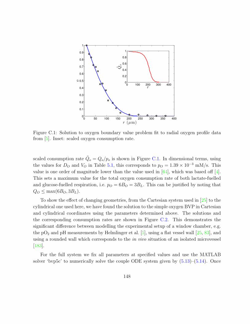
0 50 100 150 200 250 300 350 4000

0.1

0.2

0.3

0.4

0.5

0.6

0.7

0.8

0.9

1

r (µm)

o

0 100 200 300 4000

0.2

0.4

0.6

0.8

1

r

Qo

Figure C.1: Solution to oxygen boundary value problem fit to radial oxygen profile datafrom [5]. Inset: scaled oxygen consumption rate.

scaled consumption rate Qo = Qo/po is shown in Figure C.1. In dimensional terms, using

the values for DO and VO in Table 5.1, this corresponds to pO = 1.39× 10−3 mM/s. This

value is one order of magnitude lower than the value used in [64], which was based off [4].

This sets a maximum value for the total oxygen consumption rate of both lactate-fuelled

and glucose-fuelled respiration, i.e. pO = 6BO = 3BL. This can be justified by noting that

QO ≤ max(6BO, 3BL).

To show the effect of changing geometries, from the Cartesian system used in [25] to the

cylindrical one used here, we have found the solution to the simple oxygen BVP in Cartesian

and cylindrical coordinates using the parameters determined above. The solutions and

the corresponding consumption rates are shown in Figure C.2. This demonstrates the

significant difference between modelling the experimental setup of a window chamber, e.g.

the pO2 and pH measurements by Helmlinger et al. [5], using a flat vessel wall [25, 83], and

using a rounded wall which corresponds to the in vivo situation of an isolated microvessel

[183].

For the full system we fix all parameters at specified values and use the MATLAB

solver ‘bvp5c’ to numerically solve the couple ODE system given by (5.13)–(5.14). Once

148

0 50 100 150 200 250 300 350 4000

0.1

0.2

0.3

0.4

0.5

0.6

0.7

0.8

0.9

1

r (µm)

o

cylindrical

Cartesian

0 100 200 300 4000

0.2

0.4

0.6

0.8

1

r

Qo

Figure C.2: The Cartesian solution to oxygen boundary value problem fit to radial oxygenprofile data from [5] is the same as that in Figure C.1. The cylindrical solution utilizesthe same parameters as the Cartesian solution. This visualizes the effect of changinggeometries (Cartesian: flat wall; cylindrical: rounded wall). Inset: Corresponding scaledoxygen consumption rate.

again the Jacobian matrices for the boundary conditions and the corresponding first order

system are specified and the absolute and relative residual tolerances are set to 10−7. The

formula 5.15 is used to determine the resulting glucose concentration. The ATP production

is then determined by the formula (5.19).

C.4 Biochemical Summary

Preliminaries

The direction of the arrows in the reactions to follow are taken to be in the direction

that is predominantly exhibited in the environment that is being considered; they do not

imply irreversibility of the reaction. The reactions presented below are sometimes the

sum of many reactions in which case the Enzyme Commission (EC) number(s) will be

149

stated. These reactions are protonated to a physiological pH of 7.3, to remain consistent

with the pathways in the HumanCyc database [184]. The reactions presented below hold

at physiological pH 6.9 ≤ pH ≤ 7.4. In many cases, the nomenclature is simplified to

promote readability (e.g. the name D-glucopyranose which encompasses both α−D and

β−D glucose will be referred to simply as ‘glucose’). Molecular formulae are given in

Tables C.1. The primary purpose of the following biochemical summary is to determine the

relation between oxygen consumption, glucose consumption and ATP turnover in various

simplified metabolic regimes. The ATP yield will be emphasized by boxing the number of

ATP produced (and subsequently consumed) under a reaction and in summary equations.

This is the key to translating the biochemical reactions into ATP yields that will be used

in the mathematical model.

Transport across cell membrane

Glucose transport: We will simply write glucose transport across the cell membrane as

one molecule transported from extracellular space (subscript e) to the cytosol (subscript c).

The stoichiometry of this transmembrane transport is tissue-dependent and humans express

sodium-dependent transporters [185] and glucose/H+ symporters but predominantly utilize

uniporters [186]:

Ge → Gc. (C.12)

Cystolic processes: Glycolysis

The molecules involved in the reactions presented in this section all occur in the cytosol;

the subscript c on the molecules will be omitted in this subsection for simplicity.

Glycolysis: The conversion of glucose to pyruvate is the first step of cellular respi-

ration that will be used for the glucose-fuelled summary reactions to follow. The process

of glycolysis includes ten reactions catalyzed by the following enzymes in the given or-

der: (i) glucokinase/hexokinase (EC 2.7.1.1/2.7.1.2), (ii) glucose-6-phosphate isomerase

(EC 5.3.1.9), (iii) 6-phosphofructokinase (EC 2.7.1.11), (iv) fructose-biphosphate aldolase

(EC 4.1.2.13), (v) triosephosphate isomerase (EC 5.3.1.1), (vi) glyceraldehyde-3-phosphate

dehydrogenase (EC 1.2.1.12), (vii) phosphoglycerate kinase (EC 2.7.2.3), (viii) phospho-

glycerate mutase (EC 5.4.2.11/5.4.2.12), (ix) phosphoglycerate enolase (EC 4.2.1.11), and

150

(x) pyruvate kinase (EC 2.7.1.40). The summary reaction for glycolysis is:

G + 2ADP + 2Pi + 2NAD+ → 2P + 2ATP + 2NADH + 2H+ + 2H2O (C.13)

ATP hydrolysis: We assume ATP is consumed at the same rate that it is produced.

Reactions that have utilized this reaction will have the number of ATP consumed in a

box underneath the reaction arrow. This cellular energy consumption is given below and

is the stoichiometric proton source [187]. Due to the pKa of phosphate, it may buffer a

significant proportion of these protons, or other buffers may diminish this effect. They will

appear in summary equations as cytosolic protons H+c .

ATP + H2O→ ADP + Pi + H+ (C.14)

Lactate dehydrogenase (LDH): This enzyme (EC 1.1.1.27) facilitates the conver-

sion between pyruvate and lactate. This is necessary for NADH regeneration (oxidation)

without oxygen.

P + NADH + H+GGGBFGGG L− + NAD+ (C.15)

Glucose to Lactate:=(C.13)+ 2×(C.14)+2×(C.15). This is the net fermentation

reaction given in (5.1) that characterizes glycolytic cell population.

GkG

GGGGGGA

22L− + 2H+. (C.16)

Note: Cytosolic H+ production during conversion of glucose to lactate is a result of

ATP consumption, not the release of H+ from the neutral lactic acid.

Transport into mitochondria

The subscript m denotes molecules inside the mitochondrial matrix. We will omit con-

sideration of transport across the outer mitochondrial membrane since the molecules that

must subsequently cross the inner mitochondrial matrix can easily traverse the large porins

of the outer membrane, expect in the case of phosphate transport due to the necessity of

151

protonation. We will differentiate the intermembrane space (with the subscript i) when

considering the proton gradient across the inner mitochondrial matrix.

A key consideration for these reactions that involve molecules passing from one cell

compartment to another is that any charge differences induced by transport must be com-

pensated for with the corresponding cost to the proton gradient. While the reactions are

all charge balanced with respect to the total reaction, if they are not electroneutral with

respect to each cell compartment (each subscript) on both sides of the reaction, then the

equivalent proton transport must be included. This ensures the critical maintenance of the

electrochemical gradient across the inner mitochondrial membrane.

Malate-aspartate shuttle: This shuttle effectively delivers NADH from the cytosol

into the matrix to be utilized by ETC. We will take this to be the dominant shuttle

mechanism and thus consider the glycerol phosphate shuttle to be negligible (it is less

efficient). Sum of reactions/transport: (i) malate dehydrogenase (cytosol, EC 1.1.1.37),

(ii) malate import (iii) malate oxoglutarate antiporter, (iv) malate dehydrogenase (matrix),

(v) aspartate aminotransferase (matrix, EC 2.6.1.1), (vi) glutamate-aspartate antiporter,

(vii) aspartate aminotransferase (intermembrane space), (viii) oxaloacetate export. This

shuttle is electroneutral but does diminish the proton gradient:

NADHc + H+c + NAD+

m → NAD+c + NADHm + H+

m (C.17)

Pyruvate transport: The mitochondrial pyruvate carrier has been identified [188,

189] but the exact stoichiometry remains unclear. Here we will assume the transport is

symport with H+. If this is not the case it would have minimal effect on the system since

it only accounts for a one proton reduction in the gradient per pyruvate.

Pc + H+i → Pm + H+

m (C.18)

Glycolysis + Transport:=(C.12)+(C.13)+2×(C.17)+2×(C.18)

Ge + 2ADP + 2Pi + 2NAD+m + 2H+

i → 2Pm + 2ATP + 2NADHm + 4H+m + 2H2O (C.19)

The subscript on extracellular glucose will be omitted in what follows.

ATP-ADP translocase: This is required for ATP produced in mitochondria to reach

152

the cytosol and ADP in cytosol to be recycled into mitochondria.

ADPc + ATPm → ADPm + ATPc (C.20)

This diminishes the electrochemical gradient by one charge and must be compensated for

with the opposite and equal charge transfer.

Phosphate carrier: The transport of phosphate is taken to be antiport with OH−

[190]. However the net reaction is complicated by the multiple protonations of phosphate

at physiological pH. The pKa of phosphate in cells is 6.82, lower than the typical pH of the

cytosol and mitochondrial matrix and approximately equal to the intermembrane space pH

[191]. To fully model this process a multi compartment intracellular buffering model would

have to be constructed. Under the restriction that Pi exists predominantly as a hydrogen

phosphate ion (HPO2−4 ) in the cytosol and mitochondrial matrix, and can be sufficiently

converted to dihydrogen phosphate ion (H2PO−4 ) in the intermembrane space, the form

required for transport [190]. The neutral summary reaction is:

Pi,c + 2H+i → Pi,m + 2H+

m. (C.21)

To derive this we will briefly distinguish between P2−i :=HPO2−

4 and P−i :=H2PO−4 . It is

the sum of the following processes:

1. outer membrane transport: P2−i,c → P2−

i,i ,

2. intermembrane protonation: P2−i,i + H+

i → P−i,i,

3. hydroxide antiport: P−i,i + OH−m → P−i,m + OH−i ,

4. mitochondrial disassociation: P−i,m → P2−i,m + H+

m,

5. hydroxide balance: H+i + OH−i → H2Oi, H+

m + OH−m → H2Om,

6. water exchange: H2Oi → H2Om.

ATP transport:=(C.20)+(C.21). The transport of ATP into the cytosol, and reimport

of phosphate and ADP is summarized by:

ADPc + Pi,c + 2H+i + ATPm → ADPm + Pi,m + 2H+

m + ATPc (C.22)

153

Mitochondrial matrix processes

The molecules in this section without subscripts are all present in the mitochondrial matrix

(typically denoted with subscript m).

Pyruvate dehydrogenase complex: The link between glycolysis and the citric acid

cycle.

P + CoA + NAD+ → Ac-CoA + NADH + CO2 (C.23)

Citric acid cycle: The summary of reactions catalyzed by: (i) citrate synthase (EC

2.3.3.1), (ii) aconitase hydratase (EC 4.2.1.3), (iii) isocitrate dehydrogenase (EC 1.1.1.41),

(iv) oxoglutarate dehydrogenase (EC 1.2.4.2), (v) succinyl-CoA synthetase (EC 6.2.1.4),

(vi) succinate dehydrogenase (EC 1.3.5.1), (vii) fumarase (EC 4.2.1.2), (viii) malate de-

hydrogenase (EC 1.1.1.37). We also include phosphate exchange for conversion of energy

output of pathways from GTP to ATP yield alone via nucleoside-diphosphate kinase (EC

2.7.4.6).

Ac-CoA + 3NAD+ + Q + ADP + Pi + 2H2O→CoA + 3NADH + QH2 + ATP + 2H+

m + 2CO2 (C.24)

Pyruvate cofactor yield:=(C.23)+(C.24)+(C.22)

P+4NAD++Q+ADPc+Pi,c+2H+i +2H2O→ 4NADH+QH2+ATPc+4H+

m+3CO2 (C.25)

Electron transport chain (ETC)

NADH oxidation: The complete ETC is the sum of Complex I, Complex III and Complex

IV. Used to calculate the number of intermembrane protons generated per NADH.

NADH +1

2O2 + 11H+

m → NAD+ + 10H+i + H2O (C.26)

QH2 oxidation: Partial ETC (from Q) is the sum of Complex III and Complex IV.

Used to calculate the number of intermembrane protons generated per QH2.

QH2 +1

2O2 + 6H+

m → Q + 6H+i + H2O (C.27)

154

ATP synthase: It requires the transport of ten protons from the intermembrane space

across the inner membrane into the mitochondrial matrix to drive a single revolution of

the 10 subunits of ATP synthase [21]. This enables the production of 3 ATP molecules.

3ADP + 3Pi + 10H+i → 3ATP + 7H+

m + 3H2O (C.28)

ATP production by ETC:=(C.28)+3×(C.22). The net movement of 16 protons

results in 3 ATP in the cytosol.

3ADPc + 3Pi,c + 16H+i → 3ATPc + 3H2O + 13H+

m (C.29)

Respiration summaries

Pyruvate and ETC:=(C.25)+4×(C.26)+(C.27)

P + 2.5O2 + ADPc + Pi,c + 46H+m → ATPc + 3CO2 + 44H+

i + 3H2O (C.30)

Glucose and ETC:=(C.19)+2×(C.30)+2×(C.26)

G + 6O2 + 4ADPc + 4Pi,c + 110H+m → 4ATPc + 6CO2 + 106H+

i + 10H2O (C.31)

Glucose-fuelled ATP yield:=(C.31)+106/16=6.625×(C.29). A total of 6.625× 3 =

19.875 ATP are generated by the ETC per glucose molecule bringing the total to φg =

19.875 + 4 = 23.875 ATP per glucose.

G + 6O2 + φgADPc + φgPi,c + φgH+m → 6CO2 + (φg + 6)H2O + φgATPc (C.32)

Glucose-fuelled respiration:=(C.32)+ φg ×(C.14)

G + 6O2 + φgH+mGGGGGGA

23.8756CO2 + 6H2O + φgH

+c (C.33)

In order for this summary reaction to balance we must assume that the proton load

induced by ATP consumption in the cytosol is then transferred to the intermembrane

space. We can then dismiss these protons by assuming they are lost to proton leak, i.e.

155

H+i → H+

m, or we could have them be used as fuel for sustained ATP production. For

simplicity, to remain consistent in this respect to previous ATP yield estimates and since

proton leak is a significant factor in loss of energy metabolism efficiency, we will assume

the former approach yielding:

G + 6O2

kOGGGGGGA

23.8756CO2 + 6H2O (C.34)

Lactate and ETC:=Reverse reaction of (C.15)+(C.18)+(C.17)+(C.26)+(C.30)

L− + 3O2 + ADPc + Pi,c + 55H+m → 3CO2 + 53H+

i + 4H2O (C.35)

Lactate-fuelled ATP yield:=(C.35)+53/16=3.3125×(C.29). A total of φ` = 3.3125×3 + 1 = 10.9375 ≈ 11 ATP are generated per lactate molecule.

L− + 3O2 + φ`ADPc + φ`Pi,c + (φ` + 1)H+m → 3CO2 + (φell + 3)H2O + φ`ATPc (C.36)

Lactate-fuelled respiration:=(C.36)+φ`×(C.14).

L− + 3O2 + (φ` + 1)H+mGGGA

113CO2 + 3H2O + φ`H

+c (C.37)

Once again, if we desire to eliminate protons, we will assume H+c → H+

i → H+m. Thus

ending at:

Lactate-fuelled respiration:=(C.36)+ φ`×(C.14).

L− + 3O2 + H+m

kLGGGGGGA

113CO2 + 3H2O (C.38)

C.5 Metabolism reaction details

Presented below are the constituent steps of metabolic processes including glycolysis,

malate-aspartate shuttle, citric acid cycle and electron transport chain. In some cases the

156

Molecule Symbol FormulaMetabolites in mathematical modeloxgen O2 O2

lactate L− C3H5O−3glucose G C6H12O6

Coenzymesadenosine monophosphate AMP C10H12N5O4-PO2−

3

adenosine diphosphate ADP AMP-PO3−3

adenosine triphosphate ATP ADP-PO4−3

nicotinamide adenine dinucleotide NAD+ C21H26N7O14P−2reduced NAD+ NADH NAD+-H2−

coenzyme Q10 Q C59H90O4

ubiquinol QH2 C59H92O4

coenzyme A CoA C21H32N7O16P3S4−

acetyl CoA Ac-CoA CoA-C2H2O4−

Other moleculesprotona H+ H+

water H2O H2Ocarbon dioxide CO2 CO2

phosphateb Pi HPO2−4

pyruvate P C3H3O−3

Table C.1: Molecular formulae for the central molecules presented in metabolic reactionsconsidered in (C.12)–(C.38). The formulae presented are those that predominantly existat physiological pH 6.9 ≤ pH ≤ 7.4 and in this range the reactions are balanced in massand charge.a The proton typically exists as hydronium H3O+ in water.b A pKa value for phosphate is 6.82 so H2PO−4 exists at significant concentrations, especiallyin acidic environments found in cancer cells and in the intermembrane space of most cells,where pH values are low.

157

reactions have been simplified, especially those that comprise the ETC. It should be noted

that all reactions are balanced in mass and charge at physiological pH, 6.6 ≤ pH ≤ 7.4,

based on the pKa values of the molecules.

Glycolysis

These are the ten enzyme-catalysed steps of glycolysis including enzyme commission (EC)

numbers. Glycolytic intermediary formulae at physiological pH are given in Table C.2

while other molecules are given in Table C.4.

1. Glucokinase/hexokinase (EC 2.7.1.1/2.7.1.2)

G + ATP→ G6P + ADP + H+ (C.39)

2. glucose-6-phosphate isomerase (EC 5.3.1.9)

G6P→ F6P (C.40)

3. 6-phosphofructokinase (EC 2.7.1.11)

F6P + ATP→ FBP + ADP + H+ (C.41)

4. fructose-biphosphate aldolase (EC 4.1.2.13)

FBP→ G3P + DHAP (C.42)

5. triosephosphate isomerase (EC 5.3.1.1)

DHAP→ G3P (C.43)

6. glyceraldehyde-3-phosphate dehydrogenase (EC 1.2.1.12)

G3P + NAD+ + Pi → BPG + NADH + H+ (C.44)

158

Molecule Symbol Formula Reactionsglucose G C6H12O6 (C.39)glucose 6-phosphate G6P C6H11O9P2− (C.39),(C.40)fructose 6-phosphate F6P C6H11O9P2− (C.40),(C.41)fructose-1, 6-biphosphate FBP C6H10O12P4−

2 (C.41),(C.42)glyceraldehyde 3- phosphate G3P C3H5O6P2− (C.42),(C.43),(C.44)dihydroxyacetone phosphate DHAP C3H5O6P2− (C.42),(C.43)1,3-biphosphoglycerate BPG C3H4O10P4−

2 (C.44),(C.45)3-phosphoglycerate PG3 C3H4O7P3− (C.45),(C.46)2-phosphoglycerate PG2 C3H4O7P3− (C.46),(C.47)phosphoenolpyruvate PEP C3H2O6P3− (C.47),(C.48)pyruvate P C3H3O−3 (C.48)

Table C.2: Molecular formulae for glycolytic intermediaries involved in the metabolic re-actions (C.39)–(C.48). Chemical formulas presented are those that predominantly exist atphysiological pH 6.6 ≤ pH ≤ 7.4 based on the pKa values of the molecules, and in thisrange the reactions are balanced in mass and charge.

7. phosphoglycerate kinase (EC 2.7.2.3)

BPG + ADP→ PG3 + ATP (C.45)

8. phosphoglycerate mutase (EC 5.4.2.11/5.4.2.12)

PG3→ PG2 (C.46)

9. phosphoglycerate enolase (EC 4.2.1.11)

PG2→ PEP + H2O (C.47)

10. pyruvate kinase (EC 2.7.1.40)

PEP + ADP + H+ → P + ATP (C.48)

159

Malate-aspartate shuttle

Most treatments of this shuttle present it as a two-compartment system, but here we will

explicitly consider the cytosol, inter membrane space and mitochondrial matrix. While

always occurring in the mitochondrial matrix, depending on the source, malate dehydro-

genase and aspartate aminotransferase are presented as occurring in either the cytosol or

intermembrane space. We will assume malate dehydrogenase is predominantly cytosolic

and that aspartate aminotransferase predominantly occurs in the intermembrance space.

The former is justified because if this occurred in the intermembrane space it would re-

quire the transport of the relatively large coenzyme NADH across the outer mitochondrial

membrane rather than import of malate and export oxaloacetate. The latter is less con-

sequential since if aspartate aminotransferase was cystolic it would require the export of

two molecules and import of one molecule, however these molecules would all cancel out in

either case. Below are the six steps of the malate-aspartate shuttle, responsible for effec-

tively transferring a reduced NADH from the cytosol into the mitochondrion. The formulae

for molecules that are also CAC intermediaries are provided in Table C.3, namely, malate

(M), oxaloacetate (OAA) and 2-oxoglutarate (α), while those that are not are provided in

Table C.4.

1. malate dehydrogenase (cytosol, EC 1.1.1.37)

OAAc + NADHc + H+c → Mc + NAD+

c (C.49)

2. outer mitochondrial membrane transport of malate

Mc → Mi (C.50)

3. malate-oxoglutarate antiporter

Mi + αm → Mm + αi (C.51)

4. malate dehydrogenase (matrix, EC 1.1.1.37)

Mm + NAD+m → OAAm + NADHm + H+

m (C.52)

160

5. aspartate aminotransferase (matrix, EC 2.6.1.1)

OAAm + Glut−m → Aspm + αm (C.53)

6. glutamate-aspartate antiporter

Aspm + Glut−i → Aspi + Glut−m (C.54)

7. aspartate aminotransferase (intermembrane space, EC 2.6.1.1)

Aspi + αi → OAAi + Glut−i (C.55)

8. OAA export

OAAi → OAAc (C.56)

Citric acid cycle

The ten constituent reactions of the CAC are provided below. The formulae for CAC

intermediaries are given in Table C.3 while all others are given in Table C.4.

1. Citrate synthase (EC 2.3.3.1)

OAA + Ac-CoA + H2O→ Cit + CoA + H+ (C.57)

2. Aconitase hydratase (EC 4.2.1.3)

Cit→ cis-Acon + H2O (C.58)

cis-Acon + H2O→ Iso (C.59)

3. Isocitrate dehydrogenase (EC 1.1.1.41)

Iso + NAD+ → OAS + NADH + H+ (C.60)

OAS + H+ → α + CO2 (C.61)

161

Molecule Symbol Formula Reactionsoxaloacetate OAA C4H2O2−

5 (C.49),(C.52),(C.53),(C.55),(C.56),(C.57),(C.66)

citrate Cit C6H5O3−7 (C.57),(C.58)

cis-aconitate cis-Acon C6H3O3−6 (C.58),(C.59)

isocitrate Iso C6H5O3−7 (C.59),(C.60)

oxalosuccinate OAS C6H3O3−7 (C.60),(C.61)

2-oxoglutarate α C5H4O2−5 (C.51),(C.53),(C.55),(C.61),(C.62)

succinyl-CoA s-CoA CoA-C4H3O5−3 (C.62),(C.63)

succinate Suc C4H4O2−4 (C.63),(C.64)

fumarate F C4H2O2−4 (C.64),(C.65)

malate M C4H4O2−5 (C.49),(C.51),(C.52),(C.65),(C.66)

Table C.3: Molecular formulae for citric acid cycle intermediates involved in the metabolicreactions (C.57)–(C.66). Chemical formulas presented are those that predominantly existat physiological pH 6.6 ≤ pH ≤ 7.4 based on the pKa values of the molecules, and in thisrange the reactions are balanced in mass and charge.

4. oxoglutarate dehydrogenase (EC 1.2.4.2)

α + NAD+ + CoA→ S-CoA + NADH + CO2 (C.62)

5. succinyl-CoA synthetase (EC 6.2.1.4)

S-CoA + GDP + Pi → Suc + CoA + GTP (C.63)

6. succinate dehydrogenase (EC 1.3.5.1)

Suc + Q→ F + QH2 (C.64)

7. fumarase (EC 4.2.1.2)

F + H2O→ M (C.65)

8. malate dehydrogenase (EC 1.1.1.37)

M + NAD+ → OAA + NADH + H+ (C.66)

162

Nucleoside-diphosphate kinase (NDK, EC 2.7.4.6): Phosphate exchange for conversion

of energy output of pathways to ATP yield alone.

GTP + ADP→ GDP + ATP (C.67)

Electron transport chain

The net reactions of the complexes that make up the electron transport chain (ETC) are

presented below in a simplified form.

Complex I:

NADH + Q + 5H+m → NAD+ + QH2 + 4H+

i (C.68)

Complex III:

QH2 + 2H+m + 2Cytc3+ → Q + 4H+

i + 2Cytc2+ (C.69)

Complex IV:

2Cytc2+ + 4H+m +

1

2O2 → H2O + 2Cytc3+ + 2H+

i (C.70)

Liver functions

Processes that maintain vessel concentrations:

Alanine deamination (alanine to pyruvate): Consumes 4 ATP.

Gluconeogenesis (pyruvate to glucose): Consumes 6 ATP.

C.6 The effect of respiratory ATP yield on the results

The calculations contained in Chapter 5 consider a respiratory ATP yield of 28.9 [20]. This

corresponds to the traditional system where ATP yield does not include the costs associ-

ated with ATP consumption and phosphate transport. Preliminary considerations, that

admittedly use strong assumptions, suggest that the ATP yield may be as low as 24 ATP

per glucose molecules. The recalibrated results, using this lower ATP yield, are presented

in Figures C.3, C.4, C.5 are analogous to Figures 5.5, 5.6, 5.8. The difference in results

is that the contribution of respiratory processes is diminished relative to glycolytic ATP

163

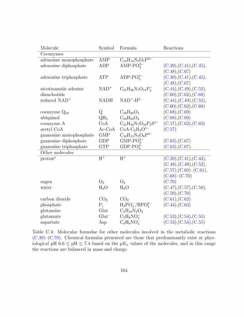
Molecule Symbol Formula ReactionsCoenzymesadenosine monophosphate AMP C10H12N5O7P2−

adenosine diphosphate ADP AMP-PO3−3 (C.39),(C.41),(C.45),

(C.48),(C.67)adenosine triphosphate ATP ADP-PO4−

3 (C.39),(C.41),(C.45),(C.48),(C.67)

nicotinamide adenine NAD+ C21H26N7O14P−2 (C.44),(C.49),(C.52),dinucleotide (C.60),(C.62),(C.68)reduced NAD+ NADH NAD+-H2− (C.44),(C.49),(C.52),

(C.60),(C.62),(C.68)coenzyme Q10 Q C59H90O4 (C.68),(C.69)ubiquinol QH2 C59H92O4 (C.68),(C.69)coenzyme A CoA C21H32N7O16P3S4− (C.57),(C.62),(C.63)acetyl CoA Ac-CoA CoA-C2H2O4− (C.57)guanosine monophosphate GMP C10H12N5O8P2−

guanosine diphosphate GDP GMP-PO3−3 (C.63),(C.67)

guanosine triphosphate GTP GDP-PO4−3 (C.63),(C.67)

Other moleculesprotona H+ H+ (C.39),(C.41),(C.44),

(C.48),(C.49),(C.52),(C.57),(C.60)–(C.61),(C.68)–(C.70)

oxgen O2 O2 (C.70)water H2O H2O (C.47),(C.57),(C.58),

(C.59),(C.70)carbon dioxide CO2 CO2 (C.61),(C.62)phosphate Pi H2PO−4 /HPO2−

4 (C.44),(C.63)glutamine Glut C5H10N2O3

glutamate Glut− C5H8NO−4 (C.53),(C.54),(C.55)aspartate Asp C4H6NO−4 (C.53),(C.54),(C.55)

Table C.4: Molecular formulae for other molecules involved in the metabolic reactions(C.39)–(C.70). Chemical formulas presented are those that predominantly exist at phys-iological pH 6.6 ≤ pH ≤ 7.4 based on the pKa values of the molecules, and in this rangethe reactions are balanced in mass and charge.

164

0 50 100 150 200 250 300 350 4000

1

2

3

4

5

6x 10

−3

r (µm)

AT

P p

rod

uctio

n (

mM

/s)

Glycolysis

L−respiration

G−respiration

Figure C.3: The base case for ATP turnover (consumption/production) rates correspondingto consumption rates given in Figure 5.4 with altered respiratory ATP parameters. Thecontributions of the pathways are bounded by the total ATP turnover rate PATP . Glycolysisdominates in hypoxic/anoxic regions while glucose-fuelled respiration occurs sparingly nearthe blood vessel. Lactate-fuelled cells are consuming the byproduct of the glycolytic cellswhere there is oxygen present.

production, and thus the share of the total ATP yield due to oxygen-fuelled metabolism is

lessened.

165

0 50 100 150 200 250 300 350 4000

1

2

3

4

5

6

7

8

9x 10

−3

r (µm)

AT

P p

rod

uctio

n (

mM

/s)

Glycolysis

L−respiration

G−respiration

Figure C.4: ATP turnover (consumption/production) rates for cells exhibiting the Warburgeffect with altered respiratory ATP parameters (differs from base case because ΛO decreasedfrom 4000 to 100). The contributions of the pathways are bounded by the total ATPturnover rate PATP . Glycolysis is dominant in all regions of the tumour. Glucose-fuelledrespiration occurs sparingly near the blood vessel. Lactate-fuelled cells are consuming thebyproduct of the glycolytic cells where there is oxygen present.

166

1 2 3 4 5 60

50

100

150

200

Φ

Glycolysis

L−respiration

G−respiration

1. base 2. W 3. Glyc 4. LDH 5. Resp 6. R-WΛO 4000 100 N/A N/A 4000 100BG 1 1 0 0 1 1BL 1 1 1 0 0 0BO 1 1 0 1 0 0

Figure C.5: The contributions of the pathways are bounded by the total ATP turnoverrate Φ in a unit annulus of tissue. This more accurately represents the total contributionof each cell population to metabolism. From left to right the bars denote the follow-ing cell populations: 1. Base case: Tissue that exhibits lactate consumption in hypoxicconditions with parameters in Table 5.1. 2. Warburg effect: Tissue utilizing aerobicglycolysis. 3. Glycolytic knockdown: Tissue experiencing complete glycolytic inhibi-tion. 4. LDH inhibitor: Tissue experiencing complete LDH inhibition. 5. Respirationknockdown: Tissue experiencing mitochondrial inhibition with glycolysis repression byoxygen. 6. Respiration knockdown and Warburg effect: Mitochondrial inhibitionwith aerobic glycolysis. The dashed red line shows a threshold of Φ = 100. If either of thereactions which block glycolysis are knocked out (glycolysis or LDH inhibitors) the totalATP produced is less than half the threshold. If on the other hand respiration is inhibitedthen either (i) if oxygen represses glycolysis there is minimal ATP production, or (ii) ifglycolysis is independent of oxygen concentration there is more ATP produced than thethreshold.

167

Appendix D

Additional nanoparticle release and

protein expression work

This appendix serves as supplementary material for Chapter 6. The preliminary nanopar-

ticle release profile fitting with definitions for the goodness of fit measure χ2 and additional

protein expression experiments that went unpublished is outlined here.

D.1 Preliminary nanoparticle models

Preliminary nanoparticle release experiments suggested a biexponential release with decay

was an appropriate model. Here we will outline this result while noting that a simpler

decay equation was sufficient for fitting in Chapter 6.

For cisplatin released from liposomes, a biexponential release is assumed. Biexponen-

tial processes are common in pharmocokinetics to describe various phenomenon (e.g. the

clearance of doxorubicin from plasma [192]) where two similar yet separate processes occur

with differing rate constants. This biexponential release profile is characterized by an ini-

tial burst followed by a slower sustained release. We can motivate the functional form by

considering a simple system of ordinary differential equations (ODEs) that includes both

the initial rapid release of some cisplatin and the sustained release due to encapsulation in

the liposome. To facilitate this, we assume that the administered liposomes consists of cis-

platin that is rapidly released at rate rb and slowly released at rate rs. The concentrations

168

of rapidly and slowly released cisplatin are denoted by cb and cs respectively, and the lipo-

somes are initially comprised of a fixed amount of quick release and prolonged release given

by cb0 and cs0 respectively (see Figure D.1). For both release processes, only a fraction, φ,

of the total amount of contained cisplatin is released, an amount that depends primarily

on the acidity of the environment. Even in an acidic environment, our data shows that

55% of the cisplatin is never released from the liposome. The total amount of administered

cisplatin, denoted cT , satisfies the relation cT = cb0 +cs0 where the total amount of released

cisplatin is given by φcT . In addition to the two types of release, we must also consider

the natural decay of released cisplatin at a rate dL. The system of ODEs is then:

dcbdt

= −rbcb (D.1)

dcsdt

= −rscs (D.2)

dcedt

= rbcb + rscs − dLce (D.3)

with the solution of interest being the released cisplatin

ce(t) = Ab exp(−rbt) + Af exp(−rf t)− (Ab + Af )exp(−dLt),

where

Ab =φcb0rbdL − rb

, Af =φcf0rfdL − rf

.

We use equations (D.1)–(D.3) to obtain parameters to describe the release profile data

in neutral and acidic environments. The pH-dependent parameters that differ between

environments will be the fraction of released cisplatin φ and the decay rate of the cisplatin

dL; the release parameters remain constant between both environments. We will quantify

the goodness of fit for a model f with p parameters to N observations yi with the reduced

chi-squared statistic χ2red = χ2/ν, where ν is the degrees of freedom, typically set to

ν = N − p− 1 and

χ2 =N∑i=1

yi − f(xi)

σ2i

,

where σ2i is the variance of the ith observation. It is typically assumed that χ2

red < 1 is

overfitting and χ2red > 1 is an inadequate model with the goal being to get χ2

red as close as

possible to one. Fitting the parameters to the release profile data yields a very accurate

169

Parameter Units Fit Valuerb h−1 0.5737rs h−1 0.05352

d(n)L h−1 0.0009932

d(a)L h−1 0.001703cb0 µM 0.4099cf0 µM 0.5901φ(n) - 0.2300φ(a) - 0.3790

Table D.1: Parameters for the preliminary release profile experiments.

(over)fit as can be seen in Figure D.2 (χ2red = 0.1032, N = 18, p = 8). The parameters are

given in Table D.1.

It is worth noting that a single exponential fit does not provide an accurate prediction

for liposome release in these experiments, although monoexponential fits are commonly

sufficient. The model in this case would be (D.1) and dcedt

= rbcb − dLce. Attempting to

fit our release profiles with this model leads to fits that overestimate the release at times

immediately following the initial burst (e. g. t=6, 7 hours) and then underestimates values

for later times, as can be seen in Figure D.3. The reason for this is that the relatively small

standard deviations for early times are causing the rate of release to be large enough to fit

the burst while driving the decay rate dL to zero in an attempt to fit the underestimated

later time points with larger standard deviations. In fact, setting the value dL = 0 improves

the fit slightly with χ2red = 3.799 (N = 18, p = 5); this is the result shown in Figure D.3.

Allowing the release rate rb to be locally fitted to each experiment does not improve the

fitting statistic (χ2red = 4.1102, N = 18, p = 6; results not shown).

D.1.1 Liposomal model

As mentioned in Chapter 6, the unsatisfactory fit in the neutral microenvironment to the

final nanoparticle release experiments could be fit by the addition of a single additional

parameter accounting for liposomal erosion. The fit to this model is given in Figure D.4

(χ2red = 0.61, N = 15, p = 3); this would have negligible effect on the acidic release

(χ2red = 0.58, N = 15, p = 3).

170

Figure D.1: Depiction of biexponential drug model corresponding to the extension of (D.1)–(D.3) to cellular concentrations for nanoparticle release and delayed transmembrane trans-port of self-assembling cis-platinum nanoparticles (SACNs) and free cisplatin in an acidicenvironment.

171

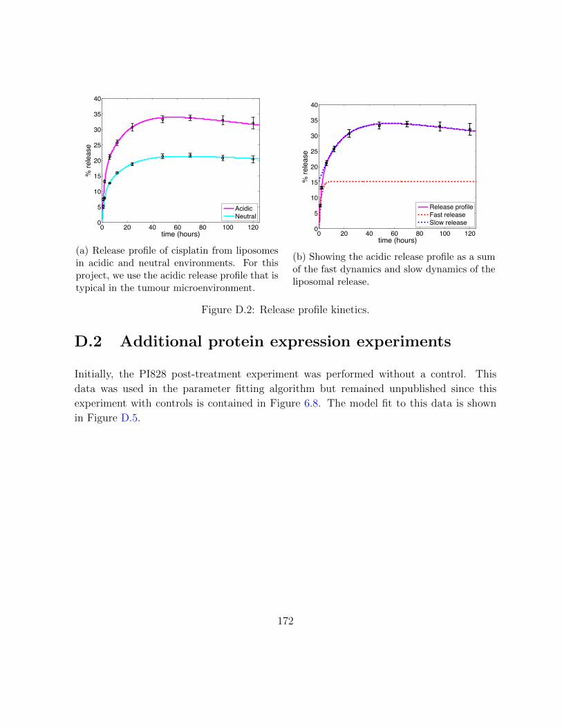
0 20 40 60 80 100 1200

5

10

15

20

25

30

35

40

time (hours)

% re

leas

e

AcidicNeutral

(a) Release profile of cisplatin from liposomesin acidic and neutral environments. For thisproject, we use the acidic release profile that istypical in the tumour microenvironment.

0 20 40 60 80 100 1200

5

10

15

20

25

30

35

40

time (hours)

% re

leas

e

Release profileFast releaseSlow release

(b) Showing the acidic release profile as a sumof the fast dynamics and slow dynamics of theliposomal release.

Figure D.2: Release profile kinetics.

D.2 Additional protein expression experiments

Initially, the PI828 post-treatment experiment was performed without a control. This

data was used in the parameter fitting algorithm but remained unpublished since this

experiment with controls is contained in Figure 6.8. The model fit to this data is shown

in Figure D.5.

172

0 20 40 60 80 100 1200

5

10

15

20

25

30

35

40

time (hours)

% re

leas

e

AcidicNeutral

Figure D.3: Attempting to fit the release profile of cisplatin from liposomes in acidic andneutral environments using a single exponential.

173

0 20 40 60 80 100 1200

10

20

30

40

50

60

70

time (hours)

% re

leas

e

AcidicNeutral

Figure D.4: Fitting the release profile of cisplatin from liposomes in acidic and neutralenvironments using a liposomal release model.

0 10 20 30 400

1000

2000

3000

4000

5000

6000

time (hours)

% c

aspa

se e

xpre

ssio

n(o

ver c

ontro

l)

(a)

0 10 20 30 400

20

40

60

80

100

120

time (hours)

% p

Akt e

xpre

ssio

n(o

ver c

ontro

l)

(b)

Figure D.5: The inhibition of pAkt by PI828 post treatment with SACN D.5b and thesynergistic increase in caspase expression as compared to SACN alone-treated controlsD.5a.

174

Appendix E

Reactive oxygen species and

antioxidant model

A collaborative work that I made both analytical and numerical contributions to, is briefly

outlined below with a focus on those aspects which I was directly involved in.

E.1 Introduction

H2O2 is produced in eukaryotes during metabolic processes [193, 194] and by other external

and internal sources such as growth factors [195, 196]. The concentration level of H2O2

plays a role in the initiation progression and treatment efficacy of major diseases such as

cancer, diabetes, Alzheimers disease and Parkinsons disease [197, 198, 199, 200, 201, 202,

203]. H2O2 is also involved in critical cell signalling processes such as cell growth and

apoptosis [204, 205, 206, 207].

H2O2 is highly reactive and can directly and indirectly damage cell compartments, hence

cells must employ detoxifying mechanisms to remove excess H2O2 [208, 209, 210]. One of

the principal mechanisms for detoxification is glutathione peroxidase, which along with

other detoxifying agents such as catalase remove H2O2 [211, 212]. Whether or not these

antioxidants work independently or they have evolved symbiotically to assist each other

with H2O2 detoxification is not clear. To unravel this we derive a relationship between the

concentration of H2O2, the production rate of H2O2 and the concentrations of antioxidants

175

based on the kinetic equations which govern the detoxification of H2O2 by glutathione

peroxidase-1 and catalase. We use this relationship to show that catalase and glutathione

peroxide-1 behaves in a synergetic way. This synergy could help in understanding many

pathological cases, the efficacy of therapies and the design of new drugs or therapies.

E.2 Mathematical model

The three major families of antioxidants that exist in cells, which help to regulate and

detoxify H2O2, are the glutathione peroxidase family, the peroxiredoxin family and cata-

lase. In our model we assume that catalase and glutathione peroxidases are the major

antioxidants in the system to avoid the extraneous complexity of the full problem. We

also utilize the fact that glutathione peroxidase-1 is the predominant member of the glu-

tathione peroxidase family in removing H2O2 and thus only consider its effect in our model

[213]. We also assume that catalase, which is sequestered in the peroxisomes, is exposed to

the same concentration levels of H2O2. We will discuss the affect of these assumptions in

the discussion section and argue that these assumptions do not affect the main conclusion

of this paper. We use chemical reaction equations to derive corresponding kinetic equa-

tions for the concentrations of involved species and thus obtain a relationship between the

concentrations of these species at steady state.

The detoxification of H2O2 by catalase is given by the chemical reaction

H2O2

kcatGGGGGGGAO2 + 2H2O. (E.1)

In this process H2O2 is converted to harmless oxygen and water in the presence of catalase.

GPx has been the subject of previous mathematical models [214] and its mechanism is

well established [215, 216]. The action of these enzymes rely on the presence of a specific

cofactor: glutathione (GSH) which is responsible for converting GPx0 to [GS-GPx] and

then [GS-GPx] back to its reduced form GPxr. These reduced forms can now once again

eliminate H2O2 from the environment. The generally accepted molecular reactions that

occur in the conversion of H2O2 to H2O, in dilute solutions, is represented by the following

176

three reactions [216]:

GPxr + H2O2 + H+k1

GGGGGGAGPx0 + H2O, (E.2)

GPx0 + GSHk2

GGGGGGA[GS-GPx] + H2O, (E.3)

[GS-GPx] + GSHk3

GGGGGGAGPxr + GSSG + H+, (E.4)

where k1, k2 and k3 are the reaction rates calculated by Antunes et al. [215] and given in

Table E.1. These reactions are commonly summarized as

H2O2 + 2GSHGPx

GGGGGGGGAGSSG + 2H2O. (E.5)

Table E.1: Rate constants for the GPx system from [215].

Rate (µM−1s−1)k1 21k2 0.04k3 10

We will now write down a system of equations that correspond to the reactions (E.1)–

(E.4). An equation that tracks H+ and H2O concentrations are not included, under the

assumption that reactions are independent of pH and water content. The two major as-

sumptions are: (i) spatial independence, this leads to a system of ODEs, and (ii) the

concentration of catalase remains constant. We will denote this constant catalase concen-

tration by C. Letting x1 = [GPxr], x2 = [GPx0], x3 = [[GS-GPx]] denote the concentra-

tions of GPx and its intermediate forms during recycling, x4 = [H2O2] the concentration

177

of hydrogen peroxide, and x5 = [GSH] gives the following system of ODEs:

x1 = k3x3x5 − k1x1x4, (E.6)

x2 = k1x1x4 − k2x2x5, (E.7)

x3 = k2x2x5 − k3x3x5, (E.8)

x4 = −k1x1x4 − kcatCx4 + p4, (E.9)

x5 = −k3x3x5 − k2x2x5 + p5, (E.10)

(E.11)

where p4 and p5 are the constant production rates of H2O2 and GSH respectively. Note

than an equation for GSSG is omitted since it only plays the role of a waste product.

We are interested in finding the steady state solution to (E.6)–(E.10) and will now

derive the concentration of H2O2 as a function of x1, x2, x5 and C. Equations (E.6)–(E.8)

sum to zero, so the total concentration of GPx is fixed at some total value eT satisfying

x1 + x2 + x3 = eT . This relationship is only valid because there are no sources or sinks

more any of these species. Furthermore, the concentration of [GS-GPx] is negligible since

k2 k1 and k2 k3, so we will use the approximation x1 + x2 = eT . Using these

assumptions, the steady state concentrations can be found, or we could look at temporal

behaviour.

E.3 Results

I have analyzed the aforementioned system in multiple scenarios. Along with performing

numerical analytical analysis of this system, I have also proven stability results. We have

also used the model to quantify the synergy between catalase and glutathione-peroxidase-1

which amplifies the detoxification power of glutathione peroxidase-1. Hence any change

(upregulation or downregulation) in the catalase concentration has a direct affect on the

glutathione peroxidase-1 activity and has to be included in understanding any related

phenomena. Also we propose that the activity of glutathione peroxidase-1 could be regu-

lated by changing the concentration of catalase. The synergistic relationship between these

antioxidants is reported in [174]. This work was expanded to include the effects of cell per-

meability, especially the role of aquaporin expression. This has important consequences

for the efficacy of ascorbic acid for cancer treatment [175]. While I was involved in model

178

development and calculating system solutions, I am not the first author of these results,

so they are omitted.

179

References

[1] S. Ramanujan, G. C. Koenig, T. P. Padera, B. R. Stoll, and R. K. Jain, “Local

imbalance of proangiogenic and antiangiogenic factors: a potential mechanism of

focal necrosis and dormancy in tumors,” Cancer Res., vol. 60, pp. 1442–1448, 2000.

[2] R. K. Jain, R. T. Tong, and L. L. Munn, “Effect of vascular normalization by an-

tiangiogenic therapy on interstitial hypertension, peritumor edema, and lymphatic

metastasis: insights from a mathematical model,” Cancer Res., vol. 67, pp. 2729–

2735, 2007.

[3] J. J. Casciari, S. V. Sotirchos, and R. M. Sutherland, “Mathematical modelling of

microenvironment and growth in EMT6/Ro multicellular tumour spheroids,” Cell

Prolif., vol. 25, pp. 1–22, 1992.

[4] J. J. Casciari, S. V. Sotirchos, and R. M. Sutherland, “Variations in tumor cell

growth rates and metabolism with oxygen concentration, glucose concentration, and

extracellular pH,” J. Cell. Physiol., vol. 151, pp. 386–394, 1992.

[5] G. Helmlinger, F. Yuan, M. Dellian, and R. K. Jain, “Interstitial pH and pO2 gradi-

ents in solid tumors in vivo: high-resolution measurements reveal a lack of correla-

tion,” Nat. Med., vol. 3, pp. 177–182, Feb 1997.

[6] R. A. Gatenby and P. K. Maini, “Mathematical oncology: cancer summed up,”

Nature, vol. 421, no. 6921, pp. 321–321, 2003.

[7] A. R. Anderson and V. Quaranta, “Integrative mathematical oncology,” Nature Re-

views Cancer, vol. 8, no. 3, pp. 227–234, 2008.

180

[8] A. Pandey, A. Kulkarni, B. Roy, A. Goldman, S. Sarangi, P. Sengupta, C. Phipps,

J. Kopparam, M. Oh, S. Basu, et al., “Sequential application of a cytotoxic nanopar-

ticle and a PI3K inhibitor enhances antitumor efficacy,” Cancer research, 2013.

[9] N. Bellomo, N. Li, and P. K. Maini, “On the foundations of cancer modelling: selected

topics, speculations, and perspectives,” Mathematical Models and Methods in Applied

Sciences, vol. 18, no. 04, pp. 593–646, 2008.

[10] T. S. Deisboeck, Z. Wang, P. Macklin, and V. Cristini, “Multiscale cancer modeling,”

Annual review of biomedical engineering, vol. 13, 2011.

[11] T. Roose, S. J. Chapman, and P. K. Maini, “Mathematical models of avascular tumor

growth,” Siam Review, vol. 49, no. 2, pp. 179–208, 2007.

[12] B. Ribba, T. Alarcon, K. Marron, P. K. Maini, and Z. Agur, “The use of hybrid

cellular automaton models for improving cancer therapy,” in Cellular Automata,

pp. 444–453, Springer, 2004.

[13] J. Ferlay, H.-R. Shin, F. Bray, D. Forman, C. Mathers, and D. M. Parkin, “Estimates

of worldwide burden of cancer in 2008: GLOBOCAN 2008,” International journal of

cancer, vol. 127, no. 12, pp. 2893–2917, 2010.

[14] L. Kachuri, P. De, L. Ellison, and R. Semenciw, “Cancer incidence, mortality and

survival trends in Canada, 1970–2007,” Chronic diseases and injuries in Canada,

vol. 33, no. 2, pp. 69–80, 2013.

[15] D. Hanahan and R. A. Weinberg, “The hallmarks of cancer,” Cell, vol. 100, pp. 57–

70, 2000.

[16] J. Folkman, “Tumor angiogenesis: therapeutic implications,” N. Engl. J. Med.,

vol. 285, pp. 1182–1186, 1971.

[17] D. Hanahan and R. A. Weinberg, “Hallmarks of cancer: The next generation,” Cell,

vol. 144, no. 5, pp. 646 – 674, 2011.

[18] D. Hanahan and J. Folkman, “Patterns and emerging mechanisms of the angiogenic

switch during tumorigenesis,” Cell, vol. 86, pp. 353–364, 1996.

[19] R. K. Jain, “Transport of molecules across tumor vasculature,” Cancer Metastasis

Rev., vol. 6, pp. 559–593, 1987.

181

[20] M. D. Brand, “The efficiency and plasticity of mitochondrial energy transduction,”

Biochemical Society Transactions, vol. 33, no. 5, pp. 897–904, 2005.

[21] P. R. Rich, “The molecular machinery of Keilin’s respiratory chain,” Biochemical

Society Transactions, vol. 31, no. 6, pp. 1095–1106, 2003.

[22] O. Warburg, “On the origin of cancer cells,” Science, vol. 123, pp. 309–314, 1956.

[23] M. G. Vander Heiden, L. C. Cantley, and C. B. Thompson, “Understanding the

Warburg effect: the metabolic requirements of cell proliferation,” science, vol. 324,

no. 5930, pp. 1029–1033, 2009.

[24] K. Smallbone, D. J. Gavaghan, R. A. Gatenby, and P. K. Maini, “The role of acidity

in solid tumour growth and invasion,” Journal of Theoretical Biology, vol. 235, no. 4,

pp. 476–484, 2005.

[25] H. R. Molavian, M. Kohandel, M. Milosevic, and S. Sivaloganathan, “Fingerprint

of cell metabolism in the experimentally observed interstitial pH and pO2 in solid

tumors,” Cancer Res., vol. 69, pp. 9141–9147, 2009.

[26] L. A. Sauer, J. W. Stayman, and R. T. Dauchy, “Amino acid, glucose, and lactic acid

utilization in vivo by rat tumors,” Cancer research, vol. 42, no. 10, pp. 4090–4097,

1982.

[27] P. Sonveaux, F. Vegran, T. Schroeder, M. C. Wergin, J. Verrax, Z. N. Rabbani,

C. J. De Saedeleer, K. M. Kennedy, C. Diepart, B. F. Jordan, et al., “Targeting

lactate-fueled respiration selectively kills hypoxic tumor cells in mice,” The Journal

of clinical investigation, vol. 118, no. 12, p. 3930, 2008.

[28] A. Di Marco, M. Gaetani, and B. Scarpinato, “Adriamycin (NSC-123,127): a new

antibiotic with antitumor activity.,” Cancer chemotherapy reports. Part 1, vol. 53,

no. 1, p. 33, 1969.

[29] B. Rosenberg and L. Vancamp, “Platinum compounds: a new class of potent anti-

tumour agents,” Nature, vol. 222, pp. 385–386, 1969.

[30] A. Lorch, A. Kleinhans, A. Kramar, C. K. Kollmannsberger, J. T. Hartmann,

C. Bokemeyer, O. Rick, and J. Beyer, “Sequential versus single high-dose chemother-

apy in patients with relapsed or refractory germ cell tumors: long-term results of a

182

prospective randomized trial,” Journal of Clinical Oncology, vol. 30, no. 8, pp. 800–

805, 2012.

[31] A. Ardizzoni, L. Boni, M. Tiseo, F. V. Fossella, J. H. Schiller, M. Paesmans, D. Ra-

dosavljevic, A. Paccagnella, P. Zatloukal, P. Mazzanti, et al., “Cisplatin-versus

carboplatin-based chemotherapy in first-line treatment of advanced non–small-cell

lung cancer: an individual patient data meta-analysis,” Journal of the National Can-

cer Institute, vol. 99, no. 11, pp. 847–857, 2007.

[32] B. Sirohi, M. Arnedos, S. Popat, S. Ashley, A. Nerurkar, G. Walsh, S. Johnston, and

I. Smith, “Platinum-based chemotherapy in triple-negative breast cancer,” Annals

of oncology, vol. 19, no. 11, pp. 1847–1852, 2008.

[33] G. M. Tozer, “Measuring tumour vascular response to antivascular and antiangio-

genic drugs,” Br. J. Radiol., vol. 76 Spec No 1, pp. 23–35, 2003.

[34] A. A. Van der Veldt, M. Lubberink, I. Bahce, M. Walraven, M. P. de Boer, H. N.

Greuter, N. H. Hendrikse, J. Eriksson, A. D. Windhorst, P. E. Postmus, et al.,

“Rapid decrease in delivery of chemotherapy to tumors after anti-VEGF therapy:

implications for scheduling of anti-angiogenic drugs,” Cancer cell, vol. 21, no. 1,

pp. 82–91, 2012.

[35] R. K. Jain, “Normalization of tumor vasculature: an emerging concept in anti-

angiogenic treatment,” Science, vol. 307, pp. 58–62, 2005.

[36] T. T. Batchelor, A. G. Sorensen, E. di Tomaso, W.-T. Zhang, D. G. Duda, K. S.

Cohen, K. R. Kozak, D. P. Cahill, P.-J. Chen, M. Zhu, et al., “AZD2171, a pan-VEGF

receptor tyrosine kinase inhibitor, normalizes tumor vasculature and alleviates edema

in glioblastoma patients,” Cancer cell, vol. 11, no. 1, pp. 83–95, 2007.

[37] J. Folkman, “Angiogenesis and apoptosis,” Seminars in Cancer Biology, vol. 13,

no. 2, pp. 159 – 167, 2003.

[38] G. M. Tozer, C. Kanthou, C. S. Parkins, and S. A. Hill, “The biology of the combre-

tastatins as tumour vascular targeting agents,” Int. J. Exp. Pathol., vol. 83, pp. 21–

38, 2002.

[39] H. Hurwitz, L. Fehrenbacher, W. Novotny, T. Cartwright, J. Hainsworth, W. Heim,

J. Berlin, A. Baron, S. Griffing, E. Holmgren, N. Ferrara, G. Fyfe, B. Rogers, R. Ross,

183

and F. Kabbinavar, “Bevacizumab plus irinotecan, fluorouracil, and leucovorin for

metastatic colorectal cancer,” N. Engl. J. Med., vol. 350, no. 23, pp. 2335–2342, 2004.

[40] A. Sandler, R. Gray, M. C. Perry, J. Brahmer, J. H. Schiller, A. Dowlati, R. Lilen-

baum, and D. H. Johnson, “Paclitaxel–carboplatin alone or with bevacizumab for

non–small-cell lung cancer,” New England Journal of Medicine, vol. 355, no. 24,

pp. 2542–2550, 2006.

[41] F. M. Gabhann and A. S. Popel, “Targeting neuropilin-1 to inhibit VEGF signaling

in cancer; comparison of therapeutic approaches,” PLoS Comput. Biol., vol. 2, 2006.

[42] S. Wu and R. Singh, “Resistance to chemotherapy and molecularly targeted thera-

pies: rationale for combination therapy in malignant melanoma,” Current molecular

medicine, vol. 11, no. 7, pp. 553–563, 2011.

[43] L. L. Belyanskaya, S. Hopkins-Donaldson, S. Kurtz, A. P. Simoes-Wust, S. Yousefi,

H.-U. Simon, R. Stahel, and U. Zangemeister-Wittke, “Cisplatin activates Akt in

small cell lung cancer cells and attenuates apoptosis by survivin upregulation,” In-

ternational journal of cancer, vol. 117, no. 5, pp. 755–763, 2005.

[44] A. V. Rao, G. Akabani, and D. A. Rizzieri, “Radioimmunotherapy for non-Hodgkin’s

lymphoma,” Clin. Med. Res., vol. 3, pp. 157–165, 2005.

[45] S. M. Moghimi, A. C. Hunter, and J. C. Murray, “Long-circulating and target-specific

nanoparticles: theory to practice,” Pharmacol. Rev., vol. 53, pp. 283–318, 2001.

[46] Y. Matsamura and H. Maeda, “A new concept for macromolecular therapeutics in

cancer chemotherapy: mechanisms of tumoritropic accumulation of protein and the

antitumor agent smancs,” Cancer Res., vol. 46, pp. 6387–6392, 1986.

[47] J. Fang, H. Nakamura, and H. Maeda, “The EPR effect: unique features of tumor

blood vessels for drug delivery, factors involved, and limitations and augmentation

of the effect,” Advanced drug delivery reviews, vol. 63, no. 3, pp. 136–151, 2011.

[48] Y. Lu and P. S. Low, “Folate-mediated delivery of macromolecular anticancer ther-

apeutic agents,” Adv. Drug Deliv. Rev., vol. 54, pp. 675–693, 2002.

184

[49] J. F. Ross, P. K. Chaudhuri, and M. Ratnam, “Differential regulation of folate re-

ceptor isoforms in normal and malignant tissues in vivo and in established cell lines.

Physiologic and clinical implications,” Cancer, vol. 73, pp. 2432–2443, 1994.

[50] R. J. Lee and P. S. Low, “Folate-mediated tumor cell targeting of liposome-entrapped

doxorubicin in vitro,” Biochim. Biophys. Acta, vol. 1233, pp. 134–144, 1995.

[51] J. Sudimack and R. J. Lee, “Targeted drug delivery via the folate receptor,” Adv.

Drug Deliv. Rev., vol. 41, pp. 147–162, 2000.

[52] P. C. Brooks, A. M. Montgomery, M. Rosenfeld, R. A. Reisfeld, T. Hu, G. Klier, and

D. A. Cheresh, “Integrin αvβ3 antagonists promote tumor regression by inducing

apoptosis of angiogenic blood vessels,” Cell, vol. 79, pp. 1157–1164, 1994.

[53] S. Sengupta, D. Eavarone, I. Capila, G. Zhao, N. Watson, T. Kiziltepe, and

R. Sasisekharan, “Temporal targeting of tumour cells and neovasculature with a

nanoscale delivery system,” Nature, vol. 436, pp. 568–572, 2005.

[54] S. Awasthi, “A dendrimer-based prodrug for use in an anti-cancer nanocell,” Master’s

thesis, Massachusetts Institute of Technology, 2007.

[55] M. Kohandel, C. A. Haselwandter, M. Kardar, S. Sengupta, and S. Sivaloganathan,

“Quantitative model for efficient temporal targeting of tumor cells and neovascula-

ture,” Computational and Mathematical Methods in Medicine, vol. 2011, 2011.

[56] D. Hanahan, G. Bergers, and E. Bergsland, “Less is more, regularly: metronomic

dosing of cytotoxic drugs can target tumor angiogenesis in mice,” J. Clin. Invest.,

vol. 105, pp. 1045–1047, 2000.

[57] R. S. Kerbel and B. A. Kamen, “The anti-angiogenic basis of metronomic chemother-

apy,” Cancer Rev., vol. 4, pp. 423–436, 2004.

[58] S. Man, G. Bocci, G. Francia, S. K. Green, S. Jothy, D. Hanahan, P. Bohlen, D. J.

Hicklin, G. Bergers, and R. S. Kerbel, “Antitumor effects in mice of low-dose (metro-

nomic) cyclophosphamide administered continuously through the drinking water,”

Cancer Research, vol. 62, pp. 2731–2735, 2002.

[59] C. Phipps, “Combination of chemotherapy and anitangiogenic therapies: A mathe-

matical modelling approach,” Master’s thesis, University of Waterloo, 2010.

185

[60] T. Alarcon, H. M. Byrne, and P. K. Maini, “A cellular automaton model for tumour

growth in inhomogeneous environment,” Journal of Theoretical Biology, vol. 225,

no. 2, pp. 257–274, 2003.

[61] K. Smallbone, R. A. Gatenby, R. J. Gillies, P. K. Maini, and D. J. Gavaghan,

“Metabolic changes during carcinogenesis: potential impact on invasiveness,” Jour-

nal of Theoretical Biology, vol. 244, no. 4, pp. 703–713, 2007.

[62] R. K. Jain and L. T. Baxter, “Mechanisms of heterogeneous distribution of mon-

oclonal antibodies and other macromolecules in tumors: Significance of elevated

interstitial pressure,” Cancer Res., vol. 48, pp. 7022–7032, 1988.

[63] A. Bertuzzi, A. Fasano, A. Gandolfi, and C. Sinisgalli, “ATP production and necrosis

formation in a tumour spheroid model,” Math. Model. Nat. Phenom, vol. 2, no. 3,

pp. 30–46, 2007.

[64] K. L. Kiran, D. Jayachandran, and S. Lakshminarayanan, “Mathematical modelling

of avascular tumour growth based on diffusion of nutrients and its validation,” The

Canadian Journal of Chemical Engineering, vol. 87, no. 5, pp. 732–740, 2009.

[65] R. Venkatasubramanian, M. A. Henson, and N. S. Forbes, “Incorporating energy

metabolism into a growth model of multicellular tumor spheroids,” Journal of theo-

retical biology, vol. 242, no. 2, pp. 440–453, 2006.

[66] R. K. Jain, “Transport of molecules in the tumor interstitium: a review,” Cancer

Res., vol. 47, pp. 3039–3051, 1987.

[67] L. T. Baxter and R. K. Jain, “Transport of fluid and macromolecules in tumors. I.

Role of interstitial pressure and convection,” Microvasc. Res., vol. 37, pp. 77–104,

1989.

[68] L. T. Baxter and R. K. Jain, “Transport of fluid and macromolecules in tumors. II.

Role of heterogeneous perfusion and lymphatics,” Microvasc. Res., vol. 40, pp. 246–

263, 1990.

[69] L. T. Baxter and R. K. Jain, “Transport of fluid and macromolecules in tumors. III.

Role of binding and metabolism,” Microvasc. Res., vol. 41, pp. 5–23, 1991.

186

[70] L. T. Baxter and R. K. Jain, “Transport of fluid and macromolecules in tumors.

IV. A microscopic model of the perivascular distribution,” Microvasc. Res., vol. 41,

pp. 252–272, 1991.

[71] P. A. Netti, L. T. Baxter, Y. Boucher, R. Skalak, and R. K. Jain, “Macro- and

microscopic fluid transport in living tissues: Application to solid tumors,” AIChE

Journal, vol. 43, no. 3, pp. 818–834, 1997.

[72] S. Whitaker, “Flow in porous media I: A theoretical derivation of Darcy’s law,”

Transport in porous media, vol. 1, no. 1, pp. 3–25, 1986.

[73] C. Breward, H. Byrne, and C. Lewis, “The role of cell-cell interactions in a two-phase

model for avascular tumour growth,” Journal of Mathematical Biology, vol. 45, no. 2,

pp. 125–152, 2002.

[74] C. J. Breward, H. M. Byrne, and C. E. Lewis, “A multiphase model describing

vascular tumour growth,” Bulletin of mathematical biology, vol. 65, no. 4, pp. 609–

640, 2003.

[75] E. A. Swabb, J. Wei, and P. M. Gullino, “Diffusion and convection in normal and

neoplastic tissues,” Cancer Res., vol. 34, pp. 2814–2822, 1974.

[76] E. H. Starling, “The influence of mechanical factors on lymph production,” The

Journal of physiology, vol. 16, no. 3-4, p. 224, 1894.

[77] O. t. Kedem and A. Katchalsky, “Thermodynamic analysis of the permeability of

biological membranes to non-electrolytes,” Biochimica et biophysica Acta, vol. 27,

pp. 229–246, 1958.

[78] P. Hahnfeldt, D. Panigrahy, J. Folkman, and L. Hlatky, “Tumor development under

angiogenic signaling: A dynamical theory of tumor growth, treatment response and

postvascular dormancy,” Cancer Res., vol. 59, pp. 4770–4775, 1999.

[79] Y. Boucher, L. T. Baxter, and R. K. Jain, “Interstitial pressure gradients in tissue-

isolated and subcutaneous tumors: implications for therapy,” Cancer research,

vol. 50, no. 15, pp. 4478–4484, 1990.

[80] C. S. Patlak, D. A. Goldstein, and J. F. Hoffman, “The flow of solute and solvent

across a two-membrane system,” J. Theor. Biol., vol. 5, pp. 426–442, 1963.

187

[81] C. Phipps and M. Kohandel, “The effect of interstitial fluid pressure on angiogenic

behavior in solid tumors,” Computational and Mathematical Methods in Medicine,

vol. 2011, 2011.

[82] B. R. Stoll, C. Migliorini, A. Kadambi, L. L. Munn, and R. K. Jain, “A mathematical

model of the contribution of endothelial progenitor cells to angiogenesis in tumors:

implications for antiangiogenic therapy,” Blood, vol. 102, pp. 2555–2561, 2003.

[83] J. R. Griffiths, D. J. McIntyre, F. A. Howe, and M. Stubbs, “Why are cancers acidic?

A carrier-mediated diffusion model for H+ transport in the interstitial fluid,” Novartis

Found. Symp., vol. 240, pp. 46–62, 2001.

[84] L. C. Garg and T. H. Maren, “The rates of hydration of carbon dioxide and dehydra-

tion of carbonic acid at 37,” Biochimica et Biophysica Acta (BBA)-General Subjects,

vol. 261, no. 1, pp. 70–76, 1972.

[85] J. P. Kirkpatrick, D. M. Brizel, and M. W. Dewhirst, “A mathematical model of

tumor oxygen and glucose mass transport and metabolism with complex reaction

kinetics,” Radiat. Res., vol. 159, pp. 336–344, 2003.

[86] A. Krogh, “The number and distribution of capillaries in muscles with calculations

of the oxygen pressure head necessary for supplying the tissue,” The Journal of

physiology, vol. 52, no. 6, pp. 409–415, 1919.

[87] J. J. Blum, “Concentration profiles in and around capillaries,” American Journal of

Physiology–Legacy Content, vol. 198, no. 5, pp. 991–998, 1960.

[88] E. P. Salathe and T.-C. Wang, “Substrate concentrations in tissue surrounding single

capillaries,” Mathematical Biosciences, vol. 49, no. 3, pp. 235–247, 1980.

[89] A. Bertuzzi, A. Fasano, A. Gandolfi, and C. Sinisgalli, “Necrotic core in EMT6/Ro

tumour spheroids: Is it caused by an ATP deficit?,” Journal of theoretical biology,

vol. 262, no. 1, pp. 142–150, 2010.

[90] B. Mendoza-Juez, A. Martınez-Gonzalez, G. F. Calvo, and V. M. Perez-Garcıa, “A

mathematical model for the glucose-lactate metabolism of in vitro cancer cells,”

Bulletin of mathematical biology, pp. 1–18, 2012.

188

[91] R. E. Zeebe, “On the molecular diffusion coefficients of dissolved CO2, HCO−3 , CO2−3

and and their dependence on isotopic mass,” Geochimica et Cosmochimica Acta,

vol. 75, no. 9, pp. 2483–2498, 2011.

[92] A. Tamimi, E. B. Rinker, and O. C. Sandall, “Diffusion coefficients for hydrogen

sulfide, carbon dioxide, and nitrous oxide in water over the temperature range 293-

368 K,” Journal of Chemical and Engineering Data, vol. 39, no. 2, pp. 330–332,

1994.

[93] D. M. Himmelblau, “Diffusion of dissolved gases in liquids,” Chemical Reviews,

vol. 64, no. 5, pp. 527–550, 1964.

[94] K. Kigoshi and T. Hashitani, “The self-diffusion coefficients of carbon dioxide, hydro-

gen carbonate ions and carbonate ions in aqueous solutions,” Bulletin of the Chemical

Society of Japan, vol. 36, no. 10, pp. 1372–1372, 1963.

[95] L. Yuan-Hui and S. Gregory, “Diffusion of ions in sea water and in deep-sea sedi-

ments,” Geochimica et cosmochimica acta, vol. 38, no. 5, pp. 703–714, 1974.

[96] S. A. Feig, G. S. Shaber, G. F. Schwartz, A. Patchefsky, H. I. Libshitz, J. Edeiken,

R. Nerlinger, R. F. Curley, and J. D. Wallace, “Thermography, mammography, and

clinical examination in breast cancer screening review of 16,000 studies,” Radiology,

vol. 122, no. 1, pp. 123–127, 1977.

[97] Q. Zhao, J. Zhang, R. Wang, and W. Cong, “Use of a thermocouple for malignant

tumor detection,” Engineering in Medicine and Biology Magazine, IEEE, vol. 27,

no. 1, pp. 64–66, 2008.

[98] A. C. F. Ribeiro, O. Ortona, S. M. N. Simoes, C. I. A. V. Santos, P. M. R. A. Praz-

eres, A. J. M. Valente, V. M. M. Lobo, and H. D. Burrows, “Binary mutual diffusion

coefficients of aqueous solutions of sucrose, lactose, glucose, and fructose in the tem-

perature range from (298.15 to 328.15) K,” Journal of Chemical & Engineering Data,

vol. 51, no. 5, pp. 1836–1840, 2006.

[99] C. K. N. Li, “The glucose distribution in 9l rat brain multicell tumor spheroids and

its effect on cell necrosis,” Cancer, vol. 50, no. 10, pp. 2066–2073, 1982.

189

[100] L. Hlatky, R. K. Sachs, and E. L. Alpen, “Joint oxygen-glucose deprivation as the

cause of necrosis in a tumor analog,” Journal of cellular physiology, vol. 134, no. 2,

pp. 167–178, 1988.

[101] L. A. M. Van der Wielen, M. Zomerdijk, J. Houwers, and K. Luyben, “Diffusivities of

organic electrolytes in water,” Chemical Engineering Journal, vol. 66, no. 2, pp. 111–

121, 1997.

[102] K. Groebe and W. Mueller-Klieser, “Distributions of oxygen, nutrient, and metabolic

waste concentrations in multicellular spheroids and their dependence on spheroid

parameters,” European biophysics journal, vol. 19, no. 4, pp. 169–181, 1991.

[103] R. T. Ferrell and D. M. Himmelblau, “Diffusion coefficients of nitrogen and oxygen

in water,” Journal of Chemical and Engineering Data, vol. 12, no. 1, pp. 111–115,

1967.

[104] J. Freyer and R. Sutherland, “Determination of diffusion constants for metabolites in

multicell tumor spheroids,” in Oxygen Transport to TissueIV, pp. 463–475, Springer,

1983.

[105] J. J. Casciari, S. V. Sotirchos, and R. M. Sutherland, “Glucose diffusivity in multi-

cellular tumor spheroids,” Cancer research, vol. 48, no. 14, pp. 3905–3909, 1988.

[106] C. Kelly, K. Smallbone, and M. Brady, “Tumour glycolysis: the many faces of HIF,”

Journal of theoretical biology, vol. 254, no. 2, pp. 508–513, 2008.

[107] Y. Jiang, J. Pjesivac-Grbovic, C. Cantrell, and J. P. Freyer, “A multiscale model for

avascular tumor growth,” Biophysical journal, vol. 89, no. 6, pp. 3884–3894, 2005.

[108] G. Schaller and M. Meyer-Hermann, “Multicellular tumor spheroid in an off-lattice

Voronoi-Delaunay cell model,” Physical Review E, vol. 71, no. 5, p. 051910, 2005.

[109] G. Schaller and M. Meyer-Hermann, “Continuum versus discrete model: a compar-

ison for multicellular tumour spheroids,” Philosophical Transactions of the Royal

Society A: Mathematical, Physical and Engineering Sciences, vol. 364, no. 1843,

pp. 1443–1464, 2006.

[110] J. Pfeuffer, I. Tkac, and R. Gruetter, “Extracellular-intracellular distribution of glu-

cose and lactate in the rat brain assessed noninvasively by diffusion-weighted 1H

190

nuclear magnetic resonance spectroscopy in vivo,” Journal of Cerebral Blood Flow &

Metabolism, vol. 20, no. 4, pp. 736–746, 2000.

[111] K. Groebe, S. Erz, and W. Mueller-Klieser, “Glucose diffusion coefficients determined

from concentration profiles in EMT6 tumor spheroids incubated in radioactively la-

beled L-glucose,” in Oxygen Transport to Tissue XVI, pp. 619–625, Springer, 1994.

[112] I. Tannock, “The relation between cell proliferation and the vascular system in a

transplanted mouse mammary tumour,” British Journal of Cancer, vol. 22, no. 2,

p. 258, 1968.

[113] X. Zhang, C. G. Li, C. H. Ye, and M. L. Liu, “Determination of molecular self-

diffusion coefficient using multiple spin-echo NMR spectroscopy with removal of con-

vection and background gradient artifacts,” Analytical chemistry, vol. 73, no. 15,

pp. 3528–3534, 2001.

[114] M. Liu, J. K. Nicholson, A. John, and J. C. Lindon, “Measurement of biomolecular

diffusion coefficients in blood plasma using two-dimensional 1H-1H diffusion-edited

total-correlation NMR spectroscopy,” Analytical chemistry, vol. 69, no. 8, pp. 1504–

1509, 1997.

[115] M. G. Nichols and T. H. Foster, “Oxygen diffusion and reaction kinetics in the pho-

todynamic therapy of multicell tumour spheroids,” Physics in medicine and biology,

vol. 39, no. 12, p. 2161, 1999.

[116] W. F. Mueller-Klieser and R. M. Sutherland, “Oxygen consumption and oxygen

diffusion properties of multicellular spheroids from two different cell lines,” in Oxygen

Transport to TissueVI, pp. 311–321, Springer, 1984.

[117] J. Grote, R. Susskind, and P. Vaupel, “Oxygen diffusivity in tumor tissue (DS-

carcinosarcoma) under temperature conditions within the range of 20–40C,”

Pflugers Archiv, vol. 372, no. 1, pp. 37–42, 1977.

[118] I. F. Tannock, “Oxygen diffusion and the distribution of cellular radiosensitivity in

tumours,” British Journal of Radiology, vol. 45, no. 535, pp. 515–524, 1972.

[119] B. W. Pogue, J. A. O’Hara, C. M. Wilmot, K. D. Paulsen, and H. M. Swartz, “Es-

timation of oxygen distribution in RIF-1 tumors by diffusion model-based interpre-

191

tation of pimonidazole hypoxia and Eppendorf measurements,” Radiation Research,

vol. 155, no. 1, pp. 15–25, 2001.

[120] A. Dasu, I. Toma-Dasu, and M. Karlsson, “Theoretical simulation of tumour oxy-

genation and results from acute and chronic hypoxia,” Physics in medicine and bi-

ology, vol. 48, no. 17, p. 2829, 2003.

[121] D. R. Grimes, C. Kelly, K. Bloch, and M. Partridge, “A method for estimating the

oxygen consumption rate in multicellular tumour spheroids,” Journal of The Royal

Society Interface, vol. 11, no. 92, p. 20131124, 2014.

[122] I. Fatt, C. J. Giasson, and T. D. Mueller, “Non-steady-state diffusion in a mul-

tilayered tissue initiated by manipulation of chemical activity at the boundaries,”

Biophysical journal, vol. 74, no. 1, pp. 475–486, 1998.

[123] K. Uchida, M. Mochizuki, and K. Niizeki, “Diffusion coefficients of co2 molecule and

bicarbonate ion in hemoglobin solution measured by fluorescence technique,” Jpn. J.

Physiol, vol. 33, pp. 619–634, 1983.

[124] P. Carmeliet and R. K. Jain, “Angiogenesis in cancer and other diseases,” Nature,

vol. 407, pp. 249–257, 2000.

[125] D. Fukumura and R. K. Jain, “Tumor microenvironment abnormalities: causes,

consequences, and strategies to normalize,” J. Cell. Biochem., vol. 101, pp. 937–949,

2007.

[126] D. Fukumura, L. Xu, Y. Chen, T. Gohongi, B. Seed, and R. K. Jain, “Hypoxia and

acidosis independently up-regulate vascular endothelial growth factor transcription

in brain tumors in vivo,” Cancer Res., vol. 61, pp. 6020–6024, 2001.

[127] D. D’Arcangelo, F. Facchiano, L. M. Barlucchi, G. Melillo, B. Illi, L. Testolin, C. Gae-

tano, and M. C. Capogrossi, “Acidosis inhibits endothelial cell apoptosis and function

and induces basic fibroblast growth factor and vascular endothelial growth factor ex-

pression,” Circ. Res., vol. 86, pp. 312–318, 2000.

[128] A. Bellocq, S. Suberville, C. Philippe, F. Bertrand, J. Perez, B. Fouqueray,

G. Cherqui, and L. Baud, “Low environmental pH is responsible for the induc-

tion of nitric-oxide synthase in macrophages. Evidence for involvement of nuclear

factor-kappaB activation,” J. Biol. Chem., vol. 273, pp. 5086–5092, 1998.

192

[129] C. H. Heldin, K. Rubin, K. Pietras, and A. Ostman, “High interstitial fluid pressure

- an obstacle in cancer therapy,” Nat. Rev. Cancer, vol. 4, pp. 806–813, 2004.

[130] R. T. Tong, Y. Boucher, S. V. Kozin, F. Winkler, D. J. Hicklin, and R. K. Jain,

“Vascular normalization by vascular endothelial growth factor receptor 2 blockade

induces a pressure gradient across the vasculature and improves drug penetration in

tumors,” Cancer Res., vol. 64, pp. 3731–3736, Jun 2004.

[131] C.-L. E. Helm, M. E. Fleury, A. H. Zisch, F. Boschetti, and M. A. Swartz, “Synergy

between interstitial flow and VEGF directs capillary morphogenesis in vitro through a

gradient amplification mechanism,” Proceedings of the National Academy of Sciences

of the United States of America, vol. 102, no. 44, pp. 15779–15784, 2005.

[132] N. Ferrara and W. J. Henzel, “Pituitary follicular cells secrete a novel heparin-binding

growth factor specific for vascular endothelial cells,” Biochemical and biophysical

research communications, vol. 161, no. 2, pp. 851–858, 1989.

[133] D. M. Ornitz and N. Itoh, “Fibroblast growth factors,” Genome Biol, vol. 2, no. 3,

pp. 1–12, 2001.

[134] F. Rastinejad, P. J. Polverini, and N. P. Bouck, “Regulation of the activity of a new

inhibitor of angiogenesis by a cancer suppressor gene,” Cell, vol. 56, no. 3, pp. 345–

355, 1989.

[135] M. S. O’Reilly, L. Holmgren, Y. Shing, C. Chen, R. A. Rosenthal, M. Moses, W. S.

Lane, Y. Cao, E. H. Sage, and J. Folkman, “Angiostatin: a novel angiogenesis in-

hibitor that mediates the suppression of metastases by a Lewis lung carcinoma,” cell,

vol. 79, no. 2, pp. 315–328, 1994.

[136] M. S. O’Reilly, T. Boehm, Y. Shing, N. Fukai, G. Vasios, W. S. Lane, E. Flynn,

J. R. Birkhead, B. R. Olsen, and J. Folkman, “Endostatin: an endogenous inhibitor

of angiogenesis and tumor growth,” cell, vol. 88, no. 2, pp. 277–285, 1997.

[137] G. A. Truskey, F. Yuan, and D. F. Katz, Transport phenomena in biological systems.

Pearson Prentice Hall, 2004.

[138] R. K. Jain, “Determinants of tumor blood flow: a review,” Cancer research, vol. 48,

no. 10, pp. 2641–2658, 1988.

193

[139] MATLAB, R2013a. Natick, Massachusetts, United States: The MathWorks Inc.,

2013.

[140] B. Endrich, H. S. Reinhold, J. F. Gross, and M. Intaglietta, “Tissue perfusion in-

homogeneity during early tumor growth in rats,” J. Natl. Cancer Inst., vol. 62,

pp. 387–393, 1979.

[141] D. S. Izyumov, A. V. Avetisyan, O. Y. Pletjushkina, D. V. Sakharov, K. W. Wirtz,

B. V. Chernyak, and V. P. Skulachev, “Wages of fear: transient threefold decrease in

intracellular ATP level imposes apoptosis,” Biochimica et Biophysica Acta (BBA)-

Bioenergetics, vol. 1658, no. 1, pp. 141–147, 2004.

[142] O. Feron, “Pyruvate into lactate and back: from the Warburg effect to symbiotic

energy fuel exchange in cancer cells,” Radiotherapy and Oncology, vol. 92, no. 3,

pp. 329–333, 2009.

[143] E. C. Nakajima and B. Van Houten, “Metabolic symbiosis in cancer: Refocusing the

Warburg lens,” Molecular carcinogenesis, 2012.

[144] A. K. Bouzier, P. Voisin, R. Goodwin, P. Canioni, and M. Merle, “Glucose and

lactate metabolism in C6 glioma cells: evidence for the preferential utilization of

lactate for cell oxidative metabolism,” Developmental neuroscience, vol. 20, no. 4-5,

pp. 331–338, 1998.

[145] J. Katz, K. Brand, S. Golden, and D. Rubinstein, “Lactate and pyruvate metabolism

and reducing equivalent transfer in Ehrlich ascites tumor,” Cancer Research, vol. 34,

no. 4, pp. 872–877, 1974.

[146] H. Pelicano, D. S. Martin, R. H. Xu, and P. Huang, “Glycolysis inhibition for anti-

cancer treatment,” Oncogene, vol. 25, no. 34, pp. 4633–4646, 2006.

[147] R. A. Gatenby and R. J. Gillies, “Glycolysis in cancer: a potential target for therapy,”

The international journal of biochemistry & cell biology, vol. 39, no. 7, pp. 1358–1366,

2007.

[148] C. Granchi and F. Minutolo, “Anticancer agents that counteract tumor glycolysis,”

ChemMedChem, vol. 7, no. 8, pp. 1318–1350, 2012.

194

[149] M. Dellian, G. Helmlinger, F. Yuan, and R. K. Jain, “Fluorescence ratio imaging of

interstitial pH in solid tumours: effect of glucose on spatial and temporal gradients,”

British journal of cancer, vol. 74, no. 8, p. 1206, 1996.

[150] P. Voisin, V. Bouchaud, M. Merle, P. Diolez, L. Duffy, K. Klint, J.-M. Franconi, and

A.-K. Bouzier-Sore, “Microglia in close vicinity of glioma cells: correlation between

phenotype and metabolic alterations,” Frontiers in neuroenergetics, vol. 2, p. 131,

2010.

[151] R. L. Elstrom, D. E. Bauer, M. Buzzai, R. Karnauskas, M. H. Harris, D. R. Plas,

H. Zhuang, R. M. Cinalli, A. Alavi, C. M. Rudin, et al., “Akt stimulates aerobic

glycolysis in cancer cells,” Cancer research, vol. 64, no. 11, pp. 3892–3899, 2004.

[152] A. Le, C. R. Cooper, A. M. Gouw, R. Dinavahi, A. Maitra, L. M. Deck, R. E. Royer,

D. L. Vander Jagt, G. L. Semenza, and C. V. Dang, “Inhibition of lactate dehydro-

genase A induces oxidative stress and inhibits tumor progression,” Proceedings of the

National Academy of Sciences, vol. 107, no. 5, pp. 2037–2042, 2010.

[153] P. Costantini, E. Jacotot, D. Decaudin, and G. Kroemer, “Mitochondrion as a novel

target of anticancer chemotherapy,” Journal of the National Cancer Institute, vol. 92,

no. 13, pp. 1042–1053, 2000.

[154] R. W. Putnam and A. Roos, “Which value for the first dissociation constant of

carbonic acid should be used in biological work,” Am J Physiol, vol. 260, no. 5 Pt 1,

pp. C1113–C1116, 1991.

[155] N. Martin, I. Robey, E. Gaffney, R. Gillies, R. Gatenby, and P. Maini, “Predicting the

safety and efficacy of buffer therapy to raise tumour pHe: an integrative modelling

study,” British journal of cancer, vol. 106, no. 7, pp. 1280–1287, 2012.

[156] F. Ravandi, J. E. Cortes, D. Jones, S. Faderl, G. Garcia-Manero, M. Y. Konopleva,

S. O’Brien, Z. Estrov, G. Borthakur, D. Thomas, et al., “Phase I/II study of combi-

nation therapy with sorafenib, idarubicin, and cytarabine in younger patients with

acute myeloid leukemia,” Journal of Clinical Oncology, vol. 28, no. 11, pp. 1856–1862,

2010.

[157] D. Takabatake, T. Fujita, T. Shien, K. Kawasaki, N. Taira, S. Yoshitomi, H. Taka-

hashi, Y. Ishibe, Y. Ogasawara, and H. Doihara, “Tumor inhibitory effect of gefitinib

195

(ZD1839, iressa) and taxane combination therapy in EGFR-overexpressing breast

cancer cell lines (MCF7/ADR, MDA-MB-231),” International journal of cancer,

vol. 120, no. 1, pp. 181–188, 2007.

[158] P. Sengupta, S. Basu, S. Soni, A. Pandey, B. Roy, M. S. Oh, K. T. Chin, A. S.

Paraskar, S. Sarangi, Y. Connor, et al., “Cholesterol-tethered platinum II-based

supramolecular nanoparticle increases antitumor efficacy and reduces nephrotoxic-

ity,” Proceedings of the National Academy of Sciences, vol. 109, no. 28, pp. 11294–

11299, 2012.

[159] T. Eissing, H. Conzelmann, E. D. Gilles, F. Allgower, E. Bullinger, and P. Scheurich,

“Bistability analyses of a caspase activation model for receptor-induced apoptosis,”

J. Biol. Chem., vol. 279, pp. 36892–36897, Aug 2004.

[160] H. S. Choi, S. Han, H. Yokota, and K. H. Cho, “Coupled positive feedbacks provoke

slow induction plus fast switching in apoptosis,” FEBS Lett., vol. 581, pp. 2684–2690,

Jun 2007.

[161] J. G. Albeck, J. M. Burke, S. L. Spencer, D. A. Lauffenburger, and P. K. Sorger,

“Modeling a snap-action, variable-delay switch controlling extrinsic cell death,” PLoS

Biol., vol. 6, pp. 2831–2852, Dec 2008.

[162] S. L. Spencer and P. K. Sorger, “Measuring and modeling apoptosis in single cells,”

Cell, vol. 144, pp. 926–939, Mar 2011.

[163] M. H. Cardone, N. Roy, H. R. Stennicke, G. S. Salvesen, T. F. Franke, E. Stan-

bridge, S. Frisch, and J. C. Reed, “Regulation of cell death protease caspase-9 by

phosphorylation,” Science, vol. 282, pp. 1318–1321, Nov 1998.

[164] E. Asselin, G. B. Mills, and B. K. Tsang, “XIAP regulates Akt activity and caspase-

3-dependent cleavage during cisplatin-induced apoptosis in human ovarian epithelial

cancer cells,” Cancer Res., vol. 61, pp. 1862–1868, Mar 2001.

[165] H. C. Dan, M. Sun, S. Kaneko, R. I. Feldman, S. V. Nicosia, H. G. Wang, B. K.

Tsang, and J. Q. Cheng, “Akt phosphorylation and stabilization of X-linked inhibitor

of apoptosis protein (XIAP),” J. Biol. Chem., vol. 279, pp. 5405–5412, Feb 2004.

196

[166] Q. L. Deveraux, E. Leo, H. R. Stennicke, K. Welsh, G. S. Salvesen, and J. C. Reed,

“Cleavage of human inhibitor of apoptosis protein XIAP results in fragments with

distinct specificities for caspases,” EMBO J., vol. 18, pp. 5242–5251, Oct 1999.

[167] M. Hornle, N. Peters, B. Thayaparasingham, H. Vorsmann, H. Kashkar, and

D. Kulms, “Caspase-3 cleaves XIAP in a positive feedback loop to sensitize melanoma

cells to TRAIL-induced apoptosis,” Oncogene, vol. 30, pp. 575–587, Feb 2011.

[168] S. E. Winograd-Katz and A. Levitzki, “Cisplatin induces PKB/Akt activation and

p38(MAPK) phosphorylation of the EGF receptor,” Oncogene, vol. 25, pp. 7381–

7390, Nov 2006.

[169] M. Muzio, B. R. Stockwell, H. R. Stennicke, G. S. Salvesen, and V. M. Dixit, “An

induced proximity model for caspase-8 activation,” J. Biol. Chem., vol. 273, pp. 2926–

2930, Jan 1998.

[170] V. M. Gonzalez, M. A. Fuertes, C. Alonso, and J. M. Perez, “Is cisplatin-induced

cell death always produced by apoptosis?,” Mol. Pharmacol., vol. 59, pp. 657–663,

Apr 2001.

[171] P. Li, D. Nijhawan, I. Budihardjo, S. M. Srinivasula, M. Ahmad, E. S. Alnemri,

and X. Wang, “Cytochrome c and dATP-dependent formation of Apaf-1/caspase-9

complex initiates an apoptotic protease cascade,” Cell, vol. 91, pp. 479–489, Nov

1997.

[172] N. MacDonald, “Time delay in simple chemostat models,” Biotechnology and bio-

engineering, vol. 18, no. 6, pp. 805–812, 1976.

[173] T. Maiwald and J. Timmer, “Dynamical modeling and multi-experiment fitting with

PottersWheel,” Bioinformatics, vol. 24, no. 18, pp. 2037–2043, 2008.

[174] H. Molavian, C. Phipps, M. Kohandel, B. G. Wouters, and S. Sivaloganathan, “Ob-

servation of a synergy between catalase and peroxidase-1 and its effect on the con-

centration of H2O2.” submitted, 2014.

[175] H. Molavian, C. Phipps, M. Kohandel, B. G. Wouters, and S. Sivaloganathan, “Cata-

lase activity and cell permeability to hydrogen peroxide; the central players in the

efficacy of pharmacological concentrations of ascorbic acid for cancer treatment.”

submitted, 2014.

197

[176] A. C. Shieh and M. A. Swartz, “Regulation of tumor invasion by interstitial fluid

flow,” Physical biology, vol. 8, no. 1, p. 015012, 2011.

[177] M. Wu, H. B. Frieboes, S. R. McDougall, M. A. Chaplain, V. Cristini, and J. Lowen-

grub, “The effect of interstitial pressure on tumor growth: coupling with the blood

and lymphatic vascular systems,” Journal of theoretical biology, vol. 320, pp. 131–151,

2013.

[178] S. A. Mousa and L. H. Anwar, “Anti-angiogenesis therapy as an adjunct to

chemotherapy in oncology,” in Angiogenesis Modulations in Health and Disease,

pp. 143–155, Springer, 2013.

[179] A. Ozcelikkale, S. Ghosh, and B. Han, “Multifaceted transport characteristics of

nanomedicine: Needs for characterization in dynamic environment,” Molecular phar-

maceutics, vol. 10, no. 6, pp. 2111–2126, 2013.

[180] B. Abdollahi, N. Dunlap, and H. B. Frieboes, “Bridging the gap between modeling of

tumor growth and clinical imaging,” in Abdomen and Thoracic Imaging, pp. 463–487,

Springer, 2014.

[181] M. A. Biot, “Theory of elasticity and consolidation for a porous anisotropic solid,”

Journal of Applied Physics, vol. 26, no. 2, pp. 182–185, 1955.

[182] W. Ehlers and B. Markert, “A linear viscoelastic biphasic model for soft tissues based

on the theory of porous media,” Journal of biomechanical engineering, vol. 123, no. 5,

pp. 418–424, 2001.

[183] C. Phipps, H. Molavian, and M. Kohandel, “A microscale mathematical model for

metabolic symbiosis.” submitted, 2014.

[184] P. Romero, J. Wagg, M. L. Green, D. Kaiser, M. Krummenacker, and P. D. Karp,

“Computational prediction of human metabolic pathways from the complete human

genome,” Genome biology, vol. 6, no. 1, p. R2, 2004.

[185] R. K. Crane, D. Miller, and I. Bihler, “The restrictions on possible mechanisms of

intestinal active transport of sugars,” Membrane transport and metabolism, vol. 439,

1961.

198

[186] C. V. Iancu, J. Zamoon, S. B. Woo, A. Aleshin, and J.-y. Choe, “Crystal structure of

a glucose/H+ symporter and its mechanism of action,” Proceedings of the National

Academy of Sciences, vol. 110, no. 44, pp. 17862–17867, 2013.

[187] R. A. Robergs, F. Ghiasvand, and D. Parker, “Biochemistry of exercise-induced

metabolic acidosis,” American Journal of Physiology-Regulatory, Integrative and

Comparative Physiology, vol. 287, no. 3, pp. R502–R516, 2004.

[188] S. Herzig, E. Raemy, S. Montessuit, J.-L. Veuthey, N. Zamboni, B. Westermann,

E. R. Kunji, and J.-C. Martinou, “Identification and functional expression of the

mitochondrial pyruvate carrier,” Science, vol. 337, no. 6090, pp. 93–96, 2012.

[189] D. K. Bricker, E. B. Taylor, J. C. Schell, T. Orsak, A. Boutron, Y.-C. Chen, J. E.

Cox, C. M. Cardon, J. G. Van Vranken, and N. Dephoure, “A mitochondrial pyruvate

carrier required for pyruvate uptake in yeast, drosophila, and humans,” Science,

vol. 337, no. 6090, pp. 96–100, 2012.

[190] R. Stappen and R. Kramer, “Kinetic mechanism of phosphate/phosphate and

phosphate/OH-antiports catalyzed by reconstituted phosphate carrier from beef

heart mitochondria,” Journal of Biological Chemistry, vol. 269, no. 15, pp. 11240–

11246, 1994.

[191] A. M. Porcelli, A. Ghelli, C. Zanna, P. Pinton, R. Rizzuto, and M. Rugolo, “pH dif-

ference across the outer mitochondrial membrane measured with a green fluorescent

protein mutant,” Biochemical and biophysical research communications, vol. 326,

no. 4, pp. 799–804, 2005.

[192] A. Gabizon, R. Catane, B. Uziely, B. Kaufman, T. Safra, R. Cohen, F. Martin,

A. Huang, and Y. Barenholz, “Prolonged circulation time and enhanced accumula-

tion in malignant exudates of doxorubicin encapsulated in polyethylene-glycol coated

liposomes,” Cancer Res., vol. 54, pp. 987–992, 1994.

[193] B. Halliwell and J. M. Gutteridge, “Free radicals in biology and medicine,” 1989.

[194] W. Droge, “Free radicals in the physiological control of cell function,” Physiological

reviews, vol. 82, no. 1, pp. 47–95, 2002.

[195] M. Ohba, M. Shibanuma, T. Kuroki, and K. Nose, “Production of hydrogen peroxide

by transforming growth factor-beta 1 and its involvement in induction of egr-1 in

199

mouse osteoblastic cells,” The Journal of Cell Biology, vol. 126, no. 4, pp. 1079–

1088, 1994.

[196] V. J. Thannickal and B. L. Fanburg, “Activation of an H2O2-generating NADH

oxidase in human lung fibroblasts by transforming growth factor β1,” Journal of

Biological Chemistry, vol. 270, no. 51, pp. 30334–30338, 1995.

[197] B. Halliwell, “Oxidative stress and cancer: have we moved forward?,” Biochem. j,

vol. 401, pp. 1–11, 2007.

[198] M. B. Spina and G. Cohen, “Dopamine turnover and glutathione oxidation: im-

plications for Parkinson disease,” Proceedings of the National Academy of Sciences,

vol. 86, no. 4, pp. 1398–1400, 1989.

[199] S. Fahn and G. Cohen, “The oxidant stress hypothesis in Parkinson’s disease: evi-

dence supporting it,” Annals of neurology, vol. 32, no. 6, pp. 804–812, 1992.

[200] B. Halliwell, “Role of free radicals in the neurodegenerative diseases,” Drugs & aging,

vol. 18, no. 9, pp. 685–716, 2001.

[201] H. Wiseman and B. Halliwell, “Damage to DNA by reactive oxygen and nitrogen

species: role in inflammatory disease and progression to cancer,” Biochem. J, vol. 313,

pp. 17–29, 1996.

[202] S. P. Hussain, L. J. Hofseth, and C. C. Harris, “Radical causes of cancer,” Nature

Reviews Cancer, vol. 3, no. 4, pp. 276–285, 2003.

[203] J. L. Evans, I. D. Goldfine, B. A. Maddux, and G. M. Grodsky, “Oxidative stress

and stress-activated signaling pathways: a unifying hypothesis of type 2 diabetes,”

Endocrine reviews, vol. 23, no. 5, pp. 599–622, 2002.

[204] Y. Y. Lo and T. F. Cruz, “Involvement of reactive oxygen species in cytokine and

growth factor induction of c-fos expression in chondrocytes,” Journal of Biological

Chemistry, vol. 270, no. 20, pp. 11727–11730, 1995.

[205] M. Sundaresan, Z.-X. Yu, V. J. Ferrans, K. Irani, and T. Finkel, “Requirement for

generation of H2O2 for platelet-derived growth factor signal transduction,” Science,

vol. 270, no. 5234, pp. 296–299, 1995.

200

[206] H. Sauer, M. Wartenberg, and J. Hescheler, “Reactive oxygen species as intracellular

messengers during cell growth and differentiation,” Cellular Physiology and Biochem-

istry, vol. 11, no. 4, pp. 173–186, 2001.

[207] A. Dumont, S. P. Hehner, T. G. Hofmann, M. Ueffing, W. Droge, and M. L. Schmitz,

“Hydrogen peroxide-induced apoptosis is CD95-independent, requires the release of

mitochondria-derived reactive oxygen species and the activation of NF-κB,” Onco-

gene, vol. 18, no. 3, 1999.

[208] J. A. Imlay, “Pathways of oxidative damage,” Annual Reviews in Microbiology,

vol. 57, no. 1, pp. 395–418, 2003.

[209] J. A. Imlay, S. M. Chin, and S. Linn, “Toxic DNA damage by hydrogen peroxide

through the Fenton reaction in vivo and in vitro,” Science, vol. 240, no. 4852, pp. 640–

642, 1988.

[210] B. Gonzalez-Flecha, J. C. Cutrin, and A. Boveris, “Time course and mechanism

of oxidative stress and tissue damage in rat liver subjected to in vivo ischemia-

reperfusion,” Journal of Clinical Investigation, vol. 91, no. 2, p. 456, 1993.

[211] G. Cohen and P. Hochstein, “Glutathione peroxidase: The primary agent for the

elimination of hydrogen peroxide in erythrocytes*,” Biochemistry, vol. 2, no. 6,

pp. 1420–1428, 1963.

[212] H. Sies, “Glutathione and its role in cellular functions,” Free Radical Biology and

Medicine, vol. 27, no. 9, pp. 916–921, 1999.

[213] S. Toppo, L. Flohe, F. Ursini, S. Vanin, and M. Maiorino, “Catalytic mechanisms

and specificities of glutathione peroxidases: variations of a basic scheme,” Biochimica

et Biophysica Acta (BBA)-General Subjects, vol. 1790, no. 11, pp. 1486–1500, 2009.

[214] C. F. Ng, F. Q. Schafer, G. R. Buettner, and V. G. J. Rodgers, “The rate of cellular

hydrogen peroxide removal shows dependency on GSH: mathematical insight into in

vivo H2O2 and GPx concentrations,” Free radical research, vol. 41, no. 11, pp. 1201–

1211, 2007.

[215] F. Antunes, A. Salvador, and R. E. Pinto, “PHGPx and phospholipase A2/GPx:

Comparative importance on the reduction of hydroperoxides in rat liver mitochon-

dria,” Free Radical Biology and Medicine, vol. 19, no. 5, pp. 669–677, 1995.

201

[216] L. Flohe and I. Brand, “Kinetics of glutathione peroxidase,” Biochimica et Biophysica

Acta (BBA)-Enzymology, vol. 191, no. 3, pp. 541–549, 1969.

202