mathematical modelling of glass forming processes - · pdf filemathematical modelling of glass...

Mathematical Modelling of Glass Forming Processes

J. A. W. M. GrootR. M. M. Mattheij

K. Y. Laevsky

January 29, 2009

Contents

1 Introduction 4

1.1 Glass Forming . . . . . . . . . . . . . . . . . . . . . . . . . . . . . . . . . . . . . . . . . 4

1.2 Process Simulation . . . . . . . . . . . . . . . . . . . . . . . . . . . . . . . . . . . . . . 6

1.3 Outline . . . . . . . . . . . . . . . . . . . . . . . . . . . . . . . . . . . . . . . . . . . . 8

2 Mathematical Model 8

2.1 Geometry, Problem Domains and Boundaries . . . . . . . . . . . . . . . . . . . . . . . . 8

2.2 Balance Laws . . . . . . . . . . . . . . . . . . . . . . . . . . . . . . . . . . . . . . . . . 10

2.2.1 Thermodynamics . . . . . . . . . . . . . . . . . . . . . . . . . . . . . . . . . . . 10

2.2.2 Mechanics . . . . . . . . . . . . . . . . . . . . . . . . . . . . . . . . . . . . . . 13

3 Parison Press Model 15

3.1 Mathematical Model . . . . . . . . . . . . . . . . . . . . . . . . . . . . . . . . . . . . . 16

3.2 Slender-Geometry Approximation . . . . . . . . . . . . . . . . . . . . . . . . . . . . . . 17

3.3 Motion of the Plunger . . . . . . . . . . . . . . . . . . . . . . . . . . . . . . . . . . . . . 23

3.4 Simulation model . . . . . . . . . . . . . . . . . . . . . . . . . . . . . . . . . . . . . . . 26

3.5 Results . . . . . . . . . . . . . . . . . . . . . . . . . . . . . . . . . . . . . . . . . . . . . 29

4 Blow Model 32


4.2 Glass-Air Interfaces . . . . . . . . . . . . . . . . . . . . . . . . . . . . . . . . . . . . . . 34

4.3 Variational Formulation . . . . . . . . . . . . . . . . . . . . . . . . . . . . . . . . . . . . 36


4.5 Results . . . . . . . . . . . . . . . . . . . . . . . . . . . . . . . . . . . . . . . . . . . . . 41

5 Direct Press Model 44



5.3 Results . . . . . . . . . . . . . . . . . . . . . . . . . . . . . . . . . . . . . . . . . . . . . 48

1

Abstract

An important process in glass manufacture is the forming of the product. The forming process takes placeat high rate, involves extreme temperatures and is characterised by large deformations. The process canbe modelled as a coupled thermodynamical/mechanical problem with corresponding interaction betweenglass, air and equipment. In this paper a general mathematical model for glass forming is derived, whichis specified for different forming processes, in particular pressing and blowing. The model should be ableto correctly represent the flow of the glass and the energy exchange during the process. Various modellingaspects are discussed for each process, while several key issues, such as the motion of the plunger andthe evolution of the glass-air interfaces, are examined thoroughly. Finally, some examples of processsimulations for existing simulation tools are provided.

2

Nomenclature

Br [-] Brinkman numberFr [-] Froude numberNu [-] Nusselt numberPe [-] Peclet numberRe [-] Reynolds numberFe [N] external force on plungerFg [N] force of glass on plungerL [m] characteristic lengthT [K] temperatureTg [K] glass temperatureTm [K] mould temperatureV [m s−1] characteristic flow velocityVp [m s−1] plunger velocitycp [J kg−1 K−1] specific heatg [m s−2] gravitational accelerationp [Pa] pressurerp [m] radius of plungert [s] timezp [m] vertical plunger positionα [W m−2 K−1] heat transfer coefficientβ [N m−3 s] friction coefficientλ [W m−1 K−1] effective conductivityµ [kg m−1 s−1] (dynamic) viscosityρ [kg m−3] densitye [-] unit vectorn [-] unit normalt [-] unit tangentu [m s−1] flow velocityuw [m s−1] wall velocityx [m] positionI [-] unit tensorE [s−1] strain rate tensorT [Pa] stress tensor

3

1 Introduction

Nowadays glass has a wide range of uses. By nature glass has some special characteristics, including shock-resistance, soundproofing, transparency and reflecting properties, which makes it particularly suitable for awide range of applications, such as windows, television screens, bottles, drinking glasses, lenses, fibre opticcables, sound barriers and many other applications. It is therefore not surprising that glass manufacture isan extensive branch of industry.

1.1 Glass Forming

The manufacture of a glass product can be subdivided into several processes. Below a common series ofglass manufacturing processes are described in the order of their application.

Melting: In industry the vast majority of glass products is manufactured by melting raw materials andrecycled glass in tank furnaces at an elevated temperature [35, 61]. Examples of raw materialsinclude silica, boric oxide, phosphoric oxide, soda and lead oxide. The temperature of the moltenglass in the furnace usually ranges from 1200 to 1600 C. A slow formation of the liquid is requiredto avoid bubble forming [61].

Forming: The glass melt is cut into uniform gobs, which are gathered in a forming machine. In the form-ing machine the molten gobs are successively forced into the desired shape. The forming techniqueused depends on the type of product. Forming techniques include pressing, blowing and combina-tions of both, and are discussed further on. During the formation the glass slightly cools down tobelow 1200 C. After the formation the glass objects are rapidly cooled down as to take a solid form.

Annealing: Development of stresses during the formation of glass may lead to static fatigue of the product,or even to dimensional changes due to relaxation or optical refraction. The process of reduction andremoval of stresses due to relaxation is called annealing [61].

In an annealing process the glass objects are positioned in a so-called Annealing Lehr, where theyare reheated to a uniform temperature region, and then again gradually cooled down. The rate ofcooling is determined by the allowable final permanent stresses and property variations throughoutthe glass [61].

Surface treatment: An exterior surface treatment is applied to reduce surface defects. Flaws in the glasssurface are removed by chemical etching or polishing. Subsequent flaw formation may be preventedby applying a lubricating coating to the glass surface. Crack growth is prevented by chemical tem-pering (ion exchange strengthening), thermal tempering or formation of a compressive coating. Formore information about flaw removal and strengthening of the glass surface the reader is referred to[61].

The process step of interest in this paper is the actual glass formation. Below three widely used formingtechniques are discussed. See [24, 61, 73] for further details on glass forming.

Press process: Commercial glass pressing is a continuous process, where relatively flat products (e.g.lenses, TV screens) are manufactured by pressing a gob that comes directly from the melt [61]. This

4

process is usually referred to as the press process. In this paper also the term direct press is used todistinguish the process from the parison press, which is explained further on.

The direct press is depicted in Fig. 1. Initially, the glass gob is positioned in the centre of a mould.Over the mould a plunger is situated. In order to enclose the space between the mould and theplunger, so that the glass cannot flow out during the process, a ring is positioned on top of the mould.During the direct press the plunger moves down through the ring so that the gob is pressed into thedesired shape.

ring

glass

mould

plunger

F 1: P

Press-blow process: A hollow glass object is formed by inflating a glass preform with pressurised air.This is called the final blow. The preform is also called parison.

In a press-blow process first a preform is constructed by a press stage, to avoid confusion with thedirect press here referred to as the parison press. Figure 2 shows a schematic drawing of a press-blowprocess. In the press stage a glass gob is dropped down into a mould, called the blank mould, andthen pressed from below by a plunger (see Fig. 2(a)). Once the gob is inside the blank mould, thebaffle (upper part of the mould) closes and the plunger moves gradually up. When the plunger is atits highest position, the ring closes itself around the plunger, so that the mould-plunger constructionis closed from below. Finally, when the plunger is lowered, the ring is decoupled from the blankmould and the glass preform is carried by means of a robotic arm to another mould for the blowstage (final blow). In the blow stage the preform is usually first left to sag due to gravity for a shortperiod. Then pressurised air is blown inside to force the glass in a mould shape (see Fig. 2(b). It isimportant to know the right shape of the preform beforehand for an appropriate distribution of glassover the mould wall.

Blow-blow process: A blow-blow process is based on the same principle as a press-blow process, buthere the preform is produced by a blow stage. By means of a blow stage a hollow preform canbe formed, which is required for the production of narrow-mouth containers. In practice the glassgob is blown twice to create the preform. Figure 3 shows a schematic drawing of the first blowstage of a blow-blow process. First in the settle blow the glass gob is blown from above to form theneck of the container (see Fig. 3(a)), then in the counter blow from below to form the preform (see

5

gob

mould

plunger

baffle

(a) parison press

preform

(b) final blow

F 2: S -

ring

glass

mould

(a) settle blow

preform

(b) counter blow

F 3: S -

Fig. 3(b)). After the counter blow the preform is carried to the mould for the second blow stage,the final blow. The final blow is basically the same as in the press-blow process, but the preform istypically different.

The temperature of the material of the forming machine is typically around 500 C. Because of the hightemperature of the gob, the surface temperature of the material will increase. To keep the temperature ofthe material within acceptable bounds the mould and plunger are heat insulated by means of water-cooledchannels.

1.2 Process Simulation

In the recent past glass forming techniques were still based on empirical knowledge and hand on expe-rience. It was difficult to gain a clear insight into forming processes. Experiments with glass forming

6

machines were in general rather expensive and time consuming, whereas the majority had to be performedin closed constructions under complicated circumstances, such as high temperatures.

Over the last few decades numerical process simulation models have become increasingly important inunderstanding, controlling and optimising the process [35, 71]. Since measurements are often complicated,simulation models may offer a good alternative or can be used for comparison of results.

The growing interest of glass industry for computer simulation models has been a motivation for a fairnumber of publications on this subject. The earliest papers dealt with computer simulation of glass con-tainer blowing [7, 14]. The first publication in which both stages of the press-blow process were modelledwas presented in [74], although the model did not include aspects such as the drop of the gob into the blankmould and the transfer of the preform to the mould for the final blow [30].

Shortly afterward also the first PhD theses on the modelling of glass forming processes appeared. Anumerical model for blowing was published in [9]. Not much later a simplified mathematical model forpressing was presented in [29]. Both models assumed axial symmetry of the forming process.

Subsequent publications reported the development of more advanced models. A fully three-dimensionalmodel for pressing TV panels was addressed in [37]. A complete model for the three-dimensional simu-lation of TV panel forming and conditioning, including gob forming, pressing cooling and annealing wasdeveloped by TNO [49]. A simulation model for the complete press-blow process, from gob forming untilthe final blow, was presented in [30]. The model also included effects of viscoelasticity and surface ten-sion. Finally, an extensive work on the mathematical modelling of glass manufacturing was published inthe book entitled ‘Mathematical Simulation in Glass Technology’ [35].

More recent papers focus on optimisation of glass forming processes [27]. For instance a numericaloptimisation method to find the optimum tool geometry in a model for glass pressing was introduced in[44]. Optimisation methods have also been developed to estimate heat transfer coefficients [11] or theinitial temperature distribution in glass forming simulation models [43]. An engineering approach to findthe optimum preform shape for glass blowing was addressed in [41]. Their algorithm attempts to optimisethe geometry of the blank mould in the blow-blow process, given the mould shape at the end of the secondblow stage. More recently, an optimisation algorithm for predictive control over a class of rheologicalforming processes was presented in [4].

By far most papers on modelling glass forming processes use FEM (Finite Element Methods) for thenumerical simulation. Exceptions are [75], in which a Finite Volume Method is used, and [16], in whichBoundary Element Methods are used. FEM in models for forming processes usually go together withre-meshing techniques, sometimes combined with an Eulerian formulation or a Lagrangian method. In[49] remeshing was completely avoided by using an arbitrary Euler-Lagrangian approach to compute themesh for the changing computational domain due to the motion of the plunger and by using a Pseudo-Concentration Method to track the glass-air interfaces. In [22] a Level Set Method was used to track theglass-air interfaces in a FEM based model for glass blowing.

In this paper a general mathematical model for the aforementioned forming processes is derived. Sub-sequently, the model is specified for different forming processes, thereby discussing diverse modellingaspects. The paper focusses on the most relevant aspects of the forming process, rather than supplying amodel that is as complete as possible. As discussed previously, a considerable amount of work on mod-elling glass forming processes has been done in the recent past. For completeness, comparison or reviewing

7

various references to different simulation models are included. Finally, some examples of process simula-tions for existing simulation tools are provided. Most of the work in this paper has been done by CASA1

(Centre for Analysis, Scientific computing and Applications).

1.3 Outline

The paper is structured as follows. First in § 2 the physical aspects of glass forming are described and ageneral mathematical model for glass forming is derived. Then the mathematical model is specified for theparison press in § 3, for both the counter blow and the final blow in § 4 and for the direct press in § 5. Ineach of these sections also a computer simulation model for the forming process in question is describedand some results are presented.

2 Mathematical Model

This section presents a mathematical model for glass forming in general. The section has the following

structure. First Section 2.1 defines the physical domains into which a glass forming machine can be subdi-

vided and in which the boundary value problems for glass forming are defined. Then Section 2.2 describes

the physical aspects of glass forming, sets up the resulting balance laws and derives the corresponding

boundary value problems. Subsection 2.2.1 is concerned with the thermodynamics and Subsection 2.2.2

with the mechanics.

2.1 Geometry, Problem Domains and Boundaries

In order to formulate a mathematical model for glass forming, the forming machine is subdivided intosubdomains. First the space enclosed by the equipment is subdivided into a glass domain and an air domain.Then separate domains for components of the equipment (e.g. mould, plunger) are considered. Subdomainsof the equipment are of interest when modelling the heat exchange between glass, air and equipment. Onthe other hand, for less advanced heat transfer modelling it can be assumed that the equipment has constanttemperature, so that the mathematical model can be restricted to the glass and air domain. In this case theequipment domains are disregarded.

Figure 4 illustrates the domain decomposition of 2D axi-symmetrical forming machines for the directpress, parison press, counter blow and final blow, respectively. The entire open domain of the formingmachine, consisting of equipment, glass melt and air, is denoted by Σ. The ‘flow’ domain Ω consists ofthe open glass domain Ωg, the open air domain Ωa and the glass-air interface(s) Γi. For blowing Ω :=Ωg ∪ Ωa ∪ Γi is fixed, while for pressing Ω changes in time. Furthermore, Ωg and Ωa are variable in timefor any forming process. The boundaries of the domains are:

Γb : baffle boundary Γi : glass-air interface Γm : mould boundaryΓo : outer boundary Γp : plunger boundary Γr : ring boundaryΓs : symmetry axis

1A research group in the Department of Mathematics and Computer Science of Eindhoven University of Technology

8

ΓΓΓΓi

r

zmould

plunger

ring

glass airΩΩΩΩg ΩΩΩΩa

tn ΓΓΓΓp

ΓΓΓΓr

ΓΓΓΓm

ΓΓΓΓo

ΓΓΓΓs

ΓΓΓΓoΓΓΓΓo

(a)

plunger

mould

baffle

Ωg

glass

Ωa air

Γs

Γb

Γo

ΓoΓm

Γi

Γp

Γg,o

t

n

z

r

(b)

Γa,o

Γg,o

Γs

Ωg

glass

Ωa

air

Γi

Γm

baffleΓb

Γo

Γo

n

t

Γi

mould

r

z

(c)

n

t

Ωa

air

Ωa

air

Ωgglass

ΓoΓm

Γi

Γi

Γs

Γo,a Γo,g

mould

r

z

(d)

F 4: 2D -

Note that not necessarily all boundaries exist for each forming machine. Domain Σ is enclosed by Γo ∪ Γs.Domain Ω is enclosed by ∂Ω := Ω ∩

(Γe ∪ Γo ∪ Γs

), with

Γe := Γb ∪ Γm ∪ Γp ∪ Γr (equipment boundary). (2.1)

In addition, define ∂Ωa := Ωa ∩ ∂Ω and ∂Ωg := Ωg ∩ ∂Ω. Finally, the boundaries for the glass domain andthe air domain are distinguished:

Γa,e = ∂Ωa ∩ Γe, Γg,e = ∂Ωg ∩ Γe, Γa,o = ∂Ωa ∩ Γo, Γg,o = ∂Ωg ∩ Γo.

9

Remark 2.1 In pressing sometimes only the forces acting on the glass are of interest. If the density and

viscosity of air are negligible compared to the density and the viscosity of glass, the mathematical model

may be restricted to the glass domain Ωg. In this case the interface Γi is replaced by Γo.

2.2 Balance Laws

2.2.1 Thermodynamics

Glass forming involves high temperatures within a typical range of 800 C-1400 C. Temperature variationswithin this range may cause significant changes in the mechanical properties of the glass.

• The range of viscosity for varying temperature is relatively large for glass: it amounts from 10 Pa sat the melting temperature (about 1500 C) to 1020 Pa s at room temperature. The viscosity increasesrapidly as a glass melt is cooled, so that the glass will retain its shape after the forming process.Typical values for the viscosity in glass forming processes lie between 102 and 105Pa s [61, 73].

The temperature dependence for the viscosity of glass within the forming temperature range is givenby the VFT-relation, due to Vogel, Fulcher and Tamman [61, 73]:

µ(T )\[Pa s] = exp(− A + B/(T − TL)

). (2.2)

Quantities A [-], B [ C] and TL [ C] represent the Lakatos coefficients, which depend on the com-position of the glass melt. Figure 5 shows how strongly the viscosity depends on temperature forsoda-lime-silica glass with Lakatos coefficients A = 3.551, B = 8575 C and TL = 259 C [52].

800 850 900 950 1000 1050 1100 1150 12002

2.5

3

3.5

4

4.5

5

5.5

Temperature (oC)

log

10 v

isco

sity

F 5: VFT-

• The following density-temperature relation can be deduced

ρ(T ) = ρ0

(1 − αV

(T − Tref

)), (2.3)

where

10

– αV [ C−1] is the volumetric thermal expansion coefficient,

– Tref [ C] is a reference temperature,

– ρ0 [kg m−3] is the density at the reference temperature.

The volumetric thermal expansion coefficient is often assumed constant; for molten glass it is typ-ically ranged from 5·10−5 to 8·10−5 C−1. The density of molten glass is of the order 2300 to2500 kg m−3 and is 5 to 8% lower than at room temperature. Thus it is quite reasonable to assumeincompressibility for molten glass [73].

Clearly, the mechanics of glass forming is related to the heat transfer in the glass. The heat transfer inglass, air and equipment is described by the heat equation for incompressible continua:

ρcp(∂T∂t

+ u·∇T)︸︷︷︸

advection

= ∇· q︸︷︷︸conductionradiation

+ 2µ(E:∇ ⊗ u

)︸︷︷︸dissipation

, in

Σ , (2.4)

where the temperature distribution T [K] is unknown. Here

Σ denotes domain Σ minus the interfacesbetween the continua. On the interfaces between different continua a steady state temperature transition isimposed,

[[λn·∇T

]]= 0. (2.5)

The heat flux q [W m−2] is the result of the contribution of both conduction and radiation,

q = −λ · ∇T, (2.6)

where λ is the effective conductivity [W m−1K−1], given by

λ = λc + λr. (2.7)

Here λc is the thermal conductivity and λr is the radiative conductivity. The thermal conductivity measures1.0 W m−1K−1 at room temperature for soda-lime glass and increases with approximately 0.1 W m−1K−1

per 100 K. In this paper it is assumed to be constant. The calculation of the radiative conductivity λr isoften a complicated process. However, for non-transparent glasses it can be simplified by the Rosselandapproximation [18, 54, 73]

λr(T ) =163

n2σT 3

α, (2.8)

where

• σ is the Stefan Boltzmann radiation constant [W m−2K−4],

• n is the average refractive index [-],

• α is the absorption coefficient [m−1].

11

The radiative conductivity λr in the sense of (2.8) is called the Rosseland parameter. Relation (2.8) cannotbe applied for highly transparent glasses, since in this case not all radiation is absorbed by the glass melt[73]. A more simple approach is to omit the radiative term, which is often reasonable for clear glass [36,39]. For more information on heat transfer in glass by radiation the reader is referred to [35, 39, 40, 45, 73].The specific heat cp is in general slightly temperature dependent. In [3] an increase in the specific heat ofless than ten percent in a temperature range of 900 K to 1300 K for soda-lime-silica glass is reported. Forvarious specific heat capacity models the reader is referred to [3, 60].

In order to analyse the energy exchange problem quantitatively the heat equation is written in dimen-sionless form. Define a typical: velocity V , length scale L, viscosity µ, specific heat cp, effective conduc-tivity λ, glass temperature Tg and mould temperature Tm. Then introduce the dimensionless variables

t∗ :=VtL, x∗ :=

xL, u∗ :=

uV, T ∗ :=

T − Tm

Tg − Tm, c∗p :=

cp

cp, λ∗ :=

λ

λ, µ∗ =

µ

µ,(2.9)

For convenience all dimensionless variables, spaces and operators with respect to the dimensionless vari-ables are denoted with superscript ∗. Substitution of the dimensionless variables (2.9) in the heat equationand splitting up the effective conductivity into (2.7) lead to the dimensionless form,

Pe(∂T∗

∂t∗+ u∗ ·∇∗T∗

)= ∇∗ ·

(λ∗∇∗T∗

)+ 2µ∗Br

(E∗:∇∗ ⊗ u∗

), in

Σ∗, (2.10)

where

Pe =ρcpVLλ

, (2.11)

Br =µV2

λ(Tg − Tm

) (2.12)

are the Peclet number and the Brinkman number, respectively. The Peclet number represents the ratio ofthe advection rate to the diffusion rate. On the other hand, the Brinkman number relates the dissipation rateto the conduction rate. The dimensionless numbers are useful for assessing the order of magnitude of thedifferent terms in (2.10).

The energy BCs follow from symmetry and heat exchange with the surroundings:(λ∇T

)·n = 0, on Γs(

λ∇T)·n = α

(T − T∞

), on Γo,

where T∞ is the temperature of the surroundings. The heat transfer coefficient α [W m−2K−1] can differfor separate equipment domains, such as the mould and the plunger. Let α be a typical value for the heattransfer coefficient, then the Nusselt number is defined by

Nu =αLλ. (2.13)

The dimensionless boundary conditions become(λ∗∇T ∗

)·n = 0, on Γs(

λ∗∇T ∗)·n = Nu α∗

(T∗ − T∗∞

), on Γo,

(2.14)

with α∗ = α/α. On the other hand, if the heat transfer in the equipment domain is not of interest, theboundary condition on Γo in (2.14) is imposed on Γe, with T∞ the surface temperature of the mould.

12

2.2.2 Mechanics

A balance law for the mechanics of the glass melt is formulated. In general, glass can be treated as anisotropic viscoelastic Maxwell material [3, 8, 9, 61], that is the strain rate tensor can be split up into anelastic and a viscous part:

E = Ee + Ev, (2.15)

where the elastic and viscous strain rate tensors, Ee and Ev respectively, are given by [9]

Ee =1 − 2ν

E

(αV

∂T∂t

+13

tr(T ))

+1 + ν

Edev(T ) (2.16)

Ev =1

2µdev(T ). (2.17)

Here αV [ C−1] is the volumetric thermal expansion coefficient, E [Pa] is the Young’s modulus, ν [-] isthe Poisson’s ratio and T [Pa s−1] denotes the stress rate tensor. However, at relatively low viscosities therelation between shear stress and viscosity becomes approximately linear. For example, for soda lime silicaglasses the viscosity as a function of the strain rate and the temperature becomes [6, 63]

µ(E,T ) =µ0(T )

1 + 3.5 · 10−6E µ0.760 (T )

, (2.18)

where µ0 is the Newtonian viscosity. Consequently, the motion of glass is dominated by viscous flowand the influence of elastic effects can be neglected [3, 8, 61]. Moreover, as verified in § 2.2.1, glass ispractically incompressible in the forming temperature range, from which it follows that

tr(E) = 0. (2.19)

It can be concluded that glass in the forming temperature range behaves as an incompressible Newtonianfluid [3, 8, 73], i.e.

T = −pI + 2µE, (2.20)

with

E =12(∇ ⊗ u + (∇ ⊗ u)T )

. (2.21)

For simplicity the pressurised air is considered as an incompressible, viscous fluid with uniform viscos-ity. Thus the motion of glass melt and pressurised air is described by the Navier-Stokes equations forincompressible fluids. These involve the momentum equations,

ρ(∂u∂t

+ u·(∇ ⊗ u

))︸︷︷︸inertia

= −∇p︸︷︷︸pressure

+ ρg︸︷︷︸gravity

+ 2∇·(µE

)︸︷︷︸viscosity

, in Ω \ Γi, (2.22)

and the continuity equation, which follows directly from (2.19),

∇·u = 0, in Ω \ Γi. (2.23)

13

The unknowns are the flow velocity u [m s−1] and the pressure p [Pa].

Flow problem (2.22)-(2.23) is coupled to the energy problem (2.10) in two ways: firstly the viscosityis temperature dependent and secondly the heat transfer is partly described by convection and diffusion.

In order to apply a quantitative analysis the Navier-Stokes equations are written in dimensionless form.First a dimensionless pressure is defined by

p∗ :=LpµV

. (2.24)

The gravity force can be written as −ρgez, where ez is the unit vector in z-direction. Substitution of thedimensionless variables (2.9) and (2.24) into the Navier-Stokes equations (2.22)-(2.23) and division by theorder of magnitude of the diffusion term, µV

L2 , lead to the dimensionless Navier-Stokes equations

Re(∂u∗

∂t∗+ u∗ ·

(∇∗ ⊗ u∗

))= −∇∗p∗ −

ReFr

ez + 2∇∗ ·(µ∗E∗

), in Ω∗ \ Γ∗i ,

∇∗ ·u∗ = 0, in Ω∗ \ Γ∗i ,(2.25)

where

Re =ρVLµ

, (2.26)

Fr =V2

gL(2.27)

are the Reynolds number and the Froude number, respectively. The Reynolds number measures the ra-tio of inertial forces to viscous forces, while the froude number measures the ratio of inertial forces togravitational forces.

The jump conditions between two immiscible viscous fluids are the continuity of the flow velocity,

[[u]] = 0, (2.28)

as well as the continuity of its tangential derivative,

[[(∇ ⊗ u

)· t]] = 0, (2.29)

and a dynamic jump condition stating the balance of stress across the fluid interface [33, 47],

[[T n]] = 0. (2.30)

Remark 2.2 If the influence of surface tension is taken into account, the dynamic jump condition is

[[T n]] = −γκn, (2.31)

where n points in the air domain. Here γ[N m−1] denotes the surface tension and κ[m−1] denotes the

curvature. The influence of surface tension highly depends on the glass composition [61]. In this paper the

influence of surface tension is simply neglected.

14

Boundary conditions for the flow problem can be determined as follows. On Γs symmetry conditionsare imposed. On Γg,e a suitable slip condition for the glass should be adopted. The air can escape throughsmall cavities in (part of) the mould wall. This aspect can be modelled by allowing air to flow freelythrough the mould wall. Thus free-stress conditions are proposed on this part of the equipment boundary,which is referred to as Γ

(1)a,e. A free-slip condition is prescribed on the remaining part, Γ

(2)a,e. On Γo the normal

stress should be equal to the external pressure.

A commonly used boundary condition to describe fluid flow at an impenetrable wall [15, 21, 31, 53] isNavier’s slip condition:(

T n + β(u − uw))· t = 0, (2.32)

where β is the friction coefficient [N m−3s] and uw is the velocity of the wall [m s−1]. A similar conditioncan be obtained by using the Tresca model [18]. Introduce a dimensionless friction coefficient,

β∗ :=Lβµ, (2.33)

then the dimensionless Navier’s slip condition reads:(T∗n + β∗(u∗ − u∗w)

)· t = 0. (2.34)

The order of magnitude of the friction coefficient depends on many parameters, such as the type of glass,temperature, pressure or presence of a lubricant [17, 20, 53].

Remark 2.3 For β∗ → ∞Navier’s slip condition together with the boundary condition for an impenetrable

wall, (u∗ − u∗w)·n = 0, can be reformulated as a no slip condition:

u∗ = u∗w. (2.35)

In summary, the boundary conditions for the flow problem can be formulated as:

u∗ ·n = 0, T∗n· t = 0, on Γs,

(u∗ − u∗w)·n = 0,(T∗n + β∗(u∗ − u∗w)

)· t = 0, on Γg,e,

T∗n·n = 0, T

∗n· t = 0, on Γ(1)a,e,

(u∗ − u∗w)·n = 0, T∗n· t = 0, on Γ

(2)a,e,

T∗n·n = p0, T

∗n· t = 0, on Γo,

(2.36)

where p0 is the external pressure.

3 Parison Press Model

This section presents a mathematical model for the parison press. Section 3.1 specifies the mathematical

model described in § 2 for the parison press. By restricting the analysis to a narrow channel between

the plunger and the mould, an analytical approximation of the flow can be derived. Section 3.2 explains

this concept, known as the slender geometry approximation [53]. Section 3.3 describes the motion of the

plunger by an ordinary differential equation. It appears that the motion of the plunger is coupled to the

flow, which considerably complicates the parison press model. Section 3.4 presents a numerical simulation

model for the parison press. The motion of the free boundaries is emphasised. Finally, Section 3.5 shows

some examples of parison press simulations. The simulation tool used for these results is presented in [36].

15

3.1 Mathematical Model

In Section 2.2 the balance laws for glass forming were formulated. In this section these balance laws arefurther specified for the parison press process. Typical values for the parison press are:

glass density : ρg = 2.5 · 103 kg m−3

glass viscosity : µg = 104 kg m−1s−1

gravitational acceleration : g = 9.8 m s−2

flow velocity : V = 10−1 m s−1

length scale of the parison : L = 10−2 mglass temperature : Tg = 1000 Cmould temperature : Tm = 500 Cspecific heat of glass : cp = 1.5 · 103 J kg−1K−1

effective conductivity of glass : λ = 5 W m−1K−1,

As a result the following dimensionless numbers are found:

Peglass ≈ 7.6 · 102, Brglass ≈ 4.0 · 10−3, Reglass ≈ 2.5 · 10−4, Fr ≈ 1.0 · 10−1. (3.1)

Apparently, the heat transport in glass is dominated by thermal advection. As a result the heat equa-tion (2.10) simplifies to

dT ∗

dt∗=∂T ∗

∂t∗+ u∗ ·∇∗T ∗ = 0, in Ω∗g, (3.2)

Thus the temperature remains constant along streamlines. Consequently, if the initial temperature distribu-tion in the glass is (approximately) uniform, the glass viscosity can be considered constant. From the smallReynolds number for glass it can be concluded that the inertia forces can be neglected with respect to theviscous forces. Furthermore,

Reglass

Fr≈ 2.5 · 10−3,

which means that also the contribution of gravitational forces is rather small. In conclusion, the glass flowcan be described by the Stokes flow equations:

∇∗ ·T ∗ = 0, ∇∗ ·u∗ = 0, in Ω∗g, (3.3)

where T ∗ is the dimensionless stress tensor, which satisfies (2.20) in terms of the dimensionless variables.The air domain is ignored for the following reasons. Firstly, the force of the plunger acts directly on theglass domain. Secondly, the density and viscosity of air are negligible compared to those of glass, sothat air hardly forms any obstacle for the glass flow. Thirdly, the simplification of the heat equation toconvection equation (3.2) gives reason to restrict the energy exchange problem to the glass domain, or alltogether ignore the heat transfer in case of an uniform initial glass temperature. Subsequently, the glass-airinterfaces are treated as an outer boundary of the flow domain, Γo, on which free-stress conditions areimposed. Note that although the problem can be considered as a free-boundary problem, the geometry isconstrained by the mould and the plunger.

16

Remark 3.1 Close to the equipment wall extreme temperature variations occur over a small length scale.

Therefore, the conductive heat flux close to the equipment wall should, strictly speaking, not be disregarded

[53, 64]. Moreover, the viscosity in this region may increase by several orders, so that the fluid friction

may not be negligible and the influence of heat generation by dissipation should be taken into account

for optimal accuracy [53]. Although the reader should take notice of these boundary layer effects, in this

paper it is simply assumed that they are small enough to be ignored. For more advanced heat modelling

during the parison press the reader is referred to [25, 40, 64].

The boundary conditions for the flow problem (2.36) can be specified for the parison press:

u∗ ·n = 0, T∗n· t = 0, on Γs,

(u∗ − Vpez)·n = 0,(T∗n + β∗p(u∗ − Vpez)

)· t = 0, on Γg,p,

u∗ ·n = 0,(T∗n + β∗mu∗

)· t = 0, on Γg,m,

T∗n·n = 0, T

∗n· t = 0, on Γo.

(3.4)

In the remainder of this section it is assumed that the glass gob initially has an uniform temperaturedistribution, so that with (3.2) it follows that µ = µ is constant.

3.2 Slender-Geometry Approximation

In the model for glass pressing the analysis can be restricted to the flow in a narrow channel between plungerand mould. In other words, the analysis focusses on the flow in the slender geometry around the plunger,while the flow between the plunger top and the baffle (Fig. 4(b)) is considered practically stagnant. For amore complete analysis the reader is referred to [53]. In the slender-geometry approximation of the flowtwo typical length scales ` and L are considered, with ` L, where ` is the length scale for the width ofthe channel and L is the length scale for the length of the channel. Thus variations in r-direction are scaledby ` and variations in z-direction are scaled by L. By means of this scaling the following dimensionlessvariables can be defined:

t∗ :=VtL, ε :=

`

L, r∗ :=

rεL, z∗ :=

zL, u∗r :=

ur

εV, u∗z :=

uz

V, p∗ :=

ε2LpµV

. (3.5)

In the remainder of this section all variables, spaces and operators are dimensionless and the superscript ∗

is ignored. Substitution of the dimensionless variables (3.5) into the Navier-Stokes equations (2.22)-(2.23)leads to the dimensionless 2D axi-symmetrical Navier-Stokes equations

ε3Re`(∂ur

∂t+ ur

∂ur

∂r+ uz

∂ur

∂z

)= −

∂p∂r

+ ε2 ∂

∂r

(1r∂

∂r(rur

))+ ε4 ∂

2ur

∂z2 , in Ωg,

εRe`(∂uz

∂t+ ur

∂uz

∂r+ uz

∂uz

∂z

)= −

∂p∂z

+∂

∂r

(1r∂

∂r(ruz

))+ ε2 ∂

2uz

∂z2 + εRe`Fr

, in Ωg, (3.6)

1r∂

∂r(rur

)+∂uz

∂z= 0, in Ωg,

where Re` is the Reynolds number with respect to length scale `, i.e.

Re` =ρV`µ

= εReL. (3.7)

17

Thus, for small ε, (3.6) can be simplified to

∂p∂r

= O(ε2), in Ωg,

∂p∂z

=∂

∂r

(1r∂

∂r(ruz

))+ O(ε2), in Ωg, (3.8)

1r∂

∂r(rur

)+∂uz

∂z= 0, in Ωg.

If the O(ε2) terms are neglected, system of equa-tions (3.8) can be recognised as Reynolds’ 2D axial-symmetrical lubrication flow [21, 53].

The equipment boundary conditions in theslender-geometry approximation can be simplifiedaccordingly [53]. Define the plunger surface and themould surface by:

r = rp(z − zp(t)

), r = rm(z), (3.9)

respectively, where z = zp(t) is the top of the plungerat time t (see Fig. 6). Consider the plunger positionzp ≡ zp(t) at a fixed time t. Then the outward unitnormal np and the counterclockwise unit tangent t p

on the plunger wall are given by

glass

plunger mould

rp

rm

zpr

z

Γp

Γo

Γs

Γm

F 6: G

np =εr′pez − er√

1 + ε2r′2p, t p =

−ez − εr′per√1 + ε2r′2p

. (3.10)

Analogously, the outward unit normal nm and the counterclockwise unit tangent tm on the plunger wall onthe mould wall are given by

nm =−εr′mez + er√

1 + ε2r′2m

, tm =ez + εr′mer√

1 + ε2r′2m

. (3.11)

By substituting (3.10)-(3.11) into Navier’s slip condition (2.32) and scaling the friction coefficient β by afactor ε the following boundary conditions are obtained

βp

((uz − Vp

)+ ε2urr′p

)=

(1 − ε2r′2p

)(∂uz∂r + ε2 ∂ur

∂z

)− 2ε2r′p

(∂uz∂z −

∂ur∂r

)√

1 + ε2r′2p, on r = rp(z − zp) (3.12)

−βm

(uz + ε2urr′m

)=

(1 − ε2r′2m

)(∂uz∂r + ε2 ∂ur

∂z

)− 2ε2r′m

(∂uz∂z −

∂ur∂r

)√

1 + ε2r′2m

, on r = rm(z), (3.13)

where Vp is the velocity of the plunger and βp, βm are the friction coefficients corresponding to the plungerand the mould, respectively. For small ε the Navier’s slip condition on the plunger and mould surfaces can

18

be written as

βp(uz − Vp

)=∂uz

∂r+ O(ε2), on r = rp(z − zp), (3.14)

−βmuz =∂uz

∂r+ O(ε2), on r = rm(z). (3.15)

The componentwise boundary condition for the impenetrable wall is

ur = (uz − Vp)r′p, on r = rp(z − zp), (3.16)

ur = uzr′m, on r = rm(z). (3.17)

Note that for βm,p → ∞ the error in boundary condition (3.14)-(3.15) due to the slender-geometry approxi-mation vanishes.

Following [42, 53] the analytical solution to system of equations (3.8) with set of boundary conditions(3.14)-(3.17) on the equipment boundary and free-stress conditions on the other boundaries can be obtained.Neglecting the O(ε2) terms system of equations (3.8) becomes

∂p∂r

= 0, in Ωg, (3.18)

∂p∂z

=∂

∂r

(1r∂

∂r(ruz

)), in Ωg, (3.19)

1r∂

∂r(rur

)+∂uz

∂z= 0, in Ωg. (3.20)

Firstly, from (3.18) it follows that p is a function of z only. Secondly, from (3.19) and the boundaryconditions it follows that

uz(r, z) =14

dpdz

(z)(r2 +

ψm(z)χp(r, z) − ψp(z)χm(r, z)χm(r, z) − χp(r, z)

)+ Vp

χm(r, z)χm(r, z) − χp(r, z)

, (3.21)

with

χp(r, z) = log(rrp(z − zp)

)− 1

βprp(z−zp) , ψp(z) = rp(z − zp)(rp(z − zp) − 2

βp

),

χm(r, z) = log(rrm(z)

)+ 1

βmrm(z) , ψm(z) = rm(z)(rm(z) + 2

βm

).

(3.22)

Thirdly, from (3.20) and the boundary conditions it follows that

ur(r, z) =1r

(rmrm

′uz(rm, z) +

∫ rm

rs∂uz

∂z(s, z)ds

)=

1r

ddz

∫ rm

rs uz(s, z)ds. (3.23)

Finally, to find the pressure gradient, Gauss’ divergence theorem is applied to the continuity equation,

0 =

∫Ωg

∇·udΩ =

∫Γg,o

u·ndΓ +

∫Γp

u·ndΓ +

∫Ωg∩Γs

u·ndΓ +

∫Γm

u·ndΓ. (3.24)

The fluxes through the symmetry axis and the mould wall are zero. Since the continuity equation also holdsin the plunger domain Σp, it holds that∫

Γp

u·ndΓ = −

∫Σp∩Γo

u·ndΓ = πVpr2p. (3.25)

19

As a result,∫Γg,o

u·ndΓ = 2π∫ rm

rp

ruzdr = −πVpr2p. (3.26)

Substitution of (3.21) into (3.26) yieldsr2(

18

dpdz

(r2 −

ψm(2χp + 1) − ψp(2χm + 1)χm − χp

)+ Vp

χm + 12

χm − χp

)r=rm

r=rp

= −Vpr2p. (3.27)

By solving (3.27) the following solution for the pressure gradient is found:

dpdz

(z) = 4Vpψp(z) − ψm(z)(

ψp(z) − ψm(z))2−

(χp − χm

)(z)

(ωp(z) − ωm(z)

) , (3.28)

with

ωp(z) = ψp(z)2 −4rp(z − zp)2

β2p

, ωm(z) = ψm(z)2 −4rm(z)2

β2m

. (3.29)

Figure 7-8 plot the solution at zp = 0.05m and zp = 0.01m, respectively, for ε = 0.1 and Vp = −0.1ms−1.The (dimensionless) geometries of the plunger and mould have been taken from [53]:

rp(z) = −0.1√

5z, rm(z) = −0.1√

5z.

For simplicity no-slip boundary conditions at the mould and plunger wall have been used. In [53] it isreported that the results are in good agreement with the numerical solution obtained by using FEM. Formore results the reader is referred to [42, 53].

20

0.005 0.01 0.015 0.02

0.06

0.08

0.1

0.12

0.14

r [m]

z [m

]

(a)

0.04 0.06 0.08 0.1 0.12 0.14 0.166

7

8

9

10

11x 10

4

z [m]

−dp

/dz

[Pa/

m]

(b) [m]

(c) r- [m/s] (d) z- [m/s]

F 7: A - zp = 0.5

mould

plun

ger

21

0.005 0.01 0.015 0.02

0.02

0.04

0.06

0.08

0.1

r [m]

z [m

]

(a)

0 0.02 0.04 0.06 0.08 0.1 0.120

1

2

3

4

5

6x 10

5

z [m]

−dp

/dz

[Pa/

m]

(b) [m]

(c) r- [m/s] (d) z- [m/s]

F 8: A - zp = 0.1

mould

plun

ger

22

3.3 Motion of the Plunger

In the previous section it was assumed that the plunger moves with a constant flow velocity. However, inpractice the plunger is pushed by a piston. This means that the flow velocity is the result of an externalforce applied to the plunger. In this section it can be seen that the plunger velocity is coupled to the glassflow, which considerably complicates the parison press model.

The press process is initiated by applying an external force Fe to the plunger. This causes the plungerto move with velocity Vp(t). This plunger velocity is the result of the total force F on the plunger, which isthe sum of the external force Fe and the force of the glass on the plunger Fg:

dVp

dt(t) =

F(t)mp

=Fe + Fg(t)

mp, (3.30)

where mp is the mass of the plunger [36, 53]. The force Fg is determined by the mechanical forces of theglass acting on the plunger and hence depends on the glass flow. The glass flow at its turn is caused bythe plunger motion. Therefore, differential equation (3.30) is fully coupled to the flow problem. Clearly,if a constant external force is applied to the plunger, the plunger moves until the force of the glass on theplunger is equal in magnitude to the external force.

Below the equation for the motion of the plunger (3.30) is examined more thoroughly. For a completeanalysis the reader is referred to [36, 53]. First the force of the glass on the plunger is analysed. At everytime t the force can be fully described by the stress tensor (2.20) over the plunger surface Γp,

Fg =

∫Γp

(T n

)·ezdΓ. (3.31)

Using the definition of the plunger surface (3.9) the surface element dΓ can be written as

dΓ = 2π√

1 + r′2p rpdz, on Γp. (3.32)

By means of the definition of the stress tensor (2.20) and the expressions for the unit normal and tangent(3.10) and the surface element (3.32), the expression for the force of the glass on the plunger becomes

Fg = 2π∫ z0

zp

((p − 2µ

∂uz

∂z

)r′p + µ

(∂ur

∂z+∂uz

∂r

))rpdz. (3.33)

where z = z0(t) is the bottom glass level at time t. Substitution of the dimensionless variables (3.5) into(3.33) yields

Fg = 2πµVL∫ z∗0

z∗p

((p∗ − 2ε2 ∂u∗z

∂z∗)r∗p′+

(ε2 ∂ur

∂z∗+∂u∗z∂r∗

))r∗pdz∗. (3.34)

Considering expression (3.34) it makes sense to define the dimensionless force of the glass on the plungeras

F∗g :=Fg

2πµVL. (3.35)

23

For small ε the dimensionless force can be simplified to

F∗g =:∫ z∗0

z∗p

(p∗r∗p

′+∂u∗z∂r∗

)r∗pdz∗ + O(ε2). (3.36)

The flow velocity and pressure in (3.36) are implicit functionals of the plunger velocity Vp. However,the slender-geometry approximation in § 3.2 can be used to find approximate solutions for u∗z and p∗. Bysubstituting (3.21) and (3.29) into (3.34)-(3.35) the dimensionless force can be written as

F∗g(t∗) = V∗p(t∗)I∗(t∗), (3.37)

with an assumed error of O(ε2), where the dimensionless function I∗(t∗) only depends on the geometry andthe friction coefficient β∗ [36, 53]. Then the equation for the motion of the plunger (3.30) in dimensionlessform becomes

dV∗pdt∗

(t∗) =2πµL2

mpV(V∗p(t∗)I∗(t∗) + F∗e

)+ O(ε2), (3.38)

where the dimensionless external force F∗e is defined in the same way as F∗g in (3.35). Typical values in theslender-geometry approximation are:

viscosity : µg = 104 kg m−1s−1


length scale of the parison : L = 10−1 mmass of the plunger : mp = 1 kg

As a result the dimensionless coefficient in (3.38) is typically

2πµL2

mpV≈ 104.

This value is rather large, which indicates that (3.38) is a stiffness equation. According to [36] this phe-nomenon can also be observed if (3.38) is solved numerically using the Euler forward scheme for timeintegration. This means that one would have to resort to an implicit time integration scheme in order tosolve (3.38). Unfortunately, a fully implicit scheme is practically impossible, since the plunger velocity isnot known explicitly. See [36] for further details on this stiffness phenomenon.

The stiffness phenomenon previously described indicates that the coupling of the equation for theplunger motion (3.30) to the boundary conditions on the plunger for the Stokes flow problem is unde-sirable. Therefore, in the following the plunger velocity Vp(t) is decoupled from the parameter Vp in theboundary conditions for the flow problem. For a more detailed analysis the reader is referred to [36]. Thefollowing lemma is used:

Lemma 3.1 Let (uυ, pυ) be the family of solutions of Stokes flow problem (3.3)-(3.4) with plunger velocity

Vp = υ. Define (u, p)υ := (uυ, pυ). Then

(u, p

)k1υ1+k2υ2

=(k1uυ1 + k2uυ2 , p0 + k1(pυ1 − p0) + k2(pυ2 − p0)

)for arbitrary constants k1, k2.

24

The lemma can be proven by direct substitution of the solution(k1uυ1 +k2uυ2 , p0+k1(pυ1−p0)+k2(pυ2−p0)

)into the Stokes flow problem with plunger velocity Vp = k1υ1 + k2υ2 [36]. In the remainder of this sectionall variables, spaces and operators are dimensionless and the superscript ∗ is ignored. From lemma 3.1 itimmediately follows that

(u, p

)υ =

(υu1, p0 + υ(p1 − p0)

), (3.39)

and as a result,

Fg,υ = Fg,0 + υ(Fg,1 − Fg,0

). (3.40)

Substitution of (3.40) with υ = Vp(t) into the dimensionless form of (3.30) yields

dVp

dt(t) =

2πµL2

mpV

(Vp(t)

(Fg,1(t) + Fg,0(t)

)+ Fg,0(t) + Fe

). (3.41)

The force Fg,1(t) can be calculated by solving the Stokes flow problem in Ωg(t) with plunger velocityVp = 1. Thus the equation for the motion of the plunger is decoupled from the boundary conditions for theStokes flow problem. Note that the Stokes flow problem is still coupled to differential equation (3.41) asthe geometry of the glass domain is determined by the plunger velocity.

The time dependency of the plunger velocity seems a bit awkward as the Stokes flow problem is notexplicitly time dependent; the flow merely changes in time through the changing geometry. It seems moreconvenient to define the force of the glass on the plunger and the plunger velocity as functions of theplunger position z := zp:

Fg := Fg(z), Vp := Vp(z). (3.42)

As a result also the motion of the plunger can be described by the plunger position. By the chain rule ofdifferentiation,

dVp

dt(t) =

dVp

dz(z)Vp(z). (3.43)

As for the initial condition, let z = 0 and Vp = V0 at t = 0. Then the motion of the plunger involves thefollowing initial value problem:

12

dV2p

dz(z) =

2πµL2

mpV

(Vp(z)

(Fg,1(z) + Fg,0(z)

)+ Fg,0(z) + Fe

)Vp(0) = V0

(3.44)

Since the plunger velocity does not need to be known to determine the glass domain at given plungerposition z, an implicit time integration scheme can be used to solve (3.44), thus overcoming the stiffnessproblem [36].

25

3.4 Simulation model

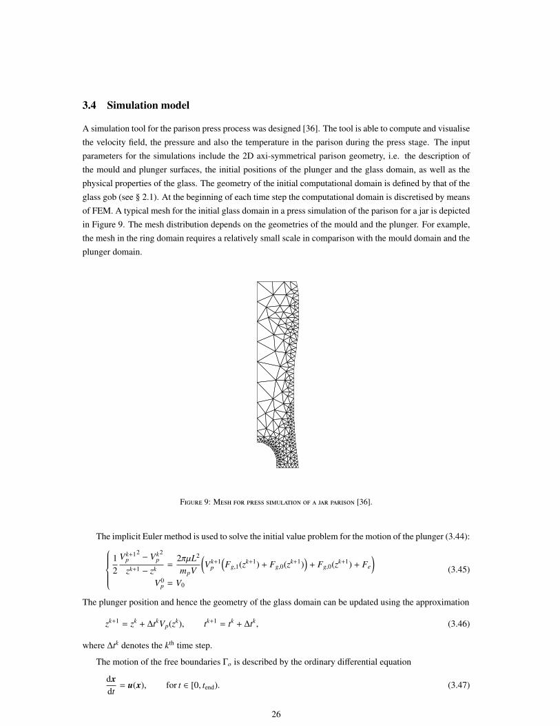
A simulation tool for the parison press process was designed [36]. The tool is able to compute and visualisethe velocity field, the pressure and also the temperature in the parison during the press stage. The inputparameters for the simulations include the 2D axi-symmetrical parison geometry, i.e. the description ofthe mould and plunger surfaces, the initial positions of the plunger and the glass domain, as well as thephysical properties of the glass. The geometry of the initial computational domain is defined by that of theglass gob (see § 2.1). At the beginning of each time step the computational domain is discretised by meansof FEM. A typical mesh for the initial glass domain in a press simulation of the parison for a jar is depictedin Figure 9. The mesh distribution depends on the geometries of the mould and the plunger. For example,the mesh in the ring domain requires a relatively small scale in comparison with the mould domain and theplunger domain.

F 9: M [36].

The implicit Euler method is used to solve the initial value problem for the motion of the plunger (3.44):12

Vk+1p

2− Vk

p2

zk+1 − zk =2πµL2

mpV

(Vk+1

p

(Fg,1(zk+1) + Fg,0(zk+1)

)+ Fg,0(zk+1) + Fe

)V0

p = V0

(3.45)

The plunger position and hence the geometry of the glass domain can be updated using the approximation

zk+1 = zk + ∆tkVp(zk), tk+1 = tk + ∆tk, (3.46)

where ∆tk denotes the kth time step.

The motion of the free boundaries Γo is described by the ordinary differential equation

dxdt

= u(x), for t ∈ [0, tend). (3.47)

26

Let xi, i = 1, . . . ,N be the nodes on a free boundary Γ f ⊂ Γo and let xki be an approximation of x(tk) (see

Fig. 10). Then the new position of the ith node can be obtained by the explicit scheme

xk+1i = xk

i + ∆t uki , (3.48)

with uki := u(xk

i ). A particular question is how to deal with this moving boundary. Depending on thevelocity a situation may be encountered where the obtained position xk+1

i lies outside Ωg (see Fig. 10). In

t@@thhh t((( t""t

PPPPPP

t !!!!

!!tAAAU

t

Γp Γm

Γ f

Ωg(tk)

HHH

HHHY

Ωg(tk+1)

ixki

ixk+1

i

vkit

@@@R

xk+1i

XXXXXt!!!!!t

F 10: T [36].

this situation one of the strategies described below may be used. For simplicity only explicit integration isconsidered.

One approach to deal with the moving boundary is to decrease the time step:

xk+1i = xk

i + αki ∆t uk

i , αki ∈ (0, 1], (3.49)

where xk+1i is the new position of the ith node obtained with the decreased time step. The kth time step can be

defined by ∆tki := mini α

ki ∆t, such that the nodes are situated inside the glass domain at time tk+1 := tk +∆tk

i ,as depicted in Fig. 10. Unfortunately, this algorithm introduces a variable time step that turns out to be tooirregular in practice and can be excessively small. In order to have consistency in the topology of thecomputational domain the time step should be constant [36].

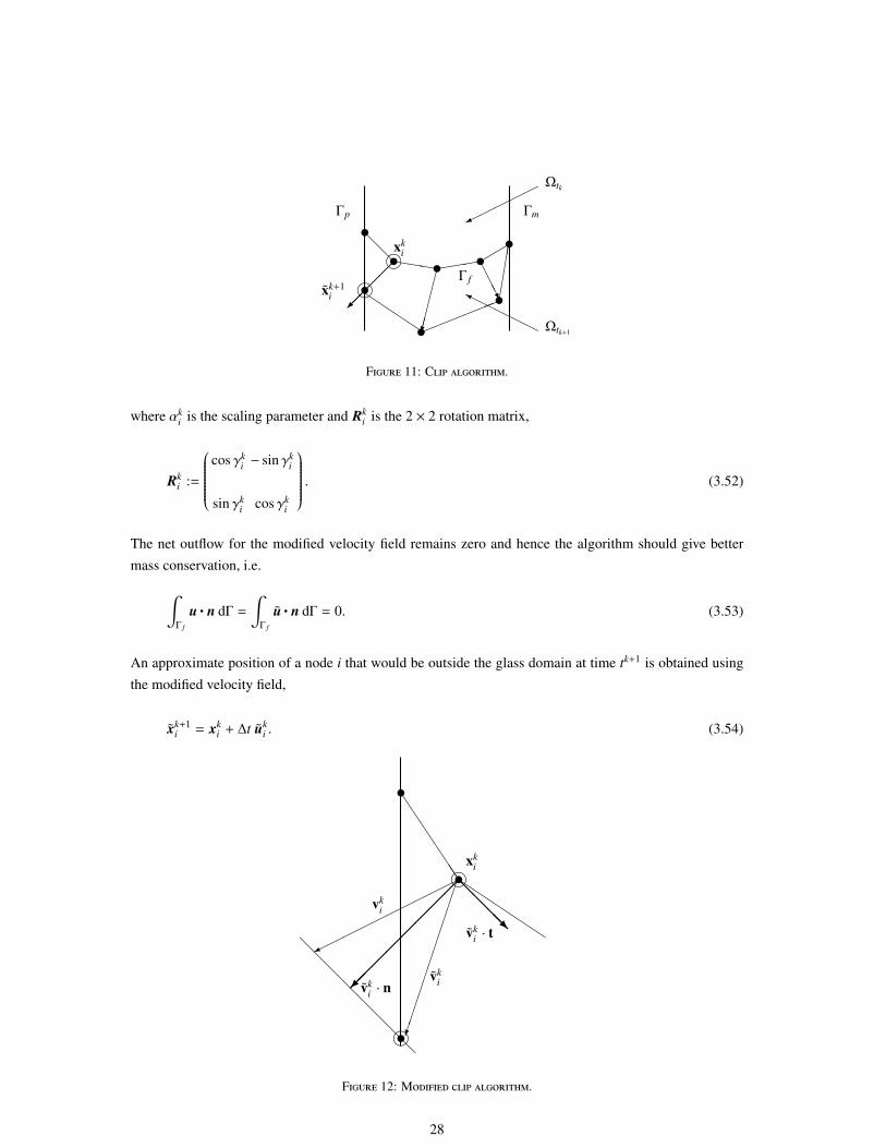
An alternative is illustrated in Fig. 11; the so-called clip algorithm leads the nodes along a discrete‘solution curve’ until they reach the boundary, thereby clipping the trajectories on the boundary. Thus nodei, which would originally leave the physical domain at time tk+1, is clipped on the boundary by (3.49), butwith αk

i = 1 for a non-clipped node; the time step only differs for clipped nodes. Regrettably, also thisalgorithm has an evident drawback: the clipping influences the mass conservation property of the glassdomain [36].

The clip algorithm can be modified to enforce better mass conservation [36]. To this end alter the veloc-ities at the nodes that would otherwise end up outside the glass domain, such that their normal componentstays the same, i.e.

uki ·n = uk

i · n, (3.50)

while the tangential component uki · t is obtained by rotating the velocity vector, such that xk

i ends up onthe equipment boundary (see Fig. 12). This can be formulated as

uki := αk

i Rki uk

i , (3.51)

27

t@@thhh t((( t""t

QQQQ

!!!!

!!tAAAU

t

Γp Γm

Γ f

Ωtk

HHH

HHY

Ωtk+1

ixki

tixk+1i

F 11: C .

where αki is the scaling parameter and Rk

i is the 2 × 2 rotation matrix,

Rki :=

cos γk

i − sin γki

sin γki cos γk

i

. (3.52)

The net outflow for the modified velocity field remains zero and hence the algorithm should give bettermass conservation, i.e.∫

Γ f

u·n dΓ =

∫Γ f

u·n dΓ = 0. (3.53)

An approximate position of a node i that would be outside the glass domain at time tk+1 is obtained usingthe modified velocity field,

xk+1i = xk

i + ∆t uki . (3.54)

tJJJJJJJtQQQQQQ

ixki

vki

vki

vk

i · n

@@@@Rvk

i · t@@@@@@@@ti

F 12: M .

28

Instead of (3.48) also an implicit time integration scheme can be used:

xk+1i = xk

i + ∆t uk+1i . (3.55)

In order to use (3.55) it is necessary to compute the flow velocity in Ωg(tk+1). However, even though theplunger position is known in the sense of (3.46), the free boundary of Ωg(tk+1) is still unknown. Thisdifficulty can be overcome by employing an algorithm that iterates on xk+1

i . Unfortunately, this straight-forward approach requires each iteration the solution of a Stokes flow problem, which is computationallytoo costly. In [36] a numerical tool is introduced that overcomes the essential difficulty of the implicitnessof the scheme by using the fact that the flow velocity is autonomous. In [69] this matter is examined intomore detail.

3.5 Results

In this section simulations of the pressing of a jar and a bottle parison are shown. This includes thevisualisation of the velocity and pressure fields, the tracking of the free boundaries of the glass flow domainand the computation of the motion of the plunger. For more results of the simulation tool used the readeris referred to [36]. Furthermore, see [30] for results of a different parison press model.

First consider the simulation of the pressing of a jar parison. The simulation starts at the moment thegob of glass has entered the mould and the baffle has closed. Figure 13 visualises the flow velocity fieldin the glass domain during pressing. Here full slip of glass at the equipment boundary is assumed, that isβ = 0. The plunger moves upward forcing the glass to fill the space between the mould and the plunger.When the glass hits the mould the pressure increases. Figure 14 depicts the flow velocity of the glass inthe neck part ring of the jar in the final stage of the parison press. Figure 15 shows the pressure field. It isimportant to know the pressure of the glass onto the mould during the process, so that a similar pressurecan be applied from the outside in order to keep the separate parts of the mould together [36].

Next consider the simulation of the pressing of a bottle parison. The initial position of the top of theplunger in the simulation is close to the attachment of the ring to the mould. When the glass gob is droppedinto the mould it almost reaches the ring before the plunger starts moving (see Fig. 16(a)). Figure 16visualises the flow velocity of the glass during pressing. Figure 17 depicts the flow velocity in the bottleneck in the final stage of the parison press. Figure 18 shows the pressure field. The results are similar tothe jar parison simulation. Again full slip of glass at the equipment boundary is assumed.

29

0

0.02

0.04

0.06

0.08

0.1

0.12

(a)

0

0.02

0.04

0.06

0.08

0.1

0.12

0.14

(b)

0

0.02

0.04

0.06

0.08

0.1

(c)

0

0.02

0.04

0.06

0.08

(d)

F 13: P : [m/s] [36]

(a) (b) (c) (d)

F 14: P ( ): [36]

1

1.05

1.1

1.15

1.2

(a)

1

1.05

1.1

1.15

1.2

1.25

1.3

1.35

(b)

1

1.1

1.2

1.3

1.4

1.5

1.6

1.7

(c)

1

1.1

1.2

1.3

1.4

1.5

1.6

1.7

1.8

(d)

F 15: P : [bar] [36]

30

0

0.02

0.04

0.06

0.08

0.1

0.12

0.14

(a)

0

0.05

0.1

0.15

(b)

0

0.02

0.04

0.06

0.08

(c)

0

0.02

0.04

0.06

0.08

(d)

F 16: P : [m/s] [36]

(a) (b) (c) (d)

F 17: P ( ): [36]

1

1.05

1.1

1.15

(a)

1

1.05

1.1

1.15

1.2

(b)

1

1.05

1.1

1.15

1.2

1.25

1.3

1.35

1.4

(c)

1

1.1

1.2

1.3

1.4

1.5

(d)

F 18: P : [bar] [36]

31

4 Blow Model

This section presents a mathematical model for blowing. Section 4.1 specifies the mathematical model

described in § 2 for the counter blow and the final blow. In addition to the flow of glass, also the flow of

air is modelled. A particular question is how to deal with the glass-air interfaces. Section 4.2 discusses

several techniques. Subsequently, Section 4.3 explains how a variational formulation is used to combine

the physical problems for glass and air as well as the jump conditions on the interfaces into one statement.

Section 4.4 presents a numerical simulation model for the blow-blow process. Finally, Section 4.5 shows

some examples of process simulations. The simulation tool used for the results is presented in [23].


In Section 2.2 the balance laws for glass forming were formulated. In this section these balance laws arefurther specified for glass blowing. Since the final blow stage starts with the preform obtained in either theparison press stage of the counter blow stage, the orders of magnitude of most physical parameters for theseforming processes are typically the same. The temperature of the glass melt in the final blow is usuallyslightly lower than in the preceding stage, but this does not lead to a significant difference in the order ofmagnitude of the physical parameters. Therefore, the same typical values for both the counter blow and thefinal blow are considered:







The main difference from the physical parameters in the parison press is that the time duration of a blowstage is typically much larger, hence the flow velocity is much smaller. The dimensionless numbers corre-sponding to either blow stage are:

Peglass ≈ 76, Brglass ≈ 4.0 · 10−5, Reglass ≈ 2.5 · 10−5, Fr ≈ 1.0 · 10−3. (4.1)

The Peclet number for glass is moderately large, while the Brinkman number is negligibly small. Thus theheat transfer is dominated by advection, convection and radiation:

(∂T ∗

∂t∗+ u∗ ·∇∗T ∗

)= ∇∗ ·

(λ∗∇∗T ∗

), (4.2)

with

λ∗ :=λ

ρcpVL, (4.3)

32

rather than its definition (2.9) in § 2.2.1. The Reynolds number for glass is sufficiently small to neglect theinertia terms in the Navier-Stokes equations (2.25). The order of magnitude of the gravity term is given by

Reglass

Fr≈ 2.5 · 10−2,

which is not extremely small. Therefore, the glass flow is described by the Stokes flow equations:

∇∗ ·T ∗ = g∗, ∇∗ ·u∗ = 0, (4.4)

where T ∗ is the dimensionless stress tensor, which satisfies (2.20) in terms of the dimensionless variables,and g∗ is the dimensionless gravity force, given by

g∗ = −ReFr

ez. (4.5)

Subsequently, the air domain is considered. Note that the arguments to ignore the air domain in the parisonpress model do not apply to the blow model. Firstly, the inflow pressure is applied at the mould entranceand not directly on the glass, so that in this case the transport phenomena in air are of higher interest forthe blow model. Secondly, because the influence of the heat flux cannot be ignored, the energy exchangebetween the glass and its surroundings should be taken into account. For hot pressurised air the followingtypical values are considered2:

initial air temperature : T0 = 750 C,specific heat of air : cp = 103 J kg−1K−1,thermal conductivity of air : λ = 10−1 W m−1K−1.air density : ρ = 1 kg m−3,air viscosity : µ = 10−4 kg m−1s−1.

The resulting dimensionless numbers are:

Peair ≈ 102, Brair ≈ 4 · 10−8, Reair ≈ 1. (4.6)

It can be concluded that the heat transfer in air is described by (4.2), while the flow of air is described bythe full Navier-Stokes equations (2.25). This means that the model for the air flow is more complicatedmodel than for the glass flow, while the motion of glass is most interesting. Therefore, air is replaced by afictitious fluid with the same physical properties as air, but with a much higher viscosity, e.g. µa = 1. Thenthe Reynolds number of the fictitious fluid Re ≈ 10−4 is small enough to reasonably neglect the influenceof the inertia forces. On the other hand, the viscosity of the fictitious fluid is still much smaller than theviscosity of glass, so that the pressure drop in the air domain is negligible compared to the pressure dropin the glass domain [2]. Thus the flow of the ficitious fluid can be described by the Stokes flow equations(4.4).

Remark 4.1 If the glass temperature and the pressure in air can be reasonably assumed to be uniform,

the calculations can be restricted to the glass domain and the glass-air interfaces can be treated as free

boundaries with a prescribed pressure. In this case it can be recommended to use Boundary Element

Methods to solve the flow problem [15, 16].2The true orders of magnitude may be slightly different from their rough estimates in the table, but this will not affect the final

results.

33

The boundary conditions for the flow problem are given in § 2.2, but can be further specified for glassblowing. Free-stress conditions are imposed for air at the mould wall. If no lubricate is used, usually ano-slip condition is imposed for glass at the mould wall. For modelling of the slip condition in the presenceof a lubricate the reader is referred to [17, 18, 38]. As a result the boundary conditions for the flow problembecome:

u∗ ·n = 0, T∗n· t = 0, on Γs,

u∗ ·n = 0, u∗ · t = 0, on Γg,e,

T∗n·n = 0, T

∗n· t = 0, on Γa,e,

T∗n·n = p0, T

∗n· t = 0, on Γo,

(4.7)

with

p0 =

pin on Γa,o

0 on Γg,o,(4.8)

where pin is the pressure at which air is blown into the mould. Alternatively, one may prefer to introducethe boundary condition

u∗ ·n = 0, T∗n· t = 0, on Γg,o. (4.9)

This boundary condition avoids outflow of glass through the mould entrance during blowing. However, thisinvolves the definition of separate boundaries Γa,o and Γg,o, rather than the single boundary Γo. Moreover,these boundaries can change in time. In the next section it can be seen that this is not always convenient,particularly if a single fixed mesh is used for the discretisation of the flow domain. Instead Γg,o can beconceived as the boundary between the glass and the ring, thereby imposing a no-slip condition,

u∗ = 0, on Γg,o. (4.10)

Note that in this case Γa,o and Γg,o remain fixed.

The boundary conditions for the energy exchange problem are defined on the boundary of the flowdomain:(

λ∗∇T ∗)·n = 0, on Γs ∪ Γe,(

λ∗∇T ∗)·n = Nu α∗

(T∗ − T∗∞

), on Γo,

(4.11)

4.2 Glass-Air Interfaces

A two-phase fluid flow problem is considered, involving the flow of both glass and air. The flow domain Ω

is described by the geometry of the mould and hence fixed. On the other hand, the air domain Ωa and theglass domain Ωg are separated by moving interfaces Γi, as depicted in Fig. 4(c)-4(d), and therefore changein time. In order to model the two-phase fluid flow problem, the glass-air interfaces have to captured. Thereare different numerical techniques to deal with the moving interfaces in two-phase fluid flow problems.They can be classified in two main categories [22]: interface-tracking techniques (ITT) and interface-

capturing techniques (ICT).

Interface-tracking techniques (ITT) attempt to find the moving interfaces explicitly. ITT involve sep-arate discretisations of domains Ωa and Ωg; the meshes of both domains are updated as the flow evolves

34

by following the flow velocity on the interfaces (see e.g. § 3.4). The major challenge of ITT is the meshupdate. The procedure of updating the mesh can become increasingly computationally expensive as themesh size decreases or the mesh has to be updated more frequently. See [7, 14, 30] for examples of ITT inmathematical modelling of glass blow processes.

Interface-capturing techniques (ICT) are based on an implicit formulation of the interfaces by means ofinterface functions, which allow ICT to function on a fixed mesh for domain Ω. An interface function marksthe location of the corresponding interface by a given level set. Two widely used ICT are Volume-Of-Fluid

(VOF) Methods [28, 56] and Level Set Methods [1, 10, 58, 68].

In VOF methods the interface function denotes the fraction of volume within each element of eitherfluid. VOF methods are conservative and can deal with topological changes of the interface. However, theyare often rather inaccurate; high order of accuracy is hard to achieve because of the discontinuity of theinterface function [48]. Furthermore, they can suffer from small remnants of mixed-fluid zones (‘flotsamand jetsam’) [46, 51]. Still VOF methods are attractive because of their rigorous conservation properties.

In Level Set Methods the interface is generally represented by the zero contour of the interface function.Level Set Methods automatically deal with topological changes and it is in general easy to obtain highorder of accuracy [48]. In addition, properties of the interfaces, such as the normal and the curvature,are straightforward to calculate. Also Level Set Methods generalise easily to three dimensions [65]. Adrawback of Level Set Methods is that they are not conservative. Poor mass conservation of Level SetMethods for incompressible two-phase fluid flow problems is addressed in [19, 48, 72]. A major concernin Level Set Methods is the re-initialisation of the interface function in order to avoid numerical problems.For examples of Level Set Methods in mathematical modelling of glass blow processes the reader is referredto [2, 22].

Of the aforementioned methods Level Set Methods seem to be most attractive for this application. Theinterfaces are accurately captured, topological changes are naturally dealt with, a generalisation to threedimensions is relatively easy and complicated re-meshing algorithms are avoided. In order to compensatefor the mass loss or gain coupled Level Set and VOF Methods have been developed [51, 62, 67]. However,[22] reports a change in mass of less than 1% during the glass blow process simulations, which can befurther improved by using higher order time integration schemes or by taking smaller time steps. Thisindicates that in this case Level Set Methods are suited to be used as ICT.

The basic idea of Level Set Methods is to embed the moving interfaces as the zero level set of theinterface function φ, the so-called level set function (see Fig. 19):

φ(x, t

)= 0, x ∈ Γi(t). (4.12)

The equation of motion of the interfaces follows by the chain rule,

∂φ

∂t(x, t

)+ u·∇φ

(x, t

)= 0, x ∈ Γi(t) (4.13)

Here the flow velocity is obtained from the Stokes flow problem (4.4). Initially, the level set functionis defined as the signed Euclidean distance function to the interfaces Γi(0). If furthermore the level setequation (4.13) is extended to the flow domain the corresponding level set problem becomes

35

∂φ

∂t+ u·∇φ = 0, in Ω,

∂φ

∂t(x, 0) :=

−d(x,Γi(0)

), x ∈ Ωa(0)

d(x,Γi(0)

), x ∈ Ωg(0),

(4.14)

where

d(x,Γ

)= inf

y∈Γ‖x − y‖2 . (4.15)

Note that since two interfaces are involved φ isnot everywhere differentiable. This problem canbe overcome by defining two level set functions φ1

and φ2, one for each interface, and subsequentlysolving the two corresponding level set problems.Then the level set function for both interfaces isφ = minφ1, φ2.

F 19: L

One of the difficulties encountered in Level Set Methods is maintaining the desired shape of the level setfunction. The flow velocity does not preserve the signed distance property, but may instead considerablydistort and stretch the shape of the function, which eventually leads to additional numerical difficulties[12, 58]. To avoid this the evolution of the level set function is stopped at a certain point in time to rebuildthe signed distance function. This process is referred to as re-initialisation. There are several ways toaccomplish this. One approach is to solve the partial differential equation [50, 58, 68]

∂φ

∂τ+ sign(φ0)

(‖∇φ‖2 − 1

)= 0, in Ω, (4.16)

with φ(x, 0) = φ0 := φ(x, t), to steady state. If properly implemented the function φ converges rapidly to thesigned distance function around the interface [50, 68]. However, the technique does not properly preservethe location of the interface [58, 66]. This problem was fixed in [66] by adding a constraint to (4.16) thatenforces mass conservation within the grid cells. This re-initialisation technique has appeared to be quitesuccessful in practice. Another approach is to solve the Eikonal equation,

‖∇φ‖2 = 1, (4.17)

given φ = 0 on Γi, using Fast Marching Methods (FMM) [57, 58, 13]. FMM build the solution outwardstarting from a narrow band around the interface and subsequently marching along the grid points. Depend-ing on the implementation FMM can be extremely computationally efficient. A Fast Marching Method isdiscussed in § 4.4.

4.3 Variational Formulation

The variational formulation combines the physical problems for glass and air as well as the jump conditionson the interfaces into one statement. This results in a single problem formulation for the entire flow domain,while Level Set Methods can be used to deal with the interfaces. Moreover, the variational formulation isused for the discretisation by FEM in the simulation model.

36

First consider a variational formulation of Stokes flow problem (4.4), (4.7). Define vector spaces

Q := L2(Ω), (4.18)

U :=

u ∈ H1(Ω)d∣∣∣ u·n = 0 on Γs, u = 0 on Γg,e

, (4.19)

where L2(Ω) is the set of Lebesgue 2-integrable functions over Ω and H1(Ω) is the first order Hilbertspace over Ω. Superscript d denotes the dimension of the flow. Then the variational formulation is to find(u, p) ∈ U × Q, such that for all (v, q) ∈ U × Q,a(v,u) + b(v, p) = c(v),

b(u, q) = 0.(4.20)

where a : U × U 7→ R and b : U × Q 7→ R are bilinear forms and c : U 7→ R is a linear form, defined by

a(v,u) =

∫Ω

µ(∇ ⊗ v

): ((∇ ⊗ u

)T+ ∇ ⊗ u

)dΩ, (4.21)

b(v, q) = −

∫Ω

q∇·v dΩ, (4.22)

c(v) = −

∫Ω

g·v dΩ +

∫Γo

p0n·v dΓ. (4.23)

It is verified that the variational formulation indeed follows from problem (4.4), (4.7) with correspondingjump conditions (2.28), (2.30) on Γi. First note that

a(v,u) − b(v, p) =

∫Ω

(∇ ⊗ v

): (µ((∇ ⊗ u

)T+ ∇ ⊗ u

)− pI

)dΩ =

∫Ω

(∇ ⊗ v

):T dΩ. (4.24)

By means of (4.24) the first equation in (4.20) can be written as∫Ω

((∇ ⊗ v

):T + g·v)dΩ =

∫Γo

p0n·v dΓ. (4.25)

The integral on the left side of (4.25) can be split up into∫Ω

((∇ ⊗ v

):T + g·v)dΩ =

∫Ωg

((∇ ⊗ v

):T + g·v)

dΩ +

∫Ωa

((∇ ⊗ v

):T + g·v)dΩ. (4.26)

Successive application of identity

∇· (T v) = v· (∇·T ) +(∇ ⊗ v

):T , (4.27)

Gauss’ divergence theorem and the boundary conditions yields∫Ωg

((∇ ⊗ v

):T + g·v)dΩ =

∫Ωg

∇· (T v) dΩ =

∫∂Ωg

n·T v dΓ =

∫Γi,g

T n·v dΓ, (4.28)

since p0 = 0 on Γg,o, and∫Ωa

((∇ ⊗ v

):T + g·v)dΩ =

∫Γi,a

T n·v dΓ +

∫Γa,o

p0n·v dΓ. (4.29)

37

Here Γi,g and Γi,a denote the interfaces construed as part of the boundary of Ωg and Ωa, respectively. As aresult,

∫Γi

[[T n·v]] dΓ = 0, (4.30)

for all v ∈ U, which implies condition (2.30). Analogously, from the second equation in (4.20) it followsthat ∫

Γi

[[u·∇q

]]dΓ = 0, (4.31)

for all q ∈ Q, which implies condition (2.28).

In addition, consider a variational formulation of energy exchange problem (4.2), (4.11). Define vectorspaces

V :=

T ∈ H1(Ω) × [0,∞)∣∣∣ T = T0 on ∂Ω, T (x, 0) = T0(x) for x ∈ Ω

, (4.32)

W :=ω ∈ H1(Ω) × [0,∞)

∣∣∣ ω = 0 on ∂Ω, limt→∞

ω(x, t) = 0 for x ∈ Ω. (4.33)

Then the variational formulation is to find T ∈ V , such that for all ω ∈ W,

∫ ∞

0

∫Ω

(T∂ω

∂t+ (Tu − λ∇T ) ·∇ω

)dΩdt =

∫ ∞

0

∫Γo

αω (T∞ − T ) dΓdt +

∫Ω

T0ω0 dΩ, (4.34)

whereω0(x) = ω(x, 0) for x ∈ Ω. It is verified that the variational formulation indeed follows from problem(4.2)-(4.11) with corresponding jump condition (2.5) on Γi. To this end split up the integral on the left sideof (4.34) into∫ ∞

0

∫Ω

(T∂ω

∂t+ (Tu − λ∇T ) ·∇ω

)dΩdt =

∫ ∞

0

∫Ωg

(T∂ω

∂t+ (Tu − λ∇T ) ·∇ω

)dΩdt

+

∫ ∞

0

∫Ωa

(T∂ω

∂t+ (Tu − λ∇T ) ·∇ω

)dΩdt. (4.35)

Successive application of the product rule for differentiation, Gauss’ divergence theorem and the boundaryconditions yields∫ ∞

0

∫Ωg

(T∂ω

∂t+ (Tu − λ∇T ) ·∇ω

)dΩdt =

∫ ∞

0

∫Ωg

(∂

∂t(Tω

)+ ∇·

(ωTu − λω∇T

))dΩdt

=

∫ ∞

0

∫Γg

ω(Tu − λ∇T

)·n dΩdt

−

∫ ∞

0

∫Γg

ωTu·n dΓdt +

∫Ωg

T0ω0 dΩ

=

∫ ∞

0

∫Γg,o

αω (T∞ − T ) dΓdt

−

∫ ∞

0

∫Γi,g

λω∇T ·n dΓdt +

∫Ωg

T0ω0 dΩ, (4.36)

38

and ∫ ∞

0

∫Ωa

(T∂ω

∂t+ (Tu − λ∇T ) ·∇ω

)dΩdt =

∫ ∞

0

∫Γa,o

αω (T∞ − T ) dΓdt

−

∫ ∞

0

∫Γi,a

λω∇T ·n dΓdt +

∫Ωa

T0ω0dΩ. (4.37)

Therefore,∫Γi

[[λω∇T ·n]] dΓ = 0, (4.38)

for all ω ∈ W, which implies condition (2.5).


A simulation model for the blow-blow process is described in [23]. The model is able to compute andvisualise the preform or container shape, the thickness of the final product as well as the stress and thermaldeformation the glass and mould undergo during the process. Input parameters for the simulations are thegob volume or the glass preform, the mould shape, the temperature distribution of the glass and a prescribedinlet air pressure, as well as the physical properties of the glass. The 2D axi-symmetrical geometry of theinitial computational domain is defined by that of the flow domain (see § 2.1). The model does not takethe heat transfer in the mould into account. See [25, 30] for a complete description of the heat transferbetween the glass and the mould. FEM are used to solve the problems. Triangular Mini-elements are usedfor the discretisation of the flow problem. Typical meshes for the moulds for the parison and the bottle aredepicted in Fig. 20.

(a) parison (b) bottle

F 20: T -

39

A streamline-upwind Petrov-Galerkin (SUPG) method is used to obtain a stabilised formulation of theenergy equation [5, 22, 32]. The upwind parameter is defined by

ξ =hξ2

u·∇ϕi

‖u‖2, in ei. (4.39)

Here h is the width of the element in flow direction, ϕi is the ith basis function, ei is the ith element and ξ isa tuning parameter. In the classical case ξ = 1 and in the modified case [22, 59]

ξ =12

√∆t2 +

(h‖u‖2

)+

14

(h

u·Au

)2(u·∇ϕi

), in ei, (4.40)

for some matrix A.

A triangulated Fast Marching Method is used as a re-initialisation algorithm to maintain the level setfunction as a signed distance function [2, 22, 34, 57]. The method assumes that the level set values at thenodes within a narrow band around the interface are the correct signed distance values and then builds asigned distance function outward by marching along the nodes. Figure 21 shows the algorithmic represen-tation of the Fast Marching Method for a two-dimensional mesh. The curve represents a glass-air interface.The algorithm is initialised by computing initial values for distance function d in all nodes adjacent to theinterface φ−1(0). A second order accurate initialisation procedure is discussed in [13]. The nodes adjacentto the interface, to which the initial values are assigned, are tagged as proximate and are colour markedas orange in Fig. 21(a). The proximate nodes are the first nodes to be added to the set of accepted nodes,which contains all nodes of which the corresponding values are accepted as a distance value. The remain-ing nodes are initially tagged as distant, which are colour marked as black in Fig. 21, and are not (yet)of interest. The nodes adjacent to the set of accepted nodes are candidates to be added to either the setof accepted nodes or the set of distant nodes and are the trial nodes, which are colour marked as green inFig. 21(b). These nodes have a trial value assigned to them that might not yet be the correct distance value.When the values of all trial nodes have been updated, the trial nodes are removed from the set of trial nodesand added to the set of accepted nodes (see Fig. 21(c)). If multiple values are assigned to a trial node, thesmallest one holds. This procedure repeats itself until the set of accepted nodes contains all grid points.

An element in Fig. 21(c) with one trial node C with two accepted nodes A and B is considered. If themesh is structured as in Fig.21 and the angle between edges AB and AC is right, then the distance value dC

at node C is the solution of the quadratic equation

(dC − dA

)2+

(dB − dA

)2=

(dC − dB

)2. (4.41)

Suppose the mesh is not structured, but the triangles have different edges. Figure 22 shows a triangle withangles α, β, γ and edge lengths a, b, c. The interface is approximated by a line l such that the distance fromnodes A and B to l is equal to the approximate distance to the interface, that is dA and dB, respectively.Suppose dB ≤ dA. Then the angle δ between AB and l is determined by sin(δ) = dA−dB

c . As a result distancevalue dC can be computed by

dC = a sin(δ + β) + dB. (4.42)

40

Interface

(a)

Interface

(b)

Interface

A

B

C

(c)

proximate: correct value by assumption

distant: not yet considered

trial: value might not be correct

accepted: value updated by FMM

(d)

F 21: FMM

dBdA

A

C

B

b

a

c

aaaa

bbbbdddd

l

dA-dB

gggg

F 22: T FMM

It should be verified that the shortest distance to l from C intersects the triangle. Therefore the followingrequirement has to be satisfied:

0 ≤ acos(δ + β)

cos(δ)≤ c. (4.43)

If requirement (4.43) is not fulfilled, the update is performed by taking

dC = min(dA + b, dB + a

). (4.44)

Finally, it is also possible to consider triangles with only one accepted node. If for example only A isaccepted, then the values at B and C can be computed as dB = dA + c and dC = dA + b.

41

4.5 Results

In this section simulations of the blow-blow process for a bottle are shown. The outer surface of the preformin the final blow is used as the mould shape for the counter blow. The propagation of the interfaces and thetemperature distribution during the blow stages are visualised. For more results of the simulation modelused the reader is referred to [22, 23]. Furthermore, see [8, 14, 30, 55] for results of different simulationmodels.

First consider the simulation of the counter blow. The initial temperature of the mould and the air inthe counter blow are 500 C. The gob has an uniform initial temperature distribution. The inlet air pressureis 138kPa. Figure 23 visualises the evolution of the glass domain (red) and the air domain (blue) andFigure 24 shows the temperature distribution.

t=0.0s 0.25s 0.75s 1.75s

F 23: E [23]. G , .

F 24: T [23].

42

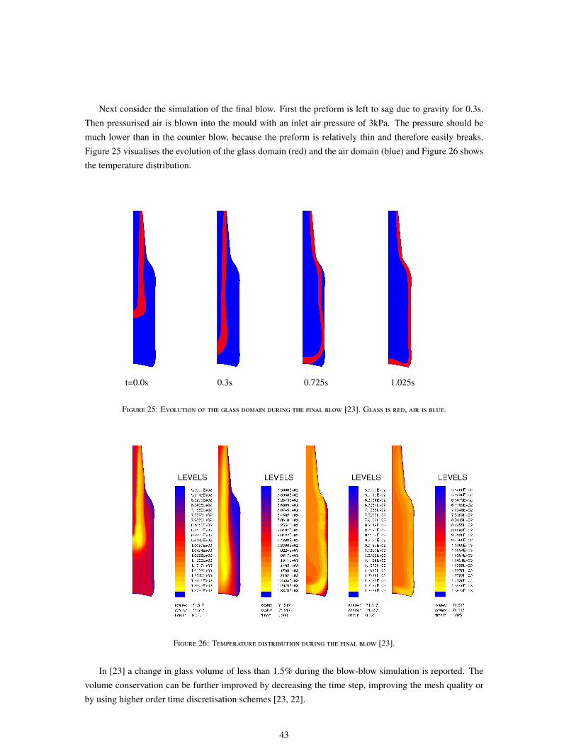
Next consider the simulation of the final blow. First the preform is left to sag due to gravity for 0.3s.Then pressurised air is blown into the mould with an inlet air pressure of 3kPa. The pressure should bemuch lower than in the counter blow, because the preform is relatively thin and therefore easily breaks.Figure 25 visualises the evolution of the glass domain (red) and the air domain (blue) and Figure 26 showsthe temperature distribution.

t=0.0s 0.3s 0.725s 1.025s

F 25: E [23]. G , .

F 26: T [23].

In [23] a change in glass volume of less than 1.5% during the blow-blow simulation is reported. Thevolume conservation can be further improved by decreasing the time step, improving the mesh quality orby using higher order time discretisation schemes [23, 22].

43

5 Direct Press Model

This section presents a mathematical model for the direct press. Since physical problems in the direct

press model are described in glass, air and equipment, it is more complicated than the parison press

model described in § 3 and the blow model described in § 4. Section 3.1 specifies the mathematical model

described in § 2 for the direct press. Features from both the blow model and the parison press model are

combined in the direct press model. Section 3.4 presents a numerical simulation model for the direct press.

An essential difference with the parison press is the way the mesh is updated. Finally, Section 3.5 shows

some examples of two-dimensional TV panel press simulations. The simulation tool used for these results

is presented in [26].


In Section 2.2 the balance laws for glass forming were formulated. In this section these balance laws arefurther specified for direct pressing. Essentially, the typical values for most physical parameters for directpressing are the same as for parison pressing; the main difference is the larger time duration of the directpress and hence the smaller velocity:







The corresponding dimensionless numbers are:

Peglass ≈ 76, Brglass ≈ 4.0 · 10−5, Reglass ≈ 2.5 · 10−5, Fr ≈ 1.0 · 10−3. (5.1)

In conclusion, the heat transfer in glass is dominated by convection and radiation,

(∂T ∗

∂t∗+ u∗ ·∇∗T ∗

)= ∇∗ ·

(λ∗∇∗T ∗

), (5.2)

where λ∗ is defined by Eq. (4.3), and the glass flow is described by the Stokes flow equations,

∇∗ ·T ∗ = g∗, ∇∗ ·u∗ = 0, (5.3)

where T ∗ is the dimensionless stress tensor and g∗ is the dimensionless gravity force, given by Eq. (4.5).As the glass is always in contact with both air and equipment and the influence of radiation and convectioncannot be disregarded, it is interesting to model the heat transfer in the whole domain Σ. Consider the

44

typical values for the physical properties of air in § 4.1. Then the following dimensionless numbers can befound:

Peair ≈ 102, Brair ≈ 4 · 10−8, Reair ≈ 1. (5.4)

Since the Peclet number for air is not extremely large, heat transfer by conduction and radiation shouldbe taken into account. Heat transfer by dissipation can be neglected. The flow of air is described by thefull Navier-Stokes flow equations, but these can eventually be simplified to the Stokes flow equations byreplacing air by a fictitious fluid (see § 4.4). In the equipment there is no flow, so the heat exchange isdescribed by:

∂T ∗

∂t∗= ∇∗ ·

(λ∗∇∗T ∗

), (5.5)

Separate domains for the mould, plunger and ring should be defined. The mould and plunger can againconsist of parts with different material properties, for which separate subdomains should be defined. Forexample, if the mould and plunger are heat insulated by means of water-cooled channels to keep the tem-perature of the material within acceptable bounds, also the water-cooled channels should be taken intoaccount. In this paper each of the mould, the plunger and the ring is considered as an entity with constantphysical properties.

The boundary conditions given in § 2.2 are specified for the direct press. Free-slip conditions areimposed for air at the equipment boundary, except for the furthest end of the ring wall, where free flowof air is allowed. In order to distinguish these boundary conditions the ring boundary Γr is subdividedinto two parts Γ

(1)r and Γ

(1)r , as it is illustrated in Fig. 27, denoting the inner boundaries of the lower part

and the upper part of the ring, respectively. Finally, the boundary conditions for the flow problem can beformulated as:

u∗ ·n = 0, T∗n· t = 0, on Γs,

(u∗ − Vpez)·n = 0,(T∗n + β∗p(u∗ − Vpez)

)· t = 0, on Γg,p,

u∗ ·n = 0,(T∗n + β∗mu∗

)· t = 0, on Γg,m,

u∗ ·n = 0,(T∗n + β∗r u∗

)· t = 0, on Γg,r,

u∗ ·n = 0, T∗n· t = 0, on Γa,m ∪ Γa,p ∪ Γ

(1)a,r,

T∗n·n = 0, T

∗n· t = 0, on Γ(2)a,r.

(5.6)

Alternatively, one may prefer a small normal velocity of air on the impermeable equipment boundary toensure that air does not get trapped during the simulation. The boundary conditions for the energy exchangeproblem are given by (2.14).

Essentially, a slender-geometry approximation such as in (3.2) is also possible for the direct press modelas the glass becomes fairly long and thin during pressing (e.g. television screens, lenses). Unfortunately,in this case the influence of convection and radiation is too large to assume the temperature, and hencethe viscosity, will remain constant for constant initial temperature is constant. As a result an analyticalsolution to the slender-geometry approximation cannot be found as easily as for the parison press. Theslender-geometry approximation for the direct press is not considered in this paper.

45

ΓΓΓΓi

r

zmould

plunger

ring

glass airΩΩΩΩg ΩΩΩΩa

tn ΓΓΓΓp

ΓΓΓΓr

ΓΓΓΓm

ΓΓΓΓo

ΓΓΓΓs

ΓΓΓΓoΓΓΓΓo ring

ΓΓΓΓr(2)

ΓΓΓΓo ΓΓΓΓo

mould

plunger

ΓΓΓΓr(1)

ΓΓΓΓmΓΓΓΓp

F 27: P


Obviously, the direct press model is much more complicated than the parison press model described in§ 3 and the blow model described in § 4. It involves a coupled system of physical problems consistingof a Stokes flow problem, an energy exchange problem and a moving interface problem. In addition, thecomputational domain has a rather complicated geometry, which is changing in time, and is subdividedinto several subdomains, each with different physical properties.

A simulation model for the two-dimensional direct press process is described in [26]. The model isable to compute and visualise the velocity field and the pressure in glass and air, as well as the stress andthermal deformation the glass and mould undergo during the process. Furthermore, it can reproduce thetemperature distribution in glass, air and equipment. A complete three-dimensional simulation tool withmany additional features, such as several advanced radiation models and an annealing process simulationmodel, is described in [49]. Input parameters for the simulations are the gob volume, the equipmentgeometry, the initial temperature distribution and the physical properties of the glass and the equipment.Each time step the computational domain is discretised by means of FEM. Triangular Mini-elements areused for the discretisation of the flow problem. Figure 28 shows the deformation of a typical mesh in thepress model from t = 0 s to 1.5 s, where t = 1.5 s is the end time of the process. The mesh for the lowestplunger position in Figure 28(d) is provided as input for the press model. Then the elements in the flowdomain are stretched in vertical direction by raising the plunger to its initial position to obtain the initialmesh (see Fig. 28(a). In each subsequent time step a mesh is generated that fits the plunger position at thattime following an arbitrary Euler-Lagrange approach, that is each mesh consists of the same numbers ofelements along each dimension of the domain. Thus the mesh of the flow domain is compressed by theplunger, until the mesh for the lowest plunger position is regained. In this way time consuming remeshingis avoided, although remeshing is still necessary if the quality of the elements can become at issue as theyare stretched or compressed [26].

Some modelling aspects of the direct press have already been discussed in § 3 and § 4.

• The motion of the plunger is modelled analogously to the parison press model (see § 3.3, § 3.4).

46

• The evolution of the glass-air interface can be modelled analogously to the blow model (see § 4.2).The direct press model described in [26, 49] uses a Pseudo-Concentration Method [70] to track theinterface.

• Air is replaced by a fictitious fluid (see § 4.4).

• The energy equation is stabilised by means of a SUPG method (see § 4.4).

(a) t = 0.0s (b) t = 0.5s

(c) t = 1.0s (d) t = 1.5s

F 28: T TV

47

5.3 Results

In this section two-dimensional simulations of the pressing of a TV panel are shown. This includes thevisualisation of the flow velocity and temperature distribution, the tracking of the glass-air interfaces andthe computation of the motion of the plunger. For more results of the simulation tool used the reader isreferred to [26, 49]. Moreover, see [18, 37, 76] for results of different direct press models.

Figure 29 visualises the (pseudo-)concentration of glass during pressing. In the figures glass is red andair is blue. The transition layer of the concentration between glass and air becomes thinner and smoother asthe mesh is refined. A no-slip condition for glass at the equipment wall is used, which explains the stronglycurved interface.

Figure 30 visualises the temperature distribution during pressing. The initial temperature of the glassis 1000 C and the initial temperature of the air and the equipment is 500 C. The glass gradually heats upthe equipment at the contact surface. Apart from a thin boundary layer of roughly 0.2 mm, the temperatureof the equipment does not become higher than 550 C within 1.5s. By contrast, the glass rapidly heats upthe air.

In order to verify the accuracy of numerical solutions, the volume conservation of the glass is examined.Figure 31 depicts the ratio of the glass volume to the initial glass volume as a function of time. It can beobserved that the glass volume initially makes a relatively strong jump. Possibly, the solver has somedifficulties in accurately meeting the initial conditions. At t = 0.5s a loss volume of less than 1% isobserved, which is a good result. The maximum change of volume during the simulation was 1.11%. Thevolume change can be further reduced by decreasing the time step, improving the mesh quality or by usinghigher order time discretisation schemes. Good volume conservation is also reported in [26].

48

(a) t = 0.0s (b) t = 0.25s

(c) t = 0.5s (d) t = 0.75s

(e) t = 1.0s (f) t = 1.5s

F 29: C TV

49

(a) t = 0.0s (b) t = 0.5s

(c) t = 1.0s (d) t = 1.5s

F 30: T TV

0 0.25 0.5 0.75 1 1.25 1.5

0.98

0.99

1

1.01

1.02

time [s]

gla

ss v

olu

me

/ in

itia

l gla

ss v

olu

me

F 31: G

50

References

[1] D. Adalsteinsson and J. A. Sethian. A fast level set method for propagating interfaces. J. Comp. Phys,118:269–277, 1995.

[2] S. M. A. Allaart-Bruin, B. J. Linden, and R. M. M. Mattheij. Modelling the glass press-blow pro-cess. In A. Di Bucchianico, R. M. M. Mattheij, and M. A. Peletier, editors, Progress in Industrial

Mathematics at ECMI 2004 (Proceedings 13th European Conference on Mathematics for Industry,

Eindhoven, The Netherlands, June 21-25, 2004), volume 8 of Mathematics in Industry / The European

Consortium for Mathematics in Industry, pages 351–355. Springer, Berlin, 2006.

[3] C. L. Babcock. Silicate Glass Technology Methods. John Wiley & Sons, Inc., U.S.A., 1977.

[4] T. Bernard and E. Ebrahimi Moghaddam. Nonlinear model predictive control of a glass formingprocess based on a finite element model. In Proceedings of the 2006 IEEE International Conference

on Control Applications, 2006.

[5] A. N. Brooks and T. J. R. Hughes. Stream-line upwind/petrov-galerkin formulation for convectiondominated flows with particular emphasis on the incompressible navier-stokes equations. Comput.

Methods Appl. Mech. Eng., 32:199–259, 1982.

[6] M. Brown. A review of research in numerical simulation for the glass-pressing process. Proc. IMechE,

Part B: J. Engineering Manufacture, 221(9):1377–1386, 2007.

[7] J. M. A. Cesar de Sa. Numerical modelling of glass forming processes. Eng. Comput., 3:266–275,1986.

[8] J. M. A. Cesar de Sa. Numerical Modelling of Incompressible Problems in Glass Forming and Rubber

Technology. PhD thesis, University College of Swansea, 1986.

[9] J. M. A. Cesar de Sa, R. M. Natal Jorge, C. M. C. Silva, and R. P. R. Cardoso. A computational modelfor glass container forming processes. In Europe Conference on Computational Mechanics Solids,

Structures and Coupled Problems in Engineering.

[10] Y. C. Chang, T. Y. Hou, B. Merriman, and S. Osher. A level set formulation of eulerian interfacecapturing methods for incompressible fluid flows. J. Comp. Phys, 124:449–464, 1996.

[11] J. Choi, D. Ha, J. Kim, and R. V. Grandhi. Inverse design of glass forming process simulation usingan optimization technique and distributed computing. Journal of Materials Processing Technology,148:342–352, 2004.

[12] D. L. Chopp. Computing minimal surfaces via level set curvature flow. J. Comp. Phys, 106(1):77–91,1993.

[13] D. L. Chopp. Some improvements on the fast marching method. SIAM Journal of Scientific Comput-

ing, 23(1):230–244, 2001.

[14] A. Cormeau, I. Cormeau, and J. Roose. Numerical simulation of glass-blowing. In J. F. T. Pittman,O. C. Zienkiewicz, R. D. Wood, and J. M. Alexander, editors, Numerical Analysis of Forming Pro-

cesses, pages 219–237. Wiley, New York, 1984.

51

[15] W. Dijkstra. Condition Numbers in the Boundary Element Method: Shape and Solvability. PhDthesis, Eindhoven University of Technology, 2008.

[16] W. Dijkstra and R. M. M. Mattheij. Numerical modelling of the blowing phase in the production ofglass containers. Electronic Journal of Boundary Elements, 6:1–23, 2008.

[17] W. C. Dowling, H. V. Fairbanks, and W. A. Koehler. A study of the effect of lubricants on moltenglass to heated metals. J. Amer. Ceramic Soc., 33:269273, 1950.

[18] G. Dussere, F. Schmidt, G. Dour, and G. Bernhart. Thermo-mechanical stresses in cast steel diesduring glass pressing process. Journal of Materials Technology, 162-163:484–491, 2005.

[19] D. Enright, R. Fedkiw, J. Ferziger, and I. Mitchell. A hybrid particel level set method for improvedinterface capturing. J. Comput. Phys., 183:83–116, 2002.

[20] M. Falipou, F. Siclorof, and C. Donnet. New method for measuring the friction between hot viscousglass and metals. Glass Sci. Technol., 72(3):59–66, 1999.

[21] A. C. Fowler. Mathematical Models in the Applied Sciences. Cambridge University Press, Cambridge,1997.

[22] C. G. Giannopapa. Development of a computer simulation model for blowing glass containers. J.

Manuf. Sci. and Eng., 130, 2008.

[23] C. G. Giannopapa and J. A. W. M. Groot. A computer simulation model for the blow-blow formingprocess of glass containers. In 2007 ASME Pressure Vessels and Piping Conf. and 8th Int. Conf. on

CREEP and Fatigue at Elevated Temp., 2007.

[24] W. Giegerich and W. Trier, editors. Glass Machines: Construction and Operation of Machines for

the Forming of Hot Glass. Springer, Berlin, 1969.

[25] S. Gregoire, J. M. A. Cesar de Sa, P. Moreau, and D. Lochegnies. Modelling of heat transfer atglass/mould interface in press and blow forming processes. Computers and Structures, 85:1194–1205, 2007.

[26] J. A. W. M. Groot. Analysis of the solver performance for stokes flow problems in glass formingprocess simulation models. Master’s thesis, Eindhoven University of Technology, 2007.

[27] J. A. W. M. Groot, C. G. Giannopapa, and R. M. M. Mattheij. Development of a numerical optimisa-tion method for blowing glass parison shapes. In Proceedings of PVP 2008: ASME Pressure Vessels

and Piping Division Conference, July 27-31, 2008.

[28] C. W. Hirth and B. D. Nichols. Volume of fluid (vof) method for the dynamics of free boundaries. J.

Comp. Phys, 39:201–225, 1981.

[29] C. E. Humpherys. Mathematical Modelling of Glass Flow during a Pressing Operation. PhD thesis,University of Sheffield, 1991.

[30] M. Hyre. Numerical simulation of glass forming and conditioning. Journal of the American Ceramic

Society, 85(5):1047–1056, 2002.

52

[31] V. John and A. Liakos. Time-dependent flow across a step: The slip with friction boundary condition.Int. J. Numer. Meth. Fluids, 50:713731, 2006.

[32] C. Johnson, U. Navert, and J. Pitkaranta. Finite element methods for linear hyperbolic problems.Comput. Methods Appl. Mech. Eng., 45:285–312, 1984.

[33] M. Kang, R. P. Fedkiw, and X.-D. Liu. A boundary condition capturing method for multiphaseincompressible flow. J. of Sci. Comput., 15(3):323–360, 2000.

[34] R. Kimmel and J. A. Sethian. Computing geodesic paths on manifolds. Proc. Natl. Acad. Sci. USA,95:8431–8435, 1998.

[35] D. Krause and H. Loch, editors. Mathematical Simulation in Glass Technology. Springer, Berlin,2002.

[36] K. Laevsky. Pressing of Glass in Bottle and Jar Manufacturing: Numerical Analysis and Computa-

tion. PhD thesis, Eindhoven University of Technology, 2003.

[37] G. Li, J. T. Jinn, W. T. Wu, and S. I. Oh. Recent development and applications of three-dimensionalfinite element modeling in bulk forming processes. Journal of Materials Processing Technology,113(2001):40–45, 2001.

[38] L. X. Li, D. S. Peng, J. A. Liu, Z. Q. Liu, and Y. Jiang. An experimental study on the lubricationbehavior of a5 glass lubricant by means of the ring compression test. Journal of Materials Processing

Technology, 102:138–142, 2000.

[39] B. J. van der Linden. Radiative Heat Transfer in Glass: The Algebraic Ray Trace Method. PhD thesis,Eindhoven University of Technology, 2002.

[40] B. J. van der Linden and R. M. M. Mattheij. A new method for solving radiative heat problems inglass. International Journal of Forming Processes, 2:41–61, 1999.

[41] D. Lochegnies, P. Moreau, and R. Guilbaut. A reverse engineering approach to the design of the blankmould for the glass blow and blow process. Glass Technology, 46(2):116–120, 2005.

[42] R. M. M. Mattheij, S. W. Rienstra, and J. H. M. ten Thije Boonkamp. Partial Differential Equations:

Modeling, Analysis, Computation. SIAM, Philadelphia, 2005.

[43] P. Moreau, D. Lochegnies, and J. Oudin. An inverse method for prediction of the prescribed temper-ature distribution in the creep forming process. Proc. Inst. Mech. Eng. J. Mech. Eng. Sci., 212:7–11,1998.

[44] P. Moreau, D. Lochegnies, and J. Oudin. Optimum tool geometry for flat glass pressing. International

Journal of Forming Processes, 2:81–94, 1999.

[45] T. M. Nagtegaal. Optical Method for Temperature Profile Measurements in Glass Melts. PhD thesis,Eindhoven University of Technology, 2002.

[46] W. F. Noh and P. Woodward. Simple line interface calculations. In A. I. van de Vooren and P. J.Zandbergen, editors, Proceedings of the Fifth International Conference on Numerical Methods in

Fluid Dynamics, volume 59 of Lecture Notes in Physics, pages 330–340. Springer, New York, 1976.

53

[47] M. Oevermann, R. Klein, M. Berger, and J. Goodman. A projection method for two-phase incom-pressible flow with surface tension and sharp interface resolution. Tech. rep. ZIB-report, no. 00-17,Konrad-Zuse-Zentrum fur Informationstechnik Berlin, 2000.

[48] E. Olsson and G. Kreis. A conservative level set method for two phase flow. J. Comp. Phys, 210:225–246, 2005.

[49] O. Op den Camp, D. Hegen, G. Haagh, and M. Limpens. Tv panel production: Simulation of theforming process. Ceram. Eng. Sci. Proc., 24(1):1–19, 2003.

[50] D. Peng and G. Kreis. A pde-based fast local level set method. J. Comp. Phys, 155:410–438, 1999.

[51] S. P. van der Pijl, A. Segal, C. Vuik, and P. Wesseling. A mass-conserving level-set method formodelling of multi-phase flows. Int. J. Numer. Meth. Fluids, 47:339–361, 2005.

[52] L. D. Pye, A. Montenero, and I. Joseph. Properties of Glass-Forming Melts. CRC Press, 2005.

[53] S. W. Rienstra and T. D. Chandra. Analytical approximations to the viscous glass-flow problem inthe mould-plunger pressing process, including an investigation of boundary conditions. Journal of

Engineering Mathematics, 39:241–259, 2001.

[54] S. Rosseland. Note on the absorption of radiation within a star. Monthly Notices of the Royal Astro-

nomic Society, 84:525–528, 1924.

[55] N. Sadegh, G. J. Vachtsevanos, E. J. Barth, D. K. Pirovolou, and M. H. Smith. Modelling the glassforming process. Glass Technology, 38:216218, 1997.

[56] R. Scardovelli and S. Zaleski. Direct numerical simulation of free-surface and interfacial flow. Annu.

Rev. Fluid Mech., 31:567–603, 1999.

[57] J. A. Sethian. A fast marching level set method for montonically advancing fronts. Proc. Nat. Acad.

Sci., 93(4):1591–1595, 1996.

[58] J. A. Sethian. Level Set Methods and Fast Marching Methods. Cambridge University Press, USA,1999.

[59] F. Shakib. Finite Element Analysis of the Incompressible Euler and Navier-Stokes Equation. PhDthesis, Stanford University, 1989.

[60] D. E. Sharp and L. B. Ginther. Effect of composition and temperature on the specific heat of glass. J.

Amer. Ceramic Soc., 34:260271, 1951.

[61] J. E. Shelby. Introduction to Glass Science and Technology. The Royal Society of Chemistry, Cam-bridge, second edition, 2005.

[62] S. V. Shepel and B. L. Smith. New finite-element/finite-volume level set formulation for modellingtwo-phase incompressible flows. J. Comp. Phys, 218:479494, 2006.

[63] J. H. Simmons and C. J. Simmons. Nonlinear viscous flow in glass forming. Am. Ceramic Soc. Bull.,68(11):1949–1955, 1989.

54

[64] K. Storck, D. Loyd, and B. Augustsson. Heat transfer modelling of the parison forming in glassmanufacturing. Glass Technology, 39(6), 1998.

[65] M. Sussman, A. S. Almgren, J. B. Bell, P. Colella, L. H. Howell, and M. L. Welcome. An adaptivelevel set approach for incompressible two-phase flows. J. Comp. Phys, 148:81–124, 1999.

[66] M. Sussman and E. Fatemi. An efficient, interface-preserving level set re-distancing algorithm and itsapplication to interfacial incompressible fluid flow. SIAM J. Sci. Comput., 20(4):1165–1191, 1995.

[67] M. Sussman and E. G. Pucket. A coupled level set and volume-of-fluid method for computing 3d andaxisymmetric incompressible two-phase flows. J. Comp. Phys, 162:301–337, 2000.

[68] M. Sussman, P. Smereka, and S. Osher. A level set approach for computing solutions to incompress-ible two-phase flow. J. Comp. Phys, 114:146–159, 1994.

[69] B. Tasic. Numerical Methods for Solving ODE Flow. PhD thesis, Eindhoven University of Technol-ogy, 2004.

[70] E. Thompson. Use of pseudo-concentration to follow creeping viscous flow during transient analysis.Int. J. for Numerical Methods in Fluids, 7:749–761, 1986.

[71] F. V. Tooley. The Handbook of Glass Manufacture, Vol II. Aslee Publishing Co, New York, 1984.

[72] A.-K. Tornberg and B. Engquist. A finite element based level-set method for multiphase flow appli-cations. Comput. Visual. Sci., 3(1):93–101, 2000.

[73] H. de Waal and R. G. C. Beerkens, editors. NCNG Handboek voor de Glasfabricage. TNO-TPD-Glastechnologie, second edition, 1997.

[74] J. H. Williams, D. R. J. Owen, and J. M. A. Cesar de Sa. The numerical modelling of glass formingprocesses. In H. C. Bharwaj, editor, Collected Papers of the XIV International Congress on Glass,pages 138–145, Calcutta, 1986. Indian Ceramic Society.

[75] K. Yigitler. Numerical simulation of blowing of axisymmetric wide-mouth glass containers. InProceedings of the Colloquium on Modelling of Glass Forming.

[76] H. Zhou, B. Yan, and D. Li. Three-dimensional numerical simulation of the pressing process in tvpanel production. Simulation, 82(3):193–203, 2006.

55

mathematical modelling of glass forming processes - · pdf filemathematical modelling of glass...

Documents