mathematical modelling of environmental and life … · environmental and life sciences problems....
TRANSCRIPT

Series on
Mathematical Modellingof
Environmental and Life Sciences Problems
Proceedings of the fourth workshopSeptember, 2005, Constanta, Romania

Scientific Committee
Lazar Dragos
Marius Iosifescu
George Dinca
Dorel Homentcovschi
Alexandru Morega
Ioan Rosca
Silviu Sburlan
Harry Vereecken

Series on
Mathematical Modelling
of
Environmental and
Life Sciences Problems
Proceedings of the fourth workshopSeptember, 2005, Constanta, Romania
Edited by
Stelian Ion
Gabriela Marinoschi
Constantin Popa
EDITURA ACADEMIEI ROMANEBucuresti, 2006

c© EDITURA ACADEMIEI ROMANE, 2006
All rights reserved.
Addres: EDITURA ACADEMIEI ROMANECalea 13 Septembrie nr. 13, sector 5,050711, Bucharest, Romania,Tel.: 4021-318 81 46, 4021-318 81 06,Fax: 4021-318 24 44,E-mail: [email protected],Internet: http://www.ear.ro
Descrierea CIP a Bibliotecii Nationale a Romaniei
SERIES ON MATHEMATICAL MODELLING OFENVIRONMENTAL AND LIFE SCIENCES PROBLEMS.WORKSHOP (2005; Constanta
Series on Mathematical modelling of environmental and lifesciences problems: Proceedings of the fourth Workshop:Constanta Romania, september 2005/ed.: Stelian Ion, GabrielaMarinoschi, Constantin Popa. - Bucuresti: Editura AcademieiRomane, 2006
ISBN (10) 973-27-1358-5 ; ISBN (13) 978-973-27-1358-7
I. Ion, Stelian (ed.)II. Marinoschi, Gabriela (ed.)III. Popa, Constantin (ed.)
51(063)
This book was sponsored by SOFTWIN Bucharest
Editor: Dan-Florin DUMITRESCUTechnical editing: Sofia MORARComputer editing: Stelian IONCover design: Mariana SERBANESCU
———————————————————————–11.07.2006. Format 16/70×100.UDC: 519.283: 57(028); 51
———————————————————————–

Table of Contents
Mathematical aspects of the study of the cavitation in liquidsAlina Barbulescu and Cristian Stefan Dumitriu . . . . . . . . . . . . . . . . . . . . . . . . . 7
Evolutionary Algorithms in Image Reconstruction from Limited DataAndrei Bautu, Elena Bautu and Constantin Popa . . . . . . . . . . . . . . . . . . . . . . . 15
The Dynamics of Systems Modeling Acute InflammationCristina Bercia . . . . . . . . . . . . . . . . . . . . . . . . . . . . . . . . . . . . . . . . . . . . . . . . . . . . 27
Self-Propulsion of an Oscillatory Wing Including Ground EffectsAdrian Carabineanu . . . . . . . . . . . . . . . . . . . . . . . . . . . . . . . . . . . . . . . . . . . . . . . . . 39
Thermal Coupling Numerical Models for Boundary Layer Flows overa Finite Thickness Plate Exposed to a Time-Dependent TemperatureEmilia Mladin Cerna and Dorin Stanciu . . . . . . . . . . . . . . . . . . . . . . . . . . . . . . 55
Mathematical Modeling of the Dynamic Crack Propagation in aDouble Cantilever BeamEduard-Marius Craciun, Tudor Udrescu and George Cırlig . . . . . . . . . . . . . . . 69
Noise prediction model for wind turbinesAlexandru Dumitrache and Horia Dumitrescu . . . . . . . . . . . . . . . . . . . . . . . . . . 79
Quasimonotone ODE Approximation of Nonlinear Diffusion ProcessStelian Ion . . . . . . . . . . . . . . . . . . . . . . . . . . . . . . . . . . . . . . . . . . . . . . . . . . . . . . . . . 87
Minimum Free Energy Configuration of the Planar Lipidic Bilayer.Analytical SolutionsStelian Ion and Dumitru Popescu . . . . . . . . . . . . . . . . . . . . . . . . . . . . . . . . . . . . . 95
Numerical Study of Axisymmetric Slow Viscous Flow Past TwoSpheresGheorghe Juncu . . . . . . . . . . . . . . . . . . . . . . . . . . . . . . . . . . . . . . . . . . . . . . . . . . . . 103
Approach to nonstationary (transient) Birth-Death ProcessesAlexei Leahu . . . . . . . . . . . . . . . . . . . . . . . . . . . . . . . . . . . . . . . . . . . . . . . . . . . . . . . 113
Statistical simulation and analysis of some software reliability modelsAlexei Leahu and Elena Carmen Lupu . . . . . . . . . . . . . . . . . . . . . . . . . . . . . . . . . 119
A Mathematical Model Describing the Vulnerability to Pollution ofGroundwater in the Proximity of Slatina TownAnca Marina Marinov and Victor Moldoveanu . . . . . . . . . . . . . . . . . . . . . . . . . 123

6
Analysis of a Preconditioned CG Method for an Inverse BioelectricField ProblemMarcus Mohr, Constantin Popa and Ulrich Rude . . . . . . . . . . . . . . . . . . . . . . . . 135
Dosimetric Estimates in Biological Tissue Exposed to MicrowaveRadiation in the Near Field of an AntennaMihaela Morega, Alina Machedon and Marius Neagu . . . . . . . . . . . . . . . . . . . . 147
Lower bounds on the weak solution of a moving-boundary problemdescribing the carbonation penetration in concreteAdrian Muntean and Michael Bohm . . . . . . . . . . . . . . . . . . . . . . . . . . . . . . . . . . 161
Discretization Techniques and Numerical Treatment For First KindIntegral EquationsElena Pelican and Elena Bautu . . . . . . . . . . . . . . . . . . . . . . . . . . . . . . . . . . . . . . 171
A fast approximation for discrete LaplacianConstantin Popa and Tudor Udrescu . . . . . . . . . . . . . . . . . . . . . . . . . . . . . . . . . . 181
Gibbs regularized tomographic image reconstruction with DW algo-rithm based on generalized oblique projectionsConstantin Popa and Rafal Zdunek . . . . . . . . . . . . . . . . . . . . . . . . . . . . . . . . . . . . 191
Post–Synaptic Nicotinic Currents Triggered by the AcetylcholineDistribution within the Synaptic CleftAnca Popescu and Alexandru Morega . . . . . . . . . . . . . . . . . . . . . . . . . . . . . . . . . 201
Effect of tricyclic antidepressants on the frog epitheliumCorina Prica, Emil Neaga, Beatrice Macri, Dumitru Popescu and Maria LuizaFlonta . . . . . . . . . . . . . . . . . . . . . . . . . . . . . . . . . . . . . . . . . . . . . . . . . . . . . . . . . . . . . 211
On the Solvability of Navier-Stokes EquationsCristina Sburlan . . . . . . . . . . . . . . . . . . . . . . . . . . . . . . . . . . . . . . . . . . . . . . . . . . . 223
The Influence of Initial Fields on the Propagation of AttenuatedWaves along an Edge of a Cubic CrystalOlivian Simionescu-Panait . . . . . . . . . . . . . . . . . . . . . . . . . . . . . . . . . . . . . . . . . . 231
Model for molecular dynamics simulation of radiation-induced defectformation in fcc metalsDaniel Sopu, Bogdan Nicolescu and M.A. Gırtu . . . . . . . . . . . . . . . . . . . . . . . . 243

Proceedings of the Fourth Workshop onMathematical Modellingof Environmental and Life Sciences ProblemsConstanta, Romania, September, 2005, pp. 7–14
Mathematical aspects of the studyof the cavitation in liquids
Alina Barbulescu∗ and Cristian Stefan Dumitriu∗∗
In a liquid, an ultrasonic field can carry along small bubbles or can produce cavi-tation bubbles, whose movements determine drastic effects as: erosion, unpassivation andemulsification, chemical reactions, sonoluminescence, pressure variation, that have as a effectoscillations whose frequencies differ from that of the incident ultrasound wave.
We found out that the frequency of these electrical signals, generated by the cavitation
bubbles, at their exterior, corresponds to the frequency of the mechanical waves, generated
by the collapse of the cavitation bubbles. We present the mathematical models for the
voltage induced by the cavitation bubbles in diesel.
1. Experimental set-up
The cavitation is the process of the appearance of one or many gas cavities ina liquid. An ultrasonic field that goes over a liquid can produce or move cavitationbubbles.
To make the study of the ultrasonic cavitation in liquids, we used an ultrasoundgenerator. The frequency of the ultrasound produced by it is constant.
The experimental set-up consists in a core-tank, which contains the studiedliquid. Two metallic electrodes are put in the tank. They are connected with anacquisition card, that digitizes analog signals and stores the resulting digital patternin the on-board memory.
In some papers ([2], [4], [6]) we studied the voltage induced in water by thecavitation bubbles produced by the ultrasonic generator.
Now we shall make a comparative study of the signals captured in diesel and incrude petroleum.
∗ “Ovidius” University, Constanta, Romania e-mail: [email protected]∗∗ Utilnavorep S.A., Constanta, Romania.

8 alina barbulescu and cristian stefan dumitriu
2. Definitions
In order to discuss our results we need some notions concerning the time seriesanalysis.
Definition 1. A discrete time process is a sequence of random variables (Xt; t ∈Z).
Definition 2. A discrete time process (Xt; t ∈ Z) is called stationary if:
(∀)t ∈ Z, E(X2t ) <∞,
(∀)t ∈ Z, E(Xt) = µ, (∀)t ∈ Z,
(∀)h ∈ Z, Cov(Xt, Xt+h) = γ(h).
where E(X) is the expectation value of the random variable X and Cov(X,Y ) is thecorrelation of the random variables X and Y.
Definition 3. The function defined on Z,by:
ρ(h) =Cov(Xt, Xt+h)√σ2(Xt)σ2(Xt+h)
=γ(h)
γ(0)
is called the autocorrelation function of the process (Xt; t ∈ Z).σ2(Xt) is the variance of the variable Xt.The most used estimator of ρ(h) is the empiric autocorrelation function, ACF:
ρ(h) =
∑n−|h|t=1 (xt − x)(xt+|h| − x)∑n
t=1(xt − x)2,
where xt is a realization ofXt, h is the lag, n is a fixed natural number and x =∑n
t=1 xt
nis the arithmetic mean of the values x1, ..., xn.
Definition 4. If (Xt; t ∈ Z) is a stationary process, the function defined by:
τ(h) =Cov(Xt −X∗
t , Xt−h −X∗t−h)
D2(Xt −X∗t )
, h ∈ Z+
is called the partial autocorrelation function, where X∗t (X∗
t−h) is the affine regressionof Xt (Xt−h ) with respect to Xt−1, ..., Xt−h+1.
The most used estimator of τ(h)τ(h) is the empiric partial autocorrelation func-tion, PACF.
Definition 5. Consider
B(Xt) = Xt−1
Φ(B) = 1− ϕ1B − ...− ϕpBp, ϕp 6= 0,
Θ(B) = 1− θ1B − θ2B2 − ...− θpBq, θp 6= 0,
∆dXt = (1−B)dXt.

cavitation in liquids 9
Fig. 1. The voltage induced in diesel.
The process (Xt; t ∈ Z+) is called an autoregressive integrated moving average processof p, d and q orders, ARIMA (p, d, q), if :
Φ(B)∆dXt = Θ(B)εt,
where the absolute values of the roots of Φ and Θ are greater than 1 and (εt; t ∈ Z)is a white noise.
If d = 0 = q, the ARIMA(p, d, q) process is an autoregressive of p order, AR(p),process.
If p = d = 0, the ARIMA(p, d, q) process is an moving average of q order, MA(q)process.
If d = 0, the ARIMA(p, d, q) process is an autoregressive moving a-verage of pand q orders, ARMA(p, q) process.
Remarks. The ARMA(p, q) process is stationary.
3. Results
In the Figure 1 we can see the electrical signal induced by the cavitation in diesel(voltage, function of time), captured by the acquisition card and processed by us.
We made the analysis of this signal. It can be seen that there are some aberrantvalues, that must be removed. After this process, the remained values were studied.
First, the autocorrelation function (ACF) of the voltage, at the lags between1 and 16, was calculated and the confidence interval, at the confidence level 95%,was determined.

10 alina barbulescu and cristian stefan dumitriu
Fig. 2. The coefficients of the model ARIMA(3, 0, 6).
The values of ACF were outside the confidence interval. The form of the ACFwas an exponential decreasing and that of PACF was of damped sine wave oscillation.These remarks enable us to think that the process could be of ARIMA type. We alsothought at this type of models because the simple models are not convenient point ofview of the errors. Point of view of physics, the ARIMA models found by us ([2], [4],[6]) for the signals induced in water satisfy the experimental and theoretical resultsknown from the literature.
Forty models were analyzed. To chose between them, the Schwarz (SBC) andAkike (AIC) criteria were used. The preferred values were that of the SBC criterion.The selected model – ARIMA(3, 0, 6) – had the least SBC value.
The fist step was to test the hypothesis H0: the coefficients of the model arezero, at the significance level 5%.

cavitation in liquids 11
The values of the model coefficients and of the t-ratio are given in the Figure 2.The values of the t-ratio (the Figure 2, the last nine rows and the column 4)
are greater than the values of the quantila of the Student function with 5 033 libertydegrees, at the significance level 5%.
Also, the probabilities to accept the hypothesis H0 are practically zero (the lastcolumn of the Figure 2), so H0 is rejected.
In order to prove that the model is a good one, point of view of statistics, theautocorrelation function and the partial autocorrelation function of the residuals werecalculated. The graphs of these functions can be seen in the Figures 3 and 4 and theirvalues, in the Tables 1 and 2.
Fig. 3. The ACF of the residuals in the model ARIMA(3, 0, 6).
Fig. 4. The PACF of the residuals in the model ARIMA(3, 0, 6).
In the Figures 3 and 4 we see that the values of the autocorrelation functionand of the partial autocorrelation function of the residuals are inside the confidenceintervals, at 0.95 confidence level.
The following data are provided by the table 1:– the lags, between 1 and 16 – in the column 1;– the autocorrelation of the errors – in the column 2;– in the column 4 – the values of the Box-Ljung statistics, which are in the
interval [0.184, 18.572], so, less than ℵ2(15) ;

12 alina barbulescu and cristian stefan dumitriu
– in the last column: the probability to accept the hypothesis that the residualsform a white noise, which are between 0.741 and 0.968.
The values of the partial autocorrelation function, at the lags between 1 and16, are given in the second column of the Table 2. They are very small. Also, themodulus of the standard errors (Tables 1 and 2) is small (0.014).
So, the hypothesis that the residuals form a white noise can be accepted. There-fore, the model is well selected.
Table 1
The values of PACF of the residuals
Table 2
The values of ACF of the residuals

cavitation in liquids 13
4. Conclusions
In the experiments made we found out that when an ultrasound propagatesthrough a liquid, a potential difference between two points appears. It has bothharmonic and subharmonic components.
The equation of the voltage induced in diesel, at 80 W is:
Vn − 2.3798Vn−1 + 2.2495Vn−2 − 0.8465Vn−3 = εn − 1.279εn−1+
+0.8222εn−2 + 0.0313εn−3 − 0.1189εn−4 + 0.0998εn−5 − 0.0416εn−6,
where n ∈ N, n ≥ 3 and εn, n ∈ N is a white noise.An analogous study, made for the voltage induced in crude petroleum, in the
same condition as for the diesel (Figure 5), conduced us to an ARIMA(3, 1, 4) model,without a constant term.
It was expected that the results don’t differ too much, since the chemical com-positions of the too liquids were not too different.
The two models differs also from that obtained in water:– at 80 W, which was ([2]) an AR(2), given by:
Vn = 1.5636298Vn−1 − 0.89193194Vn−2 + εn,
where n ∈ N, n ≥ 3 and εn, n ∈ N is a white noise.– at 120 W, which was of ARMA(2,1) type, given by ([6]):
Vn = 1.3006553Vn−1− 0.7035790Vn−2 + εn − 0.6128040εn−1,
where n ∈ N, n ≥ 3 and εn, n ∈ N is a white noise.– at 180 W, which was of ARIMA(2, 1, 0) type, given by ([4]):
(1− 1.2313304B+ 0.84409B2)(1 −B)Vn = εn,
where n ∈ N, n ≥ 3 and εn, n ∈ N is a white noise.So, we proved that the voltage induced by the cavitation bubbles in liquids
depends on the liquids and on the power of the ultrasonic generator.
References
[1] A. Barbulescu,Time series, with applications, Junimea, Iasi, 2002 (in Romanian).
[2] A. Barbulescu, Some models for the voltage, Analele Stiintifice ale UniversitatiiOvidius, Seria Matematica, vol. 10 (2), 2002, pp. 1–7
[3] A. Barbulescu, V. Marza, Some results regarding the ultrasonic cavitation, ActaUniversitatis Apulensis, Mathematics–Informatics, Part B, no. 7/2004, pp. 31–38
[4] A. Barbulescu, V. Marza, Some models for the voltage induced in a liquid bycavitation, Proceedings of Conference 2004: Dynamical systems and applications,Antalya, Turkya, 5-10.07.2004, pp. 158–165.

14 alina barbulescu and cristian stefan dumitriu
[5] A. Barbulescu, V. Marza, Electrical phenomena induced by cavitation in oil, Sci-entific Bulletin of the Politehnica University of Timisoara, Transactions on Me-chanics, Tome 49(63).
[6] A. Barbulescu, V. Marza,Electrical effect induced at the exterior of the cavitationbubbles, Acta Physica Polonica (submitted).

Proceedings of the Fourth Workshop onMathematical Modellingof Environmental and Life Sciences ProblemsConstanta, Romania, September, 2005, pp. 15–26
Evolutionary Algorithms in Image Reconstructionfrom Limited Data
Andrei Bautu∗ , Elena Bautu ∗∗ and Constantin Popa∗∗∗
We consider in this paper two classes of evolutionary methods for improving the ART
Kaczmarz procedure in case of data limitation: genetic algorithm and particle swarm op-
timization, respectively. They are combined in various ways with the classical Kaczmarz
projection method, in two classes of hybrid algorithms. Experiments ilustrating the effi-
ciency of these new methods are presented for consistent least-squares formulation of some
image reconstruction problems.
1. Limitation of data in practice and theory
In this section we shall analyse from both practical and theoretical viewpointsthe “data limitation” aspect appearing in two very important practical problems:medical computerized tomography (MCT, for short) and electromagnetic geotomog-raphy (EGT, for short). The corresponding idealized and simplified (two dimensional)situations are presented in Figures 1 and 2 below. In Figure 1 we supposed that foreach position of the CT scanner, only one X-ray is emited (SiR, i = 1, 2, . . . ,m). Si
is the source and R is the receptor; the body-section which is analysed is “contained”in the rectangular region ABCD.
Figure 2 describes an EGT problem; ABCD is the rectangular underground re-gion which is analysed, AB and CD are holes in which are introduced electromagneticwaves sources S1, S2, . . . , Sp and receptors R1, R2, . . . , Rq, respectively (see [2]).
In both cases, the rectangular regions ABCD are uniformely discretized in anumber n of pixels, P1, P2, . . . , Pn (see figure 3).
∗ “Mircea cel Batran” Naval Academy, Constanta, Romania, e-mail: [email protected]∗∗ “Ovidius” University, Constanta, Romania, e-mail: [email protected]∗∗∗ “Ovidius” University, Constanta, Romania, e-mail: [email protected]
This paper was supported by the PNCDI INFOSOC Grant 131/2004.

16 andrei bautu et al.
Fig. 1. The MCT problem.
Fig. 2. The EGT problem. Fig. 3. Pixels discretization.
The mathematical model of the reconstruction procedure, for both EGT andMCT problems is a linear least-squares formulation,
min ‖Ax− b‖ (1)
with A an m × n matrix and b ∈ Rm. The right hand side b is constructed bymeasuring the X-rays or electromagnetic waves intensities at sources and receptors(see [3], [5] for details). Concerning the matrix A, the number n of its columns isexactly the number of pixels in the discretization from figure 3, whereas the numberm of its rows corresponds to the number of X-rays in the MCT case (SiR denotedby Ei, i = 1, 2, . . . ,m) or electromagnetic waves source-receptor combinations in theEGT case (SkRl, k = 1, . . . , p, l = 1, . . . , q denoted by Ei, i = 1, 2, . . . ,m = pq).The value of the (A)ij component is the length of the segment intersection betweenthe Ei ray and the pixel Pj (see Figure 4). If such an intersection is empty, the

image reconstruction 17
Fig. 4. Matrix coefficients.
corresponding (A)ij coefficient is set to 0. Following such a construction, the matrixA becomes sparse, rank-defficient and ill-conditioned (see [3] for details). Moreover,because of measurement errors, the right hand side b fails to belong to the range ofA, thus the problem (1) becomes inconsistent. In the present paper we shall consideronly the consistent case of (1) and let the inconsistent one for a future work.
Remark 1. In any of the above mentioned cases, for the discrete reconstructionproblem (1), in practical applications we are looking for its unique minimal normsolution, denoted in what follows by xLS.
By “data” associated to problem (1) we understand the matrix A and the vectorb. Moreover, because the number n of pixels in the discretization from figure 3 isimposed by technical reasons, we may consider our “data” as essentially determinedbym, the number of X-rays/electromagnetic waves that are used for scanning ABCD.From a practical point of view, this number is limited at least by the following tworeasons:
• for MCT – a too big number m of X-rays used for scanning a body can becomedangerous for its health;
• for EGT – in practice, the underground analysed regionABCD is very big, thusthe length of the holes AB and CD is so; then, if we would like a “complete”scanning of the area we would need a very big number of sources and receptors,which is not possible from technical reasons.
From a theoretical view point the above described “data limitation” can be in-terpreted according to some properties of the fundamental vector subspaces associatedto the problem matrix A. In this sense we shall denote by At, N(A), R(A), A+ thetranspose, null space, range and Moore-Penrose pseudoinverse of A and by S(A; b),the set of all solutions of (1) in the consistent case, in which (1) can be written in theclassical formulation
Ax = b. (2)

18 andrei bautu et al.
It is well known (see [2]) that
S(A; b) = xLS +N(A), xLS⊥N(A), (3)
where⊥ denotes the orthogonality w.r.t. the euclidean scalar product 〈·, ·〉. Accordingto (3), “data limitation” in problem (2) would mean that the null space N(A) has an“enough big” dimension (e.g. a factor c times the total dimension n of the supportspace Rn). The above mentioned practical view points about data limitation arefitting into this considerations because, if the number of rays m is strictly less thanthe number of pixels n, then the dimension of N(A) is positive (but we may havea positive dimension for N(A) also for m > n; see the example from below and theresults in Table 1. As a consequence, because any solution x∗ ∈ S(A; b) is given by
x∗ = xLS + PN(A)(x∗), (4)
where PS(x) denotes the (euclidean) orthogonal projection onto the subspace S, ifthe null space N(A) is “big enough” w.r.t the support space Rn (see the above con-siderations and the remark 1) and x∗ has a corresponding “big” component, then thedifference
x∗ − xLS = PN(A)(x∗) (5)
becomes important enough to destroy the accuracy of the reconstructed image. Allthese considerations are ilustrated by the following example in which a real imagereconstruction EGT problem is simulated (the same procedure will be used in theexperiments from section 3 of the paper).
Example 1. Our simulation procedure is the following: we consider an imageartifficially created (see Figure 5) as a vector xex ∈ Rn, for a given number n ≥ 2 ofpixels (as in Figure 3). Each component xex
i is a real number in the interval [0, 1] andcorresponds to the grey maping scale from Figure 6. This gives us the grey originalimage in Figure 5 (in this case we have n = 144). Then, the original image area wasscanned as in Figure 2, by using p ≥ 1 sources and q ≥ 1 receptors, equally distributedon AB and CD. In this way we obtained the m × n system matrix A (see Figure 4)with m = pq.
Table 1
Limited data tests characteristics
Scanning (p = q) m n rank(A) dim(N(A))
6 × 6 36 144 35 109
8 × 8 64 144 61 83
10 × 10 100 144 96 48
12 × 12 144 144 120 24
16 × 16 256 144 131 13
24 × 24 576 144 133 11
36 × 36 1296 144 133 11
48 × 48 2304 144 133 11

image reconstruction 19
Fig. 5. Original image (upper left) and reconstruction results for p sources and p receivers(where p ∈ 6, 8, 10, 12, 16, 24, 36, 48).
0 0.1 0.2 0.3 0.4 0.5 0.6 0.7 0.8 0.9 1
Fig. 6. Grey mapping scale

20 andrei bautu et al.
The right hand side b ∈ Rm was defined by
b = Axex, (6)
such that the problem (1) becomes consistent. For the tests from figure 5 we usedp = q (i.e. m = p2) with p ∈ 6, 8, 10, 12, 16, 24, 36, 48 (for p ∈ 6, 8, 10, 12 we havem ≤ n, i.e. the “practical” limited data case). The values of the rank(A) and dim(A)were computed in each case and are presented in Table 1. The original image xex
from Figure 5 has components in N(A), thus (see (5))
xex 6= xLS . (7)
We then applied to (1) the classical Kaczmarz algorithm (KA, for short) withthe initial approximation x0 = 0 (which gives us xLS as the limit of the sequence ofapproximations; see e.g. [2], [3], [5]). After 100 iterations for the cases presented inTable 1 we got the results from Figure 5. We can observe there that in the “practicallimited data” situations (p = q = 6, 8, 10, 12) the reconstructed images (which corre-sponds to xLS) are far from the original one (the first 5 images following the originalone), whereas for “enough much data” (e.g. p = q = 24, 36, 48) the reconstructedimages are closer to the original, but still not satisfactory (this because also in thesecases – see Table 1 – the null space of A has dimension 11, which is still big w.r.t.the support space dimension n = 144).
Thus, in order to get a good enough approximation of x∗, with Kaczmarz’salgorithm used in Example 1, we need to start it with an initial approximation x0 ∈ Rn
such thatPN(A)(x
0) ≈ PN(A)(x∗). (8)
According to (7) we will then have
limh→∞
xh = PN(A)(x0) + xLS ≈ PN(A)(x
∗) + xLS = x∗, (9)
thus, a much better approximation for x∗. For generating such a “good” initialapproximation x0 as in (8) we decided to use two evolutionary algorithms. They willbe described in the next section, whereas in the last one we shall combine one of themwith the previous Kaczmarz algorithm in our numerical experiments.
2. Evolutionary Algorithms
Evolutionary algorithms, like genetic algorithms (GA) and particle swarmoptimization algorithms (PSO), can be used to solve problems like ((1)) and ((2)).Evolutionary algorithms are stochastic algorithms that use a set of candidate solutions(called individuals) which evolve in time towards better solutions. Each individualis rated by a fitness function. The algorithms presented in this paper use a fitnessfunction that minimizes the errors defined as
ff (x) =1
1 + ‖Ax− b‖ , (10)
where x ∈ [0, 1]n is the current image (see Example 1).

image reconstruction 21
2.1. Genetic Algorithm
The GA, which we tested, is an extension of the unary function optimization GAdescribed in [4]. In the GA view, a possible solution is an organism that is adaptingto the its environment in order to fit better within it. A GA’s set of possible solutionsis called population. Each solution from the population is called a chromosome.Data structures that define a chromosome are called genes. Most genetic algorithmswork by evolving their population with the help of three genetic operators: crossover,mutation, and selection.
Our GA implementation uses a fixed size population of pop−size chromosomes,each chromosome being a vector with elements from [0, 1] (the chromosome’s genes).The values of the ith gene represents the absortion value of the ith pixel in the image.
Crossover is a binary operator which combines genes from a two chromosomes(called parents) to obtain two of new chromosomes (called offsprings), which replacetheir parents in the population. Chromosomes are selected for mating with cross−rateprobability. For each pair of chromosomes, a random crossover point is selected andgenes to the left of that point are swapped between chromosomes.
Mutation is a unary operator that affects the genes of a single chromosome.Each gene suffers mutation with mut−rate probability. It modifies each gene with agiven probability by replacing the old value with a randomly generated new value.
Selection is a population-wide operator that creates a new population based onthe old one. There are many possible selection operators available, but we imple-mented a classical Monte Carlo selection scheme (called roulette wheel selection).
For our genetic algorithm the values range of the above described parameters arethe following: for pop−size from 10 to 200, mut−rate—1% to 25%, cross−rate—30%to 70%.
2.2. Particle Swarm Optimization Algorithm
We tested an n-dimensional extension of the PSO algorithm described in [4]. Inthe PSO view, a possible solution is an organism that is moving in the search space inorder to find better places than their current location. The set of possible solutions iscalled swarm). Each solution from the swarm is called a particle. A particle stateis defined by current position, velocity, memory, and neighbours.
In our implementation, a particle is a vector of n tuples of reals from [0, 1].The values in the ith tuple represent the current position (i.e. pixel absortion value),velocity and best so far position of the particle in ith search dimension.
The number of particles is denoted by part−count parameter. Each particleevolves based on its own memory and its neighbours memory (only one neighbour inour implementation). On each iteration, velocity and position components of particlesare updated using the formulas:
v′t+1 = vt · inertia+ rand() · cognitive · (bt − pt) + rand() · social · (nt − pt), (11)
vt+1 = min(vmax,max(−vmax, v′t+1)), (12)
p′t+1 = pt + vt+1, (13)

22 andrei bautu et al.
pt+1 = min(1,max(0, p′t+1)). (14)
The values used for the above described parameters are the following: for part−countfrom 10 to 100, inertia—1% to 50%, cognitive and social—75% to 200%, vmax—0.1to 1.0.
2.3. Hybrid Algorithms
As we presented in the experiments section of the paper, the genetic algorithmperformed is quite bad compared to PSO and Kaczmarz algorithms. Hybrid algo-rithms from Kaczmarz and PSO were created in order to combine the benefits of thistwo algorithms.
First hybrid algorithm (FHA) has two stages: during the first stage it runs thePSO algorithm described earlier; in the second stage, it uses the best solution fromthe first stage as the starting approximation for Kaczmarz algorithm.
Second hybrid algorithm (SHA) runs Kaczmarz and PSO algorithms in an al-ternate manner, by applying for each particle, after each iteration of PSO one step ofthe Kaczmarz algorithm.
3. Experiments
We present our results for four image reconstruction experiments. The simu-lation procedure is the same as in Example 1. The four original images are showedin Figure 6 and their characteristics in Table 2 (left to right, according to Figure 7).For each image, we ran all five algorithms with various settings, and we present theresults after 100 iterations with the following parameters:
• KA: no settings required;
• GA: pop−size = 50, mut−rate = 5%, and cross−rate = 70%;
• PSO: part−count = 50, vmax = 1.0, inertia = 0.3, cognitive = 1.2, andsocial = 1.2;
• FHA and SHA: same settings as for PSO.
Table 2
Test images properties
Image Size (pixels) Source Unique colors
Test 1 8 × 8 Drawing 9
Test 2 12 × 12 Drawing 8
Test 3 20 × 20 Scanned photo 71
Test 4 40 × 40 Scanned photo 177

image reconstruction 23
Fig. 7. Test images.
After 100 iterations, GA doesn’t produce a good image (Figure 8). We suspectthat a different encoding scheme or operators should be tried (there are many geneticoperators and they can be combined to form different algorithms).
PSO has some not very satisfactory results for Test 1 and Test 2 (see Figure 9)and has no valid solution for Test 3 and Test 4 images.
For Test 1 and 2, KA found some images which are affected by noise (see Figure10), which is common in (classical) Kaczmarz image reconstructions (see [3], [2]).This noise is making further improvements difficult. For Test 3 and Test 4 it has nosatisfactory results.
FHA performed much better than PSO and a little better than KA (see Figure11). Reconstructed images are affected by noise of the KA in the second stage of thealgorithm.
SHA found an almost perfect Test 1 and Test 2 solution and it found verygood solutions for Test 3 and Test 4 (see figure 12). It performed much better thanKaczmarz algorithm alone or the other evolutionary algorithms presented in thisarticle. It seems that KA drives the reconstruction process towards the “good” image,while PSO helps filtering the image in order to eliminate the noise.
Fig. 8. GA results after 100 iterations.
4. Conclusions and Future work
The consideration and results from this paper are at a very begining. The firstnext step will be to apply them to inconsistent least-squares formulations of the type

24 andrei bautu et al.
Fig. 9. PSO results after 100 iterations.
Fig. 10. KA results after 100 iterations.
Fig. 11. FHA results after 100 iterations.
Fig. 12. SHA results after 100 iterations.

image reconstruction 25
(1), whereas a further research will be concerned with a theoretical analysis of thenew obtained image reconstruction methods, together with comparisons with othernew and efficient techniques in the field (see e.g. [3]).
References
[1] Bjorck, A., Numerical methods for least squares problems, SIAM Philadelphia,1996.
[2] Censor Y., Stavros A. Z., Parallel optimization: theory, algorithms and applica-tions, “Numer. Math. and Sci. Comp.” Series, Oxford Univ. Press, New York,1997.
[3] Kennedy, J., Eberhart, R., Particle Swarm Optimisation, Proceedings of IEEEInternational Conference on Neural Networks, Perth, Western Australia, 1995,Vol. 3, 1942–1948.
[4] Michalewicz, Z., Genetics Algorithms + Data Structures = Evolution Programs,Springer-Verlag, New York, 1996.
[5] Natterer F., The Mathematics of Computerized Tomography, John Wiley andSons, New York, 1986.
[6] Popa C., Zdunek R., Kaczmarz extended algorithm for tomographic image re-construction from limited-data, Math. and Computers in Simulation, 65 (2004),579–598.


Proceedings of the Fourth Workshop onMathematical Modellingof Environmental and Life Sciences ProblemsConstanta, Romania, September, 2005, pp. 27–38
The Dynamics of Systems ModelingAcute Inflammation
Cristina Bercia∗
In this paper, we consider three-dimensional non-linear dynamical systems of predator-prey type with nine parameters, which model the acute inflammation of the human bodydue to an infection, defined clinically as sepsis.
We establish the domains in the parameters space where the equilibrium points exist
and the set of conditions for them to be local attractors. We also perform bifurcation analysis
and establish the types of dynamics of the systems. We obtain the global phase portrait
for each type of dynamics by numerical integration. Varying one or two of the parameters,
bifurcation diagrams are presented.
1. Introduction
In this paper we have considered two systems of ordinary differential equationswith 9 parameters which model the acute inflammation and septic shock of the humanbody due to an infection or a trauma. The first model is presented in the paper ofBrause [1], the second one in Kumar et al. [2].
The differential systems, having 3 variables u = (u1, u2, u3), are of predator-preytype
u′ = F (u), F (u) =
α1u1(1− u1)− α2u1u2
−β1u2 + u2(1− u2)(β2u1 + β3u3)−γ1u3 + γ2h ((u2 − θ) /γ3)
. (1)
Here u1 and u2 are concentrations, so they have values in [0, 1] and the domain of
system’s variables is D := [0, 1]2× (0,∞). The parameters αi, i = 1, 2, βi, γi, i = 1, 3,and θ are strictly positive.
∗ Polytechnica University of Bucharest, Department of Mathematics, Romania, e-mail:[email protected]

28 cristina bercia
Next, we shall study all the possible dynamics of these systems and for these weneed the stability and bifurcation analysis.
2. Brause’s system
In this case u ≡ (P,M,D), where P represents the influence of the pathogenagent on the organism, M the immunological response which implies the macrophagecells and D is the cell damage caused by infection. The number of macrophages growsin the presence of P , while D will also cause M to grow. The amount of additionaldamage is indicated by a sigmoid function, h(x) = 1
1+exp(x) , depending on M .
The system (1) has maximum four equilibria:
• E1 (0, 0, D1), where D1 =γ2
γ1
(1 + exp
(− θ
γ3
)) ;
• E2 (0,M2, D2), where D2 =β1
β3 (1−M2)and M2 verifies the equation
f1 (M) ≡ γ1β1
(1 + exp
(M − θγ3
))− γ2β3 (1−M) = 0 (2)
• E3 (1, 0, D1)• E4 (P ∗,M∗, D∗) – the single interior equilibrium, where M∗ = α1
α2(1− P ∗), D∗ =
γ2
γ1
(1+exp
(α1(1−P∗)−θα2
α2γ3
)) and P ∗ verifies the equation
g1 (P ) ≡ β2P +γ2β3
γ1
(1 + exp
(α1(1−P )−θα2
α2γ3
)) − α2β1
α2 − α1 (1− P )= 0 (3)
For the existence of the four equilibria we shall formulate the following two lemmata.
Lemma 1. The equilibrium points E1 and E3 exist in the domain D for everyparameter combinations.
Lemma 2. The equilibrium E2 exists in D iff
β1 ≤γ2β3
γ1
(1 + exp
(− θ
γ3
)) := β(2)1 .
Proof. The function f1 in the left hand side of equation (2) is increasing, sothe equation has a single solution M2 ∈ [0, 1] if and only if f1 (0) ≤ 0 and f1 (1) ≥ 0
which are equivalent to β1 ≤ β(2)1 .
Lemma 3. a) Assume that α1 < α2. An unique interior equilibrium E4 exists
if and only if β(1)1 < β1 < β
(3)1 , where
β(1)1 =
(α2 − α1) γ2β3
α2γ1
(1 + exp
(α1−θα2
α2γ3
)) , β(3)1 = β2 +
γ2β3
γ1
(1 + exp
(− θ
γ3
)) . (4)

the dynamics of acute inflammation 29
b) If α1 ≥ α2, then E4 exists and is unique if and only if β1 < β(3)1 .
Proof. The first component of E4 verifies the equation (3), g1 (P ∗) = 0. Butg′1 (P ) > 0, ∀P ∈ (0, 1), so the equation can have only one solution if and only ifg1 (0) < 0 < g1(1). These inequalities take the form α2β1
α2−α1> γ2β3
γ1
(1+exp
(α1−θα2
α2γ3
)) ⇔
β1 > β(1)1 and β2 + γ2β3
γ1
(1+exp
(− θ
γ3
)) > β1. Note that M∗ ∈ (0, 1) ⇔P ∗ > 1 − α2
α1which is satisfied in case a). For b), the function g1 has the limit −∞
when P decrease to 1− α2
α1, so we have an unique solution for g1 (P ) = 0⇔ g1 (1) > 0.
Remark 1. Always β(1)1 < β
(2)1 < β
(3)1 . Also, β
(1)1 ≤ 0 for α1 ≥ α2.
So we proved the following
Proposition 1. i) For α1 < α2, 0 < β1 ≤ β(1)1 , there are only E1, E2 and E3;
ii) For α1 < α2, β(1)1 < β1 ≤ β(2)
1 , or α1 ≥ α2, 0 < β1 ≤ β(2)1 , there exist all the
four equilibria;
iii) For β(2)1 < β1 < β
(3)1 , there exist only E1, E3 and E4;
iv) For β1 ≥ β(3)1 , there are E1 and E3, only.
2.1. The stability of the equilibrium points
The Jacobian matrix of the system (1), evaluated at E1 has the eigenvaluesλ1 = α1 > 0, λ2 = −γ1 < 0 and λ3 = β3γ2
γ1
(1+exp
(− θ
γ3
)) − β1. So we proved
Lemma 4. The equilibrium E1 is of saddle type, repulsive in the direction OPand attractive in the direction OD.
Lemma 5. The equilibrium point E2 is asymptotically stable if and only if
β1 < β(1)1 , while for β
(1)1 < β1 < β
(3)1 , E2 is of saddle type.
Proof. The eigenvalues corresponding to E2 are λ1 = α1 − α2M2 and
λ2 + λ3 = −γ1 −β1M2
1−M2< 0, λ2λ3 =
γ1β1M2
1−M2
γ2β3 (γ3 + 1−M2)− γ1β1
γ2γ3β3.
M2 verifies the equation (2), so the product λ2λ3 ≥ 0. But λ2 + λ3 < 0, hence
Re (λ2,3) ≤ 0. Note that λ2 or λ3 are zero if M2 = 0⇔ β1 = β(2)1 .
Hence E2 is asymptotically stable if α1
α2< M2. Because f1 defined in (2) is
increasing, this inequality is equivalent to f1
(α1
α2
)< f1 (M2) = 0 ⇔ β1 < β
(1)1 . Note
that λ1 = 0 if β1 = β(1)1 .
The Jacobian of the system (1) at E3 has the eigenvalues λ1 = −α1, λ2 = −γ1,
λ3 = β2 − β1 + β3γ2
γ1
(1+exp
(− θ
γ3
)) = β(3)1 − β1. So, we can formulate

30 cristina bercia
Lemma 6. The equilibrium point E3 is asymptotically stable if β1 > β(3)1 . For
β1 < β(3)1 , E3 is of saddle type, attractive in the directions OP and OD.
Lemma 7. If the interior equilibrium E4 exists, it is asymptotically stable.
Proof. The eigenvalues corresponding to E4 verify the characteristic equation
λ3 +A1λ2 +A2λ+A3 = 0, where A1 = γ1 + α1P
∗ + β1α1(1−P∗)α2−α1(1−P∗) ,
A2 = β1α1(γ2+α1P∗)(1−P∗)α2−α1(1−P∗) + α1β2
α2P ∗ (1− P ∗) (α2 − α1 (1− P ∗))
+α1β3γ2
α22γ3
(1− P ∗) (α2 − α1 (1− P ∗))exp
(α1(1−P∗)−θα2
α2γ3
)
(1+exp
(α1(1−P∗)−θα2
α2γ3
))2 ,
A3 = α1P∗ (1− P ∗)
(α1β1γ1
α2−α1(1−P∗) + β2γ1
γ2(α2 − α1 (1− P ∗))
)
+P ∗ (1− P ∗)α2
1β3γ2
α22γ3
(α2−α1(1−P∗)) exp
(α1(1−P∗)−θα2
α2γ3
)
(1+exp
(α1(1−P∗)−θα2
α2γ3
))2 .
The necessary and sufficient condition for E4 to be asymptotically stable is given bythe Ruth-Hurwitz criterion A1A2 > A3 and A1, A3 > 0. If E4 exists then the last twoinequalities are verified since α2 − α1 (1− P ∗) > 0 (see Lemma 3). Straightforwardcomputation shows that A1A2 −A3 > 0.
In consequence, we find the local behavior of the system (1) around the fourequilibrium points, depending on β1.
Proposition 2. i) For α1 < α2 and 0 < β1 < β(1)1 , the equilibria are: E2
asymptotically stable and E1, E3 saddle points.
ii) For max0, β
(1)1
< β1 < β
(2)1 , the existing equilibrium points are: E4 asymp-
totically stable, E1, E2 and E3 saddle points.
iii) For β(2)1 < β1 < β
(3)1 , there exist the equilibrium E4 asymptotically stable,
E1 and E3 saddle points.
iv) For β1 > β(3)1 , only E3 is asymptotically stable and E1 is saddle point.
2.2. Bifurcation analysis
We consider β1 as a control parameter, while the other parameters are fixed.The differential system (1) takes the form u′ = G(u, β1), u = (P,M,D). We plotin Fig. 1 (left), the static bifurcation diagram which is the projection of the equi-
librium curves G (u, β1) = 0 in the space (P,M, β1) ∈ [0, 1]2 × (0,∞). Solid and
broken lines correspond to stable, respectively unstable, equilibrium points. Notethat the equilibria exhibit only static bifurcation, since their eigenvalues can’t be on
the imaginary axis. In the diagram, the points of static bifurcation are(P2,M2, β
(1)1
),
(P1,M1, β
(2)1
)and
(P3,M3, β
(3)1
). We took α1 = 0.08, α2 = 0.5, β2 = 0.2, β3 = 0.9,

the dynamics of acute inflammation 31
0 0.5 10
0.5
10
0.5
1
β1
P
M
0 5 10 15 200
0.2
0.4
0.6
0.8
1
α / α
β1
E1
E2
E3
E4
E1 E
3
E1 E
3 E
4
E1 E
2 E
3 E
4
E1 E
2 E
3
β1=β
1
1
β1=β
1
2
β1=β
1
3
Fig. 1. Left – The bifurcation diagram with β1 as control parameter. Right – The static
bifurcation curves β1 = β(i)1 .
0
0.5
10
0.51
0
0.5
1
PM
D 0
0.5
1
00.5
1
0
0.5
1
PM
D
Fig. 2. Phase portrait for β1 < β(1)1 (left) and β1 ∈ (β
(1)1 , β
(2)1 ) (right).
γ1 = 0.05, γ2 = 0.03, γ3 = 0.1, θ = 0.5 and we found the bifurcation parameter values
β(1)1 = 0.439, β
(2)1 = 0.5364, β
(3)1 = 0.7364.
The points are of transcritical bifurcation type. Indeed, the condition β1 =
β(1)1 ⇔ g1 (0) = 0. Note that g1 is increasing, so P ∗ = 0 ⇒ M∗ = α1
α2, D∗ =
γ2
γ1
(1+exp
(α1−θα2
α2γ3
)) . Also β1 = β(1)1 ⇔ f1
(α1
α2
)= 0, f1 is also increasing so M2 = α1
α2
is the single root for f1 (M) = 0.Hence D2 = D∗ and we proved that the branches of stationary solutions E2 and
E4 intersect at β1 = β(1)1 . Also we proved in Lemma 2 that one eigenvalue at E2 is
zero. For β1 < β(1)1 the equilibrium E4 is unphysical.
The condition β1 = β(2)1 ⇔ f1 (0) = 0 ⇔ M2 = 0. So, D2 = D1 and the
branches of equilibria E1 and E2 intersect at β1 = β(2)1 . From Lemma 5 one eigenvalue
corresponding to E2 is zero. For β1 > β(2)1 the equilibrium E2 is unphysical.
Finally, β1 = β(3)1 ⇔ g1 (1) = 0 ⇔ P ∗ = 1. So M∗ = 1 and D∗ = D3
= γ2
γ1
(1+exp
(− θ
γ3
)) , in consequence E3 and E4 meet at β1 = β(3)1 . The equilibrium
E4 is unphysical for β1 > β(3)1 . From Lemma 6, we noticed that one eigenvalue
corresponding to E3 is zero at β1 = β(3)1 .
Next, we performed numerical integration of the system (1) for β1 correspondingto the four cases presented in proposition 2, so that we obtained phase portraits

32 cristina bercia
0
0.5
1
00.5
1
0
0.5
1
PM
D0
0.5
10
0.51
0
0.5
1
P
M
D
Fig. 3. Phase portrait for β(2)1 < β1 < β
(3)1 (left) and β1 > β
(3)1 ) (right).
topologically unequivalent (see fig. 2, fig. 3). Our analytical results are verifiedby the numerical simulations. The phase portraits indicate that the asymptoticallystable equilibrium is globally attractive in Int(D).
Then, taking as control parameters α2
α1and β1, we delimitated four regions
corresponding to different possible dynamics of the system, where the stability orinstability of the equilibria are preserved (see Fig. 1 – right).
The biological significance for these four types of dynamics of the system is:i) if the mortality rate of the macrophage M is small enough, i.e.
β1 < β(1)1 , then the infection will disappear, remaining an inflammation D2;
ii) if β1 ∈(β
(1)1 , β
(2)1
)or β1 ∈
(β
(2)1 , β
(3)1
), then the infection is defeated by M ,
but it remains chronically causing an inflammation of the cells D∗;
iii) if β1 > β(3)1 (which is greater than β2), the infection is generalized and the
immunity goes to zero, practically the organism dies.
3. Kumar’s system
In the second system u ≡ (P,M,L), where P is also the infectious pathogen,M –the early proinflammatory mediators representing a combined effect of immune cells,which attempt to destroy the pathogen. M activate later inflammatory mediatorsL which have effects of tissue damage and dysfunction and can also excite the earlymediators. The phenomenon of recruitment of the late mediators L byM is modelatedthrough h(x) = 1
1+exp(−x) .
We consider two natural parameters α = α2
α1and γ = γ2
γ1, both of them will
appear in the components and the conditions for the existence of the equilibria. Forthe rest of the paper we consider θ = 1.
The system has the following equilibria:
1) E1 (P1,M1, L1) , where P1 = M1 = 0, L1 = γ(1 + exp
(θγ3
))−1
;
2) Two possible equilibria Ei2
(P i
2,Mi2, L
i2
), i = 1, 2, where P i
2 = 0,

the dynamics of acute inflammation 33
Li2 = β1
β3(1−Mi2)
and M12 ≤M2
2 verify the equation
f2 (M) ≡ β1
(1 + exp
(θ −Mγ3
))− γβ3 (1−M) = 0; (5)
3) E3 (P3,M3, L3) , with P3 = 1,M3 = 0, L3 = L1;4) An interior equilibrium E4 (P ∗,M∗, L∗), where P ∗ = 1− αM∗,
L∗ = γ(1 + exp
(θ−M∗
γ3
))−1
and M∗ verifies the equation
g2 (M) ≡ γβ3
(1 + exp
(θ −Mγ3
))−1
+ β2 (1− αM)− β1
1−M = 0. (6)
Later, we shall formulate conditions for the existence and uniqueness of the interiorequilibrium E4 which is the case with physiological relevance.
Lemma 8. The equilibrium points E1 and E3 exist in the domain D for everyparameter combinations.
Lemma 9. Let M = θ − γ3 ln γβ3γ3
β1. a) If M ∈ [0, 1] , the equation (5) has
the following number of solutions in the interval [0, 1]: i) one solution if and only iff2 (0) ≤ 0 or f2
(M)
= 0; ii) two solutions if and only if f2 (0) ≥ 0 and f2(M)< 0;
iii) no solutions if f2(M)> 0. b) If M /∈ [0, 1], the equation f2 (M) = 0 has: i) one
solution if f2 (0) ≤ 0; ii) no solutions if f2 (0) > 0.
Lemma 10. a) f2 (0) > 0 ⇔ γ < β1
β3
(1 + exp
(1γ3
)):= γ(3). b) f2
(M)> 0
⇔ γ < β1
β3γ3a0:= γ(1), where a0 ≈ 0.2784 is the solution for a+ ln a+ 1 = 0.
Proof. a) is obvious. b) f2(M)> 0 ⇔ β1
(1 + γβ3γ3
β1
)− γβ3γ3 ln γβ3γ3
β1> 0
⇔ 1 + β1
γβ3γ3+ ln β1
γβ3γ3> 0. The last inequality holds iff β1
γβ3γ3> a0.
From the last two lemmas, we deduce the following two propositions.
Proposition 3. For γ3 <1
1+a0, there are two equilibrium points E1
2 and E22
in the plane P = 0 if and only if γ(1) < γ < γ(3).
Proof. We observe that M ∈ [0, 1]⇔ β1
β3γ3≤ γ ≤ β1
β3γ3exp
(1γ3
), next f2 (0) ≥ 0
⇔ γ ≤ β1
β3
(1 + exp
(1γ3
))and f2
(M)< 0⇔ γ > β1
β3γ3a0. We note that γ3 <
11+a0
⇔1 + exp
(1γ3
)< 1
γ3exp
(1γ3
)and 1
γ3a0≤ 1 + exp
(1γ3
), ∀γ3 > 0. So, β1
β3γ3a0< γ <
β1
β3
(1 + exp
(1γ3
))and the proposition is proved.
Proposition 4. Assume γ3 <1
1+a0. The equation (5) has: a) no solutions in
[0, 1] for γ < γ(1); b) only one solution M22 ∈ [0, 1] if γ > γ(3).

34 cristina bercia
Lemma 11. For α > 1, the equation (6) has a unique solution M∗ ∈(0, 1
α
)if
γ(−1) < γ < γ(2) and γ3 >αβ1
(α−1)(β1+αβ2), where γ(−1) = β1−β2
β3
(1 + exp
(1γ3
))and
γ(2) = αβ1
(α−1)β3
(1 + exp
(α−1αγ3
)), in the case when γ(−1) < γ(2).
Proof. Due to the condition P ∗ ∈ (0, 1), we need M∗ ∈(0, 1
α
). Notice that
g2(
1α
)< 0⇔ γ < γ(2) and g2(0) > 0 ⇔ γ > γ(−1). If g2 is decreasing on
(0, 1
α
), then
the equation g2 (M) = 0 has an unique solution on(0, 1
α
). We remark that the deriva-
tive of g2 is a difference between two positive functions, ψ1 (M) = γβ3
γ3
exp(
1−Mγ3
)
(1+exp
(1−M
γ3
))2
and ψ2 (M) = β2α + β1
(1−M)2with coefficients totally independent on each other.
The condition ψ1
(1α
)< ψ2(0) ⇔ γ < β1+αβ2
β3
γ3
(1+exp
(α−1αγ3
))2
exp(
α−1αγ3
) is sufficient for the
uniqueness of M∗. The condition is γ < γ(2) for γ3 >αβ1
(α−1)(β1+αβ2).
We have discovered so far four values for the parameter γ, where the number offixed points of the system changes. It can be proved the following
Proposition 5. For α > 1 we have: i) γ(1) ≤ γ(2), γ(−1) < γ(3), for anycombination of parameters; ii) γ(2) < γ(3) if γ3 <
α−1α(1+a0)
; iii) γ(−1) ≤ 0 for β1 ≤ β2.
Proof. a) γ(1) ≤ γ(2) ⇔ α−1αγ3a0
≤ 1 + exp(
α−1αγ3
), which holds, with equality for
α−1αγ3
= 1 + a0. Then γ(2) < γ(3) ⇔ αα−1
(1 + exp α−1
αγ3
)< 1 + exp
(1γ3
). The function
ϕ (u) = 1u
(1 + exp
(uγ3
))− 1 − exp
(1γ3
)has a minimum for u = (1 + a0) γ3 and
ϕ (1) = 0. Hence ϕ (u) < 0 for u > (1 + a0) γ3 and the inequality is proved. The restof the statements are obvious.
Theorem 1. Assume that α > 1, β1 ≤ β2 and αβ1
(α−1)(β1+αβ2) < γ3 <α−1
α(1+a0).
Then a) for γ < γ(1), there are only three equilibrium points E1, E3 and E4; b) forγ(1) < γ < γ(2), all the five equilibria E1, E
12 , E
22 , E3 and E4 exist;
c) for γ(2) < γ < γ(3), E1, E12 , E
22 and E3 exist; for γ > γ(2) the equilibrium E4
becomes unphysical; d) for γ > γ(3), E1, E22 and E3 still exist.
3.1. The stability of the equilibria and the bifurcation analysis
Proposition 6. The equilibrium point E1 is a saddle-point, always stable inL-direction and unstable in P -direction.
Proof. The Jacobian matrix of the system (1) evaluated at E1 has the eigenvalues
λ1 = α1, λ2 = −γ1, λ3 = β3γ(1 + exp
(θγ3
))−1
− β1. The eigenvectors for λ1 and λ2
are v1 = (1, 0, 0)T
and, respectively, v2 = (0, 0, 1)T.
Proposition 7. The equilibrium point E3 is saddle for γ > γ(−1) and positiveattractor for γ < γ(−1). The plane M = 0 is always its stable invariant manifold.

the dynamics of acute inflammation 35
Proof. For E3 the eigenvalues are
λ1 = −α1, λ2 = −γ1, λ3 = β2 − β1 + β3γ
(1 + exp
(θ
γ3
))−1
.
E3 ispositive attractor only if λ3 < 0⇔ γ < γ(−1).
Lemma 12. For the equilibrium points Ei2, i = 1, 2, the eigenvalues λi
1, λi2, λ
i3
of the Jacobian of the system, have the following properties: i) λi1 = α1 − α2M
i2 are
positive for α ≤ 1 and have variable sign for α > 1; ii) λ12λ
13 < 0 and Reλ2
2,Re23 < 0;
iii) ∃i ∈ 1, 2 such that λi1 = 0 ⇔ f2
(1α
)= 0 ⇔ γ = γ(2); iv) ∃i ∈ 1, 2 such that
λi2 = 0 or λi
3 = 0⇔ f2(M)
= 0⇔ γ = γ(1).
Proof. Suppose E12 , E2
2 exist. λi1 = α1 − α2M
i2 < 0 ⇔ M i
2 <1α and we get i).
λi2 +λi
3 = −γ1− β1Mi2
1−Mi2< 0, λi
2λi3 =
γ1β1Mi2
γγ3β3
γβ3γ3−β1 exp
(1−Mi
2γ3
)
1−Mi2
> 0 ⇔ M i2 > M given
by lemma 9. Hence we deduce ii). For iii) we observe that λ1 = 0 ⇔ ∃i = 1, 2 suchthat M i
2 = 1α ⇔ f2
(1α
)= 0.
Proposition 8. Assume α > 1 and γ3 <α−1
α(a0+1) . If the equilibria E12 and/or
E22 exist, then E1
2 is saddle and E22 is positive attractor.
Proof. From the Lemma 12, we deduce that E12 is a saddle point for α > 1
and both equilibria are saddles for α ≤ 1. We study now only the stability of E22 for
α > 1, so it follows λ21 < 0 ⇔ M2
2 >1α . We notice that the condition M1
2 <1α < M2
2
⇔ f2(
1α
)< 0 ⇔ γ > γ(2). Then M2
2 >1α ⇔
1α ∈
(M1
2 ,M22
)or 1
α < M⇔ γ > γ(2)
or γ < β1
β3γ3exp
(α−1αγ3
). Observe that γ(2) < β1
β3γ3exp
(α−1αγ3
)⇔ γ3 <
α−1α(a0+1) . In
conclusion, if E22 exists (see Proposition 3 and 4) and γ3 < α−1
α(a0+1) , then it is apositive attractor.
For the interior equilibrium E4, the eigenvalues of the Jacobian matrix of thesystem verify the characteristic equation λ3 +A1λ
2 +A2λ+A3 = 0, where
A1 = α1 − α2M∗ +
β1M∗
1−M∗+ γ1 > 0,
A2 = −γ1M∗ (1−M∗) (g′2 (M∗) + αβ2) + (α1 − α2M
∗) ·
·(γ1 +
β1M∗
1−M∗+ αβ2M
∗ (1−M∗)
),
A3 = −γ1M∗ (α1 − α2M
∗) · (1−M∗) g′2 (M∗) > 0
in the conditions of Lemma 11 for the existence of E4. Using Routh-Hurwitz criterion,E4 is asymptotic stable if and only if A1A2 > A3.
Taking γ as a control parameter of the system, we found three points of staticbifurcation, as follows:

36 cristina bercia
Proposition 9. If a) γ3 <α−1
α(a0+1) , α > 1, or b) γ3 <1
a0+1 , α ≤ 1, then E12
and E22 appear at γ = γ(1) through a saddle-node bifurcation.
Proof. For γ = γ(1) we have f2(M)
= 0 ⇔ M12 = M2
2 = M ⇔ M i2 = 1 +
γ3 ln a0 = 1 − γ3 (a0 + 1), which belongs to (0, 1) in conditions a) and b). ThenP 1
2 = P 22 = 0, L1
2 = L22 = β1
β3γ3(a0+1) , hence E12 = E2
2 for γ = γ(1).
The eigenvalues for the linearized system u′ = DuF (E12 , γ
(1))u are
λ1 = α1 (1− α+ αγ3 (a0 + 1)) =
< 0, in case a)> 0, in case b)
, λ2 = 0,
λ3 = −γ1 + β1
(1− 1
γ3 (a0 + 1)
)< 0.
So,(SN1): DuF
(E1
2 , γ(1))
has k eigenvalues with negative real parts and a singleeigenvalue 0, with right eigenvector
v =
(0, γ2
3 (a0 + 1)2,β1
β3
)T
and left eigenvector
w =
( −β2
α1 − α2 (1− γ3 (a0 + 1)),
1
γ3 (a0 + 1) (1− γ3 (a0 + 1)),β2
β1
);
(SN2): w · ∂F∂γ
(E1
2 , γ(1))
=β3a0
a0 + 1> 0;
(SN3): w ·(DxxF
(E1
2 , γ(1))(v, v)
)= −w3
γ1β1 (a0 − 1)
γ23β3 (a0 + 1)
3 v22 < 0.
Accordingly to a theorem due to Sotomayor [4], the conditions (SN1–SN3) aresufficient for a static bifurcation point to be of saddle node type. The stability of thebifurcate branches was analysed in proposition 9.
Proposition 10. i) For α > 1 under the the hypothesis of Theorem 1, atγ = γ(2), the equilibria E1
2 and E4 meet through a transcritical bifurcation.ii) At γ = γ(3), the equilibrium points E1
2 and E1 coincide through a transcritical,assuming the hypotheses of Proposition 9.
Proof. i). For γ = γ(2), f2(
1α
)= 0 ⇒ M1
2 = 1α . Note that M2
2 > 1α if
γ3 <α−1
α(a0+1) (see the proof of Proposition 9). Also γ = γ(2) ⇒ g2(
1α
)= 0⇒M∗ = 1
α ,
since g2 (M) = 0 has a single solution. We have L12 = L∗ = β1α
β3(α−1) and P 12 = P ∗.
So, E12 coincides with E4 at γ = γ(2), when one eigenvalue corresponding to these
equilibria is zero (see Lemma 12.) ii). For γ = γ(3), f2 (0) = 0 ⇒ M12 = 0 ⇒
L12 = L1, hence E1
2 ≡ E1. From proposition 6, we deduce that only one eigenvaluecorresponding to E1 is zero for γ = γ(3).

the dynamics of acute inflammation 37
The system has to be reduced to the central manifold in the neighborhood ofeach bifurcation point and we obtain transcritical bifurcations.
The equilibrium point E4 is the only one that can experience Hopf bifurcation.We shall investigate this numerically.
3.2. Bifurcation diagram and numerical results
We use γ as a control parameter and the fixed parameters respect the conditionsof Theorem 1. Then we plot the bifurcation diagram for the system (1) and make itsprojection into the plane (γ,M), where γ ∈ (0,∞) and M ∈ [0, 1].
The bifurcation diagram contains the branches of fixed points and also the de-tection of the Hopf bifurcation point for E4 (see Fig. 4–left).
The necessary condition for equilibrium point E4 to have a Hopf bifurcation is:∃λ1,2 = ±iω, ω > 0, solution of the characteristic equation, which is equivalent toA2 > 0 and A1A2 = A3. So we find a Hopf bifurcation point for γ = γH at theintersection of the curve A1A2 = A3 (where Ai are functions of γ and M) with thebranch E4, when it exists, i.e. for 0 < γ < γ(2). Moreover the condition A1A2 > A3
is fulfilled for γ < γH , so that E4 is a stable equilibrium for γ < γH .In the diagram, solid and broken lines correspond to the stable and unstable (or
unphysical) equilibria, respectively. For the numerical simulations we took as fixedparameters α1 = 3, α = 10, β1 = 0.8, β2 = 5, β3 = γ1 = 1, γ3 = 0.25. We obtainedγH = 29.8707. The Hopf bifurcation is subcritical, since we found an unstable limit-cycle emerging from E4 for γ < γH (see Fig. 4–right and Fig. 5–left). Trajectorieswithin the limit-cycle spiral into E4 which is a focus. In consequence, there exists aninterval
(γ(1), γH
)where two stable branches of solutions coexist (E2
2 and E4). This
is an interval of bistability (see Fig. 4–left). For γ < γ(1), we found that E4 is a globalattractor (Fig. 5-right).
00.5
1
0
0.5
10
5
10
PM
D
0 20 40 600
0.2
0.4
0.6
0.8
1
γ
M
E22
E21
E4
γH
E1
Fig. 4. The bifurcation diagram for α > 1 and γ as a control parameter (left). The phase
portrait for γ = 29 ∈(γ(1), γH
). Trajectories which tend to E2
2 where P → 0, but M and
L remain elevated, are interpreted as persistent non-infectious inflammation (right).
In conclusion, we have examined the behavior of the system (1) by varying oneparameter γ and we obtained the picture of the global dynamics of the system whichcaptures the important clinically scenarios presented in [2], for β1 ≤ β2 and α > 1.

38 cristina bercia
00.5
1
0
0.5
10
0.5
1
PM
L
00.2
0.4
0
0.2
0.40
0.2
0.4
0.6
PM
L
Fig. 5. One trajectory which spiral outside the unstable limit-cycle, zoom on Fig. 4–right.During the oscillations, P falls below a threshold. The trajectory is interpreted as healthyresponse (left). The phase portrait for γ = 11 < γ(1), showing that E4 is a focus. Trajectories
which tend to E4, are interpreted as recurrent infection (right).
References
[1] R. Brause, Adaptive modeling of biochemical pathways, Intl. J. Artificial In-teligence Tools, 13 (2003), 4, 851–862.
[2] R. Kumar, G. Clermont, Y. Vodovotz, C.C. Chow, The dynamics of acute inflam-mation, J. Theor. Biology, 230 (2004), 3, 145–155.
[3] Kuznetsov, Y., Elements of Applied Bifurcation Theory. Springer-Verlag, 1995.
[4] Sotomayor, J., Generic bifurcations of dynamical systems, in M.M. Peixto (ed.),Dynamical Systems, Acad. Press, 1973.

Proceedings of the Fourth Workshop onMathematical Modellingof Environmental and Life Sciences ProblemsConstanta, Romania, September, 2005, pp. 39–54
Self-Propulsion of an Oscillatory Wing IncludingGround Effects
Adrian Carabineanu∗†
In the framework of the small perturbations theory, we study the motion of an uniform
stream past an oscillating thin wing including ground effects. Using the theory of distribu-
tions we deduce the integral equation for the jump of the pressure past the wing. We solve
the integral equation numerically and we calculate the average drag coefficient. We find that
for some kind of wings there appears a propulsive force and this force increases when the
wing is close to the ground.
1. Introduction
The problem of the oscillatory wings in subsonic flow (and implicitly in incom-pressible flow) was studied, among others by Watkins, Runyan and Woolston [14],Laschka [12], and Landahl [11]. In their theory the integral equation, originally per-formed by Kussner [10], is obtained by determining the acceleration potential due toa continuous distribution of doublets on the wing.
Latter, L. Dragos [4] studied the problem of oscillating thick wings by means ofthe fundamental solutions method.
D. Homentcovschi [8] utilized the Fourier transform for obtaining the fundamen-tal solutions of the linear Euler system and then the general integral equation relatingthe jump of the pressure and the downwash distributions for the unsteady flow past alifting surface, moving over an abstract fixed cylindrical surface. From this equationit was deduced the integral equation for the oscillating wing.
In our paper we employ the theory of distributions in order to deduce the integral
∗ University of Bucharest, Faculty of Mathematics and Informatics and Institute ofStatistics and Applied Mathematics of Romanian Academy, Bucharest, Romania, e-mail:[email protected]
† Supported by CNCSIS Grant 33379/217, 2005.

40 adrian carabineanu
equation of the oscillating thin wing. For taking into account the ground effect weutilize the image method, i.e. we consider that another oscillatory wing, symmetricalwith the original one with respect to the plane z = −d is immersed into the fluid.
Many numerical methods were developed for solving the integral equation ofsteady or oscillatory lifting surface equation. Among them we mention the methodsconsidered by A. Ichikawa [9], Ueda and Dowell [13], Eversman and Pitt [6], etc.
The great number of papers devoted to the numerical methods used for inte-grating the lifting surface integral equation is justified by the difficulties caused bythe singularities of the kernel.
In our paper, in order to discretize the integral equation, we split the kernel ofthe equation into several kernels for which we provide appropriate quadrature formulasdepending on the type of singularity of the kernel. By solving the discretized integralequation we calculate the jump of the presure over the delta wing.
After obtaining the pressure field we calculate, by performing a numerical in-tegration the average drag. We study an example of oscillatory motion of the deltawing and we notice that if the frequency surpasses a critical value, the drag becomesnegative, i.e. it appears a propulsive force. We also notice that the propulsive forceincreases when the wing is situated closer to the ground.
2. The integral equation of the problem
We consider the continuity and Euler equations for incompressible flow in a fixedCartesian frame of reference Oxyz,
div v = 0,v = (u, v, w) ,∂v
∂t+ (v · grad)v +
1
ρ0gradp = 0,
(1)
The wing and its symmetric with respect to z = −d plane have the equations:
S : F (x, y, z, t) = z − h (x, y, t) , (x, y) ∈ D (t) ,S′ : F ′ (x, y, z, t) = z + h (x, y, t)− 2d, (x, y) ∈ D (t) .
We assume that the wing is thin, i.e. there is a small parameter 0 < ε << 1 suchthat
|h| < ε,
∣∣∣∣∂h
∂x
∣∣∣∣ < ε,
∣∣∣∣∂h
∂y
∣∣∣∣ < ε.
The coordinates of the normal at the wing surface S are:
n = (nx, ny, nz, nt) =
(−∂h∂x,−∂h
∂y, 1,−∂h
∂t
). (2)
We linearize the equations around the rest state (neglecting the products of theperturbation quantities) and we write them into distributions:
∂u
∂t+
1
ρ0
∂p
∂x=
([u]S nt +
1
ρ0[p]S nx
)δS∪S′ = 0, (3)

self-propulsion of an oscillatory wing 41
∂v
∂t+
1
ρ0
∂p
∂y=
([v]S nt +
1
ρ0[p]S ny
)δS∪S′ = 0, (4)
∂w
∂t+
1
ρ0
∂p
∂z=
([w]S nt +
1
ρ0[p]S nz
)δS∪S′ = fδD − fδD′ , f =
[p]Sρ0
, (5)
∂u
∂x+∂v
∂y+∂w
∂z= ([u]S nx + [v]S ny + [w]S nz) δS∪S′ = 0, (6)
where µδS represents the simple layer distribution with density µ and [·]S is the jumpover the surface S.
From (3)–(6) we get
(∂2
∂x2+
∂2
∂y2+
∂2
∂z2
)p =
∂
∂z(ρ0fδD − ρ0fδD′) . (7)
Since(∂2
∂x2+
∂2
∂y2+
∂2
∂z2
)(− δ (t)
4π |x|
)= δ (x, y, z) δ (t) , |x| =
√x2 + y2 + z2, (8)
we get
p = −ρ0δ (t)
4π
∂
∂z
1
|x| ∗ (fδD − fδD′), (9)
whence, taking into account (3), we deduce
∂w
∂t=δ (t)
4π
∂
∂z2
1
|x| ∗ (fδD − fδD′) + fδD. (10)
From (9)–(10) we have, denoting by H (t) Heaviside’s function,
w (x, y, z, t) = −H (t)
4π
(∂2
∂x2+
∂2
∂y2
)1
|x| ∗ (fδD − fδD′) =
= − 1
4π
∫ ∞
−∞
H (t− t′) dt′∫ ∫
D(t′)∪D′(t′)
(∂2
∂x2+
∂2
∂y2
)f (x′.t)
|x− x′|dx′dy′ =
z 6=0=
1
4π
∫ t
−∞
∫ ∫
D(t′)
∂2
∂z2
[f (x′.t)
|x− x′| −f (x′.t)
|x− x′ + 2dk|
]dx′dy′dt′. (11)
In the sequel we shall introduce a new system of coordinates O(1)x(1)y(1)z(1), relatedto the lifting surface. We have the relations
x(1) = x+ V0t, y(1) = 1, z(1) = z,
x′(1) = x′ + V0t′, u(1) = x(1) − x′(1) − V0 (t− t′) . (12)
In the new coordinates, the integral representation (11) becomes, for z(1) 6= 0,

42 adrian carabineanu
w(x(1), t
)=
1
4πV0
∫ x(1)−x′(1)
−∞
du(1)
∫
D(1)
∂2
∂z(1)2
f
(x′(1).t
)√u(1)2 +
(y(1) − y′(1)
)2+ z(1)2
− f(x′(1).t
)√u(1)2 +
(y(1) − y′(1)
)2+(z(1) + 2d
)2
dx′(1)dy′(1), (13)
where D(1), the projection of the lifting surface onto the O(1)x(1)y(1)-plane, is a fixedsurface.
Considering the lifting surface subjected to harmonic oscillations, we set
w(x(1), t
)= d(1)
(x(1)
)exp (iωt) , f
(x(1), y(1), t
)= f
(x(1), y(1)
)exp (iωt) , (14)
whence it follows
∫ ∫
D(1)
dx′(1)dy′(1)∫ x(1)−x′(1)
−∞
f(x′(1), y′(1)
)exp
(−i
ω
V0
(x(1) − x′(1) − u(1)
))·
· ∂2
∂z(1)2
1√
u(1)2 +(y(1) − y′(1)
)2+ z(1)2
−
− 1√u(1)2 +
(y(1) − y′(1)
)2+(z(1) + 2d
)2
du(1) = 4πV0d(1)(x(1)
). (15)
Denoting by a the length of the wing and by 2b the chord, we introduce thedimensionless coordinates
(x, y, z, u, ξ, η) =
(x(1)
a,y(1)
b,z(1)
a,u(1)
a,x′(1)
a,y(1)
b
). (16)
For the sake of simplicity we use again the notation (x, y, z) which must not beconfounded with the notations for the variables of the fixed system Oxyz. Denoting
D =
(x, y) ; (ax, by) ∈ D(1)
and passing to limit for z → 0 we get from (15):
ab
4πV0
∫ ∫ ∗
D
f(aξ, bη) exp
(−i
ω
V0a(x− ξ)
)[∫ a(x−ξ)
−∞
exp(iω
V0u)...
(1
(u2 + b2(y − η)2)3/2+
8d2 − u2 − b2(y − η)2(u2 + b2(y − η)2 + 4d2)5/2
)]dudξdη = −d (x, y) . (17)

self-propulsion of an oscillatory wing 43
In the framework of the linearized theory,
d(x, y) exp(iωt) = w(x(1), y(1), t), (18)
where w is the projection of the velocity on the Oz(1)-axis.The velocity field is
V = V0i + v, v = ui + vj + wk,
where v is the perturbation velocity of the fluid.For calculating the downwash distribution, we employ the slipping condition
V · n |D(1)= −∂F∂t
| gradF | (19)
with
n =gradF
| gradF | = −∂h(1)
∂x(1)exp(iωt)i − ∂h(1)
∂y(1)exp(iωt)j + k. (20)
Since∂F
∂t= −iωh(1)(x(1), y(1)) exp(iωt), (21)
from (19)–(20) we obtain the linearized condition
w =
(V0∂h(1)
∂x(1)+ iωh(1)
)exp(iωt). (22)
Denoting
h(x, y) =h(1)(x(1), y(1))
a, ω =
ωa
V0,
from (18) and (22) it follows
d(x, y) = V0
(∂h(x, y)
∂x+ iωh(x, y)
). (23)
Introducing the dimensionless functions and variables
d =d
V0, f(x, y) =
f(ax, by)
V 20
, x0 = x− ξ, y0 = y − η,
eq. (17) becomes
4π
∫ ∫ ∗
D
f(ξ, η) exp(−iωx0)·[∫ x0
−∞
exp(iωu)
(1
(u2 +2y20)
3/2+
8d2 − u2 −2y20
(u2 +2y20 + 4d2)5/2
)du
]dξdη =
=∂h(x, y)
∂x+ iωh(x, y). (24)
where (x, y) ∈ D if and only if (x(1), y(1)) ∈ D(1).The star indicates the finite part in the Hadamard sense of the integral, is
the aspect ratio and ω is the reduced frequency.

44 adrian carabineanu
3. The discretization of the integral equation for the sym-metrical oscillating delta flat plate
We consider the oscillating delta wing. The equations of the leading edge ofD(1) are
y(1)± (x(1)) = ± b
a(x(1)); x(1) ∈ [0, a] (25)
and the equations of the leading edge of D are
y±(x) = ±x; x ∈ [0, 1]. (26)
For solving numerically the integral equation , we have to discretize the left handmember in order to obtain an algebraic system of equations. To this aim we split,like in [2], the kernel
K (x, y; ξ, η) =
∫ x0
−∞
exp(iωu)
(1
(u2 +2y20)
3/2+
8d2 − u2 −2y20
(u2 +2y20 + 4d2)5/2
)du
into several kernels in order to put into evidence the kind of singularities we aredealing with and to find afterwards the most convenient quadrature formulas.
We have step by step:∫ x0
−∞
exp(iωu)
(u2 +2y20)
3/2du =
∫ x0
−∞
exp(iωu)− 1
(u2 +2y20)
3/2du+
+1
2y20
(1 +
x0
|x0|
)+
1
2y20
(x0√
x20 +2y2
0
− x0
|x0|
), (27)
∫ x0
−∞
exp(iωu)− 1
(u2 +2y20)
3/2du =
∫ x0
0
exp(iωu)− 1
(u2 +2y20)
3/2du+
∫ ∞
0
exp(−iωu)− 1
(u2 +2y20)
3/2du, (28)
∫ ∞
0
exp(−iωu)− 1
(u2 +2y20)
3/2du =
= − 1
2y20
+
∫ ∞
0
cos ωu
(u2 +2y20)
3/2du− i
∫ ∞
0
sin ωu
(u2 +2y20)
3/2du. (29)
The integrals from the right hand part of (29) represent the sine and cosine Fouriertransforms of (u2 +2y2
0)−3/2 and in [3] one shows that
∫ ∞
0
cos ωu
(u2 +2y20)
3/2du =
ω
|y0|K1 (ω |y0|) , (30)
∫ ∞
0
sin ωu
(u2 +2y20)
3/2du =
π
2
ω
|y0|(L−1 (ω |y0|)− I1 (ω |y0|)) , (31)
where L−1 is a Strouve function and I1,K1 are Bessel functions and their seriesexpansions are
I1(x) =
∞∑
k=0
(x/2)2k+1
k!(k + 1)!, (32)

self-propulsion of an oscillatory wing 45
K1(x) = I1(x) lnx
2+
1
x−
∞∑
k=0
(x/2)2k+1
k! (k + 1)!(ψ(k + 1) + ψ(k + 2)), (33)
L−1(x) =
∞∑
k=0
(x/2)2k
Γ(k + 32 )Γ(k + 1
2 ). (34)
where ψ represents the logarithmic derivative of Euler’s Γ function.We also have
∫ x0
0
exp(iωu)− 1
(u2 +2y20)
3/2du =
∫ x0
0
exp(iωu)− 1− iωu+ ω2u2/2
(u2 +2y20)
3/2du−
− iω
(x02 +2y2
0)1/2
+iω
|y0|+
ω2x0
2(x02 +2y2
0)1/2−
− ω2
2ln
(x0 +
√(x0
2 +2y20)
), (35)
∫ x0
−∞
exp(iωu)8d2 − u2 −2y2
0
(u2 +2y20 + 4d2)5/2
du =
=
∫ x0
0
exp(iωu)8d2 − u2 −2y2
0
(u2 +2y20 + 4d2)5/2
du+
+12d2
∫ ∞
0
cos(ωu)
(u2 +2y20 + 4d2)5/2
du− 12id2
∫ ∞
0
sin(ωu)
(u2 +2y20 + 4d2)5/2
du−
−∫ ∞
0
cos(ωu)
(u2 +2y20 + 4d2)3/2
du+ i
∫ ∞
0
sin(ωu)
(u2 +2y20 + 4d2)3/2
du,
∫ ∞
0
cos(ωu)
(u2 +2y20 + 4d2)3/2
du =ω√
2y20 + 4d2
K1
(ω√2y2
0 + 4d2
),
∫ ∞
0
cos(ωu)
(u2 +2y20 + 4d2)5/2
du =2ω
3√2y2
0 + 4d2K2
(ω√2y2
0 + 4d2
),
∫ ∞
0
sin(ωu)
(u2 +2y20 + 4d2)3/2
du =
=ωπ
2√2y2
0 + 4d2
[L−1
(ω√2y2
0 + 4d2
)− I1
(ω√2y2
0 + 4d2
)],
∫ ∞
0
sin(ωu)
(u2 +2y20 + 4d2)5/2
du =
=ω2π
6 (2y20 + 4d2)
[I2
(ω√2y2
0 + 4d2
)− L−2
(ω√2y2
0 + 4d2
)],

46 adrian carabineanu
I2(x) =
∞∑
k=0
(x/2)2k+2
k!(k + 2)!, (36)
K2(x) = −I2(x) lnx
2+
2
x2− 1
2+
(−1)n
2
∞∑
k=0
(x/2)2k+2
k! (k + 2)!(ψ(k + 1) + ψ(k + 3)), (37)
L−2(x) =∞∑
k=0
(x/2)2k−1
Γ(k + 32 )Γ
(k − 1
2
) , (38)
Γ
(k +
3
2
)=
√π (2k + 1)!
22k+1 · k! , Γ
(k − 1
2
)=
√π (2k − 2)!
22k−2 · (k − 1)!.
Hence
K (x, y; ξ, η) = K1 (x, y; ξ, η) + ...+K14 (x, y; ξ, η)
and the integral equation becomes
4π
14∑
i=1
∫ ∫ ∗
D
f(ξ, η) exp(iωξ)Ki (x, y; ξ, η) dξdη = (39)
= −(∂h(x, y)
∂x+ iωh(x, y)
)exp(iωx).
In the sequel we shall provide adequate quadrature formulas for the integrals fromthe left hand part of the equation (39) in order to discretize it. Let
K1 (x, y; ξ, η) =1
2y20
(x0√
x20 +2y2
0
− x0
|x0|
),
K2 (x, y; ξ, η) =1
2y20
(1 +
x0
|x0|
),
K3 (x, y; ξ, η) =−iω√
x20 +2y2
0
,
K4 (x, y; ξ, η) = − ω2
2
x0
|x0|ln
(|x0|+
√x2
0 +2y20
),
K5 (x, y; ξ, η) =ω2
2ln ( |y0|)
(1 +
x0
|x0|
),
K6 (x, y; ξ, η) =ω2x0√
x20 +2y2
0
,
K7 (x, y; ξ, η) =ω
|y0|K1 (ω |y0|)−
1
2y20
− ω2
2lnω |y0|
2+ω2
2ln
2,

self-propulsion of an oscillatory wing 47
K8 (x, y; ξ, η) =
∫ x0
0
exp(iωu)− 1− iωu+ ω2u2/2
(u2 +2y20)
3/2du,
K9 (x, y; ξ, η) =
∫ x0
0
exp(iωu)8d2 − u2 −2y2
0
(u2 +2y20 + 4d2)5/2
du,
K10 (x, y; ξ, η) = − ω√2y2
0 + 4d2K1
(ω√2y2
0 + 4d2
),
K11 (x, y; ξ, η) =6ωd2
√2y2
0 + 4d2K2
(ω√2y2
0 + 4d2
),
K12 =ωπi
2√2y2
0 + 4d2
[L−1
(ω√2y2
0 + 4d2
)− I1
(ω√2y2
0 + 4d2
)],
K13 =3ω2πid2
2 (2y20 + 4d2)
[L−2
(ω√2y2
0 + 4d2
)− I2
(ω√2y2
0 + 4d2
)],
K14 (x, y; ξ, η) =iπω2
2 |y0|
(I1 (ω |y0|)− L−1 (ω |y0|) +
2
π
).
The analytical results from [1] suggest us to presume the following behaviour of theunknown function
f(ξ, η) =g(ξ, η)√ξ2 − η2
,
whence we have ∫ ∫ ∗
D
f(ξ, η) exp(iωξ)K1 (x, y; ξ, η) dξdη =
=1
2FP
∫ 1
−1
1
y20
(∫ 1
|η|
g(ξ, η)√ξ2 − η2
exp(iωξ)
(x0√
x20 +2y2
0
− x0
|x0|
)dξ
)dη, (40)
where FP stands for the finite part of the hypersingular integral as it is introduced byCh. Fox in [7]. Taking into account that x (1) = x (−1) = 1 we assume the followingbehaviour ∫ 1
|η|
g(ξ, η)√ξ2 − η2
exp(iωξ)
(x0√
x20 +2y2
0
− x0
|x0|
)dξ =
=√
1− η2G (x, y; η) , (41)
where G (x, y; η) is finite in η = ±1. We consider on D a net consisting of the nodes
(grid points, controll points)(xi, yj
)=
(i
n,2j + 1
2n
), i = 1, ..., n, j = −i,−i +
1, ..., i− 1. For the hypersingular integral occuring in (40) we may use the quadratureformula for equidistant controll points given by Dumitrescu [5]
FP
∫ 1
−1
√1− η2G (xk, yl; η)
(yl − η)2dη =
n−1∑
j=−n
G(xk, yl; yj
)Alj , (42)

48 adrian carabineanu
Alj = − arccos(yj) + arccos(yj+1) +
√1− y2
j
yj − yl
−
−
√1− y2
j+1
yj+1 − yl
− yl√1− y2
l
ln
∣∣∣∣Cl(j+1)
Clj
∣∣∣∣ (43)
with
Clj =
√1− yj ·
√1 + yl −
√1 + yj ·
√1− yl√
1− yj ·√
1 + yl +√
1 + yj ·√
1− yl
. (44)
We have the quadrature formula
G(xk, yl; yj
)=
n∑
i=j
gijBijkl (45)
with
gij = g(xij , yj
),
xij =
xi −1
2n, −i < j < i− 1,
xi −1
4n, j ∈ −i, i− 1 ,
xij =
xi −1
n, −i < j < i− 1,
xi −1
2n, j ∈ −i, i− 1 ,
(46)
Bijk =EijDijkl√
1− y2j
, (47)
Eij = exp(iωxij)
[ln
(xi +
√x2
i − y2j
)− ln
(xij +
√x2
ij − y2j
)], (48)
Dijkl =
xk − xij√
(xk − xij)2 +2
(yl − yj
)2 −xk − xij
|xk − xij |
,−i < j < i− 1. (49)
Finally we deduce
∫ ∫ ∗
D
f(ξ, η) exp(iωξ)K1 (xk, yl; ξ, η) dξdη =n∑
i=1
i−1∑
j=−i
gijK(1)ijkl, (50)
where
K(1)ijkl =
AljBijkl
2. (51)
Let
K2 (x, y; ξ, η) =1
2y20
(1 +
x0
|x0|
). (52)

self-propulsion of an oscillatory wing 49
We have ∫ ∫ ∗
D
f(ξ, η) exp(iωξ)K2 (x, y; ξ, η) dξdη =
=2
2FP
∫ x
−x
1
y20
(∫ x
|η|
g(ξ, η) exp(iωξ)√ξ2 − η2
dξ
)dη. (53)
Assuming the behaviour
∫ xk
|η|
g(ξ, η) exp(iωξ)√ξ2 − η2
dξ =√x2
k − η2G(k) (xk; η) , (54)
we have ∫ ∫ ∗
D
f(ξ, η) exp(iωξ)K2 (xk, yl; ξ, η) dξdη =
=2
2FP
∫ xk
−xk
√x2
k − η2G(k) (xk; η)
(yl − η)2dη =
2
2
k−1∑
j=−k
G(k)(xk; yj
)A
(k)lj , (55)
where
A(k)lj = − arccos
(yj
xk
)+ arccos
(yj+1
xk
)+
+
√x2
k − y2j
yj − yl
−
√x2
k − y2j+1
yj+1 − yl
− yl√x2
k − y2l
ln
∣∣∣∣∣∣
C(k)l(j+1)
C(k)lj
∣∣∣∣∣∣(56)
with
C(k)lj =
√xk − yj ·
√xk + yl −
√xk + yj ·
√xk − yl√
xk − yj ·√xk + yl +
√xk + yj ·
√xk − yl
. (57)
For calculating G(k)(xk; yj
)we employ the quadrature formula
G(k)(xk; yj
)=
1√x2
k − y2j
∫ xk
|yj|g(ξ, yj) exp(iωξ)√ξ2 − y2
j
dξ =k∑
i=|j|
gijEij√x2
k − y2l
. (58)
At last we find
∫ ∫ ∗
D
f(ξ, η) exp(iωξ)K2 (xk, yl; ξ, η) dξdη =
n∑
i=1
i−1∑
j=−i
gijK(2)ijkl (59)
with
K(2)ijkl =
2
2A
(k)lj
Eij√x2
k − y2l
; i ≤ k,
0; i > k.
(60)

50 adrian carabineanu
The kernels K3 and K4 are singular. We divide and multiply them by y20 for
obtaining quadrature formulas similar to the formulas for K1. We get
∫ ∫ ∗
D
f(ξ, η) exp(iωξ) [K3 (xk, yl; ξ, η) +K4 (xk, yl; ξ, η)] dξdη =
=
n∑
i=1
i−1∑
j=−i
gijK(3,4)ijkl (61)
with
K(3,4)ijkl =
Alj
(yl − yj
)2√
1− y2j
[K3
(xk, yl;xij , yj
)+K4
(xk, yl;xij , yj
)]Eij ; i 6= j
0; i = j.(62)
Although it may happen that y0 = 0, the kernels K5,K6,K7 and K8 haveintegrable singularities and the kernelsK9,K10,K11,K12,K13 andK14 are continuousand we utilize the quadrature formulas
∫ ∫ ∗
D
f(ξ, η) exp(iωξ)Kp (xk, yl; ξ, η) dξdη =n∑
i=1
i−1∑
j=−i
gijK(p)ijkl, p = 5, ..., 14
where
K(5)ijkl =
ω2B
(k)jl Eij , i ≤ k
0, i > k,(63)
B(k)jl = (yj+1 − yl) ln |yj+1 − yl| − (yj − yl) ln |yj − yl| , (64)
K(p)ijkl = EijKp
(xk, yl;xij , yj
)/n, p = 6, ..., 14. (65)
For calculating K7 (xk, yl;xij , yl) we use the series expansions of the Bessel andStrouve functions and we take into account that
K7 (xk, yl;xij , yl) = − ω2 (ψ(1) + ψ(2))
4+πiω
4,
ψ(1) = −0.5772, ψ(2) = 0.4228. (66)
The kernels K8
(xk, yl;xij , yj
)and K9
(xk, yl;xij , yj
)are integrals which are
evaluated numerically with the trapezoidal rule.For calculating the Bessel (MacDonald) functions K1 and K2 we may utilize the
series expansions (33) and (37). We may also utilize the libraries offered by MATLAB.For calculating the kernels K12
(xk, yl;xij , yj
)and K14
(xk, yl;xij , yj
)we use
the integral representations
Iν (x) =(x/2)
ν
√πΓ (ν + 1/2)
∫ 1
−1
coshxs(1− s2
)ν−1/2ds =

self-propulsion of an oscillatory wing 51
=(x/2)
ν
√πΓ (ν + 1/2)
∫ π/2
0
(exp (x cos t) + exp (−x cos t)) sinν tdt, ν > −1/2, (67)
Lν (x) =(x/2)
ν
√πΓ (ν + 1/2)
∫ π/2
0
(exp (x cos t)− exp (−x cos t)) sinν tdt. (68)
From (34), (38) and (68) we deduce
L−1 (x) =2
π− x
π
∫ π/2
0
(exp (−x cos t)− exp (x cos t)) sin2 tdt,
L−2 (x) = − 2
πx+
2x
3π− x2
3π
∫ π/2
0
(exp (−x cos t)− exp (x cos t)) sin4 tdt,
whence, taking into account (67) it follows
L−1 − I1 =2 exp (−x)
π+
2x
π
∫ π/2
0
exp (−x cos t)(sin t− sin2 t
)dt, (69)
L−2 − I2 = − 2
πx+
2x exp (−x)3π
+2x2
3π
∫ π/2
0
exp (−x cos t)(sin t− sin4 t
)dt, (70)
and the integrals are evaluated numerically with the trapezoidal rule.
00.5
1
−1
0
1−2
0
2
Ox−axis
t=1
Oy−axis
Oz−
axis
;pre
ssur
e co
effic
ient
00.5
1
−1
0
1−2
0
2
Ox−axis
t=2
Oy−axis
Oz−
axis
;pre
ssur
e co
effic
ient
00.5
1
−1
0
1−2
0
2
Ox−axis
t=3
Oy−axis
Oz−
axis
;pre
ssur
e co
effic
ient
00.5
1
−1
0
1−2
−1
0
1
Ox−axis
t=4
Oy−axis
Oz−
axis
;pre
ssur
e co
effic
ient
Fig. 1. Pressure coefficient field for d = 10.
Denoting
Kijkl = K(1)ijkl +K
(2)ijkl +K
(3,4)ijkl +K
(5)ijkl + ...+K
(14)ijkl ,

52 adrian carabineanu
we obtain, discretizing the two-dimensional integral ecuation (24):
4π
n∑
i=1
i−1∑
j=−i
gijKijkl = −(∂h(xk, yl)
∂x+ iωh(xk, yl)
)exp(iωxk). (71)
After solving this equation we may obtain
f(xk, yl) =gij√x2
k − y2l
.
4. The average drag coefficient and the propulsive force.Numerical results
In the sequel we shall deal with the pressure coefficient
Cp(x(1), y(1), t) = Re[f(x, y) exp(iωt)]. (72)
Among the aerodynamic characteristics of the wing, in this paper we are inter-ested in the drag coefficient
CD(t) = −2
∫ ∫
D
nxCp(ax, by, t)dxdy. (73)
00.5
1
−1
0
1−2
0
2
Ox−axis
t=1
Oy−axis
Oz−
axis
;pre
ssur
e co
effic
ient
00.5
1
−1
0
1−2
0
2
Ox−axis
t=2
Oy−axis
Oz−
axis
;pre
ssur
e co
effic
ient
00.5
1
−1
0
1−2
0
2
Ox−axis
t=3
Oy−axis
Oz−
axis
;pre
ssur
e co
effic
ient
00.5
1
−1
0
1−2
−1
0
1
Ox−axis
t=4
Oy−axis
Oz−
axis
;pre
ssur
e co
effic
ient
Fig. 2. Pressure coefficient field for d = 1.
We consider the oscillating delta wing whose equation is
0 = z(1) − α exp(iω1x(1) + iωt); (x(1), y(1)) ∈ D(1) (74)

self-propulsion of an oscillatory wing 53
whenceh(x, y) = α exp(iω1x), ω1 = aω1; (x, y) ∈ D. (75)
We have thereforenx = −αω1Re
[exp(iω1x
(1) + iωt)],
whence
CD(t) = 2αω1
∫ ∫
D
Re[exp(iω1x
(1) + iωt)]Re[f(x, y) exp(iωt)]dxdy.
Denoting
T =2π
ω,
the average drag coefficient is
CD =1
T
∫ T
0
CD (t) dt = αω1
∫ ∫
D
Im[f(x, y) exp(−iω1x)]dxdy.
0 0.5 1 1.5 2 2.5 3 3.5−2.5
−2
−1.5
−1
−0.5
0
0.5
1
1.5
2
2.5
Frequency
Ave
rage
dra
g co
effic
ient
Average drag coefficient versus frequency for d=1 and d=10
−.− : d=1
− : d=10
Fig. 3. Average drag coefficient versus frequency.
In Fig. 1 and Fig. 2 we present the pressure coefficient fields (divided by α/2)for t ∈ 1, 2, 3, 4 . In fig. 1 we considered d = 10 and in fig. 2 we took d = 1. We alsopresent the wings translated along the Oz-axis with ∆z = −1. We may notice thatthe two pressure coefficients fields are very close but not identical. In fig. 3 we presentthe average drag coefficient (divided by α2) against the frequency. For ω > 1.1 theaverage drag coefficient is negative, i.e. it appears a propulsive force and we noticethat the propulsive force is biger for d = 1 (dash-dot line) than for the case d = 10(continuous line) i.e. it is bigger when the oscillatory wing is closer to the ground.
References
[1] Carabineanu, A., Incompressible flow past oscillatory wings of low aspect ratio bythe integral equations method, Int. J. Numer. Engng., 45 (1999), 1187–1201.

54 adrian carabineanu
[2] Carabineanu, A., Self-Propulsion of Aquatic Animals by Undullatory or Os-cillatory Motion, Workshop on Math. Modelling Environ. Life Sci. Problems,Constanta, (2004), 127–140.
[3] Ditkine,V. and Proudnikov, A., Transformations integrales et calcul operationnel,Editions Mir, Moscou, 1978 .
[4] Dragos, L., The theory of oscillating thick wings in subsonic flow. Lifting linetheory, Acta Mechanica, 54 (1985), 221–238.
[5] Dumitrescu, D.-F., Three methods for solving Prandtl’s equation, ZAMM, 76, 6(1996), 1–4.
[6] Eversman, W., and Pitt, D., Hybrid doublet lattice/doublet point method for liftingsurfaces in subsonic flow, J. Aircraft, 28, 9 (1991), 572–578.
[7] Fox, Ch., A generalisation of the Cauchy principal value, Canadian J. Math., 9(1957), 110–115.
[8] Homentcovschi, D., Theory of the lifting surface in unsteady motion in an inviscidfluid, Acta Mechanica, 27 (1977), 205–216.
[9] Ichikawa, A., Doublet strip method for oscillating swept tapered wings in incom-pressible flow, J. Aircraft, 22, 11 (1985), 1008–1012.
[10] Kussner, H.G., Allgemeine Tragflachentheorie, Luftfahrtforschung 17, (1940),370–378.
[11] Landahl, M.T., Kernel function for nonplane oscillating surfaces in a subsonicflow, AIAA J, 5 (1967), 1054–1054.
[12] Laschka, B., Das Potential und das Geschwindigkeitsfeld der harmonisch schwin-genden tragenden Flachs bei Unterschallstromung, ZAMM, 43 (1963), 325-335.
[13] Ueda, T. and Dowel, E.H., A new solution method for lifting surfaces in subsonicflow, AIAA J., 20, 3 (1982), 348–355.
[14] Watkins, C. E., Runyan, H. L. and Woolston, D. S. On the kernel function of theintegral equation relating the lift and downwash distributions of oscillating finitewings in subsonic flow, NACA T.R. 1234 (1955).

Proceedings of the Fourth Workshop onMathematical Modellingof Environmental and Life Sciences ProblemsConstanta, Romania, September, 2005, pp. 55–68
Thermal Coupling Numerical Models for BoundaryLayer Flows over a Finite Thickness Plate Exposed
to a Time-Dependent Temperature
Emilia Mladin Cerna∗† and Dorin Stanciu∗
The present study treats the case of a finite thickness planar plate of known material
and dimensions, exposed to a ramp change in the temperature imposed at the plate back
surface. The flow was considered laminar and of constant velocity. The temperature tem-
poral variation was modeled as a ramp-up, a smooth function that realistically replaces the
theoretical step change. The initial system state is of thermal equilibrium. Two numerical
approaches have been used to model the heat transfer performance between the fluid and
the plate: the Karman-Pohlhausen integral method and the finite-volume modeling built
in the commercial FLUENT code. The surface heat flux was found sensitive to the plate
thickness and material, as well as to the imposed temperature ramp duration and amplitude.
Although a multitude of fluid-solid combinations may be considered in the analysis, a water
flow over a steel plate was analysed here. Results are expressed in terms of a correction
factor defined as the ratio between the surface heat flux associated with the finite thickness
plate of specified material and the surface heat flux associated with the zero thickness plate.
The model was validated against differential method and integral method results reported in
the literature for the zero thickness plate and stationary regimes, the maximum error being
about 6.5%.
1. Introduction
Most of the previous works on heat convection in parallel flows over bodiesuse various boundary conditions at the contact surface. In all such cases, the platethermal resistance is not encountered in calculus, although heat transfer may be
∗ “Politehnica” University, Mechanical Engineering Department, Bucharest, Romania.† e-mail: [email protected]

56 emilia mladin cerna and dorin stanciu
highly influenced by the impact body geometry and material. In practical applicationshowever, it is most probably that the boundary conditions are known at the accessiblesurfaces, i.e. the ones that are not in contact with the flow. Use of common measuringinstruments at the contact surface between the fluid and the body would clearlydisturb the boundary layers and thus the measurements will be erroneous.
In the present paper, the authors aim to study the dynamics of the heat transferin a parallel steady laminar flow over a finite thickness plate. The transient regimeresults from a ramp change in the temperature imposed at the bottom plate sur-face (the one that is not in contact with the fluid). Two mathematical approacheshave been used for this purpose. One relies on a previously developed model [1, 2],based on the Karman-Pohlhausen integral methodology to formulate ordinary differ-ential governing equations. The model was however modified to include a forcingfunction for the time-dependent boundary condition. The second approach uses thebuilt-in finite volume conservation equations of the FLUENT code that is based onthe Patankar algorithms for incompressible flows [3]. Due to paper length restric-tions, numerical solutions are reported for a water flow over a steel plate of specifiedthickness. However, the two models may be equally used for other combinations offluids and solids, as long as the fluid Prandtl numbers are greater than 0.7. Figure 1schematically presents the physical system. The incompressible fluid flow is station-ary and laminar and has a constant temperature T∞. Its velocity U∞ is constant asno pressure gradients are assumed. The flow is parallel with a plate of thickness E,which is much smaller than its length. The plate bottom surface temperature hasan imposed temporal variation. The initial state is of thermal equilibrium in theentire system. Therefore, when the plate bottom surface temperature changes, thegenerated heat flux penetrates the plate and gives rise to a thermal boundary layerdeveloping in the fluid. While the hydrodynamic boundary layer thickness δ (x) andvelocity profile u (x, y) are constant in time, the thermal boundary layer thicknessδt (x, t) and temperature profile T (x, y, t) are time-dependent as long as the tran-sients last. The instantaneous temperature distribution within the plate Tp (x, y, t) isdistinctively illustrated in Fig. 1 for both the penetration phase and after penetrationphase.
2. Description of the models and solution methodologies
Exact analytical solutions are often impossible to find when dealing with tran-sient phenomena. On the other hand, where transient effects can be incorporatedwith similarity methods for example, the resulting solutions may impose particularrelationships between variables. For these reasons, the authors chose to use two dif-ferent approaches: (i) a semi-analytical methodology, based on the integral methodof Karman-Pohlhausen; (ii) a numerical method based on finite volumes, built-inthe FLUENT code. The first one, although approximate to some extent, has theadvantage of providing ordinary differential equations that governs the system behav-ior. Such ODE’s can then be easily integrated to study nonlinear dynamics effectsassociated with transients and embedded nonlinearities in the governing equations.

thermal coupling numerical models for boundary layer flows 57
U 8
U 8
T 8
T 8
δ(x)δt (x,t)
Tp (x,y,t)e(t) E
y
x
T0(t)
Fig. 1. Description of the physical system.
The second approach is more accurate but the use of FLUENT code does not allowenough flexibility and hides the governing equations, making thus the embedded non-linearities invisible. For example, energy equation is linear in temperature but highlynonlinear in the thermal boundary layer thickness [1, 4], which is not a variable inthe finite-volume approach.
Momentum and energy conservation equations within the fluid and the plate,as well as the energy conservation equation at the interface are used in both ap-proaches. The basic assumptions considered here for the heat transfer modeling are:(i) incompressible fluid with constant thermo-physical properties; (ii) negligible vis-cous dissipation; (iii) δt ≤ δ, (Pr ≥ 0.7); (iv) constant plate thermal conductivity; (v)one-dimensional conduction and no heat sources within the plate.
2.1. Integral method
Equations for momentum and energy conservation in their integral and differ-ential forms were used with temporally adaptive profiles for fluid and temperatureto obtain governing equations for the thermal boundary layer response [1, 2, and 5].The integral equations were solved together with proposed velocity and temperatureprofiles for the fluid and plate material. The profiles were modeled as high orderpolynomials, according to the Karman-Pohlhausen methodology. The time depen-dent polynomial coefficients allow the instantaneous adaptation of the profiles to thetransient boundary conditions. In dimensionless format and in connection to theboundary conditions, the fourth-order polynomials for the fluid profiles are [1, 5].
u∗ = 2η − 2η3 + η4, η =y
δ, (1)
θ = θs −(
2θs +1
3ω
)β + ω β2 + (2θs − ω) β3 +
(−θs +
1
3ω
)β4, (2)

58 emilia mladin cerna and dorin stanciu
where
ω ≡ x∗ Pr∆2
2
∂θs
∂τ, β =
y
δt.
In the impact plate case, two distinct temporal phases were considered sepa-rately: (i) the initial phase of plate penetration, treated as conduction through a semi-infinite body with imposed thermal condition at y = −E, and (ii) after-penetrationphase, associated with the thermal boundary layer development within the fluid (seeFig. 1). In the first phase, the instantaneous penetration depth is e (t) ≤ E and theboundary conditions allow the plate temperature profile modeling as a third polyno-mial [6]. After the heat flux reaches the front plate surface (Fig. 1), the boundaryconditions at y = 0, θp = θs, lead to a different temperature profile inside the plate[2]. The resulting polynomials are presented below:
θip = θ0 −
(3
2θ0 +
1
2ωe
)· y + E
e+ ωe ·
(y + E
e
)2
+1
2(θ0 − ωe) ·
(y + E
e
)3
(3)
with ωe ≡e2∗A Pr
2
∂θ0∂τ
and −E ≤ y ≤ −E + e (t).
θp = θs+
(θs +
2
3ωp +
PrAE2∗
6θ′0 − θ0
)y
E+ωp
( yE
)2
+2ωp − PrAE2
∗ · θ′06
( yE
)3
(4)
with ωp ≡E2
∗A Pr
2
∂θs
∂τand −E ≤ y ≤ 0 .
Temperature polynomial profiles are illustrated in Figure 2, next to those ob-tained with the aid of FLUENT code.
The penetration time is calculated with the differential equation governing theinstantaneous penetration depth e and corresponds to the condition e = E. Thisequation has been derived by using the temperature profile (4) in the plate energyconservation integral equation [1],
∂
∂τ
(e∗E∗
)(6θ0 −
e2∗E2
∗
PrAE2∗
∂θ0∂τ
)=
24 θ0PrAE∗e∗
− 2 e∗E∗
∂θ0∂τ
+PrAE2
∗
3
(e∗E∗
)3∂2θ0∂τ2
.
(5)The use of polynomial (7) in the fluid momentum integral equations lead to the
hydrodynamic boundary layer thickness:
δ = 5, 83√ν · x∗/U∞ = C
√x∗. (6)
For the energy conservation equations within the fluid and at the interface, twomore assumptions have been made in addition to the temperature profile (2) [5]:
(i) The thermal boundary layer thickness varies with the spatial coordinate xin a similar way as the hydrodynamic boundary layer thickness; it results that theirratio is x-independent, ∆ (τ) ≡ δt (x, τ) /δ (x, τ);
(ii) The temperature distribution within the fluid may be expressed as a productbetween the steady-state solution and a transient correction factor, by using the

thermal coupling numerical models for boundary layer flows 59
variable separation, θs (x, t) = θsss (x) · θt
s (t). In this way, the spatial coordinate x istreated as a parameter and the resulting governing equations (7) and (8) for the fluidare ordinary differential equations with respect to time only.
∂∆
∂τ
(3
10θs −
1
40x∗ Pr
∂θs
∂τ∆2
)=θs
x∗
[2
Pr
1
∆− 5,832
2 ( 2− θsss ) ∆ · ϕ1
](7)
+
[5.832
4Pr ( 4− θss
s ) ∆3ϕ2 −2
15∆
]∂θs
∂τ+x∗ Pr
120∆3 · ∂
2θs
∂τ2,
where ϕ1 = 2/15 ·∆− 3/140 ·∆3 + ∆4/180 and ϕ2 = ∆/90−∆3/420 + ∆4/1512.
dθs
dτ
(2 +
∆√x∗Λ
AE∗
)=
6
PrAE2∗
[(θ0 −
1
6PrAE2
∗ ·dθ0dτ
)− θs
(2Λ ·E∗
∆ · x∗+ 1
)]. (8)
It is remarkable that the governing equations (7) and (8) are coupled and highlynonlinear. However, they can be integrated by numerical techniques that are com-monly used for ordinary differential equations. The steady-state forms and solutionsare readily obtained by cancelling the time-derivatives.
The laminar flow condition imposes a Reynolds number less than the criticalvalue Rex,cr = 5 · 105, which also limits the spatial coordinate at a maximum valueof x∗ = 14 700.
The transient solutions were obtained by integrating the ordinary differentialequations by Runge-Kutta algorithms of fourth and fifth order. The integration wasperformed with different time steps, depending on the variable time responses. Mostcommonly, very small time steps were used at the beginning, due to the rapid increaseof the thermal boundary layer thickness. The subsequent system dynamics allowed forlarger time steps and thus for reasonable computational durations. The singularitiespresent at τ = 0 were avoided by considering limiting values for ∆ and θs.
2.2. Finite-volume approach
For this second method, numerical solutions were obtained with the commercialcode FLUENT 6.0. It is based on the finite control volume formulation of Navier-Stokes equations on an unstructured grid. For incompressible flows, the code usesthe segregated technique that consists in sequentially and iteratively solving the mo-mentum, pressure correction and energy equations. This solver code provides manyspatial and temporal discretization procedures, which can be selected according to theparticular case under consideration. Thus, there were employed here the second orderupwind scheme for the spatial discretization of momentum and energy equations, andthe PISO algorithm with neighbour correction for the pressure correction equation.The temporal discretization was performed with Euler second order implicit scheme.
The full fluid Navier-Stokes system was solved within a rectangle computationdomain, whose horizontal boundary (containing the upper plate surface) was extendedwith half plate length at both the leading edge and trailing edge. The vertical bound-ary was about one hundred times greater than the hydrodynamic boundary layer

60 emilia mladin cerna and dorin stanciu
a) finite-volume method b) FLUENT code
Fig. 2. Temperature profiles.
thickness. The plate computational domain coincided with its real geometry and wasused to solve the solid energy conservation equation. The two domains were meshedwith 2D quadrilateral cells having a variable density in the x and y directions aroundthe fluid-solid interface.
The initial solution was obtained by a steady state calculation for an isothermalboundary layer flow developed on the finite thickness flat plate. Once the time-dependent thermal boundary condition T0 (t) was set at the plate bottom surface(y = −E in Fig. 1), the unsteady calculation was performed and transient solutionsresulted. For the particular case of a step change in the surface temperature, the gridindependency on the numerical solution was obtained through the grid adaptationtechnique of the initial mesh at the solid-fluid boundary interface. Then, the samemesh was used for all other calculations.
The Figure 2 illustrates the temperature profiles within the fluid as well aswithin the plate, as obtained with the finite-volume approach and FLUENT code.
3. Heat transfer performance
This study analyzes the transient heat transfer performances in parallel flowsover a flat plate. Most of the correlations reported in the literature do not considerthe conduction through the plate, or, otherwise said, consider the plate of zero thick-ness and impose a condition (e.g. temperature or heat flux) at the contact surface.However, real situations deal with finite thickness plates: E 6= 0. Then, the surfacetemperature varies along the plate and the local Nusselt number (≡ hx/λ) used tocompute the local heat transfer coefficient h, becomes insufficient for using the New-ton’s law of cooling: qs (x) = h (x) [Ts (x) − T∞]. In order to point out the impactplate influence on the heat transfer, a correction factor is defined as the ratio betweenthe instantaneous heat flux associated with a finite thickness plate and the instan-

thermal coupling numerical models for boundary layer flows 61
taneous heat flux associated with a zero thickness plate, both at the same spatiallocation. The surface heat flux is easily obtained from the Fourier’s law and the tem-perature profile within the thermal boundary layer. The integral method providesthe following expression based on Eq. (2):
CF ≡ qs (E 6= 0)
qs (E = 0)=(θs +
ω
6
) ∆(E = 0)
∆ (E 6= 0). (9)
For a finite thickness plate, the interface temperature θs is always inferior tounity. As time goes to infinity, the correction factor reaches its steady-state value(ω = 0), which is also inferior to unity:
CF ss = θsss
∆ss (E = 0)
∆ss (E 6= 0)< 1. (10)
Knowledge of the steady-state correction factor would allow the use of thepresent correlations derived for a zero thickness and isothermal impact plate.
4. Selected forcing function and system parameters
In the present study, the temperature imposed at the plate bottom surface willfollow a temporal ramp variation of finite duration. The step change may be viewedas a limiting case, i.e., a ramp of zero duration. This type of forcing function hasbeen chosen as it models the real variations which are never totally abrupt. However,the developed models can be used with any other temporal variation of the imposedboundary condition so long as the variations are piece-wise smooth.
The ramp function is characterized by its durationD. In dimensionless variables,it starts from an initial value of zero, corresponding to thermal equilibrium, and afinal value of unity associated with the steady-state conditions [1].
θ0 =
1
2
[1 + sin
(π · τD− π
2
)], 0 ≤ τ < D
1, τ ≥ D(11)
The ramp profile is presented in Figure 1, in the bottom panels.Solutions were obtained for various system parameters but will be reported here
only for an illustrative case: water flow over a steel plate. The considered meanthermophysical properties are presented in Table 1. En extended paper may covermultiple other combinations. Table 2 presents the conversion of a few non-dimensionalvalues into the physical values considered in this study, fact that will enable theinterpretation of results in section 6. The flow velocity was chosen U∞ =1 m/s.
5. Model validation
Under steady-state conditions, the integral method provided the following ex-pression for the Nusselt, as derived from its definition:

62 emilia mladin cerna and dorin stanciu
Table 1
water Steel
k [W / mK] 0.59 14.7
α [m2 / s] 0.142·10−6 4·10−6
Pr 7.0 –
Table 2
C = 5, 83√
ν/U∞ = 0,00583
τ ≡ t · ν/C4 = 104 t= 11.5 sec
E∗ ≡ E/C2 = 100 E= 3.4 mm
x∗ ≡ x/C2 = 7000 x= 238 mm
Nux ≡hx
k= 0, 343Re1/2
x
1
∆ss, (12)
where h ≡ −k (∂T/∂y)y=0 / (Ts − T∞).On the other hand, the FLUENT code provided values for the same Nusselt
numbers. All values were validated against other solutions previously reported forsteady-state conditions and a zero thickness plate. Particular values and associatederrors are shown in Table 3 for water flows, location x∗ = 7 000, Rex = 237 922 andthe system parameters specified in Tables 1 and 2.
Table 3
CorrelationValue and relativeerror
Exact solution (Succec 1985):
Nux ≡ hxk
= 0, 332Re1/2x Pr1/3 309.774 (0%)
Integral solution (Padet 1998):
Nux ≡ hxk
= 0, 343Re1/2x Pr1/3 320.038 (3.3%)
Equation (12),E∗ = 0, ∆ss = 0.5076 for Pr = 7.
329.600 (6.4%)
Fluent code 311.013 (0.4%)
The assumption that the boundary layer thickness ratio ∆ is not a function ofx∗ in Eq. (7) was checked for x∗=1000 – 13000 and a plate thickness E∗ = 100. Thesteady-state values ∆ss ranged from 0.4576 to 0.4875, which leads to an interval errorof 6.2%.
The error levels of less than 6.5% rend the methodologies used here appropriatefor engineering applications. The steady-state error analysis confers credibility tothe transient solutions used further to characterize the instantaneous heat transferperformance and which cannot be compared to other previously reported results.
6. Results
First, the two methodologies were compared under steady-state conditions. Thefigure 3 presents the local temperature at the contact surface (y = 0 in Fig. 1). It isobvious that the differences are so very small that they hardly can be noticed. Thisresult gives credit to the approximate integral method, which in turn can provideanalytical expressions for heat transfer system performances. The thermal boundary

thermal coupling numerical models for boundary layer flows 63
layer thicknesses were not compared because the full Navier-Stokes solutions, obtainedwith FLUENT, do not imply the use of this variable. Under transient conditions,
Fig. 3. Steady-state local surface temperature.
Figure 4 illustrates the surface temperature dynamics for different ramp durationsand for both methods. It appears that the major differences occur in the penetrationtimes, they being much smaller when calculated with FLUENT solver. This resultmay be attributed to the 3rd polynomial profile imposed for the plate temperatureduring the penetration time, as well as to singularities encountered in the governingdifferential equations (7) and (8) when the thermal boundary layer starts developing.
Fig. 4. Surface temperature dynamics for two ramp durations and three x-locations.
The influence of the impact plate on the heat transfer performance represents

64 emilia mladin cerna and dorin stanciu
the most significant aspect of the problem. As stated earlier, results were expressedas a correction factor CF defined in Eq. (9). In this way, the influence of thermalcoupling is indicated by the difference between the CF value and unity. The platematerial and thickness, as well as the type of fluid, have a major influence on theheat transfer rates, facts that were reported in a previous publication [1,2, and 5].The purpose of this paper is to compare the approximate integral method with thefinite-volume numerical method which is built-in the widely used commercial codeFLUENT. The comparison of the two types of solutions is shown in Figure 5 fordifferent ramp durations in the forcing function of T0 and for the location x∗ = 7000.
It is obvious that all the CF-values are inferior to unity even under steady-stateconditions. However, the FLUENT code provided a value (CF = 0.9228) that is 4.7%higher that that obtained with the integral method (CF = 0.8791).
The maximum zones (bumps) indicated at the end of transients derive fromthe fact that during the penetration times, there is a heat flux to the fluid for thezero-thickness plate but no heat transfer for the finite-thickness plate. Equation (9)indicates that CF depends on the ratio of the boundary layer thicknesses associatedwith E = 0 and E 6= 0, respectively. This ratio is obviously higher than unity duringthe penetration times and induces also higher values afterwards. The “bumps” areshown to decrease as the ramp duration increases and have lower values at moreremote locations from the plate leading edge.
Under transient conditions, the instantaneous differences are significant, espe-cially due to the high penetration times related to the integral approach. However,even shifted in time, the CF-growths deduced from this method are more abrupt,rapidly approaching the steady-state values. Table 4 presents the time-averages ofthe correction factor for the curves of Figure 5. Transient time was defined as thetime needed to reach 95% of the steady-state value.
Table 4
D = 0 D = 1000 D = 2000 D = 3000
Integral method 0.8226 0.7064 0.6617 0.6011
FLUENT 0.8425 0.7057 0.6741 0.5855
Results indicate that the time-average differences between the two approachesrange from −2.4% for the step change in T0 (D = 0) to 2.6% for a ramp changeof duration D = 3 000. If the transient time is redefined, i.e. the time needed toreach 90% or 99% of the steady-state value, the time-averages diminish or increaseaccordingly.
7. Conclusion
The study aimed to characterize the heat transfer performance in the case ofa parallel laminar and stationary flow over a finite thickness plate. Two methodolo-gies were applied: a semi-analytical one based on the integral approach of Karman-

thermal coupling numerical models for boundary layer flows 65
Fig. 5. Correction factor CF for the different ramp durations and x∗ = 7000.
Pohlhausen, and a numerical simulation using the finite-volume discretization of thesystem domain with the aid of the FLUENT commercial solver. Both methods werevalidated against results previously reported for a zero-thickness plate and stationaryconditions. The paper presents an illustrative case of a water flow of 1 m/s incidentvelocity over a steel plate, 0.4 m long and 3.4 mm thick. The forcing function waschosen to be a ramp change in the temperature imposed at the plate surface, that isnot in contact with the fluid.
The interface temperature was shown to significantly vary with the spatial co-ordinate parallel to the plate, fact that does not allow anymore the simple use of aNusselt number correlation for the heat transfer rate calculus. For this reason, theheat transfer results were reported as a correction factor defined as the ratio of theheat flux associated with the finite thickness plate and the heat flux associated withthe zero thickness plate. In this way, two aspects are addressed: first, the departureof the correction factor from unity indicates the plate influence on the heat transferperformances; second, the current correlations derived for a zero thickness plate canstill be used and then corrected with the correction factor as indicated here. Re-sults related to the correction factor dynamics indicated that the two methods agreewithin 5% under steady-state conditions and within 2.6% for the transients, withhigher differences for ramps of higher durations.
The numerical solutions indicated the magnitude of the impact plate influence onthe heat transfer performances as compared to the zero thickness plate. For example,for a ramp change ofD = 3 000 (3 s), the correction factor had a time-average of about0.59, meaning 41% less heat transferred to the fluid during the transient regime. Thisresult suggests that for frequent changes (on-off regimes) in the applied temperature,or for longer ramps, the neglecting of the plate influence could lead to great errors inthe engineering application design or operation.
Despite the fact that the two solution methods used here lead to similar results,

66 emilia mladin cerna and dorin stanciu
it is obvious that the integral method is more suitable for dynamical analysis, whilethe FLUENT code should be preferred for more precise engineering calculations.
LIST OF SYMBOLS
A = a/ap – ratio of fluid and plate diffusivitiesC – proportionality factor [eq. (6)] [m1/2]E – plate thickness [m]E∗ = E
/C2 – dimensionless plate thickness
CF = qs (E 6= 0) /qs (E = 0) – correction factorD – ramp duration [eq. (11)]h – convective heat transfer coefficient [W/mK]k – thermal conductivity [W/mK]Nux = hx/k – local Nusselt numberqs – contact surface heat flux (y = 0) [W/m2]T – fluid temperature in the boundary layer [K]Tp – plate temperature [K]T∞ – freestream fluid temperature [K]T0 – bottom plate surface temperature [K]u∗ = u/U∞ – dimensionless fluid velocityU∞ – freestream fluid velocity [m/s]x∗ = x
/C2, dimensionless coordinate
y∗ = y/E, dimensionless coordinateGreek symbols:β = y/δt – dimensionless coordinate [eq. (2)]δ – velocity boundary layer thickness [m]δt – thermal boundary layer thickness [m]η = y/δ – dimensionless coordinate [eq. (7)]∆ = δt / δ – ratio of boundary layers thicknessesθ = (T − T∞) / (T ss
0 − T∞) – non-dimensional temperature in the thermal bound-ary layer
θ0 = (T − T∞) / (T ss0 − T∞) – instantaneous plate temperature at its bottom
surface (y = −E)θs = (Ts − T∞) / (T ss
0 − T∞) – dimensionless temperature at the interface (y =0)
θp = (Tp − T∞) / (T ss0 − T∞) – dimensionless plate temperature
Λ = k /kp – ratio of fluid and plate thermal conductivitiesτ = t · ν/C4 – dimensionless timeτf1 – plate penetration dimensionless timeIndices:ss – steady statep – relative to plates – relative to the contact surface (y = 0)i – relative to the plate penetration time

thermal coupling numerical models for boundary layer flows 67
References
[1] Mladin, E.C., Radulescu M., Thermal Convection in Parallel Flows over a FiniteThickness Plate and Ramp Temperature Change, Proceedings of BIRAC’02, 2002,115–124.
[2] Mladin, E.C., Lachi, M., Padet, J., Transfert de chaleur couple conduction-convection en regime instationnaire, induit par une temperature imposee sur uneplaque d’epaisseur finie, Congres Francais de Thermique, SFT Nantes, 2001, 87–92.
[3] Patankar, V.S., Numerical Heat Transfer and Fluid Flow, Hemisphere PublishingCorp. New York (1980).
[4] Mladin, E.C., Padet, J., Unsteady planar stagnation flow on a heated plate, Int.J. of Thermal Sciences (Revue Generale de Thermique), Vol. 40, No. 7 (2001)638–64.
[5] Mladin, E.C., Radulescu, M., Rebay, M., Padet, J., Transient thermal convectionin a parallel flow iver a finite thickness plate and an isothermal surface, Travauxdu Colloque Franco-Roumain COFRET’02, Bucarest, April 25-27, 2002, pp. 326–334.
[6] Oziik, M.N., Heat Conduction, 2nd Edition, John Wiley &Sons, Inc., New York,1993.
[7] Leca, A., Mladin, E.C., Stan, M., 1998, Transfer de caldura si masa, Ed. Tehnica,Bucuresti.
[8] Padet, J., Principes des transfert convectifs, Ed. Polytechnica, Paris, 1998.
[9] Sucec, J, Heat Transfer, WM.C. Brown Publishers, Iowa, 1985.


Proceedings of the Fourth Workshop onMathematical Modellingof Environmental and Life Sciences ProblemsConstanta, Romania, September, 2005, pp. 69–78
Mathematical Modelingof the Dynamic Crack Propagation
in a Double Cantilever Beam
Eduard-Marius Craciun∗†, Tudor Udrescu∗, George Cırlig∗
We consider a rapid crack propagation along its line in an elastic body subject to a
plane strain loading with constant velocity. We present the path independence of the J-
integral in the dynamic case. The velocity and acceleration of a crack in a double cantilevers
beam (DCB) are studied using analytical and numerical methods.
1. Introduction
Basic solutions of the elastodynamic crack fields are presented in the secondsection. For a rapid crack propagation in an elastic body subjected to a plane strainloading we obtain the representation of the stress and displacement fields in terms oftwo displacement potentials. Using the polar coordinates we obtain for the Mode I ofclassical fracture crack the tip stress fields.
In the third Section we present the energetical aspects of dynamic crack propa-gation.
In the last part of the paper we study the behavior of the velocity and accel-eration of a right crack in a DCB made by a non-linear material and we show therepresentation of the velocities and of the accelerations, versus the ratio of initial andcurrent lengths crack and versus the coefficient β of exponent of the strain from thestress-strain relation of two nonlinear material.
∗ “Ovidius” University of Constanta, Romania.† e-mail: [email protected]

70 marius craciun et al.
X
X1 x1
2
θ
x 2
a(t)
ΓA
C
Fig. 1. Coordinate axes for a rapidly crack propagation. The X1X2-axes are fixed in spaceand x1x2 axes are attached to the crack tip.
2. Basic solutions of the elastodynamic crack fields
In the dynamic problems, the equation of equilibrium are replaced by the equa-tion of motion. In the absence of body forces we have
σij,j − ρui = 0, i, j = 1, 3, (1)
where σij and ui are the components of stress and displacement tensor, xj representsthe moving rectangular coordinates and dot indicates a time derivative.
For a linear elastic material we have the following equation in terms of displace-ments and elastic constants:
µ∂2ui
∂x2j
+ (λ+ µ)∂2uj
∂xi∂xj= ρui, (2)
where µ and λ are Lame constants.We consider a rapid crack propagation in a body subjected to a plane strain
loading, with constant velocity V in the X1 direction as in Figure 1.We have
x1 = X1 − a(t), x2 = X2, a(t) = V t. (3)
Introducing two displacement potentials Ψ1 and Ψ2 defined by
u1 =∂Ψ1
∂ X1+
∂Ψ2
∂ X2, u2 =
∂Ψ1
∂ X2− ∂Ψ2
∂ X1(4)

Dynamic Crack Propagation in a Double Cantilever Beam 71
and introducing in Eq. (2) we get
∂2Ψ1
∂ X21
+∂2Ψ1
∂ X22
=1
c21Ψ1,
∂2Ψ2
∂ X21
+∂2Ψ2
∂ X22
=1
c22Ψ2. (5)
The wave speeds, for plane strain, are given by
c21 =λ+ µ
ρ, c2 =
µ
ρ. (6)
We have the following representation of the stress field in terms of displacementpotentials (see [1]):
σX1X1 + σX2X2 = 2(λ+ µ)
(∂2Ψ1
∂X21
+∂2Ψ1
∂X22
),
σX1X1 − σX2X2 = 2µ
(∂2Ψ1
∂X21
− ∂Ψ1
∂X22
+ 2∂2Ψ2
∂X1∂X2
),
σX1X2 = µ
(∂2Ψ2
∂X22
− ∂2Ψ2
∂X21
+ 2∂2Ψ1
∂X1∂X2
). (7)
Taking into account (3) the rate of change of each wave potential can be writtenas:
dΨ1
dt=∂Ψ1
∂t− V ∂Ψ1
∂x1, i = 1, 2. (8)
Differentiating Eq. (8) and introducing the second order derivatives of Ψi, i =1, 2 in Eqs. (5) we get the following governing equations:
β21
∂2Ψ1
∂ x21
+∂2Ψ1
∂ x22
= 0,
β2∂2Ψ2
∂ x21
+∂2Ψ2
∂ x22
= 0, (9)
where
β21 = 1−
(V
c1
)2
, β22 = 1−
(V
c2
)2
. (10)
We try to determine the wave potentials as real and respectively imaginary partsof two unknown complex functions F (z1) and, respectively, G(z2),
z1 = x1 + ix12, z2 = x1 + ix2
2. (11)
Expressing the boundary conditions for a stationary crack in mode I of classicalfracture σx2x2 = σx1x2 = 0, in terms of second derivatives of the unknown functionsF and G for x2 = 0 and x1 < 0 we have

72 marius craciun et al.
(1 + β22)[(F ′′(x)+ + (F ′′(x)−
]+ 2β2
[(G′′(x)+ + (G′′(x)−
]= 0,
2β1
[(F ′′(x)+ − (F ′′(x)−
]+ (1 + β2
1)[(G′′(x)+ − (G′′(x)−
]= 0, (12)
where + and − correspond to upper and lower faces of the crack, respectively.Adding and substracting Eqs. (12) we obtain two Riemann-Hilbert problems
(see [1], [2]), with the solutions:
F ′′(z1) =C√z1G′′(z2) =
−2β2C
(1 + β22)√z2, (13)
where C is a constant.Making the substitution z1 = r1e
iθ1 , z2 = r2eiθ2 we obtain the following expres-
sion for the Mode I crack tip stress fields:
σx1x1 =K1(t)√
2πr
1 + β22
D(t)
[(1 + 2β2
1 − β22)
√r
r1cos
θ12− 4β1β2
1 + β22
√r
r2cos
θ22
],
σx2x2 =K1(t)√
2πr
1 + β22
D(t)
[−(1 + β2
2)
√r
r1cos
θ12
+4β1β2
1 + β22
√r
r2cos
θ22
],
σx1x2 =K1(t)√
2πr
2β1
(1 + β2
1
)
D(t)
[√r
r1sin
θ12−√
r
r2sin
θ22
], (14)
where
D(t) = 4β1β2 −(1 + β2
2
)2.
3. Crack tip energy release rate
We consider the case of a crack in a two-dimensional body where the crack ispropagating along the x1-axis and the origin is attached to the crack tip (see Figure1). Let us consider a contour C that contains the propagating crack and bounds anarea A. The crack tip is surrounded by a small contour, Γ, that is fixed in size andmoves with the crack.
From the equation of motion (1) making the inner product of both sides withdisplacement rate, ui, we obtain (see [3])
∂(σij ui)
∂xj= ρui + σji
∂ui
∂xj= T + ω, (15)
where T is kinetic energy and ω represents stress work density and are given by
T =1
2ρ∂ui
∂t
∂ui
∂t, w =
∫ εij
0
σijdεij . (16)

Dynamic Crack Propagation in a Double Cantilever Beam 73
Integrating the general balance law (15) over an arbitrary area A and applyingthe convergence Green theorem we get the following balance law:
∫
C
σijnjuids =d
dt
∫ ∫
A
ρEdA+1
2
d
dt
∫ ∫
Γ
ρuiuidA+ V G (17)
with n the outward unit normal vector of curve C and G having the following form(see [13])
G =
∫
C
(ω +
1
2ρV 2 ∂ui
∂xi
∂ui
∂xi
)dx2 −
∫
C
Ti∂ui
∂xids. (18)
The first term in Eq. (17) represents the work traction across C; the first andsecond terms from the right side are the rate of increase of internal and kinetic energiesstored inside the region A and the third term represent the energy dissipated by themoving crack.
Taking into account that the displacement rate can be written as
ui = −V ∂ui
∂x1+∂ui
∂t
and under steady state condition the second term in above equation vanishes. Closeto the crack tip, we have in a small contour Γ, for the energy release rate defined as
J =G
V(20)
the following expression
J = limΓ→0
∫
Γ
[(ω + T ) dx2 − σijnj
∂ui
∂xidΓ
](21)
known in the literature as J -integral for the dynamic case. For the quasi-static caseRice [4] showed that the corresponding J -integral is path independent. In dynamiccase when the crack propagation is steady-state, i.e. ∂ui
∂t = 0, Eq. (21) is also pathindependent.
4. Crack velocity and acceleration in a DCB
We consider a double cantilever beam (DCB) of height 2h with a crack of lengtha, as in Figure 2, made by a nonlinear material characterized by the equation
σ = αεβ+12 ,
where α measures the stiffness of material (see [3], [5]). The DCB is subjected to anend load P , that remains constant during rapid crack propagation. Let a0 denote theinitial crack length and Pc the load at crack propagation.

74 marius craciun et al.
P
Pa b
2h
B
Fig. 2. A double cantilever beam subjected to a load P .
The energy balance equation during crack propagation takes the form
Pc(u− uc) = U(a)− U(a0) +K + γ(a− a0). (22)
The left side of Eq. (22) represents the work supplied to the system during the growthof the crack from its initial length a0 to the length a. The right side is composed bythe change of strain energy U(a)−U(a0), kinetic energy K and the change of surfaceenergy γ(a− a0).
From the beam theory we have for the stress σ, strain ε and deflection x2 =x2(x1) at position x1 of DCB the following expressions:
σ =Px1x2
I
(x2
2
) β−12 , ε = x2
(αI
Px1
)− 1β
, (23)
x2 (x1) =β + 1
β
(Pc
αI
) 1β[
2β
β + 1x
2β+1β
1 − a β+1β x1 +
β + 1
2β + 1a
2β+1β
], (24)
where
I = 2
∫ h2
0
xβ+12 dx2. (25)
The strain energy of the beam is given by
U(a) =
∫
V
(∫ ε
0
σ dε
)dV. (26)

Dynamic Crack Propagation in a Double Cantilever Beam 75
Using the values of σ, ε and U = x2(0) from Eqs. (23)–(24) we get
U(a) =Pcu
β + 1. (27)
Taking into account Eq. (24) in the expression of the kinetic energy
K =1
2
∫ a
0
ρh
(dx2
dt
)dx1, (28)
we obtain
K =1
6ρh
(Pc
αI
)2β
a2+3β
β V 2, (29)
with V = dadt representing crack velocity. Taking into account Eqs. (24), (27) and (29)
from the energy balance equation we obtain for crack speed during crack propagation
V 2 =6β2
(2β + 1)(β + 1)
(αI)1β
ρhP
β−1β
c a−β+1
β
[1−
(a0
a
) 2β+1β − n
(1− a0
a
)(a0
a
) β+1β
]
(30)and by differentiation of Eq. (30) with respect to time we obtain the crack accelerationac = dV
dt ,
ac =3β2
(2β + 1)(β + 1)
(αI)1β
ρhP
β−1β
c a−2β+1
β [(1− n)3β + 2
β
(a0
a
) 2β+1β
+
+β + 1
β
[2n(a0
a
) β+1β − 1
], (31)
where
naβ+1
β
0 =(β + 1)(2β + 1)
β2γ (αI)
1β (Pc)
− 1+ββ . (32)
The initial acceleration of the crack ac = ac(a0) is positive and we obtain thefollowing restriction between n and β:
n <2β + 1
β. (33)
Numerical results using Mathematica for a0
a ∈ [0, 1], β ∈ [0, 1] and n = n12β+1
βwith n1 = 0.9 are presented in Figure 3, for the variation of normalized crack speedvn,
vn =
√ρh
(αI)12β
aβ+12β
0 P1−β2β
c v =
=6β2
(2β + 1)(β + 1)
(a0
a
)β+12β
[1−
(a0
a
) 2β+1β − n
(1− a0
a
)(a0
a
) β+1β
]. (34)
We conclude that crack speed increases during the crack propagation from zero at

76 marius craciun et al.
Fig. 3. 3D Plot for n1 = 0.9.
a0
a = 1, and reaches a maximum for a0
a > 0.5.In Figure 4, we present the variation of normalized crack acceleration an,
an =
√ρh
(αI)12β
a2β+1
β
0 P1−β
βc ac =
3β2
(2β + 1)(β + 1)
(a0
a
) 2β+1β ·
·
(1− n)
(3β + 2
β
)(a0
a
) 2β+1β
+β + 1
β
[2n(a0
a
)β+1β − 1
]. (35)
The crack first accelerates from zero at a0
a = 1, reaches a maximum for a0
a ∈ (0.8, 0.9),then decelerates before coming to a complete stop at a0
a → 0.We conclude that the crack propagation is slowing as β decreases, i.e. the
material becomes stiffer with decreasing β.
5. Final remarks
In this paper we studied the dynamic crack propagation of an elastic bodysubjected to a constant velocity. Basic solution of elastodynamic crack fields are pre-sented. Mode I stress fields in a neighborhood of the crack tip and path independenceof J-integral in the dynamic case were obtained.
Analytical results were obtained for velocity and acceleration of the crack tipwith particular case of a DCB made by nonlinear material.

Dynamic Crack Propagation in a Double Cantilever Beam 77
Fig. 4. 3D Plot of acceleration for n1 = 0.9.
Numerical representation using Mathematica for different ratios of the initialand current velocities and for different values of the coefficient β from the exponentof the stress from stress-strain relation allowed us to make an image of the crack tip.We obtained that the crack speed and acceleration increase during crack growth to amaximum value and then decrease before reaching a complete stop.
Acknowledgements. The authors greatfully acknowledge the support pro-vided for this research by the Romanian Academy under GAR 96, Contract 13/2005.
References
[1] T.L. Anderson, Fracture Mechanics, Boca Raton, FL: CRC Press, 1975.
[2] N.I. Muskhelishvili, Some Basic Problems of Mathematical Theory of Elasticity,Nordhoft, Germany, 1957.
[3] E. Gdoutos, Fracture Mechanics, An Introduction, Kluwer Academic Publishers,1993.
[4] J. Rice, A path independent integral and the approximate analysis of strain con-centration by notches and cracks, J. of Appl. Mech., 35, pp. 379–386, 1968.
[5] G.C. Sih, Dynamical aspects of crack propagation, in Inelastic Behavior of Solids,Mc Graw-Hill, pp. 607–639, 1970.


Proceedings of the Fourth Workshop onMathematical Modellingof Environmental and Life Sciences ProblemsConstanta, Romania, September, 2005, pp. 79–87
Noise prediction model for wind turbines
Alexandru Dumitrache∗† and Horia Dumitrescu∗
Aerodynamic noise is generated when the rotor encounters smooth flow. It contains
airfoil self-noise and turbulence inflow noise. The present semiempirical model is coupled
with CFD and aerodynamic calculation so as to improve the accuracy of the prediction
model. By doing CFD computations, boundary layer parameters for some relevant airfoil
profiles are stored as a database which is used directly for the noise prediction model. The
total noise spectrum for a given wind turbine is compared with experiment and encouraging
result is obtained.
1. Introduction
The future of using wind energy is so exciting that it has many advantagessuch as: no air pollution, no need of any fossil or nuclear resources during opera-tion. But with the fast increase of wind energy development, it also gives rise tothe problems concerning public acceptance of wind energy. The noise and visual im-pact are the main drawbacks. The noise from wind turbines may annoy people wholive around. Therefore it’s necessary to estimate the noise level in the field wherethe wind turbines are installed. Generally, the noise from wind turbine is composedwith mechanical noise and aerodynamic noise. The mechanical noise is caused bythe different operating machine elements which can be reduced efficiently by manyengineering methods and will certainly not reduce the power output. However, theway to reduce aerodynamic noise from wind turbines should be studied together withpower efficiency. A fully established method to predict the wind turbine noise is still
∗ “Gheorghe Mihoc–Caius Iacob” Institute of Statistical Mathematics and AppliedMathematics, Bucharest, Romania.
† e-mail: [email protected] Partially supported by Research Contract 149/2004.

80 Alexandru Dumitrache and Horia Dumitrescu
limited. For engineering purpose of use, several semi-experimental noise predictionmodels are available. Some of the models are originally developed for application onhelicopter and aircraft wings. One of the first model was carried out by Grosveld [1]in 1985. In 1981, Viterna [2] applied a method to the low-frequency noise estimationfrom a wind turbine. Brooks, Pope and Marcolini [3] performed a set of experimentsfor NACA0012 airfoil sections. However, the aerodynamic and acoustic measure-ments were only based on NACA0012 airfoil which may not be suitable for otherairfoil profiles. Therefore, the boundary layer parameters at trailing edge should becalculated instead of using experimental data from NACA0012 airfoil. Unweighted,or linear-weighting, was used in the presentation of data, while the standard regula-tions, typically used in measuring the acoustic emissing from wind turbines, specifyA-weighting, which de-emphasizes frequencies below 1 000 Hz and correlates extremelywell with human subjective response.
2. Noise mechanisms of wind turbines
Nowadays, the size of wind turbine and the capacity of wind farms are becominglarger. The noise generated from wind turbines is considerably higher than before. Alarge amount of effort has to be gone into reducing noise emission from wind turbinesto make wind energy the really green energy.
The noise is generated from the wind turbine blades, gearbox and generator.There are two potential types of noise from wind turbines mechanical and aerodynamicnoise. Mechanical noise comes from the metal components moving or knocking againsteach other. Aerodynamic noise is caused by the blade passing through air.
The noises caused by wind turbine mechanical components are of tonal property,e.g. noise from the meshing gears. Due to the better engineering practices, mechanicalnoise of modern wind turbine has been dropped to a very low level and is not themain problem any longer.
2.1. Aerodynamic noise
The causes of aerodynamic noise are mainly divided into three types:– Low-frequency noise,– Turbulent inflow noise,– Airfoil self-noise [10].Low-frequency noise from wind turbine is originated by the changes of the
wind speed experienced by the blades due to the presence of the tower and the windshear. It may excite vibrations for buildings around the wind turbines.
Turbulent inflow noise. The broadband noise from wind turbines also de-pends on the turbulent inflow characteristics, especially in the case of large windturbines. The inflow turbulence creates broadband noise which are perceived by theobservers as swishing noise.
Turbulent boundary layer trailing edge (TBL-TE) noise. Trailing edgenoise has been long recognized as another major source of airfoil self-noise. It is

Noise prediction model for wind turbines 81
generated as the blade-attached turbulent boundary layer converts into the wake atthe airfoil trailing edge. The noises on suction side and on pressure side are majornoise source at low angle of attacks. However, at high angle of attacks the boundarylayer separation occurs which generates separated-flow-noise.
The trailing edge noise is also broadband.Laminar boundary layer vortex shedding (LBL-VS) noise. A wind
turbine can be operated under a Reynolds range from 105 to 106 because of thechanges of relative wind speed and the chord length at different blade radius [14].Therefore, the flow conditions on each blade sections are different from each other. Ifthe laminar boundary layer exist on one or both sides of the airfoil and cover the mostof the airfoil surface, a resonant interaction between the unsteady laminar-turbulenttransition with the trailing-edge noise will occur. This is termed as laminar boundarylayer vortex shedding noise.
It is a tonal noise that can be significant at certain operating conditions formodern wind turbines which have low angular speed and large blade radius.
Tip vortex formation noise. Evidence exists that the flow around the tip isthree dimensional, thus the pressure difference between the suction and the pressuresides result in a rotational flow region over the airfoil. This flow is described as a vortexwith a thick viscous turbulent core. The interaction between the tip vortex and thetrailing edge has the same manner as the interaction between turbulent boundarylayer and the trailing edge. Tip noise level strongly depends on the geometry detailsof the blade tip.
Trailing edge bluntness vortex shedding (TEB-VS) noise. The TEB-VSnoise results by the vortex shedding from the blunted trailing edges. The noise levelvaries with the bluntness thicknesses at each blade sections especially near the tip ofthe blade.
3. Noise prediction model for wind turbines
Numerical simulation of far-field sound on a large computational domain is ex-pensive and very difficult even for simple flow conditions. Some features of windturbine noise are of considerable importance in subjective response for wind turbinenoise. Therefore available theories require reinterpretation for application to predictwind turbine noise. The well-know Lighthill’s acoustic theory is the theoretical basisfor most of the prediction models. The self-noise prediction model introduced in thissection is based on the experimental work of Brooks, Pope, and Marcolini [3]. Theturbulent-inflow noise model is based on Amiet [7].
Turbulence characteristic. Prediction of the turbulence characteristic is cru-cial to predict the noise. The turbulence intensity and the length scale are dependedon the evaluate height above the ground and also the meteorological conditions atthe given site. The height of the wind turbine above the ground is fixed, thus theturbulence might be considered isotropic which indicates that the fluctuations are

82 Alexandru Dumitrache and Horia Dumitrescu
approximately the same in all directions. The mathematical description is given as:
w = weiωz(t−z/V0), (1)
where w is the turbulence velocity, z is the down-stream direction, ωz is the longi-tudinal frequency and V0 is the mean free stream wind velocity. This simplificationis valid for horizontal axis wind turbines. The longitudinal turbulence is the mostimportant component and it is assumed to be a horizontal sinusoidal gust of the formas equation 1. The mean square turbulence fluctuation at the height h is given by [8].
A method of computing the intensity is introduced here which is used in thepresent noise prediction model. The mean wind speed varies with height and it’soften described with the power law relationship
Vz = Vref (Z/Zref )γ , (2)
where γ is the power law factor which gives the amount of the shear:
γ = 0.24 + 0.096 log10 z0 + 0.016(log10 z0)2, (3)
Turbulence intensity can be found using the relationship:
w/V = γ[ln(30/z0)]/[ln(z/z0)], (4)
To characterize the turbulence of wind, the turbulence length scales also play animportant role. The turbulence length scale is the measurement of averaged size of agust in a certain directions which is used to determine how rapidly the gust propertiesvary in space. The turbulence length scale, given by ESDU [25], is formulated asfollowing:
LESDU = 25z0.35z−0.0630 . (5)
Inflow noise prediction. The adopted prediction model for turbulence inflow-noise in this paper is based on the model on Amiet [7]. A semi-empirical model wasgiven which was valid against wind tunnel measurements with a single airfoil sectionunder turbulent inflow. For case of rotating wind turbines, a corrected model wasgiven by Lowson [10]. The model from Amiet can be used for each blade segmentsalong the blade span. For both high and low frequency regions, Lowson shown amodel with smooth transition between the two regions:
Lp,INF = LHp,INF + 10 log10(Kc/(1 +Kc)), (6)
where LHp,INF is the sound pressure level for high frequency region:
LHp,INF = 10 log10[ρ
20c
20l(L/r2M3I2k3)(1 + k2)−7/3] + 58.4, (7)
where l denotes the turbulence length scale and I denotes the turbulence intensity.L is the blade segment semi-span. The low frequency correction Kc in equation (6)
is given asKc = 10S2Mk2/β2 , where S is a function which denote the compressibilityof the flow. The formula is suggested by Amiet:
S2 = (2πk/β2 + (1 + 2.4k/β2)−1)−1,where β2 = 1−M2. (8)

Noise prediction model for wind turbines 83
The wave number is given by Lowson which is corrected from Amiet: k = πfc/Vrel .Prediction model for TBL-TE noise and separation-stall noise. The
scaling laws for self-noise mechanisms are based on the results of Ffowcs-Williamsand Hall [5] which has been mentioned in section 2. The scaling law applied for theTBL-TE noise is basically described by:
p2 ∝ ρ20w
2(U3c /c0)(DLℓ/r2), (9)
where p2 is the mean square sound pressure at distance r from the trailing edge, Dis the directivity parameter with the value equals 1 if the observer is normal to thetrailing edge surface. ℓ is the correlation factor for the turbulence. It is approximatedby [3] that ℓ ∝ δ∗ or δ.
From this scaling law the total TBL-TE noise together with separation/stallnoise spectrum in 1/3-octave band is predicted by [3].
Prediction model for LBL-VS noise. The scaling method for LBL-VS noiseis similar with that used for TBL-TE noise. The scaling parameters are boundarylayer parameters, Mach number, angle of attack and Reynolds number. The boundarylayer thickness at trailing edge is used for LBL-VS noise prediction instead of usingboundary layer displacement thickness.
Prediction model for tip vortex formation noise. The flow around the tipis highly turbulent and the tip noise is generated due to the passage of this turbulenceover the TE edge into the wake. The TIP noise model is developed by Brooks, Popeand Marcolini [3].
SPLTIP = 10log(M2M3maxl
′2Dh/r2)− 30.5(log(St” + 0.3))2 + 126, (10)
where l′ is the spanwise extent of tip vortex at trailing edge.Prediction model for TEB-VS noise. The TEB-VS noise is scaled using the
method as TBL-TE noise and LBLVS noise. The sound pressure level frequency andthe spectral shapes are modelled as function of angle of attack and the airfoil trailingedge parameters. The model is based on the measurement of airfoil NACA0012.
The noise spectrum are predicted as:
SPLBlunt = 10log(M5.5LDh/r2) +G4(h/δ
∗arg,Ψ) +G5(h/δ
∗arg,Ψ, St
′′′
/St′′′
peak)(11)
where h is the bluntness thickness, used for calculating the Strouhal number insteadof using boundary layer thickness parameter, St
′′′
= fh/U , G4 is the peak levelspectrum and G5 is modified as the shape of the spectrum.
Boundary layer thickness calculations. For each airfoil, the boundary layerdisplacement thicknesses are calculated at both pressure side and suction side forReynolds number range 106 ∼ 2 × 10⁶ and for the attack angle range −5o ∼ 25o,by using the 2D airfoil code XFOIL [11]. To model the transition conditions, the eN
method is used in XFOIL. ncrit = 9 corresponds to the standard situation which isassumed to be the untripped case. Calculation of ncrit = 4 is also performed whichrepresent the tripped case. Therefore there is a trigger in the noise prediction codeto specify whether the flow is tripped or untripped.

84 Alexandru Dumitrache and Horia Dumitrescu
Sound directivity. The sound directivity at both high and low frequencies arebased on the research of Amiet [7]. It can be normalized by the trailing edge noiseemitted at the position of Θ = 90o and Φ = 90o . Therefore, at this position thesound directivity reaches the maximum value of 1 (valid at low frequencies). The lowfrequency directivity is applied in case of separation stall noise. The reason is thatthe turbulence eddies are comparable in size with the airfoil chord length and theeddy convection speeds are low.
The low frequency directivity is applied in case of separation stall noise. Thereason is that the turbulence eddies are comparable in size with the airfoil chordlength and the eddy convection speeds are low.
4. Analysis of the noise prediction model
In our present work, the aerodynamic code BEM [12] is coupled with the aero-dynamic noise prediction model. The induced velocities are computed by BEM codeusing a new tip correction method [12]. Also, for wind turbines operating at cer-tain yaw angle or/and tilt angle, the velocity field is accurately computed using thecoordinate transformation matrix.
In this section some results are illustrated using different input parameters (un-fortunately, not all figures shown here due to lack of space). Therefore, the model isvalidated against measurements and also some principle trends are studied. All theanalysis are based on the Bonus Combi 300 kW wind turbine since some measurementshave already been performed [13].
The effect by different airfoil contours. The first calculation is based onthe original experimental data from NACA0012 airfoil by Brooks, Pope and Marcolini[3]. The result in general fits the measured curve. In another case, when NACA634xxseries airfoils are used instead of the original NACA0012 airfoil, the predicted resultagree with measurement data well at low and high frequency range.
The boundary layer parameters at trailing edge play an important role of thetotal noise radiation level. In general, the prediction for untripped curve has betterresult at high frequency range and the tripped curve fits well with experiment curveat low frequency range. The measured overall sound power level at wind speed 8 m/sis 99.1 dB(A). The predicted overall sound power level for NACA634xx are: 97.02dB(A) (untripped boundary layer) and 96.81 dB(A) (tripped boundary layer).
Effect of the tip pitch angle. It should be mentioned here that the pitchangle of Bonus Combi 300 kW wind turbine is fixed. The motivation of changing thepitch setting is only from an analysis point of view. The sound power level decreasesby increasing the tip pitch angle. The differences between these curves are mainlyobserved in the intermediate frequency range. The reason is that the effect is onlydue to the changes of trailing edge noise and the separation-stall noise.
After doing the aerodynamic and noise calculation together, it can be seen inthis case that for the present wind turbine the optimized pitch setting is around 0 to−1 degree which produce low noise and normal energy output.
Effect of sound directivity. It is known that sound pressure level changes
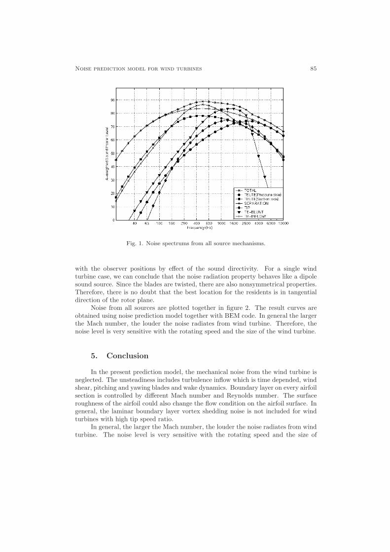
Noise prediction model for wind turbines 85
Fig. 1. Noise spectrums from all source mechanisms.
with the observer positions by effect of the sound directivity. For a single windturbine case, we can conclude that the noise radiation property behaves like a dipolesound source. Since the blades are twisted, there are also nonsymmetrical properties.Therefore, there is no doubt that the best location for the residents is in tangentialdirection of the rotor plane.
Noise from all sources are plotted together in figure 2. The result curves areobtained using noise prediction model together with BEM code. In general the largerthe Mach number, the louder the noise radiates from wind turbine. Therefore, thenoise level is very sensitive with the rotating speed and the size of the wind turbine.
5. Conclusion
In the present prediction model, the mechanical noise from the wind turbine isneglected. The unsteadiness includes turbulence inflow which is time depended, windshear, pitching and yawing blades and wake dynamics. Boundary layer on every airfoilsection is controlled by different Mach number and Reynolds number. The surfaceroughness of the airfoil could also change the flow condition on the airfoil surface. Ingeneral, the laminar boundary layer vortex shedding noise is not included for windturbines with high tip speed ratio.
In general, the larger the Mach number, the louder the noise radiates from windturbine. The noise level is very sensitive with the rotating speed and the size of

86 Alexandru Dumitrache and Horia Dumitrescu
the wind turbine. Boundary layer thickness is required as the basic input for all theself-noise prediction laws. For the wind turbine designer, the noise prediction modelshould be always coupled together with a comprehensive aerodynamic computation tomake sure that the electric power efficiency is not change too much. For wind turbinesto be sited, the prediction model can be helpful to avoid non-necessary annoyance forthe inhabitants.
References
[1] Grosveld, F.W., Prediction of Broadband Noise from Horizontal Axis Wind Tur-bines, Journal of Propulsion and Power, 1, 4, 292–299, 1985.
[2] Viterna, L.A., The NASA LeRC Wind Turbine Sound Prediction Code, Journalof Propulsion and Power, NASA CP-2185, pp. 410–418, 1981.
[3] Brooks, T. F., Pope, D. S., Marcolini, M. A., Airfoil Self-Noise and Prediction,NASA Reference Publication 1218, 1989.
[4] Lighthill, M.J., On Sound Generated Aerodynamically, Proceedings of the RoyalSociety of London, Series A, 211, pp. 564–587, 1952.
[5] Ffowcs-Williams, J.E, Hawkings, D.L, Sound Generation by Turbulence and Sur-faces in Arbitrary Motion, Philosophical Transactions of the Royal Society ofLondon, 264, A 1151, pp. 321–342, 1969.
[6] Ciskowsky, R.D., Brebbia, C. A., Boundary Element Methods in Acoustics, Com-putational Mechanics Publications, Elsevier Applied Science, 1991.
[7] Amiet, R.K., Acoustic Radiation from an Airfoil in a Turbulent Stream, Journalof Sound and Vibration, 41, 4, pp. 407–420, 1975.
[8] Ferdinand, W. G., Prediction of Broadband Noise from Horizontal Axis WindTurbines, Journal of Propulsion and Power, 1, 4, pp. 292–299, 1984.
[9] ESDU-Report, Characteristics of Atmospheric Turbulence Near the Ground, PartII: single point data for strong winds (neutral atmosphere), No. 85020, 1993.
[10] Lowson, M.V., Assessment and Prediction Model for Wind Turbine Noise: 1.Basic Aerodynamic and Acoustic Models, Flow Solution Report 93/06, pp. 1–46,1993.
[11] http://raphael.mit.edu/XFOIL.
[12] Mikkelsen, R., Soerensen, J. N., Shen W. Z., Modelling and analysis of the flowfield around a coned rotor, Wind Energy, 4, 3, pp. 121–135, 2001.
[13] Jakobsen, J., Andersen, B., Aerodynamical Noise from Wind Turbine Generators,EFP j.nr.1364/89-5, JOUR-CT 90-0107, 1993.
[14] Dumitrescu, H., Cardos, V., Dumitrache, Al., Aerodynamics of Wind Turbine,(in Romanian), Editura Academiei Romane, Bucuresti, 2001.

Proceedings of the Fourth Workshop onMathematical Modellingof Environmental and Life Sciences ProblemsConstanta, Romania, September, 2005, pp. 87–94
Quasimonotone ODE Approximationof Nonlinear Diffusion Process
Stelian Ion∗
The paper deal with the numerical approximation of a class of nonlinear diffusion pro-
cess that includes the water flow through porous media. The ordinary differential equations
used as approximation of the diffusion equation is obtained applying the finite volume scheme
for space derivatives discretization and keeping the continuum time derivative. We prove
that in certain conditions concerning the diffusion flux, its numerical approximation and the
mesh size one obtains a quasimonotone ODE system. Using the quasimonotone property we
investigate some theoretical properties of the approximative solution in the case of Richards’
equation.
1. Introduction
In this paper we develop a numerical approximation scheme for a class ofparabolic nonlinear diffusion equation and we prove a comparison theorem for theapproximation models. The mathematical model is given by
∂b(u)
∂t− diva(b(u),∇u) = 0, t > 0, x ∈ Ω,
u = uD, t > 0, x ∈ ∂Ω,u(0, x) = u0(x), x ∈ Ω,
(1)
where Ω is a domain in Rd; div and ∇ are with x ∈ Rd; and u(t, x) is the scalarunknown function. Such models are widely used in soil science, heat transfer theory,Stephen problems, etc. In the heat transfer theory one has b(s) = s,a(u,∇u) =
∗ “Gheorghe Mihoc–Caius Iacob” Institute of Mathematical Statistics and AppliedMathematics, Bucharest, Romania, e-mail: [email protected]
Supported by CERES Grant no. 4-187/2004.

88 stelian ion
k(u)∇u so that evolution of the temperature is governed by the equation
∂u
∂t− div (k(u)∇u) = 0. (2)
The unsaturated water flow through porous media is described by the well knownRichards’ equations [3]
∂θ(h)
∂t− div(K(θ)∇h+ e3K(θ)) = 0, (3)
where θ represents the relative volumetric water content, h represents the pressure,K is the hydraulic conductivity and e3 is the upward vertical versor. In this paper weconsider that the equation of the mathematical model (1) takes only one of the form(2) or (3). For more different examples of diffusion-convections operator, containingmany other references see Diaz [5].
Let us present the sufficient conditions for the existence of the weak solutionsand the comparison principle. We essentially adopt the frame of Alt and Luckhausin [1].
Assumptions on constitutive functions, boundary data, initial data and geometryof domain Ω:A1 b : R→ R is a continuous and nondecreasing function.
The empirical models of soil sciences use the functions θ(h) that are monotoneand bounded,
0 ≤ θ(h) ≤ 1.
The diffusion flux a satisfies:
A2
∣∣∣∣∣∣
∣∣∣∣∣∣
(1)a : R× Rd is a continous function in (u, ξ)(2) |a(b(u), ξ)| ≤ C
(1 +B(u)(p−1)/p + |ξ|p−1
), ∀u, ∀ξ,
(3)(a(u, ξ)− a(u, ξ∗)
)· (ξ − ξ∗) > c|ξ − ξ∗|p, ∀ξ 6= ξ∗ ∈ Rd
with 1 < p <∞ and
B(z) = b(z) · z −z∫
0
b(s)ds.
In the Richards’ equation model the growth condition (2) is ready satisfied, the hy-draulic function used in the soil sciences are upper bounded, but the uniform ellipticconditions (3) is not satisfied by all hydraulic models since the hydraulic conductivitybecomes zero as water content approach the residual values, see [3]. Also the conti-nuity condition (1) is satisfied for homogeneous soil but it is not satisfied for layeredsoils.
A3 uD ∈ Lp((0, T ) : W 1,p(Ω)) ∩ L∞((0, T )× Ω),∂uD
∂t∈ L1((0, T ) : L∞(Ω).
A4 B(u0) ∈ L1(Ω).A5 Ω ∈ Rd is open, bounded, and connected with Lipschitz boundary.
The existence of weak solutions [1].If the data satisfy A1–A5, then there exists a weak solution of the Cauchy
problem (1). A function u(t, x) is a weak solution if the following properties arefulfilled:

quasimonotone ode approximation 89
1) u− uD ∈ Lp((0, T ) : W 1,p(Ω)),
2) b(u) ∈ L∞(0, T : L1(Ω)) and∂b(u)
∂t∈ Lq(0, T : W−1,q(Ω)) with initial values
b(u0), that is,
T∫
0
⟨∂b(u)
∂t, v
⟩dt+
T∫
0
∫
Ω
(b(u)− b(u0))∂v
∂tdxdt = 0 (4)
for every v ∈ Lp(0, T : W 1,p0 (Ω)) ∩W 1,1(0, T : L1(Ω)), v(T, ·) ≡ 0.
3) a(u,∇u) ∈ Lq((0, T )× Ω) and u satisfies the differential equations, that is,
T∫
0
⟨∂b(u)
∂t, v
⟩dt+
T∫
0
∫
Ω
a(u,∇u) · ∇vdxdt = 0 (5)
for every test function v ∈ Lp(0, T : W 1,p0 (Ω)).
Pointwise comparison principleWe present here a comparison result concerning the infiltration problem, the
result is a variant of the comparison results obtained in [1] and [5]. The infiltrationproblem read as
∂θ(h)
∂t− div(κ(h)∇h+ e3κ(h)) = 0, t > 0, x ∈ Ω,
h = hD, t > 0, x ∈ ∂Ω,h(0, x) = h0(x), x ∈ Ω.
(6)
Assume that: the boundary data, initial data and the domain Ω satisfy theconditions A3, A4 and A5, respectively, the function θ(h) satisfies the conditionsA1 and the hydraulic conductivity function satisfies:
A2′
∣∣∣∣∣
∣∣∣∣∣(1)κ : R→ R+, κ(h) ≥ η,(2) |κ(h1)− κ(h2)| < C|h1 − h2|γ , γ ≥
1
2, ∀h1, h2 ∈ R.
Theorem 1 (Comparison Theorem). Let (hD, h0), (hD, h0) be such that
hD ≤ hD, h0 ≤ h0. Let (h, h) be two bounded weak solutions of infiltration problem
(6) associated to (hD, h0) and (hD, h0), respectively. Assume, in addition, that
θ(h)t, θ(h)t ∈ L1((0, T )× Ω).
Then
a) θ(h) ≤ θ(h).If in addition θ(h) and κ(h) satisfy
A2′′ for any z1, z2 such that θ(z1) = θ(z2) results κ(z1) = κ(z2)
then we have
b) h ≤ h on (0, T )× Ω.

90 stelian ion
Proof. In view of the comparison theorem in the paper [1] the result prove true ifone observes that the solution h corresponding to the datum (hD, h0) is a subsolution
of the infiltration problem associate to the datum (hD, h0). A direct proof is as follow.
For any δ > 0 let Ψδ(α) = min(1,max(0, α/δ)). The function w = Ψδ(h − h)belongs to L2(0, T : W 1,2
0 (Ω)) and its gradient is given by
∇w =
1
δ
(∇h−∇h
), if 0 < h− h < δ,
0, otherwise.
Set w as test function in (5). Then
t∫
0
∫
Ω
(θ(h)t − θ(h)t
)wdxdt+
+1
δ
t∫
0
∫
Ωδ
[κ(h)∇h− κ(h)∇h+
(κ(h)− κ(h)
)e3
]· ∇(h− h)dxdt
︸ ︷︷ ︸I
= 0,(7)
where Ωδ := x|0 < h− h < δ. The integral I can be rewritten as
I =
t∫
0
∫
Ωδ
κ(h)||∇(h− h)||2dxdt+
T∫
0
∫
Ωδ
(κ(h)− κ(h))(∇h+ e3) · ∇(h− h)dxdt.
Using Young inequality, ab ≤ C(ǫ)p−1ap + ǫq−1bq and A2′-(1) we obtain
I ≥(η − ǫ
2
) t∫
0
∫
Ωδ
||∇(h− h)||2dxdt− C(ǫ)
2
t∫
0
∫
Ωδ
(κ(h)− κ(h))2||∇h+ e3||2dxdt.
Taking ǫ < 2η and using A2′-(2) we have
t∫
0
∫
Ω
(θ(h)t − θ(h)t
)wdxdt+
c
δ
t∫
0
∫
Ωδ
||∇(h−h)||2dxdt ≤ Cδ2γ−1
t∫
0
∫
Ωδ
||∇h+e3||2dxdt.
The term on the right tends to zero as δ → 0, and the first integral on the leftconverges to
t∫
0
∫
h>h
(θ(h)− θ(h)
)
tdxdt =
t∫
0
∫
Ω
∂tmax(0, θ(h)− θ(h)
)dxdt
so, we have ∫
Ω
max(0, θ(h)− θ(h)
)(t, x)dx ≤ 0,

quasimonotone ode approximation 91
Ω
ω i
ωj
x ixj
σij
σk
xkxk ω i
σia
Ω
Fig. 1. Triangulation of polygonal domain in R2.
that led to θ(h) ≤ θ(h).From the A1 and A2′′ we see that θ(h) = θ(h) and κ(h) = κ(h) in the set
0 < h− h so that the equality (7) is reducing to
t∫
0
∫
Ωδ
||∇(h− h)||2dxdt = 0,
which lead to ∇(h − h) = 0 in 0 < h − h. Boundary conditions, the continuity of
the solutions with respect with space variable and ∇(h− h) = 0 in 0 < h− h imply
h ≤ h. This end the proof of the comparison theorem.By considering that for many interesting PDE we known only approximative
solutions it is desirable to set up a numerical algorithm which preserves some relevantproperties of exact models. The comparison principle is not only useful to demonstratethe uniqueness of the solution but it is also physical relevant. In the next we buildup a numerical scheme that preserves this principle.
2. Quasimonotone ODE Approximation. Method of Line
By the method of lines, one can associate an ordinary differential system ofequations (ODE) to a parabolic partial differential equation. The MOL consists inthe discretization of the space variable using one of the standard methods as finiteelement, finite differences or finite-volume method (FVM).
Using the FVM, one introduce a net of the inner knots xi and a set of the controlvolumes ωi.
Definition 1 (Admissible meshes). The triangulation T = (ωi, xi)i∈I iscalling an admissible meshes if it satisfies:
∣∣∣∣∣∣∣∣∣∣∣∣
∣∣∣∣∣∣∣∣∣∣∣∣
ωi is open poligonal set ⊆ Ω, xi ∈ ωi
(1) ∪i∈Iωi = Ω(2) ∀i 6= j ∈ I and ωi ∩ ωj 6= Φ, either HN−1(ωi ∩ ωj) = 0 or
σij := ωi ∩ ωj is (N − 1)− side of ωi and ωj
(3) ∀σij , [xi, xj ] ⊥ σij
(4) [xi∂ , xi] ⊥ σ∂i := ωi ∩ ∂Ω.

92 stelian ion
The space discretizated equations are derived from the integral form of (1) foreach control volume ωi (see Fig. 1),
∫
ωi
∂b(u)
∂tdx−
∫
∂ωi
a(u,∇u) · nda = 0, ∀i ∈ I.
Consider the infiltration problem (6). By a proper approximations of the volumeintegral and line integral one obtains
m(ωi)dθ(hi)
dt−∑
j∈N (i)
[Kijm(σij)
(hj − hi
dij+ e3 · nij
)]= 0,
hi|t=0 = h0i,
(8)
for t > 0 and for any i ∈ I. N (i) denotes all neighbours of ωi. For those ωi whoseboundary σa
i lay on boundary ∂Ω the corresponding term in the sum is given by
K(hi, hDi)m(σai )
(hDi − hi
d∂i+ e3 · nij
). (9)
Let
fi(h; hD) =∑
j∈N (i)
[K(hi, hj)m(σij)
(hj − hi
dij+ e3 · nij
)],
then the discrete infiltration problem read as
m(ωi)dθ(hi)
dt= fi(h; hD), hi|t=0 = h0i. (10)
We will show that, for a suitable definition of the numerical hydraulic conductiv-ity, K(·, ·), and by imposing an upper bound on the mesh size, the function f (·,hD)verifies Kamke conditions. Then using this conditions we will prove that there existsa discrete comparison result.
For that, define
K(u, v) = max(κ(u), κ(v), η0), (11)
and assume that the step size of the mesh, := max(dij), and hydraulic conductivity,κ, satisfy
A2′′′
∣∣∣∣
∣∣∣∣(1)κ : R→ R+, bounded and nondecreasing(2) η0|h1 − h2| > |κ(h1)− κ(h2)|, ∀h1, h2 ∈ R.
We note that the second requirement implies that κ is a Lipschitz functionwhich is a stronger condition than A2′-(2). The threshold η0 in (11) is necessary ifthe function κ do not satisfy the second condition A2′-(1).
Also we suppose that in addition to A1 the water content function is a differ-entiable function on (−∞, 0) and θ(h) = 1 on (0,∞),
A1′ dθ
dh> 0 on (−∞, 0).

quasimonotone ode approximation 93
Proposition 1 (Quassimonotony). Let T be an admissible mesh and letK(·, ·) be given by (11). Assume A2′′′. Then the following statements hold:
(a) If v < w then K(u,w)(w − u)−K(u, v)(v − u) > η(w − v).(b) If hD ≥ hD then
fi(h, hD) ≥ fi(h,hD).
(c) Kamke condition. If h ≥ h and hi = hi then
fi(h,hD) ≥ fi(h,hD).
Proof. The statement (a) is a simply consequence of A2′′′-(1) and the definition(11). The statement (b) results from (9).(c) We have
fi(h,hD)− fi(h,hD) =∑
j∈N (i)
m(σij)Γi,j(h,h)
with
Γi,j = K(hi, hj)hj − hi
dij−K(hi, hj)
hj − hi
dij+ (K(hi, hj)−K(hi, hj))e3 · nij .
Using (a) one obtains
Γi,j ≥ ηhj − hj
− (K(hi, hj)−K(hi, hj)) ≥ ηhj − hj
− (κ(hj)− κ(hj)).
From the condition A2′′′-(2) we see that Γi,j ≥ 0. Hence, (c) prove true.The results presented in the proposition improve our previous results [7] in
sense that f verifies the Kamke condition in less restrictive conditions on hydraulicconductivity function than those imposed there.
Theorem 2 (Comparison theorem. Discrete case). Assume the hypoth-
esis of the proposition and A1′. Let h(t) and h(t), t ∈ (0, T ), be the solutions of the
problem (10) associated to (hD,h0) and (hD, h0), respectively. Suppose that
hD ≤ hD < 0, h0 ≤ h0 < 0.
Thenh ≤ h on (0, T ).
Proof. Let α < 0 be an upper bound for boundary data and initial data, that is
hDi ≤ α, h0i ≤ α
and let T1 be such that the solutions h(t) and h(t) stay less than 0 on the interval(0, T1) [2], [4]. As θ′(h) > 0 on (0, T1) one can apply Nickel’s theorem ([8], [9]) andone obtains that
h(t) ≤ h(t) on (0, T1).

94 stelian ion
Moreover, observe that the solution hα(t) associate to the boundary data hDi = αand initial data h0i = α is a constant solution h(t)i = α (fi(α;α) = 0!). Using theinequality (b) of the proposition we have
h(t) ≤ h(t) ≤ α on (0, T1).
The inequality show that T = T1.
References
[1] H. W. Alt, S. Luckhaus, Quasilinear eliptic-parabolic differential equations, Math.Z., 183 (1983), 311–341.
[2] V. Barbu, Ecuatii diferentiale, Editura Junimea, Iasi, 1985.
[3] J. Bear, Dynamics of Fluids in Porous Media, Dover, 1988.
[4] K.E. Brenan, S.L. Campbell and L.R. Petzold, Numetical Solution of InitialValue Problems in Differential-Algebraic Equations, Classics in Applied Mathe-matics, SIAM, 1996.
[5] J.I. Diaz, Qualitative Study of Nonlinear Parabolic Equations: an Introduction,Extracta Matematicae, 16 (3) (2001), 303–341.
[6] R. Eymard, Th. Gallouet and R. Herbin, Finit Volume Method, in Handbook ofNumerical Analysis, G. Ciarlet and J.L Lions eds., North Holland, 2000.
[7] S. Ion, D. Homentcovschi and D. Marinescu, Method of Lines for SolvingRichards’ Equation, Proc. of 5th International Seminare on “Geometry, Con-tinua and Microstructures”, eds. Sanda Cleja–Tigoiu and V. Tigoiu, EdituraAcademiei Romane, 2002, pp. 125–132.
[8] V. Lakshmikantham and S. Leela, Differential and Integral Inequalities: Theoryand Applications. Academic Press, New York, 1969.
[9] K. Nickel, Bounds for the Set of Solutions of Functional-Differential Equations,MRC Tech. Summary Report No. 1782, Univ. of Wisconsin, Madison, 1977.
[10] F. Otto, L1-contraction and uniqueness for quasilinear elliptic-parabolic equa-tions, J. Differential Equations, 131 (1) (1986), 20–38.

Proceedings of the Fourth Workshop onMathematical Modellingof Environmental and Life Sciences ProblemsConstanta, Romania, September, 2005, pp. 95–102
Minimum Free Energy Configuration of the PlanarLipidic Bilayer. Analytical Solutions
Stelian Ion∗† and Dumitru Popescu∗
The paper deal with the calculus of the shape of the monolayers, which constitute
the two leaflets of the planar lipidic bilayer (BLM), that undergo external constrains. The
deformed configuration minimises the free energy of the BLM and it is determined as the
solution of a forth order elliptic equation subject to certain boundary conditions. For planar
radial symmetrical problems the general solutions of elliptic equation are obtained as a power
series expansion and it is shown they belong to the family of the Bessel functions.
1. Introduction
The main point of the paper is to obtain the solutions of the linear ellipticequation of the forth order
2u− 2ξu+ u = 0, (1)
where ξ is a real positive constant and represents the differential Laplace operator.The equations like (1) are frequently used to study the space configuration of
the planar lipid bilayer and its free energy response to the deformation ([6], [5], [7]).Briefly, the bilayer lipidic membranes (BLM) is a biological sheet like structure thatconsists in two lipidic monolayer combined tail to tail. The monolayers can be slightlystretched or compressed and undergo curvature deformations and there exists a freeenergy response to these deformations. The mechanical properties of BLM are specificto smectic liquid crystal of A type ([4], [6] and [2], [3] for more general theory of liquidcrystal).
∗ “Gheorghe Mihoc–Caius Iacob” Institute of Mathematical Statistics and AppliedMathematics, Buchares, Romania.
† e-mail: [email protected] Supported by PNCDI–VIASSAN Grant NO. 344/2004.

96 stelian ion and dumitru popescu
un
h
h
z
y
x
Fig. 1. The unperturbed (dashed line) and perturbed (solid line) position of the two mono-layer. The bilayer is 2h width in the initial state and it is infinite spread in the x, y directions
in the both states. The vector n represents the normal to the deformed surface.
Let us consider the planar structure given by the plane surface z = ±h asunperturbed position of the BLM (see fig. 1). We suppose that the two surfacesz = ±h undergo a displacement with same distance u but in opposite directions.Then deformation free energy density of unit unperturbed area can be written as [6]
ρ (x, y) = hB(uh
)2
+ hK1 (u)2 + γ|∇u|2, (2)
where: h is the monolayer equilibrium thickness, B is the compression-extensionmodulus constant, K1 is splay modulus constant and γ represents the interfacialtension constant.
The deformation free energy associated to a domain D, F(D), is defined as thesurface integral
F(D) =
∫
D
ρ(x, y)dσ. (3)
Passing to the dimensionless variable u = hu∗, x = Lx∗, y = Ly∗ and choosing thecharacteristic length L such that L2 = h
√K1/B the relation (2) becomes
ρ = hB((∗u∗)
2 + 2ξ (∇∗u∗)2 + u2
∗
), (4)
where 2ξ = γ/√K1B. The ∗ subscript denote the dimensionless quantity and it will
be suppressed in the sequel.Let us define the bilinear form a(u, v), the linear operator L[u] by
a(u, v) =uv + 2ξ∇u · ∇v + uv,
L[u] =2u− 2ξu+ u,
and the dimensionless energy J(D,u) by
J(D,u) =1
2
∫
D
a(u, u)dσ.

minimum free energy configuration of the blm 97
The deformation free energy F(D) can be expressed as
F(D,u) = 2h2√K1BJ(D,u).
Performing some calculus we obtain
J(D, v)− J(D,u) =
∫
D
L[u](v − u)dσ +
+
∫
∂D
(u∂(v − u)
∂n− (v − u)∂u
∂n+ 2ξ(v − u)∂u
∂n
)ds (5)
+ J(D, v − u) .
This identity shows that the solution of the equation L[u] = 0 that satisfies theboundary conditions
u|∂D = u0,
∂u
∂n
∣∣∣∣∂D
= u1
(6)
minimises the free energy J in the class of the functions that satisfy same boundaryconditions.
2. Analytical solutions
We shall consider the radial symmetric function defined in the whole plane. Asin [1] we search for a real power series solution of the equation (1),
Φ(r) =
∞∑
m=0
cmrα+m,
where the exponent α is a real number and c0 6= 0. Taking into account that in polarcoordinate the Laplace operator is given by
=1
r
∂
∂r
(r∂
∂r
),
one obtains
r4L[Φ] = α2(α− 2)2c0rα + (α+ 1)2(α− 1)2c1r
α+1++ α2
[(α+ 2)2c2 − 2ξc0
]rα+2 + (α+ 1)2
[(α + 3)2c3 − 2ξc1
]rα+3+
+∞∑
m=0
(α+m+ 2)2
[(α+m+ 4)2cm+4 − 2ξcm+2
]+ cm
rα+m+4.

98 stelian ion and dumitru popescu
The exponent α and coefficients cm will be determined equating the coefficientsof rα+m,m = 0, 1, · · · to zero.
One obtains a recurrence relation for the coefficients cm,
(α+m+ 4)2(α+m+ 2)2cm+4 − 2ξ(α+m+ 2)2cm+2 + cm = 0 (m = 0, 1, . . .) (7)
and four equation for α, c0, c1, c2, c3.Let us firstly study the solutions of the recurrence relation.We choose c1 = c3 = 0 and it follows that c2m+1 = 0,m = 2, 3, . . . successively.To find the even rank terms c2m we introduce another sequence bmm=0,∞ and
write c2m as
c0 = b0,
c2m =bm
(α+ 2)2 · · · (α+ 2m)2(m = 1, 2, . . .).
Substituting this expression into recurrence relation (7) we find that the terms bmverify a linear recurrence relation
bm+2 − 2ξbm+1 + bm = 0 (m = 0, 1, . . .). (8)
We note that there always exist two real solutions of this recurrence relation and wepostpone to write their explicit solutions.
It follows that the power series Φ has the form
Φ(α, r) = rα
(b0 +
∑
m=1
r2m bm(α+ 2)2 · · · (α+ 2m)2
)
and satisfies
r4L[Φ(α, r)] = rαα2[(α− 2)2c0 +
((α+ 2)2c2 − 2ξc0)
)r2].
One observes that α = 0 is a double root of the polynomial on right hand side.The solutions that we are looking for can be obtained as in the following propo-
sition
Proposition 1. If the sequence bmm=0,∞ satisfies the recurrence relation(8), then the functions I(r;b), K(r;b) given by
I(r;b) ≡ Φ(0, r) =∑
m=0
(r2
)2m bm(m!)2
, (9)
K(r;b) ≡ ∂Φ
∂α
∣∣∣∣α=0
= ln(r)I(r;b) −∑
m=1
( r2
)2m bmH(m)
(m!)2, (10)
represent the solutions of the equations (1).

minimum free energy configuration of the blm 99
The function H(m) is given by H(m) = 1 + 12 + · · ·+ 1
m .To obtain the general solution bm of the recurrence relation (8) we consider the
characteristic equationt2 − 2ξt+ 1 = 0.
Depending on the ξ this equation can have real or complex solutions.a) Case ξ > 1There exists two real positive solutions
λ =
√ξ −
√ξ2 − 1, β =
√ξ +
√ξ2 − 1
and the general solution of recurrence equation is given by
bm = C1λ2m + C2β
2m.
Consequently, we obtain that the functions I(r,b) are nothing but the Bessel functionswith imaginary argument of order zero I0 [9],
I0(λr) = I(r, λ) =∑
m=0
(rλ
2
)2m1
(m!)2,
I0(βr) = I(r, β).
(11)
One can obtain another two independent solutions by linear combination of the func-tion I and K. Among all linear combination there exist one that led to the Besselfunction K0 which is given by
K0(λr) = −K(r;λ) + ln(λ/2)I(r;λ) − γI(r;λ)
= −ln(λr/2)I0(λr) +∑
m=0
(λr
2
)2mψ(m+ 1)
(m!)2,
K0(βr) = · · ·,(12)
where ψ(m+ 1) = H(m)− γ, ψ(1) = −γ, and γ is Euler’s constant.b) Case 0 < ξ < 1There exists two complex solutions and the general solution of recurrence rela-
tion is given bybm = Acos(mθ) +Bsin(mθ),
where the angle θ is given bycos(θ) = ξ.
In this case the functions I(r,b) become
Ber(r; θ) =∑
m=0
(r2
)2m cos(mθ)
(m!)2 ,
Bei(r; θ) =∑
m=1
(r2
)2m sin(mθ)
(m!)2 .
(13)

100 stelian ion and dumitru popescu
z
1
Fig. 2. Perforation problem. The two monolayers of the bilayer have a contact pointand at great distance the monolayers rest unperturbed.
As in the first case, by linear combination, we can also obtain the following solutions
Ker(r; θ) =−lnr
2Ber(·; ·) + θ/2Bei(·; ·) + Rc(·; ·) ,
Kei(r; θ) =−lnr
2Bei(·; ·)− θ/2Ber(·; ·) + Rs(·; ·) .
(14)
The series Rs(·; ·) and Rc(·; ·) are given by
Rc
s(r; θ) =
∑
m=0
(r2
)2mcos(mθ)sin(mθ)
(m!)2 ψ(m+ 1)
The real functions (13) verify the relation
Ber(r; θ) + iBei(r; θ) = I0
(eiθ/2r
)(15)
and the real functions (14) verify the relation
Ker(r; θ) + iKei(r; θ) = K0
(eiθ/2r
). (16)
For θ = π/4 they are known as Thomson’s function and Rusell’s function, re-spectively [9].
3. Perforation of the planar bilayer problem
As an application of the previous results formulae we present here the solutionof the perforation bilayer problem (see fig. 2). The perforation of the BLM can begenerated by the thermal fluctuations of its compounds and in certain circumstancesthe perforation produce a pore in the BLM [8].

minimum free energy configuration of the blm 101
-0.2
0
0.2
0.4
0.6
0.8
1
0 2 4 6 8 10
ξ=0.781
ξ=0.000034
a)
-0.02
0
0.02
0.04
0.06
0.08
0.1
0.12
3 4 5 6 7 8 9 10
ξ=0.781
ξ=0.000034
b)
Fig. 3. The solutions of the perforation problem (17) for two valuesof the parameter ξ a) and detail b).
Mathematically, the perforation problem can be formulate as follows. Findu : R2 − 0, 0 → R such that:
L[u] = 0, inR2 − (0, 0),u|r=0 = 1, u|r=∞ = 0,∂u
∂r
∣∣∣∣r=0
= 0,∂u
∂r
∣∣∣∣r=∞
= 0,(17)
Depending of the parameters ξ we find out that the solution of the problem is
Case ξ > 1 : u(r) = (K0(λr) −K0(βr)) / (lnβ − lnλ) ,
Case ξ < 1 : u(r) = −2
θKei(r; θ).
Free energy of the perforated BLM is given by
J(u) = π r
(u∂u
∂r− u∂u
∂r+ 2ξu
∂u
∂r
)∣∣∣∣∞
0
= π r∂u∂r
∣∣∣∣r=0
.
Then we have
J(u) =
π
√ξ2 − 1
ln(ξ +
√ξ2 − 1
) , ξ > 1,
2π
√1− ξ2
arccosξ, ξ < 1.
For the following parameters of the BLM [8]: γ ≈ 15 × 10−4 Nm−1, K1 ≈ 0.93 ×10⁻¹¹ N, B ≈ 5.36 × 10⁷ Nm−2, h ≈ 11.3 × 10⁻¹⁰ m and ξ =
γ
2√K1B
≈ 3.4 × 10⁻²

102 stelian ion and dumitru popescu
one obtain J(u) ≈ 4 and then
F/kT = 2h2√K1BJ(u)/kT ≈ 50.
References
[1] W. E. Boyce and R. C. DiPrima, Elementary Differential Equations and Bound-ary Value Problems, John Wiley & Sons, 1976.
[2] J. L. Ericksen, Conservation laws for liquid crystals, Tran. Soc. Rheol. 5, 1961,pp. 23–34.
[3] J. L. Ericksen, Liquid crystals with variable degrees of orientation, Arch. Rat.Mech. Anal., 113, 1991, pp. 97–120.
[4] P. G. deGennes, The Physics of Liquid Crystals, Clarendon Press, Oxford, 1974.
[5] P. Helfrich and E. Jakobsson, Calculation of Deformation Energies and Confor-mations in Lipid Membranes Containing Gramicidin Channels, Biophys. J., Vol.57, May 1990, pp. 1075–1084.
[6] H. W. Huang, Deformation Free Energy of Bilayer Membrane and its Effect onGramicidin Channel Lifetime, Biophys. J., Vol. 50, December 1986, pp. 1061-1070.
[7] C. Nielsen, M. Goulian and O. Andersen, Energetics of Inclusion-Induced BilayerDeformation, Biophys. J., vol.74 (1998), pp. 1966–1983.
[8] D. Popescu, S. Ion, A.I. Popescu, and L. Movileanu, Elastic properties of bilayerlipid membranes and pore formation, in Planar Lipid Bilayer(BLMS) and theirApplications, H. TiTien and A. Ottowa, eds., Elsevier Sciences Publishers, 2003,pp. 173–204.
[9] G. N. Watson, Theory of Bessel Functions, Cambridge, 1966.

Proceedings of the Fourth Workshop onMathematical Modellingof Environmental and Life Sciences ProblemsConstanta, Romania, September, 2005, pp. 103–112
A Numerical Study of Axisymmetric Slow ViscousFlow Past Two Spheres
Gheorghe Juncu∗
This paper presents a computational study of the axisymmetric, slow, viscous flow
(Stokes flow) around two spheres placed parallel to their line of centers. The fourth-order
stream function equation in bispherical coordinates, was split into its coupled form, by
defining the fluid vorticity. The central, second order accurate, finite difference scheme
was used to discretize the model equations. Two numerical algorithms were employed to
solve the discrete equations: multigrid (MG) and preconditioned conjugate gradient squared
(PCGS). The preconditioners tested are approximations (ILU and multigrid iterations) of
the symmetric part of the discrete Stokes operator in bispherical coordinates. The mesh
behaviour of the convergence rate of MG and PGCG was analysed for different values of the
model parameters.
1. Introduction
The hydrodynamic interaction of two spherical particles moving slowly in a vis-cous fluid is of fundamental importance to meteorology, colloid chemistry, flow ofsuspensions and other fields from nuclear and chemical engineering, environmentalsciences, etc. The solution to the problem of two spheres rotating with constant an-gular velocities around their line of centres was obtained first by Jeffery [1], assumingnegligible inertial effects (Stokes flow). The first solution of the associated axisym-metrical problem when the spheres translate with the same velocity along their lineof centres in Stokes flow was obtained by Stimson and Jeffery [2]. Stimson and Jef-fery [2] considered only the case of equal-sized spheres in non-contact. Starting fromthese two classical articles, other creeping flow solutions were developed by Goldmanet al. [3], Wakyia [4], Cooley and O’Neill [5], Davis [6], O’Neill and Majumdar [7],
∗ “Politehnica” University of Bucharest, Polizu 1, 78126 Bucharest, Romania, e-mail:[email protected], [email protected]

104 gheorghe juncu
U 8
L L1 2
d1 d2
r
z
Fig. 1. Schematic of the problem.
Rushton and Davies [8], Haber et al. [9], Hetsroni and Haber [10] and Zinchenko [11].A detailed account of the work done on the problem of two spheres external to eachother is given by Happel and Brenner [12] and Kim and Karrila [13]. We restrictedour citation only to problems similar to that solved in this work. For this reason,related problems as electrophoretic or thermocapillary migration of two spheres arenot mentioned here.
In [1–9, 11], the momentum balance equations (the Stokes and continuity equa-tions) were solved analytically in general orthogonal curvilinear coordinate systems(bispherical coordinate system, [1–4], [6–9], [11] and tangent-sphere coordinate system[5]). The suitable analytical solutions in terms of these coordinates have been shownto be infinite series. The method of reflection was used in [10]. The application ofthe boundary integral methods to Stokes flow was discussed by Roumeliotis [14]. Fora pair of equal spheres in tandem, the Navier-Stokes equations were solved numeri-cally in bispherical coordinate system at Re = 40 by Tal et al. [15]. The aim of thiswork is to solve numerically the Stokes flow equations for two spheres in-line. Thevorticity–stream function formulation of the flow equations in bispherical coordinateswas chosen. The central, second order accurate, finite difference scheme was usedto discretize the model equations. Two numerical algorithms were tested: multigrid(MG) and preconditioned conjugate gradient squared (PCGS). The convergence rateof MG and PGCG was analysed for different spheres spacing and sizes.
2. Statement of the problem
We suppose that a homogeneous viscous fluid of constant density and viscosityflows past two rigid spheres of diameters di, i = 1,2, as illustrated in figure 1. Thediameters of the spheres are assumed considerably higher than the molecular meanfree path of the surrounding fluid. Oscillations and rotation of the spheres do notoccur during the flow. The flow is considered steady, laminar and axisymmetric. Also,the inertial effects are negligible in comparison with the viscous forces (creeping or

viscous flow past two spheres 105
Fig. 2. Cylindrical coordinates (r, z) versus bispherical coordinates (η, ξ); d1 = d2 = d.
Stokes flow).Let a system of cylindrical coordinates (r, z) be chosen so that the centres of the
spheres lie along the z-axis (see figure 1). In order to facilitate the numerical solutionof this problem, we introduce the bispherical coordinates (η, ξ) defined by (see alsofigure 2)
r =c sin ξ
cosh η − cos ξ; z =
c sinh η
cosh η − cos ξ,
where c > 0 is a characteristic length. This transformation maps the right half ofthe rz-plane (from which the surface occupied by the spheres is excluded) into therectangle η1 ≤ η ≤ η2, 0 ≤ ξ ≤ π, η1 < 0, η2 > 0. The surfaces of the spheres arelocated at η = η1 and η = η2. The relations between ηi, the diameters of the spheresdi and the distances Li of their centers from the origin of the coordinates system are:
di
2=
c
sinh | ηi|; Li = c coth | ηi| , i = 1, 2.
The following scaling is chosen: the radius of the up-stream sphere d1/2 for lengthand 4/U∞d
21 for stream function (U∞ being the free stream velocity).
In terms of dimensionless stream function, ψ, the partial differential equation ofincompressible viscous hydrodynamics in the time–independent Stokes approximationis
E4ψ = 0. (1)
The boundary conditions considered are:– spheres surfaces (η = ηi, i = 1, 2)
ψ = 0; (2)
– free stream (η → 0, ξ → 0)
ψ → 1
2
sin2 ξ
A2; (3)

106 gheorghe juncu
– symmetry axis (ξ = 0 and η 6= 0, ξ = π)
ψ = 0, (4)
where
A =cosh η − cos ξ
c, c =
2 c
d1.
The operator E2 assumes the following form in axisymmetric bispherical coor-dinates:
E2 = A2 ∂2
∂ η2+A sinh η
c
∂
∂ η+ A2 ∂2
∂ ξ2+A ( 1 − cosh η cos ξ)
c sin ξ
∂
∂ ξ. (5)
3. Numerical methods
The fourth-order stream function equation (1) was split into its coupled form
E2ψ = ω, (6)
E2ω = 0 (7)
by defining the fluid vorticity ω. Note that the vorticity defined previously is notidentical to the exact fluid vorticity (i.e. is the curl of the velocity). The relationbetween these two quantities is ω = h3 , where h3 is the metric coefficient,
h3 = csin ξ
cosh η − cos ξ.
It is convenient numerically to work with the deviation from the uniform flowψ∗,
ψ∗ = ψ − 1
2
sin2 ξ
A2.
After ψ∗ is substituted for ψ in (4a), the final form of the mathematical modelis:
E2ψ∗ = ω, (8)
E2ω = 0 (9)
with the boundary conditions:– spheres surfaces (η = ηi, i = 1,2)
ψ∗ = −1
2
sin2 ξ
A; (10)
– free stream (η → 0, ξ → 0)
ψ → 0, ω → 0; (11)

viscous flow past two spheres 107
– symmetry axis (ξ = 0 and η 6= 0, ξ = π)
ψ∗ = ω = 0. (12)
The two-dimensional region (η1, η2)×(0, π) was transformed into the unit squareby well known elementary relations. Equations (5) were discretized with the centralsecond order accurate finite difference scheme on uniform meshes with N ×N pointsand h = (N – 1)−1, N = 5, 9, 17, 33, 65 and 129. Two algorithms were employedto solve the discrete equations: (1o) the preconditioned conjugate gradient squared(PCGS) [16] and (2o) multigrid (MG).
The preconditioners used are the incomplete LU factorisation (with two extradiagonals; algorithm IC (1, 3) from [17]) and the multigrid approximation (two multi-grid cycles) of the symmetric part of the discrete operator E2. These preconditionersare similar with those analysed theoretically in [18–20] and tested experimentally in[21–25]. The structure of the MG cycle used in preconditioning is: (1.) cycle of typeV; (2.) smoothing by point Gauss-Seidel; one smoothing step is performed before thecoarse grid correction and one after in the opposite direction; (3.) prolongation bybilinear interpolation; (4.) restriction by full weighting; (5.) the coarse grid has 5× 5points. The stopping criterion used for PCGS is
‖ ri‖‖r0‖
≤ 10−6,
where ri is the residual after i iterations and ‖ ‖ the discrete Euclidean norm. Themaximum number of iterations allowed is 5 000.
The MG algorithm used is the nested FAS technique, [26], [27]. The struc-ture of the MG cycle is: 1) cycle of type V; 2) smoothing by point Gauss-Seidel;two smoothing steps are performed before the coarse grid correction and one after;3) prolongation by bilinear interpolation for corrections and cubic interpolation forsolution; 4) restriction of residuals by full weighting. Three levels were used in thenumerical experiments.
The convergence rate of PCGS is monitored by the cumulative number of multi-plications per grid point and iteration step. The following convention was adopted inthe calculation of this quantity: the number of multiplications of non-preconditionedCGS was considered as the measure unit. The numerical performances of MG areexpressed by two quantities: (1) the average reduction factor, ρ, and (2) the efficiency,τ . The average reduction factor and the efficiency are given by
ρ = (‖ri+j‖ / ‖ri‖)1/j , τ = −W/ ln ρ,
where ri is the residual after i iterations, ‖ ‖ the discrete Euclidean norm and W thenumber of multiplications per grid point and iteration step. The efficiency is alsoused for the comparison between PCGS and MG.
The computations were made using double-precision Fortran on a PC computer(COMPAQ – Presario 5358 Series, Pentium-Celeron processor).

108 gheorghe juncu
Fig. 3. Mesh behaviour of the convergence rate of PCGS for d1 = d2 = d;(a) ILU preconditioning; (b) MG preconditioning.
4. Numerical experiments
Two geometrical quantities were considered significant for the present problem:(i) the distance between the spheres (expressed by mean of 2Li/di) and (ii) the di-ameters of the spheres. First, we will consider the case of equal-sized spheres, e.g.d1 = d2 = d. For this case, the influence of the spheres spacing on the convergencerate is analysed. Secondly, for a given value of 2L1/d1, the influence of d1/d2 on theconvergence rate of the numerical algorithms will be investigated. For the ratio d1/d2
two values different from 1 were considered: 0.5 and 2.The first task in any numerical work is to validate the code’s ability to reproduce
published results accurately. For the problem studied in this work, one of the mostimportant characteristic quantities is the force Fi acting on either sphere [2],
Fi = µπ U∞d1
2
∫
γ
r3∂
∂ n
(E2 ψ
r2
)d γ,
where µ is the dynamic viscosity of the fluid, ∂/∂n is the normal derivative andthe integral is taken around any meridian γ of the sphere in a sense which is right–handedly related to the outward drawn normal n to the sphere. A comparison of thepresent results with published solutions [6] shows a good agreement.
Figures 3 show the convergence behaviour of PCGS (figure 3a for ILU precon-ditioning and figure 3b for MG preconditioning) for d1 = d2 = d. We must mentionthat CGS (i.e. the non-preconditioned algorithm) converges only on N = 5 and N= 9 meshes. Also, PCGS preconditioned with MG does not converge for 2L/d = 11on the N = 129 mesh. Based on extensive numerical experiments and on the resultsplotted in figures 3, we can note the following facts:
• The influence of the spheres spacing on the convergence rate of PCGS issignificant;
• Both preconditionings improve the robustness of the algorithm;

viscous flow past two spheres 109
Fig. 4. Mesh behaviour of the convergence rate of PCGS for different spheres spacingand sizes; ILU preconditioning.
• Preconditioning by incomplete factorisation performs better for small valuesof 2L/d;
• PCGS preconditioned by MG(2) works very well for 2L/d = 2.The influence of the spheres sizes on the PCGS convergence rate is plotted in
figures 4 and 5. From the data depicted in these figures it is difficult to draw a generalconclusion concerning the influence of the diameters ratio on the convergence rate ofPCGS. Figures 4 and 5 show that:
• for ILU preconditioning, the ratio d1/d2 does not influence significantly theconvergence rate at small spheres spacing (i.e. 2L1/d1 = 1.10);
• for values of d1 / d2 greater than one and 2L1/d1 ≥ 2.0, the convergence rateof ILU preconditioning decreases;
• for MG preconditioning, we can note the decrease in the convergence rate for2L1/d1 = 2.0 and d1/d2 = 0.5 and the increase in the convergence rate for 2L1/d1 =5.0 and d1/d2 = 0.5.
Numerical experiments with MG were made considering for the finest mesh N= 65, 129 and 257. The influence of the spheres spacing and sizes on the convergencerate of the MG algorithm is not significant. The values obtained for the averagereduction factor fall inside the interval [0.8, 0.87]. Note that the average reductionfactor for Gauss-Seidel iteration is greater than 0.990. The values computed for theefficiency vary between 255.0 and 410.0. It must be mentioned that for 2L1/d1 = 5.0,MG does not converge on the finest mesh with N = 257.
For the comparison between PCGS and MG we consider that the solution is

110 gheorghe juncu
Fig. 5. Mesh behaviour of the convergence rate of PCGS for different spheres spacing andsizes; MG preconditioning.
desired on the N = 129 mesh. Function of the values of 2L1/d1, d1/d2 and the typeof preconditioner, the efficiency of PCGS for N = 129 is comprised between 180.2 and14 000. The MG efficiency is that presented previously. Thus, for N = 129, PCGS isa competitor for MG only for 2L1/d1 = 2.0, d1/d2 ≥ 1 and MG (2) preconditioning.
References
[1] G.B. Jeffery,On the steady rotation of a solid of revolution in a viscous fluid,Proc. London Math. Soc., 14 (1915), 327.
[2] M. Stimson, G.B. Jeffery, The motion of two spheres in a viscous fluid, Proc. R.Soc., A11 (1926), 110.
[3] A.J. Goldman, R.G. Cox, H. Brenner, The slow motion of two identical arbitrarilyoriented spheres through a viscous fluid, Chem. Eng. Sci.,21 (1966), 1151.
[4] S. Wakiya. Slow motions of a viscous fluid around two spheres, J. Phys. Soc.Japan, 22 (1967) 1101.
[5] M.D.A. Cooley, M.E. O’Neill, On the slow motion of two spheres in contact alongtheir line of centres through a viscous fluid Proc. Camb. Phil. Soc., 66 (1969),407.

viscous flow past two spheres 111
[6] M.H. Davis, The slow translation and rotation of two unequal spheres in a viscousfluid, Chem. Eng. Sci., 24 (1969), 1769.
[7] M.E. O’Neill, S.R. Majumdar, Asymmetrical slow viscous fluid motion caused bythe translation or rotation of two spheres, I + II., ZAMP, 21 (1970), 164.
[8] E. Rushton, G.A. Davies, The slow unsteady settling of two fluid spheres alongtheir line of centres, Appl. Sci. Res., 28 (1973), 37.
[9] S. Haber, G. Hetsroni, A. Solan, On the low Reynolds number motion of twodroplets, Int. J. Multiphase Flow, 1 (1973), 57.
[10] G. Hetsroni, S. Haber, Low Reynolds number motion of two drops submerged inan unbounded arbitrary velocity field, Int. J. Multiphase Flow, 4 (1978), 1.
[11] A.Z. Zinchenko, The slow asymmetric motion of two drops in a viscous medium,Prikl. Matem. Mekhan., 44 (1980), 49.
[12] J. Happel, H. Brenner, Low Reynolds Number Hydrodynamics, Martinus, Nijhoff,1983.
[13] S. Kim, S. Karrila, Microhydrodynamics. Principles and Selected Applications,Butterworth-Heinemann, 1991.
[14] J. Roumeliotis, A boundary integral method applied to Stokes flow, Ph. D. Thesis,University of New South Wales, Australia, 2000.
[15] R. Tal (Thau), D.N. Lee, W.A. Sirignano, Heat and momentum transfer arounda pair of spheres in viscous flow, Int. J. Heat Mass Transfer, 27 (1984), 1953.
[16] P. Sonneveld, CGS, A fast Lanczos–type solver for nonsymmetric linear systems,SIAM J. Sci. Statist. Comput., 10 (1989), 36.
[17] J.A. Meijerink, H.A. van der Vorst, Guideliness for the usage of incomplete de-compositions in solving sets of linear equations as they occur in practical prob-lems, J. Comput. Phys., 44 (1981), 134.
[18] D. Adam, Mesh independence of Galerkin approach by preconditioning, Int. J.Comput. Math., 58 (1989), 117.
[19] C. Popa, Mesh independence of the condition number of discrete Galerkin systemsby preconditioning, Int. J. Comput. Math., 51 (1994), 127.
[20] C. Popa, Preconditioning conjugate gradient method for non-symmetric systems,Int. J. Comput. Math., 58 (1995), 117.
[21] Gh. Juncu, I. Iliuta, Preconditioned cg-like methods for solving non-linearconvection-diffusion equations, Int. J. Num. Meth. Heat Fluid Flow, 5 (1995),239.
[22] Gh. Juncu, Preconditioning by approximations of the discrete Laplacian for 2–Dnon – linear free convection elliptic equations, Int. J. Num. Meth. Heat FluidFlow, 9 (1999), 586.

112 gheorghe juncu
[23] Gh. Juncu, C. Popa, Preconditioning by approximations of the Gram matrix forconvection-diffusion equations, Mathematics and Computers in Simulations, 48(1998), 225.
[24] Gh. Juncu, C. Popa, Numerical experiments with preconditioning by Gram matrixapproximation for non-linear elliptic equations, Mathematics and Computers inSimulations, 52 (2000), 253.
[25] Gh. Juncu, C. Popa, Preconditioning by Gram matrix approximation fordiffusion-convection-reaction equations with discontinuous coefficients, Mathe-matics and Computers in Simulation, 60 (2002), 487.
[26] A. Brandt, Multi-level adaptive solutions to boundary–value problems, Math.Comput., 33 (1977), 333.
[27] W. Hackbusch, Multi-Grid Methods and Applications, Springer, Berlin, 1985.

Proceedings of the Fourth Workshop onMathematical Modellingof Environmental and Life Sciences ProblemsConstanta, Romania, September, 2005, pp. 113–118
Approach to nonstationary (transient) Birth-DeathProcesses
Alexei Leahu∗
In this paper we show how, in certain cases, nonstationary (transient) Birth-Death
Processes (BDP) may be best approximated by their finite projection, which are stationary
(recurrent positive) BDP. To illustrate, we consider nonstationary M/M/c Queueing Systems.
1. Introduction
Many mathematical models in Life Sciences, Physics, Computer Sciences, etc.are described by means of nonstationary BDP. Such processes are more difficult toapproach than stationary BDP. Our aim is to find stationary BDP nearest (in certainsense) to the initial BDP.
2. Solution of the Problem
Let’s consider BDPX = (X(t))t∈[0,+∞) defined on the probability space (Ω,F ,P)with Birth intensities (λn)n≥0 and Death intensities (µn)n≥0. The set of states beingE = 0, 1, 2, ..., we suppose that P(X(0) = 0) = 1.
In order to achieve our aim, we observe that, according to the terminologyof the book [1], BDP X may be interpreted as regenerative process with renewalcycles (Yn)n≥0 (or embedded renewal process (Sn)n≥0) as the sequence of consecutiveintervals Yn between the moments S0, S1, S2, ... when BDP X falls into the state
0, i.e., S0 = Y0 = 0, Sn =n∑
k=0
Yk and (Yn)n≥1 are nonnegative, independents,
identically distributed random variables with distribution function F (y) = P(Yn <
∗ “Ovidius” University of Constanta, Romania, e-mail: [email protected] Partially supported by Romanian Academy Grant 410/216, 2005.

114 alexei leahu
y) = P(Y1 < y), n ≥ 1. According to the same terminology, in the case then P(Yn <+∞) = 1, n ≥ 1, the processes X and S are recurrent regenerative and renewalprocesses respectively. From the point of view of real applications it is normallyto consider that P(Yn = 0) 6= 1, i.e. X is a regular BDP. Because we deals withnonstationary BDP, in fact what means that S is a stopped (transient) renewal process,i.e. P(Yn < +∞) = lim
yր+∞F (y) = F (+∞) < 1, n ≥ 1. Then the corresponding
process X will be called stopped (transient or nonstationary) regenerative process(BDP) and according to the [2] X(t) may be transcribed in this way: X(t) = X(t−SN(t)), where N(t) = maxn : Sn ≤ t is a counting renewal process correspondingto the process X .
Now we may construct finite projection X∗ of the BDP X according to thedefinition of finite projection of regenerative processes [2], i.e., the process X∗ =
(X∗(t))t∈[0,+∞), such that X∗(t) = X(t− S∗N∗(t)), where S∗
0 = Y ∗0 = 0, S∗
n =n∑
k=0
Y ∗k
and (Y ∗n )n≥1 are nonnegative, independents, identically distributed random variables
with distribution function
F ∗(y) = P(Y ∗n < y) = P(Yn < y)/P(Yn < +∞) =
P(Y1 < y)/P(Y1 < +∞), n ≥ 1.
So, X∗ is regenerative process too and, more than as, it is recurrent process because
F ∗(+∞) = limyր+∞
F ∗(y) = P(Y ∗n < +∞) = P(Yn < +∞)/P(Yn < +∞) = 1.
Remark 1. The above mentioned definition of finite projection was constructivevariant of definition, but we may use too the descriptive variant of the same definition[3] based on the
Proposition 1. Does exists unique probabilistic measure P∗ defined on themeasurable space (Ω,F) such that transient regenerative process X considered as aprocess defined on the probability space (Ω,F ,P∗) become a recurrent regenerativeprocess.
Proof. Indeed, as a consequence of the Ionescu-Tulcea’s Theorem [4], it is suffi-cient to consider the family of finite dimensional distributions
P∗(X(t1) ∈ B1, ..., X(tk) ∈ Bk, Sn ≤ t1 < ... < tk ≤ Sn+1)
for any borelian sets Bi ∈ B(R), ti ∈ [0,+∞), i = 1, k, t1 < ... < tk , k ≥ 1, n ≥ 0,where
P∗(X(t1) ∈B1, ..., X(tk) ∈ Bk, Sn ≤ t1 < ... < tk ≤ Sn+1) =
= P(X(t1) ∈B1, ..., X(tk) ∈ Bk, Sn ≤ t1 < ... < tk ≤ Sn+1/Sn+1 < +∞).
Descriptive definition of finite projection. Probability P∗ determined byProposition 1 will be called finite projection of probability P with respect to the regen-erative process X and stochastic process X∗ defined by probability distribution P∗willbe called finite projection of regenerative process X .

nonstationary birth-death processes 115
So, trajectories of the finite projectionX∗ are the trajectories of the regenerativeprocess X observed under condition that corresponding renewal moments S1, S2,...(or renewal intervals Y1, Y2,...) are finite. This justify the name “finite projection”as a generic name for a special class of conditioned processes.
The following Theorem show us that in fact finite projection X∗ of BDP is BDPtoo.
Theorem 1 [3]. Finite projection X∗ of transient BDP X with Birth intensities(λn)n≥0 and Death intensities (µn)n≥0 is BDP with Birth intensities (λ∗n)n≥0 andDeath intensities (µ∗
n)n≥0, where λ∗0 = λ0, λ∗n = λnρn+1 and µ∗
n = µn/ρn, n ≥ 1 and
ρn = PSojourn time of the process X in the set of states n, n+ 1, . . . is finitemay be calculated as continued fraction
ρn =µn
µn + λn−λnµn+1
µn+1 + λn+1−λn+1µn+2
µn+2 + λn+2−. . . , n ≥ 1. (1)
Remark 2. Finite projection X∗ of transient BDP X , being BDP too, isrecurrent BDP. Counterexample given in the paper[3] confirms that above formulatedTheorem does not guarantee that finite projection X∗ is always recurrent positive(ergodic or stationary) BDP. So, we need to know the conditions of stationarity forBDP X∗. Such conditions are given in the above mentioned paper by the following
Proposition 2. For finite projection X∗ of transient (nonstationary) BDP Xwith Birth intensities (λn)n≥0 and Death intensities (µn)n≥0 to be recurrent posi-tive (ergodic or stationary) BDP it is sufficient to be satisfied one of the followingconditions:
a) supnρn 6= 1 and inf
nλn 6= 0;
b) supnρn 6= 1 and inf
nµn 6= 0;
c)∞∑
n=1
(λn − λnρn)−1 < +∞;
d)∞∑
n=2(µn − µnρn−1)
−1 < +∞,
where ρn, n ≥ 1 are determined by formula (1).Now, let’s introduce and comment the main mathematical objects to make un-
derstandable the meaning of the words “Transient (nonstationary) BDP X may bestapproximated by its finite projection X∗”. First of all, let’s denote by F(n) the σ-algebra generated by transient BDP X until the moment Sn, n ≥ 1, and P = Q |Q is a probability defined on the measurable space (Ω,F) . Evidently, function
d : P × P 7→ R+, d(P1,P2) =∞∑
n=1
supA∈F(n)
|P1(A)−P2(A)| /n!
posses all properties of distance between probability measures P1,P2 ∈ P . Thatmeans (P , d) is a metric space.
In add, let’s introduce subfamily
PR = Q ∈ P | Q(Sn < +∞) = 1, n ≥ 1.

116 alexei leahu
So, PR consists of all probability measures Q, including finite projection P∗ ofprobability P, such that BDP X became recurrent BDP with respect to them.
Theorem 2. Finite projection P∗ of probability P is one of the best approxi-mation for probability distribution P of transient BDP X by means of elements fromPR in sense that
minQ∈PR
d(P,Q) = d(P,P∗) = e− ρ1eρ
1 ,
whereρ
1= P(S1 < +∞) = P(Y1 < +∞) =
PSojourn time of the process X in the set of states 1, 2, . . . is finiteand may be calculate by formula (1).
Proof. Let’s consider Q ∈ PR and An = Sn =∞ ∈ F(n), n ≥ 1, then
d(P,Q) =
∞∑
n=1
supA∈F(n)
|P(A)−Q(A)| /n! ≥
≥∞∑
n=1
|P(An)−Q(An)| /n! =∞∑
n=1
P(An)/n! =
=
∞∑
n=1
(1−P(Sn <∞))/n! =
∞∑
n=1
(1− ρn1)/n! = e− ρ
1eρ
1 ,
because Sn =n∑
k=0
Yk and the fact that (Yn)n≥1 are nonnegative, independents, iden-
tically distributed random variables with distribution function
F (y) = P(Yn < y) = P(Y1 < y)
implySn <∞ ⇐⇒ Y1 <∞, ..., Yn <∞,
i.e.,P(Sn <∞) = P(Y1 <∞, ..., Yn <∞) = ρn
1,
whereρ
1= P(S1 < +∞) = P(Y1 < +∞) =
= PSojourn time of the process X in the set of states 1, 2, . . . is finiteand may be calculated by formula ρ
1= P(S1 < +∞) = P(Y1 < +∞) = (1).
On the other hand, P∗ ∈ PR and for A ∈ F(n)
|P(A)−P∗(A)| =
= |P(Sn <∞)PA/Sn <∞+ P(Sn =∞)PA/Sn =∞−P∗(A)| == P(Sn =∞) |PA/Sn =∞−P∗(A)| ≤ P(Sn =∞) = 1− ρn
1.

nonstationary birth-death processes 117
So, d(P,P∗) ≤ e− ρ1eρ
1 and finally
minQ∈PR
d(P,Q) = d(P,P∗) = e− ρ1eρ
1 .
Corollary. d(P,P∗)→ 0, when ρ1→ 1.
Example. To illustrate our theoretical considerations let’s take, as example,nonstationary M/M/c Queueing Systems widely applied in Computer Science. Thatmeans flow of the arrivals is Poissonian with parameter λ > 0 (“parameter of Birth”),service time of each customer on the each of c servers is exponentially distributedrandom variable with parameter µ > 0 (“parameter of Death”). So, interpretingX(t) as the total number of customers in the system at the moment t, our systemmy be described by nonstationary BDP X = (X(t))t∈[0,+∞) with Birth intensities(λn)n≥0 and Death intensities (µn)n≥0, where λn = λ, ∀n ≥ 0, and
µn =
nµ, if 1 ≤ n ≤ c,cµ, if n > c.
According to the Theorem 2, the best approximation for M/M/c Queueing Sys-tem described by nonstationary BDPX is the (M/M/c)∗ Queueing Systems describedby finite projection X∗ of process X . By definition (M/M/c)∗ will be called finiteprojection of the M/M/c Queueing System.
On the base of Theorem 1 and Proposition 2 we deduce the followingProposition 3. Finite projection of nonstationary M/M/c Queueing System is
a stationary (M/M/c)∗ Queueing System described by BDP X∗ defined by parameters
λ∗n =
λ, if n = 0,λρn+1, if 1 ≤ n < c− 1,cµ, if n ≥ c− 1,
µn =
nµ/ρn, if 1 ≤ n < c,λ, if n ≥ c,
where
ρn =
ηn(1 + ηn)−1, if 1 ≤ n < c,cµ/λ, if n ≥ c,
and
ηn =c−1∑
i=n
i!
(n− 1)!(µ
λ)i−n+1 +
c!
(n− 1)!(µ
λ)c−n+1 1
1− nµ/λ.
In conclusion, research of the nonstationaryM/M/c Queueing Systems being difficult,may be reduced to the research of stationary (M/M/c)∗ Queueing Systems which aremore simple to investigate due to their stationarity. Quality of this approximationdepends of parameter ρ1 an it is increasing with increasing ρ1 ր 1.
References
[1] Asmussen, S., Applied Probability and Queues, Wiley, New York, 1987.

118 alexei leahu
[2] Leahu, A., Matveev, V., On finite projection of regenerative processes,
Bulet. Acad. Sci. Rep. Moldova, Ser. Math., 3 1991, 74–77.
[3] Leahu, A., Hlibiciuc, A., Finite projection and dual of Birth-Death
processes, Bulet. Acad. Sci. Rep. Moldova, Ser. Math., 3 (1994), 5–14.
[4] Loeve, M., Probability Theory, Van Nostrand, Princeton, 1960.

Proceedings of the Fourth Workshop onMathematical Modellingof Environmental and Life Sciences ProblemsConstanta, Romania, September, 2005, pp. 119–122
Statistical simulation and analysis of some softwarereliability models
Alexei Leahu∗† and Elena Carmen Lungu∗
In our work we develop statistical simulation and analysis of some software reliability
models in the case when initial number of errors is constant or random number. Some
theoretical and practical aspects of the problems will be discussed.
1. Introduction
The computer revolution is fueled by an ever more rapid technological advance-ment. Today, computer hardware and software permeates our modern society. Com-puters are embedded in telephones, home appliances, buildings, automobiles and air-craft. Science and technology demand high-performance hardware and high-qualitysoftware for making improvements and breakthroughs. Software reliability is generallyaccepted as the key factor in software quality since it quantifies software failure–whichcan make a powerful system inoperative or, even, deadly.
Concerning software reliability, basically, the approach is to apply mathematicsand statistics to model past failure data to predict future behavior of a componentor system. Our aim is to illustrate power of the statistical simulation method inthe comparative analysis of some software reliability mathematical models and veri-fication of maximum likelihood procedure of statistical estimation. Of course, otherestimation procedures are also applicable (e.g., method-of-moments, method-of-least-squares), but in this work we’ll concentrate on maximum likelihood estimates becausetheir many desirable properties (e.g., asymptotic normality, asymptotic efficiency andinvariance).
∗ “Ovidius” University of Constanta, Romania.† e-mail: [email protected] Partially supported by Romanian Academy Grant 12/25.07.2005.

120 Alexei Leahu and Elena Carmen Lupu
2. Solution of the Problem
In our work we take, as example, some variants of Jelinski-Moranda (JM) mod-els. More exactly, we propose to analyze the software reliability models based on thefollowing hypotheses:
1. The total number N of errors existing initially in the software is a constant(unknown) number or variant
1′. The total number N of errors existing initially in the software is a Poissondistributed random variable (r.v.) with parameter a > 0, i.e., P (N = n) = an
n! e−a,
∀n = 0, 1, 2, ...;2. Each error is eliminated with probability p = 1, independently of the past
trials, repair of the error being snapshot and without introduction of the new errorsor variant
2′. Each error is eliminated with probability p, 0 < p < 1, independently of thepast trials, repair of the error being snapshot and without introduction of the newerrors;
3. The time intervals between two successive failures of the software are inde-pendent exponentially distributed random variables with parameter µ > 0 or variant
3′. The time intervals between two successive failures of the software are inde-pendent Erlang distributed random variables with parameters r and µ > 0;
4. Distribution’s parameter of the interval between two successive failures of thesoftware, i.e. rate or intensity of the failures is directly proportional with the numberof non eliminated errors in the software a the begin of this interval.
So, we have (JM)1 model if the hypotheses 1, 2, 3, 4 are valid [1], (JM)2 modelif the hypotheses 1, 2′, 3, 4 are valid [1], (JM)3 model if the hypotheses 1, 2′, 3′, 4 arevalid and (JM)4 model if the hypotheses 1′, 2′, 3′, 4 are valid.
For beginning we present some results of Monte-Carlo simulations in order to es-timate probability distribution of the number Sn(t)of non eliminated errors at the mo-ment t, t ≥ 0, by means of relative frequencies fm(SN (t) = k) , k = 0, 1, 2, ....
CASE I. Model (JM)4
Table 1
a = 1, µ = 2, p = 0.5, t = 1r k 0 1 2 3 4
1 fm(SN (t) = k) 0, 692 0, 255 0, 047 0, 006 5, 58 · 10−4
2 fm(SN (t) = k) 0, 82 0, 173 0, 007 1, 22 · 10−4 4, 00 · 10−6
3 fm(SN (t) = k) 0, 93 0, 067 3, 38 · 10−4 0 0
4 fm(SN (t) = k) 0, 982 0, 018 8, 00 · 10−6 0 0
Table 2
a = 1, µ = 2 · r, p = 0.5, t = 1r k 0 1 2 3 4
1 fm(SN (t) = k) 0, 692 0, 255 0, 047 0, 0058 5, 58 · 10−4
2 fm(SN (t) = k) 0, 897 0, 101 0, 0024 1, 80 · 10−5 0
3 fm(SN (t) = k) 0, 97 0, 03 5, 40 · 10−5 0 0
4 fm(SN (t) = k) 0, 993 0, 007 2, 00 · 10−6 0 0

software reliability models 121
Remark 1. Table 1 show us how look the probabilities P(SN (t) = k) (or rela-tive frequencies fm(SN (t) = k),k = 0, 1, 2, ...) depending of r = 1, 4 , i.e., when meanvalue of interval between two successive excluded errors, being equal with r/µ = r/2,increases. In the same way, table 2 show us the behavior of probabilities P(SN (t) = k)(or relative frequencies fm(SN (t) = k), k = 0, 1, 2, ...) depending of r = 1, 4, i.e., whenmean value of interval between two successive excluded errors, being equal with r/µ,remain the same: r/µ = r/2r = 1/2. Remark 1 include also the Case II and in theboth cases we have number of trials m = 500 000 (Error±10−2 with level of confidence0.99).
CASE II. Model (JM)3
Table 1
µ = 2, p = 0.5, t = 1, N = 5r k 0 1 2 3 4 5
1 fm(SN (t) = k) 0, 101 0, 294 0, 342 0, 199 0, 058 0, 007
2 fm(SN (t) = k) 8 · 10−4 0, 0422 0, 217 0, 398 0, 277 0, 065
3 fm(SN (t) = k) 6 · 10−6 0, 00235 0, 065 0, 328 0, 444 0, 164
4 fm(SN (t) = k) 0 8, 2 · 10−5 0, 013 0, 204 0, 514 0, 27
Table 2
µ = 2 · r, p = 0.5, t = 1, N = 5r k 0 1 2 3 4 5
1 fm(SN(t) = k) 0, 101 0, 294 0, 342 0, 199 0, 058 0, 007
2 fm(SN (t) = k) 0, 056 0, 306 0, 393 0, 199 0, 044 0, 003
3 fm(SN(t) = k) 0, 038 0, 31 0, 415 0, 196 0, 039 0, 003
4 fm(SN (t) = k) 0, 03 0, 311 0, 426 0, 194 0, 036 0, 002
In order to verify experimentally maximum likelihood procedure of statisticalestimation let us remember that in our algorithm of Monte-Carlo simulation we usefundamentally the following proposition proved in the paper [2].
Proposition 1. If (Xk)k≥1 are i.i.d.r.v. such that Xk ∼ exp(µ), µ > 0,k = 1, 2, ... and K is a r.v geometrically distributed with parameter p, 0 < p ≤ 1,independently of (Xk)k≥1, then X1 +X2 +...+XK ∼ exp(µ · p), i.e., is exponentiallydistributed r.v. with parameter µ · p.
Let’s us consider that during the time interval T , T > 0, of error detections andtheir eliminations we observes intervals of length t1, t2, ..., tn, where n is the totalnumber of eliminated errors until the moment T . In this case, as a consequence ofabove formulated Proposition 1 we have the following
Proposition 2. The likelihood function L(t1, t2, ..., tn;µ0, N) for (JM)2 modelis the same as the likelihood function for (JM)1 model with the parameter µ0, whereµ0 = µ · p.
That means likelihood equations to be solve in the model (JM)2 for predictionof initial number of errors N (remainder number of errors N − SN (T )) are the sameas for model (JM)1, i.e. (see [1]),

122 Alexei Leahu and Elena Carmen Lupu
∂ lnL∂N =
n∑i=1
1N−i+1 − µ0
n∑i=1
ti = 0,
∂ ln L∂µ0
= nµ0−
n∑i=1
ti(N − i+ 1) = 0.(1)
Below, in the Case III, we present some results of simulations which reflectspossibility of prediction for parameters µ0, N .
CASE III. Model (JM)2
µ0 = µ · p = 2, T = 3
Table 1 Table 2 Table 3
p = 1 p = 1/2 p = 1/4
N∧µ0
∧
N
2 4.51 2.793 1.23 3.304 2.03 3.855 2.77 4.686 1.45 5.567 1.97 7.608 1.42 8.029 1.91 8.5010 2.65 9.32
N∧µ0
∧
N
2 1.06 2.113 .07 2.594 1.2 4.345 0.85 5.286 1.42 6.127 0.92 6.948 1.27 8.019 0.82 8.6910 0.99 10.27
N∧µ0
∧
N
2 ∅ ∅3 0.50 3.484 0.56 3.615 0.65 5.366 0.69 6.577 0.53 7.358 0.67 8.279 0.72 9.1710 0.8 10.54
3. Conclusions
Likelihood equations (1) give as sufficiently good estimator for prediction of ini-tial number of errors N (or remaining number of errors) but estimations of parameterµ0 = µ · p is not acceptable, i.e., in order to estimate µ0 we need to change design ofthe experiment.
References
[1] Vaduva, I., Fiabilitatea programelor, Editura Univiversitatii Bucuresti, 2003.
[2] Leahu, A., Lupu, E.C., Software’s Reliability with the Random Number of Errors,Proceedings of Workshops Mathematical Modeling of Environmental and LifeSciences Problems, Editura Acadademiei Romane, 2004, pp. 167–172.

Proceedings of the Fourth Workshop onMathematical Modellingof Environmental and Life Sciences ProblemsConstanta, Romania, September, 2005, pp. 123–134
A Mathematical Model Describing theVulnerability to Pollution of Groundwater in the
Proximity of Slatina Town
Anca Marina Marinov∗ and Victor Moldoveanu∗∗
This work deals with groundwater quality forecasting in the proximity of Olt River
(pumping system for the town “Slatina” water supply). Using geomorphologic data and
measured levels in the wells from the region, we predict the vulnerability of groundwater
to pollution. We calculate the discharge lost by drainage between the two layers existing
in this area, the influence of pumped discharges on the direction of the flow and on the
increase vulnerability to pollution. Our work is based on a mathematical model describing
the water advance in a saturated porous soil. For a two-dimensional system a steady flow
in a homogeneous and isotropic porous layer with constant thickness is considered for two
cases: a confined aquifer and an unconfined one. The flow system includes a lateral flow
from the natural limit of the aquifers, the Olt River and the pumped wells existing in the
proximity of the river. The path lines for individual fluid particles through the flow system
provide the points of emergence at outflow boundaries are determined by the path function.
The stream function gives the flux rate at the outflow boundary as well as throughout the
entire flow system. Our results give important information regarding the vulnerability of
groundwater to pollution in the vicinity of Olt River.
1. Introduction
Groundwater constitutes an important component of many water resource sys-tems. Due to good purification properties of the soil, groundwater is generally a verygood source of drinking water.
∗ “Politehnica” University of Bucharest; “Gheorghe Mihoc–Caius Iacob” Institute ofMathematical Statistics and Applied Mathematics.
∗∗ S.C. CONFORD PROD S.R.L.

124 anca marina marinov and victor moldoveanu
The quantity and quality problems cannot be separated. The drinking waterfor Slatina town is pumped from the groundwater. A big number of drinking wellspump the water from the phreatic aquifer and from the confined aquifer. The wellsare disposed in lines on the two borders of the river Olt.
The natural river Olt has been modified and as a result, near Slatina town, theriver became the lakes Arcesti and Slatina-Slatioara. The two lakes are connected tothe groundwater.
Water is pumped from well lines displayed in Table 1 which contains the totalnumber of wells in use and the pumped discharges in each well line. The wells aredrilled in the two aquifers existing around the river Olt.
Table 1
Pumped discharges for Slatina town
Pumping line Execution year Total num-ber of wells(in use)
Discharge[l/s]
Salcia–Slatioara 1977–1978, 1987, 1990 39(25) 113
Noua 1981–1982 13(12) 50
,,B” 1987–1988 32(22) 75
Zavoi 1986 4(3) 15
,,D” 1987 4(3) 16
Curtisoara - phreatic 1974–1975 44(34) 118
Curtisoara - confinedaquifer
1974–1975 24(18) 74
Total 160(117) 460
2. Hydrogeological Conditions
A cross section through the two aquifers is presented in Fig. 1 [3].The first layer-the phreatic aquifer – with a 5–12 m depth, with alluvium ma-
terials (coarse sand and gravel) – is in connection to the lakes. The transmisivity hasvalues between 50 and 1 000 m2/day. The wells are drilled in the phreatic aquifer inCurtisoara-Teslui area.
The confined aquifer is made up of several layers whose heights are of 5–11m,having average hydraulic transmisivity T = 350 m2/day and the hydraulic gradientI = 1.2–10 [3].
The confined aquifer storages water under pressure (Fig. 1) in the Candesti layers(15–160m). Between the phreatic and the confined aquifer there is an aquitard withlow hydraulic conductivity values and 2–25 m thickness values. The hydraulic verticalconductivity of the aquitard is approximately K ′ = 2.5–3.0× 10⁻⁴ m/day with somelocal values of 5 × 10⁻² m/day. The aquitard drainage parameter is K ′/M ′ = 1.5–3.0× 10⁻⁵ day−1.
The well lines are made up of small depth wells, of 10–15 m (Curtisoara line),

vulnerability to pollution of groundwater 125
Fig. 1. Hydrogeological section showing local groundwater flow systemin Slatioara-Salcia area.
average depth wells of 50–120 m (Curtisoara-Teslui, Salcia-Slatioara), as well as greatdepth ones.
Geo-morphologically, the pumping area is characterised by the presence of riverOlt meadow and terraces.
The hydropower planning of the downstream area of river Olt has imposed theformation of Strajesti, Arcesti, and Slatina lakes. Their presence has altered thenatural groundwater flow. The phreatic aquifer is hydraulically connected to thehydrographic net elements in the area. The water supply of the phreatic aquifer ismainly achieved by means of rainfall and the discharge from the hydrographic netcomponents whose breath surfaces are situated at higher quotas than the water tableof the aquifer.
In the dam walls there are some impervious less spaces allowing water to flowfrom the lake to the groundwater and vice versa.
3. Mathematical Modeling of Groundwater Flow in theSlatina Area
The objectives of modeling this area are:• understanding the effect of pumping on the hydrologic flow regime;• assessing the feasibility of increased pumping in time, especially in terms of
water quality.The groundwater flow simulation consists of the prediction of quantities of in-
terest based upon an equation or series of equations that describe system behaviourunder a set of assumed simplifications. A numerical method that approximates thegoverning PDE using the finite element code is considered.
The aims of our study are:• Investigating and explaining the flow patterns at different layers;

126 anca marina marinov and victor moldoveanu
Fig. 2. The measured equipotential lines in hydrologic watersheds: Slatina and Caracal.

vulnerability to pollution of groundwater 127
Fig. 3. The measured equipotential lines (constant head) for the confined aquifer Slatina,and wells’ location: 1= Area ,,B”; 2= Salcia-Slatioara; 3= Curtisoara – average depth wells;
4= Area ,,D”; 5= Area ,,Noua”,Area ,,Zvoi”.

128 anca marina marinov and victor moldoveanu
• Analyzing how the flow pattern differs with discharges in wells;• Analyzing where the groundwater discharges into the river;• Identifying the flux coming in/out of the river or of the boundaries;• Identifying the flux coming in/out of the phreatic aquifer to the confined
aquifer or vice versa.The groundwater flow can be described by combining two equations. By intro-
ducing into the continuity equation the velocity given by Darcy’s law we obtain theequation of diffusivity [2]
div(Tgradh
)= S
∂h
∂t+Q. (1)
T [L2T−1] is the transmisivity tensor defined by
T =
a∫
b
Kdz, (2)
componentwise:
Txx =
a∫
b
Kxxdz, Tyy =
a∫
b
Kyydz, Tzz =
a∫
b
Kzzdz, (3)
where a, b [L] are the layer’s limits; Kxx,Kyy,Kzz [LT−1] are the hydraulic conduc-tivity in directions x, y and z.
S [L3/ L3] is the storage coefficient or storativity (equal to the effective porosityfor the phreatic aquifer);
S =
a∫
b
Ssdz, (4)
h [L] is the hydraulic head (piezometric head), h = pρ·g + z;
Q [LT−1] is the discharge incoming into an elementary volume on the unitsurface;
Ss [1/L] is the specific storage of a saturated aquifer (the volume that a unitvolume of aquifer released from storage for a unit decline in head).
For a homogeneous and isotropic confined aquifer the diffusivity equation be-comes:
div(gradh) =S
T· ∂h∂t
+Q
T(5)
or∂2h
∂x2+∂2h
∂y2+∂2h
∂z2=S
T· ∂h∂t
+Q
T. (6)
The ratio TS is called the aquifer’s diffusivity.
For the phreatic aquifers the storage is primarily done by filling up and drainingof pores. The storage coefficient is therefore equivalent to the storage effective porositync and thus the diffusivity equation becomes:

vulnerability to pollution of groundwater 129
∂
∂x
(K(h− hs)
∂h
∂x
)+
∂
∂y
(K(h− hs)
∂h
∂y
)= nc
∂h
∂t+Q. (7)
h(x, y, t) [L] is the groundwater surface level, hs(x, y) [L] is the level of theaquitard, K(x, y) [L/T] is the hydraulic conductivity, nc(x, y) is the storage-effectiveporosity and Q(x, y, t) is the source term.
We consider separately the phreatic aquifer (Fig. 3) and the confined one (Fig. 2).The steady flow is considered.
For the confined aquifer, the diffusivity equation (6) is integrated using theboundary conditions which characterise the flow in Slatina watershed. Fig. 2 containsequipotential lines drawn using measured levels in the observation wells. This figuregives us the boundary conditions for our problem. Similarly, for the phreatic aquiferthe diffusivity equation, (7) is integrated using the boundary conditions from Fig. 3.
For the equation integration, an executable code is used. The code is based onthe finite element method and is used separately for the phreatic aquifer on the onehand and for the confined one on the other.
In the pre-processing stage the necessary data is introduced into the program:the flow type (steady or unsteady); the aquifer type (phreatic or confined); the do-main’s dimensions; pumping wells’ position; discharge in each well; network stepdimension (triangles); finite elements network generation.
Using the hydro-geological description in Fig. 1 we can choose the followingattributes of
- elements: transmisivity, ratio between secondary and main direction of trans-misivity, storage coefficient;
- nodes: initial head, aquifer thickness.The boundary conditions can be: “imposed head” or “imposed discharge”.After the integration, the post-processing stage allows the drawing of equal
piezometric head lines in the aquifer, the streamlines, the velocity vectors (moduleand direction). For the steady flow, the streamlines coincide with the pathlines. Oneach streamline the values of travel time is plotted.
Using the real boundary conditions we change the pumped discharges in thewells to obtain the piezometric head lines with the same aspect as the real ones.The difference between the real pumped discharge and the calculated one is the lostdischarge from an aquifer to the other. The flow between the aquifers is possible bydraining through the aquitard when the piezometric head is different in the phreaticand the confined aquifer.
4. Flow Analysis in the Confined Aquifer
Using the measured data in the observation wells the equal-piezometric headlines are plotted for the confined aquifer. From these equal head lines we have chosenthe boundary conditions for the aquifer.
The analyzed area has: the length L = 21000 m, the width l = 21 000 m, thethickness M = 10 m, the hydraulic conductivity K = 30 m/day, the transmisivity T
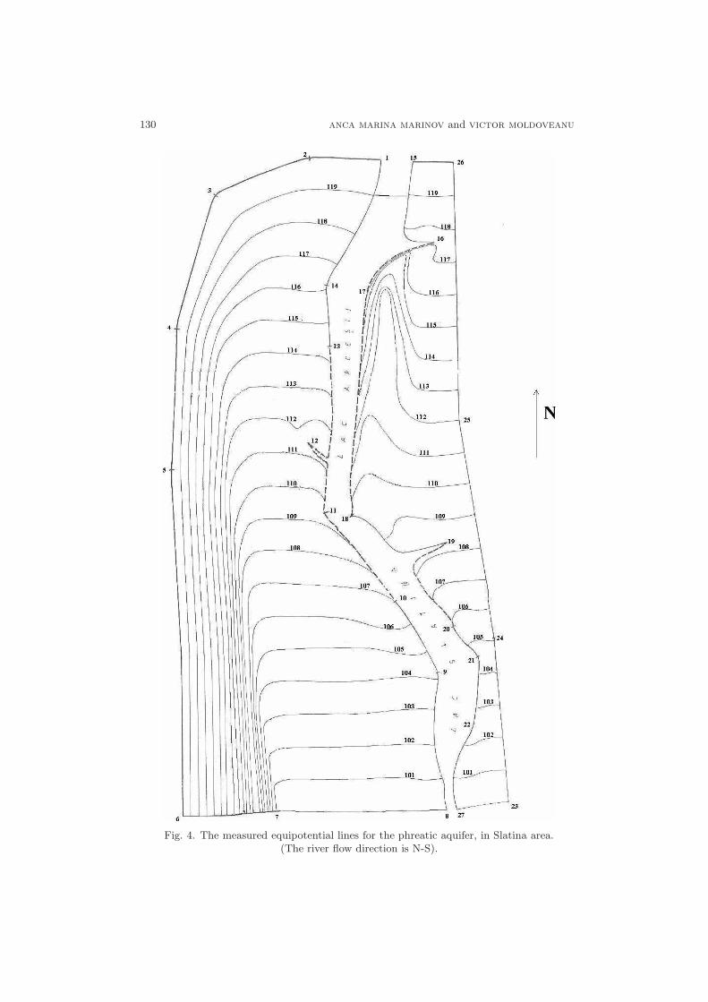
130 anca marina marinov and victor moldoveanu
Fig. 4. The measured equipotential lines for the phreatic aquifer, in Slatina area.(The river flow direction is N-S).

vulnerability to pollution of groundwater 131
= 300 m2/day, the effective porosity n = 0.2, the storage coefficient S = 0.009. Withthese data we have obtained the flow pattern presented in Fig. 4.
The flow pattern obtained by using the real pumped discharges (Fig. 4) looksvery similar to the real one (Fig. 2).
This pattern can be used to calculate the velocity at each point in the aquifer,the direction of the flow, as well as the discharge at the boundaries. The piezometriclevel varies within a minimum value of 97.67 m (in the Noua and Zavoi areas) and amaximum of 117.5 m (on the chosen boundaries). The vertical distance between thepiezometric lines is 1 m.
If we are to change the pumped values of discharges, the flow net will obviouslybe different. In order to obtain the real one we have to know the real pumpeddischarges. In the Northern part of the domain the flow has a N-S direction. In theEastern part, the flow direction is from the Eastern boundary towards the West (theleft hand of Olt well lines pump all the water coming from the East boundary). Onthe right-hand bank of Olt the flow direction is from the West boundary towards theEast.
The piezometric surface levels in the confined aquifer have smaller values thanthose of the free surface of the phreatic aquifer existing above it. A flow betweenthe two layers therefore continually tries to equalise the piezometric levels and thefree surface levels. That flow’s direction is from the phreatic to the confined aquifer,through the aquitard. The values of that discharge can be calculated analysing theflow pattern of the phreatic aquifer.
The phreatic aquifer is exposed to pollution, on account of its being at a smalldepth under the soil surface. Due to the above-explained connection between the twolayers the confined aquifer runs the risk of pollution. The Olt river (the lakes Arcestiand Slatina) has the free surface at higher levels than the phreatic aquifer’s. Hencea flow from the Olt river to the phreatic is very likely to occur. The concentration ofpollutants in the water of Olt thus determines the groundwater quality.
5. Analysis in the Unconfined Aquifer in Slatina Area
The analyzed area has: the length L = 21 000 m, the width l = 21 000 m, thethickness M = 10 m, the hydraulic conductivity K = 35 m/day, the transmisivityT = 350 m2/day, the effective porosity n = 0.2. With this data we have obtained theflow pattern presented in Fig. 5 (the right hand of the river Olt). Fig. 4 shows theequal level lines of water-table in the phreatic aquifer, measured in observation wells.
The phreatic aquifer is divided into two areas: one to the right of the Olt riverand the other to its left (Fig. 4). Each area is separately considered. The boundaryconditions take into account the impervious-less spaces in the dam walls (Q 6= 0), theimpervious ones (Q = 0), and the values of the hydraulic head (free surface levels)from the measured levels map (Fig. 4). For the phreatic aquifer the procedure isidentical to the one for the confined aquifer (only the diffusivity equation is different).
The phreatic aquifer is less pumped than the confined one. On the right handdomain there are only domestic wells which don’t modify the flow net of groundwater.

132 anca marina marinov and victor moldoveanu
Fig. 5. Equal head lines (the equal level of groundwater table) in the phreatic-(right side ofOlt) (hmax=120 m, hmin=100 m, dist=1 m), in the case without pumping wells.
To the left, in Curtisoara area, the water is pumped from an important well line. Thepumped discharges in this area influence the aspect of the flow net and determinethe groundwater pollution in case the Olt water is polluted. So, the best methodto understand the vulnerability to pollution in Curtisoara area is to calculate thedischarge values from the Olt to the groundwater, using the flow net obtained withthe above-presented code.
The level of phreatic free surface varies between 120 m (in the N) and 100 m(in the S). The phreatic is in direct connection with the lake so the lake’s level is aboundary condition for the aquifer.
For the right hand phreatic of Olt, using the boundary conditions from Fig. 3(imposed head conditions) in the numerical code, we have obtained the equipotentiallines (different from the measured ones). To obtain a flow net similar to the real onewe have inserted in the domain a number of fictious pumping wells. We have changedthe position and the discharges in the wells in order to obtain the same equipotentiallines as in the Fig. 3 (the right hand of Olt). We have thus obtained approximately,the discharges drained from the phreatic to the confined aquifer. This drainage isproduced by the decrease of the piezometric level in the confined aquifer during thepumping process from that aquifer.
In Fig. 6 the equipotential lines (equal level of water table) are plotted in thephreatic aquifer. In the Curtisoara wells we have considered pumping dischargesgreater than the real ones (the values in m3/day: 2 000, 2 000, 5 000, 5 000, 5 000,3 000, 1 500), to obtain the measured values of the water table (Fig. 4). The pumpeddischarge in Curtisoara wells is Q = 118l/s = 10195.2m3/day and the discharge usedin the model is Qp = 23 500 m3/day. The difference Qp−Q = 13304.8 m3/day is lostby drainage in the confined aquifer (depressurized by pumping).

vulnerability to pollution of groundwater 133
The velocity field in Curtisoara area shows the flow direction from the river Oltinto the well lines. So, the river quality influences the pumped water quality. We haveproved that a quantity of water is drained toward the confined aquifer. The qualityof that one is also influenced by the Olt water.
Fig. 6. Equal head lines (the equal level of groundwater table) in the phreatic-(left side ofOlt) (hmax = 120 m, hmin = 100 m, distance between head lines =1 m), in the case with
pumping wells.
Fig. 7. Equal head lines (the equal level of groundwater table) and the velocity field in thephreatic-(right side of Olt) (hmax = 120 m, hmin = 100 m, distance between head lines =1
m), in the case with pumping wells in Curtisoara area.

134 anca marina marinov and victor moldoveanu
6. Conclusions
The groundwater quality in Slatina area is influenced by the water quality ofriver Olt, especially in Curtisoara area. If the phreatic aquifer is affected by certainsurface pollution sources, then the confined aquifer will as a rule be affected as well.
A similar study could be carried out if we had a better hydrogeological descrip-tion of aquifers. The code also allows for the study of the anisotropic case and it isto be expected that the results will be closer to the real ones.
References
[1] Fried, J.J., Groundwater pollution, Elsevier S PC, New York, 1975,
[2] G.Marsily, Quantitative Hydrogeology, Academic Press Inc., 1986.
[3] Moldoveanu, V., Niculae, A., Rotar, C., Optimizarea exploatarii surselor de apasubterana potabila ale municipiului Slatina., Conferinta Zilele Hidraulicii, Ingine-ria Resurselor de Apa, UCB, 28-29 iunie 2001.

Proceedings of the Fourth Workshop onMathematical Modellingof Environmental and Life Sciences ProblemsConstanta, Romania, September, 2005, pp. 135–146
Analysis of a Preconditioned CG method for anInverse Bioelectric Field Problem
Marcus Mohr∗, Constantin Popa∗∗ and Ulrich Rude∗∗∗
This paper is a continuation of our previous analysis from [4] related to the electrocar-
diographic (ECG) inverse problem. In that paper we formulated the inverse ECG problem as
a differential inverse problem and derived an appropriate simulation procedure. As numeri-
cal solver we employed the Conjugate Gradient algorithm for the normal equations (CGNE)
together with a stopping test constructed following the discrepancy principle by Morozov.
In the current paper we consider a preconditioned version of the CGNE algorithm. The
preconditioner is constructed using the Cholesky factors of the discrete Laplacian which
forms a block of the original system matrix. We derive some theoretical results concerning
the efficiency and also the limitations of the preconditioner. Numerical experiments and
comparisons are presented for the cases analysed in [4].
1. Introduction
This paper is a continuation of our previous analysis from [4] related to theinverse problem of electrocardiography (ECG). We will therefore only briefly replaythe formulation of the problem and refer the reader to [4, 5] for further details. Inthe inverse ECG problem one attempts to determine from voltage measurements ona person’s torso the underlying electric behaviour of the heart, see e.g. [6]. Oneapproach is the so called cardiac imaging where one tries to re-construct from themeasurements the electric potential on the epicardium, the outer surface of the heart.
∗ Deparment for Sensor Technology, University of Erlangen–Nuremberg, Germany; forthis author the paper was partially supported by the DFG Junior Research Group Grant Ka1778/1
∗∗ “Ovidius” University of Constanta, Romania; for this author the paper was supportedby the PNCDI INFOSOC Grant 131/2004, e-mail: [email protected]
∗∗∗ IMMD 10- System Simulation Group, University of Erlangen–Nuremberg, Germany.

136 marcus mohr et al.
In [4] we formulated a simplified 2D version of this problem in the following form:find a function u : Ω→ R such that
∆u = 0, in Ω,
∂u
∂n= 0, on Γ \ Γ1,
u = d, on some Γ2 ( Γ.
(1)
Here Ω := (0, 1)× (0, 1), Γ is the boundary of Ω, Γ1 ∪ Γ2 ⊂ Γ with Γ2 ∩ Γ1 = ∅ andd is a given function on Γ2. In this paper we assume the configuration is as givenin Figure 1. Applying a standard discretisation of the differential parts of problem(1) by Finite Differences on a regular grid of mesh-width h = 1/n we arrive at anover-determined linear system
Ax = b , (2)
where A is an M ×N matrix of the form
A =
[∆h ES 0
](3)
with M = (n− 1)2 + (n− 1) and N = (n− 1)2 + (n− 3). The sub-matrices of A aregiven by
E =
0−1
. . .
−10
∈ R(n−1)2×(n−3) (4)
and
S =
1 0 · · · 01 0 · · · 0
. . ....
1 0 · · · 0
∈ R(n−1)×(n−1)2 . (5)
The matrix ∆h finally is simply the well-known 5-point discretisation of the 2D Lapla-cian (we assume here that both ∆h and E include a scaling by the factor h2). Theright-hand side of the system is given by
b = (0, · · · , 0, d1, · · · , dn−1)t,
where dk denotes evaluation of the prescribed function d at a given node of thediscrete grid, see also Figure 2. In this setup the problem (2) is consistent. In thereal application, however, the measurements d will contain noise and we will considerinstead, the least-squares formulation
‖ Ax− b ‖2= min! (6)

preconditioned CG method 137
ΩΓ2
Γ1
Fig. 1. Domain of the continousproblem.
rd
rd
rd
rd
r r r r
r r r r
r
r
e
e
d1
d2
dn−2
dn−1
Fig. 2. Pattern of discrete grid: • representNeumann, Neuman + Dirichet boundary
conditions and points on Γ1.
2. The preconditioned CG algorithm
In [4] we investigated the solution of the linear system (2) by means of the CGalgorithm applied to the normal equations AtAx = Atb. We employed the CGNEalgorithm in the following form (see [1])
d0 = b− Ax0 , p0 = Atd0
αi =‖ Atdi ‖22‖ Api ‖22
xi+1 = xi + αipi
di+1 = b−Axi+1 = di − αiApi
βi =‖ Atdi+1 ‖22‖ Atdi ‖22
pi+1 = Atdi+1 + βipi
for i = 0, 1, . . .
(7)
While the results obtained in [4] were satisfying with respect to the reconstruction ofthe “shape” of the exact solution, the high number of CGNE iterations was not. Thisaspect is directly related to the ill-conditioning of A from (3). In order to eliminatethe latter aspect we investigate here a special form of (right-)preconditioning of theproblem (2). Instead of the least-squares formulation (6) of (2) we consider theminimization problem
‖ Bz − b ‖2= min!, (8)
where
B = AP−1 and P−1z = x⇐⇒ Px = z, (9)

138 marcus mohr et al.
with a square and invertible matrix P . With this the preconditioned version of theCGNE algorithm (7) can be written as (see e.g. [1])
d0 = b−Bz0 = b−AP−1z0
p0 = Btd0 = P−t(Atd0)
αi =‖ Btdi ‖22‖ Bpi ‖22
=‖ Btdi ‖22‖ AP−1pi ‖22
zi+1 = zi + αipi
di+1 = di − αiBpi
βi =‖ Btdi+1 ‖22‖ Btdi ‖22
=‖ P−t(Atdi+1) ‖22‖ Btdi ‖22
pi+1 = Btdi+1 + βipi
for i = 0, 1, . . . , ifinal
(10)
and then putxifinal
= P−1zifinal. (11)
Remark 1. If we restrict ourselves to symmetric matrices P then we must solvetwo systems of the form Pv = w in each iteration step of algorithm (10). Anothersuch system must be solved once for computing the final approximate xifinal
.
It is well known, see e.g. [3], that the error reduction formula for the algorithm(7) is of the form
‖ xi − uLS ‖226C(x0)
λmin(AtA)
(λmax(A
tA)− λmin(AtA)
λmax(AtA) + λmin(AtA)
)2i
, (12)
where C(x0) > 0 is a constant depending on the initial approximation x0 and λmin(AtA),
λmax(AtA) are the minimal and maximal nonzero eigenvalues of AtA, respectively. Let
us denote in the following by Ik the identity matrix from Rk×k. Using this notationwe can write AtA for our matrix A from (3) as
AtA =
[∆2
h + I1 CCt I(n−3),
](13)
where I(n−3) = EtE, the square matrix I1 is given by
I1 = StS =
[I(n−1) 0
0 0
]∈ R(n−1)2×(n−1)2
and C is the (n− 1)2 × (n− 3) matrix defined as
C = ∆hE . (14)
A (classical) good preconditioning of the form (9) for A will be one which improvesthe condition number of the upper-left block ∆2
h + I1. Thus, if we denote by ∆2h this
matrix, i.e.∆2
h := ∆2h + I1 , (15)

preconditioned CG method 139
an “almost the best” choice for P in (9) will be
P =
[∆h 00 I(n−3)
]. (16)
In this case we have
B = A
[∆−1
h 00 I(n−3)
](17)
and
BtB =
I(n−1)2 ∆−1
h C
Ct∆−1h I(n−3)
. (18)
If we denote by T the matrixT = ∆−1
h C (19)
the following result holds.
Proposition 1. With the above definitions and notations we have the equiva-lence
λ ∈ σ(BtB) ⇐⇒λ = 1 or λ = 1 +
√µ or λ = 1−√µ > 0, µ ∈ σ(T tT ). (20)
Proof. A simple computation (for the case λ 6= 1) gives us the following sequenceof equivalences
λ ∈ σ(BtB)
⇐⇒ λ ∈ σ([I(n−1)2 TT t I(n−3)
])
⇐⇒ 0 = det
([I(n−1)2 TT t I(n−3)
]− λ
[I(n−1)2 0
0 I(n−3)
])
⇐⇒ 0 = det
([(1 − λ)I(n−1)2 T
T t (1− λ)I(n−3)
])
⇐⇒ 0 = det
([(1 − λ)I(n−1)2 0
T t (1− λ)I(n−3)
]·[I(n−1)2
11−λT
0 I(n−3) − 1(1−λ)2 T
tT
])
⇐⇒ 0 = det
(I(n−3) −
1
(1− λ)2 TtT
)
⇐⇒ 0 = det(T tT − (1− λ)2I(n−3)
)
⇐⇒ (1− λ)2 ∈ σ(T tT )
⇐⇒ 1− λ = ±√µ with µ ∈ σ(T tT )
this, together with that fact that σ(BtB) ⊂ (0,∞), proves (20).

140 marcus mohr et al.
Remark 2. From the definitions of C, ∆2h and T in (14), (15) and (19) we
obtain
T tT =Et∆h(∆2h + I1)
−1∆hE =
=Et[I(n−1)2 + ∆−1h I1∆h
−1]−1E = Et(I(n−1)2 + ∆1)−1E, (21)
where we denoted by ∆1 the symmetric non-negative definite matrix
∆1 = ∆−1h I1∆
−1h . (22)
Because of the special structure of E, see (4) we obtain from (18) that the matrixT tT is singular. Thus, for 0 = µ ∈ σ(T tT ) we get one more time λ = 1 in (20). Letnow µ 6= 0 be another eigenvalue of T tT corresponding to an eigenvector v 6= 0, i.e.
(T tT )v = µv. (23)
Because µ 6= 0 we havew := Ev 6= 0 . (24)
Thus
〈(T tT )v, v〉〈w,w〉 =
〈(I(n−1)2 + ∆1)−1w,w〉
〈w,w〉 =µ〈v, v〉〈EtEv, v〉 =
µ〈v, v〉〈In−3v, v〉
= µ
and
µ =〈(I(n−1)2 + ∆1)
−1w,w〉〈w,w〉 .
Since (I(n−1)2 + ∆1)−1 is a symmetric and positive definite matrix we obtain that
λmin[(I(n−1)2 + ∆1)−1] 6 µ 6 λmax[(I(n−1)2 + ∆1)
−1] (25)
or1
1 + λmax(∆1)6 µ 6
1
1 + λmin(∆1). (26)
Thus, if µ is “close” to the right bound in (26) i.e. (for a small ε > 0)
µ =1− ε
1 + λmin(∆1), (27)
then from (20) we can have
λ = 1−√µ = 1−√
1− ε√1 + λmin(∆1)
=
=λmin(∆1) + ε√
1 + λmin(∆1)(√
1 + λmin(∆1) +√
1− ε ). (28)
If ε is of order λmin(∆1) and if λmin(∆1) is small, which we expect from (21) forlarge values of n, then λ will be as small as λmin(∆1), i.e. no essential improvement

preconditioned CG method 141
Table 1
Spectral properties of the matrix A and the matrix B preconditioned as in (17)
n zmax(A) zmax(B) zmin(A) zmin(B) k(A) k(B)
8 7.63 1.41 1.87 ·10−05 1.3 ·10−05 ≈ 1005 ≈ 1005
16 7.81 1.41 5.21 ·10−12 3.7 ·10−12 ≈ 1012 ≈ 1012
24 7.96 1.41 9.00 ·10−17 3.9 ·10−17 ≈ 1017 ≈ 1017
32 7.97 1.41 1.40 ·10−19 2.8 ·10−18 ≈ 1020 ≈ 1018
(“compression”) of σ(AtA) will be obtained by the preconditioning (16)–(17). Someresults in this sense are presented in table 1. We denoted by zmax(A), zmax(B) andzmin(A), zmin(B) the largest and smallest singular value of A and B respectively. Thenumbers k(A), k(B) are defined by
k(x) =zmax(x)
zmin(x). (29)
Remark 3. Concerning the preconditioning (17) we want to point out the fol-lowing:
(i) It is not important that in (16) we used the identity matrix In−3. This choicewas made only to simplify the theoretical considerations that followed. Fordifferent choices we got results similar to those in Table 1.
(ii) Unfortunately, from a practical point of view, the computation of ∆−1h in (17)
can be very expensive. A “less costly” choice is
P =
[∆h 00 I(n−3)
]. (30)
In this case, at least up to some point, a theoretical analysis as in the aboveRemark 2 can be made, with similar conclusions with respect to σ(BtB). Werestrict ourselves here to present in Table 2 some numerical results regardingσ(BtB) for the choice (30).
Table 2
Spectral properties of the matrix A and the matrix B preconditioned as in (30)
n zmax(A) zmax(B) zmin(A) zmin(B) k(A) k(B)
8 7.63 13.37 1.87 ·10−05 1.30 ·10−05 ≈ 1005 ≈ 1005
16 7.81 36.15 5.21 ·10−12 3.00 ·10−12 ≈ 1012 ≈ 1013
24 7.96 66.50 9.00 ·10−17 2.00 ·10−17 ≈ 1017 ≈ 1018
32 7.97 102.69 1.40 ·10−19 3.46 ·10−19 ≈ 1020 ≈ 1021

142 marcus mohr et al.
Table 3
CG versus preconditioned CG using stopping test (31)
prescribed shape shape approx. by CG shape approx. by PCG
-505
101520253035
0 5 10 15 20 25-505
101520253035
0 5 10 15 20 25-505
101520253035
0 5 10 15 20 25
nits = 1574 nits = 52
-505
101520253035
0 5 10 15 20 25-505
101520253035
0 5 10 15 20 25-505
101520253035
0 5 10 15 20 25
nits = 3041 nits = 119
-505
101520253035
0 5 10 15 20 25-505
101520253035
0 5 10 15 20 25-505
101520253035
0 5 10 15 20 25
nits = 3035 nits = 118
-505
101520253035
0 5 10 15 20 25-505
101520253035
0 5 10 15 20 25-505
101520253035
0 5 10 15 20 25
nits = 1569 nits = 52
-505
101520253035
0 5 10 15 20 25-505
101520253035
0 5 10 15 20 25-505
101520253035
0 5 10 15 20 25
nits = 1637 nits = 53

preconditioned CG method 143
Table 4
CG versus preconditioned CG using stopping test (32)
prescribed shape shape approx. by CG shape approx. by PCG
-505
101520253035
0 5 10 15 20 25-505
101520253035
0 5 10 15 20 25-505
101520253035
0 5 10 15 20 25
nits = 1637 nits = 60
-505
101520253035
0 5 10 15 20 25-505
101520253035
0 5 10 15 20 25-505
101520253035
0 5 10 15 20 25
nits = 3045 nits = 119
-505
101520253035
0 5 10 15 20 25-505
101520253035
0 5 10 15 20 25-505
101520253035
0 5 10 15 20 25
nits = 3038 nits = 118
-505
101520253035
0 5 10 15 20 25-505
101520253035
0 5 10 15 20 25-505
101520253035
0 5 10 15 20 25
nits = 1566 nits = 52
-505
101520253035
0 5 10 15 20 25-505
101520253035
0 5 10 15 20 25-505
101520253035
0 5 10 15 20 25
nits = 1644 nits = 64

144 marcus mohr et al.
Remark 4. There is also a “good” aspect concerning the above precondition-ings with respect to our problem (6). Indeed, after the transformation (17) with Pfrom (16) or (30), a “large” part of the eigenvalues of BtB will be 1. Typically onlyup to 2n eigenvalues will be different from 1 and of those only up to (n − 3) willhave values in the interval (0, 1), see Propositon 1 in this respect. Thus, followingthe theoretical considerations from [2], the “filter factors” associated with the eigen-values of BtB greater or equal to 1 will become very small in only “few” iterationsof the preconditioned CG algorithm. Thus, we will obtain an approximation of xLS,i.e. the minimal norm solution of (6), in significantly fewer iterations than with thenon-preconditioned algorithm and this approximation will have the same quality ofreconstruction.
We can see this improvement in the following tests. We use the verificationprocedure detailed in [4, 5], i.e. we prescribe Dirichlet values along the boundary Γ1
and solve the forward problem associated with (1) to obtain “measurement” valuesd. In order to simulate noise we add a random vector xp ∈ R(n−1) to d,
dpi = di + εxp
i , i = 1, . . . , n− 1 .
We then solve (6) with b derived from dp using CG and CG preconditioned withP according to (30). For the experiments we use ε = 0.01 and test both stoppingrules from [4]. The results for the first stopping rule are given in Table 3. Here weterminated the iterations once
‖ r(k) ‖2 +N · ‖ r(k) ‖2 ·sstop 6 neps, (31)
where r(k) is the residual of the current approximation, neps = ε ‖ xp ‖2≈ 0.03 and
sstop =‖ cu(k) − cuex ‖∞ .
Here cuex denotes the values of the least-squares solution of the inverse problemfor the unperturbed data d along Γ1, while cu(k) denotes the values of the currentapproximate solution on Γ1. Since cuex is not available in practice we devised asecond stopping test that is only based on computable values, namely
‖ r(k) ‖2 +N · ‖ r(k) ‖2 · ‖ cu(k) ‖∞6 neps . (32)
The results for this second rule are given in Table 4. Both experiments demonstratethat the preconditioning yields a significant reduction in the number of iterations(nits), while retaining the quality of the reconstructed shape.
References
[1] Golub, G.H. and Van Loan, C.F., Matrix computations, The John’s HopkinsUniv. Press, Baltimore, 1983.

preconditioned CG method 145
[2] Hanke, M. and Hansen, P.C., Regularization methods for large-scale problems,Surv. Math. Ind. 3 (1993), 253–315.
[3] Kammerer, W.J. and Nashed, M.K., On the convergence of the conjugate gradi-ent method for singular linear operator equations, SIAM J. Numer. Anal., 9(1)(1972), 165–181.
[4] Mohr, M., Popa, C. and Rude, U., A Differential Inverse Problem from CardiacImaging, in Proceedings of the Third Workshop on Mathematical Modelling ofEnvironmental and Life Sciences Problems, Constanta, Romania, 27-30 May2004; Editura Academiei Romane, Bucuresti 2004, 189–204.
[5] Mohr, M., Popa, C. and Rude, U., An experimental analysis of a differential in-verse problem, Technical Report 99-1 (1999), Lehrstuhl fur Informatik 10 (Sys-temsimulation), Friedrich-Alexander-Universitat Erlangen-Nurnberg.
[6] MacLeod, R. and Brooks, D., Recent Progress in Inverse Problems in Electrocar-diology, IEEE Engineering in Medicine and Biology, 17(1) (1998), 73–83.


Proceedings of the Fourth Workshop onMathematical Modellingof Environmental and Life Sciences ProblemsConstanta, Romania, September, 2005, pp. 147–160
Dosimetric Estimates in Biological Tissue Exposedto Microwave Radiation in the Near Field of an
Antenna
Mihaela Morega∗, Alina Machedon∗ and Marius Neagu∗
Human exposure to electromagnetic field (including the microwave radiation range) is
limited by international safety guidelines, based on health considerations. Thermal health
effects are commonly considered for the radiofrequency range; in particular, for microwave
exposure, the absorbed energy that produces heat is quantified by the specific energy ab-
sorption rate, as dosimetric reference. Induced electric and magnetic field strengths are
also restricted by the exposure guidelines. We report here a numerical study of the elec-
tromagnetic field induced in several biological models by a common microwave applicator.
The sensitivity of dosimetric parameters and the compliance with exposure guidelines are
evaluated. We have examined the influence of dielectric properties dispersion on dosimetric
quantities, useful in the design and validation of experimental settings and numerical models.
1. Introduction
A wide debate developed over the last two decades, both in scientific and socialforums, on the possible health effects of human exposure to non-ionizing electromag-netic fields continues to concentrate attention without concluding results. Researchactivity was therefore developed by the international scientific community aimed atevaluating the risk associated with exposure to this type of radiation. At the sametime, various international authorities began to issue recommendations on exposurelimits valid for workers and for the population in the frequency range 0 Hz÷300 GHz.The limits specified by the guidelines are settled both at workplaces and in the liv-ing environment. The specified accepted limits are intended to be used as a basisfor planning work procedures, and designing protective facilities, as much as in the
∗ “Politehnica” University of Bucharest, Romania.

148 mihaela morega et al.
assessment of the efficacy of protective measures and practices, or in the guidance onhealth surveillance.
The most known and accepted are the guidelines developed by the InternationalCommission on Non-Ionizing Radiation Protection (ICNIRP) [1]. Other internation-ally recognized documents, such as those developed by the Institute of Electricaland Electronics Engineers (IEEE) and American National Standardization Institute(ANSI) [2] in the USA, by the Australian Radiation Protection and Nuclear SafetyAgency (ARPANSA) [3], or by the National Radiological Protection Board (NRPB)in the UK adopt the same basic approach of ICNIRP, although some differences existin numerical values, and they will be discussed in this paper. In 1999 the Council ofthe European Union has issued a Recommendation to Member States [4] to adopt acommon frame of norms on exposure of the general public to electromagnetic fieldsthat made precisely the indications supplied by ICNIRP for the protection of the pop-ulation. Presently, about 30 countries have adopted ICNIRP guidelines as nationalregulations.
The market of wireless devices is presently highly dynamic and competitive.Producers have to find new and commercial solutions, as an optimum of cost, perfor-mance, modern design, miniaturization and multifunctionality. The compliance withthe safety guidelines is also a restriction, and the manufacturer is required to includethe SAR limit in the technical specification of each product. This value is then com-pared by the consumer safety authorities with the limits stated by standards. Alsothat seems to be a simple and non-controversial process, our study investigates the socalled “technical accuracy” of safety and performance parameters assessment, basedon valid standards.
2. Basic restrictions and reference levels presently statedby standards
The ICNIRP guidelines [1], as well as the other international standards [3–5], are based on a two-level structure. Basic restrictions are defined in terms of“dosimetric quantities” that are directly related to biological effects; these quantitiesare: the current density (J) for low-frequency electric and magnetic fields, and thespecific energy absorption rate (SAR) and the power density (PD) for high-frequencyelectromagnetic fields (including microwaves). The limits are defined for exposureof all, or only a part, of the human body. For practical reasons, reference levelsare derived from basic restrictions, through appropriate dosimetric models (simplifiedcomputational and experimental models). Reference levels are expressed in termsof physical quantities (electric field strength, magnetic field strength, and equivalentplane wave power density) that can be directly measured outside the exposed bodyand inside experimental phantoms.
Given the conservative hypotheses assumed in dosimetric models, exposures tofields that are below the reference levels necessarily comply with basic restrictions,but the vice-versa is not true. Even when the reference levels are exceeded, the

dosimetric estimates in biological tissue 149
standard may be complied with, provided it can be proved that basic restrictions arenot exceeded under the specific exposure conditions.
We are interested here by the high-frequency electromagnetic field, the mi-crowave range with applications in wireless communications technologies, 0.5–3 GHz.The basic restriction for localized exposure (head and trunk) in this frequency rangeis the specific energy absorption rate (SAR) which is set in terms of maximum mass-normalized quantity, as follows:
• 2 W/kg for “any 10 g of contiguous tissue” in the ICNIRP guidelines [1] andthe European recommendation [4], while “any 10 g of contiguous tissue in the shapeof a cube” in the Australian standard [3];
• 1.6 W/kg for “1 g of tissue in the shape of a cube” in the ANSI/IEEE stan-dard [2].
Basic references [1], [2] and [4] are issued in the same period of time, 1998-1999,are based on the research and documentation literature available at the time andare still valid. At the first glance the specifications do not seem to be contradictory;however, we found some important differences in their practical use, that we attemptto emphasize on a case study presented further.
3. Physical properties of the model and general assump-tions
The work presented here examines the electromagnetic field penetration in hu-man tissue considering several conditions and particularities related to wireless com-munications in the microwave frequency range [7–9]:
(1) An antenna is the electromagnetic radiation source in our study. The electro-magnetic field produced by an antenna can be described as having several components;only one of these actually propagates through space, and this component is called theradiated field or the far field. The strength of the radiated field does decrease withdistance, since the energy must spread as it travels. The other components of theelectromagnetic field remain near the antenna and do not propagate. There are gener-ally two other components: the static field and the induction field, and their strengthdecreases very rapidly with distance. The entire field (all of the components) nearthe antenna is called the near field. In this region, approximately one wavelengthin extent, the electric field strength can be relatively high and pose a hazard to thehuman body. The dipole configuration is the most common and conventional typefor near field human exposure related to wireless personal communication systems inthe GSM frequency range (0.5 to 3 GHz); the harmonic waveform is considered in ourstudy. In numerical and experimental models, the length of the antenna is usuallyadjusted at the half wavelength, both because of modeling reasons (like symmetryconditions) and to maximize the efficiency of the emission.
(2) The exposed body is represented by a layered biological structure, with anidealized shape, inspired by the human anatomy (head or trunk); the electromagneticfield penetration depth in dispersive dielectrics, like animal tissue, depends on the ex-

150 mihaela morega et al.
ternal shape of the body, on the electric conductivities and dimensions of tissue layers;the skin and fat peripheral layers present screening effect for the electric componentof the incident field.
(3) Biological tissues are nonmagnetic and dispersive dielectric materials; for thepurpose of this study, they are considered linear, isotropic and homogeneous materials;dielectric properties are expressed in the form of the complex permittivity ε = ε−iσ/ω,or the complex conductivity σ = σ + iωε, where ε is the dielectric permittivity, σ isthe electric conductivity and ω = 2πf is the angular frequency of the electromagneticfield. The specific values for σ and εg considered in our study correspond to data inliterature [6]. For illustration, Fig. 1 shows the frequency dependence of the electricconductivity gσ and relative dielectric permittivity εsg or several anatomical tissuesinvolved in the human body exposure to electromagnetic field (skin, fat, bone, dura,cerebro-spinal-fluid, brain and muscle); the microwave frequency range used by theGSM communication system is considered.
Fig. 1. Frequency dependence of the conductivity and the permittivity of several tissues, inthe GSM frequency range.
Our research is focused on the study of two idealized anatomic structures:– model A 6 – a human (adult) head with external ellipsoidal shape, composed
by six tissue layers (skin, fat, bone, dura, csf and brain) [8, 9], and– model B 4 – a planar layered structure representing the human trunk, com-
posed by four tissue layers (skin, fat, muscle and bone).(4) The electromagnetic coupling between the antenna and the exposed body
is quantified by the so called power transfer factor, defined as the ratio betweenthe emitted and the absorbed time averaged active powers; this factor depends on:the antenna type, the shape and structure of the body and the distance betweenthe antenna and the body. We adopted for this study a constant emitted power of1 W, regardless the type of the antenna, and for a more realistic evaluation we haveexpressed the dosimetric quantities in rated (scaled) values, as it is seen in the resultssection.
(5) Our purpose is to determine some quantitative and qualitative informationon dosimetric parameters inside the body exposed to electromagnetic radiation and torelate them to prescriptions stated in human exposure guidelines and standards. Also

dosimetric estimates in biological tissue 151
the configuration of the human body in the vicinity of the antenna does not presentany obvious and accurate symmetry, we speculate a reduction of the 3D problem,to a 2D idealized model, based on axial symmetry around the antenna longitudinalaxis [8, 9]. This approximation proves to be satisfactory for global estimates, likespecific energy absorption rate, or power deposition in a tissue layer, both ratedto the total power absorbed by the body, or to the power emitted by the antenna.The approximation is also favored by the fact that the penetration depth of theelectromagnetic radiation in biological tissue at microwave frequencies is small (<30 mm) and the electromagnetic phenomena are superficial. In order to compare thequantitative results obtained with the simplified 2D models with the more realisticones obtained with 3D models one have to take into account the power transfer factor(defined above), whose value is one for the 2D models (due to the axial symmetry)and smaller than one for the realistic 3D models (generally dependent of the distancebetween the antenna and the body).
4. Electromagnetic problem formulation
The numerical computation used for the 2D FEM model is based on the FEM-LAB software [10], the Electromagnetics Module, in the axisymmetric transversal mag-netic (TM) waves application mode, time-harmonic submode. The wave equationsare applied for dispersive media, characterized by the complex electric permittivity ε
∇×(
1
µ0∇×E
)− ω2εE = 0, ∇×
(1
ε∇×H
)− ω2µ0H = 0, (1)
where the unknown field variables, in the cylindrical coordinate system and in complexform are the electric and the magnetic field strengths:
H (r, z, t) = Hϕ (r, z) eϕeiωt, E (r, z, t) = (Er (r, z) er + Ez (r, z) ez) eiωt (2)
The computational domain (Fig. 2) is limited with low-reflecting boundary con-ditions
n×(ε
µ0
)1/2
E−Hϕ = −2Hϕ0,whereHϕ0 = 0, (3)
and the boundary on the (Oz ) axis satisfies axial symmetry conditions
Er = 0,∂Ez
∂r= 0,
∂Hϕ
∂r= 0. (4)
The radiation source is introduced through a nonhomogeneous magnetic fieldboundary condition, simulating the antenna. The magnetic field condition is adjustedfor each model, so that the emitted power is constant (1 W) in all studied cases. TheFEMLAB linear stationary solver is based on Gaussian elimination. The FEM mesh iscomposed of triangular elements (Delaunay mesh with Lagrange quadratic elements),

152 mihaela morega et al.
Fig. 2. The general structure of the computational domain basedon axial symmetry.
and two accuracy tests were performed to settle its parameters: the constant radiatedpower and an energetic balance (the radiated power compared with the sum of thepower absorbed in the body and the power radiated in the antenna far field). Theoptimal mesh in our examples is settled to approx. 150 000 elements.
5. Equivalent dielectric properties
The anatomical structures presented above are further reduced to more sim-plified models, having the same external shape and dimensions and an inner homo-geneous structure. The electric properties of the reduced model (σequiv respectivelyεequiv) are computed with the 2D FEM model described earlier, by energy basedequivalence, considering that the total absorbed power and total electric energy havethe same values in the heterogeneous (composed by i different subdomaines) andequivalent homogeneous models [9]:
∫
i
σi (Ei)2dv = σequiv
∫
i
(Ei)2dv, (5)
∫
i
1
2εi (Ei)
2 dv =1
2εequiv
∫
i
(Ei)2 dv. (6)
The method presented above is applied to compute the equivalent dielectricproperties of the following reduced models, derived from model A 6 and modelB 4 presented above:

dosimetric estimates in biological tissue 153
Fig. 3. Frequency dependence of the equivalent dielectric properties (conductivityand relative permittivity), in the GSM frequency range.
– model A 2 – reduced heterogeneous head model with two subdomaines : equiv-alent skull (skin+fat+bone) and equivalent brain (dura+csf+brain);
– model A 1 – reduced homogeneous head model : equivalent head tissue;– model B 2 – reduced heterogeneous trunk model : skin (same properties and
thickness as in model B) and equivalent body tissue (fat+muscle+bone).– model B 1 – reduced homogeneous trunk model : equivalent body tissue.Fig. 3 presents the frequency dependence of the mentioned equivalent dielectric
properties computed in the GSM frequency range.The equivalent properties are useful in the design of experimental mannequins.
Tissue equivalent “phantoms” are used instead of real bodies in the experimentaldosimetry [7]. Miniature isotropic E-field sensors are commonly used as implantableprobes. The sensor is immersed into tissue equivalent liquid, and the internal electricfield in the phantom is measured; the SAR is then calculated from internal E-field.A typical phantom designed for the certification of communication equipment is de-scribed in [7] (i.e., the Specific Anthropomorphic Mannequin – SAM) and it consistsof a 2 mm polyurethane shell (σshell = 0.0012 S/m respectively εshell = 5), filled withsimulant tissue solution (σsimulant = 0.7 S/m, εsimulant = 48, at 0.835 GHz andσsimulant = 1.7 S/m, εsimulant = 41 at 1.9 GHz). As one could see, the mentionedvalues of the simulant tissue solution are comparable to the equivalent brain inFig. 3.
6. Electric field strength and penetration depth in the ex-posed body
We computed the E-field strength (rms-values) distribution inside the two ana-tomical structures exposed in the near field of the antenna at different frequencies;the antenna is placed at 0.01 m distance from the body surface. In the case of thehead (models of type A) the antenna is a center fed, half wavelength dipole and inthe case of the trunk (models of type B) the antenna is a lower end fed, quarter

154 mihaela morega et al.
a) at 0.9 GHz b) at 1.8 GHz
c) at 2.5 GHz
Fig. 4. E distribution (rms values) versus distance r, measured from thesurface of the skin – head models.
wavelength monopole. The antenna emitted power is set at 1 W in all cases in orderto express the E-field as rated (per power) values, giving the possibility to betteranalyze them and to scale them for any other value of the emitted power. Electricfield penetration in the exposed head (the models of type A) is presented in Fig. 4, atthe main frequencies in the MW considered range (0.9 GHz, 1.8 GHz and 2.5 GHz).The presented distributions of the electric field strength are computed on the axes ofmaximal values.
In a 3D numerical model, the degree of heterogeneity is significant for the com-plexity of the model and computational resources; thin layers (like skin, fat, dura andcsf) should be covered with a very dense FEM mesh. Consequently, any possibilityto simplify the structure is appreciated. The results presented in Fig. 4 support thegood agreement among equivalent models. This is a good reason to use the values

dosimetric estimates in biological tissue 155
determined for equivalent dielectric properties in the design of 3D FEM models or inexperimental phantoms for the human body.
The reduced heterogeneous structures (models A 2 and B 2) prove to achievethe most desirable compromise between the accuracy of anatomical representation andthe economy of computational resources. The E-field penetration depth was estimatedin the GSM frequency range for the presented models. Figures 5 and 6 show that thefrequency dependence of the penetration depth for the heterogeneous models (A 6and A 2, respectively B 4 and B 2) is very similar, while the same function for thehomogeneous model (A 1, respectively B 1) has a noticeable different distribution.
Fig. 5. Frequency dependence of the pene-tration depth, for type A (head) models.
Fig. 6. Frequency dependence of the pene-tration depth, for type B (trunk) models.
In the heterogeneous models, the presence of the superficial layers (skin fat andbone) has a screening effect for the electric field. The skin has a relatively highpermittivity and concentrates the electric field and the absorbed power at the surfaceof the body; one could see in figure 4 the high initial E values. The fat and thebone, with their lower permittivities act like a barrier for E-field penetration. Theseobservations support the lower level of the penetration depth for heterogeneous modelsand the almost constant value regardless the frequency.
7. SAR evaluation
We mentioned in Section 2 that the main dosimetric quantity in microwaveexposure of living bodies is the specific energy absorption rate (SAR), consideredas the basic restriction by the most referred standards. It is defined as the absorbedpower per unit mass at infinitesimal volume of tissue (SAR = σE2/ρ [W/kg]sg, whereE is the rms value of the electric field strength, σ is the electric conductivity andρ is the mass density of the tissue). SAR distribution depends on several factors:the incident field parameters (near or far field), geometric parameters (shape andstructure) of the exposed body, physical properties of the tissues (as lossy dielectrics),ground/screen/reflector effects of other objects in the field near the body.

156 mihaela morega et al.
a) at 0.9 GHz.
b) at 1.8 GHz.
c) at 2.5 GHz.
Fig. 7. SAR estimates for the type A(head) models (at 1 W emitted power).
a) at 0.9 GHz.
b) at 1.8 GHz.
c) at 2.5 GHz.
Fig. 8. SAR estimates for the type B(trunk) models (at 1W emitted power).
In this section we discuss the significance of the mass-normalized SAR over1 g versus 10 g of tissue, which represents, for an average biological tissue with themass density of 1 kg/m3, a volume associated to a cube with the edge of 0.01 m,respectively 0.022 m. The standards suggest that the cube volume should include themaximal local SAR values in the exposed area. Because the SAR, like the E-field inthe exposed region is maximal at the surface of the body, the volume is selected withone face on the body surface (in practical cases the curvature could be neglected).Figures 7 and 8 display, for three significant frequencies and for the models presentedin this case study, the following SAR quantities: the local maximal SAR (SARmax)and the averaged SAR values for 1 g and 10 g of tissue (SAR1 g, SAR10 g). Theemitted radiation power is 1 W in all studied cases and the exposed body is placedat the same distance (0.01 m) of the antenna.
One could observe several characteristics:SARmax is highly dependent on the model heterogeneity; the layered models

dosimetric estimates in biological tissue 157
a) at 0.9 GHz.
b) at 1.8 GHz.
c) at 2.5 GHz.
Fig. 9. Antenna emitted power to produceSAR 1 g and SAR 10 g admitted values in
the type A (head) models.
a) at 0.9 GHz
b) at 1.8 GHz
c) at 2.5 GHz
Fig. 10. Antenna emitted power to produceSAR 1 g and SAR 10 g admitted values in
the type B (trunk) models.
A 6 and B 4 concentrate a large amount of the total absorbed power at the surfaceof the body because the skin (the peripheral layer which is very thin) has a higherdielectric permittivity than fat and bone; however, in all models, SAR distribution ishighly focused in the area proximal to the antenna, and decreases rapidly inside thebody (as the penetration depth and electric field distribution show).
On the contrary, the averaged values, both for 1 g and 10 g of tissue, are similarfor all the compared models; they are insignificantly affected by the heterogeneity.This is because the volume of integration is not negligible in size and its characteristicdimension is larger than the thickness of the tissue layers.
For the same exposure conditions, SAR10 g is considerably smaller than SAR1 gbecause SAR distribution is highly nonuniform and decreases rapidly with the distancefrom the peak. Following the restrictions stated by the exposure standards, one couldsee the opposite relation: the limit imposed by ICNIRP for 10 g (2 W/kg) is morepermissive (higher) than the limit imposed by IEEE/ANSI for 1 g (1.6 W/kg).

158 mihaela morega et al.
A more confusing situation appears when we try to solve the “inverse problem”,that is to estimate the admissible power of the radiation source, that produces theSAR1g, respectively the SAR10 g permitted by the standards. Figures 9 and 10present the values of the emitted power able to produce SAR1g = 1.6 W/kg andSAR10 g = 2 W/kg, for each of the models considered in our case study.
The three compared models give similar values for the maximal admitted an-tenna power, because the heterogeneity of the model significantly affects local SARvalues, but seems to be less important for spatial averaged values, especially at higherfrequencies (the depth of penetration decreases with the frequency rise). However,the controversy between the two referred standards is evident and confirmed in allconsidered examples: the limit values derived from the ICNIRP guidelines [1] aretwice more permissive than the ANSI/IEEE standard [2].
8. Conclusions
The construction of the simplified 2D models used in this study arises fromthe necessity to evaluate dosimetric parameters in layered structures like anatomicaltissues when exposed to microwave radiation in wireless communications. Comparedwith more sophisticated models, the 2D models demonstrate advantages in economyof resources, accessibility and rapidity, while the results are sufficiently accurate forglobal estimates and for comparison with experimental SAR and E distributions frommeasurements on phantom human models. The method of equivalence between theheterogeneous anatomical structures and the homogeneous equivalent domains couldbe applied in different configurations. The results are useful for the optimal design of3D models. This work presents the electric field distribution inside models represen-tative for parts of the human body (head and trunk) in different exposure conditions.The penetration depth and the specific energy absorption rate are also computed.A critical study for the evaluation of SAR shows some controversies produced byimportant differences between the most known and referred human exposure interna-tional standards; this situation is quite confusing for manufacturers and for end-usersof wireless devices. The normalization method for SAR limit evaluation should bereconsidered and made more appropriate to the structure of the exposed body; weconsider that the characteristic dimension of the integration volume should be madesmaller for a more accurate estimate both in numerical and experimental models.Besides, the averaged value on a volume in the shape of a cube, over tissues withdifferent physical properties seems to have a poor physical significance. A more lo-calized SAR evaluation could be important both for the assessment of thermal andnon-thermal biological effects.
It is the role of international standardization authorities, International Electri-cal Commission (IEC), European Committee for Standardization in Electrotechnic(CENELEC), The Institute of Electrical and Electronic Engineers (IEEE) to synthe-size reliable research and to edit technical standards for the design, manufacture andconditions of use of the electric and electronic equipment.
Acknowledgment. The work presented is part of the grant CNCSIS 357/2005.

dosimetric estimates in biological tissue 159
References
[1] International Commission on Non-Ionizing Radiation Protection (ICNIRP),Guidelines for Limiting Exposure to Time-varying Electric, Magnetic and Elec-tromagnetic Fields (up to 300 GHz), Health Phys., 74 (1998), No. 4, pp. 494–522.
[2] ANSI/IEEE, Safety Levels with respect to Human Exposure to Radio FrequencyElectromagnetic Fields, 3 kHz to 300 GHz, IEEE Standard C95.1-1999.
[3] Australian Radiation Protection and Nuclear Safety Agency (ARPANSA), Max-imum Exposure Levels to Radiofrequency Fields – 3 kHz to 300 GHz, RadiationProtection Series Publication, no. 3, 2002.
[4] Council of the European Union, Council Recommendation of 12 July 1999 onthe Limitation of Exposure of the General Public to Electromagnetic Fields (0Hz to 300 GHz), Official Journal of the European Communities L199/519/EC,59-70 (1999).
[5] CENELEC, Limitation of Human Exposure to Electromagnetic Fields from De-vices Operating in the Frequency Range 0 Hz to 10 GHz, used in Electronic ArticleSurveillance (EAS), Radio Frequency Identification (RFID) and Similar Applica-tions, EN 50364:2002 http://europa.eu.int/comm/health/ph determinants/
environment/EMF/emf en.htm
[6] Gabriel C., Gabriel S., Dielectric Properties of Body Tissues at RF and Mi-crowave Frequencies, Report for Armstrong Laboratory (AFMC), Occupationaland Environmental Health Directorate - Radiofrequency Radiation Division,USA, 2002.
[7] CTIA – Certification Program Test Plan for Mobile Station Over the Air Perfor-mance Cellular Telecommunications & Internet Association Method of Measure-ment for Radiated RF Power and Receiver Performance, Revision 2.0, March2003
[8] Morega Mihaela, Machedon Alina, Numerical Models of Biological Tissues forApplications in Microwave Dosimetry, in Proceedings Third International Work-shop on Mathematical Modelling of Environmental and Life Sciences Problems,Constanta, 2004, Editura Academiei Romane, pp.254–263.
[9] Morega Mihaela, Machedon Alina, EMF Penetration in Biological Tissue whenExposed in the Near Field of a Mobile Phone Antenna, 4th International Sym-posium on Advanced Topics in Electrical Engineering, ATEE-2004, Bucharest,CD-ROM, ISBN 973-7728-31-9.
[10] FEMLAB 3.1, User’s Guide and Electromagnetics Module, COMSOL AB, 2004.


Proceedings of the Fourth Workshop onMathematical Modellingof Environmental and Life Sciences ProblemsConstanta, Romania, September, 2005, pp. 161–170
Lower bounds on the weak solution of amoving-boundary problem describing the
carbonation penetration in concrete
Adrian Muntean∗ and Michael Bohm
In this note, we discuss a 1D partly dissipative moving sharp-interface reaction-diffusion
system modeling concrete carbonation. We point out a way to obtain non-trivial lower
bounds on the concentrations of the chemically active species. A FEM approximation of the
solution illustrates numerically the behavior of the concentration profiles and interface posi-
tion. The lower bounds of Ca(OH)2(aq) concentration obtained numerically are compared
with the theoretical lower bounds.
1. Introduction
This research is motivated by the macroscopic modeling of the concrete carbon-ation process by moving the interface where the carbonation reaction
CO2(g→ aq) + Ca(OH)2(s→ aq)H2O−→ CaCO3(aq→ s) + H2O (1)
is localized. The interface, which we denote by Γ(t), advances from the outsideboundary inwards the material. It separates the region Ω1(t), in which all availableCa(OH)2(aq) has been depleted, from the yet unreacted part Ω2(t). In front of the ad-vancing interface the concentration of freely diffusing CO2 molecules is zero. Figure 1illustrates the situation. The understanding of the process and the ability to calculate,and therefore, to predict the penetration of aggressive carbon dioxide from air inwardthrough the unsaturated porous concrete matrix towards the steel reinforcement is
∗ Centre for Industrial Mathematics, Faculty of Mathematics, University of Bremen,Postfach 330440, 28334 Bremen, Germany, e-mail:muntean, [email protected]
This work was completed with the partial support of DFG SPP1122 Prediction of the
Course of Physicochemical Damage Processes Involving Mineral Materials.

162 adrian muntean and michael bohm
essential to forecast the penetration of a complex spectrum of really corrosive specieslike chlorides or sulfates. We present in Section 2 a coupled PDE-ODE model for thesimultaneous determination of concentration profiles of the active species and of theposition of the carbonation interface. Section 3 contains the weak formulation of theproblem and the main results. In Section 4, we point out a way to obtain non-triviallower bounds for Ca(OH)2(aq) concentration. We use a FEM approximation of thesolution to illustrate numerically the behavior of the concentration profiles and inter-face position. Finally, we compare the numerical lower bounds of Ca(OH)2(aq) withthe theoretical estimates. We report on these aspects in Section 5.
2. The Sharp-Interface Carbonation Model PΓ
The evolution of the interface between carbonated and uncarbonated parts inconcrete materials can be modeled (cf. [1, 5, 7]) by the following 1D moving-boundaryproblem: Determine the concentrations1 ui(x, t), i ∈ I and the interface position s(t)which satisfy for all t ∈ ST the equations:
(φφwui),t + (−Diνi2φφwui,x)x = +fi,Henry, x ∈ Ω1(t), i ∈ 1, 2,(φφwu3),t + (−D3φφwu3,x)x = +fDiss, x ∈ Ω2(t),
(φφwu4),t = +fPrec + fReacΓ, x ∈ Γ(t),
(φu5),t + (−D5φu5,x)x = +fReacΓ, x ∈ Ω1(t),
(φu6),t + (−D6φu6,x)x = 0, x ∈ Ω2(t).
(2)
The initial and boundary conditions are φφwνi2ui(x, 0) = ui0, i ∈ I, x ∈ Ω(0),φφwνi2ui(0, t) = λi, i ∈ I1, ui,x(L, t) = 0, i ∈ I2, x ∈ Ω2(t), where t ∈ ST . Specificto our problem, we impose the following interface conditions
[j1 · n]Γ(t) = −ηΓ(s(t), t) + s′(t)[φφwu1]Γ(t),
[ji · n]Γ(t) = s′(t)[φφwνi2ui]Γ(t), i ∈ 2, 5, 6,[j3 · n]Γ(t) = −ηΓ(s(t), t) + s′(t)[φφwu3]Γ(t),
(3)
s′(t) = αηΓ(s(t), t)
φφwu3(s(t), t), s(0) = s0, (4)
where νi2 := 1 (i ∈ I − 2), ν22 := φa
φw, ji := −Diνiℓφφwui (i, ℓ ∈ I1 ∪ I2) are the
corresponding diffusive fluxes, and α > 0. Here Di, L, and s0 are strictly positiveconstants, λi are prescribed in agreement with the environmental conditions to which
1We involve the following mass concentrations: u1 := [CO2(aq)], u2 := [CO2(g)], u4 :=[CaCO3(aq)], and u5 := [H2O] for the species present in the region Ω1(t) := [0, s(t)]; u3 :=[Ca(OH)2(aq)] and u6 := [H2O] for those in Ω2(t) := [s(t), L]. Here t ∈ ST :=]0, T [,T ∈]0,∞[. We use the set of indices I := I1 ∪ 4 ∪ I2. I1 := 1, 2, 5 points out the activeconcentrations in Ω1(t), and I2 := 3, 6 refers to the active concentrations present in Ω2(t).We assume that CaCO3(aq) is not transported in Ω := Ω1(t) ∪ Γ(t) ∪ Ω2(t), therefore theonly partly dissipative character of the model.

moving-boundary problem 163
(a) (b)
(c)
Fig. 1. (a) Basic geometry for PΓ model. (b) Schematic 1D geometry. (c) Definitionof the reaction interface, see also Figure 1 in [3].
Ω is exposed [2]. The initial conditions ui0 > 0 are determined by the chemistry of thecement. The hardened mixture of aggregate, cement, and water (i.e. the concrete)imposes ranges for the porosity φ > 0 and also for the water and air fractions, φw > 0and φa > 0, [2]. For a derivation of (4), see [1, 7]. The terms fi represent (seeSection 3) the r.h.s. of the ith equation in (2), where fi,Henry, fDiss, fPrec, andfReacΓ are sources or sinks by Henry-like interfacial transfer mechanisms, dissolution,precipitation, and carbonation reactions. Typical examples are (cf. [1, 7, 4, 8]):
fi,Henry := (−1)iPi(φφwu1 −Qiφφau2) (Pi > 0, Qi > 0), i ∈ 1, 2,fDiss := S3,diss(u3,eq − φφwu3), S3,diss > 0, fPrec := 0, fReacΓ := ηΓ.
(5)
Let u denote the vector of concentrations (u1, . . . , u6)t and MΛ be the set of pa-
rameters Λ := (Λ1, . . . ,Λm)t that are needed to describe the reaction rate. For ourpurposes, it suffices to assume that MΛ is a non-empty compact subset of Rm
+ . Weintroduce the function
ηΓ : R6 ×MΛ → R+ by ηΓ(u(x, t),Λ) := kφφwup1(x, t))u
q3(x, t), x = s(t). (6)
Herem := 3 and Λ := p, q, kφφw ∈ R3+. We define the rate of reaction (1) ηΓ(s(t), t),
which arises in (3) and (4), by
ηΓ(s(t), t) := ηΓ(u(s(t), t),Λ). (7)

164 adrian muntean and michael bohm
Equations (2)–(7) define the model PΓ.
3. Notation. Weak Formulation. Main Results
For each i ∈ I1 ∪ I2, we denote Hi := L2(a, b), where we set [a, b] := [0, 1] fori ∈ I1 and [a, b] := [1, 2] for i ∈ I2. Moreover, H :=
∏i∈I1∪I2
Hi, Vi = u ∈ H1(a, b) :
ui(a) = 0, i ∈ I1, Vi := H1(a, b), i ∈ I2, and V =∏
i∈I1∪I2Vi, [7]. In addition,
| · | := || · ||L2(a,b) and || · || := || · ||H1(a,b). If (Xi : i ∈ I) is a sequence of given sets Xi,
then X |I1∪I2| denotes the product∏
i∈I1∪I2Xi := X1 ×X2 ×X3 ×X5 ×X6. Note
that sometimes u(1) and u,y(1) replace u(1, t) and u,y(1, t).We re-formulate the model PΓ in terms of macroscopic quantities by performing
the transformation of all concentrations into volume-based concentrations via ui :=φφwui, i ∈ 1, 3, 4, u2 := φφau2, ui := φui, i ∈ 5, 6. We employ the Landautransformations (x, t) ∈ [0, s(t)] × ST 7−→ (y, τ) ∈ [a, b]× ST , y = x
s(t) and τ = t, for
i ∈ I1, (x, t) ∈ [s(t), L]×ST 7−→ (y, τ) ∈ [a, b]×ST , y = a+ x−s(t)L−s(t) and τ = t, for i ∈ I2
to map (PΓ) onto a region with fixed boundaries. We re-label τ by t and introduce thenew concentrations, which act in the auxiliary y-t plane, by ui(y, t) := ui(x, t)−λi(t)for all y ∈ [a, b] and t ∈ ST . Thus, the model equations are reduced to
(ui + λi),t −1
s2(t)(Diui,y),y = fi(u + λ) + y
s′(t)
s(t)ui,y, i ∈ I1, (8)
(ui + λi),t −1
(L − s(t))2 (Diui,y),y = fi(u+ λ) + (2 − y) s′(t)
L− s(t)ui,y, i ∈ I2,
where u is the vectors of concentrations (u1, u2, u3, u5, u6)t and λ:=(λ1,λ2,λ3, λ5,λ6)
t
represents the boundary data. The transformed initial, boundary, and interface con-ditions are
ui(y, 0) = 0, i ∈ I1 ∪ I2, ui(a, t) = 0, i ∈ I1, ui,y(b, t) = 0, i ∈ I2, (9)
−1
s(t)D1u1,y(1) = ηΓ(1, t) + s′(t)(u1(1) + λ1),
−1
s(t)D2u2,y(1) = s′(t)(u2(1) + λ2),
−1
L− s(t)D3u3,y(1) = ηΓ(1, t)− s′(t)(u3(1) + λ3), (10)
1
s(t)D5u5,y(1)− 1
L− s(t)D6u6,y(1) = s′(t)(u5(1) + λ5 − u6(1)− λ6), (11)
where ηΓ(1, t) represents the reaction rate that acts in the y-t plane. This is definedby
ηΓ(1, t) := ηΓ(u(ys(t), t) + λ(t),Λ) (12)
for a given Λ ∈MΛ. Finally, two ODE’s
s′(t) = ηΓ(1, t) and u′4(s(t), t) = f4(u(s(t), t)) a.e. t ∈ ST , (13)

moving-boundary problem 165
complete the model formulation, where u := (u1, u2, u3,u5, u6)t. We also assume
s(0) = s0 > 0, u4(s0, 0) = u40 ≥ 0. (14)
(8)–(14) are the transformed equations of (PΓ). Note that the model cannot becomplete without the law defining s′, see [7]. Let ϕ := (ϕ1, ϕ2, ϕ3, ϕ5, ϕ6)
t ∈ V be anarbitrary test function, and take t ∈ ST . In order to write the weak formulation of(8)–(14) in a compact form, we introduce the auxiliary notation:
a(s, u, ϕ) := 1s2
∑i∈I1
(Diui,y, ϕi,y) + 1(L−s)2
∑i∈I2
(Diui,y, ϕi,y),
bf (u, ϕ) :=∑
i∈I(fi(u), ϕi),e(s, s′, u, ϕ) := 1
s
∑i∈I1
gi(s, s′, u(1))ϕi(1) + 1
L−s
∑i∈I2
gi(s, s′, u(1))ϕi(1),
h(s, s′, u,y, ϕ) := s′
s
∑i∈I1
(yui,y, ϕi) + s′
L−s
∑i∈I2
((2 − y)ui,y, ϕi),
for any u ∈ V and λ ∈ W 1,2(ST )|I1∪I2|. Moreover, v4(t) := u4(s(t), t) for t ∈ ST .For our concrete application (see (5) and (6)), the interface terms gi(i ∈ I1 ∪ I2) aregiven by
g1(s, s
′, u) := ηΓ(1, t) + s′(t)u1(1), g3(s, s′, u) :=−ηΓ(1, t) + s′(t)u3(1),
g2(s, s′, u) := s′(t)u2(1), g5(s, s
′, u) := g6(s, s′, u) = 0,
(15)
whereas the volume terms fi (i ∈ I) are defined as
f1(u) := P1(Q1u2 − u1), f4(u) := +ηΓ(s(t), t),f2(u) :=−P2(Q2u2 − u1), f5(u+ λ) := +ηΓ(1, t),f3(u) := S3,diss(u3 − u3,eq), f6(u) := 0.
(16)
Set MηΓ := supu(y,t)∈KηΓ(1, t) : y ∈ [a, b], t ∈ ST (K := [0, k1]× [0, k3]), where
ki := maxui0(y) + λi(t), λi(t) : y ∈ [a, b], t ∈ ST , i = 1, 2, 3,k4 := maxu40(x) +MηΓT : x ∈ [0, s(t)], t ∈ ST ,kj := maxuj0(y) + λj(t) +MηΓT : y ∈ [a, b], t ∈ ST , j = 5, 6.
(17)
Definition 1 (Local Weak Solution). We call the triple (u, v4, s) a localweak solution to problem (PΓ) if there is a Sδ :=]0, δ[ with δ ∈]0, T ] such that
v4 ∈ W 1,4(Sδ), s ∈ W 1,4(Sδ), (18)
u ∈W 12 (Sδ; V,H) ∩ [Sδ 7→ L∞(a, b)]|I1∪I2| ∩ L∞(Sδ;C
0, 12−([a, b]|I1∪I2|)), (19)
and
(u′(t), ϕ) + a(s, u, ϕ) + e(s, s′, u, ϕ) = bf (u(t) + λ(t), ϕ)++h(s, s′, u,y, ϕ)− (λ′(t), ϕ) for all ϕ ∈ V, a.e. t ∈ Sδ,s′(t) = ηΓ(1, t), u′4(s(t), t) = f4(u(s(t), t)) a.e. t ∈ Sδ,
u(0) = u0 ∈ H, s(0) = s0, u4(s(0), 0) = u40.
(20)

166 adrian muntean and michael bohm
The only assumptions that we need for the structure of the reaction rate andthe model parameters are the following:(A1) There exists a positive constant Cη = Cη(Λ, u0, u, λ, T ) such that
ηΓ(u(s(t), t),Λ) ≤ Cηu(s(t), t) for all t ∈ ST .
(A2) There exists a constant cg = cg(s, s′, Cη) such that
|e(s, s′, u, ϕ)| ≤ cg(u(1), ϕ(1)) for all ϕ ∈ V.
(B) The reaction rate ηΓ (defined by (12)) is locally Lipschitz with respect to all
variables. More precisely, let (u(i), u(i)4 , s(i)), where i ∈ 1, 2, be two solutions cor-
responding to the sets of data Di := (u(i)0 , λ(i), . . . ,Λ(i))t. Set ∆u := u(2) − u(1)
and ∆Λ := Λ(2) − Λ(1). The Lipschitz condition on ∆ηΓ := ∆ηΓ = ηΓ(u(2),Λ(2)) −ηΓ(u(1),Λ(1)) reads: There exists a positive constant cL = cL(D1,D2) such that theinequality |∆ηΓ| ≤ cL(|∆u| + |∆Λ|) holds pointwise. For a special choice of ηΓ, Λ,and hence cL, see (6).(C1) k3 ≤ min[1,2]×ST
|u3,eq(y, t)| : y ∈ [1, 2], t ∈ ST ;(C2) P1Q1k2 ≤ P1k1 ≤ P2Q2k2;(C3) Q2 > Q1.
Theorem 1 (Local Existence and Uniqueness, [7]). Assume the hypothe-ses (A1)–(C2) and let the following conditions (21)–(25) be satisfied:
λ ∈ W 1,2(ST )|I1∪I2|, λ(t) ≥ 0 a.e. t ∈ ST , (21)
u0 ∈ L∞(a, b)|I1∪I2|, u0(y) + λ(0) ≥ 0 a.e. y ∈ [a, b], (22)
u40 ∈ L∞(0, s0), u4(x, 0) ≥ 0 a.e. x ∈ [0, s0], (23)
min min[1,2]×ST
u3,eq(y, t), S3,diss, P1, Q1, P2, Q2 > 0, (24)
0 < s0 ≤ s(t) ≤ L0 < L for all t ∈ ST . (25)
Then the following assertions hold:(a) There exists a δ ∈]0, T [ such that the problem (PΓ) admits a unique local solutionon Sδ in the sense of Definition 1;(b) 0 ≤ ui(y, t) + λi(t) ≤ ki a.e. y ∈ [a, b], i ∈ I1 ∪ I2 for all t ∈ Sδ, and 0 ≤u4(x, t) ≤ k4 a.e. x ∈ [0, s(t)] for all t ∈ Sδ;(c) v4, s ∈ W 1,∞(Sδ).
The main result of this note is:
Theorem 2 (Strict Lower Bounds). Assume that the hypotheses of Theo-rem 1 hold. Additionally, if (C3) holds and the initial and boundary data are strictlypositive, then there exists a range of parameters such that the positivity estimatesstated in Theorem 1 (b) are strict for all times.

moving-boundary problem 167
4. Sketch of the Proof of Theorem 2
Within this section, we sketch the basic ideas on which the proof of Theorem 2relies. For the complete proof, we refer to [7]. The main ingredients are the positivityand maximum estimates provided by Theorem 1. The idea of the proof is a refinedversion of the arguments used in [7] to show the positivity of concentrations. We focuson getting lower bounds for the Ca(OH)2(aq) concentration and only tersely suggesthow the lower bounds for the other concentrations are obtained: We choose in theweak formulation (20) the test function
ϕi =
− [u3 − u∗3γ3(t)]
−, for i = 3
0, otherwise∈ Vi for all i ∈ I. (26)
In (26) the function γ3 ∈ C1(Sδ) has to be determined such that γ′3(t) ≤ 0 for allt ∈ Sδ and γ3(0) = 1. On this way, we obtain the following identity
((u3 + λ3),t, ϕ3) +D3
(L− s)2 ||ϕ3||2 =1
L− s (−ηΓ(u(1) + λ), ϕ3(1)) +
+ s′(u3(1) + λ3, ϕ3(1)) + S3,diss(u3 + λ3 − u3,eq, ϕ3) +
+s′
L− s ((2− y)ϕ3,y, ϕ3). (27)
We collect some of the terms in (27), add the positive term −(ζu∗3γ3(t)− θu∗3, ϕ3) toits right-hand side, and select u∗3 in the interval ]0,minSδ
λ3(t)[. The constants ζ > 0and θ > 0 are chosen such that
ζγ3(t)− θ > 0 for all t ∈ [0,∞[ and limt→∞
(ζγ3(t)− θ) > 0. (28)
It yields the inequality
1
2
d
dt|ϕ3|2 +
D3
(L− s)2 ||ϕ3||2 ≤1
L− s (−ηΓ(u(1) + λ)+
+ s′(u3(1) + λ3, ϕ3(1)) + S3,diss|ϕ3|2 + S3,diss(λ3 − u3,eq + u∗3γ3(t), ϕ3)−
−(u∗3γ′3(t) + λ′3, ϕ3)− (ζu∗3γ3(t)− θu∗3, ϕ3) +
s′
L− s ((2 − y)ϕ3,y, ϕ3). (29)
We state the following auxiliary result:
Lemma 1. Let λ3 ∈ W 1,2(Sδ) (together with the respective zero extension to]0,∞[) and set σ := −S3,diss + ζ, ρ := 1
u∗
3(λ′3 − S3,dissλ3 +S3,dissu3,eq), χ := ρ − θ,
where ζ and θ are constants satisfying the restrictions (28). The following statementshold:(i) If λ3 = const., and if
ζ ∈]maxS3,diss,
σθ
θ − ρ,+∞[
and θ ∈]ρ, σ + ρ[, (30)

168 adrian muntean and michael bohm
(a) (b)(c)
Fig. 2. (a)+(b) CO2(aq) and Ca(OH)2(aq) profiles vs. space. Eachcurve refers to time t = i years, i ∈ 1, . . . , 18. (c): Interface positionagainst the exp. points “ ” (see [2]) after 18 years of exposure to
CO2 attack.
then the function
γ3(t) = −χσ
+σ + χ
σe−σt for all t ∈ [0,∞[ (31)
is the unique positive solution of the problem
γ′3(t) + σγ3(t) + χ(t) = 0, γ′3(t) < 0 for all t ∈]0,∞[ provided γ3(0) = 1. (32)
(ii) If λ3 6= const., ρ(t) > 0 for all t ∈]0,∞[, ζ as it is given in (28), and
σ − σ∫ t
0
χ(τ)eστ dτ + χ(t)eσt > 0 for all t ∈ [0,∞[, (33)
then
γ3(t) =
(1−
∫ t
0
χ(τ)eστ dτ
)e−σt for all t ∈ Sδ (34)
is the unique positive solution of (32).
Proof of Lemma 1. It is important to note that our choice of (31) (or (34))relies on ρ > 0, σ > 0, χ < 0, (28), (30), and (33). These estimates provide a strictlypositive and bounded function γ3. The statements (i) and (ii) follow by straightforwardverification. 2
Now, with γ3(t) as in Lemma 1 we force the fourth, fifth and sixth term from theright-hand side of (29) to vanish. Combining Young’s inequality and the interpolationinequality (i.e. |ϕ3|∞ ≤ c|ϕ3|1−θ||ϕ3||θ ≤ c(ξ||ϕ3|| + cξ|ϕ3|), where c = c(θ) > 0with θ ∈
[12 , 1[, and ξ, cξ belong to a compact subset of R+) we obtain: 1
2ddt |ϕ3|2 +
D3
(L−s)2 ||ϕ3||2 ≤ s′
L−s((2−y)ϕ3,y, ϕ3) ≤ ξ2
||ϕ3||2
(L−s)2 +cξ
2 c2
1−θ |s′| 11−θ (L−s) 2θ−1
1−θ |ϕ3|2, where

moving-boundary problem 169
we select ξ ∈]0, 2D3]. Since ϕ3(0) = 0, we can use Gronwall’s inequality to concludethat u3 ≥ u∗3γ3(t) for all t ∈ Sδ.
Making use of test functions similar to that in (26), we can can find non-triviallower bounds for all active concentrations, see [7] for details. 2
5. Numerical Illustration
We focus on the typical behavior of concentrations and interface penetration ina real-world situation, namely a 18 years old concrete wall made of the cement PZ35Fis exposed to CO2 attack, see Table 3.1 in [2]. The weak formulation (20) allows us
(a) (b) (c)
Fig. 3. (a) CaCO3(aq) profiles vs. space. Each curve refers to timet = i years, i ∈ 1, . . . , 18. (b)+(c) CO2(aq) and Ca(OH)2(aq) vs.
time and space.
to approximate the underlying moving-boundary problem by using the finite elementmethod. The examples shown in Figures 2–4 are obtained with a uniform 1D Galerkinscheme. Extensive numerical simulations of carbonation scenarios and details on thenumerical scheme can be found in [1, 5, 7]. Observe that steep concentration gradientsarise near Γ(t) and the calculated interface location is in the experimental range.Figure 4 shows a typical example in which numerical and theoretical lower bounds ofCa(OH)2(aq) concentration are compared. For the chosen parameter set (in which weset u∗3 = 1
100 and γ3(t) cf. (31)), the theoretical bounds underestimate the numericalprediction.
References
[1] M. Bohm, J. Kropp, A. Muntean, On a prediction model for concrete carbonationbased on moving interfaces – Interface concentrated reactions. Berichte aus derTechnomathematik 03-03, University of Bremen, 2003.
[2] D. Bunte, Zum Karbonatisierungsbedingten Verlust der Dauerhaftigkeit vonAußenbauteilen aus Stahlbeton. Dissertation, Braunschweig, 1994.

170 adrian muntean and michael bohm
time(years) u3(theor.) u3(numer.)
2 0.03758 0.076815 0.04247 0.0768911 0.04590 0.0769316 0.04751 0.0769418 0.04796 0.07695
Fig. 4. Theoretical vs. numerical lower bounds of Ca(OH)2(aq) con-centration.
[3] J. Crank, Chemical and biological problems. MBP in Heat Flow and Diffusion,Eds. Ockendon, J.R. et al., 62–70, Oxford, 1974.
[4] Logan, J. D. Transport Modeling in Hydrogeochemical Systems. Springer-Verlag,Berlin, 2001.
[5] A. Muntean, M. Bohm, On a prediction model for the service life of concretestructures based on moving interfaces. In Proceedings of ICLODC, Eds. Stan-genberg, F. et al., 209–218, Bochum, 2004.
[6] A. Muntean, M. Bohm, Dynamics of a moving reaction interface in a concretewall, to appear in Free and Moving Boundary Problems. Theory and Applica-tions, Editors J. F. Rodrigues et al., Birkhauser, 2006.
[7] A. Muntean, A Moving-boundary problem: modeling, analysis and simulation ofconcrete carbonation, Dissertation, University of Bremen, 2006.
[8] Ortoleva, P. J. Geochemical Self-Organization. OUP, Oxford, 1994.

Proceedings of the Fourth Workshop onMathematical Modellingof Environmental and Life Sciences ProblemsConstanta, Romania, September, 2005, pp. 171–180
Discretization Techniques and Numerical TreatmentFor First Kind Integral Equations
Elena Pelican∗ and Elena Bautu∗
Many real-world problems are modeled by first kind integral equations (e.g., back-
wards heat equation, inverse scattering problems, the hanging cable, geological prospecting,
computerized tomography, electric potential problems, diffusion and biochemical reactions,
etc). In this paper we realize a comparative study for solving this type of equations, with
continuous kernels. As discretization techniques, we use the collocation method (the classical
version, and the extended one, proposed by one of the authors in a previous paper) and the
quadrature method. We use Kovarik-like algorithms as numerical solvers for the associated
linear systems; the experiments present systematic tests. We compare the above mentioned
methods for certain types of such equations.
1. Introduction
Let K : L2([0, 1]) −→ L2([0, 1]) be the integral operator
Kx(t) =
∫ 1
0
k(t, s)x(s)ds, (1)
with continuous kernel k : [0, 1] × [0, 1] −→ R. An inverse problem for first kindintegral equation (denoted from now on by FKIE) is: for a given right hand sidey ∈ L2([0, 1]), find x ∈ L2([0, 1]) such that
Kx(t) = y(t), ∀ t ∈ [0, 1]. (2)
The drawback of the problem (2) is its ill-posed nature. Even if we know or canprove that (2) has solution, this one is not stable (with respect to small changes in y ).
∗ “Ovidius” University of Constanta, Faculty of Mathematics and Computer Science,Romania, e-mail: [email protected], [email protected]
The paper was supported by the PNCDI INFOSOC Grant 131/2004.

172 elena pelican and elena bautu
And it is the stability issue that is of main concern because y is often a measuredquantity and therefore subject to errors. As in most cases y /∈ R(K) (where byR(K) we denoted the range of K), the equation (2) has no longer solution. Thus,if in addition, we suppose that y ∈ D(K+), where by D(K+) = R(K) ⊕ R(K)⊥
we denoted the domain for the Moore-Penrose pseudoinverse of the linear compactoperatorK from (2) (see e.g. [1]), we can reformulate (2) as the least-squares problem:find x ∈ L2([0, 1]) such that
‖ Kx− y ‖L2([0,1])= min!, (3)
where ‖ f ‖L2([0,1])= (∫ 1
0(f(t))2dt)
12 . It is well known that, if (3) holds, then the
problem (4) has a minimal norm solution, xLS , given by
xLS = K+y. (4)
This solution also satisfies (in classical sense) the associated normal equationK∗Kx =
K∗y, where K∗ is the adjoint of K defined by K∗z(τ) =∫ 1
0 k(s, τ)z(s)ds, τ ∈ [0, 1].In what follows, we shall shortly present some methods for approximating xLS givenby (5).
2. Discretization Techniques
In this section we shall present the following discretization techniques for FKIE:the collocation method, Nystrom’s quadrature formula, and Landweber-Friedman’siterations.
2.1. Collocation Method
For n ≥ 2 arbitrary fixed and Tn = t1, . . . , tn the set of (collocation) pointsin [0, 1] (0 ≤ t1 < t2 < . . . < tn ≤ 1), we consider the collocation discretization of (2):find x ∈ L2([0, 1]) such that
Kx(ti) = y(ti), ∀ i = 1, . . . , n. (5)
If ti ∈ Tn we define kti: [0, 1] −→ R and yi by kti
(s) = k(ti, s), ∀ s ∈ [0, 1], yi =y(ti), i = 1, . . . , n. Then, the equation (7) can be written as
Cnx = y, (6)
where y ∈ Rn and Cn : L2 −→ Rn are defined by Cnz = (〈kt1 , z〉, . . . , 〈ktn, z〉)t,
y = (y1, . . . , yn)t. Ify ∈ R(K), (7)
let xLS be the minimal norm least-squares solution of (2) and xLSn the similar one for
(7) (or (9)), given byxLS = K+y, xLS
n = C+n y. (8)

discretization techniques for first kind integral equations 173
Assumption CW. It exists a sequence of positive integers 0 < n1 < n2 <. . . < np < np+1 < . . . such that dim(Ynp
) < dim(Ynp+1), ∀ p ≥ 1, with Yn =spankt, t ∈ Tn.
Remark 1. The above assumption CW tells us that the number of linearlyindependent functions kt in the subspaces Yn tends to infinity together with n, but notall the functions in each Yn are linearly independent, as in the original assumption(see [4]).
Let ∆n be defined ∆n = supt∈[0,1]
(inf
ti∈Tn
|t− ti|). The following result is proved in [5]
(Theorem 4).Theorem 1. Under the above assumption CW, if (7) holds, and lim
n−→∞∆n = 0,
thenlim
n−→∞‖ xLS
n − xLS ‖= 0. (9)
In [5] it is proven that xLSn can be computed as
xLSn (t) =
n∑
j=1
αjk(sj , t), t ∈ [0, 1], (10)
where α = (α1, α2, . . . , αn) is the minimal norm solution of the system
Anα = bn (11)
and the entries for matrix An and vector bn are given by
(An)ij =
∫ 1
0
k(si, t)k(sj , t)dt, (bn)i = y(si), i, j = 1, . . . , n.
For the case y ∈ R(K) ⊕ R(K)⊥, it is considered instead of (2), its normalequation
Qx = w, (12)
where Q = K∗K, w = K∗y. Because of the equality (see [1]) Q+w = K+y, it resultsthat the equations (2) and (20) have the same minimal norm solution xLS given by(12). Then, we replace (4) by the problem: find x ∈ L2([0, 1]) such that
n∑
i=1
(Qx(ti)− w(ti)
)2
= min! (13)
In this case, under a similar assumption as CW, Theorem 1 still holds (see [5]),where xLS
n is the minimal norm solution for (20).Also, xLS
n can be computed as
xLSn (t) =
n∑
j=1
αjQ(sj , t), t ∈ [0, 1], (14)

174 elena pelican and elena bautu
where α = (α1, α2, . . . , αn) is the minimal norm solution of the (consistent) systemQnα = w and, in this case, the entries for matrix Qn and vector w are given by
(Qn)ij =
∫ 1
0
Q(si, t)Q(sj , t)dt, w = (w(t1), . . . , w(tn)), i, j = 1, . . . , n.
2.2. Nystrom’s Quadrature Formula
The idea of this method is to approximate the integral operator from (1)with the sequence of integral operators as follows
(Knx)(s) :=
n∑
k=1
α(n)k k(s, t
(n)k )x(t
(n)k ), s ∈ [0, 1]. (15)
The solution for (1) will be approximated by the sequence of solutions for
Knxn = y. (16)
The main results for this method are the following two theorems (for proof, see [4]).
Theorem 2. Let xn be the solution forn∑
k=1
αkk(s, tk)xn(tk) = y(s), with
s ∈ [0, 1]. Then the values x(n)j = xn(tj), j = 1, . . . , n, verify the linear system
n∑
k=1
αkk(tj , tk)x(n)k = y(tj), j = 1, 2, . . . n. (17)
Theorem 3. The sequence Knn≥1 is pointwise convergent, Knx → Kx, asn→∞ for any x ∈ C([0, 1]), but does not converge in norm.
Remark 2. In practice, we shall approximate the solution for (2) with thesolution for the system
Knxn = yn, (18)
where(Kn)ij = αkk(tj , tk), (xn)k = xn(t
(n)k ), (yn)j = y(tnj ). (19)
If the problem (2) is not consistent, then instead of (18), we consider a least-squaresformulation ‖Knxn − yn‖ = min!
2.3. Landweber-Friedman’s iterations
The Landweber-Friedman method is an iterative scheme for approxima-ting the solution for a FKIE. It is define as: for x0 ∈ L2([0, 1]), and k = 0, 1, . . .
xk = xk−1 + ωK∗(y −Kxk−1), 0 < ω < 2/ ‖K∗K‖ . (20)
In 1951, Landweber proved that xk → K+y, k →∞, for y ∈ R(K). But ‖xk‖ → ∞for y /∈ R(K). Thus, the area of application for this method is resctricted to consistentequations of the form (2).
In practice, this method can be applied by approximating the integrals from(20) using a quadrature formula (e.g., the Simpson composite rule).

discretization techniques for first kind integral equations 175
3. Kovarik-like Algorithms for Symmetric Matrices
With well-posed problems, better results are obtained as we refine the discretiza-tion. However, for a FKIE, refining the discretization causes the discrete problem tomore mirror the ill-posed nature of continuous problem. In fact, MATLAB computa-tions of the condition number of the matrices for the linear systems obtained using thetypes of discretization from the previous section are confirming this. All the abovementioned matrices are rank-defficient, very ill-conditioned, and symmetric. Thus,using a classical direct or iterative method to solve these systems is not a good idea.
A class of iterative solvers for relatively dense symmetric linear systems are theKovarik-like approximative orthogonalization algorithms (see [3]). We shall brieflydescribe them in what follows.
Algorithm KOBS. Let A0 = A a symmetric matrix. For k = 0, 1, . . . do:Kk = (I −Ak)(I +Ak)−1, Ak+1 = (I +Kk)Ak.
Theorem 4. If none of the eigenvalues of A is in the set
E =
− 1
αj, j ∈ IN | α0 = 1, αj+1 = 2αj + 1
,
then the sequence (Ak)k≥0 generated as above is well defined, convergent, andlim
k→∞Ak = A+A.
Remark 3. Actually, this algorithm acts as a preconditioner for the matrix A.So, it can be combined with any other solver.
In order to avoid the computation of the inverse at each step of the previousalgorithm, we shall use a modified version of that one. The inverse (I + Ak)−1
will be approximated by (q ≥ 1 arbitrary fixed) S(Ak; q) =∑q
i=0 ai(−Ak)i, with
a0 = 0, aj+1 = 2j+12j+2 · aj , j > 0 (see [3]).
Algorithm MKOBS. Let A0 = A a symmetric matrix with σ(A) ⊂ [0, 1]. Weconstruct the sequence (Ak)k≥0, (Kk)k≥0 via:
Kk = (I −Ak)S(Ak;nk); Ak+1 = (I +Kk)Ak. (21)
Remark 4. In order to minimize the computational effort per iteration, inapplications we choose nk = 1, ∀k ≥ 1. The algorithm becomes
Kk = (I −Ak)
(I − 1
2Ak
); Ak+1 = (I +Kk)Ak. (22)
For solving the linear least-squares problem of the form
‖Ax− b‖ = min! (23)
the following right hand side (rhs, for short) version of algorithm MKOBS wasproposed in [3].
Algorithm MKOBS-rhs. Let A0 = A, b0 = b; for k = 0, 1, . . . do
Kk = (I −Ak)S(Ak;nk), Ak+1 = (I +Kk)Ak, bk+1 = (I +Kk)bk. (24)

176 elena pelican and elena bautu
In [3] are proved the following results.Theorem 5. (i) If the problem (2) is consistent, then the sequence (bk)k≥0 is
convergent and
limk→∞
bk = A+b = xLS . (25)
(ii) If the problem (2) is not consistent, then the sequence (Akbk)k≥0 is convergent
and
limk→∞
Akbk = A+b = xLS . (26)
In this case, limk→∞
∥∥bk∥∥ =∞.
Remark 5. The last relationship can generate problems. That’s why, in prac-tice, it is used a modified version of MKOBS-rhs algorithm.
Algorithm MKOBS-rhs-1.
Kk = (I −Kk)(I − 1
2Ak), Ak+1 = (I +Kk)Ak, α(k+1) = (I +Kk)2α(k). (27)
Remark 6. The above algorithm MKOBS-rhs-1 has the same convergencebehaviour as described in Theorem 5.
4. Numerical Experiments
The experiments were ran with different settings and convergence results arepresented in Table 1. The convergence speed with respect to the number of iterationsis very high (around 16 iterations), although it does not improve significantly withthe increase in the number of collocation points. The tests were conducted on twodirections; first, we tested the algorithms presented earlier on a problem with a knownsolution, and second, on a problem where we do not know of the existence of a solution,moreover the problem may be inconsistent.
4.1. Numerical experiments – The problem
Consider the FKIE (1)–(2) with the kernel
k(s, t) =1√
(1 + (s− t)2)3, s, t ∈ [0, 1].
The problem is a simplified version of a problem arising from the field of electricalpotential generated by a known electic field. It was specifically chosen as a modelproblem to test the algorithms presented, since it is a symmetric function, thus beingappropriate to all three discretization methods described.
For y(s) = sin(arctan(1−s))−sin(arctan(−s)), a solution is x(t) = 1 (y ∈ R(K))– denote this case as problem (Pa).For y(s) = s, there is no known solution for the equation, thus the problem may beinconsistent – denote this case as problem (Pb). The solution for (Pa) with KOBS

discretization techniques for first kind integral equations 177
Table 1
Pa: KOBS and MKOBS maximum admissible error 10−6
Collocation points KOBS iterations MKOBS iterations
10 18 18
50 16 16
100 16 16
200 15 15
and MKOBS are very similar (see Figure 1) and at the same time very close to theknown solution x(t) = 1. The kernel is symmetric, so Nystrom method can be usedfor discretization; the solution found in 21 iterations with a maximum allowed errorof 10−3 is presented in Figure 2. If MKOBS is left to run more than 21 iterations inorder to obtain a smaller residual, the effect is quite opposite: the error grows rapidlyand the algorithm diverges. The solution found by the Landweber Friedman iterativemethod yields a good result in maximum 50 iterations, although it’s shape doesn’tresemble that of the solutions found with (M)KOBS. Also, for a greater number ofiterations the method diverges.
a) KOBS and MKOBS solutions b) Residual norm for MKOBS-rhs
Fig. 1. Pa: KOBS and MKOBS with collocation discretization with 10 points.
With respect to problem (Pb), the same tests were ran. Both collocation methodand Nystrom discretization techniques yielded similar results in terms of the shape ofthe solution. The residual norm of the solution found, when collocation discretizationwas used, was 103 times bigger than the residual norm of the solution following Nys-trom quadrature method as a discretization technique. Landweber Friedman iterativemethod does not reach a satisfactory result, thus confirming what has been proven intheory that it is only suited for the consistent case.

178 elena pelican and elena bautu
a) MKOBS with Nystrom method b) Residual norm for MKOBS-rhs
Fig. 2. Pa: MKOBS with Nystrom method, 21 iterations, residual 10−3.
a) Landweber-Friedman solution b) Rezidual norm for LF
Fig. 3. Pa: Landweber-Friedman in 50 iterations.

discretization techniques for first kind integral equations 179
a) KOBS and MKOBS solutions b) Residual norm for MKOBS-rhs
Fig. 4. Pb: KOBS and MKOBS using collocation discretization (100 points).
a) Landweber-Fridman solutions b) Residual norm for LF
Fig. 5. Pb: Landweber-Fridman solutions.

180 elena pelican and elena bautu
References
[1] T.L. Boullion and P.L. Odell, Generalized inverse matrices. Willey-Interscience,[2] R. Kress, Linear Integral Equations, Springer-Verlag, 1989.[3] M. Mohr, C. Popa, U. Rude, A Kovarik Type Algorithm without Matrix Inver-
sion for the Numerical Solution of Symmetric Least-Squares Problems, Lehrstul-bericht 05-2, 2005
[4] M.Z. Nashed, G. Wahba, Convergence rates of approximate least-squares solu-tions of linear integral and operator equation of the first kind Math. of Comp.,28(125) (1974).
[5] E. Pelican, Extensions of Projection and Collocation Methods for First KindIntegral Equations, submitted to Rev. Roumaine Math. Pures Appl.

Proceedings of the Fourth Workshop onMathematical Modellingof Environmental and Life Sciences ProblemsConstanta, Romania, September, 2005, pp. 181–190
A fast approximation for discrete Laplacian
Constantin Popa∗ and Tudor Udrescu∗
The discrete Laplacian is used as preconditioner in many partial differential equations
modelling real world problems. Consequently, a fast approximation for the discrete Laplacian
is essential. According to this, in the present paper we describe two multigrid approaches
based on the original formulation by Braess [1]. The first one deals with Braess’ original
method, whereas the second algorithm is an adaptation of the full multigrid method (see e.g.
[2]). Numerical experiments presented for 2D Poisson equation, illustrate the robustness and
the efficiency of our approaches compared to classical solvers.
1. Fast approximation of the discrete Laplacian
Many important classes of partial differential equations (PDEs, for short) giverise, after finite element or finite differences approximations to big, sparse, ill-condi-tioned (possible non-symmetric) linear systems of equations of the form
Ax = b. (1)
Among the most important and efficient solvers for (1) are the Conjugate Gradientalgorithms (CG, for short, see [5]), which for non-symmetric matrices A becomesthe CGN method, i.e. the CG algorithm applied to the normal equation of (1),AtAx = Atb. The CGN method has an “error reduction factor” of the form (see [5])
‖ b−Auk ‖≤ 2
(k2(A)− 1
k2(A) + 1
)k
‖ b−Au0 ‖, (2)
where k2(A) is the spectral condition number of A. The bigger the value of k2(A),closer to 1 will be the error reduction factor in (2) and the convergence of the CGN
∗ “Ovidius” University of Constanta, Faculty of Mathematics and Computer Science,Romania, e-mail: [email protected] and [email protected]
Supported from PNCDI INFOSOC Grant 131/2004.

182 constantin popa and tudor udrescu
method will slow down. In order to eliminate this bad aspect, we can perform apreconditioning to the initial system (1). One possibility in this sense is to use asymmetric and positive definite matrix (SPD, for short) P with a decomposition ofthe form (e.g. Cholesky)
P = CCt. (3)
The preconditioned version of (1) can be written as (see e.g. [7], [8])
(C−1AC−t)(Ctx) = C−1b⇔ Ax = b, (4)
withA = C−1AC−t, x = Ctx, b = C−1b. (5)
Then, the Preconditioned CGN algorithm (PCGN, for short), i.e. CGN applied tothe preconditioned system (4)–(5) (see [5] for details) has a similar error reductionformula with (2) holds, but with k2(A) instead of k2(A). If k2(A)≪ k2(A), (e.g. for“mesh independent” preconditioning) then the convergence of PCGN is much fasterthan that of CGN, but, it requires in each iteration two inversions of the matrix P .If this is not done in an efficient way the “much better” behaviour of PCGN remainsonly at a theoretical level and the method is useless in practice.
Remark 1. Even though a Cholesky-like decomposition of P as in (3) is avail-able, for big dimensions of (1) the forward and backward substitutions required byP−1 = C−tC−1 can be too costly.
This is the reason for which we must look for much faster algorithms. In thispaper we shall present two of them for the case P = ∆h, with ∆h the 5-point stencildiscretization of the 2D Laplacian, i.e.
∆h =
−1−1 4−1−1
h
. (6)
There are many important cases in which the theory behind preconditioning (4)–(5) suggests the use of ∆h; for example, if we consider the 2D convection-diffusionproblem −∆u+ α · ∂u
∂x + β · ∂u∂y = f, in Ω ⊂ R2
u = g, on ∂Ω(7)
discretized with centered finite differences, then the symmetric part of the discretiza-tion matrix A,
M =1
2(A+At), (8)
recommended as a preconditioner in [4], is exactly ∆h from (6). Another exampleis when we use the variational finite element algorithm (VFEM, for short). If wesuppose that Ω is a polygonal domain with a triangulation as in Figure 1 then, theclassical VFEM with piecewise liniar basis functions in H1
0 (Ω) gives us that the Grammatrix associated to this basis in the H1
0 -norm is exactly ∆h from (6). This Grammatrix is recommended as an efficient preconditioner in (4) in the papers [7], [8] (seealso the references therein).

a fast approximation for discrete laplacian 183
Fig. 1. Triangulation of a polygonal domain.
2. Braess multigrid algorithm
D. Braess proposed in [1] an interesting and efficient multigrid algorithm (MG,for short), based on the “red-black” version of the classical Gauss-Seidel iteration(RBGS, for short), which we shall briefly describe in what follows. By again referingto Figure 1, the points marked with • will be the “black” ones (B), the other “red”(R). With respect to this triangulation for Ω, we consider the Poisson equation
−∆u = f, in Ω = (0, 1)2
u = 0, on ∂Ω(9)
With picewise linear basis functions VFEM we obtain the associated linear system (his the mesh size).
Ahxh = bh, (10)
where
(Ah)ij =
1, if i = j− 1
4 , if i 6= j and pi, pj are adjacent in Ωh,0, otherwise
(11)
i.e exactly ∆h from (6), up to a multiplicative factor. If ΩH denotes the set of allblack points, then the RGBS iteration can be splitted into 2 “disjoint” steps as follows(see [1])
(GIhx
h)i =
xh
i , pi ∈ ΩH14
∑j x
hj + bhi , pi /∈ ΩH
(12)
(GIIh xh)i =
14
∑j x
hj + bhi , pi ∈ ΩH
xhi , pi /∈ ΩH
(13)
Remark 2. We have to observe that, if N is the total number of points inΩh (i.e. the dimension of Ah), then each step of the RGBS from (12)–(13) requiresapproximately 5·N
2 flops (because of the 5-diagonal structure of Ah in (11). Thiscomputational effort fits well into the general theory about efficient MG algorithm(see [2]).

184 constantin popa and tudor udrescu
The 2-grid algorithm proposed by Braess in [1] can be written as follows:
Step1 xh,k,1 = (GIIh GI
h)(xh,k,0)
Step2 xh,k,2 = GIh(xh,k,0)
Step3 compute the residual dh = bh −Ah · xh,k,2
restrict dh to ΩH and solve the coarse grid equationyi = 1
4
∑jHyj + di, i ∈ ΩH
yi = 0, i ∈ Ωh \ ΩH(14)
Step4 correction xh,k,3 = xh,k,2 + y
Step5 xh,k,4 = GIh(xh,k,3) and set xh,k+1,0 = xh,k,4
Remark 3. We have to observe that, without the coarse grid solution in Step3, the other steps of (14) are just the two parts of RGBS (12), (13), which gives aO(N) computational effort.
Starting from (14), in the same paper, Braess describes the general multigridalgorithm (more than two levels, denoted by BMG). Thus, if q = 0, 1, . . . , qmax aresuccesive discretization levels as in Figure 1, Ωq, A
qxq = bq, the corresponding gridand discrete systems, respectively, and
hq−1 =√
2hq, (15)
the associated mesh sizes, the (q + 1)-grid BMG algorithm can be written as follows:
Step1 xq,k,1 = (GIIq GI
q)(xq,k,0)
xq,k,2 = GIqx
q,k,1 (16)
Step2 compute dq = bq −Aqxq,k,2;
let yq−1 be the solution of
Aq−1yq−1 = dq−1 (∗)1. if q = 1 then (∗) is solved exactly;
2. if q > 1 then µ iterations (µ = 1, 2, 3) of the q − 1 algorithm are performed for(∗) with yq−1,0,0 = 0.
For µ = 1 in (17) we get the V-cycle MG algorithm shown in Figure 2, for qmax = 3.For µ = 2 and 3 we get the W-cycle type algorithm described in Figure 3 and Figure4 (also for qmax = 3). The following convergence result is proved in [1].
Theorem 1. The error reduction factor per iteration in the (q + 1)-grid BMGalgorithm (17) and with respect to the energy norm, i.e.
‖ xq,k+1,0 − xq ‖Aq≤ δq ‖ xq,k,0 − xq ‖Aq , (17)
is given by the recursion
δ0 = 0, δq =1
2(1 + δµ
q−1), q = 1, . . . , qmax. (18)

a fast approximation for discrete laplacian 185
Fig. 2. V-cycle MG algorithm with µ = 1.
Fig. 3. W-cycle MG algorithm with µ = 2.
Fig. 4. W-cycle MG algorithm with µ = 3.
Remark 4. Some values of δqmax for different combinations (µ, qmax) are de-scribed in Table 1 below.
Table 1
Error reduction factors δqmax
qmax
0 1 2 3 4 5 6 7 8
1 0 0.5 0.750 0.875 0.938 0.969 0.985 ≈ 1 ≈ 1µ 2 0 0.5 0.625 0.696 0.742 0.776 0.801 0.821 0.837
3 0 0.5 0.563 0.589 0.602 0.610 0.614 0.616 0.617

186 constantin popa and tudor udrescu
3. The Full Multigrid Algorithm
The Full Multigrid Algorithm (FMG, for short) was first proposed by A. Brandtin [2]. We shall briefly describe it’s main ideas by using the particular case with 3grids presented in Figure 5 below. The algorithms in the square brackets are classical
Fig. 5. The Full Multigrid Algorithm.
V-cycle MG methods. We start with an approximation x0 of the solution on thecoarsest grid Ωh0 ; we interpolate x0 to x1 on Ωh1 ; then we perform an (h1, h0) V-cycle µ1-times on x1 and get x1; we interpolate x1 to x2 on Ωh2 (the finest level in ourcase); then we perform an (h2, h1, h0) V-cycle µ2-times on x2 and get x2. According toBrandt, if the interpolation of the coarse grid solution to finer ones and the numbersof V-cycle sweeps µ1 and µ2 are chosen in an appropiate way we get for x2 the sameorder of approximation as the order of truncation error given by the discretizationscheme used, i.e. (in our case see [3])
‖ x2 − u2 ‖= O(h22), (19)
for an approximate norm ‖ · ‖ (where u2 is the exact discrete solution on Ωh2).Starting from the above mentioned basic ideas of the FMG algorithm, we constructedthe following one which uses the elements from Section 2. For this, let h0, h1, . . . , hq
(hq−1 =√
2hq) be (q + 1)-grids, Ωq as in Section 2; Ak and bk, k = 0, . . . , q will bethe matrices and right hand side of the associated linear systems on Ωhk
.
Note 1. The matrices Ak have the same elements as in (11) (thus we don’t need toconstruct them), only their structure is determined by the connections between theΩhk
points.
Note 2. The right hand sides bk can be easily obtained from bqmax by using theconnections of the finite element basis functions between two succesive levels.
Note 3. For interpolating a solution xq−1 = (xq−1i )i from Ωhq−1 to xq from Ωhq
wedo the following two steps.
IS1. Compute (xqi )i on Ωhq
by
xqi =
xq−1
i , i ∈ Ωhq−1
0, i ∈ Ωhq\ Ωhq−1
(20)

a fast approximation for discrete laplacian 187
IS2. Compute xq on Ωhqby
xq = GIq(x
q), (21)
with GI as in (12). Ωh = Ωq and ΩH = Ωq−1.
Now we can describe the FMG version of Braess BMG algorithm (BFMG, for short).
Step 1 Solve (exactly) A0x0 = b0 for x0 on Ωh0 ; Set k = 0;
Step 2 (i) if k = q then GO TO Step 3
(ii) if k < qmax then
1. interpolate xk to xk+1 as in (20)-(21)
2. set xk+1 = xk+1
3. perform µk+1 sweeps of a V-cycle on xk+1 according to the gridsh0, . . . , hk+1 and get xk+1
4. set k = k + 1 and GO TO (i)
Step 3 The approximate solution is xq .
Note. In each of the above V-cycles the system on the coarsest grid Ωh0 issolved exactly.
Proposition 1. Let k ∈ 1, . . . , q arbitrary fixed, hk−1, hk two consecutivelevels, xk−1 the exact solution of Ak−1xk−1 = bk−1 and xk on level hk obtained as in(20)–(21). Then,
maxpi∈Ωk
|xki − uk
i | = O(h2k−1). (22)
Proof. Because xk−1 is the exact solution on Ωk−1 we have
xk−1i = uk−1
i , ∀pi ∈ Ωk−1. (23)
Let now uex : Ω → R be the exact (unique) solution of our continuous problem (9).From the theory of the approximation error in FEM method (see e.g. [3]) we get
uexi = uk−1
i + ck−1i · h2
k−1 = uki + cki · h2
k, (24)
where ck−1i and cki are uniformly bounded independently on h and i, i.e
m ≤ ck−1i ≤M ; m ≤ cki ≤M, ∀i, k. (25)
Moreover, from the definition of the exact solution uk on Ωk, and the construction ofxk in (20)-(21) we have that (by also using (23))
xki = bki +
1
4
∑
j∈N(i)
xkj = bki +
1
4
∑
j∈N(i)
xk−1j =
= bki +1
4
∑
j∈N(i)
uk−1j , pi ∈ Ωk \ Ωk−1, (26)

188 constantin popa and tudor udrescu
uki = bki +
1
4
∑
j∈N(i)
ukj , pi ∈ Ωk−1. (27)
Then, from (24)–(27) we get, for any pi ∈ Ωk \ Ωk−1,
uki − xk
i =1
4
∑
j∈N(i)
(ukj − uk−1
j ) = O(h2k−1), (28)
which gives us (22) and completes the proof. 2
We are now able to prove the approximation property of the above describedBFMG algorithm. For this, let’s suppose we have a sequence of consecutive gridsq = 0, 1, . . . , qmax as in Figure 5 satisfying (15). We consider a BFMG algorithm asdescribed before, in which we solve exactly the systems on the coarser grid q = 0 andperform µq ≥ 1 iterations of the corresponding V-cycles algorithms q = 1, . . . , qmax
(i.e. µ1 ≥ 1 iterations for the V-cycle with the grids (h0, h1); µ2 ≥ 1 iterations for theV-cycle with the grids (h0, h1, h2), . . ., µqmax ≥ 1 iterations with the final completeV-cycle, i.e. with all the grids (h0, h1, . . . , hqmax)).
Theorem 2. Let xqmax be the final vector on Ωqmax generated with the abovedescribed BFMG algorithm. Then there exists integers
µ1 ≥ 1, µ2 ≥ 1, . . . , µqmax ≥ 1 (29)
such thatmax
pi∈Ωqmax
|xqmax
i − uqmax
i | = O(h2qmax
), (30)
where uqmax is the exact discrete solution on Ωqmax .
Proof. The proof is almost obvious according to Proposition 1. Indeed, for twoconsecutive grids (hq−1, hq), q = 1, . . . , qmax if the solutionon grid Ωhq−1 , x
q−1 satisfy
maxpi∈Ωq−1
|xq−1i − uq−1
i | = O(h2q−1) (31)
it results from Proposition 1 that for the approximation xq on Ωhqwe have
maxpi∈Ωq
|xqi − uq
i | = O(h2q−1) = 2O(h2
q) (32)
Thus, what we need is to eliminate the factor 2 from (32) with µq V-cycles on thegrids (h0, . . . , hq). Theoretically this number depends on the number of levels (seeTable 1), but it exists and it can be theoretically determined according to (18) andTable 1. This completes the proof. 2
Remark 5. Although in theory the above values µq can be big (for a big numberof levels), in practical applications only some of them must be taken equal with 2, theother ones being 1 (see Section 4 of the paper). This confirms the considerations madeby Brandt in [2].

a fast approximation for discrete laplacian 189
4. Numerical experiments
We considered in our experiments the 2D Poisson equation
−∆u = f, in Ω = (0, 1)2
u = 0, on ∂Ω(33)
with the exact solution uexh = exy sin(πx) sin(πy). We applied the BMG algorithm
described in Section 2 on a workstation equipped with an Intel Pentium 4 Processorwith a clock speed of 3 Ghz and 1 GB RAM of DDR memory. The application wascoded in the Java language, and we used the Java Runtime Environment Version 5.0to run all tests. The results obtained for different levels of grid coarseness and µiterations of the BMG algorithm are shown in Table 2. In comparison, performingthe same test using only Gauss-Seidel iterations, takes 1 840 seconds on the sameplatform! Additionally, we present in Table 3 the results obtained with the BFMG
Table 2
Computational times for BMG(n = 128)
Time [s]Algorithmtype
µ = 1 µ = 2 µ = 3
5-Grid 13.88 11.49 17.78
6-Grid 52.51 10.09 18.66
7-Grid 50.84 10.50 23.29
8-Grid ∞ 10.69 30.47
9-Grid ∞ 11.52 40.07
Table 3
Computational times for BFMG
Time [s]Algorithmtype
n = 32 n = 64 n = 128
2-Grid 1.36 - -
3-Grid 0.42 10.245 -
4-Grid 0.29 2.293 -
5-Grid 0.23 1.202 13.81
6-Grid 0.22 0.971 5.61
7-Grid 0.21 0.951 4.48
8-Grid 0.21 0.912 4.32
9-Grid 0.20 0.911 4.43
algorithm on grids with different number of levels and using three mesh sizes (32,64 and 128). If the number of levels is relatively small, the computational effort islarge, due to the cost of solving directly the system on the coarsest grid. In ourexperiments we have used for µi, i = 0, . . . , qmax the value 1, with one exception ineach case – µqmax−1 = 2. For assesment of the performance of the BMG algorithm,we also present the 3D plot of the relative errors between the solution computed ateach iteration of the algorithm and the solution computed directly by solving thesystem Ahudirect = bh. Figures 6, 7, 8, 9, 10 and 11 illustrate the the relative errorsfor the case of the 5-grid BMG algorithm with a mesh size of 32 and µ = 2. Thenumerical experiments presented clearly illustrate the robustness and efficiency of ourapproaches compared to classical solvers.

190 constantin popa and tudor udrescu
Fig. 6. First iteration. Fig. 7. Second iteration. Fig. 8. Third iteration.
Fig. 9. Fourth iteration. Fig. 10. Fifth iteration. Fig. 11. Sixth iteration.
References
[1] Braess, D. The contraction number of a multigrid method for solving the Poissonequation, Numerische Mathematik, 37 (1981), 387–404.
[2] Brandt, A. Multi-level adaptive solutions to boundary-value problems, Math. ofComput., 31 (1977), 138, 333–390.
[3] Ciarlet, Ph. G. The finite element method for elliptic problems, North-Holland,New York, 1979.
[4] Elman, H. C. and Schultz, M. H. Preconditioning by fast direct methods fornonself-adjoint nonseparable elliptic equations, SIAM J. Numer. Anal., 23(1)(1986), 44–57.
[5] Golub, G.H. and Van Loan, C.F. Matrix computations, The Johns Hopkins Uni-versity Press, Baltimore, 1996.
[6] Hackbusch, W. Elliptic differential equations. Theory and numerical treatmentSpringer-Verlag, Berlin, 1987.
[7] Popa, C. Mesh independence of the condition number of discrete Galerkin systemsby preconditioning, Intern. J. Comp. Math., 51 (1994), 127–132.
[8] Popa, C. Preconditioning conjugate gradient method for non-symmetric systems,Intern. J. Comp. Math., 58 (1995), 117–133.

Proceedings of the Fourth Workshop onMathematical Modellingof Environmental and Life Sciences ProblemsConstanta, Romania, September, 2005, pp. 191–200
Gibbs regularized tomographic imagereconstruction with DW algorithm based on
generalized oblique projections
Constantin Popa∗ and Rafal Zdunek∗∗
In our previous paper [4] we considered the Diagonal Weighting algorithm (DW) for
consistent linear least-squares formulations coming from the field of image reconstruction
and processing. There, we proposed a new construction for the Sparsity Pattern Oriented
(SPO) family of matrices in the case of Component Averaging (CAV) version of the DW
method. This new choice was compared with the classical one proposed in the paper by
Censor and Byrne for some image reconstruction model problems from borehole tomography.
But, unfortunately in practical applications the corresponding mathematical least-squares
formulation is inconsistent and ill-conditioned. In order to cover also this general case, in the
present paper we propose a Tikhonov-like regularization for this inconsistent case together
with a regularized version of the CAV method. The regularization method is based on
the Gibbs prior from statistical image reconstruction with Green and Gaussian potential
functions. Numerical experiments are also presented for geophysical imaging in borehole
tomography.
1. The classical CAV algorithm
In this section we shall very briefly replay the constructions and considerationsfrom [4]. Let A be an m × n (sparse) real matrix, b ∈ Rm, ai = (ai1, .., ain)t ∈ Rn
∗ “Ovidius” University, Faculty of Mathematics and Computer Science, Constanta, Ro-mania, e-mail:[email protected]; for this author the paper was supported by thePNCDI INFOSOC Grant 131/2004.
∗∗ Institute of Telecommunications, Teleinformatics and Acoustics, Wroclaw Uni-versity of Technology, Wybrzeze Wyspianskiego 27, 50-370 Wroclaw, Poland, e-mail:[email protected]

192 constantin popa and rafal zdunek
the i-th row of A and bi ∈ R the i-th component of b. We shall denote by 〈·, ·〉 and‖ · ‖ the Euclidean scalar product and the associated norm, respectively. With thesenotations we shall define the hyperplane Hi = x ∈ Rn, 〈x, ai〉 = bi and subspaceSi = x ∈ Rn, 〈x, ai〉 = 0 associated to the i-th equation of the linear system
Ax = b. (1)
If G is a diagonal positive semi-definite n × n matrix G = diag(g1, g2, . . . , gn),gj ≥ 0, ∀ j = 1, . . . , n we shall denote by G−1 its Moore-Penrose pseudoinverse
(G−1)ij =
1gj, if i = j, gj 6= 0
0, else(2)
and by 〈·, ·〉G, ‖ · ‖G the scalar semi-product and the associated semi-norm definedby
〈x, y〉G =
n∑
j=1
gjxjyj, ‖ x ‖2G= 〈x, x〉G, ∀ x, y ∈ Rn. (3)
With these notations we can define the generalized oblique projection of a pointx ∈ Rn onto Hi or Si with respect to G by
PGHi
(x) = x+bi − 〈x, ai〉〈ai, ai〉G−1
G−1ai, PGSi
(x) = x− 〈x, ai〉〈ai, ai〉G−1
G−1ai. (4)
A family Gii=1,...,m of real diagonal n× n matrices such that
Gi = diag(gi1, gi2, . . . , gin), gij ≥ 0,
m∑
i=1
Gi = I (5)
(with I the unit matrix) will be called sparsity pattern oriented (SPO, for short)with respect to the matrix A if, for every i = 1, . . . ,m, j = 1, . . . , n, we have gij = 0 ifand only if aij = 0. Then, the Diagonal Weighting algorithm (DW) for the system(1) can be written as: let x0 ∈ Rn be the initial approximation and for k = 0, 1, . . .do
xk+1 = xk + λk
m∑
i=1
Gi(PGi
Hi(xk)− xk), (6)
where λk ∈ (0, 2) are relaxation parameters. If for j = 1, . . . , n the numbers sj ∈0, 1, . . . ,m are defined by
sj = card(i ∈ 1, . . . ,m, aij 6= 0) (7)
and the elements of Gi by
gij =
1sj, if aij 6= 0
0, if aij = 0(8)

tomographic image reconstruction 193
then the method (7) will be called the Component Averaging algorithm (CAV,for short; see [2]). In [4] we proposed the following different construction for the aboveSPO family:
gij =|aij |∑n
k=1 |akj |. (9)
Remark 1. In [2] it is proved that, for consistent systems as (1) and λk = 1,∀ k ≥ 0, then for x0 = 0 the sequence (xk)k≥0 generated with the DW algorithm (6)converges to the minimal norm solution xLS of (1).
2. The regularized formulation
As we have already mentioned before, in practical applications the problem (1)becomes inconsistent and has to be reformulated in the least-squares sense
‖ Ax∗ − b ‖= min! (10)
Keeping the notation xLS for its minimal norm solution, because of the ill-conditioningof A this can be much different than the exact image xEX . In order to eliminate thisdifficulties we consider the regularized weighted least-squares version of the problem(10): find x∗ ∈ Rn such that
min Ψ(x∗) = minx∈RN
Ψ(x), Ψ(x) = ||Ax − b||2Σ−1 + βR(x), (11)
where Σ is a symmetric and positive definite m×m matrix which attributes weightsto data, β is a regularization parameter, and R(x) is functional that measures theroughness in the image. For constructing R we start from observations (according toGaussian distribution)
p(b|x) =1√
(2π)m|Σ|exp
(−1
2‖ Ax− b ‖2Σ−1
)(12)
and combine them with the image (w.r.t Gibbs prior from statistical image recon-struction)
p(x) =1
Zexp
β
n∑
j=1
∑
k∈Nj
wjkV (xj − xk, δ)
, (13)
where Z – the partition function – is supposed to be constant. Then, following theBayes theorem (see [1]) we get
maxx
(p(b|x) =
p(b|x)p(x)p(b)
)= min
x(−2 log p(x|b)). (14)
In this way the above regularized formulation (11) becomes
min Ψ(x∗) = minx∈RnΨ(x) = −2 log p(x|b), (15)

194 constantin popa and rafal zdunek
with
Ψ(x) = ||Ax− b||2Σ−1 + β
n∑
j=1
∑
k∈Nj
wjkV (xj − xk, δ). (16)
As potential function V in (16) we consider the following two variants (see [5] formore variants):Green
V (Green)(xj − xk, δ) = δ log
[cosh
(xj − xk
δ
)](17)
Gaussian
V (Gaussian)(xj − xk, δ) =
(xj − xk
δ
)2
. (18)
If we define by U(x) the function
U(x) =
n∑
j=1
∑
k∈Nj
wjkV (xj − xk, δ), (19)
then the regularized version of CAV that we proposed, RCAV for short (also accordingto the arguments in [3]), is the following
xk+1 = xk + λk
m∑
i=1
Gi
(PGi
Hi(xk)− xk
)− 2β∇U(xk). (20)
Remark 2. In the Gaussian approach (17), the expression of U(x) becomes
U(x) =1
δ2xT
(I − W
4
)x, (21)
where I ∈ Rn×n is a unit matrix, and
W = (wjk), wjk =
1, for k ∈ N,E,W, Sj0, else
(22)
Remark 3. The Hessian of the minimization functional Ψ(x) from (16), for theGaussian potential function (18) is given by H = ∇2Ψ(x) = ATΣ−1A+ 2β
δ2
(I − W
4
).
By construction the matrix I − W4 is symmetric and irreducible diagonally dominant,
thus invertible. From its symmetry and Gershgorin’s theorem it then result that it isalso positive definite. This fact, together with the positive definiteness of the matrix Σtells us that the Hessian H is symmetric and positive definite, thus the functional Ψis strictly convex. This means that the regularized problem (15)–(16) has a uniques-olution which satisfies the “normal equation” ∇Ψ = 0. This is an argument forconsidering the regularized CAV step as in (20) (see some details in [3]).

tomographic image reconstruction 195
0.1
0.15
0.2
0.25
0.3
0.35
0.4
0.45
0.5
0 5 10 15 20 25 30
0
5
10
15
20
25
30
0 5 10 15 20 25 30
0
5
10
15
20
25
300.15
0.2
0.25
0.3
0.35
0.4
0.45
Fig. 1. Original image (left); minimal-norm least-squares solution (right).
3. Numerical Results
The proposed method is tested on the data from borehole tomography. In thisapplication, the system of linear equations (1) is inconsistent and rank-deficient. Thus,the minimal-norm least-squares solution is in a certain distance to the true solution.This is shown in Fig. 1, where the left image presents the true solution (xEX), andthe right one xLS . In the tests, we use the noise-free and noisy data generated fromthe true image. The noisy data were perturbed with a zero-mean Gaussian noisewith SNR = 30 dB. The images reconstructed with the CAV, Gaussian regularizedCAV, and Gibbs regularized CAV are illustrated in Figs. 2–6. The distance andrelative errors between the current reconstruction x(k) and the true image xEX arepresented in Figs. 7–10.
4. Conclusions
Fig. 2 shows that the reconstruction with CAV for noise-free data is convergentto xLS , whereas for noisy data the best results are obtained for 50 iterations, andmore iterations gradually degrades the image. This is also well visible in Figs. 7–10. The proposed regularization robustly stabilizes the reconstruction (see Figs. 3–6).Carefully adjusted regularization parameter assures the monotonic convergence, whichis shown in Figs. 7–10 (parameter β or γ). The use of the Green function in (16)gives better results than the Gaussian function (see Figs. 3–10) but this is achievedwith higher complexity. For the Gaussian function the total energy function can beexpressed in a very simplified form (see (21)).
Summing up, the Gibbs regularized CAV is a very robust algorithm especiallyin application to noisy data in borehole tomography. The use of the Green functionto penalize the reconstruction gives slightly better results than the typical Gaussianfunction, but this entails an increase in an overall computational cost.

196 constantin popa and rafal zdunek
0 5 10 15 20 25 30
0
5
10
15
20
25
300.2
0.25
0.3
0.35
0.4
0.45
0 5 10 15 20 25 30
0
5
10
15
20
25
300.2
0.25
0.3
0.35
0.4
0 5 10 15 20 25 30
0
5
10
15
20
25
300.2
0.25
0.3
0.35
0.4
0 5 10 15 20 25 30
0
5
10
15
20
25
30
0.2
0.25
0.3
0.35
0.4
0.45
0 5 10 15 20 25 30
0
5
10
15
20
25
300.15
0.2
0.25
0.3
0.35
0.4
0.45
0.5
0 5 10 15 20 25 30
0
5
10
15
20
25
30 0.05
0.1
0.15
0.2
0.25
0.3
0.35
0.4
0.45
0.5
Fig. 2. Images reconstructed from noise-free (upper) and noisy (bottom) data with CAV at50, 150 and 250 iterations, respectively.
0 5 10 15 20 25 30
0
5
10
15
20
25
300.2
0.25
0.3
0.35
0.4
0 5 10 15 20 25 30
0
5
10
15
20
25
30 0.2
0.25
0.3
0.35
0.4
0 5 10 15 20 25 30
0
5
10
15
20
25
30 0.2
0.25
0.3
0.35
0.4
0 5 10 15 20 25 30
0
5
10
15
20
25
30 0.2
0.25
0.3
0.35
0.4
0 5 10 15 20 25 30
0
5
10
15
20
25
30 0.2
0.25
0.3
0.35
0.4
0 5 10 15 20 25 30
0
5
10
15
20
25
300.2
0.25
0.3
0.35
0.4
Fig. 3. Images reconstructed from noise-free data with Gaussian regularized CAV forγ = 0.01 (upper), γ = 0.1 (bottom), at 50, 150 and 250 iterations, respectively.

tomographic image reconstruction 197
0 5 10 15 20 25 30
0
5
10
15
20
25
300.2
0.25
0.3
0.35
0.4
0.45
0 5 10 15 20 25 30
0
5
10
15
20
25
30
0.2
0.25
0.3
0.35
0.4
0.45
0 5 10 15 20 25 30
0
5
10
15
20
25
30
0.2
0.25
0.3
0.35
0.4
0.45
0 5 10 15 20 25 30
0
5
10
15
20
25
30 0.2
0.25
0.3
0.35
0.4
0.45
0 5 10 15 20 25 30
0
5
10
15
20
25
30 0.2
0.25
0.3
0.35
0.4
0 5 10 15 20 25 30
0
5
10
15
20
25
300.2
0.25
0.3
0.35
0.4
Fig. 4. Images reconstructed from noisy data with Gaussian regularized CAV for γ = 0.01(upper), γ = 0.1 (bottom), at 50, 150 and 250 iterations, respectively.
0 5 10 15 20 25 30
0
5
10
15
20
25
30
0.22
0.24
0.26
0.28
0.3
0.32
0.34
0.36
0.38
0.4
0.42
0 5 10 15 20 25 30
0
5
10
15
20
25
300.24
0.26
0.28
0.3
0.32
0.34
0.36
0.38
0.4
0.42
0 5 10 15 20 25 30
0
5
10
15
20
25
300.22
0.24
0.26
0.28
0.3
0.32
0.34
0.36
0.38
0.4
0.42
0 5 10 15 20 25 30
0
5
10
15
20
25
30 0.22
0.24
0.26
0.28
0.3
0.32
0.34
0.36
0.38
0.4
0.42
0 5 10 15 20 25 30
0
5
10
15
20
25
30 0.22
0.24
0.26
0.28
0.3
0.32
0.34
0.36
0.38
0.4
0.42
0 5 10 15 20 25 30
0
5
10
15
20
25
30
0.25
0.3
0.35
0.4
Fig. 5. Images reconstructed from noise-free data with Green regularized CAV for β = 10−3
(upper), β = 5 × 10⁻⁴ (bottom), at 50, 150 and 250 iterations, respectively.
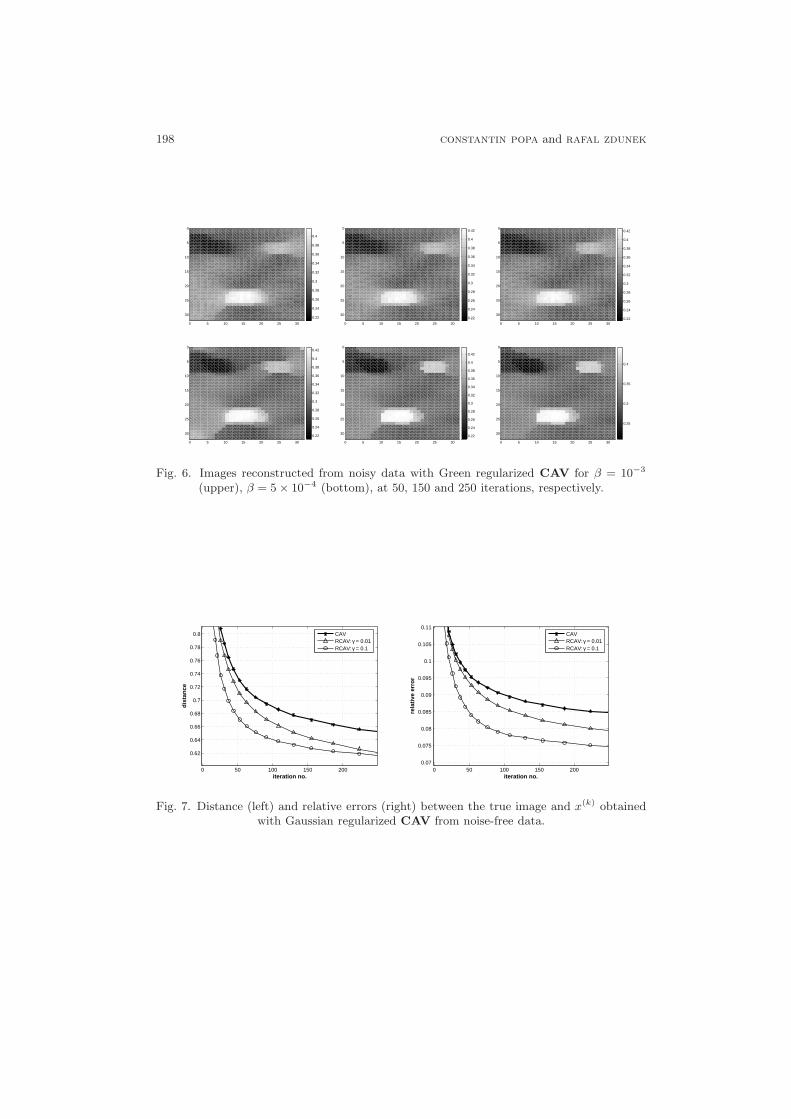
198 constantin popa and rafal zdunek
0 5 10 15 20 25 30
0
5
10
15
20
25
300.22
0.24
0.26
0.28
0.3
0.32
0.34
0.36
0.38
0.4
0 5 10 15 20 25 30
0
5
10
15
20
25
300.22
0.24
0.26
0.28
0.3
0.32
0.34
0.36
0.38
0.4
0.42
0 5 10 15 20 25 30
0
5
10
15
20
25
300.22
0.24
0.26
0.28
0.3
0.32
0.34
0.36
0.38
0.4
0.42
0 5 10 15 20 25 30
0
5
10
15
20
25
300.22
0.24
0.26
0.28
0.3
0.32
0.34
0.36
0.38
0.4
0.42
0 5 10 15 20 25 30
0
5
10
15
20
25
300.22
0.24
0.26
0.28
0.3
0.32
0.34
0.36
0.38
0.4
0.42
0 5 10 15 20 25 30
0
5
10
15
20
25
30
0.25
0.3
0.35
0.4
Fig. 6. Images reconstructed from noisy data with Green regularized CAV for β = 10−3
(upper), β = 5 × 10⁻⁴ (bottom), at 50, 150 and 250 iterations, respectively.
0 50 100 150 200
0.62
0.64
0.66
0.68
0.7
0.72
0.74
0.76
0.78
0.8
iteration no.
dis
tan
ce
CAVRCAV: γ = 0.01RCAV: γ = 0.1
0 50 100 150 2000.07
0.075
0.08
0.085
0.09
0.095
0.1
0.105
0.11
iteration no.
rela
tive
err
or
CAVRCAV: γ = 0.01RCAV: γ = 0.1
Fig. 7. Distance (left) and relative errors (right) between the true image and x(k) obtainedwith Gaussian regularized CAV from noise-free data.

tomographic image reconstruction 199
0 50 100 150 2000.6
0.7
0.8
0.9
1
1.1
1.2
iteration no.
dis
tan
ce
CAVRCAV: γ = 0.01RCAV: γ = 0.1
50 100 150 2000.08
0.09
0.1
0.11
0.12
0.13
0.14
0.15
0.16
iteration no.
rela
tive
err
or
CAVRCAV: γ = 0.01RCAV: γ = 0.1
Fig. 8. Distance (left) and relative errors (right) between the true image and x(k) obtainedwith Gaussian regularized CAV from noisy data.
0 50 100 150 200
0.55
0.6
0.65
0.7
0.75
0.8
0.85
0.9
0.95
1
iteration no.
dis
tan
ce
CAVRCAV: β = 1E−3RCAV: β = 5E−4
0 50 100 150 200
0.06
0.07
0.08
0.09
0.1
0.11
0.12
0.13
0.14
0.15
iteration no.
rela
tive
err
or
CAVRCAV: β = 1E−3RCAV: β = 5E−4
Fig. 9. Distance (left) and relative errors (right) between the true image and x(k) obtainedwith Green regularized CAV from noise-free data.
0 50 100 150 200
0.5
0.6
0.7
0.8
0.9
1
1.1
1.2
iteration no.
dis
tan
ce
CAVRCAV: β = 1E−3RCAV: β = 5E−4
0 50 100 150 2000.06
0.07
0.08
0.09
0.1
0.11
0.12
0.13
0.14
0.15
0.16
iteration no.
rela
tive
err
or
CAVRCAV: β = 1E−3RCAV: β = 5E−4
Fig. 10. Distance (left) and relative errors (right) between the true image and x(k) obtainedwith Green regularized CAV from noisy data.

200 constantin popa and rafal zdunek
References
[1] H. Akaike, Likelihood and Bayes Procedure, In Bayesian Statistics, J. M.Bernardo, et al. (Eds.), University Press, Valencia, 143/166 (1980).
[2] Y. Censor, D. Gordon, R. Gordon, Component averaging: an efficient iterativeparallel algorithm for large and sparse unstructured problems, Parallel Comput-ing, 27 (2001), pp. 777–808.
[3] M. Jiang, G. Wang, Convergence studies on iterative algorithms for image re-construction, IEEE Transactions on Medical Imaging, 22(5) (2003), 569–579.
[4] C. Popa, R. Zdunek, New generalized oblique projections in DW algorithm withapplication to borehole tomography, in: Proceedings of The Third Workshop onMathematical Modelling of Environmental and Life Sciences problems, May 27-30, 2005 Constanta, Romania, pp. 231–241, Editura Academiei Romane, Bu-curesti, 2004.
[5] C. Popa, R. Zdunek, Penalized Least-Squares Image Reconstruction for Bore-hole Tomography. Proceedings of ALGORITMY 2005 Conference, Vysoke Tatry–Podbanske, Slovakia, March 13–18, 2005, pp. 260–269.

Proceedings of the Fourth Workshop onMathematical Modellingof Environmental and Life Sciences ProblemsConstanta, Romania, September, 2005, pp. 201–210
Post–Synaptic Nicotinic Currents Triggered by theAcetylcholine Distribution within the Synaptic Cleft
Anca Popescu∗ and Alexandru Morega∗∗
A mathematical model that describes the postsynaptic nicotinic currents out of the
acetylcholine distributions within the synaptic cleft is proposed. The model describes the
most important steps of synaptic transmission: neurotransmitter release from presynap-
tic vesicles, its diffusion in the synaptic cleft, receptor-neurotransmitter coupling, and the
induced post-synaptic current inflow. Relying on previous results on acetylcholine distri-
bution in the synaptic space, the current work is concerned with the postsynaptic currents
that convect through open nicotinic acetylcholine receptors, which act as ionic channels.
The nicotinic currents are the outcome of a deterministic model that is based on the intra-
synaptic cleft acetylcholine space-time distribution, and on the nicotinic receptors opening
dynamics. The mathematical model is solved numerically, using the FEMLAB 3.1 software
package by a Galerkin finite element method.
1. Intoduction
Synaptic transmission, or the transmission of the information between neuronsin the nervous system, occurs through several mechanisms: neurotransmitter releasefrom the presynaptic neuron, as a result of neurotransmitter binding to the receptor,and inward ionic current flow through open receptors leading to postsynaptic mem-brane depolarization [1], [2], [4], [5]. In order to model synaptic transmission, allthese important steps have to be considered. Previous models focus either on neuro-
∗ Department of Bioengineering and Biotechnology, “Politehnica” University ofBucharest, Romania and Department of Biophysics, “Carol Davilla” University of Medicineand Pharmacy Bucharest, Romania.
∗∗ Department of Bioengineering and Biotechnology, Department of Electrical Engineer-ing, “Politehnica” University of Bucharest and ”Gheorghe Miho–Caius Iacob” Institute ofStatistical Mathematics and Applied Mathematics, Romanian Academy.

202 anca popescu and alexandru morega
transmitter release and diffusion [9], [11], [12], or on electrical phenomena occurringat postsynaptic level [9], [8]. The model proposed in this paper is concerned withcomputing postsynaptic currents out of neurotransmitter distribution in the synap-tic cleft, in the particular case of a nicotinic synapse, where the neurotransmitter isacetylcholine (ACh) that acts on a specific class of ACh receptors: nicotinic, ionotropicreceptors, which – as a result of their stimulation – open ionic channels.
Fig. 1. The nicotinic synapse.
Since nicotinic synapses are widely distributed in the human nervous system(both in central nervous system and at the neuromuscular junction) and since thereare several debilitating diseases affecting the nicotinic synapse, a global model ofthis type of synapse is necessary in order to better understand particular synapticphysiology and pathology. Further more, such a model would offer the possibility ofpre-clinical testing the effects produced by drugs that act on the nicotinic synapses.
By adjusting the numerical parameters that occur in the model, the model canbe easily modified for any type of chemical synapse (involving ionotropic postsynapticreceptors).
2. Physical and Mathematical Models
The neuro-muscular junction is a particular type of synapse using acetylcholine(ACh) as neurotransmitter, which binds to specific receptors called nicotinic receptors

acetylcholine distribution within the synaptic cleft 203
[4], [5]. Figure 1 shows a sketch of the synaptic domain and of the processes involvedin neurotransmission, that our model accounts for.
2.1. ACH Release and Diffusion
ACh concentration diffusion is modeled on a 2D geometry that assumes Carte-sian symmetry for the synaptic space (Fig. 2). The hatched squares in the synapticspace sketch correspond to the enzyme ACh-esterase.
20
550
100
50
18
nm
nmnm
nm
nm
Fig. 2. 2D synaptic geometry used for modeling ACh concentration diffusion. The overallwidth of the synapse is 30 × 50 nm [1], [4], [5].
Our model accounts for the degradation of ACh by the ACh-esterase enzyme(the hatched squares in the synaptic sketch, Fig. 2). The concentration of ACh isgiven by [9], [11], [12]
dC
dt= ∇ · (D∇C) , (1)
where C is the ACh concentration and D is the diffusivity of ACh - in this specificenvironment, D = 4 · 10−4µm2/µs, C(0) = 0.
The boundary conditions [9], [11], [12] are given by
n · (D∇C) = Q(t), (2)
on the ACh release portsn· (D∇C) = −kC, (3)
on the ACh-esterase portsn · (D∇C) = 0,
elsewhere.Here k = 2 ·10−3µm/µs is the activity constant of the ACh-esterase enzyme [11]
and Q(t) is the ACh flux through the release ports [9]
Q(t) =S0C0
lτ(1− e
−4τT
)e−tτ , (4)

204 anca popescu and alexandru morega
where S0 = 65 nm2 is the average, maximum (initial) cross-section area of the pre-
synaptic vesicle, C0 = 0.3 molecule/nm3 is the initial ACh concentration, l = 18 nmis the diameter of the release port, and T = 6.25µs is the characteristic time of thediffusion process. For τ (the characteristic time of the ACh release process) we usehere τ ≈ T (the values should vary according to different ACh release kinetics).
The total amount of ACh in the synaptic place is computed by
CA (t) =
∫
synapse
C (t) dS, (5)
where CA is the total number of ACh molecules in the synaptic space, d is the depthof the synaptic space, d = 10 µm, and nx = 30 is the average number of geometricperiods in our simplified model of the synaptic space.
The mathematical model was solved numerically by the finite element methodusing FEMLAB 3.1i [3].
2.2. Receptor dynamics
ACh receptors present two binding sites for ACh molecules. Only the double-ligated receptor opens, permitting the inward current flow. There are several interme-diate states of the receptor between the non-ligated-closed-receptor and the double-ligated-open-receptor [5], [6]. The transition rates between intermediate states dependon the available amount of ACh. Our model is based on a simplifying hypothesis :it considers only two different states of the receptor – open and closed (Fig. 3). Thetransition rates between these two states are chosen such as to account for the inter-mediate steps: k+ (transition closed-open receptor) = 0.04 ms−1, and k− (transitionopen-closed) = 0.02 ms−1 [6].
k
k
+
−R R*
Fig. 3. Receptor dynamics – simplified model. R–closednicotinic receptors, R∗ – open nicotinic receptors.
The mathematical model is made of the following Cauchy-type problem
d∗R∗ (t)
dt= k+R (t)− k−R∗ (t) , R∗ (0) = 0, (6)
whereR∗ (t) +R (t) = Rtotal (t) , (7)
R∗ (t) is the number of open synaptic receptors,R (t) is the number of closed receptors,and Rtotal = 105 is the total number of postsynaptic receptors. All these processesoccur only if there is enough free ACh in the synaptic space. Considering that the

acetylcholine distribution within the synaptic cleft 205
amount of free ACh equals the difference between the amount of total synaptic AChand the amount of bound (to receptors) ACh, and the every open receptor is boundto 2 ACh molecules, this condition can be written as
CA (t)− 2R∗ (t) > 0, (8)
Non-dimensional equations
Considering the following changes of variables
N =Rtot −RRtot
, τ =t
T, (9)
where
T =1
k+ − k−, (10)
the non-dimensional form of problem (6) is
dN
dτ+N =
k+
k+ + k−, N(0) = 0. (11)
The solution to this problem poses no difficulties: it was computed numerically bya finite differences backward Euler technique using a constant time-step algorithmimplemented in MATLAB [7]. Accuracy test consisted of using several values for thetime step and checking that the results do not change.
2.3. The Postsynaptic Voltage
The postsynaptic voltage was computed based on a equivalent electrical circuitof the membrane shown in Fig. 4 [9], [10].
R
R
ex
in
EUg
ACh
cm
Fig. 4. Equivalent electrical circuit of the membrane. E – membrane-specific equivalente.m.f. (due to ionic pumps in the membrane); Rex – resistance of the extra-cellular space;Rin – resistance of the intracellular space, Cm – membrane capacity; gACh – membrane
conductance (due to open nicotinic receptors), U – postsynaptic voltage.
The postsynaptic voltage is obtained by solving, again, a Cauchy-type problem

206 anca popescu and alexandru morega
CmdU
dt+ U
[gACh (t) +
1
Rex
]=
E
Rx, U (0) = E, (12)
where
gACh (t) = γR∗ (t) , (13)
where E = −70 mV is membrane-specific equivalent e.m.f., Rex = 5·104 Ω is the resis-tance of the extra-cellular space, Rin (approx. 0) is the resistance of the intracellularspace, Cm = 4 ·10−12 F is the membrane capacity, gACh is the membrane conductance(due to open nicotinic receptors), γ = 20 pS is the single-channel conductance (for 1single nicotinic channel), and U is the postsynaptic voltage.
The non-dimensional form of problem (12) is
dU
dτ+ U [γRexRtotN (τ) + 1] = 1, U (0) = 1, (14)
with
U =U
E, τ =
t
T, and T =
1
RexCm. (15)
In this case too, the solution poses no difficulties: it was computed numericallyby the same finite differences backward Euler technique using a constant time-stepalgorithm implemented in MATLAB [7]. The same type of accuracy test with respectto the time step was performed.
3. Results
The number of ACh molecules in the synaptic space during the first 6.25 µs(T = 1
)and 62.5 µs
(T = 10
)is shown in Fig. 5.
Fig. 5. ACh diffusion dynamics.
Figure 6 presents the receptor opening dynamics.

acetylcholine distribution within the synaptic cleft 207
Fig. 6. Receptor dynamics.
We also investigated how the opening kinetics of the postsynaptic receptors influ-ences the triggering profiles: Figure 7 shows the results, for different opening/closingrates.
Fig. 7. Receptors triggering profiles for different opening kinetics.
From top:k+
k+ + k−
=5
3;
4
3;
3
3;
2
3;
1
3;
0.5
3;
0.25
3.
While ACh concentration rapidly reaches high values, only a small number ofreceptors open in the same period of time (6.25µs from the moment t = 0). Figure 8compares the ACh and receptor profiles in the first 6.25µs after the initiation of theACh release process.
Depolarization of the membrane occurs rapidly after the first receptor channels

208 anca popescu and alexandru morega
Fig. 8. ACh vs receptor dynamics.
open, and reaches a positive value. Either different opening kinetics for the receptorsor different values from the extra-cellular resistance or single-channel conductanceslightly modify the plateau. Figure 9 shows the postsynaptic membrane voltage com-
puted from our model, fork+
k+ + k−=
2
3and the values for the extra-cellular resistance
and single-channel conductance mentioned in the text above.
Fig. 9. Postsynaptic membrane voltage.

acetylcholine distribution within the synaptic cleft 209
4. Discussion and Conclusions
Apparently, cholinergic synaptic transmission involves 3 important processes,each with its own time constant:
• TACh = 6.25 µs – for ACh diffusion;
• Tr = 16.5 ms – for receptor opening;
• Tm = 0.25 µs – for membrane depolarization.
Although the fastest process is depolarization of the membrane, the leadingprocess (i.e. triggers all the other processes) is the ACh release and diffusion. Thereceptors need a longer time to reach a plateau. In our model, the full saturation ofreceptors (100% of the receptors open) cannot be achieved, because of the opening
kinetics of the receptors
(k+
k+ + k−=
2
3
). In a model that considers k− = 0 (Fig. 7
the third curve from the top), saturation is achieved after approximately 80 ms. Thefirst two curves in the same figure are merely theoretical – they suppose a negativevalue for k− , which is not possible from a biological point of view.
The concentration vs open-receptor profiles show that is enough ACh to open thepostsynaptic receptors in the first phase: ACh concentration grows much faster thanthe number of open receptors. The influence of the ACh concentration on receptorkinetics becomes important after a much longer time (not in the time-domain of oursimulation). Depolarization of the membrane occurs rapidly after receptor-opening.The characteristic peak of postsynaptic membrane depolarization is not explained inour model because of several aspects that our model does not account for: differentrelease kinetics for ACh (simulating trains of impulses, which covers better for thephysiological situation), the “refractory period” of the receptors - receptors close aftera certain time, and enter a refractory state, where they stay closed, independentlyfrom the ACh molecules still existing in the cleft; the propagation of depolarization onthe postsynaptic membrane. Further simulations should also consider the influence ofACh on the receptor opening profiles – k+ and k− should vary with the concentration,but effect of a burst of impulses arriving at pre-synaptic level, the saturation ofreceptors.
References
[1] Bennett M.R., Synaptic transmission at single buttons in sympathetic ganglia,News Physiol. Sci.,15 (2000), pp. 98–101.
[2] Castonguay A. et al., Differential regulation of transmitter release by presynapticand glial Ca2+ internal stores at the neuromuscular synapse, J. Neurosci., 21(2001), No. 6, pp. 1911–1922.
[3] COMSOL AB – FEMLAB 3.1i.

210 anca popescu and alexandru morega
[4] Dimoftache C., Sonia Herman, Principii de biofizica umana, Editura Universitara“Carol Davilla”, Bucuresti, 2003.
[5] Guyton A.C., Textbook of medical physiology, 8th Edition, W.B. Saunders Comp.,1991.
[6] Keleshian A.M. et al., Evidence for cooperativity between nicotinic acetylcholinereceptors in patch-clamp records, Biophys. J., 78 (2000), pp. 1–12.
[7] MathWorks – MATLAB 6.5
[8] Popescu, Anca, Al. Morega, Current and Voltage Distribution Within the Synap-tic Cleft – A Modelling Study, in:Proceedings of the Third Workshop on Math-ematical Modelling of Environmental and Life Sciences Problems, Constanta,Romania, Editura Academiei Romane, 2005.
[9] Popescu, Anca and Al. Morega, Current and Voltage Distribution Within theSynaptic Cleft, in: Proceedings of the Second Workshop on Mathematical Mod-elling of Environmental and Life Sciences Problems, Bucharest, Romania, Edi-tura Academiei Romane, Bucuresti, 2005.
[10] Savtchenko, L.P. et al., Effect of voltage drop within the synaptic cleft on thecurrent and voltage generated at a single synapse, Biophysics. J., 78 (2000),No.3, pp. 1119–1125.
[11] Smart J.L. et al., Analysis of synaptic transmission in the neuromuscular junc-tion using a continuum finite element model, Biophysics. J., 75 (1998), pp. 1679–1688.
[12] Tai, K. et al., Finite element simulations of acetylcholine diffusion in the neuro-muscular junction, Biophysics, J., 64 (2003), pp. 2234–2241.

Proceedings of the Fourth Workshop onMathematical Modellingof Environmental and Life Sciences ProblemsConstanta, Romania, September, 2005, pp. 211–222
Effect of tricyclic antidepressantson the frog epithelium
Corina Prica∗†, Emil Neaga∗, Beatrice Macri∗, DumitruPopescu∗ and Maria Luiza Flonta∗
Our study was undertaken with the aim of testing the action of tricyclic antidepres-
sants, amitryptiline (AMT) imipramine (IMI) and desipramine (DES) on the epithelium
sodium channel (ENaC) using the voltage-clamp technique on the frog epithelium (Rana
ridibunda). The epithelium sodium channel belongs to Deg/ENaC family, like ASICs and
many other putative members in the brain. We have studied the effect of amitryptiline,
imipramine and his metabolite desipramine on the short-circuit current (Isc) and transmem-
brane conductance (Gt) on the range of concentration of 1 µM to 200 M. We observed that
all three antidepressant have a dual effect on short-circuit current Isc, and on the conduc-
tance, increasing these two parameters on the range of concentration 1-50 µM and reducing
them at the concentration 100-200 µM. These results suggest once again, multiple effects
of tricylic antidepressant on different ionic channels and receptor: blocks sodium current
sensitive at TTX from neurons DRG and cardiac muscle, interact with the channels and
carriers of K+ and act on the cholinergic receptors, inhibits the recapture of serotonin and
norepinephrine. All these effects of tricyclic antidepressants could be utilized to explain the
effect of antidepressive and all secondary effects witch appear during the treatment.
1. Introduction
Amiloride sensitive Na+ channels are essential control elements for the regulationof Na+ transport into cells and across epithelia.
∗ Faculty of Biology, University of Bucharest, Splaiul Independentei, 91-95, 050095,Bucharest, Romania.
“Gheorghe Mihoc–Caius Iacob” Institute of Statistical Mathematics and Applied Math-ematics, Calea 13 Septembrie 13, 050711, Bucharest, Romania.
† e-mail: [email protected], phone 0040-21-318 15 69, fax 0040-21-318 15 73.

212 corina prica et al.
Sodium is the most abundant ion in the extracellular fluid and total body sodiumis an important determinant for the regulation of the extracellular fluid volume. Thekidney of land vertebrates possesses mechanism that regulate salt balance with thetendency to retain salt and water in the body in order to preserve the volume of theextra cellular fluid and to maintain adequate blood circulation. The epithelial sodiumchannel (ENaC) in the renal distal part of the nephron is an important component inthe control of sodium balance. ENaC is located in the apical or the outward-facingmembrane of many other salt-reabsorbing epithelia and facilitates Na+ movementacross this membrane as a first step in the process of Na+ transport.
Epithelial tissues play a critical role in controlling the whole body internal envi-ronment, by providing gas exchange, solute and water uptake and contain the routesfor secretion and excretion. Typically, they are arranged in sheets consisting of oneor more layers of communicating cells that realize the transport function.
A characteristic of all epithelial is their polarity: the apical (luminal) membraneis morphologically and functionally distinct from the basal and lateral membrane.
Specialized junctions that connect the cells to each other make up the transitionbetween the apical and lateral membrane at the luminal border. The apical bordercan be exposed to air (epidermis, tracheal and corneal epithelium) or it can face thelumen of the cavity of the organ that contains solutions with an ionic and solutecomposition that differs strongly from the body fluids (gut, blandder, small intestineand kidney tubule). The basal and lateral sides called the basolateral domains havespecialized regions for cell-cell adhesions and for signal transduction.
According to the permeability properties of the tight junctions, epithelia areclassified in tight and leaky.
Leaky epithelia (small intestine, gall blander and proximal kidney tubule) arecharacterized by a high permeability of the paracellular pathway. Their apical mem-branes mainly posses co-transporter systems, such as Na+/glucose and Na+/ Po3−
4
and antiporter systems as, for instance, Na+/H+ that provide Na+ uptake.Na+ movement across the tight epithelia such as urinary bladder, distal kidney
tubule and large intestine the paracellular pathway has a low permeability. ApicalNa+ uptake occurs through Na+ selective channels. The two steps involved in Na+
transport across tight epithelia are illustrated in Fig. 2.ENaC is involved in regulation of Na+ uptake by facelifting the entry of ENaC
ions into the cell driven by an electrochemical gradient. This gradient is generatedby Na+/K +–ATPase. Which extrudes tree Na+ ions from the cell in the exchangefor two K+ ions and thus maintaining cell concentration of Na+ low and K+ high.The electrochemical K+ gradient across the Na+/K+–ATPase are responsible formaintaining the intracellular negative potential that facilitates Na+ uptake at theapical border. It is generally accepted that under most circumstances that Na+/K+–ATPase only works at about one-third of this maximal capacity. However, the uptakeof Na+ is the rate-limiting step for the Na+ reabsorption and the represents theprincipal target of transport regulation.

effect of tricyclic antidepressants on the frog epithelium 213
Fig. 1. Na+ transport across leaky epithelia. Fig. 2. Na+ transport across tight epithelia.
2. Aims
It is generally accepted that there is a relationship between chronic pain anddepression [8]. In this sense, it is known that serotonin, noradrenaline [1] and opi-oids [5] are involved in both nociceptive and depressive disorders, as well as in themechanism of action underlying the antinociceptive [13, 14] and antidepressive ef-fects of antidepressants [2]. In clinical practice, antidepressants – usually tricyclics –are widely used in several painful conditions, as well as opioids and other analgesicsand have been proven to be effective in the management of pain of diverse aetiology[15, 7, 10]. On the other hand, it has been previously reported that opiate analgesicswith monoaminergic reuptake inhibitory properties may induce an antidepressant-likeeffect in mice [11] accounting for the interrelationship between these two entities.
In spite of the wide use of antidepressants in painful disorders, the nature ofantidepressant-induced analgesia remains to be elucidated. It has been suggestedthat antidepressant drugs have specific analgesic properties, and a body of clinical[8, 9] and experimental [ 12, 14, 4] types of evidence together seems to demonstratethat the analgesic may be independent of the antidepressant effects.
However, the relationships between antidepressive and analgesic effects of thesedrugs have not yet been fully elucidated [6].
The analgesic mechanism of amitriptyline, imipramine and desipramine is un-clear. One explanation is that it blocks Na channels, reducing in this way spontaneousactivity in nerve fibres, which cause pain. A new class of ion channels known as theDeg/ENaC (degenerins-epithelial Na channel) family which includes ASIC, DRASICmediate pain induced by acidosis in damaged or inflamed tissue. The same familyincludes also EnaC, which can be easily studied in the amphibian epithelial model.
This study was undertaken with the aim of testing the actions of amitriptyline,imipramine and desipramine on native epithelial Na channels from frog skin. We as-sumed that, having a common protein structure, characterization of the amitriptyline-ENaC interaction could help to elucidate the analgesic mechanism of this antidepres-sant.

214 corina prica et al.
3. Materials and Methods
3.1. Mounting of the epithelium
Preparation of the frog skin. Frog (Rana ridibunda), weighting around 50 g,were kept at 17o C with free access to tap water. The abdominal skin of doubly pithedfrog was dissected and mounted in an Ussing-type Lucite chamber. The chamberensured negligible edge damage and allowed continuos perfusion with fresh solutionsof both the mucosal and serosal sides of the epithelium, at a rate of 5 mL min –1.The tissue area in contact with the bathing media was 1 cm2.
In order to perform measurements of the transepithelial current and voltageunder many different circumstances, i.e with varying solutions on the outer and innerside of the tissue, we mounted the preparation in a chamber. The tissue was placed asa flat sheet between two fluids filled compartments. This technique is often attributedto H.H. Ussing (1949). The “Ussing chamber” we used is shown in Fig. 3.
Fig. 3. The “Ussing chamber”. Fig. 4. Design of Ussing chamber.
These compartments were filled with Ringer solution to equal levels, this main-taining the pressure difference across the tissue equal to zero. When the two chamberhalves were put together with screws, the edges of the tissue became compressed be-tween the rim (R) on the left and the right compartment. The pressure that wasthen extending on the tissue’s edge could be adjusted by changing the thickness ofthe gasket, which was put between the two chamber halves. In this way edge damageof the tissue was minimized. A thin film of the silicon vacuum grease on the rim ofeach chamber half was used to seal the chamber and also the further reduce edgesdamage. The skin area are exposed to the bathing solution was 0,5 cm2. Both cham-ber compartments were continuously perfused during the experiment with a solutionflow of 4–6 ml/min. The incoming fluid next to directed towards the tissue face. Inthis way a layer of stagnant fluid next to the tissue was prevented. The design of thechamber allowed for rapid change of solution without of voltage clamping, Fig. 4.
Each chamber halve had its own reservoir, which consisted of the beaker filledwith a Ringer solution, was placed on the higher level than the chamber, so that thesolution flow was maintained by gravity.

effect of tricyclic antidepressants on the frog epithelium 215
Fig. 5. The voltage clamp circuit.
One end of the tubing was connected with a metal tube that was placed into thebeaker. The other end of the tubing was connected with the chamber. The solutioncould easily be changed by moving the metal end of the tubing from one reservoirinto another. The fluid left the chamber via the upper side, through spillways thatcontained paper strips. In this way the compartments always remained filled withsolution, also when the (by accident) one of the reservoirs became empty. The paperstrips allowed the fluid to leave the chamber continuously. Via the strips the fluidwas collected in the glass beakers. It could be used again by emptying the beakers inthe reservoirs.
3.2. The voltage clamp
The purpose of noise analysis is the study of the fluctuation in conductanceof an ionic pathway in a cell membrane. This conductance fluctuation (G) are di-rectly proportional to the fluctuation in current (I) measured under voltage clampconditions.
So, one can record current fluctuation in order to obtain information about theconductance fluctuation. Indeed, the shape of their spectra will be identical. On theother hand, the relation between conductance fluctuation and fluctuation in voltagemeasured under current clamp conditions is more complicated.The relation betweenthe power spectral density of the voltage and conductance fluctuation will depend onthe frequency dependence of the impedance of the membrane.
For this reason, we performed the experiments under voltage clamp conditions.This yields information about the number of channels, the single channel current andthe probability that the channel is in a specific state. Prerequisite for the measure-ments of the membrane noise is a low-noise measuring circuit. A schematic plot of the

216 corina prica et al.
voltage clamp circuit we used is shown in Fig. 5. The voltage clamp is a feedback cir-cuit that keeps the voltage across the epithelium constant by varying the current flowthrough the epithelium. In order to avoid large junction potentials, the connectionbetween the voltage input and current output of the clamp was made by two current(I) and two-voltage (V) electrodes, figure 5. They consisted of Ag/AgCl/3M KClelectrodes which were in contact with the solutions in the “Ussing chamber” throughagar bridges ( 3 gr agar per 100 ml 1M KCl ). The two voltage electrodes placed toeach side of the epithelium allow the recording of the transepithelial potential (PD)and two current electrodes allow injection of the clamp current. Voltage clamp of PDto zero allows to assess IscNa transport (INa) was defined as the amiloride-sensitivecomponent of Isc. An automatic electronic circuit clamps the spontaneous potentialdifference across the epithelium to aero ( voltage clamping to short-circuit state). Thevoltage clamp is an automatic fed-back device intended to impose a constant voltageacross the epithelium. The input stage of the clamp consisted of the low-noise differ-ential amplifier ( DA ) with a gain of 100x. The feedback ampifier (FBA) convertsthe voltage offset at the input to current. Moreover, the FBA is made as summingamplifier so that a clamp potential between –100 to + 100 mV can be imposed tothe epithelium. Via an external input (Vcom) this potential could be varied undercomputer control to record current-voltage relations.
The epithelium can be represented as a RC-network. The impedance of thiscircuit varies among the different tissues. This RC circuit influence the frequencycharacteristics of the voltage clamp. The frequency response of the voltage clampcircuit could be varied by changing the capacitance in the FBA and by varying theresistance of the potentiometer ( R ) which was installed in the feedback circuit. Whenthe feedback loop was closed this resistance was 470 Ω . Concomitantly the resistancewas gradually decreased to make the response of the voltage clamp faster. An optimaladjustment of the feedback capacitance and of R was obtained by inspection of thetransepithelial current and the voltage response to train of square wave pulses with afrequency of 200 Hz which was applied at Vcom. The feedback current was measuredwith a current to voltage converter. The output signal of this amplifier was connectedto three different setups.
1. The transepithelial current was continuously recorded on a XT-recorder. Thetransepithelial conductance was obtained from the current deflections caused by theapplication of 10 mV transepithelial potential pulses at Vcom.
2. After inversion (I), the signal was displayed on the liquid-crystal display andcould be sampled under computer control.
3. The output signal was connected via a high pass filter ( HPF ) with adjustablecut-off frequency to a voltage amplifier with a total gain of 1000. The output of thisamplifier ( In) was sent to a computer for analysis.
3.3. Noise system
With noise analysis, we intend to analyse the random fluctuation in current asso-ciated with ionic movement through biological membranes. The thermal or Brownianmovement to which the charge carriers are subjected produces what is called ther-

effect of tricyclic antidepressants on the frog epithelium 217
mal or Johnson-Nyquist noise. In non-equilibrium conditions (net ionic current flow),other contributions besides the thermal noise exist, together denoted as excess noise.In the accessible ms to s time range, distinctive features (e.g. Lorentzian) in the spec-tral analysis (power spectrum) of the current fluctuation originate from stochasticchanges in the conductive pathways for ion movements through the membrane. Theunderlying processes for this “ Lorentzian noise “ are though to consist of probabilisticopening and closing events of ion channels. When recorded, in conditions where thevoltage across the membrane is maintained constant, the fluctuation in current is di-rectly proportional to the conductance fluctuation. Information about the number ofchannels in the ensemble and about the single channel current can be obtained fromthe analysis of the noise caused by random blockage of ion channels by reversibleblockers. Fluctuation of current caused by random interaction of the blocker withthe channel give rise to Lorentzian noise. Its relaxation time varies with blocker con-centration which enables the calculation of the rate constants of the blocker and thesingle channel parameters.
The power density spectrum of fluctuations in current that passes through gatedchannels has a Lorentzian shape. To resolve the entire frequency range, we measuredcurrent fluctuations in a frequency range between 0,2 Hz and 1 kHz. To guarantee asufficiently fine spectral resolution, and to keep the measuring time short, we analyzedthe current-noise signal in two different frequency ranges: a low and a high frequencyrange. The 1000x amplified fluctuations in current ( In from clamp ) were sent to twoseparate modules (designated HS and LS in Fig. 12) each consisting of a pre-filterand an anti-aliasing filter. The fundamental frequency was fixed in most experimentsto 0.5 Hz.
The output of the pre-filter and the anti-aliasing filter was amplified (1-20×)to optimize the analog-to- digital conversion in the computer. The low and the highsignal were sampled consecutively by a multiplexer and sent via a sample and holdsystem (S&H) to an A/D converter. After digitising, data were converted from thetime to the frequency domain using an FFT (Fast Fourier Transform) software rou-tine and a double logarithmic plot of the power density S(f) as the function of thefrequency (f) was displayed on the computer’s monitor. An individual spectrum wasobtained from a series of 50 periods of data acquisition (sweeps). Each sweep con-sisted of a sequential digitization of the low (4096 points/2 sec) and then the high(4096 points/0.25 sec) analog signals. The duration of the sweep was therefore 2.25sec and approximately 3 minutes were required to obtain and process the 50 sweep fora single spectrum which was displayed immediately on the computer’s monitor. TheFFT output frequencies for the LS ranged from 0.5 to 256 Hz and for the HS from 4to 2048 Hz. In order to obtain spectra that can easily be analyzed by a computer, thenumber of frequency points was reduced. Each octave was divided in 8 intervals andthe average value of LS and HS frequency was calculated for each interval. This re-sulted in 8 values per octave that yielded 74 spectral data points in the power densityspectrum. The data were saved on disk for further analysis.

218 corina prica et al.
4. Fitting procedure
Theoretical calculations on the stochastic conductance ( or current ) fluctuationbetween multiple conductance states of an ionic channel predict PDS that contain anumber of Lorentzian curves equal to the number of conductance states minus one.The Lorentzian function :
S(f) =So
1 +(
ffc
)2
is characterized by two parameters: the plateau value S0 represents the noise powerat zero Hz and the corner frequency fc is the frequency where the noise power hasdropped to its half-maximal value ( So/2).
In the fitting procedure of 1/f excess noise of the preparation must be taken intoaccount. Instrumental noise becomes dominant at higher frequencies and is excludedfrom the fit by selecting a suitable frequency range.
5. Three state model
In the presence of the blocker the channels are distributed among three states:
closedφ←→α
openKon[B]←→Koff
blocked
P c P o P b
Where α and β are the rates of the open-close reaction. The parameters Kon
and Koff are association and the dissociation rates of the blocker, respectively. Theprobability of the channel of being closed is Pc, whereas of the blocked state is Pb. Inthe absence of the blocker (B) the open probability is :
Po =α
α+ β.
The power density is now equal to the sum of two Lorentzian functions:
S (f) =S
(1)o
1 +[
ff(1)
]2 +S
(2)o
1 +[
ff(2)
]2 .
Thus is the case of three states “open”, “closed” or “blocked” the power densityspectrum of the fluctuation in current is the sun of two Lorentzian functions. Thecorner frequency and plateau value of the Lorentzian components will depend on theconcentration of the blocker. Patch clamp experiments univocally indicate that ENaCfluctuates between open and closed times with long mean open and closed times andwould give rise to a Lorentzian with a corner frequency smallere than or in the rangeof 0.1 Hz. Therefore, in the frequency range of our analysis, expose of the ephiteliumto a blocker, give rise to a single Lorentzian in the PDS. From the blocker-inducednoise, we determined Po and No.

effect of tricyclic antidepressants on the frog epithelium 219
Imipramine Amitryptiline Desipramine
Fig. 6. The effect of imipramine, amittryptiline and desipramine on short-circuit current Isc
in Ringer Cl solution.
Imipramine Amitryptiline Desipramine
Fig. 7. The effect of imipramine, amittryptiline and desipramine on short-circuit current Isc
in Ringer SO4 solution.
The two Lorentzian parameters, the low-frequency plateau (So) and the cornerfrequency (fc) were determined by non-linear curve fiting of the spectra presuminga first order interaction between channel and blocker. The on- (Kon) and off (Koff)rate constant of the blocking reaction were calculated from:
2πfc = Kon[B] +Koff ,
where [B] is the blocker concentration. Using the values of the Na current and theLorentzian parameters (fc and So) obtained from noise analysis, we estimated iNa siNo.
iNa =So (2πfc)
2
4INaK01 [B], N0 =
INa
iNa.
6. Results
This study is a continuation of a research started with amitryptiline. We ef-fectuated a curve dose-effect (1–200 µM) and we have found out that the tricyclic

220 corina prica et al.
antidepressants have the higher effect at a concentration of 10 µM. We used two dif-ferent solution of Ringer; Ringer Cl− and Ringer SO4 to see if exist a different effectof chlorine ions.
Graph 1 to 11, represent the effect of short-circuit current Isc when we appliedthe antidepressants on the apical membrane of the epithelium. The current increaseprogressive until a concentration of 50 µM and at higher concentration appears aninhibitory effect. The effect is similar in Ringer Cl or Ringer SO solutions, whichexclude a specific effect of tricyclic antidepressant on chlorine ions conductance, whichdemonstrate that the flow of sodium is modulate by tricyclic antidepressant.
We observed that all three antidepressant have a dual effect on short-circuitcurrent Isc, and on the conductance, increasing these two parameters on the range ofconcentration 1–50 µM and reducing them at the concentration 100–200 µM. The in-hibitory effect of tricyclic antidepressants on sodium ions flow at higher concentrationcan be explain by phenomenon of feed-back inhibition of ENaC at higher concentra-tion on Na intracellular. These results suggest once again, multiple effects of tricylicantidepressant on different ionic channels and receptor: blocks sodium current sen-sitive at TTX from neurons DRG and cardiac muscle, interact with the channelsand carriers of K+ and. act on the cholinergic receptors., inhibits the recapture ofserotonin si norepinephrine
All these effects of tricyclic antidepressant could be utilized to explain the ef-fect of antidepressive and analgesic and all secondary effects witch appear during thetreatment. But we must mentions that in our experimental studies the concentrationthat we used is higher that plasmatic concentration which is 1 µM. This suggests ex-istence receptors with higher affinity responsible for the therapeutic effects of tricyclicantidepressants.
We also observed that at a concentration of 10 µM the amitryptiline has a highereffect comparative with imipramine and desipramine (graph 12).
References
[1] Basbaum, A.I., Fields, H.L., Endogenous pain control systems: brainstem spinalpathways and endorphin circuitry, Annu. Rev. Neurosci., 7 (1984), pp. 309–338.
[2] Carlsson, A., Corrodi, H., Fuxe, K., Hokfelt, T., Effects of some antidepressantdrugs on the depletion of intraneuronal brain catechol-amine stores caused by4-alpha-dimethyl-meta-tyramine, Eur. J. Pharmacol., 5 (1969), pp. 367–373.
[3] Casas, J., Gibert-Rahola, J., Chover, A.J., Mico, J.A., Test-dependent relation-ship of the antidepressant and analgesic effects of amitriptyline. Methods Find.Exp. Clin. Pharmacol, 17 (1995), pp. 583–588
[4] Casas, J., Gibert-Rahola, J., Valverde, O., Tejedor-Real, P., Romero, P Mico,J.A.,Antidepressants, is there a correlation between their analgesic and antide-pressant effect?, Eur. Neuropsychopharmacol., 3 (1993), pp. 343–344.

effect of tricyclic antidepressants on the frog epithelium 221
[5] De Gandarias, J.M., Irazusta, J.,Varona, A., Gil, J., Fernandez, D., Casis, L.,Effect of imipramine on enkephalin-degrading peptidases, Eur. Neuropsychophar-macol., 9 (1999), pp. 493–499.
[6] O’Malley, P.G., Balden, E., Tomkins, G., Santoro, J., Kroenke, K., Jackson, J.L.,Treatment of fibromyalgia with antidepressants. A meta-analysis, J. Gen. Intern.Med., 15 (2000), pp. 659–666.
[7] Onghena, P., Van Houdenhove, B., Antidepressant-induced analgesia in chronicnon-malignant pain: a meta-analysis of 39 placebo-controlled studies, Pain, 49(1992), pp. 205–219.
[8] Magni, G., Conlon, P., Arsie, D., Tricyclic antidepressants in the treatment ofcancer pain: a review, Pharmacopsychiatry, 20 (1987), 160–164.
[9] Magni, G., The use of antidepressants in the treatment of chronic pain. A reviewof the current evidence, Drugs, 42 (1991), pp. 730–74.
[10] McQuay, H.J., Tramer, M., Nye, B.A., Carroll, D., Wiffen, P.J., Moore R.A., Asystematic review of antidepressants in neuropathic pain, Pain, 68 (1996), pp.217–227.
[11] Rojas-Corrales, M.O., Gibert-Rahola, J., Mico, J.A., Tramadol inducesantidepressant-type effects in mice, Life Sci., 63 (1998), pp. PL175–PL180.
[12] Spiegel, K., Kalb, R., Pasternak, G.W., Analgesic activity of tricyclic antide-pressants. Ann. Neurol. 13 (1983), pp. 462–65.
[13] Schmauss, C., Emrich, H.M., Narcotic antagonist and opioid treatment in psychi-atry, in: Rogers, R.J., Cooper, S.J. (Eds.), En dorphins, Opiates and BehavioralProcesses, Wiley, New Delhi, 1988, pp. 327–351.
[14] Valverde, O., Mico, J.A., Maldonado, R., Mellado, M.L., Gibert-Rahola, J.,Participation of opioid and monoaminergic mechanisms on the antinociceptiveeffect induced by tricyclic antidepressants in two behavioral pain test in mice,Prog. Neuropsychopharmacol. Biol. Psychiatry, 18 (1994), pp. 1073–1092.
[15] Tura, B., Tura, S.M., The analgesic effect of tricyclic antidepressants, Brain Res.,518 (1990), pp. 19–22.
[16] Walsh, T.D., Antidepressants in chronic pain, Clin. Neuropharmacol., 6 (1983),pp. 271–295.


Proceedings of the Fourth Workshop onMathematical Modellingof Environmental and Life Sciences ProblemsConstanta, Romania, September, 2005, pp. 223–230
On the Solvability of Navier-Stokes Equations
Cristina Sburlan∗
In this paper we investigate the solvability of Navier-Stokes system, in case of an
incompressible dynamical viscous fluid. The system can be reduced to an evolution problem
in which are involved a linear monotone operator and a compact nonlinear one. We will use
functional and topological methods to study the problem, such as Fourier method and the
topological degree.
1. Introduction
The solvability of the Navier-Stokes system represents an actual problem.We consider the steady state flow equation as a bifurcation problem with re-
spect to the dynamical viscosity, and this approach permits us to use the powerfultopological degree methods to study this problem.
Then, in the next section, we consider the linearized Navier-Stokes system(Stokes equation) for the flow of incompressible fluids and we succeed to find theweak solution of this evolution problem as a Fourier series.
2. Coincidence Degree for Steady State Flow of Incom-pressible Fluids
First we present the theoretical approach to the coincidence degree, and thenwe apply this theory to the steady state flow of incompressible fluids. Let H be areal Hilbert space and consider L : D(L) ⊆ H → H a linear and maximal monotone
∗ Faculty of Mathematics and Computer Science, “Ovidius” University of Constanta,Romania, e-mail:c [email protected]

224 cristina sburlan
operator and N : D(N ) ⊆ H → H a (nonlinear) compact one. We can write
λL+N = I + λL − I +N = (I + λL)(I − (I + λL)−1(I −N )),
so we have the equivalence
λLy +N (y) = 0⇔ y − (I + λL)−1(I −N )(y) = 0 (1)
Denote byM(λ) the compact operator (I+λL)−1(I−N ). For D ⊂ H open boundedset such that λLy +N (y) 6= 0, ∀y ∈ ∂D, we define the coincidence degree of (L,N )relatively to D by
dλ((L,N ), D) := dLS(I −M(λ), D, 0), (2)
(dLS stands for Leray-Schauder degree). This coincidence degree has all the proper-ties of Leray-Schauder degree, such that(P1) (The solution property). If dλ((L,N ), D) 6= 0, then equation (1) has at leastone solution in D.(P2) (The homotopy invariance). Let (λt)t∈[0,1] ⊂ (0,+∞) be a continuous deforma-tion such that equation λtLy +N (y) = 0 has no solutions y ∈ ∂D for all t ∈ [0, 1].Then dλt
((L,N ), D) is independent of t ∈ [0, 1].Denote by C(L) the set of all characteristic values of L. We have the following
theorem (see [3] and [5]).
Theorem 1. Suppose that there exists k > 0 such that
‖N (y)‖ ≤ k ‖y‖ , y ∈ H.
If λ0 ∈ C(L) is such that dist(λ0, C(L)\λ0) > 2k, then equation (1) has at leastone bifurcation point with λ ∈ (λ0 − k, λ0 + k).
We set S = (λ, u) ∈ Λ×H |λLu+N (u) = 0 and S′ = S ∪ C(L)×0. Dueto classical bifurcation Rabinowitz theorem we state:
Theorem 2. Under the hypotheses of Theorem 1, the maximal connected setSλ0 ⊂ S′ intersecting (λ0−k, λ0 +k)×H is either unbounded in Λ×H or it containsa finite number of points (λj , 0) with λj ∈ Λ. Moreover, the number of these pointshaving odd algebraic multiplicity – including (λ0, 0) – is even.
Remark 1. The above results remain true if, instead the condition from Theo-rem 1, N satisfies the following condition
∃k > 0 such that ‖N (y)‖ ≤ k ‖y‖2 , y ∈ H.
Let now Ω ⊆ RN , (N = 2 or 3), be a domain with smooth boundary ∂Ω anddenote by Q := Ω× (0,+∞) and by Σ := ∂Ω× (0,+∞).
We will study the case of the steady state flow
ut = 0⇔ u = const. (in t) = u0(x)

on the solvability of navier-stokes equations 225
regarding the flow equation as the eigenvalue equation
(u · ∇)u(x, t)− ν∆u(x, t) +∇p(x, t) = f(x, t) (3)
with respect to the eigenvalue parameter ν – the dynamical viscosity, and the bound-ary conditions are given by
u = 0 on Σ. (4)
If Ω is unbounded, we consider moreover that
u→ 0 for |x| → +∞.
We study the incompressible fluids, so we also have the condition
∇ · u = 0. (5)
Suppose that Ω is pathwise connected. The space (Lp(Ω))N can be decomposed asfollows
(Lp(Ω))N = Hp(Ω)⊕ ∇g|g ∈ W 1,p(Ω), 1 < p < +∞,
where X = Hp(Ω) := u ∈ (C∞0 (Ω))N |∇ · u = 0‖·‖Lp(Ω) .
Hence each u ∈ (Lp(Ω))N can be uniquely represented as
u = u1 + u2, u1 ∈ Hp(Ω), u2 ∈ ∇g|g ∈W 1,p(Ω).
Denote by Pu = u1 the projection from (Lp(Ω))N onto its divergence free partHp(Ω), called the Helmholtz projection. It is a bounded linear operator and it pre-serves the regularity, i.e., P ((Wm,p(Ω))N ) ⊂ (Wm,p(Ω))N with continuous embed-ding. Moreover, Hp(Ω) = P ((Lp(Ω))N ) is a reflexive, separable Banach space (see[10]).
Because P∇p = 0, applying P to the steady state flow equation we obtain
P (u · ∇)u− νP∆u = Pf, P (∇ · u) = 0. (6)
Let E := y ∈ Hp(Ω)|y ∈ (W 1,p0 (Ω))N be a subspace of Hp(Ω). Denote by
A ∈ L(E,E∗) the Stokes operator
< Ay,w >:=
N∑
i=1
∫
Ω
∇yi · ∇widx, ∀y, ∀w ∈ E
and define the threelinear form
b(y, z, w) :=
N∑
i,j=1
∫
Ω
yiDizjwjdx, ∀y, ∀z, ∀w ∈ E
which determines the nonlinear operator C : E → E∗
< C(y), w >:= b(y, y, w), ∀y, ∀w ∈ E.

226 cristina sburlan
Then we can reformulate (6) as the eigenvalue problem
νAy + C(y) = Pf, (7)
where A is symmetric, i.e. < Ay,w >=< y,Aw >, and strictly monotone because
< Ay, y >=
N∑
i=1
∫
Ω
∇yi · ∇yidx =
∫
Ω
|∇y|2 dx > 0, ∀y ∈ E.
Since b is threelinear on E we have that there exists c > 0 such that
‖C(y)‖ ≤ c ‖y‖2 , ∀y ∈ E, (8)
and we deduce that there exists k > 0 such that
‖(C − Pf)(y)‖ ≤ k ‖y‖2 , y ∈ E.
If Ω is a bounded set, for p = 2 we have that E and X are Hilbert spaces andthe embedding E →X is compact (2 ≤ N ≤ 3) (from Sobolev-Kondrashov theorem).
Then the operator C : E ⊂ X → X, C = I (C−Pf), is compact (as the composition
of a compact operator with a continuous one). Similarly, the operator A = I A iscompact, too. Equation (7) becomes
νAy + C(y) = 0
and we can apply to this equation the above theory.If Ω is a complementary set (therefore unbounded) of a compact domain P ,
i.e., Ω = RN − P , the operators A and C are not compact because the Sobolev-Kondrashov theorem does not work in this case. We solve this problem using thefollowing theorem (see [4]):
Theorem 3 (Browder-Ton). Let X be a reflexive separable Banach spaceand S ⊂ X be a countable set. Then there exist a separable Hilbert space W and acompact one-to-one linear operator ψ : W → X such that S ⊂ ψ(W ) and ψ(W ) isdense in X.
When X is the reflexive separable Banach space Hp(Ω), let ψ : W → X be theabove compact one-to-one linear operator and ϕ : X∗ → W be the adjoint operatordefined by
(ϕ(v), w) =< v, ψ(w) >, v ∈ X∗, w ∈ W,where (·, ·) is the scalar product in W .
Then, denoting by L := ϕAψ : W →W (linear, maximal monotone and compactoperator) and N := ϕ(C − Pf)ψ : W → W (nonlinear compact operator), problem(7) is equivalent with
νLy +N (y) = 0, y ∈W. (9)
Now the above theory is applicable to this equation, so writing it as a eigenvalueproblem and using the coincidence degree we obtain the bifurcation points.

on the solvability of navier-stokes equations 227
3. Fourier Method for Stokes equation
In this section we try to find the weak solution of the linearized Navier-Stokessystem as a Fourier series.
Consider the Navier-Stokes system, for the flow of an incompressible fluid:
(∇ · u)(x, t) = 0 (10)
ut(x, t) + (u · ∇)(x, t) − ν∆u(x, t) +∇p(x, t) = f(x, t), (x, t) ∈ Q (11)
u = 0 on Σ, (12)
where Ω ⊆ RN , N = 2 or 3, is a bounded domain with smooth boundary ∂Ω andQ := Ω× (0,+∞), Σ := ∂Ω× (0,+∞).
Suppose that the body forces are of potential type, i.e.
f(x, t) = ∇xV (x, t)
and denote by q := V − p, where p is the (unknown) pressure in fluid. Then we canwrite (11) under the form:
ut(x, t) + (u · ∇)u(x, t)− ν∆u(x, t) = ∇q(x, t).
We study the case of a dynamical viscous fluid, with big ν. In this case we have
ν∆u (x, t)≫ (u · ∇) u (x, t)
and we can approximate the above equation with:
ut − ν∆u (x, t) = ∇q (x, t) . (13)
Let X := y ∈(L2 (Ω)
)N;∇ · y = 0, y · n = 0 on ∂Ω be the Hilbert space of
“incompressible fluids”, E := y ∈(H1
0 (Ω))N
;∇ · y = 0 be subspace of X and let
P :(L2 (Ω)
)N → X be Leray projector.Denote again by A ∈ L (E,E) the Stokes operator:
(Ay,w) =
N∑
i=1
∫
Ω
∇yi · ∇widx, ∀ y, w ∈ E.
Then we can reformulate problem (13) as an evolution equation
dy
dt+ νAy = P (q),
whereA is symmetric, i.e. (Ay,w) = (y,Aw), and strongly monotone, because (Ay, y) ≥‖y‖2 .

228 cristina sburlan
For solving this problem, we will apply the Fourier method developed in [6].Here, E is a Hilbert space with respect to the energetic inner product:
(y, w)E := (Ay,w) , ∀ y, w ∈ E,
and the embedding E → X is compact. Identifying X with its dual X∗, we have
E → X → E∗.
Consider the duality map J : E → E∗,
< Jy, w >:= (y, w)E , ∀y, w ∈ E
which is a linear homeomorphism with ‖Jy‖E∗ = ‖y‖E , ∀y ∈ E (see [11]), and itis an extension of A, i.e. Jy = Ay, ∀y ∈ E. Now consider the Friedrichs extensionB : D (B) ⊆ X → X of the operator A,
By := Jy, ∀y ∈ D (B) ,
where D (B) := y ∈ E | Jy ∈ X. The Friedrichs extension is maximal monotone(D (B) is dense in X), B is closed, self-adjoint and strongly monotone, i.e. (By, y) ≥c ‖y‖2 , ∀y ∈ D (B) , and the inverse operator B−1 : X → X is linear, continuous,self-adjoint and compact. Because the embedding E → X is compact, we have thefollowing result (see [4]).
Theorem 4. There exist the sequences en ⊂ E and λn ⊂ (0,+∞) that areeigensolutions of B, i.e.,
(Ben, w) = λn (en, w) , ∀w ∈ X,n ∈ N
such that1. en is an orthonormal basis in E;2.√
λnen
is an orthonormal basis in X ;
3. λnen is an orthonormal basis in E∗;4. λn is a divergent sequence increasing to +∞.
Consider the Cauchy problem in X :y
′
(t) +By (t) = P (q) (t) , t ∈ (0, T )y (0) = y0,
(14)
where 0 < T <∞, and y0 ∈ X. We have also P (q) ∈ L2 ((0, T );X) .We will find the solution y (t) as a Fourier series in X of the form
y (t) =∑
n≥1
bn (t) en. (15)
Formally, we arrive to the scalar Cauchy problem:b′
n (t) + λnbn (t) = Pq,n (t)bn (0) = y0n,
(16)

on the solvability of navier-stokes equations 229
where y0n and Pq,n (t) are the Fourier coefficients y0n := 〈y0, en〉E = λn (y0, en),Pq,n (t) := 〈P (q) (t) , en〉E = λn (P (q) (t) , en) , a.a. t ∈ (0, T ). After solving (16) weobtain
bn (t) = y0ne−νλnt +
∫ t
0
Pq,n (s) eνλn(s−t)ds (17)
and it is true the result
Proposition 1. The function y(t) given by (15) and (17) belongs to the spaceC((0, T );E) ∩ H1((0, T );E∗) and it is the unique weak solution of problem (14),namely:
y (0) = y0 and
(y′ (t) , w) + (By (t) , w) = (P (q) (t) , w) , ∀w ∈ E.Furthermore, if P (q) ∈ H1((0, T );X), then y ∈ C((0, T );E) ∩ C1((0, T );X) and thisis the classical solution of problem (14).
Sketch of proof. We have that:
b′
n (t) = −νλny0ne−νλnt + Pq,n (t) + νλn
∫ t
0
P ′q,n (s) eνλn(s−t)ds
and we prove the estimations:
|bn (t)|2 ≤ 2(y20ne−2νλnt +
(∫ t
0
∣∣∣Pq,n (s) eνλn(s−t)∣∣∣ds)2
) ≤
≤ 2
(y20n + T
∫ T
0
|Pq,n (s)|2 ds
),
∣∣∣b′n (t)∣∣∣2
λ2n
≤ 3
(ν2y2
0n +|Pq,n (t)|2
λ2n
+ν2T
λ21
∫ T
0
∣∣P ′q,n (t)
∣∣2 ds
).
One can show the convergence of the corresponding Fourier series by using theCauchy’s uniformly convergence criteria. 2
Remark 2. With slight modifications, these results are also true in the casewhen Ω is the complementary set of a compact one in RN .
4. Conclusions
We have developed a mathematical theory writing the steady state flow of in-compressible fluids as an eigenvalue problem in abstract spaces, and we deduce notonly the existence of solutions, but also the branch structure of solutions and thebifurcation points, which is perfectly concordant with the physical meaning of theproblem. Also, using Fourier method for Stokes equation we deduce not only the ex-istence and uniqueness of the weak solution, but we determine explicitly this solutionand its properties.

230 cristina sburlan
References
[1] P. Constantin, C. Foias, Navier-Stokes Equations, Chicago Lectures in Mathemat-ics series, 1988.
[2] D. Fujiwara, H. Morimoto, An Lr-theorem of the Helmholtz decomposition vectorfields, J. Fac. Sci. Univ. Tokio, Sect. IA Math., (24) (1977), pp. 685–700.
[3] C. Mortici, S. Sburlan, A Coincidence Degree for Bifurcation Problems, NonlinearAnalysis (53), 2003, pp. 715–721.
[4] S. Sburlan, G. Morosanu, Monotonicity Methods for PDE’s, MB-11 / PAMM,Budapest, 1999.
[5] C. Sburlan, S. Sburlan, Topological Degree Approach to Steady State Flow, in Anal-ysis and Optimization of Differential Systems, Ed. Kluwer Academic Publishers,2002, pp. 369–374.
[6] S. Sburlan, C. Sburlan, Fourier Method for Evolution Problems, PAMM, Bu-dapest, 2002.
[7] S. Sburlan, Gradul topologic, Editura Academiei Romane, Bucuresti, 1983.
[8] H. Sohr, The Navier-Stokes Equations. An Elementary Functional Analytic Ap-proach, Birkhauser Verlag, 2001.
[9] R. Temam, Navier-Stokes Equations. Theory and Numerical Analysis, North-Holland Publishing Company, 1977.
[10] W. von Wahl, The Equations of Navier-Stokes and Abstract Parabolic Equations,Friedr. Vieweg&Sohn, Braunschweig/Wiesbaden, 1985.
[11] E.Zeidler, Applied Functional Analysis, Springer-Verlag, Berlin, 1995.

Proceedings of the Fourth Workshop onMathematical Modellingof Environmental and Life Sciences ProblemsConstanta, Romania, September, 2005, pp. 231–242
The Influence of Initial Fields on the Propagation ofAttenuated Waves along an Edge of a Cubic Crystal
Olivian Simionescu-Panait∗
This paper investigates the conditions of propagation of attenuated waves in cubic
crystals subject to initial deformation and electric fields. The analysis is extended to all
symmetry classes belonging to the cubic system, exhibiting, or not, the piezoelectric effect.
We derive the velocities of propagation and the attenuation coefficients in closed-form, and we
analyze the influence of the initial fields on the wave polarization in the case of propagation
along a cube edge. In this particular case, for special choices of the initial electric field,
we derive approximate expressions for the solutions. We perform a parametric study on
the influence of the initial mechanical and electric fields on wave velocities and attenuation
coefficients.
1. Introduction
Last years, problems related to electroelastic materials subject to incrementalfields superposed on initial mechanical and electric fields have attracted considerableattention, due their complexity and to multiple applications (see, for example, [2] and[18]). The basic equations of the theory of piezoelectric bodies subject to infinitesimaldeformations and fields superposed on initial mechanical and electric fields, wereestablished by Eringen and Maugin in the well-known monograph [4]. In [17] E. Soosobtained the governing equations in an alternate and simpler way.
In paper [1] the fundamental equations for piezoelectric crystals subject to ini-tial fields have been established and important results concerning the dynamic andstatic local stability conditions of such media were obtained. In particular, the prob-lem of plane wave propagation in piezoelectric crystals subject to initial fields was
∗ “Gheorghe Mihoc–Caius Iacob” Institute of Mathematical Statistics and AppliedMathematics of the Romanian Academy, Calea 13 Septembrie, No. 13, 050711 Bucharest,Romania, e-mail: o [email protected]

232 olivian simionescu-panait
considered. In order to clarify the complicated aspects regarding the influence ofthe initial fields on plane wave propagation in piezoelectric crystals, for various sym-metry classes, Soos and Simionescu studied in [15] the case of 6-mm type crystals.This case is important, due to its complexity from theoretical point of view, and itspractical applications. In [8, 9] we obtained for 6-mm type crystals the plane wavevelocities in closed form, analyzed the directions of polarization, defined new electro-mechanical coupling coefficients, and demonstrated the influence of initial fields onthe shape of slowness surfaces. In [10] we studied the electrostrictive effect on planewave propagation in isotropic solids subject to initial fields. In [11] we investigatedthe conditions of propagation of plane waves in cubic crystals subject to initial defor-mations and electric fields. We developed the previous results studying the problemof attenuated wave propagation in isotropic solids and cubic crystals subject to ini-tial electro-mechanical fields (see [12, 13, 14]). Our results generalize, in a significantmanner, those presented in classical works such as [5, 7, 16].
In this paper we investigate the conditions for attenuated wave propagation incubic crystals subject to initial deformation and electric fields. The crystal is supposedto be a linear elastic dielectric, the analysis being extended to all the symmetryclasses belonging to the cubic system, with or without the piezoelectric effect. Wederive the velocities of propagation and the coefficients of attenuation in closed-form,and analyze the influence of the initial fields on the wave polarization in the case ofpropagation along a cube edge. In this particular case, supposing special forms ofthe initial electric field, we obtain approximate expressions of the obtained solutionsin order to compare them with classical solutions. Finally, we perform a parametricstudy on the influence of the initial mechanical and electric fields on wave velocitiesand attenuation coefficients.
2. Fundamental equations
The basic equations of piezoelectric bodies for infinitesimal deformations andfields superposed on initial deformations and electric fields were given by Eringenand Maugin in their monograph [4]. An alternate derivation of these equations wasobtained by Baesu, Fortune and Soos in [1].
We assume the material to be an elastic dielectric, which is nonmagnetizableand conducts neither heat, nor electricity. We shall use the quasi-electrostatic ap-proximation of the equations of balance. Furthermore, we assume that the elasticdielectric is linear and homogeneous, that the initial homogeneous deformations areinfinitesimal and that the initial homogeneous electric field has small intensity. Todescribe this situation we use three different configurations : the reference configu-ration BR in which at time t = 0 the body is undeformed and free of all fields; the
initial configurationB in which the body is deformed statically and carries the ini-
tial fields; the present (current) configuration Bt obtained fromB by applying time
dependent incremental deformations and fields. In what follows, all the fields related
to the initial configurationB will be denoted by a superposed “”.

propagation of attenuated waves 233
In this case the homogeneous field equations take the following form:
ρ u = div Σ, div ∆ = 0,
rot e = 0 ⇔ e = −grad ϕ,
(1)
whereρ is the mass density, u is the incremental displacement from
B to Bt, Σ
is the incremental mechanical nominal stress tensor, ∆ is the incremental electricdisplacement vector, e is the incremental electric field and ϕ is the incremental electricpotential. All incremental fields involved into the above equations depend on thespatial variable x and on the time t.
We have the following incremental constitutive equations:
Σkl =Ωklmn um,n+
Λmkl ϕ, m + dklmnum,n,
∆k =Λkmn un,m+
ǫkl el =
Λkmn un,m−
ǫkl ϕ, l.
(2)
In these equationsΩklmn are the components of the instantaneous elasticity
tensor, dklmn are the components of attenuation (damping) tensor,Λkmn are the
components of the instantaneous coupling tensor andǫkl are the components of the
instantaneous dielectric tensor. The instantaneous coefficients can be expressed interms of the classical moduli of the material and on the initial applied fields as follows:
Ωklmn=
Ωnmlk= cklmn+
Skn δlm − ekmn
El −enkl
Em −ηkn
El
Em,
Λmkl= emkl + ηmk
El,
ǫkl=
ǫlk= ǫkl = δkl + ηkl,
(3)
where cklmn are the components of the constant elasticity tensor, ekmn are the com-ponents of the constant piezoelectric tensor, ǫkl are the components of the constant
dielectric tensor,Ei are the components of the initial applied electric field and
Skn
are the components of the initial applied symmetric (Cauchy) stress tensor.It is important to observe that the previous material moduli have the following
symmetry properties:
cklmn = clkmn = cklnm = cmnkl, emkl = emlk,
dklmn = dlkmn = dklnm = dmnkl, ǫkl = ǫlk.
Hence, in general there are 21 independent elastic coefficients cklmn, as well as 21independent attenuation components dklmn, 18 independent piezoelectric coefficientseklm and 6 independent dielectric coefficients ǫkl. From the relations (3) we see
that
Ωklmn is not symmetric in indices (k, l) and (m,n) and
Λmkl is not symmetricin indices (k, l). It follows that, generally, there are 45 independent instantaneous

234 olivian simionescu-panait
elastic moduliΩklmn, 27 independent instantaneous coupling moduli
Λmkl and 6
independent instantaneous dielectric moduliǫkl.
The main goal of this work is to study the conditions for propagation of in-cremental mechanical attenuated waves in an unbounded three dimensional materialdescribed by the previous constitutive equations. Therefore, we suppose that thedisplacement vector and the electric potential have the following form:
u(x, t) = a exp(−α · x)exp[i(ωt− p · x)],
ϕ(x, t) = a exp[i(ωt− p · x)].(4)
Here a and a are constants, characterizing the amplitude of the wave, p = p n
(with n2 = 1) is a constant vector, p representing the wave number and n denotingthe direction of propagation of the wave, α = α n (with α defining the attenuationcoefficient). Here ω is the frequency of the wave. The velocity of propagation of thewave is defined by v = ω/p. The validity of the hypothesis saying that the directionof propagation coincides with the direction of attenuation was analyzed in monograph[6].
Introducing these forms of u and ϕ into the field equations (1) and taking intoaccount the constitutive equations (2), (3) we obtain the condition of propagation ofattenuated waves:
Q a =
ρ ω2a (5)
with the components of the instantaneous acoustic tensorQ having the following
form:
Qlm=
Ωklmn (pk − iαk)(pn − iαn) +
(Λuvl pupv)[
Λrsm (pr − iαr)(ps − iαs)]
ǫij pipj
+
+iωdklmn(pk − iαk)(pn − iαn).
(6)
It is evident, that for the problem of attenuated wave propagation these com-
ponents are complex numbers and that the tensorQ is not symmetric. Consequently,
the arguments used in [1] and [3] to derive the condition of propagation, supposingthe symmetry and the positive definiteness of the acoustic tensor, are no longer validhere, for the general formulation.
In this paper we deal with the problem of propagation of attenuated waves alongan edge of a cubic crystal subject to initial electro-mechanical fields. For particulardirections of propagation and attenuation we shall obtain the phase velocities, theattenuation coefficients and we shall study the corresponding polarization.

propagation of attenuated waves 235
3. Attenuated wave propagation along an edge of a cubiccrystal subject to initial electro-mechanical fields
It is known that, in the case of a cubic crystal, the elasticity tensor containsthree independent constants (see [16], or [7]). Using Voigt’s convention we have:
c =
c11 c12 c12 0 0 0c12 c11 c12 0 0 0c12 c12 c11 0 0 00 0 0 c44 0 00 0 0 0 c44 00 0 0 0 0 c44
. (7)
Among the five symmetry classes belonging to the cubic system, only 43m and 23classes exhibit the piezoelectric effect, for the others (i.e. m3m, 432,m3) the piezo-electric effect is absent.
Similarly, the attenuation tensor possesses three independent coefficients:
d =
d11 d12 d12 0 0 0d12 d11 d12 0 0 0d12 d12 d11 0 0 00 0 0 d44 0 00 0 0 0 d44 00 0 0 0 0 d44
. (8)
In case of symmetry classes 43m and 23, the piezoelectric tensor contains oneconstant:
e =
0 0 0 e14 0 00 0 0 0 e14 00 0 0 0 0 e14
, (9)
while the dielectric tensor has one constant, for all five symmetry classes:
η =
η 0 00 η 00 0 η
. (10)
To study the attenuated wave propagation along the [001] axis, we shall assumethat the direction of propagation coincides with x3 axis (i.e. n3 = 1, n1 = n2 = 0).
It follows that the acoustic tensorQ has the following components:
Qlm= [
Ω3lm3 +
Λ33l
Λ33m
ǫ33
+ iωd3lm3](p− iα)2 =
Q′lm (p− iα)2. (11)
If we denote by V =
ρ ω2
(p− iα)2, the condition of propagation (5) will take the
form of an eigenvector problem:
Q′ a = V a, (12)

236 olivian simionescu-panait
or:
(
Q′lm −V δlm)am = 0, l = 1, 3. (13)
This problem is usually associated to the following eigenvalue problem (characteristicequation):
det(
Q′lm −V δlm) = 0. (14)
Note that, for this particular direction of propagation the acoustic tensor becomes
symmetric,
Q′lm=
Q′ml.
Thus we obtain the components of the tensor
Q′ in the form:
Q′11= a = c44 + iωd44+
S33 −
η
1 + η
E21 ,
Q′12=
Q′21= b = − η
1 + η
E1
E2,
Q′13=
Q′31= c = − η
1 + η
E1
E3,
Q′22= d = c44 + iωd44+
S33 −
η
1 + η
E22 ,
Q′23=
Q′32= e = − η
1 + η
E2
E3,
Q′33= f = c11 + iωd11+
S33 −
η
1 + η
E23 .
(15)
From the analysis of the form of the previous coefficients, we can easily observe thatthe piezoelectric effect is absent, for this direction of propagation, even if the crystalis piezoelectric active.
With this notation, the condition of propagation (13) becomes:
a a1 + b a2 + c a3 = V a1
b a1 + d a2 + e a3 = V a2
c a1 + e a2 + f a3 = V a3,
(16)
while, the characteristic equation (14) has the form:
F (V ) =
∣∣∣∣∣∣
a− V b cb d− V ec e f − V
∣∣∣∣∣∣= 0. (17)
4. Analysis of particular cases
In order to obtain the phase velocities and the attenuation coefficients in closedform, in what follows we shall present two important particular cases:
4.1. Longitudinal initial electric field (
E1=
E2= 0,
E3 6= 0)
This case can be defined as an electro-acoustic Pockels effect (see [4] for theanalogous electro-optical effect). Here, the expressions b, c, e being zero, the charac-

propagation of attenuated waves 237
teristic equation (17) has the following roots:
V1 = V2 = c44 + iωd44+S33,
V3 = c11 + iωd11+S33 −
η
1 + η
E23 .
(18)
As regards the polarization of the obtained waves, using the condition of propa-gation (16) in this particular case, we can easily see that V3 corresponds to a longitu-dinal wave with electrostrictive effect, while V1 = V2 are linked to transverse waves,arbitrarily polarized.
To find the phase velocities and attenuation coefficients related to the previousroots, we shall denote by:
V3 = AL + iBL =
ρ ω2
(pL − iαL)2,
AL = c11+S33 −
η
1 + η
E23 , BL = ωd11.
(19)
It yields a phase velocity vL, in the form:
v2L =
ω2
p2L
=2(A2
L +B2L)
ρ (√A2
L +B2L +AL)
, (20)
and an attenuation coefficient αL, given by the relation:
α2L =
ρ ω2
2·√A2
L +B2L −AL
A2L +B2
L
. (21)
We can conclude that the displacement vector, in this particular case, has theform uL = (0, 0, uL
3 ), with:
uL3 (x3, t) = a3exp(−αLx3)exp
[iω(t− x3
vL)
]. (22)
We easily observe that the attenuation affects the phase velocity vL (by ω), and theamplitude of the longitudinal wave (by αL). Moreover, the electrostrictive effect is
represented by the term − η
1 + η
E23 .
To obtain an approximate solution of this problem, we shall denote by ǫ =ωd11/c11 a non-dimensional number. Supposing that ǫ≪ 1, we shall approximate theexpression (20) and (21) for phase velocity and attenuation coefficient, to first orderin ǫ.
Neglecting the terms containing powers of order greater than ǫ, we derive theapproximate form of the phase velocity:
vL ≃ v∗L√
1 + ψ, v∗L =
√c11/
ρ, ψ =
S33 −
η
1 + η
E23
c11. (23)

238 olivian simionescu-panait
Here v∗L is the longitudinal velocity in the classical case, without initial fields, and ψis a non-dimensional number describing the influence of the initial fields.
In a similar way, we can derive an approximate form of the attenuation coeffi-cient:
αL ≃ α∗L ·
1
(1 + ψ)3/2, α∗
L =τω2
2v∗L, τ = d11/c11. (24)
Here α∗L is the attenuation coefficient in the case without initial fields, as defined in
[7].Applying the same procedure, as in the case of the longitudinal wave, we find
the phase velocity and attenuation coefficients for the transverse waves. So, using thenotation:
V1 = V2 = AT + iBT =
ρ ω2
(pT − iαT )2,
AT = c44+S33, BT = ωd44,
(25)
we obtain the phase velocity vT in the form:
v2T =
ω2
p2T
=2(A2
T +B2T )
ρ (√A2
T +B2T +AT )
, (26)
and the attenuation coefficient αT , as:
α2T =
ρ ω2
2·√A2
T +B2T −AT
A2T +B2
T
. (27)
We can conclude that the displacement vector, in this case, has the form uT =(uT
1 , uT2 , 0), with:
uTk (x3, t) = akexp(−αTx3)exp
[iω(t− x3
vT)
], k = 1; 2. (28)
We observe that the phase velocity vT depends on ω and the amplitude is affected byαT . Similar approximate forms for the phase velocity and attenuation coefficient canbe obtained in this case, too.
4.2. Transverse initial electric field (
E1 6= 0,
E2 6= 0,
E3= 0)
This case can be defined as an electro-acoustic Kerr effect (see [4] for the anal-ogous electro-optical effect).
In this case, the coefficients c and e being zero, the characteristic equation (17)has the following three roots:
V ′1 = c44+
S33 +iωd44, V
′2 = c44+
S33 +iωd44 −
η
1 + η(
E21 +
E22),
V ′3 = c11+
S33 +iωd11.
(29)

propagation of attenuated waves 239
As regards the polarization of the obtained waves, using the condition of prop-agation (16) in this particular case, we can easily see that V ′
3 corresponds to a longi-tudinal wave, while V ′
1 is linked to a transverse wave, whose polarization direction isfixed by the initial electric field. Indeed, in this case, the system (16) reduces to the
equationE1 a1+
E2 a2 = 0.
V ′2 corresponds to a transverse wave, with a direction of polarization fixed by
the initial electric field, given by the equationE2 a1−
E1 a2 = 0, normal to the
preceding direction.To find the phase velocities and attenuation coefficients related to the previous
roots, we shall proceed as in the case with longitudinal initial electric field. So, usingthe notation:
V ′3 = A′
L + iB′L =
ρ ω2
(pL − iαL)2, A′
L = c11+S33, B
′L = ωd11, (30)
we obtain a phase velocity vL in the form:
v2L =
ω2
p2L
=2(A′
L2+B′
L2)
ρ (√A′
L2 +B′
L2 +A′
L), (31)
and an attenuation coefficient αL:
α2L =
ρ ω2
2·
√A′
L2 +B′
L2 −A′
L
A′L
2 +B′L
2 . (32)
We conclude that the displacement vector, in this case, has the form uL =(0, 0, uL
3 ), with:
uL3 (x3, t) = a3exp(−αLx3)exp
[iω(t− x3
vL)
]. (33)
We observe that the attenuation affects the phase velocity vL (by ω), and the am-plitude of the longitudinal wave (by αL). In this case, the electrostrictive effect isabsent.
Applying the same procedure, we find the phase velocity and attenuation coef-ficient for the transverse waves. So, letting:
V ′1 = AT1 + iBT1 =
ρ ω2
(pT1 − iαT1)2, AT1 = c44+
S33, BT1 = ωd44, (34)
we obtain the phase velocity vT1 in the form:
v2T1
=ω2
p2T1
=2(A2
T1+B2
T1)
ρ (√A2
T1+B2
T1+AT1 )
, (35)

240 olivian simionescu-panait
and attenuation coefficient αT1 :
α2T1
=
ρ ω2
2·
√A2
T1+B2
T1−AT1
A2T1
+B2T1
. (36)
We can see that the displacement vector, in this case, has the form uT1 =(uT1
1 , uT12 , 0), where:
uT1
k (x3, t) = akexp(−αT1x3)exp
[iω(t− x3
vT1
)
], k = 1; 2. (37)
Similar approximate forms for the phase velocity and attenuation coefficient can beobtained in this case. This transverse wave is attenuated, has the polarization fixedby the initial electric field, and is not affected by the electrostrictive effect.
Finally, on letting:
V ′2 = AT2 + iBT2 =
ρ ω2
(pT2 − iαT2)2,
AT2 = c44+S33 −
η
1 + η(
E21 +
E22), BT2 = ωd44,
(38)
we obtain the phase velocity vT2 in the form:
v2T2
=ω2
p2T2
=2(A2
T2+B2
T2)
ρ (√A2
T2+B2
T2+AT2)
, (39)
and an attenuation coefficient αT2 :
α2T2
=
ρ ω2
2·
√A2
T2+B2
T2−AT2
A2T2
+B2T2
. (40)
We conclude that the displacement vector, in this case, has the form uT2 = (uT21 , uT2
2 , 0),with:
uT2
k (x3, t) = akexp(−αT2x3)exp
[iω(t− x3
vT2
)
], k = 1; 2. (41)
Similar approximate forms for the phase velocity and attenuation coefficient can beobtained in this case. This transverse wave is attenuated, has the polarization fixedby the initial electric field, and is affected by the electrostrictive effect.
4.3. Parametric study
Here we analyze the influence of the initial mechanical and electric fields on wavevelocities and attenuation coefficients, corresponding to a longitudinal initial electricfield.

propagation of attenuated waves 241
In Table 1 we compute the rapport between longitudinal wave velocities in thecase without initial fields, and with initial strain fields of order 1%, 2% and 5%,resp. of attenuation coefficients (see formulae (23) and (24)). The influence of initialelectric field on wave velocities and attenuation coefficients is very weak, even if its
intensity is important:E1= 103
√Pa = 108 V/m. The superior value corresponds to
a traction stressS11, while the inferior value is related to a compression stress
S11,
that generate the initial strain fields. One can observe important differences betweenthese values, due to the initial strain fields.
Table 1
The influence of initial strain fields on wave velocities and atten-uation coefficients for longitudinal initial electric field
0% initial strain field 1% 2% 5%
vL/v∗L 1 1.005/0.995 1.010/0.990 1.025/0.975
αL/α∗L 1 0.985/1.015 0.971/1.031 0.929/1.080
References
[1] E. Baesu, D. Fortune and E. Soos, Incremental behaviour of hyperelastic di-electrics and piezoelectric crystals, J. Appl. Math. Phys. (ZAMP), 54, 160–178(2003).
[2] J.C. Baumhauer and H.F. Tiersten, Nonlinear electrostatics equations for smallfields superimposed on a bias, J. Acoust. Soc. Amer., 54, 1017–1034 (1973).
[3] N.D. Cristescu, E.M. Craciun and E. Soos, Mechanics of elastic composites,Chapmann & Hall/CRC, Boca Raton (2004).
[4] A.C. Eringen and G.A. Maugin, Electrodynamics of continua, vol. I, Springer,New York (1990).
[5] F.I. Fedorov, Theory of elastic waves in crystals, Plenum Press, New York (1968).
[6] L. Landau and E. Lifchitz, Electrodynamique des milieux continus, MIR, Moscou(1969).
[7] D. Royer and E. Dieulesaint, Elastic waves in solids, vol. I – Free and guidedpropagation, Springer, Berlin (2000).
[8] O. Simionescu-Panait, The influence of initial fields on wave propagation inpiezoelectric crystals, Int. J. Appl. Electromagnetics and Mechanics, 12, 241–252 (2000).
[9] O. Simionescu-Panait, Progressive wave propagation in the meridian plane of a6mm-type piezoelectric crystal subject to initial fields, Math. and Mech. Solids,6, 661-670 (2001).

242 olivian simionescu-panait
[10] O. Simionescu-Panait, The electrostrictive effect on wave propagation in isotropicsolids subject to initial fields, Mech. Res. Comm., 28, 685–691 (2001).
[11] O. Simionescu-Panait, Wave propagation in cubic crystals subject to initial me-chanical and electric fields, J. Appl. Math. Phys. (ZAMP), 53, 1038–1051 (2002).
[12] O. Simionescu-Panait, Propagation of attenuated waves in isotropic solids subjectto initial electro-mechanical fields, Proc. of Symp. New Trends in ContinuumMechanics, 267–275, Ed. Theta, Bucharest (2005) (in press).
[13] O. Simionescu Panait, Propagation of attenuated waves along an edge of a cubiccrystal subject to initial electro-mechanical fields, Math. and Mech. Solids, 10(2005) (in press).
[14] O. Simionescu-Panait, Attenuated wave propagation on a face of a cubic crystalsubject to initial electro-mechanical fields, Int. J. Appl. Electromagnetics andMechanics (2005) (in press).
[15] O. Simionescu and E. Soos, Wave propagation in piezoelectric crystals subjectedto initial deformations and electric fields, Math. and Mech. Solids, 6, 437–446(2001).
[16] I.I. Sirotin and M.P. Shaskolskaya, Crystal physics, Nauka, Moscow (1975) (inRussian).
[17] E. Soos, Stability, resonance and stress concentration in prestressed piezoelectriccrystals containing a crack, Int. J. Engn. Sci., 34, 1647–1673 (1996).
[18] H.F. Tiersten, On the accurate description of piezoelectric resonators subject tobiasing deformations, Int. J. Engn. Sci., 33, 2239–2259 (1995).

Proceedings of the Fourth Workshop onMathematical Modellingof Environmental and Life Sciences ProblemsConstanta, Romania, September, 2005, pp. 243–253
Model for molecular dynamics simulation ofradiation-induced defect formation in fcc metals
Daniel Sopu∗. Bogdan Nicolescu∗∗, and M.A. Gırtu∗∗∗
We present here a model that describes the radiation-induced defect formation during
prolonged irradiation of nuclear materials using molecular dynamics simulation methods.
The purpose of the simulation is to study the formation of vacancies and interstitial defects
in the face centered cubic metals and to set the ground for comparing and contrasting the
localization of the heat spikes and of the resulting molten region in metallic targets. The
interactions between the high energy ion and the atoms in the target are modelled by the
Ziegler-Biersack-Littmark potential, which gives a good fit to reasonably accurate quantum
calculations of interatomic potentials in the repulsive region, while the equilibration within
the system can be described by means of the Morse potential. The energetic ion (with initial
kinetic energy lower than 5 keV) impinging on a dense solid produces a sequence of atomic
collisions that cause structural defects and can even lead to a local melting of the crystal,
followed by quenching into a strongly disordered phase.
1. Introduction
The degradation of the physical properties of the metal alloys used in pressurevessels in nuclear power plants as well as in metal coatings for fusion-based alternative
∗ Department of Physics, “Ovidius” University of Constanta, Romania∗∗ Department of Mathematics, “Ovidius” University” of Constanta, Romania.
∗∗∗ Department of Physics, “Ovidius” University of Constanta, Romania,e-mail: [email protected]
Supported in part by the Romanian Ministry of Education and Research througha PNCDI-INFOSOC grant 131/20.08.2004 and a CNCSIS grant 881/2004, as well as byCopyRo – The Romanian Society for Reproduction Rights, through the research grant1636/2004.

244 daniel sopu et al.
energy sources can be modeled at the shortest length and time scales (nanometers andpicoseconds) using molecular dynamics simulations [15]. The energetic ion impingingon a dense solid produces a sequence of atomic collisions that cause structural defects,such as vacancies and interstitial defects and can even lead to a local melting of thecrystal, followed by quenching into a strongly disordered phase [2].
The study of the formation of such defects in the low energy range (namely belowabout 5 keV), where elastic collisions dominate the slowing-down process, computersimulation methods have been commonly used [2]. Binary collision approximationmethods provide a fairly efficient means for calculating ion ranges, but moleculardynamics (MD) methods, although require larger computational efforts in terms ofmemory and computer time, describe the interactions involved in radiation damagemuch more realistically [15].
The slowing down of ions in solid materials is conventionally interpreted to bedue to two separate processes, electronic and nuclear slowing down (stopping) [21].Defining the stopping power as the energy loss per unit distance, it was shown [21]that electronic slowing down dominates the stopping of the impinging ion at high ionenergies (higher than roughly 1 keV/amu). However, when the ion has slowed downsufficiently, nuclear slowing down will always sooner or later becomes significant. Themaximum of the nuclear stopping curve typically occurs at energies around 1 keV/amuwhile the minimum at about 100 keV/amu. (It should be noted, however, that for verylight ions slowing down in heavy materials, the nuclear stopping is weaker than theelectronic at all energies.) Therefore, at keV energies the electronic slowing down doesnot significantly contribute to the production of lattice defects. Defect production ischiefly caused by nuclear stopping, i.e. elastic collisions between a recoiling ion andatoms in the medium.
When an energetic projectile ion collides with a target atom in a crystal latticeand gives enough energy to it, the lattice atom will collide with other lattice atoms,resulting in a large number of successive collisions. All such atomic collision processesinitiated by a single ion are called a collision cascade. A collision cascade is a complexprocess that can be divided into three phases [5]. The initial stage, during whichatoms collide strongly, is called the collisional phase, and typically lasts about 0.1–1ps. In the second phase, the high kinetic energy of the atoms affected by the collisionprocesses decreases by dissipation in the crystal by means of heat conduction. Thisphase is called the thermal spike, and lasts roughly 1 ns. During the last phase,after the cooling down, the crystal is usually left with a large quantity of defects.The defects can vary from vacancies and interstitial atoms to complex interstitial-dislocation loops and volume defects [11, 16]. If the lattice temperature is high enough,many of these defects will relax by thermally activated migration [9]. This is the socalled relaxation phase of the collision cascade.
The type of damage produced during ion irradiation may be very complex andvaries a great deal for different ion types, sample materials and implantation con-ditions. However, some general characteristics can be identified for irradiation ofmetals. For instance, at a certain irradiation intensity (roughly 1014 ions/cm2 forsome metals) the sample may become amorphous [16].

molecular dynamics simulation 245
2. Model
In molecular dynamics simulations the time evolution of a system of atoms iscalculated by solving the equations of motion numerically [1, 10]. Since the move-ment of each individual atom involved in a collisions cascade can be followed in MDsimulations, they offer the most realistic way of examining defect formation duringion implantation. One of the very first uses of molecular dynamics methods was infact simulation of collision sequences in metals [6, 8]; since then MD simulations havebeen used to study a large variety of phenomena in collision cascades [16].
The molecular dynamics simulation process starts by calculating the force actingon each atom in the system. The equations of motion for the system are solved usingsome suitable algorithm [3, 17]. The solution yields the change in the atom positions,velocities and accelerations over a finite time step ∆t. After the atoms have beenmoved the simulation continues by recalculating the forces in the new positions. Theatoms that are included in the calculation are usually placed in an face-centered cubiclattice within an orthogonal simulation cell.
The forces governing the simulation can be obtained from classical or quan-tum mechanical calculations. Although promising advances have recently been madeusing tight-binding molecular dynamics methods, quantum molecular dynamics meth-ods are still far too time-consuming to allow simulation of full collision cascades [7].Therefore classical MD simulations have to be used in the foreseeable future for de-scriptions of energetic collision cascades.
In classical MD simulations the interaction between atoms in the sample aredescribed with an interatomic potential V (r), generally assumed to depend only onthe distance r between two atoms. Probably the most common choices for the in-teratomic potential are the Lennard-Jones [12] and Morse [14] potentials, the formermore suitable for closed shell systems such as the noble gases while the latter moreappropriate for metals. The expressions for these potentials are:
VLJ(r) = 4ε[(σr
)12
−(σr
)6](1)
and
VM (r) = Dea(1−r/re)(1− ea(1−r/re)
)(2)
for the Lennard-Jones and Morse cases, respectively. In these equations r is thedistance between the atoms. Also, σ and ε are the characteristic length and energyscales of the Lennard-Jones interaction, while re is the equilibrium bond distance, Dis the depth of the potential energy well function, and a controls the width of thepotential.
The type of interaction occurring between the projectile ion and the neutralatoms in the target depends on the energy of the incoming ion. At energies largerthan 1 keV the slowing down is mostly due to electrons, while at lower energies theslowing down is mostly nuclear. Consequently, the interactions have to be consideredcarefully. Collisions of the impinging particle with the recoil atoms can be describedby repulsive interactions, which at small distances can be regarded as essentially

246 daniel sopu et al.
Coulombic. At greater distances, the electron clouds screen the nuclei from eachother and the repulsive potential can be described by multiplying the Coulombicrepulsion between nuclei with a screening function,
VZBL(r) =1
4πε0
Z1Z2
rϕ(r), (3)
where ϕ(r) goes to unity as the distance r between the nuclei vanishes, and Z1 andZ2 are the charges of the interacting nuclei.
A large number of different repulsive potentials and screening functions havebeen proposed over the years, some determined semi-empirically, others from the-oretical calculations. A much used repulsive potential is the one given by Ziegler,Biersack and Littmark (ZBL) [21]. It has been constructed by fitting a universalscreening function to theoretically obtained potentials calculated for a large varietyof atom pairs. The ZBL screening function has the form
ϕ(r) = 0.1818e−3.2r/r+0.5099e−0.9423r/r+0.2802e−0.4029r/r+0.02817e−0.2016r/r, (4)
where
r =0.8854
Z0.231 + Z0.23
2
aB (5)
(aB being the Bohr atomic radius, equal to 0.529 A). It can be verified that at smalldistances ϕ(r) goes to unity, while as the distance increases the screening is moreeffective and ϕ(r) vanishes.
3. Simulation-algorithm, parameters and initial state prepa-ration
In molecular dynamic simulations the time evolution of a system of atoms is cal-culated by solving the equations of motion numerically. In the Newtonian formalismthe force acting on an atom is calculated based on the sum of the contributions ofall other particles, taking into account the gradient of the interatomic potential [1].After the force calculation, the equations of motion for the system are solved usingan integration algorithm, to provide the new positions and velocities for each particleat the next moment. The time step, ∆t, is appropriately chosen to optimize a com-promise between accuracy and duration of the simulation. The process is repeated bycalculating the forces in the new positions and integrating to find the new positionsand velocities.
Our simulation algorithm is based on Newtons classical laws of motion. Theequations of motion for the typical equilibrium simulation, performed at constantenergy (in the microcanonical ensemble), are given simply by Newtons second law.The most common integration algorithm is the so called velocity Verlet algorithm[19], whose defining relations are:
r(t+ ∆t) = r(t) + v(t)∆t + a(t)(∆t)2/2, (6)
v(t + ∆t) = v(t) + [a(t) + a(t+ ∆t)](∆t)/2. (7)

molecular dynamics simulation 247
The positions and velocities at a given moment are determined based on the positionsand velocities at the previous moment and the accelerations at both the previous andthe present time.
In more sophisticated simulations at constant temperature and pressure, theequations of motion are more complicated, originating, however, from the same New-tons law. The temperature and the pressure of the system are kept constant forinstance by scaling the velocities and positions of all the particles, respectively, fol-lowing a certain equilibration time frame. A typical approach is the one proposed byBerendsen [4], which introduces the scaling factors
λ =
√1 +
∆t
τT
(Td
T− 1)
(8)
and
µ = 3
√1− β∆t
τP
(Pd − P
), (9)
where the temperature and pressure equilibration times (τT and τP , respectively) areusually > 100∆t. Here, Td and Pd are the desired temperature and pressure, while βis the isothermal compressibility (inverse bulk modulus).
The infinite range of the potential implies that every particle interacts with allthe other particles. As the simulated systems grow larger and larger the numberof force computations grows with the square of the number of particles, leading tolong computer times for each run. A partial solution to this problem is the potentialtruncation, suggested by the rapid decrease of the strength of the interaction at largedistances [1]. Typical cutoff radii are rc = 2.5σ for the Lennard-Jones, rc = 1.8re,about 5 A for the Morse, and around 3 A for the ZBL potential.
A second step in reducing computational time is the use of a neighbor list [18].The neighbor list keeps track of the particles located just outside the cutoff radiusof a certain particle, to minimize the search for interaction candidates. Given thesmall number of particles used in this work the use of neighbor lists is not justified.However, for future simulations, with larger number of particles the use of a neighborlist is likely to reduce significantly the computation time.
The most important criterion for selecting the minimum size of the simulationcell during a recoil event calculation is that all atoms within the cutoff distance of therecoil atom must be present at all times during the simulation. Therefore, a simulationcell with a side length of 10–15 A is large enough to contain all atoms that, at a givenmoment, interact with the recoil atom. This typically amounts to a cell containing50–100 atoms. A length of 10–15 A, however, cannot contain the entire path of animplanted ion in the keV energy range, as it may move several hundreds or thousandsof angstroms in the implanted sample. Therefore, a mechanism for ensuring that therecoil atom is always surrounded by lattice atoms is needed. We investigate herecollision cascades of low energy ions (lower than 1 keV), and we used a lattice of 1 000such atoms.
As the number of particles used in the simulations is relatively small a realsystem can be simulated only using periodic boundary conditions [1]. The boundary

248 daniel sopu et al.
conditions apply only along the two transverse directions with respect to the incomingion and insure that i) once a particle escapes through a wall it has to enter the systemfrom the opposite side, and ii) when distances between particles are evaluated, onehas to choose between the particle or its image in the adjacent box to determine thetotal force on the respective particle. To prevent unphysical double counting (of boththe particle and its image) one has to impose the condition that the size of the box islarger than twice the cutoff distance, rc. One possible drawback of using conventionalperiodic boundary conditions is the risk for the recoil atom to move in a simulationcell damaged by its own previous motion. This is another reason to choose a largersystem.
The time step ∆t is usually fixed in simulations of systems in thermal equi-librium. In collision cascade calculations the initial time step must be very short.Therefore, using a fixed time throughout the simulation is very ineffective. Instead,we choose the length of the time step dynamically to allow a good compromise be-tween the speed and the accuracy of the simulation. The time step is made inverselyproportional to the velocity of the fasted moving atom. Thus, the time step becomeslonger as the recoil atom slows down, significantly reducing the calculation time. Afterthe collisional phase the time step is held constant again, equal to 2 fs.
4. Results and discussion
The simulations were performed on a personal computer with an Intel Celeronprocessor running at 2.4 GHz clock speed, using an in house program written in Cbased on the MDRANGE program [13].
The equilibrium state of the system is prepared by equilibrating 1 000 copperatoms located on a fcc crystalline lattice. In the initial displacement calculation, pe-riodic boundary conditions and a constant time step of 2 fs are used. The atoms aregiven initial velocities in random directions following a Maxwell distribution corre-sponding to a given initial temperature. The final (desired) temperature is set for300 K. The simulation is carried out until the average temperature averaged overthe last 2 000 time steps yields the desired temperature T (within the error bounds).Figure 1 shows the time evolution of the system temperature during the equilibra-tion stage, starting from 450 K and ending with fluctuations around 300 K. Thecharacteristic temperature equilibration time was τT = 100∆t = 200 fs.
During the preparation of the equilibrium state the pressure of the system is alsomonitored (see Fig. 2). The cell size is scaled such that the system returns to atmo-spheric pressure, as during the first steps of the equilibration process it departs fromthe initial value of atmospheric pressure. The characteristic pressure equilibrationtime was τP = 100∆t = 200 fs.
The time evolution of order parameter of the fcc lattice is shown in Fig. 3. Asthe initial positions of all atoms where on a perfect lattice, the order parameter startsas unity and decreases due to displacements from the lattice values.
The initial state for the collision simulations is shown in Fig. 4 (left). The systemis made up of one incoming copper ion of various kinetic energies, initially located at

molecular dynamics simulation 249
Fig. 1. Temperature versustime during the preparationof the initial state for the
collision simulation.
Fig. 2. Pressure versus timeduring the preparation ofthe initial state for the col-
lision simulation.
Fig. 3. Order parame-ter versus time during thepreparation of the initialstate for the collision sim-
ulation.
10 A away from the target, impinging centrally, at normal incidence, on 1 000 copperatoms. The target was previously equilibrated for 5 000 fs (2 500 simulation steps).The grayscale coding shown in Fig. 4, ranging from high energies (black and darkgrey) to room temperature kinetic energies (light grey), is valid for all figures in thiswork.
Fig. 4. The initial state of the collision simulation (left), the result of the collision witha 500 eV particle, after 140 fs from the contact (right), and the grayscale energy coding(bottom): 1) > 25 eV, 2) 25–5 eV, 3) 5–1.2 eV, 4) 1.2–0.7 eV, 5) 0.7–0.5 eV, 6) 0.5–0.35eV, 7) 0.35–0.2 eV, 8) 0.2–0.14 eV, 9) 0.14–0.1 eV, 10) 0.1–0.06 eV, 11) 0.06–0.03 eV, 12)
0.03–0.005 eV, 13) < 0.005 eV. This color coding is valid for all figures in this work.
Simulations were performed at various initial energies of the incoming particle:10, 20, 50, 100, 200, 500, and 1 000 eV. We show here details of our simulations fortwo of the most interesting cases, namely at 50 eV (Fig. 5) and 500 eV (Fig. 6).
Displayed in Fig. 5 are two-dimensional images of the system at various timesduring the collision process. It can be seen that the projectile particle is rapidlyslowed down in the target and that the damage is limited in the system. The collision

250 daniel sopu et al.
Fig. 5. Two dimensional images of the collision processes at various times in the caseof an 50 eV incoming particle.
phase lasts less than 200 fs, being followed by a thermal spike during which the heatis dissipated in roughly 1 000 fs. The relaxation phase lasts more than 2 000 fs, thedefects, not very numerous, migrating through the lattice.
In the case of a 500 eV projectile, the damaging effects of the collision aremore spectacular. As shown in Fig. 6, the collision phase lasts less than 200 fs. Theenergy of the incoming particle is transferred to the target atoms causing major defectformation. The thermal spike allows the heat dissipation in roughly 1 000 fs. Again,the relaxation phase lasts more than 2 000 fs, the defects, much more numerous thistime, migrating through the lattice. It can be seen that the left part of the system wasmelted during the collision, being left in an roughly amorphous state, while the right

molecular dynamics simulation 251
Fig. 6. Two dimensional images of the collision processes at various times in the caseof an 500 eV incoming particle.
part was less affected and preserved its crystallinity. The displacements caused bythe recoil atom lead to various defects, most often, Frenkel pairs (an interstitial atom,leaving behind a vacant lattice site). The number of defects increases, as expectedwith the kinetic energy of the incoming particle. For energies of 1000 eV the particlesbreaks through the target, which clearly shows that a larger simulation cell with alarger number of atoms is needed to describe the collision properly.
The number of Frankel pairs varies strongly between individual recoil events,which suggests that if one wishes to make quantitative conclusions on defect pro-duction from MD simulations of collision cascades, it is essential to simulate a largenumber of events in order to obtain a statistically significant average of the numberof defects produced.

252 daniel sopu et al.
5. Conclusions
We reported studies of the interaction involving low energy ions impinging onfcc metal surfaces aimed at revealing the damage caused by the recoil events. We usedmolecular dynamics simulations to describe the radiation-induced defect formation incopper. We found that, as expected, the number of defects increases with the kineticenergy of the incoming particle, for energies larger that 1 000 eV the simulation cellbeing insufficient. We found that to study quantitatively the defect production, it isimperative that a large number of collision events are simulated for a proper averagingof the results.
References
[1] M.P. Allen and D.J. Tildesley, Computer simulation of liquids, Clarendon, Oxford,1987.
[2] Averback, R.S. and T. Diaz de la Rubia, Displacement Damage in IrradiatedMetals and Semiconductors., in Solid State Physics , 51, edited by H. Ehrenfestand F. Spaepen, Academic Press, New York, 1997.
[3] D. Beeman, Some Multistep Methods for Use in Molecular Dynamics Calculations,J. Comp. Phys., 20 (1976), 130.
[4] A. Berendsen, Some Multistep Methods for Use in Molecular Dynamics Calcula-tions, J. Chem. Phys., 81 (1984), 3684.
[5] W. Bolse, Ion-beam induced atomic transport through bi-layer interfaces of low-and medium-Z metals and their nitrides, Mat. Sci. Eng. Rep., R12 (1994), 53.
[6] C. Erginsoy, G. H. Vineyard, and A. Englert, Dynamics of Radiation Damage ina Body-Centered Cubic Lattice, Phys. Rev., 133 (1964), 595.
[7] W. M. C. Foulkes and R. Haydock, Tight-binding models and density-functionaltheory, Phys. Rev. B, 39 (1989), 12520.
[8] J. B. Gibson, A. N. Goland, M. Milgram, and G. H. Vineyard, Dynamics ofRadiation Damage, Phys. Rev., 120 (1960), 1229.
[9] H. L. Heinisch, B. N. Singh, and T. Diaz de la Rubia, Calibrating a multi-modelapproach to defect production in high-energy collision cascades, J. Nucl. Mat.,212-215 (1994), 127.
[10] D. W. Heermann, Computer Simulation Methods in Theoretical Physics,Springer, Berlin, 1986.
[11] P. Jung, Atomic displacement functions of cubic metals, J. Nucl. Mat., 117(1983), 70.
[12] J.E. Lennard-Jones, Proc. Camb. Phil. Soc., 27 (1931), 469.

molecular dynamics simulation 253
[13] K. Nordlund et al., The MDRANGE program, V1.0-V1.83b,http://beam.helsinki.fi/ knordlun/mdh/mdh program.html, August 2002.
[14] P.M. Morse, Diatomic molecules according to the wave mechanics. II Vibrationallevels, Phys. Rev., 34 (1929), 57.
[15] K. Nordlund, M. Ghaly, R.S. Averback, M. Caturla, T. Diaz de la Rubia andJ. Tarus, Defect production in collision cascades in elemental semiconductors andfcc metals, Phys. Rev. B, 57 (1998), 7556.
[16] T. Diaz de la Rubia and M. W. Guinan, New Mechanism of Defect Production inMetals: A Molecular-Dynamics Study of Interstitial-Dislocation-Loop Formationat High-Energy Displacement Cascades, Phys. Rev. Lett., 66 (1991), 2766.
[17] R. Smith and D. E. Harrison, Jr., Algorithms for molecular dynamics simulationsof keV particle bombardment, Computers in Physics Sep/Oct 1989 (1989), 68.
[18] S.M. Thompson, Use of neighbor lists in molecular dynamics, CCP5 Quaterly, 8(1983), 20.
[19] L. Verlet, Computer experiements on classical fluids. I. Thermodynamical prop-erties of Lennard-Jones molecules, Phys. Rev. 159 (1967), 98.
[20] L. Verlet, Computer experiements on classical fluids. II. Equilibrium correlationfunction, Phys. Rev., 165 (1968), 201.
[21] J. F. Ziegler, J. P. Biersack, and U. Littmark, The Stopping and Range of Ionsin Matter, Pergamon, New York, 1985.