mathematical modelling and simulation of pneumatic systems

9

Mathematical Modelling and Simulation of Pneumatic Systems

Dr. Djordje Dihovicni and Dr. Miroslav Medenica Visoka tehnicka skola, Bulevar Zorana Djindjica 152 a, 11070

Serbia

1. Introduction

Program support, simulation and the animation of dual action pneumatic actuators

controlled with proportional spool valves are developed. Various factors are involved, such

as time delay in the pneumatic lines, leakage between chambers, and air compressibility in

cylinder chambers as well as non-linear flow through the valve. Taking into account the

complexity of the model, and the fact that it is described by partial different equations, it is

important to develop the program support based on numerical methods for solving this

kind of problems. Simulation and program support in Maple and Matlab programming

languages are conducted, and it is shown the efficiency of the results, from engineering view

of point.

These pneumatic systems have a lot of advantages if we compare them with the same

hydraulic types; they are suitable for clean environments, and much safer. In accordance

with project and space conditions, valves are positioned at relatively large distance from

pneumatic cylinder.

Considering real pneumatic systems, it is crucial to describe them with time delay,

nonlinearities, with attempt of not creating only academic model. Despite of these problems,

development of fast algorithms and using the numerical methods for solving partial

different equations, as well as enhanced simulation and animation techniques become the

necessity. Various practical stability approaches, for solving complex partial equations, used

similar algorithms, (Dihovicni, 2006).

In the third part it is described special group of distributed parameter systems, with

distributed control, where control depends of one space and one time coordinate. It has been

presented mathematical model of pneumatic cylinder system. The stability on finite space

interval is analyzed and efficient program support is developed.

Solving problem of constructing knowledge database of a decision making in process safety

is shown in fourth part. It is provided analyses of the requirements as well the analyses of

the system incidents caused by specification, design and the implementation of the project.

Main focus of this part is highlighted on practical stability problem and conditions for

optimal performance of pneumatic systems. Algorithm of decision making in safety of

pneumatic systems is developed, and the system has been realized taking into account C#

approach in Windows environment.

www.intechopen.com

Advances in Computer Science and Engineering

162

2. Representation of pneumatic cylinder-valve system

Deatiled mathematical model of dual action pneumatic actuator system, controlled by proportional spool valves, is shown in paper (Richer, 2000), and it is carefully considered effects of non-linear flow through the valve, leakage between chambers, time delay, attenuation and other effects. These pneumatic systems have a lot of advantages if we compare them with the same hydraulic types, they are suitable for clean environments, and much safer. In accordance with project and space conditions, valves are positioned at relatively large distance from pneumatic cylinder. Typical pneumatic system includes pneumatic cylinder, command device, force, position and pressure sensors, and as well as connecting tubes.

Fig. 1. Schematic representation of the pneumatic actuator system

The motion equation for the piston- road assembly is described as:

( ) - -1 1 2 2L p f L a r

dM M x ┚ x F F P A P A P A

dt+ ⋅ + ⋅ + + = • • •$ $ (1)

where ML is the external mass, Mp is the piston and rod assembly mass, x represents the piston position, ß is the viscous friction coefficient, Ff is the Coulomb friction force, FL is the external force, P1 and P2 are the absolute pressures in actuator's chambers, Pa is the absolute

www.intechopen.com


163

ambient pressure, A1 and A2 are the piston effective areas, and Ar is the rod cross sectional area. The general model for a volume of gas consists of state equation, the concervation of mass, and the energy equation. Using the assumptions that the gas is ideal, the pressures and temperature within the chambre are homogeneous, and kinetic and potential energy terms are negligible, it should be written the equation for each chamber. Taking into account that control volume V, density ┩, mass m, pressure P, and temperature T, equation for ideal gas is described as:

P ┩ R T= • • (2)

where, R is gas constant. Mass flow is given with:

( )dm ┩ V

dt= • •$ (3)

and it can be expressed as:

-ul izm m ┩ V ┩ V= • + • $$ $ $ (4)

where, ,ul izm m$ $ are input and output mass flow. Energy equation is described with:

( )- - -ul iz v ul in izq q k C m T m T W U+ • • • • = $$ $ (5)

where qul and qiz are the heat transfer terms, k is the specific heat ratio, Cv is the specific heat at constant volume, Tin is the temperature of the incoming gas flow, W is the rate of change in the work, and U$ is the change of the internal energy. The total change of the internal is given:

( ) ( ) ( )-

1 1

1 1v

d dU C m T P V V P P V

dt k dt k= • • = • • = • + •⋅$ $ $ (6)

and it is used the expression, ( )-/ 1vC R k= . If we use the term U P V= •$ $ and supstitute the equation (6) into equation (5), it yields:

( )- - -

- - -

1

1 1 1ul iz ul ul iz

k P kq q m T m T P V V P

k ┩ T k k+ ⋅ • • • • = • •• $ $$ $ (7)

If we assume that input flow is on the gas temperature in the chambre, which is considered for analyze, then we have:

( ) ( )- - -

-

1

1ul iz ul iz

k Vq q m m V P

k ┩ k P• + • = ••$ $$ $ (8)

Further simplification may be developed by analysing the terms of heat transfer in the equation (8). If we consider that the process is adiabatic (qul-qiz=0), the derivation of the pressure in the chamber is:

( )- -ul iz

P PP k m m k V

┩ V V= • • • ••$ $$ $ (9)

www.intechopen.com


164

and if we substitute ┩ from the equation (2), then it yields:

( )- -ul iz

R T PP k m m k V

V V

⋅= • • • •$ $$ $ (10)

and if we consider that the process is isothermal (T=constant), then the change of the internal energy can be written as:

vU C m T= • •$ $ (11)

and the equation (8) can be written as:

( )- - -in out in out

Pq q P V m m

┩= • •$ $ $ (12)

and then:

( )- -in out

R T PP m m V

V V

⋅= • •$ $$ $ (13)

Comparing the equation (10) and the equation (13), it can be shown that the only difference is in heat transfer factor term k. Then both equations are given:

( )- -ul in iz out

R T PP ┙ m ┙ m ┙ V

V V

⋅= • • • • •$ $$ $ (14)

where ┙, ┙ul, and ┙iz can take values between 1 i k, in accordance with heat transfer during the time of the process . If we choose the origin of piston displacement at the middle of the stroke, the volume equation can be expressed as:

0

1( )2

i i iV V A L x⎛ ⎞⎛ ⎞= + • ±⎜ ⎟⎜ ⎟⎝ ⎠⎝ ⎠ (15)

where i=1,2 is cylinder chambers, index V0i is non active volume at the end of the stroke, Ai is effective piston area, L is the piston stroke, and x is the position of the piston. If we change the equation (15) into equation (14), and pressure time derivation in pneumatic cylinder chambers, then it yields:

( ) - -1 1

( )2 2

ii ul ul iz iz

oi i oi i

P AR TP ┙ m ┙ m ┙ x

V A L x V A L x

•⋅= ⋅ • • • • •⎛ ⎞ ⎛ ⎞+ ⋅ ⋅ ± + • • ±⎜ ⎟ ⎜ ⎟⎝ ⎠ ⎝ ⎠$ $ $ $ (16)

2.1 Mathematical model valve-cylinder

In the literature, (Andersen, 1967), two basic equations which consider the flow change in pneumatic systems, are:

- -i

P wR u ┩

s t

∂ ∂= • •∂ ∂ (17)

www.intechopen.com


165

-2

1u P

s t┩ c

∂ ∂= •∂ ∂• (18)

where P is the pressure through the tube, u is the velocity, ┩ is the air density, c is the sound speed, s is the tube axis coordinate, and Rt is the tube resistance. If we use mass flow through the tube, t tm ┩ A w= • •$ , where At is cross sectional area., finally it yields:

- -1 t t

tt t

m RPm

s A t ┩ A

∂∂ = • •∂ ∂ •$ $ (19)

-2

t tm A P

s tc

∂ ∂= •∂ ∂$

(20)

The overall analysis is based on turbulent flow in the tube, which is presented in figure 2.

Fig. 2. Turbulent flow in the tube

Differentiating the equation (19), and the equation (20) with respect s, it is given the equation of mass flow through the tube:

-

2 22

2 20i i i im m R m

c┩ tt s

∂ ∂ ∂• + • =∂∂ ∂$ $ $

(21)

The equation represents generalized wave equation, with new terms, and can be solved by using the form (Richer, 2000), like:

( ) ( ) ( ), ,tm s t φ t ξ s t= •$ (22)

where ( ),ξ s t and ( )φ t are new functions. Supstituing equation (22) into equation (21) it yields:

-

2 22 ' ' ''

2 2( 2 ) ( ) 0t tR Rξ ξ ξ

c φ φ φ φ φ ξ┩ t ┩t s

⎛ ⎞ ⎛ ⎞∂ ∂ ∂• • + • + • • + • + • =⎜ ⎟ ⎜ ⎟∂∂ ∂ ⎝ ⎠ ⎝ ⎠ (23)

Simplifying the equation for ξ, it is determined φ(t), so after the supstitution in equation (23), remaining of the equation ξ, doesn't contain the terms of firt order, so:

'2 0tRφ φ┩

• + • = (24)

and that yields to:

( ) 2tR

t┩φ t e••= (25)

www.intechopen.com


166

The result equation for ξ, will be in that case:

-

22 22

2 2 20

4tRξ ξ

c φ ξt s ┩∂ ∂• + • =∂ ∂ ⋅ (26)

which represents dispersive hyperbolic equation. Tubes are usually not so long, so it might be assumpted that the dispersion is small, and it can't be neglected. Using that assumption it yields:

-

2 22

2 20

ξ wc φ

t s

∂ ∂• =∂ ∂ (27)

which represents the classical one-dimension wave equation, which can be solved by using specific boundary and initial conditions:

( )( )

( ) ( )

,0 0

,0 0

0,

ξ s

ξs

t

ξ t h t

⎧ =⎪∂⎪ =⎨ ∂⎪⎪ =⎩ (28)

The solution for the problem of boundary-initial values is given in the literature, (Richer, 2000), and can be expressed as:

( )-

0 /

,( ) /

if t s c

ξ s t sh t if t s c

c

<⎧⎪= ⎨ ⎛ ⎞• >⎜ ⎟⎪ ⎝ ⎠⎩ (29)

The input wave will reach the end of the tube in time interval ┬=Lt/c. Supstituing t with Lt/c in the equation (24), and ┩ from the state equation, it is given:

-

2T TR R T L

P cφ e

⋅ •⋅= (30)

where P is the pressure. Mass flow at the end of the tube, when s=Lt is given with:

( )2

0

,

T T

t

R R T Lt tt tP c

Lif t

cm L t

L Le h t if t

c c

⋅ ⋅ ⋅⋅

⎧ <⎪⎪= ⎨ ⎛ ⎞⎪ • ⋅ >⎜ ⎟⎪ ⎝ ⎠⎩$ (31)

The tube resistance Rt, can be calculated, (Richer, 2000/, and it is shown by following equation:

2

2t

t t

┩ wLp f R w L

D

⋅Δ = • • = • • (32)

where f is the friction factor, and D is inner diameter of the tube. For laminar flow, f=64/Re, where Re, is Reynolds number. The resistance of the tube then becomes:

www.intechopen.com


167

2

32t

┤R

D

•= (33)

where ┤ is dynamic viscosity of the air. If the Blasius formula is used, then it yields:

1/4

0.316

Ref = (34)

so the flow resistance for the turbulent flow then becomes:

3/42

0.158 Ret

┤R

D= • • (35)

2.2 Program support

Program support is developed in Maple programing language. # # File for simulation # the disperzive hyperbolic equation # Definition the number of precision Digits: =3: # Definition of the disperse hyperbolic equation pdeq : = diff(ξ, t)^2-c^2*φ*diff(┱,s)^2; # Definition of initial conditions init1:= ξ(s,0)=0: init2:= diff(ξ, t)=0 init3:= ξ(0,t)=Heaviside(t) # Creating the procedure for numeric solving pdsol :=pdsolve(pdeq,init1, init2,init3): #Activating the function for graphic display # the solutions of the equation plot (i(t), t=0.. 10, i=0.04…008, axes=boxed, ytickmarks=6);

2.3 Animation

The animation is created in Matlab programming language, (Dihovicni, 2008). % Solving the disperse equation

% -

2 22

2 20

ξ wc φ

t s

∂ ∂• =∂ ∂

% % Problem definition g='squareg'; % b='squareb3'; % 0 o % 0 c=1; a=0; f=0; d=1;

www.intechopen.com


168

% Mesh [p,e,t]=initmesh('squareg'); % Initial coditions:

% ( ),0 0ξ s =

% ( ),0 0ξ

st

∂ =∂

% ( ) ( )0,ξ t h t=

% using higher program modes % time definition x=p(1,:)';

y=p(2,:)';

u0=atan(cos(pi/2*x));

ut0=3*sin(pi*x).*exp(sin(pi/2*y));

% Desired solution in 43 points between 0 and 10.

n=43;

tlist=linspace(0,10,n);

% Solving of hyperbolic equation

uu=hyperbolic(u0,ut0,tlist,b,p,e,t,c,a,f,d);

% Interpolation of rectangular mesh

delta=-1:0.1:1;

[uxy,tn,a2,a3]=tri2grid(p,t,uu(:,1),delta,delta);

gp=[tn;a2;a3];

% Creating the animation

newplot;

M=moviein(n);

umax=max(max(uu));

umin=min(min(uu));

for i=1:n,...

if rem(i,10)==0,...

end,...

pdeplot(p,e,t,'xydata',uu(:,i),'zdata',uu(:,i),'zstyle','continuous',...

'mesh','off','xygrid','on','gridparam',gp,'colorbar','off');...

axis([-1 1 -1 1 umin umax]); caxis([umin umax]);...

M(:,i)=getframe;...

if i==n,...

if rem(i,10)==0,...

end,...

pdeplot(p,e,t,'xydata',uu(:,i),'zdata',uu(:,i),'zstyle','continuous',...

'mesh','off','xygrid','on','gridparam',gp,'colorbar','off');...

axis([-1 1 -1 1 umin umax]); caxis([umin umax]);...

M(:,i)=getframe;...

if i==n,...

if rem(i,10)==0,...

end,...

www.intechopen.com


169

Fig. 3. Animation of the disperse equation

2.4 Conclusions

The complex mathematical model of dual action pneumatic actuators controlled with

proportional spool valves (Richer, 2000) is presented. It is shown the adequate program

support in Maple language, based on numerical methods. The simulation and animation is

developed in Matlab programming language. The simplicity of solving the partial different

equations, by using this approach and even the partial equations of higher order, is crucial

in future development directions.

3. Program support for distributed control systems on finite space interval

Pneumatic cylinder systems significantly depend of behavior of pneumatic pipes, thus it is

very important to analyze the characteristics of the pipes connected to a cylinder.

Mathematical model of this system is described by partial different equations, and it is well

known fact that it is distributed parameter system. These systems appear in various areas of

engineering, and one of the special types is distributed parameter system with distributed

control.

3.1 Mathematical model of pneumatic cylinder system

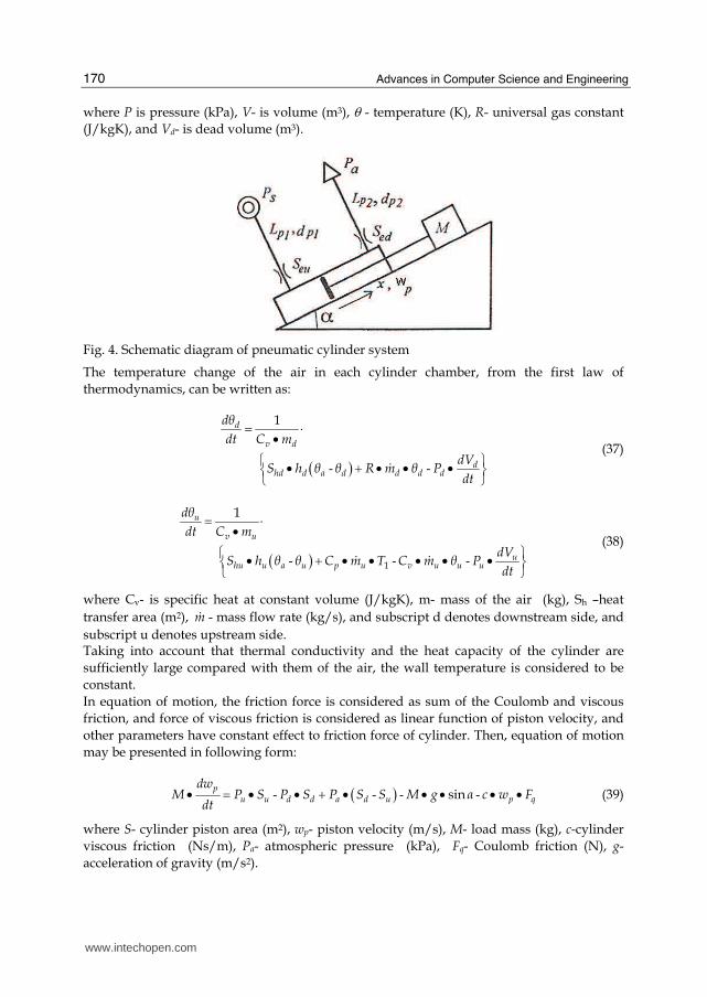
The Figure 4 shows a schematic diagram of pneumatic cylinder system. The system consists

of cylinder, inlet and outlet pipes and two speed control valves at the charge and discharge

sides. Detailed procedure of creating this mathematical model is described in, (Tokashiki,

1996).

For describing behavior of pneumatic cylinder, the basic equations that are used are: state

equation of gases, energy equation and motion equation, (Al Ibrahim, 1992).

-1 ddVdP P V dθ

R θ G Pdt V θ dt dt

•⎛ ⎞= • + • • •⎜ ⎟⎝ ⎠ (36)

www.intechopen.com


170

where P is pressure (kPa), V- is volume (m3), θ - temperature (K), R- universal gas constant

(J/kgK), and Vd- is dead volume (m3).

Fig. 4. Schematic diagram of pneumatic cylinder system

The temperature change of the air in each cylinder chamber, from the first law of

thermodynamics, can be written as:

( )- -

1d

v d

dhd d a d d d d

dθdt C m

dVS h θ θ R m θ P

dt

= ⋅•⎧ ⎫• + • • •⎨ ⎬⎩ ⎭$

(37)

( )- - -1

1u

v u

uhu u a u p u v u u u

dθdt C m

dVS h θ θ C m T C m θ P

dt

= ⋅•⎧ ⎫• + • • • • •⎨ ⎬⎩ ⎭$ $

(38)

where Cv- is specific heat at constant volume (J/kgK), m- mass of the air (kg), Sh –heat

transfer area (m2), m$ - mass flow rate (kg/s), and subscript d denotes downstream side, and

subscript u denotes upstream side. Taking into account that thermal conductivity and the heat capacity of the cylinder are

sufficiently large compared with them of the air, the wall temperature is considered to be

constant.

In equation of motion, the friction force is considered as sum of the Coulomb and viscous

friction, and force of viscous friction is considered as linear function of piston velocity, and

other parameters have constant effect to friction force of cylinder. Then, equation of motion

may be presented in following form:

( )- - - -sinp

u u d d a d u p q

dwM P S P S P S S M g ┙ c w F

dt• = • • + • • • • • (39)

where S- cylinder piston area (m2), wp- piston velocity (m/s), M- load mass (kg), c-cylinder

viscous friction (Ns/m), Pa- atmospheric pressure (kPa), Fq- Coulomb friction (N), g-

acceleration of gravity (m/s2).

www.intechopen.com


171

By using the finite difference method, it can be possible to calculate the airflow through the

pneumatic pipe. The pipe is divided into n partitions.

Applying the continuity equation, and using relation for mass of the air m ┩ A z= • • ∂ and

mass flow m ┩ A w= • •$ , it can be obtained:

-

-1i

i i

mm m

t

∂ =∂ $ $ (40)

Starting from the gas equation, and assuming that the volume of each part is constant,

deriving the state equation it follows, (Kagawa, 1994):

( )--1

i i i ii i

dP R θ R m dθm m

dt V V dt

• •= + •$ $ (41)

The motion equation of the air, is derived from Newton's second law of motion and is

described as:

-

-

2

i i q ii i i

i

P P ww ┣w w w

t ┩ ├ z d z

+ ∂∂ = • • • •∂ • ∂ (42)

where λ is pipe viscous friction coefficient and is calculated as a function of the Reynolds

number:

364, Re 2.5 10

Re┣ x= < (43)

0.25 30.3164 Re , Re 2.5 10┣ x= ≥ (44)

The respective energy can be written as:

- -1 2 1 2st i i i i iE E E L L QΔ = + + (45)

where E1i is input energy, E2i is output energy, L1i is cylinder stroke in downstream side, and

L2i is cylinder stroke in upstream side of pipe model, and the total energy is calculated as

sum of kinematic and potential energy.

Deriving the total energy ΔEst , it is obtained the energy change ΔEst:

2

11( ( ) )

2 2i i

st v i i i

w wdE C m θ m

dt−⎧ ⎫⎛ ⎞+⎪ ⎪⎛ ⎞⎜ ⎟Δ = • • + • •⎨ ⎬⎜ ⎟⎜ ⎟⎝ ⎠⎪ ⎪⎝ ⎠⎩ ⎭

(46)

In equation (45), the inflow and outflow energy as well as the work made by the inflow and

outflow air can be presented :

From the following equation the heat energy Q can be calculated:

( )-i h a iQ h S θ θ= • • (47)

where h is is heat transfer coefficient which can be easily calculated from the Nusselt

number Nu, and thermal conductivity k:

www.intechopen.com


172

2 i i

ip

Nu kh

d

•= (48)

where dp is pipe diameter.

Nusselt number can be calculated from Ditus and Boelter formula for smooth tubes, and for

fully developed turbulent flow:

0.8 0.40.023 Re Pri iNu = • • (49)

and thermal conductivity k can be calculated as a linear function of temperature:

5 37.95 10 2.0465 10i ik θ= • • + • (50)

3.2 Distributed parameter systems

During analyzes and synthesis of control systems, fundamental question which arises is

determination of stability. In accordance with engineer needs, we can roughly divide

stability definitions into: Ljapunov and non-Ljapunov concept. The most useful approach of

control systems is Ljapunov approach, when we observe system on infinite interval, and

that in real circumstances has only academic significance.

Let us consider n- dimensional non-linear vector equation:

( )dxf x

dt= (51)

for 0dx

dt= solution of this equation is xs=0 and we can denote it as equilibrium state.

Equilibrium state xr=0 is stable in sense of Ljapunov if and only if for every constant and

real number ε, exists δ(ε)>0 and the following equation is fulfilled, (Gilles, 1973):

0 0tx x ├== ≤ (52)

for every t ≥0

x ┝< (53)

If following equation exists:

0 0x → for t →∞ (54)

then system equilibrium state is asymptotic stable.

System equilibrium state is stable, if and only if exists scalar, real function V(x), Ljapunov function, which for , 0x r r const< = > , has following features:

a. ( )V x is positively defined

b. ( )dV x

dt is negatively semi defined for t≥0

System equilibrium state is asymptotic stable, if and only if exists:

www.intechopen.com


173

( )dV x

dt is negatively defined for t≥0

Derivation of function V(x) , ( )dV x

dt can be expressed:

( ) ( ) ( ) ( )T T

x x

dV x dxV x V x f x

dt dt= ∇ • • = ∇ • (55)

and

1

.

.

.

.

x

n

x

x

⎡ ⎤∂⎡ ⎤⎢ ⎥⎢ ⎥∂⎢ ⎥⎢ ⎥⎢ ⎥⎢ ⎥⎢ ⎥⎢ ⎥⎢ ⎥⎢ ⎥∇ = ⎢ ⎥⎢ ⎥⎢ ⎥⎢ ⎥⎢ ⎥⎢ ⎥⎢ ⎥⎢ ⎥∂⎢ ⎥⎢ ⎥∂⎢ ⎥⎢ ⎥⎣ ⎦⎣ ⎦

(56)

By using Ljapunov function successfully is solved problem of asymptotic stability of system

equilibrium state on infinite interval.

From strictly engineering point of view it is very important to know the boundaries where

system trajectory comes during there's motion in state space. The practice technical needs

are responsible for non- Ljapunov definitions, and among them is extremely important

behaving on finite time interval- practical stability. Taking into account that system can be

stabile in classic way but also can posses not appropriate quality of dynamic behavior,

and because that it is not applicable, it is important to take system in consideration in

relation with sets of permitted states in phase space which are defined for such a problem.

In theory of control systems there are demands for stability on finite time interval that for

strictly engineering view of point has tremendous importance. The basic difference

between Ljapunov and practical stability is set of initial states of system (Sα) and set of

permitted disturbance (Sε). Ljapunov concept of stability, demands existence of sets Sα

and Sε in state space, for every opened set Sβ permitted states and it is supplied that

equilibrium point of that system will be totally stable, instead of principle of practical

stability where are sets (Sα and Sε) and set Sβ which is closed, determined and known in

advance.

Taking into account principle of practical stability, the following conditions must be

satisfied:

• determine set Sβ - find the borders for system motion

• determine set Sε - find maximum amplitudes of possible disturbance

• determine set Sα of all initial state values

In case that this conditions are regularly determined it is possible to analyze system stability

from practical stability view of point.

www.intechopen.com


174

3.2 Practical stability

Problem of asymptotic stability of system equilibrium state can be solved for distributed

parameter systems, which are described by equation:

( )2

2( , , , ...) 0,

x x xf t x t T

z t t

⎛ ⎞∂ ∂ ∂= ∈⎜ ⎟⎜ ⎟∂ ∂ ∂⎝ ⎠ (57)

with following initial conditions:

( ) ( )0,0x t x t= (58)

To satisfy equation (57), space coordinate z cannot be explicitly defined. The solution of

equation (23) is 0x

z

∂ =∂ , and let the following equation exists:

( ) ( )-, r

xx t z x t

z

∂ =∂ (59)

Assumption 1: Space coordinate z on time interval t∈ (0,T) is constant.

Accepting previous assumption, and equation (58), we have equation for equilibrium state

for system described by equation (57):

( ) 0rx t = (60)

For defining asymptotic stability of equilibrium state the functional V is used:

( ) ( )0

l

V x W x dt= ∫ (61)

where W is scalar of vector x .

We choose functional V like:

( )0

1

2

TTV x x x dt= • •∫ (62)

when it is used expression for norm:

0

TTx x xdt= •∫ (63)

For asymptotic stability of distributed parameter systems described by equation (7), we use

Ljapunov theorems, applied for functional V :

( ) ( ) 2

20

( , , , ... )l

Tx

dV x x xW x f t x dt

dz t t

⎛ ⎞∂ ∂= ∇ • • •⎜ ⎟⎜ ⎟∂ ∂⎝ ⎠∫ (64)

www.intechopen.com


175

where W is scalar function of x.

Let consider distributed parameter system described by following equation:

3

3

x x

tt

∂ ∂= ∂∂ (65)

and initial conditions:

( ) ( )0, ,2

Kx z x T z= • (66)

We use the assumption that equation (61) and initial conditions (62) are not explicit

functions of space coordinate z, so stationary state of system (61) with appropriate border

conditions is represented by following equation:

( ) 0,rx z = with3

30

x

z

∂ =∂ (67)

For determination of asymptotic stability of equilibrium system state, we use functional V

which is expressed:

( ) ( )0

l

V x W x dt= ∫ (69)

where W is scalar function of x .

Functional V is described by :

( ) 41,

4V x t z dt= • ⎡ ⎤ •⎣ ⎦∫ (70)

and the following condition V(x)>0 is fulfilled.

Derivation of functional V is given by following equation:

( )( ) ( )( )

33 3

30 0

4 41, 0,

4

L LdV x x xx dt x dt

dz tz

x T z x z

∂ ∂= • • = • • =∂∂⎡ ⎤ • ⎡ ⎤⎣ ⎦ ⎣ ⎦∫ ∫

(71)

By using equation (65) and by including it in equation (71) it is obtained:

( ) ( )-

44

( 1 ) ( , )4

dV x Kx T z

dz

⎛ ⎞= • ⎡ ⎤⎜ ⎟ ⎣ ⎦⎜ ⎟⎝ ⎠ (72)

and it yields:

( )

0dV x

dt< when K4<1/4, 0.7K < (73)

www.intechopen.com


176

which is necessary and sufficient condition for asymptotic stability of equilibrium state for

system described by equations (61) and (62).

3.3 Distributed control

Control of distributed parameter systems, which depends of time and space coordinate is

called distributed control. If we choose control U, for pressure difference in two close parts

of pneumatic pipe, and for state X, if we choose air velocity through the pneumatic pipe,

with assumptions that are shown during derivation of mathematical model of pneumatic

pipe, finally it is obtained:

[ ], 0,X X

X a X X b U z Lt z

∂ ∂+ • + • • = • ∈∂ ∂ (74)

where 1

,2

┣а bd ┩ ├ z

= =• • .

Nominal distributed control can be solved by using procedure which is described in

(Novakovic, 1989), and result of that control is nominal state wN(t,z) of chosen system. In

that case it yields:

( )( )

( )1 1

,

1,

NN

X XL X t z X

b t b z

a X X U t zb

∂ ∂= • + • •∂ ∂+ • • • =

(75)

where L is appropriate operator. System (73) is exposed to many disturbances, so the real dynamic must be different from nominal. It is applied deviation from nominal system state, then the nominal system state can be realized as:

( ) ( ) ( )-, , , , 0Nx t z X t z X t z z L= < ⋅ . (76)

Time derivation of deviation from nominal system state, can be presented by following equation:

( ) ( ) ( )

-, , ,Nx t z X t z X t z

t t t

∂ ∂ ∂=∂ ∂ ∂ (77)

and from equations (74), it yields:

( ) ( ) -

,,

x t z Xr t z X a X X b U

t z

∂ ∂= + • + • • •∂ ∂ (78)

where NXr

t

∂= ∂

3.4 Application

Using the concept of extern linearization, which is described in, (Meyer, 1983), we can include distributed control in the following form:

www.intechopen.com


177

( ) ( )-, / ,

0

N

XU t z a k X X k X X X r b

z

z L

∂⎡ ⎤= • • + • • + • +⎢ ⎥∂⎣ ⎦≤ ≤

(79)

Including the equation (79) in the equation (78), it yields:

( ) ( )-

,, , 0

x t zk x t z z L

t

∂ = • ≤ ≤∂ (80)

Functional V is chosen in the form:

( ) ( ) ( )2 2

0

1 1, ,

2 2

L

V x x t z dz x t z= • ⎡ ⎤ • = •⎣ ⎦∫ (81)

Derivation of functional V is given as:

( )( ) ( )

0

2

0

, 2

L

L

dV x xx dz

dt t

k x t z dz k V x

∂= • •∂= • ⎡ ⎤ • = • •⎣ ⎦

∫∫

(82)

Taking into account that V(x) is positive defined functional, time derivation of functional

given by equation (82) will be negative defined function for k>0, and in that way all

necessary conditions from Ljapunov theorem applied to functional V, are fulfilled.

1

.

.

.

.

x

n

x

x

∂⎡ ⎤⎢ ⎥∂⎢ ⎥⎢ ⎥⎢ ⎥⎢ ⎥∇ = ⎢ ⎥⎢ ⎥⎢ ⎥⎢ ⎥∂⎢ ⎥∂⎢ ⎥⎣ ⎦

(83)

3.5 Program support

For this kind of symbolically presented problems, the most elegant solution can be achieved by using program language Maple. # # Program support for determination of stability of # distributed parameter systems on finite space interval # described by equation

# 3

x xf

tz

∂ ∂⎛ ⎞= • ⎜ ⎟∂∂ ⎝ ⎠

#

www.intechopen.com


178

# Definition of procedure dpst

dpst:=proc(ulaz3)

# Read input values

read ulaz3;

# Determination of functional V

V:=1/4*int[x(t,z)∧2,z]=norm[x(t,z)]; # Determination of functional V derivation

dV/dz:=int[x(t,z)*diff(x,t),t] # Applying partial integration on equation dV/dt

with(student)

intpart[Int(x*diff(x∧2,z∧2), x)] # Presentation of equation dV/dt

dV/dt;

# Calculation of values for parameter K for which the system is stable

result:= solve(dV/dt,K)

#

If the procedure dpst would be operational for determination the values of parameter K for

which the system is stable, it is necessary to create files with input parameters for current

procedure. For case that is analytically calculated, it is created file input3 with following

input data:

dx/dt=diff(x∧3,z∧3)

x(0,z)= =K/2*x(T,z)

# Program support for distributed parameter systems with distributed control

#

# Definition of procedure dpsdc

dpsdc:=proc(input 1)

# Reading of input parameter values

read input1;


V:=1/2*int[x(t,z)^2,z]=norm[x(t,z)];

# Determinatation of time derivation of functional V

dV/dt:=int[x(t,z)*diff(x,t),z];

# Calculation of time derivation of functional V

derivationfunctional:=solve(dV/dt, z=0..1);

# Calculation the values of parameter K for which the system is stable

solution:=solve(derivationfunctional,K);

For using the procedure dpsdc for determination the values of parameter K it is necessary to

create files that contain input parameters for given procedure. In case, which is calculated,

the file input 1 with input data:

dx/dt=-k*(x,z);

By using task read it yields to reading procedure dpsdc. Specification of input1 as argument

of the procedure dpsdc starts the process of calculation the values of parameter K for which

this distributed parameter system is stable on finite space interval.

It is developed, program support for other types of distributed parameter systems.

www.intechopen.com


179

#

# Program support for determination of stability of

# distributed parameter systems on finite space interval

# described by equation

# x x

ft z

∂ ∂⎛ ⎞= •⎜ ⎟∂ ∂⎝ ⎠

#

# Definition of procedure srppr

srppr:=proc(ulaz1)

# Read input values

read ulaz1;


V:=1/2*int[x(t,z)^2,z]=norm[x(t,z)];

#Determinatation of time derivation of functional V

dV/dt:=int[x(t,z)*diff(x,t),z];

#Solving the functional V

derivationfunctional:=solve(dV/dt, z=0..1);

# Calculation the solution for parameter K for which is

# the system stable

solution:=solve(derfunctional,K);

If the procedure srppr would be operational for determination of value of parameter K for which the system is stable, it is necessary to create files with input parameters for current procedure. It is created file input1 with following data : dx/dt=-vz*diff(x,z); x(t,0)=-K*x(t,l) # Program support for determination of stability of # distributed parameter diffusion systems on finite space # interval # Definition of procedure srppr srpdp:=proc(ulaz2) # Read input values read input1; # Determination of functional V V:=1/2*int[exp(2*┛*z)*x(t,z)^2, z=0..1]; # Determinatation of time derivation of functional V dV/dt:=diff(V,t); # Applying partial integration on equation dV/dt intpart[Int(exp(2*┛*z)*diff(x,z)^2,z=0..1)]=( ┛^2+π^2/l^2)*int[exp(2* ┛*z)*x^2, z=0..1); # Calculation of values for parameter K for which the system is stable resenje:=solve(dV/dt,K); If the procedure spdsr would be operational for determination of value of parameter K for which the system is stable, it is necessary to create files with input parameters for current procedure. It is created file ula2 with following data: dx/dt=diff(x^2,z^2)+2*a*diff(x,z)-b*x x(t,0)=x(t,l)=0

www.intechopen.com


180

3.6 Conclusion

Special class of control systems is focus of our scientific paper. Our main idea is to present a

practical stability solution for this type of systems with distributed control. From practical

view of point, it is crucial to find intervals on which the system is stable, and it is achieved

by using this unique approach. Concerning on one-dimensional problem, where

mathematical model of distributed parameter system is presented by equations which are

dependable of time and only one space coordinate, successfully is applied new method for

determination of stability on finite space interval for distributed parameter systems of

higher order. The program support proved the efficiency of the theory, and it is developed

for various types of distributed parameter systems.

4. Decision making in safety of pneumatic systems

One of the most important tasks in the safety engineering lays in the construction of a

knowledge database of decision support for the pneumatic systems, and on that way to

ensure optimal conditions, improve quality and boost efficiency. Methods of analysis of

control systems and simulation methods, which are used for observing dynamic behavior of

linear systems with time delay, and distributed parameter systems, based on linear algebra,

operation calculus, functional analyse, integral differential equations and linear matrix non-

equations has shown long ago that modern electronic components can be used to achieve

more consistent quality at lower cost in safety engineering. The main idea to do so is that the

quality service is maintained and controlled. Applying the Fuzzy theory in decision making

has given very good results, and provided a flexible framework and over the years

numerous mathematical models have been developed.

There are two basic problems to solve in decision making situations: obtaining alternative,

and achieving consensus about solution from group of experts. First problem takes into

account individual information which existed in collective information units. The later

usually means an agreement of all individual opinions. Usually it is considered two

approaches for developing a choice process in solving of decision making problems: a direct

approach where solution is derived on the basis of the individual relations and as well

indirect approach where solution is based on a collective preference relation. In safe

engineering technical and economic benefits over hard-wired, discrete components has

shown PLC. Main problem in process engineering is practical stability of the system. Chosen

system should be stable in required period of time, and this important task is obtained by

using practical stability theory for distributed parameter systems. Most pneumatic systems

for instance, are described by partial different equations and they belong to group of

distributed parameter systems.

4.1 Definitions and conditions of practical stability

Let us consider first order hyperbolic distributed parameter system, which is decribed by

the following state- space equation:

( ) ( )0 1

,,

x t z xA x t z A

t z

∂ ∂= • +∂ ∂ (84)

with appropriate function of initial state

www.intechopen.com


181

( ) ( )0 , ,

0 , 0x

x t z ┰ t z

t ┬ z ┞

=≤ ≤ ≤ ≤ (85)

where ( ),x t z is n-component real vector of system state, A is matrix appropriate dimension, t is time and z is space coordinate. Definition 1: Distributed parameter system described by equation (84) that satisfies initial

condition (85) is stable on finite time interval in relation to [ξ(t,z), β, T, Z] if and only if:

( ) ( )[ ] [ ], , ( , )

0, , 0,

T

x x┰ t z ┰ t z ξ t z

t ┬ z ┪

• <∀ ∈ ∀ ∈ (86)

then it follows

( ) ( )[ ] [ ]

, ) , ,

0, 0,

Tx t z x t z ┚t T z Z

• <∀ ∈ ∀ ∈ (87)

where ξ(t,z) is scalar function with feature ( )0 , , 0 , 0ξ t z ┙ t ┬ z ┞< ≤ ≤ ≤ ≤ ≤ where ┙ is real number, ┚ € R and ┚ > ┙. Let calculate the fundamental matrix for this class of system:

( ) ( ) ( )-1

,,

d s ┫A sI A s ┫

d┫Φ = • •Φ (88)

where after double Laplace transformation, and necessary approximation finally it is obtained, (Dihovicni, 2007):

( ) ( ), expt z A t zΦ = ⋅ ⋅ (89)

where 0 1

1

I A AA

A

− ⋅= .

Theorem1: Distributed parameter system described by equation (84) that satisfies internal condition (85) is stable on finite time interval in relation to [ξ(t,z), β, T, Z] if it is satisfied following condition:

( )2┤ A t z ┚e

┙• • < (90)

Proof: Solution of equation (84) with initial condition (85) is possible to describe as:

( ) ( ) ( ), , 0,0x t z t z ┰= Φ ⋅ (91)

By using upper equation it follows:

( ) ( ) ( ) ( )

( ) ( ), , 0,0 ,

0,0 ,

T T T

x

T

x

x t z x t z ┰ t z

┰ t z

⎡ ⎤• = •Φ ⋅⎣ ⎦⎡ ⎤•Φ⎣ ⎦

(92)

By using well-known ineqality

www.intechopen.com


182

( ) [ ] ( ){ }, exp expt z A t z ┤ A t zΦ = • • ≤ • • (93)

and taking into account that:

( ) ( )( ) ( )( )0,0 0,0

0,0 0,0

T

x x

T T

x x

┰ ┰ ┙

┰ ┰ ┙

• <= < (94)

then it follows:

( ) ( ) ( )2, ,

┤ A t zTx t z x t z e ┙• ≤ •i i (95)

Applying the basic condition of theorem 1 by using equation (91) to further inequality it is obtained, (Dihovicni, 2007):

( ) ( ), ,T ┚x t z x t z ┙ ┚

┙⎛ ⎞• < • <⎜ ⎟⎝ ⎠ (96)

Theorem 2: Distributed parameter system described by equation (84) that satisfied initial condition (85) is stable on finite time interval in relation to [ξ(t,z), β, T, Z] if it is satisfied following condition:

( )

[ ] [ ]/

1

0, 0,

┤ A t z ┚ ┙e

┬ ┞ A

t ┬ z ┪

• • < + •∀ ∈ ∀ ∈

(97)

The proof of this theorem is given in (Dihovicni, 2006).

Let (.)

x is any vector norm and any matrix norm 2⋅ which originated from this vector.

Following expresions are used:

( )1/2

2

Tx x x= • and ( )1/2 *2

┣ A A⋅ = •

where * and T are transpose-conjugate and transport matrixes. It is important to define matrix measure as:

( ) -

0

1 1lim┝

┝ A┤ A

┝→+ •= (98)

The matrix measure µ may be defined in three different forms according to the norm which is used:

( ) ( )( ) ( )( ) ( )

11,

2

1

max Re

1max

2

max Re

n

kk iki i k

Ti

n

ii kik

┤ A a a

┤ A ┣ A A

┤ A a a

= ≠

∞ =

⎛ ⎞= +⎜ ⎟⎜ ⎟⎝ ⎠= +

⎛ ⎞= +⎜ ⎟⎝ ⎠

∑

∑ (99)

www.intechopen.com


183

Definition 2: Distributed parameter system described by equation (84) that satisfies initial

condition (85) is stable on finite time interval in relation to [ξ(t,z), β, T, Z] if and only if, (Dihovicni, 2007):

( ) ( )2

, ,x┰ t z ξ t z< (100)

then follows

( )2

x t ┚< (101)

where ξ(t,z) is scalar function with feature ( )0 , ) , 0 , 0ξ t z ┙ t ┬ z ┞< ≤ ≤ ≤ ≤ ≤ ┙ is real number, ┚ € R and ┚ > ┙. Theorem 3: Distributed parameter system described by equation (84) that satisfies initial

condition (85) is stable on finite time interval in relation to [┙, β, T, Z] if it is satisfied following condition:

( ) ( )[ ] [ ]2

12

/

1

0, 0,

┤ A t z ┚ ┙e

┤ A

t T z Z

⋅ ⋅−< +

∀ ∈ ∀ ∈ (102)

Proof: Solution of equation (1) with initial condition (2) is possible to describe by using fundamental matrix as:

( ) ( ) ( ), , 0,0x

x t z t z ┰= Φ • (103)

By using the norms of left and right side of the equation (103) it follows:

( ) ( ) ( )2, ,

┤ A t zTx t z x t z e ┙⋅ ⋅⋅ ≤ ⋅ (104)

and by using well-known inequality

( ) ( ){ }2

exp expA t z ┤ A t z• • ≤ • • (105)

0 , 0t z≥ ≥

it follows:

( ) ( ) ( )2

2 2, 0,0

┤ A t z

xx t z e ┰⋅ ⋅≤ • (106)

and by using equation (100) it is obtained:

( ) ( )2

2,

┤ A t zx t z ┙ e

• •≤ • (107)

so finally it is obtained:

( ) ( ) ( ){ }2 122

, 1┤ A t z

x t z ┙ e ┤ A•≤ ⋅ + (108)

www.intechopen.com


184

Applying the basic condition of theorem 3 by using equation (19) it is obtained:

( )

[ ] [ ]2

0, , 0,

x t ┚

t T z Z

<∀ ∈ ∀ ∈ (109)

Theorem 4: Distributed parameter system described by equation (85) that satisfies initial

condition (86) is stable on finite time interval in relation to [┙, β, T, Z], if it is satisfied following condition, (Dihovicni, 2007):

( )[ ] [ ]0, , 0,

┤ A t z ┚e

┙t T z Z

• • <∀ ∈ ∀ ∈

(110)

Theorem 5: Distributed parameter system described by equation (84) that satisfies initial

condition (85) is stable on finite time interval in relation to [t0, J, ┙, ┚, Z], if it is satisfied

following condition:

( ) ( )[ ] [ ]

-0 max

2 20 max1 ,

0, 0,

t t z ┫ ┚t t ┫ e

┙t J z Z

⋅ ⋅ •⎡ ⎤+ • • <⎣ ⎦∀ ∈ ∀ ∈

(111)

where σmax represents maximum singular value of matrix. The proof of this theorem is given

in (Dihovicni, 2007).

4.2 Architecture

There are few well known stages in developing computer decision support systems based on knowledge which include choosing suitable mathematical tools, formalization of the subject area, and development of the corresponding software. In the first phase the problem lays in making right diagnosis and in analyses of the requirements and as well the analyses of the system incidents caused by specification, design and the implementation of the project, (Bergmans, 1996). The problem of diagnostics may be stated such as finite number of subsets, or it should be applied classical investigation methods, (Thayse, 1996). System architecture consists of the following modules:

• Stability checking module. This module is designed as program for checking the

practical stability of the system. If the system passes this check it goes further to other

modules.

• Analysis module of safe fault-tolerant controllers, I/O, engineering and pressure

transmitters.

• Diagnostics module

• Knowledge Module of all possible situations and impacts to pneumatic systems

• Optimal solution- decision making module

• Presentation module

For system realization an object oriented programming approach has been used, and the

program has been developed using the C# language. Each module has a supportive

library, and the logical structure is based on the classes, which are described down below

for ilustrating purpose.

www.intechopen.com


185

• Main classes are:

• Analyses group which has a primary task of collecting necessary facts about system.

• Practical stability group which determines if the system is stable or not. If the system is

unstable in view of practical stability, then it is automaticly rejected.

• Diagnosis group describes all possible casualities for not required results, or potencial

casualities for not optimal costs.

• Performance group is used for the optimal performance.

• Cost group is used for the optimal cost effect.

• Decision making algorithm for optimal performance and cost consists of two phases:

• Phase 1 is used for input Analyses class, Practical stability class and diagnosis class.

• Phase 2 is used for output Performance and Cost group.

4.3 Conclusion

By analysing process systems from safety and optimal cost perspective, it is important to recognize which systems are not stable in real conditions. From engineering state of view we are interested in such a systems which are stable in finite periods of time, so our first concern should be to maintain stable and safe systems. Our knowledge database is created in DB2, and it involved all possible reasons for non adequate performanse. Key modules for obtaining best performance, safety and the low cost are a good base for the program support in C# programming language and the UML representation.

5. References

Al-Ibrahim, A.M., and Otis, D.R., Transient Air Temperature and Pressure Measurements During

the Charging and Discharging Processes of an Actuating Pneumatic Cylinder,

Proceedings of the 45th National Conference on Fluid Power, 1992

Andersen, B..; Wiley, J. (1967), The Analysis and Design of Pneumatic Systems, INC. New York-

London-Sydney, 1967

Bergmans J., Gutnikov S., Krasnoproshin V., Popok S. and Vissia H., Computer-Base Support

to Decision-Making in Orthopaedics, International Conference on Intelligent

Technologies in Human related Sciences, vol. 2: Leon, Spain, (1996) pp 217-223

Dihovicni, Dj.; Nedic, N. (2006), Stability of Distributed Parameter Systems on Finite Space

Interval, 32-end Yupiter Conference, Zlatibor, September 2006, pp 306-312

Dihovicni, Dj.; Nedic, N. (2007), Practical Stability of Linear Systems with Delay in State,

AMSE, Association for the Advancement of Modelling & Simulation Techniques in

Enterprises, Tassin La-Demi-Lune, France, Vol 62 n0 2 (2007) pp 98-104

Dihovicni, Dj.; Nedic, N., “Simulation, Animation and Program Support for a High Performance

Pneumatic Force Actuator System”, Mathematical and Computer Modelling 48 (2008),

Elsevier, Washington, pp. 761–768

Gilles, E; Systeme mit verteilten Parametern, Wien 1973

Kagawa T Fujita T, Takeuchi M. Dynamic Response and Simulation Model of Pneumatic Pipe

Systems, Proc 7th Bath International Fluid Power Workshop 1994

Novakovic, B.; Metode vodjenja tehnickih sistema, Skolska knjiga, Zagreb 1989

Richer, E.; Hurmuzlu, Y., A High Performance Pneumatic Force Actuator System, ASME Journal

of Dynamic Systems Measurement and Control, September 2000, pp 416-425

www.intechopen.com


186

Thayse A., Gribont P, Approche Logique de LIInteligence Artificielle l De la Logique, Bordas,

(1997).

Tokashiki, L.; Fujita, T. ; Kogawa T., Pan W., Dynamic, Characteristics of Pneumatic Cylinders

Including pipes, 9th Bath International Fluid Power Workshop, September 1996, pp

1-14

www.intechopen.com

Advances in Computer Science and EngineeringEdited by Dr. Matthias Schmidt

ISBN 978-953-307-173-2Hard cover, 462 pagesPublisher InTechPublished online 22, March, 2011Published in print edition March, 2011

InTech EuropeUniversity Campus STeP Ri Slavka Krautzeka 83/A 51000 Rijeka, Croatia Phone: +385 (51) 770 447 Fax: +385 (51) 686 166www.intechopen.com

InTech ChinaUnit 405, Office Block, Hotel Equatorial Shanghai No.65, Yan An Road (West), Shanghai, 200040, China

Phone: +86-21-62489820 Fax: +86-21-62489821

The book Advances in Computer Science and Engineering constitutes the revised selection of 23 chapterswritten by scientists and researchers from all over the world. The chapters cover topics in the scientific fields ofApplied Computing Techniques, Innovations in Mechanical Engineering, Electrical Engineering andApplications and Advances in Applied Modeling.

How to referenceIn order to correctly reference this scholarly work, feel free to copy and paste the following:

Djordje Dihovicni and Miroslav Medenica (2011). Mathematical Modelling and Simulation of PneumaticSystems, Advances in Computer Science and Engineering, Dr. Matthias Schmidt (Ed.), ISBN: 978-953-307-173-2, InTech, Available from: http://www.intechopen.com/books/advances-in-computer-science-and-engineering/mathematical-modelling-and-simulation-of-pneumatic-systems

© 2011 The Author(s). Licensee IntechOpen. This chapter is distributedunder the terms of the Creative Commons Attribution-NonCommercial-ShareAlike-3.0 License, which permits use, distribution and reproduction fornon-commercial purposes, provided the original is properly cited andderivative works building on this content are distributed under the samelicense.

https://creativecommons.org/licenses/by-nc-sa/3.0/

mathematical modelling and simulation of pneumatic systems

Documents