mathematical modeling using differential equations, and

Mathem

atical Modeling using Diff

erential Equations, and Netw

ork Theory • Ioannis Dassios

Mathematical Modeling using Differential Equations, and Network Theory

Printed Edition of the Special Issue Published in Applied Sciences

wwww.mdpi.com/journal/applsci

Ioannis DassiosEdited by

Mathematical Modeling usingDifferential Equations, and NetworkTheory

Mathematical Modeling usingDifferential Equations, and NetworkTheory

Special Issue Editor

Ioannis Dassios

MDPI • Basel • Beijing • Wuhan • Barcelona • Belgrade • Manchester • Tokyo • Cluj • Tianjin

Special Issue Editor

Ioannis Dassios

University College Dublin

Ireland

Editorial Office

MDPI

St. Alban-Anlage 66

4052 Basel, Switzerland

This is a reprint of articles from the Special Issue published online in the open access journal

Applied Sciences (ISSN 2076-3417) (available at: https://www.mdpi.com/journal/applsci/special

issues/network theory).

For citation purposes, cite each article independently as indicated on the article page online and as

indicated below:

LastName, A.A.; LastName, B.B.; LastName, C.C. Article Title. Journal Name Year, Article Number,

Page Range.

ISBN 978-3-03928-825-0 (Hbk) ISBN 978-3-03928-826-7 (PDF)

c© 2020 by the authors. Articles in this book are Open Access and distributed under the Creative

Commons Attribution (CC BY) license, which allows users to download, copy and build upon

published articles, as long as the author and publisher are properly credited, which ensures maximum

dissemination and a wider impact of our publications.

The book as a whole is distributed by MDPI under the terms and conditions of the Creative Commons

license CC BY-NC-ND.

Contents

About the Special Issue Editor . . . . . . . . . . . . . . . . . . . . . . . . . . . . . . . . . . . . . . vii

Ioannis Dassios

Special Issue on Mathematical Modeling Using Differential Equations and Network TheoryReprinted from: Appl. Sci. 2020, 10, 1895, doi:10.3390/app10051895 . . . . . . . . . . . . . . . . . 1

Adel Ouannas, Amina-Aicha Khennaoui, Samir Bendoukha, Thoai Phu Vo, Viet-Thanh

Pham and Van Van Huynh

The Fractional Form of the Tinkerbell Map Is ChaoticReprinted from: Appl. Sci. 2018, 8, 2640, doi:10.3390/app8122640 . . . . . . . . . . . . . . . . . . . 5

Pieter Audenaert, Didier Colle and Mario Pickavet

Policy-Compliant Maximum Network FlowsReprinted from: Appl. Sci. 2019, 9, 863, doi:10.3390/app9050863 . . . . . . . . . . . . . . . . . . . 17

Ping Guo, Zhen Sun, Chao Peng, Hongfei Chen and Junjie Ren

Transient-Flow Modeling of Vertical Fractured Wells with Multiple Hydraulic Fractures inStress-Sensitive Gas ReservoirsReprinted from: Appl. Sci. 2019, 9, 1359, doi:10.3390/app9071359 . . . . . . . . . . . . . . . . . . . 35

Manuel De la Sen and Asier Ibeas

Parametrical Non-Complex Tests to Evaluate Partial Decentralized Linear-Output FeedbackControl Stabilization Conditions from Their Centralized Stabilization CounterpartsReprinted from: Appl. Sci. 2019, 9, 1739, doi:10.3390/app9091739 . . . . . . . . . . . . . . . . . . . 59

Dejan Brkic and Pavel Praks

Short Overview of Early Developments of the Hardy Cross Type Methods for Computation ofFlow Distribution in Pipe NetworksReprinted from: Appl. Sci. 2019, 9, 2019, doi:10.3390/app9102019 . . . . . . . . . . . . . . . . . . . 79

Bo Li, Yun Wang and Xiaobing Zhou

Multi-Switching Combination Synchronization of Three Fractional-Order Delayed SystemsReprinted from: Appl. Sci. 2019, 9, 4348, doi:10.3390/app9204348 . . . . . . . . . . . . . . . . . . . 95

Hassan Khan, Rasool Shah, Dumitru Baleanu, Poom Kumam and Muhammad Arif

Analytical Solutions of (2+Time Fractional Order) Dimensional Physical Models, UsingModified Decomposition MethodReprinted from: Appl. Sci. 2020, 10, 122, doi:10.3390/app10010122 . . . . . . . . . . . . . . . . . . 113

Izaz Ali, Hassan Khan, Rasool Shah, Dumitru Baleanu, Poom Kumam and Muhammad Arif

Fractional View Analysis of Acoustic Wave Equations, Using Fractional-OrderDifferential EquationsReprinted from: Appl. Sci. 2020, 10, 610, doi:10.3390/app10020610 . . . . . . . . . . . . . . . . . . 133

v

About the Special Issue Editor

Ioannis Dassios is currently a UCD Research Fellow/Assistant Professor at AMPSAS,

University College Dublin, Ireland. His research interests include dynamical systems, mathematics

of networks, differential and difference equations, singular systems, fractional calculus, optimization

methods, linear algebra, and mathematical modeling (materials, electrical power systems, economic

models, etc). He studied Mathematics, completed a two-year MSc in Applied Mathematics and

Numerical Analysis, and obtained his Ph.D. degree in Applied Mathematics at University of Athens,

Greece with the grade ”Excellent” (highest mark in the Greek system). He had positions at

the University of Edinburgh, U.K; University of Manchester, U.K.; and University of Limerick,

Ireland. He has published more than 55 articles in internationally leading academic journals and

has participated in several international collaborations. He has served as a reviewer more than 500

times in more than 75 different journals, he has been member in scientific and organizing committees

of international conferences, and he is also member of editorial boards of peer-reviewed journals.

Finally, he has received several awards such as travel grants, for reviewing and for his contributions

to his institute.

vii

applied sciences

Editorial

Special Issue on Mathematical Modeling UsingDifferential Equations and Network Theory

Ioannis Dassios

AMPSAS, University College Dublin, Dublin 4, Ireland; [email protected]

Received: 1 March 2020; Accepted: 3 March 2020; Published: 10 March 2020

1. Introduction

This special issue collects the latest results on differential/difference equations, the mathematicsof networks, and their applications to engineering, and physical phenomena. The Special Issuehas 42 submissions and eight high-quality papers which got published with original research results.The Special Issue brought together mathematicians with physicists, engineers, as well as other scientists.Topics covered in this issue:

• Differential/difference equations• Mathematics of networks• Fractional calculus• Partial differential equations• Discrete calculus• Mathematical models using dynamical systems

2. Acoustic Wave Equations Using Fractional-Order Differential Equations

In [1], the authors present a newly developed technique, defined as a variational homotopyperturbation transform method in order to solve fractional-order acoustic wave equations. The basicidea behind this article is to extend the variational homotopy perturbation method to the variationalhomotopy perturbation transform method.

The proposed method is an accurate and straightforward technique to solve fractional-orderpartial differential equations, and can be considered as a practical analytical technique to solvenon-linear fractional partial differential equations compared to other analytical techniques existing inthe literature. Several illustrative examples verify the method.

3. Analytical Solutions of Dimensional Physical Models Using Modified Decomposition Method

In [2], the authors present a new analytical technique based on an innovative transformation inorder to solve (2+time fractional-order) dimensional physical models. The proposed method is basedon the hybrid methodology of Shehu transformation along with the Adomian decomposition method.

The solutions of the targeted problems are represented by graphs and are obtained in a series formthat has the desired rate of convergence. The method is, in general, a practical analytical techniqueto solve linear and non-linear fractional partial differential equations. Numerical examples are givenusing the proposed method.

4. Multi-Switching Combination Synchronization of Fractional-Order Delayed Systems

In [3] the authors investigate multi-switching combination synchronization of three fractional-orderdelayed systems. This is actually a generalization of previous multi-switching combinationsynchronization of fractional-order systems by introducing time-delays.

Based on the stability theory of linear fractional-order systems with multiple time-delays,the article provides appropriate controllers to obtain multi-switching combination synchronization of

Appl. Sci. 2020, 10, 1895; doi:10.3390/app10051895 www.mdpi.com/journal/applsci1

Appl. Sci. 2020, 10, 1895

three non-identical fractional-order delayed systems. In addition, numerical simulations show thatthey are in accordance with the theoretical analysis given.

5. An Overview of Early Developments of the Hardy–Cross-Type Methods

In [4], the authors provide an overview of early developments of the Hardy–Cross-type methodsfor computation of flow distribution in pipe networks.

Cross originally proposed a method for analysis of flow in networks of conduits or conductorsin 1936. His method was the first really useful engineering method in the field of pipe networkcalculation. Only electrical analogs of hydraulic networks were used before the Hardy–Cross method.A problem with flow resistance versus electrical resistance makes these electrical analog methodsobsolete. The method by Hardy–Cross is taught extensively at faculties, and it remains an importanttool for the analysis of looped pipe systems. Engineers today mostly use a modified Hardy–Crossmethod that considers the whole looped network of pipes simultaneously (use of these methodswithout computers is practically impossible).

In addition, in [4] a method from a Russian practice published during the 1930s, which is similarto the Hardy–Cross method, is also described. Some notes from the work of Hardy–Cross are alsopresented. Furthermore, an improved version of the Hardy–Cross method, which significantly reducesthe number of iterations, is presented and discussed.

Finally, the authors present results on tested multi-point iterative methods, which can be used asa substitution for the Newton–Raphson approach used by Hardy–Cross.

6. Parametrical Non-Complex Tests to Evaluate Partial Decentralized Linear-Output FeedbackControl Stabilization Conditions

In [5], the authors formulate sufficiency-type linear-output feedback decentralized closed-loopstabilization conditions if the continuous-time linear dynamic system can be stabilized under linearoutput-feedback centralized stabilization.

The provided tests are simple to evaluate, while they are based on the quantification of thesufficient smallness of the parametrical error norms between the control, output, interconnection andopen-loop system dynamics matrices and the corresponding control gains in the decentralized caserelated to the centralized counterpart.

The tolerance amounts of the various parametrical matrix errors are described by the maximumallowed tolerance upper-bound of a small positive real parameter that upper-bounds the variousparametrical error norms. Such a tolerance is quantified by considering the first or second powers ofsuch a small parameter.

The results are seen to be directly extendable to quantify the allowed parametrical errors thatguarantee the closed-loop linear output-feedback stabilization of a current system related to its nominalcounterpart. Several numerical examples are included and discussed in the article.

7. Transient-Flow Modeling of Vertical Fractured Wells with Multiple Hydraulic Fractures

Massive hydraulic fracturing of vertical wells has been extensively employed in the developmentof low-permeability gas reservoirs. The existence of multiple hydraulic fractures along a vertical wellmakes the pressure profile around the vertical well complex.

In [6], the authors study the pressure dependence of permeability in order to develop a seepagemodel of vertically fractured wells with multiple hydraulic fractures. Both transformed pseudo-pressureand perturbation techniques have been employed to linearize the proposed model.

The proposed work further enriches the understanding of the influence of the stress sensitivity onthe performance of a vertical fractured well with multiple hydraulic fractures and can be used to moreaccurately interpret and forecast the transient pressure.

Some key points in the article are the superposition principle and a hybrid analytical-numericalmethod that are used to obtain the bottom-hole pseudo-pressure solution, the type curves for

2

Appl. Sci. 2020, 10, 1895

pseudo-pressure that are presented and identified, and finally, the discussion that is included onthe effects of the relevant parameters on the type curve and the error caused by neglecting thestress sensitivity.

8. Policy-Compliant Maximum Network Flows

Computer network administrators are often interested in the maximal bandwidth that can beachieved between two nodes in the network, or how many edges can fail before the network getsdisconnected. Classic maximum flow algorithms that solve these problems are well-known. However,in practice, network policies are in effect, severely restricting the flow that can actually be set up.These policies are put into place to conform to service level agreements and optimize networkthroughput, and can have a large impact on the actual routing of the flows.

In [7], the authors model the problem and define a series of progressively more complex conditionsand algorithms that calculate increasingly tighter bounds on the policy-compliant maximum flowusing regular expressions and finite-state automata. This is the first time that specific conditionsare deduced, which characterize how to calculate policy-compliant maximum flows using classicalgorithms on an unmodified network.

9. The Fractional Form of the Tinkerbell Map Is Chaotic

In [8], the authors are concerned with a fractional Caputo-difference form of the well-knownTinkerbell chaotic map. The dynamics of the proposed map are investigated numerically throughphase plots, bifurcation diagrams, and Lyapunov exponents considered from different perspectives.

In addition, a stabilization controller is proposed, and the asymptotic convergence of the states isestablished by means of the stability theory of linear fractional discrete systems. Numerical results areemployed to confirm the analytical findings.

Funding: This Editorial was supported by: Science Foundation Ireland, by funding Ioannis Dassios under GrantNo. SFI/15/IA/3074.

Acknowledgments: This issue would not have been possible without the help of a variety of talented authors,professional reviewers, and the dedicated editorial team of Applied Sciences. Thank you to all the authors andreviewers for this opportunity. Finally, thanks to the Applied Sciences editorial team.

Conflicts of Interest: The author declares no conflict of interest.

References

1. Ali, I.; Khan, H.; Shah, R.; Baleanu, D.; Kumam, P.; Arif, M. Fractional View Analysis of Acoustic WaveEquations, Using Fractional-Order Differential Equations. Appl. Sci. 2020, 10, 610. [CrossRef]

2. Khan, H.; Farooq, U.; Shah, R.; Baleanu, D.; Kumam, P.; Arif, M. Analytical Solutions of (2+Time FractionalOrder) Dimensional Physical Models, Using Modified Decomposition Method. Appl. Sci. 2020, 10, 122.[CrossRef]

3. Li, B.; Wang, Y.; Zhou, X. Multi-Switching Combination Synchronization of Three Fractional-Order DelayedSystems. Appl. Sci. 2019, 9, 4348. [CrossRef]

4. Brkic, D.; Praks, P. Short Overview of Early Developments of the Hardy Cross Type Methods for Computationof Flow Distribution in Pipe Networks. Appl. Sci. 2019, 9, 2019. [CrossRef]

5. De la Sen, M.; Ibeas, A. Parametrical Non-Complex Tests to Evaluate Partial Decentralized Linear-OutputFeedback Control Stabilization Conditions from Their Centralized Stabilization Counterparts. Appl. Sci.2019, 9, 1739. [CrossRef]

6. Guo, P.; Sun, Z.; Peng, C.; Chen, H.; Ren, J. Transient-Flow Modeling of Vertical Fractured Wells withMultiple Hydraulic Fractures in Stress-Sensitive Gas Reservoirs. Appl. Sci. 2019, 9, 1359. [CrossRef]

3

Appl. Sci. 2020, 10, 1895

7. Audenaert, P.; Colle, D.; Pickavet, M. Policy-Compliant Maximum Network Flows. Appl. Sci. 2019, 9, 863.[CrossRef]

8. Ouannas, A.; Khennaoui, A.; Bendoukha, S.; Vo, T.; Pham, V.; Huynh, V. The Fractional Form of the TinkerbellMap Is Chaotic. Appl. Sci. 2018, 8, 2640. [CrossRef]

c© 2020 by the authors. Licensee MDPI, Basel, Switzerland. This article is an open accessarticle distributed under the terms and conditions of the Creative Commons Attribution(CC BY) license (http://creativecommons.org/licenses/by/4.0/).

4

applied sciences

Article

The Fractional Form of the Tinkerbell Map Is Chaotic

Adel Ouannas 1, Amina-Aicha Khennaoui 2, Samir Bendoukha 3, Thoai Phu Vo 4,

Viet-Thanh Pham 5,* and Van Van Huynh 6

1 Department of Mathematics and Computer Science, University of Larbi Tebessi, Tebessa 12002, Algeria;[email protected]

2 Department of Mathematics and Computer Sciences, University of Larbi Ben M’hidi, Oum El Bouaghi 04000,Algeria; [email protected]

3 Electrical Engineering Department, College of Engineering at Yanbu, Taibah University, Medina 42353,Saudi Arabia; [email protected]

4 Faculty of Electrical and Electronics Engineering, Ton Duc Thang University, Ho Chi Minh City, Vietnam;[email protected]

5 Nonlinear Systems and Applications, Faculty of Electrical and Electronics Engineering,Ton Duc Thang University, Ho Chi Minh City, Vietnam

6 Modeling Evolutionary Algorithms Simulation and Artificial Intelligence, Faculty of Electrical andElectronics Engineering, Ton Duc Thang University, Ho Chi Minh City, Vietnam; [email protected]

* Correspondence: [email protected]

Received: 3 December 2018; Accepted: 12 December 2018; Published: 16 December 2018

Abstract: This paper is concerned with a fractional Caputo-difference form of the well-knownTinkerbell chaotic map. The dynamics of the proposed map are investigated numerically throughphase plots, bifurcation diagrams, and Lyapunov exponents considered from different perspectives.In addition, a stabilization controller is proposed, and the asymptotic convergence of the states isestablished by means of the stability theory of linear fractional discrete systems. Numerical resultsare employed to confirm the analytical findings.

Keywords: fractional discrete calculus; discrete chaos; Tinkerbell map; bifurcation; stabilization

1. Introduction

Throughout the last 50 years, chaotic dynamical systems have attracted increasing attention dueto their applicability in a range of diverse and multidisciplinary fields. A dynamical system is saidto be chaotic if its states are extremely sensitive to small variations in the initial conditions. Anotherimportant property of chaotic systems is that they have attractors characterized by a complicated setof points with a fractal structure commonly referred to as a strange attractor. This chaotic behaviorwas first observed in continuous dynamical systems and was thought to be an undesirable property.The first chaotic system encountered in the modeling of a real-life phenomena is that of Lorenz [1],which describes atmospheric convection. Soon after, researchers found that chaotic systems can also bediscrete. A number of chaotic maps were proposed throughout the years including the Hénon map [2],the logistic map [3], the Lozi map [4], the 3D Stefanski map [5], the Rössler map [6], and many more.Recently, nonlinear oscillations on Riemannian manifolds that can exhibit a chaotic behavior wereintroduced in [7,8]. Other related works include an investigation of the chaotic dynamics in a fractionallove model with an external environment, as in [9], and an extension using a fuzzy function [10].

In recent years, with the growing interest in fractional discrete calculus [11], people have startedlooking into fractional chaotic maps. Although fractional maps come with considerable addedcomplexity, they provide better flexibility in the modeling of natural phenomena and lead to richerdynamics with more degrees of freedom. Among the fractional chaotic maps that have been proposed,studied, and applied over the last five years are the fractional logistic map [12], the fractional Hénon


Appl. Sci. 2018, 8, 2640

map [13], the generalized hyperchaotic Hénon map [14], and the fractional unified map [15]. Perhapsthe main concern of the research community has been the possibility of controlling and synchronizingthese types of maps [15–20]. An application of a generalized fractional logistic map to data encryptionand its FPGA implementation was achieved in [21].

In this paper, we are interested in the Tinkerbell discrete-time chaotic system, which is of the form:

{x (n + 1) = x2 (n)− y2 (n) + αx (n) + βy (n) ,y (n + 1) = 2x (n) y (n) + γx (n) + δy (n) ,

(1)

where α, β, γ, and δ are system parameters and n represents the discrete iteration step. It is rumoredthat the map (1) derives its name from the famous Cinderella story, as the trajectory followed by themap resembles that of Tinkerbell appearing in the movie adaptation of the fairy tale. The Tinkerbellmap has been studied by many as it exhibits very rich dynamics including a chaotic behavior and arange of periodic states. For instance, its bifurcation subject to different scenarios and initial settingshas been studied in [22–25]. A more comprehensive study was performed in [26]. The authorsidentified conditions for the existence of fold bifurcation, flip bifurcation, and Hopf bifurcation in theTinkerbell map.

In order to visualize the dynamics of the map (1), we resort to phase plots, bifurcation diagrams,and Lyapunov exponent estimation. We assume parameter values α = 0.9, β = −0.6013, γ = 2,and δ = 0.5 and initial states (x (0) , y (0)) = (−0.72,−0.64). The results are depicted in Figure 1.The Tinkerbell map’s phase plot is depicted in Figure 1a. Based on Figure 1b, we can see that theestimated Lyapunov exponents of (1) are given by λ1 ≈ 0.2085 and λ2 ≈ −0.4925. It is well knownthat a positive Lyapunov exponent indicates a chaotic behavior. The remaining parts of Figure 1 depictthe bifurcation diagrams of the map (1) with respect to different parameters. These diagrams confirmthat the map exhibits a range of different behaviors.

It should be clear to the reader that the Tinkerbell map has rich dynamics and is heavily dependenton its parameters, as well as the initial setting. The main objective of this paper is to investigate thefractional Caputo-difference form of the Tinkerbell map in order to benefit from the added degreesof freedom due to the fractional nature. It is expected that the fractional form will have even richerdynamics and may consequently be more suitable for applications that require a higher entropy levelsuch as data/image encryption.

6

Appl. Sci. 2018, 8, 2640

Figure 1. (a) Attractor of the Tinkerbell map (2) with (α, β, γ, δ) = (0.9,−0.6013, 2, 0.5) and initialconditions (x (0) , y (0)) = (−0.72,−0.64). (b) Estimated Lyapunov exponents by means of the Jacobianmatrix method. (c) Bifurcation plot with α ∈ [−0.5, 1] as the critical parameter and Δα = 0.0075.(d) Bifurcation plot with β ∈ [−0.6,−0.1] as the critical parameter and Δβ = 0.0025. (e) Bifurcationplot with γ ∈ [0, 2.1] as the critical parameter and Δγ = 0.01. (f) Bifurcation plot with δ ∈ [−1, 0.6] asthe critical parameter and Δδ = 0.008.

2. Fractional Tinkerbell Map

In this section, we use recent developments in fractional discrete calculus to define theCaputo-difference fractional map corresponding to (1). First, let us define the υth fractional sumof anarbitrary function X (t) [27] as:

Δ−υa X (t) =

1Γ (υ)

t−υ

∑s=a

(t − s − 1)(υ−1) X (s) , (2)

for t ∈ Na+n−υ and υ > 0, where Na := {a, a + 1, a + 2, ...}. Note that the term t(υ) is known as thefalling function and may be defined by means of the Gamma function Γ as:

t(υ) =Γ (t + 1)

Γ (t + 1 − υ). (3)

7

Appl. Sci. 2018, 8, 2640

Based on this definition of the fractional sum, we may define the Caputo-like fractionaldifference operator.

In this section, we would like to produce a fractional difference form of the Tinkerbell map (1).First, we take the difference form, which for function x (t) : Na → R with fractional order υ �∈ N isgiven by:

CΔυa x (t) = Δ−(n−υ)

a Δnx (t) . (4)

Substituting yields the final form proposed in [28], which is defined as:

CΔυa x (t) =

1Γ (n − υ)

t−(n−υ)

∑s=a

(t − s − 1)(n−υ−1) Δnx (s) , (5)

where t ∈ Na+n−υ and n = �υ�+ 1.We are now ready to examine the fractional map. First, we take the difference form of (1) to obtain:

{Δx (n) = x2 (n)− y2 (n) + (α − 1) x (n) + βy (n) ,Δy (n) = 2x (n) y (n) + γx (n) + (δ − 1) y (n) .

(6)

We may replace the standard difference in (6) with the Caputo-difference, which yields:⎧⎪⎪⎪⎨⎪⎪⎪⎩

CΔυa x (t) = x2 (t − 1 + υ)− y2 (t − 1 + υ)

+ (α − 1) x (t − 1 + υ) + βy (t − 1 + υ) ,CΔυ

a y (t) = 2x (t − 1 + υ) y (t − 1 + υ) + γx (t − 1 + υ)

+ (δ − 1) y (t − 1 + υ) ,

(7)

for t ∈ Na+1−υ, 0 < υ ≤ 1, a is the starting point, and CΔυa is a Caputo-like difference operator. The case

υ = 1 corresponds to the non-fractional scenario (1).

3. Dynamics of the Fractional Tinkerbell Map

In this section, we will employ numerical tools to assess the dynamics of the proposed fractionalTinkerbell map (7). For that, we will need a discrete numerical formula that allows us to evaluatethe states of the map in fractional discrete time. According to [29] and other similar studies, we canevaluate (7) numerically as:

⎧⎪⎪⎪⎪⎪⎪⎪⎨⎪⎪⎪⎪⎪⎪⎪⎩

x (n) = x (0) + 1Γ(υ)

n∑

j=1

Γ(n−j+υ)Γ(n−j+1)

[x2 (j − 1)− y2 (j − 1)

+ (α − 1) x (j − 1) + βy (j − 1)] ,

y (n) = y (0) + 1Γ(υ)

n∑

j=1

Γ(n−j+υ)Γ(n−j+1) [2x (j − 1) y (j − 1)

+γx (j − 1) + (δ − 1) y (j − 1)] ,

(8)

where we assumed a = 0 for simplicity. This yields an initial-value problem similar to that of [30],which allows us to use a similar discrete integral equation.

Using Formula (8), we may obtain the states of the fractional Tinkerbell map and consequentlyproduce time series plots of the states, phase-space plots, and bifurcation diagrams. We start with asimple case where the parameters and initial conditions are identical to those adopted in the standardcase, i.e., (α, β, γ, δ) = (0.9,−0.6013, 2, 0.5) and (x (0) , y (0)) = (−0.72,−0.64). Given the fractionalorder υ = 0.98, Figure 2 depicts the discrete time evolution of the states. Since the time series inFigure 2 do not indicate the existence or absence of chaos definitively, it is more convenient to showthe trajectories followed by the map in state space. Figure 3 shows the phase plots for different valuesof the fractional order υ ∈ {0.995, 0.99, 0.97, 0.952}. We see that the overall Tinkerbell shape remains

8

Appl. Sci. 2018, 8, 2640

valid for a short range of fractional orders. As the order gets close to 0.95, the trajectory almostcompletely disappears.

Figure 2. Time evolution of the fractional Tinkerbell map’s states with parameters (α, β, γ, δ) =

(0.9,−0.6013, 2, 0.5), initial conditions (x (0) , y (0)) = (−0.72,−0.64), and fractional order υ = 0.98.

Figure 3. Phase plots of the fractional Tinkerbell map (7) for parameters (α, β, γ, δ) = (0.9,−0.6013, 2, 0.5),initial conditions (x (0) , y (0)) = (−0.72,−0.64), and different fractional orders.

Although the phase plots give an indication of the behavior of the map, it is not until wevisualize the bifurcation of the map subject to different parameters that a more complete picture forms.We choose the parameter β as the critical parameter and varied it over the range β ∈ [−0.6,−0.1]in steps of Δβ = 0.0025. The process may be easily repeated for other parameters. The bifurcation

9

Appl. Sci. 2018, 8, 2640

diagrams obtained using the same parameter and initial condition values from earlier are depicted inFigure 4. We observe that although the general dynamics remain similar, the intervals seem to becomeshorter as the fractional order is decreased.

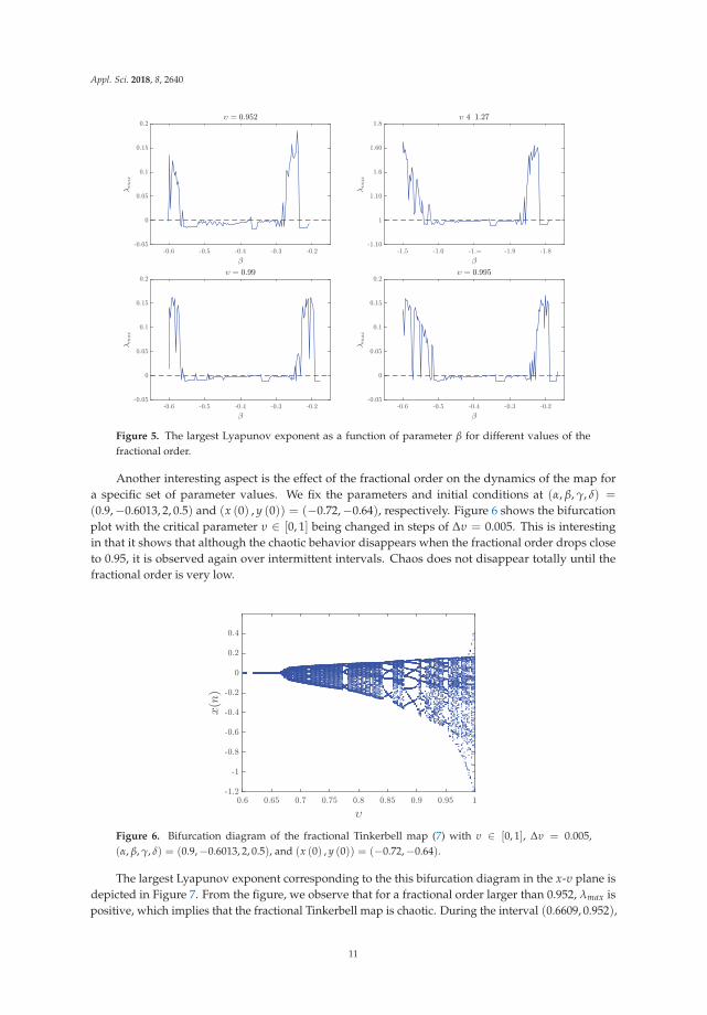
Even though these bifurcation diagrams suggest the existence of chaos in the fractional Tinkerbellmap, they are not definitive. Generally, in order to prove the existence of chaos, we must use multipletools including time series, phase portraits, Poincaré maps, power spectra, bifurcation diagrams,Lyapunov exponents, etc. The next tool at our disposal is Lyapunov exponents. We calculate theseexponents by means of the Jacobian method. It is well known that when λmax is positive and the pointsin the corresponding bifurcation diagram are dense, the map is highly likely to be chaotic. Figure 5shows the largest Lyapunov exponents corresponding to the same bifurcation diagrams depicted inFigure 4 in the x-β plane. We can observe clearly that for certain ranges of the parameter β, chaos exists.

Figure 4. Bifurcation diagrams of the fractional Tinkerbell map (7) with β ∈ [−0.6,−0.1] beingchanged in steps of Δβ = 0.0025, parameters (α, γ, δ) = (0.9, 2, 0.5), initial conditions (x (0) , y (0)) =(−0.72,−0.64), and different fractional orders.

10

Appl. Sci. 2018, 8, 2640

Figure 5. The largest Lyapunov exponent as a function of parameter β for different values of thefractional order.

Another interesting aspect is the effect of the fractional order on the dynamics of the map fora specific set of parameter values. We fix the parameters and initial conditions at (α, β, γ, δ) =

(0.9,−0.6013, 2, 0.5) and (x (0) , y (0)) = (−0.72,−0.64), respectively. Figure 6 shows the bifurcationplot with the critical parameter υ ∈ [0, 1] being changed in steps of Δυ = 0.005. This is interestingin that it shows that although the chaotic behavior disappears when the fractional order drops closeto 0.95, it is observed again over intermittent intervals. Chaos does not disappear totally until thefractional order is very low.

Figure 6. Bifurcation diagram of the fractional Tinkerbell map (7) with υ ∈ [0, 1], Δυ = 0.005,(α, β, γ, δ) = (0.9,−0.6013, 2, 0.5), and (x (0) , y (0)) = (−0.72,−0.64).

The largest Lyapunov exponent corresponding to the this bifurcation diagram in the x-υ plane isdepicted in Figure 7. From the figure, we observe that for a fractional order larger than 0.952, λmax ispositive, which implies that the fractional Tinkerbell map is chaotic. During the interval (0.6609, 0.952),

11

Appl. Sci. 2018, 8, 2640

λmax is observed to change intermittently between positive and negative signs, which means that chaosstarts to appear and disappear. Finally, for values lower than 0.6609, chaos disappears completely.These results agree with the bifurcation diagram in Figure 6.

Figure 7. The largest Lyapunov exponent as a function of the fractional order υ for the same parametersand initial conditions in Figure 6.

4. Control of the Fractional Tinkerbell Map

In this section, we show that the proposed fractional Tinkerbell can be stabilized by means of asimple adaptive feedback controller. In order to be able to establish the asymptotic convergence ofthe controlled states towards zero, we first need to recall some important results from the literatureconcerning the asymptotic stability of fractional discrete systems. Since fractional discrete calculus isstill relatively new, the existing literature related to stability is very limited. There are two main waysof establishing asymptotic stability. The first relies on the linearity of the system and places conditionson the eigenvalues of the Jacobian [31]. The second scheme is a generalization of the well-knownLyapunov direct method [32]. Although, the Lyapunov method is powerful and can support differenttypes of systems, its has yet to be established for delayed fractional discrete systems, which renders itunusable for the system at hand. Hence, our objective here is to design the control laws to linearizethe system, which will allow us to use the stability theory of linear systems. The following theoremsummarizes the result of [31].

Theorem 1. The zero equilibrium of the linear fractional discrete system:

CΔυa F (t) = MF (t + υ − 1) , (9)

where F(t) = ( f1(t), ..., fn(t))T, 0 < υ ≤ 1, and M ∈ Rn×n, is asymptotically stable if the eigenvalues λ of

M satisfy:

λ ∈{

z ∈ C : |z| <(

2 cos|arg z| − π

2 − υ

)υ

and |arg z| > υπ

2

}(10)

for all t ∈ Na+1−υ.

Consider the controlled version of (7) given by:⎧⎪⎪⎪⎨⎪⎪⎪⎩

CΔυa x (t) = x2 (t − 1 + υ)− y2 (t − 1 + υ) + (α − 1) x (t − 1 + υ)

+βy (t − 1 + υ) + ux (t − 1 + υ) ,CΔυ

a y (t) = 2x (t − 1 + υ) y (t − 1 + υ) + γx (t − 1 + υ)

+ (δ − 1) y (t − 1 + υ) + uy (t − 1 + υ) ,

(11)

12

Appl. Sci. 2018, 8, 2640

where ux (t) and uy (t) are adaptive control terms. The following theorem presents the proposedcontrol laws.

Theorem 2. The states of the controlled 2D fractional Tinkerbell map (11) are guaranteed to converge towardszero asymptotically subject to: {

ux (t) = y2 (t)− x2 (t) ,uy (t) = −2x (t) y (t)− γx (t) .

(12)

Proof. Substituting (12) into (11) yields the dynamics:

{CΔυ

a x (t) = (α − 1) x (t − 1 + υ) + βy (t − 1 + υ) ,CΔυ

a y (t) = (δ − 1) y (t − 1 + υ) ,(13)

or more compactly:CΔυ

a (x (t) , y (t))T = A (x (t) , y (t))T , (14)

with:

A =

(α − 1 β

0 δ − 1

). (15)

The eigenvalues of Aare simply λ1 = α − 1 and λ2 = δ − 1. It is straight forward to see thatthese eigenvalues satisfy the conditions of Theorem 1. Consequently, the zero solution of (13) isasymptotically stable, and the states of the controlled map (11) are asymptotically stabilized.

The result of Theorem 2 can be easily put to the test. Consider, for instance, parameters(α, β, γ, δ) = (0.9,−0.6013, 2, 0.5), initial conditions (x (0) , y (0)) = (−0.72,−0.64), and fractionalorder υ = 0.98. Using a modified version of the numerical formula (8), we obtain the states depictedin Figure 8. Clearly, the states do converge towards the all-zero solution. Although the convergencewas only established for the commensurate case, experiments have shown that the proposed controllaws are also valid for the incommensurate case. Figure 9 shows the controlled states with the sameparameters and initial conditions from above, but with different fractional orders (υ1, υ2) = (0.99, 0.95).Again, we see that the states do in fact converge towards zero, indicating successful stabilization.However, it is apparent that the convergence happens faster in the commensurate case where υ1 = υ2.

Figure 8. Stabilized states of the controlled fractional Tinkerbell map (11) with parameters (α, β, γ, δ) =

(0.9,−0.6013, 2, 0.5), initial conditions (x (0) , y (0)) = (−0.72,−0.64), and fractional order υ = 0.98.

13

Appl. Sci. 2018, 8, 2640

Figure 9. Stabilized states of the controlled fractional Tinkerbell map (11) with parameters (α, β, γ, δ) =

(0.9,−0.6013, 2, 0.5), initial conditions (x (0) , y (0)) = (−0.72,−0.64), and fractional orders (υ1, υ2) =

(0.99, 0.95).

5. Conclusions

In this paper, we have considered a fractional Caputo-difference form of the standard Tinkerbellchaotic map, which is well known for its rich dynamics and interesting characteristics. The dynamicsof the fractional Tinkerbell map were investigated numerically using phase plots, bifurcation diagrams,and Lyapunov exponents. Through this investigation, we observed that the fractional order has asignificant effect on the fractional map’s dynamics. This confirms what has been reported previouslyin the literature and suggests that the fractional map is superior to the standard one, as it includesmore degrees of freedom.

We have also introduced a feedback linearization stabilizing controller for the proposed mapand established the asymptotic convergence of the states towards the all-zero solution by means ofthe stability theory of linear fractional discrete systems. The success of the proposed scheme wasdemonstrated through numerical simulations both in the commensurate and incommensurate cases.

Although feedback linearization is simple to design and implement, its practicality has beenchallenged by many in the control and cybernetics research communities. For future work, we planto investigate other control schemes that can perform better in terms of the power consumption andother essential criteria. The main challenge that we anticipate is the limited literature concerning thestability of fractional discrete systems, especially on the Lyapunov method. This would have to beaddressed in order to be able to establish the convergence of any new control scheme.

Author Contributions: Conceptualization, A.O.; investigation, A.-A.K.; methodology, A.O. and A.-A.K.; projectadministration, V.-T.P.; resources, S.B.; software, S.B. and T.P.V.; supervision, V.V.H.; validation, T.P.V.; writing,original draft, V.-T.P.; writing, review and editing, V.V.H.

Funding: This research received no external funding.

Conflicts of Interest: The authors declare no conflict of interest.

References

1. Lorenz, E.N. Deterministic nonperiodic flow. J. Atmos. Sci. 1963, 20, 130–141. [CrossRef]2. Hénon, M. A two-dimensional mapping with a strange attractor. Commun. Math. Phys. 1976, 50, 69–77.

[CrossRef]3. May, R. Simple mathematical models with very complicated dynamics. Nature 1976, 261, 459–467. [CrossRef]

[PubMed]4. Lozi, R. Un atracteur étrange du type attracteur de Hénon. J. Phys. 1978, 39, 9–10.5. Stefanski, K. Modelling chaos and hyperchaos with 3D maps. Chaos Solitons Fractals 1998, 9, 83–93. [CrossRef]

14

Appl. Sci. 2018, 8, 2640

6. Itoh, M.; Yang, T.; Chua, L. Conditions for impulsive synchronization of chaotic and hyperchaotic systems.Int. J. Bifurc. Chaos 2001, 11, 551–558. [CrossRef]

7. Fiori, S. Nonlinear damped oscillators on Riemannian manifolds: Fundamentals. J. Syst. Sci. Complex. 2016,29, 22–40. [CrossRef]

8. Fiori, S. Nonlinear damped oscillators on Riemannian manifolds: Numerical simulation. Commun. NonlinearSci. Numer. Simul. 2017, 47, 207–222. [CrossRef]

9. Huang, L.; Bae, Y. Chaotic dynamics of the fractional-love model with an external environment. Entropy2018, 20, 53. [CrossRef]

10. Huang, L.; Bae, Y. Nonlinear behavior in fractional-order Romeo and Juliet’s love model influenced byexternal force with fuzzy function. Int. J. Fuzzy Syst. 2018, 1–9. [CrossRef]

11. Goodrich, C.; Peterson, A.C. Discrete Fractional Calculus; Springer: Berlin, Germany, 2015.12. Wu, G.; Baleanu, D. Discrete fractional logistic map and its chaos. Nonlinear Dyn. 2013, 75, 283–287.

[CrossRef]13. Hu, T. Discrete chaos in fractional Hénon map. Appl. Math. 2014, 5, 2243–2248. [CrossRef]14. Shukla, M.K.; Sharma, B.B. Investigation of chaos in fractional order generalized hyperchaotic Hénon map.

Int. J. Electron. Commun. 2017, 78, 265–273. [CrossRef]15. Khennaoui, A.; Ouannas, A.; Bendoukha, S.; Wang, X.; Pham, V.T. On Chaos in the Fractional–Order

Discrete-Time Unified System and its Control Synchronization. Entropy 2018, 20, 530. [CrossRef]16. Megherbi, O.; Hamiche, H.; Djennoune, S.; Bettayeb, M. A new contribution for the impulsive

synchronization of fractional–order discrete-time chaotic systems. Nonlinear Dyn. 2017, 90, 1519–1533.[CrossRef]

17. Zhang, X.; Li, Z.; Chang, D. Dynamics, circuit implementation and synchronization of a newthree-dimensional fractional-order chaotic system. Int. J. Electron. Commun. 2017, 82, 435–445. [CrossRef]

18. Khennaoui, A.; Ouannas, A.; Bendoukha, S.; Grassi, G.; Wang, X.; Pham, V. Generalized and inversegeneralized synchronization of fractional-order discrete-time chaotic systems with non-identical orders anddimensions. Adv. Differ. Equ. 2018, 2018, 303. [CrossRef]

19. Bendoukha, S.; Ouannas, A.; Wang, X.; Khennaoui, A.; Pham, V.T.; Grassi, G.; Huynh, V. The co-existenceof different synchronization types in fractional-order discrete-time chaotic systems with non-identicaldimensions and orders. Entropy 2018, 20, 710. [CrossRef]

20. Ouannas, A.; Khennaoui, A.; Bendoukha, S.; Grassi, G. On the Q-S chaos synchronization of fractional-orderdiscrete-time systems: general method and examples. Discrete Dyn. Nat. Soc. 2018, 2018, 2950357. [CrossRef]

21. Ismail, S.; Said, L.; Rezk, A.; Radwan, A.; Madian, A.; Abu-Elyazeed, M.; Soliman, A. Generalized fractionallogistic map encryption system based on FPGA. Int. J. Electron. Commun. 2017, 80, 114–126. [CrossRef]

22. Aulbach, B.; Colonius, F. Six Lectures on Dynamical Systems; World Scientific: Singapore, 1996.23. Nusse, H.; Yorke, J. Dynamics: Numerical Explorations; Springer: New York, NY, USA, 1997.24. Davidchack, R.; Lai, Y.; Klebanoff, A.; Bollt, E. Towards complete detection of unstable periodic orbits in

chaotic systems. Phys. Lett. A 2001, 287, 99–104. [CrossRef]25. Mcsharry, P.; Ruffino, P. Asymptotic angular stability in non-linear systems: Rotation numbers and winding

numbers. Dyn. Syst. 2003, 18, 191–200. [CrossRef]26. Yuan, S.; Jiang, T.; Jing, Z. Bifurcation and chaos in the tinkerbell map. Int. J. Bifurc. Chaos 2011, 21, 3137–3156.

[CrossRef]27. Atici, F.M.; Eloe, P.W. Discrete fractional calculus with the nabla operator. Electron. J. Qual. Theory Differ.

Equ. Spec. Ed. I 2009, 3, 1–12. [CrossRef]28. Abdeljawad, T. On Riemann and Caputo fractional differences. Comput. Math. Appl. 2011, 62, 1602–1611.

[CrossRef]29. Anastassiou, G. Principles of delta fractional calculus on time scales and inequalities. Math. Comput. Model.

2010, 52, 556–566. [CrossRef]30. Chen, F.; Luo, X.; Zhou, Y. Existence Results for Nonlinear Fractional Difference Equation. Adv. Differ. Equ.

2010, 2011, 713201. [CrossRef]

15

Appl. Sci. 2018, 8, 2640

31. Cermak, J.; Gyori, I.; Nechvatal, L. On explicit stability condition for a linear fractional difference system.Fract. Calc. Appl. Anal. 2015, 18, 651–672. [CrossRef]

32. Wu, G.; Baleanu, D.; Luo, W. Lyapunov functions for Riemann–Liouville-like discrete fractional equations.Appl. Math. Comput. 2017, 314, 228–236.


16

applied sciences

Article

Policy-Compliant Maximum Network Flows

Pieter Audenaert *, Didier Colle and Mario Pickavet

Faculty of Engineering and Architecture, Department of Information Technology, Ghent-University-imec,9052 Ghent, Belgium; [email protected] (D.C.); [email protected] (M.P.)* Correspondence: [email protected]; Tel.: +32-(0)9-33-14900

Received: 19 January 2019; Accepted: 23 February 2019; Published: 28 February 2019

Abstract: Computer network administrators are often interested in the maximal bandwidth that canbe achieved between two nodes in the network, or how many edges can fail before the networkgets disconnected. Classic maximum flow algorithms that solve these problems are well-known.However, in practice, network policies are in effect, severely restricting the flow that can actuallybe set up. These policies are put into place to conform to service level agreements and optimizenetwork throughput, and can have a large impact on the actual routing of the flows. In this work,we model the problem and define a series of progressively more complex conditions and algorithmsthat calculate increasingly tighter bounds on the policy-compliant maximum flow using regularexpressions and finite state automata. To the best of our knowledge, this is the first time that specificconditions are deduced, which characterize how to calculate policy-compliant maximum flows usingclassic algorithms on an unmodified network.

Keywords: communication networks; maximum flow; network policies; algorithms

1. Introduction

Connecting two nodes in a computer communication network involves setting up paths, possiblymore than one. Often, this is done with resiliency in mind: clearly, having more than one path betweennodes, it might be possible to route around a failed link or node, depending on the paths themselvesand the failed node or link. Also, network operators provide multiple paths between nodes in order toincrease the maximum achievable throughput or flow in between these nodes.

In practice, however, network policies are in effect, effectively restricting the flow that can be setup between two nodes in the network. Specific restrictions can be implemented to optimize routing,due to security constraints or because of policies and agreements between different network operators.As one example, inter-domain paths in the internet often fulfill a valley-free routing constraint [1,2]which is a simple condition that models real-life business agreements between different operators.Compared to a policy-free routing model, these conditions severely restrict allowed paths and mighthave a large impact on the overall throughput between two nodes when the conditions are strictlyenforced. Conditions also influence path diversity, which in turn has a large impact on the overallresiliency of the connection.

Calculating the maximum throughput that can be achieved between two nodes in a network caneasily be done via classic techniques solving the maximum flow problem, such as the algorithm ofFord–Fulkerson or the push-relabel method [3,4]. However, these algorithms do not take into accountpolicies and do not enforce any condition or constraint at all. In this work, we will adapt generic flowalgorithms, such that the flow that is achieved actually is a policy-compliant maximum flow. Policiesare defined using finite state automata (FSA) [5,6], as their expressive power is sufficient for manypurposes in real life, while still being conceptually simple.

We will define an algorithm that exactly solves the policy-compliant maximum flow problem,however, at the expense of a large computational footprint. Then, we will continue to adapt the classic


Appl. Sci. 2019, 9, 863

algorithms and datastructures such that they take into account policies that can be expressed usingFSA. These algorithms, however, do not guarantee exact solutions to the problem anymore; theymerely provide lower bounds to the exact answer. At each step, we are able to tighten the lowerbound, such that it comes closer to the exact solution. However, each step also implies additionalcomputational work, so we are trading off the quality of the results with the time needed to runthe algorithms.

The rest of the paper is organized as follows. First, in Section 2 we provide some backgroundabout policies and how they can model certain conditions and constraints that are applied in reallife. We also point out some difficulties that arise when trying to adapt the classic algorithms. Then,in Section 3 we discuss the formal model and the classic algorithms from literature, and how we canformally model policy-compliant connections. Next, in Section 4 we adapt the algorithms that werediscussed in Section 3 to obtain a series of techniques that allow us to calculate lower bounds to theproblem. Finally, Section 5 discusses the results obtained, and concludes this work, after which weprovide an outlook to future work.

2. Background and Context

Policies are very important in today’s internet. Specific agreements between operators are oftenhidden from prying eyes, but they can have a huge impact on how specific paths are set up betweenthem. It turns out that many network policies, used in practice, can be translated in very simple formallanguages, all belonging to a class of formal languages called “regular languages” [5,6]. This class isone of the most basic classes of languages used in computer science, as it is non-trivial but containsa very broad range of languages with widely differing properties that are very useful in practice.

The complexity of properties which we can express using regular languages is larger than wouldbe expected at first sight. To provide a non-trivial, albeit contrived example, consider a governmentthat wants to contact its embassy located in another country. Some links are trusted, as they areoperated by friendly states, but some links in between may be eavesdropped upon by a rival state.Traffic crossing such links needs to be encrypted; once encrypted, traffic may be routed through anylink in the network. The receiving party will need to decrypt the message, before it can be distributed tointernal data-processing departments. The government thus places into force the following conditions:traffic from the government to the embassy should either be sent through links owned exclusively byfriendly states, or it should pass the encryption box, after which it can be routed through any link.However, if encrypted, the message has to be decrypted before delivery at the internal departments atthe embassy, i.e., pass through a specific decryption box.

It is clear that enforcing such policies is important, moreover such policies should be formalizedinstead of specified in vague terms as above. Regular languages fit that job quite well, as they allowpolicies like the one above, next to other much more involved policies, to be specified without anypossibility for misunderstanding. Moreover, once specified, network-routes can be automaticallyvalidated against a set of policies, and compliance can be trivially checked.

Taking into account policies in the network, a natural question is to ask for their impact on therouting between nodes in the network. More specifically, in this work we are mainly interested in theirimpact on the maximum flow achievable between two nodes. Indeed, previously acceptable pathssuddenly do not obey the specific policies, and as such, some routes, maybe all, will become invalid.Thus, the policy-compliant maximum flow between two nodes needs to be redefined and recalculated.Gaining insight into the flow-structure between two nodes also tells us something about resiliencyin the network. Operators might be convinced their network has sufficient spare capacity, however,depending on the policy at hand and the specific structure of the network, a failing link might havetremendous consequences as re-routing traffic around the failure might invalidate the policy whichis unacceptable.

We thus come to the following main problem-statement that will be treated in this work: how tocalculate or approximate the policy-compliant maximum flow between two nodes?

18

Appl. Sci. 2019, 9, 863

Clearly, policy-compliance and both the theoretical and practical consequences are important inthe design and operation of networks. From a practical point of view, much information can be foundabout policies and being compliant, and multiple frameworks for the management and monitoringof policies exist and are in current use. In contrast, few theoretical models have been developed,and literature is sparse when taking a more fundamental approach to the problem.

Caesar and Rexford [7] discuss how routing policies came into existence, and how theprotocols have evolved over time and became increasingly complex. They discuss how commonpolicies are implemented and address the problems that arise in applying and supporting policies.Feamster et al. [8] discuss fundamental objectives for interdomain routing and traffic engineering andprovide practical guidelines. They show how greater flexibility can be gained in several situations anddemonstrate the manipulation of traffic via small changes in specific routes. The paper by Hu et al. [9]proposes an approach to overcome the inherent constraints of compliant recovery schemes. Adaptingprotocols, they succeed in improving route diversity, in turn increasing resilience.

Klöti et al. [10] proposed a graph-transformation technique that constructs a tensor productof a graph and a finite state automaton. They show how to model policies using FSA and applystandard flow maximization algorithms on the transformed graph in order to obtain bounds forthe policy-compliant maximum flow problem. Sobrinho et al. [11] provide a deep mathematicalanalysis to gain insight in the inner workings of route-vector protocols. They relate this to a class ofrouting policies and quantify how much intrinsic connectivity is lost due to typical routing policies.Erlebach et al. [12] approximate the maximum number of edge- and node-disjoint valid paths betweentwo nodes, via an involved mathematical theory and specific approximation-algorithms.

Soulé et al. [13] provide a declarative formal language based on logical formulas and regularexpressions to express network policies in the Merlin framework. After compilation, a constraintsolver allocates paths. Tools are provided to verify whether conditions are violated. Hinrichs et al. [14]introduce a declarative policy management language. They focus on expressive power so that policiescan be expressed naturally while still being able to enforce policies efficiently. They focus on enterprisenetworks, and their design using formal mathematical languages is attractive.

Raghavan et al. [15] provide a practical authenticated source routing system that allows forfine-grained path selection and enforcement of cryptographic policies. Capabilities can be defined andcomposed resulting in complex statements defining specific policies.

Godfrey et al. [16] introduce so-called pathlet routing, pathlets being building blocks whichcan be concatenated to obtain end-to-end routes fulfilling policy constraints. Pathlet routing canhandle typical policies, but also other recent multipath routing proposals or source-routing approaches.Batista et al. [17] propose a policy-based OpenFlow network management framework using the Ponderpolicy definition language. They focus on simplicity of the system, trying to infer both static anddynamic conflicts. In [18] they update their work and propose a more theoretical approach toconflict detection using first-order mathematical logic to model flows. A Prolog rule-engine appliescondition-action rules to infer problems. Xu and Rexford [19] discuss problems concerning multipathinterdomain routing and introduce MIRO (Multi-path Interdomain ROuting), which gives transitdomains control over the flow across their infrastructure. MIRO remains backwards compatible withother technologies and offers large flexibility with reasonable overhead.

3. Graph Model and Basic Algorithms

We now introduce basic concepts that are needed in this work. Intuitively, we can think abouta flow network like an oil-producing plant, where oil is drilled at one site and needs to be transportedto an oil depot via a set of pipes. Following the flow from the source to the sink, the oil can be splitor joined at junctions. Most important here is the fact that the path that was followed by a certainmolecule of oil is of no importance: it carries no history and passes through junctions anonymously.In contrast, in this work, we need to pay attention to the specific path that a certain amount of flowhas followed: it carries its history with itself, see Figure 1. The amount of history that accompanies

19

Appl. Sci. 2019, 9, 863

the flow is, however, limited: it is represented via its state, and the number of possible different statesis limited by the size of the automaton (cf. infra). To understand how to model policies using FSA,we refer to [10].

oil

ab

c

de

f

g

Figure 1. It doesn’t matter for oil whether it followed path abc, path def or path dgc, but in this paper,we do care about the specific paths followed. Policies about which path is acceptable and which path isnot, are expressed via constraints on the labels across the paths, i.e., abc, def and dgc.

3.1. Flow Networks and Flows

We now introduce flow networks and flows, following the approach taken by Cormen et al. [4].These definitions might differ from other approaches in several aspects, e.g., the fact that the capacityfunction c and the flow f are total functions, allowing more concise and elegant definitions ofconstraints. The rationale behind this way of defining the context is included in Cormen et al. [4] andwe refer interested readers to study the mathematical discussions in that book. We thus define a flownetwork G = (V, E) as a directed graph together with a capacity function c : V × V → R such thateach edge (u, v) ∈ E has a nonnegative capacity c(u, v) ≥ 0. Note that c is a total function such that,if (u, v) /∈ E, we have c(u, v) = 0. Moreover, we require that if E contains a certain edge (u, v), thenthere is no reverse edge (v, u) present in E. We also disallow loops such that ∀u : (u, u) /∈ E. Twospecific nodes in the graph are now chosen out of V, one vertex being the source s and one vertexbeing the sink t. We now want to send a flow from s to t, a flow being a total function f : V × V → R

subject to the following constraints:

• A capacity constraint which expresses that flow can never exceed capacity:

∀u, v ∈ V : 0 ≤ f (u, v) ≤ c(u, v) (1)

• A flow conservation constraint which expresses that for all nodes (except source and sink) theincoming flow equals the outgoing flow:

∀u ∈ V − {s, t} : ∑v∈V

f (v, u) = ∑v∈V

f (u, v) (2)

Note that f (u, v) = 0 if (u, v) /∈ E.The value | f | of a flow is defined as the flow leaving the source minus the flow arriving at the

source: | f | = ∑v∈V f (s, v)− ∑v∈V f (v, s). Equivalently, we can define the value of the flow just as wellas | f | = ∑v∈V f (v, t)− ∑v∈V f (t, v). Note that one can define the value of the flow using a formulacontaining only s but not t, or a formula containing only t but not s; one never needs both s and t inone formula at the same time, see the book by Cormen et al. [4]. Also note that we allow ∑v∈V f (v, s)as well as ∑v∈V f (t, v) to be strictly larger than 0. The classic problem, given a flow network G, is tomaximize the flow | f | from s to t under the constraints above. (The |.|-notation denotes flow value, notabsolute value or cardinality.)

3.2. Residual Graphs and Augmenting Paths

One line of solving this so-called maximum flow problem is via the introduction of residualgraphs and the calculation of augmenting paths. In short, we iteratively increase the value of the flow,starting with ∀u, v ∈ V : f (u, v) = 0. At each step, we calculate an augmenting path in the residualgraph, which is nothing but the original graph, extended with return-edges. We will now formallydefine the necessary concepts.

20

Appl. Sci. 2019, 9, 863

First, we define the residual capacity c f : V × V → R in the following way. We iterate over alledges (u, v) ∈ E and for each such edge we define the following:

{c f (u, v) = c(u, v)− f (u, v)

c f (v, u) = f (u, v)(3)

If there is no edge between u and v in any direction, i.e., (u, v) /∈ E and (v, u) /∈ E, then bothc f (u, v) = 0 and c f (v, u) = 0.

Next, we define the residual network Gf = (V, Ef ), where Ef = {(u, v) ∈ V × V : c f (u, v) > 0}.So, for each edge in the original graph we have a residual edge if the capacity of that edge is not filledup yet, and moreover we add a reverse edge when it carries any flow at all.

This residual graph will now be used to find augmenting paths. Given a flow network G = (V, E)and a flow f , an augmenting path p is defined as a path from s to t in the residual network, that isp = [e1, e2, . . . , en], such that

• edges belong to Ef , thus∀ei : ei ∈ Ef , (4)

• we start in s, thus∃v : e1 = (s, v), (5)

• succeeding edges are connected, thus

∀i ∈ {1, . . . , n − 1} : ∃u, v, w : ei = (u, v) ∧ ei+1 = (v, w) (6)

• we end in t, thus∃v : en = (v, t). (7)

In order to increase the flow f , we will change the flow along the edges of the augmenting path pwith the maximum amount possible, namely the residual capacity of the path p which is

c f (p) = min{c f (u, v) : (u, v) ∈ p}. (8)

The flow f can now be increased to a new flow f ′ as follows:

f ′(u, v) =

⎧⎪⎪⎨⎪⎪⎩

f (u, v) + c f (p) if (u, v) ∈ p,

f (u, v)− c f (p) if (v, u) ∈ p,

f (u, v) otherwise.

(9)

Iteratively finding augmenting paths in a residual graph and increasing the flow will finallycome to a stop when there are no augmenting paths anymore. Then, the maximum flow has beenreached. Depending on the procedure used to find augmenting paths, the above algorithm is calledFord–Fulkerson or Edmonds–Karp.

3.3. Realization of a Flow

Apart from calculating the value of the maximum flow in a flow network, we are also interestedin the actual paths followed by the flow; this set of paths is called the “realization” of the flow.Augmenting paths are a device to calculate the maximum flow, however, augmenting paths are notreal paths in the flow network as they might comprise edges from Ef that are not in E. Define a path p

21

Appl. Sci. 2019, 9, 863

from s to t in G in exactly the same way as an augmenting path, except that edges in the path shouldbe contained in E instead of Ef . Thus, in addition to (5)–(7), we replace (4) with

∀ei : ei ∈ E. (10)

Given a flow network G and accompanying maximum flow f , it is possible to determine a set

S = {(p1, c1), (p2, c2), . . . , (pn, cn)} (11)

that realizes that flow. Intuitively, we start with no flow in the network at all. Then, for each of thepaths pi we fill all edges of that path with an additional amount ci. After all paths are processed,we obtain the maximum flow f .

Construction of this set S can be done simultaneously with the calculation of the maximum flow.During execution of the maximum flow algorithm, we perform the following steps every time a newaugmenting path p with additional flow amount c has been found, starting with an empty set S = {}.

1. We split the augmenting path in forward sections and backward sections. That is,if p = [e1, e2, . . . , en], we cut it down and obtain [[e1, . . . , ei], [ej, . . . , ek], . . . , [el , . . . , en]] such thatevery section [ex, . . . , ey] contains only edges from E or only edges from Ef − E. Without losinggenerality, we only discuss the case where the augmenting path p consists of two forwardsections with one backward section in between, thus p = [[e1, . . . , ei], [ej, . . . , ek], [el , . . . , en]] suchthat {e1, . . . , ei, el , . . . , en} ⊆ E and {ej, . . . , ek} ⊆ Ef − E.

2. For this backward section [ej, . . . , ek] there must exist a path p′ carrying some flow in theopposite direction, which the augmenting path p is canceling out. Indeed, as [ej, . . . , ek] areedges in Ef , they have been introduced in the residual graph Gf thanks to the fact that thecorresponding forward edges in E have already been used in a previously found path. Thus,if ej = (uj, vj) and ek = (uk, vk), then S will already contain an item (p′, c′) where the pathp′ = [. . . , (vx, vk), (vk, uk), . . . , (vj, uj), (uj, uy), . . .], as the augmenting path p is crossing thatsection in the reverse direction, see Figure 2.

3. Remove this item (p′, c′) from S, and add two new paths [e1, . . . , ei, (uj, uy), . . .] and[. . . , (vx, vk), el , . . . , en], each with amount c. As such, the augmenting path has been cut andglued together with a previously found path, resulting in two new paths.

4. Now, it might be that c < c′. In that case, path p′ is not to be removed from S entirely, as it stillcarries some flow that was not canceled by p. Add (p′, c′ − c) to S.

Thus, each iteration of the maximum flow algorithm results in an augmenting path that is possiblycut in sections to remove reversed edges from the residual graph. Forward sections are glued togetherwith sections from previously found paths. When no augmenting paths can be found, the set S willcontain paths and associated flow amounts, that together sum up to the maximum flow. That is,if upon termination S = {(p1, c1), . . . , (pn, cn)}, we have

f (u, v) = ∑{(pi ,ci):(u,v)∈pi}

ci (12)

s

e1 ei

el en

tuyujvjvk ukvx

ej

ek

Figure 2. Three sections: forward, backward and forward.

22

Appl. Sci. 2019, 9, 863

Thanks to the fact that every flow has a realization and the fact that it is easy to derive the flowfrom a realization, from now on we identify a realization of a flow and the flow itself, and use the twoconcepts as one.

4. Policy-Compliant Paths and Algorithms

We now continue to define the concept of policy-compliant paths. Then we want to find themaximum flow in the network, allowing only the use of such policy-compliant paths. We will providealgorithms that calculate lower bounds, as well as exact solutions.

4.1. Finite State Automata

We now proceed to define finite state automata [5,6], which are the simplest of all classic automata.Note that we will only consider deterministic automata, although for finite state automata we have thatnon-determinism does not add expressive power, i.e., the class of deterministic finite state automata isexactly the same as the class of non-deterministic finite state automata.

We define a deterministic finite state automaton as M = (Q, Σ, δ, q0, F), where

• Q is a finite set of internal states,• Σ is a finite set of symbols, called the input alphabet,• δ : Q × Σ → Q is the (total) transition function,• q0 ∈ Q is the start (or initial) state,• F ⊆ Q is the set of final states.

Such an automaton works as follows. Initially, we start with an input word w ∈ Σ∗, where Σ∗

is the set of strings obtained by concatenating zero or more symbols from Σ. Each of these symbolsof the word w gets consumed, from left to right, while the automaton changes its state accordinglyto its transition function, taking as input the current state and the symbol just read. If the automatonstarts in state q0, and finishes reading the word w while reaching state q, then we say that the wordw is accepted by the automaton if and only if q ∈ F. For convenience, we introduce the extendedtransition function δ∗ : Q×Σ∗ → Q, where the second argument is a string rather than a single symbol.We define δ∗ recursively as follows:

δ∗(q, w) =

{q if w = λ,

δ∗(δ(q, a), v) if w = av,(13)

where a ∈ Σ and v, w ∈ Σ∗. Note that we also introduced the empty word λ out of convenience forthis definition. We won’t need it any further in this work.

4.2. Labeled Networks and Policy-Compliant Paths

Given a certain flow network G = (V, E) and an FSA M, we define a labeling function l : E → Σthat attaches one symbol to every edge of the graph, which becomes a labeled flow network. Before,we were interested in all paths from source to sink, in order to maximize the total flow value of thenetwork. Now, we constrain the allowed paths to only those that are accepted by the FSA M. Formally,we define a policy-compliant path p from s to t in G to be a sequence of edges from E, such that thesymbols that are encountered, in order, constitute a word that is accepted by M. Thus, in addition to(5)–(7) and (10), we add the following constraint:

δ∗(q0, l(e1)l(e2) . . . l(en)) ∈ F (14)

Thus, we are looking for paths from source to sink that are accepted by the automaton. Now wecan define the policy-compliant maximum flow problem (PCMF) as calculating the maximum flow | f |

23

Appl. Sci. 2019, 9, 863

from s to t in a labelled flow network Gf , subject to the constraint that all paths that realize the flow fare accepted by an FSA M, i.e., they are policy-compliant paths.

4.3. Brute Force Approach

A basic, inefficient way of solving the policy-compliant maximum flow problem is by way of bruteforce. In its essence, we first calculate all policy-compliant paths from source to sink, and afterwardtry out all different orders in which these paths can be filled up. The maximum flow will be reachedby at least one of these orderings. As such, this approach will result in the exact solution, however,at the expense of large computational complexity and memory requirements. Indeed, as we employour search via e.g., a depth-first-search, it might be the case that we need to visit a certain vertexu ∈ E more than once, because the internal state of the FSA might be different. Effectively, we need tobuild a new graph GBF that contains tuples of vertices and states. After appropriately defining theedges between these tuples, a typical depth-first-search might be used to enumerate successively allpolicy-compliant paths. More formally, we perform the following steps.

1. Define GBF as the graph with VBF = {(u, q) : u ∈ V ∧ q ∈ Q} and EBF = {((u1, q1), (u2, q2)) :u1, u2 ∈ V ∧ q1, q2 ∈ Q ∧ (u1, u2) ∈ E ∧ δ(q1, l((u1, u2))) = q2}. That is, the vertices of GBF areall possible tuples of vertices in V and states in Q, and the vertices in GBF are connected if andonly if the corresponding vertices u1 and u2 in V were connected by an edge e ∈ E, such that theFSA changes its state from q1 to q2 when reading the symbol l(e) associated with the originaledge. Thus, we are defining GBF as the Cartesian product of V and Q.

2. Start a depth-first-search from (s, q0) to all (t, q) such that q ∈ F. This will produce all pathsof the form p = [e1, . . . , en] with ∀ei : ei ∈ EBF while ∃v ∈ VBF : e1 = ((s, q0), v) and ∃v ∈VBF : ∃q ∈ F : en = (v, (t, q)). Every such path corresponds to a policy-compliant path in G,and every policy-compliant path in G will be found this way. Collect all paths found by thisdepth-first-search in the set BF = {p1, . . . , pn}.

3. Generate all permutations of the elements in this set BF; this results in n! sequences of the npaths. Each of these sequences will correspond to an ordering in which we fill the paths to theirresidual capacity at that time. Note that it is not necessary to generate all permutations at once.It is sufficient to do this iteratively via e.g., the Steinhaus–Johnson–Trotter algorithm.

4. Each such sequence s = [ps1, . . . , ps

n] contains exactly the same items as BF itself. We definean empty flow fs(u, v) = 0 and iterate through this sequence: for each path ps

i = [esi,1, . . . , es

i,m] wecalculate mins

i = min{c(esi,j)− fs(es

i,j) : 1 ≤ j ≤ m} which represents the largest amount of flowthat can be accommodated along the path ps

i at that moment. The flow fs can now be increasedto a new flow f ′s as follows:

f ′s(u, v) =

{fs(u, v) + mins

i if (u, v) ∈ psi ,

fs(u, v) otherwise.(15)

5. After all paths psi are processed, the final flow fs will be a lower bound for the policy-compliant

maximum flow for the network G. Thus, max{| fs|} will be the value of the policy-compliantmaximum flow.

It is clear that this approach results in the exact value of the solution to the policy-compliantmaximum flow problem. However, except for small networks and automata it will quickly take toomuch space and time to execute.

4.4. First Lower Bound

To cut down on the needed computational resources, we start from the classic Ford–Fulkersonor Edmonds–Karp algorithm. In its essence, these algorithms start with an empty flow, after which anew augmenting path is looked for in the residual graph. If found, this augmenting path gives rise to

24

Appl. Sci. 2019, 9, 863

an augmented flow, after which the residual graph is updated. Then, a new iteration is started. Onceno new augmented paths can be found, the algorithm has reached the maximum flow.

In order to apply this approach to the policy-compliant maximum flow problem, it will benecessary to keep track of how the flow actually is realized, throughout the execution of thealgorithm. This relates to the fact that flows cannot merge and split anonymously anymore,as discussed previously.

As a first step, it will be necessary to keep track of the different state-transitions that occur whenflow crosses an edge e = (u, v) ∈ E in a path p and changes state during that transition from statequ ∈ Q in vertex u to state qv ∈ Q in vertex v. To that aim, we define transitions t to be membersof the set Q × Q = {(qu, qv) : qu ∈ Q ∧ qv ∈ Q}. For every edge e ∈ E we will now keep trackof all transitions that cross that edge, and thus define the total function T : V × V × Q × Q → R.This function keeps track of the amount of flow that crosses the edge (u, v) while changing statefrom qu to qv as the value T(u, v, qu, qv). As a direct consequence, we have at all times ∀u, v ∈ V :∑qu ,qv∈Q T(u, v, qu, qv) = f (u, v) ≤ c(u, v) which expresses the fact that a flow over an edge can besplit up in different transitions, the amount of which add up exactly to the amount of flow crossingthat very edge.

Keeping track of this function T allows the algorithm to discriminate between the different statesin one single vertex, and the amount of the flow that is actually passing through that vertex having thatstate at that moment. This information is then used to glue together already found policy-compliantpaths and a newly found augmenting path. In detail, this procedure works as follows.

1. Beginning with a labeled network G and a FSA M, we start a new flow and set f (u, v) = 0 forall vertices u and v. Moreover, we set T(u, v, qu, qv) = 0 for all vertices u, v ∈ V and all statesqu, qv ∈ Q.

2. Finding the first policy-compliant augmenting path can be straightforwardly done. Indeed,as the residual graph Gf is still the same as the original graph G (because ∀u, v : f (u, v) = 0),the augmenting path that is found in the first iteration will be a path containing only forwardsections. The flow is then updated according to (9).

3. From the second iteration on, we need to take into account the reverse edges in the residualgraph with great care. Now, it is not sufficient anymore to simply look for policy-compliantpaths containing only forward sections, as an augmenting path may now contain reverse edgesfrom the residual graph. In general, we will look for an augmenting path p = [e1, . . . , en] whereei ∈ Ef , that can have multiple forward and backward sections, and which can thus be splitas p = [[e1, . . . , ei], [ej, . . . , ek], . . . , [el , . . . , en]], such that each section [ex, . . . , ey] only containsedges from either E or Ef − E. We will now determine the constraints that are to be applied toensure that the newly found augmenting path p can be split up and glued together with otherpolicy-compliant paths that are already part of the flow f .

4. For simplicity, we discuss the case where the augmenting path p consists of two forwardsections with one backward section in between, that is p = [[e1, . . . , ei], [ej, . . . , ek], [el , . . . , en]]

such that {e1, . . . , ei, el , . . . , en} ⊆ E and {ej, . . . , ek} ⊆ Ef − E. To identify the vertices involved,suppose that ej = (uj, vj) and ek = (uk, vk), so p = [[e1, . . . , ei], [(uj, vj), . . . , (uk, vk)], [el , . . . , en]],see Figure 2. Starting from state q0, the start state of the automaton, we will reach statequj = δ∗(q0, l(e1) . . . l(ei)) after we crossed all edges [e1, . . . , ei] in the first forward section ofthe augmenting path.

5. The first forward section of the augmenting path that we have found will be cut at this point, atthe cut-vertex uj. For this first approach to obtain a lower bound for the PCMF problem, we assertthe overly restrictive constraint that ∃uy ∈ V and ∃quy ∈ Q such that

(uj, uy) ∈ E ∧ T(uj, uy, quj , quy) > 0. (16)

25

Appl. Sci. 2019, 9, 863

Choose such an edge e = (uj, uy) ∈ E and state quy ∈ Q. When the augmenting path p is cut atvertex uj, we can glue the new flow that comes in via the forward section [e1, . . . , ei] to the flowthat leaves vertex uj in state quj via edge e = (uj, uy) and reaches state quy at the other end invertex uy. This flow is already available and does not concern us anymore.

6. Now, we need to cancel flow that used to cross the edges [(vk, uk), . . . , (vj, uj)], that is thebackward section of the augmenting path p, crossed in the opposite direction. This givesrise to a second condition for this algorithm to find augmenting paths. This section containsa flow, reaching state quj at the end. Tracing back where this flow comes from, we requirethat there must exist some flow passing vertex vk in state qvk ∈ Q which crosses the edges[(vk, uk), . . . , (vj, uj)] finally reaching vertex uj in state quj . This observation immediatelytranslates to the following condition:

∃qvk ∈ Q : δ∗(qvk , l((vk, uk)) . . . l((vj, uj))) = quj . (17)

Choose such a qvk ∈ Q. Then, the flow that is already present in the network and passes vertex vkin state qvk will be canceled over the section [(vk, uk), . . . , (vj, uj)].

7. We now need to consider the last forward section [el , . . . , en]. This section starts in vertex vk andends in the sink t, thus ∃v ∈ V : el = (vk, v) and ∃v ∈ V : en = (v, t). We know that, havingreached state qvk in vk, we will cross edges [el , . . . , en] and need to reach some state qt ∈ F toobtain a policy-compliant augmenting path. This immediately gives rise to the third and lastcondition, which can be stated as

δ∗(qvk , l(el) . . . l(en)) = qt ∈ F. (18)

8. Suppose all conditions (16)–(18) for this augmenting path are fulfilled, which means that we havefound an augmenting path that can be joined with the already available policy-compliant pathsto increase the total policy-compliant flow. We now need to calculate the amount of flow that canbe sent over this augmenting path. First, define cuj = min{c f (u, v) : (u, v) ∈ [e1, . . . , ei]} to be thecapacity that is at most available along the first forward section of the augmenting path and thus atthe endpoint uj of this section. Likewise, define cvk = min{c f (u, v) : (u, v) ∈ [el , . . . , en]} to be theamount of flow that is at most available along the second forward section of the augmenting path,and thus the maximum amount of flow that can be diverted at the starting point vk of this section.For the backward section of the augmenting path, define cvkuk = T(vk, uk, qvk , quk ), . . . , cvjuj =

T(vj, uj, qvj , quj), to determine the already crossing flow over the backward edges, taking intoaccount the state-transitions which we derived above. Taking everything together, we have

c f (p) = min{cuj , cvkuk , . . . , cvjuj , cvk} (19)

(cf. (8)). This denotes the additional flow c f (p), under the assumption that c f (p) > 0, that cannow be sent over the newly found augmenting path p, such that the resulting flow f can berealized via only policy-compliant paths.

9. We now want to update the value of the flow f . This can be done via (9). However, we also needto update the specific values of the function T, for all edges involved in the augmenting path. First,we update T for all edges e = (ux, uy) in the forward section [e1, . . . , ei] via T′(ux, uy, qux , quy) =

T(ux, uy, qux , quy) + c f (p). Thus, for such an edge e = (ux, uy) we add an additional c f (p) unitsof flow that change state from qux to quy while crossing edge e. For all edges [(vk, uk), . . . , (vj, uj)],which are crossed in the reverse direction in the backward section of the augmenting path,we set T′(ux, uy, qux , quy) = T(ux, uy, qux , quy) − c f (p), actually canceling out the pre-existenttransitions in that section. Finally, for the edges in the final forward section [el , . . . , en] we updatethe transitions via T′(ux, uy, qux , quy) = T(ux, uy, qux , quy) + c f (p). This concludes the updates of

26

Appl. Sci. 2019, 9, 863

the transitions-function T and the work that needs to be done when an augmenting path hasbeen found.

10. Iterate steps (3)–(9), that is, keep searching for augmenting paths that fulfill conditions (16)–(18)and update the flow f according to (9) and the transition-function T via the equations above.Once no more augmenting paths are found, stop iterating.

11. The resulting flow f can be realized via a set {p1, . . . , pn} of n policy-compliant paths pi. Thus,the value | f | is a lower bound for the value of the policy-compliant maximum flow problem.

4.5. Second Lower Bound

Although the approach described above results in correct lower bounds for the policy-compliantmaximum flow problem, we point out that the conditions (16)–(18) that are imposed upon augmentingpaths are very restrictive. Indeed, it is easy to describe specific cases where the approach missesadditional augmenting paths due to these conditions, which can easily be relaxed at the expense ofadditional computational work. The next approach, which will result in a second lower bound that istighter than the first bound, starts by relaxing condition (16).

In its essence, this condition says that for an augmenting path, containing a backward section,it is necessary to glue the immediately previous forward section to a pre-existent policy-compliantpath at the cut-vertex, via an exact match of the state in that cut-vertex. Clearly, this is too restrictivea condition as it would be sufficient if the augmenting flow arriving at that vertex could be continuedvia the same edges, however taking different intermediate states in between.

1. To make this formal, consider the augmenting path p = [e1, . . . , en] where ei ∈ Ef ,which may have multiple forward and backward sections, and which can thus be split asp = [[e1, . . . , ei], [ej, . . . , ek], . . . , [el , . . . , en]], such that each section [ex, . . . , ey] only containsedges from either E or Ef − E. For simplicity, we once more discuss the case wherethe augmenting path p consists of two forward sections with one backward section inbetween, that is p = [[e1, . . . , ei], [ej, . . . , ek], [el , . . . , en]] such that {e1, . . . , ei, el , . . . , en} ⊆ Eand {ej, . . . , ek} ⊆ Ef . To identify the vertices involved, say that ej = (uj, vj) and ek =

(uk, vk), so p = [[e1, . . . , ei], [(uj, vj), . . . , (uk, vk)], [el , . . . , en]]. The state at uj is defined asquj = δ∗(q0, l(e1) . . . l(ei)).

2. For flow f , suppose that the policy-compliant paths P = {p1, . . . , pn} are the part of the realizationof f that crosses uj. Thus, ∀pi ∈ P : ∃vi ∈ V : (uj, vi) ∈ pi. For each of these policy-compliantpaths pi, the state upon arriving in uj is denoted by qi

uj. Moreover, there might be more than

one path pi ∈ P that arrives in uj with state qiuj

, that is for some i and j it might be the case that

i �= j and qiuj

= qjuj . The amount of flow that policy-compliant path pi carries is denoted by ci,

thus ∀pi ∈ P : (pi, ci) ∈ S, cf. (11).3. Now, instead of stating in the first condition (16) that there must be a policy-compliant path

pi ∈ P such that quj = qiuj

with ci > 0 it is, in fact, sufficient that there exists a path pi ∈ P suchthat following the rest of the policy-compliant path pi after crossing uj results in a final state at thesink t even though quj �= qi

uj. More formally, if pi = [ei

1, . . . , eik, ei

l , . . . , ein] such that ei

k = (ux, uj)

and eil = (uj, uy) for some ux ∈ V and uy ∈ V, then it is sufficient to impose, instead of (16),

simply that∃pi ∈ P : δ∗(quj , l(ei

l) . . . l(ein)) ∈ F. (20)

Choose such a pi ∈ P. That way, we are confident that the prefix l(e1) . . . l(ei) canbe joined together with a suffix l(ei

l) . . . l(ein) such that for the whole word holds that

δ∗(q0, l(e1) . . . l(ei)l(eil) . . . l(ei

n)) ∈ F.4. At this point, we have to be careful which policy-compliant flows crossing the backward section

[ej, . . . , ek] we are going to cancel. Indeed, as the first section [e1, . . . , ei] is glued together with

27

Appl. Sci. 2019, 9, 863

some policy-compliant path pi ∈ P at vertex uj via condition (20), we are looking for statesqvk ∈ Q at vertex vk such that, instead of (17) the following formula holds:

∃qvk ∈ Q : δ∗(qvk , l((vk, uk)) . . . l((vj, uj))) = qiuj

. (21)

Indeed, after crossing section [ej, . . . , ek] in reverse direction we want to end in state qiuj

insteadof quj .

5. Having fulfilled the condition to allow canceling flow across the backward section of theaugmenting path, we now need to check whether the flow arriving in vk in state qvk can actuallybe diverted via the last forward section [el , . . . , en] to the sink t reaching state qt which needs tobe a final state. This is accurately expressed by (18) which we can leave unmodified.

6. Suppose conditions (18), (20) and (21) have been fulfilled. Then calculate the residual capacity(19). Update flow f via (9) across the augmenting path using the value for the residual capacity,and update transitions-function T across the augmenting path as done previously.

7. Finally, we need to update the transitions-function T across the final part of the policy-compliantpath pi, cf. (20). This final part consists of the edges [ei

l , . . . , ein], and thus we need to update T

for all edges (ux, uy) in this partial path. We update T via the formulae T′(ux, uy, qiux , qi

uy) =

T(ux, uy, qiux , qi

uy)− c f (p) and T′(ux, uy, qux , quy) = T(ux, uy, qux , quy) + c f (p), where we use thenotation qi

ux for the state that is reached at vertex ux when starting in state qiuj

in vertex uj,while qux denotes the state that is reached at vertex ux when starting in state quj in vertex uj.After these updates, the augmenting path is processed entirely, and a new iteration can start.

Note that, in comparison to the approach for obtaining the first lower bound, condition (20)not only has merits for being more relaxed, it also carries a serious drawback as checking whethercondition (20) holds involves more computational work than (16). One possible approach to checkwhether (20) actually holds, is by a depth-first walkthrough of the realization associated with theflow f . However, this is complicated by the fact that the flow might have multiple valid realizations,some of which are compatible with (20), while some are not. We discuss this now in detail.

1. Consider the augmenting path p = [[e1, . . . , ei], [(uj, vj), . . . , (uk, vk)], [el , . . . , en]] from above,where the state at uj is defined as quj = δ∗(q0, l(e1) . . . l(ei)). Suppose there exist two

policy-compliant paths pi ∈ P and pj ∈ P, such that their states in vertex uj are qiuj

and qjuj

respectively. Suppose that the realization of the flow that gave rise to these paths pi and pj is suchthat pi = [. . . , (uj, u1), (u1, u3), (u3, u4), (u4, t)] and pj = [. . . , (uj, u2), (u2, u3), (u3, u5), (u5, t)]and moreover that l((uj, u1)) = a, l((u1, u3)) = b, l((u3, u4)) = c, l((u4, t)) = d, l((uj, u2)) = e,l((u2, u3)) = f , l((u3, u5)) = g and finally l((u5, t)) = h with {a, b, c, d, e, f , g, h} ⊆ Σ. Then,as pi and pj are policy-compliant paths in the set P, it directly follows that δ∗(qi

uj, abcd) ∈ F and

δ∗(qjuj , e f gh) ∈ F, see Figure 3.

uj

u1

u3

u4

t

u2 u5

a b c d

e f g h

Figure 3. Fulfilling condition (20).

2. Suppose that moreover it holds that δ∗(qiuj

, abgh) ∈ F and δ∗(qjuj , e f cd) ∈ F, that is, for the paths

pi and pj it doesn’t really matter which way they take in the second diamond. However, supposethat δ∗(quj , abgh) ∈ F as well as δ∗(quj , e f cd) ∈ F but δ∗(quj , abcd) /∈ F and also δ∗(quj , e f gh) /∈ F.

28

Appl. Sci. 2019, 9, 863

3. Now, there is no way to fulfill condition (20), as no policy-compliant path through uj thatis part of the realization of f allows the prefix l(e1) . . . l(ei) to be extended by a suffixto arrive at a final state in the sink. However, if the realization of the flow f wassuch that it contained the policy-compliant paths [. . . , (uj, u1), (u1, u3), (u3, u5), (u5, t)] and[. . . , (uj, u2), (u2, u3), (u3, u4), (u4, t)], then the prefix of the augmenting path p could have beenextended via a matching suffix to a final state. In short, condition (20) would have been fulfilled.

Thus, although the relaxed condition (20) can be used to generate augmenting paths that wouldgo unnoticed if applying (16), it suffers from the fact that previous decisions (like how to routepolicy-compliant paths in case of multiple possibilities) can have a large impact on the number ofaugmenting paths that can be found later on. As such, we have no guarantee that this second approachwill always calculate the exact value for the policy-compliant maximum flow problem, but merelya lower bound. However, as (20) and (21) are fulfilled everytime (16) and (17) are fulfilled, we canimmediately derive that the second lower bound will be tighter than the first lower bound.

4.6. Third Lower Bound

Considering the approaches taken to calculate the first and the second lower bound, observe thatat several times choices have to be made, e.g., when fulfilling condition (17). Apart from the fact thatsome of the conditions might be overly restrictive, we face the fact that we might miss augmentingpaths during the search when we make a bad choice, as well as the fact that we might need additionaliterations to reach the point where no more augmenting paths can be found. For example, consider (17)and suppose that multiple states exist that fulfill the condition. By choosing one of them, an alreadypresent policy-compliant path is chosen too, which implies that the amount of flow that can be canceledhas an upper bound that is equal to the minimum value of residual capacity across the backward section.In turn, this restricts the total amount of flow that can be sent over the augmenting path due to (19).

Thus, in order to allow as much flow as possible to be sent over the augmenting path that isconstructed, one can check at the same time whether other transitions can be applied in parallel,such that the total amount of flow that is canceled across the backward section is maximized. First, wewant to allow multiple pre-existing policy-compliant paths that cross the cut-vertex to be involved inthe process, such that we do not have to choose at all which path we want to work with in (20). Multiplepolicy-compliant paths might fulfill the condition, even reaching the same state in the cut-vertex butfollowing another way to the sink. Also, we want to allow multiple states at the end of the backwardsection to be involved in the process, such that we do not have to choose at all which state we want towork with in (21). Multiple states might fulfill the condition, and they even might be equal to eachother even though they are part of different policy-compliant paths. We need to match the possibilitiesin both sets to maximize the flow that we can cancel along the backward section in the middle of theaugmenting path. This being, of course, under the additional condition (18).

We start again with augmenting path p, set P and set S. Now select a subset P′ ⊆ P such that

∀pi ∈ P′ : δ∗(quj , l(eil) . . . l(ei

n)) ∈ F (22)

∀pi ∈ P′ : δ∗(qivk

, l((vk, uk)) . . . l((vj, uj))) = qiuj

(23)

∀pi ∈ P′ : δ∗(qivk

, l(el) . . . l(en)) ∈ F (24)

Σpi∈P′ci ≤ min(cuj , cvk ). (25)

This set P′ can be iteratively built, starting from the empty set and choosing and adding pi’s while(25) holds. Once the iteration comes to a stop, augment the flow along the path p with the value Σpi∈P′ciand update f and T. As the conditions (18), (20) and (21) imply that (22)–(24) will also hold, we obtainonce more a tighter bound. However, there is no guarantee that the policy-compliant maximum flow

29

Appl. Sci. 2019, 9, 863

will be reached. This is the most generic specification of a solution to the policy-compliant maximumflow problem that we derived.

4.7. Implementation and Experimental Results

Implementing classical maximum flow algorithms is not difficult as they are well-studied. Typicalapproaches include augmenting path algorithms, push-relabel algorithms and others. They have varyingcomplexities in solving the problem. In practice, execution times are also dependent on the structureand density of the network. We chose an augmenting path approach. Finite state automata are typicallyimplemented in a table-driven way, and it is quite straightforward to implement them efficiently, like wedid. However, combining a maxflow algorithm with an FSA multiplies the complexities of both. Indeed,sending a flow over an edge multiple times was now allowed, as the states at the beginning and the endof the edge when crossing it for the first time might be different from the states while crossing it a secondtime. Thus, utmost care is needed to implement these algorithms correctly. All code is freely available inSupplementary Materials.

Although this paper is mainly intended as a theoretical study, we performed a large number ofexperiments validating our approach and formulas, in order to build some insights in the practicaluse of our approach, execution times and the accuracy reached. However, these values must beinterpreted as rough estimates, and can only serve as rules-of-thumb, as much is dependent on theactual networks and finite state automata used in the experiments. Indeed, for evaluating the work,a network generator was implemented which allowed for the use of random networks having differingnumbers of vertices and edges. Of course, the higher the density of edges, the more paths can befound and the higher the calculation time for the varying parts of the algorithms. We experimentedwith graphs having up to 256 vertices, with a random choice of edges (from one to the maximumnumber, i.e., n(n − 1)/2). Also, we implemented an FSA generator, which allowed experimenting withdifferent policies, all expressed as regular expressions. The maximal number of states allowed wasmaximally of the same order as the number of vertices, and clearly it holds that allowing more statesleads to higher computational times. Indeed, a flow can reach a vertex in about O(|V|) possible states,which also means that an algorithm looking for augmenting paths can be in about O(|V|2) states itself.Also, the flow over any edge is now parameterized by the states of both endpoints of the edge; as weuse up to |V| possible states this results in the memory-use for function T scaling in the order O(|V|4).

For our experiments with networks with up to 32 vertices and FSAs with up to 32 states, we foundthat running the brute-force algorithm either finished within a second, or did not finish even after30 min, after which we always stopped the experiments. Careful investigation shows that the densityof the network, combined with the structure of the FSA, is of prime importance to whether or not thealgorithm finishes fast. For all the randomly generated experiments where the brute-force approachfinished and provided us with the maximal value, the first lower bound also reached that samemaximal value, but even in the worst observed cases in less than a millisecond, which is three ordersof magnitude faster than the brute-force approach. The first lower bound algorithm could not findthe maximal value only for specifically designed networks and FSAs, such as the network in Figure3, aimed specifically at fooling the algorithm. For random experiments, the second lower boundalgorithm always gives the same result as the first algorithm, taking only a little bit more time toexecute. The third lower bound tries out much more combinations and comes closer to the brute-forceapproach in computational time, and in our random experiments always obtained the same maximalflow values as the second lower bound. We also executed random experiments with up to 256 verticeswithout having the maximal flow value, because the brute-force algorithm did not terminate. For thesubset of these experiments where the three lower bound algorithms did terminate, also no differenceswere obtained in the resulting values. Thus, differences in the accuracy of results were never detectedin any random experiment, and could only be obtained with specifically designed and contrivednetworks and automata. Runtimes for the first lower bound algorithm, for random networks havingup to 256 vertices, are shown in Figure 4. If the algorithm finished, it typically finished fast (i.e., within

30

Appl. Sci. 2019, 9, 863

about 10 s), as can be seen in the figure. If it didn’t finish, we aborted the execution after 30 min(not depicted).

Concluding, we advise to use the first lower bound algorithm, as it terminates very fast and forour random experiments always reached the maximal value when known, i.e., when the brute-forceapproach also finished. It couldn’t find the maximal value only in contrived examples, specificallydesigned to fool the algorithm. Also, we did not encounter random experiments where the threealgorithms gave different results, so there is no reasonable situation where one might recommendusing the second or third algorithm. We would like to stress again that the execution times we obtainedvaried wildly, being highly dependent on the structure of the network, the accompanying FSA and thecombinatorial combination of the two.

1E+0

1E+1

1E+2

1E+3

1E+4

1E+5

1E+6

1E+7

1E+8

0 32 64 96 128 160 192 224 256

Runt

ime

(μs.

)

|V|

Figure 4. Runtimes for the first lower bound algorithm, for random networks with up to 256 vertices.

5. Conclusions and Future Work

Knowing the maximum throughput between two nodes in a network is key knowledge fora network operator. In practice, network policies severely complicate this task and often leave thequestion open-ended. We put forward a formal model with which it is possible to model real-life policyconstraints, and we analyzed the impact of policies on throughput. As exact solutions are difficultto obtain, we defined a series of conditions and algorithms that allow us to calculate a sequence ofincreasingly tighter bounds on the exact value. These algorithms are built upon classic algorithmslike Ford–Fulkerson to solve the generic maximum flow problem, which are adapted to our needsand augmented with specific functions to ease bookkeeping of additional data like transitions or thespecific realization associated with the flow.

Although the approach to specify the conditions on the augmenting paths in order to enforce theirpolicy-compliance is reasonable in combination with Ford-Fulkerson, it requires complex formulae thatexpress conditions on the augmenting path, end-to-end. Future work in the direction of push-relabelalgorithms would solve this problem: on the basis of local conditions, it might be possible to expressspecific constraints that guarantee path-compliancy upon arrival of the flow.

Supplementary Materials: All code is freely available and downloadable at http://www.dna.idlab.ugent.be.

Author Contributions: Conceptualization and methodology: P.A., D.C. and M.P.; software, validation, formalanalysis, resources, visualization, writing: P.A.; investigation, writing—review and editing: P.A., D.C. and M.P.

Funding: This research was funded by Ghent University—imec, IOP 2016 Derudder-Pickavet.

Acknowledgments: The authors wish to thank Ghent University—imec for the support.


31

Appl. Sci. 2019, 9, 863

Abbreviations

The following abbreviations are used in this manuscript:

FSA Finite state automatonPCMF Policy-compliant maximum flow

References

1. Gao, L. On Inferring Autonomous System Relationships in the Internet. IEEE/ACM Trans. Netw. 2001,9, 733–745. [CrossRef]

2. Gao, L.; Rexford, J. Stable Internet Routing Without Global Coordination. IEEE/ACM Trans. Netw. 2001,9, 681–692. [CrossRef]

3. Ford, D.R.; Fulkerson, D.R. Flows in Networks; Princeton University Press: Princeton, NJ, USA, 2010.4. Cormen, T.H.; Leiserson, C.E.; Rivest, R.L.; Stein, C. Introduction to Algorithms, 3rd ed.; The MIT Press:

Cambridge, MA, USA, 2009.5. Hopcroft, J.E.; Ullman, J.D. Formal Languages and Their Relation to Automata; Addison-Wesley Longman

Publishing Co., Inc.: Boston, MA, USA, 1969.6. Linz, P. An Introduction to Formal Language and Automata; Jones and Bartlett Publishers, Inc.: Burlington, MA,

USA, 2006.7. Caesar, M.; Rexford, J. BGP Routing Policies in ISP Networks. IEEE Netw. 2005, 19, 5–11.

doi:10.1109/MNET.2005.1541715. [CrossRef]8. Feamster, N.; Borkenhagen, J.; Rexford, J. Guidelines for Interdomain Traffic Engineering. SIGCOMM

Comput. Commun. Rev. 2003, 33, 19–30. [CrossRef]9. Hu, C.; Chen, K.; Chen, Y.; Liu, B. Evaluating Potential Routing Diversity for Internet Failure

Recovery. In Proceedings of the 29th Conference on Information Communications, San Diego, CA, USA,14–19 March 2010; IEEE Press: Piscataway, NJ, USA, 2010; pp. 321–325.

10. Klöti, R.; Kotronis, V.; Ager, B.; Dimitropoulos, X. Policy-Compliant Path Diversity and Bisection Bandwidth.In Proceedings of the 2015 IEEE Conference on Computer Communications (INFOCOM), Kowloon,Hong Kong, China, 26 April–1 May 2015.

11. Sobrinho, J.L.; Quelhas, T. A Theory for the Connectivity Discovered by Routing Protocols. IEEE/ACM Trans.Netw. 2012, 20, 677–689. [CrossRef]

12. Erlebach, T.; Hall, A.; Panconesi, A.; Vukadinovic, D. Cuts and Disjoint Paths in the Valley-Free Model.Internet Math. 2007, 3, 333–359. [CrossRef]

13. Soulé, R.; Basu, S.; Kleinberg, R.; Sirer, E.G.; Foster, N. Managing the Network with Merlin. In Proceedingsof the Twelfth ACM Workshop on Hot Topics in Networks, College Park, MD, USA, 21–22 November 2013;ACM: New York, NY, USA, 2013; pp. 24:1–24:7. [CrossRef]

14. Hinrichs, T.L.; Gude, N.S.; Casado, M.; Mitchell, J.C.; Shenker, S. Practical Declarative Network Management.In Proceedings of the 1st ACM Workshop on Research on Enterprise Networking (WREN ’09), Barcelona,Spain, 21 August 2009; ACM: New York, NY, USA, 2009; pp. 1–10. [CrossRef]

15. Raghavan, B.; Verkaik, P.; Snoeren, A.C. Secure and Policy-compliant Source Routing. IEEE/ACM Trans. Netw.2009, 17, 764–777. [CrossRef]

16. Godfrey, P.B.; Ganichev, I.; Shenker, S.; Stoica, I. Pathlet Routing. SIGCOMM Comput. Commun. Rev. 2009,39, 111–122. [CrossRef]

17. Batista, B.; de Campos, G.; Fernandez, M. A proposal of policy based OpenFlow network management.In Proceedings of the 2013 20th International Conference on Telecommunications (ICT), Casablanca, Morocco,6–8 May 2013; pp. 1–5. [CrossRef]

32

Appl. Sci. 2019, 9, 863

18. Lopes Alcantara Batista, B.; Lima de Campos, G.; Fernandez, M. Flow-based conflict detection in OpenFlownetworks using first-order logic. In Proceedings of the 2014 IEEE Symposium on Computers andCommunication (ISCC), Funchal, Portugal, 23–26 June 2014; pp. 1–6. [CrossRef]

19. Xu, W.; Rexford, J. MIRO: Multi-path Interdomain Routing. SIGCOMM Comput. Commun. Rev. 2006,36, 171–182. [CrossRef]


33

applied sciences

Article

Transient-Flow Modeling of Vertical Fractured Wellswith Multiple Hydraulic Fractures in Stress-SensitiveGas Reservoirs

Ping Guo 1,*, Zhen Sun 1, Chao Peng 2, Hongfei Chen 3 and Junjie Ren 1,4

1 State Key Laboratory of Oil and Gas Reservoir Geology and Exploitation, Southwest Petroleum University,Chengdu 610500, China; [email protected] (Z.S.); [email protected] (J.R.)

2 PetroChina Coalbed Methane Company Limited, Beijing 100083, China; [email protected] Research Institute of Exploration & Development of Changqing Oilfield Company, PetroChina,

Xi’an 710018, China; [email protected] School of Sciences, Southwest Petroleum University, Chengdu 610500, China* Correspondence: [email protected]; Tel.: +86-028-83032346

Received: 18 February 2019; Accepted: 28 March 2019; Published: 31 March 2019

Abstract: Massive hydraulic fracturing of vertical wells has been extensively employed in thedevelopment of low-permeability gas reservoirs. The existence of multiple hydraulic fractures alonga vertical well makes the pressure profile around the vertical well complex. This paper studiesthe pressure dependence of permeability to develop a seepage model of vertical fractured wellswith multiple hydraulic fractures. Both transformed pseudo-pressure and perturbation techniqueshave been employed to linearize the proposed model. The superposition principle and a hybridanalytical-numerical method were used to obtain the bottom-hole pseudo-pressure solution. Typecurves for pseudo-pressure are presented and identified. The effects of the relevant parameters (suchas dimensionless permeability modulus, fracture conductivity coefficient, hydraulic-fracture length,angle between the two adjacent hydraulic fractures, the difference of the hydraulic-fracture lengths,and hydraulic-fracture number) on the type curve and the error caused by neglecting the stresssensitivity are discussed in detail. The proposed work can enrich the understanding of the influenceof the stress sensitivity on the performance of a vertical fractured well with multiple hydraulicfractures and can be used to more accurately interpret and forecast the transient pressure.

Keywords: gas flow; stress-sensitive porous media; multiple hydraulic fractures; vertical fracturedwell

1. Introduction

Gas flow in porous media has recently attracted much attention and stimulated great interestin the development of oil and gas reservoirs [1–15]. In the past decades, many gas reservoirs withstress-sensitive permeability have been discovered and developed around the world. During thedevelopment process of stress-sensitive reservoirs, the continuously decreasing formation pressureleads to the decrease of the formation permeability. Therefore, it is critical to investigate the effectof the stress sensitivity of the permeability on the production. Recently, lots of models have beenestablished to study the performance of various wells in stress-sensitive reservoirs [16–18].

On the other hand, in order to obtain economic benefit, hydraulic fracturing has been widelyapplied in the development of low-permeability gas reservoirs. A great variety of seepage modelsof vertical fractured wells have been proposed and the characteristic of pressure response has beenstudied in detail. Gringarten et al. [19] established a seepage model of a vertical fractured well withtwo symmetrical infinite-conductivity hydraulic fractures, which can be used to identify the linearflow. Later, by considering the effect of the fluid flow within the hydraulic fractures, a seepage


Appl. Sci. 2019, 9, 1359

model of a vertical fractured well with two symmetrical finite-conductivity hydraulic fractures wasestablished [20,21], which can identify the bilinear flow. Some researchers pointed out the existenceof two asymmetrical hydraulic fractures in practice and established some seepage models of verticalfractured wells with two asymmetrical hydraulic fractures [22–27]. In fact, massive hydraulic fracturingusually creates fractured network or several main hydraulic fractures near the wellbore instead of twosymmetrical/asymmetrical hydraulic fractures [28–31]. Recently, seepage models of vertical fracturedwells with multiple hydraulic fractures have received more attention. Shaoul et al. [32] proposed anumerical model of a vertical fractured well with multiple hydraulic fractures and investigated thepressure behavior of a vertical fractured well. Restrepo and Tiab [33] and Wang et al. [34] establishedsemi-analytical models of a vertical fractured well with multiple infinite-conductivity hydraulicfractures. Ren and Guo [35] and Luo and Tang [36] proposed semi-analytical models of a verticalfractured well with multiple finite-conductivity hydraulic fractures. Compared with the pressurebehavior of vertical fractured wells with two hydraulic fractures, the pressure response of verticalfractured wells with multiple hydraulic fractures is very complex. Although the effect of relevantparameters on the pressure response of vertical fractured wells with multiple hydraulic fractures hasbeen studied, and the characteristics of the type of curves is not clearly understood. More important,little work has focused on vertical fractured wells with multiple hydraulic fractures in stress-sensitivegas reservoirs. In particular, the effect of relevant parameters on the error caused by neglecting thestress sensitivity has not been recognized clearly.

In this paper, we propose a seepage model of vertical fractured wells with multiple finite-conductivity hydraulic fractures. Type curves are identified and analyzed. The effects of relevantparameters on type curves and the error caused by neglecting the stress sensitivity are discussed indetail. This work can enrich the understanding of the influence of stress sensitivity on the performanceof vertical fractured wells with multiple hydraulic fractures.

2. Physical Model

Complex geometry patterns of hydraulic fractures for vertical fractured wells can be described bythe multiple-fracture model which is shown in Figure 1. Some assumptions of the present model aregiven as follows:

(1) The gas reservoir is a homogeneous and laterally infinite formation with a constant thickness.The top and bottom boundaries of the gas reservoir are assumed to be impermeable.

(2) The finite-conductivity hydraulic fractures emanate from the wellbore in the horizontal plane(as shown in Figure 1b) and completely penetrate the formation in the vertical plane. The length ofeach hydraulic fracture may be different.

(3) The vertical fractured well produces only from the hydraulic fractures and the production rateof the vertical fractured well keeps constant.

(4) The permeabilities of both the reservoir and hydraulic fractures change with pressure.(5) The gas reservoir has a constant temperature and uniform initial pressure.

(a) (b)

Figure 1. Vertical fractured well with multiple hydraulic fractures and its model. (a) Complex geometrypattern, (b) Multiple fracture model.

36

Appl. Sci. 2019, 9, 1359

3. Mathematical Model

A semi-analytical model of vertical fractured well with multiple finite-conductivity hydraulicfractures in stress-sensitive gas reservoirs is established and solved by incorporating various methodsand techniques. The nomenclatures of the present model are listed in Appendix A. The flow chart ofsolution methodology is shown in Figure 2.

Figure 2. Flow chart of the solution methodology.

3.1. Flow Model for Stress-Sensitive Gas Reservoirs

The reservoir permeability changes with reservoir pressure and can be described as follows [37]:

k = kie−γ(ψi−ψ), (1)

where ψ is the pseudo-pressure, which is defined as

ψ =∫ p

0

2pμZ

dp. (2)

The governing equation of gas flow in stress-sensitive porous media is given as follows [37]:

∂2ψ

∂r2 +1r

∂ψ

∂r+ γ

(∂ψ

∂r

)2= eγ(ψi−ψ) φμct

ki

∂ψ

∂t. (3)

Both gas viscosity μ and total compressibility ct in Equation (3) are functions of pressure. In orderto simplify the proposed model and obtain an analytical solution, many research papers [26,37,38]treat the values of μ and ct in Equation (3) as constants, which could make the simulation results beaccurate enough for engineering requirements. Following the suggestion by Wang [37], the values of μ

and ct are evaluated at the initial condition, i.e., μ = μ(pi) and ct = ct(pi) in this paper.

37

Appl. Sci. 2019, 9, 1359

With the assumption of the uniform initial pressure, the initial condition is expressed as

ψ(r, t = 0) = ψi. (4)

The gas reservoir is assumed to be laterally infinite, and thus, the outer boundary condition is

ψ(r → ∞, t) = ψi. (5)

The inner boundary condition for a point source can be written as

limr→0

e−γ(ψi−ψ)r∂ψ

∂r=

pscq(r = 0, t)TπkihTsc

. (6)

Introducing the dimensionless variables listed in Table 1, Equations (3)–(6) are rewritten as

∂2ψD

∂r2D

+1

rD

∂ψD

∂rD− γD

(∂ψD

∂rD

)2= eγDψD

∂ψD

∂tD, (7)

ψD(rD, tD = 0) = 0, (8)

ψD(rD, tD = 0) = 0, (9)

limrD→0

e−γDψD rD∂ψD

∂rD= −qD(rD = 0, tD). (10)

Table 1. Definitions of dimensionless variables.

Nomenclature Definition

Dimensionless pseudo − pressure ψD = πkihTscQsc pscT (ψi − ψ)

Dimensionless transformed pseudo − pressure ξD = πkihTscQsc pscT ξ

Dimensionless time tD = kitφctμr2

w

Dimensionless distance rD = rrw

Dimensionless wellbore storage coefficient CD = C2πφcthr2

w

Dimensionless flow rate qD =q

Qsc

Dimensionless flow − rate density qfD =rwqfQsc

Dimensionless permeability modulus γD = γQsc pscTπkihTsc

Fracture conductivity coefficient CfD = kfiwfkirw

The point source model including Equations (7)–(10) shows strong non-linearity which can bealleviated by introducing the following expression [16]:

ψD(rD, tD) = − 1γD

ln[1 − γDξD(rD, tD)]. (11)

The perturbation technique, Laplace transform, and superposition principle [39] were employedto obtain the pressure distribution in the gas reservoir with a vertical fractured well with multiplehydraulic fractures producing at a constant rate (see Appendix B):

ξD0(rD, θ, s) =n

∑j=1

[∫ LfjD

0q f D(α, θfj, s)K0(

√s√

r2D + α2 − 2rDα cos

(θ − θfj

))dα

]. (12)

38

Appl. Sci. 2019, 9, 1359

3.2. Flow Model for Stress-Sensitive Hydraulic Fractures

The dimensionless model for gas flow within stress-sensitive hydraulic fractures is given as (seeAppendix C)

∂2ξfD(xiD, tD)

∂x2iD

− 2π

CfDqfD(xiD, tD) = 0, (0 < xiD < LfiD), (13)

∂ξfD(xiD, tD)

∂xiD

∣∣∣∣xiD=0

= − 2π

CfDQiD(tD). (14)

QiD(tD) =∫ LfiD

0q f D(xiD, tD)dxiD, (15)

n

∑j=1

QjD(tD) = 1. (16)

According to the relationship between Cartesian coordinate system (xi, yi) and polar coordinatesystem (r, θ) (see Figure 3), Equations (13)–(16) can be rewritten in the polar coordinate system asfollows:

∂2ξfD(rD, θfi, tD)

∂r2D

− 2π

CfDqfD(rD, θfi, tD) = 0, (0 < rD < LfiD), (17)

∂ξfD(rD, θfi, tD)

∂rD

∣∣∣∣rD=0

= − 2π

CfDQiD(tD), (18)

QiD(tD) =∫ LfiD

0q f D(rD, θfi, tD)drD, (19)

n

∑j=1

QjD(tD) = 1. (20)

Figure 3. Schematic of different coordinate systems.

Integrating Equation (17) from 0 to x′ with respect to rD yields

∂ξfD(x′, θfi, tD)

∂rD− ∂ξfD(0, θfi, tD)

∂rD=

2π

CfD

∫ x′

0q f D(x′′ , θfi, tD)dx′′ . (21)

Substituting Equations (18) and (19) into Equation (21) yields

39

Appl. Sci. 2019, 9, 1359

∂ξfD(x′, θfi, tD)

∂rD+

2π

CfD

∫ LfiD

0q f D(rD, θfi, tD)drD =

2π

CfD

∫ x′

0q f D(x′′ , θfi, tD)dx′′ . (22)

Integrating Equation (22) from 0 to rD with respect to rD yields

ξwHD(tD)− ξfD(rD, θfi, tD) =2π

CfD

[rD

∫ LfiD

0q f D(rD, θfi, tD)drD−

∫ rD

0

∫ x′

0q f D(x′′ , θfi, tD)dx′′ dx′

], (23)

where

ξwHD(tD) = ξfD(0, θfi, tD). (24)

3.3. Coupled Discrete Model

The flow model for gas reservoirs can associate with the flow model for hydraulic fractures bythe following relationship:

ψfD(rD, θfi, tD) = ψD(rD, θfi, tD), (0 < rD < LfiD). (25)

Substituting Equations (11) and (A37) into Equation (25), one can derive

ξfD(rD, θfi, tD) = ξD(rD, θfi, tD). (26)

The zero-order perturbation solution of the ξD is accurate enough in practice, and thus wecan obtain

ξD(rD, θfi, tD) = ξD0(rD, θfi, tD). (27)

Combining Equations (26) and (27) yields that

ξfD(rD, θfi, tD) = ξD0(rD, θfi, tD). (28)

Substituting Equation (28) into Equation (23) leads to

ξwHD(tD)− ξD0(rD, θfi, tD) =2π

CfD

[rD

∫ LfiD

0q f D(rD, θfi, tD)drD−

∫ rD

0

∫ x′

0q f D(x′′ , θfi, tD)dx′′ dx′

]. (29)

Taking the Laplace transform of Equation (29), one can obtain

ξwHD(s)− ξD0(rD, θfi, s) =2π

CfD

[rD

∫ LfiD

0q f D(rD, θfi, s)drD−

∫ rD

0

∫ x′

0q f D(x′′ , θfi, s)dx′′ dx′

]. (30)

Substituting Equation (12) into Equation (30), one can derive

ξwHD(s)−n∑

j=1

[∫ LfjD0 q f D(α, θfj, s)K0(

√s√


(θfi − θfj

))dα]

= 2πCfD

[rD∫ LfiD

0 q f D(rD, θfi, s)drD−∫ rD

0

∫ x′0 q f D(x′′ , θfi, s)dx′′ dx′

].

(31)

Employing the Laplace transform of Equations (19) and (20), one can obtain

n

∑i=1

∫ LfiD

0q f D(rD, θfi, s)drD =

1s

. (32)

The coupled model consists of Equations (31) and (32), which can be solved by the numericaldiscrete method [40]. Each hydraulic fracture is discretized into some segments, and the flow rate in

40

Appl. Sci. 2019, 9, 1359

each segment is considered to stay the same at a certain time. The discrete schematic of a hydraulicfracture of a vertical fractured well is shown in Figure 4.

Figure 4. Discrete schematic of the ith hydraulic fracture of a vertical fractured well.

And then, the discrete forms of Equations (31) and (32) can be obtained as follows

ξwHD(s)−n∑

i=1

Ni∑

j=1

[qfi,jD(s)

∫ ri,j+1Dri,jD

K0(√

s√

r2mk,vD + α2 − 2rmk,vDα cos(θfk − θfi))dα

]+

2πCfD

{v−1∑

i=1qfk,iD(s)·[(v − i) · ΔL2

fkD] +ΔL2

fkD8 · qfk,vD(s)− rmk,vD

i=Nk∑

i=1qfk,iD(s)ΔLfkD

}= 0,

(33)

n

∑i=1

Ni

∑j=1

[qfi,jD(s)ΔLfiD

]=

1s

, (34)

where 1 ≤ k ≤ n, 1 ≤ v ≤ Nk and ΔLfiD = LfiD/Ni.

Equations (33) and (34) compose(

n∑

i=1Ni + 1

)linear equations with

(n∑

i=1Ni + 1

)unknowns.

The unknowns are ξwHD(s) and qfk,vD(s) (1 ≤ k ≤ n, 1 ≤ v ≤ Nk), which can be obtained by solvingthe linear equations, and then the wellbore storage and the skin near the wellbore can be taken intoaccount by the following formula [41]

ξwD(s) =sξwHD(s) + Sf

s + s2CD[sξwHD(s) + Sf

] . (35)

With the aid of the numerical inversion method [42], ξwD(s) in Laplace space is transformed intoξwD(tD) in real space

ξwD(tD) =ln 2tD

N

∑i=1

ViξwD(s), (N = 8), (36)

wheres =

i ln 2tD

, (37)

41

Appl. Sci. 2019, 9, 1359

Vi = (−1)N2 +i

min (i, N2 )

∑k= i+1

2

kN2 +1(2k)!(

N2 − k

)!k!(k − 1)!(i − k)!(2k − i)!

. (38)

Finally, the dimensionless bottom-hole pseudo-pressure of a vertical fractured well with constantproduction rate is obtained by ψwD(tD) = −ln[1 − γD · ξwD(tD)]/γD.

4. Model Validation and Application

Because there is no analytical inversion solution of ξwD(s), it is difficult to discuss the accuracy ofthe Laplace transform by comparing the analytical inversion solution with the numerical inversionsolution [43]. In order to validate the proposed model and show how this model was used in practice,the drawdown test data of a vertical fractured well with four fracture wings were collected fromthe published literature [44]. The drawdown test data in the literature [44] were generated by thereservoir simulator which is based on the implicit finite difference method. The vertical fractured wellproduces at a constant production rate of 0.1639 m3/s. Basic parameters of the vertical fractured wellare listed in Table 2. The proposed model is employed to simulate the bottom-hole pressure underthe constant-rate-production condition. The simulated bottom-hole pseudo-pressure and bottom-holepressure are compared with the results published in the literature [44]. It is shown from Figure 5 thatthe simulated bottom-hole pseudo-pressure and bottom-hole pressure by the proposed model are ingood agreement with the bottom-hole pressure data published in the literature [44], which validatesthe proposed model.

Furthermore, the proposed model can be used to predict the bottom-hole pressure underthe constant-rate-production condition. Based on the proposed model, it was easy to obtain thebottom-hole pressure of the vertical fractured well at any given time. For example, when the verticalfractured well produces at a constant production rate of 0.1639 m3/s, the bottom-hole pressures are41.132 MPa, 37.676 MPa, 31.484 MPa at t = 100, 1000, 10000 hours, respectively.

Table 2. Parameters of a vertical fractured well with four fracture wings in the published literature [44].

Parameter Value

Reservoir thickness, h, m 7.62Reservoir porosity, φ 0.075

Initial reservoir permeability, ki, mD 0.05Initial fracture permeability, kfi, mD 3927

Initial reservoir pressure, pi, MPa 44.785Initial reservoir pseudo-pressure, ψi, MPa2/(mPa · s) 9.6321 × 104

Total compressibility, ct, MPa−1 1.43 × 10−2

Wellbore radius, rw, m 0.0762Gas viscosity, μ, mPa · s 0.0252

Reservoir temperature, T, K 412.04Fracture width, wf, m 0.0061

Well production rate, Qsc, m3/s 0.1639Polar angles of the hydraulic fractures, θfj, degree 0, π/2, π, 3π/2

Lengths of the hydraulic fractures, Lfj, m 149.413, 2.987, 149.413, 2.987

42

Appl. Sci. 2019, 9, 1359

(a) bottom-hole pseudo-pressure

(b) bottom-hole pressure

Figure 5. Comparisons of bottom-hole pseudo-pressure and bottom-hole pressure between oursimulation results and the test data [44]. (a) bottom-hole pseudo -pressure, (b) bottom-hole pressure

5. Results and Analysis

5.1. Type Curves and Flow Regimes

The bottom-hole pseudo-pressure of a vertical fractured well with multiple hydraulic fractures instress-sensitive gas reservoirs was calculated by the proposed model. Type curves for the bottom-holepseudo-pressure were plotted and the characteristics of the bottom-hole pseudo-pressure behaviorwas analyzed. The established model in this work was suitable for multiple hydraulic fractures witharbitrary fracture number, arbitrary fracture length, and arbitrary fracture orientation. In order toinvestigate the effect of the hydraulic-fracture distribution on the pseudo-pressure response, withoutloss of generality, we mainly focused on the vertical fractured well with four fracture wings which isshown in Figure 6. The first and second fracture wings were assumed to have the equal length (Xf),and the third and fourth fracture wings were set to be the equal length (Yf).

Figure 7 shows the type curves for the bottom-hole pseudo-pressure of a vertical fracturedwell with multiple hydraulic fractures in stress-sensitive gas reservoirs. The type curves for thebottom-hole pseudo-pressure consist of the pseudo-pressure curve (x−axis: tD/CD, y−axis: ψwD) andthe pseudo-pressure derivative curve (x−axis: tD/CD, y−axis: ψ′

wD · tD/CD). It is observed that thereare seven possible flow regions in the type curves as follows:

43

Appl. Sci. 2019, 9, 1359

Figure 6. Schematic of a vertical fractured well with four fracture wings.

10-4 10-3 10-2 10-1 100 101 102 103 104 105 106 107 108 109 101010-4

10-3

10-2

10-1

100

101

102

tD/CD

wD

, ' w

Dt D

/CD

wD, D=0'wD tD/CD, D=0

wD, D=0.05'wD tD/CD, D=0.05

wD, D=0.1'wD tD/CD, D=0.1

wD, D=0.15'wD tD/CD, D=0.15

5

6

7

Slope=1/2

Slope=1/4

1 2 3

4

Figure 7. Type curves for the bottom-hole pseudo-pressure of a vertical fractured well with multiplehydraulic fractures in stress-sensitive gas reservoirs with different values of the γD (n = 4, Lf1 = Lf2 =

Xf = 20 m, Lf3 = Lf4 = Yf = 80 m, θ = 30◦, CfD = 5 × 104, Sf = 10−3, CD = 0.1).

(1) Wellbore storage period (WSP): The produced gas comes from the storage gas in the wellbore,and the gas in the reservoir has not flowed into the wellbore. Both the pseudo-pressure curve and thepseudo-pressure derivative curve exhibit as straight lines with the slope being one.

(2) Transitional flow after wellbore storage period (TFAWSP): the gas in the reservoir begins toflow into the wellbore. This flow period is controlled by both the wellbore storage and skin near thewellbore. The pseudo-pressure derivative curve appears as a “hump”.

(3) Bilinear flow period (BFP): Linear flows take place within the hydraulic fractures andperpendicular to the hydraulic-facture surfaces in the reservoir simultaneously. The pseudo-pressurederivative curve exhibits as a straight line with the slope being 1/4.

(4) Transitional flow after bilinear flow period (TFABFP): The duration of this flow period isdependent on the difference of the hydraulic-fracture lengths. The shorter the hydraulic-fracturelength is, the earlier the BFP ends. Therefore, this flow period will occur when the BFP of the shorterhydraulic fracture ends and the longer hydraulic fracture still lies in the BFP. The pseudo-pressurederivative curve appears as a straight line with the slope in the range of 1/4–1/2.

(5) Linear flow period (LFP): When the BFP of each hydraulic fracture ends, the LFP will appear.In this period, the linear flow perpendicular to the hydraulic-facture surfaces in the reservoir dominatesin the area near the wellbore. The pseudo-pressure derivative curve appears as a straight line with theslope being 1/2.

44

Appl. Sci. 2019, 9, 1359

(6) Transitional flow after linear flow period (TFALFP): When the pressure wave continues totravel in the reservoir, the interference between the pressure waves from different hydraulic fractureswill take place, which makes the slope of the pseudo-pressure derivative curve be greater than 1/2.It should be noted that the stress sensitivity begins to obviously affect the type curves in this period.As the magnitude of the γD increases, the pseudo-pressure and its derivative curves are shifted up.

(7) Pseudo-radial flow period (PRFP): Compared with the previous flow period (i.e., the TFALFP),much slower growth of the pseudo-pressure drop was observed. The pseudo-pressure derivativewithout the effect of the stress sensitivity (i.e., γD = 0) keeps a value of 0.5, while the magnitude of thepseudo-pressure derivative with the effect of the stress sensitivity (i.e., γD > 0) increases with the time.Furthermore, the pseudo-pressure and its derivative increase with increasing the value of the γD at afixed time. Therefore, if the stress sensitivity of the gas reservoir is stronger, the larger pressure drop isneeded to remain the constant rate of produced well.

In order to quantify the effect of the stress sensitivity on the pseudo-pressure, the relativedifference between the pseudo-pressures with and without the effect of the stress sensitivity isintroduced as follows

δ =|ψwDl − ψwDnl|

ψwDl× 100%, (39)

where ψwDnl and ψwDl are the bottom-hole pseudo-pressures with and without the effect of the stresssensitivity, respectively.

Figure 8 shows the effect of the dimensionless permeability modulus (γD) on the relativedifference between the pseudo-pressures with and without the effect of the stress sensitivity. Withthe increase of the time, the relative difference δ first increases very slowly and finally increasesrapidly. Considering the flow regimes, it was found that the impact of the stress sensitivity on thepseudo-pressure was negligibly small during and before the LFP, while after the LFP, this impactbecame more and more obvious with the increase of the time. Furthermore, the δ became larger withincreasing the magnitude of the γD at a fixed time.

10-4 10-3 10-2 10-1 100 101 102 103 104 105 106 107 108 109 10100

20

40

60

80

100

tD/CD

(%)

D=0.05

D=0.1

D=0.15

Figure 8. Effect of the γD on the relative difference between the pseudo-pressures with and withoutthe effect of the stress sensitivity (n = 4, Lf1 = Lf2 = Xf = 20 m, Lf3 = Lf4 = Yf = 80 m, θ = 30◦,CfD = 5 × 104, Sf = 10−3, CD = 0.1).

5.2. Sensitivity Analysis

Besides the dimensionless permeability modulus (γD), other parameters may have effects on thetype curve and the relative difference between the pseudo-pressures with and without the effect of thestress sensitivity. Therefore, it is critical to conduct the sensitivity analysis of relevant parameters.

45

Appl. Sci. 2019, 9, 1359

Figures 9 and 10 show the effects of the fracture conductivity coefficient (CfD) on the type curveand the relative difference between the pseudo-pressures with and without the effect of the stresssensitivity, respectively. It is obvious that the impact of the CfD on the type curve takes place in theearly periods (i.e., from the TFAWSP to the LFP), where the values of the pseudo-pressure and itsderivative increase with the decrease of the magnitude of the CfD. Furthermore, it was found fromFigure 9 that as the value of the CfD increases, the duration of the BFP becomes shorter and the starttime of the LFP becomes earlier. As shown in Figure 10, the δ was little affected by the CfD in allperiods, and this was because the main impact of the CfD on the pseudo-pressure occurred in theearly periods, but the effect of the stress sensitivity on the pseudo-pressure was negligibly small in theearly periods.

10-4 10-3 10-2 10-1 100 101 102 103 104 105 106 107 108 109 101010-4

10-3

10-2

10-1

100

101

tD/CD

wD

, ' w

Dt D

/CD

wD, CfD=1 104

'wDtD/CD, CfD=1 104

wD, CfD=5 104

'wDtD/CD, CfD=5 104

wD, CfD=1 105

'wDtD/CD, CfD=1 105

Figure 9. Type curves for the bottom-hole pseudo-pressure of a vertical fractured well with multiplehydraulic fractures in stress-sensitive gas reservoirs with different values of the CfD (n = 4, Lf1 = Lf2 =

Xf = 50 m, Lf3 = Lf4 = Yf = 50 m, θ = 90◦, Sf = 10−3, CD = 0.1, γD = 0.1).

10-4 10-3 10-2 10-1 100 101 102 103 104 105 106 107 108 109 10100

5

10

15

20

25

30

35

40

tD/CD

(%)

CfD=1 104

CfD=5 104

CfD=1 105

Figure 10. Effect of the CfD on the relative difference between the pseudo-pressures with and withoutthe effect of the stress sensitivity (n = 4, Lf1 = Lf2 = Xf = 50 m, Lf3 = Lf4 = Yf = 50 m, θ = 90◦,Sf = 10−3, CD = 0.1, γD = 0.1).

Figures 11 and 12 show the effects of the length of the hydraulic fractures (Lf) on the type curveand the relative difference between the pseudo-pressures with and without the effect of the stresssensitivity, respectively. It is seen from Figure 11 that the Lf has an important effect on the magnitudes

46

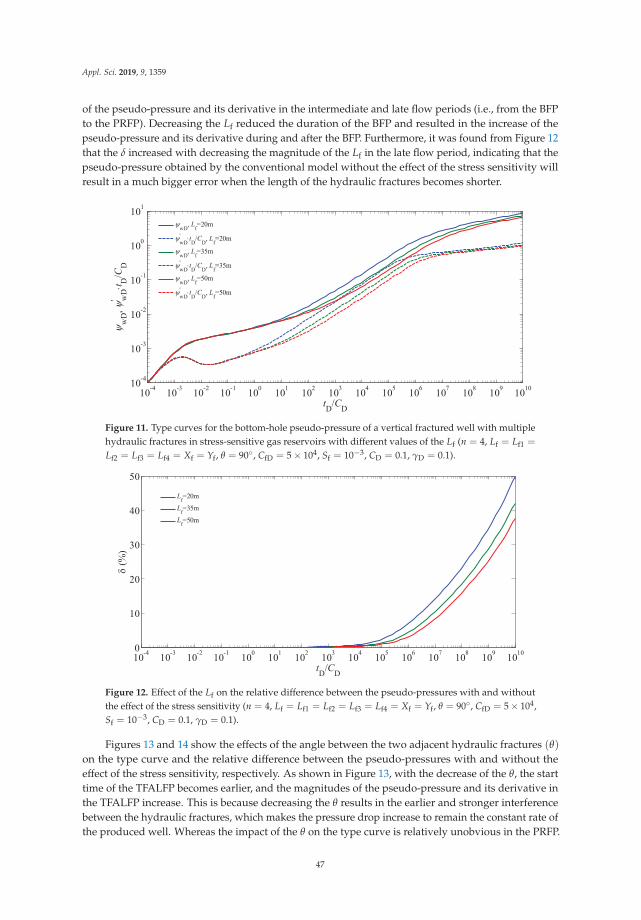
Appl. Sci. 2019, 9, 1359

of the pseudo-pressure and its derivative in the intermediate and late flow periods (i.e., from the BFPto the PRFP). Decreasing the Lf reduced the duration of the BFP and resulted in the increase of thepseudo-pressure and its derivative during and after the BFP. Furthermore, it was found from Figure 12that the δ increased with decreasing the magnitude of the Lf in the late flow period, indicating that thepseudo-pressure obtained by the conventional model without the effect of the stress sensitivity willresult in a much bigger error when the length of the hydraulic fractures becomes shorter.

10-4 10-3 10-2 10-1 100 101 102 103 104 105 106 107 108 109 101010-4

10-3

10-2

10-1

100

101

tD/CD

wD

, ' w

Dt D

/CD

wD, Lf=20m'wDtD/CD, Lf=20m

wD, L

f=35m

'wDtD/CD, Lf=35m

wD, L

f=50m

'wDtD/CD, Lf=50m

Figure 11. Type curves for the bottom-hole pseudo-pressure of a vertical fractured well with multiplehydraulic fractures in stress-sensitive gas reservoirs with different values of the Lf (n = 4, Lf = Lf1 =

Lf2 = Lf3 = Lf4 = Xf = Yf, θ = 90◦, CfD = 5 × 104, Sf = 10−3, CD = 0.1, γD = 0.1).

10-4 10-3 10-2 10-1 100 101 102 103 104 105 106 107 108 109 10100

10

20

30

40

50

tD/CD

(%)

Lf=20m

Lf=35mLf=50m

Figure 12. Effect of the Lf on the relative difference between the pseudo-pressures with and withoutthe effect of the stress sensitivity (n = 4, Lf = Lf1 = Lf2 = Lf3 = Lf4 = Xf = Yf, θ = 90◦, CfD = 5 × 104,Sf = 10−3, CD = 0.1, γD = 0.1).

Figures 13 and 14 show the effects of the angle between the two adjacent hydraulic fractures (θ)on the type curve and the relative difference between the pseudo-pressures with and without theeffect of the stress sensitivity, respectively. As shown in Figure 13, with the decrease of the θ, the starttime of the TFALFP becomes earlier, and the magnitudes of the pseudo-pressure and its derivative inthe TFALFP increase. This is because decreasing the θ results in the earlier and stronger interferencebetween the hydraulic fractures, which makes the pressure drop increase to remain the constant rate ofthe produced well. Whereas the impact of the θ on the type curve is relatively unobvious in the PRFP.

47

Appl. Sci. 2019, 9, 1359

Furthermore, it is seen from Figure 14 that the δ increases with decreasing the magnitude of the θ

during and after the TFALFP, indicating that the effect of the stress sensitivity on the pseudo-pressurebecomes greater when the θ decreases.

10-4 10-3 10-2 10-1 100 101 102 103 104 105 106 107 108 109 101010-4

10-3

10-2

10-1

100

101

tD/CD

wD

, ' w

Dt D

/CD

wD, =7.5o

'wDtD/CD, =7.5o

wD, =30o

'wDtD/CD, =30o

wD, =90o

'wDtD/CD, =90o

Figure 13. Type curves for the bottom-hole pseudo-pressure of a vertical fractured well with multiplehydraulic fractures in stress-sensitive gas reservoirs with different values of the θ (n = 4, Lf1 = Lf2 =

Xf = 50 m, Lf3 = Lf4 = Yf = 50 m, CfD = 5 × 104, Sf = 10−3, CD = 0.1, γD = 0.1).

10-4 10-3 10-2 10-1 100 101 102 103 104 105 106 107 108 109 10100

10

20

30

40

50

(%)

tD/CD

=7.5o

=30o

=90o

Figure 14. Effect of the θ on the relative difference between the pseudo-pressures with and without theeffect of the stress sensitivity (n = 4, Lf1 = Lf2 = Xf = 50 m, Lf3 = Lf4 = Yf = 50 m, CfD = 5 × 104,Sf = 10−3, CD = 0.1, γD = 0.1).

Introducing the coefficient of β = |Xf − Yf|/(Xf + Yf) to quantify the difference of thehydraulic-fracture lengths, the effects of β on the type curve, and the relative differences between thepseudo-pressures with and without the effect of the stress sensitivity are shown in Figures 15 and 16,respectively. It is obvious that the difference of the hydraulic-fracture lengths becomes larger as themagnitude of the β increases. The range of the β is from zero to one. As shown in Figure 15, with thedecrease of the β, the end of the BFP takes place later, the duration of the TFABFP becomes shorter,and the start time of the LFP occurs earlier. The reason for the existence of the TFABFP is that thedifference of the hydraulic-fracture lengths leads to the inconsistency of the end times for the BFPfor each hydraulic fracture. If β is equal to zero, the TFABFP may not even appear. Furthermore,the difference of the hydraulic-fracture lengths makes the pseudo-pressure and its derivative increase

48

Appl. Sci. 2019, 9, 1359

in the TFABFP. It is interesting to find in Figure 15 that during the TFALFP, the pseudo-pressure andits derivative increase as the β decreases. This may be because that for the distribution of the hydraulicfractures shown in Figure 6, the interference between hydraulic fractures enhances with the decreaseof the β in the TFALFP. As shown in Figure 16, the β has an effect on the error caused by neglecting thestress sensitivity during and after the TFALFP. Decreasing the β results in the increase of the error.

10-4 10-3 10-2 10-1 100 101 102 103 104 105 106 107 108 109 101010-4

10-3

10-2

10-1

100

101

tD/CD

wD

, ' w

Dt D

/CD

wD, =0'wD tD/CD, =0

wD, =0.6'wD tD/CD, =0.6

wD, =0.8'wD tD/CD, =0.8

Figure 15. Type curves for the bottom-hole pseudo-pressure of a vertical fractured well with multiplehydraulic fractures in stress-sensitive gas reservoirs with different values of the β (n = 4, Lf1 = Lf2 = Xf,Lf3 = Lf4 = Yf, Xf + Yf = 100 m, θ = 90◦, CfD = 5 × 104, Sf = 10−3, CD = 0.1, γD = 0.1).

10-4 10-3 10-2 10-1 100 101 102 103 104 105 106 107 108 109 10100

5

10

15

20

25

30

35

40

tD/CD

(%)

=0=0.6=0.8

Figure 16. Effect of the β on the relative difference between the pseudo-pressures with and withoutthe effect of the stress sensitivity (n = 4, Lf1 = Lf2 = Xf, Lf3 = Lf4 = Yf, Xf + Yf = 100 m, θ = 90◦,CfD = 5 × 104, Sf = 10−3, CD = 0.1, γD = 0.1).

Figures 17 and 18 show the effects of the hydraulic-fracture number (n) on the type curve and therelative difference between the pseudo-pressures with and without the effect of the stress sensitivity,respectively. The distribution of the hydraulic fractures was assumed to be uniform (i.e., the anglebetween the two arbitrary adjacent hydraulic fractures was equal). As shown in Figure 17, it isobvious that the n affects the pseudo-pressure behavior in all periods except for the WSP. Increasingthe n leads to the decrease of the pseudo-pressure and its derivative. Due to the increase of the n,the angle between the two adjacent hydraulic fractures was reduced, and thus the interference betweenhydraulic fractures occurred earlier and the effect of this interference on the pseudo-pressure was

49

Appl. Sci. 2019, 9, 1359

more significant. Figure 18 indicates that a smaller value of the n leads to a bigger error caused byneglecting the stress sensitivity during and after the TFALFP.

10-4 10-3 10-2 10-1 100 101 102 103 104 105 106 107 108 109 101010-4

10-3

10-2

10-1

100

101

tD/CD

wD

, ' w

Dt D

/CD

wD, n=4

'wD tD/CD, n=4

wD, n=8

'wD tD/CD

, n=8

wD, n=12

'wD tD/CD

, n=12

Figure 17. Type curves for the bottom-hole pseudo-pressure of a vertical fractured well with multiplehydraulic fractures in stress-sensitive gas reservoirs with different values of the n (Lf1 = Lf2 = Xf =

80 m, Lf3 = Lf4 = Yf = 80 m, θ = 360◦/n, CfD = 5 × 104, Sf = 10−3, CD = 0.1, γD = 0.1).

10-4 10-3 10-2 10-1 100 101 102 103 104 105 106 107 108 109 10100

5

10

15

20

25

30

35

tD/CD

(%)

n=4n=8n=12

Figure 18. Effect of n on the relative difference between the pseudo-pressures with and withoutthe effect of the stress sensitivity (Lf1 = Lf2 = Xf = 80 m, Lf3 = Lf4 = Yf = 80 m, θ = 360◦/n,CfD = 5 × 104, Sf = 10−3, CD = 0.1, γD = 0.1).

6. Conclusions

We have established a non-linear model of a vertical fractured well with multiple hydraulicfractures in gas reservoirs by incorporating the pressure-dependent permeability. Both transformedpseudo-pressure and perturbation techniques were employed to linearize the proposed model.Superposition principle and numerical discrete methods were used to obtain the semi-analyticalsolution. Type curves for pseudo-pressure were plotted and discussed in detail. The influence ofrelevant parameters on the type curve and the relative difference between the pseudo-pressures withand without the effect of the stress sensitivity were analyzed. Some main conclusions are listedas follows:

(1) The type curve of a vertical fractured well with multiple hydraulic fractures was identifiedby seven possible flow regions. Compared with the conventional model of a vertical fractured wellwith two symmetrical hydraulic-fracture wings, two transitional flow regimes (i.e., the TFABFP and

50

Appl. Sci. 2019, 9, 1359

TFALFP) were observed, which were caused by the difference of the hydraulic-fracture lengths andthe interference between hydraulic fractures, respectively.

(2) As the time increased, the pressure drops increased, which made the permeability decrease.The impact of the stress sensitivity on the pseudo-pressure increased with the increase of the time.Furthermore, the influence of the stress sensitivity on the pseudo-pressure was negligibly small in theearly and intermediate flow periods but becomes very significant in the late flow period.

(3) Some relevant parameters, such as dimensionless permeability modulus, fracture conductivitycoefficient, hydraulic-fracture length, angle between the two adjacent hydraulic fractures, the differenceof the hydraulic-fracture lengths, and hydraulic-fracture number, not only affected the type curve, butalso have an influence of the error caused by neglecting the stress sensitivity.

Author Contributions: Data curation, Z.S.; Formal analysis, P.G.; Funding acquisition, J.R.; Investigation, Z.S.;Methodology, P.G.; Project administration, P.G.; Visualization, H.C.; Writing—original draft, Z.S.; Writing—reviewand editing, C.P.

Funding: We acknowledge the support provided by the Open Fund of the State Key Laboratory of Oil andGas Reservoir Geology and Exploitation (PLN201627) and the Scientific Research Starting Project of SWPU (No.2017QHZ031).


Appendix A. Symbol Description

NomenclatureC wellbore storage coefficient, m3/PaCfD fracture conductivity coefficientcft total compressibility of hydraulic fracture, Pa−1

ct total compressibility of gas reservoir, Pa−1

h reservoir thickness, mk reservoir permeability, m2

kfi initial fracture permeability, m2

ki initial reservoir permeability, m2

Lfj length of the jth hydraulic fracture, mn hydraulic-fracture numberp reservoir pressure, Papf fracture pressure, Papi initial reservoir pressure, Papsc pressure at standard condition, Paq flow rate of point source, m3/sqf flow-rate density, m2/sQi production rate of the ith hydraulic fracture, m3/sQsc well production rate, m3/sr radial distance, r =

√x2 + y2, m

rw wellbore radius, ms Laplace transform variableSf skin factort time, sT reservoir temperature, KTsc temperature at standard condition, Kwf fracture width, mxi, yi xi- and yi-coordinates, mZ Z-factor of gasμ gas viscosity, Pa · sγ permeability modulus, (Pa · s)/Pa2

ψ reservoir pseudo-pressure, Pa2/(Pa · s)ψf fracture pseudo-pressure, Pa2/(Pa · s)ψi initial reservoir pseudo-pressure, Pa2/(Pa · s)

51

Appl. Sci. 2019, 9, 1359

ψw bottom-hole pseudo-pressure, Pa2/(Pa · s)ξD dimensionless transformed reservoir pseudo-pressureξfD dimensionless transformed fracture pseudo-pressureξwD dimensionless transformed bottom-hole pseudo-pressure with wellbore storage and skinξwHD dimensionless transformed bottom-hole pseudo-pressure without wellbore storage and skinφ reservoir porosityφf fracture porosityθ polar angle, degreeθfj polar angle of the jth hydraulic fracture, degreeΔLfi length of discrete segment of the ith hydraulic fracture, mSubscriptD dimensionlessi, j the jth discrete segment in the ith hydraulic fractureSuperscript− Laplace space

Appendix B. Pressure Distribution in a Gas Reservoir with a Vertical Fractured Well withMultiple Hydraulic Fractures Producing at a Constant Rate

With the aid of Equation (11), Equations (7)–(10) can be rewritten as

∂2ξD

∂r2D

+1

rD

∂ξD

∂rD=

11 − γDξD

∂ξD

∂tD, (A1)

ξD(rD, tD = 0) = 0, (A2)

ξD(rD, tD = 0) = 0, (A3)

limrD→0

rD∂ξD

∂rD= −qD(rD = 0, tD). (A4)

The perturbation technique of γD was employed to obtain that

ξD = ξD0 + γDξD1 + γ2DξD2 + · · · , (A5)

− 1γD

ln[1 − γDξD] = ξD +12

γDξ2D + · · · , (A6)

11 − γDξD

= 1 + γDξD + γ2Dξ2

D + · · · . (A7)

Considering a small value of γD in general, the zero-order perturbation solution was accurateenough for engineering requirements. So, Equations (A1)–(A4) can be rewritten as

∂2ξD0

∂r2D

+1

rD

∂ξD0

∂rD=

∂ξD0

∂tD, (A8)

ξD0(rD, tD = 0) = 0, (A9)

ξD0(rD → ∞, tD) = 0, (A10)

limrD→0

rD∂ξD0

∂rD= −qD(rD = 0, tD). (A11)

Laplace transform was employed to solve the above model and it is defined by

f (s) =∫ ∞

0f (tD)e−stD dtD, (A12)

where f is an arbitrary variable in real space.

52

Appl. Sci. 2019, 9, 1359

Taking the Laplace transform of Equations (A8)–(A11), one can obtain

∂2ξD0

∂r2D

+1

rD

∂ξD0∂rD

= sξD0, (A13)

ξD0(rD → ∞, s) = 0, (A14)

limrD→0

rD∂ξD0∂rD

= −qD(rD = 0, s). (A15)

The solution of Equations (A13)–(A15) in Laplace space can be derived as

ξD0(rD, s) = qD(rD = 0, s)K0(rD

√s). (A16)

According to Equation (A16), the superposition principle [39] was employed to obtain the pressuredistribution in a gas reservoir with a vertical fractured well with multiple hydraulic fractures producingat a constant rate

ξD0(rD, θ, s) =n

∑j=1

[∫ LfjD

0q f D(α, θfj, s)K0(

√s√


(θ − θfj

))dα

]. (A17)

Appendix C. Derivation of Dimensionless Model for Gas Flow within Stress-SensitiveHydraulic Fractures

Considering the effect of the pressure-dependent permeability of hydraulic fractures,the governing equation for gas flow in the ith hydraulic fracture is

∂2ψf

∂x2i+

∂2ψf

∂y2i+ γ

[(∂ψf∂xi

)2+

(∂ψf∂yi

)2]= eγ(ψi−ψf)

φfμcftkfi

∂ψf∂t

, (A18)

where 0 < xi < Lfi, −wf2 < yi <

wf2 .

The volume within the hydraulic fracture was very small, and thus the compressibility of thehydraulic fracture was neglected. Then Equation (A18) was reduced to

∂2ψf

∂x2i+

∂2ψf

∂y2i+ γ

[(∂ψf∂xi

)2+

(∂ψf∂yi

)2]= 0. (A19)

The flow-rate density of the ith hydraulic fracture is given as

qf(xi, t) =hTsckie−γ(ψi−ψ)

2pscT

[∂ψ(xi, yi, t)

∂yi

∣∣∣∣yi=

wf2

− ∂ψ(xi, yi, t)∂yi

∣∣∣∣yi=− wf

2

], (A20)

where 0 < xi < Lfi.The interface boundary condition between the wellbore and the ith hydraulic fracture is

h∫ wf

2

− wf2

Tsck f ie−γ(ψi−ψf)

2pscT∂ψf(xi, yi, t)

∂xidyi

∣∣∣∣∣xi=0

= Qi(t), (A21)

where Qi(t) is the production rate from the ith hydraulic fracture, which is expressed as

Qi(t) =∫ Lfi

0qf(xi, t)dxi. (A22)

53

Appl. Sci. 2019, 9, 1359

The total production rate of the vertical fractured well is the sum of the production rate of eachhydraulic fracture, and thus we can obtain

n

∑i=1

Qi(t) = Qsc. (A23)

The gas velocity should be continuous at the interface between the hydraulic fracture and reservoir,and thus the boundary conditions of the fracture surface are given as

Tsckfie−γ(ψi−ψf)


∂yi

∣∣∣∣∣yi=

wf2

=Tsckie−γ(ψi−ψ)

2pscT∂ψ(xi, yi, t)

∂yi

∣∣∣∣∣yi=

wf2

, (A24)

Tsckfie−γ(ψi−ψf)


∂yi

∣∣∣∣∣yi=− wf

2

=Tsckie−γ(ψi−ψ)

2pscT∂ψ(xi, yi, t)

∂yi

∣∣∣∣∣yi=− wf

2

. (A25)

Introducing the following expressions [16]

ψf = ψi +1γ

ln[1 − γ · ξf], (A26)

ψ = ψi +1γ

ln[1 − γ · ξ], (A27)

Equations (A19)–(A21), (A24), and (A25) can be rewritten as

∂2ξf(xi, yi, t)∂x2

i+

∂2ξf(xi, yi, t)∂y2

i= 0,

(0 < xi < Lfi, −wf

2< yi <

wf2

), (A28)

qf(xi, t) = − hTscki

2pscT

[∂ξ(xi, yi, t)

∂yi

∣∣∣∣yi=

wf2

− ∂ξ(xi, yi, t)∂yi

∣∣∣∣yi=− wf

2

], (0 < xi < Lfi), (A29)

h∫ wf

2

− wf2

Tsck f i

2pscT∂ξf(xi, yi, t)

∂xidyi

∣∣∣∣∣xi=0

= −Qi(t), (A30)

Tsckfi2pscT

∂ξf(xi, yi, t)∂yi

∣∣∣∣yi=

wf2

=Tscki

2pscT∂ξ(xi, yi, t)

∂yi

∣∣∣∣yi=

wf2

, (A31)

Tsckfi2pscT

∂ξf(xi, yi, t)∂yi

∣∣∣∣yi=− wf

2

=Tscki

2pscT∂ξ(xi, yi, t)

∂yi

∣∣∣∣yi=− wf

2

. (A32)

The width of the hydraulic fracture was very small, and thus the pressure changes within theith hydraulic fracture in the yi direction can be neglected. Then the average pressure within the ithhydraulic fracture in the yi direction is introduced as follows:

ξf(xi, t) =1

wf

∫ wf2

− wf2

ξf(xi, yi, t)dyi, (0 < xi < Lfi). (A33)

With the aid of Equations (A31)–(A33), Equation (A28) becomes

∂2ξf(xi, t)∂x2

i+

ki

wfkfi

[∂ξ(xi, yi, t)

∂yi

∣∣∣∣yi=

wf2

− ∂ξ(xi, yi, t)∂yi

∣∣∣∣yi=− wf

2

]= 0, (0 < xi < Lfi). (A34)

Substituting Equation (A29) into Equation (A34) yields

54

Appl. Sci. 2019, 9, 1359

∂2ξf(xi, t)∂x2

i− 2pscT

wfkfihTscqf(xi, t) = 0, (0 < xi < Lfi). (A35)

According to Equation (A33), Equation (A30) is expressed as

hwfTsckfi2pscT

∂ξf(xi, t)∂xi

∣∣∣∣xi=0

= −Qi(t). (A36)

Introducing the dimensionless variables, Equations (A26), (A35), (A36) are rewritten as follows:

ψfD = − 1γD

ln[1 − γD · ξfD], (A37)

∂2ξfD(xiD, tD)

∂x2iD

− 2π

CfDqfD(xiD, tD) = 0, (0 < xiD < LfiD), (A38)

∂ξfD(xiD, tD)

∂xiD

∣∣∣∣xiD=0

= − 2π

CfDQiD(tD). (A39)

The dimensionless expressions of Equations (A22) and (A23) are given as

QiD(tD) =∫ LfiD

0q f D(xiD, tD)dxiD, (A40)

n

∑j=1

QjD(tD) = 1. (A41)

References

1. Wang, Y.; Zhang, C.; Chen, T.; Ma, X. Modeling the Nonlinear Flow for a Multiple-fractured Horizontal Wellwith Multiple Finite-conductivity Fractures in Triple Media Carbonate Reservoir. J. Porous Media 2018, 21,1283–1305. [CrossRef]

2. Wang, Y.; Yi, X. Flow Modeling of Well Test Analysis for A Multiple-fractured Horizontal Well in TripleMedia Carbonate Reservoir. Int. J. Nonlinear Sci. Numer. Simul. 2018, 19, 439–457. [CrossRef]

3. Wang, Y.; Yi, X. Transient Pressure Behavior of a Fractured Vertical Well with A Finite-conductivity Fracturein Triple Media Carbonate Reservoir. J. Porous Media 2017, 20, 707–722. [CrossRef]

4. Ren, J.; Guo, P. A Novel Semi-analytical Model for Finite-conductivity Multiple Fractured Horizontal Wellsin Shale Gas Reservoirs. J. Nat. Gas Sci. Eng. 2015, 24, 35–51. [CrossRef]

5. Ren, J.; Guo, P. Anomalous Diffusion Performance of Multiple Fractured Horizontal Wells in Shale GasReservoirs. J. Nat. Gas Sci. Eng. 2015, 26, 642–651. [CrossRef]

6. Ren, J.; Guo, P. Nonlinear Seepage Model for Multiple Fractured Horizontal Wells with the Effect of theQuadratic Gradient Term. J. Porous Media 2018, 21, 223–239. [CrossRef]

7. Ren, J.; Guo, P. A General Analytical Method for Transient Flow Rate with the Stress-sensitive Effect. J.Hydrol. 2018, 565, 262–275. [CrossRef]

8. Ren, J.; Guo, P. Analytical Method for Transient Flow Rate with the Effect of the Quadratic Gradient Term.J. Pet. Sci. Eng. 2018, 162, 774–784. [CrossRef]

9. Ren, J.; Guo, P.; Peng, S.; Ma, Z. Performance of Multi-stage Fractured Horizontal Wells with StimulatedReservoir Volume in Tight Gas Reservoirs Considering Anomalous Diffusion. Environ. Earth Sci. 2018, 77,768. [CrossRef]

10. Ren, J.; Guo, P.; Guo, Z.; Wang, Z. A Lattice Boltzmann Model for simulating Gas Flow in Kerogen Pores.Transp. Porous Med. 2015, 106, 285–301. [CrossRef]

11. Ren, J.; Guo, P.; Peng, S.; Yang, C. Investigation on Permeability of Shale Matrix using the Lattice BoltzmannMethod. J. Nat. Gas Sci. Eng. 2016, 29, 169–175. [CrossRef]

12. Ren, J.; Guo, P.; Guo, Z. Rectangular Lattice Boltzmann Equation for Gaseous Microscale Flow. Adv. Appl.Math. Mech. 2016, 8, 306–330. [CrossRef]

55

Appl. Sci. 2019, 9, 1359

13. Ren, J.; Guo, P. Lattice Boltzmann Simulation of Steady Flow in a Semi-Elliptical Cavity. Commun. Comput.Phys. 2017, 21, 692–717. [CrossRef]

14. Ren, J.; Zheng, Q.; Guo, P.; Peng, S.; Wang, Z.; Du, J. Pore-scale Lattice Boltzmann Simulation ofTwo-component Shale Gas Flow. J. Nat. Gas Sci. Eng. 2019, 61, 46–70. [CrossRef]

15. Ren, J.; Zheng, Q.; Guo, P.; Zhao, C. Lattice Boltzmann Model for Gas Flow through Tight Porous Mediawith Multiple Mechanisms. Entropy 2019, 21, 133. [CrossRef]

16. Pedrosa, O.A. Pressure Transient Response in Stress-Sensitive Formations; SPE California Regional Meeting:Oakland, CA, USA, 1986.

17. Zhang, Z.; He, S.; Liu, G.; Guo, X.; Mo, S. Pressure Buildup Behavior of Vertically Fractured Wells withStress-sensitive Conductivity. J. Pet. Sci. Eng. 2014, 122, 48–55. [CrossRef]

18. Wang, J.; Jia, A.; Wei, Y.; Qi, Y. Approximate Semi-analytical Modeling of Transient Behavior of HorizontalWell Intercepted by Multiple Pressure-dependent Conductivity Fractures in Pressure-sensitive Reservoir.J. Pet. Sci. Eng. 2017, 153, 157–177. [CrossRef]

19. Gringarten, A.C.; Ramey, H.J.; Raghavan, J.R. Unsteady-state Pressure Distributions Created by a Well witha Single Infinite-conductivity Vertical Fracture. SPE J. 1974, 14, 347–360. [CrossRef]

20. Cinco-Ley, H.; Samaniego, F.; Dominguez, N. Transient Pressure Behavior for a Well with aFinite-conductivity Vertical Fracture. SPE J. 1978, 18, 253–264.

21. Bennett, C.O.; Reynolds, A.C.; Raghavan, R.; Elbel, J.L. Performance of Finite-conductivity, VerticallyFractured Wells in Single-layer Reservoirs. SPE Form. Eval. 1986, 1, 399–412. [CrossRef]

22. Bennett, C.O.; Rosato, N.D.; Reynolds, A.C.; Raghavan, R. Influence of Fracture Heterogeneity and WingLength on the Response of Vertically Fractured Wells. SPE J. 1983, 23, 219–230. [CrossRef]

23. Rodriguez, F.; Cinco-Ley, H.; Samaniego, V.F. Evaluation of Fracture Asymmetry of Finite-conductivityFractured Wells. SPE Prod. Eval. 1992, 7, 233–239. [CrossRef]

24. Berumen, S.; Tiab, D.; Rodriguez, F. Constant Rate Solutions for a Fractured Well with an AsymmetricFracture. J. Pet. Sci. Eng. 2000, 25, 49–58. [CrossRef]

25. Tiab, D.; Lu, J.; Nguyen, H.; Owayed, J. Evaluation of Fracture Asymmetry of Finite-conductivity FracturedWells. J. Energy Resour. Technol. 2010, 132, 1–7. [CrossRef]

26. Wang, L.; Wang, X.; Li, J.; Wang, J. Simulation of Pressure Transient Behavior for AsymmetricallyFinite-conductivity Fractured Wells in Coal Reservoirs. Transp. Porous Media 2013, 97, 353–372. [CrossRef]

27. Wang, L.; Wang, X. Type Curves Analysis for Asymmetrically Fractured Wells. J. Energy Resour. Technol.2014, 136, 023101. [CrossRef]

28. Fisher, M.K.; Wright, C.A.; Davidson, B.M.; Goodwin, A.K.; Fielder, E.O.; Buckler, W.S.; Steinsberger, N.P.Integrating Fracture Mapping Technologies to Improve Stimulations in the Barnett Shale. SPE Prod. Facil.2005, 20, 85–93. [CrossRef]

29. Mayerhofer, M.J.; Lolon, E.P.; Youngblood, J.E.; Heinze, J.R. Integration of Microseismic-Fracture-MappingResults with Numerical Fracture Network Production Modeling in the Barnett Shale; SPE Annual TechnicalConference and Exhibition: San Antonio, TX, USA, 2006.

30. Fan, Z.Q.; Jin, Z.H.; Johnson, S.E. Oil-gas Transformation Induced Subcritical Crack Propagation andCoalescence in Petroleum Source Rocks. Int. J. Fract. 2014, 185, 187–194. [CrossRef]

31. Ren, J.; Guo, P. Nonlinear Flow Model of Multiple Fractured Horizontal Wells with Stimulated ReservoirVolume including the Quadratic Gradient Term. J. Hydrol. 2017, 554, 155–172. [CrossRef]

32. Shaoul, J.R.; Behr, A.; Mtchedlishvili, G. Developing a Tool for 3D Reservoir Simulation of HydraulicallyFractured Wells. SPE Reservoir Eval. Eng. 2007, 10, 50–59. [CrossRef]

33. Restrepo, D.P.; Tiab, D. Multiple fractures transient response. In Proceedings of the SPE Latin American andCaribbean Petroleum Engineering Conference, Cartagena de Indias, Colombia, 31 May–3 June 2009.

34. Wang, L.; Wang, X.; Luo, E.; Wang, J. Analytical Modeling of Flow Behavior for Wormholes in NaturallyFractured-vuggy Porous Media. Transp. Porous Media 2014, 105, 539–558. [CrossRef]

35. Ren, J.; Guo, P. Performance of Vertical Fractured Wells with Multiple Finite-conductivity Fractures.J. Geophys. Eng. 2015, 12, 978–987. [CrossRef]

36. Luo, W.; Tang, C. Pressure-transient Analysis of Multiwing Fractures Connected to a Vertical Wellbore. SPEJ. 2015, 20, 360–367. [CrossRef]

37. Wang, H.T. Performance of Multiple Fractured Horizontal Wells in Shale Gas Reservoirs with Considerationof Multiple Mechanisms. J. Hydrol. 2014, 510, 299–312. [CrossRef]

56

Appl. Sci. 2019, 9, 1359

38. Li, X.P.; Cao, L.N.; Luo, C.; Zhang, B.; Zhang, J.Q.; Tan, X.H. Characteristics of Transient Production RatePerformance of Horizontal Well in Fractured Tight Gas Reservoirs with Stress-sensitivity Effect. J. Pet.Sci. Eng. 2017, 158, 92–106. [CrossRef]

39. Ozkan, E. Performance of Horizontal Wells. Ph.D. Thesis, University of Tulsa, Tulsa, OK, USA, 1988.40. Wan, J. Well Models of Hydraulically Fractured Horizontal Wells. Master’s Thesis, Stanford University, Palo

Alto, CA, USA, 1999.41. Van Everdingen, A.F.; Hurst, W. The Application of the Laplace Transformation to Flow Problems in

Reservoirs. Trans. AIME 1949, 186, 305–324. [CrossRef]42. Stehfest, H. Numerical Inversion of Laplace Transforms. Commun. ACM 1970, 13, 47–49. [CrossRef]43. Akanji, L.T.; Falade, G.K. Closed-Form Solution of Radial Transport of Tracers in Porous Media Influenced

by Linear Drift. Energies 2019, 12, 29. [CrossRef]44. Choo, Y.K.; Wu, C.H. Transient Pressure Behavior of Multiple-fractured Gas Wells. In Proceedings of the

SPE/DOE Low Permeability Reservoirs Symposium, Denver, CO, USA, 18–19 May 1987.

© 2019 by the authors. Licensee MDPI, Basel, Switzerland. This article is an open accessarticle distributed under the terms and conditions of the Creative Commons Attribution(CC BY) license (http://creativecommons.org/licenses/by/4.0/).

57

applied sciences

Article

Parametrical Non-Complex Tests to Evaluate PartialDecentralized Linear-Output Feedback ControlStabilization Conditions from Their CentralizedStabilization Counterparts

Manuel De la Sen 1,* and Asier Ibeas 2

1 Institute of Research and Development of Processes IIDP, University of the Basque Country, Campus ofLeioa, 48940 Leioa (Bizkaia), Spain

2 Department of Telecommunications and Systems Engineering, Universitat Autònoma de Barcelona UAB,08193 Barcelona, Spain; [email protected]


Received: 18 March 2019; Accepted: 22 April 2019; Published: 26 April 2019

Abstract: This paper formulates sufficiency-type linear-output feedback decentralized closed-loopstabilization conditions if the continuous-time linear dynamic system can be stabilized under linearoutput-feedback centralized stabilization. The provided tests are simple to evaluate, while they arebased on the quantification of the sufficiently smallness of the parametrical error norms between thecontrol, output, interconnection and open-loop system dynamics matrices and the correspondingcontrol gains in the decentralized case related to the centralized counterpart. The tolerance amounts ofthe various parametrical matrix errors are described by the maximum allowed tolerance upper-boundof a small positive real parameter that upper-bounds the various parametrical error norms. Such atolerance is quantified by considering the first or second powers of such a small parameter. The resultsare seen to be directly extendable to quantify the allowed parametrical errors that guarantee theclosed-loop linear output-feedback stabilization of a current system related to its nominal counterpart.Furthermore, several simulated examples are also discussed.

Keywords: Output-feedback; centralized control; decentralized control; closed-loop stabilization

1. Introduction

Control systems are very important in real world applications and, therefore, they have beeninvestigated exhaustively concerning their properties of stability, stabilization, controllability controlstrategies etc. See, for instance, [1–4] and references therein. Some extra constraints inherent tosome systems, like solution positivity in the case of biological systems or human migrations orthe needed behavior robustness against parametrical changes of disturbance actions add additionalcomplexity to the related investigations and need the use of additional mathematical or engineeringtools for the research development, [5–7]. A large variety of modeling and design tools have to beinvoked and developed in the analysis depending on the concrete systems under study and theirpotential applications as, for instance, the presence of internal and external delays, discretization,dynamics modeling based on fractional calculus, the existence of complex systems with interconnectedsubsystems, [8–13], hybrid coupled continuous/digital tandems, nonlinear systems and optimizationand estimation techniques [14–19] as well as robotic and fuzzy-logic based systems, [20,21]. In particular,decentralized control is a useful tool for controlling dynamic systems by cutting some links between thedynamics coupling a set of subsystems integrated in the whole system at hand. It is claimed to keep themain properties related to the use of centralized control such as stability, controllability, observability,etc. In summary, a centralized controller keeps all the information on the system and coupling links as


Appl. Sci. 2019, 9, 1739

available to the control designer while decentralized control ignores some of such information or evencuts on occasions some of coupling signals between the various subsystems integrated in the wholesystem at hand. It can be pointed out that the stability studies are often performed trough Lyapunovtheory which requires to find a Lyapunov function (see [20,21] and some references therein). It turnsout that, if the neglected couplings are strong and are not taken into account by the controller, thestabilization and other properties such as the controllability can become lost. The use of decentralizedstabilization and control tools is of interest when the whole system has physically separated subsystemsthat require the implementation of local control actuators but the control has to be global for the wholesystem. An ad-hoc example provided in [2–4,19] where decentralized control is of a great designinterest is the case of several coupled cascade hydroelectric power plants allocated in the same riverbut separated far away from each other. It has to be pointed out that the term “decentralized control”versus “centralized control” refers to the eventual cut of links of the shared information betweentandems of integrated subsystems, or coupling signals between them, to be controlled rather than tothe physical disposal of the controller. In other words, if the whole controller keeps and uses all theinformation on measurable outputs and control components design to implement the control law, sucha control is considered to have a centralized nature even if its various sub-control stations are not jointlyallocated. It is a common designer´s basic idea in mind for complex control designs to try to minimizethe modeling designs and computational loads without significantly losing the system´s performanceand its essential properties. For instance, in [8], the dynamic characteristic of a discrete-time system isgiven as an extended state space description in which state variables and output tracking error areintegrated while they are regulated independently. The proposed robust model predictive control ismuch simpler than the traditional versions since the information of the upper and lower bounds ofthe time-varying delay are used for design purposes. On the other hand, in [9], a control law mightbe synthesized for a hydropower plant with six generation units working in an alternation scheme.To assess the behavior of the controlled system, a model of such a nonlinear plant is controlled bya fractional proportional/integral/derivative control device through a linearization of its set points,the fractional part being relevant in the approach on the controller derivative actions. In addition, aset of applied complex control problems are studied, for instance, in [10–16] with the aim of givingdifferent ad hoc simplification tools to deal with the appropriate control methodologies. In particular,a decentralized control approach is proposed in [16].

In this paper, the decentralized control design versus its decentralized control counterpart, undereventual output linear feedback, are studied from the point of view of the amount of information thatcan be lost or omitted in terms of the total or partial knowledge of the coupled dynamics betweensubsystems necessary in the decentralized case to keep the closed-loop stability. The study is made byusing the information on the worst-case deviation, in terms of norms, between the respective matricesof open-loop dynamics and the respective controller gains under which the closed-loop stability iskept. This paper is organized as follows. The problem statement is given in Section 2 while themain stabilization results of the paper are provided in Section 3. The proofs of some of the results ofSection 3, which are technically involved, but conceptually simple, are distributed in various technicalauxiliary that are given in Appendices A and B. It is claimed to give a non-complex method to testthe feasibility of the implementation of decentralized control and conditions for its design, which bea fast and simpler stability test compared to Lyapunov stability theory [20,21], for instance, under apartial removal of information or physical cuts of links of coupling dynamics between the varioussubsystems or state, control and output components. Section 4 discusses several examples and, finally,the concluding remarks end the paper.

Notation

n = {1, 2, · · · , n},R+ = { z ∈ R : z > 0} ; R0+ = { z ∈ R : z ≥ 0},

60

Appl. Sci. 2019, 9, 1739

sp(A) and det(A) are the spectrum and determinant of A ∈ Rn×n, respectively. For A ∈ Rq×�, being ingeneral rectangular, ‖A‖ denotes any unspecified norm of A, ‖A‖2 denotes the �2 or spectral norm of amatrix A, ρ(A) denotes its spectral radius, and ‖.‖∞ denotes the H∞-norm of a stable real rational transfermatrix or function, Iq denotes the qth identity matrix, and i =

√−1 is the complex imaginary unit.Let A ∈ Rn×n be symmetric. Then, λmax(A) and λmin(A) are, respectively, the maximum and

minimum eigenvalues of A.Mn×n

E is the set of Metzler matrices (any off-diagonal entry is non-negative) of nth order.Zn×n is the set of Z-matrices (any off-diagonal entry is non-positive) of nth order.Mn×n is the set of M-matrices (Z-matrices which are stable or critically stable) of nth order.Assume that A =

(Aij

), B =

(Bij)∈ Rn×n. Then, the notations A�B, A � B and A �� B, are,

respectively, equivalent to B≺A, B ≺ A and B ≺≺ A, meaning that Aij ≥ Bij, Aij ≥ Bij (and B � A)and Aij > Bij; ∀i, j ∈ n, respectively. In particular, A�0, A � 0 and A �� 0 are reworded as A isnon-negative, positive and strictly positive, respectively, and A≺0, A ≺ 0 and A ≺≺ 0 are reworded asA is non-positive, negative and strictly negative, respectively.

2. Problem Statement

Consider the following linear and time-invariant system under linear output-feedback centralizedcontrol:

.xc(t) = Acxc(t) + Bc uc(t); xc(0) = xc0 (1)

yc(t) = Ccxc(t) + Dcuc(t) (2)

uc(t) = Kcyc(t) (3)

where xc(t) ∈ Rn is the state vector; uc(t) ∈ Rm is the centralized control vector; yc(t) ∈ Rp is theoutput; Ac, Bc, Cc and Dc are the system, control, output and input–output interconnection matrices,respectively, of orders being compatible with the dimensions of the above vectors; and Kc ∈ Rm×p is thecontrol matrix. If the system runs in a decentralized control context, we have:

.xd(t) = Adxd(t) + Bd ud(t) ; xd(0) = xd0 (4)

yd(t) = Cdxd(t) + Ddud(t) (5)

ud(t) = Kdyd(t) (6)

where xd(t) ∈ Rn is the state vector; ud(t) ∈ Rm is the centralized control vector; yd(t) ∈ Rp is theoutput; Ad, Bd, Cd and Dd are the system, control, output and input–output interconnection matrices,respectively, of orders being compatible with the dimensions of the above vectors; and Kd ∈ Rm×p isthe control matrix.

Basically, the differences between centralized and decentralized controls are as follows:

(1) In the centralized control, all control components, or more generally, all subsystems if subsystemsare considered in the model, have a complete information on the output available for feedback.This means that all control components or block-control inputs are available for controlling eachstate component (or each individual substate including several state components in the case ofa more generic decomposition structure). Basically, the matrix Kc has a complete non-diagonalor block non-diagonal structure. In the decentralized control, the various input components orblock-control inputs are not available for controlling each state component. Thus, Kd does nothave a complete free design structure of its non-diagonal part and in some cases (completelydecentralized disposal) its diagonal or block diagonal.

(2) In a more general context, some control or output links can be cut in the decentralized casefor the sake of computational simplicity or a more economic control design. In our case, thedecentralized input, output and interconnection matrices Bd, Cd and Dd can be distinct from the

61

Appl. Sci. 2019, 9, 1739

centralized ones and, roughly speaking, to a have a “more diagonal” or “sparser” structure thantheir centralized counterparts Bc, Cc and Dc. If the parameterization of the system (or dynamics)matrix is available to the designer, then some off-diagonal block matrices of Ac could be zeroed orsimply re-disposed in a more sparse structure to construct Ad.

(3) The only strictly necessary condition for the system to be subject to partially (or, respectively,fully) decentralized control is that some (or, respectively, all) of the off-diagonal entries of Kd areforced to be zero even if the system, control, output and interconnection matrices remain identicalin Equations (4) and (5) with respect to Equations (1) and (2).

Assumption 1. The system in Equations (1) and (2) is linear output-feedback stabilizable via some centralizedcontrol law (Equation (3)).

Note that Assumption 1 does not hold if the open-loop system in Equations (1) and (2) has unstableor critically stable fixed modes that cannot be removed via linear feedback.

Proposition 1. If Assumption 1 holds, then there exists a centralized stabilizing controller gain Kc ∈ Rm×p

such that the matrices (Im −KcDc) and(Ip −DcKc

)are non-singular, thus the closed-loop centralized control

system is solvable and given by:

.xc(t) =

(Ac + Bc(Im −KcDc)

−1KcCc)xc(t); xc(0) = xc0 (7)

yc(t) =(Ip −DcKc

)−1Ccxc(t) (8)

and asymptotically stable for any given xc0 ∈ Rn under the generated control law:

uc(t) = (Im −KcDc)−1KcCcxc(t) (9)

that is, the polynomial p(s) = det(sIn −Ac − Bc(Im −KcDc)−1KcCc

)is Hurwitz.

Proof. The replacement of Equation (3) into Equations (1) and (2) yields Equation (7)–(9). Since the (1)and (2) is linear output stabilizable, a stabilizing controller gain Kc ∈ Rm×p has to exist such that (7)–(9)are solvable and the closed-loop dynamics is stable. �

Assumption 2. The system in Equations (4) and (5) is linear output-feedback stabilizable via some decentralizedcontrol law (Equation (6)).

In the same way as Proposition 1, we get the following result:

Proposition 2. If Assumption 2 holds, then there exists a decentralized stabilizing controller gain Kd ∈ Rm×p

such that the matrices (Im −KdDd) and(Ip −DdKd

)are non-singular, thus the closed-loop decentralized control

system is solvable and given by:

.xd(t) =

(Ad + Bd(Im −KdDd)

−1KdCd)xd(t); xd(0) = xd0 (10)

yd(t) =(Ip −DdKd

)−1Cdxd(t) (11)

and asymptotically stable for any given xd0 ∈ Rn under the control law:

ud(t) = (Im −KdDd)−1KdCdxd(t) (12)

that is, the polynomial p(s) = det(sIn −Ad − Bd(Im −KdDd)

−1KdCd)

is Hurwitz.

62

Appl. Sci. 2019, 9, 1739

Proposition 3. Assume that Ad = Ac, Bd = Bc, Cd = Cc and Dd = Dc, and that the system in Equations (1)and (2) is not linear output-feedback stabilizable via some centralized control law (Equation (3)). Then, it is notstabilizable under any linear output-feedback decentralized control (Equation (6)) either.

Proof. Obviously, if there is no completely free-design matrix Kc that stabilizes Equations (1) and (2),then there is no Kd with at least a forced zero off-diagonal entry that stabilizes it since Kd has extradesign constraints related to Kc. �

It can be pointed out that decentralized control has also been proved to be useful in applications.For instance, an integral-based event-triggered asymptotic stabilization of a continuous-time linearsystem is studied in [17] by considering actuator saturation and observer-based output feedback areconsidered. In the proposed scheme, the sensors and actuators are implemented in a decentralizedmanner and a type of Zeno-free decentralized integral-based event condition is designed to guaranteethe asymptotic stability of the closed-loop systems. On the other hand, two decentralized fuzzylogic-based control schemes with a high-penetration non-storage wind-diesel system are studied in [18]for small power system with high-penetration wind farms. In addition, several examples concerningdecentralized control are described in [4] to illustrate the theoretical design analysis. A typical describedcase is that of tandems of electrical power system with a tandem disposal on the same river which arenot physically nearly allocated. The next section discusses some simple sufficiency-type conditionswhich ensure that, provided that the system is stabilizable under linear output-feedback centralizedcontrol, it is also stabilizable under decentralized control in two cases: (a) the system matrix remainsidentical but the other parameterization matrices can eventually vary; and (b) the system matrixcan vary as well in the decentralized case with respect to the centralized one. A result elated to themaintenance of the stability of a matrix under an additive matrix perturbation is summarized througha set of sufficiency-type conditions simple to test in Theorem A1. Theorem A2 proves sufficiency-typefor the stability of the matrix function A(t) = A0 + A(t) with A0 stable and A(t) being time-varying.Appendix B includes calculations and auxiliary results to quantify the tolerance to cut some dynamicslinks between subsystems, state components or control centers or components while keeping theclosed-loop stability of the whole coupled system. The results of Appendices A and B are used in theproofs of the main results in the next section.

3. Main Results

The first set of technical results which follow are concerned with centralized and decentralizedcontrol stabilizability.

Assertion 1. A necessary and sufficient condition for the system to be linear state-stabilizable via somecentralized control law is that rank[sIn −Ac Bc] = n for all Res ≥ 0.

Proof. Assume that rank[sIn −Ac Bc] = n1 < n for some Res ≥ 0. Then, there is some Laplace

transform[xT(s) , uT(s)

]T

= Lap[xT(t) , uT(t)

]T � 0 such that [sIn −Ac Bc]

[xT(s) , uT(s)

]T = 0 for

some Res ≥ 0 and [sIn −Ac Bc]

[In

Kc

]x(s) = 0 for any Kc ∈ Rn×n and some x(s) � 0 with Res ≥ 0

since rank([sIn −Ac Bc]

[In

Kc

])≤ min

(rank[sIn −Ac Bc] , rank

[In

Kc

])≤ min(n1 , n) ≤ n1 < n for some

Res ≥ 0. Therefore, the closed-loop system has some unstable or critically stable solution forany given (centralized) control gain. This proves the necessary part. Sufficiency follows since, ifrank[sIn −Ac Bc] = n, then x(s) ≡ 0 for all Res ≥ 0 and some Kc ∈ Rn×n which can be found so that

min(rank[sIn −Ac Bc] , rank

[In

Kc

])= min(n, n) = n. �

63

Appl. Sci. 2019, 9, 1739

Assertion 1. is a particular adapted ad-hoc test for stabilizability of the celebrated Popov–Belevitch–Hautus rank controllability test [6]. Note that, if there exist unstable or critically stable fixed modes(i.e., those present in the open-loop system that cannot be removed via feedback control), then neithercentralized nor decentralized stabilizing control laws can be synthesized. Note that the stabilizabilityrank test of Assumption 1 can only be evaluated for the critically and unstable eigenvalues of Ac

instead for all the open right-hand complex plane. In all the remaining points of such a plane, the testalways gives a full rank of the tested matrix. The parallel controllability test should always be appliedin the same matrix to any eigenvalues of Ac.

Assertion 2. A necessary condition for the system to be linear state-stabilizable via some partially or totallydecentralized control is that it be stabilizable via centralized control (i.e., Assertion 1 holds).

Proof. It is obvious from Assertion 1 since any gain Kd used for centralized or decentralized is sparserthan a centralized gain counterpart so that the proof follows from Assertion 1. �

Assertion 3. A necessary condition for the system to be linear output-stabilizable via some partially or totallydecentralized control is that it be stabilizable via centralized control (i.e., that Assertion 1 holds).

Proof. It is obvious from Assertions 1 and 2 that, when replacing Kc → (Im −KcDc)−1KcCc andKd → (Im −KdDd)

−1KdCd (see Equations (9) and (12)), the second replacement happens under sparserparameterizations. �

Now, consider the closed-loop system matrices from Equations (7) and (10) for the case A = Ac =

Ad.Acc = A + Bc(Im −KcDc)

−1KcCc; Adc = A + Bd(Im −KdDd)−1KdCd

with its parametrical error being:

Adc = Acc −Adc = Bc(Im −KcDc)−1KcCc − Bd(Im −KdDd)

−1KdCd

A first main technical result follows:

Theorem 1. If Assumption 1 holds, assume also that Kc ∈ Rm×p is a centralized linear output-feedbackstabilizing controller gain such that the resulting closed-loop system matrix Acc ∈ Rn×n has a stability abscissa(−ρcc) < 0. Then, the following properties hold:

(i) Adc ∈ Rn×n is a closed-loop stability matrix under a linear output-feedback stabilizing controller gainKd ∈ Rm×p if any of the subsequent sufficiency-type conditions holds:

(1) The H∞-norm of (sIn −Acc)−1Adc satisfies ‖(sIn −Acc)−1Adc‖∞ < 1,(2) ‖Adc‖2 < 1/ sup

ω∈R0+

‖(iωIn −Acc)−1‖2.

Other alternative sufficiency-type conditions to Conditions 1 and 2 for the stability of Adc are:(3) ρ

(A−1

cc Adc)< 1,

(4) ‖A−1cc Adc‖2 < 1,

(5) ‖Adc‖2 < 1/‖A−1cc ‖2, that is, λmax

(AT

dcAdc)< λmin

(AT

ccAcc),

in the following particular cases:(a) Acc ≺ 0 and Adc � Acc; and(b) Acc =

(Accij

)∈Mn×n

E and Adc =(Adci j

)fulfills Adci j ≤ Accij ; ∀i, j(� i) ∈ n.

(ii) Assume that Property (i) holds and that the number of inputs and outputs are identical, i.e., p = m,and decompose both the controller gain matrices as sums of their diagonal and off-diagonal parts leading toKc = Kcd + Kcod and Kd = Kdd + Kdod, thus K = Kc −Kd = (Kcd −Kdd) + (Kcod −Kdod). Then, the systemis stabilizable under partially decentralized control linear output-feedback control in the sense that Equations(4) and (5), is asymptotically stable under a control law (Equation (6)), if Kd ∈ Rm×p is such that, if there

64

Appl. Sci. 2019, 9, 1739

is at least one non-diagonal zero entry in at least one of its rows in the off-diagonal controller error matrixKod = Kcod −Kdod. If Kod = 0, then the system is stabilizable under decentralized control.

Proof. Property (i) is a direct translation of the results of Theorem A1 in Appendix A to the closed-loopsystem matrices. Property (ii) holds if Property (i) holds with an off-diagonal controller error matrixbetween the centralized a decentralized controller gain that has at least one non-diagonal zero at somerow (or its identically zero) so that a feedback from some crossed output to some of the inputs is notprovided to the control law for closed-loop stabilization the stabilization. �

The following result follows for the time-varying case from Theorem 1 and Theorem A2:

Corollary 1. Assume that Adc(t) and then Adc(t) are everywhere piecewise-continuous time-varying. Then,Theorem 1 still holds if Condition 1 is replaced with kcc

ρccsup

0≤τ<t‖Adc(τ)‖ < 1; ∀t ∈ R0+ with kcc ≥ 1 and ρcc > 0

being real constants such that e−Acct ≤ kcce−ρcct; ∀t ∈ R0+.

Remark 1. Theorem 1 (ii) has been stated for the case m = p. Note that the case m > p (i.e., there are moreinputs than outputs) is irrelevant for the stabilization from the strict algebraic point of view since the (m− p)extra inputs would be redundant. In the case that m ≤ p, Theorem 1 (ii) might be directly generalized to a

subsystem´s decomposition philosophy if a number q ≤ m of subsystems of inputs and outputs(uT

1 , uT2 , · · · , uT

q

)Tand

(yT

1 , yT2 , · · · , yT

q

)Twith ui ∈ Rmi , yi ∈ Rpi ; ∀i ∈ n with p =

∑qi=1 pi and m =

∑qi=1 mi.

Remark 2. Theorem 1 can be easily generalized to cases when some dynamics transmission links betweenstate, input or output components (or subsystems, in general) can be suppressed by manipulation. In moregeneral cases, it is possible to extend Theorem 1 to combinations of the subsequent situations with the matrixdecompositions having the same sense (in the various modified contexts) as that of Theorem 1 (ii):

• Case 1. Suppression of some transmission links between the coupled open-loop dynamics

by examining the decompositions: Ac = Acd + Acod, Ad = Add + Adod, and A = Ac − Ad =

(Acd −Add) + (Acod −Adod).

(a) If there is at least one non-diagonal zero entry in at least one of its rows in the off-diagonal controllererror matrix Aod = Acod −Adod which is not a corresponding zero in Acod; and (b) if there is at leastone non-diagonal zero entry in at least one of its rows in the off-diagonal controller error matrixKod = Kcod −Kdod, then the closed-loop system is stabilizable under a partial decentralized control evenif some links of the dynamics between crossed components are cut if Theorem 1 (ii) holds. If onlyCondition a is addressed, then the system is stabilizable by centralized control when cutting certaintransmission links between coupled dynamics in the open-loop system. This idea can be extended tototal decentralized control for a purely diagonal open-loop system´s dynamics under full zeroing of theoff-diagonal corresponding error dynamics. It can be also generalized to the “ad hoc” decompositionsbetween subsystems. Other cases with similar interpretations in the new contexts are:

• Case 2. Suppression of some crossed entries in the open-loop control matrix by examining thedecompositions: Bc = Bcd + Bcod, Bd = Bdd + Bdod, and B = Bc − Bd = (Bcd − Bdd) + (Bcod − Bdod).

• Case 3. Suppression of some crossed entries in the open-loop output matrix by examining the

decompositions: Cc = Ccd + Ccod, Cd = Cdd + Cdod, and C = Cc −Cd = (Ccd −Cdd) + (Ccod −Ddod).• Case 4. Suppression of some crossed entries in the open-loop interconnection matrix by examining

the decompositions: Dc = Dcd + Dcod, Dd = Ddd + Ddod, and D = Dc −Dd = (Dcd −Ddd) +

(Dcod −Ddod).• Case 5. Any combinations of Cases 1–4.

65

Appl. Sci. 2019, 9, 1739

Problem 1. Find a stabilizing decentralized family of control gains by assuming that Ad = Ac, such thatA = Ac −Ad = 0 and Assumption 1 holds with Kc being a stabilizing centralized controller gain.

The following more general result for the eventual case A � 0 (that is Ac � Ad eventually), followsfrom Theorem 1, Theorem A1 and Theorem A2 and Lemmas B1, B2 and B3:

Theorem 2. Define the following error matrices between the centralized and decentralized systemparameterizations:

A = Ac −Ad ; B = Bc − Bd; C = Cc −Cd; D = Dc −Dd; K = Kc −Kd (13)

such that ‖ A‖ ≤ σAε, ‖ B‖ ≤ σBε, ‖ C‖ ≤ σcε, ‖ D‖ ≤ σDε and ‖ K‖ ≤ σKε for some ε ∈ R0+ and given σA, σB,σC, σD ∈ R+. Assume that:

(1) Assumption 1 holds;(2) Kc ∈ Rm×p is a centralized linear output-feedback stabilizing controller gain such that the resulting

closed-loop system matrix Acc ∈ Rn×n has a stability abscissa (−ρcc) < 0 and such that ‖KcDc‖2 < 1 (sothat (Im −KcDc) is non-singular);

(3) Ac = Ad = A; and(4) Define ε∗ = min (1 , ε, ε1 , ε2), where:

ε =

√(σD‖Kc‖+ σK‖Dc‖)2 + 4σDσK/‖(Im −KcDc)−1‖ − (σD‖Kc‖+ σK‖Dc‖)

2σDσK,

ε1 =‖(Im −KcDc)−1‖

2[‖Kc‖σD + εσDσK + ‖Dc‖ σK]; ε2 = 1/

⎛⎜⎜⎜⎜⎝adc supω∈R0+

‖(iωIn −Acc)−1‖2

⎞⎟⎟⎟⎟⎠,where

adc = (1− ‖KcDc‖)−1×[σB‖KcCc‖+ ( ‖Bc‖+ ‖KcCc‖)(‖Kc‖σC + ‖Cc‖ σK + C [‖Kc‖σD + ‖Dc‖ σK])],

where the non-negative real constant C is given in Equation (A17). Then, the following properties hold:(i) If σA = 0 (that is, Ac = Ad), then Adc is stable and ε ∈ [0 , ε∗]. (ii) If ‖ A‖2 ≤ σAε, then Adc is stable

and ε ∈ [0 , ε′∗] where ε′∗ = min (1 , ε, ε1 , ε′2) and ε′2 = 1/

⎛⎜⎜⎜⎜⎝(adc + σA) supω∈R0+

‖(iωIn −Acc)−1‖2⎞⎟⎟⎟⎟⎠.

(iii) If A(t) is piecewise continuous and bounded, then Property (ii) holds by replacing ‖ A‖2 ≤ σAε bysup

0≤t<∞‖ A(t)‖2 ≤ σAε.

Remark 3. Some quantified results are given in Lemmas B.2 and B.3 to modify ε2(and hence ε′2) in Theorem 2by considering the second power of ε in the calculations of the disturbed parameterization guaranteeing theclosed-loop stability in the decentralized case.

Remark 4. If the corresponding parametrical error matrices of Equation (13) have some zero off-diagonal entries(or off-diagonal block matrices in the more general case that the system is described by coupled subsystems), thenwe have at least a partial closed-loop stabilization under decentralized control or, eventually, cut coupled dynamiclinks to the light of the various Cases 1–5 described after Remark 2 such that closed-loop stability is preserved.

Remark 5. Theorem 2 also applies to the case of state-feedback control by replacing the output matricesCc , Cd → In and fixing σC = 0.

66

Appl. Sci. 2019, 9, 1739

Remark 6. Theorem 2 also applies directly to the cases where Equations (1)–(3) are a given nominal asymptoticallystable closed-loop system configuration and Equations (4)–(6) are a perturbed one whose closed-loop asymptoticstability maintenance related to its nominal counterpart is a suited objective and which is not necessarily ofpartial of compete decentralized type.

4. Simulation Examples

This Section contains some numerical simulation examples to illustrate the theoretical resultsintroduced in Section 3.

Example 1. Consider the interconnected linear system with less inputs than outputs given by, [19]:

.x1(t) = A11x1(t) + A12x2(t) + B1u1(t).x2(t) = A21x1(t) + A22x2(t) + B2u2(t)

y1(t) = C1x1(t)y2(t) = C2x2(t)

with x1(t)T =

[x11(t) x12(t)

], x2(t)

T =[

x21(t) x22(t)]

and matrices defined by:

A11 =

[1 00 2

], A12 = A21 =

[ −1 00 −1

], A22 =

[ −1 00 −2

], B1 =

[12

], B2 =

[21

]

C1 = C2 = I2

This system can be cast into the form of Equations (1) and (2) by composing the matrices:

Ac =

⎡⎢⎢⎢⎢⎢⎢⎢⎢⎢⎢⎢⎢⎣1 0 −1 00 2 0 −1−1 0 −1 00 −1 0 −2

⎤⎥⎥⎥⎥⎥⎥⎥⎥⎥⎥⎥⎥⎦, Bc =

⎡⎢⎢⎢⎢⎢⎢⎢⎢⎢⎢⎢⎢⎣1 02 00 20 1

⎤⎥⎥⎥⎥⎥⎥⎥⎥⎥⎥⎥⎥⎦, Cc = I4, Dc = 0

Note that matrix Ac is unstable with eigenvalues given by {2.36, .1.41,−1.41,−2.23}. A staticfeedback output controller of the form of Equation (3) can be designed for this system, which leads tothe following gain:

Kc =

[ −9.3 8.2 −0.015 0.020.01 −0.01 0.375 0.25

]that places the closed-loop poles at {−0.84,−1.1,−2.8,−3.3} and thus stabilizes the closed-loop system.The static feedback gain Kc corresponds to a centralized controller as it can be readily observed.The question that arises now is whether a decentralized controller defined by:

Kd =

[ −9.3 8.2 0 00 0 0.375 0.25

]

is enough to stabilize the system or not. Note that Kd is a block-diagonal matrix with zerooff-block-diagonal entries. Theorem 1 enables us to guarantee the asymptotic stability of the abovesystem when the decentralized controller Kd is used. Therefore, Ad = Ac, Bd = Bc and Cd = Cc whilethe feedback gain Kd is restricted to the proposed particular structure. In this way, consider nowAcc = Ac + BcKcCc, Adc = Ac + BcKdCc and Adc = Bc(Kc −Kd)Cc. Condition 2 of Theorem 1 (i) yields:

0.055 = ‖Adc‖2 < 1

supω∈R0+

‖(iωI4 −Acc)−1‖2

= 0.07

67

Appl. Sci. 2019, 9, 1739

Consequently, we can conclude from Theorem 1 that the closed-loop system controlled by thedecentralized static output gain Kd is asymptotically stable. Thus, we have been able to easily analyzethe stability of the decentralized case from the stability property of the centralized one. Figure 1 showsthe trajectories of the closed-loop system when the gain Kd is deployed with initial conditions given byx1(t)

T =[−3 −4

], x2(t)

T =[

5 6]. It can be observed in Figure 1 that all the states converge to

zero as predicted by Theorem 1.

Figure 1. States evolution when the decentralized controller Kd is employed.

Example 2. Consider the linear system with the same number of inputs and outputs composed of two identicalpendulums THAT are coupled by a spring and subject to two distinct inputs, as displayed in Figure 2, [19].

Figure 2. Two inverted pendulums coupled by a spring.

The mathematical model of such interconnected system is given by:

.x1(t) = A11x1(t) + A12x2(t) + B1u1(t).x2(t) = A21x1(t) + A22x2(t) + B2u2(t)

y1(t) = C1x1(t)y2(t) = C2x2(t)

with x1(t)T =

[θ1

.θ1

], x2(t)

T =[θ2

.θ2

]and matrices defined by:

A11 = A22 =

⎡⎢⎢⎢⎢⎣ 0 1gl − ka2

ml2 −μ⎤⎥⎥⎥⎥⎦, A12 = A21 =

⎡⎢⎢⎢⎢⎣ 0 0ka2

ml2 0

⎤⎥⎥⎥⎥⎦, B1 = B2 =

[01

ml2

]

68

Appl. Sci. 2019, 9, 1739

C1 = C2 =[

1 0]

where g represents the gravity, μ accounts for the friction, m = m1 = m2 are the masses of bothpendulums, k is the spring constant and the meanings of the geometrical parameters are shown inFigure 2. This linear model corresponds to the linearization of the pendulum nonlinear equationsaround the up-right position equilibrium point. The following values were used in simulation, [19]:

gl= 1,

1ml2

= 1, μ = 1,km

= 2,al= 0.5

This system can be cast into the form of Equations (1) and (2) as:

Ac =

⎡⎢⎢⎢⎢⎢⎢⎢⎢⎢⎢⎢⎢⎣0 1 0 0

0.5 −1 0.5 00 0 0 1

0.5 0 0.5 −1

⎤⎥⎥⎥⎥⎥⎥⎥⎥⎥⎥⎥⎥⎦, Bc =

⎡⎢⎢⎢⎢⎢⎢⎢⎢⎢⎢⎢⎢⎣0 01 00 00 1

⎤⎥⎥⎥⎥⎥⎥⎥⎥⎥⎥⎥⎥⎦, Cc =

[1 0 0 00 0 1 0

], Dc = 0

A static output feedback controller can be designed for this system to achieve its asymptoticstability. In this way, the feedback gain

Kc =

[2.92 0.650.64 2.80

]

places the closed-loop poles at {−0.5± 1.5i,−0.5± 1.4i} with negative real parts. Now, we implement adecentralized controller with feedback gain given by:

Kd =

[2.92 0

0 2.80

]

Theorem 2 is now used to analyze the stability of the closed-loop system when this controlleris employed. This case is of practical importance and corresponds to the situation when the localcontroller has only available for control purposes the information regarding the local output, and notthe output of the complete system. Thus, the centralized and decentralized systems are the same andonly the static feedback gain changes. Theorem 2 conditions are applied with σA = σB = σC = σD = 0,σK = ‖Kc −Kd‖2 = 0.65 while the stability condition for this special case (see Appendix B) reads:

0.65 = 0.65× 1× 1 = ‖Kc −Kd‖2‖Bc‖2‖Cc‖2 < 1

Accordingly, the closed-loop system attained with the decentralized controller is asymptoticallystable and all the outputs will converge to zero asymptotically. Figure 3 displays the evolution of bothangles from initial conditions x1(t)

T =[

0.5 −0.5], x2(t)

T =[

0.15 0.5], where it can be observed

that both pendulums are stabilized in the up-right position with the decentralized controller.

69

Appl. Sci. 2019, 9, 1739

Figure 3. Evolution of the angles of both pendulums.

Example 3. Consider the linear interconnected system given by:

.xc(t) = Acxc(t) + Bcuc(t)yc(t) = Ccxc(t) + Dcuc(t)

with matrices defined by:

Ac =

⎡⎢⎢⎢⎢⎢⎢⎢⎢⎣−1 0.4 0.30.2 −2 0.1−0.1 0.2 −3

⎤⎥⎥⎥⎥⎥⎥⎥⎥⎦, Bc =

⎡⎢⎢⎢⎢⎢⎢⎢⎢⎣1 0.1 00 2 00 0 2

⎤⎥⎥⎥⎥⎥⎥⎥⎥⎦, Cc =

⎡⎢⎢⎢⎢⎢⎢⎢⎢⎣1 0.1 00 1 0.10 0 1

⎤⎥⎥⎥⎥⎥⎥⎥⎥⎦, Dc = 0.1I3

This system is controlled by the static output feedback gain given by:

Kc =

⎡⎢⎢⎢⎢⎢⎢⎢⎢⎣0.19 0.05 0.040.05 −0.01 0.03−0.02 0.02 −0.46

⎤⎥⎥⎥⎥⎥⎥⎥⎥⎦which places the closed-loop poles at {−1.17,−2,−2.1}. The decentralized system is now given by:

Ad = Ac, Bd =

⎡⎢⎢⎢⎢⎢⎢⎢⎢⎣1 0 00 2 00 0 2

⎤⎥⎥⎥⎥⎥⎥⎥⎥⎦, Cd = I3, Dd = 0

The decentralized system corresponds to the case when some transmission links have beensuppressed from the original open-loop coupled dynamics, as considered in Remark 2. The followingdecentralized gain iz employed to stabilize the decentralized system in Equations (4)–(6) parameterizedby the above matrices:

Kd =

⎡⎢⎢⎢⎢⎢⎢⎢⎢⎣0.19 0 0

0 −0.01 00 0 −0.46

⎤⎥⎥⎥⎥⎥⎥⎥⎥⎦Theorem 2 is used to analyze the stability of the decentralized closed-loop system. To this end, we

calculate:‖Ac −Ad‖2 = σA = 0

0.1 = ‖Bc − Bd‖2 ≤ σBε = 2.7× 0.07 = 0.19

0.1 = ‖Cc −Cd‖2 ≤ σCε = 2.7× 0.07 = 0.19

70

Appl. Sci. 2019, 9, 1739

0.1 = ‖Dc −Dd‖2 ≤ σDε = 2.7× 0.07 = 0.19

0.07 = ‖Kc −Kd‖2 ≤ σKε = 2.7× 0.07 = 0.19

With these values, we can compute ε = 0.31, ε1 = 0.24, ε2 = 0.071 so that 0.07 = ε < ε∗ =min(1, ε, ε1, ε2) = 0.071. Since ‖KcDc‖2 = 0.05 < 1, we are in conditions of applying Theorem 2 (i) andwe can conclude that the decentralized closed-loop system is asymptotically stable. In this way, thepresented results allow establishing the stability of the decentralized system by a simple method basedon the stability and design of the centralized system. Figure 4 shows the state variables evolutionfrom the initial state x(t)T =

[5 −5 1

]. As shown in Figure 4, the state variables converge to zero

asymptotically, as concluded from Theorem 2.

Figure 4. Evolution of the state space variables when the decentralized controller Kd is used.

5. Concluding Remarks

This paper is devoted to formulating sufficiency-type linear-output feedback decentralizedclosed-loop stabilization conditions if the continuous-time linear dynamic system can be stabilizedunder linear output-feedback centralized stabilization. The developed stability tests are conceptuallysimple to evaluate and they rely on the quantification in terms of worst-case norms of interconnectionand open-loop system dynamics matrices and the corresponding control gains in the decentralizedcase compared to the centralized counterpart. The tolerances of the various parametrical matrixerrors have been quantified by considering the first or second powers of a small parameter. Such aparameter is a design factor to characterize in the worst-case for the allowed tolerances to theperturbed parameterization norms. Simulated examples are discussed to illustrate the obtained results.The decentralized control design versus its decentralized control counterpart, under eventual outputlinear feedback, has been studied from the point of view of the amount of information that can be lostor omitted in terms of the total or partial knowledge of the coupled dynamics between subsystemsnecessary in the decentralized case to keep the closed-loop stability. A foreseen related future workrelies on the application of the method to some applied control problems such as consensus protocolsunder decentralized control and continuous-discrete hybrid controller designs.

Author Contributions: Author M.D.l.S. contributed to the manuscript in the aspects of conceptualization;methodology; formal analysis; investigation; writing original draft preparation; writing review and editing;supervision and fund acquisition. Author A.I. contributed to the manuscript in the various aspects of preparationof the numerical experiments; software implementation; visualization and original draft preparation.

Funding: This research was co-funded by the Spanish Government and the European Fund of RegionalDevelopment FEDER, grant numbers DPI2015-64766-R and DPI2016-77271-R (MINECO/FEDER, UE) and theUniversity of the Basque Country UPV /EHU, grant PGC 17/33.

71

Appl. Sci. 2019, 9, 1739

Acknowledgments: The authors are grateful to the Spanish Government for grants DPI2015-64766-R andDPI2016-77271-R (MINECO/FEDER, UE), and to UPV /EHU for grant PGC 17/33. They also thank the referees fortheir useful comments.


Appendix A Auxiliary Stability Results on Perturbed Matrices under Constant and Time-VaryingPerturbations of Stability Matrices

Theorem A1. Assume that A0 ∈ Rn×n is a stability matrix with stability abscissa (−ρc) < 0. Then,A = A0 + A is a stability matrix if any of the subsequent sufficiency-type conditions holds:

(1) The H∞-norm of (sIn −A0)−1A satisfies ‖(sIn −A0)

−1A‖∞ < 1,(2) ‖A‖2 < 1/ sup

ω∈R0+

‖(iωIn −A0)−1‖2.

Other alternative sufficiency-type conditions to Conditions 1 and 2 for the stability of A are:(3) ρ

(A−1

0 A)< 1,

(4) ‖A−10 A‖2 < 1,

‖A‖2 < 1/‖A−10 ‖2, that is, λmax

(ATA

)< λmin

(AT

0 A0), in the following particular cases:

(a) A0 ≺ 0 and A ≺ −A0; and(b) A0 =

(A0i j

)∈Mn×n

E and A =(Ai j

)fulfils Ai j ≥ −A0i j ; ∀i, j(� i) ∈ n.

Proof. Note that

det(sIn −A) = det(sIn −A0 − A

)= det

((sIn −A0)

(In − (sIn −A0)

−1A))

= det(sIn −A0) det(In − (sIn −A0)

−1A);∀s ∈ C

(A1)

and then det(sIn −A) = det(sIn −A0) det(In − (sIn −A0)

−1A)� 0 Then, for all s � sp(A), and also for

all s ∈ sp(A0) if the H∞-norm of (sIn −A0)−1A, which exists since A0 is a stability matrix, satisfies

‖(sIn −A0)−1A‖∞ < 1, which is guaranteed if ‖A‖2 < 1/ sup

ω∈R0+

‖(iωIn −A0)−1‖2. Then, A is a stability

matrix if Conditions 1 or 2 holds. On the other hand, if A0 and A are negative (implying that A ≺ −A0),or if they are both Metzler-stable (implying for all off-diagonal entries that Ai j ≥ −A0i j ; ∀i, j(� i) ∈ n),then their dominant abscissa (perhaps multiple) eigenvalue is real and negative since A0 being astability matrix is claimed to guarantee that A is stable. Since A0 is a stability matrix, it is non-singularwith eigenvalues with negative real parts. Then, by the continuity of the eigenvalues with respectto the matrix entries, A = A0

(In + A−1

0 A)

is a stability matrix if ρ(A−1

0 A)≤ ‖A−1

0 A‖2 ≤ ‖A−10 ‖2‖A‖2 < 1

leading to the sufficiency of Conditions 3–5 for the stability of A if is A0 stable. The last, sufficientcondition comes directly by upper-bounding Condition 4 by norm product and it is equivalent to‖A‖2 = λ1/2

max

(ATA

)< 1/‖A−1

0 ‖2 = 1/λ1/2max

(A−1

0 A−T0

)= λ1/2

min

(AT

0 A0). �

Theorem A2. Assume that A0 ∈ Rn×n is a stability matrix and that A(t) = A0 + A(t), where A : R0+ → Rn×n

is piecewise-continuous and bounded. Then, A : R0+ → Rn×n is stable if k0ρ0

sup0≤τ≤t

‖A(τ)‖ < 1; ∀t ∈ R0+,

where (−ρ0) < 0 is the stability abscissa of A0 and k0 = k0(‖A0‖) ≥ 1 is a real constant satisfying‖eA0t‖ ≤ k0e−ρ0t;∀t ∈ R0+.

Proof. Consider the linear time-varying system:

.x(t) =

(A0 + A(t)

)x(t), x(0) = x0 ; ∀t ∈ R0+ (A2)

72

Appl. Sci. 2019, 9, 1739

where A : R0+ → Rn×n is piecewise-continuous and bounded [1]. Such a system is globallyasymptotically stable if and only if A : R0+ → Rn×n is a stability matrix. The state-trajectory solutionof Equation (A2) satisfies:

‖x(t)‖ ≤ ‖eA0t‖ ‖x0‖+∫ t

0

∥∥∥eA0(t−τ)∥∥∥ ‖A(τ)‖ ‖x(τ)‖ dτ≤ k0e−ρ0t‖x0‖+ k0

ρ0sup

0≤τ≤t‖x(τ)‖

= K0e−ρ0t‖x0‖+ k0ρ0

sup0≤τ≤t

(‖A(τ)‖

)‖x(t′)‖; ∀t ∈ R0+

(A3)

Let t′ = t′(t) be defined for each t ∈ R0+ as t′ ={z = max

0≤τ≤tτ : ‖x(z)‖ ≥ ‖x(t)‖

}. Then,

‖x(t)‖ ≤ sup0≤τ≤t

‖x(τ)‖ = sup0≤τ≤t′

‖x(τ)‖ = ‖x(t′)‖ ≤ k0−ρ0t′‖x0‖+ k0

ρ0sup

0≤τ≤t‖A(τ)‖ ‖x(t′)‖; ∀t ∈ R0+ (A4)

Since 1 > k0ρ0

sup0≤τ≤t

‖A(τ)‖; ∀t ∈ R0+, one gets:

‖ x(t)‖ ≤ ‖ x(t′)‖ = sup0≤τ≤t′

‖x(τ)‖ ≤(1− k0

ρ0sup

0≤τ<∞‖A(τ)‖

)−1

k0e−ρ0t′‖x0‖

≤M = k0

(1− k0

ρ0sup

0≤τ<∞‖A(τ)‖

)−1

‖x0‖ ; ∀t ∈ R0+

(A5)

Therefore, x(t) is bounded for any t ∈ R0+ if x0 is finite. Now, assume the following cases.

Case a: For any Ts ∈ R+, the sequence

⎧⎪⎪⎨⎪⎪⎩ supnTs≤t<(n+mn)Ts

‖x(t)‖⎫⎪⎪⎬⎪⎪⎭∞

n=k

is strictly decreasing for some

finite positive integer k = k(Ts) and some positive sequence {mn} of bounded integer numbers which

satisfies mn+1 > mn − 1 for n ≥ 0. As a result,


‖x(t)‖⎫⎪⎪⎬⎪⎪⎭∞

n=k

→ 0 as n→∞ for any

given Ts > 0. Then, one gets from Equation (A3) that ‖x(t)‖ → 0 , as t→∞ since ‖x(nTs + t)‖≤k0

⎛⎜⎜⎜⎜⎝1 + 1ρ0

supnTs≤τ<t

‖x(τ)‖⎞⎟⎟⎟⎟⎠; ∀t ∈ (nTs , (n + 1)Ts). The result is proved for this case.

Case b: For some Ts ∈ R+, a sequence


‖x(t)‖⎫⎪⎪⎬⎪⎪⎭∞

n=0

can be built, with {mn}∞n=0 →∞ as

m→∞ satisfying sup(n+mn)Ts≤t<(n+mn)Ts

‖x(t)‖ = supnTs≤t<(n+mn+mn+mn )Ts

‖x(t)‖ ≥ supnTs≤t<(n+mn)Ts

‖x(t)‖ ; n ≥ 0

(note that the above inequality cannot be strict as n→∞ since it has already been proven that ‖x(t)‖ <+∞; ∀t ∈ R0+). However, then one gets from Equation (A3) for some tn+1 ∈ [n + mn , n + mn + mn+mn)

since 1 > k0ρ0

sup0≤τ≤t

‖A(τ)‖; ∀t ∈ R0+:

supnTs≤t<(n+mn)Ts

‖x(t)‖ ≤ supnTs≤t<(n+mn+mn+mn )Ts

‖x(t)‖≤ K0e−ρ0(tn+1−nTs)‖x(nTs)‖

+K0ρ0

supnTs≤t<(n+mn+mn+mn )Ts

(‖A(τ)‖

)sup

nTs≤t<(n+mn+mn+mn )T‖x(t)‖

< K0e−ρ0(tn+1−nTs)‖x(nTs)‖+ supnTs≤t<(n+mn+mn+mn )T

‖x(t)‖(A6)

If n→∞ , mn →∞ , then (tn+1 −mn+mn)→∞ , thus the following contradiction arises:

0 = lim supn→∞

⎛⎜⎜⎜⎜⎜⎝ supnTs≤t<(n+mn+mn+mn )Ts

‖x(t)‖ − supnTs≤t<(n+mn+mn+mn )Ts

‖x(t)‖⎞⎟⎟⎟⎟⎟⎠ < 0.

73

Appl. Sci. 2019, 9, 1739

Thus, Case b is not possible and the whole result follows from Case a. �

Note that the stability abscissa of A0, that is, (−ρ0) < 0 is not smaller than the dominanteigenvalue abscissa.

Appendix B Calculations for solving Problem 1

Assume that the matrix (Im −KcDc) is non-singular with ‖KcDc‖2 < 1 and A = Ac = Ad. Then,one gets from Equations (10) and (13) that:

Ad + Bd(Im −KdDd)−1KdCd

= A +(Bc − B

)(Im −KcDc − Δ0

)−1(KcDc − Δ1

)= A +

(Bc − B

) [(Im −KcDc)

(Im − (Im −KcDc)

−1Δ0)]−1

(KcCc − Δ1

)= A +

(Bc − B

) (Im − (Im −KcDc)

−1Δ0)−1

(Im −KcDc)−1(

KcCc − Δ1)

= A +(Bc − B

) (Im + Δ2

)(Im −KcDc)

−1(KcCc − Δ1

)(A7)

provided that D and K are such that (Im −KdDd)−1 =

(Im −KcDc − Δ0

)−1 exists (note that this always

holds if D = 0p×m and K = 0m×p from Assumption 1), where:

Δ0 = KdDd −KcDc = K(D−Dc

)−KcD =

(K −Kc

)D− KDc (A8)

Δ1 = K(Cc − C

)+ KcC =

(Kc − K

)C + KCc (A9)

Δ2 =[Im − (Im −KcDc)

−1Δ0]−1 − Im (A10)

and note that‖Δ0‖ ≤ ε [‖Kc‖σD + εσDσK + ‖Dc‖ σK] (A11)

‖Δ1‖ ≤ ε [‖Kc‖σC + εσCσK + ‖Cc‖ σK] (A12)

and one gets from Banach´s Perturbation Lemma [7] that

‖Δ2‖ ≤ 1 +1

1− ‖(Im −KcDc)−1Δ0‖≤ 1 +

1

1− ‖(Im −KcDc)−1‖ ‖Δ0‖(A13)

provided that ‖Δ0‖ < δ0 = 1/‖(Im −KcDc)−1‖. Equivalently, if

q(ε) = σDσkε2 + (σD‖Kc‖+ σK‖Dc‖)ε− 1/‖(Im −KcDc)

−1‖ < 0 (A14)

since q(ε) is a convex parabola with zeros ε1 < 0 and ε = ε2 > 0, Equation (A14) holds, guaranteeingthat ‖Δ0‖ < δ0, if ε ∈ [0 , ε), where:

ε =

√(σD‖Kc‖+ σK‖Dc‖)2 + 4σDσK/‖(Im −KcDc)−1‖ − (σD‖Kc‖+ σK‖Dc‖)

2σDσK(A15)

Before continuing with the calculations, we give the following auxiliary result:

Lemma B1. If (Im −KcDc) is non-singular with ‖KcDc‖2 < 1 and ‖Δ0‖ < δ0 = 1/‖(Im −KcDc)−1‖,equivalently if ε ∈ [0 , ε), with ε defined in Equation (A15), then ‖Δ2‖ ≤ C‖Δ0‖ < 1 with a norm-dependentreal constant C ≥ 1

2δ0if ε ∈ [0 , ε1) with

ε1 =‖(Im −KcDc)−1‖

2[‖Kc‖σD + εσDσK + ‖Dc‖ σK](A16)

74

Appl. Sci. 2019, 9, 1739

Proof. One gets from Equation (A10) and Banach´s Perturbation Lemma [7] that, if ‖Δ2‖ ≤ C‖Δ0‖ forsome C ∈ R+, then:

1

1−C‖Δ0‖≥ ‖

(Δ2 + Im

)−1‖ = ‖Im − (Im −KcDc)−1Δ0‖ ≥ 1− ‖(Im −KcDc)

−1‖ ‖Δ0‖

provided that C < 1/‖Δ0‖. One gets that the above inequality holds if 1/‖Δ0‖ > C ≥ 12δ0≥

‖(Im−KcDc)−1‖1+‖Δ0‖ ‖(Im−KcDc)−1‖ and, one gets from Equation (A11) that

‖Δ2‖ ≤ εC [‖Kc‖σD + εσDσK + ‖Dc‖ σK] < 1 (A17)

if ε < ε1. �

Now, rewrite the system matrices of closed-loop dynamics of Equations (7) and (10), equivalentlyEquation (A7), with A = Ac = Ad and its incremental value as follows:

Acc = A + Bc(Im −KcDc)−1KcCc (A18)

Adc = A + Bd(Im −KdDd)−1KdCd (A19)

Adc = Acc −Adc = Bc(Im −KcDc)−1KcCc − Bd(Im −KdDd)−1KdCd

= Bc(Im −KcDc)−1KcCc −(Bc − B

) (Im + Δ2

)(Im −KcDc)

−1(KcCc − Δ1

)= Bc(Im −KcDc)−1KcCc − Bc

(Im + Δ2

)(Im −KcDc)

−1(KcCc − Δ1

)+B

(Im + Δ2

)(Im −KcDc)

−1(KcCc − Δ1

)= Bc(Im −KcDc)−1Δ1

−BcΔ2(Im −KcDc)−1KcCc + BcΔ2(Im −KcDc)−1Δ1

+B(Im −KcDc)−1

KcCc − B(Im −KcDc)−1

Δ1

+BΔ2(Im −KcDc)−1

KcCc − BΔ2(Im −KcDc)−1

Δ1

(A20)

Now, the following technical result follows directly from Equations (A20), (A11), (A12) and (A17),the norm upper-bounding values of the control, output interconnection and controller matrix errorsand Lemma B1:

Lemma B2. The following properties hold for any ε ∈ [0 , ε) with ε = min(ε , ε1) calculated from Equations(A15) and (A16):

(i)

‖Adc‖ ≤ ‖Bc‖(1− ‖KcDc‖)−1[‖Δ1‖

(1 + ‖Δ2‖

)+ ‖KcCc‖‖Δ2‖

]+ε (1− ‖KcDc‖)−1

σB(1 + ‖Δ2‖

)(‖KcCc‖+ ‖Δ1‖

)≤ ε‖Bc‖(1− ‖KcDc‖)−1

×[(‖Kc‖σC + εσCσK + ‖Cc‖ σK)(1 + ‖KcCc‖+ εC [‖Kc‖σD + εσDσK + ‖Dc‖ σK])C [‖Kc‖σD + ‖Dc‖ σK + εσDσK]]

+ε (1− ‖KcDc‖)−1σB(1 + εC [‖Kc‖σD + εσDσK + ‖Dc‖ σK])(‖KcCc‖+ ε [‖Kc‖σC + εσCσK + ‖Cc‖ σK] )

(A21)

(ii) If, furthermore, ε ≤ 1, then εr ≤ ε for any real r ≥ 1 so that one gets from Equation (A21) by taking theupper-bound ε2 for ε3 that

‖Adc‖ ≤ ε‖Bc‖(1− ‖KcDc‖)−1(‖Δ10‖+ ‖KcCc‖‖Δ20‖

)+ ε2‖Δ20‖ ‖Bc‖(1− ‖KcDc‖)−1

+ε (1− ‖KcDc‖)−1σB‖KcCc‖+ε2 (1− ‖KcDc‖)−1

σB(‖Δ10‖+ ‖KcCc‖‖Δ20‖

)+ε3 (1− ‖KcDc‖)−1

σB‖Δ20‖‖Δ10‖≤ uε + vε2 ≤ (u + v)ε

(A22)

75

Appl. Sci. 2019, 9, 1739

where Δi = εΔi0 for i = 1, 2 and it has been used that ε3 ≤ ε2, with

u = ‖Bc‖(1− ‖KcDc‖)−1(‖Δ10‖+ ‖KcCc‖‖Δ20‖

)+ (1− ‖KcDc‖)−1

σB‖KcCc‖v = (1− ‖KcDc‖)−1

σB‖Δ20‖‖Δ10‖+‖Δ20‖ ‖Bc‖(1− ‖KcDc‖)−1+ (1− ‖KcDc‖)−1σB(‖Δ10‖+ ‖KcCc‖‖Δ20‖

) (A23)

(iii) If the upper-bound ε is used for ε2 and ε3, one gets that

‖Adc‖ ≤ ε‖Bc‖(1− ‖KcDc‖)−1

×[(‖Kc‖σC + σCσK + ‖Cc‖ σK)(1 + C [‖Kc‖σD + σDσK + ‖Dc‖ σK]) + ‖KcCc‖C [‖Kc‖σD + σDσK + ‖Dc‖ σK]]

+ε (1− ‖KcDc‖)−1σB(1 + C [‖Kc‖σD + σDσK + ‖Dc‖ σK])(‖KcCc‖+ [‖Kc‖σC + σCσK + ‖Cc‖ σK] )

(A24)

which also yields that ‖Adc‖ ≤ εadc + o(ε) in the case that ε < 1 after grouping all the additive contributions ofterms in εi for i ≥ 2 into an additive bounded term, which converges to zero as ε→ 0 , where

adc = (1− ‖KcDc‖)−1

×[σB‖KcCc‖+ ( ‖Bc‖+ ‖KcCc‖)(‖Kc‖σC + ‖Cc‖ σK + C [‖Kc‖σD + ‖Dc‖ σK])](A25)

�

Now, the following technical result follows directly from Lemma B2 and Theorem A1 (i):

Lemma B3. Define ε2 = 1/

⎛⎜⎜⎜⎜⎝adc supω∈R0+

‖(iωIn −Acc)−1‖2⎞⎟⎟⎟⎟⎠ from Equation (A25) and assume that ‖KcDc‖2 < 1

and that ε2 < min (ε , ε1, 1). Then, Adc is stable if Acc is stable and ε ∈ [0 , ε2]. By using Equations (A22) and(A23), a better bound of the maximum allowable ‖Adc‖2 is found as ε ∈ [0 , ε3] with ε3 < min (ε , ε20, 1) and

ε20 =√

u2+4vω−u2v .

Proof. Note from Theorem A1 (i) that the H∞-norm of (sIn −Acc)−1Adc satisfies ‖(sIn −Acc)−1Adc‖∞ < 1,which is guaranteed if ε < ε2, then Adc is stable since Acc is stable. The result follows by taking also intoaccount, in addition, the constraints in Equations (A15) and (A16) of Lemma B.1 by using ε3 ≤ ε2 ≤ ε.If the second power of ε is considered and the third one is upper-bounded as ε3 ≤ ε2, we examinethe stability constraint uε + vε2 < ω = 1/ sup

ω∈R0+

‖(iωIn −Acc)−1‖2 by building the convex parabola

θ(ε) = vε2 + uε −ω < 0 whose negative and positive zeros are ε1,2 = −u±√u2+4vω2v . Hence, the second

part of the result. �

References

1. Ibeas, A.; de la Sen, M. Robustly stable adaptive control of a tandem of master-slave robotic manipulators withforce reflection by using a multiestimation scheme. IEEE Trans. Cybern. Part B Cybern. 2006, 36, 1162–1164.[CrossRef]

2. Barambones, O.; Garrido, A.J.; Garrido, I. Robust speed estimation and control of an induction motor drivebased on artificial neural networks. Int. J. Adapt. Control Signal Process. 2008, 22, 440–444. [CrossRef]

3. Bakule, L.; de la Sen, M. Decentralized stabilization of networked complex composite systems with nonlinearperturbations. In Proceedings of the 2009 International Conference on Control and Automation, Christchurch,New Zealand, 9–11 December 2009; Volume 1–3, pp. 2272–2277.

4. Singh, M.G. Decentralised Control; North-Holland Systems and Control Series; North Holland PublishingCompany: New York, NY, USA, 1981; Volume 1.

5. Berman, A.; Plemmons, R.J. Nonnegative Matrices in the Mathematical Sciences; Academic Press: New York, NY,USA, 1979.

6. Kailath, T. Linear Systems; Prentice-Hall Inc.: Englewood Cliffs, NJ, USA, 1980.7. Ortega, J.M. Numerical Analysis; Academic Press: New York, NY, USA, 1972.

76

Appl. Sci. 2019, 9, 1739

8. Shi, H.; Li, P.; Wang, L.; Su, C.; Yu, J.; Cao, J. Delay-range-dependent robust constrained model predictivecontrol for industrial processes with uncertainties and unknown disturbances. Complexity 2019, 2019, 2152014.[CrossRef]

9. Rosas-Jaimes, O.A.; Munoz-Hernandez, G.A.; Mino-Aguilar, G.; Castaneda-Camacho, J.; Gracios-Marin, C.A.Evaluating fractional PID control in a nonlinear MIMO model of a hydroelectric power station. Complexity2019, 2019, 9367291. [CrossRef]

10. Xu, L.; Lou, S.; Xu, P.; Zhang, G. Feedback control and parameter invasion for a discrete competitiveLotka-Volterra system. Discret. Dyn. Nat. Soc. 2018, 2018, 7473208. [CrossRef]

11. Rana, S.M.S. Chaotic dynamics and control of discrete ratio-dependent predator-prey system. Discret. Dyn.Nat. Soc. 2017, 2017, 4537450. [CrossRef]

12. Hassan, A.; Dvorkin, Y.; Deka, D.; Chertkov, M. Chance-constrained ADMM approach for decentralizedcontrol of distributed energy resources. In Proceedings of the 2018 Power Systems Computation Conference(PSCC), Dublin, Ireland, 11–15 June 2018; pp. 1–7.

13. Shao, S.; Yang, H.; Jiang, B.; Cheng, S. Decentralized fault tolerant control for a class of interconnectednonlinear systems. IEEE Trans. Cybern. 2018, 48, 178–186. [CrossRef] [PubMed]

14. Nayyar, N.; Kalathil, D.; Jain, R. Optimal decentralized control with asymmetric one-step delayed informationsharing. IEEE Trans. Control Netw. Syst. 2018, 5, 653–654. [CrossRef]

15. Wei, C.; Luo, J.; Yin, Z.; Wei, X.; Yuan, J. Robust estimation-free decentralized prescribed performance controlof nonaffine nonlinear large-scale systems. Int. J. Robust Nonlinear Control 2018, 28, 174–196. [CrossRef]

16. Wang, Y.; Lopez, J.A.; Sznaier, M. Convex optimization approaches to information structured decentralizedcontrol. IEEE Trans. Autom. Control 2018, 63, 3393–3403. [CrossRef]

17. Zhang, H.G.; Yu, H.; Hao, F. Decentralized integral-based event-triggered stabilization for linear plant withactuator saturation and output feedback. Appl. Sci. 2017, 7, 11. [CrossRef]

18. Lotfy, M.E.; Senjyu, T.; Farahat, M.A.F.; Abdel-Gawad, A.F.; Lei, L.; Datta, M. Hybrid genetic algorithmfuzzy-based control schemes for small power system with high penetration wind farms. Appl. Sci. 2018,8, 373. [CrossRef]

19. Fu, Q.; Gu, P.; Wu, J.-R. Decentralized Iterative Learning Control for Large-scale Interconnected LinearSystems with Fixed Initial Shifts. Int. J. Control. Syst. 2017, 15, 1991–1994. [CrossRef]

20. He, W.; Dong, Y. Adaptive fuzzy neural network control for a constrained robot using impedance learning.IEEE Trans. Neural Netw. Learn. Syst. 2018, 29, 1174–1186. [CrossRef] [PubMed]

21. He, W.; Dong, Y. Design and adaptive control for an upper limb robotic exoskeleton in presence of inputsaturation. IEEE Trans. Neural Netw. Learn. Syst. 2019, 30, 97–108. [CrossRef] [PubMed]


77

applied sciences

Review

Short Overview of Early Developments of the HardyCross Type Methods for Computation of FlowDistribution in Pipe Networks

Dejan Brkic 1,2,3,*,† and Pavel Praks 1,2,*

1 European Commission, Joint Research Centre (JRC), 21027 Ispra, Italy2 IT4Innovations, VŠB—Technical University of Ostrava, 708 00 Ostrava, Czech Republic3 Research and Development Center “Alfatec”, 18000 Niš, Serbia* Correspondence: [email protected] (D.B.); [email protected] or [email protected] (P.P.)† On a short visit at IT4Innovations, VŠB—Technical University of Ostrava.

Received: 9 March 2019; Accepted: 16 April 2019; Published: 16 May 2019

Abstract: Hardy Cross originally proposed a method for analysis of flow in networks of conduits orconductors in 1936. His method was the first really useful engineering method in the field of pipenetwork calculation. Only electrical analogs of hydraulic networks were used before the Hardy Crossmethod. A problem with flow resistance versus electrical resistance makes these electrical analogmethods obsolete. The method by Hardy Cross is taught extensively at faculties, and it remainsan important tool for the analysis of looped pipe systems. Engineers today mostly use a modifiedHardy Cross method that considers the whole looped network of pipes simultaneously (use of thesemethods without computers is practically impossible). A method from a Russian practice publishedduring the 1930s, which is similar to the Hardy Cross method, is described, too. Some notes fromthe work of Hardy Cross are also presented. Finally, an improved version of the Hardy Crossmethod, which significantly reduces the number of iterations, is presented and discussed. We alsotested multi-point iterative methods, which can be used as a substitution for the Newton–Raphsonapproach used by Hardy Cross, but in this case this approach did not reduce the number of iterations.Although many new models have been developed since the time of Hardy Cross, the main purposeof this paper is to illustrate the very beginning of modeling of gas and water pipe networks andventilation systems. As a novelty, a new multi-point iterative solver is introduced and comparedwith the standard Newton–Raphson iterative method.

Keywords: Hardy Cross method; pipe networks; piping systems; hydraulic networks; gas distribution

1. Introduction

Hardy Cross solved the problem of distribution of flow in networks of pipes in his article “Analysisof Flow in Networks of Conduits or Conductors” [1] published on 13 November 1936.

Networks of pipes are nonlinear systems since the relation between flow and pressure is not linear.On the contrary, the relation between current and voltage in electrical networks with regular resistorsis governed by the linear Ohm’s law. Electrical circuits with diodes as well as hydraulic networksare nonlinear systems where resistance depends on current and voltage, i.e., on flow and pressure,respectively [2]. Nonlinear electrical circuits are electrical circuits containing nonlinear components.Nonlinear components can be resistive, capacitive, and inductive.

The distribution of flow in a network of pipes depends on the known inputs and consumptions atall nodes, on the given geometry of pipes, and on network topology. A stable state of flow in a networkmust satisfy Kirchhoff’s laws, which are statements of the conservation of mass and energy. Although intheory an indefinite number of flow distributions that satisfy that the conservation of mass is possible,


Appl. Sci. 2019, 9, 2019

only one distribution from this set also satisfies the conservation of energy for all closed paths formedby pipes in the network. This state is unique for the given network and in- and outflows [3].

Since the relation between flow and pressure is not linear, Hardy Cross used a relation betweenan increment of flow and an increment of pressure, as this relation is linear for the given quantity offlow. If, however, the increments are fairly large, this linear relation is somewhat in error, such as for gascompressible flow. However, if the pressure drop in pipes is minor, such as in a municipality networkfor natural gas distribution, the Hardy Cross method can be used without significant errors [4–6].Moreover, the Hardy Cross method can also be used for water pipe networks (district heating [7] andcooling networks [8]) and ventilation systems [9,10] (a related formulation is presented in Appendix).

The Hardy Cross method is an iterative method, i.e., a method using successive corrections [4].Lobacev and Andrijašev in the 1930s, writing in Russian, offered similar methods [11,12]. Probablybecause of the language barrier and the political situation in Soviet Russia, Hardy Cross was not awareof Lobacev and Andrijašev’s contributions.

Today, engineers use the most improved version of the Hardy Cross method (the ΔQ method [13];for Δp, see [14]), which analyzes the whole looped network of pipes simultaneously [15].

As a novel approach presented for the first time here, we tested multi-point iterative methods [16,17]that can be used as a substitution for the Newton–Raphson approach used by Hardy Cross. This approach,however, did not in this case reduce the number of required iterations to reach the final balanced solution.

One example of the pipe network for distribution of gas is analyzed using the original Hardy Crossmethod [1] in Section 3.1, its related equivalent from Russian literature [11,12] in Section 3.2, the improvedversion of the Hardy Cross method [15,17,18] in Section 3.3, and finally the approach which uses multi-pointiterative methods instead of the commonly used Newton–Raphson method in Section 3.4.

2. Network Piping System; Flow Distribution Calculation

2.1. Topology of the Network

The first step in solving a pipe network problem is to make a network map showing pipe diameters,lengths and connections between pipes (nodes). Sources of natural gas supply and consumption rateshave to be assigned to nodes. For convenience in locating pipes, code numbers are assigned to eachpipe and closed loop of pipes (represented by roman numbers for loops in Figure 1). Pipes on thenetwork periphery are common to one loop and those in the network interior are common to two loops.Figure 1 is an example of a pipe network for distribution of natural gas for consumption in households.

Figure 1. The network of pipes for natural gas distribution for domestic consumption.

The next step is to write the initial gas flow distribution through pipes in the network.This distribution must be done according to Kirchhoff’s first law. The choice of initial flows isnot critical, and the criterion should satisfy Kirchhoff’s first law for every node in the network [3].The total gas flow arriving at a node equals the total gas flow that leaves that node. The same

80

Appl. Sci. 2019, 9, 2019

conservation law is also valid for the whole network in total (except for gas input and outputnodes that cannot be changed during calculations; see consumption nodes in Figure 1). The sum ofpseudo-pressure drops along any closed path must be approximately zero for the network to be inbalance according to Kirchhoff’s second law. In this paper, the flow distribution, which satisfies both ofKirchhoff’s laws, will be calculated using the Hardy Cross iterative method.

2.2. A Hydraulic Model

The Renouard formula; Equation (1) best fits a natural gas distribution system built with polyvinylchloride (PVC) pipes [19,20]. Computed pressure drops are always less than the actual drop since themaximal consumption occurs only during extremely severe winter days [21,22].

f = Δp2 = p21 − p2

2 = 4810·ρr·L·Q1.82

D4.82(1)

where f is a function of pressure, �r is relative gas density (dimensionless), ρr = 0.64, L is the pipelength (m), D is the pipe diameter (m), Q is flow (m3/s), and p is pressure (Pa).

As shown in Appendix A, other formulas are used in the case of waterworks systems [23,24] andventilation networks [7].

Regarding the Renouard formula (Equation (1)), one has to be careful since the pressure dropfunction, f , does not relate pressure drop, but actually the difference of the quadratic pressure at

the input and the output of the pipe. This means that√

Δp2 =√

p21 − p2

2 is not actually pressuredrop despite using the same unit of measurement, i.e., the same unit is used as for pressure (Pa).The parameter

√Δp2 can be noted as a pseudo-pressure drop. In fact, the gas is actually compressed,

and hence that volume of the gas is decreased, and then such a compressed volume of the gas isconveying with a constant density through the gas distribution pipeline. The operating pressure fora typical distribution gas network is 4× 105 Pa abs, i.e., 3× 105 Pa gauge, and accordingly the volumeof the gas decreases four times compared to the volume of the gas in normal (or standard) conditions.Pressure in the Renouard formula is for normal (standard) conditions.

The first derivative f’ of the Renouard relation (Equation (2)), where the flow is treated as a variable,is used in the Hardy Cross method.

f ′ =∂ f (Q)

∂Q= 1.82·4810·ρr·L·Q0.82

D4.82(2)

First assumed gas flow in each pipe is listed in the third column of Table 1. The plus or minussign preceding flow indicates the direction of flow through the pipe for the particular loop [18,25].A plus sign denotes counterclockwise flow in the pipe within the loop, while the minus sign clockwise.The loop direction can be chosen to be clockwise or counterclockwise (in Figure 1, all loops arecounterclockwise).

3. The Hardy Cross Method; Different Versions

The Hardy Cross method is presented here: the original approach in Section 3.1, a versionof the Hardy Cross method from Russian practice in Section 3.2, the modified Hardy Crossmethod in Section 3.3, and finally the method that uses multi-point iterative procedures insteadthe Newton–Raphson method and which can be implemented in all the aforementioned methods.

3.1. The Hardy Cross Method; Original Approach

The pressure drop function for each pipe is listed in Table 1 (for initial flow pattern, in the fourthcolumn). The sign in front of the pressure drop function shown in the fourth column is the same asfor flow from the observed iteration. The fifth column of Table 1 includes the first derivatives of thepressure drop function, where the flow is treated as a variable. The column of the function of pressure

81

Appl. Sci. 2019, 9, 2019

drops is computed algebraically, while the column of the first derivatives is estimated numerically foreach loop. Flow correction ΔQ has to be computed for each loop x (Equation (3)).

ΔQx =

⎛⎜⎜⎜⎜⎝∑± f∣∣∣ f ′∣∣∣

⎞⎟⎟⎟⎟⎠x

=

⎛⎜⎜⎜⎜⎜⎜⎜⎜⎝∑±4810·ρr·L·Q1.82

D4.82∑∣∣∣∣1.82·4810·ρr·L·Q0.82

D4.82

∣∣∣∣⎞⎟⎟⎟⎟⎟⎟⎟⎟⎠

x

(3)

For the network from Figure 1, flow corrections for the first iteration in each loop can be calculatedusing Equation (4).(∣∣∣− f ′1

∣∣∣+ ∣∣∣ f ′7 ∣∣∣+ ∣∣∣ f ′8 ∣∣∣+ ∣∣∣ f ′9 ∣∣∣+ ∣∣∣− f ′10

∣∣∣+ ∣∣∣− f ′12

∣∣∣)·ΔQI = − f1 + f7 + f8 + f9 − f10 − f12(∣∣∣− f ′2∣∣∣+ ∣∣∣− f ′11

∣∣∣+ ∣∣∣ f ′12

∣∣∣)·ΔQII = − f2 − f11 + f12(∣∣∣− f ′3∣∣∣+ ∣∣∣ f ′4 ∣∣∣+ ∣∣∣ f ′10

∣∣∣+ ∣∣∣ f ′11

∣∣∣+ ∣∣∣− f ′14

∣∣∣)·ΔQIII = − f3 + f4 + f10 + f11 − f14(∣∣∣ f ′5 ∣∣∣+ ∣∣∣− f ′9∣∣∣+ ∣∣∣ f ′13

∣∣∣+ ∣∣∣ f ′14

∣∣∣)·ΔQIV = f5 − f9 + f13 + f14(∣∣∣ f ′6 ∣∣∣+ ∣∣∣− f ′8∣∣∣+ ∣∣∣ f ′13

∣∣∣)·ΔQV = f6 − f8 + f13

⎫⎪⎪⎪⎪⎪⎪⎪⎪⎪⎪⎬⎪⎪⎪⎪⎪⎪⎪⎪⎪⎪⎭(4)

In the second iteration, the calculated correction ΔQ has to be added algebraically to the assumedgas flow (the first initial flow pattern). Further, the calculated correction ΔQ has to be subtractedalgebraically from the gas flow computed in the previous iteration. This means that the algebraicoperation for the first correction is the opposite of its sign, i.e., add when the sign is minus, and vice versa.A pipe common to two loops receives two corrections simultaneously. The first correction is fromthe particular loop under consideration, while the second one is from the adjacent loop, which theobserved pipe also belongs to.

Table 1. Procedure for the solution of the flow problem for the network from Figure 1 using themodified Hardy Cross method (first two iterations)—First iteration.

Iteration 1

Loop Pipe a Q b f = p21 − p2

2c |f

′| d ΔQ1

e ΔQ2f Q1 =Q

I

1 −0.3342 −144518566.8 787025109.2 −0.0994 −0.43367 +0.7028 +859927106.7 2226902866.0 −0.0994 +0.60348 +0.3056 +306964191.0 1828124435.8 −0.0994 −0.0532 = +0.15309 +0.2778 +800657172.4 5245486154.8 −0.0994 −0.0338 = +0.1446

10 −0.1364 −241342976.1 3220265516.7 −0.0994 +0.0142 ‡ −0.221712 −0.0167 −6238747.4 679911398.4 −0.0994 +0.0651 ‡ −0.0511

Σ fI = +1575448179.8 13987715480.9

II2 −0.0026 −80628.9 56440212.4 −0.0651 −0.067711 −0.1198 −14582531.0 221537615.9 −0.0651 +0.0142 ‡ −0.170712 +0.0167 +6238747.4 679911398.4 −0.0651 +0.0994 ∓ +0.0511

Σ fII = −8424412.4 957889226.7

III

3 −0.2338 −406110098.1 3161336093.1 −0.0142 −0.24804 +0.0182 +1530938.1 153093808.5 −0.0142 +0.0040

10 +0.1364 +241342976.1 3220265516.7 −0.0142 +0.0994 ∓ +0.221711 +0.1198 +14582531.0 221537615.9 −0.0142 +0.0651 ∓ +0.170714 −0.0278 −21840183.8 1429824980.5 −0.0142 −0.0338 ± −0.0757

Σ fIII = −170493836.7 8186058014.8

IV

5 +0.0460 +7523646.2 297674697.0 +0.0338 +0.07989 −0.2778 −800657172.4 5245486154.8 +0.0338 +0.0994 ‡ −0.1446

13 +0.0278 +21840183.8 1429824980.5 +0.0338 −0.0532 = +0.008414 +0.0278 +21840183.8 1429824980.5 +0.0338 +0.0142∓ +0.0757

82

Appl. Sci. 2019, 9, 2019

Table 1. Cont.

Iteration 1

Loop Pipe a Q b f = p21 − p2

2c |f

′| d ΔQ1

e ΔQ2f Q1 =Q

Σ fIV = −749453158.7 8402810812.8

V6 +0.0182 +3479197.2 347919720.0 +0.0532 +0.07148 −0.3056 −306964191.0 1828124435.8 +0.0532 +0.0994 ‡ −0.1530

13 −0.0278 −21840183.8 1429824980.5 +0.0532 −0.0338 ± −0.0084

Σ fV = −325325177.5 3605869136.3

Iteration 2

Loop Pipe Q1 = Q f = p21 − p2

2

∣∣∣f′∣∣∣ ΔQ1 ΔQ2 Q2 = Q

I

1 −0.4336 −232172997.6 974431560.7 −0.0058 −0.43947 +0.6034 +651439280.6 1965036192.1 −0.0058 +0.59768 +0.1530 +87112249.4 1036457217.8 −0.0058 −0.0178= +0.12949 +0.1446 +243990034.4 3070921097.1 −0.0058 −0.0098= +0.1290

10 −0.2217 −584137977.5 4795666298.0 −0.0058 +0.0018 ‡ −0.225712 −0.0511 −47725420.6 1700518680.1 −0.0058 −2.1·10−5 ± −0.0569

Σ fI = +118505168.7 13543031045.9

II2 −0.0677 −30372941.9 816962908.0 +2.1·10−5 −0.067611 −0.1707 −27780459.9 296182372.8 +2.1·10−5 +0.0018 ‡ −0.168912 +0.0511 +47725420.6 1700518680.1 +2.1·10−5 +0.0058 ∓ +0.0569

Σ fII = −10427981.2 2813663960.8

III

3 −0.2480 −451970989.4 3317464222.8 −0.0018 −0.24974 +0.0040 +99061.2 44589235.4 −0.0018 +0.0023

10 +0.2217 +584137977.5 4795666298.0 −0.0018 +0.0058 ∓ +0.225711 +0.1707 +27780459.9 296182372.8 −0.0018 −2.1·10−5 = +0.168914 −0.0757 −135261698.0 3251481942.9 −0.0018 −0.0098 ± −0.0873

Σ fIII = +24784811.3 11705384072.0

IV

5 +0.0798 +20483898.1 467437803.0 +0.0098 +0.08969 −0.1446 −243990034.4 3070921097.1 +0.0098 +0.0058 ‡ −0.1290

13 +0.0084 +2454799.0 534076127.2 +0.0098 −0.0178 = +0.000414 +0.0757 +135261698.0 3251481942.9 +0.0098 +0.0018 ∓ +0.0873

Σ fIV = −85789639.2 7323916970.2

V6 +0.0714 +41857166.9 1067095933.1 +0.0178 +0.08928 −0.1530 −87112249.4 1036457217.8 +0.0178 +0.0058 ‡ −0.1294

13 −0.0084 −2454799.0 534076127.2 +0.0178 −0.0098 ± −0.0004

Σ fV = −47709881.5 2637629278.1a Pipe lengths, diameters and initial flow distribution are shown in Table 2 and Figure 1; b f calculated using theRenouard Equation (1); c f ′ calculated using the first derivative of the Renouard, Equation (2), where flow is variable;d calculated using the matrix Equation (10) and entering ΔQ with the opposite sign (using the original Hardy Crossmethod for Iteration 1: ΔQI= +0.1126; ΔQII= −0.0088; ΔQIII = −0.0208; ΔQIV = −0.0892; ΔQV= −0.0902; using theLobacev method for Iteration 1: ΔQI = −0.1041; ΔQII = −0.0644; ΔQIII= −0.0780; ΔQIV= + 0.1069; ΔQV= −0.1824);e ΔQ2 is ΔQ1 from the adjacent loop; f the final calculated flow in the first iteration is used for the calculation in thesecond iteration, etc.; g if Q and Q1 have a different sign, this means that the flow direction is opposite to that in theprevious iteration, etc. (this occurs with the flow in pipe 13 between Iteration 3 and 4).

The upper sign after the second correction in Table 1 is plus if the flow direction in the mutualpipe coincides with the assumed orientation of the adjacent loop, and minus if it does not (Figure 2).The lower sign is the sign in front of correction ΔQ calculated for the adjacent loop (Figure 2).

83

Appl. Sci. 2019, 9, 2019

Figure 2. Rules for the upper and lower sign (correction from the adjacent loop; second correction).

Details of the signs of corrections were reported by Brkic [18] and Corfield et al. [25].The algebraic operation for the second correction should be the opposite of its lower sign when its

upper sign is the same as the sign in front of flow Q, and, as indicated by its lower sign, when its uppersign is opposite to the sign in front of flow Q.

The calculation procedure is repeated until the net algebraic sum of pressure functions aroundeach loop is as close to zero as the desired degree of precision demands. This also means that thecalculated corrections of flow and the change in calculated flow between two successive iterations isapproximately zero. The pipe network is then in approximate balance and the calculation after theHardy Cross can be terminated.

In the original Hardy Cross method, the corrections for the first iteration are:

ΔQI =1575448179.813987715480.9

= +0.1126

ΔQII =−8424412.4957889226.7

= −0.0088

ΔQIII =−170493836.78186058014.8

= −0.0208

ΔQIV =−749453158.78402810812.8

= −0.0892

andΔQV =

−325325177.53605869136.3

= −0.0902

3.2. A Version of the Hardy Cross Method from Russian Practice

As mentioned in the Introduction, two Russian authors, Lobacev [11] and Andrijašev [12],proposed a similar method to Hardy Cross [1]. These two methods are also from the 1930s. It is notclear if Hardy Cross had been aware of the contribution of these two authors from Soviet Russia andvice versa, but most probably the answer to this question is no, for both sides. The main differencebetween the Hardy Cross and Andrijašev methods is that in the method of Andrijašev contours canbe defined to include few loops. This strategy only complicates the situation, while the number ofrequired iterations remains unchanged.

Further on, the Andrijašev method can be seen from the example in the paper of Brkic [3].Here, the method of Lobacev is shown in more detail. In the Hardy Cross method, the influence ofadjacent loops is neglected. The Lobacev method takes into consideration this influence (Equation (5)):

+(∣∣∣− f ′1

∣∣∣+ ∣∣∣ f ′7 ∣∣∣+ ∣∣∣ f ′8 ∣∣∣+ ∣∣∣ f ′9 ∣∣∣+ ∣∣∣− f ′10

∣∣∣+ ∣∣∣− f ′12

∣∣∣)·ΔQI +∣∣∣ f ′12

∣∣∣·ΔQII +∣∣∣ f ′10

∣∣∣·ΔQIII +∣∣∣ f ′9 ∣∣∣·ΔQIV +

∣∣∣ f ′8 ∣∣∣·ΔQV = − f1 + f7 + f8 + f9 − f10 − f12∣∣∣ f ′12

∣∣∣·ΔQI −(∣∣∣− f ′2

∣∣∣+ ∣∣∣− f ′11

∣∣∣+ ∣∣∣ f ′12

∣∣∣)·ΔQII −∣∣∣ f ′11

∣∣∣·ΔQIII = − f2 − f11 + f12

+∣∣∣ f ′10

∣∣∣·ΔQI −∣∣∣ f ′11

∣∣∣·ΔQII −(∣∣∣− f ′3

∣∣∣+ ∣∣∣ f ′4 ∣∣∣+ ∣∣∣ f ′10

∣∣∣+ ∣∣∣ f ′11

∣∣∣+ ∣∣∣− f ′14

∣∣∣)·ΔQIII −∣∣∣ f ′14

∣∣∣·ΔQIV = − f3 + f4 + f10 + f11 − f14

+∣∣∣ f ′9 ∣∣∣·ΔQI −

∣∣∣ f ′14

∣∣∣·ΔQIII −(∣∣∣ f ′5 ∣∣∣+ ∣∣∣− f ′9

∣∣∣+ ∣∣∣ f ′13

∣∣∣+ ∣∣∣ f ′14

∣∣∣)·ΔQIV −∣∣∣ f ′13

∣∣∣·ΔQV = f5 − f9 + f13 + f14

+∣∣∣ f ′8 ∣∣∣·ΔQI −

∣∣∣ f ′13

∣∣∣·ΔQIV −(∣∣∣ f ′6 ∣∣∣+ ∣∣∣− f ′8

∣∣∣+ ∣∣∣ f ′13

∣∣∣)·ΔQV = f6 − f8 + f13

⎫⎪⎪⎪⎪⎪⎪⎪⎪⎪⎪⎬⎪⎪⎪⎪⎪⎪⎪⎪⎪⎪⎭(5)

84

Appl. Sci. 2019, 9, 2019

In Equation (5), signs in front of terms from the left side of the equal signs have to be determined(this is much more complex than in the Hardy Cross method). Thus, in the Lobacev method, if(∑

f )x > 0, then the sign in front of(∑∣∣∣ f ′∣∣∣)

xhas to be positive, and vice versa (for the first iteration,

this can be seen in Table 1; fI = +1575448179.8 > 0, fII = −8424412.4 < 0, fIII = −170493836.7 < 0,fIV = −749453158.7 < 0, fV = −325325177.5 < 0). The sign for the other terms (these terms aresufficient in the Hardy Cross method) are determined using further rules and the scheme in Figure 3.

Figure 3. Rules for terms from Lobacev equations, which do not exist in the Hardy Cross method.

As shown in Figure 3 if (∑

f )x > 0 and if the assumed flow coincides with the loop direction,then the sign of flow in the adjacent pipe is negative and, if the flow does not coincide with the loopdirection, then the sign of flow in the adjacent pipe is positive. Conversely, if (

∑f )x < 0 and if the

assumed flow coincides with the loop direction, then the sign of flow in the adjacent pipe is positiveand, if the flow does not coincide with the loop direction, then the sign of flow in the adjacent pipeis negative. This procedure determines the signs in the front of the flow corrections (ΔQ), which areshown in Figure 3 with black letters (and also in Figure 4 for our pipe network example).

Figure 4. Rules for terms from Lobacev equations, which do not exist in the Hardy Cross methodapplied for the network from Figure 1.

85

Appl. Sci. 2019, 9, 2019

If (∑

f )x from the adjacent loop is positive, while the loop direction and assumed flow do notcoincide, the flow correction from the adjacent loop changes its sign, and, conversely, if (

∑f )x from the

adjacent loop is positive, while the loop direction and assumed flow coincide, the flow correction fromthe adjacent loop does not change its sign. If (

∑f )x from the adjacent loop is negative, while the loop

direction and assumed flow do not coincide, the flow correction from the adjacent loop does not changeits sign, and, conversely, if (

∑f )x from the adjacent loop is negative, while the loop direction and

assumed flow do not coincide, the flow correction from the adjacent loop changes its sign. These fourparameters are connected in Figure 3 with the same colored lines. Flow corrections (ΔQ) shown inFigure 4 with different colors are used with the related signs in Equation (5). They are chosen ina similar way as explained in the example in Figure 3.

Thus, instead of the simple equations of the original Hardy Cross method, the system of equationshas to be solved in the Lobacev method (Equation (6)).

+13987715480.9·ΔQI + 679911398.4·ΔQII + 3220265516.7·ΔQIII + 5245486154.8·ΔQIV + 1828124435.8·ΔQV = +1575448179.8+679911398.4·ΔQI − 957889226.7·ΔQII − 221537615.9·ΔQIII = −8424412.4

+3220265516.7·ΔQI − 221537615.9·ΔQII − 8186058014.8·ΔQIII − 1429824980.5·ΔQIV = −170493836.7+5245486154.8·ΔQI − 1429824980.5·ΔQIII − 8402810812.8·ΔQIV − 1429824980.5·ΔQV = −749453158.7

+1828124435.8·ΔQI − 1429824980.5·ΔQIV − 3605869136.3·ΔQV = −325325177.5

⎫⎪⎪⎪⎪⎪⎪⎪⎪⎪⎬⎪⎪⎪⎪⎪⎪⎪⎪⎪⎭(6)

Underlined terms in Equation (6) do not exist in the Hardy Cross method.

In the Lobacev method, corrections for the first iterations are ΔQx =Δ(ΔQx)

Δ , where Δ for the firstiteration is (Equation (7)):

Δ =

∣∣∣∣∣∣∣∣∣∣∣∣∣∣∣

13987715480.9679911398.43220265516.75245486154.81828124435.8

679911398.4−957889226.7−221537615.9

00

3220265516.7−221537615.9−8186058014.8−1429824980.5

0

5245486154.80

−1429824980.5−8402810812.8−1429824980.5

1828124435.800

−1429824980.5−3605869136.3

∣∣∣∣∣∣∣∣∣∣∣∣∣∣∣= +3.97·10+48 (7)

while ΔQx for the first iteration is (Equation (8)).

Δ(ΔQI) =

∣∣∣∣∣∣∣∣∣∣∣∣∣∣∣

1575448179.8−8424412.4−170493836.7−749453158.7−325325177.5

679911398.4−957889226.7−221537615.9

00

3220265516.7−221537615.9−8186058014.8−1429824980.5

0

5245486154.80

−1429824980.5−8402810812.8−1429824980.5

1828124435.800

−1429824980.5−3605869136.3

∣∣∣∣∣∣∣∣∣∣∣∣∣∣∣= −4.14·10+47 (8)

The correction for the first loop in the first iteration is (Equation (9)).

ΔQI =Δ(ΔQI)

Δ=−4.14·10+47

+3.97·10+48= −0.1041 (9)

Other corrections in the first iteration are ΔQII = −0.0644, ΔQIII = −0.0780, ΔQIV = +0.1069 andΔQV = −0.1824.

The Lobacev method is more complex compared to the original Hardy Cross method. However,the number of required iterations is not reduced using the Lobacev procedure compared with theoriginal Hardy Cross procedure.

86

Appl. Sci. 2019, 9, 2019

3.3. The Modified Hardy Cross Method

The Hardy Cross method can be noted in matrix form. The gas distribution network in Figure 1has five independent loops (Equation (10)).

⎡⎢⎢⎢⎢⎢⎢⎢⎢⎢⎢⎢⎢⎢⎢⎢⎢⎢⎣

∑∣∣∣ f ′I ∣∣∣0000

0∑∣∣∣ f ′II∣∣∣000

00∑∣∣∣ f ′III∣∣∣00

000∑∣∣∣ f ′IV ∣∣∣0

0000∑∣∣∣ f ′V ∣∣∣

⎤⎥⎥⎥⎥⎥⎥⎥⎥⎥⎥⎥⎥⎥⎥⎥⎥⎥⎦x

⎡⎢⎢⎢⎢⎢⎢⎢⎢⎢⎢⎢⎢⎢⎢⎢⎢⎢⎣

ΔQI

ΔQII

ΔQIII

ΔQIV

ΔQV

⎤⎥⎥⎥⎥⎥⎥⎥⎥⎥⎥⎥⎥⎥⎥⎥⎥⎥⎦=

⎡⎢⎢⎢⎢⎢⎢⎢⎢⎢⎢⎢⎢⎢⎢⎢⎢⎢⎣

∑ ± fI∑ ± fII∑ ± fIII∑ ± fIV∑ ± fV

⎤⎥⎥⎥⎥⎥⎥⎥⎥⎥⎥⎥⎥⎥⎥⎥⎥⎥⎦(10)

Equation (4) provides for each particular loop in the network the same corrections as Equation (10)using matrix calculation. Epp and Fowler [15] improved the original Hardy Cross method [1] by replacingsome of the zeroes in the non-diagonal terms of Equation (10). For example, if pipe 8 is mutual for loop I andV, the first derivative of the pressure drop function for the observed pipe, where flow treated as a variable,will be put with a negative sign in the first column and the fifth row, and also in the fifth column and thefirst row (Equation (11)).

⎡⎢⎢⎢⎢⎢⎢⎢⎢⎢⎢⎢⎢⎢⎢⎢⎢⎢⎣

∑∣∣∣ f ′I ∣∣∣ − f ′12 − f ′10 − f ′9 − f ′8− f ′12

∑∣∣∣ f ′II∣∣∣ − f ′11 0 0− f ′10 − f ′11

∑∣∣∣ f ′III∣∣∣ − f ′14 0− f ′9 0 − f ′14 − f ′13− f ′8 0 0 − f ′13

∑∣∣∣ f ′V ∣∣∣

⎤⎥⎥⎥⎥⎥⎥⎥⎥⎥⎥⎥⎥⎥⎥⎥⎥⎥⎦x

⎡⎢⎢⎢⎢⎢⎢⎢⎢⎢⎢⎢⎢⎢⎢⎢⎢⎢⎣

ΔQI

ΔQII

ΔQIII

ΔQIV

ΔQV

⎤⎥⎥⎥⎥⎥⎥⎥⎥⎥⎥⎥⎥⎥⎥⎥⎥⎥⎦=

⎡⎢⎢⎢⎢⎢⎢⎢⎢⎢⎢⎢⎢⎢⎢⎢⎢⎢⎣

∑ ± fI∑ ± fII∑ ± fIII∑ ± fIV∑ ± fV

⎤⎥⎥⎥⎥⎥⎥⎥⎥⎥⎥⎥⎥⎥⎥⎥⎥⎥⎦(11)

In the modified Hardy Cross method, corrections for the first iterations are shown in Equation (12),and the solutions are listed in Table 1.

⎡⎢⎢⎢⎢⎢⎢⎢⎢⎢⎢⎢⎢⎢⎢⎢⎢⎢⎣

+13987715480.9−679911398.4−3220265516.7−5245486154.8−1828124435.8

−679911398.4+957889226.7−221537615.9

00

−3220265516.7−221537615.9+8186058014.8−1429824980.5

0

−5245486154.80

−1429824980.5+8402810812.8−1429824980.5

−1828124435.800

−1429824980.5+3605869136.3

⎤⎥⎥⎥⎥⎥⎥⎥⎥⎥⎥⎥⎥⎥⎥⎥⎥⎥⎦x

⎡⎢⎢⎢⎢⎢⎢⎢⎢⎢⎢⎢⎢⎢⎢⎢⎢⎢⎣

ΔQI

ΔQII

ΔQIII

ΔQIV

ΔQV

⎤⎥⎥⎥⎥⎥⎥⎥⎥⎥⎥⎥⎥⎥⎥⎥⎥⎥⎦=

⎡⎢⎢⎢⎢⎢⎢⎢⎢⎢⎢⎢⎢⎢⎢⎢⎢⎢⎣

+1575448179.8−8424412.4−170493836.7−749453158.7−325325177.5

⎤⎥⎥⎥⎥⎥⎥⎥⎥⎥⎥⎥⎥⎥⎥⎥⎥⎥⎦(12)

This procedure significantly reduces the number of iterations required for the solution of theproblem (Figure 5).

Figure 5. The number of required iterations for the solution using the original vs. the improved HardyCross method.

87

Appl. Sci. 2019, 9, 2019

The first two iterations for the network in Figure 1 are shown in Table 1. Pipe diameters andlengths, as well as the first, assumed, and the final calculated flow distributions for the network inbalance are shown in Table 2.

The gas velocity in the network is small (can be up to 10–15 m/s). The network can be thesubject of diameter optimization (as in [4]), which can also be done by using the Hardy Cross method(diameter correction ΔD should be calculated for known and locked flow, where the first derivativeof the Renouard function has to be calculated for diameter as a variable). The network should stayunchanged, even if planned gas consumption on nodes 5, 6, 8 and 10 increases, as pipes 4 and 13 willbe useful thanks to increased gas flow.

Similar examples, but for water flow, can be seen in [26]. Optimization of pipe diameters ina water distributive pipe network using the same approach can be seen in [6].

Table 2. Pipe diameters and lengths, flows, and velocities of gas within pipes.

a Pipe Number Diameter (m) Length (m) b Assumed Flows (m3/h) c Calculated Flows (m3/h) Gas Velocity (m/s)

1 0.305 1127.8 1203.2 1583.6 1.52 0.203 609.6 9.2 245.2 0.53 0.203 853.4 841.6 899.7 1.94 0.203 335.3 65.6 7.5 0.015 0.203 304.8 165.6 320.2 0.76 0.203 762.0 65.6 322.7 0.77 0.203 243.8 2530.0 2149.6 4.68 0.203 396.2 1100.0 462.4 1.09 0.152 304.8 1000.0 465.0 1.8

10 0.152 335.3 491.2 813.5 3.111 0.254 304.8 431.2 609.1 0.812 0.152 396.2 60.0 204.8 0.813 0.152 548.6 100.0 d−2.6 −0.00914 0.152 548.6 100.0 312.7 1.2

a Network from Figure 1 (flows are for normal pressure conditions; real pressure in the network is 4× 105 Pa abs,i.e., 3× 105 Pa); b chosen to satisfy Kirchhoff’s first law for all nodes (dash arrows in Figure 1); c calculated to satisfyKirchhoff’s first law for all nodes and Kirchhoff’s second law for all closed path formed by pipes (full errors inFigure 1); d the minus sign means that the direction of flow is opposite to the initial pattern for assumed flows.

3.4. The Multi-Point Iterative Hardy Cross Method

The here described multipoint method can substitute the Newton–Raphson iterative procedureused in all the above described methods. Recently, we successfully used this multipoint methodfor acceleration of the iterative solution of the Colebrook equation for flow friction modeling [16,17].On the contrary, for the gas network example in Figure 1, the multipoint method requires the samenumber of iterations as the original Newton–Raphson procedure.

For the test, we used the three-point method from Džunic et al. [27]. Flow corrections ΔQI fromEquations (10) and (11) from the first loop I should be calculated using the three-point procedure (Equation (13)):⎧⎪⎪⎪⎪⎪⎪⎪⎪⎪⎪⎨⎪⎪⎪⎪⎪⎪⎪⎪⎪⎪⎩

ΔQI = − (∑± fI)i

(∑∣∣∣ f ′I ∣∣∣)i

, where i = 1;

ΔQI = − (∑± fI)i

(∑± fI)i−2·(∑± fI)i+1

· (∑± fI)i+1

(∑∣∣∣ f ′I ∣∣∣)i

, where i = 2;

ΔQI = − (∑± fx)i+2

(∑∣∣∣ f ′I ∣∣∣)i·

⎡⎢⎢⎢⎢⎣1−2· (∑± fI)i+1(∑± fI)i

−((∑± fI)i+1(∑± fI)i

)2⎤⎥⎥⎥⎥⎦·[1− (

∑± fI)i+2(∑± fI)i+1

]·[1−2· (

∑± fI)i+2(∑± fI)i

] , where i > 2;(13)

Formulas of flow corrections ΔQI depend on the counter i. The algorithm starts from i= 1, in whichthe multipoint method is the same as the original Newton–Raphson procedure (Equation (13a)):

ΔQI = −(∑± fI)i(∑∣∣∣ f ′I ∣∣∣)i (13a)

88

Appl. Sci. 2019, 9, 2019

In the second iteration, i= 2, flow corrections ΔQI have a little bit more complicated form (Equation (13b)):

ΔQI = −(∑± fI)i

(∑± fI)i − 2·(∑± fI)i+1

· (∑± fI)i+1(∑∣∣∣ f ′I ∣∣∣)i (13b)

The symbol (∑± fI)i represents stored values from the first iteration, whereas (

∑± fI)i+1 representsvalues from the second iteration.

For the third iteration, i = 3, flow corrections ΔQI have the most complicated form (Equation (13c)):

ΔQI = −(∑± fx)i+2(∑∣∣∣ f ′I ∣∣∣)i·

[1− 2· (

∑± fI)i+1(∑± fI)i

−((∑± fI)i+1(∑± fI)i

)2]·[1− (

∑± fI)i+2(∑± fI)i+1

]·[1− 2· (

∑± fI)i+2(∑± fI)i

] (13c)

This iterative process can continue, as the formula from the third iteration is also used for iterationsi = 4, 5, 6, 7, etc. This procedure should be done for all loops in the network separately (in our case forI, II, III, IV and V). However, to simplify calculations, derivative-free methods can be used [28,29].

4. Conclusions

Hardy Cross simplified mathematical modeling of complex problems in structural and hydraulicengineering long before the computer age. Moment distributions in indeterminate concrete structuresdescribed with differential equations were too complex for the time before computers. Hardy Cross laterapplied these finding from structural analysis to balancing of flow in pipe networks. He revolutionized howthe profession addressed complicated problems. Today, in engineering practice, the modified Hardy Crossmethod proposed by Epp and Fowler [15] is used rather than the original version of the Hardy Crossmethod [1]. Methods proposed by Hamam and Brameller [30], as well as by Wood and Charles [31]and Wood and Rayes [32], are used in common practice [33], too. Moreover, the node-oriented methodproposed by Shamir and Howard [34] is also based on the Hardy Cross method.

Professional engineers use a different kind of looped pipeline in professional software [35], but.even today, engineers invoke the name of Hardy Cross with awe. When petroleum and natural gas orcivil engineers have to figure out what is happening in looped piping systems [36], they inevitablyturn to what is generally known as the Hardy Cross method. The original Hardy Cross method is stillextensively used for teaching and learning purpose [6]. Here, we introduced into the Hardy Crossmethod the multi-point iterative approach instead of the Newton–Raphson iterative approach, but itdoes not affect the number of required iterations to reach the final solution in our case.

The view of Hardy Cross was that engineers lived in the real world with real problems and that itwas their job to come up with answers to questions in design tasks, even if initial approximations wereinvolved. After Hardy Cross, the essential idea which he wished to present involves no mathematicalrelations except the simplest arithmetic.

For example, ruptures of pipes with leakage can be detected using the Hardy Cross methodbecause every single-point disturbance affects the general distribution of flow and pressure [37,38].

This paper has the purpose of illustrating the very beginning of modeling of gas or water pipenetworks. As noted by Todini and Rossman [39], many new models have been developed since thetime of Hardy Cross.

Some details about the life and work of Hardy Cross are given in Appendix B.

Author Contributions: The paper is a product of the joint efforts of the authors, who worked together on modelsof natural gas distribution networks. P.P. has a scientific background in applied mathematics and programmingwhile D.B. has a background in control and applied computing in mechanical and petroleum engineering. D.B.performed calculations with advice from P.P. who has extensive experience with the implementation of probabilisticgas network modeling tools.

89

Appl. Sci. 2019, 9, 2019

Funding: Resources to cover the Article Processing Charge were provided by the European Commission.This article is registered as Pubsy JRC116624 in the internal system for publications of the European Commission,Joint Research Center.

Acknowledgments: We acknowledge support from the European Commission, Joint Research Centre(JRC), Directorate C: Energy, Transport and Climate, Unit C3: Energy Security, Distribution and Markets,and we especially thank Marcelo Masera and Ricardo Bolado-Lavin for their scientific supervision andapprovals. We also thank John Cawley from IT4Innovations, who as a native speaker kindly checked thecorrectness of English expressions throughout the paper. This work was partially supported by the Ministryof Education, Science and Technological Development of the Republic of Serbia through the project iii44006 andby the Ministry of Education, Youth and Sports of the Czech Republic through the National Programme ofSustainability (NPS II) project “IT4Innovations excellence in science-LQ1602”. Dejan Brkic acknowledges supportfrom the mentioned Czech’s project LQ1602 for funding of his stay in Ostrava at IT4Innovations.

Conflicts of Interest: The authors declare no conflict of interest. Neither the European Commission, the VŠB—Technical University of Ostrava, or the Alfatec nor any person acting on their behalf is responsible for any usewhich might be made of this publication.

Nomenclature

The following symbols are used in this paper:

ρr relative gas density (-); here ρr = 0.64ρ density of air (kg/m3); here ρ = 1.2 kg/m3

L length of pipe (m)D diameter of pipe (m)Q flow (m3/s)ΔQ flow correction (m3/s)p pressure (Pa)Δp pressure correction (Pa)f function of pressuref ′ first derivative of function of pressureλ Darcy (Moody) flow friction factor (dimensionless)Re Reynolds number (dimensionless)εD relative roughness of inner pipe surface (dimensionless)Cd flow discharge coefficient (dimensionless)A area of ventilation opening (m2)π Ludolph number; π ≈3.1415i counter

Appendix A Hydraulic Models for Water Pipe Networks and for Ventilation Systems

To relate pressure p [40] with flow Q, instead of Equation (1), which is used for gas distributionnetworks in municipalities, for water distribution the Darcy–Weisbach correlation and Colebrookequation are recommended (Equation (A1)) [23,41–47], and for ventilation systems, the Atkinsonequation (Equation (A2)) [9]:

1√λ= −2·log10

(2.51Re · 1√

λ+ ε

3.71·D)

Δp = 8·ρ·λ·L·Q2

π2·D5

⎫⎪⎪⎪⎬⎪⎪⎪⎭ (A1)

Δp =ρ

2·C2d·A2 ·Q2 (A2)

Appendix B The Life and Work of Hardy Cross

Hardy Cross (1885–1959) was one of America’s most brilliant engineers [48–55]. He receiveda BSc degree in arts in 1902 and BSc degree in science in 1903, both from Hampden-Sydney College,where he taught English and Mathematics. Hardy Cross was also awarded a BSc degree in 1908 fromMassachusetts Institute of Technology and an MCE degree from Harvard University in 1911, both incivil engineering. He taught civil engineering at Brown University from 1911 to 1918. He left teachingtwice to become involved in the practice of structural and hydraulic engineering, from 1908 to 1909,

90

Appl. Sci. 2019, 9, 2019

and from 1918 to 1921. The most creative years of Hardy Cross were spent at the University of Illinois inChampaign-Urbana where he was a professor of structural engineering from 1921 to 1937. His famousarticle “Analysis of flow in networks of conduits or conductors” was published in 1936 in UrbanaChampaign University Illinois Bulletin; Engineering Experiment Station number 286 [1]. His nameis also famous in the field of structural engineering [53–55]. He developed the moment distributionmethod for statically indeterminate structures in 1932 [56]. This method has been superseded by morepowerful procedures, however the moment distribution method made possible the efficient and safedesign of many reinforced concrete buildings for the duration of an entire generation. Furthermore, thesolution of the here discussed pipe network problems was a byproduct of his explorations in structuralanalysis. Later, Hardy Cross was Chair of the Department of Civil Engineering at Yale, from 1937 tothe early 1950s.

Related to the moment distribution method for statically indeterminate structures developed byHardy Cross in 1932 [56], it need to be noted that in 1922 and 1923, Konstantin A. Cališev, emigrant fromSoviet Russia, writing in Serbian, offered a similar method of solving the slope deflection equationsby successive approximations [57–60]. The method of Hardy Cross is an improved version of theCališev’s method, but with important circumstance that Hardy Cross most probably was not aware ofCališev’s contributions. As noted in [49]: “It was Hardy Cross’s genius that he recognized he couldbypass adjusting rotations to get to the moment balance at each and every node.”, which was the partthat Cališev did not developed.

References

1. Cross, H. Analysis of flow in networks of conduits or conductors. Eng. Exp. Stn. 1936, 34, 3–29. Availableonline: http://hdl.handle.net/2142/4433 (accessed on 28 March 2019).

2. Katzenelson, J. An algorithm for solving nonlinear resistor networks. Bell Syst. Tech. J. 1965, 44, 1605–1620.[CrossRef]

3. Gay, B.; Middleton, P. The solution of pipe network problems. Chem. Eng. Sci. 1971, 26, 109–123. [CrossRef]4. Brkic, D. Iterative methods for looped network pipeline calculation. Water. Resour. Manag. 2011, 25,

2951–2987. [CrossRef]5. Brkic, D. A gas distribution network hydraulic problem from practice. Petrol. Sci. Technol. 2011, 29, 366–377.

[CrossRef]6. Brkic, D. Spreadsheet-based pipe networks analysis for teaching and learning purpose. Spreadsheets Educ. (EJSIE)

2016, 9, 4646. Available online: https://sie.scholasticahq.com/article/4646.pdf (accessed on 28 March 2019).7. Brkic, D.; Tanaskovic, T.I. Systematic approach to natural gas usage for domestic heating in urban areas.

Energy 2008, 33, 1738–1753. [CrossRef]8. Augusto, G.L.; Culaba, A.B.; Tanhueco, R.M. Pipe sizing of district cooling distribution network using

implicit Colebrook-White Equation. J. Adv. Comput. Intell. 2016, 20, 76–83. [CrossRef]9. Aynsley, R.M. A resistance approach to analysis of natural ventilation airflow networks. J. Wind Eng. Ind. Aerodyn.

1997, 67, 711–719. [CrossRef]10. Kassai, M.; Poleczky, L.; Al-Hyari, L.; Kajtar, L.; Nyers, J. Investigation of the energy recovery potentials in

ventilation systems in different climates. Facta Univ. Ser. Mech. Eng. 2018, 16, 203–217. [CrossRef]11. Лобaчев, B.Г. Новый метод увязки колец при рaсчете водопроводных сетей. Caнитaрнaя техникa 1934,

2, 8–12. (In Russian)12. Aндрияшев, М.М. Техникa рaсчетa водопроводной сети. Москвa, Огиз: Cоветское зaконодaтельство.

1932. (In Russian)13. Niazkar, M.; Afzali, S.H. Analysis of water distribution networks using MATLAB and Excel spreadsheet:

Q-based methods. Comput. Appl. Eng. Educ. 2017, 25, 277–289. [CrossRef]14. Niazkar, M.; Afzali, S.H. Analysis of water distribution networks using MATLAB and Excel spreadsheet:

H-based methods. Comput. Appl. Eng. Educ. 2017, 25, 129–141. [CrossRef]15. Epp, R.; Fowler, A.G. Efficient code for steady flows in networks. J. Hydraul. Div. ASCE 1970, 96, 43–56.16. Praks, P.; Brkic, D. Choosing the optimal multi-point iterative method for the Colebrook flow friction equation.

Processes 2018, 6, 130. [CrossRef]17. Praks, P.; Brkic, D. Advanced iterative procedures for solving the implicit Colebrook equation for fluid flow

friction. Adv. Civ. Eng. 2018, 2018, 5451034. [CrossRef]

91

Appl. Sci. 2019, 9, 2019

18. Brkic, D. An improvement of Hardy Cross method applied on looped spatial natural gas distributionnetworks. Appl. Energy 2009, 86, 1290–1300. [CrossRef]

19. Coelho, P.M.; Pinho, C. Considerations about equations for steady state flow in natural gas pipelines. J. Braz.Soc. Mech. Sci. Eng. 2007, 29, 262–273. [CrossRef]

20. Bagajewicz, M.; Valtinson, G. Computation of natural gas pipeline hydraulics. Ind. Eng. Chem. Res. 2014, 53,10707–10720. [CrossRef]

21. Pambour, K.A.; Cakir Erdener, B.; Bolado-Lavin, R.; Dijkema, G.P.J. Development of a simulation frameworkfor analyzing security of supply in integrated gas and electric power systems. Appl. Sci. 2017, 7, 47.[CrossRef]

22. Praks, P.; Kopustinskas, V.; Masera, M. Probabilistic modelling of security of supply in gas networks andevaluation of new infrastructure. Reliab. Eng. Syst. Saf. 2015, 144, 254–264. [CrossRef]

23. Colebrook, C.F. Turbulent flow in pipes with particular reference to the transition region between the smoothand rough pipe laws. J. Inst. Civ. Eng. 1939, 11, 133–156. [CrossRef]

24. Brkic, D.; Praks, P. Unified friction formulation from laminar to fully rough turbulent flow. Appl. Sci. 2018, 8,2036. [CrossRef]

25. Corfield, G.; Hunt, B.E.; Ott, R.J.; Binder, G.P.; Vandaveer, F.E. Distribution design for increased demand. InGas Engineers Handbook; Segeler, C.G., Ed.; Industrial Press: New York, NY, USA, 1974; Chapter 9; pp. 63–83.

26. Brkic, D. Discussion of “Economics and statistical evaluations of using Microsoft Excel Solver in pipe networkanalysis” by Oke, I.A.; Ismail, A.; Lukman, S.; Ojo, S.O.; Adeosun, O.O.; Nwude, M.O. J. Pipeline Syst. Eng.2018, 9, 07018002. [CrossRef]

27. Džunic, J.; Petkovic, M.S.; Petkovic, L.D. A family of optimal three-point methods for solving nonlinearequations using two parametric functions. Appl. Math. Comput. 2011, 217, 7612–7619. [CrossRef]

28. Khdhr, F.W.; Saeed, R.K.; Soleymani, F. Improving the Computational Efficiency of a Variant of Steffensen’sMethod for Nonlinear Equations. Mathematics 2019, 7, 306. [CrossRef]

29. Behl, R.; Salimi, M.; Ferrara, M.; Sharifi, S.; Alharbi, S.K. Some Real-Life Applications of a Newly ConstructedDerivative Free Iterative Scheme. Symmetry 2019, 11, 239. [CrossRef]

30. Hamam, Y.M.; Brameller, A. Hybrid method for the solution of piping networks. Proc. Inst. Electr. Eng. 1971,118, 1607–1612. [CrossRef]

31. Wood, D.J.; Charles, C.O.A. Hydraulic network analysis using linear theory. J. Hydraul. Div. ASCE 1972, 98,1157–1170.

32. Wood, D.J.; Rayes, A.G. Reliability of algorithms for pipe network analysis. J. Hydraul. Div. ASCE 1981, 107,1145–1161.

33. Brkic, D.; Praks, P. An efficient iterative method for looped pipe network hydraulics free of flow-corrections.Fluids 2019, 4, 73. [CrossRef]

34. Shamir, U.; Howard, C.D.D. Water distribution systems analysis. J. Hydraul. Div. ASCE 1968, 94, 219–234.35. Lopes, A.M.G. Implementation of the Hardy-Cross method for the solution of piping networks.

Comput. Appl. Eng. Educ. 2004, 12, 117–125. [CrossRef]36. Elaoud, S.; Hafsi, Z.; Hadj-Taieb, L. Numerical modelling of hydrogen-natural gas mixtures flows in looped

networks. J. Pet. Sci. Eng. 2017, 159, 532–541. [CrossRef]37. Bermúdez, J.-R.; López-Estrada, F.-R.; Besançon, G.; Valencia-Palomo, G.; Torres, L.; Hernández, H.-R.

Modeling and simulation of a hydraulic network for leak diagnosis. Math. Comput. Appl. 2018, 23, 70.[CrossRef]

38. Adedeji, K.B.; Hamam, Y.; Abe, B.T.; Abu-Mahfouz, A.M. Leakage detection and estimation algorithm forloss reduction in water piping networks. Water 2017, 9, 773. [CrossRef]

39. Todini, E.; Rossman, L.A. Unified framework for deriving simultaneous equation algorithms for waterdistribution networks. J. Hydraul. Eng. 2012, 139, 511–526. [CrossRef]

40. Ghazanfari, S.A.; Wahid, M.A. Heat transfer enhancement and pressure drop for fin-and-tube compactheat exchangers with delta winglet-type vortex generators. Facta Univ. Ser. Mech. Eng. 2018, 16, 233–247.[CrossRef]

41. Brkic, D. Review of explicit approximations to the Colebrook relation for flow friction. J. Pet. Sci. Eng. 2011,77, 34–48. [CrossRef]

42. Brkic, D. Lambert W function in hydraulic problems. Math. Balk. 2012, 26, 285–292. Available online:http://www.math.bas.bg/infres/MathBalk/MB-26/MB-26-285-292.pdf (accessed on 29 March 2019).

92

Appl. Sci. 2019, 9, 2019

43. Brkic, D.; Cojbašic, Ž. Evolutionary optimization of Colebrook’s turbulent flow friction approximations.Fluids 2017, 2, 15. [CrossRef]

44. Praks, P.; Brkic, D. One-log call iterative solution of the Colebrook equation for flow friction based on Padépolynomials. Energies 2018, 11, 1825. [CrossRef]

45. Brkic, D.; Praks, P. Accurate and Efficient Explicit Approximations of the Colebrook Flow Friction EquationBased on the Wright ω-Function. Mathematics 2019, 7, 34. [CrossRef]

46. Brkic, D. Solution of the implicit Colebrook equation for flow friction using Excel. Spreadsheets Educ. 2017,10, 4663. Available online: https://sie.scholasticahq.com/article/4663.pdf (accessed on 29 March 2019).

47. Olivares Gallardo, A.P.; Guerra Rojas, R.A.; Alfaro Guerra, M.A. Evaluación experimental de la soluciónanalítica exacta de la ecuación de Colebrook-White. Ing. Investig. Y Tecnol. 2019, 20, 1–11. (In Spanish)[CrossRef]

48. Eaton, L.K. Hardy Cross: American Engineer; University of Illinois Press: Champaign, IL, USA, 2006.49. Eaton, L.K. Hardy Cross and the “Moment Distribution Method”. Nexus Netw. J. 2001, 3, 15–24. [CrossRef]50. Weingardt, R.G. Hardy Cross, A man ahead of his time. Struct. Mag. 2005, 3, 40–41.51. Weingardt, R.G. Hardy Cross and Albert A. Dorman. Leadersh. Manag. Eng. 2004, 4, 51–54. [CrossRef]52. Cross, H. Engineers and Ivory Towers; McGraw-Hill: New York, NY, USA, 1952.53. Volokh, K.Y. On foundations of the Hardy Cross method. Int. J. Solids Struct. 2002, 39, 4197–4200. [CrossRef]54. Baugh, J.; Liu, S. A general characterization of the Hardy Cross method as sequential and multiprocess

algorithms. Structures 2016, 6, 170–181. [CrossRef]55. Zweig, C.M. Hardy Cross, The Tinkerer. Civ. + Struct. Eng. Mag. 2014. Available online: https://csengineermag.

com/article/hardy-cross-the-tinkerer/ (accessed on 10 April 2019).56. Cross, H. Analysis of continuous frames by distributing fixed-end moments. Am. Soc. Civ. Eng. Trans. 1932,

96, 1793.57. Fresl, K.; Gidak, P.; Hak, S. Iz povijesti razvoja iteracijskih postupaka (From the history of development of

iterative procedures). Građevinar 2010, 62, 959–970. Available online: https://hrcak.srce.hr/61473 (accessed on10 April 2019). (In Serbian).

58. Cališev, K. Izracunavanje višestruko staticki neodređenih sistema pomocu postepenih aproksimacija.Teh. List Udruženja Jugosl. Inženjera Arhit. 1923, 5, 17–21. (In Serbian)

59. Timošenko, S. History of Strength of Materials: With a Brief Account of the History of Theory of Elasticity andTheory of Structures; McGraw-Hill: New York, NY, USA, 1953; ISSN 0486611876.

60. Samuelsson, A.; Zienkiewicz, O.C. History of the stiffness method. Int. J. Numer. Methods Eng. 2006, 67,149–157. [CrossRef]


93

applied sciences

Article

Multi-Switching Combination Synchronization ofThree Fractional-Order Delayed Systems

Bo Li 1, Yun Wang 1,* and Xiaobing Zhou 2

1 School of Computer Science and Engineering, Southeast University, Nanjing 211189, China; [email protected] School of Information Science and Engineering, Yunnan University, Kunming 650091, China;

[email protected]* Correspondence: [email protected]

Received: 19 July 2019; Accepted: 13 August 2019; Published: 15 October 2019��

Abstract: Multi-switching combination synchronization of three fractional-order delayed systemsis investigated. This is a generalization of previous multi-switching combination synchronizationof fractional-order systems by introducing time-delays. Based on the stability theory of linearfractional-order systems with multiple time-delays, we propose appropriate controllers to obtainmulti-switching combination synchronization of three non-identical fractional-order delayed systems.In addition, the results of our numerical simulations show that they are in accordance with thetheoretical analysis.

Keywords: multi-switching combination synchronization; time-delay; fractional-order; stability

1. Introduction

Fractional calculus has attracted researchers from various fields due to fractional dimensionswidely existing in nature and engineering fields [1–3]. Compared to the integer-order dynamicalsystems, the fractional-order counterparts can exhibit more complex dynamical behaviors. Some ofthe researches on integer-order dynamical systems can be generalized to fractional-order dynamicalsystems. Fractional-order dynamical systems have been widely investigated, such as synchronization [4],identification [5], stabilization [6] and approximate entropy analysis [7,8]. Time-delay is a frequentlyencountered phenomenon in real applications, such as physical, communication, economical,pneumatic and biological systems [9]. Introducing time-delay into a system can enrich its dynamiccharacteristics and describe a real-life phenomenon more precisely. Thus, the fractional-order delayeddifferential equation (FDDE) is becoming a hot topic for scientists and engineers, and it has manytheoretical and practical applications [10]. Nowadays, the chaotic behavior and synchronization ofFDDE attract intensive research interests. In [11], Bhalekar et al. introduced the fractional-order delayedLiu system. The fractional-order delayed financial system was presented in [12], and hybrid projectivesynchronization between the aforementioned two systems was achieved in [13]. The fractional-orderdelayed Chen system was proposed in [14], while its adaptive synchronization was investigated in [15].The fractional-order delayed porous media was proposed in [16]. In [17], a fractional-order delayedNewton–Leipnik system was taken as an example to present intermittent synchronizing delayedfractional nonlinear system.

Due to its wide applications in secure communication, synchronization of fractional-orderdelayed chaotic systems are extensively investigated [18–21]. However, all the above-mentionedand other synchronization schemes are in traditional drive–response ways, which only have uniquedrive and response systems. Recently, Luo et al. [22] extended the traditional drive–responsesynchronization to combination synchronization, which has two drive systems and one responsesystem. Compared to the drive–response synchronization, combination synchronization has stronger


Appl. Sci. 2019, 9, 4348

anti-decode and anti-attack abilities in image encryption and secure communication, in whichorigin messages are split into two parts and each part can be embedded into two separate drivesystems. There are many works on combination synchronization [23–26]. To further strengthenthe security in secure communication, Vincent et al. [27] proposed multi-switching combinationsynchronization scheme, in which the two drive systems are synchronized with the response systemin different states. Based on the nonlinear control technique, Zheng [28] studied multi-switchingcombination synchronization of three non-identical chaotic systems. Khan [29] investigated adaptivemulti-switching combination synchronization among three non-identical chaotic systems. In [30],Ahmad et al. proposed globally exponential multi-switching combination synchronization scheme,and applied it to secure communications. Multi-switching combination synchronization was appliedin encrypted audio communication in [31]. The previous work on multi-switching combinationsynchronization schemes are based on integral-order chaotic systems. To improve the securityin these synchronization schemes, based on fractional-order chaotic systems, Bhat et al. [32]extended the work in [27] to study multi-switching combination synchronization among threenon-identical fractional-order chaotic systems. Khan et al. [33] investigated multi-switchingcombination-combination synchronization among a class of four non-identical fractional-order chaoticsystems. In multi-switching combination-combination synchronization scheme, the state variables oftwo drive systems synchronize with different state variables of two response systems simultaneously,which makes the security of this scheme higher than that in [32].

Since time-delay is a frequently encountered phenomenon in real applications, and the time-delaycan be used as an additional parameter in synchronization to increase security in secure communication,we consider the work in [32] to investigate multi-switching combination synchronization scheme fornon-identical fractional-order delayed systems by introducing time-delays in fractional-order systems.

The rest of this paper is organized as follows. In Section 2, the concept of fractional calculus and thestability theory of linear fractional-order systems with multiple time-delays are briefly introduced. Themulti-switching combination synchronization scheme of three non-identical fractional-order delayedsystems is analyzed in Section 3. In Section 4, numerical simulations performed using MATLAB arepresented. Finally, conclusions are drawn in Section 5.

2. Preliminaries

Fractional calculus is a generalization of integration and differentiation to non-integer orderfundamental operator aDr

t , which is defined as

aDrt =

⎧⎪⎨⎪⎩

dr

dtr : r > 0,1 : r = 0,∫ t

a (dτ)−r : r < 0.(1)

There are several different definitions for the fractional-order differential operator [34]. Because theCaputo definition is easy to understand and is frequently used in the literature, we apply this definitionin this paper, which is

aDrt f (t) =

1Γ(n − r)

∫ t

a

f (τ)t − τ

r−n+1

dτ (2)

where 1 < r < n.

Lemma 1 ([35]). Suppose f (t) ∈ Cαa ([a, b]), Dα

a f (t) ∈ Cβa ([a, b]), α > 0, β > 0, m − 1 < β < m, n − 1 <

α < n, thenCa Dβ

t

(Ca Dα

t f (t))=C

a Dαt (

Ca Dβ

t f (t)) =Ca Dα+β

t f (t) (3)

96

Appl. Sci. 2019, 9, 4348

Lemma 2 ([35]). Consider

Ca Dα

t xn =Γ(n + 1)xn−α

Γ(n + 1 − α)

C

aDα

t x (4)

Lemma 3 ([35]). Let φ(t) ∈ R be a continuous and derivable function. Then, for any time instant t ≥ t0

12

Dqφ2(t) = φ(t)Dqφ(t), ∀q ∈ (0, 1) (5)

Given the following n-dimensional linear fractional-order system with multiple time-delays [36]:⎧⎪⎪⎪⎪⎪⎪⎪⎪⎪⎪⎪⎪⎪⎪⎨⎪⎪⎪⎪⎪⎪⎪⎪⎪⎪⎪⎪⎪⎪⎩

Dq1 y1(t) = α11y1(t − τ11) + α12y2(t − τ12)

+ · · ·+ α1nyn(t − τ1n),

Dq2 y2(t) = α21y1(t − τ21) + α22y2(t − τ22)

+ · · ·+ α2nyn(t − τ2n),...

Dqn yn(t) = αn1y1(t − τn1) + αn2y2(t − τn2)

+ · · ·+ αnnyn(t − τnn),

(6)

where qi ∈ (0, 1) is the fractional-derivative order, yi(t) is the state, and τij > 0 is the time-delay,the initial value yi(t) = φi(t) is given by −maxτij = −τmax ≤ t ≤ 0, A = [aij] ∈ Rn×n is thecoefficient matrix.

Performing Laplace transform on the system in Equation (6) yields

Δ(s) · Y(s) = b(s), (7)

where Y(s) = (Y1(s), Y2(s), ..., Yn(s))T is the Laplace transform of y(t) =

(y1(t), y2(t), ..., yn(t))T , b(s) = (b1(s), b2(s), ..., bn(s))T is the remaining non-linear part,the characteristic matrix of the system in Equation (6) is

Δ(s) =

⎛⎜⎜⎜⎜⎝

sq1 − α11e−sτ11 −α12e−sτ12 · · · −α1ne−sτ1n

−α21e−sτ21 sq2 − α22e−sτ22 · · · −α2ne−sτ2n

......

. . ....

−αn1e−sτn1 −αn2e−sτn2 · · · sqn − αnne−sτnn

⎞⎟⎟⎟⎟⎠ . (8)

Theorem 1 ([36]). If all the roots of the characteristic equation det(Δ(s)) = 0 have negative real parts, thenthe zero solution of the system in Equation (6) is Lyapunov globally asymptotically stable.

Corollary 1 ([36]). If q1 = q2 = · · · = qn = β ∈ (0, 1), all the eigenvalues λ of the coefficient matrixA satisfy | arg(λ)| > βπ/2, and the characteristic equation det(Δ(s)) = 0 has no purely imaginary rootsfor any τij > 0, i, j = 1, 2, . . . , n, then the zero solution of the system in Equation (6) is Lyapunov globallyasymptotically stable.

3. Multi-Switching Combination Synchronization Scheme

Multi-switching combination synchronization among three non-identical fractional-order delayedsystems is investigated in this section.

The two drive systems are

Dαx(t) = x(t) + x(t − τ) + A(x(t), x(t − τ)),

x(t) = x(0), t ∈ [−τ, 0],(9)

97

Appl. Sci. 2019, 9, 4348

andDαy(t) = y(t) + y(t − τ) + B(y(t), y(t − τ)),

y(t) = y(0), t ∈ [−τ, 0].(10)

The response system is

Dαz(t) = z(t) + z(t − τ) + C(z(t), z(t − τ)) + U,

z(t) = z(0), t ∈ [−τ, 0],(11)

in which, α ∈ (0, 1) is the fractional order, τ > 0 is the time-delay, U = (U1, ..., Un) is the controllervector, x = (x1, ..., xn)T ∈ Rn, y = (y1, ..., yn)T ∈ Rn and z = (z1, ..., zn)T ∈ Rn are state vectors,and A : R2n → Rn, B : R2n → Rn and C : R2n → Rn are continuous vector functions.

Define the error state as eklm = fkzk − gl xl − hmym(k, l, m = 1, ..., n). Then, we have the errorstate vector

e(t) = Fz − Gx − Hy, (12)

where e(t) is the vector form of eklm, F = diag{ f1, f2, . . . , fn} ∈ Rn×n, G = diag{g1, g2, . . . , gn} ∈ Rn×n

and H = diag{h1, h2, . . . , hn} ∈ Rn×n are real scaling matrix. Accordingly, eklm(t − τ) = fkzk(t − τ)−gl xl(t − τ)− hmym(t − τ).

Definition 1 ([27]). The systems in Equations (9) and (10) and the system in Equation (11) are defined to bemulti-switching combination synchronization if F, G, H are non-zeros, and k �= l �= m, k = l �= m, k �= l =m, k = m �= l, such that:

limt→+∞

‖ e(t) ‖= limt→+∞

‖ Fz − Gx − Hy ‖= 0 (13)

where ‖ . ‖ represents the matrix norm.

Remark 1. If k = l = m, the systems in Equations (9) and (10) and the system in Equation (11) are defined tobe combination synchronization [22].

Remark 2. If the scaling matrix F �= 0, G = 0 or H = 0, the multi-switching combination synchronizationmentioned above is simplified to multi-switching hybrid projective synchronization.

From the systems in Equations (9)–(11), we have the error system as follows

Dαe(t) = FDαz(t)− GDαx(t)− HDαy(t) (14)

To achieve multi-switching combination synchronization among the above systems, a non-linearcontroller is constructed:

U = Ke(t) + GA(x(t), x(t − τ)) + HB(y(t), y(t − τ))− FC(z(t), z(t − τ)), (15)

where K = K − I, I is an n-dimensional unit matrix, K = diag{k1, k2, . . . , kn} is a feedback gain matrix.Substituting the systems in Equations (9)–(11) and (15) into the system in Equation (14), we have

Dαe(t) = (k + I)e(t) + e(t − τ) = Ke(t) + e(t − τ). (16)

Thus, the multi-switching combination synchronization between the systems in Equations (9)and (10) and the system in Equation (11) is changed into the analysis of the asymptotical stability ofthe system in Equation (16).

In light of Corollary 1, a sufficient condition to achieve multi-switching combinationsynchronization between the systems in Equations (9) and (10) and the system in Equation (11)is obtained as follows.

98

Appl. Sci. 2019, 9, 4348

Proposition 1. Multi-switching combination synchronization between the systems in Equations (9) and (10)and the system in Equation (11) can be achieved if there exists a matrix K = diag{k1, k2, . . . , kn} in the systemin Equation (16) such that ki < −1/ sin(απ/2), (i = 1, 2, . . . , n).

Proof. For the system in Equation (16), A = K + I is the coefficient matrix. Since ki <

−1/ sin(απ/2), α ∈ (0, 1), the eigenvalues of A are λi = ki + 1 < 0, (i = 1, 2, . . . , n). Then,|arg(λ)| > π/2 > απ/2 holds.

Performing Laplace transform on the system in Equation (16) yields

Δ(s) · E(s) = sα−1e(0) + e(0)e−sτ∫ 0

−τe−sτ dx, (17)

where E(s) is the Laplace transform of e(t), e(0) = Fz(0)− Gx(0)− Hy(0), Δ(s) = sa I − K − e−sτ I isthe characteristic matrix. Then,

det(Δ(s)) =∣∣sα I − K − e−sτ I

∣∣ = (sa − k1 − e−sτ)(sa − k2 − e−sτ) . . . (sa − kn − e−sτ) = 0. (18)

Assume(sa − ki − e−sτ) = 0, i = 1, 2, . . . , n. (19)

has a root s = wi = |w| (cos(π/2) + i sin(±π/2)). Thus,

|w|α (cos(απ/2) + i sin(±απ/2))− ki − cos(ωτ) + i sin(ωτ) = 0. (20)

From the above equation, we can get

|w|α cos(απ/2)− ki = cos(ωτ),

|w|α sin(±απ/2) = − sin(ωτ).(21)

Hence,|w|2α − 2ki cos(απ/2) |w|α + k2

i − 1 = 0. (22)

Since ki < −1/ sin(απ/2), α ∈ (0, 1), the discriminant of the roots satisfies

Δ = (−2ki cos(απ/2))2 − 4(k2i − 1)

= 4(1 − k2i sin2(απ/2))

< 0.

(23)

Then, Equation (22) has no real solutions, and Equation (18) has no purely imaginary roots.In light of Corollary 1, the zero solution of the system in Equation (16) is globally asymptotically

stable, i.e., multi-switching combination synchronization is obtained between the systems inEquations (9) and (10) and the system in Equation (11).

4. Numerical Examples

Numerical simulations were carried out to illustrate the above proposed multi-switchingcombination synchronization scheme. We used the same systems as in [32] with time-delays, whichare fractional-order delayed Lorenz, Chen, and Rössler systems, and the numerical simulations werecarried out in MATLAB.

99

Appl. Sci. 2019, 9, 4348

The fractional-order delayed Lorenz system [37] was considered as the first drive system⎧⎪⎪⎨⎪⎪⎩

Dαx1 = a1(x2 − x1),

Dαx2 = c1x1 − x2 − x1x3,

Dαx3 = x1x2 − b1x3(t − τ).

(24)

The system in Equation (24) exhibits a chaotic attractor, as illustrated in Figure 1. The system inEquation (24) can be rewritten as

Dαx(t) = x(t) + x(t − τ) + A(x(t), x(t − τ)),

x(t) = x(0), t ∈ [−τ, 0],(25)

where

A(x(t), x(t − τ)) =

⎛⎜⎝ a1x2 − (a1 + 1)x1 − x1(t − τ)

c1x1 − 2x2 − x1x3 − x2(t − τ)

x1x2 − (b1 + 1)x3(t − τ)− x3

⎞⎟⎠ . (26)

(a) (b)

(c) (d)

Figure 1. Chaotic attractor of Lorenz system with α = 0.95, τ = 0.4: (a) x3 − x1 plane; (b) x3 − x2

plane; (c) x2 − x1 plane; and (d) x3 − x1 − x2 space.

The fractional-order delayed Chen system [14] is the second drive system⎧⎪⎪⎨⎪⎪⎩

Dαy1 = a2(y2 − y1),

Dαy2 = (c2 − a2)y1 − y1y3 + c2y2,

Dαy3 = y1y2 − b2y3(t − τ).

(27)

100

Appl. Sci. 2019, 9, 4348

The system in Equation (27) displays a chaotic attractor, as shown in Figure 2. We rewrite thesystem in Equation (27) as

Dαy(t) = y(t) + y(t − τ) + B(y(t), y(t − τ)),

y(t) = y(0), t ∈ [−τ, 0],(28)

where

B(y(t), y(t − τ)) =

⎛⎜⎝ a2(y2 − y1)− y1 − y1(t − τ)

(c2 − a2)y1 − y1y3 + (c2 − 1)y2 − y2(t − τ)

y1y2 − (b2 + 1)y3(t − τ)− y3

⎞⎟⎠ . (29)

(a) (b)

(c)

100

y3

0-100-50

0

y1

50

-50

0

50

y 2

(d)

Figure 2. Chaotic attractor of Chen system with α = 0.95, τ = 0.4: (a) y3 − y1 plane; (b) y3 − y2 plane;(c) y2 − y1 plane; and (d) y3 − y1 − y2 space.

The fractional-order delayed Rössler system is the response system, given by⎧⎪⎪⎨⎪⎪⎩

Dαz1 = −(z2 + z3) + 0.2z1(t − τ) + U1,

Dαz2 = z1 + a3z2 + U2,

Dαz3 = z3(z1 − m3) + b3 + U3.

(30)

where U1, U2 and U3 are determined afterwards. Without the controllers, the system in Equation (30)exhibits a chaotic attractor, as illustrated in Figure 3. The system in Equation (30) is rewritten as

Dαz(t) = z(t) + z(t − τ) + C(z(t), z(t − τ)) + U,

z(t) = z(0), t ∈ [−τ, 0],(31)

101

Appl. Sci. 2019, 9, 4348

where

C(z(t), z(t − τ)) =

⎛⎜⎝ −(z2 + z3)− 0.8z1(t − τ)− z1

z1 + (a3 − 1)z2 − z2(t − τ)

z3(z1 − m3) + b3 − z3 − z3(t − τ)

⎞⎟⎠ . (32)

For the systems in Equations (24), (27) and (30), there are eight possible switch combinationsynchronization cases.

When k �= l �= m, we have e123, e231, e312 and e132, e213, e321.When k = m �= l, we have e121, e232, e313 and e131, e212, e323.When k �= l = m, we have e122, e233, e311 and e133, e211, e322.When k = l �= m, we have e112, e223, e331 and e113, e221, e332.

(a) (b)

(c) (d)

Figure 3. Chaotic attractor of Rössler system with α = 0.95, τ = 0.4: (a) z1 − z3 plane; (b) z2 − z3 plane;(c) z1 − z2 plane; and (d) z2 − z1 − z3 space.

We randomly pick two cases⎧⎪⎪⎨⎪⎪⎩

e123 = f1z1 − g2x2 − h3y3,

e231 = f2z2 − g3x3 − h1y1, case 1

e312 = f3z3 − g1x1 − h2y2.

(33)

and ⎧⎪⎪⎨⎪⎪⎩

e112 = f1z1 − g1x1 − h2y2,

e223 = f2z2 − g2x2 − h3y3, case 2

e331 = f3z3 − g3x3 − h1y1.

(34)

In the following, we analyze these two cases in detail.

102

Appl. Sci. 2019, 9, 4348

Case 1

From the systems in Equations (24), (27) and (30), we have the error dynamical system⎧⎪⎪⎨⎪⎪⎩

Dαe123 = f1Dαz1 − g2Dαx2 − h3Dαy3,


Dαe312 = f3Dαz3 − g1Dαx1 − h2Dαy2.

(35)

such that ⎧⎪⎪⎪⎪⎨⎪⎪⎪⎪⎩

limt→+∞

‖ f1z1 − g2x2 − h3y3 ‖= 0,

limt→+∞

‖ f2z2 − g3x3 − h1y1 ‖= 0,

limt→+∞

‖ f3z3 − g1x1 − h2y2 ‖= 0.

(36)

Substituting the systems in Equations (24), (27) and (30) into the system in Equation (35) yields⎧⎪⎪⎪⎪⎪⎪⎪⎪⎪⎪⎨⎪⎪⎪⎪⎪⎪⎪⎪⎪⎪⎩

Dαe123 = f1(−(z2 + z3) + 0.2z1(t − τ) + U1)− g2(c1x1 − x2 − x1x3)

− h3(y1y2 − b2y3(t − τ)),

Dαe231 = f2(z1 + a3z2 + U2)− g3(x1x2 − b1x3(t − τ))

− h1(a2(y2 − y1)),

Dαe312 = f3(z3(z1 − m3) + b3 + U3)− g1(a1(x2 − x1))

− h2((c2 − a2)y1 − y1y3 + c2y2).

(37)

Here, we obtain the following results.

Theorem 2. Multi-switching combination synchronization between the systems in Equations (24) and (27)and the system in Equation (30) can be achieved with the following controllers

⎧⎪⎪⎪⎪⎪⎪⎪⎪⎪⎪⎪⎪⎪⎪⎪⎪⎪⎪⎨⎪⎪⎪⎪⎪⎪⎪⎪⎪⎪⎪⎪⎪⎪⎪⎪⎪⎪⎩

U1 =1f1{(k1 − 1)( f1z1 − g2x2 − h3y3) + g2(c1x1 − 2x2 − x1x3 − x2(t − τ))

+ h3(y1y2 − (b2 + 1)y3(t − τ)− y3)− f1(−(z2 + z3)− 0.8z1(t − τ)− z1)},

U2 =1f2{(k2 − 1)( f2z2 − g3x3 − h1y1) + g3(x1x2 − (b1 + 1)x3(t − τ)− x3)

+ h1(a2(y2 − y1)− y1 − y1(t − τ))− f2(z1 + (a3 − 1)z2 − z2(t − τ))},

U3 =1f3{(k3 − 1)( f3z3 − g1x1 − h2y2) + g1(a1x2 − (a1 + 1)x1 − x1(t − τ))

+ h2((c2 − a2)y1 − y1y3 + (c2 − 1)y2 − y2(t − τ))

− f3(z3(z1 − m3) + b3 − z3 − z3(t − τ))}.

(38)

Supposing F �= 0 and G = 0 or H = 0, we have the following results.

103

Appl. Sci. 2019, 9, 4348

Corollary 2. (i) Supposing that fi �= 0, gi = 0 and hi �= 0 (i = 1, 2, 3), multi-switching hybrid projectivesynchronization between the systems in Equations (27) and (30) can be achieved with the following controllers

⎧⎪⎪⎪⎪⎪⎪⎪⎪⎪⎪⎪⎪⎪⎪⎪⎨⎪⎪⎪⎪⎪⎪⎪⎪⎪⎪⎪⎪⎪⎪⎪⎩

U1 =1f1{(k1 − 1)( f1z1 − h3y3) + h3(y1y2 − (b2 + 1)y3(t − τ)− y3)

− f1(−(z2 + z3)− 0.8z1(t − τ)− z1)},

U2 =1f2{(k2 − 1)( f2z2 − h1y1) + h1(a2(y2 − y1)− y1 − y1(t − τ))

− f2(z1 + (a3 − 1)z2 − z2(t − τ))},

U3 =1f3{(k3 − 1)( f3z3 − h2y2) + h2((c2 − a2)y1 − y1y3 + (c2 − 1)y2 − y2(t − τ))

− f3(z3(z1 − m3) + b3 − z3 − z3(t − τ))}.

(39)

(ii) Similarly, supposing that fi �= 0, gi �= 0 and hi = 0 (i = 1, 2, 3), multi-switching hybrid projectivesynchronization between the systems in Equations (24) and (30) can be achieved with the following controllers

⎧⎪⎪⎪⎪⎪⎪⎪⎪⎪⎪⎪⎪⎪⎪⎪⎨⎪⎪⎪⎪⎪⎪⎪⎪⎪⎪⎪⎪⎪⎪⎪⎩

U1 =1f1{(k1 − 1)( f1z1 − g2x2) + g2(c1x1 − 2x2 − x1x3 − x2(t − τ))

− f1(−(z2 + z3)− 0.8z1(t − τ)− z1)},

U2 =1f2{(k2 − 1)( f2z2 − g3x3) + g3(x1x2 − (b1 + 1)x3(t − τ)− x3)

− f2(z1 + (a3 − 1)z2 − z2(t − τ))},

U3 =1f3{(k3 − 1)( f3z3 − g1x1) + g1(a1x2 − (a1 + 1)x1 − x1(t − τ))

− f3(z3(z1 − m3) + b3 − z3 − z3(t − τ))}.

(40)

Corollary 3. Supposing that fi �= 0, gi = 0 and hi = 0 (i = 1, 2, 3), the system in Equation (30) can bestabilized to its equilibrium O(0, 0, 0) with the following controllers

⎧⎪⎪⎪⎪⎪⎪⎪⎨⎪⎪⎪⎪⎪⎪⎪⎩

U1 =1f1{(k1 − 1)( f1z1)− f1(−(z2 + z3)− 0.8z1(t − τ)− z1)},

U2 =1f2{(k2 − 1)( f2z2)− f2(z1 + (a3 − 1)z2 − z2(t − τ))},

U3 =1f3{(k3 − 1)( f3z3)− f3(z3(z1 − m3) + b3 − z3 − z3(t − τ))}.

(41)

Case 2

From the systems in Equations (24), (27) and (30), we have⎧⎪⎪⎨⎪⎪⎩



Dαe331 = f3Dαz3 − g3Dαx3 − h1Dαy1.

(42)

such that ⎧⎪⎪⎪⎪⎨⎪⎪⎪⎪⎩

limt→+∞

‖ f1z1 − g1x1 − h2y2 ‖= 0,

limt→+∞

‖ f2z2 − g2x2 − h3y3 ‖= 0,

limt→+∞

‖ f3z3 − g3x3 − h1y1 ‖= 0.

(43)

104

Appl. Sci. 2019, 9, 4348

Substituting the systems in Equations (24), (27), and (30) into the system in Equation (42) yields:⎧⎪⎪⎪⎪⎪⎪⎪⎪⎪⎪⎨⎪⎪⎪⎪⎪⎪⎪⎪⎪⎪⎩

Dαe112 = f1(−(z2 + z3) + 0.2z1(t − τ) + U1)− g1(a1(x2 − x1))

− h2((c2 − a2)y1 − y1y3 + c2y2),

Dαe223 = f2(z1 + a3z2 + U2)− g2(c1x1 − x2 − x1x3)

− h3(y1y2 − b2y3(t − τ)),

Dαe331 = f3(z3(z1 − m3) + b3 + U3)− g3(x1x2 − b1x3(t − τ))

− h1(a2(y2 − y1)).

(44)

Here, we have the following similar results.

Theorem 3. Multi-switching combination synchronization between the systems in Equations (24) and (27)and the system in Equation (30) can be achieved with the following controllers

⎧⎪⎪⎪⎪⎪⎪⎪⎪⎪⎪⎪⎪⎪⎪⎪⎨⎪⎪⎪⎪⎪⎪⎪⎪⎪⎪⎪⎪⎪⎪⎪⎩

U1 =1f1{(k1 − 1)( f1z1 − g1x1 − h2y2) + g1(a1x2 − (a1 + 1)x1 − x1(t − τ))

+ h2((c2 − a2)y1 − y1y3 + (c2 − 1)y2 − y2(t − τ))− f1(−(z2 + z3)− 0.8z1(t − τ)− z1)},

U2 =1f2{(k2 − 1)( f2z2 − g2x2 − h3y3) + g2(c1x1 − 2x2 − x1x3 − x2(t − τ))

+ h3(y1y2 − (b2 + 1)y3(t − τ)− y3)− f2(z1 + (a3 − 1)z2 − z2(t − τ))},

U3 =1f3{(k3 − 1)( f3z3 − g3x3 − h1y1) + g3(x1x2 − (b1 + 1)x3(t − τ)− x3)

+ h1(a2(y2 − y1)− y1 − y1(t − τ))− f3(z3(z1 − m3) + b3 − z3 − z3(t − τ))}.

(45)

Corollary 4. (i) Supposing that fi �= 0, gi = 0 and hi �= 0 (i = 1, 2, 3), multi-switching hybrid projectivesynchronization between the systems in Equations (27) and (30) can be achieved with the following controllers

⎧⎪⎪⎪⎪⎪⎪⎪⎪⎪⎪⎪⎪⎪⎪⎪⎨⎪⎪⎪⎪⎪⎪⎪⎪⎪⎪⎪⎪⎪⎪⎪⎩

U1 =1f1{(k1 − 1)( f1z1 − h2y2) + h2((c2 − a2)y1 − y1y3 + (c2 − 1)y2 − y2(t − τ))

− f1(−(z2 + z3)− 0.8z1(t − τ)− z1)},

U2 =1f2{(k2 − 1)( f2z2 − h3y3) + h3(y1y2 − (b2 + 1)y3(t − τ)− y3)

− f2(z1 + (a3 − 1)z2 − z2(t − τ))},

U3 =1f3{(k3 − 1)( f3z3 − h1y1) + h1(a2(y2 − y1)− y1 − y1(t − τ))

− f3(z3(z1 − m3) + b3 − z3 − z3(t − τ))}.

(46)

(ii) Supposing that fi �= 0, gi �= 0 and hi = 0 (i = 1, 2, 3), hybrid projective synchronization between thesystems in Equations (24) and (30) can be achieved with the following controllers

⎧⎪⎪⎪⎪⎪⎪⎪⎪⎪⎪⎪⎪⎪⎪⎪⎨⎪⎪⎪⎪⎪⎪⎪⎪⎪⎪⎪⎪⎪⎪⎪⎩

U1 =1f1{(k1 − 1)( f1z1 − g1x1) + g1(a1x2 − (a1 + 1)x1 − x1(t − τ))

− f1(−(z2 + z3)− 0.8z1(t − τ)− z1)},

U2 =1f2{(k2 − 1)( f2z2 − g2x2) + g2(c1x1 − 2x2 − x1x3 − x2(t − τ))

− f2(z1 + (a3 − 1)z2 − z2(t − τ))},

U3 =1f3{(k3 − 1)( f3z3 − g3x3) + g3(x1x2 − (b1 + 1)x3(t − τ)− x3)

− f3(z3(z1 − m3) + b3 − z3 − z3(t − τ))}.

(47)

105

Appl. Sci. 2019, 9, 4348

Corollary 5. Supposing that fi �= 0, gi = 0 and hi = 0 (i = 1, 2, 3), the system in Equation (30) can bestabilized to its equilibrium O(0, 0, 0) with the following controllers

⎧⎪⎪⎪⎪⎪⎪⎪⎨⎪⎪⎪⎪⎪⎪⎪⎩

U1 =1f1{(k1 − 1)( f1z1)− f1(−(z2 + z3)− 0.8z1(t − τ)− z1)},

U2 =1f2{(k2 − 1)( f2z2)− f2(z1 + (a3 − 1)z2 − z2(t − τ))},

U3 =1f3{(k3 − 1)( f3z3)− f3(z3(z1 − m3) + b3 − z3 − z3(t − τ))}.

(48)

The system parameters are given as a1 = 10, b1 = 83 , c1 = 28, a2 = 35, b2 = 3, c2 =

28, a3 = 0.4, b3 = 0.2, m3 = 10, thus the systems in Equations (24), (27) and (30) exhibit chaoticbehaviors, respectively. We assume f1 = f2 = f3 = 1, g1 = g2 = g3 = 1 and h1 = h2 = h3 = 1,and the initial values are (x1(0), x2(0), x3(0)) = (−20, 2, 3), (y1(0), y2(0), y3(0)) = (7, 4.04, 20) and(z1(0), z2(0), z3(0)) = (1, 2, 40), respectively. Multi-switching combination synchronization betweenthe systems in Equations (24), (27) and (30) can be realized with K = diag{−10,−10,−10}. Figure 4illustrates synchronization errors e123, e231, e312. Figure 5 shows synchronization states x2 + y3 vs. z1,x3 + y1 vs. z2 and x1 + y2 vs. z3 of the drive systems in Equations (24) and (27) and the responsesystem in Equation (30). Figure 6 displays synchronization errors e112, e223, and e331. Figure 7 illustratessynchronization states x1 + y2 vs. z1, x2 + y3 vs. z2 and x3 + y1 vs. z3 of the drive systems inEquations (24) and (27) and the response system in Equation (30). In Figures 4–7, we can see thatthe multi-switching combination synchronization errors converge to zero, i.e., the multi-switchingcombination synchronizations for Cases 1 and 2 are achieved, respectively.

The feedback gain matrix K is an important factor to affect the convergence of the error systems.With the increase of the absolute value of ki, the convergence time will be shortened. Thus, we carriedout one more simulation with K = diag{−40,−40,−40}. Figures 8 and 9 illustrate the synchronizationerrors for Cases 1 and 2, respectively. By comparing Figures 4 and 8, as well as Figures 6 and 9, it iseasy to see that convergence times are shortened obviously.

(a) (b)

(c)

Figure 4. Synchronization errors among the systems in Equations (24), (27) and (30) with k1 = k2 =

k3 = −10: (a) e123; (b) e231; and (c) e312.

106

Appl. Sci. 2019, 9, 4348

(a) (b)

(c)

Figure 5. Responses for states between the systems in Equations (24) and (27) and the system inEquation (30): (a) x2 + y3 vs. z1; (b) x3 + y1 vs. z2; and (c) x1 + y2 vs. z3.

(a) (b)

(c)


k3 = −10: (a) e112; (b) e223; and (c) e331.

107

Appl. Sci. 2019, 9, 4348

(a) (b)

(c)

Figure 7. Responses for states between the systems in Equations (24) and (27) and the system inEquation (30): (a) x1 + y2 vs. z1; (b) x2 + y3 vs. z2; and (c) x3 + y1 vs. z3.

(a) (b)

(c)


k3 = −40: (a) e123; (b) e231; and (c) e312.

108

Appl. Sci. 2019, 9, 4348

(a) (b)

(c)


k3 = −40: (a) e112; (b) e223; and (c) e331.

5. Conclusions

We extended previous work [32] to investigate multi-switching combination synchronizationamong three non-identical fractional-order delayed systems by introducing time-delays. Based on thestability theory for linear fractional-order systems with multiple time-delays, we designed appropriatecontrollers to obtain multi-switching combination synchronization among three non-identicalfractional-order delayed systems. The simulations are in accordance with the theoretical analysis.

On the one hand, when applying multi-switching combination synchronization of fractional-orderdelayed chaotic systems in secure communications, fractional-order and time-delay can enrich systems’dynamics. On the other hand, the origin information can be separated into two parts and embeddeddifferent parts in separate drive systems via combination synchronization scheme. Besides, becausethe switched states are unpredictable, this synchronization scheme can increase the security of thetransmitted information in secure communication. Thus, the communication security will be enhanced,which makes multi-switching combination synchronization of fractional-order delayed chaotic systemsable to find better applications in security communication.

Author Contributions: Methodology, X.Z.; Writing—Original Draft Preparation, B.L.; Writing—Review andEditing, Y.W.; and Funding Acquisition, X.Z.

Funding: This work was supported by the Natural Science Foundations of China under Grant No. 61463050,the NSF of Yunnan Province under Grant No. 2015FB113.

Acknowledgments: The authors sincerely thank the anonymous reviewers for their constructive comments andinsightful suggestions.


109

Appl. Sci. 2019, 9, 4348

References

1. Mandelbrot, B.B. The Fractal Geometry of Nature; WH Freeman: New York, NY, USA, 1983; Volume 173.2. Boukal, Y.; Darouach, M.; Zasadzinski, M.; Radhy, N.E. Large-scale fractional-order systems: Stability

analysis and their decentralised functional observers design. IET Control. Theory Appl. 2017, 12, 359–367.[CrossRef]

3. Caponetto, R. Fractional Order Systems: Modeling and Control Applications; World Scientific: Singapore, 2010;Volume 72.

4. Azar, A.T.; Vaidyanathan, S.; Ouannas, A. Fractional Order Control and Synchronization of Chaotic Systems;Springer: Berlin/Heidelberg, Germany, 2017; Volume 688.

5. Fahim, S.M.; Ahmed, S.; Imtiaz, S.A. Fractional order model identification using the sinusoidal input.ISA Trans. 2018, 83, 35–41. [CrossRef]

6. Lin, C.; Chen, B.; Wang, Q.G. Static output feedback stabilization for fractional-order systems in TS fuzzymodels. Neurocomputing 2016, 218, 354–358. [CrossRef]

7. Bendoukha, S.; Ouannas, A.; Wang, X.; Khennaoui, A.A.; Pham, V.T.; Grassi, G.; Huynh, V. The Co-existenceof Different Synchronization Types in Fractional-order Discrete-time Chaotic Systems with Non–identicalDimensions and Orders. Entropy 2018, 20, 710. [CrossRef]

8. Liu, Z.; Xia, T.; Wang, J. Fractional two-dimensional discrete chaotic map and its applications to theinformation security with elliptic-curve public key cryptography. J. Vib. Control 2018, 24, 4797–4824.[CrossRef]

9. Richard, J.P. Time-delay systems: An overview of some recent advances and open problems. Automatica2003, 39, 1667–1694. [CrossRef]

10. Mircea, G.; Neamtu, M.; Opris, D. Uncertain, Stochastic and Fractional Dynamical Systems with Delay:Applications; Lambert Academic Publishing: Saarbrücken, Germany, 2011.

11. Bhalekar, S.; Daftardar-Gejji, V. Fractional ordered Liu system with time-delay. Commun. Nonlinear Sci.Numer. Simul. 2010, 15, 2178–2191. [CrossRef]

12. Wang, Z.; Huang, X.; Shi, G. Analysis of nonlinear dynamics and chaos in a fractional order financial systemwith time delay. Comput. Math. Appl. 2011, 62, 1531–1539. [CrossRef]

13. Wang, S.; Yu, Y.; Wen, G. Hybrid projective synchronization of time-delayed fractional order chaotic systems.Nonlinear Anal. Hybrid Syst. 2014, 11, 129–138. [CrossRef]

14. Daftardar-Gejji, V.; Bhalekar, S.; Gade, P. Dynamics of fractional-ordered Chen system with delay. Pramana2012, 79, 61–69. [CrossRef]

15. Song, X.; Song, S.; Li, B. Adaptive synchronization of two time-delayed fractional-order chaotic systemswith different structure and different order. Optik 2016, 127, 11860–11870. [CrossRef]

16. Moaddy, K. Control and stability on chaotic convection in porous media with time delayed fractional orders.Adv. Differ. Equ. 2017, 2017, 311. [CrossRef]

17. Hu, J.B.; Zhao, L.D.; Xie, Z.G. Studying the intermittent stable theorem and the synchronization of a delayedfractional nonlinear system. Chin. Phys. B 2013, 22, 080506. [CrossRef]

18. Djennoune, S.; Bettayeb, M.; Al-Saggaf, U.M. Synchronization of fractional–order discrete–time chaoticsystems by an exact delayed state reconstructor: Application to secure communication. Int. J. Appl. Math.Comput. Sci. 2019, 29, 179–194. [CrossRef]

19. Ding, D.; Qian, X.; Wang, N.; Liang, D. Synchronization and anti-synchronization of a fractional orderdelayed memristor-based chaotic system using active control. Mod. Phys. Lett. B 2018, 32, 1850142. [CrossRef]

20. Velmurugan, G.; Rakkiyappan, R. Hybrid projective synchronization of fractional-order chaotic complexnonlinear systems with time delays. J. Comput. Nonlinear Dyn. 2016, 11, 031016. [CrossRef]

21. He, S.; Sun, K.; Wang, H. Synchronisation of fractional-order time delayed chaotic systems with ringconnection. Eur. Phys. J. Spec. Top. 2016, 225, 97–106. [CrossRef]

22. Runzi, L.; Yinglan, W.; Shucheng, D. Combination synchronization of three classic chaotic systems usingactive backstepping design. Chaos Interdiscip. J. Nonlinear Sci. 2011, 21, 043114. [CrossRef]

23. Sun, J.; Cui, G.; Wang, Y.; Shen, Y. Combination complex synchronization of three chaotic complex systems.Nonlinear Dyn. 2015, 79, 953–965. [CrossRef]

24. Xi, H.; Li, Y.; Huang, X. Adaptive function projective combination synchronization of three differentfractional-order chaotic systems. Optik 2015, 126, 5346–5349. [CrossRef]

110

Appl. Sci. 2019, 9, 4348

25. Zhou, X.; Jiang, M.; Huang, Y. Combination synchronization of three identical or different nonlinear complexhyperchaotic systems. Entropy 2013, 15, 3746–3761. [CrossRef]

26. Jiang, C.; Liu, S.; Wang, D. Generalized combination complex synchronization for fractional-order chaoticcomplex systems. Entropy 2015, 17, 5199–5217. [CrossRef]

27. Vincent, U.E.; Saseyi, A.; McClintock, P.V. Multi-switching combination synchronization of chaotic systems.Nonlinear Dyn. 2015, 80, 845–854. [CrossRef]

28. Zheng, S. Multi-switching combination synchronization of three different chaotic systems via nonlinearcontrol. Optik 2016, 127, 10247–10258. [CrossRef]

29. Khan, A.; Khattar, D.; Prajapati, N. Adaptive multi switching combination synchronization of chaoticsystems with unknown parameters. Int. J. Dyn. Control 2018, 6, 621–629. [CrossRef]

30. Ahmad, I.; Shafiq, M.; Al-Sawalha, M.M. Globally exponential multi switching-combination synchronizationcontrol of chaotic systems for secure communications. Chin. J. Phys. 2018, 56, 974–987. [CrossRef]

31. Hammami, S. Multi-switching combination synchronization of discrete-time hyperchaotic systems forencrypted audio communication. IMA J. Math. Control. Inf. 2018, 36, 583–602. [CrossRef]

32. Bhat, M.A.; Khan, A. Multi-switching combination synchronization of different fractional-order non-lineardynamical systems. Int. J. Model. Simul. 2018, 38, 254–261. [CrossRef]

33. Khan, A.; Bhat, M.A. Multi-switching combination–combination synchronization of non-identicalfractional-order chaotic systems. Math. Methods Appl. Sci. 2017, 40, 5654–5667. [CrossRef]

34. Podlubny, I. Fractional Differential Equations: An Introduction to Fractional Derivatives, Fractional DifferentialEquations, to Methods of Their Solution and Some of Their Applications; Elsevier: Amsterdam, The Netherlands,1998; Volume 198.

35. Kvitsinskii, A. Fractional integrals and derivatives: theory and applications. Teor. Mater. Fiz. 1993, 3, 397–414.36. Deng, W.; Li, C.; Lü, J. Stability analysis of linear fractional differential system with multiple time delays.

Nonlinear Dyn. 2007, 48, 409–416. [CrossRef]37. Tang, J. Synchronization of different fractional order time-delay chaotic systems using active control.

Math. Probl. Eng. 2014, 2014, 262151. [CrossRef]


111

applied sciences

Article

Analytical Solutions of (2+Time Fractional Order)Dimensional Physical Models, Using ModifiedDecomposition Method

Hassan Khan 1, Umar Farooq 1, Rasool Shah 1, Dumitru Baleanu 2,3, Poom Kumam 4,5,* and

Muhammad Arif 1

1 Department of Mathematics, Abdul Wali khan University, Mardan 23200, Pakistan;[email protected] (H.K.); [email protected] (U.F.);[email protected] (R.S.); [email protected] (M.A.)

2 Department of Mathematics, Faculty of Arts and Sciences, Cankaya University, 06530 Ankara, Turkey;[email protected]

3 Institute of Space Sciences, 077125 Magurele-Bucharest, Romania4 Center of Excellence in Theoretical and Computational Science (TaCS-CoE) & Department of Mathematics,

Faculty of Science, King Mongkut’s University of Technology Thonburi (KMUTT), 126 Pracha Uthit Rd.,Bang Mod, Thung Khru, Bangkok 10140, Thailand

5 Department of Medical Research, China Medical University Hospital, China Medical University,Taichung 40402, Taiwan


Received: 24 October 2019; Accepted: 21 November 2019; Published: 23 December 2019

Abstract: In this article, a new analytical technique based on an innovative transformation is used tosolve (2+time fractional-order) dimensional physical models. The proposed method is the hybridmethodology of Shehu transformation along with Adomian decomposition method. The series formsolution is obtained by using the suggested method which provides the desired rate of convergence.Some numerical examples are solved by using the proposed method. The solutions of the targetedproblems are represented by graphs which have confirmed closed contact between the exact andobtained solutions of the problems. Based on the novelty and straightforward implementation ofthe method, it is considered to be one of the best analytical techniques to solve linear and non-linearfractional partial differential equations.

Keywords: Shehu transformation; Adomian decomposition; analytical solution; Caputo derivatives;(2+time fractional-order) dimensional physical models

1. Introduction

Fractional calculus is considered to be a powerful tool for modeling complex phenomenon.Recently, the researchers have shown the greatest interest towards fractional calculus becauseof its numerous applications in different fields of sciences. Despite complicated background offractional calculus, it came into being from simple question of L’Hospital. The first order representslope of a function, what will it represent for fractional order ( 1

2 )? To find the answer of thisquestion, the mathematicians have managed to open a new window of opportunities to improvethe mathematical modeling of real world problems, which has given birth to many new questions andintriguing results. These newly established results have numerous implementation in many areas ofengineering [1,2], such as fractional-order Buck master and diffusion problems [3], fractional-ordertelegraph model [4,5], fractional KdV-Burger-Kuramoto equation [6], fractal vehicular traffic flow [7],fractional Drinfeld-Sokolov-Wilson equation [8], fractional-order anomalous sub-diffusion model [9],fractional design of hepatitis B virus [10], fractional modeling chickenpox disease [11], fractional


Appl. Sci. 2020, 10, 122

blood ethanol concentration model [12], fractional model for tuberculosis [13], fractional vibrationequation [14], fractional Black-Scholes option pricing equations [15], fractionally damped beams [16],fractionally damped coupled system [17], fractional-order heat, wave and diffusion equations [18,19],fractional order pine wilt disease model [20], fractional diabetes model [21] etc.

Nowadays, the focus of the researchers is to develop different numerical and analytical techniquesfor the solution of fractional-order models. Therefore, different types of analytical and numericalmethods have been developed and used for the solution of different fractional models. The analyticalalgorithm, the history of integral transform traced back to the time when Laplace started workan integral transform in 1780s and Joseph Fourier in 1822. Integral transformations are withoutquestion one of the most useful and effective methods in theoretical and applied mathematics,with numerous uses in quantum physics, mechanical engineering and several other areas of science.Moreover, the integral transform is used in chemistry, architecture, and other social sciences to evaluatevarious models [22]. In recent years, different integral transform such as Laplace transform [23–25], Fourier transform [26,27], Hankel transform [28], Mellin transform [29], Z-transform [30], Wavelettransform [31], Elzaki transform [32,33], Mahgoub transform [34], Aboodh transform [35], Mohandtransform [36], Sumudu transform [37,38], Hermite transform [39] etc have been used for the solutionof different physical models.

Originality of the paper: In this article, we have applied a new analytical technique, which isbased on generalization of sumudu and laplace transform with Adomian decomposition method(ADM) to solve (2+time fractional-order) dimensional physical models. In the present researchwe have analyzed the fractional view of some important physical problems by using Shehudecomposition method (SDM). Some important fractional-order problems are solved, which providethe best information about the targeted physical problems as compare to integer-order problemssolution. The results of the integer-order problem are compared with the fractional-order problems.In conclusion, in the present research work, we provided and improved the existing physical modelsof integer-order by using the idea of fractional calculus. The modified mathematical models offractional-order derivative are solved by using a new and sophisticated analytical method. Moreover,the proposed analytical method has provided the solutions of the problems that have a very closecontact with the exact solutions of the problems. The methodology can be extended towards otherfractional-order partial differential equations, that are frequently occurred in science and engineering.

The rest of the paper is organized as: In Section 2, we presented the basic definitions andtheorem of the proposed method. In Section 3, we have discussed the implementation of proposedtransformation. In Section 4 we evaluated the numerical examples by using the proposed techniqueand discussed the plots. In Section 5 we lastly summarized our results.

2. Preliminaries Concepts

In this section, we present some fundamental and appropriate definitions and preliminaryconcepts related to the fractional calculus and the Shehu transformation.

Definition 1. Shehu transformShehu transformation is new and similar to other integral transformation which is defined for functions of

exponential order [40]. We take a function in the set A define by

A = {u(τ) : ∃, ρ1, ρ2 > 0, |u(τ)| < Me|τ|ρi , i f τ ∈ [0, ∞), (1)

The Shehu transform which is represented by S(.) for a function u(τ) is defined as

S{u(τ)} = V(s, μ) =∫ ∞

0u(τ)e

−sτμ u(τ)dτ, τ > 0, s > 0. (2)

114

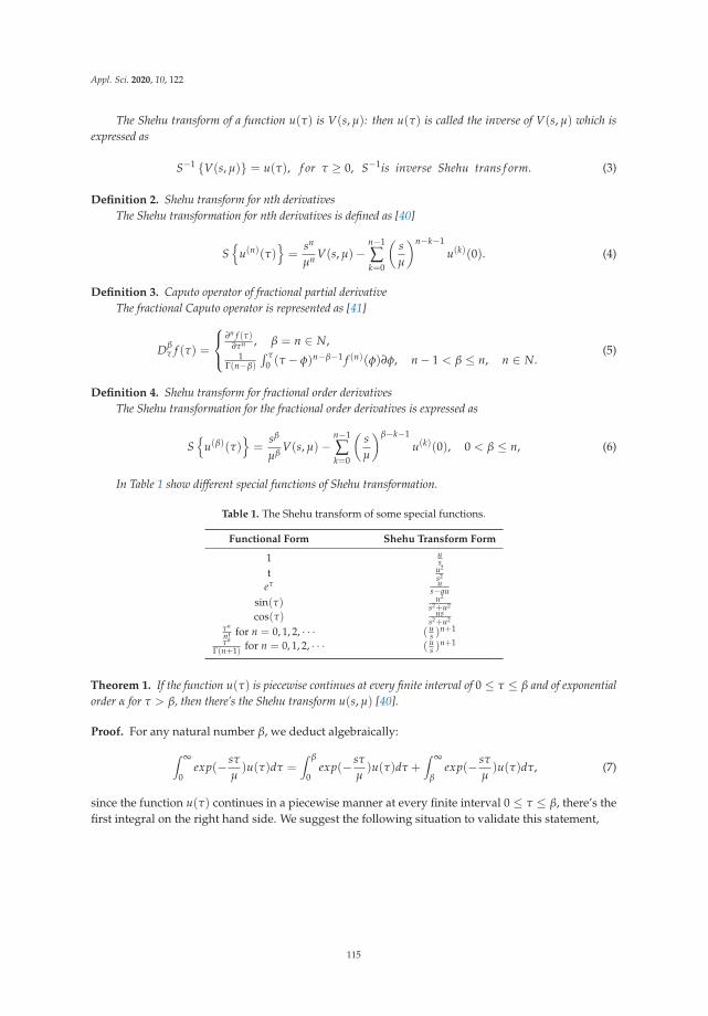
Appl. Sci. 2020, 10, 122

The Shehu transform of a function u(τ) is V(s, μ): then u(τ) is called the inverse of V(s, μ) which isexpressed as

S−1 {V(s, μ)} = u(τ), f or τ ≥ 0, S−1is inverse Shehu trans f orm. (3)

Definition 2. Shehu transform for nth derivativesThe Shehu transformation for nth derivatives is defined as [40]

S{

u(n)(τ)}=

sn

μn V(s, μ)−n−1

∑k=0

(sμ

)n−k−1u(k)(0). (4)

Definition 3. Caputo operator of fractional partial derivativeThe fractional Caputo operator is represented as [41]

Dβτ f (τ) =

⎧⎨⎩

∂n f (τ)∂τn , β = n ∈ N,

1Γ(n−β)

∫ τ0 (τ − φ)n−β−1 f (n)(φ)∂φ, n − 1 < β ≤ n, n ∈ N.

(5)

Definition 4. Shehu transform for fractional order derivativesThe Shehu transformation for the fractional order derivatives is expressed as

S{

u(β)(τ)}=

sβ

μβV(s, μ)−

n−1

∑k=0

(sμ

)β−k−1u(k)(0), 0 < β ≤ n, (6)

In Table 1 show different special functions of Shehu transformation.

Table 1. The Shehu transform of some special functions.

Functional Form Shehu Transform Form

1 us

t u2

s2

eτ us−au

sin(τ) u2

s2+u2

cos(τ) uss2+u2

τn

n! for n = 0, 1, 2, · · · ( us )

n+1

τn

Γ(n+1) for n = 0, 1, 2, · · · ( us )

n+1

Theorem 1. If the function u(τ) is piecewise continues at every finite interval of 0 ≤ τ ≤ β and of exponentialorder α for τ > β, then there’s the Shehu transform u(s, μ) [40].

Proof. For any natural number β, we deduct algebraically:

∫ ∞

0exp(− sτ

μ)u(τ)dτ =

∫ β

0exp(− sτ

μ)u(τ)dτ +

∫ ∞

βexp(− sτ

μ)u(τ)dτ, (7)

since the function u(τ) continues in a piecewise manner at every finite interval 0 ≤ τ ≤ β, there’s thefirst integral on the right hand side. We suggest the following situation to validate this statement,

115

Appl. Sci. 2020, 10, 122

|∫ ∞

αexp(− sτ

μ)u(τ)dτ| ≤

∫ ∞

α|exp(− sτ

μ)u(τ)|dτ

≤∫ ∞

αexp(− sτ

μ)|u(τ)|dτ

≤∫ ∞

αexp(− sτ

μ)Nexp(βτ)dτ

= N∫ ∞

αexp(− (s − βu)τ

u)dτ

= − Nu(s − βu)

limγ−→∞

[exp(− (s − βu)τ

u)dτ

]γ

0

=Nu

(s − βu).

(8)

The proof is complete.

3. Implementation of Shehu Transform

In this section, we have considered a time fractional (2+time fractional-order) dimensionalphysical model in the form

uβτ(�,�, τ) = κu��(�,�, τ) + £u(�,�, τ) + ℵu(�,�, τ), β ∈ [1, 2] (9)

with initial conditionu(�,�, 0) = u(�,�), (10)

while κ is a non-linear operator and £ linear operator.Applying the Shehu transform to both sides of the Equation (9) we obtain

S{

uβτ(�,�, τ)

}= S {κu��(�,�, τ) + £u(�,�, τ) + ℵu(�,�, τ)} , β ∈ [1, 2]. (11)

Using the differential property of Shehu transformation we have,

sβ

μβ

{V(s, μ)− μ

su(0)− μ2

s2 u′(0)}

= S {κu��(�,�, τ) + £u(�,�, τ) + ℵu(�,�, τ)} . (12)

Simplifying Equation (12), we obtain

V(s, μ) = +μβ

sβS {κu��(�,�, τ) + £u(�,�, τ) + ℵu(�,�, τ)}+ μ

su(0) +

μ2

s2 u′(0). (13)

Applying the inverse Shehu transformation, we get

u(�,�, τ) = S−1{

μβ

sβS {κu��(�,�, τ) + £u(�,�, τ) + ℵu(�,�, τ)}

}+ u(0) + τu

′(0). (14)

The nonlinear term ℵu(�,�, τ) is evaluated by using the procedure of Adomian polynomialdecomposition given by

ℵu(�,�, τ) =∞

∑m=0

Am(u0, u1, · · · ), m = 0, 1, · · · (15)

where,

Am(u0, u1, · · · ) = 1m!

[dm

dλm ℵ(

∞

∑i=0

λiui

)]λ=0

, m > 0. (16)

116

Appl. Sci. 2020, 10, 122

With the help of Equation (16), Equation (15) can be written as

u(�,�, τ) = S−1

{μβ

sβS

{κu��(�,�, τ) + £u(�,�, τ) +

∞

∑m=0

Am

}}+ u(0) + τu

′(0). (17)

Finally, we obtain the recursive relation as

u0(�,�, τ) = u(0) + τu′(0), m = 0

um(�,�, τ) = S−1

{μβ

sβS

{κu(m−1)��(�,�, τ) + £u(m−1)(�,�, τ) + ℵu(m−1)(�,�, τ) +

∞

∑m=0

Am

}}, m ≥ 1.

(18)

4. Applications and Discussion

Example 1. Consider the (2+time fractional-order) dimensional hyperbolic wave model:

uβτ(�,�, τ) =

112

�2u��(�,�, τ) +112

�2u��(�,�, τ), β ∈ (1, 2) (19)

with initial conditionsu(�,�, 0) = �4, uτ(�,�, 0) = �4. (20)

If β = 2, then the exact solution of Equation (19) is

u(�,�, τ) = �4 sinh(t) +�4 cosh(t), (21)

Taking the Shehu transform of Equation (19) we obtain

sβ

μβ

{V(s, μ)− μ

su(0)− μ2

s2 u′(0)}

= S{

112

�2u��(�,�, τ) +1

12�2u��(�,�, τ)

}. (22)

Simplifying Equation (22), we get

V(s, μ) =μβ

sβS{

112

�2u��(�,�, τ) +112

�2u��(�,�, τ)

}+

μ

su(0) +

μ2

s2 u′(0). (23)

Applying inverse Shehu transform, we get

u(�,�, τ) = u(0) + u′(0)τ + S−1

{μβ

sβS{

112

�2u��(�,�, τ) +112

�2u��(�,�, τ)

}}. (24)

Thus we get the following recursive scheme

u0(�,�, τ) = u(0) + u′(0)τ = �4 +�4τ, (25)

um+1(�,�, τ) = S−1{

μβ

sβS{

112

�2um��(�,�, τ) +112

�2um��(�,�, τ)

}}. (26)

Using Equation (26), for m = 0, 1, 2, 3, · · · we get the following values

117

Appl. Sci. 2020, 10, 122

u1(�,�, τ) = �4 τβ

β!+�4 τβ+1

(β + 1)!,

u2(�,�, τ) = �4 τ2β

(2β)!+�4 τ2β+1

(2β + 1)!,

u3(�,�, τ) = �4 τ3β

(3β)!+�4 τ3β+1

(3β + 1)!,

u4(�,�, τ) = �4 τ4β

(4β)!+�4 τ4β+1

(4β + 1)!,

(27)

...

Now using the values of u0, u1, u2, u3, · · · , we get Shehu transformation solution for example 1

u(�,�, τ) = �4 +�4τ +�4 τβ

β!+�4 τβ+1

(β + 1)!+�4 τ2β

(2β)!+�4 τ2β+1

(2β + 1)!+�4 τ3β

(3β)!+

�4 t3β+1

(3β + 1)!+�4 τ4β

(4β)!+�4 τ4β+1

(4β + 1)!+ · · ·

(28)

After simplification, we get

u(�,�, τ) = �4{

1 +τβ

β!+

τ2β

(2β)!+

τ3β

(3β)!+

τ4β

(4β)!+ · · ·

}+�4

{τ +

τβ+1

(β + 1)!+

τ2β+1

(2β + 1)!+

τ3β+1

(3β + 1)!+

τ4β+1

(4β + 1)!+ · · ·

}.

(29)

In particular, when β → 2, the analytical solution of Shehu transform become as

u(�,�, τ) = �4{

1 +τ2

2!+

τ4

(4)!+

τ6

(6)!+

τ8

(8)!+ · · ·

}+�4

{τ +

τ3

(3)!+

τ5

(5)!+

τ7

(7)!+

τ9

(9)!+ · · ·

}, (30)

which provide the close form solution as

u(�,�, τ) = �4 cosh(τ) +�4 sinh(τ). (31)

Figures 1 and 2 represent the exact and analytical solutions of Example 1. The solutions-graphs haveconfirmed the closed contact between the exact solution and the analytical solution obtained by the proposedmethod. In Figure 3, the solution of Example 1 are calculated at different fractional-order β of the derivative.It is investigated that the solutions at different fractional-orders β are convergent to an integer-order solutionof Example 1. Figure 4 represent the solution verses time graph for Example 1. It is observed that as the timefractional-order varies toward time integer-order, the time fractional-order solutions also approaches to thesolution of an integer-order problem of Example 1. All the above solution analysis of Example 1 indicate thatSDM is an efficient and effective method to solve fractional-order partial differential equations that are frequentlyarising in science and engineering.

118

Appl. Sci. 2020, 10, 122

Figure 1. Represents the exact solution of Example 1 at β = 2.

Figure 2. Represents the analytical solution of Example 1 at β = 2.

Figure 3. Represents the solution at different fractional order of Example 1.

119

Appl. Sci. 2020, 10, 122

Figure 4. Represents the solution at different fractional order of Example 1.

In Table 2, the solutions of Shehu transform decomposition method (SDM) and Adomian decompositionmethod (ADM) are compared with each other. The comparison has shown that the solutions of proposed methodare in strong agreement with the solution of ADM.

Table 2. Comparison of SDM and ADM [42] of Example 1 at τ = 0.1.

SDM (m = 5) SDM (m = 3) SDM ( m= 5) ADM (m = 5) AE of SDM

� � β = 1.75 β = 2 β = 2 β = 2 β = 2

1 1 1.111568974 1.105195833 1.10519608 1.10519609 2.51 × 10−5

2 2 17.78510358 17.68313333 17.6831373 17.6831374 4.02 × 10−4

3 3 90.03708688 89.52086250 89.5208829 89.5208828 2.03 × 10−3

4 4 284.5616573 282.9301334 282.930198 282.930199 6.44 × 10−3

5 5 694.7306086 690.7473959 690.747553 690.747552 1.57 × 10−2

Example 2. Consider the (2+time fractional-order) dimensional Heat model:

uβτ(�,�, τ) = u��(�,�, τ) + u��(�,�, τ), β ∈ (0, 1] (32)

with initial conditionu(�,�, 0) = sin(�) cos(�). (33)


u(�,�, τ) = e−2τ sin(�) cos(�). (34)

Taking Shehu transform of Equation (32)

sβ

μβ

{V(s, μ)− μ

su(0)

}= S {u��(�,�, τ) + u��(�,�, τ)} , (35)

Simplifying Equation (35), we get as

V(s, μ) =μ

su(0) +

μβ

sβS {u��(�,�, τ) + u��(�,�, τ)} . (36)

Applying inverse Shehu transform, we get

120

Appl. Sci. 2020, 10, 122

u(�,�, τ) = u(0) + S−1{

μβ

sβS {u��(�,�, τ) + u��(�,�, τ)}

}. (37)


u0(�,�, τ) = u(0) = sin(�) cos(�), (38)

um+1(�,�, τ) = S−1{

μβ

sβS {um��(�,�, τ) + um��(�,�, τ)}

}, (39)


u1(�,�, τ) = −2 sin(�) cos(�) τβ

(β)!,

u2(�,�, τ) = 4 sin(�) cos(�) τ2β

(2β)!,

u3(�,�, τ) = −8 sin(�) cos(�) τ3β

(3β)!,

u4(�,�, τ) = 16 sin(�) cos(�) τ4β

(4β)!,

(40)

...


u(�,�, τ) = sin(�) cos(�)− 2 sin(�) cos(�) τβ

(β)!+ 4 sin(�) cos(�) τ2β

(2β)!+

− 8 sin(�) cos(�) τ3β

(3β)!+ 16 sin(�) cos(�) τ4β

(4β)!+ · · ·

(41)


u(�,�, τ) = sin(�) cos(�){

1 − 2τβ

(β)!+ 4

τ2β

(2β)!+−8

τ3β

(3β)!+ 16

τ4β

(4β)!+ · · ·

}, (42)

which converge to the solution

u(�,�, τ) = sin(�) cos(�)Eβ(−2τβ), (43)

For particular case β → 1, the Shehu transform solution become as

u(�,�, τ) = sin(�) cos(�)e−2τ . (44)

Figures 5 and 6 show the exact and analytical solution of Example 2 respectively. The graphicalrepresentation have confirmed the closed contact of the obtained solution with the exact solution of Example 2.Similarly, Figures 7 and 8 represents the fractional-order solution of Example 2 for two and three space. Bothgraphs support the convergence phenomena of fractional-order problems to an integer-order problem of Example 2.

121

Appl. Sci. 2020, 10, 122

Figure 5. Represents the exact solution of Example 2 at β = 1.


Figure 7. u(�,�, τ) Represents the solution at different fractional order of Example 2.

122

Appl. Sci. 2020, 10, 122

Figure 8. u(�,�, τ) Represents the solution at different fractional order of Example 2.

Example 3. Consider the (2 + time f ractional) dimensional diffusion model:

uβτ(�,�, τ) = u��(�,�, τ) + u��(�,�, τ), β ∈ (0, 1] (45)

with the initial conditionu(�,�, 0) = e�+�. (46)


u(�,�, τ) = e�+�+2τ (47)


sβ

μβ

{V(s, μ)− μ

su(0)

}= S {u��(�,�, τ) + u��(�,�, τ)} . (48)


V(s, μ) =μ

su(0) +

μβ

sβS {u��(�,�, τ) + u��(�,�, τ)} . (49)

Applying inverse operator of Shehu transform, we get

u(�,�, τ) = u(0) + S−1{

μβ

sβS {u��(�,�, τ) + u��(�,�, τ)}

}. (50)


u0(�,�, τ) = u(0) = e�+�,

um+1(�,�, τ) = S−1{

μβ

sβS {um��(�,�, τ) + um��(�,�, τ)}

}, (51)


123

Appl. Sci. 2020, 10, 122

u1(�,�, τ) = 2e�+� τβ

(β)!,

u2(�,�, τ) = 4e�+� τ2β

(2β)!,

u3(�,�, τ) = 8e�+� τ3β

(3β)!,

u4(�,�, τ) = 16e�+� τ4β

(4β)!,

(52)

...

Now using the values of u0, u1, u2, u3, · · · , we get Shehu transformation solution for Example 3

u(�,�, τ) = e�+� + 2e�+� τβ

(β)!+ 4e�+� τ2β

(2β)!+ 8e�+� τ3β

(3β)!+ 16e�+� τ4β

(4β)!+ · · · . (53)


u(�,�, τ) = sin(�) cos(�){

1 + 2τβ

(β)!+ 4

τ2β

(2β)!+ 8

τ3β

(3β)!+ 16

τ4β

(4β)!+ · · ·

}. (54)

The close form solution become as

u(�,�, τ) = sin(�) cos(�)Eβ(2τβ). (55)

When β → 1 the calculated result provide the exact solution in the close form

u(�,�, τ) = sin(�) cos(�)e2τ . (56)

Figures 9 and 10 show the exact and analytical solutions of Example 3. Both figures are almost coincidentconfirming the close contact of both exact and obtained solution. Figures 11 the SDM solutions at differentfractional-order β are calculated for Example 3. The convergence phenomena of fractional-order solution towardsexact solution is observed. The method is found to be very simple and straightforward to solve fractional-orderdifferent equations.

Figure 9. Exact solution of Example 3 at β = 1.

124

Appl. Sci. 2020, 10, 122


Figure 11. The solution graph at different fractional order β.

Example 4. Consider the (2 + time f ractional) dimensional telegraph model:

uβτ(�,�, τ) =

12

u��(�,�, τ) +12

u��(�,�, τ)− 2ut(�,�, τ)− u(�,�, τ), β ∈ (1, 2], (57)

with initial conditions

u(�,�, 0) = sinh(�) sinh(�), uτ(�,�, 0) = −2 sinh(�) sinh(�). (58)


u(�,�, τ) = sinh(�) sinh(�)e−2τ . (59)


sβ

μβ

{V(s, μ)− μ

su(0)− μ2

s2 u′(0)}

= S{

12

u��(�,�, τ) +12

u��(�,�, τ)− 2ut(�,�, τ)− u(�,�, τ)

}, (60)


V(s, μ) =μβ

sβS{

12

u��(�,�, τ) +12

u��(�,�, τ)− 2ut(�,�, τ)− u(�,�, τ)

}+

μ

su(0) +

u2

s2 u′(0), (61)

125

Appl. Sci. 2020, 10, 122

Applying inverse of Shehu transform, we get

u(�,�, τ) = u(0) + τu′(0) + S−1

{μβ

sβS{

12

u��(�,�, τ) +12

u��(�,�, τ)− 2ut(�,�, τ)− u(�,�, τ)

}}. (62)


u0(�,�, τ) = u(0) + τu′(0) =

sinh(�) sinh(�)− 2t sinh(�) sinh(�),

um+1(�,�, τ) = S−1{

μβ

sβS{

12

um��(�,�, τ) +12

um��(�,�, τ)− 2umτ(�,�, τ)− um(�,�, τ)

}}, (63)


u1(�,�, τ) = 4 sinh(�) sinh(�) τβ

(β)!,

u2(�,�, τ) = −8β(β − 1)! sinh(�) sinh(�)τ2β

(2β − 1)!(β)!,

u3(�,�, τ) = 16β(2β − 1)(β − 1)!(2β − 2)! sinh(�) sinh(�)τ3β−2

(β)!(2β − 1)!(3β − 2)!,

(64)

...

Now using the values of u0, u1, u2, u3, · · · , we get Shehu transformation solution for Example 4

u(�,�, τ) = sinh(�) sinh(�)− 2τ sinh(�) sinh(�) + 4sinh(�) sinh(�)τβ

(β)!− 8

β(β − 1)! sinh(�) sinh(�)τ2β

(2β − 1)!(β)!+

16β(2β − 1)(β − 1)!(2β − 2)! sinh(�) sinh(�)τ3β−2

(β)!(2β − 1)!(3β − 2)!+ · · · .

(65)


u(�,�, τ) = sinh(�) sinh(�){

1 − 2τ + 4τβ

β!− 8

β(β − 1)!τ2β

(2β − 1)!(β)!+

16β(2β − 1)(β − 1)!(2β − 2)!τ3β−2

(β)!(2β − 1)!(3β − 2)!+ · · ·

}. (66)


u(�,�, τ) = sinh(�) sinh(�){

1 − 2τ + 4τ2

2!− 8

τ3

3!+ 16

τ4

4!+ · · ·

}. (67)

The calculated result provide the exact solution in the close form

u(�,�, τ) = sinh(�) sinh(�)e−2τ . (68)

Figures 12 and 13, display the exact and analytical solutions of Example 4. The solution graph of SDMis very similarly to the exact solution of Example 4. In Figure 14, we plotted the solutions of Example 4 atdifferent fractional-order β. The fractional-order solutions are found to be convergent towards the exact solutionof Example 4. It is investigated from the solution analysis that the present method is a sophisticated technique tosolve fractional-order problems.

126

Appl. Sci. 2020, 10, 122


Figure 13. analytical solution of Example 4 at β = 2.

Figure 14. The solution graph at different fractional order β. of Example 4.

Example 5. Consider the non-linear (2 + time f ractional) dimensional Burger’s model:

uβτ(�,�, τ) = u��(�,�, τ) + u��(�,�, τ) + u�(�,�, τ)u(�,�, τ), β ∈ (0, 1], (69)

with initial conditionu(�,�, 0) = �+�. (70)

127

Appl. Sci. 2020, 10, 122


u(�,�, τ) =�+�1 − τ

. (71)


sβ

μβ

{V(s, μ)− μ

su(0)

}= S {u��(�,�, τ) + u��(�,�, τ) + u�(�,�, τ)u(�,�, τ)} , (72)

The simplifying Equation (72), we get as

V(s, μ) =μ

su(0) +

μβ

sβS {u��(�,�, τ) + u��(�,�, τ) + u�(�,�, τ)u(�,�, τ)} , (73)

By applying inverse of Shehu transform, we get

u(�,�, τ) = u(0) + τu′(0) + S−1

{μβ

sβS {u��(�,�, τ) + u��(�,�, τ) + u�(�,�, τ)u(�,�, τ)}

}, (74)


u0(�,�, τ) = u(0) = �+�, (75)

um+1(�,�, τ) = S−1{

μβ

sβS {um��(�,�, τ) + um��(�,�, τ) + um�(�,�, τ)um(�,�, τ)}

}. (76)

For nonlinear term, use the Equation (12) in recursive scheme (76), we obtain

um+1(�,�, τ) = S−1

{μβ

sβS

{um��(�,�, τ) + um��(�,�, τ) +

∞

∑m=0

Am(u0, u1, · · · )}}

. (77)


u1(�,�, τ) = (�+�) tβ

(β)!,

u2(�,�, τ) = 2(�+�) τ2β

(2β)!,

u3(�,�, τ) = 4(�+�) τ3β

(3β)!+ (�+�)(2β)!

t3β

β!β!(3β)!,

(78)

...


u(�,�, τ) = �+�+ (�+�) τβ

(β)!+ 2(�+�) τ2β

(2β)!+ 4(�+�) τ3β

(3β)!+ (�+�)(2β)!

τ3β

β!β!(3β)!+ · · · . (79)


u(�,�, τ) = (�+�){

1 +τβ

(β)!+ 2

τ2β

(2β)!+ 4

τ3β

(3β)!+ (2β)!

τ3β

β!β!(3β)!+ · · ·

}. (80)


u(�,�, τ) = (�+�){

1 + τ + τ2 + τ3 + · · ·}

. (81)

128

Appl. Sci. 2020, 10, 122

The calculated result provide the exact solution in the close form

u(�,�, τ) =�+�1 − τ

. (82)

Figures 15 and 16 are plotted to discuss the exact and analytical solutions of Example 5. The SDM solutionsare in good contact with the exact solution of the Example 5. Figures 17 and 18 are plotted to analyze thefractional-order solutions of Example 5 at fractional-order β = 0.75 and 0.50 respectively. The graphical analysishas verified the applicability of the proposed method.



Figure 17. The solution of fractional-order β = 0.75 of Example 5.

129

Appl. Sci. 2020, 10, 122

Figure 18. The solution of fractional-order β = 0.5 of Example 5.

5. Results and Discussion

In the present research work, we implemented a new analytical technique SDM for the solution ofsome important problems which are frequently arising in science and engineering, such as hyperbolicwave equation, heat equation, diffusion equation, telegraph and Burgers equations. The Caputodefinition of fractional-derivative is used to define fractional-derivative. The proposed method isthe combination of Shehu transformation and Adomian decomposition method which is known asShehu decomposition method. For applicability and novelty of present method, we applied it differentphysical problems for applied sciences. These problems have been solved by using SDM for bothfractional and integer-order of the targeted problems. In this connection some figure analysis havebeen done to demonstrate the obtained results in a sophisticated manner. It is investigated that SDMsolution have a very close contact with the exact solution of the problems. It is also observed that thefractional-order problems are convergent towards the solution of an integer-order problem. Moreover,the high rate of convergence of the current method is noted during the simulation. It is calculatedthat the SDM can be considered as one of the best analytical technique to solve fractional partialdifferential equations.

6. Conclusions

In the present article, we presented some fractional-view analysis of physical problems, arisingin science and engineering. A new and sophisticated analytical technique, which is known asShehu transform decomposition method is implemented for both fractional and integer-orders of theproblems. The Caputo definition of fractional derivative is used to express fractional-order derivative.For applicability and reliability of the proposed methods, some illustrative examples are presentedfrom different areas of applied science. It has been investigated through graphical representation thatthe present technique provides an accurate and deserving analysis about the physical happening ofthe problems. It is observed through simulations of the present algorithm that as fractional-orderof the derivative approaches to integer order of the problem then fractional-order solutions areconvergent to integer-order solutions. Moreover, the present method is preferred as compared to othermethod because of its better rate of convergence. This direction motivates the researchers towards theimplementation of the current method for other non-linear fractional partial differential equations.

Author Contributions: Conceptualization, R.S. and H.K.; Methodology, M.A.; Software, R.S.; Validation, R.S.and U.F.; Formal Analysis, R.S.; Investigation, R.S. and D.B.; Resources, H.K. and P.K.; Writing—Original DraftPreparation, R.S.; Writing—Review and Editing, H.K., U.F. and P.K.; Visualization, M.A.; Supervision, D.B., P.K.;Project Administration, P.K.; Funding Acquisition, P.K.

Funding: Center of Excellence in Theoretical and Computational Science (TaCS-CoE) Faculty of Science, KingMongkuts University of Technology Thonburi (KMUTT).

130

Appl. Sci. 2020, 10, 122


References

1. Abd-Elhameed, W.M.; Youssri, Y.H. Fifth-kind orthonormal Chebyshev polynomial solutions for fractionaldifferential equations. Comput. Appl. Math. 2018, 37, 2897–2921. [CrossRef]

2. Shah, R.; Khan, H.; Farooq, U.; Baleanu, D.; Kumam, P.; Arif, M. A New Analytical Technique to SolveSystem of Fractional-Order Partial Differential Equations. IEEE Access 2019, 7, 150037–150050. [CrossRef]

3. Jain, S. Numerical analysis for the fractional diffusion and fractional Buckmaster equation by the two-stepLaplace Adam-Bashforth method. Eur Phys. J. Plus 2018, 133, 19. [CrossRef]

4. Prakash, A. Analytical method for space-fractional telegraph equation by homotopy perturbation transformmethod. Nonlinear Eng. 2016, 5, 123–128. [CrossRef]

5. Khan, H.; Shah, R.; Baleanu, D.; Kumam, P.; Arif, M. Analytical Solution of Fractional-Order HyperbolicTelegraph Equation, Using Natural Transform Decomposition Method. Electronics 2019, 8, 1015. [CrossRef]

6. Safari, M.; Ganji, D.D.; Moslemi, M. Application of He’s variational iteration method and Adomian’sdecomposition method to the fractional KdV–Burgers–Kuramoto equation. Comput. Math. Appl. 2009, 58,2091–2097. [CrossRef]

7. Kumar, D.; Tchier, F.; Singh, J.; Baleanu, D. An efficient computational technique for fractal vehicular trafficflow. Entropy 2018, 20, 259. [CrossRef]

8. Singh, J.; Kumar, D.; Baleanu, D.; Rathore, S. An efficient numerical algorithm for the fractionalDrinfeld–Sokolov–Wilson equation. Appl. Math. Comput. 2018, 335, 12–24. [CrossRef]

9. Shivanian, E.; Jafarabadi, A. Time fractional modified anomalous sub-diffusion equation with a nonlinearsource term through locally applied meshless radial point interpolation. Mod. Phys. Lett. B 2018, 32, 1850251.[CrossRef]

10. Ullah, S.; Khan, M.A.; Farooq, M. A new fractional model for the dynamics of the hepatitis B virus using theCaputo-Fabrizio derivative. Eur. Phys. J. Plus 2018, 133, 237. [CrossRef]

11. Qureshi, S.; Yusuf, A. Modeling chickenpox disease with fractional derivatives: From caputo toatangana-baleanu. Chaos Solitons Fractals 2019, 122, 111–118. [CrossRef]

12. Qureshi, S.; Yusuf, A.; Shaikh, A.A.; Inc, M.; Baleanu, D. Fractional modeling of blood ethanol concentrationsystem with real data application. Chaos Interdiscip. J. Nonlinear Sci. 2019, 29, 013143. [CrossRef] [PubMed]

13. Khan, M.A.; Ullah, S.; Farooq, M. A new fractional model for tuberculosis with relapse via Atangana–Baleanuderivative. Chaos Solitons Fractals 2018, 116, 227–238. [CrossRef]

14. Jena, R.M.; Chakraverty, S. Residual Power Series Method for Solving Time-fractional Model of VibrationEquation of Large Membranes. J. Appl. Comput. Mech. 2019, 5, 603–615.

15. Jena, R.M.; Chakraverty, S. A new iterative method based solution for fractional Black–Scholes option pricingequations (BSOPE). SN Appl. Sci. 2019, 1, 95. [CrossRef]

16. Jena, R.M.; Chakraverty, S.; Jena, S.K. Dynamic response analysis of fractionally damped beams subjected toexternal loads using homotopy analysis method. J. Appl. Comput. Mech. 2019, 5, 355–366.

17. Abd-Elhameed, W.M.; Youssri, Y.H. Spectral tau algorithm for certain coupled system of fractional differentialequations via generalized Fibonacci polynomial sequence. Iran. J. Sci. Technol. Trans. A Sci. 2019, 43, 543–554.[CrossRef]

18. Khan, H.; Shah, R.; Kumam, P.; Arif, M. Analytical Solutions of Fractional-Order Heat and Wave Equationsby the Natural Transform Decomposition Method. Entropy 2019, 21, 597. [CrossRef]

19. Shah, R.; Khan, H.; Mustafa, S.; Kumam, P.; Arif, M. Analytical Solutions of Fractional-Order DiffusionEquations by Natural Transform Decomposition Method. Entropy 2019, 21, 557. [CrossRef]

20. Khan, M.A.; Ullah, S.; Okosun, K.O.; Shah, K. A fractional order pine wilt disease model withCaputo–Fabrizio derivative. Adv. Differ. Equ. 2018, 2018, 410. [CrossRef]

21. Singh, J.; Kumar, D.; Baleanu, D. On the analysis of fractional diabetes model with exponential law.Adv. Differ. Equ. 2018, 2018, 231. [CrossRef]

22. Qureshi, S.; Yusuf, A. Mathematical modeling for the impacts of deforestation on wildlife species usingCaputo differential operator. Chaos Solitons Fractals 2019, 126, 32–40. [CrossRef]

23. Jumarie, G. Laplace’s transform of fractional order via the Mittag–Leffler function and modifiedRiemann–Liouville derivative. Appl. Math. Lett. 2009, 22, 1659–1664. [CrossRef]

131

Appl. Sci. 2020, 10, 122

24. Kumar, S. A new analytical modelling for fractional telegraph equation via Laplace transform. Appl. Math.Model. 2014, 38, 3154–3163. [CrossRef]

25. Kazem, S. Exact solution of some linear fractional differential equations by Laplace transform.Int. J. Nonlinear Sci. 2013, 16, 3–11.

26. Namias, V. The fractional order Fourier transform and its application to quantum mechanics. IMA J. Appl.Math. 1980, 25, 241–265. [CrossRef]

27. Chen, C.M.; Liu, F.; Turner, I.; Anh, V. A Fourier method for the fractional diffusion equation describingsub-diffusion. J. Comput. Phys. 2007, 227, 886–897. [CrossRef]

28. Jiang, X.; Xu, M. The fractional finite Hankel transform and its applications in fractal space. J. Phys. AMath. Theor. 2009, 42, 385201. [CrossRef]

29. Gorenflo, R.; Iskenderov, A.; Luchko, Y. Mapping between solutions of fractional diffusion-wave equations.Fract. Calculus Appl. Anal. 2000, 3, 75–86.

30. Debnath, L.; Bhatta, D. Integral Transforms and Their Applications; Chapman and Hall/CRC: Boca Raton, FL,USA, 2014.

31. Yang, X.J. Local Fractional Functional Analysis and Its Applications; Asian Academic Publisher Limited:Hong Kong, China, 2011.

32. Neamaty, A.; Agheli, B.; Darzi, R. Applications of homotopy perturbation method and Elzaki transform forsolving nonlinear partial differential equations of fractional order. Theory Approx. Appl. 2016, 6, 91–104.

33. Jena, R.M.; Chakraverty, S. Solving time-fractional Navier–Stokes equations using homotopy perturbationElzaki transform. SN Appl. Sci. 2019, 1, 16. [CrossRef]

34. Taha, N.E.H.; Nuruddeen, R.I.; Abdelilah, K.; Hassan, S. Dualities between “Kamal and Mahgoub integraltransforms” and “Some famous integral transforms”. Br. J. Appl. Sci. Technol. 2017, 20, 1–8. [CrossRef]

35. Aboodh, K.S. The new integral transform “Aboodh Transform”. Glob. J. Pure Appl. Math. 2013, 9, 35–43.36. Aggarwal, S.; Chauhan, R. A comparative study of Mohand and Aboodh transforms. Int. J. Res. Adv. Technol.

2019, 7, 520–529. [CrossRef]37. Kılıçman, A.; Gadain, H.E. On the applications of Laplace and Sumudu transforms. J. Frankl. Inst. 2010, 347,

848–862. [CrossRef]38. Jena, R.M.; Chakraverty, S. Analytical solution of Bagley-Torvik equations using Sumudu transformation

method. SN Appl. Sci. 2019, 1, 246. [CrossRef]39. Mao, Z.; Shen, J. Hermite spectral methods for fractional PDEs in unbounded domains. SIAM J. Sci. Comput.

2017, 39, A1928–A1950. [CrossRef]40. Maitama, S.; Zhao, W. New integral transform: Shehu transform a generalization of Sumudu and Laplace

transform for solving differential equations. arXiv 2019, arXiv:1904.11370.41. Rudolf, H. (Ed.) Applications of Fractional Calculus in Physics; World Scientific: Singapore, 2000.42. Wazwaz, A.M.; Gorguis, A. Exact solutions for heat-like and wave-like equations with variable coefficients.

Appl. Math. Comput. 2004, 149, 15–29. [CrossRef]


132

applied sciences

Article

Fractional View Analysis of Acoustic Wave Equations,Using Fractional-Order Differential Equations

Izaz Ali 1, Hassan Khan 1, Rasool Shah 1, Dumitru Baleanu 2,3, Poom Kumam 4,5,*

and Muhammad Arif 1

1 Department of Mathematics, Abdul Wali Khan University, Mardan 23200, Pakistan;[email protected] (I.A.); [email protected] (H.K.); [email protected] (R.S.);[email protected] (M.A.)

2 Department of Mathematics, Faculty of Arts and Sciences, Cankaya University, 06530 Ankara, Turkey;[email protected]

3 Institute of Space Sciences, 077125 Magurele, Romania4 Center of Excellence in Theoretical and Computational Science (TaCS-CoE) & Department of Mathematics,

Faculty of Science, King Mongkut’s University of Technology Thonburi (KMUTT), 126 Pracha Uthit Rd.,Bang Mod, Thung Khru, Bangkok 10140, Thailand

5 Department of Medical Research, China Medical University Hospital, China Medical University,Taichung 40402, Taiwan


Received: 1 November 2019; Accepted: 15 December 2019; Published: 15 January 2020

Abstract: In the present research work, a newly developed technique which is known as variationalhomotopy perturbation transform method is implemented to solve fractional-order acoustic waveequations. The basic idea behind the present research work is to extend the variational homotopyperturbation method to variational homotopy perturbation transform method. The proposed schemehas confirmed, that it is an accurate and straightforward technique to solve fractional-order partialdifferential equations. The validity of the method is verified with the help of some illustrativeexamples. The obtained solutions have shown close contact with the exact solutions. Furthermore,the highest degree of accuracy has been achieved by the suggested method. In fact, the presentmethod can be considered as one of the best analytical techniques compared to other analyticaltechniques to solve non-linear fractional partial differential equations.

Keywords: homotopy perturbation method; variational iteration method; Laplace transform method;acoustic wave equations

1. Introduction

Recently, fractional calculus and fractional differential equations (FDEs) have attracted theattention of scientists, mathematicians and engineers. A number of important implementations havebeen evaluated in various fields of sciences and engineering, such as material engineering, viscoelastic,electrochemistry, electromagnetic and dynamics physics which are described by fractional partialdifferential equations (FPDEs) [1]. Analytical approaches to solve FDEs are of great interest. There is notechnique which provides an exact solution to the FDEs. Approximate approaches must be obtained byusing techniques of series solution or linearization [2], followed by the application of proper numericaldiscretization [3–5] and system solvers [6–8]. Non-linear phenomena appear in a number of fieldsof engineering and sciences, such as solid state physics, chemical kinetics, non-linear spectroscopy,fluid physics, computational biology, quantum mechanics and thermodynamics etc. The conceptof non-linearity is designed by various higher-order nonlinear partial differential equations (PDEs).For all of the physical systems, fundamental phenomena are covered by their nonlinear concepts [9,10].


Appl. Sci. 2020, 10, 610

In this paper, Laplace Variational Homotopy Perturbation Method (LVHPM) is implemented to solvethe following linear and non-linear fractional-order regularized long wave equations.

∂βυ

∂ηβ+

12

∂υ2

∂ξ− ∂

∂η

(∂2υ

∂ξ2

)= 0, 0 < ξ ≤ 1, 0 < β ≤ 1, η > 0, (1)

with initial conditionυ(ξ, 0) = ξ,

∂βυ

∂ηβ+

∂υ

∂ξ+ υ

∂υ

∂η− ∂

∂η

(∂2υ

∂ξ2

)= 0, 0 < ξ ≤ 1, 0 < β ≤ 1, η > 0, (2)

with initial condition

υ(ξ, 0) = 3α sec h2(βξ), α > 0, β =12

√α

1 + α.

∂βυ

∂ηβ+

∂υ

∂ξ− 2

∂

∂η

(∂2υ

∂ξ2

)= 0, 0 < ξ ≤ 1, 0 < β ≤ 1, η > 0, (3)

with initial conditionυ(ξ, 0) = e−ξ ,

and

∂βυ(ξ.η)∂ηβ

+∂4υ(ξ.η)

∂ξ4 = 0, 0 < ξ ≤ 1, 0 < β ≤ 1, η > 0, (4)

with initial conditionυ(ξ, 0) = sin ξ. (5)

Equation (1) is known as the fractional-order non-linear regularized long wave equation (RLWE);Equation (2) is known as the fractional-order non-linear general regularized long wave equation(GRLWE) and Equations (3) and (4) are known as fractional-order linear regularized long waveequations (RLWEs) [11].

The Benjamin Bona Mahony equation (BBME) also identified the regularized long wave (RLW)equation. This equation is the updated version of Korteweg–de Vries equation (KdV) for the modelingof tiny amplitude lengthy surface gravitational waves spreading unidirectionally in two dimensions.RLW equations have several implementations in certain areas of science, such as ion-acoustic wavesin plasma, longitudinal dispersive waves in elastic rods, magneto-hydrodynamic waves in plasma,rotating tube flow and stress waves in compressed gas bubble mixes, etc. The RLW equations aredescribed as useful models in applied physics and engineering for many significant physical structures.They also design many liquid flow nature issues where diffusion is significant, either in viscous orshock situations. It can be used to model any dissipation-related non-linear wave diffusion problem.Chemical reaction, heat conduction, mass diffusion, viscosity, thermal radiation or other sources mayresult from this dissipation, depending on problem modeling [12].

The RLW problem is a family of non-linear growth models that provides excellent designs forpredicting natural phenomena. The algorithm was initially introduced to define the undular borebehavior [13]. It was also obtained from the research of acoustic plasma waves of water and ion.An analytical solution for the RLW equation was identified under restricted initial and boundaryconditions in [14]. The fractional RLW equations also define numerous significant ocean science andengineering phenomena such as long-wave and small frequency shallow water waves. The non-linearwaves modeled on the fractional equations of RLW are of significant interest for several scientistsin ocean shallow waves of liquid. The mathematically modeled non-linear waves in the ocean werethe fractional RLW equations. Indeed, huge surface waves identified as the tsunami are describedas fractional RLW equations. The huge internal waves in the interior of the ocean, resulting from

134

Appl. Sci. 2020, 10, 610

the difference in temperature, that may destruct marine ships could be defined as fractional RLWequations in the current, highly efficient method.

In recent decades, many researchers and scientists have used analytical methods to solve thesetypes of problems such as homotopy perturbation Sumudu transform method (HPSTM) [11], Adomiandecomposition method (ADM) [15,16], least-squares method [17], optimal homotopy perturbationmethod [18], variational iteration method (VIM) homotopy perturbation method (HPM) [19] and He’shomotopy perturbation method [20]. It is observed that these methods have certain deficiencies likecalculation of Adomian polynomials, determination of Lagrange multiplier, divergent results and ahuge volume of calculations. As a result, a modified analytical technique which is known as VHPTMwas introduced to solve differential equations of fractional-order. VHPTM is the combination of threewell-known techniques namely, homotopy perturbation method, Laplace transform and variationaliteration method. The present method uses the Lagrange multiplier that can limit the consecutiveimplementation of integral operator and unmanageable computational cost. It is still maintaininghigher degree of accuracy. VHPTM [21–24] has an excellent scheme and absorbs all the beneficialcharacteristics of VIM and HPM.

Finally, He’s polynomials have been used in the correction fractional formula to develop thehomotopy perturbation method. It is observed that the proposed method is implemented withoutany use of transformation, discretization and it was found to be free from the generating round offerror. Usually, the method of variable separable needs both initial and boundary points to operate,but the present method provides an analytical solution by using initial conditions only. There is aclear advantage of the suggested method that it works without any use of Adomian polynomials, asrequired by the Adomian decomposition method. Results of the analysis show that the suggestedmethod produces the solution in a series of fast convergence that can result in a closed solution [25–30].

2. Preliminaries Concepts

Definition 1. Laplace transformation of ρ(η), η > 0 represented as [13]

Q(s) = L[ρ(η)] =∫ ∞

0e−sηρ(η)dη.

Theorem 1. The convolution of Laplace transform is

L[ρ1 × ρ2] = L[ρ1(η)]×L[ρ2(η)],

here ρ1 × ρ2, define the convolution between ρ1 and ρ2 ,

(ρ1 × ρ2)η =∫ τ

0ρ1(τ)ρ2(η − τ)dη.

Laplace transform of fractional derivative

L(

Dβη ρ(η)

)= sβQ(s) −

n−1

∑k=0

sβ−1−kρ(k)(0), n − 1 < β < n.

where Q(s) is the Laplace transformation of ρ(η).

Definition 2. The Riemann-Liouville fractional integral operator of order β ≥ 0 of a function f ∈ Cμ, μ ≥ −1is described in [21]

Iβξ g(ξ) =

1Γ(β)

∫ ξ

0(ξ − s)β−1g(s)ds,

135

Appl. Sci. 2020, 10, 610

where Γ represent the gamma function as,

Γ(β) =∫ ∞

0e−ξ ξβ−1dξ β ∈ C.

Definition 3. The fractional derivative of g(η) in the Caputo sense is defined as

Dβg(η) =∂βg(η)

∂ηβ=

⎧⎨⎩

Im−β[

∂mg(η)∂ηm

], if m − 1 < β < m, m ∈ N

∂mg(η)∂ηm , β = m.

Lemma 1. If m − 1 < β ≤ m with m ∈ N and g ∈ Cη with η ≥ −1, then

Iβ Iag(ξ) = Iβ+ag(ξ), a, β≥0.

Iβξλ =Γ(λ + 1)

Γ(γ + λ + 1)ξβ+λ, β > 0, λ > −1, ξ > 0.

IβDβg(ξ) = g(ξ)−m−1

∑k=0

g(k)(0+)ξk

k!, for ξ > 0, m − 1 < β ≤ m.

Definition 4. Function of Mittag-Leffler, Eα,β(η) for α, β > 0 is defined as

Eα,β(η) =∞

∑k=0

ηk

Γ(kα + β), α, β > 0, η ∈ C.

3. The Procedure of VHPTM

To demonstrate, the fundamental concept of the present method [21,22], we are considering

Dβη υ(ξ, η) + Rυ(ξ, η) + Nυ(ξ, η) = f (ξ, η), (6)

with initial conditionυ(ξ, 0) = g(ξ),

where f (ξ, η) is an inhomogeneous term, R and N are particular linear and non-linear differentialoperators and Dβ

η υ(ξ, η) is the Caputo fractional derivative of υ(ξ, η).By taking Laplace transform of Equation (6) on both sides, we get

£η{υ(ξ, η)} −m−1

∑k=0

sβ−1−k ∂kυ(ξ, η)

∂kη|t=0 = −£ {Rυ(ξ, η) + Nυ(ξ, η)− f (ξ, η)} ,

where υ(s) = £η(υ(ξ, η)) =∫ ∞

0 e−sηυ(η)dη.We can build a functional correction according to the variation iteration method

£η{υj+1(ξ, η)} = £{υj(ξ, η)}+ λ(s)[sβ£{

υη(ξ, η)− ∑m−1k=0 sβ−1−k ∂kυ(ξ,η)

∂kη|t=0 + £ {Rυ(ξ, η) + Nυ(ξ, η)− f (ξ, η)}

}], (7)

where λ(s) is the Lagrange multiplier. Here we put λ(s) = −1sβ [22].

Applying inverse Laplace of Equation (7)

υj+1(ξ, η) = υj(ξ, η)− £−1[

1sβ

£{

sβ ∂υ

∂η+ Rυj(ξ, η) + Nυj(ξ, η)− f (ξ, η)

}]. (8)

136

Appl. Sci. 2020, 10, 610

The basic idea in the procedure of homotopy perturbation method is that the solution can bewritten as a series in powers of p:

υ(ξ, η) =∞

∑j=0

pjυj(ξ, η) = υ0 + pυ1 + p2υ2 + p3υ3 + · · · , (9)

where the non-linear expression can be expressed as

Nυ(ξ, η) =∞

∑j=0

pj Hj(υ). (10)

Hj is He’s polynomials,

Hj(υ0 + υ1 + · · ·+ uj) =1j!

∂j

∂pj

[N

(∞

∑i=0

piυi

)]. (11)

The technique of fractional VHPTM of Equation (8) with He’s polynomials.

∞

∑j=0

pjυj(ξ, η) =∞

∑j=0

pjυj(ξ, η) + £−1

[λ(s)£

{∞

∑j=0

pj ∂βυj

∂ηβ(ξ, s) +

∞

∑j=0

pjRυj(ξ, η) +∞

∑j=0

pjHj(υ)− f (ξ, η)

}]. (12)

By comparing the coefficients of like power of p on both sides of Equation (12), we get the VHPTMsolution of the given problem.

Theorem 2. Let ξ and Y be two Banach spaces and T : ξ → Y be a contractive nonlinear operator, such thatfor all υ; υ∗ ∈; ξ, ||T(υ)− T(υ∗)|| ≤ K||υ − υ∗||, 0 < K < 1 y [31]. Then, in view of Banach contractiontheorem, T has a unique fixed point υ, such that Tυ = υ: Let us write the generated series (12), by the Laplacedecomposition method as

ξm = T(ξm−1), ξm−1 =m−1

∑m=1

υj, m = 0, 1, 2, · · ·

and supposed that ξ0 = υ0 ∈ Sp(υ), where Sp(υ) = {υ∗ ∈ ξ : ||υ − υ∗|| < p} then, we have

(B1)ξm ∈ Sp(υ)

(B2) limm→∞

ξm = υ.

Proof. (B1) In view of mathematical induction for m = 1, we have

||ξ1 − υ1|| = ||T(ξ0 − T(υ))|| ≤ K||υ0 − υ||.

Let the result be true for m − 1, then

||ξm−1 − υ|| ≤ Km−1||υ0 − υ||.

We have||ξm − υ|| = ||T(ξm−1 − T(υ))|| ≤ K||ξm−1 − υ|| ≤ Km||υ0 − υ||.

Hence, using (B1), we have

||ξm − υ|| ≤ Km||υ0 − υ|| ≤ Km p < p,

which implies that ξm ∈ Sp(υ).

137

Appl. Sci. 2020, 10, 610

(B2): Since ||ξm − υ|| ≤ Km||υ0 − υ|| and as a limm→∞ Km = 0.Therefore; we have limm→∞ ||ξm − υ|| = 0 ⇒ limm→∞ ξm = υ.

4. Numerical Examples

4.1. Example

We consider time fractional-order non-linear RLW equation

∂βυ

∂ηβ+

12

∂υ2

∂ξ− ∂∂2υ

∂η∂ξ2 = 0, 0 < ξ ≤ 1, 0 < β ≤ 1, η > 0, (13)

initial condition isυ(ξ, 0) = ξ, (14)

By using Equation (12), the fractional PDE given in Equation (13) can be written as

∞

∑j=0

pjυj+1(ξ, η) =∞

∑j=0

pjυj(ξ, η) + £−1

[λ(s)£

{sβ

∂υj(ξ, η)

∂η+

12

∂υ2j (ξ, η)

∂ξ− ∂∂2υj(ξ, η)

∂η∂ξ2

}], (15)

where λ(s) is the Lagrange multiplier

λ(s) =−1sβ

.

Applying VHPTM using He’s polynomials,

∞

∑j=0


∑j=0

pjυj(ξ, η)−∞

∑j=0

pj£−1[

1sβ

£{

sβ

(∂υ0

∂η+ p

∂υ1

∂η+ p2 ∂υ2

∂η+ · · ·

)

+12

∂

∂ξ

{υ2

0 + p(2υ0υ1) + p2(2υ0υ2 + υ21) + · · ·

}−{

p0 ∂∂2υ0

∂η∂ξ2 + p1 ∂∂2υ1

∂η∂ξ2 + p2 ∂∂2υ2

∂η∂ξ2 + · · ·}}]

,

(16)

Comparing the coefficients of p

υ0(ξ, η) = ξ,

p1υ1(ξ, η) = p1υ0(ξ, η)− p1£−1[

1sβ

£{

sβ ∂υ0(ξ, η)

∂η+

12

∂

∂ξυ2

0(ξ, η)− ∂∂2υ0(ξ, η)

∂η∂ξ2

}],

υ1(ξ, η) = ξ − ξηβ

Γ(β + 1),

p2υ2(ξ, η) = p2υ1(ξ, η)− p2£−1[

1sβ

£{

sβ ∂υ1(ξ, η)

∂η+

12

∂

∂ξ(2υ0υ1)− ∂∂2υ1

∂η∂ξ2

}],

υ2(ξ, η) = ξ − ξηβ

Γ(β + 1)+ 2ξ

η2β

Γ(2β + 1),

p3υ3(ξ, η) = p3υ2(ξ, η)− p3£−1[

1sβ

£{

sβ ∂υ1

∂η+

12(2υ0υ2 + υ2

1)−∂∂2υ2

∂η∂ξ2

}],

υ3(ξ, η) = ξ − ξηβ

Γ(β + 1)+ 2ξ

η2β

Γ(2β + 1)− ξ

Γ(2γ + 1)η3β

(Γ(2γ + 1))2Γ(3β + 1)− 4ξ

η3β

Γ(3β + 1),

···

138

Appl. Sci. 2020, 10, 610

The analytical expression is therefore obtained in the following way

υ(ξ, η) = ξ − ξηβ

Γ(β + 1)+ 2ξ

η2β

Γ(2β + 1)− ξ

Γ(2γ + 1)η3β

(Γ(γ + 1))2Γ(3β + 1)− 4ξ

η3β

Γ(3β + 1)+ · · · . (17)

If β = 1 the series form is

υ(ξ, η) = ξ(

1 − η + η2 − η3 + · · ·)

. (18)

The exact solution at β = 1

υ(ξ, η) =ξ

1 + η. (19)

Figure 1, shows the plot of exact and VHPTM solutions of example 4.1, at integer-order β = 1. It isconfirmed from the figure that both exact and VHPTM solutions are in good contact with each other.In Figure 2, the VHPTM solutions at different fractional-orders β = 1, 0.8, 0.6 and 0.4 are calculated.Investigations show that the solutions at different fractional-orders are convergent to the solution ofan integer problem as the fractional-order approaches to an integer-order.

Figure 1. Variational homotopy perturbation transform method solution of example 4.1 for β = 1.

In Table 1, we compared the solutions of VHPTM and VIM at an integer-order β = 1 forexample 4.1. In addition, the solutions at fractional-orders β = 0.55 and β = 0.75 are listed inthe table. It is observed that VHPTM solutions are almost identical with each other. The results givenin the table support the applicability of the VHPTM.

139

Appl. Sci. 2020, 10, 610

Figure 2. Variational homotopy perturbation transform method solution of example 4.1 at differentfractional order β = 1, 0.8, 0.6, 0.4.

Table 1. Comparison of VHPTM and variational iteration method (VIM) [19] of example 1 at η = 0.1.

VHPTM VHPTM VHPTM Exact Absolute Error Absolute Error

ξ β = 0.55 β = 0.75 β = 1 V IM(β = 1) V HPT M(β = 1)

0.1 0.0966295721 0.0993928867 0.0999000999 0.0999001000 1 × 10−10 1 × 10−10

0.2 0.1932591443 0.1987857735 0.1998001998 0.1998002000 2 × 10−10 2 × 10−10

0.3 0.2898887165 0.2981786602 0.2997002997 0.2997003000 3 × 10−10 3 × 10−10

0.4 0.3865182887 0.3975715470 0.3996003996 0.3996004000 4 × 10−10 4 × 10−10

0.5 0.4831478608 0.4969644337 0.4995004995 0.4995005000 5 × 10−10 5 × 10−10

0.6 0.5797774330 0.5963573204 0.5994005994 0.5994006000 6 × 10−10 6 × 10−10

0.7 0.6764070052 0.6957502072 0.6993006993 0.6993007000 7 × 10−10 7 × 10−10

0.8 0.7730365774 0.7951430939 0.7992007992 0.7992008000 8 × 10−10 8 × 10−10

0.9 0.8696661495 0.8945359807 0.8991008991 0.8991009000 9 × 10−10 9 × 10−10

1 0.9662957217 0.9939288674 0.9990009990 0.9990010000 10 × 10−09 10 × 10−09

4.2. Example

We consider time fractional-order non-linear GRLW equation

∂βυ

∂ηβ+

∂υ

∂ξ+ υ

∂υ

∂ξ− ∂∂2υ

∂η∂ξ2 = 0, 0 < ξ ≤ 1, 0 < β ≤ 1, η > 0, (20)

with initial condition

υ(ξ, 0) = 3α sec h2(βξ), α > 0, β =12

√α

1 + α. (21)


∞

∑j=0


∑j=0

pjυj(ξ, η) + pj£−1

[λ(s)£

{sβ

∂υj(ξ, η)

∂η+

∂υj(ξ, η)

∂ξ+ υj(ξ, η)

∂υj(ξ, η)

∂ξ− ∂∂2υj(ξ, η)

∂η∂ξ2

}], (22)


λ(s) =−1sβ

.

140

Appl. Sci. 2020, 10, 610


∞

∑j=0

pjυj(ξ, η) =∞

∑j=0

pjυj(ξ, η)− p£−1[

1sβ

£{

sβ

(∂υ0

∂η+ p

∂υ1

∂η+ p2 ∂υ1

∂η+ · · ·

)+

{∂υ0

∂ξ+ p1 ∂υ1

∂ξ+ p2 ∂υ2

∂ξ+ · · ·

}

+

{υ0

∂υ0

∂ξ+ p(υ0

∂υ1

∂ξ+ υ1

∂υ0

∂ξ) + p2(υ0

∂υ2

∂ξ+ υ1

∂υ1

∂ξ+ υ2

∂υ0

∂ξ) + · · ·

}−{

∂∂2υ0

∂η∂ξ2 + p1 ∂∂2υ1

∂η∂ξ2 + p2 ∂∂2υ2

∂η∂ξ2 + · · ·}}]

.

(23)


υ0(ξ, η) = 3α sec h2(βξ),

p1υ1(ξ, η) = p1υ0(ξ, η)− p1£−1[

1sβ

£{

sβ ∂υ0

∂η+

∂υ0

∂ξ+ υ0

∂υ0

∂ξ− ∂∂2υ0

∂η∂ξ2

}],

υ1(ξ, η) = 3α sec h2(βξ) + 3αβ{1 + 6αβ + cosh(2βξ)} sec h4(βξ) tanh(βξ)ηβ

Γ(β + 1),

p2υ2(ξ, η) = p2υ1(ξ, η)− p2£−1[

1sβ

£{

sβ ∂υ1

∂η+

∂υ1

∂ξ+ υ0

∂υ1

∂ξ+ υ1

∂υ0

∂ξ− ∂∂2υ1

∂η∂ξ2

}],

υ2(ξ, η) = 3α sec h2(βξ) + 3αβ{1 + 6αβ + cosh(2βξ)} sec h4(βξ) tanh(βξ)ηβ

Γ(β + 1)

− 332

αβ2{−8 − 96α − 576α2 + 3(−3 − 16α + 144α2) cosh(2βξ) + 48α cosh(4βξ) + cosh(6βξ)}

sec h8(βξ)η2β

Γ(2β + 1),

···


υ(ξ, η) = 3α sec h2(βξ) + 3αβ{1 + 6αβ + cosh(2βξ)} sec h4(βξ) tanh(βξ)ηβ

Γ(β + 1)

− 332

αβ2{−8 − 96α − 576α2 + 3(−3 − 16α + 144α2) cosh(2βξ) + 48α cosh(4βξ) + cosh(6βξ)}

sec h8(βξ)η2β

Γ(2β + 1)+

132

αβ3{−85 − 1416α − 8496β2 − 2937β3 + 4(−31 − 432α − 1584α2 + 3456α3)

cosh(2βξ)− 4(11 + 54α − 540α2) cosh(4βξ)− 4 cosh(6βξ) + 96α cosh(6βξ) + cosh(8βξ) + sec h8(βξ)

tanh(βξ)} η3β

Γ(3β + 1)+ · · ·

(24)

The exact solution at β = 1

υ(ξ, η) = 3α sec h2(β(ξ − (1 + α)η)). (25)

In Figure 3, we compared the analytical solution of VHPTM with the exact solution of example 4.2.The comparison has shown the close contact between VHPTM solution and exact solution of theproblems. Figure 4, represents VHPTM solution at different fractional-orders β = 1, 0.8, 0.6 and 0.4 Theconvergence analysis of fractional-order problems are convergent towards the integer-order problemof example 4.2, as observed.

141

Appl. Sci. 2020, 10, 610



4.3. Example

We consider time fractional-order linear RLW equation

∂βυ

∂ηβ+

∂υ

∂ξ− 2

∂∂2υ

∂η∂ξ2 = 0, 0 < ξ ≤ 1, 0 < β ≤ 1, η > 0, (26)

initial condition isυ(ξ, 0) = e−ξ , (27)

142

Appl. Sci. 2020, 10, 610


∞

∑j=0


∑j=0

pjυj(ξ, η) + pj£−1

[λ(s)£

{sβ

∂βυj

∂ηβ(ξ, η) +

∂υj

∂ξ− 2

∂∂2υj

∂η∂ξ2

}], (28)


λ(s) =−1sβ

.


∞

∑j=0

pjυj(ξ, η) =∞

∑j=0


1sβ

£{

sβ

(∂υ0

∂η+ p

∂υ1

∂η+ p2 ∂υ2

∂η+ · · ·

)

+∂

∂ξ

{υ0 + pυ1 + p2υ2 + · · ·

}− 2{

∂∂2υ0

∂η∂ξ2 + p1 ∂∂2υ1

∂η∂ξ2 + p2 ∂∂2υ2

∂η∂ξ2 + · · ·}}]

.

(29)


υ0(ξ, η) = e−ξ ,

p1υ1(ξ, η) = p1υ0(ξ, η)− p1£−1[

1sβ

£{

sβ ∂υ0

∂η(ξ, η) +

∂υ0

∂ξ− 2

∂∂2υ0

∂η∂ξ2

}],

υ1(ξ, η) = e−ξ + e−ξ ηβ

Γ(β + 1),

p2υ2(ξ, η) = p2υ1(ξ, η)− p2£−1[

1sβ

£{

sβ ∂υ1

∂η(ξ, η) +

∂υ1

∂ξ− 2

∂∂2υ1

∂η∂ξ2

}],

υ2(ξ, η) = e−ξ + e−ξ ηβ

Γ(β + 1)+ e−ξ η2β

Γ(2β + 1),

p3υ3(ξ, η) = p3υ2(ξ, η)− p3£−1[−1

sβ£{

sβ ∂υ2

∂η(ξ, η) +

∂υ2

∂ξ− 2

∂∂2υ2

∂η∂ξ2

}],

υ3(ξ, η) = e−ξ + e−ξ ηβ

Γ(β + 1)+ e−ξ η2β

Γ(2β + 1)+ e−ξ η3β

Γ(3β + 1).

···


υ(ξ, η) = e−ξ + e−ξ ηβ

Γ(β + 1)+ e−ξ η2β

Γ(2β + 1)+ e−ξ η3β

Γ(3β + 1)+ · · · . (30)


υ(ξ, η) = e−ξ

(1 + η +

η2

2!+

η3

3!+ · · ·

)(31)

The exact solution at β = 1υ(ξ, η) = eη−ξ . (32)

In Table 2, the analytical solutions of VHPTM and HPSTM are compared in terms of absoluteerror. The accuracy has been measured for both the methods. By comparison it has shown that theproposed method VHPTM has a higher degree of accuracy than HPSTM.

143

Appl. Sci. 2020, 10, 610

In Figure 5, the graphs of exact and approximate solutions of example 4.3 are plotted.The graphical representation has confirmed that exact and VHPTM solutions are coincident. The exactand approximate solutions are closed to each other and verify the validity of the proposed method.The solution of example 4.3 at different fractional-orders β = 1, 0.8, 0.6 and 0.4 are shown graphically inFigure 6. The obtained solutions support the convergence phenomena of the solution of fractional-orderproblems to the solution of integer-order problem for the example 4.3.

Table 2. Comparison of VHPTM and HPSTM [11] of example 4.3 at η = 0.0000001.

VHPTM Exact Absolute Error Absolute Error

ξ β = 1 HPST M(β = 1) V HPT M(β = 1)

0.1 0.9048374271 0.9048374180 8.396197700×10−09 9.1000000×10−10

0.2 0.8187307613 0.8187307531 2.343247660×10−09 8.2000000×10−09

0.3 0.7408182281 0.7408182207 1.098518064×10−08 7.4000000×10−09

0.4 0.6703200527 0.6703200460 2.435301980×10−08 6.7000000×10−09

0.5 0.6065306658 0.6065306597 3.925301546×10−08 6.1000000×10−09

0.6 0.5488116416 0.5488116361 5.222691016×10−08 5.5000000×10−09

0.7 0.4965853088 0.4965853038 6.061930396×10−08 5.0000000×10−09

0.8 0.4493289686 0.4493289641 6.351737693×10−08 4.5000000×10−09

0.9 0.4065696638 0.4065696597 6.159048138×10−08 4.1000000×10−09

1 0.3678794449 0.3678794412 5.612475460×10−08 3.7000000×10−09


144

Appl. Sci. 2020, 10, 610


4.4. Example

We consider time fractional-order linear RLW equation

∂βυ(ξ.η)∂ηβ

+∂4υ(ξ.η)

∂ξ4 = 0, 0 < ξ ≤ 1, 0 < β ≤ 1, η > 0, (33)

with initial conditionυ(ξ, 0) = sin ξ, (34)


∞

∑j=0


∑j=0

pjυj(ξ, η) +∞

∑j=0

pj£−1

[λ(s)£

{sβ

∂βυj(ξ.η)

∂ηβ(ξ, η) +

∂4υj(ξ.η)∂ξ4

}], (35)


λ(s) =−1sβ

,


∞

∑j=0

pjυj(ξ, η) =∞

∑j=0


1sβ

£{

sβ

(∂υ0

∂η+ p

∂υ1

∂η+ p2 ∂υ2

∂η+ · · ·

)

+∂4

∂ξ4

{υ0 + pυ1 + p2υ2 + · · ·

}}] (36)


145

Appl. Sci. 2020, 10, 610

υ0(ξ, η) = sin ξ,

p1υ1(ξ, η) = p1υ0(ξ, η)− p1£−1[

1sβ

£{

sβ ∂υ0(ξ.η)∂η

(ξ, η) +∂4υ0(ξ.η)

∂ξ4

}],

υ1(ξ, η) = sin ξ − sin ξηβ

Γ(β + 1),

p2υ2(ξ, η) = p2υ1(ξ, η)− p2£−1[1sβ

£{sβ ∂υ1(ξ.η)∂η

(ξ, η) +∂4υ1(ξ.η)

∂ξ4 }],


Γ(β + 1)+ sin ξ

η2β

Γ(2β + 1),

p3υ3(ξ, η) = p3υ2(ξ, η)− p3£−1[

1sβ

£{

sβ ∂υ2(ξ.η)∂η

(ξ, η) +∂4υ2(ξ.η)

∂ξ4

}],


Γ(β + 1)+ sin ξ

η2β

Γ(2β + 1)− sin ξ

η3β

Γ(3β + 1).

···


υ(ξ, η) = sin ξ − sin ξηβ

Γ(β + 1)+ sin ξ

η2β

Γ(2β + 1)− sin ξ

η3β

Γ(3β + 1)+ · · · . (37)


υ(ξ, η) = sin ξ

(1 − η +

η2

2!− η3

3!+ · · ·

). (38)

The exact solution at β = 1υ(ξ, η) = sin ξe−η . (39)

In Figure 7, the exact and VHPTM solution for example 4.4 are plotted. It can be seen fromthe figure that exact and VHPTM solutions are in closed contact with each other. In Figure 8,the VHPTM solutions for the example 4.4 at different fractional-orders are calculated. The convergenceof fractional-order solutions towards integer-order solution has proved the applicability of theproposed method.


146

Appl. Sci. 2020, 10, 610


5. Results and Discussion

Several numerical examples are considered checking the applicability and reliability of theproposed method. The graphical representations of the solutions of examples 1 to 4, have provided theinformation about the accuracy and reliability of the proposed method. All the results of examples1–4, confirmed strong agreement of VHPTM solutions with the exact solutions of the problems. Thegraphs represented the solutions for each problems at different fractional-order β = 1, 0.8, 0.6 and0.4. Investigations show that solutions of fractional-order problem are convergent to the solution ofinteger-order problems. Moreover, the simple and straightforward implementation of the suggestedmethod is also observed throughout the simulation. From the above properties of the present method,we expect that it can be modified for other fractional-order differential equations which arise in scienceand engineering.

6. Conclusions

In this article, the fractional view of acoustic wave equation is discussed by using a modifiedanalytical technique. The solution graphs are plotted to provide clear pictures and analysis of theobtained results. The graphical representation has suggested the greatest rate of convergence ascompared to other analytical methods. The fractional-order analysis of the acoustic wave equation isimportant to investigate the behaviour of the dynamics as compared to the classical one. Therefore,in the present application scenario, the proposed method has played a significant role to describesophisticated solutions of fractional-order partial differential equations arising in different areas ofsciences and engineering. Moreover, the present method uses the variational parameters which reducesthe calculations’ complexity. Also, the He’s polynomials have been used to obtain the solutions in anaccurate way as compared to Adomian polynomials. The rate of convergence of the suggested methodis found to be higher than other existing methods. Hence, it is concluded that the present method canbe extended to solve other fractional non-linear partial differential equations.

Author Contributions: Conceptualization, I.A. and H.K.; Methodology, R.S.; Software, H.K.; Validation, R.S.and I.A.; Formal Analysis, R.S.; Investigation, R.S. and D.B.; Resources, H.K. and P.K.; Writing—Original DraftPreparation, R.S.; Writing—Review and Editing, H.K., M.A. and P.K.; Visualization, M.A.; Supervision, D.B., P.K.;Project Administration, P.K.; Funding Acquisition, P.K. All authors have read and agreed to the published versionof the manuscript.

Funding: Center of Excellence in Theoretical and Computational Science (TaCS-CoE) Faculty of Science, KingMongkuts University of Technology Thonburi (KMUTT).

147

Appl. Sci. 2020, 10, 610


References

1. Debnath, L. Recent applications of fractional calculus to science and engineering. Int. J. Math. Math. Sci.2003, 54, 3413–3442. [CrossRef]

2. Miller, K.S.; Ross, B. An Introduction to the Fractional Calculus and Fractional Differential Equations; Wiley:New York, NY, USA, 1993.

3. Meerschaert, M.M.; Tadjeran, C. Finite difference approximations for two-sided space-fractional partialdifferential equations. Appl. Numer. Math. 2006, 56, 80–90. [CrossRef]

4. Parvizi, M.; Eslahchi, M.R.; Dehghan, M. Numerical solution of fractional advection-diffusion equation witha nonlinear source term. Numer. Algorithms 2015, 68, 601–629. [CrossRef]

5. Bu, W.; Liu, X.; Tang, Y.; Yang, J. Finite element multigrid method for multi-term time fractional advectiondiffusion equations. Int. J. Model. Simul. Sci. Comput. 2015, 6, 1540001. [CrossRef]

6. Donatelli, M.; Mazza, M.; Serra-Capizzano, S. Spectral analysis and structure preserving preconditioners forfractional diffusion equations. J. Comput. Phys. 2016, 307, 262–279. [CrossRef]

7. Donatelli, M.; Mazza, M.; Serra-Capizzano, S. Spectral analysis and multigrid methods for finite volumeapproximations of space-fractional diffusion equations. SIAM J. Sci. Comput. 2018, 40, A4007–A4039.[CrossRef]

8. Lin, X.L.; Ng, M.K.; Sun, H.W. A multigrid method for linear systems arising from time-dependenttwo-dimensional space-fractional diffusion equations. J. Comput. Phys. 2017, 336, 69–86. [CrossRef]

9. Shah, R.; Khan, H.; Kumam, P.; Arif, M. An Analytical Technique to Solve the System of Nonlinear FractionalPartial Differential Equations. Mathematics 2019, 7, 505. [CrossRef]

10. Khan, H.; Shah, R.; Baleanu, D.; Kumam, P.; Arif, M. Analytical Solution of Fractional-Order HyperbolicTelegraph Equation, Using Natural Transform Decomposition Method. Electronics 2019, 8, 1015. [CrossRef]

11. Goswami, A.; Singh, J.; Kumar, D.; Gupta, S. An efficient analytical technique for fractional partial differentialequations occurring in ion acoustic waves in plasma. J. Ocean Eng. Sci. 2019, 4, 85–99. [CrossRef]

12. Khan, Y.; Taghipour, R.; Falahian, M.; Nikkar, A. A new approach to modified regularized long waveequation. Neural Comput. Appl. 2013, 23, 1335–1341. [CrossRef]

13. Peregrine, D.H. Calculations of the development of an undular bore. J. Fluid Mech. 1966, 25, 321–330.[CrossRef]

14. Benjamin, T.B.; Bona, J.L.; Mahony, J.J. Model equations for long waves in nonlinear dispersive systems.Philos. Trans. R. Soc. Lond. Ser. A Math. Phys. Sci. 1972, 272, 47–78. [CrossRef]

15. Khalifa, A.K.; Raslan, K.R.; Alzubaidi, H.M. Numerical study using ADM for the modified regularized longwave equation. Appl. Math. Model. 2008, 32, 2962–2972. [CrossRef]

16. Achouri, T.; Omrani, K. Numerical solutions for the damped generalized regularized long-wave equationwith a variable coefficient by Adomian decomposition method. Commun. Nonlinear Sci. Numer Simul. 2009,14, 2025–2033. [CrossRef]

17. Idris, D. Least-squares quadratic B-spline finite element method for the regularised long wave equation.Comput. Methods Appl. Mech. Eng. 2000, 182, 205–215.

18. Bota, C.; Caruntu, B. Approximate analytical solutions of the regularized long wave equation using theoptimal homotopy perturbation method. Sci. World J. 2014, 2014, 721865. [CrossRef]

19. Ganji, D.D.; Tari, H.; Jooybari, M.B. Variational iteration method and homotopy perturbation method fornonlinear evolution equations. Comput. Math. Appl. 2007, 54, 1018–1027. [CrossRef]

20. Inc, M.; Ugurlu, Y. Numerical simulation of the regularized long wave equation by He’s homotopyperturbation method. Phys. Lett. A 2007, 369, 173–179. [CrossRef]

21. Noor, M.A.; Mohyud-Din, S.T. Modified variational iteration method for heat and wave-like equations.Acta Appl. Math. 2008, 104, 257–269. [CrossRef]

22. Noor, M.A.; Mohyud-Din, S.T. Variational homotopy perturbation method for solving higher dimensionalinitial boundary value problems. Math. Probl. Eng. 2008, 2008, 696734. [CrossRef]

23. Mohammad Mehdi Hosseini, S.; Tauseef Mohyud-Din, S.; Ghaneai, H. Variational iteration method forHirota-Satsuma coupled KdV equation using auxiliary parameter. Int. J. Numer. Methods Heat Fluid Flow2012, 22, 277–286. [CrossRef]

148

Appl. Sci. 2020, 10, 610

24. Mohyud-Din, S.T.; Yildirim, A.; Hosseini, M.M. Variational iteration method for initial and boundary valueproblems using He’s polynomials. Int. J. Differ. Equ. 2010, 2010, 426213. [CrossRef]

25. Liu, Y. Variational homotopy perturbation method for solving fractional initial boundary value problems.In Abstract and Applied Analysis; Hindawi: London, UK, 2012; Volume 2012.

26. Shah, R.; Khan, H.; Baleanu, D. Fractional Whitham–Broer–Kaup Equations within Modified AnalyticalApproaches. Axioms 2019, 4, 125. [CrossRef]

27. Shah, R.; Khan, H.; Farooq, U.; Baleanu, D.; Kumam, P.; Arif, M. A New Analytical Technique to SolveSystem of Fractional-Order Partial Differential Equations. IEEE Access 2019, 7, 150037–150050. [CrossRef]

28. Shah, R.; Khan, H.; Arif, M.; Kumam, P. Application of Laplace-Adomian Decomposition Method for theAnalytical Solution of Third-Order Dispersive Fractional Partial Differential Equations. Entropy 2019, 21, 335.[CrossRef]

29. Mahmood, S.; Shah, R.; Arif, M. Laplace Adomian Decomposition Method for Multi Dimensional TimeFractional Model of Navier-Stokes Equation. Symmetry 2019, 11, 149. [CrossRef]

30. Khan, H.; Shah, R.; Baleanu, D.; Arif, M. An Efficient Analytical Technique, for The Solution ofFractional-Order Telegraph Equations. Mathematics 2019, 7, 426. [CrossRef]

31. Shah, K.; Khalil, H.; Khan, R.A. Analytical solutions of fractional order diffusion equations by naturaltransform method. Iran. J. Sci. Technol. Trans. A Sci. 2018, 42, 1479–1490. [CrossRef]


149

MDPISt. Alban-Anlage 66

4052 BaselSwitzerland

Tel. +41 61 683 77 34Fax +41 61 302 89 18

www.mdpi.com

Applied Sciences Editorial OfficeE-mail: [email protected]

www.mdpi.com/journal/applsci

MDPI St. Alban-Anlage 66 4052 Basel Switzerland

Tel: +41 61 683 77 34 Fax: +41 61 302 89 18

www.mdpi.com ISBN 978-3-03928-826-7

mathematical modeling using differential equations, and

Documents