mathematical model of h control algorithm for a … · mathematical model of h ... interpreted or...

International Research Journal of Engineering and Technology (IRJET) e-ISSN: 2395 -0056

Volume: 02 Issue: 03 | June 2015 www.irjet.net p-ISSN: 2395-0072

© 2015, IRJET.NET- All Rights Reserved 117

Mathematical Model of H Control Algorithm for a Compressed Natural Gas Converted Diesel Engine

Muhidin Arifin1, Abdul Aziz Hassan2

1Associate Professor, UNISEL Motorsport Centre, Faculty of Engineering, Universiti Selangor, Malaysia 2Professor, Mechanical Engineering Department, Faculty of Engineering, Universiti Selangor, Malaysia

-----------------------------------------------------------------***---------------------------------------------------------------- Abstract - The conversion of diesel engine into compressed natural gas converted engine provides short term measure in mitigating the rising fuel cost, minimizing the emission and maintaining the current engine performance based on the market demand. The compressed natural gas converted engine is done successfully from various types of 6-cylinder diesel engines with various engine displacements. The conversion kits are commercially off the shelf items which include sensors and pressure regulators. These components are integrated into a working system. This is the most practical approach as the components come from various sources which are limited in their availability. Although the system works but it does not functioning at the optimum condition. Therefore, an H control algorithm with the consideration of external disturbances is designed and introduced to run the first prototype converted diesel engine into ignition compression engine which is powered by compressed natural gas (CNG). And, mathematical model for each sub-system of the converted engine is developed as the basis of the H control algorithm design.

Key Words: mathematical model, algorithm, conversion, external disturbance and constraints

I. INTRODUCTION The application of mathematical model for a development of H control solves system engineering controllability and stability which associated with an integration of various sub-system variables, external disturbances as inputs and modification specification of diesel engine converted into CNG engine. In particular, the challenge on stabilizing the relevant engine variables such as throttle opening, air:gas ratio, ignition timing order and gas pressure values at the manifold and injector with lower compression value are considered, where the primary objective is to optimize the engine performance during transients, while drivability and economy of consumption are the parameter constraints. The robust control framework is aggregated with the formulation of non-linear representations of engine variables of the components using linear fractional

transformation towards constant coefficient differential equation and aggregates them for state-space functions, then robust H control framework. Then bi-linear transformation with variable sample time is instrumental to account for the periodicity of the event-based processes of the engine and stabilizes the system from any disturbances.

II. CONVERSION TEST RESULTS

In brief, a diesel engine is a compression ignited internal combustion engine in which the air is compressed and diesel is injected directly into the combustion area. Then, the air temperature has increased due to the compression and diesel is rapidly ignited causing increasing pressure with the combustion area.

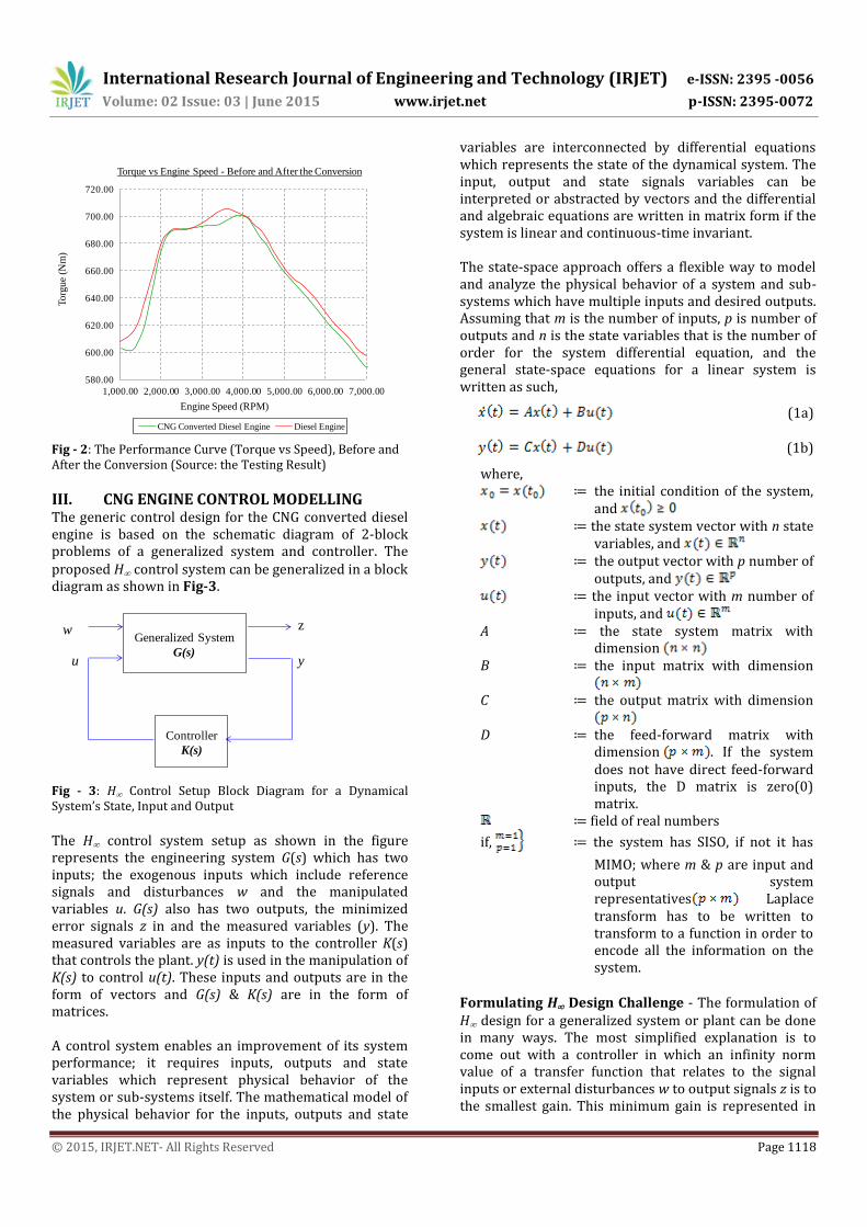
The chosen engine for this development is a 6-cylinder in-line engine as in Fig-1 which is widely used to power truck and busses. The engine is tested and measured its actual characteristic on bench dynamometer before and after the conversion as shown in Fig-2 that demonstrate the results on the torque values versus engine speed. It shows that the torque values for the CNG converted diesel engine is slightly lower than the original diesel engine at the maximum engine speed of approximately 3,800RPM.

Fig - 1: The First Prototype of CNG Conversion Engine (HINO, J08-T1 Model with 6 Cylinders and Displacement of 6,691L Diesel Engine)



© 2015, IRJET.NET- All Rights Reserved Page 1118

580.00

600.00

620.00

640.00

660.00

680.00

700.00

720.00

1,000.00 2,000.00 3,000.00 4,000.00 5,000.00 6,000.00 7,000.00

To

rgu

e (N

m)

Engine Speed (RPM)

Torque vs Engine Speed - Before and After the Conversion

CNG Converted Diesel Engine Diesel Engine

Fig - 2: The Performance Curve (Torque vs Speed), Before and After the Conversion (Source: the Testing Result)

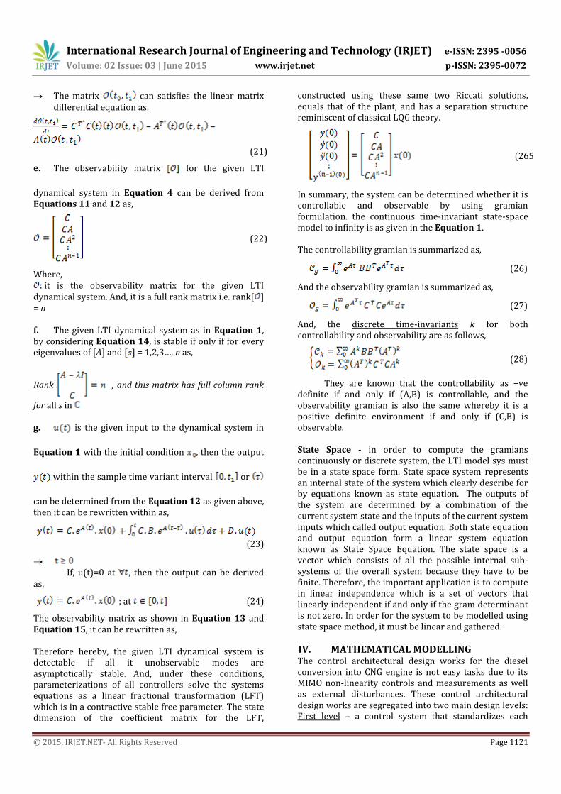
III. CNG ENGINE CONTROL MODELLING The generic control design for the CNG converted diesel engine is based on the schematic diagram of 2-block problems of a generalized system and controller. The proposed H control system can be generalized in a block diagram as shown in Fig-3.

Generalized System

G(s)

Controller

K(s)

w z

u y

Fig - 3: H Control Setup Block Diagram for a Dynamical System’s State, Input and Output

The H control system setup as shown in the figure represents the engineering system G(s) which has two inputs; the exogenous inputs which include reference signals and disturbances w and the manipulated variables u. G(s) also has two outputs, the minimized error signals z in and the measured variables (y). The measured variables are as inputs to the controller K(s) that controls the plant. y(t) is used in the manipulation of K(s) to control u(t). These inputs and outputs are in the form of vectors and G(s) & K(s) are in the form of matrices. A control system enables an improvement of its system performance; it requires inputs, outputs and state variables which represent physical behavior of the system or sub-systems itself. The mathematical model of the physical behavior for the inputs, outputs and state

variables are interconnected by differential equations which represents the state of the dynamical system. The input, output and state signals variables can be interpreted or abstracted by vectors and the differential and algebraic equations are written in matrix form if the system is linear and continuous-time invariant. The state-space approach offers a flexible way to model and analyze the physical behavior of a system and sub-systems which have multiple inputs and desired outputs. Assuming that m is the number of inputs, p is number of outputs and n is the state variables that is the number of order for the system differential equation, and the general state-space equations for a linear system is written as such,

(1a)

(1b)

where, ≔ the initial condition of the system,

and ≔ the state system vector with n state

variables, and ≔ the output vector with p number of

outputs, and ≔ the input vector with m number of

inputs, and A ≔ the state system matrix with

dimension B ≔ the input matrix with dimension

C ≔ the output matrix with dimension

D ≔ the feed-forward matrix with

dimension . If the system does not have direct feed-forward inputs, the D matrix is zero(0) matrix.

≔ field of real numbers

if, ≔ the system has SISO, if not it has

MIMO; where m & p are input and output system representatives Laplace transform has to be written to transform to a function in order to encode all the information on the system.

Formulating H Design Challenge - The formulation of H design for a generalized system or plant can be done in many ways. The most simplified explanation is to come out with a controller in which an infinity norm value of a transfer function that relates to the signal inputs or external disturbances w to output signals z is to the smallest gain. This minimum gain is represented in




this thesis as . Therefore, this arbitrary stabilizing controller must determine the value of an initial stabilizing gain at first, and then reduce it until it reaches to the value of . Eigenvalue & Eigenvector - In the case of state-space equations for the CNG converted engine formulated from closed-loop system equations in which to be controlled by using control method, is set under the two conditions: (a). , and (b). for the transfer function, where γ is the system performance bound. Controller can only be developed if the formulation of those equations into minimum of two complex Riccati Equations are +ve definite ( ) and the spectral radius of a certain variable is less than as mentioned in Equation 2 (Zhou, Doyle, & Glover, 2001)[1]. The spectral radius is the supremum among the absolute values of elements in its spectrum of a square matrix which denoted as (x). This can be done by identifying eigenvalues to determine the top eigenvalues in which the top eigenvalue is the spectral radius. If A is given

square matrix of a complex number, an

eigenvalue () and associated with eigenvector ( ), the relation can be written as,

(2)

Where, = eigenvector of complex number

I = Identity matrix = eigenvalue = positive integer, where

Then, the eigenvalues of A are also the n roots of its characteristic polynomial as written as below,

(3)

where, det = a determinant function of a real number

associated with every square matrix, = characteristic polynomial or spectrum of A

and represented by (A), in which,

= a set of spectrum of A ; if is a root for

= a spectral radius of A

The top modulus of the eigenvalues is the spectral radius which is noted as,

(4)

If, (A), then for any or , to satisfies,

(a) , and

(b) The spectral radius or the top eigenvalues is less than the performance bound to the power of two,

Linear Dynamical Responses - The correspondences transfer matrix from the system’s input and output as shown in Fig-3 can be written as,

(5)

Using Laplace Transform Method that transforms the time-domain of at initial condition which functions are with respect to time as in Equation 1 to the frequency domain which functions are respect "per time" (Arendt, Batty, Hieber, & Neubrander, 2002) [2], and the top eigenvalues formulation; the State Transfer Function can be written as,

(6)

And again, Equation 1 can be transformed into a compact matrix form as,

(7)

By implying the transfer matrix of Equation 6 into Equation 7, the character can be transformed as Equation 8. This is utilized into the Linear Fractional Transformation (LFT) as suggested by Zhou (2001).

(8)

Where, : the shorthand for State-Space

realization or written as

Notices that, but, the transfer matrix G(s) is not a Transfer Function. Therefore, the State Variable or the State Response of of the linear time-invariant dynamical system as in Equation 1 with respect to the initial conditions , and input , have to be transformed using Laplace Transform as summarized below as suggested by (Olivi, 1993, pp. 3-4).

;

(9a)

(9b)

Then,




(10)

a sample time during the external

disturbances or, the state variable, of at the

initial condition can be defined as,

; (11)

Therefore, the formulation for the system output can be derived on Equation 10 as below,

; (12)

Notes: Values of matrix [A] and [B] are controllable if any initial states are , and the final state satisfies that a. Controllability - it exists a controlling of from

to where provided that

from Equation 7 is in the column space of Equation 9, which is transformulated via Laplace Transform as, Then,

(13)

It is positive definite for any t > 0, where, : a controllable matrix

: adjoint operator of [B] or complex conjugate transpose of [B]

: adjoint operator of [A] or complex conjugate transpose of [A] where, the matrix is a positive definite at any t > 0

: State-Transition Matrix

: a sample time during instability period. And, the performance efficiency of the dynamical system can be derived as,

(14)

And, the controlling of is given by the merging between Equation 9 and Equation 10,

(15)

This can be desired to be transferred to the state plant, and the matrix satisfies the linear matrix differential equation as,

(16)

b. The controllability matrix for the given LTI

dynamical system in Equation 1 can be derived from Equations 15 and 16 as,

(17)

Where, : controllability matrix for the given LTI dynamical

system And, the controllability matrix has to be a full row rank. Therefore the system is controllable, i.e. rank( ) = n; n =

1,2, 3… The matrix has full row rank for all in (formulation is written from Equation 17. Assume that the converse, the matrix is not full row rank for , then there is a vector , so

Therefore,

(18)

where, : complex conjugate transpose of [x] From Equation 18, the system is controllable if (Doyle J. , Glover, Khargonekar, & Francis, 1989)[3],

i. Matrix C has full rank

ii. Matrix C has n columns that are linearly independent, therefore, each of n states of the system is reachable giving the system proper inputs through variable u(k)

c. The given dynamical system as in Equation 4, by considering Equation 18, is stable if only if for every eigenvalues of [A] and [ ], where i = 1, 2, 3…, n as,

Rank (19)

d. Observability - the pair of matrix [C] and [A] for the given dynamical system as in the second equation of Equation 4 are observable if for any and the

initial state is x(0) = x0, can be determined from the input u(t) and output y(t) within the interval of which is

transformulated via Laplace Transform as,

(20)

notes that, it is positive definite for any t > 0




The matrix can satisfies the linear matrix differential equation as,

(21)

e. The observability matrix for the given LTI

dynamical system in Equation 4 can be derived from Equations 11 and 12 as,

(22)

Where, : it is the observability matrix for the given LTI

dynamical system. And, it is a full rank matrix i.e. rank[ ] = n f. The given LTI dynamical system as in Equation 1, by considering Equation 14, is stable if only if for every eigenvalues of [A] and [ ] = 1,2,3…, n as,

Rank , and this matrix has full column rank

for all s in g. is the given input to the dynamical system in

Equation 1 with the initial condition , then the output

within the sample time variant interval or

can be determined from the Equation 12 as given above, then it can be rewritten within as,

(23)

If, u(t)=0 at , then the output can be derived

as,

; at (24)

The observability matrix as shown in Equation 13 and Equation 15, it can be rewritten as, Therefore hereby, the given LTI dynamical system is detectable if all it unobservable modes are asymptotically stable. And, under these conditions, parameterizations of all controllers solve the systems equations as a linear fractional transformation (LFT) which is in a contractive stable free parameter. The state dimension of the coefficient matrix for the LFT,

constructed using these same two Riccati solutions, equals that of the plant, and has a separation structure reminiscent of classical LQG theory.

(265

In summary, the system can be determined whether it is controllable and observable by using gramian formulation. the continuous time-invariant state-space model to infinity is as given in the Equation 1. The controllability gramian is summarized as,

(26)

And the observability gramian is summarized as,

(27)

And, the discrete time-invariants k for both controllability and observability are as follows,

(28)

They are known that the controllability as +ve definite if and only if (A,B) is controllable, and the observability gramian is also the same whereby it is a positive definite environment if and only if (C,B) is observable. State Space - in order to compute the gramians continuously or discrete system, the LTI model sys must be in a state space form. State space system represents an internal state of the system which clearly describe for by equations known as state equation. The outputs of the system are determined by a combination of the current system state and the inputs of the current system inputs which called output equation. Both state equation and output equation form a linear system equation known as State Space Equation. The state space is a vector which consists of all the possible internal sub-systems of the overall system because they have to be finite. Therefore, the important application is to compute in linear independence which is a set of vectors that linearly independent if and only if the gram determinant is not zero. In order for the system to be modelled using state space method, it must be linear and gathered.

IV. MATHEMATICAL MODELLING The control architectural design works for the diesel conversion into CNG engine is not easy tasks due to its MIMO non-linearity controls and measurements as well as external disturbances. These control architectural design works are segregated into two main design levels: First level – a control system that standardizes each




actuator’s setting especially on throttle angles, gas injector, inlet and outlet valves, cam angles and time firing of sparks; and Second level – a control system that capable of interpreting driver’s requirements, handling transition of the gears transmission, gas pressure and quantity balance in the gas tank, and managing for any failures in which can be up to reconfiguring those engine variables. Fig-5 presents the general architectural of MIMO for the CNG Conversion Engine.

Engine Control Management

for CNG Conversion

Diesel Engine

Throttle Angle,

Loading Weight,

Engine Heat,

Engine Speed

Engine Torque

Engine Temperature

Regulator Gas Pressure,

Driver’s Desired Speed,

Vehicle Weight,

Input Signals Output Signals

Fig - 5: The General Architectural of the Engine Control Management for the MIMO CNG Conversion Diesel Engine

The system design for the engine control management must consume specification on data of those variables which acts as the references to counter-correct on any control problems. These processes are embodied by a highly accuracy non-linear modelling control system with variables fundamental data. The modelling control system and the controller should be implemented independently based on its software and hardware utilization. The connection flow of the variables data for the control system is as simply segregated into sub-system which is done by systems identification and formulation. The objective is to stabilize the overall system if there is any modification and replacement of the components or variables. It does not influence the other modules. The confirmation of the simulation is demonstrated and proven by numerical analysis using H Control Method in the next chapter. Numbers of implementation and programming issues with regards to the modelling and control algorithm generations and the execution are discussed. State Variables Identification - The model that is described in this chapter consists of parameter-dependent systems and two-dimensional nonlinear functions, which mapping the model parameters over the operating envelope. The dynamic systems are linear in the input, the state, and the output respectively, yet their state-space data depends on parameters, which are tabulated in terms of states of the model or exogenous variables. In the construction of the model the dynamics are linearized analytically as far as possible, whereas the local gains are calculated by numerical linearization of the look-up sub-systems as shown in Fig-6.

Example - the dynamics of the crankshaft are considered to be quasi-stationary due to the large inertia, in comparison to the air and cng flow processes, and are not modelled explicitly. Therefore engine speed is considered to be a slowly-varying exogenous variable. Even though the dynamics of the crankshaft are not part of the model, the model is still too large and too complex to be identified as a whole. In spite of the complex interactions between the components of the model, they are therefore treated separately for the purposes of system identification. In view of the additional complexity of engine experiments and limited experimental capabilities, the only way forward is to identify in a simplistic approach the individual variables using standard system identification techniques for SISO systems of each engine elements.

Intake Manifold

mi

mo

ma

mcng

mcng

Preg

Pa

Vm

ma

Pm TmTa

mc

Combustion

e

eng

Engine Dynamicsload

Tc

Cooling System

Tw

Emission

Gas Injector

N

mbf

Crank angle Sensor ()

Ignition

Fig - 6: The Schematic Diagram for the whole system and sub-system for the CNG Conversion Diesel Engine

V. ENGINE ELEMENTS The internal engine system variables and engine dynamics of SI engines is proposed to be divided into five (5) basic sub-systems for the purpose of modelling as the state variables for the system (Guzzella & Onder, 2010, p. 25) [4],

i. The internal energy in the inlet and outlet manifold

ii. The air flow through the throttle valve and intake manifold,

iii. The injection of fuel through the injector and wall wetting,

iv. The exhaust emission which includes the vehicle and combustion delays, the gas mixing and the emission sensor, and

v. The torque output which includes the induction to the power stroke delays and several nonlinearities.

A CNG conversion engine requires all these sub-systems as well, but sub-systems (ii) and (iii) are difference as compared to gasoline SI engines. These are due to the injection of fuel directly before the combustion for the CNG conversion engine is in the form of gaseous state.




This is in contrast with a gasoline SI engine, in which the fuel is injected during the intake valves are opened. If the large hydrocarbon emission is associated with this approach, the SI engine will be in a disadvantageous situation [4] (Guzzella & Onder, 2010). On the other hand, the injection of gas has no storage effects at the manifold walls and the fresh mixed air and gas has no atomization phenomena. So, the gaseous state in the manifold is important penalty in modelling the engine controller. In contrast with the gasoline SI engines, there are two new important sub-systems which consume in the cng engine, (Dyntar, Onder, & Guzzella, 2002)[5],

(a). A backflow within the air flow which describes as a

substantial transport of fresh charge back to the intake manifold, and

(b). An injection timing dependent torque characteristic

which injecting the gas when the intake valves are opened then stratification takes place in the cylinder.

a. Throttle The throttle body receives the primary air supply for the engine as compared to an idle operation in which the air is supplied via a by-pas. At any situation of the engine cycle, the first key decision for the overall engine performance is the mass of the air flow rate that enters into the throttle. This is equivalent as the function to the driver’s demand to its required speed and the pressure ration across the throttle body. This can be considered as the engine dynamics for the mass of air flow rate trajectories OR the value of the throttle angle in which demanded by the driver. The throttle angle that is measured from the throttle plate to the axis of the air flow direction, is treated as an external disturbances input to the throttle body into the system. The components of the throttle body are purely made assumption as a mechanical system and the value of the friction is negligible. The changes of the mass flow rate of the air are relied on the position of the throttle angle. Next, therefore, the rate of the air mass flow into the manifold can be expressed in two functions:

(a). An empirical function of the throttle angle with the

function of air mass flow rate, and

(b). A function of the atmospheric and manifold pressure for the flow function is under chocked.

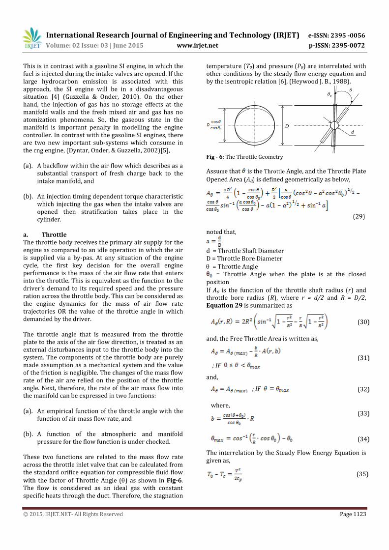
These two functions are related to the mass flow rate across the throttle inlet valve that can be calculated from the standard orifice equation for compressible fluid flow with the factor of Throttle Angle () as shown in Fig-6. The flow is considered as an ideal gas with constant specific heats through the duct. Therefore, the stagnation

temperature (T0) and pressure (P0) are interrelated with other conditions by the steady flow energy equation and by the isentropic relation [6], (Heywood J. B., 1988).

D

d

o

Fig - 6: The Throttle Geometry

Assume that is the Throttle Angle, and the Throttle Plate

Opened Area (A) is defined geometrically as below,

(29)

noted that,

d = Throttle Shaft Diameter D = Throttle Bore Diameter = Throttle Angle

= Throttle Angle when the plate is at the closed position If A is the function of the throttle shaft radius (r) and throttle bore radius (R), where r = d/2 and R = D/2, Equation 29 is summarized as

(30)

and, the Free Throttle Area is written as,

; IF (31)

and,

; IF (32)

where,

(33)

(34)

The interrelation by the Steady Flow Energy Equation is given as,

(35)




where, : M is March Number, is the sound of speed

which is . And, the interrelation of the

isentropic relation is given as,

(36)

and, stationery isentropic flow through an orifice is characterized by the flow function as,

;

IF (37)

; IF (38)

where,

(39)

where it is at the critical pressure ratio, : Constant coefficient in which its value relies on

Specific Heat Ratio and Mark Number M. If the flow function is chocked, then Equation 38 is written as the chocked flow function as below,

(40)

Throttle angle ( ) and pressure ratio (PR) in which intake manifold pressure (Pm) with respect to the ambient pressure ( ) defines the air mass flow via the intake throttle ( ). Therefore, this air mass flow is defined by adapting 2D function using discharge coefficient (CD) as a free parameter as shown in Equations 41a, 41b and 41c,

or (41a)

(41b)

For pressure ratio across the throttle less than the

critical value ( = 0.528, and ), then Equation

37 is substituted into Equation 41a and the air mass flow rate ( ) is given as follow [6] (Heywood J. B., 1988),

(41c)

If the flow function is chocked, Equation 40 is substituted into Equation 41c, and then the air mass flow rate is given as follow,

(41d)

Therefore, this model considers the lower pressure behaviour with a switching condition in the compressibility equation after considering the parameters and its variable values for the mass air flow rate that goes through the throttle angle as finalized in the Equation 41d. These are part of the parameters for the development of the robust control modelling. It can be simplified by assuming that the ambient pressure (Po) and ambient temperature (To) are constant. The determination of the gradients with respect to the throttle angle () and

pressure ratio using numerical linearization of the

operating envelope can be determined by referring to the steady-state air mass flow environment. This phenomenon is inclusive in the modelling as well as in the implementation in calculating the air mass flow disturbances with respect to the current operating point.

b. Intake Manifold The intake manifold is modelled into the control system design based on parameters of the manifold pressure and mixed ratio of mass air-gas flow rate. It is modelled as a differential equation on the net of changes between the incoming and outgoing of mass flow rate. The manifold pressure is derived with the respect to time in which it is proportionate to these changes as according to the ideal gas law. The model which is done by Crossley & Cook (1991) [7] is slightly different due to its incorporation with emission gas recirculation (EGR). Yet, this can easily be added as recommended. The mass of the intake manifold flow into the combustion is up-to the intake valve is off. This cycle period of air-gas ratio (AGR) is considered as isolated event for each combustion cylinder, in which the AGR for a cylinder is fixed till the next engine cycle. A model of the control system is desired in order to synchronous the relation between the air flow with the engine cycle. Thus, an optimum emissions performance is achieved even though the gas injection time is constrained to be at a specified point in the engine cycle. The air flow dynamic that goes into the intake manifold is derived with the respect to time-based phenomenon, and is synchronous with the crank shaft motion (). This dynamic motion is converted into an isolated model with the respect to time-varying that is based on the engine speed (N) (Powell, Fekete, & Chen, 1998) [8]. The time domain differential equation of the air flow dynamic is transformed into the crank angle domain as below,




(42)

The assumption of a general quantity of its changes, x(t) in the crank angle domain can be substituted into Equation 42,

OR (43)

The air pumped flow ( ) into and out from the manifold which represent as and respectively are identical only under a steady state environment. A continuity equation based on ideal gas law can be applied to the intake manifold provided that the values of the manifold pressure (Pm) and manifold temperature (Tm) are constant. Therefore, this air filling and emptying into and from the manifold dynamically are expressed as follow (Chang, 1993) [9], (Heywood J. B., 1988) [6],

(44)

The air mass flow rate is pumped out from the intake manifold into the combustion cylinder, in which the mass flow rate that goes into the combustion is written as (Heywood J. B., 1988),

(45)

By combining Equation 44 with Equation 45, the air mass flow rate that passing through the manifold then enters into the combustion cylinder, which ignores the inertial effects in the manifold within a sample time variant of the air inducted per in-take stoke as,

(46)

In other means, the total air mass flow rate that charges into the combustion cylinder ( ) with the function of

throttle angle ( ), engine speed (N) within a certain time cycle engine (t) is determined by multiplying it with a constant value as follow,

(47)

And, the value of air mass flow rate that charges into the combustion cylinder is determined by,

(48)

But, the intake manifold dynamics is modelled as a first differential equation (Khan, Spurgeon, & Puleston, 2001) [10].

(49)

Therefore, this model considers the lower pressure behaviour with a switching condition in the compressibility equation after considering the

parameters and its variable values for the mass flow rate that goes through the intake manifold with the function of the manifold pressure and engine speed. So, the mass flow rate of the output from the manifold into the combustion chamber is alternately determined by Equation 50 (Crossley & Cook, 1991) [7].

(50)

c. Air : CNG Ratio [Lambda ()] State Variable The value of air:cng is very important variable as for the purpose of controlling the fuel for the CNG converted diesel engine based on different engine model and parameters. There are several effects on the amount of the air mass flow together with the cng mass flow that enters into the combustion cylinder: throttling the air flow rate, aerodynamics resistance and resonances at the intake manifold, air+cng mass back flow value due to closing of inlet valve, and together with the rebounding of the burned gasses from the combustion into the inlet piping. This also affects the amount of air+cng that fit into the displacement volume or swept volume under regulator pressure and manifold pressure as well the ambient pressure via standard equation ma = o Vd (Po=1.013 bar & normalized air density o = 1.29 kg/m3). The value of air: fuel ratio or lambda () influences the engine’s work effectiveness (We) and thermal efficiency effectiveness (e) which is based on two variations - on the values of lambda air ( ) and lambda fuel ( ),

(Kiencke & Nielsen, Automotive Control Systems for Engine, Driveline and Vehicle, 2005) [11] - in this study is the value of lambda cng ( ) in two (2) situation;

First – variation of and is determined by driver. If

>1 (Lean Operation) means the fuel is injected less into the manifold mixer than the required Stoichiometric Ratio (LSR) for combustion. If < 1 (Rich Operation) means the fuel is injected more into the manifold mixer than the required LSR. Second – variation of and is

determined by driver. If >1 (Lean Operation) means the air is injected more into the manifold mixer than the required Stoichiometric Ratio (LSR) for combustion. If < 1 (Rich Operation) means the air is injected less into the manifold mixer than the required LSR. The graph in Fig-7 shows the affect of the thermal efficiency (e%) due to the variation values of f and a as the basic operation of an engine, in which the fuel injection and ignition timing are assumed under an optimal control. These variation values of relative air and fuel supplies affect the values of exhaust emission gasses as shown in Fig-8 as well. These variation values in controlling the engine are formulated below.




0

10

20

30

40

50

60

70

80

90

100

0.8 1 1.2 1.4 1.6 1.8 2

Th

erm

al E

ffic

ien

cy (

%)

Lambda ()

Variation-1 Lambda(f) Variation-2 Lambda(f)

Variation-1 Lambda(a) Variation-2 Lambda(a)

Variation (a)

Variation (f)

Fig - 7: The Affect of the Thermal Efficiency (e %) due to the Variation Values of f and a (after, Kiencke & Nielsen, 2005) [11]

0

100

200

300

400

500

600

9 11 13 15 17 19

Par

ts p

er M

illion (

PP

M)

Air/Fuel Ratio

O2 NOx CO2 HC CO

Fig - 8: The Emission Gasses under Stoichiometric with different A/F Ratio, (after Heywood, 1988) [6]

The value of lambda () is determined by the fraction between the real value of mass flow as compared to theoretical value for both air and fuel, as Equation 56a.

(51a)

where, the value of is the ratio between the relative value of air and cng as below,

Relative air supply: (51b)

Relative fuel supply: (51c)

notes that, the lambda ratio of the air and cng (as the fuel) in which they are respectively the ratio between the real mass and the theoretical mass values as below,

and (52)

Under a normal condition, the combustion process has to be under a stoichiometric condition, which is called Stoichiometric Ratio (LSR) as the ratio between mass air

to mass fuel under the theoretical condition. This value can be defined from the look-up table – Table D.4: Data of Fuel Properties, (Heywood J. B., 1988, p. 915) [6].

(53)

As mentioned in Section d, the value of air mass flow rate ( ) that enters into the intake manifold is controlled by the throttle angle which determines the value of . Then the value is consequently variant

by the EMSys to achieve the desired air:CNG ratio. This is an important variable for engine control. As referred to Fig-8 and Fig-9, there are three different situations and concepts in managing the fuel which is considered in the engine control modelling, (Gassenfeit & Powell, 1989) [12].

(a). S

ituation < 1 (Rich Mixture) – engine generates a maximum power because the relative value of fuel ( ) is injected higher than the air supply. This

situation happens during the engine is being warming-up and produces high exhaust emission of NOx.

(b). Situation = 1 (Stoichiometric Mixture) – engine generates an adequate power for any given vehicle loads and produces reasonable exhaust emissions of NOx.

(c). Situation 1 < < 1.5 (Moderate Lean Mixture) – engine generates a reasonable efficiency because the relative value of air (a) is throttled higher that the injected fuel supply. This situation produces higher emissions of NOx.

Situation > 1.5 (Lean Mixture) – engine generates higher efficiency because the relative value of air (a) is higher as compared to the value of . This situation of

engine produces higher NOx which requires a catalytic converter at the exhaust emissions. Through the relative value of air supply (a) which enter the throttle angle (), the driver can get the desired torque as in the reference data inputs such as from the speed of the engine, the value to the total load of the truck, the value of pressures and few other inputs as in the control design. These values of the cng ( ) in

which to be injected & mixed with the air, have to be regulated by the fuel control model in order to pre-determine the air : cng ratio (). This study focuses on the manifold injection method in injecting the cng into the mixer as shown in Fig-9.



© 2015, IRJET.NET- All Rights Reserved 27

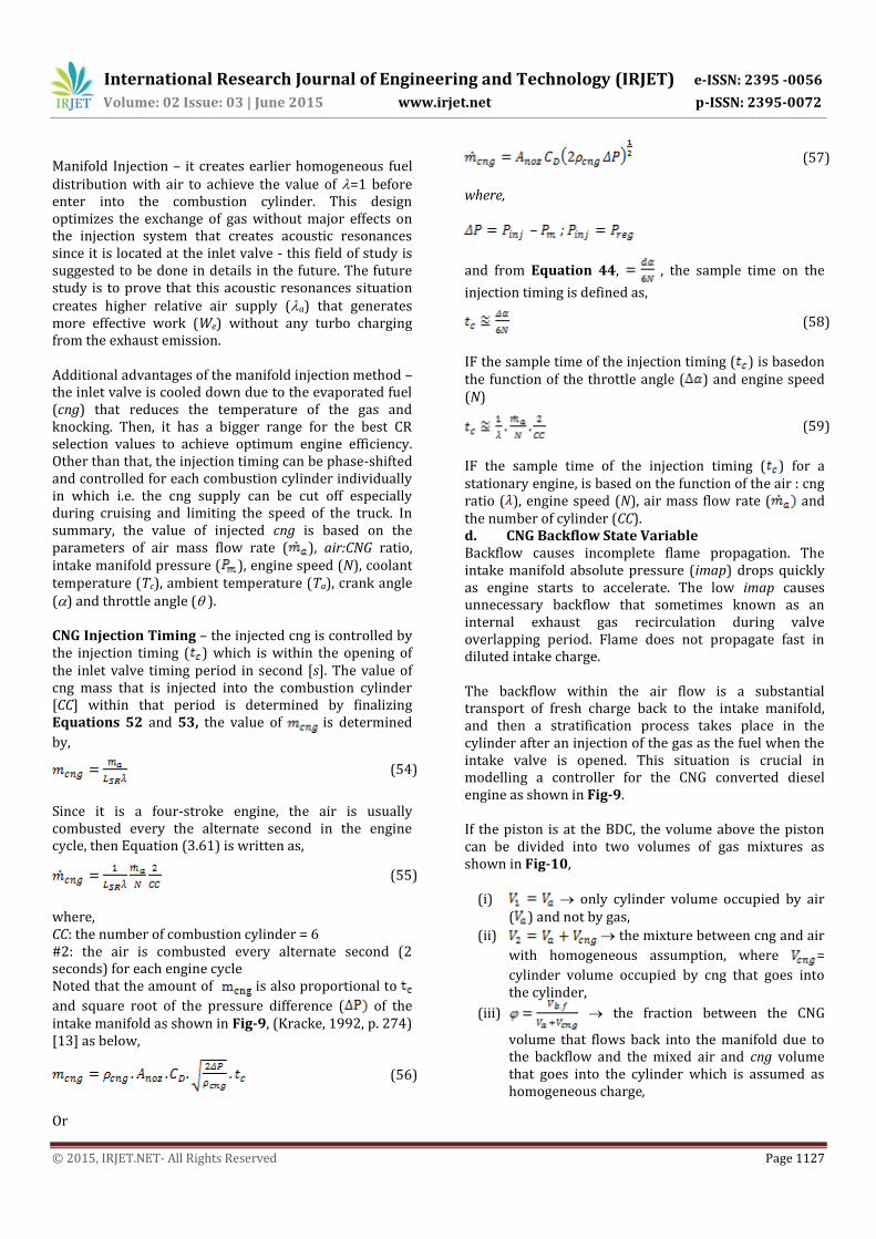
Manifold Injection – it creates earlier homogeneous fuel distribution with air to achieve the value of =1 before enter into the combustion cylinder. This design optimizes the exchange of gas without major effects on the injection system that creates acoustic resonances since it is located at the inlet valve - this field of study is suggested to be done in details in the future. The future study is to prove that this acoustic resonances situation creates higher relative air supply (a) that generates more effective work (We) without any turbo charging from the exhaust emission. Additional advantages of the manifold injection method – the inlet valve is cooled down due to the evaporated fuel (cng) that reduces the temperature of the gas and knocking. Then, it has a bigger range for the best CR selection values to achieve optimum engine efficiency. Other than that, the injection timing can be phase-shifted and controlled for each combustion cylinder individually in which i.e. the cng supply can be cut off especially during cruising and limiting the speed of the truck. In summary, the value of injected cng is based on the parameters of air mass flow rate ( ), air:CNG ratio, intake manifold pressure ( ), engine speed (N), coolant temperature (Tc), ambient temperature (Ta), crank angle () and throttle angle ( ). CNG Injection Timing – the injected cng is controlled by the injection timing ( ) which is within the opening of the inlet valve timing period in second [s]. The value of cng mass that is injected into the combustion cylinder [CC] within that period is determined by finalizing Equations 52 and 53, the value of is determined

by,

(54)

Since it is a four-stroke engine, the air is usually combusted every the alternate second in the engine cycle, then Equation (3.61) is written as,

(55)

where, CC: the number of combustion cylinder = 6 #2: the air is combusted every alternate second (2 seconds) for each engine cycle Noted that the amount of is also proportional to

and square root of the pressure difference ( of the intake manifold as shown in Fig-9, (Kracke, 1992, p. 274) [13] as below,

(56)

Or

(57)

where,

;

and from Equation 44, , the sample time on the

injection timing is defined as,

(58)

IF the sample time of the injection timing ( ) is basedon the function of the throttle angle ( ) and engine speed (N)

(59)

IF the sample time of the injection timing ( ) for a stationary engine, is based on the function of the air : cng ratio ( ), engine speed (N), air mass flow rate ( and the number of cylinder (CC). d. CNG Backflow State Variable Backflow causes incomplete flame propagation. The intake manifold absolute pressure (imap) drops quickly as engine starts to accelerate. The low imap causes unnecessary backflow that sometimes known as an internal exhaust gas recirculation during valve overlapping period. Flame does not propagate fast in diluted intake charge. The backflow within the air flow is a substantial transport of fresh charge back to the intake manifold, and then a stratification process takes place in the cylinder after an injection of the gas as the fuel when the intake valve is opened. This situation is crucial in modelling a controller for the CNG converted diesel engine as shown in Fig-9. If the piston is at the BDC, the volume above the piston can be divided into two volumes of gas mixtures as shown in Fig-10,

(i) only cylinder volume occupied by air ( ) and not by gas,

(ii) the mixture between cng and air

with homogeneous assumption, where =

cylinder volume occupied by cng that goes into the cylinder,

(iii) the fraction between the CNG

volume that flows back into the manifold due to the backflow and the mixed air and cng volume that goes into the cylinder which is assumed as homogeneous charge,




(iv) the stratification

process that occurs which is contemplated in the calculation of the backflow, VBDC = cylinder volume during piston at BDC for homogeneous charge where ,

The dynamics behaviour of the air and gas as the fuel is due to the reflow of the fresh air/gas mixture back into the intake manifold. The stratification process that occurs has to be contemplated in the calculation of the backflow. In the same time, an overlapping of the injection timing and inlet valve closing is also considered which is influencing the dynamic of the system, (Dyntar, Onder, & Guzzella, 2002) [5]. So, from items (i) to (iv) above can be reconstructed as,

OR, OR, (60)

Notes that,

; ; (61)

Assumed that, due to the air mixtures with

CNG,

So, and, (62)

If Items (iv) above is merged with Equation 62, the mass of backflow can be determined as,

(63)

From the assumption made in Equation 63, the stratification factor as in Equation 61 can be rewritten as,

(64)

Intake Manifold

ma

mcng

(k)mcng

mb.f

Preg

Emission

Gas Injector

Combustion

cylinderBDC

V2

V1mcng.c

mb.mmcng(inj)

mc

TDC

(1-k)mcng = mcng.c

Fig - 9: The Schematic Diagram for the CNG Converted Diesel Engine with Backlash

0.2

0.4

0.6

0.8

1.0

1.2

1.4

1.6

120600.0

0

Crank Angle ()

R= l/r = 3.5

Fig - 10: Piston Speed/Mean Speed is a Function of Crank Angle, when R=3.5

Then, the value of mass backflow is finally determined as in Equation 65,

(65)

Due to the mass backflow some of the mixed air and cng, which returns back to the manifold, therefore the total mass flow that enters to the cylinder is determined by,

(66)

Few variables have to be considered in formulating to calculate the amount of CNG in the cylinder during the inlet valve is closing as shown in Fig-12,

(a). The maximum amount of cng mass enters the combustion area (mcng.c)

(b). The amount of cng mass flows from the combustion area back to the intake manifold (mb.f)

(c). The balance amount of cng mass in the combustion area after inlet valve is closed (mcng.c)

(d). The balance amount of cng mass in the manifold because of the injection delay (mb.m)

(e). The amount of cng mass injected (mcng.inj)

(f). The amount of ratio between the cng that flows back into the manifold and the maximum volume of cng in which it is assumed as homogeneous charge (),




where = 0 if all the cng flows into the combustion area and there is no backflow occurs

(g). A physical interpretation of the stratification factor (f)

(h). Status of injection overlapping (o), where Io = 0 if all cng is injected into the combustion; Io = 1 if all cng is not injected into the combustion area, but it will be injected after the mentioned stroke.

The engine experiences various transients of parameter if it starts in a cold starting; such as engine speed, temperatures and iMAP. These are all changing dramatically in the first few cycles which include backflow. These transients considers as disturbances which makes the air:CNG ratio accuracy is difficult to be controlled. From the experiment, Fig-11 and Fig-12 demonstrates the over-lean or over-rich air:cng mixtures slows down the flame propagation speed for the first before the 5th engine cycle from approximately 100kPa drops to 40kPa, and in the same time causes a significant unburned gasses emission.

0

10

20

30

40

50

60

70

80

90

100

110

0 1 2 3 4 5 6 7 8 9 10 11 12

imap

(k

Pa)

Engine Cycle

Intake Manifold Absolute Pressure (imap) due to Backflow

Fig - 11: The Intake Manifold absolute pressure (iMAP) drops from approximately 100kPa to 40kPa before the 5th engine cycle after the engine starts due to the backflow that causes incomplete flame propagation ( is approximately 0.289).

0

20

40

60

80

100

120

140

0 10 20 30 40 50 60 70 80

Air

Mass

Flo

w r

ate

(g/s

)

Intake Manifold Pressure (cmHg)

4000 RPM

3500 RPM

3000 RPM

2600 RPM

2000 RPM

1600 RPM

1200 RPM

800 RPM

10 degree

WOT

18 degree

21 degree

26 degree

36 degree

36

26

21

18

10

Wide Opened Throttle

(WOT)

Throttle Angle ()

Fig - 12: Variations of Air Mass Flow Rate pass Throttle with Intake Manifold Pressure (iMAP), Throttle Angle & Engine Speed, (after Heywood, 1988) [6].

Therefore, the value of homogeneous charge or the fraction between the cng volume that flows back into the manifold as backflow and the mixed air and cng volume as mentioned in Section (iii) above can be determined from the fraction of graph area as shown approximately, in which the value for is approximately 0.289.

e. Compression Stroke A compression stroke starts when both inlet and outlet valves are closed; the mixture gas and air is in the combustion area as it is being compressed to a small fraction of its small volume; draws a fresh charge in to the crankcase; and combustion is initiated towards the end of the compression stroke as the piston approaches the TC; then the cylinder pressure rises more rapidly. Fig-13 shows the standard geometrical reciprocating engine in considering all the parameters and the relevant geometrical equations for the development of control modelling, (Heywood J. B., 1988) [6].

L

B

l

r

s

Vd

VcTDC

BDC

D

Fig - 13: The Geometrical Diagram for the Engine Variables such as Piston, Connecting Rod (l), Crank Radius (r), Crank Angle (), Bore (D), Stroke (sst) and Distance between the Crank Axis and the Piston Pin (s)

Determined that,

(67)

(68)

(69)

The HINO Engine is a six-cylinder four-stroke engine with 120 of crankshaft revolution separates the ignition of each successive cylinder, in which each cylinder fires on every other crank revolution; the firing order is 1-4-2-




6-3-5. The intake, compression, combustion and exhaust strokes occur simultaneously (at any given time, one cylinder is in each phase).

The compression can be determined by delaying the combustion of each intake charge of the crank rotation from the end of the intake stroke by 120. Referring to Fig-13, one of the important characteristic in generating the engine speed is the mean piston speed ( ) as below,

(Heywood J. B., 1988, p. 45) [6],

(70)

Where, N = rotational speed of the crankshaft

= Mean piston speed is more appropriate

parameter as a function of speed compared to the cr ank rotational speed for correlating engine behaviour (i.e. gas flow velocities in the intake and the cylinder are all scale with the mean speed)

Where else, the instantaneous piston velocity ( ) is

obtained from the movement of the piston pin along with the axis as referred with the respect to time,

(71)

For, t = 0, the piston velocity is zero (0) which is at the beginning of the stroke. Therefore, Equation 69 can be differentiated and substituted into Equation 71, and the ratio between the instantaneous piston velocity and the mean speed can be summarized as follow,

(72)

(73)

IF piston is at TDC, THEN and , IF piston is at BDC, THEN and , THEN the derivatives for the piston stroke ( ) over

the crank angle (d) from Equation 73 is written as,

(74)

Introducing and as the two constant multiplying factors, where

; (75)

(76)

f. Internal Combustion Dynamics The dynamics analysis of the internal combustion engine is based on the Otto cycle process of a reciprocating piston engine. The total power exerted from the engine combustion that acts on the n system particles in the cylinder is significant to the total of kinetic energy of the system with respect to the rate of time From Equation 67, the swept volume (Vd) can also be determined by,

(77)

Combustion dynamics – the work done by the force (F) after combustion which is given by, The power exerted from the work done is given as,

(78)

The Second Newton Law,

, then

(79)

Kinetic energy (Ke) which is converted and exerted into the combustion chamber with respect to time is as follow,

(80)

Since Equations 79 and 80 are identical numerically equal and the scalar of the formulation product is commutative to each other, then,

OR (81)

g. Internal Rigid Body Dynamics The characteristic of the rigid body of the engine dynamics due to the power exerted is formulated in order to determine the continuity of the conservation of energy law which generates moment of force, then torque at the crankshaft. This dynamics characteristic is considered equivalent to the finite number of the particles. An assumption is made to a one rigid body with two particles have to be in equilibrium at the centre of mass (CoM) as shown in Fig-14. The centre of mass can be determined as the equivalent system of two particles of mass mA and mB with the total mass of the system (m), so,

and (82)

From Fig-14, geometrically defined also as,

and, (83)

(84)

Then, Equation 84 is written as,




(85)

By differentiating Equations 83 and 85, then merging them as,

and, (86)

(87)

Kinetic Energy - Let consider the formulation of the kinetic energy and moment of force on the piston, crankshaft and connecting rod by referring to Fig-15 and Fig-16. The assumption that all the rigid body are symmetric and the centre of mass for each of them are at their geometric centre. Therefore, the geometrical total mass model for each dynamics mechanism is approximated as follows,

com

A

B

l

b

a

Fig-14: An Assumption of a Rigid Body Diagram Equilibrium for the Engine Mechanism Dynamics

(88)

rod mass) (89)

(90)

The formulation for the total kinetic energy of the mechanism system is determined as,

(91)

L

D

l

r

s

TDC

BDC

P

y

x

Fig - 15: The Free Rigid Body Diagram

Then, the total kinetic energy is for the mechanism at mQ and mP. So,

(92)

Noted that, for simplification, let’s consider Equation 87 instead of Equation 92 for the formulation of vP. Therefore,

and, (93)

Then, Equation 92 is formulated as,

or (94)

(95)

Noted that the 2nd part of the Equation 97 it seems that a moment of inertia (Ic [kgm2]) is generated from mP and mQ with the distance r which affects the crankshaft. Therefore, the above equation can be formulated as,

(96)

Where,

(97)

Exerted Power – referring to Fig-16, the power is exerted onto the dynamics mechanism system as,

(98)

Where, Mt : turning moment acting on the crankshaft [N.m]

: power [kW] or [N.m/s] or [J/s] Patm: atmosphere pressure [N/m2] P: pressure acts on piston [N/m2]

Ac: piston area = [m2




l

r

s

P

y

x

mP

mQ

mC

vQ

vP

Fig-16: The Assumption of Total Mass for the Mechanism of the Dynamics System Model

l

r

s

PAp

y

xmC

vQ

vP

Mt

PatmAp

Fig-17: The Exerted Power and Moment of Force Modelling on the Dynamics Mechanism System

Noted from Equations 82 and 97 are emerged as,

(99)

Then, the differential equation is written as follow,

(100)

Then, replace Equation 99 into Equation 101,

(101)

Assumption is made that the engine is running at a constant speed even the truck carries a higher load. The approximation is valid and the term with factor of angular acceleration is zero, so Equation 101 can be written as,

(102)

Therefore, the turning moment with respect to the angular velocity of the crankshaft is determined as,

(103)

Or by replacing Equation 98 into Equation 103, so, the above equation is also expressed by,

(104)

Substituting Equation 87 into Equation 102, and solving differential the 2nd part of the equation to determine the turning moment,

(105)

As noted earlier that,

(106)

And, assumption – the mass of the connecting rod and crankshaft ( ) is neglected due to its small value as

compared to the pressure from the combustion acts on them. Therefore, the turning moment ( ) is equal to the pressure moment in the combustion cylinder (Mp). So,

(107)

And, from Equation 88 generates the moments due to the inertia (Mi) of the moving parts in the mechanism system due to the as given below,

(108)

Based on the values given, the moment of combustion pressure (Mp) and the moment due to the inertia of the moving parts (Mi) are plotted vs crank angle as shown in Fig-18 with the Mean Effective Moment (MeM) value for Mp of 85.7Nm as in green ink, and Mi of 4.7Nm as in blue ink. h. Engine Dynamics An establishment of a modelling control system from the characteristics of an engine such as the air mass flow-out rate from the manifold, then pressurized into the combustion chamber based on the pulse setting, are not an easy function. These tasks make more complex with the conditions in the inlet and outlet of the manifold and the gas inertia. However, it can be done by assuming that the condition is a quasi-steady operating condition with an empirical relationship. As a conventional engine, the




combustion cylinder pumps mass air flow rate ( ) into the cylinder with an engine speed (N).

-200

-100

0

100

200

300

400

500

600

700

0 60 120 180 240 300 360 420 480 540 600 660 720

Mom

ents

(N

.m)

Crank Angle (Degree)

Moments due to Combustion Pressure and Inertia

Moment due to Inertia (Mi) Moment due to Combustion Pressure (Mp)

Mean Value for Mi Mean Value for Mp

Fig-18: The values of Moments due to Inertia (Mi) and Combustion Pressure (Mp) and their Mean Effective Moments (MeM) vs Crank Angle

-10

0

10

20

30

40

50

0 100 200 300 400 500 600 700

Cy

lin

der

Pre

ssu

re (

bar

)

Crank Angle (degree)

Cylinder Pressure & Crank Angle

Diesel Engine Diesel-CNG Converted Diesel Engine

Fig - 19: The values of Cylinder Pressure (P, bar) is determined via testing result between Diesel and CNG converted diesel engine vs Crank Angle (degree), Pmax (CNG converted diesel engine) is approximately 39bar at TDC (720 degree)

Due to the holding down of the cam timing, the exhaust gas recirculation is being increased. It makes the mass flow of fresh air in the combustion chamber is being decreased. Therefore, the deteriorated mass flow rate of the air is under a polynomial regression which fits for a nonlinear relationship between the cam phasing (CAM), manifold pressure and engine speed (Heywood J. B., 1988). Then, the gas is injected into the exhaust manifold area when the inlet valves are opened that permits to introduce a stratification charge in the combustion cylinder which influences the engine torque efficiency consequently as shown in Fig-18, (Dyntar, Onder, & Guzzella, 2002) [5]. The experiential relationship in computing the value of Torque (eng) is due to the function of engine speed (N), total truck load (load), mass flow rate into the

combustion area (mm), air:gas ratio , fuel thermal

/heating value and the value of the spark advance

(), (Crossley & Cook, 1991) [7]. Equation 105 demonstrates the empirical relationship with the function of mass of the air charge, air/gas mixture ratio, spark advance and engine speed in producing the computation torque. This is one of the variables in developing the algorithm for the control system. The determination value for the Engine Torque is depending on the values of engine speed, total truck load, air:gas ratio, and thermal transfer rate,

for the function of (109)

where, = fuel thermal /heating value

= fuel consumption efficiency

= volumetric efficiency = air density inlet

= air:gas ratio aims to keep the stoichiometric

relative air:gas ratio, = 1 for the best of conversion efficiency, throttle control and ignition timing. The relationship of those functions in Equation 58 is determined as below,

(110)

Power from the engine can be determined as,

(111)

Notes that,

: where is air mass flow rate (g/h) and is

gas mass flow rate (g/h) and the ratio is estimated from 0.056 ~ 0.083

: where sfc is specific fuel consumption of

and the best value for SI engine is 270

g/kWh the heating value which is accepted by the

commercial is between 42 ~ 44 MJ/kg. The value of the torque can also be determined by analytical curve fitting technique which are from the testing data using dynamometer in which can estimate the steady-state brake torque as below, (Khan, Spurgeon, & Puleston, 2001) (Crossley & Cook, 1991) [7],

(112)

And, the crankshaft speed-state equation can be written as,

(113)

noted that, : value of torque that produced by the engine [Nm]

: truck loading [Nm] 1, 2, 3, …., 10 : are constant coefficients




air / fuel ratio : mass of air that goes into the combustion area [g]

: spark advance degree before TDC [ =30] : engine speed [rad/sec] : effective engine inertia [kgm2]

The torque can also be determined by taking Equation (105) and Equation (118),

(114a)

(114b)

Where, the value of engine torque, for CNG engine is

determined from the experiment based on the engine speed, N as plotted in Fig-20 as comparable to diesel engine. i. On the Road Power Load The truck has to be capable of moving on any road levels at a steady speed. Therefore, it requires enough power to drive the truck and this is called “On the Road Power Load” which is useful to be set as a reference point if it is necessary. The Power from the road load for the truck is to overcome the rolling resistance which is consumed from the friction of the tires and the aerodynamics drag resistance against the wind loading. For the given Rolling Resistance (CR) and the drag coefficient (CD), the approximate value for road power load (Pr) is given by, (Heywood J. B., 1988, pp. 48-50) [6],

(115)

From those values as suggested above, the merging of Equations 56, 57 and 58 can be written as,

(116)

The value of torque produced by the CNG engine is acceptable as compared to the diesel engine before the conversion is plotted in Fig-20. j. Mean Effective Pressure The work done is the combustion in each cylinder that produces torque. The torque value is generated by the measurements in the particular CNG converted diesel engine which has the ability to do work depending on the engine size used. The useful relative engine performance measurement is by dividing the work per cycle by the cylinder volume displaced per cycle – unit: force per unit area – is called Mean Effective Pressure (MEP). Another approach utilizing the engine dynamics model to estimate the MEP is by extracting the instantaneous torque from flywheel speed fluctuation measurement and converts it to MEP by considering each of the action torque components. The power per cylinder is related to the indicated work per cycle is by, (Heywood J. B., 1988)

580.00

600.00

620.00

640.00

660.00

680.00

700.00

720.00

1,000.00 2,000.00 3,000.00 4,000.00 5,000.00 6,000.00 7,000.00

To

rgu

e (N

m)

Engine Speed (RPM)

Torque vs Engine Speed - Before and After the Conversion


Fig-20: The Performance Curve (Torque vs Speed), Before and After the Conversion (Source: the Result from this Project)

[6],

(117)

Where, = 2; for four-stroke engine. Therefore, the

work per cycle is determined by,

; W is the work done per unit cycle (118)

Therefore, the MEP in [kPa] is determined by dividing Equation 105 with swept volume of the cylinder which is determined in Equation 65,

[kPa] (119)

Then, mep can also be expressed in terms of torque,

[kPa] (120)

-500

-400

-300

-200

-100

0

100

200

300

400

500

600

-360 -300 -240 -180 -120 -60 0 60 120 180 240 300 360

Torq

ue

(Nm

)

Crank Angle (Degree)

Torque vs Crank Angle at 1,500 Nm 40% Load


mep (-46.9Nm):CNG Converted Diesel Engine mep (-16.8Nm): Diesel Engine

Fig-21: The Comparison Engine Torque Values between cng and Diesel Engines at 1,500RPM with Additional 40% Total Truck Load vs Crank Angle

k. Engine Thermal The temperature for the burned gas in the cylinder of SI engine during the combustion period is commonly about 2,000K to 3,000K with a heat flux value of approximately




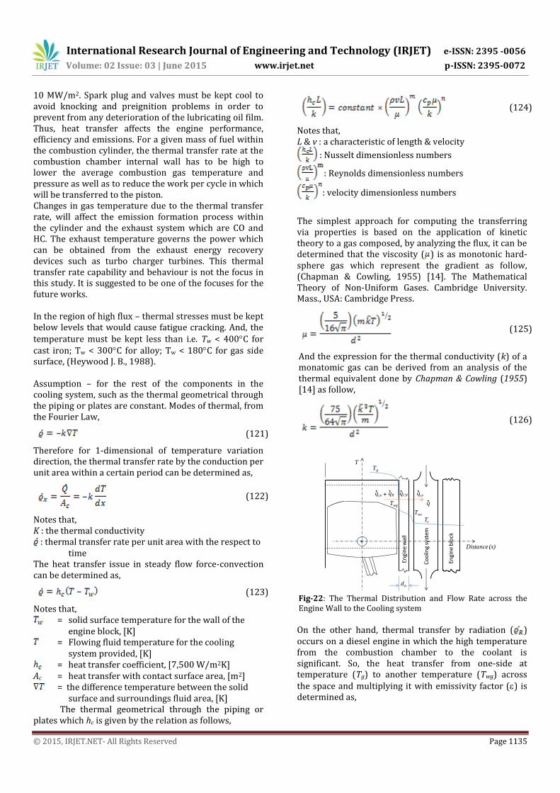
10 MW/m2. Spark plug and valves must be kept cool to avoid knocking and preignition problems in order to prevent from any deterioration of the lubricating oil film. Thus, heat transfer affects the engine performance, efficiency and emissions. For a given mass of fuel within the combustion cylinder, the thermal transfer rate at the combustion chamber internal wall has to be high to lower the average combustion gas temperature and pressure as well as to reduce the work per cycle in which will be transferred to the piston. Changes in gas temperature due to the thermal transfer rate, will affect the emission formation process within the cylinder and the exhaust system which are CO and HC. The exhaust temperature governs the power which can be obtained from the exhaust energy recovery devices such as turbo charger turbines. This thermal transfer rate capability and behaviour is not the focus in this study. It is suggested to be one of the focuses for the future works. In the region of high flux – thermal stresses must be kept below levels that would cause fatigue cracking. And, the temperature must be kept less than i.e. Tw < 400C for cast iron; Tw < 300C for alloy; Tw < 180C for gas side surface, (Heywood J. B., 1988). Assumption – for the rest of the components in the cooling system, such as the thermal geometrical through the piping or plates are constant. Modes of thermal, from the Fourier Law,

(121)

Therefore for 1-dimensional of temperature variation direction, the thermal transfer rate by the conduction per unit area within a certain period can be determined as,

(122)

Notes that, K : the thermal conductivity

: thermal transfer rate per unit area with the respect to time

The heat transfer issue in steady flow force-convection can be determined as,

(123)

Notes that, = solid surface temperature for the wall of the

engine block, [K] = Flowing fluid temperature for the cooling

system provided, [K] = heat transfer coefficient, [7,500 W/m2K]

Ac = heat transfer with contact surface area, [m2] = the difference temperature between the solid

surface and surroundings fluid area, [K] The thermal geometrical through the piping or

plates which hc is given by the relation as follows,

(124)

Notes that, L & v : a characteristic of length & velocity

: Nusselt dimensionless numbers

: Reynolds dimensionless numbers

: velocity dimensionless numbers

The simplest approach for computing the transferring via properties is based on the application of kinetic theory to a gas composed, by analyzing the flux, it can be determined that the viscosity ( ) is as monotonic hard-sphere gas which represent the gradient as follow, (Chapman & Cowling, 1955) [14]. The Mathematical Theory of Non-Uniform Gases. Cambridge University. Mass., USA: Cambridge Press.

(125)

And the expression for the thermal conductivity (k) of a monatomic gas can be derived from an analysis of the thermal equivalent done by Chapman & Cowling (1955) [14] as follow,

(126)

Co

olin

g sy

stem

Engi

ne

blo

ck

Engi

ne

wal

l

Tc

Twg q

T

Distance (x)

qR

qcv

+ qCN

qcv

Tg

Twc

dw

Fig-22: The Thermal Distribution and Flow Rate across the Engine Wall to the Cooling system

On the other hand, thermal transfer by radiation ( ) occurs on a diesel engine in which the high temperature from the combustion chamber to the coolant is significant. So, the heat transfer from one-side at temperature (Tg) to another temperature (Twg) across the space and multiplying it with emissivity factor () is determined as,




(127)

The thermal flow from the IC area to the cooling system is demonstrated in Fig–22. The heat flux from the combustion area to the combustion wall ( ) has two thermal flow rate which are convective ( ) and radiation ( ) rates. Therefore, the total thermal flow rate from the internal combustion to the wall is defined as,

(128)

Then the thermal flow in the internal combustion area is determined as,

(129)

Since the radiation rates is negligible in the SI engine, so the thermal flow rate in the internal combustion area is written as,

(130)

And, the thermal flow rate at the engine wall ( ) is determined as,

(131)

And, the thermal flow rate at the coolant ( ) is determined as,

(132)

Therefore, the total thermal flow rate from the internal combustion wall to the cooling system is determined as,

(133)

an assuming that,

So, Equation 132 is finally written as,

(134)

Notes that and are input signals from,

: Engine wall Temperature [K]

: Coolant Temperature [K]

External Disturbances - Uncertainty is always present, or inherent, in complex systems such as this CNG converted diesel engine. Such system should be robust with due to its any inherent uncertainties, in which the basis for the design and analysis is by a mathematical model of each dynamic processes of each sub-system together with any associated uncertainties. There are a number of different sources of uncertainties which arises naturally from different locations of a system. Repeated experiment and accurate measurements at the stage of experimentation should be considered. Besides, the selection and estimation of suitable parameterization

model, interpretation of residuals at the stage of system identification and approximation of the numerical numbers during the model construction.

How the assumptions made and errors incurred at the different stages influence the overall accuracy of the model is difficult to assess. A precise error analysis is hardly possible because the pieces of quantitative information are not readily compatible. However, the effects of all these kinds of errors should be of second order and negligible in comparison to the changes in dynamics as a result of the parameter variations across the operating envelope. Still, it would be very useful, if also such sources of uncertainty could be integrated in a standard framework. In this study, the parameter variations are known in a number of operating points. For simplicity, the ambient conditions, i.e. pressure and temperature, are assumed to be constant. With this approach, the fundamental limitations of the physical system, the control configuration and the model itself are known. This ultimate focuses on the engine modelling to design a robust control system using H synthesis and analysis techniques, such as H closed loop shaping and its analysis. For that purpose, nonlinear representations of the key engine variables are reformulated using linear fractional transformations in the next section and aggregated in a robust control framework. Linear time-invariant models are derived with fixed operating points as well as a linear parameter-dependent system as a continuous function of engine variables across the operating envelope.

VI. MODEL VALIDATION The control modelling and overall behaviour for the robustness of the control system design has to be validated by putting all the sub-systems into the control structure flow as shown in Fig-23. All the signal inputs from the sensors – gas pressure at the regulator and manifold, engine block temperature, engine speed, engine torque and truck load. As such, the gas pressure changes from the regulator to the combustion area with external disturbances are prescribed. The engine control system design must consume specification on data of those variables which acts as the references to counter-correct on any control problems. These processes are embodied by a highly accuracy non-linear modelling control system with variables fundamental data. The modelling control system and the controller should be implemented independently based on its software and hardware utilization. The connection flow of the variables data for the control system is as simply shown in Fig-24 as simulated using “simulink” model logs – the control structure flow. If there are any




modification and replacement of the components or variables, it does not influence the other modules.

Driver’s

Desired Speed

Throttle Angle

N

Reg

ula

tor

CNG Tankdmg/dt

dma/dt

Inta

ke

Man

ifo

ld

dmm/dt

Pm

Co

mb

ust

ion E

ngin

e

Th

rott

le

En

gin

e D

yan

am

ics

ds/dt

Tru

ck &

Carr

ier

Vehicle Weight

Loading Weight

WV

WL

Drag torque

(laod)

Preg

Valve Timing

Crank Angle

Co

oli

ng S

yst

em

Tru

ck w

ith

Lo

ad

ing N

cwc

PT

dVt/dt

N

engload

back

flo

w

Fig - 23: CNG Converted Diesel Engine Model Logs: The Control Structure Flow with multi-variables

desired rpm

throttle angle

(theta)

engine speed

(omega)

1

driver’s desired

speed

theta

omega

Controller

Regulatormgdot

Gas injector

Preg

Mass flow rate

(mgdot)

Regulator Pressure

(Preg)

2

Throttle & Intake Manifold

Mixed mass flow rate

(mmdot)

Manifold Pressure

(Pm)

Combustion

Engine

madot

Pm

omega

Piston Speed (sdot)

Dynamics

Engine

Teng

TloadInjector +

Backflow

mcdot

Crank angle (lamda)

Valve timing (Vtdot)

mcdot

sdotCam angular

Velocity(omega)

3

Vehicle Weight (WV)

4

Loading weight (WL)

emission

omega

Vtdot

lamda

Drag Torque

Cooling System

Torque total load

(Tload)Tw Tc

TcTc

Engine walltempt.(Tw)

Simulation

Inputs

EngineSpeed (N)

Exhaustemission

throttle angle (theta)

Torque total load (Tload)

Coolant (Tc)

mgdot

Fig - 24: Non-linear CNG Converted Diesel Engine Model for validation process

VII. CONCLUSION AND RECOMMENDATION The application of robust design into designing an engine control system is motivated from the practical experience and “trial-and-error” efforts. This chapter formulates the entire engine variables in which are proven by the next chapter from the theoretical and mathematical formulation. There are 3 attempts in modelling the control algorithm. It is based on the set of linear time-invariant models for each variables of the engine system. Although the models are genuinely discrete and event-based, it is found to be easier to carry out the design under a frequency domain continuously. The solutions are deal with engine variables and unstructured description uncertainties, therefore to employ first the H closed loop shaping as suggested from the past various researches done actively since

1988 by the top scientist. Back to the study case - as the cng is fed to the injector at the pressure of approximately between 3 to 5 bar above the intake manifold pressure, and the pressure in the cng tank is about 200 to 220 bar, therefore, the regulator is used to reduce the pressure just before in the intake manifold. Since the natural gas is decompressed down to 3 to 5 bar causes the cng temperature decreases. Consequently, the gas temperature is used to account the evaluation of the injection pulse widths and cng mass flow rate into the exhaust of the manifold and so on. The further formulation of the engine variables are demonstrated in Chapter 4 in configuring the state-space equations for the system. The development of the closed loop shaping towards the justification of stability, controllability and observability of the system are also explained. Then the next step is the application of H loop-shaping in which is a design methodology in modern control theory. It combines the traditional intuition of classical control methods with H optimization techniques to achieve controller with internal stability system and performance properties hold good, in spite of bounded differences between the nominal plant assumed in design and the true plant encountered in practice. Essentially, the control system designer describes the desired responsiveness and noise-suppression properties by weighting the plant transfer function in the frequency domain; the resulting 'loop-shape' is then 'robustified' through optimization. Robustification usually has little effect at high and low frequencies, but the response around unity-gain crossover is adjusted to maximise the system's stability margins. H loop-shaping can be applied to MIMO systems. H loop shaping is validated by using MATLAB-simulink, since this method of robusting the system using H is at the infant stages, even though some of the application has already deployed in the industry at the earlier stage. In 1995, Hyde, Glover and Shanks have published related to the method which successfully applied, have been successful at the earlier stage. In addition, they published another paper which describes as successful application to a steerable marine radar tracker is an example. Nevertheless, the H control system is able to cope with all the changes, such as external disturbances and dynamical disturbances. The control system is robust or insensitive with respect to the conversion parameters which can be interpreted as disturbances or uncertainty to the system behavior. And yet, a control system model can never be perfect; estimations and approximations have to be made available during the formulation, and parameters of the systems variables are determined based on estimation and not exactly, as such, numerical errors may or may not occur along the model




development process. If disturbances or uncertainties are naturally existed in the system, a model-based control on the basis of an inverted model is generally not advisable. This is due to that an exact compensation is problematic in the presence of uncertainties and nevertheless the CNG converted engine is stable running during the road testing.

VIII. SYMBOLS

: mass air flow rate that goes into manifold,

[g/s] : throttle plate opened area, [mm2]

: throttle angle, []

& : upstream pressure [bar ] and temperature,

[K] : downstream pressure of throttle (it is

assumed that the pressure is the same value at the minimum area or no pressure recovery occurs), [bar]

: Critical Pressure Ratio (CPR)

: discharge coefficient (is determined through

experimental) : Specific Heat Ratio (cp/cv); [ = 1.4 if CPR =

0.528; [ = 1.3 if CPR = 0.546] cp : Specific Heat at constant pressure [J/kg K] cv : Specific Heat at constant volume [J/kg K]

: stationery isentropic flow function

: Gas Constant

N : engine speed [rad/s] : crank angle [deg] Vm : manifold volume [m3] Vd : engine swept volume [m3]

: mass flow rate that goes into the intake

manifold [g/s] : Volumetric efficiency (measures the pumping

performance of the cylinder and inlet valve which relies on the value of Pm.

: Mass of air inducted per intake stroke

: The steady-state value of which can be

determined by table look-up based on prototype testing

: given sample of time variant

Pr : Power [kW] : mass of the vehicle [kg]

: weight of the vehicle, [kN]

: ambient air density [1.225kg/m3]

: coefficient of Rolling Resistance, [0.012 < <

0.015] : Drag Coefficient, [0.3 < 0.5]

: Frontal area of the vehicle [m2]

: Speed of the vehicle [km/h]

K : constant value which can be adjusted to provide an appropriate air flow into each combustion cylinder as a function of in

which determined by experiment R : Specific Gas Constant Tm : manifold temperature (K)

: mass air flow rate into the manifold (g/s)

: mass air flow rate from the manifold and

goes into the cylinder for combustion (g/s) =

: rate of change of manifold pressure (bar/s)

: constant coefficient

: injector pressure

: regulator pressure

: manifold pressure

: injector nozzle minimum area

: discharge coefficient

: density for CNG




: Moment of Inertia at crankshaft [kg.m2]

CR : Compression Ratio (10 ~ 12 is considered in the study)

R : Connecting Rod Crank Radius Ratio (3.5 ~ 4.0 is considered)

s : distance between the piston pin and crank rotation axis.

sst : piston stroke. Ap : piston surface area D : piston bore Vd : swept volume Mt : turning moment acting on the crankshaft

[N.m] : Power [kW] or [N.m/s] or [J/s]

Patm : atmosphere pressure [N/m2] P : pressure acts on piston [N/m2]

Ac : piston area = [m2]

Ptank : Pressure in the gas tank [bar] : Throttle Angle [] Preg : Pressure in the Regulator outlet [bar] Pm : Pressure in the Intake Manifold outlet [bar] dmg/dt : Mass flow rate (gas) [g/s] dma/dt : Mass flow rate (air) [g/s] dmc/dt : Mass flow rate (air that enters to combustion

cylinder) A/F : air/gas ratio [g/s] dmbf / dt : mass flow rate for backflow [g/s] ds/dt : the stroke with the respect to time [mm/s] dVt/dt : Valve timing [s] : Crank angle [] : Crank angular speed [rad/s] WV : Vehicle Weight [kN] WL : Loading Weight [kN] WT : Vehicle Total Weight [kN] eng : Engine Torque [kNm] load : Total vehicle load Torque [kN] Pr : Power out of the Vehicle [kW] N : Vehicle Speed [RPM] T : Coolant Temperature [K] Tw : Engine wall Temperature [K]

: Boltzmann’s constant [1.38110-23 J/K]

: mass of the gas molecule [kg]

: Diameter of the molecule [mm]

IX. BIBLIOGRAPHY

[1]. Zhou, K., Doyle, J. C., & Glover, K. (2001). Robust and Optimal Control. New Jersey: Prentice Hall.

[2]. Arendt, W., Batty, C. J., Hieber, M., & Neubrander, F. (2002). Vector-Valued Laplace Transforms and Cauchy Problems (3rd Edition). Boston: Birkhäuser Verlag.

[3]. Doyle, J. C., Glover, K., & Francis, B. A. (1989). State-Space Solutions to Standard H2 and H-infinity Control Problems. IEEE Transactions on Automatic Control 34(8), (pp. 831-847).

[4]. Guzzella, L., & Onder, C. H. (2010). Introduction to Modelling and Control of Internal Combustion Engine Systems (2nd ed.). Berlin: Springer.

[5]. Dyntar, D., Onder, C., & Guzzella, L. (4-7 March, 2002). Modelling and Control of CNG Engines. SAE Technical Paper Series , 2002-01-1295, pp. SP-1690.

[6]. Heywood, J. B. (1988). Internal Combustion Engine Fundamentals. New York, USA: McGraw-Hill.

[7]. Crossley, P. R., & Cook, J. A. (1991). A Nonlinear Model for Drivetrain System Development. IEE Conference 'Control 91'. 2, pp. 921-925. Edinburgh : IEE Conference Publication 332.

[8]. Powell, J. D., Fekete, N. P., & Chen, F. C. (1998). Observer-Based Air-Fuel Ratio Control. IEEE Control Systems, 72-83.

[9]. Chang, C. E. (1993). Air-Fuel Ratio Control in an IC Engine using an Event-Based Observer. PhD

Thesis, Stanford University, Mechanical Engineering, Stanford, CA.

[10]. Khan, M. K., Spurgeon, S. K., & Puleston, P. F. (2001). Robust Speed Control of an Automotive Engine Using Second Order Sliding Modes. Proceedings of the European Control Conference, (pp. 974-978). UK.

[11]. Kiencke, U., & Nielsen, L. (2005). Automotive Control Systems for Engine, Driveline and Vehicle. New York, USA: SAE International.

[12]. Gassenfeit, E., & Powell, J. (1989). Algorithms for Air-Fuel Ratio Estimation Using Internal Combustion Engine Cylinder. SAE Technical Paper.

[13]. Kracke, A. (1992). Untersuchung der Gemischbildung durch Hochdruckeinspritzung bei PKW-Dieselmotoren. VDI Firtschrittbericht 12. 175, p. 275. Dusseldorf, Germany: VDI Verlag.

[14]. Chapman, S., & Cowling, T. G. (1955). The Mathematical Theory of Non-Uniform Gases. Cambridge University. Mass., USA: Cambridge Press.




BIOGRAPHIES:

Associate Prof. Ir. Muhidin B. Arifin UNISEL Motorsport Centre Faculty of Engineering Universiti Selangor MALAYSIA

Professor Ir. Dr. Abdul Aziz Hassan Department of Mechanical Engineering Faculty of Engineering Universiti Selangor MALAYSIA

mathematical model of h control algorithm for a … · mathematical model of h ... interpreted or...

Documents