mathematical methods of theoretical physics - tu wientph.tuwien.ac.at/~svozil/publ/2011-m.pdf ·...
TRANSCRIPT

K A R L S V O Z I L
M AT H E M AT I C A L M E T H -O D S O F T H E O R E T I C A LP H Y S I C S
E D I T I O N F U N Z L

Copyright © 2012 Karl Svozil
P U B L I S H E D B Y E D I T I O N F U N Z L
First printing, August 2012

Contents
Introduction 17
Part I: Metamathematics and Metaphysics 21
1 Unreasonable effectiveness of mathematics in the natural sciences 23
2 Methodology and proof methods 27
3 Numbers and sets of numbers 31
Part II: Linear vector spaces 33
4 Finite-dimensional vector spaces 35
4.1 Basic definitions 35
4.1.1 Fields of real and complex numbers, 35.—4.1.2 Vectors and vector space, 36.
4.2 Linear independence 37
4.3 Subspace 37
4.3.1 Scalar or inner product [§61], 37.—4.3.2 Hilbert space, 39.
4.4 Basis 39
4.5 Dimension [§8] 39
4.6 Coordinates [§46] 40
4.7 Finding orthogonal bases from nonorthogonal ones 42
4.8 Mutually unbiased bases 43
4.9 Direct sum 44

4
4.10 Dual space 44
4.10.1 Dual basis, 45.—4.10.2 Dual coordinates, 47.—4.10.3 Representation of
a functional by inner product, 48.
4.11 Tensor product 48
4.11.1 Definition, 48.—4.11.2 Representation, 49.
4.12 Linear transformation 49
4.12.1 Definition, 49.—4.12.2 Operations, 49.—4.12.3 Linear transformations
as matrices, 50.
4.13 Projector or Projection 51
4.13.1 Definition, 51.—4.13.2 Construction of projectors from unit vectors, 52.
4.14 Change of basis 53
4.15 Rank 54
4.16 Determinant 54
4.16.1 Definition, 54.—4.16.2 Properties, 54.
4.17 Trace 55
4.17.1 Definition, 55.—4.17.2 Properties, 55.
4.18 Adjoint 55
4.18.1 Definition, 55.—4.18.2 Properties, 56.—4.18.3 Matrix notation, 56.
4.19 Self-adjoint transformation 56
4.20 Positive transformation 57
4.21 Unitary transformations and isometries 57
4.21.1 Definition, 57.—4.21.2 Characterization of change of orthonormal basis,
57.—4.21.3 Characterization in terms of orthonormal basis, 58.
4.22 Orthogonal projectors 59
4.23 Proper value or eigenvalue 59
4.23.1 Definition, 59.—4.23.2 Determination, 59.
4.24 Normal transformation 62
4.25 Spectrum 63
4.25.1 Spectral theorem, 63.—4.25.2 Composition of the spectral form, 63.
4.26 Functions of normal transformations 64
4.27 Decomposition of operators 64
4.27.1 Standard decomposition, 64.—4.27.2 Polar representation, 65.—4.27.3 Decomposition
of isometries, 65.—4.27.4 Singular value decomposition, 65.—4.27.5 Schmidt de-
composition of the tensor product of two vectors, 66.
4.28 Commutativity 66
4.29 Measures on closed subspaces 68
4.29.1 Gleason’s theorem, 68.—4.29.2 Kochen-Specker theorem, 69.
4.30 Hilbert space quantum mechanics and quantum logic 70
4.30.1 Quantum mechanics, 70.—4.30.2 Quantum logic, 73.—4.30.3 Diagrammatical
representation, blocks, complementarity, 75.—4.30.4 Realizations of two-dimensional
beam splitters, 76.—4.30.5 Two particle correlations, 79.

5
5 Tensors 87
5.1 Notation 87
5.2 Multilinear form 88
5.3 Covariant tensors 88
5.3.1 Basis transformations, 89.—5.3.2 Transformation of Tensor components,
90.
5.4 Contravariant tensors 90
5.4.1 Definition of contravariant basis, 90.—5.4.2 Connection between the trans-
formation of covariant and contravariant entities, 91.
5.5 Orthonormal bases 92
5.6 Invariant tensors and physical motivation 92
5.7 Metric tensor 92
5.7.1 Definition metric, 92.—5.7.2 Construction of a metric from a scalar prod-
uct by metric tensor, 92.—5.7.3 What can the metric tensor do for us?, 93.—5.7.4 Transformation
of the metric tensor, 94.—5.7.5 Examples, 94.—5.7.6 Decomposition of tensors,
97.—5.7.7 Form invariance of tensors, 97.
5.8 The Kronecker symbol δ 102
5.9 The Levi-Civita symbol ε 102
5.10 The nabla, Laplace, and D’Alembert operators 103
5.11 Some tricks 103
5.12 Some common misconceptions 104
5.12.1 Confusion between component representation and “the real thing”, 104.—
5.12.2 A matrix is a tensor, 104.
Part III: Functional analysis 111
6 Brief review of complex analysis 113
6.1 Differentiable, holomorphic (analytic) function 114
6.2 Cauchy-Riemann equations 114
6.3 Definition analytical function 114
6.4 Cauchy’s integral theorem 115
6.5 Cauchy’s integral formula 116
6.6 Laurent series 117
6.7 Residue theorem 118
6.8 Multi-valued relationships, branch points and and branch cuts 121
6.9 Riemann surface 121

6
7 Brief review of Fourier transforms 123
8 Distributions as generalized functions 127
8.1 Heaviside step function 131
8.2 The sign function 132
8.3 Useful formulæ involving δ 133
8.4 Fourier transforms of δ and H 135
9 Green’s function 143
9.1 Elegant way to solve linear differential equations 143
9.2 Finding Green’s functions by spectral decompositions 145
9.3 Finding Green’s functions by Fourier analysis 147
Part IV: Differential equations 153
10 Sturm-Liouville theory 155
10.1 Sturm-Liouville form 155
10.2 Sturm-Liouville eigenvalue problem 156
10.3 Adjoint and self-adjoint operators 157
10.4 Sturm-Liouville transformation into Liouville normal form 158
10.5 Varieties of Sturm-Liouville differential equations 160
11 Separation of variables 163
12 Special functions of mathematical physics 167
12.1 Gamma function 167
12.2 Beta function 169
12.3 Fuchsian differential equations 169
12.3.1 Regular, regular singular, and irregular singular point, 170.—12.3.2 Power
series solution, 171.
12.4 Hypergeometric function 182
12.4.1 Definition, 182.—12.4.2 Properties, 184.—12.4.3 Plasticity, 185.—12.4.4 Four
forms, 188.
12.5 Orthogonal polynomials 188

7
12.6 Legendre polynomials 189
12.6.1 Rodrigues formula, 189.—12.6.2 Generating function, 190.—12.6.3 The
three term and other recursion formulae, 190.—12.6.4 Expansion in Legendre poly-
nomials, 192.
12.7 Associated Legendre polynomial 193
12.8 Spherical harmonics 194
12.9 Solution of the Schrödinger equation for a hydrogen atom 194
12.9.1 Separation of variables Ansatz, 195.—12.9.2 Separation of the radial part
from the angular one, 195.—12.9.3 Separation of the polar angle θ from the az-
imuthal angle ϕ, 196.—12.9.4 Solution of the equation for the azimuthal angle
factorΦ(ϕ), 196.—12.9.5 Solution of the equation for the polar angle factorΘ(θ),
197.—12.9.6 Solution of the equation for radial factor R(r ), 199.—12.9.7 Composition
of the general solution of the Schrödinger Equation, 201.
13 Divergent series 203
13.1 Convergence and divergence 203
13.2 Euler differential equation 204
Bibliography 207
Index 219


List of Figures
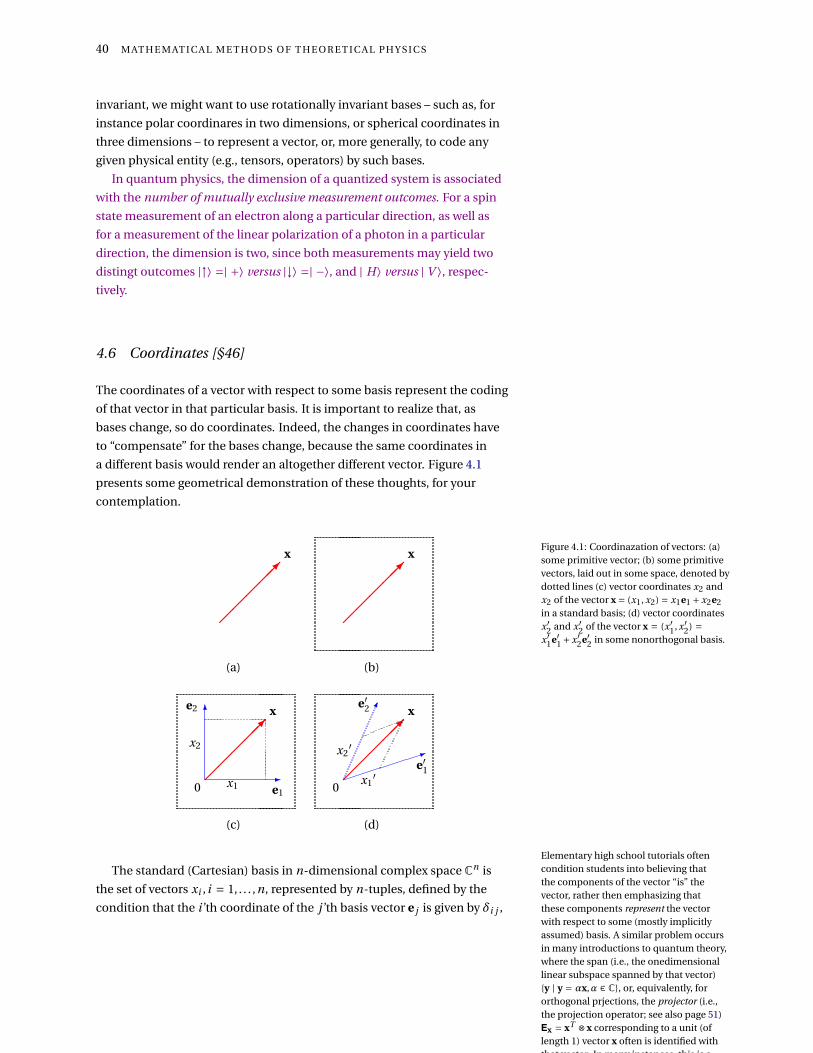
4.1 Coordinazation of vectors: (a) some primitive vector; (b) some primitive
vectors, laid out in some space, denoted by dotted lines (c) vector coordi-
nates x2 and x2 of the vector x = (x1, x2) = x1e1 + x2e2 in a standard ba-
sis; (d) vector coordinates x ′2 and x ′
2 of the vector x = (x ′1, x ′
2) = x ′1e′1+x ′
2e′2in some nonorthogonal basis. 40
4.2 A universal quantum interference device operating on a qubit can be re-
alized by a 4-port interferometer with two input ports 0,1 and two output
ports 0′,1′; a) realization by a single beam splitter S(T ) with variable trans-
mission T and three phase shifters P1,P2,P3; b) realization by two 50:50
beam splitters S1 and S2 and four phase shifters P1,P2,P3,P4. 77
4.3 Coordinate system for measurements of particles travelling along 0Z 80
4.4 Planar geometric demonstration of the classical two two-state particles cor-
relation. 80
4.5 Simultaneous spin state measurement of the two-partite state represented
in Eq. (4.123). Boxes indicate spin state analyzers such as Stern-Gerlach
apparatus oriented along the directions θ1,ϕ1 and θ2,ϕ2; their two out-
put ports are occupied with detectors associated with the outcomes “+”
and “−”, respectively. 83
7.1 Integration path to compute the Fourier transform of the Gaussian. 125
8.1 Dirac’s δ-function as a “needle shaped” generalized function. 127
8.2 Delta sequence approximating Dirac’s δ-function as a more and more “nee-
dle shaped” generalized function. 127
8.3 Plot of a test function ϕ(x). 130
8.4 Plot of the Heaviside step function H(x). 131
8.5 Plot of the sign function sgn(x). 132
8.6 Composition of f (x) 140
9.1 Plot of the two paths reqired for solving the Fourier integral. 148
9.2 Plot of the path reqired for solving the Fourier integral. 150


List of Tables
4.1 Comparison of the identifications of lattice relations and operations for
the lattices of subsets of a set, for experimental propositional calculi, for
Hilbert lattices, and for lattices of commuting projection operators. 73
10.1Some varieties of differential equations expressible as Sturm-Liouville dif-
ferential equations 161


13
This book is dedicated to the memory ofProf. Dr.math. Ernst Paul Specker – Amez–Droz,11.2.1920 – 10.12.2011


15
It is not enough to have no concept, one must alsobe capable of expressing it. From the German original in Karl Kraus,
Die Fackel 697, 60 (1925): “Es genügt nicht,keinen Gedanken zu haben: man muss ihnauch ausdrücken können.”


Introduction
T H I S I S A F I R S T AT T E M P T to provide some written material of a course
in mathemathical methods of theoretical physics. I have presented this
course to an undergraduate audience at the Vienna University of Technol-
ogy. Only God knows (see Ref. 1 part one, question 14, article 13; and also 1 Thomas Aquinas. Summa Theologica.Translated by Fathers of the EnglishDominican Province. Christian ClassicsEthereal Library, Grand Rapids, MI, 1981.URL http://www.ccel.org/ccel/
aquinas/summa.html
Ref. 2, p. 243) if I have succeeded to teach them the subject! I kindly ask the
2 Ernst Specker. Die Logik nicht gleichzeitigentscheidbarer Aussagen. Dialectica, 14(2-3):239–246, 1960. D O I : 10.1111/j.1746-8361.1960.tb00422.x. URL http://dx.
doi.org/10.1111/j.1746-8361.1960.
tb00422.x
perplexed to please be patient, do not panic under any circumstances, and
do not allow themselves to be too upset with mistakes, omissions & other
problems of this text. At the end of the day, everything will be fine, and in
the long run we will be dead anyway.
I A M R E L E A S I N G T H I S text to the public domain because it is my convic-
tion and experience that content can no longer be held back, and access to
it be restricted, as its creators see fit. On the contrary, we experience a push
toward so much content that we can hardly bear this information flood, so
we have to be selective and restrictive rather than aquisitive. I hope that
there are some readers out there who actually enjoy and profit from the
text, in whatever form and way they find appropriate.
M Y OW N E N C O U N T E R with many researchers of different fields and dif-
ferent degrees of formalization has convinced me that there is no single
way of formally comprehending a subject 3. With regards to formal rigour, 3 Philip W. Anderson. More is different.Science, 177(4047):393–396, August 1972.D O I : 10.1126/science.177.4047.393. URLhttp://dx.doi.org/10.1126/science.
177.4047.393
there appears to be a rather questionable chain of contempt – all too of-
ten theoretical physicists suspiciously look down at the experimentalists,
mathematical physicists suspiciously look down at the theoreticians, and
mathematicians suspiciously look down at the mathematical physicists. I
have even experienced the doubts formal logicians expressed about their
collegues in mathematics! For an anectodal evidence, take the claim of a
very prominant member of the mathematical physics community, who
once dryly remarked in front of a fully packed audience, “what other peo-
ple call ‘proof’ I call ‘conjecture’!”
S O P L E A S E B E AWA R E that not all I present here will be acceptable to ev-
erybody; for various reasons. Some people will claim that I am too confus-

18
ing and utterly formalistic, others will claim my arguments are in desparate
need of rigour. Many formally fascinated readers will demand to go deeper
into the meaning of the subjects; others may want some easy-to-identify
pragmatic, syntactic rules of deriving results. I apologise to both groups
from the onset. This is the best I can do; from certain different perspec-
tives, others, maybe even some tutors or students, might perform much
better.
I A M C A L L I N G for a greater unity in physics; as well as for a greater esteem
on “both sides of the same effort;” I am also opting for more pragmatism;
one that acknowledges the mutual benefits and oneness of theoretical and
empirical physical world perceptions. Schrödinger 4 cites Democritus with 4 Erwin Schrödinger. Nature and theGreeks. Cambridge University Press,Cambridge, 1954
arguing against a too great separation of the intellect (διανoια, dianoia)
and the senses (αισθησεις, aitheseis). In fragment D 125 from Galen 5, p. 5 Hermann Diels. Die Fragmente derVorsokratiker, griechisch und deutsch.Weidmannsche Buchhandlung, Berlin,1906. URL http://www.archive.org/
details/diefragmentederv01dieluoft
408, footnote 125 , the intellect claims “ostensibly there is color, ostensibly
sweetness, ostensibly bitterness, actually only atoms and the void;” to
which the senses retort: “Poor intellect, do you hope to defeat us while
from us you borrow your evidence? Your victory is your defeat.” German: Nachdem D. [[Demokri-tos]] sein Mißtrauen gegen dieSinneswahrnehmungen in dem Satzeausgesprochen: ‘Scheinbar (d. i. konven-tionell) ist Farbe, scheinbar Süßigkeit,scheinbar Bitterkeit: wirklich nur Atomeund Leeres” läßt er die Sinne gegen denVerstand reden: ‘Du armer Verstand, vonuns nimmst du deine Beweisstücke undwillst uns damit besiegen? Dein Sieg istdein Fall!’
P RO F E S S O R E R N S T S P E C K E R from the ETH Zürich once remarked that, of
the many books of David Hilbert, most of them carry his name first, and
the name(s) of his co-author(s) appear second, although the subsequent
author(s) had actually written these books; the only exception of this rule
being Courant and Hilbert’s 1924 book Methoden der mathematischen
Physik, comprising around 1000 densly packed pages, which allegedly
none of these authors had really written. It appears to be some sort of
collective efforts of scholar from the University of Göttingen.
So, in sharp distinction from these activities, I most humbly present my
own version of what is important for standard courses of contemporary
physics. Thereby, I am quite aware that, not dissimilar with some attempts
of that sort undertaken so far, I might fail miserably. Because even if I
manage to induce some interest, affaction, passion and understanding in
the audience – as Danny Greenberger put it, inevitably four hundred years
from now, all our present physical theories of today will appear transient 6, 6 Imre Lakatos. Philosophical Papers.1. The Methodology of Scientific ResearchProgrammes. Cambridge University Press,Cambridge, 1978
if not laughable. And thus in the long run, my efforts will be forgotten; and
some other brave, courageous guy will continue attempting to (re)present
the most important mathematical methods in theoretical physics.
H AV I N G I N M I N D this saddening piece of historic evidence, and for as long
as we are here on Earth, let us carry on and start doing what we are sup-
posed to be doing well; just as Krishna in Chapter XI:32,33 of the Bhagavad
Gita is quoted for insisting upon Arjuna to fight, telling him to “stand up,
obtain glory! Conquer your enemies, acquire fame and enjoy a prosperous
kingdom. All these warriors have already been destroyed by me. You are only

19
an instrument.”
o


Part I:
Metamathematics and Metaphysics


1
Unreasonable effectiveness of mathematics in the natu-
ral sciences
All things considered, it is mind-boggling why formalized thinking and
numbers utilize our comprehension of nature. Even today people muse
about the unreasonable effectiveness of mathematics in the natural sci-
ences 1. 1 Eugene P. Wigner. The unreasonableeffectiveness of mathematics in thenatural sciences. Richard Courant Lecturedelivered at New York University, May11, 1959. Communications on Pure andApplied Mathematics, 13:1–14, 1960. D O I :10.1002/cpa.3160130102. URL http:
//dx.doi.org/10.1002/cpa.3160130102
Zeno of Elea and Parmenides, for instance, wondered how there can be
motion, either in universe which is infinitely divisible, or discrete. Because,
in the dense case, the slightest finite move would require an infinity of ac-
tions. Likewise in the discrete case, how can there be motion if everything
is not moving at all times 2?2 H. D. P. Lee. Zeno of Elea. CambridgeUniversity Press, Cambridge, 1936; PaulBenacerraf. Tasks and supertasks, and themodern Eleatics. Journal of Philosophy,LIX(24):765–784, 1962. URL http://
www.jstor.org/stable/2023500;A. Grünbaum. Modern Science and Zeno’sparadoxes. Allen and Unwin, London,second edition, 1968; and Richard MarkSainsbury. Paradoxes. CambridgeUniversity Press, Cambridge, UnitedKingdom, third edition, 2009. ISBN0521720796
A related question regards the physical limit state of a hypothetical
lamp, considered by Thomson 3, with ever decreasing switching cycles.
3 James F. Thomson. Tasks and supertasks.Analysis, 15:1–13, October 1954
For the sake of perplexion, take Neils Henrik Abel’s verdict denouncing
that (Letter to Holmboe, January 16, 1826 4), “divergent series are the in-
4 Godfrey Harold Hardy. Divergent Series.Oxford University Press, 1949
vention of the devil, and it is shameful to base on them any demonstration
whatsoever.” This, of course, did neither prevent Abel nor too many other
discussants to investigate these devilish inventions.
If one encodes the physical states of the Thomson lamp by “0” and “1,”
associated with the lamp “on” and “off,” respectively, and the switching
process with the concatenation of “+1” and “-1” performed so far, then the
divergent infinite series associated with the Thomson lamp is the Leibniz
series
s =∞∑
n=0(−1)n = 1−1+1−1+1−·· · A= 1
1− (−1)= 1
2(1.1)
which is just a particular instance of a geometric series (see below) with
the common ratio “-1.” Here, “A” indicates the Abel sum 5 obtained from a 5 Godfrey Harold Hardy. Divergent Series.Oxford University Press, 1949“continuation” of the geometric series, or alternatively, by s = 1− s.
As this shows, formal sums of the Leibnitz type (1.1) require specifi-
cations which could make them unique. But has this “specification by
continuation” any kind of physical meaning?
In modern days, similar arguments have been translated into the pro-

24 M AT H E M AT I C A L M E T H O D S O F T H E O R E T I C A L P H Y S I C S
posal for infinity machines by Blake 6, p. 651, and Weyl 7, pp. 41-42, which 6 R. M. Blake. The paradox of temporalprocess. Journal of Philosophy, 23(24):645–654, 1926. URL http://www.jstor.
org/stable/20138137 Hermann Weyl. Philosophy of Mathe-matics and Natural Science. PrincetonUniversity Press, Princeton, NJ, 1949
could solve many very difficult problems by searching through unbounded
recursively enumerable cases. To achive this physically, ultrarelativistic
methods suggest to put observers in “fast orbits” or throw them toward
black holes 8.
8 Itamar Pitowsky. The physical Church-Turing thesis and physical computationalcomplexity. Iyyun, 39:81–99, 1990
The Pythagoreans are often cited to have believed that the universe
is natural numbers or simple fractions thereof, and thus physics is just a
part of mathematics; or that there is no difference between these realms.
They took their conception of numbers and world-as-numbers so seriously
that the existence of irrational numbers which cannot be written as some
ratio of integers shocked them; so much so that they allegedly drowned
the poor guy who had discovered this fact. That is a typical case in which
the metaphysical belief in one’s own construction of the world overwhelms
critical thinking; and what should be wisely taken as an epistemic finding is
taken to be ontologic truth.
The connection between physics and formalism has been debated by
Bridgman 9, Feynman 10, and Landauer 11, among many others. The ques- 9 Percy W. Bridgman. A physicist’s sec-ond reaction to Mengenlehre. ScriptaMathematica, 2:101–117, 224–234, 193410 Richard Phillips Feynman. The Feynmanlectures on computation. Addison-WesleyPublishing Company, Reading, MA, 1996.edited by A.J.G. Hey and R. W. Allen11 Rolf Landauer. Information is physical.Physics Today, 44(5):23–29, May 1991.D O I : 10.1063/1.881299. URL http:
//dx.doi.org/10.1063/1.881299
tion, for instance, is imminent whether we should take the formalism very
serious and literal, using it as a guide to new territories, which might even
appear absurd, inconsistent and mind-boggling; just like Alice’s Adven-
tures in Wonderland. Should we expect that all the wild things formally
imaginable have a physical realization?
Note that the formalist Hilbert 12, p. 170, is often quoted as claiming
12 David Hilbert. Über das Unendliche.Mathematische Annalen, 95(1):161–190, 1926. D O I : 10.1007/BF01206605.URL http://dx.doi.org/10.1007/
BF01206605; and Georg Cantor. Beiträgezur Begründung der transfiniten Men-genlehre. Mathematische Annalen,46(4):481–512, November 1895. D O I :10.1007/BF02124929. URL http:
//dx.doi.org/10.1007/BF02124929
that nobody shall ever expel mathematicians from the paradise created
by Cantor’s set theory. In Cantor’s “naive set theory” definition, “a set is
German original: “Aus dem Paradies, dasCantor uns geschaffen, soll uns niemandvertreiben können.”
a collection into a whole of definite distinct objects of our intuition or of
our thought. The objects are called the elements (members) of the set.” If
Cantor’s German original: “Unter einer“Menge” verstehen wir jede Zusammen-fassung M von bestimmten wohlunter-schiedenen Objekten m unsrer Anschau-ung oder unseres Denkens (welche die“Elemente” von M genannt werden) zueinem Ganzen.”
one allows substitution and self-reference 13, this definition turns out to be
13 Raymond M. Smullyan. What is theName of This Book? Prentice-Hall, Inc., En-glewood Cliffs, NJ, 1992a; and Raymond M.Smullyan. Gödel’s Incompleteness Theo-rems. Oxford University Press, New York,New York, 1992b
inconsistent; that is self-contradictory – for instance Russel’s paradoxical
“set of all sets that are not members of themselves” qualifies as set in the
Cantorian approach. In praising the set theoretical paradise, Hilbert must
have been well aware of the inconsistencies and problems that plagued
Cantorian style set theory, but he fully dissented and refused to abandon
its stimulus.
Is there a similar pathos also in theoretical physics?
Maybe our physical capacities are limited by our mathematical fantasy
alone? Who knows?
For instance, could we make use of the Banach-Tarski paradox 14 as a
14 Robert French. The Banach-Tarskitheorem. The Mathematical Intelligencer,10:21–28, 1988. ISSN 0343-6993. D O I :10.1007/BF03023740. URL http://dx.
doi.org/10.1007/BF03023740; andStan Wagon. The Banach-Tarski Paradox.Cambridge University Press, Cambridge,1986
sort of ideal production line? The Banach-Tarski paradox makes use of the
fact that in the continuum “it is (nonconstructively) possible” to transform
any given volume of three-dimensional space into any other desired shape,
form and volume – in particular also to double the original volume – by
transforming finite subsets of the original volume through isometries, that
is, distance preserving mappings such as translations and rotations. This,

U N R E A S O N A B L E E F F E C T I V E N E S S O F M AT H E M AT I C S I N T H E N AT U R A L S C I E N C E S 25
of course, could also be perceived as a merely abstract paradox of infinity,
somewhat similar to Hilbert’s hotel.
By the way, Hilbert’s hotel 15 has a countable infinity of hotel rooms. It 15 Rudy Rucker. Infinity and the Mind.Birkhäuser, Boston, 1982is always capable to acommodate a newcomer by shifting all other guests
residing in any given room to the room with the next room number. Maybe
we will never be able to build an analogue of Hilbert’s hotel, but maybe we
will be able to do that one far away day. Anton Zeilinger has quoted Tony Kleinas saying that “every system is a perfectsimulacrum of itself.”
After all, science finally succeeded to do what the alchemists sought for
so long: we are capable of producing gold from mercury 16. 16 R. Sherr, K. T. Bainbridge, and H. H.Anderson. Transmutation of mer-cury by fast neutrons. Physical Re-view, 60(7):473–479, Oct 1941. D O I :10.1103/PhysRev.60.473. URL http:
//dx.doi.org/10.1103/PhysRev.60.473
o


2
Methodology and proof methods
F O R M A N Y T H E O R E M S there exist many proofs. For instance, the 4th edi-
tion of Proofs from THE BOOK 1 lists six proofs of the infinity of primes 1 Martin Aigner and Günter M. Ziegler.Proofs from THE BOOK. Springer,Heidelberg, four edition, 1998-2010.ISBN 978-3-642-00855-9. URLhttp://www.springerlink.com/
content/978-3-642-00856-6
(chapter 1). Chapter 19 refers to nearly a hundred proofs of the fundamen-
tal theorem of algebra, that every nonconstant polynomial with complex
coefficients has at least one root in the field of complex numbers.
W H I C H P RO O F S , if there exist many, somebody choses or prefers is often
a question of taste and elegance, and thus a subjective decision. Some
proofs are constructive 2 and computable 3 in the sense that a construction 2 Douglas Bridges and F. Richman. Varietiesof Constructive Mathematics. CambridgeUniversity Press, Cambridge, 1987; andE. Bishop and Douglas S. Bridges. Con-structive Analysis. Springer, Berlin, 19853 Oliver Aberth. Computable Analysis.McGraw-Hill, New York, 1980; KlausWeihrauch. Computable Analysis. AnIntroduction. Springer, Berlin, Heidelberg,2000; and Vasco Brattka, Peter Hertling,and Klaus Weihrauch. A tutorial oncomputable analysis. In S. Barry Cooper,Benedikt Löwe, and Andrea Sorbi, editors,New Computational Paradigms: ChangingConceptions of What is Computable, pages425–491. Springer, New York, 2008
method is presented. Tractability is not an entirely completely different
issue 4 – note that even “higher” polynomial growth of temporal or space
4 Georg Kreisel. A notion of mechanis-tic theory. Synthese, 29:11–26, 1974.D O I : 10.1007/BF00484949. URL http:
//dx.doi.org/10.1007/BF00484949;Robin O. Gandy. Church’s thesis and prin-ciples for mechanics. In J. Barwise, H. J.Kreisler, and K. Kunen, editors, The KleeneSymposium. Vol. 101 of Studies in Logicand Foundations of Mathematics, pages123–148. North Holland, Amsterdam, 1980;and Itamar Pitowsky. The physical Church-Turing thesis and physical computationalcomplexity. Iyyun, 39:81–99, 1990
and memory resources of a computation with some parameter may result
in a solution which is unattainable “for all practical purposes” (fapp) 5.
5 John S. Bell. Against ‘measurement’.Physics World, 3:33–41, 1990. URL http:
//physicsworldarchive.iop.org/
summary/pwa-xml/3/8/phwv3i8a26
F O R T H O S E O F U S with a rather limited amount of storage and memory,
and with a lot of troubles and problems, is is quite consolating that it is not
(always) necessary to be able to memorize all the proofs that are necessary
for the deduction of a particular corollary or theorem which turns out to
be useful for the physical task at hand. In some cases, though, it may be
necessary to keep in mind the assumptions and derivation methods that
such results are based upon. For example, how many readers may be able
to immediately derive the simple power rule for derivation of polynomials
– that is, for any real coefficient a, the derivative is given by (r a)′ = ar a−1?
Most of us would acknowledge to be aware of, and be able and happy to
apply, this rule.
L E T U S J U S T L I S T some concrete examples of the perplexing varieties of
proof methods used today.
For the sake of listing a mathematical proof method which does not
have any “constructive” or algorithmic flavour, consider a proof of the
following theorem: “There exist irrational numbers x, y ∈R−Qwith x y ∈Q.”

28 M AT H E M AT I C A L M E T H O D S O F T H E O R E T I C A L P H Y S I C S
Consider the following proof:
case 1:p
2p
2 ∈Q;
case 2:p
2p
2 6∈Q, thenp
2p
2p
2
= 2 ∈Q.
The proof assumes the law of the excluded middle, which excludes all
other cases but the two just listed. The question of which one of the two
cases is correct; that is, which number is rational, remains unsolved in the
context of the proof. – Actually, a proof that case 2 is correct andp
2p
2is a
transcendential was only found by Gelfond and Schneider in 1934! The Gelfond-Schneider theorem statesthat, if n and m are algebraic numbersthat is, if n and m are roots of a non-zeropolynomial in one variable with rationalor equivalently, integer, coefficients withn 6= 0,1 and if m is not a rational number,then any value of nm = em logn is atranscendental number.
A T Y P I C A L P RO O F B Y C O N T R A D I C T I O N is about the irrationality ofp
2.
Suppose thatp
2 is rational (false); that isp
2 = nm for some n,m ∈ N.
Suppose further that n and m are coprime; that is, they have no common
positive divisor other than 1 or, equivalently, if their greatest common
divisor is 1. Squaring the (wrong) assumptionp
2 = nm yields 2 = n2
m2 and
thus n2 = 2m2. We have two different cases: either n is odd, or n is even.
case 1: suppose that n is odd; that is n = (2k+1) for some k ∈N; and thus
n2 = 4k2 +2k +1 is again odd (the square of an even number is again odd);
but that cannot be, since n2 equals 2m2 and thus should be even; hence we
arrive at a contradiction.
case 2: suppose that n is even; that is n = 2k for some k ∈ N; and thus
4k2 = 2m2 or 2k2 = m2. Now observe that by assumption, m cannot be
even (remember n and m are coprime, and n is assumed to be even), so
m must be odd. By the same argument as in case 1 (for odd n), we arrive
at a contradiction. By combining these two exhaustive cases 1 & 2, we
arrive at a complete contradiction; the only consistent alternative being the
irrationality ofp
2.
S T I L L A N OT H E R I S S U E is whether it is better to have a proof of a “true”
mathematical statement rather than none. And what is truth – can it
be some revelation, a rare gift, such as seemingly in Srinivasa Aiyangar
Ramanujan’s case?
T H E R E E X I S T A N C I E N T and yet rather intuitive – but sometimes distract-
ing and errorneous – informal notions of proof. An example 6 is the Baby- 6 M. Baaz. Über den allgemeinen gehaltvon beweisen. In Contributions to GeneralAlgebra, volume 6, pages 21–29, Vienna,1988. Hölder-Pichler-Tempsky
lonian notion to “prove” arithmetical statements by considering “large
number” cases of algebraic formulae such as (Chapter V of Ref. 7),7 Otto Neugebauer. Vorlesungen über dieGeschichte der antiken mathematischenWissenschaften. 1. Band: VorgriechischeMathematik. Springer, Berlin, 1934. page172
n∑i=1
i 2 = 1
3(1+2n)
n∑i=1
i .
As naive and silly this Babylonian “proof” method may appear at first
glance – for various subjective reasons (e.g. you may have some suspicions
with regards to particular deductive proofs and their results; or you sim-
ply want to check the correctness of the deductive proof) it can be used to

M E T H O D O L O G Y A N D P RO O F M E T H O D S 29
“convince” students and ourselves that a result which has derived deduc-
tively is indeed applicable and viable. We shall make heavy use of these
kind of intuitive examples. As long as one always keeps in mind that this
inductive, merely anecdotal, method is necessary but not sufficient (suf-
ficiency is, for instance, guaranteed by complete induction) it is quite all
right to go ahead with it.
Another altogether different issue is knowledge acquired by revelation
or by some authority. Oracles occur in modern computer science, but only
as idealized concepts whose physical realization is highly questionable if
not forbidden.
L E T U S shortly enumerate some proof methods, among others:
1. (indirect) proof by contradiction;
2. proof by mathematical induction;
3. direct proof;
4. proof by construction;
5. nonconstructive proof.
T H E C O N T E M P O R A RY notion of proof is formalized and algorithmic.
Around 1930 mathematicians could still hope for a “mathematical the-
ory of everything” which consists of a finite number of axioms and algo-
rithmic derivation rules by which all true mathematical statements could
formally be derived. In particular, as expressed in Hilbert’s 2nd problem
[Hilbert, 1902], it should be possible to prove the consistency of the axioms
of arithmetic. Hence, Hilbert and other formalists dreamed, any such for-
mal system (in German “Kalkül”) consisting of axioms and derivation rules,
might represent “the essence of all mathematical truth.” This approach, as
curageous as it appears, was doomed.
G Ö D E L 8, Tarski 9, and Turing 10 put an end to the formalist program. 8 Kurt Gödel. Über formal unentscheidbareSätze der Principia Mathematica undverwandter Systeme. Monatshefte fürMathematik und Physik, 38(1):173–198,1931. D O I : 10.1007/s00605-006-0423-7.URL http://dx.doi.org/10.1007/
s00605-006-0423-79 Alfred Tarski. Der Wahrheitsbegriff inden Sprachen der deduktiven Disziplinen.Akademie der Wissenschaften in Wien.Mathematisch-naturwissenschaftlicheKlasse, Akademischer Anzeiger, 69:9–12,193210 A. M. Turing. On computable numbers,with an application to the Entschei-dungsproblem. Proceedings of theLondon Mathematical Society, Series2, 42, 43:230–265, 544–546, 1936-7 and1937. D O I : 10.1112/plms/s2-42.1.230,10.1112/plms/s2-43.6.544. URLhttp://dx.doi.org/10.1112/plms/
s2-42.1.230,http://dx.doi.org/10.
1112/plms/s2-43.6.544
They coded and formalized the concepts of proof and computation in
general, equating them with algorithmic entities. Today, in times when
universal computers are everywhere, this may seem no big deal; but in
those days even coding was challenging – in his proof of the undecidability
of (Peano) arithmetic, Gödel used the uniqueness of prime decompositions
to explicitly code mathematical formulæ!
F O R T H E S A K E of exploring (algorithmically) these ideas let us consider the
sketch of Turing’s proof by contradiction of the unsolvability of the halting
problem. The halting problem is about whether or not a computer will
eventually halt on a given input, that is, will evolve into a state indicating

30 M AT H E M AT I C A L M E T H O D S O F T H E O R E T I C A L P H Y S I C S
the completion of a computation task or will stop altogether. Stated differ-
ently, a solution of the halting problem will be an algorithm that decides
whether another arbitrary algorithm on arbitrary input will finish running
or will run forever.
The scheme of the proof by contradiction is as follows: the existence of a
hypothetical halting algorithm capable of solving the halting problem will
be assumed. This could, for instance, be a subprogram of some suspicious
supermacro library that takes the code of an arbitrary program as input
and outputs 1 or 0, depending on whether or not the program halts. One
may also think of it as a sort of oracle or black box analyzing an arbitrary
program in terms of its symbolic code and outputting one of two symbolic
states, say, 1 or 0, referring to termination or nontermination of the input
program, respectively.
On the basis of this hypothetical halting algorithm one constructs an-
other diagonalization program as follows: on receiving some arbitrary
input program code as input, the diagonalization program consults the
hypothetical halting algorithm to find out whether or not this input pro-
gram halts; on receiving the answer, it does the opposite: If the hypothetical
halting algorithm decides that the input program halts, the diagonalization
program does not halt (it may do so easily by entering an infinite loop).
Alternatively, if the hypothetical halting algorithm decides that the input
program does not halt, the diagonalization program will halt immediately.
The diagonalization program can be forced to execute a paradoxical task
by receiving its own program code as input. This is so because, by consider-
ing the diagonalization program, the hypothetical halting algorithm steers
the diagonalization program into halting if it discovers that it does not halt;
conversely, the hypothetical halting algorithm steers the diagonalization
program into not halting if it discovers that it halts.
The complete contradiction obtained in applying the diagonalization
program to its own code proves that this program and, in particular, the
hypothetical halting algorithm cannot exist.
A universal computer can in principle be embedded into, or realized
by, certain physical systems designed to universally compute. Assuming
unbounded space and time, it follows by reduction that there exist physical
observables, in particular, forecasts about whether or not an embedded
computer will ever halt in the sense sketched earlier, that are provably
undecidable.
\
3
Numbers and sets of numbers
T H E C O N C E P T O F N U M B E R I N G T H E U N I V E R S E is far from trivial. In par-
ticular it is far from trivial which number schemes are appropriate. In the
pythagorean tradition the natural numbers appear to be most natural. Ac-
tually Leibnitz (among others like Bacon before him) argues that just two
number, say, “0” and “1,” are enough to creat all of them.
EV E RY P R I M A RY E M P I R I C A L E V I D E N C E seems to be based on some click
in a detector: either there is some click or there is none. Thus every empiri-
cal physical evidence is composed from such elementary events.
Thus binary number codes are in good, albeit somewhat accidential, ac-
cord with the intuition of most experimentalists today. I call it “accidential”
because quantum mechanics does not favour any base; the only criterium
is the number of mutually exclusive measurement outcomes which de-
termines the dimension of the linear vector space used for the quantum
description model – two mutually exclusive outcomes would result in a
Hilbert space of dimension two, three mutually exclusive outcomes would
result in a Hilbert space of dimension three, and so on.
T H E R E A R E , of course, many other sets of numbers imagined so far; all
of which can be considered to be encodable by binary digits. One of the
most challenging number schemes is that to the real numbers 1. It is totally 1 S. Drobot. Real Numbers. Prentice-Hall,Englewood Cliffs, New Jersey, 1964different from the natural numbers insofar as there are undenumerably
many reals; that is, it is impossible to find a one-to-one function – a sort of
“translation” – from the natural numbers to the reals.
Cantor appears to be the first having realized this. In order to proof it,
he invented what is today often called Cantor’s diagonalization technique,
or just diagonalization. It is a proof by contradiction; that is, what shall
be disproved is assumed; and on the basis of this assumption a complete
contradiction is derived.
For the sake of contradiction, assume for the moment that the set of
reals is denumerable. (This assumption will yield a contradiction.) That

32 M AT H E M AT I C A L M E T H O D S O F T H E O R E T I C A L P H Y S I C S
is, the enumeration is a one-to-one function f : N→ R (wrong), i.e., to
any k ∈ N exists some rk ∈ R and vice versa. No algorithmic restriction is
imposed upon the enumeration, i.e., the enumeration may or may not be
effectively computable. For instance, one may think of an enumeration
obtained via the enumeration of computable algorithms and by assuming
that rk is the output of the k’th algorithm. Let 0.dk1dk2 · · · be the successive
digits in the decimal expansion of rk . Consider now the diagonal of the
array formed by successive enumeration of the reals,
r1 = 0.d11 d12 d13 · · ·r2 = 0.d21 d22 d23 · · ·r3 = 0.d31 d32 d33 · · ·...
......
.... . .
(3.1)
yielding a new real number rd = 0.d11d22d33 · · ·. Now, for the sake of contra-
diction, construct a new real r ′d by changing each one of these digits of rd ,
avoiding zero and nine in a decimal expansion. This is necessary because
reals with different digit sequences are equal to each other if one of them
ends with an infinite sequence of nines and the other with zeros, for exam-
ple 0.0999. . . = 0.1. . .. The result is a real r ′ = 0.d ′1d ′
2d ′3 · · · with d ′
n 6= dnn ,
which differs from each one of the original numbers in at least one (i.e., in
the “diagonal”) position. Therefore, there exists at least one real which is
not contained in the original enumeration, contradicting the assumption
that all reals have been taken into account. Hence, R is not denumerable.
Bridgman has argued 2 that, from a physical point of view, such an 2 Percy W. Bridgman. A physicist’s sec-ond reaction to Mengenlehre. ScriptaMathematica, 2:101–117, 224–234, 1934
argument is operationally unfeasible, because it is physically impossible
to process an infinite enumeration; and subsequently, quasi on top of
that, a digit switch. Alas, it is possible to recast the argument such that r ′d
is finitely created up to arbitrary operational length, as the enumeration
progresses.
\

Part II:
Linear vector spaces


4
Finite-dimensional vector spaces
V E C TO R S PAC E S are prevalent in physics; they are essential for an un- “I would have written a shorter letter,but I did not have the time.” (Literally: “Imade this [letter] very long, because I didnot have the leisure to make it shorter.”)Blaise Pascal, Provincial Letters: Letter XVI(English Translation)
derstanding of mechanics, relativity theory, quantum mechanics, and
statistical physics.
4.1 Basic definitions
In what follows excerpts from Halmos’ beautiful treatment “Finite-Dimensional
Vector Spaces” will be reviewed 1. Of course, there exist zillions of other 1 Paul R.. Halmos. Finite-dimensional Vec-tor Spaces. Springer, New York, Heidelberg,Berlin, 1974
very nice presentations, among them Greub’s “Linear algebra,” and Strang’s
“Introduction to Linear Algebra,” among many others, even freely down-
loadable ones 2 competing for your attention. 2 Werner Greub. Linear Algebra, volume 23of Graduate Texts in Mathematics. Springer,New York, Heidelberg, fourth edition, 1975;Gilbert Strang. Introduction to linearalgebra. Wellesley-Cambridge Press,Wellesley, MA, USA, fourth edition, 2009.ISBN 0-9802327-1-6. URL http://math.
mit.edu/linearalgebra/; HowardHomes and Chris Rorres. ElementaryLinear Algebra: Applications Version. Wiley,New York, tenth edition, 2010; SeymourLipschutz and Marc Lipson. Linear algebra.Schaum’s outline series. McGraw-Hill,fourth edition, 2009; and Jim Hefferon.Linear algebra. 320-375, 2011. URLhttp://joshua.smcvt.edu/linalg.
html/book.pdf
The more physically oriented notation in Mermin’s book on quan-
tum information theory 3 is adopted. Vectors are typed in bold face. The
3 N. David Mermin. Lecture notes onquantum computation. 2002-2008.URL http://people.ccmr.cornell.
edu/~mermin/qcomp/CS483.html; andN. David Mermin. Quantum ComputerScience. Cambridge University Press,Cambridge, 2007. ISBN 9780521876582.URL http://people.ccmr.cornell.edu/
~mermin/qcomp/CS483.html
overline sign stands for complex conjugation; that is, if a = ℜa + iℑa is a
complex number, then a =ℜa − iℑa.
Unless stated differently, only finite-dimensional vector spaces are
considered.
4.1.1 Fields of real and complex numbers
In physics, scalars are either real or complex numbers and their associated
fields. Thus we shall restrict our attention to these cases.
A field ⟨F,+, ·,−,−1 ,0,1⟩ is a set together with two operations, usually
called addition and multiplication, and denoted by “+” and “·” (often “a·b”
is identified with the expression “ab” without the center dot) respectively,
such that the following axioms hold:
(i) closure of F under addition and multiplication for all a,b ∈ F, both a +b
and ab are in F;
(ii) associativity of addition and multiplication: for all a, b, and c in F, the
following equalities hold: a + (b + c) = (a +b)+ c, and a(bc) = (ab)c;

36 M AT H E M AT I C A L M E T H O D S O F T H E O R E T I C A L P H Y S I C S
(iii) commutativity of addition and multiplication: for all a and b in F, the
following equalities hold: a +b = b +a and ab = ba;
(iv) additive and multiplicative identity: There exists an element of F,
called the additive identity element and denoted by 0, such that for all
a in F, a +0 = a. Likewise, there is an element, called the multiplicative
identity element and denoted by 1, such that for all a in F, 1 · a = a.
(To exclude the trivial ring, the additive identity and the multiplicative
identity are required to be distinct.)
(v) Additive and multiplicative inverses: for every a in F, there exists an
element −a in F, such that a + (−a) = 0. Similarly, for any a in F other
than 0, there exists an element a−1 in F, such that a · a−1 = 1. (The ele-
ments +(−a) and a−1 are also denoted −a and 1b , respectively.) Stated
differently: subtraction and division operations exist.
(vi) Distributivity of multiplication over addition For all a, b and c in F, the
following equality holds: a(b + c) = (ab)+ (ac).
4.1.2 Vectors and vector spaceFor proofs and additional information see§2 in
Paul R.. Halmos. Finite-dimensional Vec-tor Spaces. Springer, New York, Heidelberg,Berlin, 1974
A linear vector space ⟨V,+, ·,−,0,1⟩ is a set V of elements called vectors
satisfying certain axioms; among them, with respect to addition of vectors:
(i) commutativity,
(ii) associativity,
(iii) the uniqueness of the origin or null vector 0, as well as
(iv) the uniqueness of the negative vector;
with respect to multiplication of vectors with scalars associativity:
(v) the existence of a unit factor 1; and
(vi) distributivity with respect to scalar and vector additions, that is
(α+β)x =αx+βx,
α(x+y) =αx+αy, with x,y,∈V and scalars α,β,(4.1)
respectively.
Examples of vector spaces are:
(i) The set C of complex numbers: C can be interpreted as a complex
vector space by interpreting as vector addition and scalar multiplication
as the usual addition and multiplication of complex numbers, and with
0 as the null vector;

F I N I T E - D I M E N S I O N A L V E C TO R S PAC E S 37
(ii) The set Cn , n ∈ N of n-tuples of complex numbers: Let x = (x1, . . . , xn)
and y = (y1, . . . , yn). Cn can be interpreted as a complex vector space
by interpreting as vector addition and scalar multiplication as the or-
dinary addition x + y = (x1 + y1, . . . , xn + yn) and the multiplication
αx = (αx1, . . . ,αxn) by a complex number α, respectively; the null tuple
0 = (0, . . . ,0) is the neutral element of vector addition;
(iii) The set P of all polynomials with complex coefficients in a variable
t : P can be interpreted as a complex vector space by interpreting as
vector addition and scalar multiplication as the ordinary addition of
polynomials and the multiplication of a polynomial by a complex num-
ber, respectively; the null polynomial is the neutral element of vector
addition.
4.2 Linear independence
A set S = x1,x2, . . . ,xk ⊂V of vectors xi in a linear vector space is linear
independent if no vector can be written as a linear combination of other
vectors in this set S; that is, xi =∑1≤ j≤k, j 6=i α j x j .
Equivalently, linear independence of the vectors in B means that no
vector in S can be written as a linear combinations of others in S. That
is, let x1, . . . ,xk ; if∑n
i=1αi xi = 0 implies αi = 0 for each i , then the set
S= x1,x2, . . . ,xk is linearly independent.
4.3 SubspaceFor proofs and additional information see§10 in
Paul R.. Halmos. Finite-dimensional Vec-tor Spaces. Springer, New York, Heidelberg,Berlin, 1974
A nonempty subset M of a vector space is a subspace or, used synony-
muously, a linear manifold if, along with every pair of vectors x and y
contained in M, every linear combination αx+βy is also contained in M.
If U and V are two subspaces of a vector space, then U+V is the sub-
space spanned by U and V; that is, the set of all vectors z = x+y, with x ∈Uand y ∈V.
M is the linear span
M= span(U,V) = span(x,y) = αx+βy |α,β ∈ F,x ∈U,x ∈V. (4.2)
A generalization to more than two vectors and more than two subspaces
is straightforward.
For every vector space V, the set containing the null vector 0, and the
vector space V itself are subspaces of V.
4.3.1 Scalar or inner product [§61]
A scalar or inner product presents some form of measure of “distance” or
“apartness” of two vectors in a linear vector space. It should not be con-
fused with the bilinear functionals (introduced on page 44) that connect a

38 M AT H E M AT I C A L M E T H O D S O F T H E O R E T I C A L P H Y S I C S
vector space with its dual vector space, although for real Euclidean vector
spaces these may coincide, and although the scalar product is also bilinear
in its arguments. It should also not be confused with the tensor product
introduced on page 48.
An inner product space is a vector space V, together with an inner
product; that is, with a map ⟨· | ·⟩ : V×V −→ R or C, in general F, that
satisfies the following three axioms for all vectors and all scalars:
(i) Conjugate symmetry: ⟨x | y⟩ = ⟨y | x⟩. For real, Euclidean vector spaces, thisfunction is symmetric; that is ⟨x | y⟩ =⟨y | x⟩.(ii) Linearity in the first (and second) argument:
⟨αx+βy | z⟩ =α⟨x | z⟩+β⟨v | z⟩.(ii) Positive-definiteness: ⟨x | x⟩ ≥ 0; with equality only for x = 0.
The norm of a vector x is defined by
‖x‖ =√⟨x | x⟩ (4.3)
One example is the dot product
⟨x|y⟩ =n∑
i=1xi yi (4.4)
of two vectors x = (x1, . . . , xn) and y = (y1, . . . , yn) in Cn , which, for real
Euclidean space, reduces to the well-known dot product ⟨x|y⟩ = x1 y1 +·· ·+xn yn = ‖x‖‖y‖cos∠(x,y).
It is mentioned without proof that the most general form of an inner
product in Cn is ⟨x|y⟩ = yAx†, where the symbol “†” stands for the conju-
gate transpose, or Hermitian conjugate, and A is a positive definite Hermi-
tian matrix (all of its eigenvalues are positive).
Two nonzero vectors x,y ∈V, x,y 6= 0 are orthogonal, denoted by “x ⊥ y”
if their scalarproduct vanishes; that is, if
⟨x|y⟩ = 0. (4.5)
Let E be any set of vectors in an inner product space V. The symbols
E⊥ = x | ⟨x|y⟩ = 0,x ∈V,∀y ∈E (4.6)
denote the set of all vectors in V that are orthogonal to every vector in E.
Note that, regardless of whether or not E is a subspace (E may be just See page 37 for a definition of subspace.
vectors of an incomplete basis), E⊥ is a subspace. Furthermore, E is con-
tained in (E⊥)⊥ = E⊥⊥. In case E is a subspace, we call E⊥ the orthogonal
complement of E.
The following projection theorem is mentioned without proof. If M is
any subspace of a finite-dimensional inner product space V, then V is the
direct sum of M and M⊥; that is, M⊥⊥ =M.
For the sake of an example, suppose V = R2, and take E to be the set
of all vectors spanned by the vector (1,0); then E⊥ is the set of all vectors
spanned by (0,1).

F I N I T E - D I M E N S I O N A L V E C TO R S PAC E S 39
4.3.2 Hilbert space
A (quantum mechanical) Hilbert space is a linear vector space V over the
field C of complex numbers equipped with vector addition, scalar multi-
plication, and some scalar product. Furthermore, closure is an additional
requirement, but nobody has made operational sense of that so far: If
xn ∈V, n = 1,2, . . ., and if limn,m→∞(xn −xm ,xn −xm) = 0, then there exists
an x ∈V with limn→∞(xn −x,xn −x) = 0.
Infinite dimensional vector spaces and continuous spectra are non-
trivial extensions of the finite dimensional Hilbert space treatment. As a
heuristic rule, which is not always correct, it might be stated that the sums
become integrals, and the Kronecker delta function δi j defined by
δi j =
0, for i 6= j ;
1, for i = j. (4.7)
becomes the Dirac delta function δ(x − y), which is a generalized function
in the continuous variables x, y . In the Dirac bra-ket notation, unity is
given by 1 = ∫ +∞−∞ |x⟩⟨x|d x. For a careful treatment, see, for instance, the
books by Reed and Simon 4. 4 Michael Reed and Barry Simon. Methodsof Mathematical Physics I: Functional Anal-ysis. Academic Press, New York, 1972; andMichael Reed and Barry Simon. Methods ofMathematical Physics II: Fourier Analysis,Self-Adjointness. Academic Press, NewYork, 1975
4.4 Basis
For proofs and additional information see§7 in
Paul R.. Halmos. Finite-dimensional Vec-tor Spaces. Springer, New York, Heidelberg,Berlin, 1974
A (linear) basis (or a coordinate system) is a set B of linearly independent
vectors so that every vector in V is a linear combination of the vectors in
the basis; hence B spans V.
A vector space is finite dimensional if its basis is finite; that is, its basis
contains a finite number of elements.
4.5 Dimension [§8]
The dimension of V is the number of elements in B ; all bases B contain
the same number of elements.
What basis should one choose? Note that a vector is some directed
entity with a particular length, oriented in some (vector) “space.” It is “laid
out there” in front of our eyes, as it is: some directed quantity. A priori,
this space, in its most primitive form, is not equipped with a basis, or
synonymuously, frame of reference, or reference frame. Insofar it is not
yet coordinatized. In order to formalize the notion of a vector, we have
to code this vector. As for numbers (e.g., by different bases, or by prime
decomposition), there exist many “competing” ways to code a vector.
Some of these ways are rather straightforward, such as, in particular, the
Cartesian basis, or, used synonymuosly, the standard basis. Other bases
are less suggestive at first; alas it may be “economical” or pragmatical to
use them; mostly to cope with, and adapt to, the symmetry of a physical
configuration: if the physical situation at hand is, for instance, rotationally
40 M AT H E M AT I C A L M E T H O D S O F T H E O R E T I C A L P H Y S I C S
invariant, we might want to use rotationally invariant bases – such as, for
instance polar coordinares in two dimensions, or spherical coordinates in
three dimensions – to represent a vector, or, more generally, to code any
given physical entity (e.g., tensors, operators) by such bases.
In quantum physics, the dimension of a quantized system is associated
with the number of mutually exclusive measurement outcomes. For a spin
state measurement of an electron along a particular direction, as well as
for a measurement of the linear polarization of a photon in a particular
direction, the dimension is two, since both measurements may yield two
distingt outcomes |↑⟩ =| +⟩ versus |↓⟩ =| −⟩, and | H⟩ versus | V ⟩, respec-
tively.
4.6 Coordinates [§46]
The coordinates of a vector with respect to some basis represent the coding
of that vector in that particular basis. It is important to realize that, as
bases change, so do coordinates. Indeed, the changes in coordinates have
to “compensate” for the bases change, because the same coordinates in
a different basis would render an altogether different vector. Figure 4.1
presents some geometrical demonstration of these thoughts, for your
contemplation.
x
x
(a) (b)
6
-e1
e2
x1
x2
0
x
1
x1′
x2′
e′1
e′2
0
x
(c) (d)
Figure 4.1: Coordinazation of vectors: (a)some primitive vector; (b) some primitivevectors, laid out in some space, denoted bydotted lines (c) vector coordinates x2 andx2 of the vector x = (x1, x2) = x1e1 + x2e2in a standard basis; (d) vector coordinatesx′2 and x′2 of the vector x = (x′1, x′2) =x′1e′1 +x′2e′2 in some nonorthogonal basis.
Elementary high school tutorials oftencondition students into believing thatthe components of the vector “is” thevector, rather then emphasizing thatthese components represent the vectorwith respect to some (mostly implicitlyassumed) basis. A similar problem occursin many introductions to quantum theory,where the span (i.e., the onedimensionallinear subspace spanned by that vector)y | y = αx,α ∈ C, or, equivalently, fororthogonal prjections, the projector (i.e.,the projection operator; see also page 51)Ex = xT ⊗ x corresponding to a unit (oflength 1) vector x often is identified withthat vector. In many instances, this is agreat help and, if administered properly, isconsistent and fine (fapp).
The standard (Cartesian) basis in n-dimensional complex space Cn is
the set of vectors xi , i = 1, . . . ,n, represented by n-tuples, defined by the
condition that the i ’th coordinate of the j ’th basis vector e j is given by δi j ,

F I N I T E - D I M E N S I O N A L V E C TO R S PAC E S 41
where δi j is the Kronecker delta function
δi j =
0, for i 6= j ;
1, for i = j. (4.8)
Thus,e1 = (1,0, . . . ,0),
e2 = (0,1, . . . ,0),...
en = (0,0, . . . ,1).
(4.9)
In terms of these standard base vectors, every vector x can be written as
a linear combination
x =n∑
i=1xi ei = (x1, x2, . . . , xn), (4.10)
or, in “dot product notation,” that is, “column times row” and “row times
column;” the dot is usually omitted (the superscript “T ” stands for trans-
position),
x = (x1, x2, . . . , xn)T · (e1,e2, . . . ,en) =
x1
x2...
xn
(e1,e2, . . . ,en), (4.11)
(the superscript “T ” stands for transposition) of the product of the coor-
dinates xi with respect to that standard basis. Here the equality sign “=”
really means “coded with respect to that standard basis.”
In what follows, we shall often identify the column vectorx1
x2...
xn
containing the coordinates of the vector x with the vector x, but we always
need to keep in mind that the tuples of coordinates are defined only with
respect to a particular basis e1,e2, . . . ,en; otherwise these numbers lack
any meaning whatsoever.
Indeed, with respect to some arbitrary basis B = f1, . . . , fn of some n-
dimensional vector space V with the base vectors fi , 1 ≤ i ≤ n, every vector
x in V can be written as a unique linear combination
x =n∑
i=1xi fi = (x1, x2, . . . , xn) (4.12)
of the product of the coordinates xi with respect to the basis B.
The uniqueness of the coordinates is proven indirectly by reductio
ad absurdum: Suppose there is another decomposition x = ∑ni=1 yi fi =

42 M AT H E M AT I C A L M E T H O D S O F T H E O R E T I C A L P H Y S I C S
(y1, y2, . . . , yn); then by subtraction, 0 = ∑ni=1(xi − yi )fi = (0,0, . . . ,0). Since
the basis vectors fi are linearly independent, this can only be valid if all
coefficients in the summation vanish; thus xi −yi = 0 for all 1 ≤ i ≤ n; hence
finally xi = yi for all 1 ≤ i ≤ n. This is in contradiction with our assumption
that the coordinates xi and yi (or at least some of them) are different.
Hence the only consistent alternative is the assumption that, with respect
to a given basis, the coordinates are uniquely determined.
A set B = a1, . . . ,an of vectors is orthonormal if, whenever for both ai
and a j which are in B it follows that
⟨ai | a j ⟩ = δi j . (4.13)
Any such set is called complete if it is not contained in any larger orthonor-
mal set. Any complete set is a basis.
4.7 Finding orthogonal bases from nonorthogonal ones
A Gram-Schmidt process is a systematic method for orthonormalising a set
of vectors in a space equipped with a scalar product, or by a synonym pre-
ferred in matematics, inner product. The Gram-Schmidt process takes a The scalar or inner product ⟨x|y⟩ of twovectors x and y is defined on page 37. InEuclidean space such as Rn , one oftenidentifies the “dot product” x ·y = x1 y1 +·· ·+ xn yn of two vectors x and y with theirscalar or inner product.
finite, linearly independent set of base vectors and generates an orthonor-
mal basis that spans the same (sub)space as the original set.
The general method is to start out with the original basis, say, x1,x2,x3, . . . ,xn,
and generate a new orthogonal basis y1,y2,y3, . . . ,yn by
y1 = x1,
y2 = x2 −py1 (x2),
y3 = x3 −py1 (x3)−py2 (x3),...
yn = xn −∑n−1i=1 pyi (xn),
(4.14)
where
py(x) = ⟨x|y⟩⟨y|y⟩y, and p⊥
y (x) = x− ⟨x|y⟩⟨y|y⟩y (4.15)
are the orthogonal projections of x onto y and y⊥, respectively (the latter
is mentioned for the sake of completeness and is not required here). Note
that these orthogonal projections are idempotent and mutually orthogo-
nal; that is,
p2y(x) = py(py(x)) = ⟨x|y⟩
⟨y|y⟩⟨y|y⟩⟨y|y⟩y = py(x),
(p⊥y )2(x) = p⊥
y (p⊥y (x)) = x− ⟨x|y⟩
⟨y|y⟩y−( ⟨x|y⟩⟨y|y⟩ −
⟨x|y⟩⟨y|y⟩⟨y|y⟩2
)y,= p⊥
y (x),
py(p⊥y (x)) = p⊥
y (py(x)) = ⟨x|y⟩⟨y|y⟩y− ⟨x|y⟩⟨y|y⟩
⟨y|y⟩2 y = 0;
(4.16)
see also page 51.
Subsequently, in order to obtain an orthonormal basis, one can divide
every basis vector by its length.

F I N I T E - D I M E N S I O N A L V E C TO R S PAC E S 43
The idea of the proof is as follows (see also Greub 5, section 7.9). In 5 Werner Greub. Linear Algebra, volume 23of Graduate Texts in Mathematics. Springer,New York, Heidelberg, fourth edition, 1975
order to generate an orthogonal basis from a nonorthogonal one, the first
vector of the old basis is identified with the first vector of the new basis;
that is y1 = x1. Then, the second vector of the new basis is obtained by
taking the second vector of the old basis and subtracting its projection on
the first vector of the new basis. More precisely, take the Ansatz
y2 = x2 +λy1, (4.17)
thereby determining the arbitrary scalar λ such that y1 and y2 are orthogo-
nal; that is, ⟨y1|y2⟩ = 0. This yields
⟨x2|y1⟩+λ⟨y1|y1⟩ = 0, (4.18)
and thus, since y1 6= 0,
λ=−⟨x2|y1⟩⟨y1|y1⟩
. (4.19)
To obtain the third vector y3 of the new basis, take the Ansatz
y3 = x3 +µy1 +νy2, (4.20)
and require that it is orthogonal to the two previous orthogonal basis
vectors y1 and y2; that is ⟨y1|y3⟩ = ⟨y2|y3⟩ = 0. As a result,
µ=−⟨x3|y1⟩⟨y1|y1⟩
, ν=−⟨x3|y2⟩⟨y2|y2⟩
. (4.21)
A generalization of this construction for all the other new base vectors
y3, . . . ,yn is straightforward.
Consider, as an example, the standard Euclidean scalar product denoted
by “·” and the basis (0,1), (1,1). Then two orthogonal bases are obtained
obtained by taking
(i) either the basis vector (0,1) and
(1,1)− (1,1) · (0,1)
(0,1) · (0,1)(0,1) = (1,0),
(ii) or the basis vector (1,1) and
(0,1)− (0,1) · (1,1)
(1,1) · (1,1)(1,1) = 1
2(−1,1).
4.8 Mutually unbiased bases
Two orthonormal bases x1, . . . ,xn and y1, . . . ,yn are said to be mutually
unbiased if their scalar or inner products are
|⟨xi |y j ⟩|2 = 1
n(4.22)
44 M AT H E M AT I C A L M E T H O D S O F T H E O R E T I C A L P H Y S I C S
for all 1 ≤ i , j ≤ n. Note without proof – that is, you do not have to be
concerned that you need to understand this from what has been said so far
– that the elements of two or more mutually unbiased bases are mutually
“maximally apart.”
In physics, one seeks maximal sets of orthogonal bases whose elements
in different bases are maximally apart 6 . Such maximal sets are used in 6 W. K. Wootters and B. D. Fields. Optimalstate-determination by mutually unbi-ased measurements. Annals of Physics,191:363–381, 1989. D O I : 10.1016/0003-4916(89)90322-9. URL http://dx.doi.
org/10.1016/0003-4916(89)90322-9;and Thomas Durt, Berthold-Georg En-glert, Ingemar Bengtsson, and KarolZyczkowski. On mutually unbiasedbases. International Journal of Quan-tum Information, 8:535–640, 2010.D O I : 10.1142/S0219749910006502.URL http://dx.doi.org/10.1142/
S0219749910006502
quantum information theory to assure maximal performance of certain
protocols used in quantum cryptography, or for the production of quan-
tum random sequences by beam splitters. They are essential for the prac-
tical exploitations of quantum complementary properties and resources.
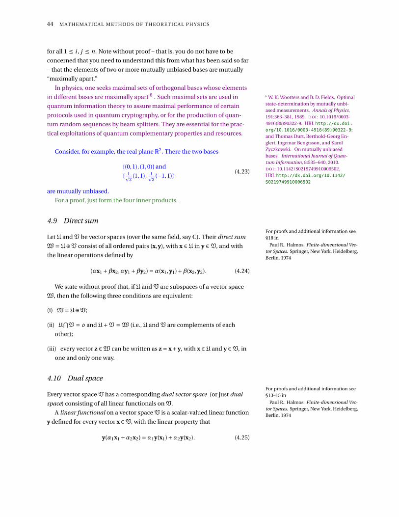
Consider, for example, the real plane R2. There the two bases
(0,1), (1,0) and
1p2
(1,1), 1p2
(−1,1)(4.23)
are mutually unbiased.
For a proof, just form the four inner products.
4.9 Direct sumFor proofs and additional information see§18 in
Paul R.. Halmos. Finite-dimensional Vec-tor Spaces. Springer, New York, Heidelberg,Berlin, 1974
Let U and V be vector spaces (over the same field, say C). Their direct sum
W = U⊕V consist of all ordered pairs (x,y), with x ∈ U in y ∈V, and with
the linear operations defined by
(αx1 +βx2,αy1 +βy2) =α(x1,y1)+β(x2,y2). (4.24)
We state without proof that, if U and V are subspaces of a vector space
W, then the following three conditions are equivalent:
(i) W=U⊕V;
(ii) U⋂V = 0 and U+V = W (i.e., U and V are complements of each
other);
(iii) every vector z ∈W can be written as z = x+y, with x ∈U and y ∈V, in
one and only one way.
4.10 Dual spaceFor proofs and additional information see§13–15 in
Paul R.. Halmos. Finite-dimensional Vec-tor Spaces. Springer, New York, Heidelberg,Berlin, 1974
Every vector space V has a corresponding dual vector space (or just dual
space) consisting of all linear functionals on V.
A linear functional on a vector space V is a scalar-valued linear function
y defined for every vector x ∈V, with the linear property that
y(α1x1 +α2x2) =α1y(x1)+α2y(x2). (4.25)

F I N I T E - D I M E N S I O N A L V E C TO R S PAC E S 45
For example, let x = (x1, . . . , xn), and take y(x) = x1.
For another example, let again x = (x1, . . . , xn), and let α1, . . . ,αn ∈ C be
scalars; and take y(x) =α1x1 +·· ·+αn xn .
If we adopt a bracket notation “[·, ·]” for the functional
y(x) = [x,y], (4.26)
then this “bracket” functional is bilinear in its two arguments; that is,
[α1x1 +α2x2,y] =α1[x1,y]+α2[x2,y], (4.27)
and
[x,α1y1 +α2y2] =α1[x,y1]+α2[x,y2]. (4.28)
The square bracket can be identified withthe scalar (dot) product [x,y] = ⟨x | y⟩only for Euclidean vector spaces Rn ,since for complex spaces this would nolonger be positive definite. That is, forEuclidean vector spaces Rn the inner orscalar product is bilinear.
If V is an n-dimensional vector space, and if B = f1, . . . , fn is a basis
of V, and if α1, . . . ,αn is any set of n scalars, then there is a unique linear
functional y on V such that [fi ,y] =αi for all 0 ≤ 1 ≤ n.
A constructive proof of this theorem can be given as follows: Since every
x ∈ V can be written as a linear combination x = x1f1 + ·· · + xn fn of the
base vectors in B in a unique way; and since y is a (bi)linear functional, we
obtain
[x,y] = x1[f1,y]+·· ·+xn[fn ,y], (4.29)
and uniqueness follows. With [fi ,y] = αi for all 0 ≤ 1 ≤ n, the value of [x,y]
is determined by [x,y] = xiαi +·· ·+xnαn .
4.10.1 Dual basis
We now can define a dual basis, or, used synonymuously a reciprocal basis.
If V is an n-dimensional vector space, and if B= f1, . . . , fn is a basis of V,
then there is a unique dual basis B∗ = f∗1 , . . . , f∗n in the dual vector space
V∗ with the property that
[ f ∗i , f j ] = δi j , (4.30)
where δi j is the Kronecker delta function. More generally, if g is the metric
tensor, the dual basis is defined by
g (f∗i , f j ) = δi j . (4.31)
or, in a different notation in which f∗j = f j ,
g (f j , fi ) = δ ji . (4.32)
In terms of the inner product, the representation of the metric g as out-
lined and characterized on page 92 with respect to a particular basis
B = f1, . . . , fn is gi j = g (fi , f j ) = ⟨fi | f j ⟩. Note that the coordinates gi j
of the metric g need not necessarily be positive definite. For example, spe-
cial relativity uses the “pseudo-Euclidean” metric g = diag(+1,+1,+1,−1)

46 M AT H E M AT I C A L M E T H O D S O F T H E O R E T I C A L P H Y S I C S
(or just g = diag(+,+,+,−)), where “diag” stands for the diagonal matrix
with the arguments in the diagonal. The metric tensor gi j represents a bilin-
ear functional g (x,y) = xi y j gi j that issymmetric; that is, g (x,y) = g (x,y) and non-degenerate; that is, for any nonzero vectorx ∈V, x 6= 0, there is some vector y ∈V, sothat g (x,y) 6= 0. g also satisfies the triangleinequality ||x−z|| ≤ ||x−y||+ ||y−z||.
The dual space V∗ is n-dimensional.
In a real Euclidean vector space Rn with the dot product as scalar prod-
uct, the dual basis of an orthogonal basis is also orthogonal. Moreover,
for an orthonormal basis, the bases vectors are uniquely identifiable by
ei −→ ei∗ = ei
T . This is not true for nonorthogonal bases.
In a proof by reductio ad absurdum. Suppose there exist a vector ei∗
in the dual basis B∗ which is not in the “original” ortogonal basis B; that
is, [ei∗,ej] = δi j for all ej ∈B. But since B is supposed to span the corre-
sponding vector space V, ei∗ has to be contained in B. Moreover, since for
a real Euclidean vector space Rn with the dot product as scalar product, the
two products [·, ·] = ⟨· | ·⟩ coincide, ei∗ has to be collinear – for normalized
basis vectors even identical – to exactly one element of B.
For nonorthogonal bases, take the counterexample explicitly mentioned
at page 47.
How can one determine the dual basis from a given, not necessarily
orthogonal, basis? The tuples of row vectors of the basis B= f1, . . . , fn can
be arranged into a matrix
B=
f1
f2...
fn
=
f1,1 · · · f1,n
f2,1 · · · f2,n...
......
fn,1 · · · fn,n
. (4.33)
Then take the inverse matrix B−1, and interprete the columns vectors of B−1
as the tuples of the dual basis B∗.
For orthogonal but not orthonormal bases, the term reciprocal basis can
be easily explained from the fact that the norm (or length) of each vector in
the reciprocal basis is just the inverse of the length of the original vector.
For a proof, consider B ·B−1 = In .
(i) For example, if
B= e1,e2, . . . ,en = (1,0, . . . ,0), (0,1, . . . ,0), . . . , (0,0, . . . ,1)
is the standard basis in n-dimensional vector space containing unit
vectors of norm (or length) one, then (the superscript “T ” indicates
transposition)
B∗ = e∗1 ,e∗2 , . . . ,e∗n
= (1,0, . . . ,0)T , (0,1, . . . ,0)T , . . . , (0,0, . . . ,1)T
=
1
0...
0
,
0
1...
0
, . . . ,
0
0...
1

F I N I T E - D I M E N S I O N A L V E C TO R S PAC E S 47
has elements with identical components, but those tuples are the trans-
posed tuples.
(ii) If
X= α1e1,α2e2, . . . ,αn en = (α1,0, . . . ,0), (0,α2, . . . ,0), . . . , (0,0, . . . ,αn),
α1,α2, . . . ,αn ∈ R, is a “dilated” basis in n-dimensional vector space
containing unit vectors of norm (or length) αi , then
X∗ = 1α1
e∗1 , 1α2
e∗2 , . . . , 1αn
e∗n
=
( 1α1
,0, . . . ,0)T , (0, 1α2
, . . . ,0)T , . . . , (0,0, . . . , 1αn
)T
=
1α1
1
0...
0
, 1α2
0
1...
0
, . . . , 1αn
0
0...
1
has elements with identical components of inverse length 1
αi, and again
those tuples are the transposed tuples.
(iii) Consider the nonorthogonal basis B = (1,2), (3,4). The associated
row matrix is
B=(
1 2
3 4
).
The inverse matrix is
B−1 =(
−2 132 − 1
2
);
and the associated dual basis is obtained from the columns of B−1 by
B∗ =(
−232
),
(1
− 12
)=
12
(−4
3
), 1
2
(2
−1
).
4.10.2 Dual coordinates
With respect to a given basis, the components of a vector are often written
as tuples of ordered (“xi is written before xi+1” – not “xi < xi+1”) scalars as
column vectors
x =
x1
x2...
xn
, (4.34)
whereas the components of vectors in dual spaces are often written in
terms of tuples of ordered scalars as row vectors
x∗ = (x∗1 , x∗
2 , . . . , x∗n ). (4.35)

48 M AT H E M AT I C A L M E T H O D S O F T H E O R E T I C A L P H Y S I C S
The coordinates (x1, x2, . . . , xn)T =
x1
x2...
xn
are called covariant, whereas the
coordinates (x∗1 , x∗
2 , . . . , x∗n ) are called contravariant, . Alternatively, one can
denote covariant coordinates by subscripts, and contravariant coordinates
by superscripts; that is (see also Havlicek 7, Section 11.4), 7 Hans Havlicek. Lineare Algebra fürTechnische Mathematiker. HeldermannVerlag, Lemgo, second edition, 2008
xi =
x1
x2...
xn
and xi = (x∗1 , x∗
2 , . . . , x∗n ). (4.36)
Note again that the covariant and contravariant components xi and xi are
not absolute, but always defined with respect to a particular (dual) basis.
The Einstein summation convention requires that, when an index vari-
able appears twice in a single term it implies that one has to sum over all of
the possible index values. This saves us from drawing the sum sign “∑
i for
the index i ; for instance xi yi =∑i xi yi .
In the particular context of covariant and contravariant components –
made necessary by nonorthogonal bases whose associated dual bases are
not identical – the summation always is between some superscript and
some subscript; e.g., xi y i .
Note again that for orthonormal basis, xi = xi .
4.10.3 Representation of a functional by inner productFor proofs and additional information see§67 in
Paul R.. Halmos. Finite-dimensional Vec-tor Spaces. Springer, New York, Heidelberg,Berlin, 1974
The following representation theorem is about the connection between
any functional in a vector space and its inner product; it is stated without
proof: To any linear functional z on a finite-dimensional inner product
space V there corresponds a unique vector y ∈V, such that
z(x) = [x,z] = ⟨x | y⟩ (4.37)
for all x ∈V.
Note that in real vector space Rn and with the dot product, y = z.
4.11 Tensor productFor proofs and additional information see§24 in
Paul R.. Halmos. Finite-dimensional Vec-tor Spaces. Springer, New York, Heidelberg,Berlin, 1974
4.11.1 Definition
For the moment, suffice it to say that the tensor product V⊗U of two linear
vector spaces V and U should be such that, to every x ∈V and avery y ∈ U
there corresponds a tensor product z = x⊗ y ∈V⊗U which is bilinear in
both factors.

F I N I T E - D I M E N S I O N A L V E C TO R S PAC E S 49
If A= f1, . . . , fn and B= g1, . . . ,gm are bases of n- and m- dimensional
vector spaces V and U, respectively, then the set Z of vectors zi j = fi ⊗g j
with i = 1, . . .n and j = 1, . . .m is a basis of the tensor product V⊗U.
A generalization to more than one factors is straightforward.
4.11.2 Representation
The tensor product z = x⊗y has three equivalent representations:
(i) as the scalar coordinates xi y j with respect to the basis in which the
vectors x and y have been defined and coded;
(ii) as the quasi-matrix zi j = xi y j , whose components zi j are defined with
respect to the basis in which the vectors x and y have been defined and
coded;
(iii) as a quasi-vector or “flattened matrix” defined by the Kronecker
product z = (x1y, x2y, . . . , xn y) = (x1 y1, x1 y2, . . . , xn yn). Again, the scalar
coordinates xi y j are defined with respect to the basis in which the
vectors x and y have been defined and coded.
In all three cases, the pairs xi y j are properly represented by distinct mathe-
matical entities.
4.12 Linear transformationFor proofs and additional information see§32-34 in
Paul R.. Halmos. Finite-dimensional Vec-tor Spaces. Springer, New York, Heidelberg,Berlin, 1974
4.12.1 Definition
A linear transformation (or, used synonymuosly, linear operator A on a
vector space V is a correspondence that assigns every vector x ∈V a vector
Ax ∈V, in a linear way that
A(αx+βy) =αAx+βAy, (4.38)
identically for all vectors x,y ∈V and all scalars α,β.
4.12.2 Operations
The sum S = A+B of two linear transformations A and B is defined by
Sx =Ax+Bx for every x ∈V.
The product P = AB of two linear transformations A and B is defined by
Px =A(Bx) for every x ∈V.
The notation AnAm = An+m and (An)m = Anm , with A1 = A and A0 = 1turns out to be useful.
With the exception of commutativity, all formal algebraic properties of
numerical addition and multiplication, are valid for transformations; that
is A0 = 0A = 0, A1 = 1A = A, A(B+C) = AB+AC, (A+B)C = AC+BC,

50 M AT H E M AT I C A L M E T H O D S O F T H E O R E T I C A L P H Y S I C S
and A(BC) = (AB)C. In matrix notation, 1 = 1, and the entries of 0 are 0
everywhere.
The inverse operator A−1 of A is defined by AA−1 =A−1A= I.The commutator of two matrices A and B is defined by
[A,B] =AB−BA. (4.39)
The commutator should not be confusedwith the bilinear funtional introduced fordual spaces.
The polynomial can be directly adopted from ordinary arithmetic; that
is, any finite polynomial p of degree n of an operator (transformation) Acan be written as
p(A) =α01+α1A1 +α2A2 +·· ·+αnAn =n∑
i=0αi Ai . (4.40)
The Baker-Hausdorff formula
e iABe−iA = B + i [A,B]+ i 2
2![A, [A,B]]+·· · (4.41)
for two arbitrary noncommutative linear operators A and B is mentioned
without proof (cf. Messiah, Quantum Mechanics, Vol. 1 8). 8 A. Messiah. Quantum Mechanics,volume I. North-Holland, Amsterdam,1962
If [A,B] commutes with A and B, then
eAeB = eA+B+ 12 [A,B]. (4.42)
4.12.3 Linear transformations as matrices
Due to linearity, there is a close connection between a matrix defined by an
n-by-n square array
A = ⟨i |A| j ⟩ = ai j =
α11 α12 · · · α1n
α21 α22 · · · α2n...
... · · · ...
αn1 αn2 · · · αnn
(4.43)
containing n2 entries, also called matrix coefficients or matrix coordinates,
αi j and a linear transformation A, encoded with respect to a particular
basis B. This can be well understood in terms of transformations of the
basis elements, as every vector is a unique linear combination of these
basis elements; more explicitly, see the Ansatz yi =Axi in Eq. (4.50) below.
Let V be an n-dimensional vector space; let B = f1, f2, . . . , fn be any
basis of V, and let A be a linear transformation on V. Because every vector
is a linear combination of the basis vectors fi , it is possible to define some
matrix coefficients or coordinates αi j such that
Af j =∑
iαi j fi (4.44)
for all j = 1, . . . ,n. Again, note that this definition of a transformation
matrix is tied up with a basis.

F I N I T E - D I M E N S I O N A L V E C TO R S PAC E S 51
In terms of this matrix notation, it is quite easy to present an example
for which the commutator [A,B] does not vanish; that is A and B do not
commute.
Take, for the sake of an example, the Pauli spin matrices which are
proportional to the angular momentum operators along the x, y , z-axis 9: 9 Leonard I. Schiff. Quantum Mechanics.McGraw-Hill, New York, 1955
σ1 =σx =(
0 1
1 0
),
σ2 =σy =(
0 −i
i 0
),
σ1 =σz =(
1 0
0 −1
).
(4.45)
Together with unity, i.e., I2 = diag(1,1), they form a complete basis of all
(4×4) matrices. Now take, for instance, the commutator
[σ1,σ3] =σ1σ3 −σ3σ1
=(
0 1
1 0
)(1 0
0 −1
)−
(1 0
0 −1
)(0 1
1 0
)
= 2
(0 −1
1 0
)6=
(0 0
0 0
).
(4.46)
4.13 Projector or Projection
For proofs and additional information see§41 in
Paul R.. Halmos. Finite-dimensional Vec-tor Spaces. Springer, New York, Heidelberg,Berlin, 1974
4.13.1 Definition
If V is the direct sum of some subspaces M and N so that verey z ∈ V
can be uniquely written in the form z = x+y, with x ∈M and with y ∈N,
then the projector, or, uses synonymuosly, projection on M along N is the
transformation E defined by Ez = x. Conversely, Fz = y is the projector on
N along M.
A linear transformation E is a projector if and only if it is idempotent;
that is, EE=E.
For a proof note that, if E is the projector on M along N, and if z = x+y,
with x ∈M and with y ∈N, the the decomposition of x yields x+0, so that
E2z = EEz = Ex = x = Ez. The converse – idempotence “EE = E” implies
that E is a projector – is more difficult to prove. For this proof we refer to
the literature; e.g., Halmos 10. 10 Paul R.. Halmos. Finite-dimensional Vec-tor Spaces. Springer, New York, Heidelberg,Berlin, 1974
We also mention without proof that a linear transformation E is a pro-
jector if and only if 1−E is a projector. Note that (1−E)2 = 1−E−E+E2 =1−E; furthermore, E(1−E) = (1−E)E=E−E2 = 0.
Furthermore, if E is the projector on M along N, then 1−E is the projec-
tor on N along M.

52 M AT H E M AT I C A L M E T H O D S O F T H E O R E T I C A L P H Y S I C S
4.13.2 Construction of projectors from unit vectors
How can we construct projectors from unit vectors, or systems of orthog-
onal projectors from some vector in some orthonormal basis with the
standard dot product?
Let x be the coordinates of a unit vector; that is ‖x‖ = 1. Then the dyadic
or tensor product (also in Dirac’s bra and ket notation)
Ex = x⊗xT = |x⟩⟨x|
=
x1
x2...
xn
(x1, x2, . . . , xn)
=
x1(x1, x2, . . . , xn)
x2(x1, x2, . . . , xn)...
xn(x1, x2, . . . , xn)
=
x1x1 x1x2 · · · x1xn
x2x1 x2x2 · · · x2xn...
......
...
xn x1 xn x2 · · · xn xn
(4.47)
is the projector associated with x.
If the vector x is not normalized, then the associated projector is
Ex = x⊗xT
⟨x | x⟩ = |x⟩⟨x|⟨x | x⟩ (4.48)
This construction is related to px on page 42 by px(y) =Exy.
For a proof, let Ex = x⊗xT , then
ExEx = (x⊗xT ) · (x⊗xT )
=
x1
x2...
xn
(x1, x2, . . . , xn)
x1
x2...
xn
(x1, x2, . . . , xn)
=
x1
x2...
xn
(x1, x2, . . . , xn)
x1
x2...
xn
(x1, x2, . . . , xn)
=
x1
x2...
xn
·1 · (x1, x2, . . . , xn) =
x1
x2...
xn
(x1, x2, . . . , xn) =Ex.

F I N I T E - D I M E N S I O N A L V E C TO R S PAC E S 53
Fo two examples, let x = (1,0)T and y = (1,−1)T ; then
Ex =(
1
0
)(1,0) =
(1(1,0)
0(1,0)
)=
(1 0
0 0
),
and
Ey = 1
2
(1
−1
)(1,−1) = 1
2
(1(1,−1)
−1(1,−1)
)= 1
2
(1 −1
−1 1
).
4.14 Change of basis
For proofs and additional information see§46 in
Paul R.. Halmos. Finite-dimensional Vec-tor Spaces. Springer, New York, Heidelberg,Berlin, 1974
Let V be an n-dimensional vector space land let X = x1, . . . ,xn and Y =y1, . . . ,yn be two bases in V.
Take an arbitrary vector x ∈V. In terms of the two bases X and Y, x can
be written as
x =n∑
i=1xi xi =
n∑i=1
y i yi , (4.49)
where xi and y i stand for the coordinates of the vector x with respect to the
bases X and Y, respectively.
What is the relation between the coordinates xi and y i ? Suppose that,
as an Ansatz, we define a linear transformation between the corresponding
vectors of the bases X and Y by
yi =Axi , (4.50)
for all i = 1, . . . ,n. Note that somewhat “hidden” in Eq. (4.50) there is a
matrix multiplication which can be made explicit: let ai j be the matrix
components corresponding to A in the basis X; then
y j =Ax j =n∑
i=1ai j xi . (4.51)
Here, the subscript “ j ” refers to the j th coordinate of y, whereas in Eq.
(4.50) the subscript “ j ” refers to the j th vectors x j and yi in the two bases
X and Y, respectively.
Then, since
x =n∑
j=1y j y j =
n∑j=1
y j Ax j =n∑
j=1y j
n∑i=1
ai j xi =n∑
i=1
(n∑
j=1ai j y j
)xi ;
and hence by comparison of the coefficients in Eq. (4.49),
xi =n∑
j=1ai j y j . (4.52)

54 M AT H E M AT I C A L M E T H O D S O F T H E O R E T I C A L P H Y S I C S
4.15 Rank
The (column or row) rank, ρ(A) of a linear transformation A in an n-
dimensional vector space V is the maximum number of linearly indepen-
dent (column or, without proof, equivalently, row) vectors of the associated
n-by-n square matrix ai j .
4.16 Determinant
4.16.1 Definition
Suppose A = ai j is the n-by-n square matrix representation of a linear
transformation A in an n-dimensional vector space V. We shall define its
determinant recursively.
First, a minor Mi j of an n-by-n square matrix A is defined to be the
determinant of the (n −1)× (n −1) submatrix that remains after the entire
i th row and j th column have been deleted from A.
A cofactor Ai j of an n-by-n square matrix A is defined in terms of its
associated minor by
Ai j = (−1)i+ j Mi j . (4.53)
The determinant of a square matrix A, denoted by detA or |A|, is a scalar
regursively defined by
detA =n∑
j=1ai j Ai j =
n∑i=1
ai j Ai j (4.54)
for any i (row expansion) or j (column expansion), with i , j = 1, . . . ,n. For
1×1 matrices, detA = a11.
4.16.2 Properties
The following properties of determinants are mentioned without proof:
(i) If A and B are square matrices of the same order, then detAB = detAdetB .
(ii) If either two rows or two columns are exchanged, then the determinant
is multiplied by a factor “−1.”
(iii) det(AT ) = detA.
(iv) The determinant detA of a matrix A is non-zero if and only if A is
invertible. In particular, if A is not invertible, detA = 0. If A has an
inverse matrix A−1, then det(A−1) = (detA)−1.
(v) Multiplication of any row or column with a factor α results in a deter-
minant which is α times the original determinant.

F I N I T E - D I M E N S I O N A L V E C TO R S PAC E S 55
4.17 Trace
4.17.1 DefinitionThe German word for trace is Spur.
The trace of an n-by-n square matrix A = ai j , denoted by TrA, is a scalar
defined to be the sum of the elements on the main diagonal (the diagonal
from the upper left to the lower right) of A; that is (also in Dirac’s bra and
ket notation),
TrA = a11 +a22 +·· ·+ann =n∑
i=1ai i =
n∑i=1
⟨i |A|i ⟩. (4.55)
4.17.2 Properties
The following properties of traces are mentioned without proof:
(i) Tr(A+B) = TrA+TrB ;
(ii) Tr(αA) =αTrA, with α ∈C;
(iii) Tr(AB) = Tr(B A);
(iv) TrA = TrAT ;
(v) Tr(A⊗B) = TrATrB ;
(vi) the trace is the sum of the eigenvalues of a normal operator;
(vii) det(e A) = eTrA ;
(viii) the trace is the derivative of the determinant at the identity;
(xi) the complex conjugate of the trace of an operator is equal to the trace
of its adjoint; that is (TrA) = Tr(A†);
(xi) the trace is invariant under rotations of the basis and under cyclic
permutations.
A trace class operator is a compact operator for which a trace is finite
and independent of the choice of basis.
4.18 Adjoint
4.18.1 Definition
Let V be a vector space and let y be any element of its dual space V∗.
For any linear transformation A, consider the bilinear functional y′(x) = Here [·, ·] is the bilinear functional, not thecommutator.[x,y′] = [Ax,y] Let the adjoint transformation A† be defined by
[x,A†y] = [Ax,y]. (4.56)

56 M AT H E M AT I C A L M E T H O D S O F T H E O R E T I C A L P H Y S I C S
4.18.2 Properties
We mention without proof that the adjoint operator is a linear operator.
Furthermore, 0† = 0, 1† = 1, (A+B)† = A† +B†, (αA)† = αA†, (AB)† = B†A†,
and (A−1)† = (A†)−1; as well as (in finite dimensional spaces)
A†† =A. (4.57)
4.18.3 Matrix notation
In matrix notation and in complex vector space with the dot product, note
that there is a correspondence with the inner product (cf. page 48) so that,
for all z ∈V and for all x ∈V, there exist a unique y ∈V with
[Ax,z]
= ⟨Ax | y⟩= ⟨y |Ax⟩= yi Ai j x j
= yi ATj i x j
= x AT
y
= [x,A†z]
= ⟨x |A†y⟩= xi A†
i j y j
= x A† y ,
(4.58)
and hence
A† = (A)T = AT , or A†i j = A j i . (4.59)
In words: in matrix notation, the adjoint transformation is just the trans-
pose of the complex conjugate of the original matrix.
4.19 Self-adjoint transformation
The following definition yields some analogy to real numbers as compared
to complex numbers (“a complex number z is real if z = z”), expressed in
terms of operators on a complex vector space. An operator A on a linear
vector space V is called self-adjoint, if
A† =A. (4.60)
In terms of matrices, a matrix A corresponding to an operator A in some
fixed basis is self-adjoint if
A† = (Ai j )T = Ai j = Ai j = A. (4.61)
More generally, if the matrix corresponding to A in some basis B is Ai j ,
then the matrix corresponding to A∗ with respect to the dual basis B∗ is
(Ai j )T .

F I N I T E - D I M E N S I O N A L V E C TO R S PAC E S 57
In real inner product spaces, the usual word for a self-adjoint transfor-
mation is symmetric transformation. In complex inner product spaces, the
usual word for self-adjoint is Hermitian transformation.
For the sake of an example, consider again the Pauli spin matrices
σ1 =σx =(
0 1
1 0
),
σ2 =σy =(
0 −i
i 0
),
σ1 =σz =(
1 0
0 −1
).
(4.62)
which, together with unity, i.e., I2 = diag(1,1), are all self-adjoint.
The following operators are not self-adjoint:(0 1
0 0
),
(1 1
0 0
),
(1 0
i 0
),
(0 i
i 0
). (4.63)
4.20 Positive transformation
A linear transformation A on an inner product space V is positive, that
is in symbols A ≥ 0, if it is self-adjoint, and if ⟨Ax | x⟩ ≥ 0 for all x ∈ V. If
⟨Ax | x⟩ = 0 implies x = 0, A is called strictly positive.
4.21 Unitary transformations and isometriesFor proofs and additional information see§73 in
Paul R.. Halmos. Finite-dimensional Vec-tor Spaces. Springer, New York, Heidelberg,Berlin, 1974
4.21.1 Definition
Note that a complex number z has absolute value one if z = 1/z, or zz = 1.
In analogy to this “modulus one” behavior, consider unitary transforma-
tions, or, used synonymuously, isometries U for which
U∗ =U† =U−1, or UU† =U†U= I. (4.64)
Alternatively, we mention without proof that the following conditions are
equivalent:
(i) ⟨Ux |Uy⟩ = ⟨x | y⟩ for all x,y ∈V;
(ii) ‖Ux‖ = ‖x‖ for all x,y ∈V;
4.21.2 Characterization of change of orthonormal basis
Let B = f1, f2, . . . , fn be an orthonormal basis of an n-dimensional inner
product space V. If U is an isometry, then UB= Uf1,Uf2, . . . ,Ufn is also an
orthonormal basis of V. (The converse is also true.)

58 M AT H E M AT I C A L M E T H O D S O F T H E O R E T I C A L P H Y S I C S
4.21.3 Characterization in terms of orthonormal basis
A complex matrix U is unitary if and only if its row (or column) vectors
form an orthonormal basis.
This can be readily verified 11 by writing U in terms of two orthonormal 11 J. Schwinger. Unitary operators bases.In Proceedings of the National Academy ofSciences (PNAS), volume 46, pages 570–579,1960. D O I : 10.1073/pnas.46.4.570. URLhttp://dx.doi.org/10.1073/pnas.46.
4.570
bases B= e1,e2, . . . ,en B′ = f1, f2, . . . , fn as
Ue f =n∑
i=1e†
i fi =n∑
i=1|ei ⟩⟨fi |. (4.65)
Together with U f e =∑n
i=1 f†i ei =∑n
i=1 |fi ⟩⟨ei | we form
ek Ue f
= ek∑n
i=1 e†i fi
=∑ni=1(ek e†
i )fi
=∑ni=1δki fi
= fk .
(4.66)
In a similar wey we find that
Ue f f†k = e†
k ,
fk U f e = fk ,
U f e e†k = f†
k .
(4.67)
Moreover,Ue f U f e
=∑ni=1
∑nj=1 |ei ⟩⟨fi ||f j ⟩⟨e j |
=∑ni=1
∑nj=1 |ei ⟩δi j ⟨e j |
=∑ni=1 |ei ⟩⟨ei |
= I.
(4.68)
In a similar way we obtain U f eUe f = I. Since
U†e f =
n∑i=1
(e†i )†f†
i =U f e , (4.69)
we obtain that U†e f = (Ue f )−1 and U†
f e = (U f e )−1.
Note also that the composition holds; that is, Ue f U f g =Ueg .
If we identify one of the bases B and B′ by the Cartesian standard basis,
it becomes clear that, for instance, every unitary operator U can be written
in terms of an orthonormal basis B= f1, f2, . . . , fn by “stacking” the vectors
of that orthonormal basis “on top of each other;” that is For proofs and additional information see§5.11.3, Theorem 5.1.5 and subsequentCorollary in
Satish D. Joglekar. Mathematical Physics:The Basics. CRC Press, Boca Raton, Florida,2007
U=
f1
f2...
fn
. (4.70)
Thereby the vectors of the orthonormal basis B serve as the rows of U.

F I N I T E - D I M E N S I O N A L V E C TO R S PAC E S 59
Also, every unitary operator U can be written in terms of an orthonor-
mal basis B = f1, f2, . . . , fn by “pasting” the (transposed) vectors of that
orthonormal basis “one after another;” that is
U= (fT
1 , fT2 , · · · , fT
n
). (4.71)
Thereby the (transposed) vectors of the orthonormal basis B serve as the
columns of U.
Of course, any permutation of vectors in B would also yield unitary
matrices.
4.22 Orthogonal projectorsFor proofs and additional information see§75 & 76 in
Paul R.. Halmos. Finite-dimensional Vec-tor Spaces. Springer, New York, Heidelberg,Berlin, 1974
A linear transformation E is an orthogonal projector if and only if E = E2 =E∗.
If E1,E2, . . . ,En are orthogonal projectors, then a necessary and suffi-
cient condition that E = E1 +E2 +·· ·+En be an orthogonal projector is that
Ei E j = 0 whenever i 6= j ; that is, that all Ei are pairwise orthogonal.
4.23 Proper value or eigenvalueFor proofs and additional information see§54 in
Paul R.. Halmos. Finite-dimensional Vec-tor Spaces. Springer, New York, Heidelberg,Berlin, 1974
4.23.1 Definition
A scalar λ is a proper value or eigenvalue, and a non-zero vector x is a
proper vector or eigenvector of a linear transformation A if
Ax =λx. (4.72)
In an n-dimensional vector space V The set of the set of eigenvalues and
the set of the associated eigenvectors λ1, . . . ,λk , x1, . . . ,xn of a linear
transformation A form an eigensystem of A.
4.23.2 Determination
Since the eigenvalues and eigenvectors are those scalars λ vectors x for
which Ax = λx, this equation can be rewritten with a zero vector on the
right side of the equation; that is (I = diag(1, . . . ,1) stands for the identity
matrix),
(A−λI)x = 0. (4.73)
Suppose that A−λI is invertible. Then we could formally write x = (A−λI)−10; hence x must be the zero vector.
We are not interested in this trivial solution of Eq. (4.73). Therefore,
suppose that, contrary to the previous assumption, A−λI is not invert-
ible. We have mentioned earlier (without proof) that this implies that its
determinant vanishes; that is,
det(A−λI) = |A−λI| = 0. (4.74)
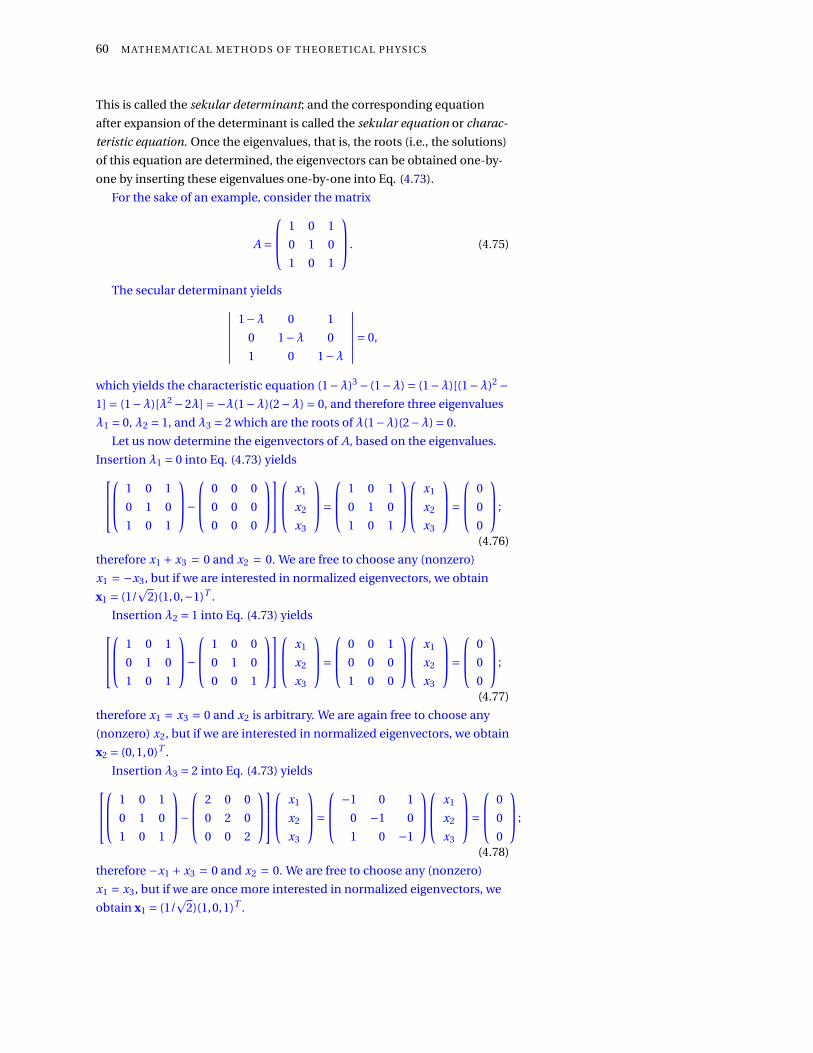
60 M AT H E M AT I C A L M E T H O D S O F T H E O R E T I C A L P H Y S I C S
This is called the sekular determinant; and the corresponding equation
after expansion of the determinant is called the sekular equation or charac-
teristic equation. Once the eigenvalues, that is, the roots (i.e., the solutions)
of this equation are determined, the eigenvectors can be obtained one-by-
one by inserting these eigenvalues one-by-one into Eq. (4.73).
For the sake of an example, consider the matrix
A =
1 0 1
0 1 0
1 0 1
. (4.75)
The secular determinant yields∣∣∣∣∣∣∣1−λ 0 1
0 1−λ 0
1 0 1−λ
∣∣∣∣∣∣∣= 0,
which yields the characteristic equation (1−λ)3 − (1−λ) = (1−λ)[(1−λ)2 −1] = (1−λ)[λ2 −2λ] =−λ(1−λ)(2−λ) = 0, and therefore three eigenvalues
λ1 = 0, λ2 = 1, and λ3 = 2 which are the roots of λ(1−λ)(2−λ) = 0.
Let us now determine the eigenvectors of A, based on the eigenvalues.
Insertion λ1 = 0 into Eq. (4.73) yields 1 0 1
0 1 0
1 0 1
−
0 0 0
0 0 0
0 0 0
x1
x2
x3
=
1 0 1
0 1 0
1 0 1
x1
x2
x3
=
0
0
0
;
(4.76)
therefore x1 + x3 = 0 and x2 = 0. We are free to choose any (nonzero)
x1 = −x3, but if we are interested in normalized eigenvectors, we obtain
x1 = (1/p
2)(1,0,−1)T .
Insertion λ2 = 1 into Eq. (4.73) yields 1 0 1
0 1 0
1 0 1
−
1 0 0
0 1 0
0 0 1
x1
x2
x3
=
0 0 1
0 0 0
1 0 0
x1
x2
x3
=
0
0
0
;
(4.77)
therefore x1 = x3 = 0 and x2 is arbitrary. We are again free to choose any
(nonzero) x2, but if we are interested in normalized eigenvectors, we obtain
x2 = (0,1,0)T .
Insertion λ3 = 2 into Eq. (4.73) yields 1 0 1
0 1 0
1 0 1
−
2 0 0
0 2 0
0 0 2
x1
x2
x3
=
−1 0 1
0 −1 0
1 0 −1
x1
x2
x3
=
0
0
0
;
(4.78)
therefore −x1 + x3 = 0 and x2 = 0. We are free to choose any (nonzero)
x1 = x3, but if we are once more interested in normalized eigenvectors, we
obtain x1 = (1/p
2)(1,0,1)T .

F I N I T E - D I M E N S I O N A L V E C TO R S PAC E S 61
Note that the eigenvectors are mutually orthogonal. We can construct
the corresponding orthogonal projectors by the dyadic product of the
eigenvectors; that is,
E1 = x1 ⊗xT1 = 1
2 (1,0,−1)T (1,0,−1) = 12
1(1,0,−1)
0(1,0,−1)
−1(1,0,−1)
= 12
1 0 −1
0 0 0
−1 0 1
E2 = x2 ⊗xT
2 = (0,1,0)T (0,1,0) =
0(0,1,0)
1(0,1,0)
0(0,1,0)
=
0 0 0
0 1 0
0 0 0
E3 = x3 ⊗xT
3 = 12 (1,0,1)T (1,0,1) = 1
2
1(1,0,1)
0(1,0,1)
1(1,0,1)
= 12
1 0 1
0 0 0
1 0 1
(4.79)
Note also that A can be written as the sum of the products of the eigen-
values with the associated projectors; that is (here, E stands for the corre-
sponding matrix), A = 0E1 +1E2 +2E3.
If the eigenvalues obtained are not distinct und thus some eigenvalues
are degenerate, the associated eigenvectors traditionally – that is, by con-
vention and not necessity – are chosen to be mutually orthogonal. A more
formal motivation will come from the spectral theorem below.
For the sake of an example, consider the matrix
B =
1 0 1
0 2 0
1 0 1
. (4.80)
The secular determinant yields∣∣∣∣∣∣∣1−λ 0 1
0 2−λ 0
1 0 1−λ
∣∣∣∣∣∣∣= 0,
which yields the characteristic equation (2 −λ)(1 −λ)2 + [−(2 −λ)] =(2−λ)[(1−λ)2 − 1] = −λ(2−λ)2 = 0, and therefore just two eigenvalues
λ1 = 0, and λ2 = 2 which are the roots of λ(2−λ)2 = 0.
Let us now determine the eigenvectors of B , based on the eigenvalues.
Insertion λ1 = 0 into Eq. (4.73) yields 1 0 1
0 2 0
1 0 1
−
0 0 0
0 0 0
0 0 0
x1
x2
x3
=
1 0 1
0 2 0
1 0 1
x1
x2
x3
=
0
0
0
;
(4.81)
therefore x1 + x3 = 0 and x2 = 0. Again we are free to choose any (nonzero)
x1 = −x3, but if we are interested in normalized eigenvectors, we obtain
x1 = (1/p
2)(1,0,−1)T .

62 M AT H E M AT I C A L M E T H O D S O F T H E O R E T I C A L P H Y S I C S
Insertion λ2 = 2 into Eq. (4.73) yields 1 0 1
0 2 0
1 0 1
−
2 0 0
0 2 0
0 0 2
x1
x2
x3
=
−1 0 1
0 0 0
1 0 −1
x1
x2
x3
=
0
0
0
;
(4.82)
therefore x1 = x3; x2 is arbitrary. We are again free to choose any values of
x1, x3 and x2 as long x1 = x3 as well as x2 are satisfied. Take, for the sake
of choice, the orthogonal normalized eigenvectors x2,1 = (0,1,0)T and
x2,2 = (1/p
2)(1,0,1)T , which are also orthogonal to x1 = (1/p
2)(1,0,−1)T .
Note again that we can find the corresponding orthogonal projectors by
the dyadic product of the eigenvectors; that is, by
E1 = x1 ⊗xT1 = 1
2 (1,0,−1)T (1,0,−1) = 12
1(1,0,−1)
0(1,0,−1)
−1(1,0,−1)
= 12
1 0 −1
0 0 0
−1 0 1
E2,1 = x2,1 ⊗xT
2,1 = (0,1,0)T (0,1,0) =
0(0,1,0)
1(0,1,0)
0(0,1,0)
=
0 0 0
0 1 0
0 0 0
E2,2 = x2,2 ⊗xT
2,2 = 12 (1,0,1)T (1,0,1) = 1
2
1(1,0,1)
0(1,0,1)
1(1,0,1)
= 12
1 0 1
0 0 0
1 0 1
(4.83)
Note also that B can be written as the sum of the products of the eigen-
values with the associated projectors; that is (here, E stands for the corre-
sponding matrix), B = 0E1 +2(E1,2 +E1,2). This leads us to the much more
general spectral theorem.
The following theorems are enumerated without proofs.
If A is a self-adjoint transformation on an inner product space, then ev-
ery proper value (eigenvalue) of A is real. If A is positive, or stricly positive,
then every proper value of A is positive, or stricly positive, respectively
Due to their idempotence EE=E, projectors have eigenvalues 0 or 1.
Every eigenvalue of an isometry has absolute value one.
If A is either a self-adjoint transformation or an isometry, then proper
vectors of A belonging to distinct proper values are orthogonal.
4.24 Normal transformation
A transformation A is called normal if it commutes with its adjoint; that is,
[A,A∗] =AA∗−A∗A= 0.
It follows from their definition that Hermitean and unitary transforma-
tions are normal.
We mention without proof that a normal transformation on a finite-
dimensional unitary space is (i) Hermitian, (ii) positive, (iii) strictly posi-
tive, (iv) unitary, (v) invertible, (vi) idempotent if and only if all its proper

F I N I T E - D I M E N S I O N A L V E C TO R S PAC E S 63
values are (i’) real, (ii) positive, (iii) strictly positive, (iv) of absolute value
one, (v) different from zero, (vi) equal to zero or one.
4.25 SpectrumFor proofs and additional information see§78 in
Paul R.. Halmos. Finite-dimensional Vec-tor Spaces. Springer, New York, Heidelberg,Berlin, 1974
4.25.1 Spectral theorem
Let V be an n-dimensional linear vector space. The spectral theorem states
that to every self-adjoint (more general, normal) transformation A on an
n-dimensional inner product space there correspond real numbers, the
spectrum λ1,λ2, . . . ,λk of all the eigenvalues of A, and their associated
orthogonal projectors E1,E2, . . . ,Ek where 0 < k ≤ n is a strictly positive
integer so that
(i) the λi are pairwise distinct,
(ii) the Ei are pairwise orthogonal and different from 0,
(iii)∑k
i=1 Ei = In , and
(iv) A=∑ki=1λi Ei is the spectral form of A.
4.25.2 Composition of the spectral form
If the spectrum of a Hermitian (or, more general, normal) operator A is
nondegenerate, that is, k = n, then the i th projector can be written as the
dyadic or tensor product Ei = xi ⊗ xTi of the i th normalized eigenvector
xi of A. In this case, the set of all normalized eigenvectors x1, . . . ,xn is n
othonormal basis of the vector space V. If the spectrum of A is degenerate,
then the projector can be chosen to be the orthogonal sum of projectors
corresponding to orthogonal eigenvectors, associated with the same eigen-
values.
Furthermore, for a Hermitian (or, more general, normal) operator A, if
1 ≤ i ≤ k, then there exist polynomials with real coefficients, such as, for
instance,
pi (t ) = ∏1 ≤ j ≤ k
j 6= i
t −λ j
λi −λ j(4.84)
so that pi (λ j ) = δi j ; moreover, for every such polynomial, pi (A) =Ei .
For a proof, it is not too difficult to show that pi (λi ) = 1, since in this
case in the product of fractions all numerators are equal to denominators,
and pi (λ j ) = 0 for j 6= i , since some numerator in the product of fractions
vanishes.
Now, substituting for t the spectral form A = ∑ki=1λi Ei of A, as well as
decomposing unity in terms of the projectors Ei in the spectral form of A;

64 M AT H E M AT I C A L M E T H O D S O F T H E O R E T I C A L P H Y S I C S
that is, In =∑ki=1 Ei , yields
pi (A) =∏1≤ j≤k, j 6=i
A−λ j In
λi−λ j
=∏1≤ j≤k, j 6=i
∑kl=1λl El−λ j
∑kl=1 El
λi−λ j
=∏1≤ j≤k, j 6=i
∑kl=1 El (λl−λ j )
λi−λ j
=∑kl=1 El
∏1≤ j≤k, j 6=i
λl−λ j
λi−λ j
=∑kl=1 Elδl i =Ei .
(4.85)
With the help of the polynomial pi (t ) defined in Eq. (4.84), which re-
quires knowledge of the eigenvalues, the spectral form of a Hermitian (or,
more general, normal) operator A can thus be rewritten as
A=k∑
i=1λi pi (A) =
k∑i=1
λi∏
1≤ j≤k, j 6=i
A−λ j Inλi −λ j
. (4.86)
If A = ∑ki=1λi Ei is the spectral form of a self-adjoint transformation
A on a finite-dimensional inner product space, then a necessary and
sufficient condition (“if and only if = iff”) that a linear transformation Bcommutes with A is that it commuts with each Ei , 1 ≤ i ≤ r .
4.26 Functions of normal transformations
Suppose A =∑ki=1λi Ei is a normal transformation with its spectral form. If
f is an arbitrary complex-valued function defined at least at the eigenval-
ues of A, then a linear transformation f (A) can be defined by
f (A) =k∑
i=1f (λi )Ei . (4.87)
For the definition of the “square root” for every positve operator A),
considerp
A=k∑
i=1
√λi Ei . (4.88)
Clearly, (p
A)2 =pAp
A=A.
4.27 Decomposition of operatorsFor proofs and additional information see§83 in
Paul R.. Halmos. Finite-dimensional Vec-tor Spaces. Springer, New York, Heidelberg,Berlin, 1974
4.27.1 Standard decomposition
In analogy to the decomposition of every imaginary number z =ℜz + iℑz
with ℜz,ℑz ∈ R, every arbitrary transformation A on a finite-dimensional
vector space can be decomposed into two Hermitian operators B C such
thatA=B+ iC; with
B= 12 (A+A†),
C= 12i (A−A†).
(4.89)

F I N I T E - D I M E N S I O N A L V E C TO R S PAC E S 65
4.27.2 Polar representation
The analogue of the polar representation of every imaginary number z =Re iϕ with R,ϕ ∈ R, R > 0, 0 ≤ϕ< 2π, every arbitrary transformation A on a
finite-dimensional inner product space can be decomposed into a unique
positive transform P and an isometry U, such that A = UP. If A is invertible,
then U is uniquely determined by A. A necessary and sufficient condition
that A is normal is that UP=PU.
4.27.3 Decomposition of isometries
Any unitary or orthogonal transformation in finite-dimensional inner
product space can be composed from a succession of two-parameter uni-
tary transformations in two-dimensional subspaces, and a multiplication
of a single diagonal matrix with elements of modulus one in an algorith-
mic, constructive and tractable manner. The method is similar to Gaussian
elimination and facilitates the parameterization of elements of the unitary
group in arbitrary dimensions (e.g., Ref. 12, Chapter 2). 12 F. D. Murnaghan. The Unitary and Rota-tion Groups. Spartan Books, Washington,D.C., 1962
It has been suggested to implement these group theoretic results by
realizing interferometric analogues of any discrete unitary and hermitean
operators in a unified and experimentally feasible way by “generalized
beam splitters” 13. 13 M. Reck, Anton Zeilinger, H. J. Bernstein,and P. Bertani. Experimental realizationof any discrete unitary operator. PhysicalReview Letters, 73:58–61, 1994. D O I :10.1103/PhysRevLett.73.58. URL http:
//dx.doi.org/10.1103/PhysRevLett.
73.58; and M. Reck and Anton Zeilinger.Quantum phase tracing of correlatedphotons in optical multiports. In F. DeMartini, G. Denardo, and Anton Zeilinger,editors, Quantum Interferometry, pages170–177, Singapore, 1994. World Scientific
4.27.4 Singular value decomposition
The singular value decomposition (SVD) of an (m ×n) matrix A is a factor-
ization of the form
A=UΣV, (4.90)
where U is a unitary (m ×m) matrix (i.e. an isometry), V is a unitary (n ×n)
matrix, and Σ is a unique (m ×n) diagonal matrix with nonnegative real
numbers on the diagonal; that is,
Σ=
σ1...
. . . · · · 0 · · ·σr
......
...
· · · 0 · · · · · · 0 · · ·...
......
...
. (4.91)
The entries σ1 ≥σ2 · · · ≥σr >0 of Σ are called singular values of A. No proof
is presented here.

66 M AT H E M AT I C A L M E T H O D S O F T H E O R E T I C A L P H Y S I C S
4.27.5 Schmidt decomposition of the tensor product of two vectors
Let U and V be two linear vector spaces of dimension n ≥ m and m, re-
spectively. Then, for any vector z ∈U⊗V in the tensor product space, there
exist orthonormal basis sets of vectors u1, . . . ,un ⊂ U and v1, . . . ,vm ⊂V
such that z =∑mi=1σi ui ⊗vi , where the σi s are nonnegative scalars and the
set of scalars is uniquely determined by z.
Equivalently 14, suppose that |z⟩ is some tensor product contained in 14 M. A. Nielsen and I. L. Chuang. QuantumComputation and Quantum Information.Cambridge University Press, Cambridge,2000
the set of all tensor products of vectors U⊗V of two linear vector spaces U
and V. Then there exist orthonoral vectors |ui ⟩ ∈U and |v j ⟩ ∈V so that
|z⟩ =∑iσi |ui ⟩|vi ⟩, (4.92)
where the σi s are nonnegative scalars; if |z⟩ is normalized, then the σi s are
satisfying∑
i σ2i = 1; they are called the Schmidt coefficients.
For a proof by reduction to the singular value decomposition, let |i ⟩ and
| j ⟩ be any two fixed orthonormal bases of U and V, respectively. Then, |z⟩can be expanded as |z⟩ = ∑
i j ai j |i ⟩| j ⟩, where the ai j s can be interpreted
as the components of a matrix A. A can then be subjected to a singular
value decomposition A = UΣV, or, written in index form (note that Σ =diag(σ1, . . . ,σn) is a diagonal matrix), ai j = ∑
l ui lσl vl j ; and hence |z⟩ =∑i j l ui lσl vl j |i ⟩| j ⟩. Finally, by identifying |ul ⟩ =
∑i ui l |i ⟩ as well as |vl ⟩ =∑
l vl j | j ⟩ one obtains the Schmidt decompsition (4.92). Since ui l and vl j
represent unitary martices, and because |i ⟩ as well as | j ⟩ are orthonormal,
the newly formed vectors |ul ⟩ as well as |vl ⟩ form orthonormal bases as
well. The sum of squares of the σi s is one if |z⟩ is a unit vector, because
(note that σi s are real-valued) ⟨z|z⟩ = 1 = ∑lmσlσm⟨ul |um⟩⟨vl |vm⟩ =∑
lmσlσmδlm =∑l σ
2l .
4.28 Commutativity
For proofs and additional information see§84 in
Paul R.. Halmos. Finite-dimensional Vec-tor Spaces. Springer, New York, Heidelberg,Berlin, 1974
A set M = A1,A2, . . . ,Ak of self-adjoint transformations on a finite-
dimensional inner product space are mutually commuting if and only if
there exists a self-adjoint transformation R and a set of real-valued func-
tions F = f1, f2, . . . , fk of a real variable so that A1 = f1(R), A2 = f2(R), . . .,
Ak = fk (R). If such a maximal operator R exists, then it can be written as
a function of all transformations in the set M; that is, R = G(A1,A2, . . . ,Ak ),
where G is a suitable real-valued function of n variables (cf. Ref. 15, Satz 8). 15 John von Neumann. Über Funktionenvon Funktionaloperatoren. Annals ofMathematics, 32:191–226, 1931. URLhttp://www.jstor.org/stable/1968185
The maximal operator R can be interpreted as containing all the infor-
mation of a collection of commuting operators at once; stated pointedly,
rather than consider all the operators in M separately, the maximal opera-
tor R represents M; in a sense, the operators Ai ∈ M are all just incomplete
aspects of, or individual functional views on, the maximal operator R.
Let us demonstrate the machinery developed so far by an example.

F I N I T E - D I M E N S I O N A L V E C TO R S PAC E S 67
Consider the normal matrices
A=
0 1 0
1 0 0
0 0 0
, B=
2 3 0
3 2 0
0 0 0
, C=
5 7 0
7 5 0
0 0 11
,
which are mutually commutative; that is, [A,B] = AB−BA = [A,C] =AC−BC= [B,C] =BC−CB= 0.
The eigensystems – that is, the set of the set of eigenvalues and the set of
the associated eigenvectors – of A, B and C are
1,−1,0, (1,1,0)T , (−1,1,0)T , (0,0,1)T ,
5,−1,0, (1,1,0)T , (−1,1,0)T , (0,0,1)T ,
12,−2,11, (1,1,0)T , (−1,1,0)T , (0,0,1)T .
They share a common orthonormal set of eigenvalues 1p2
1
1
0
,1p2
−1
1
0
,
0
0
1
which form an orthonormal basis of R3 or C3. The associated projectors are
obtained by the dyadic or tensor products of these vectors; that is,
E1 = 12
1 1 0
1 1 0
0 0 0
,
E2 = 12
1 −1 0
−1 1 0
0 0 0
,
E3 =
0 0 0
0 0 0
0 0 1
.
Thus the spectral decompositions of A, B and C are
A=E1 −E2 +0E3,
B= 5E1 −E2 +0E3,
C= 12E1 −2E2 +11E3,
(4.93)
respectively.
One way to define the maximal operator R for this problem would be
R=αE1 +βE2 +γE3,
with α,β,γ ∈ R− 0 and α 6= β 6= γ 6= α. The functional coordinates fi (α),
fi (β), and fi (γ), i ∈ A,B,C, of the three functions fA(R), fB(R), and fC(R)
chosen to match the projector coefficients obtained in Eq. (4.93); that is,
A= fA(R) =E1 −E2 +0E3,
B= fB(R) = 5E1 −E2 +0E3,
C= fC(R) = 12E1 −2E2 +11E3.

68 M AT H E M AT I C A L M E T H O D S O F T H E O R E T I C A L P H Y S I C S
It is no coincidence that the projectors in the spectral forms of A, B and
C are identical. Indeed it can be shown that mutually commuting normal
operators always share the same eigenvectors; and thus also the same
projectors.
Let the set M = A1,A2, . . . ,Ak be mutually commuting normal (or
Hermitian, or self-adjoint) transformations on an n-dimensional inner
product space. Then there exists an orthonormal basis B = f1, . . . , fn
such that every f j ∈B is an eigenvalue of each of the Ai ∈ M. Equivalently,
there exist n orthogonal projectors (let the vectors f j be represented by
the coordinates which are column vectors) E j = f j ⊗ fTj such that every E j ,
1 ≤ j ≤ n occurs in the spectral form of each of the Ai ∈M.
4.29 Measures on closed subspaces
In what follows we shall assume that all (probability) measures or states
w behave quasi-classically on sets of mutually commuting self-adjoint
operators, and in particular on orthogonal projectors.
Suppose E = E1,E2, . . . ,En is a set of mutually commuting orthogo-
nal projectors on a finite-dimensional inner product space V. Then, the
probability measure w should be additive; that is,
w(E1 +E2 · · ·+En) = w(E1)+w(E2)+·· ·+w(En). (4.94)
Stated differently, we shall assume that, for any two orthogonal projec-
tors E,F so that EF= FE= 0, their sum G=E+F has expectation value
⟨G⟩ = ⟨E⟩+⟨F⟩. (4.95)
We shall consider only vector spaces of dimension three or greater, since
only in these cases two orthonormal bases can be interlinked by a common
vector – in two dimensions, distinct orthonormal bases contain distinct
basis vectors.
4.29.1 Gleason’s theorem
For a Hilbert space of dimension three or greater, the only possible form of
the expectation value of an self-adjoint operator A has the form 16 16 Andrew M. Gleason. Measures onthe closed subspaces of a Hilbert space.Journal of Mathematics and Mechanics(now Indiana University MathematicsJournal), 6(4):885–893, 1957. ISSN 0022-2518. D O I : 10.1512/iumj.1957.6.56050".URL http://dx.doi.org/10.1512/
iumj.1957.6.56050; Anatolij Dvurecen-skij. Gleason’s Theorem and Its Appli-cations. Kluwer Academic Publishers,Dordrecht, 1993; Itamar Pitowsky. Infi-nite and finite Gleason’s theorems andthe logic of indeterminacy. Journal ofMathematical Physics, 39(1):218–228,1998. D O I : 10.1063/1.532334. URLhttp://dx.doi.org/10.1063/1.532334;Fred Richman and Douglas Bridges. Aconstructive proof of Gleason’s theorem.Journal of Functional Analysis, 162:287–312, 1999. D O I : 10.1006/jfan.1998.3372.URL http://dx.doi.org/10.1006/jfan.
1998.3372; and Asher Peres. QuantumTheory: Concepts and Methods. KluwerAcademic Publishers, Dordrecht, 1993
⟨A⟩ = Tr(ρA), (4.96)
the trace of the operator product of the density matrix (which is a positive
operator of the trace class) ρ for the system with the matrix representation
of A.
In particular, if A is a projector E corresponding to an elementary yes-no
proposition “the system has property Q,” then ⟨E⟩ = Tr(ρE) corresponds to
the probability of that property Q if the system is in state ρ.

F I N I T E - D I M E N S I O N A L V E C TO R S PAC E S 69
4.29.2 Kochen-Specker theorem
For a Hilbert space of dimension three or greater, there does not exist any
two-valued probability measures interpretable as consistent, overall truth
assignment 17. As a result of the nonexistence of two-valued states, the 17 Ernst Specker. Die Logik nicht gle-ichzeitig entscheidbarer Aussagen. Di-alectica, 14(2-3):239–246, 1960. D O I :10.1111/j.1746-8361.1960.tb00422.x.URL http://dx.doi.org/10.1111/j.
1746-8361.1960.tb00422.x; and SimonKochen and Ernst P. Specker. The problemof hidden variables in quantum mechan-ics. Journal of Mathematics and Mechanics(now Indiana University Mathematics Jour-nal), 17(1):59–87, 1967. ISSN 0022-2518.D O I : 10.1512/iumj.1968.17.17004. URLhttp://dx.doi.org/10.1512/iumj.
1968.17.17004
classical strategy to construct probabilities by a convex combination of all
two-valued states fails entirely.
In Greechie diagram 18, points represent basis vectors. If they belong to
18 J. R. Greechie. Orthomodular latticesadmitting no states. Journal of Com-binatorial Theory, 10:119–132, 1971.D O I : 10.1016/0097-3165(71)90015-X.URL http://dx.doi.org/10.1016/
0097-3165(71)90015-X
the same basis, they are connected by smooth curves.
if fi fi fifififififififififi
fififififi.
........................
..............
.......
.............
.................................. ........... .......... ........... ............ .............. .................
...........................................
.........................
.
..................................................
.................................................
...............................................
..............................................
.............................................
............................................
...........................................
.........................................
........................................
.........................................
........................................
.....................................
.....................................
......................................
.......................................
.........................................
..........................................
...........................................
............................................
.............................................
..............................................
..........................
.....................
...................
..............................
...............................................................................................................................
........................
.........................
..............
.......
.............
.....................
............................................................................................................
................................................
.
..................................................
.................................................
...............................................
..............................................
.............................................
............................................
...........................................
.........................................
........................................
.........................................
........................................
.....................................
.....................................
......................................
.......................................
.........................................
..........................................
...........................................
............................................
.............................................
..............................................
..........................
.....................
...................
.................................................... .......... ........... ............ .............. ................. ................... ......................
........................
................................................................................................................................................... .............. ................ ................... ...................... .........................
............................................
...................................................................................
........................................ ....................................... ...................................... ....................................... ........................................ ..................................................................................
..................................
........... ......................... ...................... ................... ................ .............. ..................................................................................................................................................
............................................
...........................................
.......................................................................................................................................................................................................................................................................................
.....................................................................................
M
A
L
B
J
D
K
C
IN
ER
HO
FQ
GP
a
b
c
d
e
fg
hi
The most compact way of deriving the Kochen-Specker theorem in four
dimensions has been given by Cabello 19. For the sake of demonstra- 19 Adán Cabello, José M. Estebaranz, andG. García-Alcaine. Bell-Kochen-Speckertheorem: A proof with 18 vectors. PhysicsLetters A, 212(4):183–187, 1996. D O I :10.1016/0375-9601(96)00134-X. URL http:
//dx.doi.org/10.1016/0375-9601(96)
00134-X; and Adán Cabello. Kochen-Specker theorem and experimental test onhidden variables. International Journalof Modern Physics, A 15(18):2813–2820,2000. D O I : 10.1142/S0217751X00002020.URL http://dx.doi.org/10.1142/
S0217751X00002020
tion, consider a Greechie (orthogonality) diagram of a finite subset of the
continuum of blocks or contexts embeddable in four-dimensional real
Hilbert space without a two-valued probability measure The proof of the
Kochen-Specker theorem uses nine tightly interconnected contexts a =A,B ,C ,D, b = D ,E ,F ,G, c = G , H , I , J , d = J ,K ,L, M , e = M , N ,O,P ,
f = P ,Q,R, A, g = B , I ,K ,R, h = C ,E ,L, N , i = F , H ,O,Q consisting of
the 18 projectors associated with the one dimensional subspaces spanned
by the vectors from the origin (0,0,0,0) to A = (0,0,1,−1), B = (1,−1,0,0),
C = (1,1,−1,−1), D = (1,1,1,1), E = (1,−1,1,−1), F = (1,0,−1,0), G =(0,1,0,−1), H = (1,0,1,0), I = (1,1,−1,1), J = (−1,1,1,1), K = (1,1,1,−1),
L = (1,0,0,1), M = (0,1,−1,0), N = (0,1,1,0), O = (0,0,0,1), P = (1,0,0,0),
Q = (0,1,0,0), R = (0,0,1,1), respectively. Greechie diagrams represent
atoms by points, and contexts by maximal smooth, unbroken curves.
In a proof by contradiction,note that, on the one hand, every observable
proposition occurs in exactly two contexts. Thus, in an enumeration of the
four observable propositions of each of the nine contexts, there appears
to be an even number of true propositions, provided that the value of an

70 M AT H E M AT I C A L M E T H O D S O F T H E O R E T I C A L P H Y S I C S
observable does not depend on the context (i.e. the assignment is non-
contextual). Yet, on the other hand, as there is an odd number (actually
nine) of contexts, there should be an odd number (actually nine) of true
propositions.
4.30 Hilbert space quantum mechanics and quantum logic
4.30.1 Quantum mechanics
The following is a very brief introduction to quantum mechanics. Introduc-
tions to quantum mechanics can be found in Refs. 20. 20 Richard Phillips Feynman, Robert B.Leighton, and Matthew Sands. TheFeynman Lectures on Physics. QuantumMechanics, volume III. Addison-Wesley,Reading, MA, 1965; L. E. Ballentine.Quantum Mechanics. Prentice Hall,Englewood Cliffs, NJ, 1989; A. Messiah.Quantum Mechanics, volume I. North-Holland, Amsterdam, 1962; Asher Peres.Quantum Theory: Concepts and Methods.Kluwer Academic Publishers, Dordrecht,1993; and John Archibald Wheeler andWojciech Hubert Zurek. Quantum Theoryand Measurement. Princeton UniversityPress, Princeton, NJ, 1983
All quantum mechanical entities are represented by objects of Hilbert
spaces 21. The following identifications between physical and theoretical
21 John von Neumann. Mathematis-che Grundlagen der Quantenmechanik.Springer, Berlin, 1932; and GarrettBirkhoff and John von Neumann. Thelogic of quantum mechanics. An-nals of Mathematics, 37(4):823–843,1936. D O I : 10.2307/1968621. URLhttp://dx.doi.org/10.2307/1968621
objects are made (a caveat: this is an incomplete list).
In what follows, unless stated differently, only finite dimensional Hilbert
spaces are considered. Then, the vectors corresponding to states can be
written as usual vectors in complex Hilbert space. Furthermore, bounded
self-adjoint operators are equivalent to bounded Hermitean operators.
They can be represented by matrices, and the self-adjoint conjugation is
just transposition and complex conjugation of the matrix elements. Let
B= b1,b2, . . . ,bn be an orthonormal basis in n-dimensional Hilbert space
H. That is, orthonormal base vectors in B satisfy ⟨bi ,b j ⟩ = δi j , where δi j is
the Kronecker delta function.
(I) A quantum state is represented by a positive Hermitian operator ρ of
trace class one in the Hilbert space H; that is
(i) ρ† = ρ = ∑ni=1 pi |bi ⟩⟨bi |, with pi ≥ 0 for all i = 1, . . . ,n, bi ∈B, and∑n
i=1 pi = 1, so that
(ii) ⟨ρx | x⟩ = ⟨x | ρx⟩ ≥ 0,
(iii) Tr(ρ) =∑ni=1⟨bi | ρ | bi ⟩ = 1.
A pure state is represented by a (unit) vector x, also denoted by | x⟩, of
the Hilbert space H spanning a one-dimensional subspace (manifold)
Mx of the Hilbert space H. Equivalently, it is represented by the one-
dimensional subspace (manifold) Mx of the Hilbert space H spannned
by the vector x. Equivalently, it is represented by the projector Ex =|x⟩⟨x | onto the unit vector x of the Hilbert space H.
Therefore, if two vectors x,y ∈H represent pure states, their vector sum
z = x+ y ∈ H represents a pure state as well. This state z is called the
coherent superposition of state x and y. Coherent state superpositions
between classically mutually exclusive (i.e. orthogonal) states, say | 0⟩and | 1⟩, will become most important in quantum information theory.
Any pure state x can be written as a linear combination of the set of
orthonormal base vectors b1,b2, · · ·bn, that is, x =∑ni=1βi bi , where n is

F I N I T E - D I M E N S I O N A L V E C TO R S PAC E S 71
the dimension of H and βi = ⟨bi | x⟩ ∈C.
In the Dirac bra-ket notation, unity is given by 1 = ∑ni=1 |bi ⟩⟨bi |, or just
1 =∑ni=1 |i ⟩⟨i |.
(II) Observables are represented by self-adjoint or, synonymuously, Hermi-
tian, operators or transformations A = A† on the Hilbert space H such
that ⟨Ax | y⟩ = ⟨x | Ay⟩ for all x,y ∈H. (Observables and their correspond-
ing operators are identified.)
The trace of an operator A is given by TrA=∑ni=1⟨bi |A|bi ⟩.
Furthermore, any Hermitian operator has a spectral representation as
a spectral sum A = ∑ni=1αi Ei , where the Ei ’s are orthogonal projection
operators onto the orthonormal eigenvectors ai of A (nondegenerate
case).
Observables are said to be compatible if they can be defined simultane-
ously with arbitrary accuracy; i.e., if they are “independent.” A criterion
for compatibility is the commutator. Two observables A,B are compati-
ble, if their commutator vanishes; that is, if [A,B] =AB−BA= 0.
It has recently been demonstrated that (by an analog embodiment using
particle beams) every Hermitian operator in a finite dimensional Hilbert
space can be experimentally realized 22. 22 M. Reck, Anton Zeilinger, H. J. Bernstein,and P. Bertani. Experimental realizationof any discrete unitary operator. PhysicalReview Letters, 73:58–61, 1994. D O I :10.1103/PhysRevLett.73.58. URL http:
//dx.doi.org/10.1103/PhysRevLett.
73.58
(III) The result of any single measurement of the observable A on a state
x ∈H can only be one of the real eigenvalues of the corresponding Her-
mitian operator A. If x is in a coherent superposition of eigenstates of A,
the particular outcome of any such single measurement is believed to
be indeterministic 23; that is, it cannot be predicted with certainty. As a 23 Max Born. Zur Quantenmechanik derStoßvorgänge. Zeitschrift für Physik, 37:863–867, 1926a. D O I : 10.1007/BF01397477.URL http://dx.doi.org/10.1007/
BF01397477; Max Born. Quantenmechanikder Stoßvorgänge. Zeitschrift für Physik, 38:803–827, 1926b. D O I : 10.1007/BF01397184.URL http://dx.doi.org/10.1007/
BF01397184; and Anton Zeilinger. Themessage of the quantum. Nature, 438:743, 2005. D O I : 10.1038/438743a. URLhttp://dx.doi.org/10.1038/438743a
result of the measurement, the system is in the state which corresponds
to the eigenvector ai of A with the associated real-valued eigenvalue αi ;
that is, Ax =αn an (no Einstein sum convention here).
This “transition” x → an has given rise to speculations concern-
ing the “collapse of the wave function (state).” But, subject to tech-
nology and in principle, it may be possible to reconstruct coherence;
that is, to “reverse the collapse of the wave function (state)” if the pro-
cess of measurement is reversible. After this reconstruction, no infor-
mation about the measurement must be left, not even in principle.
How did Schrödinger, the creator of wave mechanics, perceive the
ψ-function? In his 1935 paper “Die Gegenwärtige Situation in der Quan-
tenmechanik” (“The present situation in quantum mechanics” 24), on 24 Erwin Schrödinger. Die gegenwärtigeSituation in der Quantenmechanik.Naturwissenschaften, 23:807–812, 823–828,844–849, 1935b. D O I : 10.1007/BF01491891,10.1007/BF01491914, 10.1007/BF01491987.URL http://dx.doi.org/10.1007/
BF01491891,http://dx.doi.org/10.
1007/BF01491914,http://dx.doi.org/
10.1007/BF01491987
page 53, Schrödinger states, “the ψ-function as expectation-catalog:
. . . In it [[the ψ-function]] is embodied the momentarily-attained sum
of theoretically based future expectation, somewhat as laid down in
a catalog. . . . For each measurement one is required to ascribe to the
ψ-function (=the prediction catalog) a characteristic, quite sudden

72 M AT H E M AT I C A L M E T H O D S O F T H E O R E T I C A L P H Y S I C S
change, which depends on the measurement result obtained, and so can-
not be foreseen; from which alone it is already quite clear that this sec-
ond kind of change of the ψ-function has nothing whatever in common
with its orderly development between two measurements. The abrupt
change [[of the ψ-function (=the prediction catalog)]] by measurement
. . . is the most interesting point of the entire theory. It is precisely the
point that demands the break with naive realism. For this reason one
cannot put the ψ-function directly in place of the model or of the physi-
cal thing. And indeed not because one might never dare impute abrupt
unforeseen changes to a physical thing or to a model, but because in the
realism point of view observation is a natural process like any other and
cannot per se bring about an interruption of the orderly flow of natural
events.” German original: “Die ψ-Funktion alsKatalog der Erwartung: . . . Sie [[die ψ-Funktion]] ist jetzt das Instrument zurVoraussage der Wahrscheinlichkeit vonMaßzahlen. In ihr ist die jeweils erreichteSumme theoretisch begründeter Zukun-ftserwartung verkörpert, gleichsam wie ineinem Katalog niedergelegt. . . . Bei jederMessung ist man genötigt, der ψ-Funktion(=dem Voraussagenkatalog) eine eige-nartige, etwas plötzliche Veränderungzuzuschreiben, die von der gefundenenMaßzahl abhängt und sich nicht vorherse-hen läßt; woraus allein schon deutlich ist,daß diese zweite Art von Veränderungder ψ-Funktion mit ihrem regelmäßigenAbrollen zwischen zwei Messungen nichtdas mindeste zu tun hat. Die abrupteVeränderung durch die Messung . . . ist derinteressanteste Punkt der ganzen Theorie.Es ist genau der Punkt, der den Bruchmit dem naiven Realismus verlangt. Ausdiesem Grund kann man die ψ-Funktionnicht direkt an die Stelle des Modells oderdes Realdings setzen. Und zwar nicht etwaweil man einem Realding oder einemModell nicht abrupte unvorhergeseheneÄnderungen zumuten dürfte, sondernweil vom realistischen Standpunkt dieBeobachtung ein Naturvorgang ist wiejeder andere und nicht per se eine Unter-brechung des regelmäßigen Naturlaufshervorrufen darf.
The late Schrödinger was much more polemic about these issues;
compare for instance his remarks in his Dublin Seminars (1949-1955),
published in Ref. 25, pages 19-20: “The idea that [the alternate mea-
25 Erwin Schrödinger. The Interpretationof Quantum Mechanics. Dublin Seminars(1949-1955) and Other Unpublished Essays.Ox Bow Press, Woodbridge, Connecticut,1995
surement outcomes] be not alternatives but all really happening simul-
taneously seems lunatic to [the quantum theorist], just impossible. He
thinks that if the laws of nature took this form for, let me say, a quar-
ter of an hour, we should find our surroundings rapidly turning into a
quagmire, a sort of a featureless jelly or plasma, all contours becoming
blurred, we ourselves probably becoming jelly fish. It is strange that
he should believe this. For I understand he grants that unobserved na-
ture does behave this way – namely according to the wave equation.
. . . according to the quantum theorist, nature is prevented from rapid
jellification only by our perceiving or observing it.”
(IV) The probability Px(y) to find a system represented by state ρx in
some pure state y is given by the Born rule which is derivable from
Gleason’s theorem: Px(y) = Tr(ρxEy). Recall that the density ρx is a
positive Hermitian operator of trace class one.
For pure states with ρ2x = ρx, ρx is a onedimensional projector ρx =
Ex = |x⟩⟨x| onto the unit vector x; thus expansion of the trace and Ey =|y⟩⟨y| yields Px(y) = ∑n
i=1⟨i | x⟩⟨x|y⟩⟨y | i ⟩ = ∑ni=1⟨y | i ⟩⟨i | x⟩⟨x|y⟩ =∑n
i=1⟨y | 1 | x⟩⟨x|y⟩ = |⟨y | x⟩|2.
(V) The average value or expectation value of an observable A in a quan-
tum state x is given by ⟨A⟩y = Tr(ρxA).
The average value or expectation value of an observable A=∑ni=1αi Ei
in a pure state x is given by ⟨A⟩x = ∑nj=1
∑ni=1αi ⟨ j | x⟩⟨x|ai ⟩⟨ai | j ⟩ =∑n
j=1
∑ni=1αi ⟨ai | j ⟩⟨ j | x⟩⟨x|ai ⟩ = ∑n
j=1
∑ni=1αi ⟨ai | 1 | x⟩⟨x|ai ⟩ =∑n
i=1αi |⟨x | ai ⟩|2.
(VI) The dynamical law or equation of motion can be written in the form
x(t ) = Ux(t0), where U† = U−1 (“† stands for transposition and complex
conjugation) is a linear unitary transformation or isometry.

F I N I T E - D I M E N S I O N A L V E C TO R S PAC E S 73
The Schrödinger equation i —h ∂∂t ψ(t ) = Hψ(t ) is obtained by identify-
ing U with U= e−iHt/—h , where H is a self-adjoint Hamiltonian (“energy”)
operator, by differentiating the equation of motion with respect to the
time variable t .
For stationary ψn(t ) = e−(i /—h)En tψn , the Schrödinger equation
can be brought into its time-independent form Hψn = Enψn . Here,
i —h ∂∂t ψn(t ) = Enψn(t ) has been used; En and ψn stand for the n’th
eigenvalue and eigenstate of H, respectively.
Usually, a physical problem is defined by the Hamiltonian H. The
problem of finding the physically relevant states reduces to finding a
complete set of eigenvalues and eigenstates of H. Most elegant solutions
utilize the symmetries of the problem; that is, the symmetry of H. There
exist two “canonical” examples, the 1/r -potential and the harmonic
oscillator potential, which can be solved wonderfully by these methods
(and they are presented over and over again in standard courses of
quantum mechanics), but not many more. (See, for instance, 26 for a 26 A. S. Davydov. Quantum Mechanics.Addison-Wesley, Reading, MA, 1965detailed treatment of various Hamiltonians H.)
4.30.2 Quantum logic
The dimensionality of the Hilbert space for a given quantum system de-
pends on the number of possible mutually exclusive outcomes. In the
spin– 12 case, for example, there are two outcomes “up” and “down,” asso-
ciated with spin state measurements along arbitrary directions. Thus, the
dimensionality of Hilbert space needs to be two.
Then the following identifications can be made. Table 4.1 lists the iden-
tifications of relations of operations of classical Boolean set-theoretic and
quantum Hillbert lattice types.
generic lattice order relation “meet” “join” “complement”propositional implication disjunction conjunction negation
calculus → “and” ∧ “or” ∨ “not” ¬“classical” lattice subset ⊂ intersection ∩ union ∪ complement
of subsetsof a setHilbert subspace intersection of closure of orthogonallattice relation subspaces ∩ linear subspace
⊂ span ⊕ ⊥lattice of E1E2 =E1 E1E2 E1 +E2 −E1E2 orthogonal
commuting projectionnoncommuting lim
n→∞(E1E2)n
projectionoperators
Table 4.1: Comparison of the identifica-tions of lattice relations and operations forthe lattices of subsets of a set, for experi-mental propositional calculi, for Hilbertlattices, and for lattices of commutingprojection operators.
(i) Any closed linear subspace Mp spanned by a vector p in a Hilbert space
H – or, equivalently, any projection operator Ep = |p⟩⟨p| on a Hilbert
space H corresponds to an elementary proposition p. The elementary
“true”-“false” proposition can in English be spelled out explicitly as

74 M AT H E M AT I C A L M E T H O D S O F T H E O R E T I C A L P H Y S I C S
“The physical system has a property corresponding to the associated
closed linear subspace.”
It is coded into the two eigenvalues 0 and 1 of the projector Ep (recall
that EpEp =Ep).
(ii) The logical “and” operation is identified with the set theoretical in-
tersection of two propositions “∩”; i.e., with the intersection of two
subspaces. It is denoted by the symbol “∧”. So, for two propositions p
and q and their associated closed linear subspaces Mp and Mq,
Mp∧q = x | x ∈Mp, x ∈Mq.
(iii) The logical “or” operation is identified with the closure of the linear
span “⊕” of the subspaces corresponding to the two propositions. It is
denoted by the symbol “∨”. So, for two propositions p and q and their
associated closed linear subspaces Mp and Mq,
Mp∨q =Mp ⊕Mq = x | x =αy+βz, α,β ∈C, y ∈Mp, z ∈Mq.
The symbol ⊕ will used to indicate the closed linear subspace spanned
by two vectors. That is,
u⊕v = w | w =αu+βv, α,β ∈C, u,v ∈H.
Notice that a vector of Hilbert space may be an element of Mp ⊕Mq
without being an element of either Mp or Mq, since Mp ⊕Mq includes
all the vectors in Mp ∪Mq, as well as all of their linear combinations
(superpositions) and their limit vectors.
(iv) The logical “not”-operation, or “negation” or “complement,” is identi-
fied with operation of taking the orthogonal subspace “⊥”. It is denoted
by the symbol “ ′ ”. In particular, for a proposition p and its associated
closed linear subspace Mp, the negation p ′ is associated with
Mp′ = x | ⟨x | y⟩ = 0, y ∈Mp,
where ⟨x | y⟩ denotes the scalar product of x and y.
(v) The logical “implication” relation is identified with the set theoretical
subset relation “⊂”. It is denoted by the symbol “→”. So, for two propo-
sitions p and q and their associated closed linear subspaces Mp and
Mq,
p → q ⇐⇒Mp ⊂Mq.
(vi) A trivial statement which is always “true” is denoted by 1. It is repre-
sented by the entire Hilbert space H. So,
M1 =H.
F I N I T E - D I M E N S I O N A L V E C TO R S PAC E S 75
(vii) An absurd statement which is always “false” is denoted by 0. It is
represented by the zero vector 0. So,
M0 = 0.
4.30.3 Diagrammatical representation, blocks, complementarity
Propositional structures are often represented by Hasse and Greechie di-
agrams. A Hasse diagram is a convenient representation of the logical
implication, as well as of the “and” and “or” operations among proposi-
tions. Points “ • ” represent propositions. Propositions which are implied
by other ones are drawn higher than the other ones. Two propositions are
connected by a line if one implies the other. Atoms are propositions which
“cover” the least element 0; i.e., they lie “just above” 0 in a Hasse diagram of
the partial order.
A much more compact representation of the propositional calculus
can be given in terms of its Greechie diagram 27. In this representation, the 27 J. R. Greechie. Orthomodular latticesadmitting no states. Journal of Com-binatorial Theory, 10:119–132, 1971.D O I : 10.1016/0097-3165(71)90015-X.URL http://dx.doi.org/10.1016/
0097-3165(71)90015-X
emphasis is on Boolean subalgebras. Points “ ” represent the atoms. If
they belong to the same Boolean subalgebra, they are connected by edges
or smooth curves. The collection of all atoms and elements belonging to
the same Boolean subalgebra is called block; i.e., every block represents
a Boolean subalgebra within a nonboolean structure. The blocks can be
joined or pasted together as follows.
(i) The tautologies of all blocks are identified.
(ii) The absurdities of all blocks are identified.
(iii) Identical elements in different blocks are identified.
(iii) The logical and algebraic structures of all blocks remain intact.
This construction is often referred to as pasting construction. If the blocks
are only pasted together at the tautology and the absurdity, one calls the
resulting logic a horizontal sum.
Every single block represents some “maximal collection of co-measurable
observables” which will be identified with some quantum context. Hilbert
lattices can be thought of as the pasting of a continuity of such blocks or
contexts.
Note that whereas all propositions within a given block or context are
co-measurable; propositions belonging to different blocks are not. This
latter feature is an expression of complementarity. Thus from a strictly
operational point of view, it makes no sense to speak of the “real physical
existence” of different contexts, as knowledge of a single context makes
impossible the measurement of all the other ones.
Einstein-Podolski-Rosen (EPR) type arguments 28 utilizing a configu- 28 Albert Einstein, Boris Podolsky, andNathan Rosen. Can quantum-mechanicaldescription of physical reality be con-sidered complete? Physical Review,47(10):777–780, May 1935. D O I :10.1103/PhysRev.47.777. URL http:
//dx.doi.org/10.1103/PhysRev.47.777
ration sketched in Fig. 4.5 claim to be able to infer two different contexts

76 M AT H E M AT I C A L M E T H O D S O F T H E O R E T I C A L P H Y S I C S
counterfactually. One context is measured on one side of the setup, the
other context on the other side of it. By the uniqueness property 29 of cer- 29 Karl Svozil. Are simultaneous Bellmeasurements possible? New Jour-nal of Physics, 8:39, 1–8, 2006. D O I :10.1088/1367-2630/8/3/039. URLhttp://dx.doi.org/10.1088/
1367-2630/8/3/039
tain two-particle states, knowledge of a property of one particle entails
the certainty that, if this property were measured on the other particle
as well, the outcome of the measurement would be a unique function of
the outcome of the measurement performed. This makes possible the
measurement of one context, as well as the simultaneous counterfactual
inference of another, mutual exclusive, context. Because, one could argue,
although one has actually measured on one side a different, incompatible
context compared to the context measured on the other side, if on both
sides the same context would be measured, the outcomes on both sides
would be uniquely correlated. Hence measurement of one context per side
is sufficient, for the outcome could be counterfactually inferred on the
other side.
As problematic as counterfactual physical reasoning may appear from
an operational point of view even for a two particle state, the simultaneous
“counterfactual inference” of three or more blocks or contexts fails because
of the missing uniqueness property of quantum states.
4.30.4 Realizations of two-dimensional beam splitters
In what follows, lossless devices will be considered. The matrix
T(ω,φ) =(
sinω cosω
e−iφ cosω −e−iφ sinω
)(4.97)
introduced in Eq. (4.97) has physical realizations in terms of beam splitters
and Mach-Zehnder interferometers equipped with an appropriate number
of phase shifters. Two such realizations are depicted in Fig. 4.2. The el-
ementary quantum interference device Tbs in Fig. 4.2a) is a unit consisting
of two phase shifters P1 and P2 in the input ports, followed by a beam split-
ter S, which is followed by a phase shifter P3 in one of the output ports. The
device can be quantum mechanically described by 30 30 Daniel M. Greenberger, Mike A. Horne,and Anton Zeilinger. Multiparticle in-terferometry and the superpositionprinciple. Physics Today, 46:22–29, Au-gust 1993. D O I : 10.1063/1.881360. URLhttp://dx.doi.org/10.1063/1.881360
P1 : |0⟩ → |0⟩e i (α+β),
P2 : |1⟩ → |1⟩e iβ,
S : |0⟩ → pT |1′⟩+ i
pR |0′⟩,
S : |1⟩ → pT |0′⟩+ i
pR |1′⟩,
P3 : |0′⟩ → |0′⟩e iϕ,
(4.98)
where every reflection by a beam splitter S contributes a phase π/2 and
thus a factor of e iπ/2 = i to the state evolution. Transmitted beams remain
unchanged; i.e., there are no phase changes. Global phase shifts from
mirror reflections are omitted. Withp
T (ω) = cosω andp
R(ω) = sinω, the
corresponding unitary evolution matrix is given by
Tbs (ω,α,β,ϕ) =(
i e i (α+β+ϕ) sinω e i (β+ϕ) cosω
e i (α+β) cosω i e i β sinω
). (4.99)

F I N I T E - D I M E N S I O N A L V E C TO R S PAC E S 77
P3,ϕ
S(T )
0 0′
1′1
Tbs (ω,α,β,ϕ)
-
-
-
-
@
@@@@@@
@@@@@@@
P4,ϕM
M
S1 S2
0 0′
1′1 c
b
TM Z (α,β,ω,ϕ)
-
-
-
-
P3,ω
a)
b)
HHHH
HHHHHHH
HHH
P1,α+β
P1,α+β
P2,β
P2,β
Figure 4.2: A universal quantum interfer-ence device operating on a qubit can berealized by a 4-port interferometer withtwo input ports 0,1 and two output ports0′,1′; a) realization by a single beam split-ter S(T ) with variable transmission T andthree phase shifters P1,P2,P3; b) realiza-tion by two 50:50 beam splitters S1 and S2and four phase shifters P1,P2,P3,P4.

78 M AT H E M AT I C A L M E T H O D S O F T H E O R E T I C A L P H Y S I C S
Alternatively, the action of a lossless beam splitter may be described by the
matrix 31 31 The standard labelling of the input andoutput ports are interchanged, thereforesine and cosine are exchanged in thetransition matrix.
(ip
R(ω)p
T (ω)pT (ω) i
pR(ω)
)=
(i sinω cosω
cosω i sinω
).
A phase shifter in two-dimensional Hilbert space is represented by either
diag(e iϕ,1
)or diag
(1,e iϕ
). The action of the entire device consisting of
such elements is calculated by multiplying the matrices in reverse order in
which the quanta pass these elements 32; i.e., 32 B. Yurke, S. L. McCall, and J. R. Klauder.SU(2) and SU(1,1) interferometers. Phys-ical Review A, 33:4033–4054, 1986. URLhttp://dx.doi.org/10.1103/PhysRevA.
33.4033; and R. A. Campos, B. E. A. Saleh,and M. C. Teich. Fourth-order interferenceof joint single-photon wave packets inlossless optical systems. Physical Review A,42:4127–4137, 1990. D O I : 10.1103/Phys-RevA.42.4127. URL http://dx.doi.org/
10.1103/PhysRevA.42.4127
Tbs (ω,α,β,ϕ) =(
e iϕ 0
0 1
)(i sinω cosω
cosω i sinω
)(e i (α+β) 0
0 1
)(1 0
0 e iβ
).
(4.100)
The elementary quantum interference device TM Z depicted in Fig. 4.2b)
is a Mach-Zehnder interferometer with two input and output ports and
three phase shifters. The process can be quantum mechanically described
byP1 : |0⟩ → |0⟩e i (α+β),
P2 : |1⟩ → |1⟩e iβ,
S1 : |1⟩ → (|b⟩+ i |c⟩)/p
2,
S1 : |0⟩ → (|c⟩+ i |b⟩)/p
2,
P3 : |b⟩ → |b⟩e iω,
S2 : |b⟩ → (|1′⟩+ i |0′⟩)/p
2,
S2 : |c⟩ → (|0′⟩+ i |1′⟩)/p
2,
P4 : |0′⟩ → |0′⟩e iϕ.
(4.101)
The corresponding unitary evolution matrix is given by
TM Z (α,β,ω,ϕ) = i e i (β+ω2 )
(−e i (α+ϕ) sin ω
2 e iϕ cos ω2
e iα cos ω2 sin ω
2
). (4.102)
Alternatively, TM Z can be computed by matrix multiplication; i.e.,
TM Z (α,β,ω,ϕ) = i e i (β+ω2 )
(e iϕ 0
0 1
)1p2
(i 1
1 i
)(e iω 0
0 1
)·
· 1p2
(i 1
1 i
)(e i (α+β) 0
0 1
)(1 0
0 e iβ
).
(4.103)
Both elementary quantum interference devices Tbs and TM Z are uni-
versal in the sense that every unitary quantum evolution operator in
two-dimensional Hilbert space can be brought into a one-to-one cor-
respondence with Tbs and TM Z . As the emphasis is on the realization of
the elementary beam splitter T in Eq. (4.97), which spans a subset of the
set of all two-dimensional unitary transformations, the comparison of
the parameters in T(ω,φ) = Tbs (ω′,β′,α′,ϕ′) = TM Z (ω′′,β′′,α′′,ϕ′′) yields
ω = ω′ = ω′′/2, β′ = π/2−φ, ϕ′ = φ−π/2, α′ = −π/2, β′′ = π/2−ω−φ,
ϕ′′ =φ−π, α′′ =π, and thus
T(ω,φ) = Tbs (ω,−π2
,π
2−φ,φ− π
2) = TM Z (2ω,π,
π
2−ω−φ,φ−π). (4.104)
F I N I T E - D I M E N S I O N A L V E C TO R S PAC E S 79
Let us examine the realization of a few primitive logical “gates” corre-
sponding to (unitary) unary operations on qubits. The “identity” element
I2 is defined by |0⟩→ |0⟩, |1⟩→ |1⟩ and can be realized by
I2 = T(π
2,π) = Tbs (
π
2,−π
2,−π
2,π
2) = TM Z (π,π,−π,0) = diag(1,1) . (4.105)
The “not” gate is defined by |0⟩→ |1⟩, |1⟩→ |0⟩ and can be realized by
not= T(0,0) = Tbs (0,−π2
,π
2,−π
2) = TM Z (0,π,
π
2,π) =
(0 1
1 0
). (4.106)
The next gate, a modified “pI2,” is a truly quantum mechanical, since it
converts a classical bit into a coherent superposition; i.e., |0⟩ and |1⟩. pI2 is
defined by |0⟩→ (1/p
2)(|0⟩+|1⟩), |1⟩→ (1/p
2)(|0⟩−|1⟩) and can be realized
by
√I2 = T(
π
4,0) = Tbs (
π
4,−π
2,π
2,−π
2) = TM Z (
π
2,π,
π
4,−π) = 1p
2
(1 1
1 −1
).
(4.107)
Note thatpI2 ·
pI2 = I2. However, the reduced parameterization of T(ω,φ) is
insufficient to representpnot, such as
pnot= Tbs (
π
4,−π,
3π
4,−π) = 1
2
(1+ i 1− i
1− i 1+ i
), (4.108)
withpnot
pnot= not.
4.30.5 Two particle correlations
In what follows, spin state measurements along certain directions or an-
gles in spherical coordinates will be considered. Let us, for the sake of
clarity, first specify and make precise what we mean by “direction of mea-
surement.” Following, e.g., Ref. 33, page 1, Fig. 1, and Fig. 4.3, when not 33 G. N. Ramachandran and S. Ramase-shan. Crystal optics. In S. Flügge, editor,Handbuch der Physik XXV/1, volume XXV,pages 1–217. Springer, Berlin, 1961
specified otherwise, we consider a particle travelling along the positive
z-axis; i.e., along 0Z , which is taken to be horizontal. The x-axis along 0X
is also taken to be horizontal. The remaining y-axis is taken vertically along
0Y . The three axes together form a right-handed system of coordinates.
The Cartesian (x, y , z)–coordinates can be translated into spherical
coordinates (r ,θ,ϕ) via x = r sinθcosϕ, y = r sinθ sinϕ, z = r cosθ,
whereby θ is the polar angle in the x–z-plane measured from the z-axis,
with 0 ≤ θ ≤ π, and ϕ is the azimuthal angle in the x–y-plane, measured
from the x-axis with 0 ≤ ϕ < 2π. We shall only consider directions taken
from the origin 0, characterized by the angles θ and ϕ, assuming a unit
radius r = 1.
Consider two particles or quanta. On each one of the two quanta, cer-
tain measurements (such as the spin state or polarization) of (dichotomic)
observables O(a) and O(b) along the directions a and b, respectively, are

80 M AT H E M AT I C A L M E T H O D S O F T H E O R E T I C A L P H Y S I C S
-
6
3]
0 Z
Y
Xθ
ϕ
Figure 4.3: Coordinate system for mea-surements of particles travelling along0Z
performed. The individual outcomes are encoded or labeled by the sym-
bols “−” and “+,” or values “-1” and “+1” are recorded along the directions
a for the first particle, and b for the second particle, respectively. (Suppose
that the measurement direction a at “Alice’s location” is unknown to an
observer “Bob” measuring b and vice versa.) A two-particle correlation
function E(a,b) is defined by averaging over the product of the outcomes
O(a)i ,O(b)i ∈ −1,1 in the i th experiment for a total of N experiments; i.e.,
E(a,b) = 1
N
N∑i=1
O(a)i O(b)i . (4.109)
Quantum mechanically, we shall follow a standard procedure for ob-
taining the probabilities upon which the expectation functions are based.
We shall start from the angular momentum operators, as for instance de-
fined in Schiff’s “Quantum Mechanics” 34, Chap. VI, Sec.24 in arbitrary 34 Leonard I. Schiff. Quantum Mechanics.McGraw-Hill, New York, 1955directions, given by the spherical angular momentum co-ordinates θ and
ϕ, as defined above. Then, the projection operators corresponding to the
eigenstates associated with the different eigenvalues are derived from the
dyadic (tensor) product of the normalized eigenvectors. In Hilbert space
based 35 quantum logic 36, every projector corresponds to a proposition 35 John von Neumann. MathematischeGrundlagen der Quantenmechanik.Springer, Berlin, 193236 Garrett Birkhoff and John von Neumann.The logic of quantum mechanics. Annalsof Mathematics, 37(4):823–843, 1936.D O I : 10.2307/1968621. URL http:
//dx.doi.org/10.2307/1968621
that the system is in a state corresponding to that observable. The quan-
tum probabilities associated with these eigenstates are derived from the
Born rule, assuming singlet states for the physical reasons discussed above.
These probabilities contribute to the correlation and expectation func-
tions.
Two-state particles:
Classical case:
For the two-outcome (e.g., spin one-half case of photon polarization)
case, it is quite easy to demonstrate that the classical expectation function
in the plane perpendicular to the direction connecting the two particles is
a linear function of the azimuthal measurement angle. Assume uniform
distribution of (opposite but otherwise) identical “angular momenta”
shared by the two particles and lying on the circumference of the unit circle
in the plane spanned by 0X and 0Y , as depicted in Figs. 4.3 and 4.4.
........................
.........................
.........................
.........................
........................
.......................
.......................
........................
..................................................
..............................................................................................................................................
......
........................
.......................
......................
.
........................
.........................
.........................
.........................
........
........
........
........
........
........
.........................
.........................
....................
.....
....................
....
......................
.
.......................
........................
.........................
......................... ......................... ........................ ........................ ..................................................
.........................
........................
.......................
.......................
........................
.........................
.........................
.........................
........................
a
+
−
........................
.........................
.........................
.........................
........................
.......................
...............................................
......................................................................................................................................................................................................
........................
.......................
.......................
........................
.........................
.........................
.........................
.............
...........
.............
...........
.........................
.........................
.........................
........................
.......................
.......................
........................
......................... ......................... ......................... ........................ ........................ ......................... ..................................................
...............................................
.......................
........................
.........................
.........................
.........................
........................
b
−
+
........................
.........................
.........................
.........................
........................
.......................
...............................................
......................................................................................................................................................................................................
........................
.......................
.......................
........................
.........................
.........................
.........................
.............
...........
.............
...........
.........................
.........................
.........................
........................
.......................
.......................
........................
......................... ......................... ......................... ........................ ........................ ......................... ..................................................
...............................................
.......................
........................
.........................
.........................
.........................
........................
θ
θ
θ+
−·+=−
+·−=−
+
a
b
Figure 4.4: Planar geometric demonstra-tion of the classical two two-state particlescorrelation.
By considering the length A+(a,b) and A−(a,b) of the positive and

F I N I T E - D I M E N S I O N A L V E C TO R S PAC E S 81
negative contributions to expectation function, one obtains for 0 ≤ θ =|a −b| ≤π,
Ecl,2,2(θ) = Ecl,2,2(a,b) = 12π [A+(a,b)− A−(a,b)]
= 12π [2A+(a,b)−2π] = 2
π |a −b|−1 = 2θπ −1,
(4.110)
where the subscripts stand for the number of mutually exclusive measure-
ment outcomes per particle, and for the number of particles, respectively.
Note that A+(a,b)+ A−(a,b) = 2π.
Quantum case:
The two spin one-half particle case is one of the standard quantum
mechanical exercises, although it is seldomly computed explicitly. For the
sake of completeness and with the prospect to generalize the results to
more particles of higher spin, this case will be enumerated explicitly. In
what follows, we shall use the following notation: Let |+⟩ denote the pure
state corresponding to e1 = (0,1), and |−⟩ denote the orthogonal pure state
corresponding to e2 = (1,0). The superscript “T ,” “∗” and “†” stand for
transposition, complex and Hermitian conjugation, respectively.
In finite-dimensional Hilbert space, the matrix representation of pro-
jectors Ea from normalized vectors a = (a1, a2, . . . , an)T with respect to
some basis of n-dimensional Hilbert space is obtained by taking the dyadic
product; i.e., by
Ea =[
a,a†]= [
a, (a∗)T ]= a⊗a† =
a1a†
a2a†
. . .
an a†
=
a1a∗
1 a1a∗2 . . . a1a∗
n
a2a∗1 a2a∗
2 . . . a2a∗n
. . . . . . . . . . . .
an a∗1 an a∗
2 . . . an a∗n
.
(4.111)
The tensor or Kronecker product of two vectors a and b = (b1,b2, . . . ,bm)T
can be represented by
a⊗b = (a1b, a2b, . . . , an b)T = (a1b1, a1b2, . . . , anbm)T (4.112)
The tensor or Kronecker product of some operators
A=
a11 a12 . . . a1n
a21 a22 . . . a2n
. . . . . . . . . . . .
an1 an2 . . . ann
and B=
b11 b12 . . . b1m
b21 b22 . . . b2m
. . . . . . . . . . . .
bm1 bm2 . . . bmm
(4.113)
is represented by an nm ×nm-matrix
A⊗B=
a11B a12B . . . a1nB
a21B a22B . . . a2nB
. . . . . . . . . . . .
an1B an2B . . . annB
=
a11b11 a11b12 . . . a1nb1m
a11b21 a11b22 . . . a2nb2m
. . . . . . . . . . . .
annbm1 annbm2 . . . annbmm
.
(4.114)
Observables:

82 M AT H E M AT I C A L M E T H O D S O F T H E O R E T I C A L P H Y S I C S
Let us start with the spin one-half angular momentum observables of a
single particle along an arbitrary direction in spherical co-ordinates θ and
ϕ in units of —h 37; i.e., 37 Leonard I. Schiff. Quantum Mechanics.McGraw-Hill, New York, 1955
Mx = 1
2
(0 1
1 0
), My = 1
2
(0 −i
i 0
), Mz = 1
2
(1 0
0 −1
). (4.115)
The angular momentum operator in arbitrary direction θ, ϕ is given by its
spectral decomposition
S 12
(θ,ϕ) = xMx + yMy + zMz =Mx sinθcosϕ+My sinθ sinϕ+Mz cosθ
= 12σ(θ,ϕ) = 1
2
(cosθ e−iϕ sinθ
e iϕ sinθ −cosθ
)
= − 12
(sin2 θ
2 − 12 e−iϕ sinθ
− 12 e iϕ sinθ cos2 θ
2
)+ 1
2
(cos2 θ
212 e−iϕ sinθ
12 e iϕ sinθ sin2 θ
2
)= − 1
2
12
[I2 −σ(θ,ϕ)
]+ 12
12
[I2 +σ(θ,ϕ)
].
(4.116)
The orthonormal eigenstates (eigenvectors) associated with the eigen-
values − 12 and + 1
2 of S 12
(θ,ϕ) in Eq. (4.116) are
|−⟩θ,ϕ ≡ x− 12
(θ,ϕ) = e iδ+(−e−
iϕ2 sin θ
2 ,eiϕ2 cos θ
2
),
|+⟩θ,ϕ ≡ x+ 12
(θ,ϕ) = e iδ−(e−
iϕ2 cos θ
2 ,eiϕ2 sin θ
2
),
(4.117)
respectively. δ+ and δ− are arbitrary phases. These orthogonal unit vectors
correspond to the two orthogonal projectors
F∓(θ,ϕ) = 1
2
[I2 ∓σ(θ,ϕ)
](4.118)
for the spin down and up states along θ and ϕ, respectively. By setting all
the phases and angles to zero, one obtains the original orthonormalized
basis |−⟩, |+⟩.
In what follows, we shall consider two-partite correlation operators
based on the spin observables discussed above.
1. Two-partite angular momentum observable
If we are only interested in spin state measurements with the associated
outcomes of spin states in units of —h, Eq. (4.120) can be rewritten to
include all possible cases at once; i.e.,
S 12
12
(θ,ϕ) =S 12
(θ1,ϕ1)⊗S 12
(θ2,ϕ2). (4.119)
2. General two-partite observables
The two-particle projectors F±± or, by another notation, F±1±2 to indi-
cate the outcome on the first or the second particle, corresponding to
a two spin- 12 particle joint measurement aligned (“+”) or antialigned
(“−”) along arbitrary directions are
F±1±2 (θ,ϕ) = 1
2
[I2 ±1σ(θ1,ϕ1)
]⊗ 1
2
[I2 ±2σ(θ2,ϕ2)
]; (4.120)

F I N I T E - D I M E N S I O N A L V E C TO R S PAC E S 83
where “±i ,” i = 1,2 refers to the outcome on the i ’th particle, and the
notation θ,ϕ is used to indicate all angular parameters.
To demonstrate its physical interpretation, let us consider as a con-
crete example a spin state measurement on two quanta as depicted in
Fig. 4.5: F−+(θ,ϕ) stands for the proposition
‘The spin state of the first particle measured along θ1,ϕ1 is “−” and the spin
state of the second particle measured along θ2,ϕ2 is “+” .’
ZZ
−+
θ1,ϕ1 −+
θ2,ϕ2
-
Figure 4.5: Simultaneous spin state mea-surement of the two-partite state repre-sented in Eq. (4.123). Boxes indicate spinstate analyzers such as Stern-Gerlachapparatus oriented along the directionsθ1,ϕ1 and θ2,ϕ2; their two output portsare occupied with detectors associatedwith the outcomes “+” and “−”, respec-tively.More generally, we will consider two different numbers λ+ and λ−, and
the generalized single-particle operator
R 12
(θ,ϕ) =λ−
1
2
[I2 −σ(θ,ϕ)
]+λ+
1
2
[I2 +σ(θ,ϕ)
], (4.121)
as well as the resulting two-particle operator
R 12
12
(θ,ϕ) =R 12
(θ1,ϕ1)⊗R 12
(θ2,ϕ2)
=λ−λ−F−−+λ−λ+F−++λ+λ−F+−+λ+λ+F++.(4.122)
Singlet state:
Singlet states |Ψd ,n,i ⟩ could be labeled by three numbers d , n and i ,
denoting the number d of outcomes associated with the dimension of
Hilbert space per particle, the number n of participating particles, and the
state count i in an enumeration of all possible singlet states of n particles
of spin j = (d − 1)/2, respectively 38. For n = 2, there is only one singlet 38 Maria Schimpf and Karl Svozil. Aglance at singlet states and four-partitecorrelations. Mathematica Slovaca,60:701–722, 2010. ISSN 0139-9918.D O I : 10.2478/s12175-010-0041-7.URL http://dx.doi.org/10.2478/
s12175-010-0041-7
state, and i = 1 is always one. For historic reasons, this singlet state is also
called Bell state and denoted by |Ψ−⟩.Consider the singlet “Bell” state of two spin- 1
2 particles
|Ψ−⟩ = 1p2
(|+−⟩−|−+⟩). (4.123)
With the identifications |+⟩ ≡ e1 = (1,0) and |−⟩ ≡ e2 = (0,1) as before,
the Bell state has a vector representation as
|Ψ−⟩ ≡ 1p2
(e1 ⊗e2 −e2 ⊗e1)
= 1p2
[(1,0)⊗ (0,1)− (0,1)⊗ (1,0)] =(0, 1p
2,− 1p
2,0
).
(4.124)
The density operator ρΨ− is just the projector of the dyadic product of this
vector, corresponding to the one-dimensional linear subspace spanned by

84 M AT H E M AT I C A L M E T H O D S O F T H E O R E T I C A L P H Y S I C S
|Ψ−⟩; i.e.,
ρΨ− = |Ψ−⟩⟨Ψ−| =[|Ψ−⟩, |Ψ−⟩†
]= 1
2
0 0 0 0
0 1 −1 0
0 −1 1 0
0 0 0 0
. (4.125)
Singlet states are form invariant with respect to arbitrary unitary trans-
formations in the single-particle Hilbert spaces and thus also rotation-
ally invariant in configuration space, in particular under the rotations
|+⟩ = e i ϕ2(cos θ
2 |+′⟩− sin θ2 |−′⟩
)and |−⟩ = e−i ϕ2
(sin θ
2 |+′⟩+cos θ2 |−′⟩
)in the
spherical coordinates θ,ϕ defined earlier [e. g., Ref. 39, Eq. (2), or Ref. 40, 39 Günther Krenn and Anton Zeilinger.Entangled entanglement. Physical ReviewA, 54:1793–1797, 1996. D O I : 10.1103/Phys-RevA.54.1793. URL http://dx.doi.org/
10.1103/PhysRevA.54.179340 L. E. Ballentine. Quantum Mechanics.Prentice Hall, Englewood Cliffs, NJ, 1989
Eq. (7–49)].
The Bell singlet state is unique in the sense that the outcome of a spin
state measurement along a particular direction on one particle “fixes” also
the opposite outcome of a spin state measurement along the same direc-
tion on its “partner” particle: (assuming lossless devices) whenever a “plus”
or a “minus” is recorded on one side, a “minus” or a “plus” is recorded on
the other side, and vice versa.
Results:
We now turn to the calculation of quantum predictions. The joint prob-
ability to register the spins of the two particles in state ρΨ− aligned or
antialigned along the directions defined by (θ1, ϕ1) and (θ2, ϕ2) can be
evaluated by a straightforward calculation of
PΨ−±1±2 (θ,ϕ) = Tr[ρΨ− ·F±1±2
(θ,ϕ
)]= 1
4
1− (±11)(±21)
[cosθ1 cosθ2 + sinθ1 sinθ2 cos(ϕ1 −ϕ2)
].
(4.126)
Again, “±i ,” i = 1,2 refers to the outcome on the i ’th particle.
Since P=+P 6= = 1 and E = P=−P 6=, the joint probabilities to find the two
particles in an even or in an odd number of spin-“− 12 ”-states when mea-
sured along (θ1, ϕ1) and (θ2, ϕ2) are in terms of the expectation function
given by
P= = P+++P−− = 12 (1+E)
= 12
1− [
cosθ1 cosθ2 − sinθ1 sinθ2 cos(ϕ1 −ϕ2)]
,
P 6= = P+−+P−+ = 12 (1−E)
= 12
1+ [
cosθ1 cosθ2 + sinθ1 sinθ2 cos(ϕ1 −ϕ2)]
.
(4.127)
Finally, the quantum mechanical expectation function is obtained by the
difference P=−P 6=; i.e.,
EΨ−−1,+1(θ1,θ2,ϕ1,ϕ2) =−[cosθ1 cosθ2 +cos(ϕ1 −ϕ2)sinθ1 sinθ2
].
(4.128)
By setting either the azimuthal angle differences equal to zero, or by as-
suming measurements in the plane perpendicular to the direction of parti-
F I N I T E - D I M E N S I O N A L V E C TO R S PAC E S 85
cle propagation, i.e., with θ1 = θ2 = π2 , one obtains
EΨ−−1,+1(θ1,θ2) = −cos(θ1 −θ2),
EΨ−−1,+1(π2 , π2 ,ϕ1,ϕ2) = −cos(ϕ1 −ϕ2).(4.129)
The general computation of the quantum expectation function for
operator (4.122) yields
EΨ−λ1λ2 (θ,ϕ) = Tr[ρΨ− ·R 1
212
(θ,ϕ
)]== 1
4
(λ−+λ+)2 − (λ−−λ+)2
[cosθ1 cosθ2 +cos(ϕ1 −ϕ2)sinθ1 sinθ2
].
(4.130)
The standard two-particle quantum mechanical expectations (4.128)
based on the dichotomic outcomes “−1” and “+1” are obtained by setting
λ+ =−λ− = 1.
A more “natural” choice of λ± would be in terms of the spin state ob-
servables (4.119) in units of —h; i.e., λ+ = −λ− = 12 . The expectation func-
tion of these observables can be directly calculated via S 12
; i.e.,
EΨ−− 12 ,+ 1
2(θ,ϕ) = Tr
ρΨ− ·
[S 1
2(θ1,ϕ1)⊗S 1
2(θ2,ϕ2)
]= 1
4
[cosθ1 cosθ2 +cos(ϕ1 −ϕ2)sinθ1 sinθ2
]= 14 EΨ−−1,+1(θ,ϕ).
(4.131)


5
Tensors
What follows is a “corollary,” or rather an extension, of what has been
presented in the previous chapter; in particular, dual vector spaces (page
44), and the tensor product (page 48).
5.1 Notation
In what follows, let us consider the vector space Rn of dimension n; a
basis B = e1,e2, . . . ,en consisting of n basis vectors ei , and k arbitrary
vectors x1,x2, . . . ,xk ∈ Rn ; the vector xi having the vector components
X i1, X i
2, . . . , X ik ∈R or C.
Please note again that, just like any tensor (field), the tensor product
z = x⊗y has three equivalent representations:
(i) as the scalar coordinates X i Y j with respect to the basis in which the
vectors x and y have been defined and coded; this form is often used in
the theory of (general) relativity;
(ii) as the quasi-matrix zi j = X i Y j , whose components zi j are defined
with respect to the basis in which the vectors x and y have been defined
and coded; this form is often used in classical (as compared to quan-
tum) mechanics and electrodynamics;
(iii) as a quasi-vector or “flattened matrix” defined by the Kronecker
product z = (X 1y, X 2y, . . . , X n y) = (X 1Y 1, . . . , X 1Y n , . . . , X nY 1, . . . , X nY n).
Again, the scalar coordinates X i Y j are defined with respect to the basis
in which the vectors x and y have been defined and coded. This latter
form is often used in (few-partite) quantum mechanics.
In all three cases, the pairs X i Y j are properly represented by distinct math-
ematical entities.
Tensor fields define tensors in every point of Rn separately. In general,
with respect to a particular basis, the components of a tensor field depend
on the coordinates.

88 M AT H E M AT I C A L M E T H O D S O F T H E O R E T I C A L P H Y S I C S
We adopt Einstein’s summation convention to sum over equal indices
(one pair with a superscript and a subscript). Sometimes, sums are written
out explicitly.
In what follows, the notations “ x · y”, “ (x, y)” and “ ⟨x | y⟩” will be used
synonymously for the scalar product or inner product. Note, however, that
the notation “ x · y” may be a little bit misleading; for example, in the case
of the “pseudo-Euclidean” metric diag(+,+,+, · · · ,+,−) it is no more the
standard Euclidean dot product diag(+,+,+, · · · ,+,+).
For a more systematic treatment, see for instance Klingbeil’s or Dirschmid’s
introductions 1. 1 Ebergard Klingbeil. Tensorrechnungfür Ingenieure. Bibliographisches In-stitut, Mannheim, 1966; and Hans JörgDirschmid. Tensoren und Felder. Springer,Vienna, 1996
5.2 Multilinear form
A multilinear form
α : Rk 7→R (5.1)
is a map satisfying
α(x1,x2, . . . , Ax1i +Bx2
i , . . . ,xk ) = Aα(x1,x2, . . . ,x1i , . . . ,xk )
+Bα(x1,x2, . . . ,x2i , . . . ,xk )
(5.2)
for every one of its (multi-)arguments.
5.3 Covariant tensors
Let xi = ∑nji=1 X ji
i e ji = X jii e ji be some tensor in an n–dimensional vector
space V labelled by an index i . A tensor of rank k
α : Rk 7→R (5.3)
is a multilinear form
α(x1,x2, . . . ,xk ) =n∑
i1=1
n∑i2=1
· · ·n∑
ik=1X i1
1 X i22 . . . X ik
k α(ei1 ,ei2 , . . . ,eik ). (5.4)
The
Ai1i2···ik =α(ei1 ,ei2 , . . . ,eik ) (5.5)
are the components of the tensor α with respect to the basis B.
Question: how many coordinates are there?
Answer: nk .
Question: proof that tensors are multilinear forms.
Answer: by insertion.
α(x1,x2, . . . , Ax1j +Bx2
j , . . . ,xk )

T E N S O R S 89
=n∑
i1=1
n∑i2=1
· · ·n∑
ik=1X ii
1 X i22 . . . [A(X 1)
i j
j +B(X 2)i j
j ] . . . X ikk α(ei1 ,ei2 , . . . ,ei j , . . . ,eik )
= An∑
i1=1
n∑i2=1
· · ·n∑
ik=1X ii
1 X i22 . . . (X 1)
i j
j . . . X ikk α(ei1 ,ei2 , . . . ,ei j , . . . ,eik )
+Bn∑
i1=1
n∑i2=1
· · ·n∑
ik=1X ii
1 X i22 . . . (X 2)
i j
j . . . X ikk α(ei1 ,ei2 , . . . ,ei j , . . . ,eik )
= Aα(x1,x2, . . . ,x1j , . . . ,xk )+Bα(x1,x2, . . . ,x2
j , . . . ,xk )
5.3.1 Basis transformations
Let B and B′ be two arbitrary bases of Rn . Then every vector e′i of B′ can
be represented as linear combination of basis vectors from B:
e′i =n∑
j=1a j
i e j , i = 1, . . . ,n. (5.6)
Formally, one may treat e′i and ei as scalar variables e ′i and e j , respectively;
such that a ji = ∂e ′i
∂e j.
Consider an arbitrary vector x ∈ Rn with components X i with respect to
the basis B and X ′i with respect to the basis B′:
x =n∑
i=1X i ei =
n∑i=1
X ′i e′i . (5.7)
Insertion into (5.6) yields
x =n∑
i=1X i ei =
n∑i=1
X ′i e′i =n∑
i=1X ′i n∑
j=1a j
i e j =n∑
i=1
[n∑
j=1a j
i X ′i]
e j . (5.8)
A comparison of coefficient yields the transformation laws of vector com-
ponents
X j =n∑
j=1a j
i X ′i . (5.9)
The matrix a = a ji is called the transformation matrix. In terms of the
coordinates X j , it can be expressed as
a ji = ∂X j
∂X ′i
. (5.10)
A similar argument using
ei =n∑
j=1a′ j
i e′j , i = 1, . . . ,n (5.11)
yields the inverse transformation laws
X ′ j =n∑
j=1a′ j
i X i . (5.12)

90 M AT H E M AT I C A L M E T H O D S O F T H E O R E T I C A L P H Y S I C S
Again, formally, we may treat e′i and ei as scalar variables e ′i and e j , respec-
tively; such that a′ ji =
∂ei∂e ′j
. Thereby,
ei =n∑
j=1a′ j
i e′j =n∑
j=1a′ j
i
n∑k=1
akj ek =
n∑j=1
n∑k=1
[a′ ji ak
j ]ek , (5.13)
which, due to the linear independence of the basis vectors ei of B, is only
satisfied if
a′ ji ak
j = δki or a′a = I. (5.14)
That is, a′ is the inverse matrix of a. In terms of the coordinates X j , it can
be expressed as
a′ ji =
∂X ′ j
∂Xi. (5.15)
5.3.2 Transformation of Tensor components
Because of multilinearity (!) and by insertion into (5.6),
α(e′j1,e′j2
, . . . ,e′jk) =α
(n∑
i1=1ai1
j1ei1 ,
n∑i2=1
ai2j2
ei2 , . . . ,n∑
ik=1aik
jkeik
)
=n∑
i1=1
n∑i2=1
· · ·n∑
ik=1ai1
j1ai2
j2· · ·aik
jkα(ei1 ,ei2 , . . . ,eik ) (5.16)
or
A′j1 j2··· jk
=n∑
i1=1
n∑i2=1
· · ·n∑
ik=1ai1
j1ai2
j2· · ·aik
jkAi1i2...ik . (5.17)
5.4 Contravariant tensors
5.4.1 Definition of contravariant basis
Consider again a covariant basis B = e1,e2, . . . ,en consisting of n basis
vectors ei . Just as on page 45 earlier, we shall define a contravariant basis
B∗ = e1,e2, . . . ,en consisting of n basis vectors ei by the requirement that
the scalar product obeys
δji = ei ·e j ≡ (ei ,e j ) ≡ ⟨ei | e j ⟩ =
1 if i = j
0 if i 6= j. (5.18)
To distinguish elements of the two bases, the covariant vectors are
denoted by subscripts, whereas the contravariant vectors are denoted by
superscripts. The last terms ei · e j ≡ (ei ,e j ) ≡ ⟨ei | e j ⟩ recall different
notations of the scalar product.
Again, note that (see also below) the dual basis vectors of an orthonor-
mal basis can be coded identically (i.e. one-to-one) as compared to the
components of the original basis vectors; that is, in this case, the compo-
nents of the dual basis vectors are just rearranged in the transposed form of
the original basis vectors.

T E N S O R S 91
The entire tensor formalism developed so far can be applied to define
contravariant tensors as multinear forms
β : Rk 7→R (5.19)
by
β(x1,x2, . . . ,xk ) =n∑
i1=1
n∑i2=1
· · ·n∑
ik=1Ξ1
i1Ξ2
i2. . .Ξk
ikβ(ei1 ,ei2 , . . . ,eik ). (5.20)
The
B i1i2···ik =β(ei1 ,ei2 , . . . ,eik ) (5.21)
are the components of the contravariant tensor β with respect to the basis
B∗.
More generally, suppose V is an n-dimensional vector space, and B =f1, . . . , fn is a basis of V; if gi j is the metric tensor, the dual basis is defined
by
g ( f ∗i , f j ) = g ( f i , f j ) = δi
j , (5.22)
where again δij is Kronecker delta function, which is defined
δij =
0, for i 6= j ;
1, for i = j, (5.23)
regardless of the order of indices, and regardless of whether these indices
represent covariance and contravariance.
5.4.2 Connection between the transformation of covariant and contravari-
ant entities
Because of linearity, we can make the formal Ansatz
e′ j =∑i
b ji ei , (5.24)
where b ji = b is the transformation matrix associated with the contravari-
ant basis. How is b related to a, the transformation matrix associated with
the covariant basis?
By exploiting (5.18) one can find the connection between the trans-
formation of covariant and contravariant basis elements and thus tensor
components; that is,
δji = e′i ·e′ j = (ak
i ek ) · (b jl el ) = ak
i b jl ek ·el = ak
i b jl δ
lk = ak
i b jk , (5.25)
and
b = a−1 = a′. (5.26)
The entire argument concerning transformations of covariant tensors and
components can be carried through to the contravariant case. Hence, the
92 M AT H E M AT I C A L M E T H O D S O F T H E O R E T I C A L P H Y S I C S
contravariant components transform as
β(e′ j1 ,e′ j2 , . . . ,e′ jk ) =β(
n∑i1=1
a′ j1i1
ei1 ,n∑
i2=1a′ j2
i2ei2 , . . . ,
n∑ik=1
a′ jkik
eik
)
=n∑
i1=1
n∑i2=1
· · ·n∑
ik=1a′ j1
i1a′ j2
i2· · ·a′ jk
ikβ(ei1 ,ei2 , . . . ,eik ) (5.27)
or
B ′ j1 j2··· jk =n∑
i1=1
n∑i2=1
· · ·n∑
ik=1a′ j1
i1a′ j2
i2· · ·a′ jk
ikB i1i2...ik . (5.28)
5.5 Orthonormal bases
For orthonormal bases,
δji = ei ·e j ⇐⇒ ei = ei , (5.29)
and thus the two bases are identical
B=B∗ (5.30)
and formally any distinction between covariant and contravariant vectors
becomes irrelevant. Conceptually, such a distinction persists, though.
5.6 Invariant tensors and physical motivation
5.7 Metric tensor
Metric tensors are defined in metric vector spaces. A metric vector space
(sometimes also refered to as “vector space with metric” or “geometry”) is a
vector space with inner or scalar product.
This includes (pseudo-) Euclidean spaces with indefinite metric. (I.e.,
the distance needs not be positive or zero.)
5.7.1 Definition metric
A metric is a functional Rn 7→Rwith the following properties
• ||x−y|| = 0 ⇐⇒ x = y,
• ||x−y|| = ||y−x|| (symmetry),
• ||x−z|| ≤ ||x−y||+ ||y−z|| (triangle inequality).
5.7.2 Construction of a metric from a scalar product by metric tensor
The metric tensor is defined by the scalar product
gi j = ei ·e j ≡ (ei ,e j ) ≡ ⟨ei | e j ⟩. (5.31)

T E N S O R S 93
and
g i j = ei ·e j ≡ (ei ,e j ) ≡ ⟨ei | e j ⟩. (5.32)
By definition of the (dual) basis in Eq. (4.32) on page 45,
g ij = g i l gl j = δi
j . (5.33)
which is a reflection of the covariant and contravariant metric tensors be-
ing inverse, since the basis and the associated dual basis is inverse (and
vice versa). Note that it easy to change a covarant tensor into a contravari-
ant and vice versa by the application of a metric tensor. This can be seen
as follows. Because of linearity, any contravariant basis vector ei can be
written as a linear sum of covariant basis vectors:
ei = Ai j e j . (5.34)
Then,
g i k = ei ·ek = (Ai j e j ) ·ek = Ai j (e j ·ek ) = Ai jδkj = Ai k (5.35)
and thus
ei = g i j e j (5.36)
and
ei = gi j e j . (5.37)
Question: Show that, for orthonormal bases, the metric tensor can be
represented as a Kronecker delta function in all basis (form invariant); i.e.,
δi j ,δij ,δ j
i ,δi j .
Question: Why is g a tensor? Show its multilinearity.
5.7.3 What can the metric tensor do for us?
Most often it is used to raise/lower the indices; i.e., to change from con-
travariant to covariant and conversely from covariant to contravariant.
In the previous section, the metric tensor has been derived from the
scalar product. The converse is true as well. The metric tensor represents
the scalar product between vectors: let x = X i ei ∈ Rn and y = Y j e j ∈ Rn be
two vectors. Then ("T " stands for the transpose),
x ·y ≡ (x,y) ≡ ⟨x | y⟩ = X i ei ·Y j e j = X i Y j ei ·e j = X i Y j gi j = X T g Y . (5.38)
It also characterizes the length of a vector: in the above equation, set
y = x. Then,
x ·x ≡ (x,x) ≡ ⟨x | x⟩ = X i X j gi j ≡ X T g X , (5.39)
and thus
||x|| =√
X i X j gi j =√
X T g X . (5.40)
The square of an infinitesimal vector d s = dxi is
(d s)2 = gi j dxi dx j = dxT g d x. (5.41)

94 M AT H E M AT I C A L M E T H O D S O F T H E O R E T I C A L P H Y S I C S
Question: Prove that ||x|| mediated by g is indeed a metric; that is, that
g represents a bilinear functional g (x,y) = xi y j gi j that is symmetric; that
is, g (x,y) = g (x,y) and nondegenerate; that is, for any nonzero vector x ∈V,
x 6= 0, there is some vector y ∈V, so that g (x,y) 6= 0.
5.7.4 Transformation of the metric tensor
Insertion into the definitions and coordinate transformations (5.10) and
(5.15) yields
gi j = ei ·e j = a′li e′l ·a′m
j e′m = a′li a′m
j e′l ·e′m = a′li a′m
j g ′lm = ∂X ′l
∂X i
∂X ′m
∂X jg ′
lm .
(5.42)
Conversely,
g ′i j = e′i ·e′j = al
i el ·amj em = al
i amj el ·em = al
i amj glm = ∂X l
∂X ′i∂X m
∂X ′ jgl m . (5.43)
If the geometry (i.e., the basis) is locally orthonormal, glm = δlm , then
g ′i j = ∂X l
∂X ′i∂Xl
∂X ′ j .
In terms of the Jacobian matrix
J ≡ Ji j = ∂X ′i
∂X j≡
∂X ′1∂X 1 · · · ∂X ′1
∂X n
.... . .
...∂X ′n∂X 1 · · · ∂X ′n
∂X n
, (5.44)
the metric tensor in Eq. (5.42) can be rewritten as
g = J T g ′ J ≡ gi j = Jl i Jm j g ′lm . (5.45)
If the manifold is embedded into an Euclidean space, then g ′l m = δlm and
g = J T J .
The metric tensor and the Jacobian (determinant) are thus related by
det g = (det J T )(det g ′)(det J ). (5.46)
5.7.5 Examples
In what follows a few metrics are enumerated and briefly commented. For
a more systematic treatment, see, for instance, Snapper and Troyer’s Metric
Affine geometry 2. 2 Ernst Snapper and Robert J. Troyer. MetricAffine Geometry. Academic Press, NewYork, 1971
n-dimensional Euclidean space
g ≡ gi j = diag(1,1, . . . ,1︸ ︷︷ ︸n times
) (5.47)
One application in physics is quantum mechanics, where n stands
for the dimension of a complex Hilbert space. Some definitions can be

T E N S O R S 95
easily adopted to accommodate the complex numbers. E.g., axiom 5 of the
scalar product becomes (x, y) = (x, y), where “(x, y)” stands for complex
conjugation of (x, y). Axiom 4 of the scalar product becomes (x,αy) =α(x, y).
Lorentz plane
g ≡ gi j = diag(1,−1) (5.48)
Minkowski space of dimension n
In this case the metric tensor is called the Minkowski metric and is often
denoted by “η”:
η≡ ηi j = diag(1,1, . . . ,1︸ ︷︷ ︸n−1 times
,−1) (5.49)
One application in physics is the theory of special relativity, where
D = 4. Alexandrov’s theorem states that the mere requirement of the
preservation of zero distance (i.e., lightcones), combined with bijectivity
(one-to-oneness) of the transformation law yields the Lorentz transforma-
tions 3. 3 A. D. Alexandrov. On Lorentz transforma-tions. Uspehi Mat. Nauk., 5(3):187, 1950;A. D. Alexandrov. A contribution to chrono-geometry. Canadian Journal of Math.,19:1119–1128, 1967a; A. D. Alexandrov.Mappings of spaces with families of conesand space-time transformations. Annalidi Matematica Pura ed Applicata, 103:229–257, 1967b; A. D. Alexandrov. On theprinciples of relativity theory. In Classicsof Soviet Mathematics. Volume 4. A. D.Alexandrov. Selected Works, pages 289–318.1996; H. J. Borchers and G. C. Hegerfeldt.The structure of space-time transforma-tions. Communications in MathematicalPhysics, 28:259–266, 1972; Walter Benz.Geometrische Transformationen. BI Wis-senschaftsverlag, Mannheim, 1992; June A.Lester. Distance preserving transfor-mations. In Francis Buekenhout, editor,Handbook of Incidence Geometry. Elsevier,Amsterdam, 1995; and Karl Svozil. Con-ventions in relativity theory and quantummechanics. Foundations of Physics, 32:479–502, 2002. D O I : 10.1023/A:1015017831247.URL http://dx.doi.org/10.1023/A:
1015017831247
Negative Euclidean space of dimension n
g ≡ gi j = diag(−1,−1, . . . ,−1︸ ︷︷ ︸n times
) (5.50)
Artinian four-space
g ≡ gi j = diag(+1,+1,−1,−1) (5.51)
General relativity
In general relativity, the metric tensor g is linked to the energy-mass dis-
tribution. There, it appears as the primary concept when compared to the
scalar product. In the case of zero gravity, g is just the Minkowski metric
(often denoted by “η”) diag(1,1,1,−1) corresponding to “flat” space-time.
The best known non-flat metric is the Schwarzschild metric
g ≡
(1−2m/r )−1 0 0 0
0 r 2 0 0
0 0 r 2 sin2θ 0
0 0 0 − (1−2m/r )
(5.52)
with respect to the spherical space-time coordinates r ,θ,φ, t .

96 M AT H E M AT I C A L M E T H O D S O F T H E O R E T I C A L P H Y S I C S
Computation of the metric tensor of the ball
Consider the transformation from the standard orthonormal three-
dimensional “cartesian” coordinates X1 = x, X2 = y , X3 = z, into spher-
ical coordinates (for a definition of spherical coordinates, see also page
79) X ′1 = r , X ′
2 = θ, X ′3 = ϕ. In terms of r ,θ,ϕ, the cartesian coordinates
can be written as X1 = r sinθcosϕ ≡ X ′1 sin X ′
2 cos X ′3, X2 = r sinθ sinϕ ≡
X ′1 sin X ′
2 sin X ′3, X3 = r cosθ ≡ X ′
1 cos X ′2. Furthermore, since we are dealing
with the cartesian orthonormal basis, gi j = δi j ; hence finally
g ′i j =
∂X l
∂X ′i∂Xl
∂X ′ j≡ diag(1,r 2,r 2 sin2θ), (5.53)
and
(d s)2 = (dr )2 + r 2(dθ)2 + r 2 sin2θ(dϕ)2. (5.54)
The expression (d s)2 = (dr )2 + r 2(dϕ)2 for polar coordinates in two
dimensions (i.e., n = 2) is obtained by setting θ =π/2 and dθ = 0.
Computation of the metric tensor of the Moebius strip
Parameter representation of the Moebius strip:
Φ(u, v) =
(1+ v cos u2 )sinu
(1+ v cos u2 )cosu
v sin u2
(5.55)
with u ∈ [0,2π] represents the position of the point on the circle, and
v ∈ [−a, a] a > 0, where 2a is the “width” of the Moebius strip.
Φv = ∂Φ
∂v=
cos u2 sinu
cos u2 cosu
sin u2
(5.56)
Φu = ∂Φ
∂u=
− 12 v sin u
2 sinu + (1+ v cos u
2
)cosu
− 12 v sin u
2 cosu − (1+ v cos u
2
)sinu
12 v cos u
2
(5.57)
(∂Φ
∂v)T ∂Φ
∂u=
cos u2 sinu
cos u2 cosu
sin u2
T − 1
2 v sin u2 sinu + (
1+ v cos u2
)cosu
− 12 v sin u
2 cosu − (1+ v cos u
2
)sinu
12 v cos u
2
= −1
2
(cos
u
2sin2 u
)v sin
u
2− 1
2
(cos
u
2cos2 u
)v sin
u
2
+1
2sin
u
2v cos
u
2= 0 (5.58)
(∂Φ
∂v)T ∂Φ
∂v=
cos u2 sinu
cos u2 cosu
sin u2
T cos u
2 sinu
cos u2 cosu
sin u2

T E N S O R S 97
= cos2 u
2sin2 u +cos2 u
2cos2 u + sin2 u
2= 1 (5.59)
(∂Φ
∂u)T ∂Φ
∂u=
− 12 v sin u
2 sinu + (1+ v cos u
2
)cosu
− 12 v sin u
2 cosu − (1+ v cos u
2
)sinu
12 v cos u
2
T − 1
2 v sin u2 sinu + (
1+ v cos u2
)cosu
− 12 v sin u
2 cosu − (1+ v cos u
2
)sinu
12 v cos u
2
= 1
4v2 sin2 u
2sin2 u +cos2 u +2v cos2 u cos
u
2+ v2 cos2 u cos2 u
2
+1
4v2 sin2 u
2cos2 u + sin2 u +2v sin2 u cos
u
2+ v2 sin2 u cos2 u
2
+1
4v2 cos2 1
2u = 1
4v2 + v2 cos2 u
2+1+2v cos
1
2u
=(1+ v cos
u
2
)2+ 1
4v2 (5.60)
Thus the metric tensor is given by
g ′i j = ∂X s
∂X ′i∂X t
∂X ′ j gst = ∂X s
∂X ′i∂X t
∂X ′ j δst
≡(Φu ·Φu Φv ·Φu
Φv ·Φu Φv ·Φv
)= diag
((1+ v cos u
2
)2 + 14 v2,1
).
(5.61)
5.7.6 Decomposition of tensors
Although a tensor of rank n transforms like the tensor product of n tensors
of rank 1, not all rank-n tensors can be decomposed into a single tensor
product of n tensors of rank 1.
Nevertheless, by a generalized Schmidt decomposition (cf. page 66), any
rank-n tensor can be decomposed into the sum of nk tensor products of n
tensors of rank 1.
5.7.7 Form invariance of tensors
A tensor (field) is form invariant with respect to some basis change if its
representation in the new basis has the same form as in the old basis.
For instance, if the “12122–component” T12122(x) of the tensor T with
respect to the old basis and old coordinates x equals some function f (x)
(say, f (x) = x2), then, a necessary condition for T to be form invariant
is that, in terms of the new basis, that component T ′12122(x ′) equals the
same function f (x ′) as before, but in the new coordinates x ′. A sufficient
condition for form invariance of T is that all coordinates or components of
T are form invariant in that way (but maybe with different f ).
Although form invariance is a gratifying feature, a tensor (field) needs
not be form invariant. Indeed, while
S(x) ≡(
x22 −x1x2
−x1x2 x21
)(5.62)

98 M AT H E M AT I C A L M E T H O D S O F T H E O R E T I C A L P H Y S I C S
is a form invariant tensor field with respect to the basis (0,1), (1,0) and
orthogonal transformations (rotations around the origin)(cosϕ sinϕ
−sinϕ cosϕ
), (5.63)
T (x) ≡(
x22 x1x2
x1x2 x21
)(5.64)
is not (please verify). This, however, does not mean that T is not a valid,
“respectable” tensor field; it is just not form invariant under rotations.
A physical motivation for the use of form invariant tensors can be given
as follows. What makes some tuples (or matrix, or tensor components in
general) of numbers or scalar functions a tensor? It is the interpretation
of the scalars as tensor components with respect to a particular basis. In
another basis, if we were talking about the same tensor, the tensor compo-
nents; tht is, the numbers or scalar functions, would be different.
Ultimately, these tensor coordinates are numbers; that is, scalars, which
are encodings of a multilinear function. As these tensor components are
scalars, they can thus be treated as scalars. For instance, due to commuta-
tivity and associativity, one can exchange their order. (Notice, though, that
this is generally not the case for differential operators such as ∂i = ∂/∂xi .)
A form invariant tensor with respect to certain transformations is a
tensor which retains the same functional form if the transformations are
performed; that is, if the basis changes accordingly. That is, in this case,
the functional form of mapping numbers or coordinates or other entities
remains unchanged, regardless of the coordinate change. Functions re-
main the same but with the new parameter components as arguement. For
instance; 4 7→ 4 and f (X1, X2, X3) 7→ f (X ′1, X ′
2, X ′3).
Furthermore, if a tensor is invariant with respect to one transformation,
it need not be invariant with respect to another transformation, or with
respect to changes of the scalar product; that is, the metric.
Nevertheless, totally symmetric (antisymmetric) tensors remain totally
symmetric (antisymmetric) in all cases:
Ai1i2...is it ...ik = Ai1i2...it is ...ik =⇒ A′j1i2... js jt ... jk
= ai1j1
ai2j2· · ·ais
jsait
jt· · ·aik
jkAi1i2...is it ...ik
= ai1j1
ai2j2· · ·ais
jsait
jt· · ·aik
jkAi1i2...it is ...ik
= ai1j1
ai2j2· · ·ait
jtais
js· · ·aik
jkAi1i2...it is ...ik
= A′j1i2... jt js ... jk
(5.65)
Ai1i2...is it ...ik =−Ai1i2...it is ...ik = =⇒ A′j1i2... js jt ... jk
= ai1j1
ai2j2· · ·ais
jsait
jt· · ·aik
jkAi1i2...is it ...ik
=−ai1j1
ai2j2· · ·ais
jsait
jt· · ·aik
jkAi1i2...it is ...ik
=−ai1j1
ai2j2· · ·ait
jtais
js· · ·aik
jkAi1i2...it is ...ik .
=−A′j1i2... jt js ... jk
(5.66)
In physics, it would be nice if the natural laws could be written into a
form which does not depend on the particular reference frame or basis

T E N S O R S 99
used. Form invariance thus is a gratifying physical feature, reflecting the
symmetry against changes of coordinates and bases.
After all, physicists dont want the formalization of their fundamental
laws not to artificially depend on, say, spacial directions, or on some par-
ticular basis, if there is no physical reason why this should be so. Therefore,
physicists tend to be crazy to write down everything in a form invariant
manner.
One strategy to accomplish form invariance is to start out with form
invariant tensors and compose – by tensor products and index reduction
– everything from them. This method guarantees form invarince (at least
in the 0’th order). Nevertheless, note that, while the tensor product of form
invariant tensors is again a form invariant tensor, not every form invariant
tensor might be decomposed into products of form invariant tensors.
Let |+⟩ ≡ (0,1) and |−⟩ ≡ (1,0). For a nondecomposable tensor, consider
the sum of two-partite tensor products (associated with two “entangled”
particles) Bell state (cf. Eq. (4.124) on page 83) in the standard basis
|Ψ−⟩ = 1p2
(|+−⟩−|−+⟩)≡
(0, 1p
2,− 1p
2,0
)
≡ 12
0 0 0 0
0 1 −1 0
0 −1 1 0
0 0 0 0
.
(5.67)
|Ψ−⟩, together with the other threeBell states |Ψ+⟩ = 1p
2(|+−⟩+|−+⟩),
|Φ+⟩ = 1p2
(|−−⟩+|++⟩), and
|Φ−⟩ = 1p2
(|−−⟩−|++⟩), forms an or-
thonormal basis of C4.
Why is |Ψ−⟩ not decomposable? In order to be able to answer this ques-
tion, consider the most general two-partite state
|ψ⟩ =ψ−−|−−⟩+ψ−+|−+⟩+ψ+−|+−⟩+ψ++|++⟩, (5.68)
with ψi j ∈ C, and compare it to the most general state obtainable through
products of single-partite states |φ1⟩ = α−|−⟩+α+|+⟩ |φ2⟩ = β−|−⟩+β+|+⟩with αi ,βi ∈C; that is
|φ⟩ = |φ1⟩|φ2⟩= (α−|−⟩+α+|+⟩)(β−|−⟩+β+|+⟩)=α−β−|−−⟩+α−β+|−+⟩+α+β−|+−⟩+α+β+|++⟩,
(5.69)
and compare |ψ⟩ with |φ⟩. Since the two-partite basis states | − −⟩ ≡(1,0,0,0), | − +⟩ ≡ (0,1,0,0), | + −⟩ ≡ (0,0,1,0), | + +⟩ ≡ (0,0,0,1) are
linear independent (indeed, orthonormal), we obtain ψ−− = α−β−,
ψ−+ = α−β+, ψ+− = α+β−, ψ++ = α+β+ from that comparison. Hence,
ψ−−/ψ−+ = β−/β+ = ψ+−/ψ++, and thus a necessary and sufficient con-
dition for a two-partite state to be decomposable is that its amplitudes
obey
ψ−−ψ++ =ψ−+ψ+−. (5.70)

100 M AT H E M AT I C A L M E T H O D S O F T H E O R E T I C A L P H Y S I C S
This is not satisfied for the Bell state |Ψ−⟩ in Eq. (5.67), because in this case
ψ−− =ψ++ = 0 and ψ−+ = −ψ+− = 1/p
2. Such nondecomposability is in
physics referred to as entanglement 4. 4 Erwin Schrödinger. Discussion ofprobability relations between sepa-rated systems. Mathematical Pro-ceedings of the Cambridge Philosoph-ical Society, 31(04):555–563, 1935a.D O I : 10.1017/S0305004100013554.URL http://dx.doi.org/10.1017/
S0305004100013554; Erwin Schrödinger.Probability relations between sepa-rated systems. Mathematical Pro-ceedings of the Cambridge Philosoph-ical Society, 32(03):446–452, 1936.D O I : 10.1017/S0305004100019137.URL http://dx.doi.org/10.1017/
S0305004100019137; and ErwinSchrödinger. Die gegenwärtige Situa-tion in der Quantenmechanik. Natur-wissenschaften, 23:807–812, 823–828,844–849, 1935b. D O I : 10.1007/BF01491891,10.1007/BF01491914, 10.1007/BF01491987.URL http://dx.doi.org/10.1007/
BF01491891,http://dx.doi.
org/10.1007/BF01491914,http:
//dx.doi.org/10.1007/BF01491987
Note also that |Ψ−⟩ is a singlet state, as it is invariant under the rotations
(if you do not believe this please check yourself)
|+⟩ = e i ϕ2(cos θ
2 |+′⟩− sin θ2 |−′⟩
),
|−⟩ = e−i ϕ2(sin θ
2 |+′⟩+cos θ2 |−′⟩
) (5.71)
in the spherical coordinates θ,ϕ defined earlier on page 79, but it cannot
be composed or written as a product of a single (let alone form invariant)
two-partite tensor product.
In order to prove form invariance of a constant tensor, one has to trans-
form the tensor according to the standard transformation laws (5.17) and
(5.21), and compare the result with the input; that is, with the untrans-
formed, original, tensor. This is sometimes referred to as the “outer trans-
formation.”
In order to prove form invariance of a tensor field, one has ta addition-
ally transform the spatial coordinates on which the field depends; that
is, the arguments of that field; and then compare. This is sometimes re-
ferred to as the “inner transformation.” This will become clearer with the
following example.
Consider the tensor field defined by its components
Ai j (x1, x2) =(−x1x2 −x2
2
x21 x1x2
)with respect to the standard basis (1,0), (0,1). Is A form invariant with
respect to rotations around the origin? That is, A should be form invariant
with repect to transformations x ′i = ai j x j with
ai j =(
cosϕ sinϕ
−sinϕ cosϕ
).
“Outer” transformation: The right hand term in A′i j = ai k a j l Akl (xn) can
be rewritten as a product of three matrices; that is,
ai k a j l Akl (xn) = ai k Akl a j l = ai k Akl(aT )
l j ≡ a · A ·aT .
aT stands for the transposed matrix; that is, (aT )i j = a j i .(cosϕ sinϕ
−sinϕ cosϕ
)(−x1x2 −x2
2
x21 x1x2
)(cosϕ −sinϕ
sinϕ cosϕ
)=
=(
−x1x2 cosϕ+x21 sinϕ −x2
2 cosϕ+x1x2 sinϕ
x1x2 sinϕ+x21 cosϕ x2
2 sinϕ+x1x2 cosϕ
)(cosϕ −sinϕ
sinϕ cosϕ
)=

T E N S O R S 101
=
cosϕ(−x1x2 cosϕ+x2
1 sinϕ)+ −sinϕ
(−x1x2 cosϕ+x21 sinϕ
)++sinϕ
(−x22 cosϕ+x1x2 sinϕ
) +cosϕ(−x2
2 cosϕ+x1x2 sinϕ)
cosϕ(x1x2 sinϕ+x2
1 cosϕ)+ −sinϕ
(x1x2 sinϕ+x2
1 cosϕ)+
+sinϕ(x2
2 sinϕ+x1x2 cosϕ) +cosϕ
(x2
2 sinϕ+x1x2 cosϕ)
=
=
x1x2(sin2ϕ−cos2ϕ
)+ 2x1x2 sinϕcosϕ
+(x2
1 −x22
)sinϕcosϕ −x2
1 sin2ϕ−x22 cos2ϕ
2x1x2 sinϕcosϕ+ −x1x2(sin2ϕ−cos2ϕ
)−+x2
1 cos2ϕ+x22 sin2ϕ −(
x21 −x2
2
)sinϕcosϕ
Let us now perform the “inner” transform
x ′i = ai j x j =⇒
x ′1 = x1 cosϕ+x2 sinϕ
x ′2 = −x1 sinϕ+x2 cosϕ.
Thereby we assume (to be corroborated) that the functional form in the
new coordinates are identical to the functional form of the old coordinates.
A comparison yields
−x ′1 x ′
2 = −(x1 cosϕ+x2 sinϕ
)(−x1 sinϕ+x2 cosϕ)=
= −(−x21 sinϕcosϕ+x2
2 sinϕcosϕ−x1x2 sin2ϕ+x1x2 cos2ϕ)=
= x1x2(sin2ϕ−cos2ϕ
)+ (x2
1 −x22
)sinϕcosϕ
(x ′1)2 = (
x1 cosϕ+x2 sinϕ)(
x1 cosϕ+x2 sinϕ)=
= x21 cos2ϕ+x2
2 sin2ϕ+2x1x2 sinϕcosϕ
(x ′2)2 = (−x1 sinϕ+x2 cosϕ
)(−x1 sinϕ+x2 cosϕ)=
= x21 sin2ϕ+x2
2 cos2ϕ−2x1x2 sinϕcosϕ
and hence
A′(x ′1, x ′
2) =(
−x ′1x ′
2 −(x ′2)2
(x ′1)2 x ′
1x ′2
)is invariant with respect to basis rotations
(cosϕ,−sinϕ), (sinϕ,cosϕ)
.
Incidentally, A(x) can be written as the product of two invariant tensors
bi (x) and c j (x):
Ai j (x) = bi (x)c j (x),
with b(x1, x2) = (−x2, x1), and c(x1, x2) = (x1, x2). This can be easily checked
by comparing the components:
b1c1 = −x1x2 = A11,

102 M AT H E M AT I C A L M E T H O D S O F T H E O R E T I C A L P H Y S I C S
b1c2 = −x22 = A12,
b2c1 = x21 = A21,
b2c2 = x1x2 = A22.
Under rotations, b and c transform into
ai j b j =(
cosϕ sinϕ
−sinϕ cosϕ
)(−x2
x1
)=
(−x2 cosϕ+x1 sinϕ
x2 sinϕ+x1 cosϕ
)=
(−x ′
2
x ′1
)
ai j c j =(
cosϕ sinϕ
−sinϕ cosϕ
)(x1
x2
)=
(x1 cosϕ+x2 sinϕ
−x1 sinϕ+x2 cosϕ
)=
(x ′
1
x ′2
).
This factorization of A is nonunique, since
A(x1, x2) =(
−x1x2 −x22
x21 x1x2
)=
(−x2
2
x1x2
)⊗
(x1
x2,1
).
5.8 The Kronecker symbol δ
For vector spaces of dimension n the totally symmetric Kronecker symbol
δ, sometimes referred to as the delta symbol δ–tensor, can be defined by
δi1i2···ik =
+1 if i1 = i2 = ·· · = ik
0 otherwise (that is, some indices are not identical).(5.72)
5.9 The Levi-Civita symbol ε
For vector spaces of dimension n the totally antisymmetric Levi-Civita
symbol ε, sometimes referred to as the Levi-Civita symbol ε–tensor, can be
defined by the number of permutations of its indices; that is,
εi1i2···ik =
+1 if (i1i2 . . . ik ) is an even permutation of (1,2, . . .k)
−1 if (i1i2 . . . ik ) is an odd permutation of (1,2, . . .k)
0 otherwise (that is, some indices are identical).(5.73)
Hence, stands for the the sign of the permutation in the case of a permuta-
tion, and zero otherwise.
In two dimensions,
εi j ≡(ε11 ε12
ε21 ε22
)=
(0 1
−1 0
).
In three dimensional Euclidean space, the cross product, or vector
product of two vectors a ≡ ai and b ≡ bi can be written as a×b ≡ εi j k a j bk .

T E N S O R S 103
5.10 The nabla, Laplace, and D’Alembert operators
The nabla operator
∇=(∂
∂x1,∂
∂x2, . . . ,
∂
∂xn
). (5.74)
is a vector differential operator in an n-dimensional vector space V. In
index notation, ∇i = ∂x = ∂xi .
In three dimensions and in the standard Cartesian basis,
∇=(∂
∂x1,∂
∂x2,∂
∂x3
)= e1
∂
∂x1+e2
∂
∂x2+e3
∂
∂x3. (5.75)
It is often used to define basic differential operations; in particular, (i) to
denote the gradient of a scalar field f (x1, x2, x3) (rendering a vector field),
(ii) the divergence of a vector field v(x1, x2, x3) (rendering a scalar field), and
(iii) the curl (rotation) of a vector field v(x1, x2, x3) (rendering a vector field)
as follows:
grad f =∇ f =(∂ f
∂x1,∂ f
∂x2,∂ f
∂x3
), (5.76)
divv =∇·v = ∂v1
∂x1+ ∂v2
∂x2+ ∂v3
∂x3, (5.77)
rotv =∇×v =(∂v3
∂x2− ∂v2
∂x3,∂v1
∂x3− ∂v3
∂x1,∂v2
∂x1− ∂v1
∂x2
). (5.78)
The Laplace operator is defined by
∆=∇2 =∇·∇= ∂2
∂2x1+ ∂2
∂2x2+ ∂2
∂2x3. (5.79)
In special relativity and electrodynamics and wave theory, as well as
in by the Minkowski space of dimension four, the D’Alembert operator is
defined by the Minkowski metric η= diag(1,1,1,−1)
= ∂i∂i = ηi j∂
i∂ j =∇2 − ∂2
∂2t=∇·∇− ∂2
∂2t= ∂2
∂2x1+ ∂2
∂2x2+ ∂2
∂2x3− ∂2
∂2t.
(5.80)
5.11 Some tricks
There are some tricks which are commonly used. Here, some of them are
enumerated:
(i) Indices which appear as internal sums can be renamed arbitrarily
(provided their name is not already taken by some other index). That is,
ai bi = a j b j for arbitrary a,b, i , j .
(ii) With the euclidean metric, δi i = n.
(iii) ∂X i
∂X j = δij .
(iv) With the euclidean metric, ∂X i
∂X i = n.

104 M AT H E M AT I C A L M E T H O D S O F T H E O R E T I C A L P H Y S I C S
(v) For threedimensional vector spaces (n = 3) and the euclidean metric,
the Grassmann identity holds:
εi j kεklm = δi lδ j m −δi mδ j l . (5.81)
(vi) For threedimensional vector spaces (n = 3) and the euclidean metric,
|a×b| =√εi j kεi st a j as bk bt =
√|a|2|b|2 − (a ·b)2 =
√√√√det
(a ·a a ·b
a ·b b ·b
)=
|a||b|sinθab .
(vii) Let u, v ≡ X ′1, X ′
2 be two parameters associated with an orthonormal
cartesian basis (0,1), (1,0), and letΦ : (u, v) 7→ R3 be a mapping from
some area of R2 into a twodimensional surface of R3. Then the metric
tensor is given by gi j = ∂Φk
∂X ′i∂Φm
∂X ′ j δkm .
5.12 Some common misconceptions
5.12.1 Confusion between component representation and “the real thing”
Given a particular basis, a tensor is uniquely characterized by its compo-
nents. However, without reference to a particular basis, any components
are just blurbs.
Example (wrong!): a rank-1 tensor (i.e., a vector) is given by (1,2).
Correct: with respect to the basis (0,1), (1,0), a rank-1 tensor (i.e., a
vector) is given by (1,2).
5.12.2 A matrix is a tensor
See the above section.
Example (wrong!): A matrix is a tensor of rank 2.
Correct: with respect to the basis (0,1), (1,0), a matrix represents a
rank-2 tensor. The matrix components are the tensor components.
Consider the following examples in three-dimensional vector space. Let
r 2 =∑3i=1 x2
i .
1.∂ j r = ∂ j
√∑i x2
i = 12
1√∑i x2
i
2x j = x j
r (5.82)
By using the chain rule one obtains
∂ j rα =αrα−1(∂ j r
)=αrα−1(
x j
r
)=αrα−2x j (5.83)
and thus ∇rα =αrα−2x.
2.
∂ j logr = 1r
(∂ j r
)(5.84)
With ∂ j r = x j
r derived earlier in Eq. (5.83) one obtains ∂ j logr = 1r
x j
r =x j
r 2 , and thus ∇ logr = xr 2 .

T E N S O R S 105
3.
∂ j
[(∑i (xi −ai )2
)− 12 + (∑
i (xi +ai )2)− 1
2]=
=− 12
[1
(∑
i (xi−ai )2)32
2(x j −a j
)+ 1
(∑
i (xi+ai )2)32
2(x j +a j
)]=
−(∑i (xi −ai )2
)− 32(x j −a j
)− (∑i (xi +ai )2
)− 32(x j +a j
).
(5.85)
4.∇( r
r 3
)≡∂i
(rir 3
)= 1
r 3 ∂i ri︸︷︷︸=3
+ri
(−3 1
r 4
)( 12r
)2ri = 3 1
r 3 −3 1r 3 = 0. (5.86)
5. With the earlier solution (5.86) one obtains, for r 6= 0,
∆( 1
r
)≡∂i∂i
1r = ∂i
(− 1
r 2
)( 12r
)2ri =−∂i
rir 3 = 0.
(5.87)
6. With the earlier solution (5.86) one obtains
∆( rp
r 3
)≡∂i∂i
r j p j
r 3 = ∂i
[pi
r 3 + r j p j
(−3 1
r 5
)ri
]=
= pi
(−3 1
r 5
)ri +pi
(−3 1
r 5
)ri+
+r j p j
[(15 1
r 6
)( 12r
)2ri
]ri + r j p j
(−3 1
r 5
)∂i ri︸︷︷︸=3
=
= ri pi1
r 5 (−3−3+15−9) = 0
(5.88)
7. With r 6= 0 and constant p one obtains Note that, in three dimensions, theGrassmann identity (5.81) εi j kεklm =δi lδ j m −δi mδ j l holds.∇× (p× r
r 3 ) ≡ εi j k∂ jεklm plrm
r 3 = plεi j kεklm
[∂ j
rm
r 3
]=
= plεi j kεklm
[1
r 3 ∂ j rm + rm
(−3
1
r 4
)(1
2r
)2r j
]=
= plεi j kεklm
[1
r 3 δ j m −3r j rm
r 5
]=
= pl (δi lδ j m −δi mδ j l )
[1
r 3 δ j m −3r j rm
r 5
]=
= pi
(3
1
r 3 −31
r 3
)︸ ︷︷ ︸
=0
−p j
(1
r 3 ∂ j ri︸︷︷︸=δi j
−3r j ri
r 5
)=
≡ − p
r 3 +3
(rp
)r
r 5 .
8.∇× (∇Φ)
≡ εi j k∂ j∂kΦ
= εi k j∂k∂ jΦ
= εi k j∂ j∂kΦ
=−εi j k∂ j∂kΦ= 0.
(5.89)
This is due to the fact that ∂ j∂k is symmetric, whereas εi j k ist totally
antisymmetric.

106 M AT H E M AT I C A L M E T H O D S O F T H E O R E T I C A L P H Y S I C S
9. For a proof that (x×y)×z 6= x× (y×z) consider
(x×y)×z
≡ εi j lε j km xk ym zl
=−εi l jε j km xk ym zl
=−(δi kδl m −δi mδlk )xk ym zl
=−xi y ·z+ yi x ·z.
(5.90)
versusx× (y×z)
≡ εi l jε j km xl yk zm
= (δi kδlm −δi mδlk )xl yk zm
= yi x ·z− zi x ·y.
(5.91)
10. Let w = pr with pi = pi
(t − r
c
), whereby t and c are constants. Then,
divw = ∇·w
≡ ∂i wi = ∂i
[1
rpi
(t − r
c
)]=
=(− 1
r 2
)(1
2r
)2ri pi + 1
rp ′
i
(−1
c
)(1
2r
)2ri =
= − ri pi
r 3 − 1
cr 2 p ′i ri .
Hence, divw =∇·w =−(
rpr 3 + rp′
cr 2
).
rotw = ∇×w
εi j k∂ j wk = ≡ εi j k
[(− 1
r 2
)(1
2r
)2r j pk +
1
rp ′
k
(−1
c
)(1
2r
)2r j
]=
= − 1
r 3 εi j k r j pk −1
cr 2 εi j k r j p ′k =
≡ − 1
r 3
(r×p
)− 1
cr 2
(r×p′) .
11. Let us verify some specific examples of Gauss’ (divergence) theorem,
stating that the outward flux of a vector field through a closed surface is
equal to the volume integral of the divergence of the region inside the
surface. That is, the sum of all sources subtracted by the sum of all sinks
represents the net flow out of a region or volume of threedimensional
space: ∫V
∇·wd v =∫F
w ·df. (5.92)
Consider the vector field w = (4x,−2y2, z2) and the (cylindric) volume
bounded by the planes x2 + y2 = 4, z = 0 und z = 3.
Let us first look at the left hand side∫V∇·wd v of Eq. (5.92):
∇w = div w = 4−4y +2z

T E N S O R S 107
=⇒∫V
div wd v =3∫
z=0
d z
2∫x=−2
d x
p4−x2∫
y=−p
4−x2
d y(4−4y +2z
)=
cylindric coordinates:
[ x = r cosϕ
y = r sinϕ
z = z
]
=3∫
z=0
d z
2∫0
r dr
2π∫0
dϕ(4−4r sinϕ+2z
)==
3∫z=0
d z
2∫0
r dr(4ϕ+4r cosϕ+2ϕz
)∣∣∣∣2π
ϕ=0=
=3∫
z=0
d z
2∫0
r dr (8π+4r +4πz −4r ) =
=3∫
z=0
d z
2∫0
r dr (8π+4πz)
= 2
(8πz +4π
z2
2
)∣∣∣∣z=3
z=0= 2(24+18)π= 84π
Now consider the right hand side∫F
w ·df of Eq. (5.92). The surface
consists of three parts: the upper plane F1 of the cylinder is character-
ized by z = 0; the lower plane F2 of the cylinder is characterized by z = 3;
the side area F3 of the cylinder is characterized by x2 + y2 = 4. df must
be normal to these surfaces, pointing outwards; hence
F1 :∫
F 1
w ·df1 =∫
F1
4x
−2y2
z2 = 0
0
0
−1
d xd y = 0
F2 :∫
F2
w ·df2 =∫
F2
4x
−2y2
z2 = 9
0
0
1
d xd y =
= 9∫
Kr=2
d f = 9 ·4π= 36π
F3 :∫
F3
w ·df3 =∫
F3
4x
−2y2
z2
(∂x
∂ϕ× ∂x
∂z
)dϕd z (r = 2 = const.)
∂x
∂ϕ=
−r sinϕ
r cosϕ
0
=
−2sinϕ
2cosϕ
0
;∂x
∂z=
0
0
1
=⇒(∂x
∂ϕ× ∂x
∂z
)=
2cosϕ
2sinϕ
0

108 M AT H E M AT I C A L M E T H O D S O F T H E O R E T I C A L P H Y S I C S
=⇒ F3 =2π∫
ϕ=0
dϕ
3∫z=0
d z
4 ·2cosϕ
−2(2sinϕ)2
z2
2cosϕ
2sinϕ
0
=
=2π∫
ϕ=0
dϕ
3∫z=0
d z(16cos2ϕ−16sin3ϕ
)== 3 ·16
2π∫ϕ=0
dϕ(cos2ϕ− sin3ϕ
)==
[ ∫cos2ϕdϕ = ϕ
2 + 14 sin2ϕ∫
sin3ϕdϕ = −cosϕ+ 13 cos3ϕ
]=
= 3 ·16
2π
2−
[(1+ 1
3
)−
(1+ 1
3
)]︸ ︷︷ ︸
=0
= 48π
For the flux through the surfaces one thus obtains∮F
w ·df = F1 +F2 +F3 = 84π.
12. Let us verify some specific examples of Stokes’ theorem in three di-
mensions, stating that ∫F
rot b ·df =∮
CF
b ·ds. (5.93)
Consider the vector field b = (y z,−xz,0) and the (cylindric) volume
bounded by spherical cap formed by the plane at z = a/p
2 of a sphere
of radius a centered around the origin.
Let us first look at the left hand side∫F
rot b ·df of Eq. (5.93):
b =
y z
−xz
0
=⇒ rot b =∇×b =
x
y
−2z
Let us transform this into spherical coordinates:
x =
r sinθcosϕ
r sinθ sinϕ
r cosθ
⇒ ∂x
∂θ= r
cosθcosϕ
cosθ sinϕ
−sinθ
;∂x
∂ϕ= r
−sinθ sinϕ
sinθcosϕ
0
df =(∂x
∂θ× ∂x
∂ϕ
)dθdϕ= r 2
sin2θcosϕ
sin2θ sinϕ
sinθcosθ
dθdϕ
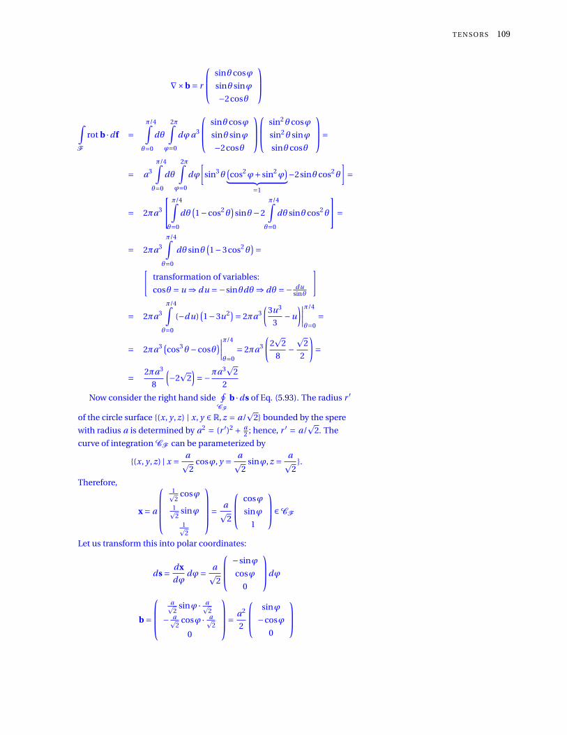
T E N S O R S 109
∇×b = r
sinθcosϕ
sinθ sinϕ
−2cosθ
∫F
rot b ·df =π/4∫
θ=0
dθ
2π∫ϕ=0
dϕa3
sinθcosϕ
sinθ sinϕ
−2cosθ
sin2θcosϕ
sin2θ sinϕ
sinθcosθ
=
= a3
π/4∫θ=0
dθ
2π∫ϕ=0
dϕ
[sin3θ
(cos2ϕ+ sin2ϕ
)︸ ︷︷ ︸=1
−2sinθcos2θ
]=
= 2πa3
π/4∫θ=0
dθ(1−cos2θ
)sinθ−2
π/4∫θ=0
dθ sinθcos2θ
=
= 2πa3
π/4∫θ=0
dθ sinθ(1−3cos2θ
)=[
transformation of variables:
cosθ = u ⇒ du =−sinθdθ⇒ dθ =− dusinθ
]
= 2πa3
π/4∫θ=0
(−du)(1−3u2)= 2πa3
(3u3
3−u
)∣∣∣∣π/4
θ=0=
= 2πa3 (cos3θ−cosθ
)∣∣∣∣π/4
θ=0= 2πa3
(2p
2
8−p
2
2
)=
= 2πa3
8
(−2
p2)=−πa3
p2
2
Now consider the right hand side∮
CF
b ·ds of Eq. (5.93). The radius r ′
of the circle surface (x, y , z) | x, y ∈ R, z = a/p
2 bounded by the spere
with radius a is determined by a2 = (r ′)2 + a2 ; hence, r ′ = a/
p2. The
curve of integration CF can be parameterized by
(x, y , z) | x = ap2
cosϕ, y = ap2
sinϕ, z = ap2
.
Therefore,
x = a
1p2
cosϕ
1p2
sinϕ
1p2
= ap2
cosϕ
sinϕ
1
∈CF
Let us transform this into polar coordinates:
ds = dx
dϕdϕ= ap
2
−sinϕ
cosϕ
0
dϕ
b =
ap2
sinϕ · ap2
− ap2
cosϕ · ap2
0
= a2
2
sinϕ
−cosϕ
0

110 M AT H E M AT I C A L M E T H O D S O F T H E O R E T I C A L P H Y S I C S
Hence the circular integral is given by
∮CF
b ·ds = a2
2
ap2
2π∫ϕ=0
(−sin2ϕ−cos2ϕ)︸ ︷︷ ︸
=−1
dϕ=− a3
2p
22π=−a3πp
2.
c

Part III:
Functional analysis


6
Brief review of complex analysis
The curriculum at the Vienna University of Technology includes complex
analysis and Fourier analysis in the first year, so when taking this course
in the second year, students need just to memorize these subjects. In what
follows, a very brief review of complex analysis will therefore be presented.
For more detailed introductions to complex analysis, take, for instance,
the classical book by Ahlfors 1, among a zillion other very good ones 2. We 1 Lars V. Ahlfors. Complex Analysis: AnIntroduction of the Theory of AnalyticFunctions of One Complex Variable.McGraw-Hill Book Co., New York, thirdedition, 19782 Klaus Jänich. Funktionentheorie.Eine Einführung. Springer, Berlin,Heidelberg, sixth edition, 2008. D O I :10.1007/978-3-540-35015-6. URL10.1007/978-3-540-35015-6; andDietmar A. Salamon. Funktionentheorie.Birkhäuser, Basel, 2012. D O I : 10.1007/978-3-0348-0169-0. URL http://dx.doi.
org/10.1007/978-3-0348-0169-0. seealso URL http://www.math.ethz.ch/ sala-mon/PREPRINTS/cxana.pdf
shall study complex analysis not only for its beauty, but also because it
yields very important analytical methods and tools; mainly for the com-
putation of definite integrals. These methods will then be required for the
computation of distributions and Green’s functions, which will be reviewed
later.
If not mentioned otherwise, it is assumed that the Riemann surface,
representing a “deformed version” of the complex plane for functional
purposes, is simply connected. Simple connectedness means that the
Riemann surface it is path-connected so that every path between two
points can be continuously transformed, staying within the domain, into
any other path while preserving the two endpoints between the paths. In
particular, suppose that there are no “holes” in the Riemann surface; it is
not “punctured.”
Furthermore, let i be the imaginary unit with the property that i 2 = −1
be the solution of the equation x2 +1 = 0. Any complex number z can be
decomposed into real numbers x, y , r and ϕ such that
z =ℜz + iℑz = x + i y = r e iϕ, (6.1)
with x = r cosϕ and y = r sinϕ; where Euler’s formula
e iϕ = cosϕ+ i sinϕ (6.2)
has been used. Note that, in particular, Euler’s identity
e iπ =−1, or e iπ+1 = 0, (6.3)
holds. For many mathematicians this is the “most beautiful” theorem 3. 3 David Wells. Which is the most beau-tiful? The Mathematical Intelligencer,10:30–31, 1988. ISSN 0343-6993. D O I :10.1007/BF03023741. URL http:
//dx.doi.org/10.1007/BF03023741andDavid Wells. Which is the most beau-tiful? The Mathematical Intelligencer,10:30–31, 1988. ISSN 0343-6993. D O I :10.1007/BF03023741. URL http:
//dx.doi.org/10.1007/BF03023741

114 M AT H E M AT I C A L M E T H O D S O F T H E O R E T I C A L P H Y S I C S
Euler’s formula can be used to derive de Moivre’s formula for integer n
(for non-integer n the formula is multi-valued for different arguments ϕ):
e i nϕ = (cosϕ+ i sinϕ)n = cos(nϕ)+ i sin(nϕ). (6.4)
If z =ℜz we call z a real number. If z = iℑz we call z a purely imaginary
number.
6.1 Differentiable, holomorphic (analytic) function
Consider the function f (z) on the domain G ⊂ Domain( f ).
f is called differentiable or at the point z0 if the differential quotient
d f
d z
∣∣∣∣z0
= f ′(z)∣∣
z0= ∂ f
∂x
∣∣∣∣z0
= 1
i
∂ f
∂y
∣∣∣∣z0
(6.5)
exists.
If f is differentiable in the entire domain G it is called holomorphic, or,
used synonymuously, analytic.
6.2 Cauchy-Riemann equations
The function f (z) = u(z)+ i v(z) (where u and v are real valued functions)
is analytic or holomorph if and only if (ab = ∂a/∂b)
ux = vy , uy =−vx . (6.6)
For a proof, differentiate along the real, and then along the complex axis,
taking
f ′(z) = limx→0f (z+x)− f (z)
x = ∂ f∂x = ∂u
∂x + i ∂v∂x , and
f ′(z) = limy→0f (z+i y)− f (z)
i y = ∂ f∂i y =−i ∂ f
∂y =−i ∂u∂y + ∂v
∂y .(6.7)
For f to be analytic, both partial derivatives have to be identical, and thus∂ f∂x = ∂ f
∂i y , or
∂u
∂x+ i
∂v
∂x=−i
∂u
∂y+ ∂v
∂y. (6.8)
By comparing the real and imaginary parts of this equation, one obtains
the two real Cauchy-Riemann equations
∂u∂x = ∂v
∂y ,∂v∂x =− ∂u
∂y .(6.9)
6.3 Definition analytical function

B R I E F R E V I E W O F C O M P L E X A N A LY S I S 115
Since if f is analytic in G , all derivatives of f exist, and all mixed deriva-
tives are independent on the order of differentiations. Then the Cauchy-
Riemann equations imply that
∂∂x
(∂u∂x
)= ∂
∂x
(∂v∂y
)=
∂∂y
(∂v∂x
)=− ∂
∂y
(∂u∂y
), and
∂∂y
(∂u∂x
)= ∂
∂y
(∂v∂y
)=
− ∂∂x
(∂v∂x
)= ∂
∂x
(∂u∂y
),
(6.10)
and thus (∂2
∂x2 + ∂2
∂y2
)u = 0, and
(∂2
∂x2 + ∂2
∂y2
)v = 0 . (6.11)
If f = u + i v is analytic in G , then the lines of constant u and v are
orthogonal.
The tangential vectors of the lines of constant u and v in the two-
dimensional complex plane are defined by the two-dimensional nabla
operator ∇u(x, y) and ∇v(x, y). Since, by the Cauchy-Riemann equations
ux = vy and uy =−vx
∇u(x, y) ·∇v(x, y) =(
ux
uy
)·(
vx
vy
)= ux vx +uy vy = ux vx + (−vx )ux = 0
(6.12)
these tangential vectors are normal.
f is angle (shape) preserving conformal if and only if it is holomorphic
and its derivative is everywhere non-zero.
Consider an analytic function f and an arbitrary path C in the com-
plex plane of the arguments parameterized by z(t ), t ∈ R. The image of C
associated with f is f (C ) =C ′ : f (z(t )), t ∈R.
The tangent vector of C ′ in t = 0 and z0 = z(0) is
dd t f (z(t ))
∣∣∣t=0
= dd z f (z)
∣∣∣z0
dd t z(t )
∣∣∣t=0
=λ0e iϕ0 dd t z(t )
∣∣∣t=0
. (6.13)
Note that the first term dd z f (z)
∣∣∣z0
is independent of the curve C and only
depends on z0. Therefore, it can be written as a product of a squeeze
(stretch) λ0 and a rotation e iϕ0 . This is independent of the curve; hence
two curves C1 and C2 passing through z0 yield the same transformation of
the image λ0e iϕ0 .
6.4 Cauchy’s integral theorem
If f is analytic on G and on its borders ∂G , then any closed line integral of f
vanishes ∮∂G
f (z)d z = 0 . (6.14)
No proof is given here.

116 M AT H E M AT I C A L M E T H O D S O F T H E O R E T I C A L P H Y S I C S
In particular,∮
C⊂∂G f (z)d z is independent of the particular curve, and
only depends on the initial and the end points.
For a proof, subtract two line integral which follow arbitrary paths
C1 and C2 to a common initial and end point, and which have the same
integral kernel. Then reverse the integration direction of one of the line
integrals. According to Cauchy’s integral theorem the resulting integral
over the closed loop has to vanish.
Often it is useful to parameterize a contour integral by some form of
∫C
f (z)d z =∫ b
af (z(t ))
d z(t )
d td t . (6.15)
Let f (z) = 1/z and C : z(ϕ) = Re iϕ, with R > 0 and −π<ϕ≤π. Then
∮|z|=R f (z)d z = ∫ π
−π f (z(ϕ)) d z(ϕ)dϕ dϕ
= ∫ π−π
1Reiϕ R i e iϕdϕ
= ∫ π−π iϕ
= 2πi
(6.16)
is independent of R.
6.5 Cauchy’s integral formula
If f is analytic on G and on its borders ∂G , then
f (z0) = 1
2πi
∮∂G
f (z)
z − z0d z . (6.17)
No proof is given here.
The generalized Cauchy’s integral formula or, by another term, Cauchy’s
differentiation formula states that if f is analytic on G and on its borders
∂G , then =⇒
f (n)(z0) = n!2πi
∮∂G
f (z)
(z − z0)n+1 d z . (6.18)
No proof is given here.
Cauchy’s integral formula presents a powerful method to compute
integrals. Consider the following examples.
(i) For a starter, let us calculate∮|z|=3
3z +2
z(z +1)3 d z.
The kernel has two poles at z = 0 and z = −1 which are both inside the
domain of the contour defined by |z| = 3. By using Cauchy’s integral

B R I E F R E V I E W O F C O M P L E X A N A LY S I S 117
formula we obtain for “small” ε∮|z|=3
3z+2z(z+1)3 d z
= ∮|z|=ε
3z+2z(z+1)3 d z +∮
|z+1|=ε3z+2
z(z+1)3 d z
= ∮|z|=ε
3z+2(z+1)3
1z d z +∮
|z+1|=ε3z+2
z1
(z+1)3 d z
= 2πi0! [[ d 0
d z0 ]] 3z+2(z+1)3
∣∣∣z=0
+ 2πi2!
d 2
d z23z+2
z
∣∣∣z=−1
= 2πi0!
3z+2(z+1)3
∣∣∣z=0
+ 2πi2!
d 2
d z23z+2
z
∣∣∣z=−1
= 4πi −4πi
= 0.
(6.19)
(ii) Consider ∮|z|=3
e2z
(z+1)4 d z
= 2πi3!
3!2πi
∮|z|=3
e2z
(z−(−1))3+1 d z
= 2πi3!
d 3
d z3
∣∣e2z∣∣
z=−1
= 2πi3! 23
∣∣e2z∣∣
z=−1
= 8πi e−2
3 .
(6.20)
Suppose g (z) is a function with a pole of order n at the point z0; that is
g (z) = f (z)
(z − z0)n (6.21)
where f (z) is an analytic function. Then,∮∂G
g (z)d z = 2πi
(n −1)!f (n−1)(z0) . (6.22)
6.6 Laurent series
Every function f which is analytic in a concentric region R1 < |z − z0| < R2
can in this region be uniquely written as a Laurent series
f (z) =∞∑
k=−∞(z − z0)k ak (6.23)
The coefficients ak are (the closed contour C must be in the concentric
region)
ak = 1
2πi
∮C
(χ− z0)−k−1 f (χ)dχ . (6.24)
The coefficient
a−1 = 1
2πi
∮C
f (χ)dχ (6.25)
is called the residue, denoted by “Res.”
No proof is given here.
Note that if g (z) is a function with a pole of order n at the point z0;
that is g (z) = h(z)/(z − z0)n , where h(z) is an analytic function. Then the
terms k ≤−(n +1) vanish in the Laurent series. This follows from Cauchy’s
integral formula
ak = 1
2πi
∮c(χ− z0)−k−n−1h(χ)dχ= 0 (6.26)
für −k −n −1 ≥ 0.

118 M AT H E M AT I C A L M E T H O D S O F T H E O R E T I C A L P H Y S I C S
6.7 Residue theorem
Suppose f is analytic on a simply connected open subset G with the excep-
tion of finitely many (or denumerably many) points zi . Then,∮∂G
f (z)d z = 2πi∑zi
Res f (zi ) . (6.27)
No proof is given here.
The residue theorem presents a powerful tool for calculating integrals,
both real and complex. Let us first mention a rather general case of a situa-
tion often used. Suppose we are interested in the integral
I =∫ ∞
−∞R(x)d x
with rational kernel R,; that is, R(x) = P (x)/Q(x), where P (x) and Q(x)
are polynomials (or can at least be bounded by a polynomial) with no
common root (and therefore factor). Suppose further that the degrees of
the polynomials is
degP (x) ≤ degQ(x)−2.
This condition is needed to assure that the additional upper or lower path
we want to add when completing the contour does not contribute; that is,
vanishes.
Now first let us analytically continue R(x) to the complex plane R(z);
that is,
I =∫ ∞
−∞R(x)d x =
∫ ∞
−∞R(z)d z.
Next let us close the contour by adding a (vanishing) path integral∫x
R(z)d z = 0
in the upper (lower) complex plane
I =∫ ∞
−∞R(z)d z +
∫x
R(z)d z =∮→&x
R(z)d z.
The added integral vanishes because it can be approximated by∣∣∣∣∫xR(z)d z
∣∣∣∣≤ limr→∞
(const.
r 2 πr
)= 0.
With the contour closed the residue theorem can be applied for an
evaluation of I ; that is,
I = 2πi∑zi
ResR(zi )
for all singularities zi in the region enclosed by “→ &x. ”
Let us consider some examples.

B R I E F R E V I E W O F C O M P L E X A N A LY S I S 119
(i) Consider
I =∫ ∞
−∞d x
x2 +1.
The analytic continuation of the kernel and the addition with vanish-
ing a semicircle “far away” closing the integration path in the upper
complex half-plane of z yields
I = ∫ ∞−∞
d xx2+1
= ∫ ∞−∞
d zz2+1
= ∫ ∞−∞
d zz2+1
∫x
d zz2+1
= ∫ ∞−∞
d z(z+i )(z−i ) +
∫x
d z(z+i )(z−i )
= ∮ 1(z−i ) f (z)d z with f (z) = 1
(z+i )
= 2πi Res(
1(z+i )(z−i )
)∣∣∣z=+i
= 2πi f (+i )
= 2πi 1(2i )
=π.
(6.28)
Closing the integration path in the lower complex half-plane of z yields
(note that in this case the contour integral is negative because of the
path orientation)
I = ∫ ∞−∞
d xx2+1
= ∫ ∞−∞
d zz2+1
= ∫ ∞−∞
d zz2+1
∫lower path
d zz2+1
= ∫ ∞−∞
d z(z+i )(z−i ) +
∫lower path
d z(z+i )(z−i )
= ∮ 1(z+i ) f (z)d z with f (z) = 1
(z−i )
= 2πi Res(
1(z+i )(z−i )
)∣∣∣z=−i
=−2πi f (−i )
= 2πi 1(2i )
=π.
(6.29)
(ii) Consider
F (p) =∫ ∞
−∞e i px
x2 +a2 d x
with a 6= 0.
The analytic continuation of the kernel yields
F (p) =∫ ∞
−∞e i pz
z2 +a2 d z =∫ ∞
−∞e i pz
(z − i a)(z + i a)d z.
Suppose first that p > 0. Then, if z = x + i y , e i pz = e i px e−py → 0 for
z →∞ in the upper half plane. Hence, we can close the contour in the
upper half plane and obtain with the help of the residue theorem.
If a > 0 only the pole at z = +i a is enclosed in the contour; thus we
obtainF (p) = 2πi Res ei pz
(z+i a)
∣∣∣z=+i a
= 2πi ei 2 pa
2i a
= πa e−pa .
(6.30)

120 M AT H E M AT I C A L M E T H O D S O F T H E O R E T I C A L P H Y S I C S
If a < 0 only the pole at z = −i a is enclosed in the contour; thus we
obtain
F (p) = 2πi Res ei pz
(z−i a)
∣∣∣z=−i a
= 2πi e−i 2 pa
−2i a
= π−a e−i 2pa
= π−a epa .
(6.31)
Hence, for a 6= 0,
F (p) = π
|a|e−|pa|. (6.32)
For p < 0 a very similar consideration, taking the lower path for con-
tinuation – and thus aquiring a minus sign because of the “clockwork”
orientation of the path as compared to its interior – yields
F (p) = π
|a|e−|pa|. (6.33)
(iii) Not all singularities are “nice” poles. Consider∮|z|=1
e1z d z.
That is, let f (z) = e1z and C : z(ϕ) = Re iϕ, with R = 1 and −π < ϕ ≤ π.
This function is singular only in the origin z = 0, but this is an essential
singularity near which the function exhibits extreme behavior. and can
be expanded into a Laurent series
f (z) = e1z =
∞∑l=0
1
l !
(1
z
)l
around this singularity. In such a case the residue can be found only by
using Laurent series of f (z); that is by comparing its coefficient of the
1/z term. Hence, Res(e
1z
)∣∣∣z=0
is the coefficient 1 of the 1/z term. The
residue is not, with z = e iϕ,
a−1 = Res(e
1z
)∣∣∣z=0
6= 12πi
∮C e
1z d z
= 12πi
∫ π−π e
1eiϕ d z(ϕ)
dϕ dϕ
= 12πi
∫ π−π e
1eiϕ i e iϕdϕ
= 12π
∫ π−π e−eiϕ
e iϕdϕ
= 12π
∫ π−π e−eiϕ+iϕdϕ
= 12π
∫ π−π i d
dϕe−eiϕdϕ
= i2πe−eiϕ
∣∣∣π−π= 0.
(6.34)
Why?

B R I E F R E V I E W O F C O M P L E X A N A LY S I S 121
Thus, by the residue theorem,∮|z|=1
e1z d z = 2πi Res
(e
1z
)∣∣∣z=0
= 2πi . (6.35)
For f (z) = e−1z , the same argument yields Res
(e−
1z
)∣∣∣z=0
=−1 and thus∮|z|=1 e−
1z d z =−2πi .
6.8 Multi-valued relationships, branch points and and branch
cuts
Suppose that the Riemann surface of is not simply connected.
Suppose further that f is a multi-valued function (or multifunction).
An argument z of the function f is called branch point if there is a closed
curve Cz around z whose image f (Cz ) is an open curve. That is, the multi-
function f is discontinuous in z. Intuitively speaking, branch points are the
points where the various sheets of a multifunction come together.
A branch cut is a curve (with ends possibly open, closed, or half-open)
in the complex plane across which an analytic multifunction is discontinu-
ous. Branch cuts are often taken as lines.
6.9 Riemann surface
Suppose f (z) is a multifunction. Then the various z-surfaces on which f (z)
is uniquely defined, together with their connections through branch points
and branch cuts, constitute the Riemann surface of f . The required leafs
are called Riemann sheet.
A point z of the function f (z) is called a branch point of order n if
through it and through the associated cut(s) n + 1 Riemann sheets are
connected.


7
Brief review of Fourier transforms
That complex continuous waveforms or functions are comprised of a num-
ber of harmonics seems to be an idea at least as old as the Pythagoreans. In
physical terms, Fourier analysis 1 attempts to decompose a function into 1 Kenneth B. Howell. Principles of Fourieranalysis. Chapman & Hall/CRC, BocaRaton, London, New York, Washington,D.C., 2001; and Russell Herman. Intro-duction to Fourier and Complex Analysiswith Applications to the Spectral Analysis ofSignals. University of North Carolina Wilm-ington, Wilmington, NC, 2010. URL http:
//people.uncw.edu/hermanr/mat367/
FCABook/Book2010/FTCA-book.pdf.Creative Commons Attribution-NoncommercialShare Alike 3.0 UnitedStates License
its constituent frequencies, known as a frequency spectrum. More formally,
the goal is the expansion of periodic and aperiodic functions into periodic
ones.
A function f is periodic if there exist a period L ∈ R such that, for all x in
the domain of f ,
f (L+x) = f (x). (7.1)
Suppose that a function is periodic in the interval [−L,L] with period
2L. Then, under certain “mild” conditions – that is, f must be piecewise
continuous and have only a finite number of maxima and minima – f can
be decomposed into a Fourier series
f (x) = a0
2+
∞∑n=1
[an cos
(nπx
L
)+bn sin
(nπx
L
)]
an = 1
L
L∫−L
d x f (x)cos(nx) n ≥ 0
bn = 1
L
L∫−L
d x f (x)sin(nx) n > 0
Suppose again that a function is periodic in the interval [−π,π] with pe-
riod 2π. Then, under certain “mild” conditions – that is, f must be piece-
wise continuous and have only a finite number of maxima and minima – f
can be decomposed into
f (x) =∞∑
k=−∞ck e i kx , with ck = 1
2π
∫ π
−πf (x)e−i kx d x. (7.2)
More generally, let f be a periodic function in the interval [−L2,L2] with
period L (we later consider the limit L →∞). Then, with
x → 2π
Lx,

124 M AT H E M AT I C A L M E T H O D S O F T H E O R E T I C A L P H Y S I C S
under similar “mild” conditions as mentioned earlier f can be decom-
posed into a Fourier series
f (x) =∞∑
k=−∞ck e
2πi kxL , with ck = 1
L
∫ 1L
− 1L
f (x)e−i 2πi kxL d x. (7.3)
With the definition k = 2πk/L, Eqs. (7.6) can be combined into
f (x) = 1
L
∞∑k=−∞
∫ 1L
− 1L
f (x ′)e−i k(x′−x)d x ′. (7.4)
Let us compute the Fourier series of
f (x) =−x, für −π≤ x < 0;
+x, für 0 ≤ x ≤π.
f (x) = a0
2+
∞∑n=1
[an cos(nx)+bn sin(nx)
]an = 1
π
π∫−π
d x f (x)cos(nx) n ≥ 0
bn = 1
π
π∫−π
d x f (x)sin(nx) n > 0
f (x) = f (−x); that is, f is an even function of x; hence bn = 0.
n = 0: a0 = 1
π
π∫−π
d x f (x) = 2
π
π∫0
xd x =π.
n > 0:
an = 1
π
π∫−π
f (x)cos(nx)d x = 2
π
π∫0
x cos(nx)d x =
= 2
π
sin(nx)
nx
∣∣∣∣π0−
π∫0
sin(nx)
nd x
= 2
π
cos(nx)
n2
∣∣∣∣π0=
= 2
π
cos(nπ)−1
n2 =− 4
πn2 sin2 nπ
2=
0 for even n
− 4
πn2 for odd n
=⇒ f (x) = π
2− 4
π
(cos x + cos3x
9+ cos5x
25+·· ·
)=
= π
2− 4
π
∞∑n=0
cos[(2n +1)x]
(2n +1)2
Furthermore, define ∆k = 2π/L. Then Eq. (7.4) can be written as
f (x) = 1
2π
∞∑k=−∞
∫ 1L
− 1L
f (x ′)e−i k(x′−x)d x ′∆k. (7.5)

B R I E F R E V I E W O F F O U R I E R T R A N S F O R M S 125
Now, in the “aperiodic” limit L →∞ we obtain the Fourier transformation
f (x) = 12π
∫ ∞−∞
∫ ∞−∞ f (x ′)e−i k(x′−x)d x ′dk, or
f (x) = ∫ ∞−∞ f (k)e i kx dk, and
f (k) = ∫ ∞−∞ f (x)e−i kx d x.
(7.6)
Let us compute the Fourier transform of the Gaussian
f (x) = e−x2.
Hint: e−t 2is analytic in the region −k ≤ Imt ≤ 0; also∫ ∞
−∞d te−t 2 =π1/2 .
f (k) = 1p2π
∞∫−∞
d xe−x2e i kx = (completing the exponent)
= 1p2π
∞∫−∞
d xe−k24 e
−(x− i
2 k)2
Variable transformation: t = x − i
2k =⇒ d t = d x =⇒
f (k) = e−k24p
2π
+∞−i k2∫
−∞−i k2
d te−t 2
-
6
C-
Im t
Re t
− i2 k
-6?
Figure 7.1: Integration path to compute theFourier transform of the Gaussian.
∮C
d te−t 2 =−∞∫
+∞d te−t 2 +
+∞− i2 k∫
−∞− i2 k
d te−t 2 = 0,
because e−t 2is analytic in the region −k ≤ Im t ≤ 0.
=⇒+∞− i
2 k∫−∞− i
2 k
d te−t 2 =+∞∫
−∞d te−t 2
f (k) = 1p2π
e−k24
+∞∫−∞
d te−t 2
︸ ︷︷ ︸pπ
= e−k24p2
.


8
Distributions as generalized functions
In the days when Dirac developed quantum mechanics, there was a need
to define “singular scalar products” such as “⟨x | y⟩ = δ(x − y),” with some
generalization of the Kronecker delta function δi j which is zero whenever
x 6= y and “large enough” needle shaped (see Fig. 8.1) to yield unity when
integrated over the entire reals; that is, “∫ ∞−∞⟨x | y⟩d y = ∫ ∞
−∞δ(x − y)d y = 1.”
6
δ(x)
xFigure 8.1: Dirac’s δ-function as a “needleshaped” generalized function.
6δ(x)
xrrrr r r r r
b
bbb
b
bb b δ1(x)
δ2(x)
δ3(x)
δ4(x)
Figure 8.2: Delta sequence approximatingDirac’s δ-function as a more and more“needle shaped” generalized function.
One of the first attempts to formalize these objects was in terms of
functional limits. Take, for instance, the delta sequence which is a sequence
of strongly peaked functions for which in some limit the sequences fn(x −y) with, for instance,
δn(x − y) =
n for y − 12n < x < y + 1
2n
0 else(8.1)
become the delta function δ(x − y). That is, in the fuctional sense (see
below)
limn→∞δn(x − y) = δ(x − y). (8.2)
Note that the area of this particular δn(x − y) above the x-axes is indepen-
dent of n, since its width is 1/n and the height is n.
Other delta sequences are
δn(x) = npπ
e−n2x2, (8.3)
= 1
π
sin(nx)
x, (8.4)
= = (1∓ i )( n
2π
) 12
e±i nx2(8.5)
= 1
πx
e i nx −e−i nx
2i, (8.6)
= 1
π
ne−x2
1+n2x2 , (8.7)
= 1
2π
∫ n
−ne i xt d t = 1
2πi xe i xt
∣∣∣n
−n, (8.8)
= 1
2π
sin[(
n + 12
)x]
sin( 1
2 x) , (8.9)

128 M AT H E M AT I C A L M E T H O D S O F T H E O R E T I C A L P H Y S I C S
= 1
π
n
1+n2x2 , (8.10)
= n
π
(sin(nx)
nx
)2
. (8.11)
Other commonly used limit forms of the δ-function are the Gaussian,
Lorentzian, and Dirichlet forms
δε(x) = limε→0
1pπε
e−x2
ε2 , (8.12)
= limε→0
1
π
ε
x2 +ε2 , (8.13)
= limε→0
1
πxsinεx, (8.14)
respectively. Again, the limit
δ(x) = limε→0
δε(x) (8.15)
has to be understood in the functional sense (see below).
Naturally, such “needle shaped functions” were viewed suspiciouly
by many mathematicians at first, but later they embraced these types of
functions 1 by developing a theory of functional analysis or distributions. 1 I. M. Gel’fand and G. E. Shilov. Gener-alized Functions. Vol. 1: Properties andOperations. Academic Press, New York,1964. Translated from the Russian byEugene Saletan
Distributions q are quasi-functions of one or more variables which can
be interpreted in the “weak sense” as functionals; that is, by integrating
them with suitable, “good” test functions ϕ of the class D of test functions
F (ϕ) =∫ ∞
−∞q(x)ϕ(x)d x. (8.16)
Recall that a functional is some mathematical entity which maps a func-
tion or another mathematical object into scalars in a linear manner; that
is,
F (c1ϕ1 + c2ϕ2) = c1F (ϕ1)+ c2F (c2ϕ2ϕ2). (8.17)
In particular, the δ function maps to
F (ϕ) =∫ ∞
−∞δ(x − y)ϕ(x)d x =ϕ(y). (8.18)
Let us see if the sequence δn with
δn(x − y) =
n for y − 12n < x < y + 1
2n
0 else
defined in Eq. (8.1) and depicted in Fig. 8.2 is a delta sequence; that is, if,
for large n, it converges to δ in a functional sense. In order to verify this
claim, we have to integrate δn(x) with “good” test functions ϕ(x) and take
the limit n →∞; if the result is ϕ(0), then we can identify δn(x) in this limit
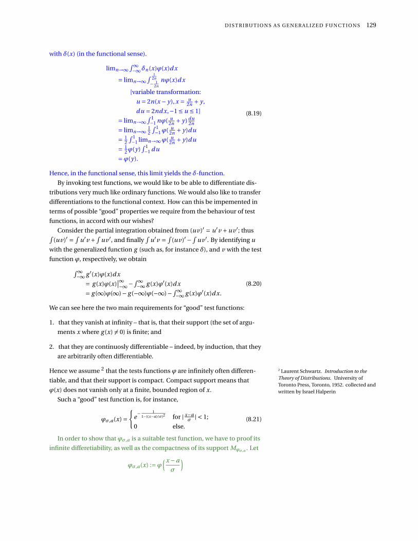
D I S T R I BU T I O N S A S G E N E R A L I Z E D F U N C T I O N S 129
with δ(x) (in the functional sense).
limn→∞∫ ∞−∞δn(x)ϕ(x)d x
= limn→∞∫ 1
2n
− 12n
nϕ(x)d x
[variable transformation:
u = 2n(x − y), x = u2n + y ,
du = 2nd x,−1 ≤ u ≤ 1]
= limn→∞∫ 1−1 nϕ( u
2n + y) du2n
= limn→∞ 12
∫ 1−1ϕ( u
2n + y)du
= 12
∫ 1−1 limn→∞ϕ( u
2n + y)du
= 12ϕ(y)
∫ 1−1 du
=ϕ(y).
(8.19)
Hence, in the functional sense, this limit yields the δ-function.
By invoking test functions, we would like to be able to differentiate dis-
tributions very much like ordinary functions. We would also like to transfer
differentiations to the functional context. How can this be impemented in
terms of possible “good” properties we require from the behaviour of test
functions, in accord with our wishes?
Consider the partial integration obtained from (uv)′ = u′v +uv ′; thus∫(uv)′ = ∫
u′v + ∫uv ′, and finally
∫u′v = ∫
(uv)′− ∫uv ′. By identifying u
with the generalized function g (such as, for instance δ), and v with the test
function ϕ, respectively, we obtain∫ ∞−∞ g ′(x)ϕ(x)d x
= g (x)ϕ(x)∣∣∞−∞−∫ ∞
−∞ g (x)ϕ′(x)d x
= g (∞)ϕ(∞)− g (−∞)ϕ(−∞)−∫ ∞−∞ g (x)ϕ′(x)d x.
(8.20)
We can see here the two main requirements for “good” test functions:
1. that they vanish at infinity – that is, that their support (the set of argu-
ments x where g (x) 6= 0) is finite; and
2. that they are continuosly differentiable – indeed, by induction, that they
are arbitrarily often differentiable.
Hence we assume 2 that the tests functions ϕ are infinitely often differen- 2 Laurent Schwartz. Introduction to theTheory of Distributions. University ofToronto Press, Toronto, 1952. collected andwritten by Israel Halperin
tiable, and that their support is compact. Compact support means that
ϕ(x) does not vanish only at a finite, bounded region of x.
Such a “good” test function is, for instance,
ϕσ,a(x) =
e− 1
1−((x−a)/σ)2 for | x−aσ | < 1;
0 else.(8.21)
In order to show that ϕσ,a is a suitable test function, we have to proof its
infinite differetiability, as well as the compactness of its support Mϕσ,a . Let
ϕσ,a(x) :=ϕ( x −a
σ
)

130 M AT H E M AT I C A L M E T H O D S O F T H E O R E T I C A L P H Y S I C S
and thus
ϕ(x) =
e−1
1−x2 for |x| < 1
0 for |x| ≥ 1
This function is drawn in Fig. 8.3.
0.37
−1 1
ϕ(x)
Figure 8.3: Plot of a test function ϕ(x).
First, note, by definition, the support Mϕ = (−1,1), because ϕ(x) van-
ishes outside (−1,1)).
Second, consider the differentiability of ϕ(x); that is ϕ ∈ C∞(R)? Note
that ϕ(0) =ϕ is continuous; and that ϕ(n) is of the form
ϕ(n)(x) =
Pn (x)(x2−1)2n e
1x2−1 for |x| < 1
0 for |x| ≥ 1,
where Pn(x) is a finite polynomial in x (ϕ(u) = eu =⇒ ϕ′(u) = dϕdu
dud x2
d x2
d x =ϕ(u)
(− 1
(x2−1)2
)2x etc.) and [x = 1−ε] =⇒ x2 = 1−2ε+ε2 =⇒ x2−1 = ε(ε−2)
limx↑1
ϕ(n)(x) = limε↓0
Pn(1−ε)
ε2n(ε−2)2n e1
ε(ε−2) =
= limε↓0
Pn(1)
ε2n22n e−1
2ε =[ε= 1
R
]= lim
R→∞Pn(1)
22n R2ne−R2 = 0,
because the power e−x of e decreases stronger than any polynomial xn .
Note that the complex continuation ϕ(z) is not an analytic function
and cannot be expanded as a Taylor series on the entire complex plane C
although it is infinitely often differentiable on the real axis; that is, although
ϕ ∈ C∞(R). This can be seen from a uniqueness theorem of complex anal-
ysis. Let B ⊆ C be a domain, and let z0 ∈ B the limit of a sequence zn ∈ B ,
zn 6= z0. Then it can be shown that, if two analytic functions f und g on B
coincide in the points zn , then they coincide on the entire domain B .
Not, take B = R and the vanishing analytic function f ; that is, f (x) = 0.
f (x) coincides with ϕ(x) only in R/Mϕ. As a result, ϕ cannot be analytic.
Indeed, ϕσ,~a(x) diverges at x = a ±σ. Hence ϕ(x) cannot be Taylor ex-
panded, and
C∞(Rk )6=⇒⇐=analytic function (‘C∞(Ck )’)
Other “good” test function are 3 3 Laurent Schwartz. Introduction to theTheory of Distributions. University ofToronto Press, Toronto, 1952. collected andwritten by Israel Halperin
φc,d (x)
1n (8.22)
obtained by choosing n ∈N−0 and a ≤ c < d ≤ b and by defining
φc,d (x) =
e−( 1
x−c + 1d−x
)for c < x < d , and
0 else.(8.23)
If ϕ(x) is a “good” test functen, then
xαPn(x)ϕ(x) (8.24)

D I S T R I BU T I O N S A S G E N E R A L I Z E D F U N C T I O N S 131
with any Polynomial Pn(x), and in particular xnϕ(x) also is a “good” test
function.
Equipped with “good” test functions which have a finite support and are
infinitely often differentiable, we can now give meaning to the transference
of differential quotients from the objects entering the integral towards the
test function by partial integration. First note again that (uv)′ = u′v +uv ′
and thus∫
(uv)′ = ∫u′v +∫
uv ′ and finally∫
u′v = ∫(uv)′−∫
uv ′. Hence, by
identifying u with g , and v with the test function ϕ, we obtain
F ′(ϕ) := ∫ ∞−∞
(d
d x q(x))ϕ(x)d x
= q(x)ϕ(x)∣∣∞
x=−∞−∫ ∞−∞ q(x)
(d
d xϕ(x))
d x
=−∫ ∞−∞ q(x)
(d
d xϕ(x))
d x
=−F (ϕ′).
(8.25)
By induction we obtain
F (n)(ϕ) =∫ ∞
−∞
(d n
d xn q(x)
)ϕ(x)d x = (−1)nF (ϕ(n)) = F ((−1)nϕ(n)). (8.26)
8.1 Heaviside step function
One of the possible definitions of the Heaviside step function H(x), and
maybe the most common one – they differ in the value H(0)of at the origin
x = 0, a difference which is irrelevant measure theoretically for “good”
functions since it is only about an isolated point – is
H(x −x0) =
1 for x ≥ x0
0 for x < x0(8.27)
It is plotted in Fig. 8.4.
xb
rH(x)
Figure 8.4: Plot of the Heaviside stepfunction H(x).
It is also very common to define the Heaviside step function as the
integral of the δ function; likewise the delta function is the derivative of the
Heaviside step function; that is,
H(x −x0) = ∫ x−x0−∞ δ(t )d t ,
dd x H(x −x0) = δ(x −x0).
(8.28)
In the spirit of the above definition, it might have been more appropriate to
define H(0) = 12 ; that is,
H(x −x0) =
1 for x > x012 for x = x0
0 for x < x0
(8.29)
and, since this affects only an isolated point at x = 0, we may happily do so
if we prefer.

132 M AT H E M AT I C A L M E T H O D S O F T H E O R E T I C A L P H Y S I C S
The latter equation can – in the sense of functionals – be proved through
integration by parts as follows. Take∫ ∞−∞
[d
d x H(x −x0)]ϕ(x)d x
= H(x −x0)ϕ(x)∣∣∞−∞−∫ ∞
−∞ H(x −x0)[
dd xϕ(x)
]d x
= H(−∞)ϕ(−∞)−ϕ(+∞)−∫ ∞x0
[d
d xϕ(x)]
d x
=−∫ ∞x0
[d
d xϕ(x)]
d x
=− ϕ(x)∣∣∞
x0
=−[ϕ(∞)−ϕ(x0)]
=ϕ(x0).
(8.30)
Some other formulae involving the Heaviside step function are
H(±x) = limε→0+
∓i
2π
∫ +∞
−∞e i kx
k ∓ iεdk, (8.31)
and
H(x) = 1
2+
∞∑l=0
(−1)l (2l )!(4l +3)
22l+2l !(l +1)!P2l+1(x), (8.32)
where P2l+1(x) is a Legendre polynomial. Furthermore,
δ(x) = limε→0
1
εH
( ε2−|x|
). (8.33)
An integral representation of H(x) is
H(x) = limε ↓ 0+∓ 1
2πi
∫ ∞
−∞1
t ± iεe∓i xt d t . (8.34)
One commonly used limit form of the Heaviside step function is
H(x) = limε→0
Hε(x) = limε→0
1
πx
[π2+ tan−1 x
ε
]. (8.35)
respectively.
Another limit representation is by a variant of the sine integral function
Si(x) = ∫ x0 (sin t )/t d t as follows 4 4 Eli Maor. Trigonometric Delights. Prince-
ton University Press, Princeton, 1998. URLhttp://press.princeton.edu/books/
maor/H(x) = limt→∞ Ht (x)
= limn→∞ 2π
∫ n0
sin(kx)x d x
= 2π
∫ ∞0
sin(kx)x d x.
(8.36)
8.2 The sign function
The sign function is defined by
sgn(x −x0) =
−1 forx < x0
0 forx = x0
+1 forx > x0
. (8.37)
It is plotted in Fig. 8.5.
x
b
r
bsgn(x)
Figure 8.5: Plot of the sign function sgn(x).
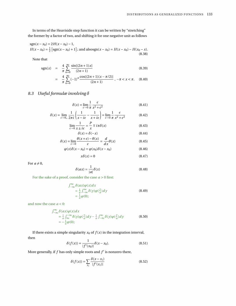
D I S T R I BU T I O N S A S G E N E R A L I Z E D F U N C T I O N S 133
In terms of the Heaviside step function it can be written by “stretching”
the former by a factor of two, and shifting it for one negative unit as follows
sgn(x −x0) = 2H(x −x0)−1,
H(x −x0) = 12
[sgn(x −x0)+1
]; and alsosgn(x −x0) = H(x −x0)−H(x0 −x).
(8.38)
Note that
sgn(x) = 4
π
∞∑n=0
sin[(2n +1)x]
(2n +1)(8.39)
= 4
π
∞∑n=0
(−1)n cos[(2n +1)(x −π/2)]
(2n +1), −π< x <π. (8.40)
8.3 Useful formulæ involving δ
δ(x) = limε→0
1
π
ε
x2 +ε2 (8.41)
δ(x) = limε→0+
1
2πi
(1
x − iε− 1
x + iε
)= limε→0
1
π
ε
x2 +ε2 (8.42)
limε→0
1
x ± iε= P
x∓ iπδ(x) (8.43)
δ(x) = δ(−x) (8.44)
δ(x) = limε→0
θ(x +ε)−θ(x)
ε= d
d xθ(x) (8.45)
ϕ(x)δ(x −x0) =ϕ(x0)δ(x −x0) (8.46)
xδ(x) = 0 (8.47)
For a 6= 0,
δ(ax) = 1
|a|δ(x) (8.48)
For the sake of a proof, consider the case a > 0 first:∫ ∞−∞δ(ax)ϕ(x)d x
= 1a
∫ ∞−∞δ(y)ϕ( y
a )d y
= 1aϕ(0);
(8.49)
and now the case a < 0:∫ ∞−∞δ(ax)ϕ(x)d x
= 1a
∫ −∞∞ δ(y)ϕ( y
a )d y − 1a
∫ ∞−∞δ(y)ϕ( y
a )d y
=− 1aϕ(0);
(8.50)
If there exists a simple singularity x0 of f (x) in the integration interval,
then
δ( f (x)) = 1
| f ′(x0)|δ(x −x0). (8.51)
More generally, if f has only simple roots and f ′ is nonzero there,
δ( f (x)) =∑xi
δ(x −xi )
| f ′(xi )| (8.52)

134 M AT H E M AT I C A L M E T H O D S O F T H E O R E T I C A L P H Y S I C S
where the sum extends over all simple roots xi in the integration interval.
In particular,
δ(x2 −x20) = 1
2|x0|[δ(x −x0)+δ(x +x0)] (8.53)
For a proof, note that, since f has only simpleroots, it can be expanded
around these roots by
f (x) ≈ (x −x0) f ′(x0)
with nonzero f ′(x0) ∈R. By identifying f ′(x0) with a in Eq. (8.48) we obtain
Eq. (8.52).
δ′( f (x)) =N∑
i=0
f ′′(xi )
| f ′(xi )|3 δ(x −xi )+N∑
i=0
f ′(xi )
| f ′(xi )|3 δ′(x −xi ) (8.54)
|x|δ(x2) = δ(x) (8.55)
−xδ′(x) = δ(x) (8.56)
δ(m)(x) = (−1)mδ(m)(−x), (8.57)
where the index (m) denotes m–fold differentiation;
xm+1δ(m)(x) = 0, (8.58)
where the index (m) denotes m–fold differentiation;
x2δ′(x) = 0 (8.59)
δ(x) = d 2
d x2 [xθ(x)] (8.60)
If δ3(~r ) = δ(x)δ(y)δ(r ) with~r = (x, y , z), then
δ3(~r ) = δ(x)δ(y)δ(z) =− 1
4π∆
1
r(8.61)
δ3(~r ) =− 1
4π(∆+k2)
e i kr
r(8.62)
δ3(~r ) =− 1
4π(∆+k2)
coskr
r(8.63)
In quantum field theory, phase space integrals of the form
1
2E=
∫d p0θ(p0)δ(p2 −m2) (8.64)
if E = (~p2 +m2)(1/2) are exploited.

D I S T R I BU T I O N S A S G E N E R A L I Z E D F U N C T I O N S 135
8.4 Fourier transforms of δ and H
If fx (x) is a sequence of functions converging, for n →∞ toward a func-
tion f in the functional sense (i.e. via integration of fn and f with “good”
test functions), then the Fourier transform f of f can be defined by 5 5 M. J. Lighthill. Introduction to FourierAnalysis and Generalized Functions. Cam-bridge University Press, Cambridge, 1958;and Kenneth B. Howell. Principles ofFourier analysis. Chapman & Hall/CRC,Boca Raton, London, New York, Washing-ton, D.C., 2001
f (k) = limn→∞∫ ∞−∞ fn(x)e−i kx d x. (8.65)
Since e−i kx is not a particularly “good” function, f needs not be an ordi-
nary function 6.6 B.L. Burrows and D.J. Colwell. TheFourier transform of the unit step func-tion. International Journal of Math-ematical Education in Science andTechnology, 21(4):629–635, 1990. D O I :10.1080/0020739900210418. URL http://
dx.doi.org/10.1080/0020739900210418
The Fourier transform of the δ-function can be obtained by insertion
into Eq. (7.6)
δ(k) = ∫ ∞−∞δ(x)e−i kx d x
= e−i 0k∫ ∞−∞δ(x)d x
= 1.
(8.66)
That is, the Fourier transform of the δ-function is just a constant. δ-spiked
signals carry all frequencies in them.
The Fourier transform of the Heaviside step function can also be ob-
tained by insertion into Eq. (7.6)
H(k) = ∫ ∞−∞ H(x)e−i kx d x
= 12
[δ(k)− i
πk
].
(8.67)
A caveat first: the following proof should not be understood in the usual
functional, but rather in a functional sense.
H(k) = ∫ ∞−∞ H(x)e−i kx d x
= ∫ ∞0 e−i kx d x;
H(−k) = ∫ ∞−∞ H(x)e+i kx d x
= ∫ ∞0 H(x)e+i kx d x
[variable transformation: x →−x]
=−∫ −∞0 e−i kx d x
= ∫ 0−∞ e−i kx d x.
(8.68)
Now separate the even part E from the odd part O of H ; that is, define
E(k) = (H(k)+H(−k))
= ∫ +∞−∞ e−i kx d x,
O(k) = (H(k)−H(−k))
= ∫ ∞0
[e−i kx −e+i kx
]d x,
=−2i∫ ∞
0 sin(kx)d x,
H(k) = 12 (E(k)+O(k)).
(8.69)
The two integrals defining E and O do not converge. However, one may
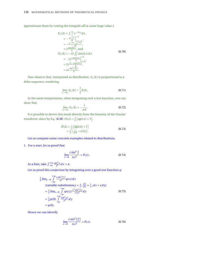
136 M AT H E M AT I C A L M E T H O D S O F T H E O R E T I C A L P H Y S I C S
approximate them by cutting the integrals off at some large value L
EL(k) = ∫ +L−L e−i kx d x,
= − e−i kx
i k
∣∣∣+L
x=−L,
=− e−i kL−e+i kL
i k ,
= 2 sin(kL)k , and
OL(k) =−2i∫ L
0 sin(kx)d x
= −2i cos(kx)k
∣∣∣+L
x=0,
= 2i [1−cos(kL)]k ,
= 4isin2( kL
2 )k .
(8.70)
Now observe that, interpreted as distribution, EL(k) is proportional to a
delta sequence, rendering
limL→∞
EL(k) = 1
2δ(k). (8.71)
In the same intepretation, when integrating over a test function, one can
show that
limL→∞
OL(k) =− i
πk. (8.72)
It is possible to derive this result directly from the linearity of the Fourier
transform: since by Eq. (8.38) H(x) = 12
[sgn(x)+1
],
H(k) = 12
[sgn(k)+ 1
]= 1
2
[ 1iπk +δ(k)
].
(8.73)
Let us compute some concrete examples related to distributions.
1. For a start, let us proof that
limε→0
εsin2 xε
πx2 = δ(x). (8.74)
As a hint, take∫ +∞−∞
sin2 xx2 d x =π.
Let us proof this conjecture by integrating over a good test function ϕ
1π limε→0
+∞∫−∞
εsin2( xε
)x2 ϕ(x)d x
[variable substitutiony = xε , d y
d x = 1ε ,d x = εd y]
= 1π limε→0
+∞∫−∞
ϕ(εy) ε2 sin2(y)ε2 y2 d y
= 1πϕ(0)
+∞∫−∞
sin2(y)y2 d y
=ϕ(0).
(8.75)
Hence we can identify
limε→0
εsin2( xε
)πx2 = δ(x). (8.76)

D I S T R I BU T I O N S A S G E N E R A L I Z E D F U N C T I O N S 137
2. In order to prove that 1π
ne−x2
1+n2x2 is a δ-sequence we proceed again by
integrating over a good test function ϕ, and with the hint that+∞∫−∞
d x/(1+x2) =π we obtain
limn→∞ 1π
+∞∫−∞
ne−x2
1+n2x2ϕ(x)d x
[variable substitutiony = xn, x = yn , d y
d x = n,d x = d yn ]
= limn→∞ 1π
+∞∫−∞
ne−
( yn
)2
1+y2 ϕ( y
n
) d yn
= 1π
+∞∫−∞
limn→∞[
e−( y
n
)2
ϕ( y
n
)] 11+y2 d y
= 1π
+∞∫−∞
[e0ϕ (0)
] 11+y2 d y
= ϕ(0)π
+∞∫−∞
11+y2 d y
= ϕ(0)π π
=ϕ (0) .
(8.77)
Hence we can identify
limn→∞
1
π
ne−x2
1+n2x2 = δ(x). (8.78)
3. Let us proof that xnδ(n)(x) = Cδ(x) and determine the constant C . We
proceed again by integrating over a good test function ϕ. First note that
if ϕ(x) is a good test function, then so is xnϕ(x).∫d xxnδ(n)(x)ϕ(x) =
∫d xδ(n)(x)
[xnϕ(x)
]== (−1)n
∫d xδ(x)
[xnϕ(x)
](n) =
= (−1)n∫
d xδ(x)[nxn−1ϕ(x)+xnϕ′(x)
](n−1) =·· ·
= (−1)n∫
d xδ(x)
[n∑
k=0
(n
k
)(xn)(k)ϕ(n−k)(x)
]=
= (−1)n∫
d xδ(x)[n!ϕ(x)+n ·n!xϕ′(x)+·· ·+xnϕ(n)(x)
]== (−1)nn!
∫d xδ(x)ϕ(x);
hence, C = (−1)nn!. Note that ϕ(x) is a good test function then so is
xnϕ(x).
4. Let us simplify∫ ∞−∞δ(x2 −a2)g (x) d x. First recall Eq. (8.52) stating that
δ( f (x)) =∑i
δ(x −xi )
| f ′(xi )| ,
whenever xi are simple roots of f (x), and f ′(xi ) 6= 0. In our case, f (x) =x2 −a2 = (x −a)(x +a), and the roots are x =±a. Furthermore,
f ′(x) = (x −a)+ (x +a);

138 M AT H E M AT I C A L M E T H O D S O F T H E O R E T I C A L P H Y S I C S
hence
| f ′(a)| = 2|a|, | f ′(−a)| = |−2a| = 2|a|.
As a result,
δ(x2 −a2) = δ((x −a)(x +a)
)= 1
|2a|(δ(x −a)+δ(x +a)
).
Taking this into account we finally obtain
+∞∫−∞
δ(x2 −a2)g (x)d x
=+∞∫−∞
δ(x−a)+δ(x+a)2|a| g (x)d x
= g (a)+g (−a)2|a| .
(8.79)
5. Let us evaluate
I =∫ ∞
−∞
∫ ∞
−∞
∫ ∞
−∞δ(x2
1 +x22 +x2
3 −R2)d 3x (8.80)
for R ∈R,R > 0. We may, of course, remain tn the standard ccartesian co-
ordinate system and evaluate the integral by “brute force.” Alternatively,
a more elegant way is to use the spherical symmetry of the problem and
use spherical coordinates r ,Ω(θ,ϕ) by rewriting I into
I =∫
r ,Ωr 2δ(r 2 −R2)dΩdr . (8.81)
As the integral kernel δ(r 2 −R2) just depends on the radial coordinate
r the angular coordinates just integrate to 4π. Next we make use of Eq.
(8.52), eliminate the solution for r =−R, and obtain
I = 4π∫ ∞
0 r 2δ(r 2 −R2)dr
= 4π∫ ∞
0 r 2 δ(r+R)+δ(r−R)2R dr
= 4π∫ ∞
0 r 2 δ(r−R)2R dr
= 2πR.
(8.82)
6. Let us compute∫ ∞
−∞
∫ ∞
−∞δ(x3 − y2 +2y)δ(x + y)H(y −x −6) f (x, y)d x d y . (8.83)
First, in dealing with δ(x + y), we evaluate the y integration at x =−y or
y =−x:∞∫
−∞δ(x3 −x2 −2x)H(−2x −6) f (x,−x)d x
Use of Eq. (8.52)
δ( f (x)) =∑i
1
| f ′(xi )|δ(x −xi ),

D I S T R I BU T I O N S A S G E N E R A L I Z E D F U N C T I O N S 139
at the roots
x1 = 0
x2,3 = 1±p1+8
2= 1±3
2=
2
−1
of the argument f (x) = x3 − x2 −2x = x(x2 − x −2) = x(x −2)(x +1) of the
remaining δ-function, together with
f ′(x) = d
d x(x3 −x2 −2x) = 3x2 −2x −2;
yields
∞∫−∞
d xδ(x)+δ(x −2)+δ(x +1)
|3x2 −2x −2| H(−2x −6) f (x,−x) =
= 1
|−2| H(−6)︸ ︷︷ ︸= 0
f (0,−0)+ 1
|12−4−2| H(−4−6)︸ ︷︷ ︸= 0
f (2,−2)+
+ 1
|3+2−2| H(2−6)︸ ︷︷ ︸= 0
f (−1,1)
= 0
7. When simplifying derivativs of generalized functions it is always use-
ful to evaluate their properties – such as xδ(x) = 0, f (x)δ(x − x0) =f (x0)δ(x − x0), or δ(−x) = δ(x) – first and before proceeding with the
next differentiation or evaluation. We shall present some applications of
this “rule” next.
First, simplify (d
d x−ω
)H(x)eωx (8.84)
as followsd
d x [H(x)eωx ]−ωH(x)eωx
= δ(x)eωx +ωH(x)eωx −ωH(x)eωx
= δ(x)e0
= δ(x)
(8.85)
8. Next, simplify (d 2
d x2 +ω2)
1
ωH(x)sin(ωx) (8.86)
as follows
d 2
d x2
[ 1ωH(x)sin(ωx)
]+ωH(x)sin(ωx)
= 1ω
dd x
[δ(x)sin(ωx)︸ ︷︷ ︸
= 0
+ωH(x)cos(ωx)]+ωH(x)sin(ωx)
= 1ω
[ωδ(x)cos(ωx)︸ ︷︷ ︸
δ(x)
−ω2H(x)sin(ωx)]+ωH(x)sin(ωx) = δ(x)
(8.87)

140 M AT H E M AT I C A L M E T H O D S O F T H E O R E T I C A L P H Y S I C S
9. Let us compute the nth derivative of
f (x) =
0, für x < 0;
x, für 0 ≤ x ≤ 1;
0, für x > 1.
(8.88)
`pp
10x
f (x)
``p p
10x
f1(x)
f1(x) = H(x)−H(x −1)= H(x)H(1−x)
f2(x)
x
f2(x) = x
Figure 8.6: Composition of f (x)
As depicted in Fig. 8.6, f can be composed from two functions f (x) =f2(x) · f1(x); and this composition can be done in at least two ways.
Decomposition (i)
f (x) = x[H(x)−H(x −1)
]= xH(x)−xH(x −1)
f ′(x) = H(x)+xδ(x)−H(x −1)−xδ(x −1)
Because of xδ(x −a) = aδ(x −a),
f ′(x) = H(x)−H(x −1)−δ(x −1)
f ′′(x) = δ(x)−δ(x −1)−δ′(x −1)
and hence by induction
f (n)(x) = δ(n−2)(x)−δ(n−2)(x −1)−δ(n−1)(x −1)
for n > 1.
Decomposition (ii)
f (x) = xH(x)H(1−x)
f ′(x) = H(x)H(1−x)+xδ(x)︸ ︷︷ ︸= 0
H(1−x)+xH(x)(−1)δ(1−x)︸ ︷︷ ︸−H(x)δ(1−x)
=
= H(x)H(1−x)−δ(1−x) = [δ(x) = δ(−x)] = H(x)H(1−x)−δ(x −1)
f ′′(x) = δ(x)H(1−x)︸ ︷︷ ︸= δ(x)
+ (−1)H(x)δ(1−x)︸ ︷︷ ︸−δ(1−x)
−δ′(x −1) =
= δ(x)−δ(x −1)−δ′(x −1)
and hence by induction
f (n)(x) = δ(n−2)(x)−δ(n−2)(x −1)−δ(n−1)(x −1)
for n > 1.
10. Let us compute the nth derivative of
f (x) = |sin x|, for −π≤ x ≤π;
0, for |x| >π.(8.89)
f (x) = |sin x|H(π+x)H(π−x)
|sin x| = sin x sgn(sin x) = sin x sgn x für −π< x <π;

D I S T R I BU T I O N S A S G E N E R A L I Z E D F U N C T I O N S 141
hence we start from
f (x) = sin x sgn xH(π+x)H(π−x),
Note that
sgn x = H(x)−H(−x),
( sgn x)′ = H ′(x)−H ′(−x)(−1) = δ(x)+δ(−x) = δ(x)+δ(x) = 2δ(x).
f ′(x) = cos x sgn xH(π+x)H(π−x)+ sin x2δ(x)H(π+x)H(π−x)++sin x sgn xδ(π+x)H(π−x)+ sin x sgn xH(π+x)δ(π−x)(−1) =
= cos x sgn xH(π+x)H(π−x)
f ′′(x) = −sin x sgn xH(π+x)H(π−x)+cos x2δ(x)H(π+x)H(π−x)++cos x sgn xδ(π+x)H(π−x)+cos x sgn xH(π+x)δ(π−x)(−1) =
= −sin x sgn xH(π+x)H(π−x)+2δ(x)+δ(π+x)+δ(π−x)
f ′′′(x) = −cos x sgn xH(π+x)H(π−x)− sin x2δ(x)H(π+x)H(π−x)−−sin x sgn xδ(π+x)H(π−x)− sin x sgn xH(π+x)δ(π−x)(−1)++2δ′(x)+δ′(π+x)−δ′(π−x) =
= −cos x sgn xH(π+x)H(π−x)+2δ′(x)+δ′(π+x)−δ′(π−x)
f (4)(x) = sin x sgn xH(π+x)H(π−x)−cos x2δ(x)H(π+x)H(π−x)−−cos x sgn xδ(π+x)H(π−x)−cos x sgn xH(π+x)δ(π−x)(−1)++2δ′′(x)+δ′′(π+x)+δ′′(π−x) =
= sin x sgn xH(π+x)H(π−x)−2δ(x)−δ(π+x)−δ(π−x)++2δ′′(x)+δ′′(π+x)+δ′′(π−x);
hence
f (4) = f (x)−2δ(x)+2δ′′(x)−δ(π+x)+δ′′(π+x)−δ(π−x)+δ′′(π−x),
f (5) = f ′(x)−2δ′(x)+2δ′′′(x)−δ′(π+x)+δ′′′(π+x)+δ′(π−x)−δ′′′(π−x);
and thus by induction
f (n) = f (n−4)(x)−2δ(n−4)(x)+2δ(n−2)(x)−δ(n−4)(π+x)++δ(n−2)(π+x)+ (−1)n−1δ(n−4)(π−x)+ (−1)nδ(n−2)(π−x)
(n = 4,5,6, . . .)
b


9
Green’s function
This chapter marks the beginning of a series of chapters dealing with
the solution to differential equations of theoretical physics. Very often,
these differential equations are linear; that is, the “sought after” function
Ψ(x), y(x),φ(t ) et cetera occur only as a polynomial of degree zero and one,
and not of any higher degree, such as, for instance, [y(x)]2.
9.1 Elegant way to solve linear differential equations
Green’s function present a very elegant way of solving linear differential
equations of the form
Lx y(x) = f (x), with the differential operator
Lx = an(x) d n
d xn +an−1(x) d n−1
d xn−1 + . . .+a1(x) dd x +a0(x)
=∑nj=0 a j (x) d j
d x j ,
(9.1)
where ai (x), 0 ≤ i ≤ n are functions of x. The idea is quite straightfor-
ward: if we are able to obtain the “inverse” G of the differential operator L
defined by
LxG(x, x ′) = δ(x −x ′), (9.2)
with δ representing Dirac’s delta function, then the solution to the in-
homogenuous differential equation (9.1) can be obtained by integrating
G(x −x ′) alongside with the inhomogenuous term f (x ′); that is,
y(x) = ∫ ∞−∞G(x, x ′) f (x ′)d x ′. (9.3)
This claim, as posted in Eq. (9.3), can be verified by explicitly applying the
differential operator Lx to the solution y(x),
Lx y(x)
=Lx∫ ∞−∞G(x, x ′) f (x ′)d x ′
= ∫ ∞−∞LxG(x −x ′) f (x ′)d x ′
= ∫ ∞−∞δ(x −x ′) f (x ′)d x ′
= f (x).
(9.4)
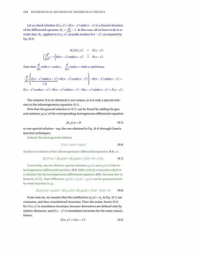
144 M AT H E M AT I C A L M E T H O D S O F T H E O R E T I C A L P H Y S I C S
Let us check whether G(x, x ′) = θ(x − x ′)sinh(x − x ′) is a Green’s function
of the differential operator Lx = d 2
d x2 −1. In this case, all we have to do is to
verify that Lx , applied to G(x, x ′), actually renders δ(x − x ′), as required by
Eq. (9.2).
LxG(x, x ′) = δ(x −x ′)(d 2
d x2 −1
)Θ(x −x ′)sinh(x −x ′) ?= δ(x −x ′)
Note thatd
d xsinh x = cosh x,
d
d xcosh x = sinh x; and hence
d
d x
δ(x −x ′)sinh(x −x ′)︸ ︷︷ ︸= 0
+Θ(x −x ′)cosh(x −x ′)
−Θ(x −x ′)sinh(x −x ′) =
δ(x−x ′)cosh(x−x ′)+Θ(x−x ′)sinh(x−x ′)−Θ(x−x ′)sinh(x−x ′) = δ(x−x ′).
The solution (9.4) so obtained is not unique, as it is only a special solu-
tion to the inhomogenuous equation (9.1).
Note that the general solution to (9.1) can be found by adding the gen-
eral solution y0(x) of the corresponding homogenuous differential equation
Lx y(x) = 0 (9.5)
to one special solution – say, the one obtained in Eq. (9.4) through Green’s
function techniques.
Indeed, the most general solution
Y (x) = y(x)+ y0(x) (9.6)
clearly is a solution of the inhomogenuous differential equation (9.4), as
Lx Y (x) =Lx y(x)+Lx y0(x) = f (x)+0 = f (x). (9.7)
Conversely, any two distinct special solutions y1(x) and y2(x) of the in-
homogenuous differential equation (9.4) differ only by a function which is
a solution tho the homogenuous differential equation (9.5), because due to
linearity of Lx , their difference yd (x) = y1(x)− y2(x) can be parameterized
by some function in y0
Lx [y1(x)− y2(x)] =Lx y1(x)+Lx y2(x) = f (x)− f (x) = 0. (9.8)
From now on, we assume that the coefficients a j (x) = a j in Eq. (9.1) are
constants, and thus translational invariant. Then the entire Ansatz (9.2)
for G(x, x ′) is translation invariant, because derivatives are defined only by
relative distances, and δ(x − x ′) is translation invariant for the same reason.
Hence,
G(x, x ′) =G(x −x ′). (9.9)

G R E E N ’ S F U N C T I O N 145
For such translation invariant systems, the Fourier analysis represents an
excellent way of analyzing the situation.
Let us see why translanslation invariance of the coefficients a j (x) =a j (x + ξ) = a j under the translation x → x + ξ with arbitrary ξ – that is,
independence of the coefficients a j on the “coordinate” or “parameter”
x – and thus of the Green’s function, implies a simple form of the latter.
Translanslation invariance of the Green’s function really means
G(x +ξ, x ′+ξ) =G(x, x ′). (9.10)
Now set ξ=−x ′; then we can define a new green’s functions which just de-
pends on one argument (instead of previously two), which is the difference
of the old arguments
G(x −x ′, x ′−x ′) =G(x −x ′,0) →G(x −x ′). (9.11)
What is important for applications is the possibility to adapt the solu-
tions of some inhomogenuous differential equation to boundary and initial
value problems. In particular, a properly chosen G(x − x ′), in its depen-
dence on the parameter x, “inherits” some behaviour of the solution y(x).
Suppose, for instance, we would like to find solutions with y(xi ) = 0 for
some parameter values xi , i = 1, . . . ,k. Then, the Green’s function G must
vanish there also
G(xi −x ′) = 0 for i = 1, . . . ,k. (9.12)
9.2 Finding Green’s functions by spectral decompositions
Suppose ψi (x) are eigenfunctions of the differential operator Lx , and λi
are the associated eigenvalues; that is,
Lxψi (x) =λiψi (x). (9.13)
Suppose further that Lx is of degree n, and therefore (we assume with-
out proof) that we know all (a complete set of) the n eigenfunctions
ψ1(x),ψ2(x), . . . ,ψn(x) of Lx . In this case, orthogonality of the system of
eigenfunctions holds, such that
n∑i=1
ψi (x)ψi (x ′) = δ(x −x ′). (9.14)
ψi (x ′) stands for the complex conjugate of ψi (x ′). The sum in Eq. (9.14)
stands for an integral in the case of contiuous spectrum of Lx .
Take, for instance the differential equation corresponding to the har-
monic oscillator
Lt = d 2
d t 2 +k2, (9.15)

146 M AT H E M AT I C A L M E T H O D S O F T H E O R E T I C A L P H Y S I C S
with ω ∈R. Then the associated eigenfunctions are
ψk (t ) = e−i kt , (9.16)
with ∞ ≤ k ≤ ∞. Taking the complex conjugate and integration over k
yields ∫ ∞−∞ψk (t )ψk (t ′)dk
= ∫ ∞−∞ e−i kt e i kt ′dk
= ∫ ∞−∞ e−i k(t−t ′)dk
= δ(t − t ′).
(9.17)
Then the Green’s function of Lx can be written as the spectral sum of
the absolute squares of the eigenfunctions, devided by the eigenvalues λ j ;
that is,
G(x −x ′) =n∑
j=1
ψ j (x)ψ j (x ′)λ j
. (9.18)
For the sake of proof, apply the differential operator Lx to the Greens
function Ansatz G of Eq. (9.18) and verify that it satisfies Eq. (9.2):
LxG(x −x ′)
=Lx∑n
j=1ψ j (x)ψ j (x′)
λ j
=∑nj=1
[Lxψ j (x)]ψ j (x′)λ j
=∑nj=1
[λ jψ j (x)]ψ j (x′)λ j
=∑nj=1ψ j (x)]ψ j (x ′)
= δ(x −x ′).
(9.19)
From the Euler-Bernoulli bending theory we know (no proof is given
here) that the equation for the quasistatic bending of slender, isotropic, ho-
mogeneous beams of constant cross-section under an applied transverse
load q(x) is given by
Lx y(x) = d 4
d x4 y(x) = q(x) ≈ c, (9.20)
with constant c ∈R. Let us further assume the boundary conditions
y(0) = y(L) = d 2
d x2 y(0) = d 2
d x2 y(L) = 0. (9.21)
Also, we require that y(x) vanishes everywhere except inbetween 0 and L;
that is, y(x) = 0 for x = (−∞,0) and for x = (l ,∞). Then in accordance with
these boundary conditions, the system of eigenfunctions ψ j (x) of Lx can
be written as
ψ j (x) =√
2
Lsin
(π j x
L
)(9.22)
for j = 1,2, . . .. The associated eigenvalues
λ j =(π j
L
)4

G R E E N ’ S F U N C T I O N 147
can be verified through explicit differentiation
Lxψ j (x) =Lx
√2L sin
(π j x
L
)=Lx
√2L sin
(π j x
L
)=
(π jL
)4 √2L sin
(π j x
L
)=
(π jL
)4ψ j (x).
(9.23)
The cosine functions which are also solutions of the Euler-Bernoulli equa-
tions (9.20) do not vanish at the origin x = 0.
Hence,
G(x −x ′)(x) = 2L
∑∞j=1
sin(π j x
L
)sin
(π j x′
L
)(π jL
)4
= 2L3
π4
∑∞j=1
1j 4 sin
(π j x
L
)sin
(π j x′
L
) (9.24)
Finally we are in a good shape to calculate the solution explicitly by
y(x) = ∫ L0 G(x −x ′)g (x ′)d x ′
≈ ∫ L0 c
[2L3
π4
∑∞j=1
1j 4 sin
(π j x
L
)sin
(π j x′
L
)]d x ′
≈ 2cL3
π4
∑∞j=1
1j 4 sin
(π j x
L
)[∫ L0 sin
(π j x′
L
)d x ′
]≈ 4cL4
π5
∑∞j=1
1j 5 sin
(π j x
L
)sin2
(π j2
) (9.25)
9.3 Finding Green’s functions by Fourier analysis
If one is dealing with translation invariant systems of the form
Lx y(x) = f (x), with the differential operator
Lx = and n
d xn +an−1d n−1
d xn−1 + . . .+a1d
d x +a0
=∑nj=0 a j (x) d j
d x j ,
(9.26)
with constant coefficients a j , then we can apply the following strategy
using Fourier analysis to obtain the Green’s function.
First, recall that, by Eq. (8.66) on page 135 the Fourier transform of the
delta function δ(k) = 1 is just a constant; with our definition unity. Then, δ
can be written as
δ(x −x ′) = 1
2π
∫ ∞
−∞e i k(x−x′)dk (9.27)
Next, consider the Fourier transform of the Green’s function
G(k) =∫ ∞
−∞G(x)e−i kx d x (9.28)
and its back trasform
G(x) = 1
2π
∫ ∞
−∞G(k)e i kx dk. (9.29)
Insertion of Eq. (9.29) into the Ansatz LxG(x −x ′) = δ(x −x ′) yields
LxG(x)
=Lx1
2π
∫ ∞−∞ G(k)e i kx dk
= 12π
∫ ∞−∞ G(k)
(Lx e i kx
)dk = 1
2π
∫ ∞−∞ e i kx dk.
(9.30)

148 M AT H E M AT I C A L M E T H O D S O F T H E O R E T I C A L P H Y S I C S
and thus, through comparison of the integral kernels,
12π
∫ ∞−∞
[G(k)Lx −1
]e i kx dk = 0,
G(k)Lk −1 = 0,
G(k) = (Lk )−1 ,
(9.31)
where Lk is obtained from Lx by substituting every derivative dd x in the
latter by i k in the former. in that way, the Fourier transform G(k) is ob-
tained as a polynomial of degree n, the same degree as the highest order of
derivative in Lx .
In order to obtain the Green’s function G(x), and to be able to integrate
over it with the inhomogenuous term f (x), we have to Fourier transform
G(k) back to G(x).
Then we have to make sure that the solution obeys the initial con-
ditions, and, if necessary, we have to add solutions of the homogenuos
equation LxG(x −x ′) = 0. That is all.
Let us consider a few examples for this procedure.
1. First, let us solve the differential operator y ′ − y = t on the intervall
[0,∞) with the boundary conditions y(0) = 0.
We observe that the associated differential operator is given by
Lt = d
d t−1,
and the inhomogenuous term can be identified with f (t ) = t .
We use the Ansatz G1(t , t ′) = 12π
+∞∫−∞
G1(k)e i k(t−t ′)dk; hence
Lt G1(t , t ′) = 1
2π
+∞∫−∞
G1(k)
(d
d t−1
)e i k(t−t ′)︸ ︷︷ ︸
= (i k −1)e i k(t−t ′)
dk =
= δ(t − t ′) = 1
2π
+∞∫−∞
e i k(t−t ′)dk
Now compare the kernels of the Fourier integrals of Lt G1 and δ:
G1(k)(i k −1) = 1 =⇒ G1(k) = 1
i k −1= 1
i (k + i )
G1(t , t ′) = 1
2π
+∞∫−∞
e i k(t−t ′)
i (k + i )dk
The paths in the upper and lower integration plain are drawn in Frig.
9.1.
Re k
Im k
× −i
region t − t ′ > 0
region t − t ′ < 0
∨∧ > > -
6
Figure 9.1: Plot of the two paths reqired forsolving the Fourier integral.
The “closures” throught the respective half-circle paths vanish.
residuum theorem: G1(t , t ′) = 0 for t > t ′
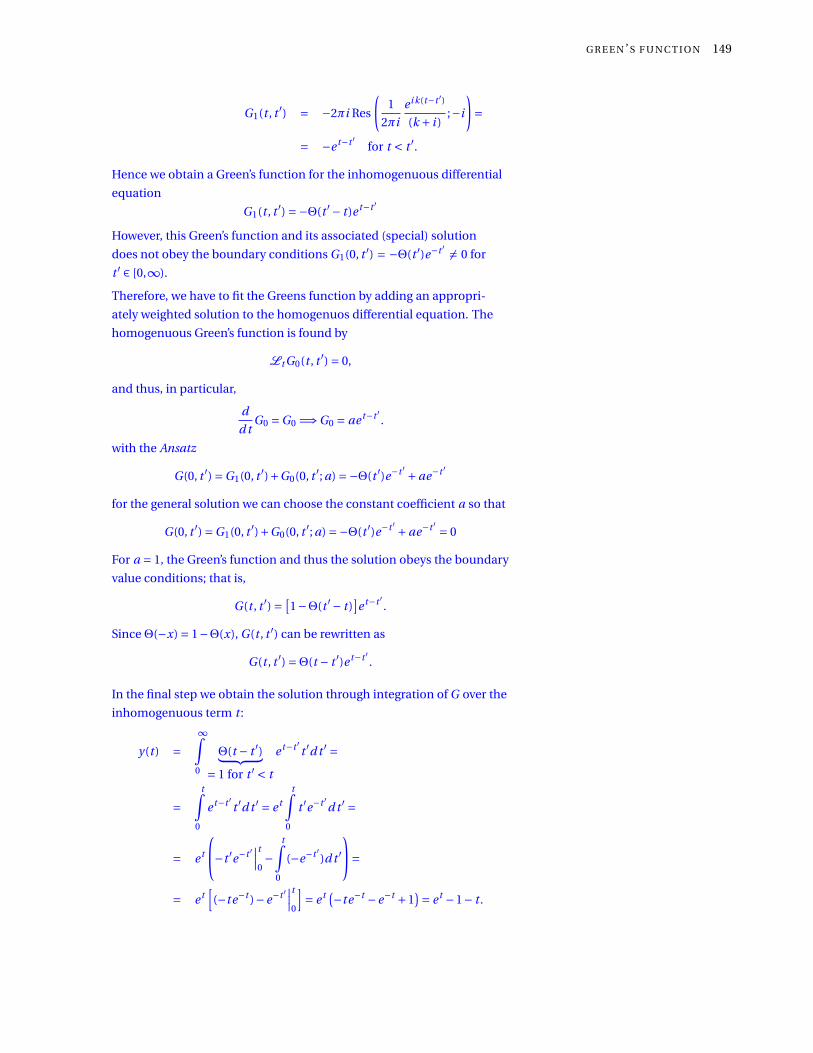
G R E E N ’ S F U N C T I O N 149
G1(t , t ′) = −2πi Res
(1
2πi
e i k(t−t ′)
(k + i );−i
)=
= −e t−t ′ for t < t ′.
Hence we obtain a Green’s function for the inhomogenuous differential
equation
G1(t , t ′) =−Θ(t ′− t )e t−t ′
However, this Green’s function and its associated (special) solution
does not obey the boundary conditions G1(0, t ′) = −Θ(t ′)e−t ′ 6= 0 for
t ′ ∈ [0,∞).
Therefore, we have to fit the Greens function by adding an appropri-
ately weighted solution to the homogenuos differential equation. The
homogenuous Green’s function is found by
Lt G0(t , t ′) = 0,
and thus, in particular,
d
d tG0 =G0 =⇒G0 = ae t−t ′ .
with the Ansatz
G(0, t ′) =G1(0, t ′)+G0(0, t ′; a) =−Θ(t ′)e−t ′ +ae−t ′
for the general solution we can choose the constant coefficient a so that
G(0, t ′) =G1(0, t ′)+G0(0, t ′; a) =−Θ(t ′)e−t ′ +ae−t ′ = 0
For a = 1, the Green’s function and thus the solution obeys the boundary
value conditions; that is,
G(t , t ′) = [1−Θ(t ′− t )
]e t−t ′ .
SinceΘ(−x) = 1−Θ(x), G(t , t ′) can be rewritten as
G(t , t ′) =Θ(t − t ′)e t−t ′ .
In the final step we obtain the solution through integration of G over the
inhomogenuous term t :
y(t ) =∞∫
0
Θ(t − t ′)︸ ︷︷ ︸= 1 for t ′ < t
e t−t ′ t ′d t ′ =
=t∫
0
e t−t ′ t ′d t ′ = e t
t∫0
t ′e−t ′d t ′ =
= e t
−t ′e−t ′∣∣∣t
0−
t∫0
(−e−t ′ )d t ′=
= e t[
(−te−t )−e−t ′∣∣∣t
0
]= e t (−te−t −e−t +1
)= e t −1− t .

150 M AT H E M AT I C A L M E T H O D S O F T H E O R E T I C A L P H Y S I C S
2. Next, let us solve the differential equation d 2 yd t 2 + y = cos t on the intervall
t ∈ [0,∞) with the boundary conditions y(0) = y ′(0) = 0.
First, observe that
L = d 2
d t 2 +1.
The Fourier Ansatz for the Green’s function is
G1(t , t ′) = 1
2π
+∞∫−∞
G(k)e i k(t−t ′)dk
L G1 = 1
2π
+∞∫−∞
G(k)
(d 2
d t 2 +1
)e i k(t−t ′)dk =
= 1
2π
+∞∫−∞
G(k)((i k)2 +1)e i k(t−t ′)dk =
= δ(t − t ′) = 1
2π
+∞∫−∞
e i k(t−t ′)dk =
Hence
G(k)(1−k2) = 1
ant thus
G(k) = 1
(1−k2)= −1
(k +1)(k −1)
The Fourier transformation is
G1(t , t ′) = − 1
2π
+∞∫−∞
e i k(t−t ′)
(k +1)(k −1)dk =
= − 1
2π2πi
[Res
(e i k(t−t ′)
(k +1)(k −1);k = 1
)+
Res
(e i k(t−t ′)
(k +1)(k −1);k =−1
)]Θ(t − t ′)
The path in the upper integration plain is drawn in Fig. 9.2.Re k
Im k
× ×> >
-
6
Figure 9.2: Plot of the path reqired forsolving the Fourier integral.G1(t , t ′) = − i
2
(e i (t−t ′) −e−i (t−t ′)
)Θ(t − t ′) =
= e i (t−t ′) −e−i (t−t ′)
2iΘ(t − t ′) = sin(t − t ′)Θ(t − t ′)
G1(0, t ′) = sin(−t ′)Θ(−t ′) = 0 weil t ′ > 0
G ′1(t , t ′) = cos(t − t ′)Θ(t − t ′)+ sin(t − t ′)δ(t − t ′)︸ ︷︷ ︸
= 0G ′
1(0, t ′) = cos(−t ′)Θ(−t ′) = 0 wie vorher

G R E E N ’ S F U N C T I O N 151
G1 already satisfies the boundary conditions; hence we do not need to
find the Green’s function G0 of the homogenuous equation.
y(t ) =∞∫
0
G(t , t ′) f (t ′)d t ′ =∞∫
0
sin(t − t ′) Θ(t − t ′)︸ ︷︷ ︸= 1 for t > t ′
cos t ′d t ′ =
=t∫
0
sin(t − t ′)cos t ′d t ′ =t∫
0
(sin t cos t ′−cos t sin t ′)cos t ′d t ′ =
=t∫
0
[sin t (cos t ′)2 −cos t sin t ′ cos t ′
]d t ′ =
= sin t
t∫0
(cos t ′)2d t ′−cos t
t∫0
si nt ′ cos t ′d t ′ =
= sin t
[1
2(t ′+ sin t ′ cos t ′)
]∣∣∣t
0−cos t
[sin2 t ′
2
]∣∣∣t
0=
= t sin t
2+ sin2 t cos t
2− cos t sin2 t
2= t sin t
2.
c


Part IV:
Differential equations


10
Sturm-Liouville theory
This is only a very brief “dive into Sturm-Liouville theory,” which has many
fascinating aspects and connections to Fourier analysis, the special func-
tions of mathematical physics, operator theory, and linear algebra 1. In 1 Garrett Birkhoff and Gian-Carlo Rota.Ordinary Differential Equations. JohnWiley & Sons, New York, Chichester,Brisbane, Toronto, fourth edition, 1959,1960, 1962, 1969, 1978, and 1989; M. A.Al-Gwaiz. Sturm-Liouville Theory andits Applications. Springer, London, 2008;and William Norrie Everitt. A catalogue ofSturm-Liouville differential equations. InSturm-Liouville Theory, Past and Present,pages 271–331. Birkhäuser Verlag, Basel,2005. URL http://www.math.niu.edu/
SL2/papers/birk0.pdf
physics, many formalizations involve second order differential equations,
which, in their most general form, can be written as 2
2 Russell Herman. A Second Course in Or-dinary Differential Equations: DynamicalSystems and Boundary Value Problems.University of North Carolina Wilming-ton, Wilmington, NC, 2008. URL http:
//people.uncw.edu/hermanr/mat463/
ODEBook/Book/ODE_LargeFont.pdf.Creative Commons Attribution-NoncommercialShare Alike 3.0 UnitedStates License
Lx y(x) = a0(x)y(x)+a1(x)d
d xy(x)+a2(x)
d 2
d x2 y(x) = f (x). (10.1)
The differential operator is defined by
Lx y(x) = a0(x)+a1(x)d
d x+a2(x)
d 2
d x2 . (10.2)
The solutions y(x) are often subject to boundary conditions of various
forms.
Dirichlet boundary conditions are of the form y(a) = y(b) = 0 for some
a,b.
Neumann boundary conditions are of the form y ′(a) = y ′(b) = 0 for some
a,b.
Periodic boundary conditions are of the form y(a) = y(b) and y ′(a) =y ′(b) for some a,b.
10.1 Sturm-Liouville form
Any second order differential equation of the general form (10.1) can be
rewritten into a differential equation of the Sturm-Liouville form
Sx y(x) = dd x
[p(x) d
d x
]y(x)+q(x)y(x) = F (x), with
p(x) = e∫ a1(x)
a2(x) d x,
q(x) = p(x) a0(x)a2(x) = a0(x)
a2(x) e∫ a1(x)
a2(x) d x,
F (x) = p(x) f (x)a2(x) =
f (x)a2(x) e
∫ a1(x)a2(x) d x
,
(10.3)
The associated differential operator
Sx = dd x
[p(x) d
d x
]+q(x)
= p(x) d 2
d x2 +p ′(x) dd x +q(x)
(10.4)

156 M AT H E M AT I C A L M E T H O D S O F T H E O R E T I C A L P H Y S I C S
is called Sturm-Liouville differential operator.
For a proof, we insert p(x), q(x) and F (x) into the Sturm-Liouville form
of Eq. (10.3) and compare it with Eq. (10.1).
d
d x
[e
∫ a1(x)a2(x) d x d
d x
]+ a0(x)
a2(x) e∫ a1(x)
a2(x) d x
y(x) = f (x)a2(x) e
∫ a1(x)a2(x) d x
e∫ a1(x)
a2(x) d x
d 2
d x2 + a1(x)a2(x)
dd x + a0(x)
a2(x)
y(x) = f (x)
a2(x) e∫ a1(x)
a2(x) d xa2(x) d 2
d x2 +a1(x) dd x +a0(x)
y(x) = f (x).
(10.5)
10.2 Sturm-Liouville eigenvalue problem
The Sturm-Liouville eigenvalue problem is given by the differential equa-
tion
Sxφ(x) =λρ(x)φ(x), ord
d x
[p(x) d
d x
]φ(x)+ [q(x)−λρ(x)]φ(x) = 0
(10.6)
for x ∈ (a,b) and continuous p(x) > 0, p ′(x), q(x) and ρ(x) > 0.
We mention without proof (for proofs, see, for instance, Ref. 3) that 3 M. A. Al-Gwaiz. Sturm-Liouville Theoryand its Applications. Springer, London,2008• the eigenvalues λ turn out to be real, countable, and ordered, and that
there is a smallest eigenvalue λ1 such that λ1 <λ2 <λ2 < ·· ·;
• for each eigenvalue λ j there exists an eigenfunction φ j (x) with j − 1
zeroes on (a,b);
• eigenfunctions corresponding to different eigenvalues are orthogonal,
and can be normalized, with respect to the weight function ρ(x); that is,
⟨φ j |φk⟩ =∫ b
aφ j (x)φk (x)ρ(x)d x = δ j k (10.7)
• the set of eigenfunctions is complete; that is, any piecewise smooth
function can be represented by
f (x) =∑∞k=1 ckφk (x),
with
ck = ⟨ f |φk (x)⟩⟨φk (x)|φk (x)⟩ .
(10.8)
• the orthonormal (with respect to the weight ρ) set φ j (x) | j ∈ N is a
basis of a Hilbert space with the inner product
⟨ f | g ⟩ =∫ b
af (x)g (x)ρ(x)d x. (10.9)

S T U R M - L I O U V I L L E T H E O RY 157
10.3 Adjoint and self-adjoint operators
In operator theory, just as in matrix theory, we can define an adjoint oper-
ator via the scalar product defined in Eq. (10.9). In this formalization, the
Sturm-Liouville differential operator S is self-adjoint.
Let us first define the domain of a differential operator L as the set of
all square integrable (with respect to the weight ρ(x)) functions ϕ satisfying
boundary conditions. ∫ b
a|ϕ(x)|2ρ(x)d x <∞. (10.10)
Then, the adjoint operator L † is defined by satisfying
⟨ψ |Lϕ⟩ = ∫ ba ψ(x)[Lϕ(x)]ρ(x)d x
= ⟨L †ψ |ϕ⟩ = ∫ ba [L †ψ(x)]ϕ(x)ρ(x)d x
(10.11)
for all ψ(x) in the domain of L † and ϕ(x) in the domain of L .
Note that in the case of second order differential operators in the stan-
dard form (10.2) and with ρ(x) = 1, we can move the differential quotients
and the entire differential operator in
⟨ψ |Lϕ⟩ = ∫ ba ψ(x)[Lxϕ(x)]ρ(x)d x
= ∫ ba ψ(x)[a2(x)ϕ′′(x)+a1(x)ϕ′(x)+a0(x)ϕ(x)]d x
(10.12)
from ϕ to ψ by one and two partial integrations.
Integrating the kernel a1(x)ϕ′(x) by parts yields∫ b
aψ(x)a1(x)ϕ′(x)d x = ψ(x)a1(x)ϕ(x)
∣∣ba −
∫ b
a(ψ(x)a1(x))′ϕ(x)d x. (10.13)
Integrating the kernel a2(x)ϕ′′(x) by parts twice yields∫ ba ψ(x)a2(x)ϕ′′(x)d x = ψ(x)a2(x)ϕ′(x)
∣∣ba −
∫ ba (ψ(x)a2(x))′ϕ′(x)d x
= ψ(x)a2(x)ϕ′(x)∣∣b
a − (ψ(x)a2(x))′ϕ(x)∣∣b
a +∫ b
a (ψ(x)a2(x))′′ϕ(x)d x
= ψ(x)a2(x)ϕ′(x)− (ψ(x)a2(x))′ϕ(x)∣∣b
a +∫ b
a (ψ(x)a2(x))′′ϕ(x)d x.(10.14)
Combining these two calculations yields
⟨ψ |Lϕ⟩ = ∫ ba ψ(x)[Lxϕ(x)]ρ(x)d x
= ∫ ba ψ(x)[a2(x)ϕ′′(x)+a1(x)ϕ′(x)+a0(x)ϕ(x)]d x
= ψ(x)a1(x)ϕ(x)+ψ(x)a2(x)ϕ′(x)− (ψ(x)a2(x))′ϕ(x)∣∣b
a
+∫ ba [(a2(x)ψ(x))′′− (a1(x)ψ(x))′+a0(x)ψ(x)]ϕ(x)d x.
(10.15)
If the terms with no integral vanish (because of boundary contitions or
other reasons); that is, if
ψ(x)a1(x)ϕ(x)+ψ(x)a2(x)ϕ′(x)− (ψ(x)a2(x))′ϕ(x)∣∣b
a = 0,
then Eq. (10.15) reduces to
⟨ψ |Lϕ⟩ =∫ b
a[(a2(x)ψ(x))′′− (a1(x)ψ(x))′+a0(x)ψ(x)]ϕ(x)d x, (10.16)

158 M AT H E M AT I C A L M E T H O D S O F T H E O R E T I C A L P H Y S I C S
and we can identify the adjoint differential operator Lx with
L †x = d 2
d x2 a2(x)− dd x a1(x)+a0(x)
= dd x
[a2(x) d
d x +a′2(x)
]−a′
1(x)−a1(x) dd x +a0(x)
= a′2(x) d
d x +a2(x) d 2
d x2 +a′′2 (x)+a′
2(x) dd x −a′
1(x)−a1(x) dd x +a0(x)
= a2(x) d 2
d x2 + [2a′2(x)−a1(x)] d
d x +a′′2 (x)−a′
1(x)+a0(x).(10.17)
If
L †x =Lx , (10.18)
the operator Lx is called self-adjoint.
In order to prove that the Sturm-Liouville differential operator
S = dd x
[p(x) d
d x
]+q(x) = p(x) d 2
d x2 +p ′(x) dd x +q(x) (10.19)
from Eq. (10.4) is self-adjoint, we verify Eq. (10.17) with S † taken from Eq.
(10.16). Thereby, we identify a2(x) = p(x), a1(x) = p ′(x), and a0(x) = q(x);
hence
S †x = a2(x) d 2
d x2 + [2a′2(x)−a1(x)] d
d x +a′′2 (x)−a′
1(x)+a0(x)
= p(x) d 2
d x2 + [2p ′(x)−p ′(x)] dd x +p ′′(x)−p ′′(x)+q(x)
= p(x) d 2
d x2 +p ′(x) dd x q(x)
=Sx .
(10.20)
Alternatively we could argue from Eqs. (10.17) and (10.18), noting that a
differential operator is self-adjoint if and only if
L †x = a2(x) d 2
d x2 −a1(x) dd x +a0(x)
=L †x = a2(x) d 2
d x2 + [2a′2(x)−a1(x)] d
d x +a′′2 (x)−a′
1(x)+a0(x).(10.21)
By comparison of the coefficients,
a2(x) = a2(x),
a1(x) = [2a′2(x)−a1(x)],
a0(x) =+a′′2 (x)−a′
1(x)+a0(x),
(10.22)
and hence,
a′2(x) = a1(x), (10.23)
which is exactly the form of the Sturm-Liouville differential operator.
10.4 Sturm-Liouville transformation into Liouville normal form
Let, for x ∈ [a,b],
[Sx −λρ(x)]y(x) = 0,d
d x
[p(x) d
d x
]y(x)+ [q(x)−λρ(x)]y(x) = 0,[
p(x) d 2
d x2 +p ′(x) dd x +q(x)−λρ(x)
]y(x) = 0,[
d 2
d x2 + p ′(x)p(x)
dd x + q(x)−λρ(x)
p(x)
]y(x) = 0
(10.24)

S T U R M - L I O U V I L L E T H E O RY 159
be a second order differential equation of the Sturm-Liouville form 4. 4 Garrett Birkhoff and Gian-Carlo Rota.Ordinary Differential Equations. JohnWiley & Sons, New York, Chichester,Brisbane, Toronto, fourth edition, 1959,1960, 1962, 1969, 1978, and 1989
This equation (10.24) can be written in the Liouville normal form con-
taining no first order differentiation term
− d 2
d t 2 w(t )+ [q(t )−λ]w(t ) = 0, with t ∈ [0,c]. (10.25)
It is obtained via the Sturm-Liouville transformation
ξ= t (x) = ∫ xa
√ρ(s)p(s) d s,
w(t ) = 4√
p(x(t ))ρ(x(t ))y(x(t )),(10.26)
where
q(t ) = 1
ρ
[−q − 4
ppρ
(p
(1
4p
pρ
)′)′]. (10.27)
The apostrophe represents derivation with respect to x.
Suppose we want to know the normalized eigenfunctions of
−x2 y ′′−3x y ′− y =λy , with x ∈ [1,2] (10.28)
with the boundary conditions y(1) = y(2) = 0.
The first thing we have to do is to transform this differential equation
into its Sturm-Liouville form by identifying a2(x) = −x2, a1(x) = −3x,
a0 =−1, ρ = 1 and f =λy ; and hence
p(x) = e∫ (−3x)
(−x2)d x = e
∫ 3x d x = e3log x = x3,
q(x) = p(x) (−1)(−x2)
= x,
F (x) = p(x) λy(−x2)
=−λx y , and hence ρ(x) = x.
(10.29)
As a result we obtain the Sturm-Liouville form
1
x(−(x3 y ′)′−x y) =λy . (10.30)
In the next step we apply the Sturm-Liouville transformation
ξ= t (x) = ∫ √ρ(x)p(x) d x = ∫ d x
x = log x,
w(t (x)) = 4√
p(x(t ))ρ(x(t ))y(x(t )) = 4px4 y(x(t )) = x y ,
q(t ) = 1x
[−x − 4p
x4(x3
(1
4px4
)′)′]= 0.
(10.31)
We now take the Ansatz y = 1x w(t (x)) = 1
x w(log x) and finally obtain the
Liouville normal form
−w ′′ =λw . (10.32)
As an Ansatz for solving the Liouville normal form we use
w(ξ) = a sin(pλξ)+b cos(
pλξ) (10.33)
The boundary conditions translate into x = 1 → ξ = 0, and x = 2 → ξ =log2. From w(0) = 0 we obtain b = 0. From w(log2) = a sin(
pλ log2) = 0 we
obtain√λn log2 = nπ.

160 M AT H E M AT I C A L M E T H O D S O F T H E O R E T I C A L P H Y S I C S
Thus the eigenvalues are
λn =(
nπ
log2
)2
. (10.34)
The associated eigenfunctions are
wn(ξ) = a sin
[nπ
log2ξ
], (10.35)
and thus
yn = 1
xa sin
[nπ
log2log x
]. (10.36)
We can check that they are orthonormal by inserting into Eq. (10.7) and
verifying it; that is,
2∫1
ρ(x)yn(x)ym(x)d x = δnm ; (10.37)
more explicitly,
2∫1
d xx(
1x2
)a2 sin
(nπ log x
log2
)sin
(mπ
log xlog2
)[variable substitution u = log x
log2dud x = 1
log21x , u = d x
x log2 ]
=u=1∫
u=0du log2a2 sin(nπu)sin(mπu)
= a2(
log2
2
)︸ ︷︷ ︸
= 1
2∫ 1
0du sin(nπu)sin(mπu)︸ ︷︷ ︸
= δnm
= δnm .
(10.38)
Finally, with a =√
2log2 we obtain the solution
yn =√
2
log2
1
xsin
(nπ
log x
log2
). (10.39)
10.5 Varieties of Sturm-Liouville differential equations
A catalogue of Sturm-Liouville differential equations comprises the fol-
lowing species, among many others 5. Some of these cases are tabellated 5 George B. Arfken and Hans J. Weber.Mathematical Methods for Physicists.Elsevier, Oxford, 6th edition, 2005. ISBN0-12-059876-0;0-12-088584-0; M. A. Al-Gwaiz. Sturm-Liouville Theory and itsApplications. Springer, London, 2008;and William Norrie Everitt. A catalogue ofSturm-Liouville differential equations. InSturm-Liouville Theory, Past and Present,pages 271–331. Birkhäuser Verlag, Basel,2005. URL http://www.math.niu.edu/
SL2/papers/birk0.pdf
as functions p, q , λ and ρ appearing in the general form of the Sturm-
Liouville eigenvalue problem (10.6)
Sxφ(x) =−λρ(x)φ(x), ord
d x
[p(x) d
d x
]φ(x)+ [q(x)+λρ(x)]φ(x) = 0
(10.40)
in Table 10.1.
X

S T U R M - L I O U V I L L E T H E O RY 161
Equation p(x) q(x) −λ ρ(x)
Hypergeometric xα+1(1−x)β+1 0 µ xα(1−x)β
Legendre 1−x2 0 l (l +1) 1Shifted Legendre x(1−x) 0 l (l +1) 1
Associated Legendre 1−x2 − m2
1−x2 l (l +1) 1
Chebyshev I√
1−x2 0 n2 1p1−x2
Shifted Chebyshev Ip
x(1−x) 0 n2 1px(1−x)
Chebyshev II (1−x2)32 0 n(n +2)
√1−x2
Ultraspherical (Gegenbauer) (1−x2)α+12 0 n(n +2α) (1−x2)α−
12
Bessel x − n2
x a2 xLaguerre xe−x 0 α e−x
Associated Laguerre xk+1e−x 0 α−k xk e−x
Hermite xe−x20 2α e−x
Fourier 1 0 k2 1(harmonic oscillator)Schrödinger 1 l (l +1)x−2 µ 1(hydrogen atom)
Table 10.1: Some varieties of differentialequations expressible as Sturm-Liouvilledifferential equations


11
Separation of variables
This chapter deals with the ancient alchemic suspicion of “solve et coagula”
that it is possible to solve a problem by separation and joining together –
for a counterexample see the Kochen-Specker theorem on page 69) – trans-
lated into the context of partial differential equations; that is, equations
with derivatives of more than one variable. Already Descartes mentioned
this sort of method in his Discours de la méthode pour bien conduire sa
raison et chercher la verité dans les sciences (English translation: Discourse
on the Method of Rightly Conducting One’s Reason and of Seeking Truth) 1 1 Rene Descartes. Discours de la méthodepour bien conduire sa raison et chercherla verité dans les sciences (Discourse onthe Method of Rightly Conducting One’sReason and of Seeking Truth). 1637. URLhttp://www.gutenberg.org/etext/59
stating that (in a newer translation 2)
2 Rene Descartes. The Philosophical Writ-ings of Descartes. Volume 1. CambridgeUniversity Press, Cambridge, 1985. trans-lated by John Cottingham, Robert Stoothoffand Dugald Murdoch
[Rule Five:] The whole method consists entirely in the ordering and arranging
of the objects on which we must concentrate our mind’s eye if we are to dis-
cover some truth . We shall be following this method exactly if we first reduce
complicated and obscure propositions step by step to simpler ones, and then,
starting with the intuition of the simplest ones of all, try to ascend through
the same steps to a knowledge of all the rest. [Rule Thirteen:] If we perfectly
understand a problem we must abstract it from every superfluous conception,
reduce it to its simplest terms and, by means of an enumeration, divide it up
into the smallest possible parts.
The method of separation of variables is one among a couple of strate-
gies to solve differential equations 3, but it is a very important one in 3 Lawrence C. Evans. Partial differ-ential equations. Graduate Studies inMathematics, volume 19. AmericanMathematical Society, Providence, RhodeIsland, 1998; and Klaus Jänich. Analysisfür Physiker und Ingenieure. Funktionen-theorie, Differentialgleichungen, SpezielleFunktionen. Springer, Berlin, Heidel-berg, fourth edition, 2001. URL http:
//www.springer.com/mathematics/
analysis/book/978-3-540-41985-3
physics.
Separation of variables can be applied whenever we have no “mixtures
of derivatives and functional dependencies;” more specifically, whenever
the partial differential equation can be written as a sum
Lx,yψ(x, y) = (Lx +Ly )ψ(x, y) = 0, or
Lxψ(x, y) =−Ly )ψ(x, y).(11.1)
Because in this case we may make a multiplicative Ansatz
ψ(x, y) = v(x)u(y). (11.2)

164 M AT H E M AT I C A L M E T H O D S O F T H E O R E T I C A L P H Y S I C S
Inserting (11.2) into (11.1) effectively separates the variable dependencies
Lx v(x)u(y) =−Ly v(x)u(y),
u(y) [Lx v(x)] =−v(x)[Ly u(y)
],
1v(x) Lx v(x) =− 1
u(y) Ly u(y) = a,
(11.3)
with constant a, because Lx v(x)v(x) does not depend on x, and
Ly u(y)u(y) does not
depend on y . Therefore, neither side depends on x or y ; hence both sides
are constants.
As a result, we can treat and integrate both sides separately; that is,
1v(x) Lx v(x) = a,
1u(y) Ly u(y) =−a,
(11.4)
or As a result, we can treat and integrate both sides separately; that is,
Lx v(x)−av(x) = 0,
Ly u(y)+au(y) = 0.(11.5)
This separation of variable Ansatz can be very often used whenever the
Laplace operator ∆ = ∇ ·∇ is involved, since there the partial derivatives
with respect to different variables occur in different summands.
For the sake of demonstration, let us consider a few examples.
1. Let us separate the homogenuous Laplace differential equation
∆Φ= 1
u2 + v2
(∂2Φ
∂u2 + ∂2Φ
∂v2
)+ ∂2Φ
∂z2 = 0 (11.6)
in parabolic cylinder coordinates (u, v , z) with x = ( 12 (u2 − v2),uv , z
).
The separation of variables Ansatz is
Φ(u, v , z) =Φ1(u)Φ2(v)Φ3(z).
Then,1
u2 + v2
(Φ2Φ3
∂2Φ1
∂u2 +Φ1Φ3∂2Φ2
∂v2
)+Φ1Φ2
∂2Φ
∂z2 = 0
1
u2 + v2
(Φ′′
1
Φ1+ Φ
′′2
Φ2
)=−Φ
′′3
Φ3=λ= const.
λ is constant because it does neither depend on u, v (because of the
right hand sideΦ′′3 (z)/Φ3(z)), nor on z (because of the left hand side).
Furthermore,Φ′′
1
Φ1−λu2 =−Φ
′′2
Φ2+λv2 = l 2 = const.
with constant l for analoguous reasons. The three resulting differential
equations are
Φ′′1 − (λu2 + l 2)Φ1 = 0,
Φ′′2 − (λv2 − l 2)Φ2 = 0,
Φ′′3 +λΦ3 = 0.

S E PA R AT I O N O F VA R I A B L E S 165
2. Let us separate the homogenuous (i) Laplace, (ii) wave, and (iii) dif-
fusion equations, in elliptic cylinder coordinates (u, v , z) with~x =(a coshu cos v , a sinhu sin v , z) and
∆ = 1
a2(sinh2 u + sin2 v)
[∂2
∂u2 + ∂2
∂v2
]+ ∂2
∂z2 .
ad (i): Again the separation of variables Ansatz isΦ(u, v , z) =Φ1(u)Φ2(v)Φ3(z).
Hence,
1a2(sinh2 u+sin2 v)
(Φ2Φ3
∂2Φ1∂u2 +Φ1Φ3
∂2Φ2∂v2
)=−Φ1Φ2
∂2Φ∂z2 ,
1a2(sinh2 u+sin2 v)
(Φ′′
1Φ1
+ Φ′′2
Φ2
)=−Φ′′
3Φ3
= k2 = const. =⇒Φ′′3 +k2Φ3 = 0
Φ′′1
Φ1+ Φ′′
2Φ2
= k2a2(sinh2 u + sin2 v),Φ′′
1Φ1
−k2a2 sinh2 u =−Φ′′2
Φ2+k2a2 sin2 v = l 2,
(11.7)
and finally,Φ′′
1 − (k2a2 sinh2 u + l 2)Φ1 = 0,
Φ′′2 − (k2a2 sin2 v − l 2)Φ2 = 0.
ad (ii): the wave equation is given by
∆Φ= 1
c2
∂2Φ
∂t 2 .
Hence,
1
a2(sinh2 u + sin2 v)
(∂2
∂u2 + ∂2
∂v2 +)Φ+ ∂2Φ
∂z2 = 1
c2
∂2Φ
∂t 2 .
The separation of variables Ansatz isΦ(u, v , z, t ) =Φ1(u)Φ2(v)Φ3(z)T (t )
=⇒ 1a2(sinh2 u+sin2 v)
(Φ′′
1Φ1
+ Φ′′2
Φ2
)+ Φ′′
3Φ3
= 1c2
T ′′T =−ω2 = const.,
1c2
T ′′T =−ω2 =⇒ T ′′+ c2ω2T = 0,
1a2(sinh2 u+sin2 v)
(Φ′′
1Φ1
+ Φ′′2
Φ2
)=−Φ′′
3Φ3
−ω2 = k2,
Φ′′3 + (ω2 +k2)Φ3 = 0
Φ′′1
Φ1+ Φ′′
2Φ2
= k2a2(sinh2 u + sin2 v)Φ′′
1Φ1
−a2k2 sinh2 u =−Φ′′2
Φ2+a2k2 sin2 v = l 2,
(11.8)
and finally,Φ′′
1 − (k2a2 sinh2 u + l 2)Φ1 = 0,
Φ′′2 − (k2a2 sin2 v − l 2)Φ2 = 0.
ad (iii): The diffusion equation is ∆Φ= 1D∂Φ∂t .
The separation of variables Ansatz isΦ(u, v , z, t ) =Φ1(u)Φ2(v)Φ3(z)T (t ).
Let us take the result of (i), then
1a2(sinh2 u+sin2 v)
(Φ′′
1Φ1
+ Φ′′2
Φ2
)+ Φ′′
3Φ3
= 1D
T ′T =−α2 = const.
T = Ae−α2Dt
Φ′′3 + (α2 +k2)Φ3 = 0 =⇒Φ′′
3 =−(α2 +k2)Φ3 =⇒Φ3 = Be ipα2+k2 z
(11.9)

166 M AT H E M AT I C A L M E T H O D S O F T H E O R E T I C A L P H Y S I C S
and finally,Φ′′
1 − (α2k2 sinh2 u + l 2)Φ1 = 0
Φ′′2 − (α2k2 sin2 v − l 2)Φ2 = 0
g
12
Special functions of mathematical physics
This chapter follows several good approaches 1. For reference, consider 2. 1 N. N. Lebedev. Special Functions andTheir Applications. Prentice-Hall Inc.,Englewood Cliffs, N.J., 1965. R. A. Sil-verman, translator and editor; reprintedby Dover, New York, 1972; Herbert S.Wilf. Mathematics for the physical sci-ences. Dover, New York, 1962. URLhttp://www.math.upenn.edu/~wilf/
website/Mathematics_for_the_
Physical_Sciences.html; W. W. Bell.Special Functions for Scientists and En-gineers. D. Van Nostrand Company Ltd,London, 1968; Nico M. Temme. Specialfunctions: an introduction to the classicalfunctions of mathematical physics. JohnWiley & Sons, Inc., New York, 1996. ISBN0-471-11313-1; George E. Andrews, RichardAskey, and Ranjan Roy. Special Functions,volume 71 of Encyclopedia of Mathematicsand its Applications. Cambridge Uni-versity Press, Cambridge, 1999. ISBN0-521-62321-9; Vadim Kuznetsov. Specialfunctions and their symmetries. Part I:Algebraic and analytic methods. Post-graduate Course in Applied Analysis, May2003. URL http://www1.maths.leeds.
ac.uk/~kisilv/courses/sp-funct.pdf;and Vladimir Kisil. Special functionsand their symmetries. Part II: Algebraicand symmetry methods. PostgraduateCourse in Applied Analysis, May 2003.URL http://www1.maths.leeds.ac.uk/
~kisilv/courses/sp-repr.pdf2 Milton Abramowitz and Irene A. Stegun,editors. Handbook of MathematicalFunctions with Formulas, Graphs, andMathematical Tables. Number 55 inNational Bureau of Standards AppliedMathematics Series. U.S. GovernmentPrinting Office, Washington, D.C., 1964.Corrections appeared in later printingsup to the 10th Printing, December, 1972.Reproductions by other publishers, inwhole or in part, have been available since1965; Yuri Alexandrovich Brychkov andAnatolii Platonovich Prudnikov. Handbookof special functions: derivatives, integrals,series and other formulas. CRC/Chapman& Hall Press, Boca Raton, London, NewYork, 2008; and I. S. Gradshteyn and I. M.Ryzhik. Tables of Integrals, Series, andProducts, 6th ed. Academic Press, SanDiego, CA, 2000
Special functions often arise as solutions of differential equations; for
instance as eigenfunctions of differential operators in quantum mechanics.
Sometimes they occur after several separation of variables and substitution
steps have transformed the physical problem into something manageable.
For instance, we might start out with some linear partial differential equa-
tion like the wave equation, then separate the space from time coordinates,
then separate the radial from the angular components, and finally separate
the two angular parameter. After we have done that, we end up with sev-
eral separate differential equations of the Liouville form; among them the
Legendre differential equation leading us to the Legendre polynomials.
In what follows a particular class of special functions will be consid-
ered. These functions are all special cases of the hypergeometric function ,
which is the solution of the hypergeometric equation. The hypergeometric
function exhibis a high degree of “plasticity,” as many elementary analytic
functions can be expressed by them.
First, as a prerequisite, let us define the gamme function. Then we pro-
ceed to second order Fuchsian differential equations; followed by a rewrit-
ing of this Fuchsian differential equations into hypergeometric equation.
Then we study the hypergeometric function as a solution to the hyperge-
ometric equation. Finally, we mention some particular hypergeometric
functions, such as the Legendre orthogonal polynomials, and others.
Again, if not mentioned otherwise, we shall restrict our attention to
second order differential equations. Sometimes – such as for the Fuchsian
class – a generalization is possible but not very relevant for physics.
12.1 Gamma function
Although the gamma function Γ(x) is an extension of the factorial function
n! as
Γ(n +1) = n! for n ∈N, (12.1)
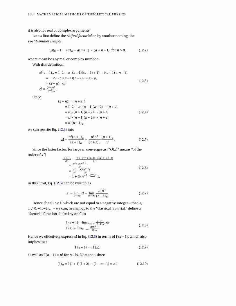
168 M AT H E M AT I C A L M E T H O D S O F T H E O R E T I C A L P H Y S I C S
it is also for real or complex arguments.
Let us first define the shifted factorial or, by another naming, the
Pochhammer symbol
(a)0 = 1, (a)n = a(a +1) · · · (a +n −1), for n > 0, (12.2)
where a can be any real or complex number.
With this definition,
z!(z +1)n = 1 ·2 · · ·z · (z +1)((z +1)+1) · · · ((z +1)+n −1)
= 1 ·2 · · ·z · (z +1)(z +2) · · · (z +n)
= (z +n)!, or
z! = (z+n)!(z+1)n
.
(12.3)
Since(z +n)! = (n + z)!
= 1 ·2 · · ·n · (n +1)(n +2) · · · (n + z)
= n! · (n +1)(n +2) · · · (n + z)
= n! · (n +1)(n +2) · · · (n + z)
= n!(n +1)z ,
(12.4)
we can rewrite Eq. (12.3) into
z! = n!(n +1)z
(z +1)n= n!nz
(z +1)n
(n +1)z
nz . (12.5)
Since the latter factor, for large n, converges as [“O(x)” means “of the
order of x”](n+1)z
nz = (n+1)((n+1)+1)···((n+1)+z−1)nz
= nz+O(nz−1)nz
= nz
nz + O(nz−1)nz
= 1+O(n−1)n→∞−→ 1,
(12.6)
in this limit, Eq. (12.5) can be written as
z! = limn→∞z! = lim
n→∞n!nz
(z +1)n. (12.7)
Hence, for all z ∈ Cwhich are not equal to a negative integer – that is,
z 6= 0,−1,−2, . . . – we can, in analogy to the “classical factorial,” define a
“factorial function shifted by one” as
Γ(z +1) = limn→∞ n!nz
(z+1)n, or
Γ(z) = limn→∞ n!nz−1
(z)n.
(12.8)
Hence we effectively express z! in Eq. (12.3) in terms of Γ(z +1), which also
implies that
Γ(z +1) = zΓ(z), (12.9)
as well as Γ(n +1) = n! for n ∈N. Note that, since
(1)n = 1(1+1)(1+2) · · · (1−n −1) = n!, (12.10)

S P E C I A L F U N C T I O N S O F M AT H E M AT I C A L P H Y S I C S 169
Eq. (12.8) yields
Γ(1) = limn→∞
n!n0
(1)n= lim
n→∞n!n!
= 1. (12.11)
We state without proof that, for positive real parts ℜx, Γ(x) has an inte-
gral representation as
Γ(x) =∫ ∞
0t x−1e−t d t . (12.12)
Also the next formulae
Γ( 12 ) =p
π, or, more generally,
Γ( n2 ) =p
π (n−2)!!2(n−1)/2 , for n > 0, and
Γ(x)Γ(1−x) = πsin(πx) , Euler’s reflection formula,
(12.13)
are stated without proof.
Here, the double factorial is defined by
n!! =
1 for n =−1,0, and
2 ·4 · · · (n −2) ·n
= (2k)!! =∏ki=1(2i )
= 2n/2(1 ·2 · · · (n−2)
2 · n2
)= k!2k for positive even n = 2k,k ≥ 1, and
1 ·3 · · · (n −2) ·n
= (2k −1)!! =∏ki=1(2i −1)
= 1·2···(2k−2)·(2k−1)·(2k)(2k)!!
= (2k)!k!2k for odd positive n = 2k −1,k ≥ 1.
(12.14)
Stirling’s formula [again, O(x) means “of the order of x”]
logn! = n logn −n +O(log(n)), or
n! n→∞−→ p2πn
( ne
)n , or, more generally,
logΓ(x) =√
2πx
( xe
)x (1+O
( 1x
)) (12.15)
is stated without proof.
12.2 Beta function
The beta function, also called the Euler integral of the first kind, is a special
function defined by
B(x, y) =∫ 1
0t x−1(1− t )y−1d t = Γ(x)Γ(y)
Γ(x + y)for ℜx,ℜy > 0 (12.16)
No proof of the identity of the two representations in terms of an integral,
and of Γ-functions is given.
12.3 Fuchsian differential equations
Many differential equations of theoretical physics are Fuchsian equations.
We shall therefore study this class in some generality.

170 M AT H E M AT I C A L M E T H O D S O F T H E O R E T I C A L P H Y S I C S
12.3.1 Regular, regular singular, and irregular singular point
Consider the homogenuous differential equation [Eq. (10.1) on page 155 is
inhomogenuos]
Lx y(x) = a2(x)d 2
d x2 y(x)+a1(x)d
d xy(x)+a0(x)y(x) = 0. (12.17)
If a0(x), a1(x) and a2(x) are analytic at some point x0 and in its neighbor-
hood, and if a2(x0) 6= 0 at x0, then x0 is called an ordinary point, or regular
point. We state without proof that in this case the solutions around x0 can
be expanded as power series. In this case we can divide equation (12.17) by
a2(x) and rewite it
1
a2(x)Lx y(x) = d 2
d x2 y(x)+d(x)d
d xy(x)+e(x)y(x) = 0, (12.18)
with d(x) = a1(x)/a2(x) and e(x) = a0(x)/a2(x).
If, however, a2(x0) = 0 and a1(x0) or a0(x0) are nonzero, the x0 is called
singular point of (12.17). The simplest case is if a0(x0) has a simple zero at
x0; then both d(x) and e(x) in (12.18) have at most simple poles.
Furthermore, for reasons disclosed later – mainly motivated by the
possibility to write the solutions as power series – a point x0 is called a
regular singular point of Eq. (12.17) if
limx→x0
(x −x0)a1(x)
a2(x), as well as lim
x→x0
(x −x0)2a0(x)
a2(x)(12.19)
both exist. If any one of these limits does not exist, the singular point is an
irregular singular point.
A very important case is the case of the Fuchsian differential equation,
where in (12.18)
• d(x) has at most a single pole, and
• e(x) has at most a double pole.The simples realization of this
case is for
a2(x) = a(x −x0),
a1(x) = b(x −x0),
a0(x) = c.
Stated differently, a linear ordinary differential equation is called Fuchsian
if every singular point, including infinity, is regular. Hence, in Eq. (12.18),
the equation is of the Fuchsian class if the coefficients are of the form
d(x) =∏kj=1
q1(x)(x−x j ) , and
e(x) =∏kj=1
q0(x)(x−x j )2 ,
(12.20)
where the x1, . . . , xk are k (singular) points, and q1(x) and q0(x) are poly-
nomials of degree less then or equal to k and 2k, respectively. Hence, the
coefficients of Fuchsian equations must be rational functions; that is, they
must be of the form P (x)Q(x) , where P (x) and Q(x) are polynomials in x with
real coefficients.
The hypergeometric differential equation is a Fuchsian differential equa-
tion which has at most three regular singularities, including infinity, at 0, 1,
and ∞ 3. 3 Vadim Kuznetsov. Special functionsand their symmetries. Part I: Algebraicand analytic methods. PostgraduateCourse in Applied Analysis, May 2003.URL http://www1.maths.leeds.ac.uk/
~kisilv/courses/sp-funct.pdf

S P E C I A L F U N C T I O N S O F M AT H E M AT I C A L P H Y S I C S 171
12.3.2 Power series solution
Now let us get more concrete about the solution of Fuchsian equations by
power series.
In order to get a feeling for power series solutions of differential equa-
tions, consider the “first order” Fuchsian equation 4 4 Ron Larson and Bruce H. Edwards.Calculus. Brooks/Cole Cengage Learning,Belmont, CA, 9th edition, 2010. ISBN978-0-547-16702-2y ′−λy = 0. (12.21)
Make the Ansatz that the solution can be expanded into a power series of
the form
y(x) =∞∑
j=0a j x j . (12.22)
Then, Eq. (12.21) can be written as
(d
d x
∑∞j=0 a j x j
)−λ∑∞
j=0 a j x j = 0,∑∞j=0 j a j x j−1 −λ∑∞
j=0 a j x j = 0,∑∞j=1 j a j x j−1 −λ∑∞
j=0 a j x j = 0,∑∞m= j−1=0(m +1)am+1xm −λ∑∞
j=0 a j x j = 0,∑∞j=0( j +1)a j+1x j −λ∑∞
j=0 a j x j = 0,
(12.23)
and hence, by comparing the coefficients of x j , for n ≥ 0,
( j +1)a j+1 =λa j , or
a j+1 = λa j
j+1 = a0λ j+1
( j+1)! , and
a j = a0λ j
j ! .
(12.24)
Therefore,
y(x) =∞∑
j=0a0λ j
j !x j = a0
∞∑j=0
(λx) j
j != a0eλx . (12.25)
In the Fuchsian case let us consider the following generalized power
series Ansatz around a regular singular point x0, which can be motivated by
Eq. (12.20), and by the Laurent series expansion (6.23)–(6.25) on page 117:
d(x) = A1(x)x−x0
=∑∞j=0α j (x −x0) j−1, for 0 < |x −x0| < r1,
e(x) = A2(x)(x−x0)2 =∑∞
j=0β j (x −x0) j−2, for 0 < |x −x0| < r2,
y(x) = (x −x0)σ∑∞
l=0 wl (x −x0)l =∑∞l=0 wl (x −x0)l+σ, with w0 6= 0.
(12.26)

172 M AT H E M AT I C A L M E T H O D S O F T H E O R E T I C A L P H Y S I C S
Eq. (12.18) then becomes
d 2
d x2 y(x)+d(x) dd x y(x)+e(x)y(x) = 0,[
d 2
d x2 +∑∞
j=0α j (x −x0) j−1 dd x y(x)+∑∞
j=0β j (x −x0) j−2]∑∞
l=0 wl (x −x0)l+σ = 0,
(l +σ)(l +σ−1)∑∞
l=0 wl (x −x0)l+σ−2
+[(l +σ)
∑∞l=0 wl (x −x0)l+σ−1
]∑∞j=0α j (x −x0) j−1
+[∑∞l=0 wl (x −x0)l+σ]∑∞
j=0β j (x −x0) j−2 = 0,
(l +σ)(l +σ−1)∑∞
l=0 wl (x −x0)l+σ−2
+[(l +σ)
∑∞l=0 wl (x −x0)l+σ−1
]∑∞j=0α j (x −x0) j−1
+[∑∞l=0 wl (x −x0)l+σ]∑∞
j=0β j (x −x0) j−2 = 0,
(x −x0)σ−2 ∑∞l=0(x −x0)l [(l +σ)(l +σ−1)wl
+(l +σ)wl∑∞
j=0α j (x −x0) j
+wl∑∞
j=0β j (x −x0) j]= 0,
(x −x0)σ−2 ∑∞l=0(l +σ)(l +σ−1)wl (x −x0)l
+∑∞l=0(l +σ)wl
∑∞j=0α j (x −x0)l+ j
+∑∞l=0 wl
∑∞j=0β j (x −x0)l+ j = 0.
Next, in order to reach a common power of (x − x0), we perform an index
identification l = m in the first summand, as well as an index shift
l + j = m, j = m − l , since l ≥ 0 and j ≥ 0 ⇒ 0 ≤ l ≤ m
in the second and third summands (where the order of the sums change):
(x −x0)σ−2 ∑∞l=0(l +σ)(l +σ−1)wl (x −x0)l
+∑∞j=0
∑∞l=0(l +σ)wlα j (x −x0)l+ j
+∑∞j=0
∑∞l=0 wlβ j (x −x0)l+ j = 0,
(x −x0)σ−2 ∑∞m=0(m +σ)(m +σ−1)wm(x −x0)m
+∑∞m=0
∑ml=0(l +σ)wlαm−l (x −x0)l+m−l
+∑∞m=0
∑ml=0 wlβm−l (x −x0)l+m−l = 0,
(x −x0)σ−2∑∞
m=0(x −x0)m [(m +σ)(m +σ−1)wm
+∑ml=0(l +σ)wlαm−l
+∑ml=0 wlβm−l
]= 0,
(x −x0)σ−2∑∞
m=0(x −x0)m [(m +σ)(m +σ−1)wm
+ ∑ml=0 wl
((l +σ)αm−l +βm−l
)]= 0.
(12.27)
If we can divide this equation through (x − x0)σ−2 and exploit the linear
independence of the polynomials (x − x0)m , we obtain an infinite number
of equations for the infinite number of coefficients wm by requiring that all
the terms “inbetween” the [· · ·]–brackets in Eq. (12.27) vanish individually.
In particular, for m = 0 and w0 6= 0,
(0+σ)(0+σ−1)w0 +w0((0+σ)α0 +β0
)= 0
σ(σ−1)+σα0 +β0 = f0(σ) = 0.(12.28)
The radius of convergence of the sulution will, in accordance with the
Laurent series expansion, extend to the next singularity.

S P E C I A L F U N C T I O N S O F M AT H E M AT I C A L P H Y S I C S 173
Note that in Eq. (12.28) we have defined f0(σ) which we will use now.
Furthermore, for successive m, and with the definition of fk (σ) =αkσ+βk ,
we obtain the sequence of linear equations
w0 f0(σ) = 0
w1 f0(σ+1)+w0 f1(σ) = 0,
w2 f0(σ+2)+w1 f1(σ+1)+w0 f2(σ) = 0,...
wn f0(σ+n)+wn−1 f1(σ+n −1)+·· ·+w0 fn(σ) = 0.
(12.29)
which can be used for an inductive determination of the coefficients wk .
Eq. (12.28) is a quadratic equation σ2 +σ(α0 −1)+β0 = 0 for the charac-
teristic exponents
σ1,2 = 1
2
[1−α0 ±
√(1−α0)2 −4β0
](12.30)
We state without proof that, if the difference of the characteristic expo-
nents
σ1 −σ2 =√
(1−α0)2 −4β0 (12.31)
is nonzero and not an integer, then the two solutions found from σ1,2
through the generalized series Ansatz (12.26) are linear independent.
If, however σ1 = σ2 +n with n ∈ Z then we can only obtain a single
solution of the Fuchsian equation. In order to obtain anotherlinear inde-
pendent solution we have to employ the d’Alambert reduction, which is a
general method to obtain another, linear independent solution y2(x) from
an existing particular solution y1(x) by
y2(x) = y1(x)∫
xu(s)d s. (12.32)
Inserting y2(x) from (12.32) into the Fuchsian equation (12.18), and using

174 M AT H E M AT I C A L M E T H O D S O F T H E O R E T I C A L P H Y S I C S
the fact that by assumption y1(x) is a solution of it, yields
d 2
d x2 y2(x)+d(x) dd x y2(x)+e(x)y2(x) = 0,
d 2
d x2 y1(x)∫
x u(s)d s +d(x) dd x y1(x)
∫x u(s)d s +e(x)y1(x)
∫x u(s)d s = 0,
dd x
[d
d x y1(x)]∫
x u(s)d s + y1(x)u(x)
+d(x)[
dd x y1(x)
]∫x u(s)d s + y1(x)u(x)+e(x)y1(x)
∫x u(s)d s = 0,[
d 2
d x2 y1(x)]∫
x u(s)d s +[
dd x y1(x)
]u(x)+
[d
d x y1(x)]
u(x)+ y1(x)[
dd x u(x)
]+d(x)
[d
d x y1(x)]∫
x u(s)d s +d(x)y1(x)u(x)+e(x)y1(x)∫
x u(s)d s = 0,[d 2
d x2 y1(x)]∫
x u(s)d s +d(x)[
dd x y1(x)
]∫x u(s)d s +e(x)y1(x)
∫x u(s)d s
+d(x)y1(x)u(x)+[
dd x y1(x)
]u(x)+
[d
d x y1(x)]
u(x)+ y1(x)[
dd x u(x)
]= 0,[
d 2
d x2 y1(x)]∫
x u(s)d s +d(x)[
dd x y1(x)
]∫x u(s)d s +e(x)y1(x)
∫x u(s)d s
+y1(x)[
dd x u(x)
]+2
[d
d x y1(x)]
u(x)+d(x)y1(x)u(x) = 0,[d 2
d x2 y1(x)]+d(x)
[d
d x y1(x)]+e(x)y1(x)
∫x u(s)d s
+y1(x)[
dd x u(x)
]+
2[
dd x y1(x)
]+d(x)y1(x)
u(x) = 0,
y1(x)[
dd x u(x)
]+
2[
dd x y1(x)
]+d(x)y1(x)
u(x) = 0,
(12.33)
and finally,
u′(x)+u(x)
2
y ′1(x)
y1(x)+d(x)
= 0. (12.34)
Let us consider some examples involving Fuchsian equations of the
second order.
1. Let w ′′+ p1(z)w ′+ p2(z)w = 0 a Fuchsian equation. Derive from the
Laurent series expansion of p1(z) and p2(z) with Cauchy’s integral
formula the following equations:
α0 = limz→z0 (z − z0)p1(z),
β0 = limz→z0 (z − z0)2p2(z),(12.35)
where z0 is a regular singular point.
Let us consider α0 and the Laurent series for
p1(z) =∞∑
k=−1ak (z − z0)k withak = 1
2πi
∮p1(s)(s − z0)−(k+1)d s.
The summands vanish for k < −1, because p1(z) has at most a pole of
order one at z0. Let us change the index : n = k +1 (=⇒ k = n −1) and
αn := an−1; then
p1(z) =∞∑
n=0αn(z − z0)n−1,
where
αn = an−1 = 1
2πi
∮p1(s)(s − z0)−nd s;
in particular,
α0 = 1
2πi
∮p1(s)d s.

S P E C I A L F U N C T I O N S O F M AT H E M AT I C A L P H Y S I C S 175
Because the equation is Fuchsian, p1(z) has only a pole of order one at
z0; and p1(z) is of the form
p1(z) = a1(z)
(z − z0)= p1(z)(z − z0)
(z − z0)
and
α0 = 1
2πi
∮p1(s)(s − z0)
(s − z0)d s,
where p1(s)(s − z0) is analytic around z0; hence we can apply Cauchy’s
integral formula:
α0 = lims→z0
p1(s)(s − z0)
An easy way to see this is with the Ansatz: p1(z) = ∑∞n=0αn(z − z0)n−1;
multiplication with (z − z0) yields
(z − z0)p1(z) =∞∑
n=0αn(z − z0)n .
In the limit z → z0,
limz→z0
(z − z0)p1(z) =αn
Let us consider β0 and the Laurent series for
p2(z) =∞∑
k=−2bk (z − z0)k withbk = 1
2πi
∮p2(s)(s − z0)−(k+1)d s.
The summands vanish for k < −2, because p2(z) has at most a pole of
second order at z0. Let us change the index : n = k +2 (=⇒ k = n −2) and
βn := bn−2. Hence,
p2(z) =∞∑
n=0βn(z − z0)n−2,
where
βn = 1
2πi
∮p2(s)(s − z0)−(n−1)d s,
in particular,
β0 = 1
2πi
∮p2(s)(s − z0)d s.
Because the equation is Fuchsian, p2(z) has only a pole of the order of
two at z0; and p2(z) is of the form
p2(z) = a2(z)
(z − z0)2 = p2(z)(z − z0)2
(z − z0)2
where a2(z) = p2(z)(z − z0)2 is analytic around z0
β0 = 1
2πi
∮p2(s)(s − z0)2
(s − z0)d s;
hence we can apply Cauchy’s integral formula
β0 = lims→z0
p2(s)(s − z0)2.

176 M AT H E M AT I C A L M E T H O D S O F T H E O R E T I C A L P H Y S I C S
An easy way to see this is with the Ansatz: p2(z) = ∑∞n=0βn(z − z0)n−2.
multiplication with (z − z0)2, in the limit z → z0, yields
limz→z0
(z − z0)2p2(z) =βn
2. For z =∞, transform the Fuchsian equation w ′′+p1(z)w ′+p2(z)w = 0
above into the new variable t = 1z .
t = 1
z, z = 1
t, u(t ) := w
(1
t
)= w(z)
d z
d t=− 1
t 2 =⇒ d
d z=−t 2 d
d t
d 2
d z2 =−t 2 d
d t
(−t 2 d
d t
)=−t 2
(−2t
d
d t− t 2 d 2
d t 2
)= 2t 3 d
d t+ t 4 d 2
d t 2
w ′(z) = d
d zw(z) =−t 2 d
d tu(t ) =−t 2u′(t )
w ′′(z) = d 2
d z2 w(z) =(2t 3 d
d t+ t 4 d 2
d t 2
)u(t ) = 2t 3u′(t )+ t 4u′′(t )
Insertion into the Fuchsian equation w ′′+p1(z)w ′+p2(z)w = 0 yields
2t 3u′+ t 4u′′+p1
(1
t
)(−t 2u′)+p2
(1
t
)u = 0,
and hence,
u′′+[
2
t− p1
( 1t
)t 2
]u′+ p2
( 1t
)t 4 u = 0
with p1(t ) :=[
2
t− p1
( 1t
)t 2
]und p2(t ) := p2
( 1t
)t 4 ist u′′+ p1(t )u′+ p2(t )u =
0.
3. Find out whether the following differential equations are Fuchsian, and
enumerate the regular singular points:
zw ′′+ (1− z)w ′ = 0,
z2w ′′+ zw ′−ν2w = 0,
z2(1+ z)2w ′′+2z(z +1)(z +2)w ′−4w = 0,
2z(z +2)w ′′+w ′− zw = 0.
(12.36)
ad 1: zw ′′+ (1− z)w ′ = 0 =⇒ w ′′+ (1− z)
zw ′ = 0
z = 0:
α0 = limz→0
z(1− z)
z= 1, β0 = lim
z→0z2 ·0 = 0.
The equation for the characteristic exponent is
σ(σ−1)+σα0 +β0 = 0 =⇒σ2 −σ+σ= 0 =⇒σ1,2 = 0.

S P E C I A L F U N C T I O N S O F M AT H E M AT I C A L P H Y S I C S 177
z =∞: z = 1t
p1(t ) = 2
t−
(1− 1
t
)1t
t 2 = 2
t−
(1− 1
t
)t
= 1
t+ 1
t 2 = t +1
t 2
=⇒ not Fuchsian.
ad 2: z2w ′′+ zw ′− v2w = 0 =⇒ w ′′+ 1
zw ′− v2
z2 w = 0.
z = 0:
α0 = limz→0
z1
z= 1, β0 = lim
z→0z2
(−v2
z2
)=−v2.
=⇒σ2 −σ+σ− v2 = 0 =⇒σ1,2 =±v
z =∞: z = 1t
p1(t ) = 2
t− 1
t 2 t = 1
t
p2(t ) = 1
t 4
(−t 2v2)=−v2
t 2
=⇒ u′′+ 1
tu′− v2
t 2 u = 0 =⇒σ1,2 =±v
=⇒ Fuchsian equation.
ad 3:
z2(1+z)2w ′′+2z(z+1)(z+2)w ′−4w = 0 =⇒ w ′′+2(z +2)
z(z +1)w ′− 4
z2(1+ z)2 w = 0
z = 0:
α0 = limz→0
z2(z +2)
z(z +1)= 4, β0 = lim
z→0z2
(− 4
z2(1+ z)2
)=−4.
=⇒σ(σ−1)+4σ−4 =σ2 +3σ−4 = 0 =⇒σ1,2 = −3±p9+16
2=
−4
+1
z =−1:
α0 = limz→−1
(z +1)2(z +2)
z(z +1)=−2, β0 = lim
z→−1(z +1)2
(− 4
z2(1+ z)2
)=−4.
=⇒σ(σ−1)−2σ−4 =σ2 −3σ−4 = 0 =⇒σ1,2 = 3±p9+16
2=
+4
−1z =∞:
p1(t ) = 2
t− 1
t 2
2( 1
t +2)
1t
( 1t +1
) = 2
t− 2
( 1t +2
)1+ t
= 2
t
(1− 1+2t
1+ t
)
p2(t ) = 1
t 4
− 41t 2
(1+ 1
t
)2
=− 4
t 2
t 2
(t +1)2 =− 4
(t +1)2

178 M AT H E M AT I C A L M E T H O D S O F T H E O R E T I C A L P H Y S I C S
=⇒ u′′+ 2
t
(1− 1+2t
1+ t
)u′− 4
(t +1)2 u = 0
α0 = limt→0
t2
t
(1− 1+2t
1+ t
)= 0, β0 = lim
t→0t 2
(− 4
(t +1)2
)= 0.
=⇒σ(σ−1) = 0 =⇒σ1,2 =
0
1
=⇒ Fuchsian equation.
ad 4:
2z(z +2)w ′′+w ′− zw = 0 =⇒ w ′′+ 1
2z(z +2)w ′− 1
2(z +2)w = 0
z = 0:
α0 = limz→0
z1
2z(z +2)= 1
4, β0 = lim
z→0z2 −1
2(z +2)= 0.
=⇒σ2 −σ+ 1
4σ= 0 =⇒σ2 − 3
4σ= 0 =⇒σ1 = 0,σ2 = 3
4.
z =−2:
α0 = limz→−2
(z +2)1
2z(z +2)=−1
4, β0 = lim
z→−2(z +2)2 −1
2(z +2)= 0.
=⇒σ1 = 0, σ2 = 5
4.
z =∞:
p1(t ) = 2
t− 1
t 2
(1
2 1t
( 1t +2
))= 2
t− 1
2(1+2t )
p2(t ) = 1
t 4
(−1)
2( 1
t +2) =− 1
2t 3(1+2t )
=⇒ no Fuchsian. Klasse!
4. Determine the solutions of
z2w ′′+ (3z +1)w ′+w = 0
around the regular singular points.
The singularities are at z = 0 and z =∞.
Singularities at z = 0:
p1(z) = 3z +1
z2 = a1(z)
zmit a1(z) = 3+ 1
z
p1(z) has a pole of higher order than one; hence this is no Fuchsian
equation; and z = 0 is an irregular singular point.
Singularities at z =∞:

S P E C I A L F U N C T I O N S O F M AT H E M AT I C A L P H Y S I C S 179
• Transformation z = 1
t, w(z) → u(t ):
u′′(t )+[
2
t− 1
t 2 p1
(1
t
)]·u′(t )+ 1
t 4 p2
(1
t
)·u(t ) = 0.
The new coefficient functions are
p1(t ) = 2
t− 1
t 2 p1
(1
t
)= 2
t− 1
t 2 (3t + t 2) = 2
t− 3
t−1 =−1
t−1
p2(t ) = 1
t 4 p2
(1
t
)= t 2
t 4 = 1
t 2
• check whether this is a regular singular point:
p1(t ) =−1+ t
t= a1(t )
tmit a1(t ) =−(1+ t ) regulär
p2(t ) = 1
t 2 = a2(t )
t 2 mit a2(t ) = 1 regulär
a1 and a2 are regular at t = 0, hence this is a regular singular point.
• Ansatz around t = 0: the transformed equation is
u′′(t )+ p1(t )u′(t )+ p2(t )u(t ) = 0
u′′(t )−(
1
t+1
)u′(t )+ 1
t 2 u(t ) = 0
t 2u′′(t )− (t + t 2)u′(t )+u(t ) = 0
The generalized power series is
u(t ) =∞∑
n=0wn t n+σ
u′(t ) =∞∑
n=0wn(n +σ)t n+σ−1
u′′(t ) =∞∑
n=0wn(n +σ)(n +σ−1)t n+σ−2
If we insert this into the transformed differential equation we obtain
t 2 ∑∞n=0 wn(n +σ)(n +σ−1)t n+σ−2−
− (t + t 2)∑∞
n=0 wn(n +σ)t n+σ−1 +∑∞n=0 wn t n+σ = 0∑∞
n=0 wn(n +σ)(n +σ−1)t n+σ−∑∞n=0 wn(n +σ)t n+σ−
− ∑∞n=0 wn(n +σ)t n+σ+1 +∑∞
n=0 wn t n+σ = 0
Change of index: m = n +1, n = m −1 in the third sum yields
∞∑n=0
wn
[(n +σ)(n +σ−2)+1
]t n+σ−
∞∑m=1
wm−1(m −1+σ)t m+σ = 0.
In the second sum, substitute m for n
∞∑n=0
wn
[(n +σ)(n +σ−2)+1
]t n+σ−
∞∑n=1
wn−1(n +σ−1)t n+σ = 0.

180 M AT H E M AT I C A L M E T H O D S O F T H E O R E T I C A L P H Y S I C S
We write out explicitly the n = 0 term of the first sum
w0
[σ(σ−2)+1
]tσ+
∞∑n=1
wn
[(n +σ)(n +σ−2)+1
]t n+σ−
−∞∑
n=1wn−1(n +σ−1)t n+σ = 0.
Now we can combine the two sums
w0
[σ(σ−2)+1
]tσ+
+∞∑
n=1
wn
[(n +σ)(n +σ−2)+1
]−wn−1(n +σ−1)
t n+σ = 0.
The left hand side can only vanish for all t if the coefficients vanish;
hence
w0
[σ(σ−2)+1
]= 0, (12.37)
wn
[(n +σ)(n +σ−2)+1
]−wn−1(n +σ−1) = 0. (12.38)
ad (12.37) for w0:
σ(σ−2)+1 = 0
σ2 −2σ+1 = 0
(σ−1)2 = 0 =⇒ σ(1,2)∞ = 1
The charakteristic exponent is σ(1)∞ =σ(2)∞ = 1.
ad (12.38)for wn : For the coefficients wnwe have the recursion for-
mula
wn
[(n +σ)(n +σ−2)+1
]= wn−1(n +σ−1)
=⇒ wn = n +σ−1
(n +σ)(n +σ−2)+1wn−1.
Let us insert σ= 1:
wn = n
(n +1)(n −1)+1wn−1 = n
n2 −1+1wn−1 = n
n2 wn−1 = 1
nwn−1.
We can fix w0 = 1, hence:
w0 = 1 = 1
1= 1
0!
w1 = 1
1= 1
1!
w2 = 1
1 ·2= 1
2!
w3 = 1
1 ·2 ·3= 1
3!...
wn = 1
1 ·2 ·3 · · · · ·n= 1
n!And finally,
u1(t ) = tσ∞∑
n=0wn t n = t
∞∑n=0
t n
n!= te t .

S P E C I A L F U N C T I O N S O F M AT H E M AT I C A L P H Y S I C S 181
• Notice that both characteristic exponents are equal; hence we have to
employ the d’Alambert reduction
u2(t ) = u1(t )
t∫0
v(s)d s
with
v ′(t )+ v(t )
[2
u′1(t )
u1(t )+ p1(t )
]= 0.
Insertion of u1 and p1 ein,
u1(t ) = te t
u′1(t ) = e t (1+ t )
p1(t ) = −(
1
t+1
),
yields
v ′(t )+ v(t )
(2
e t (1+ t )
te t − 1
t−1
)= 0
v ′(t )+ v(t )
(2
(1+ t )
t− 1
t−1
)= 0
v ′(t )+ v(t )
(2
t+2− 1
t−1
)= 0
v ′(t )+ v(t )
(1
t+1
)= 0
d v
d t= −v
(1+ 1
t
)d v
v= −
(1+ 1
t
)d t
Upon integration of both sides we obtain∫d v
v= −
∫ (1+ 1
t
)d t
log v = −(t + log t ) =−t − log t
v = exp(−t − log t ) = e−t e− log t = e−t
t,
and hence an explicit form of v(t ):
v(t ) = 1
te−t .
If we insert this into the equation for u2 we obtain
u2(t ) = te t∫ t
0
1
te−t d t .
• Therefore, with t = 1z , u(t ) = w(z), the two linear independent solu-
tions around the regular singular point at z =∞ are
w1(z) = 1
zexp
(1
z
), and

182 M AT H E M AT I C A L M E T H O D S O F T H E O R E T I C A L P H Y S I C S
w2(z) = 1
zexp
(1
z
) 1z∫
0
1
te−t d t .
12.4 Hypergeometric function
12.4.1 Definition
A hypergeometric series is a series
∞∑j=0
c j , (12.39)
with c j+1/c j is a rational function of j , so that it can be factorized by
c j+1
c j= ( j +a1)( j +a2) · · · ( j +ap )
( j +b1)( j +b2) · · · ( j +bq )
x
j +1. (12.40)
The factor j +1 in the denominator has been chosen to define the fachtor
j ! in the definition below; if it does not arise “naturally” we may just obtain
it by compensating it with the factor j + 1 in the numerator. With this
ratio, the hypergeometric series (12.39) can be written i terms of shifted
factorials, or, by another naming, the Pochhammer symbol, as∑∞j=0 c j
= c0∑∞
j=0(a1) j (a2) j ···(ap ) j
(b1) j (b2) j ···(bq ) j
x j
j !
= c0p Fq
(a1, . . . , ap
b1, . . . ,bp; x
), or
= c0p Fq(a1, . . . , ap ;b1, . . . ,bp ; x
).
(12.41)
Apart from this definition via hypergeometric series, the Gauss hyperge-
ometric function, or, used synonymuously, the Gauss series
2F1
(a,b
c; x
)= 2F1 (a,b;c; x) =∑∞
j=0(a) j (b) j
(c) j
x j
j !
= 1+ abc x + 1
2!a(a+1)b(b+1)
c(c+1) x2
(12.42)
can be defined as a solution of a Fuchsian differential equation which has
at most three regular singularities at 0, 1, and ∞.
Indeed, any Fuchsian equation with finite regular singularities at x1 and
x2 can be rewritten into the Gaussian form with regular singularities at 0,
1, and ∞. This can be demonstrated by rewriting any such equation of the The Bessel equation has a reg-
ular singular point at 0, and an
irregular singular point at infinity.
formw ′′(x)+
(A1
x−x1+ A2
x−x2
)w ′(x)
+(
B1(x−x1)2 + B2
(x−x2)2 + C1x−x1
+ C2x−x2
)w(x) = 0
(12.43)
through transforming Eq. (12.43) into the hypergeometric equation[d 2
d x2 + (a +b +1)x − c
x(x −1)
d
d x+ ab
x(x −1)
]2F1(a,b;c; x) = 0, (12.44)
S P E C I A L F U N C T I O N S O F M AT H E M AT I C A L P H Y S I C S 183
where the solution is proportional to the Gauss hypergeometric function
w(x) −→ (x −x1)σ(1)1 (x −x2)σ
(2)2 2F1(a,b;c; x), (12.45)
and the variable transform as
x −→ x = x−x1x2−x1
, with
a =σ(1)1 +σ(1)
2 +σ(1)∞ ,
b =σ(1)1 +σ(1)
2 +σ(2)∞ ,
c = 1+σ(1)1 −σ(2)
1 .
(12.46)
where σ(i )j stands for the i th characteristic exponent of the j th singularity.
Whereas the full transformation from Eq. (12.43) to the hypergeometric
equation (12.44) will not been given, we shall show that the Gauss hyperge-
ometric function 2F1 satisfies the hypergeometric equation (12.44).
First, define the differential operator
ϑ= xd
d x, (12.47)
and observe that
ϑ(ϑ+ c −1)xn = x dd x
(x d
d x + c −1)
xn
= x dd x
(xnxn−1 + cxn −xn
)= x d
d x (nxn + cxn −xn)
= x dd x (n + c −1) xn
= n (n + c −1) xn .
(12.48)
Thus, if we apply ϑ(ϑ+ c −1) to 2F1, then
ϑ(ϑ+ c −1) 2F1(a,b;c; x)
=ϑ(ϑ+ c −1)∑∞
j=0(a) j (b) j
(c) j
x j
j !
=∑∞j=0
(a) j (b) j
(c) j
j ( j+c−1)x j
j !
=∑∞j=1
(a) j (b) j
(c) j
j ( j+c−1)x j
j !
=∑∞j=1
(a) j (b) j
(c) j
( j+c−1)x j
( j−1)!
[index shift: j → n +1,n = j −1,n ≥ 0]
=∑∞n=0
(a)n+1(b)n+1(c)n+1
(n+1+c−1)xn+1
n!= x
∑∞n=0
(a)n (a+n)(b)n (b+n)(c)n (c+n)
(n+c)xn
n!= x
∑∞n=0
(a)n (b)n(c)n
(a+n)(b+n)xn
n!= x(ϑ+a)(ϑ+b)
∑∞n=0
(a)n (b)n(c)n
xn
n!= x(ϑ+a)(ϑ+b) 2F1(a,b;c; x),
(12.49)
where we have used that
(a)n+1 = a(a +1) · · · (a +n −1)(a +n) = (a)n(a +n). (12.50)

184 M AT H E M AT I C A L M E T H O D S O F T H E O R E T I C A L P H Y S I C S
Writing out ϑ in Eq. (12.49) explicitly yields
ϑ(ϑ+ c −1)−x(ϑ+a)(ϑ+b) 2F1(a,b;c; x) = 0,x d
d x
(x d
d x + c −1)−x
(x d
d x +a)(
x dd x +b
)2F1(a,b;c; x) = 0,
dd x
(x d
d x + c −1)−
(x d
d x +a)(
x dd x +b
)2F1(a,b;c; x) = 0,
dd x +x d 2
d x2 + (c −1) dd x −
(x2 d 2
d x2 +x dd x +bx d
d x +ax dd x +ab
)2F1(a,b;c; x) = 0,(
x −x2) d 2
d x2 + (1+ c −1−x −x(a +b)) dd x +ab
2F1(a,b;c; x) = 0,
− (x(x −1)) d 2
d x2 − (c −x(1+a +b)) dd x −ab
2F1(a,b;c; x) = 0,
d 2
d x2 + x(1+a+b)−cx(x−1)
dd x + ab
x(x−1)
2F1(a,b;c; x) = 0.
(12.51)
12.4.2 Properties
There exist many properties of the hypergeometric series. In the following
we shall mention a few.
d
d z2F1(a,b;c; z) = ab
c2F1(a +1,b +1,c +1; z). (12.52)
d
d z2F1(a,b,c; z) = d
d z
∞∑n=0
(a)n(b)n
(c)n
zn
n!=
=∞∑
n=0
(a)n(b)n
(c)nn
zn−1
n!
=∞∑
n=1
(a)n(b)n
(c)n
zn−1
(n −1)!
Index shift n → n +1, m = n −1:
d
d z2F1(a,b;c; z) =
∞∑n=0
(a)n+1(b)n+1
(c)n+1
zn
n!
As
(x)n+1 = x(x +1)(x +2) · · · (x +n −1)(x +n)
(x +1)n = (x +1)(x +2) · · · (x +n −1)(x +n)
(x)n+1 = x(x +1)n
holds, we obtain
d
d z2F1(a,b;c; z) =
∞∑n=0
ab
c
(a +1)n(b +1)n
(c +1)n
zn
n!= ab
c2F1(a +1,b +1;c +1; z).
We state Euler’s integral representation for ℜc > 0 and ℜb > 0 without
proof:
2F1(a,b;c; x) = Γ(c)
Γ(b)Γ(c −b)
∫ 1
0t b−1(1− t )c−b−1(1−xt )−ad t . (12.53)

S P E C I A L F U N C T I O N S O F M AT H E M AT I C A L P H Y S I C S 185
For ℜ(c −a −b) > 0, we also state Gauss’ theorem
2F1(a,b;c;1) =∞∑
j=0
(a) j (b) j
j !(c) j= Γ(c)Γ(c −a −b)
Γ(c −a)Γ(c −b). (12.54)
For a proof, we can set x = 1 in Euler’s integral representation, and the
Beta function defined in Eq. (12.16).
12.4.3 Plasticity
Some of the most important elementary functions can be expressed as
hypergeometric series; most importantly the Gaussion one 2F1, which is
sometimes denoted by just F . Let us enumerate a few.
ex = 0F0(−;−; x) (12.55)
cos x = 0F1(−;1
2;−x2
4) (12.56)
sin x = x 0F1(−;3
2;−x2
4) (12.57)
(1−x)−a = 1F0(a;−; x) (12.58)
sin−1 x = x 2F1(1
2,
1
2;
3
2; x2) (12.59)
tan−1 x = x 2F1(1
2,1;
3
2;−x2) (12.60)
log(1+x) = x 2F1(1,1;2;−x) (12.61)
H2n(x) = (−1)n(2n)!n! 1F1(−n;
1
2; x2) (12.62)
H2n+1(x) = 2x(−1)n(2n +1)!
n! 1F1(−n;3
2; x2) (12.63)
Lαn (x) =(
n +αn
)1F1(−n;α+1; x) (12.64)
Pn(x) = P (0,0)n (x) = 2F1(−n,n +1;1;
1−x
2), (12.65)
Cγn (x) = (2γ)n(
γ+ 12
)n
P(γ− 1
2 ,γ− 12 )
n (x), (12.66)
Tn(x) = n!( 12
)n
P(− 1
2 ,− 12 )
n (x), (12.67)
Jα(x) =( x
2
)αΓ(α+1)
0F1(−;α+1;−1
4x2), (12.68)
where H stands for Hermite polynomials, L for Laguerre polynomials,
P (α,β)n (x) = (α+1)n
n! 2F1(−n,n +α+β+1;α+1;1−x
2) (12.69)
for Jacobi polynomials, C for Gegenbauer polynomials, T for Chebyshev
polynomials, P for Legendre polynomials, and J for the Bessel functions of
the first kind, respectively.
1. Let us prove that
log(1− z) =−z 2F1(1,1,2; z).

186 M AT H E M AT I C A L M E T H O D S O F T H E O R E T I C A L P H Y S I C S
Consider
2F1(1,1,2; z) =∞∑
m=0
[(1)m]2
(2)m
zm
m!=
∞∑m=0
[1 ·2 · · · · ·m]2
2 · (2+1) · · · · · (2+m −1)
zm
m!
With
(1)m = 1 ·2 · · · · ·m = m!, (2)m = 2 · (2+1) · · · · · (2+m −1) = (m +1)!
follows
2F1(1,1,2; z) =∞∑
m=0
[m!]2
(m +1)!zm
m!=
∞∑m=0
zm
m +1.
Index shift k = m +1
2F1(1,1,2; z) =∞∑
k=1
zk−1
k
and hence
−z 2F1(1,1,2; z) =−∞∑
k=1
zk
k.
Compare with the series
log(1+x) =∞∑
k=1(−1)k+1 xk
kfür −1 < x ≤ 1
If one substitutes −x for x, then
log(1−x) =−∞∑
k=1
xk
k.
The identity follows from the analytic continuation of x to the complex
z plane.
2. Let us prove that, because of (a + z)n =∑nk=0
(n
k
)zk an−k ,
(1− z)n = 2F1(−n,1,1; z).
2F1(−n,1,1; z) =∞∑
i=0
(−n)i (1)i
(1)i
zi
i !=
∞∑i=0
(−n)izi
i !.
Consider (−n)i
(−n)i = (−n)(−n +1) · · · (−n + i −1).
For evenn ≥ 0 the series stops after a finite number of terms, because
the factor −n+ i −1 = 0 für i = n+1 vanishes; hence the sum of i extends
only from 0 to n. Hence, if we collect the factors (−1) which yield (−1)i
we obtain
(−n)i = (−1)i n(n −1) · · · [n − (i −1)] = (−1)i n!(n − i )!
.

S P E C I A L F U N C T I O N S O F M AT H E M AT I C A L P H Y S I C S 187
Hence, insertion into the Gauss hypergeometric function yields
2F1(−n,1,1; z) =n∑
i=0(−1)i zi n!
i !(n − i )!=
n∑i=0
(n
i
)(−z)i .
This is the binomial series
(1+x)n =n∑
k=0
(n
k
)xk
with x =−z; and hence,
2F1(−n,1,1; z) = (1− z)n .
3. Let us prove that, because of arcsin x =∑∞k=0
(2k)!x2k+1
22k (k!)2(2k+1),
2F1
(1
2,
1
2,
3
2;sin2 z
)= z
sin z.
Consider
2F1
(1
2,
1
2,
3
2;sin2 z
)=
∞∑m=0
[( 12
)m
]2( 32
)m
(sin z)2m
m!.
We take
(2n)!! := 2 ·4 · · · · · (2n) = n!2n
(2n −1)!! := 1 ·3 · · · · · (2n −1) = (2n)!2nn!
Hence(1
2
)m
= 1
2·(
1
2+1
)· · ·
(1
2+m −1
)= 1 ·3 ·5 · · · (2m −1)
2m = (2m −1)!!2m(
3
2
)m
= 3
2·(
3
2+1
)· · ·
(3
2+m −1
)= 3 ·5 ·7 · · · (2m +1)
2m = (2m +1)!!2m
Therefore, ( 12
)m( 3
2
)m
= 1
2m +1.
On the other hand,
(2m)! = 1 ·2 ·3 · · · · · (2m −1)(2m) = (2m −1)!!(2m)!! == 1 ·3 ·5 · · · · · (2m −1) ·2 ·4 ·6 · · · · · (2m) ==
(1
2
)m
2m ·2mm! = 22mm!(
1
2
)m=⇒
(1
2
)m= (2m)!
22mm!
Upon insertion one obtains
F
(1
2,
1
2,
3
2;sin2 z
)=
∞∑m=0
(2m)!(sin z)2m
22m(m!)2(2m +1).
Comparing with the series for arcsin one finally obtains
sin zF
(1
2,
1
2,
3
2;sin2 z
)= arcsin(sin z) = z.

188 M AT H E M AT I C A L M E T H O D S O F T H E O R E T I C A L P H Y S I C S
12.4.4 Four forms
We state without proof the four forms of Gauss’ hypergeometric function 5. 5 T. M. MacRobert. Spherical Harmonics.An Elementary Treatise on HarmonicFunctions with Applications, volume 98 ofInternational Series of Monographs in Pureand Applied Mathematics. Pergamon Press,Oxford, 3rd edition, 1967
F (a,b;c; x) = (1−x)c−a−bF (c −a,c −b;c; x) (12.70)
= (1−x)−aF(a,c −b;c;
x
x −1
)(12.71)
= (1−x)−bF(b,c −a;c;
x
x −1
). (12.72)
12.5 Orthogonal polynomials
Many systems or sequences of functions may serve as a basis of linearly in-
dependent functions which are capable to “cover” – that is, to approximate
– certain functional classes 6. We have already encountered at least two 6 Russell Herman. A Second Course in Or-dinary Differential Equations: DynamicalSystems and Boundary Value Problems.University of North Carolina Wilming-ton, Wilmington, NC, 2008. URL http:
//people.uncw.edu/hermanr/mat463/
ODEBook/Book/ODE_LargeFont.pdf.Creative Commons Attribution-NoncommercialShare Alike 3.0 UnitedStates License; and Francisco Marcellánand Walter Van Assche. Orthogonal Polyno-mials and Special Functions, volume 1883of Lecture Notes in Mathematics. Springer,Berlin, 2006. ISBN 3-540-31062-2
such prospective bases [cf. Eq. (7.2)]:
1, x, x2, . . . , xk , . . . with f (x) =∑∞k=0 ck xk ,
e i kx | k ∈Zfor f (x +2π) = f (x)
with f (x) =∑∞k=−∞ ck e i kx ,
where ck = 12π
∫ π−π f (x)e−i kx d x.
(12.73)
In particular, there exist systems of orthogonal functions of that kind.
In order to claim this, let us first define what orthogonality means in the
functional context. Just as for linear vector spaces, we can define an inner
product or scalar product of two real-valued functions f (x) and g (x) by the
integral 7 7 Herbert S. Wilf. Mathematics for thephysical sciences. Dover, New York, 1962.URL http://www.math.upenn.edu/
~wilf/website/Mathematics_for_the_
Physical_Sciences.html
⟨ f | g ⟩ =∫ b
af (x)g (x)ρ(x)d x (12.74)
for some suitable weight function ρ(x) ≥ 0. Very often, the weight function
is set to unity; that is, ρ(x) = ρ = 1. We notice without proof that ⟨ f |g ⟩ satisfies all requirements of a scalar product. A system of functions
ψ0,ψ1,ψ2, . . . ,ψk , . . . is orthogonal if
⟨ψ j |ψk⟩ =∫ b
aψ j (x)ψk (x)ρ(x)d x = δ j k . (12.75)
Suppose, in some generality, that f0, f1, f2, . . . , fk , . . . is a sequence of
nonorthogonal functions. Then we can apply a Gram-Schmidt orthogonal-
ization process to these functions and thereby obtain orthogonal functions
φ0,φ1,φ2, . . . ,φk , . . . by
φ0(x) = f0(x),
φk (x) = fk (x)−∑k−1j=0
⟨ fk |φ j ⟩⟨φ j |φ j ⟩φ j (x).
(12.76)
Note that the proof of the Gram-Schmidt process in the functional context
is analoguous to the one in the vector context.

S P E C I A L F U N C T I O N S O F M AT H E M AT I C A L P H Y S I C S 189
12.6 Legendre polynomials
The system of polynomial functions 1, x, x2, . . . , xk , . . . is such a non or-
thogonal sequence in this sense, as, for instance, with ρ = 1 and b =−a = 1,
⟨1 | x2⟩ =∫ b=1
a=−1x2d x = b3 −a3
3= 2
3. (12.77)
Hence, by the Gram-Schmidt process we obtain
φ0(x) = 1,
φ1(x) = x − ⟨x|1⟩⟨1|1⟩ 1
= x −0 = x,
φ2(x) = x2 − ⟨x2|1⟩⟨1|1⟩ 1− ⟨x2|x⟩
⟨x|x⟩ x
= x2 − 2/32 1−0x = x2 − 1
3 ,...
(12.78)
If we are “forcing” a “normalization” of
φk (1) = 1, (12.79)
then this system of orthogonal polynomials is the classical Legendre poly-
nomialsP0(x) = 1,
P1(x) = x,
P2(x) = (x2 − 1
3
)/ 2
3 = 12
(3x2 −1
),
...
(12.80)
Why should we be interested in orthonormal systems of functions?
Because, as pointed out earlier, they could be the eigenfunctions and solu-
tions of certain differential equation, such as, for instance, the Schrödinger
equation, which may be subjected to a separation of variables. For Leg-
endre polynomials the associated differential equation is the Legendre
equation
(x2 −1)[Pl (x)]′′+2x[Pl (x)]′ = l (l +1)Pl (x), for l ∈N0 (12.81)
whose Sturm-Liouville form has been mentioned earlier in Table 10.1 on
page 161. For a proof, we refer to the literature.
12.6.1 Rodrigues formula
We just state the Rodrigues formula for Legendre polynomials
Pl (x) = 1
2l l !d l
d xl(x2 −1)l , for l ∈N0. (12.82)
without proof.
190 M AT H E M AT I C A L M E T H O D S O F T H E O R E T I C A L P H Y S I C S
For even l , Pl (x) = Pl (−x) is an even function of x, whereas for odd
l , Pl (x) = −Pl (−x) is an odd function of x; that is, Pl (−x) = (−1)l Pl (x).
Moreover, Pl (−1) = (−1)l and P2k+1(0) = 0.
This can be shown by the substitution t = −x, d t = −d x, and insertion
into the Rodrigues formula:
Pl (−x) = 1
2l l !d l
dul(u2 −1)l
∣∣∣∣∣u=−x
= [u →−u] =
= 1
(−1)l
1
2l l !d l
dul(u2 −1)l
∣∣∣∣∣u=x
= (−1)l Pl (x).
Because of the “normalization” Pl (1) = 1 we obtain
Pl (−1) = (−1)l Pl (1) = (−1)l .
And as Pl (−0) = Pl (0) = (−1)l Pl (0), we obtain Pl (0) = 0 for odd l .
12.6.2 Generating function
For |x| < 1 and |1| < 1 the Legendre polynomials have the following generat-
ing function
g (x, t ) = 1p1−2xt + t 2
=∞∑
l=0t l Pl (x). (12.83)
No proof is given here.
12.6.3 The three term and other recursion formulae
Among other things, generating functions are useful for the derivation of
certain recursion relations involving Legendre polynomials.
For instance, for l = 1,2, . . ., the three term recursion formula
(2l +1)xPl (x) = (l +1)Pl+1(x)+ l Pl−1(x), (12.84)
or, by substituting l −1 for l , for l = 2,3. . .,
(2l −1)xPl−1(x) = lPl (x)+ (l −1)Pl−2(x), (12.85)
can be proven as follows.
g (x, t ) = 1p1−2t x + t 2
=∞∑
n=0t nPn(x)
∂
∂tg (x, t ) =−1
2(1−2t x + t 2)−
32 (−2x +2t ) = 1p
1−2t x + t 2
x − t
1−2t x + t 2
∂
∂tg (x, t ) = x − t
1−2t x + t 2
∞∑n=0
t nPn(x) =∞∑
n=0nt n−1Pn(x)
(x − t )∞∑
n=0t nPn(x)− (1−2t x + t 2)
∞∑n=0
nt n−1Pn(x) = 0

S P E C I A L F U N C T I O N S O F M AT H E M AT I C A L P H Y S I C S 191
∞∑n=0
xt nPn(x)−∞∑
n=0t n+1Pn(x)−
∞∑n=1
nt n−1Pn(x)+
+∞∑
n=02xnt nPn(x)−
∞∑n=0
nt n+1Pn(x) = 0
∞∑n=0
(2n +1)xt nPn(x)−∞∑
n=0(n +1)t n+1Pn(x)−
∞∑n=1
nt n−1Pn(x) = 0
∞∑n=0
(2n +1)xt nPn(x)−∞∑
n=1nt nPn−1(x)−
∞∑n=0
(n +1)t nPn+1(x) = 0,
xP0(x)−P1(x)+∞∑
n=1t n
[(2n +1)xPn(x)−nPn−1(x)− (n +1)Pn+1(x)
]= 0,
hence
xP0(x)−P1(x) = 0, (2n +1)xPn(x)−nPn−1(x)− (n +1)Pn+1(x) = 0,
hence
P1(x) = xP0(x), (n +1)Pn+1(x) = (2n +1)xPn(x)−nPn−1(x).
Let us prove
Pl−1(x) = P ′l (x)−2xP ′
l−1(x)+P ′l−2(x). (12.86)
g (x, t ) = 1p1−2t x + t 2
=∞∑
n=0t nPn(x)
∂
∂xg (x, t ) =−1
2(1−2t x + t 2)−
32 (−2t ) = 1p
1−2t x + t 2
t
1−2t x + t 2
∂
∂xg (x, t ) = t
1−2t x + t 2
∞∑n=0
t nPn(x) =∞∑
n=0t nP ′
n(x)
∞∑n=0
t n+1Pn(x) =∞∑
n=0t nP ′
n(x)−∞∑
n=02xt n+1P ′
n(x)+∞∑
n=0t n+2P ′
n(x)
∞∑n=1
t nPn−1(x) =∞∑
n=0t nP ′
n(x)−∞∑
n=12xt nP ′
n−1(x)+∞∑
n=2t nP ′
n−2(x)
tP0 +∞∑
n=2t nPn−1(x) = P ′
0(x)+ tP ′1(x)+
∞∑n=2
t nP ′n(x)−
−2xtP ′0−
∞∑n=2
2xt nP ′n−1(x)+
∞∑n=2
t nP ′n−2(x)
P ′0(x)+ t
[P ′
1(x)−P0(x)−2xP ′0(x)
]+
+∞∑
n=2t n[P ′
n(x)−2xP ′n−1(x)+P ′
n−2(x)−Pn−1(x)] = 0
P ′0(x) = 0, hence P0(x) = const.
P ′1(x)−P0(x)−2xP ′
0(x) = 0.
192 M AT H E M AT I C A L M E T H O D S O F T H E O R E T I C A L P H Y S I C S
Because of P ′0(x) = 0 we obtain P ′
1(x)−P0(x) = 0, hence P ′1(x) = P0(x), and
P ′n(x)−2xP ′
n−1(x)+P ′n−2(x)−Pn−1(x) = 0.
Finally we substitute n +1 for n:
P ′n+1(x)−2xP ′
n(x)+P ′n−1(x)−Pn(x) = 0,
hence
Pn(x) = P ′n+1(x)−2xP ′
n(x)+P ′n−1(x).
Let us prove
P ′l+1(x)−P ′
l−1(x) = (2l +1)Pl (x). (12.87)
(n +1)Pn+1(x) = (2n +1)xPn(x)−nPn−1(x)
∣∣∣∣ d
d x
(n +1)P ′n+1(x) = (2n +1)Pn(x)+ (2n +1)xP ′
n(x)−nP ′n−1(x)
∣∣∣·2(i): (2n +2)P ′
n+1(x) = 2(2n +1)Pn(x)+2(2n +1)xP ′n(x)−2nP ′
n−1(x)
P ′n+1(x)−2xP ′
n(x)+P ′n−1(x) = Pn(x)
∣∣∣· (2n +1)
(ii): (2n +1)P ′n+1(x)−2(2n +1)xP ′
n(x)+ (2n +1)P ′n−1(x) = (2n +1)Pn(x)
We subtract (ii) from (i):
P ′n+1(x)+2(2n +1)xP ′
n(x)− (2n +1)P ′n−1(x) =
= (2n+1)Pn(x)+2(2n+1)xP ′n(x)−2nP ′
n−1(x);
hence
P ′n+1(x)−P ′
n−1(x) = (2n +1)Pn(x).
12.6.4 Expansion in Legendre polynomials
We state without proof that square integrable functions f (x) can be written
as series of Legendre polynomials as
f (x) =∑∞l=0 al Pl (x), with expansion coefficients
al = 2l+12
+1∫−1
f (x)Pl (x)d x.(12.88)
Let us expand the Heaviside function defined in Eq. (8.27)
H(x) =
1 for x ≥ 0
0 for x < 0(12.89)
in terms of Legendre polynomials.

S P E C I A L F U N C T I O N S O F M AT H E M AT I C A L P H Y S I C S 193
We shall use the recursion formula (2l +1)Pl = P ′l+1 −P ′
l−1 and rewrite
al = 1
2
1∫0
(P ′
l+1(x)−P ′l−1(x)
)d x = 1
2
(Pl+1(x)−Pl−1(x)
)∣∣∣1
x=0=
= 1
2
[Pl+1(1)−Pl−1(1)
]︸ ︷︷ ︸= 0 because of
“normalization”
−1
2
[Pl+1(0)−Pl−1(0)
].
Note that Pn(0) = 0 for odd n; hence al = 0 for even l 6= 0. We shall treat
the case l = 0 with P0(x) = 1 separately. Upon substituting 2l +1 for l one
obtains
a2l+1 =−1
2
[P2l+2(0)−P2l (0)
].
We shall next use the formula
Pl (0) = (−1)l2
l !
2l((
l2
)!)2 ,
and for even l ≥ 0 one obtains
a2l+1 = −1
2
[(−1)l+1(2l +2)!22l+2((l +1)!)2
− (−1)l (2l )!22l (l !)2
]=
= (−1)l (2l )!22l+1(l !)2
[(2l +1)(2l +2)
22(l +1)2 +1
]=
= (−1)l (2l )!22l+1(l !)2
[2(2l +1)(l +1)
22(l +1)2 +1
]=
= (−1)l (2l )!22l+1(l !)2
[2l +1+2l +2
2(l +1)
]=
= (−1)l (2l )!22l+1(l !)2
[4l +3
2(l +1)
]=
= (−1)l (2l )!(4l +3)
22l+2l !(l +1)!
a0 = 1
2
+1∫−1
H(x)P0(x)︸ ︷︷ ︸= 1
d x = 1
2
1∫0
d x = 1
2;
and finally
H(x) = 1
2+
∞∑l=0
(−1)l (2l )!(4l +3)
22l+2l !(l +1)!P2l+1(x).
12.7 Associated Legendre polynomial
Associated Legendre polynomials P ml (x) are the solutions of the general
Legendre equation
(1−x2) d 2
d x2 −2x dd x +
[l (l +1)− m2
1−x2
]P m
l (x) = 0, ord
d x
((1−x2) d
d x P ml (x)
)+
[l (l +1)− m2
1−x2
]P m
l (x) = 0(12.90)

194 M AT H E M AT I C A L M E T H O D S O F T H E O R E T I C A L P H Y S I C S
Eq. (12.90) reduces to the Legendre equation (12.81) on page 189 for m = 0;
hence
P 0l (x) = Pl (x). (12.91)
More generally, by differentiating m times the Legendre equation (12.81) it
can be shown that
P ml (x) = (−1)m(1−x2)
m2
d m
d xm Pl (x). (12.92)
By inserting Pl (x) from the Rodrigues formula for Legendre polynomials
(12.82) we obtain
P ml (x) = (−1)m(1−x2)
m2 d m
d xm1
2l l !d l
d xl (x2 −1)l
= (−1)m (1−x2)m2
2l l !d m+l
d xm+l (x2 −1)l .(12.93)
In terms of the Gauss hypergeometric function the associated Legen-
dre polynomials can be generalied to arbitrary complex indices µ, λ and
argument x by
Pµ
λ(x) = 1
Γ(1−µ)
(1+x
1−x
) µ2
2F1
(−λ,λ+1;1−µ;
1−x
2
). (12.94)
No proof is given here.
12.8 Spherical harmonics
Let us define the spherical harmonics Y ml (θ,ϕ) by
Y ml (θ,ϕ) =
√(2l +1)(l −m)!
4π(l +m)!P m
l (cosθ)e i mϕ for − l ≤ m ≤ l .. (12.95)
Spherical harmonics are solutions of the differential equation
[∆+ l (l +1)]Y ml (θ,ϕ) = 0. (12.96)
This equation is what typically remains after separation and “removal” of
the radial part of the Laplace equation ∆ψ(r ,θ,ϕ) = 0 in three dimensions
when the problem is invariant (symmetric) under rotations.
12.9 Solution of the Schrödinger equation for a hydrogen atom
Suppose Schrödinger, in his 1926 annus mirabilis which seem to have been
initiated by a trip to Arosa with ‘an old girlfriend from Vienna’ (apparently
it was neither his wife Anny who remained in Zurich, nor Lotte, Irene and
Felicie 8), came down from the mountains or from whatever realm he 8 Walter Moore. Schrödinger life andthought. Cambridge University Press,Cambridge, UK, 1989
was in with that woman – and handed you over some partial differential
equation for the hydrogen atom – an equation
12µ
(P 2
x +P 2y +P 2
z
)ψ= (E −V )ψ , or, with V =− e2
4πε0r ,
−[
—h2
2µ ∆+ e2
4πε0r
]ψ(x) = Eψ , or[
∆+ 2µ—h2
(e2
4πε0r +E)]ψ(x) = 0,
(12.97)

S P E C I A L F U N C T I O N S O F M AT H E M AT I C A L P H Y S I C S 195
which would later bear his name – and asked you if you could be so kind to
please solve it for him. Actually, by Schrödinger’s own account 9 he handed 9 Erwin Schrödinger. Quantisierung alsEigenwertproblem. Annalen der Physik,384(4):361–376, 1926. ISSN 1521-3889.D O I : 10.1002/andp.19263840404. URLhttp://dx.doi.org/10.1002/andp.
19263840404
over this eigenwert equation to Hermann Klaus Hugo Weyl; in this instance
he was not dissimilar from Einstein, who seemed to have employed a (hu-
man) computator on a very regular basis. He might also have hinted that µ,
e, and ε0 stand for some (reduced) mass, charge, and the permittivity of the
vacuum, respectively, —h is a constant of (the dimension of) action, and E
is some eigenvalue which must be determined from the solution of (12.97).
So, what could you do? First, observe that the problem is spherical
symmetric, as the potential just depends on the radius r =px ·x, and also
the Laplace operator ∆ = ∇ ·∇ allows spherical symmetry. Thus we could
write the Schrödinger equation (12.97) in terms of spherical coordinates
(r ,θ,ϕ) with x = r sinθcosϕ, y = r sinθ sinϕ, z = r cosθ, whereby θ is the
polar angle in the x–z-plane measured from the z-axis, with 0 ≤ θ ≤ π,
and ϕ is the azimuthal angle in the x–y-plane, measured from the x-axis
with 0 ≤ ϕ < 2π (cf page 79). In terms of spherical coordinates the Laplace
operator essentially “decays into” (i.e. consists addiditively of) a radial part
and an angular part
∆=(∂∂x
)2 +(∂∂y
)2 +(∂∂z
)2
= 1r 2
[∂∂r
(r 2 ∂
∂r
)+ 1
sinθ∂∂θ sinθ ∂
∂θ + 1sin2 θ
∂2
∂ϕ2
].
(12.98)
12.9.1 Separation of variables Ansatz
This can be exploited for a separation ov variable Ansatz, which, according
to Schrödinger, should be well known (in German sattsam bekannt) by now
(cf chapter 11.1). We thus write the solution ψ as a product of functions of
separate variables
ψ(r ,θ,ϕ) = R(r )Y ml (θ,ϕ) = R(r )Θ(θ)Φ(ϕ) (12.99)
The spherical harmonics Y ml (θ,ϕ) has been written already as a reminder
of what has been mentioned earlier on page 194. We will come back to it
later.
12.9.2 Separation of the radial part from the angular one
For the time being, let us first concentrate on the radial part R(r ). Let us
first totally separate the variables of the Schrödinger equation (12.97) in
radial coordinates 1
r 2
[∂∂r
(r 2 ∂
∂r
)+ 1
sinθ∂∂θ sinθ ∂
∂θ + 1sin2 θ
∂2
∂ϕ2
]+ 2µ
—h2
(e2
4πε0r +E)ψ(r ,θ,ϕ) = 0,
(12.100)

196 M AT H E M AT I C A L M E T H O D S O F T H E O R E T I C A L P H Y S I C S
and multiplying it with r 2∂∂r
(r 2 ∂
∂r
)+ 2µr 2
—h2
(e2
4πε0r +E)
+ 1sinθ
∂∂θ sinθ ∂
∂θ + 1sin2 θ
∂2
∂ϕ2
ψ(r ,θ,ϕ) = 0,
(12.101)
so that, after division by ψ(r ,θ,ϕ) = Y ml (θ,ϕ) and writing separate vari-
ables on separate sides of the equation,
1R(r )
∂∂r
(r 2 ∂
∂r
)+ 2µr 2
—h2
(e2
4πε0r +E)
R(r )
=− 1Y m
l (θ,ϕ)
1
sinθ∂∂θ sinθ ∂
∂θ + 1sin2 θ
∂2
∂ϕ2
Y m
l (θ,ϕ)(12.102)
Because the left hand side of this equation is independent of the angular
variables θ and ϕ, and its right hand side is independent of the radius
r , both sides have to be constant; say λ. Thus we obtain two differential
equations for the radial and the angular part, respectively∂
∂rr 2 ∂
∂r+ 2µr 2
—h2
(e2
4πε0r+E
)R(r ) =λR(r ), (12.103)
and 1
sinθ
∂
∂θsinθ
∂
∂θ+ 1
sin2θ
∂2
∂ϕ2
Y m
l (θ,ϕ) =−λY ml (θ,ϕ). (12.104)
12.9.3 Separation of the polar angle θ from the azimuthal angle ϕ
As already hinted in Eq. (12.133) The angular portion can still be sepa-
rated by the Ansatz Y ml (θ,ϕ) = Θ(θ)Φ(ϕ), because, when multiplied by
sin2θ/[Θ(θ)Φ(ϕ)], Eq. (12.104) can be rewritten assinθ
Θ(θ)
∂
∂θsinθ
∂Θ(θ)
∂θ+λsin2θ
+ 1
Φ(ϕ)
∂2Φ(ϕ)
∂ϕ2 = 0, (12.105)
and hence
sinθΘ(θ)
∂∂θ sinθ ∂Θ(θ)
∂θ +λsin2θ =− 1Φ(ϕ)
∂2Φ(ϕ)∂ϕ2 = m2, (12.106)
where m is some constant.
12.9.4 Solution of the equation for the azimuthal angle factorΦ(ϕ)
The resulting differential equation forΦ(ϕ)
d 2Φ(ϕ)
dϕ2 =−m2Φ(ϕ), (12.107)
has the general solution
Φ(ϕ) = Ae i mϕ+Be−i mϕ. (12.108)
AsΦmust obey the periodic poundary conditionsΦ(ϕ) = Φ(ϕ+ 2π), m
must be an integer. The two constants A,B must be equal if we require the

S P E C I A L F U N C T I O N S O F M AT H E M AT I C A L P H Y S I C S 197
system of functions e i mϕ|m ∈ Z to be orthonormalized. Indeed, if we
define
Φm(ϕ) = Ae i mϕ (12.109)
and require that it normalized, it follows that∫ 2π0 Φm(ϕ)Φm(ϕ)dϕ
= ∫ 2π0 Ae−i mϕAe i mϕdϕ
= ∫ 2π0 |A|2dϕ
= 2π|A|2= 1,
(12.110)
it is consistent to set
A = 1p2π
; (12.111)
and hence,
Φm(ϕ) = e i mϕ
p2π
(12.112)
Note that, for different m 6= n,∫ 2π0 Φn(ϕ)Φm(ϕ)dϕ
= ∫ 2π0
e−i nϕp2π
ei mϕp2π
dϕ
= ∫ 2π0
ei (m−n)ϕ
2π dϕ
= − i ei (m−n)ϕ
2(m−n)π
∣∣∣2π
0= 0,
(12.113)
because m −n ∈Z.
12.9.5 Solution of the equation for the polar angle factorΘ(θ)
The left hand side of Eq. (12.106) contains only the polar coordinate. Upon
division by sin2θ we obtain
1Θ(θ)sinθ
ddθ sinθ dΘ(θ)
dθ +λ= m2
sin2 θ, or
1Θ(θ)sinθ
ddθ sinθ dΘ(θ)
dθ − m2
sin2 θ=−λ,
(12.114)
Now, first, let us consider the case m = 0. With the variable substitution
x = cosθ, and thus d xdθ =−sinθ and d x =−sinθdθ, we obtain from (12.114)
dd x sin2θ dΘ(x)
d x =−λΘ(x),d
d x (1−x2) dΘ(x)d x +λΘ(x) = 0,(
x2 −1) d 2Θ(x)
d x2 +2x dΘ(x)d x =λΘ(x),
(12.115)
which is of the same form as the Legendre equation (12.81) mentioned on
page 189.
Consider the series Ansatz
Θ(x) = a0 +a1x +a2x2 +·· ·+ak xk +·· · (12.116)

198 M AT H E M AT I C A L M E T H O D S O F T H E O R E T I C A L P H Y S I C S
for solving (12.115). Insertion into (12.115) and comparing the coefficients This is actually a “shortcut” solution of theFuchian Equation mentioned earlier.of x for equal degrees yields the recursion relation(
x2 −1) d 2
d x2 [a0 +a1x +a2x2 +·· ·+ak xk +·· ·]+2x d
d x [a0 +a1x +a2x2 +·· ·+ak xk +·· ·]=λ[a0 +a1x +a2x2 +·· ·+ak xk +·· ·],(
x2 −1)
[2a2 +·· ·+k(k −1)ak xk−2 +·· ·]+[2xa1 +2x2a2x +·· ·+2xkak xk−1 +·· ·]
=λ[a0 +a1x +a2x2 +·· ·+ak xk +·· ·],(x2 −1
)[2a2 +·· ·+k(k −1)ak xk−2 +·· ·]
+[2a1x +4a2x2 +·· ·+2kak xk +·· ·]=λ[a0 +a1x +a2x2 +·· ·+ak xk +·· ·],
[2a2x2 +·· ·+k(k −1)ak xk +·· ·]−[2a2 +·· ·+k(k −1)ak xk−2 +·· ·]+[2a1x +4a2x2 +·· ·+2kak xk +·· ·]
=λ[a0 +a1x +a2x2 +·· ·+ak xk +·· ·],[2a2x2 +·· ·+k(k −1)ak xk +·· ·]
−[2a2 +·· ·+k(k −1)ak xk−2
+(k +1)kak+1xk−1 + (k +2)(k +1)ak+2xk +·· ·]+[2a1x +4a2x2 +·· ·+2kak xk +·· ·]
=λ[a0 +a1x +a2x2 +·· ·+ak xk +·· ·],
(12.117)
and thus, by taking all polynomials of the order of k and proportional to xk ,
so that, for xk 6= 0 (and thus excluding the trivial solution),
k(k −1)ak xk − (k +2)(k +1)ak+2xk +2kak xk −λak xk = 0,
k(k +1)ak − (k +2)(k +1)ak+2 −λak = 0,
ak+2 = akk(k+1)−λ
(k+2)(k+1) .
(12.118)
In order to converge also for x = ±1, and hence for θ = 0 and θ = π,
the sum in (12.116) has to have only a finite number of terms. Because if
the sum would be infinite, the terms ak , for large k, would converge to
akk→∞−→ a∞ with constant a∞ 6= 0, and thusΘwould diverge asΘ(1)
k→∞≈ka∞
k→∞−→ ∞ . That means that, in Eq. (12.118) for some k = l ∈ N, the
coefficient al+2 = 0 has to vanish; thus
λ= l (l +1). (12.119)
This results in Legendre polynomialsΘ(x) ≡ Pl (x).
Let us now shortly mention the case m 6= 0. With the same variable
substitution x = cosθ, and thus d xdθ = −sinθ and d x = −sinθdθ as before,
the equation for the polar dependent factor (12.114) becomesd
d x (1−x2) dd x + l (l +1)− m2
1−x2
Θ(x) = 0, (12.120)
This is exactly the form of the general Legendre equation (12.90), whose
solution is a multiple of the associated Legendre polynomialΘml (x) ≡
P ml (x), with |m| ≤ l .

S P E C I A L F U N C T I O N S O F M AT H E M AT I C A L P H Y S I C S 199
12.9.6 Solution of the equation for radial factor R(r )
The solution of the equation (12.103)
d
dr r 2 ddr + 2µr 2
—h2
(e2
4πε0r +E)
R(r ) = l (l +1)R(r ) , or
− 1R(r )
ddr r 2 d
dr R(r )+ l (l +1)− 2µe2
4πε0 —h2 r = 2µ—h2 r 2E
(12.121)
for the radial factor R(r ) turned out to be the most difficult part for Schrödinger10. 10 Walter Moore. Schrödinger life and
thought. Cambridge University Press,Cambridge, UK, 1989
Note that, since the additive term l (l +1) in (12.121) is dimensionless, so
must be the other terms. We can make this more explicit by the substitu-
tion of variables.
First, consider y = ra0
obtained by dividing r by the Bohr radius
a0 = 4πε0—h2
me e2 ≈ 5 10−11m, (12.122)
thereby assuming that the reduced mass is equal to the electron mass
µ≈ me . More explicitly, r = y 4πε0 —h2
me e2 . Second, define ε= E2µa2
0
—h2 .
These substitutions yield
− 1R(y)
dd y y2 d
d y R(y)+ l (l +1)−2y = y2ε, or
−y2 d 2
d 2 yR(y)−2y d
d y R(y)+ [l (l +1)−2y −εy2
]R(y) = 0.
(12.123)
Now we introduce a new function R via
R(ξ) = ξl e−12 ξR(ξ), (12.124)
with ξ = 2yn and by replacing the energy variable with ε = − 1
n2 , with n ∈N−0, so that
ξ d 2
d 2ξR(ξ)+ [2(l +1)−ξ] d
d y R(ξ)+ (n − l −1)R(ξ) = 0. (12.125)
The discretization of n can again be motivated by requiring physical
properties from the solution; in particular, convergence. Consider again a
series solution Ansatz
R(ξ) = c0 + c1ξ+ c2ξ2 +·· ·+ckξ
k +·· · , (12.126)
200 M AT H E M AT I C A L M E T H O D S O F T H E O R E T I C A L P H Y S I C S
which, when inserted into (12.123), yields
ξ d 2
d 2ξ[c0 + c1ξ+ c2ξ
2 +·· ·+ckξk +·· ·]
+[2(l +1)−ξ] dd y [c0 + c1ξ+ c2ξ
2 +·· ·+ckξk +·· ·]
+(n − l −1)[c0 + c1ξ+ c2ξ2 +·· ·+ckξ
k +·· ·]= 0,
ξ[2c2 +·· ·k(k −1)ckξk−2 +·· ·]
+[2(l +1)−ξ][c1 +2c2ξ+·· ·+kckξk−1 +·· ·]
+(n − l −1)[c0 + c1ξ+ c2ξ2 +·· ·+ckξ
k +·· ·]= 0,
[2c2ξ+·· ·+k(k −1)ckξk−1 +·· ·]
+2(l +1)[c1 +2c2ξ+·· ·+k + ckξk−1 +·· ·]
−[c1ξ+2c2ξ2 +·· ·+kckξ
k +·· ·]+(n − l −1)[c0 + c1ξ+ c2ξ
2 +·· ·ckξk +·· ·]
= 0,
[2c2ξ+·· ·+k(k −1)ckξk−1 +k(k +1)ck+1ξ
k +·· ·]+2(l +1)[c1 +2c2ξ+·· ·+kckξ
k−1 + (k +1)ck+1ξk +·· ·]
−[c1ξ+2c2ξ2 +·· ·+kckξ
k +·· ·]+(n − l −1)[c0 + c1ξ+ c2ξ
2 +·· ·+ckξk +·· ·]
= 0,
(12.127)
so that, by comparing the coefficients of ξk , we obtain
k(k +1)ck+1ξk +2(l +1)(k +1)ck+1ξ
k = kckξk − (n − l −1)ckξ
k ,
ck+1[k(k +1)+2(l +1)(k +1)] = ck [k − (n − l −1)],
ck+1(k +1)(k +2l +2) = ck (k −n + l +1),
ck+1 = ckk−n+l+1
(k+1)(k+2l+2) .
(12.128)
The series terminates at some l = q when q = n− l −1, or n = q + l +1. Since
q , l , and 1 are all integers, n must be an integer as well. And since q ≥ 0, n
must be at least l +1, or
l ≤ n −1. (12.129)
Thus, we end up with an associated Laguerre equation of the formξ
d 2
dξ2 + [2(l +1)−ξ]d
dξ+ (n − l −1)
R(ξ) = 0, with n ≥ l +1, and n, l ∈Z.
(12.130)
Its solutions are the associated Laguerre polynomials L2l+1n+l which are the
the (2l +1)-th derivatives of the Laguerre’s polynomials L2l+1n+l ; that is,
Ln(x) = ex d n
d xn (xne−x ) ,
Lmn (x) = d m
d xm Ln(x).(12.131)
This yields a normalized wave function
Rn(r ) =N(
2rna0
)le− r
a0n L2l+1n+l
(2r
na0
), with
N =− 2n2
√(n−l−1)!
[(n+l )!a0]3 ,(12.132)
where N stands for the normalization factor.

S P E C I A L F U N C T I O N S O F M AT H E M AT I C A L P H Y S I C S 201
12.9.7 Composition of the general solution of the Schrödinger Equation
Now we shall coagulate and combine the factorized solutions (12.133) into Always remember the alchemic principleof solve et coagula!a complete solution of the Schrödinger equation
ψn,l ,m(r ,θ,ϕ)
= Rn(r )Y ml (θ,ϕ)
= Rn(r )Θml (θ)Φm(ϕ)
=− 2n2
√(n−l−1)!
[(n+l )!a0]3
(2r
na0
)le− r
a0n L2l+1n+l
(2r
na0
)P m
l (x) ei mϕp2π
.
(12.133)
[

13
Divergent series
In this final chapter we will consider divergent series, which, as has already
been mentioned earlier, seem to have been “invented by the devil” 1. Un- 1 Godfrey Harold Hardy. Divergent Series.Oxford University Press, 1949fortunately such series occur very often in physical situation; for instance
in celestial mechanics or in quantum field theory, and one may wonder
with Abel why, “for the most part, it is true that the results are correct, which
is very strange” 2. 2 Christiane Rousseau. Divergent series:Past, present, future . . .. preprint, 2004.URL http://www.dms.umontreal.ca/
~rousseac/divergent.pdf13.1 Convergence and divergence
Let us first define convergence in the context of series. A series
∞∑j=0
a j = a0 +a1 +a2 +·· · (13.1)
is said to converge to the sum s, if the partial sum
sn =n∑
j=0a j = a0 +a1 +a2 +·· ·+an (13.2)
tends to a finite limit s when n →∞; otherwise it is said to be divergent.
One of the most prominent series is the Leibniz series 3 3 Gottfried Wilhelm Leibniz. Letters LXX,LXXI. In Carl Immanuel Gerhardt, editor,Briefwechsel zwischen Leibniz und Chris-tian Wolf. Handschriften der KöniglichenBibliothek zu Hannover,. H. W. Schmidt,Halle, 1860. URL http://books.google.
de/books?id=TUkJAAAAQAAJ; Charles N.Moore. Summable Series and ConvergenceFactors. American Mathematical Society,New York, NY, 1938; Godfrey Harold Hardy.Divergent Series. Oxford University Press,1949; and Graham Everest, Alf van derPoorten, Igor Shparlinski, and ThomasWard. Recurrence sequences. Volume104 in the AMS Surveys and Monographsseries. American mathematical Society,Providence, RI, 2003
s =∞∑
j=0(−1) j = 1−1+1−1+1−·· · , (13.3)
which is a particular case q =−1 of a geometric series
s =∞∑
j=0q j = 1+q +q2 +q3 +·· · = 1+qs (13.4)
which, since s = 1+qs, converges to s = 1/(1−q) if |q | < 1. Another one is
s =∞∑
j=0(−1) j+1 j = 1−2+3−4+5−·· · =
( ∞∑j=0
(−1) j
)( ∞∑k=0
(−1)k
), (13.5)
which, in the same sense as the Leibnitz series is 1/[1− (−1)] = 1/2, sums
up to 1/4.
204 M AT H E M AT I C A L M E T H O D S O F T H E O R E T I C A L P H Y S I C S
13.2 Euler differential equation
In what follows we demonstrate that divergent series may make sense, in
the way Abel wondered. That is, we shall show that the first partial sums
of divergent series may yield “good” approximations of the exact result;
and that, from a certain point onward, more terms contributing to the
sum might worsen the approximation rather an make it better – a situation
totally different from convergent series, where more terms always result in
better approximations.
Let us, with Rousseau, for the sake of demonstration of the former
situation, consider the Euler differential equation(x2 d
d x +1)
y(x) = x, or(
dd x + 1
x2
)y(x) = 1
x . (13.6)
We shall solve this equation by two methods: we shall, on the one hand,
present a divergent series solution, and on the other hand, an exact solu-
tion. Then we shall compare the series approximation to the exact solution
by considering the difference.
A series solution of the Euler differential equation can be given by
ys (x) =∞∑
j=0(−1) j j !x j+1. (13.7)
That (13.7) solves (13.6) can be seen by inserting the former into the latter;
that is, (x2 d
d x +1)∑∞
j=0(−1) j j !x j+1 = x,∑∞j=0(−1) j ( j +1)!x j+2 +∑∞
j=0(−1) j j !x j+1 = x,
[change of variable in the first sum: j → j −1 ]∑∞j=1(−1) j−1( j +1−1)!x j+2−1 +∑∞
j=0(−1) j j !x j+1 = x,∑∞j=1(−1) j−1 j !x j+1 +x +∑∞
j=1(−1) j j !x j+1 = x,
x +∑∞j=1(−1) j
[(−1)−1 +1
]j !x j+1 = x,
x +∑∞j=1(−1) j [−1+1] j !x j+1 = x,
x = x.
(13.8)
On the other hand, an exact solution can be found by quadrature; that
is, by explicit integration (see, for instance, Chapter one of Ref. 4). Consider 4 Garrett Birkhoff and Gian-Carlo Rota.Ordinary Differential Equations. JohnWiley & Sons, New York, Chichester,Brisbane, Toronto, fourth edition, 1959,1960, 1962, 1969, 1978, and 1989
the homogenuous first order differential equation(d
d x +p(x))
y(x) = 0, or d y(x)d x =−p(x)y(x), or d y(x)
y(x) =−p(x)d x. (13.9)
Integrating both sides yields
log |y(x)| = −∫p(x)d x +C , or|y(x)| = K e−
∫p(x)d x , (13.10)
where C is some constant, and K = eC . Let P (x) = ∫p(x)d x. Hence, heuris-
tically, y(x)eP (x) is constant, as can also be seen by explicit differentiation

D I V E RG E N T S E R I E S 205
of y(x)eP (x); that is,
dd x y(x)eP (x) = eP (x) d y(x)
d x + y(x) dd x eP (x)
= eP (x) d y(x)d x + y(x)p(x)eP (x)
= eP (x)(
dd x +p(x)
)y(x)
= 0
(13.11)
if and, since eP (x) 6= 0, only if y(x) satisfies the homogenuous equation
(13.9). Hence,y(x) = ce−
∫p(x)d x is the solution of(
dd x +p(x)
)y(x) = 0
(13.12)
for some constant c.
Similarly, we can again find a solution to the inhomogenuos first order
differential equation (d
d x +p(x))
y(x)+q(x) = 0, or(d
d x +p(x))
y(x) =−q(x)(13.13)
by differentiating the function y(x)eP (x) = y(x)e∫
p(x)d x ; that is,
dd x y(x)e
∫p(x)d x = e
∫p(x)d x d
d x y(x)+p(x)e∫
p(x)d x y(x)
= e∫
p(x)d x(
dd x +p(x)
)y(x) −e
∫p(x)d x q(x).
(13.14)
Hence, for some constant y0 and some a, we must have, by integration,
y(x)e∫ x
a p(t )d t = y0 −∫ x
a e∫ t
a p(s)d s q(t )d t , and whence
y(x) = y0e−∫ x
a p(t )d t −e−∫ x
a p(t )d t∫ x
a e∫ t
a p(s)d s q(t )d t ,(13.15)
with y(a) = y0.
Coming back to the Euler differential equation and identifying p(x) =1/x2 and q(x) =−1/x we obtain, up to a constant,
y(x) =−e−∫ x
0d tt2
∫ x0 e
∫ t0
d ss2
(− 1t
)d t
= e1x∫ x
0e−
1t
t d t
= e∫ x
0e
1x − 1
t
t d t .
(13.16)
With the change of coordinate Ansatz
ξ= xz −1, z = x
1+ξ , d z =− x(1+ξ)2 dξ (13.17)
the integral (13.16) can be rewritten as
y(x) =∫ ∞
0
e−ξx
1+ξdξ. (13.18)
Note that whereas the series solution ys (x) diverges for all nonzero x,
the solution y(x) in (13.18) converges and is well defined for all x ≥ 0.

206 M AT H E M AT I C A L M E T H O D S O F T H E O R E T I C A L P H Y S I C S
Let us now estimate the absolute difference between ysk (x) which repre-
sents “ys ((x) truncated after the kth term” and y(x); that is, let us consider
|y(x)− ysk (x)| =∣∣∣∣∫ ∞
0e−
ξx
1+ξ dξ−∑kj=0(−1) j j !x j+1
∣∣∣∣ . (13.19)
It can be shown 5 that, for any x ≥ 0 this difference can be estimated by a 5 Christiane Rousseau. Divergent series:Past, present, future . . .. preprint, 2004.URL http://www.dms.umontreal.ca/
~rousseac/divergent.pdf
bound from above
|y(x)− ysk (x)| ≤ k!xk+1. (13.20)
For a proof, observe that, since∑nk=0 ak = a0
1−r n+1
1−r = a0r 1−r n
1−r (13.21)
it is true that1
1−ζ =∑
k = 0n−1(−1)kζk + (−1)n ζn
1+ζ . (13.22)
Thus
f (x) = ∫ ∞0
e−ζx
1−ζ dζ
= ∫ ∞0 e−
ζx
(∑k = 0n−1(−1)kζk + (−1)n ζn
1+ζ)
dζ
=∑k = 0n−1
∫ ∞0 (−1)kζk e−
ζx dζ+∫ ∞
0 (−1)n ζn e−ζx
1+ζ dζ.
(13.23)
Since
k! = Γ(k +1) =∫ ∞
0zk e−k d z, (13.24)
one obtains ∫ ∞0 ζk e−
ζx dζ
[substitution: z = ζx ,dζ= xd z ]
= ∫ ∞0 xk+1zk e−z d z
= xk+1k!,
(13.25)
and hence
f (x) =∑k = 0n−1
∫ ∞0 (−1)kζk e−
ζx dζ+∫ ∞
0 (−1)n ζn e−ζx
1+ζ dζ
=∑k = 0n−1(−1)k xk+1k!+∫ ∞
0 (−1)n ζn e−ζx
1+ζ dζ
= fn(x)+Rn(x),
(13.26)
where fn(x) represents the partial sum of the power series, and Rn(x)
stands for the remainder, the difference between f (x) and fn(x). The
absolute of the remainder can be estimated by
|Rn(x)| = ∫ ∞0
ζn e−ζx
1+ζ≤ ∫ ∞
0 ζne−ζx
= n!xn+1.
(13.27)
As a result, the remainder grows with growing number of terms contribut-
ing to the sum; a characterisztic feature of divergent series (for convergent
series, the remainder decreases).
c

Bibliography
Oliver Aberth. Computable Analysis. McGraw-Hill, New York, 1980.
Milton Abramowitz and Irene A. Stegun, editors. Handbook of Math-
ematical Functions with Formulas, Graphs, and Mathematical Tables.
Number 55 in National Bureau of Standards Applied Mathematics Series.
U.S. Government Printing Office, Washington, D.C., 1964. Corrections
appeared in later printings up to the 10th Printing, December, 1972. Re-
productions by other publishers, in whole or in part, have been available
since 1965.
Lars V. Ahlfors. Complex Analysis: An Introduction of the Theory of An-
alytic Functions of One Complex Variable. McGraw-Hill Book Co., New
York, third edition, 1978.
Martin Aigner and Günter M. Ziegler. Proofs from THE BOOK. Springer,
Heidelberg, four edition, 1998-2010. ISBN 978-3-642-00855-9. URL
http://www.springerlink.com/content/978-3-642-00856-6.
M. A. Al-Gwaiz. Sturm-Liouville Theory and its Applications. Springer,
London, 2008.
A. D. Alexandrov. On Lorentz transformations. Uspehi Mat. Nauk., 5(3):
187, 1950.
A. D. Alexandrov. A contribution to chronogeometry. Canadian Journal of
Math., 19:1119–1128, 1967a.
A. D. Alexandrov. Mappings of spaces with families of cones and space-
time transformations. Annali di Matematica Pura ed Applicata, 103:
229–257, 1967b.
A. D. Alexandrov. On the principles of relativity theory. In Classics of Soviet
Mathematics. Volume 4. A. D. Alexandrov. Selected Works, pages 289–318.
1996.
Philip W. Anderson. More is different. Science, 177(4047):393–396, August
1972. D O I : 10.1126/science.177.4047.393. URL http://dx.doi.org/10.
1126/science.177.4047.393.

208 M AT H E M AT I C A L M E T H O D S O F T H E O R E T I C A L P H Y S I C S
George E. Andrews, Richard Askey, and Ranjan Roy. Special Functions,
volume 71 of Encyclopedia of Mathematics and its Applications. Cam-
bridge University Press, Cambridge, 1999. ISBN 0-521-62321-9.
Thomas Aquinas. Summa Theologica. Translated by Fathers of the English
Dominican Province. Christian Classics Ethereal Library, Grand Rapids,
MI, 1981. URL http://www.ccel.org/ccel/aquinas/summa.html.
George B. Arfken and Hans J. Weber. Mathematical Methods for Physicists.
Elsevier, Oxford, 6th edition, 2005. ISBN 0-12-059876-0;0-12-088584-0.
M. Baaz. Über den allgemeinen gehalt von beweisen. In Contributions
to General Algebra, volume 6, pages 21–29, Vienna, 1988. Hölder-Pichler-
Tempsky.
L. E. Ballentine. Quantum Mechanics. Prentice Hall, Englewood Cliffs, NJ,
1989.
John S. Bell. Against ‘measurement’. Physics World, 3:33–41, 1990. URL
http://physicsworldarchive.iop.org/summary/pwa-xml/3/8/
phwv3i8a26.
W. W. Bell. Special Functions for Scientists and Engineers. D. Van Nostrand
Company Ltd, London, 1968.
Paul Benacerraf. Tasks and supertasks, and the modern Eleatics. Journal
of Philosophy, LIX(24):765–784, 1962. URL http://www.jstor.org/
stable/2023500.
Walter Benz. Geometrische Transformationen. BI Wissenschaftsverlag,
Mannheim, 1992.
Garrett Birkhoff and Gian-Carlo Rota. Ordinary Differential Equations.
John Wiley & Sons, New York, Chichester, Brisbane, Toronto, fourth edi-
tion, 1959, 1960, 1962, 1969, 1978, and 1989.
Garrett Birkhoff and John von Neumann. The logic of quantum mechan-
ics. Annals of Mathematics, 37(4):823–843, 1936. D O I : 10.2307/1968621.
URL http://dx.doi.org/10.2307/1968621.
E. Bishop and Douglas S. Bridges. Constructive Analysis. Springer, Berlin,
1985.
R. M. Blake. The paradox of temporal process. Journal of Philosophy, 23
(24):645–654, 1926. URL http://www.jstor.org/stable/2013813.
H. J. Borchers and G. C. Hegerfeldt. The structure of space-time transfor-
mations. Communications in Mathematical Physics, 28:259–266, 1972.

B I B L I O G R A P H Y 209
Max Born. Zur Quantenmechanik der Stoßvorgänge. Zeitschrift für
Physik, 37:863–867, 1926a. D O I : 10.1007/BF01397477. URL http://dx.
doi.org/10.1007/BF01397477.
Max Born. Quantenmechanik der Stoßvorgänge. Zeitschrift für Physik, 38:
803–827, 1926b. D O I : 10.1007/BF01397184. URL http://dx.doi.org/
10.1007/BF01397184.
Vasco Brattka, Peter Hertling, and Klaus Weihrauch. A tutorial on com-
putable analysis. In S. Barry Cooper, Benedikt Löwe, and Andrea Sorbi,
editors, New Computational Paradigms: Changing Conceptions of What is
Computable, pages 425–491. Springer, New York, 2008.
Douglas Bridges and F. Richman. Varieties of Constructive Mathematics.
Cambridge University Press, Cambridge, 1987.
Percy W. Bridgman. A physicist’s second reaction to Mengenlehre. Scripta
Mathematica, 2:101–117, 224–234, 1934.
Yuri Alexandrovich Brychkov and Anatolii Platonovich Prudnikov. Hand-
book of special functions: derivatives, integrals, series and other formulas.
CRC/Chapman & Hall Press, Boca Raton, London, New York, 2008.
B.L. Burrows and D.J. Colwell. The Fourier transform of the unit step
function. International Journal of Mathematical Education in Science and
Technology, 21(4):629–635, 1990. D O I : 10.1080/0020739900210418. URL
http://dx.doi.org/10.1080/0020739900210418.
Adán Cabello. Kochen-Specker theorem and experimental test on hidden
variables. International Journal of Modern Physics, A 15(18):2813–2820,
2000. D O I : 10.1142/S0217751X00002020. URL http://dx.doi.org/10.
1142/S0217751X00002020.
Adán Cabello, José M. Estebaranz, and G. García-Alcaine. Bell-Kochen-
Specker theorem: A proof with 18 vectors. Physics Letters A, 212(4):183–
187, 1996. D O I : 10.1016/0375-9601(96)00134-X. URL http://dx.doi.
org/10.1016/0375-9601(96)00134-X.
R. A. Campos, B. E. A. Saleh, and M. C. Teich. Fourth-order interference
of joint single-photon wave packets in lossless optical systems. Physical
Review A, 42:4127–4137, 1990. D O I : 10.1103/PhysRevA.42.4127. URL
http://dx.doi.org/10.1103/PhysRevA.42.4127.
Georg Cantor. Beiträge zur Begründung der transfiniten Mengen-
lehre. Mathematische Annalen, 46(4):481–512, November 1895. D O I :
10.1007/BF02124929. URL http://dx.doi.org/10.1007/BF02124929.
A. S. Davydov. Quantum Mechanics. Addison-Wesley, Reading, MA, 1965.

210 M AT H E M AT I C A L M E T H O D S O F T H E O R E T I C A L P H Y S I C S
Rene Descartes. Discours de la méthode pour bien conduire sa raison et
chercher la verité dans les sciences (Discourse on the Method of Rightly
Conducting One’s Reason and of Seeking Truth). 1637. URL http://www.
gutenberg.org/etext/59.
Rene Descartes. The Philosophical Writings of Descartes. Volume 1. Cam-
bridge University Press, Cambridge, 1985. translated by John Cottingham,
Robert Stoothoff and Dugald Murdoch.
Hermann Diels. Die Fragmente der Vorsokratiker, griechisch und deutsch.
Weidmannsche Buchhandlung, Berlin, 1906. URL http://www.archive.
org/details/diefragmentederv01dieluoft.
Hans Jörg Dirschmid. Tensoren und Felder. Springer, Vienna, 1996.
S. Drobot. Real Numbers. Prentice-Hall, Englewood Cliffs, New Jersey,
1964.
Thomas Durt, Berthold-Georg Englert, Ingemar Bengtsson, and Karol Zy-
czkowski. On mutually unbiased bases. International Journal of Quantum
Information, 8:535–640, 2010. D O I : 10.1142/S0219749910006502. URL
http://dx.doi.org/10.1142/S0219749910006502.
Anatolij Dvurecenskij. Gleason’s Theorem and Its Applications. Kluwer
Academic Publishers, Dordrecht, 1993.
Albert Einstein, Boris Podolsky, and Nathan Rosen. Can quantum-
mechanical description of physical reality be considered complete?
Physical Review, 47(10):777–780, May 1935. D O I : 10.1103/PhysRev.47.777.
URL http://dx.doi.org/10.1103/PhysRev.47.777.
Lawrence C. Evans. Partial differential equations. Graduate Studies in
Mathematics, volume 19. American Mathematical Society, Providence,
Rhode Island, 1998.
Graham Everest, Alf van der Poorten, Igor Shparlinski, and Thomas Ward.
Recurrence sequences. Volume 104 in the AMS Surveys and Monographs
series. American mathematical Society, Providence, RI, 2003.
William Norrie Everitt. A catalogue of Sturm-Liouville differential equa-
tions. In Sturm-Liouville Theory, Past and Present, pages 271–331.
Birkhäuser Verlag, Basel, 2005. URL http://www.math.niu.edu/SL2/
papers/birk0.pdf.
Richard Phillips Feynman. The Feynman lectures on computation.
Addison-Wesley Publishing Company, Reading, MA, 1996. edited by
A.J.G. Hey and R. W. Allen.

B I B L I O G R A P H Y 211
Richard Phillips Feynman, Robert B. Leighton, and Matthew Sands. The
Feynman Lectures on Physics. Quantum Mechanics, volume III. Addison-
Wesley, Reading, MA, 1965.
Robert French. The Banach-Tarski theorem. The Mathematical Intelli-
gencer, 10:21–28, 1988. ISSN 0343-6993. D O I : 10.1007/BF03023740. URL
http://dx.doi.org/10.1007/BF03023740.
Robin O. Gandy. Church’s thesis and principles for mechanics. In J. Bar-
wise, H. J. Kreisler, and K. Kunen, editors, The Kleene Symposium. Vol. 101
of Studies in Logic and Foundations of Mathematics, pages 123–148. North
Holland, Amsterdam, 1980.
I. M. Gel’fand and G. E. Shilov. Generalized Functions. Vol. 1: Properties
and Operations. Academic Press, New York, 1964. Translated from the
Russian by Eugene Saletan.
Andrew M. Gleason. Measures on the closed subspaces of a Hilbert
space. Journal of Mathematics and Mechanics (now Indiana Univer-
sity Mathematics Journal), 6(4):885–893, 1957. ISSN 0022-2518. D O I :
10.1512/iumj.1957.6.56050". URL http://dx.doi.org/10.1512/iumj.
1957.6.56050.
Kurt Gödel. Über formal unentscheidbare Sätze der Principia Math-
ematica und verwandter Systeme. Monatshefte für Mathematik und
Physik, 38(1):173–198, 1931. D O I : 10.1007/s00605-006-0423-7. URL
http://dx.doi.org/10.1007/s00605-006-0423-7.
I. S. Gradshteyn and I. M. Ryzhik. Tables of Integrals, Series, and Products,
6th ed. Academic Press, San Diego, CA, 2000.
J. R. Greechie. Orthomodular lattices admitting no states. Journal of Com-
binatorial Theory, 10:119–132, 1971. D O I : 10.1016/0097-3165(71)90015-X.
URL http://dx.doi.org/10.1016/0097-3165(71)90015-X.
Daniel M. Greenberger, Mike A. Horne, and Anton Zeilinger. Multiparticle
interferometry and the superposition principle. Physics Today, 46:22–29,
August 1993. D O I : 10.1063/1.881360. URL http://dx.doi.org/10.
1063/1.881360.
Werner Greub. Linear Algebra, volume 23 of Graduate Texts in Mathemat-
ics. Springer, New York, Heidelberg, fourth edition, 1975.
A. Grünbaum. Modern Science and Zeno’s paradoxes. Allen and Unwin,
London, second edition, 1968.
Paul R.. Halmos. Finite-dimensional Vector Spaces. Springer, New York,
Heidelberg, Berlin, 1974.

212 M AT H E M AT I C A L M E T H O D S O F T H E O R E T I C A L P H Y S I C S
Godfrey Harold Hardy. Divergent Series. Oxford University Press, 1949.
Hans Havlicek. Lineare Algebra für Technische Mathematiker. Helder-
mann Verlag, Lemgo, second edition, 2008.
Jim Hefferon. Linear algebra. 320-375, 2011. URL http://joshua.
smcvt.edu/linalg.html/book.pdf.
Russell Herman. A Second Course in Ordinary Differential Equations:
Dynamical Systems and Boundary Value Problems. University of North
Carolina Wilmington, Wilmington, NC, 2008. URL http://people.
uncw.edu/hermanr/mat463/ODEBook/Book/ODE_LargeFont.pdf.
Creative Commons Attribution-NoncommercialShare Alike 3.0 United
States License.
Russell Herman. Introduction to Fourier and Complex Analysis with Ap-
plications to the Spectral Analysis of Signals. University of North Carolina
Wilmington, Wilmington, NC, 2010. URL http://people.uncw.edu/
hermanr/mat367/FCABook/Book2010/FTCA-book.pdf. Creative Com-
mons Attribution-NoncommercialShare Alike 3.0 United States License.
David Hilbert. Mathematical problems. Bulletin of the American
Mathematical Society, 8(10):437–479, 1902. D O I : 10.1090/S0002-
9904-1902-00923-3. URL http://dx.doi.org/10.1090/
S0002-9904-1902-00923-3.
David Hilbert. Über das Unendliche. Mathematische Annalen, 95(1):
161–190, 1926. D O I : 10.1007/BF01206605. URL http://dx.doi.org/10.
1007/BF01206605.
Howard Homes and Chris Rorres. Elementary Linear Algebra: Applica-
tions Version. Wiley, New York, tenth edition, 2010.
Kenneth B. Howell. Principles of Fourier analysis. Chapman & Hall/CRC,
Boca Raton, London, New York, Washington, D.C., 2001.
Klaus Jänich. Analysis für Physiker und Ingenieure. Funktionentheo-
rie, Differentialgleichungen, Spezielle Funktionen. Springer, Berlin,
Heidelberg, fourth edition, 2001. URL http://www.springer.com/
mathematics/analysis/book/978-3-540-41985-3.
Klaus Jänich. Funktionentheorie. Eine Einführung. Springer, Berlin,
Heidelberg, sixth edition, 2008. D O I : 10.1007/978-3-540-35015-6. URL
10.1007/978-3-540-35015-6.
Satish D. Joglekar. Mathematical Physics: The Basics. CRC Press, Boca
Raton, Florida, 2007.

B I B L I O G R A P H Y 213
Vladimir Kisil. Special functions and their symmetries. Part II: Algebraic
and symmetry methods. Postgraduate Course in Applied Analysis, May
2003. URL http://www1.maths.leeds.ac.uk/~kisilv/courses/
sp-repr.pdf.
Ebergard Klingbeil. Tensorrechnung für Ingenieure. Bibliographisches
Institut, Mannheim, 1966.
Simon Kochen and Ernst P. Specker. The problem of hidden variables
in quantum mechanics. Journal of Mathematics and Mechanics (now
Indiana University Mathematics Journal), 17(1):59–87, 1967. ISSN 0022-
2518. D O I : 10.1512/iumj.1968.17.17004. URL http://dx.doi.org/10.
1512/iumj.1968.17.17004.
Georg Kreisel. A notion of mechanistic theory. Synthese, 29:11–26,
1974. D O I : 10.1007/BF00484949. URL http://dx.doi.org/10.1007/
BF00484949.
Günther Krenn and Anton Zeilinger. Entangled entanglement. Physical
Review A, 54:1793–1797, 1996. D O I : 10.1103/PhysRevA.54.1793. URL
http://dx.doi.org/10.1103/PhysRevA.54.1793.
Vadim Kuznetsov. Special functions and their symmetries. Part I: Alge-
braic and analytic methods. Postgraduate Course in Applied Analysis,
May 2003. URL http://www1.maths.leeds.ac.uk/~kisilv/courses/
sp-funct.pdf.
Imre Lakatos. Philosophical Papers. 1. The Methodology of Scientific
Research Programmes. Cambridge University Press, Cambridge, 1978.
Rolf Landauer. Information is physical. Physics Today, 44(5):23–29, May
1991. D O I : 10.1063/1.881299. URL http://dx.doi.org/10.1063/1.
881299.
Ron Larson and Bruce H. Edwards. Calculus. Brooks/Cole Cengage
Learning, Belmont, CA, 9th edition, 2010. ISBN 978-0-547-16702-2.
N. N. Lebedev. Special Functions and Their Applications. Prentice-Hall
Inc., Englewood Cliffs, N.J., 1965. R. A. Silverman, translator and editor;
reprinted by Dover, New York, 1972.
H. D. P. Lee. Zeno of Elea. Cambridge University Press, Cambridge, 1936.
Gottfried Wilhelm Leibniz. Letters LXX, LXXI. In Carl Immanuel Gerhardt,
editor, Briefwechsel zwischen Leibniz und Christian Wolf. Handschriften
der Königlichen Bibliothek zu Hannover,. H. W. Schmidt, Halle, 1860. URL
http://books.google.de/books?id=TUkJAAAAQAAJ.
June A. Lester. Distance preserving transformations. In Francis Bueken-
hout, editor, Handbook of Incidence Geometry. Elsevier, Amsterdam, 1995.

214 M AT H E M AT I C A L M E T H O D S O F T H E O R E T I C A L P H Y S I C S
M. J. Lighthill. Introduction to Fourier Analysis and Generalized Functions.
Cambridge University Press, Cambridge, 1958.
Seymour Lipschutz and Marc Lipson. Linear algebra. Schaum’s outline
series. McGraw-Hill, fourth edition, 2009.
T. M. MacRobert. Spherical Harmonics. An Elementary Treatise on Har-
monic Functions with Applications, volume 98 of International Series of
Monographs in Pure and Applied Mathematics. Pergamon Press, Oxford,
3rd edition, 1967.
Eli Maor. Trigonometric Delights. Princeton University Press, Princeton,
1998. URL http://press.princeton.edu/books/maor/.
Francisco Marcellán and Walter Van Assche. Orthogonal Polynomials and
Special Functions, volume 1883 of Lecture Notes in Mathematics. Springer,
Berlin, 2006. ISBN 3-540-31062-2.
N. David Mermin. Lecture notes on quantum computation. 2002-2008.
URL http://people.ccmr.cornell.edu/~mermin/qcomp/CS483.html.
N. David Mermin. Quantum Computer Science. Cambridge University
Press, Cambridge, 2007. ISBN 9780521876582. URL http://people.
ccmr.cornell.edu/~mermin/qcomp/CS483.html.
A. Messiah. Quantum Mechanics, volume I. North-Holland, Amsterdam,
1962.
Charles N. Moore. Summable Series and Convergence Factors. American
Mathematical Society, New York, NY, 1938.
Walter Moore. Schrödinger life and thought. Cambridge University Press,
Cambridge, UK, 1989.
F. D. Murnaghan. The Unitary and Rotation Groups. Spartan Books,
Washington, D.C., 1962.
Otto Neugebauer. Vorlesungen über die Geschichte der antiken mathema-
tischen Wissenschaften. 1. Band: Vorgriechische Mathematik. Springer,
Berlin, 1934. page 172.
M. A. Nielsen and I. L. Chuang. Quantum Computation and Quantum
Information. Cambridge University Press, Cambridge, 2000.
Asher Peres. Quantum Theory: Concepts and Methods. Kluwer Academic
Publishers, Dordrecht, 1993.
Itamar Pitowsky. The physical Church-Turing thesis and physical compu-
tational complexity. Iyyun, 39:81–99, 1990.

B I B L I O G R A P H Y 215
Itamar Pitowsky. Infinite and finite Gleason’s theorems and the logic of
indeterminacy. Journal of Mathematical Physics, 39(1):218–228, 1998.
D O I : 10.1063/1.532334. URL http://dx.doi.org/10.1063/1.532334.
G. N. Ramachandran and S. Ramaseshan. Crystal optics. In S. Flügge,
editor, Handbuch der Physik XXV/1, volume XXV, pages 1–217. Springer,
Berlin, 1961.
M. Reck and Anton Zeilinger. Quantum phase tracing of correlated
photons in optical multiports. In F. De Martini, G. Denardo, and Anton
Zeilinger, editors, Quantum Interferometry, pages 170–177, Singapore,
1994. World Scientific.
M. Reck, Anton Zeilinger, H. J. Bernstein, and P. Bertani. Experimental
realization of any discrete unitary operator. Physical Review Letters, 73:
58–61, 1994. D O I : 10.1103/PhysRevLett.73.58. URL http://dx.doi.org/
10.1103/PhysRevLett.73.58.
Michael Reed and Barry Simon. Methods of Mathematical Physics I:
Functional Analysis. Academic Press, New York, 1972.
Michael Reed and Barry Simon. Methods of Mathematical Physics II:
Fourier Analysis, Self-Adjointness. Academic Press, New York, 1975.
Fred Richman and Douglas Bridges. A constructive proof of Gleason’s
theorem. Journal of Functional Analysis, 162:287–312, 1999. D O I :
10.1006/jfan.1998.3372. URL http://dx.doi.org/10.1006/jfan.
1998.3372.
Christiane Rousseau. Divergent series: Past, present, future . . .. preprint,
2004. URL http://www.dms.umontreal.ca/~rousseac/divergent.
pdf.
Rudy Rucker. Infinity and the Mind. Birkhäuser, Boston, 1982.
Richard Mark Sainsbury. Paradoxes. Cambridge University Press, Cam-
bridge, United Kingdom, third edition, 2009. ISBN 0521720796.
Dietmar A. Salamon. Funktionentheorie. Birkhäuser, Basel, 2012. D O I :
10.1007/978-3-0348-0169-0. URL http://dx.doi.org/10.1007/
978-3-0348-0169-0. see also URL http://www.math.ethz.ch/ sala-
mon/PREPRINTS/cxana.pdf.
Leonard I. Schiff. Quantum Mechanics. McGraw-Hill, New York, 1955.
Maria Schimpf and Karl Svozil. A glance at singlet states and four-partite
correlations. Mathematica Slovaca, 60:701–722, 2010. ISSN 0139-9918.
D O I : 10.2478/s12175-010-0041-7. URL http://dx.doi.org/10.2478/
s12175-010-0041-7.

216 M AT H E M AT I C A L M E T H O D S O F T H E O R E T I C A L P H Y S I C S
Erwin Schrödinger. Quantisierung als Eigenwertproblem. An-
nalen der Physik, 384(4):361–376, 1926. ISSN 1521-3889. D O I :
10.1002/andp.19263840404. URL http://dx.doi.org/10.1002/andp.
19263840404.
Erwin Schrödinger. Discussion of probability relations between separated
systems. Mathematical Proceedings of the Cambridge Philosophical
Society, 31(04):555–563, 1935a. D O I : 10.1017/S0305004100013554. URL
http://dx.doi.org/10.1017/S0305004100013554.
Erwin Schrödinger. Die gegenwärtige Situation in der Quantenmechanik.
Naturwissenschaften, 23:807–812, 823–828, 844–849, 1935b. D O I :
10.1007/BF01491891, 10.1007/BF01491914, 10.1007/BF01491987. URL
http://dx.doi.org/10.1007/BF01491891,http://dx.doi.org/10.
1007/BF01491914,http://dx.doi.org/10.1007/BF01491987.
Erwin Schrödinger. Probability relations between separated systems.
Mathematical Proceedings of the Cambridge Philosophical Society, 32
(03):446–452, 1936. D O I : 10.1017/S0305004100019137. URL http:
//dx.doi.org/10.1017/S0305004100019137.
Erwin Schrödinger. Nature and the Greeks. Cambridge University Press,
Cambridge, 1954.
Erwin Schrödinger. The Interpretation of Quantum Mechanics. Dublin
Seminars (1949-1955) and Other Unpublished Essays. Ox Bow Press,
Woodbridge, Connecticut, 1995.
Laurent Schwartz. Introduction to the Theory of Distributions. University
of Toronto Press, Toronto, 1952. collected and written by Israel Halperin.
J. Schwinger. Unitary operators bases. In Proceedings of the National
Academy of Sciences (PNAS), volume 46, pages 570–579, 1960. D O I :
10.1073/pnas.46.4.570. URL http://dx.doi.org/10.1073/pnas.46.4.
570.
R. Sherr, K. T. Bainbridge, and H. H. Anderson. Transmutation of mer-
cury by fast neutrons. Physical Review, 60(7):473–479, Oct 1941. D O I :
10.1103/PhysRev.60.473. URL http://dx.doi.org/10.1103/PhysRev.
60.473.
Raymond M. Smullyan. What is the Name of This Book? Prentice-Hall,
Inc., Englewood Cliffs, NJ, 1992a.
Raymond M. Smullyan. Gödel’s Incompleteness Theorems. Oxford Univer-
sity Press, New York, New York, 1992b.
Ernst Snapper and Robert J. Troyer. Metric Affine Geometry. Academic
Press, New York, 1971.

B I B L I O G R A P H Y 217
Ernst Specker. Die Logik nicht gleichzeitig entscheidbarer Aussagen. Di-
alectica, 14(2-3):239–246, 1960. D O I : 10.1111/j.1746-8361.1960.tb00422.x.
URL http://dx.doi.org/10.1111/j.1746-8361.1960.tb00422.x.
Gilbert Strang. Introduction to linear algebra. Wellesley-Cambridge
Press, Wellesley, MA, USA, fourth edition, 2009. ISBN 0-9802327-1-6. URL
http://math.mit.edu/linearalgebra/.
Karl Svozil. Conventions in relativity theory and quantum mechanics.
Foundations of Physics, 32:479–502, 2002. D O I : 10.1023/A:1015017831247.
URL http://dx.doi.org/10.1023/A:1015017831247.
Karl Svozil. Are simultaneous Bell measurements possible? New Journal
of Physics, 8:39, 1–8, 2006. D O I : 10.1088/1367-2630/8/3/039. URL http:
//dx.doi.org/10.1088/1367-2630/8/3/039.
Alfred Tarski. Der Wahrheitsbegriff in den Sprachen der deduktiven
Disziplinen. Akademie der Wissenschaften in Wien. Mathematisch-
naturwissenschaftliche Klasse, Akademischer Anzeiger, 69:9–12, 1932.
Nico M. Temme. Special functions: an introduction to the classical func-
tions of mathematical physics. John Wiley & Sons, Inc., New York, 1996.
ISBN 0-471-11313-1.
James F. Thomson. Tasks and supertasks. Analysis, 15:1–13, October 1954.
A. M. Turing. On computable numbers, with an application to the
Entscheidungsproblem. Proceedings of the London Mathematical
Society, Series 2, 42, 43:230–265, 544–546, 1936-7 and 1937. D O I :
10.1112/plms/s2-42.1.230, 10.1112/plms/s2-43.6.544. URL http:
//dx.doi.org/10.1112/plms/s2-42.1.230,http://dx.doi.org/
10.1112/plms/s2-43.6.544.
John von Neumann. Über Funktionen von Funktionaloperatoren. An-
nals of Mathematics, 32:191–226, 1931. URL http://www.jstor.org/
stable/1968185.
John von Neumann. Mathematische Grundlagen der Quantenmechanik.
Springer, Berlin, 1932.
Stan Wagon. The Banach-Tarski Paradox. Cambridge University Press,
Cambridge, 1986.
Klaus Weihrauch. Computable Analysis. An Introduction. Springer, Berlin,
Heidelberg, 2000.
David Wells. Which is the most beautiful? The Mathematical Intelligencer,
10:30–31, 1988. ISSN 0343-6993. D O I : 10.1007/BF03023741. URL http:
//dx.doi.org/10.1007/BF03023741.

218 M AT H E M AT I C A L M E T H O D S O F T H E O R E T I C A L P H Y S I C S
Hermann Weyl. Philosophy of Mathematics and Natural Science. Prince-
ton University Press, Princeton, NJ, 1949.
John Archibald Wheeler and Wojciech Hubert Zurek. Quantum Theory
and Measurement. Princeton University Press, Princeton, NJ, 1983.
Eugene P. Wigner. The unreasonable effectiveness of mathematics
in the natural sciences. Richard Courant Lecture delivered at New
York University, May 11, 1959. Communications on Pure and Applied
Mathematics, 13:1–14, 1960. D O I : 10.1002/cpa.3160130102. URL
http://dx.doi.org/10.1002/cpa.3160130102.
Herbert S. Wilf. Mathematics for the physical sciences. Dover, New
York, 1962. URL http://www.math.upenn.edu/~wilf/website/
Mathematics_for_the_Physical_Sciences.html.
W. K. Wootters and B. D. Fields. Optimal state-determination by mutually
unbiased measurements. Annals of Physics, 191:363–381, 1989. D O I :
10.1016/0003-4916(89)90322-9. URL http://dx.doi.org/10.1016/
0003-4916(89)90322-9.
B. Yurke, S. L. McCall, and J. R. Klauder. SU(2) and SU(1,1) inter-
ferometers. Physical Review A, 33:4033–4054, 1986. URL http:
//dx.doi.org/10.1103/PhysRevA.33.4033.
Anton Zeilinger. The message of the quantum. Nature, 438:743, 2005.
D O I : 10.1038/438743a. URL http://dx.doi.org/10.1038/438743a.

Index
adjoint operator, 157
adjoints, 55
analytic function, 114
antisymmetric tensor, 102
associated Laguerre equation, 200
associated Legendre polynomial, 193
Babylonian “proof”, 28
basis, 39
basis change, 53
Bell state, 83, 99
Bessel equation, 182
Bessel function, 185
beta function, 169
block, 75
Bohr radius, 199
Born rule, 72
boundary value problem, 145
branch point, 121
Cauchy’s differentiation formula, 116
Cauchy’s integral formula, 116
Cauchy’s integral theorem, 115
Cauchy-Riemann equations, 114
change of basis, 53
characteristic equation, 59
characteristic exponents, 173
Chebyshev polynomial, 161, 185
cofactor, 54
coherent superposition, 70
commutator, 50
completeness, 42
conformal map, 115
context, 75
contravariant coordinates, 48
convergence, 203
coordinate system, 39
covariant coordinates, 48
cross product, 102
curl, 103
d’Alambert reduction, 173
D’Alembert operator, 103
degenerate eigenvalues, 61
delta sequence, 127
delta tensor, 102
determinant, 54
diagonal matrix, 46
differentiable, 114
differential equation, 143
dimension, 39
direct sum, 44
Dirichlet boundary conditions, 155
distributions, 128
divergence, 103, 203
divergent series, 203
domain, 157
dot product, 38
double factorial, 169
dual basis, 45
dual space, 44
dual vector space, 44
eigenfunction, 145
eigensystem, 59
eigenvalue, 59, 145
eigenvector, 59
Einstein summation convention, 48
entanglement, 100
Euler differential equation, 204
Euler integral, 169
Euler’s formula, 113
Euler’s identity, 113
field, 35
form invariance, 97
Fourier analysis, 145, 147
Fourier series, 123
Fourier transform, 123
Fourier transformation, 125
Fuchsian equation, 167, 169
functional analysis, 128
Functions of normal transformation, 64
gamma function, 167
Gauss series, 182
Gauss theorem, 185
Gauss’ theorem, 106
Gegenbauer polynomial, 161, 185
general Legendre equation, 193
Generalized Cauchy’s integral formula,
116
generating function, 190
geometric series, 203
Gleason’s theorem, 72
gradient, 103
Gram-Schmidt process, 42, 188
Grassmann identity, 104
Greechie diagram, 69, 75
Hasse diagram, 75
Heaviside function, 192
Heaviside step function, 131
Hermite polynomial, 161, 185
Hermitian transformation, 57
Hilbert space, 39
holomorphic function, 114
homogenuous differential equation, 144
hypergeometric equation, 167, 182
hypergeometric function, 167, 182, 194
hypergeometric series, 182
imaginary unit, 113
inhomogenuous differential equation,
143
initial value problem, 145
inner product, 37, 42, 88, 188

220 M AT H E M AT I C A L M E T H O D S O F T H E O R E T I C A L P H Y S I C S
inverse operator, 50
irregular singular point, 170
isometry, 57, 72
Jacobi polynomial, 185
Jacobian matrix, 94
Kochen-Specker theorem, 69
Kronecker delta function, 39, 41, 91
Kronecker product, 49, 87
Laguerre polynomial, 161, 185, 200
Laplace operator, 103, 164
Laurent series, 117, 171
Legendre equation, 189, 197
Legendre polynomial, 161, 185, 198
Legendre polynomials, 189
Levi-Civita symbol, 102
linear functional, 44
linear independence, 37
linear manifold, 37
linear operator, 49
linear span, 37
linear transformation, 49
linear vector space, 36
Liouville normal form, 159
matrix, 50
maximal operator, 66
measures, 68
metric, 92, 94
metric tensor, 45, 91, 92
minor, 54
Moivre’s formula, 114
multi-valued function, 121
multifunction, 121
mutually unbiased bases, 43
nabla operator, 103, 115
Neumann boundary conditions, 155
norm, 38
normal transformation, 62
ordinary point, 170
orthogonal complement, 38
orthogonal functions, 188
orthogonal projector, 59, 68
orthonormal, 42
othogonality, 38
partial differential equation, 163
Pauli spin matrices, 51, 57
periodic boundary conditions, 155
periodic function, 123
Pochhammer symbol, 168, 182
polynomial, 50
positive transformation, 57
power series solution, 171
probability measures, 68
product of transformations, 49
projection, 51
projection theorem, 38
projector, 40, 51
proper value, 59
proper vector, 59
pure state, 70
quantum logic, 73
quantum mechanics, 70
quantum state, 70
radius of convergence, 172
rank, 54
reciprocal basis, 45
regular point, 170
regular singular point, 170
residue, 117
Residue theorem, 118
Riemann surface, 113
Rodrigues formula, 189, 194
scalar product, 37, 42, 88, 188
Schmidt coefficients, 66
Schmidt decomposition, 66
Schrödinger equation, 194
sekular determinant, 59
sekular equation, 59
self-adjoint transformation, 56
sheet, 121
shifted factorial, 168, 182
sign function, 132
sine integral, 132
singlet state, 83
singular point, 170
singular value decomposition, 65
singular values, 65
span, 37, 40
spectral form, 63
spectral theorem, 63
spectrum, 63
spherical coordinates, 79, 96, 195
spherical harmonics, 194
Spur, 55
state, 70
states, 68
Stirling’s formula, 169
Stokes’ theorem, 108
Sturm-Liouville differential operator, 156
Sturm-Liouville eigenvalue problem, 156
Sturm-Liouville form, 155
Sturm-Liouville transformation, 159
subspace, 37
sum of transformations, 49
symmetric transformation, 57
tensor product, 48
three term recursion formula, 190
trace, 55
trace class, 55
transformation matrix, 50
unitary transformation, 57, 72
vector product, 102
weight function, 188