mathematical methods in finance: modeling and numerical
TRANSCRIPT

Instituto de Matematica Pura e Aplicada
Mathematical Methods in Finance:
Modeling and Numerical Analysis
Leonardo Erick Muller
July 31, 2009
Advisor: Jorge ZubelliCo-Advisor: Max O. Souza

Abstract
This thesis concerns the study of strategies and the development of math-ematical methods to deal with three specific problems in quantitative finance.
In the first problem, we address the use of Fourier methods for derivativepricing. We present a novel method to compute options prices, which extendsthe existing literature of Fourier methods in finance. The method makesit possible to price several payoffs not treated in the literature and also aportfolio of derivatives with different maturities.
We study the approximation of Fourier operators in different frameworks,having the financial application as a particular case. We also present a non-uniform fast Fourier transform (NUFFT) for the approximations used hereand several numerical results.
The second problem concerns commodity pricing. We present a modelfor the liquefied natural gas (LNG) market based on a multidimensionalstochastic process. Several derivatives over LNG are also presented with anumerical method to evaluate them.
In the third problem, we present a way of using interest rate derivativesto recover market expectation regarding future decisions by the monetaryauthority. This chapter describes a model that has monetary decisions asinput and it proposes some regularization techniques in order to recoverinterest rate expectations from real data.
Contents
Introduction 4
1 Preliminaries and Notation 71.1 Fourier Transform . . . . . . . . . . . . . . . . . . . . . . . . . 71.2 Probability and Stochastic Processes . . . . . . . . . . . . . . 101.3 Mathematical Finance . . . . . . . . . . . . . . . . . . . . . . 11
2 Fourier Methods in Finance 162.1 Review of FFT Methods in Finance . . . . . . . . . . . . . . . 17
2.1.1 Fourier Transformation with Attenuation Factor . . . . 172.1.2 Generalized Fourier Transform . . . . . . . . . . . . . 18
2.2 The Fourier Transform for Tempered Distributions . . . . . . 20
3 Approximation of Fourier Operators 253.1 Spectral Approximation of the Free-Space Heat Kernel . . . . 273.2 Non-uniform Quadratures . . . . . . . . . . . . . . . . . . . . 293.3 Heat Kernel . . . . . . . . . . . . . . . . . . . . . . . . . . . . 36
4 The Algorithm for Computing Non-uniform Quadratures 444.1 FFT for Uniform Real Space Non-uniform Fourier Space . . . 454.2 NUFFT: the General Case . . . . . . . . . . . . . . . . . . . . 464.3 Numerical Example . . . . . . . . . . . . . . . . . . . . . . . . 48
5 A Liquefied Natural Gas Pricing Model 565.1 Spot Price Model . . . . . . . . . . . . . . . . . . . . . . . . . 585.2 LNG Derivatives . . . . . . . . . . . . . . . . . . . . . . . . . 60
5.2.1 Forward . . . . . . . . . . . . . . . . . . . . . . . . . . 605.2.2 Cancellation Options . . . . . . . . . . . . . . . . . . . 61
5.3 Least-Squares Monte Carlo . . . . . . . . . . . . . . . . . . . . 655.3.1 An Example . . . . . . . . . . . . . . . . . . . . . . . . 66
1

6 Interest Rates 706.1 Model and Notation . . . . . . . . . . . . . . . . . . . . . . . 71
6.1.1 Future Contract . . . . . . . . . . . . . . . . . . . . . . 726.1.2 Options on IDI . . . . . . . . . . . . . . . . . . . . . . 74
6.2 Recovering Probabilities . . . . . . . . . . . . . . . . . . . . . 766.3 Numerical Results . . . . . . . . . . . . . . . . . . . . . . . . . 806.4 Conclusion . . . . . . . . . . . . . . . . . . . . . . . . . . . . . 83
7 Final Considerations and Future Work 84
Bibliography 87
2

Acknowledgments
First of all I would like to thank Jorge P. Zubelli for being a very supportiveadvisor. After four years working together, he became more than an advisor,a friend. Someone I could talk to about mathematics but also about life ingeneral (as general as you can imagine and sometimes even more). His hugespectrum of interests is in part responsible for the diversity of this thesis, Iam very grateful for that. He always gave me total liberty to work on thesubjects I was interested on. Now I see that in a very subtle way he alsomade me work on the subject of his interest.
I would also like to thank Max O. Souza. Max was my advisor at PUCduring my college years and have introduced me to mathematical economics.He is in part responsible for my decision of pursuing my M.Sc. in this area.During my PhD Max returned, now as my co-advisor, and I am very gladwe could work together again. Max is the most optimistic person I know.If I publish half the papers he is sure I will, then certainly I will be a greatresearcher. With this kind of motivation, Max made me think “Yes I can”before the Obama fever, and is responsible for the energy necessary to over-come the moments I was certain I was not going to make it. While writingmy thesis he was always very supportive, even when the dirty work had tobe done. I am very thankful for his eight years of guidance and friendship.
I would like to thank Rana and all of my family for the support duringthe last years, and for the help they gave me to correct the spelling errors inthis thesis. I am also thankful for the help Heloisa gave me in reviewing thistext.
Finally I would like to thank Marco Avellaneda, Sebastian Jaimungaland Fernando Aiube for our inspiring conversations, and Rodrigo Targinofor having helped me with part of the code used in this thesis.
3
Introduction
The development of mathematical finance goes back to Bachelier, a studentof Henri Poincare, who in 1900 presented his PhD thesis [Bac00]. Bachelierdeveloped (before Einstein) the first theory of Brownian motion and used itto model the price of a stock in time. He even managed to find prices for calland put options. Bachelier’s work was neglected until Jimmie Savage andPaul Samuelson rediscovered it in the 1950s.
After the work of Bachelier, several others presented important works inthe mathematical finance field, but the major breakthrough was achieved byBlack-Scholes-Merton [BS73] [Mer73]. In 1973, they proved a pricing formulafor call options, under accepted assumptions. This result had tremendouspractical implications and eventually led the authors to be awarded the Nobelprize in 1997 (Black died in 1995).
At the time Scholes and Merton received the Nobel prize, they were al-ready partners at the hedge fund Long-Term Capital Management (LTCM).The bailout of LTCM happened a year after Merton and Scholes receivedthe Nobel prize. In September 21, 1998 the Business Week had the followingheadline:
“Misfire Wall Street’s Rocket Scientists thought they had a sure-fire way to beat the markets. Boy, were they wrong!” (Business-Week 09/21/1998)
After the bailout, LTCM kept operations. In 2000, when the fund wasliquidated, the banks that financed LTCM had been paid back. The mainproblem with LTCM was the risk management. After the bailout of LTCM,risk management became a major issue in the financial industry. Until today,regulation for hedge funds is an important topic of debate.
Despite their unpleasant experience in the markets, the work of Black-Scholes-Merton had, and still has, a great influence among practitioners andscholars. After their seminal papers, several other works have followed andthe mathematical finance field have received a large amount of attention.Since their work, which involves stochastic calculus and partial differential
4
equations, an increasing number of mathematical techniques have been ap-plied to finance, ranging from asymptotic methods [FPS00], [SZ07], to con-trolled Markov Processes [FS06].
In the present thesis, we make a contribution to the mathematical financefield by presenting new models for some problems in quantitative financeand developing new mathematical techniques with applications in finance.To do so, we address three different problems in quantitative finance, alwayspresenting solid solutions, from the mathematical model to the numericalmethods.
Most of the mathematical techniques used in each problem of this thesisare similar and a brief review of it is given in Chapter 1. For the reader’sconvenience, we try to make each part self-contained.
The first problem this thesis addresses is the use of Fourier methods inderivative pricing. Fourier methods have been widely used in finance, seeChapter 2 for a review. Our work extends the literature by presenting arigorous analysis of the discretization of Fourier operator that are related tomathematical finance.
In Chapter 2, we present a Fourier analytic solution of the pricing prob-lem. This solution expresses derivative prices in terms of Fourier inversion.It uses explicit formulas for the characteristic functions of the underlyingprice, that are known for several models in the financial literature.
Numerical evaluations of the Fourier transform is a non-trivial computa-tion due to the oscillatory nature of the integral. We present bounds for thenumerical approximation of the Fourier transform for some different func-tions, including the Fourier transform of the principal value of a function.We pay special attention to the heat kernel case, where the estimate resultsin a spectral resolution for the heat kernel. The results for these numericalevaluations of the Fourier transform are presented in Chapter 3. The heatkernel case is addressed in Section 3.3.
The estimates for the computations of the Fourier transform of Chap-ter 3 are based on a non-uniform grid, so it is not possible to use FFT as afast algorithm for the computations. To overcome this issue, we present anon-uniform fast Fourier transform (NUFFT) in Chapter 4. Another simplereason for the need of such techniques is the ubiquitous change of variablefrom prices to their logarithms.
Putting together the bounds of Chapter 3 and the NUFFT algorithmof Chapter 4, we construct a fast algorithm for the Fourier approximation,where less nodes are needed than in the uniform case. We present severalnumerical examples in Section 4.3. We also show some numerical results forthe formulas of Chapter 2.
In Chapter 5, we address the study of a commodity model in the pres-
5

ence of an arbitrageur. We develop a multi-dimensional stochastic modelthat describes market prices when a specific seller has some price or logisticadvantages over the majority of the market.
We use this model to explain the liquefied natural gas (LNG) marketprice, which has typically very little data. The model overcomes such lackof data by modeling LNG as a derivative of natural gas in several countries,which have plenty of data available. Using this model, we are able to studyseveral derivatives over LNG.
Numerical methods for such multi-dimensional problems are time con-suming. To overcome this difficulty, we employ Monte Carlo methods tocompute derivative prices.
The third and final problem we study deals with interest rates modeling.We present a model that mixes two processes: one continuous and anotherwith pure jumps. The continuous process represents the uncertainty of in-terest rates originated by small market fluctuations, while the pure jumpprocess represents the monetary authority changes in the target rate.
The mathematical challenge imposed by this problem is the model’s cal-ibration to market data. We use regularization techniques to overcome thischallenge. The model is presented in Chapter 6, where some numerical resultsare shown.
We believe the reader will find in this thesis that the development ofquantitative models in finance goes hand in hand with the development ofthe appropriate mathematical techniques to solve them.
6

Chapter 1
Preliminaries and Notation
In this chapter, we give a brief overview of the mathematical techniques usedin this work and present the notation used.
1.1 Fourier Transform
In this section, we recall the Fourier transform definition, both for notationalreasons and for the reader’s convenience.
The Fourier transform, for f ∈ S(Rm), is denoted here as
f(ξ) := F [f ](ξ) :=
∫
Rm
eiξxf(x)dx , (1.1)
where S(Rm) is the Schwartz space of C∞(Rm) functions of rapid decrease,see [RS75]. This is not the usual definition found in the mathematical liter-ature. However, it is standard in probability, see [Chu01] and in the financeliterature, see [CT04].
The Fourier transform is a linear bijection from S(Rm) onto S(Rm), whoseinverse is given by the Fourier inversion formula
f(x) = F−1[f ](x) =1
(2π)m
∫
Rm
e−iξxf(ξ)dξ . (1.2)
We also recall the Fourier transform for f ∈ S ′(Rm), where S ′(Rm) is thespace of tempered distributions, which is the dual of S(Rm), the Fouriertransform can be defined as
(F [f ], ϕ) = (2π)m(f,F−1[ϕ]
)ϕ ∈ S(Rm) , (1.3)
see [RR04]. This definition makes the Fourier transform in S ′(Rm) an exten-sion of the Fourier transform in S(Rm). The Fourier transform for L1(Rm)and L2(Rm) are restrictions of the Fourier transform for S ′(Rm).
7

The Fourier transform has several useful properties. Some of them arereviewed below with the purpose of calling attention to the notation usedhere:
• F [f(x− a)] (ξ) = eiaξf(ξ)
• Dαf (ξ) = F [(ix)αf ] (ξ)
• (−iξ)αf (ξ) = F [Dαf ] (ξ)
Some specific distributions are often used in this thesis. To present the nota-tion, we give a brief overview of them. First, consider the Cauchy principalvalue
1/x : S (R) → R
f → (1/x, f) := −∫∞−∞
f(x)x
dx ,
where
−∫ ∞
−∞
f(x)
xdx := lim
ǫ↓0
(∫ ∞
ǫ
f(x)
xdx+
∫ −ǫ
−∞
f(x)
xdx
).
This defines a distribution in S ′ (R).Another important distribution is the Heaviside function
H(x) :=
1 ifx > 0
0 ifx ≤ 0.
In this work, we use the notation
Xx0(x) :=
1 ifx > x0
0 ifx ≤ x0
and XA(x) :=
1 if x ∈ A
0 if x /∈ A. (1.4)
Hence H(x) = X0(x). The Fourier transform of the Heaviside function isgiven by
H(ξ) =
(− 1
iξ+ πδ0
), (1.5)
where 1/iξ is interpreted as a principal value and δ is the delta function atthe origin given by δ(f) := f(0), for f ∈ S (R).
Another concept we recall is the convolution, which is defined for f, g ∈S(R) as
(f ∗ g)(y) =
∫
R
f(y − x)g(x)dx .
8
The convolution can be defined for f ∈ S(R) and T ∈ S ′(R) as
(T ∗ f)(ψ) = T (f ∗ ψ) ∀ ψ ∈ S(R) ,
where f(x) := f(−x). It is possible to define the Fourier transform in thiscase as
F [T ∗ f ] = F [f ]F [T ] ,
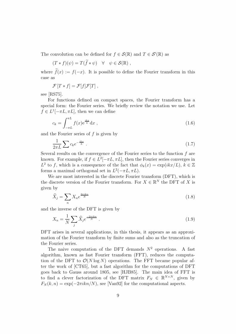
see [RS75].For functions defined on compact spaces, the Fourier transform has a
special form: the Fourier series. We briefly review the notation we use. Letf ∈ L1[−πL, πL], then we can define
ck =
∫ πL
−πLf(x)e
ikxL dx , (1.6)
and the Fourier series of f is given by
1
2πL
∑cke
− ikxL . (1.7)
Several results on the convergence of the Fourier series to the function f areknown. For example, if f ∈ L2[−πL, πL], then the Fourier series converges inL2 to f , which is a consequence of the fact that φk(x) = exp(ikx/L), k ∈ Zforms a maximal orthogonal set in L2(−πL, πL).
We are most interested in the discrete Fourier transform (DFT), which isthe discrete version of the Fourier transform. For X ∈ RN the DFT of X isgiven by
Xj =∑
n
Xne2πikn
N (1.8)
and the inverse of the DFT is given by
Xn =1
N
∑
j
Xje−2πikn
N . (1.9)
DFT arises in several applications, in this thesis, it appears as an approxi-mation of the Fourier transform by finite sums and also as the truncation ofthe Fourier series.
The naive computation of the DFT demands N2 operations. A fastalgorithm, known as fast Fourier transform (FFT), reduces the computa-tion of the DFT to O(N logN) operations. The FFT became popular af-ter the work of [CT65], but a fast algorithm for the computations of DFTgoes back to Gauss around 1805, see [HJB85]. The main idea of FFT isto find a clever factorization of the DFT matrix FN ∈ RN×N , given byFN (k, n) = exp(−2πikn/N), see [Van92] for the computational aspects.
9

1.2 Probability and Stochastic Processes
In this section, we present a brief overview of the topics on probability andstochastic processes used herein. References on the subject are [CW90] and[Sat99].
In this thesis, the triple (Ω,F ,P) denotes a complete probability space,where Ω is a set of points ω, F is a σ-algebra containing all P-null sets, andP is a probability measure. When we say that X is a random variable onthe probability space (Ω,F ,P), we mean that X is real-valued function onΩ, measurable with respect to F .
The characteristic function of a random variable is defined as
ϕ(z) = E[eizX
]. (1.10)
For properties of the characteristic function and a review of probability theorywe refer to [CW90].
The filtered complete probability space is denoted by (Ω,F ,F,P), where,as in [Pro04], we write F for the filtration (Ft)0≤t≤∞ and we assume that
F0 contains all the P-null sets. We useP−→ to denote convergence in proba-
bility, see [CW90] and the French acronyms cadlag (continu a droite, limitea gauche) is used to define the right continuous, left limited process, see[Pro04].
The main class of stochastic processes we are interested in this work arethe Levy processes, see [Sat99] for a comprehensive treatment of the subject.We briefly review the definition of a Levy process
Definition: A Levy process is a cadlag stochastic process, (Xt)t≥0, on (Ω,F ,F,P)taking values in R and with the following properties:
• Independent increments. That is, given t0 ≤ . . . ≤ tN , and definedYn := Xtn −Xtn−1 we have YnNn=1 independent;
• Stationary increments. That is, the distribution of Xt+s −Xt does notdepend on t;
• Stochastic continuity. That is,
Xt+hP−→h↓0
Xt .
An important stochastic process is the Brownian motion.
Definition: A Brownian motion is a adapted continous stochastic process(Wt)t≥0, on (Ω,F ,F,P) taking values in R and with the following properties:
10
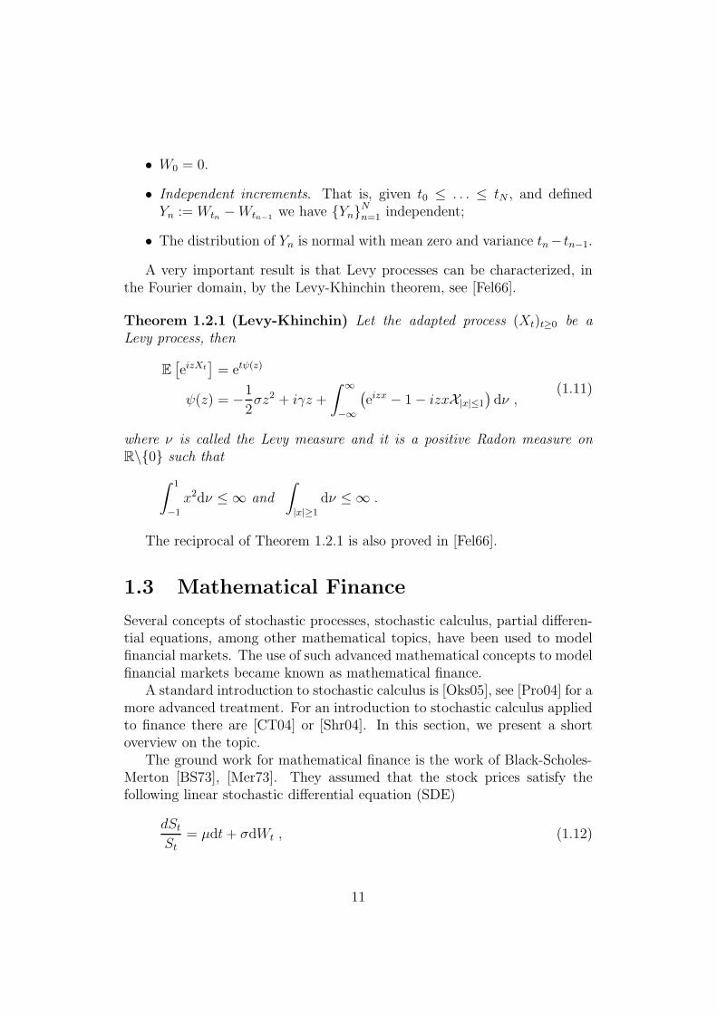
• W0 = 0.
• Independent increments. That is, given t0 ≤ . . . ≤ tN , and definedYn := Wtn −Wtn−1 we have YnNn=1 independent;
• The distribution of Yn is normal with mean zero and variance tn− tn−1.
A very important result is that Levy processes can be characterized, inthe Fourier domain, by the Levy-Khinchin theorem, see [Fel66].
Theorem 1.2.1 (Levy-Khinchin) Let the adapted process (Xt)t≥0 be aLevy process, then
E[eizXt
]= etψ(z)
ψ(z) = −1
2σz2 + iγz +
∫ ∞
−∞
(eizx − 1 − izxX|x|≤1
)dν ,
(1.11)
where ν is called the Levy measure and it is a positive Radon measure onR\0 such that
∫ 1
−1
x2dν ≤ ∞ and
∫
|x|≥1
dν ≤ ∞ .
The reciprocal of Theorem 1.2.1 is also proved in [Fel66].
1.3 Mathematical Finance
Several concepts of stochastic processes, stochastic calculus, partial differen-tial equations, among other mathematical topics, have been used to modelfinancial markets. The use of such advanced mathematical concepts to modelfinancial markets became known as mathematical finance.
A standard introduction to stochastic calculus is [Oks05], see [Pro04] for amore advanced treatment. For an introduction to stochastic calculus appliedto finance there are [CT04] or [Shr04]. In this section, we present a shortoverview on the topic.
The ground work for mathematical finance is the work of Black-Scholes-Merton [BS73], [Mer73]. They assumed that the stock prices satisfy thefollowing linear stochastic differential equation (SDE)
dStSt
= µdt+ σdWt , (1.12)
11

where Wt is a Brownian motion defined on the filtered complete probabilityspace (Ω,F ,F,P). The SDE (1.12) has an unique solution given by
St = S0 exp
((µ− σ2
2
)t+ σWt
). (1.13)
St given by (1.13) is known as geometrical Brownian motion (GBM).One of the most important problems addressed by mathematical finance
is the pricing of a contingent claim. In this thesis, we are only interestedin European contingent claim. An European contingent claim with maturitytime T is a L2(Ω, dP), FT -measurable random variable. Several authorsmake no distinction between contingent claim and derivative contract. Here,an European derivative contract on the underlying asset S and maturity timeT is a L2(Ω, dP), σ(ST )-measurable random variable, so it can be written asg(ST ), where g is called the payoff of the derivative. In this work, we omitthe word European.
The most important financial derivatives are the call and put options.A call option, with maturity time T and strike K, is a contract that givesthe owner the right at the delivery time T to buy stock for the strike priceK. Considering that, the price at T is given by ST and the payoff can beexpressed as (ST −K)+, where (x)+ := max(x, 0). Similarly, the put optiongives the owner the right to sell the asset and its payoff is given by (K−ST )+.The call and put payoff are shown in Figure 1.1.
Call option
Value
STK
Put option
Value
STK
Figure 1.1: Payoff for the call option, with strike K, is shown on the left, andpayoff for the put option, with strike K, is shown on the right.
Consider a market with d assets whose prices are given by a cadlag processSt ∈ Rd, on a filtered complete probability space (Ω,F ,F,P), for notational
12

convenience consider that one of the assets is a risk-free investment, pay-ing interest rates r. A simple trading strategy can be defined by a simplepredictable d-dimentional process
ϕt := ϕ0X0(t) +n∑
j=0
ϕjX(Tj ,Tj+1](t) , (1.14)
where T0 = 0 < T1 < . . . < Tn+1 = T are non-anticipating random times andϕj is a bounded random variable that is FTj
-measurable, see [Pro04]. In itsgeneral form, a trading strategy is a process that can be approximated, in theuniform convergence in (t, ω), by simple predictabel processes, see [Pro04].
Given a strategy, we can define the strategy value for a given time t as
V ϕ(t) = ϕ(0)S(0) +
∫ t
0
ϕ(s)dS(s) . (1.15)
A strategy is called self-financing if
dV ϕ(t) = ϕ(t)dS(t) . (1.16)
We say that a market is arbitrage free if there is no self-financing strategy,ϕ, with
P(V ϕ(T ) ≥ erTV ϕ(0)
)= 1 and P
(V ϕ(T ) > erTV ϕ(0)
)> 0 , (1.17)
where r is the risk-free rate.In the seminal work [BS73], Black and Scholes built a self-financing strat-
egy, ϕ, using the stock price, modeled by a GBM (1.13), and the risk-freeinvestment. The strategy is built to have the same payoff as the call optionat time T . Such strategy is called replicating strategy. Considering that ϕ isa self-financing strategy and that the value of V ϕ(T ) and the payoff at timeT are the same, the price of the call option at t = 0 must be V ϕ(0). Thatis known as the rule of one price and is a consequence of the non-arbitragehypothesis. Black and Scholes found the following formula for the price of acall option with maturity T, and strike K
C(S0, K, T ) = S0N(d+) −KerTN(d−)
d+ =log(S0
K
)+(r + σ2
2
)T
σ√T
d− = d+ − σ√T .
(1.18)
The price is independent of the drift coefficient µ in (1.13). This is a centralresult in mathematical finance.
13

Following Black and Scholes, several authors developed the idea of riskneutral pricing. This idea is based in the notion of an equivalent martingalemeasure, which is an equivalent measure such that the discounted prices,e−rtSt, are martingales, see [CT04]. The following theorem is a central resultin mathematical finance.
Theorem 1.3.1 (Fundamental theorem of asset pricing [CT04]) A mar-ket model defined by (Ω,F ,F,P) and asset prices (St)t∈[0,T ] is arbitrage-freeif and only if there exists an equivalent martingale measure Q.
A proper mathematical statement of the fundamental theorem of asset pric-ing is beyond the scope of this brief review. References on Theorem 1.3.1 fordiscrete time are [HP81] and [MR05]. The continuous version can be foundin [DS94], [DS98], and [Yan98]. In these work the notion of non arbitrageand admissible strategies are rigorously studied.
A consequence of the Theorem 1.3.1 is that for a given contingent claimH , let V (t, H) denote its price. Then
V (t, H) = EQ[e−r(T−t)H
∣∣Ft
], (1.19)
this formula is known as risk neutral pricing formula. A simple example ofchange of measure can be given in the geometrical Brownian case. Under themartingale equivalent measure (1.13) becomes
St = S0ert−σ2
2t+σfWt , (1.20)
where Wt is a Brownian motion under Q, the existence of such measure is aconsequence of the Girsanov theorem, see [Oks05].
Formula 1.19 reduces the pricing problem to computing an integral. How-ever, in general, the density of the process does not have a closed form rep-resentation. To overcome this difficulty, we use the characteristic function.
In (1.13), logSt has normal distribution with mean µ− σ2
2and variance σ2.
The characteristic function of a random variable with distribution N(b, σ2)is given by
ϕ(z) = et“
ibz−σ2z2
2
”
. (1.21)
Letting b = µ − σ2
2in Equation (1.21), we have the characteristic for log
prices in the Black and Scholes model.Following Black-Scholes-Merton, several other authors presented different
models for stock prices. For example, Merton [Mer75] introduced normallydistributed jumps in the log price. A different approach to jumps was given
14

[BS73] ln(ϕ(z)) = ibz − σ2
2z2
[Mer75] ln(ϕ(z)) = izb − σ2
2z2 + λ
(eiµz−
12z2δ2 − 1
)
[Kou02] ln(ϕ(z)) = izb − σ2
2z2 + izλ
(p
λ+ − iz+
1 − p
λ− + iz
)
Table 1.1: The log of the characteristic functions of some processes used infinance, with t=1.
by [Kou02] who introduced an asymmetric exponential density for the jumps.Characteristic functions for these models can be seen in Table 1.1. For manyother models in which the characteristic function is available see [CT04].
A popular class of models used in finance are the stochastic volatilitymodel and among them the most popular is the Heston model [Hes93]. TheSDE for Heston model is given by
dSt = Stµdt+√vtStdW
1t ,
dvt = −λ (vt − v) dt+ ν√vtdW
2t ,
(1.22)
where W 1t and W 2
t are Brownian motions with correlation ρ. The character-istic function for the Heston model is given by
ϕt(z) = eC(z,t)v+D(z,t)v , (1.23)
where
β(z) = λ− iρνz
d(z) =√β(z)2 − 2 (−z2/2 − iz/2) ν2
r+(z) = (β(z) + d(z))/ν2
r−(z) = (β(z) − d(z))/ν2
g(z) = r−(z)/r+(z)
D(z, t) = r−(z)1 − e−d(z)t
1 − g(z)e−d(z)t
C(z, t) = λ
(r−(z)t− 2
ν2ln
(1 − ge−d(z)t
1 − g(z)
)).
In [Hes93], Heston presented a closed form solution for options pricing, whichis one of the main reasons for the popularity of this model. For a review onthe Heston model see [Gat06].
15
Chapter 2
Fourier Methods in Finance
Fourier methods in finance are used in a variety of situations. Several authorsused Fourier methods to find analytical formula for the price of derivatives.Heston [Hes93] used Fourier analysis to find an explicit solution of a parabolicpartial differential equation with mixed differentiation terms, that models theprice of a call option. To do so, Heston explicitly derived the formula for thecharacteristic function of a stochastic volatility model.
The characteristic function of several processes used in finance are knownin closed form. We have for example the Levy-Khinchin representation givenin Theorem 1.2.1. Duffie, Pan and Singleton [DPS00] found the characteristicfunction for general jump-diffusion model and also the derivative price for aspecial class of payoff functions.
In a different direction, Carr-Madan[CM99] and Lewis [Lew00] used theFourier transform to find the price of an European call option in the Fourierspace and then used FFT to find the price in real space. The main idea ofthe method is that European derivatives are convolutions in real space ofthe payoff and the density of the asset on the maturity date. In order tocompute option prices, Carr-Madan [CM99] had to set a damping constantand Lewis [Lew00] had to set a translation in the complex plane to invertthe generalized Fourier transform.
Lee [Lee04] has shown that the accuracy of the method presented by Carr-Madan is sensitive to the choice of the damping constant. Lee presented astrategy to choose the damping parameter. He also extended the methodto several others payoff functions, and presented some bounds for the FFTapproximation.
The FFT approach was also used by [JJSB] and [JSB], to price Americanoptions by the Fourier time stepping. In a different direction [LFBO07] usedRichardson extrapolation to the prices of Bermudian options in order to priceAmerican options.
16

As opposed to [CM99] and [Lew00], this thesis deals with the Fouriertransform for generalized functions. Therefore, no dumping parameter isneeded, and the characteristic function is only used in real space.
This chapter is organized as following. In Section 2.1, we briefly reviewthe two ground works on the application of FFT to finance. In Subsection2.1.1, we review the work of Carr-Madan and in Subsection 2.1.2, we reviewthe work of Lewis. In Section 2.2, we present a new approach based on theFourier transform for tempered distributions. Our method applies to severalderivatives not treated by [CM99], [Lew00], [Lee04], and [DPS00].
2.1 Review of FFT Methods in Finance
In this section, we give a brief overview on the work of Carr-Madan andLewis. See [CM99], [Lew00], [Lee04] or [CT04] for a complete review.
2.1.1 Fourier Transformation with Attenuation Factor
In [CM99], the authors developed a method to numerically calculate the priceof call options for several strikes. The pricing formula for a given strike, ek,is
CT (k) =
∫ +∞
k
e−rT(es − ek
)ρT (s)ds ,
for some risk-neutral density, ρT for the log-prices, as in Equation 1.19. Theattenuated price is defined as
CαT (k) := eαkCT (k) . (2.1)
In general, CT (k) in not integrable, but CαT is. The Fourier transform of the
attenuated price is
CαT (ξ) =
∫ +∞
−∞eiξkCα
T (k)dk
= erTϕ (ξ − (α + 1)i)
α2 + α + ξ2 + i(2α + 1)ξ,
(2.2)
where ϕ is the characteristic function of the distributions ρ. The attenuationfactor makes it necessary to use the characteristic function defined in thecomplex plane. The price can be obtained by Fourier inversion
CT (k) = e−αkF−1[CαT
](k) (2.3)
17

The Fourier transform in 2.3 can be approximated by FFT. In [CT04] adifferent approach was used. More precisely, let
C1T (k) = CT (k) − (1 − ek−rT )+ , (2.4)
so,
C1T (ξ) =
∫ +∞
−∞eiξkC1
T (k)dk
= eiξrTϕ(ξ − i) − 1
iξ(1 + iξ).
(2.5)
The problem with (2.5) is the slow decay of C1T (ξ) for large ξ, to improve
that they used
C2T (k) = CT (k) − Cσ
BS(k) , (2.6)
where CσBS(k) is the Black and Scholes price for an option with volatility σ,
strike ek and maturity T . So
C2T (ξ) =
∫ +∞
−∞eiξkC2
T (k)dk
= eiξrTϕ(ξ − i) − ϕBS(ξ)
iξ(1 + iξ),
(2.7)
where ϕBS(ξ) = exp(−σ2T
2(ξ2 + iξ)
). The decay in (2.7) is exponential for
most of applications to finance, while the decay of (2.5), is polynomial. Theproblem with (2.7) is that we need to find a good σ to improve the methodand we need to compute CBS for every strike.
2.1.2 Generalized Fourier Transform
In a different direction from Carr-Madan [CM99], Lewis [Lew00] works withthe analytic continuation of the Fourier transform. For a given asset St andpayoff f at T , the value of the contract at t = 0, for observed prices s = log S0
is
C(s) = e−rT∫ ∞
−∞f(es+x+rT )ρT (x)dx , (2.8)
which follows from Equation (1.19). To use the Fourier transform in (2.8)some assumptions are needed:
18

• ρ is Fourier integrable in a strip S1. That is, there are a, b ∈ R suchthat
∫ ∞
−∞e−ax|ρ(x)|dx ≤ ∞
∫ ∞
−∞e−bx|ρ(x)|dx ≤ ∞ .
This holds for several processes used in finance. For example, log-normal jump diffusion has S1 = C.
• g(x) = f(ex+rT ) is Fourier integrable in a strip S2 with S = S1∩S2 6= ∅.Again this hypothesis is valid for several payoffs used in finance. Forexample, consider the call option, then S2 = z ∈ C | Im(z) > 1.
Given z ∈ S,
∫ ∞
−∞eizsC(s)ds = e−rT
∫ ∞
−∞ρT (x)
∫ ∞
−∞eizsg(x+ s)dsdx
= e−rT∫ ∞
−∞e−izxρT (x)
∫ ∞
−∞eizyg(y)dydx.
(2.9)
Hence,
F [C] (z) = e−rTϕ(−z)F [g] (z) , (2.10)
where ϕ is the characteristic function ϕ(z) = F [ρT ] (z). The transform ofthe call options, for Im(z) > 1, is given by
F[(
ex+rT −K)+]
=
∫eixz
(ex+rT −K
)+dx
=ek(iz+1)−izrT
iz − z2.
(2.11)
The price of the call options is then given by
C(S) =e−rT
2π
∫ iω+∞
iω−∞e−izsF [C] (z)dz
=e−rT
2π
∫ iω+∞
iω−∞e−izsϕ(−z)e
k(iz+1)−izrT
iz − z2dz ,
(2.12)
for some ω in (1, 1 + α), where α depends on the characteristic function, see[Lew00].
19

2.2 The Fourier Transform for Tempered Dis-
tributions
In this section, we present a method to obtain derivative prices from char-acteristic functions. This method is related to [Lew00], see Subsection 2.1.2,but different from Lewis, we use the Fourier transform only in the real space.We consider payoffs in S ′ (R) and densities in S (R), see Chapter 1. For a spe-cial class of payoffs, that contains several important derivatives in financialmarkets, we explicitly present the formula for the value of the derivative.
In our first result, we express the pricing formula as a convolution. In thefollowing theorem, we establish a simple assumption for the validity of thepricing formula, under fairly general conditions. In Theorem 2.2.2, we usethe former result to prove a pricing formula for more general payoffs.
Theorem 2.2.1 Let f be the payoff at time T of an European derivative,such that
g(s) := f(es+rT
)∈ S ′(R).
Suppose ρT ∈ S(R), then the price is given by
Cg(s) = e−rTF−1[F [g] F [ρ]
](s) ,
where f(x) := f(−x).
Proof: The risk-neutral pricing (1.19) can be written as
Gg(s) = e−rT∫ ∞
−∞f(es+x+rT )ρT (x)dx , (2.13)
so, by definition of g, it follows that
Gg(s) = e−rT∫ ∞
−∞g(x+ s)ρT (x)dx
= e−rT (g ∗ ρ)(s) .(2.14)
The result then follows from the definition of the Fourier transform for con-volutions.
Using Theorem 2.2.1, we can obtain an explicit formula for several payoffsused in finance, not necessarily in S ′(R). The pricing formula is given in thenext theorem.
20

Theorem 2.2.2 Consider a payoff of the form
g(x) =n∑
j=1
(c+j + d+
j ex)Xvj
(x) +m∑
k=1
(c−k + d−k ex
)Xvk
(−x) , (2.15)
over an asset ST with density ρT ∈ S(R). Then the price of the contract isgiven by
Gf (s) =e−rT
2π−∫
e−irT ξF [ρ](−ξ)
iξ
(m∑
k=1
c−k e−ivkξ −n∑
j=1
c+j eiξvj
)e−iξsdξ
+e−rT
2π
∫e−irT ξ
F [ρ](−ξ)1 + iξ
(m∑
k=1
+d−k e−ivkξ −n∑
j=1
d+j eiξvj
)e−iξsdξ
+e−rT
2
(m∑
k=1
c−k −n∑
j=1
c+j
)+ es+rT
m∑
k=1
d+k .
(2.16)
Proof: Notice that
gl(x) := g(x) − ex∑
d+k
=
n∑
j=1
c+j Xvj(x) − d+
j exX−vj(−x) +
m∑
k=1
(c−k + d−k ex
)Xvk
(−x) ,(2.17)
so gl ∈ S ′(R). The Fourier transform of gl is given by
F[gl](ξ) =
n∑
j=1
c+j eiξvjF [H ] + d+j
eiξvj
1 + iξ
+m∑
k=1
c−k e−ivkξF [H ](−ξ) + d−ke−ivkξ
1 + iξ
=
(1
iξ+ πδ
)( m∑
k=1
c−k e−ivkξ −n∑
j=1
c+j eiξvj
)
+1
1 + iξ
(n∑
j=1
d+j eiξvj +
m∑
k=1
+d−k e−ivkξ
).
(2.18)
21

Using the risk-neutral pricing formula (1.19), we obtain
Gg(s) = e−rT∫ ∞
−∞g(x+ s+ rT )ρT (x)dx
= e−rT
(∫ ∞
−∞gl(x+ s + rT )ρT (x)dx+
∫ ∞
−∞ex+s+rTρT (x)dx
m∑
k=1
d+k
)
= e−rT∫ ∞
−∞gl(x+ s+ rT )ρT (x)dx+ es+rT
m∑
k=1
d+k .
(2.19)
In the last equation, we used the martingale property of discounted prices.So, according to Theorem 2.2.1, we have
Gg(s) =e−rT
2π−∫
e−irT ξF [ρ](−ξ)
iξ
(m∑
k=1
c−k e−ivkξ −n∑
j=1
c+j eiξvj
)e−iξsdξ
+e−rT
2π
∫e−irT ξ
F [ρ](−ξ)1 + iξ
(m∑
k=1
+d−k e−ivkξ −n∑
j=1
d+j eiξvj
)e−iξsdξ
+e−rT
2
(m∑
k=1
c−k −n∑
j=1
c+j
)+ es+rT
m∑
k=1
d+k .
(2.20)
The payoff function given by Equation (2.15) used in Theorem 2.2.2 is verygeneral. We now give a brief overview of some payoffs to which Theorem2.2.2 applies. For an introduction to payoffs used in financial markets see[Hul08].
• Call
gC(x) = Xk(x)(ex − ek
)
This option gives the owner the right to buy at time T the asset forthe strike price ek.
• Digital
gD(x) = Xk (x)
This option gives the owner one unit of money if the stock is abovesome strike ek at maturity T.
22

• Bull Spread
gBull(x) = Xk1 (x)(ex − ek1
)−Xk2 (x)
(ex − ek2
)
This payoff is made of buying a call with strike ek1 and selling a callwith strike ek2, all the calls with the same maturity and k2 > k1.
• Butterfly
gB(x) =Xk1 (x)(ex − ek1
)− 2Xk2 (x)
(ex − ek2
)
+ Xk3 (x)(ex − ek3
)
This payoff is made of buying a call with strikes ek1 and ek3 and sellingtwo calls with strike ek2 , all the calls with the same maturity, k3 > k1
and k2 = log((ek1 + ek3)/2
).
• Straddle
gS(x) = Xk (x)(ex − ek
)+ X−k (−x)
(ek − ex
)
This payoff is made of buying a call option, and buying a put optionwith the same strike, ek and the same maturity T.
The payoffs of the Digital, Butterfly, Bull Spread and Straddle are shown inFigure 2.1, the payoffs of the call and put options are shown in Figure 1.1.
The pricing method presented in this section has one main advantage overthe method presented by Carr-Madan, Subsection 2.1.1 and Lewis, Subsec-tion 2.1.2. In Theorem 2.2.2 no extra parameter was needed, while in Lewisand Carr-Madan, the definition of an extra parameter is needed. The gener-alized payoff formula of Theorem 2.2.2 makes it possible to obtain a closedform pricing formula for a portfolio of derivatives, which is often the case inthe markets.
All Fourier transforms found in this section involve either h(ξ)/ξ or h(ξ)/(1+iξ). Numerical inversion for this kind of function will be treated in Chapter3.
23
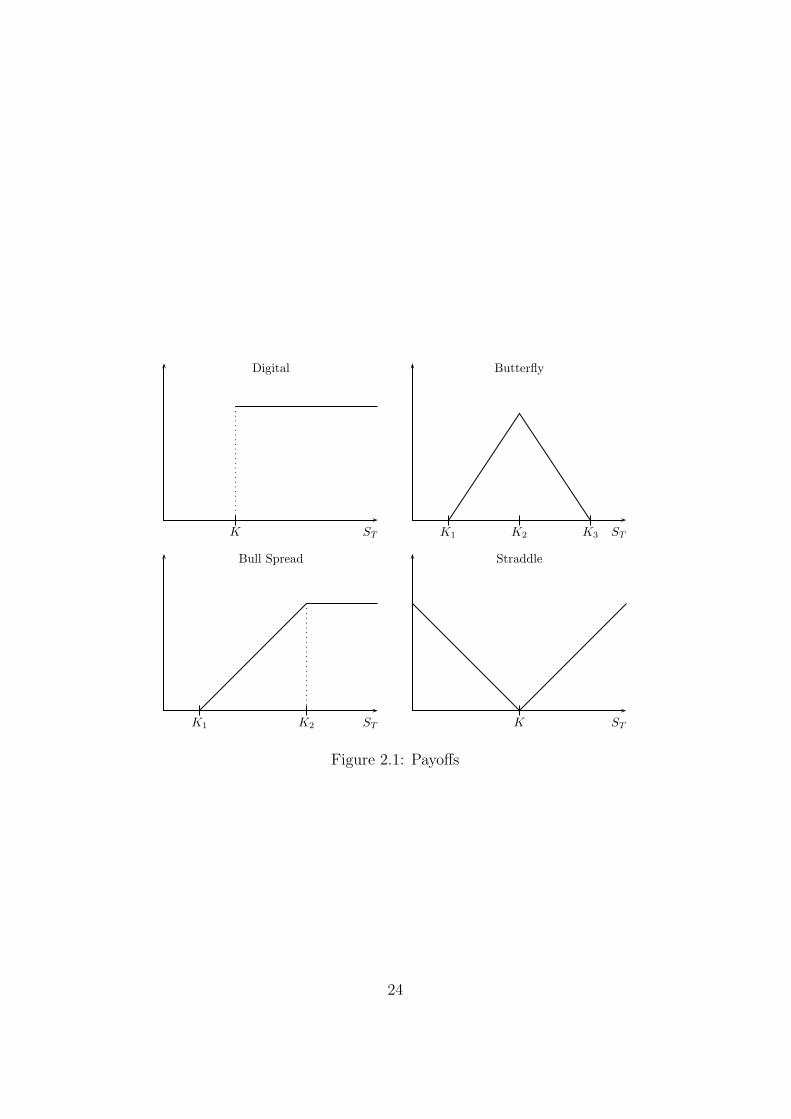
Digital
STK
Butterfly
STK1 K2 K3
Bull Spread
STK1 K2
Straddle
STK
Figure 2.1: Payoffs
24

Chapter 3
Approximation of FourierOperators
Fourier methods have been used for several problems, ranging from physicsand electromagnetism to mathematical finance.
From the physics and engineering point of view, this chapter presentsa fast method for the evaluation of the heat potentials. Here we followthe lines given by the work of Greengard and Lin [GL00], who developedan approximation method based on non-uniform quadrature. This kind ofmethod was used in [LG07] to solve inhomogeneous heat equation in freespace.
In this chapter, we improve the approximation method developed byGreengard and Lin [GL00] by obtaining a sharper bound, which is valid fora class of functions having the heat kernel as a particular case. In anotherdirection, we present bounds for other types of Fourier transforms arisingfrom the lack of differentiability of the transformed function.
We start with a simple example as motivation. Consider the heat equationproblem for a finite rod,
ut = uxx t > 0, |x| ≤ Lπ
u(−Lπ, t) = u(Lπ, t) = 0
u(x, 0) = f(x) |x| ≤ Lπ .
The solution is given by
u(x, t) = KL(x, t) ∗ f(x) , (3.1)
where KL(x, t) is the heat kernel
KL(x, t) :=1
2πL
∞∑
k=−∞e−t(
kL)
2
eikLx . (3.2)
25
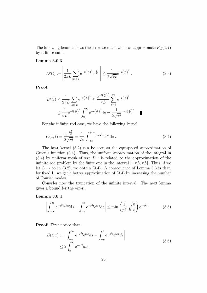
The following lemma shows the error we make when we approximate KL(x, t)by a finite sum.
Lemma 3.0.3
Ep(t) :=
∣∣∣∣∣∣1
2πL
∑
|k|>pe−t(
kL)
2
eikLx
∣∣∣∣∣∣≤ 1
2√πt
e−t(pL)
2
. (3.3)
Proof:
Ep(t) ≤ 1
2πL
∑
|k|>pe−t(
kL)
2
≤ e−t(p
L)2
πL
∞∑
s=1
e−t(sL)
2
≤ 1
πLe−t(
pL)
2∫ ∞
0
e−t(sL)
2
ds =1
2√πt
e−t(pL)
2
For the infinite rod case, we have the following kernel
G(x, t) =e−
x2
4t
2√πt
=1
2π
∫ +∞
−∞e−s
2teisxds . (3.4)
The heat kernel (3.2) can be seen as the equispaced approximation ofGreen’s function (3.4). Thus, the uniform approximation of the integral in(3.4) by uniform mesh of size L−1 is related to the approximation of theinfinite rod problem by the finite one in the interval [−πL, πL]. Thus, if welet L → ∞ in (3.2), we obtain (3.4). A consequence of Lemma 3.3 is that,for fixed L, we get a better approximation of (3.4) by increasing the numberof Fourier modes.
Consider now the truncation of the infinite interval. The next lemmagives a bound for the error.
Lemma 3.0.4∣∣∣∣∫ ∞
−∞e−s
2teisxds−∫ p
−pe−s
2teisxds
∣∣∣∣ ≤ min
(1
pt,
√π
t
)e−p
2t (3.5)
Proof: First notice that
E(t, x) :=
∣∣∣∣∫ ∞
−∞e−s
2teisxds−∫ p
−pe−s
2teisxds
∣∣∣∣
≤ 2
∫ ∞
p
e−s2tds .
(3.6)
26
Then, a simple integration by parts results in
E(t, x) ≤ 2
∫ ∞
p
Ds
(e−s
2t) −1
2stds
≤ −e−s2t
st
∣∣∣∣∣
∞
p
−∫ ∞
p
e−s2t 1
s2tds ≤ e−p
2t
pt.
(3.7)
For the other inequality observe that
E(t, x) ≤ 2
∫ ∞
p
e−s2tds ≤ 2
∫ ∞
0
e−(y+p)2tdy
≤ 2e−p2t
∫ ∞
0
e−y2tdy =
√π
te−p
2t .
(3.8)
Lemma 3.0.4 shows that for large values of t we need lower p to obtain thesame accuracy. In the opposite direction, consider the error for the uniformquadrature
EQn =
∣∣∣∣∣
∫ p
−pe−s
2teisxds−N∑
k=1
e−s2kteiskx
∣∣∣∣∣ , (3.9)
where sk = −p + 2pN
(k − 1). EQn increases with t. In order to observe
this, notice that∣∣∣Ds
(e−s
2teisx)∣∣∣ = e−s
2t√x2 + 4s2t2, which for x = 0 has
a maximum of√t(√
2e)−1
.An example of the approximation of the Fourier transform by uniform
quadrature is given in Figure 3.1. In order to use FFT we must have ∆x∆s =2π/N , so we have to define xj = xmin + j∆x, j = 0, . . . , N − 1, wherexmin = −(N/2)∆x.
The problem shown by Figure 3.1 is that for large values of t we musthave a dense sampling on a small suport, while for small t we have to en-large the support of the sampling. In this thesis, we focus on non-uniformapproximations to overcome this limitation of uniform approximations.
3.1 Spectral Approximation of the Free-Space
Heat Kernel
In this section, we give a brief overview of the work of Greengard and Lin[GL00], which was the starting point of this chapter. In their work, theyaddressed the following question:
27

−0.80 −0.48 −0.16 0.16 0.48
−1.20
−0.72
−0.24
0.24
0.72
t = 0.1, ∆s = 0.5, N = 6410−12x
101x −0.80 −0.48 −0.16 0.16 0.48
0.000
0.072
0.144
0.216
0.288
t = 10, ∆s = 0.5, N = 6410−1x
101x
−0.240 −0.144 −0.048 0.048 0.144
−0.30
−0.18
−0.06
0.06
0.18
t = 0.1, ∆s = 0.15, N = 6410−1x
102x −0.240 −0.144 −0.048 0.048 0.144
−0.030
0.012
0.054
0.096
0.138
t = 10, ∆s = 0.15, N = 6410−5x
102x
Figure 3.1: The error of the uniform approximation to the Fourier transform,as in (3.9) is shown for different values of ∆s and t.
“How many quadrature points are required on an interval [a, b] inthe Fourier domains in order to resolve the spectrum to withinsome specified precision ǫ?”(Greengard and Lin [GL00])
To answer this question they presented a discretization of the heat kernelbased in the Gauss-Legendre quadrature, as seen in Theorem 3.1.1. In thisthesis, as in [GL00], we work with Gauss-Legendre quadrature. To simplifynotation consider the following definition.
Definition: From here on, we always use Sn[a,b] := (s1, . . . , sn) and Wn[a,b] :=
(w1, . . . , wn) to denote the nodes and weights for the n-point Gauss-Legendrequadrature on the interval [a, b].
With this definition we can present the following theorem.
Theorem 3.1.1 ([GL00]) Given n, and ǫ, let Sn[a,b] and Wn[a,b] be the nodes
and weights for the Gauss-Legendre quadrature, where [a, b] = [2j , 2j+1] thenfor t > t0, we have
∣∣∣∣∣
∫ b
a
e−ts2
eixsds−n∑
j=1
wje−ts2j eixsj
∣∣∣∣∣ ≤ ǫ(b− a)
+
√2π(b− a)√
n
((b− a)|x|
2n+
√− log(ǫ)√
n
)2n (3.10)
28
∣∣∣∣∣
∫ b
a
e−ts2
eixsds−n∑
j=1
wje−ts2j eixsj
∣∣∣∣∣ ≤ǫ(b− a)
p
+
√2π(b− a)√
n
((b− a)|x|
2n+
√− log(ǫt0)√
n
)2n (3.11)
where exp(−p2t0)/√
7πt0 = ǫ.
A different version of this theorem will be shown in Theorem 3.3.3, whichis based in Theorem 3.2.3. We will also present results for the estimationof the Fourier transform of h(s)/s and h(s)/(1 + is) (Theorems 3.2.4, 3.2.6,3.3.4, and 3.3.7).
3.2 Non-uniform Quadratures
In the previous section, we have shown the problem with the uniform quadra-ture to approximate the continuous Fourier transform. Historically, non-uniform quadratures have been used as an improvement over the uniformcase. In this section, we present some bounds for the sampling error fornon-uniform approximations of the Fourier transform for a special class offunctions.
The first result of this section is a simple application of Stirling’s approx-imation,
√2πn
2n+12 e−n < n! < 2
√πn
2n+12 e−n , (3.12)
see [AS65]. The result of the following lemma will be used in the sequel.
Lemma 3.2.1
n!4
(2n)!3≤ 2
√nπ
(1
α1n
)2n
andn!4
(2n)!2≤ 4nπ
(1
2
)4n
, (3.13)
where α1 := 8/e.
Proof: These results follow from Stirling’s approximation (3.12). For thefirst inequality, notice that
n!4
(2n)!3≤
(2√πn
2n+12 e−n
)4
(√2π(2n)
4n+12 e−2n
)3
≤ 2√nπ( e
23n
)2n
= 2√nπ
(1
α1n
)2n
.
29
For the second inequality, we have
n!4
(2n)!2≤
(2√πn
2n+12 e−n
)4
(√2π(2n)
4n+12 e−2n
)2
= 4nπ
(1
2
)4n
.
The second result used in this chapter is the standard estimate for n-pointGauss-Legendre quadrature (see [DR75]).
Theorem 3.2.2 Let Sn[a,b] and Wn[a,b] be the nodes and weights for the n-point
Gauss-Legendre quadrature on the interval [a, b]. Then, if h ∈ C2n[a, b],
EQn (h) :=
∣∣∣∣∣
∫ b
a
h(s)ds−n∑
j=1
wjh(sj)
∣∣∣∣∣
≤ (b− a)2n+1(n!)4
(2n + 1)(2n)!3sups∈(a,b)
∣∣D2n (h(s))∣∣ .
The approximations of Fourier transform in this section concern a specificclass of functions.
Definition: We say that h(s; β) ∈ Dn[a,b](f) if h(s; β) ∈ C2n[a, b], and if
derivatives of h(s; β) in s is bounded by
∣∣Djsh(s; β)
∣∣ ≤ βj
2 (2n)j
2f(s) ,
for some bounded f . A short definition of Dn[a,b](f) is given by
Dn[a,b](f) :=
h(s; β) ∈ C2n[a, b];
∣∣Djsh(s; β)
∣∣ ≤ βj
2 (2n)j
2f(s) j = 1, . . . , 2n.
When clear from the context, we denote Dn[a,b](f) by D and h(s; β) by h(s).
We are particularly interested in the Heat kernel, Lemma 3.3.1 proves that
h(s; t) = e−ts2 ∈ Dn
[a,b]
((4nπ)1/4e−ts
2/2).
The result of the next theorem will be later shown as an extension andimprovement to [GL00]. Theorem 3.2.3, when applied to the heat kernel,can be used, for example, to solve the inhomogeneous heat equation in freespace, see [LG07].
Using Lemma 3.2.1 and Theorem 3.2.2, we can prove our first approxi-mation of the Fourier transform.
30

Theorem 3.2.3 Given n, let Sn[a,b] and Wn[a,b] be the nodes and weights for
the Gauss-Legendre quadrature. Then, if h ∈ Dn[a,b](f) it follows that
∣∣∣∣∣
∫ b
a
h(s)eixsds−n∑
j=1
wjh(sj)eixsj
∣∣∣∣∣
≤√π(b− a)√
nf ∗(
(b− a)|x|α1n
+(b− a)
√2β
α1
√n
)2n
,
(3.14)
where f ∗ = maxs∈[a,b] f(s) and α1 = 8/e.
Proof: From h ∈ Dn[a,b](f) we have
∣∣D2n(h(s)eisx
)∣∣ ≤2n∑
j=0
(2n
j
) ∣∣Djh(s)∣∣ ∣∣D2n−j (eisx
)∣∣
≤2n∑
j=0
(2n
j
)β
j
2 (2n)j
2 f(s)|x|2n−j
≤ f(s)2n∑
j=0
(2n
j
)(√2βn
)j|x|2n−j
≤ f(s)(|x| +
√2βn
)2n
.
(3.15)
Using (3.15), it follows from Theorem 3.2.2 that
EQn :=
∣∣∣∣∣
∫ b
a
h(s)eixsds−n∑
j=1
wjh(sj)eixsj
∣∣∣∣∣
≤ (b− a)2n+1(n!)4
(2n + 1)(2n)!3f ∗(|x| +
√2βn
)2n
≤ (b− a)2n+1
(2n+ 1)
(2√nπ( e
23n
)2n)f ∗(|x| +
√2βn
)2n
,
where we used Lemma 3.2.1 in the last inequality. The final step is given by
EQn ≤ (b− a)8
√nπ
(2n+ 1)f ∗(
(b− a)|x|α1n
+(b− a)
√2β
α1
√n
)2n
≤ (b− a)√π√
nf ∗(
(b− a)|x|α1n
+(b− a)
√2β
α1
√n
)2n
.
31
The next approximation concerns the principal value of some Fouriertransform. This kind of transformation is often seen in several differentsituations. As an example, we have the Fourier transform of
v(x) =
∫ x
−∞g(s)ds , (3.16)
which is given by
F [v](ξ) = F [g](ξ)
(πδ − 1
iξ
).
Such transformation is very often found in mathematical finance, see Section2.2, and probability, in which it is used to compute cumulative probability.
Theorem 3.2.4 Given n, let Sn[a,b] and Wn[a,b] be the nodes and weights for
the Gauss-Legendre quadrature. Then, if h ∈ Dn[a,b](f) with 0 /∈ [a, b], it
follows that∣∣∣∣∣
∫ b
a
h(s)
iseisxds−
n∑
j=1
wjh(sj)
isjeixsj
∣∣∣∣∣ ≤ f ∗(b− a
4sm
)2n+18πesm
√2βn
n
+
√π(b− a)√
nf ∗|x|
((b− a)|x|nα1
+(b− a)
√2β
α1
√n
)2n
,
(3.17)
where α1 = 8/e, s = max (|a|, |b|), s = min (|a|, |b|), f ∗ = maxs∈[a,b] f(s), andsm = arg maxs∈[a,b] exp(|s|√2βn)|s|−2n−1.
Proof: We bound the derivative∣∣∣∣D
js
(eisx
is
)∣∣∣∣ =
∣∣∣∣∣−ieisx
j∑
k=0
(j
k
)(ix)k
(j − k)!(−1)j−k
sj−k+1
∣∣∣∣∣
=
∣∣∣∣∣−i(−1)jeisxj!
sj+1
j∑
k=0
(−isx)kk!
∣∣∣∣∣
≤ j!
|s|j+1
∣∣∣∣∣
j∑
k=0
(−isx)kk!
∣∣∣∣∣ .
(3.18)
By Taylor’s theorem for some s with |s| < |s|, we then have∣∣∣∣D
js
(eisx
is
)∣∣∣∣ ≤j!
|s|j+1
∣∣∣∣e−isx − (−ixs)j+1
(j + 1)!
∣∣∣∣
≤ j!
|s|j+1
(1 +
(|x|s)j+1
(j + 1)!
).
(3.19)
32

Using the bound (3.19), we are ready to compute
∣∣∣∣D2n
(h(s)eisx
is
)∣∣∣∣ ≤2n∑
j=0
(2n
j
) ∣∣D2n−jh(s)∣∣∣∣∣∣D
j
(eisx
is
)∣∣∣∣
≤2n∑
j=0
(2n
j
)(β2n)
2n−j
2 f(s)j!
|s|j+1
(1 +
(|x|s)j+1
(j + 1)!
)
≤ f(s)
2n∑
j=0
((2n)!
|s|2n+1
|s√2βn|2n−j(2n− j)!
+
(2n
j
)√2βn
2n−j |x|j |x|s|s|(j + 1)
)
≤ f(s)
((2n)!e|s|
√2βn
|s|2n+1+
|x|s|s|(√
2βn+ |x|)2n),
(3.20)
where the second line is a consequence of h ∈ D and (3.19). Using Lemma3.2.1 and Theorem 3.2.2, it follows from (3.20) that
E :=
∣∣∣∣∣
∫ b
a
h(s)eixs
isds−
n∑
j=1
wjh(sj)e
ixsj
isj
∣∣∣∣∣
≤ (b− a)2n+1
(2n+ 1)f ∗
((4π
24n
)esm
√2βn
s2n+1m
+ 2√nπ( e
n8
)2n
|x|(√
2βn+ |x|)2n)
≤ f ∗
((b− a
4sm
)2n+116πesm
√2βn
2n+ 1+
2√nπ(b− a)
2n + 1x
((b− a)
√2β
α1
√n
+(b− a)|x|nα1
)2n)
≤ f ∗
((b− a
4sm
)2n+18πesm
√2βn
n+
√π(b− a)|x|√
n
((b− a)
√2β
α1
√n
+(b− a)|x|nα1
)2n).
It is interesting to observe that the minimum for exp(|s|√2βn)|s|−2n−1 is
achieved at s = 2n+1√2βn
with value(√
2βn/(2n+ 1))2n+1
.Theorem 3.2.4 is related to Theorem 3.2.3. To see this, first notice that
Theorem 3.2.4 has the extra term f ∗ ((b− a)/(4sm))2n+1 8π exp(sm√
2βn)/n,besides that, the second line of (3.17) is the the bound obtained in Theorem3.2.3 times |x|.
Theorem 3.2.4 is not valid when 0 ∈ [a, b]. Thus a different approach isneeded in this case. To treat it, we find an approximation of
I1(x) := −∫
|s|≤δ
h(s)
iseisxds . (3.21)
33

To approximate I1 we assume that the derivatives of h at 0 are available.The following lemma gives the desired approximation.
Lemma 3.2.5 For a given δ and h ∈ Cn+1[−δ, δ], we then have
EI1(n, δ) :=
∣∣∣∣∣−∫
|s|<δ
eixsh(s)
isds−
n∑
j=1
h(j)(0)f δj−1(x)
j!i− h(0)
∫
|s|≤δ
sin(sx)
sds
∣∣∣∣∣
≤ sup|s|<δ
∣∣Dn+1h(s)∣∣ 2δn+1
(n + 1) (n+ 1)!,
(3.22)
where
f δn(x) :=
n∑
j=0
n!
(n− j)!
δn−j
(−ix)j+1
((−1)n−je−ixδ − eixδ
).
Proof: First notice that
I1(x) = −∫
|s|≤δ
h(s)
iseisxds
= −∫
|s|<δ
eisx
is
(n∑
j=0
h(j)(0)sj
j!+h(n+1)(z(s))sn+1
(n + 1)!
)ds
= −i∫
|s|<δeisx
(n∑
j=1
h(j)(0)sj−1
j!+h(n+1)(z(s))sn+1
(n+ 1)!
)ds+ h(0)−
∫
|s|<δ
eixs
isds ,
(3.23)
where z(s) ∈ [−s, s] ⊂ [−δ, δ] that is given by the Taylor’s theorem. Theresult follows from the fact that
fn(x) =
∫
|s|≤δsneixsds .
Our next approximation concerns h(s)/(c + is). One example of theappearance of such transform is
u(x) = ecx∫ ∞
x
g(s)e−csds .
34

The Fourier transform of u is given by
F [u](ξ) =F [g](ξ)
c+ iξ. (3.24)
Such functions are seen in several applications, for example, [CM99] used asimilar transform to find option prices. In Section 2.2, Fourier transformssimilar to (3.24) were also seen. The following theorem presents a bound forthe Fourier transform for this type of functions.
Theorem 3.2.6 Given n, let Sn[a,b] and Wn[a,b] be the nodes and weights for
the Gauss-Legendre quadrature. Then, if h ∈ Dn[a,b](f) it follows that
∣∣∣∣∣
∫ b
a
h(s)
c+ iseixsds−
n∑
j=1
wjh(sj)
c+ isjeixsj
∣∣∣∣∣ ≤ f ∗(
b− a
4|c+ s|
)2n+18πe
√2βn(c2+s2)
nexc
+
√π(b− a)√
nf ∗|x|
((b− a)|x|α1n
+(b− a)
√2β
α1
√n
)2n
,
where α1 = 8/e, s = max(|a|, |b|), s = min(|a|, |b|), and f ∗ = maxs∈[a,b] f(s).
Proof: To calculate a bound for the derivative consider
∣∣∣∣Dj
(eisx
c+ is
)∣∣∣∣ =
∣∣∣∣∣eisx
j∑
k=0
(j
k
)(ix)k
(j − k)!(−i)j−k(c + is)j−k
∣∣∣∣∣
=
∣∣∣∣∣eisxj!
(c+ is)j+1
j∑
k=0
(ix)k(−i)k(c+ is)k
k!
∣∣∣∣∣
≤ j!
|c+ is|j+1
∣∣∣∣∣
j∑
k=0
(xc + ixs)k
k!
∣∣∣∣∣ .
(3.25)
Using Taylor’s theorem for some d ∈ C with |d| < |x|√c2 + s2, we have
∣∣∣∣Dj
(eisx
c+ is
)∣∣∣∣ ≤j!
|c+ is|j+1
∣∣∣∣exceisx − dj+1
(j + 1)!
∣∣∣∣
≤ j!
|c+ is|j+1
(exc +
(|x|√c2 + s2)j+1
(j + 1)!
).
(3.26)
35

Using the fact that h ∈ D and (3.26), we are ready to estimate
∣∣∣∣D2n
(h(s)eisx
c+ is
)∣∣∣∣ ≤2n∑
j=0
(2n
j
) ∣∣D2n−jh(s)∣∣∣∣∣∣D
j
(eisx
c+ is
)∣∣∣∣
≤2n∑
j=0
(2n
j
)(2βn)
2n−j
2 f(s)j!
|c+ is|j+1
(exa +
(|x|√c2 + s2)j+1
(j + 1)!
)
≤f(s)exc2n∑
j=0
(2n)!
|c+ is|2n+1
(√2βn(c2 + s2)
)2n−j
(2n− j)!+
+ f(s)2n∑
j=0
(2n
j
)√2βn
2n−j |x|j |x|(j + 1)
≤ f(s)
((2n)!exce
√2βn(c2+s2)
|c+ is|2n+1+ |x|
(√2βn+ |x|
)2n).
(3.27)
We used (3.27), Lemma 3.2.1, and Theorem 3.2.2 to obtain the followingestimate
E(n) :=
∣∣∣∣∣
∫ b
a
h(s)
c+ iseixsds−
n∑
j=1
wjh(sj)
c+ isjeixsj
∣∣∣∣∣
≤(b− a)2n+1(n!)4
(2n+ 1)(2n)!2f ∗ exce
√2βn(c2+s2)
|c+ is|2n+1
+(b− a)2n+1(n!)4
(2n+ 1)(2n)!3f ∗|x|
(√2βn+ |x|
)2n
≤8π
(b− a
4|c+ is|
)2n+1f ∗exce
√2βn(c2+s2)
n
+
√π(b− a)√
nf ∗|x|
((b− a)
√2β
α1
√n
+|x|(b− a)
α1n
)2n
.
It is interesting to notice that Theorem 3.2.4 and 3.2.6 are essentially thesame if we let c→ 0.
3.3 Heat Kernel
In this section, we focus on the heat kernel, h(s) = e−ts2. This particular case
of Section 3.2 was studied by [GL00], as seen in Section 3.1. Here, we extend
36

their results to different transform and improve the bound they obtained.We prove versions of Theorems 3.2.3, 3.2.4, and 3.2.6 for the heat kernel.
With these results, we are able to, given a precision ǫ, find for any t > t0 fora given t0, the required quadrature points in the Fourier domain to achievethis precision.
First, we prove that, given [a, b] and n, we have h(s) = e−ts2 ∈ Dn
[a,b](f),for some f .
Lemma 3.3.1 If h(s) = e−ts2, then we have
∣∣Djh(s)∣∣ ≤ β
j
2nj
2 f(s) j = 1, . . . , n (3.28)
for β = 2te
and f(s) = (4nπ)14 e−
ts2
2 .
Proof: From [Sza51], we have the following estimate for Hermite functions
1
n!|hn(x)| ≤
√2n
√n!
e−x2
2 , (3.29)
so, when h(s) = e−ts2,
Dj(e−ts
2)
= tj
2 Djx
(e−x
2)∣∣∣
x=s√t
= tj
2hj
(s√t).
(3.30)
Using (3.29) and (3.30), we have the following bound for the derivative∣∣∣Dj
(e−ts
2)∣∣∣ ≤ (2t)
j
2
√j!e−
ts2
2 . (3.31)
Now using (3.12), we have∣∣∣Dj
(e−ts
2)∣∣∣ ≤ (2t)
j
2
√2√πjj+
12 e−je−
ts2
2
≤(
2t
e
) j2
nj2 (4nπ)
14 e−
ts2
2 .
All theorems in the previous section deal with integrals over finite inter-vals. We now present some bounds for the truncation of the infinite integral.
Lemma 3.3.2∣∣∣∣∣−∫ ∞
−∞
e−s2t
seisxds−−
∫ p
−p
e−s2t
seisxds
∣∣∣∣∣ ≤ min
(1
pt,
√π
t
)e−p
2t
p∣∣∣∣∣
∫ ∞
−∞
e−s2t
a + iseisxds−
∫ p
−p
e−s2t
a+ iseisxds
∣∣∣∣∣ ≤ min
(1
pt,
√π
t
)e−p
2t
√a2 + p2
(3.32)
37

Proof: First notice that
E1(t, x) :=
∣∣∣∣∣−∫ ∞
−∞
e−s2t
seisxds−−
∫ p
−p
e−s2t
seisxds
∣∣∣∣∣ ≤ 2
∫ ∞
p
e−s2t
sds .
Using integration by parts, we have
E1(t, x) ≤ 2
∫ ∞
p
Ds
(e−s
2t) −1
2s2tds =
e−s2t
s2t
∣∣∣∣∣
∞
p
−∫ ∞
p
e−s2t 2
s2tds
≤ e−p2t
p2t,
so we have one of the bounds. Now consider
E1(t, x) ≤ 2
∫ ∞
p
e−s2t
sds = 2
∫ ∞
0
e−(y+p)2t
y + pds
≤ 2e−p
2t
p
∫ ∞
0
e−y2tds =
√π
t
e−p2t
p.
(3.33)
For the second integral, notice that
E2(t, x) :=
∣∣∣∣∣
∫ ∞
−∞
e−s2t
a + iseisxds−
∫ p
−p
e−s2t
a+ iseisxds
∣∣∣∣∣ ≤ 2
∫ ∞
p
e−s2t
√a2 + s2
ds .
It follows from integration by parts that
E2(t, x) ≤ 2
∫ ∞
p
Ds
(e−s
2t)
−2st√a2 + s2
ds
=e−s
2t
st√a2 + s2
∣∣∣∣∣
∞
p
−∫ ∞
p
e−s2t
√a2 + s2
(1
s2+
1
a2 + s2
)ds
≤ e−p2t
pt√a2 + p2
.
Finally consider
E2(t, x) ≤ 2
∫ ∞
p
e−s2t
√a2 + s2
ds = 2
∫ ∞
0
e−(y+p)2t
√a2 + (y + p)2
ds
≤ 2e−p
2t
√a2 + p2
∫ ∞
0
e−y2tds =
√πe−p
2t
√t (a2 + p2)
38

We now present the version of Theorem 3.2.3 for the heat kernel. Thisresult follows the line of [GL00], which proved Theorem 3.1.1. Theorem 3.3.3has some improvements over Theorem 3.1.1, as we show next.
Theorem 3.3.3 Given n, and ǫ, let Sn[a,b] and Wn[a,b] be the nodes and weights
for the Gauss-Legendre quadrature, where [a, b] = [2j , 2j+1] then for t > t0,we have
∣∣∣∣∣
∫ b
a
e−ts2
eixsds−n∑
j=1
wje−ts2j eixsj
∣∣∣∣∣ ≤ ǫ(b− a)
+2(b− a)π
34
n14
e−t0s2
2
((b− a)x
α1n+
√− log(ǫ)
α2
√n
)2n (3.34)
∣∣∣∣∣
∫ b
a
e−ts2
eixsds−n∑
j=1
wje−ts2j eixsj
∣∣∣∣∣ ≤ ǫ(b− a)
p
+2(b− a)π
34
n14
e−t0s2
2
(b− a)x
α1n+
√− log
((ǫ√t0)
α2
√n
2n
,
(3.35)
where p =√− log
(ǫ√t0)/t0, s = min(|a|, |b|), α1 = 8/e, and α2 = 4
√2/e.
Proof: For (b − a)√t <
√− log(ǫ) and (b − a)
√t <
√− log(ǫ
√t0) the
theorem is a consequence of Theorem 3.2.3 and Lemma 3.3.1. For a√t =
(b− a)√t >
√− log(ǫ), we have
∣∣∣∣∫ b
a
e−ts2
eisxds
∣∣∣∣ ≤ e−ta2
∫ b
a
ds
≤ ǫ(b− a) .
(3.36)
For a√t = (b− a)
√t >
√− log(ǫ
√t0), it follows that
∣∣∣∣∫ b
a
e−ts2
eisxds
∣∣∣∣ ≤ e−ta2
∫ b−a
0
e−tx2
dx ≤ ǫ√t0
∫ b−a
0
e−
„
− log(ǫ√
t0)(b−a)2
«
x2
dx
39

so defining y =
q
− log(ǫ√t0)
b−a x, we have
∣∣∣∣∫ b
a
e−ts2
eisxds
∣∣∣∣ ≤ ǫ
√t0(b− a)√
− log(ǫ√t0)∫ q
− log(ǫ√t0)
0
e−y2
dy
≤ ǫ
√t0(b− a)√
− log(ǫ√t0)√π
2.
Now let p =
q
− log(ǫ√t0)√
t0then
∣∣∣∣∫ b
a
e−ts2
eisxds
∣∣∣∣ ≤ ǫb− a
p(3.37)
The above result improves [GL00] for large values of s, due to the fastdecay of the function e−t0s
2/2 presented in Theorem 3.3.3 that is not presentin [GL00]. Another difference is that while we use α1 ≈ 2.94, [GL00] uses 2.The result of [GL00] has the advantage of using
√n, where in our result we
have n1/4. See Figure 3.2 for a comparison of the results.
0 6 12 18 24−120
−92
−64
−36
−8
n
log(error)[1, 2], smax = −3 and t = 2
[GL00](4.32)
0 6 12 18 24−70
−54
−38
−22
−6
n
log(error) [4, 8], smax = −3 and t = 0.5
[GL00](4.32)
Figure 3.2: Comparison of the accuracy for a given n and t of the estimatesin Equation (3.34) and [GL00].
We also study a version of Theorem 3.2.4 for the heat kernel case.
Theorem 3.3.4 Given n, and ǫ, let Sn[a,b] and Wn[a,b] be the nodes and weights
for the Gauss-Legendre quadrature, where [a, b] = [2j, 2j+1], then for t > t0,
40

we have
∣∣∣∣∣
∫ b
a
h(s)
iseisxds−
n∑
j=1
wjh(sj)
isjeixsj
∣∣∣∣∣ ≤ 27/2π5/4
(b− a
4sm
)2n+1eκ(sm)
n34
+(b− a)e−t0a2 (4π3)1/4
n14
(√− log(ǫ)
α2
√n
+(b− a)x
nα1
)2n
+ ǫ log
(b
a
),
(3.38)
where α1 = 8/e, α2 = 4√
2/e, sm = arg maxs∈[a,b] e|s|
√2βn|s|−2n, and κ(s) =
min(n/e,−t0s2
m + sm√
−4 log(ǫ)n/√
(b− a)e).
Proof: For (b− a)√t >
√− log(ǫ), we have
∣∣∣∣∣
∫ b
a
e−tξ2
iξeisξdξ
∣∣∣∣∣ ≤ e−ta2
∫ b
a
1
ξdξ ≤ e−t(b−a)
2
∫ b
a
1
ξdξ
≤ ǫ
∫ b
a
1
ξdξ ≤ ǫ (log(b) − log(a)) .
(3.39)
For (b− a)√t ≤
√− log(ǫ), observe that
maxt>0
(−ts2 + s
√4tn
e
)=n
e, (3.40)
and
−ts2m + sm
√4tn
e≤ −t0s2
m + sm
√−4 log(ǫ)n
(b− a)e. (3.41)
The result then follows from Lemma 3.0.4 and Theorem 3.2.3.
The bound in Theorem 3.3.4 is valid for every interval of the form [2j, 2j+1].For practical applications, we cannot make j → −∞, so we need another ap-proximation for an interval of the type [−δ, δ]. For this purpose, we presenta version of Lemma 3.2.5 for the heat kernel case.
Lemma 3.3.5
EI1(n, δ) :=
∣∣∣∣∣−∫
|s|<δ
eixse−ts2
isds−
n∑
j=1
h(j)(0)f δj−1(x)
j!− h(0)−
∫
|s|≤δ
eixs
isds
∣∣∣∣∣
≤ 2
π14
(2e
n+ 1
)n+12
tn+1
2δn+1
n34
,
41
(3.42)
where f δn(x) is as in Lemma 3.2.5 and
h(j)(0) =
0 If j = 2n+ 1(2n)!n!
(−t)n If j = 2n.
Proof: Using Lemma 3.2.5 and (3.12), we then have
EI1(n, δ) ≤ sup|y|<δ
∣∣Dn+1h(y)∣∣ 2δn+1
(n + 1) (n+ 1)!
≤ 2 (4π)14 n
14
(2te
)n+12 (n + 1)
n+12 δn+1
(n+ 1) (n + 1)!
≤ 2
π14
(2e
n+ 1
)n+12
tn+1
2δn+1
n34
.
(3.43)
The bound in Lemma 3.3.5 grows with t. It is possible to find an uniformbound version of the previous lemma.
Lemma 3.3.6 Given κ > 0 and t > t, we have
EI1(n, δ) :=
∣∣∣∣∣−∫
|s|<δ
eixse−ts2
isds−
n∑
j=1
h(j)(0)f√tδ
j−1(x/√t)
j!− h(0)−
∫
|s|≤δ
eixs
isds
∣∣∣∣∣
≤ 2
π14
(2e
n + 1
)n+12
tn+1
2δn+1
n34
+ κ ,
(3.44)
where fn(x) as in 3.2.5, h(j)(0) as in Lemma 3.3.5, and
κ =√π
e−tδ2
√tδ2
.
Proof: A simple change of variables shows that
−∫
|s|<δ
eixse−ts2
isds = −
∫ √tδ
−√tδ
ei x√
tye−y
2
iydy .
Then, for t > t, we have∣∣∣∣∣−∫
|s|<δ
eixse−ts2
isds
∣∣∣∣∣ =
∣∣∣∣∣−∫ √
tδ
−√tδ
eix y
√
t e−y2
iydy
∣∣∣∣∣+∣∣∣∣∣2∫ ∞
√tδ
eix y
√
t e−y2
iydy
∣∣∣∣∣ .
The result follows from Lemma 3.3.2 and Lemma 3.3.5.
42

Our final bound is a version of Theorem 3.2.6 for the heat kernel.
Theorem 3.3.7 For a given ǫ, let Sn[a,b] and Wn[a,b] be the nodes and weights
for the Gauss-Legendre quadrature, then for t > t0, we have
∣∣∣∣∣
∫ b
a
h(s)
c+ iseixsds−
n∑
j=1
wjh(sj)
c+ isjeixsj
∣∣∣∣∣ ≤ 27/2π5/4
(b− a
4|c+ ia|
)2n+1exce
ne
“
1+ c2
a2
”
n3/4
+(4π3)
1/4a
n14
e−t0a2 |x|
(√− log(ǫ)
α2
√n
+|x|α1n
)2n
+ ǫ
(sinh−1
(b
c
)− sinh−1
(ac
)),
where α1 = 8/e and α2 = 4√
2/e.
Proof: For (b− a)√t >
√− log(ǫ), we have
∣∣∣∣∣
∫ b
a
e−ts2
c+ iseixsds
∣∣∣∣∣ ≤ e−ta2
∫ b
a
1√c2 + s2
ds
≤ ǫ
(sinh−1
(b
c
)− sinh−1
(ac
)).
(3.45)
For (b− a)√t ≥
√− log(ǫ), notice that
maxt≥0
(−ts2 +
√c2 + s2
√4nt
e
)=n
e
(1 +
c2
s2
). (3.46)
In Section 3.2, we made some comments about the relation between The-orems 3.2.4 and 3.2.6. Considering that Theorems 3.3.4 and 3.3.7 are ap-plications of Theorems 3.2.4 and 3.2.6 for the heat kernel, some relationbetween these results are natural. The relation follows from the fact that,given [a, b] = [2j, 2j+1], we have
limc→0
(sinh−1
(b
c
)− sinh−1
(ac
))= log
(b
a
),
so, the bounds in Theorem 3.2.6 converges to the bounds in Theorem 3.2.4.
43
Chapter 4
The Algorithm for ComputingNon-uniform Quadratures
In this chapter, we introduce the non-uniform fast Fourier transform (NUFFT).This algorithm will be used to present a fast algorithm for the bounds devel-oped in Chapter 3.
The fast Fourier transform is used in many applications where uniformly-spaced samples arise. But for several applications, such as iterative magneticresonance image (MRI) reconstruction or geology, no uniform samples areavailable. To make use of the computational advantage of the FFT for non-uniform grids, NUFFT algorithm was developed. In this chapter, we give abrief review of the fast Fourier transform for non-uniform sampling.
To introduce the problem, consider Π :=[−1
2, 1
2
)and
IN :=
k ∈ Z | −N
2≤ k <
N
2
.
The discrete Fourier transform for non-equispaced grid is given by
f(vj) =∑
k∈IN
fke−2πixkvj (j ∈ IM ) , (4.1)
where xk ∈ Π and vn ∈ NΠ. The Fourier transform in its form (4.1) is non-uniform in both real and Fourier space. The NUFFT algorithm to addressthis problem is called type 3 NUFFT. Special algorithms are available whenthe grid is uniform in real or Fourier space. The problem
f(vj) =∑
k∈IN
fke−2πikvj (j ∈ IM) , (4.2)
44

is called type 1 NUFFT. And the type 2 NUFFT is given by
f(j) =∑
k∈IN
fke−2πixkj/N (j ∈ IM) . (4.3)
For xk = k∆x and vj = j∆v, with ∆x∆v = N−1 we have the usual fastFourier transform.
The computation of the NUFFT has been addressed by several authors,see for example [Ste98], [PST98], [AD96], [DR95] and [DR93]. The NUFFTalgorithm we present here follows closely [Ste98] and [PST98].
This chapter is organized as following. In Section 4.1, we give a briefoverview for the algorithm for type 1 NUFFT (4.2). The algorithm for type3 NUFFT (4.1) is addressed in Section 4.2. In Section 4.3 we present somenumerical examples concerning the accuracy of NUFFT computation, thebounds of Chapter 3 and some results for pricing financial derivatives usingthe formulas of Chapter 2.
4.1 FFT for Uniform Real Space Non-uniform
Fourier Space
First, we present the algorithm for non-uniformity in Fourier space, that istype 1 NUFFT (4.2). To compute this transform, it is necessary to define anoversampling factor α > 1 and set n := ⌈α1N⌉, where ⌈⌉ is the notation forthe ceiling functions [GKP89]. Let ϕ be a function with period 1 that hasuniformly convergent Fourier series. We approximate f(v) by
f(v) = s1(v) :=∑
j∈In
gjϕ
(v − j
n
). (4.4)
Replacing ϕ in (4.4) by its Fourier series, we get
s1(v) =∑
k∈Z
gkcke−2πikv
=∑
r∈Z
∑
n∈In
gk+nrck+nre−2πi(k+nr)v ,
(4.5)
where
gk :=∑
j∈Ingje
2πi kjn ,
ck :=
∫
Π
ϕ(v)e2πikvdv .
(4.6)
45

Using the fact that |ck| → 0 as |k| → ∞, we can assume that ϕ and n are sothat the summation in (4.5) can be approximated by 0 for r 6= 0. Comparing(4.2) to (4.5), it is natural to define
gk :=
fk/ck If k ∈ IN
0 If k /∈ IN. (4.7)
Using (4.7), we can calculate g by the Fourier inversion
gj =1
n
∑
k∈IN
gke−2πi kj
n . (4.8)
The final step towards the approximation of (4.2) is to find a function ψ1
with supp ψi ⊂ [−m/n,m/n], with m ≪ n that approximates ϕ. Thisapproximation makes the summation in (4.4) attractive. Finally we have theapproximation given by
f(vj) ≈∑
j∈In,m(vj )
gjψ
(vj −
j
n
), (4.9)
where In,m(v) =j ∈ In| − m
n≤ v − j
n≤ m
n
. Notice that for j /∈ In,m, the
value of ψ (vj − j/n) is zero, because vj − j/n is outside the support of ψ1.So the type 1 NUFFT makes O (α1N log(α1N)) arithmetical operations.
As in [Ste98] and [PST98], we chose ϕ as the dilated periodized Gaussianbell
ϕG(x) :=1√πb
∑
r∈Z
e−n2 (x+r)2
b , (4.10)
with b = 2αm(2α−1)π
. The Fourier transform of ϕ is given by
ϕG(k) =1
ne−(πk
n )2b . (4.11)
The truncated version of ϕG is given by
ψG(x) :=1√πb
∑
r∈Z
e−n2 (x+r)2
b X[−m,m] (n(x+ r)) . (4.12)
46

4.2 NUFFT: the General Case
To find an approximation for (4.1), let ϕ1 ∈ L2(R) and define
G(x) =∑
k∈IN
fkϕ1 (x− xk) . (4.13)
Let 0 < m ≪ 1, a = 1 + 2m and α1 > 1 be given. Define n1 := ⌈α1N⌉and n2 := an1. We can compute the Fourier transform of G by
G(v) =∑
k∈IN
fke−2πixkvϕ1(v) . (4.14)
Comparing (4.14) and (4.1), we see that if we know G(v), we can computef(v) by
f(vj) =G(vj)
ϕ1(vj). (4.15)
For this, we need to compute G(v). To do so, first note that
G(v) =1
n1
∑
k∈IN
fk
∫
R
e−2πixvϕ1 (x− xk) dx
=∑
k∈IN
fk∑
r∈Z
∫
aΠ
e−2πi(x+ra)vϕ1 (x+ ra− xk) dx .
(4.16)
Discretizing the integral in (4.16) by a rectangular rule with size n−11 , we get
G(v) ≈∑
k∈IN
fk∑
r∈Z
∑
j∈In2
e−2πi
“
j
n1+ra
”
vϕ1
(j
n1
+ ra− xk
). (4.17)
The approximation (4.17) is more time consuming than the original problem.To solve this problem, we approximate ϕ1 by ψ1 with suppψ1 ⊂ mΠ. Notethat (−a
2, a
2) +Π ⊂ (−1−m, 1+m), so replacing ϕ1 in (4.17) by ψ1 the sum
is zero for r 6= 0. Then, by changing the sum order in (4.17) we have
G(v) ≈ S(v) :=∑
j∈In2
(∑
k∈IN
fkψ1
(j
n1− xk
))e−2πi( j
n1)v, (4.18)
with this, we can compute
Fj =∑
k∈IN
fkψ1
(j
n1
− xk
)(j ∈ In2) . (4.19)
47

This calculation takes only mn2 multiplications and not n2N which wouldmake (4.19) useless. With this formulation we reduce the problem (4.1) to
S(v) =1
n1
∑
j∈In2
Fje−2πi( j
n1)v. (4.20)
Equation (4.20) is still non-uniform in v, but it is uniform in j. So problem(4.20) is now a type 1 NUFFT that was already treated in Section 4.1.
Following [PST98], we choose for ϕ1 the dilated periodized Gaussian bell
ϕGa (x) :=1√πb
∑
r∈Z
e−n2 (x+ar)2
b . (4.21)
with b = 2αm(2α−1)π
. The Fourier transform of ϕGa is given by
ϕGa (k) =1
ne−(πk
n )2b . (4.22)
The truncated version of ϕGa is given by
ψGa (x) :=1√πb
∑
r∈Z
e−n2 (x+r)2
b X[−m,m] (n(x+ r)) . (4.23)
4.3 Numerical Example
In this section, we show some results based on the bounds we presentedin Chapter 3 and the NUFFT algorithm we presented in this chapter. Wedeveloped an algorithm that uses the bounds in Chapter 3 to construct agrid of a given precision and then uses NUFFT to compute the value for anon-uniform grid in s.
We are mainly interested in testing the bounds of Chapter 3, to do soseveral types of error are addressed in this section.
• Total error;
ET =
∣∣∣∣∫ ∞
−∞h(s)eisxds− NUFFT (ωnh(sn), sn, xn)
∣∣∣∣ .
• Truncation error
Ep =
∣∣∣∣∫ ∞
−∞h(s)eisxds−
∫ p
−ph(s)eisxds
∣∣∣∣ .
48

• Quadrature error
EQ =
∣∣∣∣∣
∫ p
−ph(s)eisxds−
N∑
n=1
ωnh(sn)eisnx
∣∣∣∣∣ .
• NUFFT error
ENU =
∣∣∣∣∣
N∑
n=1
ωnh(sn)eisnx − NUFFT(ωnh(sn), sn, x)
∣∣∣∣∣ .
First, consider the discretization of the heat kernel given by Equation(3.4). Using Theorem 3.2.3 (or Theorem 3.3.3), which controls EQ andLemma 3.0.4, which controls Ep, ignoring the error due to the NUFFT ap-proximation, ENU , it is possible to, given ǫ, find the non-uniform mesh toachieve the desired accuracy, that is find a mesh such that Ep + EQ < ǫ.
As a first example, we construct a quadrature to achieve an accuracyof ǫ1 = 10−5 and ǫ2 = 10−10. The numerical result of this quadrature iscompared with the true value given in (3.4). The results are shown in Figure4.1.
−4.0 −2.4 −0.8 0.8 2.4
−1.8
−1.1
−0.4
0.3
1.0
×10−6 Error
x −4.0 −2.4 −0.8 0.8 2.4
−2.7
−1.5
−0.3
0.9
2.1
×10−11 Error
x
Figure 4.1: The error of the NUFFT approximation for (3.4), with meshgiven by Theorem 3.2.3 and Lemma 3.0.4. In both graphics we have t = 1.The graphic on the left is for ǫ1 = 10−5 and uses 69 points to discretize (3.4).The graphic on the right is for ǫ2 = 10−10 and uses 122 points.
The good result shown in Figure 4.1 depends on the right choice of theparameters of the NUFFT approximation. In the algorithm, we only builtestimates for the errors Ep and EQ. Thus, large values of ENU can makethe algorithm fail to achieve the desired precision. This problem is shownin Figure 4.2, where we compare the approximation results given precisionǫ = 10−10 for different values of m, which defines the support of ψ, see Section4.2.
49
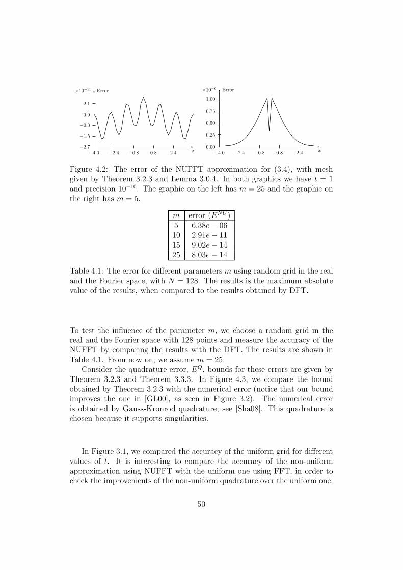
−4.0 −2.4 −0.8 0.8 2.4
−2.7
−1.5
−0.3
0.9
2.1
×10−11 Error
x −4.0 −2.4 −0.8 0.8 2.40.00
0.25
0.50
0.75
1.00
×10−6 Error
x
Figure 4.2: The error of the NUFFT approximation for (3.4), with meshgiven by Theorem 3.2.3 and Lemma 3.0.4. In both graphics we have t = 1and precision 10−10. The graphic on the left has m = 25 and the graphic onthe right has m = 5.
m error (ENU)5 6.38e− 0610 2.91e− 1115 9.02e− 1425 8.03e− 14
Table 4.1: The error for different parameters m using random grid in the realand the Fourier space, with N = 128. The results is the maximum absolutevalue of the results, when compared to the results obtained by DFT.
To test the influence of the parameter m, we choose a random grid in thereal and the Fourier space with 128 points and measure the accuracy of theNUFFT by comparing the results with the DFT. The results are shown inTable 4.1. From now on, we assume m = 25.
Consider the quadrature error, EQ, bounds for these errors are given byTheorem 3.2.3 and Theorem 3.3.3. In Figure 4.3, we compare the boundobtained by Theorem 3.2.3 with the numerical error (notice that our boundimproves the one in [GL00], as seen in Figure 3.2). The numerical erroris obtained by Gauss-Kronrod quadrature, see [Sha08]. This quadrature ischosen because it supports singularities.
In Figure 3.1, we compared the accuracy of the uniform grid for differentvalues of t. It is interesting to compare the accuracy of the non-uniformapproximation using NUFFT with the uniform one using FFT, in order tocheck the improvements of the non-uniform quadrature over the uniform one.
50

Interval [0.5,1]
0 3 6 9 12−60
−45
−30
−15
0
ln(error)
n
NumericalBound
Interval [4,8]
0 10 20 30 40 50−60
−45
−30
−15
0
ln(error)
n
Figure 4.3: Comparison of the quadrature error, EQ, with the bound givenby Theorem 3.2.3. The solid line is the error obtained comparing the resultcomputed by our quadrature with the Gauss-Kronrod quadrature. The dot-ted line is the bound from Theorem 3.2.3. The results are presented for twodifferent integration intervals.
To do so, we set a precision (ǫ = 10−4) and establish a non-uniform grid toachieve the desired accuracy for t ∈ [1, 10], using the results of Chapter 3.For the uniform approximation we use the same grid size and range as thenon-uniform one. The results are shown in Figure 4.4.
−2.40 −1.44 −0.48 0.48 1.440.0
1.5
3.0
4.5
6.0
Uniform (t = 1)×10−4 Error
×101
x
−2.40 −1.44 −0.48 0.48 1.440.0
0.6
1.2
1.8
2.4
Uniform (t = 10)×10−1
×101
Error
x
−2.40 −1.44 −0.48 0.48 1.440.0
2.0
4.0
6.0
8.0
Non-Uniform (t = 1)×10−5
×101
Error
x
−2.40 −1.44 −0.48 0.48 1.440.0
0.7
1.4
2.1
2.8
Non-Uniform (t = 10)×10−9
×101
Error
x
Figure 4.4: Comparison of the accuracy of the non-uniform approximationwith the uniform one. For the non-uniform approximation, the grid is chosenbased in Theorem 3.2.3 and for the uniform approximation, the same gridsize and range as the non-uniform case is used.
51
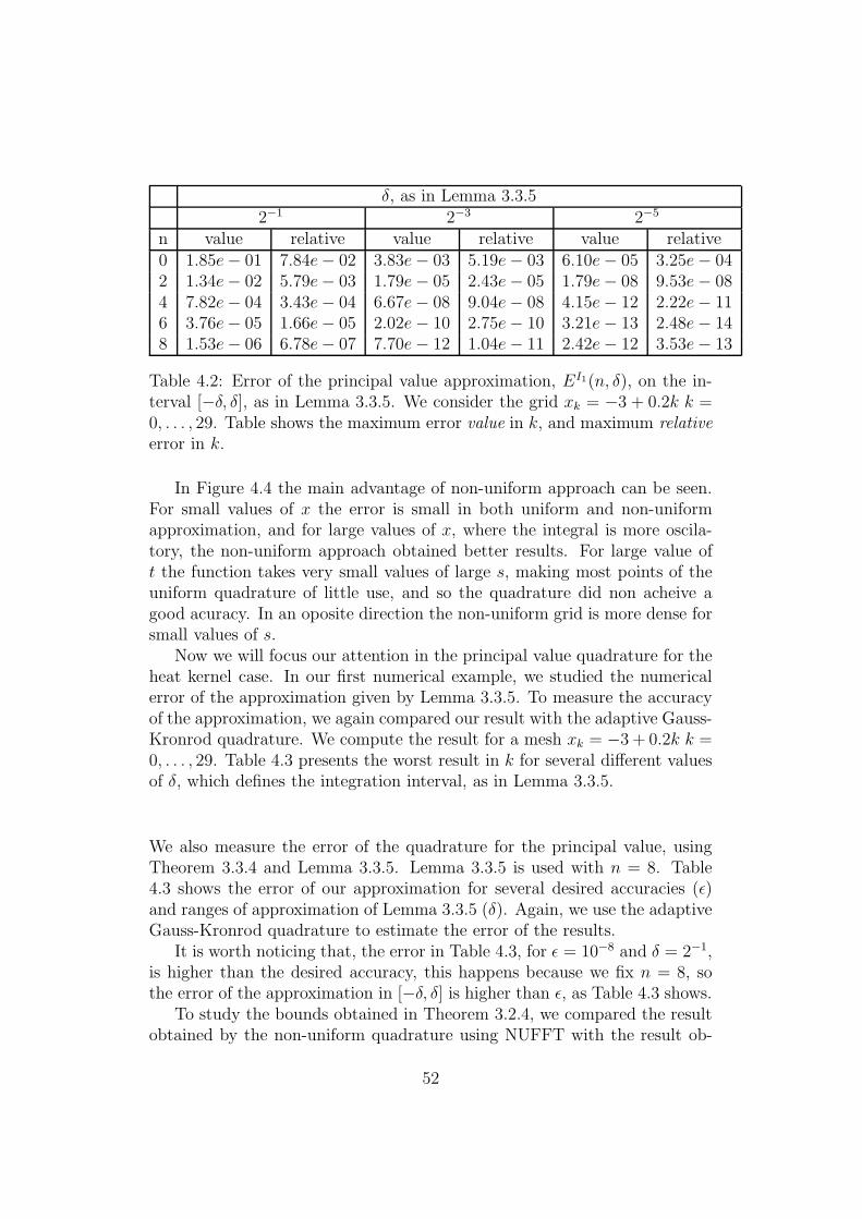
δ, as in Lemma 3.3.52−1 2−3 2−5
n value relative value relative value relative0 1.85e− 01 7.84e− 02 3.83e− 03 5.19e− 03 6.10e− 05 3.25e− 042 1.34e− 02 5.79e− 03 1.79e− 05 2.43e− 05 1.79e− 08 9.53e− 084 7.82e− 04 3.43e− 04 6.67e− 08 9.04e− 08 4.15e− 12 2.22e− 116 3.76e− 05 1.66e− 05 2.02e− 10 2.75e− 10 3.21e− 13 2.48e− 148 1.53e− 06 6.78e− 07 7.70e− 12 1.04e− 11 2.42e− 12 3.53e− 13
Table 4.2: Error of the principal value approximation, EI1(n, δ), on the in-terval [−δ, δ], as in Lemma 3.3.5. We consider the grid xk = −3 + 0.2k k =0, . . . , 29. Table shows the maximum error value in k, and maximum relativeerror in k.
In Figure 4.4 the main advantage of non-uniform approach can be seen.For small values of x the error is small in both uniform and non-uniformapproximation, and for large values of x, where the integral is more oscila-tory, the non-uniform approach obtained better results. For large value oft the function takes very small values of large s, making most points of theuniform quadrature of little use, and so the quadrature did non acheive agood acuracy. In an oposite direction the non-uniform grid is more dense forsmall values of s.
Now we will focus our attention in the principal value quadrature for theheat kernel case. In our first numerical example, we studied the numericalerror of the approximation given by Lemma 3.3.5. To measure the accuracyof the approximation, we again compared our result with the adaptive Gauss-Kronrod quadrature. We compute the result for a mesh xk = −3 + 0.2k k =0, . . . , 29. Table 4.3 presents the worst result in k for several different valuesof δ, which defines the integration interval, as in Lemma 3.3.5.
We also measure the error of the quadrature for the principal value, usingTheorem 3.3.4 and Lemma 3.3.5. Lemma 3.3.5 is used with n = 8. Table4.3 shows the error of our approximation for several desired accuracies (ǫ)and ranges of approximation of Lemma 3.3.5 (δ). Again, we use the adaptiveGauss-Kronrod quadrature to estimate the error of the results.
It is worth noticing that, the error in Table 4.3, for ǫ = 10−8 and δ = 2−1,is higher than the desired accuracy, this happens because we fix n = 8, sothe error of the approximation in [−δ, δ] is higher than ǫ, as Table 4.3 shows.
To study the bounds obtained in Theorem 3.2.4, we compared the resultobtained by the non-uniform quadrature using NUFFT with the result ob-
52

δ, as in Lemma 3.3.52−1 2−5
ǫ #ξ EQ ET #ξ EQ ET
1e− 2 20 1.61e− 06 7.92e− 03 48 1.91e− 09 7.93e− 031e− 5 46 1.53e− 06 9.59e− 06 90 2.47e− 12 8.69e− 061e− 8 70 1.53e− 06 1.53e− 06 132 2.47e− 12 9.41e− 09
Table 4.3: Numerical results for the approximation of the principal valueFourier transform using Theorem 3.3.4 and Lemma 3.3.5. For some desiredprecision (ǫ), the table shows the number of grid points (ξ), the quadratureerror (EQ), and the total error (ET ).
tained by the Gauss-Kronrod quadrature, the results are shown in Figure4.5.
Interval [0.5,1]
0 3 6 9 12−40
−30
−20
−10
0
NumericalBound
ln(error)
n
Interval [4,8]
0 5 10 15 20−70
−55
−40
−25
−10
ln(error)
n
NumericalBound
Figure 4.5: Comparison of the quadrature error, EQ, with the bound givenby Theorem 3.2.4. The solid line is the error obtained comparing the resultcomputed by our quadrature with the Gauss-Kronrod quadrature. The dot-ted line is the bound from Theorem 3.2.4. The results are presented for twodifferent integration intervals.
Now consider the third quadrature, for h(s)/(c+is), given by Theorem 3.2.6.Lemma 3.3.2 finds estimates for the truncation of the infinite integral, so wecan find a finite integration interval [−p, p] that approximates the finite one.In Theorem 3.3.3, we used dyadic intervals to find a partition [−p, p]. Thechoice of the smaller interval, [−2−j, 2−j], proves to have a significant impacton the number of nodes, as seen in Table 4.3.
To study the bounds obtained in Theorem 3.2.6, we compared the resultobtained by the non-uniform quadrature using NUFFT with the result ob-tained by the Gauss-Kronrod quadrature. The results are shown in Figure4.6.
53

Minimum interval [−2−j , 2−j]j = 1 j = 3
ǫ #ξ EQ ET #ξ EQ ET
1e− 1 21 3.90e− 05 5.83e− 02 45 7.63e− 07 5.83e− 021e− 3 43 1.36e− 07 7.84e− 04 74 5.58e− 09 7.84e− 041e− 5 61 4.33e− 10 8.67e− 06 103 6.73e− 13 8.67e− 06
Table 4.4: Numerical accuracy of Theorem 3.2.6. For some desired precision(ǫ), table shows the number of grid points (#ξ), the quadrature error (EQ),and the total error (ET ).
Interval [0.5,1]
0 2 4 6 8 10−54
−42
−30
−18
−6
ln(error)
n
NumericalBound
Interval [4,8]
0 6 12 18 24−60
−45
−30
−15
0
ln(error)
n
NumericalBound
Figure 4.6: Comparison of the quadrature error, EQ, with the bound givenby Theorem 3.2.6. The solid line is the error obtained comparing the resultobtained by our quadrature with the Gauss-Kronrod quadrature. The dottedline is the bound from Theorem 3.2.6. The results are presented for twodifferent integration intervals.
To our final result, we study the error obtained by the quadrature whencomputing the value of a call option, as studied in Chapter 2. The results areshown for the Black and Scholes case, for which the bounds of Theorem 3.2.4and Theorem 3.2.6 apply directly. We used the Black and Sholes framework,so the answer has a closed form solution given by Equation (1.18). Thismakes it possible to validate the method and measure its accuracy. Forthe example, we use σ = 0.3, r = 0 and K = 10. The result is shownin Figure 4.3. In Chapter 7, numerical results for the Heston and Mertonmodels will be shown.
54
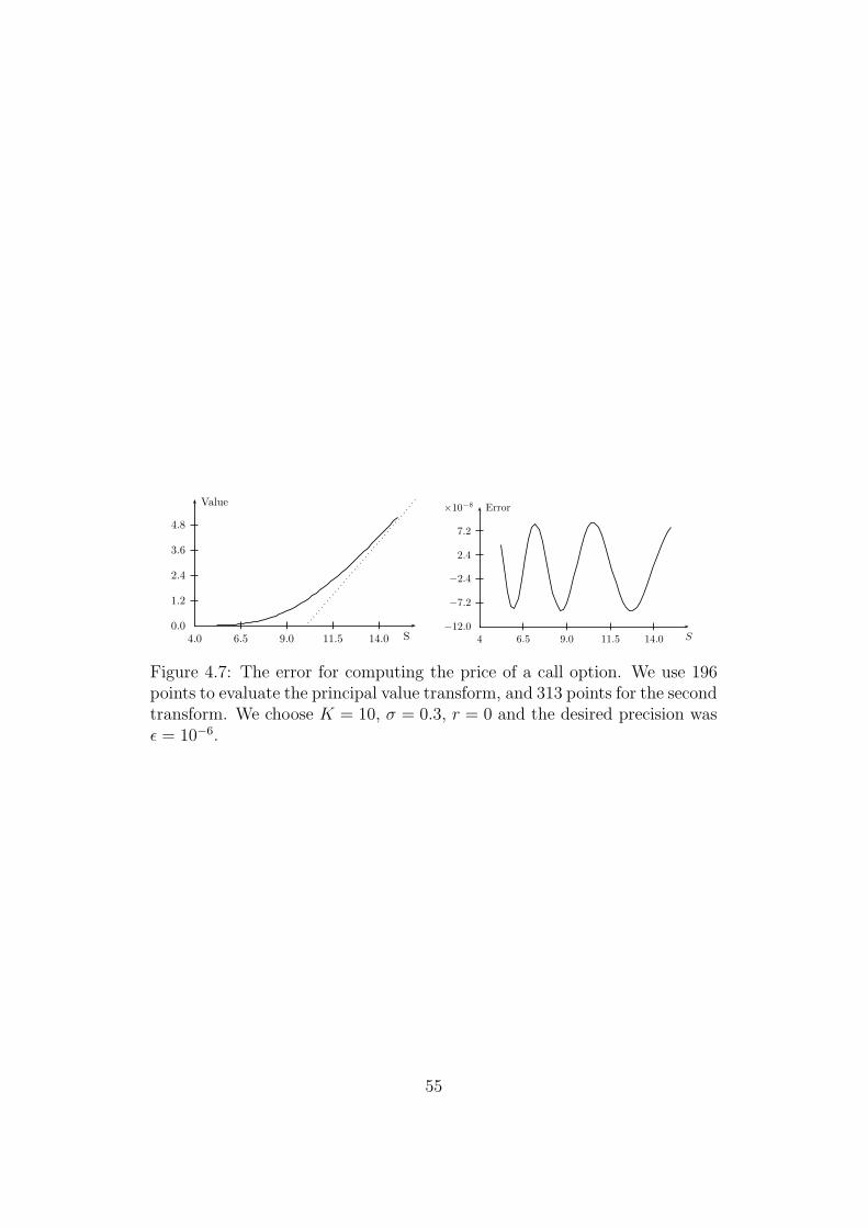
4.0 6.5 9.0 11.5 14.00.0
1.2
2.4
3.6
4.8
Value
S 4 6.5 9.0 11.5 14.0
−12.0
−7.2
−2.4
2.4
7.2
×10−8 Error
S
Figure 4.7: The error for computing the price of a call option. We use 196points to evaluate the principal value transform, and 313 points for the secondtransform. We choose K = 10, σ = 0.3, r = 0 and the desired precision wasǫ = 10−6.
55

Chapter 5
A Liquefied Natural GasPricing Model
Energy commodities form an important part of most markets. Several mer-cantile exchanges around the world trade energy commodities in differentforms. Oftentimes, the broad literature in mathematical finance is not di-rectly applied to commodities due to their special nature.
One of the main differences between commodities and financial derivativesis the presence of the cost of carry, which consists of the cost of holding aposition in a commodity. To enter in a long position in a commodity, whichmeans buying a commodity like rice, soy or oil, there is the cost of storage,the cost of financing the position and the cash flow for owning the asset.The important implication of the cost of carry is that we do not have anon-arbitrage price for future prices of commodities. What we do have is anon-arbitrage interval.
Another interesting characteristic of commodity prices is its mean revert-ing nature [Sch97]. This makes commodities related to interest rate deriva-tives, to establish a parallel with the financial literature.
The differences between financial derivatives and commodities resultedin two subjects each one of them with a specific literature. See for example[Bla76], [Sch97], [DL92].
An instance of a commodity is natural gas. It is an important source ofgeneration of electricity, as fuel for vehicles, and in households for heatingand cooking. The global demand for natural gas has been increasing steadilyin the last years. Because of its nature, transportation is a crucial issue forthe natural gas market. There are two ways of transporting natural gas:pipelines and liquefied natural gas (LNG). If there is a pipeline available,then it is the cheapest transportation option. LNG is the alternative whenno pipeline is available since it takes up to 1/600th the volume of natural gas
56

and then can be transported by special ships, known as LNG carriers.LNG has received a lot of attention in recent years. Several studies have
been made about natural gas and LNG, like [VJ06],[Jen03],[SLNv05] justto mention some of them. Even for political reasons LNG has attractedattention:
“Given notable cost reductions for both liquefaction and trans-portation of LNG, significant global trade is developing, (...) Andhigh natural gas prices projected by distant futures prices havemade imported gas a more attractive option for us.”(Alan Greenspan,2004)
LNG “per se” is not directly considered a commodity, because it is nottraded in any mercantile exchange. LNG trades are over-the-counter (OTC)and in general between two countries. LNG does not constitute a local mar-ket, we cannot try to find a proxy for the price in any specific market, thereason being that the owner of the cargo is trying to find arbitrage oppor-tunities among different markets. In the Asian-Pacific market, LNG pricesare indexed to crude oil prices. In Europe, there are different indices, suchas crude oil (note that crude oil prices are different in Asia and Europe), ora basket of indexes (like oil products, coal, inflation, among others). In theUSA, LNG is usually indexed by the Henry Hub gas prices.
In this chapter, we present a model for the spot price of LNG, althoughmost results apply to other commodities. Our model reflects most of thestylized facts on natural gas markets. The intuition brought up by the modelhelps to explain the international correlation of natural gas prices in theworld [SLNv05], which is a consequence of the LNG seller as an arbitrageurof international gas market. The LNG producer sells to the market withhigher prices and this causes a decrease in local prices.
One of the main advantages of our model is that no data for LNG isused, in the sense that we find the spot price for LNG based on the prices ofnatural gas for each of the local markets. This makes it possible to calibratethe model using the huge amount of data for natural gas.
Once the spot price is modeled, we are able to treat derivatives andintroduce some contracts for LNG. The two contracts that we study arefutures for LNG and cancellation options. This second contract is uncommonin the literature 1. It is a contract that gives the owner the right to buy LNG
1Flexibility in LNG contracts has been growing significantlyin recent years. See for example the cancellation contract(http://www.eia.doe.gov/oiaf/analysispaper/global/lngmarket.html). It exemplifiesseveral new contracts for short-term markets that have been used.
57

in a given date and the right to cancel the contract by paying some fee oncertain dates. Some uses and motivation of this contract are shown in Section5.2.
5.1 Spot Price Model
The first step towards modeling LNG is finding its spot price. As it turnsout, LNG has several idiosyncrasies, such as trades over-the-counter (OTC),generally between two countries and LNG is a global market. Furthermore,we do not have any database regarding LNG trades. Those are some of theaspects we considered while constructing the model.
Natural gas is a commodity in most countries. Several mercantile ex-changes have derivatives over natural gas prices. Just to give an example, letus consider the the USA. The most used reference pricing point in the USAis the Henry Hub. It is the pricing point for natural gas contracts traded onthe New York Mercantile Exchange (NYMEX). The NYMEX trades futurecontracts for natural gas (called Henry Hub Futures), they also have optionsover Henry Hub futures. Natural gas prices are very well modeled in eachmarket. We use the fact that there is a model for natural gas in every countryto model LNG as a derivative using all the different prices around the globeas primary asset for this derivative.
N
Henry Hub
NBP
JCC
max(HH − f1, NBP − f2, JCC − f3)
Figure 5.1: The LNG seller has access to several markets, and maximizes theprofit in all of them.
58
In order to model the market, let us consider a specific producer likeNigeria, for example. Nigeria can sell LNG to any country, see Figure 5.1.For instance, if it sells in the USA, Nigeria will receive the spot price fornatural gas in the USA, which in general is related to NYMEX Henry Hubprices. In order to sell in the USA, the producer pays the netback costs(transport, liquefaction, re-gasification...). The profit of selling to the USAis then the Henry Hub price subtracted by the netback cost. The price will begiven by a profit maximization by this seller. Some basic market hypotheseswill be needed:
• The seller has access to K markets, and pays fk ∈ R of netback costin order to sell to market k.
• The prices of natural gas are given by St ∈ RK+ , a K-dimensional
stochastic process defined on the filtered, probability space (Ω,F ,F,Q).In the kth market, natural gas is a commodity and the price will begiven by the stochastic process Skt . We assume that Q is a martingaleequivalent measure for a given market price of risk, see [MR05].
If the producer sells to market k, he receives a profit of Skt − fk. Themaximum profit is given by
G(St) = maxk=1,...,K
(Skt − fk
)(5.1)
In this model, we consider that the amount of natural gas traded by LNG issmall, so it does not affect local market prices. This is clearly a simplification.
To buy a cargo from a specific producer, the buyer has to pay no lessthan G(St), assuming that he pays the netback costs. Doing so the seller isindifferent to selling the cargo or maximizing the profit arbitrating in globalmarkets.
This price rule implies that buying LNG is no better than buying in thelocal market. Once LNG is re-gasified and is inside a specific market, itbecomes natural gas and so has the price given by the local market.
This model reflects several aspects of the LNG market in which everyseller and buyer has different netback costs. It is common for a country toconcentrate the demand for LNG, which occurs when a market has a spike inprices for natural gas. In this case, this same country is the natural destinyfor every free cargo.
Notice that by defining the spot value as in equation (5.1) makes the spotprice itself a derivative of natural gas price.
59

The model presented here will be used in the next section, where weintroduce some derivatives for LNG. We will also introduce some applicationsof the derivative markets as hedge for energy markets.
5.2 LNG Derivatives
Natural gas is a very important component in the world energy matrix. As aconsequence, hedging with this strategic resource is crucial. Changes in theprices of local markets are important. For this kind of hedging, derivativesover natural gas at local markets are the best choice. Those derivatives aretraded at mercantile exchanges.
Based on the LNG model presented above, it is natural to ask why shouldsomeone hedge using LNG, when the cheapest choice is hedging in localmarkets.
We now will try to explain the reasons for such hedging. There are somecountries where natural gas prices cannot be hedged in local markets. Notevery country has mercantile exchanges trading natural gas. In those cases,LNG contracts are an interesting way of hedging.
We add that the market has its micro-structure. For instance, it is alwaysbetter for the seller, due to logistic reasons, to sell in advance. This logisticrisk is not in the model itself and may give a discount over the theoreticalprice, making LNG interesting for the buyer.
Several countries, and even some firms, are worried about changes in de-mand, which is essential to hedge against. Other reasons for hedging might beproblems in pipelines, problems in local production, excess of demand basedon bigger than expected growth. To hedge against such events, the optionto buy more gas is needed. In this context, LNG is a highly competitivealternative.
5.2.1 Forward
Forward prices of LNG are straightforward once we have the spot price model.The price is given by
FG(t, T, St) = E [G(ST )| Ft] , (5.2)
considering that interest rates are independent with natural gas prices. Itis interesting to notice that G(ST ) is not traded, but risk-neutral pricingapplyies because the hedging strategy can be done trading S. This is themost basic contract possible and it is an useful hedge alternative when there
60

is certainty about the future demand, so the owner of the contract is buyingin advance.
5.2.2 Cancellation Options
Future contracts are not flexible enough to cover all the hedge possibilitiesneeded. In this section we present a contract that is an attempt to deal withwider hedging possibilities.
Its is natural to have a contract that gives the owner the right, but notthe obligation to buy. This makes it possible to hedge against uncertainty ina future time.
We can generalize this flexibility. During the validity of the contract, theowner may receive some information that allows him to know beforehandthat the cargo will not be needed. In this case, he may want to cancel thecargo in advance.
We now define a contract that has these properties.
Definition: The cancellation option is a contract that gives the holder thefollowing rights:
• At times t1, . . . , tN ≤ T the holder has the right to cancel the contractpaying fees c1, . . . , cN , respectively.
• If the holder does not cancel the contract, then at time T , then he willbuy the LNG cargo paying A ·S1
T +B, where A is a proportion of somebenchmark market, and B is a fixed cost.
The value of a cancellation option at time t, for market price St is denotedby V (t, St).
To value this contract, first note that at delivery the value of the contractis
V (T, ST ) = GT (ST ) −(AS1
T +B). (5.3)
Or if we can cancel at deliver tN = T
V (T, ST ) = max(GT (ST ) −
(AS1
T +B),−cN
). (5.4)
To help fix the notation, consider the example of the cancellation option forwhich it is possible to cancel for t = T as in equation (5.4). The payoff isshown in Figure 5.2.
61

S2 =
A·S
1 −
c
S2 =
AS
1
Area 1 Area 2 Area 3
S2
T
c
A S1
T
Figure 5.2: Payoff when it is possible to cancel at delivery time, as given byEquation (5.4). The fee to cancel is c and B = 0. In area 1, the payoff ispositive, so it is not optimal to cancel. In area 2, the payoff is negative butbetter than the fee. In Area 3, the payoff is smaller than the cancellationfee, so it is optimal to cancel.
We can find the value of the cancellation option backwards. To do this,we first define auxiliary functions V n(t, S) defined on [tn−1, tn]×RK . Lettingt ∈ [tn−1, tn), V
n is given by
V n(t, S) = E [V n(tn, Stn)| Ft] . (5.5)
For time tn, with n < N the value of V n is given by
V n(tn, Stn) = max(V n+1(tn, Stn),−cn
). (5.6)
If the contract does not give the right to cancel at time T , then the finalpayoff is given by (5.3). So
V N+1(T, ST ) = GT (ST ) −(AS1
T +B),
where the (N + 1)-st interval is [tN , T ] and corresponds to the period afterthe last cancellation date. If the contract gives the right to cancel at T , thefinal payoff would be given by (5.4). Thus, we would have
V N(T, ST ) = max(GT (ST ) −
(AS1
T +B),−cN
).
By means of such construction, we are able to find the price for every t ∈[0, T ], where we have
V (t, S) = V n(t, S) for t ∈ [tn−1, tn) .
62
We now study some properties of such contracts. Several aspects of thecontract should be considered, like monotonicity in A and B. Another naturalquestion is a characterization of redundant fees and when a new cancellationdate actually increases the flexibility of the contract. The following theoremsummarizes some properties of the cancellation contracts.
Theorem 5.2.1 For a cancellation contract, we have the following proper-ties:
1. The contract value is nonincreasing in A;
2. The contract value is nonincreasing in B; and
3. If for some j < i, we have that cj < cie−r(ti−tj), then removing the
cancellation date tj does not affect the contract value.
Proof: For t = T , properties (1) and (2) are a consequence of ST ≥ 0, andthe payoff formula (5.3) or (5.4), so V (T, ST ;A,B) is nondecreasing in Aand B. For t ∈ [0, T ), the result follows from the construction of V and thefact that given X ≤ Y , with X and Y Fs-adapted, then for t < s we haveE [X|Ft] < E [Y |Ft], and max (X, c) ≤ max (Y, c).
To prove (3), suppose that we have cj , ci with j < i and cj ≥ cie−r(ti−tj).
Saving cj at tj and investing at risk free rate, at ti we pay ci ≤ cjer(ti−tj) at
ti, so the cancellation at tj can be ignored.
The results (1 ) and (2 ) of Theorem 5.2.1 show that increasing the deliveryprice for LNG decreases the price of the contract. Result (3 ) of of Theorem5.2.1 establishes conditions on the cancellation fee, so we can remove datesthat are never optimal for cancellation.
We can also study the value of the cancellation optionality. In this case,we must define the value of the contract without any cancellation possibility.The contract without cancellation possibility is simply a forward given by
F V (t, St) = E[GT −
(AS1
T +B)∣∣Ft
]. (5.7)
Using (5.7), we can define the optionality value as
O(t, St) = V (t, St) − F V (t, St). (5.8)
Some properties of the optionality value are given in the next theorem.
Corollary 5.2.2 The optionality value has several properties:
63
1. The optionality value is always positive;
2. The optionality value is nondecreasing in A;
3. The optionality value is nondecreasing in B; and
4. If for some j < i, we have that cj < cie−r(ti−tj), then removing the
cancellation date tj does not affect the optionality value.
Proof: For t = T , property (1) follows from the definition V and F V . Fort in general, it follows from the fact that given X ≤ Y , where X and Y areFs-adapted, then for t < s we have E [X|Ft] < E [Y |Ft], and max (X, c) ≤max (Y, c), as property (1) of Theorem 5.2.1.
To prove property (2), notice that for a given A > A we have F VA (t, St)−
F VeA(t, St) = (A − A)E [S1
T | Ft] > 0. Suppose that OA(t, St) < OeA(t, St), so
buying VA, FeA, and selling V
eA and FA, you receive VA + FeA − V
eA − FA > 0at t. Then two possibilities should be considered:
• If the owner of VeA cancels the contract, we cancel it too. We receive the
fee for the contract A and pay the same fee for cancelling the contractA, so the payoff at cancellation date is zero, and at T is (A−A)S1
T > 0.
• If the owner does not cancel, we do not cancel it either. The payoff atT is zero.
This is an arbitrage opportunity, so we must have OA(t, St) ≥ OeA(t, St). The
proof of property (3) is similar to that of (2).The value of the future does not depend on the cancellations dates, so
property (4) follows from property (4) of Theorem 5.2.1.
The result above has an intuitive explanation. Property (1 ) follows fromthe fact that the cancellation contract is an option over a forward, so its valueis always above the forward value. Properties (1 ) and (2 ) of Theorem 5.2.1show that the price of the contract drops with A and B, so the probability ofa negative payoff increases, and therefore the value of the cancellation rightis higher. This explains (2 ) and (3 ) of Corollary 5.2.2.
The final result of this section gives a restriction on parameters A and B.
Proposition 5.2.3 If A ≤ 1 and B ≤ mink=1,...,K (−fk), it is never optimalto cancel.
Proof: At T , the owner of the contract can receive a LNG cargo, payingAS1
T +B < GT (S).
64

The result above shows a case where the optionality has null value. Whenwe have A and B as in Proposition 5.2.3, it is never optimal to cancel, so thevalue of the optionality is zero.
The results mentioned above are useful not only for theoretical reasons,but also because they can be used to test and validate numerical implemen-tation.
5.3 Least-Squares Monte Carlo
Pricing the contracts of the previous section requires the use of numericaltechniques. Numerical methods for high dimensional problems have receiveda lot of attention and recently several Monte Carlo methods have been pro-posed. They turn out to be very efficient for those problems [Gla04].
In this section, we describe the method used to solve numerically themodel. The method we chose was the regression-based Monte Carlo proposedby [LS01].
The convergence of the method, under fairly general conditions, wasproved by [CLP02]. For example, considering only Markovian processesSt ∈ Rk such that St ∈ L2(Ω, dP), ∀t ∈ [0, T ], then convergence of least-squares Monte Carlo method for cancellation options follows from [CLP02].
The main idea of the method is to use the fact that
E [V (tn+1, S(tn+1))| Ftn]
is Ftn-measurable, so that it may be represented as
E[e−r(tn+1−tn)V (tn+1, S(tn+1)) | S(tn) = x
]=
∞∑
r=1
βrγr(x) , (5.9)
for some base γr of L2(Rk). We can approximate (5.9) by
V (tn, S(tn)) ≈R∑
r=1
βrγr(S(tn)). (5.10)
To compute β, we solve the following problem by least-squares
γ1(S
1(tn)) · · · γR(S1(tn))...
. . ....
γ1(SJ(tn)) · · · γR(SJ(tn))
β1...βR
= e−r(tn+1−tn)
V (tn+1, S
1(tn+1))...
V (tn+1, SJ(tn+1))
(5.11)
65

Using equation (5.6), we have
V (tn, S(tn)) ≈ max
(R∑
r=1
βrγr(S(tn)),−cn). (5.12)
5.3.1 An Example
The goal of this section is to present some numerical results obtained byleast-squares Monte Carlo. The model we choose for the price dynamicsis the mean reverting process, which is very popular for commodities. See[BCSS95] and [Sch97] for studies in the mean reverting nature of commodityprices. The price dynamic in this model is given by
Sit = eXit
dX it = κi
(θi −X i
t
)dt+
∑
j
Ai,jdWj(t) .(5.13)
The solutions is then
Xi(t) = e−κi(t−s)Xi(s)+θi(1 − e−κi(t−s))+
∫ t
s
e−κi(t−u)∑
j
Ai,jdWj(u). (5.14)
It is easy to see that
E [Xi] = µi = e−κi(t−s)Xi(s) + θi(1 − e−κi(t−s)
)
Cov [Xi(t), Xj(t) | Fs] =1
(κi + κj)
(1 − e−(κi+κj)(t−s)
)(AAt)(i,j) .
(5.15)
Taking t→ ∞ in the covariance, we obtain the ergodic covariance.We will now study the sensibility of the model and the numerical method.
Unless not otherwise specified, the following parameters will be used:
• The base is the polinomial base;
• Maximum degree of the basis is 5;
• Number of simulations: 3 × 10⁴;
• A = 1.0, B = 2.0, r = 0;
• fee=(1, 1.25);
• Cancellation dates (0.5, 1.0) and T = 1.5;
66
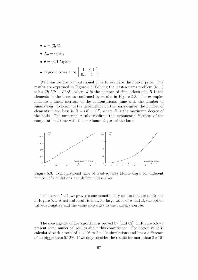
• κ = (3, 3);
• X0 = (3, 3);
• θ = (3, 1.5); and
• Ergodic covariance
[1 0.1
0.1 1
].
We measure the computational time to evaluate the option price. Theresults are expressed in Figure 5.3. Solving the least-squares problem (5.11)takes O(JR2 + R3/3), where J is the number of simulations and R is theelements in the base, as confirmed by results in Figure 5.3. The examplesindicate a linear increase of the computational time with the number ofsimulations. Concerning the dependence on the basis degree, the number ofelements in the base is R = (K + 1)P , where P is the maximum degree ofthe basis. The numerical results confirms this exponential increase of thecomputational time with the maximum degree of the base.
10 50 90 130 1707.5
37.5
67.5
97.5
127.5
Simulation Number (103)
Time(s)
1 2 3 4 5 6 7 8 92
32
62
92
122
Degree of the base
Time(s)
Figure 5.3: Computational time of least-squares Monte Carlo for differentnumber of simulations and different base sizes.
In Theorem 5.2.1, we proved some monotonicity results that are confirmedin Figure 5.4. A natural result is that, for large value of A and B, the optionvalue is negative and the value converges to the cancellation fee.
The convergence of the algorithm is proved by [CLP02]. In Figure 5.5 wepresent some numerical results about this convergence. The option value iscalculated with a total of 1× 10⁴ to 2× 10⁵ simulations and has a differenceof no bigger than 5.12%. If we only consider the results for more than 5×10⁴
67
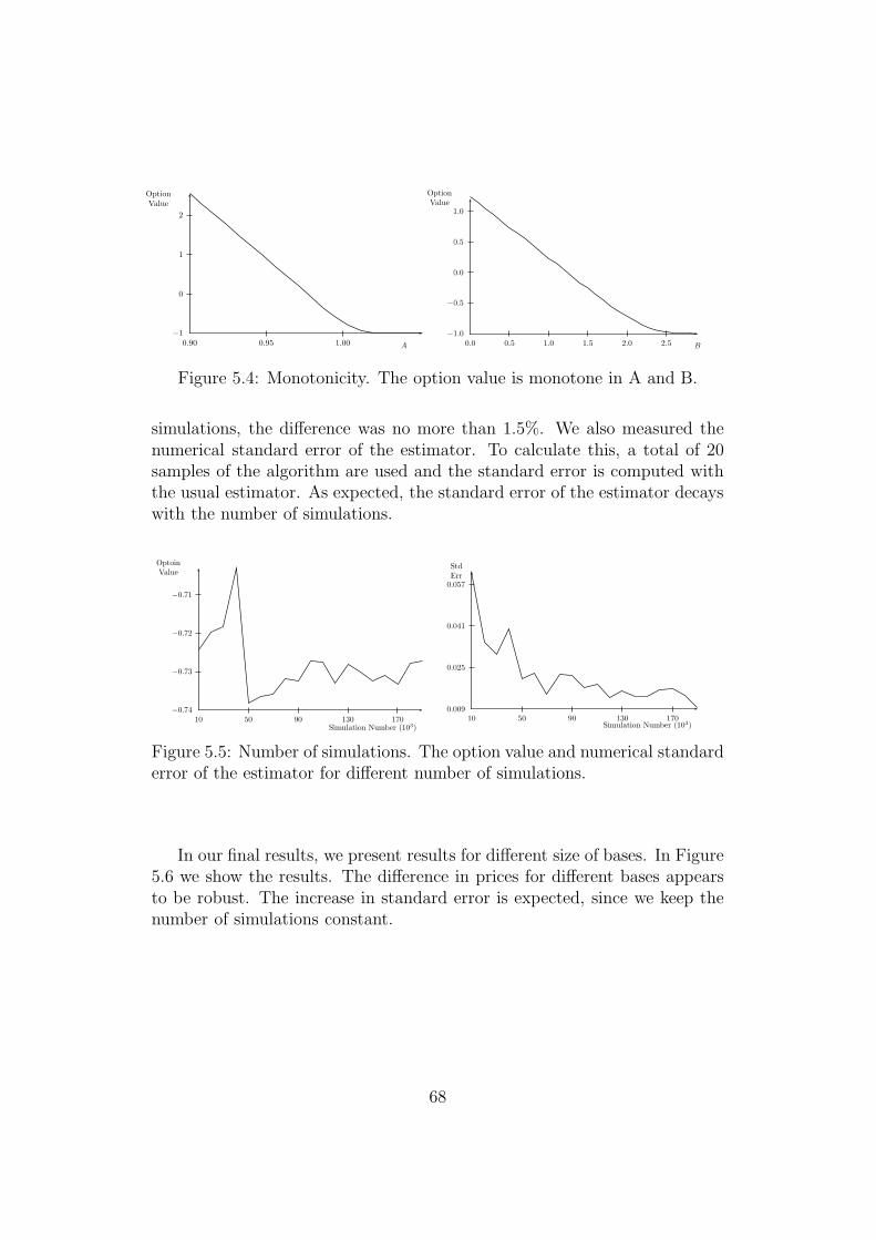
0.90 0.95 1.00
−1
0
1
2
A
Option
Value
0.0 0.5 1.0 1.5 2.0 2.5
−1.0
−0.5
0.0
0.5
1.0
B
Option
Value
Figure 5.4: Monotonicity. The option value is monotone in A and B.
simulations, the difference was no more than 1.5%. We also measured thenumerical standard error of the estimator. To calculate this, a total of 20samples of the algorithm are used and the standard error is computed withthe usual estimator. As expected, the standard error of the estimator decayswith the number of simulations.
10 50 90 130 170−0.74
−0.73
−0.72
−0.71
Simulation Number (103)
OptoinValue
10 50 90 130 1700.009
0.025
0.041
0.057
Simulation Number (103)
StdErr
Figure 5.5: Number of simulations. The option value and numerical standarderror of the estimator for different number of simulations.
In our final results, we present results for different size of bases. In Figure5.6 we show the results. The difference in prices for different bases appearsto be robust. The increase in standard error is expected, since we keep thenumber of simulations constant.
68
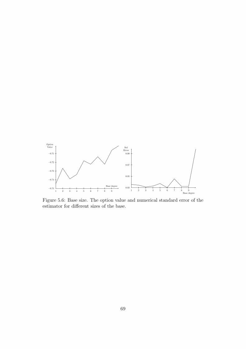
1 2 3 4 5 6 7 8 9
−0.75
−0.74
−0.73
−0.72
−0.71
Base degree
Option
Value
1 2 3 4 5 6 7 8 9
0.03
0.05
0.07
0.09
Base degree
Std
Error
Figure 5.6: Base size. The option value and numerical standard error of theestimator for different sizes of the base.
69

Chapter 6
Interest Rates
In many countries, a monetary authority decides the short rate target. Ituses open market operations to execute this policy. In the United States,the short rate role is performed by the federal funds and the target decisionis chosen by the Federal Open Market Committee (FOMC). In Brazil, themonetary authority instrument is the Special System for Settlement andCustody (SELIC), and the decision of the short rate target is made by theMonetary Policy Committee (COPOM). Furthermore, there is an importantshort-term rate, the Interbank Deposit (DI), that follows very closely theSELIC rate.
The Chicago Board of Trade (CBOT) has future contracts on US federalfunds among other derivatives. The Brazilian Securities, Commodities andFutures Exchange (BM&FBOVESPA) has one-day interbank deposit futurecontracts, and options on average one-day interbank deposit rate index con-tract. Those derivatives over short rates have received a lot of attentionrecently due to the increase in their liquidity.
In this chapter we propose a model for short-term rates taking into consid-eration monetary authority. We use such model to recover expectation aboutfuture decisions by the monetary authority, from derivative contracts. To doso, we were led to use regularization techniques to deal with the ill-posednessnature of the problem.
Some work has been done to incorporate monetary decisions to interestrate models as pure jump process [Pia05]. In a different direction, marketdata can be used to recover the probability of each possible monetary policydecision [CCM05]. The idea of recovering probabilities from derivatives datagoes back to [BL78]. More recent work has been done by [JR96]. The litera-ture on regularization and inverse problems is quite extense. See [Zub05] forgeneral references and [Ave99], [EE05], [EHH06] for applications in quanti-tative finance.
70

6.1 Model and Notation
In this section, we present a model for the short rate. This model is basedon the central bank target rate and the spread between the target and therealized rate. This chapter focus on the Brazilian market, and we will givenow a brief review of the two relevant short rates for this chapter. For acomplete review see [For08].
• Special System for Settlement and Custody (SELIC) - It is the averageone day operation guaranteed by the Brazilian federal government se-curities. The model is based on the SELIC target (rS) decided by theCOPOM. So the rS, if expressed as an annual compounded tax, is amultiple of 25 basis points (bp) annually compounded, where a bp is1/100th of a percentage point.
• Interbank Deposit (DI) - It is the average one day operation guaranteedby private securities (rDI).
Before we describe our model, we will give a brief overview of the Vasicekinterest rate model [Vas77]. This model will be later used for modelingthe spread between DI and SELIC. For a complete review of interest ratemodels see [JW01]. In the Vasicek model, the interest rate process is givenby an Ornstein-Uhlenbeck process on the filtered complete probability space(Ω1,F1,F1,P1). The dynamics for the short rate x(t), t > 0, is given by
dx(t) = k(θ − x(t))dt+ σdW (t) . (6.1)
The solution of the stochastic differential equation (6.1) for s < t is given by
x(t) = x(s)e−k(t−s) + θ(1 − e−k(t−s)
)+ σ
∫ t
s
e−k(t−u)dW (u) . (6.2)
To model the SELIC target rate, note that this process is constant betweenthe COPOM’s meeting, we assume that the monetary authority only changesthe rate at scheduled meetings. We define τj for the time of the jth meetingafter a starting time t. We define rS on (Ω2,F2,F2,P2) as
rS(t) := H0X[t0,τ1](t) +N∑
j=1
HjX(τj ,τj+1](t) , (6.3)
where Hj is the target rate decided at the jth meeting. Since F2τj
correspond
to the information up to the jth meeting we must have Hj ∈ F2τj
. TheCOPOM meeting only changes the rate on 25 bp, so
ln (Hj(ω)) − 1
2.5 · 10−3∈ N ∀j ∈ N, ω ∈ Ω2 (6.4)
71

We assume Ω2 finite.To model the DI rate, we consider the direct product and the product
measure both denoted by ⊗ and given by (Ω1⊗Ω2,F1⊗F2,F1⊗F2,P1⊗P2),and the DI rate is given by
rDI(t) = x(t) + rS(t) , (6.5)
where, to define x and rS in this probability space, we use the projectionrS(ω1, ω2) := rS(ω2), and x(ω1, ω2) := x(ω1), but from now on, we make nodistinction between x and x, and rS and rS.
So far, we have focused on the real measure P1⊗P2, but it is well known inthe literature of interest rate the existence of risk premium in bond markets[FB87]. Recent studies have shown the presence of risk premium in federalfund derivatives [PS08]. So we need to study a risk neutral measure, whichis denoted as Q := Q1 ⊗ Q2.
We assume a constant market price of risk process, λ, for the risk-neutralmeasure. It will be denoted by λ, so
dx(t) = k(θP − x(t))dt+ σdW (P)
dx(t) = k(θQ − x(t))dt+ σdW (Q) ,
where
θP =λ
σ+ θQ .
For the SELIC target we study only the risk neutral, Q2, which is the im-portant probability to study derivative pricing. We can also supose no riskpremium for the SELIC rate, as in the expectations hypothesis [Pia03].
6.1.1 One-Day Interbank Deposit Futures Contract
The BM&FBOVESPA has future contracts over DI. The basis of each suchcontract is the unit price defined as 100.000 discounted by DI. This derivativeis quoted as the annual percentage rate compounded daily based on a 252-dayyear, to two decimal places, that we denote here as cot. So, we have
PU = (1 +cot
100)
T−t252 .
The daily cash flow of the owner of the contract is
PU
((1 +
cot
100
) 1252
− e1
252rDI
).
In the next theorem we present a pricing formula for this contract.
72

Theorem 6.1.1 The price of the future contract is given by
FDI(t, T, rDI(t)) = PV (t, T, x(t))∑
ω∈Ω2
e(−R T
trS(u,ω)du)Q2(ω), (6.6)
where
PV (t, T ) = A(t, T )e−B(t,T )x(t)
B(t, T ) =1
k
(1 − e−k(T−t)
)
A(t, T ) = e
“
θ− σ2
2k2
”
(B(t,T )−T+t)−σ2
4kB(t,T )2
.
Proof: The future price is given by
FDI (t, T, rDI (t)) = E[e−
R T
trDI(s)ds
∣∣∣Ft
].
From the definition of rDI and Equation (6.2), we have
rDI(t) = rS(t)+x(s)e−k(t−s) +θ(1−e−k(t−s))+σ
∫ t
s
e−k(t−u)dW (u) . (6.7)
To compute the integral in (6.7), note that
∫ T
t
x(t)e−k(u−t)du = x(t)1
k
(1 − e−k(T−t)
)= x(t)B(t, T )
∫ T
t
θ(1 − e−k(u−t))du = θ
(T − t− 1
k
(1 − e−k(T−t)
))
= θ (T − t−B(t, T ))∫ T
t
∫ u
t
e−k(u−s)dW (s)du =1
k
∫ T
t
(1 − e−k(T−s)
)dW (s) .
(6.8)
Then, we have
E[e−
R T
tx(s)ds|Ft
]= e−θ(T−t−B(t,T ))−x(t)B(t,T )E
[e−σ
R T
tB(T,s)dW (s)
].
The term associated with the expectation integral above, can be computedas
E[eσ
R T
tB(T,s)dW (s)
]= e
σ2
2
R T
tB(T,s)2dsE
[e−
σ2
2
R T
tB(T,s)2(s)−σ
R T
tB(T,s)dW (s)
]
= eσ2
2
R T
tB(T,s)2ds .
73

The last remaining integral is given by
∫ T
t
B(T, s)2ds =1
k2
(T − t− 2
k
(1 − e−k(T−t)
)+
1
2k
(1 − e−2k(T−t))
)
=1
k2
(T − t−B(t, T ) − k
2B(t, T )2
).
The result now follows from
E[e
R T
t(x(s)+rS(s))ds
]= E
[e
R T
tx(s)ds
]E[e
R T
trS(s)ds
]
= E[e
R T
tx(s)ds
]∑e(−
R T
trS(u,ω)du)Q2(ω) .
We remark that the future price can be written as
FDI(t, T, ω) = PV (t, T )e(−R T
ty(u,ω)du)
FDI(t, T ) =∑
FDI(t, T, ω)Q2(ω) .(6.9)
6.1.2 Options on Average One-Day Interbank DepositRate Index
The Interbank Deposit Rate Index (IDI) is an index that the BM&FBOVESPAcreated. It is defined as
IDIt = 105eR t
t0rDI(s)ds
,
where t0 was chosen as 2003-01-02.The IDI option is a plain vanilla derivative over the IDI index. To find
its arbitrage free value, the following result is needed.
Lemma 6.1.2 ([BM01]) Let log(X) be a log-normal random variable withmean (µ) and variance (σ2). Then
E
[(K −X
)+]
= −e(µ+ 12σ2)N
(−µ + log(K) − σ2
σ
)+KN
(−µ+ log(K)
σ
).
where N is the cumulative standard normal distribution
N(y) =1√2π
∫ y
−∞e−z
2/2dz .
Using Lemma 6.1.2 we can prove a pricing formula for the IDI options, whichis given in the next theorem.
74

Theorem 6.1.3 The IDI call options price is given by
CIDI(t, T,K, x(t), ω) = IDItN (d1(ω)) −KFDI(t, T, ω)N (d2(ω)) ,
where
d1(ω) =−µ + ln (V (ω))
σ,
d2(ω) =−µ + ln (V (ω)) − σ2
σ,
V (ω) =1
K
(IDIte
R T
ty(s,ω)ds
),
µ = −x(t)B(t, T ) − θ (T − t− B(t, T )) ,
σ2 =σ2
k2
(T − t−B(t, T ) − k
2B(t, T )2
).
Proof: The price of a call option is given by
CIDI(t, T, x(t), ω) = E
[e−
R T
trDI(s)ds
(105e
R T
0 rDI(s)ds −K)+∣∣∣∣Ft
]
= Ke−R T
trS(s,ω)dsE
[(V (ω) − e−
R T
tx(s)ds
)+∣∣∣∣Ft
],
where
V (ω) =105
Ke(
R t
0r(s)ds+
R T
trS(s,ω)ds)
=1
K
(IDIte
R T
trS(s,ω)ds
).
Defining µ and σ for the mean and variance of the process
−∫ T
t
x(s)ds,
respectively. Using (6.8), it follows that
µ = −x(t)B(t, T ) − θ (T − t−B(t, T ))
σ2 =σ2
k2
(T − t−B(t, T ) − k
2B(t, T )2
).
Then,
CIDI(t, T,K, x(t), ω) = IDItN (d1(ω)) −KFDI(t, T, ω)N (d2(ω)) ,(6.10)
75

where
d1(ω) =−µ+ ln (V (ω))
σ,
d2(ω) =−µ+ ln (V (ω)) − σ2
σ.
Since the space Ω2 is taken to be discrete, the price of the Call optioncan be written as
CIDI(t, T, x(t)) =∑
ω∈Ω2
CIDI(t, T, x(t), ω)Q2(ω) . (6.11)
The same arguments can be used to find the price of the put option
PIDI(t, T,K, x(t), ω) = KFDI(t, T, ω)N (−d2(ω)) − IDItN (−d1(ω)) .(6.12)
6.2 Recovering Probabilities
The main target of this chapter is to use the model presented in Section 6.1to recover the probabilities associated to the paths of the short rate target,rS. First, the spread is studied, then the problem of recovering the targetrate path’s probability is addressed.
For the real probability of the spread model, P1, we use daily quotes forDI, and SELIC. The maximum likelihood [BM01] is applied to calibrate thereal measure. For risk neutral probability, future contracts where there wasno uncertainty about the SELIC rate, are used. Those contracts are the onesthat have no COPOM meeting before the maturity, so rS is deterministicuntil maturity. The result is shown in Table 6.1.
Parameter Valuek 128.18θ −2.89e−4
θQ −6.89e−4
σ2 1.82e−5
Table 6.1: Parameter estimation for the real and risk neutral dynamic of rDI .
We assume that Ω2 is finite and has only paths with positive probability,that is ω ∈ Ω2 ⇒ Q2(ω) > 0. This reduces the problem of recovering theprobability Q2 to that of finding p = (Q2(ω1), . . . ,Q2(ωU))t.
76

Suppose there are future contract quotes, Fifi=1, with expiration, T Fi fi=1,
and call options quotes,Cjcj=1, with the associated pair of strikes and ma-turity, Kj , T
Cj cj=1. Using (6.9) and (6.11), we can try to recover Q2 solving
FDI(t, Ti) =∑
FDI(t, Ti, ω)Q2(ω) i = 1, . . . , f
CIDI(t, Tj , Kj) =∑
CIDI(t, Tj , Kj, ω)Q2(ω) j = 1, . . . , c(6.13)
This problem is linear although its dimension is quite high. We use thefollowing notation
Ek,u =
FDI(t, Tk) − FDI(t, Tk, ωu) if 0 < k ≤ f
CIDI(t, Tj, Kj) − CIDI(t, Tj, Kj, ωu) 0 < j = k − f + 1 ≤ c.
(6.14)
Using the notation in Equation (6.14), the problem (6.13) is simply Ep = 0,so finding a risk neutral probability is equivalent to finding a positive solutionof a linear system. The next theorem gives a very simple condition for nonarbitrage of market prices.
Theorem 6.2.1 A set of prices, Fifi=1, Cjcj=1 is arbitrage free, if andonly if, there is p ∈ Rn
++ such that Ep = 0, where R++ denotes the set ofstrictly positive real numbers.
Proof: The result follows from the Fundamental Theorem of asset pricing(Theorem 1.3.1) and by noticing that, by assumption, Q2(ω) > 0 for ω ∈Ω2.
The next theorem gives some characterization of the set of arbitrage freeprices.
Theorem 6.2.2 ([Rom08]) Let S be the row space of E, then
• S ∩ Rn+ = ∅ ⇔ S⊥ ∩ Rn
++ 6= ∅ ; and
• S ∩ Rn++ = ∅ ⇔ S⊥ ∩ Rn
+ 6= ∅.
The problem of solving Ep = 0 is ill-posed. In this chapter, we proposesome regularization for this problem. The main idea of regularization is finda family (Rγ)γ>0, such that
limγ↓0
RγEp = p ∀p ∈ Rn .
77

Where the solutions of the regularizated problem
Rγp = 0,
s.t. p ∈ Rn++
n∑
j=1
pj = 1
(6.15)
is well-posed. In our case, instead of solving Ep = 0 for some p ∈ Rn++, we
solve
minp‖DEp‖2 + gγ(p, p
∗)
s.t.
n∑
j=1
pj = 1
pj ≥ 0 j = 1, . . . , n
Where p∗ is a prior probability. In this sections we present a choice for D,several choices for the family (gγ)γ>0 and different priors.
For market data, the condition number of E is usually very high, some-times above 1014. One of the reasons for this problem is the different mag-nitudes of the assets treated. To mitigate it, we use a preconditioner matrixD, defined as
D = Diag(‖E1,1:U‖−1, . . . , ‖Ef+c,1:U‖−1) , (6.16)
where Ej,1:U is the jth row of the matrix E.
From now on, E denotes the preconditioned E = DE.As in many Inverse Problems and in Approximation Theory, one has to
consider different notions of distance. In particular we shall use the follow-ings:
• dJ(r1, r2) = ‖r′1 − r′2‖22 =
∑n ((r1 (t+n ) − r1 (t−n )) − (r2 (t+n ) − r2 (t−n )))
2.
This distance represents the geometric Euclidean distance of jumpssize, it is related to the quadratic variation of the paths’ differences.The distance dJ focus on the idea that the distance of the paths arebased on the change of interest rate on each COPOM meeting.
• dA(r1, r2) = ‖r1 − r2‖1 =∫ Tt|r1(s) − r2(s)| ds. This distance repre-
sents the difference of accumulated interest rates. The distance dAfocuses on the difference of interest rate applied in the economy duringa certain period of time.
78
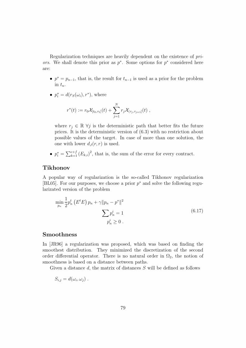
Regularization techniques are heavily dependent on the existence of pri-ors. We shall denote this prior as p∗. Some options for p∗ considered hereare:
• p∗ = pn−1, that is, the result for tn−1 is used as a prior for the problemin tn.
• p∗i = d(rS(ωi), r∗), where
r∗(t) := r0X[t0,τ1](t) +
N∑
j=1
rjX(τj ,τj+1](t) ,
where rj ∈ R ∀j is the deterministic path that better fits the futureprices. It is the deterministic version of (6.3) with no restriction aboutpossible values of the target. In case of more than one solution, theone with lower dJ(r, r) is used.
• p∗i =∑c+f
k=1 (Ek,i)2, that is, the sum of the error for every contract.
Tikhonov
A popular way of regularization is the so-called Tikhonov regularization[BL05]. For our purposes, we choose a prior p∗ and solve the following regu-larizated version of the problem
minpn
1
2ptn(EtE
)pn + γ‖pn − p∗‖2
∑pin = 1
pin ≥ 0 .
(6.17)
Smoothness
In [JR96] a regularization was proposed, which was based on finding thesmoothest distribution. They minimized the discretization of the secondorder differential operator. There is no natural order in Ω2, the notion ofsmoothness is based on a distance between paths.
Given a distance d, the matrix of distances S will be defined as follows
Si,j = d(ωi, ωj) .
79
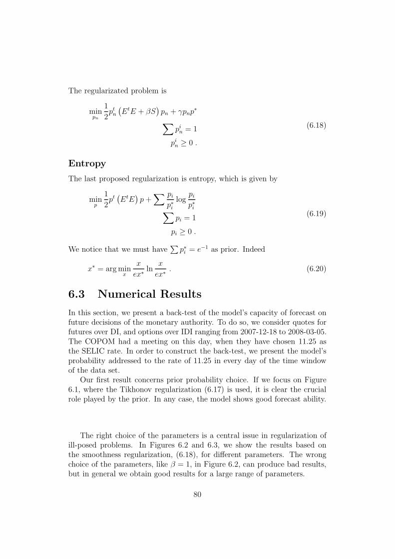
The regularizated problem is
minpn
1
2ptn(EtE + βS
)pn + γpnp
∗
∑pin = 1
pin ≥ 0 .
(6.18)
Entropy
The last proposed regularization is entropy, which is given by
minp
1
2pt(EtE
)p+
∑ pip∗i
logpip∗i∑
pi = 1
pi ≥ 0 .
(6.19)
We notice that we must have∑p∗i = e−1 as prior. Indeed
x∗ = arg minx
x
ex∗ln
x
ex∗. (6.20)
6.3 Numerical Results
In this section, we present a back-test of the model’s capacity of forecast onfuture decisions of the monetary authority. To do so, we consider quotes forfutures over DI, and options over IDI ranging from 2007-12-18 to 2008-03-05.The COPOM had a meeting on this day, when they have chosen 11.25 asthe SELIC rate. In order to construct the back-test, we present the model’sprobability addressed to the rate of 11.25 in every day of the time windowof the data set.
Our first result concerns prior probability choice. If we focus on Figure6.1, where the Tikhonov regularization (6.17) is used, it is clear the crucialrole played by the prior. In any case, the model shows good forecast ability.
The right choice of the parameters is a central issue in regularization ofill-posed problems. In Figures 6.2 and 6.3, we show the results based onthe smoothness regularization, (6.18), for different parameters. The wrongchoice of the parameters, like β = 1, in Figure 6.2, can produce bad results,but in general we obtain good results for a large range of parameters.
80

0% error50% error
100% error
Probability
2007-12-18 2008-01-14 2008-02-07 2008-02-280.00
0.15
0.30
0.45
0.60
0.75
0.90
Figure 6.1: Probability of having interest rate of 11.25% at the meeting of2008-03-05. The probability is based on the solution of (6.17), using a mixedprobability, error as prior, and γ = 10−1.
β =100
β =10−2
β =10−6
Probability
2007-12-18 2008-01-14 2008-02-07 2008-02-280.00
0.15
0.30
0.45
0.60
0.75
0.90
Figure 6.2: Probability of having interest rate of 11.25% at the meeting of2008-03-05. The probability is based on the solution of (6.18) for γ = 10−5,using pn−1 as prior.
Our final result presents the forecast based on the entropy regularization(6.19), and can be seen in Figure 6.4.
81

γ =10−1
γ =10−5
γ =10−9
Probability
2007-12-18 2008-01-14 2008-02-07 2008-02-280.00
0.15
0.30
0.45
0.60
0.75
0.90
Figure 6.3: Probability of having interest rate of 11.25% at the meeting of2008-03-05. The probability is based on the solution of (6.18) for β = 10−2,using the vector based on the distances as prior.
γ 1
γ 10−2
Probability
2007-12-18 2008-01-14 2008-02-07 2008-02-280.00
0.15
0.30
0.45
0.60
0.75
0.90
Figure 6.4: Probability of having interest rate of 11.25% at the meeting of2008-03-05. The probability is based on the solution of (6.19), using error asprior.
82
6.4 Conclusion
The objective of this chapter was to recover the monetary authority decisionprobabilities, using market data on derivatives over interest rates. The resultsof this section show that our goal was achieved. The model, when combinedwith the proper regularization techniques can recover with good accuracymarket expectation from data.
The choice of the right regularization technique plays a central role inrecovering the probabilities due to the ill-posed nature of the problem. Someregularization techniques did not present good results for this problem, suchas the entropy (6.19), while others such as smoothness (6.18) and Tikhonov(6.17) presented good results. The Tikhonov method achieved even betterresults, as seen in Figure 6.1, and it is interesting to notice the effect of theright prior in the quality of the results.
83
Chapter 7
Final Considerations andFuture Work
Quantitative finance is the source of a number of mathematical problemsin a wide range of areas with immediate impact to market applications. Inthis thesis, we addressed three different problems in quantitative finance andwhile studying them, we worked on the development of new mathematicaltechniques and new applications of well known mathematical methods torelevant problems in finance.
In this final chapter, we draw some final comments on the results pre-sented in this thesis and also point out some directions towards future work.
In Chapters 2, 3, and 4 we focused our attention on Fourier methods andits use in finance. In Chapter 2, we presented a pricing formula for severalderivatives. It is valid for a broad range of stochastic processes models,including Heston, Merton, and Kou models. Some numerical results wereshown in Section 4.3 based on quadrature techniques presented in Chapter 3.
One of the applications of the results of this part of the thesis is thatputting together the pricing formula of Chapter 2, the bounds for Fouriertransform in Chapter 3, and the algorithm of Chapter 4, it is possible to finda grid that achieves a desired accuracy in pricing a portfolio of derivatives,even when this portfolio has different maturities.
The bounds developed in Chapter 3 have Black-Sholes model as a naturalexample, but to find the proper bounds for different models proved to be adifficult task. We are now working on bounds based on the Faa di Bruno’sformula [Har06].
It is interesting to notice that, even using the same bounds we usedfor the Black-Scholes case, the non-uniform quadrature proved itself to bevery accurate for several models. In Figure 7.1, we show some results forthe Heston model, whose characteristic is given by Equation 1.23. We also
84

present some preliminary results for the Merton model, given in Figure 7.2,and Kou model, given in Figure 7.3. The characteristic function for thoselast two processes are given in Table 1.1.
4 6 8 10 12
0.0
0.8
1.6
2.4
3.2 Value
S 4 6 8 10 12
7.8
8.1
8.4
8.7
Error×10−6
S
Figure 7.1: The error in the price computation of a call option in the Hestonmodel, using the bounds of Chapter 3. The parameters used were v = 0.02,v = 0.03, ν = 0.4, ρ = −0.7, λ = 1.3, k = log(10), Sk = 5 + 0.4 · j forj = 1, . . . , 20, precision ǫ = 10−2, r = 0, and t = 1. We used 472 meshpoints.
4 6 8 10 12
0.0
0.7
1.4
2.1
2.8
Value
S 4 6 8 10 12
−3.0
−1.8
−0.6
0.6
1.8
Error
S
×10−6
Figure 7.2: The error in the price computation of a call option in the Mertonmodel, using the bounds of Chapter 3. The parameters used were µ = 0,λ = 1.3, σ = 0.2, δ = 0.1, k = log(10), Sk = 5 + 0.4 · j for j = 1, . . . , 20,precision ǫ = 10−4, r = 0, and t = 1. We used 184 mesh points.
In another direction, we are also working on different quadrature schemesto evaluate the pricing formula of Theorem 2.2.2, but again bounds for thederivatives of the characteristic functions must be estimated.
85

4 6 8 10 12
0.0
0.7
1.4
2.1
2.8
Value
S 4 6 8 10 12
4.05
4.10
4.15
4.20
Error
S
×10−2
Figure 7.3: The error in the price computation of a call option in the Koumodel, using the bounds of Chapter 3. The parameter used were λ = 1,ν1 = 0.4, ν2 = 0.6, p = 0.4, σ = 0.2, k = log(10), Sk = 5 + 0.4 · j forj = 1, . . . , 20, precision ǫ = 10−2, r = 0, and t = 1. We used 124 meshpoints.
The quadrature bounds presented in Chapter 3 have several applications.Among them, it is possible to extend the numerical solution of the inhomo-geneous heat equation in free space, used in [LG07], to more general initialconditions. Even within the same class of initial conditions, the bounds de-veloped here represent some improvement over [LG07], see Figure 3.2. Anumerical study of such application is a possible follow up of Chapter 3 andan important extension of the numerical results presented in Section 4.3.
The bounds obtained in Chapter 3 include bounds for∫h(s)eixsds ,
∫h(s)eixs
isds , and
∫h(s)eixs
c+ isds .
We are currently working on estimates for∫
h(s)eixs
(c+ is)nds ,
following the lines of the previous bounds. The difficulty here lies in thefactor n, which implies a polynomial growth of the derivative, and makes itdifficult to find a sharp estimate.
In Chapter 5, we presented a model for LNG prices, and several deriva-tives over the spot price. The model reflects several stylized facts about thismarket. We are now working on the calibration of the model for real data.We are also working on extending the bound of Chapter 3 to the multidimen-sional case, so it would be possible to attack the numerical solution of themodel developed in Chapter 5 with the same techniques used in Chapters 2and 3.
Finally, in Chapter 6 we presented a model for interest rates taking intoaccount the monetary policy. Using inverse problem techniques we were able
86

to recover market expectation about the monetary authority decision. Theapplications of these techniques in financial planning are self-evident. InSection 6.3, we presented some numerical results obtained by the model aswell as some back-test examples.
During the development of this thesis options on One-Day Interbank De-posit Futures Contract became liquid. Thus, we will incorporate those con-tracts to the model in a future work. We are currently developing an algo-rithm based on the convex hull [BDH96] in order to find the set of arbitragefree prices. We intend to apply the ideas of Chapter 6 for general discreteframeworks, and one possible application of such result would be the set ofarbitrage free prices for several digital options.
87
Bibliography
[AD96] C. Anderson and M.D. Dahleh. Rapid computation of the discreteFourier transform. SIAM Journal on Scientific Computing, 17:913,1996.
[AS65] M. Abramowitz and I.A. Stegun. Handbook of mathematical func-tions with formulas, graphs, and mathematical table. Courier DoverPublications, 1965.
[Ave99] Marco Avellaneda. An introduction to option pricing and the math-ematical theory of risk [ MR1678312 (2000e:91029)]. In Introductionto mathematical finance (San Diego, CA, 1997), volume 57 of Proc.Sympos. Appl. Math., pages 25–48, Providence, RI, 1999. Amer.Math. Soc.
[Bac00] L. Bachelier. Theorie de la speculation. Gauthier-Villars Paris, 1900.
[BCSS95] H. Bessembinder, J.F. Coughenour, P.J. Seguin, and M.M.Smoller. Mean reversion in equilibrium asset prices: evidence fromthe futures term structure. Journal of Finance, pages 361–375, 1995.
[BDH96] C.B. Barber, D.P. Dobkin, and H. Huhdanpaa. The quickhull algo-rithm for convex hulls. ACM Transactions on Mathematical Software(TOMS), 22(4):469–483, 1996.
[BL78] D.T. Breeden and R.H. Litzenberger. Prices of State-ContingentClaims Implicit in Option Prices. Journal of Business, 51(4):621,1978.
[BL05] J. Baumeister and A. Leitao. Topics in inverse problems. PublicacoesMatematicas do IMPA.[IMPA Mathematical Publications]. InstitutoNacional de Matematica Pura e Aplicada (IMPA), Rio de Janeiro,25, 2005.
[Bla76] F. Black. The pricing of commodity contracts. Journal of FinancialEconomics, 3:167–179, 1976.
88
[BM01] D. Brigo and F. Mercurio. Interest Rate Models: Theory and Prac-tice. Springer, 2001.
[BS73] Fischer Black and Myron Scholes. The pricing of options and corpo-rate liabilities. Journal of Political Economy, 81(3):637–654, 1973.
[CCM05] J.B. Carlson, B.E.N.R. Craig, and W.R. Melick. Recovering mar-ket expectations of fomc rate changes with options on federal fundsfutures. The Journal of Futures Markets, 25(12):1203–1242, 2005.
[Chu01] K.L. Chung. A course in probability theory. Academic press, 2001.
[CLP02] E. Clement, D. Lamberton, and P. Protter. An analysis of a leastsquares regression method for American option pricing. Finance andStochastics, 6(4):449–471, 2002.
[CM99] P. Carr and D. Madan. Option valuation using the fast Fouriertransform. Journal of Computational Finance, 2(4):61–73, 1999.
[CT65] J.W. Cooley and J.W. Tukey. An algorithm for the machine calcu-lation of complex Fourier series. Mathematics of computation, pages297–301, 1965.
[CT04] R. Cont and P. Tankov. Financial modelling with jump processes.Chapman & Hall/CRC, 2004.
[CW90] Kai Lai Chung and Ruth J. Williams. Introduction to StochasticIntegral. Birkhauser, 1990.
[DL92] A. Deaton and G. Laroque. On the Behaviour of Commodity Prices.Review of Economic Studies, 59(1):1–23, 1992.
[DPS00] D. Duffie, J. Pan, and K. Singleton. Transform analysis and assetpricing for affine jump-diffusions. Econometrica, pages 1343–1376,2000.
[DR75] P.J. Davis and P. Rabinowitz. Methods of Numerical Integration.New York, 1975.
[DR93] A. Dutt and V. Rokhlin. Fast Fourier transforms for nonequispaceddata. SIAM Journal on Scientific computing, 14:1368, 1993.
[DR95] A. Dutt and V. Rokhlin. Fast Fourier transforms for nonequispaceddata, II. Applied and Computational Harmonic Analysis, 2(1):85–100, 1995.
89
[DS94] F. Delbaen and W. Schachermayer. A general version of thefundamental theorem of asset pricing. Mathematische Annalen,300(1):463–520, 1994.
[DS98] F. Delbaen and W. Schachermayer. The fundamental theorem ofasset pricing for unbounded stochastic processes. MathematischeAnnalen, 312(2):215–250, 1998.
[EE05] Herbert Egger and Heinz W. Engl. Tikhonov regularization appliedto the inverse problem of option pricing: convergence analysis andrates. Inverse Problems, 21(3):1027–1045, 2005.
[EHH06] Herbert Egger, Torsten Hein, and Bernd Hofmann. On decouplingof volatility smile and term structure in inverse option pricing. In-verse Problems, 22(4):1247–1259, 2006.
[FB87] Eugene F. Fama and Robert R. Bliss. The information in long-maturity forward rates. American Economic Review, 77:68092, 1987.
[Fel66] W. Feller. An introduction to probability theory and its applications.Vol II. New York, 1, 1966.
[For08] E. Fortuna. Mercado financeiro produtos e servicos. Qualitymark,2008.
[FPS00] J.P. Fouque, G. Papanicolaou, and K.R. Sircar. Derivatives in finan-cial markets with stochastic volatility. Cambridge University Press,2000.
[FS06] W.H. Fleming and H.M. Soner. Controlled Markov processes andviscosity solutions. Springer, 2006.
[Gat06] J. Gatheral. The volatility surface: a practitioner’s guide. Wiley,2006.
[GKP89] R.L. Graham, D.E. Knuth, and O. Patashnik. Concrete mathemat-ics: a foundation for computer science. Addison-Wesley LongmanPublishing Co., Inc. Boston, MA, USA, 1989.
[GL00] L. Greengard and P. Lin. Spectral Approximation of the Free-Space Heat Kernel. Applied and Computational Harmonic Analysis,9(1):83–97, 2000.
[Gla04] P. Glasserman. Monte Carlo methods in financial engineering.Springer, 2004.
90

[Har06] M. Hardy. Combinatorics of partial derivatives. the electronic jour-nal of combinatorics, 13(R1):1, 2006.
[Hes93] S.L. Heston. A closed-form solution for options with stochasticvolatility with applications to bond and currency options. Reviewof Financial Studies, 6(2):327–343, 1993.
[HJB85] M.T. Heideman, D.H. Johnson, and C.S. Burrus. Gauss and thehistory of the fast Fourier transform. Archive for History of ExactSciences, 34(3):265–277, 1985.
[HP81] J.M. Harrison and S.R. Pliska. Martingales and stochastic integralsin the theory of continous trading. Stochastic processes and theirapplications, 11:215–260, 1981.
[Hul08] J. Hull. Options, futures, and other derivatives. Pearson PrenticeHall, 2008.
[Jen03] J.T. Jensen. The LNG revolution. Energy Journal, 24(2):1–46, 2003.
[JJSB] K.R. Jackson, S. Jaimungal, V. Surkov, and S.F. Building. Fourierspace time-stepping for option pricing with levy models.
[JR96] J.C. Jackwerth and M. Rubinstein. Recovering Probability Distri-butions from Option Prices. Journal of Finance, 51(5):1611–1631,1996.
[JSB] S. Jaimungal, V. Surkov, and S.F. Building. A Levy Based Frame-work for Commodity Derivative Valuation via FFT.
[JW01] J. James and N. Webber. Interest rate modelling. Wiley Chichester,United Kingdom, 2001.
[Kou02] SG Kou. A Jump-Diffusion Model for Option Pricing. ManagementScience, 48(8):1086, 2002.
[Lee04] R.W. Lee. Option pricing by transform methods: extensions,unification and error control. Journal of Computational Finance,7(3):51–86, 2004.
[Lew00] A.L. Lewis. A Simple Option Formula for General Jump-Diffusionand Other Exponential Levy Processes. 2000.
91
[LFBO07] R. Lord, F. Fang, F. Bervoets, and K. Oosterlee. A fast andaccurate FFT-based method for pricing early-exercise options un-der Levy processes. Center for Mathematics and Computer Science(CWI), 2007.
[LG07] J.R. Li and L. Greengard. On the numerical solution of the heatequation I: Fast solvers in free space. Journal of ComputationalPhysics, 226(2):1891–1901, 2007.
[LS01] FA Longstaff and ES Schwartz. Valuing American options by simu-lation: a simple least-squares approach. Review of Financial Studies,14(1):113–147, 2001.
[Mer73] R.C. Merton. Theory of rational option pricing. The Bell Journalof Economics and Management Science, pages 141–183, 1973.
[Mer75] R.C. Merton. Option pricing when underlying stock returns arediscontinuous. 1975.
[MR05] M. Musiela and M. Rutkowski. Martingale methods in financialmodelling. Springer, 2005.
[Oks05] Bernt Oksendal. Stochastic Differential Equation. Springer, 2005.
[Pia03] M. Piazzesi. Affine term structure models. Handbook of FinancialEconometrics, 2003.
[Pia05] Monika Piazzesi. Bond yields and the federal reserve. Journal ofPolitical Economy, 113(2):311–344, 2005.
[Pro04] P.E. Protter. Stochastic integration and differential equations.Springer, 2004.
[PS08] Monika Piazzesi and Eric Swanson. Futures prices as risk-adjustedforecasts of monetary policy. Journal of Monetary Economics, 2008.
[PST98] D. Potts, G. Steidl, and M. Tasche. Fast Fourier transforms fornonequispaced data: A tutorial. Modern Sampling Theory: Mathe-matics and Applications, pages 249–274, 1998.
[Rom08] S. Roman. Advanced linear algebra. Springer, 2008.
[RR04] Michael Renardy and Robert C. Rogers. An Introduction to PartialDifferential Equations. Springer, 2004.
92
[RS75] M. Reed and B. Simon. Methods of modern mathematical physics.II: Fourier analysis, self-adjointness. 1975.
[Sat99] K.I. Sato. Levy processes and infinitely divisible distributions. Cam-bridge University Press, 1999.
[Sch97] E.S. Schwartz. The stochastic behavior of commodity prices: Impli-cations for valuation and hedging. Journal of finance, pages 923–973,1997.
[Sha08] LF Shampine. Vectorized adaptive quadrature in MATLAB. Journalof Computational and Applied Mathematics, 211(2):131–140, 2008.
[Shr04] S.E. Shreve. Stochastic Calculus for Finance II: Continuous TimeModels. Springer New York, 2004.
[SLNv05] B. Siliverstovs, G. L’Hegaret, A. Neumann, and C. vonHirschhausen. International market integration for natural gas?A cointegration analysis of prices in Europe, North America andJapan. Energy Economics, 27(4):603–615, 2005.
[Ste98] G. Steidl. A note on fast Fourier transforms for nonequispaced grids.Advances in computational mathematics, 9(3):337–352, 1998.
[SZ07] M.O. Souza and J.P. Zubelli. On the Asymptotics of Fast Mean-Reversion Stochastic Volatility Models. International Journal ofTheoretical and Applied Finance, 10(5):817, 2007.
[Sza51] O. Szasz. On the relative extrema of the Hermite orthogonal func-tions. J. Indian Math. Soc, 25:129–134, 1951.
[Van92] C. Van Loan. Computational frameworks for the fast Fourier trans-form. Society for Industrial Mathematics, 1992.
[Vas77] Oldrich Vasicek. An equilibruium characterization of the term struc-ture. Journal of financial Economics, 5:177–188, 1977.
[VJ06] J.A. Villar and F.L. Joutz. The relationship between crude oil andnatural gas prices. EIA manuscript, October, 2006.
[Yan98] J.A. Yan. A new look at the fundamental theorem of asset pricing.J. Korean Math. Soc, 35(3):659–673, 1998.
[Zub05] Jorge Zubelli. Inverse problems in finance: A short survey on calibra-tion techniques. Proceedings of the Second Brazilian Conference onStatistical Modelling in Insurance and Finance, pages 64–76, 2005.
93