APPENDIX

An Introduction to Mathematica

Mathematica is a powerful tool for performing both symbolic and numerical calculations. It is available on all major computing platforms, including Mac­intosh, Windows, and UNIX systems. The notebook interface on all systems is very similar. A user normally enters commands in cells in a notebook window and executes these commands to see the results appear in the same notebook. Starting with version 3.0 of Mathematica, the notebook interface has become quite sophisticated. In addition to Mathematica input and output, the notebooks can now contain graphics and typeset text, including all mathematics symbols and complicated equations. The style of a cell determines whether it contains live input and output or just text. Similar to a word processor, several other spe­cialized cell styles are available to create section headings, subheadings, etc. A

large number of pull-down menus are available to manipulate information in different notebook cells.

Mathematica is a complex system and requires considerable practice to be­come proficient in its use. However, getting started with it and using it as an advanced calculator requires understanding of only a few basic concepts and knowledge of a few commands. This brief introduction is intended as a quick-start guide for the users of this text. Serious users should consult many excellent books on Mathematica listed at the end of this chapter. Mathematica has an excellent online Help system as well. This Help system has usage in­structions and examples of all Mathematica commands. The entire Mathematica book is available online as well, and is accessible through the Help browser.

677

678 Appendix: An Introduction to Mathematica ------~----------------~~---------------

A.I Basic Manipulations in Mathematica

Mathematica performs a wide variety of numeric, graphic, and symbolic op­erations. Expressions are entered using a syntax similar to that of common programming languages such as BASIC, FOIrrRAN, or C. Some of the operators available are: + (add), - (subtract), • (multiply), / (divide), A (exponentiate), and Sqrt[ 1 (square root). The multiplication operator is optional between two variables.

A command can be split into any number oflines. The Enter key (or Option­Return) on the keyboard is used to actually execute the command line contain­ing the insertion point (blinking vertical line). Note on some keyboards the usual Return key (the one used to move to the next line) is labelled as Enter. As far as Mathematica is concerned, this is still a Return key. A semicolon [; 1 is used at the end of a line of Mathematica input if no output is desired. This feature should be used freely to suppress printout of long intermediate expressions that no one cares to look at anyway.

1 + 5 + 32 * 43/34 '3

29650

4913

As seen from this example, Mathematica normally does rational arithmetic. 1b get a numerical answer, the function N can be used:

N[l + 5 + 32 * 43/34'3]

6.03501

The N function (or any other function requiring a single argument) can also be applied using the / / operator, as follows:

6.03501

A.I.l Caution on Mathematica Input Syntax It is important to remember that Mathematica commands are case-sensitive. The built-in functions all start with an uppercase letter. Also you must be very careful in using brackets. Different brackets have different meanings. Arguments to functions must be enclosed in square brackets ([ D. Curly braces ({ l) are used to define lists and matrices. Parentheses '()' do not have any

A.I Basic Manipulations in Mathematica 679 --------------------------~----------------

built-in function and therefore, can be used to group terms in expressions, if desired.

Th indicate a multiplication operation, you can use either an asterisk (*) or simply one or more blank spaces between the two variables. When a number precedes a variable, even a blank is not necessary. Sometimes, this convention can lead to unexpected problems, as demonstrated in the following examples.

Suppose you want the product of variables a and b. A space is necessary between the two variables. Without a space, Mathematica simply defines a new symbol ab and does not give the intended product.

a = 10; b = 3;

2ab

2ab

No space is needed between 2 and a, but there must be a space or an asterisk (*) between a and b to get the product 2ab.

2ab

6 0

Ifwe enter 2a'3b without any spaces, it is interpreted as 2a3b and not as 2a3b .

6000

In situations like these, it is much better to use parentheses to make the association clear. For example, there is no ambiguity in the following form:

(2a) - (3b)

512000000 000

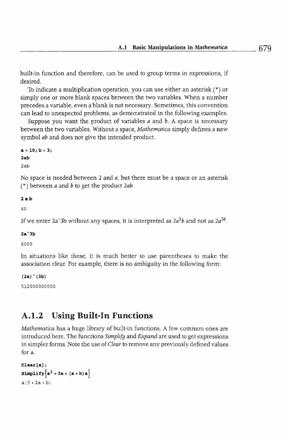
A.l.2 Using Built-In Functions Mathematica has a huge library of built-in functions. A few common ones are introduced here. The functions Simplify and Expand are used to get expressions in simpler forms. Note the use of Clear to remove any previously defined values for a.

Clear[a];

S~lify[a2+3&+ (&+b)&]

a (3+2a+b)

680 Appendix: An Introduction to Mathematica ------~----~------------------------------

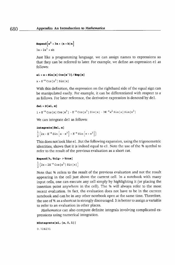
Bxpand[a2 +3a+ (a+b)a]

3a + 2a2 + ab

Just like a programming language, we can assign names to expressions so that they can be referred to later. For example, we define an expression el as follows:

el = x + Sin [x] COB [x"3) IBxp [x)

x + ECx Cos [x3 ] Sin [xl

With this definition, the expression on the righthand side of the equal sign can be manipulated easily. For example, it can be differentiated with respect to x as follows. For later reference, the derivative expression is denoted by del.

del = D[el, x)

1 + E- X Cos [xl Cos [x3 l - E- X Cos [x3 ] Sin [x] - 3E- xx 2 Sin [xl Sin [x3 ]

We can integrate del as follows:

Integrate [del, x)

~ ( 2x + E-x Sin [x - x 3 ] + E-x Sin [ x + x 3 ] )

This does not look like el. But the following expansion, using the trigonometric identities, shows that it is indeed equal to el. Note the use of the % symbol to refer to the result of the previous evaluation as a short cut.

Bxpand[%, 'l'rig- > 'l'rue)

~ (2X + 2E-x Cos [x3 ] sin [x] )

Note that % refers to the result of the previous evaluation and not the result appearing in the cell just above the current cell . In a notebook with many input cells, one can execute any cell simply by highlighting it (or placing the insertion point anywhere in the cell). The % will always refer to the most recent evaluation. In fact, the evaluation does not have to be in the current notebook and can be in any other notebook open at the same time. Therefore, the use of % as a shortcut is strongly discouraged. It is better to assign a variable to refer to an evaluation in other places.

Mathematica can also compute definite integrals involving complicated ex­pressions using numerical integration.

NIntegrate[el, {x,a,l»)

0.724231

A.I Basic Manipulations in Mathematica 681 --------------------------~----------------

A.1.3 Substitution Rule The symbol /. (slash-period) is a useful operator and is used to substitute different variables or numerical values into existing expressions. For example, the expression el can be evaluated at x = 1.5, as follows:

e1 I. x->1.5

1. 2 834 6

The arrow symbol is a combination of a hyphen (-) and a greater than sign (», and is known as a rule in Mathematica. Of course, more complicated substitutions are possible. The following example illustrates defining a new expression called e2 by substituting x = a + Sin(b] in expression el.

e2 • e1 I . (x->a + sin [b])

10 + Sin [3] + E -10- Sin [31 Cos [ (10 + Sin [3] ) 3 ] Sin [10 + Sin [3]]

Substitute a = 1 and b = 2 in expression e2.

e2 I. (a->l, b->2)

1+Si n [2 ] +E-10-Sin[21 Cos[(1+sin[2])2] Sin [1+Sin [2]]

Th get the numerical result after substituting a = 1 and b = 2 in expression e2, we can use the N function:

N[e2 I. (a->l, b->2]1

1.9092 8

Note that the same result can also be obtained as follows:

a = 1; b = 2; N[e21

1.90 928

However, the substitution form is much more desirable. This second form de­fines the symbols a and b to have the indicated numerical values. Mathematica will automatically substitute these values into any subsequent evaluation that involves a and b.

a + b x

1 + 2x

The only way to get symbolic expressions involving a and b later would be to explicitly clear these variables, as follows:

682 Appendix: An Introduction to Mathemarica ------~--~==~~~----------------------

Clear[a, b]; a + b x

a +bx

A.2 Lists and Matrices

Lists are quantities enclosed in curly braces ({}). They are one of the basic data structures used by Mathematica. Many Mathematica functions expect ar­guments in the form of lists and return results as lists. When working with these functions, it is important to pay close attention to the nesting of braces. 'TWo expressions that are otherwise identical, except that one is enclosed in a single set of braces and the other in double braces, mean two entirely different things to Mathematica. Beginners often don't pay close attention to braces and get frustrated when Mathematica does not do what they think it should be doing.

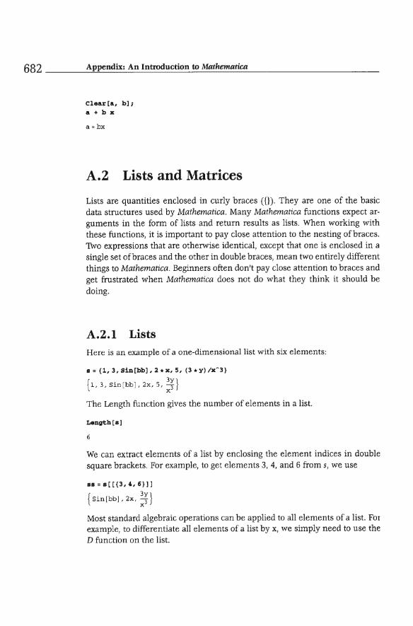
A.2.1 Lists Here is an example of a one-dimensional1ist with six elements:

a= {1,3,Sin[bb),2*x,S, (3*y)/x"3}

{ . 3Y } 1,3, Sw [bb J , 2x, 5 , x3

The Length function gives the number of elements in a list.

Length [a)

6

We can extract elements of a list by enclosing the element indices in double square brackets. For example, to get elements 3,4, and 6 from 5, we use

aa = a([p, 4, 6}])

{ . 3Y } S~n[bbJ, 2x, x 3

Most standard algebraic operations can be applied to all elements of a list. For example, to differentiate all elements of a list by x, we simply need to use the D function on the list.

A.2 Lists and Matrices 683 ------------------------------------------

D[n,x]

{O , 2 , _9~ } x

Multidimensional lists can be defined in a similar way. Here is an example of a two-dimensional list with the first row having one element, the second row three elements, and the third row as the s list defined above.

a= {{l}, {2,3,4},8}

{{li, (2, 3, 4), {1, 3, Sin [bb ] , 2x , 5 , 3;} } x

Langth[a]

3

Elements of a list can be extracted by specifying the row number and the element number within each row in pairs of square brackets. For example, to get the second row oflist a, we use the following structure:

a[[2]]

( 2, 3, 4 )

1b get the sixth element ofthe third row oflist a, we use the following structure:

a[[3,6]]

3y

x3

Obviously, Mathematica will generate an error message if you try to get an element that is not defined in a list. For example, trying to get the fourth element from the second row will produce the following result:

a[ [2, 'll

Part :: partw : Part ( 4 of ( 2, 3, 4) does not exist.}

{( l ) , ( 2, 3, 4 ), {l' 3, Sin [bb], 2x, 5 , ~;}}[2, 4]

Sometimes it is necessary to change the structure of a list. Flatten and Partition functions are simple ways to achieve this. Flatten removes all internal braces and converts any multidimensional list into a single flat list, keeping the order the same as that in the original list. For example, we can define a new one­dimensional1ist b by flattening list a as follows :

b = Flatten [a]

{ . 3Y } 1 , 2 , 3 , 4 , 1, 3 , S1n [bb] , 2x, 5, x 3

684 Appendix: An Introduction to Mathematica ------~------------------------------------

Using Partition, we can create partitions (row structure) in a given list. The second argument of Partition specifies the number of elements in each row. Extra elements that do not define a complete row are ignored.

Partition[b, 3]

{{1, 2, 3}, (4, 1, 3), {Sin[bb;, 2x , 5}}

partition[b, 4]

{{ l, 2 , 3, 4}, {l, 3, Sin[bb], 2x}}

A.2.2 Matrices Matrices are special two-dimensional lists in which each row has exactly the same number of elements. Here we define a 3 x 4 matrix m:

m .. ((l,2,3,4}I(5,6 , 7,8},(9,lO,1l,1211

{ {l, 2, 3, 4}, {S, 6, 7, 8}, {9, 10, 11 , 12}}

1b see the result displayed in a conventional matrix form, we use MatrixForm.

MatrixForm[mj

[ ~ ~ ; : 1 9 10 11 12

ThbleForm is another way of displaying multidimensional lists.

TableForm[mj

1 2 3 4 S 6 7 8 9 10 11 12

The following two-dimensional list is not a valid matrix because the number of elements in each row is not the same. However, there is no error message produced because it is still a valid list in Mathematica.

a = {{l}, {2, 3}, {4, 5, 6}}

{ {1}, {2 , 3}, {4 , 5, 6}}

MatrixForm[a]

r (l) 1 (2, 3) {4, 5, 6}

A.2 Lists and Matrices 685 --------------------------==~~~==~-----

Once a matrix is defined, standard matrix operations can be performed on it. For example, we can define a new matrix mt as the 'Itanspose of m.

mt = Transpose [m] ; KatrixForm [mt]

1 5 9 2 6 10 3 7 11 4 8 12

Matrices can be multiplied by using . (period) between their names.

KatrixForm[mt.m]

107 122 1 37 152 122 140 158 176 137 158 179 200 152 176 200 224

Using • or a blank will produce an error or simply element-by-element multi­plication.

Thread: : tdlen: Objects o f unequal length i n ({ I, 5 , 9 ), ( 2 , 6, 10), ( 3, 7,11 ), {4, 8 , 12 } } {{ I , 2, 3 , 4}, ( 5, 6, 7, 8), {9, 10, 11 , 12 } } cannot be combined .

{ {I , 2 , 3 , 4}, {5, 6, 7, 8}, {9, 10, 11 , 12 } } { {1 , 5 , 9}, {2, 6, 10}, {3, 7, 11}, {4, 8 , 12}}

Here we get an element-by-element product and not the matrix product.

mt *mt

{{1, 25 , 81l, {4, 36 , 100}, {9, 49, 121 l, {16 , 64, 144}}

When using MatrixForm, it is very important to note that the MatrixForm is used for display purposes only. If a matrix is defined with the MatrixForm in it, that matrix definition cannot be used in any subsequent calculation. For example, consider the following definition of matrix m used previously:

m = KatrixForm[ {{ 1,2, 3, 4}, {S, 6,7, 8}, {9, 10, 11, 12}} I

(1 2 3 4 1 5 6 7 8 9 10 11 12

The output looks exactly like it did in the earlier case. However, we cannot per­form any operations on matrix m in this form. For example, using the 'Itanspose function on m simply returns the initial matrix m wrapped in Ttanspose.

686 Appendix: An Introduction to Mathematica ------~----------------------------------

'l'ranspose[m)

Transpose [[~9 ~ ~ :)l 10 11 12

The solution obviously is not to use the MatrixForm in the definition of ma­trices. After the definition, we can use the MatrixForm to get a nice-looking display.

m = {{l, 2, 3, 4}, {5, 6, 7, 8}, {9, 10, 11, 12}}; KatrixForm[lII)

(1 2 3 4 1 5 6 7 8 9 10 11 12

Elements of matrices can be extracted using the double square brackets. For example, the second row of m can be extracted as follows:

m2 = 81[[2)]

(5, 6, 7, 8)

The element in the second row and the fourth column is

m[ [2, 4]]

8

Extracting a column is a little more difficult. The simplest way is to transpose the matrix and then take its desired row (which obviously corresponds to the original column). For example, the second column of matrix m is extracted as follows:

c2 = 'l'ranspose[m] [[2]]

{2, 6, 10}

Matrices can also be defined in terms of symbolic expressions. For example, here is a 2 x 2 matrix called m.

m = {{y, 2*x}, ({3*y)/xA 3, 4*Y)); KatrixForm[m]

(, !~ 1

Determinant of m:

Det[m]

_ 6y + 4y2 x 2

Inverse of m:

A.2 Lists and Matrices 687 ---------------------------=~========~----

mi = Inverse [m] ; 4y

6y 2 -- +4y

x2

3y

Matrixl!'orm[mi]

2x - 6y 2 -- +4y

x2

y 6y 2

- x 2 + 4y

Check the inverse:

MatrizForm(Simplify(mi.m]]

(~ ~) Operations, such as differentiation and integration, are performed on each element of a matrix.

D(m,y]IIMatrixl!'orm

Integrate(m,x]IIMatrixForm

( XV X2) -?;r 4xy

A.2.3 Generating Lists with the Thble Function The Thb1e function is a handy tool to generate lists or matrices with a systematic pattern. For example, to generate a 3 x 5 matrix with all entries as zero, we use the following form:

m='l'able[O, {3}, {5}];M&trixForm[m]

(0 0 0 0 0 1 00000 o 0 0 00

The first argument to the Table function can be any expression. Here is a 3 x 4 matrix whose entries are equal to the sum ofrow and column indices divided by 3/\ (column index).

z ='l'able[(i+j)/3'j, {i,1,3}, {j, 1, 4}];Matdxl!'orm[zJ

2 1 4 5 11TItlT

4 5 2 1 ~ 2i 27 4 5 2 7 J ~ ~ 81

688 Appendix: An Introduction to Mathematica ----~~---------------------------------

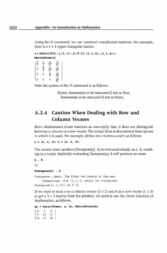
Using the If command, we can construct complicated matrices. For example, here is a 4 x 4 upper triangular matrix:

z"Table[If[i>j,O, (i+j)/3~jl, {i,1,4}, {j,1,4}];

HatrixForm[z]

2 1 4 5 J J 27 8I 0 4 5 2

9 27 27

0 0 2 7 9 8I

0 0 0 8 8I

Note the syntax of the If command is as follows:

If[test, Statements to be executed if test is 'Ihle, Statements to be executed if test is False]

A.2.4 Caution When Dealing with Rowand Column Vectors

Since Mathematica treats matrices as essentially lists, it does not distinguish between a column or a row vector. The actual form is determined from syntax in which it is used. For example, define two vectors a and b as follows:

a " Il, 2, 3); b .. 14, 5, 6};

The matrix inner product ('Il:'anspose[a]. b) is evaluated simply as a . b, result­ing in a scalar. Explicitly evaluating 'Il:'anspose[a]. b will produce an error.

a • b

32

Transpose!a] • b

Transpose: : nmtx: The first two levels of the one-

dimensional list {I, 2, 3) cannot be transposed.

Transpose [ {l, 2, 3} 1 . 14, 5, 6}

If we want to treat a as a column vector (3 x 1) and b as a row vector (1 x 3) to get a 3 x 3 matrix from the product, we need to use the Outer function of Mathematica, as follows:

ab • OUter[Times , a , b]; HatrixForm[ab]

(1:2 t~ t~ 1

A.3 Solving Equations 689 --------------------------------~~--------

Another way to explicitly define a 3 x 1 column vector is to enter it as a two­dimensional list. Here, each entry defines a row of a matrix with one column.

a = {{1}, 12}, 13l}; Matrixl'orm[a]

Now'Itanspose[a] . b makes sense. However, the result is a 1 x 1 matrix and not a scalar.

'l'raDBpolle raj • b

{3 2 }

Obviously, now a . b will produce an error because the dimensions do not match.

a.b

Dot : : dotsh: Tensors {{1}, {2}, {3}}

and {4, 5, 6} have incompatible shapes.

{{ lL {2 }, (3}). {4, 5, 6}

Th get a 3 x 3 matrix, we need to define b as a two-dimensional matrix with only one row, as follows:

b = {{4, 5, 6l}

( {4 , 5 , 6 })

Now a (3 xl) . b (1 x 3) can be evaluated directly, as one would expect.

MatrixForm[a . b]

[4 5 6 1 8 10 12

12 15 18

A.3 Solving Equations

An equation in Mathematica is defined as an expression with two parts sep­arated by two equal signs (==), without any spaces between the two signs. Thus, the following is an equation:

x"3 - 3 == 0

-3 + x 3 == 0

690 Appendix: An Introduction to Mathematica ----~~----------------------------------

Note that you get the following strange-looking error message if you try to define an equation with a single equal sign. (The error message makes sense if you know more details of how Mathematica handles expressions internally.)

Set:: write: Tag Plus in - 3 +x3 is Protected.

o

Equations can also be assigned to variables for later reference. For example, we can call the above equation eq so that we can refer to it in other computations.

eq • xA 3 - 3 •• 0

-3 + x3 ;; 0

A single equation, or a systems of equations, can be solved using the Solve command.

sol = Solve [eq, xl

{{x-? - (_3)1/3}, {x-? 3l/3 }, {x-? (_1)2/3 3l / 3}}

Note that the solution is returned in the form of a two-dimensional list of substitution rules. Because of this form, we can substitute any solution into an­other expression if desired. For example, we can substitute the second solution back into the equation to verify that the solution is correct, as follows:

eq I. sol [[2]]

True

The Solve command tries to find all possible solutions using symbolic manip­ulations. If a numerical solution is desired, the NSolve command is usually much faster.

NSolve[x'3 - 3 -= 0, x]

{{x -? -0.721125 + 1. 24902I}, {x -? -0 . 721125 - 1. 24902I}, (x -? 1. 44225))

Both Solve and NSolve commands can be used for systems of linear or nonlin­ear equations .

• qn1 • x + 2y + 3: •• '1; eqn2 • 5x + 5y + ,: =. 20; eqn3 • 3y + 4z .~ 125; sol = Solve[{eqn1, eqn2, eqn3} , {x, y, :}l

{{X-?_527 y-?635 z-->-~}} 13' 13' 13

A.4 Plotting in Mathematica 691 -------------------------------~------------

Notice that even when there is only one solution, the result is a two-dimen­sional list. If we want to evaluate a given function at this solution point, we still need to extract the first element of this list. For example:

a = N[Sin[xy] Cos [yZ] / .sol [[lJ J J

-0.810238

The following substitution produces the same result but in the form of a list whose structure must be kept in mind if it is to be used in other expressions.

b = N[Sin[xyJ Cos [yz] / .sol]

{- O. 810238}

For example, since a is a scalar as defined by the first form, it can be used in any matrix operation. However, b can only be used with appropriate-sized matrices.

a{a1, a2, a3}

{-O . 810238al, -O.810238a2, -O.810238a3}

b{al, a2, a3}

Thread: : tdlen : Objects of unequal length

in {-0 .810238'}{al, a2, a3} cannot be combined.

{-O.810238}{al, a2, a3}

A linear system of equations, written in matrix form as Kd = R, can be solved very efficiently using the LinearSolve[K, R] command, as follows:

K= {{2, 4, 5}, {7, 9, 2}, {1, 2, 13}};

11.= {1,2,3};

LinearSolve [X, II.J

{ 21 13 1} 20' - 20' 4"

A.4 Plotting in Mathematica

Mathematica supports both two-dimensional and three-dimensional graphics. The Plot command provides support for two-dimensional graphs of one or more functions specified as expressions or functions. The following shows the plot of an expression in the interval from -2 to 2.

692 ________ A~pp~e_n_d_u __ :A __ n_I_n_tto __ d_u_ct_io_n __ to __ M_a_ffl_mn __ a_n_c_a ________________________ _

pl = Plot[Sin[x] Cos[x]/(1+x"2),(x,-2,2}];

-2 -1 1

Multiple plots can be shown on the same graph using the Show command. The following example plots an expression and its first derivative. Each plot command automatically displays a resulting graph. For multiple plots, usually the final plot showing all graphs superimposed is of interest. Using Display­Function as Identi ty suppresses the display of intermediate plots.

del = D[Sin[x] C08[x]/(1+x"2),x]; p2 • Plot(del,(x,-2,2}, PlotStyle->(RGBColor[O,O,l]},

DisplayFunction -> Identity]; Show[(pl,p2}l ;

The RGBColor function returns a combination color by mixing specified amounts of red, green and blue colors. In the example, the Blue component is set to 1 and the others to 0 to get a blue color. Use MalhemuUcu on1ine He1p to

explore many other plot options.

__________________________________ ~A~.4~P~1=o~llin=·~g~m~M=m~h~em~an~c=a~ ______ 693

Note that before generating the plot for the derivative, we defined a new expression and then used it in the plot function. If we had actually used the derivative operation inside the argument of the Plot function, we would get a series of strange error messages, as follows:

Plot[D[Sin[x] Cos[x]/(1+xA2),x],{x,-2,2}];

General: : ivar : -2. is not a valid variable.

General: : i var : -2. is not a valid variable.

General : : ivar : -2. is not a valid variable .

General : : stop: Further output of General : : ivar will be suppressed during this calculation .

Plot : : plnr :

a Sin[x] Cos [xJ is not a machine-size real number at x = - 2 .. x 1 + x 2

Plot : : plnr :

a Sin [x ] Cos [x) is not a machine-size real number at x = -1. 83773. x 1 + x 2

Plot : : plnr :

a Sin [x) Cos [x) is not a machine-size real number at x = -1. 66076. x 1 + x2

General: : stop: Further output of plot: : plnr will be suppressed during this calculation.

1

0.8

0.6

0.4

0.2

0.2 0 . 4 0 . 6 0.8 1

The reason for the error is that Plot and several other built-in functions do not evaluate their arguments (for valid reasons but difficult to explain here). We can force them to evaluate the arguments by enclosing the computation inside Evaluate, as follows:

694 Appendix: An Introduction to Mathematica ------~-----------------------------------

plot [Evaluate[D[Sin[x] Cos[x]/(1+x"2),x]],(x,-2,2}];

-1 1

Functions of two variables can be shown either as contour plots or as three­dimensional surface plots.

f = Sin [x] Cos [y]

Cos [y] Sin [xl

ContourPlot [f, {x, -7f, 7f}, {y, -7f, 7f} , PlotPoints- > 50] ;

Plot3D[f, {x, -7f, 7f}, {y, -7f, 7f}];

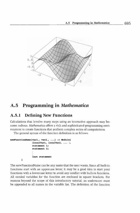
______________________________ ~A~.=5~P~IU~wrn==nun==1=·n3g~in~M=a=t~h=mn~a~ri~ca~ _______ 695

A.5 Programming in Mathematica

A.S.l Defining New Functions Calculations that involve many steps using an interactive approach may be· come tedious. Mathematica offers a rich and sophisticated programming envi· ronment to create functions that perform complex series of computations.

The general syntax of the function definition is as follows:

newFunctionName[var1., var2., .•• J := Module[ {localVar1, localVar2, '" }, statement 1; statement 2;

last statement

The newFunctionName can be any name that the user wants. Since an built·in functions start with an uppercase letter, it may be a good idea to start your functions with a lowercase letter to avoid any conflict with built·in functions. All needed variables for the function are enclosed in square brackets. For reasons beyond the scope of this introductory tutorial, an underscore must be appended to all names in the variable list. The definition of the function

696 Appendix: An Introduction to Mathematica ------~----------------~----------------

starts with := followed by the word Module and an opening square bracket. The first line in the definition is a list oflocal variables that are to be used only inside the body of the function. Outside of the function, these variables do not exist. The list oflocal variables ends with a comma. The remainder of the function body can contain as many statements as needed to achieve the goal of the function. Each statement ends with a semicolon. The last statement does not have a semicolon and is the one that is returned by the function when it is used. The end of the function is indicated by the closing square bracket.

Simple one-line functions that do not need any 10ca1 variables can be defined simply as follows:

oneLineFcn[varl_. var2_ •••• J I- expression involving vars

An example of a one-line function is presented in the next section. As an example of Module, we define the following function to return stresses in thick-walled cylinders. The tangential and radial stresses in an open-ended thick cylinder are given by the following formulas:

. 2 ( 2) P, ri ro at = -2--2 1 + '2

ro - ri r _ Pirl' ( r&) ar - -2--2 1 - '2

ro - Ti r

where Pi is internal pressure on the cylinder, Ti and TO are inner and outer radii and r is radius of the point where the stress is desired.

thickCylinderStresses [pL, rL, rO_, r-l : = Module [{ cl, c2, at, ar},

cl = pi * ri 2/ (r02 _ ri 2 ) ; c2 = r02/r2; at = cl(l + c2); ar = cl(l- c2); {at, ar}

After entering the function definition, the input must be executed to actually tell Mathematica about the new function. Unless there is an error, the execution of the function definition line does not produce any output. After this, the function can be used as any other Mathematica function. For example, we can compute stresses in a cylinder with pi = 20, ri = 5, TO = 15, and r = 10 as follows:

A.5 Programming in Mathcmatica 697 ----------------------~~~--~------------

thickCylinderStresses[20,5,15,10]

{ ~ _ 25} 8' 8

Leaving some variables in symbolic form, we can get symbolic results:

{st, sr} = thickCylinderStresses [20,5,15, r]

These expressions can be plotted to see the stress distribution through the cylinder wall.

Plot[{st, sr}, {r, 5, 15},AxesLabel- > {Or", "Stress"},

PlotStyle- > {{GrayLevel[Oj}, {GrayLevel[0.5]}}];

Stress

10

-10 /

~i~;!

A natural question might be to see what happens to the stresses as the cylinder becomes thin. This question can be answered by evaluating the stresses at the center of wall thickness as a function of inner radius, as follows:

{st, sr} = thickcylinderStresses [20, ri, 15, (ri + 15) /2]

20ri2(1+ 900 ) 20ri2 (1 - 900 )

{ (lS+ri )2 , (lS+ri )2 }

225 - r i 2 22 5 -ri2

A plot of these expressions is as follows:

Plot[{st, sr}, {ri, 5, 14},AxesLabel- > {Orin, "Stress"},

Plot Style- > {{GrayLevel [0 .5]}, {GrayLevel [O]}}] ;

698 Appendix: An Introduction to Mathenuuica ------~------------------------------------

Stress

150

100

50

~=t====~====~====~====~4 ri

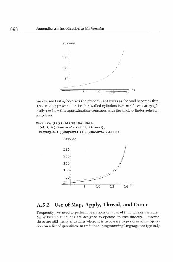
We can see that O't becomes the predominant stress as the wan becomes thin. The usual approximation for thin-waned cylinders is at = -0/. We can graph­ically see how this approximation compares with the thick cylinder solution, as follows:

Plot [{st, (20 (ri + 15) /2) /(15 - ri)},

{ri, 5,l4.},AxesLabel- > {"ri", "Stress"},

PlotStyle- > {{GrayLevel [O]}, {GrayLevel [0 .5]}}];

Stress

250

200

150

100

50

8 10 12 14 ri

A.S.2 Use of Map, Apply, Thread, and Outer Frequently, we need to perform operations on a list of functions or variables. Many built-in functions are designed to operate on lists directly. However, there are still many situations where it is necessary to perform some opera­tion on a list of quantities. In traditional programming language, we typically

__________________________________ A~.5~_P_IO~~~a_nnn __ lll_·~g~i_n_M __ a_th_mn __ ati __ c_a _________ 699

perform these operations using a Do loop or an equivalent. Mathematica has a Do loop that can be used in a similar way. However, it also offers many other elegant and more convenient ways of doing the same thing. Map, Thread, and Apply are three of these handy functions. These functions have been used in several examples in this text. We illustrate the use of these functions in the portfolio example considered in Chapter 1.

Suppose we are given historical rates of returns from different investments that we have entered as lists in Mathematica.

blueChipStocks = {18.24, 12.12, 15.23, 5.26, 2.62, 10.42}; techStocks = {12. 24, 19.16, 35.07, 23.46, -10.62, -7.43} ; realEstate = {8 .23,8.96,8.35,9.16,8. 05,7 .29}; bonds = {8.12, 8.26, 8.34, 9.01, 9.11, 8.95};

We want to compute the average rate of return. The computation is fairly simple. We just need to add all rates of returns and divide them by the number of returns. Computing the sum or multiplication of all elements of a list is done very conveniently by using Apply. It does not matter how long the list is or whether it consists of numerical or symbolic quantities.

App1y[Plus,blueChipStocksj

63 . 89

The first argument of Apply is the function to be applied, and the second is the list of items. Multiplication of all elements can be computed in exactly the same way.

Apply[Times,blueChipStocksj

483484 .

Obviously, the function to be applied must expect a list as its argument. For example, applying Sin function to a list will not produce any useful result.

Apply[Sin,blueChipStocksj

Sin: : a rgx : Sin called with 6 arguments; 1 argument is expected.

Sin[18 . 24, 12.12, 15 . 23, 5.26, 2. 62, 10.42J

The Map function is similar to Apply, but it applies a function to each element of a list. For example, if we want to compute the Sin of each term in the blueChipStocks list, we can do it as follows:

Map[Sin,blueChipStocksj

{-0. 572 503, -0.431695, 0.459972, -0.853771, 0.498262 , -0 . 83888 }

700 Appendix: An Introduction to Mathematica ------~-------------------------------------

Th compute the average, all we need to do now is divide the sum by the number of entries in the list. The Length function, described earlier, does exactly this. Thus, the following one-line program can compute the average of any list.

average [n-l : = Apply[Plus, nl /Length[nl

average [blueChipStocksl

10.6483

Th compute average rates of returns of all investment types, we can use the average function repeatedly on other lists of returns. However, it is much more convenient to define a list of all investments and simply Map the average function to each element of a list. We first define a list of all returns and then use the average function defined above.

returns = {blueChipStocks,techStocks,realEstate,bonds}

{{ 18.24, 12.12, 15 .23 , 5.26, 2.62, 10.42}, {12.24, 19.16 , 35.07, 23.46, -10.62, -7.43}, (8.23, 8.96, 8.35 , 9.16, 8.05, 7.29), (8.12, 8.26, 8.34,9.01,9.11,8.95))

averageReturns = Map [average, returns I

(10.6483, 11.98, 8 .34, 8.63167 )

The elegance of these constructs is that we never need to know how long the lists really are. We can keep adding or deleting elements into any ofthe lists and the process will keep working. Map and Apply functions are used so frequently in Mathematica programming that several short cuts have been designed to make their use even more efficient. One such useful technique is combining Map with the function definition itself. In the example of computing averages, we had to define a function (called average) and then apply it to elements of the list using Map. We can do exactly the same thing, without explicitly defining the function, as follows:

averageReturnS = Map [APply[Plus, #]/Length[#]&, returns]

(10.6483, 11.98 , 8.34, 8.63167)

We can see that the first argument is exactly the definition of the function. The pound (#) sign stands for the function argument. The ampersand (&) at the end is very important. It essentially tells Mathematica that we are defining a function as the first argument of Map.

The computation of the covariance matrix involves several uses of Apply. We define covariance between two investments i and j as follows:

________________________________ A_._5 __ P_IU~~~rum __ m_l_·n~g~i_n_M_a_t_h_mn __ a_ri_ca _________ 701

where n = total number of observations, rjk = rate of return of investment j for the kth observation, and iLj is the average value of the investment j. The following function implements this computation. The first two lines compute averages, and the third line returns the above sum.

coVariance [x_, Y-l : = Module [{xb, yb, n = Length [xl },

xb = Apply [Plus, x] In; yb = Apply [Plus, y] In;

Apply[Plus, (x - xb) (y - yb)] In

] ;

Using this function, we can compute the covariance between, say, blueChip­Stocks and bonds as follows:

coVariance [blueChipStocks, bonds 1

- 1. 9532

Computing the entire covariance matrix this way would be tedious. The Outer function, described earlier, feeds all combinations of investments to the co Vari­ance function and thus, we can generate the entire matrix using the follOwing line of Mathematica input.

Q = OUter [coVariance, returns, returns, 1]; MatrixFo:rm[Q]

29.0552 40.3909 - 0.287883 -1.9532 40.3909 267 .344 6.83367 -3.69702

- 0.287883 6.83367 0.375933 -0.0566333 - 1.9532 -3.69702 -0.0566333 0.159714

The Thread function is similar to Map as it threads a function over its argu­ments. The most common use of this function in the text has been to define rules for substitution into an expression. Suppose we have a function of four variables that we would like to evaluate at a given point.

f = Xl X2 + Sin [x3 ] Cos [x,] ;

pt = {1.1,2.23, 3.2,4.556};

vars = {Xl' x2' x3' x,J;

A tedious way to evaluate f at the given point is as follows:

2.46209

702 Appendix: An Introduction to Mathemanca ------~----------------~-----------------

A more convenient way is to use Thread to define the substitution rule.

Thread[vars- > pt]

{xl .... 1.1,x2 .... 2.23,x3 .... 3.2,x4 .... 4.556 )

f/ • Thread [vars- > pt]

2.46209

Again, the advantage of the last form is clear. We don't have to change anything if the number of variables is increased or decreased.

A.6 Packages in Mathematica

Mathematica comes with a wide variety of special packages. Among these are the linear algebra and graphics packages. These packages provide additional commands for manipulating matrices and plots. Loading the matrix manipu­lation commands from the LinearAlgebra Package and Graphics' Legend pack­ages is accomplished as fonows:

Needs["LinearAlgebra'MatrixManipulation'"];

Needs ["Graphics' Legend' "] ;

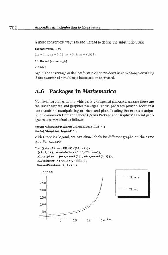
With Graphics'Legend, we can show labels for different graphs on the same plot. For example,

Plot[{st, (20(ri+15)/2)/(15-ri)},

{ri, 5, l'}, AxesLabel- > {"ri", "Stress"},

PlotStyle- > {{GrayLevel [0] }, {GrayLevel [0 .5]}},

PlotLegend- > {"Thick", "Thin"},

LegendPosition- > {l, O}];

Stress

250

200

150

100

50

~~====~8~--~1~0----~1~2----~1~4 ri

-- Thick

--... ---- Thin

_______________________________________ A_._7 __ 0_nli_·_ne __ H_el~p _______ 703

The large number of functions created for this text are included in the Op­timizationTho1box package. Specific instructions for loading and using this package are included on the accompanying CD.

A.7 Online Help

Mathematica contains a complete online Help system. The Help menu provides access to all Mathematica features. In fact, the entire Mathematica book is online. In addition you can obtain information about any command by typing ? followed by the command name. This form also supports the use of wild­cards. For example, to get a listing of all commands that start with letter G, type

?G*

Gamma GarnmaRegulari zed Gaussianlntegers GaussKronrod GaussPoints GCD

Gear GegenbauerC General GenerateBitmapCaches Genera teConditions GeneratedCell

Generic GraphicsSpacing Get GrayLevel GetContext Greater GetLinebreaklnformationPacket GreaterEqual GoldenRatio GridBaseline Goto GridBox Gradient GridBoxOptions Graphics GridFrame" Graphics3D GridLines GraphicsArray GroebnerBas is GraphicsData GroupPageBreakWi t hin

Detailed instructions about a specific command can be obtained by typing? fonowed by the command name. For example,

?GaussPoints

GaussPoints is an option for Nlntegrate. With GaussPoints- > n, the Gaussian part of Gauss - Kronrod quadrature uses n points. With GaussPoints - > Automatic, an internal algorithm chooses the number of points.

Bibliography

Abel, M.L. and Braselton, J.P', Mathematica by Example, Academic Press, San Diego, 1997.

Bahder, T. , Mathematica for Scientists and Engineers, Addison-Wesley, Reading, MA, 1995.

704 _____ A-"p-"p-'-en_d_ix==.:...: .::..:A=n:....:I=n.::..:tro.::..:.::..:d.::..:u.::..:c.::..:ti=on==-:t-'-o-'-M.::..:a-'-th-'-ema::..:....:.:..:.:ti..::·c.::..:a~ ___________ _

Gray, J.w., Mastering Mathematica, AP Professional, Cambridge, MA, 1994.

Gray, T. and Glynn, J., A Beginner's Guide to Mathematica, Version 2, Addison-Wesley, Reading, MA, 1992.

Maeder, R., Programming in Mathematica, 3rd Edition, Addison-Wesley, Redwood City, CA,1997.

Shaw, w.T. and Tigg, J., Applied Mathematica: Getting Started, Getting It Done, Addison­Wesley, Reading, MA, 1994.

Wagner, D.B., Power Programming with Mathematica, McGraw-Hill, New York, 1996.

Wickham-Jones, T., Mathematica Graphics: 'Techniques and Applications, TELOS (Springer-Verlag), Santa Clara, CA, 1994.

Wolfram, S., The Mathematica Book, 3rd Edition, Wolfram Media/ Cambridge University Press, Boston, MA, 1996.

Bibliography

Arora, J.S., Introduction to Optimum Design, McGraw-Hill, New York, 1989.

Avriel, M. and Golany, B., Mathematical Programming for Industrial Engineers, Marcel Dekker, New York, 1996.

Bates, D.M. and Watts, D.G., Nonlinear Regression Analysis and Its Applications, Wiley, New York, 1988.

Bazarra, M.S., Jarvis, J.J., and Sherali, H.D., Linear Programming and Network Flows, Wiley, New York, 1990.

Bazarra, M.S., Sherali, H.D., and Shetty, C.M., Nonlinear Programming.' Theory and Al­gorithms, 2nd Edition, Wiley, New York, 1993.

Bertsekas, D.P., Nonlinear Programming, Athena Scientific, Belmont, MA, 1995.

Beveridge, Gordon S.G., and Schechter, R.S., Optimization: Theory and Practice, McGraw­Hill , New York, 1970.

Biegler, L.T, Coleman, TF., Conn, A.R., and Santosa, F.N. (editors), Large-Scale Op­timization with Applications, Part 1: Optimization in Inverse Problems and Design, Springer-Verlag, New York, 1997.

Biegler, L.T, Coleman, TF., Conn, A.R., and Santosa, F.N. (editors), Large-Scale Op­timization with Applications, Part II: Optimal Design and Control, Springer-Verlag, New York, 1997.

Biegler, L.T. , Coleman, T.F., Conn, A.R., and Santosa, F.N. (editors), Large-Scale Optimiza­tion with Applications, Part III. Molecular Structure and Optimization, Springer-Verlag, New York, 1997.

Dantzig, G.B. and Thapa, M.N., Linear Programming 1: Introduction, Springer-Verlag, New York, 1997.

705

706 _______ B_i~b_lio~~~a~p~h~y ________________________________________ __

Degarmo, E.P, Sullivan, w.G., Bontadelli, J.A., and Wicks, E.M., Engineering Economy, Prentice-Hall, Englewood Cliffs, NJ, 1997.

Dennis, J.E., Schnabel, R.B., Numerical Methods for Unconstrained Optimization and Non­linear Equations, Prentice-Hall, Englewood Cliffs, NJ, 1983.

Ertas, A. and Jones, J.C., The Engineering Design Process, 2nd Edition, Wiley, New York, 1996.

Fang, S.-C. and Puthenpura, S., Linear Optimization and Extensions, AT&T, Prentice-Hall, Englewood Cliffs, NJ, 1993.

Fiacco, A.Y., Introduction to Sensitivity and Stability Analysis in Nonlinear Programming, Academic Press, New York, 1983.

Fiacco, A.Y. and McCormick, G.P' , Nonlinear Programming: Sequential Unconstrained Minimization 'Techniques, Wiley, New York, 1968.

Fletcher, R., Practical Methods of Optimizations, Second Edition, Wiley, New York, 1987.

Gen, M. and Cheng, R., Genetic Algorithms and Engineering Design, Wiley, New York, 1997.

Gill, P.E., Murray, w., and Wright, M.H., Practical Optimization, Academic Press, New York, 1981.

Gill, P.E., Murray, w., and Wright, M.H., Numerical Linear Algebra and Optimization, Addison-Wesley, Reading, MA, 1991.

Goldberg, D .E., Genetic Algorithms in Search, Optimization, and Machine Learning, Addison­Wesley, Reading, MA, 1989.

Gomez, S. and Hennart, J. -P. (editors), Advances in Optimization and Numerical Analysis, Kluwer Academic Publishers, Dordrecht, 1994.

Hansen, E., Global Optimization Using Interval Analysis, Marcel Dekker, New York, 1992.

Hayhurst, G., Mathematical Programming Applications, Macmillan, New York, 1987.

Hentenryck, P. Van, Michel, L., and Deville, Y, Numerica: A Modeling Language for Global Optimization, MIT Press, Cambridge, MA, 1997.

Hertog, D. den, Interior Point Approach to Linear, Quadratic and Convex Programming, Kluwer Academic Publishers, Dordrecht, 1994.

Hestenes, M., Conjugate Direction Methods in Optimization, Springer-Verlag, Berlin, 1980.

Himmelblau, D.M., Applied Nonlinear Programming, McGraw-Hill, New York, 1972.

Hymann, B., Fundamentals of Engineering Design, Prentice-Hall, Englewood Cliffs, NJ, 1998.

Jahn, J., Introduction to the Theory of Nonlinear Optimization, 2nd Revised Edition, Springer-Verlag, Berlin, 1996.

Jeter, M.W., Mathematical Programming: An Introduction to Optimization, Marcel Dekker, New York, 1986.

Kolman, B. and Beck, R.E., Elementary Linear Programming with Applications, Academic Press, New York, 1980.

Luenberger, D.G., Linear and Nonlinear Programming, 2nd Edition, Addison-Wesley, Reading, MA, 1984.

BiblioOTaphy 707 __________________________________ __ __

McAloon, K. and'Itetkoff, C" Optimization and Computational Logic, Wiley, New York, 1996.

McCormick, G,P, Nonlinear Programming, Theory, Algorithms, and Applications, Wiley, New York, 1983,

Megiddo, N. Progress in Mathematical Programming: Interior-Point and Related Methods, Springer-Verlag, New York, 1989,

Nash, S.G. and Sofer, A., Linear and Nonlinear Programming, McGraw-Hill, New York, 1996,

Nazareth, J,L., Computer Solution of Linear Programs, Oxford University Press, New York, 1987.

Ozan, T., Applied Mathematical Programming for Engineenng and Production Management, Prentice-Hall, Englewood Cliffs, NJ, 1986,

Padberg, M" Linear Optimization and Extensions, Springer-Verlag, Berlin, 1995.

Pannell, D.J" Introduction to Practical Linear Programming, Wiley, New York, 1997.

Papalambros, P.Y. and Wilde, D,J" Principles of Optimal Design: Modeling and Computa-tion, Cambridge University Press, Cambridge, 1988,

Peressini, A.L. , Sullivan, F.E., and Uhl, Jr., J.J" The Mathematics of Nonlinear Program­ming, Springer-Verlag, New York, 1988,

Pierre, D.A. and Lowe, M,J" Mathematical Programming Via Augmented Lagrangians,' An Introduction with Computer Programs, Addison-Wesley, Reading, MA, 1975.

Pike, RW., Optimization for Engineering Systems, Van Nostrand Reinhold, New York, 1986.

Polak, E., Computational Methods in Optimization, Academic Press, New York, 1971.

Polak, E. and Polak, E., Optimization: Algorithms and Consistent Approximations, Springer­Verlag, New York, 1997,

Pshenichnyj, B. N" The Linearization Method for Constrained Optimization, Springer­Verlag, Berlin, 1994,

Rao, S,S" Engineering Optimization: Theory and Practice, 3rd Edition, Wiley, New York, 1996,

Rardin, RL" Optimization In Operations Research, Prentice-HaU, Upper Saddle River, NJ, 1998.

Reeves, C.R. (editor), Modern Heuristic Thchniques for Combinatorial Problems, Blackwell Scientific Publications, Oxford, 1993.

Scales, L. E" Introduction to Nonlinear Optimization, Macmillan, London, 1985, Schittkowski, K., Nonlinear Programming Codes: Information, Thsts, Performance, Springer­

Verlag, Berlin, 1980.

Schittkowski, K., More Thst Examples for Nonlinear Programming Codes, Springer-Verlag, Berlin, 1987.

Shapiro, J.F., Mathematical Programming: Structures and Algorithms, Wiley, New York, 1979.

Shor, N,Z., Minimization Methods for Non-Differentiable Functions, Springer-Verlag, New York,1985.

708 Bibliography --------~~--------------------------------

Stark, R.M. and Nicholls, R.L., Mathematical Foundations for Design: Civil Engineering Systems, McGraw-Hill, New York, 1972.

Starkey, C. V, Basic Engineering Design, Edward Arnold, London, 1988.

Suh, N.P., The Principles of Design, Oxford University Press, New York, 1990.

Xie, Y. M. and Steven, G.P., Evolutionary Structural Optimization, Springer-Verlag, Berlin, 1997.

Abel, M.L. , 703 Active constraint, 148 Active set method, 535

for dual QP, 552 ActiveSetDualQP function, 554 Active set QP algorithm, 538 ActiveSetQP function, 539

options, 539 Additive property of constraints, 144 Aggregate constraint, 144 ALPF algorithm, 596 ALPF function, 597

options, 597 ALPF method, 581 Analytical line search, 232 AnalyticalLineSearch function, 234

options, 234 Angle between vectors, 79 Approximate line search

constrained, 630 unconstrained, 251

Approximation using Taylor series, 89 ArmijoLineSearch function, 252 Armijo's rule, 251

Index

Arora, J .S., 31, 705 Artificial objective function, 350 Augmented Lagrangian penalty

function, 590 Averiel, M. , 420, 705

Bahder, T., 703 Barrier function, 588 Basic feasible solutions of LP, 334 Basic idea of simplex method, 339 Basic set, bringing a new variable into,

341 BasicSimplex function , 353 BasicSimplex function, options, 353 Basic solutions of LP, 334 BasicSolutions function, 338 Bates, D.M., 13, 705 Bazarra, M.S., 199, 420, 705 Beck, R.E., 420, 706 Bertsekas, D.P., 199, 705 Beveridge, 131, 705 BFGS formula for Hessian, 646 BFGS formula for inverse Hessian, 289 Biegler, L.T. , 645, 647, 705

709

710 Index --------------------------------------------

Bland's rule, 371, 390 Bontadelli, J.A., 18, 706 Braselton, J.P', 703 Building design example

ALPF solution, 604 graphical solution, 64 KT solution, 161 problem formulation, 2 sensitivity analysis, 180 SQP solution, 641

Capital recovery factor (crt), 21 Car payment example, 22 Cash flow diagram, 24 CashFlowDiagram function, 24 Changes in constraint rhs, 378 Changes in objective function

coefficients, 382 Cheng, R., 303, 706 Choleski decomposition, 564 CholeskiDecomposition function, 566 Cofactors of a matrix, 82 Coleman, T.F., 645, 647, 705 Combinatorial problems, 303 Complementary slackness, 151, 439,

497 Composite objective function, 14 Compound interest formulas, 19 Concave functions, 113 Conjugate gradient method, 262

with non-negativity constraints, 553 ConjugateGradient function, 262

options, 263 Conn, A.R., 645, 647, 705 Constant term in the objective function,

317 Constraint function contours, 50 Constraint normalization, 582 Convergence criteria

interior point, 451, 508, 522 unconstrained, 228

Conversion to standard LP form, 317 Converting maximization to

minimization, 137 Convex feasible sets, 118

Convex functions, 112 Convex optimization problem, 121,

502 Convex set, 117 Convexity, check for complicated

functions, 113, 116 ConvexityCheck function, 122 Covariance, 10 coVariance function, 68 crf function, 23 Cycling in LP, 370

Dantzig, G.B., 420, 705 Data fitting example

problem formulation, 12 solution using optimality conditions,

142 solution using QuasiNewtonMethod,

299 Degarmo, E.P., 18, 706 Degenerate solution, 370 Dennis, J.E., 302, 706 Descent direction, 229, 504, 520, 536,

563 DescentDirectionCheck function, 230 Design variables, 2 Determinant of a matrix, 80 Deville, Y, 303, 706 DFP formula, 288 Disjoint feasible region, 61 Dual feasibility, 467 Dual function, 621 Dual LP problem, 440 Dual QP for direction finding, 620 Dual QP problem, 497, 620

Economic factors, 24 Eigenvalues, 84 Elementary row operations, 320 Equal interval search, 236 EquallntervalSearch function, 237 Equality (EQ) constraints, 14 Ertas, A. , 31 , 706 Exact penalty function, 590 Exterior penalty function, 586

__________________________________________________________ I_n_d_e_x _________ 711

Fang, S.-C., 481, 706 Feasibility condition, 151 Feasible region, 50 Fiacco, A.V. , 581, 706 Fletcher, R , 581, 706 Fletcher-Reeves formula, 262 FormDualLP function, 443

options, 443 FormDualQP function, 443

options, 443

Gauss-Jordan form, 320 GaussJordanForm function, 324 Gen, M., 303, 706 Genetic algorithm, 303 Gill, P.E., 581 , 585, 706 Global optimization, 303 Glynn, J. , 704 Golany, B. , 420, 705 Goldberg, D.E. , 303, 706 Golden ratio, 3, 243 Golden section search, 243 GoldenSectionSearch function, 244 Gomez, S., 581 , 706 Gordon, S.G., 131, 705 Gradient condition, 151 Gradient vector, 92, 95 Graphical optimization, 16,47 Graphical solution, appropriate range

for variables, 49 GraphicalSolution function, 57

options, 58 Gray, J .w., 704 Gray, T. , 704 Greater-than type (GE) constraints, 14

Hansen, E., 303, 706 Hayhurst, G., 31,706 Hennart, J .-P., 581, 706 Hentenryck, p.v., 303, 706 Hertog, D. , 481, 706 Hessian matrix, 92, 95 Hessian of Lagrangian, 646 Hestenes, M., 302, 706 Himmelblau, D.M., 302, 706

http://www-c.mcs.an1.gov Ihomel otcl Guide/ SoftwareGuide, 420

Hymann, B., 31 , 706

Identity matrix, 76, 564 Inactive constraint, 148 Inconsistent system of equations, 325 Inequality constraint, 14 Inflection pOint, 133 Initial interior point, 452, 503 Interest functions, 19 Interior penalty function, 587 Interior point methods for LP, 17, 437 Interior point methods for QP, 17, 495,

503 Inventory-carrying charges, 7 Inverse barrier function, 588, 589 Inverse Hessian update, 288 Inverse of a matrix, 81 Investment risk, 10

Jacobian matrix, 100, 622 Jahn, J ., 131, 706 Jeter, M.W., 131, 706 Jones, J.C., 31 , 706

Karush-Kuhn-Thcker (KT) conditions, 147

Khachiyan, L.G., 481 Kolman, B., 420, 706 KT conditions, 147

abnormal case, 173 geometric interpretation of, 165 for LP, 438 for QP, 495, 536

KT point, 151 KTSolution function, 158

options, 159

Lagrange multipliers, 150, 498, 536, 552, 591,621

recovering from LP, 378 Lagrangian duality in NLP, 199 Lagrangian function, 150, 552, 591 , 621 Lagrangian for standard QP, 496

712 Index ------~-------------------------------------

Length of a vector, 79 Less-than type (LE) constraints, 14 Life cycle cost, 18 Line search techniques, 231 Linear independence of vectors, 87 Linear programming eLP), 15, 315, 437 Linear system of equations, 319 LinearAlgebra'Choleski' package, 566 Linearization, 608 Linearize function, 609 Linearized problem, 609 Local duality, 199 Local maximum, 133 Local minimum, 133 Logarithmic barrier function, 588, 589 Lowe, M.J., 131, 707 LV decomposition algorithm, 330 LV decomposition, solving equations,

328 LVDecompositionSteps function, 332 Luenberger, D.G., 420, 706

Maeder, R., 704 Main diagonal of a matrix, 76 Matrix,76 Matrix inverse identities, 82 Matrix inversion using Gauss-Jordan

form, 327 Matrix operations, 76 Matrix relationships, 77 Maximization problem, 14 Maximum constraint violation, 628 McAloon, K., 131, 707 McCormick, G.P., 581, 706, 707 Megiddo, N., 481, 707 Merit function, 628, 647

minimum of, 630 Michel, L., 303, 706 Minimization problem, 14 ModifiedNewton function, 273

options, 273 Modified Newton method, 272 Multiple objective functions, 14 Multiple solutions, 368 Murray, w., 581, 585, 706

Nash, S.G., 199,420,707 Nazareth, J.L., 420, 707 Necessary conditions, 507, 589

unconstrained problem, 132 Negative values on constraint

right-hand sides, 317 Network problem, 359 NewFVsingSensitivity function, 177 NewtonRaphson function, 101 Newton-Raphson method, 100, 465, 520 Nicholls, R.L., 31, 708 No feasible solution, 365 Nonconvex functions, 113 Nonconvex set, 117 Nondegenerate solution, 370 Non-differentiable functions, 302 Nonlinear programming (NLP) , 16, 581 Normal to a surface, 97 Null space, 448, 481

projection matrix, 484, 567 NullSpace function, 484 Numerical methods

for general NLP, 581 for unconstrained, 17, 227

Objective function adding a constant, 136 change using Lagrange multipliers,

176,380 contours, 52 rate of change of, 176

Open top container example KT solution and sufficient conditions,

196 RSQP solution, 651

Open-top rectangular container, problem formulation, 29

Optimality conditions, 552 for convex problems, 181 finding an optimum using, 134 for standard LP, 438 for unconstrained problems, 132

Optimality criteria methods, 16, 131 Optimization problem formulation, 2

involving annual cost, 29

Index 713 --------------------------------------------

Optimization problems classification of, 15 solution methods, 16

OptimizationTbolbox'Chap3Tbols' package, 90, 101

OptimizationTbolbox'CommonFunctions' package, 87, 96, 110, 122

OptimizationTholbox'ConstrainedNLP' package, 597, 609, 615, 632

OptimizationTbolbox'EconomicFactors' package, 2 3

OptimizationTbolbox'GraphicaISolution' package, 57

OptimizationTbolbox'InteriorPoint' package, 443, 455, 470

OptimizationTbolbox'LPSimplex' package, 324, 332, 338, 353, 393

OptimizationTbolbox'Optimality Conditions' package, 137, 158, 177

OptimizationTbolbox'Quadratic Programming' package, 498, 510, 524, 539, 554

OptimizationTbolbox'Unconstrained package, 230, 234, 237, 241, 244, 249, 252, 254, 262, 273, 289

Optimization variables, 2 Optimum ofLP problems, 319 Ozan, T., 31, 707

Padberg, M., 481, 707 Pannell, D.J., 31, 420, 707 Papalambros, P.Y., 31, 707 PAS algorithm for LP, 454 PAS algorithm for QP, 509 Penalty methods, 585 Penalty number, 586 Penalty parameter, 628

effect on convergence, 607 Peressini, AL., 1 31, 707 Performance of different unconstrained

methods, 281 Phase I & II simplex method, 350 Physical interpretation of Lagrange

multipliers, 176 Pierre, D.A, 131, 707

Pike, R.W., 31, 707 PlotSearchPath function, 254 Polak, E., 302, 707 Polak-Ribiere formula, 262 Portfolio management example

ActiveSetQP solution, 546 Graphical solution, 67 PrimalDualQP solution, 532 problem formulation, 9

Positive definite matrix, 498, 646 Positive semidefinite matrix, 564 Possible cases using K'IConditions, 153 Post-optimality analysis, 376 Primal affine scaling method for LP, 445 Primal affine scaling method for QP, 502 PrimalAffineLP function, 455

options, 455 PrimalAffineQP function, 510

options, 510 Primal-dual interior point for LP, 464 Primal-dual LP algorithm, 468 PrimaIDualLP function, 470

options, 470 PrimaIDualQP function, 524

options, 525 Primal-dual QP algOrithm, 523 Primal dual QP method, 520 Primal feasibility, 467 Primal LP problem, 438 Principal minors, 85 PrincipalMinors function, 110 Procedure for graphical solution, 48 Projection matrix, 448 Pshenichnyj, B.N. , 629, 7 07 Purchase versus rent example, 24 Purification procedure, 453 Puthenpura, S., 481,706

Quadratic form, 106 differentiation of, 107 matrix form of, 107 sign of, 108

QuadraticForm function, 110 Quadratic interpolation, 246 Quadratic programming (QP), IS, 495

714 Index ------------------------------------------

QuadraticSearch function, 249 Quasi-Newton methods, 288 QuasiNewtonMethod function, 289

options, 289

Range space, 481 Range space projection matrix, 484 Rank function, 87 Rank of a matrix, 86 Rao, S.S., 31, 707 Rardin, R.L., 31, 420, 707 Rectangular matrix, 76 Reeves, C.R., 303, 707 Refined sequential quadratic

programming, 645 Regularity condition, 149 RevisedSimplex function, 393

options, 393 Revised simplex algorithm, 390 Revised simplex method, 387 Row exchanges, 322 RSQP function, 647

options, 647

Salvage value, 24, 29 Santosa, F.N., 645, 647, 705 Scales, L.E., 581, 707 Scaling objective function, 137 Scaling optimization variables, 585 Scaling transformation for LP, 446 Scaling transformation for QP, 564, 567 Schechter, R.S., 131, 705 Schnabel, R.B., 302, 706 Search methods, 302 Section search, 240 SectionSearch function, 241 Sensitivity analysis

in NLp, 175 using revised simplex, 402

Sensitivity Analysis option of the BasicSimplex function, 385

SensitivityAnalysis option of the RevisedSimplex function, 406

Sequential linear programming, 614 Sequential quadratic programming, 620

Series function, 90 sfdf function, 23 Shapiro, J.F., 581, 707 Shaw, w'T., 704 Sherali, H.D., 199,420, 705 Shetty, C.M., 199, 420, 705 Shittkowski, K., 302, 707 Shor, N.Z., 131, 707 Shortest route problem, 359 Sign of a quadratic form

eigenvalue test, 109 principal minors test, 109

Simplex method, 17, 340 matrix form of, 387 unusual situations, 365

Simplex tableau, 344 Single payment compound amount

factor (spca£), 19 Single payment present worth factor

(sppw£),19 Sinking fund deposit factor (sfd£), 21 Slack variables, 591

elimination of, 592 for nonlinear problems, 150

SLP algorithm, 614 SLP function, 615

options, 615 Sofer, A., 199, 420, 707 Solution of nonlinear equations, 100 Solving equations, 608 spcaf function, 23 sppwf function, 23 SQP algorithm, 631 SQP function, 632

options, 632 SQP method, 581 SQP, refinements to, 645 Square matrix, 76 Standard form of an optimization

problem, 13 Standard LP problem, 316 Stark, R.M. , 31, 708 Starkey, C.V, 31, 708 Starting feasible solution, 340, 537 Stationary point, 133

Index 715 ----------------------------------~==~----

Status of constraints, 377 Steepest descent method, 254 SteepestDescent function, 254

options, 254 Step length, 506, 521, 537 Step length calculations, 231 Steven, G.P' , 303, 708 Stock cutting example, 397 Sufficient conditions for NLP, 187 Sufficient conditions for unconstrained

problems, 133 Suh, N.P., 31,708 Sullivan, F.E. , 131, 707 Sullivan, w.G., 18, 706 Surfaces, 96 Switching conditions, 151, 552 Symmetric matrix, 76

Thngent plane, 97 ThylorSeriesApprox function, 89 Thapa, M.N. , 420, 705 Tigg, J. , 704 Time value of money, 18 Tire manufacturing plant

PrimalDualLP solution, 477 problem formulation, 5 RevisedSimplex solution, 415

1fanspose of a matrix, 76 1fetkoff, C. , 131 , 707

Uhl, J .J. , Jr. , 131, 707 Unbounded solution, 366

Unconstrained minimization techniques, 15, 253

UnconstrainedOptimality function, 137 options, 137

Uniform series compound amount factor (uscaf), 20

Uniform series present worth factor (uspwt), 21

Unrestricted variables, 318 Updating Lagrange multipliers, 595, 647 uscaf function, 23 uspwffunction, 23

Vector, 76 Vector norm, 7 9 Vertex optimum for LP, 453

Wagner, D.B., 704 Water treatment facilities, 2 6 Watts, D.G. , 13, 705 Web page for LP software, 420 Weighted sum of functions, 14 Wickham..Jones, T. , 704 Wicks, E.M., 18, 706 Wilde, D.J. , 31, 707 Wolfram, S., 704 Wright, M.H., 581, 585, 706

Xie, Y.M., 303, 708

Zigzagging in steepest descent method, 259