(math5476m) math3475 (advanced) modern numerical …mark/math3475/... · (math5476m) math3475:...

MATH3475 Prof. M A Kelmanson L1/HO 0

(MATH5476M) MATH3475(Advanced) Modern Numerical Methods

Professor M A Kelmanson

amt6mak

TextBox

Handouts for lectures 1 to 4 and Examples Sheet 1


Course details (MATH5476M) MATH3475(ADVANCED) MODERN NUMERICAL METHODSSemester 2, 2015-2016, (20) 15 credits

Lecturer Professor M A Kelmanson, Room 10.07, School of Mathematics (Satellite).

Course web site Supporting material for the course can be obtained from the URLhttp://www1.maths.leeds.ac.uk/∼mark/MATH3475 (accessiblevia the VLE) at which downloadable example sheets andMaple worksheets areavailable. The site contains a comprehensive reading list (see below).

Contact hours 3 p.w. in weeks 1-11, onMonday 1-2, Wednesday 12-1andThursday 2-3. Level-5students have an additional lecture, in weeks 6-11, onFriday 12-1. All lectures arein Lecture Theatre 1on Level 7 (the bottom floor) of the Roger Stevens Building.

Example sheets There will be 5 example sheets, handed out approximately fortnightly. MATH5476Mstudents will get 1 additional sheet. Model solutions to allexamples will be provided.

Examples classes There will be 33 contact hours comprising 29 lectures and 4 examples classes, detailsof which are given in the course overview. Six additional contact hours, one of whichbe an examples class, will be devoted to a supplementary topic that is compulsory forMATH5476M students and optional for MATH3475 students.

Handouts Throughout the course, notes to supplement those given in the lectures will be pro-vided. These will normally take the form of extensive mathematical manipulations,complicated diagrams, extra worked examples, more difficult/optional material andMaple Worksheets that bring the algorithms to life.

Student workload As per MATH3474, it is essential that you try the examplesbefore the examplesclasses, so that you are able to ask specific questions. This is far more constructivefor all concerned. Please do not come to the examples classes“cold”, as this wastestime for those students who have made the effort to try the problems beforehand.

Examination 100% assessment by 212 - or 3-hour examination at end of semester.

Course aim The course aims to extend the ideas in MATH3474 in the same style and philosophy.

Booklist An extensive booklist is available on the course website, onwhich recommendedtexts are highlighted and links to the University library catalogue are included.

(MATH5476M) MATH3475: (Advanced) Modern Numerical Methods (Prof. M A Kelmanson)Course Overview, Semester 2, 2015–16

Key: L = Lecture; C = Examples class; S = Supplementary level-5 topic lecture.(ESn) = distribution of Examples Sheet n; * = commencement of new topic.; † = MATH5476M students only

# = L28 falls on the 2016 May bank holiday, so will have to be rescheduled at a mutually convenient time in week XI.

Week Session Content

Monday 1-2 L1* Strong, weak & variational formulations; self-adjoint 2nd-order differential operators.I Wednesday 12-1 L2 2-point BVPs in 1-D; inhomogeneous BCs; basis & trial functions; defect; essential & natural BCs.

Thursday 2-3 L3 Galerkin weighted-residual method; application to general and self-adjoint BVPs. (ES1)

Monday 1-2 L4 Pointwise residual; nodal collocation; incorporating BCs; regular- & Chebyshev-nodes.II Wednesday 12-1 L5 Variational principles; Euler-Lagrange equation; energy functionals; incorporating BCs.

Thursday 2-3 L6 Rayleigh-Ritz method; relationship to Galerkin method; inhomogeneous mixed BCs.

Monday 1-2 L7 2-D BVPS; inhomogeneous BCs; 2-D basis functions; Rayleigh-Ritz solution of Poisson’s equation.III Wednesday 12-1 L8 Finite element basis functions; Lagrangian & Hermitian elements. (ES2)

Thursday 2-3 C1 Examples sheet 1/2 on Residual/Variational Methods for BVPs

Monday 1-2 L9 Galerkin FEM for 2-point BVPs; linear Lagrange elements; discontinuities; Dirac-δ terms.IV Wednesday 12-1 L10 Rayleigh-Ritz FEM for self-adjoint 2-point BVPs.

Thursday 2-3 L11 Galerkin FEM with quadratic Lagrange elements; effect of element size on convergence.

Monday 1-2 L12 Cubic Hermitian elements; continuity of inter-element derivatives. (ES3)

V Wednesday 12-1 L13 FEM errors; convergence in the L2 and energy norms; h-adaptivity; p-adaptivity.Thursday 2-3 L14 Gauss-Legendre quadrature; error formulae; asymptotic error estimates. (ES4)

Monday 1-2 C2 Examples sheet 3/4 on Finite Element Methods for BVPs & Gauss-Legendre quadratureVI Wednesday 12-1 L15* Stability; resume of single- and multi-step methods for ODEs; linearisation; reduced equation.

Thursday 2-3 L16 Parasitic solutions; strong, weak, relative & absolute stability.Friday 12-1 S1† Volterra and Fredholm equations of the first, second and third kinds; characteristic values.

Monday 1-2 L17 Stability polynomial; complex reduced equation; hk stability diagram.VII Wednesday 12-1 L18 Parabolic & hyperbolic PDEs; stability of 1-D advection equation; truncation error & consistency.

Thursday 2-3 L19 The equivalent PDE; rounding error; convergence; Lax’ equivalence theorem. (ES5)

Friday 12-1 S2† Quadrature rules for marching methods for 1-D Volterra equations of the first and second kind.

Monday 1-2 L20 Stability analysis via eigenvalues; matrix polynomials; normal matrices.VIII Wednesday 12-1 L21 Fourier/von Neumann error decomposition; error resolution; aliasing.

Thursday 2-3 L22 Amplification factor; complex G plane; CFL condition.Friday 12-1 S3† Trial-function approximations for FIE2s; exact and approximate solutions.

Easter holidayMonday 1-2 L23 Dissipation & dispersion; decay of high frequencies; Klein-Gordon equation.

IX Wednesday 12-1 C3 Examples sheet 5 on Stability, Consistency & ConvergenceThursday 2-3 L24 Spectral error analysis; dissipation & dispersion errors; leading & lagging errors.Friday 12-1 S4† Iterative Neumann-series method for 1-D Fredholm equations of the second kind.

Monday 1-2 L25* Trigonometric interpolation; discrete Fourier transform. (ES6)

X Wednesday 12-1 L26 Properties of DFTs; periodic coefficients; aliasing error; spectral convergence & differentiation.Thursday 2-3 L27 Spectral interpolation on infinite domains; Whittaker’s and trigonometric cardinal functions.Friday 12-1 S5† Converged Neumann series implying direct methods; Gauss-Legendre quadrature for FIE2s.

Monday 1-2 L28# Spectral differentiation matrices for periodic data; supergeometric convergence.XI Wednesday 12-1 L29 Non-periodic cardinal function; Chebyshev interpolation & differentiation matrix on [−1, 1].

Thursday 2-3 C4 Examples sheet 6 on Spectral MethodsFriday 12-1 S6† Nystrom method for FIE2s; error analysis.

1

(MATH5476M) MATH3475: (Advanced) Modern Numerical Methods (Prof. M A Kelmanson)Course Material, Semester 2, 2015–16

Lecture Examples Sheet Title

3 1 Residual Methods for 1-D BVPs8 2 Variational Methods for 1-D and 2-D BVPs12 3 Finite Element Methods for 1-D BVPs15 4 Gauss-Legendre Quadrature19 5 Stability, Consistency & Convergence26 6 Spectral Methods

S1–S6 7† Integral-Equation Methods (MATH5476M students only)

Lectures Maple worksheet Title

1–4 3475 1.mws Residual Methods for BVPs: 1-D Galerkin and Collocation5–7 3475 2.mws Variational Methods for BVPs: 1-D and 2-D Rayleigh-Ritz

8–10 3475 3.mws Finite Element Method: Linear Galerkin and Rayleigh-Ritz11–13 3475 4.mws Finite Element Method: Quadratic Galerkin, Convergence & Errors

14 3475 5.mws Gauss-Legendre Quadrature15–17 3475 6.mws Stability of Numerical Solution of ODEs18–19 3475 7.mws Stability of 1-D Advection Equation

20 3475 8.mws Eigenvalue Analysis of Stability21–23 3475 9.mws Error Resolution, Aliasing & High-Frequency Decay

24 3475 10.mws Amplification, Dissipation & Dispersion of Errors25-26 3475 11.mws Discrete Fourier Transforms & Spectral Convergence

27 3475 12.mws Trigonometric and Whittaker Cardinal Functions28 3475 13.mws Lagrange and Trigonometric Differentiation Matrices29 3475 14.mws Chebyshev Cardinal Function & Differentiation Matrix

S1–S6 3475 15.mws Volterra and Fredholm Integral Equations

2


1 Boundary-Value Problems

We develop methods for solving: (a)two-point BVPscomprising a second-order ODELu(x) = f(x) at

x ∈ (a, b) ⊆ R, augmented by BCs atx = a andx = b, and;(b) BVPs comprising a second-order PDE

Lu(x, y) = f(x, y) at (x, y) ∈ R ⊂ R2, augmented by BCs on the boundaryC of domainR. §§1.2

and 1.3 introduce the concept of aweak formulationin two forms — weighted-residual and variational

— in order to approximate the solution of a BVPglobally in the solution domain. By contrast, thefinite

element method(FEM) of §1.4 uses a weak formulation in order to approximate the solution of a BVP

locally by piecewise interpolationover a small region known as anelement, and then to assemble these

local approximations to construct a global solution.

1.1 Fundamentals

1.1.1 Strong, weak and variational formulations

Boundary-value problems (BVPs) comprising a set of ordinary differential equations (ODEs) or par-

tial differential equations (PDEs) augmented by appropriate boundary conditions (BCs) can be solved

numerically in a variety of ways that discretise the original continuous problem, which has an infinite

number ofdegrees of freedom, into a discrete, finite-dimensional one. Thus discretised, an approximate

solution may be obtained using appropriate techniques.

• In a strong formulation, the one most commonly encountered, thegoverning differential equation

is approximated using differences involving afinite number of pointsthat enforce information

locally. Thus the finite-difference method (FDM) is based upon a strong formulation, as is the

collocated-residualmethod in§1.2.3.

• In a weak formulation, the governing differential equation is recast into aweighted-integral form

using integration by parts, the key aspect being that theunknown solutionis integrated at the

expense of differentiating aknown weighting function. The former is approximated by a linear

combination of afinite number of basis functions, typically low-order polynomials, in which de-

termination of the coefficients effectively solves the problem. Theweighted-residualweak formu-

lation of §1.2.1 is applicable toall BVPs.

• If the solution of a BVP can be expressed as a physical extremum of an integralfunctional (see

§1.3) then the governing differential equation may be recastinto variational form in which, as

for the weak formulation, the solution is approximated by a finite combination of basis functions.

The minimisation form(see§1.3.2) can be found for BVPs in which the governing differential

equations involveself-adjoint operators(see§1.1.2).

In BVPs where discontinuous solutions are possible (such asshock waves) the weak or variational formu-

lation are the only physically meaningful ones since the undefined derivatives of discontinuous variables

cannot be approximated in strong formulations.


1.1.2 Self-adjoint second-order differential operators

The general linear second-order partial-differential operatorL acting onu(x) for x ∈ Rn is defined by

Lu ≡n∑

i=1

n∑

j=1

aij∂2u

∂xi∂xj+

n∑

i=1

bi∂u

∂xi+ c u , (1.1)

in which coefficientsaij , bi andc are functions ofx = (x1, . . . , xn), the coefficientsaij being symmetric

(aij = aji) whenu is continuously twice differentiable. The adjoint operator L∗ is then

L∗u ≡

n∑

i=1

n∑

j=1

∂2(aiju)

∂xi∂xj−

n∑

i=1

∂(biu)

∂xi+ c u . (1.2)

Equations (1.1), (1.2) and the symmetry ofaij reveal thatL is self-adjoint, i.e.L = L∗, provided

bi =

n∑

j=1

∂aij∂xj

; (1.3)

then, the self-adjoint form ofL is, upon usingaji = aij ,

Lu =

n∑

i=1

n∑

j=1

∂

∂xi

(aij

∂u

∂xj

)+ c u . (1.4)

Hence ifL has constant coefficients, it cannot contain any first derivatives if it is to be self-adjoint. If

aij < 0 andc ≥ 0 in (1.4),L is said to bepositive-definite. Settingn = 1 and changing∂ to d yields the

corresponding results for ODEs in two-point BVPs.

2 Example 1.1 A two-point BVP from physics

A rod of lengthL hanging vertically (along a downwardsx-axis) from a fixed end (x = 0) stretches

due to gravity, so that material originally atx undergoes a smalldisplacement, u(x), to x + u(x); then

e(x) =du

dxis thestrain in the rod. Stretching produces an internal forcev(x) = α(x) e(x), whereα(x)

is the (local)elastic constant. For the rod to remain in equilibrium, the difference between the internal

forces at the two ends of every increment[x, x+ δx] in the bar must balance the external force of gravity.

Newton’s third law then gives a downwards force balance of

v(x+ δx)− v(x) +A(x) δx ρ(x) g = 0 ,

whereA(x) is the bar’s cross-sectional area,ρ(x) its density andg the acceleration due to gravity. Setting

f(x) ≡ A(x)ρ(x)g, dividing byδx and lettingδx→ 0, we obtain the ODE

− d

dx

(α(x)

du

dx

)= f(x) x ∈ (0, L) . (1.5)

• The operator in (1.5) is both positive-definite and self-adjoint; physically, this means that the

equilibrium solutionu minimises energy, and this principle will be invoked in§1.3.2.

• At the fixed endx = 0 we must haveu(0) = 0. This specification ofu is called anessential(or

kinematicor Dirichlet) BC. It arises because the zero displacement atx = 0 is prescribed.

• At the free end,x = L, there is no internal force and sov(L) = 0, or α(L)u′(L) = 0. This is

called anatural (or non-essentialor dynamicor Neumann) BC because it arises directly from the

physics without prior specification.2


✷ Example 1.2 Galerkin weighted-residual method: calculations for lowM

Galerkin’s weighted-residual method is applied to the BVP

ex u′′ + ex u′ + u = 1 x ∈ (−1, 1) u(−1) = 0︸︷︷︸homogeneous essential BC

u′(1) = 0︸︷︷︸homogeneous natural BC

,

whose exact solution is (seeMaple worksheet3475 1.mws)

u(x) ≈ 1 + e−x/2(0.6981J1(2e

−x/2)− 1.9649Y1(2e−x/2)

)

≈ 1.6129 + 0.8465x − 0.7297x2 + 0.2043x3 + 0.05482x4 +O(x5) . (1.26)

whereJ1 andY1 are respectively theBessel functions of the first and second kind of order 1. Note that

q = p′, so the ODE is self-adjoint, and thatB = β = 0. Hence (1.24) and (1.25) respectively give

bi = −∫ 1

−1f φi dx and Aij =

∫ 1

−1

{p φ′iφ

′j − r φi φj

}dx i = 1(1)M , j = 1(1)i︸︷︷︸

lower triangular elements

which for this BVP take the specific forms

bi = −∫ 1

−1φi dx and Aij =

∫ 1

−1

{ex φ′iφ

′j − φi φj

}dx i = 1(1)M , j = 1(1)i ,

in which the remaining entries ofA are given by symmetry. Since the trial function is

uM(x) =

M∑

i=1

ci φi(x) for which uM(−1) = 0, we may chooseφi(x) = (1 + x)xi−1 so that

uM(x) = (1 + x)(c1 + c2x+ . . . cMx

M−1).

Using 16-digit arithmetic inMaple worksheet3475 1.mws, we find

u2(x) = 1.5999 + 0.9995x − 0.6004x2

u3(x) = 1.5978 + 0.8468x − 0.6280x2 + 0.1231x3

u4(x) = 1.6102 + 0.8788x − 0.7215x2 + 0.09226x3 + 0.08234x4

all of which should be compared with (1.26). Note that these approximations yieldu′2(1) ≈ 0.2011,

u′3(1) ≈ −0.0399 and u′4(1) ≈ −0.0419, none of which satisfy the natural BCin a pointwise sense.

However, we couldenforcethe natural BC in order to determinec1 in terms of the other coefficients:

u′M(1) ≡ 0 for all M ⇒ c1 =

M∑

i=2

(1− 2i) ci . (1.27)

However, doing this would change all of the general coefficient formulae from (1.22) onwards. We

remark that, asM increases, the accuracy of the calculations must increase otherwise the matrixA may

become ill-conditioned. This is demonstrated in the following example. ✷


2 Example 1.3 Galerkin weighted-residual method: rounding errors for higherM

Galerkin’s weighted-residual method is applied to the BVP

u′′ + u′ + u = x2 x ∈ (−1, 1) u(−1) = 0︸︷︷︸homogeneous essential BC

u′(1) + 2u(1) = 1︸︷︷︸inhomogeneous natural BC

,

whose exact solution is readily determined to be

u(x) ≈ x(x− 2) + e−x/2(2.812004351 sin

√32 x+ 0.4977629886 cos

√32 x

). (1.28)

In Example 1.2 the essential conditionφi(−1) = 0 was used to select suitable basis functions. Clearly

this condition is necessarybut not sufficient; they must also be chosen tospanthe solution space as much

as possible. Sinceu(−1) = 0 in this example, we examine the factorisation

u(x) ≈ (1 + x)(0.4978 − 0.3114x − 0.0307x2 +O(x3)

)

of the exact solution (1.28), which is guaranteed to satisfythe essential BC. Since the term in parentheses

is spanned by all positive-integer powers ofx, the basis chosen for this problem should emulate this

property. Hence suitable choices for basis functions are, for i = 1(1)M ,

φ(1)i (x) = (1 + x)i or φ

(2)i (x) = (1 + x)xi−1 or φ

(3)i (x) = (1 + x)2 Ti−1(x) . (1.29)

The entire procedure is automated inMaple worksheet3475 1.mws for M = 5(1)8 . The following

figures show logarithmic plots of the errorslog10 |u− uM | over the interval[−1, 1] whenM = 5, 6, 7

and8, when (left) 8- and (right) 16-digit arithmetic is used to compute the exact integrals inAij and bi

using the basis functions inφ(1)i (x) (1.29).

–11

–10

–9

–8

–7

–6

–5

–4

–0.8 –0.4 0 0.2 0.40.6 0.8 1

log10|u

−u

M|

x

–11

–10

–9

–8

–7

–6

–5

–4

–0.8 –0.4 0 0.2 0.40.6 0.8 1

log10|u

−u

M|

x


When the integrals are evaluated numerically, the corresponding error plots are as follows.

–7

–6

–5

–4

–3

–2

–1

–0.8 –0.4 0 0.2 0.40.6 0.8 1

log10|u

−u

M|

x

–11

–10

–9

–8

–7

–6

–5

–0.8 –0.4 0 0.2 0.40.6 0.8 1log10|u

−u

M|

x

The above results clearly illustrate the effect of implementation and/or hardware on theory.

The following results were obtained using 16-digit arithmetic and exact integration of the basis functions

in φ(2)i (x) (1.29) andφ(4)

i (x) = (1 + x)x2i respectively.

–11

–10

–9

–8

–7

–6

–5

–0.8 –0.4 0 0.2 0.40.6 0.8 1

log10|u

−u

M|

x

–8

–6

–4

–2

–0.8 –0.4 0 0.2 0.40.6 0.8 1

log10|u

−u

M|

x

As expected,φ(2)i (x) performs as well asφ(1)

i (x) but φ(4)i (x) cannot span the exact solution and

so the error does not decrease with increasingM . Finally, note from the results in the left-hand figure

immediately above that the error|u − uM | oscillates in sign preciselyM times in (-1,1): the weighted-

residual error is qualitatively reminiscent of a minimax error. 2


The following plots show the values oflog10 |u(x) − uM(x)| for M = 5 (left) andM = 10 (right),

when the collocation points are regularly spaced interior nodes (black line) and interior Chebyshev nodes

(blue line):

x(r)i

= −1 + 2i− 2

M − 1or x

(c)i

= − cosi− 2

M − 1π i = 3(1)M . (1.34)

Also shown for comparison are the approximations (red line)obtained by minimising the residual in a

least-squares sense that is independent of collocation points. This approximation improves with increas-

ing complexity off(x) but is difficult to undertake whenf(x) is not a polynomial inx.

–4

–3

–2

–1

–0.8 –0.4 0 0.4 0.8x

–10

–9

–8

–7

–6

–0.8 –0.4 0 0.4 0.8x

For this problem, simply locating the collocation nodes at the Chebyshev points reduces the error by ap-

proximately two orders of magnitude. Note from the results of Example 1.3 that the Galerkin weighted-

residual errors are far smaller than the collocated-residual errors for the same value ofM .

Also evident from Example 1.3 is the oscillatory nature of the error of the Galerkin weighted-residual

method, which is not present in the above results. However, if in (1.33) the termu′(x) is dropped from

the mixed BC to leave the Dirichlet BC2u(1) = 1, the DD plots corresponding to the above DM ones

are

–6

–5

–4

–3

–2

–0.8 –0.4 0 0.4 0.8x

–12

–11

–10

–9

–8

–7

–6

–0.8 –0.4 0 0.4 0.8x

in which the errors are now oscillatory and more uniform in absolute magnitude; this is reminiscent of

the near-minimax error associated with Chebyshev interpolation. 2


2 Example 1.6 Constructing DD trial functions by inspection

By varying the parameters in (1.31) we may account for all eight possible combinations of BC, each of

which will give different values for the coefficientsℓ0 andℓ1. When the basis functionsφi = xi−1 are

used, the following table summarises these coefficients.

Case a0 a1 b0 b1 ℓ0 ℓ1

DD 1 0 1 01

2(B +A)

1

2(B −A)

DN 1 0 0 1 B +A B

ND 0 1 1 0 B −A A

DM 1 0 β 1(β + 1)A+B

2β + 1

B − βA

2β + 1

MD α 1 1 0(α− 1)B +A

2α− 1

αB −A

2α− 1

NM 0 1 β 1B − (β + 1)A

βA

MN α 1 0 1(α− 1)B +A

αB

MM α 1 β 1(β + 1)A+ (α− 1)B

2αβ + α− β

αB − βA

2αβ + α− β

Note that in case DD theψi can be chosenby inspection to satisfyψi(−1) = ψi(1) = 0. For example,

for a BVP withu(−1) = A andu(1) = B, the DD row in the table suggests

uM(x) =1

2

{(B +A) + (B −A)x

}+ (1 + x)(1− x)

M∑

i=3

ci φi(x) ,

so that

ψi(x) = (1 + x)(1− x)φi(x) i = 3(1)M ,

the only restriction being that the set{ψi} should span the solution space.2

MATH3475 Prof. M A Kelmanson Exs 1 100

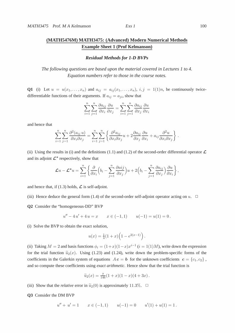
(MATH5476M) MATH3475: (Advanced) Modern Numerical MethodsExample Sheet 1 (Prof Kelmanson)

Residual Methods for 1-D BVPs

The following questions are based upon the material covered in Lectures 1 to 4.

Equation numbers refer to those in the course notes.

Q1 (i) Let u = u(x1, . . . , xn) and aij = aij(x1, . . . , xn), i, j = 1(1)n, be continuously twice-

differentiable functions of their arguments. Ifaij = aji, show that

n∑

i=1

n∑

j=1

∂aij

∂xi

∂u

∂xj

=n∑

i=1

n∑

j=1

∂aij

∂xj

∂u

∂xi

and hence thatn∑

i=1

n∑

j=1

∂2(aij u)

∂xi∂xj

=

n∑

i=1

n∑

j=1

{∂2aij

∂xi∂xj

u+ 2∂aij

∂xj

∂u

∂xi

+ aij

∂2u

∂xi∂xj

}.

(ii) Using the results in (i) and the definitions (1.1) and (1.2) of the second-order differential operatorL

and its adjointL∗ respectively, show that

Lu− L∗u =

n∑

i=1

{∂

∂xi

(bi −

n∑

j=1

∂aij

∂xj

)u+ 2

(bi −

n∑

j=1

∂aij

∂xj

) ∂u∂xi

},

and hence that, if (1.3) holds,L is self-adjoint.

(iii) Hence deduce the general form (1.4) of the second-order self-adjoint operator acting onu. 2

Q2 Consider the “homogeneous-DD” BVP

u′′ − 4u′ + 4u = x x ∈ (−1, 1) u(−1) = u(1) = 0 .

(i) Solve the BVP to obtain the exact solution,

u(x) = 14(1 + x)

(1 − e2(x−1)

).

(ii) TakingM = 2 and basis functionsφi = (1+x)(1−x)xi−1 (i = 1(1)M ), write down the expression

for the trial functionu2(x). Using (1.23) and (1.24), write down the problem-specific forms of the

coefficients in the Galerkin system of equationsA c = b for the unknown coefficientsc = {c1, c2} ,

and so compute these coefficients usingexact arithmetic. Hence show that the trial function is

u2(x) = 7146 (1 + x)(1 − x)(4 + 3x) .

(iii) Show that therelative error in u2(0) is approximately11.3%. 2

Q3 Consider the DM BVP

u′′ + u′ = 1 x ∈ (−1, 1) u(−1) = 0 u′(1) + u(1) = 1 .

MATH3475 Prof. M A Kelmanson Exs 1 101

(i) Show that the exact solution of the BVP is

u(x) = x− 1 + 2e−(x+1) .

(ii) TakingM = 2 and basis functionsφi = (1+x)xi−1 (i = 1(1)M ), write down the expression for the

trial function u2(x). Repeat the procedure ofQ2 (ii) and hence show that in this case the trial function is

u2(x) = 17(1 + x)(3x− 2) .

(iii) Show that the relative error in the natural-BC quantity u′2(1) + u2(1) is approximately28.6%. 2

Q4 This question solves the BVP ofQ3 by the spectral collocated-residual method of§1.2.3.

(i) TakingM = 4 and basis functionsφi = xi−1, follow the procedure of Examples 1.4 and 1.5 in the

notes to show that the first two coefficients in the trial function u4(x) are determined by the BCs as

c1 = 13 (1 − 5c3 − 2c4) and c2 = 1

3 (1 − 2c3 − 5c4) .

(ii) Show that, in the formula (1.32), we presently have

ℓ0 + ℓ1x = 13(1 + x) ψ3(x) = 1

3(3x2 − 2x− 5) ψ4(x) = 13(3x3 − 5x− 2) .

(iii) Show that the pointwise residual,R(u) ≡ u′′ + u′ − 1, gives

R(u4) =(

43 + 2x

)c3 +

(3x2 + 6x− 5

3

)c4 −

23 .

(iv) Collocate the residual at the regularly spaced nodes in(−1, 1) and so show that the equations lead

to c3 = 38 andc4 = −1

8 . Hence show using the results in (i) that the trial function obtained is

u(R)4 (x) = − 5

24 + 724x+ 3

8x2 − 1

8x3 .

(v) Collocate the residual at the Chebyshev nodes in(−1, 1) and so show that the equations lead to

c3 = 2459 andc4 = − 8

59 . Hence show using the results in (i) that the trial function obtained is

u(C)4 (x) = −15

59 + 1759x+ 24

59x2 − 8

59x3 .

(vi) Show, using the exact solution of the BVP (fromQ4) and the results of (iv) and (v), that the relative

errors in the boundary valuesu(R)4 (1) andu(C)

4 (1) are respectively23.2% and12.7% . 2

Hints, comments and quick-check answers to numerical questions

A1 (i) The order of summation does not matter. (iii) Useaij = aji.

A2 (ii) Use∫ 1

−1fodd(x) dx = 0 and

∫ 1

−1feven(x) dx = 2

∫ 1

0feven(x) dx to simplify the calculations.

(iii) The relative error inu3(0) is much smaller, being≈ 0.756%; but hand calculation of the 12 entries

in A andb is tedious.

A3 (ii) u2(x) is quadratic here but was cubic inQ2. (iii) This figure drops rapidly to5.4% and0.75%

for M = 3 andM = 4 respectively. Such relative errors are critically dependent on the particular ODE,

and can be several orders of magnitude larger than this whenp, q, r andf become more complicated.

A4 (ii) Both ψ3 andψ4 satisfyhomogeneous versions of both BCs. (iv) & (v) Use (1.34) to locate the

nodes.

(math5476m) math3475 (advanced) modern numerical …mark/math3475/... · (math5476m) math3475:...

Documents