math 400 equation solving -...
TRANSCRIPT
MATH 400NUMERICAL ANALYSISEQUATION SOLVING
Some equations cannot be solved exactly, but it is possible to approximate theirsolution. A simple example is:
cosx = x
Often when working with equations it is better to put everything on one side:
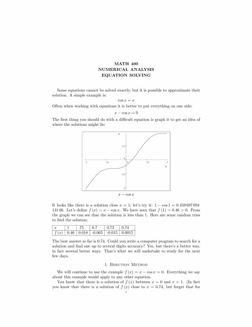
x− cosx = 0The first thing you should do with a difficult equation is graph it to get an idea ofwhere the solutions might lie:
52.50-2.5-5
2.5
0
-2.5
-5
x
y
x
y
x− cosx
It looks like there is a solution close x = 1; let’s try it: 1 − cos 1 = 0.459 697 694131 86. Let’s define f (x) = x − cosx. We have seen that f (1) = 0.46 > 0. Fromthe graph we can see that the solution is less than 1. Here are some random triesto find the solution:
x 1 .75 0.7 0.73 0.74f (x) 0.46 0.018 -0.065 -0.015 0.0015
The best answer so far is 0.74. Could you write a computer program to search for asolution and find one up to several digits accuracy? Yes, but there’s a better way,in fact several better ways. That’s what we will undertake to study for the nextfew days.
1. Bisection Method
We will continue to use the example f (x) = x − cosx = 0. Everything we sayabout this example would apply to any other equation.You know that there is a solution of f (x) between x = 0 and x = 1. (In fact
you know that there is a solution of f (x) close to x = 0.74, but forget that for1
2 MATH 400 NUMERICAL ANALYSIS EQUATION SOLVING
now.) Your goal is to find two numbers a and b very close together that bracketthe solution. That is, you want to find two numbers a and b very close togethersuch that the solution is in the interval [a, b].Here is the important observation, since f is a continuous function it suffices to
find numbers a and b close together such that f (a) and f (b) have different signs;one is positive and one is negative. Equivalently, find a and b close together such
that f (a) f (b) ≤ 0. Then if you take x = a+ b
2as your estimate of the solution to
f (x) = 0, and if r is the true solution, you know that |x− r| < b− a
2.
Here’s an example: for f (x) = x− cosx you know f (0.73) < 0 and f (0.74) > 0(see table above). Thus there is a solution r such that
0.73 < r < 0.74
r ∈ (0.73, 0.74)
Thus:|r − 0.735| < 0.005
x = 0.735 may not be an exact solution, but it is within 0.005 of the exact solution.That’s pretty good information.The bisection method is a regular way of finding numbers a and b as close
together as you want (within the limits of machine accuracy) bracketing the solution
of a given equation f (x) = 0. Once you have a and b you can say thata+ b
2is the
approximate solution to the equation with an error of no more thanb− a
2.
The idea is simple. Let r be the true (unknown) solution. If you have numbersa and b such that a ≤ r ≤ b. you can find new numbers a0 ≤ r ≤ b0 such that
b0 − a0 =b− a
2. Here’s how you do it.
// assume a < b and f(a)f(b) <= 0c = (a + b) / 2if f(a)*f(c) < 0 thena’ = ab’ = c
elsea’ = cb’ = b
endif// now a’ < b’ and f(a’)f(b’) <= 0 and b’-a’ = (b-a)/2
Suppose you want to approximate the solution of an equation f (x) = 0 withina tolerance tol. Start with two numbers a and b bracketing the solution, andbring them closer and closer together, continuing to bracket the solution, untilb− a < tol.
MATH 400 NUMERICAL ANALYSIS EQUATION SOLVING 3
// assume a < b and f(a)f(b) <= 0while b-a > 2*tol doc = (a + b) / 2if f(a)*f(c) < 0 thenb = c
elsea = c
endifendwhile// now a < b and f(a)f(b) <= 0 and b-a <= 2*tol
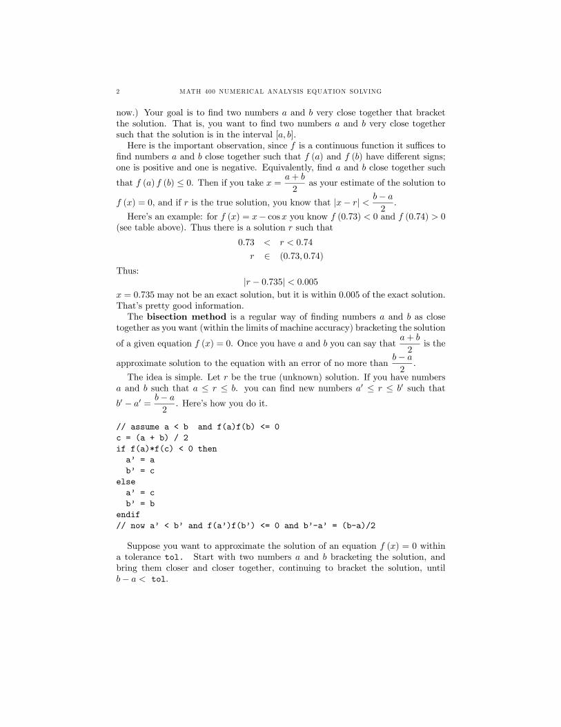
Here’s some sample Mathematica output for the bisection routine. You can seehow you start with the interval [0, 1] and end with [0.739014, 0.739136] bracketing
the solution. The approximate solution is0.739014 + 0.739136
2= 0.739075, and
the maximum error is0.739136− 0.739014
2= 0.000 061
In[28]:= f@x_D := x− Cos@xD;r= bisect@f, 0., 1., 0.0001Df@rD
80.5, 1.<
80.5, 0.75<
80.625, 0.75<
80.6875, 0.75<
80.71875, 0.75<
80.734375, 0.75<
80.734375, 0.742188<
80.738281, 0.742188<
80.738281, 0.740234<
80.738281, 0.739258<
80.73877, 0.739258<
80.739014, 0.739258<
80.739014, 0.739136<
Out[29]= 0.739075
Out[30]= −0.0000174493
4 MATH 400 NUMERICAL ANALYSIS EQUATION SOLVING
Whenever you have a method for solving equations, there are several questionsthat need to be kept in mind, together with their answers for the bisection method:
(1) What kinds of equations is the method good for?(a) f (x) = 0 where f is continuous and the function changes sign around
the solution.(2) What information is needed to start the method?
(a) an interval [a, b] on which f is continuous and where f (a) f (b) ≤ 0(3) Does the method always converge to an approximate solution? If not, how
can we tell if we are converging on an exact solution?(a) The bisection method always converges to an exact solution.
(4) How close is an approximate solution to the exact solution?(a) For the bisection method we always have two numbers, a and b, that
bracket the solution. The error between the approximate solutiona+ b
2and the exact solution is always less than
b− a
2.
(5) How many steps does it take to get an approximate solution within tol ofthe exact solution, and how much work is necessary for each step?(a) the number of steps is the smallest non-negative integer larger than
log2b− a
tol− 1
(b) each step requires two evaluations of f (x) and a few arithmetic op-erations and comparisons (but see below for an algorithm that onlyrequires one evaluation)
(c) In our example: log21− 00.0001
− 1 = 12. 29, so we should have, and do
have, 13 steps.
Here is another version of the algorithm that makes only one function evaluationeach time through the main loop (and possibly one more assignment). Assume youstart with a and b and you have already calculated fa = f (a). This version istwice as fast as the previous version, so it is the one you should always use for thebisection method.
// assume a < b and f(a)f(b) <= 0while b-a > 2*tol doc = (a + b) / 2fc = f(c)if fa*fc < 0 thenb = c
elsea = cfa=fc
endifendwhile// now a < b and f(a)f(b) <= 0 and b-a <= 2*tol
2. Newton-Raphson Method
When you are trying to solve an equation f (x) = 0 and (a) f is differentiableand (b) the derivative of f is not too expensive to compute and (c) you know a

MATH 400 NUMERICAL ANALYSIS EQUATION SOLVING 5
number a not too far from the actual solution, then you can use a method dueinitially to Newton. Even if condition (c) is not satisfied, sometimes you can useNewton’s method to quickly improve the result you get from a slower but morerobust solving method (like bisection).Let’s start from a very general, surprisingly interesting idea (it leads to the whole
discipline of dynamical systems): given a function F (x) and a starting point a1,what happens if you create a sequence:
a1, a2 = F (a1) , a3 = F (a2) , . . . , ai+1 = F (ai) , . . .
Class try on calculators for F (x) = cosx. Start with 1 and just keep pressingthe cosine key. You get a number x = 0.7390 . . . that satisfies cosx = x.Class give examples of sequences that go to infinity or oscillate.In general, if the sequence ai converges to some number a then you have solved
the equation F (a) = a or F (a)− a = 0. The point a is called a fixed point of F .The fixed point of cosx is x = 0.7390...But when does the sequence converge? A sequence is guaranteed to converge
under the following circumstances. Let r be the point of convergence and c =|r − a1|. If |F 0 (x)| < 1 for x ∈ [r − c, r + c], then the sequence stays inside thisinterval and converges to r. Of course, if all you know is F and a1 you cannot usethis test for convergence because you don’t know r. But if |F 0 (x)| < 1 on a largeregion around a1 you have hope that the sequence converges.In the example F (x) = cosx, |F 0 (x)| = |− sinx| < 1 around the starting point
a1 = 1.Let’s examine the sequence 1, cos 1, cos (cos 1) , . . .more closely:
Out[8]= 81., 0.540302, 0.857553, 0.65429, 0.79348, 0.701369,0.76396, 0.722102, 0.750418, 0.731404, 0.744237,0.735605, 0.741425, 0.737507, 0.740147, 0.738369,0.739567, 0.73876, 0.739304, 0.738938, 0.739184,0.739018, 0.73913, 0.739055, 0.739106, 0.739071,0.739094, 0.739079, 0.739089, 0.739082, 0.739087<
I’ve taken these numbes and calculated their differences:
Out[10]= 8−0.459698, 0.317251, −0.203263, 0.139191, −0.0921116,0.0625909, −0.0418573, 0.0283153, −0.0190137,0.0128333, −0.00863261, 0.00582035, −0.0039182,0.00264045, −0.00177813, 0.001198, −0.000806882,0.000543573, −0.000366136, 0.000246643, −0.000166137,0.000111914, −0.0000753858, 0.0000507812,−0.0000342066, 0.0000230421, −0.0000155214,0.0000104554, −7.04288 ×10⁻⁶, 4.74417× 10⁻⁶<
Then I calculated the ratios of the differences:
6 MATH 400 NUMERICAL ANALYSIS EQUATION SOLVING
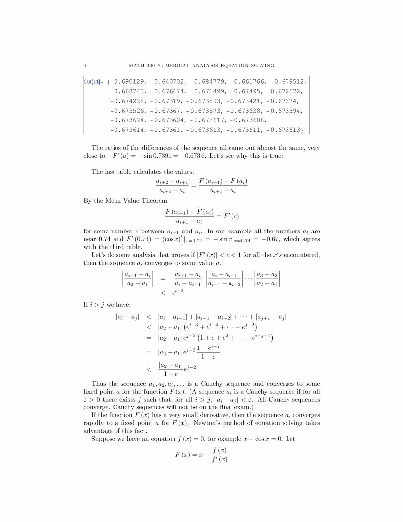
Out[11]= 8−0.690129, −0.640702, −0.684779, −0.661766, −0.679512,−0.668743, −0.676474, −0.671499, −0.67495, −0.672672,−0.674228, −0.67319, −0.673893, −0.673421, −0.67374,−0.673526, −0.67367, −0.673573, −0.673638, −0.673594,−0.673624, −0.673604, −0.673617, −0.673608,−0.673614, −0.67361, −0.673613, −0.673611, −0.673613<
The ratios of the differences of the sequence all came out almost the same, veryclose to −F 0 (a) = − sin 0.7391 = −0.673 6. Let’s see why this is true:
The last table calculates the values:
ai+2 − ai+1ai+1 − ai
=F (ai+1)− F (ai)
ai+1 − ai
By the Mean Value Theorem
F (ai+1)− F (ai)
ai+1 − ai= F 0 (c)
for some number c between ai+1 and ai. In our example all the numbers ai arenear 0.74 and F 0 (0.74) = (cosx)
0 |x=0.74 = − sinx|x=0.74 = −0.67, which agreeswith the third table.Let’s do some analysis that proves if |F 0 (x)| < e < 1 for all the x0s encountered,
then the sequence ai converges to some value a.¯̄̄̄ai+1 − aia2 − a1
¯̄̄̄=
¯̄̄̄ai+1 − aiai − ai−1
¯̄̄̄ ¯̄̄̄ai − ai−1ai−1 − ai−2
¯̄̄̄· · ·¯̄̄̄a3 − a2a2 − a1
¯̄̄̄< ei−2
If i > j we have:
|ai − aj | < |ai − ai−1|+ |ai−1 − ai−2|+ · · ·+ |aj+1 − aj |< |a2 − a1|
¡ei−3 + ei−4 + · · ·+ ej−2
¢= |a2 − a1| ej−2
¡1 + e+ e2 + · · ·+ ei−j−1
¢= |a2 − a1| ej−2
1− ei−j
1− e
<|a2 − a1|1− e
ej−2
Thus the sequence a1, a2, a3, . . . is a Cauchy sequence and converges to somefixed point a for the function F (x). (A sequence ai is a Cauchy sequence if for allε > 0 there exists j such that, for all i > j, |ai − aj | < ε. All Cauchy sequencesconverge. Cauchy sequences will not be on the final exam.)If the function F (x) has a very small derivative, then the sequence ai converges
rapidly to a fixed point a for F (x). Newton’s method of equation solving takesadvantage of this fact.Suppose we have an equation f (x) = 0, for example x− cosx = 0. Let
F (x) = x− f (x)
f 0 (x)
MATH 400 NUMERICAL ANALYSIS EQUATION SOLVING 7
Notice that F (a) = a if and only if f (a) = 0, so if we start with some value a1andthe sequence ai+1 = F (ai) converges to a, then f (a) = 0 and the equation issolved.A solution to f (x) = 0 is a fixed point for F (x). Moreover:
F 0 (x) =f (x) f 00 (x)
[f 0 (x)]2
If a1 is close to a then F 0 (a1) is close to 0 and a1, a2, . . . can be expected to convergerapidly to a (that is, a few terms gives a lot of correct digits for a).Newton’s Method of solving an equation f (x) = 0 consists of taking a first
guess a1 and generating a sequence of (hopefully) improves estimates ai+1 = ai −f (ai)
f 0 (ai)converging to the solution of the equation.
Let’s try it with f (x) = x − cosx. In this case F (x) = x − x− cosx1 + sinx
=
x sinx+ cosx
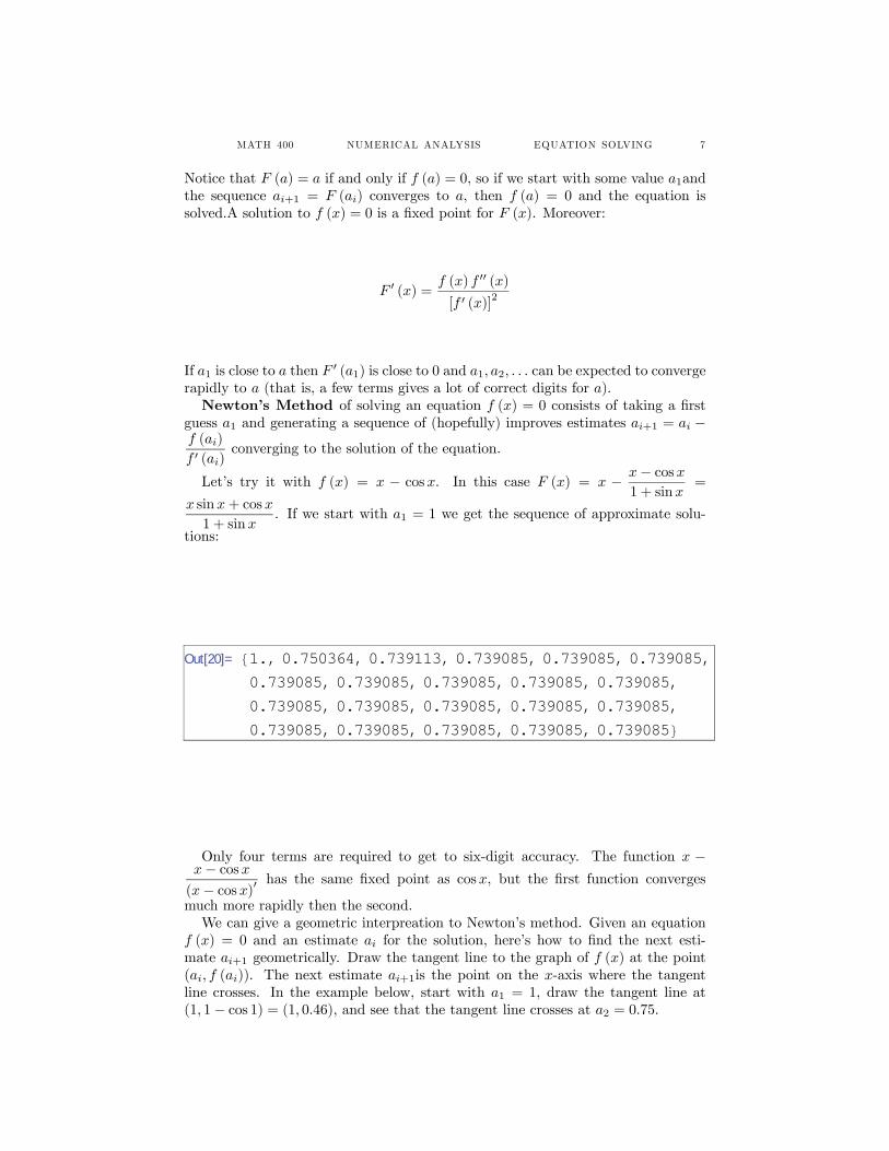
1 + sinx. If we start with a1 = 1 we get the sequence of approximate solu-
tions:
Out[20]= 81., 0.750364, 0.739113, 0.739085, 0.739085, 0.739085,0.739085, 0.739085, 0.739085, 0.739085, 0.739085,0.739085, 0.739085, 0.739085, 0.739085, 0.739085,0.739085, 0.739085, 0.739085, 0.739085, 0.739085<
Only four terms are required to get to six-digit accuracy. The function x −x− cosx(x− cosx)0
has the same fixed point as cosx, but the first function converges
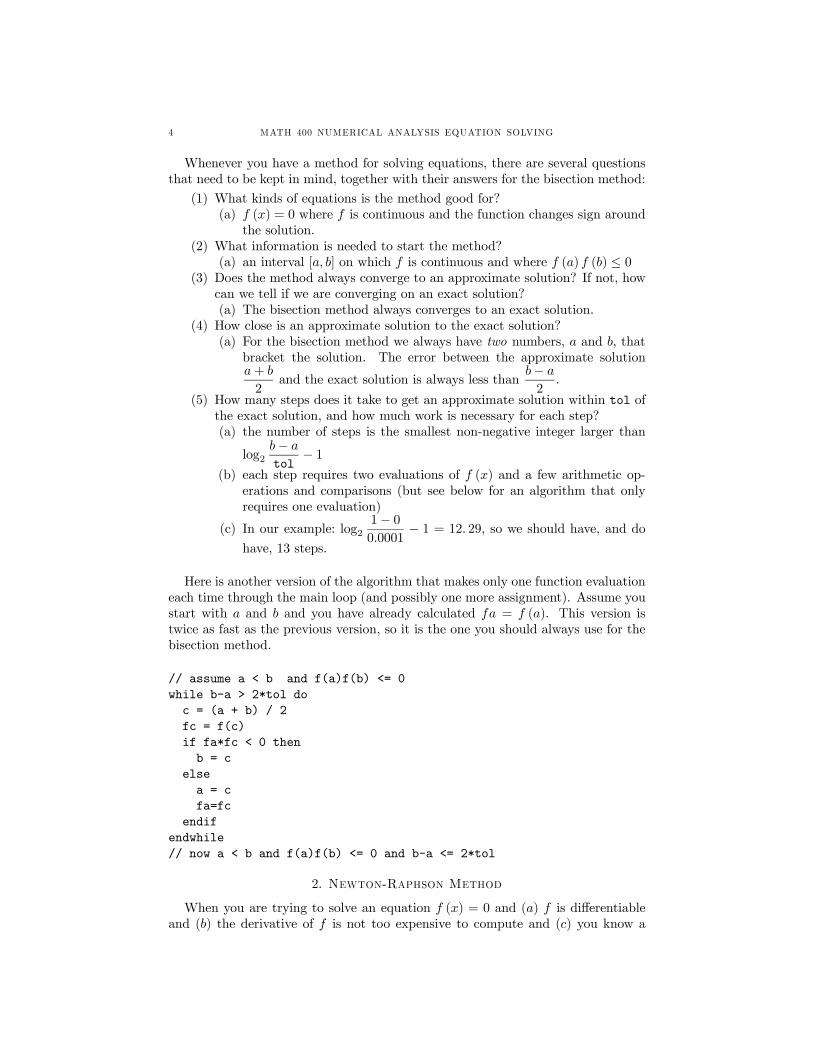
much more rapidly then the second.We can give a geometric interpreation to Newton’s method. Given an equation
f (x) = 0 and an estimate ai for the solution, here’s how to find the next esti-mate ai+1 geometrically. Draw the tangent line to the graph of f (x) at the point(ai, f (ai)). The next estimate ai+1is the point on the x-axis where the tangentline crosses. In the example below, start with a1 = 1, draw the tangent line at(1, 1− cos 1) = (1, 0.46), and see that the tangent line crosses at a2 = 0.75.
8 MATH 400 NUMERICAL ANALYSIS EQUATION SOLVING
1.510.50-0.5
1
0.5
0
-0.5
-1
-1.5
-2
x
y
x
y
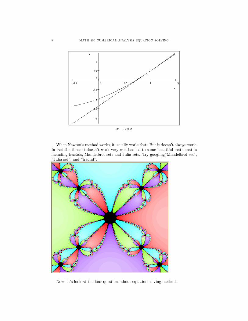
x− cosx
When Newton’s method works, it usually works fast. But it doesn’t always work.In fact the times it doesn’t work very well has led to some beautiful mathematicsincluding fractals, Mandelbrot sets and Julia sets. Try googling“Mandelbrot set”,“Julia set”, and “fractal”.
Now let’s look at the four questions about equation solving methods.
MATH 400 NUMERICAL ANALYSIS EQUATION SOLVING 9
(1) What kinds of equations is the method good for?(a) f (x) = 0 where f is differentiable and f 0 (x) 6= 0 at the point x where
f (x) = 0.(2) What information is needed to start the method?
(a) it is usually a good idea to pick a starting point a not too far from thesolution.
(3) Does the method always converge to an approximate solution? If not, howcan we tell if we are converging on an exact solution?(a) Newton’s method does not always converge to a solution of the equa-
tion. Consider the equation (x− 1)1/3 = 0, whose solution is x = 1.
If f (x) = (x− 1)1/3 then f 0 (x) =1
3 (x− 1)2/3and x − f (x)
f 0 (x)=
x− 3 (x− 1) = 3− 2x. Even if we pick a starting point very close tothe actual solution, Newton’s method diverges. Here are the successivevalues generated by Newton’s method starting at 1.0001. Insteadofgetting closer and closer to the correct solution 1, the approximationsmove away from 1.
Out[35]= 81.0001, 0.9998, 1.0004, 0.9992, 1.0016,0.9968, 1.0064, 0.9872, 1.0256, 0.9488, 1.1024,0.7952, 1.4096, 0.1808, 2.6384, −2.2768,7.5536, −12.1072, 27.2144, −51.4288, 105.858<
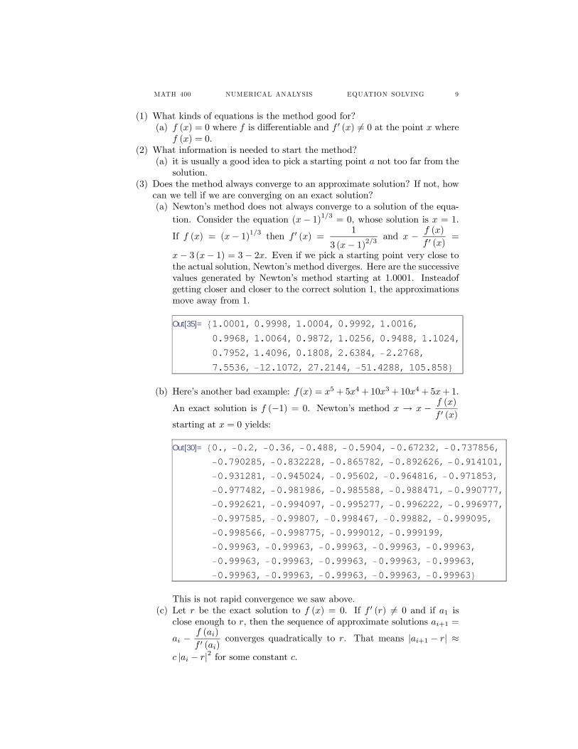
(b) Here’s another bad example: f(x) = x5 +5x4 +10x3 +10x4 +5x+1.
An exact solution is f (−1) = 0. Newton’s method x → x − f (x)
f 0 (x)starting at x = 0 yields:
Out[30]= 80., −0.2, −0.36, −0.488, −0.5904, −0.67232, −0.737856,−0.790285, −0.832228, −0.865782, −0.892626, −0.914101,−0.931281, −0.945024, −0.95602, −0.964816, −0.971853,−0.977482, −0.981986, −0.985588, −0.988471, −0.990777,−0.992621, −0.994097, −0.995277, −0.996222, −0.996977,−0.997585, −0.99807, −0.998467, −0.99882, −0.999095,−0.998566, −0.998775, −0.999012, −0.999199,−0.99963, −0.99963, −0.99963, −0.99963, −0.99963,−0.99963, −0.99963, −0.99963, −0.99963, −0.99963,−0.99963, −0.99963, −0.99963, −0.99963, −0.99963<
This is not rapid convergence we saw above.(c) Let r be the exact solution to f (x) = 0. If f 0 (r) 6= 0 and if a1 is
close enough to r, then the sequence of approximate solutions ai+1 =
ai −f (ai)
f 0 (ai)converges quadratically to r. That means |ai+1 − r| ≈
c |ai − r|2 for some constant c.
10 MATH 400 NUMERICAL ANALYSIS EQUATION SOLVING
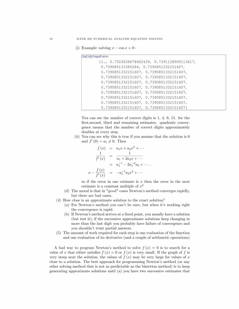
(i) Example: solving x− cosx = 0 :
Out[14]//InputForm=
{1., 0.7503638678402439, 0.7391128909113617, 0.739085133385284, 0.7390851332151607, 0.7390851332151607, 0.7390851332151607, 0.7390851332151607, 0.7390851332151607, 0.7390851332151607, 0.7390851332151607, 0.7390851332151607, 0.7390851332151607, 0.7390851332151607, 0.7390851332151607, 0.7390851332151607, 0.7390851332151607, 0.7390851332151607, 0.7390851332151607, 0.7390851332151607, 0.7390851332151607}
You can see the number of correct digits is 1, 4, 9, 15. for thefirst,second, third and remaining estimates. quadratic conver-gence means that the number of correct digits approximatelydoubles at every step.
(ii) You can see why this is true if you assume that the solution is 0and f 0 (0) = a1 6= 0. Then
f (x) = a1x+ a2x2 + · · ·
1
f 0 (x)=
1
a1 + 2a2x+ · · ·= a−11 − 2a−21 a2 + · · · .
x− f (x)
f 0 (x)= −a−11 a2x
2 + · · ·
so if the error in one estimate is x then the error in the nextestimate is a constant multiple of x2
(d) The moral is that in "good" cases Newton’s method converges rapidly,but there are bad cases.
(4) How close is an approximate solution to the exact solution?(a) For Newton’s method you can’t be sure, but when it’s working right
the convergence is rapid.(b) If Newton’s method arrives at a fixed point, you usually have a solution
(but test it); if the successive approximate solutions keep changing inmore than the last digit you probably have failure of convergence andyou shouldn’t trust partial answers.
(5) The amount of work required for each step is one evaluation of the functionand one evaluation of its derivative (and a couple of arithmetic operations)
A bad way to program Newton’s method to solve f (x) = 0 is to search for avalue of x that either satisfies f (x) = 0 or f (x) is very small. If the graph of f isvery steep near the solution, the values of f (x) may be very large for values of xclose to a solution. The best approach for programming Newton’s method (or anyother solving method that is not as predictable as the bisection method) is to keepgenerating approximate solutions until (a) you have two successive estimates that
MATH 400 NUMERICAL ANALYSIS EQUATION SOLVING 11
are almost the same; or (b) you have exceeded some fixed number of estimates andyou decide the method isn’t converging. For example, to solve f (x) = 0:
// Assume a function f(x) and its derivative df(x)n = 0next_guess = your_first_guessRepeatlast_guess = next_guessnext_guess = last_guess-f(last_guess)/df(last_guess)n = n+1
Until n > some_big_number orabs(next_guess-last_guess) < 1e-15*max(1,abs(next_guess))
Return(next_guess)
3. Secant Method
Sometimes you may have an equation f (x) = 0, and you may not want to useNewton’s method because either you cannot differentiate f (x) or the derivativeis difficult or time-consuming to evaluate accurately. In that case you can usethe secant method, which is just Newton’s method with a twist. The twistis that instead of using the derivative f 0 (x) you use the approximate derivativef (x2)− f (x1)
x2 − x1. More specifically, instead of starting with one point, like Newton’s
method, you start the secand method with two points, call them x1 and x2.Thenyou define a sequence:
xi+1 = xi −f (xi)
f (xi)− f (xi−1)
xi − xi−1
= xi −(xi − xi−1) f (xi)
f (xi)− f (xi−1)
It would appear that you could simplify this further toxi−1f (xi)− xif (xi−1)
f (xi)− f (xi−1);
however this version is prone to errors of destructive subtraction near the end ofconvergence when xi ≈ xi−1, so the last displayed version is better to use.From a geometric point of view, xi+1 is the place where the x-axis meets the line
through the points (xi−1f (xi−1)) and (xi, f (xi)). Because this intersection point
with the secant line is likely to be closer to a solution the the midpointxi + xi−1
2,
the secand method usually converges faster than the midpoint method.Ideally the points you start with, x1and x2,should be close to a solution. The
method does not converge quite as rapidly as Newton’s method, but it may requireless calculation per step (when f 0 (x) is expensive to compute).Let’s do the same example as we did with the other solution methods: x−cosx =
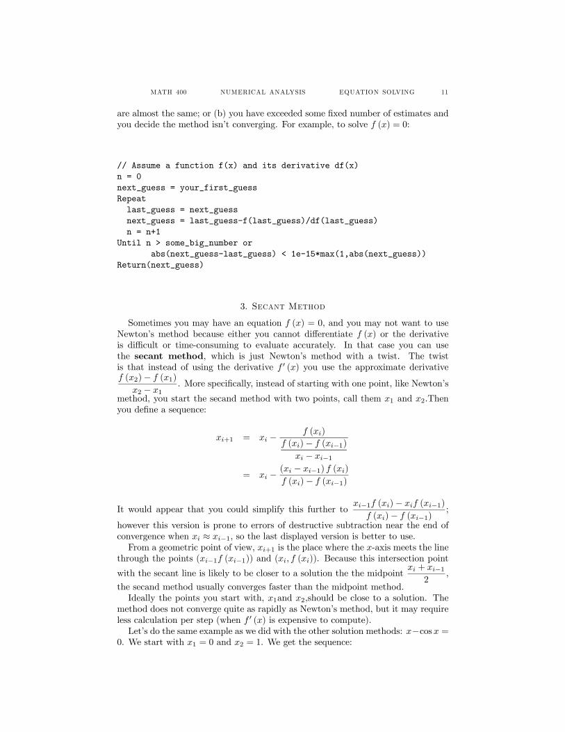
0. We start with x1 = 0 and x2 = 1. We get the sequence:
12 MATH 400 NUMERICAL ANALYSIS EQUATION SOLVING
{0., 1., 0.6850733573260451, 0.736298997613654, 0.7391193619116293, 0.7390851121274639, 0.7390851332150012, 0.7390851332151607, 0.7390851332151607}
Convergence of the secant mathod required seven steps instead of the four re-quired for Newton’s method, but the same answer was achieved. Here’s the code Iused. Note the efficiency that reduces to one function evaluation of f (x) per cyclethrough the Repeat..Until loop.
// Assume a function f(x)n = 0last_guess = your_first_guessnext_guess = your_second_guessf_last_guess = f(last_guess)f_next_guess = f(next_guess)Repeatprevious_guess = last_guessf_previous_guess = f_last_guesslast_guess = next_guessf_last_guess = f_next_guessnext_guess= last_guess-(last_guess-previous_guess)*f_last_guess
/(f_last_guess-f_previous_guess)f_next_guess = f(next_guess)n = n+1
Until n > some_big_number orabs(next_guess-last_guess) < 1e-15*max(1,abs(next_guess))
Return(next_guess)
Now let’s answer the five questions for the secant method:
(1) What kinds of equations is the method good for?(a) f (x) = 0 where f is continuous.
(2) What information is needed to start the method?(a) it is usually a good idea to pick a starting points x1 and x2 not too
far from the solution.(3) Does the method always converge to an approximate solution? If not, how
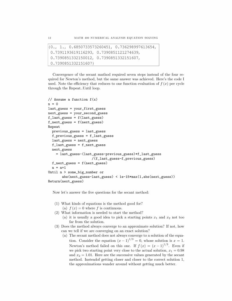
can we tell if we are converging on an exact solution?(a) The secant method does not always converge to a solution of the equa-
tion. Consider the equation (x− 1)1/3 = 0, whose solution is x = 1.Newton’s method failed on this one. If f (x) = (x− 1)1/3. Even ifwe pick two starting point very close to the actual solution, x1 = 0.98and x2 = 1.01. Here are the successive values generated by the secantmethod. Insteadof getting closer and closer to the correct solution 1,the approximations wander around without getting much better.
MATH 400 NUMERICAL ANALYSIS EQUATION SOLVING 13
Out[37]//InputForm=
{0.98, 1.01, 0.9967251999792668, 1.0021417353168995, 0.9996248215803948, 1.0005278436924738, 1.000050669459455, 0.9996476513451229, 0.9999121142941335, 1.000361412779169, 1.0000847806033957, 0.9996396374457038, 0.9999148704191396, 1.0003604786830136, 1.000085090857832, 0.9996395342270821, 0.999914904838969, 1.0003604672072877, 1.0000850946829056, 0.9996395329520879, 0.9999149052639692, 1.0003604670656205, 1.000085094730128, 0.9996395329363469, 0.9999149052692161, 1.0003604670638717, 1.000085094730711, 0.9996395329361527, 0.9999149052692808, 1.0003604670638502, 1.0000850947307183, 0.99963953293615}
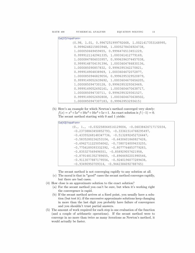
(b) Here’s an example for which Newton’s method converged very slowly:f(x) = x5+5x4+10x3+10x4+5x+1. An exact solution is f (−1) = 0.The secant method starting with 0 and 1 yields:
Out[43]//InputForm=
{0., 1., -0.032258064516129004, -0.06038426717172034, -0.23738863450852793, -0.33361514768295497, -0.43355268148347736, -0.5132892452726447, -0.5835280236253104, -0.6430601860827428, -0.6942711225056062, -0.7380724009433255, -0.7756189393332392, -0.8077764853779283, -0.835327569496551, -0.858929057621958, -0.8791481352789655, -0.8964692201990546, -0.9113077887179556, -0.9240196077289438, -0.93490950709314, -0.9442386092788765}
The secant method is not converging rapidly to any solution at all.(c) The moral is that in "good" cases the secant method converges rapidly,
but there are bad cases.(4) How close is an approximate solution to the exact solution?
(a) For the secant method you can’t be sure, but when it’s working rightthe convergence is rapid.
(b) If the secant method arrives at a fixed point, you usually have a solu-tion (but test it); if the successive approximate solutions keep changingin more than the last digit you probably have failure of convergenceand you shouldn’t trust partial answers.
(5) The amount of work required for each step is one evaluation of the function(and a couple of arithmetic operations). If the secant method were toconverge in no more than twice as many iterations as Newton’s method, itwould actually be faster.
14 MATH 400 NUMERICAL ANALYSIS EQUATION SOLVING
4. Homework due April 11
Let f (x) = x5 + 1000x4 + x3 + x2 + x+ 1.(1) Show that f (0) > 0.(2) Find a number a such that f (a) < 0. (Hint: why does a have to be
negative?)(3) Conclude that there is at least one solution to f (x) = 0 between a and 0.(4) Write code for the bisection method, Newton’s method and the secant
method to find the solution of f (x) = 0.(5) For your three solutions (one for each method), find the value of f (x).(6) For your three solutions, estimate the distance to the true solution. (You
may NOT use equation-solving software from Mathematica or other soft-ware packages. Create your own estimates.)
5. Regula Falsi or False Position Method
The method of false position combines the secant and bisection method. It isvery old, as shown by its Latin name. Like the bisection method, false positionstarts with two points a and b that bracket a solution of your equation f (x) = 0.That is, we start with two points a and b such that f (a) f (b) ≤ 0. The nextestimate for the root, c, is calculated exactly like the secant method:
c = b− (b− a) f (b)
f (b)− f (a)
The next step is like the bisection method. Decide which interval, (a, c) or (c, b),contains the solution to the equation and use those endpoints for the next step.Unlike the bisection method, you cannot be sure that the new interval is much
smaller than the original interval (a, b), so the criterion for stopping the algorithmwill be more like the criterion used in the secant method: you stop when the newestimates stop changing significantly. Here’s the entire algorithm in pseudo-code:
MATH 400 NUMERICAL ANALYSIS EQUATION SOLVING 15
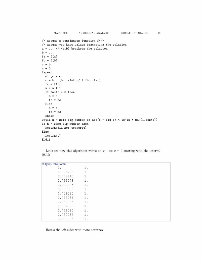
// assume a continuous function f(x)// assume you know values bracketing the solutiona = ... // (a,b) brackets the solutionb = ...fa = f(a)fb = f(b)c = bn = 0Repeatold_c = cc = b - (b - a)*fb / ( fb - fa )fc = f(c)n = n + 1If fa*fc < 0 thenb = cfb = fc
Elsea = cfa = fc
EndifUntil n > some_big_number or abs(c - old_c) < 1e-15 * max(1,abs(c))If n > some_big_number thenreturn(did not converge)
Elsereturn(c)
Endif
Let’s see how this algorithm works on x − cosx = 0 starting with the interval(0, 1):
Out[16]//TableForm=0. 1.0.736299 1.0.738945 1.0.739078 1.0.739085 1.0.739085 1.0.739085 1.0.739085 1.0.739085 1.0.739085 1.0.739085 1.0.739085 1.0.739085 1.
Here’s the left sides with more accuracy:
16 MATH 400 NUMERICAL ANALYSIS EQUATION SOLVING
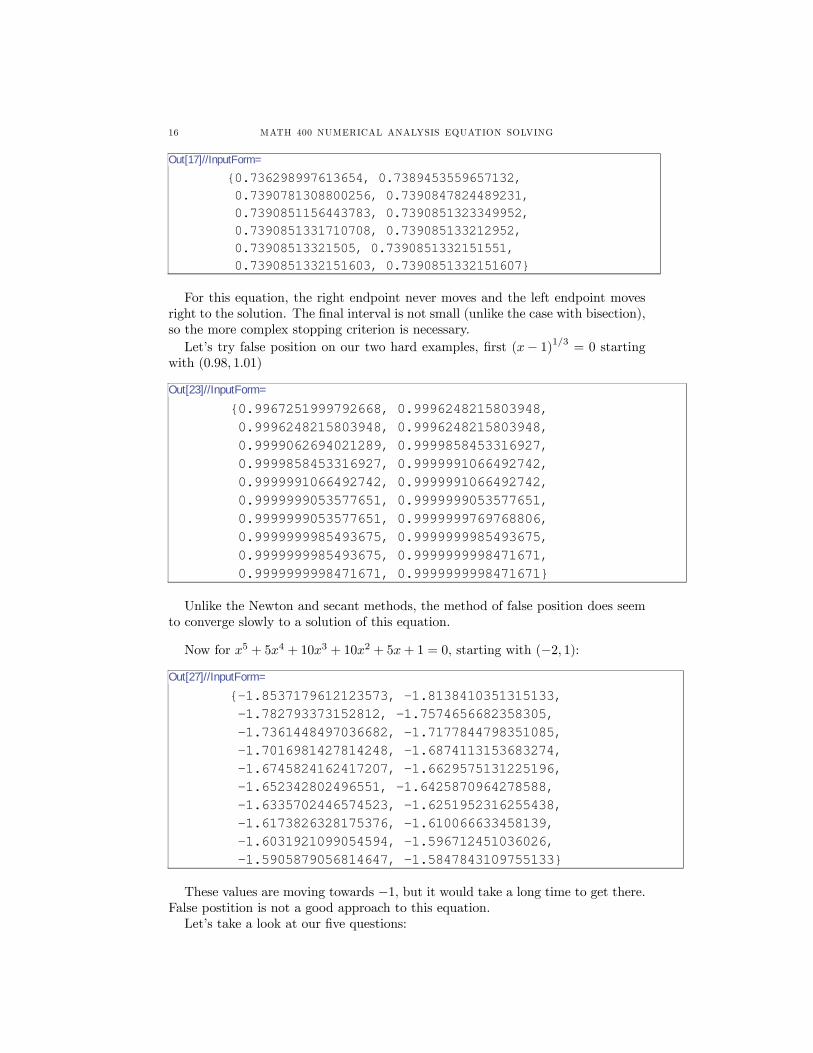
Out[17]//InputForm=
{0.736298997613654, 0.7389453559657132, 0.7390781308800256, 0.7390847824489231, 0.7390851156443783, 0.7390851323349952, 0.7390851331710708, 0.739085133212952, 0.73908513321505, 0.7390851332151551, 0.7390851332151603, 0.7390851332151607}
For this equation, the right endpoint never moves and the left endpoint movesright to the solution. The final interval is not small (unlike the case with bisection),so the more complex stopping criterion is necessary.Let’s try false position on our two hard examples, first (x− 1)1/3 = 0 starting
with (0.98, 1.01)
Out[23]//InputForm=
{0.9967251999792668, 0.9996248215803948, 0.9996248215803948, 0.9996248215803948, 0.9999062694021289, 0.9999858453316927, 0.9999858453316927, 0.9999991066492742, 0.9999991066492742, 0.9999991066492742, 0.9999999053577651, 0.9999999053577651, 0.9999999053577651, 0.9999999769768806, 0.9999999985493675, 0.9999999985493675, 0.9999999985493675, 0.9999999998471671, 0.9999999998471671, 0.9999999998471671}
Unlike the Newton and secant methods, the method of false position does seemto converge slowly to a solution of this equation.
Now for x5 + 5x4 + 10x3 + 10x2 + 5x+ 1 = 0, starting with (−2, 1):
Out[27]//InputForm=
{-1.8537179612123573, -1.8138410351315133, -1.782793373152812, -1.7574656682358305, -1.7361448497036682, -1.7177844798351085, -1.7016981427814248, -1.6874113153683274, -1.6745824162417207, -1.6629575131225196, -1.652342802496551, -1.6425870964278588, -1.6335702446574523, -1.6251952316255438, -1.6173826328175376, -1.610066633458139, -1.6031921099054594, -1.596712451036026, -1.5905879056814647, -1.5847843109755133}
These values are moving towards −1, but it would take a long time to get there.False postition is not a good approach to this equation.Let’s take a look at our five questions:
MATH 400 NUMERICAL ANALYSIS EQUATION SOLVING 17
(1) What kinds of equations is the method good for?(a) f (x) = 0 where f is continuous and the function changes sign around
the solution.(2) What information is needed to start the method?
(a) numbers a and b bracketing the root: f (a) f (b) ≤ 0.(3) Does the method always converge to an approximate solution? If not, how
can we tell if we are converging on an exact solution?(a) The method of false position always keeps the root bracketed but may
not converge in a reasonable number of iterations to the root.(4) How close is an approximate solution to the exact solution?
(a) You cannot be sure because the changing interval (a, b) may not getsmall even though one end converges rapidly to a solution. As withNewton and secant, the best criterion is that the estimate c does notchange significantly from one iteration to the next.
(5) The amount of work required for each step is one evaluation of the function(and a couple of arithmetic operations).
6. Laguerre’s Method
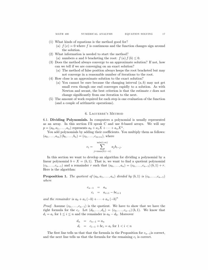
6.1. Dividing Polynomials. In computers a polynomial is usually representedas an array. In this section I’ll speak C and use 0-based arrays. We will sayp = (a0, a1, . . . , an) represents a0 + a1X + · · ·+ anX
n.You add polynomials by adding their coefficients. You multiply them as follows:
(a0, . . . , am) (b0, . . . , bn) = (c0, . . . , cm+n), where
ci =
min(i,m)Xj=max(0,i−n)
ajbi−j .
In this section we want to develop an algorithm for dividing a polynomial by alinear polynomial b +X = (b, 1). That is, we want to find a quotient polynomial(c0, . . . , cn−1) and a remainder r such that (a0, . . . , an) = (c0, . . . , cn−1) (b, 1) + r.Here is the algorithm:
Proposition 1. The quotient of (a0, a1, . . . , an) divided by (b, 1) is (c0, . . . , cn−1)where
cn−1 = an
ci = ai+1 − bci+1
and the remainder is a0 + a1 (−b) + · · ·+ an (−b)n
Proof. Assume (c0, . . . , cn−1) is the quotient. We have to show that we have theright formula for the ci. Let (d0, . . . , dn) = (c0, . . . , cn−1) (b, 1). We know thatdi = ai for 1 ≤ i ≤ n and the remainder is a0 − d0. Moreover
dn = cn−1 = an
di = ci−1 + bci = ai for 1 < i < n
The first line tells us that that the formula in the Proposition for cn−1is correct,and the next line tells us that the formula for the remaining ci is correct.
18 MATH 400 NUMERICAL ANALYSIS EQUATION SOLVING
The formula for the remainder is classical. If X + b divides a polynomial p (X)with quotient q (X) and remainder r (which must be a constant), then
p (X) = q (X) (X + b) + r
p (−b) = q (−b) (0) + r
= r
¤
6.2. How to find all the roots of a polynomial. To find the roots of a polyno-
mial p (X), find one root r and let q (X) =p (X)
X − r(since r is a root, X − r divides
p (X) exactly). Then find all the roots of q (X). This process is called “deflation”;the idea is to reduce finding all the roots of a degree n polynomial to finding oneroot, then finding all the roots of a degree n − 1 polynomial. Of course next youwill find one root of q (X), deflate again, find a root of the quotient, deflate again,find a root of the next quotient, etc., until all the roots are found.
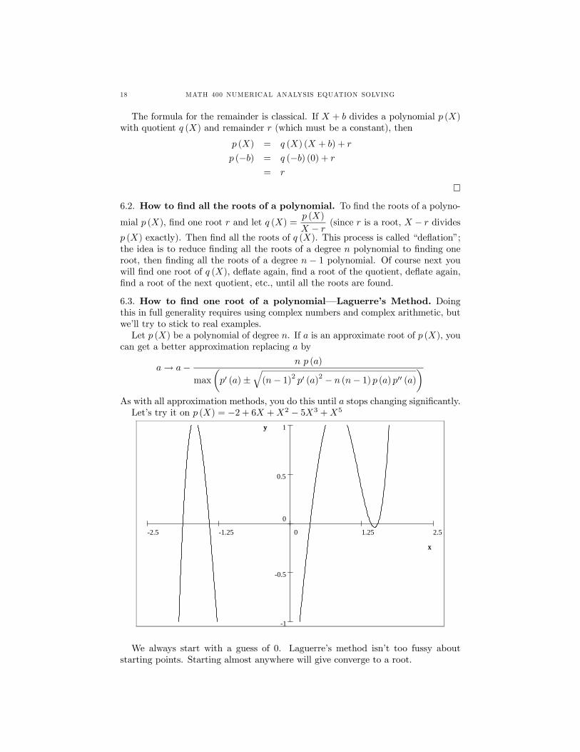
6.3. How to find one root of a polynomial–Laguerre’s Method. Doingthis in full generality requires using complex numbers and complex arithmetic, butwe’ll try to stick to real examples.Let p (X) be a polynomial of degree n. If a is an approximate root of p (X), you
can get a better approximation replacing a by
a→ a− n p (a)
max
µp0 (a)±
q(n− 1)2 p0 (a)2 − n (n− 1) p (a) p00 (a)
¶As with all approximation methods, you do this until a stops changing significantly.Let’s try it on p (X) = −2 + 6X +X2 − 5X3 +X5
2.51.250-1.25-2.5
1
0.5
0
-0.5
-1
x
y
x
y
We always start with a guess of 0. Laguerre’s method isn’t too fussy aboutstarting points. Starting almost anywhere will give converge to a root.
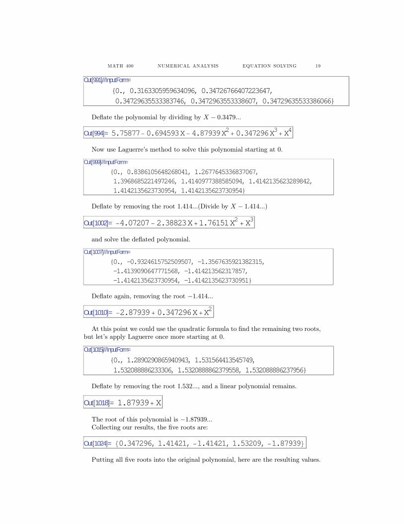
MATH 400 NUMERICAL ANALYSIS EQUATION SOLVING 19
Out[991]//InputForm=
{0., 0.3163305959634096, 0.34726766407223647, 0.34729635533383746, 0.3472963553338607, 0.34729635533386066}
Deflate the polynomial by dividing by X − 0.3479...
Out[994]= 5.75877−0.694593X−4.87939X2+0.347296X3+X4
Now use Laguerre’s method to solve this polynomial starting at 0.
Out[999]//InputForm=
{0., 0.8386105648268041, 1.2677645336837067, 1.3968685221497246, 1.4140977388585094, 1.4142135623289842, 1.4142135623730954, 1.4142135623730954}
Deflate by removing the root 1.414...(Divide by X − 1.414...)
Out[1002]= −4.07207−2.38823X+1.76151X2+X3
and solve the deflated polynomial.
Out[1007]//InputForm=
{0., -0.9324615752509507, -1.3567635921382315, -1.4139090647771568, -1.414213562317857, -1.4142135623730954, -1.4142135623730951}
Deflate again, removing the root −1.414...
Out[1010]= −2.87939+0.347296X+X2
At this point we could use the quadratic formula to find the remaining two roots,but let’s apply Laguerre once more starting at 0.
Out[1015]//InputForm=
{0., 1.2890290865940943, 1.531564413545749, 1.532088886233306, 1.5320888862379558, 1.532088886237956}
Deflate by removing the root 1.532..., and a linear polynomial remains.
Out[1018]= 1.87939+X
The root of this polynomial is −1.87939...Collecting our results, the five roots are:
Out[1024]= 80.347296,1.41421, −1.41421,1.53209, −1.87939<
Putting all five roots into the original polynomial, here are the resulting values.
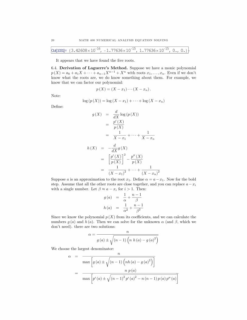
20 MATH 400 NUMERICAL ANALYSIS EQUATION SOLVING
Out[1031]= 83.42608×10⁻¹⁶, −1.77636×10−15,1.77636×10−15,0.,0.< ’It appears that we have found the five roots.
6.4. Derivation of Laguerre’s Method. Suppose we have a monic polynomialp (X) = a0 + a1X + · · ·+ an−1X
n−1 +Xn with roots x1, . . . , xn. Even if we don’tknow what the roots are, we do know something about them. For example, weknow that we can factor our polynomial:
p (X) = (X − x1) · · · (X − xn) .
Note:log (p (X)) = log (X − x1) + · · ·+ log (X − xn)
Define:
g (X) =d
dXlog (p (X))
=p0 (X)
p (X)
=1
X − x1+ · · ·+ 1
X − xn
h (X) = − d
dXg (X)
=
∙p0 (X)
p (X)
¸2− p00 (X)
p (X)
=1
(X − x1)2 + · · ·+
1
(X − xn)2
Suppose a is an approximation to the root x1. Define α = a−x1. Now for the boldstep. Assume that all the other roots are close together, and you can replace a−xiwith a single number. Let β ≈ a− xi for i > 1. Then:
g (a) =1
α+
n− 1β
h (a) =1
α2+
n− 1β2
Since we know the polynomial p (X) from its coefficients, and we can calculate thenumbers g (a) and h (a). Then we can solve for the unknown α (and β, which wedon’t need). there are two solutions:
α =n
g (a)±r(n− 1)
³n h (a)− g (a)2
´We choose the largest denominator:
α =n
max
∙g (a)±
r(n− 1)
³nh (a)− g (a)2
´¸=
n p (a)
max
∙p0 (a)±
q(n− 1)2 p0 (a)2 − n (n− 1) p (a) p00 (a)
¸
MATH 400 NUMERICAL ANALYSIS EQUATION SOLVING 21
Of course everything here is an approximation, but we can expect that a− α isa better approximation of x1 than a alone. So if a is our first guess at a root ofp (X), the next guess will be:
a→ a− n p (a)
max
∙p0 (a)±
q(n− 1)2 p0 (a)2 − n (n− 1) p (a) p00 (a)
¸
Finally, let’s see how Laguerre’s method does with our five questions.
(1) What kinds of equations is the method good for?(a) polynomial equations
(2) What information is needed to start the method?(a) any number, but it’s hard to guess which root will be found
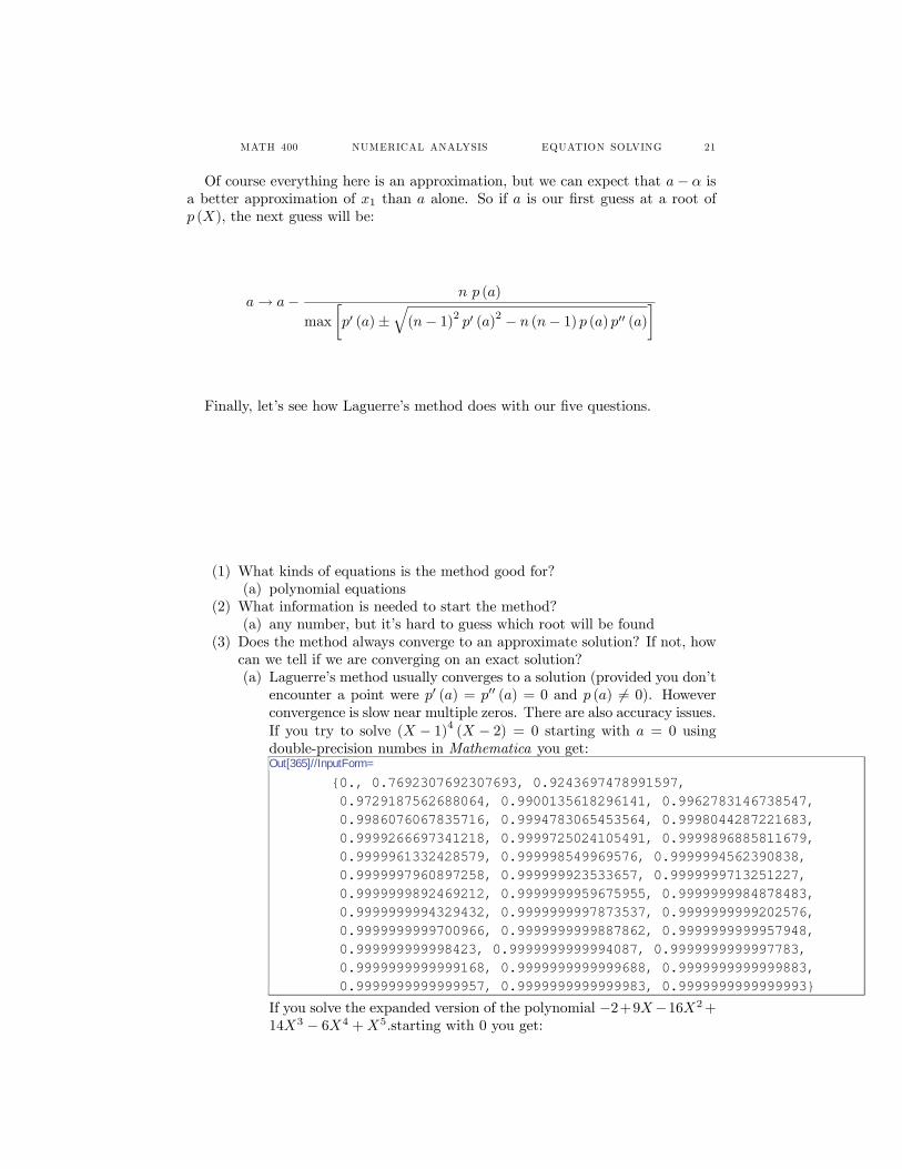
(3) Does the method always converge to an approximate solution? If not, howcan we tell if we are converging on an exact solution?(a) Laguerre’s method usually converges to a solution (provided you don’t
encounter a point were p0 (a) = p00 (a) = 0 and p (a) 6= 0). Howeverconvergence is slow near multiple zeros. There are also accuracy issues.If you try to solve (X − 1)4 (X − 2) = 0 starting with a = 0 usingdouble-precision numbes in Mathematica you get:Out[365]//InputForm=
{0., 0.7692307692307693, 0.9243697478991597, 0.9729187562688064, 0.9900135618296141, 0.9962783146738547, 0.9986076067835716, 0.9994783065453564, 0.9998044287221683, 0.9999266697341218, 0.9999725024105491, 0.9999896885811679, 0.9999961332428579, 0.999998549969576, 0.9999994562390838, 0.9999997960897258, 0.999999923533657, 0.9999999713251227, 0.9999999892469212, 0.9999999959675955, 0.9999999984878483, 0.9999999994329432, 0.9999999997873537, 0.9999999999202576, 0.9999999999700966, 0.9999999999887862, 0.9999999999957948, 0.999999999998423, 0.9999999999994087, 0.9999999999997783, 0.9999999999999168, 0.9999999999999688, 0.9999999999999883, 0.9999999999999957, 0.9999999999999983, 0.9999999999999993}
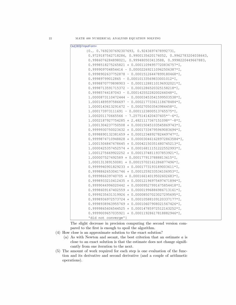
If you solve the expanded version of the polynomial −2+9X−16X2+14X3 − 6X4 +X5.starting with 0 you get:
22 MATH 400 NUMERICAL ANALYSIS EQUATION SOLVING
Out[383]//InputForm=
{0., 0.7692307692307693, 0.9243697478992731, 0.9729187562718286, 0.9900135620176052, 0.9962783204038643, 0.9986076284898021, 0.999480503413588, 0.9998220449667883, 0.9998518275265821 + 0.00011094957720836757*I, 0.999909704854416 - 0.000022692110962506387*I, 0.9998902637752878 - 0.00015126447899180468*I, 0.99989799012865 - 0.00010133569833001012*I, 0.9998870779898903 - 0.00011288110196932021*I, 0.9998713591715372 - 0.0001286520325158218*I, 0.99985744187043 - 0.00014255228200266048*I, 1.0000873110472444 - 0.00003453541599503538*I, 1.0001489597586697 - 0.00021773361118678484*I, 1.0000143613291672 - 0.000270503543984458*I, 1.000173973111691 - 0.0001123800513765575*I, 1.000201170665566 - 7.2575141420437605*^-6*I, 1.0002187927754285 + 2.4821117367151098*^-8*I, 1.0001304237750508 + 0.00015045103545869743*I, 0.9999930750023632 + 0.00017334795969083694*I, 0.9998890132381659 + 0.0001234892782449747*I, 0.9999874710948828 + 0.000030461628972863584*I, 1.0001506847678645 + 0.00042150351680745213*I, 1.0000425357452574 + 0.00016811151222552993*I, 1.0001275669922252 + 0.0001374811937853921*I, 1.000007527492589 + 0.0001779137888813615*I, 1.000131389150081 + 0.00015702161286877496*I, 0.9999940901829233 + 0.0001773193189003611*I, 0.9998862653041746 + 0.0001259233534106953*I, 0.999986639740705 + 0.00016614019502602683*I, 0.9998933210412435 + 0.00012196975497471894*I, 0.9999044996020442 + 0.00009527991675854418*I, 0.9998609167402559 + 0.00001996886986713161*I, 0.9999235631319926 + 0.00008507023027295695*I, 0.9998936972573724 + 0.00010588109120337177*I, 0.9998938963955769 + 0.00010607908021567426*I, 0.9999865606544525 + 0.00014785972512163252*I, 0.9999009657035921 + 0.00011928617818882946*I, "did not converge"}
The slight decrease in precision computing the second version com-pared to the first is enough to spoil the algorithm.
(4) How close is an approximate solution to the exact solution?(a) As with Newton and secant, the best criterion that an estimate a is
close to an exact solution is that the estimate does not change signifi-cantly from one iteration to the next.
(5) The amount of work required for each step is one evaluation of the func-tion and its derivative and second derivative (and a couple of arithmeticoperations).
MATH 400 NUMERICAL ANALYSIS EQUATION SOLVING 23
7. Homework Due Monday 4/18
(1) Use the method of false position to find a root of x5 + 1000x4 + x3 + x2 +x+ 1 = 0
(2) Write programs to (a) implement polynomial division; and (b) implementLaguerre’s method, and use them to find all the roots of x5− 9x4+17x3+29x2 − 60x− 50 = 0.