math 3968 - differential geometry - tullotullo.ch/static/math3968lecturenotes.pdf · math 3968 -...

MATH 3968 - DIFFERENTIAL GEOMETRY

ANDREW TULLOCH

Contents

1. Curves in RN 22. General Analysis 23. Surfaces in R3 33.1. The Gauss Bonnet Theorem 84. Abstract Manifolds 9

1

MATH 3968 - DIFFERENTIAL GEOMETRY 2

1. Curves in RN

Definition 1.1. A curve is said to be regular if α′(t) ̸= 0 for all t

Definition 1.2. Let α be a curve parametrized by arc length. The number |α′′(s)| = k(s) is calledthe curvature of α at s.

Definition 1.3 (Frenet equations).

t′ = kn

n′ = −kt+ τb

b′ = −τn

Definition 1.4. Total curvature of a unit speed curve α(s) from a to b is defined as∫ b

a

kds = θ(b)− θ(a)

Definition 1.5. The winding number k is defined as the integer such that, for a closed curve, thetotal curvature ∫ b

a

kds = 2πk

Theorem 1.6 (Rotation Theorem). For a piecewise smooth simple closed curve, traversed in ananti-clockwise direction around a bounded region of the plane, the winding number is 1

2. General Analysis

Definition 2.1 (Homeomorphism). A map is a homeomorphism is it is continuous and has acontinuous inverse.

Definition 2.2 (Diffeomorphism). A map is a diffeomorphism is it is smooth and has a smoothinverse

Definition 2.3 (Differential of a smooth map). The differential of a smooth map φ : RN → RM isdefined as follows. Let w ∈ RM , and let α be a differentiable curve such that α(0) = p, α′(0) = w.Then the composition β = φ ◦ α is differentiable, and we have

dφp(w) = β′(0) = (φ ◦ α)′(0)

Theorem 2.4 (Inverse function theorem). Let ϕ : U ⊂ RN → RM be a differentiable mapping andsuppose that the differential dϕ is an isomorphism at p ∈ U . Then there exists a neighbourhoodV ⊂ U and a neighbourhood W of F (p) such that ϕ is a diffeomorphism.

Theorem 2.5 (Implicit function theorem).


Definition 2.6. A map ϕ is regular at a point p if the matrix of dϕ has full rank at p. A criticalpoint has that the matrix of dϕ does not have a full rank at p.

Definition 2.7 (Implicitly defined surfaces). Let f : R3 → R be a smooth function. Let p be apoint in R3 with f(p) = 0 and f ′(p) ̸= 0. Then there exists a neighbourhood of the point a suchthat there exists a smooth parameterisation ϕ : U → R3 of the set of solutions to f(x) = 0.

Remark. This allows us to define surfaces implicitly as the set of solutions to some function. E.g.the sphere in R3, the sphere S2 is defined as the set of solutions to

f(x, y, z) = x2 + y2 + z2 − 1 = 0

3. Surfaces in R3

Definition 3.1. A regular surface is defined intuitively that for every point p ∈ S, there exists adiffeomorphism between some open set U ∈ R2 and a neighbourhood V of that point p ∈ S

Definition 3.2. Let ϕ : U → R3 be a parametrization of a surface S. The tangent space TpS tothe surface at a point p ∈ U is the image of the mapping

dϕp : R2 → R3

Theorem 3.3 (Surface as a graph). Let S ⊂ R3 be a regular surface and p ∈ S. Then there existsa neighbourhood V of p in S such that V is the graph of a differentiable function which has one ofthe following forms: z = f(x, y), y = g(z, x), x = h(z, y).

Definition 3.4 (Surface of revolution). Let C(v) = (α(v), 0, β(v)) be a curve in the xz plane. Thenwe can parameterise the surface formed by revolving the curve about the z axis by

ϕ(u, v) = (α(v) cosu, α(v) sinu, βv)

Definition 3.5 (First fundamental form). Let S be a surface parameterised by ϕ : (u1, u2) ⊂R2 → R3. Write Ei =

∂ϕ∂ui . Then we can define the matrix g of the second fundamental form I as

gij = ⟨Ei, Ej⟩

Definition 3.6. The arc length of a parameterised curve α(t) = ϕ(u1(t), u2(t)) is given by

s(t) =

∫ t

0

|α′(t)|dt =∫ t

0

√∑giju′iu′j

Definition 3.7 (Area of a regular surface). Let R ⊂ S be a bounded region of a regular surface,contained in the coordinate neighbourhood of the parameterization ϕ : U ⊂ R2 → R3. The positivenumber ∫∫

Q

|E1 × E2|du1du2 = A(R), Q = ϕ−1(R)


Definition 3.8 (Orientation). A regular surface is orientable if it is possible to cover it with a familyof coordinate neighbourhoods in such a way that if a point p ∈ S belongs to two neighbourhoods ofthis family, then the change of coordinate matrix has a positive determinant at p. If such a choiceis not possible, then the surface is called non-orientable.

Definition 3.9 (Normal vector). We define the normal vector N to a regular surface S as

N(p) =E1 × E2

|E1 × E2|(p)

Definition 3.10 (Gauss Map). Let S ⊂ R3 be a regular surface with an orientation N. The mapN : S → R3 takes its values in the unit sphere S2, and this map N : S → S2 is called the Gaussmap.

Proposition 3.11. The differential dNp : Tp(S) → Tp(S) is a self adjoint linear map - i.e.

⟨dNp(w), v⟩ = ⟨w, dNp(v)⟩

Definition 3.12. The matrix of the second fundamental form is given by

IIij = hij = −⟨Nui ,Ej⟩ = −⟨dN(Ei),Ej⟩ = ⟨N,Eij⟩

We haveIIp(X) = −⟨dNp(X), X⟩

Definition 3.13 (Normal curvature). The normal curvature of a space curve kn is defined askn = kcosθ, where θ is the angle between N and n.

Definition 3.14. The principle curvatures are the eigenvalues of −dNp.

Theorem 3.15. If the normal curvatures IIp(X) with |X| = 1 are not all equal, then there is anorthonormal basis e1, e2 of TpS such that

IIp(cos θe1 + sin θe2 = k1 cos2 θ + k2 sin2 θ

where k1, k2 are the principle curvatures as defined above.

Definition 3.16. A point p ∈ S where k1 = k2 is called an umbilical point

Definition 3.17. A curve α(t) is asymptotic if its normal curvature is zero for all t.

Definition 3.18. A curve is a line of curvature if α′(t) is an eigenvector of −dNα(t) for all t

Definition 3.19. The Gauss curvature of an oriented surface at a point p is

K(p) = det(−dNp) = k1(p)k2(p)

The mean curvature of S at p is

H(p) =1

2trace(−dNp)


Theorem 3.20.−(dNp)

T = (II)(I)−1

K =h11h22 − h212g11g22 − g212

H =h11g22 − 2h12g12 + h22g11

2(g11g22 − g212)

Definition 3.21 (Minimal surface). A surface is a minimal surface if its mean curvature is iden-tically zero.

H ≡ 0

Definition 3.22. A coordinate chart ϕ : U ⊂ R2 → Σ ⊂ R3 is called isothermal if g11 = g22, g12 =

g22 = 0. This is equivalent to saying (I) is a multiple of the identity.

Theorem 3.23. If ϕ is isothermal, then ϕ(U) = Σ is a minimal surface if and only if ∇2ϕ = 0

Definition 3.24 (Isometry). A diffeomorphism

ψ : §1 → S2

is an isometry if it preserves the inner product, i.e. for all p ∈ S1 and X,Y ∈ TPS1

⟨X,Y ⟩p = ⟨dψp(X), dψp(Y )⟩ψ(p)

This is equivalent toIp(X) = Iψ(p)(dψp(X)

If for each p ∈ S1, there is an open neighbourhood U1 of p and a map ψ : U1 → S2, then we saythat S1 is locally isometric to S2.

Theorem 3.25. If two surfaces ψ : U → S1 and φ : U → S2 have the same coefficients for gij,then S1 and S2 are locally isometric.

Definition 3.26 (Christoffel symbols). Define the Christoffel symbols Γijk by

ϕu1u1 = Γ111ϕu1 + Γ2

11ϕu2 + L1N

ϕu1u2 = Γ112ϕu1 + Γ2

12ϕu2 + L2N

ϕu2u1 = Γ121ϕu1 + Γ2

21ϕu2 + L̂2N

ϕu2u2 = Γ122ϕu1 + Γ2

22ϕu2 + L3N

Taking inner products with Ei gives


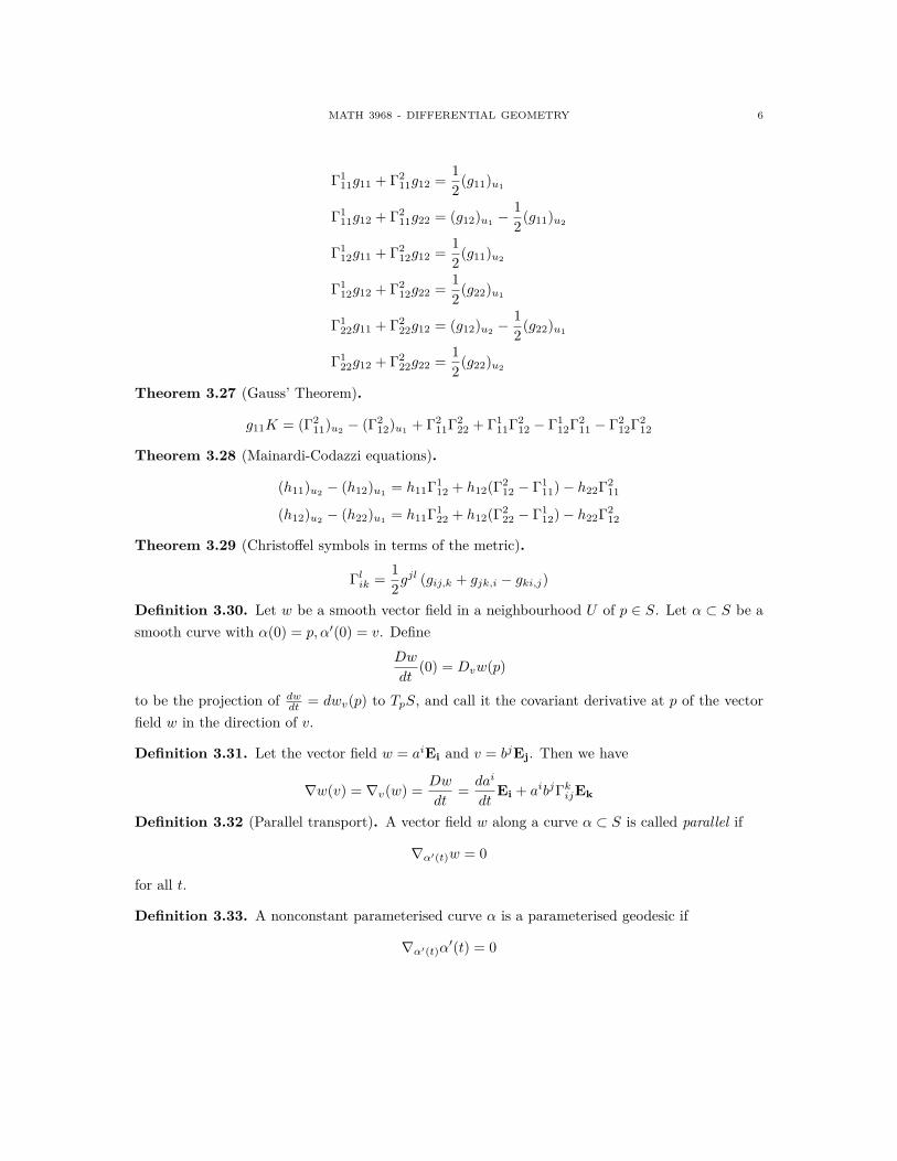
Γ111g11 + Γ2

11g12 =1

2(g11)u1

Γ111g12 + Γ2

11g22 = (g12)u1 −1

2(g11)u2

Γ112g11 + Γ2

12g12 =1

2(g11)u2

Γ112g12 + Γ2

12g22 =1

2(g22)u1

Γ122g11 + Γ2

22g12 = (g12)u2 −1

2(g22)u1

Γ122g12 + Γ2

22g22 =1

2(g22)u2

Theorem 3.27 (Gauss’ Theorem).

g11K = (Γ211)u2 − (Γ2

12)u1 + Γ211Γ

222 + Γ1

11Γ212 − Γ1

12Γ211 − Γ2

12Γ212

Theorem 3.28 (Mainardi-Codazzi equations).

(h11)u2 − (h12)u1 = h11Γ112 + h12(Γ

212 − Γ1

11)− h22Γ211

(h12)u2 − (h22)u1 = h11Γ122 + h12(Γ

222 − Γ1

12)− h22Γ212

Theorem 3.29 (Christoffel symbols in terms of the metric).

Γlik =1

2gjl (gij,k + gjk,i − gki,j)

Definition 3.30. Let w be a smooth vector field in a neighbourhood U of p ∈ S. Let α ⊂ S be asmooth curve with α(0) = p, α′(0) = v. Define

Dw

dt(0) = Dvw(p)

to be the projection of dwdt = dwv(p) to TpS, and call it the covariant derivative at p of the vector

field w in the direction of v.

Definition 3.31. Let the vector field w = aiEi and v = bjEj. Then we have

∇w(v) = ∇v(w) =Dw

dt=dai

dtEi + aibjΓkijEk

Definition 3.32 (Parallel transport). A vector field w along a curve α ⊂ S is called parallel if

∇α′(t)w = 0

for all t.

Definition 3.33. A nonconstant parameterised curve α is a parameterised geodesic if

∇α′(t)α′(t) = 0


i.e. if its tangent vector field is parallel along the curve.

Definition 3.34. Let w be a smooth field of unit vectors along a curve α where α lies in an orientedsurface. Then define the algebraic value of the covariant derivative [∇α′(t)w] by

∇α′(t)w = [∇α′(t)w]N × w(t)

Definition 3.35. Let α be a curve parameterised by arc length. The algebraic value of ∇α′(t)α′(t)

is called the geodesic curvature of α and is denoted by kg.

Remark. Up to sign, ∇α′(t)α′(t) is the tangential projection of α′′(s), and so the geodesic curvature

is up to sign the tangential component of a′′(s).

Theorem 3.36. For a curve α in an oriented surface S, we have

k2 = k2n + k2g

Remark. Thus, α is a geodesic if and only if its geodesic curvature is identically zero.

Theorem 3.37. Let γ(t) = ϕ(u1(t), u2(t)). Then γ′(t) = (ui)′Ei. Then we have γ is a geodesic ifand only if

0 = ∇γ′(t)γ′(t)

= ∇γ′(t)(uj)′Ej

= (uj)′′Ej + (uj)′∇(ui)′EiEj

= [(uk)′′ + (uj)′(ui)′Γkij ]Ek

if and only if(uk)′′ + (uj)′(ui)′Γkij = 0

for k = 1, 2

Theorem 3.38. A point and a tangent vector to that point uniquely determine a geodesic in asufficiently small neighbourhood of that point.

Theorem 3.39. For each p ∈ Σ, there is some neighbourhood U of p such that for any q ∈ U , thegeodesic from p to q has length less than or equal to the length of any other path from p to q.

Theorem 3.40. Let v and w be smooth unit vector fields along a curve α ⊂ S. Then

[∇α′(t)w]− [∇α′(t)v] =dθ

dt

where θ is a smooth choice of angle from v to w.


3.1. The Gauss Bonnet Theorem. We first prove a local version, and then the full globaltheorem.

The depth of this (global) theorem lies in its topological content rather than in its geometriccontent, and its most striking feature is that it relates the two.

In fact, a corollary is

Corollary. For an orientable compact surface S,∫∫S

Kdσ = 2πχ(S)

Theorem 3.41 (Theorem of Turning Tangents). Let S be an oriented surface, and ϕ : U → S acoordinate chart. Let α be a simple, closed, parameterised curve, regular in each interval [ti, ti+1].

Choose a smooth angle function θi on each [ti, ti+1] which measures the angle from E1 to α′.Denote by γi the external angle at ti. Then

k∑i=0

(θi(ti+1)− θi(ti)) +k∑i=0

γi = ±2π

and the above sum is 2π if α is a positively oriented curve.

Theorem 3.42 (Local Gauss-Bonnet Theorem). Let S be an oriented surface, U ⊂ R2 be homeo-morphic to an open disk and ϕ : U → S be a coordinate chart compatible with the orientation, suchthat g12 = 0.

Let R ⊂ ϕ(U) be a simple region and α a positively oriented piecewise regular curve whose traceequals ∂R. Let α be parameterised by arc length, with vertices at s0, s1, . . . , sk.

Thenk∑i=0

∫ si+1

si

kg(s)ds+

∫∫R

Kdσ +

k∑i=0

γi = 2π

Corollary. Let R ⊂ ϕ(U) be a simple region with piecewise regular boundary, and α : [0, l] → S bean arc length parametrisation of ∂R. Take a unit vector w0 ∈ Tα(0)S and let w be the vector fieldalong α generated by the parallel transport of w0. Then we have

∆θ = θ(l)− θ(0) =

∫∫R

Kdσ

where θ is a continuous choice of angle from E1 to w.

Definition 3.43. The Euler characteristic χ(S) of a surface S is given by χ(S) = V − E + F ,where V,E, F are the number of vertices, edges and faces of any triangulation of S.

Theorem 3.44. If two surfaces S1 and S2 are homeomorphic, then χ(S1) = χ(S2).

Theorem 3.45.χ(S) = 2− 2g


where g is the number of holes of S, called the genus of S.

Theorem 3.46 (Global Gauss-Bonnet). Let R ⊂ S be a regular region of an oriented surface withpositively oriented boundary curves Ci. Write γj for the external angles of the curves Ci. THen∑

i

∫Ci

kg(s)ds+

∫∫R

Kdσ +∑j

γj = 2πχ(S)

Definition 3.47. A point p is said to be a singular point of the smooth vector field v on S if

v(p) = 0

Take a positively oriented simple closed curve α enclosing an isolated singular point of a vectorfield v. Let θv be a smooth choice of angle from E1 to v. THen

θv(l)− θv(0) = 2πI

for some integer I. We call I the index of v at p.

Theorem 3.48 (Poincarè-Hopf Theorem). Let v be a smooth vector field on S with isolated singularpoints p1, . . . , pn. Then

n∑i=1

Ii = χ(S)

Corollary (Hairy-Ball theorem). If S is not homeomorphic to a torus, then any smooth vectorfield on S must vanish somewhere.

Theorem 3.49 (Morse’s Theorem). Let f : S → R be a smooth function on a compact orientedsurface S such that all critical points (dfp = 0) are non-degenerate (detA(p) ̸= 0, where A is theHessian matrix of f).

Let• M = number of local maxima,• m = number of local minima,• s = number of saddle points.

ThenM − s+m = χ(S)

This is independent of the function f , and depends only upon the topology of S.

4. Abstract Manifolds

Definition 4.1 (Abstract manifolds).

An abstract surface is a set Σ together with a family of maps

ϕα : Uα → Σ


of open sets Uα ⊂ R2 into Σ so that

• ∪αϕα(Uα) = Σ

• Whenever α, β are such that Wαβ = ϕα(Uα)∩ϕβ(Uβ) ̸= ∅, then ϕ−1α (Wαβ), ϕ

−1β (W )αβ ⊂ R2

are open andϕ−1β ◦ ϕα : ϕ−1

α (Wαβ) → ϕ−1β (Wαβ)

Definition 4.2. A function f :M → R is smooth at p ∈M if for all coordinate charts ϕ : U →M

about p,f ◦ ϕ : U ⊂ RN → R

is smoothA map f :M1 →M2 between smooth manifolds is smooth at p ∈M1 if for all coordinate charts

ϕ : U →M1 about p, and coordinate chart ψ : V →M2

ψ−1 ◦ f ◦ ϕ : U ⊂ RN1 → RN2

It is called smooth if it is smooth at every point.

Definition 4.3. Two manifoldsM1 andM2 are diffeomorphic if there is a smooth map f :M1 →M2

that has a smooth inverse.A necessary condition is that the manifolds have the same dimension.

Definition 4.4. A smooth parameterised curve in a (smooth) manifold M is a smooth map α :

(a, b) →M

Definition 4.5 (Tangent vectors as equivalence classes of curves). A tangent vector v to the smoothmanifold M at p ∈M is an equivalence class [α] of curve α : (−ϵ, ϵ) →M with α(0) = p.

Fix a coordinate chart ϕ : U →M around p. If α1, α2 satisfy α1(0) = α2(0) = p, then we define

α1 ∼ α2 ⇔ (ϕ−1 ◦ α1)′(0) = (ϕ−1 ◦ α2)

′(0)

This is independent of the choice of ϕ

Definition 4.6 (Derivation). A derivation is a map from the real vector space of smooth functionon M to R, which is linear and satisfies the product rule at p, i.e.

D(fg) = fD(g) + gD(f)

Theorem 4.7. THe set of all derivations at p ∈ MN forms an n-dimensional vector space, withbasis

∂

∂ui: ϕ 7→ ∂ϕ(p)

∂ui

whereϕ : (u1, . . . , un) 7→ ϕ(u1, . . . , un)


Definition 4.8 (Tangent vector as an operator that acts on functions). There is a one-to-onecorrespondence between equivalence classes of curves through p and derivations at p. We can thusalternatively define a tangent vector at p to be a derivation at p.

Definition 4.9. A smooth manifold M is orientable if it has an atlas (i.e. may be covered withcoordinate neighbourhoods) so that whenever p� ∈M lies in the image of two local parameterisationsϕ and ψ, the change of basis matrix at p has positive determinant.

If this is possible, then the choice of such an atlas is called an orientation of M , and we say thatM is oriented.

An orientation of a smooth manifold M can be thought of as an orientation of every tangentplane that “varies smoothly”.

Definition 4.10 (Tangent Bundle). Define

TM = {(p, v) : p]inM, v ∈ TpM}

Definition 4.11. A smooth vector field on the smooth manifold M is a smooth map v :M → TM

such that vp ∈ TpM for each p ∈M .

Definition 4.12. Let v, w be smooth vector fields on M . A covariant derivative on a smoothmanifold M is a map

∇ : (v, w) 7→ ∇vw

such that

• ∇v is linear in v i.e. ∇fu+gv(w) = f∇u(w) + g∇v(w)

• Each ∇v satisfies linearity over R: ∇v(u+ w) = ∇v(u) +∇v(w)

• Each ∇v satisfies the product rule

∇v(fu) = f∇v(u) + v(f)u

Definition 4.13 (Levi-Civita connection). On a Riemannian manifold, there is a unique covariantderivative satisfying the following two conditions:

∇ ∂

∂ui

∂

∂uj= ∇ ∂

∂uj

∂

∂ui

and viewing ∂∂ui as a derivation,

∂

∂ui(⟨ ∂

∂uj,∂

∂uk⟩) = ⟨∇ ∂

∂ui

∂

∂uj,∂

∂uk⟩+ ⟨ ∂

∂uj,∇ ∂

∂ui

∂

∂uk⟩

Definition 4.14 (Christoffel symbols on an abstract manifold). Define the Christoffel symbols Γkijwith respect to a local coordinate chart by

∇ ∂

∂ui

∂

∂uj= Γkij

∂

∂uk


We haveΓkij =

1

2gkl (gil,j + gjl,i − gij,l)

which defines a unique covariant derivative.

Definition 4.15 (Geodesic). A geodesic is a curve α satisfying

∇′αα

′ = 0

This gives us the equations(uk)′′ + Γkij(u

i)′(uj)′ = 0

for k = 1, . . . , n

Definition 4.16. The hyperbolic plane is defined to be the upper half plane with the metric (writingu1 = x, u2 = y)

g11 =1

y2, g12 = 0, g22 =

1

y2

math 3968 - differential geometry - tullotullo.ch/static/math3968lecturenotes.pdf · math 3968 -...

Documents