math 312 - analysis 1math.uchicago.edu/~subhadip/coursedocuments/analysis-i/math312... ·...

Math 312 - Analysis 1

Lectures by Marianna CsornyeiNotes by Zev Chonoles

The University of Chicago, Fall 2012

Lecture 1 (2012-10-02) 1

Lecture 2 (2012-10-04) 4

Lecture 3 (2012-10-09) 9

Lecture 4 (2012-10-11) 13

Lecture 5 (2012-10-16) 18

Lecture 6 (2012-10-18) 21

Lecture 7 (2012-10-23) 26

Lecture 8 (2012-10-25) 30

Lecture 9 (2012-10-30) 31

Lecture 10 (2012-11-01) 32

Lecture 11 (2012-11-06) 37

Lecture 12 (2012-11-08) 41

Lecture 13 (2012-11-13) 42

Lecture 14 (2012-11-15) 47

Lecture 15 (2012-11-20) 52

Lecture 16 (2012-11-27) 57

Lecture 17 (2012-11-29) 61

Lecture 18 (2012-12-04) 65

Introduction

Math 312 is one of the nine courses offered for first-year mathematics graduate students at theUniversity of Chicago. It is the first of three courses in the year-long analysis sequence.

These notes were live-TeXed, though I edited for typos and added diagrams requiring the TikZpackage separately. I used the editor TeXstudio.

I am responsible for all faults in this document, mathematical or otherwise; any merits of thematerial here should be credited to the lecturer, not to me.

Please email any corrections or suggestions to [email protected].

Acknowledgments

Thank you to all of my fellow students who sent me corrections, and who lent me their own notesfrom days I was absent. My notes are much improved due to your help.

mailto:[email protected]

Lecture 1 (2012-10-02)

The course will cover a mixture of real analysis and probability. Homeworks will be due on theThursday of the following week. Homeworks will be 10% of the grade and the midterm and finaltogether will be the other 90%. The exams will be in class.

The abstract setting for measure theory is as follows. We have a set X, with power set P (X). Asubset A ⊆ P (X) is called a σ-algebra when

1. ∅ ∈ A,

2. for any A ∈ A, its complement (X \A) ∈ A, and

3. for any A1, A2, . . . ,∈ A, their union⋃∞n=1An ∈ A.

Some immediate consequences are:

• We also have X ∈ A.

• A is also closed under countable intersections; for any A1, A2, . . . ∈ A,⋂∞n=1An ∈ A. This is

because

X \∞⋂n=1

An =

∞⋃n=1

(X \An).

• If A,B ∈ A, then A \B ∈ A because

A \B = A ∩ (X \B).

The most extreme cases of σ-algebras are ∅, X and P (X).

A more interesting example is when X is a topological space and A is the σ-algebra generated byall open sets of X. This is called the Borel σ-algebra on X.

The σ-algebra generated by a collection of sets is the smallest σ-algebra that contains all of thosesets. This can be constructed by considering all of the σ-algebras containing those sets, and takingtheir intersection. The intersection of σ-algebras can easily be seen to be a σ-algebra.

Let’s consider a fundamental topological space, R. What can we say about Borel sets in R?

• Open sets are Borel.

• Closed sets, being complements of open sets, are Borel.

• Countable intersections of open sets (called Gδ sets) are Borel.

• Countable unions of closed sets (called Fσ sets) are Borel.

Some examples of Fσ sets that are neither open nor closed are [0, 1) and Q. Their complements arenecessarily Gδ sets, and will also be neither open nor closed.

Homework. Is Q a Gδ set?

Continuing our list of Borel sets in R,

• Countable unions of Gδ sets (called Gδσ sets) are Borel.

• Countable intersections of Fσ sets (called Fσδ sets) are Borel.

Last edited2012-12-08

Math 312 - Analysis 1 Page 1Lecture 1

• Countable intersections of Gδσ sets (called Gδσδ sets) are Borel.

• Countable unions of Fσδ sets (called Fσδσ sets) are Borel.

• · · ·

It is a theorem that each of these new classes is strictly bigger than the previous one; there is nofinite step when we get no new sets. We do not even get all Borel sets when we look at all sequencesof δ’s and σ’s. We must go all the way to ω1 (the first uncountable ordinal) to get all Borel sets.Most of the time, we do not think beyond the first few steps here, but in descriptive set theory thisis studied in more detail.

A pair (X,A) of a set X together with a σ-algebra A on X is called a measure space (more precisely,a measurable space). The elements of A are called A-measurable sets, or just measurable sets if theσ-algebra is understood.

Homework. What is the σ-algebra generated by the half-open intervals [a, b)? How is it related tothe Borel σ-algebra - smaller, bigger, not comparable?

Definition. Given two measurable spaces (X,A) and (Y,B), a map f : X → Y is called measurableif f−1(B) ∈ A for all B ∈ B.

Since it is difficult to understand what the Borel sets of R are, this would seem to be a difficultcondition to check. But in fact, when (Y,B) = (R,Borel), a map f : X → R is A-measurable if

x ∈ X | f(x) < c ∈ A and x ∈ X | f(x) > c ∈ A

for all c ∈ R. This is because the open half-lines already generate the entire Borel σ-algebra. Moregenerally, if C is a collection of subsets of Y that generate the σ-algebra B, then a map f : X → Yis measurable if f−1(C) ∈ A for all C ∈ C.

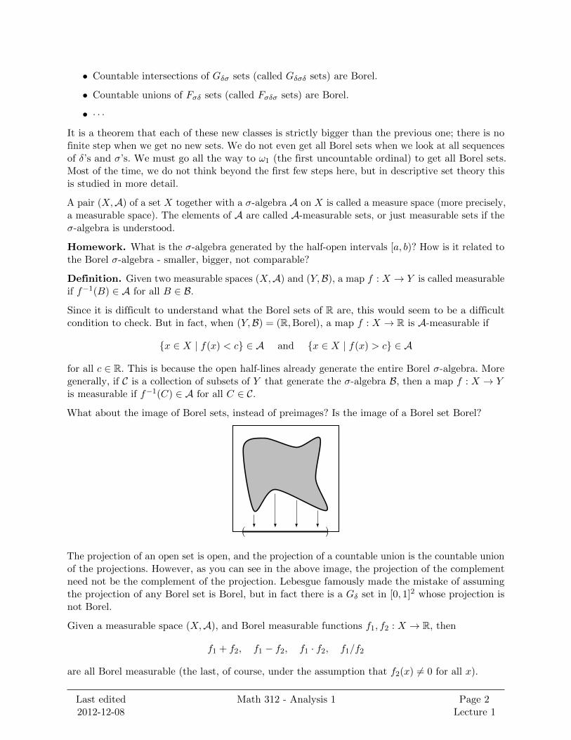
What about the image of Borel sets, instead of preimages? Is the image of a Borel set Borel?

( )

The projection of an open set is open, and the projection of a countable union is the countable unionof the projections. However, as you can see in the above image, the projection of the complementneed not be the complement of the projection. Lebesgue famously made the mistake of assumingthe projection of any Borel set is Borel, but in fact there is a Gδ set in [0, 1]2 whose projection isnot Borel.

Given a measurable space (X,A), and Borel measurable functions f1, f2 : X → R, then

f1 + f2, f1 − f2, f1 · f2, f1/f2

are all Borel measurable (the last, of course, under the assumption that f2(x) 6= 0 for all x).



Proof. The function f1 + f2 can be obtained as the composition

XF=(f1,f2)−−−−−−−−→ R× R +−−→ R

The composition of measurable functions is measurable, so it suffices to show that F and + aremeasurable. The function + is measurable (in fact, it is continuous). Because sets of the formG1 ×G2, where G1, G2 ⊆ R are open, generate the Borel σ-algebra on R× R, it is enough to showthat F−1(G1 ×G2) ∈ A for any open G1, G2 ⊆ R. But this is clear, because

F−1(G1 ×G2) = f−11 (G1) ∩ f−1(G2).

Definition. The extended real line is R = R ∪ ±∞. The open balls around +∞ are sets of theform (a,∞] and the open balls around −∞ are sets of the form [−∞, a).

Homework. If f1, f2, . . . : X → R are Borel measurable, prove that g = sup(fn) : X → R is Borelmeasurable.



Lecture 2 (2012-10-04)

Definition. Given a set X and a σ-algbera A on X, a function µ : A → [0,∞] is a measure if

1. µ(∅) = 0

2. (σ-additivity) For disjoint sets A1, A2, . . .,

∞∑n=1

µ(An) = µ

( ∞⋃n=1

An

)

Examples.

• The counting measure on X: for any σ-algebra A ⊆ P (X), we define µ(A) = |A|.

• The Dirac measure: given an x ∈ X,

δx(A) =

1 if x ∈ A,0 if x /∈ A.

• An atomic measure is one of the form µ =∑cjδxj , so that

µ(A) =∑xj∈A

cj

Note that any measure can be broken into an atomic part and a non-atomic part (i.e. ameasure for which no points have positive measure). This is somewhat of a hint for thefollowing homework:

Homework. Is there a σ-algebra A which is countably infinite?

Some properties of measures include:

• σ-additive =⇒ additive (just take Aj = ∅ for large j)

• Monotonicity: if A ⊆ B, then µ(A) ≤ µ(B). Note that

µ(B) = µ(A) + µ(B \A)

but you should not write this as

µ(B \A) = µ(B)− µ(A)

because we could have µ(B) = µ(A) =∞.

• Given A1 ⊆ A2 ⊆ · · · ,

µ

( ∞⋃n=1

An

)= lim

n→∞µ(An).

Proof. The sets Ai are not disjoint, but consider instead the sets A1, A2 \ A1, A3 \ A2, . . .which are disjoint.



Then∞⋃n=1

An = A1 ∪∞⋃n=1

(An+1 \An)

so

µ

( ∞⋃n=1

An

)= µ(A1) + µ(A2 \A1) + µ(A3 \A2) + · · ·

= limn→∞

(µ(A1) + µ(A2 \A1) + · · ·+ µ(An \An−1))

= limn→∞

µ(An)

• What about when we have A1 ⊇ A2 ⊇ · · · ? It is not true in general that

µ

( ∞⋂n=1

An

)= lim

n→∞µ(An).

For example, consider the counting measure on N, and A1 = N, A2 = 2, 3, . . . , , A3 =3, 4, . . ., etc. Then their intersection is ∅ which has µ(∅) = 0, even though µ(An) =∞ forall n. Howver, if there is at least one n where µ(An) is finite, then the statement is true.

Proof. Without loss of generality, we can assume that µ(A1) is finite. Then

µ(A1 \A2) + µ(A2 \A3) + · · ·︸︷︷︸limn→∞

µ(A1 \An)

+µ

( ∞⋂n=1

An

)= µ(A1).

Because µ(A1) is finite, we can write µ(A1 \An) = µ(A1)− µ(An), so

limn→∞

µ(A1 \An) = limn→∞

(µ(A1)− µ(An))

and therefore

µ(A1)− limn→∞

µ(An) + µ

( ∞⋂n=1

An

)= µ(A1).

Let X be a compact metric space and A the Borel σ-algebra on X. Is a finite Borel measure µdetermined by the measure of the balls?

Homework (∗). The answer is no; find an example. Federer wasn’t able to find an example, afterthinking about it for a day, but the construction is simple once you see it.

We say that f : X → R is simple if it is measurable and takes only finitely many values. Equivalently,there are some disjoint sets A1, . . . , An and cj ∈ R such that

f =n∑j=1

cjχAj .



You can visualize this as

c1

c2

c3

c4

A1 A2 A3 A4

We define for a simple function f ≥ 0∫Af dµ =

n∑j=1

cjµ(A ∩Aj).

If g ≥ 0 is an arbitrary measurable function, then we define∫Ag dµ = sup

f simplef≤g

∫Af dµ.

Thus, we are approximating our function f from below by simple functions.

We need to restrict to nonnegative functions, even though ±∞ are not being allowed as values ofour functions in this definition, because (for example) we cannot integrate g(x) = 1

x on R with thisdefinition; there is no simple function f ≤ g. This illustrates the difference between being finiteeverywhere and being bounded.

For an arbitrary measurable function g, we set

g+ = max(0, g), g− = −min(0, g)

so that g = g+ − g− and then define∫Ag dµ =

∫Ag− dµ−

∫Ag− dµ.

From now on, when I write a function, it will be assumed to be measurable, even if I don’t say so.

Given a measure µ and an f ≥ 0, we can make a new measure ν defined by

ν(A) =

∫Af dµ.



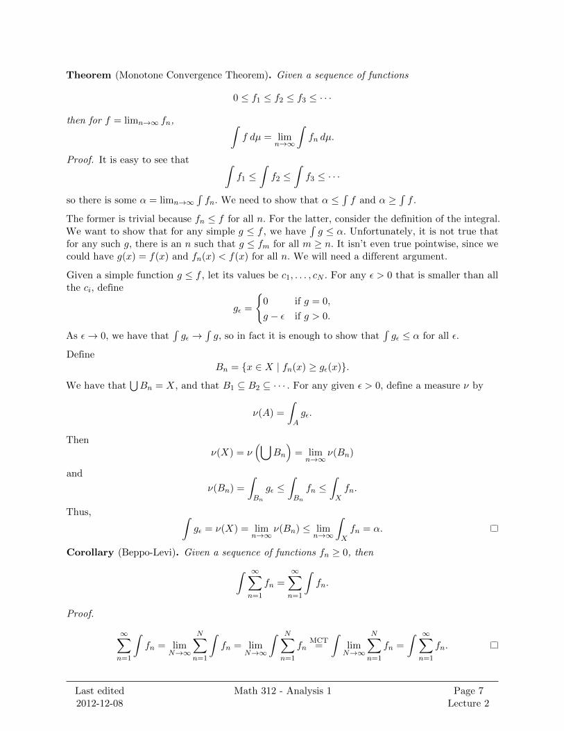
Theorem (Monotone Convergence Theorem). Given a sequence of functions

0 ≤ f1 ≤ f2 ≤ f3 ≤ · · ·

then for f = limn→∞ fn, ∫f dµ = lim

n→∞

∫fn dµ.

Proof. It is easy to see that ∫f1 ≤

∫f2 ≤

∫f3 ≤ · · ·

so there is some α = limn→∞∫fn. We need to show that α ≤

∫f and α ≥

∫f .

The former is trivial because fn ≤ f for all n. For the latter, consider the definition of the integral.We want to show that for any simple g ≤ f , we have

∫g ≤ α. Unfortunately, it is not true that

for any such g, there is an n such that g ≤ fm for all m ≥ n. It isn’t even true pointwise, since wecould have g(x) = f(x) and fn(x) < f(x) for all n. We will need a different argument.

Given a simple function g ≤ f , let its values be c1, . . . , cN . For any ε > 0 that is smaller than allthe ci, define

gε =

0 if g = 0,

g − ε if g > 0.

As ε→ 0, we have that∫gε →

∫g, so in fact it is enough to show that

∫gε ≤ α for all ε.

DefineBn = x ∈ X | fn(x) ≥ gε(x).

We have that⋃Bn = X, and that B1 ⊆ B2 ⊆ · · · . For any given ε > 0, define a measure ν by

ν(A) =

∫Agε.

Thenν(X) = ν

(⋃Bn

)= lim

n→∞ν(Bn)

and

ν(Bn) =

∫Bn

gε ≤∫Bn

fn ≤∫Xfn.

Thus, ∫gε = ν(X) = lim

n→∞ν(Bn) ≤ lim

n→∞

∫Xfn = α.

Corollary (Beppo-Levi). Given a sequence of functions fn ≥ 0, then∫ ∞∑n=1

fn =

∞∑n=1

∫fn.

Proof.

∞∑n=1

∫fn = lim

N→∞

N∑n=1

∫fn = lim

N→∞

∫ N∑n=1

fnMCT=

∫limN→∞

N∑n=1

fn =

∫ ∞∑n=1

fn.



Corollary (Fatou’s Lemma). Given a sequence of functions fn ≥ 0,∫lim infn→∞

fn ≤ lim infn→∞

∫fn.

Homework. Find an example where this inequality is strict.

Proof. By definition,lim infn→∞

fn = limn→∞

inffn, fn+1, fn+2, . . .︸︷︷︸gn

.

We have that 0 ≤ gn ≤ gn+1 ≤ · · · and therefore∫lim infn→∞

fn =

∫limn→∞

gn = limn→∞

∫gn ≤ lim inf

n→∞

∫fn

because gn ≤ fn.

Corollary (Lebesgue Theorem). Given a sequence of functions fn such that |fn| ≤ g, where g is afunction such that

∫g <∞, ∫

limn→∞

fn = limn→∞

∫fn.

Homework. Find a sequence of functions fn converging pointwise to a function f which do notsatisfy the conclusion of this theorem.

Proof. Let f = limn→∞ fn. In fact, a stronger statement is true: as n→∞,∣∣∣∣∫ fn −∫f

∣∣∣∣ ≤ ∫ |fn − f | → 0.

We have that |fn − f | ≤ 2g. Let hn = 2g − |fn − f |, so that hn ≥ 0. Apply Fatou:∫lim infn→∞

hn︸︷︷︸2g

≤ lim infn→∞

∫hn.

Therefore ∫2g ≤ lim inf

n→∞

(∫2g − |fn − f |

)=

∫2g + lim inf

n→∞

(−∫|fn − f |

).

Therefore

lim supn→∞

(∫|fn − f |

)≤ 0

which implies that in fact ∫|fn − f | → 0.



Lecture 3 (2012-10-09)

Last time, we talked about measure spaces (X,A, µ).

Definition. We say that a measure space is complete if, for any A ∈ A such that µ(A) = 0, wehave B ∈ A for every subset B ⊆ A. By monotonicity of measures, they will also be null.

Claim. The σ-algebra generated by A and all subsets of null sets is the σ-algebra of all sets Ssuch that there are A1, A2 ∈ A with A1 ⊆ S ⊆ A2 and µ(A2 \ A1) = 0. We can then defineµ(S) = µ(A1) = µ(A2).

Definition. An outer measure is a function µ : A → [0,∞], where A is an arbitrary collection ofsets, such that

• µ(∅) = 0,

• σ-sub-additivity: µ(⋃An) ≤

∑µ(An) for any A1, A2, . . . ∈ A.

We can create an outer measure as follows: for an arbitrary collection of sets A, and an arbitraryfunction α : A → [0,∞], we can define for any A ∈ P (X)

φα(A)def= inf

∑µ(An) | A ⊆

⋃An, An ∈ A.

If there is no cover of A by some An ∈ A, then φα(A) =∞.

We now want to create a measure from this outer measure:

α, A(arbitrary)

−→ φα, P (X)(outer measure)

−→ µ,Mφ(measure)

Definition. Given an outer measure φ, we say that A is φ-measurable if, for any set S,

φ(S) = φ(S ∩A) + φ(S \A).

We will see that the collection of φ-measurable sets will form a complete measure space. First, notethat we always have

φ(S) ≤ φ(S ∩B) + φ(S \B).

If φ(A) = 0, and B ⊆ A, then S ∩ B ⊆ B ⊆ A implies that φ(S ∩ B) = 0, and S \ B ⊆ S impliesthat φ(S \B) ≤ φ(S), so that

φ(S) ≤ 0 + φ(S \B)

hence φ(S) = φ(S \B), hence φ(B) = 0.

S

A B



Now we want to check that

φ(S) = φ(S ∩ (A ∪B)) + φ(S \ (A ∪B)).

We have thatφ(S) = φ(S ∩A) + φ(S \A).

Thereforeφ(S \A) = φ((S \A) ∩B︸︷︷︸

S∩B

) + φ((S \A) \B︸︷︷︸S\(A∪B)

)

andφ(S ∩A) + φ(S ∩B) = φ(S ∩ (A ∪B))

φ(S ∩ (A ∪B)) = φ(S ∩ (A ∪B) ∩A︸︷︷︸S∩A

) + φ((S ∩ (A ∪B)) \A︸︷︷︸S∩B

).

The rest of the argument you should study on your own.

If our initial arbitrary collection of sets A is such that ∅ ∈ A, and for any A,B ∈ A, we haveA ∪B,A ∩B,A \B ∈ A, and we further assume that α is an outer measure on A such that for anyA,B ∈ A we have

α(A) = α(A ∩B) + α(A \B)

then the resulting σ-algebra M will contain A, i.e. A ⊆M.

Here is a special case. Consider ‘‘bricks’’, i.e. sets of the form

n∏i=1

[ai, bi) ⊆ Rn

and let A be the set of finite unions of such sets. Let α be the volume function. Then φα is the outerLebesgue measure, M consists of the Lebesgue measurable sets, and µ is the Lebesgue measure. Wecan do the same construction on the bricks for any additive function α; the resulting measure willalways contain at least the Borel sets.

Definition. We say that µ is a Borel measure on a σ-algebra M if

• The σ-algebra M⊇ Borel sets.

• Some people require that µ is σ-finite, i.e. there exist A1, A2, . . . with µ(An) <∞ such thatµ(X \

⋃An) = 0.

• Some people require that µ(K) <∞ for any compact K (in Rn, this just says that boundedsets have finite measure).

Definition. We say that a measure µ is regular when for any A ∈ A,

µ(A) = inf∑µ(Gn) | Gn are open, A ⊆

⋃Gn = infµ(G) | G open, A ⊆ G

For any ε > 0, we can choose G such that µ(A) ≤ µ(G) ≤ µ(A) + ε. Letting ε → 0, we can seethat for any A there is a Gδ set containing A of the same measure. By the same argument for thecomplement, we have an Fσ ⊆ A of the same measure.

Now we’ll start on a new topic.

Let λ be the Lebesgue measure on Rn, and B(Rn) the Borel sets in Rn.



Definition. For any X ⊆ Rn, a differential basis for X is a collection D ⊆ X × B(Rn) such that

• For any (x,A) ∈ D, we have λ(A) > 0.

• For any x ∈ X and r > 0, there is some (x,A) ∈ D such that A ⊆ B(x, r), the ball of radiusr around x.

Given an x ∈ Rn and A ⊆ Rn, let r(A) be the smallest radius such that A ⊆ B(x, r(A)).

We say that a differential basis D is regular when it satisfies the following property: for any x ∈ X,there exist a δ > 0 and r0 > 0, depending on x, such that for any (x,A) ∈ D with r(A) < r0,

λ(A) ≥ δ · λ(B(x, r(A))).

In other words, D is regular when, for any x ∈ X, there is a positive ratio δ for which all sufficientlysmall (x,A) ∈ D take up at least δ of their bounding ball.

Examples.

• The symmetrical basis: all balls with center x. This is regular.

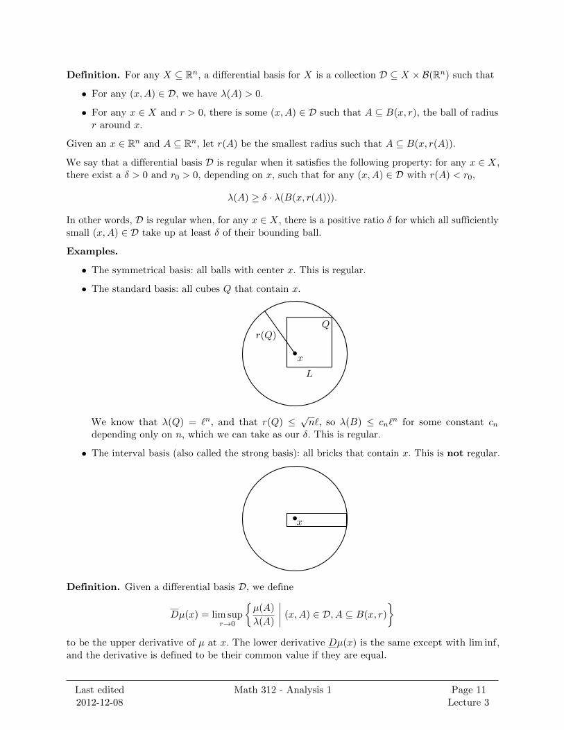
• The standard basis: all cubes Q that contain x.

•x

r(Q)Q

L

We know that λ(Q) = `n, and that r(Q) ≤√n`, so λ(B) ≤ cn`

n for some constant cndepending only on n, which we can take as our δ. This is regular.

• The interval basis (also called the strong basis): all bricks that contain x. This is not regular.

•x

Definition. Given a differential basis D, we define

Dµ(x) = lim supr→0

µ(A)

λ(A)

∣∣∣∣ (x,A) ∈ D, A ⊆ B(x, r)

to be the upper derivative of µ at x. The lower derivative Dµ(x) is the same except with lim inf,and the derivative is defined to be their common value if they are equal.



Example. Let f : R → R be a differentiable function that is monotone increasing, and defineµ([a, b)) = f(b)−f(a). This defines a Borel measure µ on R. We’ll choose D = symmetrical basis, so

limr→0

µ(B(x, r))

λ(B(x, r))= lim

r→0

f(x+ r)− f(x− r)2r

.

This is the symmetric derivative. Note that f did not have to be differentiable at x for this to exist.In contrast, if we chose the standard basis or interval basis (which are the same in one dimension),then we’d get the limit

limy,z→xx∈[y,z]

f(y)− f(x)

y − z

which exists if and only if f is differentiable.

Definition. We define the maximal operator of a measure µ to be

M(x) = Mµ(x) = sup(x,A)∈D

µ(A)

λ(A).

Note that if µ = µ1 + µ2, then Mµ ≤Mµ1 +Mµ2 . We only get an inequality because the set whichmaximizes µ1 + µ2 need not maximize µ1 and µ2 separately.



Lecture 4 (2012-10-11)

Today we’ll be working in Rn, and all our measures will be Borel measures that are σ-finite.

Let µ1, µ2 be measures.

Definition. We say that µ1 is absolutely continuous with respect to µ2, and we write µ1 µ2,when µ2(A) = 0 implies µ1(A) = 0.

Definition. We say that µ1 is singular with respect to µ2, and we write µ1 ⊥ µ2, if there existdisjoint A1, A2 ⊂ Rn such that µ1(Rn \A1) = 0 and µ(Rn \A2) = 0.

Theorem (Radon-Nykodim). If µ1 µ2, then there is an f such that µ1(A) =∫A f dµ2 for all A.

We say that f is the Radon-Nykodim derivative of µ1 with respect to µ2, and we write that f = dµ1dµ2

.

Theorem. For any µ1, µ2, we can decompose µ1 = α+ β such that α µ2 and β ⊥ µ2.

Homework. Show that dµ1dµ3

= dµ1dµ2· dµ2dµ3

for any µ1 µ2 µ3.

Last class, we defined the maximal operator Mµ of a measure µ, which is a function on Rn, andnoted that Mµ1+µ2 ≤Mµ1 +Mµ2 .

Theorem. For any finite measure µ, we have

λ(x ∈ Rn |Mµ(x) > t

)≤ 3n · µ(Rn)

t

for any t ≥ 0.

Lemma. If B1, . . . , Bn are finitely many balls, there exists a subset Bi1 , . . . , Bik of pairwise disjointballs such that ⋃

j

(3Bij ) ⊇⋃i

Bi

where 3B means the ball with the same center as B and three times the radius.

Proof of lemma. We use a greedy algorithm. At each step, choose the largest ball that is disjointfrom all earlier chosen ones. This will obviously terminate because there are only finitely many balls.

Any ball Ba not chosen will intersect some ball Bb that was chosen, and Ba must have radius lessthan or equal to Bb (otherwise Bb would not have been chosen), so that expanding Bb by a factorof 3 will cover all of Ba.

Note that this statement is false if we allow infinitely many balls; for example we could have nestedballs around the same center whose radii go to infinity.

· · ·



Homework. Prove that the statement of the lemma is true even with infinitely many balls, aslong as the radii are bounded, allowing the chosen subcollection of balls to also be infinite, andreplacing 3 with some arbitrary constant.

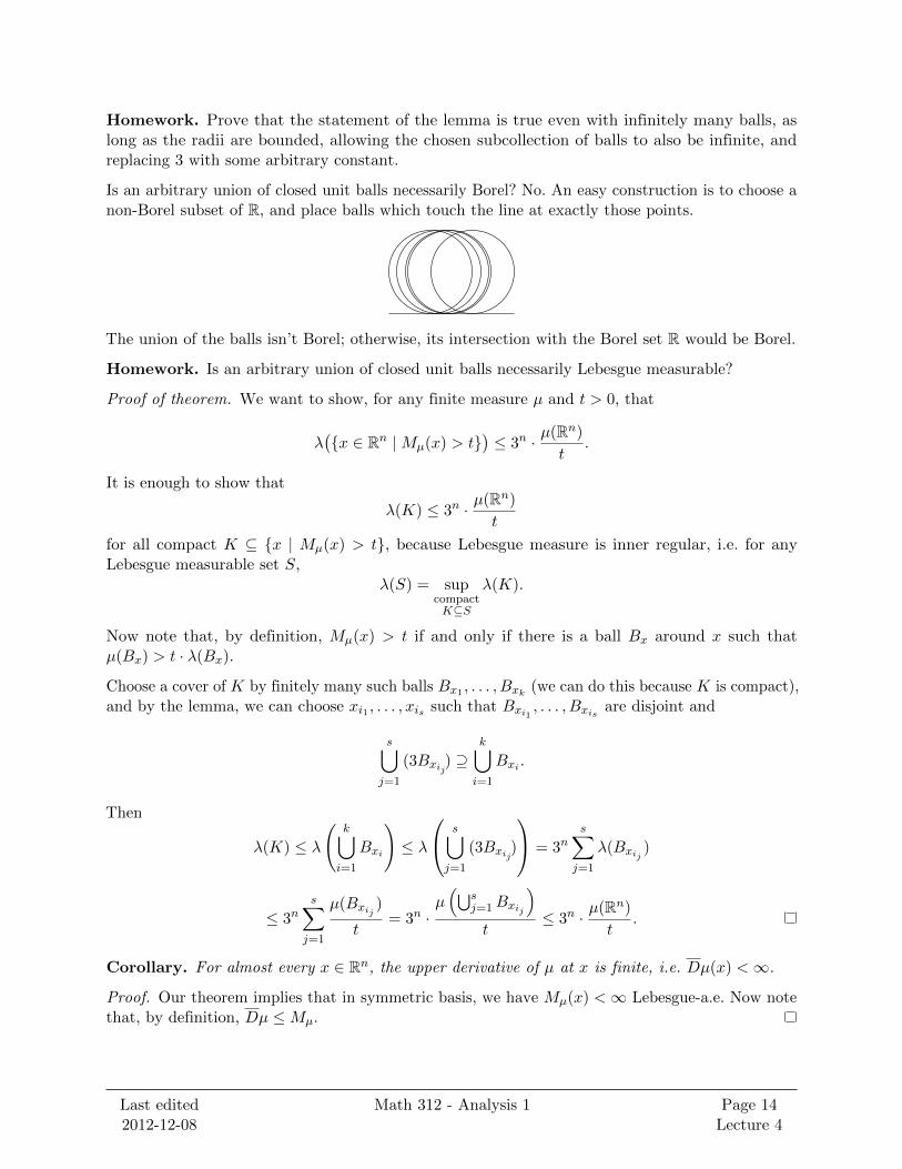
Is an arbitrary union of closed unit balls necessarily Borel? No. An easy construction is to choose anon-Borel subset of R, and place balls which touch the line at exactly those points.

The union of the balls isn’t Borel; otherwise, its intersection with the Borel set R would be Borel.

Homework. Is an arbitrary union of closed unit balls necessarily Lebesgue measurable?

Proof of theorem. We want to show, for any finite measure µ and t > 0, that

λ(x ∈ Rn |Mµ(x) > t

)≤ 3n · µ(Rn)

t.

It is enough to show that

λ(K) ≤ 3n · µ(Rn)

t

for all compact K ⊆ x | Mµ(x) > t, because Lebesgue measure is inner regular, i.e. for anyLebesgue measurable set S,

λ(S) = supcompactK⊆S

λ(K).

Now note that, by definition, Mµ(x) > t if and only if there is a ball Bx around x such thatµ(Bx) > t · λ(Bx).

Choose a cover of K by finitely many such balls Bx1 , . . . , Bxk (we can do this because K is compact),and by the lemma, we can choose xi1 , . . . , xis such that Bxi1 , . . . , Bxis are disjoint and

s⋃j=1

(3Bxij) ⊇k⋃i=1

Bxi .

Then

λ(K) ≤ λ

(k⋃i=1

Bxi

)≤ λ

s⋃j=1

(3Bxij)

= 3ns∑j=1

λ(Bxij )

≤ 3ns∑j=1

µ(Bxij )

t= 3n ·

µ(⋃s

j=1Bxij

)t

≤ 3n · µ(Rn)

t.

Corollary. For almost every x ∈ Rn, the upper derivative of µ at x is finite, i.e. Dµ(x) <∞.

Proof. Our theorem implies that in symmetric basis, we have Mµ(x) <∞ Lebesgue-a.e. Now notethat, by definition, Dµ ≤Mµ.



Note that, for a regular basis D,

µ(A)

λ(A)≤ µ(B)

λ(A)=µ(B)

λ(B)︸︷︷︸<∞

· λ(B)

λ(A)︸︷︷︸< 1

δ

where (x,A) ∈ D, with A ⊆ B(x, r(A)) = B, and 1δ is from the regularity of D.

Theorem. If µ is singular, then Dµ(x) = 0 a.e.

Proof. By hypothesis, there exists a Lebesgue null set N such that µ(Rn \ N) = 0. We need toshow that Dµ(x) = 0 for a.e. x ∈ Rn \N .

If N is closed, there is nothing to prove, because any x ∈ Rn \N can be separated from N by asufficiently small open ball.

Now choose a compact K ⊆ N such that µ(N \K) < ε2.

Let µ = µ1 +µ2, where µ1(A) = µ(A∩K) and µ2(A) = µ(A∩Kc). We have that Dµ ≤ Dµ1 +Dµ2,and that Dµ1 is 0 a.e.

Note that

λ(x ∈ Rn | Dµ2(x) > t

)≤ λ

(x ∈ Rn |Mµ2(x) > t

)≤ 3n · µ2(Rn)

t≤ 3n · ε

2

t.

Letting t = ε, and using that Dµ1 is 0 a.e.,

λ(x ∈ Rn | Dµ(x) > t

)≤ λ

(x ∈ Rn |Mµ2(x) > t

)≤ 3nt.

Now let t→ 0. This shows that λ(x ∈ Rn | Dµ(x) > 0) = 0.

What happens when µ λ? By Radon-Nykodim, we have that µ =∫f dλ for some f , and it is a

theorem (which we are about to prove) that

f =dµ

dλ= Dµ a.e.

Now let f be a function such that∫|f | dλ <∞, i.e. f ∈ L1.

Definition. We say that x ∈ Rn is a Lebesgue point of f if

limr→0

1

λ(B(x, r))

∫B(x,r)

|f(t)− f(x)| dt = 0.

Theorem. For any f ∈ L1, almost every x ∈ Rn is a Lebesgue point of f .

Proof. Define the measure

µx(A) =

∫A|f(t)− f(x)| dt.

We need to show that Dµx(x) = 0 for almost all x. We will assume the following lemma for themoment:

Lemma. For f ∈ L1 and any ε > 0, there is a continuous, compactly supported g such that∫Rn |f − g| < ε.



Now fix an ε > 0, and choose g from the lemma such that∫|f − g| < ε2. Let h = f − g, so that

f = g + h. We have|f(t)− f(x)| ≤ |g(t)− g(x)|+ |h(t)− h(x)|

It is easy to see that

limr→0

1

λ(B(x, r))

∫B(x,r)

|g(t)− g(x)| dt = 0

for all x (this essentially follows from g being continuous), so now we just need to look at h. Define

νx(A) =

∫A|h(t)− h(x)| dt.

Our work so far shows that that Dµx ≤ Dνx. Using the triangle inequality to produce a bound,and dividing by λ(A),

νx(A)

λ(A)≤∫A |h(t)| dλλ(A)

+ |h(x)| · λ(A)

λ(A).

Thus,

x ∈ Rn | Dµx > 2ε] ⊆ x ∈ Rn | Dνx > 2ε

⊆x ∈ Rn

∣∣∣∣ there exist arbitrarilysmall B 3 x such that

∫B |h(t)| dtλ(B)

> ε

∪ x ∈ Rn | |h(x)| > ε.

Call the first set S1 and the second set S2. Note that the first set is precisely where the maximaloperator of h is greater than ε. Thus, from the lemma,

λ(S1) ≤ 3n · ε2

ε= 3nε

and because∫|f − g| =

∫|h| < ε2, we have

λ(S2) ≤∫|h|ε≤ ε.

Because ε > 0 is arbitrary, we can conclude that

λ(x ∈ Rn | Dµx > 0) = 0.

Thus, the set of non-Lebesgue points of f is null. Now we prove our other claim. Given a measureµ λ, we can let f = dµ

dλ , and then we see that as we take smaller and smaller balls B 3 x,∣∣∣∣µ(B)

λ(B)− f(x)

∣∣∣∣ =

∣∣∣∣( 1

λ(B)

∫Bf(t) dλ

)− f(x)

∣∣∣∣=

∣∣∣∣ 1

λ(B)

∫B

(f(t)− f(x))

∣∣∣∣ ≤ 1

λ(B)

∫B|f(t)− f(x)| → 0.

This demonstrates that we have dµdλ = Dµ a.e.



Proof of lemma.

1. If r is large enough then∫B(0,r)c |f | < ε.

2. If M is large enough then∫x : |f(x)|>M |f | < ε.

Let⋃Am = A, so that Am = A ∩ x ∈ Rn | mε ≤ f < (m+ 1)ε. Then

A = B(0, r) ∩ x ∈ Rn | |f | ≤M

Choose compact Km ⊆ Am such that ∫Am\Km

|f | ≤ ε′

and also such that λ(Am \Km) ≤ ε′. We can do this because λ is inner regular, so that for each Amthere is a sequence Km,i ⊆ Am of compact sets such that λ(Am \Km,i) <

1i , and WLOG we can

assume Km,i ⊆ Km,i+1, so letting dν = f dλ,

limn→∞

ν(Kn) = ν(An).

Define g = mε on Kn. Extend it to a continuous function g : B(0, r)→ [−M,M ], with g = 0 outsideB(0, r).



Lecture 5 (2012-10-16)

What we’ve proved so far: the maximal operator theorem and the covering lemma. These involvedballs and the symmetric basis.

We proved that Dµ(x) <∞ a.e., that it equals 0 a.e. if the measure µ is singular, and that it equalsthe Radon-Nykodim derivative of µ in every regular basis.

Maximal operator theorem for cubes: up to a constant, it is the same as for balls. If cn is the ratiobetween the volume of a unit cube and a unit ball in dimension n,

1

λ(Q)

∫Q|f | dµ ≤ 1

λ(Q)

∫B|f | = λ(B)

λ(Q)

1

λ(B)

∫B|f | ≤ cn

1

λ(B)

∫B|f |

Federer’s Geometric Measure Theory is a good reference book. If you just want to know what’s true,read this book; but it uses its own notation, so any time you read a theorem, you’ll have to referback to the previous one, and then the one before that, etc. You can also read Stein’s HarmonicAnalysis which covers a lot more than we’ll get to in this course.

Let A ⊆ Rn be a Lebesgue measurable set, and define f(x) = χA(x) =

1 if x ∈ A,0 if x /∈ A.

Let µ =∫f dλ, so that µ(B) = λ(A ∩B). For x ∈ Rn, define

d(x,A), d(x,A), d(x,A)

to be the lower derivative, upper derivative, and derivative of µ at x with respect to the symmetricbasis. These are, respectively, the lim inf, lim sup, and lim as r → 0 of

λ(A ∩B(x, r))

λ(B(x, r)).

Almost every point in Rn is a Lebesgue point of f ; this implies that d(x,A) = 1 for almost all x ∈ A,and d(x,A) = 0 for almost all x /∈ A.

Theorem. For any set A (not necessarily measurable),

1. d(x,A) = 1 for almost all x ∈ A.

2. d(x,A) = 0 for almost all x /∈ A ⇐⇒ A is measurable.

Definition. Given any set A, we say that H ⊇ A is a measurable hull of A if H is measurable andif, for any measurable B ⊇ A, we have λ(H \B) = 0.

Any set has a hull; for any A, we can define

λ(A) = infG⊇AG open

λ(G)

and then choose G1, G2, . . . such that Gn ⊇ A and λ(Gn)→ λ(A). Take H =⋂Gn.

Remark. If H1 and H2 are measurable hulls of A, then λ(H14H2) = 0.

Remark. For any measurable B, H ∩B is a measurable hull of A ∩B.



Proof of 1. For any set A, let H be a measurable hull. Then for all x,

d(x,A) = d(x,H), d(x,A) = d(x,H), d(x,A) = d(x,H)

so d(x,A) = d(x,H) = 1 for almost all x ∈ H, hence for almost all x ∈ A.

Proof of 2. The ⇐= implication is OK, and for =⇒ , suppose that d(x,A) = 0 for a.e. almost allx ∈ A. We know that d(x,H) = 1 for almost all x ∈ H, so we must have that at almost every pointin H \A, the density is 1, and at almost every point in H \A, the density is 0. Thus, λ(H \A) = 0,so A = H \ (H \ A), and H is measurable and H \ A is measurable because it is a null set, andhence A is measurable.

Definition. The Denjoy topology, or the density topology, on Rn, is defined by letting a set A beopen if it is measurable and d(x,A) = 1 for all x ∈ A. We’ll say that A is d-open because bothDenjoy and density start with d.

Why is it a topology?

Finite intersections: It is trivial that if A1 and A2 are d-open, then A1 ∩A2 is d-open.

Arbitrary unions: If the Aα are d-open, then certainly the density at every x ∈⋃Aα is 1, but

why must⋃Aα be measurable? This need not be a countable union. It will suffice to check that

Rn \⋃Aα is measurable. Thus, it will be enough to show that for almost all x ∈

⋃Aα, then

d(x,Rn \⋃Aα) = 0. We will in fact check this for every point in the union. If x ∈

⋃Aα, then

x ∈ Aα for some α, so that Rn \⋃Aα ⊆ Rn \ Aα. We know that Rn \ Aα has density 0 at any

x ∈ Aα (because of our assumption that d(x,Aα) = 1 for all x ∈ Aα), and therefore any smallerset must have density 0 at x ∈ Aα, i.e.

d(x,Rn \⋃Aα) ≤ d(x,Rn \Aα) = 0.

We needed the assumption that d(x,Aα) = 1 at every x ∈ Aα because, without it, we wouldn’thave been able to get our hands on ‘‘almost all of

⋃Aα’’; if we’d been taking arbitrary measurable

Aα, we’d only have d(x,Aα) = 1 for almost all x ∈ Aα, and this wouldn’t tell us anything aboutd(x,Aα) at almost all x ∈

⋃Aα because the arbitrary union can make things much bigger.

We have R = ∅ ∪ R; are there any other examples of d-open sets whose complements are alsod-open? No:

Theorem. The d-topology is connected; in other words, if R is the disjoint union of two d-opensets, then one of them is empty.

Proof. Suppose that d(x,A) = 1 for all x ∈ A and that d(x,A) = 0 for all x /∈ A. Let’s consider thefunction

f(x) =

∫ x

0χA =

λ((0, x) ∩A) if x > 0,

−λ((0, x) ∩A) if x < 0.

This is differentiable at any point of density for A, and in fact has derivative 1 at any point ofdensity for A, essentially by the definition of the derivative; because we are assuming that anyx ∈ R is either a point of density of A or of R \A, then f is differentiable everywhere, and

f ′(x) =

1 if x ∈ A,0 if x /∈ A,

but every derivative has the Darboux property, namely, that if g(x1) = a and g(x2) = b, then forany c ∈ [a, b], there is some x ∈ [x1, x2] such that g(x) = c. Thus, either A = R or A = ∅.



We say that δ > 0 is good if, for every measurable A ⊆ R such that λ(A) > 0, λ(R \A) > 0, thereis an x ∈ R such that

δ ≤ d(x,A) ≤ d(x,A) ≤ 1− δ

Homework (∗). Prove that δ = 14 is good.

In fact, the optimal δ is the unique real root of 8δ3 +8δ2−δ−1 = 0. It’s approximately δ = 0.2684 . . .

Corollary. Every set of positive measure in R2 contains the vertices of a regular triangle.

Proof. Choose a density point x in the set, and choose a ball around x such that

λ(A ∩B(x, r)) >1

2λ(B(x, r)).

Then if A∗ denotes A rotated by 60, we also have λ(A∗ ∩B(x, r)) > 12λ(B(x, r)), so there is some

y ∈ A ∩A∗ ∩B(x, r).

More generally, the same is true for the vertices of a square, or any finite configuration of points.Is it true that for any sequence xn → 0 in R, that every measurable A ⊆ R contains a copy of it?Unknown in general; if xn → 0 really fast we know it’s true.

There is a µ such that Dµ =∞ a.e. when we differentiate with respect to the strong differentialbasis (i.e. bricks). We can even choose a measure of the form µ =

∫f . However, we can’t use a

characteristic function f = χA, because almost every x ∈ A is a strong-density point of A.



Lecture 6 (2012-10-18)

Theorem (Steinhaus Theorem). Let A ⊆ Rn be measurable with λ(A) > 0. Let

A−A = x− y ∈ Rn | x, y ∈ A.

Then A−A contains a ball around 0.

Proof. Choose x ∈ A to be a density point, and take a small ball B(x, r) around x which A almostentirely fills, say

λ(A ∩B(x, r))

λ(B(x, r))> 0.9.

Choose a r0 > 0 such thatλ(B(x, r) ∩B(x+ z, r))

λ(B(x, r))> 0.99

for all |z| < r0, i.e. a distance r0 such that shifting the ball B(x, r) a distance < r0 in any directionstill mostly intersects the original ball.

x

Then comparing how much A can still intersect B(x + z, r), we see that we must have thatA ∩ (A+ z) 6= ∅ for all |z| < r0, so that A−A ⊇ B(0, r0).

Homework. Given measurable A,B ⊆ Rn with λ(A), λ(B) > 0, prove that

A+Bdef= x+ y | x ∈ A, y ∈ B

contains a ball, i.e. its interior is non-empty.

The d-topology

Here are some facts:

• Open = every point is a density point

• Open in Euclidean topology =⇒ open in d-topology

• Closed in Euclidean topology =⇒ closed in d-topology

• Lebesgue null =⇒ closed in d-topology

• Lebesgue measurable ⇐⇒ Gδ in d-topology, hence also⇐⇒ Fσ in d-topology, hence also⇐⇒ Borel in d-topology

Homework. What are the compact sets in the d-topology?

Homework. Show that the d-topology in R2 is not the same as the product topology from twocopies of R with the d-topology.



Definition. For any finite p, we say that f ∈ Lp(µ) if∫|f |p dµ <∞, and define its p-norm to be

‖f‖p = ‖f‖Lp(µ) =

(∫|f |p dµ

)1/p

.

For p = ∞, we say that f ∈ L∞(µ) if there exists a K such that |f | ≤ K a.e., and we define its∞-norm to be

‖f‖∞ = inf|f |≤K a.e.

K.

If we define a measure ν by ν =∫f dλ where f ∈ L1(λ) but f /∈ Lp(λ) for any p > 1, then if we try

to differentiate ν with respect to a non-regular basis there can be problems.

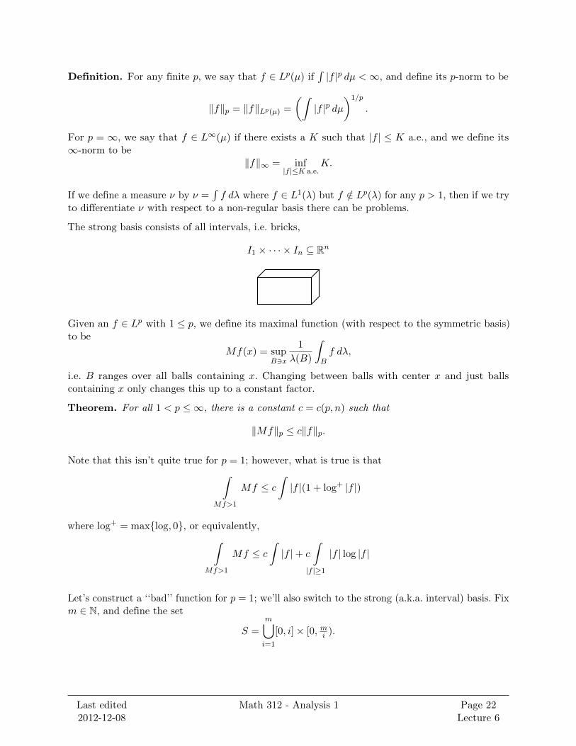
The strong basis consists of all intervals, i.e. bricks,

I1 × · · · × In ⊆ Rn

Given an f ∈ Lp with 1 ≤ p, we define its maximal function (with respect to the symmetric basis)to be

Mf(x) = supB3x

1

λ(B)

∫Bf dλ,

i.e. B ranges over all balls containing x. Changing between balls with center x and just ballscontaining x only changes this up to a constant factor.

Theorem. For all 1 < p ≤ ∞, there is a constant c = c(p, n) such that

‖Mf‖p ≤ c‖f‖p.

Note that this isn’t quite true for p = 1; however, what is true is that∫Mf>1

Mf ≤ c∫|f |(1 + log+ |f |)

where log+ = maxlog, 0, or equivalently,∫Mf>1

Mf ≤ c∫|f |+ c

∫|f |≥1

|f | log |f |

Let’s construct a ‘‘bad’’ function for p = 1; we’ll also switch to the strong (a.k.a. interval) basis. Fixm ∈ N, and define the set

S =

m⋃i=1

[0, i]× [0, mi ).



m

· · ·

m

1 1 1 1

m/2m/3

Note thatλ(S) = m

(1 + 1

2 + · · ·+ 1m

)∼ m log(m).

Let’s say that λ(S) = mLm, so that Lm ∼ log(m).

Now we will ‘‘fill’’ the unit square with disjoint similar copes of S. We do this in countably infinitelymany steps. In the first step, divide the unit square into m×m squares, and put a (scaled) copy ofS in each one.

· · ·

The measure of each scaled copy of S is Lmm , so that the proportion of the unit square that is covered

is exactly Lmm . Thus,

(1− Lm

m

)is missing. In the second step, divide up the remaining area into

small squares and do the same thing to each of them as what we just did to the unit square.

(one of the m2 squares in the above picture)

After the nth step, there will be(1− Lm

m

)nmissing from the square, which → 0 as n→∞ because

Lm ∼ log(m). Thus after doing this infinitely many times, there is a only null set U in the unit



square which we have not covered. Thus, we have

[0, 1]2 = disjoint union of S1, S2, . . . together with the null set U,

where the Si’s are scaled copies (with assorted scaling factors) of the original set S.

Let Gn ⊇ U be open sets with λ(Gn) < 12n . Define, for an (as yet) unchosen constant k,

gn = k ·(χGn + χlower left corners

of all the Si

),

where the ‘‘lower left corner’’ of an Si means the following region:

Remark. Obviously, gn depends on k; but note that the function gn also implicitly depends on ourinitial choice of m. This is important because we will later want to choose functions gn constructedin the above manner, but where each of them uses a different value of m.

In S (the original), the lower left corner has measure 1 and the whole set S has measure mLm, sothe ratio of the measures of the lower left corners and the union of the Si’s is 1

mLm. Thus,∫

gn ≤k

2n+

k

mLm.

Key observation: every x /∈ U (i.e. every x in some Si) is contained in a rectangle on which theaverage value of gn is ≥ k

m . For example,

Letting MSgn denote the maximal function of gn with respect the strong basis, this observationimplies that

MSgn(x) = supR3x

1

λ(R)

∫Rgn dλ ≥

k

m

for all x /∈ U (the supremum ranges over all rectangles R containing x).

For all small ε > 0 and large K, we choose an m such that Lm > 2Kε , and then set k = mK, so that

k

mLm=

K

Lm<ε

2.



Finally, note that we can choose n such that k2n <

ε2 . Thus, for all ε > 0 and K, we can choose

m, k, n such that∫gn =

k

2n+

k

mLm< ε and MSgn(x) ≥ K almost everywhere.

To summarize: for all ε and K, there is a g = gε,K such that∫g < ε and MSg > K.

Now define

g =

∞∑n=1

g1/2n,2n

so that ∫g =

∞∑n=1

∫g1/2n,2n ≤

∞∑n=1

1

2n= 1 =⇒ g ∈ L1,

even though MSg ≥MSg1/2n,2n > 2n for all n, i.e. MSg =∞.

This gets us an L1 function whose maximal operator is infinite, but how can we modify thisconstruction to a make a function whose derivative is also infinite?

In the construction of each function g1/2n,2n as n goes to ∞, let the maximum size of the staircasesused go to 0 (i.e., given the m chosen in the construction of g1/2n,2n , instead of initially subdividingthe unit square into m×m, divide it up even more finely). Then letting g =

∑g1/2n,2n again, we

can get DSg infinite almost everywhere.

This is necessary because the maximal operator is a supremum over all rectangles containing agiven point, while the derivative is defined in terms of shrinking sequences of rectangles containinga given point, so the increasing ‘‘badness’’ of the functions g1/2n,2n needs to be visible at smallerand smaller scales in order for the derivative to notice.

Going back to our theorem, here are two lemmas.

Lemma. For any f as in the theorem,

µ(x |Mf(x) > t) ≤ c

t

∫|f |> t

2

|f | dµ.

Lemma. For any g ≥ 0, ∫g dµ =

∫ ∞0

µ(x | g(x) > t) dt.

Proof. Using Fubini’s theorem, which we didn’t cover in class,∫ ∞0

µ(x | g(x) > t) dt =

∫ ∞0

∫χx|g(x)>t(x) dµ dt

=

∫ ∫ ∞0

χx|g(x)>t(x) dt︸︷︷︸∫ g(x)0 1 dt

dµ =

∫g(x) dµ .

This second lemma makes intuitive sense because it is one way of capturing the idea that theintegral is the area under a curve.



Lecture 7 (2012-10-23)

There will be no class on Thursday; there will instead be office hours in case anyone has questionsbefore the exam, which is next week (October 30).

Let M denote the collection of all measurable functions on a set X, and by M+, the collection of allnon-negative measurable functions f : X → [0,∞].

Consider an operator M : M → M+, such as the maximal operator M(f) = supB3x1|B|∫B |f |.

Suppose that ‖Mf‖∞ ≤ ‖f‖∞ for all f ∈M and M(f + g) ≤Mf +Mg, and also suppose that, forsome measure µ on X, there is some c > 0 such that

µ(x : Mf > t) < c‖f‖1t

.

(This last condition is called the ‘‘weak 1-1 inequality’’.)

Claim. Then there are constants cp, c′ such that ‖Mf‖p ≤ cp‖f‖p for all p > 1 and every f ∈M,

and ∫Mf>1

Mf(x) dµ ≤ c′∫X|f |(1 + log+ |f |) dµ.

Lemma. We have that

µ(x |Mf(x) > t) ≤ 2c

t

∫|f |> t

2

|f | dµ.

Proof. ‘‘Cut’’ f at ± t2 , and call this function f1; in other words take

f1 = maxminf, t2,−t2.

Let f2 = f − f1. Then |f1| ≤ t2 everywhere, so that by our assumptions about M , we have

‖Mf1‖∞ ≤ t2 , and hence Mf1 ≤ t

2 a.e. We also have

Mf ≤Mf1 +Mf2.

Let A = x |Mf(x) > t. Then for almost all x ∈ A,

t < Mf(x) ≤ t

2+Mf2(x)

so for almost all x ∈ A, t2 ≤Mf2(x). Now note that

µ(A) ≤ µ(x |Mf2(x) > t2)

weak 1-1≤ c‖f2‖1

t/2=

2c

t

∫X|f2| =

2c

t

∫|f |> t

2

|f2| ≤2c

t

∫|f |> t

2

|f |.

Lemma. For any g ∈M+, ∫Xg dµ =

∫ ∞0

µ(x | g(x) > t) dt.

Proof. This is clear from our intuition about integrals.



Proof of our claim. We have∫X|Mf |p dµ =

∫ ∞0

µ(x |Mf(x) > t1/p) dt.

Making the change of variables y = t1/p, this is equal to∫ ∞0

pyp−1µ(x |Mf(x) > y) dy.

From our first lemma, we have an inequality∫ ∞0

pyp−1µ(x |Mf(x) > y) dy ≤∫ ∞

0pyp−1 2c

y

∫|f |> y

2

|f | dµ dy

and then letting cp = 2cp,∫ ∞0

pyp−1µ(x |Mf(x) > y) dy ≤∫ ∞

0pyp−1 2c

y

∫|f |> y

2

|f | dµ dy =

∫∫0<y<2|f |

cpyp−2|f | dµ dy

= cp

∫|f |>0

|f |

(∫ 2|f |

0yp−2 dy

)dµ ≤ cp

∫|f |p

where, in the final expression above, the value of cp has changed by a constant factor.

Recall that a strong Lebesgue point just means a Lebesgue point with respect to the strong basis.

Theorem. If f ∈ Lp(R2) for p > 1, then almost every point is a strong Lebesgue point of f .

Lemma. For a measurable function f : [0, 1]2 → R+ such that f ∈ Lp for p > 1, let ϕ be themeasure defined by ϕ(A) =

∫A f dµ. Then∫

[0,1]2DSϕdλ ≤ cp‖f‖p.

Proof of Lemma. Fix some y. Take the maximal function in the x coordinate:

m(x, y) = supa≤x≤ b

1

b− a

∫ b

af(u, y) du

where supa≤x≤ b means the supremum over all intervals [a, b] ⊆ [0, 1] containing x. We will see thatm ∈ Lp. Define

E =

(x, y)

∣∣∣∣∣∣ limc≤ y≤ d(d−c)→0

1

d− c

∫ d

cm(x, v) dv = m(x, y)

.

If x ∈ [a, b], then

1

(b− a)(d− c)

∫[a,b]×[c,d]

f =1

d− c

∫ d

c

(1

b− a

∫ b

af(u, v) du

)dv ≤ 1

d− c

∫ d

cm(x, v) dv.



If (x, y) ∈ E, thenDSϕ(x, y) ≤ m(x, y).

Therefore, if we show that almost every point in [0, 1]2 is in E, and additionally show that∫[0,1]2 m(x, y) is bounded by cp‖f‖p, we will have proved the lemma.

We know that for one-dimensional functions in L1, almost every point is a Lebesgue point; thus, ifwe show that m is L1([0, 1]2), we will have that almost every one-dimensional ‘‘slice’’ of m is inL1([0, 1]), thereby implying that for almost every slice x × [0, 1], almost every point of the sliceis in E; this then implies that almost every point of [0, 1]2 is in E (apply Fubini’s theorem to thecharacteristic function of E).

Now we see that will be enough to show that∫

[0,1]2 m ≤ cp‖fp‖. This follows from the claim weproved earlier today:

∫[0,1]2

m ≤

∫[0,1]2

mp

1/p

=

(∫ 1

0

∫ 1

0mp(x, y) dx dy

)1/p

≤(∫ 1

0cp

∫ 1

0f(x, y)p dx dy

)1/p

= cp‖f‖p.

Proof of Theorem. WLOG, we can assume we are working in the unit square, because being aLebesgue point is a local property; we are taking smaller and smaller balls around a point, so wecan forget about what the function is doing far away.

Let f ∈ Lp. Choose a continuous g such that ‖f−g‖p < ε2. Let h = f−g, and define ϕ(S) =∫S |h| dλ.

Define two setsA = x : |h(x)| > ε, B = x : DSϕ(x) > ε.

We will show that these sets are small.

Note that ∫[0,1]2

h ≤ ‖h‖p < ε2

so that λ(A) ≤ ε. The lemma then implies that λ(B) ≤ cpε.

If x /∈ A ∪B, then (letting R be a sufficiently small rectangle)∫R|f(t)− f(x)| dt ≤

∫R|f(t)− g(t)| dt︸︷︷︸≤ ε|R| since x/∈B

+

∫R|g(t)− g(x)| dt︸︷︷︸

≤ ε|R| since g is continuousand R was chosen small enough

+

∫R|g(x)− f(x)| dx︸︷︷︸

= |g(x)−f(x)|·|R|≤ ε|R| since x /∈A

.

Thus, for any given ε > 0, the measure of the set of points x where

lim supR→x

1

|R|

∫R|f(t)− f(x)| dt > cε

is less than cε.

We’ve shown that in any regular basis, we can differentiate any L1 function (this fact, applied tocharacteristic functions, implies that almost every point of a set is a density point).



We’ve shown that in the strong basis, we can differentiate any Lp function for p > 1, but notnecessarily L1 functions (this fact, applied to characteristic functions, implies that almost everypoint of a set is a strong density point).

If, instead of axis-parallel rectangles, we take the basis consisting of all rectangles including rotatedones, then NOTHING IS TRUE.

Homework (∗). There exists a compact K ⊆ R2 of positive measure such that, for each x ∈ K,there exists a line segment that meets K at no other point. (Such a set is called a ‘‘hedgehog’’.)

A hedgehog set demonstrates that the rotated rectangle basis is bad; for any x ∈ K, we can choosesome other y ∈ K arbitrarily close to it such that, taking the line from x to y, we can find a linesegment and then a very thin rectangle around that line segment where most of the rectangle isdisjoint from the set K, making the density go to 0.



Lecture 8 (2012-10-25)

No class - office hours to ask questions before midterm.



Lecture 9 (2012-10-30)

Midterm.



Lecture 10 (2012-11-01)

Today we’ll go back over some more basic material that not everyone has seen yet.

Recall the definition of Lp space:

Definition. Given a measure space (X,µ), and a function f on X such that∫|f |p dµ < ∞, we

say that f ∈ Lp(µ). When there exists a K such that |f(x)| ≤ K almost everywhere, we say thatf ∈ L∞(µ).

Definition. A normed space is a vector space V with a function ‖ · ‖ : V → R such that

• ‖f‖ ≥ 0 for all f , with equality if and only if f = 0

• ‖cf‖ = |c| · ‖f‖

• ‖f1 + f2‖ ≤ ‖f1‖+ ‖f2‖

We say that V is complete if ρ(f, g) = ‖f − g‖ is a complete metric. A complete normed space iscalled a Banach space.

As we will see later, the norms

‖f‖p =

(∫|f |p dµ

)1/p

, ‖f‖∞ = infK : |f(x)| ≤ K a.e.

make Lp and L∞, respectively, into complete normed spaces, but only after we identify functions fand g if f = g a.e. (otherwise we can have ‖f‖ = 0 even when f 6= 0).

Theorem (Holder’s Inequality). For any f ∈ Lp and g ∈ Lq where 1p + 1

q = 1, and either

1 < p, q <∞ or p = 1, q =∞, we have fg ∈ L1 and

‖fg‖1 ≤ ‖f‖p‖g‖q.

Lemma. For any a, b ≥ 0 and 0 < λ < 1, we have aλb1−λ ≤ λa+ (1− λ)b.

Proof of lemma. Taking logarithms of both sides,

λ log(a) + (1− λ) log(b) ≤ log(λa+ (1− λ)b).

But log is concave,

x

y

log(x)

log(a)

log(b)

a b

so this is true.



Proof of Holder. Let’s do the case when ‖f‖p = 1 and ‖g‖q = 1 first. Let λ = 1p and 1− λ = 1

q , andlet a = |f(x)|p and b = |g(x)|q. The lemma implies that

|f(x)| · |g(x)| ≤ 1

p|f(x)|p +

1

q|g(x)|q,

and therefore ∫|f(x)| · |g(x)| ≤ 1

p

∫|f(x)|p︸︷︷︸= 1

+1

q

∫|g(x)|q︸︷︷︸= 1

=1

p+

1

q= 1.

In the general case, we can just let F = f‖f‖p and G = g

‖g‖q , so that we can apply the special case to

see that ∫|FG| ≤ 1

and hence ∫|fg|

‖f‖p‖g‖q≤ 1 =⇒

∫|fg| ≤ ‖f‖p‖g‖q.

Finally, if p = 1 and q =∞, we have that∫|fg| ≤

∫|f | ·K = K

∫|f |

when |g| ≤ K almost everywhere.

Theorem (Minkowski Inequality). For any 1 ≤ p ≤ ∞, we have

‖f + g‖p ≤ ‖f‖p + ‖g‖p

for any f, g ∈ Lp.

Proof. If p = 1 or p =∞, this is trivial. Now suppose 1 < p <∞. First, let’s show that f + g ∈ Lp:by the convexity of the logarithm again, we can see that∣∣∣∣f + g

2

∣∣∣∣p ≤ |f |p + |g|p

2

and therefore |f + g|p ≤ 2p−1(|f |p + |g|p). This shows that f + g ∈ Lp.

Now let q be the solution to 1p + 1

q = 1 and let F ∈ Lp. Then we claim |F |p−1 ∈ Lq. This is becausepq − q = p implies (

|F |p−1)q

= |F |p

and moreover‖|F |p−1‖qq = ‖F‖pp.

Now for the final step. Note that

‖f + g‖pp =

∫|f + g|p =

∫|f + g|p−1︸︷︷︸∈Lq

|f + g| ≤∫|f + g|p−1|f |+

∫|f + g|p−1|g|

Holder≤

∥∥|f + g|p−1∥∥q· ‖f‖p +

∥∥|f + g|p−1∥∥q· ‖g‖p = ‖f + g‖p/qp · ‖f‖p + ‖f + g‖p/qp ‖g‖p.



Therefore‖f + g‖pp ≤ ‖f + g‖p/qp (‖f‖p + ‖g‖p),

but since p− p/q = p(1− 1q ) = 1, this implies

‖f + g|p ≤ ‖f‖p + ‖g‖p.

Given a normed linear space B, and a sequence b1, b2, . . . ∈ B, let sn =∑n

j=1 bj ∈ B. Then we saythat the series

∑∞j=1 bj converges if there is an s ∈ B such that ‖sn − s‖ → 0. We say that it is

absolutely convergent if∑∞

j=1 ‖bj‖ <∞.

Theorem (Riesz-Fisher). For any 1 ≤ p ≤ ∞, Lp is complete.

Lemma. For any normed linear space B, B is complete if and only if every absolutely convergentsequence converges.

Proof of lemma. Suppose B is complete. For any absolutely convergent sequence b1, b2, . . . ,∈ B,

‖sn − sm‖ =

∥∥∥∥∥∥m∑

j=n+1

bj

∥∥∥∥∥∥ ≤m∑

j=n+1

‖bj‖ < ε

if n is large enough. Thus the sequence of sn’s is Cauchy, and because B is complete the limit exists.

Now conversely, suppose that b1, b2, . . . ∈ B is a Cauchy sequence, and assume that every absolutelyconvergent sequence in B converges. Then for any k, there exists an Nk such that for all n,m ≥ Nk,we have ‖bm − bn‖ < 1

2k. Thus,

bN1 + (bN2 − bN1) + (bN3 − bN2) + · · ·

is absolutely convergent because

‖bN1‖+ ‖bN2 − bN1‖+ ‖bN3 − bN2‖+ · · · ≤ ‖bN1‖+1

2+

1

4+

1

8+ · · · <∞

The partial sums of this series are just bN1 , bN2 , . . ., so that by the assumption that every absolutelyconvergent series converges, there must be some b ∈ B such that bNk → b. But since b1, b2, . . . is aCauchy sequence, we must also have that bn → b.

Homework. Prove the p =∞ case of the Riesz-Fisher theorem.

Proof of Riesz-Fisher. Let 1 ≤ p <∞. Then for any sequence f1, f2, . . . ∈ Lp, we want to show∑‖fn‖p︸︷︷︸σ

<∞ =⇒∑

fn converges in Lp to some function f.

Let gn =∑n

j=1 |fj |, which is in Lp. In particular, by Minkowski’s inequality,

‖gn‖p ≤n∑j=1

‖fj‖p ≤ σ,

and therefore∫|gn|p ≤ σp. The sequence of functions gn is monotone increasing, so gpn gp, and

therefore ∫gp = lim

∫gpn ≤ σp =⇒ gp <∞ a.e. =⇒ g <∞ a.e.



Thus,∑|fn(x)| converges for almost all x, so

f(x)def=∑

fn(x)

converges for almost all x. But we still need to show that the partial sums sn =∑n

j=1 fj(x) satisfy‖f − sn‖p → 0. To see this, observe that∫

|f − sn|p ≤∫

(|f |+ |sn|)p ≤∫

(2g)p,

and because |f − sn|p ∈ L1 and |f − sn|p → 0 a.e., we have that |f − sn|p → 0 in L1, which is thecase if and only if |f − sn| → 0 in Lp.

For the rest of this class, assume we have a finite measure space, so that µ(X) <∞.

Proposition. For any f ∈ Lp and ν < p, we also have f ∈ Lν . More generally,

L∞ ⊆ Lp ⊆ Lν ⊆ · · · ⊆ L1.

Proof. Intuitively, this is because raising to any power higher than 1 is no longer concave, it isconvex, making Minkowski’s inequality fail.

Letting X1 = x ∈ X | f(x) ≤ 1 and X2 = x ∈ X | f(x) > 1, we have that∫X

|f |p =

∫X1

|f |p

︸︷︷︸≤µ(X)<∞

+

∫X2

|f |p ≥∫X2

|f |ν

because |f |p ≥ |f |ν on X2, so that ∫X

|f |ν =

∫X1

|f |ν

︸︷︷︸≤µ(X)<∞

+

∫X2

|f |ν

is finite, and therefore f ∈ Lν .

Proposition. If f ∈ L∞, then f ∈ Lp for any p. Moreover, ‖f‖p → ‖f‖∞ as p→∞.

Proof. For any t < ‖f‖∞, we have that µ(A) > 0 where A = x | f(x) > t. Then∫X

|f |p ≥∫A

|f |p ≥∫A

tp = tpµ(A).

Thus ‖f‖p ≥ tµ(A)1/p. As p→∞, we have that

lim infp→∞

‖f‖p ≥ t · 1,

and therefore lim inf ‖f‖p ≥ ‖f‖∞. In the other direction, |f | ≤ ‖f‖∞ a.e., so that∫|f |p ≤

∫‖f‖p∞ = ‖f‖p∞ · µ(X),

and hence ‖f‖p ≤ ‖f‖∞ · µ(X)1/p. Therefore, lim supp→∞ ‖f‖p ≤ ‖f‖∞ · 1.



Homework. If µ(X) <∞, is it true that if f ∈ Lp for all 1 < p <∞, then f ∈ L∞?

Theorem. For any 1 ≤ p ≤ ∞, the simple functions are dense in Lp.

Proof. The case of p =∞ is easy - to define a simple function close to f ∈ L∞, break up the rangeof f in steps of size ε, and on the set x | kε ≤ f(x) < (k + 1)ε, set the simple function to be kε.This is a simple function because it will only take on finitely many values (since ‖f‖∞ is finite),and it differs from f by at most ε everywhere.

Now let 1 ≤ p <∞. Note that it is enough to show the claim is true for f ≥ 0. Fix an ε > 0, andlet A = x | f(x) > δ where δ is chosen such that∫

X/A|f |p < ε

4.

Choose an n such that An = x : f(x) ≤ n satisfies∫X\An

fp <ε

4.

Lastly, choose η such thatε

4µ(An)= ηp.

Then, again breaking up the range of f , we define the set

Mν = x ∈ An | (ν − 1)η ≤ f(x) ≤ νη,

and now we can define the simple function

g(x) =

0 if x /∈ An,(ν − 1) if x ∈Mν .

This satisfies∫|f − g|p =

∫X\A|f |p +

∑ν

∫Mν

|f − g|p +

∫A/An

|f |p <( ε

4

)+ ηp · µ(An)︸︷︷︸

= ε/4

+( ε

4

)< ε.

Next time, we’ll look more at the special properties of 1p + 1

q = 1. In particular, we’ll prove that the

dual of Lp is Lq and the dual of L1 is L∞.



Lecture 11 (2012-11-06)

There will be no class on Thursday.

There were 3 questions on the exam, with a maximum score of 1 each. The grading scale for themidterm is

A 2

B 1.5

C 1

D 0.5

Some people were confused about the definition of a measurable function. Recall that, for measurablespaces (X,A) and (Y,B), a function f : X → Y is (A,B)-measurable if for all B ∈ B, we havef−1(B) ∈ A. When Y is a topological space, then we just say A-measurable, because (unless specifiedotherwise) Y will be given the Borel σ-algebra. This is equivalent to requiring that f−1(G) ∈ A forall open G ⊆ Y .

Let’s get back to what we talked about last class.

Definition. Let B be a normed linear space. A linear map Λ : B → R (or Λ : B → C) is called alinear functional.

Definition. Let B1, B2 be normed linear spaces. A linear map A : B1 → B2 is called a linearoperator. We say that A is bounded if there is some K for which ‖Ax‖ ≤ K‖x‖ for all x ∈ B1. Thebest possible K is

sup‖x‖=1

‖Ax‖.

We call this the norm of A. It turns out that the bounded linear operators themselves form a normedlinear space under this norm; and in particular, we call

B∗ = bounded linear functionals Λ on B

the dual of B, which is a normed linear space with ‖Λ‖ = sup‖x‖=1 |Λ(x)|.

Example. Let B = Rn, with norm

‖x‖ = ‖x‖2 =(∑

x2j

)1/2.

What is B∗? Let e1, . . . , en denote the standard basis for Rn, and given a linear functional Λ, letΛ(ei) = ci. Then

Λ(x) =∑

xjcj = 〈x, c〉 ≤ ‖x‖2 · ‖c‖2,

so ‖Λ‖ ≤ ‖c‖2, and because |Λ(c)| = ‖c‖22 we must have that ‖Λ‖ = ‖c‖2. The map identifying Λwith c is linear, and it preserves norms. Thus B∗ ∼= B.

Theorem. For any 1 < p, q <∞ with 1p + 1

q = 1, or p = 1, q =∞, we have (Lp)∗ = Lq.

Remark. Note that this implies (L2)∗ = L2. Also, (L∞)∗ 6= L1.

What do we really mean by this theorem? For any Λ ∈ (Lp)∗, there is some g ∈ Lq such thatΛ(f) =

∫fg dµ for all f ∈ Lp.



Proof. Suppose that g ∈ Lq. Define Λ(f) =∫fg dµ. We need to show that this is in fact a bounded

linear operator.

It is obvious that Λ is linear, and it is bounded by Holder’s inequality:

|Λ(f)| =∣∣∣∣∫ fg

∣∣∣∣ ≤ ‖f‖p‖g‖q.This shows that ‖Λ‖ ≤ ‖g‖q, and in fact we have equality, because choosing f = gq−1, we have‖f‖pp = ‖g‖qq, and therefore ∣∣∣∣∫ fg

∣∣∣∣ =

∫|gq| = ‖f‖p‖g‖q.

Now we want to prove that any element of (Lp)∗ can be obtained this way. We will prove it in thecase that µ is finite, i.e. µ(X) <∞.

Homework. Prove this claim when µ is any σ-finite measure.

Given a linear functional Λ ∈ (Lp)∗, how can we construct the corresponding g? For any meausurableset A, we have that χA ∈ L∞ ⊆ Lp (this inclusion holds because µ is finite). Now denote Λ(χA) =ϕ(A). We claim that ϕ is a measure (note that we don’t know ϕ(A) will be positive, so this couldbe a signed measure).

Given pairwise disjoint measurable A1, A2, . . . we have

A =

∞⋃j=1

Aj =

( n⋃j=1

Aj

)∪( ∞⋃j=n+1

Aj︸︷︷︸Bn

).

Because Λ is linear,

ϕ(A) =

n∑j=1

ϕ(Aj) + ϕ(Bn).

We need to show that ϕ(Bn)→ 0 as n→∞. Because Λ is bounded,

|ϕ(Bn)| = |Λ(χBn)| ≤ ‖Λ‖ · ‖χBn‖Lp =↑

not truefor p=∞

‖Λ‖ · µ(Bn)1/p.

Because

µ(Bn) =∞∑

j=n+1

µ(Aj)→ 0 as n→∞,

we are done. Note that this also demonstrates that ϕ µ. By the Radon-Nykodim theorem, thereis some g ∈ L1 such that

Λ(χA) = ϕ(A) =

∫gχA dµ.

So, we just need to show that g ∈ Lq. In the case that p = 1, we have∣∣∣∣∫Ag dµ

∣∣∣∣ = Λ(χA) ≤ ‖Λ‖ · µ(A),



and therefore ∣∣∣∣ 1

µ(A)

∫Ag dµ

∣∣∣∣ ≤ ‖Λ‖for any meausurable A with µ(A) > 0. This shows that |g| ≤ ‖Λ‖ µ-a.e.

For 1 < p <∞, because

Λ(h) =

∫hg dµ for every characteristic function h,

we therefore also have that

Λ(h) =

∫hg dµ for every simple function h

because Λ and∫

are linear, and then

Λ(h) =

∫hg dµ for every L∞ function h

because if h ∈ L∞ then for any ε > 0 there is some simple h1 such that ‖h − h1‖∞ < ε (we’veproved this before), and this means that∣∣∣∣Λ(h)−

∫hg

∣∣∣∣ =

∣∣∣∣Λ(h− h1)−∫

(h− h1)g + Λ(h1)−∫h1g︸︷︷︸

= 0

∣∣∣∣ ≤ |Λ(h− h1)|︸︷︷︸≤‖Λ‖·‖h−h1‖p≤‖Λ‖·εµ(X)1/p

+

∣∣∣∣∫ (h− h1)g

∣∣∣∣︸︷︷︸≤ ε·‖g‖1

.

Because g ∈ L1, the sets An = x : |g(x)| ≤ n have the property that µ(X \ An)→ 0 as n→∞.Let

f = |g|q−1 · sign(g) · χAn .Because f ∈ L∞, we know that Λ(f) =

∫fg. We have∫

An

|g|q = Λ(f) ≤ ‖Λ‖ ·(∫

X|f |p

)1/p

= ‖Λ‖ ·(∫

An

|g|q)1/p

and therefore (∫An

|g|q)1−1/p

=

(∫An

|g|q)1/q

≤ ‖Λ‖

for all n, which implies that ‖g‖q ≤ ‖Λ‖. To show that there is actually equality, choose f suchthat ‖f‖pp = ‖g‖qq.

Now we will prove Fubini’s theorem. First, we need to discuss what it means to take the product oftwo measures.

Given two measure spaces (X,A, µ) and (Y,B, ν), for any A ∈ A and B ∈ B, we define ϕ(A×B) =µ(A) · ν(B). We extend ϕ to a measure on the σ-algebra on Z = X × Y which is generated by setsof the form A×B for A ∈ A, B ∈ B.

Theorem (Fubini). If ϕ is σ-finite and∫Z f dϕ exists, then the function

g(x)def=

∫Yf(x, y) dν

exists for almost all x ∈ X, and ∫Xg(x) dµ =

∫Zf dϕ.



Homework. Let X = Y = [0, 1], and define f : X × Y → R to be

f(x, y) =

1 if x = y,

0 if x 6= y.

Let µ be Lebesgue measure on X, and ν be counting measure on Y . Calculate∫X

(∫Yf(x, y) dν

)dµ

and ∫Y

(∫Xf(x, y) dµ

)dν,

and explain why Fubini fails.

Homework. On the midterm, you showed that for measurable A,B ⊆ [0, 1], the function

f(t) = λ(A ∩ (B + t))

is continuous. Now, find∫f(t).



Lecture 12 (2012-11-08)

No class.



Lecture 13 (2012-11-13)

Today we’ll talk about calculus of several variables.

On the real line, we know ∫ b

af(x) dx = F (b)− F (a), f = F ′.

Note that a, b is the boundary of the interval [a, b].

Does this generalize to higher dimensions? That is, given some region H, can we say∫H

(something) =

∫∂H

(something else) ?

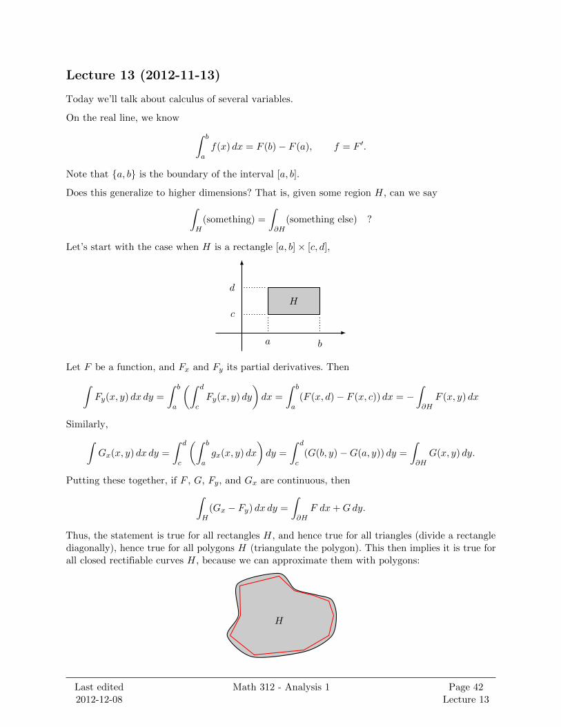
Let’s start with the case when H is a rectangle [a, b]× [c, d],

H

a b

c

d

Let F be a function, and Fx and Fy its partial derivatives. Then∫Fy(x, y) dx dy =

∫ b

a

(∫ d

cFy(x, y) dy

)dx =

∫ b

a(F (x, d)− F (x, c)) dx = −

∫∂H

F (x, y) dx

Similarly,∫Gx(x, y) dx dy =

∫ d

c

(∫ b

agx(x, y) dx

)dy =

∫ d

c(G(b, y)−G(a, y)) dy =

∫∂H

G(x, y) dy.

Putting these together, if F , G, Fy, and Gx are continuous, then∫H

(Gx − Fy) dx dy =

∫∂H

F dx+Gdy.

Thus, the statement is true for all rectangles H, and hence true for all triangles (divide a rectanglediagonally), hence true for all polygons H (triangulate the polygon). This then implies it is true forall closed rectifiable curves H, because we can approximate them with polygons:

H



with ∫P→∫H,

∫∂P→∫∂H

.

Finally, this implies it is true for all H with rectifiable boundary (rectifiable means finite length).

Remark. What exactly do we mean by∫γ f dg for a curve γ? We break up γ into smaller and

smaller segments

y1

y2

y3 y4y5

y6

y7

y8x0

x1

x2

x3x4

x5

x6

x7 x8

and then define the integral to be the limit of the quantity∑f(yj)(g(xj)− g(xj−1)).

Given a domain H ⊆ Rd (which may have holes),

and a function ϕ = (ϕ1, . . . , ϕd) on H, we say that a function u : H → R is a primitive of ϕ if u isdifferentiable on H and u′ = ϕ.

Does every function have a primitive? No. Suppose u′ = (f, g), and that u is twice differentiable; iff = ux and g = uy, then

fy = uxy = uyx = gx.

Our result above implies that for any rectifiable curves γ and γ′ with endpoints (x0, y0) and (x, y),

(x0, y0)

(x, y)

γ

γ′

(x0, y0)

(x, y)

we will have ∫γf dx+ g dy = u(x, y)− u(x0, y0) =

∫γ′f dx+ g dy.



Therefore, a necessary condition is that∫γ = 0 for any closed curve γ. When we assume everything

is nice, it turns out this is also a sufficient condition.

Theorem. Given continuous f, g on H, there is a primitive u for ϕ = (f, g) if and only if∫γ f dx+ g dy = 0 for any closed curve γ.

Proof. We just did the =⇒ direction.

To see ⇐= , fix some (x0, y0) ∈ H, and define

u(x, y) =

∫γf dx+ g dy

where γ is any curve that connects (x0, y0) to (x, y).

Because

u(x, y + h)− u(x, y)

h=

∫ y+hy g(t) dt

h→ g(y) as h→ 0

and similarly with x and f , we are done.

Theorem. If f, g are differentiable on H, and H is simply connected, then there exists a primitiveu for (f, g) if and only if gx = fy.

Proof. We’ve done the =⇒ direction.

To see ⇐= , note that because H is simply connected, the region bounded by any curve γ in H isa domain A entirely contained inside H, and therefore∫

γf dx+ g dy =

∫Agx − fy︸︷︷︸

= 0

dxdy = 0.

Definition. If u is twice differentiable, we say that u is harmonic if

∆u = uxx + uyy = 0.

∆ is called the Laplace operator.

Examples. Clearly, any linear function is harmonic. For a second order polynomial u = ax2 +bxy+ cy2, we have ∆u = 2a+ 2c, so that x2− y2 and xy are a basis for the vector space of harmonicsecond order polynomials.

Homework. Find a basis for the vector space of harmonic polynomials in x and y of degree 6.

The key property of harmonic functions is that their value at a point is determined by their integralon a circle around that point, which is what we’ll prove now.

We know that ∫HGx =

∫∂H

G,

∫HFy = −

∫∂H

F.

Let’s choose G = uxv and F = uyv, for some function v. We get that∫H

(uxxv + uxvx) dxdy =

∫∂H

uxv,

∫H

(uyyv + uyvy) dx dy = −∫∂H

uyv.



Thus ∫H

(∆u)v + 〈u′, v′〉 dxdy =

∫∂H

v(ux dy − uy dx) =

∫∂H

v · ∂u∂n

ds

where ux dy − uy dx = 〈u′, (dy,−dx)〉 = 〈u′, n′〉 (?) and n is the normalized unit vector in the radialdirection (see picture below). This is known as the first Green formula.

The second Green formula (or symmetric Green formula) says that∫H

(∆u · v −∆v · u) =

∫∂H

v · ∂u∂n− u · ∂v

∂n.

Choosing v ≡ 1, we have ∫H

∆u =

∫∂H

∂u

∂n,

and therefore, if u is harmonic, then ∫∂H

∂u

∂nds = 0.

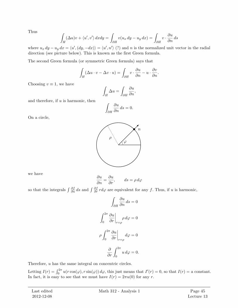
On a circle,

ρ

n

ϕ

we have∂u

∂n=∂u

∂r, ds = ρ dϕ

so that the integrals∫ ∂f∂n ds and

∫ ∂f∂r rdϕ are equivalent for any f . Thus, if u is harmonic,∫

∂H

∂u

∂nds = 0

∫ 2π

0

∂u

∂r

∣∣∣∣r=ρ

ρ dϕ = 0

ρ

∫ 2π

0

∂u

∂r

∣∣∣∣r=ρ

dϕ = 0

∂

∂r

∫ 2π

0u dϕ = 0.

Therefore, u has the same integral on concentric circles.

Letting I(r) =∫ 2π

0 u(r cos(ϕ), r sin(ϕ)) dϕ, this just means that I ′(r) = 0, so that I(r) = a constant.In fact, it is easy to see that we must have I(r) = 2πu(0) for any r.



If u is harmonic and v = 14(x2 + y2), then ∆v = 1. Letting H = B(0, ρ),∫

Hu =

∫ 2π

0

(u · 1

2ρ− 1

4ρ2∂u

∂r

)ρ dϕ =

ρ2

2

∫ 2π

0u dϕ.

Therfore1

πρ2

∫B(0,ρ)

u =1

2π

∫ 2π

0u dϕ.

This says that the average of u on the disc is equal to its average on a circle, which is equal to u(0).

Let’s consider harmonic functions that depend only on one variable. For example, if u(x, y) = u(x),then we have uxx + uyy = uxx = 0, so u = ax+ b.

Homework. If u(x, y) depends only on r, what form must u have? What if u depends only on ϕ?

Let’s consider the Laplacian in polar coordinates. We will write u(r, ϕ) = u(r cos(ϕ), r sin(ϕ)). Whatdoes it mean to say ∆u = 0? We have

ur = ux cos(ϕ) + uy sin(ϕ)

sourr = (uxx cos(ϕ) + uxy sin(ϕ)) cos(ϕ) + (uyx cos(ϕ) + uyy sin(ϕ)) sin(ϕ).

We also haveuϕ = −ux · r sin(ϕ) + uy · r cos(ϕ)

so

uϕϕ = −r(−uxxr sin(ϕ)+uxyr cos(ϕ)) sin(ϕ)−ux cos(ϕ)+r cos(ϕ)(−uyxr sin(ϕ)+uyyr cos(ϕ))−uyr sin(ϕ)

Taken all together, we therefore have ∆u = 0 implies

uϕϕ + r2urr + rur = 0.

If u depends only on r, then r2 · u′′ + ru′ = 0, so that r · f ′ + f = 0 where u′ = f , and therefore

f ′

f= −1

r

(log(f))′ = − log(r)′

so u = c log(r) + d.



Lecture 14 (2012-11-15)

Homework. Does the function(

yx2+y2

, −xx2+y2

)have a primitive on the following domains? If yes,

find one.

1. The upper half plane

2. The lower half plane

3. The right half plane

4. The left half plane

5. R2 \ 0

Last time, we showed that log(r) is harmonic on R2 \ 0.

Let u, v be harmonic, and assume that v is of the form v = − log(r) + w.

ρ

R

Because u and v are harmonic (i.e. ∆u = 0 and ∆v = 0) and using the second Green’s identity,

0 =

∫ 2π

0R

[u

(− 1

R+∂u

∂r

∣∣∣∣r=R

)− (− log(R) + w)

∂u

∂r

∣∣∣∣r=R

]−∫ 2π

0ρ

[u

(−1

ρ+∂u

∂r

∣∣∣∣r=ρ

)− (− log(ρ) + w)

∂u

∂r

∣∣∣∣r=ρ

]

=

∫ 2π

0

(u∂w

∂r

∣∣∣∣r=R

− w∂u∂r

∣∣∣∣r=R

)︸︷︷︸

= 0

R−∫ 2π

0

(u∂w

∂r

∣∣∣∣r=ρ

− w∂u∂r

∣∣∣∣r=ρ

)︸︷︷︸

= 0

ρ+

∫ 2π

0

−uR·R∣∣∣∣r=R

+R log(R)

∫ 2π

0

∂u

∂r

∣∣∣∣r=R︸︷︷︸

= 0

−ρ log(ρ)

∫ 2π

0

∂u

∂r

∣∣∣∣r=ρ︸︷︷︸

= 0

+

∫ 2π

0

u

ρ· ρ∣∣∣∣r=ρ

Thus, letting

I(r) =

∫ 2π

0u(r cos(ϕ), r sin(ϕ)),

we have that 0 = −I(r) + I(ρ), so that I(r) = constant = 2πu(0, 0).

Corollary (Maximum Principle). If u is harmonic on a domain H, then if there is any (x0, y0) ∈ Hsuch that u(x0, y0) = max(x,y)∈H u(x, y), then u is constant. Moreover, the same is true for a localmaximum.



Proof. Suppose that u(x0, y0) is maximal on B((x0, y0), R). Then for any 0 < r < R,

1

2π

∫ 2π

0u(x0 + r cos(ϕ), y0 + r sin(ϕ)) = u(x0, y0),

so1

2π

∫ 2π

0(u(x0, y0)− u(x0 + r cos(ϕ), y0 + r sin(ϕ)))︸︷︷︸

≥ 0

= 0,

so because u is continuous, we must have that u is constant on B((x0, y0), R).

For the case of a global maximum, suppose S = supH u. If S =∞, then nothing to prove, and ifS <∞, let A = z | u(z) = S. By what we’ve proved about local maxima, A must be open; butbecause u is continuous, A must be closed. Because H is a domain, it is connected, so this forcesA = ∅ or A = H.

The minimum principle is also true, because the negative of a harmonic function is still harmonic.

Corollary (Uniqueness). If u and v are harmonic on H, and continuous on the closure H, thenu|∂H = v|∂H implies that u = v on H.

Proof. If u and v are harmonic on H, then u− v is also harmonic on H, and u− v|∂H = 0. If u− vis not constant, then maxH(u− v) can only be attained on ∂H, and same for the minimum.

Remark. We are assuming throughout that the boundaries of our domains H are rectifiable curves,so in particular, domains H are assumed to be precompact.

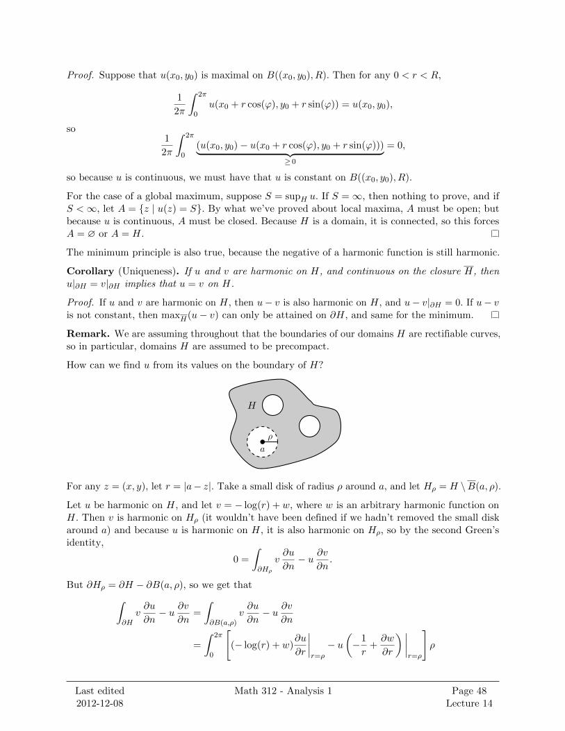
How can we find u from its values on the boundary of H?

a

ρ

H

For any z = (x, y), let r = |a− z|. Take a small disk of radius ρ around a, and let Hρ = H \B(a, ρ).

Let u be harmonic on H, and let v = − log(r) + w, where w is an arbitrary harmonic function onH. Then v is harmonic on Hρ (it wouldn’t have been defined if we hadn’t removed the small diskaround a) and because u is harmonic on H, it is also harmonic on Hρ, so by the second Green’sidentity,

0 =

∫∂Hρ

v∂u

∂n− u ∂v

∂n.

But ∂Hρ = ∂H − ∂B(a, ρ), so we get that∫∂H

v∂u

∂n− u ∂v

∂n=

∫∂B(a,ρ)

v∂u

∂n− u ∂v

∂n

=

∫ 2π

0

[(− log(r) + w)

∂u

∂r

∣∣∣∣r=ρ

− u(−1

r+∂w

∂r

) ∣∣∣∣r=ρ

]ρ



= − log(ρ)

∫ 2π

0

∂u

∂r

∣∣∣∣r=ρ︸︷︷︸

= 0

ρ+

∫ 2π

0

(w∂u

∂r− u∂w

∂r

)︸︷︷︸

= 0, by second Green’s

ρ+

∫ 2π

0u

= 2πu(a)

and therefore ∫∂H

((− log(r) + w)

∂u

∂n− ∂(− log(r) + w)

∂nu

)= 2πu(a).

This is known as the third Green’s identity.

The Dirichlet problem is, for a given function f , how to find a w with ∆w = 0 and w|∂H = f . Itturns out that if F is twice differentiable, and F |∂H = f , then we can take w = minF

∫H |F

′|2; thatis, the minimum is attained at a function F which is harmonic (we leave this without proof).

Definition. The Green function ga(z) = − log(r) + wa is defined as follows. We want

1. continuous on H and ≡ 0 on ∂H.

2. ga(z) ≥ 0 (in fact ga > 0 except on the boundary); this is because − log(r) is arbitrarily largeclose to r = a (we threw out a small disk around a though), so the function is positive atsome point, so 0 (the value on the boudnary) must be the minimum.

3. ga + log |a− z| is harmonic on H.

It turns out that these properties specify ga(z) uniquely.

Theorem. For any a 6= b, ga(b) = gb(a).

Proof. We take the domain H and throw out disks of radius ρ around a and b, to avoid thesingularities of the logarithms there. Call the resulting domain Hρρ, i.e.

Hρρ = H \ (B(a, ρ) ∪B(b, ρ)).

Then because ga and gb are harmonic on Hρρ, and because they are 0 on ∂H, we have∫∂Hρρ

(ga∂gb∂n− gb

∂ga∂n

)= 0 and

∫∂H

(ga∂gb∂n− gb

∂ga∂n

)= 0

which, because ∂H = ∂Hρρ + ∂B(a, ρ) + ∂B(b, ρ), implies∫∂B(a,ρ)

(ga∂gb∂n− gb

∂ga∂n

)+

∫∂B(b,ρ)

(ga∂gb∂n− gb

∂ga∂n

)= 0.

Note that ∫∂B(a,ρ)

(ga∂gb∂r

∣∣∣∣r=ρ

− gb∂ga∂r

∣∣∣∣r=ρ

)ρ

=

∫∂B(a,ρ)

[(− log(r) + wa)

∂gb∂r

∣∣∣∣r=ρ

− gb∂(− log(r) + wa)

∂r

∣∣∣∣r=ρ

]ρ,

and (because wa is harmonic) the only non-zero term in this is∫gb

1

ρρ = 2πgb(a).



However, we have to be careful in applying the same calculation to the other integral, namely∫∂B(b,ρ), because in the expression

∫∂B(a,ρ)

(ga∂gb∂r

∣∣∣∣r=ρ

− gb∂ga∂r

∣∣∣∣r=ρ

)ρ

switching a and b gives a minus sign. Thus,

2πgb(a)− 2πga(b) = 0,

and we are done.

Now we will compute the Green function for B(0, 1). We write ga(z) = − log |z − a|+ w. We knowthat we want ga(z) = 0 if |z| = 1, and choosing a = 0, we see that g0(z) = − log(z) works. Whathappens for a 6= 0 though?

We apply Appollonius’s theorem, which is that the set of points z such that |z−a||z−b| = constant is acircle,

a b

Homework. Prove Appollonius’s theorem.

We choose a b such that |a| · |b| = 1, and we see that the circle for which |z−b||z−a| = 1|a| is precisely the

circle |z| = 1.

We have

log |z − b| − log |z − a| = log

(1

|a|

)and

w = log |z − b|+ log |a|,

so that

ga(z) = log

(|a| · |z − b||z − a|

).

Let z = (r cos(ϕ), r sin(ϕ)), a = (ρ cos(θ), ρ sin(θ)), and b = (1ρ cos(θ), 1

ρ sin(θ)).

Then

log |z − a| = 1

2log |z − a|2 =

1

2log(r2 + ρ2 − 2rρ cos(ϕ− θ)

),

so that∂

∂rlog |z − a| = 1

2· 2r − 2ρ(cos(ϕ− θ))r2 + ρ2 − 2rρ cos(ϕ− θ)

and∂

∂rlog |z − b| = 1

2·

2r − 21ρ(cos(ϕ− θ))

r2 + 1ρ2− 2r 1

ρ cos(ϕ− θ).

Therefore

− ∂

∂nlog

(|a||z − b||z − a|

)=

1− ρ2

1− 2ρ cos(ϕ− θ) + ρ2.



Theorem. If u is harmonic on B(0, 1), then

u(a) =1

2π

∫ 2π

0u(cos(ϕ), sin(ϕ)) · 1− ρ2

1− 2ρ cos(ϕ− θ) + ρ2

for every ρ < 1.

The function P (ρ, δ) = 1−ρ21−2ρ cos(δ)+ρ2

is very special, so it has a name: the Poisson kernel.

Corollary.1

2π

∫ 2π

0P (ρ, ϕ− θ) = 1.

Homework. Prove that P (x, y) = P (ρ cos(δ), ρ sin(δ)) is harmonic.



Lecture 15 (2012-11-20)

Recall that last time, we defined the Poisson kernel

P (ρ, δ) =1− ρ2

1− 2ρ cos(δ) + ρ2.

We know that P is harmonic.

Theorem. If u is harmonic on |z| < 1 and continuous on |z| ≤ 1, then

u(a) = u(ρ cos(ν), ρ sin(ν)) =1

2π

∫ 2π

0u · P (ρ, ϕ− ν) dϕ.

Theorem. If f = f(cos(ϕ), sin(ϕ)) is continuous, then

u(a)def=

1

2π

∫ 2π

0f · P (ρ, ϕ− ν) dϕ

is harmonic on the open disc |z| < 1. and

u∗(a) =

u(a) if |a| < 1,

f(a) if |a| = 1

is continuous. Thus, the Poisson kernel preserves continuity.

Proof. Because P is harmonic, and finite sums of harmonic functions are harmonic, then in thelimit, the integral defining u(a) is harmonic.

Now, we want to show that u∗(a) is continuous, i.e. that u(a) is close to f(a′) if a is close to a′:

a

a′

This is because the Poisson kernel will weight values close to a′ more than further points. Thus, weare taking the weighted average concentrated around a′. When a is close to a′, we have that ρ ≈ 1and ν ≈ ϕ, so that the Poisson kernel is approximately

1− ρ2

2[1− cos(ν − ϕ)]]≈ small

small.

Homework. Formally prove that u∗(a) is continuous.

For the following material, you should read the proofs somewhere yourself.

Definition. Given f ∈ L1([0, 2π]), the Fourier coefficients of f are defined to be

cn =1

2π

∫ 2π

0f(x)e−inx, −∞ < n < +∞.



Theorem.

1. f ∈ L1 implies that cn → 0 as n→ ±∞.

2. f ∈ L2 implies that∑|cn|2 <∞. Moreover,

∑|cn|2 = ‖f‖2.

Remark. In the measure space (Z, P (Z),#) (i.e., Z with the counting measure), then c(n) ∈ L2 ifand only if

∑|cn|2 <∞. L2 of this measure space is usually referred to as `2. The Fourier transform

is a bijection between L2 functions on S1 and L2 functions on Z.

Remark. We can define the partial sum functions

SN =N∑

n=−Ncne

int.

The sequence of SN ’s is Cauchy in L2, and therefore it converges in L2.

Note that1

2π

∫ 2π

0einxe−imx dx =

1 if n = m,

0 if n 6= m.

In fact, defining an inner product on L2 by 〈f, g〉 =∫fg, we have that the functions einx√

2π form an

orthonormal basis of L2 (note that we have normalized them with a factor of 1√2π

). We also see that

〈f, f〉 =

∫|f |2 = ‖f‖2.

Convolution

Integrating against the Poisson kernel is a special case of something called convolution.

Given f : Z→ C such that∑∞

n=−∞ |f(n)| <∞, then

f(x) =∞∑

n=−∞f(n)eixn,

(Z is the unit circle, i.e. R/[0, 2π]).

Now consider

f(x) · g(x) =

( ∞∑n=−∞

f(n)eixn)( ∞∑

m=−∞g(m)eimx

).

By Fubini’s theorem, this is equal to∑n+m

f(n)g(m)eix(n+m) =∑k

eikx∑

k=m+n

f(m)g(n) = (f ∗ g)(x),

where f ∗ g is the convolution of f and g.

Proposition. If f, g ∈ L1(Z), then (f ∗ g) ∈ L1(Z).



Proof. ∑k

|(f ∗ g)(k)| =∑k

∣∣∣∣ ∑k=m+n

f(n)g(m)

∣∣∣∣≤∑k

∑k=m+n

|f(n)||g(m)|

=

(∑n

|f(n)|)(∑

k

|g(k −m)|)

= ‖f‖1‖g‖1

Now, instead of considering the functions n 7→ einx, let’s look at t 7→ eixt, where x, t ∈ Rd and xtmeans the dot product of x and t.

Definition. For f, g ∈ L1(Rd), define their convolution to be

(f ∗ g)(x) =

∫Rdf(y)g(x− y) dy.

Theorem. For any f, g ∈ L1(Rd),

1. f ∗ g exists at almost every x.

2. f ∗ g ∈ L1 and ‖f ∗ g‖1 ≤ ‖f‖1‖g‖1.

3. ∗ is commutative and associative.

Proof. Observe that∫Rd

∫Rd|f(y)||g(x− y)| dy dx =

∫Rd|f(y)|

(∫Rd|g(x− y)| dx

)dy

=

∫|f(y)| · ‖g‖1 dy = ‖f‖1‖g‖1,

which proves claim 2. This also implies that∫|f(y)||g(x− y)| dy <∞

at almost every x, so indeed f ∗ g exists a.e., which is claim 1.

Claim 3 is clear; for example, swap f and g in the sum for commutativity.

Homework. If f ∈ L1 and g ∈ Lp, does it follow that f ∗ g ∈ Lp and ‖f ∗ g‖p ≤ ‖f‖1‖g‖p?

Homework. If 1p + 1

q = 1 and f ∈ Lp, g ∈ Lq, show that f ∗ g is continuous and tends to 0 as|x| → ∞.

Homework. Prove that there is no ‘‘unit’’ function, i.e. that there is no f ∈ L1 such that f ∗ g = gfor every g ∈ L1.

Lemma. Let f ∈ L1 and y ∈ Rd. Define fy(x) = f(x+ y). Then

limy→0‖fy − f‖1 = 0.



Proof. If f is continuous and compactly supported, then this is trivial; if we integrate a small ε ona bounded set, we’ll get something small.

Now, take an arbitrary f ∈ L1, and choose a g which is continuous and compactly supported suchthat ‖f − g‖1 < ε. Then

fy − f = (fy − gy) + (gy − g) + (g − f),

Note that fy − gy = (f − g)y, so that

‖fy − f‖1 ≤ ‖fy − gy‖1 + ‖gy − g‖1 + ‖g − f‖1 < 3ε.

For t ∈ R, let ft (not translation) be a non-negative function such that∫ft = 1 and ft(x) = 0 for

|x| > t. These functions are ‘‘approximate units’’.

t

We can think of ft ∗ g as a weighted average of g around 0.

Theorem. For any g ∈ L1, we have ‖ft ∗ g − g‖1 → 0 as t→ 0.

Proof. First, note that

‖ft ∗ g − g‖1 =

∫ ∣∣∣∣ ∫ ft(y)g(x− y) dy − g(x)

∣∣∣∣ dx=

∫ ∣∣∣∣ ∫ ft(y)(g(x− y)− g(x)) dy

∣∣∣∣ dx≤∫ t

−t

∫Rd|g(x− y)− g(x)| dx ft(y) dy

and, by the lemma, once t is sufficiently small we have that

≤ ε∫|y|<t

ft(y) dy = ε.

Example. We could take

ft(y) =χB(0,t)(y)

λ(B(0, t)),

in which case

(ft∗g)(x) =

∫g(x−y)ft(y) dy

commutativity=

1

λ(B(0, t))

∫Rdg(y)χB(0,t)(x−y) dy =

1

λ(B(0, t))

∫B(0,t)

g,

which goes to g(x) a.e.

Example. Let 1p + 1

q = 1. We could take f ∈ Lp, and map g ∈ Lq to∫fg. We know that

‖f‖p = ‖Λf‖ = supg∈Lq‖g‖q=1

|Λf (g)|.



Theorem. Let 1p + 1

q = 1, with p <∞. For any f ∈ Lp and g ∈ Lq,

(f ∗ g)(x) =

∫f(x− y)g(y) dy

exists for every x, and in fact is continuous. Moreover, ‖f ∗ g‖∞ ≤ ‖f‖p‖g‖q.

Theorem. Let ft be approximate units, and let g ∈ Lp with 1 < p <∞. Then ‖ft ∗ g − g‖p → 0 ast→ 0.

Proof. It will suffice to prove that for any h ∈ Lq,∫Rd

(ft ∗ g − g)h ≤ (small constant)‖h‖q,

because Lp is the dual of Lq and this would show that the operator norm of the integrate-against-(ft ∗ g − g) operator on Lq (which is equal to the Lp norm of ft ∗ g − g) is small. We knowthat

g(x) =

∫ft(y)g(x) dy,

so that ∫ ∫(g(x− y)− g(x))ft(y)h(x) dy dx ≤

∫|y|<t‖gy − g‖p‖h‖q dy.

Therefore, it will suffice to show that ∫|y|<t‖gy − g‖p → 0

as t→ 0; but this is clear.



Lecture 16 (2012-11-27)

Today we’ll be starting probability. We’ll mainly discuss some terminology and notations.

Definition. We say that (Ω,F , P ) is a probability space when it is measure space (Ω being theunderlying set, F the σ-algebra, and P the measure) such that P (Ω) = 1. We say that Ω is the setof outcomes, F is the σ-algebra of events, and P is the probability measure.

Examples.

• We can make a probability space representing flipping a coin n times. We let Ω = H,Tn,F = all subsets of Ω, and P (ω) = 1

2n for each ω ∈ Ω.

• Now suppose we are flipping a coin infinitely many times. Then Ω consists of all infinitesequences of H and T , and F is the σ-algebra generated by cylinder sets, e.g.

(x1, x2, . . .) ∈ Ω | x1 = H,x2 = T, . . . , xn = H.

Finally, we define P to be the product measure (12δH + 1

2δT )N, or in other words the measuresuch that P (C) = 1

2n when C is a cylinder set in which the first n coordinates have been fixed.

Definition. A random variable X is a function X : Ω → (−∞,∞) such that X−1(B) ∈ F forevery Borel B ⊆ R. We define

µX(B)def= P (X ∈ B) = P (X−1(B)),

which specifies a measure on R. We say that this is the distribution of X. The distribution functionof X is the function defined by F (x) = µX((−∞, x]) = P (X ≤ x).

Here are some basic properties of the distribution function.

• limx→∞

F (x) = 1.

• limx→−∞

F (x) = 0.

• F is monotone increasing.

• F is right continuous, but not necessarily left continuous:

limε→0+

F (x+ ε) = F (x) 6= limε→0−

F (x+ ε).

It turns out these properties actually characterize the functions F which are distribution functions.We can see this by defining

µX((−∞, x])def= F (x),

then extending µX to all Borel sets.

Definition. If there is a function f : R → [0,∞) such that P (a ≤ x ≤ b) =∫ ba f , we say that

f is the density of X. If it exists, we then have that∫∞−∞ = 1, and if f is continuous at x then

f(x) = F ′(x).

Definition. The characteristic function of an event E ∈ F , i.e. the function

χE(ω) =

1 if ω ∈ E,0 if ω /∈ E,

is called an indicator function when we are doing probability.



Examples.

• Returning to flipping coins, we let (Ω,F , P ) represent flipping a coin infinitely many times.Define

Xn(ω1, ω2, . . .) = ωn =

1 if nth flip is head,

0 if nth flip is tail,

and let Sn = X1 + · · ·+Xn. Then Sn is the number of heads in the first n flips. Define Fn tobe the σ-algebra of events that depend only on the first n flips. Then Sn is also a randomvariable on (Ω,Fn, P ), but Sn+1 is not.

• Let µ be a probability measure on (R,Borel). Consider the random variable X : R→ R whichis the identity function on R. Then µX = µ.

• We say that X has normal distribution with mean µ and variance σ2 if X has density

f(x) =1√

2πσ2e−(x−µ)2/2σ.

In particular, the standard normal distribution (µ = 0, σ = 1) has density f(x) = 1√2πe−x

2/2,

so that

Φ(x) =

∫ x

−∞

1√2π

e−t2/2 dt.

• If X is a random variable and g : R→ R is a Borel-measurable function, then Y = g(X) isalso a random variable.

• The Cantor function

0

1

12

14

34

13

23

19

29

79

89 10

is a continuous function from R to [0, 1], and it is a distribution of some random variable (itmeets all of the criteria we set above). It has no atoms (i.e., no points of positive measure),and no density function. Its distribution is also not absolutely continuous with respect to theLebesgue measure, because the Cantor function maps the Cantor set (which has Lebesguemeasure 0) onto [0, 1] (which has positive Lebesgue measure).

Definition. The expected value E(X) of a random variable X is defined to be

E(X) =

∫X dP =

∫x dµX .

However, E(X) may not exist, because the function could approach both positive and negativeinfinity.

It is easy to see that for any Borel-measurable g, we have

E(g(X)) =

∫g(x) dµX ,



and that if X has density function f , we have

E(g(X)) =

∫f(x)g(x) dx.

Definition. The variance Var(X) of a random variable X is defined to be

Var(X) = E((X − E(X))2)

= E(X2 − 2X · E(X) + E(X)2)

= E(X2)− 2E(X)E(X) + E(X)2

= E(X2)− E(X)2.

The variance is often denoted by σ2, so that σ =√

Var(X) (you can see that Var(X) is non-negativevia Cauchy-Schwarz, Jensen’s inequality, or simply by noting that Var(X) is the expected value ofsomething non-negative).

Theorem (Markov’s inequality). For any random variable X, we have

P (|X| ≥ c) ≤ E(|X|)c

.

Proof. Define a new random variable Xc by Xc = cχ|X|≥c. It is easy to see that Xc ≤ |X|. Nownote that

c · P (|X| ≥ c) = c · P (Xc = c) = E(Xc) ≤ E(|X|).

Theorem (Chebyshev’s inequality). For any random variable X, we have

P (|X − E(X)| ≥ c) ≤ Var(X)

c2.

Proof. Applying Markov, we immediately get that

P (|X − E(X)|2 ≥ c2) ≤ Var(X)

c2.

Homework. Show that for any Borel-measurable, non-decreasing f : [0,∞) → [0,∞) and anynon-negative random variable X, we have, for all c,

P (X ≥ c) ≤ E(f(X))

f(c).

Definition. We say that events A,B ∈ F are independent if P (A ∩ B) = P (A) · P (B). Moregenerally, the collection of events Aαα∈I is independent if

P (Aα1 ∩ · · · ∩Aαn) = P (Aα1) · · ·P (Aαn)

for all finite subsets α1, . . . , αn ∈ I. Note that this is not the same as the Aα’s being pairwiseindependent.

Example. Suppose we are rolling a die twice. Let

A1 = sum of the rolls is 7,A2 = first roll is 1,



A3 = second roll is 6.

It is easy to see that

P (A1) = P (A2) = P (A3) =1

6.

We have

P (A1 ∩A2) = P (A1 ∩A3) = P (A2 ∩A3) =1

36,

so the events A1, A2, A3 are pairwise independent, but

P (A1 ∩A2 ∩A3) =1

366= 1

6· 1

6· 1

6,

so the collection is not independent.

Definition. If Fα for α ∈ I are σ-algebras, we say that the Fα’s are independent if

P (Aα1 ∩ · · · ∩Aαn) = P (Aα1) · · ·P (Aαn)

for all Aα1 ∈ Fα1 , . . . , Aαn ∈ Fαn .

To any random variable X, there is a corresponding σ-algebra FX = X−1(B) | Borel B ⊆ R,which is the smallest σ-algebra on which X is measurable.



Lecture 17 (2012-11-29)

Independence of Random Variables

Let X1, . . . , Xn be random variables.

Definition. Their joint distribution is the function

F (t1, . . . , tn) = P (X1 ≤ t1, . . . , Xn ≤ tn).

Their joint density, if it exists, is the function f such that∫Bf(x1, . . . , xn) dx1 · · · dxn = P ((X1, . . . , Xn) ∈ B)

for all Borel B ⊆ Rn. We define

µ(B)def= P ((X1, . . . , Xn) ∈ B).

The following statements are equivalent:

• X1, . . . , Xn are independent

• The σ-algebras T1, . . . , Tn are independent

• µ = µ1 × · · · × µn

• If the densities exist, f(x1, . . . , xn) = f1(x1) · · · fn(xn)

• P (X1 ∈ B1, . . . , Xn ∈ Bn) = P (X1 ∈ B1) · · ·P (Xn ∈ Bn).

For any X and Y , we know that E(X + Y ) = E(X) + E(Y ) because the integral is additive. If Xand Y are independent, it is also true that E(XY ) = E(X)E(Y ). We can see this by looking atdiscrete events (simple functions): if X = cj with probability pj (we call this event Aj) and Y = dmwith probability qm (we call this event Bm), then

E(X) =∑

pjcj , E(Y ) =∑

qmdm,

and because P (Aj and Bm) = pjqm, we have

E(XY ) =∑j,m

pjqmcjdm.

We can then pass to arbitrary measurable functions in the standard way (take monotone limits ofnon-negative simple functions to get arbitrary non-negative measurable functions, then considerdifferences of non-negative measurable functions).

Homework. We’ve shown that independent random variables X and Y are orthogonal, i.e. theysatisfy E(XY ) = E(X)E(Y ). Is the converse true?

Proposition. If X1, . . . , Xn are pairwise orthogonal, then

Var(X1 + · · ·+Xn) = Var(X1) + · · ·+ Var(Xn).



Proof. Because Var(X) = Var(X + c) for a constant c, we can assume that E(Xj) = 0 for all j.Then

Var(X1 + · · ·+Xn) = E[(X1 + · · ·+Xn)2

]= E(

∑X2j + 2(

∑XiXj))

=∑E(X2

i ) + 2∑E(XiXj)

=∑

Var(Xi) + 2E(Xi)︸︷︷︸= 0

E(Xj)︸︷︷︸= 0

= Var(X1) + · · ·+ Var(Xn)

There are extreme cases where Var is not additive:

Var(X −X) = 0, Var(X +X) = 4Var(X).

Definition. When we are doing probability, we refer to convergence in measure as convergence inprobability. Thus, Xn → X in probability when for all ε > 0, P (|Xn −X| > ε)→ 0 as n→∞.

Definition. When we are doing probability, we refer to convergence a.e. as almost sure convergence.Thus, Xn → X almost surely when there exists an event A with P (A) = 1 such that Xn(ω)→ X(ω)for all ω ∈ A.

Homework. Suppose that X1, X2, . . . have the property that E(Xn)→ µ and Var(Xn)→ 0. Showthat Xn → µ in probability, but not necessarily almost surely.

Definition. We say X1, X2, . . . are independent indentically distributed (i.i.d.) random variableswhen they are independent and have the same distribution. Intuitively, this means they are differentoccurrences of the same variable, e.g. X1 = flipping a coin, X2 = flipping the coin again, etc.Denoting E(Xj) = µ and Var(Xj) = σ2 for all j, we have that

E

(X1 + · · ·+Xn

n

)= µ, Var

(X1 + · · ·+Xn

n

)=σ2

n.

Theorem (Weak law of large numbers). If X1, X2, . . . are i.i.d., then

X1 + · · ·+Xn

n→ µ

in probability.

Theorem (Strong law of large numbers). If X1, X2, . . . are i.i.d., then

X1 + · · ·+Xn

n→ µ

almost surely.

Recall that for a sequence of sets A1, A2, . . ., we define lim supj→∞Aj =⋂∞m=1

⋃∞j=mAj .

Theorem (Borel-Cantelli lemma).

1. If∑P (Aj) <∞, then P (lim supj→∞Aj) = 0.

2. If∑P (Aj) =∞ and the Aj are independent, then P (lim supj→∞Aj) = 1.



Proof of 1. This is clear because the tail of a convergent sum goes to 0.

Proof of 2. For any m,

P (Acm ∩Acm+1 ∩ · · · )independence

=∞∏n=m

(1− P (An)) = 0

because∑∞

n=m P (An) =∞. Then Am ∪Am+1 ∪ · · · happens almost surely, i.e. P (⋃∞n=mAn) = 1,

so that

P

( ∞⋂m=1

∞⋃n=m

An

)= 1.

Theorem (Kolmogorov 0-1 Law). Let X1, X2, . . . be random variables. Define the σ-algebras

F1 = σ(X1) G1 = σ(X2, X3, . . .)

F2 = σ(X1, X2) G2 = σ(X3, X4, . . .)

· · · · · ·

Then F1 ⊆ F2 ⊆ · · · and G1 ⊇ G2 ⊇ · · · , but the limit F0 =⋃∞n=1Fn is only an algebra, not

necessarily a σ-algebra. However, the limit T =⋂∞n=1 Gn is a σ-algebra.

If A is measurable with respect to T , then either P (A) = 0 or P (A) = 1.

Lemma. Suppose that F0 is an algebra, and F is the σ-algebra generated by F0. Then for everyA ∈ F and every ε > 0, there is some B ∈ F0 such that P (A MB) < ε.

Proof of lemma. It will suffice to show that the collection G of sets A which have this property is aσ-algebra. Trivially, we have that F0 ⊆ G. If A ∈ G, then Ac ∈ G because P (A M B) < ε impliesthat P (Ac MBc) < ε, and Bc ∈ F0 because B ∈ F0.

Now we need to show that if A1, A2, . . . ∈ G, then⋃∞n=1An ∈ G.

First approach (from class): Choose Bj ∈ F0 such that P (Aj MBj) <ε

2j. We know that

P

( N⋃j=1

Aj M∞⋃j=1

Bj

)< ε

if N is large enough, and

P

( N⋃j=1

Bj M∞⋃j=1

Bj

)< ε,

so

P

( N⋃j=1

Aj MN⋃j=1

Bj

)< 2ε,

and hence

P

( ∞⋃j=1

Aj MN⋃j=1

Bj

)< 4ε (?)

proving the lemma.



Second approach (not from class): Let C =⋃∞n=1An ∈ G. Let ε > 0, and choose an m such that

P

( m⋃j=1

Aj

)≥ P (C)− ε

2.

For j = 1, . . . ,m, choose Bj ∈ F0 such that P (Aj MBj) ≤ ε/2j+1. Let B =⋃mj=1Bj , and note that

C MB ⊆( m⋃j=1

Aj MBj

)∪(C \

m⋃j=1

Aj

),

so that P (C MB) < ε, and hence C =⋃mj=1Aj ∈ G.

Proof of Kolmogorov. We want to show that if A ∈ T , then P (A) = 0 or P (A) = 1.

For any ε > 0, choose a Bε ∈⋃∞j=1Fj (remember, this is only an algebra) such that P (AMBε) < ε.

Then Bε ∈ Fn for some n; recall that A ∈ Gn for every n, and Fn and Gn are independent. Therefore,P (A ∩Bε) = P (A)P (Bε). Also note that

P (A ∩Bε) ≥ P (A)− P (A MBε) ≥ P (A)− ε.

Thus, as ε→ 0,

=P (A ∩Bε) P (A)P (Bε)

=P (A) P (A)P (A)

hence P (A) = P (A)2, hence P (A) = 0 or P (A) = 1.

Definition. We define the Fourier transform of a function g to be

g(z) =

∫ ∞−∞

e−ixz g(x) dx.

The inverse Fourier transform is

g(x) =1

2π

∫ ∞−∞

eixz g(x) dx.

Definition. We say that g is a Schwartz function when g is C∞, and all of the derivatives g(j)(x)tend to 0 as x→ ±∞ faster than any polynomial.

It turns out that if g is Schwartz, then g is Schwartz.



Lecture 18 (2012-12-04)

Today, we’ll prove the Central Limit Theorem.

Let g be a Schwartz function, and let g be its Fourier transform, i.e.

g(y) =

∫ ∞−∞

e−ixy g(x) dx.

Recall that the inverse Fourier transform can be obtained as

g(y) =1

2π

∫ ∞−∞

eixy g(x) dx.

The function e−x2/2 acts (almost) as an identity:

e−x2/2 =√

2π e−y2/2.

We will also need the fact that∫fg =

∫f(x)

∫e−ixy g(y) dy dx =

∫g(y)

∫e−ixyf(x) dx︸︷︷︸

f

dy =

∫gf .

Definition. The characteristic function ϕ of X is defined by ϕ(t) = E(eiXt). In general, this is acomplex-valued function.

Observe that ϕ(0) = 1, and that for any t, we have |ϕ(t)| ≤ 1. Also, ϕ is continuous because thedominated convergence theorem implies that

lims→t

ϕ(s) = lims→t

E(eiXs) = ϕ(t).

If X has density f , then

ϕ(t) =

∫eixt f(x) dx = f(−t).

It turns out that if X and Y have the same characteristic function, then they have the samedistribution. To prove this, we need some sort of ‘‘inversion’’ (when X and Y have densities, wecould apply actual Fourier inversion, but we need something that works in general). If X1, . . . , Xn

are independent random variables, then

ϕX1+···+Xn(t) = E(ei(X1+···+Xn)t) = E(eiX1t · · · eiXnt) =↑

independence

ϕX1(t) · · ·ϕXn(t).

If X has a normal distribution with mean 0 and variance 1, then

ϕ(t) =

∫eixt

1√2π

e−x2/2 dx = e−t

2/2

because eixte−x2/2 = e−(x−t)2/2e−t

2/2.

For a random variable X and any a, b,

ϕaX+b = eibtϕX(at),

so the characteristic function of a normal distribution with mean µ and variance σ2 is eiµte−σ2t2/2.

If E(|X|) <∞, then ϕ′(0) = iE(X). More generally, if the higher moments of X are finite, i.e. ifwe have E(|X|k) <∞ for some k, then ϕ(j)(0) = ijE(Xj) for all 1 ≤ j ≤ k.



Lemma. Let X1, . . . , Xn be i.i.d. random variables, with mean µ and variance σ2. Let

Yn =X1 + · · ·+Xn − nµ√

σ2n.

Then ϕYn(t)→ e−t2/2 (the normal distribution) as n→∞.

Proof. We can write

ϕ(t) = 1 + ϕ′(0)t+1

2ϕ′′(0)t2 + εtt

2,

where εt → 0 as t→ 0. We can assume WLOG that µ = 0 and σ = 1, so we get

ϕ(t) = 1− t2

2+ εtt

2.

We have that

ϕYn(t) =

[ϕ

(t√n

)]n,

so

limn→∞

ϕYn(t) = limn→∞

(1− t2

2n+ εt/

√n

t2

n

)n=

(1− t2

2n+δnn

)n,

where δn → 0 as n→∞ (because εt/√n → 0 as n→∞). Taking logarithms,

limn→∞

log(ϕYn(t)) = limn→∞

n log

(1− t2

2n+δnn

)︸︷︷︸

− t2

2n+ ρn

n

where ρn → 0 as n→∞, so

limn→∞

log(ϕYn(t)) = − t2

2,

and hence ϕYn(t) = e−t2/2.

Theorem (Central limit theorem). Let X1, . . . , Xn be i.i.d. random variables with mean µ andvariance σ2. Then

limn→∞

P

(a ≤ X1 + · · ·+Xn − µn

σ√n

≤ b)

=1√2π

∫ b

ae−x

2/2 dx.

Proof. We need to prove that if µn is a sequence of distributions with ϕn(t) → e−t2/2, then

limn→∞

µn([a, b]) = 1√2π

∫ ba e−x2/2 dx.

Our approach will be to approximate χ[a,b] with Schwartz functions. We can find a Schwartz functiong = gε with 0 ≤ g ≤ 1, g(x) = 1 on [a, b], and g(x) = 0 on (−∞, a− ε) ∪ (b+ ε,∞). We claim that

limn→∞

∫g(x) dµn(x) =

1√2π

∫g(x)e−x

2/2.

Note that, if this is true, then as ε→ 0, we get

µn([a, b]) =1√2π

∫ b

ae−x

2/2 dx



as desired. Now, we need to prove this claim.

Observe that ∫ ∞−∞

g(x) dµn(x) =

∫1

2π

∫e−xy g(y) dy dµn(x)

where g(y) =∫e−ixy g(x) dx, so∫ ∞−∞

g(x) dµn(x) =1

2π

∫ (∫eixy dµn(x)

)g(y) dy =

1

2π

∫ϕn(y)g(y) dy.

Taking the limit as n→∞,

limn→∞

∫ ∞−∞

g(x) dµn(x) =1

2π

∫e−y

2/2 g(y) dy.

Now use that∫fg =

∫fg and e−y2/2 =

√2πe−y

2/2.

Let X be a random variable with characteristic function ϕ and distribution µ. We want to expressϕ in terms of µ somehow. We claim that

µ([a, b]) = limT→∞

1

2π

∫ T

−T

e−iya − e−iyb

iyϕ(y) dy,

as long as a, b are points where F (the distribution function) is continuous, or equivalently, as longas a, b are not atoms for the measure µ. The integrand in the above expression can tend to both−∞ and ∞, so the integral over all of R may not exist, but this limit will exist because there willbe cancellations. The denominator of iy doesn’t lead to infinite values, because∣∣∣∣ϕ(y) · e

−iya − e−iyb

iy

∣∣∣∣ ≤ ∣∣∣∣e−iya − e−iybiy

∣∣∣∣ ≤ b− a.Proof. Note that

1

2π

∫ T

−T

e−iya − e−iyb

iyϕ(y) dy =

1

2π

∫ T

−T

e−iya − e−iyb

iy

∫ ∞−∞

eixy dµ(x) dy

=1

2π

∫ ∞−∞

∫ T

−T

eiy(x−a) − eiy(x−b)

iydy dµ(x)

For any c > 0, ∫ T

−T

eicx

ixdx = 2

∫ cT

0

sin(x)

xdx

(we can see this by splitting the exponential into sine and cosine). Also, recall that

limT→∞

∫ T

0

sin(x)

x=π

2.

Thus, if x− a and x− b have the same sign, then

limT→∞

∫ T

−T

eiy(x−a) − eiy(x−b)

iydy = 0,

and if x− a > 0 and x− b < 0, we get that it equals 4 · π2 = 2π.



math 312 - analysis 1math.uchicago.edu/~subhadip/coursedocuments/analysis-i/math312... ·...

Documents