math 112: introduction to analysis lecture notes
TRANSCRIPT

Math 112: Introduction to AnalysisLecture Notes
David Perkinson
Spring 2021

Contents
Week 1, Monday: Syllabus 4
Week 1, Wednesday: Induction 11
Week 1, Friday: Sets 16
Week 2, Monday: More sets, Cartesian products 20
Week 2, Wednesday: Relations and equivalence relations 23
Week 2, Friday: Equivalence classes 26
Week 3, Monday: Functions 28
Week 3, Wednesday: More functions 32
Week 3, Friday: Modular arithmetic 37
Week 4, Friday: Field axioms 41
Week 4, Friday: Field axioms addendum 46
Week 5, Monday: Order axioms 48
Week 5, Wednesday: Completeness 52
Week 5, Friday: Extrema 55
Week 6, Monday: Complex numbers I 59
Week 6, Wednesday: Complex numbers II 63
Week 6, Friday: Complex numbers III 68
2

CONTENTS 3
Week 7, Monday: Topology 73
Week 7, Friday: Sequences I 78
Week 8, Monday: Sequences II 83
Week 9, Monday: New-from-old limit theorem 87
Week 9, Wednesday: Monotone Convergence Theorem 92
Week 9, Friday: Misc. limit theorems, infinite limits, and Cauchy sequences 95
Week 10, Monday: Series 101
Week 10, Wednesday: Series tests I 107
Week 10, Friday: Series tests II 112
Week 11, Monday: Series tests III 118
Week 11, Wednesday: Limits of functions 123
Week 11, Friday: Continuity and derivatives 129
Week 13, Monday: Power series I 135
Week 13, Wednesday: Power series II 140
Week 13, Friday: Taylor series I 144
Week 14, Monday: Taylor series II 149
Week 14, Wednesday: Two theorems from calculus 157
Week 14, Friday: Three theorems by Euler 162
handouts 166
Mathematical writing 167
Proof templates 171
Axioms for the real numbers 174
Week 1, Monday: Syllabus
Place: Online via ZoomTime: MWF S02 12:15–1:00, S04 1:35–14:25 p.m.
Instructor: David Perkinson ([email protected])Office Hours: See our course Moodle page.
Problem Sessions: See our course Moodle page.Lecture notes: See our course homepage.
Supplemental reference: Introduction to Analysis, by Irena SwansonSupplies: graphics tablet or tablet computer with stylus
Course homepage: https://people.reed.edu/~davidp/112/
Course description
This course covers the field axioms, the real and complex fields, real and completesequences and series, an introduction to complex functions, continuity and differen-tiation; power series and the complex exponential. Prerequisite: Mathematics 111(Calculus) or equivalent.
Learning outcomes
After taking this course, students will be able to:
• understand the field axioms and use them to derive properties of the real numbers;
• understand the basic properties of complex numbers;
• understand limits of sequences, series, and real and complex functions;
• better understand the underlying theory of calculus;
• read and write rigorous mathematical proofs in the context of analysis;
• work as part of a small group to solve mathematical problems; and
• communicate mathematical ideas verbally and in writing.
4

5
Distribution requirements
This course can be used towards your Group III, “Natural, Mathematical, and Psy-chological Science,” requirement. It accomplishes the following goals for the group:
• Use and evaluate quantitative data or modeling, or use logical/mathematicalreasoning to evaluate, test, or prove statements.
• Given a problem or question, formulate a hypothesis or conjecture, and designan experiment, collect data or use mathematical reasoning to test or validate it.
This course does not satisfy the “primary data collection and analysis” requirement.

6 CHAPTER 1. WEEK 1, MONDAY
Course design
Nearly all of our meetings will break down into four components:
• Reading. Every class will have an assigned reading which you must complete andengage with before we meet.
• Lecture. A short online lecture and quiz accompanies each reading assignmentand must be completed before the start of the corresponding class. Questionsthat arise during the lecture/quiz will be addressed at the beginning of class orthrough our Math 112 Slack channel.
• Active class sessions. Our 50-minute meetings will focus on group work withyour peers. Collaborative problem-solving will allow you to interact with andgrow your understanding of the material. There will be many opportunities forpresenting solutions and proofs to your peers.
• Homework. I will assign two or three harder homework problems for you tocomplete after class. These are due two class periods later via Gradescope.
The purpose of this structure is to scaffold your learning so that you will first engagewith easy quiz problems based on your reading and the recorded mini-lecture, then bol-ster skills through collaborative problem-solving, and finally gain mastery over contentby engaging with homework problems.
Here’s an example of how the course design will play out in practice: Suppose that it’sFriday of the second week of classes. Before class starts, you’ll complete the reading,lecture, and online quiz related to that day’s content. You will use Gradescope to turnin the homework problems related to the content delivered on Monday of the secondweek of classes. We will then spend the class period engaged in group work relatedto the reading assignment and recorded lecture. You will leave that class prepared towork on the homework problems which are due Wednesday of the third week. If youhave difficulty with the homework problems or any of the course material, you couldattend office hours.1
Texts
The course will use our Math 112 Lecture Notes as its primary text. This is a free PDFfile available on the course homepage which will be updated as the semester proceeds.(If you find typos or have suggestions for improving the notes, please let me know!) Wewill use Irena Swanson’s Introduction to Analysis, also freely available at our coursehomepage, as a supplement to support the reading in the lecture notes.
1You could also work on the problems with peers (see the Collaboration section), attend theproblem session or drop-in tutoring (see the Help section), or ask a question via email or Slack (seethe Slack section).

7
Reading assignments and mini-lectures
The required reading and recorded lectures are essential to the course and provide aleaping off point for each of our class meetings. The associated quizzes are intended toensure that you are following the text and lecture at an appropriate level; they shouldnot be particularly hard, though some of the problems will be nontrivial. The quizzesare embedded into the mini-lecture videos (posted to the course homepage) and aredue before class. These quizzes will be assessed on the basis of completion, not onscore.
Breakout rooms
Most of class time will be spent in small Zoom breakout rooms working on interestingproblems with classmates. The participants in each group will vary from class-to-class.I will rotate among the rooms to see how everyone is doing. It is also possible torequest my assistance if your group needs immediate help. You should work throughthe problems for the day in order. At times, your group will not be able to make itthrough every problem—that’s expected and is OK, in general. You can work on theseproblems on your own, if interested, and in any case, solutions will be provided. Classwill end with everyone together for a brief discussion of the day’s problems.
The ability to work collaboratively and to communicate mathematics verbally is amajor goal of the course. In a successful group, members work together to make sureeveryone is supported, is comfortable, and participates—it’s not just about finding asolution to each problem. So please look out for the other members of your group. Atechnical point to help with communication: everyone is expected to have their video onduring group meetings. Please talk with me if you have persistent technical problemsthat will prevent your use of video.
Homework
Homework is due via Gradescope2 every class meeting, based on the content coveredtwo meetings prior. Excellent solutions take many forms, but they all have the followingcharacteristics:
• they use complete sentences, even when formulas or symbols are involved;
• they are written as explanations for other students in the course; in particular,they fully explain all of their reasoning and do not assume that the reader willfill in details;
• when graphical reasoning is called for, they include large, carefully drawn andlabeled diagrams;
2Gradescope is an online homework submission and evaluation platform. You will receive a link toregister for our class’s Gradescope page during the first week of classes.

8 CHAPTER 1. WEEK 1, MONDAY
• they are neatly typeset using the LATEX document preparation system. A guideto LATEX resources is available on the course homepage.
I reserve the right to not accept late homework. If health or family matters mightimpede the timely completion of your homework, please contact me as early as possible.
Collaboration
You are permitted and encouraged to work with your peers on homework problems.You must cite those with whom you worked, and you must write up solutions indepen-dently. Duplicated solutions will not be accepted and constitute a violationof the Honor Principle.
Feedback
You will receive timely feedback on your homework via Gradescope, either from meor the course grader (another mathematics undergraduate). Most homework problemswill be graded on a five-point scale (5 = perfect; 4 = minor mistake; 3 = major mistake,right idea; 2 = significant idea; 1 = attempted, 0 = none of the above.) The quality ofyour writing will be taken into account. If your answer is incorrect, this will be reflectedin the score, and there will also be a comment indicating where things went wrong withyour solution. You are strongly encouraged to engage with this comment, understandyour error, and try to come up with a correct solution. You are very welcome to postquestions about old homework problems to the Slack channel (see below) and talkabout them with me in office hours (see the Help section).
Tests
We will have two midterm exams and a final exam. Calculators, computers, phones,collaboration, books, and the Internet are prohibited during exams.
• Exam 1: distributed via email Monday, February 15; due via Gradescope Wednes-day, February 17.
• Exam 2: distributed via email Wednesday, March 17; due via Gradescope Friday,March 19.
• Exam 3: as scheduled by the Registrar, May 10–13.
Joint expectations
As members of a communal learning environment, we should all expect consideration,fairness, patience, and curiosity from each other. Our aim is to all learn more throughcooperation and genuine listening and sharing, not to compete or show off. I expectdiligence and academic and intellectual honesty from each of you. You should expectthat I will do my best to focus the course on interesting, pertinent topics, and that Iwill provide feedback and guidance which will help you excel as a student.

9
Help
There are a number of resources you can access for help with this course’s content.Everyone is welcome and encouraged to attend my office hours. They are an oppor-tunity to clarify difficult material and also delve deeper into topics that interest you.Additionally, there will be two evening problem sessions each week. These will pro-vide a structured, facilitated environment in which you can collaborate on homeworkand better understand the material. The math department also hosts drop-in tutor-ing on Zoom Sunday, Monday, Tuesday, Wednesday, and Thursday 7–9p.m. Tutorswill be available to clarify concepts and help you with homework problems.
Links for office hours, problem sessions, and drop-in tutoring are available at our courseMoodle page.
Finally, every Reed student is entitled to one hour of free individual tutoring per week.Use the tutoring app in IRIS to arrange to work with a student tutor.
Slack
My two sections of Math 112 this term have a shared Slack channel. Use the Slackchannel to ask questions (of me or the class), collaborate on problems, and shareresources. The Slack channel is an extension of our classroom and the above jointexpectations extend to this setting. You will receive an email invitation to join ourSlack channel during the first week of classes.
The Internet
You are welcome to use Internet resources to supplement content we cover in thiscourse, with the exception of solutions to homework problems. Copying solutionsfrom the Internet is an Honor Principle violation and will result in anacademic misconduct report.
Academic accommodations
If you have a documented disability requiring academic accommodation, please haveDisability & Accessibility Resources (DAR) provide a letter during the first week ofclasses. I will then contact you to schedule a meeting during which we can discussyour accommodations. If you believe you have an undocumented disability and thataccommodations would ensure equal access to your Reed education, I would be happyto help you contact DAR.
Required technology
Besides access to Zoom, Math 112 requires each participant to have access to a graphicstablet3 or tablet computer with stylus, e.g., iPad). This technology will allow you toshare handwritten notes during online class and office hour meetings, and will likely
3Graphics tablets are computer input devices that connect to a laptop or desktop computer viaUSB or Bluetooth and then allow you to hand-draw images and writing. Quality graphics tablets can

10 CHAPTER 1. WEEK 1, MONDAY
prove useful in other coursework and online collaboration with peers. One recom-mended graphics tablet is the Wacom Intuos model CTL4100 (around $80). ReedCollege will reimburse up to $100. To receive a reimbursement, submit your receipt to
https://docs.google.com/forms/d/e/1FAIpQLScXdkPzhQ2xj0YlY9kJnyN_KPVzI_
79zRWV-Qfy0L6Pgfdvjw/viewform
Grades
Your grade will reflect a composite assessment of the work you produce for the class,weighted in the following fashion: 35% homework, 25% final exam, 20% exam 2, 10%exam 1, 5% completion of quizzes, 5% class participation.
Remember: Math is hard, but we’re going to get through this together!
be purchased for less than the price of a textbook.

Week 1, Wednesday: Induction
(Supplemental reading: Sections 1.4 and 1.5 in Swanson.)
Our first goal is to learn how to write a perfect proof by induction. (This materialoverlaps with that in Math 113, but it’s important enough to go over twice.)
Example (template).
Proposition 1. For all integers n ≥ 1,
1 + 2 + · · ·+ n =n(n+ 1)
2.
We’ll discuss this theorem a bit before proving it by induction. For the case n = 3, itsays:
1 + 2 + 3 =3 · 4
2,
and it’s easy to see that both sides of this equation are equal to 6. When n = 4, wehave
1 + 2 + 3 + 4 = 10 =4 · 5
2.
There is a tricky way to prove this theorem without using induction. Consider thefollowing for the case n = 6:
1 + 2 + 3 + 4 + 5 + 66 + 5 + 4 + 3 + 2 + 17 + 7 + 7 + 7 + 7 + 7
+= 6 · 7
Adding the sum twice gives 6 · 7 = 42. Divide by two to get the sum:
1 + 2 + 3 + 4 + 5 + 6 =6 · 7
2= 21.
In a picture:
11

12 CHAPTER 2. WEEK 1, WEDNESDAY
The 7× 7 square contains our sum twice—once in yellow and once in blue. The proofclearly generalizes:
1 + 2 + · · · + (n− 1) + nn + (n− 1) + · · · + 2 + 1
(n+ 1) + (n+ 1) + · · · + (n+ 1) + (n+ 1)
+= n · (n+ 1).
Divide by two to get the general sum formula:
1 + 2 + · · ·+ (n− 1) + n =n(n+ 1)
2.
We now give a proof of the proposition using induction. Please use it as a template foryour own induction proofs.
Proof. We will prove this by induction. For the base case, n = 1, the result holds sincein that case
1 + 2 + · · ·+ n = 1 =1 · (1 + 1)
2.
It follows that
1 + 2 + · · ·+ (n+ 1) = (1 + 2 + · · ·+ n) + (n+ 1)
=n(n+ 1)
2+ (n+ 1) (by the induction hypothesis)
=n(n+ 1) + 2(n+ 1)
2
=(n+ 1)(n+ 2))
2
=(n+ 1)((n+ 1) + 1)
2.
So the result holds for the case n+ 1, too. The proposition follows by induction.
Rules.

13
1. Always start a proof by induction by telling your reader that you are giving a proofby induction.
2. Next, show that result holds for the smallest value of n in question—in this case,n = 1.
3. Note that we assume the result is true for some n ≥ 1. If we said, instead: “assumethe result holds for n ≥ 1”, this would mean we’re assuming the result for all n ≥ 1.But that would be circular: we’d be assuming what we are trying to prove. Instead,at the induction step, we are merely saying that if we did know the result for aparticular value of n, we could prove that it follows for the next value of n.
4. End the proof with a �. This tells the reader the proof is over.
Summation notation. For integers m ≤ n, and a function f defined at m,m +1, . . . , n, we use the notation
n∑k=m
f(k) := f(m) + f(m+ 1) + · · ·+ f(n).
(Note: the notation A := B means A is defined to be B.) A closer look:
n∑k=mdummy variable lower bound: sum starts here
upper bound: sum stops here
Greek letter sigma for “sum”
Example. Suppose that f(k) = k2. Then
2∑k=−1
f(k) = f(−1) + f(0) + f(1) + f(2)
= (−1)2 + 02 + 12 + 22
= 1 + 0 + 1 + 4
= 6.
For this same sum we could write∑2
k=−1 k2 or
∑2t=−1 t
2, for example.
Note: If m > n, then by convention, we take∑n
k=m f(k) := 0. This is called theempty sum.

14 CHAPTER 2. WEEK 1, WEDNESDAY
More examples.
4∑i=2
(2i+ i2) = (2 · 2 + 22) + (2 · 3 + 32) + (2 · 4 + 42) = 47
5∑k=1
2 = 2 + 2 + 2 + 2 + 2 = 10.
In general,n∑
k=m
(af(k) + bg(k)) = a
n∑k=m
f(k) + b
n∑k=m
g(k).
Product notation. There is a similar notation for products:
n∏k=m
f(k) := f(m) · f(m+ 1) · · · f(n).
For example,n∏k=1
k = 1 · 2 · · ·n =: n!.
If m > n, we define the empty product by∏n
k=m f(k) := 1. (So, for example, 0! = 1.)
Back to induction. We now state and proof Proposition 1 in summation notation:
Proposition 1. For n ≥ 1n∑i=1
i =n(n+ 1)
2.
Proof. We will prove this by induction. The base case holds since
1∑i=1
i = 1 =1 · (1 + 1)
2.
Then
n+1∑i=1
i =n∑i=1
i+ (n+ 1)
=n(n+ 1)
2+ (n+ 1) by the induction hypothesis
=n(n+ 1) + 2(n+ 1)
2

15
=(n+ 1)(n+ 2)
2
=(n+ 1)((n+ 1) + 1)
2.
So the result then holds for n+1, too. The result holds for all n ≥ 1, by induction.
Another example.
Proposition 2. Shown∑k=1
k2 =n(n+ 1)(2n+ 1)
6
for n ≥ 1.
Proof. We will prove this by induction. The base case holds since
1∑k=1
k2 = 12 = 1 =1 · (1 + 1)(2 · 1 + 1)
6.
Suppose the result holds from some n ≥ 1:
12 + 22 + · · ·+ n2 =n(n+ 1)(2n+ 1)
6. (2.1)
Then
n+1∑k=1
k2 = 12 + · · ·+ n2 + (n+ 1)2
=n(n+ 1)(2n+ 1)
6+ (n+ 1)2 (by equation (2.1))
=n(n+ 1)(2n+ 1) + 6(n+ 1)2
6
=(n+ 1)(n(2n+ 1) + 6(n+ 1))
6
=(n+ 1)(2n2 + 7n+ 6)
6
=(n+ 1)(n+ 2)(2n+ 3)
6
=(n+ 1)((n+ 1) + 1)(2(n+ 1) + 1)
6.
Thus, the result then holds for n+1, too. Our result follows for all n ≥ by induction.

Week 1, Friday: Sets
(Supplemental reading: Section 2.1 in Swanson.)
A set is a collection of objects. The objects in a set are the set’s elements or members.If A is a set, we write m ∈ A if m is an element of A and m /∈ A if m is not in A.
Examples.
1. A = [0, 1) is the set of real numbers x such that 0 ≤ x < 1.
2. {1, 2, 3} has three elements: 1, 2, and 3.
3. Note that{0, 1, 0, 0, 2, 2, 1, 1} = {0, 1, 2} .
Sets don’t contain the same element twice.
4. The elements of sets do not need to be numbers, e.g., { , , 17}.
5. A = {{1, 2, 3}} has only one element—the set {1, 2, 3}. Thus, for this set,
{1, 2, 3} ∈ A and 1 /∈ A.
The empty set. The empty set is the set with no elements. It is denoted by ∅, andwe write ∅ = {}. For any object x, we have x /∈ ∅. For example, ∅ /∈ ∅. On the otherhand, note that the set {∅} is not empty—it has one element, namely, ∅ ∈ {∅}.
Propositional definition of a set. Let A be a set, and let P (x) be a proposition—astatement that is either true or false—that depends on elements x ∈ A. We use thefollowing notation sometimes to define sets
{x ∈ A : P (x)} .
We read this: “the set of elements x in the set A such that P (x) is true. The colon, :,translates as ”such that“. Some examples:
{x ∈ R : 0 ≤ x < 1} = [0, 1){x ∈ R : x2 = −1
}= ∅{
x ∈ R : x2 = 1}
= {−1, 1} .
16

17
Some special sets:
integers Z := {. . . ,−2,−1, 0, 1, 2, . . . }natural numbers N := Z≥0 := {0, 1, 2, . . . }
positive natural numbers N+ := N>0 := Z>0 := {1, 2, . . . }
rational numbers Q :={ab
: a, b ∈ Z and b 6= 0}
real numbers R (more about these soon)
complex numbers C (more about these soon).
Subsets and operations.
Definition. Let A and B be sets. Then A is a subset of B, denoted A ⊆ B, if everyelement of A is an element of B. If A ⊆ B, we may use the notation B ⊇ A and saythat B is a superset of A: so A is a subset of B if and only if B is a superset of A.
Time out for a remark about notation: In mathematics, the symbol “⇒” means “im-plies”. Please use this rule: only use this symbol in your writing if it can be replacedby the word “implies”. It is common for people who are just beginning to write math-ematics to use the symbol to mean “equals” or “the next step in the argument is”.That’s not acceptable from now on.
Using this notation, we can write that A ⊆ B if
x ∈ A ⇒ x ∈ B.
For some examples of subsets, we have
N ⊆ Z ⊆ Q ⊆ R ⊆ C.
Definition. Let A and B be sets. Then A = B if (i) A ⊆ B, and (ii) B ⊆ A. Onthe other hand, A is a proper subset of B, denoted A ( B, if A ⊆ B and A 6= B. Inthat case, we might write A ⊂ B (although some texts do not make the distinction innotation between ⊆ and ⊂).
Examples. We have A ⊆ A, and (0, 1) := {x ∈ R : 0 < x < 1} ( R. We also have ∅ ⊆A since otherwise there would need to be an element of ∅ that in not in A. That’simpossible since ∅ has no elements.
Warning: Don’t confuse ⊆ with ∈. For example, 1 ∈ {1, 2} but it is not truethat 1 ⊆ {1, 2}. Instead, {1} ⊆ {1, 2}.
Definition. The intersection of sets A and B is
A ∩B := {x : x ∈ A and x ∈ B} ,

18 CHAPTER 3. WEEK 1, FRIDAY
the set of elements that are in both A and B. Their union is
A ∪B := {x : x ∈ A or x ∈ B} ,
the set of elements that are in A or B (or both1). The complement2 of B in A is
A \B := {x : x ∈ A and x /∈ B} ,
the set of elements in A but not in B. The sets A and B are disjoint if
A ∩B = ∅.
Proofs for statements involving sets.
Many theorems in mathematics are, abstractly, statements that one set is contained inanother. There is a standard style for these proofs that goes like this:
Template.
Proposition. If . . . some hypotheses go here . . . , then
A ⊆ B.
Proof. Let a ∈ A. Then [use hypotheses, definitions, calculations here]. Therefore, a ∈B.
Here is an example where we put the template to use. I’ve put comments in red inthe proof which are just meant to explain what is going on. These comments wouldbe omitted in an actual proof.
Proposition. Let A,B,C be sets with A ⊆ B. Then
A ∩ C ⊆ B ∩ C.
Proof. Let x ∈ A ∩ C. Then x ∈ A and x ∈ C. [Here, I’ve just gone back to thedefinition of ∩.] Since A ⊆ B and x ∈ A, it follows that x ∈ B. [That’s from thedefinition of ⊆.] So now we know that x ∈ B and x ∈ C. Therefore, x ∈ B ∩ C.[Definition of ∩, again.]
Leaving out my comments, the actual proof would be:
1“or” is always inclusive in mathematical writing2Note the difference in spelling between “complement” and “compliment”—these words mean
different things.

19
Proof. Let x ∈ A ∩ C. Then x ∈ A and x ∈ C. Since A ⊆ B, and x ∈ A is followsthat x ∈ B. So now we know that x ∈ B and x ∈ C. Therefore, x ∈ B ∩ C.
Here is another simple example of a proof of this form:
Proposition. Let A,B be sets. Then
A ∩B ⊆ A ∪B.
Proof. Let x ∈ A ∩ B. Then x ∈ A and x ∈ B. Since x is in A, it follows that x isin A or B. Hence, x ∈ A ∪B. �
There is so little to prove in the last proposition, that you might be confused aboutwhat you really need to say. The point I am trying to get across is, roughly, start withan element of the set on the left-hand side, spell out the definitions, and show that theelement is necessarily in the set on the right-hand side.

Week 2, Monday: More sets, Cartesian products
(Supplemental reading: Sections 2.1 and 2.2 in Swanson.)
Template.
Proposition. If . . . some hypotheses go here . . . , then
A = B.
Proof. Let a ∈ A. Then [use hypotheses, definitions, calculations here]. Therefore,a ∈ B. Hence, A ⊆ B.
Conversely, let b ∈ B. Then [use hypothesese, definitions, calculations here]. Therefore,b ∈ A. Hence, B ⊆ A, too. Therefore, A = B. �
An example:
Proposition. Let A and B be sets, and let C := A ∪B. Suppose A ∩B = ∅. Then
A = C \B.
Proof. Let a ∈ A. Then a ∈ C = A ∪ B. Since A ∩ B = ∅ and a ∈ A, it followsthat a /∈ B. In sum, a ∈ C and a /∈ B. Therefore, a ∈ C \B. Thus A ⊆ C \B.
Conversely, let x ∈ C \ B. This means that x ∈ C and x /∈ B. But x ∈ C = A ∪ B,means that x ∈ A or x ∈ B. Since x /∈ B, it follows that x ∈ A. Therefore, C \B ⊆ A.�
Indexed unions and intersections. Let I be a set, and suppose that for each i ∈ I,you are given a set Ai. Then by definition,
∪i∈IAi := {x : x ∈ Ai for some i ∈ I}∩i∈IAi := {x : x ∈ Ai for all i ∈ I}.
If I = N, we might write ∪∞i=1Ai in place of ∪i∈N+Ai, and similarly for intersections. In
20

21
that case, your can think of these operations as follows:
∪∞i=1Ai = A1 ∪ A2 ∪ · · ·
∩∞i=1Ai = A1 ∩ A2 ∩ · · ·
Examples.
1. For each n ∈ N+, let An = [0, 1/n), an interval in R. Then
(a) ∪n∈N+An = [0, 1).
(b) ∩n∈N+An = {0}.
2. ∪r∈R {r} = R.
We will prove ∩n∈N+An = {0}. We need to show these two sets are equal, so we showinclusions in both directions. I find that when possible, it helps to first get an intuitivegrasp by writing out the indexed intersection long-hand:
∩n∈N+An = ∩n∈N+ [0, 1/n) = [0, 1) ∩ [0, 1/2) ∩ [0, 1/3) ∩ · · ·
Each successive interval is contained in the preceding one. So the intersection is gettingsmaller as we go out in the chain. Now for a formal proof:
Proof. Let x ∈ ∩n∈N+An. Then x ∈ An = [0, 1/n) for all n ∈ N. Thus,
0 ≤ x <1
n.
This means that x = 0 (which we won’t prove here). Therefore, x ∈ {0}. We haveshown the inclusion
∩n∈N+An ⊆ {0} .For the opposite inclusion: there is only one element of {0}, namely 0, and 0 ∈ [0, 1/n)for n = 1, 2, . . . . Therefore, 0 ∈ ∩n∈N+An, and hence
{0} ⊆ ∩n∈N+An.
Having shown both inclusions, we know the sets are equal. �
cartesian products
Definition. The Cartesian product of sets A and B is
A×B := {(a, b) : a ∈ A and b ∈ B} .
By (a, b) we mean an “ordered pair”. (Formally, we could define (a, b) := {a, {a, b}}.)For example, (1, 2) 6= (2, 1), whereas {1, 2} = {2, 1}. By definition,
(a, b) = (a′, b′) exactly when a = a and b = b′.

22 CHAPTER 4. WEEK 2, MONDAY
Examples.
1. Let A = {X, ?} and B = {1, 2, 3}. Then
A×B = {(X, 1), (X, 2), (X, 3), (?, 1), (?, 2), (?, 3)} .
2. Let A = [1, 2] ⊂ R and B = [1, 3] ⊂ R. Then
A×B = {(a, b) : 1 ≤ a ≤ 2 and 1 ≤ b ≤ 3} .
This is a rectangle in the plane R2:
2 4
2
4
[1, 2]× [1, 3].
3. Let A = B = R. Then A×B = R2, the ordinary real plane.
Given sets A,B,C, we can define
A×B × C := {(a, b, c) : a ∈ A, b ∈ B, and c ∈ C} ,
the collection of ordered triples. Similarly, one could define orderer quadruples, etc.The n-fold Cartesian product of a set A with itself is
An := A× · · · × A︸ ︷︷ ︸n times
.
For example, R3 = R× R× R is ordinary 3-space.

Week 2, Wednesday: Relations and equivalence relations
(Supplemental reading: Section 2.3 in Swanson.)
Relations.
Definition. A relation between sets A and B is a subset R of their Cartesian product:
R ⊆ A×B.
If (a, b) ∈ R, we may write aRb. If A = B, we say R is a relation on A.
Examples.
(a) First, we consider a toy example that does not have much meaning. Let A ={X, ?} and B = {1, 2, 3}, and R = {(X, 2), (X, 3), (?, 2)}. Then XR 2, XR 3,and ?R 2.
(b) For a more serious example we see how the “less than or equal” relation on theintegers, Z, can be thought of as a relation in the technical sense we have justintroduced. We just take
R = {(a, b) : a, b ∈ Z and a ≤ b} .
So in this case, we have aRb if and only if a ≤ b.
A relation R on a set S, i.e., R ⊆ S×S, is an equivalence relation on S if for all x, y, z ∈S:
1. xRx (the relation is reflexive)
2. If xRy, then yRx (the relation is symmetric)
3. If xRy and yRz, then xRz (the relation is transitive).
If R is an equivalence relation on S, we usually write a ∼ b instead of aRb. So re-writingthe axioms for an equivalence relation, we require for all x, y, z ∈ S:
1. x ∼ x (the relation is reflexive)
2. If x ∼ y, then y ∼ x (the relation is symmetric)
3. If x ∼ y and y ∼ z, then x ∼ z (the relation is transitive).
23

24 CHAPTER 5. WEEK 2, WEDNESDAY
Examples.
1. Is ≤ an equivalence relation on Z? It’s reflexive: a ≤ a for all a ∈ Z. It’s transitive:if a ≤ b and b ≤ c, then a ≤ c. However, it’s not symmetric: a ≤ b does notnecessarily imply b ≤ a. For example 0 < 1 but 1 6< 0. So ≤ is a relation on Z, butnot an equivalence relation.
2. The relation = is an equivalence relation on any set.
The integers modulo n. We now describe a whole class of equivalence relations onthe set of integers, Z—one for each n ∈ Z. First, fix your favorite integer n ∈ Z. Thenfor a, b ∈ Z we will say a ∼ b if a and b differ by a multiple of n: i.e., if
a− b = kn
for some k ∈ Z.
We will prove we get an equivalence relation in the next lecture. For now let’s look atsome examples. The case of n = 2 says a, b ∈ Z are equivalent if a and b differ by amultiple of 2. So we have the following equivalences
· · · ∼ −4 ∼ −2 ∼ 0 ∼ 2 ∼ 4 ∼ · · · .
and we have· · · ∼ −3 ∼ −1 ∼ 1 ∼ 3 ∼ 5 ∼ · · · .
So under this equivalence relation, the even integers are all equivalent to each other,and the odd integers are equivalent to each other. No even integer is equivalent to anodd integer. We say there are two “equivalence classes”.
For another example, consider the relation in the case n = 3: two integers are equivalentif they differ by a multiple of 3. In that case we have three equivalence classes:
· · · ∼ −6 ∼ −3 ∼ 0 ∼ 3 ∼ 6 ∼ · · · (5.1)
· · · ∼ −5 ∼ −2 ∼ 1 ∼ 4 ∼ 7 ∼ · · · (5.2)
· · · ∼ −4 ∼ −1 ∼ 2 ∼ 5 ∼ 8 ∼ · · · . (5.3)
Equivalence relations and partitions. A partition of a set S is a collection ofnonempty subsets Sk satisfying:
(a) the Sk are pair-wise disjoint: for all i, j, we have Si ∩ Sj = ∅, and
(b) the union of the Sk is S: we have ∪kSk = S.
Example. Let S = {1, 2, 3, 4, 5, 6}. The following sets form a partition of S:
S1 := {2, 4} , S2 := {1, 3, 5} , S3 := {6} .

25
No two of these sets share an element, and their union is all of S.
Fact 1: For every partition of a set S, there is an equivalence relation on S whoseequivalence classes are the subsets in the partition. The equivalence relation is definedby requiring the elements in each subset of the partition to be related to each other.
Continuing with the previous example, we are looking for a equivalence relation on S ={1, 2, 3, 4, 5, 6} whose equivalence classes are S1, S2 and S3. First considering S1 ={2, 4}, we require 2 ∼ 2, 4 ∼ 4, 2 ∼ 4, and 4 ∼ 2. The other subsets, S2 and S3 arehandled similarly, producing the required equivalence relation on S.
We have a converse to the above fact:
Fact 2: Given an equivalence relation on a set S, its set of equivalence classes parti-tions S.
As an example, consider the integers modulo 3. In 5.1, above, we saw that we get 3equivalence classes: one containing 0, one containing 1, and one containing 2. Onemay check that these equivalence classes partition the set Z: every integer is in exactlyone of these classes.
Facts 1 and 2 show that equivalence relations and partitions are essentially the samething. The interested reader could attempt to give a formal proof.

Week 2, Friday: Equivalence classes
(Supplemental reading: Section 2.3 in Swanson.)
Definition. Let ∼ be an equivalence relation on a set S. The equivalence class for x ∈ Sis
[x] := {y ∈ S : y ∼ x} .
The quotient of S by ∼ is the set of equivalence classes for ∼:
S/∼ := {[x] : x ∈ S} .
We also refer to S/∼ as “S modulo ∼” or “S mod ∼”.
Last time we introduced an equivalence relation on Z for each n ∈ Z. Fix your favoriteinteger n. Then for a, b ∈ Z we will say a ∼ b if a and b differ by a multiple of n, i.e., if
a− b = kn
for some k ∈ Z. We use the notation Z/nZ to denote Z/∼, the set of equivalenceclasses of Z modulo n.
Example. Consider the equivalence relation Z we defined above for the case n = 2.There are two equivalence classes:
[0] = {0,±2,±4, . . . }[1] = {1,±3,±5, . . . } .
The “name” of an equivalence class is not necessarily unique. In this example, wehave [0] = [2] and [1] = [−17], for instance. Note that people use these equivalenceclasses all the time: it’s just the notion of even and odd.
Example. What are the equivalence classes when n = 3? Looking above, we see thatthere are three of them:
[0] = {. . . ,−6,−3, 0, 3, 6, . . . }[1] = {. . . ,−5,−2, 1, 4, 7, . . . }[2] = {. . . ,−4,−1, 2, 5, 8, . . . } .
26
27
It’s interesting that, unlike the case n = 2, there aren’t common words for the threeequivalence classes of the integers modulo three.
Proposition. Let n ∈ Z and for a, b ∈ Z, say a ∼ b if
a− b = kn
for some integer k. Then ∼ is an equivalence relation.
Proof. We need to show that ∼ is reflexive, symmetric, and transitive. Let a, b, c ∈ Z.
Reflexivity. We have a ∼ a since a− a = n · 0. (We are letting k = 0 in the definitionof ∼.)
Symmetry. Suppose that a ∼ b. This means that there exists a k ∈ Z such that
a− b = nk.
But thenb− a = n(−k).
Hence b ∼ a.
Transitivity. Suppose that a ∼ b and b ∼ c. Then there exist k, ` ∈ Z such that
a− b = nk and b− c = n`.
Adding these two equations, we get
a− c = (a− b) + (b− c) = nk + n` = n(k + `).
Therefore, a ∼ c. To help make this last point as clear as possible, we can let m := k+`.Then m ∈ Z, and
a− c = nm.
�
Template. Here is a template for a proof that a given relation is an equivalencerelation:
Proposition. Define a relation ∼ on a set A by blah, blah, blah. Then ∼ is anequivalence relation.
Proof. Let a, b, c ∈ A.
Reflexivity. We have a ∼ a since blah, blah, blah. Therefore, ∼ is reflexive.
Symmetry. Suppose that a ∼ b. Then, blah, blah, blah. It follows that b ∼ a.Therefore ∼ is symmetric.
Transitivity. Suppose that a ∼ b and b ∼ c. Then blah, blah, blah. It followsthat a ∼ c. Therefore, ∼ is transitive.
Since ∼ is reflexive, symmetric, and transitive, it follows that ∼ is an equivalencerelation.

Week 3, Monday: Functions
(Supplemental reading: Section 2.4 in Swanson.)
Rule for proof-writing. When proving something is not the case, always give assimple a counter-example as possible. This is the opposite of trying to prove somethingis the case, in which you must be as general as possible (i.e., don’t give a “proof byexample”). For instance, if I want to disprove the statement “There are no primenumbers that are 1 modulo 4.” I can say: “The statement is not true. For example, 5is prime and 5 = 1 mod 4.”
functions
What is a function? To work up to the definition, think about some function that youknow. For instance, consider the function f(x) = x2 from calculus. The graph of f isthe set {
(x, x2) ∈ R2 : x ∈ R}.
Note that f is completely determined by its graph. To see this point clearly, note thatif I told you that I am thinking of a function whose graph is{
(x, 2 cos(x) + 3) ∈ R2 : x ∈ R},
you would be able to tell me that the function is g(x) = 2 cos(x) + 3.
Next, note that the graph of a function is actually a relation between sets. For instance,in the above two examples, it’s a relation between R and itself, i.e., a relation on R.Is every relation on R a function? The answer is “no” since a function must be single-valued. For instance, if h(1) = 4, we cannot also have h(1) = 7. So we can’t haveboth (1, 4) and (1, 7) in the graph of h.
Definition. Let A and B be sets. A function f with domain A and codomain B,denoted f : A→ B is a relation
Rf ⊆ A×B
such that:
1. For all a ∈ A, there exists b ∈ B such that (a, b) ∈ Rf .
2. If (a, b) and (a, b′) are in Rf , then b = b′.
28

29
If (a, b) ∈ Rf , then we write f(a) = b.
Remarks. Part 1 says that a function needs to be defined at each point in its domain.Part 2 says that a function is single-valued. Note that Rf , which we are using todefine f , is the graph of f .
Example. Let S = {1, 2, 3} and T = {0, 1}. Define a function f : S → T by let-ting f(1) = 0 and f(2) = f(3) = 1.
1. What is the domain of f?
2. What is the codomain of f?
3. What is the relation Rf defining f?
(See the footnote1 for the solution.)
Definition. Let f : A → B be a function. The image or range of a function is thesubset of B
im(f) := {f(a) ∈ B : a ∈ A} .
Examples.
1. Let A = {a, b, c} and let B = {1, 2, 3}, and define a function f : A → B by f(a) =f(b) = 1 and f(c) = 2:
A B
a
b
c
1
2
3
We have
domain of f : A = {a, b, c}codomain of f : B = {1, 2, 3}
image of f : {1, 2} .
Note: The words “image” and “range” mean the same thing. As is evident in theabove example, the image is a subset of the codomain, but not necessarily equal tothe codomain.
1The domain is S = {1, 2, 3}, the codomain is T = {0, 1}, and the relation is Rf ={(1, 0), (2, 1), (3, 1)}

30 CHAPTER 7. WEEK 3, MONDAY
2. The image of the function
g : R→ Rx 7→ |x− 3|
is R≥0, the set of nonnegative real numbers. The domain and codomain of g areboth R.
Definition. Let f : A→ B be a function. Then
1. f is injective or one-to-one if for all a, a′ ∈ A:
f(a) = f(a′) ⇒ a = a′.
2. f is surjective or onto ifim(f) = B.
3. f is bijective if it is injective and surjective (one-to-one and onto).
“International symbols”:
a
a′b
not injective
a
a′b
b′
b′′
injectivenot surjective
a
a′
a′′
b
b′
b′′
bijective
Proof templates. Here are templates for proving a function is injective, surjective,or bijective:
Proposition. The function f : A→ B is injective.
Proof. Let x, y ∈ A, and suppose that f(x) = f(y). Then blah, blah, blah. It followsthat x = y. Hence, f is injective.
Proposition. The function f : A→ B is surjective.
Proof. Let b ∈ B. Then blah, blah, blah. Thus, there exists a ∈ A such that f(a) = b.Hence, f is surjective.

31
Proposition. The function f : A→ B is bijective.
Proof. We first show that f is injective. [Follow the template above to show injectivity.]Next, we show f is surjective. [Follow the template above to show surjectivity.]
Let, we will see alternative proofs using inverse functions.
Examples.
1. Let f : R→ R be defined by f(x) = 2x. Then f is bijective.
Proof. To see f is injective, let x, y ∈ R and suppose that f(x) = f(y). Since f(x) =f(y), we have that 2x = 2y. Dividing by 2, we see that x = y. Hence, f is injective.
To see that f is surjective, let z ∈ R (in the codomain). Then, in the domain, wehave z/2 ∈ R , and f(z/2) = 2(z/2) = z. Hence, f is surjective.
Since f is injective and surjective, it is bijective.
2. The function
f : R→ Rx 7→ x2
is neither injective nor surjective. It’s not injective since, for instance, f(1) = f(−1),and it’s not surjective since its image is R≥0, which is not equal to the codomain, R.For instance, −1 is not in the image of f .

Week 3, Wednesday: More functions
(Supplemental reading: Section 2.4 in Swanson.)
Functions acting on sets.
Definition. Let f : A→ B be a function between sets A and B, and let C ⊆ A. Theimage of C under f is the subset of B
f(C) := {f(c) : c ∈ C} ⊆ B.
Let D ⊆ B. The inverse image of D under f is the subset of A
f−1(D) := {a ∈ A : f(a) ∈ D} .
Roughly, the image of C under f is the subset of the codomain, B, obtained by pluggingall of the elements of C into f . The inverse image of D is the subset of the domain, A,consisting of all elements that are sent into D by f . Note that the image (or range)of f , defined previously, is the image of the domain, i.e., im(f) = f(A).
Examples.
1. Let
f : R→ Rx 7→ x2.
Then
f([0, 2]) = [0, 4],
and
f−1([−1, 3]) = [−√
3,√
3].
(Reminder: in this context, [−1, 3] := {x ∈ R : −1 ≤ x ≤ 3}, for example.) Forthe latter, note that f−1([−1, 3]) = f([0, 3]) since the square of a real number isnonnegative. Then notice that [−
√3,√
3] is exactly the set of real numbers whosesquares are in [0, 3].
32

33
2. Let
f : Z→ Z/4Za 7→ [a].
Here, [a] denotes the equivalence class for 4, i.e.,
[a] := {b ∈ Z : a− b = 4k for some k ∈ Z} .
Thenf({0, 2, 4, 6, 8, . . . }) = {[0], [2]} .
andf−1([3]) = {. . . ,−9,−5,−1, 3, 7, 11, 15, . . . } .
Proposition. If f : A→ B and C ⊆ A, then
C ⊆ f−1(f(C)).
Proof. Let c ∈ C. Then f(c) ∈ f(C). Hence c ∈ f−1(f(C)). �
Remark. The proposition we just proved is no longer true if ⊆ is replaced by =. Forexample, consider the function f : R→ R defined by f(x) = x2. Let C = [0,∞). Then
C = [0,∞] ( f−1(f([0,∞))) = (−∞,∞).
Proposition. Let f : A→ B, and let X, Y ⊆ A. Then
f(X ∩ Y ) ⊆ f(X) ∩ f(Y ).
Proof. Let z ∈ f(X ∩ Y ). Then z = f(a) for some a ∈ X ∩ Y . Since a ∈ X ∩ Y , itfollows that a ∈ X, and hence, z = f(a) ∈ f(X). Similarly, since a ∈ X ∩ Y , it followsthat a ∈ Y , and hence z = f(a) ∈ f(Y ). We’ve shown z ∈ f(X) and z ∈ f(Y ), andtherefore, z ∈ f(X) ∩ f(Y ). �
Challenge. Find an example of a function f : A→ B and subsets X, Y of A such that
f(X ∩ Y ) 6= f(X) ∩ f(Y ).
Thus, we don’t necessarily have equality in the previous proposition.
Composition of functions.
Definition. Let f : A→ B and g : B → C be functions. The composition of f and gis the function
g ◦ f : A→ C
defined by (g ◦ f)(a) := g(f(a)). (See Figure 8.1.)

34 CHAPTER 8. WEEK 3, WEDNESDAY
a
A
f(a)
B
g(f(a))
C
fg ◦ f
g
Figure 8.1: The composition of two functions.
Example. Consider the two functions pictured below:
A Bf
1
2
3
4
1
2
3
B Cg
1
2
3
1
2
3
4
The composition g ◦ f is then:
A Bg ◦ f
1
2
3
4
1
2
3
4
Note that f ◦ g would not make sense since the codomain of g is not the domain of f .
Proposition. The composition of surjective functions is surjective.
Proof. Let f : A → B and g : B → C be surjective functions. We want to showthat g ◦ f : A → C is surjective. Let c ∈ C. Since g is surjective, there exists b ∈ Bsuch that g(b) = c. Since f is surjective, there exists a ∈ A such that f(a) = b. Then,
(g ◦ f)(a) := g(f(a)) = g(b) = c.
We have shown that every element of C is in the image of g ◦ f , i.e., g ◦ f is surjective.Therefore, g ◦ f is surjective. �

35
Proposition. The composition of injective functions is injective.
Proof. Let f : A → B and g : B → C be injective functions. We want to showthat g ◦ f is injective. So let a, a′ ∈ A and suppose that (g ◦ f)(a) = (g ◦ f)(a′). Inother words, g(f(a)) = g(f(a′)). Since g is injective, f(a) = f(a′). Then, since f isinjective a = a′. Thus, g ◦ f is injective. �
Corollary. The composition of bijective functions is bijective.
Proof. This is an immediate corollary of the preceding two propositions. �
Inverse functions.
Definition. Suppose f : A → B is a bijective function. Then the inverse of f is thefunction g : B → A defined by
g(b) = a if f(a) = b.
This function g is denoted by f−1. Hence, f−1(b) = a if and only if f(a) = b.
Note that the inverse function is defined only if f is bijective.
Important remark. Let f : A → B. Earlier, for every subset C ⊂ B, we de-fined f−1(C) = {a ∈ A : f(a) ∈ C}. If f is bijective, then we have two different butclosely related meanings for f−1. If b ∈ B, then f−1({b}) is a subset of A consisting ofa single element, say a. So f−1({b}) = {a}. That’s the earlier meaning of f−1, definedfor subsets of B. For the inverse of f , just defined, we have f−1(b) = a.
Exercise. For each of the following functions, state why there is no inverse, or describethe inverse function.
1.
f : R→ Rx 7→ |x|.
2.
g : R≥0 → Rx 7→ |x|.
3.
h : R≥0 → R≥0x 7→ |x|.

36 CHAPTER 8. WEEK 3, WEDNESDAY
Definition. The identity function on a set S is the function
idS : S → S
x 7→ x.
One may show the following:
1. The function f : A→ B has an inverse if and only if there exists a function g : B → Asuch that
f ◦ g = idB and g ◦ f = idA.
In this case, g = f−1.
2. If g is the inverse of f , then f is the inverse of g.
3. If f : A → B and g : B → C have inverses, then so does g ◦ f : A → C, and(g ◦ f)−1 = f−1 ◦ g−1. (Note the reversal of the order of the compositions. You putyour sock on before putting on your shoe. To reverse the process, you reverse theorder: first take off your shoe, then take off your sock.)

Week 3, Friday: Modular arithmetic
(Supplemental reading: Example 2.3.10 in Swanson.)
Fix n ∈ Z, and recall Z/nZ, the integers modulo n. Its elements are the equivalenceclasses1, for the equivalence relation given by a ∼ b if a− b = kn for some k ∈ Z.
Example. The elements of Z/5Z are the equivalence classes for the integers modulo 5:
[0] = {. . . ,−15,−10,−5, 0, 5, 10, 15, . . . }[1] = {. . . ,−14,−9,−4, 1, 6, 11, 16, . . . }[2] = {. . . ,−13,−8,−3, 2, 7, 12, 17, . . . }[3] = {. . . ,−12,−7,−2, 3, 8, 13, 18, . . . }[4] = {. . . ,−11,−6,−1, 4, 9, 14, 19, . . . }
Note that the equivalence classes partition Z: each element of Z is in exactly one ofthese sets. We know that must be the case since we are working with an equivalencerelation. Also, recall that the equivalence classes do not have unique names. Forinstance, [1] = [6] = [−14]. Any two elements of the same equivalence class mayserve as a representative for the equivalence class. We have chosen the “standardrepresentatives” in this case.
There are exactly n equivalence classes for Z/nZ:
Z/nZ = {[0], [1], . . . , [n− 1]} .
This follows from a standard result of elementary number theory (which we will assumewithout proof): Each integer a has a unique remainder r ∈ {0, 1, . . . , n− 1} upondivison by n. It follows that a = r + kn, and [a] = [r]. For instance, in the aboveexample, note that the equivalence class [2] consists of all those integers whose remainerupon division by 5 is equal to 2. To find the remainder upon division by 5, we canadd or subtract 5s until we get to a number between 0 and 4. The difference betweenthat number and the original number will be some multiple of 5, and hence the twonumbers will be equivalent (and therefore belong to the same equivalence class).
1Recall that if ∼ is an equivalence relation on a set A, then the equivalence class for an elementa ∈ A is the subset of A defined by [a] := {x ∈ A : x ∼ a}.
37

38 CHAPTER 9. WEEK 3, FRIDAY
Definition. The numbers 0, . . . , n − 1 are called the standard representatives for theelements of Z/nZ.
Important notation. Again, fix n ∈ Z and let ∼ be the equivalence relation on Zdefined by a ∼ b if a− b = nk for some k ∈ Z. Then, if a ∼ b, we write
a = b mod n
and say a is equal to b mod (or modulo) n.
Example. We have
28 = 22 mod 3, 33333 = 0 mod 3, 7 = 12 mod 5, 134 = 4 = 9 = −6 mod 5.
Note that 28 and 22 both have a remainder of 1 upon division by 3. Therefore, theyboth equal 1 modulo 3. In general, two numbers are the same modulo n if and only ifthey have the same remainder upon division by n.
Modular addition and multiplication
It turns out the addition and multiplication modulo n have a miraculous and extremelyuseful property:
Proposition 1. Let a, a′, b, b′, n ∈ Z and suppose that
a′ = a mod n and b′ = b mod n.
Thena′ + b′ = a+ b mod n and a′b′ = ab mod n.
Proof. Since a = a′ mod n and b = b′ mod n, there are integers k and ` such that
a′ = a+ kn and b′ = b+ `n.
We then have
a′ + b′ = (a+ kn) + (b+ `n) = (a+ b) + (k + `)n.
Thus, (a′ + b′)− (a+ b) is a multiple of n. This means
a′ + b′ = a+ b mod n.
Similarly,a′b′ = (a+ kn)(b+ `n) = ab+ (a`+ kb+ k`n)n.
So a′b′ and ab differ by a multiple of n. Thus,
a′b′ = ab mod n.

39
Example. We have
2 + 4 = 1 mod 5 and 2 · 4 = 3 mod 5.
Now, pick some random integers equivalent to 2 and 4 modulo 5, say 12 and 119,respectively: 2 = 12 mod 5 and 4 = 119 mod 5. Compare the following calculationwith the one we just did:
12 + 119 = 131 = 1 mod 5 and 12 · 119 = 1428 = 3 mod 5.
The point is: it doesn’t matter which representatives we pick for equivalences classeswhen doing arithmetic modulo n.
Here is another example: it turns out that 61234 = 1 mod 5. There are two ways tosee this—one much harder than the other. The first way would be to multiply 6 byitself 1234 times to find
61234 = 1732379250784311705176250882257708301496015396192567495371732614880752400871169994529068236589846749362776819680548436903764998373282710761889295067153626224411626400828902110953397848321171649505344345091523804741479399403475492481577374563714344875179653434497389873227035019055954428562022397680573941777462364995879482333585428161616053043017565934169582942626743609111951678685089418568380365655592065035761568184740932154765308074525500549643420339660570902440119972233854360573349265714550130678661859347154787046323758952117165815423383201126915413514946378616402788079378042112779332622008421219605849378881375846449614678547997867027771586431623496521692936194869871189110975700858236818633323144274142613679161190931094133860886932238754383337441616446755433877978151676971336837648216013452195410646025186312119047035620428437436577556869185659352811910096895578226171464048835337975361593424475051581642484227301745969638555856404916265709727645696 = 1 mod 5.
The other is to first note that 6 = 1 mod 5, and use the fact that multiplication “playsnicely” (to paraphrase the Proposition 1) with equivalence modulo 5:
61234 = 11234 = 1 mod 5.
In fact, 6n = 1 mod 5 for any n ∈ N. Here is a similar example: since 4 = −1 mod 5,we have
41234567 = (−1)1234567 = −1 = 4 mod 5,
and41234568 = (−1)1234568 = 1 mod 5,
Definition (Addition and multiplication for Z/nZ). For each [a], [b] ∈ Z/nZ, define
[a] + [b] := [a+ b] and [a][b] = [ab].
The first thing to notice in the expression [a] + [b] = [a + b] is that the + on theright-hand side and the + on the left-hand side are different. The + on the right-hand

40 CHAPTER 9. WEEK 3, FRIDAY
side is ordinary addition of integers. The + on the left-hand side is a new operation:it defines how to add not integers but equivalence classes of integers. The meaning ofthe + on the left-hand side is a new thing which we are just now defining. It says this:in order to add two equivalence classes: (i) choose any representative integers for thoseclasses, say a and b, (ii) add the representatives as integers, a + b ∈ Z, and then (iii)take the equivalence class of the result, [a+ b]. Similar remarks hold for multiplication.
Since addition and multiplication depend on the representatives a and b that we choosefor the equivalence classes, we need to make sure that the resulting sum [a + b] doesnot depend on that choice. So suppose that a′ and b′ are different choices for theseequivalence classes. In other words, suppose that
[a] = [a′] and [b] = [b′].
We need to make sure that
[a] + [b] = [a′] + [b′] and [a][b] = [a′][b′].
Now, by the definition given just above, [a] + [b] := [a + b] and [a′] + [b′] := [a′ + b′],and similarly for multiplication.2 So we need to check that
[a+ b] = [a′ + b′] and [ab] = [a′b′].
Proposition 1 comes to the rescue: since [a] = [a′], we have a = a′ mod n, and simi-larly, b = b′ mod n. Proposition 1 then says a+ b = a′+ b′ mod n and ab = a′b′ mod n.In other words, a+ b and a′+ b′ are both representatives of the same equivalence classand similarly for ab and a′b′, as desired.
Example. Here are addition and multiplication tables for Z/4Z. Note: For ease ofnotation in the tables below, we use standard representatives to represent equivalenceclasses. In other words, we will write a instead of [a] where a ∈ {0, 1, 2, 3}:
+ 0 1 2 30 0 1 2 31 1 2 3 02 2 3 0 13 3 0 1 2
· 0 1 2 30 0 0 0 01 0 1 2 32 0 2 0 23 0 3 2 1
.
2The notation := means “is defined by”.

Week 4, Friday: Field axioms
Field axioms
(Supplemental reading: Example 2.6 in Swanson.)
Our next goal is to make a short, complete list of the rules characterizing the realnumbers. Anything that can be said about the real numbers will follow from theserules, and, roughly, the real numbers is the only object that satisfies these rules. Therewill be three parts: (i) the nine field axioms, (ii) the four order axioms, and (iii) thecompleteness axiom. For right now, we will concentrate on the field axioms.
Definition. A field is a set F with two operations1:
+ :F × F → F (addition) and · :F × F → F (multiplication),
satisfying the following axioms:
A1. Addition is commutative. For all x, y ∈ F ,
x+ y = y + x.
A2. Addition is associative. For all x, y, z ∈ F ,
(x+ y) + z = x+ (y + z).
A3. There is an additive identity. There is an element of F , usually denoted 0, suchthat for all x ∈ F ,
x+ 0 = x.
A4. There are additive inverses. For all x ∈ F , there is an element y ∈ F such that
x+ y = 0.
The element y is denoted −x. Thus,−x is the element of F which when addedto x yields 0. (Subtraction is then defined by x− y := x+ (−y) for all x, y ∈ F .)
1In this context, “operation” is just another word for “function”. Our functions take an orderedpair of elements of F and return another element of F .
41
42 CHAPTER 10. WEEK 4, FRIDAY
M1. Multiplication is commutative. For all x, y ∈ F ,
xy = yx.
M2. Multiplication is associative. For all x, y, z ∈ F ,
(xy)z = x(yz).
M3. There is a multiplicative identity. There is an element, usually denoted 1, suchthat:
(a) 1 6= 0, and
(b) 1x = x for all x ∈ F .
M4. There are multiplicative inverses. For each nonzero x ∈ F , there is a y ∈ F suchthat
xy = 1.
The element y is denoted 1/x or x−1. Thus, 1/x is the element of F which whenmultiplied by x yields 1. (Division is then defined by x/y := xy−1 for nonzero y.)
D. Multiplication distributes over addition. For all x, y, z ∈ F ,
x(y + z) = xy + xz.
Thus, there are four field axioms governing addition, four governing multiplication,and one dictating how addition and multiplication interact.
Remark. The axioms for addition and multiplication are quite similar. Here aretwo subtle things to notice, however; (i) by definition, the additive and multiplicativeidentities are not equal (0 6= 1), and (ii) only nonzero elements of a field are requiredto have multiplicative inverses.
Examples. The examples of fields with which you are most familiar are the ratio-nals, Q, and the reals, R. Later in this course, we will consider the field of complexnumbers, C. It turns out that Z/nZ, with the addition and multiplication we definedearlier, is a field if and only if n is a prime number.2 The only axiom that is notsatisfied by Z/nZ for general n is the existence of multiplicative inverses for nonzeroelements (M4).
2Indeed, although Z/nZ has many uses, the only two reasons it was introduced in this course is tohelp with the understanding of equivalence relations and field axioms.

43
Consider the addition and multiplication tables for Z/5Z and Z/6Z (where we write kinstead of [k] for each equivalence class):
Z/5Z
+ 0 1 2 3 40 0 1 2 3 41 1 2 3 4 02 2 3 4 0 13 3 4 0 1 24 4 0 1 2 3
· 0 1 2 3 40 0 0 0 0 01 0 1 2 3 42 0 2 4 1 33 0 3 1 4 24 0 4 3 2 1
Z/6Z
+ 0 1 2 3 4 50 0 1 2 3 4 51 1 2 3 4 5 02 2 3 4 5 0 13 3 4 5 0 1 24 4 5 0 1 2 35 5 0 1 2 3 4
· 0 1 2 3 4 50 0 0 0 0 0 01 0 1 2 3 4 52 0 2 4 0 2 43 0 3 0 3 0 34 0 5 2 0 4 25 0 5 4 3 2 1
.
The additive identity for Z/5Z is [0]. Note that axiom A3 says the identity is usuallydenoted 0, and we will often do that in the case of Z/nZ, but note that in the caseof Z/5Z, for instance, 0 is really [0] = {. . . ,−10,−5, 0, 5, 10, . . . }. The additive identityfor Z/6Z is [0] = {. . . ,−12,−6, 0, 6, 12, . . . }, again, an infinite set.
Commutativity of addition and multiplication for Z/nZ can seen in the above examplesvia the symmetry of the addition and multiplication tables about the northwest-to-southeast diagonal.
Here is an important point: if x is an element of a field, then −x is defined to be theadditive inverse of x, i.e., the field element which when added to x gives the additiveidentity, 0. Similarly, if x is nonzero, then 1/x is defined to be the multiplicativeinverse of x, i.e., the field element which when multiplied by x gives the multiplicativeidentity 1. For instance, since [2][3] = [1] in Z/5Z, we have that
1
[2]= [3] and
1
[3]= [2].
If we know that we are working in Z/5Z, we might abbreviate these to 1/2 = 3and 1/3 = 2.
Note that every nonzero element of Z/5Z has a multiplicative inverse. (It turns outthat Z/5Z satisfies all of the field axioms.) On the other hand, the only nonzeroelements of Z/6Z with multiplicative inverses are 1 and 5. You can see this in themultiplication table, above: only the columns for 1 and 5 contain 1s. (In general, thenonzero elements of Z/nZ with multiplicative inverses turn out to be [k] such that kand n share no prime factors in common.)

44 CHAPTER 10. WEEK 4, FRIDAY
A final fun fact: the smallest field is Z/2Z. Every field needs an additive identity, 0and a distinct multiplicative identity 1, and Z/2Z has no elements besides these.
Non-examples.
• The set of natural numbers, N = {0, 1, 2, . . . } with its usual addition and multi-plication does not form a field. It violates axioms A4 and M4 (the existence ofadditive and multiplicative inverses). For instance, no natural number besides 0has an additive inverse (0 is its own additive inverse), and no natural numberbesides 1 has a multiplicative inverse.
• The set of integers, Z, satisfies all of the axioms except M4: no integers besides±1have multiplicative inverses.
• Consider the set X := R \Q with ordinary addition and multiplication. Then Xis not a field. For instance, it does not have an additive or a multiplicativeidentity since both 0 and 1 are elements of Q. There is another serious problem.Consider the elements ±
√2 ∈ X. We have −
√2 +√
2 = 0 /∈ X. So addition isnot defined for X (recall that addition for X would be a function X ×X → X,so the result of the sum of two elements of X must be an element of X).
As said earlier, everything that can be known about the real numbers follows fromthe fact that the reals satisfy the field axioms (along with the order axioms and thecompleteness axiom, which we will examine later). For instance, we all know that if xis a real number then x · 0 = 0. But why is that? Can you prove it? Note that it is notone of the field axioms. The following proposition shows that this result holds in anyfield (including, for example, Z/5Z). One may think of this as a game: the nine fieldaxioms are the rules, and you need to use them to show x · 0 = 0. It is surprisinglytricky (see the first displayed line of the proof—how could one know that’s a reasonablefirst step?)!
Proposition. Let F be a field, and let x ∈ F . Then x · 0 = 0.
Proof. We have
x · 0 = x(0 + 0) (since 0 is the additive identity)
= x · 0 + x · 0 (distributivity).
Since F is a field, we know x · 0 ∈ F and hence has an additive inverse −(x · 0).

45
Continuing from above,
x · 0 = x · 0 + x · 0⇒ −(x · 0) + x · 0 = −(x · 0) + (x · 0 + x · 0)
⇒ 0 = −(x · 0) + (x · 0 + x · 0) (definition of additive inverse)
⇒ 0 = (−(x · 0) + x · 0) + x · 0 (associativity of addition)
⇒ 0 = 0 + x · 0 (definition of additive inverse)
⇒ 0 = x · 0 (0 is the additive identity).

Week 4, Friday: Field axioms addendum
Here we provide several more examples of implications of the field axioms. Each of theresults is a basic property of Q and of R. We would like to see how they follow solelyfrom the field axioms (and, thus, hold for any field).
First, the field axioms dictate the existence of an additive identity, but they nowherestipulate that the additive identity is unique. Could there be two distinct elements ofa field, say 01 and 02, such that both 01 + x = x and 02 + x = x for all x in the field?It turns out that the answer is “no”:
Proposition. Let F be a field. Then F has a unique additive identity.
Proof. Suppose that 01 and 02 are both additive identities for F . This means that
01 + x = x and 02 + x = x
for all x ∈ F . Then,
01 = 01 + 02 (since 02 is an additive identity)
= 02 (since 01 is an additive identity).
Thus, 01 = 02.
A similar argument proves that a field has a unique multiplicative identity.
Proposition. (Cancellation law for addition.) Let F be a field, and let x, y, z ∈ F .Then
x+ y = x+ z ⇒ y = z.
Proof. Since F is a field, x has an additive inverse. Therefore,
x+ y = x+ z ⇒ −x+ (x+ y) = −x+ (x+ z) (a property of =)
⇒ (−x+ x) + y = (−x+ x) + z (associativity of addition)
⇒ 0 + y = 0 + z (definition of −x)
⇒ y = z ( 0 is the additive identity).
46

47
Proposition. Let F be a field, and let x, y ∈ F . Then xy = 0 if and only if x = 0or y = 0.
Proof. (⇒) Suppose that xy = 0 but x 6= 0. Since F is a field, x has a multiplicativeinverse x−1. Then
xy = 0 ⇒ x−1(xy) = x−1 · 0 (property of =)
⇒ x−1(xy) = 0 (previous proposition)
⇒ (x−1x)y = 0 (associativity of ·)⇒ 1 · y = 0 (definition of x−1)
⇒ y = 0 (1 is the mult. identity).
Similarly, if y 6= 0, then x = 0.
(⇐) Conversely, if either x = 0 or y = 0, then the previous proposition implies xy =0.
Example. In contrast to the proposition we just proved, note that in Z/6Z, wehave [2] 6= [0] and [3] 6= [0], but
[2][3] = [0].
Thus, Z/6Z is not a field.
Proposition. Let F be a field, and let x ∈ F . Then
(−1)x = −x.
Proof. (Note that there is something to prove here! On the left we have the productof the additive inverse of 1 with x, and on the right we have the additive inverse of x.To show they are equal, we need to show (−1)x is the additive inverse of x, i.e., if weadd it to x, we get 0.)
Compute:
x+ (−1)x = 1 · x+ (−1)x ( 1 is the multiplicative identity)
= (1 + (−1))x (distributivity)
= 0 · x (definition of −1)
= 0 (proved earlier).

Week 5, Monday: Order axioms
Order axioms
(Supplemental reading: Example 2.6 in Swanson.)
The real numbers have more structure than that described by the field axioms. Forinstance, we know that, for instance,
√2 < 6, which does not follow from just the field
axioms. What does “<” even mean here? A complete answer to that question wouldrequire a rigorous definition of R. Instead, we first summarize the essential properties.
Definition. An ordered field is a field F with a relation, denoted <, satisfying
O1. (Trichotomy) For all x, y ∈ F , exactly one of the following statements is true:
x < y, y < x, x = y.
O2. (Transitivity) The relation < is transitive, i.e., for all x, y, z ∈ F ,
x < y and y < z =⇒ x < z.
O3. (Additive translation) For all x, y, z ∈ F ,
x < y =⇒ x+ z < y + z.
O4. (Multiplicative translation) For all x, y, z ∈ F ,
x < y and 0 < z =⇒ xz < yz.
Remark. Of course, we write x > y if y < x, and we write x ≤ y if either x = y orx < y, and so on.
In the next proposition, we list several properties of < with which you are familiar inthe context of Q or R. We will see that these properties follow from the order axioms,alone.
Proposition 1. Let x, y, z, w be elements of an ordered field F . Then
48

49
1. x < y ⇒ −y < −x.
2. x < y and z < 0⇒ xz > yz.
3. x2 > 0 if x 6= 0.
4. 1 > 0 and −1 < 0.
5. w < x and y < z ⇒ w + y < x+ z.
Proof. 1. We have
x < y ⇒ −x+ x < −x+ y (additive translation)
⇒ −y + (−x+ x) < −y + (−x+ y) (additive translation)
⇒ −y + (−x+ x) < (−y + y) + (−x) (assoc. and commutativity of +)
⇒ −y + 0 < 0 + (−x) (def. of −x and −y)
⇒ −y < −x (0 is the additive identity).
2. If z < 0, then −z > 0 by part 1. Then, by multiplicative translation,
x < y ⇒ (−z)x < (−z)y
⇒ −(zx) < −(zy) (exercise: (−a)b = −(ab))
⇒ −(−(zx) > −(−(zy)) (by part 1)
⇒ zx > zy (exercise: −(−a) = a).
3. Suppose that x 6= 0. By trichotomy, either x > 0 or x < 0. We consider these casesseparately. If x > 0, then use multiplicative translation:
x > 0 ⇒ x · x > x · 0 ⇒ x2 > 0.
If x < 0, use part 2:
x < 0 ⇒ x · x > x · 0 ⇒ x2 > 0.
4. By part 3, we have 1 = 12 > 0. Then applying part 1,
0 < 1 ⇒ −1 < −0 ⇒ −1 < 0.
5. Left as an exercise.

50 CHAPTER 12. WEEK 5, MONDAY
Exercise. Can the field Z/5Z be ordered, i.e., can a relation < on Z/5Z be definedthat satisfies the order axioms?
Absolute value. Here we define the absolute value function for a complete orderedfield, and prove some of its basic properties. We then prove one of the most importanttheorems in analysis—the triangle inequality. It will soon become one of our maintools.
Definition. Let F be an ordered field. The absolute value of x ∈ F is
|x| :=
{x if x ≥ 0
−x if x < 0.
Proposition 2. For all x in an ordered field F ,
−|x| ≤ x ≤ |x|.
Proof. There are three cases (by trichotomy):
x = 0: In this case −|x| = x = |x| = 0, and the result holds.
x > 0: In this case |x| = x. Hence, x ≤ x = |x|, which is the right half of the result.For the left half, note that |x| = x > 0, implies −|x| < 0. Then, since −|x| < 0and 0 < x, by transitivity −|x| ≤ x.
x < 0: In this case, |x| = −x > 0, which implies x < 0 < |x|. By transitivity, x ≤ |x|.On the other hand |x| = −x implies −|x| = x. In particular, −|x| ≤ x.
Proposition 3. If x and a are elements of an ordered field F , then |x| ≤ a if and onlyif −a ≤ x ≤ a.
Proof. This proof is similar to that of Proposition 1 and is left as an exercise for theinterested reader.
As mentioned above, the following result will be very important in the sequel. It isworth reading its (short) proof.
Theorem. (Triangle inequality.) If x and y are elements of an ordered field, then
|x+ y| ≤ |x|+ |y|.
Proof. By Proposition 2, we have
−|x| ≤ x ≤ |x| and − |y| ≤ y ≤ |y|.
51
By Proposition 1, part 5, we can add these inequalities to get
−|x| − |y| ≤ x+ y ≤ |x|+ |y|,
and hence−(|x|+ |y|) ≤ x+ y ≤ |x|+ |y|.
The result now follows by letting a = |x|+ |y| in Proposition 3.
Example. Here are several instances of the triangle inequality in the case of Q or R:
5 = |2 + 3| ≤ |2|+ |3| = 5
1 = | − 2 + 3| ≤ | − 2|+ |3| = 5
5 = | − 2− 3| ≤ | − 2|+ | − 3| = 5.
When, in general, does equality hold in the triangle inequality?
Week 5, Wednesday: Completeness
Completeness
(Supplemental reading: Example 2.7 in Swanson.)
We now come to the last axiom we need to characterize the real numbers: completeness.Let F be any ordered field, and let S ⊆ F . To state the axiom, we first need somevocabulary:
• B ∈ F is an upper bound for S if s ≤ B for all s ∈ S,
• b ∈ F is an lower bound for S if b ≤ s for all s ∈ S,
• S is bounded if it has both an upper bound and a lower bound.
Example. Let S := (0, 1) := {x ∈ R : 0 < x < 1}, a subset of the ordered field R.Then any number greater than or equal to 1 is an upper bound for S. For exam-ple, 1, π, 42, and 106 are all upper bounds. Similarly, any number less than or equalto 0 is a lower bound. For example, 0, −1, −π are all lower bounds. Not every set hasa lower bound. For example, if S = Z, the integers, then S is a subset of the orderedfield R which has neither an upper bound nor a lower bound.
Some more vocabulary:
• B ∈ F is a supremum for S if it is a least upper bound. This means that B is anupper bound and if B′ is any upper bound, then B ≤ B′. If B exists, then wewrite B = sup(S) or B = lub(S).
• b ∈ F is an infimum for S if it is a greatest lower bound. This means that bis a lower bound and if b′ is any lower bound, then b′ ≤ b. If b exists, then wewrite b = inf(S) or b = glb(S).
Examples.
1. If S = (0, 1) ⊂ R, then sup(S) = 1 and inf(S) = 0.
Important: Note that, as in this example, the supremum and infimumof a set are not necessarily elements in the set.
52

53
2. Let S = [0, 1) = {x ∈ R : 0 ≤ x < 1} ⊂ R. Then sup(S) = 1 and inf(S) = 0, asbefore. However, this time inf(S) ∈ S while sup(S) /∈ S.
3. If S = (−2,∞) = {x ∈ R : −2 < x} ⊂ R, then supS does not exist and inf S = −2.
4. If S = {1/n : n = 1, 2, 3, . . . } ⊂ R, then sup(S) = 1 ∈ S and inf(S) = 0 /∈ S. Notethat in this example, finding the infimum is a way to take a limit of the sequenceof rationals 1, 1/2, 1/3, 1/4, . . .
We’ve just seen that if a set S has a sup or inf, then it may or may not be thecase that either is contained in S. This leads to a bit more vocabulary: if S has asupremum B and B ∈ S, then we call B the maximum or maximal element of S andwrite max(S) = B. Similarly, if S has in infimum b and b ∈ S, then we call b theminimum of minimal element of S and write min(S) = b.
Example. If S = (0, 1] ⊂ R, then max(S) = 1 and min(S) does not exist andinf(S) = 0.
Definition. An ordered field F is complete if every nonempty subset of F which isbounded above has a supremum.
Consider the ordered field of rational numbers, Q, and pick any sequence of rationalnumbers converging to π, say by just truncating the decimal expansion, and put thesenumbers into a set
S = {3, 3.1, 3.14, 3.141, 3.1415, 3.14159, . . . }.
Each of the numbers in S is rational, e.g., 3.14 = 314100
. Does this set of rational numbershave a supremum? The answer depends on which field we are working in. In R, theanswer is “yes”: supS = π (and it’s not in S). However, in Q it does not have asupremum. To see this, suppose that B ∈ Q. If π < B, then there is a rationalnumber B′ such that π < B′ < B.1 So B′ is an upper bound for S that is smallerthan B. Therefore, in this case B is not a least upper bound. On the other hand,if B < π, then there is an element s ∈ S such that B < s (since we can get arbitrarilyclose to π by taking the decimal expansion for π and truncating it sufficiently far out).In this case, B is not an upper bound for S. The rational numbers have this “defect”:there are nonempty subsets of Q that are bounded above but have no least upperbound. Thus, both Q and R are ordered fields, but of these two, only R also satisfiesthe completeness axiom. (Of course, we have not proved these properties of Q and Rsince, in fact, we have not even given definitions for either of these field. Instead, weare appealing to the reader’s prior experience with these number systems.)
1One way to create B′ is to go out in the decimal expansion for π far enough to get a number muchcloser to π than to B, then slightly round up that number by adding 1 to the last decimal place. Theresulting number will be slightly bigger than π and less than B.

54 CHAPTER 13. WEEK 6, WEDNESDAY
Challenge. Show that an order field is complete if and only if every nonempty subsetof F which is bounded below has an infimum.
Theorem. There exists a unique complete ordered field. By uniqueness, we meanthat if F1 and F2 are complete ordered fields, then there exists a bijection g : F1 → F2
such that for all a, b ∈ F1,
1. g(a+ b) = g(a) + g(b),
2. g(ab) = g(a)g(b),
3. if a > 0, then g(a) > 0.
Proof. We will accept this result on faith for now and possibly return to it later. �
Since g is a bijection, we can think of it as simply a relabeling of the elements of F1:each element a ∈ F1 is now called g(a) ∈ F2, instead. The list requirements on gamounts to saying that F1 and F2 are the same ordered fields up to relabeling.
We finally get to our ultimate goal:
Definition. The complete ordered field is called the field of real numbers, denoted R.
While we have not given a construction of the real numbers, the previous theoremsays that anything we can prove about the real numbers may be derived from thefourteen field axioms, the four order axioms, and the completeness axiom (i.e., thatevery nonempty subset that is bounded above has a supremum).
Important vocabulary. We will use the vocabulary introduced in this lecture exten-sively in the second half of this course. Here is a summary: First there are propertiespertaining to subsets of an ordered field: upper bound, lower bound, bounded, supre-mum, infimum, maximum, and minimum. Second, there is a property an ordered fieldmay possess: completeness. Please take a few moments now to review these terms,trying to come up with your own examples.

Week 5, Friday: Extrema
Extrema
Before getting to the main propositions for today, we provide some templates for prov-ing statements involving bounds for sets.
Proof template. Define a subset S ⊂ R by blah, blah, blah, and let B be the realnumber blah. Then B is an upper bound for S.
Proof. Let s ∈ S. Then blah, blah, blah. It follows that s ≤ B.
Proof template. Define a subset S ⊂ F by blah, blah, blah, and let B be the realnumber blah. Then B = supS.
Proof. We first show that B is an upper bound for S. Let s ∈ S. Then blah, blah,blah. It follows s ≤ B. Next we show that B is a least upper bound for S. Supposethat B′ is an upper bound for S. Then blah, blah, blah. It follows that B ≤ B′.
An alternative, to the preceding template, which is sometimes easy to use:
Proof template. Define a subset S ⊂ R by blah, blah, blah, and let B be the realnumber blah. Then B = supS.
Proof. We first show that B is an upper bound for S. Let s ∈ S. Then blah, blah, blah.It follows s ≤ B. Next we show that B is a least upper bound for S. Suppose B′ < B.Then B′ is not an upper bound for S since blah, blah, blah.
The templates for lower bounds and infima are similar.
Example. Claim: Let S = (−∞, 1). Then sup(S) = 1.
Proof. We first show that 1 is an upper bound for S. This follows immediately fromthe definition of S = (−∞, 1) := {x ∈ R : x < 1}. So if s ∈ S then s < 1. Next, weshow that 1 is a least upper bound for S. Suppose x < 1. Then (x+1)/2, the midpointbetween x and 1, is an element of S and is greater than x, it follows that x is not anupper bound for S. In sum, 1 is an upper bound for S and anything smaller then 1 isnot an upper bound. So 1 = sup(S).
55

56 CHAPTER 14. WEEK 5, FRIDAY
We move on now to our main results for this lecture. The last two are especiallyinteresting and important for what is to come.
Suppose F is an ordered field and S ⊆ F . Define the subset −S ⊆ F by
−S := {−s : s ∈ S} .
For instance, if S = (2, 5) ⊂ R, then −S = (−5,−2). Note that inf(−S) = −5 =− sup(S), an instance of our first proposition, below. Also note that, in general,−(−S) = S.
Proposition 1. Using the notation from above,
(a) if inf(−S) exists, then sup(S) exists and sup(S) = − inf(−S);
(b) if sup(S) exists, then inf(−S) exists and inf(−S) = − sup(S).
Proof. We will just prove the first part, the second being similar. Suppose that inf(−S)exists, and for ease of notation, let t = inf(−S). We must show that sup(S) existsand sup(S) = −t. We first show that −t is an upper bound for S. Take s ∈ S.Then −s ∈ −S, and so it follows that t ≤ −s (by definition of inf(−S)). It followsthat −t ≥ s. Hence, −t is an upper bound for S. Next, suppose that x is anyupper bound for S. We first claim that −x is a lower bound for −S: given y ∈ −S,we have −y ∈ S, and hence, x ≥ −y (since x is an upper bound for S). It followsthat −x ≤ y. We have shown that −x is a lower bound for −S. Since t = inf(−S) is thegreatest lower bound for −S, we have −x ≤ t. From this, it follows that x ≥ −t. Wehave shown that −t is the least upper bound for S, i.e., −t = − inf(−S) = sup(S).
For the next proposition, recall that and ordered field is complete if each of its nonemptysubsets that is bounded above has a least upper bound, i.e., a supremum.
Proposition 2. Let F be an ordered field, and suppose that every nonempty subsetof F that is bounded below has an infimum. Then F is complete.
Proof. Let ∅ 6= S ⊆ F , and suppose S is bounded above, say by B ∈ F . We wouldlike to show that S has a supremum. First, note that −B is a lower bound for −S:if x ∈ −S, then −x ∈ S, and hence, B ≥ −x. It follows that −B ≤ x. Next,since −S is bounded below, by hypothesis, −S has an infimum inf(−S). Then byProposition 1, we see that sup(S) exists (and is equal to − inf(−S)). We have shownthat every nonempty subset of F that is bounded above has a least upper bound, i.e., Fis complete.
The next result shows that there are no infinitely small positive elements in anyordered field!

57
Proposition 3 (No infinitesimals.) Let F be an ordered field. Let x ∈ F and supposethat
0 ≤ x ≤ y
for all y ∈ F with y > 0. Then x = 0. In other words, the only nonnegative elementof F that is less than or equal to all the positive elements of F is 0. No positive elementof F can be less than or equal to all the positive elements of F .
Proof. Since x ≥ 0, by trichotomy there are two possibilities: x > 0 or x = 0. Forsake of contradiction, suppose that x > 0. Then let y := x/2. We claim that y < xand y > 0 in contradiction to the hypotheses concerning x. The only possibility thenleft is that x = 0, as desired.
The reasoning we just used for y is clearly in agreement with our experience with therational or real numbers. However, we are working in an arbitrary ordered field. Sowe now check that, in general, if x > 0 and y = x/2, then y < x and y > 0.
We have already shown that since F is an ordered field, 1 > 0. By additive translation,adding 1 to both sides of the inequality, we get 2 := 1+1 > 1. By transitivity, 2 > 1 > 0implies 2 > 0. Therefore, 2 6= 0 (again by trichotomy). The point of all of the above isthat 2 6= 0, and hence has a multiplicative inverse, which we naturally denote by 1/2.Why is 1/2 > 0, necessarily? Answer: by trichotomy, either 1/2 = 0, 1/2 < 0, or 1/2 >0. We rule out the first two possibilities. If 1/2 = 0, then 1 = 2 · (1/2) = 2 · 0 = 0.But 1 6= 0 in a field. If 1/2 < 0, then multiplying through 2 > 0 by 1/2 wouldyield 1 < 0, which we saw in an earlier lecture is impossible.
Continuing: since 2 > 1, multiplicative translation by 1/2 gives 1 > 1/2. Thenmultiplicative translation by x > 0 gives x > x/2, i.e., x > y. Finally, to see that y > 0,start with x > 0. Multiplicative translation by 1/2 > 0 yields x/2 > (1/2) · 0 = 0,i.e., y > 0.
The next proposition will be very useful later on. It says that if a set has a supremum,then even if the supremum is not an element of the set, then if can be approximatedarbitrarily closely with an element of the set. For example, consider the interval S :=(0, 1) ⊂ R. Then sup(S) = 1 /∈ S. Can we approximate sup(S) to within a toleranceof ε := 0.001 by an element in the set? Sure: take x := 1 − 0.0001 = 0.9999, forinstance. Then x ∈ S and is within 0.001 of the supremum, 1.
Proposition 4. Let S be a subset of an ordered field F , and suppose that M := supSexists. Given ε ∈ F with ε > 0, there exists s ∈ S such that M − s < ε.
Proof. To help with understanding this proof, here is a picture for the case of S beingan interval in F = R:
( )
MM − ε

58 CHAPTER 14. WEEK 5, FRIDAY
Note that (i) M−s < ε is equivalent to M−ε < s and (ii) since M = sup(S) and s ∈ Sit follows that s is in the interval (M − ε,M ]. Thus, we are trying to argue that forany ε > 0, we can find an s in S that’s between M − ε and M . Of course, if M ∈ S,we could take M = s, but that’s not the main point of this proposition.
The proof starts here. By the additive translation order axiom, we can add M − ε toboth sides of the inequality 0 < ε to get
(M − ε) + 0 < (M − ε) + ε.
Using associativity and addition and the definition of the additive inverse −ε, we seethat
M − ε < M.
Since M is the least upper bound of S, we know that if M ′ is an upper bound of S, thenM ≤M ′. In particular, M−ε cannot be an upper bound of S because M−ε < M . (Inother words, since M − ε is strictly smaller than the least upper bound, it cannot bean upper bound.) The fact that M − ε is not an upper bound of S, means there existssome s ∈ S such that M − ε < s. We now add ε− s to both sides of this inequality toobtain the desired inequality:
M − s = (M − ε) + (ε− s) < s+ (ε− s) = ε.
To summarize: since M−ε is strictly smaller than the least upper bound of S, it cannotbe an upper bound for S. This means that there exists some s ∈ S such that M−ε < s,and the result follows.
A similar proposition holds for infima.

Week 6, Monday: Complex numbers I
Complex numbers I
(Supplemental reading: Section 3.1 in Swanson.)
Definition. The complex numbers or complex plane, denoted C, is the set R2 :=R× R = {(a, b) : a, b ∈ R} with addition defined by
(a, b) + (c, d) := (a+ c, b+ d),
and multiplication defined by
(a, b)(c, d) := (ac− bd, ad+ bc)
for all (a, b), (c, d) ∈ C.
Thus, the complex numbers are the ordinary plane, R2, with vector addition and a“twisted” multiplication. We have added algebraic operations to the geometric ob-ject R2 to create C.
Example. We have(2, 3) + (−4, 6) = (−2, 9)
and(2, 3)(−4, 6) = (2(−4)− 3 · 6, 2 · 6 + 3(−4)) = (−26, 0).
Proposition. C is a field.
Proof. The verification is left to the reader with some hints provided below:
Addition in C is commutative. To see this, let (a, b), (c, d) ∈ C. Then
(a, b) + (c, d) = (a+ c, b+ d) (definition of addition in C)
= (c+ a, d+ b) (addition in R is commutative)
= (c, d) + (d, c) (definition of addition in C).
The additive identity for C is (0, 0): for all (a, b) ∈ C,
(a, b) + (0, 0) := (a+ 0, b+ 0) = (a, b).
59

60 CHAPTER 15. WEEK 6, MONDAY
The multiplicative identity for C is (1, 0): for all (a, b) ∈ C,
(a, b)(1, 0) := (a · 1− b · 0, a · 0 + b · 1) = (a, b).
Nonzero elements of C have multiplicative inverses: for all (a, b) ∈ C, we have
(a, b)
(a
a2 + b2,−b
a2 + b2
)=
(a · a
a2 + b2− b · −b
a2 + b2, a · −b
a2 + b2+ b · a
a2 + b2
)
=
(a2 + b2
a2 + b2,−ab+ ba
a2 + b2
)= (1, 0) .
�
Algebraic notation for complex numbers. Here we want to introduce theordinary algebraic notation for complex numbers as an alternative to the “geometric”notation we used in our definition. There is an injection
s : R→ Cx 7→ (x, 0)
and this injection “respects addition” meaning that for all x, y ∈ R, we have s(x+y) =s(x) + s(y):
s(x+ y) = (x+ y, 0) = (x, 0) + (y, 0) = s(x) + s(y).
Similarly, s respects multiplication: for all x, y ∈ R,
s(xy) = (xy, 0) = (x, 0)(y, 0) = s(x)s(y).
(The read should check that (xy, 0) = (x, 0)(y, 0) using the definition of multiplicationfor C.)
The injection s allows us to think of the real numbers as the x-axis in the complexplane. In this way it is natural to just write x for the complex number (x, 0). Thus, forexample, in the context of the complex numbers, we will think of the real number
√2
as the point (√
2, 0) in the plane. Since s preserves addition and multiplication, noconflict will arise in doing arithmetic with elements in R versus with their correspondingelements in the complex plane.
You may have seen complex numbers written in the form a+ bi where a, b ∈ R and i =√−1. In order to understand that notation, the reader should first verify the following:
for each (a, b) ∈ C,(a, b) = (a, 0) + (b, 0)(0, 1). (15.1)
As explained above, for every real number x, we write x in place of (x, 0) ∈ C, andnow we define
i := (0, 1).

61
With this convention, (15.1) becomes
(a, b) = (a, 0) + (b, 0)(0, 1) = a+ bi.
Note that (1, 0) is then just written as 1 and (0, 0) is written as 0, which is perfectsince (1, 0) is the multiplicative identity and (0, 0) is the additive identity of C.
To see that it is reasonable to think of i = (0, 1) as a square root of −1, we square i:
i2 := (0, 1)(0, 1) = (0 · 0− 1 · 1, 0 · 1 + 1 · 0) = (−1, 0) = −1.
Let’s be careful with that last step, (−1, 0) = −1. The notation −1 means “the thingwe add to the multiplicative identity to get the additive identity”. In our case, themultiplicative identity is (1, 0) and the additive identity is (0, 0), and we have
(−1, 0) + (1, 0) = (−1 + 1, 0 + 0) = (0, 0) = 0.
So i2 = −1, i.e., i2 is the additive inverse of the multiplicative identity of C.
The notation a+bi is better suited for arithmetic calculations. The rule (a, b)+(c, d) =(a+ b, c+ d) becomes
(a+ bi) + (c+ di) = (a+ c) + (b+ d)i,
and the rule (a, b)(c, d) = (ac− bd, ad+ bc) becomes
(a+ bi)(c+ di) = ac+ adi+ bci+ bdi2
= ac+ adi+ bci+ bd(−1)
= ac+ adi+ bci− bd= (ac− bd) + (ad+ bc)i.
In other words, we manipulate these symbols as ordinary algebraic expressions butwith the rule i2 = −1.
So we have two ways of thinking about complex numbers: geometrically, as points (a, b)in the plane, and algebraically as expressions a+ bi.
Examples. Here are some examples featuring the algebraic notation.
1. (5− 6i) + 4(2 + 5i) = (5− 6i) + (8 + 20i) = 13 + 14i.
2. (4 + 3i)(1 + i) + (3 + 2i) = (1 + 7i) + (3 + 2i) = 4 + 9i.
3. Since C is a field, every nonzero complex number has a multiplicative inverse. Aswith any field, if z is a nonzero element, its inverse is denote 1/z. In this example,we will compute
1
3 + 5i,

62 CHAPTER 15. WEEK 6, MONDAY
the multiplicative inverse of 3 + 5i. There is a trick for computing this: multiplythe top and bottom by the conjugate, 3− 5i:
1
3 + 5i=
1
3 + 5i· 3− 5i
3− 5i
=3− 5i
(3 + 5i)(3− 5i)
=3− 5i
32 + 52
=3
34− 5
34i.
In the end, we are able to express the multiplicative inverse of 3+5i in the form a+biwith a, b ∈ R. Recall that earlier, using the geometric notation, we found that theinverse of a general nonzero (a, b) ∈ C is(
a
a2 + b2,−b
a2 + b2
).
In algebraic notation, this is
1
a+ bi=
1
a+ bi· a− bia− bi
=a− bia2 + b2
=a
a2 + b2− b
a2 + b2i,
which agrees with what we just found in the case of 3 + 5i.
4. Here, we use the conjugation trick to write 2+4i6+i
in the form a+ bi with a, b ∈ R:
2 + 4i
6 + 7i=
2 + 4i
6 + 7i· 6− 7i
6− 7i
=(2 + 4i)(6− 7i)
(6 + 7i)(6− 7i)
=40 + 10i
62 + 72
=40 + 10i
85
=8 + 2i
17
=8
17+
2
17i.

Week 6, Wednesday: Complex numbers II
Complex numbers II
(Supplemental reading: Sections 3.2 and 3.3 in Swanson.)
C cannot be ordered. It turns out that the field C cannot be ordered. To see this,recall that if x is any nonzero element in an ordered field, we showed that x2 > 0.In particular, letting x = 1, we saw that 1 > 0, and then that −1 < 0. Suppose Ccould be ordered. Then, since i is nonzero, we would have that i2 > 0, but in fact,i2 = −1 < 0. By the trichotomy axiom, we cannot have both i2 > 0 and i2 < 0.
The triangle inequality for complex numbers. Our goal today is to prove thetriangle inequality for the complex numbers. You may recall that we already provedthe triangle inequality for any ordered field F :
|x+ y| ≤ |x|+ |y|
for all x, y ∈ F . A problem arises immediately in trying to extend this result to thecomplex numbers: our definition of |x| depended on F being ordered, yet, C can notbe ordered. So we start with a new definition of “absolute value” that will work in thecontext of complex numbers.
Definition. Let z = a+ bi ∈ C. The conjugate of z is
z̄ := a− bi.
The modulus or length of z is
|z| :=√zz̄ =
√a2 + b2.
The real part of z isRe(z) := a
and the imaginary part of z isIm(z) := b.
Remarks.
63

64 CHAPTER 16. WEEK 6, WEDNESDAY
1. Geometrically, taking the conjugate amounts to flipping about the x-axis (also knowas the real axis in the context of complex numbers):
z = a+ bi
z̄ = a− bi
2. The modulus of a complex number is the distance of the number from the origin:
z = a+ bi
b
a
|z| =√ a2 + b2
3. Note that both the real and imaginary part of a complex number are real numbers.For instance Im(2 + 3i) = 3 ∈ R.
4. If r ∈ R, we already have a definition of its absolute value
|r| :=
{r if r ≥ 0,
−r if r < 0.
However, we may now consider r = r + 0 · i as a complex number and compute itsmodulus:
|r| =√r2 + 02 =
√r2.
Note that the expression on the right,√r2, is the ordinary absolute value of r as a
real number. So there is no conflict in our notation for |r|.
Practice problems. (Solutions appear on the last page.)
1. Let z = 4 + 2i+ (5 + i)i. Find Re(z) and Im(z).
2. Let z = 4 + 5i. What is z̄? What is |z|? What are z + z̄ and z − z̄ ?

65
Proposition. Let z, w ∈ C. Then
1. ¯̄z = z.
2. |z̄| = |z|.
3. z + w = z̄ + w̄.
4. zw = z̄ w̄.
5. |zw| = |z||w|.
6. |Re(z)| ≤ |z| and |Im(z)| ≤ |z|.
7. z + z̄ = 2Re(z) and z − z̄ = 2i Im(z).
8. (triangle inequality for complex numbers) |z + w| ≤ |z|+ |w|.
9. If z 6= 0, then z/|z| is a unit vector, i.e.,∣∣∣∣ z|z|∣∣∣∣ = 1.
Proof.
1. Let z = a+ bi. Then
¯̄z = (a+ bi) = a− bi = a+ bi = z.
2. Using part 1,|z̄| =
√z̄ ¯̄z =
√z̄ z =
√z z̄ = z.
3. Let z = a+ bi and w = c+ di. Then
z + w = (a+ bi) + (c+ di)
= (a+ c) + (b+ d)i
= (a+ c)− (b+ d)i
= (a− bi) + (c− di)= z̄ + w̄.
4. Exercise.
5.|zw| =
√(zw)zw =
√(zw)(z̄w̄) =
√(zz̄)(ww̄) =
√zz̄√ww̄ = |z||w|.
6. If z = a+ bi, we have
|z| =√a2 + b2 ≥
√a2 = |a| = |Re(z)|.

66 CHAPTER 16. WEEK 6, WEDNESDAY
The result for the complex part of z is similar.
7. Let z = a+ bi. Then
z + z̄ = (a+ bi) + (a− bi) = 2a = 2Re(z),
andz − z̄ = (a+ bi)− (a− bi) = 2bi = 2i Im(z).
8.
|z + w|2 = (z + w)(z + w) (definition of modulus)
= (z + w)(z̄ + w̄) (part 3)
= z z̄ + z w̄ + z̄ w + w̄ w
= |z|2 + z w̄ + z̄ w + |w|2
= |z|2 + z w̄ + z̄ w̄ + |w|2 (part 1)
= |z|2 + z w̄ + zw̄ + |w|2 (part 4)
= |z|2 + 2Re(z w̄) + |w|2 (part 6)
≤ |z|2 + 2|Re(z w̄)|+ |w|2
≤ |z|2 + 2|zw̄|+ |w|2 (part 5)
= |z|2 + 2|z||w̄|+ |w|2 (part 4)
= |z|2 + 2|z||w|+ |w|2 (part 2)
= (|z|+ |w|)2 .
Now take square roots to get the result.
9. ∣∣∣∣ z|z|∣∣∣∣ =
∣∣∣∣z · 1
|z|
∣∣∣∣ = |z|∣∣∣∣ 1
|z|
∣∣∣∣ = |z| 1
|z|= 1.
�

67
The picture below may help to give an intuitive understanding of the triangle inequality.
(0, 0)
z|z|
w
|w|
z + w
|z +w| |w|
Solutions to practice problems.
1. We havez = 4 + 2i+ (5 + i)i = 4 + 2i+ 5i− 1 = 3 + 7i.
Hence, Re(z) = 3 and Im(z) = 7.
2. If z = 4 + 5i, then
z̄ = 4− 5i
|z| =√
42 + 52 =√
41
z + z̄ = 4 + 5i+ 4− 5i = 8 = 2 Re(z)
z − z̄ = 4 + 5i− (4− 5i) = 10i = 2i Im(z).
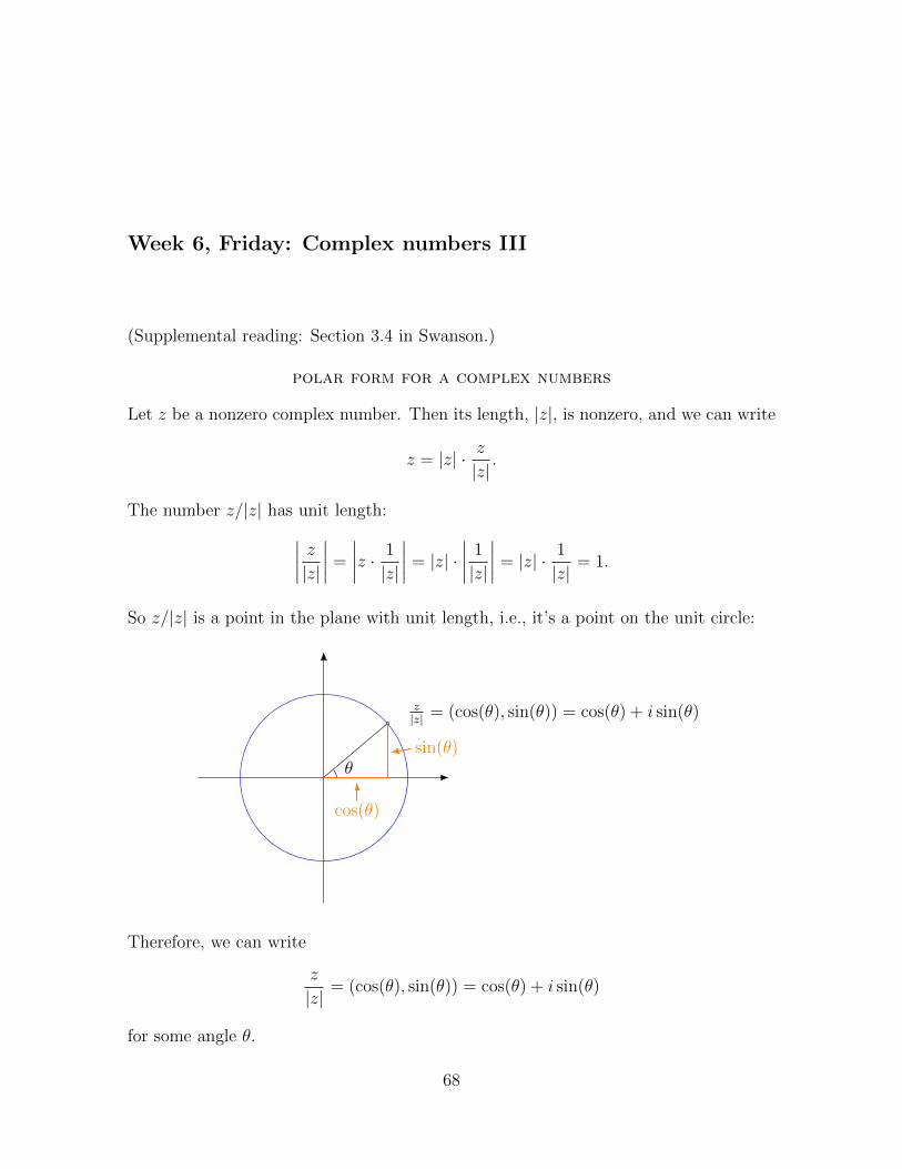
Week 6, Friday: Complex numbers III
(Supplemental reading: Section 3.4 in Swanson.)
polar form for a complex numbers
Let z be a nonzero complex number. Then its length, |z|, is nonzero, and we can write
z = |z| · z|z|.
The number z/|z| has unit length:∣∣∣∣ z|z|∣∣∣∣ =
∣∣∣∣z · 1
|z|
∣∣∣∣ = |z| ·∣∣∣∣ 1
|z|
∣∣∣∣ = |z| · 1
|z|= 1.
So z/|z| is a point in the plane with unit length, i.e., it’s a point on the unit circle:
z|z| = (cos(θ), sin(θ)) = cos(θ) + i sin(θ)
cos(θ)
sin(θ)θ
Therefore, we can write
z
|z|= (cos(θ), sin(θ)) = cos(θ) + i sin(θ)
for some angle θ.
68

69
Definition. The angle or argument of z ∈ C \ {0} is
arg(z) := θ
where θ is then angle shown above. The polar form for z is
z = |z|(cos(θ) + i sin(θ)).
The polar form describes z in terms of its length |z| and angle θ.
Examples.
1. Let z = 7 + 7i. Then|z| =
√72 + 72 = 7
√2
andz
|z|=
1√2
+1√2i =
√2
2+
√2
2i.
Plotting this complex number, it’s clear angle is 45◦ = π/4. So the polar form for zis
z = 7√
2(
cos(π
4
)+ sin
(π4
)i).
2. Let z =√
3 + i. The length of z is
|z| =√√
32
+ 12 =√
3 + 1 = 2.
Hence,z
|z|=
√3
2+
1
2i.
You should notice that (√
3/2, 1/2) is the point on the unit circle with angle 30◦ =π/6. Hence, arg(z) = π/6, and the polar form for z is
z = 2(
cos(π
6
)+ sin
(π6
)i).
3. Let z = 3 + 5i:
z = 3 + 5i
3
5
θ

70 CHAPTER 17. WEEK 6, FRIDAY
The length of z is|z| =
√32 + 52 =
√34,
the angle of z is
arg(z) = tan−1(
5
3
)≈ 59◦ ≈ 1.03 rad.
Therefore, the polar form for z is
z =√
34(cos(θ) + sin(θ)i)
where θ = tan−1(5/3).
geometry of addition and multiplication in C
The geometry of addition in C is just the geometry of vector addition. It is given bythe “parallelogram rule”:
(0, 0)
z
w
z + w
To see the geometry of multiplication, the secret is to use polar form. Given twononzero complex numbers z, w ∈ C, write each in polar form
z = |z| (cos(θ) + sin(θ)i)
w = |w| (cos(ψ) + sin(ψ)i) .
Their product is then
zw = |z| (cos(θ) + sin(θ)i) |w| (cos(ψ) + sin(ψ)i)
= |z||w| (cos(θ) + sin(θ)i) (cos(ψ) + sin(ψ)i)
= |zw| (cos(θ) + sin(θ)i) (cos(ψ) + sin(ψ)i)
= |zw| (cos(θ) cos(ψ)− sin(θ) sin(ψ) + (cos(θ) sin(ψ) + cos(ψ) sin(θ)) i)

71
= |zw| (cos(θ + ψ) + sin(θ + ψ)i) .
The last step uses the angle sum formulas for cosine and sine. The last line gives thepolar form for zw and reveals the geometry: when multiplying two complex numbers,angles add and lengths multiply.
Example. Consider the complex number
α = 0.95
(cos
(2π
15
)+ sin
(2π
15i
)).
What will the sequence of complex numbers
1 = α0, α, α2, α3, . . .
look like in the plane? The length of α is 0.95, and so the length of αn = (0.95)n.Since 0.95 is less than 1, its powers will get smaller and smaller, which means that thissequence of points will get closer and closer to the origin. The argument of α is anangle that is 1/15-th of the circle. To get to each successive number in the sequence,we multiply by α, which adds that angle to each succesive number, and scale by 0.95.So the sequence spirals around the origin, getting closed to the origin with each step.
The Sage code on cocalc.com that produced this image is on the next page.

72 CHAPTER 17. WEEK 6, FRIDAY
Code on cocalc.com:
s = 15
a = 0.98*exp(I*2*pi/s)
p = list_plot([a^n for n in range(12)])
q = parametric_plot\left( cos(x),sin(x)),(x,0,2*pi),color=’salmon’)
(p+q).show(aspect_ratio=1,axes=false,frame=true)

Week 7, Monday: Topology
Topology
(Supplemental reading: Section 3.5 in Swanson.)
For the following, let F = R or C.
Definition. The distance between z, w ∈ F is
d(z, w) := |z − w|.
Example. In C, with z = a+ bi and w = c+ di,
d(z, w) =√
(a− c)2 + (b− d)2.
a− c
b− d
z = a+ bi
w = c+ di
Definition. The open ball centered at z ∈ F of radius r ∈ R > 0 is the subset
B(z; r) := {w ∈ F : |w − z| < r} .
Example.
1. If F = R, then what we have just called a ball is an open interval. For example,in R, we have B(3; 1) = (2, 4):
(
2
)
43
B(3; 1) = (2, 4) : .
73

74 CHAPTER 18. WEEK 7, MONDAY
2. Here is a picture of the ball of radius 1 in C centered at 1 + i:
B(1 + i; 1) :1 + i
1
.
Definition. A subset U ⊆ F is open if it contains an open ball about each of itspoints. This means that for all u ∈ U , there exists ε > 0 such that
B(u; ε) ⊆ U.
A key point here is that the open ball must be entirely contained inside U :
x
ε
U
B(x; ε)
In the above picture, U ⊂ C is the set of all points inside the outer dashed line. Insideof U , we show a typical point x and an example of an open ball about x completelycontained inside of U . As we test points nearer the boarder of U , the choice for ε willneed to become smaller.
Example.
1. The empty set ∅ ⊂ F is open.
2. The set F , itself, is open (whether F = R or C). Proof: Given x ∈ F , the openball B(x; 1) ⊂ F .
3. An open interval (a, b) ⊆ R is open. Given c ∈ (a, b), let ε be either c− a or b− c,whichever is smallest. Then the open interval centered at c and with radius ε iscontained in (a, b). For instance, take the interval (0, 4), and let c = 3. Then (0, 4)contains the open ball of radius 1 about c, i.e., it contains the interval (2, 4). Thisopen ball is shown in blue below:

75
0 4
3( )
4. A union of open intervals in R is an open set. In fact, every subset of R is a unionof open intervals. We prove this and the analogous result for C in a propositionbelow.
5. In C = R2 the Cartesian product (a, b) × (c, d) is open. (This is a rectangle in R2
not containing its boundary.)
6. The closed interval [1, 2) is not open. The problem is the endpoint 1. We have 1 ∈[1, 2] but there is no open ball (interval) centered at 1 and contained in [1, 2). Anyopen interval about 1 will contain points less that 1 and hence not in the set [1, 2).
7. The closed disc D := {z ∈ C : |z| ≤ 1} is not open. The problem is each of thepoints with modulus 1 sitting on the boundary of D. Any open ball about one ofthese points will contain points that are not in D, i.e., it will not be completelycontained in D:
zB(z; ε)
D
Proposition. Every open set in F is a union of open balls.
Proof. Let U ⊆ F be open. Since U is open, for each u ∈ U , there exists εu > 0 suchthat
B(u; εu) ⊆ U.
We claim ⋃u∈U
B(u; εu) = U.
To see this, first let v ∈ ∪u∈UB(u; εu). Then v ∈ B(u; εu) for some u ∈ U (in fact, v ∈B(v; εv)), and sinceB(u; εu) ⊆ U , we have v ∈ U . To see the reverse inclusion let v ∈ U .Then v ∈ B(v; vev), and hence, v is in the union ∪u∈UB(u; εu).

76 CHAPTER 18. WEEK 7, MONDAY
Proposition. Every nonempty open subset of F has infinitely many elements.
Proof. Let U be a nonempty open subset of F . Since U is nonempty, it containssome point u. Since U is open, it must contain an open ball B(u; ε) about U . Butevery open ball contains infinitely many points. For instance B(u; ε) contains thepoints {u+ ε/n : n = 2, 3, 4, . . . }.
Corollary. No finite set of points is open. In particular, for each z ∈ F , the set {z}is not open.
Definition. The set of open sets of F forms a topology on F . This means that
1. ∅ and F are open.
2. An arbitrary union of open sets is open.
3. A finite intersection of open sets is open.
Regarding part 3, note that an infinite intersection of open sets might not be open.For example,
∞⋂n=1
B(z; 1/n) = {z}
which is not open (since it is finite). For a more concrete example, note that
∞⋂n=1
(− 1
n,
1
n
)= {0} .
Definition. A subset C ⊆ F is closed if its complement F \ C is open.
Example.
1. F is closed since F \ F = ∅, and ∅ is open.
2. Similarly ∅ is closed since F \ ∅ = F , and F is open. (Thus, we have seen that Fand ∅ are both open and closed.1)
3. If B ⊆ F is an open ball, the F \B is closed. For instance, if F = R and B = (0; 1),then
R \ (−1, 1) = (−∞,−1] ∪ [1,∞)
is closed.
1If it seems paradoxical to you that there are sets, like the empty set, that are both open and closed,you are not alone (cf. Hitler learns topology where “null set”= “empty set”, “neighborhood”=“openball”).
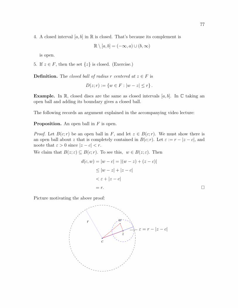
77
4. A closed interval [a, b] in R is closed. That’s because its complement is
R \ [a, b] = (−∞, a) ∪ (b,∞)
is open.
5. If z ∈ F , then the set {z} is closed. (Exercise.)
Definition. The closed ball of radius r centered at z ∈ F is
D(z; r) := {w ∈ F : |w − z| ≤ r} .
Example. In R, closed discs are the same as closed intervals [a, b]. In C taking anopen ball and adding its boundary gives a closed ball.
The following records an argument explained in the accompanying video lecture:
Proposition. An open ball in F is open.
Proof. Let B(c; r) be an open ball in F , and let z ∈ B(c; r). We must show there isan open ball about z that is completely contained in B(c; r). Let ε := r − |z − c|, andnoote that ε > 0 since |z − c| < r.
We claim that B(z; ε) ⊆ B(c; r). To see this, w ∈ B(z; ε). Then
d(c, w) = |w − c| = |(w − z) + (z − c)|
≤ |w − z|+ |z − c|
< ε+ |z − c|
= r.
Picture motivating the above proof:
r
c
z
w
ε = r − |z − c|

Week 7, Friday: Sequences I
Sequences I
(Supplemental reading: Start reading Chapter 8 in Swanson.)
A sequence of complex numbers or complex sequence is a function
N>0 → C.
If s is such a function, instead of s(n), we usually write sn. Essentially, the function sis just an unending ordered sequence of numbers:
s1, s2, s3, . . .
The sequence s can be notated in various ways, including
{sn}n>0 , {sn}∞n=1 , {sn}n , {sn} ,
among others. A real sequence is a special case of a complex sequence in which theimage of s is in R ⊂ C.
Example. Some examples of sequences:
1.
{1}∞n=1 = 1, 1, 1, . . .
2. The first term in the following sequence is 4:
{n}n≥4 = 4, 5, 6, . . .
3.
{(−1)n}n≥0 = 1,−1, 1,−1, . . .
4. {1
n2
}∞n=1
= 1,1
4,1
9,
1
16, . . .
78

79
Definition. Let {an} be a sequence of complex numbers, and let a ∈ C. Then thelimit of the sequence {an} as n goes to infinity is a, denoted limn→∞ an = a, if forall ε > 0, there exists N ∈ R such that n > N implies |a− an| < ε. If limn→∞ an = afor some a ∈ C, we say {an} is convergent, and if there is no such a, we say the sequencediverges.
Here is a shorthand for writing the definition: limn→∞ an = a if ∀ε > 0, ∃N ∈ R suchthat n > N ⇒ |a − an| < ε. The symbols ∀ and ∃ are called quantifiers. They standfor “for all” and “there exists”, respectively.
It is notoriously difficult to fully appreciate all that is packed into the definition of thelimit of a sequence. So the reader is encouraged to take their time and be patient!Here are some pointers to get started:
1. Most importantly, the condition |a−an| < ε means that an is within a distance of εof a, i.e., it’s in the ball of radius ε centered at a:
ε
a
an
2. The rough idea of the limit is that as n get large, an gets close to a. By itself, thisidea is too vague. What is meant by “gets close to”? Also, is it OK if some but notall an get close to a.
3. The number ε is a challenge: “Can you make the distance between an and a lessthan ε? The number N is the response: ”Yes, if you go out further than N steps inthe sequence, then the all of the numbers in the sequence past that point are withina distance ε of a.“
4. Then number N is a function of ε. If ε > 0 is made smaller, then N usually needsto be made larger—you need to go out further in the sequence to get closer to thelimit. So it might be better to write N(ε) or Nε instead of just N to highlight thisdependence.
5. This might be very helpful in understanding our definition: limn→∞ an = a is equiv-alent to saying that for every ε > 0, all but a finite number of the an are inside theball of radius ε centered at a.

80 CHAPTER 19. WEEK 7, FRIDAY
The following is a template for a limit proof that works directly from the definition ofthe limit:
Proof Template. limn→∞ an = a.
Proof. Given ε > 0, let N = blah. Then if n > N , we have
|a− an| = blah
=
≤=
<
= ε.
For the proof to be valid, at least one strict inequality,“<”, is required.
Example. Let a ∈ C, and consider the constant sequence {a}n = a, a, a, . . . . Then limn→∞ a =a.
Proof. We are considering the sequence {an} such that an = a for all n. Given ε > 0,let N = 0. Then n > N implies
|a− an| = |a− a| = 0 < ε.
Thus, limn→∞ a = a.
Note that in the above proof, we could have chosen any number N ∈ R. The distanceof every term in the sequence is a distance of 0 from a, and 0 < ε by choice of ε.
Example. limn→∞
1
n= 0.
Proof. Given ε > 0, let N := 1/ε. Then n > N implies∣∣∣∣0− 1
n
∣∣∣∣ =
∣∣∣∣ 1n∣∣∣∣
=1
n(since n > 0)
<1
N(since n > N)
= ε (since N = 1/ε).

81
The above proof is typical in that the value for N is unmotivated. The reader canverify each step of the proof, but may be mystified by the choice of N . That’s becauseone usually constructs a limit proof by starting at the end of the proof (on scratchpaper): we want |a − an| < ε, and then work backwards to find N . For instance, inthis last proof, in the end, we want ∣∣∣∣0− 1
n
∣∣∣∣ < ε.
This statement is equivalent to1
n< ε,
which is equivalent to1
ε< n.
Thus, if we take N =1
εand assume n > N , we are OK:
1
ε= N < n.
All of our steps are reversible, so things are going to work out.
Example. Let’s apply that same reasoning to construct a proof that
limn→∞
(1 + 1/√n) = 1.
Here an = 1 + 1/√n and a = 1. In the end, we will want |a− an| < ε, i.e.,
|1− (1 + 1/√n)| < ε.
On scratch paper we work out
|1− (1 + 1/√n)| < ε⇔ | − 1/
√n| < ε
⇔ 1√n< ε
⇔ 1
ε<√n
⇔ 1
ε2<√n
Thus, we can take N = 1/ε2. Now we are ready to write the formal proof:

82 CHAPTER 19. WEEK 7, FRIDAY
Claim. limn→∞(1 + 1/√n) = 1
Proof. Given ε > 0, let N = 1/ε2 and suppose that n > N . It follows that∣∣∣∣1− (1 +1√n
)∣∣∣∣ =1√n
<1√N
(since n > N)
= ε (since N = 1/ε2).
(Note that n > N ⇒√n >√N ⇒ 1√
N> 1√
n.)

Week 8, Monday: Sequences II
Sequences II
(Supplemental reading: Sections 8.1 and 8.2 in Swanson.)
Recall the definition of the limit of a sequence of complex numbers: we say limn→∞ an =a if for all ε > 0 there exists N ∈ R such that n > N implies |a− an| < ε.
To prove a sequence {an} doesn’t have a limit, we need to show that for all a ∈ C, thelimit of {an} is not a. To make sense of what this means in terms of the definition ofthe limit, one pointer is that the negation of “for all” is “there exists”, and vice versa:if it is not true that“for ε > 0, there exists N . . . ”, then there exists ε > 0 such thatfor all N . . . The following proposition illustrates this principle.
Proposition. The sequence {(−1)n} = −1, 1,−1, 1, . . . diverges.
Proof. Let a be any complex number. We claim that {(−1)n} does not converge to a.To see this, let ε = 1, and let N be any real number. There is some even number n > N ,and for this n,
|a− (−1)n| = |a− 1|.
Similarly, these is some odd number n > N , and for this n,
|a− (−1)n| = |a+ 1|.
Next, using the triangle inequality, we see
2 = |(a− 1)− (a+ 1)| ≤ |a− 1|+ | − (a+ 1)| = |a− 1|+ |a+ 1|.
Since 2 ≤ |a− 1|+ |a+ 1|, at least one of |a− 1| or |a+ 1| is greater than or equal to 1.So it follows that there exists some n > N such that
|a− (−1)n| 6< ε.
The motivation for the above proof is the following picture:
83

84 CHAPTER 20. WEEK 8, MONDAY
−1 1
a
There is no way to find a ∈ C that is both close to −1 and close to 1. In the proof,we applied the triangle inequality to the triangle in the picture to conclude that thedistance from a to at least one of 1 or −1 must be at least 1. That leads to taking ε = 1.(The argument works by taking any ε such that 0 < ε ≤ 1.)
We next prove a result that will be of great use later on. Start with a number α ∈ C, andconsider the sequence {αn} = α, α2, α3, . . . . What is the behavior of this sequence?Does it converge? The answer, of course, depends on the initial choice of α. Thekey to unlocking the behavior of the sequence is to consider the polar form of α.Say α = |α|(cos(θ)+ i sin(θ)). Then αn = |α|n(cos(nθ)+ i sin(nθ)). So the length of αn
is |α|n and the angle (or argument) of αn is n times the angle of α. So it seems clearthat if |α| > 1, the sequence “diverges to∞”, spinning as it goes (unless the angle of αis 0). Similarly, of |α|, the sequence is sucked into the origin. What if |α| = 1? Then αis a point on the unit circle, and unless arg(α) = 0, the sequence will perpetually spinaround the circle, never converging. See Figure 20.1.
Figure 20.1: If α is one of the blue points, above, then sequence {αn} converges. Itconverges to 1 if α = 1, to 0 if |α| < 0, and diverges, otherwise.
Proposition. Let α ∈ C and consider the sequence {αn}. There are three cases:
1. limn→∞ αn = 1 if α = 1;
2. limn→∞ αn = 0 if |α| < 1;
3. {αn} diverges, otherwise, i.e., if α 6= 1 and |α| ≥ 1.
85
Proof. For case 1, where α = 1, we get the constant sequence 1, 1, 1, . . . Last time wesaw that the limit of a constant sequence is just the constant (given ε > 0, we cantake N to be any real number).
For case 2, suppose that |α| < 1. If α = 0, then αn is the constant sequence 0, 0, 0, . . . ,with limit 0. Otherwise, given ε > 0, we need to find N ∈ R such that if n > N , then
|0− αn| < ε.
This is equivalent to showing that
|α|n < ε.
To find N , we solve for n in the above equation:
|α|n < ε ⇔ ln(|α|n) < ln(ε) ⇔ n ln(|α|) < ln(ε) ⇔ n > ln(ε)/ ln(|α|).
There are a couple of subtleties in the above calculation. In the first step, we usedthe fact that taking logs preserves inequalities. This is because the log is an increasingfunction: ln(x) < ln(y) if and only if x < y. In the last step of the calculation, theinequality is reversed since |α| < 1 means that ln(|α|) < 0. To complete the proofthat limn→∞ α
n = 0 in this case, let N := ln(ε)/ ln(|α|) and suppose that n > N .Running the string of implications displayed above in reverse, we see that it followsthat n > N implies
|0− αn| = |α|n < ε,
as required.
The last case is the toughest. Suppose that α 6= 1 and |α| ≥ 1. We must showthat {αn} is divergent. We prove this by contradiction. Suppose that limn→∞ α
n = λfor some λ ∈ C. Define
ε :=|α− 1|
2.
Note that ε > 0 since α 6= 1. We’ll see below that this particular ε will give usinsurmountable problems. Since limn→∞ α
n = λ, there exists N ∈ R such that
n > N =⇒ |λ− αn| < ε =|α− 1|
2.
Now, if n > N , it follows that n+ 1 > N , too. Hence,
|λ− αn+1| < |α− 1|2
.
Therefore, if n > N , it follows that
|αn+1 − αn| = |(λ− αn)− (λ− αn+1)|≤ |λ− αn|+ |λ− αn+1| (triangle inequality)

86 CHAPTER 20. WEEK 8, MONDAY
<|α− 1|
2+|α− 1|
2= |α− 1|,
i.e.,|αn+1 − αn| < |α− 1|
for all n > N . On the other hand,
|αn+1 − αn| = |α|n|α− 1|≥ |α− 1| since |α| ≥ 1.
Thus, our assumption that limn→∞ αn = λ has allowed us to show that there is an N
such that n > N implies both
|αn+1 − αn| < |α− 1|
and|αn+1 − αn| ≥ |α− 1|.
That’s not impossible. So there is no such λ.
Example. The sequence{(
1+i2
)n}converges since∣∣∣∣1 + i
2
∣∣∣∣ =1
2|i+ 1| = 1
2
√12 + 12 =
√2
2< 1.
The sequence {in} does not converge since |i| = 1 and i 6= 1. A picture of the firstsequence appears below:

Week 9, Monday: New-from-old limit theorem
Math 112 lecture for Monday, Week 9
New-from-old limit theorem
(Supplemental reading: Theorem 8.4.3 in Swanson.)
In general, it is difficult to give limit proofs using ε-N arguments. We give an exampleof this difficulty, and then reveal a much easier, high-level approach.
Example. limn→∞
n3 + 2n
5n3 + 2=
1
5.
Proof. Given ε > 0, let N = 2/ε, and suppose n > N . Then∣∣∣∣n3 + 2n
5n3 + 2− 1
5
∣∣∣∣ =
∣∣∣∣5(n3 + 2n)− (5n3 + 2)
5(5n3 + 2)
∣∣∣∣=
∣∣∣∣ 10n− 2
5(5n3 + 2)
∣∣∣∣<
∣∣∣∣10n− 2
5n3 + 2
∣∣∣∣<
∣∣∣∣10n− 2
5n3
∣∣∣∣<
∣∣∣∣10n
5n3
∣∣∣∣=
∣∣∣∣ 2
n2
∣∣∣∣<
∣∣∣∣ 2n∣∣∣∣
=2
n<
2
N
87

88 CHAPTER 21. WEEK 9, MONDAY
=2
2/ε
= ε.
Limit theorems. Often, a sequence can constructed from simpler sequences usingalgebraic operations (addition, substraction, multiplication, and division). In this case,the following theorem is useful:
Theorem. (New-from-old limit theorem.) Suppose that limn→∞ sn = s and thatlimn→∞ tn = t. Then,
1. limn→∞(sn + tn) = limn→∞ sn + limn→∞ tn = s+ t.
2. limn→∞(sntn) = (limn→∞ sn)(limn→∞ tn) = st.
3. limn→∞
sntn
=limn→∞ snlimn→∞ tn
=s
tprovided t 6= 0.
Corollary. If a and b are real or complex constants, then limn→∞(asn) = a limn→∞ sn =as and, more generally, limn→∞(asn + btn) = a limn→∞ sn + b limn→∞ tn = as+ bt.
We will provide proofs of these results at the end of these notes. (Note: Pay particularattention to the proof of part 1 given there. It contains some important, generally usefulideas.) First, though, we will illustrate the use of our theorem.
Building blocks. We have seen that for c ∈ C, the constant sequence has limit c,i.e., limn→∞ c = c. And we have also seen that
limn→∞
1
n= 0.
In the following examples, we will see how complicated sequences can be evaluated usingthese building blocks and the new-from-old limit theorem (LT). Note the importanttrick in part 4.
Examples.
1.
limn→∞
(5 +
1
n
)= lim
n→∞5 + lim
n→∞
1
n(LT 1)
= 5 + 0 = 5.
89
2.
limn→∞
1
n2= lim
n→∞
(1
n· 1
n
)
=
(limn→∞
1
n
)(limn→∞
1
n
)(LT 2)
= 0 · 0 = 0.
3.
limn→∞
5
n2= lim
n→∞
(5 · 1
n· 1
n
)
= ( limn→∞
5)
(limn→∞
1
n
)(limn→∞
1
n
)(LT 2)
= 5 · 0 = 0.
4.
limn→∞
n3 + 2n
5n3 + 2= lim
n→∞
1n3 (n3 + 2n)1n3 (5n3 + 2)
(NB: important trick)
= limn→∞
1 + 2n2
5 + 2n3
=limn→∞
(1 + 2
n2
)limn→∞
(5 + 2
n3
) (LT3)
=limn→∞ 1 + limn→∞
2n2
limn→∞ 5 + limn→∞2n3
(LT1)
=1 + limn→∞
2n2
5 + limn→∞2n3
(constant sequences)
=1 + 0
5 + 0(as in example 3)
=1
5.
Proof of new-from-old limit theorem.
For part 1, we need to show that
limn→∞
(sn + tn) = limn→∞
sn + limn→∞
tn = s+ t.

90 CHAPTER 21. WEEK 9, MONDAY
Let ε > 0. Since limn→∞ sn = s, there exists Ns such that n > Ns implies
|s− sn| <ε
2.
Similarly, since limn→∞ tn = t, there exists Nt such that n > Nt implies
|t− tn| <ε
2.
Define N to be the maximum of Ns and Nt:
N := max {Ns, Nt} .
Thus, N ≥ Ns and N ≥ Nt.
Suppose n > N . Then, since n > N ≥ Ns, it follows that
|s− sn| <ε
2.
Similarly, since n > N ≥ Nt, it follows that
|t− tn| <ε
2.
Hence, if n > N ,
|(s+ t)− (sn + tn)| = |(s− sn) + (t− tn)| ≤ |s− sn|+ |t− tn| <ε
2+ε
2= ε.
That completes the proof of part 1.
For part 2, we show that
limn→∞
(sntn) = ( limn→∞
sn)( limn→∞
tn) = st.
Given ε > 0, define
η = min
{1,
ε
1 + |s|+ |t|
}.
This means η is the minimum of the two displayed quantities. So η ≤ 1 and η ≤ε/(1 + |s| + |t|) (and equality holds in at least one of these). As above, we can find asingle N such that n > N implies
|s− sn| < η and |t− tn| < η. (21.1)
Now for the creative part: we can write
sntn − st = (s− sn)(t− tn)− s(t− tn)− t(s− sn).
(Check this by multiplying out the expression on the right.) It follows that
|st− sntn| = |sntn − st|

91
= |(s− sn)(t− tn)− s(t− tn)− t(s− sn)|≤ |(s− sn)(t− tn)|+ |s(t− tn)|+ |t(s− sn)| (triangle inequality)
= |(s− sn)||(t− tn)|+ |s||(t− tn)|+ |t||(s− sn)|< η · η + |s|η + |t|η (Equation (21.1))
≤ η + |s||η + |t|η (since η ≤ 1)
= η(1 + |s|+ |t|)
< ε
(since η ≤ ε
1 + |s|+ |t|
).
The proof for part 3 is similar, and we leave it as an exercise for the interested reader�
Proof of the corollary to the new-from-old limit theorem.
Suppose a and b are constants. Then
limn→∞
(asn + btn) = limn→∞
(asn) + limn→∞
(btn) (LT1)
= limn→∞
a limn→∞
sn + limn→∞
b limn→∞
tn (LT2)
= a limn→∞
(sn) + b limn→∞
tn (limit of constant seq.)
= as+ bt.
To see that limn→∞(asn) = a limn→∞ sn, let b = 0, above. �

Week 9, Wednesday: Monotone Convergence Theorem
Math 112 lecture for Wednesday, Week 9
Monotone Convergence Theorem
(Supplemental reading: Section 8.6 Swanson.)
Today, we will prove two results: (i) convergent sequences are bounded (but not con-versely), and (ii) the Monotone Convergence Theorem.
Definition. A sequence {sn} of complex numbers is bounded if there exists B ∈ Rsuch that
|sn| ≤ B
for all n.
If the sn are all real numbers, then this definition of boundedness coincides with theone we gave earlier. In general, it means that all of the numbers in the sequence arecontaining in a closed ball of finite radius centered at the origin:
B
Theorem. Every convergent sequence is bounded.
Proof. Let {sn} be a convergent sequence, and say limn→∞ sn = s. Apply the definitionof the limit with ε = 1 to find an N ∈ R such that n > N implies
|s− sn| < 1.
92
93
We apply the reverse triangle inequality:
1 > |s− sn| = |sn − s| ≥ |sn| − |s| ⇒ 1 + |s| > |sn|.
Thus, if n > N then |sn| < 1 + |s|. So we have accomplished the hardest part bybounding all but finitely many points in the sequence by the real number 1 + |s|, butit could be that s1, s2, . . . , sN are further away from the origin. So let
B = max {|s1|, |s2|, . . . , |sN |, 1 + |s|} .
This means that we have set B equal to the maximum number in the given set. Itfollows that
|sn| ≤ B
for all n.
Remark. The converse of the above theorem does not hold. For instance, considerthe sequence 1,−1, 1,−1, . . . It is bounded but does not converge.
monotone convergence theorem
Definition. A sequence of real numbers {sn} is monotone increasing if sn ≤ sn+1 forall n. It is monotone decreasing if sn ≥ sn+1 for all n.
Note that monotone increasing is synonymous with non-decreasing since the conditionis sn ≤ sn+1, not sn < sn+1. An analogous remark holds for monotone decreasingsequence.
Example. The constant sequence 1, 1, 1, . . . is both monotone increasing and mono-tone decreasing.
Theorem. (Monotone Convergence Theorem, MCT). If {sn} is a monotone increasingsequence that is bounded above or a monotone decreasing sequence that is boundedbelow, then {sn} converges. (And it converges to sup {sn} or inf {sn}, respectively.)
Proof. Suppose that {sn} is monotone increasing and bounded above. (The casewhere {sn} is monotone decreasing and bounded below is similar, or it can be reducedto the increasing case by considering {−sn}.) By completeness of the real numbers,the set {sn} has a supremum. Say s = sup {sn}. We claim that limn→∞ sn = s. Tosee this, let ε > 0. Then s − ε < s, i.e., s − ε is strictly less than the least upperbound of {sn}. This means that s− ε is not an upper bound for that set. Therefore,there exists some sN such that s − ε < sN , i.e., s − sN < ε. However, since thesequence {sn} is a monotone increasing sequence, if n > N , it follows that sn ≥ sN ,and hence, −sn ≤ −sN . Adding s to both sides yields s − sn ≤ s − sN . Now, since sis an upper bound for the set, we also have 0 ≤ s− sn. Putting this all together:
0 ≤ s− sn ≤ s− sN < ε
94 CHAPTER 22. WEEK 9, WEDNESDAY
for all n > N . It follows that |s−sn| < ε for all n > N . We have shown that limn→∞ sn =s, as claimed. �
Example. Here is an example of the monotone convergence theorem in use. De-fine s1 = 1, and for each n ≥ 1, define sn+1 :=
√1 + sn. The first few terms of the
sequence are
1,√
1 + 1,
√1 +√
1 + 1, . . .
To find the limit, we first appeal to the monotone convergence theorem. We showthe sequence is monotone increasing, i.e., that sn ≤ sn+1 by induction. For the basecase, n = 1, note that s1 = 1 ≤ s2 =
√2. Now suppose that sn ≤ sn+1 for some n ≥ 1.
It follows thatsn+2 =
√1 + sn+1 ≥
√1 + sn = sn+1.
(Here, we have used that f(x) =√x is an increasing function: if x < y, then
√x <√y.)
The result now follows for all n by induction.
To use the monotone convergence theorem, we must also verify that the sequence isbounded above. We show it’s bounded above by 2 by induction. For the base case,note that s1 = 1 ≤ 2. Suppose that sn ≤ 2 for some n ≥ 1. Then
sn+1 =√
1 + sn ≤√
1 + 2 =√
3 ≤ 2.
The result holds for all n by induction.
The monotone convergence theorem now tells us the sequence has a limit. Say that limn→∞ sn =s. We would like to evaluate s. We will appeal to a result we have not yet shown:if f(x) is a continuous function, then limn→∞ f(sn) = f(limn→∞ sn) = f(s). We applythis letting f(x) =
√x:
sn+1 =√
1 + sn ⇒ limn→∞
sn+1 =√
limn→∞
(1 + sn) =√
1 + s.
It is an easy exercise to show that limn→∞ sn+1 = limn→∞ sn = s.1 Therefore, we see
s =√
1 + s.
Squaring both sides,
s2 = 1 + s ⇒ s2 − s− 1 = 0 ⇒ s =1±√
5
2
by the quadratic equation. By squaring, we introduced an extraneous answer. Since0 ≤ sn for all n, it follows that 0 = lim 0 ≤ lim sn = s. 2 Hence, s must be nonnegative.It follows that
s =1 +√
5
2.
1Here we are comparing the sequence {sn} to the “shifted sequence” {sn+1} = s2, s3, . . . . If sn iswithin ε of s for all n > N , then so is sn+1 since n > N implies that n+ 1 > N .
2In general, taking limits “preserves inequalities”. We will discuss this later.

Week 9, Friday: Misc. limit theorems, infinite limits, and Cauchysequences
Misc. limit theorems, infinite limits, and Cauchy sequences
(Supplemental reading: Sections 8.3, 8.4, 8.7, and 8.8 in Swanson.)
Miscellaneous limit theorems
We state several theorems here about limits. The numbering refers to Swanson’s text,where the interested reader may find the proofs.
Theorem 8.4.1. Limits are unique: if limn→∞ sn = s and limn→∞ sn = s′, then s = s′.
Proof. Let ε > 0. Since limn→∞ sn = s and limn→∞ sn = s′, there exists an N suchthat n > N implies that |s − sn| < ε/2 and |s′ − sn| < ε/2. As usual, we can take Nlarge enough so that it applies to both limits simultaneously. By the triangle inequality,we then have that for n > N ,
|s− s′| = |(s− sn)− (s′ − sn)| ≤ |s− sn|+ |s′ − sn| < ε/2 + ε/2 = ε.
We have shown that |s−s′| < ε for all ε > 0. Since there are no infinitely small positivenumbers, it follows that |s− s′| = 0, and hence, s = s′.
Theorem 8.4.11. (Squeeze theorem.) Let {an}, {bn}, and {cn} be real sequences,and suppose that an ≤ bn ≤ cn for all n. Then, if limn→∞ an = limn→∞ cn, it followsthat
limn→∞
an = limn→∞
bn = limn→∞
cn.
Example. Here, we prove that limn→∞
n2 − 3
n3 + 6n+ 1= 0 using the squeeze theorem. We
haven2 − 3
n3 + 6n+ 1≤ n2
n3 + 6n+ 1≤ n2
n3=
1
n;
Thus,
0 ≤ n2 − 3
n3 + 6n+ 1≤ 1
n
95

96 CHAPTER 23. WEEK 9, FRIDAY
for n > 1. Given that limn→∞ 0 = 0 and limn→∞
1
n= 0, it follows that
limn→∞
n2 − 3
n3 + 6n+ 1= 0
by the squeeze theorem.
Example. Consider the sequence
{sin(n)
n
}. Since | sin(n)| ≤ 1, we have
− 1
n≤ sin(n)
n≤ 1
n.
Then, since
limn→∞
− 1
n= lim
n→∞
1
n= 0,
it follows that
limn→∞
sin(n)
n= 0
by the squeeze theorem.
Theorem 8.4.10. The operation of taking limits preserves inequalities: Supposethat {an} and {bn} are convergent real sequences and that an ≤ bn for all n (or forall n past a certain point) then
limn→∞
an ≤ limn→∞
bn.
Remark. The operation of taking limits does not preserve strict inequality. Forexample, compare the constant sequence {0} with the sequence
{1n
}. We have
0 <1
n
for all n, but
limn→∞
0 = limn→∞
1
n.
Subsequences
We form a subsequence from a giving sequence by dropping terms from the sequence(but leaving an infinite number):
sequence: s1, s2, s3, s4, s5, s6, s7, s8, s9, s10, s11, . . .
subsequence: s2, s3, s4, s6, s9, s11, . . .

97
Definition. Let {sn} be a sequence, and let n0 < n1 < n2 < . . . be any sequence ofnatural numbers. Then the sequence {snk
}∞k=0 is called a subsequence of {sn}.
Example. In the previous example,
n0 = 2, n2 = 3, n3 = 4, n4 = 6, n4 = 9, n5 = 11, . . .
Example. Let sn = 1/n for n = 1, 2, . . . . Then the following is a subsequence of {sn}:
{s2k}∞k=1 = s2, s4, s6, s8, . . .
=1
2,1
4,1
6,1
8, . . .
Theorem. (Main theorem for subsequences.) If {sn} is a sequence converging to sand {snk
} is any subsequence, then {snk} also converges to s. (Every subsequence of
a convergent sequence is convergent and has the same limit.)
Example. The previous theorem is especially useful for proving non-convergence. Forinstance, consider the sequence {(−1)n}. It has the constant sequence {1} and theconstant sequence {−1} as subsequences. The former converges to 1 and the latterto −1. We can deduce that {(−1)n} diverges (since otherwise all subsequence wouldneed to converge to the same value).
Infinite limits
Definition. A real sequence {an} diverges to ∞ if for all B ∈ R, there exists N ∈ Rsuch that n > N implies
an > B.
The sequence diverges to −∞ if for all B ∈ R, there exists N ∈ R such that n > Nimplies
an < B.
We writelimn→∞
an =∞ or limn→∞
an = −∞,
respectively.
What this means: If limn→∞ sn = ∞, and you come up with a number B, nomatter how large, eventually, all of the terms in the sequences are larger than B.If limn→∞ sn = −∞, and you come up with a number B, no matter how negative,eventually, all of the terms in the sequences are less than B.

98 CHAPTER 23. WEEK 9, FRIDAY
Example. To prove limn→∞ n2 =∞, let B ∈ R. Given B, let N =
√|B|. Then
n > N ⇒ n >√|B| ⇒ n2 > |B| ⇒ n2 > B.
Cauchy sequences.
The real numbers fill the “holes” in Q. For instance, consider the set of rationalnumbers
S ={x ∈ Q : x2 ≤ 2
}.
This is a nonempty set of Q and bounded above, but it does not have a supremum in Q.One way to construct R is to use decimals. However that approach is a little tougherthan it might first seem. (To point out one difficulty, two different decimals can beequal, e.g., 0.999 · · · = 1.000 . . . .) We will now outline a different approach. There aresequences of rationals that “want to converge”. For example, take the sequence we getby truncating the decimal expansion of
√2:
1, 1.4, 1.41, 1.414, 1.4142, . . .
However, without real numbers, this sequence has nowhere to converge to.
A key idea in one approach to the construction of R is to think of sequences of rationalnumbers as real numbers. For instance, we can think of the above sequence as
√2.
A real number that is already a rational number, e.g., 1/2, can be thought of asthe constant sequence 1/2, 1/2, 1/2, . . . There are some obvious problems with thisapproach:
1. We only want to consider sequences of rationals that “want to converge”. Whatcould this mean?
2. There are many different sequences that want to converge to the same point. Forinstance, the constant sequence {0} and the sequence {1/n} both converge to 0, asdo infinitely many other sequences.
We fix the first problem with the following definition:
Definition. A sequence of numbers (rational, real, or complex) {sn} is a Cauchysequence if for ε > 0, there exists N ∈ R such that m,n > N implies
|sm − sn| < ε.
Remark. The rough idea behind this definition is that as you go out far in thesequence, the points in the sequence start to clump together—the distance between allthe remaining points is small.
Proposition. Every convergent sequence is a Cauchy sequence.

99
Proof. Suppose that {sn} is a convergent sequence, and let ε > 0. Say limn→∞ sn = s.Then there exists N such that n > N implies
|s− sn| <ε
2.
But then, if m,n > N , by the triangle inequality,
|sm − sn| = |(s− sn)− (s− am)| ≤ |s− sn|+ |s− sm| <ε
2+ε
2= ε.
We’ve shown that |sm − sn| for all m,n > N . Hence {sn} is Cauchy.
Theorem. A sequence of real or complex numbers is convergent if and only if it is aCauchy sequence.
Proof. See Swanson’s text, Section 8.7.
Remark. The above theorem does not hold for Q. For instance, take a sequence ofrational numbers that converges to
√2 in R. That sequence will be a Cauchy sequence
of rational numbers, but it will not converge in the rational numbers.
Definition of the real numbers
Let C be the set of all Cauchy sequences of rational numbers. As a first approximation,we could try to define R := C. The problem with this is that multiple Cauchy sequenceswill want to have the same limit. Again, for instance, consider the constant sequence 0and the sequence {1/n}. To fix that we define an equivalence relation:
Definition. Let {sn} , {tn} ∈ C. We say
{sn} ∼ {tn}
iflimn→∞
(sn − tn) = 0.
Any easy check shows that ∼ is an equivalence relation on C. An equivalence classfor the relation is the set of all Cauchy sequences of rational numbers that want toconverge to the same thing. We can then define the real numbers to be the sets ofthese equivalence classes:
Definition. The real numbers are
R := C/∼ .
with addition and multiplication defined by
[{sn}] + [{tn}] := [{sn + tn}]

100 CHAPTER 23. WEEK 9, FRIDAY
[{sn}][{tn}] := [{sntn}].
There are a lot of details to check:
1. Are addition and multiplication well-define or do they depend on the choice of repre-sentatives for the equivalence classes? (Recall we had the same consideration whendefining addition and multiplication for equivalence classes of integers modulo n.)
2. Do we get a field?
3. How do we define an order relation on R?
We’ll stop here, though.

Week 10, Monday: Series
Series
(Supplemental reading: Section 9.1 in Swanson.)
Definition. Let {an} be a sequence of real or complex numbers. The n-th partial sumof {an} is
sn :=n∑i=1
ai.
Example. The third partial sum of {1/n}n≥1 is
s3 =1
1+
1
2+
1
3=
11
6.
Note in the following definition that a series is a special kind of sequence, and, hence,all our earlier results about sequences apply.
Definition. Let {an} be a sequence of real or complex numbers. The infinite serieswhose n-th term is an is the sequence of partial sums
{sn} = a1, a1 + a2, a1 + a2 + a3, . . .
If {sn} converges, say lim sn = s, then we write
∞∑i=1
ai := limn→∞
sn = s,
and s is called the sum of the series. If {sn} diverges, we say the series diverges.
Example. Consider the series∞∑i=1
1
n(n+ 1).
101

102 CHAPTER 24. WEEK 10, MONDAY
The first few partial sums are
s1 =1
1(1 + 1)=
1
2
s2 =1
1(1 + 1)+
1
2(2 + 1)=
1
2+
1
6=
2
3
s3 =1
1(1 + 1)+
1
2(2 + 1)+
1
3(3 + 1)=
3
4.
It looks like
sn =n− 1
n. (24.1)
If that’s the case, then∞∑i=1
1
n(n+ 1)= lim
n→∞
n− 1
n= lim
n→∞
(1− 1
n
)= 1.
We could easily establish equation (24.1) by induction, but here is another (somewhattricky) approach: note that
1
n(n+ 1)=
1
n− 1
n+ 1.
Thus, the n-th partial sum for the series is
sn =
(1
1− 1
2
)+
(1
2− 1
3
)+
(1
3− 1
4
)+ · · ·+
(1
n− 1− 1
n
)+
(1
n− 1
n+ 1
)
=1
1− 1
n+ 1.
The above sum is called a telescoping sum—all its intermediate terms collapse. Wehave
∞∑n=1
1
n(n+ 1):= lim
n→∞sn = lim
n→∞
(1
1− 1
n+ 1
)= 1.
Proposition. (Limit theorem for series.) Suppose that∑∞
n=1 an = a and∑∞
n=1 bn = b,and let r a real or complex number. Then
1.∑∞
n=1(an + bn) =∑∞
n=1 an +∑∞
n=1 bn = a+ b.
2.∑∞
n=1(ran) = r∑∞
n=1 an = ra.
Proof. Let sn and tn be the n-th partial sums for∑∞
n=1 an and∑∞
n=1 bn, respectively.We are given that limn→∞ sn = a and limn→∞ tn = b. From our limit theorems forordinary limits, we have limn→∞(sn+ tn) = a+ b and limn→∞(rsn) = ra. But sn+ tn isthe n-th partial sum for
∑∞n=1(an+bn) and rsn is the n-th partial sum for lim∞n=1(ran) =
ra. The result follows.
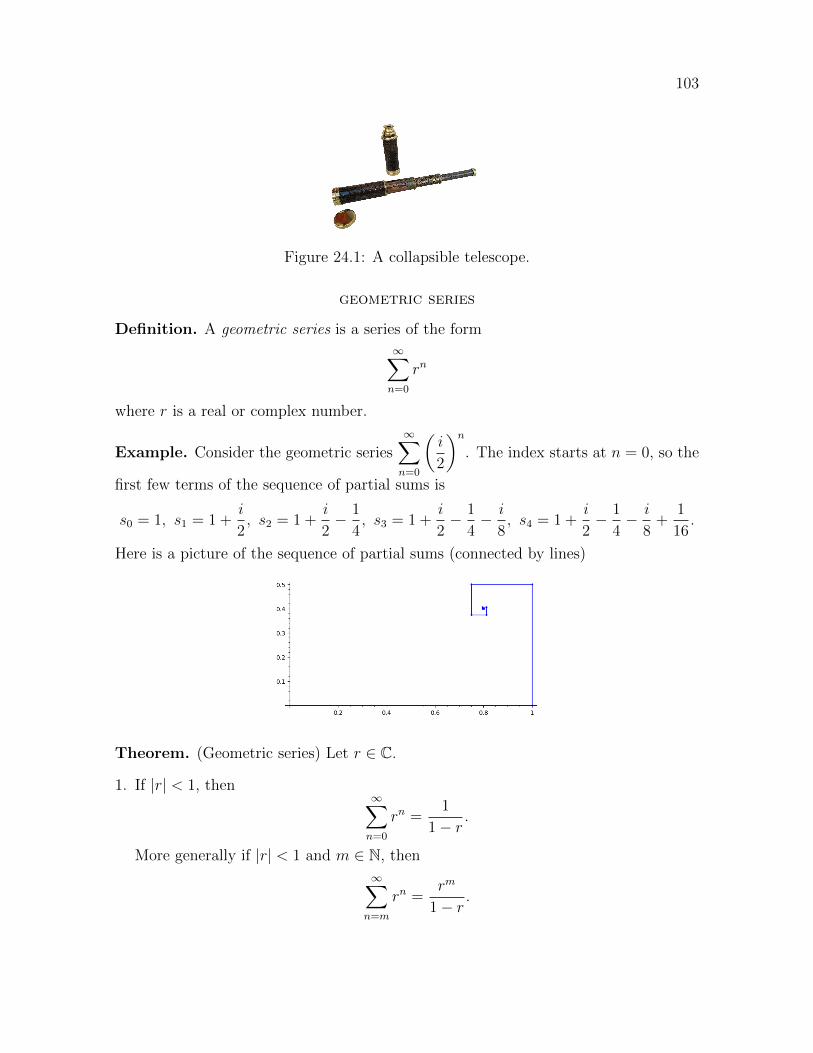
103
Figure 24.1: A collapsible telescope.
geometric series
Definition. A geometric series is a series of the form
∞∑n=0
rn
where r is a real or complex number.
Example. Consider the geometric series∞∑n=0
(i
2
)n. The index starts at n = 0, so the
first few terms of the sequence of partial sums is
s0 = 1, s1 = 1 +i
2, s2 = 1 +
i
2− 1
4, s3 = 1 +
i
2− 1
4− i
8, s4 = 1 +
i
2− 1
4− i
8+
1
16.
Here is a picture of the sequence of partial sums (connected by lines)
Theorem. (Geometric series) Let r ∈ C.
1. If |r| < 1, then∞∑n=0
rn =1
1− r.
More generally if |r| < 1 and m ∈ N, then
∞∑n=m
rn =rm
1− r.

104 CHAPTER 24. WEEK 10, MONDAY
2. If |r| ≥ 1, then∑∞
n=0 rn diverges.
Example. Let
α = (20/21)
(1
2+
√3
2i
)=
1
2.1+
√3
2.1i,
a point with argument 30◦ and length slightly less than 1. According to the geometricseries theorem, the series converges to
∞∑n=0
αn =1
1− α≈ 0.68 + 1.85 i.
Here is a picture of the partial sums for∑∞
n=0 αn
Note that the angle at which each successive line rotates is arg(α) = 30◦. Can you seewhy?
Example Compute the following sums:
(a)∑∞
n=0
(i2
)n(b)
∑∞n=0 5
(23
)n(c)
∑∞n=2
(34
)n(d)
∞∑n=0
(4i)n (e)∞∑n=3
722n
10n.
Note that in (c), the sum starts with n = 2, and in (e), the sum starts with n = 3.
solution: (a) Since |i/2| = 1/2 < 1, the formula for the sum of a geometric seriesapplies, and we get
∞∑n=0
(i
2
)n=
1
1− i2
=2
2− i=
2
2− i· 2 + i
2 + i=
4 + 2i
5.
(b) Using the limit theorems for series and the formula for the sum of a geometricseries, we have
∞∑n=0
5
(2
3
)n= 5
∞∑n=0
(2
3
)n= 5 · 1
1− 23
= 15.

105
(c) Using the formula for a geometric series, we have
∞∑n=2
(3
4
)n=
(3/4)2
1− 34
=9
4.
Note: Another way to approach this problem is to first compute the sum startingwith n = 0:
∞∑n=0
(3
4
)n=
1
1− 34
= 4,
and then subtract the terms corresponding to n = 0, 1:
4− 1− 3
4=
9
4.
This method takes more steps and, in practice, is a likely source of arithmetic errors.
(d) Since |4i| = 4 ≥ 1, the series∑∞
n=0 (4i)n diverges.
(e) We have
∞∑n=3
722n
10n=∞∑n=3
74n
10n
= 7∞∑n=3
(4
10
)n
= 7∞∑n=3
(2
5
)n
= 7
(2
5
)3 ∞∑n=0
(2
5
)n
= 7
(2
5
)31
1− 2/5
= 7
(2
5
)35
3=
7 · 825 · 3
=56
75.
Proof of the geometric series theorem. An easy induction argument shows that
n∑i=0
rn =1− rn+1
1− r

106 CHAPTER 24. WEEK 10, MONDAY
for r 6= 1. Suppose that |r| < 1. By the above formula, the n-th partial sum of theseries is
sn =1− rn+1
1− r.
Using our limit theorems, we get
limn→∞
sn = limn→∞
1− rn+1
1− r
=1
1− r· limn→∞
(1− rn+1) (since1
1− ris a constant)
=1
1− r
(limn→∞
1− limn→∞
rn+1)
=1
1− r
(limn→∞
1− 0)
(since |r| < 1)
=1
1− r.
Next, use our limit theorem for series to get
∞∑n=m
rn = rm + rm+1 + rm+2 + · · · = rm(1 + r + r2 + . . . ) = rm∞∑n=0
rn =rm
1− r.
Now suppose that |r| ≥ 1. If r = 1, then the n-th partial sum of the series is sn = n,which gives a divergent sequence. Next, suppose that |r| ≥ 1 and r 6= 1. Recall thatin that case, we showed earlier that limn→∞ r
n diverges. For the sake of contradictionsuppose the series converges. Say
∑∞n=0 r
n = s. From our earlier formula, we know
sn =1− rn+1
1− r.
Solve for rn+1 to get rn+1 = 1− (1− r)sn, and hence,
rn =1
r(1− (1− r)sn).
We are assuming limn→∞ sn = s, and therefore, using our limit theorems
limn→∞
rn =1
r(1− (1− r)s).
However, we know limn→∞ rn diverges when |r| ≥ 1 and r 6= 1. This contradiction
shows that∑∞
n=0 rn must diverge.

Week 10, Wednesday: Series tests I
Series tests I
(Supplemental reading: Section 9.2 in Swanson.)
Our next goal is to present the standard collection of tests for determining whether aseries converges.1 Here is the list:
1. the geometric series test
2. the n-th term test
3. the comparison test
4. the limit comparison test
5. the alternating series test
6. the absolute convergence test
7. the ratio test
8. the root test
9. the integral test
10. the p-series test.
We have already discussed the geometric series test, but we will state it again here forcompleteness and for review.
1. The geometric series test. Let r ∈ C. The series∑∞
n=0 rn converges if and only
if |r| < 1. When |r| < 1,∞∑n=0
rn =1
1− r.
More generally, for a ∈ C and k ∈ N, if |r| < 1, then
∞∑n=k
arn =ark
1− r.
Examples. (See earlier in our notes for more examples.)
1Note that knowing that a series converges is different from knowing its limit.
107
108 CHAPTER 25. WEEK 10, WEDNESDAY
1.∞∑n=0
(i
2
)n=
1
1− i2
=2
2− i=
2
2− i· 2 + i
2 + i=
4
5+
1
5i.
2.∞∑n=2
8
(2n+2
5n
)= 8
∞∑n=2
4n
5n= 8
∞∑n=2
(4
5
)n= 8
(4
5
)21
1− 45
=128
5.
3.∑
n=1(4i)n diverges since |4i| = 4 ≥ 1.
2. The n-th term test. The n-th term test is a criterion for divergence of a complexseries. It says that if limn→∞ an 6= 0, then
∑an diverges. If limn→∞ an = 0, we cannot
conclude that∑∞
n=0 converges, as we will see with the harmonic series, below.
Proposition. If limn→∞ an 6= 0, then∑an diverges.
Proof. To prove this result, we prove its contrapositive2: if∑an converges, then
limn→∞ an = 0. To see this, suppose that∑an = s, i.e., lim sn = s where sn =
∑nk=1 ak
is the n-th partial sum of {an}. We have that sn − sn−1 = an. Therefore, using ourlimit theorems
limn→∞
an = limn→∞
(sn − sn−1) = limn→∞
sn − limn→∞
sn−1 = s− s = 0.
�
Examples.
1. The series∑∞
n=1(−1)n diverges since limn→∞(−1)n not does exist. In particular,limn→∞(−1)n 6= 0.
2. The series∑∞
n=13n2−2n+1
2n2+5does not converge since lim 3n2−2n+1
2n2+5= 3
26= 0.
3. Consider series∑∞
n=11n. We have lim 1
n= 0, however, as we will see below, this
series diverges. So the converse of the proposition does not hold. The propositioncan only be used to prove divergence (not convergence).
The harmonic series. The harmonic series is the series
∞∑n=1
1
n= 1 +
1
2+
1
3+
1
4+ . . .
Here is a plot of its partial sums, 1, 1 + 1/2, 1 + 1/2 + 1/3, . . . :
2The contrapositive of a statement “P implies Q” is “not Q implies not P”.

109
It looks like these partial sums might be converging, but in fact they do not. You maynotice that this plot is reminiscent of the graph of the logarithm, which hints that tosee substantial growth in the partial sums, we will need to consider partial sums of anexponentially-growing number of terms of the series. The first proof that the harmonicseries diverges, which we present below, is due to Nicole Orseme around 1350. Thetheorem is a special case of the p-series test which we will discuss later and easily proveusing the integral test.
Theorem. The harmonic series diverges.
Proof. The first partial sum of the harmonic series is
1∑n=1
1
n= 1.
The second partial sum is2∑
n=1
1
n= 1 +
1
2
The fourth:
22∑n=1
1
n= 1 +
1
2+
(1
3+
1
4
)≥ 1 +
1
2+
(1
4+
1
4
)= 1 +
1
2+
1
2= 1 + 2 · 1
2.
The eighth:
23∑n=1
1
n= 1 +
1
2+
(1
3+
1
4
)+
(1
5+
1
6+
1
7+
1
8
)
≥ 1 +1
2+
(1
4+
1
4
)+
(1
8+
1
8+
1
8+
1
8
)
= 1 + 3 · 1
2.

110 CHAPTER 25. WEEK 10, WEDNESDAY
An induction proof shows that
s2k =2k∑n=1
1
n≥ 1 +
k
2.
for all k ≥ 0. Thus, the sequence of partial sums for the harmonic series is unboundedand, hence, diverges.
3. The comparison test. In the following proposition, notice that the test onlyapplies to nonnegative real sequences. Also, notice the crucial role of the monotoneconvergence theorem in the proof. (Recall that MCT says that if a real sequence ismonotone and bounded above, then it converges.)
Proposition (series comparison test). Suppose that {an} and {bn} are real se-quences with
0 ≤ an ≤ bn
for all n. Then
(a)∑bn converges ⇒
∑an converges.
(b)∑an diverges ⇒
∑bn diverges.
Proof. Let
sn = a1 + a2 + · · ·+ an
tn = b1 + b2 + · · ·+ bn
be the respective partial sums. Since an ≤ bn for all n, we have sn ≤ tn for all n. Sinceboth sequences have nonnegative terms, their sequences of partial sums are monotoneincreasing. To prove part (a), suppose that
∑bn converges, and say
∑bn = t. This
means that lim tn = t. By the monotone convergence theorem, we know that t =sup {tn}. Thus,
sn ≤ tn ≤ t = sup {tn} .
Hence, {sn} is both monotone increasing and bounded above. Again by the monotoneconvergence theorem, {sn} converges, i.e.,
∑an converges.
Part (b) is the contrapositive of part (a) and, hence, follows immediately.
Examples.
1. For all n ≥ 1
0 ≤ 1
(n+ 1)2≤ 1
n(n+ 1).

111
We showed in an earlier lecture that∑∞
n=11
n(n+1)converges to 1. Thus, by compar-
ison to∑∞
n=11
n(n+1),
∞∑n=1
1
(n+ 1)2=
1
22+
1
32+
1
42+ . . .
converges. It then follows that
∞∑n=1
1
n2=
1
12+
1
22+
1
32+
1
42+ . . .
(The partial sums of the last two displayed series differ by 1, so the convergence ofone implies the convergence of the other.)
2. The series∞∑n=1
1
n2 +√n
converges by comparison with∞∑n=1
1
n2since
0 ≤ 1
n2 +√n≤ 1
n2.
3. The series∞∑n=1
1√n
diverges by comparison with∞∑n=1
1
nsince
0 ≤ 1
n≤ 1√
n
for all n, and the harmonic series,∞∑n=1
1
n, diverges.
We will continue with our list of tests next time.

Week 10, Friday: Series tests II
Series tests II
(Supplemental reading: Section 9.2 in Swanson.)
We continue our discussion of the standard tests for determining whether a seriesconverges.
1. the geometric series test
2. the n-th term test
3. the comparison test
4. the limit comparison test
5. the alternating series test
6. the absolute convergence test
7. the ratio test
8. the root test
9. the integral test
10. the p-series test.
4. The limit comparison test. In the following, note the key hypotheses that thesequences have positive terms and that the limit of their quotient is nonzero. Sincea sequence converges if and only if its tail converges, one may also apply the limitcomparison test to sequences that are positive after a finite number of terms.
Proposition (limit comparison test). Suppose {an} and {bn} are real sequencesof positive terms and that
limn→∞
anbn
= L 6= 0.
The∑an converges if and only if
∑bn converges.
Remark. Whether∑
n an converges depends upon how quickly the terms an die off.For instance,
∑∞n=1
1n2 converges but
∑∞n=1
1n
does not. Even though lim 1n2 = lim 1
n= 0,
the terms of{
1n
}do not die off quickly enough. The condition an
bn= L 6= 0 means
112

113
that an and bn grow or diminish at comparable rates, unlike the case of∑∞
n=11n2
and∑∞
n=11n.
Example. Consider the series∞∑n=1
6n+ 7
2n2 − 4.
For large n,6n+ 7
2n2 − 4≈ 6n
2n2=
3
n.
Since the harmonic series,∑∞
n=11n
diverges, we expect∑∞
n=16n+72n2−4 will also diverge.
To make this intuition precise, we use the limit comparison test with an = 6n+72n2−4 and
bn = 1n:
anbn
=6n+ 7
2n2 − 4· n
1=
6n2 + 7n
2n2 − 4−→ 3 6= 0
as n→∞. Thus,∑∞
n=16n+72n2−4 diverges by limit comparison with the harmonic series.
Exercise. By a similar argument, show that∑∞
n=17
2n2−4 converges using limit com-
parison with∑∞
n=11n2 .
Proof of the limit comparison test. Suppose that lim anbn
= L 6= 0. Since an > 0, bn > 0,
and L 6= 0, we have L > 0. Apply the definition of the limit with ε = 12L > 0 to find N
such that n > N implies ∣∣∣∣L− anbn
∣∣∣∣ < 1
2L.
Thus, anbn
is within a distance of L/2 from L, i.e., it is in the interval pictured below:
12L 3
2LL
.
Then1
2L <
anbn
<3
2L ⇒ 1
2Lbn < an <
3
2Lbn.
If∑an converges, the ordinary comparison theorem implies that
∑12Lbn converges.
Hence, using our earlier limit theorems1, so does 2L
∑12Lbn =
∑bn. Similarly, if
∑bn
converges, then so does 32L∑bn =
∑32Lbn. Then since an <
32Lbn, the comparison
theorem says∑an converges.
Now suppose that R > 1 or R =∞. Then we can take N such that
n > N ⇒ an+1
an> 1 an+1 > an.
1If∑cn converges and k is a constant, then
∑kcn converges and equals k
∑cn.

114 CHAPTER 26. WEEK 10, FRIDAY
By transitivity of ≥, we have an ≥ aN+1 > 0 for all n > N . Thus, limn→∞ an 6= 0, andthe series diverges by the n-th term test.
5. The alternating series test.
We saw earlier that if∑an converges, then limn→∞ an = 0. We also saw that
the converse does not hold, in general. For instance∑∞
n=11n
diverges even thoughlimn→∞
1n
= 0. We now discuss the case of a special type of series for which theconverse does hold.
Proposition (alternating series test). Let {an} be a monotonically decreasingsequence of positive terms. Then
∑∞n=1(−1)n+1an converges if and only if limn→∞ an =
0.
Examples. The alternating harmonic series is the series
∞∑n=1
(−1)n+1 1
n= 1− 1
2+
1
3− 1
4+ · · · .
To see that it converges, apply the alternating series test with an = 1n. (Check that
the test applies:{
1n
}is a monotonically decreasing sequence of positive terms, and
limn→∞1n
= 0.)
The alternating harmonic series is the canonical example of what is called a condition-ally convergent series: it converges, but the series formed by taking the absolute valuesof it terms,
∑∞n=1 |(−1)n+1 1
n| =
∑∞n=1
1n
diverges.
Proof of the alternating series test.
(⇒) Suppose that∑∞
n=1(−1)n+1an converges. By the n-th term test, it follows that limn→∞(−1)n+1an =0. We have seen that if {bn} is any sequence, real or complex, that limn→∞ bn = 0 ifand only if limn→∞ |bn| = 0. Applying that here, we conclude that limn→∞ an = 0.
(⇐) Now suppose that limn→∞ an = 0. We must argue that the sequence of partialsums {sn} for
∑∞n=1(−1)n+1an converges. Our strategy is to divide these partial sums
into two subsequences, {s2n} and {s2n+1}—the even- and the odd-indexed terms—andto argue that these two subsequences converge to the same value. First consider {s2n}:
s2n = (a1 − a2) + (a3 − a4) + · · ·+ (a2n−1 − a2n).
The terms of s2n are grouped as above to make it clear that since {an} is monotoni-cally decreasing, each of the a2k−1 − a2k is nonnegative. Thus, {s2n} is monotonicallyincreasing. Further, looking at this sequence a different way makes it clear that s2n isbounded above by a1:
s2n = a1 − (a2 − a3)− (a4 − a5)− · · · − (a2n−2 − a2n−1)− a2n ≤ a1.
By the monotone convergence theorem, we conclude that
limn→∞
s2n = s
115
for some s ∈ R. It then follows that
limn→∞
s2n+1 = limn→∞
(s2n + an+1) = limn→∞
s2n + limn→∞
an+1 = s+ 0 = s.
(We know that limn→∞ an+1 = 0 by the n-term test.) Since
limn→∞
s2n = limn→∞
s2n+1 = s,
it looks like there is some hope of showing that limn→∞ sn = s. In fact, that is true,and we can give a straight ε-N proof. Let ε > 0, and then take N so that n > Nimplies.
limn→∞
|s− s2n| < ε and limn→∞
|s− s2n+1| < ε
simultaneously. But this just says that every term of the sequence {sn} is within εof s: n > 2N + 1 implies |s− sn| < ε.
6. The absolute convergence test.
Definition. A series of complex numbers∑an is absolutely convergent if
∑|an|
is convergent. If∑an converges but
∑|an| does not, then
∑an is conditionally
convergent.
Example. To emphasize the example presented earlier: the alternating harmonic se-ries,
∑∞n=1(−1)n+1 1
n, converges (by the alternating series test), but
∑∞n=1
∣∣(−1)n+1 1n
∣∣ =∑∞n=1
1n
does not. So the alternating harmonic series is conditionally convergent.
Many of our series tests apply to only series whose terms are nonnegative reals. Thefollowing proposition is of central importance: it shows how these series tests can saysomething about arbitrary complex series.
Proposition (absolute convergence test). Let∑an be a complex series. Then
if∑an is absolutely convergent, it is convergent:∑
|an| convergent =⇒∑
an convergent.
Examples. The series
∞∑n=1
(−1)n+1 1
n2= 1− 1
4+
1
9− 1
16+ · · ·
converges by the absolute convergence test since
∞∑n=1
∣∣∣∣(−1)n+1 1
n2
∣∣∣∣ =∞∑n=1
1
n2,
and we have seen that∑∞
n=11n2 converges.

116 CHAPTER 26. WEEK 10, FRIDAY
Similarly,∞∑n=1
cos(n) + i sin(n)
n2
is absolutely convergent since
∞∑n=1
∣∣∣∣cos(n) + i sin(n)
n2
∣∣∣∣ =∞∑n=1
| cos(n) + i sin(n)|n2
=∞∑n=1
1
n2.
Proof of the absolute convergence test. Suppose that∑∞
n=1 |an| converges. We will usethe fact that a real or complex series converges if and only it is a Cauchy sequence inorder to prove that
∑∞n=1 an converges.
Definesn = a1 + ·+ an and s̃n = |a1|+ ·+ |an|,
the partial sums for∑∞
n=1 an and∑∞
n=1 |an|, respectively. We are given that {s̃n}converges and must show that {sn} converges. Let ε > 0. Since {s̃n} converges, it is aCauchy sequence. Thus, there exists N such that m,n > N implies
|s̃m − s̃n| < ε.
Without loss of generality, suppose that m ≥ n. Then, using the triangle inequality,
|sm − sn| = |an+1 + · · ·+ am|≤ |an+1|+ · · ·+ |am|= ||an+1|+ · · ·+ |am||= |s̃m − s̃n|< ε.
Thus, {sn} is a Cauchy sequence and therefore converges. In other words,∑∞
n=1 anconverges.
A peculiar property of conditionally convergent series. What happens if yourearrange the terms of an infinite series? To be precise, define a rearrangement of aseries
∑an to be a series
∑bn where the elements of {an} and {an} are in bijection—
same sums but in different orders. By the commutative law for addition, one mightexpect to get the same behavior: one of the series converges if and only if the otherdoes, and it they do converge, they converge to the same value. It turns out thatthis is true for absolutely convergent series but not for conditionally convergent ones.For instance, all rearrangements of the series
∑∞n=1
1n2 will converge to the same value.
On the other hand the value of a rearrangement of∑∞
n=1(−1)n+! 1n
will depend on therearrangement—even whether the series will converge. Something even wilder is true:
Proposition. Let∑an be a conditionally convergent real series, and let a be any real
number. Then there is a rearrangement of∑an that converges to a. Further, there

117
are rearrangements of∑an that diverge to ∞, that diverge to −∞, and that fail to
have any limit.
The idea behind the proof is the following. Say∑an is conditionally convergent.
Then let∑pn be the same as
∑an but with all negative terms an < 0 set equal to
zero. Similarly, let∑qn be the same as
∑an but with all positive terms set equal
to zero. Using the monotone convergence theorem, one may show that since∑an is
conditionally convergent,∑pn diverges to ∞ and
∑qn diverges to −∞. To get a
rearrangement of∑an that converges to an arbitrary real number a do the following.
Assume a > 0, the case of a ≤ 0 being similar. Create the rearrangement of∑an
in steps. First add enough terms of∑pn until we first get a number bigger than a.
That’s possible since∑pn diverges to∞. Next, add enough terms from
∑qn until we
get first get a number less than a, possible since∑qn diverges to −∞. Continue now
by adding further terms from∑pn until we first get a number above a, and then add
further terms from∑qn until we first get below a. Continue ad infinitum. The next
part of the argument is to show the resulting rearrangement converges to a. A similarargument holds in the cases where a = ±∞.

Week 11, Monday: Series tests III
Series tests III
(Supplemental reading: Section 9.2 in Swanson.)
We continue our discussion of the standard tests for determining whether a seriesconverges:
1. the geometric series test
2. the n-th term test
3. the comparison test
4. the limit comparison test
5. the alternating series test
6. the absolute convergence test
7. the ratio test
8. the root test
9. the integral test
10. the p-series test.
7. The ratio test.
Proposition (ratio test). Let {an} be a sequence of positive real numbers, andsuppose that
limn→∞
an+1
an= R.
Then
1. if R < 1, then∑an converges;
2. if R > 1 or R =∞, then∑an diverges;
3. if R = 1, the test is inconclusive.
118

119
Example. The ratio test shows that∑∞
n=01n!
converges since, as n→∞,
1(n+1)!
1n!
=n!
(n+ 1)!=
1
n+ 1−→ 0 < 1.
Example. To see that the case R = 1 is inconclusive, consider the series∑∞
n=11n
and∑∞n=1
1n2 . The former series diverges and the latter converges, yet we have
limn→∞
1n+11n
= 1 and limn→∞
1(n+1)2
1n2
= 1.
Example. Even if a series does not have positive terms, one can use the ratio testto consider if a series is absolutely convergent. For instance, we can see that theseries
∑∞n=(−1)nn
(12n
)is absolutely convergent (hence, convergent), since
limn→∞
(n+ 1)(
12n+1
)n(
12n
) = limn→∞
n
n+ 1· 1
2=
1
2< 1.
Note. The tell-tale sign that the ratio test might apply is the presence of factorialsand exponents.
Proof of the ratio test. First suppose that limn→∞an+1
an= R < 1. Fix any real number r
such that 0 ≤ R < r < 1. Our goal, roughly, is to apply the comparison test to∑an,
comparing it with the convergent geometric series∑rn. Applying the definition of the
limit, we can find N such that n > N implies |R− an+1
an| < ε where ε has been choose
small enough so that this condition forces an+1
an< r:
1rR
(R− ε
)R + ε
Thus, n > N implies that 0 ≤ an+1
an< r, i.e.,
0 ≤ an+1 < anr.
In particular, taking n = N + 1, this means
aN+2 < aN+1r
and thenaN+3 < aN+2r < aN+1r
2.
Continuing,aN+4 < aN+3r < aN+1r
3,

120 CHAPTER 27. WEEK 11, MONDAY
and so on. Letting c := aN+1, we may show by induction that
aN+k < crk−1
for k ≥ 2. Since |r| = r < 1, the series
∞∑k=2
crk−1 = cr
∞∑k=0
rk
converges. By the comparison test, the series∑∞
n=N+2 an converges. Since this is a tailof our original series
∑an, the original series converges.
Now suppose that R > 1 or R =∞. Then we can take N such that
n > N ⇒ an+1
an> 1 an+1 > an.
By transitivity of ≥, we have an ≥ aN+1 > 0 for all n > N . Thus, limn→∞ an 6= 0, andthe series diverges by the n-th term test.
8. The root test. We will not discuss this test, but include it here as one of thestandard tests.
Proposition (root test). Let∑an be a series of nonnegative terms. Suppose that
lim a1/nn = b. If b < 1, the series converges. If b > 1, the series diverges. If b = 1, the
test is inconclusive.
9. The integral test.
Proposition (integral test). Suppose f(x) is a continuous, positive, decreasing func-tion whose domain contains (0,∞). Then
∑f(n) converges if and only if limn(
∫ n1f(x) dx)
converges, i.e., if and only if∫∞1f(x) dx converges.
Example. We can use the integral test to give a quick proof that the harmonic seriesdiverges:∫ ∞
1
1
xdx = lim
n→∞
∫ n
1
1
xdx = lim
n→∞lnx∣∣n1
= limn→∞
(lnn− ln 1) = limn→∞
lnn =∞.
Thus,∑∞
n=11n
diverges by the integral test.
Similarly, we may show that∑∞
n=11n2 converges:∫ ∞
1
1
x2dx = lim
n→∞
∫ n
1
1
x2dx = lim
n→∞−1
x
∣∣n1
= limn→∞
(− 1
n+ 1) = 1.
Therefore,∑∞
n=11n2 converges by the integral test.

121
Proof of the integral test. Consider the standard pictures for the upper and lower Rie-mann sums for the integral of f :
1
R1
2
R2
3
R3
4
R4
5
R5
6
. . .
upper sum
1
r1
2
r2
3
r3
4
r4
5
r5
lower sum
6
. . .
graph of f
For each n = 1, 2, . . . , we have
area(Rn) = base(Rn) · height(Rn) = 1 · f(n) = f(n). (27.1)
Similarly,area(rn) = base(rn) · height(rn) = 1 · f(n+ 1) = f(n+ 1). (27.2)
Further, since f is decreasing and nonnegative
area(rn) ≤∫ n+1
n
f(x) dx ≤ area(Rn),
and thus, using (27.1) and (27.2),
f(n+ 1) ≤∫ n+1
n
f(x) dx ≤ f(n). (27.3)
Summing, we get
k∑n=1
f(n+ 1) ≤k∑
n=1
∫ n+1
n
f(x) dx ≤k∑
n=1
f(n).
Then note that
k∑n=1
∫ n+1
n
f(x) dx =
∫ 2
1
f(x) dx+
∫ 3
2
f(x) dx+ · · ·+∫ k+1
k
f(x) dx =
∫ k+1
1
f(x) dx
since we are just adding areas under the graph of f . So the result follows from theordinary comparison theorem applied to (27.3).

122 CHAPTER 27. WEEK 11, MONDAY
10. The p-series test.
Proposition (p-series test). Let p ∈ R. Then the series∑ 1
np
converges if and only if p > 1.
Example. The p-series tests says these series converge:
∞∑n=1
1
n3/2,
∞∑n=1
1
n1.000001
and these series do not:∞∑n=1
13√n,
∞∑n=1
1
n0.999999.
Proof of the p-series test. Apply the integral test. We did the case p = 1 earlier. Soassume p 6= 1. In that case, we get∫ ∞
1
1
xdx =
∫ ∞1
x−1 dx
= limn→∞
∫ n
1
x−1 dx
= limn→∞
1
1− px1−p
∣∣n1
=1
1− plimn→∞
(n1−p − 1)
=
{1p−1 if p > 1
∞ if p < 1.
Interesting question. Does the following sum converge:
∞∑n=1
1
n1+ 1n
?
The p-series test does not apply since the exponent is not constant.

Week 11, Wednesday: Limits of functions
Limits of functions
(Supplemental reading: Sections 4.1 and 4.2 in Swanson.)
We now switch our focus from limits of sequences and series to limits of functions.Let F = R or C.
Recall that the definition of the derivative of a function f at a point a looks somethinglike this:
f ′(a) = limh→0
f(a+ h)− f(a)
h.
Here we are taking the limit of the function
g(h) := limh→0
f(a+ h)− f(a)
h,
and that function is not defined at exactly the point of interest, i.e., at h = 0:
g(0) =f(a+ 0)− f(a)
0=
0
0= undefined.
In this way, a main use of the limit of a function is to determine what value a functionshould have at a point at which it is not defined. We are able to make this determinationsince the function is nicely behaved at all nearby points. The following definitioncharacterizes the types of points, called limit points, at which we might hope to computea limit.
Definition. Let A ⊆ F . A point x ∈ F is a limit point of A if every open ballcentered at x contains a point of A not equal to x. In other words, for all r > 0 thereexists y ∈ B(x, r) ∩ A such that x 6= y.
Roughly, a limit point x of a set A can be approximated arbitrary closely by pointsbesides x that are within A.
Examples.
1. The limit points of A = (0, 1) ⊂ R are all points in the closed interval [0, 1]. Notethat 0 and 1 are limit points of A that are not in A.
123

124 CHAPTER 28. WEEK 11, WEDNESDAY
2. The limit points of A = (0, 1)∪{7} ⊂ R are again the points of [0, 1]. That’s becausethere is an open interval (ball) about 7 that contains no points of A besides 7 (forinstance, the interval (6, 8) contains no points in A besides 7). We naturally call 7an isolated point of A.
3. The set of limit points of the “punctured ball” B(0; 1) \ 0 of radius 1 centered atthe origin in C is the closed ball
B(0; 1) := {z ∈ C : |z| ≤ 1} .
Every point in the punctured open ball is a limit point, but so are the points on theboundary and the origin.
Definition. Let F = R or C, as usual. Let A ⊆ F and f : A → F . Let a ∈ F be alimit point of A. Then the limit of f(x) as x approaches a is L ∈ F if for all ε > 0,there exists δ > 0 such that if x ∈ A and 0 < |x− a| < δ, then
|f(x)− L| < ε.
If the limit is L, then we write limx→a f(x) = L.
Remark. If you wanted to pack the definition of limx→a f(x) = L into symbols, youcould write
∀ε > 0,∃δ > 0, s.t. f ((B(a; δ) \ {a}) ∩ A) ⊆ B(L; ε).
In the case where F = R, we can interpret the definition of the limit using the graphof f :
L
aδ δ
ε
ε
x
f(x)
Meaning of ε and δ in the definition of the limit when F = R.
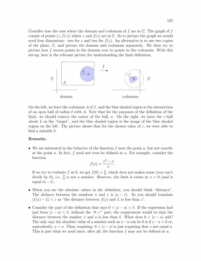
125
Consider now the case where the domain and codomain of f are in C. The graph of fconsist of points (z, f(z)) where z and f(z) are in C. So to picture the graph we wouldneed four dimensions—two for z and two for f(z). An alternative is to use two copiesof the plane, C, and picture the domain and codomain separately. We then try topicture how f moves points in the domain over to points in the codomain. With thisset-up, here is the relevant picture for understanding the limit definition:
C
domain
A
aδ
f
CL
ε
codomain
On the left, we have the codomain A of f , and the blue shaded region is the intersectionof an open ball of radius δ with A. Note that for the purposes of the definition of thelimit, we should remove the center of the ball, a. On the right, we have the ε-ballabout L as the “target”, and the blue shaded region is the image of the blue shadedregion on the left. The picture shows that for the chosen value of ε, we were able tofind a suitable δ.
Remarks.
• We are interested in the behavior of the function f near the point a, but not exactlyat the point a. In fact, f need not even be defined at a. For example, consider thefunction
f(x) =x2 − xx
.
If we try to evaluate f at 0, we get f(0) = 00, which does not makes sense (you can’t
divide by 0), i.e., 00
is not a number. However, the limit is exists at x = 0 (and isequal to −1).
• When you see the absolute values in the definition, you should think “distance”.The distance between the numbers u and v is |u − v|. So you should translate|f(x)− L| < ε as “the distance between f(x) and L is less than ε”.
• Consider the part of the definition that says 0 < |x − a| < δ. If the expression hadjust been |x − a| < δ, without the “0 <” part, the requirement would be that thedistance between the number x and a is less than δ. What does 0 < |x − a| add?The only way the absolute value of a number such as x−a can be 0 is if x−a = 0 or,equivalently, x = a. Thus, requiring 0 < |x− a| is just requiring that x not equal a.This is just what we need since, after all, the function f may not be defined at a.

126 CHAPTER 28. WEEK 11, WEDNESDAY
• Note the quantifiers “for all” and “there exists” in the definition. Just as with thedefinition of limits of sequences, it takes a while to appreciate their importance, butthey are essential. First take the “for all” part. The definition say that for all ε > 0,we are going to want |f(x)−L| < ε. Translating: for all ε > 0, we will want to makethe distance between f(x) and L less that ε > 0. Our goal is to make f close to L,and the ε is a measure of how close. By making ε small and requiring |f(x)−L| < ε,we are ensuring that f(x) is within a distance of ε from L.
Next, consider the “there exists” part of the definition. It says that if you want f(x)to be within a distance of ε of L, then you need to make 0 < |x − a| < δ. In otherwords, you need to make x within a distance of δ of a (remembering that we don’tcare what happens when x = a).
Given any ε > 0 (a challenge to make f(x) close to L), you want to find an appro-priate distance δ > 0 (so that if x is δ-close to a, then f(x) is ε-close to L).
With sequences, the game was: given ε find N . With functions, the game becomes:given ε, find δ.
Warning. At some point, in proving a statement of the form limx→a f(x) = L, youwill be tempted to have δ be a function of x. That is not allowed! (On the other hand,δ is typically a function of ε, just as with sequences, N is typically a function of ε (butcannot be a function of n).)
Example. Consider the function
f : F → F
x 7→ 5x+ 3.
Then limx→2 5x+ 3 = 13.
Proof. Given ε > 0, let δ = ε/5. Then if
0 < |x− 2| < δ,
it follows that
|f(x)− 13| = |(5x+ 3)− 13|= |5x− 10|= 5|x− 2|< 5δ
= 5 · ε5
= ε.

127
Example. Prove that limx→0 x cos(1/x) = 0.
−1 −0.5 0 0.5 1−0.6
−0.4
−0.2
0
0.2
0.4
0.6
Graph of f(x) = x cos(1/x).
Proof. Given ε > 0, let δ = ε. Suppose that 0 < |x − 0| < δ; in other words, supposethat 0 < |x| < ε. Then, since | cos(y)| ≤ 1 for all y, we have
|x cos(1/x)| = |x|| cos(1/x)|≤ |x|< δ
= ε.
Example. Proving limit statements for simple function like f(x) = x2 can be achallenge. For instance, here we prove the “obvious” statement that limx→5 x
2 = 25.This example points out the need for better tools (e.g., a new-from-old limit theoremlike we had with sequences that allows us to avoid going down to the level of using ε-δarguments).
Proof. Given ε > 0, let δ = min {1, ε/11}, i.e., δ is the minumum of 1 and ε/11.So δ ≤ 1 and δ ≤ ε/11 (with equality holding in at least one of these). Supposethat x satisfies 0 < |x − 5| < δ. Since δ ≤ 1, the distance between x and 5 is lessthan 1. It follows 4 < x < 6, and hence, adding 5 across this string of inequalities, weget 9 < x+ 5 < 11. In particular, |x+ 5| < 11. Therefore,
|x2 − 25| = |(x+ 5)(x− 5)| = |x+ 5||x− 5| < 11|x− 5|.
Now, since δ ≤ ε/11 and |x− 5| < δ, it follows that
|x2 − 25| < 11|x− 5| < 11 · ε11
= ε,
as required.
Example. Claim: limx→16
√x = 4.

128 CHAPTER 28. WEEK 11, WEDNESDAY
Proof. Given ε > 0, let δ = 4ε, and suppose that
0 < |x− 16| < δ =ε
4.
Then
|√x− 4| =
∣∣∣∣(√x− 4) ·√x+ 4√x+ 4
∣∣∣∣=|x− 16||√x+ 4|
<|x− 16|
4
=1
4|x− 16|
<1
4δ
= ε.
Week 11, Friday: Continuity and derivatives
Continuity and derivatives
(Supplemental reading: Sections 5.1, 6.1, and 6.2 in Swanson.)
Our results will hold for real and complex functions unless noted. To treat both casessimultaneously, let F = R or C.
New-from-old limit theorems.
Functions can sometimes be decomposed into sums and products of simpler functions.Taking a cue from what we did earlier with sequences, we first find limits of somesimple functions using ε-δ proofs, and then we prove a general result that allows us tocompute limits of more complicated functions built from these without resorting to ε-δproofs.
Recall the definition of a limit of a function:
Definition. Let A ⊆ F . A point x ∈ F is a limit point of A if every open ballcentered at x contains a point of A not equal to x. In other words, for all r > 0 thereexists y ∈ B(x, r) ∩ A such that x 6= y.
Now we compute the limits of a couple of simple functions. These, combined with the“new-from-old” limit theorem we prove next, will allow us to easily compute the limitsof all rational functions, i.e., of all quotients of polynomials.
Proposition. Let a, c ∈ F . Then
1. limx→a
c = c.
2. limx→a
x = a.
Proof.
1 In this case, our function is f(x) = c for all x, and we are claiming the limit is c.Given ε > 0,
|f(x)− c| = |c− c| = 0 < ε
129

130 CHAPTER 29. WEEK 11, FRIDAY
for all x. This means the ε-δ definition of the limit is satisfied for any choice of δ > 0,reflecting that fact that it is pretty easy to make f(x) close to c!
2 Here, f(x) = x for all x, and we claim the limit is a. Given ε > 0, let δ = ε. Then,if we assume 0 < |x− a| < δ = ε, it follows that
|f(x)− a| = |x− a| < ε.
Here is the function-version of a “new-from-old” limit theorem, analogous to the onegiven earlier for sequences. It allows us to determine limits of functions that are builtfrom simpler functions.
Theorem. Suppose that limx→a f(x) = L and limx→a g(x) = M . Then,
1. limx→a(f(x) + g(x)) = limx→a f(x) + limx→a g(x) = L+M ,
2. limx→a f(x)g(x) = (limx→a f(x)) (limx→a g(x)) = LM ,
3.
limx→a
f(x)
g(x)=
limx→a f(x)
limx→a g(x)=
L
M,
provided limx→a g(x) 6= 0.
Proof. The proof of this theorem is almost identical to the proof of the limit theoremsfor sequences given earlier.
1 Given ε > 0 there exists δ > 0 such that 0 < |x− a| < δ implies
|f(x)− L| < ε
2and |g(x)−M | < ε
2.
(Again, as in the earlier proof for sequences, at first we might find a δ1 for f and a δ2for g, then let δ := min {δ1, δ2} to work simultaneously for both f and g.) It thenfollows that for 0 < |x− a| < δ,
|(f(x) + g(x))− (L+M)| = |(f(x)− L) + (g(x)−M)|≤ |f(x)− L|+ |g(x)−M |
<ε
2+ε
2= ε.
We leave the proofs of parts 2 and 3 these as exercises.

131
Example. Claim: limx→5 x2 = 25.
Proof. From the earlier Proposition, we have limx→5 x = 5. Using our limit theorem,
limx→5
x2 = limx→a
(x · x) =(
limx→5
x)(
limx→5
x)
= 5 · 5 = 25.
Compare how easy this proof was compared to the earlier ε-δ proof in which wechose δ = min {1, ε/11}.
Example. Claim: limx→1
x2 + 5
x3 − 3x+ 1= −6.
Proof.
limx→1
x2 + 5
x3 − 3x+ 1=
limx→1(x2 + 5)
limx→1(x3 − 3x+ 1)
=(limx→1 x)2 + limx→1 5
(limx→1 x)3 + limx→1(−3) limx→1 x+ limx→1 1
=12 + 5
13 − 3 · 1 + 1
= −6.
Continuity.
In the previous example, we found the limit of f(x) = x2+5x3−3x+1
at x = 1 to simplybe f(1). A similar proof would show that for any a ∈ F , we have limx→a f(x) = f(a).This function is an example of a continuous function, where we can find the valueof the limit simply by evaluating the function at the limit point. If you think of thepurpose of the limit as saying what the value of a function should be at a point wherethe function is undefined, then the continuous functions are the uninteresting ones.
Definition. Let A ⊆ F and f : A→ F . Then f is continuous at a ∈ A if for all ε > 0there exist δ > 0 such that |x−a| < δ implies |f(x)−f(a)| < ε. We say f is continuousor continous on A if f is continuous at every point of A.
Remarks.
1. In comparing the definition limits with that of continuity, note that in the latter,we have the condition |x − a| < δ rather than 0 < |x − a| < δ and the condition|f(x) − f(a)| < ε rather than |f(x) − L| < ε. This says that if every point of A isa limit point of A, for instance if A is an open or closed ball, then f is continuouson A if and only if
limx→a
f(x) = f(limx→a
x) = f(a)

132 CHAPTER 29. WEEK 11, FRIDAY
for all a ∈ A. (Thus, we sometimes say the continuous functions are those thatcommute with limits.) In other words, to find the limit of f(x) as x approaches a,we simply evaluate f at a. For instance, every polynomial or quotient of polynomials,every trig function, the exponential function, logarithms, the square root function,and the absolute value function are continuous wherever they defined.
On the other hand, if a ∈ A is not a limit point of A, the definition of continuityimplies that f is automatically continuous at a. We leave this as an exercise. Aclose look at the definition of limits reveals that limits are not defined for pointsthat are not limit points of the domain.
2. Using the limit theorems, is easy to show that sums, products and quotients (wheredefined) of continuous functions are continuous.
3. A straightforward argument from the definitions shows that compositions of contin-uous functions are continuous.
Derivatives.
Definition. Let A ⊆ F , and let a ∈ A be a limit point of A. Let f : A → F . Thenthe derivative of f at a is
df
dx(a) := f ′(a) := lim
h→0
f(a+ h)− f(a)
h
provided this limit exists. If the limit exists, we say f is differentiable at a.
Remark. Equivalently, we could define the derivative at a to be
f ′(a) := limx→a
f(x)− f(a)
x− a.
Example. Let f : C→ C be defined by f(z) = z2. Then f ′(i) = 2i.
Proof. Calculate:
f ′(i) = limh→0
f(i+ h)− f(i)
h
= limh→0
(i+ h)2 − i2
h
= limh→0
(i2 + 2ih+ h2)− i2
h
= limh→0
2ih+ h2
h

133
= limh→0
(2i+ h)
= 2i.
The usual properties of derivatives hold over C as well as R:
(zn)′ = nzn−1, (f + g)′ = f ′ + g′, (cf)′ = c(f ′) for a constant c,
including the product and quotient rules:
(fg)′ = f ′g + fg′,
(f
g
)′=f ′g − fg′
g2,
and the chain rule:(f ◦ g)′(a) = f ′(g(a))g′(a).
Proposition. Differentiable functions are continuous. Suppose f : A→ F is differen-tiable, and let a be a limit point of A. Then f is continuous at a.
Proof. Using our limit theorems, we have
0 = f ′(a) · 0
=
(limx→a
f(x)− f(a)
x− a
)(limx→a
(x− a))
= limx→a
(f(x)− f(a)
x− a· (x− a)
)= lim
x→a(f(x)− f(a)) .
Thus, limx→a (f(x)− f(a)) = 0. We now us the facts that limx→a (f(x)− f(a))and limx→a f(a) exist along with the sum formula for limits to see that limx→a f(x)exists and
limx→a
f(x) = limx→a
(f(x)− f(a)) + limx→a
f(a) = 0 + f(a) = f(a).
So limx→a f(x) = f(a), as required.
Proposition (product rule). Suppose that f and g are differentiable as somepoint a ∈ F . Then so is their product, fg, and
(fg)′(a) = f ′(a)g(a) + f(a)g′(a).

134 CHAPTER 29. WEEK 11, FRIDAY
Proof. We have
(fg)′(x) = limh→0
(fg)(a+ h)− (fg)(a)
h(def. of the derivative)
= limh→0
f(a+ h)g(a+ h)− f(a)g(a)
h(def. of fg)
= limh→0
f(a+ h)g(a+ h)− f(a)g(a+ h) + f(a)g(a+ h)− f(a)g(a)
h(tricky!)
= limh→0
(f(a+ h)− f(a))g(a+ h) + f(a)(g(a+ h)− g(a))
h
= limh→0
(f(a+ h)− f(a))g(a+ h)
h+ lim
h→a
f(a)(g(a+ h)− g(a))
h
= limh→0
f(a+ h)− f(a)
hlimh→a
g(a+ h) + f(a) limh→a
g(a+ h)− g(a)
h
= f ′(a)g(a) + f(a)g′(a).
The fact that limh→0 g(a+ h) = g(limh→a(a+ h)) = g(a) follows from the fact that g,being differentiable at a, is continuous at a.
Corollary (quotient rule). Suppose that f and g are differentiable as some point a ∈F and that g(a) 6= 0. Then the quotient, f/g is differentiable at a, and(
f
g
)′(a) =
f ′(a)g(a)− f(a)g′(a)
g(a)2.
Proof. Apply the product rule and the chain rule:(f
g
)′(a) =
(f · 1
g
)′(a)
= f ′(a)1
g(a)+ f(a)
(1
g
)′(a)
= f ′(a)1
g(a)+ f(a)
(− g
′(a)
g(a)2
)
=f ′(a)g(a)− f(a)g′(a)
g(a)2.

Week 13, Monday: Power series I
Power series I
(Supplemental reading: Section 9.3 in Swanson.)
Definition. Let {an} be a sequence of complex numbers. The series
f(z) =∞∑n=0
anzn
is a (complex) power series with n-th coefficient an.
Remarks.
1. A power series may be thought of as a family of ordinary series of the type we’vejust studied. We get one series for each point z ∈ C. For instance, consider theseries
∑∞n=0
zn
n!. Letting z = 1 gives the series
∑∞n=0
1n!
, and letting z = 2 + 3i gives∑∞n=0
(2+3i)n
n!.
2. The n-th term of the series is anzn, and the n-th coefficient is an.
3. Suppose that f(z) =∑∞
n=0 anzn converges for all D ⊆ C. Then f defines a func-
tion f : D → C.
Theorem (Main theorem for power series. Let f(z) =∑∞
n=0 anzn be a complex
power series. Then one of the following holds:
1. f(z) converges only when z = 0.
2. f(z) converges for all z ∈ C.
3. There exists a real number R > 0 such that f(z) converges absolutely when |z| < Rand diverges for |z| > R.
Definition. The number R defined above is called the radius of convergence for theseries. We say R = 0 in case 1 and R =∞ in case 2 of the theorem.
We will prove this theorem next time. To find the radius of convergence, one usuallyuses the ratio test.
135

136 CHAPTER 30. WEEK 13, MONDAY
Example. Find the radius of convergence for f(z) =∑∞
n=0zn
n!.
Solution. The ratio tests applies after taking absolute values of the terms:∣∣∣ zn+1
(n+ 1)!
∣∣∣/∣∣∣znn!
∣∣∣ =n!
(n+ 1)!· |z|
n+1
|z|n=|z|n+ 1
→ 0,
as n → ∞. So the ratio test says that the series converges absolutely for all z ∈ C.Therefore, the radius of convergence is ∞.
Example. Find the radius of convergence of f(z) =∑∞
n=015nzn.
Solution. One could use the geometric series test here, but we’ll use the ratio testagain: ∣∣∣ 1
5n+1zn+1
∣∣∣/∣∣∣ 1
5nzn∣∣∣ =
5n
5n+1
|z|n+1
|z|n=|z|5→ |z|
5,
as n→∞ The ratio test says the series converges if
|z|5< 1
and diverges if |z|5> 1. We have
|z|5< 1 ⇒ |z| < 5.
So the series converges absolutely for |z| < 5 and diverges for |z| > 5, i.e., the radiusof convergence is 5. (On the boundary, where |z| = 5, we know the series diverges bythe geometric series test:
∑∞n=0
(z5
)ndiverges if |z/5| ≥ 1.)
Example. Find the radius of convergence of the power series
∞∑n=0
(3n)!
n!(2n)!zn.
Solution. Apply the ratio test:((3(n+ 1))!
(n+ 1)!(2(n+ 1))!
)|z|n+1
/((3n)!
n!(2n)!
)|z|n =
(3(n+ 1))!
(3n)!
n!
(n+ 1)!
(2n)!
(2(n+ 1))!|z|
=(3n+ 3)(3n+ 2)(3n+ 1)
(n+ 1)(2n+ 2)(2n+ 1)|z|
−→ 27
4|z|,
as n→∞. By the ratio test, we get convergence if
27
4|z| < 1,
137
or in other words,
|z| < 27
4.
So the radius of convergence is 274
.
A version of the ratio test for power series. Let f(z) =∑∞
n=0 anzn. Apply the
ratio test for series (remembering to take absolute values since the ratio test requirespositive terms):
|an+1||z|n+1
|an||z|n=|an+1||an|
|z| → r|z|,
where
r = limn→∞
|an+1||an|
≥ 0
which we are supposing exists. The ratio test then says we get convergence if
r|z| < 1.
If r = 0, the power series convergences for all z, and the radius of convergence is ∞.Otherwise, the power series converges for z satisfying
|z| < 1
r,
and the radius of convergence is 1/r. However, note that
1
r=
1
limn→∞|an+1||an|
= limn→∞
|an||an+1|
.
If r = 0, we’ll have limn→∞|an||an+1| =∞. So we get the following result:
Proposition (Ratio test for power series). Let f(z) =∑∞
n=0 anzn be a complex
power series with (eventually) nonzero coefficients, and suppose that
limn→∞
|an||an+1|
= R ∈ R ∪ {∞} .
Then R is the radius of convergence of f .
warning: Note that the ratio test for an ordinary series of positive terms∑∞
n=0 anrequires checking whether
limn→∞
an+1
an< 1.
Compare this with the limit in the proposition. There are two differences: (i) We takeabsolute values since we are not assuming the terms in the power series are positive,and (ii) The order in which an and an+1 appear in the numerator and denominatorswitch.

138 CHAPTER 30. WEEK 13, MONDAY
Example. Repeating the previous example using the power series ratio test ratherthan the ordinary ratio test we would do the following calculation:(
(3n)!
n!(2n)!
)/((3(n+ 1))!
(n+ 1)!(2(n+ 1))!
)=
(3n)!
(3(n+ 1))!
(n+ 1)!
n!
(2(n+ 1))!
(2n)!
=(n+ 1)(2n+ 2)(2n+ 1)
(3n+ 3)(3n+ 2)(3n+ 1)
−→ 4
27,
as n→∞. Using the power series ratio test is quicker than using the usual ratio testsince we leave out factors of |z| and we don’t have to solve for |z| at the end.
Example. Here is an example from the Math 112 notes by Ray Mayer (Math 112Notes). Consider the power series
f(z) =∞∑n=0
zn2
n2.
What is its radius of convergence? The ratio test and power series ratio test do notdirectly apply to f(z) since its k-th coefficient is 0 unless k = n2 for some integer n
(and, hence, we cannot divide by it). In this case, define an := zn2
n2 , and then
∞∑n=0
an =∞∑n=0
zn2
n2.
We can then apply the ordinary ratio test to∑∞
n=0 an, which is a series of nonzeroterms:
|an+1||an|
=
∣∣∣∣∣ z(n+1)2
(n+ 1)2
∣∣∣∣∣/∣∣∣∣∣zn
2
n2
∣∣∣∣∣ =n2
(n+ 1)2|z|n2+2n+1
|z|n2 =n2
(n+ 1)2|z|2n+1.
We have
limn→∞
n2
(n+ 1)2|z|2n+1 =
{0 if |z| < 1
∞ if |z| > 1.
It follows that the radius of convergence for the original series is R = 1. When |z| = 1,the series converges absolutely since
∑∞n=0
1n2 converges by the p-series test.
Let D = {z ∈ C : |z| ≤ 1} be the closed unit disk, and consider the function
f : D → C
z 7→∞∑n=0
zn2
n2.
To picture f draw the following picture in the plane, centered at the origin, and lookat its image after applying f :

139
f?
The image is pictured below:
Image of concentric circles and radial lines under f(z) =∞∑n=0
zn2
n2.
The fractal-like boundary is the image of the boundary of the disc. We see thatwhen z is small, the function looks almost like the identity function—sending circlesin the domain to near-circles in the codomain. As z approaches the boundary of thedisc, f gets more and more “confused”.

Week 13, Wednesday: Power series II
Power series II
(Supplemental reading: Sections 9.3 and 9.4 in Swanson.)
Our goal is to prove the following:
Theorem (Existence of radius of convergence.) Let f(z) =∑∞
n=0 anzn be a real
or complex power series. Then one of the following holds:
(a) f(z) converges only when z = 0.
(b) f(z) converges for all z ∈ C.
(c) There exists a positive real number R such that f(z) converges absolutely for |z| <R and diverges for |z| > R.
Definition. The R in the above theorem is the radius of convergence of f(z). Wedefine R = 0 if f(z) converges only when z = 0, and we take R :=∞ if f(z) convergesfor all z ∈ C.
We will need the following lemma:
Lemma. Let f(z) =∑∞
n=0 anzn be a complex power series and suppose that f(w)
converges for some w ∈ C \ {0}. Then f(z) converges absolutely for all z ∈ C suchthat |z| < |w|:
0
z w
Proof. Recall that if a series converges then the limit of its sequence of terms must goto zero and that convergent sequences are bounded. Therefore,
∞∑n=0
anwn convergent ⇒ lim
n→∞anw
n = 0
140

141
⇒ {anwn} bounded
⇒ ∃M ∈ R≥0 such that |anwn| ≤M for all n.
Now suppose that |z| < |w|. We will use the comparison test to show that∑∞
n=0 anzn
is absolutely convergent. First note that
0 ≤ |anzn| =∣∣∣anwn ( z
w
)n∣∣∣ = |anwn|∣∣∣ zw
∣∣∣ ≤M∣∣∣ zw
∣∣∣n . (31.1)
Definer :=
∣∣∣ zw
∣∣∣ .Then |r| < 1, so the following geometric series converges:
∞∑n=0
Mrn = M1
1− r.
Hence, by (31.1) and the comparison theorem,∑∞
n=0 anzn is absolutely convergent.
Corollary. If∑∞
n=0 anwn diverges and |z| > |w|, then
∑∞n=0 anz
n diverges.
Proof. If∑∞
n=0 anzn converged, then by the lemma, with the letters z and w swapped,∑∞
n=0 anwn would converge, too.
Proof of the main theorem. Suppose that (a) and (b) do not hold. Then there existvarious points w 6= 0 at which the series converges. We first collect the lengths ofthese w in a set:
S := {r ∈ R : ∃w ∈ C s.t. |w| = r and f(w) =∑∞
n=0 anwn converges} :
0
w
r
Then S is a set of real numbers, and we’d like to show that S has a supremum. First,since f(0) converges, |0| = 0 ∈ S. So S is nonempty. Next, we claim that S isbounded above. To see this, note that since (b) does not hold, there exists some w̃ ∈ Csuch that f(w) diverges. By the lemma, it follows that f(z) diverges for all z suchthat |z| > |w̃|. Thus, S is bounded above by |w̃|. Therefore, by completeness of thereal numbers, sup(S) exists. Define R := sup(S). Our next goal is to show that R isthe radius of convergence for f .

142 CHAPTER 31. WEEK 13, WEDNESDAY
On the one hand, if |z| < R, then |z| is strictly less than the least upper bound for S.Hence, |z| is not an upper bound for S. This means there exists r ∈ S such that |z| < r.By definition of S, we have r = |w| for some w ∈ C such that f(w) converges. Thelemma then implies that
∑∞n=0 |anzn| converges, i.e., f(z) converges absolutely.
On the other hand, if |z| > R, then |z| is greater than the least upper bound for S,which means that |z| 6∈ S, which in turn means that f(z) does not converge.
Power series have a remarkable property with respect to differentiation. We state theresult but do not include a proof:
Theorem (Differentiation of power series). Suppose that f(z) =∑∞
n=0 anzn has
radius of convergence R. Then f is differentiable for all z in the open ball of radius Rcentered at the origin
B(0;R) := {w ∈ C : |w| < R} ,
and
f ′(z) =∞∑n=0
nanzn−1.
Further, the radius of convergence for f ′(z) is R, the same as for f .
If f ′ has radius of convergence R, just like f , then we can apply the Theorem to f ′, toconclude that f ′′ also has radius of convergence R. We then apply the Theorem to f ′′
to conclude f ′′′ has radius of convergence R, and so on.
Corollary. Inside its radius of convergence, a power series is infinitely differentiable.
Remark. Differentiability of a function is a measure of its smoothness. For instance,the graph of a differentiable function will not be pointy (as is, for example, that ofthe function x 7→ |x|). If the second derivative exists, then the function is even moresmooth. Thinking of the derivative as speed, this would mean that the speed does notchange abruptly. If the third derivative exists, then the acceleration does not changeabruptly, etc. By this measure, the smoothest functions are those that are infinitelydifferentiable.
Example. Most real functions, even differentiable ones, are not infinitely differen-tiable. Consider the function f : R → R given by f(x) = x
43 . It is differentiable with
derivative f ′(x) = 43x
13 . However, f ′′(0) does not exist. One conclusion we can draw
from this is that f cannot be written as a power series with some positive radius ofconvergence.
Example. Consider the power series
f(z) =∞∑n=0
zn.

143
By our knowledge of geometric series (or by a quick calculation using the ration test),we know that f has radius of convergence R = 1. So by the above theorem,
f ′(z) =∞∑n=0
nzn−1
has radius of convergence 1. On the other hand, since f is a geometric series,
f(z) =1
1− zfor |z| < 1. Taking the derivative of both sides of this equation, we get
∞∑n=0
nzn−1 =1
(1− z)2
for |z| < 1. For instance, letting z = 1/2, we get
1 +2
2+
3
4+
4
8+
5
16+ · · · = 1
(1− 1/2)2= 4.
So far, we have been considering power series “centered at 0”. The balls in which theyconverge are centered at the origin. To provide more versatility, we make the following
Definition. Let {an} be a sequence of complex numbers, and let c ∈ C. The series
f(z) =∞∑n=0
an(z − c)n
is a (complex) power series centered at c.
Remark. All of our previous results now apply to this more general context. A powerseries centered at c will have a radius of convergence R, and the series will be infinitelydifferentiable in the ball of radius R centered at c. To compute R, one may use thepower series ratio test without modification, or one may use the ordinary ration test,substituting |z − c| for |z|.
Example. Consider the power series (centered at 3):
f(z) =∞∑n=0
n2(z − 3)n.
Its radius of convergence may be computed using the power series ratio test:
R = limn→∞
n2
(n+ 1)2= 1.
Alternatively, we can use the ordinary ratio test:
limn→∞
(n+ 1)2|z − 3|n+1
n2|z − 3|n= lim
n→∞
(n+ 1)2
n2|z − 3| = |z − 3|.
We have |z − 3| < 1 if and only if z is in the ball of radius 1 about the point 3.

Week 13, Friday: Taylor series I
(Supplemental reading: Sections 6.5 and 9.7 in Swanson.)
Taylor series I
The purpose of Taylor series is to approximate functions by polynomials.
Suppose that f : D → C for some open set D ⊆ C, and let a ∈ D. Suppose thatthe k-th derivative f (k)(a) exists for all k ≥ 0.
Recall that by definition,
f ′(a) = limh→0
f(a+ h)− f(a)
h.
Therefore, if h is small, we have
f ′(a) ≈ f(a+ h)− f(a)
h.
Solving for f(a+ h) gives
f(a+ h) ≈ f(a) + f ′(a)h.
for h close to 0. Finally, define z = a+ h and substitute to get
f(z) ≈ f(a) + f ′(a)(z − a)
for z close to a. Geometrically, we have approximated f near z using a linear function(which is the equation for its tangent line). We call this a first-order approximationof f . The idea behind a Taylor polynomial or Taylor series is to get higher-order andmore accurate approximations of f .
Here is a heuristic that is useful in understanding where Taylor series come from.Suppose you know that f(z) is given by a power series
f(z) = a0 + a1(z − a) + a2(z − a)2 + a3(z − a)3 + a4(z − a)4 + a5(z − a)5 + · · ·
Then it follows that
f ′(z) = a1 + 2a2(z − a) + 3a3(z − a)2 + 4a4(z − a)3 + 5a5(z − a)4 + · · ·
144
145
f ′′(z) = 2 · 1 a2 + 3 · 2 a3(z − a) + 4 · 3 a4(z − a)2 + 5 · 4 a5(z − a)3 + · · ·f (3)(z) = 3 · 2 · 1 a3 + 4 · 3 · 2 a4(z − a) + 5 · 4 · 3 a5(z − a)2 + · · ·f (4)(z) = 4 · 3 · 2 · 1 a4 + 5 · 4 · 3 · 2 a5(z − a) + · · ·
...
Next, evaluate these derivatives at z = a—at which point, all terms of the form (z−a)k
vanish—and solve for the ai:
f ′(a) = a1 ⇒ a1 = f ′(a)
f ′′(a) = 2 · 1 a2 ⇒ a2 =f ′′(a)
2!
f (3)(a) = 3 · 2 · 1 a3 ⇒ a3 =f (3)(a)
3!
f (3)(a) = 3 · 2 · 1 a3 ⇒ a3 =f (3)(a)
3!
f (4)(a) = 4 · 3 · 2 · 1 a4 ⇒ a3 =f (4)(a)
4!...
Thus, if f is a power series, we can determine the coefficients:
f(z) =∞∑n=0
f (n)(a)
n!(z − a)n.
Note: By definition, f (0)(a) = f(a), and f (n) is the n-th derivative for n ≥ 1.
Definition. The k-th order Taylor polynomial for f centered at a is
k∑n=0
f (n)(a)
n!(z − a)n,
and the Taylor series for f centered at a is
∞∑n=0
f (n)(a)
n!(z − a)n.
Example. The first-order Taylor polynomial of f is
f(a) + f ′(a)(z − a),

146 CHAPTER 32. WEEK 14, FRIDAY
which is the approximation we derived earlier using the definition of the derivative of f .
Example. Consider the polynomial
f(z) = 3− 2z + 3z2 + z3
To find the Taylor series centered at a = 1, we compute the relevant derivatives:
f ′(z) = −2 + 6z + 3z2, f ′′(z) = 6 + 6z, f (3)(z) = 6,
and all higher-order derivatives are 0. The second-order Taylor polynomial of f cen-tered at a = 1 is
T2(z) := f(1) + f ′(1)(z − 1) +f ′′(1)
2!(z − 1)2
= 5 + 7(z − 1) + 6(z − 1)2.
Here is a plot of f and T2 near z = 1 (T2 is in red, and note that these axes havedifferent scales):
Close to z = 1, the second-order Taylor polynomial is a great approximation for f .
The third-order Taylor polynomial is
T3(z) := f(1) + f ′(1)(z − 1) +f ′′(1)
2!(z − 1)2 +
f (3)(1)
3!(z − 1)3
= 5 + 7(z − 1) + 6(z − 1)2 + (z − 1)3.
Since all derivatives of f of order 4 or higher are 0, the fourth- and higher-order Taylorpolynomials are all equal to this third-order Taylor polynomial (as is the Taylor series).In fact, this third-order Taylor polynomial is as good an approximation to f as youcould ever want: you can check for yourself that if you multiply out T3, you actually
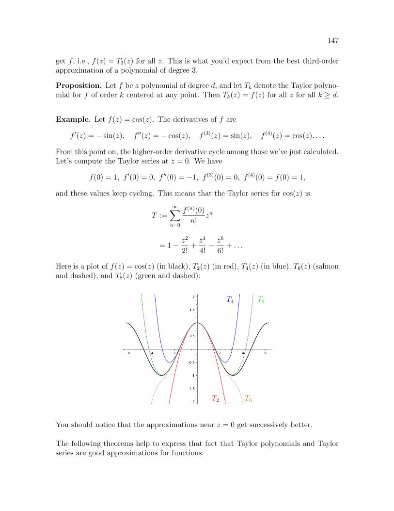
147
get f , i.e., f(z) = T3(z) for all z. This is what you’d expect from the best third-orderapproximation of a polynomial of degree 3.
Proposition. Let f be a polynomial of degree d, and let Tk denote the Taylor polyno-mial for f of order k centered at any point. Then Tk(z) = f(z) for all z for all k ≥ d.
Example. Let f(z) = cos(z). The derivatives of f are
f ′(z) = − sin(z), f ′′(z) = − cos(z), f (3)(z) = sin(z), f (4)(z) = cos(z), . . .
From this point on, the higher-order derivative cycle among those we’ve just calculated.Let’s compute the Taylor series at z = 0. We have
f(0) = 1, f ′(0) = 0, f ′′(0) = −1, f (3)(0) = 0, f (4)(0) = f(0) = 1,
and these values keep cycling. This means that the Taylor series for cos(z) is
T :=∞∑n=0
f (n)(0)
n!zn
= 1− z2
2!+z4
4!− z6
6!+ . . .
Here is a plot of f(z) = cos(z) (in black), T2(z) (in red), T4(z) (in blue), T6(z) (salmonand dashed), and T8(z) (green and dashed):
T2
T4
T6
T8
You should notice that the approximations near z = 0 get successively better.
The following theorems help to express that fact that Taylor polynomials and Taylorseries are good approximations for functions.

148 CHAPTER 32. WEEK 14, FRIDAY
Theorem (Taylor’s theorem over C). Let A ⊆ C and let f : A → C. Supposethat B(a; r) ⊆ A and that f has derivatives of orders 1, . . . , n on B(a; r) where n ≥ 1.Let Tn,a be the Taylor polynomial of order n for f centered at a. Then for all ε > 0there exists δ > 0 such that if z ∈ B(a; δ), then
|f(z)− Tn,a(z)| < ε.
Theorem. (Taylor’s theorem over R) Let A ⊆ R and let f : A→ R. Suppose thatA contains an open interval containing the closed interval [u, v]. Also suppose thatall the derivatives up to order n exist and are continuous on [u, v] and the (n + 1)-thderivative exists on (u, v). Let a ∈ A, and let Tn,a be the Taylor polynomial of order nfor f centered at a. Then for all x ∈ [u, v], there exists a number c strictly between xand a such that
f(x) = Tn,a(x) +1
(n+ 1)!f (n+1)(c)(x− a)n+1.
How to interpret this last theorem. The term
1
(n+ 1)!f (n+1)(c)(x− a)n+1 = f(x)− Tn,a(x)
is the error in approximating f by its n-th order Taylor polynomial In particular, if|fn+1| is bounded by M on the interval [u, v], then the error is bounded:∣∣∣∣ 1
(n+ 1)!f (n+1)(c)(x− a)n+1
∣∣∣∣ ≤ M
(n+ 1)!|x− a|n+1.
Note that if x is close to a then the factor 1(n+1)!
· (x − a)n+1 will be very small. (For
instance, for any constant α, we have limn→∞αn+1
(n+1)!= 0.)

Week 14, Monday: Taylor series II
(Supplemental reading: Sections 6.5 and 9.7–9 in Swanson.)
Taylor series II
Convergence of Taylor series. Given a function f(z) whose derivatives of all ordersexist at a point a, then it makes sense to compute the Taylor series of f(z) centeredat a:
T (z) =∞∑n=0
f (n)(a)
n!(z − a)n.
Then T (z) is a power series in z − a, and so it has a radius of convergence R. Thequestion arises: at points z inside the disk of convergence (centered at a), i.e., where |z−a| < R, is it true that f(z) = T (z). Over the complex numbers, the answer is “yes”,but over the real numbers things are more complicated:
Example. Consider the function
f(x) =
{0 if x ≤ 0
e−1/x2
if x > 0.
Its graph look like this:
Then it turns out that the derivatives of f of all orders exist at 0, and they are all 0.Hence, it’s Taylor polynomial is 0. However, f(x) > 0 for all x > 0. So f is not equalto its Taylor polynomial centered at 0 on any interval about 0.
149

150 CHAPTER 33. WEEK 14, MONDAY
In the last lecture, we saw that over the reals, the error term in approximating thefunction f with by its n-th Taylor polynomial is
|f(x)− Tn(x)| =∣∣∣∣f (n+1)(c)
(n+ 1)!
∣∣∣∣ |x− a|n+1 (33.1)
where c is a point between x and a. Suppose that f (n+1) is bounded in some intervalcontaining x and a by a constant, independent of n. In other words, suppose there isa constant B such that for all n, ∣∣f (n+1)(c)
∣∣ ≤ B
for all c in some interval containing x and a. In that case we have
limn→∞
|f(x)− Tn(x)| = limn→∞
B
(n+ 1)!|x− a|n+1 = 0.1
It is easy to check that x 7→ |x| is a continuous function and, hence, commutes withlimits. This means that
limn→∞
|f(x)− Tn(x)| =∣∣∣ limn→∞
f(x)− Tn(x)∣∣∣ = |f(x)− T (x)|.
Hence, in this case, the real function f will converge to its Taylor series.
Example. The real Taylor series for cos(x) centered at 0 is
T (x) = 1− x2
2!+x4
4!− x6
6!+ · · · .
An easy application of the ratio test shows that its radius of convergence is R = ∞.Then at any point c we have that cos(n)(c) is either ± cos(c) or ± sin(c), which are allbounded by B = 1. Therefore, cos(x) = T (x) for all x ∈ R.
Example. For a more problematic example, consider the Taylor series for f(x) = ln(x)centered at x = 1. We have
f ′(x) =1
x, f ′′(x) = − 1
x2, f (3)(x) =
2 · 1x3
, f (4)(x) = −3 · 2 · 1x4
, f (5)(x) =4 · 3 · 2 · 1
x5,
and so on: f (n)(x) = (−1)n−1 (n−1)!xn
. In general, for n > 0, the n-th coefficient for theTaylor series centered at 1 is
f (n)(1)
n!= (−1)n−1
(n− 1)!
n!=
(−1)n−1
n.
1For any real or complex number α, we have limn→∞αn
n! = 0. A roundabout way to see this is to
note that∑∞n=0
zn
n! has radius of convergence R = ∞. Hence, for all z, the sequence of terms of theseries converges to 0.

151
Thus, the Taylor series for f centered at 1 is
T (x) :=∞∑n=0
f (n)(1)
n!(x− 1)n
=∞∑n=1
(−1)n−1(n− 1)!
n!(x− 1)n
=∞∑n=1
(−1)n−11
n(x− 1)n
= (x− 1)− (x− 1)
2+
(x− 1)2
3− (x− 1)4
4+ · · · .
We can use the power series ratio test find the radius of convergence:
limn→∞
∣∣∣∣(−1)n−1
n
∣∣∣∣/ ∣∣∣∣(−1)n
n+ 1
∣∣∣∣ = limn→∞
n+ 1
n= 1.
Hence, the series converges (absolutely) for |x − 1| < 1 and diverges for |x − 1| > 1.Thus, in the open interval of radius 1 centered at 1, i.e., in (0, 2), the series convergesabsolutely. What happens on the boundary? At x = 2, we get the alternating harmonicseries
T (2) = 1− 1
2+
1
3− 1
4+ . . . ,
which converges by the alternating series test. At x = 0, we have
T (0) = −1 +1
2+
1
3+
1
4+ · · · ,
which diverges since its partial sums differ from those of the harmonic series by aconstant.
Does the Taylor series for ln(x) converge to ln(x) on (0, 2)? It turns out that it does,but the argument depends on a different formulation for there error term when approxi-mating a function by a Taylor polynomial. There is a further interesting question: whathappens when x = 2, on the boundary of the interval of convergence? We have seenabove that T (1) is the alternating harmonic series. Is it true that ln(2) = T (2) Theanswer is, again, yes. The details appear below for those who are interested.
The complex exponential function
The usual exponential, cosine, and sine functions generalize to functions on the wholecomplex plane. Moreover, the generalization leads to a hidden relation among all threefunctions (Euler’s formula).

152 CHAPTER 33. WEEK 14, MONDAY
Definition. For z ∈ C define the power series
E(z) :=∞∑n=0
zn
n!= 1 + z +
z2
2!+z3
3!+z4
4!+ . . .
C(z) :=∞∑n=0
(−1)nz2n
(2n)!= 1− z2
2!+z4
4!− z6
6!+ . . .
S(z) :=∞∑n=0
(−1)nz2n+1
(2n+ 1)!= z − z3
3!+z5
5!− z7
7!+ . . .
Exercise. Here are a few straightforward exercises concerning these functions:
1. Use the ratio test to show that E(z), C(z), and S(z) converge for all z ∈ C.
2. Show that C(−z) = C(z) and S(−z) = −S(z).
3. Show that
E ′(z) = E(z), C ′(z) = −S(z), and S ′(z) = C(z).
4. Show that C2(z) + S2(z) = 1. (Hint: use derivatives.)
5. For z ∈ R, a real number, show that these functions are the Taylor series for ez, cos(z),and sin(z).
Proposition. For x ∈ R,
E(x) = ex, C(x) = cos(x), and S(x) = sin(x).
Proof. It suffices to show that ex, cos(x), and sin(x) equal their Taylor series. Thatfollows from the error term for the approximation of a function by a Taylor polynomialwhich we have discussed previously. For instance, let f(x) = ex, and let Tn(x) be then-th order Taylor polynomial for ex. Given x ∈ R, there exists c between x and 0 suchthat
ex − Tn(x) =f (n+1)(c)
(n+ 1)!xn+1 =
ecxn+1
(n+ 1)!.
Therefore,
ex − T (x) = limn→∞
ex − Tn(x) = ec limn→∞
xn+1
(n+ 1)!= 0.2
We gave the argument for cos(x) in an earlier example, and the example for sin(x) issimilar.
2See the previous footnote for an proof that limn→∞xn
n! = 0.

153
Thus, for instance, we know that E(√
2) = e√2. What can we say about something
like e2+3i? What about cos(2 + 3i)? It turns out that up to this point, we have nodefinition of what it means take the exponential, cosine, or sine of a complex number.So we are free to decide what these mean, as we do in the following definition:
Definition. For z ∈ C let
exp(z) = E(z), cos(z) = C(z), sin(z) = S(z).
Proposition (Euler’s formula). For all z ∈ C, we have
eiz = cos(z) + i sin(z).
Proof. We have
exp(iz) = 1 + (iz) +(iz)2
2!+
(iz)3
3!+
(iz)4
4!+
(iz)5
5!+
(iz)6
6!+ . . .
= 1 + (iz) +i2z2
2!+i3z3
3!+i4z4
4!+i5z5
5!+i6z6
6!+ . . .
= 1 + iz − z2
2!− iz
3
3!+z4
4!+ i
z5
5!− z6
6!+ . . .
=
(1− z2
2!+z4
4!− z6
6!+ . . .
)+ i
(z − z3
3!+z5
5!+ . . .
)= cos(z) + i sin(z).
Thus for instance, we may parametrize the unit circle centered at the origin by
R→ Ct 7→ eit.
Corollary. For z ∈ C
cos(z) =exp(iz) + exp(−iz)
2and sin(z) =
exp(iz)− exp(−iz)
2i.
Proof. Exercise.
One thing that is not immediately clear from our definition of ez is that it obeys theusual exponent laws for all complex numbers! We show that now.
Proposition. Let w, z ∈ C. Then

154 CHAPTER 33. WEEK 14, MONDAY
1. exp(−z) =1
exp(z).
2. exp(w + z) = exp(w) exp(z)
Proof. For part 1, fix w ∈ C and define the function f(z) = exp(w+z) exp(−z). Applythe product and chain rules for differentiation with respect to z to find
f ′(z) = exp′(w + z) exp(−z) + exp(w + z) exp′(−z)
= exp(w + z) exp(−z)− exp(w + z) exp(−z)
= 0.
It follows that f(z) = c for some constant c. To find the constant, we just need toevaluate f at any point, say z = 0. We find f(0) = exp(w+0) exp(0) = exp(w). Hence,f(z) = f(w) for all z ∈ C:
exp(z + w) exp(−z) = exp(w). (33.2)
Equation (33.2) holds for all w, z ∈ C. In particular, setting w = 0, we find
exp(z) exp(−z) = exp(0) = 1.
This proves part 1. Part 2 then immediately follows.
Remark. Give z = x+ iy ∈ C where x, y ∈ R, we have
ez = ex+iy = exeiy = ex(cos(y) + i sin(y)).
Note that on the right, we have the polar form for the complex number ez. Hence,
|ez| = ex and arg(ez) = y.
In general, exponential notation arises naturally when writing a complex number inpolar form:
w = r(cos(θ) + sin(θ)) = reiθ.
The geometry of multiplication of complex numbers—that lengths multiply and anglesadd—takes the form
(reiθ)(seiψ) = rseiθ+iψ = rsei(θ+ψ).

155
Appendix
We would like to show that ln(x) converges to its Taylor series centered at 1 on theinterval (0, 2]. Earlier, we calculated the derivatives
ln(n+1)(c) = (−1)nn!
cn+1
and found the Taylor series to be
T (x) =∞∑n=1
(−1)n−1(x− 1)n
n= (x− 1)− (x− 1)
2+
(x− 1)2
3− (x− 1)4
4+ · · · ,
which converges on (0, 2].
To show ln(x) = T (x) on this interval takes several steps. First note that the casex = 1 is trivial: ln(1) = 0 = T (1). The case of the endpoint x = 2 will be handled atthe end. We first consider the two cases 0 < x < 1 and 1 < x < 2 separately. For thelatter, we will need to use an alternative form of the error term.
Let Tn(x) denote the n-th Taylor polynomial for ln(x). For the case where 0 < x < 1,we use Equation (33.1) to get
| ln(x)− Tn(x)| = 1
(n+ 1)!
n!
cn+1|x− 1|n+1 =
1
n+ 1·(
1− xc
)n+1
.
where 0 < x < c < 1. In this case, 1− x < c, and therefore
1
n+ 1·(
1− xc
)n+1
<1
n+ 1−→ 0,
as n→∞. Hence, we see that ln(x) = T (x) on (0, 1).
For the next case, we need a different form for the remainder.
Theorem. Let A ⊆ R and let f : A → R. Suppose that A contains an open intervalcontaining the closed interval [u, v]. Also suppose that all the derivatives up to ordern exist and are continuous on [u, v] and the (n + 1)-th derivative exists on (u, v). Leta ∈ A, and let Tn,a be the Taylor polynomial of order n for f centered at a. Then forall x ∈ [u, v], there exists a number c strictly between x and a such that
f(x) = Tn,a(x) +1
n!f (n+1)(c)(x− a)(x− c)n. (33.3)
Proof. See Swanson, Theorem 6.5.5.
We apply this theorem to ln(x) in the case 1 < x < 2. We have
| ln(x)− Tn(x)| = 1
n!
n!
cn+1(x− 1)(x− c)n =
(x− 1)(x− c)n
cn+1
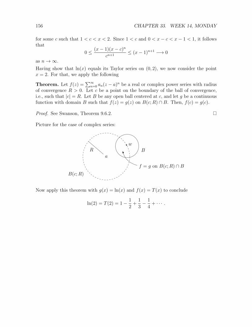
156 CHAPTER 33. WEEK 14, MONDAY
for some c such that 1 < c < x < 2. Since 1 < c and 0 < x− c < x− 1 < 1, it followsthat
0 ≤ (x− 1)(x− c)n
cn+1≤ (x− 1)n+1 −→ 0
as n→∞.
Having show that ln(x) equals its Taylor series on (0, 2), we now consider the pointx = 2. For that, we apply the following
Theorem. Let f(z) =∑∞
n=0 an(z − a)n be a real or complex power series with radiusof convergence R > 0. Let c be a point on the boundary of the ball of convergence,i.e., such that |c| = R. Let B be any open ball centered at c, and let g be a continuousfunction with domain B such that f(z) = g(z) on B(c;R) ∩B. Then, f(c) = g(c).
Proof. See Swanson, Theorem 9.6.2.
Picture for the case of complex series:
B(c;R)
a
Rw
B
f = g on B(c;R) ∩B
Now apply this theorem with g(x) = ln(x) and f(x) = T (x) to conclude
ln(2) = T (2) = 1− 1
2+
1
3− 1
4+ · · · .

Week 14, Wednesday: Two theorems from calculus
(Supplemental reading: Sections 5.2 and 5.3 in Swanson.)
Two theorems from calculus
The extreme value theorem. We present proofs of two basic theorems whose proofsare usually skipped in a first course in calculus: the extreme value theorem and theintermediate value theorem.
The extreme value theorem is of fundamental importance in the theory of optimizationsince it states conditions under which the existence of a maximal and minimal valuefor a function is guaranteed.
Theorem (extreme value theorem, EVT). If f : [a, b] → R is continuous, then fachieves is maximum and minimum on [a, b], i.e., there exists xmax, xmin ∈ [a, b] suchthat
f(xmin) ≤ f(x) ≤ f(xmax)
for all x ∈ [a, b].
xminxmax
a b
Figure 34.1: A continuous function on a closed interval [a, b] with the points at whichit achieves its (global) minimum and maximum labeled.
157

158 CHAPTER 34. WEEK 14, WEDNESDAY
There are three important hypotheses in the EVT: (i) f is continuous, (ii) the intervalis closed, and (iii) the interval is bounded.1 The following three examples show that ifyou violate any one of these, the theorem no longer holds.
Example 1. Let f : [0, 1]→ R be defined by
f(x) =
{x if 0 < x < 112
if x = 0 or 1.
Then f is defined on a closed and bounded interval but is not continuous. It has nomaximum or minimum:
−1 −0.5 0.5 1
−1
−0.5
0.5
1
Graph of f .
Example 2. The identity function
g : (0, 1)→ (0, 1) ⊂ Rx 7→ x
is continuous and defined on a bounded interval, but the interval is not closed. Thefunction g has no minimum or maximum:
−1 −0.5 0.5 1
−1
−0.5
0.5
1
Graph of g.
1Note that (ii) does not imply (iii). For instance, the intervals [0,∞) and (−∞,∞) are bothclosed—their complements are open—but not bounded.
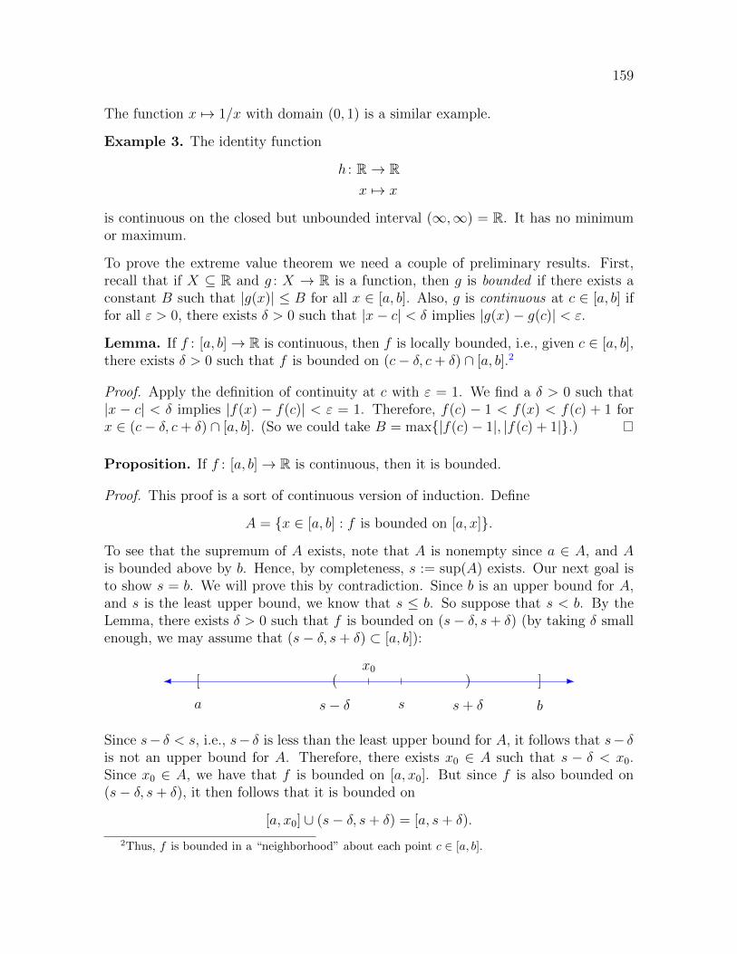
159
The function x 7→ 1/x with domain (0, 1) is a similar example.
Example 3. The identity function
h : R→ Rx 7→ x
is continuous on the closed but unbounded interval (∞,∞) = R. It has no minimumor maximum.
To prove the extreme value theorem we need a couple of preliminary results. First,recall that if X ⊆ R and g : X → R is a function, then g is bounded if there exists aconstant B such that |g(x)| ≤ B for all x ∈ [a, b]. Also, g is continuous at c ∈ [a, b] iffor all ε > 0, there exists δ > 0 such that |x− c| < δ implies |g(x)− g(c)| < ε.
Lemma. If f : [a, b]→ R is continuous, then f is locally bounded, i.e., given c ∈ [a, b],there exists δ > 0 such that f is bounded on (c− δ, c+ δ) ∩ [a, b].2
Proof. Apply the definition of continuity at c with ε = 1. We find a δ > 0 such that|x − c| < δ implies |f(x) − f(c)| < ε = 1. Therefore, f(c) − 1 < f(x) < f(c) + 1 forx ∈ (c− δ, c+ δ) ∩ [a, b]. (So we could take B = max{|f(c)− 1|, |f(c) + 1|}.)
Proposition. If f : [a, b]→ R is continuous, then it is bounded.
Proof. This proof is a sort of continuous version of induction. Define
A = {x ∈ [a, b] : f is bounded on [a, x]}.
To see that the supremum of A exists, note that A is nonempty since a ∈ A, and Ais bounded above by b. Hence, by completeness, s := sup(A) exists. Our next goal isto show s = b. We will prove this by contradiction. Since b is an upper bound for A,and s is the least upper bound, we know that s ≤ b. So suppose that s < b. By theLemma, there exists δ > 0 such that f is bounded on (s− δ, s+ δ) (by taking δ smallenough, we may assume that (s− δ, s+ δ) ⊂ [a, b]):
[
a
]
b
)
s+ δ
(
s− δ s
x0
Since s− δ < s, i.e., s− δ is less than the least upper bound for A, it follows that s− δis not an upper bound for A. Therefore, there exists x0 ∈ A such that s − δ < x0.Since x0 ∈ A, we have that f is bounded on [a, x0]. But since f is also bounded on(s− δ, s+ δ), it then follows that it is bounded on
[a, x0] ∪ (s− δ, s+ δ) = [a, s+ δ).
2Thus, f is bounded in a “neighborhood” about each point c ∈ [a, b].

160 CHAPTER 34. WEEK 14, WEDNESDAY
In particular, f is bounded on [a, s+ δ/2]. So s+ δ/2 ∈ A, contradicting the fact thats = sup(A). We conclude that, in fact, s = b.
Finally, we show that b ∈ A by using an argument similar to the one we just used. Wehave established the fact that b = sup(A). By the Lemma, we know that there existsδ > 0 such that f is bounded on (b − δ, b + δ) ∩ [a, b] = (b − δ, b]. Since b is the leastupper bound for A and b− δ is less than b, it follows that b− δ is not an upper boundfor A. So there exists x1 ∈ A such that b− δ < x1. Hence, f is bounded on
[a, x1] ∪ (b− δ, b] = [a, b],
as required.
We now know that a continuous function on a closed bounded interval is bounded.This is the key tool in proving the extreme value theorem.
Proof of the extreme value theorem. We just need to prove that xmax always exists. Ifwe know that, then to prove that xmin exists, apply our result to the function −f(which also continuous on [a, b]). The maximum we find for −f will be a minimumfor f .
Consider the setim(f) = f([a, b]) = {f(x) : x ∈ [a, b]}.
By our Proposition, f is bounded on [a, b], which is equivalent to saying the set im(f)is a bounded set. Since im(f) is also nonempty, e.g., f(a) ∈ im(f), we can let s :=sup(im(f)). Our proof is finished if we can show that s ∈ im(f) for in that case, thereexists some x̃ ∈ [a, b] such that f(x̃) = s, and f(x̃) ≥ f(x) for all x ∈ [a, b].
We prove s ∈ im(f) by contradiction. Suppose it is not, and define
g : [a, b]→ R
x 7→ 1
s− f(x).
Since, by supposition, s 6∈ im(f), the function g is well-defined (we never divide by 0)and continuous. By the Proposition, g is therefore bounded. However, we will nowshow that g can’t be bounded. Since s = sup(im(f)), there are points s′ ∈ im(f) thatare arbitrarily close to s, and writing s′ = f(x′), we see g(x′) = 1
s−f(x′) = 1s−s′ will be
arbitrarily large. In detail, given any potential bound B ∈ R, choose ε > 0 such that1ε> B. Next, consider s − ε. Since it is less than the least upper bound s for im(f)
and s 6∈ im(f), there exists s′ ∈ im(f) such that s− ε < s′ < s. Since s′ ∈ im(f), thereexists x′ ∈ [a, b] such that f(x′) = s′. We then have
g(x′) =1
s− f(x′)=
1
s− s′>
1
s− (s− ε)=
1
ε= B.
Hence, g has no upper bound B.

161
The intermediate value theorem. The intermediate value theorem is intuitivelyobvious, but its proof requires familiarity with the completeness property of the realnumbers.
Theorem (intermediate value theorem, IVT). Let f : [a, b]→ R be a continuousfunction such that f(a) < 0 and f(b) > 0. Then there exists s ∈ (a, b) such thatf(s) = 0.
Proof. Define the set
A := {x ∈ [a, b] : f is negative at all points in [a, x]}.
We have a ∈ A since f(a) < 0. Thus, A 6= ∅. Since A ⊆ [a, b], the set A is boundedabove by b. By completeness of R is follows that s := sup(A) exists. We are done ifwe can show that f(s) = 0.
We first argue that s 6∈ {a, b}. First, since f(a) < 0 and f is continuous, there is aδa > 0 such that f is negative on the interval [a, a+ δa). This shows s 6= a. Next, sincef(b) > 0 and f is continuous, there exists a δb > 0 such that f is positive on (b− δb, b].Hence, s 6= b. Therefore, s ∈ (a, b).
Now note that if f(c) > 0 for any point c ∈ [a, b], then c is an upper bound for A. Ifit were not, then there would an x ∈ A such that c < x. But then, by definition of A,the function f is negative on [a, x] and since c ∈ [a, x], that would mean f(c) < 0. Inparticular, since s is the least upper bound for A, the function f cannot be positive atany point strictly less than s. Thus, we have shown that
[a, s) ⊆ A.
For sake of contradiction, suppose that f(s) < 0. By continuity of f , there exists δ > 0such that f is negative on (s − δ, s + δ) ∩ [a, b]. Since s ∈ (a, b), we can take δ smallenough to that (s− δ, s+ δ) ∩ [a, b] = (s− δ, s+ δ). But then f is negative on
[a, s) ∪ (s+ δ/2] = [a, s+ δ/2],
which shows that s+ δ/2 ∈ A, contradicting the fact that s is an upper bound for A.
Next, for the sake of contradiction, suppose that f(s) > 0. By continuity of f it followsthat f is positive in a small interval (s − η, s + η). Since s 6∈ {a, b}, we can assume(s − η, s + η) ⊂ A. Then, for instance, letting c := s − η/2, we see that f(c) > 0. Asdiscussed above, that means that c is an upper bound for A. But that’s impossiblesince c < s and s is the least upper bound for A.
We conclude that f(s) = 0, as desired.
Week 14, Friday: Three theorems by Euler
Theorem 1. The number e is irrational.
Proof. Euler discovered that e =∑∞
n=01n!
, and used that to prove that e is irrational.To start, we can at least see that e is an integer since
2 = 1 +1
1!< e = 1 +
1
1!+
1
2!+
1
3!+
1
4!+ · · · < 1 +
(1 +
1
2+
1
22+
1
23+ · · ·
)= 3.
Now, for the sake of contradiction, suppose that e is rational, and write e = pq
withp, q ∈ Z≥1. Since e is not an integer, q > 1. We have
p
q= e =
∞∑n=0
1
n!=⇒ e−
q∑n=0
1
n!=
∞∑n=q+1
1
n!
=⇒ q!
(e−
q∑n=0
1
n!
)=
∞∑n=q+1
q!
n!(35.1)
The expression on the left-hand side of (35.1),
q!
(e−
q∑n=0
1
n!
),
is an integer since e = pq
and q!n!∈ Z when q ≥ n. We conclude that the right-hand side
of (35.1) is also an integer:∞∑
n=q+1
1
n!∈ Z.
However,
∞∑n=q+1
q!
n!=
q!
(q + 1)!+
q!
(q + 2)!+
q!
(q + 3)!+ · · ·
=1
q + 1+
1
(q + 2)(q + 1)+
1
(q + 3)(q + 2)(q + 1)+ · · ·
162

163
<1
q + 1+
1
(q + 1)2+
1
(q + 1)3+ · · ·
=1
q + 1
∞∑n=0
(1
q + 1
)n
=1
q + 1· 1
1− 1(q+1)
(geometric series formula)
=1
q< 1.
Contradicting the fact that this sum is an integer.
Theorem 2.∞∑n=1
1
n2=π2
6.
Proof. We first recall some basic algebra. If P (z) is a polynomial of degree n with realor complex coefficients, then it will have n (not necessarily distinct) roots, r1, . . . , rn.1
We can then writeP (z) = k(z − r1) · · · (z − rn)
for some constant k. If no ri = 0, we can rewrite this expression as
P (z) = (−1)nkr1 · · · rn(
1− z
r1
)· · ·(
1− z
rn
).
Now further assume that P (0) = 1. We then have
1 = P (0) = (−1)nkr1 · · · rn,
and, thus,
P (z) =
(1− z
r1
)· · ·(
1− z
rn
). (35.2)
Consider sin(z) = z − z3
3!+z5
5!− · · · , and divide by z to define
P (z) = 1− z2
3!+z4
5!− · · · (35.3)
so that P (z) =sin(z)
zfor z 6= 0, and at z = 0, we have.
P (0) = 1 = limz→0
sin(z)
z.
1By roots we mean P (rk) = 0 for each k.

164 CHAPTER 35. WEEK 14, WEDNESDAY
Since sin(kπ) is zero for all integers k, it follows that P (kπ) = 0 for all nonzerointegers k = ±1,±2, . . . Therefore, skipping several technical details, we emulate (35.2)and write
P (z) =(
1− z
π
)(1 +
z
π
)(1− z
2π
)(1 +
z
2π
)(1− z
3π
)(1 +
z
3π
)· · ·
=
(1− z2
π2
)(1− z2
4π2
)(1− z2
9π2
)· · ·
Going back to the definition (35.3) of P , we have shown that
1− z2
3!+z4
5!− · · · =
(1− z2
π2
)(1− z2
4π2
)(1− z2
9π2
)· · ·
Comparing the coefficient of z2 on both sides, we find
−1
6= −
∞∑n=1
1
n2π,
and the result follows.
Exercise. Show that∞∑n=1
1
n4=π4
90.
What about∞∑n=1
1
n3? This number was shown to be irrational in 1978. It is an open
question whether there is a rational r such that the sum is equal to rπ3.
Theorem 3. There are infinitely many prime numbers.
Proof. Let s ∈ C. Then
∞∏p prime
(1
1− p−s
)=
∞∏p prime
(1 + p−s + p−2s + p−3s + · · ·
)
=
(1 +
1
2s+
1
22s+ · · ·
)(1 +
1
3s+
1
32s+ · · ·
)· · ·
Patiently multiplying out the final expression, and using the fact the each positiveinteger can be uniquely factored into primes, you will find that
ζ(s) :=∞∑n=1
1
ns=
∞∏p prime
(1
1− p−s
)

165
If were only finitely many primes, the product on the right would be finite, and hencewe could evaluate it as a complex number when s = 1. However,
ζ(1) =∞∑n=1
1
n,
which diverges.
Note: The function ζ(s) =∞∑n=1
1
zsis known as the Riemann zeta function. Our
previous result states that
ζ(2) =π2
6.

handouts
166

167
Mathematical writing
Audience
In all of the writing you do for a course based on this text, take your audience to be yourfellow classmates. That will determine the amount of detail you need to include—donot skip important details, and do not include details that are not essential.
Sentences!
The most important rule is that your writing should consist solely of complete sen-tences. A sentence starts with a capital letter and ends with a period. If you have along calculation, you might want to neatly display it, but it should still be part of asentence; something like this:
Our result then follows from a calculation:
blah = blah
= blah
...
= blah.
Use of symbols
For better readability, do not start a sentence with a mathematical symbol (i.e., amathematical symbol does not count as a capital letter):
No: f is injective by not surjective.
Yes: The function f is injective by not surjective.
In informal mathematical writing—the kind you might use on a blackboard or onscratch paper—it is common to use the symbols shown below:
⇒ : ”implies”
⇔ : ”if and only if”
∀ : ”for all”
∃ : ”there exists”
In your formal written work, e.g., homework assignments, do not use these. Instead,write out the words. It is slightly more work for you, but it makes life easier for yourreader. Of course, you will need to use symbols in your writing—just do not use thoselisted in formal writing. On the other hand, here are some symbols from logic weencourage you to never use, even in informal work: “∧” for “and”, “∨” for “or”, and“∼” for “not”. Again, it is easier on your read to use the word instead of these symbols.

168 CHAPTER 36. HANDOUTS
Red herrings
Whenever you a finish a proof by contradiction and now have the ideas in front ofyou, ask yourself whether a straightforward proof (without contradiction) is at least asclear as the one you have given. If so, make the change. It makes for a less convolutedargument. Apply similar reasoning to any proof where you have replaced the statementof the result by its (logically equivalent) contrapositive (not Q implies P , rather than Pimplies Q).
More generally, review your proofs to see if you have included irrelevant information.
The “backwards” proof.
Theorem. Suppose x ∈ R. Then (x+ 1)2 − (x− 1)2 = 4x.
Incorrect proof. Calculate:
(x+ 1)2 − (x− 1)2 = 4x
(x2 + 2x+ 1)− (x2 − 2x+ 1) = 4x
x2 + 2x+ 1− x2 + 2x− 1 = 4x
4x = 4x.
The problem with this “proof” is in its first line: it seems to assert as true exactlywhat it is trying to prove—circular reasoning. To make the mistake even more clear,consider the following false statement, which uses the same reasoning:
Theorem. In R, we have
1 = 0.
Incorrect proof. Calculate:
1 = 0
0 · 1 = 0 · 00 = 0.
To fix the proof of the original theorem, one could just list the lines of the proof inreverse order—hence, the moniker “backwards”—starting with 4x = 4x. However,notice another flaw with the proof: by just listing these lines, we break the rule that aproof consists of sentences. Here is the correct form, fixing both problems:
Theorem. Suppose x ∈ R. Then (x+ 1)2 − (x− 1)2 = 4x.

169
Proof. Calculate:
(x+ 1)2 − (x− 1)2 = (x2 + 2x+ 1)− (x2 − 2x+ 1)
= x2 + 2x+ 1− x2 + 2x− 1
= 4x.
Miscellaneous
• To prove a statement is false, give a specific concrete counterexample. Try tofind the simplest one. The counterexample is more convincing and easier on thereader than an abstract argument. Conversely, to prove a statement is true, anexample, although sometimes helpful, is not a proof. You must show why thestatement is true in all instances. Some examples:
Statement: f(n) = n+ 2 is even for all n ∈ Z.
Disproof: Note that f(1) = 3, which is not even.
Statement: f(n) = n+ 2 is divisible by 7 for all n ∈ Z.
False proof: We have f(12) = 14, which is divisible by 7.
• If you use the phrase “by definition” in your writing, make sure to be specific: bydefinition of what? For example, you might write “by definition of a Hausdorffspace”. Using the phrase “by definition” in isolation is usually ambiguous, andif your reader cannot determine which definition your are referring to, then it isno help at all—everything in mathematics follows from the definitions!
• When writing down a calculation, avoid crossing out terms (for example, whenterms cancel in fractions or when they add up to zero). This type of bookkeepingis easy for the writer, who is crossing out sequentially, but is usually confusingfor the reader, who sees all of the crosses at once.
TEX pointers
• When defining a function, use \colon rather than :, as in
f\colon X\to Y.
The latter symbol is regarded as an operator and is padded by unwanted spaces.
• Use the TEX versions of the trig functions, e.g., \cos(t), \tan(t), etc., ratherthen plain cos(t), tan(t), etc. The same goes for logarithms:\log(t), \ln(t).
• Add a little space before a differential, e.g., \int x\,dx, which gives∫x dx rather
than \int xdx, which gives∫xdx.

170 CHAPTER 36. HANDOUTS
Here is a link to a nice three-page article on mathematical writing by Francis Su:
Writing Mathematics Well
and a one-page summary:
Some Guidelines for Good Mathematical Writing

171
Proof templates
The “blah, blah, blah”s appearing in the template proofs below usually consists of twoparts. The first part is automatic: you expand the statement of the theorem usingrelevant definitions so that the reader understands what you are trying to prove. Thesecond is where the real math occurs. It often requires some insight and creativity.
By convention, the proofs of certain types of statements are expected to have a certainstructure. Here, we provide examples of some of these that are important for us.Deviating from these structures risks confusing your reader and, thus, usually entailthe addition of a few words of guidance in your proof.
Induction
Proposition. For all n ≥ 1, we have
1 + 2 + · · ·+ n =n(n+ 1)
2.
Proof. We will prove this by induction. For the base case, n = 1, the result holds sincein that case
1 + 2 + · · ·+ n = 1 =1 · (1 + 1)
2.
It follows that
1 + 2 + · · ·+ (n+ 1) = (1 + 2 + · · ·+ n) + (n+ 1)
=n(n+ 1)
2+ (n+ 1) (by the induction hypothesis)
=n(n+ 1) + 2(n+ 1)
2
=(n+ 1)(n+ 2))
2
=(n+ 1)((n+ 1) + 1)
2.
So the result holds for the case n+ 1, too. The proposition follows by induction.
Rules.
1. Always start a proof by induction by telling your reader that you are giving a proofby induction.
2. Next, show that result holds for the smallest value of n in question—in this case,n = 1.

172 CHAPTER 36. HANDOUTS
3. Note that we assume the result is true for some n ≥ 1. If we said, instead: “assumethe result holds for n ≥ 1”, this would mean we’re assuming the result for all n ≥ 1.But that would be circular: we’d be assuming what we are trying to prove. Instead,at the induction step, we are merely saying that if we did know the result for aparticular value of n, we could prove that it follows for the next value of n.
4. End the proof with a �. This tells the reader the proof is over.
Set containment
Definition. Let A and B be sets. Then A is a subset of B, denoted A ⊆ B if a ∈ Aimplies a ∈ B.
Definition. Let A and B be sets. Then these sets are equal, denoted A = B ifboth A ⊆ B and B ⊆ A.
Definition. Let A and B be sets. Then the union of A and B is
A ∪B := {x : x ∈ A or x ∈ B} .
In words, x ∈ A ∪B if x is in A or x ∈ B. The intersection of A and B is
A ∩B := {x : x ∈ A and x ∈ B} .
In words, x ∈ A ∩B if x ∈ A and x ∈ B.
Theorem. Let A and B be sets defined by [some condition]. Then A ⊆ B.
Proof. Let a ∈ A. Then blah, blah, blah. Therefore, a ∈ B. It follows that A ⊆ B.
Theorem. Let A and B be sets defined by [some condition]. Then A = B.
Proof. Suppose a ∈ A. Then blah, blah, blah. Therefore a ∈ B, too. Thus, A ⊆ B.
To show the opposite containment, suppose that b ∈ B. Then blah, blah, blah.Thus, b ∈ A. It follows that B ⊆ A.
Equivalence relations
Theorem. Define a relation ∼ on a set A by blah, blah, blah. Then ∼ is an equivalencerelation.
Proof. Let a, b, c ∈ A.
Reflexivity. We have a ∼ a since blah, blah, blah. Therefore, ∼ is reflexive.
Symmetry. Suppose that a ∼ b. Then, blah, blah, blah. It follows that b ∼ a.Therefore ∼ is symmetric.

173
Transitivity. Suppose that a ∼ b and b ∼ c. Then blah, blah, blah. It followsthat a ∼ c. Therefore, ∼ is transitive.
Since ∼ is reflexive, symmetric, and transitive, it follows that ∼ is an equivalencerelation.
Injectivity, surjectivity, bijectivity
Proposition. The function f : A→ B is injective.
Proof. Let x, y ∈ A, and suppose that f(x) = f(y). Then blah, blah, blah. It followsthat x = y. Hence, f is injective.
Proposition. The function f : A→ B is surjective.
Proof. Let b ∈ B. Then blah, blah, blah. Thus, there exists a ∈ A such that f(a) = b.Hence, f is surjective.
Proposition. The function f : A→ B is bijective.
Proof. (Alternative 1.) We first show that f is injective. [Follow the template above toshow injectivity.] Next, we show f is surjective. [Follow the template above toe showsurjectivity.]
Proof. (Alternative 2) Define g : B → A as follows: blah, blah, blah. Note that g ◦f =idA since blah, blah, blah. Next, note that f ◦ g = idB since blah, blah, blah.

174 CHAPTER 36. HANDOUTS
Axioms for the real numbers
Field axioms
Definition A field is a set F with two operations, + :F × F → F (addition) and· :F × F → F (multiplication), satisfying the following axioms:
A1. Addition is commutative. For all x, y ∈ F ,
x+ y = y + x.
A2. Addition is associative. For all x, y, z ∈ F ,
(x+ y) + z = x+ (y + z).
F3. There is an additive identity. There is an element of F , usually denoted 0, suchthat for all x ∈ F ,
x+ 0 = x.
F4. There are additive inverses. For all x ∈ F , there is an element y ∈ F such that
x+ y = 0.
The element y is denoted −x. (Subtraction is then defined by x− y := x+ (−y)for all x, y ∈ F .)
M1. Multiplication is commutative. For all x, y ∈ F ,
xy = yx.
M2. Multiplication is associative. For all x, y, z ∈ F ,
(xy)z = x(yz).
M3. There is a multiplicative identity. There is an element, usually denoted 1, suchthat:
(a) 1 6= 0, and
(b) 1x = x for all x ∈ F .
M4. There are multiplicative inverses. For each nonzero x ∈ F , there is a y ∈ F suchthat
xy = 1.
The element y is denoted 1/x or x−1. (Division is then defined by x÷ y := xy−1
for nonzero y.)

175
D. Multiplication distributes over addition. For all x, y, z ∈ F ,
x(y + z) = xy + xz.
Order axioms
Definition. An ordered field is a field F with a relation, denoted <, satisfying
O1. (Trichotomy) For all x, y ∈ F , exactly one of the following statements is true:
x < y, y < x, x = y.
O2. (Transitivity) The relation < is transitive, i.e., for all x, y, z ∈ F ,
x < y and y < z =⇒ x < z.
O3. (Additive translation) For all x, y, z ∈ F ,
x < y =⇒ x+ z < y + z
O4. (Multiplicative translation) For all x, y, z ∈ F ,
x < y and 0 < z =⇒ xz < yz.
Remark: of course, we write x > y if y < x, and we write x ≤ y if either x = y orx < y.
Completeness
Let S be a subset of an ordered field F . An element M ∈ F is an upper bound for S ifM ≥ s for all s ∈ S. An element M ∈ F is the least upper bound or supremum for S ifit is an upper bound and is less than or equal to every upper bound. In this case, wewrite M = lubS or M = supS. Similarly, an element m ∈ F is a lower bound for S ifm ≤ s for all s ∈ S. An element m ∈ F is the greatest lower bound or infimum for Sif it is a lower bound and is greater than or equal to every lower bound. In this case,we write m = glbS or m = inf S.
Definition. An ordered field F is complete if every nonempty subset S ⊆ F whichhas an upper bound has a least upper bound in F .
The real numbers
Theorem. There exists a complete ordered field.
It can also be shown that any two complete ordered fields are isomorphic, i.e, they arethe same except for renaming elements. Thus, there is essentially one complete orderedfield, and it is the set of real numbers, R.