materials processing: techniques and applications, s. viswanathan
TRANSCRIPT

117
117 Sensors and Modeling in Materials Processing: Techniques and Applications, S. Viswanathan, R.G. Reddy, and J.C. Malas, eds., The Minerals, Metals, & Materials Society, Warrendale, PA., 1997. pp. 117-142.
EFFECT OF TRANSVERSE DEPRESSIONS AND OSCILLATION MARKS ON
HEAT TRANSFER IN THE CONTINUOUS CASTING MOLD
B. G. Thomas, D. Lui, and B. Ho
Department of Mechanical and Industrial Engineering University of Illinois at Urbana-Champaign
1206 West Green Street Urbana, IL 61801
Abstract Results from mathematical models and plant experiments are combined to quantify the effect of transverse depressions and oscillation marks on heat transfer in the continuous casting mold. A heat transfer model has been developed to calculate transient heat conduction within the solidifying steel, coupled with the steady-state heat conduction with the continuous casting mold wall. The model features a detailed treatment of the interfacial gap between the shell and mold, including mass and momentum balances on the solid and liquid powder layers. The model predicts the solidified shell thickness down the mold, temperature in the mold and shell, thickness of the resolidified and liquid powder layers, heat flux distribution down the mold, mold water temperature rise, ideal taper of the mold walls, and other related phenomena. The important effect of non-uniform distribution of superheat is incorporated using the results from previous 3-D turbulent fluid flow calculations within the liquid cavity. Results from plant experiments confirm that transverse surface depressions and oscillation marks form at the meniscus and move down the mold. Measurements of mold thermocouple temperatures and breakout shell thickness were used to calibrate the models. The results indicate that the surface depressions and oscillation marks are filled with mold flux, but still have a significant effect on decreasing heat transfer. The predicted mold temperature fluctuations are consistent with measurements. If the depressions become filled with air, their effect is greatly increased. These results should be useful in the difficult task of interpreting transient mold thermocouple signals for on-line quality monitoring.

118
118Introduction
Many different types of intermittent surface defects on steel slabs arise during initialsolidification in the mold of the continuous casting machine. These defects include deeposcillation marks, surface depressions, and cracks. They may lead to quality problems, such asslivers, in the final rolled product. In severe cases, breakouts may occur, where liquid steel burststhrough a thin section of the shell and drains over the casting machine below the mold.
It is recognized that on-line monitoring of temperature fluctuations in the mold walls usingthermocouple signals should be useful in identifying the presence of such surface defects. [1]This is already used for the prediction and prevention of breakouts. [2]
If better understood, patterns in the temperature signals might also be used to predict surfacequality problems, which would ease the burden of surface inspection. Developing algorithms tomatch thermocouple signals with these problems is a difficult task, however. A critical step isunderstanding the relationship between thermocouple signals and the condition of the mold /metal interface, including the shape of the solid shell surface. This work attempts to contributetowards this understanding by developing mathematical models of interface heat transfer, andapplying them to quantify the effect of transverse surface depressions and oscillation marks onheat flow in the continuous casting mold.
Description of Phenomena
Figure 1 illustrates the solidifying steel shell moving down the mold during the initial stages ofsolidification in a continuous casting machine with mold flux. To help prevent sticking betweenthe shell and mold, and to entrain liquid mold flux into the interfacial gap, the mold is oscillatedvertically throughout casting. Each oscillation cycle creates a depression in the solidifying shellat the meniscus, called an “oscillation mark”. The cause of these depressions has been thesubject of much study. They are believed to form due to a variety of different mechanisms,which may act in combination. These include freezing and overflow of the meniscus, [3] thermalstresses in the solidifying shell [4] and bending of the weak shell by the interaction betweenpressure in the liquid flux layers and ferrostatic pressure. [3]
Contact Resistances
Molten Steel Pool
Solidifying Steel ShellOscillation Mark
CopperMold
Liquid Flux
Air Gap
Flux Powder
Flux Rim
Meniscus
Steel surface level
Solidified Flux
Figure 1 - Schematic of initial solidification near meniscus
During stable casting, these oscillation marks appear as shallow, equally-spaced horizontaldepressions on the surface of final as-cast steel slabs and blooms. If the metal level is unstabledue to turbulence or waves on the top surface, the oscillation marks will become nonuniform andthe solid surface may contain other more serious defects, such as ripples or deep depressions.

119
119As the strand moves down the mold, heat transfer is controlled by heat conduction across theinterfacial gap between the mold and shell,. The gap contains layers of solid and liquid flux andpossibly air. Heat transfer is reduced locally beneath surface depressions because the gap islarger there. If the gap becomes filled with air, its lower thermal conductivity further reduces heatflow. The reduction in heat flow results in a thinner solidified shell locally. In addition, as eachdepression passes by a given point on the mold wall, the temporary drop in the rate of heattransfer causes a temporary drop in the mold wall temperature. Analysis of these mold walltemperatures should enable prediction of the surface defects that produced them, if therelationship can be quantified. In addition, simultaneous examination of the temperatures anddepressions can be used to further understand the nature of the gap.
Previous Work
Experimental Studies
Previous work has presumed a relationship between oscillation mark depth and mold heattransfer. Oscillation marks are believed to increase the effective gap, reduce heat transfer, andretard shell growth. [5-7] This relationship has been used to explain many phenomena incontinuous casting. For example, Mahapatra et al. [5] observed lower heat transfer on the insideradius and at low casting speed. This was attributed to deeper oscillation marks for theseconditions.
Other experimental works with both oil lubricated billet molds [8-10] and flux-lubricated slabmolds [11, 12] have established a minimum in heat flux for “middle-carbon” steels with carboncontents of 0.10 - 0.12%C. Depending on the lubricant used, these steels have a mold heat fluxabout 15-30% lower than steels with above 0.25%C. [8, 9, 11, 12] This drop in heat transfer hasbeen associated with the deeper oscillation marks that have been observed in these steels byseveral researchers. Tiedje and Langer [13] reported the deepest oscillation marks to appear in0.07 and 0.13 %C steels. In flux-lubricated steels, Cramb and Mannion [14] found the deepestoscillation marks in 0.10% C steel. Mahapatra et al. [5] reported that 0.04 - 0.09%C steels had0.5 - 1.25 mm deep oscillation marks, compared with only 0.35 - 0.8 mm depths for highercarbon steels.
To understand mold heat transfer and interpret mold thermocouple signals, this relationshipbetween oscillation mark / depressions and heat transfer needs to be quantified. Little previouswork has been done.
Mathematical Models
Many mathematical models have been developed of the continuous casting process, which arepartly summarized in a previous literature review. [15] Many of these models are verysophisticated (even requiring supercomputers to run) so are infeasible for use in an operatingenvironment. Of the remaining models which consider the mold, most simulate eithersolidification of the shell, or heat conduction through the mold. There is usually a simplifiedtreatment of the interfacial gap, despite its known importance. A few models have consideredmore detailed treatment of the powder layers in the gap. [16] These models have generallyoversimplified the shell and mold. To study practical problems, such as the effect of shellsurface depressions on heat transfer in an operating caster, two new models were developed andapplied in this work.
Bloom surface defect measurements
An example of the mold temperature signals that were recorded by thermocouples embedded inthe copper walls of a continuous casting mold is shown in Figure 2. These three particular signalportions were recorded from a bloom caster at BHP RBPD in Newcastle, Australia forconditions given in Table I. [17] They record the passage of a particular deep transversedepression, as it moved down the mold.

120
120The horizontal axis indicates the time since the depression was created at the meniscus.Knowing the casting speed (0.5 m min-1), and metal level (-125mm), this axis is also related todistance below the top of the mold.
Figure 2 quantifies how a surface depression causes a drop in the recorded mold temperature asit passes by each mold thermocouple. The time when each thermocouple reaches its minimumtemperature coincides exactly with the time required for that portion of the shell to travel to thatthermocouple.
50
60
70
80
90
100
110
0 20 40 60 80
Mea
sure
d M
old
Tem
pera
ture
(C
)
Time Below Meniscus (s)
Distance Below Top of Mold (mm)0 350 450250
250 mm thermocouple
450 mm thermocouple
350 mm thermocouple
Figure 2 - Mold thermocouple signals (RBPD bloom caster).
Note that the shape of the temperature profile remains similar, also. Indeed, the distinctive patternof the thermocouple signals for about 15 minutes is what enabled an exact match to be madebetween time and position on the final bloom. [17] A series of 14 severe transverse surfacedepressions on the surface of two blooms matched exactly with time-shifted drops in moldtemperature as those defects passed by each thermocouple. By extrapolating back to themeniscus metal level, it was possible to determine the time that each defect was formed. Thistime corresponded exactly with 14 peaks in mold level that were recorded during that time period.
In addition to illustrating the correspondence between surface depressions and thermocouplesignals, this work demonstrated that the depressions were formed at the meniscus due to gradualchanges in metal level. [17] The defects were spaced about 600 mm apart, and were experiencedon the first blooms cast after a startup or grade change. Their cause may be related to excessivebuildup of the solidified flux rim at the meniscus with certain startup powders, combined withmold level fluctuations, possibly due to periodic bulging below the mold. Further details andsolutions to the problem are discussed elsewhere. [17]
The severity of the temperature drop recorded by mold thermocouples depends on the nature ofthe interfacial gap and the severity of the defect. The depressions in this work were about 200mm in length, with a maximum depth of about 2 mm. Although each depression extendedaround the entire bloom perimeter, measurements were made on the narrow face, where therewere no rolls to deform the surface.

121
121Knowing both the temperature drops and the dimensions of the defect, it was possible to calibratemathematical models, described later in this work, to increase understanding of the interfacialgap. The results determined that the gap must have been filled with mold flux while in the mold.The same methodology is employed in the present work to understand the nature of theinterfacial gap and heat transfer losses resulting from oscillation marks.
Breakout shell measurements
Measurements were performed on a breakout shell to quantify the relationship betweenoscillation mark depth and shell thickness with distance below the meniscus. The breakout shellwas obtained from a slab cast at LTV Steel under conditions given in Table I. Measurementswere made down the wide-face centerline (mid-wide face), the narrow-face centerline (mid-narrow face), and the wide face outer radius at a distance of 75 mm from the corner (off-cornerwide face) opposite the corner where the breakout occurred.
Oscillation mark depths were measured along all three of these locations, as shown in Figure 3.The maximum distance was measured between each oscillation mark and a flat surface (15 mmlong) that was placed against the shell. Measurements were made using a profilometer gaugeand photocopy enlargements of silicone rubber impressions of specific longitudinal sections ofshell. The estimated accuracy is within ±0.02 mm.
The corresponding shell thickness profiles are shown in Figure 4. Each data point is averagedfrom 3 different transverse measurements at 12.7 mm intervals down each shell. Replicate testsdetermined the accuracy of these measurements to be ± 0.11 mm.
The distance between oscillation marks, Lpitch, averages about 10.5 mm, which is close to theratio of the casting speed (1.016 m min-1) and the oscillation frequency (85 cycles per min), asexpected.
Oscillation Mark Depth
Based on Figure 3, there is no relation between oscillation mark depth and distance down themold, beyond the first 100 mm. There is a slight trend of increasing depth with distance over thefirst 100 mm below the meniscus. These measurements confirm that oscillation marks form atthe meniscus and do not change their shape beyond the first 100 mm.
Oscillation mark depth was deepest and most variable along the off-corner wide face location.Here, the average depth was 0.33 ± 0.17 mm, with an average width of 3.78 mm. Average depthwas only 0.31 ± 0.09 mm along the wideface and 0.22 ±0.10 mm along the narrowface. This islikely explained the nature of surface flow near the meniscus, which is most chaotic at theoffcorner position. Here, the standing wave height fluctuates greatly and interrupts the uniformflow of liquid flux feeding into the gap at the meniscus, so creates deeper, more variable marks.
A reasonable correlation exists between oscillation mark depth and width, as deeper marksgenerally tended to be wider. This is shown in Figure 5, which presents several exampleoscillation mark shapes. However, the deepest oscillation marks were actually surfacedepressions, which were irregular in shape with large widths sometimes exceeding 10 mm.These wide, irregular marks, produced the most obvious locally thin regions in the shells. Theirprofiles are presented later.
Shell thickness
The shell thickness is generally greatest along the midwide face, where superheat dissipation is aminimum. This is shown in Figure 4. Shell growth down the narrow face and off-cornerregions is slower due to the larger superheat, perhaps combined with decreased interfacial heattransfer due to larger air gap(s). Growth along the narrowface is slowest, particularly near thepoint of jet impingement between 300 and 1000 mm below the meniscus, where most of thesuperheat is dissipated on this shell. Oscillation marks are clearly less important than these otherfactors, as their shallower depth on the narrow face would tend to make the shell thicker.

122
122
0
0.2
0.4
0.6
0.8
1
0 200 400 600 800 1000 1200 1400
Mid Wide FaceOff-Corner Wide FaceNarrow Face
Osc
illat
ion
Mar
k D
epth
(m
m)
Distance Below Meniscus (mm)
Figure 3 - Oscillation mark depth measured down break-out shells.
0
5
1 0
1 5
2 0
2 5
3 0
3 5
0 200 400 600 800 1000 1200 1400
Measured (Mid-Wide Face)Measured (Narrow Face)Measured (Off-Corner Wide Face)Predicted (Off-Corner Wide Face)
Shel
l Thi
ckne
ss (
mm
)
Distance Below Meniscus (mm)
Figure 4 - Comparison of predicted shell thickness down the mold with breakout shellmeasurements.

123
123
- 0 . 8
- 0 . 6
- 0 . 4
- 0 . 2
0
0 . 2
0 1 2 3 4 5 6 7
Osc
illat
ion
Mar
k D
epth
(m
m)
Distance down strand surface from start of mark (mm)
Figure 5 - Profiles of individual oscillation marks (located 320-380 mm below meniscus onwideface off-corner breakout shell)
Relationship between mark depth and shell thickness
To explore the effect of oscillation mark depth on shell thickness, the shell thickness data, ds, wasnormalized according to the time spent in the mold, assuming a simple square root relationship.The normalized variable, called the solidification constant, K, is ds√Vc/z. Typical results areshown in Figure 6. Examination of K at different distances down the mold, z, reveals that theshell thickness grows faster at first than predicted by this relation, as K is large. It drops to aminimum from 150 < z < 400 mm, before increasing with distance down the rest of the mold.This variation is consistent with the effect of superheat.
The effect of oscillation mark depth on shell growth is slight, but consistent. Deeper oscillationmarks decrease shell growth rate (represented by K) for every region of every breakout shellexamined. [18] The trend is strongest high in the mold, where gap heat conduction has thestrongest influence on heat transfer, (and consequently shell thickness). Lower down the mold,the variability almost obscures the trend, unless the marks are very deep.
The results also revealed that groups of adjacent oscillation marks work together to affect heattransfer. Thus, in constructing Figure 6, each x data point was obtained by averaging the depthsof the oscillation mark and its two neighbors (3 points). This greatly improved the correlationbetween increasing oscillation mark depth and decreasing shell growth rate.
In general, deeper oscillation marks had a thinner corresponding shell thickness. However, thevery wide, irregular marks had the thinnest shells, even though they were relatively shallow. Thisis because the region of reduced heat transfer extends over a longer distance. This indicates thatoscillation mark area may be a better measure of the effect of oscillation marks on heat transferthan just their depth.

124
124
3 . 2
3 . 4
3 . 6
3 . 8
4
4 . 2
4 . 4
4 . 6
0 . 1 0 . 1 5 0 . 2 0 . 2 5 0 . 3 0 . 3 5 0 . 4 0 . 4 5 0 . 5
K Factor for Z - Distance: 0-150mm
K Factor for Z - Distance: 150 - 400mmK Factor for Z - Distance: 400 - 800mmK Factor for Z - Distance: 800 - 1316mm
K F
acto
r (m
m/s
econ
d0
.5)
Oscillation Mark Depth (mm)Figure 6 - Effect of Oscillation Mark Depth on Shell Growth Along Various Regions of the
Mid-Wideface Breakout Shell for 3 Oscillation Marks
CON1D Model Description
A heat transfer model, CON1D, [19] has been developed to predict the time-averaged temperaturedistribution in the shell, mold, and gap. It consists of 2-D steady-state heat conduction within themold, coupled with 1-D transient heat flow through the solidifying steel shell, as it moves downthrough the mold. The model simulates axial behavior down a chosen position on the moldperimeter. Mid-wideface and mid-narrow face simulations can thus be conducted separately.The model features a detailed treatment of the interface, which controls heat flow as shown inFigure 7. A brief description of the model is given here, as further details are providedelsewhere. [19, 20]
Heat Conduction in the Solidifying Steel Shell
Temperature in the thin solidifying steel shell is governed by the 1-D transient heat conductionequation, which includes grade- and temperature-dependent thermal properties:
ρCp* ∂T∂t = k
∂2T
∂x2 + ∂k∂T
∂T
∂x 2 (1)
where Cp* = Cp + ∆HL
Tliq-Tsol
This equation assumes that axial heat conduction is negligible, (due to the large advectioncomponent) and that latent heat is evolved linearly between the solidus and liquidus temperatures.The simulation domain is a slice through the liquid steel and solid shell pictured in Figure 8together with the boundary conditions. The boundary condition on the external surface of theshell imposes the heat flux lost to the interfacial gap, qint, which depends on the behavior of theflux layer, described in detail later. The internal solid / liquid steel interface incorporates the“superheat flux” delivered from the turbulent liquid pool, described next.

125
125
mold solidshell
liquidcoolingwater
Tem
pera
ture
(˚C
)
0 25 26 50Distance (mm)
solidifying "mushy" zone
55
1500
1100
20010020
1525
1450
gap
Figure 7 - Typical temperature distributionin slab casting showingimportance of interface
Heat flux (MW/m2)
Peak near meniscus
Copper Moldand Gap
Liquid Steel
1.0123
400
200
top of mold
4
0
Mold Exit
600
Heat Inputto shell insidefrom liquid(qsh )
Water Spray Zone
Meniscus
Narrow face(Peak near mold exit)
SolidifyingSteel Shell
1200 ˚C1300 ˚C
1400 ˚C1500 ˚C
1100 ˚C
800
Wide face(Very little superheat)
x
z
Dis
tanc
e be
low
men
iscu
s (m
m)
23 mm
Heat removed from shell surface to gap (qint)
Heat flux (MW/m2)
Figure 8 - Typical isotherms and boundaryconditions calculated on shellsolidifying in mold
Superheat Delivery
Before it solidifies, the steel must first cool from its initial pour temperature to the liquidustemperature. Due to turbulent convection in the liquid pool, the “superheat” contained in thisliquid is not distributed uniformly. A small database of results from a 3-D fluid flow model [21]is used to determine the heat flux delivered to the solid / liquid interface due to the superheatdissipation, as a function of distance below the meniscus, qsh. Examples of this function areincluded in Figure 8, which represents results for a typical bifurcated, downward-directingnozzle. The initial condition on the liquid steel at the meniscus is then simply the liquidustemperature.
This superheat function incorporates the variation in superheat flux according to the superheattemperature difference, ∆Tsh, casting speed, Vc, and nozzle configuration. The influence of thisfunction is insignificant to shell growth on most of the wide face, where superheat flux is smalland contact with the mold is good.
Heat Conduction in the Mold
Two dimensional, steady state temperatures within a rectangular vertical section through theupper portion of the mold are calculated by solving:
km ( ∂2T∂x2 +
∂2T∂y2 ) = 0 (2)
Below the meniscus region, (generally chosen to extend from the top of the mold to 50 mmbelow the meniscus), heat flow is almost one dimensional. Heat flow through the mold is thencharacterized simply by:

126
126Thotc = Twater + qint (
1.hwater
+ dmkm
) (3)
The calculation requires, as boundary conditions, the heat flux across the interface, qint, the initialcooling water temperature, Twater, and the effective heat transfer coefficient to the water, hwater.
Convection to the Cooling Water
The effective heat transfer coefficient between the cooling water and the cold face (“water-side”)of the mold, hwater, is calculated including a possible resistance due to scale deposits on thesurface of the cooling water channels:
hwater = 1
dscalekscale
+ 1
hfin
(4)
To account for the complex nature of heat flow in the undiscretized width direction, the heattransfer coefficient between the mold cold face and the cooling water, hfin, treats the sides of thewater channels as heat-transfer fins.
hfin = hw wch
Lch + √2hw km(Lch-wch)
Lch tanh √2hw dm
km(Lch-wch) (5)
where Lch, wch, dm, dch are geometry parameters shown in Figure 9 and km is the mold (copper)thermal conductivity. The heat transfer coefficient between the water and the sides of the waterchannel, hw, is calculated assuming turbulent flow through an equivalent-diameter pipe. [22]
This equation assumes that the base of the water slot has constant temperature, so is mostaccurate for closely-spaced slots. The presence of the water slots can either enhance or diminishthe heat transfer relative to a mold with constant thickness, dm. Deep, closely-spaced slotsaugment the heat transfer coefficient, (hfin larger than hw) while shallow, widely-spaced slotsinhibit heat transfer. In most molds, hfin and hw are very close.
Heat Transfer Across the Interfacial Gap
Heat transfer across the interfacial gap governs the heat flux leaving the steel, qint, to enter themold. To calculate this at every position down the mold, the model evaluates an effective heattransfer coefficient, hgap, between the surface temperatures of the steel shell, Ts, and the hot faceof the mold wall, Thotc:
qint = hgap (Ts - Thotc) (6)
hgap = 1
(daka
+ dfkf
+ dlkl
+ doeffkoeff
) + hrad
Heat conduction depends on the thermal resistances of four different layers. These depend onthe time-averaged thickness profiles down the mold of the air gap, da, solid flux layer, df, liquidflux layer, dl, oscillation marks, doeff, and their corresponding thermal conductivities. The mostimportant resistances are usually the flux layers, whose thicknesses are calculated as described inthe next section.

127
127The equivalent air gap, da, is specified as input data and includes contact resistances at the flux /shell and flux / mold interfaces. It may also include a gap due to shrinkage of the steel shell,which is calculated using a separate thermal-stress model. [23] The shrinkage gap is affected bythe mold taper and also by mold distortion, which can be calculated by anothermodel.[Thomas, 1991 #89] This gap is important when simulating down positions nearthe corner.
Non-uniformities in the flatness of the shell surface are incorporated into the model through theprescribed average depth, dmark, and width, Lmark, of the oscillation marks, as pictured in Figure10. The oscillation marks affect the thermal resistance in two different ways. Firstly, they reduceheat conduction by providing an extra gap, represented by the effective average depth of themarks, doeff:
doeff = 0.5 Lmark dmark
(Lpitch-Lmark)
1 + 0.5 dmarkkmark
1
dlkl
+dfkf
+ Lmark
(7)
where Lpitch is the ratio of the casting speed to the oscillation frequency, freq. This gap isassumed to be filled with either flux or air, depending on the local shell temperature. Secondly,the oscillation marks consume mold flux, so affect the behavior of the flux layer thicknesses, asdescribed in the next section.
When the gap is large, significant heat is transferred by radiation across the semi-transparent fluxlayer.
hrad = m2 σ (Ts2 + Thotc2)(Ts + Thotc)
0.75 a (dl + df) + 1εs
+ 1εm
- 1(8)
This depends on the absorption, a, and refractive index, m, of the powder, and emissivities of thesteel and mold surfaces, εs and εm.
Below the mold, heat flux is applied as a function of spray cooling practice (based on water flux),natural convection, and heat conduction to the rolls. This enables the model to simulate the entirecontinuous casting process, if desired.
d
X
Y
o
Copper Mold
WaterChannel
Bolt
Fin
d
mI
m
wch
d ch
Tcold Thotc
Lch
Figure 9 - Horizontal section throughmold
doeff
dmarkT = Ts
SteelFlux
Lmark
Lpitchdosc
Figure 10 - Model treatment of oscillationmarks
128
128Mass and Momentum Balances on Powder Flux Layers
Flux is assumed to flow down the gap as two distinct layers: solid and liquid. The solid layer isassumed to move at a steady velocity, Vf, which is always greater than zero and less than thecasting speed, Vc, according to the input factor, ff.
Vf = ff Vc (0 < ff < 1) (9)
Velocity across the liquid layer is governed by the simple force balance:
∂ ∂x µ
∂vz∂x = (ρ - ρflux) g (10)
where a small body force opposing flow down the wide face is created by the difference betweenthe ferrostatic pressure from the liquid steel, ρ g, and the average weight of the flux, ρflux g.
The casting speed is imposed at the point of contact between the shell and the liquid layer, whichis assumed to flow in a laminar manner, owing to its high viscosity. The viscosity of the moltenflux, µ, is assumed to vary exponentially with distance across the gap, according to thetemperature:
µ = µo
To - Tfsol
T - Tfsol
n(11)
where Tfsol is the solidification temperature of the flux, µo is the flux viscosity measured atreference temperature, To, (usually 1300 ˚C), and the exponent, n, is an empirical constant chosento fit the measured data.
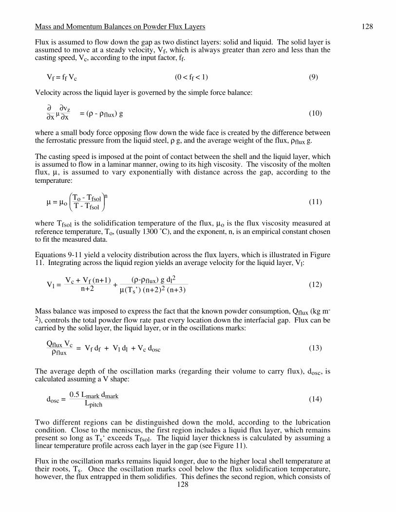
Equations 9-11 yield a velocity distribution across the flux layers, which is illustrated in Figure11. Integrating across the liquid region yields an average velocity for the liquid layer, Vl:
Vl = Vc + Vf (n+1)
n+2 + (ρ-ρflux) g dl2
µ(Ts’) (n+2)2 (n+3) (12)
Mass balance was imposed to express the fact that the known powder consumption, Qflux (kg m-
2), controls the total powder flow rate past every location down the interfacial gap. Flux can becarried by the solid layer, the liquid layer, or in the oscillations marks:
Qflux Vcρflux
= Vf df + Vl dl + Vc dosc (13)
The average depth of the oscillation marks (regarding their volume to carry flux), dosc, iscalculated assuming a V shape:
dosc = 0.5 Lmark dmark
Lpitch (14)
Two different regions can be distinguished down the mold, according to the lubricationcondition. Close to the meniscus, the first region includes a liquid flux layer, which remainspresent so long as Ts‘ exceeds Tfsol. The liquid layer thickness is calculated by assuming alinear temperature profile across each layer in the gap (see Figure 11).
Flux in the oscillation marks remains liquid longer, due to the higher local shell temperature attheir roots, Ts. Once the oscillation marks cool below the flux solidification temperature,however, the flux entrapped in them solidifies. This defines the second region, which consists of
129
129totally solid flux, moving downward at the uniform speed, Vf. The oscillation marks no longertransport flux, so become filled with air.
sol liq oeff
mold
liquidflux
Vf
solid flux
dl doeffdf
velocity profile
T'
shell
V
temperature profile
equivalentlayer foroscillation marks
kf kl koeff
c
Thotc
Tfsol
Ts
x
T's
m
Figure 11 - Velocity and temperature profiles across interfacial gap layers (no air gap)
Solution Methodology
The CON1D model requires simultaneous solution of three different systems of equations: 1-Dtransient heat conduction and solidification of the steel shell, 2-D steady state heat conduction inthe mold, and the equations balancing heat, mass and momentum in the gap. The equations aresolved by first performing a transient 1-D simulation of the shell, gap and mold. The model usesan explicit, central-finite difference algorithm, which limits the maximum time step size, ∆t. Theresults are used as initial conditions for the 2-D mold calculation, which is solved analytically bysuperposition, relating distance down the mold, z, to time in the shell through the casting speed.Subsequently, the model iterates between the 1-D shell and 2-D mold calculations usingsuccessive substitution until convergence is achieved. This produces a self-consistent prediction,which is stable for all coupled simulations investigated and converges in 3-4 iterations.
The model has been incorporated into a user-friendly FORTRAN program, CON1D. Theprogram requires less than 500 KBytes of memory and runs on a personal computer in less than1 minute.
Model Verification and Calibration
The model was first validated through comparison with known analytical solutions for metal-controlled solidification, [24] and with other models, which is described elsewhere. [25] It wasthen calibrated to match experimental measurements obtained under similar conditions to thebreakout shell described in the previous section. These measurements included the cooling watertemperature rise, the time-average temperature of several thermocouples embedded in the coppermold walls, and the thickness profile of the breakout shells. This calibration step is crucialbecause so many of the model parameters are uncertain.

130
130Calibration was performed along the center of the wide face. Calibration is simplified herebecause there is no large air gap, such as found near the corners. This is because ferrostaticpressure pushes the long, wide, weak shell against the mold wide face to maintain as close acontact as possible.
The input parameters used in the simulations are given in Table I. Many of these parameterswere measured (left side of table) while others are estimates of physical constants. Theremaining parameters were adjusted to calibrate the model. These include the velocity of thesolid flux layer, ff, air gaps, and the thermal conductivity of the mold flux layers. Several othersets of calibrated parameters could have been chosen with equal matching of the measurements.
Table I Simulation Conditions and Parameters
Slab breakout Bloom Model ParametersMold specifications da 0. - 0.025 mm
Slab size (z=0) 1500 x 225 mm 650 x 413 mm kair 0.06 Wm-1K-1
Mold Length 900 mm 900 mm km 315 W m-1K-1
Working mold length 815 mm 775 mm Twater 30 ˚CMold thickness dm(0) 57 mm 15 mm ρflux 2500 kg m-3
Channel Lch, dch, wch 24, 25, 5 mm plate mold Tfsol 980˚CMold curvature radius 11.76 m µo 1.28 PoiseWater velocity, VW 7.8 m s-1 To 1300 ˚C
n 0.85Steel Composition 0.044%C 0.055 %C kf 1.24 Wm-1K-1
Liquidus, Tliq 1528 ˚C 1527 ˚C kl 3.4 Wm-1K-1
Solidus, Tsol 1509 ˚C 1500 ˚C kscale 0.55 Wm-1K-1
dscale 0.01 mmCasting Conditions σ 5.67x10⁻⁸ Wm-2K-4
Casting speed, Vc 1.016 m min-1 0.5 m min-1 a 900 m-1
Initial temperature, To 1555 ˚C 1546 ˚C m 1.5Superheat, ∆Tsh 27 ˚C 19 ˚C εs, εm 0.8, 0.5Consumption, Qflux 0.4 kg m-2 ff 16.4 pct
fsol 70 pctOscillation Data g 9.8 m s-2
Stroke 10 mm ρ 7400 kg m-3
Frequency, freq 1.417 Hz ∆HL 272 kJ kg-1
Average depth, dmark 0.33 mm Lpitch 12 mmAverage width, Lmark 3.78 mm ∆t 0.0005 sPitch (measured) 10.5 mm ∆x 0.3 mm
Mold Cooling Water Temperature Rise
The measured average rate of heat flux extracted from the mold should match that calculated bythe model via:
Q (kW/m2) = Vc
zmold ∑
mold qint * ∆t (15)
This heat transfer rate is readily inferred from the temperature increase of the mold cooling water,∆Twater, which is also calculated:
∆Twater = ∑mold
qint Lch Vc ∆t
ρw Cpw Vw wch dch(16)

131
131where ρw, Cpw, and Vw are the cooling water density, specific heat, and speed. This equationassumes that the cooling water slots have uniform rectangular dimensions, wch and dch, andspacing, Lch. Heat entering the hot face (between two water channels) is assumed to pass entirelythrough the mold to heat the water flowing through the cooling channels. The prediction must bemodified to account for missing slots due to bolts or water slots which are beyond the slab width,so do not participate in heat extraction.
For the LTV mold, the predicted cooling water temperature rise of 8.9 ˚C matches the measuredrise. The predicted mean heat flux of 1495 kW/m2 is thus also consistent with measurements.
Mold Temperatures
Figure 12 shows an example comparison between the predicted and measured temperatures atseveral locations down the LTV mold. The conditions were very similar to those of the breakoutin Table I. The differences, given in run 2 in Ho, [20] include Vc=1.07 m min–1, ∆Tsh=21˚C,Qflux=0.6 kg m-2, and a flux rim at the meniscus. The agreement suggests that the model isreasonably calibrated for typical casting conditions for this caster. This figure also shows thepredicted hot face and cold face temperature profiles. The sudden changes in temperature aredue to a 6.35 mm increase in water channel depth in the upper 300 mm of this test mold.
Figure 12 - Comparison between CON1D calculated and measured mold temperatures
Shell Thickness
Figure 4 includes a comparison of the predicted shell thickness profile with measurements downthe breakout shell. Shell thickness is defined in the model by linearly interpolating the positionbetween the liquidus and solidus isotherms corresponding to the specified solid fraction, fsol. Growth of the shell naturally depends upon the combination of the interfacial and superheatfluxes. The superheat distribution is important as Figure 8 shows that the two heat flux curvesare of the same magnitude in the lower regions of the mold near the narrow face where the hot

132
132molten steel jet impinges against the solidifying shell. The model is seen to match themeasurements reasonably well.
Other Validation
The model predicts the thickness and velocity profiles expected in the powder layers in theinterfacial gap. For example, Figure 13 shows the solid and liquid flux layer thickness profilesexpected for the conditions in Figure 12 (Table 1). Unfortunately, no reliable samples could beobtained to validate these results, although the predictions of flux layer thickness on the order of1 mm are consistent with findings at other plants. [20] Also, mold friction measurements shouldcorrelate with the model predictions of the length of the liquid layer, if data were available.Finally, model predictions of surface temperature of the steel shell could be compared withmeasurements from optical pyrometers located just below mold exit.
Figure 13 - Calculated flux layer thickness profile
CON1D model results
The calibrated CON1D model was run to perform a parametric study on the effect of the averageoscillation mark area on the time-averaged heat transfer and shell growth. The average interfacialheat transfer coefficient, hgap, was decreased by increasing the average effective depth of theoscillation marks, doeff, according to the average mark dimensions using Eqs. 6 and 7. Otherparameters were left at their calibrated or measured values given in Table I.
For a fair comparison, the mold flux consumption rate for each run, Qfluxi, was changedaccording to the oscillation mark area, assuming that oscillation marks with larger volumesconsume more flux as they move downward at the casting speed:
Qfluxi = Qflux + ρflux (dosci - dosc) (17)

133
133Table II shows the conditions assumed and results for a typical case, based on Table I conditions,and extreme cases of no oscillation marks and very deep oscillation marks. The increasedvolume of the deeper oscillation marks is predicted to significantly increase flux consumption,according to Eqs. 14 and 17. It is important to note that if the consumption rate was not adjustedin this manner, then increasing oscillation mark depth would decrease the average gap thicknessand thereby tend to increase the average mold heat transfer and shell thickness.
Table II Effect of Oscillation Marks on Mold Heat Transfer
No marks Typical Deep marks UnitsOscillation marks
Volume 0. 0.62 3.00 mm2/cmDimensions, dmark x Lmark 0. x 0. 0.33 x 3.78 0.70 x 8.6 mm x mmAverage layer thickness, dosc 0. 0.052 0.251 mm
Flux consumption, Qflux 0.27 0.40 0.90 kg m-2
Heat transfer coefficient (local)Osc. mark eff., koeff / doeff ∞ 85000 14000 Wm-2K-1
Radiation, hrad 133 137 160 Wm-2K-1
Gap, hgap (flux-filled) 1890 1859 1720 Wm-2K-1
Average mold heat flux, Qint 1573 1493 1322 kW m-2
Shell thickness at mold exit 23.4 23.0 21.4 mmSurface temperature at mold exit 902 983 1068 ˚C
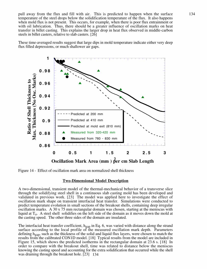
The results in Table II predict that deep oscillation marks decrease overall mold heat transfer byroughly 15%, relative to that with no oscillation marks. The shell thickness decreasesaccordingly, although the percentage drop is only 8% at mold exit. This is because the reducedheat transfer also increases the surface temperature of the shell exiting the mold. The hotter shellcontains more heat and is also softer and weaker.
The calculated effect of oscillation mark depth on average shell thickness is illustrated in Figure14. Shell thickness data were normalized by dividing by the corresponding thickness obtainedwith no oscillation marks, which has the maximum average thickness for a given case. Theoscillation mark size was characterized by the area of the oscillation marks per unit length downthe strand surface (0.5 dmark Lmark / Lpitch). This is consistent with the importance of depth,width, and distance between the oscillation marks on heat transfer, which is quantified in Eq. 7.
The results predict that shell thickness decreases with deeper, wider, and / or more frequentoscillation marks, as expected. The effect is greatest near the meniscus (eg. 200 mm data), wherethe interfacial gap is the most influential factor controlling heat flow. Further down the mold, theincreased thermal resistance of the thicker solid shell makes the oscillation marks less important.Shallow, flux-filled oscillation marks have a minimal effect on heat transfer because their thermalresistance (doeff / koeff) is so small relative to the rest of the gap and the solid shell.
The shell thickness predictions are compared with a few measured points in Figure 14. Thesepoints are not easy to obtain because it is difficult to estimate the thickness that the shell wouldhave attained at a given location without the oscillation marks present. Thus, measured datapoints was only obtained at locations that had locally abnormally deep marks, relative to adjacentregions which could be used for comparison. Considering the scatter and uncertainty, theagreement with the model prediction is reasonable. Increasing oscillation mark area per unitlength down the strand surface tends to decrease the shell thickness.
If typical oscillation marks become filled with air sometime before mold exit, hgap is predicted todecrease by almost 50% from 1859 to 946 Wm-2K-1. Clearly, the material filling the gap has atremendous effect on mold heat transfer. Oscillation marks become much more important if they
134
134pull away from the flux and fill with air. This is predicted to happen when the surfacetemperature of the steel drops below the solidification temperature of the flux. It also happenswhen mold flux is not present. This occurs, for example, when there is poor flux entrainment orwith oil lubrication. Thus, there should be a greater influence of oscillation marks on heattransfer in billet casting. This explains the larger drop in heat flux observed in middle-carbonsteels in billet casters, relative to slab casters. [26]
These time-averaged results suggest that large dips in mold temperature indicate either very deepflux filled depressions, or much shallower air gaps.
0 . 8 6
0 . 8 8
0 . 9
0 . 9 2
0 . 9 4
0 . 9 6
0 . 9 8
1
0 0 . 5 1 1 . 5 2 2 . 5 3
Predicted at 200 mm
Predicted at 410 mm
Predicted at mold exit (810 mm)
Measured from 320-420 mm
Measured from 760 - 830 mm
Rat
io o
f Sh
ell T
hick
ness
to
Max
. Thi
ckne
ss (
No
Osc
. Mar
ks)
Oscillation Mark Area (mm ) per cm Slab Length2
Figure 14 - Effect of oscillation mark area on normalized shell thickness
Two-Dimensional Model Description
A two-dimensional, transient model of the thermal-mechanical behavior of a transverse slicethrough the solidifying steel shell in a continuous slab casting mold has been developed andvalidated in previous work. [23] The model was applied here to investigate the effect ofoscillation mark shape on transient interfacial heat transfer. Simulations were conducted topredict temperature evolution in small sections of the breakout shells, containing deep irregularoscillation marks. A 30 x 75 mm rectangular domain was chosen, starting at the meniscus withliquid at To. A steel shell solidifies on the left side of the domain as it moves down the mold atthe casting speed. The other three sides of the domain are insulated.
The interfacial heat transfer coefficient, hgap in Eq. 6, was varied with distance along the strandsurface according to the local profile of the measured oscillation mark depth. Parametersdefining hgap, such as the thickness of the solid and liquid flux layers, were chosen to match theresults from the calibrated CON1D model. [18] Typical results from the model are included inFigure 15, which shows the predicted isotherms in the rectangular domain at 23.6 s. [18] Inorder to compare with the breakout shell, time was related to distance below the meniscusknowing the casting speed and accounting for the extra solidification that occurred while the shellwas draining through the breakout hole. [23]

135
135
Osc. Markat 367mm
Osc. Markat 379mm
Osc. Markat 387mm
1000
1050
1100
1100 ˚C
1200
1300
1250
1200
1150
1250
1200 ˚C
11501200
1475(T sol)
1493 ˚C(T shell)
1532 ˚C(T liq) 75mm
30mm
Z,t
X
Liquid SteelMold Wall
Solid Shell
insulated (q=0)
insulated (q=0)
conv
ectio
n h(
z,
d osc
)
Figure 15 - Example 2-D heat flow model temperature distribution in shell section (with air-filled gap).
Two-Dimensional Transient Results
The CON1D model has quantified the effect of surface depressions on the steady-state heattransfer during continuous slab casting with mold flux. Next, the 2-D model is applied toinvestigate the local variations in heat transfer, shell growth, and surface temperature produced byindividual groups of depressions on selected regions of the strand surface.
Shell thickness
Results for a section of shell with three typical oscillation marks (with areas of .34, .78, and 0.29mm2) are presented in Figure 16. The predicted shell thickness is compared with correspondingmeasurements of the breakout shell. The general agreement simply illustrates the reasonablecalibration of the model, which was done for average oscillation marks similar to these (Table I).

136
136Figure 16 also shows the measured surface profile for this section of shell, from which gap heattransfer coefficients were constructed using Eq. 6.
- 1
- 0 . 5
0
0 . 5
1
1 . 5
2
2 . 5
1 3
1 3 . 5
1 4
1 4 . 5
1 5
1 5 . 5
1 6
3 9 0 4 0 0 4 1 0 4 2 0 4 3 0
Osc
illat
ion
Mar
k D
epth
(m
m)
Shell Thickness (m
m)
Distance Below Meniscus (mm)
6
1 4
8
2 3
8
1 2
Surface Temp. RiseDue to Osc. Marks ( C)
Predicted (No Osc. Marks)
Measured Shell Thickness
Predicted (with Flux-Filled Osc. Marks)
Oscillation Mark Depth
o
Figure 16 - Comparison of predicted and measured shell thickness with oscillation mark profileand surface temperatures for small, flux-filled oscillation marks
Each individual mark is almost too small to affect the shell thickness locally. The deepest (0.49 x2.80 mm) middle mark in Figure 16 produces just a slight dip in shell thickness, which is enoughto obscure the more important, general effect of reduced average shell growth rate. Withoutoscillation marks, the shell growth rate at 400 mm below the meniscus is predicted to be 0.021mm per mm down the strand. These flux-filled oscillation marks produce a shell that is about0.2 mm (1.5%) thinner.
Results from a section of shell with deeper surface depressions are shown in Figures 17 and 18.The four oscillation marks in this section of shell are seen to be very wide and deep, with areas of1.8, 2.5, 1.9, and 1.1 mm2. Even filled with flux, they significantly reduce the local shell growth.The decrease in shell thickness is predicted to range from 0.5 to 0.9 mm over this section (6%maximum loss). These predictions almost exactly match measurements from the breakout shell,as shown in Figure 17. This match is significant because the model calibration was performedfor a different oscillation mark depth and did not consider local variations.
The maximum thickness loss is found midway along the section containing the four deeposcillation marks. Note that this does not coincide with the deepest oscillation mark. This isbecause these marks act as a group to reduce shell growth locally. Due to the nature of two-dimensional conduction within the shell, the number (or length) of the group of marks actingtogether is expected to roughly equal the local shell thickness. Thus, the group that controlsgrowth at a particular point on the shell increases in number with distance down the mold. Nearthe meniscus, a single deep mark can produce a noticeable drop in shell thickness. By mold exit,however, only the effects of at least three oscillation marks extending over 30 mm can bedistinguished.
To quantify the importance of the material filling the oscillation marks, the simulation of the deeposcillation mark section of shell was repeated using a lower thermal conductivity for theoscillation mark layer. Specifically, the material was changed from flux to air (Table I). Theresults in Figure 18 show the dramatic effect on heat transfer.

137
137
- 1
- 0 . 5
0
0 . 5
1
1 . 5
2
2 . 5
1 1 . 5
1 2
1 2 . 5
1 3
1 3 . 5
1 4
1 4 . 5
1 5
3 6 0 3 7 0 3 8 0 3 9 0 4 0 0
Osc
illat
ion
Mar
k D
epth
(m
m)
Shell Thickness (m
m)
Distance Below Meniscus (mm)
5 2
8 6 7 7
5 7
2 2
3 3Surface Temp. RiseDue to Osc. Marks ( C)
Predicted (No Osc. Marks)
MeasuredShell Thickness
Predicted (with Flux-Filled Osc. Marks)
Oscillation Mark Depth
o
Figure 17 - Comparison of predicted and measured shell thickness with oscillation mark profileand surface temperatures for large, flux-filled oscillation marks
- 1
- 0 . 5
0
0 . 5
1
1 . 5
2
2 . 5
8
9
1 0
1 1
1 2
1 3
1 4
1 5
3 6 0 3 7 0 3 8 0 3 9 0 4 0 0
Osc
illat
ion
Mar
k D
epth
(m
m)
Shell Thickness (m
m)
Distance Below Meniscus (mm)
8 8
266 305
300
149
249Surface Temp. RiseDue to Osc. Marks ( C)
Predicted (No Osc. Marks)
Measured Shell Thickness
Predicted (with Air-Filled Osc. Marks)
Oscillation Mark Depth
o
Figure 18 - Comparison of predicted and measured shell thickness with oscillation mark profileand surface temperatures for large, air-filled oscillation marks

138
138The shell thickness is predicted to decrease by more than 3 mm (20%) in the region with air-filled oscillation marks. This does not match the measurements. This offers further proof thatthe oscillation marks in this investigation were not filled with air when they were in the mold.
Surface Temperature
Figures 16 - 18 also include the difference between the surface temperatures predicted with andwithout oscillation marks, labeled at significant locations along the shell. Surface temperature ismore sensitive than shell thickness and corresponds directly with oscillation mark depthvariations along the shell surface. Note that the oscillation marks increase the surfacetemperature even between the marks, where there is always a minimal gap between the shell andthe mold. This is due to two-dimensional heat flow and further illustrates how several oscillationmarks act together.
Small oscillation marks filled with flux increase temperature very little. At the root of a typicalsmall (0.34 mm2) oscillation mark in Figure 16, the temperature rise reaches only 14 ˚C. Suchsmall variations are unlikely to produce any noticeable change in the mold temperature, relative toother parameters affecting heat flux, such as random changes in the flux layer thicknesses or gapproperties.
Large oscillation marks filled with flux are predicted to produce significant rises in surfacetemperature of the strand. Figure 17 shows the surface temperature increases to 22 to 86 ˚Chotter than the 978˚C value predicted without oscillation marks. Like shell thickness, the extentof this variation decreases with distance down the mold. The changes in heat flux accompanyingthese temperature variations correspond to 20 to 50 ˚C fluctuations in mold temperature,depending on the location of the thermocouples. These temperature differences are typical ofobserved fluctuations in the recorded signals.
The temperature results in Figures 15 and 18 indicate the dangerous effect of air-filled surfacedepressions. The local surface temperature beneath a series of 2.0 mm2 depressions filled withair rises more than 300 ˚C to nearly 1300 ˚C. The lower strength of the shell at this temperature,combined with its smaller thickness, would make the shell very weak locally and prone to failure.This simulation illustrates how deep surface depressions, combined with a mold flux entrainmentproblem that leads to deep air-filled depressions, could produce serious problems, such as abreakout. Large temperature differences between adjacent regions of the shell surface might alsolead to crack formation. Finally, the large fluctuations in heat flux that accompany thesetemperature differences could be detected by the large fluctuations in the mold temperaturesignals they produce.
Discussion
Surface depressions, including oscillation marks, decrease heat transfer during continuouscasting in the mold. This is manifested by drops in mold wall temperature, increased shellsurface temperature and reduced shell thickness. The magnitude of these effects is proportionalto the drop in heat transfer, which depends on the depth, width, and number of surfacedepressions per unit length along the shell, and the material that fills them.
Some of the temperature fluctuations recorded by thermocouples in the mold wall are clearly dueto anomolously large depressions on the strand surface moving down the mold at the castingspeed. These can be identified by a consistent time lag between dips recorded by thermocouplesspaced vertically down the mold. The time lag corresponds to the casting speed and distancebetween thermocouples, as shown in Figure 2. Groups of oscillation marks with a similar largearea are predicted to create a similar effect.
Oscillation marks likely have a greater importance in billet heat transfer, because the interfacialgap with vapor products from oil-based lubrication has such a low thermal conductivity. In flux-based casting operations, this work has shown that some, if not most, surface depressions arealways filled with flux while in the mold. The impact of depressions on heat transfer under thesegood casting conditions is perhaps less than commonly thought, (only about 10% even for deepdepressions).

139
139The tremendous effect of air gaps suggests that problems in keeping the gap consistently filledwith mold flux likely pose a greater threat to quality than the depth of the surface depressions.Future research should focus on the nature of the mold flux properties in filling the gap.Important factors to consider are the entrainment of flux at the meniscus, the loss of contactbetween the shell and the flux layers, and the break-up of the flux layer as it is dragged down themold wall. Thus, flux properties such as coefficient of friction with the mold walls and tensilestrength may be important and should be measured.
On-line quality monitoring systems should be developed to search for patterns in thermocouplesignals and identify the likely presence of surface quality problems as they form in the mold.Corrective action can then be taken, and downgrading made as appropriate. Like shell surfacetemperature, mold thermocouple signals are more sensitive to changes in heat flux than is theshell thickness.
However, the use of thermocouple signals to detect defects is not easy. This is because 1)depressions do not always lead to defects and 2) many complex phenomena affect heat transfer,which are not related to depressions. For example, local increases in flux layer thickness andreductions in flux layer conductivity (eg. due to porosity) may lower gap heat transfer. Theseother factors, which have received little attention, are at least as important as surface depressionsin controlling heat flux and thermocouple signals. [27] Thus, the lower heat transfer observed inmiddle-carbon steels is likely caused more by the higher solidification temperature mold fluxes(and accompanying thicker layers) employed for these grades, than to deeper oscillation marks.
Nevertheless, this work encourages on-line monitoring by showing how depressions affect thetemperature history of the surface of the strand and can be detected by mold wall thermocouples.Further work is needed to determine the relationship between these thermal histories and defectformation.
Conclusions
Experimental measurements and calibrated solidification heat conduction models have beenapplied to understand the effect of surface depressions and oscillation marks on heat transfer andtemperature in a continuous slab casting mold. Specific conclusions are:
1) Many surface defects, such as oscillation marks, originate at the meniscus and move downthe mold at the casting speed. Their size and shape appears not to change over most of thelength of the mold.
2) Surface depressions and oscillation marks reduce heat transfer, which slows shell growth,increases surface temperature, and causes dips in mold thermocouple signals. The magnitudeof the effect depends on the size of the depression and the material filling it.
3) Shell thickness in the mold is reduced with increasing depth, width, and proximity of adjacentoscillation marks, which act together in groups. Typical flux-filled oscillation marks with 0.6mm2/cm produce a 1.5% drop in shell thickness. A group of 2 mm2/cm marks produced a6% decrease in shell thickness.
4) All of the oscillation marks and depressions investigated in this work were determined to befilled with mold flux.
5) The wideface off-corner region had the greatest variation in oscillation mark depth, whichproduced the greatest variation in local shell thickness.
6) Large (2 mm2), air-filled depressions are predicted to drastically reduce heat transfer, slowshell growth by 20%, and increase surface temperature by 300 ˚C, which could lead toproblems such as breakouts and cracks.

140
1407) The effect of oscillation marks on heat transfer decreases with distance down the mold. Theyare most influential just below the meniscus, before the resistance of the solidified shellbegins to control heat flow and lessen their importance.
8) Shell surface temperature and mold temperature are more sensitive to changes in heat fluxcaused by surface depressions than is the solidified shell thickness.
9) Large transverse surface depressions, or groups of deep oscillation marks can be positivelyidentified by their characteristic effect on thermocouple signals as they move down the mold.Other phenomena occurring in the gap, such as the formation of air gaps, are also importantto heat transfer and the accompanying fluctuations in thermocouple signals.
This work has taken initial steps to quantify the effect of imperfections in the cast surface shapeon interfacial heat transfer. The findings should help improve the accuracy of model predictionsof solidification heat transfer. In addition, they should be relevant to the interpretation ofthermocouple signals for on-line quality monitoring.
Nomenclature
a absorption coefficient (m-1) Tfsol Solidification temperature of fluxCp Specific heat of steel (J kg-1 K-1) Thotc Mold surface temperatured Thickness in x direction (mm) Twater Mold cooling water temperaturedmark Oscillation mark depth Ts Steel surface temperaturedosc Effective mark thickness (volume) To Reference temperature for µdoeff Effective mark thickness (heat flow) ∆Tsh Superheat (Tliq - Tsol)dscale Scale layer on mold cold face Vc Casting speed (m min-1)ds Steel shell thickness Vf Velocity of solid flux (mm s-1)ff Fraction Vc of solid flux speed Vz Casting direction velocity (mm s-1)g Gravity (9.81 m s-2) wch Cooling water channel width (mm)h Heat transfer coefficient (W m-2 K-1) x Shell thickness direction (mm)hrad Radiation across flux h ∆x Mesh spacing (mm)hfin Mold cold face h y Mold width direction (mm)hwater Effective mold / water h z Casting direction (mm)hw Mold surface / water h εs Emmisitivityhgap Shell / mold gap effective h εm Mold emissivity∆HL Latent heat of fusion of steel (kJ kg-1) µ Flux viscosity (T) (Poise)k Thermal conductivity (W m-1 K-1) µ0 Flux viscosity at To (Poise)koeff Effective k of osc. marks (W m-1 K-1) ρ Density of steel (kg m-3)K Solidification constant (mm2s-1) ρflux Flux density (kg m-3)Lpitch Distance between osc. marks (mm) σ Stefan Boltzman constantLmark Width of oscillation marks (mm)Lch Cooling water channel thickness (mm) Subscriptsm Refractive indexn Flux viscosity exponent (Eq. 11) solidifying steel shell (default)qint Shell / mold interface heat flux (W m-2) water mold cooling waterqsh Liquid / shell interface heat flux (W m-2) m mold wallQflux Mold flux consumption (kg m-2) a air gapt Time (s) flux mold flux∆t Time step size (s) f solid mold flux layerT Temperature (˚C) l liquid mold flux layerTliq Liquidus temperature s steel surface (oscillation mark root)Tsol Solidus temperature s’ steel surface

141
141References
1. J.K. Brimacombe, “Empowerment with Knowledge - toward the Intelligent Mold for theContinuous Casting of Steel Billets,” Metallurgical Transactions B, 24B (1993), 917-935.
2. W.H. Emling and S. Dawson, “Mold Instrumentation for Breakout Detection andControl,” in Steelmaking Conference Proceedings, 74, Iron and Steel Society,Warrendale, PA, 1991), 197-217.
3. E. Takeuchi and J.K. Brimacombe, “The formation of oscillation marks in thecontinuous casting of steel slabs,” Metallurgical Transactions B, 15B (Sept) (1984), 493-509.
4. B.G. Thomas and H. Zhu, “Thermal Distortion of Solidifying Shell Near Meniscus inContinuous Casting of Steel” (Paper presented at Solidification Science and ProcessingConference, Honolulu, HI, 1995, JIM / TMS).
5. R.B. Mahapatra, J.K. Brimacombe and I.V. Samarasekera, “Mold Behavior and itsInfluence on Product Quality in the Continuous Casting of Slabs: Part II. Mold HeatTransfer, Mold Flux Behavior, Formation of Oscillation Marks, Longitudinal Off-cornerDepressions, and Subsurface Cracks,” Metallurgical Transactions B, 22B (December)(1991), 875-888.
6. J.E. Kelly et. al., “Initial Development of Thermal and Stress Fields in ContinuouslyCast Steel Billets,” Metallurgical Transactions A, 19A (10) (1988), 2589-2602.
7. I.V. Samarasekera, J.K. Brimacombe and R. Bommaraju, “Mold Behavior andSolidification in the Continuous Casting of Steel Billets,” Transactions of Iron and SteelSociety, 5 (1984), 79-105.
8. I. Halliday, “Continuous casting at Barrow,” J. Iron Steel Instit, 191 (1959), 121-163.
9. S.N. Singh and K.E. Blazek, “Heat Transfer and Skin Formation in a ContinuousCasting Mold as a Function of Steel Carbon Content,” in Open Hearth Proceedings, 57,(Warrendale, PA: Iron and Steel Society, 1974), 16-36.
10. K.E. Blazek, I.G. Saucedo and H.T. Tsai, “Investigation on mold heat transfer duringcontinuous casting,” in Steelmaking Proceedings, 71, Iron and Steel Society,Warrendale, PA, 1988), 411-421.
11. M. Wolf, “Investigation into the relationship between heat flux and shell growth incontinuous casting moulds,” Trans Iron Steel Instit Japan, 20 (1980), 710-717.
12. A. Grill, K. Sorimachi and J.K. Brimacombe, “Heat Flow, Gap Formation and Break-Outs in the Continuous Casting of Steel Slabs,” Metallurgical Transactions, 7B (1976),177-189.
13. N. Tiedje and E.W. Langer, “Metallographic examination of breakouts from acontinuous billet caster,” Scandinavian J. Metallurgy, 21 (1992), 211-217.
14. A.W. Cramb and F.J. Mannion, “The measurements of meniscus marks at BethlehemSteel’s Burns Harbor slab caster,” in Steelmaking Proceedings, 68, (Warrendale, PA:Iron and Steel Society, 1985), 349-359.
15. B.G. Thomas, “Mathematical Modeling of the Continuous Slab Casting Mold, a State ofthe Art Review,” in Mold Operation for Quality and Productivity, A. Cramb, eds.,(Warrendale, PA: Iron and Steel Society, 1991), 69-82.

142
14216. R. Bommaraju and E. Saad, “Mathematical modelling of lubrication capacity of moldfluxes,” Steelmaking Conference Proceedings, 73 (1990), 281-296.
17. M.S. Jenkins et. al., “Investigation of Strand Surface Defects using MoldInstrumentation and Modelling,” in Steelmaking Conference Proceedings, 77,(Warrendale, PA: Iron and Steel Society, 1994), 337-345.
18. D. Lui, “Effect of Oscillation Marks on Heat Transfer in the Continuous Casting Mold”(Masters Thesis, University of Illinois, 1995).
19. B.G. Thomas, B. Ho and G. Li, “CON1D User’s Manual” (Report, University ofIllinois, 1994).
20. B. Ho, “Characterization of Interfacial Heat Transfer in the Continuous Slab CastingProcess” (Masters Thesis, University of Illinois at Urbana-Champaign, 1992).
21. X. Huang, B.G. Thomas and F.M. Najjar, “Modeling Superheat Removal duringContinuous Casting of Steel Slabs,” Metallurgical Transactions B, 23B (6) (1992), 339-356.
22. C.A. Sleicher and M.W. Rouse, 18 (1975), 677-683.
23. A. Moitra and B.G. Thomas, “Application of a Thermo-Mechanical Finite ElementModel of Steel Shell Behavior in the Continuous Slab Casting Mold,” in SteelmakingConference Proceedings, 76, Iron and Steel Society, 1993), 657-667.
24. M.C. Flemings, Solidification Processing, (McGraw Hill, 1974), 17-19.
25. B.G. Thomas and B. Ho, “Spread Sheet Model of Continuous Casting,” J. EngineeringIndustry, 118 (1) (1996), 37-44.
26. M.M. Wolf, “Mold Heat Transfer and Lubrication Control - Two Major Functions ofCaster Productivity and Quality Assurance,” in PTD Conference Proceedings, 13,(Warrendale, PA: Iron and Steel Society, 1995), 99-117.
27. M.R. Ozgu and B. Kocatulum, “Thermal Analysis of the Burns Harbor No. 2 SlabCaster Mold,” in Steelmaking Conference Proceedings, 76, Iron and Steel Society,Warrendale, PA, 1993), 301-308.
Acknowledgments
Funding for this work was provided by the Continuous Casting Consortium at the University ofIllinois (Allegheny Ludlum, AK Steel, Armco, BHP, Inland, LTV, Stollberg) The authors alsowish to thank researchers at LTV Steel, (Cleveland, OH) for providing plant data and the NationalCenter for Supercomputing Applications for computing time.