material requirements planning - dspace.mit.edu · material requirement times can be determined....
TRANSCRIPT

Material Requirements Planning
Lecturer: Stanley B. Gershwin
MRP Overview
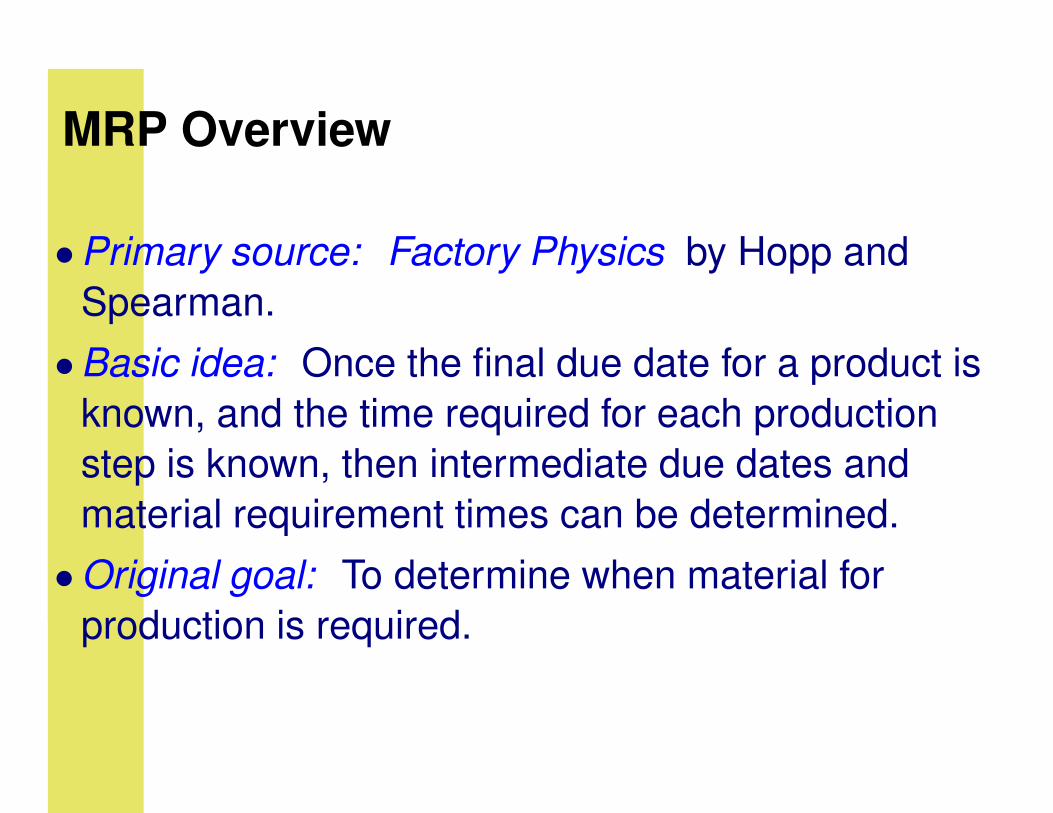
• Primary source: Factory Physics by Hopp and Spearman.
• Basic idea: Once the final due date for a product is known, and the time required for each production step is known, then intermediate due dates and material requirement times can be determined.
• Original goal: To determine when material for production is required.
Demand MRP Overview
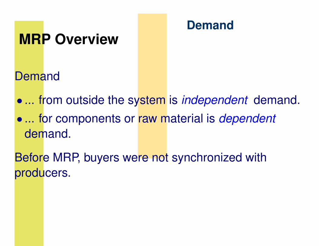
Demand
• ... from outside the system is independent demand.• ... for components or raw material is dependent demand.
Before MRP, buyers were not synchronized with producers.

Planning Algorithm MRP Overview
• Start at the due date for a finished product (or end item ) (Tk).
• Determine the last operation, the time required for that operation (tk−1), and the material required for that operation.
• The material may come from outside, or from earlier operations inside the factory.
• Subtract the last operation time from the due date to determine when the last operation should start.

Planning Algorithm MRP Overview
Tk−1 = Tk − tk−1
• The material required must be present at that time. • Continue working backwards. • However, since more than one component may be needed at an operation, the planning algorithm must work its way backwards along each branch of a tree — the bill of materials.

Planning Algorithm MRP Overview
Time
• In some MRP systems, time is divided into time buckets — days, weeks, or whatever is convenient.
• In others, time may be chosen as a continuous variable.
DiscussionMRP Overview
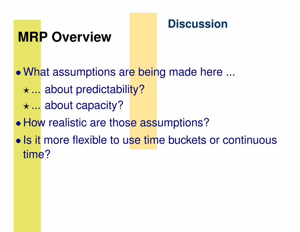
• What assumptions are being made here ... � ... about predictability? � ... about capacity?
• How realistic are those assumptions? • Is it more flexible to use time buckets or continuous time?

Jargon MRP Overview
• Push system: one in which material is loaded basedon planning or forecasts, not on current demand.� MRP is a push system.
• Pull system: one in which production occurs in response to the consumption of finished goods inventory by demand.
• Which is better?
Level 1
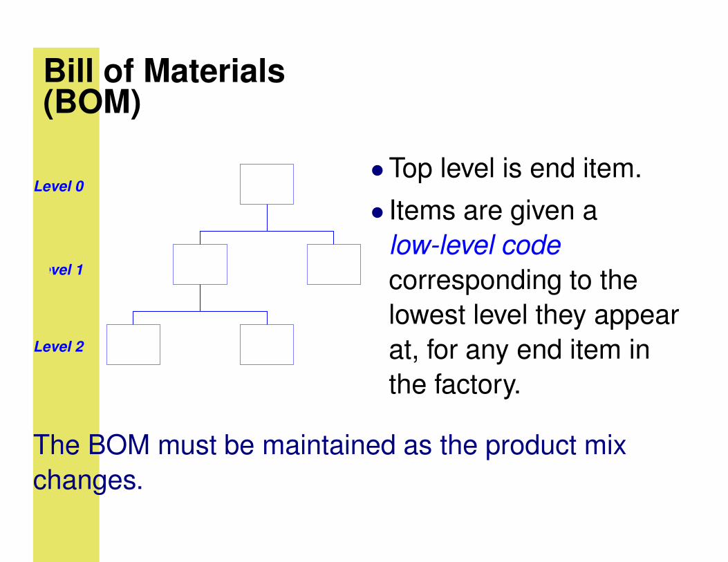
Bill of Materials(BOM)
• Top level is end item. Level 0
• Items are given a low-level code corresponding to the lowest level they appear
Level 2 at, for any end item in the factory.
The BOM must be maintained as the product mix changes.

MasterProductionSchedule• Information concerning independent demand. • Gross requirements: What must be delivered in the future, and when.
• On-hand inventory: Finished good already available.• Net requirements: (Gross requirements) – (On-hand inventory).

Master ExampleProductionSchedule Netting
Week 1 2 3 4 5 6 7 8
Gross requirements 15 20 50 10 30 30 30 30 Projected on-hand 30 15 -5 Net requirements 0 5 50 10 30 30 30 30 • 15 of the initial 30 units of inventory are used to satisfy Week 1 demand.
• The remaining 15 units are 5 less than required to satisfy Week 2 demand.

Master ExampleProduction Schedule Lot Sizing
• Lot sizes are 75. The first arrival must occur in Week 2. • 75 units last until Week 4, so plan arrival in Week 5. • Similarly, deliveries needed in Weeks 5 and 7.
Week 1 2 3 4 5 6 7 8
Gross requirements 15 20 50 10 30 30 30 30 Cumulative gross 15 35 85 95 125 155 185 215 Planned order receipts 30 0 75 0 0 75 0 75 0 Cumulative receipts 30 105 105 105 180 180 255 255

MasterProductionSchedule
300cumulative gross
cumulative receipts 250
200
150
100
50
0 0 1 2 3 4 5 6 7 8 week
Example
Cumulatives
Material requirements are determined by considering whether inventory would otherwise become negative.
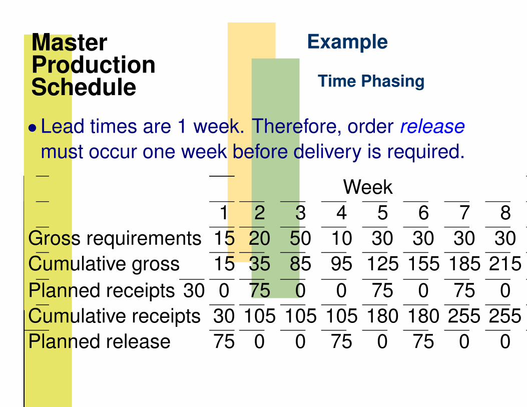
Master ExampleProduction Schedule Time Phasing
• Lead times are 1 week. Therefore, order releasemust occur one week before delivery is required.
Week 1 2 3 4 5 6 7 8
Gross requirements 15 20 50 10 30 30 30 30 Cumulative gross 15 35 85 95 125 155 185 215 Planned receipts 30 0 75 0 0 75 0 75 0Cumulative receipts 30 105 105 105 180 180 255 255Planned release 75 0 0 75 0 75 0 0
Master ExampleProduction Schedule BOM Explosion
• Now, do exactly the same thing for all the components required to produce the finished goods (level 1).
• Do it again for all the components of those components (level 2).
• Et cetera.

InputsData
• Master Production Schedule — demand – quantities and due dates
• Item Master File — for each part number: description, BOM, lot-sizing, planning lead times
• Inventory Status – finished goods, work-in-progress
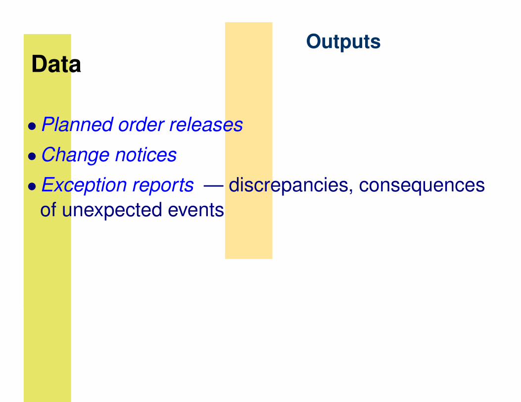
OutputsData
• Planned order releases • Change notices • Exception reports — discrepancies, consequences of unexpected events
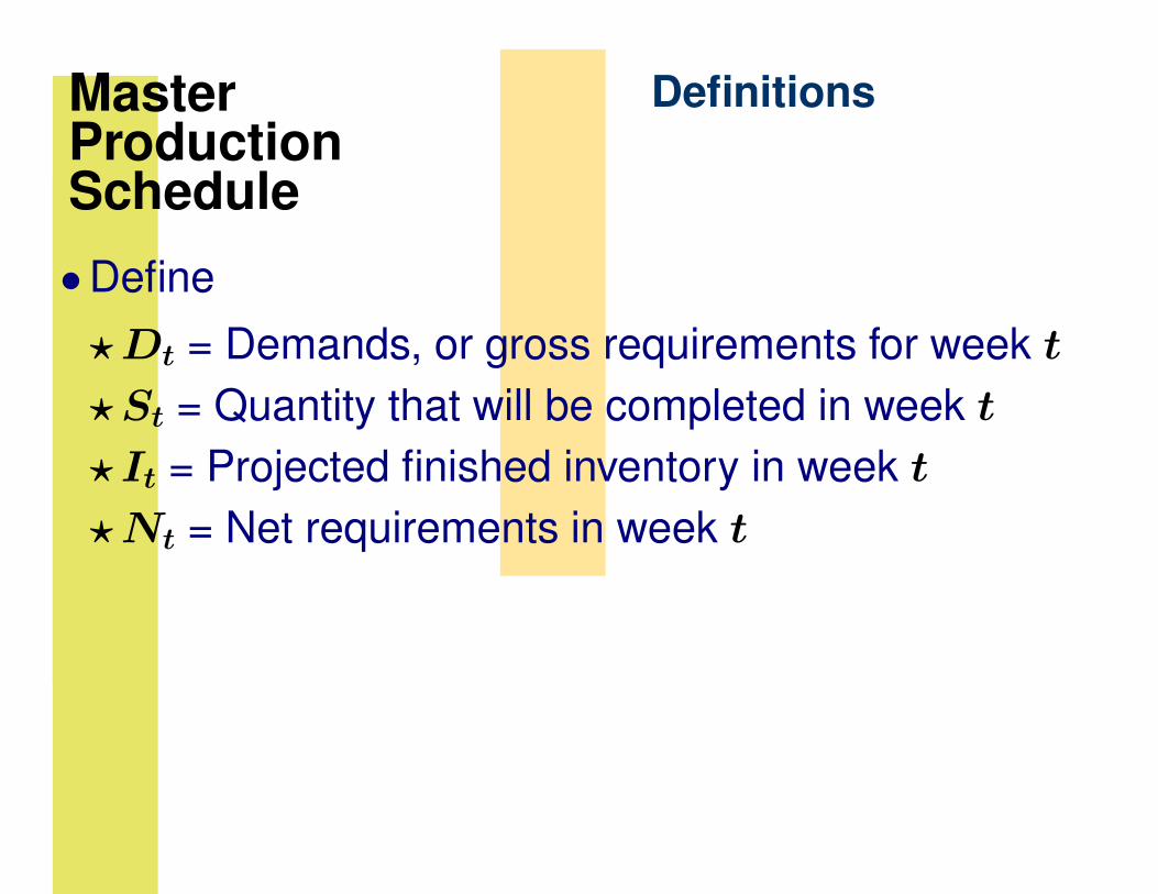
Master DefinitionsProductionSchedule• Define �Dt = Demands, or gross requirements for week t
�St = Quantity that will be completed in week t
�It = Projected finished inventory in week t
�Nt = Net requirements in week t
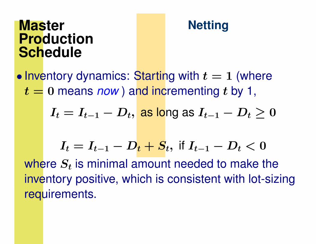
Master NettingProductionSchedule• Inventory dynamics: Starting with t = 1 (where
t = 0 means now ) and incrementing t by 1,It = It−1 − Dt, as long as It−1 − Dt � 0
It = It−1 − Dt + St, if It−1 − Dt < 0
where St is minimal amount needed to make the inventory positive, which is consistent with lot-sizing requirements.

�
Master NettingProductionSchedule• Net requirements: Let t� be the first time when It−1 − Dt < 0. Then,
�⎧ 0 if t < t�
Nt = It−1 − Dt < 0 if t = t�
⎧ � Dt if t > t�
• From net requirements, we calculate required production (scheduled receipts) St, t > t�.
• St is adjusted for new orders or new forecasts. • Then procedure is repeated for the next T �.

MasterProductionSchedule
Gross requirementsProjected on-hand 20Adjusted scheduled receiptsNet requirements
Netting
Example
Week1 2 3 4 5 6 7 815 20 50 10 30 30 30 305 5 55 45 15 -1520 100
0 0 0 0 0 15 30 30

MasterProductionSchedule
Gross requirements Projected on-hand 20 Net requirements Scheduled receipts�
Adjusted scheduled receipts * original plan
Netting
Example
Week 1 2 15 20 5 5 0 0 10 10
350550
410450100
5 6 7 8 30 30 30 30 15 -15 0 15 30 30
0 20 100
• The 10 units planned for week 1 were deferred to week 2. • The 100 units planned for week 4 were expedited to week 3.
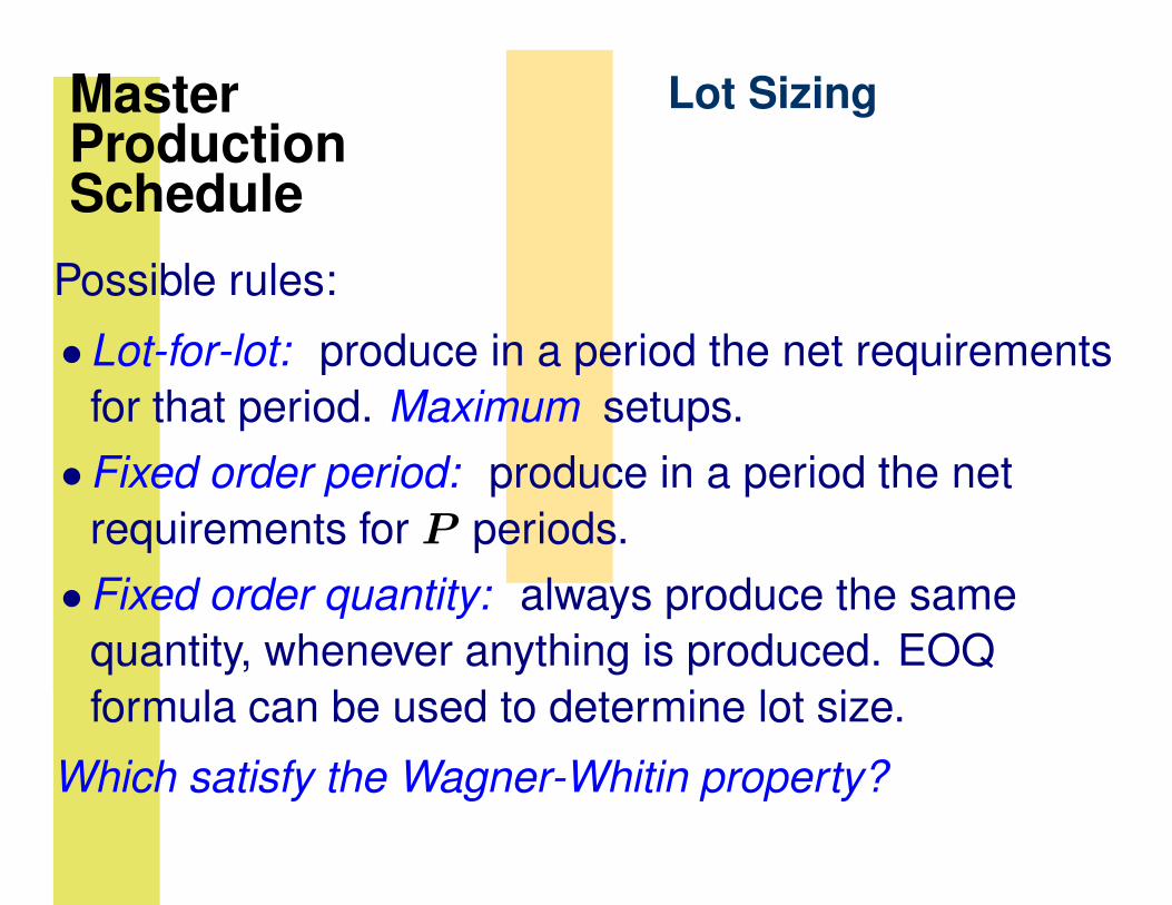
Master Lot SizingProductionSchedulePossible rules: • Lot-for-lot: produce in a period the net requirements for that period. Maximum setups.
• Fixed order period: produce in a period the net requirements for P periods.
• Fixed order quantity: always produce the same quantity, whenever anything is produced. EOQ formula can be used to determine lot size. Which satisfy the Wagner-Whitin property?
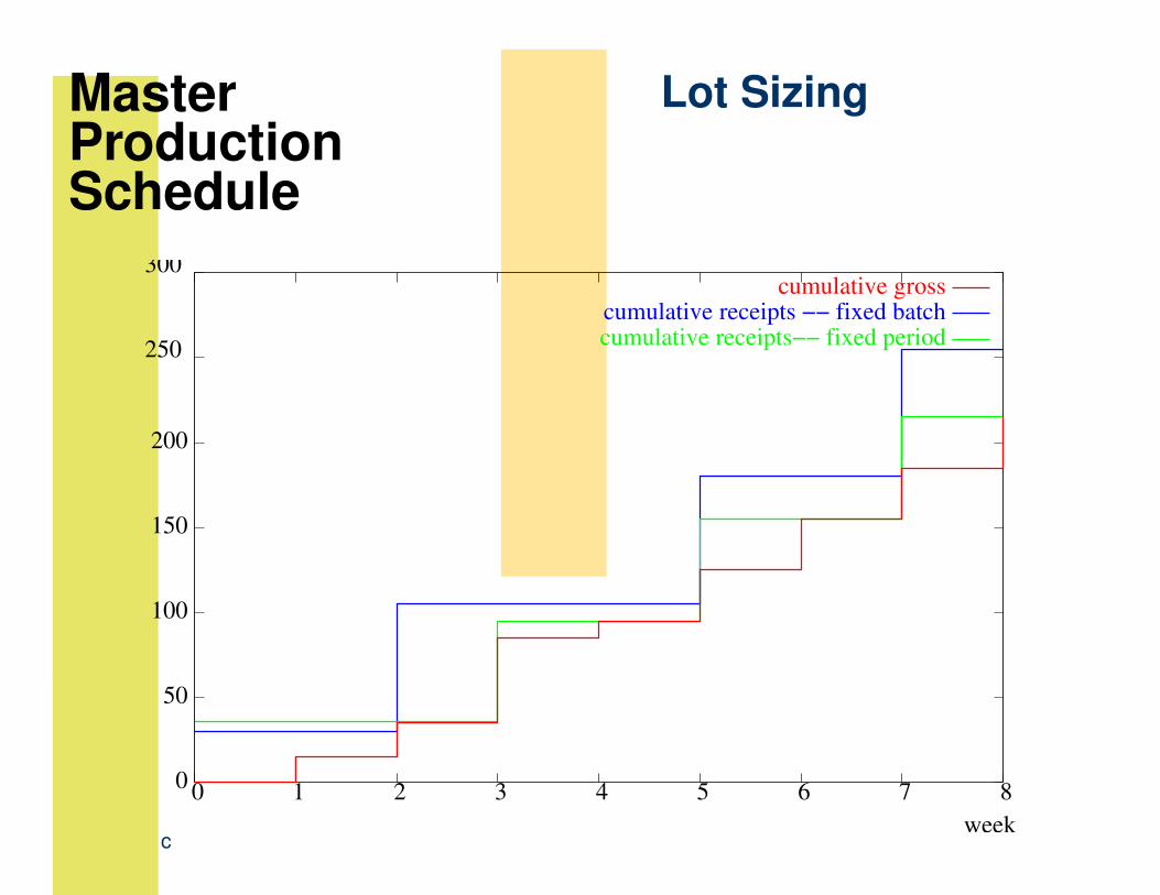
Master Lot SizingProductionSchedule
300cumulative gross
cumulative receipts −− fixed batchcumulative receipts−− fixed period250
200
150
100
50
0 0 1 2 3 4 5 6 7 8
c week

Master BOM ExplosionProductionSchedule• After scheduling production for all the top level (Level 0) items, do the same for Level 1 items.
• The planned order releases for Level 0 are the gross requirements for Level 1.
• Do the same for Level 2, 3, etc.

Uncertainty/Variability Reality
• MRP is deterministic but reality is not. Therefore, thesystem needs safety stock and safety lead times .
• Safety stock protects against quantity uncertainties.� You don’t know how much you will make, so plan to make a little extra.
• Safety lead time protects against timing uncertainties. � You don’t know exactly when you will make it, so plan to make it a little early.

Uncertainty/Variability Reality
Safety Stock
• Instead of having a minimal planned inventory of zero, the (positive) safety stock is the planned minimal inventory level.
• Whenever the actual minimal inventory differs from the safety stock, adjust planned order releases accordingly.

Uncertainty/Variability Reality
Safety Lead Time
• Add some extra time to the planned lead time.

Uncertainty/Variability Reality
Yield Loss
• Yield = expected fraction of parts started that are successfully produced.
• Actual yield is random. • If you need to end up with N items, and the yield is
y, start with N/y. • However, the actual production may differ from N , so safety stock is needed.

Other problems Reality
• Capacity is actually finite. • Planned lead times tend to be long (to compensate for variability). � Also, workers should start work on a job as soon as it is released, and relax later (usually possible because of safety lead time). Often, however, they relax first, so if a disruption occurs, the job is late.

Other problems Reality
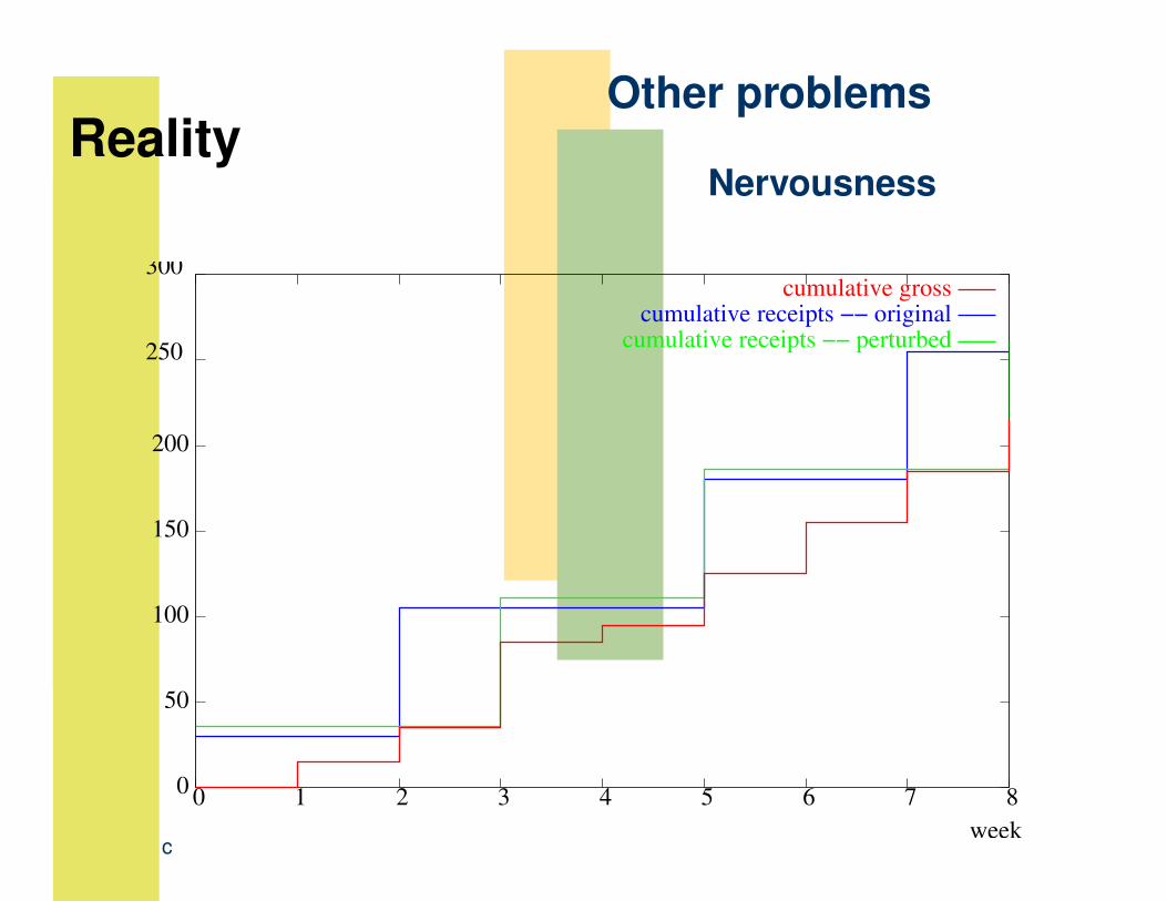
Nervousness
• Nervousness — drastic changes in schedules due to small deviations from plans — (chaos?)
• Nervousness results when a deterministic calculation is applied to a random system, and local perturbations lead to global changes.
Other problems Reality
Nervousness
300cumulative gross
cumulative receipts −− originalcumulative receipts −− perturbed250
200
150
100
50
0 0 1 2 3 4 5 6 7 8
c week
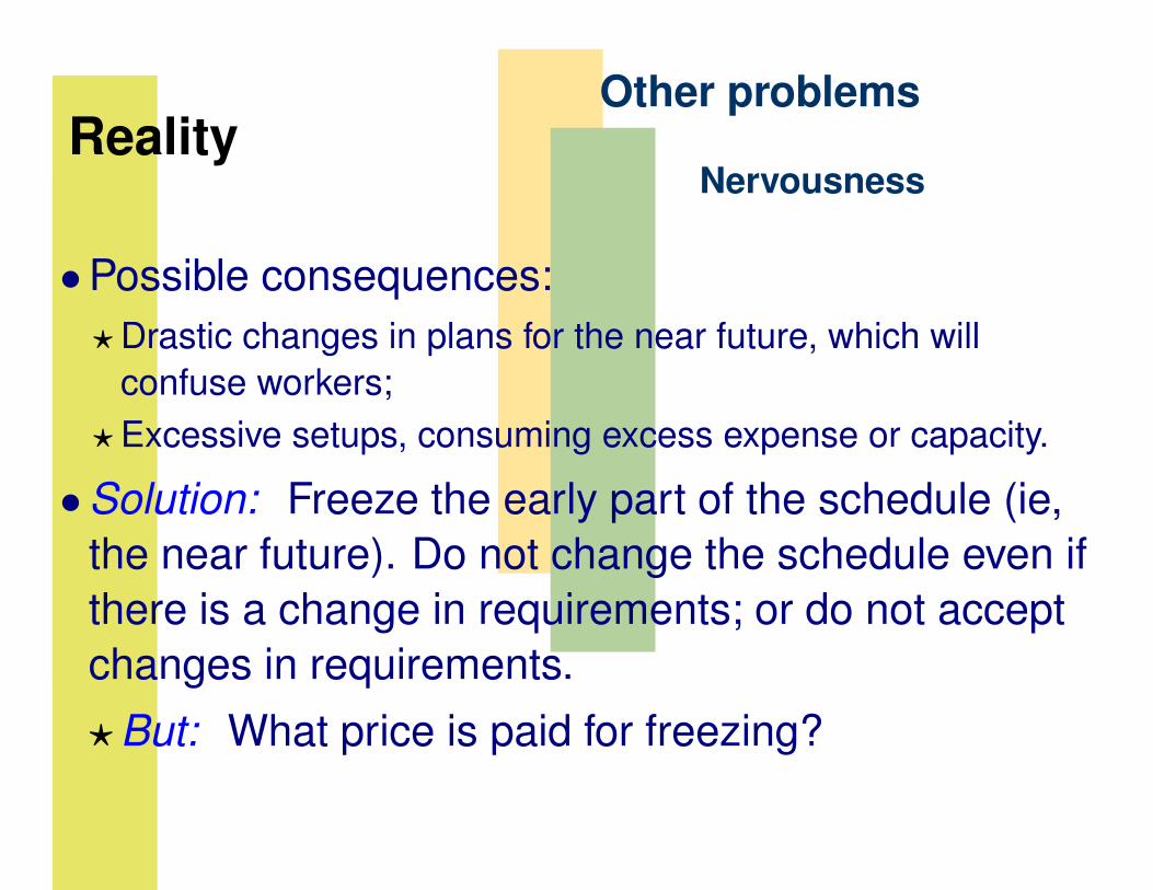
Other problems Reality
Nervousness
• Possible consequences: � Drastic changes in plans for the near future, which willconfuse workers;
� Excessive setups, consuming excess expense or capacity.• Solution: Freeze the early part of the schedule (ie, the near future). Do not change the schedule even if there is a change in requirements; or do not accept changes in requirements. � But: What price is paid for freezing?

Fundamental problem Reality • MRP is a solution to a problem whose formulation isbased on an unrealistic model, one which is � deterministic � infinite capacity
• As a result, � it frequently produces non-optimal or infeasible schedules, and
� it requires constant manual intervention to compensate for poor schedules.
• On top of that, nervousness amplifies inevitable variability.
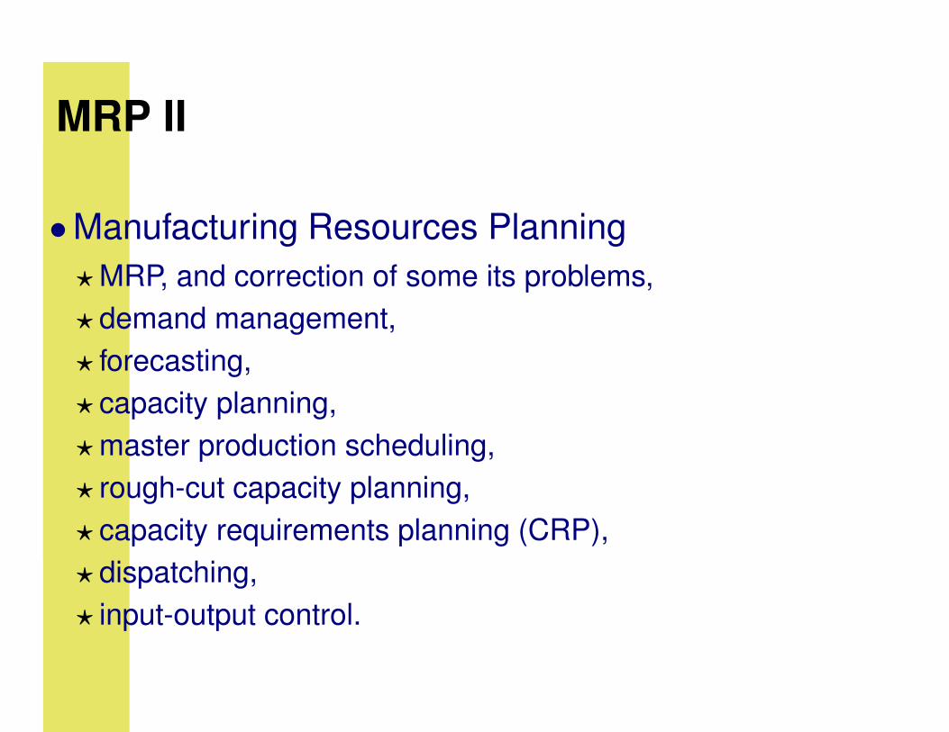
MRP II
• Manufacturing Resources Planning � MRP, and correction of some its problems, � demand management, � forecasting, � capacity planning, � master production scheduling, � rough-cut capacity planning, � capacity requirements planning (CRP), � dispatching, � input-output control.
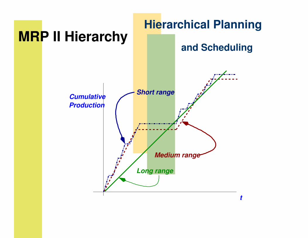
Hierarchical Planning MRP II Hierarchy
and Scheduling
Cumulative Short range
Production
Medium range
Long range
t
Hierarchical Planning MRP II Hierarchy
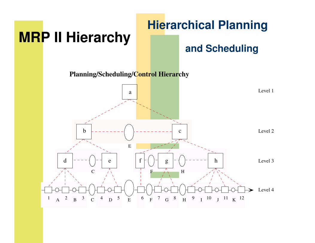
and Scheduling
Planning/Scheduling/Control Hierarchy
Level 1
Level 2
Level 3
Level 4
F G H I J KA B C D E 6 7 8 9 10 11 121 2 3 4 5
C F H
E
a
b c
d e f g h
Hierarchical Planning MRP II Hierarchy
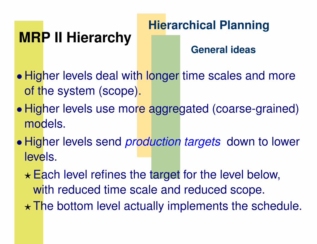
General ideas
• Higher levels deal with longer time scales and more of the system (scope).
• Higher levels use more aggregated (coarse-grained) models.
• Higher levels send production targets down to lower levels. � Each level refines the target for the level below,with reduced time scale and reduced scope.
� The bottom level actually implements the schedule.

Hierarchical Planning MRP II Hierarchy
General ideas
Production targets
Level k
Level k−1
Capacity reports
Production targets Capacity reports
Uncontrolled events Material movement commands

Hierarchical Planning MRP II Hierarchy
Long-Range Planning
• Range: six months to five years. • Recalculation frequency: 1/month to 1/year. • Detail: part family. • Forecasting • Resource planning — build a new plant? • Aggregate planning — determines rough estimates of production, staffing, etc.

Hierarchical Planning MRP II Hierarchy
Intermediate-Range Planning
• Demand management — converts long range forecast and actual orders into detailed forecast.
• Master production scheduling • Rough-cut capacity planning — capacity check for feasibility.
• CRP — better than rough cut, but still not perfect. Based on infinite capacity assumption.

Hierarchical Planning MRP II Hierarchy
Short-Term Control/Scheduling
• Daily Plan � Production target for the day
• Shop Floor Control � Job dispatching — which job to run next? � Input-output control — release � Often based on simple rules � Sometimes based on large deterministic mixed(integer and continuous variable) optimization

Hierarchical Planning MRP II Hierarchy
Issues
• The high level and low level models sometimes don’t match. � The high level aggregation is not done accurately.� Actual events make the production target obsolete.� Consequence: Targets may be infeasible or tooconservative.
• The short-term schedule may be recalculated too frequently. � Consequence: Instability.
MIT OpenCourseWarehttp://ocw.mit.edu
2.854 / 2.853 Introduction to Manufacturing SystemsFall 2010
For information about citing these materials or our Terms of Use, visit: http://ocw.mit.edu/terms.