Matching for Pseudo-Panel Inference

Jason SeawrightDepartment of Political Science,

Northwestern University

August 6, 2009

Abstract

Panel data, though highly valuable for answering questions about change over time, remaincomparatively scarce. Nonetheless, inferences about change over time remain important in avariety of social-scientific endeavors. This paper argues that an approach to pseudo-panel in-ference based on matching can help answer questions about individual-level change over timewhen the necessary panel data are absent. In comparison with a purely cross-sectional modeland two major pseudo-panel alternatives, matching performs best or nearly best when the crit-ical assumptions are met and is the least bad option when assumptions fail. This argumentis developed through Monte Carlo simulations based on two panel data sets. The empiricalvalue of pseudo-panel techniques in comparison with purely cross-sectional analysis for eval-uating hypotheses regarding change over time is illustrated with an example regarding theparty-system change in Venezuela during the 1990s that led to the election of Hugo Chavez.

1

1 Introduction

Panel data, though highly valuable for answering questions about change over time, remain

comparatively scarce. In many countries, few if any panel studies have ever been conducted;

for students of these areas, alternative means of learning about change over time must be

sought. Even in developed and widely-studied countries, there are inevitably a variety of im-

portant politically-relevant events which occur during periods when no panel surveys with

relevant questions are in process. This is certainly a problem for hypotheses regarding the

effects of rare and unpredictable categories of events: is it plausible to expect analysts to an-

ticipate the occurrence of important yet unannounced events such as the 2001 terrorist attacks

on New York and Washington, D.C., and to field the first wave of appropriate panel surveys in

advance? Slower-moving events such as party-system change often pose similar challenges,

since their character and significance often only become apparent partway through the process

or even at its conclusion.

The relative scarcity of appropriate panel data with respect to certain categories of events

poses important problems for the development of theory. For example, Green, Palmquist, and

Schickler (2002: 194) note that no panel data appear to exist that span a major episode of party-

system deterioration, a problem for analysts interested in explaining the effects of a specific

party-system change on mass beliefs and behavior, as well as for researchers engaged in testing

theoretical propositions regarding the causes and process of party-system decline and collapse.

There likewise appear to be few if any panel surveys spanning a major regime change — either

from authoritarianism toward democracy or vice versa.

In spite of these difficulties, inferences about change over time remain important in a va-

riety of social-scientific endeavors. Often, scholars approach this difficult mismatch between

theory and data resources by restricting questions to the elite level — for which quantitative

or qualitative post hoc panel data are easier to construct. In the context of explaining dramatic

episodes of party-system change in South America in recent decade, for example, Dietz and

Myers (2007) and Tanaka (1998, 2006) both focus substantially on elite politics, even though

2

voters are almost by definition central actors in most processes of party-system change. A com-

mon alternative deals with the lack of panel data while retaining a focus on mass politics by

treating purely cross-sectional analysis as if it justified inferences regarding change over time.

With respect to Venezuela’s party-system crisis, one example of this approach, considered in

greater depth below, is Morgan (2007).

Is it possible to statistically improve on the alternative of treating purely cross-sectional re-

sults as informative regarding some (often implicit) underlying panel model? Under the right

circumstances, it is possible to do better, although analyzing true panel data is always the best

alternative. This paper argues that an approach to pseudo-panel inference based on matching,

discussed at greater length below, is the best approach to answering questions about individual-

level change over time when the necessary panel data are absent. In comparison with a purely

cross-sectional model and two major pseudo-panel alternatives, matching performs best or

nearly best when the critical assumptions are met and is the least bad option when assumptions

fail. This argument is developed below in five steps. First, the general framework shared by

all pseudo-panel techniques is characterized, and the central assumptions are defined. Second,

a historically common but typically suboptimal approach, cohort averaging, is briefly consid-

ered. Third, the estimators evaluated in this paper (two-stage auxiliary instrumental variables

analysis, multiple imputation, and matching) are introduced.

In the fourth section, Monte Carlo results regarding the estimation of three effect parame-

ters are presented. For each of the three effects, which involve two different panel data sources,

the true panel estimate is calculated for each simulated sample and then each pseudo-panel es-

timate of that effect is compared with the panel gold standard. These simulations provide

evidence in favor of the argument that matching is the preferred pseudo-panel technique. The

empirical value of these techniques in comparison with purely cross-sectional analysis for

evaluating hypotheses regarding change over time is illustrated with an example regarding the

party-system change in Venezuela during the 1990s that led to the election of Hugo Chavez.

3

2 The Pseudo-Panel Setup

Suppose that two cross-sectional surveys exist for a given population, with survey 1 happening

earlier than survey 2. The surveys may have different numbers of respondents, recorded as

N1 and N2. The model of interest involves a dependent variable, Y , measured in survey

2, a set of contemporary independent variables, W, also included in survey 2, and one or

more pseudopanel variables, P, which are measured only in survey 1. Chronologically later

analogues of the P variables may be available in survey 2; often, some of these are used as the

dependent variable or as contemporary independent variables in the model. However, because

surveys 1 and 2 do not form a panel, the P variables themselves are not available for inclusion

in the model.

In general, there is no way to adequately estimate the model of interest in such a setup.

However, under the right special circumstances, a range of second-best approximations to the

true panel model may be available.1 Specifically, suppose that a collection of one or more

auxiliary variables, Z, is included in both survey 1 and survey 2. Pseudo-panel approximation

to the true panel model is a possibility if the Z variables: (1) do not all belong in the model

of interest; (2) are at least moderately predictive of the P variables, conditional on the W

variables; (3) are roughly time-invariant; and (4) meet an orthogonality condition to be char-

acterized below. When these conditions are met, then a range of techniques may be used to

construct approximations of P using the measures of the Z variables found in survey 2.

If all of the Z variables in fact belong in the model, then no progress can be made. In

such a situation, the proposed Z variables are part of W and therefore provide no unused

materials from which a pseudo-panel inference might be constructed. This exclusion restriction

parallels that for instrumental variables techniques and raises similar concerns for directly

causal interpretations of the resulting parameter estimates.

The second condition is perhaps self-evident. If the auxiliary variables are to be used to

1In pseudo-panel situations, estimation of a model with panel refinements such as fixed or random effects, covari-ance structures in the error term, and so forth (e.g., Wooldridge 2000) can rarely succeed. The discussion below setssuch refinements aside. Less sophisticated analysis may nonetheless help answer some important questions when thepseudo-panel assumptions discussed below are met.

4

construct approximations of the pseudo-panel variables, it must be the case that the auxiliary

variables contain some predictive information about P beyond what is present in W. Other-

wise, any approximation constructed from Z either will fall within the column space of W

and therefore create problems when the model of interest is estimated, or will be independent

of P and therefore uninformative about the relationships of interest. Note that this condition

does not require a causal relationship between the auxiliary variables and the pseudo-panel

variables; a purely statistical relationship suffices, and indeed there is no special advantage to

be had if the relationship is in fact causal. This highlights an important difference between

the necessary properties of auxiliary variables for pseudo-panel inference and many common

interpretations of the conditions for successful causal inference using instrumental variables.

Useful auxiliary variables must be reasonably time-invariant, as condition three suggests,

because otherwise the approximation constructed from them may represent an estimate of an

analogue to P measured at time 2, rather than an estimate of the genuine P variables from time

1. Because the auxiliary variables are assumed not to change over time, then the relationship

between P and Z measured in the first survey must be identical to the relationship between

P (which are still at time 1) and Z measured in the second survey. This identity justifies

the various kinds of imputation into survey 2 that characterize the pseudo-panel techniques

discussed below.

Finally, an orthogonality condition must be met. Let Proj(A,B) represent the projection

of A onto the column space of B. Successful pseudo-panel inference requires:

P− Proj(P,Z) ⊥W (1)

If this condition is met, then the (inevitably) omitted variance of the pseudo-panel variables

will cause the fewest possible distortions in the coefficient estimates for the contemporary in-

dependent variables. Indeed, because the omitted portion of the pseudo-panel variables will

generally be orthogonal to the included portion (by construction) and also to the contemporary

independent variables (by condition 1), for OLS regression models this condition in conjunc-

5

tion with the others mentioned allows for unbiased and consistent estimation of the model

(see, e.g., Franklin 1990). For less linear models, no unbiasedness or consistency results can

generally be obtained when any relevant variable is omitted. However, even for these models,

condition 1 often serves to minimize trouble regarding omitted variable bias.

For example, coefficients in discrete-choice models are implicitly normalized by the unex-

plained variation in order to identify the model (see Yatchew and Griliches 1985, Wooldridge

2002: 470-72 regarding probit models, as well as Cramer 2005 for the parallel argument re-

garding logit models). Thus, there is bias in pseudo-panel applications for which the model

of interest is one of the standard discrete-choice families because the omitted variance in the

pseudo-panel variables inflates the normalization factor of the models. Yet the bias will in-

volve a constant proportional attenuation of each coefficient and will not change the relative

magnitude of each variable’s estimated effect on the probability of the outcome.2 While the

coefficient estimates will not be consistent, ratios of coefficient estimates are consistent and

hence comparisons of coefficient magnitudes within a single model are viable. However, coef-

ficients from models estimated using different samples are not directly comparable. In general,

pseudo-panel inference cannot always eliminate bias, but it can often reduce the magnitude and

substantive importance of the bias.

When auxiliary variables exist that meet the four criteria discussed above, then pseudo-

panel inference is possible. A variety of competing implementations build from these basic

principles in somewhat divergent ways, as will be described below. First, however, a brief

comment is in order on a set of quite different econometric techniques for pseudo-panel infer-

ence.2Correcting for the attenuation induced by pseudo-panel is possible. The coefficient for the omitted component of

variation is, by assumption, equal to the coefficient for the included estimate of the lagged variable, and the variance ofthe omitted portion can be estimated from the first-stage equation at the earlier point in time. No other unknowns areincluded in the formula for the attenuation. However, since the attenuation is uniform across variables, the correctionwill simply increase the size of all coefficients by the same amount. Furthermore, the correction would introduceanother source of uncertainty into the resulting coefficients. Hence, correction is probably not worthwhile for mostapplications.

6

3 Cohort Averaging

For some models, pseudo-panel inference can be achieved by averaging data on individuals to

generate estimated data on what are referred to as “cohort” means (Deaton 1985), i.e., means

among individuals who share the same scores on the auxiliary variables. For example, suppose

the model of interest is of the family:

Yt,i = βPt−1,i + γWt,i + εt,i (2)

Here, as before, problems arise because the model requires measures of Pt−1,i which are

not available in the data, although the data do include measures of Pt,i and of the matrix

of covariates Wt,i. Suppose that there are K different observed combinations of values on

the auxiliary variables, Z, and that at least one respondent is observed with each of these

combinations in each cross-sectional survey. Form Pt,k by averaging across all observations

of Pt,i for individuals with the kth combination of values on the Z variables. Yt,k and Wt,k

can be formed analogously. Because groups formed by equivalent combinations of values on

the auxiliary variables are present in each cross-section, then for t ≥ 2 an estimate of Pt−1,k is

now available: it can simply be copied over from the previous survey wave.

How can these cohort averages be related to the model in Equation 2? If we take expecta-

tions, within cohort groups, of both sides of the equation, we get:

Ecohort(Yt,i) = Ecohort(βPt−1,i + γWt,i + εt,i)

= βEcohort(Pt−1,i) + γEcohort(Wt,i) + Ecohort(εt,i) (3)

The sample cohort means Yt,k, Pt−1,k, and Wt,k are estimates of the population group

expectations in Equation 3. Hence, it seems reasonable to substitute the sample cohort means

in for the cohort expectations as a way of estimating the parameters in Equation 3 using sample

data. Because the original model, in Equation 2 is linear in parameters, the parameters in the

7

cohort-averaged model given in Equation 3 are the same as the parameters in the individual

model. Thus, something may potentially be learned about the individual-level relationships

using a panel of cohort-averaged data.

Aside from the restriction to models which are linear in the parameters, two additional chal-

lenges may potentially limit the range of applicability of the cohort-averaging approach. First,

sample cohort averages diverge from population cohort averages due to sampling error. Hence,

an errors-in-variables model is needed to produce credible parameter estimates. This problem

is somewhat less intimidating than it may be in other errors-in-variables situations, since the

distinctive errors in question are due to sampling rather than poorly understood measurement

effects. Sample standard deviations and a normality assumption provide raw materials for one

possible set of estimates of the desired parameters net the results of error in estimated cohort

averages. Deaton (1985) works through the details of theory and estimation, while Angrist

(1991) develops a two-stage least squares interpretation of Wald estimators for grouped data

that include Deaton’s model as a special case. Verbeek and Nijman (1992) argue that, for at

least some model specifications, the errors-in-variables aspect of the cohort-averaged model

can be fairly safely disregarded if each cohort has at least 100 to 200 members in each cross

section. By contrast, Devereaux (2007) uses Monte Carlo experiments to suggest that the

bias due to sampling error in the cohort means can be substantial even for samples of tens of

thousands and an errors-in-variables model is indeed needed.

A second challenge to the applicability of the cohort-averaging approach to the pseudo-

panel problem is less easy to address. After replacing individuals with cohorts as the cases of

interest, analysts will typically have relatively few effective data points in a given survey; K

is necessarily much smaller than N . Hence, parameter estimates resulting from this approach

will only be useful if there are many sequential cross-section surveys available, resulting in

a cohort panel that is substantially time-dominated. In situations for which only a handful of

cross-sections are available, the cohort-averaged model may in fact be unidentified, but even if

identified will certainly suffer from low statistical power.

8

4 Individual-Level Solutions

In addition to the sometimes useful but often limited cohort-averaging approach to pseudo-

panel inference, a variety of solutions are available which make use of data at the individual,

rather than the cohort, level. Of these approaches, three will be considered here: two-stage

auxiliary instrumental variables, multiple imputation, and pseudo-panel matching. Most other

existing individual-level pseudo-panel techniques are essentially variants of the first two ap-

proaches considered here. Pseudo-panel matching is an idea that has occasionally been men-

tioned, and is related to matching approaches to the more general problem of missing data

(Little and Rubin 2002), but matching in a pseudo-panel context has not previously been dis-

cussed at length or compared with alternative estimators.

These techniques share important features. Each uses some transformation f() on the aux-

iliary variables Z to calculate f(Z), which then serves as a stand-in for P in estimating the final

model. Hence, the omitted variables P are replaced by the (hopefully smaller in magnitude

and less statistically problematic) omitted variables P− f(Z). This process of approximation

might seem to raise errors-in-variables issues for estimation of coefficients associated with

f(Z). Such is the case if one or more of the pseudo-panel conditions does not apply to the

research situation in question. However, when the conditions are met, the framework becomes

more similar to that of instrumental variables; if the same coefficient applies for different com-

ponents of the variance in P, then no special problems arise.

Often, discussion of these methods has assumed that pseudo-panel variables enter linearly

into OLS regression models. However, analysts may face circumstances in which pseudo-

panel inference may be necessary for less linear models, including GLMs or models with

interaction terms involving the pseudo-panel variables. Interaction terms involving the pseudo-

panel variables in principle raise no new issues; if the correct conditions are met, then inference

can succeed. In practice, as will be seen below, pseudo-panel inference for such models may

be quite inefficient and suffer from substantial small-sample bias, even for estimators that

work well in the linear context. Even with more challenging models involving interactions,

9

however, some techniques still offer improvements over purely cross-sectional models when

assumptions are met. For GLMs and other nonlinear models, as discussed earlier, pseudo-

panel inference will result in estimates that are inconsistent, but typically in less problematic

ways than when the pseudo-panel variables are simply disregarded.

4.1 Two-Stage Auxiliary Instrumental Variables

An ingenious and frequently-discussed individual-level approach to the pseudo-panel problem

is two-stage auxiliary instrumental variables, or 2SAIV (Franklin 1989). The analyst uses the

survey data from the first time period to develop and estimate a statistical model of each of the

pseudo-panel variables as a function of the time-invariant variables. For example, assuming

for simplicity’s sake that there is a single pseudo-panel variable, then the first-stage model will

typically be of the form:

E(Pi) = f(Z1,i) (4)

This model need not be causal, nor indeed need it be fully-specified in the usual sense. This

is so because estimates of f(·) will be used to classify cases in future cross-sections on the ba-

sis of their most likely score of Pi given the time-invariant variables; counterfactual causal

interpretations or statistical claims about consistent estimation of parameters that exist outside

the context of the immediate estimation problem are irrelevant. The interpretation is clearest

when Z consists of a collection of dichotomous variables, and f(·) is a linear regression-type

expression which includes all orders of interactions among the Z variables. In this instance,

E(Pi) is just the population average score of the pseudo-panel variable among all individ-

uals with a given collection of scores on the auxiliary variables — i.e., using the language

introduced above, E(Pi) is just the cohort mean for the cohort to which individual i belongs.

Estimation then consists of computing the sample average of P for members of that cohort.

More generally, in some appropriate parametric or nonparametric way, the scholar esti-

mates f(·). Very often, for the sake of simplicity and efficiency, OLS regression is used in

10

this first stage of analysis. Using the results from the estimation, regardless of the specifics of

implementation, fitted values P are formed as follows:

Pi = f(Z2,i) (5)

These fitted values are then treated as if they were a measure of the relevant variable from

the time of the first cross-section. For the relatively simple case of dichotomous Z variables

and full interactions, this amounts to imputing the estimated cohort mean to each member

of the cohort; for more complex models, the interpretation involves some generalization or

specialization of this pattern. Note that the function f(·) is assumed to apply in the same way

to respondents in the cross sections at time 2 and at time 1. Substantively, this assumption

requires that respondents to the second survey answer the survey questions that produce the Z

variables in the same way that they would have answered those questions at the time the earlier

data set was constructed. That is, this is a restatement of the condition of temporal stability

discussed as a prerequisite for pseudo-panel inference above.

The resulting values for Pi are functions of Z2,i, which is fixed, and f(·), which is a con-

sistent estimate of an underlying descriptive relationship that we assume to be stable. Hence,

we may conclude that the Pi’s are consistent estimates of the most likely values for Pi given

the underlying stable cohort relationships that exist in the data. As a consequence, standard

results regarding bias due to random measurement error do not apply; the randomness in the

Pi’s gradually disappears as the sample size increases.

If estimates of f(·) converge to a fixed function as the number of first-cross-section cases

goes to infinity, then the asymptotic consequence of approximating the unavailable Pi with the

estimated f(Z2,i) as an independent variable in some statistical analysis is the introduction of

an omitted variable that is orthogonal by construction to the included variable f(Z2,i). That is,

the desired statistical analysis can be conducted if Pi−f(Z2,i) is treated as an omitted variable.

As such, as discussed in the section on general prerequisites for pseudo-panel inference, it will

be extremely important that this omitted variable be orthogonal to any independent variables

11

included in the statistical analysis. This assumption cannot be directly verified, although it can

be checked whether the equivalent of this omitted variable for time 1 is orthogonal to period

equivalents of the contemporary independent variables.

In finite samples, of course, sampling error is also a concern, and the extra resulting uncer-

tainty in the final analysis due to using model estimates to generate the missing variable in the

second cross-section may be incorporated through bootstrapping.

A first major concern regarding 2SAIV is that, since it deterministically imputes estimates

of the pseudo-panel variables, it is highly likely to produce versions of those variables that have

too little variance. In effect, the harder-to-predict components of the variables will simply be

dropped, shrinking the imputed estimates to the estimated mean for cases with similar scores on

the auxiliary variables. By thus shrinking the variance of the pseudo-panel variables, 2SAIV

may produce distortions in coefficient estimates in the model of interest — especially when

that model is nonlinear and estimated via maximum-likelihood methods. A second potential

source of trouble is that, in practice, 2SAIV most often relies on a parametric analysis of

the relationships between the auxiliary and the pseudo-panel variables. If these relationships

involve important unmodeled interactions or other forms of nonlinearities, then 2SAIV may

lose important information. Third and last is the concern that 2SAIV may create problems of

multicollinearity when more than one pseudo-panel variable is of interest. Each variable will

generally be estimated by a weighted sum of the same auxiliary variables; unless each pseudo-

panel variable turns out to have an associated auxiliary variable that is a useful predictor of

it but not of the other pseudo-panel variables, serious problems of multicollinearity become

likely.

4.2 Multiple Imputation for Pseudo-Panel Inference

Gelman, King, and Liu (1998) offer a related approach to solving the pseudo-panel problem,

developing a Bayesian hierarchical multiple imputation model that uses information about in-

dividuals and surveys in order to generate several plausible sets of values for desired variables

12

omitted from a given survey, at the same time generating sets of plausible values for indi-

vidual missing responses on questions that were indeed asked in each of the surveys under

consideration. Three aspects of this technique are novel in comparison with 2SAIV: the use

of multiple imputation to capture uncertainty and produce estimated versions of the pseudo-

panel variables with more appropriate variances, the ability to simultaneously address partial or

complete missingness in multiple variables, and the use of a hierarchical model for imputation.

For a hierarchical model, each response to each analyzed question in each survey cross-

section is modeled as having a probability distribution whose form is a function of the Z

variables, as well as any relevant variables measured at the level of the survey (such as time

of fieldwork, survey firm, and so forth). After the parameters linking the Z variables and

any variables at the survey level to the shape of each response’s probability distribution are

estimated, a fitted distribution can be associated with each missing survey response. Multiple

imputation then involves taking several draws from that fitted distribution and conducting the

desired analysis for each draw.

When working with hierarchical models, researchers need to pay attention to degrees of

freedom at multiple levels of analysis. In this context, the number of respondents per survey

matters, but the number of surveys matters as well for reasoning about the amount of lever-

age available for estimating parameters connected with variables at the survey level. If, for

example, there are only two relevant surveys available and one omits a question entirely (the

prototypical situation for pseudo-panel inference), there are effectively no degrees of freedom

for components of the model at the level of the survey, and the hierarchical analysis derives

all of its information from the individuals in the single survey that includes the question of

interest. Hence, for a small number of surveys, and especially for only two cross-sections, the

Bayesian hierarchical multiple imputation model is more or less similar to 2SAIV’s first-stage

model. The details of the model and of estimation can obviously differ, and the hierarchical

approach becomes substantially different as the number of surveys increases, but for many

pseudo-panel applications the two methods involve a fundamentally similar analytic approach

to information from the first survey wave and a similar use of the auxiliary variables. Given

13

the problems of hierarchical modeling in contexts with only two surveys, and in order to focus

as directly as possible on the aspects of this approach that are distinctively about pseudo-panel

inference, the discussion below will replace Gelman et al.’s Bayesian hierarchical approach

to generating probability distributions for the missing pseudo-panel variables with the sim-

pler one-level linear modeling of 2SAIV. This decision is intended to take no sides in debates

regarding Bayesian vis-a-vis frequentist statistics, or regarding the relative desirability of hi-

erarchical modeling in general; instead, the point is simply that these are broader debates that

provide relatively little insight into the specific problem of optimizing pseudo-panel inference.

Gelman et al.’s model also differs from 2SAIV in its simultaneous attention to missing data

in variables that are present in every wave of the survey and to the missing data represented by

the pseudo-panel variables. There is certainly much to be said in favor of principled approaches

to missing data, both in panel contexts and more generally. However, the selection of one or

another approach to missing data in the contemporary independent variables for a pseudo-

panel inference is a problem that, once again, is logically separate from the question of how

to optimize the specifically pseudo-panel aspects of inference. Hence, once more, for the sake

of comparability all techniques considered below will simply omit cases with missing data on

relevant variables.

These simplifications for the sake of comparability highlight one major difference between

Gelman et al.’s approach to pseudo-panel inference and that of Franklin: this second technique

multiply imputes the pseudo-panel variables rather than deterministically imputing the mean

of the distribution for each case to each variable. Because multiple imputation generates a vari-

able with a more appropriate variance, one of the three concerns regarding 2SAIV discussed in

the previous section is resolved. However, pseudo-panel multiple imputation retains the other

two potentially problematic features: it is parametric in its analysis of the relation between the

auxiliary and pseudo-panel variables, and it is prone to generating multicollinearity when more

than one pseudo-panel variable is employed.

14

4.3 Matching for Pseudo-Panel Inference

The two individual-level approaches to the pseudo-panel problem just discussed share an odd

feature: none of them ever involves any direct connection between responses in the first and

second surveys. Conceptually, forming such a connection is obviously a goal of pseudo-panel

inference. Yet the 2SAIV and multiple imputation approaches produce a final model that

involves only comparisons among responses given by different respondents in the second sur-

vey, rather than connections between responses given during the first and second surveys. In

these approaches, all comparisons over time are mediated through the parametric model of

the whole-sample relationship between the auxiliary and pseudo-panel variables. There would

be intuitive appeal to a technique that permitted somewhat more direct over-time connections

between individual responses.

Matching techniques (Rubin 2006; Rosenbaum 2002) provide a useful approach to con-

necting individual responses across survey waves in pseudo-panel scenarios. Generally dis-

cussed in the context of causal inference, matching methods solve the problem of devising

case-by-case connections between two samples in such a way that the matched cases are as

close to each other as possible on a set of matching variables. For causal inference purposes,

these matching variables are typically hypothesized confounders, and the purpose of matching

is to eliminate their influence from a final estimate of the causal effect of interest. Turning

to pseudo-panel inference, a fairly straightforward application of matching may be used to

connect cases in the two surveys. The auxiliary variables should be used as the matching vari-

ables. After matches are established, the mean value of the pseudo-panel variables among the

relevant matched cases in the first survey should be imputed to each case in the second survey.

Under ideal, and quite unrealistic, circumstances, some analytic results can be provided

regarding this approach; these results are provided only in informal sketch, as they fundamen-

tally do not apply to most actual pseudo-panel analysis.3 Suppose, as in the discussion of

3Alternative proofs can also be developed, generally requiring either unrealistic conditions regarding the data orpoint-blank assertions that, for a given situation, matching suffices to produce consistent estimates of the pseudo-panelvariables. The proof sketched in the text is thus provided not as the only possibility, but rather as illustrative of theproblems with relying on analytic, as opposed to Monte Carlo, results for reasoning about the real-world properties of

15

cohort averaging above, that the data form only some finite number K of different possible

combinations of values on the auxiliary variables Z. Let N1 represent the number of cases

in the first sample, and N2 the number of cases in the second sample. Assume that cases in

the first sample are randomly sampled from a population such that each new case has a fixed

positive probability of belonging to each of the K combinations of values on the auxiliary

variables. Now, let the ratio of N1 to N2 go to infinity. Given these conditions, there will be

infinitely many perfect matches from the first survey for each case in the second survey. Fur-

thermore, the mean of those matched cases on the P variables will be identically equal to the

mean of P at the time of the first survey for the subpopulation of cases with that combination

of scores on Z. Because the relevant case from the second survey also belongs to that subpop-

ulation, it is clear that the sample mean of P for the matched first-wave cases is equal to the

subpopulation mean of P at the time of the first survey for the second-survey case in question.

If we further assume that the difference between any case’s specific value of P and that case’s

subpopulation mean is statistically unrelated to the contemporary independent variables and to

the error term in the statistical model of interest, then substituting the subpopulation mean for

the case’s specific value of P will result in reasonable estimation of the model (i.e., consistency

for OLS regression as N2 goes to infinity, manageable patterns of inconsistency for logit and

probit models, and so forth).

These results are unhelpful in practice primarily because, in most pseudo-panel applica-

tions, the ratio of N1 to N2 is approximately 1. As a consequence of this, it is difficult to

discuss the theoretical properties of applied matching approaches to pseudo-panel inference;

they may or may not be favorable relative to the available alternatives. However, compared

with 2SAIV and multiple imputation, matching would seem to have two important advan-

tages. First, matching need not result in multicollinearity when multiple pseudo-panel vari-

ables are of interest. The matching estimate of the P variables is not a linear function of the

Z variables, but rather an average of first-wave measures of P as grouped by Z. To the extent

that the P variables themselves are not highly collinear, their grouped averages are not no-

pseudo-panel matching.

16

tably likely to suffer from multicollinearity. Second, matching in effect uses a semiparametric

approach to the relationship between the auxiliary variables and the pseudo-panel variables

(Heckman, Ichimura, and Todd 1998), so the potential drawbacks of parametric approaches do

not fully apply. Furthermore, when pairwise matching is used — such that each case at time

2 is matched to only one case at time 1 — the variance of the imputed pseudo-panel variable

will be basically correct without resorting to multiple imputation.

Bootstrapping (Efron and Tibshirani 1994; Davison and Hinkley 1997) can generate use-

ful estimates of the standard errors for 2SAIV and multiple imputation, but not for matching

approaches to pseudo-panel inference. The problem is that matching is such a non-smooth

transformation of the data that bootstrap methods are inconsistent, and hence estimated stan-

dard errors may be too small or too large (Abadie and Imbens 2006). Fortunately, an alterna-

tive, consistent simulation method is available for estimating standard errors and confidence

intervals and for conducting hypothesis tests: subsampling (Politis, Romano, and Wolf 1999).

Subsampling is similar to bootstrapping, with a few key differences. In bootstrapping, simu-

lated samples are drawn at random from the data with replacement to generate a new random

sample of the same size as the original sample. By contrast, in subsampling, simulated sam-

ples are drawn at random from the data without replacement to generate a new random sample

which is substantially smaller than the original sample. Subsampling thus involves the gen-

eration of repeated samples from the original population distribution, whereas bootstrapping

generates repeated samples from the sample distribution. This difference substantially weakens

the consistency requirements for subsampling, making this approach a useful way to estimate

uncertainty for matching estimators. The discrepancy between standard errors for the original

sample size and the smaller sample size for the simulated data sets vanishes asymptotically, of

course. However, in finite samples, a correction can be applied by dividing estimated variances

by a finite-sample correction factor: the ratio of the convergence rate term for the true sample

size to the same term for the subsample size. With these technical details in hand, matching

methods for pseudo-panel inference become entirely plausible in application.

17

5 Relative Strengths and Weaknesses of Pseudo-Panel

Techniques

While the preceding discussion has raised some potential strengths and weaknesses of various

pseudo-panel techniques, their relative finite-sample merits remain a broadly open question.

This section develops guidance regarding the relative usefulness of each approach based on a

series of Monte Carlo studies constructed around two real-world panel data sources. The anal-

ysis suggests that the matching and multiple imputation approaches to pseudo-panel inference

both represent improvements over the baseline alternative of ignoring the pseudo-panel struc-

ture of the data. Indeed, matching and multiple imputation have generally similar properties

in these studies, with the exception that multiple imputation can break down somewhat less

gracefully than matching when the orthogonality assumption is violated.

Two panel data sets are used as the basis for the Monte Carlo analysis presented below. The

first is the 2000 Mexico National Election Study, a four-wave panel survey covering the year

of the first election in Mexican history in which an opposition party won the presidency. The

second is the 1990-1991-1992 panel study from the American National Election Studies, which

covers the second half of the George Herbert Walker Bush presidency as well as the campaign

during which H. Ross Perot was one of the most successful third-party presidential candidates

in recent American history. For each data set, a simple panel model of party identification

is estimated, as well as pseudo-panel approximations of that model. Monte Carlo analysis

proceeds by generating samples of various sizes from the data with replacement. For each

iteration, one sample is drawn for time 2 (and also used for the true panel model), and a second

separate sample is drawn for time 1.

For each iteration of the simulation, five estimates are produced: one using the true panel

model, which is used as the criterion against which all others are compared; another based on

the purely cross-sectional model that can be estimated by omitting all over-time components of

the specification and generally ignoring the pseudo-panel structure of the data; a third relying

18

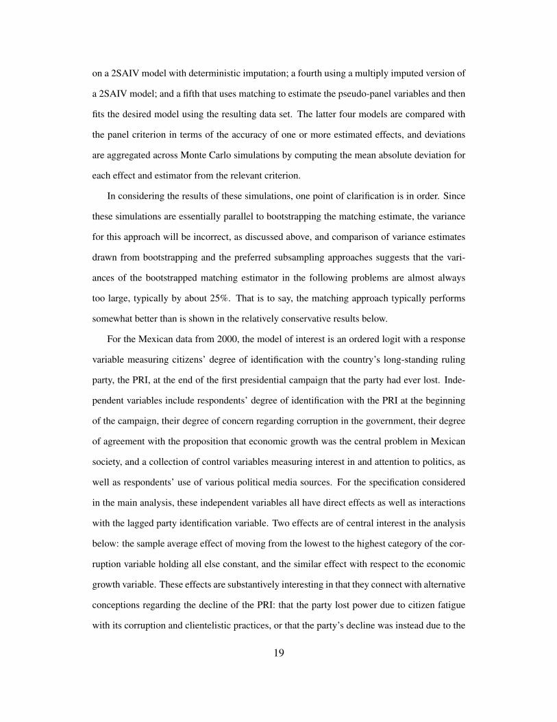
on a 2SAIV model with deterministic imputation; a fourth using a multiply imputed version of

a 2SAIV model; and a fifth that uses matching to estimate the pseudo-panel variables and then

fits the desired model using the resulting data set. The latter four models are compared with

the panel criterion in terms of the accuracy of one or more estimated effects, and deviations

are aggregated across Monte Carlo simulations by computing the mean absolute deviation for

each effect and estimator from the relevant criterion.

In considering the results of these simulations, one point of clarification is in order. Since

these simulations are essentially parallel to bootstrapping the matching estimate, the variance

for this approach will be incorrect, as discussed above, and comparison of variance estimates

drawn from bootstrapping and the preferred subsampling approaches suggests that the vari-

ances of the bootstrapped matching estimator in the following problems are almost always

too large, typically by about 25%. That is to say, the matching approach typically performs

somewhat better than is shown in the relatively conservative results below.

For the Mexican data from 2000, the model of interest is an ordered logit with a response

variable measuring citizens’ degree of identification with the country’s long-standing ruling

party, the PRI, at the end of the first presidential campaign that the party had ever lost. Inde-

pendent variables include respondents’ degree of identification with the PRI at the beginning

of the campaign, their degree of concern regarding corruption in the government, their degree

of agreement with the proposition that economic growth was the central problem in Mexican

society, and a collection of control variables measuring interest in and attention to politics, as

well as respondents’ use of various political media sources. For the specification considered

in the main analysis, these independent variables all have direct effects as well as interactions

with the lagged party identification variable. Two effects are of central interest in the analysis

below: the sample average effect of moving from the lowest to the highest category of the cor-

ruption variable holding all else constant, and the similar effect with respect to the economic

growth variable. These effects are substantively interesting in that they connect with alternative

conceptions regarding the decline of the PRI: that the party lost power due to citizen fatigue

with its corruption and clientelistic practices, or that the party’s decline was instead due to the

19

emergence of the PAN as a credible alternative in terms of economic management.4.

The corruption effect is substantially easier to estimate than the economics effect through

pseudo-panel approximation given the set of auxiliary variables in this survey, both because

the specification for the economics effect clearly and substantially violates the key orthogo-

nality assumption for pseudo-panel inference and also because of the relative variances of the

two variables. The formula given in 5 provides a useful measure of the degree to which linear

relationships between the pseudopanel variables and a contemporaneous variable of interest

violate the orthogonality assumption. For the Mexico data, both correlations are by normal

standards quite small: 0.01 for the corruption variable and 0.12 for the economics variable.

Yet the effects of interest are themselves reasonably small (-0.03 for corruption and -0.05 for

economics), so even relatively small violations of the orthogonality assumption can prove sub-

stantively important — and the difference between the corruption and economics correlations

will prove to be quite consequential.

cor(P− E(P|Z),Wk − E(Wk|W−k)) (6)

A related issue that also makes the economic growth effect more challenging to estimate

through pseudo-panel inference is that the variance of the economic growth variable is substan-

tially smaller than that for the corruption variable: 0.14 as compared with 0.25. The smaller

variance makes the pseudo-panel estimation challenge comparatively harder, in that an equiv-

alent amount of unexplained variance would wipe out a great deal more of the variance of the

growth variable than of the corruption variable. For these reasons, the corruption effect might

be regarded as a realistic but relatively easy test case for pseudo-panel inference, while the

growth effect can be seen as a substantially more difficult test.

Figure 1 shows the results regarding the estimation of the corruption effect for a collection

of Monte Carlo studies for which the sample size of the Mexican data is set to values from 500

4For more discussion of the election in question, as well as its historical and regime-transformational context, seeDominguez and Lawson (2004)

20

500 1000 1500 2000

0.00

50.

010

0.01

50.

020

0.02

5

Sample Size

Ave

rage

Div

erge

nce

from

Crit

erio

n

Ignore Pseudo−PanelMatchingMultiple Imputation2SAIV

Figure 1: Relative Performance of Pseudo-Panel Estimators for the Corruption Effect

21

to 2000. For smaller samples, it appears that pseudo-panel inference is a difficult and perhaps

even hopeless endeavor: in these studies, 2SAIV is clearly worse than disregarding the pseudo-

panel structure of the data, and matching is at best a small improvement. Multiple imputation

provides significant gains over estimating a purely cross-sectional model, although as will

be seen below, these gains are highly sensitive to even small violations of the orthogonality

assumption or to misspecification of the first-wave model.

Starting with sample sizes of about 1000, matching and multiple imputation become in-

creasingly similar, converging to a roughly 20% improvement over ignoring the pseudo-panel

structure. For sample sizes of 2000 or larger, bias largely disappears from the matching esti-

mator (for samples of 2000, the bootstrap estimate of bias is -0.0009), whereas bias remains

a more important component of the discrepancies for ignoring the pseudo-panel structure (an

estimated bias of -0.0079), multiple imputation (0.0056), and 2SAIV (-0.0122). The rough

equivalence of matching and multiple imputation for larger samples, combined with the near-

zero bias for matching, makes clear that matching has a substantially larger estimated variance

than multiple imputation. This remains true even when the estimated variance is corrected by a

roughly 25% shrinkage; however, applying such a correction makes clear that matching is the

best performer in this simulation for larger samples, outperforming the purely cross-sectional

alternative by roughly 35%.

These results should make clear that, even under favorable circumstances, pseudo-panel

inference will not be a full substitute for collecting and analyzing panel data. Fitting the true

model obviously remains the first-best alternative. However, when the first-best is unavailable,

matching provides a promising second-best pseudo-panel alternative.

As discussed above, the economics effect is more challenging to estimate than the corrup-

tion effect, and Figure 2 shows that no pseudo-panel technique improves on fitting a purely

cross-sectional model when the orthogonality assumption does not hold. Even though no tech-

nique succeeds in this context, there are nonetheless differences worth noting. First, as with the

results for the corruption effect, the 2SAIV estimator is always dominated by other pseudo-

panel estimators: matching and multiple imputation for smaller sample sizes, and matching

22

500 1000 1500 2000

0.00

50.

010

0.01

50.

020

0.02

5

Sample Size

Ave

rage

Div

erge

nce

from

Crit

erio

n

Ignore Pseudo−PanelMatchingMultiple Imputation2SAIV

Figure 2: Relative Performance of Pseudo-Panel Estimators for the Economics Effect

23

alone for larger samples. Second, the multiple imputation estimator is converging, quite

quickly in N , to the wrong result. This makes multiple imputation an unwise estimator when

the orthogonality assumption is violated, and a risky one when the assumption’s validity is in

doubt. Finally, matching appears to be only a little bit worse than the cross-sectional estimator

in this difficult context — and after correcting for the inflation in the bootstrapped variance for

matching, the two estimators are about equivalent. This makes the matching estimator appear

to be particularly attractive: when assumptions are met, it performs essentially as well as the

pseudo-panel alternatives, and it presents less risk in situations where assumptions fail.

As a cross-check to ensure that the findings reported above are not due to peculiarities of

the Mexican data, a parallel Monte Carlo analysis was conducted using ANES panel data from

the early 1990s and a substantially different model specification. The dependent variable in

this analysis is a dichotomous variable indicating whether or not respondents were willing or

able to place themselves on the liberal-conservative ideological scale in the 1992 wave of the

survey. Covariates include a parallel ideological measure from 1990, as well as an indicator for

whether the respondent voted for Perot in the 1992 presidential elections — which enters the

model both directly and in interaction with the 1990 ideological indicator. Substantively, the

question of interest is whether the experience of voting for Perot made it easier or harder for

voters to conceptualize themselves in terms of conventional American political categories.5.

The effect of interest is the sample average effect of switching from a vote for one of the tradi-

tional party candidates to a vote for Perot, holding constant 1990 ideological self-placement.

The advantage of a nonparametric approach to producing the pseudo-panel estimates will

be most evident when the parametric function linking the auxiliary variables Z with the pseudo-

panel variables P is misspecified. That is the case for the Perot example; a RESET test of the

linear model specification relating P and Z, adding quadratic and cubic transformations of

the fitted value to the regression, produces a p-value of 0.00014, suggesting that unmodeled

nonlinearity is almost certainly present.

This specification error shows the advantages of the nonparametric approach adopted by

5For more discussion of the election in question, as well as its political aftereffects, see Rapoport and Stone (2005)

24

500 1000 1500 2000

0.00

0.02

0.04

0.06

0.08

0.10

Sample Size

Ave

rage

Div

erge

nce

from

Crit

erio

n

Ignore Pseudo−PanelMatchingMultiple Imputation2SAIV

Figure 3: Relative Performance of Pseudo-Panel Estimators for the Perot Model

25

the matching estimator, as can be seen in the results presented in Figure 3. For moderate to

large sample sizes, matching shows a small but consistent advantage over disregarding the

pseudo-panel structure of the data; if anything, for larger sample sizes, the gains to matching

are larger than those for the Mexico corruption effect discussed above. Both of the more

parametric approaches to pseudo-panel inference, multiple imputation and 2SAIV, perform

miserably for small sample size. Indeed, due to issues regarding the incorrect variance of the

estimated pseudo-panel variable, 2SAIV produces somewhat worse results for large sample

sizes than for smaller samples; the estimator is slowly converging to a dramatically incorrect

result. Multiple imputation improves substantially for larger samples, converging to essentially

the same result as the purely cross-sectional model. However, the unmodeled nonlinearity

in the relationship between the auxiliary and pseudo-panel variables precludes any real gains

from this technique. Once again, the matching approach emerges as the preferred pseudo-panel

technique. However, it is perhaps reasonable to conclude that the advantages of matching are

in part contingent on the nature of the relationships between the Z and P variables: if these

relationships are linear or have some other known and modeled functional form, then, as we

have seen, matching has much less of an advantage over multiple imputation.

Beyond the degree to which pseudo-panel assumptions are met in a given application, the

nature of the final model of interest is relevant to the performance of the various estimators,

as well. The models explored to date have all been from the generalized linear model family,

and have all featured interactions between the pseudo-panel variable and the contemporane-

ous control variable of interest. These relatively non-linear specifications favor matching and

multiple imputation over 2SAIV because the variance of the estimated pseudo-panel variable

plays a critical role in producing parameter estimates. For more linear specifications, the vari-

ance of the imputed P variables is of decreasing relevance. Hence, as the degree of overall

additivity and linearity in the model increases, the three pseudo-panel techniques should show

increasingly similar properties.

The results of several Monte Carlo studies, each conducted for samples of 1000 cases

confirm this expectation. Table 1 presents the mean absolute deviation from the criterion effect,

26

Ignore Pseudo-Panel Matching 2SAIV Multiple ImputationMexico Interactive GLM 0.589 0.539 0.659 0.475

Corruption EffectMexico Additive GLM 0.327 0.295 0.311 0.315

Corruption EffectMexico Additive Linear 0.323 0.302 0.287 0.301Model Corruption EffectMexico Interactive GLM 0.299 0.314 0.362 0.381

Economic EffectMexico Additive GLM 0.172 0.198 0.247 0.173

Economic EffectMexico Additive Linear 0.239 0.242 0.264 0.232Model Economic Effect

Perot Interactive 0.210 0.188 0.676 0.378GLM Effect

Perot Additive 0.160 0.111 0.453 0.109GLM Effect

Perot Additive 0.287 0.182 0.287 0.185Linear Model Effect

Table 1: Monte Carlo Results for Models of Varying Linearity

27

presented as a percentage of the effect of interest. The results show that all approaches tend

to become more similar – and often more reliable – as the model of interest becomes more

linear. For each of the three effects discussed above, the table presents results from three

specifications: a GLM specification with an interaction term, which is identical to that used

above; a GLM specification that eliminates the interaction but is otherwise the same; and a

purely additive OLS specification. For all three data sources, the pseudo-panel approaches

converge dramatically in mean estimated error as the specification becomes more additive and

linear. However, even with purely additive OLS models in the second wave of the analysis,

matching remains an attractive — and, indeed, sometimes the most attractive – alternative.

In summary, as anticipated due to the dual advantages of a nonparametric approach to creat-

ing the estimated pseudo-panel variables and an elegantly empirical mode of imputing pseudo-

panel variables with correct variances, matching is the best overall approach to pseudo-panel

inference. Under optimal circumstances, matching performs as well as its competitors, and it

breaks down more gracefully when assumptions are violated. However, matching may some-

times be less effective with smaller sample sizes. Of course, it is important to bear in mind that

this study’s results have clearly shown that no analytic approach will consistently reproduce

exact panel results. All are second-best. Of the second-best alternatives when no panel data

have been collected, matching is often the preferred approach, and generally promises gains

over the alternative of fitting a purely cross-sectional model.

6 Understanding Party Identification Collapse: A South

American Application

During the period from 1983 to 1993, identification with the established parties in Venezuela

fell from about 60% to roughly 35%. Unfortunately, no politically-relevant long-term panel

surveys were administered during this time period, and so this major decline has been difficult

to analyze. Nonetheless, a range of hypotheses have been offered. Decline in identification

28

with the traditional parties may be due to voters’ decision to blame those parties for the per-

sistent economic crisis that Venezuela suffered during the 1980s and 1990s (e.g., Coppedge

2005). Alternatively, identifiers may have abandoned their parties because those parties were

responsible for too many (or perhaps too few, or badly-executed) neoliberal economic reforms;

the parties may have gotten the size of the state wrong, and so their partisans punished them by

defecting (e.g., Levitsky and Burgess 2003). As a third hypothesis, the decline in identification

with the traditional parties may result from the ideological positioning of those parties: the

parties were both located toward the right of the Venezuelan political spectrum, leaving cen-

trists and leftists in the representational cold. Perhaps these individuals grew tired of waiting

for the parties to incorporate their preferences and transferred their loyalties elsewhere (Mor-

gan 2007). Finally, concerns about corruption may have undermined partisans’ loyalties by

convincing them that traditional politicians really only looked out for themselves (see, again,

Coppedge 2005).

While all of these hypotheses involve motives that some individuals may have held in

transferring their loyalties away from the Venezuelan traditional parties, it is clearly impossible

to determine how common any of them was in the Venezuelan population without recourse to

systematic data. In the primary study which has attempted to bring data to an analysis of this

question, Morgan (2007) considers cross-sectional data from 1998 in an effort to understand

change in patterns of party identification since the 1980s. These data show a strong relationship

between ideology and identification with the traditional parties, leading to the conclusion that,

“[I]deology has a significant and substantial impact on partisanship. Respondents who placed

themselves on the left were more likely to abandon the traditional parties than those on the right

were” (Morgan 2007: 89). Comparatively little role is found for economic evaluations or issues

about neoliberalism and the size of the state; the corruption hypothesis is not incorporated in

the analysis.

Can pseudo-panel analysis improve our understanding of the collapse of identification with

the traditional party system in Venezuela, in comparison with a cross-sectional analysis? One

simple initial descriptive comparison enabled by the use of pseudo-panel data is to track levels

29

Right Center Left

1983

Per

cent

Iden

tifyi

ng w

ith T

radi

tiona

l Par

ties

0.4

0.5

0.6

0.7

0.8

Right Center Left

1993

Per

cent

Iden

tifyi

ng w

ith T

radi

tiona

l Par

ties

0.1

0.2

0.3

0.4

0.5

0.6

Figure 4: Identification with Venezuelan Traditional Parties in 1983 and 1993, by Ideology

30

of identification with the traditional parties by ideological groupings over time. Figure 4 shows

such a comparison, considering patterns of identification in 1983 and 1993.

Even without resorting to modeling, the data presented in the figure raise substantial ques-

tions regarding the plausibility of attributing the collapse of identification with traditional par-

ties to ideological discrepancies. To begin with, identification with the traditional parties had a

substantial ideological structuring as early as 1983, at the tail end of the period of traditional-

party dominance in Venezuelan politics and near the historical peak for traditional-party iden-

tification. Even when the party system was strong, rightists identified with the parties more

than did others, while leftists and the non-ideological identified at the lowest rates.

A second and at least equally important point is that the decline in identification with the

traditional parties between 1983 and 1993 involves a drop of 20% to 25% in traditional parti-

sanship within each of the ideological groupings. Leftists may have abandoned the traditional

party system at a somewhat greater rate; the data suggest a 29% drop for this one group. Yet

the difference between this decline and that for the other groups is not statistically significant

and is clearly dwarfed by the magnitude of the declines across the board. This suggests that

the major cause ought to cross-cut ideology, and all but rules out ideology as a central cause of

the decline. Here we see the advantage of even very simple informal pseudo-panel analysis in

comparison with purely cross-sectional attempts to answer panel-type questions.

Turning to more formal modes of analysis, Table 2 presents the results of applying the

three pseudo-panel techniques, as well as a purely cross-sectional approximation, to a logit

model that predicts identification with traditional parties in 1993 as a function of identification

in 1983, the opinion that corruption is the biggest contemporary problem, the opinion that poor

economic performance is the biggest problem, and a variable measuring whether the respon-

dent feels that the Venezuelan state is too small, about the right size, or too big. The auxiliary

variables employed in estimating these models include respondents’ age cohort, housing qual-

ity, education, income, self-reported parents’ pattern of identifying with traditional parties, and

respondents’ ideologies. Ideology is used as an auxiliary variable both because supplementary

evidence not reported here suggests that ideology in Venezuela is reasonably stable over time

31

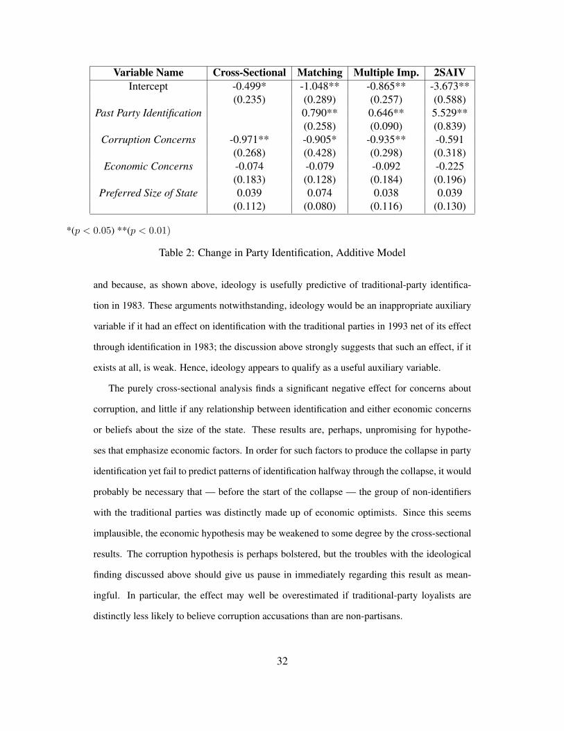
Variable Name Cross-Sectional Matching Multiple Imp. 2SAIVIntercept -0.499* -1.048** -0.865** -3.673**

(0.235) (0.289) (0.257) (0.588)Past Party Identification 0.790** 0.646** 5.529**

(0.258) (0.090) (0.839)Corruption Concerns -0.971** -0.905* -0.935** -0.591

(0.268) (0.428) (0.298) (0.318)Economic Concerns -0.074 -0.079 -0.092 -0.225

(0.183) (0.128) (0.184) (0.196)Preferred Size of State 0.039 0.074 0.038 0.039

(0.112) (0.080) (0.116) (0.130)

*(p < 0.05) **(p < 0.01)

Table 2: Change in Party Identification, Additive Model

and because, as shown above, ideology is usefully predictive of traditional-party identifica-

tion in 1983. These arguments notwithstanding, ideology would be an inappropriate auxiliary

variable if it had an effect on identification with the traditional parties in 1993 net of its effect

through identification in 1983; the discussion above strongly suggests that such an effect, if it

exists at all, is weak. Hence, ideology appears to qualify as a useful auxiliary variable.

The purely cross-sectional analysis finds a significant negative effect for concerns about

corruption, and little if any relationship between identification and either economic concerns

or beliefs about the size of the state. These results are, perhaps, unpromising for hypothe-

ses that emphasize economic factors. In order for such factors to produce the collapse in party

identification yet fail to predict patterns of identification halfway through the collapse, it would

probably be necessary that — before the start of the collapse — the group of non-identifiers

with the traditional parties was distinctly made up of economic optimists. Since this seems

implausible, the economic hypothesis may be weakened to some degree by the cross-sectional

results. The corruption hypothesis is perhaps bolstered, but the troubles with the ideological

finding discussed above should give us pause in immediately regarding this result as mean-

ingful. In particular, the effect may well be overestimated if traditional-party loyalists are

distinctly less likely to believe corruption accusations than are non-partisans.

32

Cross−Sec. Matching Multiple Imp. 2SAIV

Effects for 1983 Traditional−Party Identifier

−0.

25−

0.20

−0.

15−

0.10

−0.

050.

00

Cross−Sec. Matching Multiple Imp. 2SAIV

Effects for 1983 Non−Identifier−

0.25

−0.

20−

0.15

−0.

10−

0.05

0.00

Figure 5: Corruption Effect Sizes for the Venezuela Example

Pseudo-panel analysis can, to at least some extent, address this concern by controlling

imperfectly for past partisanship. The results reported in Table 2 for the preferred matching

method, as well as the often-competitive multiple imputation approach, suggest that this is not

a serious problem. Both models produce estimates for the corruption coefficient that are close

to the cross-sectional results. Indeed, the results of these two approaches are substantially close

across the board for this model and these data. 2SAIV, by contrast, produces distinctly differ-

ent and, in light of the Monte Carlo results above and substantive reflection, probably inferior

results: in effect, 2SAIV finds little evidence of change in the system of party identifications

between 1983 and 1993, claiming that the only (and overwhelmingly powerful!) predictor of

identification at the end of the time period is identification at the beginning. In any case, setting

aside the inferior 2SAIV and cross-sectional results, the data substantially support the hypoth-

esis that corruption was closely connected with declines in identification with the traditional

parties in Venezuela.

Since the coefficients presented in Table 2 are drawn from a logit analysis, and hence the

33

effect of corruption depends to some extent on the values of other explanatory variables, it may

be helpful to present simulated effects as an illustration of the results and also to determine the

extent to which it is plausible to regard corruption as a leading cause of the 25% decline in

party identification in Venezuela. Figure 5 shows the estimated effects of corruption for each

of the four models for two individuals, one who was a traditional-party identifier in 1983, and

who has no special concerns about the economy or the size of the state, and another who is

identical other than that she did not identify with the traditional parties in 1983. Of special

note is the fact that the preferred technique, matching, identifies substantially larger effects

than does 2SAIV, the most problematic alternative.

While matching (and multiple imputation) provide estimates that are essentially identical

with those found by the purely cross-sectional model, the difference between the two remains

crucial: the two pseudo-panel techniques find this effect conditional on past patterns of party

identification, while the cross-sectional effect is in this regard unconditional. Thus, pseudo-

panel analysis permits clearer answers regarding patterns of change over time in Venezuelans’

party identification than can be achieved using a purely cross-sectional model, even though the

numerical results are similar.

7 Conclusions

Pseudo-panel analysis is no replacement for work with true panel data when such evidence

is available. When the data do not exist, however, pseudo-panel techniques can offer a better

approximation of the unavailable true panel model than can be achieved through purely cross-

sectional analysis, conditional on the data meeting a key orthogonality assumption. For the

many circumstances in which panel data are needed but nonexistent, pseudo-panel matching,

in particular, offers a frequently plausible alternative.

34

References

Angrist, Joshua D. 1991. “Grouped-Data Estimation and Testing in Simple Labor-Supply

Models.” Journal of Econometrics 47:243–66.

Coppedge, Michael. 2005. Explaining Democratic Deterioration in Venezuela through Nested

Inference. In The Third Wave of Democratization in Latin America: Advances and Set-

backs, ed. Frances Hagopian & Scott P. Mainwaring. Cambridge: Cambridge University

Press pp. 289–316.

Cramer, J.S. 2005. Omitted Variables and Misspecified Disturbances

in the Logit Model. Technical report University of Amsterdam

http://www.tinbergen.nl/discussionpapers/05084.pdf: .

Deaton, Angus. 1985. “Panel Data from Time Series of Cross-Sections.” Journal of Econo-

metrics 30:109–26.

Devereaux, Paul J. 2007. “Small-Sample Bias in Synthetic Cohort Models of Labor Supply.”

Journal of Applied Econometrics 22:839–48.

Franklin, Charles H. 1989. “Estimation across Data Sets: Two-Stage Auxiliary Instrumental

VariablesEstimation (2SAIV).” Political Analysis 1:1–23.

Gelman, Andrew, Gary King & Chuanhai Liu. 1998. “Not Asked and Not Answered: Mul-

tiple Imputation for Multiple Surveys.” Journal of the American Statistical Association

93:846–57.

Levitsky, Steven & Katrina Burgess. 2003. “Explaining Populist Party Adaptation in Latin

America: Environmental andOrganizational Determinants of Party Change in Argentina,

Mexico, Peru,and Venezuela.” Comparative Political Studies 36(8):859–80.

Verbeek, M. & T. Nijman. 1992. “Can Cohort Data Be Treated as Geniune Panel Data?”

Empirical Economics 17:9–23.

Wooldridge, Jeffrey M. 2002. Econometric Analysis of Cross Section and Panel Data. Cam-

bridge: MIT Press.

35

Yatchew, A. & Z. Griliches. 1985. “Specification error in probit models.” The Review of Eco-

nomics and Statistics 67:134–39.

36