matching application access patterns to storage … application access patterns to storage device...
TRANSCRIPT

Matching Application Access Patterns to
Storage Device Characteristics
JIRI SCHINDLER
May 2004
cmu-pdl-03-109
Dept. of Electrical and Computer Engineering
Carnegie Mellon University
5000 Forbes Ave.
Pittsburgh, PA 15213
Submitted in partial fulfillment of the requirements
for the degree of Doctor of Philosophy.
Thesis committee
Prof. Gregory R. Ganger, Chair
Prof. Anastassia Ailamaki
Dr. John Howard, Sun Microsystems
Dr. Erik Riedel, Seagate Research
c© 2004 Jiri Schindler

ii · Matching Application Access Patterns to Storage Device Characteristics
Keywords: storage systems performance, database systems, disk arrays, MEMS-
based storage

To Katrina.

iv · Matching Application Access Patterns to Storage Device Characteristics

Abstract
Conventional computer systems have insufficient information about storage device
performance characteristics. As a consequence, they utilize the available device re-
sources inefficiently, which, in turn, results in poor application performance. This
dissertation demonstrates that a few high-level, device-independent hints encap-
sulating unique storage device characteristics can achieve significant I/O perfor-
mance gains without breaking the established abstraction of a storage device as a
linear address space of fixed-size blocks. A piece of system software (here referred
to as storage manager), which translates application requests into individual I/Os,
can automatically match application access patterns to the provided characteris-
tics. This results in more efficient utilization of storage devices and thus improved
application performance.
This dissertation (i) identifies specific features of disk drives, disk arrays, and
MEMS-based storage devices not exploited by conventional systems, (ii) quantifies
the potential performance gains these features offer, and (iii) demonstrates on three
different implementations (FFS file system, database storage manager, and disk
array logical volume manager) the benefits to the applications using these storage
managers. It describes two specific attributes: the access delay boundaries
attribute delineates efficient accesses to storage devices and the parallelism
attribute exploits the parallelism inherent to a storage device. The two described
performance attributes mesh well with existing storage manager data structures,
requiring minimal changes to their code. Most importantly, they simplify the error-
prone task of performance tuning.
Exposing performance characteristics has the biggest impact on systems with
regular access patterns. For example in database systems, when decision support
(DSS) and on-line transaction processing (OLTP) workloads run concurrently,
DSS experiences a speed up of up to 3×, while OLTP exhibits a 7% speedup.
With a single layout taking advantage of access parallelism, a database table can
be scanned efficiently in both dimensions. Additionally, scan operations run in
time proportional to the amount of query payload; unwanted portions of a table
are not touched while scanning at full bandwidth.

vi · Matching Application Access Patterns to Storage Device Characteristics

Acknowledgements
The work presented here is a result of my collaboration with fellow graduate stu-
dents John Linwood Griffin, Steve Schlosser, and Minglong Shao who contributed
their talents, ideas, and many hours that went into developing prototypes, debug-
ging, and result collection. Many thanks to John Bucy who developed disk model
libraries that were used in the Clotho prototype.
I am indebted to many people for their support, encouragement, and friendship
through my work on my dissertation. First and foremost, my advisor Greg Ganger
has been tremendous in providing guidance and showing exceptional patience and
dedication to my success. He has made himself always available and provided feed-
back on moment’s notice on any and all aspects of my work. Anastassia Ailamaki,
in addition to serving on my thesis committee, acted as my unofficial second advi-
sor and mentor. Her help and extra push at the right time have been instrumental
for my development. I am greatful to John Howard and Erik Riedel for agreeing
to serve on my thesis committee and working it into their busy schedules. Their
close monitoring of my progress and detailed comments have been invaluable.
I feel priviledged to have been part of a great research group: The Parallel Data
Laboratory. My friends and research partners Steve Schlosser and John Linwood
Griffin have been fabulous in both capacities. Without their help and encourage-
ment I would not have been able to finish. I am also thankful to Craig Soules, Eno
Thereska, Jay Wylie, Garth Goodson, John Strunk, Chris Lumb, Andy Kloster-
man, and David Petrou for their willingess to engage in discussions that shaped my
ideas. I have enjoyed tremendously working with Minglong Shao who has tought
me a lot about databases.
My special thanks to the member companies of the Parallel Data Lab Consor-
tium for their generous contributions to my research. I am also indebted to the
PDL and D-level staff. Karen Lindenfelser and Linda Whipkey have always kept
my spirits high. Joan Digney has been instrumental in proof-reading my disser-
tation. Tim Talpas made sure that all the equipment in the machine room was
always running. And finally, I am grateful for the D-level espresso machine that
kept me going.

viii · Matching Application Access Patterns to Storage Device Characteristics

Contents
1 Introduction 1
1.1 Problem definition . . . . . . . . . . . . . . . . . . . . . . . . . . . 1
1.2 Thesis statement . . . . . . . . . . . . . . . . . . . . . . . . . . . . 2
1.3 Overview . . . . . . . . . . . . . . . . . . . . . . . . . . . . . . . . 2
1.3.1 Explicit performance hints . . . . . . . . . . . . . . . . . . . 3
1.3.2 Improving efficiency across a spectrum of access patterns . 4
1.3.3 Restoring interface abstractions . . . . . . . . . . . . . . . . 4
1.3.4 Minimal system changes . . . . . . . . . . . . . . . . . . . . 5
1.4 Contributions . . . . . . . . . . . . . . . . . . . . . . . . . . . . . . 6
1.4.1 Analysis and evaluation . . . . . . . . . . . . . . . . . . . . 6
1.4.2 Improvements to system performance . . . . . . . . . . . . 7
1.4.3 Automated characterization of disk performance . . . . . . 8
1.5 Organization . . . . . . . . . . . . . . . . . . . . . . . . . . . . . . 8
2 Background and Related Work 9
2.1 Storage interface evolution . . . . . . . . . . . . . . . . . . . . . . . 9
2.2 Implicit storage contract . . . . . . . . . . . . . . . . . . . . . . . . 11
2.2.1 Request size limitations . . . . . . . . . . . . . . . . . . . . 11
2.2.2 Restricted expressiveness . . . . . . . . . . . . . . . . . . . 13
2.3 Exploiting device characteristics . . . . . . . . . . . . . . . . . . . 13
2.3.1 Disk-specific knowledge . . . . . . . . . . . . . . . . . . . . 13
2.3.2 Storage models . . . . . . . . . . . . . . . . . . . . . . . . . 14
2.3.3 Extending storage interfaces . . . . . . . . . . . . . . . . . . 15
2.4 Device performance characterization . . . . . . . . . . . . . . . . . 17
2.5 Accesses to multidimensional data structures . . . . . . . . . . . . 18
2.5.1 Database systems . . . . . . . . . . . . . . . . . . . . . . . . 18
2.5.2 Scientific computation applications . . . . . . . . . . . . . . 20

x · Matching Application Access Patterns to Storage Device Characteristics
3 Explicit Performance Characteristics 23
3.1 Storage model . . . . . . . . . . . . . . . . . . . . . . . . . . . . . . 23
3.1.1 Storage manager . . . . . . . . . . . . . . . . . . . . . . . . 24
3.1.2 Storage devices . . . . . . . . . . . . . . . . . . . . . . . . . 26
3.1.3 Division of labor . . . . . . . . . . . . . . . . . . . . . . . . 27
3.1.4 LBN address space annotations . . . . . . . . . . . . . . . . 28
3.1.5 Storage interface . . . . . . . . . . . . . . . . . . . . . . . . 29
3.1.6 Making storage contract more explicit . . . . . . . . . . . . 30
3.2 Disk drive characteristics . . . . . . . . . . . . . . . . . . . . . . . 30
3.2.1 Physical organization . . . . . . . . . . . . . . . . . . . . . 31
3.2.2 Logical block mappings . . . . . . . . . . . . . . . . . . . . 32
3.2.3 Mechanical characteristics . . . . . . . . . . . . . . . . . . . 33
3.2.4 Firmware features . . . . . . . . . . . . . . . . . . . . . . . 35
3.3 MEMS-based storage devices . . . . . . . . . . . . . . . . . . . . . 39
3.3.1 Physical characteristics . . . . . . . . . . . . . . . . . . . . 39
3.3.2 Parallelism in MEMS-based storage . . . . . . . . . . . . . 42
3.3.3 Firmware features . . . . . . . . . . . . . . . . . . . . . . . 44
3.4 Disk arrays . . . . . . . . . . . . . . . . . . . . . . . . . . . . . . . 44
3.4.1 Physical organization . . . . . . . . . . . . . . . . . . . . . 45
3.4.2 Data striping . . . . . . . . . . . . . . . . . . . . . . . . . . 45
3.4.3 Parallel access . . . . . . . . . . . . . . . . . . . . . . . . . 46
4 Discovery of Disk Drive Characteristics 47
4.1 Characterizing disk drives with DIXtrac . . . . . . . . . . . . . . . 48
4.2 Characterization algorithms . . . . . . . . . . . . . . . . . . . . . . 49
4.2.1 Layout extraction . . . . . . . . . . . . . . . . . . . . . . . 49
4.2.2 Disk mechanics parameters . . . . . . . . . . . . . . . . . . 52
4.2.3 Cache parameters . . . . . . . . . . . . . . . . . . . . . . . 54
4.2.4 Command processing overheads . . . . . . . . . . . . . . . . 58
4.2.5 Scheduling algorithms . . . . . . . . . . . . . . . . . . . . . 59
4.3 DIXtrac implementation . . . . . . . . . . . . . . . . . . . . . . . . 59
4.4 Results and performance . . . . . . . . . . . . . . . . . . . . . . . . 61
4.4.1 Extraction times . . . . . . . . . . . . . . . . . . . . . . . . 61
4.4.2 Validation of extracted values . . . . . . . . . . . . . . . . . 62
5 The Access Delay Boundaries Attribute 67
5.1 Encapsulation . . . . . . . . . . . . . . . . . . . . . . . . . . . . . . 67
5.1.1 Disk drive . . . . . . . . . . . . . . . . . . . . . . . . . . . . 67
5.1.2 Disk array . . . . . . . . . . . . . . . . . . . . . . . . . . . . 68

Contents · xi
5.1.3 MEMStore . . . . . . . . . . . . . . . . . . . . . . . . . . . 68
5.2 System design . . . . . . . . . . . . . . . . . . . . . . . . . . . . . . 69
5.2.1 Explicit contract . . . . . . . . . . . . . . . . . . . . . . . . 69
5.2.2 Data allocation and access . . . . . . . . . . . . . . . . . . . 69
5.2.3 Interface implementation . . . . . . . . . . . . . . . . . . . 70
5.3 Evaluating ensembles for disk drives . . . . . . . . . . . . . . . . . 71
5.3.1 Measuring disk performance . . . . . . . . . . . . . . . . . . 71
5.3.2 System-level benefits . . . . . . . . . . . . . . . . . . . . . . 78
5.3.3 Predicting improvements in response time . . . . . . . . . . 79
5.4 Block-based file system . . . . . . . . . . . . . . . . . . . . . . . . . 80
5.4.1 FreeBSD FFS overview . . . . . . . . . . . . . . . . . . . . 81
5.4.2 FreeBSD FFS modifications . . . . . . . . . . . . . . . . . . 82
5.4.3 FFS experiments . . . . . . . . . . . . . . . . . . . . . . . . 83
5.5 Log-structured file system . . . . . . . . . . . . . . . . . . . . . . . 86
5.5.1 Performance tradeoff . . . . . . . . . . . . . . . . . . . . . . 86
5.5.2 Variable segment size . . . . . . . . . . . . . . . . . . . . . 88
5.6 Video servers . . . . . . . . . . . . . . . . . . . . . . . . . . . . . . 88
5.6.1 Soft real-time . . . . . . . . . . . . . . . . . . . . . . . . . . 89
5.6.2 Hard real-time . . . . . . . . . . . . . . . . . . . . . . . . . 90
5.7 Database storage manager . . . . . . . . . . . . . . . . . . . . . . . 90
5.7.1 Overview . . . . . . . . . . . . . . . . . . . . . . . . . . . . 91
5.7.2 Robust storage management . . . . . . . . . . . . . . . . . 93
5.7.3 Implementation . . . . . . . . . . . . . . . . . . . . . . . . . 96
5.7.4 Evaluation . . . . . . . . . . . . . . . . . . . . . . . . . . . 97
5.7.5 DB2 experiments . . . . . . . . . . . . . . . . . . . . . . . . 98
5.7.6 RAID experiments . . . . . . . . . . . . . . . . . . . . . . . 102
5.7.7 Shore experiments . . . . . . . . . . . . . . . . . . . . . . . 103
6 The Parallelism Attribute 109
6.1 Encapsulation . . . . . . . . . . . . . . . . . . . . . . . . . . . . . . 110
6.1.1 Access to two-dimensional data structures . . . . . . . . . . 110
6.1.2 Equivalence class abstraction . . . . . . . . . . . . . . . . . 112
6.1.3 Disk array . . . . . . . . . . . . . . . . . . . . . . . . . . . . 112
6.1.4 MEMStore . . . . . . . . . . . . . . . . . . . . . . . . . . . 114
6.2 System design . . . . . . . . . . . . . . . . . . . . . . . . . . . . . . 115
6.2.1 Explicit contract . . . . . . . . . . . . . . . . . . . . . . . . 115
6.2.2 Data allocation and access . . . . . . . . . . . . . . . . . . . 115
6.2.3 Interface implementation . . . . . . . . . . . . . . . . . . . 116
6.3 Atropos logical volume manager . . . . . . . . . . . . . . . . . . . 118

xii · Matching Application Access Patterns to Storage Device Characteristics
6.3.1 Atropos design . . . . . . . . . . . . . . . . . . . . . . . . . 118
6.3.2 Quantifying access efficiency . . . . . . . . . . . . . . . . . 120
6.3.3 Formalizing quadrangle layout . . . . . . . . . . . . . . . . 122
6.3.4 Normal access . . . . . . . . . . . . . . . . . . . . . . . . . . 125
6.3.5 Quadrangle access . . . . . . . . . . . . . . . . . . . . . . . 125
6.3.6 Implementing quadrangle layout . . . . . . . . . . . . . . . 129
6.3.7 Practical system integration . . . . . . . . . . . . . . . . . . 131
6.4 Database storage manager exploiting parallelism . . . . . . . . . . 133
6.4.1 Database tables . . . . . . . . . . . . . . . . . . . . . . . . . 133
6.4.2 Data layout . . . . . . . . . . . . . . . . . . . . . . . . . . . 135
6.4.3 Allocation . . . . . . . . . . . . . . . . . . . . . . . . . . . . 137
6.4.4 Access . . . . . . . . . . . . . . . . . . . . . . . . . . . . . . 137
6.4.5 Implementation details . . . . . . . . . . . . . . . . . . . . . 138
6.4.6 Experimental setup . . . . . . . . . . . . . . . . . . . . . . . 139
6.4.7 Scan operator results . . . . . . . . . . . . . . . . . . . . . . 140
6.4.8 Database workloads . . . . . . . . . . . . . . . . . . . . . . 144
6.4.9 Results summary . . . . . . . . . . . . . . . . . . . . . . . . 148
6.4.10 Improving efficiency for a spectrum of workloads . . . . . . 149
7 Conclusions and Future Work 153
7.1 Concluding remarks . . . . . . . . . . . . . . . . . . . . . . . . . . 153
7.2 Directions for future research . . . . . . . . . . . . . . . . . . . . . 154
Bibliography 155
A Modeling disk drive media access 169
A.1 Basic assumptions . . . . . . . . . . . . . . . . . . . . . . . . . . . 169
A.2 Non-zero-latency disk . . . . . . . . . . . . . . . . . . . . . . . . . 170
A.2.1 No track switch . . . . . . . . . . . . . . . . . . . . . . . . . 170
A.2.2 Track switch . . . . . . . . . . . . . . . . . . . . . . . . . . 170
A.3 Zero-latency disk . . . . . . . . . . . . . . . . . . . . . . . . . . . . 171
A.3.1 No track switch . . . . . . . . . . . . . . . . . . . . . . . . . 171
A.3.2 Track switch . . . . . . . . . . . . . . . . . . . . . . . . . . 172
A.4 Expected Access Time . . . . . . . . . . . . . . . . . . . . . . . . . 174
B Storage interface functions 175

Figures
3.1 Two approaches to conveying storage device performance attributes. 24
3.2 Mapping of application read() calls to storage device read requests
by a FFS storage manager. . . . . . . . . . . . . . . . . . . . . . . 25
3.3 The mechanical components of a modern disk drive. . . . . . . . . 31
3.4 Typical mapping of LBNs onto physical sectors. . . . . . . . . . . 32
3.5 Representative seek profiles. . . . . . . . . . . . . . . . . . . . . . . 36
3.6 Average rotational latency for ordinary and zero-latency disks as a
function of track-aligned request size. . . . . . . . . . . . . . . . . . 38
3.7 High-level view of a MEMStore. . . . . . . . . . . . . . . . . . . . . 40
3.8 Data layout with LBN mappings. . . . . . . . . . . . . . . . . . . 41
3.9 MEMStore data layout. . . . . . . . . . . . . . . . . . . . . . . . . 42
4.1 Computing MTBRC. . . . . . . . . . . . . . . . . . . . . . . . . . . 53
4.2 The comparion of measured and simulated response time CDFs for
IBM Ultrastar 18ES and Seagate Cheetah 4LP disks. . . . . . . . . 63
4.3 The comparion of measured and simulated response time CDFs for
Quantum Atlas III and Atlas 10K disks. . . . . . . . . . . . . . . . 64
5.1 Disk access efficiency. . . . . . . . . . . . . . . . . . . . . . . . . . . 73
5.2 Getting zero-latency-disk-like efficiency from ordinary disks. . . . . 74
5.3 Expressing head time. . . . . . . . . . . . . . . . . . . . . . . . . . 75
5.4 Average head time for track-aligned and unaligned reads for the
Quantum Atlas 10K II. . . . . . . . . . . . . . . . . . . . . . . . . 76
5.5 Breakdown of measured response time for a zero-latency disk. . . . 77
5.6 Response time and its standard deviation for track-aligned and un-
aligned disk access. . . . . . . . . . . . . . . . . . . . . . . . . . . . 78
5.7 Relative improvement in response time for ensemble-based access
over normal access in the face of changing technology. . . . . . . . 81
5.8 Mapping system-level blocks to disk sectors. . . . . . . . . . . . . . 82
5.9 LFS overall write cost for the Auspex trace as a function of segment
size. . . . . . . . . . . . . . . . . . . . . . . . . . . . . . . . . . . . 87

xiv · Matching Application Access Patterns to Storage Device Characteristics
5.10 Worst-case startup latency of a video stream for track-aligned and
unaligned accesses. . . . . . . . . . . . . . . . . . . . . . . . . . . . 89
5.11 Query optimization and execution in a typical DBMS. . . . . . . . 91
5.12 Buffer space allocation with performance attributes. . . . . . . . . 96
5.13 TPC-H I/O times with competing traffic (DB2). . . . . . . . . . . 99
5.14 TPC-H trace replay on RAID5 configuration (DB2). . . . . . . . . 103
5.15 TPC-H queries with competing traffic (Shore). . . . . . . . . . . . 104
5.16 TPC-H query 12 execution time as a function of TPC-C competing
traffic (Shore). . . . . . . . . . . . . . . . . . . . . . . . . . . . . . 106
5.17 TPC-H query 12 execution (DB2) . . . . . . . . . . . . . . . . . . 107
6.1 Example describing parallel access to two-dimensional data structures.111
6.2 Atropos quadrangle layout. . . . . . . . . . . . . . . . . . . . . . . 119
6.3 Comparison of access efficiencies. . . . . . . . . . . . . . . . . . . . 121
6.4 Comparison for response times for random access. . . . . . . . . . 122
6.5 Single quadrangle layout. . . . . . . . . . . . . . . . . . . . . . . . 124
6.6 An alternative representation of quadrangle access. . . . . . . . . . 128
6.7 Comparison of measured and predicted response times. . . . . . . . 130
6.8 Atropos quadrangle layout for different RAID levels. . . . . . . . . 134
6.9 Data allocation with capsules. . . . . . . . . . . . . . . . . . . . . . 135
6.10 Mapping of a database table with 16 attributes onto Atropos logical
volume. . . . . . . . . . . . . . . . . . . . . . . . . . . . . . . . . . 136
6.11 Capsule allocation for the G2 MEMStore. . . . . . . . . . . . . . . 138
6.12 Table scan on Atropos disk array with different number of attributes.142
6.13 Table scan on G2 MEMStore with different number of attributes. . 144
6.14 TPC-H performance for different layouts. . . . . . . . . . . . . . . 146
6.15 Compound workload performance for different layouts. . . . . . . . 148
6.16 Comparison of three database workloads for different data layouts. 149
6.17 Comparison of disk efficiencies for three database workloads. . . . 150
A.1 Accessing data on disk track. . . . . . . . . . . . . . . . . . . . . . 173

Tables
3.1 Representative SCSI disk characteristics. . . . . . . . . . . . . . . . 34
3.2 Basic MEMS-based storage device parameters. . . . . . . . . . . . 39
3.3 MEMS-based storage device parameters. . . . . . . . . . . . . . . . 44
4.1 Break down of DIXtrac extraction times. . . . . . . . . . . . . . . 61
4.2 Address translation details. . . . . . . . . . . . . . . . . . . . . . . 62
4.3 Demetit figures (RMS ). . . . . . . . . . . . . . . . . . . . . . . . . 65
5.1 Relative response time improvement with track-aligned requests. . 80
5.2 FreeBSD FFS results. . . . . . . . . . . . . . . . . . . . . . . . . . 84
5.3 TpmC (transactions-per-minute) and CPU utilization. . . . . . . . 105
6.1 Parameters used by Atropos. . . . . . . . . . . . . . . . . . . . . . 123
6.2 Quadrangle parameters across disk generations. . . . . . . . . . . . 131
6.3 Device parameters for the G2 MEMStore. . . . . . . . . . . . . . . 140
6.4 Database access results for Atropos logical volume manager. . . . . 141
6.5 Database access results for G2 MEMStore. . . . . . . . . . . . . . . 143
6.6 TPC-C benchmark results with Atropos disk array LVM. . . . . . 147

xvi · Matching Application Access Patterns to Storage Device Characteristics

1 Introduction
1.1 Problem definition
The abstraction of storage devices into a linear space of fixed-size blocks plays an
important role in the architecture of computer systems. It cleanly separates host
system software from storage-device-specific control code, facilitating data access
and retrieval. A new storage device can easily be plugged into an existing system,
without requiring any modifications to the host software. Similarly, the storage
device control code can transparently implement new algorithms for optimizing
data access behind this abstraction. However, storage interface abstraction also
hides important non-linearities in access times to different blocks, addressed by
an integer called the logical block number (LBN). The difference in access times,
ranging by more than an order of magnitude, stems from both the devices’ physi-
cal characteristics and their architectural organizations. Thus, exercising efficient
access patterns that yield shorter response times can bring about significant I/O
performance improvements.
In order to work around the large non-linearities in access times, computer sys-
tems combine three different approaches. First, the host system software, which
this dissertation refers to as the storage manager, and the storage device adhere
to an unwritten contract, which states that (i) LBNs near each other can be ac-
cessed faster than those farther away and that (ii) accessing LBNs sequentially
is generally much more efficient than accessing them in random order. Second,
the storage manager (e.g., inside a file system or a database system) guesses de-
vice characteristics and adjusts access patterns to improve I/O performance. This
guessing is based on assumptions about the underlying storage device technology
and a set of manually-tunable parameters. Third, the storage device observes I/O
access patterns and attempts to dynamically adapt its behavior to service requests
more efficiently.
The simple unwritten contract mentioned above works well when access pat-
terns are regular and static; the data layout can be linearized in the LBN address
space to achieve efficient sequential access. However, the simple contract is not
2 · Matching Application Access Patterns to Storage Device Characteristics
sufficient for (i) mixed streams (i.e., regular but not sequential accesses), (ii) reg-
ular access patterns to non-linear structures (e.g., two dimensional data), or (iii)
when access patterns change over time. Therefore, the latter two approaches de-
scribed in the preceding paragraph are needed as well. However, they exhibit a
common shortcoming; the storage interface used in today’s systems does not allow
the exchange of sufficient information. Even though both the storage manager and
the storage device employ elaborate algorithms in attempting to maximize overall
performance, they have only a crude notion of what the other is doing and make
their decisions largely in isolation. In particular, the storage manager is unaware
of the most efficient access patterns, and thus cannot exercise them. The storage
device, in turn, tunes the execution of access patterns that are inherently far from
optimal. In contrast, providing sufficient information could result in better I/O
performance through more efficient use of storage device resources without guess
work or duplication of effort at both sides of the storage interface.
Using storage managers that rely on built-in storage device models with man-
ually tunable parameters poses another set of problems. These parameters often
do not capture in enough detail underlying storage device mechanisms governing
the I/O performance. They are also labor-intensive and prone to misconfiguration.
Even whey they are set properly, they do not cope well with dynamic workload
changes; they must be manually re-tuned by a system administrator each time a
workload changes. Finally, the assumptions of the models describing storage de-
vice performance break the interface abstraction. As a consequence, when a new
storage device is plugged into the system, the model may no longer be applicable.
In short, the absence of communication between the storage manager and the
storage device leads to inefficient utilization of storage device resources and poor
performance, especially for workloads that change dynamically.
1.2 Thesis statement
With sufficient information, a storage manager can exploit unique storage device
characteristics to achieve better, more robust I/O performance. This informa-
tion can be abstract from device specifics, device-independent, and yet expressive-
enough to allow a storage manager to tune its access patterns to a given device.
1.3 Overview
This dissertation contends that storage device resources are not utilized to their
full potential because too much information is hidden from storage manager. High-
level storage interfaces abstracting a storage device as a linear address space of

1.3 Overview · 3
fixed-size blocks do not convey sufficient information to allow storage managers
make decisions leading to efficient use of the storage device.
With more expressive interfaces, storage managers and storage devices can
exchange information and make more informed choices on both sides of the storage
interface. For example, only the storage manager has detailed information about
the application priorities of requests going to the storage device. On the other hand,
only the storage device has exact information about its internal state. Combining
this knowledge appropriately will allow a storage manager can take advantage
of the device’s unique strengths and avoid access patterns leading to inefficient
execution at the storage device. This dissertation explores what information a
storage device should expose to aid storage managers in making more informed
decisions about access patterns that result in more efficient utilization of storage
resources and improved application I/O performance.
1.3.1 Explicit performance hints
A storage device can expose its performance characteristics in a few, high-level
static performance attributes. With detailed information about application, a stor-
age manager uses these explicit hints to match the application access patterns to
the characteristics of the storage device and generate requests that can be exe-
cuted efficiently. However, the storage manager should not control how or when
requests should be executed; such device-specific decisions depend on the state of
the storage device and should be done below the storage interface, where appro-
priate information is available.
In addition to bridging the performance gap between the host and the storage
device, static performance attributes simplify storage manager implementation.
The storage manager need not implement models describing a device’s performance
or rely on possibly incorrect settings of the manually tunable parameters. Instead,
with explicit hints, the storage manager can dynamically, and without human
intervention, adjust application access patterns, simplifying the difficult and error-
prone task of performance tuning.
This dissertation describes two examples of static performance attributes. The
access delay boundaries attribute allows efficient execution of access patterns
consisting of mid-sized I/Os (tens to hundreds of KB) for non-sequential accesses
to mixed streams. The parallelism attribute allows efficient accesses to multi-
dimensional data structures laid out in the storage device’s linear address space.
Specifically, measurements described in this dissertation show it can facilitate ef-
ficient accesses to two-dimensional structures in both dimensions for a variety of
access patterns with a single data layout.

4 · Matching Application Access Patterns to Storage Device Characteristics
If a storage device does not provide its performance characteristics directly,
an intermediary, separate from the storage manager, can often discover these and
encapsulate them into the performance hints to be passed to the storage manager.
This intermediary, called a discovery tool, does not affect the critical path for I/O
requests going to the storage device. This dissertation describes one such tool that
works for modern disk drives.
1.3.2 Improving efficiency across a spectrum of access patterns
Application access patterns span a spectrum ranging from highly structured ac-
cesses to completely non-structured random ones. Because of their nature, random
accesses can be made efficient only by qualitative changes in technology; no pro-
vision of more information between storage devices and applications can improve
their efficiency. At the opposite end of the spectrum, complete control over access
patterns (that do no change over time) allows an application to lay data out to
take advantage of efficient sequential accesses.
The performance attributes proposed by this dissertation improve the efficiency
of access patterns that fall between these two ends of the spectrum: regular access
patterns that change over time due to dynamic workload changes. One example
includes access patterns consisting of intermixed streams. While each stream in
isolation could take advantage of efficient sequential access, a simultaneous access
to multiple streams, whose number changes dynamically, results in non-sequential
storage device accesses. Another example is a system with static (and possibly
multi-dimensional) data structures where dynamic workload changes yield differ-
ent access patterns. This behavior is typical for relational database systems, where
different queries result in different accesses, while the data structures (relations)
change very slowly relative to the changes in access patterns. The access delay
boundaries and parallelism attributes aid applications in data layout and con-
struction of more efficient access patterns compared to traditional systems that,
in the absence of sufficient information provided by storage devices, rely on guess
work and duplicate effort on both sides of the storage interface.
1.3.3 Restoring interface abstractions
Providing explicit hints also restores storage interface abstractions. These hints
replace assumptions about device’s inner-workings built into current storage man-
agers, yet they preserve the unwritten contract between the storage device and the
storage manager. This dissertation does not argue that this contract is not useful.
It shows that, by itself, it does not allow applications to take full advantage of the

1.3 Overview · 5
performance available in today’s storage devices, including single disk drives, disk
arrays, and emerging technologies such as MEMS-based storage.
This approach does not prevent the storage device from further optimizing the
execution of efficient access patterns based on explicit hints. The storage man-
ager can, and should, relegate any device-specific decisions or optimizations (e.g.,
scheduling) to the storage device. Hidden away behind the storage interface, the
storage device can make these decisions with more accurate and detailed infor-
mation that would otherwise be difficult to expose to the storage manager. This
clean separation allows code developers to write storage managers devoid of device-
specific detail; yet the storage manager can still dynamically adapt its access pat-
terns using the static hints provided by the storage device.
1.3.4 Minimal system changes
An alternative approach to the one proposed in this dissertation is to push in-
formation down to the storage device. While this approach may fulfill the same
goals this dissertation sets forth, namely, more efficient use of storage resources,
the mechanisms to achieve the goals may require extensive changes to the current
storage interface. Specifically, the amount of application-specific state that must
be conveyed to the storage device can be substantial. Thus, modifying the storage
manager and application code for this purpose would likely involve larger amounts
of new system design and software engineering.
The approach proposed and discussed in this dissertation, on the other hand,
meshes well with the existing code and data structures of a variety of storage
managers. It does not require a new system design and implementation to be
developed from scratch. It makes minimal changes to the existing host software
structures and requires no changes to the firmware of current storage devices. It
contends that, together with knowledge of application state and its access patterns,
the storage manager is the right place where a little bit of information provided
in these explicit hints can bring significant performance wins. It shows that the
data structures of the Shore database storage manager [Carey et al. 1994], Fast
File System [McKusick et al. 1984], and Log-structured File System [Rosenblum
and Ousterhout 1992] (all examples of storage managers), can easily accommodate
and benefit from performance hints with only small changes to their source code.
The proposed mechanism for conveying performance hints to the storage man-
ager follows the same minimalist approach. The performance characteristics are
encapsulated into a well-defined (small) set of attributes. These attributes do not
break established abstractions between the storage device and the storage man-
ager; they simply annotate the current abstraction of a storage system, namely

6 · Matching Application Access Patterns to Storage Device Characteristics
the linear address space of fixed-size LBNs. The storage manager makes function
calls with specific LBN values that return the values of the desired attribute.
1.4 Contributions
This dissertation makes four main contributions:
– It shows how static performance hints provided by a storage device can be
used for dynamic adjustment of application access patterns, allowing them to
utilize storage device resources more efficiently. It gives two specific examples
of performance attributes that encapsulate performance characteristics of
single disks, disk arrays, and MEMS-based storage.
– It describes the minimal changes to current storage manager structures nec-
essary to take advantage of explicit performance hints and demonstrates
them on two different storage manager implementations; a database storage
manager, called Shore, and a block-based Fast File System, which is part of
the BSD operating system.
– It quantifies performance improvements to different classes of applications
using three different storage managers (e.g., FFS, Shore, and logical volume
managers inside disk arrays). It measures the benefits to file system and
database workloads on three different storage manager implementations. Fi-
nally, it analytically evaluates the benefits to a Log-structured File System
and a multimedia streaming server.
– It demonstrates how this approach can be used in today’s systems without
modifications to current storage devices thanks to a specialized discovery
tool. This tool, which sits between a storage manager and the storage de-
vice, can describe the performance characteristics of a specific device and
transparently export them to the storage manager.
1.4.1 Analysis and evaluation
Today, disk drives are the most prevalent devices being used for on-line stor-
age. This dissertation identifies performance characteristics of state-of-the-art disk
drives. Building upon this evaluation, it explores the characteristics of disk arrays,
which group several disks for better performance and reliability. It also explores
the unique performance characteristics of an emerging storage technology, called
MEMS-based storage. The performance impact of exposing device characteristics
is evaluated both by analytical models and experimentation. This information can

1.4 Contributions · 7
provide up to 50% improvement in disk efficiency and a significant reduction in
response time variance for accesses that utilize explicit information about disk
characteristics. With proper data layouts, RAID configurations can leverage the
per-disk improvements and deliver it to applications.
1.4.2 Improvements to system performance
Exposing performance characteristics has the biggest impact on systems with reg-
ular (but not necessarily sequential) access patterns. On the other hand, applica-
tions with random access patterns that cannot be tuned to achieve efficient accesses
will experience only limited or no improvements. In particular random small I/O
activity (e.g., online transactional processing), will see only limited, or no, perfor-
mance improvements. Additionally, these limited improvements may only occur
when random workloads occur concurrently with other workloads exhibiting more
regular access patterns.
Fortunately, many systems and applications exhibit regular access patterns to
large (relative to the individual I/O size) sets of related data. This regularity al-
lows storage managers to dynamically adjust the sizes of individual I/Os that can
be executed by storage devices more efficiently. The results described in this dis-
sertation show a 20% reduction in run time for large file operations in block-based
file systems. For log-structured file systems, a 44% lower write cost to segments
is achieved. Multimedia servers achieve a 56% increase in the number of concur-
rent streams serviceable on a video server and up to 5× lower startup latency for
streams newly admitted to the server.
A database storage manager using explicit performance attributes can achieve
I/O efficiency nearly equivalent to sequential streaming, even in the presence of
competing random I/O traffic. Exposing these attributes also simplifies manual
configuration and restores the optimizer’s assumptions about the relative costs of
different access patterns expressed in query plans. The performance of stand-alone
decision support workload (DSS) improves by 10% on average, with some queries
seeing up to 1.5× speedup. More importantly, when running concurrently with
an on-line transaction processing (OLTP) workload, DSS workload performance
improves by up to 3×, while OLTP also exhibits a 7% speedup.
Utilizing the access delay boundaries and parallelism attributes, a data-
base storage manager can implement a single data layout for 2-D tables (relations)
that yields efficient accesses in both dimensions. The access efficiencies are equal
or very close (within 6%) to the efficiencies achieved with data layouts optimized
for accesses in the respective dimension, but trading off efficiency in the other
dimension. For example, scan operators operate with maximum efficiency, while

8 · Matching Application Access Patterns to Storage Device Characteristics
requesting only the data needed by the query. Unwanted portions of a table can
be skipped while scanning at full speed, resulting in scan times proportional to
the amount of data actually used by queries.
1.4.3 Automated characterization of disk performance
The discovery tool described in this dissertation, called DIXtrac, automatically
characterizes the performance of modern disk drives. It can extract over 100
performance-critical parameters in 2–6 minutes without human intervention or
special hardware support. While only a small fraction of these parameters is encap-
sulated as the set of performance attributes to be passed to the storage manager,
this accurate characterization is useful for other applications requiring detailed
knowledge of device parameters [Lumb et al. 2000; Wang et al. 1999; Yu et al.
2000]. In particular, the access delay boundaries performance attribute encap-
sulates the extracted disk track sizes and the parallelism attribute additionally
encapsulates the head-switch and/or one-cylinder seek time.
1.5 Organization
The reminder of the dissertation is organized as follows. Chapter 2 describes pre-
vious work related to exposing information about storage devices for application
performance gains. Chapter 3 describes in detail the proposed approach of encap-
sulating storage device performance characteristics into a few high-level attributes
annotating the device’s LBN linear address space. It also discusses in detail the
underlying storage device characteristics. Chapter 4 describes a discovery tool,
which can determine the performance characteristics of modern disk drives using
conventional SCSI interface. Chapter 5 describes a performance attribute called
access delay boundaries, and evaluates how utilizing this attribute improves
performance for file systems and database systems. Chapter 6 describes another
performance attribute, called parallelism, and shows how it improves perfor-
mance for database query operators. Chapter 7 summarizes the contributions of
this dissertation and suggests some avenues for future work.

2 Background and Related Work
2.1 Storage interface evolution
Virtually all of today’s storage devices use an interface that presents them as a
linear space of equally-sized blocks (e.g., SCSI or IDE [Schmidt 1995]) . Each block
is uniquely addressed by an integer, called a logical block number (LBN), from 0
to LBNmax (which is the number of blocks minus one). This interface separates
a storage device and its software from the host running applications; the clean
separation between the two allows changes to occur on either side of the interface
without affecting the other. For example, a new storage device can be simply
connected to the host, without any modifications to the storage manager code.
The storage device abstraction offered by this interface also provides a simple
programming model. Within this abstraction, a piece of system software, called
the storage manager (SM for short), accepts requests for data from applications
through a well-defined API. The SM then transforms these requests into individ-
ual I/O operations and issues them to the storage device on behalf of the host
applications. Because the SM communicates with these applications, it can utilize
the knowledge of all the applications’ access patterns to generate non-competing
I/O operations.
Before this storage interface existed, the storage manager was also responsible
for controlling storage device specifics such as positioning of the read/write heads,
data encoding, and handling of media errors. With such tight coupling between the
storage device and the SM, plugging a new storage device into the host required
software changes to the storage manager. It also had one important advantage.
The storage manager could leverage its intimate knowledge of device’s performance
characteristics and application access patterns. This knowledge, combined with the
ability to control the mechanics of the storage device, allowed the storage manager
to fully utilize storage device resources by turning the application access patterns
into efficient I/O operations.
In particular, many algorithms have been developed for efficient scheduling of
read/write heads of rotating drums and disk drives, minimizing disk access latency

10 · Matching Application Access Patterns to Storage Device Characteristics
and/or variance in response time [Bitton and Gray 1988; Denning 1967; Daniel
and Geist 1983; Fuller 1972; Geist and Daniel 1987]. These algorithms combine the
knowledge of outstanding I/O requests, the ability to precisely control read/write
head positioning, and detailed knowledge of device characteristics.
Current state-of-the art storage devices (i.e., disk drives and disk arrays) em-
ploy a variety of mechanisms for media defect management and for correcting
transient read/write errors as well as algorithms for improving I/O performance
such as prefetching, write-back caching, and data reorganization. Because these
functions are tightly coupled to the electronics [Quantum Corporation 1999] or
architecture [Hitz et al. 1994; Wilkes et al. 1996], it is difficult to cleanly expose
them to the storage manager. Hence, today’s device controllers include firmware
algorithms for efficient request scheduling while hiding device details from the
storage manager behind the storage device interface.
The high-level storage interface frees the storage manager from device-specific
knowledge, allowing it to concentrate only on data allocation and the generation of
I/Os according to application needs. The storage manager simply sends read and
write commands to the device. Behind the storage interface, the device schedules
outstanding requests and carries out the steps necessary to execute the commands.
If an error occurs, the device tries to fix it locally. If not possible, it simply reports
back to the storage manager that the command failed. The storage manager then
decides how to handle the error according to the application’s needs.
Unfortunately, the storage interface abstraction has a side effect: It hides the
large non-linearities, which stem from both the device’s physical characteristics
and the firmware algorithms, forcing both the storage manager and the device to
make decisions in isolation. Unlike before, scheduling decisions (now taking place
inside the device firmware below the interface) are made without knowledge of
application access patterns. The device sees a small part of the pattern, whereas
the storage manager may know the entire pattern. On the other hand, the stor-
age manager is not provided with enough knowledge to turn access patterns into
efficient I/O operations. As a result, there exist complex approaches that attempt
to bridge this information gap in order to achieve better performance.
The solutions for bring more information across storage interface fall into three
categories. The first category relies on implicit contract between devices and stor-
age managers. The second category either explicitly or implicitly breaks the exist-
ing interface abstraction by making assumptions about the device’s architecture
and inner-workings. Finally, the third category proposes different APIs that en-
able better matching of (specific) application access patterns to the underlying
characteristics.

2.2 Implicit storage contract · 11
2.2 Implicit storage contract
The simplest, and perhaps most extensively used, hints about non-linear access
times to logical blocks are captured in an unwritten contract between the storage
manager and the storage device. This contract states that
(i) LBNs near each other can be accessed faster than those farther away, and
(ii) accessing LBNs sequentially is much more efficient than random access.
As instructed by this contract, the storage manager attempts to issue larger, more
efficient I/O requests whenever possible. A prime example is the Log-structured
File System [Rosenblum and Ousterhout 1992]. LFS accumulates small writes into
contiguous segments of logical blocks and writes them in one large, more efficient
access. Multimedia servers exploit sequentiality by allocating contiguous logical
blocks to the same stream [Bolosky et al. 1996; Santos and Muntz 1997; Vin
et al. 1995]. With sufficient buffer space, a video server can issue large sequential
I/Os well ahead of the time the data is actually needed. Storage devices adhere
to this contract by implementing algorithms that detect sequentiality and issue
prefetch requests in an anticipation of a future I/O issued by the host [Quantum
Corporation 1999; Worthington et al. 1995]. Similarly, they dynamically rearrange
data on the media to improve access locality [Ruemmler and Wilkes 1991; Wilkes
et al. 1996].
2.2.1 Request size limitations
System software designers would like to always use large requests to maximize effi-
ciency. Unfortunately, in practice, resource limitations and imperfect information
about future accesses make this difficult. Four system-level factors oppose the use
of ever-larger requests: (1) responsiveness, (2) limited buffer space, (3) irregular
access patterns, and (4) storage space management.
Responsiveness
Although larger requests increase efficiency, they do so at the expense of higher
latency. This trade-off between efficiency and responsiveness is a recurring issue
in computer system design with a cost that can be particularly steep for disk
systems. A latency increase can manifest itself in several ways. At the local level,
the non-preemptive nature of disk requests combined with the long access times
of large requests (35–50 ms for 1 MB requests) can result in substantial I/O wait
times for small, synchronous requests. This problem has been noted for both FFS
and LFS [Carson and Setia 1992; Seltzer et al. 1995]. At the global level, grouping

12 · Matching Application Access Patterns to Storage Device Characteristics
substantial quantities of data into large disk writes usually requires heavy use of
write-back caching.
Although application performance is usually decoupled from the eventual write-
back, application changes are not persistent until the disk writes complete. Making
matters worse, the amount of data that must be delayed and buffered to achieve
large enough writes continues to grow. As another example, many video servers
fetch video segments in carefully-scheduled rounds of disk requests. Using larger
disk requests increases the time for each round, which increases the time required
to start streaming a new video. Section 5.6 quantifies the start-up latency required
for modern disks.
Buffer space
Although memory sizes continue to grow, they remain finite. Large disk requests
stress memory resources in two ways. For reads, large disk requests are usually
created by fetching more data farther in advance of the actual need for it; this
prefetched data must be buffered until it is needed. For writes, large disk requests
are usually created by holding more data in a write-back cache until enough con-
tiguous data is dirty; this dirty data must be buffered until it is written to disk.
The persistence problem discussed above can be addressed with non-volatile RAM,
but the buffer space issue will remain. For video servers, ever-larger requests in-
crease both buffer space requirements and stream initiation latency [Chang and
Garcia-Molina 1996; 1997; Keeton and Katz 1993].
Irregular access patterns
Large disk requests are most easily generated when applications use regular ac-
cess patterns and large files. Although sequential full-file access is relatively com-
mon [Baker et al. 1991; Ousterhout et al. 1985; Vogels 1999], most data objects are
much smaller than the disk request sizes needed to achieve good disk efficiency. For
example, most files are well below 32 KB in size in UNIX-like systems [Ganger and
Kaashoek 1997; Sienknecht et al. 1994] and below 64 KB in Microsoft Windows
systems [Douceur and Bolosky 1999; Vogels 1999]. Directories and file attribute
structures are almost always much smaller. To achieve sufficiently large disk re-
quests in such environments, access patterns across data objects must be predicted
at layout time.
Although approaches to grouping small data objects have been explored [Gab-
ber and Shriver 2000; Ganger and Kaashoek 1997; Ghemawat 1995; Rosenblum
and Ousterhout 1992], all are based on imperfect heuristics, and thus they rarely
group things perfectly. Even though disk efficiency is higher, incorrectly grouped

2.3 Exploiting device characteristics · 13
data objects result in wasted disk bandwidth and buffer memory, since some
fetched objects will go unused. As the target request size grows, identifying suffi-
ciently strong inter-relationships becomes more difficult.
Storage space management
Large disk requests are only possible when closely related data is collocated on the
disk. Achieving this collocation requires that on-disk placement algorithms be able
to find large regions of free space when needed. Also, when grouping multiple data
objects, growth of individual data objects must be accommodated. All of these
needs must be met with little or no information about future storage allocation
and deallocation operations. Collectively, these facts create a complex storage
management problem. Systems can address this problem with combinations of pre-
allocation heuristics [Bovet and Cesati 2001; Giampaolo 1998], on-line reallocation
actions [Lumb et al. 2000; Rosenblum and Ousterhout 1992; Smith and Seltzer
1996], and idle-time reorganization [Blackwell et al. 1995; Matthews et al. 1997].
There is no straightforward solution and the difficulty grows with the target disk
request size, because more related data must be clustered.
2.2.2 Restricted expressiveness
The implicit contract does not fully exploit the performance potential of a storage
device. For example, it does not convey to the storage manager when larger I/O
sizes, which put more pressure on the host resources, do not yield any additional
performance benefit. It also unduly increases the complexity of both the storage
manager and the storage device firmware. For example, both implement prefetch
algorithms that increase the efficiency of sequential accesses, unnecessarily dupli-
cating identical functionality. Using more expressive methods that complement
this contract without breaking the storage interface abstractions, can provide ad-
ditional benefit. They also simplify the implementation of both systems, as demon-
strated in this dissertation.
2.3 Exploiting device characteristics
A lot of research has focused on exploiting device-specific characteristics to achieve
better application performance. These solutions, however, usually break the stor-
age abstractions, because they require device-specific knowledge. As a result, when
a new storage device is placed into the system, these solutions do not yield the
expected benefit; the storage manager has to be reprogrammed to adapt to the
specific features of the new device. Other approaches rely on detailed models with

14 · Matching Application Access Patterns to Storage Device Characteristics
configurable parameters that must be manually tuned to a specific device [IBM
Corporation 2000; McKusick et al. 1984; Shriver et al. 1998].
2.3.1 Disk-specific knowledge
Much recent related work has promoted zone-based allocation and detailed disk-
specific request generation for small requests. The Tiger video server [Bolosky
et al. 1996] allocated primary copies of videos to the outer portions of each disk’s
LBN space in order to exploit the higher bandwidth of the outer zones. Secondary
copies were allocated to the lower bandwidth zones. VanMeter [1997] suggested
that there was general benefit in changing file systems to understand that different
regions of the disk provide different bandwidths.
By utilizing even more detailed disk information, several researchers have
shown substantial decreases in small request response times [Chao et al. 1992; En-
glish and Stepanov 1992; Huang and cker Chiueh 1999; Wang et al. 1999; Yu et al.
2000]. For small writes, these systems detect the position of the head and re-map
data to the nearest free block in order to minimize the positioning costs [Huang
and cker Chiueh 1999; Wang et al. 1999]. For small reads, the SR-Array [Yu et al.
2000] determines the head position when the read request is to be serviced and
reads the closest of several replicas.
The Gamma database system [DeWitt et al. 1990] accessed data in track-
sized I/Os by simply knowing the number of sectors per track. Unfortunately,
simple mechanisms like this are no longer possible because of high-level device
interfaces and built-in firmware functions. For example, zoned geometries and
advanced defect management in current disks result in cylinders being composed
of tracks with variable number of sectors (see Table 3.1). No single value for the
number of sectors per track is correct across the device.
Using disk drive track size to set the RAID stripe unit size improves I/O per-
formance. Chen and Patterson [1990] developed a method for determining proper
stripe unit for a disk array and concluded that a stripe unit near track size is
optimal. Similar to the database case, however, a single value is not sufficient for
modern multi-zoned disks; it does not realize the full potential of modern disk
drives. Using values that exactly match track size, on the other hand, can do so as
illustrated in Section 5.7.6. At the file system level, aligning access to stripe unit
boundaries and writing full stripes avoids expensive read-modify-write operations
for RAID 4 and RAID 5 configurations [Chen et al. 1994; Hitz et al. 1994].

2.3 Exploiting device characteristics · 15
2.3.2 Storage models
Various storage managers have built more detailed models of the underlying stor-
age devices [McKusick et al. 1984; VERITAS Software Company 2000], but these
models may not reflect the functions inside the device. In general, the process of
building storage models is ad-hoc, device-dependent, and often does not provide
the right abstractions. Many SMs just ignore details because of the complexity
involved in handling the various protocols and mechanisms. The SMs that do re-
quire and use detailed-information, i.e., current disk-head position to achieve the
promised performance gains [Chao et al. 1992; Lumb et al. 2000; Wang et al. 1999;
Yu et al. 2000], use very detailed models tailored to one specific disk type [Kotz
et al. 1994].
The Fast File System allocation of data into cylinder groups [McKusick et al.
1984] is based on the notion that related data and metadata should be put in
the same cylinder to minimize seeks. Similarly, the data allocation allowed block
interleaving to accommodate disks that could not read two consecutive sectors.
Even though these algorithms (and their tuning knobs) still exist inside the FFS
and its derivatives, they cannot be properly set because of the high-level interface
that does not expose the necessary information.
Built-in models (e.g.,inside database systems [IBM Corporation 1994]) can
receive parameter values in two different ways. The SM can query the storage
device, or alternatively, these parameters can be manually set by an administrator.
Naturally, the former approach is more desirable. However, today’s systems do not
provide an effective way of conveying this information that is device-independent.
Device-provided parameters
The SCSI interface includes a variety of additional commands that query and/or
control the device’s internal organization and behavior [Schmidt 1995]. For disk
drives, these commands include information about data layout, and cache organi-
zation. However, current commands are not getting the job done because they are
vendor-specific, proprietary, and often too oriented to the particulars of a single
storage device type.
Manually-tuned parameters
Similar to file systems, database systems include data allocation and access algo-
rithms that use device parameters to influence their decisions. These parameters
are manually set by a database administrator (DBA). For example, IBM DB2’s
EXTENTSIZE and PREFETCHSIZE parameters determine the maximal size of a single

16 · Matching Application Access Patterns to Storage Device Characteristics
I/O operation [IBM Corporation 2000], and the DB2 STRIPED CONTAINERS param-
eter instructs the storage manager to align I/Os on stripe boundaries. Database
storage managers complement DBA knob settings with methods that dynamically
determine the I/O efficiency of differently-sized requests by issuing I/Os of dif-
ferent sizes and measuring their response time. Unfortunately, these methods are
error-prone and often yield sub-optimal results. These mechanisms are also quite
sensitive and prone to human errors. In particular, high-level generic parameters
make it difficult for the storage manager to adapt to the device-specific characteris-
tics and dynamic changes to workload. This results in inefficiency and performance
degradation.
2.3.3 Extending storage interfaces
Many works demonstrated how extending storage interfaces with functions that
expose information about device specifics can improve application performance.
The following paragraphs discuss three specific aspects of this research that include
the freedom to rearrange requests to improve aggregate performance and better
utilization of resources by exposing some additional information about storage
organization.
Masking access latency
Recent efforts have proposed mechanisms that exploit freedom to reorder storage
accesses in order to mask access latency. Storage latency estimator descriptors
estimate the latency for accessing the first byte of data and the expected bandwidth
for subsequent transfer [VanMeter 1998]. Steere [1997] proposed a construct, called
a set iterator, that exploits asynchrony and non-determinism in data accesses to
reduce aggregate I/O latency. The River projects use efficient streaming from
distributed heterogeneous nodes to maximize I/O performance for data-intensive
applications [Arpaci-Dusseau et al. 1999; Mayr and Gray 2000].
Other research has exploited similar ideas at the file system level. Parallel file
systems achieve higher I/O throughput from the underlying, inherently parallel,
hardware [Freedman et al. 1996; Krieger and Stumm 1997]. As demonstrated by
Kotz [1994], a parallel file system rearranging application requests into larger, more
efficient I/Os to individual disks provides significant improvements to scientific
workloads. Similarly, I/O request criticality annotations based on file system and
application needs provide greater scheduling flexibility at the storage subsystem
level, resulting in better application performance [Ganger 1995].

2.3 Exploiting device characteristics · 17
Exposing information about device organization
Arpaci-Dusseau and Arpaci-Dusseau [2001] recently termed a system building
practice that exploits knowledge of the underlying subsystem structure gray-box
approach. Using such approach, Burnett et al. [2002] built algorithms, which can
determine the OS management policies for buffer caches. Their findings can be ex-
tended to the storage manager (e.g., a file system), allowing it to determine which
I/Os are going to be serviced from cache and schedule I/O requests accordingly.
Wong and Wilkes [2002] proposed new storage interface operations which en-
able more intelligent buffer management. Using promote/demote operations, the
host and the storage device can explicitly coordinate which data is cached where,
avoiding double buffering and hence effectively increasing the cache footprint.
Denehy et al. [2002] extended the gray box approach to building an interface
between storage devices and file systems. This interface exposes parallelism and
failure-isolation information to a log-structured file system, which can make dy-
namic decisions about data placement and balance load between individual disks
of the exposed RAID group. Their approach is similar to the one presented here;
the storage device provides hints to a file system storage manager, called I-LFS,
which then adjusts its behavior to improve performance and reliability.
Object-based storage interface
The object-based storage interface, advocated by the NASD project [Gibson et al.
1998] and drafted as an ANSI interface specification [National Committee for
Information Technology Standards 2002], proposes to use variable size objects, in-
stead of fixed size blocks, as the interface between hosts and storage devices. These
higher level semantics pass hints to the storage device. Combined with the ability
to assign various attributes to different objects, these hints can be used within the
storage device to allow, for example, object collocation and other performance-
related operations behind the object-based storage interface. However, there must
still exist some kind of a storage manager within the storage device to be able
to allocate and manage the individual blocks of the storage media and map them
into an object exported by the storage interface. Although the storage manager is
now found on the opposite side of the physical interface, the work explored in this
dissertation is suited to this object model as well.
Applications providing hints to storage managers
Patterson et al. [1995] proposed a mechanism, called informed prefetching and
caching, whereby applications provide hints about intended access patterns to a

18 · Matching Application Access Patterns to Storage Device Characteristics
storage manager, called TIP. Based on these hints, which are inserted by the appli-
cation programmer, the storage manager makes a decision which blocks it should
prefetch, cache for reuse, or discard. TIP uses cost-benefit analysis to allocate
buffers when they have the biggest impact on application performance. Brown
et al. [2001] devised a method for using compiler-generated hints about out-of-
core application access patterns. The hints, which are similar to those manually
generated for TIP, inform an operating system buffer manager which data are
likely to be accessed in the future and which are likely no longer needed. With
such information, the manager can discard data no longer needed and prefetch
data ahead of the time they are actually accessed.
While this dissertation takes the approach of exposing information from the
lower layers up, the two approaches are complimentary. The performance at-
tributes advocated in this dissertation allow a storage manager (e.g., TIP or the
virtual memory manager) to efficiently execute prefetching requests and compute
more accurate estimates for the costs of different access patterns.
2.4 Device performance characterization
Worthington et al. [1995] have described methods for retrieving various param-
eters from SCSI disk drives for several disk drives. The combination of inter-
rogative and empirical extraction techniques can determine information about
disk geometry, data layout, mechanical overheads, cache behavior, and command
processing overheads. The accuracy of these techniques has been evaluated by a
highly-configurable disk simulator called DiskSim [Bucy and Ganger 2003]. This
event-driven simulator offers over 100 parameters characterizing the disk drive
module, though some are dependent on others or meaningful only in certain cases.
Talagala et al. [2000] extracted approximate values for disk geometries, me-
chanical overheads and layout parameters using micro-benchmarks consisting of
only read and write requests, by timing the requests with progressively increas-
ing request strides. Their approach is independent of the disk’s interface and thus
works for potentially any disk. The emphasis being on extracting approximate val-
ues quickly, their algorithms achieve lower accuracy of the extracted information
than the combination of interrogative and empirical extraction for SCSI disks.
2.5 Accesses to multidimensional data structures
Mapping multi-dimensional data structures (e.g., large non-sparse matrices or
database tables) into a linear LBN space without providing additional infor-
mation to applications generally makes efficient access possible only along one

2.5 Accesses to multidimensional data structures · 19
dimension. However two important classes of systems, namely relational database
systems and data-intensive out-of-core scientific computation applications, often
access data along multiple dimensions. Thus, they can benefit from methods that
can allow efficient accesses along multiple dimensions without the need to reorga-
nize data every time their access patterns change.
2.5.1 Database systems
Relational database management systems (DBMS) facilitate efficient access to two-
dimensional structured data in response to application’s or user’s requests (a.k.a.
queries). A component of a relational DBMS, usually called the storage manager,
is responsible for the layout of two-dimensional tables (relations) and facilitation
of efficient accesses to these tables. Access patterns are governed by the type of
query and depend on data layout within and across relations. Ultimately, they
are determined by a query optimizer whose goal is to minimize the overall query
execution cost.
At a high level, database access patterns can be divided into two broad cate-
gories: random accesses or regular accesses (either in row- or column-major) to a
portion of data in a table. The former access pattern is a result of point queries.
Whenever possible, point queries use an index structure to determine the address
where the data is stored. Walking through the index and fetching the desired data
typically results in random accesses. The latter access type is called scan and it
is a basic building block for the SELECT, PROJECT, and JOIN relational oper-
ators when indexes cannot be used. Thus, the main responsibility of a database
storage manager is to ensure efficient execution of these operations for a variety
of workloads executing different queries against the two-dimensional relations.
Data organization
Today’s DBMSs leverage the efficiency of sequential accesses, stated in the unwrit-
ten contract, for laying out 2D relational tables. They predict the common order
of access by a workload and choose a layout optimized for that order, knowing
that accesses along the other major axis will be inefficient.
In particular, online transaction processing (OLTP) workloads, which make
updates to full records, favor efficient row-order access. On the other hand, deci-
sion support system (DSS) workloads often scan a subset of table columns and get
better performance using an organization with efficient column-order access [Ra-
mamurthy et al. 2002]. Without explicit support from the storage device, however,
a DBMS system cannot efficiently support both workloads with one data organi-
zation.

20 · Matching Application Access Patterns to Storage Device Characteristics
The different storage models (a.k.a. page layouts) employed by current DBMSs
trade the performance of row-major and column-major order accesses. The page
layout prevalent in commercial DBMSs, called the N-ary storage model (NSM),
stores a fixed number of full records (all n attributes) in a single page (typically
8 KB). This page layout is optimized for OLTP workloads with row-major access
and random I/Os. This layout is also efficient for scans of entire tables; the DBMS
can sequentially scan one page after another. However, when only a subset of
attributes is desired (e.g., the column-major access prevalent in DSS workloads),
the DBMS must fetch full pages with all attributes, effectively reading the entire
table even though only a fraction of the data is needed.
To alleviate the inefficiency of column-major access with NSM, a decomposition
storage model [Copeland and Khoshafian 1985] (DSM) vertically partitions a table
into individual columns. Each DSM page thus contains a single attribute for a fixed
number of records. However, fetching full records requires n accesses to single-
attribute pages and n − 1 joins on the record ID to reconstruct the entire record.
The stark difference between row-major and column-major efficiencies for the
two layouts described above is so detrimental to database performance that Ra-
mamurthy et al. [2002] proposed maintaining two copies of each table to avoid it.
This solution requires twice the capacity and must propagate updates to each copy
to maintain consistency. The parallelism attribute proposed in this dissertation
eliminates this need for two replicas while allowing efficient access in both orders.
Exploiting device characteristics
Memory latency has been recognized as an increasingly important performance
bottleneck for some compute- and memory-intensive database applications [Ail-
amaki et al. 1999; Boncz et al. 1999]. To address the problem, recent research
proposed two approaches to improving the utilization of processor caches: (i) em-
ploying data layouts utilizing cache characteristics and (ii) incorporating the cost
of different memory access patterns into query optimization costs.
The first approach uses a new data page layout [Ailamaki et al. 2001] and in-
dexing structures [Chen et al. 2002; Rao and Ross 1999] tailored to cache charac-
teristics. The cache-sensitive data layout, called PAX, partitions data into clusters
of the same attribute and aligns them on cache line boundaries. This organization
minimizes the number of cache misses and leverages prefetching (fetching whole
cache line) when sequentially scanning (in memory) through a subset of table
columns (attributes). The second approach factors processor cache access parame-
ters into the optimization process by incorporating data access pattern and cache
characteristics into the query operator cost functions [Manegold et al. 2002].

2.5 Accesses to multidimensional data structures · 21
The previously proposed techniques optimize cache and memory accesses. This
dissertation extends that work by bridging the performance gap between non-
volatile memory (storage devices) and main memory. For example, similar to in-
page data partitioning, the storage manager can allocate data on access delay
boundaries and prefetch them in extents corresponding to the number of LBNs
between two consecutive boundaries. The parallelism attribute gives database
storage managers the flexibility to request just the data needed by the query.
With a single data layout, it can request data both in row- and column-major
orders while utilizing the available access parallelism to achieve maximal aggregate
bandwidth afforded by the particular access pattern.
2.5.2 Scientific computation applications
Scientific applications access large sets of data to perform calculations. To pro-
vide the required bandwidth, application runtime environments spread data across
many disks to leverage access parallelism and speed up execution time.
Since I/O operations are the dominant factor in execution time, parallel algo-
rithms strive to minimize the amount of data transfered between main memory and
non-volatile storage. The parallel disk model (PDM) [Vitter and Shriver 1994] has
become the de facto standard for analyzing algorithm performance. It expresses
algorithm execution time in terms of four parameters: N is the number of items in
the problem instance, M is the number of items that can fit into main memory, B
is the number of items per disk block, and D is the number of disks. This model,
however, does not account for different access efficiencies of sequential and random
I/O [Vengroff and Vitter 1995].
Execution environments for parallel applications include interfaces for parallel
I/O, memory management, and communication with remote processors. Parallel
I/O can be realized by parallel filesystems [Corbett and Feitelson 1994; Krieger and
Stumm 1997] or direct block access [Kotz et al. 1994; Vengroff 1994]. Regardless
of the specific mechanism, these components collectively provide the functions of
a storage manager – data layout across parallel-accessible storage devices and I/O
execution.
Data organization
Many out-of-core parallel algorithms do I/O in memory loads; that is, they re-
peatedly load some subset of the data into memory, process it, and write it out.
Each transfer is a large, but not necessarily contiguous, set of data [Kotz et al.
1994]. The memory load operations include scanning and sorting [Vengroff and
Vitter 1995] and bit-permute/complement permutations [Cormen 1993] of one-

22 · Matching Application Access Patterns to Storage Device Characteristics
dimensional data (a.k.a. streams). The streams are striped across all the available
storage devices to achieve access parallelism.
Another type of parallel algorithms accesses two-dimensional data structures
to perform linear algebra operations on large matrices such as LU factorization and
matrix multiply. These operations form the basis for many scientific applications;
their kernels are used as benchmarks for parallel computers running scientific out-
of-core applications [Bailey et al. 1993]. The majority of these operations access
one element in row-major and the other in column-major. Depending on the type
of operation, the two elements can be two different matrices (matrix multiply),
the same matrix (LU factorization), or a matrix and a vector (solving a linear
system Az = x). With current storage device abstractions, the data organization
has shortcomings similar to relational databases — one of the matrix dimensions
is chosen as the primary access order (typically row-major) [Vengroff and Vitter
1995], to take advantage of the unwritten contract’s efficient sequential access.
Naturally, access along the other order is less efficient.
A third type of scientific applications performs range queries through multi-
dimensional space. To perform these searches efficiently, application execution en-
vironments use indexing structures (e.g., K-D-B-tree, R*-tree, and B-tree). When
applications execute point and range queries in multi-dimensional space, the exe-
cution environment uses these index structures for data access [Arge et al. 2002].
The three types of scientific computing applications exhibit access patterns
that are very similar to the common access patterns exercised by database sys-
tems. The access patterns of the first application type are analogous to regular,
but not necessarily purely sequential, accesses to relational tables with the SE-
LECT, PROJECT, and JOIN operators. The second type of applications accesses
two-dimensional structures in row- or column-order. Finally, the third type of ap-
plications exercises access patterns that are analogous to random accesses of OLTP
workloads through index structures.
Exploiting device characteristics
It is apparent from the preceding paragraphs that execution of scientific appli-
cations is indeed similar to query execution in relational DBMS. Both use opti-
mization techniques for minimizing I/O costs and exercise similar access patterns.
Just like for database systems, exposing performance attributes to the storage
managers of scientific applications can improve their execution.
The access delay boundaries attribute can yield more efficient execution
of the first two types of scientific applications; a storage manager can match I/O
size (i.e., the block size, B, of the parallel disk model) to the number of LBNs

2.5 Accesses to multidimensional data structures · 23
between two consecutive boundaries. The parallelism attribute is instrumental
for the second type of applications in determining the mapping of two-dimensional
matrices. It can ensure efficient access in both dimensions as well as help the first
type of applications exploit the level of parallelism inherent to the storage device.
Not only can the PDM D parameter be automatically matched to the p value
of the parallelism attribute, but the explicit LBN mappings provided by the
storage device will allow application execution environments’ storage managers
to properly map data structures to ensure parallel access. Since the accesses of
the third type of scientific applications are mostly random, the overall benefit of
exposing performance attributes will have only a limited effect; this is analogous
to OLTP workloads in database systems.
This dissertation focuses on evaluating the benefits of exposing performance
attributes to database systems. However, we believe that the results reported here
are equally applicable to scientific computation applications given their similarity
to database systems and the similarity of access patterns they exercise.

24 · Matching Application Access Patterns to Storage Device Characteristics

3 Explicit Performance Characteristics
A carefully designed storage interface can provide device-specific performance
characteristics and encapsulate them in device neutral attributes. These attributes
annotate the linear address space of fixed-size blocks, identified by a logical block
number (LBN), which is a storage device abstraction provided by current inter-
faces such as SCSI or IDE [Schmidt et al. 1995]. With these annotations, a piece
of host software, called the storage manager (SM), can match application access
patterns to these explicitly stated characteristics, take advantage of the device’s
unique strengths, and avoid accesses that are inefficient.
This chapter describes the storage interface model and the mechanisms for
conveying performance attributes. It also describes performance characteristics
of devices for secondary storage. It describes the characteristics of disk drives
(the most prevalent on-line storage device in today’s systems), disk arrays, and
MEMS-based storage devices (MEMStore) [Carley et al. 2000] that are still being
researched. These devices are expected to complement or even replace disk drives
as on-line storage in the future [Schlosser et al. 2000; Uysal et al. 2003]. Finally,
it discusses how these characteristics influence different access patterns.
3.1 Storage model
The storage model, depicted in Figure 3.1, builds upon established computer sys-
tems architecture, which consists of, among others, two components relevant to
this dissertation: a host and a storage device. The host (e.g., a web server) is a
separate component that includes memory and a general purpose CPU capable
of running various applications. The storage device includes the media for non-
volatile storage and any additional hardware required for control and access to
this media. These controllers may include ASICs, memory, and even CPUs.
A high-level storage interface cleanly separates the host functions from those of
the storage device. It abstracts device-specifics away from the host, allowing it to
work transparently with any storage device. This dissertation extends this inter-
face to provide performance information to the applications running on the host,

26 · Matching Application Access Patterns to Storage Device Characteristics
STORAGE Manager
APPLICATION
performance attributes
I/O requests
DEVICE Interface
storagedevice
host
(a) Storage model.
SCSI
STORAGE Manager
APPLICATION
storagedevice
host
tool
DISCOVERY
performance attributes
I/O requests
(b) Discovery tool.
Fig. 3.1: Two approaches to conveying storage device performance attributes. Figure(a) illustrates a host and a storage device that communicate via the extended interface thatconveys the necessary performance attributes. The device interface is physically a part of thestorage device. Figure (b) shows an alternate apporach where the storage device speaks througha conventional SCSI. A device-specific discovery tool extracts performance chatacteristics andexports them to the SM. Note that the same SM works with either approach.
while requiring minimal changes to the host software and maintaining the estab-
lished interface abstractions. With these explicit hits, encapsulated in performance
attributes, hosts can adjust their access patterns and thus utilize device-unique
features to transparently improve application performance. These attributes are
expressed in a device-neutral way and are provided by the device; applications do
not require manual tuning. Thus, they also simplify the task of storage adminis-
tration.
3.1.1 Storage manager
At the most basic level, a storage manager is a piece of software running on the host
that translates API calls, originating from the host application, to I/O requests
that are issued to the storage device. The SM uses a set of policies and mechanisms
that harmonize application needs with efficient I/O accesses. The SM fulfills three
different roles for applications: (i) data allocation, (ii) data access, and (iii) buffer
management. The application simply requests data in the format prescribed by
the API; it is not concerned with where the data is and how it is retrieved.

3.1 Storage model · 27
VFS
read()
diskqsort()
SCSIREAD
BUFFERCACHE
FFS
clusteringcluster()
allocation
da device driver
ffs_alloc()access
dev() FFS storage
manager
Fig. 3.2: Mapping of application read() calls to storage device read requests by aFFS storage manager. The application system call enters the virtual file system. The call thenenters the FFS and is handled appropriately either from the buffer cache or from the storageitself. The device is accessed by a device driver that includes a request scheduler (implementedby the diskqsort() function). Note that the storage manager includes various functions that arespread out in different parts of the kernel.
There are many different, and often specialized, SMs. For example, they can be
built into a file system, which itself is a part of an OS, or be a part of specialized
applications (e.g., databases) that bypass the OS file system and talk directly to
storage devices. They can even be a part of a storage subsystem; for example
many high-end storage arrays include an SM that maps logical volumes to back-
end storage devices. In this case, the storage manager is physically collocated with
the storage device where it manages the underlying storage devices, but not the
array itself.
Architecturally, the SM and the application are separate, as depicted in Fig-
ure 3.1. In practice, the storage manager can be entangled with the application
code. For example, the functions of BSD’s Fast File System (FFS) that constitute
the storage manager, as depicted in Figure 3.2, communicate directly with the
functions for file management (e.g., access control, naming etc.). In this case, the
API between the storage manager and the FFS “application” are individual file
system blocks. It is the responsibility of the storage manager to assign individual
LBNs to the file system blocks and to collocate file system blocks of the same file.
The FFS application merely requests the appropriate file system blocks of a given
file.

28 · Matching Application Access Patterns to Storage Device Characteristics
Data allocation
Data allocation performed by an SM utilizes knowledge of application needs. It
receives hints, either explicitly or implicitly, that disclose application’s intents.
Using the FFS as an example, the file system tells a storage manager that it needs
to allocate new blocks for this file when new data is appended to a particular
file. With this information, the SM can make an intelligent decision and allocate
new blocks next to the already-allocated ones. This enables the efficient execution
of a sequential access pattern to the file, thanks to the implicit storage contract
described in Section 2.2. More generally, a storage manager uses static information,
both from the application and the storage device, to make a decision in anticipation
of likely application behavior (e.g., sequential access).
Data access
While allocation decisions are based on static information, data access is a result of
the application’s dynamic state. Using the FFS example, when several applications
want to simultaneously read several files, the resulting accesses are a mix of the
sequential file accesses originally anticipated by the applications. The I/Os seen
by the storage device, however, are not sequential and hence much less efficient.
Thus, the storage manager makes a dynamic decision that balances the needs of
all applications without undue performance penalty. Providing static information
about performance characteristics to the storage manager can help it make these
decisions about dynamic behavior. With explicit performance attributes, the stor-
age device can hint at proper I/O sizes that will be turned into efficient accesses
by the device’s internal mechanisms.
3.1.2 Storage devices
A storage device is any device that can hold data for at least a limited amount
of time, such as a disk drive, tape, high-performance storage array, or even a
cache appliance [Network Appliance, Inc. 2002; Tacit Networks 2002]. It commu-
nicates with the storage manager via a well-defined storage interface. This device
interface encapsulates the specifics of the device’s underlying mechanisms into
device-independent performance attributes of the storage interface as shown in
Figure 3.1.
A storage device, however, need not support the proposed storage interface.
An existing device that communicates via traditional storage protocols (e.g., SCSI
or IDE) can sit behind a specialized performance characteristics discovery tool.
This tool then substitutes the functionality of the device interface, which would
normally export a device’s performance attributes (see Figure 3.1(b)).

3.1 Storage model · 29
The architecture that includes the discovery tool has two advantages. First, it
allows device performance characteristics, not normally communicated via their
interfaces, to be exploited. Second, it does not require any changes to the host
SM. When a new device is added to the system, it is plugged in together with a
new discovery tool. Transparent to the storage manager, the tool knows how to
extract the device’s performance characteristics. The downside of this approach is
that the discovery tool may not work with the storage device.
Ideally, a discovery tool would be supplied by the storage device manufacturers
and implemented, for example, within a device driver. This way, the tool can also
exploit proprietary interfaces to communicate with the storage device. Although
labor intensive, it is also possible to build a discovery tool for a device that support
just standard read and write commands. Such a tool can assemble test vectors
of individually timed read and write commands [Worthington et al. 1995] to
determine device characteristics.
These test vector requests can be either interjected into the stream of requests
coming from the storage manager or the discovery can be made off-line as a one-
time cost during device initialization. The advantage of the former approach is that
the discovery tool can dynamically tune the performance attributes at a cost of
interfering with the normal stream of requests. The latter approach does not slow
down the device, but depending on the type of the device, its characteristics may
change over time due to device’s internal optimizations or grown media defects.
Chapter 4 describes a discovery tool that can accurately extract detailed disk
drive performance characteristics. While it is specific to a particular type of storage
device (it uses assumptions about the innards of the particular device), it fulfills
its role; the device-specifics do not propagate to the storage manager. This ensures
that the same storage manager can utilize the new device’s performance charac-
teristics without any modifications to the SM code. More importantly, it allows
us to experimentally evaluate the architecture described in this dissertation.
3.1.3 Division of labor
Both components in the storage model make decisions that are governed by what
information is readily available at the component and what additional information,
if any, will be provided by the other component. The storage manager controls
how application access patterns are turned into individual requests to the storage
device. It can make better informed decisions than the storage device itself because
it has more context about application activities. To aid the SM in deciding what
access patterns its storage requests should use, the device provides static hints to
the SM.

30 · Matching Application Access Patterns to Storage Device Characteristics
Dynamic decisions that depend on the current state of the storage device (e.g.,
current position of the read/write heads, or the content of prefetch buffers) should
be made below the interface. A storage manager should relegate these device-
specific decisions (e.g., I/O request scheduling) to the storage device where they
can be made more efficiently. Instead, the SM is only concerned with generating
I/Os that can be executed efficiently. How these I/Os are executed, however, is
decided by the device.
The FFS storage manager example in Figure 3.2 includes a C-LOOK scheduling
algorithm (a variant of a SCAN algorithm [Denning 1967], which is implemented
as a part of the diskqsort() routine). The FFS scheduler makes its decisions on a
crude notion of relative distances in the LBN space. Instead, the scheduling should
be pushed down to the device, where it can be made more efficiently with more
detailed information (for instance, by using a SPTF scheduler [Seltzer et al. 1990;
Worthington et al. 1994], which is built into modern disk drive firmware [Quantum
Corporation 1999]).
3.1.4 LBN address space annotations
A storage device exports static performance attributes that annotate the linear
address space of fixed-size blocks, identified by a logical block number (LBN). This
annotation creates relations among the individual LBNs of the storage interface.
Given an attribute with particular semantics and a single LBN , other LBNs
satisfying the relation described by the attribute are returned.
This dissertation describes in detail two examples of these attributes and eval-
uates the benefits these attributes have for a variety of applications and workloads.
– access delay boundaries
This attribute denotes preferred storage request access patterns (i.e., the
sets of contiguous LBNs that yield most efficient accesses). This attribute
encapsulates traxtent (an extent of LBNs mapped onto one disk drive track)
[Schindler et al. 2002] or a stripe unit in RAID configurations. This attribute
captures the following notions: (i) requests that are exactly aligned on the
reported boundaries and span all the blocks of a single unit are most efficient,
and (ii) requests smaller than the preferred groupings, should be aligned on
the boundary. If they are not aligned, they should not cross it.
– parallelism
Given an LBN , this attribute describes which other LBNs can be accessed
in parallel. The level of parallelism depends on the striping and RAID groups
and the number of spindles. For example, a logical volume of a storage array

3.1 Storage model · 31
that has n mirrored replicas can access up to n different LBNs in parallel.
Similarly, a MEMStore can access a collection of LBNs in parallel thanks
to the many read/write tips that move in unison.
Denehy et al. [2002] describe other attributes, not pertaining to performance,
that annotate a device’s LBN address space. These attributes describe different
fault isolation domains that occur due to different RAID levels and mappings of
LBNs of a single logical volume to disks with different performance characteris-
tics. They can be exposed in much the same way as the performance attributes
described in this dissertation.
3.1.5 Storage interface
The following functions allow storage managers to take advantage of the perfor-
mance attributes described above and use them during data allocation and access.
Each function is described in more detail in the subsequent chapters devoted to
the respective attributes. Appendix B lists the C definition of all storage inteface
functions.
get parallelism(LBN) returns the number of blocks, p, that can be accessed by
the storage device in parallel with the provided LBN .
get equivalent(LBN) returns a set of disjoint LBNs, called an equivalence class,
ELBN , that can be potentially accessed together. A set of p equivalence class
members can be accessed in parallel.
get ensemble(LBN) returns the exact access delay boundaries, LBNmin and
LBNmax, where LBNmin ≤ LBN ≤ LBNmax.
batch() marks a batch of read and write commands that are to access the
media in parallel.
Conceptually, the storage device interface provides the functions that are called
by the storage manager. In practice, going from the storage manager to the storage
device across a bus or network with every function call is too expensive. Thus,
these functions should be implemented within the storage device driver and run
locally at the host. During system initialization, the storage device can provide
the necessary parameters to the device driver. The device driver then uses these
parameters to figure out any associations among the LBNs and return them to
the storage manager.
Alternatively, these functions could be implemented with commands already
defined in the SCSI protocol. The get parallelism() function can be implemented

32 · Matching Application Access Patterns to Storage Device Characteristics
by inquiry SCSI command. The batch() function corresponds to linking individual
SCSI commands with the Link bit set. SCSI linking ensures that no other com-
mands are executed in the middle of the submitted linked batch. The get ensemble()
function maps to the read capacity SCSI command with the PMI bit set. Ac-
cording to the specification, this command returns the last LBN before a sub-
stantial delay in data transfer. The get equivalent() function can use the mode
sense SCSI command to return a list of LBNs in a new mode page. However,
because of the performance penalties described above, the SCSI interface should
not implement these functions. Instead, the SCSI Mode Pages should only provide
the information necessary for local execution of these functions.
3.1.6 Making storage contract more explicit
Exposing performance characteristics by annotating the LBN address space fits
well with current system designs. It builds upon, rather than replaces, the im-
plicit storage contract. Providing more explicit performance hints allows storage
managers to make better, more informed decisions. Because of this contract, stor-
age managers administer devices in fixed blocks that make allocation policies and
space management easier. Extent-based file systems are one example [McVoy and
Kleiman 1991; VERITAS Software Company 2000]. Other storage managers group
individual LBNs into larger blocks (e.g., file system blocks or database pages) to
be used by the API above a storage manager.
Developing mechanisms that minimize the changes required to take advantage
of the performance benefits described in the subsequent chapters is one of the
goals of this research. As a consequence of this decision, these mechanisms are still
based on best-effort performance. These static annotations, by themselves, do not
provide any performance guarantees suitable for quality-of-service applications.
However, they aid in building such applications, as demonstrated in Section 5.6.
The more explicit contract between a storage manager and storage devices
promoted in this dissertation does not limit the storage device. It is free to apply
dynamic optimizations behind the storage interface as long as the contract stays
in place. For example, it can dynamically remap logical blocks to different areas
of storage device to better accomodate the needs of the application.
3.2 Disk drive characteristics
Disk drives are the most prevalent storage device in today’s computer systems.
Desktops use single disk drives while high-end storage systems aggregate several.
Grouping disk drives into a single logical volume enhances performance and failure
protection [Patterson et al. 1988]. A logical volume is thus an abstraction of a

3.2 Disk drive characteristics · 33
Zone (Notch)
Track
Sector
Cylinder
Upper Surface
Lower SurfacePlatter
Arm
Read/Write Head
Fig. 3.3: The mechanical components of a modern disk drive.
storage device with a linear address space whose LBNs are mapped to the LBNs
of the individual disks comprising the logical volume. This section describes the
components of disk drives with an impact on I/O performance.
3.2.1 Physical organization
As depicted in Figure 3.3, a disk drive consists of a set of round platters that
rotate on a spindle. Each platter is coated with magnetic media on both sides and
each surface is accessed by a separate read/write head. The head is attached to
an arm and the set of arms holding all read/write heads pivots the radius of the
platter to access all media as the platter spins around. All heads share a channel
responsible for transforming the magnetic signal into bit values. Thus only one
head can be engaged at any time, accessing data on only one surface.
The magnetic media is formatted into concentric circles called tracks. A single
track is divided into individual 512-byte sectors, each uniquely addressable. The
set of tracks on all surfaces with the same circumference is called a cylinder. Since
the inner tracks have smaller circumference than the outer ones, they contain fewer
sectors. A set of cylinders consisting of tracks with the same number of sectors per
track is called a zone. Disk platters of a typical 2003 disk drive are approximately
2.5 in. in diameter and include 8 to 15 zones. The ratio of sectors per track of the

34 · Matching Application Access Patterns to Storage Device Characteristics
rota
tion
5600
58
0X
X
581
20
21
22
20
039
919
559199
5611
739380
738379
740381
579
758
Fig. 3.4: Typical mapping of LBNs onto physical sectors. For clarity, this disk mapsLBNs only onto a single surface of a platter. Normal disks map those on both surfaces beforemoving to the next platter.
outermost and innermost zone is slightly less than two (typically 1.6–1.8). More
details on current disk characteristics are given by Anderson et al. [2003].
To access data on the disk, the set of arms pivots to seek to a cylinder with
a particular radial distance from the center of the platter. Once the set of arms
is positioned and the correct head engaged, the head waits for the requested data
to rotate around. This is commonly referred to as rotational latency. When the
desired set of sectors arrives underneath the head, the disk starts media transfer.
If the set of contiguous LBNs of a single I/O request spans two tracks, the disk
head must move the the adjacent cylinder or another head must be engaged to
read the second track of the same cylinder. Since the individual tracks comprising
a cylinder are not perfectly aligned, the head needs to be repositioned above the
correct track. Collectively, this is called head switch.
The disk can start bus transfer of the data as soon as the data starts streaming
from the media. Alternatively, the disk can buffer the data and transfer them all
at once. The latter approach has the advantage that the interconnect between
the disk and the host is not blocked for extended periods of time; bus transfer is
usually faster than media transfer.
3.2.2 Logical block mappings
Disk drives map the LBNs of the linear space abstraction to physical sectors.
The LBNs are assigned sequentially on each track with the subsequent LBN
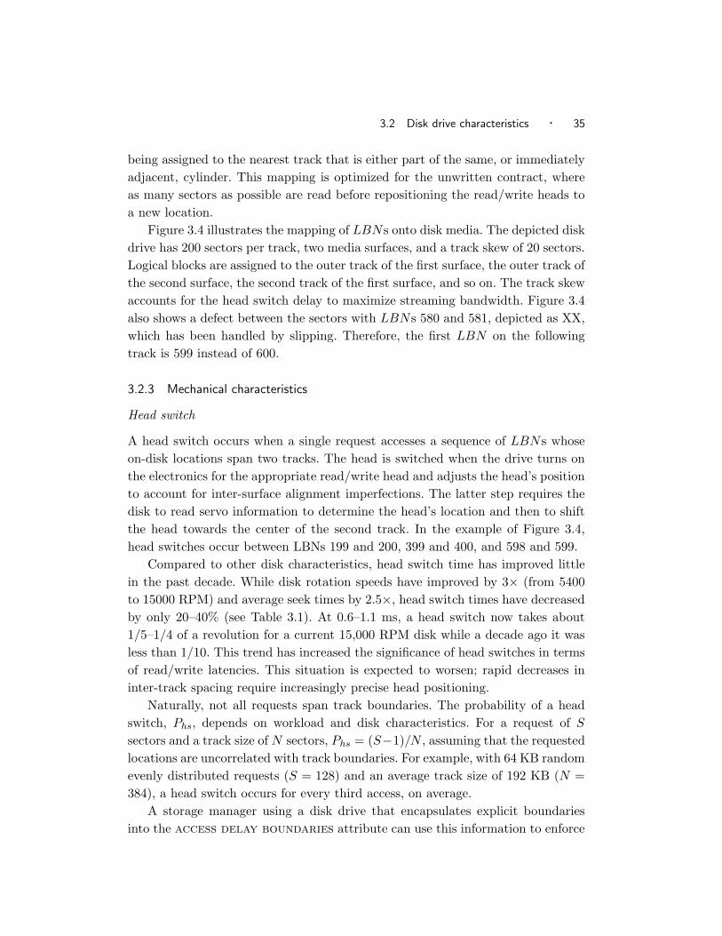
3.2 Disk drive characteristics · 35
being assigned to the nearest track that is either part of the same, or immediately
adjacent, cylinder. This mapping is optimized for the unwritten contract, where
as many sectors as possible are read before repositioning the read/write heads to
a new location.
Figure 3.4 illustrates the mapping of LBNs onto disk media. The depicted disk
drive has 200 sectors per track, two media surfaces, and a track skew of 20 sectors.
Logical blocks are assigned to the outer track of the first surface, the outer track of
the second surface, the second track of the first surface, and so on. The track skew
accounts for the head switch delay to maximize streaming bandwidth. Figure 3.4
also shows a defect between the sectors with LBNs 580 and 581, depicted as XX,
which has been handled by slipping. Therefore, the first LBN on the following
track is 599 instead of 600.
3.2.3 Mechanical characteristics
Head switch
A head switch occurs when a single request accesses a sequence of LBNs whose
on-disk locations span two tracks. The head is switched when the drive turns on
the electronics for the appropriate read/write head and adjusts the head’s position
to account for inter-surface alignment imperfections. The latter step requires the
disk to read servo information to determine the head’s location and then to shift
the head towards the center of the second track. In the example of Figure 3.4,
head switches occur between LBNs 199 and 200, 399 and 400, and 598 and 599.
Compared to other disk characteristics, head switch time has improved little
in the past decade. While disk rotation speeds have improved by 3× (from 5400
to 15000 RPM) and average seek times by 2.5×, head switch times have decreased
by only 20–40% (see Table 3.1). At 0.6–1.1 ms, a head switch now takes about
1/5–1/4 of a revolution for a current 15,000 RPM disk while a decade ago it was
less than 1/10. This trend has increased the significance of head switches in terms
of read/write latencies. This situation is expected to worsen; rapid decreases in
inter-track spacing require increasingly precise head positioning.
Naturally, not all requests span track boundaries. The probability of a head
switch, Phs, depends on workload and disk characteristics. For a request of S
sectors and a track size of N sectors, Phs = (S−1)/N , assuming that the requested
locations are uncorrelated with track boundaries. For example, with 64 KB random
evenly distributed requests (S = 128) and an average track size of 192 KB (N =
384), a head switch occurs for every third access, on average.
A storage manager using a disk drive that encapsulates explicit boundaries
into the access delay boundaries attribute can use this information to enforce

36
·M
atc
hin
gA
pplica
tion
Acc
ess
Patt
erns
toSto
rage
Dev
ice
Char
act
eristics
Head Avg. Sectors Number
Disk Year RPM Switch Seek per Track of Tracks Capacity
HP C2247 1992 5400 1 ms 10 ms 96–56 25649 1 GBQuantum Viking 1997 7200 1 ms 8.0 ms 216–126 49152 4.5 GBIBM Ultrastar 18 ES 1998 7200 1.1 ms 7.6 ms 390–247 57090 9 GBIBM Ultrastar 18LZX 1999 10000 0.8 ms 5.9 ms 382–195 116340 18 GBQuantum Atlas 10K 1999 10000 0.8 ms 5.0 ms 334–224 60126 9 GBFujitsu MAG3091 1999 10025 0.7 ms 5.2 ms 420–273 49125 9 GBQuantum Atlas 10K II 2000 10000 0.6 ms 4.7 ms 528–353 52014 9 GBSeagate Cheetah X15 2000 15000 0.8 ms 3.9 ms 386–286 103750 18 GBSeagate Cheetah 36ES 2001 10028 0.6 ms 5.2 ms 738–574 105208 36 GBMaxtor Atlas 10K III 2002 10000 0.6 ms 4.5 ms 686–396 124088 36 GBFujitsu MAN3367MP 2002 10025 0.6 ms 4.5 ms 738–450 118776 36 GB
Table 3.1: Representative SCSI disk characteristics. Note the small change in head switch time relative to other characteristics. Althoughthere exist versions of the Seagate Fujitsu, and Maxtor drives with higher capacities, the lower capacity drives are typically installed in disk arraysto maximize the number of available spindles.

3.2 Disk drive characteristics · 37
track-aligned access. This improves the response time of most requests by the 0.6–
1.1 ms head switch time. For a conventional system that is not aware of track
boundaries, almost every request will involve a head switch as S approaches N .
Seek
Since a seek involves moving the set of arms from one radial location (i.e., cylin-
der) to another, seek time is expressed as a function of cylinder distance rather
than as a function of distance in the LBN space. Figure 3.5 shows seek profiles
for representative disks from Table 3.1. For small distances (i.e., several cylinders)
and medium distances, the seek time profile follows a curve that can be approxi-
mated by√
d, where d equals cylinder distance [Ruemmler and Wilkes 1993]. For
sufficiently large d, the seek time is a linear function of cylinder distance. Finally,
the average seek time listed in Table 3.1 corresponds to d being equal to 1/3 of the
full-strobe seek distance; the average seek value of every possible distance from
every possible location on the disk.
Thanks to a steady increase in linear bit densities in today’s disk, more LBNs
fit within a track (e.g., 686 for a 2002 Maxtor Atlas 10K III disk vs. 96 for a 1992
HP C2247) and due to improvements in servo technology, a seek of a few cylinders,
for some disks up to five, is now equivalent to a head switch. With these two trends
combined, an increasingly larger number of LBNs can be serviced with a fixed
positioning cost.
Rotational speed
Another factor that contributes to the total positioning cost is rotational latency.
Even though rotational speed improvements have kept up with improvements in
seek times, accessing two randomly chosen locations within a few cylinders (i.e., a
few thousand LBNs away) will produce, on average, a rotational latency of half a
revolution. Compared to a short-distance sub-millisecond seek, this 2–3 ms delay
becomes increasingly more important. With properly chosen access patterns able
to exploit firmware features that minimize the impact of rotational latency, as
discussed in the next section, the access cost penalty can be minimized to that of
a seek.
3.2.4 Firmware features
Zero-latency access and scheduling are two prominent disk firmware features that
improve I/O performance by reducing the time disk head is not transferring data.
With all else being equal, overall request service time is reduced and thus the

38 · Matching Application Access Patterns to Storage Device Characteristics
0 2000 4000 6000 8000 100000
2
4
6
8
10
12Full Seek Curve (Quantum Atlas 10K)
Seek Distance [Cylinders]
See
k T
ime
[ms]
0 2000 4000 6000 8000 100000
2
4
6
8
10
12Full Seek Curve (Fujitsu MAG3091)
Seek Distance [Cylinders]S
eek
Tim
e [m
s]
0 5000 10000 150000
2
4
6
8
10
12Full Seek Curve (Quantum Atlas 10K II)
Seek Distance [Cylinders]
See
k T
ime
[ms]
0 4000 8000 120000
2
4
6
8
10
12Full Seek Curve (Seagate Cheetah X15)
Seek Distance [Cylinders]
See
k T
ime
[ms]
0 10000 20000 300000
2
4
6
8
10
12Full Seek Curve (Seagate Cheetah 36ES)
Seek Distance [Cylinders]
See
k T
ime
[ms]
0 10000 20000 30000 400000
2
4
6
8
10
12Full Seek Curve (Maxtor Atlas 10K III)
Seek Distance [Cylinders]
See
k T
ime
[ms]
Fig. 3.5: Representative seek profiles.

3.2 Disk drive characteristics · 39
efficiency of disk accesses increases. We define disk efficiency as the ratio between
the time spent in useful data transfer (i.e., media read or write) to total request
service time.
Zero-latency access
Zero-latency access, also known as immediate access or access-on-arrival, improves
request response time by accessing disk sectors as they arrive underneath the
disk head. When disk wants to read S contiguous sectors, the simplest approach
is to position the head (through a combination of seek and rotational latency)
to the first sector and read the S sectors in ascending LBN order. With zero-
latency access support, disk firmware can read the S sectors from the media into
its buffers in any order. In the best case, in which exactly one track is read, the
head can start reading data as soon as the seek is completed; no rotational latency
is involved because all sectors on the track are needed. The S sectors are read into
an intermediate buffer, assembled in ascending LBN order, and sent to the host.
The same concept applies to writes, except that data must be moved from host
memory to the disk’s buffers before it can be written onto the media.
As an example of zero-latency access on the disk from Figure 3.4, consider a
read request for LBNs 200–399. First, the head is moved to the track containing
these blocks. Suppose that, after the seek, the disk head is positioned above the
sector containing LBN 380. A zero-latency disk can immediately read LBNs 380–
399. It then reads the sectors with LBNs 200–379. This way, the entire track can
be read in one rotation even though the head arrived in the “middle” of the track.
The expected rotational latency for a zero-latency disk decreases as the request
size increases, as shown in Figure 3.6. Therefore, a request to the zero-latency
access disk for all N sectors on a track requires only one revolution after the
seek. An ordinary disk, on the other hand, has an expected rotational latency of
(N − 1)/(2 · N), or approximately 1/2 revolution, regardless of the request size
and thus a request requires anywhere from one to two (average of 1.5) revolutions.
Appendix A derives a formula for computing expected rotational latency as a
function of request size.
Scheduling
High-end disk drives [Quantum Corporation 1999] include algorithms for request
scheduling. These algorithms are variants of the SPTF (Shortest Positioning Time
First) algorithm [Seltzer et al. 1990; Jacobson and Wilkes 1991; Worthington et al.
1994] and strive to increase disk efficiency by minimizing overall positioning time
(i.e., the sum of seek and rotational latency). Given the current disk head position

40 · Matching Application Access Patterns to Storage Device Characteristics
Average Rotational Latency for a 10K RPM disk
0
1
2
3
4
5
6
0% 25% 50% 75% 100%I/O size [% of track size]
Rot
atio
nal l
aten
cy [m
s]Zero-latency DiskOrdinary Disk
Fig. 3.6: Average rotational latency for ordinary and zero-latency disks as a functionof track-aligned request size. The request size is expressed as a percentage of the track size.
and a queue of pending requests, the SPTF algorithm chooses its next request from
the queue based on which request can be serviced with the smallest positioning
time. Minimizing the disk head positioning time results in smaller request response
times and hence improved efficiency.
As SPTF-based scheduling algorithms require detailed information about cur-
rent disk head position, the natural place for their implementation is inside the
firmware behind the storage device interface. Even though several research projects
implemented SPTF-like algorithms outside of disk firmware [Huang and cker Chi-
ueh 1999; Lumb et al. 2002; Yu et al. 2000], doing so required either detailed
disk models calibrated to specific disks or significant efforts that did not yield
the efficiency afforded by algorithms built into the firmware. Hence, for best-effort
workloads, a storage manager should use scheduling as a transparent feature of a
modern disk drive that sits below the storage interface rather than implementing
it itself.
As described by previous studies [Jacobson and Wilkes 1991; Worthington
et al. 1994], the efficiency of disk accesses improves with increased queue depth of
pending requests. However, the complicated spatio-temporal relationships between
the LBNs of the storage interface are quite difficult to capture in a high level
attribute annotating the device LBN address space. Hence, a storage manager
should exploit this feature by adding a rule that larger queue depths improve
efficiency to the unwritten contract. In today’s systems, this fact is overlooked.

3.3 MEMS-based storage devices · 41
Device capacity 3.46 GBAverage random seek 0.56 msStreaming bandwidth 38 MB/s
Table 3.2: Basic MEMS-based storage device parameters. MEMStores will have a capacityof a few GB, sub-millisecond random seek times, and streaming bandwidth on par with disk drives.
3.3 MEMS-based storage devices
Microelectromechanical systems (MEMS) are mechanical structures on the order
of 10–1000 µm in size fabricated on the surface of silicon wafers [Maluf 2000; Wise
1998]. These microstructures are created using photolithographic processes simi-
lar to those used to manufacture other semiconductor devices (e.g., processors and
memory) [Fedder et al. 1996]. MEMS structures can be made to slide, bend, and
deflect in response to electrostatic or electromagnetic forces from nearby actua-
tors or from external forces in the environment. A MEMS-based storage device
uses MEMS for either positioning of recording elements (e.g., magnetic read/write
heads) or the magnetic media sled.
MEMStores are the goal of efforts at several research centers, including IBM
Zurich Research Laboratory [Vettiger et al. 2000] and Carnegie Mellon University
(CMU). While actual devices do not yet exist, Table 3.2 shows their predicted high-
level characteristics. This section briefly describes relevant physical characteristics
including their interesting form of internal parallelism. This description is based
on the CMU MEMStore design [Griffin et al. 2000a; Schlosser et al. 2000].
3.3.1 Physical characteristics
Most MEMStore designs, such as that illustrated in Figure 3.7, consist of a media
sled and an array of several thousand probe tips. Actuators position the spring-
mounted media sled in the X-Y plane, and the stationary probe tips access data
as the sled is moved in the Y dimension. Each read/write tip accesses its own
small portion of the media, which naturally divides the media into square regions
and reduces the range of motion required by the media sled. For example, in the
device shown in Figure 3.7, there are 100 read/write tips and, thus, 100 squares.
Data are stored in linear columns along the Y dimension. As with disks, a
MEMStore must position the probe tips before media transfer can begin. This
positioning is done by moving the sled in the X direction, to reach the right
column, and in the Y direction, to reach the correct starting offset within the
column. The X and Y seeks occur in parallel, and so the total seek time is the
maximum of the two independent seek times. Once the media sled is positioned,
read/write tips access data as the sled moves at a constant rate in the Y direction.

42 · Matching Application Access Patterns to Storage Device Characteristics
Actuators Media sled
Read/write tips access media in parallel
Fig. 3.7: High-level view of a MEMStore. The major components of a MEMStore are thesled containing the recording media, MEMS actuators to position the media, and the read/writetips that access the media. This picture emphasizes the media organization, which consists of atwo-dimensional array of squares, each of which is accessed by a single read/write tip (not shown).As the media is positioned, each tip accesses the same position within its square, thus providingparallel access to data.
As in disks, data are stored in multi-byte sectors, such as 512 bytes, to reduce
the overhead of extensive error correction coding (ECC). These sectors generally
map one-to-one with the LBNs exposed via the device interface. Unlike disks,
a MEMStore stripes each sector across many tips for two reasons: performance
and fault tolerance. A single tip’s transfer rate is quite low, and transferring an
entire sector with a single tip would require 10× more time than a random seek.
In addition, some of the 1000s of probe tips will be defective, and encoding each
sector across tips allows the ECC to cope with tip failures. Data are striped across
multiple tips for these reasons and grouped together into 512 byte LBNs.
Once striping is assumed, it is useful to consider that the number of active tips
has been reduced by the striping factor (the number of tips over which a single
LBN has been striped), and that each tip accesses a single, complete 512 byte
LBN . In this way, there is a virtual geometry which is imposed on the physical
media, one which exposes full 512 byte LBNs. The example shown in Figure 3.7
has, in reality, 6400 read/write tips with each LBN striped over 64 tips. But once
striping is assumed, the virtual device shown in the figure has only 100 read/write
tips, each accessing a single (striped) LBN at a time.
Given the implicit storage contract described in Section 2.2, MEMStores assign
LBNs to physical locations in accordance with the general expectations of host

3.3 MEMS-based storage devices · 43
4
8
0
18
22
26
31
44
53
40
49
36
45
54
63
67
58
71
56
62
72
76
80
9
13
17
5
27
10 11
12 14
15 16
6
3
7
1 2
19 20
21 23
24 25
28 29
30 32
37 38
39 41
42 43
46 47
48 50
51 52
55
57 59
60 61
64 65
66 68
69 70
73 74
75 77
78 79
33 34 35
Fig. 3.8: Data layout with LBN mappings. The LBNs marked with ovals are at the samelocation within each square and can potentially be accessed in parallel. Depending on otherconstraints, only a subset of those LBNs can be accessed at once.
software: that sequential LBNs can be streamed with maximum efficiency and
that similar LBNs involve shorter positioning delays than very different ones. As
with disk drives, the focus is on the former, with the latter following naturally.
Figure 3.8 shows how LBN numbers are assigned in a simple device. Starting
in the first square, ascending LBN numbers are assigned across as many squares
as can be accessed in parallel to exploit tip parallelism. In this example, three
LBNs can be accessed in parallel, so the first three LBNs are assigned to the
first three squares. The next LBNs are numbered downward to provide physical
sequentiality. Once the bottom of the squares is reached, numbering continues in
the next set of squares, but in the upward direction until the top of the squares
is reached. This reversal in the LBN numbering allows the sled to simply change
direction to continue reading sequential data, maintaining the expectation that
sequential access will be fast.
It is useful to complete the analogy to disk storage, as illustrated in Figure 3.9.
A MEMStore cylinder consists of all LBNs that can be accessed without reposi-
tioning the sled in the X dimension. Because of power constraints, only a subset
of the read/write tips can be active at any one time, so reading an entire cylinder
will require multiple Y dimension passes. Each of these passes is referred to as a
track, and each cylinder can be viewed as a set of tracks. In Figures 3.8 and 3.9,
each cylinder has three tracks. As in disks, sequential LBNs are first assigned
to tracks within a cylinder and then across cylinders to maximize bandwidth for

44 · Matching Application Access Patterns to Storage Device Characteristics
*
**
*
**
*
**
*
**
*
**
*
**
*
**
*
**
*
**
x
x
x
x
x
x
x
x
x|
|
|
|
|
|
|
|
|
| |
| |
| |
| |
| |
| |
| |
| |
| |
| |
| |
| |
| |
| |
| |
| |
| |
| |
Nx
Ny
Sx
Sy
x *Sectors of one track Sectors of one cylinder
Fig. 3.9: MEMStore data layout. This picture illustrates the organization of LBNs into tracksand cylinders and the geometric parameters of the MEMStore. Cylinders are the groups of allLBNs which are at the same offset in the X dimension. In this picture, all of the LBNs of asample cylinder are marked as stars. Because the number of LBNs that can be accessed at onceis limited by the power budget of the device, a cylinder is accessed sequentially in tracks. TheLBNs of a sample track are marked as squares in this picture. Three tracks comprise a singlecylinder, since it takes three passes to access an entire cylinder. The parameters Nx and Ny arethe number of squares in the X and Y directions, and Sx and Sy are the number of LBNs in asingle square in each direction.
sequential streaming and to allow LBN locality to translate to physical locality.
3.3.2 Parallelism in MEMS-based storage
Although a MEMStore includes thousands of read/write tips, it is not possible
to do thousands of entirely independent reads and writes. There are significant
limitations on what locations can be accessed in parallel. Thus, MEMStores can
treat tip parallelism as a means to increase sequential bandwidth or to access a
small set of LBNs in parallel. The size of the set and the locations of these LBNs
are constrained by physical characteristics.
When a seek occurs, the media is positioned to a specific offset relative to the
entire read/write tip array. As a result, at any point in time, all of the tips access
the same locations within their squares. An example of this is shown in Figure 3.8
in which LBNs at the same location within each square are identified with ovals.
Hence, they can potentially be accessed in parallel.

3.3 MEMS-based storage devices · 45
It is important to note that the number of parallel-accessible LBNs is very
small relative to the total number of LBNs in a MEMStore. In the 3.46 GB
device described in Table 3.2, only 100 LBNs are potentially accessible in parallel
at any point out of a total of 6,750,000 total LBNs in the device. Limitations arise
from two factors: the power consumption of the read/write tips, and components
shared among read/write tips. It is estimated that each read/write tip will consume
1–3 mW when active and that continuously positioning the media sled would
consume 100 mW [Schlosser et al. 2000]. Assuming a total power budget of 1 W,
only between 300 and 900 read/write tips can be utilized in parallel which, for
realistic devices, translates to 5–10% of the total number of tips. This gives the
true number of LBNs that can actually be accessed in parallel. In our example
device, perhaps only 10 of 100 LBNs can actually be accessed in parallel.
In most MEMStore designs, several read/write tips will share physical com-
ponents, such as read/write channel electronics, track-following servos, and power
buses. Such component sharing makes it possible to fit more tips, which in turn
increases volumetric density and reduces seek distances. It also constrains which
subsets of tips can be active together.
Figure 3.8 shows a simple example illustrating how LBNs are parallel-accessible.
If one third of the read/write tips can be active in parallel, a system could choose
up to 3 LBNs out of 9 (shown with ovals) to access together. The three LBNs
chosen could be sequential (e.g., 33, 34, and 35), or could be disjoint (e.g., 33,
38, and 52). In each case, all of those LBNs would be transferred to or from the
media in parallel. The pictures showing tracks within contiguous rows of squares
are just for visual simplicity. The tips over which any sector is striped would be
spread widely across the device to distribute the resulting heat load and to create
independence of tip failures. Likewise, the squares of sequentially numbered LBNs
would be physically spread.
Table 3.3 lists parameters describing the virtual geometry of a device with
example values taken from the device shown in Figures 3.8 and 3.9. The number
of parallel-accessible LBNs p, is set by the power budget of the device, as de-
scribed in Section 3.3.1. The total number of squares, N , is defined by the virtual
geometry of the device. Since sequential LBNs are laid out over as many parallel
tips as possible to optimize for sequential access, the number of squares in the
X dimension, Nx, is equal to the level of parallelism, p. The number of squares
in the Y dimension is the total number of squares, N , divided by p. The sectors
per square in either direction, Sx and Sy, is determined by the bit density of each
square. These parameters, along with Nx and Ny, determine the number of sec-
tors per track, ST , and the number of sectors per cylinder, SC . The number of
parallel-accessible LBNs is simply equal to the total number of squares, N , as

46 · Matching Application Access Patterns to Storage Device Characteristics
Name Symbol Example
p Level of parallelism 3N Number of squares 9Sx Sectors per square in X 3Sy Sectors per square in Y 3
Nx Number of squares in X p 3Ny Number of squares in Y N/p 3ST Sectors per track Sy × Nx 9SC Sectors per cylinder ST × Ny 27
Table 3.3: MEMS-based storage device parameters. These are the parameters required todetermine equivalence classes of LBNs that can be potentially accessed in parallel. The first fiveparameters are determined by the physical capabilities of the device and the last four are derivedfrom them. The values in the rightmost column are for the simple device shown in Figures 3.8and 3.9.
there is an equivalent LBN in each square. A two-step algorithm that uses the
MEMStore parameters can calculate all the LBNs that can be accessed in parallel,
as described in Section 6.1.4.
3.3.3 Firmware features
Although physical MEMS-based storage devices do not yet exist, they are expected
to use the storage interface abstraction of fixed-size blocks [Schlosser et al. 2000;
Schlosser et al. 2003].
Scheduling
Griffin et al. [2000b] showed that sled-position-sensitive scheduling algorithms
(e.g., SPTF) outperform basic algorithms such as LOOK or FCFS that do not
require detailed device information. Hence, MEMStores, when implemented, are
likely to include scheduling algorithms built into their firmware just like disk drives.
The storage manager atop a MEMStore can thus exploit scheduling in much the
same way it would with disk drives as described in Section 3.2.4.
3.4 Disk arrays
Since disk drives are the basic building blocks of RAID groups, their media ac-
cess characteristics are the same. However, two unique features distinguish RAID
groups from single disks: data striping and parallel access.

3.4 Disk arrays · 47
3.4.1 Physical organization
To achieve higher concurrency of data accesses and to improve data reliability,
high-end storage systems group together several disk drives to form a single logi-
cal storage device, also called a logical volume. The various RAID levels [Patterson
et al. 1988] trade off reliability, capacity, and performance by striping the logical
volume’s LBNs across individual disks in different patterns [Chen et al. 1994;
Menon and Mattson 1992; Hou et al. 1993]. At the most basic level, the RAID
controller firmware algorithms control striping and initiate data repair after a disk
failure. More advanced controllers can automatically spread out load among the
individual disks or switch to a different RAID level to adapt to changes in work-
loads [Wilkes et al. 1996]. They also implement advanced algorithms for caching
and prefetching of data to mask access latencies.
A RAID controller performs the functions described in the previous paragraphs
atop individual disk drives. It exports a logical volume as a linear address space of
LBNs, which, for current storage interfaces, provides no additional information to
the application-specific storage managers (e.g., inside a filesystem or a relational
database system) about the available parallelism. This disk array-unique feature,
however, is important for parallel access to two-dimensional data structures such
as relational database systems as well as the algorithms (e.g., sort or join) that
operate on these two-dimensional structures [Graefe 1993; Mehta and DeWitt
1995; 1997]. Exposing this information via a well-defined interface, as proposed in
this dissertation, can provide significant performance benefits to these algorithms.
A RAID controller can be thought of as a specialized storage manager; it
exploits the characteristics of its underlying devices i.e., individual disks. However,
it sits behind the device interface, as depicted in Figure 3.1, encapsulating disk
characteristics and other disk-array-unique features into performance attributes,
which are then exposed to the application-specific storage manager.
3.4.2 Data striping
Striping is the process of mapping the logical blocks that form the exported logical
volume to the LBNs of the individual disks comprising the RAID group. While
there are many different ways to do this [Patterson et al. 1988], in general, the
striping process takes a fixed number of blocks, called a stripe unit, and maps it
into LBNs of one disk drive. The next logical stripe unit (e.g., the collection of the
same number of consecutive LBNs that are immediately adjacent in the logical
volume’s address space) is then mapped to the next disk drive. This process is
repeated with stripe units being mapped to the disks in a round-robin fashion.
Thus, stripe units that are not consecutive in the logical volume’s address space

48 · Matching Application Access Patterns to Storage Device Characteristics
are mapped to consecutive locations of the individual disk’s LBN address space.
In addition to protecting against data loss (e.g., with parity stripe or a mirrored
copy of the data), the stripe units can provide the aggregate bandwidth from all
disks in the RAID group. With appropriately sized I/Os that are correctly aligned
on stripe unit boundaries, each disk can perform sequential access. The RAID
controller then assembles the returned data to a single stream.
Choosing the appropriate stripe unit size has direct impact on the performance
for a given workload [Patterson et al. 1988; Chen and Patterson 1990; Chen et al.
1994; Ganger et al. 1994]. In the absence of other information, stripe units approx-
imating the disk track size provide good overall performance [Chen and Patterson
1990]. However, the inability to express these track boundaries, combined with the
zoned-geometries of modern disk drives, results in a loss of potential performance
at the RAID controller level and subsequently at the application level [Schindler
et al. 2003]. Matching stripe units to a disk’s track size, and exporting this exact
size to the application’s storage manager, can recover the lost performance, as
demonstrated in this dissertation.
3.4.3 Parallel access
Striping also provides parallel access to data. With stripe units mapped to different
disk drives and I/Os sized to match stripe unit size and boundaries, the disk drives
in the RAID group can access data in parallel. RAID 1 and RAID 5 configurations
(the two most often used in disk arrays) can achieve n reads in parallel, where n
is the number of disks in the RAID group. While the proper access parallelism
is known at the RAID controller level, this information is not propagated to the
application-specific storage managers where it is needed to determine appropriate
access patterns for workloads with parallel accesses.
4 Discovery of Disk Drive Characteristics
Today’s storage devices do not support the architecture proposed in this disserta-
tion wherein storage devices expose performance attributes to storage managers.
However, by building specialized tools, it is possible to evaluate the benefits of this
type of architecture with current of-the-shelf storage devices. These tools can dis-
cover a device’s performance characteristics, encapsulate them, and expose them
to the storage manager. With assumptions about the inner-workings of the device,
they can do so by using basic read and write commands. The device-specific al-
gorithms are confined to the discovery tool, which sits between the storage device
and the storage manager, neither of which needs to be changed. It appears to the
storage manager as if the performance attributes were exported directly from the
storage device.
This chapter describes a discovery tool called DIXtrac (DIsk eXtractor), which
can quickly and automatically characterize disk drives that understand the Small
Computer System Interface (SCSI) protocol [Schmidt et al. 1995]. Without hu-
man intervention, DIXtrac can discover accurate values for over 100 performance-
critical disk parameters.
In the context of this dissertation, however, only a small fraction of the pa-
rameters are encapsulated into the access delay boundaries and parallelism
attributes that realize the performance improvements reported in Chapter 5 and
6. In particular, the access delay boundaries performance attribute encapsu-
lates the extracted disk track sizes and the parallelism attribute additionally
encapsulates the head-switch and/or one-cylinder seek time. The vast majority of
the parameters extracted by DIXtrac are used for detailed disk models (e.g., in
disk subsystem simulators [Bucy and Ganger 2003] and implementations of rota-
tionally sensitive schedulers outside disk firmware using SPTF [Lumb et al. 2000;
Yu et al. 2000] or freeblock scheduling [Lumb et al. 2000]) but need not be exposed
to strorage managers.
DIXtrac determines most disk characteristics by measuring the per-request
service times for specific test vectors of read and write commands. Other char-
acteristics are determined by interrogative extraction, which uses the wealth of
50 · Matching Application Access Patterns to Storage Device Characteristics
SCSI command options. Most of these techniques were first proposed in previous
work [Worthington et al. 1995] and they have been improved and enhanced for
DIXtrac in several ways. First and foremost, the entire parameter extraction pro-
cess has been automated, which required a variety of changes. By automating this
process, DIXtrac greatly simplifies the process of collecting disk drive character-
istics and works seamlessly as a discovery tool in the alternative storage model
architecture described in Section 3.1 and depicted in Figure 3.1(b). Second, DIX-
trac includes an expert system for interactively discovering a disk’s layout and
geometry. Third, DIXtrac’s extraction techniques account for (some) advances in
current disk drives.
4.1 Characterizing disk drives with DIXtrac
To completely characterize a disk drive, one must describe the disk’s geometry
and layout, mechanical timings, cache parameters and behavior, and all command
processing overheads. Thus, the characterization of a disk consists of a list of
performance-critical parameters and their values. Naturally, such a characteriza-
tion makes implicit assumptions about the general functionality of a disk. For
example, DIXtrac assumes that data are stored in fixed-size sectors laid out in
concentric circles on rotating media.
To reliably determine most parameters, one needs a detailed disk map that
identifies the physical location of each logical block number (LBN) exposed by
the disk interface. Constructing this disk map requires some mechanism for deter-
mining the physical locations of specific LBNs. Using this disk map, appropriate
test vectors consisting of read and write commands can be sent to the disk to
extract various parameters. For many parameters, such as mechanical delays, test
vectors must circumvent the cache. If the structure and behavior of the cache is
known, the actual test vector can be preceded with requests that set the cache
such that the test vector requests will access the media. While it is possible to
devise such test vectors, it is more convenient if the cache can be turned off.
Therefore, to accurately characterize a disk drive, there exists a set of require-
ments that the disk interface must meet. First, it must be possible to determine
the disk’s geometry either experimentally or from manufacturer’s data. Second, it
must be possible to read and write specific LBNs (or specific physical locations).
Also, while it is not strictly necessary, it is very useful to be able to temporarily
turn off the cache. With these few capabilities, DIXtrac can determine the 100+
performance-critical parameters expected by a detailed event-driven disk simulator
such as DiskSim [Bucy and Ganger 2003].
DIXtrac currently works for SCSI disks, which fulfill the three listed require-

4.2 Characterization algorithms · 51
ments. First, the Translate option of the send diagnostic and receive diag-
nostic commands translates a given LBN to its physical address on the disk,
given as a <cylinder,head,sector> tuple. SCSI also provides the read defect
list command, which gives the physical locations of all defective sectors. With
these two commands, DIXtrac can create a complete, concise, and accurate disk
map. Second, the SCSI read and write commands take a starting LBN and a
number of consecutive blocks to be read or written, respectively. Third, the cache
can usually be enabled and disabled by changing the Cache Mode Page with the
SCSI mode select command. The validation results in Section 4.4 show that
these are sufficient for DIXtrac.
4.2 Characterization algorithms
DIXtrac’s disk characterization process can be divided into five logical steps. First,
complete layout information is extracted and a disk map is created. The informa-
tion in the disk map is necessary for the remaining steps, which involve issuing
sequences of commands to specific physical disk locations. Second, mechanical pa-
rameters such as seek times, rotational speed, head switch overheads, and write
settling times are extracted. Third, cache management policies are determined.
Fourth, command processing and block transfer overheads are measured; these
overheads rely on information from the three prior steps. Fifth, request scheduling
policies are determined. The remainder of this section details the algorithms used
for each of these steps.
4.2.1 Layout extraction
In addition to differences in physical storage configurations, the algorithms used
for mapping the logical block numbers (LBNs) exposed by the SCSI interface to
physical sectors of magnetic media vary from disk model to disk model. A common
approach places LBNs sequentially around the topmost and outermost track,
then around the next track of the same cylinder, and so on until the outermost
cylinder is full. The process repeats on the second outermost cylinder and so on
until the locations of all LBNs have been specified. This basic approach is made
more complex by the many different schemes for spare space reservation and the
mapping changes (e.g., reallocation) that compensate for defective media regions.
The firmware of some disks may reserve part of the storage space for its own use.
DIXtrac’s approach to disk geometry and LBN layout extraction experimen-
tally characterizes a given disk by comparing observations to known layout char-
acteristics. To do this, it requires two things of the disk interface: an explicit
mechanism for discovering which physical locations are defective, and an explicit

52 · Matching Application Access Patterns to Storage Device Characteristics
mechanism for translating a given LBN to its physical cylinder, surface and sector
(relative to other sectors on the same track).
DIXtrac accomplishes layout extraction in several steps, which progressively
build on knowledge gained in earlier steps.
1. It uses the read capacity command to determine the highest LBN , and
determine the basic physical geometry characteristics such as number of
cylinders and surfaces by mapping random and targeted LBNs to physical
locations using the send/receive diagnostic command.
2. It uses the read defect list command to obtain a list of all media defect
locations.
3. It determines where spare sectors are located on each track and cylinder, and
detect any other space reserved by the firmware. This is done by an expert-
system-like process of combining the results of several queries, including
whether or not (a) each track in a cylinder has the same number of LBN -
holding sectors; (b) one cylinder within a set has fewer sectors than can be
explained by the defect list; and (c) the last cylinder in a zone has too few
sectors.
4. It determines zone boundaries and the number of sectors per track in each
zone by counting the sectors on a defect-free, spare-free track in each zone.
5. It identifies the remapping mechanism used for each defective sector by back-
translating the LBNs returned in step 21.
Steps 3–5 all exploit the regularity of disk geometry and layout characteristics
to efficiently zero-in on the parameter values, rather than translating every LBN .
DIXtrac identifies the spare space reservation scheme by determining the answers
to a number of questions, including: Does each track in a cylinder have the same
number of sectors? Does one cylinder within a set have fewer sectors than can
be explained by defects? Does the last cylinder of a zone have too few sectors?
By combining these answers, DIXtrac decides which known scheme the disk uses;
so far, we have observed nine different approaches: spare tracks per zone, spare
sectors per track, spare sectors per cylinder, spare sectors per group of cylinders,
spare sectors per zone, spare sectors at the end of the disk, combinations of spare
sectors per cylinder (or group of cylinders), and spare cylinders per zone or smaller
1Remapping approaches used in modern disks include slipping, wherein the LBN -to-physicallocation map is modified to simply skip the defective sector, and remapping, wherein the LBN
that would be located at the given sector is instead located elsewhere but other mappings areunchanged. Most disks will convert to slipping whenever they are formatted via the SCSI formatcommand.

4.2 Characterization algorithms · 53
group of cylinders. The zone information is determined by simply counting the
sectors on tracks as appropriate. The remapping scheme used for each defect is
determined by back-translating the LBN that should be mapped to it (if any)
and then determining to where it has been moved.
DIXtrac uses built-in expertise to discover a disk’s algorithms for mapping
data on the disk in order to make the characterization efficient in terms of both
space and time. An alternate approach would be to simply translate each LBN
and maintain a complete array of these mappings. However, this is much more
expensive, generally requiring over 1000× the time and 300× the result space.
The price paid for this efficiency is that DIXtrac successfully characterizes only
those geometries and LBN layouts that are within its knowledge base.
In order to avoid one extra rotation when accessing consecutive blocks across
a track or cylinder boundary, disks implement track and cylinder skew. The skew
must be sufficiently large to give enough time for the head switch or seek. With
the cache disabled, the track and cylinder skew for each zone can be determined by
issuing two write commands to two consecutive blocks located on two different
tracks or cylinders. The response time of the second request is measured and the
value of track or cylinder skew is obtained as
Skew =TWrite2
∗ sectors per track
Tone revolution
Detecting track boundaries
Knowing exact track boundaries is important for determining efficient I/O sizes
in order to avoid unnecessary head switches and rotational latencies. DIXtrac
implements two different methods: a general one applicable to any disk interface
supporting a read command and a specialized one for SCSI disks, which uses the
algorithm described above.
The general extraction algorithm locates track boundaries by identifying dis-
continuities in access efficiency. Recall that the disk efficiency for requests aligned
on track boundaries increases linearly with the number of sectors being transferred
until a track boundary is crossed. Starting with sector 0 of the disk (s = 0), the
algorithm issues successive requests of increasing size, each starting at sector s
(i.e., read 1 sector starting at s, read 2 sectors starting at s, etc.). The extractor
avoids rotational latency variance by synchronizing with the rotation speed, issu-
ing each request at (nearly) the same offset in the rotational period; rotational
latency could also be addressed by averaging many observations, but at a sub-
stantial cost in extraction time. Eventually, an S-sector read returns in more time
than a linear model suggests (i.e., S = N +1), which identifies sector s+N as the

54 · Matching Application Access Patterns to Storage Device Characteristics
start of a new track. The algorithm then repeats with s = s + S − 1.
The method described above is clearly suboptimal; the actual implementation
uses a binary search algorithm to discover when S = N +1. In addition, once N is
determined for a track, the common case of each subsequent track being the same
size is quickly verified. This verification checks for a discontinuity between s+N−1
and s+N . If one exists, it sets s = s+N−1 and moves on. Otherwise, it sets S = 1
and uses the base method; this occurs mainly on the first track of each zone and
on tracks containing defects. With these enhancements, the algorithm extracts the
track boundaries of a 9 GB disk in four hours. Talagala et al. [2000] describe a
much quicker algorithm that extracts approximate geometry information; however,
for our purposes, the exact track boundaries must be identified.
One difficulty with using read requests to detect track boundaries is the caching
performed by disk firmware. To obviate the effects of firmware caching, the algo-
rithm interleaves 100 parallel extraction operations to widespread disk locations,
such that the cache is flushed each time it returns to block s. An alternative ap-
proach would be to use write requests; however, this is undesirable because of the
destructive nature of writes and because some disks employ write-back caching.
4.2.2 Disk mechanics parameters
Similar to previous work [Worthington et al. 1995], DIXtrac’s central technique
for extracting disk mechanics parameters is to measure the minimum time be-
tween two request completions, called the MTBRC. MTBRC(X, Y ) denotes the
minimum time between the completions of requests of type X and Y . Finding the
minimum time is an iterative process in which the inter-request distance is varied
until the minimal time is observed, effectively eliminating rotational latency for
request Y . An MTBRC value is a sum of several discrete service time compo-
nents, and the individual components can be isolated via algebraic manipulations
as described below.
Time stamps are taken at the initiation and completion of each request, and
MTBRC is computed as the difference of the two completion times as depicted
in Figure 4.1. Finding the minimum time is an iterative process in which the
inter-request distance is varied until the minimal time is observed. The inter-
request distance is the rotational distance between the physical starting locations
of request X and Y .
Since MTBRC includes overheads, e.g., thermal re-calibration or interrupt
delivery to the host computer, it is not sufficient to measure MTBRC only once,
but rather to conduct a series of measurements for each request pair. The com-
putation of MTBRC proceeds as follows: Take several sets of measurements with

4.2 Characterization algorithms · 55
Com-mand
Seek RotationalLatency
MediaAccess
BusTransfer
Com-pletion
HostDelay
Com-mand
RotationalLatency
MediaAccess
BusTransfer
Com-pletion
MTBRC
Inter-Request Distance = X
SectorN
SectorN + X
Request 1 Request 2
Track Start Track End
TIME
Fig. 4.1: Computing MTBRC. The depicted time-line shows the service time componentsfor MTBRC1(1-sector-read, 1-sector-read on the same track) request pair. The accessed track isshown as a straight line. Timestamps are taken at the start and completion of each request. Theinter-request distance is the difference between the starting locations of the two requests. Figurereproduced with the permission of authors [Worthington et al. 1995].
each set containing at least 10 measurements. Discard from each set any values
that differ by more that 10% from the median of the set. Find a mean value from
the remaining values. The number of sets and the number of values in each set
can vary and depends on the type of measurement.
Head switch time
To access sectors on a different surface, a disk must switch on the appropriate
read/write head. The time for head switch includes changing the data path and
re-tracking (i.e., adjusting the position of the head to account for inter-surface
variations). The head switch time can be computed from two MTBRCs:
MTBRC1 =
Host Delay1 + Command + Media Xfer + Bus Xfer + Compl
MTBRC2 =
Host Delay2 + Command + Head Switch + Media Xfer + Bus Xfer + Compl
to get
Head Switch = (MTBRC2 − Host Delay2) − (MTBRC1 − Host Delay1)
This algorithm measures the effective head switch (i.e., the time not overlapped
with command processing or data transfer). While it may not be physically exact,
it is appropriate for disk models and schedulers [Worthington et al. 1995].

56 · Matching Application Access Patterns to Storage Device Characteristics
Seek time
To extract seek times, DIXtrac uses the seek command that, given a logical block
number, positions the arm over the track with that block. Extracted seek time
for distance d consists of measuring 5 sets of 10 inward and 10 outward seeks
from a randomly chosen cylinder. Seek times are measured for seeks of every
distance between 1 and 10 cylinders, every 2nd distance up to 20 cylinders, every
5th distance up to 50 cylinders, every 10th distance up to 100 cylinders, every
25th distance up to 500 cylinders, and every 100th seek distance beyond 500
cylinders. Seek times can also be extracted using MTBRCs, though using the
seek command is much faster. For disks that do not implement seek (although
all of the disks tested here did), DIXtrac measures MTBRC(1-sector write, 1-
sector read) and MTBRC(1-sector write, 1-sector read incurring k-cylinder seek).
The difference between these two values represents the seek time for k cylinders.
Write settle time
Before starting to write data to the media after a seek or head switch, most disks
allow extra time for finer position verification to ensure that the write head is very
close to the center of the track. The write settle time can be computed from head
switch and a pair of MTBRCs: MTBRC1(one-sector-write, one-sector-write on
the same track) and MTBRC2(one-sector-write, one-sector-write on a different
track of the same cylinder). The two MTBRC values are the sum of head switch
and write settle. Therefore, the head switch is subtracted from the measured time
to obtain effective write settle time. As with head switch overhead, the value
indicates settling time not overlapped with any other activity. If the extracted
value is negative, it indicates that write settling completely overlaps with some
other activity (e.g., command processing, bus transfer of data, etc.).
Rotational speed
DIXtrac measures rotation speed via MTBRC(1-sector-write, same-sector-write).
In addition, the nominal specification value can generally be obtained from the
Geometry Mode Page using the mode sense command.
4.2.3 Cache parameters
SCSI disk drive controllers typically contain 512 KB to 8 MB of RAM. This mem-
ory is used for various purposes such as: working memory for firmware, a speed-
matching buffer, a prefetch buffer, a read cache, or a write cache. The prefetch
buffer and read/write cache space is typically divided into a set of circular buffers,

4.2 Characterization algorithms · 57
called segments. Unlike segments of processor caches, they have variable lengths
and start points. The cache management policies regarding prefetch, write-back,
etc. vary widely among disk models. More recent disks provide algorithms that
dynamically partition the cache into different number of segments that are of vari-
able size. While DIXtrac can recognize such a policy, its current algorithms cannot
determine the exact behavior of these dynamic algorithms.
The extraction of each cache parameter follows the same approach: construct
a hypothesis and then validate or disprove it. Testing most hypotheses consists
of three steps. First, the cache is polluted by issuing several random requests of
variable length, each from a different cylinder. The number of random requests
should be larger than the number of segments in the cache. This pollution of the
cache tries to minimize the effects of adaptive algorithms and ensures that the
first request in the hypothesis test will propagate to the media. Second, a series
of cache setup requests are issued to put the cache into a desired state. Finally,
the hypothesis is tested by issuing one or more requests and determining whether
or not they hit in the cache. In its cache characterization algorithms, DIXtrac
assumes that a read or write cache hit takes, at most, 1/4 of the full revolution
time.
This value has been empirically determined to provide fairly robust hit/miss
categorizations, though it is not perfect (e.g., it is possible to service a miss in less
than 1/4 of a revolution). Thus, the extraction algorithms are designed to explicitly
or statistically avoid the short media access times that cause miscategorization.
Basic parameters
DIXtrac starts cache characterization by extracting four basic parameters. Given
the results of these basic tests, the other cache parameters can be effectively ex-
tracted. The four basic hypotheses are:
Cache discards block after transferring it to the host. A read is issued
for one block followed immediately by read of the same block. If the second
read command takes more than 1/4 of a revolution to complete, then it is
a miss and the cache does not keep the block in cache after transferring it
to the host.
Disk prefetches data to the buffer after reading one block. A read is is-
sued to block n immediately followed by a read to block n+1. If the second
read command completion time is more than 1/4 of a revolution, then it
is a cache miss and the disk does not prefetch data after the read. This test
assumes that the bus transfer and host processing time will cause enough

58 · Matching Application Access Patterns to Storage Device Characteristics
delay to incur a “miss” and a subsequent one rotation delay on reading block
n + 1 if the disk were to access the media.
WRITEs are cached. A read is issued to block n immediately followed by a
write to the same block. If the write completion time is more than 1/4 of
a revolution, then the disk does not cache writes.
READs hit on data placed in cache by WRITEs. A write is issued to
block n followed by a read of the same block. If the read completion time
is more that 1/4 of a revolution, then the read is a cache miss and read
hits are not possible on written data stored in cache.
Cache segments
Number of read segments. The number of segments is set to some hypothesized
number N (e.g. N = 64). First, the cache is polluted as described above. Second,
N reads are issued to the first logical block LBNk of N distinct cylinders, where
1 ≤ k ≤ N . Third, the contents of the cache is probed. If the disk retains the
read value in the cache after transferring it to the host, N reads are issued to
LBNk; otherwise, if the disk prefetches blocks after a read, N reads are issued to
LBNk + 1. If any of the reads take longer than 1/4 of a revolution, it is assumed
that a cache miss occurred. The value of N is decremented and the algorithm
repeated. If all reads were cache hits, the cache used at least N segments. In that
case, N should be incremented and the algorithm repeated.
Using a binary search, the correct value of N is found. DIXtrac also determines
if the disk cache uses an adaptive algorithm for allocating the number of segments
by keeping track of the upper boundaries during the binary search. If an upper
boundary for which there has been both a miss and a hit is encountered, then the
cache uses an adaptive algorithm and the reported value may be incorrect.
DIXtrac’s algorithm for determining the number of segments assumes that
a new segment is allocated for reads of sectors from distinct cylinders. It also
assumes that every disk’s cache either retains the read block in cache or uses
prefetching. Both assumptions have held true for all tested disks.
Number of write segments. DIXtrac counts write segments with the same
basic algorithm as for read segments, simply replacing the read commands with
writes. Some disks allow sharing of the same segment for reads and writes. In
this case, the number of write segments denotes how many segments out of the
total number (which is the number of read segments) can be also used for caching
writes. For disks where reads and writes do not share segments, simply adding
the two numbers gives the total number of segments.

4.2 Characterization algorithms · 59
Size of a segment. An initial value is chosen for the segment size S (e.g.,
the number of sectors per track in a zone). If the cache retains cached values after
a transfer to the host, N reads of S blocks are issued each starting at LBNk,
where N is the previously determined number of read segments. Then, the cache
is probed by issuing N one-block reads at LBNk. If there were no misses, S is
incremented and the algorithm repeated.
If the cache discards the cached value after a read, one-block reads are issued
to LBNk, after waiting sufficiently long for each prefetch to finish (e.g., several
revolutions). This will help determine if there are hits on LBNk + 1. As before,
binary search is used to find the segment size S and to detect possible adaptive
behavior. This algorithm assumes that prefetching can fill the entire segment. If
it is not the case, the segment size may be underestimated.
Prefetching
Number of prefetched sectors. A one-block read is issued at LBN1 which is
the logical beginning of the cylinder. After a sufficiently long period of time (i.e.,
4 revolutions), the cache is probed by issuing a one-block read to LBN1 + P
where P is the hypothesized prefetch size. By selecting appropriate LBN1 values,
DIXtrac can determine the maximum prefetch size and whether the disk prefetches
past track and cylinder boundaries.
Track prefetching algorithm. Some disks implement an algorithm that au-
tomatically prefetches all of track n + 1 only after read requests fetch data from
track n−1 and n on the same cylinder. This algorithm minimizes the response time
for the read blocks from n+1st track which is a part of a sequential access pattern.
To test for this behavior, DIXtrac pollutes cache then issues entire-track reads
track n − 1 and n. After waiting at least one revolution, a it issues a one-block
read to a block on track n + 1. If there was a cache hit and the previous prefetch
size indicated 0, then the disk implements this track-based prefetch algorithm.
Zero-latency access
To minimize the media access time, some disks can access sectors as they pass
under the head rather than in strictly ascending order. This is known as zero-
latency read/write or read/write-on-arrival. To test for read-on-arrival, a one-
block read is issued at the beginning of the track followed by an entire-track
read starting at the same block. If the completion time is approximately two
revolutions, the disk does not implement read-on-arrival, because it takes one
revolution to position to the original block and another revolution to read the
data. If the time is much less, the disk implements read-on-arrival.

60 · Matching Application Access Patterns to Storage Device Characteristics
Degrees of freedom provided by the Cache Mode Page
The SCSI standard defines a Cache Mode Page that allows one to set the various
cache parameters described above. However, since the Cache Mode Page is op-
tional, typically only a subset of the parameters is changeable. To determine what
parameters are changeable and to what degree, DIXtrac runs several versions of
the cache parameter extractions. This information is also valuable for systems that
want to aggressively control disk cache behavior [Shriver et al. 1999]. The first ver-
sion observes the disk’s default cache behavior. Other versions explore the effects of
changing different Cache Mode Page fields, such as the minimal/maximal prefetch
sizes, the number/size of cache segments, the Force-Sequential-Write bit, and the
Discontinuity bit. For each, DIXtrac determines and reports whether changing the
fields has the specified effect on disk cache behavior.
The next version of tests sets the appropriate bits in the mode pages and ex-
amines the possibly changed behavior. For example, the Discontinuity bit that
is defined as “continue prefetching past a boundary” can control the amount
of prefetched data. Together with setting minimal and maximal prefetch sizes,
DIXtrac can determine if the cache allows prefetching past boundaries and if
the behavior differs from the default one. Similarly, DIXtrac disables the Force-
Sequential-Write bit and determines if the disk implements write-on-arrival under
this setting.
Finally, if possible, DIXtrac sets the number and size of segments on the Cache
Mode Page to different values and determines if the cache characteristics change.
If implemented, modifying those parameters can reveal the relationship between
the number and the size of the segments.
4.2.4 Command processing overheads
DIXtrac’s refined and automated MTBRC-based scheme extracts eight command
processing overheads:
MTBRC1(1-sector write, 1-sector read on other cylinder) =
Host Delay + Read Miss After Write + seek + Media Xfer + Bus Xfer
MTBRC2(1-sector write, 1-sector write on other cylinder) =
Host Delay + Write Miss After Write + seek + Media Xfer + Bus Xfer
MTBRC3(1-sector read, 1-sector write on other cylinder) =
Host Delay + Write Miss After Read + seek + Bus Xfer + Media Xfer
MTBRC4(1-sector read, 1-sector read miss on other cylinder) =
Host Delay + Read Miss After Read + seek + Media Xfer + Bus Xfer
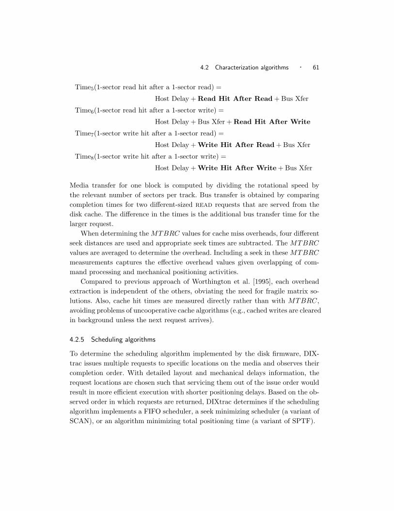
4.2 Characterization algorithms · 61
Time5(1-sector read hit after a 1-sector read) =
Host Delay + Read Hit After Read + Bus Xfer
Time6(1-sector read hit after a 1-sector write) =
Host Delay + Bus Xfer + Read Hit After Write
Time7(1-sector write hit after a 1-sector read) =
Host Delay + Write Hit After Read + Bus Xfer
Time8(1-sector write hit after a 1-sector write) =
Host Delay + Write Hit After Write + Bus Xfer
Media transfer for one block is computed by dividing the rotational speed by
the relevant number of sectors per track. Bus transfer is obtained by comparing
completion times for two different-sized read requests that are served from the
disk cache. The difference in the times is the additional bus transfer time for the
larger request.
When determining the MTBRC values for cache miss overheads, four different
seek distances are used and appropriate seek times are subtracted. The MTBRC
values are averaged to determine the overhead. Including a seek in these MTBRC
measurements captures the effective overhead values given overlapping of com-
mand processing and mechanical positioning activities.
Compared to previous approach of Worthington et al. [1995], each overhead
extraction is independent of the others, obviating the need for fragile matrix so-
lutions. Also, cache hit times are measured directly rather than with MTBRC,
avoiding problems of uncooperative cache algorithms (e.g., cached writes are cleared
in background unless the next request arrives).
4.2.5 Scheduling algorithms
To determine the scheduling algorithm implemented by the disk firmware, DIX-
trac issues multiple requests to specific locations on the media and observes their
completion order. With detailed layout and mechanical delays information, the
request locations are chosen such that servicing them out of the issue order would
result in more efficient execution with shorter positioning delays. Based on the ob-
served order in which requests are returned, DIXtrac determines if the scheduling
algorithm implements a FIFO scheduler, a seek minimizing scheduler (a variant of
SCAN), or an algorithm minimizing total positioning time (a variant of SPTF).

62 · Matching Application Access Patterns to Storage Device Characteristics
4.3 DIXtrac implementation
DIXtrac runs as a regular application on the Linux 2.2 operating system. In tests,
raw SCSI commands are passed to the disk via the raw Linux SCSI device driver
(/dev/sg). Each such SCSI command is composed in this buffer and sent to the
disk via a write system call to /dev/sg. The results of a command are obtained via
a read system call to /dev/sg. The read call then blocks until the disk completes
the command.
DIXtrac extracts parameters in the following steps. First, it initializes the drive.
Second, it performs the 4 steps of the extraction process described in Section 4.2.
Third, it writes out parameter files and cleans up.
The initialization step first sets the drive to conform to the SCSI version 2
definition via the change definition command, allowing the remainder of the
extraction to use this common command set. Next, it issues 50 random read and
write requests which serve to “warm up” the disk. Some drives have request times
which are much longer for the first few requests after they have been sitting idle for
some time. This behavior is due to several factors such as thermal re-calibration
or automatic head parking.
The clean up step restores the disk to its original configuration, resetting the
original SCSI version and cache settings. However, this restoration does not include
stored contents; the extraction steps use write commands to overwrite the original
contents of some sectors. A possible enhancement to DIXtrac would be to save the
original contents of the blocks and restore them during clean up.
To measure elapsed time, DIXtrac uses the POSIX gettimeofday system call,
which returns wall-clock time with a microsecond precision. The Linux implemen-
tation on Intel Pentium-compatible processors uses the processor’s cycle counter to
determine the time: thus the returned time has the microsecond precision defined
(but not required) by POSIX.
Before doing a write system call to the /dev/sg device, the current time is
obtained via the gettimeofday system call. gettimeofday is called again after the
read system call returns with the result of the SCSI command. The execution time
of the SCSI command is the difference between those two times. The time measured
via gettimeofday includes the overheads of the gettimeofday and read/write
calls and may include a sleep time during which other processes are scheduled.
The advantage of using gettimeofday call is that the time can be measured on
an unmodified kernel.
Although it is not required for proper functioning of DIXtrac, the parameter
extractions reported here were performed on a kernel with a modified sg driver that
samples the time in the kernel right before calling the low-level portion of the device

4.4 Results and performance · 63
driver. The measured time is returned as a part of the sg device structure that
is passed to the read and write call. This modification eliminates the overheads
of gettimeofday giving more precise time measurements. The times obtained via
the user-level gettimeofday call on the unmodified kernel are, on average, 1.5%
larger, with a maximum deviation of 6.8%, compared to the time obtained via
modified sg driver.
However, even the time obtained from the modified sg driver includes the PC
bus, host adapter, and SCSI bus overheads. Bus and device driver overheads could
be isolated by measuring time using a logical analyzer attached to the SCSI bus.
DIXtrac assumes that, on average all SCSI commands incur the same bus and
driver overheads. To eliminate bus contention issues, DIXtrac extracts data from
a disk on a dedicated SCSI bus with no other device attached. The effects of other
devices on the PC internal bus are minimized by performing extraction on an
otherwise idle system.
4.4 Results and performance
DIXtrac has been fully tested on many disk models: IBM Ultrastar 18ES, Hewlett-
Packard C2247, Quantum Viking, Quantum Atlas III, Quantum Atlas 10K, Atlas
10K II, Maxtor Atlas 10K III, Fujitsu MAG3091, Seagate Barracuda 4LP, Seagate
Cheetah 4LP, Cheetah 9LP, Cheetah 18LP, Cheetah 73LP, Cheetah 36ES, Chee-
tah X15, Cheetah X15 36LP, and Seagate Hawk. This section evaluates DIXtrac
in terms of extraction times and characterization accuracies and shows detailed re-
sults for the Ultrastar 18ES, Atlas III, Atlas 10K, and Cheetah 4LP disks. Similar
results have been obtained for the other disks.
4.4.1 Extraction times
Table 4.1 summarizes the DIXtrac extraction times. The times are broken down
to show how long each extraction step takes. With the exception of the IBM Ul-
trastar 18ES, an entire characterization takes less than three minutes. Extraction
times could be reduced further, at the expense of accuracy, by using fewer repeti-
tions for the timing extractions (e.g., seek, mechanical, and command processing
overheads).
The extraction time for the IBM Ultrastar 18ES is longer because of the layout
extraction step. The layout of this disk includes periodic unused cylinders, which
causes DIXtrac to create dummy zones and repeat time-consuming, per-zone ex-
tractions (e.g., sectors per track, track skew, etc.). Extraction for this layout could
certainly be optimized, but we are pleased that it worked at all given its unex-
pected behavior.

64 · Matching Application Access Patterns to Storage Device Characteristics
Vendor IBM Quantum SeagateDisk Model Ultrastar Atlas III Atlas 10K CheetahCapacity 9.1 GB 9.1 GB 9.1 GB 4.5 GB
Task Time (seconds)
Layout extraction 164.7 (10.6) 20.9 (0.8) 50.1 (3.9) 47.6 (0.4)Complete seek curve 45.2 (0.1) 43.5 (0.2) 33.3 (0.3) 67.3 (0.1)Mech. overheads 35.8 (1.3) 21.3 (2.5) 18.6 (1.5) 16.6 (1.4)Cache parameters 25.6 (0.6) 8.1 (0.4) 12.6 (0.3) 12.3 (1.8)Process. overheads 64.3 (2.5) 43.5 (1.5) 12.7 (0.9) 23 (2.3)
Totals 335.6 (9.2) 137.4 (3.1) 127.4 (4) 166.8 (3.4)
Table 4.1: Break down of DIXtrac extraction times. The times are mean values of fiveextractions. The values in parentheses are standard deviations. “Mech. overheads” includes theextraction of head switch, write settle, and rotation speed.
Vendor IBM Quantum SeagateDisk Model Ultrastar Atlas III Atlas 10K Cheetah
Capacity (blocks) 17916239 17783250 17783248 8887200Defects 123 56 64 21Translate 1 Address 2.41 ms 1.66 ms 0.86 ms 7.32 msTranslations 36911 7081 26437 5245
Table 4.2: Address translation details.
Table 4.2 shows the number of address translations required by DIXtrac to
characterize each disk. Note that the number of translations does not depend
directly on the capacity of the disk. Instead, it depends mainly on the sparing
scheme, the number of zones, and the number of defects. More translations are
performed for disks with more defects, because slipped and relocated blocks ob-
tained from the defect list are verified. Comparing the number of blocks to the
number of translations provides a metric of efficiency for DIXtrac’s layout dis-
covery algorithms. Given the time required for each translation, this efficiency is
important.
The disk maps obtained by the extraction process have been verified for all
eight models (24 actual disks) by doing address translation of every logical block
and comparing it to the disk map information. The run time of such verification
ranges from almost 5 hours (Quantum Atlas 10K) to 21 hours (Seagate Barracuda).
In addition to validating the extraction process, these experiments highlight the
importance of translation-count-efficiency when extracting the disk layout map.

4.4 Results and performance · 65
Vendor IBM Quantum SeagateDisk Model Ultrastar Atlas III Atlas 10K Cheetah
Trace Type M R M R M R M R
RMSOverall (ms) 0.20 0.07 1.14 0.14 0.30 0.19 0.27 0.43% TMean 4% 1% 18% 1% 9% 2% 5% 4%
Table 4.3: Demetit figures (RMS). RMSOverall is the overall demerit figure for all trace runscombined. The % T Mean value is the percent difference of the respective RMS from the meanreal disk response time. R denotes random trace and M denotes a mixed trace.
4.4.2 Validation of extracted values
Running DiskSim configured with the parameters extracted by DIXtrac allows the
evaluation of the accuracy of parameter extraction. After extracting parameters
from each disk drive, a synthetic trace was generated, and the response time of
each request in the trace was measured on the real disk. The trace run and the
extracted parameter file were then fed to DiskSim to produce simulated per-request
response times. The real and simulated response times were then compared.
Two synthetic workloads were used to test the extracted parameters. The first
synthetic workload was executed on each disk with both read and write caches
turned off. This workload tests everything except the cache parameters. It con-
sists of 5000 independent requests with 2/3 reads and 1/3 writes. The requests
are uniformly distributed across the entire disk drive. The size of the requests is
between 2 and 12 KB with a mean size of 8 KB. The inter-arrival time is uniformly
distributed between 0 and 72 ms.
The second workload focuses on the cache behavior and was executed with
the disk’s default caching policies. This trace consists of 5000 requests (2/3 reads
and 1/3 writes) with a mix of 20% sequential requests, 30% local (within 500
LBNs) requests, and 50% uniformly distributed requests. The size of the requests
is between 2 and 12 KB with a mean size of 8 KB. The inter-arrival time is
uniformly distributed between 0 and 72 ms.
For each disk, five extractions were performed to create five sets of disk param-
eters. For each set of parameters, five mixed traces and five random traces were
generated and run on the real disk as well as on the DIXtrac-configured simulated
disk. So, for each disk, 50 validation experiments were run. The simulated and
measured response times for the four disks are shown in Figure 4.2 and Figure 4.3.
Each curve is a cumulative distribution of all collected response times for the 25
runs, consisting of 125000 data points.
The difference between the response times of the real disk and the DIXtrac-
configured simulator can be quantified by a demerit figure [Ruemmler and Wilkes

66 · Matching Application Access Patterns to Storage Device Characteristics
0 5 10 15 20 250
0.1
0.2
0.3
0.4
0.5
0.6
0.7
0.8
0.9
1
IBM Ultrastar 18ES − Random Trace (RMS=0.07)
Access Time [ms]
Fra
ctio
n of
Res
pons
es
Real Disk DIXtrac/DiskSim
0 5 10 15 20 250
0.1
0.2
0.3
0.4
0.5
0.6
0.7
0.8
0.9
1
IBM Ultrastar 18ES − Mixed Trace (RMS=0.20)
Access Time [ms]
Fra
ctio
n of
Res
pons
es
Real Disk DIXtrac/DiskSim
0 5 10 15 20 250
0.1
0.2
0.3
0.4
0.5
0.6
0.7
0.8
0.9
1
Seagate Cheetah 4LP − Random Trace
Access Time [ms]
Fra
ctio
n of
Res
pons
es
Real Disk Extracted Data
0 5 10 15 20 250
0.1
0.2
0.3
0.4
0.5
0.6
0.7
0.8
0.9
1
Seagate Cheetah 4LP − Mixed Trace
Access Time [ms]
Fra
ctio
n of
Res
pons
es
Real Disk Extracted Data
Fig. 4.2: The comparion of measured and simulated response time CDFs for IBMUltrastar 18ES and Seagate Cheetah 4LP disks.

4.4 Results and performance · 67
0 5 10 15 20 250
0.1
0.2
0.3
0.4
0.5
0.6
0.7
0.8
0.9
1
Quantum Atlas III − Random Trace (RMS=0.14)
Access Time [ms]
Fra
ctio
n of
Res
pons
es
Real Disk DIXtrac/DiskSim
0 5 10 15 20 250
0.1
0.2
0.3
0.4
0.5
0.6
0.7
0.8
0.9
1
Quantum Atlas III − Mixed Trace (RMS=1.14)
Access Time [ms]
Fra
ctio
n of
Res
pons
es
Real Disk DIXtrac/DiskSim
0 5 10 15 20 250
0.1
0.2
0.3
0.4
0.5
0.6
0.7
0.8
0.9
1
Quantum Atlas 10K − Random Trace (RMS=0.19)
Access Time [ms]
Fra
ctio
n of
Res
pons
es
Real Disk DIXtrac/DiskSim
0 5 10 15 20 250
0.1
0.2
0.3
0.4
0.5
0.6
0.7
0.8
0.9
1
Quantum Atlas 10K − Mixed Trace (RMS=0.30)
Access Time [ms]
Fra
ctio
n of
Res
pons
es
Real Disk DIXtrac/DiskSim
Fig. 4.3: The comparion of measured and simulated response time CDFs for QuantumAtlas III and Atlas 10K disks.

68 · Matching Application Access Patterns to Storage Device Characteristics
1993], which is the root mean square distance in the y-dimension between the
two curves. The demerit figure, here referred to as the RMS, for each graph is
given in Table 4.3. Most of these values compare favorably with the most accurate
disk simulation models reported in the literature [Ruemmler and Wilkes 1993;
Worthington et al. 1995].
However, several suboptimal values merit discussion. For the Seagate Chee-
tah 4LP, the simulated disk with DIXtrac-extracted parameters services requests
faster than the real disk. This difference is due to smaller effective values of read
command processing overheads. Manually increasing these values by 0.35 ms re-
sults in a closer match to the real disk with RMS at 0.17 ms and 0.16 ms for the
mixed and random trace respectively.
The differences in the mixed trace runs for the two Quantum disks are due to
shortcomings of DiskSim. DIXtrac correctly determines that the disks use adaptive
cache behavior. However, because DiskSim does not model such caches, DIXtrac
configures it with average (disk-specific) values for the number and size of seg-
ments. The results show that the actual Atlas 10K disk has more cache hits than
the DiskSim model configured with 10 segments of 356 blocks. Interestingly, the
adaptive cache behavior of the real Atlas III disk is worse than the behavior of the
simulated disk configured with 6 segments and 256 blocks per segment. Manually
lowering the value of blocks per segment to 65, while keeping all other parameters
the same, gives the best approximation of the real disk behavior.
These empirical validation results provide significant confidence in the accuracy
of the parameters extracted by DIXtrac. For additional confidence, extracted data
were compared directly with the specifications given in manufacturer’s technical
manuals wherever possible. In all such cases, the extracted values match the data
in the documentation.

5 The Access Delay Boundaries Attribute
Storage-device-provided hints about proper I/O sizes can result in significant
performance improvements to applications. The access delay boundaries at-
tribute denotes groupings of contiguous logical blocks into units that yield efficient
accesses. It also simplifies the task of I/O performance tuning and reduces imple-
mentation complexity; the storage manager (or a human system administrator)
need not implement methods that guess efficient I/O sizes to achieve better per-
formance.
This chapter describes the device-specific features this attribute encapsulates
for disk drives, disk arrays, and MEMStores and quantifies in detail the per-
formance gains for disk drives. It evaluates the benefits this attribute offers to
block-based file systems, log-structured file systems, video servers, and database
systems. Finally, it demonstrates on two implementations, the FreeBSD Fast File
System [McKusick et al. 1984] and the Shore database storage manager [Carey
et al. 1994], that only minimal changes to existing storage managers are needed
to achieve significant performance gains for certain workloads.
5.1 Encapsulation
The access delay boundaries attribute encapsulates the non-linearity in access
times to adjacent logical blocks in the device’s address space due to device physical
characteristics and LBN mappings. While the reasons for these delay boundaries
are unique to each particular storage device type, they can be all expressed by
this attribute, which encapsulates several device-specific characteristics.
5.1.1 Disk drive
For disk drives, delays in accessing adjacent logical blocks occur when these blocks
are mapped to two adjacent tracks. Crossing a track boundary requires a disk head
to move to a new location, incurring head switch delay during which no data is
being transferred. On the other hand, accessing data mapped onto a single track
(i.e., between two access delay boundaries) does not incur this additional delay

70 · Matching Application Access Patterns to Storage Device Characteristics
once the disk head is positioned. For such accesses, the data is streamed with
maximum efficiency.
In addition to disk track boundaries, the access delay boundaries attribute
also encapsulates a disk firmware feature: zero-latency access. While eliminat-
ing head switches improves access efficiency by 6%–8%, combining it with this
firmware features of high-end disks provides much greater benefit as described
and quantified in Section 5.3.1. For such disks, this single attribute therefore en-
capsulates two device-specific characteristics.
5.1.2 Disk array
Logical volumes striped across several disks in a RAID group can experience delays
when either a single stripe unit spans two adjacent disk tracks, or when the logical
blocks being accessed map to more than one stripe unit. For such requests, a
single I/O results in several separate disk accesses. These smaller disk requests
will be less efficient and therefore have a negative effect on achieved throughput
and response times. The access delay boundaries attribute encapsulates the
stripe unit boundaries which, in turn, should match the access delay boundaries
of the components comprising a disk array.
The size of a stripe unit depends on several factors. Some disk array controllers
set the stripe unit size to match that of their cache lines. Other controllers with
caches that allow variable-size buffers may determine stripe unit size according
to the individual disk characteristics. However, they require disk drives to expose
their track sizes via the access delay boundaries attribute. As demonstrated
in Section 5.7.6, RAID controllers exploiting the access delay boundaries at-
tribute hints by matching stripe units to these precise values significantly outper-
form RAID groups whose stripe units, in the absence of additional information,
merely approximate disk track sizes [Chen and Patterson 1990].
5.1.3 MEMStore
Similar to its performance in disk drives, the access delay boundaries attribute
encapsulates the delay in accessing logical blocks mapped to adjacent tracks. When
these blocks are accessed, the media sled must to come to a stop and, at minimum,
reverse it direction. In the worst case, the sled must do a full strobe seek to
reach the logical block mapped onto the next cylinder. As with for disk drives, it
is expected that MEMStores will include in-firmware schedulers that implement
position-sensitive scheduling algorithms [Schlosser et al. 2000].

5.2 System design · 71
5.2 System design
Access delay boundaries break up the linear LBN address space into extents of
LBNs, here referred to as ensembles. An ensemble is thus a collection of contiguous
LBNs that will provide the most efficient device accesses. Because of device-unique
characteristics, ensemble size varies across devices as well as within a single device’s
address space. Thus, the storage manager must be able to cope with this variable
size. However, for many systems, the required changes are minimal and ensembles
are a natural choice for data allocation and access.
The access delay boundaries attribute is suitable for any system that
exhibits access patterns that are, at least to some degree, regular. Such systems
can allocate related data into ensembles of contiguous logical blocks, and then
exploit the efficiency of the ensemble-sized I/Os that are aligned on the access
delay boundary. Even though the ensemble sizes are variable, explicitly stating
where these boundaries occur allows a storage manager to decide what data to
allocate to which ensemble. A storage manager could also choose a particular
storage device whose ensemble sizes match the workload needs.
5.2.1 Explicit contract
This attribute provides an explicit contract between the SM and a storage device:
(1) Requests that are exactly aligned on the reported boundaries and span all
the blocks of a single ensemble are most efficient.
(2) Requests smaller than the preferred groupings should not, if possible, span
a boundary.
The two implementations of storage manager (i.e., a block-based file system
and a database storage manager) described in this dissertation demonstrate that
the changes required to use the ensembles that encapsulate the access delay
boundaries attribute require relatively minor changes to existing systems. This
section discusses practical design considerations involved with these changes.
5.2.2 Data allocation and access
To utilize ensemble boundary information, the storage manager’s algorithms for
data placement and request generation must support variable-sized extents. Extent-
based file systems, such as NTFS [Nagar 1997] and XFS [Sweeney 1996], allocate
disk space to files by specifying ranges of LBNs (extents) associated with each
file. Such systems lend themselves naturally to ensemble-based alignment of data:
during allocation, extent ranges can be chosen to fit track boundaries. Block-based

72 · Matching Application Access Patterns to Storage Device Characteristics
file systems, such as Ext2 [Bovet and Cesati 2001] and FFS [McKusick et al. 1984],
group LBNs into fixed-size allocation units (blocks), typically 4 KB or 8 KB.
Block-based systems can approximate track-sized extents by placing sequential
runs of blocks such that they never span track boundaries. This approach wastes
some space when track sizes are not evenly divisible by the block size. However,
this space is usually 2–3% of total storage space and could be reclaimed by the
system for storing inodes, superblocks, or fragmented blocks. Alternatively, this
space can be reclaimed if the cache manager is modified to handle partially-valid
and partially-dirty blocks.
Like any clustering storage system, a ensemble-based system must address ag-
ing and fragmentation and the standard techniques apply: pre-allocation [Bovet
and Cesati 2001; Giampaolo 1998], on-line reallocation [Lumb et al. 2000; Rosen-
blum and Ousterhout 1992; Smith and Seltzer 1996], and off-line reorganiza-
tion [Blackwell et al. 1995; Matthews et al. 1997]. For example, when a system
determines that a large file is being written, it may be useful to reserve (preallo-
cate) entire ensembles even when writing less than a ensemble worth of data. The
same holds when grouping small files [Ganger and Kaashoek 1997; Reiser 2001].
When the file system becomes aged and fragmented, on-line or off-line reorgani-
zation can be used to re-optimize the on-disk layout. Such reorganization can also
be used for retrofitting pre-existing disk partitions or adapting to a new layout of
a replacement disk. The point of this dissertation is to show that ensembles are a
good target layout for these techniques.
After allocation routines are modified to situate data on track boundaries,
system software must also be extended to generate ensemble requests whenever
possible. Usually, this will involve extending or clipping prefetch and write-back
requests based on ensemble boundaries.
5.2.3 Interface implementation
The get ensemble(LBN) function of the storage interface proposed in this disser-
tation returns access delay boundaries. Given an LBN , it returns the ensemble’s
boundaries, LBNmin and LBNmax, where LBNmin ≤ LBN ≤ LBNmax. The en-
semble size is |LBNmax − LBNmin|; a request (in consecutive LBNs) of that size
starting at LBNmin yields most efficient device access.
The sif ensemble() function, whose C declaration is listed in Appendix B,
implements the get ensemble() function. It takes four arguments: the lvh is an
opaque logical volume of a given storage device, the input argument lbn is the
LBN for which an ensemble should be returned, and the low and high arguments
return the LBNmin and LBNmax, respectively.

5.3 Evaluating ensembles for disk drives · 73
To allocate data for efficient access, a storage manager takes an lbn from a
free block list, calls sif ensemble(), and checks that none of the blocks between
the low and high blocks are allocated. If data to be allocated is smaller than
the returned ensemble, the storage manager can either call sif ensemble() with
another free lbn to find a more suitable free ensemble with fewer LBNs or mark
the remaining LBNs in the ensemble as allocated. The data is then written to the
device and all the allocation structures are updated.
To determine an I/O size that would yield efficient access (e.g., when deter-
mining how much to prefetch), the storage manager calls sif ensemble() with
the appropriate lbn to obtain the values of low and high. It then allocates a suf-
ficiently large buffer to fit all data and issues sif read(), where lbn equals the
low and cnt equals high - low. The next prefetch I/O will repeat this procedure
and use the value high + 1 as the lbn parameter.
5.3 Evaluating ensembles for disk drives
This section examines the performance benefits of ensemble-based accesses to the
disk drive, finding a 50% improvement in access efficiency and a significant reduc-
tion in response time variance. The ensemble-based access is achieved by properly
sizing and aligning I/Os on disk track boundaries, which are determined by the
DIXtrac tool. First, the improvements measured on actual disks are shown fol-
lowed by predictions for future disk generations based on an accurate analytical
model.
5.3.1 Measuring disk performance
Experimental setup
Most of the experiments described in this section were performed on two disks that
support zero-latency access (Quantum Atlas 10K and Quantum Atlas 10K II)
and two disks that do not (Seagate Cheetah X15 and IBM Ultrastar 18 ES).
The disks were attached to a 550 MHz Pentium III-based PC. The Atlas 10K II
was attached via an Adaptec Ultra160 Wide SCSI adapter, the Atlas 10K and
Ultrastar were attached via an 80 MB/s Ultra2 Wide SCSI adapter, and the
Cheetah via a Qlogic FibreChannel adapter. We also examined workloads with the
DiskSim disk simulator [Bucy and Ganger 2003] configured to model the respective
disks. Examining these disks in simulation enables us to quantify the individual
components of the overall response time, such as seek and bus transfer time.

74 · Matching Application Access Patterns to Storage Device Characteristics
Increasing efficiency
System software attempts to maximize overall performance in the face of two com-
peting pressures. On one hand, the underlying disk technology pushes for larger
request sizes in order to maximize disk efficiency. Specifically, time-consuming me-
chanical delays can be amortized by transferring large amounts of data between
each repositioning of the disk head. However, resource limitations and imperfect
information about future accesses impose costs on the use of very large requests.
With ensemble-based access, requests can be much smaller and still achieve the
same disk efficiency, as illustrated in Figure 5.1. The graphs show disk efficiency
as a function of I/O size, where disk efficiency is the fraction of total access time
(which includes seek and rotational latency) spent moving data to or from the
media. The track-aligned and unaligned lines show disk efficiency for random,
constant-sized reads within the first zone of Quantum Atlas 10K II and Seagate
Cheetah X15 disks. The drop-off in efficiency for track-aligned accesses occurs just
after a multiple of the first zone’s track size. The dotted horizontal line represents
best-case steady-state efficiency: sequential data streaming.
In Figure 5.1(a), Point B shows that reading or writing 1 MB at a time results
in a 75% disk efficiency for normal (track-unaligned) access. Point A highlights
the higher efficiency of track-aligned access (0.73, or 82% of the maximum) over
unaligned access for a track-sized request. With I/O size four times as big at
Point B, normal I/O efficiency catches up to track-aligned efficiency at Point A.
The peaks in the track-aligned curve correspond to multiples of the track size.
Importance of zero-latency access
The relative increase in the efficiency of track-based access is different for the two
disks depicted in Figure 5.1. This difference stems from the employment of zero-
latency access. While the Quantum Atlas 10K II disk, whose firmware implements
zero-latency access, experiences a 48% increase in efficiency for track-based access,
the Seagate Cheetah X15, which does not have this feature, experiences only a
moderate improvement of 8%.
The increase in disk efficiency for other zero-latency disks is similar to the
Quantum Atlas 10K II’s 48% increase. The Quantum Atlas 10K achieves 47%
higher efficiency and the Maxtor Atlas 10K III 40%. These variations are due to
different sizes of the disk’s first zone and thus different average seek times for the
random track-aligned I/Os within that zone.
Disk efficiency for track-based random I/Os increases only moderately on disks
that do not support zero-latency access: 6% for the IBM Ultrastar 18ES and 8%
for the Seagate Cheetah X15, depicted in Figure 5.1(b). For these disks, aligning

5.3 Evaluating ensembles for disk drives · 75
Quantum Atlas 10K II Efficiency vs. I/O Size
0
0.2
0.4
0.6
0.8
1.0
Dis
k ef
ficie
ncy
A
B
maximum streaming efficiency
0 256 512 768 1024 1280 1536 1792 2048I/O size [KB]
Track-aligned I/O
Unaligned I/O
(a) Zero-latency disk.
Seagate Cheetah X15 Efficiency vs. I/O Size
0
0.2
0.4
0.6
0.8
1.0
0 256 512 768 1024 1280 1536 1792 2048I/O size [KB]
Dis
k ef
ficie
ncy
Track-aligned I/O
Unaligned I/O
maximum streaming efficiency
(b) Non-zero-latency disk.
Fig. 5.1: Disk access efficiency. This graph plots disk efficiency as a function of I/O size fortrack-unaligned and track-aligned random requests within a disk’s first zone. Disk efficiency isthe fraction of total access time (which includes seek and rotational latency) spent moving datato or from the media. The maximum streaming efficiency (i.e., sequential access without seeksand rotational latencies) is less than 1.0 due to head switches between accesses to adjacent tracks.The peaks in the track-aligned curve correspond to multiples of the track size.

76 · Matching Application Access Patterns to Storage Device Characteristics
Cheetah 36ES Simulated Zero-latency (tworeq)
14.87
13.0912.26
11.35 11.33 11.79
0
2
4
6
8
10
12
14
16
1 2 4 8 16 32Requests per track
Tra
ce r
untim
e [s
]
Fig. 5.2: Getting zero-latency-disk-like efficiency from ordinary disks. The average seektime for LBNs in the disk’s first zone is 3.2 ms. The bus transfer of 738 blocks (sectors per trackin the first zone) takes 2.7 ms.
accesses on track boundaries eliminates only the 0.8–1.1ms head switch time—the
average rotational latencies of 4 ms (Ultrastar 18ES) and 2 ms (Cheetah X15) are
still incurred.
Even though disk firmware may not implement zero-latency access, it is pos-
sible to achieve zero-latency-disk-like improvements from such disks. Taking ad-
vantage of the disk firmware scheduler and command queuing, a single track-sized
request aligned on a track boundary can be broken into smaller requests that can
be issued to the disk together. The disk scheduler services them so as to minimize
the rotational latency. Once it selects a request rotationally closest to the current
head position, all other requests will be serviced without incurring any additional
rotational latency; effectively simulating zero-latency access.
Figure 5.2 shows how breaking a single track-based request into several smaller
requests achieves the desired performance. The graph shows the total run time of
a stream consisting of 1000 random track-sized and track-aligned requests going
to the disk’s first zone. One full-track request gives an average response time of
14.87 ms, which includes a seek, an average of 3 ms rotational latency, 6 ms for
media access and some amount of non-overlapping bus transfer. As this track-
sized request is broken into smaller requests, the average response time decreases
to 11.33 ms. With smaller requests issued to the disk simultaneously, the bus
transfer of data from the previous request can overlap with the media transfer of
the next request. Hence, the observed 3.55 ms improvement is larger that the 3 ms
expected improvement due to elimination of rotational latency.

5.3 Evaluating ensembles for disk drives · 77
mxferseekmxferseek
endT
2 end
T1
head time
onereq
issueT
2 issueT
1 start
T2
startT
1 = =
mxferseek
bxfer
bxfer
mxferseek
bxfer
bxfer
endT
2 end
T1
head time
tworeq
issueT
2 issueT
3 start
T2
startT
3 start
T1
bxfer
idle idle
time
Fig. 5.3: Expressing head time. The head time of a onereq request is T end
2 −T issue
2 . For tworeq,the head time is T end
2 − T end
1 . T issue is the time when the request is issued to the disk, T start iswhen the disk starts servicing the request, and T end is when completion is reported. Notice thatfor tworeq, T issue does not equal T start because of queueing at the disk.
Microbenchmark performance
Two synthetic workloads, onereq and tworeq, were used to evaluate basic track-
aligned performance. Each workload consists of 5000 random requests within the
first zone of the disk. The difference is that onereq keeps only one outstanding
request at the disk, whereas tworeq ensures one request is always queued at the
disk in addition to the one being serviced.
We compared the efficiency of both workloads by measuring the average per-
request head time. A request’s head time is the amount of time that the disk head
is dedicated to that request. The average head time is the reciprocal of request
throughput (i.e., I/Os per second). Therefore, higher disk efficiency will result in
a shorter average head time, all else being equal. We introduced head time as a
metric because it allows us to identify component delays more easily.
For onereq requests, head time equals disk response time as observed by the
device driver, because the next request is not issued until the current one is com-
plete. As usual, disk response time is the elapsed time from when a request is sent
to the disk to when completion is reported. For onereq requests, the read/write
head is idle for part of this time, because the only outstanding request is wait-
ing for a bus transfer to complete. For tworeq requests, the head time includes
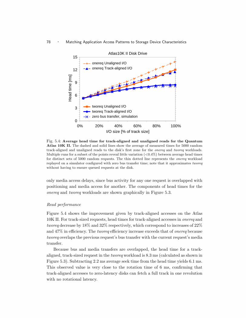
78 · Matching Application Access Patterns to Storage Device Characteristics
Atlas10K II Disk Drive
0
3
6
9
12
15
0% 20% 40% 60% 80% 100%I/O size [% of track size]
Hea
d tim
e [m
s]
onereq Unaligned I/O onereq Track-aligned I/O
tworeq Unaligned I/O tworeq Track-aligned I/O zero bus transfer, simulation
Fig. 5.4: Average head time for track-aligned and unaligned reads for the QuantumAtlas 10K II. The dashed and solid lines show the average of measured times for 5000 randomtrack-aligned and unaligned reads to the disk’s first zone for the onereq and tworeq workloads.Multiple runs for a subset of the points reveal little variation (<0.4%) between average head timesfor distinct sets of 5000 random requests. The thin dotted line represents the onereq workloadreplayed on a simulator configured with zero bus transfer time; note that it approximates tworeqwithout having to ensure queued requests at the disk.
only media access delays, since bus activity for any one request is overlapped with
positioning and media access for another. The components of head times for the
onereq and tworeq workloads are shown graphically in Figure 5.3.
Read performance
Figure 5.4 shows the improvement given by track-aligned accesses on the Atlas
10K II. For track-sized requests, head times for track-aligned accesses in onereq and
tworeq decrease by 18% and 32% respectively, which correspond to increases of 22%
and 47% in efficiency. The tworeq efficiency increase exceeds that of onereq because
tworeq overlaps the previous request’s bus transfer with the current request’s media
transfer.
Because bus and media transfers are overlapped, the head time for a track-
aligned, track-sized request in the tworeq workload is 8.3 ms (calculated as shown in
Figure 5.3). Subtracting 2.2 ms average seek time from the head time yields 6.1 ms.
This observed value is very close to the rotation time of 6 ms, confirming that
track-aligned accesses to zero-latency disks can fetch a full track in one revolution
with no rotational latency.

5.3 Evaluating ensembles for disk drives · 79
seek
bxfer
seek
media transfer
media transfer
r. lat. & h. switch & mxfer
seek
2 864 10 1412time [ms]
2.2 ms
6 ms
2 ms Normalaccess
Track-alignedaccess
Track-aligned accessout-of-order delivery
9.2 ms
bxfer
bxfer
Fig. 5.5: Breakdown of measured response time for a zero-latency disk. “Normal access”represents track-unaligned access, including seek, rotational latency (r.lat.), head switch, mediatransfer (mxfer), and bus transfer (bxfer). For track-aligned access, the in-order bus transfer doesnot overlap the media transfer. With out-of-order bus delivery, overlap of bus and media transfersis possible.
The command queueing of tworeq is needed in current systems to address the
in-order bus delivery requirement. That is, even though zero-latency disks can read
data out of order, they can only send data over the bus in ascending LBN order.
This results in only a 3% overlap, on average, between the media transfer and bus
transfer for the track-aligned access bar in Figure 5.5. The overlap would be nearly
complete if out-of-order bus delivery were used instead, as shown by the bottom
bar. Out-of-order bus delivery improves the efficiency of onereq to nearly that of
tworeq while relaxing the queueing requirement (shown as the “zero bus transfer”
curve in Figure 5.4). Although the SCSI modify data pointer command enables
out-of-order data delivery, none of the tested disks support it.
Write performance
Track-alignment also makes writes more efficient. For the onereq workload on the
Atlas 10K II, the head time of track-sized writes is 10.0 ms for track-aligned access
and 13.9 ms for unaligned access, a reduction of 28%. For tworeq, the reduction
in head time is 26% (from 13.8 ms to 10.2 ms). These reductions correspond to
efficiency increases of 39% and 35%, respectively.
The larger onereq improvement, relative to reads, occurs because the seek and
bus transfer are overlapped. The disk can initiate the seek as soon as the write
command arrives. While the seek is in progress, the data is transferred to the disk
and buffered. Since the average seek for the onereq workload is 2.2 ms and the
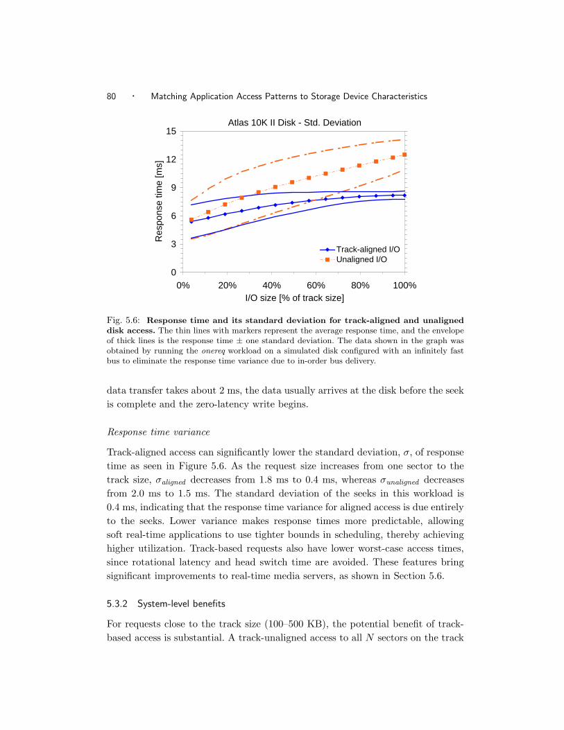
80 · Matching Application Access Patterns to Storage Device Characteristics
Atlas 10K II Disk - Std. Deviation
0
3
6
9
12
15
0% 20% 40% 60% 80% 100%I/O size [% of track size]
Res
pons
e tim
e [m
s]
Track-aligned I/OUnaligned I/O
Fig. 5.6: Response time and its standard deviation for track-aligned and unaligneddisk access. The thin lines with markers represent the average response time, and the envelopeof thick lines is the response time ± one standard deviation. The data shown in the graph wasobtained by running the onereq workload on a simulated disk configured with an infinitely fastbus to eliminate the response time variance due to in-order bus delivery.
data transfer takes about 2 ms, the data usually arrives at the disk before the seek
is complete and the zero-latency write begins.
Response time variance
Track-aligned access can significantly lower the standard deviation, σ, of response
time as seen in Figure 5.6. As the request size increases from one sector to the
track size, σaligned decreases from 1.8 ms to 0.4 ms, whereas σunaligned decreases
from 2.0 ms to 1.5 ms. The standard deviation of the seeks in this workload is
0.4 ms, indicating that the response time variance for aligned access is due entirely
to the seeks. Lower variance makes response times more predictable, allowing
soft real-time applications to use tighter bounds in scheduling, thereby achieving
higher utilization. Track-based requests also have lower worst-case access times,
since rotational latency and head switch time are avoided. These features bring
significant improvements to real-time media servers, as shown in Section 5.6.
5.3.2 System-level benefits
For requests close to the track size (100–500 KB), the potential benefit of track-
based access is substantial. A track-unaligned access to all N sectors on the track

5.3 Evaluating ensembles for disk drives · 81
involves four delays: seek, rotational latency, N sectors worth of media trans-
fer, and head switch. An N -sector track-aligned access eliminates the rotational
latency and head switch delays. This reduces access times for modern disks by
3–4 ms out of 9–12 ms, a 50% increase in efficiency.
Of course, the real benefit provided by track-based access depends on the
workload. The greatest benefit is seen by applications with medium-sized I/Os.
Streaming media services, such as video servers, MP3 servers, and CDN caches, are
examples of this type of application. Other examples include storage components
(e.g., Network Appliance’s filers [Hitz et al. 1994], HP’s AutoRAID [Wilkes et al.
1996], or EMC’s Symmetrix) that map data to disk locations in mid-sized chunks.
A system issuing large I/O sizes will see modest benefit, because positioning costs
can be amortized over large media (the right-hand
size of graph in Figure 5.1). Finally, a workload of random small requests,
(e.g., transaction processing), will experience only minimal improvement because
request sizes are too small (the left-hand side of the graph in Figure 5.1). The
remainder of this chapter evaluates these benefits on several concrete examples of
systems.
5.3.3 Predicting improvements in response time
With the analytical model derived in the previous section, it is possible to evaluate
the effects of head switch time and zero-latency firmware feature on ensemble-
based access for future generations of disks. First, the analytical model is validated
against the measurements described previously in Figure 5.1. It is then used to
show how changes in head switch time affect the relative improvement of ensemble-
based access response times.
Table 5.1 shows relative improvements in the response time of ensemble-based
accesses predicted by the analytical model as compared to measurements on a real
disk. For each workload, it lists the improvement of ensemble-based (track-aligned)
access relative to the normal (track-unaligned) access. The analytic model results
used characteristics obtained by the DIXtrac tool.
Workload full-track represents a synthetic workload with track-sized I/Os is-
sued to a location randomly chosen within the disk’s first zone. The I/O sizes were
334 sectors for the Quantum Atlas 10K disk (with head switch H = 64 sectors) and
386 sectors for the Seagate Cheetah X15 disk (with head switch H = 74 sectors).
Workload 0.8-track represents a workload to randomly chosen location within the
disk’s first zone, but I/O sizes set at 80% of first zone’s track size. The I/O sizes
are thus 268 and 309 blocks respectively for the Atlas 10K and Cheetah X15 disks.
The measured data were obtained from the experiments described in Section 5.3.1,

82 · Matching Application Access Patterns to Storage Device Characteristics
Relative Improvement in Response Time
Workload Quantum Atlas 10K Seagate Cheetah X15Analytic Measured Analytic Measured
full-track 53% 47% 12% 8%0.8-track 44% 41% 10% 7%
Table 5.1: Relative response time improvement with track-aligned requests. Notice thesubstantially larger improvement for the Quantum Atlas 10K disk, whose firmware implementszero-latency access, compared to the Seagate Cheetah X15 disk, which does not implement it.
and the analytic data were obtained from the model derived in Appendix A.
For the ensemble-based access of full-track workload, the relative improvement
in response times predicted by the analytical model is 53% for the Atlas 10K disk
and 12% for the Cheetah X15 disk, while the improvements measured on real
disks were 47% and 8% respectively. These results confirm the importance of zero-
latency access for ensemble-based access. As expected, for accesses that are less
than a full track (0.8-track workload), the relative improvement is smaller.
The small difference between the predicted and measured values in Table 5.1
indicates the model’s high accuracy. Thus, the analytical model can be used with
high confidence to explore the impact of technology changes on relative improve-
ments of ensemble-based access compared to normal (track-unaligned) access. As
can be observed from the data in Table 3.1, the technology trend of the past 10
years shows that the head switch time has improved at a slower rate than rota-
tional speed. Fortunately, as illustrated in Figure 5.7, this unfavorable trend in
disk technology is mitigated by ensemble-based access.
Figure 5.7 shows the relationship between the ratio of head switch time to
rotational speed and the relative improvement of ensemble-based access with zero-
latency feature over traditional accesses. As head switch time becomes a more
dominant factor in the overall response time, the benefit of ensemble-based access
becomes larger. For example, the ratio for a typical disk in 1992 was in the 1:9
or 1:8, while disks available in 2000 fell in the 1:7–1:5 region. For 15,000 RPM
disks introduced in 2000, the head switch time to rotational time ratio falls in the
1:5–1:4 range; the expected improvement in response time is between 55%–60%.
5.4 Block-based file system
We built a prototype implementation of an ensemble-aware file system in FreeBSD,
called Traxtent FFS [Schindler et al. 2002]. This implementation modifies the
FreeBSD Fast File System (FFS) [McKusick et al. 1984] to use the access de-
lay boundaries attribute. This section reviews the the small changes needed to

5.4 Block-based file system · 83
Relative Improvement of ensemble-based Access
1:10 1:9 1:8 1:7 1:6 1:5 1:4 1:3 1:2 1:1
Head-switch Time to Revolution Time Ratio
Impro
vem
ent
[%]
0%
25%
50%
75%
100%
125%
150%
175%
Fig. 5.7: Relative improvement in response time for ensemble-based access overnormal access in the face of changing technology. With the ratio of head switch time torevolution time becoming larger, the ensemble-based access provides more substantial improve-ments for disk accesses.
implement ensemble-aware allocation and access in the FreeBSD FFS.
5.4.1 FreeBSD FFS overview
FreeBSD v. 4 assigns three identifying block numbers to buffered disk data (Fig-
ure 5.8). The lblkno represents the offset within a file; that is, the buffer contain-
ing the first byte of file data is identified by lblkno 0. Each lblkno is associated
with one blkno (physical block number), which is an abstract representation of
the disk addresses used by the OS to simplify space management. Each blkno
directly maps to a range of contiguous disk sector numbers (LBNs), which are the
actual addresses presented to the device driver during an access. (Device drivers
adjust sector numbers to partition boundaries.) In our experiments, the file system
block size is 8 KB (sixteen contiguous LBNs). In this section, “block” refers to a
physical block.
FFS partitions the set of physical blocks into fixed-size block groups (“cylinder
groups”). Each block group contains a small amount of summary information—
inodes, free block map, etc.—followed by a large contiguous array of data blocks.
Block group size, block allocation, and media access characteristics were once based
on the underlying disk’s physical geometry. Although this geometry dependence
is no longer real, block groups are still used in their original form because they
localize related data (e.g., files in the same directory) and their inodes, resulting in
more efficient disk access. The block group size used for the experiments is 32 MB.
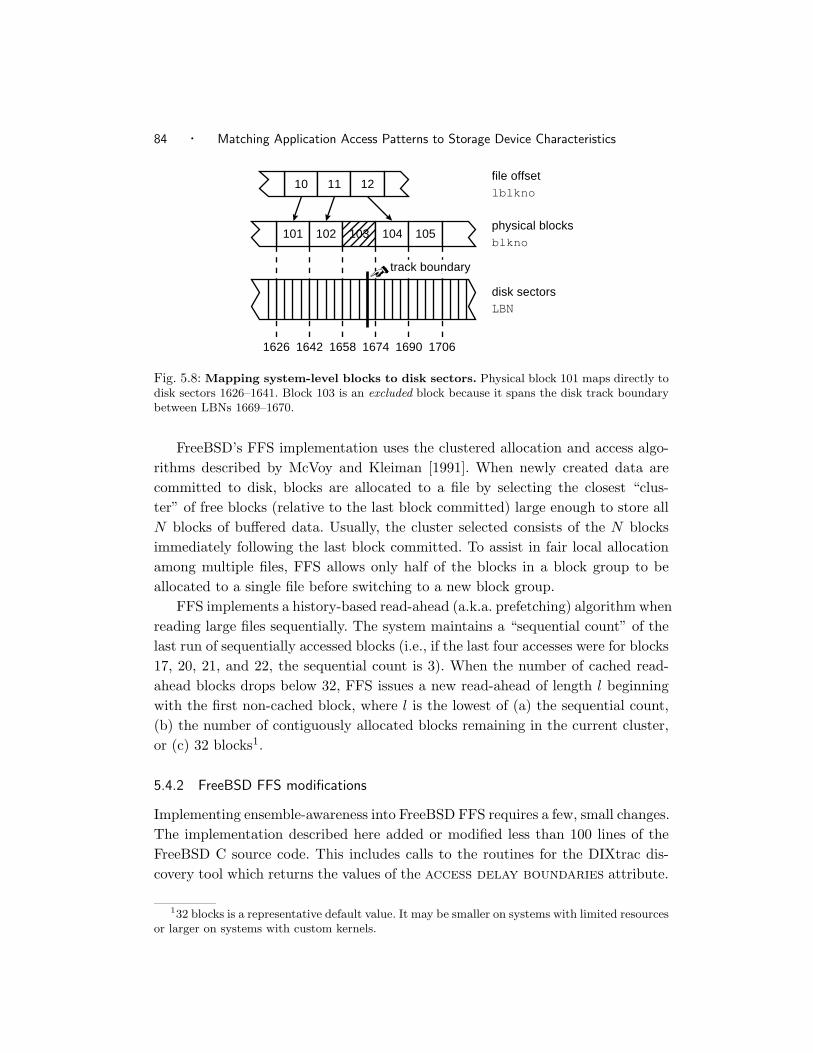
84 · Matching Application Access Patterns to Storage Device Characteristics
10 11 12
101 102 103 104 105
16421626 1658 1674 1690 1706
file offset
physical blocks
disk sectorsLBN
blkno
lblkno
track boundary
Fig. 5.8: Mapping system-level blocks to disk sectors. Physical block 101 maps directly todisk sectors 1626–1641. Block 103 is an excluded block because it spans the disk track boundarybetween LBNs 1669–1670.
FreeBSD’s FFS implementation uses the clustered allocation and access algo-
rithms described by McVoy and Kleiman [1991]. When newly created data are
committed to disk, blocks are allocated to a file by selecting the closest “clus-
ter” of free blocks (relative to the last block committed) large enough to store all
N blocks of buffered data. Usually, the cluster selected consists of the N blocks
immediately following the last block committed. To assist in fair local allocation
among multiple files, FFS allows only half of the blocks in a block group to be
allocated to a single file before switching to a new block group.
FFS implements a history-based read-ahead (a.k.a. prefetching) algorithm when
reading large files sequentially. The system maintains a “sequential count” of the
last run of sequentially accessed blocks (i.e., if the last four accesses were for blocks
17, 20, 21, and 22, the sequential count is 3). When the number of cached read-
ahead blocks drops below 32, FFS issues a new read-ahead of length l beginning
with the first non-cached block, where l is the lowest of (a) the sequential count,
(b) the number of contiguously allocated blocks remaining in the current cluster,
or (c) 32 blocks1.
5.4.2 FreeBSD FFS modifications
Implementing ensemble-awareness into FreeBSD FFS requires a few, small changes.
The implementation described here added or modified less than 100 lines of the
FreeBSD C source code. This includes calls to the routines for the DIXtrac dis-
covery tool which returns the values of the access delay boundaries attribute.
132 blocks is a representative default value. It may be smaller on systems with limited resourcesor larger on systems with custom kernels.

5.4 Block-based file system · 85
Excluded blocks and ensemble allocation
The concept of the excluded block is highlighted in Figure 5.8. Blocks that span
track boundaries are excluded from allocation decisions by marking them as used
in the free-block map. Whenever the preferred block (the next sequential block) is
excluded, we instead allocate the first block of the closest available ensemble. When
possible, mid-sized files are allocated such that they fit within a single ensemble.
For example, ensembles from the Quantum Atlas 10K result in one out of every
twenty blocks being excluded under the modified FFS. With increasing linear bit
density, the frequency of excluded blocks decreases — only one in thirty blocks is
excluded for ensembles of the Quantum Atlas 10K II disk.
Ensemble-sized access
No fundamental changes are necessary in the FFS clustered read-ahead algorithm.
FFS properly identifies runs of blocks between excluded blocks as clusters and
accesses them with a single I/O request. Until a non-sequential access is detected,
we ignore the “sequential count” to prevent multiple partial accesses to a single
ensemble; for non-sequential file sessions, the default mechanism is used. We handle
the special case where there is no excluded block between contiguous ensembles
by ensuring that no read-ahead request goes beyond a track boundary. At a low
level, unmodified FreeBSD already supports command queuing at the device and
attempts to have at least one outstanding request for each active data stream.
Data structures
When the file system is created, track boundaries are identified, adjusted to the
file system’s partition, and stored on disk. At mount time, they are read into an
extended FreeBSD mount structure. We chose this mount structure because it is
available everywhere ensemble information is needed.
5.4.3 FFS experiments
Building on the disk-level results, this section compares our prototype ensemble-
aware Traxtent FFS to the unmodified version of FFS. We also include results for
a modified FFS, here called fast start FFS, that aggressively prefetches contigu-
ous blocks. The unmodified FFS slowly ramps up its prefetching as it observes
sequential access to a file. The fast start FFS, on the other hand, prefetches up
to 32 contiguous blocks on the first access to a file, thus approximating the be-
havior of the Traxtent FFS (albeit with larger requests and no knowledge of track
boundaries).

86 · Matching Application Access Patterns to Storage Device Characteristics
Workload
FFS type 4GBscan
0.5GBdiff
1GBcopy
Postmark SSHbuild
head *
unmodified 189.6 s 69.7 s 156.9 s 53 tr/s 72.0 s 4.6 sfast start 188.9 s 70.0 s 155.3 s 53 tr/s 71.5 s 5.5 straxtents 199.8 s 56.6 s 124.9 s 55 tr/s 71.5 s 5.2 s
Table 5.2: FreeBSD FFS results. All but the head * values are an average of three runs.The individual run times deviate from their average by less than 1%. The head * value is anaverage of five runs and the individual runs deviate by less than 3.5%. Postmark reported thesame number of transactions per second in all three runs for the respective FFS, except for onerun of the unmodified FFS that reported 54 transactions per second.
Each test is performed on a freshly-booted system with a clean partition on
a Quantum Atlas 10K. The tests verify the expected performance effects: small
penalties for single sequential scan, substantial benefit for interleaved scans, and
no effect on small file activity. The results are summarized in Table 5.2.
Single large file
The first experiment is an I/O-bound linear scan through a 4 GB file. As ex-
pected, Traxtent FFS runs 5% slower than unmodified FFS or fast start FFS
(199.8 s vs. 189.6 s and 188.9 s respectively). This is because FFS is optimized
for large sequential single-file accesses and reads at the maximum disk streaming
rate, whereas Traxtent FFS inserts an excluded block one out of every twenty
blocks (5%). This penalty could be eliminated by changing the file system cache
to support buffering of partial blocks (much like IP fragments) instead of using
excluded blocks in large files, giving the block-based system extent-like flexibility.
Multiple large files
The second experiment consists of the diff application comparing two large files.
Because diff interleaves fetches from the two files, we expect to see a speedup from
improved disk efficiency. For 512 MB files, Traxtent FFS completes 19% faster than
unmodified FFS or fast start FFS. A more detailed analysis shows that Traxtent
FFS performs 6724 I/Os (average size of 160 KB) in 56.6 s while unmodified
FFS performs only 4108 I/Os (mostly 256 KB) but requires 69.7 s. The fast start
FFS performs 4094 I/Os (all but one at 256 KB) and requires 70.0 s. Subtracting
media transfer time, unmodified FFS incurs 6.9 ms of overhead (seek + rotational
latency + track switch time) per request, and Traxtent FFS incurs only 2.2 ms
of overhead per request. In fact, the 19% improvement in overall completion time
corresponds to an improvement in disk efficiency of 23%, exactly matching the

5.4 Block-based file system · 87
predicted difference between single-track accesses and 256 KB unaligned accesses
on an Atlas 10K disk.
The third experiment verifies write performance by copying a 1 GB file to
another file in the same directory. FFS commits dirty buffers as soon as a complete
cluster is created, which results in two interleaved request streams to the disk. This
test shows a 20% reduction in run time for Traxtent FFS over unmodified FFS
(124.9 s vs. 156.9 s). The fast start FFS finished in 155.3 s.
Small Files
Two application benchmarks are used to verify that the ensemble modifications do
not penalize small file workloads. Postmark [Katcher 1997] simulates the small-
file activity of busy Internet servers. Our experiments use Postmark v1.11 and
its default parameters: 5–10KB files and 1:1 read-to-write and create-to-delete
ratios. SSH-build [Seltzer et al. 2000] represents software development activity,
replacing the Andrew benchmark. Its three phases unpack the compressed tar
archive of SSH v1.2.27, generate the header files and Makefiles, and build the
program executable.
As expected, we observe little difference. The SSH-build results differ by less
than 0.2%, because the file system activity is dominated by small synchronous
writes and cache hits. The fast start FFS performs exactly like the Traxtent FFS
having an edge of 0.2% over the unmodified FFS. Postmark is 4% faster with
ensembles (55 transactions/second versus 53 for both unmodified and fast start
FFS), because the few track switches are avoided. Fast start is not important for
Postmark, because the files consist of only 1–3 blocks.
One might view these results as a negative indication of the value of en-
sembles, but they are not. Recall that FreeBSD FFS does not explicitly group
small files into large disk requests. Such grouping has been shown to yield 2–8×throughput increases for static web servers [Kaashoek et al. 1996], web proxy
caches [Shriver et al. 2001], and software development activities [Ganger and
Kaashoek 1997]. Based on our measurements, we expect that the additional 50%
increase in throughput from employing ensembles would be realized given such
grouping.
Worst case scenario
As expected, we observe no penalty to small file I/O and a minimal (5%) penalty
to the unoptimized single stream case. For random file I/O, FFS’s “sequential
count” prefetch control replaces the ensemble-based fetch mechanism, preventing
useless full-track reads. The one remaining worst-case scenario would be single-
88 · Matching Application Access Patterns to Storage Device Characteristics
block reads to the beginnings of many large files; in this case, the original FFS
will fetch the first 8KB block and prefetch the second, whereas the modified FFS
will fetch the entire first ensemble (≈ 160 KB). To evaluate this scenario, we ran
an experiment, called head *, that reads the first byte of 1000 200 KB files. The
results show a 45% penalty for ensembles (3.6 s vs. 5.2 s), closely matching the
predicted per-request service time difference (5.6 ms vs. 8.0 ms). Fortunately, this
scenario is not often expected to arise in practice. Not surprisingly, the fast start
FFS performs even worse than the Traxtent FFS with an average runtime of 5.5 s
as it prefetches even more unnecessary data.
5.5 Log-structured file system
The log-structured file system (LFS) [Rosenblum and Ousterhout 1992] was de-
signed to reduce the cost of disk writes. Towards this end, it remaps all new versions
of data into large, contiguous regions called segments. Each segment is written to
disk with a single I/O operation, amortizing the positioning cost over one large
write. A significant challenge for LFS is ensuring that empty segments are always
available for new data. LFS answers this challenge with an internal defragmen-
tation operation called cleaning. Cleaning a previously written segment involves
identifying the subset of “live” blocks, reading them into memory, and writing
them into a new segment. Live blocks are those that have not been overwritten or
deleted by later operations.
5.5.1 Performance tradeoff
There is a performance trade-off between write efficiency and the cost of clean-
ing. Larger segments offer higher write efficiency but incur larger cleaning cost
since more data has to be transferred for cleaning [Matthews et al. 1997; Seltzer
et al. 1995]. Additionally, the transfer of large segments hurts the performance
of small synchronous reads [Carson and Setia 1992; Matthews et al. 1997]. Given
these conflicting pressures, the choice of segment size must balance write efficiency,
cleaning cost, and small synchronous I/O performance. Matching segments to track
boundaries can yield higher write efficiency with smaller segments and thus lower
cleaning costs.
To evaluate the benefit of using track-based access for LFS segments, we use
the overall write cost (OWC ) metric described by Matthews et al. [1997], which
is a refinement of the write cost metric defined for the Sprite implementation of
LFS [Rosenblum and Ousterhout 1992]. It expresses the cost of writes in the file
system, assuming that all data reads are serviced from the system cache. The

5.5 Log-structured file system · 89
OWC metric is defined as the product of write cost and disk transfer inefficiency:
OWC = WriteCost × TransferInefficiency
=Nnew
written + N cleanread + N clean
written
Ndatawritten
×T actual
xfer
T idealxfer
where N is the number of segments written due to new data or read and written
due to segment cleaning, and T is the time for one segment transfer. WriteCost
depends on the workload (i.e., how much new data is written and how much old
data is cleaned) but is independent of disk characteristics. TransferInefficiency ,
on the other hand, depends only on disk characteristics. Therefore, we can use the
WriteCost values from Matthews et al. [1997] and apply to TransferInefficiency
values from Figure 5.1.
Figure 5.9 shows that OWC is lower with track-aligned disk access and that
the cost is minimized when the segment size matches the track size. Unlike our
use of empirical data for TransferInefficiency , Matthews et al. calculate it as
TransferInefficiency = Tpos ×BWdisk
Ssegment
+ 1
where Ssegment is the segment size (in bytes) and Tpos is the average positioning
time (i.e., seek and rotational latency). To verify that our results are in agreement
with their findings, we computed OWC for the Atlas 10K II based on its specifi-
cations and plotted it in Figure 5.9 (labeled “5.2 ms*40 MB/s”) with the OWC
values for the track-aligned and unaligned I/O. Because the empirical values are
for the disk’s first zone, the model values we used are too: 2.2 ms average seek,
3 ms average rotational latency, and peak bandwidth of 40 MB/s. As expected,
the model is a good match for the unaligned case.
5.5.2 Variable segment size
As shown in Figure 5.9, the lowest write cost is achieved when the size of a segment
matches the size of a track. However, different tracks may hold different numbers
of LBNs. Therefore, an LFS must allow variable segment sizes in order to match
segment boundaries to track boundaries. Fortunately, doing so is straightforward.
In an LFS, the segment usage table records information about each segment.
In the SpriteLFS implementation [Rosenblum and Ousterhout 1992], this table is
kept as an in-memory kernel structure and is stored in the checkpoint region of
the file system. The BSD-LFS implementation [Seltzer et al. 1993] stores this table
in a special file called the IFILE. Because of its frequent use, this file is almost
always in the file system’s cache.

90 · Matching Application Access Patterns to Storage Device Characteristics
LFS Overall Write Cost (Auspex Workload)
1
2
3
32 64 128 256 512 1024 2048 4MBSegment size [KB]
Ove
rall
Writ
e C
ost [
ratio
]Atlas 10k II track-aligned I/OAtlas 10k II unaligned I/O5.2ms*40MB/s (Atlas 10k II)
Fig. 5.9: LFS overall write cost for the Auspex trace as a function of segment size.The line labeled “5.2 ms*40 MB/s” is the overall write cost predicted by the transfer inefficiencymodel.
Variable-sized segments can be supported by augmenting the per-segment in-
formation in the segment usage table with a starting location (the LBN) and
length. During the initialization, each segment’s starting location and length are
set according to the corresponding track boundary information. When a new seg-
ment is allocated in memory, its size is determined from the segment usage table.
When the segment becomes full, it is written to the disk at the starting location
given in the segment usage table. The procedures for reading segments and for
cleaning are similar.
5.6 Video servers
A video server is designed to serve large numbers of video streams to clients at
guaranteed rates. To accomplish this, the server first fetches one time interval of
video (e.g., 0.5 s) for each stream. This set of fetches is called a round. Then, while
the data are transferred to clients from the server’s buffers, the server schedules
the next round of requests. Since the per-interval disk access time is less than the
round time, many concurrent streams can be supported by a single disk. Further,
by spreading video streams across D disks, D times as many concurrent streams
can be supported.
The per-interval disk request size, IOsize, is a trade-off between throughput
(the number of concurrent streams) and other considerations (buffer space and

5.6 Video servers · 91
10-disk Video Server Performance
0
20
40
60
80
100
0 100 200 300 400 500 600 700 800Number of concurrent streams
Sta
rtup
late
ncy
[s]
Track-aligned
Unaligned
Fig. 5.10: Worst-case startup latency of a video stream for track-aligned and un-aligned accesses. The startup latency is shown for a 10-disk array of Quantum Atlas 10K IIdisks, which can support up to 800 concurrent streams.
start-up latency). IOsize must be large enough so that achieved disk bandwidth
(disk efficiency times peak bandwidth) exceeds V times the video bit rate, where
V is the number of concurrent video streams supported. As IOsize increases, both
disk efficiency and TimeperIO increase, increasing both the number of supported
video streams and the round time, which is defined as V times TimeperIO.
The round time determines the startup latency of a newly admitted stream.
Assuming the video server spreads data across D disks, the worst-case startup
latency is the round time times (D + 1) [Santos et al. 2000]. The buffer space
required at the server is 2 × IOsizedisk × V . In practice, IOsize is chosen to meet
system goals given a trade-off between startup latency and the maximum num-
ber of supportable streams. Since track-aligned access increases disk efficiency, it
enables more concurrent streams to be serviced at a given IOsize.
5.6.1 Soft real-time
Most video server projects, such as Tiger [Bolosky et al. 1996] and RIO [Santos
et al. 2000], provide soft real-time guarantees. These systems guarantee that, with
a certain probability, a request will not miss its deadline. This allows a relax-
ation on the assumed worst-case seek and rotational latency and results in higher
bandwidth utilization for both track-aligned and unaligned access.
We evaluate two video servers (one ensemble-aware and one not), each con-
taining 10 Quantum Atlas 10K II disks, using the same approach as the RIO video

92 · Matching Application Access Patterns to Storage Device Characteristics
server [Santos et al. 2000]. First, we measured the time to complete a given num-
ber of simultaneous, random track-sized requests. This measurement was repeated
10,000 times for each number of simultaneous requests from 10 to 80. (80 is the
maximum number of simultaneous 4 Mb/s streams that can be supported by each
disk’s 40 MB/s streaming bandwidth.)
From the PDF of the measured response times, we obtained the round time
that would meet 99.99% of the deadlines for the 4 Mb/s rate. Given a 0.5 s
round time (which translates to a worst-case startup latency of 5.5 s for the 10-
disk array), the track-aligned system can support up to 70 streams per disk. In
contrast, the unaligned system is only able to support 45 streams per disk. Thus,
the track-aligned system can support 56% more streams at this minimal startup
latency.
To support more than 70 and 45 streams per disk for the track-aligned and
unaligned systems, the I/O size must increase. This increase in I/O size causes an
increase in the round time, which in turn increases the startup latency as shown
in Figure 5.10. At 70 streams per disk, the startup latency for the track-aligned
system is 4× smaller than for the track-unaligned system.
5.6.2 Hard real-time
Although many video servers implement soft real-time requirements, there are
applications that require hard real-time guarantees. In their admission control
algorithms, these systems must assume the worst-case response time to ensure that
no deadline is missed. In computing the worst-case response time, one assumes the
worst-case seek, transfer time, and rotational latency.
Both the track-aligned and unaligned systems have the same values for the
worst-case seek. The worst-case time for V seeks is much smaller than V times a
full strobe seek (seek from one edge of the disk to the other) and it decreases as
the number of concurrent streams (V ) increases [Reddy and Wyllie 1993]. This is
because a disk scheduler can sort the requests in each round to minimize total seek
distance. The worst-case seek time charged to a stream is equal to the worst-case
scheduled seek route that serves all streams divided by the number of streams.
However, the worst-case rotational latency for unaligned access is one revo-
lution, whereas track-based access suffers no rotational latency. The worst-case
transfer time will be similar except that the unaligned system must assume at
least one head switch will occur for each request. With a 4 Mb/s bit rate and
an I/O size of 264 KB, the track-unaligned system supports 36 streams per disk
whereas the track-based system supports up to 67 streams. This translates into
45% and 83% disk efficiency, respectively. With an I/O size of 528 KB, unaligned

5.7 Database storage manager · 93
access yields 52 streams vs. 75 for track-based access. Unaligned I/O size must
exceed 2.5 MB, with a maximum startup latency of 60.5 seconds, to achieve the
same efficiency as the track-aligned system.
5.7 Database storage manager
This section describes how a database storage manager, called Lachesis, exploits
the access delay boundaries attribute to improve the performance and robust-
ness of database I/O.
5.7.1 Overview
The task of ensuring optimal query execution in database management systems
is indeed daunting. The query optimizer uses a variety of metrics, cost estima-
tors, and run-time statistics to devise a query plan with the lowest cost. The
storage manager orchestrates the execution of queries, including I/O generation
and caching. To do so, it uses hand-tuned parameters that describe the various
characteristics of the underlying resources to balance the resource requirements
encapsulated in each query plan. To manage complexity, the optimizer makes de-
cisions about other queries and modules without runtime details, trusting that its
cost estimates are accurate. Similarly, the storage manager trusts that the plan
for each query is indeed well-chosen and that the database administrator (DBA)
has tuned the knobs correctly.
To minimize I/O costs, query optimizers and storage managers have tradi-
tionally focused on achieving efficient storage access patterns. Unfortunately, two
issues complicate this task. First, the multiple layers of abstraction between the
query execution engine and the storage devices complicate the evaluation of access
pattern efficiency. Second, when there is contention for data or resources, efficient
sequential patterns are broken up. The resulting access pattern is less efficient
because accesses which were originally sequential are now interleaved with other
requests, introducing unplanned-for seek and rotational delays. These two factors
lead to significant degradation of I/O performance and longer execution times.
Modern database management systems typically consist of several cooperating
modules; the query optimizer, the query execution engine, and the storage manager
are relevant to the topic of this dissertation. As illustrated in Figure 5.11, for each
query the optimizer evaluates the cost of each alternative execution plan and
selects the one with the lowest cost. The execution engine allocates resources for
the execution of the selected query plan, while the storage manager communicates
with the storage devices as needed.

94 · Matching Application Access Patterns to Storage Device Characteristics
OPTIMIZEROPTIMIZER
EXECUTION
STORAGE Manager
I/O requests
buffers
parsed SQL query
query planConfiguration Parameters
Fig. 5.11: Query optimization and execution in a typical DBMS.
Optimizing for I/O
Query optimizers use numerous techniques to minimize the cost of I/O operations.
Early optimizers used static cost estimators and run-time statistics [Selinger et al.
1979] collected by the storage manager to estimate the number of I/O operations
executed by each algorithm [Graefe 1993] (e.g., loading a page from a storage
device into the buffer pool or writing a page back to the device).
Due to the physical characteristics of disk drives, random I/O is significantly
slower than sequential scan. To reflect the performance difference, today’s com-
mercial database management systems (DBMS) optimizers distinguish between
random and sequential I/O using cost models that take into account the data
access pattern dictated by each query operator. Despite capturing this important
disk performance feature, however, each query is optimized separately. In addi-
tion, the optimizer has limited knowledge of the characteristics of the underlying
disk subsystem. The calculated access pattern costs are therefore not likely to be
observed during execution. To maintain robust performance, the execution engine
must uphold the assumed performance in the face of concurrent query execution.
In particular, a storage manager must be able to maintain efficient execution of
large sequential I/O access pattern even in the face of disrupting activity with
small random accesses.
Tuning I/O execution efficiency
During query execution, the execution engine asks the storage manager for data
from the disks. The storage manager considers factors such as resource availability
and contention across concurrent queries and decides each request’s size, location,

5.7 Database storage manager · 95
and temporal relationship to other requests. Request-related decisions are also
influenced by DBA-specified parameters. For instance, IBM DB2’s EXTENTSIZE
and PREFETCHSIZE parameters determine the maximal size of a single I/O oper-
ation [IBM Corporation 2000], and the DB2 STRIPED CONTAINERS parameter in-
structs the storage manager to align I/Os on stripe boundaries.
In order for the queries to be executed as planned, the storage manager must
balance the competing resource requirements of the queries being executed while
maintaining the access cost assumptions the query optimizer used when selecting a
query plan. This balance is quite sensitive and prone to human errors. In particular,
high-level generic parameters make it difficult for the storage manager to adapt to
device-specific characteristics and dynamic query mixes. This results in inefficiency
and performance degradation.
Exploiting observed storage characteristics
To achieve robust performance, storage managers need to exploit observed stor-
age system performance characteristics. DBA-specified parameters are too high
level to provide sufficient information to the storage manager, therefore DBAs
cannot finely tune all the possible performance knobs. Current storage managers
complement DBA knob settings with methods that dynamically determine the
I/O efficiency of differently-sized requests by issuing I/Os of different sizes and
measuring their response time. Unfortunately, such methods are unreliable and
error-prone and often yield sub-optimal results.
5.7.2 Robust storage management
This section describes the new storage manager architecture, which bridges the
information gap between database systems and underlying storage devices by pro-
viding the access delay boundaries attribute. This allows a DBMS to exploit
device characteristics and achieve robust performance for queries even in the face
of competing traffic. The architecture retains clean high-level abstractions between
the storage manager and the underlying storage devices and leaves unchanged the
interface between the storage manager and the query optimizer.
Overview
The cornerstone of the new architecture is to have a storage device (or automated
extraction tool) convey to the storage manager explicit information about efficient
access patterns. While the efficiency may vary for different workloads (i.e., small
random I/Os are inherently less efficient than large sequential ones), this infor-

96 · Matching Application Access Patterns to Storage Device Characteristics
mation allows a storage manager to always achieve the best possible performance
regardless of the workload mix. Most importantly, this information provides guar-
antees to the query optimizer that access patterns are as efficient as originally
assumed when the query plan was composed.
The storage manager learns about efficient device accesses directly from the
storage device, which encapsulates its performance characteristics in a few well-
defined and device-independent attributes. During query execution, the storage
manager uses these hints to orchestrate I/O patterns appropriately. No run-time
performance measurements are needed to determine efficient I/O size.
With explicit information about access pattern efficiency, the storage manager
can focus solely on data allocation and access. It groups pages together such that
they can be accessed with efficient I/Os prescribed by the storage device char-
acteristics. Such grouping meshes well with existing storage manager structures,
which call these groups segments or extents [IBM Corporation 2000; Loney and
Koch 2000]. Hence, implementing a storage manager that takes advantage of per-
formance attributes requires only minimal changes, as discussed in Section 5.7.3.
Efficient I/O accesses
As shown in Figure 5.1, by the line labeled Unaligned I/O, disk efficiency
increases as a function of the I/O size by amortizing the positioning cost over more
data transfer. To take advantage of this trend, database storage managers buffer
data and issue large I/O requests [IBM Corporation 1994; Loney and Koch 2000].
This, however, creates a tension between increased efficiency and higher demand
for buffer space. On the other hand, utilizing the access delay boundaries
attribute for ensemble-based access, can be much more efficient.
A database storage manager exercises several types of access patterns. Small
sequential writes are used for synchronous updates to the log. Small, single-page,
random I/Os are prevalent in On-line Transaction Processing (OLTP) workloads.
Large, mostly sequential I/Os occur in Decision Support System (DSS) queries.
When running compound workloads, there is contention for data or resources, and
this sequentiality is broken. In such cases, it is important that the storage manager
achieve near-streaming bandwidth when possible without unduly penalizing any
of the ongoing queries.
The Lachesis architecture exploits the efficiency of ensemble-aligned accesses.
Even with significant interleaving, it can achieve efficiency close to that of purely
sequential I/O. Furthermore, it does so without using exceptionally large requests,
which would require the use of more buffer space and increase interference with
competing traffic.

5.7 Database storage manager · 97
Despite the inherent inefficiency of an OLTP workload (where disk efficiency
is typically 3–5% [Riedel et al. 2000]), Lachesis can indirectly improve its perfor-
mance when OLTP requests are interleaved with larger I/O activity. First, with
large I/Os being more efficient, small random I/Os experience lower queueing
times. Second, with explicit information about track boundaries, pages are always
aligned. Thus, a single-page access never suffers a head switch (caused by accessing
data on two adjacent tracks). Eliminating head switch (0.8 ms for the Atlas 10K
disk in Table 3.1), however, provides only a limited improvement, because the
small-random OLTP accesses experience head switches infrequently: instead, ac-
cess costs are dominated by seek and rotational latency (averages of 5 and 3 ms
respectively), as shown in Section 5.7.7.
Benefits
The database storage manager architecture using performance attributes has sev-
eral advantages over current database storage managers.
Simplified performance tuning. Since a storage manager automatically obtains
performance characteristics directly from storage devices, some difficult and error-
prone manual configuration is eliminated. In particular, there is no need for hand-
tuning such DB2 parameters as EXTENTSIZE, PREFETCHSIZE, DB2 STRIPED CON-
TAINERS or their equivalents in other DBMS. The DBA can concentrate on other
important configuration issues.
Minimal changes to existing structures. Very few changes to current storage
manager structures are necessary. Most notably, the extent size must be made
variable and modified according to the performance attribute values. However,
decisions that affect other DBMS components, such as page size or pre-allocation
for future appends of related data, are not affected; the DBMS or the DBA are
free to set them as desired.
Preserving access costs across abstraction layers. The optimizer’s cost esti-
mation functions that determine access pattern efficiency are not modified. In fact,
one of its major contributions is ensuring that the optimizer-expected efficiency is
preserved across the DBMS abstraction layers and materialized at the lowest level
by the storage device.
Reduced buffer space pressure. With explicit delay boundaries, a database
storage manager can use smaller request sizes to achieve more efficient access. Fig-
ure 5.12 illustrates that smaller I/O requests allow smaller buffers, freeing memory
for other tasks. Despite sometimes requiring additional smaller I/Os to finish the
same job, the greatly increased efficiency of these smaller requests reduces the
overall run time.

98 · Matching Application Access Patterns to Storage Device Characteristics
buffer/prefetch size
Conventional access
Device-optimized access
ACCESS DELAY BOUNDARIESLBN/pid space
time
I/O #3I/O #2
I/O #3 I/O #4I/O #2
I/O #1
I/O #1
inefficient access
efficient access
Fig. 5.12: Buffer space allocation with performance attributes.
Lower inter-query interference. A storage manager leveraging performance
attributes consistently provides nearly streaming bandwidth for table scans even
in the face of competing traffic. It can do so with smaller I/Os and still maintain
high access efficiency. When there are several request streams going to the same
device, the smaller size results in shorter response times for each individual request
and provides better throughput for all streams (queries).
5.7.3 Implementation
This section describes the key elements of a Lachesis prototype in the latest sup-
ported release (interim-release-2) of the Shore storage manager [Carey et al. 1994].
Shore consists of several key components, including a volume manager for storing
individual pages, a buffer pool manager, lock and transaction managers, and an
ARIES-style recovery subsystem [Mohan et al. 1992]. Shore’s basic allocation unit
is called an extent and each extent’s metadata, located at the beginning of the
volume, identifies which of its pages are used.
On-disk data placement
Shore’s implementation assumes a fixed number of pages per extent (8 by default)
and allocates extents contiguously in a device’s logical block space. Therefore,
the LBN (logical block number) and the extnum (extent number) for a given
page, identified by a pid (page identifier), can be easily computed. To match
allocation and accesses to the values of the access delay boundaries attribute,
we modified Shore to support variable-sized extents. A single extent now consists

5.7 Database storage manager · 99
of a number of pages and an additional unallocated amount of space, the size of
which is less than one page.
Although page sizes are typically in powers of two, disk tracks are rarely sized
this way (see Table 3.1). Thus, the amount of internal fragmentation (i.e., the
amount of unallocated space at the end of each extent) can result in loss of some
disk capacity. Fortunately, with an 8 KB page, internal fragmentation amounts
to less than 2% and this trend becomes more favorable as media bit density, and
hence the number of sectors per track, increases.
Now, the extnum and LBN values are read from a new metadata structure.
This new structure contains information about how many LBNs correspond to
each extent and is small compared to the disk capacity (for example, 990 KB
for a 36 GB disk). Lookups do not represent significant overhead, as shown in
Section 5.7.7.
I/O request generation
Shore’s base implementation issues one I/O system call for each page read, relying
on prefetching and buffering inside the underlying OS. We modified Shore to issue
SCSI commands directly to the device driver to avoid double buffering inside
the OS. We also implemented a prefetch buffer inside Shore. The new prefetch
buffer mechanism detects sequential page accesses, and issues extent-sized I/Os.
Thus, pages trickle from this prefetch buffer into the main buffer pool as they are
requested by each page I/O request. For writes, a background thread in the base
implementation collects dirty pages and arranges them into contiguous extent-sized
runs. The runs, however, do not match extent boundaries; therefore, we increased
the run size and divided each run into extent-sized I/Os aligned on proper extent
boundaries.
Our modifications to Shore total less than 800 lines of C++ code, including
120 lines for the prefetch buffer. Another 400 lines of code implement direct SCSI
access via the Linux /dev/sg interface.
5.7.4 Evaluation
We evaluate Lachesis using two sets of experiments. The first set of experiments
replays modified I/O traces to simulate the performance benefits of Lachesis inside
a commercial database system. The original traces were captured while running the
TPC-C and TPC-H benchmarks [Transactional Processing Performance Council
2002a; 2002b] on an IBM DB2 relational database system. The second set of
experiments evaluates the Lachesis implementation inside Shore using TPC-C
and (a subset of) TPC-H.

100 · Matching Application Access Patterns to Storage Device Characteristics
The TPC-H decision-support benchmark includes 22 different queries. We ran
all the queries in sequence, one at a time. Each query processes a large por-
tion of the data. The TPC-C benchmark emulates OLTP activity, measuring the
number of committed transactions per minute. Each transaction involves a few
read-modify-write operations to a small number of records.
For each of the two sets of experiments, we first show the performance of the
TPC-H and TPC-C benchmarks as they were run in isolation. We then look at the
performance benefits Lachesis offers when both benchmarks are run concurrently.
In particular, we consider three scenarios:
No traffic simulates a dedicated DSS setup running single-user TPC-H queries.
Light traffic simulates an environment with occasional background traffic intro-
duced while executing the primary TPC-H workload. This represents a more
realistic DSS setup with updates to data and other occasional system activ-
ity.
Heavy traffic simulates an environment with DSS queries running concurrently
with a heavy OLTP workload. This represents a scenario in which decision
DSS queries are run on a live production system.
Finally, we contrast the results of the experiments with simulated Lachesis-DB2
and our implementation. The same trends in both cases provide strong evidence
that other DBMS implementations using Lachesis are likely to obtain similar
benefits.
Experimental Setup
We conducted all experiments on a system with a single 2 GHz Intel Pentium 4
Xeon processor, 1 GB of RAM, and a 36 GB Maxtor Atlas 10K III disk attached
to a dedicated Adaptec 29160 SCSI card with 160 MB/s transfer rate. The basic
parameters for this disk are summarized in Table 3.1. The system also included a
separate SCSI host bus adapter with two additional disks; one with the OS and
executables and the other for database logs. We ran our experiments on RedHat
7.3 distribution under Linux kernel v. 2.4.19, modified to include an I/O trace
collection facility. For DB2 runs, we used IBM DB2 v. 7.2.
5.7.5 DB2 experiments
We do not have access to the DB2 source code. To evaluate the benefits of Lachesis
for DB2, we simulated its effect by modifying traces obtained from our DB2 setup.
We ran all 22 queries of the TPC-H benchmark and captured their device-level

5.7 Database storage manager · 101
Lachesis-DB2 TPC-H Benchmark
0
0.2
0.4
0.6
0.8
1.0
1 2 3 4 5 6 7 8 9 10 11 12 13 14 15 16 17 18 19 20 21 22
Query # No traffic Light Heavy
Nor
ma
lize
d I/O
Tim
e
Fig. 5.13: TPC-H I/O times with competing traffic (DB2).
I/O traces. We then wrote a trace-replay tool and used it to replay the origi-
nal captured traces. Finally, we compared the trace replay time with the DB2
query execution time. The trace-replay method is quite accurate; the measured
and replayed execution times differed by at most 1.5%.
The sum of all the periods between the completion time of the last outstanding
request at the device and the issue time of the next request determined the pure
CPU time from the captured traces. It expresses the periods when the CPU is
busy, while the storage device is idle. Since the goal is to study I/O efficiency, the
pure CPU time was subtracted from the traces for a more direct comparison.
Having verified that the original captured TPC-H traces never had more than
two outstanding requests at the disk, we replayed the no-CPU-time traces in a
closed loop by always keeping two requests outstanding at the disk. This ensures
that the disk head is always busy (see Section 5.7.1) and preserves the order of
request issues and completions [Lumb et al. 2002]. Because of our trace replay
method, the numbers reported in this section represent the query I/O time, which
is the portion of the total query execution time spent on I/O operations.
To simulate Lachesis behavior inside DB2, we modified the DB2 captured
traces by compressing back-to-back sequential accesses to the same table or index
into one large I/O. We then split this large I/O into individual I/Os according to
the values of the access delay boundaries attribute. Thus, the I/Os are con-
tained within an integral number of pages that fit within two adjacent boundaries.
The resulting modified traces preserve the sequence of blocks returned by the
I/Os (i.e., no out-of-order issue and completion). Allowing requests to complete
out of order might provide additional performance improvements due to request

102 · Matching Application Access Patterns to Storage Device Characteristics
scheduling. However, we did not want to violate any unknown (to us) assumptions
inside DB2 that require data to return in strictly ascending order.
The modified traces also preserve the DB2 buffer pool usage. The original DB2
execution requires buffers for I/Os of 768 blocks (determined by the PREFETCHSIZE
parameter) whereas DB2 with Lachesis would generate I/Os of at most 672 blocks
(a single Atlas 10K III track of the outermost zone accommodates 42 8 KB-pages).
TPC-H
We hand-tuned our DB2 configuration to give it the best possible performance on
our hardware setup. We set the PREFETCHSIZE to 384 KB (48 pages × 8 KB page,
or 768 blocks), which is comparable to the I/O sizes that would be generated by
Lachesis inside DB2 running on the disk we used for our experiments2. We also
turned on DB2 STRIPED CONTAINERS to ensure proper ramp-up and prefetching
behavior of sequential I/Os. We configured the DB2 TPC-H kit with the following
parameters: a scaling factor of 10 (10 GB total table space), a page size of 8 KB,
and a 768 MB buffer pool. We put the TPC-H tablespace on a raw device (a
partition of the Atlas 10K III disk) to avoid double buffering inside Linux kernel.
The results of the TPC-H experiments are shown in Figure 5.13 by the bars
labeled No traffic. For each TPC-H query, the bar shows the resulting I/O time
of the Lachesis-simulated trace normalized to the I/O time of the original trace.
With the exception of queries 4 and 10, whose run times were respectively
4% and 1% longer, all queries benefited. Queries that are simple scans of data
(e.g., queries 1, 4, 15) in general do not benefit; the original DB2 access pattern
already uses highly efficient large sequential disk accesses thanks to our manual
performance tuning of the DB2 setup. The minor I/O size adjustments of these
sequential accesses cause small changes in performance (e.g., a 1% improvement for
queries 1 and 15 and a 4% slowdown for query 4). On the other hand, queries that
include multiple nested joins, such as query 9, benefited much more (i.e., a 33%
shorter execution time or a 1.5× speedup) because of inherently interleaved access
patterns. Interestingly, such queries are also the most expensive ones. On average,
the 22 queries in the workload experienced an 11% speedup. When weighted by
each query’s run time the average improvement is 19%, indicating that the longest
running queries see the most improvement.
The access pattern of query 10 is dominated by runs of 2–4 sequential I/O
accesses (sized at EXTENTSIZE of 768 blocks). At the end of each run, the disk head
2PREFETCHSIZE setting of 512 KB triggers a Linux kernel “feature”: a single PREFETCHSIZE-d
I/O to the raw device generated by DB2 was broken into two I/Os of 1023 and 1 block. Naturally,this results in highly inefficient accesses. Therefore, we chose 768 instead.

5.7 Database storage manager · 103
seeks to another nearby location a few cylinders away and performs another short
sequential run. The Lachesis-simulated trace, however, transforms the sequential
runs into 3–5 I/Os (the track size is at most 686 blocks) with the last being less
than a full track in size. Hence the modified trace executes more I/Os, not all of
them being track-sized.
Because of data dependencies in queries with several nested joins (e.g., queries
9 and 21), the I/O accesses were not purely sequential. Instead, they contained
several interleaved data and index scans. Even when executing such queries one
at a time, these interleaved sequential accesses in effect interfered with each other
and caused additional seek and rotational delays. Lachesis mitigated these adverse
effects, resulting in significant performance improvements.
The plans for queries 17 and 20 include two nested-loop joins and index scans.
Hence, most I/Os are small random requests of 1–2 pages; the limited performance
improvement of Lachesis comes from the elimination of head-switches with delay
boundary-aligned accesses, just like in the OLTP experiments described below.
TPC-C
Since Lachesis targets track-sized I/Os, we do not expect any benefit to small
random I/Os stemming from an OLTP workload. To ensure that Lachesis does not
hurt TPC-C performance we captured I/O traces on our DB2 system running the
TPC-C benchmark, applied the same transformations as for the TPC-H workload,
and measured the trace replay time. Eliminating CPU time was not necessary
because there were no storage device idle periods in the trace.
The DB2 configuration for the TPC-C benchmark is identical to the one de-
scribed in Section 5.7.5 (8 KB pages, a 768 MB buffer pool, a raw device partition
of the Atlas 10K III disk holding the TPC-C data and indexes). We used the
following parameters for the TPC-C benchmark: 10 warehouses (approximately
1 GB of initial data), 10 clients per warehouse, and zero keying/think time. As
expected, the experiments showed that Lachesis does not adversely affect TPC-C
performance. Using our setup, we achieved a throughput of 309.3 transactions per
minute (TpmC). The original TPC-C trace replay took 558.2 s and the Lachesis-
modified trace took 558.6 s.
Compound workload
To demonstrate Lachesis’ ability to increase I/O efficiency under competing traffic,
we simulated the effects of running TPC-C simultaneously with TPC-H queries by
injecting small 8 KB random I/Os (a reasonable approximation of TPC-C traffic)
into the disk traffic during the TPC-H trace replay. We used a Poisson arrival

104 · Matching Application Access Patterns to Storage Device Characteristics
process for the small-random I/O traffic and varied the arrival rate between 0 and
MAX arrivals per second. With the hardware setup, MAX was determined to be
150 by measuring the maximal throughput of 8 KB random I/Os.
The results are shown in Figure 5.13. As in the No traffic scenario, we normalize
the Lachesis runs to the base case of replaying the no-CPU-time original traces.
However, since there is additional traffic at the device, the absolute run times
increase (see Section 5.7.7 for details). For the Light traffic scenario, the arrival
rate λ was 25 arrivals per second, and for the Heavy traffic scenario λ was 150.
Under Heavy traffic, the original query I/O times varied between 19.0 and 1166.2 s,
yielding an average 2.6× increase in I/O time compared to No traffic.
The Lachesis-modified traces exhibit substantial improvement in the face of
competing traffic. Further, this relative value grows as the amount of competing
traffic increases, indicating the Lachesis’ robustness in the face of competing traffic.
On average, the improvement for the Light traffic and Heavy traffic scenarios was
21% (or 1.3× speedup) and 33% (1.5× speedup) respectively. Query 16 experienced
the greatest improvement, running 3 times faster in the Heavy traffic scenario.
With the exception of queries 6, 11, 14, and 17, which showed little or no benefit,
all other queries benefit the most under the Heavy traffic scenario.
5.7.6 RAID experiments
To evaluate the benefit of having explicit performance attributes from disk arrays,
we replayed the captured DB2 traces against a disk array simulated by a detailed
storage subsystem simulator, called DiskSim [Bucy and Ganger 2003]. We cre-
ated a logical volume on a RAID5 group with 4 disks configured with validated
Atlas 10K III characteristics [Schindler and Ganger 1999].
In the base case scenario, called base-RAID, we set the stripe unit size to
256 KB (or 512 disk blocks) and fixed the I/O size to match the stripe unit size.
This value approximates the 584 sectors per track in one of the disk’s zones and,
as suggested by Chen and Patterson [1990], provides the best performance in the
absence of exact workload information. In the second scenario, called ensemble-
RAID, both the RAID controller and the database SM can explicitly utilize the
precise track-size; both the stripe unit and I/O sizes are equal to 584 blocks.
The resulting I/O times of the 22 TPC-H queries, run in isolation without any
competing traffic, are shown in Figure 5.14. The graph shows the ensemble-RAID
time normalized to the base-RAID. Comparing this with the TPC-H runs on a
single disk, we immediately notice a similar trend. Queries 17 and 20 do not get
much improvement. However, most queries enjoy more significant improvement
(on average 25%, or 1.3× speedup) than in the single disk experiments.

5.7 Database storage manager · 105
RAID5 Lachesis-DB2 TPC-H Benchmark
0.0
0.2
0.4
0.6
0.8
1.0
1 2 3 4 5 6 7 8 9 10 11 12 13 14 15 16 17 18 19 20 21 22 Query #
Nor
mal
ized
I/O
Tim
e
Fig. 5.14: TPC-H trace replay on RAID5 configuration (DB2).
The performance benefits in the RAID experiments are larger because the
parity stripe, which rotates among the four disks, causes a break in sequential
access to each individual’s disk in the base-RAID. This is not a problem, however,
in the ensemble-RAID case, which achieves efficiency close to streaming bandwidth
with ensemble-sized stripe units.
5.7.7 Shore experiments
We compared the performance of our implementation, called Lachesis-Shore and
described in Section 5.7.3, to that of baseline Shore. For fair comparison, we added
(one-extent) prefetching and direct SCSI to the Shore interim-release 2 and call
it Basic-Shore. Unless stated otherwise, the numbers reported in the following
section represent an average of 5 measured runs of each experiment.
TPC-H
The Shore TPC-H kit (obtained from earlier work [Ailamaki et al. 2001]) im-
plements queries 1, 6, 12, and 14. We used a scaling factor of 1 (1 GB database)
with data generated by the dbgen program [Transactional Processing Performance
Council 2002b]. We used an 8 KB page size, a 64 MB buffer pool, and the default
8 pages per extent in Basic-Shore. The Lachesis-Shore implementation matches an
extent size to the device characteristics, which, given the location of the volume
on the Atlas 10K III disk, varied between 26 and 24 pages per extent (418 and 396

106 · Matching Application Access Patterns to Storage Device Characteristics
No traffic Light Heavy
Lachesis-Shore TPC-H Benchmark
0.0
0.2
0.4
0.6
0.8
1.0
1 6 12 14Query #
Nor
mal
ized
Tot
al T
ime
Fig. 5.15: TPC-H queries with competing traffic (Shore).
disk blocks). Figure 5.15 shows the normalized total run time for all four TPC-H
queries implemented by the TPC-H kit. Lachesis improved run times between 6%
and 15% in the No traffic scenario.
TPC-C
To ensure that Lachesis does not hurt the performance of small random I/Os in
OLTP workloads, we compared the TPC-C random transaction mix on our Basic-
and Lachesis-Shore implementations configured as described in Section 5.7.7. We
used 1 warehouse (approximately 100 MB of initial data) and varied the number
of clients per warehouse. We set the client keying/think time to zero and measured
the throughput of 3000 transactions. As shown in Table 5.3, our implementation
had minimal effect on the performance of the standalone TPC-C benchmark.
Compound workload
We modeled competing device traffic for DSS queries of the TPC-H benchmark
by running a TPC-C random transaction mix. Due to the limitations of the Shore
TPC-H and TPC-C kit implementations, we could not run the TPC-H and TPC-
C benchmarks in the same instance. Thus, we ran two instances whose volumes
were located next to each other on the same disk. Because the volumes occupied
a small part of the disk, this experiment approximates the scenario of OLTP and
DSS workloads accessing the same database.
The TPC-H instance was configured as described in Section 5.7.7 while the

5.7 Database storage manager · 107
Basic Shore Lachesis ShoreClients TpmC CPU TpmC CPU
1 844 34% 842 33%3 1147 46% 1165 45%5 1235 50% 1243 49%8 1237 53% 1246 51%
10 1218 55% 1235 53%
Table 5.3: TpmC (transactions-per-minute) and CPU utilization. The slightly betterthroughput for the Lachesis-Shore implementation is due to proper alignment of pages to trackboundaries.
TPC-C instance was configured with 1 warehouse and 1 client per warehouse,
which ensured that no transactions were aborted. We varied the amount of back-
ground OLTP traffic by changing the keying/think time of the TPC-C benchmark
to achieve a rate of 0 to TpmCMAX (maximum transactions per minute).
Figure 5.15 shows the performance results for Lachesis-Shore, normalized to
the Basic-Shore execution time. As with the DB2 trace replay experiments, Lach-
esis provides greater speedups in the face of competing traffic, than under the No
traffic scenario. Additional experiments show that Lachesis’ relative improvement
increases as a function of the amount of competing traffic. The average improve-
ment for the four TPC-H queries under the Light traffic and Heavy traffic scenarios
was 14% (or a 1.2× speedup) and 32% (a 1.5× speedup) respectively.
An important result of this experiment is shown in Figure 5.16. This figure
compares the absolute run times for each query as a function of increasing trans-
actional throughput. The two Shore implementations achieve different TpmCMAX .
While for the Basic-Shore implementation TpmCMAX was 426.1, Lachesis-Shore
achieved a 7% higher maximal throughput (456.7 transactions per minute). Thus,
Lachesis not only improves the performance of the TPC-H queries alone, but also
improves the performance of the TPC-C workload under the Heavy traffic scenario.
Extent lookup overhead
Since a Lachesis implementation uses variable size extents, we also wanted to
evaluate the potential overhead of extnum and LBN lookup. Accordingly, we
configured our Lachesis-Shore implementation with extents of uniform size (128
blocks) to match the default 8-page extent size in the Basic-Shore implementation
and ran the four TPC-H queries. In all cases, the difference was less than 1% of
the total runtimes. Thus, explicit lookup, instead of a simple computation from
the page pid in Basic-Shore, does not result in a noticeable slowdown.

108 · Matching Application Access Patterns to Storage Device Characteristics
SHORE TPC-H Query 12 Competing Traffic
0
100
200
300
400
500
600
0 100 200 300 400 500TPC-C Transactions Completed [min-1]
Tot
al R
un T
ime
[s] Basic Shore
Lachesis Shore
Fig. 5.16: TPC-H query 12 execution time as a function of TPC-C competing traffic(Shore).
Comparison to DB2 experiments
The results for compound workloads with the Lachesis-Shore implementation and
the Lachesis-modified DB2 traces show similar trends. For example, as the compet-
ing traffic to queries 1 and 12 increases, the relative performance benefit of Lachesis
increases as well. Similarly, the relative improvement for query 6 remained stable
(around 20%) under the three scenarios for both DB2 and Shore.
Two important differences between the DB2 and Shore experiments warrant
a closer look. First, under the No traffic scenario, Lachesis-Shore experienced a
larger speedup. This is because the Basic-Shore accesses are less efficient than the
accesses in the original DB2 setup. Basic-Shore uses 8-page extents, spanning 128
blocks, compared to Lachesis’ variable-sized extents of 418 and 396 blocks (the
track sizes of the two inner-most zones). DB2, on the other hand, prefetched 768
disk blocks in a single I/O, while the Lachesis-modified traces used at most 672
blocks (the outer-most zone has 686 sectors). Consequently, the base case for DB2
issues more efficient I/Os relative to its Shore counterpart, and hence the relative
improvement for Lachesis-Shore is higher.
Second, TPC-H query 14 with the DB2 trace replay did not improve much,
whereas Lachesis-Shore’s improvement grew with increasing traffic. The reason
lies in the different access patterns resulting from different join algorithms. While
DB2 used a nested-loop join with an index scan and intermediate sort of one of
its inputs, Lachesis-Shore used a hash-join. Thus, Lachesis-Shore saw a higher
improvement, whereas in the DB2 trace replay, the improvement did not change.
Finally, to demonstrate that both experimental setups yield the same quali-

5.7 Database storage manager · 109
Mixed Separate
423s
Lachesis DB2
439s
Workload
OLTPTPC-H
DB2 TPC-H Query 12 Competing Traffic
0
150
300
450
600
750
900
0 30 60 90 120 150
Competing OLTP Traffic Arrival Rate λ [s-1]
Tot
al I/
O T
ime
[s]
Original DB2
Lachesis DB2
I/O inefficiency
Fig. 5.17: TPC-H query 12 execution (DB2) The graph on the left shows the amount oftime spent in I/O operations as a function of increasing competing OLTP workload, simulatedby random 8 KB I/Os with arrival rate λ. The I/O inefficiency in the original DB2 case is due toextraneous rotational delays and disk head switches when running the compound workload. Thetwo bars illustrate the robustness of Lachesis; at each point, both the TPC-H and OLTP trafficachieve their best-case efficiency. The Mixed workload bar in the right graph corresponds to theλ = 150 Lachesis-DB2 datapoint of the left graph. The Separate bar shows the total I/O timefor the TPC-H and the OLTP-like workloads when run separately.
tative results, we compared the run times for TPC-H query 12 on Lachesis-Shore
(shown in Figure 5.16) vs. Lachesis-DB2 (shown in Figure 5.17). This query first
scans through the LINEITEM table applying all predicates, and then performs
a join against the ORDERS table data. Although the x-axes use different units,
and hence the shapes of the curves are different, the trends in those two figures
are the same. With small amounts of competing traffic, the relative improvement
of Lachesis is small. However, as the amount of competing traffic increases, the
speedup grows to 1.5× for Shore and 2× for DB2 under the Heavy traffic scenario.
Executing with maximum efficiency
Figure 5.17 demonstrates the effect of Lachesis on the performance of a DSS
workload as a function of competing OLTP I/O traffic. The graph on the left plots
the time spent in I/O operations during TPC-H query 12 execution on DB2 as
a function of increasing competing OLTP workload. As the amount of competing
traffic increases (simulated as before by random 8 KB I/Os with arrival rate λ),
the execution time of the original DB2 increases. This increase comes from I/O
inefficiency in the original DB2 stemming from extraneous rotational delays and
disk head switches when running the compound workload.

110 · Matching Application Access Patterns to Storage Device Characteristics
The graph on the left shows the amount of time spent in I/O operations as
a function of an increasing amount of competing OLTP workload. The two bars
on the right illustrate how Lachesis uses storage device resources with maximum
efficiency allowed by the workload. Even with the largest contention for the storage
device (the bar labeled Mixed), Lachesis achieves as good a performance as if
it were executing the two workloads separately. The bar on the right, labeled
Separate, adds the runtimes of the OLTP and TPC-H workloads run separately.
Even though the mostly-sequential accesses of the TPC-H workload are bro-
ken by the small random I/Os of the OLTP workload, the efficient ensemble-based
accesses guarantee the expected performance of the TPC-H workload running in
isolation. Naturally, the total runtime is larger since the device is doing more work,
but it does deliver the same efficiency to the TPC-H workload under both scenar-
ios. The 4% performance improvement in the Mixed workload comes from the
disk firmware built-in scheduler. With more requests outstanding, it can schedule
requests more efficiently.

6 The Parallelism Attribute
Several classes of applications, such as scientific computing or data mining, can
greatly benefit from exploiting internal parallelism of a storage device. While par-
allelism in disk arrays, for example, reduces latency by spreading load across mul-
tiple individual disks and improves data throughput by being able to deliver the
aggregate bandwidth of individual disks, traditional systems do not expose the
bindings of logical blocks to the individual disks. As a consequence, a storage
manager issues several requests at once expecting them to be serviced in paral-
lel. With no knowledge of how these requests map to individual disks, however,
they may produce I/Os competing for the same device rather than proceeding in
parallel, utilizing only a fraction of the available resources.
With explicit knowledge of (i) the proper level of parallelism and (ii) the map-
pings of individual logical blocks to parallel-accessible locations, a storage manager
can partition its work to most effectively utilize all available resources. The par-
allelism attribute, which conveys both notions, not only improves the utilization
of the available resources, but also simplifies storage administration. For example,
today’s database systems use an administrator tunable parameter describing how
many disks comprise a logical volume [IBM Corporation 2000]. This parameter
is used to determine the level of parallelism for sort and join algorithms [Graefe
1993]. With explicit information, this parameter need not be exposed; a database
system can automatically tune to the storage device-provided parameter.
This chapter describes device-specific features of disk arrays and MEMStores
the parallelism attribute encapsulates and shows how applications with parallel
accesses to two-dimensional data structures can benefit from this explicit knowl-
edge. It describes a design and implementation of a disk array logical volume man-
ager, called Atropos, that provides a new layout leveraging disk-specific features
for efficient parallel access. The benefits of this efficient parallel access to two-
dimensional structures are shown for database management systems (DBMS) per-
forming selective table scans. The evaluation uses two implementations of parallel-
accessible storage systems: Atropos disk array logical volume manager and emu-
lated MEMStore [Griffin et al. 2002].

112 · Matching Application Access Patterns to Storage Device Characteristics
6.1 Encapsulation
The parallelism attribute encapsulates the ability of the device to access effi-
ciently (i.e., in parallel) separate areas of the media mapped to disjoint LBNs
of the device’s address space. Such access is possible thanks to either device’s in-
ternal configuration (e.g., logical volumes consisting of several disks) or specific
technology of a single physical device such as MEMStore.
Any system that allocates data to disjoint LBNs and then accesses them
together frequently can benefit from the parallelism attribute. In particular,
device-specific characteristics encapsulated within ensure efficient access to two-
dimensional data structures that are mapped to a linear address space of fixed-
size LBNs. It allows a storage manager to turn regular access patterns in both
dimensions (i.e., row- and column-major accesses) into efficient I/Os (possibly
proceeding in parallel), even though they may map to disjoint LBNs.
6.1.1 Access to two-dimensional data structures
Figure 6.1 uses a simple example to illustrate the benefits of exposing parallelism
attribute to storage managers and applications and contrasts it with the conven-
tional systems that stripe data across disks in fixed-size stripe units. The example
depicts a two-dimensional data structure (e.g., a table of a relational database)
consisting of four columns, numbered 1, . . . , 4, and rows, labeled a, . . . , f . For sim-
plicity, the example assumes that each element of this two dimensional structure
(e.g., a1), maps to a single LBN of the storage device, which consists of two inde-
pendent disks. For the remainder of the discussion, the number of disks is referred
to as the level of parallelism, p.
To map this two-dimensional structure into a linear space of LBNs, conven-
tional systems decide a priori which order (i.e., column- or row-major) is likely to
be accessed most frequently [Copeland and Khoshafian 1985]. Using the unwritten
contract stating that sequential access is efficient, they then map a portion of the
data along the frequently-accessed-major to a range of contiguous LBNs to ensure
efficient execution of the most likely access pattern.
The example in Figure 6.1 chose a column-major access to be most prevalent,
and hence assigned the runs of [a1, b1, . . . , f1], [a2, b2, . . . , f2], [a3, b3, . . . , f3], and
[a4, b4, . . . , f4] to contiguous LBNs. The mapping of each element to the LBNs
of the individual disks is depicted in Figure 6.1(b) in a layout called Naıve. When
accessing a column, the disk array uses (i) sequential access within each disk and
(ii) parallel access to both disks, resulting in maximum efficiency.
With the a priori decision of organizing data in column-major order, accessing
data in the other major (i.e., row-major) results in accesses to disjoint LBNs.

6.1 Encapsulation · 113
0 6 23
a1 a2 a3 a4row a
b1 b2 b3 b4row b
c1 c2 c3 c4row c
d1 d2 d3 d4row d
e1 e2 e3 e4row e
f1 f2 f3 f4row f
a1 a2b1 b2c1 c2d1 d2e1 e2f1
12
a3 b3 c3 d3 e3f2 f4
col 1
col 2
col 3
col 4
LBN address space mapping table in column-major order
(a) Mapping two-dimensional data structure into linear LBN space.
0
0
8
16
24
4
disk 0 disk 1
a1 a2
a3
a4
b1 b2
b3
b4
c1
c2 c3
c4
d1
d2 d3
d4
e1
e2
e3 e4
f1
f2
f3 f4
(b) Naıve.
0
0
11
16
27
4
15
20
31
4
28 3024 26
disk 0 disk 1
a1
a2
a3
a4
b1
b2
b3
b4
c1
c2
c3
c4
d1
d2
d3
d4
e1
e2
e3
e4
f1
f2
f3
h4
(c) Parallel-efficient.
Fig. 6.1: Example describing parallel access to two-dimensional data structures.
Hence, a row-major access to a single row of [a1, a2, a3, a4] is carried out by four
separate, and less efficient, I/Os. As shown in Figure 6.1(b), where the disks of
the disk array map four LBNs per track, a1 and a4 will be read from disk 0, while
a2 and a3 will be read from disk 1. This access pattern is inefficient; it includes a
high positioning cost of a small (random) access to fetch each element from the
disk. The inefficiency of this access pattern stems from the lack of information
in conventional systems; one column is blindly allocated after another within the
LBN address space.
Even if the dimensions of the table do not naturally fit the characteristics of the
disks, it is possible to achieve efficient access in both majors with an alternative
layout depicted in Figure 6.1(c). This layout, called Parallel-efficient, utilizes both
the knowledge of stripe unit sizes (i.e., the access delay boundaries attribute)
and the number of parallel-accessible disks, p, to map columns 1 and 2 such that
their respective first row elements start on disk 0, while the first row elements of
columns 3 and 4 are mapped to disk 1. Such grouping of columns is referred to as
the layout depth, d. In this example, d equals two.
The Parallel-efficient layout still gives efficient column-major access, just like
the Naıve layout. When reading the row [a1, a2, a3, a4], the first two elements are

114 · Matching Application Access Patterns to Storage Device Characteristics
accessed from disk 0, and the other two from disk 1. Compared to the Naıve layout,
however, these accesses are much more efficient; instead of having two random
accesses, d elements of the row are accessed diagonally, incurring much smaller
positioning cost than the Naıve layout. Section 6.3 describes why this diagonal
access, called semi-sequential, is efficient. Additionally, the load is balanced across
disks and accesses to a1 and a2 on disk 0 proceed in parallel with accesses to a3
and a4 on disk 1.
The efficient access in both dimensions comes at a small cost of some wasted
space. As shown in Figure 6.1(c), some LBNs are not allocated so as to preserve
access efficiency. However, the amount of wasted space is not as severe as this
contrived example might suggest. As shown in Section 6.3.6, this space amounts
to less than 2% of the total disk capacity. Additionally, the results in Figure 5.1 of
Chapter 5 show that the apparent break in sequential access caused by skipping
over a few sectors lowers the efficiency of sequential access by at most 1%.
6.1.2 Equivalence class abstraction
The parallelism attribute encapsulates two parameters, p and d, that respec-
tively denote the number of (possibly disjoint) LBNs that can be accessed in
parallel and the number of disjoint LBNs that can be accessed efficiently. Expos-
ing these two parameters alone, however, is not sufficient for storage managers
to realize parallel and efficient access. Thus, to explicitly convey the LBNs that
can be accessed in parallel and/or efficiently, a storage device also exposes sets of
LBNs, called equivalence classes.
A grouping of LBNs into one equivalence class indicates which p LBNs can be
accessed in parallel and grouping into another equivalence class indicates which d
disjoint LBNs can be accessed efficiently (but not necessarily in parallel). Unlike
the access delay boundaries attribute, which defines a set of contiguous LBNs,
the parallelism attribute denotes a set of disjoint LBNs that can be accessed
efficiently. The access efficiency for these disjoint LBNs is at most as high, but
no higher, as the efficiency for any set of contiguous LBNs expressed by the
access delay boundaries attribute. Using the example of Figure 6.1(c), which
maps all elements of row a to LBNs in the set of {0, 8, 24, 28}, LBN 0 forms a
parallel-accessible equivalence class with LBNs 24 or 28 (parameter p) and another
equivalence class with LBN 8 for efficient access to the same disk (parameter d).
6.1.3 Disk array
For disk arrays, the parallelism attribute exposes the mapping of logical volume
LBNs onto blocks of individual disks (i.e., striping) and the number of disks, p,

6.1 Encapsulation · 115
that can independently position their heads. With such information, a storage
manager can simultaneously issue p I/Os to appropriately selected disjoint logical
volume LBNs. Internally, these I/Os are issued to the p disks of the same group
that can service, in parallel, one request each.
Exposing just the p parameter without the LBNs of an equivalence class is
not sufficient. Requests to p disjoint LBNs mapped to a single disk, but intended
to be serviced in parallel, will utilize only 1/p of the available resources (disks).
On the other hand, explicitly knowing the members of an equivalence class (i.e,
mapping of stripe units to individual disks) enables the storage manager to issue
I/Os to all p disks.
With conventional disk arrays, the mapping of LBNs to different disks could
be calculated from the stripe unit and RAID group size. However, the equivalence
class construct has much more expressive power than simple exposure of the stripe
unit size and the RAID group size and organization; the LBNs may have arbitrary
values with no apparent relationship. As shown in Section 5.7.6, matching stripe
units sizes individual disk’s track sizes yields the highest access efficiency. With
zoned disk geometries, where different tracks have different number of sectors
(that are rarely powers of two), the parallel-accessible LBNs do not follow regular
strides. Knowing individual disks’ track size, which are conveyed via the access
delay boundaries attribute, a disk array volume manager can simply determine
the proper equivalence class members and expose them to a storage manager.
The equivalence class construct and the d parameter of the parallelism at-
tribute also encapsulates a unique concept of efficient access to disjoint LBNs
mapped to a single disk. The efficient semi-sequential access to adjacent tracks
exploits two characteristics unique to disk drives: data layout with track skews,
caused by track switches, and firmware request scheduler. Both of these charac-
teristics are detailed in Section 3.2. Exploiting these two characteristics that are
encapsulated in the d parameter is instrumental in providing efficient access to
two-dimensional data structures in both row- and column-major orders.
Even though different disk array characteristics influence the values of the d
and p parameters, there exists a direct relationship between them. The parameter
d puts an upper bound on how many disjoint LBNs can be accessed from a single
disk in time equivalent to a single revolution, as shown in Section 6.3.3. With
requests issued to all p disks, a disk array can thus service at most d × p blocks
in a given amount of time. Issuing more requests will only increase access latency
with no improvement to access efficiency. As the service time for a semi-sequential
access to a single disk is determined by track switch time, issuing more than d
requests in a batch to one disk, only increase the latency. With just d requests
in the queue, the firmware scheduler can determine an optimal service order that

116 · Matching Application Access Patterns to Storage Device Characteristics
eliminates all of rotational latency. Issuing more than p batches will negate the
effect of parallel access.
6.1.4 MEMStore
For MEMStores, the parallelism attribute exposes the mapping of logical blocks
to the locations on the media sled that can be accessed as a result of single position-
ing movement of the media sled relative to the read/write tips. Once the position
is determined, a (sub)set of the available read/write tips can access several LBNs
in parallel.
For each LBN , there exists an equivalence class of LBNs that can be poten-
tially accessed in parallel. The members of the set are determined by the LBN ’s
position within device’s virtual geometry. The size of the set is determined by the
number of read/write tips in the device. Only a subset (e.g., 5–10%) of the equiva-
lence class can actually be accessed in parallel, as determined by the power budget
of the device. If read/write tips share components, then there will be constraints
on which LBNs from the set can be accessed together. Both of these constraints,
however, are hidden behind the storage interface.
Given a single LBN , a two-step algorithm [Schlosser et al. 2003] can calculate
all the LBNs belonging to one equivalence class. The algorithm uses four virtual
device geometry parameters, listed in Table 3.3: the number of parallel-accessible
squares in the x-dimension, Nx, in the y-dimension, Ny, and the number of sectors
per track, ST , and per cylinder, SC . Once the equivalence class is known, a storage
manager can choose any (sub)set of p sectors from that class. These sectors are
guaranteed to be accessed in parallel.
For MEMStores, parallel access to p LBNs is realized by a set of read/write
tips that can access media together for a given sled position. The efficient access
to d LBNs is then realized by using a different set of read/write tips and hence
proceeding in parallel as well. Thus, the distinction between p and d LBNs is
only caused by the device’s geometry and LBN mappings. For MEMStores with
square virtual geometry (i.e., when Nx = Ny), two values are equal; the same
number of locations can be accessed by turning either a row or a column of the
tips. Using the example MEMStore device in Figure 3.8, p = d = 3 and the LBN
33 forms an equivalence class {33, 34, 35} with p LBNs and another equivalence
class {33, 36, 51} with d LBNs. With a virtual geometry that is not square, or for
devices with additional power or shared-component constraints, d may be different
from p.
6.2 System design · 117
6.2 System design
The parallelism attribute is intended to facilitate efficient accesses to disjoint
LBNs. Given a two-dimensional data structure, a storage manager still allocates
data sequentially along the most-likely access major. With the equivalence class
abstraction, however, it can determine which LBNs of this sequence can be ac-
cessed in parallel as well as how to allocate data to disjoint LBN to provide
efficient access in the other major.
6.2.1 Explicit contract
The parallelism attribute provides the following explicit contract between a
storage manager and a storage device:
(1) A set of p (potentially disjoint) LBNs forms an equivalence class Ep, where
p = |Ep|. All LBNs of Ep can be always accessed in parallel.
(2) A subset of d specific (disjoint) LBNs forms an equivalence class Ed, where
d = |Ed|. All LBNs of Ed can be always accessed most efficiently, provided
the requests are issued to the device together. Accessing fewer than d LBNs
may not be as efficient as accessing all of them together.
(3) Accessing together d disjoint LBNs from the set Ed may potentially be
as efficient as accessing an equal number of sequential LBNs (denoted by
the access delay boundaries attribute) but is not guaranteed to be so.
However, accessing d LBNs from the Ed set is more efficient that accessing
d randomly chosen LBNs not belonging to the same equivalence class.
6.2.2 Data allocation and access
The abstraction of disk parallelism in the parallelism attribute with its equiva-
lence classes assures that appropriately chosen disjoint blocks i.e., LBNs that are
members of the same equivalence class, can be always accessed in parallel. Given
an LBN mapped to a particular disk and, say, two disks comprising a logical vol-
ume, any LBN mapped to a different disk is parallel-accessible and the number of
equivalence classes for that LBN equals the total number of blocks on that disk.
When the choice of a particular equivalence class ELBN is unconstrained i.e.,
when the application has no preference which LBNs are chosen, the parallelism
attribute has no clear advantage. Simply partitioning the address space of a log-
ical volume consisting of two disks into two halves, and exposing the individual
device boundaries, as done for example by ExRAID [Denehy et al. 2002], is suffi-
cient. The parallelism attribute, however, is advantageous to applications with

118 · Matching Application Access Patterns to Storage Device Characteristics
regular accesses to ordered data such as two-dimensional data structures that put
constraints on how data are mapped and accessed.
By virtue of mapping two-dimensional structures (e.g., large non-sparse matri-
ces or database tables) into a linear LBN space, efficient accesses in conventional
storage systems that do not expose additional information to storage managers are
possible only in either row-major or column-major order. Hence, a data layout that
optimizes for the most common access method is chosen with the understanding
that accesses along the other major axis are inefficient [Ramamurthy et al. 2002].
To make accesses in both dimensions efficient, one can create two copies of
the same data; one copy is then optimized for row order access and the other for
column order access [Ramamurthy et al. 2002]. Unfortunately, not only does this
double the required space, but updates must propagate to both replicas to ensure
data integrity. With proper data layout that uses the parallelism attribute, it
is possible to achieve efficient accesses in both dimensions with only one copy of
the data.
The explicit grouping of LBNs encapsulated in the parallelism attribute
allows a storage manager to properly allocate rectangular data and access them
efficiently along both dimensions using the same data organization. As illustrated
in Figure 6.1(c), two-dimensional data is mapped into a contiguous run of LBNs
along its one dimension. These contiguous LBNs can be accessed in parallel with p
efficient (e.g., ensemble-sized) I/Os. For the other dimension, the data is allocated
to the d LBNs. The access along this other dimension is also efficient; up to p sets
of LBNs (equivalence classes), each with d distinct LBNs, can be retrieved with
a single positioning cost.
For accesses to regular structures, the choice of parallel-accessible LBNs is
much more constrained and both the number and cardinality of the equivalence
classes a storage device exposes to a storage manager can be much smaller. Given
the example in Figure 6.1(c), the equivalence class for LBN 0 can only list LBNs
20 and 28 as being parallel-accessible (i.e., positionally equivalent), instead of
listing all LBN mapped to disk 1 as parallel-accessible (e.g., LBNs 4 through 7,
12 through 15, 20 through 23, and 28 through 31).
6.2.3 Interface implementation
The storage interface includes a get parallelism() function, which returns the num-
ber of blocks, p, that can be accessed by the storage device in parallel and the
number of blocks, d that can be accessed efficiently. The get equivalent(LBN)
returns a set of disjoint LBNs in the equivalence class. The batch() command
explicitly groups a collection of read or write commands. For storage devices

6.2 System design · 119
that do not provide the same level of parallelism across its entire address space,
the get parallelism() function called with an with the LBN parameter can return
values of p and d parameters, together with the appropriate equivalence classes,
relevant to the provided LBN .
The C declaration of the functions and relevant data structures exposing the
parallelism attribute are listed in Appendix B. These functions and structures
are used in the prototypes described later in the Chapter. The get parallelism()
function is implemented by sif inquiry(), which returns an lv options data
structure describing a logical volume lvh. The parallelism member is the p
parameter, depth is the d parameter, capacity is the total capacity of the log-
ical volume in LBNs, and volume block size is the number of physical blocks
mapped to a single logical volume LBN .
The get ensemble() function is implemented by sif equivalent() that, given
an lbn, returns an array,lbns, with cnt elements. This array is the the which is a
union of all possible equivalence classes Ep and Ed, formed by the original LBN .
To illustrate how a storage manager parses the information, suppose a storage
device with a logical volume with p = 2 and d = 4. Given lbn=0, a call to the
sif equivalent() would return 8 LBNs in the lbns array (cnt = 8): 0, 200,
400, 600, 800, 1000, 1200, 1400. In this set, p consecutive elements form a single
equivalence class Ep : {0, 200}, {400, 600}, {800, 1000}, {1200, 1400}. Similarly,
every p-th element forms an equivalence class Ed containing d elements: {0, 400,
800, 1200} and {200, 600, 1000, 1400}. For clarity, it may help to show the members
as a two-dimensional structure:
0 200
400 600
800 1000
1200 1400
where columns form the Ed equivalence classes and rows the Ep equivalence classes.
To allocate data for parallel access, a storage manager chooses any of the four
Ep’s. To figure out how many consecutive blocks can be accessed in parallel, the
storage manager would call sif ensemble() function. For example, given parallel-
accessible LBNs 400 and 600, the sif ensemble(400) would return LBNs 400
and 599 for low and high, while sif ensemble(600) would return LBNs 600 and
799. Hence, the storage device could access in parallel up to 200 LBNs, each with
the most efficient access. Section 6.4.3 details how the functions are used for data
allocation of two-dimensional data structures. For efficient access (that might not
occur in parallel), the storage manager can map data up to four LBN that form
one of the two Ed’s. However, no efficient access to more than one consecutive
LBN could be achieved.

120 · Matching Application Access Patterns to Storage Device Characteristics
Since non-consecutive LBNs can form an equivalence class, the interface also
provides sif batch read() and sif batch write() functions. The function ar-
guments include an array of LBNs, *lbn[], an array of each I/O’s size, *bcnt[],
an array of iovec-tors, *data[], which designates memory locations where the
data should be read/written to, and num which is the count of I/Os in a batch.
Using iovec-tors allows a storage manager to place data into consecutive memory
locations even though they are accessed from disjoint LBN at the storage device.
6.3 Atropos logical volume manager
This section describes a new disk array logical volume manager, called Atropos. It
exploits disk-specific characteristics to construct a new data organization and ex-
poses information about explicit grouping of non-contiguous logical blocks (LBNs)
mapped across multiple disks. This information is encapsulated into the paral-
lelism attribute. Combined with the access delay boundaries attribute, these
two attributes offer applications efficient access to two-dimensional data structures
in both dimensions, here referred to as row- and column-majors. By utilizing (i)
features built into disk firmware and (ii) a new data layout, Atropos delivers the
aggregate bandwidth of all disks for accesses in both majors, without penalizing
small random I/O accesses. Additionally, unlike any other layout previously de-
scribed, Atropos can also facilitate an access to a rectangular portion of data i.e.,
a subset of columns and rows.
6.3.1 Atropos design
As illustrated in Figure 6.2, Atropos lays data across p disks in basic allocation
units called quadrangles. A quadrangle is a collection of (non-contiguous) logical
volume LBNs, here referred to as V LBNs, mapped to a single disk. Each suc-
cessive quadrangle is mapped to a different disk, much like a stripe unit of an
ordinary RAID group.
A quadrangle consists of d consecutive disk tracks, with d referred to as the
quadrangle’s depth. Hence, a single quadrangle is mapped to a contiguous range of
a single disk’s logical blocks, here referred to as DLBNs. The V LBN and DLBN
sizes may differ; a single V LBN consists of b DLBNs, with b being the block
size of a single logical volume block. For example, a V LBN size can match match
application’s allocation units (e.g., an 8 KB database block size or a 4 KB file
system block size), while a DLBN is typically 512 bytes.
Each quadrangle’s dimensions are w×d logical blocks (V LBNs), where w is the
quadrangle width and equals the number of V LBNs mapped to a single track.
In Figure 6.2, both d and w are four. Section 6.3.3 describes the relationship

6.3 Atropos logical volume manager · 121
16
32
48
64
80
96
112
128
144
160
176
0
0 4 8 12
64 68 7276
128 132136 140
disk 0 disk 1 disk 2 disk 3
quadrangle 0 quadrangle 1 quadrangle 2 quadrangle 3
quadrangle 7quadrangle 6quadrangle 4 quadrangle 5
quadrangle 8 quadrangle 9 quadrangle 10 quadrangle 11
Fig. 6.2: Atropos quadrangle layout. The numbers to the left of disk 0 are the V LBNsmapped to the gray disk locations connected by the arrow and not the first block of each quad-rangle row. The arrow illustrates efficient access in the other-major.
between quadrangle dimensions and the mappings to individual logical blocks.
The mapping of V LBNs to quadrangles ensures maximal efficiency for accesses in
both majors. Access in one major proceeds sequentially in the V LBN space and
achieves the aggregate streaming bandwidth of all disks. Access in the other-major
uses non-contiguous V LBNs mapped diagonally across quadrangles located on all
p disks. This access is referred to as semi-sequential and it is symbolized by the
dashed arrow in Figure 6.2.
Atropos stripes contiguous V LBNs across quadrangles on all disks. Much like
ordinary disk arrays, which map LBNs across individual stripe units, one quad-
rangle row contains a contiguous run of V LBNs and this row is mapped to a
contiguous run of single disk’s DLBN that are located on a single track. Hence,
this sequential access naturally exploits the high efficiency of ensemble-based ac-
cess explained in Chapter 5. For example, in Figure 6.2, an access to 16 sequential
blocks starting at V LBN 0, will be broken to four sequential disk I/Os executing
in parallel and fetching full tracks with V LBNs 0–3 from disk 0, V LBNs 4–7
from disk 1, V LBNs 8–11 from disk 2, and 12–15 from disk 3.
Efficient access in the other-major is achieved by accessing semi-sequential
V LBNs. Requests to the semi-sequential V LBNs in a single quadrangle are all
issued together in a batch. The disk’s internal scheduler then chooses the request
that will incur the smallest positioning cost (the sum of seek and rotational la-
tency) and services it first. Once the first request is serviced, servicing all other

122 · Matching Application Access Patterns to Storage Device Characteristics
requests will incur only a track switch to the adjacent track. Thanks to the semi-
sequential layout, no rotational latency is incurred for any of the subsequent re-
quests, regardless of which request was serviced first.
Naturally, the sustained bandwidth of semi-sequential access is smaller than
that of sequential access. However, semi-sequential access is more efficient than
reading d effectively-random V LBNs spread across d tracks, as would be the case
in a normal striped disk array. Accessing random V LBNs will incur rotational la-
tency, averaging half a revolution per access. In the example of Figure 6.2, the semi-
sequential access, depicted by the arrow, proceeds across V LBNs 0, 16, 32, . . . , 240
and occurs on all p disks, achieving the aggregate semi-sequential bandwidth of
the disk array.
6.3.2 Quantifying access efficiency
To demonstrate the benefits of the quadrangle layout, this section quantifies the
efficiency of accesses in both majors and shows that the efficiencies surpass or
equal those of traditional systems. This higher efficiency is achieved without paying
substantial penalty for random accesses. As before, access efficiency is defined as
the fraction of total access time (which includes seek, rotational latency, and head
switches) spent reading/writing data from/to the media. Hence, the maximum
streaming efficiency (i.e., sequential access without seeks and rotational latencies)
is less than 1.0 due to head switches between accesses to adjacent tracks.
The efficiencies and response times described in the following sections are for a
single disk. With p disks in a group, each disk will experience the same efficiency
while accessing data in parallel, achieving an aggregate bandwidth of all p disks.
Efficient access in both majors
Figure 6.3 shows the access efficiency of quadrangle layout as a function of I/O
size. The I/O size is determined as the product of quadrangle depth, d, and the
number of consecutive DLBNs, b, accessed at each track. For d = 4, an I/O of a
given size S is split into four I/Os each of size S/4. Efficiency is then calculated
as the ratio between the time it takes to rotate around the S sectors (I/O size
divided by rotational speed), and the measured total response time, which also
includes an average seek of 2.46 ms and, possibly, some rotational latency.
The data in the graph was obtained by measuring the response times of requests
issued to a random DLBN within Maxtor Atlas 10K III’s outer-most zone with
686 sectors per track (343 KB) and aligned on track boundary. Hence, the drop
in sequential access efficiency at the 343 KB mark is due to an additional head
switch when the I/O size is larger than track size.

6.3 Atropos logical volume manager · 123
0 50 100 150 200 250 300 350
Access Efficiency for Maxtor Atlas 10K III
I/O size [KB]
Effi
cien
cy
0
0.2
0.4
0.6
0.8
1
sequential QUAD (d=4)other-major QUAD (d=4)other-major NORM (d=4)
sequential NORM
Fig. 6.3: Comparison of access efficiencies.
In Atropos, a large sequential access in the V LBN space is broken into indi-
vidual I/Os along acess delay boundaries (disk track boundaries), with each I/O
going to a different disk. Thus, a single disk will access at most 343 KB and the
drop in efficiency past the 343 KB mark, caused by head switch, is not experienced,
provided the original request size was at most p times w DLBNs.
The efficiency of sequential access in V LBN space with quadrangle layout
(labeled “sequential QUAD”) is identical to the efficiency of traditional layout
that stripes data across disks in track-sized units. The efficiency of semi-sequential
quadrangle access (labeled “other-major QUAD”) with I/O sizes below 124 KB is
only slightly smaller than that of the efficiency of the sequential quadrangle layout.
The efficiency of the other-major quadrangle access (“other-major QUAD”) with
I/O sizes below 124 KB is only slightly smaller than sequential access. Past this
point, the efficiency drops and then increases at a rate slower than the sequential
access efficiency. Section 6.3.3 details why this drop occurs.
The continuing increase in efficiency past the 124 KB mark is due to amortizing
the cost of a seek by larger data transfer. This increase in efficiency, however,
comes at a cost of longer request response time; to access more than 124 KB will
now require multiple revolutions. Finally, for all I/O sizes, the other-major access
efficiency with quadrangles is much larger than for traditional layout.

124 · Matching Application Access Patterns to Storage Device Characteristics
d=1 d=2 d=4 d=2 d=4QuadrangleNORM other-major NORM
Res
pons
e T
ime
[ms]
Random 8KB Access
3
0
6
9
12
15
18
21
Fig. 6.4: Comparison for response times for random access.
Random access time
Figure 6.4 compares access times for a random 8 KB chunk of data with different
data layouts. In traditional systems (labeled “NORM”), when this data is mapped
to consecutive LBNs, such access incurs an average seek of 2.46 ms and an average
rotational latency of half a revolution followed by an 8 KB media access.
When the requested 8 KB are spread across non-contiguous V LBNs on d
tracks (e.g., when accessing a single row in the Naıve layout of Figure 6.1), each
access to one V LBN incurs a seek and half a revolution rotational latency. This
results in large response time (bar labeled “other-major NORM”). In contrast,
quadrangle layout incurs smaller average rotational latency (thanks to efficient
scheduling). However, this smaller penalty is offset by one (for d = 2) or three (for
d = 4) head switches. Because the cost of a head switch is much smaller than the
cost of the average rotational latency of half a revolution, the quadrangle layout
response time is much smaller. In addition, the quadrangle access average response
time can be bounded by the choice of d, as described in Section 6.3.3. Intuitively,
the smaller the d, the lower the bound on average response time for small random
access.
6.3.3 Formalizing quadrangle layout
The parameters that define efficient quadrangle layout depend on disk character-
istics described by two parameters. The parameter N describes the number of
sectors, or DLBNs, per track and the parameter H describes the track skew in

6.3 Atropos logical volume manager · 125
Symbol Name Units
Quadrangle layout parameters
p Parallelism # of disksd Quadrange depth # of tracksb Block size # of DLBNsw Quadrange width # of V LBNs
Disk physical parameters
N Sectors per trackH Head switch in DLBNs
Table 6.1: Parameters used by Atropos.
the mapping of DLBNs to physical sectors. Track skew is a property of disk data
layouts as a consequence of track switch time. When data is accessed sequentially
on a disk beyond the end of a track, the disk must switch to the next track to
continue accessing. Switching tracks takes some amount of time, during which no
data can be accessed. While the track switch is in progress, the disk continues
to spin, of course. Therefore, sequential LBNs on successive tracks are physically
skewed so that when the switch is complete, the head will be positioned over the
next sequential LBN . This skew is expressed as the parameter H which is the
number of DLBNs that the head passes over during the track switch time1. The
layout and disk parameters are summarized in Table 6.1.
This section first derives equations that determine the expected response time
and access efficiency for normal layout (i.e., RAID striping). It then derives equa-
tions that determine the same metrics for the quadrangle layout given its b and d
parameters.
Figure 6.5 shows a sample quadrangle layout and its parameters. The top
two pictures show how quadrangle V LBNs map to DLBNs. Along the x-axis,
a quadrangle contains w V LBNs, each of size b DLBNs. In the example, one
V LBN consists of two DLBNs, and hence b = 2. As illustrated in the picture, a
quadrangle does not always use all DLBNs when the number of sectors per track,
N , is not divisible by b. In that case, there are R DLBNs that are not assigned.
The third picture shows the physical locations of each b-sized V LBN on individual
tracks, accounting for track skew, which is 3 sectors (H= 3 DLBNs).
1Some disks map DLBNs to adjacent tracks on the same surface, causing a single-cylinderseek instead of head switch during sequential access. This seek takes equal or less time than headswitch. Therefore, the value of the parameter H is corresponds to the greater of the head switchor single-cylinder seek times.

126 · Matching Application Access Patterns to Storage Device Characteristics
N
H
d
d
R R
H H H
b
b
b
b
b b b b H
w
b
b
unassigned disk LBNs
View of a quadrangle layout in the LBN space of a single disk
Quadrangle layout across LBNs mapped to disk tracks
Physical layout of disk sectors containing quadrangle LBNs
Single-track representation of quadrangle access
b
b
R
b b b b
0
22
66
44
Fig. 6.5: Single quadrangle layout.

6.3 Atropos logical volume manager · 127
6.3.4 Normal access
Expected response time
Ignoring seek, the time to access and read data from a disk drive is determined by
a firmware feature called zero-latency access. Let’s call this time Tn(N, K), which
expresses the access time for a request of K sectors that fit onto a single track of a
disk with N sectors per track. For disks that do implement this feature, this time
is equal to time Tzl , which is calculated as
Tzl(N, K) =(N − K + 1)(N + K)
2N2+
K − 1
N(6.1)
For disks that do not implement this feature the time is equal to is
Tnzl (N, K) =N − 1
2N+
K
N(6.2)
These expressions are derived in Appendix A.
Access efficiency
We can express access efficiency as the ratio between the raw rotational speed and
the time it takes to read S = kN sectors for some large k. Hence,
En =kTrev
Tn(N, N) + (k − 1)(Ths + Trev)
En ≈ kTrev
k (Ths + Trev)
where Tn(N, N) is the time to read data on the first track, and (k−1)(Ths +Trev)
is the time spent in head switches and accessing the remaining tracks. In the limit,
the access efficiency is
En(N, H) = 1 − H
N(6.3)
which is the maximal efficiency attainable from a disk. Note that it is less than
one because of a disk’s physical characteristics; due to head switches, there is a
period of time when data is not transferred from the media.
6.3.5 Quadrangle access
Expected response time
Assume we want to read S sectors in a quadrangle where S = db for some integer
d, b sectors are located on a single track, and H is the number of sectors that pass

128 · Matching Application Access Patterns to Storage Device Characteristics
by the head during a head switch. As illustrated in Figure 6.5, the locations of
the b blocks on each track are chosen to ensure most efficient access. Accessing b
on the next track can commence as soon as the disk head finishes reading on the
previous track and repositions itself above the new track. During the repositioning,
H sectors pass under the heads.
To bound the response time for reading the S sectors, we need to find suitable
values for b and d to ensure that the entire request, consisting of db sectors, is read
in at most one revolution. Hence,
db
N+
(d − 1) H
N≤ 1 (6.4)
where db/N is the media access time needed to fetch the desired S sectors and
(d − 1) H/N is the fraction of time spent in head switches when accessing all d
tracks. Then, as illustrated at the bottom of Figure 6.5, reading db sectors is going
to take the same amount of time as if we were reading db + (d − 1)H sectors
on a single track of a zero-latency access disk.Using Equation 6.1 and setting
K = db + (d − 1)H, the expected time to read S = db sectors is
Tq(N, S) = Tzl (N, db + (d − 1)H) (6.5)
The maximal number of tracks, d, from which at least one sector each can be
read in a single revolution is bound by the number of head switches that can be
done in a single revolution, so
d ≤⌊
N
H
⌋
− 1 (6.6)
If we fix d, the number of sectors, b, that yield the most efficient access (i.e.,
reading as many sectors on a single track as possible before switching to the next
one) can be determined from Equation 6.4 to get
b ≤ N + H
d− H (6.7)

6.3 Atropos logical volume manager · 129
Alternatively, if we fix b, the maximal depth, called Dmax, can be expressed
from Equation 6.4 as
Dmax ≤ N + H
b + H(6.8)
For certain values of N , db sectors do not span a full track. In that case,
db+(d − 1) H < N and there are R residual sectors, where R < b, as illustrated in
Figure 6.5. These sectors are skipped to maintain the invariant that db quadrangle
sectors can be accessed in at most one revolution.
Access efficiency
The maximal efficiency of semi-sequential quadrangle access is simply
Eq(N, H) =Trev
Tq(N, S)=
Trev
Tzl (N, db + (d − 1)H)(6.9)
with d = bN/Hc − 1 and b set accordingly.
Relaxing the one-revolution constraint
The previous section assumed a constraint that all db sectors are to be accessed
in at most one revolution. Even though relaxing this constraint might seem to
achieve better efficiency, this section shows that this intuition is wrong.
Suppose that a quadrangle with some large d is accessed such that
db
N+
(d − 1) H
N> 1
With probability 1/N , a seek will finish with disk heads positioned exactly at
the beginning of the b sectors mapped to the first track (the upper left corner
of the quadrangle in Figure 6.6). In this case, the disk will access all db sectors
with maximal efficiency (only incurring head switch of H sectors for every b-sector
read).
However, with probability 1 − 1/N , the disk heads will land somewhere “in
the middle” of the b sectors after a seek, as illustrated by the arrow in Figure 6.6.
Then, the access will incur a small rotational latency to access the beginning of
the nearest b sectors, which are, say, on the k-th track. After this initial rotational
latency, which is, on average, equal to (b − 1)/2N , the (d − k)b sectors mapped
onto (d − k) tracks can be read with maximal efficiency of the semi-sequential
quadrangle access.
To read the remaining k tracks, the disk heads will need at be positioned to
the beginning of the b sectors on the first track. This will incur a small seek and

130 · Matching Application Access Patterns to Storage Device Characteristics
L
H H Hb b b b H
H bN-(K mod N)
Collapsing quadrangle with d = 6 into a request of size db+(d-1)H
b H
H
H
H
H
b
b
b
b
N
d
Physical layout of a quadrangle across disk tracks of size N
Fig. 6.6: An alternative representation of quadrangle access.
additional rotational latency of L/N . Hence, the resulting efficiency is much lower
than when the one-revolution constraint holds.
We can express the total response time for quadrangle access without the one-
revolution constraint as
Tq(N, S) =b − 1
2N+
K
N+ Plat
L
N(6.10)
where Plat = (N − H − b − 1)/N is the probability of incurring the additional
rotational latency after reading k out of d tracks, K = db − (d − 1)H is the
effective request size, L = N − (K mod N), and S = db is the original request size.
To understand this equation, it may be helpful to refer to the bottom portion of
Figure 6.6.
The efficiencies of the quadrangle accesses with and without the one-revolution
constraint are approximately the same when the time spent in rotational latency
and seek for the unconstrained access equals to the time spent in rotational latency
incurred during passing over dR residual sectors. Hence,
dR
N=
N − 1
N
(
N − 1
2N+ Seek
)
Ignoring seek and approximating N − 1 to be N , this occurs when R 6= 0 and
d ≈ N
2R.

6.3 Atropos logical volume manager · 131
Thus, in order to achieve the same efficiency for the non-constrained access, we
will have to access at least d V LBNs. However, this will significantly increase
I/O latency. If R = 0 i.e., when there are no residual sectors, the one-revolution
constraint already yields the most efficient quadrangle access.
6.3.6 Implementing quadrangle layout
The characteristics of a particular disk, described by two parameters N and H,
determine the maximal quadrangle depth, Dmax, as shown in Equation 6.6. Thus,
the smaller the head switch time relative to the rotational speed, the deeper the
quadrangle can be in order to read all d blocks of size b in at most one revolution.
As described in Section 6.3.5, accessing more than Dmax tracks, is detrimental to
the overall performance unless d is some multiple of Dmax. In that case, the service
time for such access is a multiple of one-revolution time.
With d chosen, the maximal number, b, of DLBNs that can be accessed on a
single track is determined as shown in Equation 6.7. Again, b depends on the size
of head switch time relative to the revolution time. The smaller the head switch
time, the larger b can be, given a particular value of d.
Once both d and b are determined, the quadrangle width is
w =
⌊
N
b
⌋
and the number of residual DLBNs on each track not mapped to quadrangle is
R = N mod w
Hence, given the number of sectors per track, N , and some b and d, the fraction
of space that is wasted is R/N .
Access performance analysis
Using parameters derived in Section 6.3.3 and the analytical model described in
Appendix A, we can express the expected response time for a quadrangle access
and compare it with measurements taken from a real disk. Even though this section
presents data for accessing a single disk, the same results apply for an array of p
disk, since all disks are accessing their quadrangles in parallel.
Figure 6.7 plots response times for quadrangle accesses to the disk’s outer-most
zone as a function of I/O request size, S, and compares the values obtained from
the analytic model to measurements from a real disk. The close match between
these data sets confirms the validity of the analytical model. The data is shown

132 · Matching Application Access Patterns to Storage Device Characteristics
0 50 100 150 200 250 300 350
Quadrangle Access Maxtor Atlas 10K III
I/O size [KB]
Res
pons
e T
ime
[ms]
d=1measured
predicted
d=2d=3d=4d=5d=6
d=1
d=2
d=3d=4d=5d=6
0
2
4
6
8
10
12
Fig. 6.7: Comparison of measured and predicted response times. The solid lines showthe predictions made by the quadrangle access model. The dashed lines show measurements takenfrom a real disk. To stress the importance of rotational latency, the plotted response times donot include seek time, which was 2.46 ms. Including it would simply shift the lines up.
for the Atlas 10K III disk: N = 686, H = 139, and 6 ms revolution time.
The plotted response time does not include seek time; adding it to the response
time would simply shift the lines up by an amount equivalent to the average seek
time. The total I/O request size, S, shown along the x-axis is determined as S = db.
With d = 1, quadrangle access reduces to normal disk access. Thus, the expected
response time grows from 3 to 6 ms. For d = 6, the response time is at least
10.8 ms, even for the smallest possible I/O size; Dmax = 5 for the given disk.
The most prominent features of the graph are the steps from the 6 ms to 10–
12 ms regions. This abrupt change in response time shows the importance of the
one-revolution constraint. If this constraint is violated by an I/O size that is too
large, the penalty in response time is significant.
The data measured on the real disk (dashed lines in Figure 6.7) match the
predicted values. To directly compare the two sets of data, the average seek value
was subtracted from the measured values. The small differences occur because the
model does not account for bus transfer time, which does not proceed entirely in
parallel with media transfer.
Quadrangle sizes across disk generations
The data in Figure 6.7 showed the relationship between quadrangle dimensions
and disk characteristics of one particular disk for which the one-constraint resulted

6.3 Atropos logical volume manager · 133
Disk Year Dmax b R
HP C2247 1992 7 1 0IBM Ultrastar 18 ES 1998 7 5 0Quantum Atlas 10K 1999 6 2 0Quantum Atlas 10K II 2000 6 5 3Seagate Cheetah X15 2000 6 4 2Seagate Cheetah 36ES 2001 6 7 3Maxtor Atlas 10K III 2002 5 26 10Seagate Cheetah 73LP 2002 7 8 2
Table 6.2: Quadrangle parameters across disk generations. For each disk the amount ofspace not utilized due to residual DLBNs is less than 1% with the exception of the Atlas 10K III,where it is 1.5%.
in Dmax = 5. To determine how characteristics of disks affect quadrangle layout,
we use the derived model, to study different disks. As shown in Table 6.2, the
quadrangle dimensions remain stable across different disks of the past decade with
Dmax = 〈5, 7〉. The smaller Dmax for the Atlas 10K III is due to an unfortunately
chosen track skew/head switch of H = 139. With H = 136, Dmax = 6.
Table 6.2 also shows that, with d set to Dmax, the number of DLBNs, b,
accessed at each disk track remains below 10 (with the exception of the Maxtor
Atlas 10K III disk). Intuitively, this is because of small improvements of head
switch time relative to rotational speeds. The data also reveals another favorable
trend. The small value of the parameter R (number of DLBNs on each track not
mapped to V LBNs) for all disks results in a modest capacity tradeoff for large
performance gains. For all but the Atlas 10K III disk, less than 1% of the capacity
is wasted. For the Atlas 10K III, it is 1.5%.
6.3.7 Practical system integration
Building the Atropos logical volume out of p disks is not difficult thanks to regular
geometry of each quadrangle. Atropos collects a set of disks with the same char-
acteristics and selects a disk zone with the desired number of sectors per track,
N . Using the abstractions introduced in this dissertation, a zone is a collection
of ensembles, defined by the access delay boundaries attribute, that have the
same size.
The V LBN size, b, is set according to the application needs and it determines
the access granularity. For example, it may correspond to a file system block size
or database page size. With b, known, Atropos validates b against disk parameters
and sets the resulting d ≤ Dmax. Once d is validated, the volume is ready for use.
In practice, this can be accomplished in a two-step process. First, a storage

134 · Matching Application Access Patterns to Storage Device Characteristics
manager issues a format command with desired values of volume capacity, level
of parallelism p, and quadrangle parameters d and b. Internally, Atropos selects
appropriate set of disks out of a pool of spare ones, and formats the logical volume.
Once, it is done, the actual parameters for the logical volume are returned by the
get parallelism() command.
Single quadrangle layout
Mapping V LBNs to the DLBNs of a single quadrangle is straightforward. Each
quadrangle is identified by DLBNQ , which is the lowest DLBN of the quadran-
gle and is located at the quadrangle’s top-left corner. The DLBNs that can be
accessed semi-sequentially are easily calculated from the N and b parameters. As
illustrated in Figure 6.5, given DLBNQ = 0 and b = 2, the set {0, 24, 48, 72}contains blocks that can be accessed semi-sequentially. To maintain rectangular
appearance of the layout to an application, these DLBNs are mapped to V LBNs
{0, 10, 20, 30} when b = 2, p = 1, and V LBNQ = DLBNQ = 0.
With no media defects, Atropos only needs to know the DLBNQ of the first
quadrangle. The DLBNQ for all other quadrangles can be calculated from the N ,
d, and b parameters. With media defects handled via slipping (e.g., the primary
defects that occurred during manufacturing), certain tracks may contain fewer
DLBNs. If the number of such defects is less than R, that track can be used; if it
is not, the DLBNs on that track must be skipped. If any tracks are skipped, the
starting DLBN of each quadrangle row must be stored.
To avoid the overhead of keeping a table to remember the DLBNs for each
quadrangle row, Atropos could reformat the disk and instruct it to skip over any
tracks that contain one or more bad sectors. By examining twelve Seagate Chee-
tah 36ES disks, we found there were, on average, 404 defects per disk; eliminating
all tracks with defects wastes less than 5% of the disk’s total capacity. The tech-
niques for handling grown defects still apply.
Zoned disk geometries
With zoned-disk geometries, the number of sectors per track, N , changes across
different zones, which affects both the quadrangle width, w, and depth, d. The
latter changes because the ratio of N to H may be different for different zones;
the track switch time does not change, but the number of sectors that rotate by in
that time does. By using disks with the same geometries (e.g., same disk models),
we opt for the simple approach: quadrangles with one w can be grouped into one
logical volume and those with another w (e.g., quadrangles in a different zone)
into a different logical volume. Since modern disks have fewer than 8 zones, the

6.4 Database storage manager exploiting parallelism · 135
size of a logical volume stored across a few 72 GB disks would be tens of GBs.
Data protection
Data protection is an integral part of disk arrays and the quadrangle layout lends
itself to the protection models of traditional RAID levels. Analogous to the parity
unit, a set of quadrangles with data can be protected with a parity quadrangle. To
create a RAID5 homologue of a parity group with quadrangles, there is one parity
quadrangle unit for every p − 1 quadrangle stripe units, which rotates through
all disks. Similarly, the RAID 1 homologue can be also constructed, where each
quadrangle has a mirror on a different disk. Both protection schemes are depicted
in Figure 6.8.
6.4 Database storage manager exploiting parallelism
This section describes a method for exploiting the explicit knowledge of storage
device’s inherent parallelism to provide efficient access to database tables mapped
to a linear LBN space. It shows how such efficient access to tables in DBMS
can significantly improve performance of queries doing selective table scans. These
selective table scan can request (i) a subset of columns (restricting access along
the x-dimension), (ii) a subset of rows (restricting access along the y dimension),
or (iii) a combination of both.
6.4.1 Database tables
Database systems (DBMS) use a scan operator to sequentially access data in a
table. This operator scans the table and returns the desired records for a subset
of attributes (table fields). Internally, the scan operator issues page-sized I/Os to
the storage device, stores the pages in its buffers, and reads the data from buffered
pages. A single page (typically 8 KB) contains a fixed number of complete records
and some page metadata overhead.
The page layout prevalent in commercial DBMS, called N-ary storage model
(NSM), stores a fixed number of records for all n attributes in a single page. Thus,
when scanning a table to fetch records of only one attribute (i.e., column-major
access), the scan operator still fetches pages with data for all attributes, effec-
tively reading the entire table even though only a subset of the data is needed. To
alleviate the inefficiency of a column-major access in this data layout, an alterna-
tive page layout, called decomposition storage model (DSM), vertically partitions
data to pages with a fixed number of records of a single attribute [Copeland and
Khoshafian 1985]. However, record updates or appends require writes to n different

136 · Matching Application Access Patterns to Storage Device Characteristics
0
0
8
16
24
32
40
48
56
4
32 36
64
72
80
88
64 68
disk 0 disk 1 disk 2 disk 3
quadrangle 0 quadrangle 1 quadrangle 2 quadrangle 3
quadrangle 7quadrangle 6quadrangle 4 quadrangle 5
quadrangle 8 quadrangle 9 quadrangle 10 quadrangle 11
mirror mirror
mirrormirror
mirror mirror
(a) RAID 1 (Mirrored pair) layout.
0
0
12
24
36
48
60
72
84
4 8
52
104
48 56
96
108
120
132
96 100
disk 0 disk 1 disk 2 disk 3
parity
parity
parity
quadrangle 0 quadrangle 1 quadrangle 2 quadrangle 3
quadrangle 7quadrangle 6quadrangle 4 quadrangle 5
quadrangle 8 quadrangle 9 quadrangle 10 quadrangle 11
(b) RAID 5 layout.
Fig. 6.8: Atropos quadrangle layout for different RAID levels.

6.4 Database storage manager exploiting parallelism · 137
#0
15
0
18
#1
16
1
19
#2
17
2
20
packing records into a capsule
capsules allocated to LBNs
1 4
8
21
4
6
6
7
10
12
10 12unused space
unused space
unused space
8
sequential access
a2
a1
attr
ibut
es
Fig. 6.9: Data allocation with capsules. The capsule on the left shows packing of 12 recordsfor attributes a1 and a2 into a single capsule. The numbers within denote record number. The12-record capsules are mapped such that each attribute can be accessed in parallel and data froma single attribute can be accessed sequentially, as shown on the right. The numbers in the topleft corner are the LBNs of each block comprising the capsule.
locations, making such row-order access inefficient. Similarly, fetching full records
requires n single-attribute accesses and n−1 joins to reconstruct the entire record.
With proper allocation of data, one or more attributes of a single record can be
accessed in parallel. Given a degree of parallelism, p, accessing a single attribute
yields higher bandwidth, by accessing more data in parallel. When accessing a
subset of k + 1 attributes, the desired records can exploit the internal storage
device parallelism to fetch records in lock-step, eliminating the need for fetching
the entire table.
6.4.2 Data layout
To exploit parallel data accesses in both row- and column-major orders, we define
a capsule as the basic data allocation and access unit. A single capsule contains a
fixed number of records for all table attributes. As all capsules have the same size,
accessing a single capsule will always fetch the same number of complete records.
A single capsule is laid out such that reading the whole record (i.e., row order
access) results in parallel access to all of its LBNs.
The capsule’s individual LBNs are assigned such that they belong to the same
equivalence class, offering parallel access to any number of attributes within. If a
relation includes variable sized-attributes, all fixed-size attributes are put into one
capsule and the variable size ones are put into separate ones. To reconstruct the
entire record, the attributes from these capsules will be joined on record identifiers.
However, this access is still more efficient than complete record access in DSM;
fewer joins are needed unless all attributes have variable size.

138 · Matching Application Access Patterns to Storage Device Characteristics
16
32
48
64
80
96
112
128
144
160
176
0
0 4 8 12
64 68 7276
128 132136 140
disk 0 disk 1 disk 2 disk 3
��������� ����� � � ��������� ����� � � ��������� ����� ��� ��������� ����� ���
��������� ����� ������������ ����� ������������ ����� ��� ��������� ����� ���
��������� ����� ��� ��������� ����� ��� ��������� ����� ����� ��������� ����� �����
��� � �"!#�$&% #('&'
��� � �"!# � $&$&% # � '&'
��� � �"!#()*$&$&% #�)+'&'
�",� �"-#�$&% #('&'
� ' � �.� )#0/1$&$&% #(/&'&'
�",� �"-# � $&$&% # � '&'
�",� �"-#()*$&$&% #�)+'&'
��� � �"!#0/1$&$&% #(/&'&'
� ' � �.� )#�$&% #('&'
� ' � �.� )# � $&$&% # � '&'
� ' � �.� )#()*$&$&% #�)+'&'
�",� �"-#0/1$&$&% #(/&'&'
Fig. 6.10: Mapping of a database table with 16 attributes onto Atropos logical volume.
Adjacent capsules are laid next to each other such that records of the same
attribute in two adjacent capsules are mapped to sequential LBNs. Such layout
ensures that reading sequentially across capsules results in repositioning only at
the end of each track or cylinder. Furthermore, this layout ensures that sequential
streaming of one attribute is realized at the storage device’s aggregate bandwidth.
A simple example that lays records within a capsule and maps contiguous
capsules into the LBN space is illustrated in Figure 6.9. It depicts a capsule
layout with 12 records consisting of two attributes a1 and a2, which are 1 and
2 units in size, respectively. It also illustrates how adjacent capsules are mapped
into the LBN space of the three-by-three MEMStore example from Figure 3.8.
Finding the (possibly non-contiguous) LBNs to which a single capsule should
be mapped, as well as the location for the logically next LBN , is done by calling
the get equivalent() and get ensemble() functions. In practice, once a capsule has
been assigned to an LBN and this mapping is recorded, the locations of the other
attributes can be computed from the values returned by the interface functions.
The mapping of database tables into capsules spread across the V LBN space
of the Atropos logical volume is depicted in Figure 6.10. It shows the mapping of
a single capsule containing 100 records of a table with 16 attributes of equal size.
The capsule is mapped to the gray V LBNs marked with the dashed arrow. To
fetch the entire capsule, Atropos issues 4 semi-sequential I/Os to each of the four
disks.

6.4 Database storage manager exploiting parallelism · 139
6.4.3 Allocation
Data allocation is implemented by two routines that call the storage interface func-
tions described in Section 6.2.3. These routines do not perform the calculations
described in this section. They simply lookup data returned by the get equivalent()
and get ensemble() functions. The CapsuleResolve() routine determines an ap-
propriate capsule size using attribute sizes. The degree of parallelism, p, determines
the offsets of individual attributes within the capsule. A second routine, called
CapsuleAlloc(), assigns a newly allocated capsule to free LBNs and returns
new LBNs for the this capsule. The LBNs of all attributes within a capsule can
be found according to the pattern determined by the CapsuleResolve() routine.
The CapsuleAlloc() routine takes an LBN of the most-recently allocated
capsule, llast, finds enough unallocated LBNs in its equivalence class Elast, and
assigns the new capsule to lnew. By definition, the LBN locations of the capsule’s
attributes belong to Enew. If there are enough unallocated LBNs in Elast, Elast
= Enew. If no free LBNs in Elast exist, Enew is different from Elast. If there are
some free LBNs in Elast, some attributes may spill into the next equivalence class.
However, this capsule can still be accessed sequentially.
Allowing a single capsule to have LBNs in two different equivalence classes
does not waste any space. However, accessing all attributes of these split capsules
is accomplished by two separate parallel accesses, the latter being physically se-
quential to the former. Given capsule size in LBNs, c, there is one split capsule
for every |E| mod cp capsules. If one wants to ensure that every capsule is always
accessible in a single parallel operation, one can waste 1/ (|E| mod cp) of device
capacity. These unallocated LBNs can contain indexes or database logs.
Because of the layout, lnew is not always equal to llast + 1. This discontinuity
occurs at the end of each track. Calling get ensemble() determines if llast is the
last LBN of the current track. If so, the CapsuleAlloc() simply offsets into Elast
to find the proper lnew. The offset is a multiple of p and the number of blocks a
capsule occupies. If llast is not at the end of the track, then lnew = llast + 1.
Figure 6.11 illustrates the allocation of capsules with two attributes a1 and a2
of size 1 and 2 units, respectively, to the LBN space of a G2 MEMStore using
the sequential-optimized layout. The depicted capsule stores a1 at capsule offset
0, and the two blocks of a2 at offsets p and 2p. These values are offset relative to
the capsule’s LBN position within ELBN .
6.4.4 Access
For each capsule, a DBMS storage manager maintains its starting LBN from which
it can determine the LBNs of all attributes in the capsule. This is accomplished

140 · Matching Application Access Patterns to Storage Device Characteristics
#0
530
0
540
#1
531
1
541
#2
532
2
542
#20
510
20
560
#10
520
10
550
#11
521
11
551
#9
539
9
549
#19
529
19
559
#269
279
269
809
#270
1080
1070
1610
#271
1081
1071
1611
#279
1089
1079
1619
ST
attr
ibut
es
a2
a1
Fig. 6.11: Capsule allocation for the G2 MEMStore. This picture shows capsules with twoattributes a1 and a2 whose sizes are 8 and 16 bytes, respectively. Given an LBN size of 512bytes, and a level of parallelism, p = 10, a single capsule contains 64 records and maps to threeLBNs. Note that each row for capsules 0 through 269 contains contiguous LBNs of a singletrack: a1 spans track 0-269, and a2 spans two tracks with LBN ranges 270-539 and 540-809.The shaded capsules belong to the same equivalence class. Thanks to the get equivalent() andget ensemble() functions, a database system does not have to keep track of all these complicatedpatterns. Instead, it only keeps the capsule’s starting LBN . From this LBN , all other values arefound by the storage interface function calls.
by calling the get equivalent() function. Because of the allocation algorithm, the
capsules are laid out such that sequential scanning through records of the attribute
a1 results in sequential access in LBN space as depicted in Figure 6.11. This
sequential access in LBN space is realized by p batched reads executing in parallel.
When accessing both a1 and a2, up to p/c capsules can be accessed in parallel where
capsule size c = size(a1 + a2).
Streaming a large number of capsules can be also accomplished by pipelining
reads of ST sequential LBNs of attribute a1 followed by 2ST sequential LBNs
of a2. Setting a scatter-gather list for these sequential I/Os ensures that data are
put into proper places in the buffer pool. The residual capsules that span the last
segment smaller than ST are then read in parallel using batched I/Os.
6.4.5 Implementation details
The parallel scan operator is implemented as a standalone C++ application. It
includes the allocation and layout routines described in Section 6.4.3 and allows
an arbitrary range of records to be scanned for any subset of attributes. The al-
location routines and the scan operator use the interface functions described in
Section 6.2.3. These functions are exported by linked-in stub, which communi-
cates via a socket to another process. This process, called devman, implements
the code of the Atropos logical volume manager and emulates the functionality of
MEMStore device manager running firmware code.
6.4 Database storage manager exploiting parallelism · 141
The devman process accepts I/O requests through a socket. For the Atropos
logical volume manager, it determines how these requests are broken into individ-
ual disk I/Os and issues them directly to the attached SCSI disks via raw Linux
SCSI device. For MEMStore, it runs the requests through the DiskSim simula-
tor configured with the G2 MEMStore parameters. Similar to the timing-accurate
storage emulator [Griffin et al. 2002], The devman process synchronizes DiskSim’s
simulated time with the wall clock time and uses main memory for data storage.
6.4.6 Experimental setup
The experiments are conducted on a two-way 1.7 GHz Pentium 4 Xeon workstation
running Linux kernel v. 2.4.24 and RedHat 7.1 distribution. The machine for the
disk array experiment has 1024 MB memory and is equipped with two Adaptec
Ultra160 Wide SCSI adapters, each controlling two 36 GB Seagate Cheetah 36ES
disks (ST336706LC). An identical machine configuration is used for the MEMStore
experiments; it has 2 GB of memory, with half used as data store.
Atropos setup
The Atropos LVM exports a single 35 GB logical volume created from the four
disks in the experimental setup and maps it to the blocks on the disks’ outermost
zone. Unless stated otherwise, the volume was configured as RAID 0 with d = 4
and b = 1 (V LBN = DLBN = 512 bytes).
Simulating MEMStore
Our experiments rely on simulation because real MEMStores are not yet available.
A detailed model of MEMS-based storage devices has been integrated into the
DiskSim storage subsystem simulator [Bucy and Ganger 2003]. For the purposes
of this work, the MEMStore component was augmented to service requests in
batches. As a batch is serviced by DiskSim, as much of its data access as possible
is done in parallel given the geometry of the device and the level of parallelism it
can provide. If all of the LBNs in the batch are parallel-accessible, then all of its
media transfer will take place at once.
Using the interface described in Section 6.2.3, a database storage manager can
generate parallel-accessible batches of I/Os during table access. Internally, the
MEMStore device interface uses the virtual geometry parameters, described in
Section 3.3.1, to calculate equivalence classes with LBNs.
For the experiments below, the four basic device parameters are set to rep-
resent a realistic MEMStore. The parameters are based on the G2 MEMStore

142 · Matching Application Access Patterns to Storage Device Characteristics
p Level of parallelism 10N Number of squares 100Sx Sectors per square in X 2500Sy Sectors per square in Y 27M Degree of micropositioning 0
Nx Number of squares in X 10Ny Number of squares in Y 10ST Sectors per track 270SC Sectors per cylinder 2700
Table 6.3: Device parameters for the G2 MEMStore. The parameters given here take intoaccount the fact that individual 512 byte LBNs are striped across 64 read/write tips each.
from [Schlosser et al. 2000], and are shown in Table 6.3. The G2 MEMStore has
6400 probe tips, and therefore 6400 total squares. However, a single LBN is always
striped over 64 probe tips so N for this device is 6400/64 = 100. We have modi-
fied the G2 model to allow only 640 tips to be active in parallel rather than 1280
to better reflect the power constraints outlined in Section 3.3.1, making p = 10.
Therefore, for a single LBN , there are 100 LBNs in an equivalence class, and out
of that set any 10 LBNs can be accessed in parallel.
Each physical square in the G2 device contains a 2500 × 2500 array of bits.
Each 512 byte LBN is striped over 64 read/write tips. After striping, the virtual
geometry of the device works out to a 10×10 array of virtual squares, with sectors
laid out vertically along the Y dimension. After servo and ECC overheads, 27 512-
byte sectors fit along the Y dimension, making Sy = 27. Lastly, Sx = 2500, the
number of bits along the X dimension. The total capacity for the G2 MEMStore
is 3.46 GB. It has an average random seek time of 0.56 ms, and has a sustained
bandwidth of 38 MB/s.
6.4.7 Scan operator results
To quantify the advantages of the parallel scan operator, this section compares
the times required for different table accesses. It contrasts their respective per-
formance under three different layouts on a Atropos logical volume consisting of
four disks and on a single G2 MEMStore device. The first layout, called NSM, is
the traditional row-major access optimized page layout. The second layout, called
DSM, corresponds to the vertically partitioned layout optimized for column-major
access. The third layout, called CSM, uses the capsule layout and access described
in Section 6.4.3. We compare in detail the NSM and CSM cases.
Our sample database table consists of 4 attributes a1, a2, a3, and a4 sized at
8, 32, 15, and 16 bytes respectively. The NSM layout consists of 8 KB pages that

6.4 Database storage manager exploiting parallelism · 143
OperationData Layout
normal capsule
entire table scan 5.19 s 5.34 sa1 scan 5.19 s 1.06 sa1 + a2 scan 5.19 s 3.20 s100 records of a1 5.56 ms 5.37 ms
Table 6.4: Database access results for Atropos logical volume manager. The table showsthe runtime of the specific operation on the 10,000,000 record table with 4 attributes for the NSMand CSM. The rows labeled a1 scan and a1 + a2 represent the scan through all records whenspecific attributes are desired. the last row shows the time to access the data for attribute a1
from 100 records.
include 115 records. The DSM layout packs each attribute into a separate table.
For the given table header, the CSM layout produces capsules consisting of 9 pages
(each 512 bytes) with a total of 60 records. The table size is 10,000,000 records
with a total of 694 MB of data.
Atropos results
Table 6.4 summarizes the parallel scan results for the NSM and CSM cases. Scan-
ning the entire table takes respectively 5.19 s and 5.34 s for the NSM and CSM
cases. The run time difference is due to the amount of actual data being transfered.
Compared to the CSM, the NSM layout can pack data more tightly into its 8 KB
page. Given the attribute sizes and the 8 KB page size, the overhead for the NSM
layout is 2.8%, resulting in total transfer of 714 MB. The CSM layout creates,
in effect, 512-byte pages which waste more space due to internal fragmentation.
This results in an overhead of 10.6% and total transfer of 768 MB. Given the
total run time of the experiment and the amount of data transferred, the achieved
user-data bandwidth is respectively 132.9 MB/s and 137.3 MB/s for the NSM and
CSM layouts. Atropos achieves larger sustained bandwidth of user data thanks to
more efficient ensemble-based access.
As expected, CSM is highly efficient when only a subset of the attributes are
required. A table scan of a1 or a1 + a2 in the NSM case always takes 5.19 s,
since entire pages including the undesired attributes must be scanned. The CSM
case only requires a fraction of time corresponding to the amount of data for
each desired attribute. Figure 6.12 compares the runs of a full table scan for all
attributes against four scans of individual attributes.
The total runtime of four individual-attribute scans in the CSM case takes only
1.5× more time as the full table scan. In contrast, the four successive scans take
four times as long as the full table scan with the NSM layout. A scan of a single
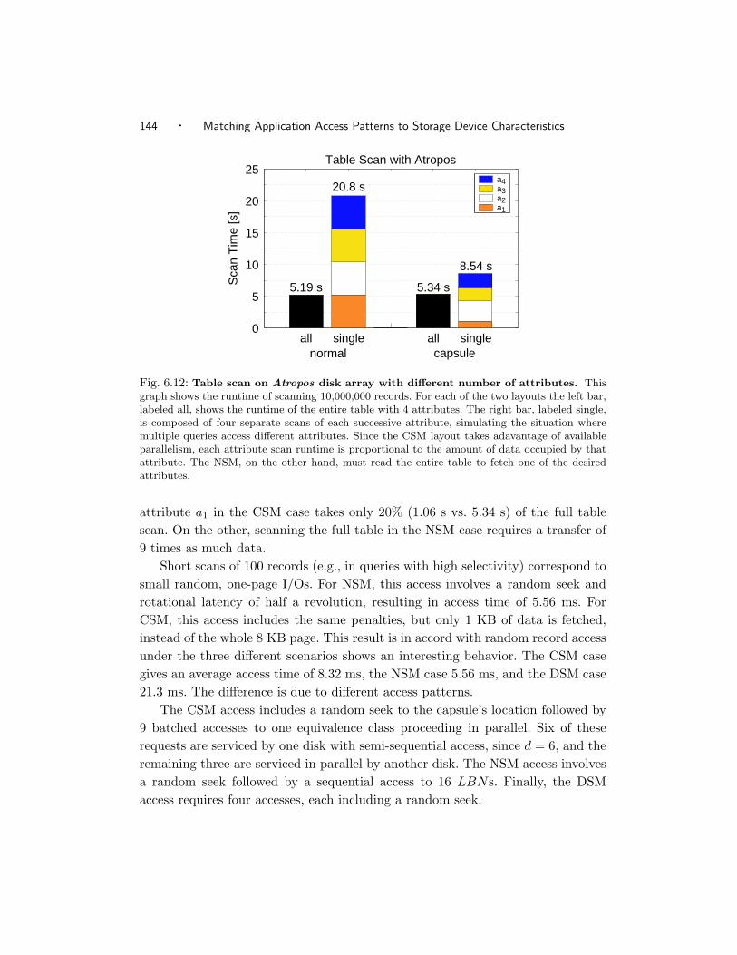
144 · Matching Application Access Patterns to Storage Device Characteristics
all single all single
5.19 s
20.8 s
5.34 s
8.54 s
normal capsule
Sca
n T
ime
[s]
Table Scan with Atropos
a4a3a2a1
0
5
10
15
20
25
Fig. 6.12: Table scan on Atropos disk array with different number of attributes. Thisgraph shows the runtime of scanning 10,000,000 records. For each of the two layouts the left bar,labeled all, shows the runtime of the entire table with 4 attributes. The right bar, labeled single,is composed of four separate scans of each successive attribute, simulating the situation wheremultiple queries access different attributes. Since the CSM layout takes adavantage of availableparallelism, each attribute scan runtime is proportional to the amount of data occupied by thatattribute. The NSM, on the other hand, must read the entire table to fetch one of the desiredattributes.
attribute a1 in the CSM case takes only 20% (1.06 s vs. 5.34 s) of the full table
scan. On the other, scanning the full table in the NSM case requires a transfer of
9 times as much data.
Short scans of 100 records (e.g., in queries with high selectivity) correspond to
small random, one-page I/Os. For NSM, this access involves a random seek and
rotational latency of half a revolution, resulting in access time of 5.56 ms. For
CSM, this access includes the same penalties, but only 1 KB of data is fetched,
instead of the whole 8 KB page. This result is in accord with random record access
under the three different scenarios shows an interesting behavior. The CSM case
gives an average access time of 8.32 ms, the NSM case 5.56 ms, and the DSM case
21.3 ms. The difference is due to different access patterns.
The CSM access includes a random seek to the capsule’s location followed by
9 batched accesses to one equivalence class proceeding in parallel. Six of these
requests are serviced by one disk with semi-sequential access, since d = 6, and the
remaining three are serviced in parallel by another disk. The NSM access involves
a random seek followed by a sequential access to 16 LBNs. Finally, the DSM
access requires four accesses, each including a random seek.

6.4 Database storage manager exploiting parallelism · 145
OperationData Layout
normal capsule
entire table scan 22.44 s 22.93 sa1 scan 22.44 s 2.43 sa1 + a2 scan 22.44 s 12.72 s100 complete records 1.58 ms 1.31 ms
Table 6.5: Database access results for G2 MEMStore. The table shows the runtime of thespecific operation on the 10,000,000 record table with 4 attributes for the NSM and CSM. Therows labeled a1 scan and a1 + a2 represent the scan through all records when specific attributesare desired. the last row shows the time to access the data for attribute a1 from 100 records.
MEMStore results
Table 6.5 summarizes the table scan results for the NSM and CSM cases. Scanning
the entire table takes respectively 22.44 s and 22.93 s for the NSM and CSM cases
and the corresponding user-data bandwidth is 30.9 MB/s and 30.3 MB/s. The
run time difference is due to the amount of actual data being transfered. Since the
NSM layout can pack data more tightly into its 8 KB page, it transfers a total
of 714 MB at a rate of 31.8 MB/s from the MEMStore. The CSM layout creates,
in effect, 512-byte pages which waste more space due to internal fragmentation.
Despite transferring 768 MB, it achieves a sustained bandwidth of 34.2 MB/s, or
7% higher than NSM. While both methods access all 10 LBNs in parallel most
of the time, the data access in the CSM case is more efficient due to smaller
repositioning overhead at the end of a cylinder.
Similar to the Atropos results, CSM is highly efficient when only a subset of the
attributes are required. A table scan of a1 or a1 +a2 in the NSM case always takes
22.44 s, since entire pages including the undesired attributes must be scanned.
The CSM case only requires a fraction of the time corresponding to the amount of
data for each desired attribute. Figure 6.13 compares the runs of a full table scan
for all attributes against four scans of individual attributes. The total runtime of
four individual-attribute scans in the CSM case takes the same amount of time as
the full table scan. In contrast, the four successive scans take four times as long
as the full table scan with the NSM layout.
Most importantly, a scan of a single attribute a1 in the CSM case takes only
one ninth (2.43 s vs. 22.93 s) of the full table scan since all ten parallel accesses
read records of a1. On the other, scanning the full table in the NSM case requires
a transfer of 9 times as much data and uses the parallelism p to access.
Short scans of 100 records (e.g., in queries with high selectivity) are 20% faster
for CSM since they fully utilize the MEMStore’s internal parallelism. Furthermore,
the latency to the first record is shorter due to smaller access units, compared to
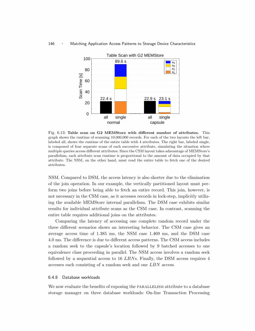
146 · Matching Application Access Patterns to Storage Device Characteristics
all single all single
22.4 s
89.6 s
22.9 s 23.1 s
0
20
40
60
80
100
Methodnormal capsule
Sca
n T
ime
[s]
Table Scan with G2 MEMStore
a4a3a2a1
Fig. 6.13: Table scan on G2 MEMStore with different number of attributes. Thisgraph shows the runtime of scanning 10,000,000 records. For each of the two layouts the left bar,labeled all, shows the runtime of the entire table with 4 attributes. The right bar, labeled single,is composed of four separate scans of each successive attribute, simulating the situation wheremultiple queries access different attributes. Since the CSM layout takes adavantage of MEMStore’sparallelism, each attribute scan runtime is proportional to the amount of data occupied by thatattribute. The NSM, on the other hand, must read the entire table to fetch one of the desiredattributes.
NSM. Compared to DSM, the access latency is also shorter due to the elimination
of the join operation. In our example, the vertically partitioned layout must per-
form two joins before being able to fetch an entire record. This join, however, is
not necessary in the CSM case, as it accesses records in lock-step, implicitly utiliz-
ing the available MEMStore internal parallelism. The DSM case exhibits similar
results for individual attribute scans as the CSM case. In contrast, scanning the
entire table requires additional joins on the attributes.
Comparing the latency of accessing one complete random record under the
three different scenarios shows an interesting behavior. The CSM case gives an
average access time of 1.385 ms, the NSM case 1.469 ms, and the DSM case
4.0 ms. The difference is due to different access patterns. The CSM access includes
a random seek to the capsule’s location followed by 9 batched accesses to one
equivalence class proceeding in parallel. The NSM access involves a random seek
followed by a sequential access to 16 LBNs. Finally, the DSM access requires 4
accesses each consisting of a random seek and one LBN access.
6.4.8 Database workloads
We now evaluate the benefits of exposing the parallelism attribute to a database
storage manager on three database workloads: On-line Transaction Processing

6.4 Database storage manager exploiting parallelism · 147
(OLTP), Decision Support System (DSS) queries, and compound workloads run-
ning both types concurrently.
The evaluation is done on a prototype implementation of a database storage
manager called Clotho [Shao et al. 2004]. In addition to using the row-major op-
timized NSM and column-major optimized DSM page layouts, Clotho can run
database queries with the CSM page layout that takes advantage of the paral-
lelism attribute exposed by a storage device (e.g., Atropos logical volume manager
or MEMStore). The Clotho storage manager is based on the Shore database storage
manager [Carey et al. 1994] and it leverages both the access delay boundaries
and parallelism attributes for page allocation and data access. The details of
Clotho implementation are described elsewhere [Shao et al. 2004].
With NSM and DSM page layouts, it is sufficient to take advantage of only
the access delay boundaries attribute (as described in Section 5.7) to achieve
efficient accesses in the respective optimized orders. However, the accesses in the
other order are inefficient. The CSM also leverages the parallelism attribute
in order to achieve efficient accesses in both dimensions. Hence, the CSM targets
environments where both access patterns are equally likely to occur.
Another page layout, called PAX, targets the same environments where both
types of accesses are likely to occur. It offers efficient execution of both access
patterns at the CPU-cache memory level [Ailamaki et al. 2001]. A single PAX page
contains all attributes, but partitions them across the page to avoid unnecessary
data fetches into CPU-cache when only a subset of attributes are needed. However,
from the prospective of the storage device, a PAX page is just like an NSM page
and therefore exhibits similar performance to NSM at the storage device level.
DSS workload performance
To compare the DSS workload performance for different layouts we run a subset
of the TPC-H decision support benchmark on our Clotho prototype. Each layout
uses an 8 KB page size. The TPC-H dataset is 1 GB and the buffer pool size is
128 MB. Figure 6.14 shows execution times relative to NSM for four representative
TPC-H queries. Q1 and Q6 are sequential scans through the largest table in the
TPC-H benchmark while Q12 and Q14 execute joins across two relations. The left
group of bars shows TPC-H execution on Atropos, whereas the right group shows
queries run on a simulated MEMStore. NSM performs the worst by a factor of
1.24× – 2.0× (except for DSM in Q1) because they must access all attributes.
The performance of DSM, compared to NSM, is better for all queries except
Q1 because of its high projectivity (i.e., number of attributes constituting query
payload). CSM performs best because it benefits from projectivity and avoids

148 · Matching Application Access Patterns to Storage Device Characteristics
Atropos disk array MEMS device
TPC-H Benchmark
0.0
0.2
0.4
0.6
0.8
1.0
1.2
1.4
1.6
Q1 Q6 Q12 Q14 Q1 Q6 Q12 Q14
Query #
Run
time
rela
tive
to N
SM
NSM DSM PAX CSM
Fig. 6.14: TPC-H performance for different layouts. Performance is shown relative to NSM.
the cost of the joins that DSM must do to reconstruct records. As expected, the
TPC-H benchmark performance for DSM and CSM is comparable, since both
storage models can efficiently access data, requesting only the attributes that
constitute the payload for the individual queries (7 attributes for Q1 and 5 for
Q6). DSM, however, must perform additional joins to reconstruct records, which
is not necessary when using CSM. NSM must fetch pages that contain full records
which results in the observed 1.24× to 2× worse performance. Not surprisingly,
PAX performs better than NSM but not as well as CSM; all attributes still have to
be fetched from a storage device into main memory. Its improvements over NSM
are due to more efficient memory access. Results with MEMStore exhibit the same
trends.
OLTP workload performance
The queries in a typical OLTP workload access a small number of records spread
across the entire database. In addition, OLTP applications have several insert and
delete statements as well as point updates. With NSM page layout, the entire
record can be retrieved by a single-page random I/O, because these layouts map
a single page to consecutive LBNs. Clotho spreads a single capsule across non-
consecutive LBNs of the logical volume, enabling efficient sequential access when
scanning a single attribute across multiple records and less efficient semi-sequential
scan when accessing full records.

6.4 Database storage manager exploiting parallelism · 149
Layout TpmC
NSM 1063PAX 1090DSM 140CSM 1002
Table 6.6: TPC-C benchmark results with Atropos disk array LVM. The table showsthe transactional throughput of the TPC-C benchmark.
The TPC-C benchmark approximates an OLTP workload on our Clotho pro-
totype with all four data layouts using 8 KB page size. TPC-C is configured with
10 warehouses, 100 users, no think time, and 60 seconds warm-up time. The buffer
pool size if 128 KB, so it only caches 10% of the database. The completed trans-
actions per minute (TpmC) throughput is repeatedly measured over a period of
120 seconds.
Table 6.6 shows the results of running the TPC-C benchmark. As expected,
DSM yields much lower throughput compared to NSM. Despite the less efficient
semi-sequential access, CSM observes only 6% lower throughput than NSM. The
frequent point updates inherent in the the TPC-C benchmark penalize CSM’s
performance: the semi-sequential access needs to to retrieve full records. This
penalty is in part compensated by the ability of the Clotho’s buffer pool manager
to create and share pages containing only the needed data.
Compound OLTP/DSS workload
Benchmarks involving compound workloads are important in order to measure
the impact on performance when different queries access the same logical volume
concurrently. With CSM, the performance degradation may be potentially worse
than in other page layouts. The originally efficient semi-sequential access to disjoint
LBNs (i.e., for OLTP queries) could be disrupted by competing I/Os from the
other workload creating inefficient access. This problem does not occur for other
layouts that map the entire page to consecutive LBNs that can be fetched in a
single media access.
We simulate a compound workload with a single-user DSS (TPC-H) workload
running concurrently with a multi-user OLTP workload (TPC-C) against our At-
ropos disk LVM and measure the differences in performance relative to the isolated
workloads. The respective TPC workloads are configured as described earlier. In
previous work [Schindler et al. 2003], we demonstrated the effectiveness of track-
aligned disk accesses on compound workloads; here, we compare all of the page
layouts using these efficient I/Os to achieve comparable results for TPC-H.

150 · Matching Application Access Patterns to Storage Device Characteristics
TPC-H query TPC-C
DSS and OLTP Compound Workload
0.0
0.2
0.4
0.6
0.8
1.0
1.2
1.4
1.6
NSM DSM PAX CSM NSM DSM PAX CSM
Slo
wdo
wn
rela
tive
to s
tand
-alo
ne w
orkl
oad
Stand-alone Compound
Fig. 6.15: Compound workload performance for different layouts. This figure expressesthe slowdown of TPC-H query 1 runtime when run concurrently with TPC-C benchmark relativeto the base case when running in isolation.
As shown in Figure 6.15, undue performance degradation does not occur: CSM
exhibits the same or lesser relative performance degradation than the other layouts.
The figure shows indicative performance results for TPC-H query 1 (others exhibit
similar behavior) and for TPC-C, relative to the base case when OLTP and DSS
queries run separately. The larger performance impact of compound workloads
on DSS with DSM shows that small random I/O traffic aggravates the impact of
seeks necessary to reconstruct a DSM page.
6.4.9 Results summary
The results for both MEMStore and the Atropos disk array demonstrate that
exposing performance attributes to database storage managers improves perfor-
mance of database workloads. For environments with only one workload type,
the access delay boundaries attribute is sufficient. The storage manager can
choose a page layout optimized for the workload type and achieve efficient accesses
by utilizing the explicit information. Naturally, the benefit of using the access
delay boundaries attribute is much larger for DSS workloads. Most DSS queries
can exploit ensemble-based access, while OLTP, dominated by small random I/O,
sees only minimal improvements.
The parallelism attribute enables efficient execution for a new type of en-
vironment with compound workloads exhibiting both row- and column-major ac-
cesses. A database system taking advantage of the parallelism attribute can

6.4 Database storage manager exploiting parallelism · 151
0.0
1.0
2.0
3.0
TPC-H Query 1 TPC-C Compound
Workload
Performance Comparison
Runtim
e r
ela
tive
to N
SM
NSM DSM CSM
Fig. 6.16: Comparison of three database workloads for different data layouts. Theworkload runtime is shown relative to NSM, which is the page layout prevalent in commercialdatabase systems. The TPC-C workload expresses the time to complete the same number oftransactions for the three different workloads. The compound workload measures the total run-time of TPC-H query 1 executed simultaneously with the TPC-C benchmark completing a fixednumber of transactions with no think time. Note that for DSM the runtime is respectively 7.5×and 4.5× larger for the TPC-C and Compound workloads.
use one data organization (CSM) for all three workload types (DSS, OLTP, and
compound workload of DSS/OLTP). In all three cases, CSM performance is equal
to or within 6% of the performance achieved with the respective layout optimized
for only one workload, as shown in Figure 6.16. This characteristic is important
for environments where workloads change over time (e.g., on-line retailers with
predominantly OLTP workload running DSS during off-peak hours). Using CSM
eliminates the need to use two replicas of data to run both workloads efficiently
and also reduces the total cost of ownership — only one set of hardware is required.
The parallelism attribute abstraction can hide device-specifics. With a few
simple storage interface constructs, described in Appendix B, a storage manager
can work seamlessly across devices with vastly different performance character-
istics such as MEMStore and disk arrays, yet experience the same quantitative
improvements.
6.4.10 Improving efficiency for a spectrum of workloads
To extrapolate how performance attributes improve efficiency across a spectrum of
access patterns, Figure 6.17 compares access in current systems using state-of-the
art techniques and systems that exploit performance attributes. It extrapolates
from the database experiments results described in Chapter 5 and 6 and data

152 · Matching Application Access Patterns to Storage Device Characteristics
Extrapolated efficiency for different workload types
0.0
0.2
0.4
0.6
0.8
1.0
OLTP DSS CompoundWorkload
Effc
ienc
yNone ADB ADB+PARmaximum streaming efficiency
Fig. 6.17: Comparison of disk efficiencies for three database workloads.
collected from raw disk accesses. It expresses the results in terms of disk access
efficiency of each individual disk of a four-disk logical volume. Disk efficiency is
defined in Chapter 5 and Figure 5.1 as the ratio between media access time (time
spent doing useful work) and total I/O service time, which also includes positioning
time. The results also take into account how much data is requested by the system
vs. how much is actually needed by the application.
The graph in Figure 6.17 compares for each workload type the disk access ef-
ficiency of the (i) current best approach that does not use any information from
storage devices (labeled None), (ii) one that uses only the access delay bound-
aries attribute (labeled ADB), and (iii) one that uses both the access delay
boundaries and the parallelism attributes (labeled ADB+PAR). The efficiency
of the base case for the OLTP workload is assessed from measurements of response
times and using DiskSim models to break response time into individual compo-
nents: seek, rotational latency, and media transfer. The results for the DSS and
compound workloads are assessed from experimental measurements on scenario
(iii) and the efficiencies for the other two scenarios are extrapolated from data in
Figure 5.1 and I/O traces for the respective workloads.
For the OLTP workload, the disk efficiency of scenario (i) is expressed for a
system using an 8 KB NSM page. Scenario (ii) also uses the NSM page layout
with 8 KB pages allocated in extents matching access delay boundaries, as
described in Section 5.7.3. Scenario (iii) uses the CSM page layout, described in
Section 6.4.2. As can be seen, performance attributes do not significantly improve

6.4 Database storage manager exploiting parallelism · 153
disk efficiency. The ADB case, however, improves overall workload performance
by almost 7% compared to the base scenario. The slightly lower efficiency for the
ADB+PAR scenario stems from using CSM instead of NSM — semi-sequential
access, instead of sequential, is used when fetching a single page. The overall
efficiency for all three scenarios is 0.21, 0.23, and 0.20 respectively.
The achieved access efficiencies are much lower than the best possible case of
maximum streaming efficiency for the following reason: OLTP workload is domi-
nated by random accesses to individual pages that are only 8 KB in size. Hence
disk access time is dominated by seeks and rotational latencies, while the time for
useful data transfer is negligible compared to the positioning time.
For the DSS workload, the data represents the average across the 22 TPC-
H queries. Scenario (i) expresses access efficiency of a system with 8 KB DSM
page layout and issuing I/Os that match stripe unit size approximating track size
(256 KB for the Maxtor Atlas 10k III disks). Scenario (ii) also uses 8 KB DSM
pages, but I/O sizes match as close as possible the access delay boundaries
attribute. Scenario (iii) uses the CSM page layout.
In contrast to the OLTP workload, performance attributes significantly im-
prove disk efficiency. The slightly lower efficiency for the ADB+PAR case com-
pared to the ADB is due to different page layout; CSM is slightly less efficient
when packing records into a single page. The achieved access efficiency for the
DSS workload is closer to the maximum streaming efficiency of the disk than for
the OLTP workload. For a given I/O, seeks are still present, but (for the majority
of the TPC-H benchmark queries), the performance attributes are able to signifi-
cantly reduce rotational latency and achieve media transfers from the majority of
the disk’s track. The only way to increase access efficiency is through reduction of
seek times. However, this can only be possible by employing a workload (query)-
specific layout, which could shorten the seek distance and hence reduce seek time,
or by improving disk’s characteristics.
For the compound DSS/OLTP workload, the data shown represents the disk
efficiency averaged over all I/Os in the workload. Recall that the workload exhibits
both small 8 KB I/Os (coming from the OLTP workload) and much larger I/Os
(coming from the DSS workload). Both scenarios (i) and (ii) use the NSM page
layout, which is prevalent in commercial DBMS, and scenario (iii) uses CSM. The
I/O sizes of each workload are the same as for the respective stand-alone workloads
described in the preceding two paragraphs. As can be seen from the graph, this
workload type benefits from utilizing both performance attributes.

154 · Matching Application Access Patterns to Storage Device Characteristics

7 Conclusions and Future Work
7.1 Concluding remarks
This dissertation demonstrates that storage managers in conventional computer
systems have insufficient information about storage device performance charac-
teristics. As a consequence, they utilize the available storage device resources in-
efficiently. This results in undue application performance degradation, especially
when competing workloads contend for the same storage device. A few high-level,
device-independent static hints about storage device performance characteristics
can achieve significant I/O performance gains for workloads exhibiting regular
access patterns.
The two examples of performance attributes proposed in this dissertation serve
as these high-level, device-independent static hints. They can capture unique de-
vice characteristics to allow storage managers to automatically tune their access
patterns to the given device. These attributes do not break established storage
interface abstractions and for certain systems, as illustrated on the example of
database systems, simple abstractions are restored. In particular, these attributes
allow a storage manager to maintain the assumptions about access efficiencies
made by other parts of the system regardless of the dynamic workload changes.
And most importantly, they greatly simplify, or completely eliminate, the difficult
and error-prone task of performance tuning.
For database systems, explicit performance attributes allow a database stor-
age manager to specialize to particular storage devices and provide more robust
performance in the presence of concurrent query execution. In particular, it can
support high I/O concurrency without disrupting planned sequential I/O perfor-
mance. It also eliminates the need for several (previously DBA-specified) parame-
ters, thereby simplifying DBMS configuration and performance tuning. Explicitly
stated characteristics restore the validity of the assumptions made by the query
optimizer about the relative costs of different storage access patterns.
Since a storage manager is any system component that translates requests for
data to the underlying mechanism for storing this data, the findings of this disser-

156 · Matching Application Access Patterns to Storage Device Characteristics
tation are applicable at many levels of the I/O path. In addition to file systems,
database systems, and logical volume managers (whose implementations are de-
tailed in this dissertation), the same mechanisms can be used in other systems as
well. For example, object-based storage systems can use the described mechanisms
to efficiently store and access objects on the underlying storage device.
Performance hints mesh well with existing system software data structures and
algorithms. Thus, computer systems need minimal changes to incorporate them
and can use unmodified existing storage devices. The three different storage man-
ager implementations described in this dissertation made no changes to storage
device hardware in order to enjoy the documented performance gains.
The evaluation of access efficiencies for state-of-the-art disk drives reveals a
few noteworthy points. Zero-latency access is an important firmware feature that
yields large improvements with track-based access. A storage manager that ex-
ploits these accesses (such as the ones described in this dissertation) can greatly
benefit. When combined with out-of-order data delivery (which is defined in the
SCSI specification, it yields additional 10% improvement in access efficiency. All
disk vendors should implement both of these features and thus create an oppor-
tunity for storage managers to exploit them.
The access delay boundaries attribute can achieve significant increase in
access efficiency (within 82% of the maximum efficiency) for random accesses that
are appropriately sized and aligned on ensemble boundaries. A variety of systems
such as disk array logical volume managers, file systems, or database systems can
match their access patterns to utilize this access efficiency. The parallelism at-
tribute offers efficient access to two dimensional data structures. Compared to
traditional systems that, in order to achieve better access efficiency, fetch extrane-
ous data that is dropped, a data layout taking advantage of this attribute allows
applications to request only the data that is needed.
The proposed mechanism for providing explicit performance hints by attribute
annotation represents only one possible solution. The focus of this dissertation
is on identifying what device-specific characteristics should be exposed to allow
better utilization of the available storage device resources rather than on how the
information should be conveyed.
7.2 Directions for future research
This dissertation encompasses a broad range of storage and computer systems.
There are many interesting topics it touched upon that are worth exploring in
more detail.

7.2 Directions for future research · 157
The obvious next step is the research of more attributes that can potentially
provide benefit to storage managers. This dissertation presents two examples of
attributes, namely the access delay boundaries and parallelism, that encap-
sulate a variety of unique storage device characteristics. It also discusses the fault-
isolation boundary attribute proposed by related research [Denehy et al. 2002].
Studying if other attributes can potentially capture additional important device
performance characteristics and evaluating by how much they improve application
performance should provide interesting insights.
The performance hints described in this dissertation are static in their nature.
They prescribe to the storage manager how to exercise its access patterns to obtain
the best possible efficiency at any level of device utilization. Because of this invari-
ant, the hints need not quantify device performance. It can be simply observed by
the storage manager which can decide if it is sufficient for the application needs.
Capturing and quantifying dynamic behavior by performance attributes may pro-
vide additional benefits. However, it will also require more substantial changes to
the storage interface and system software behavior.
Sufficient information about device performance characteristics given to a stor-
age manager can significantly improve application performance. The chosen method
of annotating device’s linear address space with attributes described in this dis-
sertation gets this job done. The thesis of this dissertation provides an interesting
basis for exploring alternative and more expressive storage interfaces. Evaluating
the tradeoff between these new interfaces and the effort required to modify existing
systems to adapt them warrants more research.
Performance characteristics discovery tools are specialized to one type of a
storage device. The DIXtrac tool described in this dissertation works with disk
drives. Building upon its methods, similar tools could be potentially built to au-
tomatically characterize disk arrays, which have more complicated internal struc-
ture. This characterization would be useful for other applications such as capacity
planning and storage outsourcing with different service-level agreements.

158 · Matching Application Access Patterns to Storage Device Characteristics

Bibliography
Ailamaki, A., DeWitt, D. J., Hill, M. D., and Skounakis, M. 2001. Weav-
ing relations for cache performance. In International Conference on Very Large
Databases. Morgan Kaufmann Publishing, Inc., 169–180.
Ailamaki, A., DeWitt, D. J., Hill, M. D., and Wood, D. A. 1999. DBMSs
on a modern processor: where does time go? In International Conference on
Very Large Databases. Morgan Kaufmann Publishing, Inc., 266–277.
Anderson, D., Dykes, J., and Riedel, E. 2003. More than an interface—SCSI
vs. ATA. In Conference on File and Storage Technologies. USENIX Association.
Arge, L., Procopiuc, O., and Vitter, J. S. 2002. Implementing i/o-efficient
data structures using tpie. In European Symposium on Algorithms. 88–100.
Arpaci-Dusseau, A. and Arpaci-Dusseau, R. 2001. Information and control
in gray-box systems. In ACM Symposium on Operating System Principles. 43–
56.
Arpaci-Dusseau, R. H., Anderson, E., Treuhaft, N., Culler, D. E.,
Hellerstein, J. M., Patterson, D., and Yelick, K. 1999. Cluster I/O
with River: making the fast case common. In Workshop on Input/Output in
Parallel and Distributed Systems.
Bailey, D. H., Barszcz, E., Dagum, L., and Simon, H. D. 1993. NAS par-
allel benchmark results 10-93. Tech. Rep. RNR–93–016, NASA Ames Research
Center, Mail Stop T045-1, Moffett Field, CA 94035.
Baker, M. G., Hartman, J. H., Kupfer, M. D., Shirriff, K. W., and
Ousterhout, J. K. 1991. Measurements of a distributed file system. In ACM
Symposium on Operating System Principles. 198–212.
Bitton, D. and Gray, J. 1988. Disk shadowing. In International Conference
on Very Large Databases. 331–338.

160 · Matching Application Access Patterns to Storage Device Characteristics
Blackwell, T., Harris, J., and Seltzer, M. 1995. Heuristic cleaning algo-
rithms in log-structured file systems. In USENIX Annual Technical Conference.
USENIX Association, 277–288.
Bolosky, W. J., Barrera, J. S., Draves, R. P., Fitzgerald, R. P., Gib-
son, G. A., Jones, M. B., Levi, S. P., Myhrvold, N. P., and Rashid,
R. F. 1996. The Tiger video fileserver. Tech. Rep. MSR–TR–96–09, Microsoft
Corporation.
Boncz, P. A., Manegold, S., and Kersten, M. L. 1999. Database architec-
ture optimized for the new bottleneck: memory access. In International Con-
ference on Very Large Databases. Morgan Kaufmann Publishers, Inc., 54–65.
Bovet, D. P. and Cesati, M. 2001. Understanding the Linux kernel. O’Reilly
& Associates.
Brown, A. D., Mowry, T. C., and Krieger, O. 2001. Compiler-based I/O
prefetching for out-of-core applications. ACM Transactions on Computer Sys-
tems 19, 2, 111–170.
Bucy, J. S. and Ganger, G. R. 2003. The DiskSim simulation environment
version 3.0 reference manual. Tech. Rep. CMU–CS–03–102, Department of Com-
puter Science Carnegie-Mellon University, Pittsburgh, PA.
Burnett, N. C., Bent, J., Arpaci-Dusseau, A. C., and Arpaci-Dusseau,
R. H. 2002. Exploiting gray-box knowledge of buffer-cache contents. In USENIX
Annual Technical Conference. 29–44.
Carey, M. J., DeWitt, D. J., Franklin, M. J., Hall, N. E., McAuliffe,
M. L., Naughton, J. F., Schuh, D. T., Solomon, M. H., Tan, C. K., Tsa-
talos, O. G., White, S. J., and Zwilling, M. J. 1994. Shoring up persistent
applications. In ACM SIGMOD International Conference on Management of
Data. 383–394.
Carley, L. R., Ganger, G. R., and Nagle, D. F. 2000. MEMS-based
integrated-circuit mass-storage systems. Communications of the ACM 43, 11,
73–80.
Carson, S. and Setia, S. 1992. Optimal write batch size in log-structured file
systems. In USENIX Workshop on File Systems. 79–91.
Chang, E. and Garcia-Molina, H. 1996. Reducing initial latency in a mul-
timedia storage system. In International Workshop on Multi-Media Database
Management Systems. 2–11.
Bibliography · 161
Chang, E. and Garcia-Molina, H. 1997. Effective memory use in a media
server. In International Conference on Very Large Databases. Morgan Kaufmann
Publishers, Inc., 496–505.
Chao, C., English, R., Jacobson, D., Stepanov, A., and Wilkes, J. 1992.
Mime: high performance parallel storage device with strong recovery guarantees.
Tech. Rep. HPL-92-9, HPL-92-9.
Chen, P. M., Lee, E. K., Gibson, G. A., Katz, R. H., and Patterson, D. A.
1994. RAID: high-performance, reliable secondary storage. ACM Computing
Surveys 26, 2, 145–185.
Chen, P. M. and Patterson, D. A. 1990. Maximizing performance in a striped
disk array. In ACM International Symposium on Computer Architecture. 322–
331.
Chen, S., Gibbons, P. B., Mowry, T. C., and Valentin, G. 2002. Fractal
prefetching B+-trees: optimizing both cache and disk performance. In ACM
SIGMOD International Conference on Management of Data. ACM Press, 157–
168.
Copeland, G. P. and Khoshafian, S. 1985. A decomposition storage model. In
ACM SIGMOD International Conference on Management of Data. ACM Press,
268–279.
Corbett, P. F. and Feitelson, D. G. 1994. Design and implementation of the
Vesta parallel file system. In Scalable High-Performance Computing Conference.
63–70.
Cormen, T. H. 1993. Fast permuting on disk arrays. Journal of Parallel and
Distributed Computing 17, 1, 41–57.
Daniel, S. and Geist, R. 1983. V-SCAN: an adaptive disk scheduling algorithm.
In International Workshop on Computer Systems Organization. IEEE, 96–103.
Denehy, T. E., Arpaci-Dusseau, A. C., and Arpaci-Dusseau, R. H. 2002.
Bridging the information gap in storage protocol stacks. In Summer USENIX
Technical Conference. 177–190.
Denning, P. J. 1967. Effects of scheduling on file memory operations. In AFIPS
Spring Joint Computer Conference. 9–21.
DeWitt, D. J., Ghandeharizadeh, S., Schneider, D. A., Bricker, A., Hui-
IHsiao, and Rasmussen, R. 1990. The Gamma database machine project.
IEEE Transactions on Knowledge and Data Engineering 2, 1, 44–62.

162 · Matching Application Access Patterns to Storage Device Characteristics
Douceur, J. R. and Bolosky, W. J. 1999. A large-scale study of file-system
contents. In ACM SIGMETRICS Conference on Measurement and Modeling of
Computer Systems. ACM Press, 59–70.
English, R. M. and Stepanov, A. A. 1992. Loge: a self-organizing disk con-
troller. In Winter USENIX Technical Conference. Usenix, 237–251.
Fedder, G. K., Santhanam, S., Reed, M. L., Eagle, S. C., Guillou, D. F.,
Lu, M. S.-C., and Carley, L. R. 1996. Laminated high-aspect-ratio mi-
crostructures in a conventional CMOS process. In IEEE Micro Electro Mechan-
ical Systems Workshop. 13–18.
Freedman, C. S., Burger, J., and DeWitt, D. J. 1996. SPIFFI-a scalable
parallel file system for the Intel Paragon. IEEE Transactions on Parallel and
Distributed Systems 7, 11, 1185–1200.
Fuller, S. H. 1972. An optimal drum scheduling algorithm. IEEE Transactions
on Computers 21, 11, 1153–1165.
Gabber, E. and Shriver, E. 2000. Lets put NetApp and CacheFlow out of
business. In SIGOPS European Workshop. 85–90.
Ganger, G. R. 1995. System-oriented evaluation of I/O subsystem performance.
Ph.D. thesis, University of Michigan, Ann Arbor, MI.
Ganger, G. R. and Kaashoek, M. F. 1997. Embedded inodes and explicit
grouping: exploiting disk bandwidth for small files. In USENIX Annual Tech-
nical Conference. 1–17.
Ganger, G. R., Worthington, B. L., Hou, R. Y., and Patt, Y. N. 1994.
Disk arrays: high-performance, high-reliability storage systems. IEEE Com-
puter 27, 3, 30–36.
Geist, R. and Daniel, S. 1987. A continuum of disk scheduling algorithms.
ACM Transactions on Computer Systems 5, 1, 77–92.
Ghemawat, S. 1995. The modified object buffer: a storage management tech-
nique for object-oriented databases. Ph.D. thesis, Massachusetts Institute of
Technology, Cambridge, MA.
Giampaolo, D. 1998. Practical file system design with the Be file system. Morgan
Kaufmann.

Bibliography · 163
Gibson, G. A., Nagle, D. F., Amiri, K., Butler, J., Chang, F. W., Gob-
ioff, H., Hardin, C., Riedel, E., Rochberg, D., and Zelenka, J. 1998.
A cost-effective, high-bandwidth storage architecture. In Architectural Support
for Programming Languages and Operating Systems. 92–103.
Graefe, G. 1993. Query evaluation techniques for large databases. ACM Com-
puting Surveys 25, 2, 73–170.
Griffin, J. L., Schindler, J., Schlosser, S. W., Bucy, J. C., and Ganger,
G. R. 2002. Timing-accurate storage emulation. In Conference on File and
Storage Technologies. USENIX Association, 75–88.
Griffin, J. L., Schlosser, S. W., Ganger, G. R., and Nagle, D. F. 2000a.
Modeling and performance of MEMS-based storage devices. In ACM SIGMET-
RICS Conference on Measurement and Modeling of Computer Systems. 56–65.
Griffin, J. L., Schlosser, S. W., Ganger, G. R., and Nagle, D. F. 2000b.
Operating system management of MEMS-based storage devices. In Symposium
on Operating Systems Design and Implementation. USENIX Association, 227–
242.
Hitz, D., Lau, J., and Malcolm, M. 1994. File system design for an NFS file
server appliance. In Winter USENIX Technical Conference. USENIX Associa-
tion, 235–246.
Hou, R. Y., Menon, J., and Patt, Y. N. 1993. Balancing I/O response time
and disk rebuild time in a RAID5 disk array. In Hawaii International Conference
on Systems Sciences.
Huang, L. and cker Chiueh, T. 1999. Implementation of a rotation latency
sensitive disk scheduler. Tech. Rep. ECSL TR-81, SUNY Stony Brook.
IBM Corporation 1994. DB2 V3 Performance Topics. IBM Corporation.
IBM Corporation 2000. IBM DB2 Universal Database Administration Guide:
Implementation. IBM Corporation.
Jacobson, D. M. and Wilkes, J. 1991. Disk scheduling algorithms based on
rotational position. Tech. Rep. HPL–CSP–91–7, Hewlett-Packard Laboratories,
Palo Alto, CA.
Kaashoek, M. F., Engler, D. R., Ganger, G. R., and Wallach, D. A.
1996. Server operating systems. In ACM SIGOPS. European workshop: Systems
support for worldwide applications. ACM, 141–148.

164 · Matching Application Access Patterns to Storage Device Characteristics
Katcher, J. 1997. PostMark: a new file system benchmark. Tech. Rep. TR3022,
Network Appliance.
Keeton, K. and Katz, R. H. 1993. The evaluations of video layout strategies
on a high-bandwidth file server. In 4th International Workshop on Network and
Operating System Support for Digital Audio and Video. 228–229.
Kotz, D. 1994. Disk-directed I/O for MIMD multiprocessors. In Symposium on
Operating Systems Design and Implementation. USENIX Association, 61–74.
Kotz, D., Toh, S. B., and Radhakrishnan, S. 1994. A detailed simulation
model of the HP 97560 disk drive. Tech. Rep. PCS–TR94–220, Department of
Computer Science, Dartmouth College.
Krieger, O. and Stumm, M. 1997. HFS: a performance-oriented flexible file
system based on building-block compositions. ACM Transactions on Computer
Systems 15, 3, 286–321.
Loney, K. and Koch, G. 2000. Oracle 8i: The Complete Reference.
Osborne/McGraw-Hill.
Lumb, C. R., Schindler, J., and Ganger, G. R. 2002. Freeblock schedul-
ing outside of disk firmware. In Conference on File and Storage Technologies.
USENIX Association, 275–288.
Lumb, C. R., Schindler, J., Ganger, G. R., Nagle, D. F., and Riedel, E.
2000. Towards higher disk head utilization: extracting free bandwidth from busy
disk drives. In Symposium on Operating Systems Design and Implementation.
USENIX Association, 87–102.
Maluf, N. 2000. An introduction to microelectromechanical systems engineering.
Artech House.
Manegold, S., Boncz, P. A., and Kersten, M. L. 2002. Generic database
cost models for hierarchical memory systems. In International Conference on
Very Large Databases. Morgan Kaufmann Publishers, Inc., 191–202.
Matthews, J. N., Roselli, D., Costello, A. M., Wang, R. Y., and An-
derson, T. E. 1997. Improving the performance of log-structured file systems
with adaptive methods. In ACM Symposium on Operating System Principles.
ACM, 238–252.
Mayr, T. and Gray, J. 2000. Performance of the One-to-One Data Pump.
http://research.microsoft.com/Gray/river/PerformanceReport.pdf.

Bibliography · 165
McKusick, M. K., Joy, W. N., Leffler, S. J., and Fabry, R. S. 1984. A fast
file system for UNIX. ACM Transactions on Computer Systems 2, 3, 181–197.
McVoy, L. W. and Kleiman, S. R. 1991. Extent-like performance from a UNIX
file system. In USENIX Annual Technical Conference. USENIX, 33–43.
Mehta, M. and DeWitt, D. J. 1995. Managing intra-operator parallelism in
parallel database systems. In International Conference on Very Large Databases.
Morgan Kaufmann Publishers, Inc., 382–394.
Mehta, M. and DeWitt, D. J. 1997. Data placement in shared-nothing parallel
database systems. VLDB Journal 6, 1, 53–72.
Menon, J. and Mattson, D. 1992. Comparison of sparing alternatives for disk
arrays. In ACM International Symposium on Computer Architecture. 318–329.
Mohan, C., Haderle, D. J., Lindsay, B. G., Pirahesh, H., and Schwarz,
P. M. 1992. ARIES: a transaction recovery method supporting fine-granularity
locking and partial rollbacks using write-ahead logging. ACM Transactions on
Database Systems 17, 1, 94–162.
Nagar, R. 1997. Windows NT File System Internals: A Developer’s Guide.
O’Reilly & Associates.
National Committee for Information Technology Standards 2002. Working Draft
SCSI Object-Based Storage Device Commands (OSD). National Committee for
Information Technology Standards.
Network Appliance, Inc. 2002. NetCache C2100. Network Appliance, Inc. .
http://www.netapp.com/products/netcache/netcache family.html.
Ousterhout, J. K., Da Costa, H., Harrison, D., Kunze, J. A., Kupfer,
M., and Thompson, J. G. 1985. A trace-driven analysis of the UNIX 4.2 BSD
file system. In ACM Symposium on Operating System Principles. 15–24.
Patterson, D. A., Gibson, G., and Katz, R. H. 1988. A case for redundant
arrays of inexpensive disks (RAID). In ACM SIGMOD International Conference
on Management of Data. 109–116.
Patterson, R. H., Gibson, G. A., Ginting, E., Stodolsky, D., and Ze-
lenka, J. 1995. Informed prefetching and caching. In ACM Symposium on
Operating System Principles. 79–95.
Quantum Corporation 1999. Quantum Atlas 10K 9.1/18.2/36.4 GB SCSI product
manual. Quantum Corporation.

166 · Matching Application Access Patterns to Storage Device Characteristics
Ramamurthy, R., DeWitt, D. J., and Su, Q. 2002. A case for fractured mir-
rors. In International Conference on Very Large Databases. Morgan Kaufmann
Publishers, Inc., 430–441.
Rao, J. and Ross, K. A. 1999. Cache conscious indexing for decision-support in
main memory. In International Conference on Very Large Databases. Morgan
Kaufmann Publishers, Inc., 78–89.
Reddy, A. L. N. and Wyllie, J. 1993. Disk scheduling in a multimedia I/O
system. In International Multimedia Conference. ACM Press, 225–234.
Reiser, H. T. 2001. ReiserFS v. 3 whitepaper. http://www.namesys.com/.
Riedel, E., Faloutsos, C., Ganger, G. R., and Nagle, D. F. 2000. Data
mining on an oltp system (nearly) for free. In ACM SIGMOD International
Conference on Management of Data. ACM, 13–21.
Rosenblum, M. and Ousterhout, J. K. 1992. The design and implementation
of a log-structured file system. ACM Transactions on Computer Systems 10, 1,
26–52.
Ruemmler, C. and Wilkes, J. 1991. Disk Shuffling. Tech. Rep. HPL-91-156,
Hewlett-Packard Company, Palo Alto, CA.
Ruemmler, C. and Wilkes, J. 1993. UNIX disk access patterns. In Winter
USENIX Technical Conference. 405–420.
Santos, J. R. and Muntz, R. 1997. Design of the RIO (randomized I/O)
storage server. Tech. Rep. 970032, UCLA Computer Science Department.
Santos, J. R., Muntz, R. R., and Ribeiro-Neto, B. 2000. Comparing random
data allocation and data striping in multimedia servers. In ACM SIGMETRICS
Conference on Measurement and Modeling of Computer Systems. ACM Press,
44–55.
Schindler, J., Ailamaki, A., and Ganger, G. R. 2003. Lachesis: robust
database storage management based on device-specific performance character-
istics. In International Conference on Very Large Databases. Morgan Kaufmann
Publishing, Inc.
Schindler, J. and Ganger, G. R. 1999. Automated disk drive characterization.
Tech. Rep. CMU–CS–99–176, Carnegie-Mellon University, Pittsburgh, PA.
Bibliography · 167
Schindler, J., Griffin, J. L., Lumb, C. R., and Ganger, G. R. 2002. Track-
aligned extents: matching access patterns to disk drive characteristics. In Con-
ference on File and Storage Technologies. USENIX Association, 259–274.
Schlosser, S. W., Griffin, J. L., Nagle, D. F., and Ganger, G. R. 2000.
Designing computer systems with MEMS-based storage. In Architectural Sup-
port for Programming Languages and Operating Systems. 1–12.
Schlosser, S. W., Schindler, J., Ailamaki, A., and Ganger, G. R. 2003.
Exposing and exploiting internal parallelism in MEMS-based storage. Tech.
Rep. CMU–CS–03–125, Carnegie-Mellon University, Pittsburgh, PA.
Schmidt, B., Northcutt, J., and Lam, M. 1995. A method and apparatus for
measuring media synchronization. In International Workshop on Network and
Operating System Support for Digital Audio and Video. 203–214.
Schmidt, F. 1995. The SCSI Bus and IDE Interface. Addison-Wesley.
Selinger, P. G., Astrahan, M. M., Chamberlin, D. D., Lorie, R. A., and
Price, T. G. 1979. Access path selection in a relational database management
system. In ACM SIGMOD International Conference on Management of Data.
ACM Press, 23–34.
Seltzer, M., Bostic, K., McKusick, M. K., and Staelin, C. 1993. An
implementation of a log-structured file system for UNIX. In Winter USENIX
Technical Conference. 307–326.
Seltzer, M., Chen, P., and Ousterhout, J. 1990. Disk scheduling revisited.
In Winter USENIX Technical Conference. 313–323.
Seltzer, M., Smith, K. A., Balakrishnan, H., Chang, J., McMains, S.,
and Padmanabhan, V. 1995. File system logging versus clustering: a perfor-
mance comparison. In USENIX Annual Technical Conference. Usenix Associa-
tion, 249–264.
Seltzer, M. I., Ganger, G. R., McKusick, M. K., Smith, K. A., Soules,
C. A. N., and Stein, C. A. 2000. Journaling versus Soft Updates: Asyn-
chronous Meta-data Protection in File Systems. In USENIX Annual Technical
Conference. 71–84.
Shao, M., Schindler, J., Schlosser, S. W., Ailamaki, A., and Ganger,
G. R. 2004. Clotho: decoupling memory page layout from storage organization.
Tech. Rep. CMU–PDL–04–102, Carnegie-Mellon University, Pittsburgh, PA.

168 · Matching Application Access Patterns to Storage Device Characteristics
Shriver, E., Gabber, E., Huang, L., and Stein, C. A. 2001. Storage man-
agement for web proxies. In USENIX Annual Technical Conference. 203–216.
Shriver, E., Merchant, A., and Wilkes, J. 1998. An analytic behavior model
for disk drives with readahead caches and request reordering. In International
Conference on Measurement and Modeling of Computer Systems. ACM, 182–
191.
Shriver, L., Smith, K., and Small, C. 1999. Why does file system prefetching
work? In USENIX. 71–83.
Sienknecht, T. F., Friedrich, R. J., Martinka, J. J., and Friedenbach,
P. M. 1994. The implications of distributed data in a commercial environ-
ment on the design of hierarchical storage management. Performance Evalua-
tion 20, 1–3, 3–25.
Smith, K. A. and Seltzer, M. 1996. A comparison of FFS disk allocation
policies. In USENIX.96. USENIX Assoc., 15–25.
Steere, D. C. 1997. Exploiting the non-determinism and asynchrony of set
iterators to reduce aggreggate file I/O latency. In ACM Symposium on Operating
System Principles. ACM, 252–263.
Sweeney, A. 1996. Scalability in the XFS file system. In USENIX Annual
Technical Conference. 1–14.
Tacit Networks 2002. Tacit cache appliance. Tacit Networks. http://-
www.tacitnetworks.com/.
Talagala, N., Dusseau, R. H., and Patterson, D. 2000. Microbenchmark-
based extraction of local and global disk characteristics. Tech. Rep. CSD–99–
1063, University of California at Berkeley.
Transactional Processing Performance Council 2002a. TPC Benchmark C. Trans-
actional Processing Performance Council.
Transactional Processing Performance Council 2002b. TPC Benchmark H. Trans-
actional Processing Performance Council.
Uysal, M., Merchant, A., and Alvarez, G. A. 2003. Using MEMS-based
storage in disk arrays. In Conference on File and Storage Technologies. USENIX
Association, 89–102.
VanMeter, R. 1997. Observing the effects of multi-zone disks. In USENIX
Annual Technical Conference. 19–30.

Bibliography · 169
VanMeter, R. 1998. SLEDs: storage latency estimation descriptors. In IEEE
Symposium on Mass Storage Systems. USENIX.
Vengroff, D. E. 1994. A transparent parallel I/O environment. In DAGS
Symposium on Parallel Computation. 117–134.
Vengroff, D. E. and Vitter, J. S. 1995. I/O-Efficient scientific computation
using TPIE. Tech. Rep. CS-1995-18, Duke University.
VERITAS Software Company 2000. VERITAS Volume Manager 3.1 Administra-
tor’s Guide. VERITAS Software Company.
Vettiger, P., Despont, M., Drechsler, U., Durig, U., Haberle, W.,
Lutwyche, M. I., Rothuizen, H. E., Stutz, R., Widmer, R., and Binnig,
G. K. 2000. The “Millipede” – more than one thousand tips for future AFM
data storage. IBM Journal of Research and Development 44, 3, 323–340.
Vin, H. M., Goyal, A., and Goyal, P. 1995. Algorithms for designing multi-
media servers. IEEE Computer Communications 18, 3, 192–203.
Vitter, J. S. and Shriver, E. A. M. 1994. Algorithms for parallel memory I:
two-level memories. Algorithmica 12, 2/3, 110–147.
Vogels, W. 1999. File system usage in Windows NT 4.0. In ACM Symposium
on Operating System Principles. ACM, 93–109.
Wang, R. Y., Patterson, D. A., and Anderson, T. E. 1999. Virtual log
based file systems for a programmable disk. In Symposium on Operating Systems
Design and Implementation. ACM, 29–43.
Wilkes, J., Golding, R., Staelin, C., and Sullivan, T. 1996. The HP
AutoRAID hierarchical storage system. ACM Transactions on Computer Sys-
tems 14, 1, 108–136.
Wise, K. D. 1998. Special issue on integrated sensors, microactuators, and mi-
crosystems (MEMS). Proceedings of the IEEE 86, 8, 1531–1787.
Wong, T. M. and Wilkes, J. 2002. My cache or yours? Making storage more
exclusive. In USENIX Annual Technical Conference. 161–175.
Worthington, B. L., Ganger, G. R., and Patt, Y. N. 1994. Scheduling
algorithms for modern disk drives. In ACM SIGMETRICS Conference on Mea-
surement and Modeling of Computer Systems. ACM Press, 241–251.

170 · Matching Application Access Patterns to Storage Device Characteristics
Worthington, B. L., Ganger, G. R., Patt, Y. N., and Wilkes, J. 1995.
On-line extraction of SCSI disk drive parameters. In ACM SIGMETRICS Con-
ference on Measurement and Modeling of Computer Systems. 146–156.
Yu, X., Gum, B., Chen, Y., Wang, R. Y., Li, K., Krishnamurthy, A., and
Anderson, T. E. 2000. Trading capacity for performance in a disk array. In
Symposium on Operating Systems Design and Implementation. USENIX Asso-
ciation, 243–258.

A Modeling disk drive media access
An analytical model is useful for determining expected performance gains for cur-
rent devices as well as those that do not yet exist. It can be used to determine
how physical characteristics influence media access and how individual disk char-
acteristics (i.e., head-switch time and zero-latency firmware feature) impact disk
performance.
In the context of this dissertation, the analytical model derived in this sec-
tion is used for predicting performance improvements with ensemble-based disk
accesses that can be realized by applications when the access delay bound-
aries attribute is exposed to them. For a given a request size and its location,
the model calculates the time for both ordinary accesses (i.e., not aligned on track
boundaries) and ensemble-based accesses (i.e., aligned on track boundaries). The
primary benefit of the model described in this section is its ability to make accu-
rate predictions for any disk described by two parameters—the number of sectors
per track, N , and the head switch time. This time is expressed as the number of
sectors passed by during head switch, H, divided by the number of sectors per
track.
A.1 Basic assumptions
Assume a disk with N sectors per track and a request of size S sectors, where
S ≤ 2N , with uniformly distributed requests across all sectors of a track. Then
the probability of a track switch, Phs, is
Phs(S, N) =
0 if S = 1∑S
i=21N
if S ≤ N
1 otherwise
(A.1)
The expected time T to access S sectors that can potentially span two tracks
on a disk can be expressed as
T = (1 − Phs)T1(N, S) + Phs (T1(N, S1) + T2(N, S, S2)) (A.2)

172 · Matching Application Access Patterns to Storage Device Characteristics
where T1(N, S1) is the time it takes to access S1 sectors on the first track and
T2(N, S, S2) is the time it takes to access S2 sectors on the second track, given a
request size of S sectors. For such requests, S1 sectors are accessed on the first
track, and S2 sectors are accessed on the second track, where S2 = S − S1. For
brevity, the times are expressed in number of revolutions for the remainder of the
discussion.
A.2 Non-zero-latency disk
A non-zero latency disk has to wait until the first sector of S sectors arrives under
the read/write head and only then starts accessing the data. As a consequence,
when a track switch occurs, the head is always at the logical end of track 1. Thus,
the head will always be positioned at the logical beginning of the track 2, which
is the beginning of S2 sectors.
A.2.1 No track switch
Let’s express the time for reading S sectors from a track, T1, assuming there is no
track switch. The head can be positioned with probability 1N
above any sector of
the track. Thus, we have to wait, with equal probability, between 0 and (N − 1)
sectors before we can access the first sector of S. Once the first sector arrives under
the head, it will take SN
revolution to access the data. Therefore, the time T1 to
read S sectors is
T1(N, S) =1
N
(
0 +1
N+
2
N+ . . . +
N − 1
N
)
+S
N=
1
N2
N−1∑
i=0
i +S
N(A.3)
The first term is the expected rotational latency and is equal to N−12N
.
A.2.2 Track switch
When a track switch occurs, which is with probability Phs, then the disk head
will be repositioned over track 2 in time to read the first sector of S2. The time
it takes to reposition the head on the new track is accounted for in the mapping
of logical blocks to physical sectors and is called track skew. Let’s call this skew
Kand assume that K = H blocks. Thus the total time T2 to access S2 sectors on
track 2 is
T2(N, S2) =H + S2
N(A.4)

A.3 Zero-latency disk · 173
A.3 Zero-latency disk
A zero-latency disk can access the S sectors on the track and read them out of their
logical order as soon as any of the requested sectors is under the read/write head.
The data is then put into an intermediate buffer on the disk controller, reordered,
and sent to the host in the correct order. As a consequence, a zero-latency disk
will spend at most 1 revolution accessing S sectors on the track, where N is the
number of sectors on the track and 1 ≤ S ≤ N .
A.3.1 No track switch
Let’s express the time T1 for reading S sectors from a track, assuming there is no
track switch, ignoring seek for the moment. There is N−SN
probability that the head
is not positioned above any of the S sectors we want to access and 1N
probability
it is exactly above the first sector of S. Therefore, there is 1N−S+1 probability we
are 0, 1, 2, or up to N − S sectors away from the first sector in S. Since the time
to access S sectors is SN
once we arrive at the start of the sectors S, the time T1a
to read S sectors is
T1a =1
N − S + 1
(
0 +1
N+
2
N+ . . . +
N − S
N
)
+S
N
=1
N(N − S + 1)
N−S∑
i=0
i +S
N(A.5)
where the first term is the expected rotational latency.
There is a probability of S−1N
that the head is anywhere within S sectors not
including the first sector of S. Thus the total access time is one revolution and
can be expressed as
T1b =1
S − 1(1 + . . . + 1) =
1
S − 1
S−1∑
i=1
1 = 1 (A.6)
Combining the terms T1a and T1b and their respective probabilities, we can
express the expected time for accessing S sectors without a track switch
T1(N, S) =N − S + 1
NT1a +
S − 1
NT1b
=N − S + 1
N
(
1
N(N − S + 1)
N−S∑
i=0
i +S
N
)
+S − 1
N
=(N − S + 1)(N + S)
2N2+
S − 1
N(A.7)
174 · Matching Application Access Patterns to Storage Device Characteristics
A.3.2 Track switch
Now, let’s assume there is a track switch, which occurs with probability Phs. Then
there are S1 sectors accessed at the first track and S2 sectors accessed at the second
track, where S2 = S −S1. The total time to access the S1 sectors is T1(N, S1). We
have to express the time it takes to read the remaining S2 sectors after the head
has been moved to track 2.
There are two cases where the head can land upon a track switch. In the first
case, when the last sector accessed by the head is the last sector of S1, the head
lands at the beginning of the S2 sectors. This case occurs with probability N−S1+1N
because there are N − S1 + 1 different positions where the head could have been
when it started accessing S1 sectors on track 1. Thus the time spent accessing
track 2, T2a, consists of waiting a fixed offset of O sectors, which takes ON
, and
reading S2 sectors, which takes S2
N. Therefore,
T2a =N − S1 + 1
N
(
S2
N+
O
N
)
=(N − S1 + 1)(S2 + O)
N2(A.8)
In the second case, when the head last accessed any but the last sector of S1,
the head can land anywhere on track 2. This occurs with probability of S1−1N
and
the time to read S2 sectors is then T2b.
Before expressing T2b, let’s examine the possible locations of the head as it
lands on track 2. If S1 + S2 ≤ N , then the head will always land outside of the S2
sectors. If S1+S2 = 2N , then the head will always land inside the S2 sectors, since
both S1 and S2 are of size N . Finally, for the case of N < S1 + S2 < 2N , there
is an overlap between S1 and S2. The size of the overlap is S1 + S2 − N sectors,
thus the probability of landing inside the overlap is S1+S2−NS1
− 1 since there are
S1 − 1 possibilities of leaving track 1 and landing on track 2. The probability
of landing outside this overlap, and therefore outside of S2, is just 1 − S1+S2−NS1−1 ,
which simplifies to N−S2
S1−1 . See figure A.1 for more details. If there is a track skew
of K sectors, K is added to S2. Now, we can express the probability Pl of landing
outside of S2 as
Pl =
1 if S1 + S2 + K ≤ NN−S2
S1−1 if S1 + S2 + K > N
0 if S1 + S2 + K = 2N
(A.9)
If the head lands on top of any part of S2, then the total time T2c to read the
S2 sectors is S2
Nwith a probability of 1
S2. Otherwise, it takes an entire revolution.
Thus,
T2c =1
S2
(
S2
N+ 1 + . . . + 1
)
=1
N+
S2−1∑
i=1
1
S2=
1
N+
S2 − 1
S2

A.3 Zero-latency disk · 175
overlap
track 1
track 1
track 2
track 2
(b)
(a)
K K
(I) (II)
S2 S2
S1 S1
S1
S2
S1
S2
overlap
Fig. A.1: Accessing data on disk track. This picture depicts the situation when the diskhead departs from anywhere within the S1 sectors but the last sector. In (a) it is assumed thathead switch is instantenous and that there is no track skew. In (b), there is a track skew ofK = 1, depicted by the gap at the begining of track 2. The head switch is still instantenous.The first column (I) depicts the situation where there is no overlap between S1 and S2 and thusPl = 1. The second column (II) depicts the situation with an overlap between S1 and S2 andthus Pl = 1 −
2
S1−1and Pl = 1 −
3
S1−1for case (a) and (b) respectively.
Given that the head departed from anywhere within the S1 sectors but the
last sector, the time T2b spent accessing S2 sectors can be expressed as
T2b = Pl
(
S2
N+
W
N
)
+ (1 − Pl)T2c
where W is the number of sectors spent waiting for the beginning of S2 and can
be expressed as
W =1
N − S2(1 + 2 + . . . + (N − S2))
=1
N − S2
(N−S2)∑
i=1
i =1
N − S2
(N − S2)(N − S2 + 1)
2
=(N − S2 + 1)
2
Combining the terms T2a and T2b and their respective probabilities, we can

176 · Matching Application Access Patterns to Storage Device Characteristics
express the expected time T2 to access the S2 sectors on track 2
T2(N, S, S2) =H
N+
N − S1 + 1
NT2a +
S1 − 1
NT2b
=H
N+
(N − S1 + 1)2(S2 + O)
N3+
+S1 − 1
N
(
Pl
N + S2 + 1
2N+ (1 − Pl)
(
1
N+
S2 − 1
S2
))
where HN
is the time for head switch. Substituting S1 in the above equation for
S − S2 we can express T2 as
T2(N, S, S2) =H
N+
(N − S + S2 + 1)2(S2 + O)
N3+
+S − S2 − 1
N
(
Pl
N + S2 + 1
2N+ (1 − Pl)
(
1
N+
S2 − 1
S2
))
(A.10)
If we assume that a head switch takes exactly K sectors, where K is the track
skew, then H = K, O = 0, and T2c is always 1 revolution since the head can
never land precisely at the first sector of S2, given that it departed from the S1−1
possible sectors on track 1. The equation A.10 then simplifies to
T2(N, S, S2) =K
N+
(N − S + S2 + 1)2S2
N3+
+S − S2 − 1
N
(
1 − Pl + Pl
N + S2 + 1
2N
)
(A.11)
A.4 Expected Access Time
Having defined all the terms in equation A.2 for both non-zero and zero latency
disks, we can express the equation as
T = (1 − Phs)T1(N, S) + Phs
S−1∑
i=1
1
S − 1(T1(N, i) + T2(N, S, S − i)) (A.12)
which gives the expected access time for S sectors that can span two tracks.

B Storage interface functions
This C header file defines a storage interface that exposes performance attributes.
These functions and structures were used in the prototype implementations de-
scribed in this dissertation.
#ifndef STORIF_H
#define STORIF_H
// size of the smallest logical block (in bytes)
#define SIF_BLOCK_SIZE 512
typedef struct lv_options {
uint4_t parallelism; // level of parallelism
uint4_t depth; // efficient blocks
uint4_t capacity; // # of SIF_BLOCK_SIZE blocks
uint4_t volume_block_size; // in SIF_BLOCK_SIZE blocks
} lv_opts_t;
#define SIF_IOV_MAXLEN 1024
typedef struct sif_iovec {
uint4_t num_elements;
struct iovec v[SIF_IOV_MAXLEN];
} sif_iov_t;
rc_t sif_inquiry(lv_t *lvh, lv_opts_t *opts);
rc_t sif_ensemble(lv_t *lvh, uint4_t lbn,
uint4_t *low, uint4_t *high);

178 · Matching Application Access Patterns to Storage Device Characteristics
rc_t sif_parallel_ensemble(lv_t *lvh, uint4_t lbn,
uint4_t *low, uint4_t *high);
rc_t sif_equivalent(lv_t *lvh, uint4_t lbn, uint4_t lbns[],
uint4_t *cnt);
rc_t sif_read(lv_t *lvh, uint4_t lbn, uint4_t cnt, sif_iov_t *data);
rc_t sif_write(lv_t *lvh, uint4_t lbn, uint4_t cnt, sif_iov_t *data);
rc_t sif_batch_read(lv_t *lvh, uint4_t *lbn[], uint4_t *bcnt[],
sif_iov_t *bufs[], uint4_t num);
rc_t sif_batch_write(lv_t *lvh,uint4_t *lbn[], uint4_t *bcnt[],
sif_iov_t *bufs[], uint4_t num);
#endif /* STORIF_H */