Matching Across Markets:

Theory and Evidence on Cross-Border Marriage∗

So Yoon Ahn†

January 3, 2018

[LINK TO THE LATEST DRAFT]

Abstract

Matching theory suggests that a demographic shock that shifts marriage market conditions

should affect all men and women, not just the group impacted by the shock. This paper uses

data on cross-border marriages in East Asia to evaluate these equilibrium effects. It exploits

two events that dramatically changed the volume of marriage migration between Vietnam and

Taiwan: the rapid emergence of matchmaking firms in the late 1990s, and a tightening of en-

try visas in Taiwan in 2004. I show that the number of marriage migrants significantly affects

the matching patterns and intra-household allocations of local people in both countries. For

instance, when marriage migration becomes easier and thus more common, a larger number of

less well-educated Vietnamese women emigrate; and those who stay in Vietnam benefit from

more control over household expenditures. This purely equilibrium phenomenon takes place

even though only a small percentage of Vietnamese women of marriageable age emigrate. My

results suggest that changes in trade and immigration policies can have far-reaching implica-

tions on marital outcomes and women’s bargaining power.

JEL classifications: C78, D10, D13, J11, J12, J18, F22

∗I am very grateful to Pierre-Andre Chiappori, Bernard Salanie, and Miguel Urquiola for their continuing guidance

and support. I also thank Gwen Ahn, Michael Best, Christine Cai, Yeon-Koo Che, Rebecca Diamond, Rebecca Dizon-

Ross, Lena Edlund, Benjamin Feigenberg, Bernard Fortin, Eyal Frank, Jaehyun Jung, Reka Juhasz, Jonas Hjort,

Simon Lee, Suresh Naidu, Anh Nguyen, Hyuncheol Bryant Kim, Dan O’Flaherty, Krishna Pendakur, Cristian Pop-

Eleches, Claudia Senik, Jenny Suh, Rodrigo Soares, Duncan Thomas, Eric Verhoogen, Danyan Zha and participants

at the Applied Microeconomics Theory Colloquium, Applied Micro Research Methods Colloquium, Development

Colloquium at Columbia University, Tallinn Ronald Coase Workshop 2016 and the EMCON 2016 at Northwestern

University for helpful discussions and comments. I thank Wei-Lin Chen and Tzu-Ting Yang for help with the data. I

gratefully acknowledge the financial support from the Reubens fellowship and the Center for Development Economics

and Policy at Columbia University.†Department of Economics, Columbia University. Contact: sa3017@columbia.edu.

1 Introduction

International migration affects many aspects of society (see, e.g., Borjas (2014)). While a large

body of literature has focused on labor migration (in which decisions are based on potential

wages), another form of migration has grown dramatically over the past three decades, namely,

international migration for the purpose of marriage (hereafter referred to as marriage migra-

tion). For instance, cross-border marriages account for 16% of marriages in the European

Union and 11-39% of marriages in several East Asian countries, including Singapore, South

Korea, and Taiwan (International Organization for Migration (2015)).1 Yet, marriage migra-

tion has been comparatively overlooked, and only a small number of studies have focused on

the causes and consequences of marriage migration for the migrant-receiving side, rarely fo-

cusing on how marriage migrants are selected, or on any consequences for the migrant-sending

side.2

In this paper, I comprehensively analyze the impacts of international marriage migration,

particularly focusing on equilibrium effects in marriage markets. Marriage migration can have

important implications for both sides of local marriage markets. The influx and outflux of

marriage migrants can alter the relative supply of men and women in the marriage markets (i.e.,

sex ratios among marriageable-aged men and women). Moreover, since migrants are generally

self-selected, the changes in sex ratios may not be uniform across socioeconomic classes, thus

changing the distributions of available men and women. These changes in marriage market

conditions can affect matching patterns and how the gains from marriage are shared between

spouses because marriage markets are competitive and one can replace his or her spouse by

another one. The welfare of all men and women in local marriage markets can change through

these equilibrium effects when the number of marriage migrants increases or decreases.

I theoretically and empirically find that the flow of marriage migrants significantly affects

matching patterns and the division of gains from marriage on both sides of local marriage

markets. Using a two-country matching model, I derive predictions on the selection of cross-

border couples, matching patterns, and intra-household surplus allocations given the cost of

cross-border marriage. I then empirically show that the cross-sectional patterns of the selection

of cross-border couples are consistent with the model’s predictions in the context of Taiwan

and Vietnam, two closely interacting markets. Furthermore, I take advantage of two events

that changed the costs and therefore the number of cross-border marriages to evaluate their

1In the United States, the share of cross-border marriages was approximately 17% in 2008-2012 (Lichteret al. (2015)). In Spain and Italy, the share of cross-border marriages increased from less than 5% in 1995 to14% and 22% in 2009, respectively. In several East Asian countries including Singapore, Taiwan and SouthKorea, cross-border marriages were very rare in the early 1990s, but they accounted for 11-39% of all newmarriages in 2008-2010 (International Organization for Migration (2015)).

2For the causes and consequences for the migrant-receiving side in the context of marriage migration, seeEdlund et al. (2013), Kawaguchi and Lee (2017), and Weiss et al. (2017).

1

impacts: the rapid emergence of matchmaking firms in the late 1990s and the visa tightening

policy instituted by Taiwan in 2004. The first event reduced the costs, and the second one

increased the costs. Using these events, I show that matching patterns and the distribution

of resources within couples are significantly affected by the magnitude of marriage migration

flows, not only for men and women who marry cross-nationally, but also for local people.

Several features of Taiwan and Vietnam make them particularly suitable and interesting

for studying this topic. First, Taiwan has received a large number of marriage migrants since

the late 1990s, with almost 30% of marriages in Taiwan involving a foreign spouse at the peak

year. This fact suggests that the impact of marriage migration could have been substantial.

Most of these marriages involve importing brides from neighboring countries. On the other

hand, Vietnam is one of the largest bride-sending countries in Asia, with Taiwan as the major

destination country. While Vietnam is second to mainland China in the number of women who

migrated to Taiwan for marriage, the former is more suitable for studying the consequences of

cross-border marriages on the sending side, as the outflow of women constitutes a meaningful

proportion of women of marriageable age in Vietnam.

The theoretical framework introduced in this paper is a two-country matching model that

captures the key aspects of the Taiwanese and Vietnamese marriage markets. Specifically, I

use a transferable utility (TU) matching model with two dimensions: socioeconomic status

(SES) and nationality.3 A key difference between this and a uni-dimensional matching model

is that cross-border marriage incurs costs, which can reduce surplus. These costs may include

bureaucratic requirements, travel costs, or cultural differences. Reflective of the two countries’

actual economic conditions and demographic structures, I assume that Taiwan is wealthier than

Vietnam, and that Taiwan has a male-biased sex ratio and Vietnam a balanced sex ratio.4 I

focus on the fixed costs of cross-border marriage due to their relevance to my empirical setting

and characterize the equilibrium under a quadratic surplus function following Chiappori et al.

(2017).5 While I concentrate on the case of two specific countries, the framework is general

enough to accommodate settings involving any two marriage (or one-to-one matching) markets

with different distributions of SES and demographic structures.

The first set of predictions is on the selection of cross-border couples. The model predicts

that the dominant form of cross-border marriage is between Taiwanese men and Vietnamese

women, rather than between Vietnamese men and Taiwanese women. Due to the sex ratio

imbalance in Taiwan, Taiwanese women tend to “marry up”; some Vietnamese women may

also want to take advantage of this opportunity by marrying cross-nationally. On the other

3SES may be interpreted as income or ability.4Vietnam has had male-skewed sex ratios at birth since the mid-2000s. However, for the cohorts that were

affected by the initial flow of cross-border marriages, the sex ratio was rather balanced.5The closed-form solution cannot be obtained in the general case. The predictions on the multiplicative

case can be obtained with a slight modification to the model presented in Chiappori et al. (2017).

2

hand, Taiwanese women do not have the same incentive because the balanced sex ratio in the

Vietnamese market makes it less favorable to women. The model also gives predictions on

the types of people who engage in cross-border marriage; it predicts intermediate selection for

Taiwanese men and positive selection for Vietnamese women. For Taiwanese men of low SES,

costs preclude cross-border marriage. Those with high SES do not marry Vietnamese women

because they have strictly better Taiwanese alternatives. For Vietnamese women, again due

to costs, those with low SES cannot engage in cross-border marriage. However, a positive

share of the top segment of Vietnamese women engages in cross-border marriage, given that

Vietnamese men are not necessarily strictly better than Taiwanese men.

The second set of predictions is on the impacts of changes in costs in Taiwan and Vietnam.

I conduct comparative statics with respect to costs and derive predictions on marriage mar-

ket outcomes (marriage rates, matching patterns, and selection of cross-border couples) and

intra-household allocations. The model predicts that when fixed costs increase, the welfare

of Taiwanese women and Vietnamese men increases, while that of Taiwanese men and Viet-

namese women decreases. Specifically, in Taiwan, the bride-receiving country, the marriage

rate of men decreases but the probability of marrying up for women increases. The equilib-

rium resource share for wives with the households also improves. The direction of the effects on

these outcomes is the opposite for Vietnam, the bride-sending country. Moreover, the model

predicts that the selection of cross-border couples becomes more positive; the average SES of

Vietnamese women who marry Taiwanese men and the average SES of Taiwanese men who

marry Vietnamese women increase. Overall, when fixed costs increase, Taiwanese women and

Vietnamese men gain and Taiwanese men and Vietnamese women lose. The total surplus from

marriages in the two countries decreases.

I begin my empirical analysis by investigating the cross-sectional patterns of the selection

of cross-border couples using individual-level data on more than 240,000 marriage migrants.

The data confirm the theoretical prediction on the dominant form of cross-border marriages:

Among all Taiwanese–Vietnamese marriages, couples with Vietnamese men and Taiwanese

women account for less than 1% of the total every year. This gendered pattern has already

been reported in the sociological, demographic and economics literatures. However, I show

that this is an equilibrium outcome rather than a descriptive pattern. The data also con-

firm predictions on the types of cross-border couples. Taiwanese men who marry Vietnamese

women tend to have junior-high or senior-high school education rather than primary-or-less or

university education, confirming the presence of intermediate selection. The positive selection

of Vietnamese women is similarly supported.

To empirically evaluate the impacts of changes in the costs of cross-border marriage, I

take advantage of a visa tightening policy that the Taiwanese government implemented in

2004. This policy increased cross-border marriage costs by making it more difficult for foreign

3

brides to pass the visa interview stage. I employ a difference-in-differences (DID) strategy with

treatment and control groups defined based on the model’s predictions. For example, to test

whether the visa tightening policy affected the marriage rate for men, I use the prediction that

only the marriage rate of low-educated men would be affected by the policy change, naturally

setting this group as the treatment group. To validate the DID strategy, I compare the pre-

trends of the control group and the treatment group. For the prediction on the selection of

cross-border couples, I compare the average education levels immediately before and after the

implementation of the policy.

The findings for Taiwan can be summarized as follows: (1) The marriage rate of Taiwanese

men with a primary or junior high school education decreased by 25% compared with the

marriage rate of those to higher education following the implementation of the visa tightening

policy. The marriage rate of Taiwanese women did not change. (2) Taiwanese women who

were more likely to be affected by the visa tightening policy (i.e., those with a non-university

education) married men with an average of 0.2 more years of education after the policy’s

implementation. (3) The average SES of brides and grooms involved in cross-border mar-

riages, as measured by education, rose significantly after the policy change. (4) The power

of wives within households, proxied by time spent on household work and spending patterns

on clothing for husbands and wives, was enhanced after the change. However, the finding on

intra-household allocations is only suggestive, as the event affected all men and women in the

country, making it difficult to find a natural control group.

To understand the impacts on the migrant-sending side and to test the predictions on intra-

household allocations more concretely, I use a unique feature of the Vietnamese setting – the

geographic concentration of matchmaking firms. It is reasonable to suspect that the provincial

locations of these firms were selected endogenously. However, the provincial selection made by

the matchmaking firms was driven by a feature that is unlikely to be correlated with female

status: the existence of Chinese (Hoa) populations in each province. This occurred mainly

because the brokerage firms needed to translate Vietnamese into Chinese and vice versa. I

show that for all provinces that sent a positive number of brides to Taiwan (except in Ho

Chi Minh City), the average proportion of the Hoa population was 0.8%, making a large

influence from the Hoa population unlikely. Most of the other observable characteristics, such

as income, do not have explanatory power for the patterns of matchmaking firms’ geographic

distribution. I also use the sudden increase in cross-border marriages during the late 1990s,

which was unlikely to be fully expected from Vietnam as a variation.

My empirical analysis for Vietnam proceeds in two steps by employing reduced-form and

structural approaches. To proxy the equilibrium shares of husbands and wives, I use data

on the consumption of gender-exclusive goods (jewelry and make-up for women, and tobacco

for men). First, I use a DID strategy to estimate the impact of cross-border marriage on

4

female bargaining power. The aforementioned geographic and time variations are used for the

DID strategy. Then, I employ a structural model to explore the broader implications of the

resource allocations of married couples. Using a collective model (Chiappori et al. (2002)) that

incorporates two decision makers, a husband and a wife, I identify the partial of the sharing

rule of married couples with respect to the intensity of cross-border marriage.

I find that the “power” of wives within local Vietnamese households increased after the surge

of cross-border marriages in the affected areas. The consumption of female-exclusive goods

increased and the consumption of male-exclusive goods decreased in the areas with greater

outflows of women. The changes in consumption were not limited to young couples who were

on the marriage market during the surge of cross-border marriages; old couples that formed

before the increase in cross-border marriage flows also changed their consumption choices.

Further, sex ratios at birth were less male-biased in the affected areas after the increased flow

of cross-border marriages, suggesting an overall improvement in female status.

From the structural estimates, I find that the share of wives increased by 106,000 VND

(approximately 4.5 USD) with a 1-percentage-point increase in the outflow of women (among

marriageable-aged women), which amounts to 3% of the average total private expenditures of

married couples.6 On average, 5% of females in a marriage cohort out-migrated in the affected

areas, but its impacts were transmitted to local couples who stay in Vietnam via equilibrium

forces.

This paper makes several contributions. First, I contribute to the literature on the impacts

of marriage market conditions on marital outcomes and household behavior. Most of the exist-

ing literature has focused on marriage markets in one country (e.g., Abramitzky et al. (2011);

Angrist (2002); Charles and Luoh (2010); Chiappori et al. (2002)). This paper shows that sex

ratio imbalances in one country can spread to neighboring marriage markets by affecting mar-

ital outcomes and gender relations in these countries. Sex ratio imbalances in Asian countries,

including China and India, two of the most populous countries in the world, are considered to

constitute a serious demographic problem, and these imbalances will not disappear in the near

future. This paper contributes to understanding of this problem by studying possible effects

of sex ratio imbalances in one country on its neighboring countries and the resulting welfare

implications in all of the countries involved.

Second, to the best of my knowledge, this paper is the first that comprehensively analyzes

the impacts of marriage migration in both migrant-receiving and migrant-sending countries,

combining theoretical approach and empirical analysis. The most closely related work to this

is Weiss et al. (2017), who propose a similar matching framework for marriage migration.

However, they focus on the impacts on only one side of the market (the migrant-receiving

6All expenditures from the survey data were normalized to the 1998 price levels. The gross domestic product(GDP) per capita in 1998 was $360.

5

side), assuming that the type of migrants is exogenously given. Here, I jointly determine the

matching and equilibrium shares of individuals in two marriage markets, providing additional

predictions on (1) how migrants are selected and (2) the impacts on the migrant-sending

side. Moreover, I extend the bidimensional matching framework developed by Chiappori et al.

(2017), by considering the different types of costs. The empirical evidence from both sides

complement the small number of existing studies on cross-border marriage that have focused on

the causes and consequences of cross-border marriage in a migrant-receiving country (Edlund

et al. (2013); Kawaguchi and Lee (2017); Weiss et al. (2017)).7 This paper also contributes to a

strand of research on marriages across different markets, including interethnic (e.g., Rubinstein

and Brenner (2013)) and interracial marriage (e.g., Chiappori et al. (2016b)).

Third, the previous literature on migration cost and selection has primarily focused on

labor migration. This study is the first to show that an increase in fixed costs results in a

more positive selection of migrants in the context of marriage migration. This finding draws

a parallel picture with labor migration (Chiquiar and Hanson (2005)) and contributes to the

large body of literature on migration costs and selection (e.g., Borjas (1987); Moraga (2011);

Bertoli et al. (2013); Feigenberg (2017)).

Finally, I contribute to the literature on collective model of household behavior by em-

ploying the exposure to a foreign marriage market as a novel distribution factor.8 One of the

challenges in this literature is to identify an exogenous distribution factor. Many of the factors

which affect resource allocations without altering income or preferences, such as relative ages

or relative education, are potentially endogenous, making it difficult to credibly estimate cou-

ples’ sharing rule.9 I estimate the sharing rule of married couples using a plausibly exogenous

distribution factor, the provincial-level exposure to a foreign marriage market in Vietnam.

The paper proceeds as follows. Section 2 provides background information on Taiwan and

Vietnam. Section 3 presents the model. Section 4 describes the data. Section 5 provides

empirical evidence on selection patterns. Sections 6 and 7 present the results regarding the

impacts of changes in the costs of cross-border marriage in Taiwan and Vietnam, respectively.

Section 8 concludes the paper by discussing the paper’s key findings and their implications for

immigration policy.

7A small number of studies have examined the causes of internal marriage migration in India. For example,Rosenzweig and Stark (1989) argue that main motivation for sending daughters to villages over long distancesfor marriage is to mitigate income risks and facilitate consumption smoothing. Fulford (2015) instead suggestshigh levels of internal migration in India are due to the geographic search for spouses given the caste level andvillage size. For family migration decisions, see, for example, Sandell (1977), Mincer (1978), and Smith andThomas (1998).

8A distribution factor is any variable that influences the decision-making processes of couples but thataffects neither preferences nor budget constraints.

9One exception is Attanasio and Lechene (2014) who use a large conditional cash transfer program in ruralMexico that was implemented in a randomized fashion.

6

2 Country Background

In this section, I provide background information on Taiwan and Vietnam, where I focus

my empirical analysis. I provide an overview of the two countries, including their economic

conditions and demographic structures. I particularly focus on the key aspects that determine

the parameters of the model.

2.1 Taiwan (A migrant-receiving side)

Taiwan is a major bride-receiving country in East Asia. With a GDP per capita of US$

22,453 as of 2016, it is one of the developed economies in East Asia along with South Korea,

Singapore, and Hong Kong. Its population size is 24 million as of 2017. Its sex ratio at

birth has been male-skewed since the mid-1980s cohorts because of son-preference and the

availability of sex-selective abortion technologies. Even prior to these cohorts, the sex ratio of

the marriage market was male-skewed due to population decline since the mid-1960s cohorts.

Because Taiwanese men tend to marry younger women, population decline led younger women

to be relatively scarce in the marriage market. As a result, despite the balanced sex ratio at

birth until the mid-1980s cohorts, the sex ratio of men to women three years younger became

male-skewed. The ratios of single men to single women three years younger has generally

been above 1.1 for people of marriageable age in the 2000s (Yang and Liu (2014)). Moreover,

because of the outmigration of women to the cities, the sex ratio imbalances have been severer

in the rural areas.

For these reasons, Taiwanese men began to seek brides from abroad. The two countries of

origins with the largest shares of foreign brides are mainland China and Vietnam. The number

of cross-border marriages grew fast during the late 1990s and 2000s when the matchmaking

firms started to operate. The rate of growth was so dramatic that in 2003, the number of

marriages including foreign brides accounted for more than 28% of all marriages. Among all

cross-border marriages in Taiwan in 2003, 67% of foreign brides were from mainland China

and 22% were from Vietnam.

2.2 Vietnam (A migrant-sending side)

Vietnam is one of the largest bride-sending countries in Asia, having sent more than 130,000

brides to East Asian countries, including Taiwan, between 2005 and 2010 (International Orga-

nization for Migration (2015)). It is in Southeast Asia and its GDP per capita was US$2,086

as of 2015. Its population size was 94 million as of 2016, making it the fourteenth populous

country in the world. The sex ratio at birth was in the normal range (105-6 boys per 100

girls) until the mid-2000s. The population growth until 1990s made young women relatively

abundant because Vietnamese men tend to marry a woman who is two to three years younger

7

than themselves (Goodkind (1997)), making the sex ratios in the marriage market balanced

or female-biased.10 The sex ratios for the cohorts affected by the cross-border marriage were

relatively balanced. For example, the cohort sex ratio of men aged 23-27 and women aged

20-24 in 1999 was 1.01.11

Cross-border marriage became a notable phenomenon in Vietnam only after the early 1990s,

particularly after the major economic agreements with Taiwan in 1993. The number of cross-

border marriages sharply increased in the late 1990s; it increased more than 20-fold, from

around 500 in 1994 to over 12,000 in 2000 (Wang and Chang (2002)). Until the mid 2000s,

Taiwan was the major destination country. However, since the mid-2000s, as Taiwan tightened

its visa policies, Vietnamese women diversified their destination countries to include South

Korea, Singapore and China.12 As of 2005, the share of cross-border marriages of all marriages

was estimated to be 3% in Vietnam (International Organization for Migration (2015)). The

share of cross-border marriages was not uniform across the eight regions in Vietnam, however,

because most marriage migrants were originally from two regions, Mekong Delta and Southeast;

for example, in Tay Ninh, a province in the Southeast region, the number of women who

migrated to Taiwan for marriage amounted to more than 20% of women of average marriageable

age in 2003.13 On average, the share of marriage migrants was 5% of a marriage cohort in 2003

in the affected provinces.14

3 Conceptual Framework

To analyze the patterns of cross-border marriage and to examine how changes in costs of

cross-border marriage affect matching and spousal welfare in each country, I build a two-

country matching model where each person is endowed with two characteristics, continuous

socioeconomic status (SES) and binary nationality. In the model, an agent can be matched to

a person from the different country, but cross-border marriage incurs some fixed costs (which

include, for instance, bureaucratic requirements).

I focus on fixed costs due to their higher relevance to my empirical setting. The emergence

of matchmaking firms in Vietnam and Taiwan reduced the costs of cross-border marriage

because such firms provided efficient matching services. In contrast, the visa tightening policy

in Taiwan increased the costs of cross-border marriage because the interview stage became

10There existed a shortage of males for the cohorts that were in their 20s and 30s during 1965-75, which wasmore attributable to the excess mortality of young men from the Vietnamese war (Mizoguchi (2010)).

11Author’s calculation using the Vietnamese census 1989. The Vietnamese census 1989 is used instead of1999 to calculate cohort sex ratio due to the tendency of under-enumeration of men in their 20s (Mizoguchi(2010)).

12However, there is no formal statistics on how many women marriage-migrated on China or Singapore.13The average age at marriage in Vietnam was 21.14The affected provinces are defined as the provinces with more than 1% of outflows of marriage migrants

among a marriage cohort in 2003.

8

stricter and required more preparation (e.g., language). These costs are one-time costs that

are more or less fixed and do not depend on types of SES; thus, focusing on the fixed costs is

a natural choice.15

In the first subsection, I introduce the model. In the second subsection, I present the

general results that do not rely on the assumptions of distributions of men and women and

the surplus function. In the last subsection, I present the particular example of Taiwan and

Vietnam and obtain predictions specific to these two marriage markets.

3.1 Model

3.1.1 Populations

The market is two sided (men and women) and each person is endowed with two characteristics,

the first one being SES (e.g. income, earning abilities) and the other one being nationality.

The type for each man (and woman) can be expressed by (x,X) ((y, Y )) where x and y are

continuous and X, Y ∈ {T, V }. T and V denote a country T and a country V although they

can be other categories in other applications.16 Without loss of generality, assume that the

continuous type x and y are uniformly distributed on [0, 1]. Let F (x,X) (G(y, Y )) denote the

joint cumulative distribution function of male (female) characteristics (x,X) ((y, Y )) over the

set [0, 1]× {T, V }.

3.1.2 Surplus

The surplus function is given as follows:

ΣXY (x, y) =

S(x, y), if X = Y

S(x, y)− λ, if X 6= Y

If the match is between different countries, there is a loss of fixed amount.

The function S is strictly increasing, continuously differentiable, and supermodular. Nor-

malize single utility as 0 and assume that S(0, 0) ≥ 0. That is, any match is better than

singlehood.

15It is interesting to compare the results under the fixed costs with the results under the multiplicative coststhat vary with surplus. I present the results from the multiplicative cost case, which is a slight modification ofChiappori et al. (2017), in the Appendix. The traditional immigration selection literature on labor migrationstudied both fixed cost and skill-dependent cost and showed that depending on the nature of the cost, immi-gration selection can be different even when we hold wage structures of the two countries fixed. I explore howthe selection would differ under different cost schemes when agents make migration decisions based on whothey would be matched with instead of potential wages in the Appendix.

16T and V can denote any kind of different marriage (or one-to-one matching) markets. To name a few,different ethnicities, different religions, and different provinces can be other applications.

9

3.1.3 Stable matching

A matching is defined as a measure µ on the set ([0, 1] × {T, V })2 and four value functions

uT (x), uV (x), vT (y) and vV (y). µ is a mapping from a given man to a given woman and it

indicates the probability that the given man is matched to the given woman. The marginals

of µ should coincide with the initial distributions of men and women, F and G. For any male

(female), uX(x) (vY (y)) is the equilibrium share he (she) receives at a stable matching.

A matching is stable if (i) no matched individual would be better off unmatched, and (ii)

no two individuals who are not matched with each other prefer being matched together to

their current pairing. Stability can be summarized by the following set of inequalities: for any

(x,X), (y, Y ), we require:

uX(x) ≥ 0, vY (y) ≥ 0 and uX(x) + vY (y) ≥ ΣXY (x, y).

For couples matched with positive probability,

uX(x) + vY (y) = ΣXY (x, y),∀((x,X), (y, Y )) ∈ Supp(µ).

If (µ, uT (x), uV (x), vT (y), vV (y)) is a stable matching, then the measure µ solves

maxν∈M

∫ΣXY (x, y)dν((x,X), (y, Y )),

whereM denotes the set of measures on the set ([0, 1]×{T, V })2 where marginal distributions

are equal to the initial measures of men and women populations. A stable matching exists

under mild continuity and compactness conditions.17

3.2 General results under fixed costs

In this subsection, I present a set of results that hold true for any positive fixed costs, without

any assumptions on the exact distributions of men and women in each country or the specific

form of the surplus function.

Proposition 1. In the stable matching, for any two couples (x,X), (y, Y )and (x′, X ′), (y′, Y ′),

if x ≥ x′, X = X ′, then y ≥ y′ almost surely.

Similarly, in the stable matching, for any two couples (x,X), (y, Y ) and (x′, X ′), (y′, Y ′), if

y ≥ y′ and Y = Y ′, then x ≥ x′ almost surely.

Proposition 1 states that for all men in a given country X, the higher type men are matched

with the higher type women regardless of women’s country of origin. For instance, for any sub-

set of agents in the stable matching including men from T country but not men from V country,

17See, Chiappori et al. (2010), Chiappori et al. (2016a), and Chiappori (2017).

10

the matching is assortative on SES regardless of the women’s nationality. However, if we take

a subset of agents in the matching including men from both T and V countries, there is no

guarantee that the matching is assortative on SES. If the cost is zero and free trade is possible

so that the market is completely combined, stable matching would be the matching that is

positive assortative on SES regardless of nationalities, since that maximizes the total surplus.

However, since the cost imposes a friction in the market, the fully assortative matching on SES

may not be maximizing the total surplus, and thus no longer stable.

In particular, the stable matching involves randomization, whereby an open set of Tai-

wanese men may marry either a Vietnamese or a Taiwanese wife with positive probability.

The next Proposition restricts the form such randomization may take. Let p(Y |x,X) denote

the probability that a male from X country with SES x marries a female from Y country.

Similarly, q(X|y, Y ) denotes the probability that a female from Y country with SES y marries

a male from X country. These probabilities are determined in the equilibrium.

Proposition 2. Suppose an open set of males from country X are indifferent between marrying

a woman from T country and a woman from V country so that 0 < p(T |x,X) < 1 in the stable

match for any x in the open set. If (x,X) is matched to either (y, T ) or (y′, V ), then y = y′.

Moreover, vX(y) = vX(y) + λ where {X} = {T, V } − {X}.Similarly, suppose an open set of females from Y country are indifferent between marrying

a man from T country and a man from V country so that 0 < q(X|y, Y ) < 1 in the stable

match for any y in the open set. If (y, Y ) is matched to either (x, T ) or (x′, V ), then x = x′.

Moreover, uY (x) = uY (x) + λ where {Y } = {T, V } − {Y }.

Proposition 2 states that if a male is matched to either a female from the same country or a

female from the different country with positive probability in the stable match, then their types

must be equal. This result may appear to be surprising, but the form of the surplus function

explains why this result holds. The surplus function consists of two parts, one relying on the

complementarities generated from the continuous types of males and females, and the other

depending only on discrete categories, and not the SES types of each agent. The continuous

types of both females are equivalent in the equilibrium because they contribute to the first

part in the exactly same way. However, due to the second part, the share of females who are

not from the same country as their match is lower than that of females who are from the same

country. The difference is precisely λ, the female from the different country bearing all the

cost.

Proposition 3. Assume that there exists an open set O such that for all (x,X) where x ∈ O,

0 < p(T |x,X) < 1. That is, (x,X) marries either a woman (y, T ) or (y, V ) with positive

probability. Then, q(X|y,X) = 0 for almost surely where {X} = {T, V } − {X}.

11

Similarly, assume that there exists an open set O′ such that for all (y, Y ) where y ∈ O′,

0 < q(T |y, Y ) < 1. That is, (y, Y ) marries either a woman (x, T ) or (x, V ) with positive

probability. Then, p(Y |y, Y ) = 0 for almost surely where {Y } = {T, V } − {Y }.

Proof. Suppose q(X|y,X) > 0. Then, (y,X) is matched to either (x, T ) or (x, V ). The

couples (x, T ), (y, V ) and (x, V ), (y, T ) generate the surplus of Σ1 = S(x, y)− λ+ S(x, y)− λ.

If switching the match, the surplus is Σ2 = S(x, y) +S(x, y) > Σ1. Contradiction. The second

part can be proved similarly.

Proposition 3 states that the direction of randomization is always one-sided for a given

neighborhood. If there were randomizations in both directions, simply switching the matches

would only remove the fixed cost because the types involved in the mixing are unique (x for

males and y for females) regardless of the nationality.

3.3 Example: Taiwan and Vietnam

In this subsection, I present the particular example of Taiwan and Vietnam following my

empirical applications. Specifically, I make additional assumptions on populations to reflect

the market conditions of the two countries and on the surplus functions to obtain a closed form

solution. I derive the matching equilibrium under these market circumstances and present the

comparative statics.

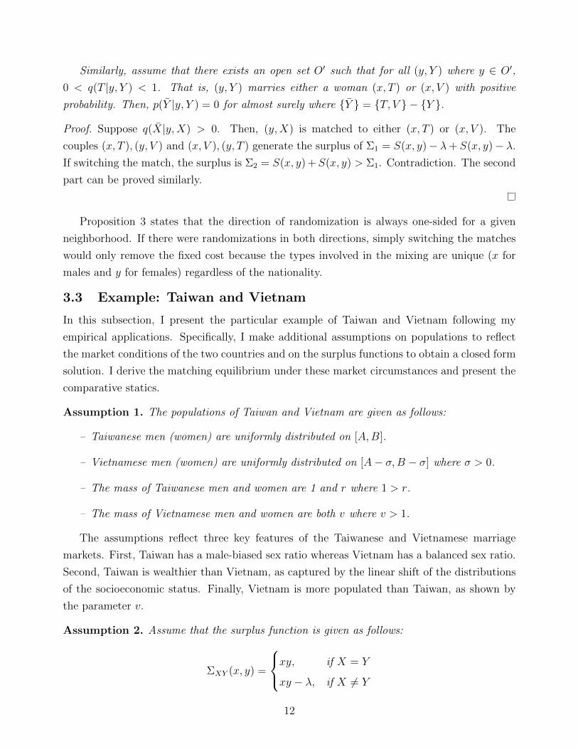
Assumption 1. The populations of Taiwan and Vietnam are given as follows:

– Taiwanese men (women) are uniformly distributed on [A,B].

– Vietnamese men (women) are uniformly distributed on [A− σ,B − σ] where σ > 0.

– The mass of Taiwanese men and women are 1 and r where 1 > r.

– The mass of Vietnamese men and women are both v where v > 1.

The assumptions reflect three key features of the Taiwanese and Vietnamese marriage

markets. First, Taiwan has a male-biased sex ratio whereas Vietnam has a balanced sex ratio.

Second, Taiwan is wealthier than Vietnam, as captured by the linear shift of the distributions

of the socioeconomic status. Finally, Vietnam is more populated than Taiwan, as shown by

the parameter v.

Assumption 2. Assume that the surplus function is given as follows:

ΣXY (x, y) =

xy, if X = Y

xy − λ, if X 6= Y

12

I use a quadratic surplus function in this example to obtain a closed form solution.18

I consider three cases under different cost schemes: (1) autarky (λ = ∞), (2) complete

integration (λ = 0), and (3) the intermediate case. The cases of (1) and (2) are trivial.

Under (1), the problem is equivalent to two uni-dimensional matching problems. Thus, the

matching is positively assortative on SES within each country. Under (2), the problem is just

one uni-dimensional matching problem, and the nationality no longer matters; the matching

is positively assortative on SES regardless of nationality. An interesting case emerges for the

intermediate case. The equilibrium is described as follows.

Proposition 4. There exists a unique equilibrium and there exists a cutoff zM(λ) such that the

matching above zM(λ) is positive assortative on SES regardless of nationalities. The matching

below zM(λ) is positive assortative on SES within each country. Depending on the value of

zM(λ), the unique stable matching has the following features:

1. If zM(λ) ≥ B − rσ

• Same as autarky.

2. If B − σ ≤ zM(λ) ≤ B − rσ

• Taiwanese men

– A Taiwanese man with x ∈ [B − rσ,B] is matched to a Taiwanese woman y

with probability 1.

y =1

rx− 1

rB +B = φT (x)

– A Taiwanese man with x ∈ [zM , B − rσ] is matched to a Taiwanese woman y

with probability rr+v

and to a Vietnamese woman with y with probability vr+v

.

y =1

r + vx+B − σ − B − rσ

r + v= φ(x)

– A Taiwanese man with x ∈ [x0,T , zM ] is matched to a Taiwanese woman with y

with probability 1.

y =1

rx− 1

rzM +

1 + v

r + vzM +M − 1 + v

r + v(B − σ) = φT (x)

where x0,T = φ−1T (A).

18For the microfoundation of this surplus function, see Browning et al. (2014) and Chiappori et al. (2017).

13

• Vietnamese men

– A Vietnamese man with x ∈ [x0,V , B − σ] is matched to a Vietnamese woman

with y with probability 1.

y = x− zM +1 + v

r + vzM +M − 1 + v

r + v(B − σ) = φV (x)

where x0,V = φ−1V (A− σ).

• Taiwanese women

– A Taiwanese woman with y ∈ [A,B] is matched to a Taiwanese man with x

with probability 1.

x = φ−1T (y) if y ≥ B − σ

x = φ−1(y) if zW ≤ y ≤ B − σ

x = φ−1T (y) if A ≤ x ≤ zW

where zW := φ(zM).

• Vietnamese women

– A Vietnamese woman with [zW , B − σ] is matched to a Taiwanese man with x

with probability 1.

x = φ−1(y)

– Vietnamese women with [A − σ, zW ] is matched to a Vietnamese man with x

with probability 1.

x = φ−1V (y)

3. If B − r(B − A) ≤ zM(λ) ≤ B − σ

• Taiwanese men

– A Taiwanese man with x ∈ [B − rσ,B] is matched to a Taiwanese woman y

with probability 1.

y =1

rx− 1

rB +B = φT (x)

– A Taiwanese man with x ∈ [B − σ,B − rσ] is matched to a Taiwanese woman

14

y with probability rr+v

and to a Vietnamese woman with y with probability vr+v

.

y =1

r + vx+B − σ − B − rσ

r + v= φ(x)

– A Taiwanese man with x ∈ [zM , B− σ] is matched to a Taiwanese woman with

y with probability r(1+v)r+v

and to a Vietnamese woman with y with probabilityv(1−r)r+v

.

y =1 + v

r + vx+M − 1 + v

r + v(B − σ) = φ(x)

where M := 1r+v

(B − σ) +B − σ − B−rσr+v

.

– A Taiwanese man with x ∈ [x0,T , zM ] is matched to a Taiwanese woman with y

with probability 1.

y =1

rx− 1

rzM +

1 + v

r + vzM +M − 1 + v

r + v(B − σ) = φT (x)

where x0,T = φ−1T (A).

• Vietnamese men

– A Vietnamese man with x ∈ [x0,V , B − σ] is matched to a Vietnamese woman

with y with probability 1.

y =1 + v

r + vx+M − 1 + v

r + v(B − σ) = φ(x) if x ≥ zM

y = x− zM +1 + v

r + vzM +M − 1 + v

r + v(B − σ) = φV (x) if x ≤ zM

where x0,V = φ−1V (A− σ).

• Taiwanese women

– A Taiwanese woman with y ∈ [A,B] is matched to a Taiwanese man with x

with probability 1.

x = φ−1T (y) if y ≥ B − σ

x = φ−1(y) if M ≤ y ≤ B − σ

x = φ−1(y) if zW ≤ y ≤M

x = φ−1T (y) if A ≤ x ≤ zW

where zW := φ(zM).

15

• Vietnamese women

– A Vietnamese woman with [M,B − σ] is matched to a Taiwanese man with x

with probability 1.

x = φ−1(y)

– A Vietnamese woman with [zW ,M ] is matched to Taiwanese man with x with

probability 1−r1+v

and Vietnamese men with [zM , B − σ] with probability r+v1+v

.

x = φ−1(y)

– Vietnamese women with [A − σ, zW ] is matched to a Vietnamese man with x

with probability 1.

x = φ−1V (y)

4. If zM(λ) ≤ B − r(B − A)

• Same as no cost.

Proof. See Appendix.

The cutoff zM(λ) for positive assortative matching on SES is determined in the equilibrium.

The idea of the equilibrium described above is as follows. Due to the cost, social surplus

may not be maximized when the matching is positive assortative on SES regardless of the

nationalities. In that case, positive assortative matching on SES regardless of the nationalities

occur only for men and women above certain types. For the low types, the benefits from

positive assortative matching cannot compensate for the cost of matching across countries.

When the cost is large enough, the equilibrium coincides with the case of autarky. When the

cost is small enough, the equilibrium is same as the complete integration case.

Figure 1 and Figure 2 present the equilibrium matchings and shares of men and women

under different levels of costs. When the two marriage markets are completely in isolation due

to high costs, only Taiwan has single men because Taiwan has a male-biased sex ratio and

Vietnam has a balanced sex ratio. Since the Taiwanese marriage market is less favorable to

men due to its male-biased sex ratio, the equilibrium shares for Taiwanese men are lower than

those for Vietnamese men. Figure 2a shows that for each SES type, the share of Taiwanese men

is lower than that of Vietnamese men, while it is the opposite for women. In another extreme,

when the two marriage markets are completely integrated with no cost, all the single men are

16

from Vietnam because the lowest types in the integrated market are Vietnamese men. In the

integrated market, the gap between the utilities of Taiwanese and Vietnamese disappear.

There are two types of equilibrium for the intermediate case. When the cost is low enough to

allow some cross-border marriages but when it is still relatively high, all Vietnamese women at

the top marry Taiwanese men. This is because they can marry Taiwanese men who are higher

types than the highest types of Vietnamese men (Figure 1b). The types below the cutoff zM(λ)

marry within their own countries. When the cost becomes even lower (Figure 1c), a wider range

of types of Vietnamese women can marry Taiwanese men; however, women who are below a

certain type start to mix between Taiwanese and Vietnamese men, since the Taiwanese men

they can marry are not necessarily better than the Vietnamese men. Again, the types below

the cutoff zM(λ) match within each country. In both cases, Vietnamese women are positively

selected and Taiwanese men are selected from the middle of the socioeconomic distributions.

3.3.1 Predictions on the selection of cross-border couples

The qualitative predictions on selection can be summarized as follows.

1. There exist Taiwanese men - Vietnamese women couples, but there do not exist Taiwanese

women - Vietnamese men couples.

2. Taiwanese men are selected from the middle of the SES distributions of all Taiwanese

men.

3. Vietnamese women are selected from the top of the SES distributions of all Vietnamese

women.

3.3.2 Comparative statics: with respect to costs of cross-border marriage

The comparative statics with respect to the costs of cross-border marriage can be derived as

follows.

Proposition 5. (Comparative statics with respect to λ)

– Cutoffs (the lowest types who engage in cross-border marriage): ∂zM∂λ

> 0, ∂zW∂λ

> 0

– Matching: ∂φT (x)∂λ

< 0, ∂φV (x)∂λ

> 0

– Singles:∂x0,T∂λ

> 0,∂x0,V∂λ

< 0

– Individual utilities: ∂uT (x)∂λ

> 0, ∂uV (x)∂λ

< 0, ∂vT (y)∂λ

< 0, ∂vV (y)∂λ

> 0

Proof. See Appendix.

17

Figure 1: Matching equilibria under different costs

TW men women

VN men women

B

A

B − σ

A− σ

1 r v v

(a) Autarky

TW men women

VN men women

B

A

zM

zWB − σ

A− σ

1 r v v

(b) Positive fixed cost: case I

TW men women

VN men women

B

A

zMzW

B − σ

A− σ

1 r v v

(c) Positive fixed cost: case II

TW men women

VN men women

B

A

B − σ

A− σ

1 r v v

(d) Complete Integration

Notes: These figures display the matching equilibria under different cost λ. The y-axis indicates the socioeconomic status. The

width of each box denotes the mass of men and women in each country. Men and women in the same color areas match positive

assortatively. The white area indicates being a single. For these illustrative figures, the parameter values A = 2, B = 6, σ = 1.4,

r = 0.7, and v = 2 are used. λ = 4.2 and λ = 2.2 are used for (b) and (c), respectively.

18

Figure 2: Equilibrium shares of matching equilibria under different costs

(a) Autarky

Male Female

Α − σ Α Β − σ Β Α − σ Α Β − σ Β0

5

10

15

20

Socioeconomic status

Equ

ilibr

ium

sha

re

countryTaiwanVietnam

(b) Positive fixed cost: case I

Male Female

Α − σ Α Β − σ Β Α − σ Α Β − σ Β0

5

10

15

20

Socioeconomic status

Equ

ilibr

ium

sha

re

countryTaiwanVietnam

(c) Positive fixed cost: case II

Male Female

Α − σ Α Β − σ Β Α − σ Α Β − σ Β0

5

10

15

20

Socioeconomic status

Equ

ilibr

ium

sha

re

countryTaiwanVietnam

(d) Complete Integration

Male Female

Α − σ Α Β − σ Β Α − σ Α Β − σ Β0

5

10

15

20

Socioeconomic status

Equ

ilibr

ium

sha

recountry

TaiwanVietnam

Notes: These figures display the equilibrium shares of the matching equilibria under different cost λ. For these illustrative figures, the parameter values

A = 2, B = 6, σ = 1.4, r = 0.7, and v = 2 are used. λ = 4.2 and λ = 2.2 are used for (b) and (c), respectively. In (a), the equilibrium shares of Vietnamese

men and women are not unique because of balanced sex ratio in Vietnam: the figure depicts the best (worst) possible case for Vietnamese women (men).

19

Table 1: Theoretical predictions on the impacts of cost increases

Taiwan Vietnam

Male Female Male Female

Number of singles + · – ·Matching patterns – + + –Intra-household allocation – + + –

Number of cross-border marriages –Avg. type of female migrant +Avg. type of male marrying a migrant +

Notes: This table summarizes the theoretical predictions on matching patterns, se-

lections, and intra-household allocations in Taiwan and Vietnam when cost of cross-

border marriage increases.

Table 1 summarizes the theoretical predictions on marital outcomes, intra-household al-

locations (individual utilities), and migration patterns when cost increases. Figure A1 shows

the comparison of probabilities of being single, marrying a local spouse, and marrying cross-

nationally, matching functions, and individual utilities under two different costs. For proba-

bilities of being single or matching patterns, not all types of men and women are affected by

cost changes. For example, Taiwanese men with low SES are matched to spouses with lower

SES when cost increases but Taiwanese men with high SES are always matched to the same

types of Taiwanese women regardless of cost. However, the predictions on individual utilities

are different: cost changes affect the utilities of all men and women in Taiwan and Vietnam

through equilibrium effects. This suggests that impacts of changes in technology (e.g., easier

travel and matchmaking services) or migration policies can be very extensive.

4 Data

I use data from several sources to test the main predictions of my model in Taiwan and

Vietnam, ranging from administrative marriage rate data to detailed household expenditure

data. This paper is the first to use data on individual-level marriage migrants containing

rich information on their characteristics as well as their spouses’.

4.1 Taiwan

4.1.1 Data on marriage migrants

To understand the characteristics of marriage migrants and their spouses and how the selec-

tion of marriage migrants were affected by the changes in the visa policies, I use the Census

of Foreign Spouses (CFS) from 2003 and the Foreign and Mainland Spouse Living Needs

20

Survey (FMSLNS) in 2008 and 2013, both conducted by the Taiwanese Ministry of Interior.

The CFS surveyed 240,837 residents who were married to Taiwanese citizens but did not

have Taiwanese citizenship themselves at the time of their marriage. The subsequent FM-

SLNS in 2008 and 2013 have smaller sample sizes of around 13,000 each year. While sample

sizes differ, these datasets all contain rich information on individual characteristics such as

age, education, marriage year, migration year, original nationality and visa type, as well as

spousal characteristics.

4.1.2 Data on local Taiwanese men

To compare the characteristics of Taiwanese men who engage in cross-border marriages and

those of local Taiwanese men, I use the Taiwanese census conducted in 2000.

4.1.3 Data on marriage data

To investigate whether the increase in the costs of cross-border marriages induced by the visa

tightening policy affected marriage rates in Taiwan, I utilize yearly marriage and population

data from 2001 to 2010. Both marriage and population data are collected at the district

level, for 368 districts, by the Department of Household Registration in Taiwan.19 For the

yearly marriage data, the number of marriages are available by sex, education and nationality.

Population data for people above the age of 15 are available by sex, education and marital

status. Using these datasets, I construct marriage rates by education for Taiwanese males

and females. The district level marriage rate for each education level is calculated by dividing

the number of marriages that involve Taiwanese male (female) by the number of singles in the

corresponding education level, where “singles” is defined as the sum of unmarried, divorced,

and widowed people.

4.1.4 Data on matching pattern

In order to evaluate the impact of visa tightening policy on matching patterns, the data

should include information on the characteristics of the spouses and the year of marriage. I

use Women’s Marriage, Fertility and Employment Survey (WMFES), a supplementary survey

to the Manpower Survey of Taiwan (an equivalent to the Current Population Survey of the

US), which contains such information. The survey has been conducted every three or four

years starting from 198820. The sample consists of women who are over 15 years old within

the representative sample of households. For this sample, the survey collects information on

their characteristics such as age, educational attainment and marital status. Furthermore,

for the currently married women, information on the characteristics of their spouses and the

19The area of Taiwan is about 1.5 times of the state New Jersey in the US.20The survey was first conducted in 1979. It was conducted annually between 1979 and 1988, but due to

budget limitations, it is conducted every three or four years since then.

21

year of marriage is also collected. I use WMFES 2006, 2010 and 2013, which also contains

information on pre-marriage nationality21, and limit the sample to only include women whose

pre-marriage nationality is Taiwanese.

4.2 Vietnam

4.2.1 Data on local Vietnamese women

To compare the characteristics of Vietnamese women who engage in cross-border marriages

and those of local Vietnamese women, I use the Vietnamese census conducted in 1999.

4.2.2 Data on household expenditures

To understand how cost changes affect intra-household resource allocations of married cou-

ples, I utilize detailed household expenditure data in Vietnam. Since we do not observe

equilibrium shares of husbands and wives, it is challenging to test the predictions on intra-

household allocations. However, this challenge can be overcome if we observe expenditures on

gender-exclusive goods. The collective model literature (e.g. see Browning et al. (2014)) has

extensively shown that if Pareto weights (respective powers) of husbands and wives change

towards wives, the consumption patterns on gender-exclusive goods change in favor of wives.

Thus, if the equilibrium shares of husbands and wives change, we would expect to observe a

larger consumption for women-exclusive goods and a smaller consumption for men-exclusive

goods.

The Vietnam Living Standards Survey (VLSS) and the Vietnam Household Living Stan-

dards Survey (VHLSS) contain detailed household level expenditures.22 As a measure to

proxy how the gains from marriage are shared within couples, I use tobacco as men-exclusive

good and jewelry, watch, make-up category as women-exclusive goods. In Vietnam, smoking

is considered as a crucial part of male social behavior and the smoking rate of men is much

higher than that of women. In 1997-8, the smoking rate of men was 52.2% and that of women

was 3.9% in rural areas (Morrow and Barraclough (2003)), suggesting that tobacco is a good

candidate for male-exclusive good.23 Since women represent the majority of luxury (jewelry

and watch) consumers in Vietnam (Luxury Market in Vietnam report, 2009), jewelry, watch,

and make-up are likely to be women-intensive expenditures. However, there is a potential

concern for watch, since watch can be a gender-neutral good. The data alleviates this con-

cern: less than 3% of single male households spent a positive amount on jewelry, watch,

21The information on pre-marriage nationality is not available for the WMFES before 2006.22These surveys have been conducted as part of the Living Standards Measurement Survey of World Bank.

The VLSS was first conducted in 1992-93 and another wave in 1997-98. The VHLSS have been collectedevery two years since 2002. The VHLSS maintains the structure of VLSS with some modifications. However,the expenditure sections are largely comparable across different waves of the VLSS and the VHLSS.

23In the country as a whole, the smoking rate for men was 50.7% and for women 3.5%.

22

and make-up category, suggesting that assuming the jewelry, watch, make-up category as

women-exclusive consumption is reasonable.

I use three waves of the survey, the 97-98 VLSS, the 2002 VHLSS and the 2004 VHLSS.

As explained in the previous section, there was a large increase in the number of cross-border

marriages between 1998 and 2000. I compare the expenditure patterns before and after this

shock. The 97-98 VLSS serves as the pre-treatment period and the 2002 VHLSS and the

2004 VHLSS are used as the post-treatment periods. I do not use 92-93 VLSS because there

is no consumer price index covering this period, making it difficult to construct a harmonized

measure of expenditure. Moreover, although the flow of cross-border marriages started in

the early 1990s, it was recognized as a new social phenomenon only in the late 1990s.

I focus on the samples of married couples whose age is between 20 and 60. I restrict

my sample to married couples living in rural areas because most marriage migrants have

been from the rural areas and economic investment was active in the urban. Additionally,

two regions in mountainous areas are excluded from the analysis due to their considerably

different ethnic composition from the rest of the country.24 For a similar reason, I also exclude

two provinces with less than sixty percent of Kinh, the major ethnicity in Vietnam.25

4.2.3 Data on the intensity of cross-border marriages in each province

I use the visa counting of Taipei Economic and Cultural Office (TECO) in Ho Chi Minh City

in 2003 to construct a measure of the intensity of cross-border marriages in each province.

TECO keeps the province-level record on the number of people who got interviews from

TECO, required for Vietnamese who want to migrate to Taiwan, as well as on the number

of people who were granted Taiwanese visa for the cross-border marriage.26 I use the total

number of visas issued for marriage migration scaled by the population of marriageable

women in each province as an intensity measure.27

24Two excluded regions are Northeast and Northwest regions. As of 2009, the fractions of Kinh were 51.28percent and 19.51 percent, respectively. Other regions except for Central Highlands have at least 80 percentof Kinh. A province with very low fraction of Kinh in the Central Highlands, Kon Tum, is additionallyexcluded.

25The excluded province is Kon Tum and Gia Lai in central Vietnam. The fractions of Kinh were 37.32percent and 49.52 percent, respectively, as of 2009. The purpose of excluding these areas is mainly becauseto make the control group comparable to the treatment group. The results are stronger when those areas areincluded in the samples.

26Since there is another TECO in Vietnam which is located in Hanoi, this number might underestimate thenumber of marriage migrants in the north Vietnam. However, many sources (Do et al. (2003); Nguyen andTran (2010)) indicate that most marriage migrants come from the south. Wang and Chang (2002) reportedthat there were more than 240 marriages agencies registered at the TECO in HCMC while there were onlytwo agencies who visited the TECO in Hanoi for migration documents in 2002.

27It is difficult to know the precise number of marriageable women in each province. As a proxy for that,I use the size of female population aged 21, which is the average age of first marriage for female.

23

4.2.4 Data on other factors

The population size of Hoa people and sex-ratios are calculated from the 1989 and 1999

Vietnamese decennial census. The data on the number of foreign direct investment firms is

from the Chamber of Commerce and Industry of Vietnam (VCCI) in the 1990s and from the

General Statistics Office of Vietnam (GSO) for the 2000s.

5 Empirical Evidence on the Selection of Cross-border Couples

This section cross-sectionally tests the theoretical predictions on the forms of cross-border

marriage and selection of marriage migrants and their spouses given in subsubsection 3.3.1.

Prediction on Selection 1. (The “mixed” couples are one kind) Taiwanese men and Viet-

namese women (TV) couples should be more prevalent than Vietnamese men and Taiwanese

women (VT) couples.

This prediction suggests that we would observe a dominant share of one type of “mixed”

couples, which is indeed confirmed by multiple sources of data. In the CFS, among all the

Taiwan - Vietnam couples who married before 2003, the share of VT couples is less than 0.5%.

The yearly marriage data from the Ministry of Interior, Taiwan bolsters this prediction. The

number of VT couples is less than 1% during all the years available in the data (2004-2010).

The gendered patterns of cross-border marriages in Asian countries has been numerously

reported in the sociological, demographic, and economics literatures. Here, I show that this

pattern can be explained as an equilibrium of the two marriage markets rather than a simply

descriptive pattern.

Prediction on Selection 2. (Taiwanese men involved in cross-border marriage) Taiwanese

men who are involved in cross-border marriage are selected from the middle segment of SES.

The model suggests that Taiwanese men who are matched to Vietnamese women are

selected from the middle of the SES distributions, not the bottom, given that the cost of

cross-border marriage is not zero. In Taiwan, to marry a Vietnamese woman, Taiwanese men

need to pay match-making firms approximately $10,000. This cost precludes cross-border

marriage for the lowest types. The high types do not marry Vietnamese women because they

have strictly better Taiwanese alternatives.

The data confirms the prediction on the intermediate selection of Taiwanese men (Fig-

ure 3). Taiwanese men who marry Vietnamese women are concentrated in the group with

junior-high or senior-high school education, not in the group with primary or less than pri-

mary education. The share of people with junior-high or senior-high education were 87% for

grooms of Vietnamese brides, whereas in the entire population of Taiwanese men, the share

is only 57%.

24

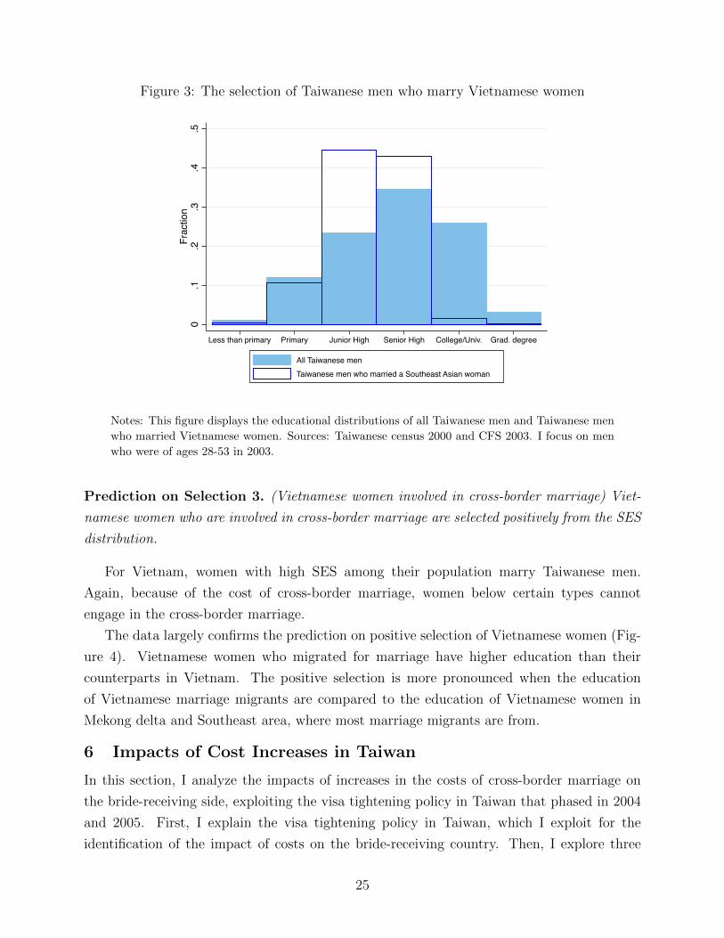
Figure 3: The selection of Taiwanese men who marry Vietnamese women

0.1

.2.3

.4.5

Frac

tion

Less than primary Primary Junior High Senior High College/Univ. Grad. degree

All Taiwanese menTaiwanese men who married a Southeast Asian woman

Notes: This figure displays the educational distributions of all Taiwanese men and Taiwanese men

who married Vietnamese women. Sources: Taiwanese census 2000 and CFS 2003. I focus on men

who were of ages 28-53 in 2003.

Prediction on Selection 3. (Vietnamese women involved in cross-border marriage) Viet-

namese women who are involved in cross-border marriage are selected positively from the SES

distribution.

For Vietnam, women with high SES among their population marry Taiwanese men.

Again, because of the cost of cross-border marriage, women below certain types cannot

engage in the cross-border marriage.

The data largely confirms the prediction on positive selection of Vietnamese women (Fig-

ure 4). Vietnamese women who migrated for marriage have higher education than their

counterparts in Vietnam. The positive selection is more pronounced when the education

of Vietnamese marriage migrants are compared to the education of Vietnamese women in

Mekong delta and Southeast area, where most marriage migrants are from.

6 Impacts of Cost Increases in Taiwan

In this section, I analyze the impacts of increases in the costs of cross-border marriage on

the bride-receiving side, exploiting the visa tightening policy in Taiwan that phased in 2004

and 2005. First, I explain the visa tightening policy in Taiwan, which I exploit for the

identification of the impact of costs on the bride-receiving country. Then, I explore three

25

Figure 4: The selection of Vietnamese women who marry Taiwanese men

A. All Vietnam B. Southeast and Mekong Delta

0.1

.2.3

.4.5

Frac

tion

Less than primary Primary Junior High Senior High College/Univ.

All Vietnamese womenVietnamese women who married a Taiwanese man

0.1

.2.3

.4.5

Frac

tion

Less than primary Primary Junior High Senior High College/Univ.

All Vietnamese womenVietnamese women who married Taiwanese men

Notes: These figures display the educational distributions of all Vietnamese women and Vietnamese

women who married Taiwanese men. The right panel displays the educational distribution of Viet-

namese women in Southeast and Mekong delta regions, the origins of most Vietnamese women who

marry Taiwanese men instead of the educational distribution of all Vietnamese women. Sources:

Vietnamese census 1999 and CFS 2003. I focus on women who were of ages 25-50 in 2003.

main outcomes: marriage rate, matching patterns, and selection of cross-border couples.28

Finally, I briefly discuss the consequences of the visa tightening policy in Vietnam.

6.1 Background: visa tightening policy

In the early 2000s in Taiwan, the strikingly high share of foreign brides raised concerns

about national security and the demographic composition of the country. Due to these

concerns, the government strengthened visa requirements by requiring compulsory interviews

to screen mainland Chinese brides in September, 2003. At first, the Immigration Bureau

started to interview 10% of all mainland spouses. However, the mandatory interview for

all women from mainland was implemented in March, 2004 (Lu (2008)). As a result, the

number of Chinese brides decreased by half between 2003 and 2004 (Figure 5). Moreover, the

Taiwanese government subsequently launched a similar policy in 2005 that involved changing

bulk processing of visas to one-on-one interviews, to better screen Southeast Asian brides.

This resulted in a further decrease in the number of foreign brides that came to Taiwan

per year. The brides from Southeast Asian countries decreased about 40 percent in a year.

28In Taiwan, it is challenging to test the impacts on intra-household allocations because all men andwomen are affected from marriage migration flows, making it difficult to find a proper control group. Ipresent suggestive evidence in the Appendix and formally tests predictions on intra-household allocations insection 7.

26

The impact of this increase in cost for women from mainland China should be in the same

direction as the case for women from Vietnam, as long as Taiwan has a higher sex ratio than

mainland China does, which indeed was the case for cohorts involved in the cross-border

marriages. The sex ratio of mainland China increased only after 1980, and the population

increased until 1975, meaning that male-biased sex ratio was unlikely. I ignore three country

effects in this paper, and treat 2004 as a treatment year.

Figure 5: Numbers and shares of cross-border marriages in Taiwan

A. Numbers B. Shares

Visa tighteningEmergence ofmatch-making firms

0

10000

20000

30000

40000

50000

Num

ber o

f cro

ss-b

orde

r mar

riage

s in

Tai

wan

1994 1996 1998 2000 2002 2004 2006 2008 2010 2012 2014 2016Year

Origins of spouses: TotalOrigin of spouses: Mainland ChinaOrigins of spouses: Foreign excl. Mainalnd China/HK/Makau Origin of spouses: Southeast Asia

Visa tighteningEmergence ofmatch-making firms

0

.1

.2

.3

Shar

e of

cro

ss-b

orde

r mar

riage

s in

Tai

wan

1994 1996 1998 2000 2002 2004 2006 2008 2010 2012 2014 2016Year

Origins of spouses: TotalOrigin of spouses: Mainland ChinaOrigins of spouses: Foreign excl. Mainalnd China/HK/Makau Origin of spouses: Southeast Asia

Sources: The Ministry of Interior, Taiwan. The numbers of cross-border marriages between 1994-

1997 are from Wang and Chang (2002).

6.2 Impacts on marital outcomes and the selection of cross-border

couples

In this section, I investigate the impact of visa tightening policy of Taiwan on martial out-

comes, selection of cross-border couples, and intra-household allocations in Taiwan. In par-

ticular, I test the predictions of the model on comparative statics given in Table 1.

6.2.1 Marriage rate

Prediction 1. When the cost of cross-border marriage increases, the marriage rate for Tai-

wanese males decreases overall. However, the decrease is concentrated among the males with

low SES; the marriage rate of those with high SES is not affected. The marriage rate for

Taiwanese females is not affected by the policy.

The prediction from the model naturally leads to a difference-in-differences (DID) as an

identification strategy. The Taiwanese men with high SES are not affected by the changes

27

Figure 6: Marriage rates of Taiwanese men and women

A. Males B. Females

LonelyPhoenix year

LonelyPhoenix year

MainlandTightening

SE AsiaTightening

0.0

2.0

4.0

6.0

8Ye

ar

2001 2002 2003 2004 2005 2006 2007 2008 2009 2010

Marriage rate

Primary Junior High Senior HighVocational University or above

LonelyPhoenix year

LonelyPhoenix year

MainlandTightening

SE AsiaTightening

0.0

2.0

4.0

6.0

8Ye

ar

2001 2002 2003 2004 2005 2006 2007 2008 2009 2010

Marriage rate

Primary Junior High Senior HighVocational University or above

Notes: The figures plot the average of district-level marriage rate (defined as the number of mar-

riages of Taiwanese divided by the number of single population) by education for each gender. The

grey lines indicate the implementation of the visa tightening policies in 2004 and 2005, respectively.

The red colors indicate the treated group and the blue colors indicate the control group. The red

vertical lines indicate the ‘lonely phoenix year’ in 2004 and 2009. Source: The Department of

Household Registration, Taiwan.

in the visa policy. Thus, they serve as a control group. The Taiwanese men with low SES

are the treatment group because they are expected to be affected by the changes in the visa

policies. I proxy SES with education. This is a better choice than other measures of SES

including income or wages because education is a pre-determined variable, and is unlikely to

be influenced by marriage or decisions after marriage. The model predicts that the increase

in the cost of cross-border marriage does not affect the marriage rate of females; the same

DID for females is conducted to test this hypothesis. I estimate the following regression,

separately for Taiwanese men and women:

Ydey = βTreate × Posty + θd + γe + δy + νXdey + εdey

where d is a district; e is educational level (primary, junior-high, senior-high, vocational,

university); and y is year of marriage. The dependent variable Y is the marriage rate by

education level at each district in a given year. The θd are district fixed effects, γe are

education fixed effects, and δy are year of marriage fixed effects. Xdey controls for the number

of male and female single population at each education level in a given district and in a given

year. Posty is one if year y is after the visa tightening policy. That is, Posty = 1 for any

y ≥ 2004. Treate is one when the education group is either primary or junior-high. If the

28

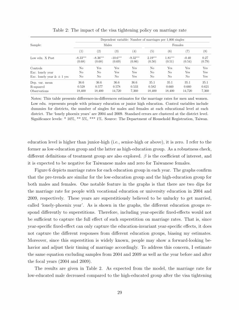
Table 2: The impact of the visa tightening policy on marriage rate

Dependent variable: Number of marriages per 1,000 singles

Sample: Males Females

(1) (2) (3) (4) (5) (6) (7) (8)

Low edu. X Post -8.33∗∗∗ -8.36∗∗∗ -10.6∗∗∗ -9.32∗∗∗ 2.19∗∗∗ 1.81∗∗∗ -0.40 0.27(0.68) (0.68) (0.69) (0.86) (0.50) (0.51) (0.54) (0.79)

Controls No Yes Yes Yes No Yes Yes Yes

Exc. lonely year No No Yes Yes No No Yes Yes

Exc. lonely year & ± 1 yrs No No No Yes No No No Yes

Dep. var. mean 36.6 36.6 36.6 36.6 35.1 35.1 35.1 35.1

R-squared 0.528 0.577 0.578 0.533 0.582 0.660 0.660 0.621

Observations 18,400 18,400 14,720 7,360 18,400 18,400 14,720 7,360

Notes: This table presents difference-in-differences estimates for the marriage rates for men and women.

Low edu. represents people with primary education or junior high education. Control variables include

dummies for districts, the number of singles for males and females at each educational level at each

district. The ‘lonely phoenix years’ are 2004 and 2009. Standard errors are clustered at the district level.

Significance levels: * 10%, ** 5%, *** 1%. Source: The Department of Household Registration, Taiwan.

education level is higher than junior-high (i.e., senior-high or above), it is zero. I refer to the

former as low-education group and the latter as high-education group. As a robustness check,

different definitions of treatment group are also explored. β is the coefficient of interest, and

it is expected to be negative for Taiwanese males and zero for Taiwanese females.

Figure 6 depicts marriage rates for each education group in each year. The graphs confirm

that the pre-trends are similar for the low-education group and the high-education group for

both males and females. One notable feature in the graphs is that there are two dips for

the marriage rate for people with vocational education or university education in 2004 and

2009, respectively. These years are superstitiously believed to be unlucky to get married,

called ‘lonely-phoenix year’. As is shown in the graphs, the different education groups re-

spond differently to superstitions. Therefore, including year-specific fixed-effects would not

be sufficient to capture the full effect of such superstition on marriage rates. That is, since

year-specific fixed-effect can only capture the education-invariant year-specific effects, it does

not capture the different responses from different education groups, biasing my estimates.

Moreover, since this superstition is widely known, people may show a forward-looking be-

havior and adjust their timing of marriage accordingly. To address this concern, I estimate

the same equation excluding samples from 2004 and 2009 as well as the year before and after

the focal years (2004 and 2009).

The results are given in Table 2. As expected from the model, the marriage rate for

low-educated male decreased compared to the high-educated group after the visa tightening

29

Figure 7: The average level of husbands’ education by the level of wives’ education

VisaTightening

1112

1314

1516

Hus

band

yea

rs o

f edu

catio

n

1998-1999 2000-2001 2002-2003 2004-2005 2006-2007 2008-2009 2010-2011

Year of marriage

Wife edu.: Univ. Wife edu.: Non-Univ.

Notes: This figure plots the average level of husbands’ education by education of wives in Taiwan.

The grey dashed line indicates the implementation of the visa tightening policies in 2004-2005. The

red colors indicate the treated group and the blue colors indicate the control group. Source: The

Women’s Marriage, Fertility and Employment Survey 2006, 2010, 2013. The couples who married

in 1998 or after are used as samples. Only Taiwanese women are used as samples.

policy. The marriage rate for low-educated group decreased by 8 to 10 marriages per 1,000

singles, depending on whether unlucky years are excluded or not. This is equivalent to 23-29%

decrease in the marriage rate for low-educated males. Different definitions of low-education

group give similar results; when the cutoff of low-educated group is lower, the estimates of β

become larger. I find a small coefficient size for females, and it is essentially zero when the

unlucky years and its windows are excluded, confirming the prediction from the model.

6.2.2 Matching patterns

Prediction 2. When the cost of cross-border marriage increases, Taiwanese females are

more likely to marry up, except for the females with high education. The matching of the

females with high SES are not affected by the policy.

The prediction for the matching patterns can also be tested using a DID. In the model,

the Taiwanese females with SES above the top Vietnamese women always match the same

set of Taiwanese men regardless of the cost. These top females in Taiwan serve as a control

group. I define this control group as the females with university education or above because

there are only few Vietnamese female with such degrees. I estimate the following regression:

Ymey = βTreate × Posty +Wifeedue + δy + νXmey + µZey + εmey

30

Table 3: The impact of visa tightening policies on matching patterns

Dep. var.: Husband years of schooling

(1) (2) (3)

Non-Univ. X Post 0.16∗ 0.18∗ 0.23∗∗

(0.097) (0.097) (0.097)

Edu/year controls No No Yes

Indiv. controls No Yes Yes

Dep. var. mean 13.64 13.64 13.64

R-squared 0.370 0.370 0.411

Observations 7,882 7,882 7,882

Notes: This table presents difference-in-differences estimates for the matching patterns. Non-

Univ. represents the educational level of wives; it is one if the level of education for wife is below

university. Otherwise, it is zero. Education-year level control variable includes the excess share of

males with education higher than that of a given woman. Individual level controls are dummies

for year of marriage, age of husband, age of wife, wife education and the excess share of males

with education higher than that of a given woman. Robust standard errors are used. Significance

levels: * 10%, ** 5%, *** 1%. Source: The Women’s Marriage, Fertility and Employment Survey

2006, 2010, 2013. The couples who married after 1998 are used as samples. Only Taiwanese

women are used as samples.

where m is each marriage; e is educational level (primary, junior-high, senior-high, vocational,

university); and y is year of marriage. The dependent variable Y is the husbands’ level of

education. The δy are year of marriage fixed effects. The control vector Xmey includes

county fixed effects, husband age and wife age. Since I test whether the partner’s education

increases given female’s education, I control for wife’s education. The education-year level

control vector Zey includes the excess share of males with education higher than e29. Posty

is one if y is 2004, when the visa tightening policy was implemented, or later. Treate is one

when the education group is below university education. If the education level is university

or above, it is zero.

Figure 7 plots the average years of education of husbands by wife’s education level.30 It

shows that the pre-trends are similar across education groups, which validates the DID as

an identification strategy. The average education level of husbands for wives with university

29Specifically, it is calculated as the difference between the share of males with education higher than eand the share of females with education e or above. For university females, I use the difference of share ofmales with university or above education and the share of females with university or above education. Thisis based on the assumption that the matching would be assortative.

30Due to small sample sizes, I aggregate education groups into two groups: group with university educationand group without university education.

31

education or above stays stable over time (if anything, there is a slight increase); and the

average education level of husbands for wives with less than university education increases

after the implementation of the visa tightening policy.

Table 3 shows the results from the regression. After the visa tightening policy, Taiwanese

women with less than university education marry a man with 0.2 more years of education.

Alternative dependent variables, including the probability of marrying up for females and

the educational years of differences for couples, also give similar results.

6.2.3 Selection of people who marry cross-nationally

Prediction 3. When the cost of cross-border marriage increases, the average SES of Tai-

wanese male who marry foreign brides increases. When the cost of cross-border marriage

increases, the average SES of foreign brides increases.

Given that the cost associated with the visa application process can be seen as more or

less fixed, the model predicts that the average SES of foreign women married to Taiwanese

men increases when the visa-related cost increases. In addition, the average SES of Taiwanese

men matched to foreign women increases because the cost becomes too high for the marginal

types. To test these predictions, I measure the SES of males and females by their level of

education and compare the educational level of the female marriage migrant right before and

right after the visa tightening policy. I estimate the following equation for female marriage

migrants and their spouses to capture the changes in SES of migrants and their spouses.

Yicy = δy + βPosty + νc + εicy

where i is an individual and y is the year of marriage (and also the year of migration

for foreign brides). The νc are county/city fixed effects. The dependent variable Y is an

indicator for each education group (primary, junior high, senior high/vocational, university

or above). Thus, the coefficient of interest β captures whether the share of each education

decreased or increased with the stricter visa policies.

Figure 8 shows the composition of education by year of marriage cohort. As predicted by

the model, the share of low-educated group (e.g. primary or junior high) decreased whereas

the share of high-educated group (e.g. senior high/vocational or university or above) in-

creased for foreign spouses. The same figures for composition of education by the origins of

brides (mainland China and Southeast Asian brides) confirm the impact of the visa tight-

ening policy. The SES of Chinese mainland brides increased right after 2004, when the visa

tightening policy targeted at mainland brides was first implemented. Likewise, when visa

screening for Southeast Asian brides was strengthened in 2005, a similar increase in education

level was observed.

32

Table 4: The impact of visa tightening policies on the SES of foreign brides

Dependent variable (=1): Primary Junior HighSenior High

or VocationalUniv. or

above

After visa-tightening (=1) -0.18∗∗∗ 0.073∗ 0.066∗ 0.043∗

(0.020) (0.040) (0.039) (0.024)

Controls Yes Yes Yes Yes

Dep. var. mean 0.28 0.39 0.29 0.04

R-squared 0.007 0.001 0.006 0.005

Observations 116,399 116,399 116,399 116,399

Notes: This table displays the results from regressing each dependent variable (indicating foreign brides

education) listed in the first row on a dummy for post visa tightening policies and controls (marriage

year fixed effects and county city fixed effects). Robust standard errors are used. Significance levels: *

10%, ** 5%, *** 1%. Sources: the Census of Foreign Spouse, 2003 and the Foreign and Mainland Spouse

Living Needs Survey, 2008. Only the foreign spouses who marry and migrate at the same time and their

grooms are included in the sample. The foreign brides or grooms who married in 1998 or after are used

as the samples.

Table 5: The impact of visa tightening policies on the SES of Taiwanese grooms of foreignbrides

Dependent variable (=1): Primary Junior HighSenior High

or VocationalUniv. or

above

After visa-tightening (=1) -0.082∗∗∗ -0.23∗∗∗ 0.19∗∗∗ 0.12∗∗∗

(0.021) (0.028) (0.040) (0.030)

Controls Yes Yes Yes Yes

Dep. var. mean 0.15 0.36 0.45 0.04

R-squared 0.006 0.023 0.015 0.018

Observations 116,399 116,399 116,399 116,399

Notes: This table displays the results from regressing each dependent variable (indicating groom educa-

tion) listed in the first row on a dummy for post visa tightening policies and controls (marriage year fixed

effects and county city fixed effects). Robust standard errors are used. Significance levels: * 10%, **

5%, *** 1%. Sources: the Census of Foreign Spouse, 2003 and the Foreign and Mainland Spouse Living

Needs Survey, 2008. Only the foreign spouses who marry and migrate at the same time and their grooms

are included in the sample. The foreign brides or grooms who married in 1998 or after are used as the

samples.

33

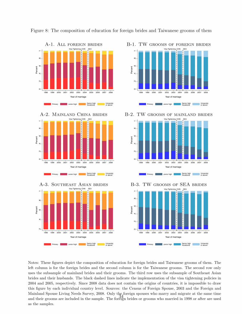
Figure 8: The composition of education for foreign brides and Taiwanese grooms of them

A-1. All foreign brides B-1. TW grooms of foreign bridesVisa Tightening: CHN SEA

0.2

.4.6

.81

Perc

ent

1998 1999 2000 2001 2002 2003 2004 2005 2006 2007 2008

Year of marriage

Primary Junior high Senior highVocational

Universityor above

Visa Tightening: CHN SEA

0.2

.4.6

.81

Perc

ent

1998 1999 2000 2001 2002 2003 2004 2005 2006 2007 2008

Year of marriage

Primary Junior high Senior highVocational

Universityor above

A-2. Mainland China brides B-2. TW grooms of mainland bridesVisa Tightening: CHN SEA

0.2

.4.6

.81

Perc

ent

1998 1999 2000 2001 2002 2003 2004 2005 2006 2007 2008

Year of marriage

Primary Junior high Senior highVocational

Universityor above

Visa Tightening: CHN SEA

0.2

.4.6

.81

Perc

ent

1998 1999 2000 2001 2002 2003 2004 2005 2006 2007 2008

Year of marriage

Primary Junior high Senior highVocational

Universityor above

A-3. Southeast Asian brides B-3. TW grooms of SEA bridesVisa Tightening: CHN SEA

.2.4

.6.8

1Pe

rcen

t

1998 1999 2000 2001 2002 2003 2004 2005 2006 2007 2008

Year of marriage

Primary Junior high Senior highVocational

Universityor above

Visa Tightening: CHN SEA

0.2

.4.6

.81

Perc

ent

1998 1999 2000 2001 2002 2003 2004 2005 2006 2007 2008

Year of marriage

Primary Junior high Senior highVocational

Universityor above

Notes: These figures depict the composition of education for foreign brides and Taiwanese grooms of them. The

left column is for the foreign brides and the second column is for the Taiwanese grooms. The second row only

uses the subsample of mainland brides and their grooms. The third row uses the subsample of Southeast Asian

brides and their husbands. The black dashed lines indicate the implementation of the visa tightening policies in

2004 and 2005, respectively. Since 2008 data does not contain the origins of countries, it is impossible to draw

this figure by each individual country level. Sources: the Census of Foreign Spouse, 2003 and the Foreign and

Mainland Spouse Living Needs Survey, 2008. Only the foreign spouses who marry and migrate at the same time

and their grooms are included in the sample. The foreign brides or grooms who married in 1998 or after are used

as the samples.

34

The patterns are similar for the Taiwanese spouses of foreign brides. One notable dif-

ference compared to the results on the foreign brides is that the average education level

of Taiwanese males who marry Southeast Asian brides went up right after 2004, not 2005,

although there was an additional increase of education level after 2005. This is because

the average cost associated with marrying any foreign bride for Taiwanese men already had

already increased in 2004.

Table 4 and Table 5 show the regression coefficients for each education level. The results

on foreign brides show that the education level shifted towards higher education. The share

of brides with primary school education decreased while the share of brides above that level

of education increased. The results for Taiwanese groom reveal similar patterns. However,

since the base education level of Taiwanese grooms marrying foreign brides is higher, the

share of people with primary or junior high education decreased and the share of people with

above junior high education (i.e. senior high/vocational or university or above) increased.

One alternative hypothesis that could explain these results is that the educational level

of the entire mainland Chinese women/Vietnamese women or the entire Taiwanese men may

have increased over time. This can be tested by looking at the educational composition of

mainland Chinese women/Vietnamese women and Taiwanese men each year. There indeed is

an increasing trend for the education level of mainland Chinese women/Vietnamese women,

but the increase is so smooth that it is hard to think that the jump in 2004-2005 is driven

solely by this trend. Similarly, the education level of Taiwanese men has grown smoothly,

which invalidates the alternative hypothesis.

6.3 Responses in Vietnam

As suggested by the model, the changes in costs of cross-border marriage should affect the

outcomes in Vietnam in the opposite direction of the impacts in Taiwan. However, it is

difficult to test the outcomes in Vietnam using the visa tightening policy of Taiwan because

Vietnamese women diversified the destination countries and migrated massively to South

Korea after the visa tightening policy (Figure 9). The change in destination countries cannot

be solely attributed to the visa tightening policy because South Korea actively invested in

Vietnam in the early 2000s, and this led to an emergence of matchmaking firms operating in

Vietnam and Korea. This lowered the cost of cross-border marriages between Vietnamese and

Koreans. If we consider only Vietnam and Korea, the predictions of the model for Vietnam

and Korea are in the same direction as in the case of Vietnam and Taiwan, because Korea

is wealthier than Vietnam and has male-biased sex ratios. However, the predictions of the

model are less clear when there are interactions between the three countries; for example,

in this case, the cost of cross-border marriage in one destination country increased but the

35

cost of that in another country decreased. Thus, in section 7, I instead focus on the cost

decrease of cross-border marriage between Vietnamese and Taiwanese during the late 1990s

to identify the impacts in Vietnam.

Figure 9: Number cross-border marriages in Vietnam

Visa tightening of TaiwanEmergence ofmatch-making firms

0

5000

10000

15000

Num

ber o

f cro

ss-b

orde

r mar

riage

s in

Vie

tnam

1995 1997 1999 2001 2003 2005 2007 2009 2011 2013Year

Origin of spouses: TaiwanOrigin of spouses: South KoreaOrigins of spouses: Taiwan or South Korea

Notes: This figure plots the number of cross-border marriages in Vietnam by destination countries.

Sources: the numbers of cross-border marriages with Taiwanese in 1995-2003 and in 2004-2014 are

from TECO HCMC and the Ministry of Interior, Taiwan, respectively. The numbers of cross-border

marriages with Korean are from the Statistics Korea.

7 Impacts of Cost Decreases in Vietnam

In this section, I evaluate the impact of changes in the cost of cross-border marriage in

Vietnam, which is the bride-sending country. Specifically, I focus on testing the model’s

prediction on intra-household allocations, which could not be fully tested in the Taiwanese

setting due to the lack of variations within the country. To investigate the intra-household

allocations, I exploit a unique feature in Vietnam: considerable geographic variation in the

origin of Vietnamese marriage migrants.31 In the following subsection, I provide background

information related to the identification strategy. Then, I present the reduced-form results

and the structural estimates of the married couples’ sharing rule.

31Using the geographic variations in Vietnam implicitly assumes multiple marriage markets in Vietnam.This assumption is reasonable because cross-provincial marriages are rare. One concern could be that therecould have been interactions between marriage markets in each province when the cost of cross-border mar-riage changes. However, this is unlikely to be the case since the internal migrations were not significantlydifferent in the affected and non-affected provinces during the periods of study (1997-2004).

36

7.1 Background: emergence of matchmaking firms and geographic

concentrations of cross-border marriages

In this subsection, I describe two sources of variations that I use to identify the impacts of

cost decrease on the intra-household allocation outcomes: the emergence of matchmaking

firms in the late 1990s and geographic concentration of cross-border marriages in certain

areas of Vietnam. Particularly, in this subsection, I explain why these can plausibly be used

as exogenous variations.

The sudden increase of cross-border marriages between Taiwan and Vietnam during the

1990s has to do with the lowered physical cost of cross-border marriages. The active economic

interaction between Taiwan and Vietnam since the early 1990s eased the travel between

the two countries. Moreover, the emergence of cross-border matchmaking firms in Taiwan

and Vietnam facilitated efficient meetings of potential grooms and brides.32 Although the

matchmaking firms started to operate in the early 1990s, the fastest expansion was during

the late 1990s and the matchmaking service became known to ordinary people in Taiwan

only after the late 1990s (Tseng (2016)).

Marriage process is efficient and quick, with the whole process of marriage taking at most

a month. The matchmaking firms are in both sides of the market. The ones in Taiwan

recruit men who want to marry Vietnamese women. Then, they organize a trip to Vietnam

to introduce several potential brides to the potential groom. If the marriage is successfully

arranged, wedding usually takes place in Vietnam and the couple returns to Taiwan together.

The potential brides are recruited by small branches of matchmaking firms in Vietnam.

These matchmakers visit the communities and recruit females who want to marry foreign

men. As the internet was not very common in Vietnam until the early 2000s, most cross-

border marriages could only be made through the brokerage firms or networks of migrant

brides, which is a notable difference compared to mail-order bride systems operated online

these days.33 This feature made cross-border marriages highly concentrated in certain regions

wherein the networks of matchmaking firms were located.

I use the sudden increase of matchmaking firms, and thus the number of cross-border

marriages, in the late 1990s to identify the impact of cross-border marriage on intra-household

allocations (Figure 9). Given the structure of matchmaking services wherein Taiwanese men

32The whole marriage packages cost around US$10,000-20,000 in 2000, and this was usually paid by Tai-wanese men.

33As of 2002, only 0.25 percent of population had access to internet (Lam et al. (2004).) According to theVietnam Internet Network Information Center (VNNIC), by the end of 2012, 35.4 percent of the populationwere internet users. The internet penetration has steadily increased since the mid-2000s and the origins ofmarriage migrants has become more diverse, although still 60-70% of marriage migrants came from MekongDelta or Southeast regions due to the established networks.

37

visiting Vietnam choose their Vietnamese bride, the variations in the number of cross-border

marriages between Taiwan and Vietnam were primarily driven by the demand factor.34 This

was less predictable from the Vietnamese side, thus providing useful exogenous variations.

Vietnamese may have predicted the increase of such demand to some extent. However, it is

hard to think that the local couples perfectly expected this sudden increase, fully internalized

this expectation, and changed their household behaviors solely based on expectations on

possibly out-migrating women.

The intensity of the sudden increase in cross-border marriages varied across regions.35

Further, there existed a considerable variation in the number of marriage migrants within

the regions; in 2003, the number of marriage migrants in the sixty four provinces varied from 0

to more than 2,000. The intensity is depicted in Figure 10. Such provincial differences in the

intensity adds a nice layer of variation that can be used to identify the effect of cross-border

marriages. However, before moving on to the main analysis, it is imperative to understand

why such geographic patterns appeared.

Marriage migration was highly concentrated in the southern regions of the country, par-

ticularly Mekong Delta region and certain provinces of the Southeast region; more than 99

percent of women who married Taiwanese men in 2003 were from either of the two regions

(Nguyen and Tran (2010)). This was mainly driven by the locational decisions of marriage

brokerage firms; in 2002, more than two-hundred matchmaking agencies visited TECO (Tai-

wan Economic and Cultural Office)36 in the southern region whereas only two visited the

north and none the central Vietnam (Wang and Chang (2002)).

Extensive research on prior literature and institutional background suggests four potential

drivers of the location of cross-border marriages. First and one of the most important factors

is the existence of Chinese (Hoa) population in those regions. Since the brokerage firms need

to communicate both in Vietnamese and Chinese (Taiwanese), most matchmakers are ethnic

Chinese (Wang and Chang (2002)). Ethnic Chinese are concentrated in the southern part of

the country. In the past, a significant number of Hoa people resided in the north but more

than 90 percent of them were forced to emigrate to China by 1980. Many Chinese in the

south also left Vietnam in the late 1970s and early 1980s but to a much lesser degree than in

the north (Banister (1985)). As a result, the vast majority of current Hoa population lives

in the southern parts of Vietnam.

Second, foreign direct investment from Taiwan could have played a role. It is easier

34It is difficult to find evidence that Taiwanese men could not find spouses in Vietnam due to the shortsupply of potential brides.

35Vietnam consists of eight regions, and sixty four provinces as of 2004. Currently, there are fifty eightprovinces. Lower administrative tiers include districts and communes.

36TECO is a representative office alternative to an embassy or a consulate which handles visa-related issues.

38

Figure 10: Geographic distribution of cross-border marriages

Notes: This map represents the intensity of cross-border marriage at the province

level. The intensity is calculated by dividing the number of cross-border marriages

(visa counting) by the number of women at age 21, the mean age of first age in 2003

in each province. Source: the visa data from TECO HCMC (Taipei Economic and

Cultural Office, Ho Chi Minh City) in 2003 and the Vietnamese census 1999.

39

Table 6: Determinants of exposure to cross-border marriages in Vietnam

Dependent variable: Intensity of cross-border marriages

univariate Multivariate

Obs. R-squared

Hoa population in rural 0.00009** 50 0.100 0.00007*(0.00004) (0.00004)

Number of FDI firms by Taiwan -0.00102 50 0.001 -0.00980(0.0013) (0.00625)

Average household expenditures 0.00012 50 0.025 0.00023(0.00008) (0.00017)

Sex ratio of teenagers -10.81 50 0.021 -4.62(9.75) (10.53)

Observations 50R-squared 0.148

Notes: The dependent variable is the intensity of cross-border marriages in 2003, the number of

marriage migrants divided by female population of aged 21, at the province level. Hoa population

is calculated from the 1989 Vietnamese census, which is pre-period of cross-border marriages. For

the sex ratios, I use the sex ratios of teenagers aged 15-17 using 1999 Vietnamese census, which

are the measures not contaminated by the marriages because legal minimum age of marriage is

18. The data on FDI is the number of Taiwanese firms in each province in 1998. The average

household expenditures are from the VLSS. Robust standard errors are used. Significance levels:

* 10%, ** 5%, *** 1%. Sources: the visa data from TECO HCMC, the Vietnamese census 1989,

1999, VLSS 1997-8, and the FDI data from the Chamber of Commerce and Industry of Vietnam

(VCCI).

for Taiwanese matchmaking firms to penetrate the province when there is an established

network of Taiwanese people. Taiwan was the biggest investor in Vietnam in terms of the

total registered capital by the end of 2006. Two biggest destination of FDI by Taiwan were

Hanoi and Ho Chi Minh city, with higher concentrations in the south, especially in the initial

years of investments (Minh (2011)).

Third potential driver is economic development of the provinces; that is, matchmakers

may have selected the provinces that were less developed as this would make the financial

benefits of international marriage further stand out. However, this is a limited possibility

because Mekong Delta is not a very poor region; out of six regions included in the study, it

has the third largest average household expenditure.

Finally, marriage market conditions could have affected the locational decisions of broker-

age firms. Sex ratio is one of the most important indicators of the marriage market condition

(Angrist (2002); Chiappori et al. (2002); Abramitzky et al. (2011)). If there is a considerable

variation in sex-ratios across provinces, it could be the case that the matchmakers have se-

lected the provinces with more females. This selection can be especially problematic because

40

sex ratios are known to be associated with the status of women. The comparison of sex

ratios by age in two affected regions reveal that there is no systematic pattern of sex ratios,

especially for the cohorts who were likely to be affected.

To understand which of the above stated factors do affect geographic distribution of

marriage migrants, I investigate the relationship between cross-border marriage intensity

and potential drivers. By exploring the correlation between them, I find factors that were

indeed relevant. Based on this, I assess whether there are concerns for the identification of

the effect in question.

Table 6 suggests that presence of Hoa population is the biggest predictor of the location

choice by the brokerage firms. FDI had no effect on the intensity of cross-border marriages,

as did sex ratio. Furthermore, the brokerage firms did not select into the poorest areas;

rather, the provinces with higher intensity of outflow of women were slightly wealthier than

the other areas.

While these findings alleviate many potential concerns, it leaves us with the question on

the comparability of regions with and without Hoa population, especially in terms of the

status of women itself or characteristics that are related. If the existence of Hoa population

is systematically correlated with those factors, it would pose problems for the identification.

However, it is not likely to be the case for several reasons. First, even in the provinces

where Hoa population is relatively big, the proportion of the ethnic group is very small. The

average proportion of Hoa population across all the provinces that sent any positive number

of brides was 0.8 percent, while the major ethnicity is Kinh, as in any other areas. Even if

Hoa population had different characteristics, the sheer population size makes it unrealistic,

if not impossible, to assume that the provinces with more Hoa population are different from

other provinces in terms of female status.

Furthermore, province-level characteristics do not move in the exact way the cross-border

marriages are distributed. The variables used as covariates or dependent variables are fairly

well-balanced across the areas (Table 7).37 One concern is the lower education level in the

areas with higher number of marriage migrants. However, relative education, which has been

known to be critical in determining bargaining positions of the couples (Browning et al.

(1994); Oreffice (2011); Browning et al. (2014)), is fairly similar across the areas since the

education levels of husbands and wives are both lower in the areas with many marriage

migrants. While this alleviates the potential concerns regarding education levels, I also

control for the education levels of husbands and wives in the main analysis to capture any

effects of education on women’s position within their marriage. To account for any potential

37The additional variables from the census also show that there are no systematic patterns of the geographicdistribution of marriage migrants on observables including industry composition and literacy rate.

41

Table 7: Summary statistics (Vietnam)

Mean value Coefficients

Husband age (in years) 41.31 -0.051(1.97) (0.074)

Wife age (in years) 38.68 -0.030(1.94) (0.073)

Husband education (in years) 7.37 -0.126**(1.34) (0.046)

Wife education (in years) 6.23 -0.140**(1.66) (0.059)

Education differences (in years) 1.13 0.013(0.69) (0.026)

Kinh (%) 95.04 -0.257(10.84) (0.405)

Expenditure (in 1,000VND) 13469 135.97(3976.33) (147.91)

Tobacco expenditure (in 1,000 VND) 309.46 8.249(147.75) (5.401)

Jewelry, watch, make-up expenditure (in 1,000 VND) 47.30 1.064(40.98) (1.531)

N 50 50

Notes: This table represents summary statistics of characteristics at the

province level before the sharp increase of cross-border marriages in the late

1990s. In column (2), the dependent variable is all the covariates and depen-

dent variables used in the regression analysis. The coefficients are obtained by

regressing each covariate and dependent variable on intensity of cross-border

marriages. Significance levels: * 10%, ** 5%, *** 1%. Source: the VLSS

1997-8.

change in the economic environment, I control for the time-varying FDI at the province level

and household level expenditures.

7.2 Impacts on intra-household allocations

Prediction 4. When the cost of cross-border marriage decreases, the power of wives within

households improves whereas the power of husbands deteriorates in the bride-sending side.

The prediction suggests that if the cost of cross-border marriage decreases, the power

of women within households improves whereas that of men within households decreases in

Vietnam. This is because given the male-skewed sex ratios in Taiwan and the balanced sex

ratios in Vietnam, sex ratio gets more male-skewed for Vietnam when the markets are more

integrated. This is favorable to Vietnamese women because they become relatively scarcer.

I test this prediction in two steps, first providing reduced-form evidence and then estimating

the impact on the sharing rule of married couples with a structural framework.

42

7.2.1 Reduced form evidence

I begin by investigating the expenditure patterns in the affected areas and in the unaffected

areas before and after the large outflow of women in the late 1990s. More specifically, I

compare the patterns before and after the sudden increase of cross-border marriages in the

late 1990s. 1997-8 serves as pre-treatment and 2002 and 2004 are post-treatment periods.

My baseline model has the following form:

yhpt = δp + γt +X ′hptβ + Z ′ptθ + ϕPostt ∗Mp + εhpt

where the subscript h denotes household, p the province, and t the year. The dependent

variable yhpt is the consumption (share) of women- and men-exclusive goods. Mp is the

intensity of cross-border marriage in province p. Postt is a binary variable that is equal to

1 if the year is after the surge of cross-border marriage and 0 otherwise. Xhpt is a vector of

control variables at the household level. It includes age, age squared, education, dummies

of ethnicity of husband (or wife), total expenditure, and the number of children. Zpt is a

vector of time-varying characteristics at the province level that includes consumer price index

and foreign direct investment. The regressions include province fixed effect δp and year fixed

effect γt absorbing time-invariant province effect and province-invariant time effects.

The coefficient of interest is ϕ. It measures whether provinces with larger outflows of

women consumed larger amounts of women-exclusive goods, or smaller amounts of men-

exclusive goods.

The results in Table 8 indicate that the households located in the areas with more marriage

migrants consume less tobacco but more jewelry, watch, and make-up. In areas with ten

percent outflow of women, households on average spend approximately 28,000 VND less

on tobacco and 26,000 VND more on jewelry, watch, and make-up. Tobacco consumption

decreased about one percent in the areas with one more percentage point of outflows of

women due to marriage migration. The effect on women-exclusive good is slightly larger;

one percentage point increase in the outflow of women is associated with approximately five

percent increase in women-exclusive good consumption. The results are similar when shares

are used instead of levels of expenditures.

One competing hypothesis would be that the results are mechanically driven by substitu-

tion arising from different expenditure growth path. However, this hypothesis can be ruled

out for two reasons. First, tobacco and jewelry, watch, make-up are both normal goods

in Vietnam. If the areas with larger outflow of women experienced higher (lower) income

growth, consumption on both goods should increase (decrease). Second, more importantly,

the income growth paths are not different for the areas with more marriage migration. This

43

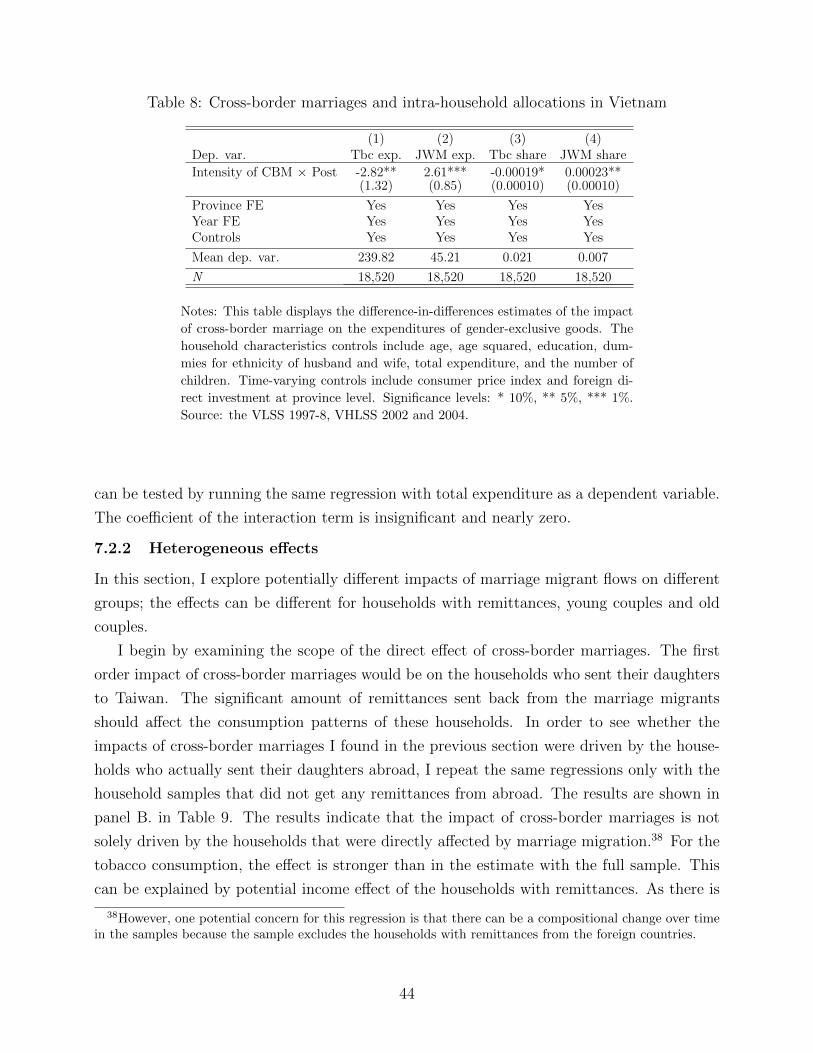
Table 8: Cross-border marriages and intra-household allocations in Vietnam

(1) (2) (3) (4)Dep. var. Tbc exp. JWM exp. Tbc share JWM share

Intensity of CBM × Post -2.82** 2.61*** -0.00019* 0.00023**(1.32) (0.85) (0.00010) (0.00010)

Province FE Yes Yes Yes YesYear FE Yes Yes Yes YesControls Yes Yes Yes Yes

Mean dep. var. 239.82 45.21 0.021 0.007

N 18,520 18,520 18,520 18,520

Notes: This table displays the difference-in-differences estimates of the impact

of cross-border marriage on the expenditures of gender-exclusive goods. The

household characteristics controls include age, age squared, education, dum-

mies for ethnicity of husband and wife, total expenditure, and the number of

children. Time-varying controls include consumer price index and foreign di-

rect investment at province level. Significance levels: * 10%, ** 5%, *** 1%.

Source: the VLSS 1997-8, VHLSS 2002 and 2004.

can be tested by running the same regression with total expenditure as a dependent variable.

The coefficient of the interaction term is insignificant and nearly zero.

7.2.2 Heterogeneous effects

In this section, I explore potentially different impacts of marriage migrant flows on different

groups; the effects can be different for households with remittances, young couples and old

couples.

I begin by examining the scope of the direct effect of cross-border marriages. The first

order impact of cross-border marriages would be on the households who sent their daughters

to Taiwan. The significant amount of remittances sent back from the marriage migrants

should affect the consumption patterns of these households. In order to see whether the

impacts of cross-border marriages I found in the previous section were driven by the house-

holds who actually sent their daughters abroad, I repeat the same regressions only with the

household samples that did not get any remittances from abroad. The results are shown in

panel B. in Table 9. The results indicate that the impact of cross-border marriages is not

solely driven by the households that were directly affected by marriage migration.38 For the

tobacco consumption, the effect is stronger than in the estimate with the full sample. This

can be explained by potential income effect of the households with remittances. As there is

38However, one potential concern for this regression is that there can be a compositional change over timein the samples because the sample excludes the households with remittances from the foreign countries.

44

Table 9: Heterogeneous effects

(1) (2)Dep. var. Tbc exp. JWM exp.

Panel A. All samples (N=18,520)

Intensity of CMB × Post -2.82** 2.61***(1.32) (0.85)

Panel B. HHs w/o remittances (N=17,916)

Intensity of CMB × Post -3.15** 2.66***(1.30) (0.84)

Panel C. HHs w/o remittances (Husb age<40) (N=8,757)

Intensity of CMB × Post -4.36** 2.58**(1.70) (1.14)

Panel D. HHs w/o remittances (Husb age≥40) (N=9,159)

Intensity of CMB × Post -1.46 2.81**(1.96) (1.25)

Notes: This table displays the difference-in-differences estimates of the impact of

cross-border marriage on the expenditures of gender-exclusive goods for different

groups. The household characteristics controls include age, age squared, education,

dummies for ethnicity of husband and wife, total expenditure, and the number of

children. Time-varying controls include consumer price index and foreign direct in-

vestment at province level. Significance levels: * 10%, ** 5%, *** 1%. Source: the

VLSS 1997-8, VHLSS 2002 and 2004.

additional income that comes from the remittances, tobacco consumption is less likely to be

reduced despite the decrease in power of husbands.

Next, I consider heterogenous effects for the younger and older couples. For older couples

that formed before the influence of the cross-border marriages, if the couples are fully com-

mitted on how to allocate their resources, the changes in marriage market conditions after

the marriage should not affect the intra-household allocations. However, if they only have a

limited commitment, resource allocations can become more favorable to wives because out-

side option for husbands deteriorates after the introduction of cross-border marriages and the

resulting low supply of women. The results in panel D. in Table 9 show that the consumption

for women-exclusive goods increased for old couples. The results suggest that the scope of

the effect can be very broad. It affects not only the migrant and young people who are on

the market when the cross-border marriage is possible, but also the economic decisions of the

couples that formed before the opening of the cross-border marriage markets. Younger cou-

ples also show evidence of increase in women’s power within the households; the consumption

on women-exclusive goods increased and the expenditure on men-exclusive good decreased,

45

bolstering the hypothesis. However, the sizes of the effects are larger for the younger couples

than for the older couples. This can be explained by the fact that those who are in the

marriage market during the time cross-border marriages are more prevalent are likely to be

influenced more intensely.39

7.2.3 Structural model

In this section, I highlight the broader implications for resource allocations of married couples.

Using a structural model incorporating more than one decision maker in a household, it is

possible to identify the partials of the sharing rule of married couples. In particular, I use a

collective model and the well-known identification results of Chiappori et al. (2002) with a

slight modification.40

Unlike the unitary model, which assumes a single utility function for each household, the

collective model allows for multiple agents with distinct utility functions. In particular, a

household maximizes its welfare function, which is a weighted sum of the individuals’ private

utility functions. Throughout my analysis, each household contains two decision makers,

a husband and a wife, who each have utility functions. It is assumed that the decision-

making process leads to Pareto-efficient outcomes. This assumption reflects reality, given

that the married couples interact very frequently. It is likely that husbands and wives know

each other’s preferences well. In particular, consumption decisions are not once-in-a-lifetime

decisions. Given the repeated interactions of married couples, it is unlikely that profitable

opportunities are left on the table without being exploited.

For the preferences, I assume egoistic preferences where each agent cares only about his

or her own consumption.41 More specifically, the utility function takes the form of ui(qi, z)

where i denotes the agent (i.e., i = h,w), qi denotes the consumption of agent i and z denotes

preference factors such as age and education level. qi can be either gender-exclusive goods

or assignable goods from which we can observe individual consumption patterns. I assume

a well-behaved utility function that is strictly quasi-concave, increasing and continuously

differentiable. I assume that the agents face the same prices.

39One potential concern for the results on young couples is that selection into marriage may have changedafter the outflow of marriage migrants. If the marriage rates were indeed affected by the outflow of women, thelowest types of men in Vietnam were more likely to be excluded from marriage. Then, the men who marriedafter the surge of cross-border marriage would have higher type than before, suggesting larger bargainingpower of men. Thus, the selection only bolsters the findings on gender-exclusive good consumption.

40They focus on the labor supply decisions of married couples whereas I concentrate on consumptiondecisions.

41Given that my analysis focus on private consumption of households, this assumption is not too extreme.However, the model can be extended to have Beckerian “caring” preferences.

46

The household solves the following program:

maxqh,qw

µ(z, s)uh(qh, z) + (1− µ(z, s))uw(qw, z) (1)

subject to

e · (qh + qw) ≤ x

where e, z, s, and x denote a price vector of ones, a vector of preference factors, a vector

of distribution factors, and total expenditure on private consumption42, respectively. Pareto

weight µ is a function of z and s and is assumed continuously differentiable with respect to

each argument. Note that distribution factors, s, affects consumption choice only through

µ. In other words, when s changes, the allocation moves along the Pareto frontier without

changing the Pareto frontier.

Under the egoistic preference assumption, the above problem is equivalent to solving two

problems of husbands and wives. That is, there exist sharing rule functions φh(x, z, s) and

φw(x, z, s) such that φh + φw = x. Each member solves below program:

maxqi

u(qi, z) (2)

subject to

e · qi ≤ φi

where i = h,w. The result follows from the second fundamental theorem of welfare economics.

Any Pareto efficient allocation can be achieved as a competitive equilibrium with a lump-sum

wealth redistribution. For the complete proof, see Browning et al. (1994).

Assuming interior solutions, equation (2) yields demand equations for husbands and wives.

I focus on two gender-exclusive goods, one for the husband and one for the wife. The demand

functions are:

ch = Ch(φh(x, z, s), z) (3)

cw = Cw(x− φh(x, z, s), z) (4)

42This can be thought of a two-stage budgeting. The households first decide on how much to allocate onpublic good and private good. For the second stage, they decide on how much to spend on different privatecommodities with the budget allocated in the first stage. The problem considered here is exactly this secondstage. The condition to guarantee two-stage budgeting is weak separability of preferences across public goodsand private goods, and I assume that this is the case.

47

where Ci is a demand function for member i (i = h,w). These two equations allow me to

identify the partials of the sharing rule. The identification result closely follows Chiappori

et al. (2002). The idea is using the fact that total private expenditure and distribution factors

affect consumption behavior only through the sharing rule. The responses of the consumption

behaviors to these variables allow me to estimate the marginal rate of substitution between

x and s for husbands and wives. Moreover, equation (3) and equation (4) generate testable

restrictions on consumption behavior.

To formalize this idea, let A = ∂ch/∂s∂ch/∂x

and B = ∂cw/∂s∂cw/∂x

when ∂ch

∂x· ∂cw∂x6= 0. For a moment,

assume that there is only one distribution factor. A and B are directly observable from

the data. From the demand equations, A = ∂ch/∂s∂ch/∂x

= φhsφhx

and B = ∂cw/∂s∂cw/∂x

= −φhs1−φhx

. Their

relationships allow the recovery of the partials of sharing rule, φhs and φhx. They are given by:

φhx =B

B − A(5)

φhs =AB

B − A(6)

assuming that A 6= B.

There is a cross-derivative restriction which needs to be satisfied.

∂

∂s(

B

B − A) =

∂

∂x(AB

B − A) (7)

If there are more than one distribution factor, there are additional restrictions imposed

by the model. Again, the distribution factors affect consumption choices only through the

sharing rule. Thus,

chslchs1

=φslφs1

=cwslcws1, ∀l = 2, . . . , L. (8)

Let Al = ∂ch/∂sl∂ch/∂x

and Bl = ∂cw/∂sl∂cw/∂x

. Then the above condition becomes:

AlBl

=A1

B1

l = 2, . . . , L. (9)

The partials of sharing rule with respect to additional distribution factors are as follows:

φhsl =AlBl

Bl − Al(10)

assuming that Al 6= Bl.

48

Given the results above, the sharing rule can be identified up to a constant function κ(z).

Estimation of the model

In this section, estimation procedures are detailed. In order to estimate the collective model,

the functional form should be chosen first. I begin with the unrestricted linear functional

form with two distribution factors given below:43

TBCipt = τ0 + τ1s1pt + τ2s2pt + τ3xipt + z′iptτ4 + εipt (11)

JWMjpt = δ0 + δ1s1pt + δ2s2pt + δ3xjpt + z′jptδ4 + εjpt (12)

where s1 and s2 denote distribution factors. xipt is total private expenditure and zipt

indicates preference factors including age, age squared, education, year dummies, province

dummies, children, consumer price index and foreign direct investment.

This functional form has several advantages. First of all, this functional form is simple and

has a straightforward interpretation. This linear Engel curve has been used ever since Engel

(1895) (Lewbel (2008)). Second, this functional form is compatible with the collective model

and allows the testing of the proportionality restrictions imposed by the model (equation (8)

or equation (9)). It does not violate any restrictions imposed by the model a priori. Third,

with this functional form, sharing rule can be identified up to a constant.

The restrictions imposed by the model (equation (9)) are as below:

τ1

δ1

=τ2

δ2

(13)

Cross derivative restriction is automatically satisfied because both sides of equation (7) are

zero.

If equation (7) is satisfied, the partials of sharing rule are given as follows:

φhx =τ3δ1

τ3δ1 − τ1δ3

(14)

φhs1 =τ1δ1

τ3δ1 − τ1δ3

(15)

φhs2 =τ2δ2

τ3δ2 − τ2δ3

(16)

Finally, the sharing rule equation is given by:

φh =τ3δ1

τ3δ1 − τ1δ3

x+τ1δ1

τ3δ1 − τ1δ3

s1 +τ2δ2

τ3δ2 − τ2δ3

s2 + κ(z) (17)

43Any number of distribution factors can be incorporated.

49

κ(z) is not identifiable, thus making the sharing rule identified up to a constant.

Distribution factors

I employ two novel distribution factors to identify the sharing rule of the married couples; they

are the intensity of cross-border marriages and the intensity of male-dominant agriculture.

First distribution factor is the intensity of cross-border marriages. To be a valid distri-

bution factor, it should affect sharing rules but not the budget constraint or preferences. To

address this, I estimate the sharing rule for households with and without remittances from

abroad. That is, after excluding the families that were directly affected by cross-border mar-

riages, it is unlikely that cross-border marriages affect the budget constraint. The intensity of

cross-border marriages is not an argument of preferences. Thus, the intensity of cross-border

marriages, which is new in the literature, qualifies as a valid distribution factor.

Moreover, the intensity of cross-border marriages is arguably exogenous, as explained

in the previous section. Many of the suggested distribution factors in the literature, such

as relative education, relative ages and relative incomes, were endogenous. It is difficult to

get credible estimates with endogenous distributions factors. Here, I take advantage of the

plausibly exogenous nature of the proposed distribution factor.

Next distribution factor, mainly for testing the efficiency assumption of the collective

model, is the intensity of male-dominant agriculture. In particular, the forest area is used

as a measure of the intensity of male-dominant agriculture. Since forestry is male labor-

intensive(Desai (1995)), a larger forest area means more economic opportunities for men.

This outside opportunity can impact the intra-houeshold balance of power. By a similar rea-

soning as above, it does not affect the preferences. Moreover, conditional on expenditures, it

also does not affect the budget constraint.

Sharing rule estimates

In this section, the results of empirical tests of collective model is presented and the sharing

rule estimates are given. First, the unrestricted equations (3) and (4) are estimated and

then the restrictions imposed by the collective model are tested. Then, the sharing rule is

estimated.

The results are presented in Table 10. The partials of sharing rule are all statistically

significant except for old couples. The partial with respect to total private expenditure

indicates that one unit (1,000VND) increase of total private expenditure is associated with

0.53 unit increase of husbands’ share. When the expenditure increases, husbands take up

approximately six percentage points more than their wives. The partial with respect to

cross-border marriages suggests that one percentage point increase of outflow of women is

50

Table 10: Sharing rule estimates in Vietnam

(1) (2) (3) (4)

Whole sample HHs w/o remit.HHs w/o remit.(Young cohort)

HHs w/o remit.(Old cohort)

φHx 0.53*** 0.52*** 0.50*** 0.66***

(0.13) (0.12) (0.14) (0.25)

φHs -106.04*** -114.72*** -103.11*** -93.07

(27.78) (27.79) (30.19) (62.66)

Mean pvt. exp. 4200.92 4126.92 3448.46 4775.61

N 18,520 17,916 8,757 9,159

Notes: This table displays the estimates of the partials of the married couples’ sharing

rule. φH indicates the share of husbands. φHx and φHs indicate the partials with respect

to total private expenditure and the intensity of cross-border marriage, respectively.

The household characteristics controls include age, age squared, education, dummies

for ethnicity of husband and wife, total expenditure, and the number of children.

Time-varying controls include consumer price index and foreign direct investment at

province level. Significance levels: * 10%, ** 5%, *** 1%. Source: the VLSS 1997-8,

VHLSS 2002 and 2004.

associated with 106 (1,000VND) less share of husbands. This amounts to approximately the

value of 120 lbs of rice. In other words, women in the areas with more outflow of women

control more money within the household. Table A4 shows that proportionality restriction

imposed by the model is not rejected. Thus, the efficiency assumption of the collective model

is satisfied.

Considering these estimates, the impact of cross-border marriages is substantial for women’s

power within the households. Furthermore, cross-border marriages can have an implication

on children’s outcome because women’s increased power within the households is known to

be related to better outcome of children (Duflo (2012)).

7.3 Impacts on sex ratios at birth

This subsection investigates how an increase in the economic value of a daughter, driven by

the opportunities of cross-border marriage, affects the sex ratios at birth in Vietnam. The

sharp increase in cross-border marriages substantially changed the expected returns from

having a daughter in Vietnam. The brides’ parents could receive about 1,000-2,000 USD

during the marriage process, which was more than twice the GDP per capita of Vietnam

in 2004 (Lu (2005)). Most of the marriage migrant daughters yearly remitted 1,400 USD

on average to their natal families, which is far more than the domestic labor migrants’

remittances (121 USD). Moreover, my findings in the previous section suggest that even

when daughters do not marry foreign men, the expected returns of having a daughter can

51

Figure 11: Sex ratios at birth in rural Vietnam

0

5000

10000

15000

Num

ber o

f Cro

ss-B

orde

r Mar

riage

s(T

aiw

an a

nd K

orea

)

106

108

110

112

114

116

Sex

Rat

io o

f Inf

ants

(≤ 1

yr o

ld)

1995 1996 1997 1998 1999 2000 2001 2002 2003 2004 2005 2006 2007 2008

Year (Conception Year)

Sex ratios of affected provincesSex ratios of unaffected provincesNumber of cross-border marraiges

Notes: This figure plots the sex ratios at birth in the provinces that were initially affected by

cross-border marriages and the rest of the provinces. The provinces with more than 1% of women

out-migrated in 2003 were classified as the affected provinces. Sources: the Vietnamese census

1999 and 2009.

still increase, because what they can gain in their marriages in the future has increased in

the affected areas after the surge of cross-border marriages. There is qualitative evidence

that the possibility of supporting a family by marrying foreign men mitigated son preference

in some Vietnamese provinces (Belanger and Linh (2011)).

Using the Vietnamese census data, I descriptively compare the sex ratios at birth in

the provinces where most marriage migrants were initially concentrated to the rest of the

provinces. I have already shown in the previous section that the most observable charac-

teristics are balanced in the affected provinces and non-affected provinces. Following the

prevalent use of internet after the mid-2000s, the origins of marriage migrants have become

more diverse, but 60-70% of marriage migrants still originate from the provinces that were

initially affected.

Figure 11 shows that the sex ratios at birth were almost identical before 2000, but after

the surge of cross-border marriages, sex ratios at birth were less male-biased in the affected

provinces. Since the introduction of ultrasound technology in the mid-2000s, there has been

an increasing trend in sex ratios at birth in both the affected and non-affected provinces.

However, the magnitude of increase in sex ratios at birth was much weaker in the affected

provinces. This finding cannot be explained by the differential availability of sex-selection

technologies because there were more mothers who knew the sex of their babies by ultrasound

52

technologies in the affected areas (Figure A3).

8 Conclusion

This paper examines the economic impacts of marriage migration in both migrant-sending

and migrant-receiving countries by answering four questions: (i) who moves, (ii) who benefits,

(iii) who loses, and (iv) to what extent. I show that the selection of migrants is governed by

the demographic structures and economic conditions of countries involved and by the costs of

cross-border marriage. Agents with low SES cannot engage in cross-border marriage due to

the associated costs. Agents with high SES in the wealthier country also do not marry across

borders because they can secure better domestic partners. I also find that the long sides of

the marriage markets benefit, and the short sides lose from the lowered cost of cross-border

marriage on various margins. Through marriage market equilibrium effects, the flows of

marriage migrants affect not only the direct marital outcomes but also the respective power

of all men and women in both countries by altering their shadow prices in the markets.

The situation in Taiwan and Vietnam may seem unique in several ways. However, there

are many other examples of marriage markets that actively interact. For example, there are

up to 300,000 Turkish-Russian married couples, and the spousal category accounted for 40%

of migrant settlements in the UK in 2009 (Charsley et al. (2012)). Other European countries,

including Spain, France, and Switzerland, have also experienced an increase in the number

of cross-border marriages in the past two decades, which could be explained by the negligible

associated costs within the European Union. Moreover, long-lasting sex ratio imbalances in

China and India could affect the dynamics of the neighboring countries’ marriage markets.

The framework developed in this paper sheds light on why this phenomenon takes place, who

becomes a marriage migrant and to what extent this can affect the welfare of local people.

This paper also illustrates the implications of cost-changing policies for marriage mar-

kets and women’s power. Many countries faced with increasing immigration, including Tai-

wan, South Korea, Denmark and the Netherlands, have implemented restrictive immigration

policies. The results of this paper suggest that such policies can have broad influences on

populations, as they can affect the economic decisions of every man and woman in countries

involved, not just those who are in or considering cross-border marriages. In countries with

male-skewed sex ratios, lowering the cost of entry for women from other countries can cer-

tainly mitigate the imbalances in the marriage market. However, at the same time, it can

decrease local women’s power within households. These findings highlight that related costs

and benefits should be carefully weighed when designing immigration policies.

53

References

Abramitzky, R., A. Delavande, and L. Vasconcelos (2011): “Marrying up: the role

of sex ratio in assortative matching,” American Economic Journal: Applied Economics,

124–157.

Angrist, J. (2002): “How do sex ratios affect marriage and labor markets? Evidence from

America’s second generation,” Quarterly Journal of Economics, 997–1038.

Attanasio, O. P. and V. Lechene (2014): “Efficient responses to targeted cash trans-

fers,” Journal of Political Economy, 122, 178–222.

Banister, J. (1985): The Population of Vietnam, 77, US Department of Commerce, Bureau

of the Census.

Belanger, D. and T. G. Linh (2011): “The impact of transnational migration on gender

and marriage in sending communities of Vietnam,” Current Sociology, 59, 59–77.

Bertoli, S., J. F.-H. Moraga, and F. Ortega (2013): “Crossing the border: Self-

selection, earnings and individual migration decisions,” Journal of Development Eco-

nomics, 101, 75–91.

Borjas, G. J. (1987): “Self-selection and the earnings of immigrants.” American Economic

Review, 77, 531–53.

——— (2014): Immigration economics, Harvard University Press.

Browning, M., F. Bourguignon, P.-A. Chiappori, and V. Lechene (1994): “In-

come and outcomes: A structural model of intrahousehold allocation,” Journal of Political

Economy, 1067–1096.

Browning, M., P.-A. Chiappori, and Y. Weiss (2014): Economics of the Family,

Cambridge University Press.

Charles, K. K. and M. C. Luoh (2010): “Male incarceration, the marriage market, and

female outcomes,” The Review of Economics and Statistics, 92, 614–627.

Charsley, K., B. Storer-Church, M. Benson, and N. Hear (2012): “Marriage-

Related Migration to the UK,” International Migration Review, 46, 861–890.

Chiappori, P.-A. (2017): Matching with Transfers: The Economics of Love and Marriage,

Princeton University Press.

54

Chiappori, P.-A., B. Fortin, and G. Lacroix (2002): “Marriage market, divorce leg-

islation, and household labor supply,” Journal of Political Economy, 110, 37–72.

Chiappori, P.-A., R. J. McCann, and L. P. Nesheim (2010): “Hedonic price equilibria,

stable matching, and optimal transport: equivalence, topology, and uniqueness,” Economic

Theory, 42, 317–354.

Chiappori, P.-A., R. J. McCann, and B. Pass (2016a): “Multi-to One-Dimensional

Optimal Transport,” Communications on Pure and Applied Mathematics.

Chiappori, P.-A., S. Oreffice, and C. Quintana-Domeque (2016b): “Black–White

Marital Matching: Race, Anthropometrics, and Socioeconomics,” Journal of Demographic

Economics, 82, 399–421.

——— (2017): “Bidimensional matching with heterogeneous preferences: education and

smoking in the marriage market,” Journal of the European Economic Association.

Chiquiar, D. and G. H. Hanson (2005): “International migration, self-selection, and the

distribution of wages: Evidence from Mexico and the United States,” Journal of Political

Economy, 113, 239–281.

Constable, N. (2010): Cross-border marriages: Gender and mobility in transnational Asia,

University of Pennsylvania Press.

Desai, J. (1995): “Vietnam through the Lens of Gender,” Hanoi: UNDP.

Do, T. N. T., H. Glind, P. Kelly, G. Kamphuis, M. Heeswijk, D. McArthur,

N. Phan, T. Tong, A. Tran, and T. Tran (2003): “Marriages of Convenience:

Context, processes and results of cross-border marriages between Vietnamese young women

and Taiwanese men,” Mobility Research and Support Center, Hanoi.

Duflo, E. (2012): “Women Empowerment and Economic Development,” Journal of Eco-

nomic Literature, 50, 1051.

Edlund, L., E. M. Liu, and J.-T. Liu (2013): “Beggar-Thy-Women: Foreign Brides and

the Domestic Front–The Case of Taiwan,” Working Paper.

Engel, E. (1895): Die Lebenskosten belgischer Arbeiter-Familien fruher und jetzt, C. Hein-

rich.

Feigenberg, B. (2017): “Fenced Out: Why Rising Migration Costs Matter,” Working

Paper.

55

Fulford, S. L. (2015): “Marriage migration in India: Vast, varied, and misunderstood,”

Tech. rep., Boston College Working Paper 820.

Goodkind, D. (1997): “The Vietnamese double marriage squeeze,” International Migration

Review, 108–127.

International Organization for Migration (2015): “Asia-Pacific migration report

2015: Migrants’ contribution to development,” .

Kawaguchi, D. and S. Lee (2017): “Brides For Sale: Cross-border Marriages and Female

Immigration,” Economic Inquiry, 55, 633–654.

Lam, D., J. Boymal, and B. Martin (2004): “Internet diffusion in Vietnam,” Technology

in Society, 26, 39–50.

Lewbel, A. (2008): “Engel curves,” The New Palgrave Dictionary of Economics, 2.

Lichter, D. T., Z. Qian, and D. Tumin (2015): “Whom do immigrants marry? Emerg-

ing patterns of intermarriage and integration in the United States,” The ANNALS of the

American Academy of Political and Social Science, 662, 57–78.

Lu, M. C.-W. (2005): “Commercially arranged marriage migration: Case studies of cross-

border marriages in Taiwan,” Indian Journal of Gender Studies, 12, 275–303.

——— (2008): “Gender, marriage and migration: contemporary marriages between mainland

China and Taiwan,” Ph.D. thesis, Research School of Asian, African and Amerindian

Studies (CNWS), Faculty of Arts, Leiden University.

Mincer, J. (1978): “Family migration decisions,” Journal of political Economy, 86, 749–773.

Minh, T. Q. (2011): “Two decades of Taiwan’s FDI in Vietnam - An Analysis and Assess-

ment,” .

Mizoguchi, N. (2010): “The Consequences of the Vietnam War on the Vietnamese Popu-

lation,” .

Moraga, J. F.-H. (2011): “New evidence on emigrant selection,” The Review of Economics

and Statistics, 93, 72–96.

Morrow, M. and S. Barraclough (2003): “Tobacco control and gender in south-east

Asia. Part II: Singapore and Vietnam,” Health Promotion International, 18, 373–380.

56

Nguyen, X. and X. Tran (2010): “Vietnamese-Taiwanese Marriages,” Asian cross-border

marriage migration: Demographic patterns and social issues, 157–176.

Oreffice, S. (2011): “Sexual orientation and household decision making.: Same-sex cou-

ples’ balance of power and labor supply choices.” Labour Economics, 18, 145–158.

Rosenzweig, M. R. and O. Stark (1989): “Consumption smoothing, migration, and

marriage: Evidence from rural India,” Journal of political Economy, 97, 905–926.

Rubinstein, Y. and D. Brenner (2013): “Pride and prejudice: using ethnic-sounding

names and inter-ethnic marriages to identify labour market discrimination,” Review of

Economic Studies, 81, 389–425.

Sandell, S. H. (1977): “Women and the economics of family migration,” The Review of

Economics and Statistics, 406–414.

Smith, J. P. and D. Thomas (1998): “On the road: Marriage and mobility in Malaysia,”

Journal of Human Resources, 805–832.

Tseng, H. (2016): Racialization of Foreign Women in the Transnational Marriage Market of

Taiwan, Cultural Politics of Gender and Sexuality in Contemporary Asia, Chapter twelve.

Wang, H.-z. and S.-m. Chang (2002): “The Commodification of International Marriages:

Cross-border Marriage Business in Taiwan and Viet Nam,” International migration, 40,

93–116.

Weiss, Y., J. Yi, and J. Zhang (2017): “Cross-border Marriage Costs and Marriage

Behavior: Theory and Evidence,” International Economic Review, Forthcoming.

Yang, W. S. and Y.-y. T. Liu (2014): “Gender imbalances and the twisted marriage

market in Taiwan,” in The Family and Social Change in Chinese Societies, Springer, 117–

130.

57

Appendix

A Proof of Proposition 1

Proof. 1. When Y = Y ′

Suppose x ≥ x′ but y′ > y on a subset of positive measure. Consider the surplus of

(x,X), (y, Y ) and (x′, X), (y′, Y ) matches:

Σ1 = ΣXY (x, y) + ΣXY (x′, y′)− 2λ1(X 6= Y )

Switching the matching generates:

Σ2 = ΣXY (x, y′) + ΣXY (x′, y)− 2λ1(X 6= Y )

By supermodularity Σ2 > Σ1. Since x ≥ x′ but y < y′ on a subset of positive measure,

the surplus can be improved by switching. Contradiction.

2. When Y 6= Y ′

Without loss of generality, let Y = X. Suppose x ≥ x′ but y′ > y on a subset of

positive measure. Consider the surplus of (x,X), (y, Y ) and (x′, X), (y′, Y ′) matches:

Σ1 = ΣXY (x, y) + ΣX′Y (x′, y′) = S(x, y) + S(x′, y′)− λ

Switching the matching generates:

Σ2 = ΣXY (x, y′) + ΣX′Y (x′, y) = S(x, y′) + S(x′, y)− λ

By supermodularity Σ2 > Σ1. Since x ≥ x′ but y < y′ on a subset of positive measure,

the surplus can be improved by switching. Contradiction.

The proof of the second part is similar.

B Proof of Proposition 2

Proof. Without a loss of generality, let X be T . Suppose a man x from country T is matched

to either a woman y from country T or a woman y′ from country V at the stable match. Let

uT (x) be his utility. Then, by stability,

uT (x) = maxs

(S(x, s)− vT (s))

= maxs′

(S(x, s′)− λ− vV (s′))

58

where vT (s) (vV (s′)) is the utility of a woman from country T (a woman from country V )

with the type s (s′); note that the maximum is reached at s = y and s′ = y′ respectively. By

the envelope theorem:

u′T (x) =∂

∂xS(x, y) =

∂

∂xS(x, y′)

Since ∂S∂x

is strictly increasing in y, y = y′.

From the stability conditions, we have

uT (x) = S(x, y)− vT (y)

= S(x, y)− λ− vV (y)

Thus, vV (y) + λ = vT (y).

The second part can be proved similarly.

C Proof of Proposition 4

Proof. There are multiple ways to approach the problem. I start with a direct approach;

assuming that the equilibrium is as explained in the Proposition, a complete characterization

on matching and surplus division can be obtained. Then, the stability conditions can be

verified. I show the case when zM(λ) ≤ B − σ. Other cases can be proved in a similar way.

– Step 1 (Matching functions):

– Taiwanese men

∗ A Taiwanese man with x ∈ [B − rσ,B] is matched to a Taiwanese woman y

with probability 1.

y =1

rx− 1

rB +B = φT (x)

∗ A Taiwanese man with x ∈ [B−σ,B− rσ] is matched to a Taiwanese woman

y with probability rr+v

and to a Vietnamese woman with y with probabilityvr+v

.

y =1

r + vx+B − σ − B − rσ

r + v= φ(x)

∗ A Taiwanese man with x ∈ [zM , B−σ] is matched to a Taiwanese woman with

y with probability r(1+v)r+v

and to a Vietnamese woman with y with probability

59

v(1−r)r+v

.

y =1 + v

r + vx+M − 1 + v

r + v(B − σ) = φ(x)

where M := 1r+v

(B − σ) +B − σ − B−rσr+v

.

∗ A Taiwanese man with x ∈ [x0,T , zM ] is matched to a Taiwanese woman with

y with probability 1.

y =1

rx− 1

rzM +

1 + v

r + vzM +M − 1 + v

r + v(B − σ) = φT (x)

where x0,T = φ−1T (A).

– Vietnamese men

∗ A Vietnamese man with x ∈ [x0,V , B−σ] is matched to a Vietnamese woman

with y with probability 1.

y =1 + v

r + vx+M − 1 + v

r + v(B − σ) = φ(x) if x ≥ zM

y = x− zM +1 + v

r + vzM +M − 1 + v

r + v(B − σ) = φV (x) if x ≤ zM

where x0,V = φ−1V (A− σ).

– Taiwanese women

∗ A Taiwanese woman with y ∈ [A,B] is matched to a Taiwanese man with x

with probability 1.

x = φ−1T (y) if y ≥ B − σ

x = φ−1(y) if M ≤ y ≤ B − σ

x = φ−1(y) if zW ≤ y ≤M

x = φ−1T (y) if A ≤ x ≤ zW

where zW := φ(zM).

– Vietnamese women

∗ A Vietnamese woman with [M,B − σ] is matched to a Taiwanese man with

x with probability 1.

x = φ−1(y)

60

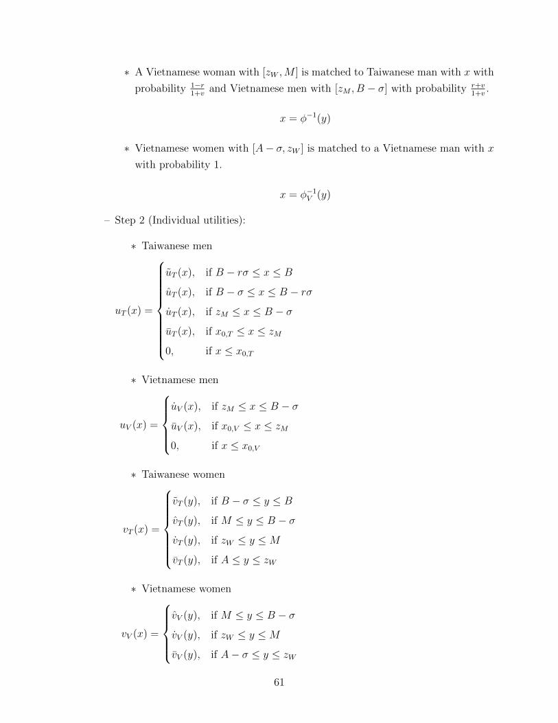
∗ A Vietnamese woman with [zW ,M ] is matched to Taiwanese man with x with

probability 1−r1+v

and Vietnamese men with [zM , B − σ] with probability r+v1+v

.

x = φ−1(y)

∗ Vietnamese women with [A− σ, zW ] is matched to a Vietnamese man with x

with probability 1.

x = φ−1V (y)

– Step 2 (Individual utilities):

∗ Taiwanese men

uT (x) =

uT (x), if B − rσ ≤ x ≤ B

uT (x), if B − σ ≤ x ≤ B − rσ

uT (x), if zM ≤ x ≤ B − σ

uT (x), if x0,T ≤ x ≤ zM

0, if x ≤ x0,T

∗ Vietnamese men

uV (x) =

uV (x), if zM ≤ x ≤ B − σ

uV (x), if x0,V ≤ x ≤ zM

0, if x ≤ x0,V

∗ Taiwanese women

vT (x) =

vT (y), if B − σ ≤ y ≤ B

vT (y), if M ≤ y ≤ B − σ

vT (y), if zW ≤ y ≤M

vT (y), if A ≤ y ≤ zW

∗ Vietnamese women

vV (x) =

vV (y), if M ≤ y ≤ B − σ

vV (y), if zW ≤ y ≤M

vV (y), if A− σ ≤ y ≤ zW

61

where

u′T (x) = Sx(x, φ(x))

uT (x) =

∫ x

B−rσSx(s, φ(s))ds+ P

u′T (x) = Sx(x, φ(x))

uT (x) =

∫ x

B−σSx(s, φ(s))ds+Q

u′T (x) = Sx(x, φ(x))

uT (x) =

∫ x

zM

Sx(s, φ(s))ds+R

u′T (x) = Sx(x, φT (x))

uT (x) =

∫ x

x0,T

Sx(s, φT (s))ds+ S

u′V (x) = Sx(x, φ(x))

uV (x) =

∫ x

zM

Sx(s, φ(s))ds+R′

u′V (x) = Sx(x, φ(x))

uV (x) =

∫ x

x0,V

Sx(s, φV (s))ds+ S′

v′T (y) = Sy(φ−1(y), y)

vT (y) =

∫ y

B−σSy(φ

−1(t), t)dt+ J

v′T (y) = Sy(φ−1(y), y)

vT (y) =

∫ y

MSy(φ

−1(t), t)dt+K

v′T (y) = Sy(φ−1(y), y)

vT (y) =

∫ y

zW

Sy(φ−1(t), t)dt+ L

v′T (y) = Sy(φ−1T (y), y)

vT (y) =

∫ y

aSy(φ

−1T (t), t)dt+O

v′V (y) = Sy(φ−1(y), y)

vV (y) =

∫ y

MSy(φ

−1(t), t)dt+K ′

v′V (y) = Sy(φ−1(y), y)

vV (y) =

∫ y

zW

Sy(φ−1(t), t)dt+ L′

v′V (y) = Sy(φ−1V (y), y)

vV (y) =

∫ y

aSy(φ

−1V (t), t)dt+O′

∗ The constants are:

S = 0

S ′ = 0

R =

∫ zM

x0,T

Sx(s, φT (s))ds

R′ =

∫ zM

x0,V

Sx(s, φV (s))ds

Q =

∫ B−σ

zM

Sx(s, φ(s))ds+

∫ zM

x0,T

Sx(s, φT (s))ds

P =

∫ B−rσ

B−σSx(s, φ(s))ds+

∫ B−σ

zM

Sx(s, φ(s))ds+

∫ zM

x0,T

Sx(s, φT (s))ds

62

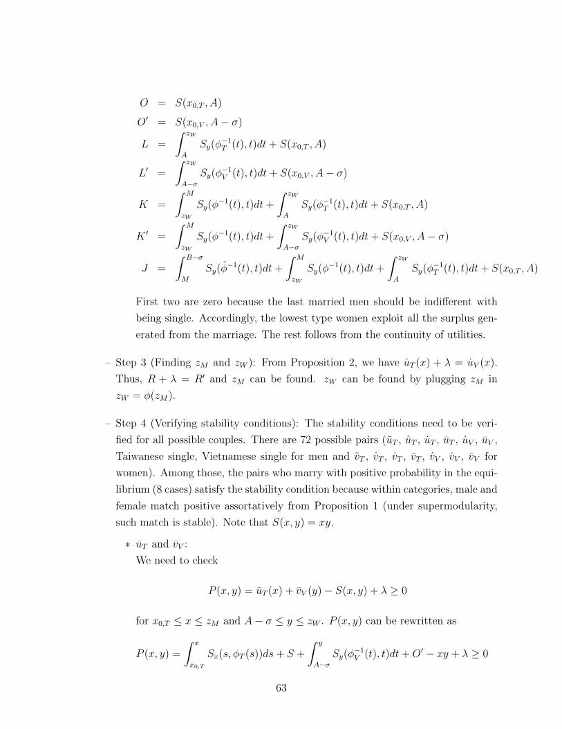
O = S(x0,T , A)

O′ = S(x0,V , A− σ)

L =

∫ zW

A

Sy(φ−1T (t), t)dt+ S(x0,T , A)

L′ =

∫ zW

A−σSy(φ

−1V (t), t)dt+ S(x0,V , A− σ)

K =

∫ M

zW

Sy(φ−1(t), t)dt+

∫ zW

A

Sy(φ−1T (t), t)dt+ S(x0,T , A)

K ′ =

∫ M

zW

Sy(φ−1(t), t)dt+

∫ zW

A−σSy(φ

−1V (t), t)dt+ S(x0,V , A− σ)

J =

∫ B−σ

M

Sy(φ−1(t), t)dt+

∫ M

zW

Sy(φ−1(t), t)dt+

∫ zW

A

Sy(φ−1T (t), t)dt+ S(x0,T , A)

First two are zero because the last married men should be indifferent with

being single. Accordingly, the lowest type women exploit all the surplus gen-

erated from the marriage. The rest follows from the continuity of utilities.

– Step 3 (Finding zM and zW ): From Proposition 2, we have uT (x) + λ = uV (x).

Thus, R + λ = R′ and zM can be found. zW can be found by plugging zM in

zW = φ(zM).

– Step 4 (Verifying stability conditions): The stability conditions need to be veri-

fied for all possible couples. There are 72 possible pairs (uT , uT , uT , uT , uV , uV ,

Taiwanese single, Vietnamese single for men and vT , vT , vT , vT , vV , vV , vV for

women). Among those, the pairs who marry with positive probability in the equi-

librium (8 cases) satisfy the stability condition because within categories, male and

female match positive assortatively from Proposition 1 (under supermodularity,

such match is stable). Note that S(x, y) = xy.

∗ uT and vV :

We need to check

P (x, y) = uT (x) + vV (y)− S(x, y) + λ ≥ 0

for x0,T ≤ x ≤ zM and A− σ ≤ y ≤ zW . P (x, y) can be rewritten as

P (x, y) =

∫ x

x0,T

Sx(s, φT (s))ds+ S +

∫ y

A−σSy(φ

−1V (t), t)dt+O′ − xy + λ ≥ 0

63

This gives Pxx = φ′T (x) = 1r, Pyy = φ−1

V′(y) = 1, and Pxy = −1. Thus, P (x, y)

is convex in (x, y) and its minimum satisfies

∂P (x, y)

∂x=∂P (x, y)

∂y= 0

Sx(x, φT (x))− Sx(x, y) = 0

Sy(φ−1V (y), y)− Sy(x, y) = 0

To satisfy both conditions, the following should be the case: y = φT (x) and

y = φV (x). This happens at the cutoff x = zM . Note that vV (zW ) + λ =

vT (zW ). P (zM , zW ) = uT (zM) + vV (zW ) − S(x, y) + λ = uT (zM) + vT (zW ) −S(x, y) = 0, so the condition is satisfied.

∗ uT and vV :

We need to check

P (x, y) = uT (x) + vV (y)− S(x, y) + λ ≥ 0

for x0,T ≤ x ≤ zM and zW ≤ y ≤M . Since we know P (zM , zW ) = 0, if P (x, y)

is decreasing in x and increasing in y, P (x, y) in all (x, y) in the ranges. This

can be shown as follows:

∂P (x, y)

∂x= φT (x)− y ≤ 0

∂P (x, y)

∂y= φ−1(y)− x ≥ 0.

For the remaining cases as well, using similar computations, it can be shown that

the difference u + v − Σ between the sum of individual utilities and potential

surplus is minimum at the boundary or at some non-negative interior point. The

explicit calculations are available upon request.

64

D Proof of Proposition 5

Proof. – ∂zM∂λ

> 0:

This can be proved by using the Leibniz integral rule.

λ = R′ −R

=

∫ zM

x0,V

Sx(s, φV (s))ds−∫ zM

x0,T

Sx(s, φT (s))ds

=

∫ zM

A−σ+ r−1r+v

zM−M+ 1+vr+v

(B−σ)

Sx(s, s− zM +1 + v

r + vzM +M − 1 + v

r + v(B − σ))ds

−∫ zM

rA+v(1−r)r+v

zM−M+ 1+vr+v

(B−σ)

Sx(s,1

rs− 1

rzM +

1 + v

r + vzM +M − 1 + v

r + v(B − σ))ds

Using the Leibniz integral rule,

∂λ

∂zM= Sx(zM , zW ) + Sx(A− σ +

r − 1

r + vzM −M +

1 + v

r + v(B − σ), A− σ)

1− rr + v

+

∫ zM

A−σ+ r−1r+v

zM−M+ 1+vr+v

(B−σ)

Sxy(s, s− zM +1 + v

r + vzM +M − 1 + v

r + v(B − σ))

1− rr + v

ds

−Sx(zM , zW ) + Sx(rA+v(1− r)r + v

zM −M +1 + v

r + v(B − σ), A)

1− rr + v

v

+

∫ zM

rA+v(1−r)r+v

zM−M+ 1+vr+v

(B−σ)

Sxy(s,1

rs− 1

rzM +

1 + v

r + vzM +M − 1 + v

r + v(B − σ))

v(1− r)r(r + v)

ds

> 0

because Sxy > 0. Thus, we have ∂zM∂λ

> 0.

– ∂zW∂λ

> 0:

zM = φ(zW ) and φ′(x) > 0. From ∂zM∂λ

> 0, ∂zW∂λ

> 0.

– ∂φT (x)∂λ

< 0

Note that φT (x) = 1rx− 1

rzM + 1+v

r+vzM +M − 1+v

r+v(B − σ). Given x, ∂φT (x)

∂zM= v(r−1)

r(r+v)< 0.

From ∂φT (x)∂λ

= ∂φT (x)∂zM

∂zM∂λ

, the result follows.

– ∂φV (x)∂λ

> 0

Note that φV (x) = x− zM + 1+vr+v

zM +M − 1+vr+v

(B−σ). Given x, ∂φV (x)∂zM

= −1 + 1+vr+v

> 0.

From ∂φV (x)∂λ

= ∂φV (x)∂zM

∂zM∂λ

, the result follows.

65

–∂x0,T∂λ

> 0

Note that x0,T = φ−1T (A) = rA+ v(1−r)

r+vzM −M + 1+v

r+v(B − σ). Using the chain rule, the

result follows.

–∂x0,V∂λ

< 0

Note that x0,V = φ−1V (A−σ) = A−σ+ r−1

r+vzM −M + 1+v

r+v(B−σ). Using the chain rule,

the result follows.

– ∂uT (x)∂λ

< 0

Use the Leibniz integral rule to show ∂uT (x)∂zM

< 0. Then use the chain rule.

– ∂uV (x)∂λ

> 0

Use the Leibniz integral rule to show ∂uV (x)∂zM

> 0. Then use the chain rule.

– ∂vT (y)∂λ

> 0

Use the Leibniz integral rule to show ∂vT (y)∂zM

> 0. Then use the chain rule.

– ∂vV (y)∂λ

< 0

Use the Leibniz integral rule to show ∂vT (y)∂zM

< 0. Then use the chain rule.

E Multiplicative cost

This subsection provides the theoretical results when cost varies with the surplus. These

results can be obtained with a minor modification to the surplus function given in Chiappori

et al. (2017). Assume the same population structures given in 3.1.1. Suppose the surplus

function is given as follows:

ΣXY (x, y) =

S(x, y), if X = Y

(1− λ)S(x, y), if X 6= Y

where λ < 1. The function S is strictly increasing, continuously differentiable, and super-

modular. Normalize single utility as 0 and assume that S(0, 0) ≥ 0.

Proposition 6. In the stable matching, if (x,X) and (x′, X) such that x ≥ x′ are matched

to (y, Y ) and (y′, Y ), respectively, y ≥ y′ almost surely.

66

Proof. Suppose x ≥ x′ but y′ > y with a positive measure. The surplus is:

Σ1 = ΣXY (x, y) + ΣXY (x′, y′)

By switching the couples, the surplus becomes

Σ2 = ΣXY (x, y′) + ΣXY (x′, y) > Σ1

by supermodularity. It contradicts to surplus maximization.

Note that under the multiplicative cost case, the matching is positive assortative on SES

within same categories of men and women. The positive assortative matching results under

the fixed cost case is stronger because a stable matching is positive assortative on SES when

holding one gender’s country and considering the two countries for the other gender. This

result does not hold anymore under multiplicative cost because the cost depends on the types

of the agents.

Proposition 7. Suppose an open set of males from X country are indifferent between mar-

rying a woman from T country and a woman from V country so that 0 < p(T |x,X) < 1 in

the stable match for any x in the open set. If (x,X) is matched to either (y, T ) or (y′, V ),

then y < y′ if X = T and y > y′ if X = V .

Similarly, suppose an open set of females from Y country are indifferent between marrying

a man from T country and a man from V country so that 0 < q(X|y, Y ) < 1 in the stable

match for any y in the open set. If (y, Y ) is matched to either (x, T ) or (x′, V ), then x < x′

if Y = T and x > x′ if Y = V .

Proof. Let X be T . Suppose a man x from country T is matched to either a woman y from

country T or a woman y′ from country V at the stable match. Let uT (x) be his utility. Then,

by stability,

uT (x) = maxs

(S(x, s)− vT (s))

= maxs′

(λS(x, s′)− vV (s′))

where vT (s) (vV (s′)) is the utility of a woman from country T (a woman from country V )

with the type s (s′); note that the maximum is reached at s = y and s′ = y′ respectively. By

the envelope theorem:

u′T (x) =∂

∂xS(x, y) = λ

∂

∂xS(x, y′)

67

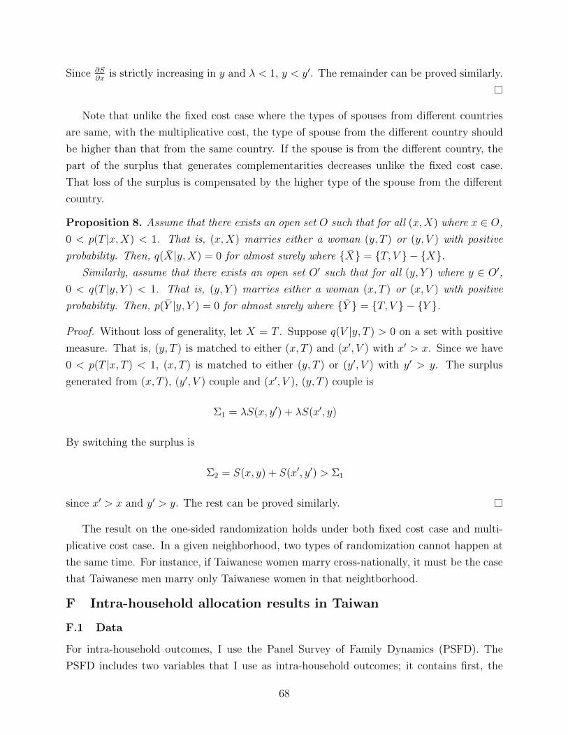
Since ∂S∂x

is strictly increasing in y and λ < 1, y < y′. The remainder can be proved similarly.

Note that unlike the fixed cost case where the types of spouses from different countries

are same, with the multiplicative cost, the type of spouse from the different country should

be higher than that from the same country. If the spouse is from the different country, the

part of the surplus that generates complementarities decreases unlike the fixed cost case.

That loss of the surplus is compensated by the higher type of the spouse from the different

country.

Proposition 8. Assume that there exists an open set O such that for all (x,X) where x ∈ O,

0 < p(T |x,X) < 1. That is, (x,X) marries either a woman (y, T ) or (y, V ) with positive

probability. Then, q(X|y,X) = 0 for almost surely where {X} = {T, V } − {X}.Similarly, assume that there exists an open set O′ such that for all (y, Y ) where y ∈ O′,

0 < q(T |y, Y ) < 1. That is, (y, Y ) marries either a woman (x, T ) or (x, V ) with positive

probability. Then, p(Y |y, Y ) = 0 for almost surely where {Y } = {T, V } − {Y }.

Proof. Without loss of generality, let X = T . Suppose q(V |y, T ) > 0 on a set with positive

measure. That is, (y, T ) is matched to either (x, T ) and (x′, V ) with x′ > x. Since we have

0 < p(T |x, T ) < 1, (x, T ) is matched to either (y, T ) or (y′, V ) with y′ > y. The surplus

generated from (x, T ), (y′, V ) couple and (x′, V ), (y, T ) couple is

Σ1 = λS(x, y′) + λS(x′, y)

By switching the surplus is

Σ2 = S(x, y) + S(x′, y′) > Σ1

since x′ > x and y′ > y. The rest can be proved similarly.

The result on the one-sided randomization holds under both fixed cost case and multi-

plicative cost case. In a given neighborhood, two types of randomization cannot happen at

the same time. For instance, if Taiwanese women marry cross-nationally, it must be the case

that Taiwanese men marry only Taiwanese women in that neightborhood.

F Intra-household allocation results in Taiwan

F.1 Data

For intra-household outcomes, I use the Panel Survey of Family Dynamics (PSFD). The

PSFD includes two variables that I use as intra-household outcomes; it contains first, the

68

information on weekly hours spent on household works and second, yearly clothing expendi-

ture of the respondents and their spouses. It also surveys the year of marriage, which allows

me to evaluate the impact of changes in visa policies on the relative status of women within

households. I use 2007 data only because that is the only year when the survey collected

information on spending for both husbands and wives.

F.2 Impact on intra-household allocations

Prediction 5. When the cost of cross-border marriage increases, the power within households

for wives improves whereas the power of husbands decreases in Taiwan.

For marriage rates and matching patterns, the changes in costs of cross-border marriage

affect only a subset of populations. However, one of the powerful results in matching literature

is that once market condition changes, the share within marriage for everyone changes. In

the specific case of the visa tightening policy, the individual utilities of women increases for

all women and the individual utilities of men decreases for all men. Thus, albeit interesting,

it is difficult to test this prediction compared to marriage rates or matching patterns because

there does not exist a natural control group. Instead, I compare men and women in terms

of measures of bargaining power within households, which is proxied by weekly hours on

household work and individual spending on clothing. Since the model predicts that the

power of wives increases and that of husbands decreases, we would expect to see that the

time spent on household work for husbands increases compared to for the wives and the

spending on clothing of husbands decreases compared to that of wives.

Yigy = βfemaleg × Posty + γg + δy + νXi + εigy

where i is an individual, g is gender, and y is the year of marriage. The controls include

the ages of husbands and wives, and district fixed effects. For the spending on clothing, I also

control for total expenditure of the household in the form of the product of level and log level

in the spirit of Working-Leser model. This allows differential impact of total expenditure by

its level.

The results are presented in Table A3. The results show that the weekly hours of house-

hold work decreases and the spending on clothing increases for wives compared to the hus-

bands after the visa tightening policy although the result on spending on clothing is not

significant. This suggests that the power of women within households is enhanced when it

becomes more difficult for Vietnamese women to enter Taiwan, which is consistent with the

theoretical prediction.

69

Figure A1: Comparative statics with respect to cost of cross-border marriages (λ1 < λ2)

A. Taiwanese Men B. Vietnamese Men C. Taiwanese Women D. Vietnamese Women

Probability of being a single

0.00

0.25

0.50

0.75

1.00

Α Β − σ Β

Prob. of marrying a Taiwanese

0.00

0.25

0.50

0.75

1.00

Α Β − σ Β

Prob. of marrying a Vietnamese

0.00

0.25

0.50

0.75

1.00

Α Β − σ Β

Matching functions

Α − σ

Α

Β − σ

Β

Α Β − σ Β

SE

S o

f Spo

uses

Individual utilities

0

5

10

15

20

Α Β − σ Β

Socioeconomic status of Taiwanese men

u T(x

)

Probability of being a single

0.00

0.25

0.50

0.75

1.00

Α − σ Α Β − σ

Prob. of marrying a Taiwanese

0.00

0.25

0.50

0.75

1.00

Α − σ Α Β − σ

Prob. of marrying a Vietnamese

0.00

0.25

0.50

0.75

1.00

Α − σ Α Β − σ

Matching functions

Α − σ

Α

Β − σ

Β

Α − σ Α Β − σ

SE

S o

f Spo

uses

Individual utilities

0

5

10

15

20

Α − σ Α Β − σ

Socioeconomic status of Vietnamese men

u V(x

)

Probability of being a single

0.00

0.25

0.50

0.75

1.00

Α Β − σ Β

Prob. of marrying a Taiwanese

0.00

0.25

0.50

0.75

1.00

Α Β − σ Β

Prob. of marrying a Vietnamese

0.00

0.25

0.50

0.75

1.00

Α Β − σ Β

Matching functions

Α − σ

Α

Β − σ

Β

Α Β − σ Β

SE

S o

f Spo

uses

Individual utilities

0

5

10

15

20

Α Β − σ Β

Socioeconomic status of Taiwanese women

v T(y

)

Probability of being a single

0.00

0.25

0.50

0.75

1.00

Α − σ Α Β − σ

Prob. of marrying a Taiwanese

0.00

0.25

0.50

0.75

1.00

Α − σ Α Β − σ

Prob. of marrying a Vietnamese

0.00

0.25

0.50

0.75

1.00

Α − σ Α Β − σ

Matching functions

Α − σ

Α

Β − σ

Β

Α − σ Α Β − σ

SE

S o

f Spo

uses

Individual utilities

0

5

10

15

20

Α − σ Α Β − σ

Socioeconomic status of Vietnamese women

v V(y

)

λ1λ2

Notes: These figures plot comparative statics results. For these illustrative figures, the parameter values A = 2, B = 6, σ = 1.4, r = 0.7, v = 2, λ1 = 2.2 and λ2 = 3

are used. The grey lines on matching graphs indicate y = x. MATLAB codes are available upon request.

70

Figure A2: Geographic distributions of cross-border marriages and ethnic Chinese population

(a) Share of cross-border marriages (b) Number of cross-border marriages (c) Share of ethnic Chinese population

Notes: These figures display the distributions of the share and number of cross-border marriages and the share of ethnic Chinese

at the province level. The thick black lines indicate the regions.

71

Figure A3: Prevalence of ultrasound technologies in rural Vietnam

0.2

.4.6

.81

Rat

e of

mot

hers

kno

win

g th

e se

x by

ultr

asou

nd

2005 2006 2007 2009 2010 2011 2012 2013

Affected Provinces Unaffected Provinces

Sources: the Population Changing Surveys in Vietnam 2004-2013.

72

Table A1: The impact of visa tightening policies on the SES of foreign brides by origins

Sample: Mainland Brides Southeast Asian Brides

Dependent variable (=1): Pri. JHSH/

Voca.Univ./above

Pri. JHSH/

Voca.Univ./above

After visa-tightening (=1) -0.14∗∗∗ 0.052 0.026 0.065∗∗ -0.12 0.062 0.076 -0.016(0.015) (0.045) (0.044) (0.028) (0.078) (0.094) (0.088) (0.036)

Controls Yes Yes Yes Yes Yes Yes Yes Yes

Dep. var. mean 0.20 0.42 0.34 0.04 0.37 0.36 0.23 0.04

R-squared 0.012 0.003 0.008 0.003 0.004 0.002 0.004 0.006

Observations 58,768 58,768 58,768 58,768 56,755 56,755 56,755 56,755

Notes: This table displays the results from regressing each dependent variable (indicating foreign brides education) listed in the second row

a dummy for post visa tightening policies and controls (marriage year fixed effects and county city fixed effects) by the origins of the foreign

brides. Note that Pri., JH, SH, Voca. and Univ. indicate Primary, Junior High, Senior High, Vocational and University, respectively. Robust

standard errors are used. Significance levels: * 10%, ** 5%, *** 1%. Sources: the Census of Foreign Spouse, 2003 and the Foreign and Mainland

Spouse Living Needs Survey, 2008. Only the foreign spouses who marry and migrate at the same time and their grooms are included in the

sample. The foreign brides or grooms who married in 1998 or after are used as the samples.

73

Table A2: The impact of visa tightening policies on the SES of Taiwanese grooms of foreign brides by origins

Sample: Grooms of Mainland Chinese Brides Grooms of Southeast Asian Brides

Dependent variable (=1): Pri. JHSH/

Voca.Univ./above

Pri. JHSH/

Voca.Univ./above

After visa-tightening (=1) -0.088∗∗∗ -0.21∗∗∗ 0.15∗∗∗ 0.14∗∗∗ -0.037 -0.23∗∗∗ 0.22∗∗ 0.013(0.022) (0.030) (0.044) (0.035) (0.060) (0.073) (0.093) (0.035)

Controls Yes Yes Yes Yes Yes Yes Yes Yes

Dep. var. mean 0.18 0.30 0.47 0.05 0.13 0.42 0.42 0.02

R-squared 0.014 0.020 0.012 0.016 0.008 0.018 0.024 0.011

Observations 58,768 58,768 58,768 58,768 56,755 56,755 56,755 56,755

Notes: This table displays the results from regressing each dependent variable (indicating groom education) listed in the second row on a

dummy for post visa tightening policies and controls (marriage year fixed effects and county city fixed effects) by the origins of the foreign

brides. Note that Pri., JH, SH, Voca. and Univ. indicate Primary, Junior High, Senior High, Vocational and University, respectively. Robust

standard errors are used. Significance levels: * 10%, ** 5%, *** 1%. Sources: the Census of Foreign Spouse, 2003 and the Foreign and Mainland

Spouse Living Needs Survey, 2008. Only the foreign spouses who marry and migrate at the same time and their grooms are included in the

sample. The foreign brides or grooms who married in 1998 or after are used as the samples.

74

Table A3: The impact of visa tightening policies on intra-household allocations in Taiwan

Dep. var.: HH work (hours per week) Yearly clothing spending (NTD)

(1) (2) (3) (4) (5) (6)

Female X Post -5.00∗∗∗ -4.98∗∗∗ -2.95 546.6 669.2 410.1(1.72) (1.62) (1.91) (1011.8) (864.9) (996.5)

Controls No Yes Yes Yes Yes Yes

Gender trend No No Yes Yes Yes Yes

Dep. var. mean (male) 4.79 4.79 4.79 4580.14 4580.14 4580.14

Dep. var. mean (female) 14.35 14.35 14.35 7234.55 7234.55 7234.55

R-squared 0.247 0.330 0.331 0.092 0.375 0.375

Observations 3,034 3,032 3,032 2,017 2,015 2,015

Notes: This table shows the results from regression in subsubsection F.2. Control variables include the education of husband,

education of wife, age of husband, age of wife and dummies for district. For spending on clothing, I also control for total

expenditure multiplied by log total expenditure in the spirit of Working-Leser specification. Robust standard errors are

used. Significance levels: * 10%, ** 5%, *** 1%. Source: Panel Survey of Family Dynamics 2007. Only Taiwanese couples

who married in 1970 and after are used as samples.

75

Table A4: Proportionality test results

Tbc exp. JWM exp.

Intensity of cross-border marriages -2.96** 2.69***

(1.31) (0.85)

Intensity of male-intensive agriculture 0.0086** -0.0050**

(0.0035) (0.0023)

Proportionality test p=0.5885

N 18,520 18,520

Notes: This table shows the results of the proportionality tests for the collec-

tive model. Intensity of cross-border marriages and intensity of male-intensive

agriculture are used as two distribution factors.

76