mat 169: calculus iii with analytic geometry - … · mat 169: calculus iii with analytic geometry...
TRANSCRIPT
MAT 169: Calculus III with Analytic Geometry
James V. Lambers
December 7, 2012
2
Contents
1 Sequences and Series 7
1.1 Introduction . . . . . . . . . . . . . . . . . . . . . . . . . . . . 7
1.1.1 Sequences and Series . . . . . . . . . . . . . . . . . . . 7
1.1.2 Vectors and the Geometry of Space . . . . . . . . . . . 8
1.1.3 Parametric Equations and Polar Coordinates . . . . . 9
1.2 Review of Calculus . . . . . . . . . . . . . . . . . . . . . . . . 10
1.2.1 Limits . . . . . . . . . . . . . . . . . . . . . . . . . . . 10
1.2.2 Continuity . . . . . . . . . . . . . . . . . . . . . . . . 11
1.2.3 Derivatives . . . . . . . . . . . . . . . . . . . . . . . . 12
1.2.4 Riemann Sums and the Definite Integral . . . . . . . . 13
1.2.5 Extreme Values . . . . . . . . . . . . . . . . . . . . . . 14
1.2.6 The Mean Value Theorem . . . . . . . . . . . . . . . . 16
1.2.7 The Mean Value Theorem for Integrals . . . . . . . . 17
1.3 Taylor’s Theorem . . . . . . . . . . . . . . . . . . . . . . . . . 18
1.4 Sequences . . . . . . . . . . . . . . . . . . . . . . . . . . . . . 21
1.4.1 What is a Sequence? . . . . . . . . . . . . . . . . . . . 21
1.4.2 Why Do We Need Sequences? . . . . . . . . . . . . . . 23
1.4.3 Recognizing Sequences . . . . . . . . . . . . . . . . . . 23
1.4.4 Limits of Sequences . . . . . . . . . . . . . . . . . . . 24
1.4.5 Relation to Limits of Functions . . . . . . . . . . . . . 26
1.4.6 Testing Convergence of Sequences . . . . . . . . . . . 27
1.4.7 Alternating Sequences . . . . . . . . . . . . . . . . . . 28
1.4.8 Growth Rates of Functions . . . . . . . . . . . . . . . 29
1.4.9 Geometric Sequences . . . . . . . . . . . . . . . . . . . 30
1.4.10 Recursively Defined Sequences . . . . . . . . . . . . . 30
1.4.11 Bounded and Monotonic Sequences . . . . . . . . . . . 31
1.4.12 Summary . . . . . . . . . . . . . . . . . . . . . . . . . 35
1.5 Series . . . . . . . . . . . . . . . . . . . . . . . . . . . . . . . 37
1.5.1 What is a Series? . . . . . . . . . . . . . . . . . . . . . 37
3
4 CONTENTS
1.5.2 Why Do We Need Series? . . . . . . . . . . . . . . . . 391.5.3 Geometric Series . . . . . . . . . . . . . . . . . . . . . 401.5.4 Telescoping Series . . . . . . . . . . . . . . . . . . . . 431.5.5 Harmonic Series . . . . . . . . . . . . . . . . . . . . . 441.5.6 Basic Convergence Tests . . . . . . . . . . . . . . . . . 441.5.7 Summary . . . . . . . . . . . . . . . . . . . . . . . . . 45
1.6 The Integral and Comparison Tests . . . . . . . . . . . . . . . 461.6.1 The Integral Test . . . . . . . . . . . . . . . . . . . . . 461.6.2 The Comparison Test . . . . . . . . . . . . . . . . . . 51
1.7 Other Convergence Tests . . . . . . . . . . . . . . . . . . . . . 541.7.1 The Alternating Series Test . . . . . . . . . . . . . . . 551.7.2 Estimating Error in Alternating Series . . . . . . . . . 561.7.3 Absolute Convergence . . . . . . . . . . . . . . . . . . 581.7.4 The Ratio Test . . . . . . . . . . . . . . . . . . . . . . 591.7.5 The Root Test . . . . . . . . . . . . . . . . . . . . . . 601.7.6 Summary . . . . . . . . . . . . . . . . . . . . . . . . . 61
1.8 Power Series . . . . . . . . . . . . . . . . . . . . . . . . . . . . 621.8.1 What is a Power Series? . . . . . . . . . . . . . . . . . 621.8.2 Convergence of Power Series . . . . . . . . . . . . . . 631.8.3 The Radius of Convergence . . . . . . . . . . . . . . . 641.8.4 Representing Functions as Power Series . . . . . . . . 641.8.5 Differentiation and Integration of Power Series . . . . 661.8.6 Summary . . . . . . . . . . . . . . . . . . . . . . . . . 68
1.9 Taylor and Maclaurin Series . . . . . . . . . . . . . . . . . . . 701.9.1 Summary . . . . . . . . . . . . . . . . . . . . . . . . . 81
1.10 Review . . . . . . . . . . . . . . . . . . . . . . . . . . . . . . . 83
2 Vectors and the Geometry of Space 872.1 Three-Dimensional Coordinate Systems . . . . . . . . . . . . 87
2.1.1 Points in Three-Dimensional Space . . . . . . . . . . . 872.1.2 Planes in Three-Dimensional Space . . . . . . . . . . . 882.1.3 Plotting Points in xyz-space . . . . . . . . . . . . . . . 892.1.4 The Distance Formula . . . . . . . . . . . . . . . . . . 892.1.5 Equations of Surfaces . . . . . . . . . . . . . . . . . . 902.1.6 Summary . . . . . . . . . . . . . . . . . . . . . . . . . 92
2.2 Vectors . . . . . . . . . . . . . . . . . . . . . . . . . . . . . . 932.2.1 Combining Vectors . . . . . . . . . . . . . . . . . . . . 942.2.2 Components . . . . . . . . . . . . . . . . . . . . . . . 952.2.3 Summary . . . . . . . . . . . . . . . . . . . . . . . . . 102
2.3 The Dot Product . . . . . . . . . . . . . . . . . . . . . . . . . 103
CONTENTS 5
2.3.1 Properties . . . . . . . . . . . . . . . . . . . . . . . . . 1052.3.2 Orthogonality . . . . . . . . . . . . . . . . . . . . . . . 1062.3.3 Projections . . . . . . . . . . . . . . . . . . . . . . . . 1062.3.4 Summary . . . . . . . . . . . . . . . . . . . . . . . . . 109
2.4 The Cross Product . . . . . . . . . . . . . . . . . . . . . . . . 1102.4.1 Parallel Vectors . . . . . . . . . . . . . . . . . . . . . . 1132.4.2 Properties . . . . . . . . . . . . . . . . . . . . . . . . . 1132.4.3 Areas . . . . . . . . . . . . . . . . . . . . . . . . . . . 1132.4.4 Volumes . . . . . . . . . . . . . . . . . . . . . . . . . . 1152.4.5 Summary . . . . . . . . . . . . . . . . . . . . . . . . . 115
2.5 Equations of Lines and Planes . . . . . . . . . . . . . . . . . . 1162.5.1 Equations of Lines . . . . . . . . . . . . . . . . . . . . 1162.5.2 Systems of Linear Equations . . . . . . . . . . . . . . 1202.5.3 Equations of Planes . . . . . . . . . . . . . . . . . . . 1262.5.4 Intersecting Planes . . . . . . . . . . . . . . . . . . . . 1282.5.5 Distance from a Point to a Plane . . . . . . . . . . . . 1292.5.6 Summary . . . . . . . . . . . . . . . . . . . . . . . . . 131
2.6 Review . . . . . . . . . . . . . . . . . . . . . . . . . . . . . . . 132
3 Parametric Curves and Polar Coordinates 1433.1 Parametric Curves . . . . . . . . . . . . . . . . . . . . . . . . 143
3.1.1 Summary . . . . . . . . . . . . . . . . . . . . . . . . . 1473.2 Calculus with Parametric Curves . . . . . . . . . . . . . . . . 148
3.2.1 Arc Length . . . . . . . . . . . . . . . . . . . . . . . . 1483.2.2 Arc Length of Parametrically Defined Curves . . . . . 1513.2.3 Tangents of Parametric Curves . . . . . . . . . . . . . 1553.2.4 Areas Under Parametric Curves . . . . . . . . . . . . 1613.2.5 Summary . . . . . . . . . . . . . . . . . . . . . . . . . 164
3.3 Polar Coordinates . . . . . . . . . . . . . . . . . . . . . . . . 1653.3.1 Conversion Between Cartesian and Polar Coordinates 1663.3.2 Polar Equations . . . . . . . . . . . . . . . . . . . . . 1683.3.3 Tangents to Polar Curves . . . . . . . . . . . . . . . . 1713.3.4 Summary . . . . . . . . . . . . . . . . . . . . . . . . . 174
3.4 Areas and Lengths in Polar Coordinates . . . . . . . . . . . . 1743.4.1 Area . . . . . . . . . . . . . . . . . . . . . . . . . . . . 1743.4.2 Arc Length . . . . . . . . . . . . . . . . . . . . . . . . 1793.4.3 Summary . . . . . . . . . . . . . . . . . . . . . . . . . 180
3.5 Review . . . . . . . . . . . . . . . . . . . . . . . . . . . . . . . 181
Index 184
6 CONTENTS
Chapter 1
Sequences and Series
1.1 Introduction
This course is the third course in the calculus sequence, following MAT167 and MAT 168. Its purpose is to prepare students for more advancedmathematics courses, particularly those pertaining to multivariable calculus(MAT 280) and numerical analysis (MAT 460 and 461). The course willfocus on three main areas, which we briefly discuss here.
1.1.1 Sequences and Series
Nearly all students have had to use a scientific calculator. Consider the fol-lowing: how does a calculator efficiently evaluate many of its functions, suchas sin, cos or exp, when its hardware is only able to perform the four basicarithmetic operations, addition, subtraction, multiplication and division?
The answer stems from the fact that it is generally not possible to eval-uate such functions exactly; rather, one has to settle for an approximation.However, this is no problem, because a calculator or computer can only rep-resent real numbers to limited accuracy anyway. To approximate a givenfunction in a manner that is suitable for a calculator, we use infinite series,which is a sum of infinitely many terms. For example, we can write
expx = 1 + x+1
2x2 +
1
6x3 + · · · =
∞∑k=0
1
k!xk.
The last term in the above equation uses sigma notation to express a sum ofinfinitely many terms in a concise way, when those terms can be describedby a pattern. The above series is called a power series because each of its
7
8 CHAPTER 1. SEQUENCES AND SERIES
terms features a power of x. When we study infinite series, we will considerimportant questions such as
• When does an infinite series sum, or converge, to a finite number?We will see that in many cases, a sum of infinitely many terms doesnot converge at all, but rather continues growing, or diverging. Forexample, consider the two series
∞∑n=1
1
n,
∞∑n=1
1
n1.01.
Although the individual terms in the series may not differ by verymuch, especially for larger values of n, the first series does not con-verge, while the second one does.
• If we truncate a series after a given number of terms, how well does thesum of the retained terms approximate the sum of the entire series?This is particularly important when using series to evaluate functionssuch as those implemented in scientific calculators. For example, sup-pose we take the abovementioned series for expx and compute onlythe first 20 terms. If x = 0.1, then the result is correct to at least 16significant digits. However, if x = 10, then we only obtain two correctdigits.
1.1.2 Vectors and the Geometry of Space
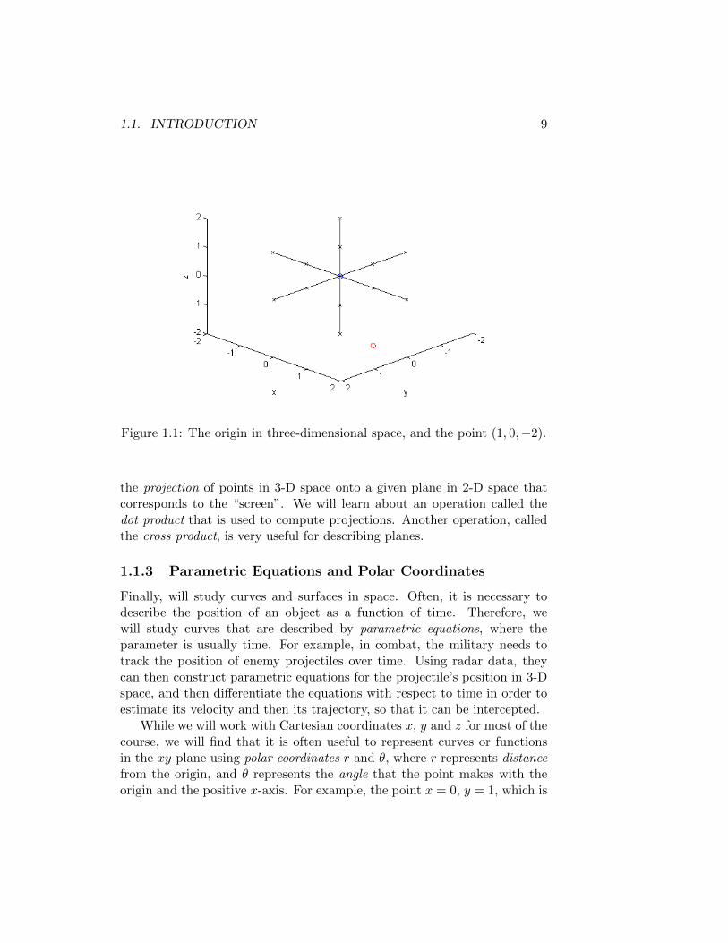
Next, we will become acquainted with three-dimensional space, in orderto prepare you for later coursework in multivariable calculus. Our basictools will be vectors, which can be used to represent either a position ordirection in space. For example, if we represent three-dimensional spaceusing Cartesian coordinates x, y and z, then the origin is the point withcoordinates x = 0, y = 0 and z = 0, typically denoted by the ordered triple(0, 0, 0). Then, the point in space (1, 0,−2) has coordinates x = 1, y = 0 andz = −2, meaning that it is located 1 unit from the origin along the positivex-axis, 0 units from the origin along the y-axis, and 2 units from the originalong the negative z-axis. This is illustrated in Figure 1.1. We will usevectors to facilitate the description of, and operations on, lines and planes.This is particularly useful in computer graphics. Consider the problem ofrendering a two-dimensional image, say for a frame in a film, of a collectionof three-dimensional objects. To what point in 2-D space does any givenpoint in 3-D space correspond? This question is answered by computing
1.1. INTRODUCTION 9
Figure 1.1: The origin in three-dimensional space, and the point (1, 0,−2).
the projection of points in 3-D space onto a given plane in 2-D space thatcorresponds to the “screen”. We will learn about an operation called thedot product that is used to compute projections. Another operation, calledthe cross product, is very useful for describing planes.
1.1.3 Parametric Equations and Polar Coordinates
Finally, will study curves and surfaces in space. Often, it is necessary todescribe the position of an object as a function of time. Therefore, wewill study curves that are described by parametric equations, where theparameter is usually time. For example, in combat, the military needs totrack the position of enemy projectiles over time. Using radar data, theycan then construct parametric equations for the projectile’s position in 3-Dspace, and then differentiate the equations with respect to time in order toestimate its velocity and then its trajectory, so that it can be intercepted.
While we will work with Cartesian coordinates x, y and z for most of thecourse, we will find that it is often useful to represent curves or functionsin the xy-plane using polar coordinates r and θ, where r represents distancefrom the origin, and θ represents the angle that the point makes with theorigin and the positive x-axis. For example, the point x = 0, y = 1, which is
10 CHAPTER 1. SEQUENCES AND SERIES
1 unit from the origin and makes a 90-degree angle with the origin and thepositive x-axis, has polar coordinates (1, π/2). Certain curves are far moreeasily described using polar coordinates. To see this, consider the equations
r = sin 2t, (x2 + y2)3/2 = 2xy.
These two equations describe the same curve, which resembles a four-leafclover. We will learn how to compute areas of regions enclosed by paramet-ric curves, and lengths of parametric curves, that are expressed in eitherCartesian or polar coordinates.
1.2 Review of Calculus
We now review some basic concepts from the first two calculus courses beforewe begin our study of the third. Recall that these two courses focused onthe following fundamental problems:
• computing the instantaneous rate of change of one quantity with re-spect to another, which is a derivative, and• computing the total change in a function over some portion of its
domain, which is a definite integral.
1.2.1 Limits
The basic problems of differential and integral calculus described in the pre-vious paragraph can be solved by computing a sequence of approximationsto the desired quantity and then determining what value, if any, the se-quence of approximations approaches. This value is called a limit of thesequence. As a sequence is a function, we begin by defining, precisely, theconcept of the limit of a function.
Definition We writelimx→a
f(x) = L
if for any open interval I1 containing L, there is some open interval I2
containing a such that f(x) ∈ I1 whenever x ∈ I2, and x 6= a. We say thatL is the limit of f(x) as x approaches a.
We writelimx→a−
f(x) = L
if, for any open interval I1 containing L, there is an open interval I2 of theform (c, a), where c < a, such that f(x) ∈ I1 whenever x ∈ I2. We say that
1.2. REVIEW OF CALCULUS 11
L is the limit of f(x) as x approaches a from the left, or the left-handlimit of f(x) as x approaches a.
Similarly, we writelimx→a+
f(x) = L
if, for any open interval I1 containing L, there is an open interval I2 of theform (a, c), where c > a, such that f(x) ∈ I1 whenever x ∈ I2. We saythat L is the limit of f(x) as x approaches a from the right, or theright-hand limit of f(x) as x approaches a.
We can make the definition of a limit a little more concrete by imposingsizes on the intervals I1 and I2, as long as the interval I1 can still be ofarbitrary size. It can be shown that the following definition is equivalent tothe previous one.
Definition We writelimx→a
f(x) = L
if, for any ε > 0, there exists a number δ > 0 such that |f(x) − L| < εwhenever 0 < |x− a| < δ.
Similar definitions can be given for the left-hand and right-hand limits.Note that in either definition, the point x = a is specifically excluded
from consideration when requiring that f(x) be close to L whenever x isclose to a. This is because the concept of a limit is only intended to describethe behavior of f(x) near x = a, as opposed to its behavior at x = a. Laterin this section we discuss the case where the two distinct behaviors coincide.
1.2.2 Continuity
In many cases, the limit of a function f(x) as x approached a could beobtained by simply computing f(a). Intuitively, this indicates that f has tohave a graph that is one continuous curve, because any “break” or “jump”in the graph at x = a is caused by f approaching one value as x approachesa, only to actually assume a different value at a. This leads to the followingprecise definition of what it means for a function to be continuous at a givenpoint.
Definition (Continuity) We say that a function f is continuous at a if
limx→a
f(x) = f(a).
We also say that f(x) has the Direct Subsitution Property at x = a.
12 CHAPTER 1. SEQUENCES AND SERIES
We say that a function f is continuous from the right at a if
limx→a+
f(x) = f(a).
Similarly, we say that f is continuous from the left at a if
limx→a−
f(x) = f(a).
The preceding definition describes continuity at a single point. In de-scribing where a function is continuous, the concept of continuity over aninterval is useful, so we define this concept as well.
Definition (Continuity on an Interval) We say that a function f is con-tinuous on the interval (a, b) if f is continuous at every point in (a, b).Similarly, we say that f is continuous on
1. [a, b) if f is continuous on (a, b), and continuous from the right at a.
2. (a, b] if f is continuous on (a, b), and continuous from the left at b.
3. [a, b] if f is continuous on (a, b), continuous from the right at a, andcontinuous from the left at b.
1.2.3 Derivatives
The basic problem of differential calculus is computing the instantaneousrate of change of one quantity y with respect to another quantity x. Forexample, y may represent the position of an object and x may representtime, in which case the instantaneous rate of change of y with respect to xis interpreted as the velocity of the object.
When the two quantities x and y are related by an equation of the formy = f(x), it is certainly convenient to describe the rate of change of y withrespect to x in terms of the function f . Because the instantaneous rateof change is so commonplace, it is practical to assign a concise name andnotation to it, which we do now.
Definition (Derivative) The derivative of a function f(x) at x = a, de-noted by f ′(a), is
f ′(a) = limh→0
f(a+ h)− f(a)
h,
provided that the above limit exists. When this limit exists, we say that f isdifferentiable at a.
1.2. REVIEW OF CALCULUS 13
Remark Given a function f(x) that is differentiable at x = a, the followingnumbers are all equal:
• the derivative of f at x = a, f ′(a),
• the slope of the tangent line of f at the point (a, f(a)), and
• the instantaneous rate of change of y = f(x) with respect to x atx = a.
This can be seen from the fact that all three numbers are defined in thesame way. 2
1.2.4 Riemann Sums and the Definite Integral
There are many cases in which some quantity is defined to be the productof two other quantities. For example, a rectangle of width w has uniformheight h, and the area A of the rectangle is given by the formula A =wh. Unfortunately, in many applications, we cannot necessarily assume thatcertain quantities such as height are constant, and therefore formulas suchas A = wh cannot be used directly. However, they can be used indirectly tosolve more general problems by employing the notation known as integralcalculus.
Suppose we wish to compute the area of a shape that is not a rectangle.To simplify the discussion, we assume that the shape is bounded by thevertical lines x = a and x = b, the x-axis, and the curve defined by somecontinuous function y = f(x), where f(x) ≥ 0 for a ≤ x ≤ b. Then, we canapproximate this shape by n rectangles that have width ∆x = (b − a)/nand height f(xi), where xi = a + i∆x, for i = 0, . . . , n. We obtain theapproximation
A ≈ An =
n∑i=1
f(xi)∆x.
Intuitively, we can conclude that as n → ∞, the approximate area An willconverge to the exact area of the given region. This can be seen by observingthat as n increases, the n rectangles defined above comprise a more accurateapproximation of the region.
More generally, suppose that for each n = 1, 2, . . ., we define the quantityRn by choosing points a = x0 < x1 < · · · < xn = b, and computing the sum
Rn =n∑i=1
f(x∗i )∆xi, ∆xi = xi − xi−1, xi−1 ≤ x∗i ≤ xi.

14 CHAPTER 1. SEQUENCES AND SERIES
The sum that defines Rn is known as a Riemann sum. Note that the interval[a, b] need not be divided into subintervals of equal width, and that f(x) canbe evaluated at arbitrary points belonging to each subinterval.
If f(x) ≥ 0 on [a, b], then Rn converges to the area under the curvey = f(x) as n → ∞, provided that the widths of all of the subintervals[xi−1, xi], for i = 1, . . . , n, approach zero. This behavior is ensured if werequire that
limn→∞
δ(n) = 0, where δ(n) = max1≤i≤n
∆xi.
This condition is necessary because if it does not hold, then, as n→∞, theregion formed by the n rectangles will not converge to the region whose areawe wish to compute. If f assumes negative values on [a, b], then, under thesame conditions on the widths of the subintervals, Rn converges to the netarea between the graph of f and the x-axis, where area below the x-axis iscounted negatively.
We define the definite integral of f(x) from a to b by∫ b
af(x) dx = lim
n→∞Rn,
where the sequence of Riemann sums {Rn}∞n=1 is defined so that δ(n) →0 as n → ∞, as in the previous discussion. The function f(x) is calledthe integrand, and the values a and b are the lower and upper limits ofintegration, respectively. The process of computing an integral is calledintegration.
1.2.5 Extreme Values
In many applications, it is necessary to determine where a given functionattains its minimum or maximum value. For example, a business wishesto maximize profit, so it can construct a function that relates its profit tovariables such as payroll or maintenance costs. We now consider the basicproblem of finding a maximum or minimum value of a general function f(x)that depends on a single independent variable x. First, we must preciselydefine what it means for a function to have a maximum or minimum value.
Definition (Absolute extrema) A function f has a absolute maximum orglobal maximum at c if f(c) ≥ f(x) for all x in the domain of f . Thenumber f(c) is called the maximum value of f on its domain. Similarly, fhas a absolute minimum or global minimum at c if f(c) ≤ f(x) for all
1.2. REVIEW OF CALCULUS 15
x in the domain of f . The number f(c) is then called the minimum valueof f on its domain. The maximum and minimum values of f are called theextreme values of f , and the absolute maximum and minimum are eachcalled an extremum of f .
Before computing the maximum or minimum value of a function, it is naturalto ask whether it is possible to determine in advance whether a functioneven has a maximum or minimum, so that effort is not wasted in trying tosolve a problem that has no solution. The following result is very helpful inanswering this question.
Theorem (Extreme Value Theorem) If f is continuous on [a, b], then f hasan absolute maximum and an absolute minimum on [a, b].
Now that we can easily determine whether a function has a maximum orminimum on a closed interval [a, b], we can develop an method for actuallyfinding them. It turns out that it is easier to find points at which f attainsa maximum or minimum value in a “local” sense, rather than a “global”sense. In other words, we can best find the absolute maximum or minimumof f by finding points at which f achieves a maximum or minimum withrespect to “nearby” points, and then determine which of these points is theabsolute maximum or minimum. The following definition makes this notionprecise.
Definition (Local extrema) A function f has a local maximum at c iff(c) ≥ f(x) for all x in an open interval containing c. Similarly, f has alocal minimum at c if f(c) ≤ f(x) for all x in an open interval containingc. A local maximum or local minimum is also called a local extremum.
At each point at which f has a local maximum, the function either hasa horizontal tangent line, or no tangent line due to not being differentiable.It turns out that this is true in general, and a similar statement applies tolocal minima. To state the formal result, we first introduce the followingdefinition, which will also be useful when describing a method for findinglocal extrema.
Definition(Critical Number) A number c in the domain of a function f isa critical number of f if f ′(c) = 0 or f ′(c) does not exist.
The following result describes the relationship between critical numbers andlocal extrema.
Theorem (Fermat’s Theorem) If f has a local minimum or local maximum
16 CHAPTER 1. SEQUENCES AND SERIES
at c, then c is a critical number of f ; that is, either f ′(c) = 0 or f ′(c) doesnot exist.
This theorem suggests that the maximum or minimum value of a functionf(x) can be found by solving the equation f ′(x) = 0.
1.2.6 The Mean Value Theorem
While the derivative describes the behavior of a function at a point, we oftenneed to understand how the derivative influences a function’s behavior on aninterval. It is often necessary to approximate a function f(x) by a functiong(x) using knowledge of f(x) and its derivatives at various points. It istherefore natural to ask how well g(x) approximates f(x) away from thesepoints.
The following result, a consequence of Fermat’s Theorem, gives limitedinsight into the relationship between the behavior of a function on an intervaland the value of its derivative at a point.
Theorem (Rolle’s Theorem) If f is continuous on a closed interval [a, b]and is differentiable on the open interval (a, b), and if f(a) = f(b), thenf ′(c) = 0 for some number c in (a, b).
By applying Rolle’s Theorem to a function f , then to its derivative f ′, itssecond derivative f ′′, and so on, we obtain the following more general result,which will be useful in analyzing the accuracy of methods for approximatingfunctions by polynomials.
Theorem (Generalized Rolle’s Theorem) Let x0, x1, x2, . . . , xn be distinctpoints in an interval [a, b]. If f is n times differentiable on (a, b), and iff(xi) = 0 for i = 0, 1, 2, . . . , n, then f (n)(c) = 0 for some number c in (a, b).
A more fundamental consequence of Rolle’s Theorem is the Mean ValueTheorem itself, which we now state.
Theorem (Mean Value Theorem) If f is continuous on a closed interval[a, b] and is differentiable on the open interval (a, b), then
f(b)− f(a)
b− a= f ′(c)
for some number c in (a, b).
Remark The expressionf(b)− f(a)
b− a
1.2. REVIEW OF CALCULUS 17
is the slope of the secant line passing through the points (a, f(a)) and(b, f(b)). The Mean Value Theorem therefore states that under the givenassumptions, the slope of this secant line is equal to the slope of the tangentline of f at the point (c, f(c)), where c ∈ (a, b). 2
The Mean Value Theorem has the following practical interpretation: theaverage rate of change of y = f(x) with respect to x on an interval [a, b] isequal to the instantaneous rate of change y with respect to x at some pointin (a, b).
1.2.7 The Mean Value Theorem for Integrals
Suppose that f(x) is a continuous function on an interval [a, b]. Then, by theFundamental Theorem of Calculus, f(x) has an antiderivative F (x) definedon [a, b] such that F ′(x) = f(x). If we apply the Mean Value Theorem toF (x), we obtain the following relationship between the integral of f over[a, b] and the value of f at a point in (a, b).
Theorem (Mean Value Theorem for Integrals) If f is continuous on [a, b],then ∫ b
af(x) dx = f(c)(b− a)
for some c in (a, b).
In other words, f assumes its average value over [a, b], defined by
fave =1
b− a
∫ b
af(x) dx,
at some point in [a, b], just as the Mean Value Theorem states that thederivative of a function assumes its average value over an interval at somepoint in the interval.
The Mean Value Theorem for Integrals is also a special case of the fol-lowing more general result.
Theorem (Weighted Mean Value Theorem for Integrals) If f is continuouson [a, b], and g is a function that is integrable on [a, b] and does not changesign on [a, b], then ∫ b
af(x)g(x) dx = f(c)
∫ b
ag(x) dx
for some c in (a, b).
18 CHAPTER 1. SEQUENCES AND SERIES
In the case where g(x) is a function that is easy to antidifferentiate andf(x) is not, this theorem can be used to obtain an estimate of the integralof f(x)g(x) over an interval.
Example Let f(x) be continuous on the interval [a, b]. Then, for any x ∈[a, b], by the Weighted Mean Value Theorem for Integrals, we have∫ x
af(s)(s− a) ds = f(c)
∫ x
a(s− a) ds = f(c)
(s− a)2
2
∣∣∣∣xa
= f(c)(x− a)2
2,
where a < c < x. It is important to note that we can apply the WeightedMean Value Theorem because the function g(x) = (x− a) does not changesign on [a, b]. 2
1.3 Taylor’s Theorem
In many cases, it is useful to approximate a given function f(x) by a poly-nomial, because one can work much more easily with polynomials than withother types of functions. As such, it is necessary to have some insight intothe accuracy of such an approximation. The following theorem, which is aconsequence of the Weighted Mean Value Theorem for Integrals, providesthis insight.
Theorem (Taylor’s Theorem) Let f be n times continuously differentiableon an interval [a, b], and suppose that f (n+1) exists on [a, b]. Let x0 ∈ [a, b].Then, for any point x ∈ [a, b],
f(x) = Pn(x) +Rn(x),
where
Pn(x) =n∑j=0
f (j)(x0)
j!(x− x0)j
= f(x0) + f ′(x0)(x− x0) +1
2f ′′(x0)(x− x0)2 + · · ·+ f (n)(x0)
n!(x− x0)n
and
Rn(x) =
∫ x
x0
f (n+1)(s)
n!(x− s)n ds =
f (n+1)(ξ(x))
(n+ 1)!(x− x0)n+1,
where ξ(x) is between x0 and x.
1.3. TAYLOR’S THEOREM 19
The polynomial Pn(x) is the nth Taylor polynomial of f with center x0,and the expression Rn(x) is called the Taylor remainder of Pn(x). Whenthe center x0 is zero, the nth Taylor polynomial is also known as the nthMaclaurin polynomial.
The final form of the remainder is obtained by applying the Mean ValueTheorem for Integrals to the integral form. As Pn(x) can be used to ap-proximate f(x), the remainder Rn(x) is also referred to as the truncationerror of Pn(x). The accuracy of the approximation on an interval can beanalyzed by using techniques for finding the extreme values of functions tobound the (n+ 1)-st derivative on the interval.
Because approximation of functions by polynomials is employed in thedevelopment and analysis of many techniques in numerical analysis, theusefulness of Taylor’s Theorem cannot be overstated. In fact, it can be saidthat Taylor’s Theorem is the Fundamental Theorem of Numerical Analysis,just as the theorem describing inverse relationship between derivatives andintegrals is called the Fundamental Theorem of Calculus.
We conclude our discussion of Taylor’s Theorem with some examples thatillustrate how the nth-degree Taylor polynomial Pn(x) and the remainderRn(x) can be computed for a given function f(x).
Example If we set n = 1 in Taylor’s Theorem, then we have
f(x) = P1(x) +R1(x)
whereP1(x) = f(x0) + f ′(x0)(x− x0).
This polynomial is a linear function that describes the tangent line to thegraph of f at the point (x0, f(x0)).
If we set n = 0 in the theorem, then we obtain
f(x) = P0(x) +R0(x),
whereP0(x) = f(x0)
andR0(x) = f ′(ξ(x))(x− x0),
where ξ(x) lies between x0 and x. If we use the integral form of the remain-der,
Rn(x) =
∫ x
x0
f (n+1)(s)
n!(x− s)n ds,
20 CHAPTER 1. SEQUENCES AND SERIES
then we have
f(x) = f(x0) +
∫ x
x0
f ′(s) ds,
which is equivalent to the Total Change Theorem and part of the Funda-mental Theorem of Calculus. Using the Mean Value Theorem for integrals,we can see how the first form of the remainder can be obtained from theintegral form. 2
Example Let f(x) = sinx. Then
f(x) = P3(x) +R3(x),
where
P3(x) = x− x3
3!= x− x3
6,
and
R3(x) =1
4!x4 sin ξ(x) =
1
24x4 sin ξ(x),
where ξ(x) is between 0 and x. The polynomial P3(x) is the 3rd Maclaurinpolynomial of sinx, or the 3rd Taylor polynomial with center x0 = 0.
If x ∈ [−1, 1], then
|Rn(x)| =∣∣∣∣ 1
24x4 sin ξ(x)
∣∣∣∣ =
∣∣∣∣ 1
24
∣∣∣∣ |x4|| sin ξ(x)| ≤ 1
24,
since | sinx| ≤ 1 for all x. This bound on |Rn(x)| serves as an upper boundfor the error in the approximation of sinx by P3(x) for x ∈ [−1, 1]. 2
Example Let f(x) = ex. Then
f(x) = P2(x) +R2(x),
where
P2(x) = 1 + x+x2
2,
and
R2(x) =x3
6eξ(x),
where ξ(x) is between 0 and x. The polynomial P2(x) is the 2nd Maclaurinpolynomial of ex, or the 2nd Taylor polynomial with center x0 = 0.
If x > 0, then R2(x) can become quite large, whereas its magnitude ismuch smaller if x < 0. Therefore, one method of computing ex using a
1.4. SEQUENCES 21
Maclaurin polynomial is to use the nth Maclaurin polynomial Pn(x) of ex
when x < 0, where n is chosen sufficiently large so that Rn(x) is small forthe given value of x. If x > 0, then we instead compute e−x using the nthMaclaurin polynomial for e−x, which is given by
Pn(x) = 1− x+x2
2− x3
6+ · · ·+ (−1)nxn
n!,
and then obtaining an approximation to ex by taking the reciprocal of ourcomputed value of e−x. 2
Example Let f(x) = x2. Then, for any real number x0,
f(x) = P1(x) +R1(x),
whereP1(x) = x2
0 + 2x0(x− x0) = 2x0x− x20,
andR1(x) = (x− x0)2.
Note that the remainder does not include a “mystery point” ξ(x) since the2nd derivative of x2 is only a constant. The linear function P1(x) describesthe tangent line to the graph of f(x) at the point (x0, f(x0)). If x0 = 1,then we have
P1(x) = 2x− 1,
andR1(x) = (x− 1)2.
We can see that near x = 1, P1(x) is a reasonable approximation to x2, sincethe error in this approximation, given by R1(x), would be small in this case.2
1.4 Sequences
1.4.1 What is a Sequence?
A sequence is an ordered list of numbers. The ordering of the numbers in asequence is indicated by an index that is associated with each number. Usu-ally, the indices are taken from the natural numbers, which are the positiveintegers 1, 2, 3, . . .. We will consider infinite sequences such as
a1, a2, a3, . . . , an, . . . .
22 CHAPTER 1. SEQUENCES AND SERIES
Each number in a sequence is called a term. In the above example, a1 is thefirst term, a2 is the second term, and an is the nth term.
There are many ways to describe sequences, but they all have one thingin common: any description of a sequence should include formula for com-puting the nth term.
Example The sequence of all even natural numbers can be described by
an = 2n, n ≥ 1, or {2n}∞n=1.
Similarly, the sequence of all odd natural numbers can be defined by
an = 2n− 1, n ≥ 1, or {2n− 1}∞n=1.
Note that in both cases, it is explicitly stated that the index of the first termis 1; this will usually be the case, but in some contexts, it is more intuitiveto use a different number, such as 0, as the index of the first term. Notethat the second form of each sequence does not specify a variable, such asa, to identify a given term. In this case, a different expression may be used,such as x or α. In the {} notation, the indices can be omitted if they arealready known. 2
Example It is often convenient to define each term in a sequence in termsof preceding terms. For example, we can define
an+1 =an2
+1
an, n ≥ 1,
provided that we include a definition of a1 to start the sequence. In thiscase, the sequence begins as follows:
a1 = 1, a2 = 1.5, a3 = 1.416̄.
What happens to an as n increases?
Sequences can also be defined in terms of more than one preceding el-ement. The best-known sequence of this type is the Fibonacci sequence,defined by
f1 = 1, f2 = 1, fn = fn−1 + fn−2.
This sequence, whose terms increase rapidly, arose from the study of breed-ing of rabbits. Because the definition of fn, for n > 2, involves three termsof the sequence, we say that the Fibonacci sequence obeys a three-termrecurrence relation.
1.4. SEQUENCES 23
The Fibonacci sequence can be defined using a formula for fn that is inclosed form; that is, it does not refer to any previous terms. However, asthis formula is
fn =1√5
(1 +√
5
2
)n− 1√
5
(1−√
5
2
)n,
it is generally preferable to use the three-term recurrence relation to computeterms of the sequence, unless, for example, one wants to compute fn for onlya few large values of n. 2
1.4.2 Why Do We Need Sequences?
In this chapter, our primary goal is to learn how to work with infinite se-ries, which are sums of the terms of a sequence, for various applications asapproximating functions in a manner that is feasible for calculators or com-puters. We will see that in order to define what it means to add infinitelymany numbers, we need the concept of a sequence.
Sequences are also useful in other contexts that are unrelated to infiniteseries. Many methods for solving mathematical problems on a computer areiterative in nature; that is, they produce a sequence of approximate solutionsto a given problem that, hopefully, are getting closer to the exact solution,in some sense. An example of this, which may be familiar to you, is Newton’smethod for finding the roots, or zeros, of a function.
1.4.3 Recognizing Sequences
The definitions of the sequences in the previous examples can be used tocompute the terms of the sequence, but sometimes, it is necessary to go theother way, and obtain a definition of a sequence from some of its terms.
There is no completely deterministic way to derive a formula for theterms of a given sequence, but a useful strategy is to examine how eachterm differs from the previous one. This examination yields the followingclues to a sequence’s definition:
• Do the terms alternate in sign? If so, this suggests that the formulafor the nth term should include a factor of (−1)n, which is equal to 1when n is even and −1 when n is odd.
• Do consecutive terms, or portions of them, have a constant ratio?Selected terms may be given as fractions, and it might be observed that
24 CHAPTER 1. SEQUENCES AND SERIES
either the numerators or denominators change by being multiplied bya factor of, for example, 3, in which case the formula for the nth termlikely includes a factor of 3n. This pattern is known as a geometricprogression.
• Do consecutive terms, or portions of them, differ by a constant amount?For example, it might be observed that each term is 4 more thanthe previous term, which suggests that the definition of the nth termshould include 4n. This pattern is known as an arithmetic progression.
Example Consider the sequence whose first few terms are
a1 = 2, a2 = −8
4, a3 =
32
7, a4 = −128
10.
The terms alternate in sign, with the even-numbered terms being negative,so the definition of an should include the factor (−1)n+1, which is equal to−1 when n is even. If we rewrite a1 = 2/1, we see that the denominatorsdiffer by 3, so we can express the denominator of an as 3n− 2. Finally, thenumerators are 2, 8, 32 and 128, which are equal to 21, 23, 25 and 27. Thatis, they are odd powers of 2, so use the first example above and conclude
an = (−1)n+1 22n−1
3n− 2, n ≥ 1.
2
1.4.4 Limits of Sequences
There are two key questions that need to be asked about any given sequence:
1. As the index increases, do the terms in the sequence converge to aparticular value?
2. If so, what is that value? If not, how does the sequence behave? Thatis, do its terms become infinitely large, or do they remain boundedbut continually oscillate?
Before we can attempt to answer these questions, we need to precisely definewhat it means for the terms of a sequence to converge.
To help us to formulate an appropriate definition, we consider an exam-ple. Consider the sequence
an =n2 + n
n2 + 2n+ 1.
1.4. SEQUENCES 25
If we rewrite this sequence as
an =n2 + 2n+ 1− (2n+ 1) + n
n2 + 2n+ 1
=n2 + 2n+ 1
n2 + 2n+ 1− n+ 1
n2 + 2n+ 1
= 1− n+ 1
n2 + 2n+ 1
= 1− n+ 1
(n+ 1)2
= 1− 1
n+ 1,
we see that the terms in this sequence become closer to 1 as n increases,because the fraction 1/(n + 1) decreases toward zero. In fact, by choosingn large enough, we can make 1/(n + 1) as small as we want. Specifically,suppose we want 1/(n + 1) < ε for some ε > 0. By solving this inequalityfor n, we find that we need only choose n so that n > 1/ε− 1. We concludethat an converges to 1 as n tends to infinity.
In general, we say that a sequence {an}∞n=1 converges to a limit L if,for any ε > 0, we can find an index N such that |an − L| < ε whenevern > N . Informally, the sequence converges to L if we can make all of itsterms, beyond some index, as close to L as we want. We write
limn→∞
an = L.
If the sequence {an} converges to L, we say that it is a convergent sequence.Otherwise, we say that it is divergent.
Now, consider the sequence defined by
an =n2 + 4n+ 3
n+ 2.
By rewriting this sequence as
an =n2 + 4n+ 4− 4 + 3
n+ 2
=n2 + 4n+ 4
n+ 2− 1
n+ 2
= n+ 2− 1
n+ 2,
26 CHAPTER 1. SEQUENCES AND SERIES
we see that as n increases, an also increases. In fact, by choosing n largeenough, we can make an as large as we want. Therefore, not only does thissequence diverge, but it tends toward infinity as n does.
In general, we say that
limn→∞
an =∞
if, for any positive number M , there is an index N such that an > Mwhenever n > N . That is, we can make all terms in the sequence, beyondsome index, as large as we want. We also say that the sequence {an} divergesto ∞.
1.4.5 Relation to Limits of Functions
Previously, we have learned much about how to compute limits of functionsat infinity. It is therefore natural to ask whether the tools used to computelimits of functions can be applied to compute limits of sequences.
Thankfully, that is in fact the case. Specifically, if a function f(x) satis-fies
limx→∞
f(x) = L,
and we define the sequence {an}∞n=1 by an = f(n) where n is a positiveinteger, then we can conclude that
limn→∞
an = L.
It follows that for any sequence {an} for which we have a formula to defineeach term an, we can apply, to a function defined using this same formula,all of the available techniques for computing limits of functions at infinityin order to compute the limit of the sequence, if it has one.
In particular, this result allows us to apply the limit laws to conclude thatthe limit of a sum, difference, product, or quotient of convergent sequences isequal to the sum, difference, product or quotient of their limits, respectively.Furthermore, raising the terms of a convergent sequence to a positive powerraises its limit to that same power, if the terms are positive. We can alsoapply the Squeeze Theorem to show that if the terms of a sequence {an} arebounded above and below by two convergent sequences that have the samelimit, then {an} converges to this limit as well.
We can also use techniques for computing limits at infinity of rationalfunctions, as demonstrated in the following example.
1.4. SEQUENCES 27
Example Consider the sequence defined by
an =2n3 + 3n2 + 4n+ 1
n3 + 5n2 + 3n+ 2, n ≥ 1.
This sequence is obtained by taking the values of the function
f(x) =2x3 + 3x2 + 4x+ 1
x3 + 5x2 + 3x+ 2, x ≥ 0.
The limit of this function as x → ∞ can be computed by dividing thenumerator and denominator by the highest power of x, which is x3. Thisyields
limx→∞
f(x) = limx→∞
2 + 3x + 4
x2+ 1
x3
1 + 5x + 3
x2+ 2
x3
= 2.
We conclude that limn→∞ an = 2 as well. 2
We introduced the concept of an infinite sequence of numbers, and pre-cisely defined what it means for such a sequence to converge to a limit, orapproach infinity. Now, we will discuss various techniques, based on thesedefinitions, for testing whether a sequence converges, and, if it does, findingits limit.
1.4.6 Testing Convergence of Sequences
We have learned that techniques for computing the limit of a function f(x),as x→∞, can be applied to compute the limit of a sequence {an} as n→∞,through the relation an = f(n), where n is any index of a term in {an}. Weapplied this approach earlier in this section to a sequence {an} in whichan was a quotient of polynomials, and divided each by the highest powerof the variable in order to compute the limit. We now illustrate the use ofsome other techniques for computing limits of functions at infinity in orderto compute limits of sequences.
Example Consider the sequence
an =√n2 + 1−
√n2 − 1, n ≥ 1.
To determine whether it converges, we compute the limit of the function
f(x) =√x2 + 1−
√x2 − 1, x ≥ 1,
28 CHAPTER 1. SEQUENCES AND SERIES
as x→∞. By multiplying and dividing f(x) by its conjugate, we obtain
f(x) =(√
x2 + 1−√x2 − 1
) √x2 + 1 +√x2 − 1√
x2 + 1 +√x2 − 1
=(√x2 + 1−
√x2 − 1)(
√x2 + 1 +
√x2 − 1)√
x2 + 1 +√x2 − 1
=(x2 + 1)− (x2 − 1)√x2 + 1 +
√x2 − 1
=2√
x2 + 1 +√x2 − 1
=2
|x|(√
1 + 1x2
+√
1− 1x2
) .As x→∞, the expressions under both radical signs approach 1, from whichwe conclude that
limn→∞
an = limx→∞
f(x) = 0.
2
Example The terms of the sequence
an =n2
en, n ≥ 1,
are fractions in which both the numerator and denominator become infiniteas n→∞. Because of the exponential, there is no “highest power of n” thatwe can divide both by in order to reveal the limit, but since the limit is theindeterminate form∞/∞, we can use l’Hospital’s Rule on the correspondingfunction f(x) = x2/ex. We have
limn→∞
an = limn→∞
n2
en= lim
n→∞
2n
en= lim
n→∞
2
en= 0.
While we are actually applying l’Hospital’s Rule to the function f(x), wecan carry out the steps on an instead, because of the equivalence of the limitof the sequence an = f(n) and the limit of the function f(x), as n and xtend to infinity. 2
1.4.7 Alternating Sequences
An alternating sequence is a sequence in which the terms alternate signs.That is, for each n, an+1 is the opposite sign of an. The presence of the al-ternating sign can make convergence analysis cumbersome, so it is desirableto be able to exclude it from consideration if possible.
1.4. SEQUENCES 29
Example The sequence
an =(−1)n
n+ 1, n ≥ 0,
is an example of an alternating sequence. To determine its limit, we considerthe related sequence
bn = |an| =1
n+ 1, n ≥ 0,
since (−1)n = 1 or −1 for any integer n, and therefore satisfies |(−1)n| = 1.It is easy seen that
limn→∞
bn = 0,
since the numerator is fixed at 1 and the denominator increases with n.Since bn → 0 as n → ∞, and bn is the magnitudes of an, it follows thatan → 0 as well. 2
1.4.8 Growth Rates of Functions
When working with sequences, it is helpful to know the relative growth ratesof functions such as polynomials or exponential functions, in order to quicklydetermine whether the terms of a sequence tend to zero, infinity, or a finitenonzero number.
Example The sequence
an =2n
n!, n ≥ 0,
cannot be related to a function of x, because n! is only defined when n is aninteger. Instead, we will try to determine whether the terms are bounded bythose of a simpler sequence, in which case we may be able to easily concludethat the limit is zero. We have, for n ≥ 1,
an =2 · 2 · 2 · · · · · 21 · 2 · 3 · · · · · n
=
(2 · 2 · 2 · · · · · 2
1 · 2 · 3 · · · · · (n− 1)
)2
n= 2
(2 · 2 · 2 · · · · · 2
3 · 4 · 5 · · · · · (n− 1)
)2
n<
4
n,
since the expression in parentheses must be less than 1. Because 1/n → 0as n → ∞, and multiplying by 4 does not change this, we conclude thatan → 0 as well. 2
From the preceding example, we see that the factorial function n! growsmore rapidly than the exponential function 2n, since otherwise the terms
30 CHAPTER 1. SEQUENCES AND SERIES
of the sequence would not tend to zero as n → ∞. The following list ofcategories of functions is ordered from most rapidly growing to least rapidlygrowing:
1. Factorial functions such as n!2. Exponential functions such as en
3. Polynomial functions such as n3
4. Logarithmic functions such as lnn, where n > 0
Relationships such as these are often used in computer science, where theyplay a role in the analysis of running time or complexity of algorithms.
1.4.9 Geometric Sequences
The geometric sequence {rn}, where r is any real number, is of particularinterest because of its frequent appearance in infinite series that arise in anumber of applications. It can exhibit three types of behavior, dependingon the value of r.
• If r = 1, then rn = 1 for any n, so the limit of {rn} is trivially equalto 1.• If |r| < 1, then rn decreases in magnitude as n increases, and therefore
the limit is equal to 0.• If |r| > 1, then rn increases in magnitude, so that the terms become
infinitely large. On the other hand, if r = −1, the terms oscillateendlessly between −1 and 1. In either case, the sequence is divergent.
1.4.10 Recursively Defined Sequences
When a sequence is defined using a formula that defines an+1 in terms of an,it is possible to compute its limit L by keeping in mind that if the sequence{an} converges, then {an+1} converges as well, and has the same limit L. Itfollows that the formula that defines an+1 in terms of an can be viewed asan equation that is satisfied by setting both an and an+1 equal to L.
Example Consider the sequence
an+1 =an2
+1
an, a1 = 1.
We assume that this sequence converges to a value L, and substitute it foran and an+1 above, since both expressions converge to L if the sequence isconvergent. We then have the equation
L =L
2+
1
L,
1.4. SEQUENCES 31
which is satisfied by either√
2 or −√
2. Since a1 = 1, all terms of thesequence must be positive, so the limit is
√2. It is interesting to note that
the original sequence can be obtained by applying Newton’s method to thefunction f(x) = x2 − 2, in order to compute
√2. 2
1.4.11 Bounded and Monotonic Sequences
In some cases, even if it is not practical to compute the limit of a sequence,it is still helpful to know whether the sequence converges. For example, thiskind of information is valuable when analyzing a method for solving an equa-tion that computes a sequence of approximations, and it is only necessaryto know whether this sequence is going to converge, since its convergencewould imply successful solution of the equation. We now introduce someterminology in order to help us to classify sequences, which will then helpus to quickly determine whether certain kinds of sequences converge.
• We say that a sequence is {an}∞n=1 is non-decreasing if an+1 ≥ an for alln ≥ 1. Similarly, we say that {an}∞n=1 is non-increasing if an+1 ≤ anfor all n ≥ 1.• We say that a sequence is {an}∞n=1 is increasing if an+1 > an for alln ≥ 1. Similarly, we say that {an}∞n=1 is decreasing if an+1 < an forall n ≥ 1.• A sequence that is either non-increasing or non-decreasing is said to
be monotonic. A sequence that is increasing or decreasing is alsomonotonic. Note that an increasing sequence is also non-decreasing,but not the other way around.• A sequence {an}∞n=1 is bounded above if there is a number M such thatan ≤M for all n ≥ 1. On the other hand, if there is a number m suchthat an ≥ m for all n ≥ 1, we say that the sequence is bounded below.• A sequence that is both bounded above and bounded below is said to
be bounded.
The reason why these terms are helpful is because of the MonotonicSequence Theorem, which states that any sequence that is both boundedand monotonic is convergent. This is because any set of numbers that isbounded above must have a least upper bound L, also known as a supremum,and if the sequence is increasing, its terms have no choice but to continuallyincrease toward L. After all, if they do not approach L, then L is not theleast upper bound, while if they exceed L, then L is not an upper bound atall. Similar reasoning applies to the case of a decreasing sequence and itsgreatest lower bound, or infinum.
32 CHAPTER 1. SEQUENCES AND SERIES
Because the notions of monotonicity and boundedness are useful in deter-mining whether a sequence converges, it is also useful to be able to determinewhether a sequence is monotonic.
Example The sequence defined by an = 1, for n ≥ 1, is an example of amonotonic sequence, because it is non-increasing and non-decreasing. It isalso bounded above and below, so it is convergent, trivially so, to the limit1. 2
Example The sequence defined by an = 1/2n, for n ≥ 0, is a decreasing,and thus monotonic, sequence. It is bounded above, by 1, and below, by 0.Therefore it converges, and its limit is 0. 2
Example The sequence defined by an = log n, for n ≥ 1, is a monotonicsequence, because it is increasing. It is bounded below by 0, but it is notbounded above, and is divergent. The same properties hold for the sequencean = 2n. 2
Example The sequence defined by an = (−1)n, for n ≥ 0, is not monotonic,because its terms oscillate continually between −1 and 1. It is boundedbelow, by −1, and above, by 1, but it is divergent. Similar properties holdfor the sequence defined by an = sinn. 2
Example Consider the sequence defined by
an = 1− 2−n, n ≥ 0.
To determine whether this sequence is increasing or decreasing, we examinethe difference between two terms and try to ascertain whether this differenceis always positive or always negative. We have
an+1−an = (1−2−(n+1))−(1−2−n) = 2−n−2−(n+1) = 2−n(1−2−1) =2−n
2= 2−(n+1).
This difference is always positive, so we conclude that {an} is an increasingsequence. 2
When the terms of a sequence are fractions, it is helpful to cross-multiplyto determine monotonicity.
Example Consider the sequence defined by
an =n+ 1
n+ 2, n ≥ 1.
1.4. SEQUENCES 33
We will show that this sequence is increasing. To accomplish this, we mustshow that an+1 > an, which is equivalent to
(n+ 1) + 1
(n+ 1) + 2>n+ 1
n+ 2,
orn+ 2
n+ 3>n+ 1
n+ 2.
Cross-multiplying, we obtain
(n+ 2)2 > (n+ 1)(n+ 3),
which, upon expansion, yields
n2 + 4n+ 4 > n2 + 4n+ 3,
which is true for all n. Therefore, the sequence is in fact increasing. 2
Example The sequence
an = (−1)n, n ≥ 0,
has terms that alternate between 1 and −1. That is, a0 = 1, a1 = −1, a2 =1, a3 = −1, and so on. Now, suppose we want to construct a formula for asequence whose terms alternate signs in pairs. That is,
a0 = a1 = 1, a2 = a3 = −1, a4 = a5 = 1,
and so on. We present two approaches to this.
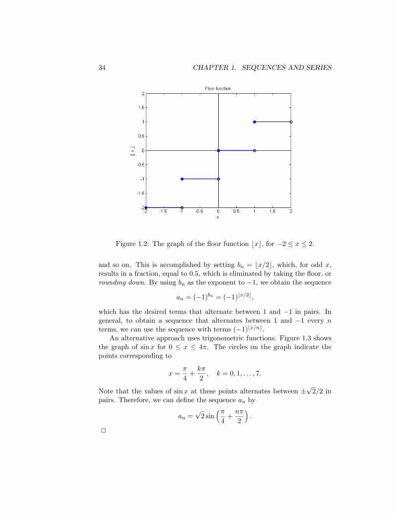
The first approach makes use of the floor function bxc. For any realnumber x, bxc is defined to be the greatest integer that is less than or equalto x. For example,
b1c = 1, bπc = 3, b14.9c = 14.
The floor function is also known as the greatest integer function, and is anexample of a step function, since its graph, shown in Figure 1.2, consists ofline segments that are arranged like steps.
To define our sequence, we use the floor function to obtain the sequenceof exponents for −1,
b0 = 0, b1 = 0, b2 = 1, b3 = 1, b4 = 2, b5 = 2,
34 CHAPTER 1. SEQUENCES AND SERIES
Figure 1.2: The graph of the floor function bxc, for −2 ≤ x ≤ 2.
and so on. This is accomplished by setting bn = bx/2c, which, for odd x,results in a fraction, equal to 0.5, which is eliminated by taking the floor, orrounding down. By using bn as the exponent to −1, we obtain the sequence
an = (−1)bn = (−1)bx/2c,
which has the desired terms that alternate between 1 and −1 in pairs. Ingeneral, to obtain a sequence that alternates between 1 and −1 every nterms, we can use the sequence with terms (−1)bx/nc.
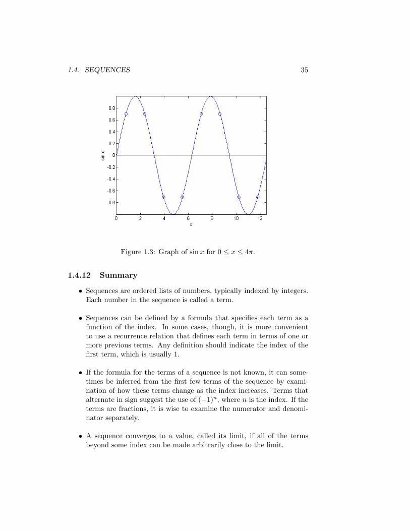
An alternative approach uses trigonometric functions. Figure 1.3 showsthe graph of sinx for 0 ≤ x ≤ 4π. The circles on the graph indicate thepoints corresponding to
x =π
4+kπ
2, k = 0, 1, . . . , 7.
Note that the values of sinx at these points alternates between ±√
2/2 inpairs. Therefore, we can define the sequence an by
an =√
2 sin(π
4+nπ
2
).
2
1.4. SEQUENCES 35
Figure 1.3: Graph of sinx for 0 ≤ x ≤ 4π.
1.4.12 Summary
• Sequences are ordered lists of numbers, typically indexed by integers.Each number in the sequence is called a term.
• Sequences can be defined by a formula that specifies each term as afunction of the index. In some cases, though, it is more convenientto use a recurrence relation that defines each term in terms of one ormore previous terms. Any definition should indicate the index of thefirst term, which is usually 1.
• If the formula for the terms of a sequence is not known, it can some-times be inferred from the first few terms of the sequence by exami-nation of how these terms change as the index increases. Terms thatalternate in sign suggest the use of (−1)n, where n is the index. If theterms are fractions, it is wise to examine the numerator and denomi-nator separately.
• A sequence converges to a value, called its limit, if all of the termsbeyond some index can be made arbitrarily close to the limit.
36 CHAPTER 1. SEQUENCES AND SERIES
• A sequence that does not converge to any value is divergent. A di-vergent sequence may have terms that tend to infinity as the indexdoes.
• The limit of a convergent sequence can be computed by using tech-niques for computing limits of functions at infinity, applied to thefunction obtained from the formula for each term of the sequence.These techniques include:
– the limit laws, such as the law that the limit of a sum is the sumof the limits
– the Squeeze Theorem
– the technique of dividing the numerator and denominator by thehighest power of x, if both are polynomials of x
• Any techniques that can be used to compute the limit of a functionf(x) as x → ∞ can also be applied to compute limits of sequences,when each term an of the sequence can be defined in terms of thevalue of a function f(n) at the term’s index n. These techniquesinclude, among others, l’Hospital’s Rule, and algebraic techniques suchas multiplying and dividing by the conjugate or the highest power ofn.
• The behavior of an alternating sequence can sometimes be studiedmore easily by examining the absolute value of its terms, thus filteringout the alternation and isolating the terms’ magnitude.
• When the terms of a sequence are defined to be a fraction, it is helpfulto consider the relative growth rates of functions to determine whetherthe terms converge to zero or tend to infinity. As a rule, exponen-tial functions grow more rapidly than polynomials, which grow morerapidly than logarithmic functions.
• A particularly useful sequence is the geometric sequence rn, for a realnumber r. This sequence converges to 1 if r = 1, to 0 if |r| < 1, anddiverges otherwise.
• If a sequence {an} is defined recursively, with an+1 defined in terms ofan, the limit can be computed by setting both equal to an unknownvalue L and solving for it. If there is more than one solution, the initialterm can be used to determine which is the limit.

1.5. SERIES 37
• A sequence {an} is increasing if its terms increase as n increases, anddecreasing if its terms decrease. A monotonic sequence is either in-creasing or decreasing. A sequence can be shown to be monotonic bycomparing consecutive terms directly, using algebraic techniques suchas cross-multiplying.
• A sequence is bounded above if its terms never exceed a given numberM , and bounded below if its terms are never exceeded by a givennumber m. A sequence that is bounded above and below is calledbounded.
• According to the Monotonic Sequence Theorem, a bounded monotonicsequence is convergent.
1.5 Series
1.5.1 What is a Series?
An infinte series, usually referred to simply as a series, is an sum of all ofthe terms of an infinite sequence. Specifically, let {an}∞n=1 be a sequence.Then we can define a series to be the sum of the terms of {an},
a1 + a2 + a3 + · · ·+ an + · · · .
We refer to the terms of {an} as the terms of the series.Writing a series in this manner is cumbersome, so we instead use sigma
notation to write this series as
∞∑n=1
an.
The expression below the upper case Greek letter sigma indicates what nameis given to the index (in this case, n), and its initial value (in this case, 1).The expression above the sigma indicates the final value of the index, or ∞for an infinite sum.
Note that this means sigma notation can be used to represent finitesums as well.In other words, if we wrote, for example, “10” above the sigmainstead of ∞, then we would be specifying that only the first 10 terms of{an} should be added. That is,
10∑n=1
an = a1 + a2 + a3 + · · ·+ a10.

38 CHAPTER 1. SEQUENCES AND SERIES
For either a finite or infinite sum, the expression to the right of the sigma iswhat is to be added, for each value of the index. This means that if n is thename assigned to the index, then every occurrence of n within the summedexpression is to be replaced with each value of the index, and the resultingterms are summed.
Example The finite sum4∑
n=0
2n
n+ 1
is evaluated as follows:
4∑n=0
2n
n+ 1=
20
0 + 1+
21
1 + 1+
22
2 + 1+
23
3 + 1+
24
4 + 1
= 1 + 1 +4
3+ 2 +
16
5
=128
15.
2
We now need to define what it means to compute the sum of infinitelymany terms. For this concept, sequences play their most important role.Given an infinite sequence {an}∞n=1 of terms to be summed, we define asequence of partial sums, denoted by {sn}∞n=1, as follows:
s1 = a1
s2 = s1 + a2
= a1 + a2
s3 = s2 + a3
= a1 + a2 + a3
...
sn = sn−1 + an
= a1 + a2 + · · ·+ an−1 + an.
Then, we can view the series as a sequence of partial sums. This leads tothe following definitions.
A series∞∑n=1
an
1.5. SERIES 39
is said to be convergent if its sequence of partial sums, {sn}∞n=1, is convergent.The limit of {sn}, if it exists, is called the sum of the series. If the sequenceof partial sums is divergent, then we say that the series is divergent.
Example Consider the series
∞∑n=0
1
2n.
The sequence of partial sums is
s0 = 1
s1 = s0 +1
2
=3
2
s2 = s1 +1
4
=7
4
s3 = s2 +1
8
=15
8...
sn =2n+1 − 1
2n
=2n(2− 2−n)
2n
= 2− 1
2n.
The partial sums converge to 2, so we say that 2 is the sum of the series. 2
1.5.2 Why Do We Need Series?
Series are applied throughout mathematics, as well as physics, computerscience, and various branches of engineering. They are particularly usefulfor describing functions or solutions of equations using sums of “simple”functions such as polynomials or basic trigonometric functions. They arealso useful for analyzing the performance of numerical methods for solvingequations.
40 CHAPTER 1. SEQUENCES AND SERIES
1.5.3 Geometric Series
The series in the preceding example is a geometric series. The general formof a geometric series is
∞∑n=0
arn,
where r is called the common ratio of the series, because each term in theseries, for n ≥ 1, is obtained by multiplying the previous term by r. Thistype of series arises in a variety of applications, such as the analysis ofnumerical methods for solving linear or differential equations.
We now try to determine whether a geometric series converges, and ifso, compute its limit. To do this, we examine the sequence of partial sums.We have
sn+1 = a+ ar + ar2 + · · ·+ arn + arn,
rsn = ar + ar2 + · · ·+ arn + arn,
which yields the relation sn+1 = a+ rsn. We also have sn+1 = sn + arn, bythe definition of a partial sum. Equating these, and rearranging, yields
a(1− rn) = sn(1− r),
which, for r 6= 1, leads to a closed-form representation of the nth partialsum,
sn = a1− rn
1− r.
We can now determine convergence of the geometric series:
• If r = 1, the nth partial sum is sn = an, and therefore the seriesdiverges.
• If r = −1, the numerator in sn oscillates between 0 and 2a, so theseries again diverges.
• If |r| > 1, then rn diverges, so due to its presence in the numerator ofsn, the series diverges.
• Finally, if |r| < 1, then rn → 0, and the series converges to
limn→∞
sn =a
1− r.
1.5. SERIES 41
We now consider several examples of geometric series.
Example The series∞∑n=1
en
10n−1
can be viewed as a geometric series, but we must be careful, because ageometric series uses an initial index of zero, while the initial index for thisseries is 1. Therefore, we must first rewrite the series to use an initial indexof zero before determining the values of a and r.
Since we wish to subtract 1 from the initial index, we must compensateby replacing n by n + 1 throughout the expression to be summed. Thisyields the equivalent series
∞∑n=0
en+1
10n= e
∞∑n=0
en
10n.
This is a geometric series with a = e and r = e/10. Since e ≈ 2.718281828,we have |r| < 1, and therefore the series converges to
a
1− r=
e
1− e10
=10e
10− e.
2
Example Consider the series
∞∑n=0
2−2n3n.
Using the laws of exponents, we rewrite this series as
∞∑n=0
(22)−n3n =
∞∑n=0
3n
4n.
It follows that this is a geometric series with a = 1 and r = 3/4, whichconverges to
a
1− r=
1
1− 34
= 4.
2
Example The series∞∑n=0
(x− 2)n
2n
42 CHAPTER 1. SEQUENCES AND SERIES
is an example of a power series, since the terms are constants times powersof (x−2). We will see much more of power series, as they are very useful forapproximating functions in a way that is practical for implementation on acalculator or computer. This particular power series is also a geometic serieswith a = 1 and r = (x − 2)/2. Therefore, it converges if |(x − 2)/2| < 1,which is true if −2 < x− 2 < 2, or 0 < x < 4. 2
Example Geometric series can be used to convert repeating decimals intofractions. Consider the repeating decimal 0.142857. This can be written asthe infinite series
142857
106+
142857
1012+
142857
1018+ · · ·+ 142857
106n,
which is a geometric series with a = 142857/106 and r = 10−6, where the 6arises due to the fact that the sequence of repeating digits has 6 terms: 1,4, 2, 8, 5 and 7. This is a convergent geometric series, and its limit is
a
1− r=
142857
106(1− 10−6)=
142857
106 − 1=
142857
999999=
1
7.
2
Example Consider the geometric series
∞∑n=0
1
2n,
for which a = 1 and r = 12 . The sum of the first 10 terms is given by
s9 = 1 +1
2+
1
22+ · · ·+ 1
29=
1− 1210
1− 12
=1023
512≈ 2.
Because |r| < 1, this series converges, and to the sum 11−r = 2. On the other
hand, changing r to 2 yields the 10th partial sum 1−210
1−2 = 1023. This seriesis divergent. 2
Earlier in this section, we defined the concept of an infinite series, andwhat it means for a series to converge to a finite sum, or to diverge. Wealso worked with one particular type of series, a geometric series, for whichit is particularly easy to determine whether it converges, and to computeits limit when it does exist. Now, we consider other types of series andinvestigate their behavior.
1.5. SERIES 43
1.5.4 Telescoping Series
Consider the series∞∑n=1
1
n− 1
n+ 1.
If we write out the first few terms, we obtain
∞∑n=1
1
n− 1
n+ 1=
(1− 1
2
)+
(1
2− 1
3
)+
(1
3− 1
4
)+
(1
4− 1
5
)+ · · ·
= 1 +
(1
2− 1
2
)+
(1
3− 1
3
)+
(1
4− 1
4
)+ · · · .
We see that nearly all of the fractions cancel one another, which reveals thepartial sum
sn =
(1− 1
2
)+
(1
2− 1
3
)+ · · ·+
(1
n− 1
n+ 1
)= 1− 1
n+ 1.
Because this sequence of partial sums converges, the series converges, to 1.This is an example of a telescoping series. It turns out that many serieshave this property, even though it is not immediately obvious.
Example The series∞∑n=1
1
n(n+ 2)
is also a telescoping series. To see this, we compute the partial fractiondecomposition of each term. This decomposition has the form
1
n(n+ 2)=A
n+
B
n+ 2.
To compute A and B, we multipy both sides by the common denominatorn(n+ 2) and obtain 1 = A(n+ 2) +Bn. Substituting n = 0 yields A = 1/2,and substituting n = −2 yields B = −1/2. The series is now
∞∑n=1
1
n(n+ 2)=
1
2
( ∞∑n=1
1
n− 1
n+ 2
)
=1
2
[(1− 1
3
)+
(1
2− 1
4
)+
(1
3− 1
5
)+
(1
4− 1
6
)+ · · ·
]=
1
2
[1 +
1
2−(
1
3− 1
3
)−(
1
4− 1
4
)− 1
5− 1
6· · ·].
44 CHAPTER 1. SEQUENCES AND SERIES
It can be seen from the first four terms above that the nth partial sum is
sn =1
2
[1 +
1
2− 1
n+ 1− 1
n+ 2
],
which converges to the limit 3/4. 2
Not all telescoping series converge. It is essential to examine the sequenceof partial sums.
1.5.5 Harmonic Series
One series of interest is actually a divergent one, the harmonic series
∞∑n=1
1
n.
This series is the best-known example of a series that diverges even thoughthe sequence of its terms converges to zero.
To see that it diverges, we can use the fact that the terms of this seriesare at least as large as those of the series
∞∑n=1
1
2dlog2 ne,
where, for each n, the nth term is 1 divided by the smallest power of 2 thatis greater than or equal to n. It can be shown that this series diverges byexamining the sequence of partial sums directly, and since
∑1/n has terms
that are at least as large, it must diverge as well.Although this series diverges, its terms are quite close to that of a series
that converges. In fact, the series
∞∑n=1
1
n1+ε,
for any ε > 0, is convergent.
1.5.6 Basic Convergence Tests
Because summing a series requires adding infinitely many numbers, it makessense, intuitively, that these numbers must get smaller as the index n→∞,if there is to be any hope that the sum will converge to a finite number.
1.5. SERIES 45
This is in fact the case: if a series converges, the sequence of its terms mustconverge to zero.
However, the converse is not true: if a series has terms that convergeto zero, it does not necessarily converge. The harmonic series, above, is anexample of a divergent series whose terms converge to zero. Instead, wecan use the contrapositive statement to arrive at a condition for divergence,rather than convergence: if the terms of a series do not converge to zero,then it diverges.
We will learn about several tests that can be used to prove that a se-ries converges, but for now, we note that certain simple combinations ormodifications of convergent series are also convergent. Specifically, if
∞∑n=1
an and∞∑n=1
bn
are convergent series, with limits Sa and Sb, respectively, then the series
∞∑n=1
an + bn,
∞∑n=1
an − bn,∞∑n=1
can,
where c is a constant, are also convergent, with limits
∞∑n=1
an + bn = Sa + Sb,∞∑n=1
an − bn = Sa − Sb,∞∑n=1
can = cSa.
Example Using the result of previous examples, we have
∞∑n=1
1
2n+
1
n(n+ 2)=
∞∑n=1
1
2n+∞∑n=1
1
n(n+ 2)
=
∞∑n=0
1
2n+1+
1
2
∞∑n=1
1
n− 1
n+ 2
=1
2
1
1− 12
+3
4
=7
4.
1.5.7 Summary
• An infinite series, or simply series, is the sum of the terms of a se-quence. Sigma notation provides a concise way of describing a series,
46 CHAPTER 1. SEQUENCES AND SERIES
using only its initial index, final index (or ∞), and definition of eachterm.
• The partial sum of a series is the sum of its first n terms, for any valueof the index n. A series converges if the sequence of its partial sumsconverges; otherwise, it diverges.
• A geometric series is any series whose terms are of the form arn, forn ≥ 0. The number r is called the common ratio. If |r| < 1, the seriesconverges to a
1−r ; otherwise, it diverges.
• A telescoping series is a series in which all but a finite number of termscancel. When a series has terms that are rational functions, a partialfraction decomposition can be used to determine whether the series isin fact a telescoping series.
• The harmonic series, with terms 1/n, is an example of a series whoseterms converge to zero, but is still divergent.
• If a series converges, then its terms must converge to zero, but theconverse is not necessarily true: a series whose terms converge to zeromay still diverge. On the other hand, if the terms of a series do notconverge to zero, then the series must diverge.
• Adding or subtracting convergent series yields a convergent series,whose sum is obtained by adding or subtracting the sums of the indi-vidual series. Similarly, multiplying the terms of a convergent seriesby a constant multiplies its sum by the same constant.
1.6 The Integral and Comparison Tests
1.6.1 The Integral Test
Previously, we have defined the sum of a convergent infinite series
∞∑n=1
an
to be the limit of the sequence of partial sums {sn}∞n=1, defined by
sk = a1 + a2 + · · ·+ ak =
k∑n=1
an.
1.6. THE INTEGRAL AND COMPARISON TESTS 47
In other words, if S is the sum of the series, then
S = limk→∞
sk = limk→∞
k∑n=1
an.
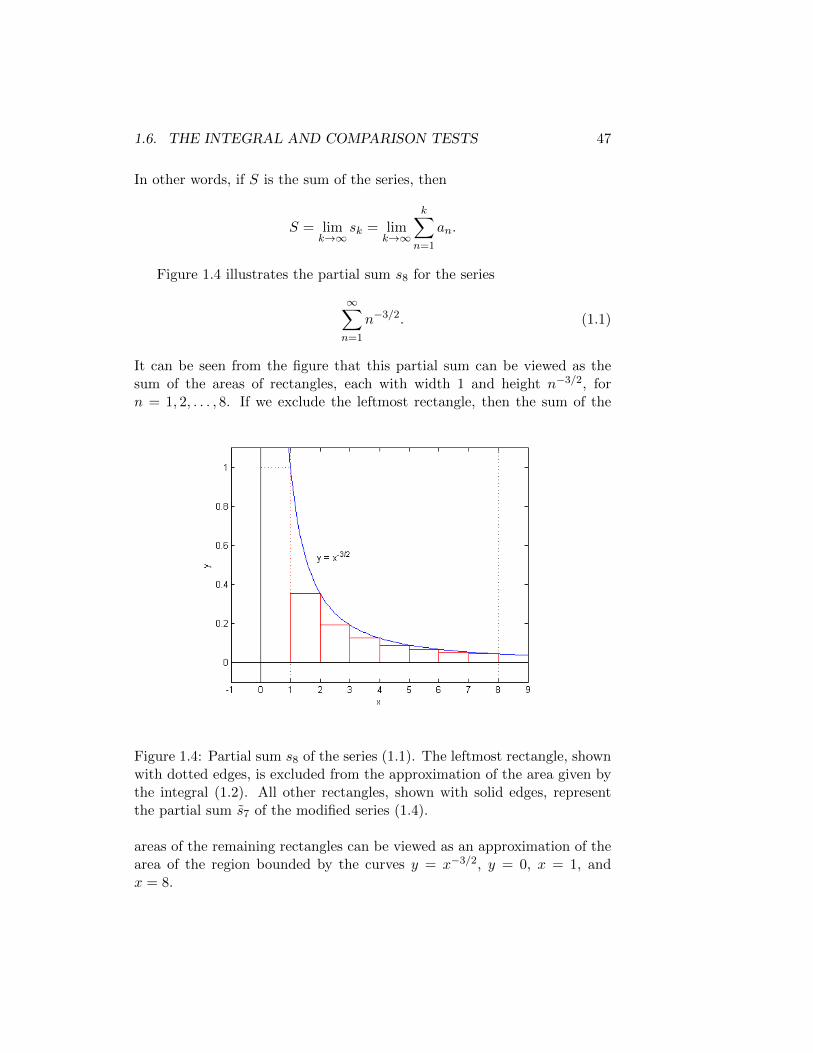
Figure 1.4 illustrates the partial sum s8 for the series
∞∑n=1
n−3/2. (1.1)
It can be seen from the figure that this partial sum can be viewed as thesum of the areas of rectangles, each with width 1 and height n−3/2, forn = 1, 2, . . . , 8. If we exclude the leftmost rectangle, then the sum of the
Figure 1.4: Partial sum s8 of the series (1.1). The leftmost rectangle, shownwith dotted edges, is excluded from the approximation of the area given bythe integral (1.2). All other rectangles, shown with solid edges, representthe partial sum s̃7 of the modified series (1.4).
areas of the remaining rectangles can be viewed as an approximation of thearea of the region bounded by the curves y = x−3/2, y = 0, x = 1, andx = 8.
48 CHAPTER 1. SEQUENCES AND SERIES
The exact value of this area is given by the integral∫ 8
1x−3/2 dx, (1.2)
which is defined to be the limit of a sequence of Riemann sums {Rm}∞m=1.Each Riemann sum approximates the area of this region by the sum of theareas of m rectangles, each of width ∆x = (8− 1)/m. Specifically, we have
Rm =m∑n=1
n−3/2 7
m. (1.3)
From the definitions of the original series (1.1) and the Riemann sum (1.3),we can see that the partial sum shown in Figure 1.4, s8, is equal to R7 +1, since 1 is the area of the leftmost, excluded rectangle. Furthermore, thepartial sum s̃8 of the modified series
∞∑n=2
n−3/2, (1.4)
defined by
s̃8 = 2−3/2 + · · ·+ 8−3/2 =
8∑n=2
n−3/2,
is a lower bound for the exact area given by the integral.This last point suggests that if we extend the interval of integration to
[1,∞), and find that the improper integral∫ ∞1
x−3/2 dx = limk→∞
∫ k
1x−3/2 dx
exists and is finite, then the modified series (1.4) must converge, because eachpartial sum of the modified series is bounded above by the “partial integral”on the interval [1, k]. If this sequence of integrals converges, it follows thatthe sequence of modified partial sums must converge, and therefore themodified series must be convergent. Because the original series (1.1) andmodified series (1.4) only differ by the inclusion of the first term 1−3/2 = 1,we conclude that the original series must be convergent as well.
Evaluating the integral (1.2), we obtain∫ ∞1
x−3/2 dx = limk→∞
∫ k
1x−3/2 dx
1.6. THE INTEGRAL AND COMPARISON TESTS 49
= limk→∞
−2x−1/2∣∣∣k1
= limk→∞
2− 2k−1/2
= 2.
It follows that the sum of the modified series (1.4) is less than 2, and thereforethe sum of the original series (1.1) must be less than 3. Unfortunately, it isnot possible to analytically compute the exact value of the sum, althoughit can be approximated numerically. Nonetheless, we at least know thatin some circumstances, we can use integrals to determine whether a seriesconverges, as this example illustrates.
Integrals can also be used to determine that a series is divergent. Supposethat the integral ∫ ∞
1f(x) dx
is divergent, meaning that it is not equal to any finite value. By examiningFigure 1.5, we can see that just as the integral from 1 to k of f(x) is anupper bound on the partial sum s̃k, that excludes the first term, this integralis also a lower bound on the partial sum sk, that includes the first term.Therefore, if the sequence of integrals from 1 to k diverges as k → ∞, itfollows that the sequence of partial sums {sk}∞k=1, consisting of values thatare greater than these integrals, must diverge as well.
We summarize this discussion by stating the Integral Test: Let the se-quence {an}∞n=1 be defined by an = f(n), for n ≥ 1, where f(x) is a con-tinuous, positive, decreasing function defined on [1,∞). If the improperintegral ∫ ∞
1f(x) dx = lim
k→∞
∫ k
1f(x) dx
converges to a finite value F , then the series
∞∑n=1
an
is convergent. Furthermore, if S is the sum of this series, then S < F + a1.On the other hand, if the integral diverges, then the series diverges.
The reason why it is important that f(x) is positive and decreasing isthat it must be ensured that the partial sums of the modified series (with thefirst term excluded) are a lower bound for the value of the integral, becauseotherwise, no conclusive statement can be made about the convergence of
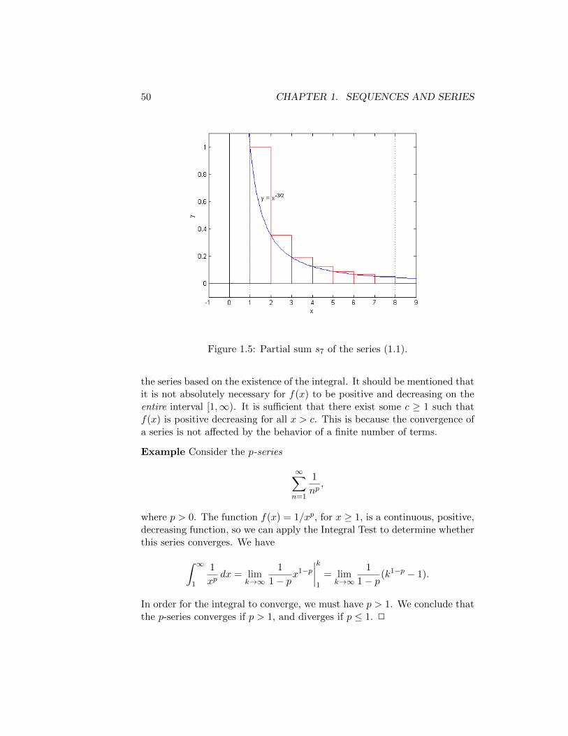
50 CHAPTER 1. SEQUENCES AND SERIES
Figure 1.5: Partial sum s7 of the series (1.1).
the series based on the existence of the integral. It should be mentioned thatit is not absolutely necessary for f(x) to be positive and decreasing on theentire interval [1,∞). It is sufficient that there exist some c ≥ 1 such thatf(x) is positive decreasing for all x > c. This is because the convergence ofa series is not affected by the behavior of a finite number of terms.
Example Consider the p-series
∞∑n=1
1
np,
where p > 0. The function f(x) = 1/xp, for x ≥ 1, is a continuous, positive,decreasing function, so we can apply the Integral Test to determine whetherthis series converges. We have∫ ∞
1
1
xpdx = lim
k→∞
1
1− px1−p
∣∣∣∣k1
= limk→∞
1
1− p(k1−p − 1).
In order for the integral to converge, we must have p > 1. We conclude thatthe p-series converges if p > 1, and diverges if p ≤ 1. 2
1.6. THE INTEGRAL AND COMPARISON TESTS 51
Example Consider the series
∞∑n=0
1
1 + n2.
We attempt to determine whether this series converges using the IntegralTest, by evaluating the integral∫ ∞
0
1
1 + x2dx.
Note that while the Integral Test, as stated previously, uses 1 for both theinitial index and the lower limit of integration, it can also be applied withdifferent values for these quantities, as long as they are consistent. We have∫ ∞
0
1
1 + x2dx = lim
k→∞tan−1 x
∣∣k0
= limk→∞
(tan−1 k − tan−1 0) =π
2.
It follows from the convergence of this integral that the series is convergent.2
1.6.2 The Comparison Test
The integral test indicates convergence or divergence of a series throughcomparison with the integral of a related function, but for many series, thisis not feasible because the integral cannot be easily evaluated. A practi-cal alternative is to compare the series to another series that is known toconverge or diverge, since there are already certain types of series whosebehavior is known.
Suppose we have two series
∞∑n=1
an and∞∑n=1
bn,
whose terms are non-negative, that satisfy 0 ≤ an ≤ bn for all n ≥ 1. Wedenote the partial sums of these series by pk and qk, respectively:
pk =k∑
n=1
an, qk =k∑
n=1
bn.
Suppose that the series∑bn is convergent to a sum Sb. Because of the
relationship between an and bn, and the fact that both sets of terms are
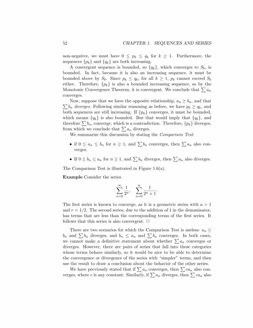
52 CHAPTER 1. SEQUENCES AND SERIES
non-negative, we must have 0 ≤ pk ≤ qk for k ≥ 1. Furthermore, thesequences {pk} and {qk} are both increasing.
A convergent sequence is bounded, so {qk}, which converges to Sb, isbounded. In fact, because it is also an increasing sequence, it must bebounded above by Sb. Since pk ≤ qk, for all k ≥ 1, pk cannot exceed Sbeither. Therefore, {pk} is also a bounded increasing sequence, so by theMonotonic Convergence Theorem, it is convergent. We conclude that
∑an
converges.Now, suppose that we have the opposite relationship, an ≥ bn, and that∑bn diverges. Following similar reasoning as before, we have pk ≥ qk, and
both sequences are still increasing. If {pk} converges, it must be bounded,which means {qk} is also bounded. But that would imply that {qk}, andtherefore
∑bn, converge, which is a contradiction. Therefore, {pk} diverges,
from which we conclude that∑an diverges.
We summarize this discussion by stating the Comparison Test:
• if 0 ≤ an ≤ bn for n ≥ 1, and∑bn converges, then
∑an also con-
verges.
• If 0 ≤ bn ≤ an for n ≥ 1, and∑bn diverges, then
∑an also diverges.
The Comparison Test is illustrated in Figure 1.6(a).
Example Consider the series
∞∑n=0
1
2n,
∞∑n=0
1
2n + 1.
The first series is known to converge, as it is a geometric series with a = 1and r = 1/2. The second series, due to the addition of 1 in the denominator,has terms that are less than the corresponding terms of the first series. Itfollows that this series is also convergent. 2
There are two scenarios for which the Comparison Test is useless: an ≤bn and
∑bn diverges, and bn ≤ an and
∑bn converges. In both cases,
we cannot make a definitive statement about whether∑an converges or
diverges. However, there are pairs of series that fall into these categorieswhose terms behave similarly, so it would be nice to be able to determinethe convergence or divergence of the series with “simpler” terms, and thenuse the result to draw a conclusion about the behavior of the other series.
We have previously stated that if∑an converges, then
∑can also con-
verges, where c is any constant. Similarly, if∑an diverges, then
∑can also
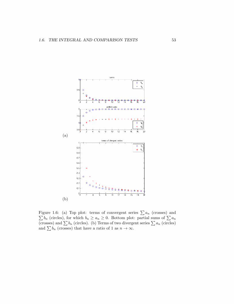
1.6. THE INTEGRAL AND COMPARISON TESTS 53
(a)
(b)
Figure 1.6: (a) Top plot: terms of convergent series∑an (crosses) and∑
bn (circles), for which bn ≥ an ≥ 0. Bottom plot: partial sums of∑an
(crosses) and∑bn (circles). (b) Terms of two divergent series
∑an (circles)
and∑bn (crosses) that have a ratio of 1 as n→∞.
54 CHAPTER 1. SEQUENCES AND SERIES
diverges, if c 6= 0. However, we have also stated that the behavior of a finitenumber of terms does not affect the convergence or divergence of a series.These facts suggest that if a series
∑bn has terms that are not exactly mul-
tiples of the terms of another series∑an, but approach being multiples in
the limit as n→∞, the two series should have the same behavior.This is in fact the case, which leads to the Limit Comparison Test:
suppose that two series∑an and
∑bn have terms that satisfy
limn→∞
anbn
= c,
where c is a nonzero, finite number. Then,∑an and
∑bn both converge,
or both diverge. This test is illustrated in Figure 1.6(b), in which the diver-gence of the series
∑bn, with the larger terms, can be used to establish the
divergence of the series∑an, which is not possible using the Comparison
Test.
Example Consider the series
∞∑n=1
n2 + 1
n3 + 3n2 + 2n,
∞∑n=1
1
n.
The second series is divergent, but we cannot use the Comparison Testdirectly on these two series, because n3 + 3n2 + 2n > n(n2 + 1) for n ≥ 1,which means that the terms of the first series are less than those of thesecond. We could try scaling the second series by a constant c > 1 and thenusing the Comparison Test, but since the Comparison Test requires that arelationship apply to all terms of both series, finding an appropriate c canbe tedious. It is easier to apply the Limit Comparison Test, which yields
limn→∞
1n
n2+1n3+3n2+2n
=n3 + 3n2 + 2n
n(n2 + 1)=n3
n3
1 + 3n + 2
n2
1 + 1n2
= 1,
from which we can conclude that the first series also diverges. 2
1.7 Other Convergence Tests
In this section, we develop additional tests that, for many series, will en-able us to quickly determine whether a given series converges or diverges.Although these new tests, like the Integral and Comparison Tests, can onlytell us whether a series converges, as opposed to helping us compute itslimit, they do offer us one advantage that the previous tests do not: theyare applicable to series whose terms are not necessarily positive.
1.7. OTHER CONVERGENCE TESTS 55
1.7.1 The Alternating Series Test
An alternating series is a series whose terms alternate signs, so that twoconsecutive terms always have opposite signs.
Example The series∞∑n=0
(−1
2
)n,
in addition to being a geometric series with a = 1 and r = −12 , is an
alternating series whose first few terms are
a0 = 1, a1 = −1
2, a2 =
1
4, a3 = −1
8.
2
Any alternating series has terms of the form an = (−1)nbn, where bn =|an| > 0. In the preceding example, bn = 1/2n.
Suppose that we have an alternating series with terms {(−1)nbn}∞n=0, forwhich bn > 0 for n ≥ 0, such that the terms are non-increasing in magnitude:bn+1 ≤ bn for n ≥ 0. While one would normally try to establish convergenceor divergence by examining the sequence of partial sums, because of thealternating signs of the terms, we will instead examine alternating partialsums.
Specifically, consider the sequence of even-numbered partial sums:
s2n = b0 − b1 + b2 + · · ·+ b2n
= (b0 − b1) + (b2 − b3) + · · ·+ b2n.
Because bn ≥ bn+1, each quantity in parentheses is a non-negative number,which means s2n ≥ (b0 − b1) for n ≥ 0. That is, the sequence of even-numbered partial sums is bounded below. A similar grouping of terms canbe used to show that s2n ≤ b0 for n ≥ 0, so this sequence is also boundedabove. In other words, it is bounded.
On the other hand, by the definition of a partial sum, we have
s2n = s2n−2 − b2n−1 + b2n = s2n−2 − (b2n−1 − b2n) ≤ s2n−2,
which shows that this sequence of partial sums is also non-increasing. Thatis, this sequencec is monotonic. It follows from the Monotonic SequenceTheorem that the sequence is convergent. A similar procedure can be used
56 CHAPTER 1. SEQUENCES AND SERIES
to show that not only does the sequence of odd-numbered partial sums con-verge, but it converges to the same limit as the even-numbered partial sums,provided that the sequence of terms converges to zero, as must be the casefor any convergent series. We conclude that the sequence of all partial sumsconverges, so the alternating series is convergent.
This leads to the Alternating Series Test: if the alternating series
∞∑n=0
(−1)nbn = b0 − b1 + b2 − b3 + · · · ,
where bn > 0 for n ≥ 0, satisfies these conditions:
bn+1 ≤ bn, n ≥ 0, and limn→∞
bn = 0,
then the series is convergent.
Example Consider the alternating series
∞∑n=1
(−1)nn
n2 + 1.
The terms in the series converge to zero as n→∞. Furthermore, by differ-entiating the function
f(x) =n
n2 + 1
with respect to x, we can confirm that this function satisfies f ′(1) = 0, andf ′(x) < 0 for x > 1. It follows that this function is non-increasing for x ≥ 1,and therefore the terms of the series are non-increasing. We conclude thatthe series passes the Alternating Series Test, and converges. 2
1.7.2 Estimating Error in Alternating Series
When computing the sum of a convergent series numerically, it is desirableto know how many terms are required in order to approximate the sum towithin a given level of accuracy. For general series, it is difficult to estimatethe error incurred by truncating the series after a given number of terms,although for some series, a variant of the Integral Test may be used. Foralternating series, however, it is particularly simple to estimate this error, ifthe series satisfies the Alternating Series Test.
Consider the general alternating series used to develop the AlternatingSeries Test. We established that the sequence of even-numbered partial sums
1.7. OTHER CONVERGENCE TESTS 57
is non-increasing. Similarly, the sequence of odd-numbered partial sums isnon-decreasing. Since both sequences converge to the same limit, which isthe sum s of the series, it follows that s lies between any two consecutivepartial sums sn and sn+1, for some n ≥ 0. Therefore,
|s− sn| ≤ |sn+1 − sn|.
However, sn+1 − sn = bn+1, the next term in the series. We conclude thatthe error in the nth partial sum is bounded above by bn+1.
We have just proved the Alternating Series Estimation Theorem: If analternating series
∞∑n=0
(−1)nbn,
where bn > 0 for n ≥ 0, satisfies these conditions:
bn+1 ≤ bn, n ≥ 0, and limn→∞
bn = 0,
then|s− sn| ≤ bn+1,
where s is the sum of the series and sn is the nth partial sum.
Example Consider the convergent alternating series
∞∑n=0
(−1
3
)n=
∞∑n=0
(−1)n1
3n.
We wish to approximate the sum s of this series with a partial sum snthat includes enough terms so that |s − sn| ≤ 0.001. By the AlternatingSeries Estimation Theorem, we must choose n so that 1/3n+1 ≤ 0.001.Rearranging, we obtain the condition 1000 ≤ 3n+1, or, by taking the naturallogarithm of both sides,
n ≥ ln 1000
ln 3− 1 =
3 ln 10
ln 3− 1 ≈ 5.29.
Therefore, we must use the first 7 terms (from n = 0 to n = 6) to approxi-mate the sum.
In this case, we can confirm that using this many terms is necessary andsufficient, since we can compute the sum of the series. This is a geometricseries with a = 1 and r = −1/3, so the sum is 1/(1− (−1/3)) = 3/4. Usingthe first 7 terms yields an error of approximately 0.000343, while using onlythe first 6 terms yields an error of approximately 0.00103. 2
58 CHAPTER 1. SEQUENCES AND SERIES
1.7.3 Absolute Convergence
Previous tests for convergence have been applicable to series whose termsare all positive, or that alternate in sign. However, many series do not fallinto either category. For such series, we can try to determine convergenceby examining a new series obtained by taking the absolute values of eachterm, and applying one of the previous tests, such as the Integral Test orComparison Test, to this modified series.
Specifically, given a series∞∑n=1
an,
suppose that we are able to determine that the modified series∑|an| is
convergent. We then say that the original series is absolutely convergent.However, we wish to determine whether the original series is convergent.Because 0 ≤ an+ |an| ≤ 2|an|, and
∑2|an| is convergent, we can employ the
Comparison Test to conclude that∑
(an+ |an|) is also convergent. However,the difference of two convergent series is also convergent, from which itfollows that the series
∞∑n=1
|an| −∞∑n=1
(|an|+ an) =
∞∑n=1
an
is convergent.This leads to the Absolute Convergence Test: an absolutely convergent
series is convergent.
Example The series∞∑n=0
cosnπx
n2 + 1
is an example of a Fourier series, which is useful for approximating functions,as well as working with data from signals and images. For any given x, theterms of this series will vary in sign, with a pattern that depends on x.However, if we consider the series obtained by taking the absolute value ofthe terms, we have
∞∑n=0
∣∣∣∣cosnπx
n2 + 1
∣∣∣∣ ≤∑n=0
1
n2 + 1≤ 1 +
∞∑n=1
1
n2,
because | cosnπx| ≤ 1 regardless of x. Using two applications of the Com-parison Test, based on the relationships above, we can conclude that theoriginal series converges. 2
1.7. OTHER CONVERGENCE TESTS 59
It is important to note that the converse of the Absolute Convergence Testis not true: a convergent series is not necessarily absolutely convergent.
Example The alternating series
∞∑n=1
(−1)n1
n
is convergent, by the Alternating Series Test, but taking the absolute valuesof the terms yields the harmonic series, which, being a p-series with p = 1,is divergent. 2
A series that is convergent, but not absolutely convergent, is said to beconditionally convergent.
1.7.4 The Ratio Test
Many of the convergence tests that we have seen impose a condition onall of the terms of a series, but this is unnecessarily restrictive, becauseconvergence of a series is not affected by a finite number of terms. Rather,it is the behavior of the terms as the index n→∞ that is most deterministicof the behavior of the entire series.
For example, suppose that a series∑an satisfies the condition∣∣∣∣an+1
an
∣∣∣∣ = L,
for some number L < 1. It follows that as n → ∞, the terms {an} behaveapproximately like a geometric series with a common ratio r that is less thanone in absolute value, because the ratio of the magnitudes of consecutiveterms is less than one, in the limit. Because such a geometric series isconvergent, and this series involves the absolute values of the terms, thissuggests that the series is absolutely convergent.
This is in fact the case, and leads to one of the most useful tests forconvergence, the Ratio Test: let
L = limn→∞
∣∣∣∣an+1
an
∣∣∣∣ ,assuming this limit exists. If L < 1, then the series is absolutely convergent.If L > 1, or the limit does not exist, then the series is divergent. If L = 1,the test is inconclusive, and another test must be used instead.

60 CHAPTER 1. SEQUENCES AND SERIES
This test is particularly useful for series whose terms involve powers ofn, exponential functions, or factorials, as this example shows.
Example Applying the Ratio Test to the series
∞∑n=0
n!
2n(n+ 1)2
yields
limn→∞
∣∣∣∣ (n+ 1)!
2n+1(n+ 2)2
/n!
2n(n+ 1)2
∣∣∣∣ = limn→∞
∣∣∣∣(n+ 1)!
n!
2n
2n+1
(n+ 1)2
(n+ 2)2
∣∣∣∣= lim
n→∞
∣∣∣∣∣n+ 1
2
(n+ 1
n+ 2
)2∣∣∣∣∣
= ∞
and therefore the series diverges. 2
1.7.5 The Root Test
A similar test to the Ratio Test is the Root Test, which is convenient forseries whose terms are raised to the nth power, where n is the index. Thebasic idea behind this test is that because a geometric series
∑rn converges
when |r| < 1, if the terms of a more general series∑an converge, in absolute
value, to an expression of the form Ln where L < 1, this series shouldconverge as well. If this is the case, then L = n
√|an|.
With this idea in mind, the Root Test is as follows: let
L = limn→∞
n√|an|,
assuming this limit exists. If L < 1, then the series is absolutely convergent.If L > 1, or the limit does not exist, then the series is divergent. If L = 1,the test is inconclusive, and another test must be used instead.
Example Applying the Root Test to the series
∞∑n=0
(1
πtan−1 n
)nyields
limn→∞
n
√∣∣∣∣( 1
πtan−1 n
)n∣∣∣∣ = limn→∞
1
πtan−1 n =
1
π
π
2=
1
2< 1,
which indicates that the series converges absolutely. 2
1.7. OTHER CONVERGENCE TESTS 61
1.7.6 Summary
• The Integral Test can be used to determine whether a series converges.If the terms {an}∞n=1 of a series are defined to be the values of acontinuous, positive, decreasing function f(n) where n is each positiveinteger, and if f(x) is integrable on the interval [1,∞), then the seriesconverges, and the sum of the series, excluding the first term a1, isbounded above by the value of the integral.
• The Integral Test can also be used to test for the divergence of aseries. If the integral of f(x) from 1 to ∞ diverges, then the serieswhose terms are defined by an = f(n), for n ≥ 1, also diverges.
• The function f(x) need not be positive and decreasing for the entiredomain of integration, but it needs to be positive and decreasing forall x > c, for some c in the domain.
• The initial index of the series and the lower limit of integration do nothave to be equal to 1, but the same value should be used for both.
• Using the Integral Test, it can be shown that the p-series, whose termsare given by an = n−p, converges if p > 1 and diverges if p ≤ 1.
• The Comparison Test states that a series whose terms are dominatedby those a convergent series is also convergent, and that a series whoseterms dominate those of a divergent series is also divergent. In bothcases, the terms of both series must be non-negative.
• The Limit Comparison Test states that if two series have terms whoseratio converges to a nonzero, finite limit, then the series have the samebehavior; that is, they both converge or both diverge. This test canbe useful in cases for which the Comparison Test is inconclusive.
• The Alternating Series Test states that an alternating series is con-vergent if its terms are non-increasing in magnitude, and converge tozero.
• If an alternating series passes the Alternating Series Test, then anypartial sum of the series deviates from the overall sum by no morethan the next term in the series.
• A series is absolutely convergent if the new series obtained by takingthe absolute values of the terms of the original series is convergent.
62 CHAPTER 1. SEQUENCES AND SERIES
• A series that is absolutely convergent is also convergent, but not neces-sarily other way around. A convergent series that fails to be absolutelyconvergent is conditionally convergent.
• The Ratio Test is one of the most useful tests for determining whethera series converges. If the ratio |an+1/an| converges to a limit that isless than 1, then
∑an converges absolutely. If the limit is larger than
1, or does not exist, then the series diverges. Otherwise, the test isinconclusive.
• The Root Test determines convergence based on the limit of the nthroot of the absolute value of the nth term, as n→∞. If the limit lessthan 1, the series converges absolutely. If the limit is greater than 1,or nonexistent, the series diverges. Otherwise, the test is inconclusive.
1.8 Power Series
Now that we have learned about how to test sequences and series for con-vergence, and, in some cases, compute their limits when they do converge,we are ready to take our next step toward our primary goal: to be able toapproximate functions to within a given degree of accuracy using “simple”functions that can readily be evaluated using simple arithmetic operations,the only ones a computer can perform. In this next step, we consider seriesthat depend on a variable x, like the functions we wish to approximate.
1.8.1 What is a Power Series?
A power series is a series of the form
∞∑n=0
cn(x− a)n,
where the constants cn, for n ≥ 0, are called the coefficients, and the numbera is called the center.
When a value is substituted for the variable x, the power series reducesto a series of constant terms that can then be tested for convergence, usingany of the tests that we have previously discussed. The result of such a test,convergence or divergence, depends on x.
1.8. POWER SERIES 63
1.8.2 Convergence of Power Series
We now illustrate, through some examples, how tests for the convergence ofgeneral series can be used to determine the values of x for which a powerseries converges.
Example Consider the power series
∞∑n=0
xn
n!.
Applying the Ratio Test, for any fixed x, yields
limn→∞
∣∣∣∣ xn+1
(n+ 1)!
/xn
n!
∣∣∣∣ = limn→∞
∣∣∣∣xn+1
xnn!
(n+ 1)!
∣∣∣∣ = limn→∞
∣∣∣∣ x
n+ 1
∣∣∣∣ = 0,
since no matter how large |x| is, eventually n will exceed it. Therefore, thispower series is absolutely convergent for all x. 2
Example The power series
∞∑n=0
nnxn =∞∑n=0
(nx)n
diverges when x 6= 0, because, by the Ratio Test,
limn→∞
∣∣∣∣((n+ 1)x)n+1
(nx)n
∣∣∣∣ = limn→∞
∣∣∣∣(1 +1
n
)n(n+ 1)x
∣∣∣∣ = limn→∞
|e(n+ 1)x| =∞.
On the other hand, if x = 0, then all terms vanish except for n = 0, and theseries (trivially) converges to 1. 2
Example Consider the power series
∞∑n=1
xn
n.
Applying the Ratio Test yields
limn→∞
∣∣∣∣ xn+1
n+ 1
/xn
n
∣∣∣∣ = limn→∞
∣∣∣∣xn+1
xnn
n+ 1
∣∣∣∣ = |x|.
It follows that the power series converges when |x| < 1, and diverges when|x| > 1. When x = 1, the series diverges, because it is the harmonic series,but when x = −1, it converges, by the Alternating Series Test. 2
64 CHAPTER 1. SEQUENCES AND SERIES
1.8.3 The Radius of Convergence
In the preceding examples, we encountered three different scenarios regard-ing convergence of a power series:
• The power series converges for all x
• The power series converges only for x = a, where a is the center of theseries
• The power series converges when |x− a| < R for some number R, anddiverges for |x− a| > R.
It can be shown that for any power series, these are the only possible out-comes of a test for convergence. In other words, there exists an interval,called the interval of convergence, such that for x in this interval, the powerseries, when evaluated at x, is convergent.
The interval may be the entire real line (−∞,∞), a single point x = a,or a finite interval of the form |x − a| < R, or a − R < x < a + R. In thiscase, the number R is called the radius of convergence. The series divergesfor |x − a| > R, but when |x − a| = R, either convergence or divergenceis possible. We say that when the interval of convergence is the entire realline, R =∞, and if it is the single point x = a, then R = 0.
1.8.4 Representing Functions as Power Series
We have learned that a convergent power series
∞∑n=0
cn(x− x0)n (1.5)
is a function of x, whose domain is the series’ interval of convergence. Givensuch a power series, it is very helpful to know which function it represents,because that knowledge can provide an easier approach to evaluating oranalyzing the function than working with the power series directly.
However, the opposite task is also very useful: given a function f(x), findthe corresponding power series. We will see that in some cases, the powerseries can be the only practical way to evaluate the function, so knowledge ofits power series is vital. One useful technique for obtaining the power seriesof a function is to relate the function to the sum of a convergent geometricseries
∞∑n=0
arn =a
1− r,
1.8. POWER SERIES 65
as the following examples show.
Example Let
f(x) =2
1 + 2x.
If we rewrite f(x) to fit the form a/(1− r), for some a and r, we obtain
f(x) =2
1− (−2x),
which, when compared to the form a/(1− r), yields a = 2 and r = −2x. Itfollows that f(x) is the sum of the geometric series
∞∑n=0
2(−2x)n,
provided that | − 2x| < 1, or |x| < 1/2. 2
The common ratio r need not be a linear function of x, as the followingexample shows.
Example Let
f(x) =1
(x− 2)2 + 4.
Trying to fit f(x) into the form a/(1 − r) requires a 1 in the denominator,which can be obtained by dividing the numerator and denominator by 4:
1
(x− 2)2 + 4=
14
(x−2)2
4 + 1=
14
1−[−(x−2
2
)2] .It follows that a = 1/4 and r = −((x− 2)/2)2, resulting in the power series
∞∑n=0
1
4
[−(x− 2
2
)2]n
=
∞∑n=0
1
4(−1)n
(x− 2
2
)2n
=
∞∑n=0
(−1)n
4n+1(x− 2)2n,
which converges when | − ((x − 2)/2)2| < 1. This inequality holds if |(x −2)/2| < 1, or |x − 2| < 2. That is, f(x) is defined by this power serieswhen 0 < x < 4. Note that in terms of the general form of a power seriesin equation (1.5), x0 = 2, while cn = 0 whenever n is odd, because onlyeven powers of (x − 2) are included. On the other hand, when n is even,cn = (−1)n/2/4n/2+1. 2
66 CHAPTER 1. SEQUENCES AND SERIES
Example A function does not have to have a constant numerator in orderto be defined using a geometric power series. Consider
f(x) =2x
2− x.
This can be rewritten as
x
2− x=
2x
2
1
1− x2
= x1
1− x2
.
The fraction is the sum of a geometric series with a = 1 and r = x/2. Itfollows that
f(x) = x
∞∑n=0
(x2
)n,
provided |r| = |x/2| < 1, or −2 < x < 2.However, this representation of f(x) does not fit the usual form of a
power series given by equation (1.5). To obtain this form, we can rewritef(x) again as follows:
f(x) = 2x
2
∞∑n=0
(x2
)n= 2
∞∑n=0
(x2
)n+1= 2
∞∑n=1
(x2
)n= 2
∞∑n=1
1
2nxn =
∞∑n=1
1
2n−1xn,
which does fit the form in equation (1.5), with c0 = 0 and cn = 1/2n−1 forn ≥ 1. 2
This last example shows that if f(x) can be represented by a power series,then so can xpf(x) for any positive integer p, simply by shifting the indicesof the coefficients {cn}∞n=0 up by p.
1.8.5 Differentiation and Integration of Power Series
We have previously learned how to compute power series representations ofcertain functions, by relating them to geometric series. We can obtain powerseries representation for a wider variety of functions by exploiting the factthat a convergent power series can be differentiated, or integrated, term-by-term to obtain a new power series that has the same radius of convergenceas the original power series. The new power series is a representation ofthe derivative, or antiderivative, of the function that is represented by theoriginal power series.
This is particularly useful when we have a function f(x) for which wedo not know how to obtain a power series representation directly. If its
1.8. POWER SERIES 67
derivative f ′(x), or its antiderivative∫f(x) dx, is a function for which a
power series representation can easily be computed, such as the examplesfrom earlier in this section, then we can integrate, or differentiate, this powerseries term-by-term to obtain a power series for f(x).
Example The function
f(x) =4
(2− x)2
is the derivative of the function
g(x) =2x
2− x,
which, from earlier in this section, has the power series representation
2x
2− x=∞∑n=1
1
2n−1xn.
This series converges when −2 < x < 2. To obtain a power series represen-tation of f(x), we differentiate this series term-by-term to obtain
4
(2− x)2=∞∑n=1
1
2n−1nxn−1 =
∞∑n=0
(n+ 1)
2nxn,
which also converges when −2 < x < 2. 2
Example The function
f(x) =1
2tan−1 x− 2
2
has the derivative
f ′(x) =1
(x− 2)2 + 4.
From earlier in this section, this function has the power series
1
(x− 2)2 + 4=∞∑n=0
(−1)n
4n+1(x− 2)2n,
whose interval of convergence is 0 < x < 4. Integrating this series term-by-term yields
1
2tan−1 x− 2
2=
∞∑n=0
(−1)n
4n+1
∫(x− 2)2n dx =
∞∑n=0
(−1)n
4n+1
(x− 2)2n+1
2n+ 1+ C.
68 CHAPTER 1. SEQUENCES AND SERIES
To determine the value of C, we substitute x = 2 into the above equation.This causes all terms in the series to vanish. We also have f(2) = 0, whichyields C = 0. 2
Example Consider the definite integral∫ 1
0
1
1 + x4dx.
Attempting to evaluate this integral using partial fraction decomposition isnot possible without introducing complex numbers. Instead, we express theintegrand as a (geometric) power series:
1
1 + x4=
1
1− (−x4)=
∞∑n=0
(−x4)n =
∞∑n=0
(−1)nx4n.
This power series has an interval of convergence of −1 < x < 1, whichcontains the interval of integration (0, 1). Integrating the power series term-by-term from 0 to 1 yields∫ 1
0
1
1 + x4dx =
∫ 1
0
∞∑n=0
(−1)nx4n dx =∞∑n=0
(−1)n∫ 1
0x4n dx =
∞∑n=0
(−1)nx4n+1
4n+ 1
∣∣∣∣10
=∞∑n=0
(−1)n
4n+ 1.
This is an alternating series, which, by the Alternating Series Test, convergessince, for all n ≥ 0,
1
4n+ 1≥ 0, lim
n→∞
1
4n+ 1= 0, and
1
4(n+ 1) + 1<
1
4n+ 1.
Using the Alternating Series Estimation Theorem, we can evaluate this in-tegral numerically, to any degree of accuracy we wish, by choosing n largeenough so that 1/(4n+ 1) is sufficiently small. 2
1.8.6 Summary
• A power series is a series whose terms are constants, called coefficients,times non-negative powers of (x − a) for some constant a, which iscalled the center of the power series.
• The convergence or divergence of power series can be determined usingthe same tests that are used for other series, except that the behaviordepends on x.
1.8. POWER SERIES 69
• A power series either converges only at the center, converges for all x,or converges within the interval |x− a| < R, where R is the radius ofconvergence, while diverging for |x − a| > R. In the latter scenario,when |x− a| = R, the power series can either converge or diverge.
• The interval of convergence contains all values of x for which the powerseries converges.
• A function f(x) can sometimes be represented as a power series byviewing it as the sum of a convergent geometric series. The key isto correctly identify what function serves as the common ratio of theseries, which may require algebraic manipulation of f(x).
• The common ratio, which must appear in the denominator of f(x),must be of the form [c(x− x0)]q, where c and x0 are constants, and qis a positive integer.
• If f(x) can be represented by a geometric power series, then so cancf(x), for any constant c, and so can xpf(x), for any positive integerp.
• Given such a function f(x), the corresponding power series converges ifthe common ratio is less than 1 in absolute value; that is, c|x−x0| < 1.The radius of convergence is 1/|c|.
• A power series representation of a function f(x) can be differentiatedterm-by-term to obtain a power series representation of its derivativef ′(x). The interval of convergence of the differentiated series is thesame as that of the original series.
• A power series representation of a function f(x) can be anti-differentiatedterm-by-term to obtain a power series representation of its anti-derivative∫f(x) dx. The value of the constant of integration, C, can be deter-
mined by substituting the center of the power series for x. The intervalof convergence of the anti-differentiated series is the same as that ofthe original series.
• A power series representation of a function f(x) can be integratedterm-by-term from a to b to obtain a series representation of the def-inite integral
∫ ba f(x) dx, provided that the interval (a, b) lies within
the interval of convergence of the power series that represents f(x).
70 CHAPTER 1. SEQUENCES AND SERIES
1.9 Taylor and Maclaurin Series
We have learned how to construct power series representations of certainfunctions by relating them to geometric series, either directly, or indirectlythrough differentiation or integration. However, these techniques are notapplicable to most functions. Therefore, we now consider the problem ofcomputing the coefficients cn, n = 0, 1, . . . , of a power series
f(x) =∞∑n=0
cn(x− x0)n
that represents a more general function f(x), at least for x near the centerx0.
To that end, we first note that the partial sum of such a power series,
Tn(x) =n∑j=0
cj(x− x0)j ,
is a polynomial of degree n. Furthermore, by substituting x = x0, we findthat
Tn(x0) = c0, T ′n(x0) = c1, T ′′n (x0) = 2c2,
and, in general,dj
dxj[Tn(x)]
∣∣∣∣x=x0
= T (j)n (x0) = j!cj .
This suggests that a function f(x), that has infinitely many derivatives atx0, can be represented by the power series
f(x) =∞∑n=0
f (n)(x0)
n!(x− x0)n,
for all x within the interval of convergence of the series. This is in fact thecase, and we call this series the Taylor series of f centered at x0. Whenx0 = 0, this Taylor series is also known as the Maclaurin series of f .
Example The Maclaurin series for f(x) = ex is given by
ex = 1 + x+x2
2+ · · · =
∞∑n=0
xn
n!,
since f (n)(0) = e0 = 1 for all n. We have seen that this series converges forall x, so ex can be represented by this power series for all x as well. 2
1.9. TAYLOR AND MACLAURIN SERIES 71
While Taylor series have many theoretical uses, they not directly usefulfor practical applications, because most functions are not infinitely differ-entiable, and, of course, any actual computation can only include a finitenumber of terms. Therefore, it is highly desirable to know how accuratelya function can be represented by its truncated Taylor series. That is, for agiven x within the interval of convergence of the Taylor series, our goal is toestimate the error Rn(x) = f(x)− Tn(x), where Tn(x), the nth partial sumof the Taylor series of f , is also known as the nth-degree Taylor polynomialof f centered at x0. The error, Rn(x), is called the Taylor remainder.
We first consider the simplest Taylor polynomial, which is T0(x) = f(x0).To obtain the error R0(x), we apply the Fundamental Theorem of Calculus,and obtain
f(x) = f(x0) +
∫ x
x0
f ′(s) ds.
That is,
R0(x) =
∫ x
x0
f ′(s) ds.
Unfortunately, expressing the remainder as an integral does little to help usto estimate its magnitude. However, we can apply the Mean Value Theoremfor Integrals to obtain
f(x) = f(x0) + f ′(ξ)(x− x0),
where ξ is between x0 and x.Now, we consider the first-degree Taylor polynomial
T1(x) = f(x0) + f ′(x0)(x− x0).
This graph of this function is the tangent line of f at x0. To obtain the errorR1(x) = f(x)−T1(x), we apply the Fundamental Theorem of Calculus twice,to represent both f and its derivative in terms of their values at x0, plus anintegral of their respective derivatives. We obtain
f(x) = f(x0) +
∫ x
x0
[f ′(x0) +
∫ s
x0
f ′′(z) dz
]ds
= f(x0) +
∫ x
x0
f ′(x0) ds+
∫ x
x0
∫ s
x0
f ′′(z) dz ds
= f(x0) + f ′(x0)(x− x0) +
∫ x
x0
∫ x
zf ′′(z) ds dz
= T1(x) +
∫ x
x0
f ′′(z)
∫ x
zds dz
72 CHAPTER 1. SEQUENCES AND SERIES
= T1(x) +
∫ x
x0
f ′′(z)(x− z) dz.
That is,
R1(x) = f(x)− T1(x) =
∫ x
x0
f ′′(z)(x− z) dz.
To obtain a more useful representation of the remainder than this integralform, we use the fact that x − z does not change sign on the interval ofintegration from x0 to x. This allows us to apply the Weighted Mean ValueTheorem for Integrals, which states that∫ b
af(x)g(x) dx = f(c)
∫ b
ag(x) dx,
where c lies in [a, b], and g(x) does not change sign on (a, b). We then obtain
f(x) = T1(x) + f ′′(ξ)
∫ x
x0
x− z dz
= T1(x) + f ′′(ξ)
∫ x−x0
0u du
= T1(x) + f ′′(ξ)(x− x0)2
2,
where ξ lies between x0 and x. That is,
R1(x) = f ′′(ξ)(x− x0)2
2.
Example Let f(x) = sinx. Then, the Taylor polynomial T1(x) is
T1(x) = sin 0 + (cos 0)(x− 0) = x.
The remainder is given by
R1(x) = −sin ξ
2x2.
Since | sinx| ≤ 1 for all x, it follows that if |x| ≤ 10−2, then the error inapproximating sinx by x is at most
|R1(x)| ≤ (10−2)2
2=
10−4
2= 5× 10⁻⁵.
2
1.9. TAYLOR AND MACLAURIN SERIES 73
We now consider the case of an nth-degree Taylor polynomial. We willneed the result∫ x
x0
∫ s1
x0
∫ s2
x0
· · ·∫ sn−1
x0
dsn · · · ds3 ds2 ds1 =(x− x0)n
n!,
previously used for n = 1 and n = 2. This formula can be proven for anarbitrary positive integer n using an inductive argument. We have
f(x) = f(x0) +
∫ x
x0
{f ′(x0) +
∫ s1
x0
[f ′′(x0) +
∫ s2
x0
(f ′′′(x0) +
∫ s3
x0
· · ·∫ sn−1
x0
{f (n)(x0) +
∫ sn
x0
f (n+1)(sn+1) dsn+1
}dsn · · · ds4
)ds3
]ds2
}ds1
= f(x0) + f ′(x0)
∫ x
x0
ds1 + f ′′(x0)
∫ x
x0
∫ s1
x0
ds2 ds1 +
f ′′′(x0)
∫ x
x0
∫ s1
x0
∫ s2
x0
ds3 ds2 ds1 + · · ·+ f (n)(x0)
∫ x
x0
∫ s1
x0
· · ·∫ sn−1
x0
dsn · · · ds2 ds1 +∫ x
x0
∫ s1
x0
· · ·∫ sn
x0
f (n+1)(sn+1) dsn+1 · · · ds2 ds1
= f(x0) + f ′(x0)(x− x0) +1
2f ′′(x0)(x− x0)2 +
1
6f ′′′(x0)(x− x0)3 +
· · ·+ f (n)
n!(x− x0)n +
∫ x
x0
∫ s1
x0
· · ·∫ sn
x0
f (n+1)(sn+1) dsn+1 · · · ds2 ds1
=n∑j=0
f (j)(x0)
j!(x− x0)j +
∫ x
x0
∫ x
sn+1
· · ·∫ x
s2
f (n+1)(sn+1) ds1 · · · dsn dsn+1
=
n∑j=0
f (j)(x0)
j!(x− x0)j +
∫ x
x0
f (n+1)(sn+1)
∫ x
sn+1
· · ·∫ x
s2
ds1 · · · dsn dsn+1
=
n∑j=0
f (j)(x0)
j!(x− x0)j +
∫ x
x0
f (n+1)(sn+1)
n!(x− sn+1)n dsn+1
= Tn(x) +Rn(x).
The transformation of the (n+1)-fold integral between the third and fourthsteps follows from the relations
x0 ≤ sn+1 ≤ sn ≤ · · · ≤ s2 ≤ s1 ≤ x,
when x0 ≤ x. Similar relations hold when x0 ≥ x.
74 CHAPTER 1. SEQUENCES AND SERIES
In summary, the Taylor polynomial and Taylor remainder are given by
Tn(x) = f(x0)+f ′(x0)(x−x0)+f ′′(x0)
2(x−x0)2+· · ·+f (n)(x0)
n!(x−x0)n =
n∑j=0
f (j)(x0)
j!(x−x0)j ,
and
Rn(x) =
∫ x
x0
f (n+1)(s)
n!(x− s)n ds.
Using the Weighted Mean Value Theorem for Integrals, as before, we obtainthe alternative form of the remainder,
Rn(x) =f (n+1)(ξ)
n!
∫ x
x0
(x− s)n ds =f (n+1)(ξ)
(n+ 1)!(x− x0)n+1,
where ξ lies between x0 and x. By computing an upper bound on |f (n+1)(x)|for x near x0, we can estimate the accuracy of an approximation of f(x) nearx0 by Tn(x).
Example The 3rd-degree Taylor polynomial for f(x) = ex, centered atx0 = 0, is given by
T3(x) = 1 + x+x2
2+x3
6,
with remainder
R3(x) =eξ
24x4,
where ξ lies between 0 and x. If we let x = 2.5, it follows that the error inan approximation of ex by T3(x) is at most
|R3(2.5)| =∣∣∣∣ eξ24
(2.5)4
∣∣∣∣ ≤ e2.5
24(39.0625) ≈ 19.828,
which is unacceptably large.
On the other hand, if we use the 3rd-degree Taylor polynomial centeredat x0 = 2,
T3(x) = e2 + e2(x− 2) +e2
2(x− 2)2 +
e2
6(x− 2)3,
with remainder
R3(x) =eξ
24(x− 2)4,
1.9. TAYLOR AND MACLAURIN SERIES 75
where ξ lies between 2 and x, we obtain the error bound
|R3(2.5)| =∣∣∣∣ eξ24
(0.5)4
∣∣∣∣ ≤ e2.5
24(0.0625) ≈ 0.0317,
which implies that using the Taylor polynomial centered at x0 = 2 is farmore accurate. 2
Taylor polynomials are quite useful for approximating functions in such away that they can easily be evaluated by a computer or calculator, becauseonce the coefficients are known, the computation can be performed usingonly basic arithmetic operations. However, as the preceding example shows,a Taylor polynomial for a given function f(x) must be used judiciously,because it can accurately approximate f(x) only when x is near the centerx0, especially when the derivatives of f are large.
Previously, we learned how to approximate a function f(x) by its Taylorpolynomial
Tn(x) =
n∑j=0
f (j)(x0)
j!(x− x0)j ,
for a given center x0. Because the Taylor polynomial of degree n consists ofthe first n+ 1 terms of its Taylor series
f(x) =
∞∑n=0
f (n)(x0)
n!(x− x0)n,
it is helpful to be able to compute all of the coefficients of the Taylor seriesof f(x), so that the coefficients of a Taylor polynomial of any degree areavailable.
Computing a Taylor series in its entirety requires that the coefficients fita pattern that can easily be discerned from the first few terms of the series.In particular, the derivatives of f(x) at x0 must fit an identifiable pattern,as in the case of the Maclaurin series for the exponential function,
ex =
∞∑n=0
1
n!xn.
In a previous example, we used the Ratio Test to conclude that this seriesconverges for all x.
In addition to the task of computing the coefficients of a Taylor series,it is also essential to determine the interval of convergence of the series. ATaylor polynomial cannot be used to approximate a function at a point at
76 CHAPTER 1. SEQUENCES AND SERIES
which the Taylor series does not converge, because the Taylor remainderdoes not converge to zero as the degree of the polynomial increases. Wenow illustrate the process of computing Taylor series of functions, and theirintervals of convergence, through some examples.
Example Consider the function
f(x) =1
1− x.
Its derivatives are
f ′(x) =1
(1− x)2, f ′′(x) =
2
(1− x)3, f (n)(x) =
n!
(1− x)n+1.
It follows that f (n)(0) = n!, and therefore the Taylor series for f centeredat 0, also known as its Maclaurin series, is
f(x) =∞∑n=0
f (n)(0)
n!xn =
∞∑n=0
xn,
which is simply a geometric series with a = 1 and r = x. We concludethat this series has a radius of convergence of R = 1, and an interval ofconvergence of (−1, 1). 2
Example The function f(x) = sinx has derivatives
f ′(x) = cosx, f ′′(x) = − sinx, f ′′′(x) = − cosx, f (4)(x) = sinx,
or, in general,
f (4n)(x) = sinx, f (4n+1)(x) = cosx, f (4n+2)(x) = − sinx, f (4n+3)(x) = − cosx,
for each nonnegative integer n. Substituting x = 0 yields
f (4n)(0) = 0, f (4n+1)(0) = 1, f (4n+2)(0) = 0, f (4n+3)(0) = −1,
or, more concisely,
f (2n)(0) = 0, f (2n+1)(0) = (−1)n, n ≥ 0.
It follows that the Maclaurin series for sinx includes only odd powers of x.We have
sinx =
∞∑n=0
(−1)n
(2n+ 1)!x2n+1.
1.9. TAYLOR AND MACLAURIN SERIES 77
By applying the Ratio Test, we find that this series converges for all x. Thatis, R =∞ and the interval of convergence (−∞,∞). 2
Example To compute the Maclaurin series for f(x) = cosx, we can use theinformation about derivatives from the previous example to obtain
f (4n)(x) = cosx, f (4n+1)(x) = − sinx, f (4n+2)(x) = − cosx, f (4n+3)(x) = sinx,
for each nonnegative integer n. Substituting x = 0 yields
f (4n)(0) = 1, f (4n+1)(0) = 0, f (4n+2)(0) = −1, f (4n+3)(0) = 0,
or, more concisely,
f (2n+1)(0) = 0, f (2n)(0) = (−1)n, n ≥ 0.
It follows that the Maclaurin series for cosx includes only even powers of x.We have
cosx =
∞∑n=0
(−1)n
(2n)!x2n.
By applying the Ratio Test, we find that this series converges for all x. Thatis, R =∞ and the interval of convergence (−∞,∞). 2
Example Consider the function f(x) = (1 + x)k, where k is a real number(not necessarily an integer). Its derivatives are
f ′(x) = k(1+x)k−1, f ′′(x) = k(k−1)(1+x)k−2, f ′′′(x) = k(k−1)(k−2)(1+x)k−3,
and, in general,
f (n)(x) = k(k − 1)(k − 2) · · · (k − n+ 1)(1 + x)k−n,
and therefore
f (n)(0) = k(k − 1)(k − 2) · · · (k − n+ 1).
It follows that the Maclaurin series for (1 + x)k is the binomial series
(1 + x)k =
∞∑n=0
k(k − 1)(k − 2) · · · (k − n+ 1)
n!xk =
∞∑n=0
(kn
)xk,
where (kn
)=k(k − 1)(k − 2) · · · (k − n+ 1)
n!
78 CHAPTER 1. SEQUENCES AND SERIES
is called a binomial coefficient. It is a generalization of(kn
)=k(k − 1)(k − 2) · · · (k − n+ 1)
n!=
k!
n!(n− k)!,
where k and n are non-negative integers. In this case, this binomial coef-ficient represents the number of ways to choose n objects from a set of kobjects.
To determine the interval of convergence, we again use the Ratio Test,which yields
limn→∞
∣∣∣∣ k(k − 1) · · · (k − n)
k(k − 1) · · · (k − n+ 1)
n!
(n+ 1)!
xn+1
xn
∣∣∣∣ = limn→∞
∣∣∣∣k − nn+ 1
∣∣∣∣ |x| = limn→∞
∣∣∣∣∣ kn − 1
1 + 1n
∣∣∣∣∣ |x| = |x|,which implies that the series converges for |x| < 1. 2
Previously, we have learned how to compute Taylor series for certainfunctions by computing the coefficients directly and recognizing the patternthat they fit. However, for many functions, this approach is not feasible,because any pattern in the coefficients is too complex to recognize. We nowillustrate how other techniques for obtaining power series can be used, some-times in tandem, to obtain Taylor series for certain well-known functions.
Example Recall the sum of a geometric series,
∞∑n=0
xn =1
1− x
provided |x| < 1. That is, the radius of convergence is R = 1. Becausethe power series representation of a function at a given center is unique, itfollows that the Maclaurin series for 1/(1−x) is the above geometric series.
Substituting −x2 for x yields
∞∑n=0
(−x2)n =∞∑n=0
(−1)nx2n =1
1− (−x2)=
1
1 + x2.
Because |x2| < 1 implies that |x| < 1, this series has the same radius ofconvergence, R = 1. Furthermore, the above series is the Maclaurin seriesfor 1/(1 + x2).
By anti-differentiating this series term-by-term, we can obtain a Maclau-rin series for tan−1 x, for |x| < 1, which is an antiderivative of 1/(1 + x2):
tan−1 x =
∫ x
0
1
1 + s2ds+ C
1.9. TAYLOR AND MACLAURIN SERIES 79
=
∫ x
0
∞∑n=0
(−1)ns2n ds+ C
=∞∑n=0
(−1)n∫ x
0s2n ds+ C
=
∞∑n=0
(−1)nx2n+1
2n+ 1+ C.
The unknown constant C is included because we have computed a specificantiderivative of 1/(1 +x2), and all antiderivatives of a given function differfrom one another by a constant. To compute C, we substitute x = 0, andbecause tan−1 0 = 0, we obtain the equation 0 = 0 +C, so we conclude thatC = 0 and the Maclaurin series for tan−1 x is
tan−1 x =∞∑n=0
(−1)nx2n+1
2n+ 1, |x| < 1.
2
Two Taylor series with the same center can trivially be added or sub-tracted in order to obtain a Taylor series for the sum or difference of thecorresponding functions. The radius of convergence of the sum or differenceis the minimum of the radii of convergence of the two series that are beingadded or subtracted.
It is also possible to multiply or divide Taylor series to obtain new Taylorseries, as the following examples show.
Example Recall the Maclaurin series for ex and cosx:
ex =
∞∑n=0
xn
n!= 1 + x+
x2
2!+x3
3!+x4
4!+ · · · ,
cosx =
∞∑n=0
(−1)nx2n
(2n)!= 1− x2
2!+x4
4!− x6
6!+ · · · .
The Taylor series for ex cosx can be obtained by multiplying these series,in the same way that polynomials are multiplied. This is because for eachnon-negative integer n, the number of terms from each series that are neededto compute the coefficient cn in the product is finite.
We have
ex cosx =
( ∞∑n=0
xn
n!
)( ∞∑m=0
(−1)mx2m
(2m)!
)
80 CHAPTER 1. SEQUENCES AND SERIES
=∞∑n=0
∞∑m=0
(−1)mx2m+n
n!(2m)!
=∞∑`=0
b`/2c∑m=0
(−1)mx`
(`− 2m)!(2m)!
= 1 + x− 1
3x3 − 1
6x4 − 1
30x5 + · · · ,
where ` = 2m+n, and, for any real number x, bxc is the “floor” of x, whichis the greatest integer that is less than or equal to x. This series convergesfor all x, like the series for ex and cosx. 2
Example Recall the Maclaurin series for sinx and cosx:
sinx =
∞∑n=0
(−1)nx2n+1
(2n+ 1)!= x− x3
3!+x5
5!− x7
7!+ · · · ,
cosx =∞∑n=0
(−1)nx2n
(2n)!= 1− x2
2!+x4
4!− x6
6!+ · · · .
To compute the Maclaurin series for tanx = sinx/ cosx, we can use poly-nomial division to divide the Maclaurin series for sinx by that of cosx, eventhough these series are not polynomials themselves, but sums of infinitelymany monomials.
First, we divide the leading terms of the two series. The first term of theseries for sinx is x, while the first term of the series for cosx is 1. Therefore,the first term of the quotient of the series, and therefore the series for tanx,is x/1 = x.
Next, we subtract x times the series for cosx from that of sinx to obtainthe remainder:
∞∑n=0
(−1)nx2n+1
(2n+ 1)!−∞∑n=0
(−1)nx2n+1
(2n)!=
∞∑n=0
(−1)n+1 2n
(2n+ 1)!x2n+1.
Then, we divide the leading term of this series, which is x3/3, by the leadingterm of the series for cosx, which is 1, to obtain the second term of thequotient, which is x3/3.
Continuing this process yields the series
tanx = x+1
3x3 +
2
15x5 +
17
315x7 +
62
2835x9 + · · ·
1.9. TAYLOR AND MACLAURIN SERIES 81
The coefficients arise from the following pattern:
1
3= − 1
3!+
1
2!,
2
15=
1
5!− 1
4!+
1
3
1
2!,
17
315= − 1
7!+
1
6!− 1
3
1
4!+
2
15
1
2!,
62
2835=
1
9!− 1
8!+
1
3
1
6!− 2
15
1
4!+
17
315
1
2!.
Note that each coefficient is expressed in terms of the previous coefficients.2
1.9.1 Summary
• If a function f(x) can be represented by a power series centered at x0,then the coefficients are given by cn = f (n)(x0)/n!, where f (n)(x0) isthe nth derivative of f evaluated at x0.
• The power series centered at x0 that represents a function f is calledthe Taylor series of f centered at x0. If x0 = 0, the Taylor series isalso called the Maclaurin series of f .
• If the Taylor series of f is truncated after the first (n + 1) terms,the result is a polynomial of degree n, called the nth-degree Taylorpolynomial of f centered at x0.
• The difference between f(x) and its nth-degree Taylor polynomialTn(x), centered at x0, is called the Taylor remainder of f . It closelyresembles the term of degree n+1 in the Taylor series, except that the(n + 1)-st derivative of f is evaluated at an unknown point betweenx0 and x. By bounding this derivative between x0 and x, one canestimate the error in approximating f(x) by Tn(x).
• One approach to computing the Taylor series of a function f(x), cen-tered at x0, is to compute the first few coefficients, given by cn =f (n)(x0)/n!, and trying to recognize a pattern that applies for all non-negative integers n.
• This approach leads to the following known Maclaurin series:
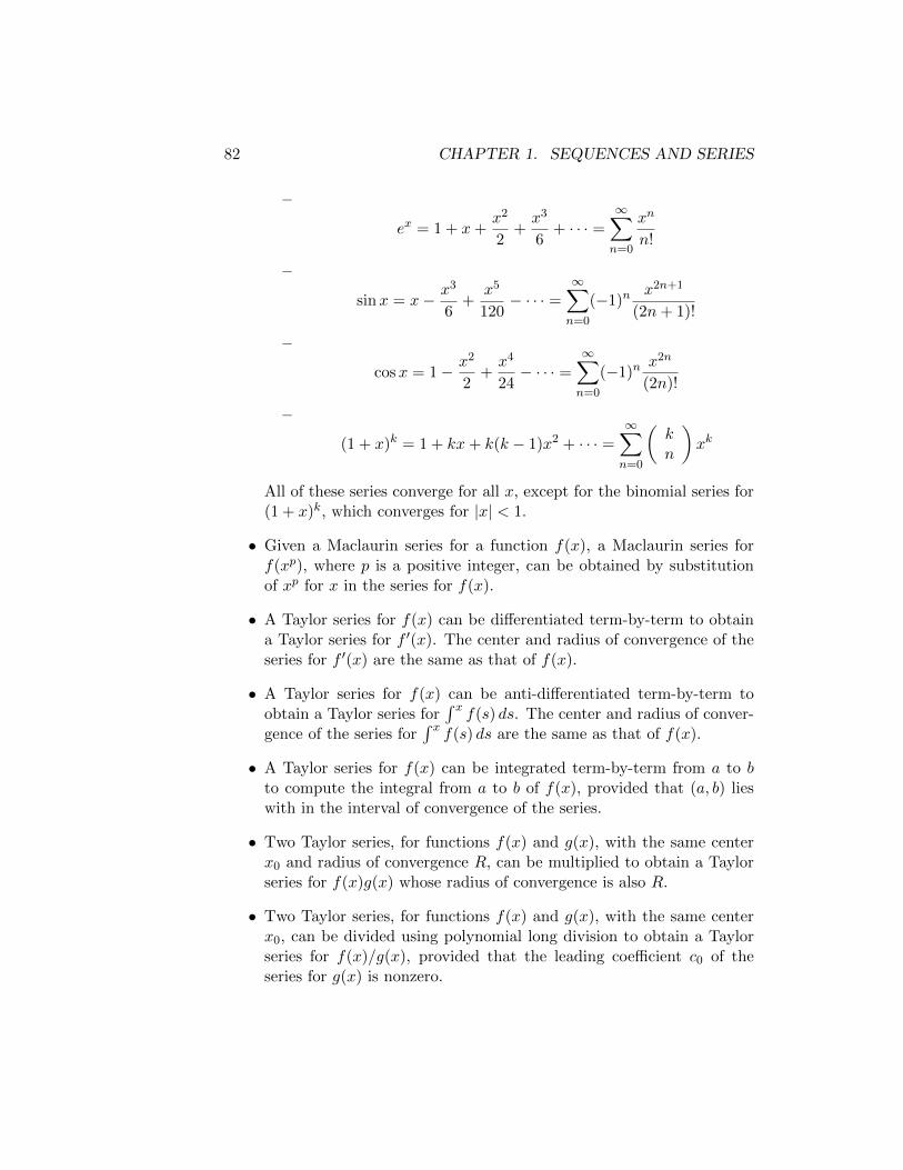
82 CHAPTER 1. SEQUENCES AND SERIES
–
ex = 1 + x+x2
2+x3
6+ · · · =
∞∑n=0
xn
n!
–
sinx = x− x3
6+
x5
120− · · · =
∞∑n=0
(−1)nx2n+1
(2n+ 1)!
–
cosx = 1− x2
2+x4
24− · · · =
∞∑n=0
(−1)nx2n
(2n)!
–
(1 + x)k = 1 + kx+ k(k − 1)x2 + · · · =∞∑n=0
(kn
)xk
All of these series converge for all x, except for the binomial series for(1 + x)k, which converges for |x| < 1.
• Given a Maclaurin series for a function f(x), a Maclaurin series forf(xp), where p is a positive integer, can be obtained by substitutionof xp for x in the series for f(x).
• A Taylor series for f(x) can be differentiated term-by-term to obtaina Taylor series for f ′(x). The center and radius of convergence of theseries for f ′(x) are the same as that of f(x).
• A Taylor series for f(x) can be anti-differentiated term-by-term toobtain a Taylor series for
∫ xf(s) ds. The center and radius of conver-
gence of the series for∫ x
f(s) ds are the same as that of f(x).
• A Taylor series for f(x) can be integrated term-by-term from a to bto compute the integral from a to b of f(x), provided that (a, b) lieswith in the interval of convergence of the series.
• Two Taylor series, for functions f(x) and g(x), with the same centerx0 and radius of convergence R, can be multiplied to obtain a Taylorseries for f(x)g(x) whose radius of convergence is also R.
• Two Taylor series, for functions f(x) and g(x), with the same centerx0, can be divided using polynomial long division to obtain a Taylorseries for f(x)/g(x), provided that the leading coefficient c0 of theseries for g(x) is nonzero.
1.10. REVIEW 83
1.10 Review
You should now be able to complete the following types of problems:
• Computing a formula for the terms of a sequence, given the first fewterms of the sequence. This involves detecting patterns such as an forsome constant a, or np for some integer p, or (−1)n for terms thatoscillate.
• Determining whether a sequence converges or diverges, and, if con-vergent, computing its limit. This may require techniques such asdividing the numerator and denominator by the highest power of n,multiplying and dividing by the conjugate of an expression involvingsquare roots, or using l’Hospital’s Rule. An understanding of whatkinds of functions grow faster than others can be helpful.
• Computing the limit of a recursively defined sequence {an}, in whichan+1 is defined in terms of an. You should also be able to show thatsuch a sequence is convergent using the Monotonic Sequence Theorem,which applies if the sequence is monotonic and bounded.
• Determining whether a geometric series∑arn converges or diverges,
by computing r and checking whether |r| < 1, and if it converges,computing its limit a/(1− r).
• Determining whether a series diverges using the Divergence Test. Aseries diverges if its terms do not converge to zero.
• Determining whether a telescoping series converges, and if it does,computing its limit. This may require partial fraction decomposition.
• Determining whether a series converges or diverges using the IntegralTest, Comparison Test, or the Limit Comparison Test. Note thatthese tests should only be applied to series whose terms are positiveand decreasing.
• Determining whether an alternating series converges, using the Alter-nating Series Test, and if it converges, computing an error estimateusing the Alternating Series Estimation Theorem.
• Determining whether a series converges or diverges using the RatioTest or the Root Test.
84 CHAPTER 1. SEQUENCES AND SERIES
• Computing a Taylor series of a given function f(x) around a givencenter x0, using the general formula for a Taylor series,
f(x) =∞∑n=0
f (n)(x0)
n!(x− x0)n.
• Using a Taylor series of a given function f(x), at a given center x0,to compute the value of a function to a given accuracy. To save time,you can use the Alternating Series Estimation Theorem to determinewhen sufficient accuracy has been achieved. This theorem states thatif s is the sum of an alternating series
s =∞∑n=0
(−1)nbn,
and sn is the nth partial sum, then
|s− sn| ≤ |bn+1|.
That is, the error in a partial sum is no larger than the first excludedterm. If the series is not alternating, then the Taylor remainder canbe used instead.
• Computing the Taylor series of a function by differentiating or inte-grating a known (or more easily obtained) Taylor series term-by-term.
• Computing a definite or indefinite integral by representing the inte-grand as a Taylor series, and integrating term-by-term. For a definiteintegral, you will be asked to compute the integral to a given accuracy.
• Using Taylor series to compute the sum of a given infinite series, byrecognizing the series as the evaluation of a known Taylor series at aspecific value of x.
When trying to determine which test should be applied to a series, it isadvisable to use a thought process such as the following:
• Do the terms even converge to zero? If not, you can simply apply theDivergence Test to conclude that the series diverges.
• Does the series fit the form of a geometric series∑arn?
1.10. REVIEW 85
• Is it a telescoping series? Such a series may have terms that are ex-pressed as a single fraction, which can then be rewritten as a differenceof two fractions using partial fraction decomposition.
• Do the terms of the series alternate in sign, due to a factor such as(−1)n? In that case, the Alternating Series Test may apply.
• If none of the above tests apply, consider the Ratio Test or the RootTest. The Root test is particularly useful if each term an of the seriesincludes an expression that is raised to the nth power. If either theRatio Test or Root Test is inconclusive, you should not attempt theother test, for it will be inconclusive as well.
• Next, consider the Integral Test, if the terms of a series describe afunction that can readily be integrated.
• Next, consider the Comparison Test, unless the terms are not clearlydecreasing, in which case the Limit Comparison Test may be morehelpful.
86 CHAPTER 1. SEQUENCES AND SERIES
Chapter 2
Vectors and the Geometry ofSpace
In this chapter, we will learn how to work with locations and directions inthree-dimensional space, in order to easily describe objects such as lines,planes and curves. This will set the stage for the study of functions of twovariables, the graphs of which are surfaces in space.
2.1 Three-Dimensional Coordinate Systems
2.1.1 Points in Three-Dimensional Space
Previously, we have identified a point in the xy-plane by an ordered pairthat consists of two real numbers, an x-coordinate and y-coordinate, whichdenote signed distances along the x-axis and y-axis, respectively, from theorigin, which is the point (0, 0). These axes, which are collectively referredto as the coordinate axes, divided the plane into four quadrants.
We now generalize these concepts to three-dimensional space, or xyz-space. In this space, a point is represented by an ordered triple (x, y, z)that consists of three numbers, an x-coordiante, a y-coordinate, and a z-coordinate. As in the two-dimensional xy-plane, these coordinates indicatethe signed distance along the coordinate axes, the x-axis, y-axis and z-axis,respectively, from the origin, denoted by O, which has coordinates (0, 0, 0).There is a one-to-one correspondence between a point in xyz-space and atriple in R3, which is the set of all ordered triples of real numbers. This cor-respondence is known as a three-dimensional rectangular coordinate system.
Example Figure 2.1 displays the point (2, 3, 1) in xyz-space, denoted by
87
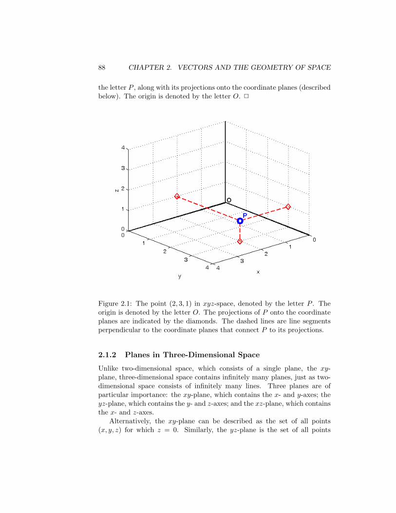
88 CHAPTER 2. VECTORS AND THE GEOMETRY OF SPACE
the letter P , along with its projections onto the coordinate planes (describedbelow). The origin is denoted by the letter O. 2
Figure 2.1: The point (2, 3, 1) in xyz-space, denoted by the letter P . Theorigin is denoted by the letter O. The projections of P onto the coordinateplanes are indicated by the diamonds. The dashed lines are line segmentsperpendicular to the coordinate planes that connect P to its projections.
2.1.2 Planes in Three-Dimensional Space
Unlike two-dimensional space, which consists of a single plane, the xy-plane, three-dimensional space contains infinitely many planes, just as two-dimensional space consists of infinitely many lines. Three planes are ofparticular importance: the xy-plane, which contains the x- and y-axes; theyz-plane, which contains the y- and z-axes; and the xz-plane, which containsthe x- and z-axes.
Alternatively, the xy-plane can be described as the set of all points(x, y, z) for which z = 0. Similarly, the yz-plane is the set of all points

2.1. THREE-DIMENSIONAL COORDINATE SYSTEMS 89
of the form (0, y, z), while the xz-plane is the set of all points of the form(x, 0, z).
Just as the x-axis and y-axis divide the xy-plane into four quadrants,these three planes divide xyz-space into eight octants. Within each octant,all x-coordiantes have the same sign, as do all y-coordinates, and all z-coordinates. In particular, the first octant is the octant in which all threecoordinates are positive.
2.1.3 Plotting Points in xyz-space
Graphing in xyz-space can be difficult because, unlike graphing in the xy-plane, depth perception is required. To simplify plotting of points, one canmake use of projections onto the coordinate planes. The projection of a point(x, y, z) onto the xy-plane is obtained by connecting the point to the xy-plane by a line segment that is perpendicular to the plane, and computingthe intersection of the line segment with the plane.
Later, we will learn more about how to compute projections of pointsonto planes, but in this relatively simple case, it follows from our workingdefinition that the projection of the point (x, y, z) onto the xy-plane is thepoint (x, y, 0). Similarly, the projection of this point onto the yz-plane isthe point (0, y, z), and the projection of this point onto the xz-plane is thepoint (x, 0, z). Figure 2.1 illustrates these projections, and how they can beused to plot a point in xyz-space. One can first plot the point’s projections,which is similar to the task of plotting points in the xy-plane, and then useline segments originating from these projections and perpendicular to thecoordinate planes to “locate” the point in xyz-space.
2.1.4 The Distance Formula
The distance between two points P1 = (x1, y1) and P2 = (x2, y2) in thexy-plane is given by the distance formula,
d(P1, P2) =√
(x2 − x1)2 + (y2 − y1)2.
Similarly, the distance between two points P1 = (x1, y1, z1) and P2 =(x2, y2, z2) in xyz-space is given by the following generalization of the dis-tance formula,
d(P1, P2) =√
(x2 − x1)2 + (y2 − y1)2 + (z2 − z1)2.
This can be proved by repeated application of the Pythagorean Theorem.
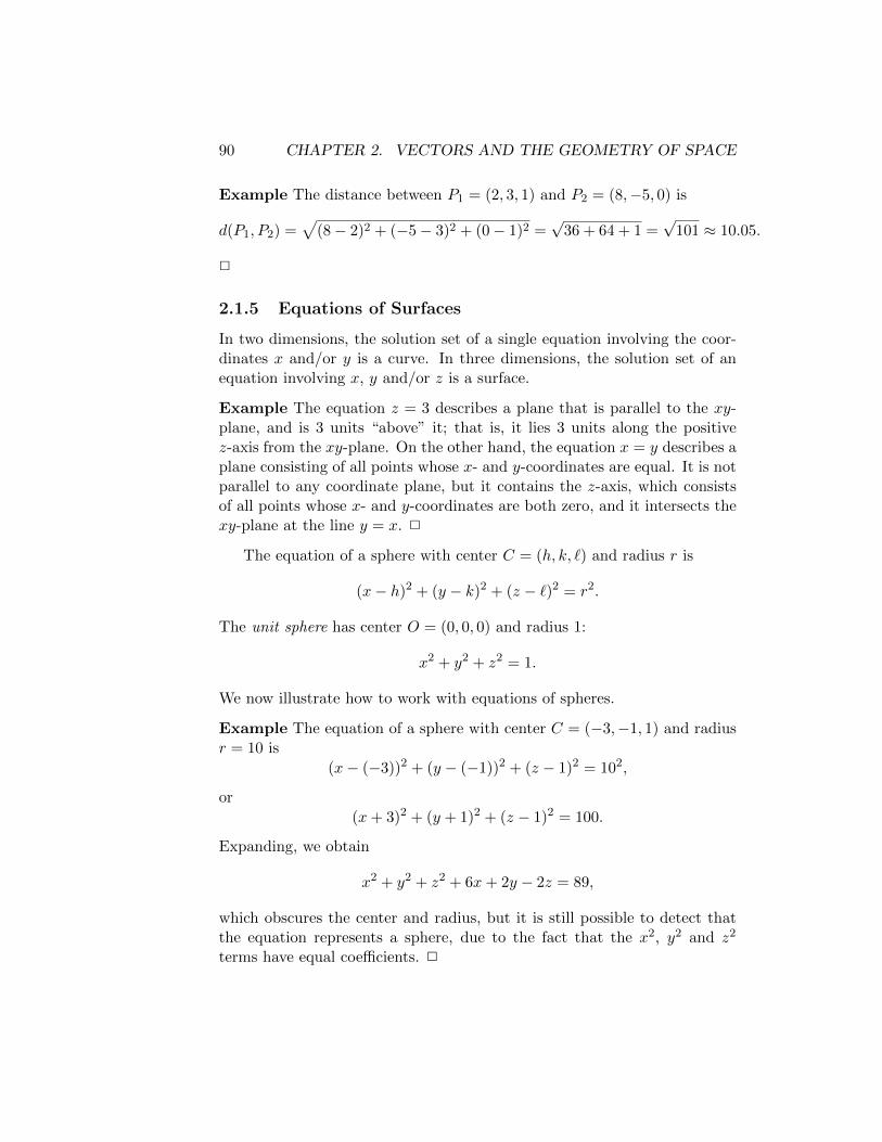
90 CHAPTER 2. VECTORS AND THE GEOMETRY OF SPACE
Example The distance between P1 = (2, 3, 1) and P2 = (8,−5, 0) is
d(P1, P2) =√
(8− 2)2 + (−5− 3)2 + (0− 1)2 =√
36 + 64 + 1 =√
101 ≈ 10.05.
2
2.1.5 Equations of Surfaces
In two dimensions, the solution set of a single equation involving the coor-dinates x and/or y is a curve. In three dimensions, the solution set of anequation involving x, y and/or z is a surface.
Example The equation z = 3 describes a plane that is parallel to the xy-plane, and is 3 units “above” it; that is, it lies 3 units along the positivez-axis from the xy-plane. On the other hand, the equation x = y describes aplane consisting of all points whose x- and y-coordinates are equal. It is notparallel to any coordinate plane, but it contains the z-axis, which consistsof all points whose x- and y-coordinates are both zero, and it intersects thexy-plane at the line y = x. 2
The equation of a sphere with center C = (h, k, `) and radius r is
(x− h)2 + (y − k)2 + (z − `)2 = r2.
The unit sphere has center O = (0, 0, 0) and radius 1:
x2 + y2 + z2 = 1.
We now illustrate how to work with equations of spheres.
Example The equation of a sphere with center C = (−3,−1, 1) and radiusr = 10 is
(x− (−3))2 + (y − (−1))2 + (z − 1)2 = 102,
or
(x+ 3)2 + (y + 1)2 + (z − 1)2 = 100.
Expanding, we obtain
x2 + y2 + z2 + 6x+ 2y − 2z = 89,
which obscures the center and radius, but it is still possible to detect thatthe equation represents a sphere, due to the fact that the x2, y2 and z2
terms have equal coefficients. 2
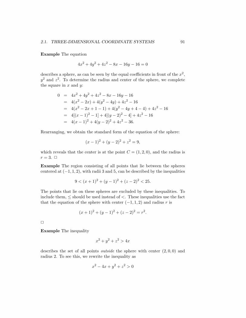
2.1. THREE-DIMENSIONAL COORDINATE SYSTEMS 91
Example The equation
4x2 + 4y2 + 4z2 − 8x− 16y − 16 = 0
describes a sphere, as can be seen by the equal coefficients in front of the x2,y2 and z2. To determine the radius and center of the sphere, we completethe square in x and y:
0 = 4x2 + 4y2 + 4z2 − 8x− 16y − 16
= 4(x2 − 2x) + 4(y2 − 4y) + 4z2 − 16
= 4(x2 − 2x+ 1− 1) + 4(y2 − 4y + 4− 4) + 4z2 − 16
= 4[(x− 1)2 − 1] + 4[(y − 2)2 − 4] + 4z2 − 16
= 4(x− 1)2 + 4(y − 2)2 + 4z2 − 36.
Rearranging, we obtain the standard form of the equation of the sphere:
(x− 1)2 + (y − 2)2 + z2 = 9,
which reveals that the center is at the point C = (1, 2, 0), and the radius isr = 3. 2
Example The region consisting of all points that lie between the spherescentered at (−1, 1, 2), with radii 3 and 5, can be described by the inequalities
9 < (x+ 1)2 + (y − 1)2 + (z − 2)2 < 25.
The points that lie on these spheres are excluded by these inequalities. Toinclude them, ≤ should be used instead of <. These inequalities use the factthat the equation of the sphere with center (−1, 1, 2) and radius r is
(x+ 1)2 + (y − 1)2 + (z − 2)2 = r2.
2
Example The inequality
x2 + y2 + z2 > 4x
describes the set of all points outside the sphere with center (2, 0, 0) andradius 2. To see this, we rewrite the inequality as
x2 − 4x+ y2 + z2 > 0
92 CHAPTER 2. VECTORS AND THE GEOMETRY OF SPACE
and then complete the square to obtain
x2 − 4x+ 4− 4 + y2 + z2 > 0.
Factoring the perfect square that has been completed, and then rearranging,yields
(x− 2)2 + y2 + z2 > 4.
This inequality, when changed to an equality, describes the sphere withcenter (2, 0, 0) and radius 2. The inequality prescribes that the distancebetween (x, y, z) and (2, 0, 0) be greater than 2, so (x, y, z) must lie outsidethis sphere. 2
2.1.6 Summary
• The three-dimensional rectangular coordinate system is the one-to-onecorrespondence between each point P in three-dimensional space, orxyz-space, and an ordered triple (x, y, z) in R3. The numbers x, y andz are the x-, y- and z-coordinates of P . The origin O is the point withcoordinates (0, 0, 0).
• The coordinate planes are: the xy-plane, the set of all points whose z-coordinate is zero; the yz-plane, the set of all points whose x-coordinateis zero; and the xz-plane, the set of all points whose y-coordinate iszero.
• The projection of a point P = (x, y, z) onto the xy-plane is the point(x, y, 0). The projection of P onto the yz-plane is the point (0, y, z).The projection of P onto the xz-plane is the point (x, 0, z).
• The distance formula states that the distance between two points inxyz-space is the square root of the sum of the squares of the differencesbetween corresponding coordinates. That is, given P1 = (x1, y1, z1)and P2 = (x2, y2, z2), the distance between P1 and P2 is given byd(P1, P2) =
√(x2 − x1)2 + (y2 − y1)2 + (z2 − z1)2.
• The equation of a sphere with center C = (x0, y0, z0) and radius r is(x− x0)2 + (y − y0)2 + (z − z0)2 = r2.
• An equation in which x2, y2 and z2 have the same coefficients describesa sphere; the center and radius can be determined by completing thesquare in x, y and z.
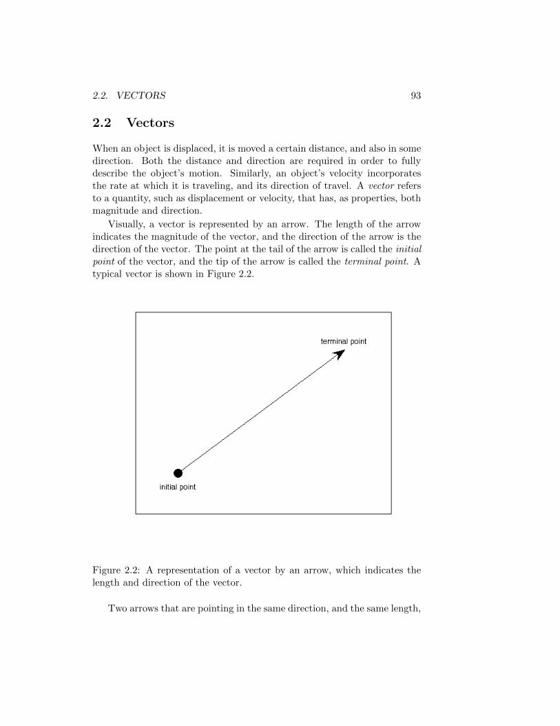
2.2. VECTORS 93
2.2 Vectors
When an object is displaced, it is moved a certain distance, and also in somedirection. Both the distance and direction are required in order to fullydescribe the object’s motion. Similarly, an object’s velocity incorporatesthe rate at which it is traveling, and its direction of travel. A vector refersto a quantity, such as displacement or velocity, that has, as properties, bothmagnitude and direction.
Visually, a vector is represented by an arrow. The length of the arrowindicates the magnitude of the vector, and the direction of the arrow is thedirection of the vector. The point at the tail of the arrow is called the initialpoint of the vector, and the tip of the arrow is called the terminal point. Atypical vector is shown in Figure 2.2.
Figure 2.2: A representation of a vector by an arrow, which indicates thelength and direction of the vector.
Two arrows that are pointing in the same direction, and the same length,
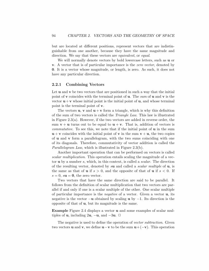
94 CHAPTER 2. VECTORS AND THE GEOMETRY OF SPACE
but are located at different positions, represent vectors that are indistin-guishable from one another, because they have the same magnitude anddirection. We say that these vectors are equivalent, or equal.
We will normally denote vectors by bold lowercase letters, such as u orv. A vector that is of particular importance is the zero vector, denoted by0. It is a vector whose magnitude, or length, is zero. As such, it does nothave any particular direction.
2.2.1 Combining Vectors
Let u and v be two vectors that are positioned in such a way that the initialpoint of v coincides with the terminal point of u. The sum of u and v is thevector u + v whose initial point is the initial point of u, and whose terminalpoint is the terminal point of v.
The vectors u, v and u + v form a triangle, which is why this definitionof the sum of two vectors is called the Triangle Law. This law is illustratedin Figure 2.3(a). However, if the two vectors are added in reverse order, thesum v + u turns out to be equal to u + v. That is, addition of vectors iscommutative. To see this, we note that if the initial point of u in the sumu + v coincides with the initial point of v in the sum v + u, the two copiesof u and v form a parallelogram, with the two sums coinciding with oneof its diagonals. Therefore, commutativity of vector addition is called theParallelogram Law, which is illustrated in Figure 2.3(b).
Another important operation that can be performed on vectors is calledscalar multiplication. This operation entails scaling the magnitude of a vec-tor u by a number s, which, in this context, is called a scalar. The directionof the resulting vector, denoted by su and called a scalar multiple of u, isthe same as that of u if s > 0, and the opposite of that of u if s < 0. Ifs = 0, su = 0, the zero vector.
Two vectors that have the same direction are said to be parallel. Itfollows from the definition of scalar multiplication that two vectors are par-allel if and only if one is a scalar multiple of the other. One scalar multipleof particular importance is the negative of a vector. Given a vector u, itsnegative is the vector −u obtained by scaling u by −1. Its direction is theopposite of that of u, but its magnitude is the same.
Example Figure 2.4 displays a vector u and some examples of scalar mul-tiples of u, including 2u, −u, and −3u. 2
The negative is used to define the operation of vector subtraction. Giventwo vectors u and v, we define u−v to be the sum u+(−v). This operation
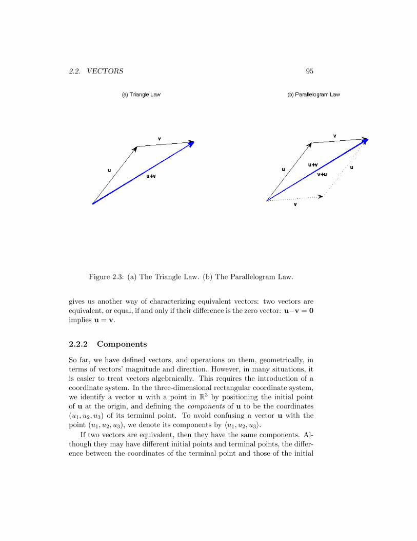
2.2. VECTORS 95
Figure 2.3: (a) The Triangle Law. (b) The Parallelogram Law.
gives us another way of characterizing equivalent vectors: two vectors areequivalent, or equal, if and only if their difference is the zero vector: u−v = 0implies u = v.
2.2.2 Components
So far, we have defined vectors, and operations on them, geometrically, interms of vectors’ magnitude and direction. However, in many situations, itis easier to treat vectors algebraically. This requires the introduction of acoordinate system. In the three-dimensional rectangular coordinate system,we identify a vector u with a point in R3 by positioning the initial pointof u at the origin, and defining the components of u to be the coordinates(u1, u2, u3) of its terminal point. To avoid confusing a vector u with thepoint (u1, u2, u3), we denote its components by 〈u1, u2, u3〉.
If two vectors are equivalent, then they have the same components. Al-though they may have different initial points and terminal points, the differ-ence between the coordinates of the terminal point and those of the initial
96 CHAPTER 2. VECTORS AND THE GEOMETRY OF SPACE
Figure 2.4: A vector u and various scalar multiples.
point are always equal to these components. That is, if a vector v has ini-tial point P1 = (x1, y1, z1) and terminal point P2 = (x2, y2, z2), then thecomponents of the vector v are
v = 〈x2 − x1, y2 − y1, z2 − z1〉.
If the initial point is the origin O = (0, 0, 0), we refer to the vector as theposition vector of the terminal point, since the components of the vector arethe same as the coordinates of the terminal point.
Example Let u be a vector with initial point U1 = (0, 0, 0) and terminalpoint U2 = (2, 3, 4). Let v be a vector with initial point V1 = (1, 2,−1) andterminal point V2 = (3, 6, 3). These vectors are equivalent, and both havecomponents 〈2, 3, 4〉. 2
The magnitude, or length, of a vector v = 〈v1, v2, v3〉, denoted by |v|,is the distance between its initial and terminal points. It follows from the
2.2. VECTORS 97
definiton of the vector’s components that
|v| =√v2
1 + v22 + v2
3.
Example Let v be a vector with initial point P1 = (−3, 4,−1) and terminalpoint P2 = (1, 5, 0). Then
|v| =√
(1− (−3))2 + (5− 4)2 + (0− (−1))2 =√
18 ≈ 4.24.
2
We have learned what it means to add, scale and subtract vectors, butonly in a geometric sense. It is essential to be able to understand theseoperations in terms of the components of vectors.
To that end, let u = 〈u1, u2, u3〉 and v = 〈v1, v2, v3〉 be vectors. Thenthe components of the sum u + v are given by
u + v = 〈u1 + v1, u2 + v2, u3 + v3〉.
We see that operating on the vectors involves applying the same operationto corresponding components.
Similarly, given a scalar s, the vector su is given by
su = 〈su1, su2, su3〉.
It follows thatu− v = 〈u1 − v1, u2 − v2, u3 − v3〉.
Example Let u = 〈7,−8, 9〉 and v = 〈−3, 4,−6〉. Then
u + v = 〈7 + (−3),−8 + 4, 9 + (−6)〉 = 〈4,−4, 3〉,
u− v = 〈7− (−3),−8− 4, 9− (−6)〉 = 〈10,−12, 15〉,
2u = 〈2(7), 2(−8), 2(9)〉 = 〈14,−16, 18〉,
and
3u− 2v = 〈3(7)− 2(−3), 3(−8)− 2(4), 3(9)− 2(−6)〉 = 〈27,−30, 39〉.
2
We have defined these operations for vectors in three dimensions, butthey generalize in a natural to way to vectors of any length. We define V3
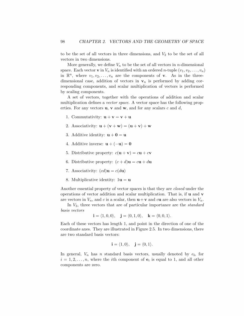
98 CHAPTER 2. VECTORS AND THE GEOMETRY OF SPACE
to be the set of all vectors in three dimensions, and V2 to be the set of allvectors in two dimensions.
More generally, we define Vn to be the set of all vectors in n-dimensionalspace. Each vector v in Vn is identified with an ordered n-tuple (v1, v2, . . . , vn)in Rn, where v1, v2, . . . , vn are the components of v. As in the three-dimensional case, addition of vectors in vn is performed by adding cor-responding components, and scalar multiplication of vectors is performedby scaling components.
A set of vectors, together with the operations of addition and scalarmultiplication defines a vector space. A vector space has the following prop-erties. For any vectors u, v and w, and for any scalars c and d,
1. Commutativity: u + v = v + u
2. Associativity: u + (v + w) = (u + v) + w
3. Additive identity: u + 0 = u
4. Additive inverse: u + (−u) = 0
5. Distributive property: c(u + v) = cu + cv
6. Distributive property: (c+ d)u = cu + du
7. Associativity: (cd)u = c(du)
8. Multiplicative identity: 1u = u
Another essential property of vector spaces is that they are closed under theoperations of vector addition and scalar multiplication. That is, if u and vare vectors in Vn, and c is a scalar, then u+v and cu are also vectors in Vn.
In V3, three vectors that are of particular importance are the standardbasis vectors
i = 〈1, 0, 0〉, j = 〈0, 1, 0〉, k = 〈0, 0, 1〉.
Each of these vectors has length 1, and point in the direction of one of thecoordinate axes. They are illustrated in Figure 2.5. In two dimensions, thereare two standard basis vectors:
i = 〈1, 0〉, j = 〈0, 1〉.
In general, Vn has n standard basis vectors, usually denoted by ei, fori = 1, 2, . . . , n, where the ith component of ei is equal to 1, and all othercomponents are zero.
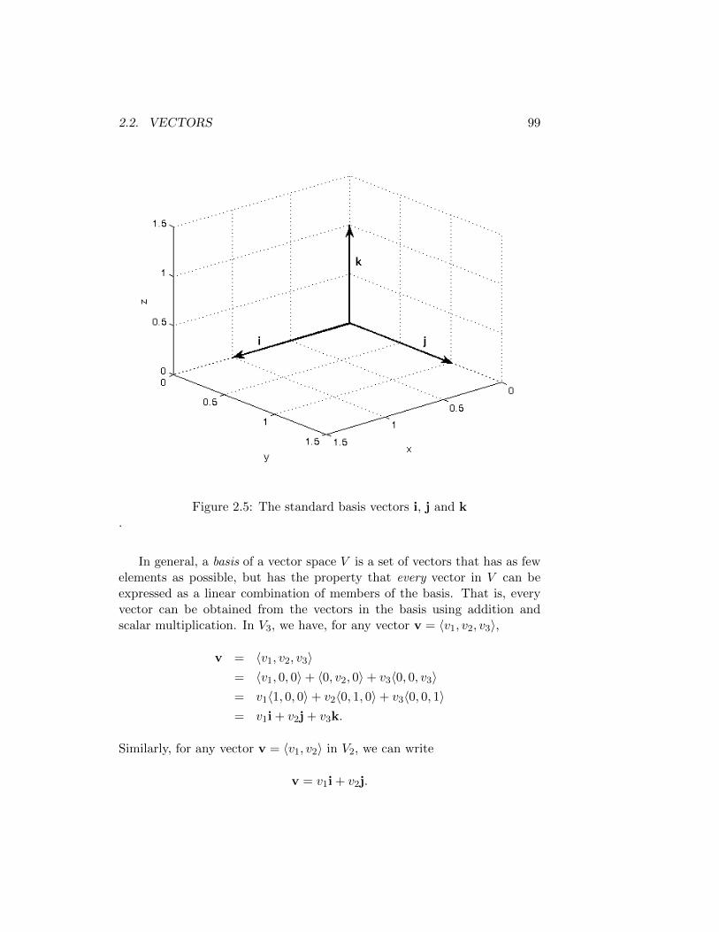
2.2. VECTORS 99
Figure 2.5: The standard basis vectors i, j and k.
In general, a basis of a vector space V is a set of vectors that has as fewelements as possible, but has the property that every vector in V can beexpressed as a linear combination of members of the basis. That is, everyvector can be obtained from the vectors in the basis using addition andscalar multiplication. In V3, we have, for any vector v = 〈v1, v2, v3〉,
v = 〈v1, v2, v3〉= 〈v1, 0, 0〉+ 〈0, v2, 0〉+ v3〈0, 0, v3〉= v1〈1, 0, 0〉+ v2〈0, 1, 0〉+ v3〈0, 0, 1〉= v1i + v2j + v3k.
Similarly, for any vector v = 〈v1, v2〉 in V2, we can write
v = v1i + v2j.
100 CHAPTER 2. VECTORS AND THE GEOMETRY OF SPACE
Example Let u = 〈2,−1, 3〉 and v = 〈−4, 5, 0〉. Then we can write
u = 2i− j + 3k, v = −4i + 5j,
and then
u + v = 2i− j + 3k− 4i + 5j = (2− 4)i + (−1 + 5)j + 3k = −2i + 4j + 3k.
2
A vector has both magnitude and direction, but often we are only inter-ested in the direction of a nonzero vector v. It is helpful to “filter out” themagnitude by normalizing it so that its magnitude is 1. This is accomplishedby dividing by its magnitude, which yields a unit vector u that has thesame direction of v. Specifically,
u =1
|v|v.
Then
|u| =∣∣∣∣ 1
|v|v
∣∣∣∣ =|v||v|
= 1.
Example Let v = 〈3,−4, 5〉. Then
|v| =√
32 + (−4)2 + 52 =√
50 = 5√
2,
and the unit vector u with the same direction as v is
u =
√2
10〈3,−4, 5〉 =
⟨3√
2
10,−2√
2
5,
√2
2
⟩.
2
Example Consider the vector w = 〈2, 4,−3〉. We wish to compute a vectorz that is in the opposite direction of w, and has magnitude 5. First, weneed to identify the magnitude and direction of w. The magnitude is givenby
|w| =√
22 + 42 + (−3)2 =√
29.
Then, a unit vector in the same direction of w is
u =
⟨2√29,
4√29,− 3√
29
⟩.
2.2. VECTORS 101
It follows that a unit vector in the opposite direction of w is
−u =
⟨− 2√
29,− 4√
29,
3√29
⟩.
We conclude that a vector in the opposite direction of w, with magnitude5, is
z = −5u = − 5
|w|w =
⟨− 10√
29,− 20√
29,
15√29
⟩.
2
Example Let v be a vector in the xy-plane with initial point (0, 0), andmagnitude
√2, that makes an angle of 3π/4 with the positive x-axis. To
find the components of v, we note that these components are equal to thecoordinates of its terminal point, because its initial point is at the origin.These coordinates are obtained from the magnitude and angle with thepositive x-axis as follows:
v =√
2
⟨cos
3π
4, sin
3π
4
⟩=√
2
⟨√2
2,
√2
2
⟩= 〈1, 1〉.
2
Example Suppose that a plane is steered northeast, at an air speed of 400mph, while the wind is blowing westward at 100 mph. To compute theground speed of the plane, which accounts for both the steering and thewind, we need to add the velocity vectors corresponding to the plane andthe wind. This yields a resultant velocity vector, whose magnitude is theground speed.
To perform the addition of the velocity vectors, we need their compo-nents. For the plane’s vector, the magnitude is 400, and its direction isidentified by an angle of π/4 radians with the positive x-axis, correspondingto northeast. It follows that the components of this vector are
v = 400⟨
cosπ
4, sin
π
4
⟩= 400
⟨√2
2,
√2
2
⟩= 〈200
√2, 200
√2〉.
Similarly, the wind’s velocity vector, which makes an angle of π radianswith the positive x-axis, corresponding to west, is
w = 100〈cosπ, sinπ〉 = 100〈−1, 0〉 = 〈−100, 0〉.
102 CHAPTER 2. VECTORS AND THE GEOMETRY OF SPACE
We now perform the addition to obtain the plane’s true course:
c = v + w = 〈200√
2, 200√
2〉+ 〈−100, 0〉 = 〈200√
2− 100, 200√
2〉.
To obtain the ground speed, we compute its magnitude, and obtain
|c| =√
(200√
2− 100)2 + (200√
2)2 = 100
√(2√
2− 1)2 + (2√
2)2 = 100
√17− 4
√2 ≈ 336.796.
We conclude that the ground speed of the plane is approximately 336.796mph, which is slower than the plane’s air speed, because the wind is largelyblowing against the direction in which the plane is steered. On the otherhand, if the wind were to blow to the north, the ground speed of the planewould be faster than its air speed. 2
Example Suppose a box is being pulled along the ground with a force of50 newtons, applied at an angle of 60◦ from the horizontal. Then, the forcevector F has a magnitude of 50, and a direction
〈cos 60◦, sin 60◦〉 =
⟨1
2,
√3
2
⟩.
It follows that F can be written as a sum of horizontal and vertical compo-nents,
F = 50
⟨1
2,
√3
2
⟩= 50
⟨1
2, 0
⟩+50
⟨0,
√3
2
⟩= 〈25, 0〉+〈0, 25
√3〉 = 25i+25
√3j.
2
2.2.3 Summary
• A vector is a quantity that has both a magnitude and a direction.It can be represented, geometrically, by an arrow that points in thevector’s direction, and has a length equal to the vector’s magnitude.The tip of the arrow is called the vector’s terminal point, and the tailof the arrow is its initial point.
• The zero vector is a vector whose magnitude is zero. It is the onlyvector that has no specific direction.
• Geometrically, the sum of two vectors u and v is the vector u + vobtained by placing the terminal point of u at the initial point of v,and defining the sum to be the vector with u’s initial point and v’sterminal point. This is called the Triangle Law.
2.3. THE DOT PRODUCT 103
• Vector addition is commutative: u + v = v + u. This is called theParallelogram Law.
• Given a number s and vector u, the vector su is a scalar multiple ofu and s is called a scalar. It has the same direction as u, and itsmagnitude is s times the magnitude of u.
• The negative of a vector u, denoted by −u, is defined by (−1)u. Ithas the opposite direction of u, and the same magnitude.
• The difference of two vectors u and v, denoted by u− v, is defined tobe u + (−v).
• The components u1, u2 and u3 of a vector u = 〈u1, u2, u3〉 are definedto be the rectangular coordinates of its terminal point (u1, u2, u3),when its initial point is the origin.
• The magnitude of a vector v = 〈v1, v2, v3〉 is equal to the distancebetween its initial point and terminal point, which is
√v2
1 + v22 + v2
3.
• The components of the sum of two vectors are the sums of correspond-ing components of the two vectors.
• The components of a vector multiplied by a scalar are the componentsmultiplied by the same scalar.
• The standard basis vectors i, j, and k are vectors of magnitude 1 thatpoint in the directions of the positive x-, y- and z-axes, respectively.Any vector in three-dimensional space can be expressed as a linearcombination of these vectors.
• A unit vector is a vector of magnitude 1. A nonzero vector can benormalized by dividing it by its magnitude, to obtain a unit vector inthe same direction.
2.3 The Dot Product
One of the most fundamental problems concerning vectors is that of com-puting the angle between two given vectors. It has numerous applicationsin mathematics and other sciences. In physics, it plays a role in the de-composition of forces into component forces that act in various directions.In computer science, it is useful for creating two-dimensional visualizationsof three-dimensional objects. In computational mathematics, it is a vital
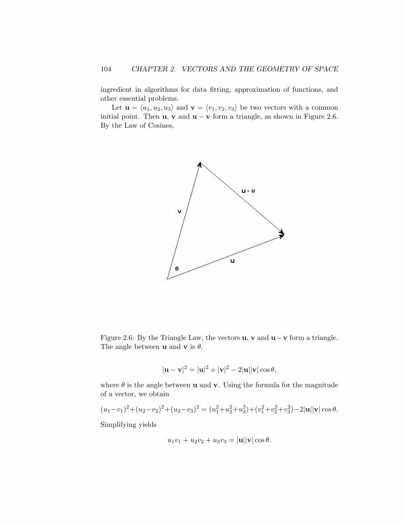
104 CHAPTER 2. VECTORS AND THE GEOMETRY OF SPACE
ingredient in algorithms for data fitting, approximation of functions, andother essential problems.
Let u = 〈u1, u2, u3〉 and v = 〈v1, v2, v3〉 be two vectors with a commoninitial point. Then u, v and u− v form a triangle, as shown in Figure 2.6.By the Law of Cosines,
Figure 2.6: By the Triangle Law, the vectors u, v and u−v form a triangle.The angle between u and v is θ.
|u− v|2 = |u|2 + |v|2 − 2|u||v| cos θ,
where θ is the angle between u and v. Using the formula for the magnitudeof a vector, we obtain
(u1−v1)2+(u2−v2)2+(u3−v3)2 = (u21+u2
2+u23)+(v2
1+v22+v2
3)−2|u||v| cos θ.
Simplifying yields
u1v1 + u2v2 + u3v3 = |u||v| cos θ.
2.3. THE DOT PRODUCT 105
We therefore define the dot product, also known as the inner product, ofu and v to be the number u · v given by
u · v = u1v1 + u2v2 + u3v3.
An equivalent definition, typically used in physics, is
u · v = |u||v| cos θ,
where θ is the angle between u and v.
Example Let u = 〈1,−1, 2〉 and v = 〈−2, 1, 3〉. Then
u · v = 1(−2) + (−1)(1) + 2(3) = −2− 1 + 6 = 3.
To obtain the angle θ between u and v, we compute
cos θ =u · v|u||v|
=3√
6√
14=
3
2√
21,
which yields θ ≈ 1.237 radians, or 70.893 degrees. 2
Example Let u and v be vectors such that |u| = 3, |v| = 4, and the anglebetween them is π/3 radians, or 60 degrees. Then
u · v = 3(4) cosπ
3= 12
1
2= 6.
2
2.3.1 Properties
The dot product has the following properties, which can be proved from thedefinition.
1. u · u = |u|2
2. Commutativity: u · v = v · u
3. Distributive property: u · (v + w) = u · v + u ·w
4. (cu) · v = c(u · v) = u · (cv), for any scalar c
5. 0 · u = 0
106 CHAPTER 2. VECTORS AND THE GEOMETRY OF SPACE
Example By the first, second and third properties, the length of a sum ofvectors u + v can be expressed in terms of inner products as follows:
|u + v|2 = (u + v) · (u + v)
= u · u + v · u + u · v + v · v= |u|2 + 2u · v + |v|2.
2
2.3.2 Orthogonality
Suppose that two nonzero vectors u and v have an angle between them thatis θ = π/2. That is, u and v are perpendicular, or orthogonal. Then, wehave
u · v = |u||v| cosπ
2= 0.
On the other hand, if u · v = 0, then we must have cos θ = 0, where θ is theangle between them, which implies that θ = π/2, and therefore u and v areorthogonal. In summary, u · v = 0 if and only if u and v are orthogonal.
Example Let u = 〈α, β〉 be any nonzero vector in V2. Then a vector thathas the same length as u, and is orthogonal to u is v = 〈β,−α〉. To verifythis, we compute
u · v = 〈α, β〉 · 〈β,−α〉 = αβ + β(−α) = 0.
By the fourth property of the dot product, w = 〈−β, α〉 also satisfies |w| =|u|, and is orthogonal to u. 2
2.3.3 Projections
When a three-dimensional object is to be displayed on a two-dimensionalsurface, it is necessary to determine where each point in the object appearswithin that surface. When a force is applied to an object from a partic-ular direction, for example to push the object along a horizontal surface,it is helpful to decompose the force into component forces that each actfrom orthogonal directions, such as vertical, corresponding to gravity, andhorizontal, corresponding to the direction of displacement.
These are examples of applications in which it is necessary to project agiven vector u = 〈u1, u2, u3〉 onto another vector v = 〈v1, v2, v3〉. Projectionrequires solving this problem: what vector, in the direction of v, is the bestapproximation of u?
2.3. THE DOT PRODUCT 107
In other words, we wish to find the vector w = cv, where c is an unknownscalar, that minimizes |u − w|, the distance between u and w. Using thepropeties of the dot product, we obtain
|u−w|2 = (u− cv) · (u− cv)
= |u|2 − 2cv · u + c2|v|2.
Differentiating with respect to c, we obtain the equation
−2v · u + 2c|v|2 = 0.
It follows that w = cv is the best approximation to u if
c =v · u|v|2
.
We therefore define the vector projection of u onto v by
w = projvu = cv =v · u|v|2
v.
This projection can also be written as
projvu =v · u|v|
v
|v|= (q · u)q = (compvu)q
whereq =
v
|v|is the unit vector in the direction of v, and
compvu = q · u =v · u|v|
is called the scalar projection of u onto v. Note that the absolute value ofthe scalar projection is also the magnitude of the vector projection.
The scalar projection can also be written as
compvu = q · u = |q||u| cos θ = |u| cos θ,
where θ is the angle between u and v, which is also the angle between uand q. Furthermore, since the vector projection of u onto v is the bestapproximation of u by a vector in the direction of v, the “error” in thisapproximation is orthogonal to v. That is,
v · (u− projvu) = v · u− v · u|v|2
v · v = v · u− v · u = 0,
108 CHAPTER 2. VECTORS AND THE GEOMETRY OF SPACE
by the properties of the dot product.
Example Let u = 〈2, 4〉 and v = 〈1, 1〉. Then the unit vector in the directionof v is
q =〈1, 1〉√
2=
⟨1√2,
1√2
⟩.
It follows that
compvu = q · u =
⟨1√2,
1√2
⟩· 〈2, 4〉 =
6√2
= 3√
2,
and
projvu = (compvu)q = 3√
2
⟨1√2,
1√2
⟩= 〈3, 3〉 .
This projection is shown in Figure 2.7. 2
Example Let u = 〈3, 4, 5〉 and v = 〈1, 1, 1〉. Then the unit vector in thedirection of v is
q =〈1, 1, 1〉√
3=
⟨1√3,
1√3,
1√3
⟩.
It follows that
compvu = q · u =
⟨1√3,
1√3,
1√3
⟩· 〈3, 4, 5〉 =
12√3
= 4√
3,
and
projvu = (compvu)q = 4√
3
⟨1√3,
1√3,
1√3
⟩= 〈4, 4, 4〉.
This projection is shown in Figure 2.8. 2
Example Suppose that a box is pulled 10 m along the ground by a constantforce of 50 N that is applied at an angle of 30◦ above the horizontal. Then,the horizontal force can be obtained by computing the vector projectionof the force vector F = 50〈cos 30◦, sin 30◦〉 onto the displacement vectorD = 10〈1, 0〉:
compDF =50⟨√
32 ,
12
⟩· 10〈1, 0〉
|10〈1, 0〉|= 25
√3,
projDF = compDFD
|D|= 25
√3
10〈1, 0〉|10〈1, 0〉
= 25√
3〈1, 0〉.
Since the displacement vector and the horizontal force vector have thesame direction, it follows that the total work done, which is defined to be
2.3. THE DOT PRODUCT 109
the product of force and distance when the force is applied in the directionof displacement, is equal to the product of the magnitudes of the horizontalforce and displacement vectors, which is
W = |projDF||D| = (25√
3)(10) = 250√
3.
More generally, the amount of work done by a force F to displace an objectalong the displacement vector D is given by
W = (projDF) ·D =(F ·D)D
|D|2·D =
(F ·D)(D ·D)
D ·D= F ·D.
This is a natural generalization of the basic formula for work, W = FD,where F is the amount of force applied to the object along the direction ofdisplacement, and D is the distance that the object is moved. 2
2.3.4 Summary
• The dot product, or inner product, of two vectors, is the sum of theproducts of corresponding components. Equivalently, it is the productof their magnitudes, times the cosine of the angle between them.
• The dot product of a vector with itself is the square of its magnitude.
• The dot product of two vectors is commutative; that is, the order ofthe vectors in the product does not matter.
• Multiplying a vector by a constant multiplies its dot product with anyother vector by the same constant.
• The dot product of a vector with the zero vector is zero.
• Two nonzero vectors are perpendicular, or orthogonal, if and only iftheir dot product is equal to zero.
• The scalar projection of a vector u onto a vector v is q ·u, where q isthe unit vector in the direction of v.
• The vector projection of u onto v is the scalar projection of u onto vtimes q, where q is the unit vector in the direction of v.
• The vector projection of u onto v is the best approximation of u inthe direction of v, in the sense that the difference between u and itsvector projection onto v is orthogonal to v.
110 CHAPTER 2. VECTORS AND THE GEOMETRY OF SPACE
• The work done by a force that is applied at an angle to the displace-ment vector can be computed by projecting the force vector onto thedisplacement vector, and then multiplying the magnitudes of the forceand displacement vectors.
2.4 The Cross Product
In three-dimensional space, or xyz-space, the set of solutions of an equationin x, y and z defines a surface. When the equation is linear, such as
y = 3, x = y, or 2x+ 3y − z = 0,
the solutions define a plane. On the other hand, a plane can also be definedin terms of any two vectors contained with in it. For example, the xy-planeis the set of all displacement vectors of the form v = xi + yj, where x and yare real numbers. That is, any vector in the xy-plane is a linear combinationof i and j.
This definition of a plane, however, does not readily lend itself to anequation that characterizes it. To obtain such an equation, it is helpful tonote that a plane can be viewed as the set of all vectors that are orthogonalto a particular direction. Therefore, given two vectors u = 〈u1, u2, u3〉 andv = 〈v1, v2, v3〉 that define a plane, we need to be able to compute a vectorw = 〈w1, w2, w3〉 that is orthogonal to both of them. Then, by the propertiesof the dot product, any vector z = cu+dv, which is contained in this plane,satisfies
w · z = w · (cu + dv) = cw · u + dw · v = 0,
so w is orthogonal to the entire plane.
To compute w, we note that because u ·w and v ·w = 0, its componentssatisfy the equations
u1w1 + u2w2 + u3w3 = 0,
v1w1 + v2w2 + v3w3 = 0.
For simplicity, we assume u1 6= 0. To eliminate w1 from the second equation,we subtract v1/u1 times the first equation from the second to obtain
u1w1 + u2w2 + u3w3 = 0,(v2 −
v1
u1u2
)w2 +
(v3 −
v1
u1u3
)w3 = 0.
2.4. THE CROSS PRODUCT 111
Multiplying the second equation by u1 yields
u1w1 + u2w2 + u3w3 = 0,
(u1v2 − u2v1)w2 + (u1v3 − u3v1)w3 = 0.
By viewing the second equation as a dot product being equal to zero, andUsing the fact that the vector 〈−β, α〉 is orthogonal to the vector 〈α, β〉, weobtain
w2 = u3v1 − u1v3, w3 = u1v2 − u2v1.
Substituting these values into the first equation yields
w1 = −u2
u1(u3v1 − u1v3)− u3
u1(u1v2 − u2v1) = u2v3 − u3v2.
We conclude that the vector
w = 〈u2v3 − u3v2, u3v1 − u1v3, u1v2 − u2v1〉
is orthogonal to both u and v. We define w to be the cross product of uand v, and write
w = u× v.
We note that the above system of equations has infinitely many solutions.We have chosen the particular solution denoted by w because its componentscan be computed without having to divide by any of the components of uand v, thus avoiding any requirement that any of these components benonzero. This condition uniquely determines the magnitude of w, but notits direction; this ambiguity will be resolved shortly.
Example Let u = 〈2,−1, 1〉 and v = 〈1, 2, 1〉. Then
u× v = 〈(−1)1− 2(1), 1(1)− 2(1), 2(2)− (−1)(1)〉 = 〈−3,−1, 5〉.
The vectors u, v and u× v are shown in Figure 2.9. 2
Example Consider the plane that contains the three points P1 = (1, 1, 0),P2 = (−1, 3, 1), and P3 = (−1,−1,−1). We wish to compute the vectorw that is orthogonal to all vectors contained in this plane. This can beaccomplished by computing vectors u and v with initial and terminal pointstaken from the three points P1, P2, and P3.
Specifically, we define
u = ~P1P2 = 〈−1− 1, 3− 1, 1− 0〉 = 〈−2, 2, 1〉,
112 CHAPTER 2. VECTORS AND THE GEOMETRY OF SPACE
v = ~P1P3 = 〈−1− 1,−1− 1,−1− 0〉 = 〈−2,−2,−1〉.
Then, we have
w = u× v
= 〈−2, 2, 1〉 × 〈−2,−2,−1〉= 〈2(−1)− 1(−2), 1(−2)− (−2)(−1),−2(−2)− 2(−2)〉= 〈0,−4, 8〉.
These vectors are shown in Figure 2.10. 2
Another way to derive the cross product is in terms of the determinantof the matrix
A =
i j ku1 u2 u3
v1 v2 v3
,where, as before, i, j and k are the standard basis vectors. We have
w = u× v = det(A).
This definition follows from Cramer’s rule, which expresses the solution toa system of linear equations in terms of determinants.
We now compute the magnitude of the cross product. We have
|w|2 = w21 + w2
2 + w23
= (u2v3 − u3v2)2 + (u3v1 − u1v3)2 + (u1v2 − u2v1)2
= u22v
23 − 2u2u3v2v3 + u2
3v22 + u2
3v21 − 2u1u3v1v3 + u2
1v23 + u2
1v22 − 2u1u2v1v2 + u2
2v21
= u22v
23 − 2u2u3v2v3 + u2
3v22 + u2
3v21 − 2u1u3v1v3 + u2
1v23 + u2
1v22 − 2u1u2v1v2 + u2
2v21 +
(u21v
21 + u2
2v22 + u2
3v23)− (u2
1v21 + u2
2v22 + u2
3v23)
= (u21 + u2
2 + u23)(v2
1 + v22 + v2
3)−(2u2v2u3v3 + 2u1v1u3v3 + 2u1v1u2v2 + u2
1v21 + u2
2v22 + u2
3v23)
= |u|2|v|2 − (u · v)2
= |u|2|v|2 − |u|2|v|2 cos2 θ
= |u|2|v|2(1− cos2 θ)
= |u|2|v|2 sin2 θ.
where θ is the angle between u and v, with 0 ≤ θ ≤ π. We conclude
|u× v| = |u||v| sin θ.
2.4. THE CROSS PRODUCT 113
The direction of u × v is not uniquely determined by the fact that itis orthogonal to both u and v, for its negative also has this property. Theproper direction is determined by the right-hand rule. This rule states thatif the fingers of the right hand are curled in the direction of rotation fromu to v, through an angle less than 180◦, then the thumb is pointing in thedirection of u× v.
2.4.1 Parallel Vectors
We have learned that the Cross Product can be used to compute a vector win V3 that is orthogonal to two given vectors u and v that, together, definea plane in xyz-space. However, two given vectors do not necessarily define aplane; it is required that they not be parallel. If u and v are parallel, then,by the definition of the cross product, we obtain
w = u× v = 0.
This is consistent with the fact that |u × v| = |u||v| sin θ, where θ is theangle between u and v. If u and v are parallel, then this angle is either 0 orπ radians, and in either case, the sine of that angle is zero.
Example The vectors u = 〈2, 1, 2〉 and v = 〈−4,−2,−4〉 are parallel, asv = −2u. That is, v has twice the magnitude of u, and the oppositedirection. It follows that u× v = 0. 2
2.4.2 Properties
The following properties are useful for performing complex vector operationsthat involve the cross product.
1. Anticommutativity: v × u = −(u× v)
2. Scalar multiplication: (cu)× v = u× (cv)
3. Distribution over addition: w×(u+v) = w×u+w×v, (u+v)×w =u×w + v ×w.
4. w · (u× v) = (w × u) · v5. w × (u× v) = (w · v)u− (w · u)v
2.4.3 Areas
The magnitude of the cross product has useful geometric applications. Con-sider a parallelogram with vectors u and v as adjacent sides, such that theangle θ between them, that is internal to the parallelogram, is not more than
114 CHAPTER 2. VECTORS AND THE GEOMETRY OF SPACE
90 degrees. The area of this parallelogram is the product of the lengths ofits base and its height. If we choose u to be its base, then, by right triangletrigonometry, its height is given by |v| sin θ, where sin θ > 0 due to the factthat 0 < θ < 90◦.
It follows that the area A of the parallelogram is
A = |u||v| sin θ = |u× v|.
That is, the magnitude of the cross product of u and v yields the area of aparallelogram with adjacent sides u and v. We have assumed that the anglebetween them is no more than 90 degrees, but if this is not the case, we canobtain the same result by instead defining the parallelogram in terms of −uand v, in view of the fact that | − u| = |u|.
This same formula can be used to compute the area of a triangle withadjacent sides defined by u and v. The area A of such a triangle is given by
A =1
2|u× v|,
since a parallelogram consists of two triangles of equal area that share aside.
Example We will compute the area of the triangle whose vertices are thepoints P1 = (1, 1, 0), P2 = (3, 0, 4) and P3 = (0, 5, 2). This triangle is half ofa parallelogram with adjacent sides
u = ~P1P2 = 〈2,−1, 4〉, v = ~P1P3 = 〈−1, 4, 2〉.
The area of this parallelogram is
|u×v| = |〈−1(2)−4(4), 4(−1)−2(2), 2(4)−(−1)(−1)〉| = |〈−18,−8, 7〉| =√
437 ≈ 23.345.
Therefore, the area of the triangle is√
545/2 ≈ 10.452.Alternatively, we can compute the angle θ between u and v, using the
dot product:
cos θ =u · v|u||v|
=1√
26√
21=
1√546
.
This yields θ = cos−1(1/√
546) ≈ 1.528 radians, or 87.547◦. Then, wecompute
|u×v| = |u||v| sin θ =√
21√
26√
1− cos2 θ =√
546
√1− 1
546=√
546
√545
546=√
545,
where we have used the identity cos2 θ + sin2 θ = 1. 2
2.4. THE CROSS PRODUCT 115
2.4.4 Volumes
The cross product and dot product can be used together to compute thevolume of a parallelepiped. Let u, v and w be three vectors that do not liewithin the same plane. Then, they define three sides of a parallelepiped, inwhich any two of them define a parallelogram that serves as one of its sixfaces.
The volume of the parallelepiped is the area of the base parallelogramtimes the height. Let the parallelogram defined by u and v be the base.We know that its area is |u × v|. To obtain the height, we first note thatthe height must be measured along a direction that is perpendicular to thebase; that is, it should be in the direction of z or −z.
Then, by right-triangle trigonometry, the height is |w|| cos θ|, where θ isthe angle between w and z. It follows that the volume V of the parallelepipedis
V = |z||w|| cos θ| = |w · z| = |w · (u× v)|.
We refer to this combination of the dot and cross products as the tripleproduct of u, v and w.
Example Consider the parallelepiped, shown in Figure 2.11, defined by thevectors
u = 〈3, 1, 1〉, v = 〈1, 5, 1〉, w = 〈0, 1, 2〉.
To compute its volume, we define the base to be the parallelogram withedges u and v. Then, we compute
z = u× v = 〈1(1)− 1(5), 1(1)− 3(1), 3(5)− 1(1)〉 = 〈−4,−2, 14〉.
Finally, we obtain the volume by the triple product
|w · (u× v)| = |w · z| = |〈0, 1, 2〉 · 〈−4,−2, 14〉| = 26.
2
2.4.5 Summary
• The cross product of two nonzero vectors u and v is a vector w = u×vthat is orthogonal to both u and v.
• The magnitude of u× v is |u||v| sin θ, where θ is the angle between uand v, with 0 ≤ θ ≤ π.
116 CHAPTER 2. VECTORS AND THE GEOMETRY OF SPACE
• The direction of u× v is determined by the direction of the thumb ofthe right hand, when the fingers are rotated from u to v through theangle θ between u and v, with 0 ≤ θ ≤ π.
• A vector that is orthogonal to all vectors in a given plane can becomputed from any three points in the plane by first subtracting thecoordinates of the points to obtain two vectors in the plane, and thencomputing their cross product.
• The cross product of two parallel vectors is the zero vector.
• The magnitude of the cross product of two vectors is the area of aparallelogram with the two vectors defining adjacent sides.
• The triple product of three vectors u, v and w, given by |w · (u×v)|,is the volume of the parallelepiped defined by u, v and w.
2.5 Equations of Lines and Planes
2.5.1 Equations of Lines
A line can be viewed, conceptually, as the set of all points in space thatsatisfy two criteria:
1. They contain a particular point, which we identify by a position vectorr0.
2. The vector between r0 and any position vector r on the line is parallelto a given vector v.
The vector with initial point r0 and terminal point r is given by s = r− r0.This vector must be parallel to v, which implies that s = tv for some scalart. It follows that any position vector r, corresponding to a point P on theline with coordinates equal to the components of r, has the form
r = r0 + tv,
where t is a scalar that is called a parameter. The parameter t is allowed toassume any value, so that any point P on the line can be obtained from thisequation, which is called the vector equation of the line. Such an equationis illustrated in Figure 2.12.
Let r = 〈x, y, z〉 be the position vector of any point P = (x, y, z) ona line, and let r0 = 〈x0, y0, z0〉 be the position vector of a particular point
2.5. EQUATIONS OF LINES AND PLANES 117
P0 = (x0, y0, z0) on the line. Furthermore, let v = 〈a, b, c〉 be the vector thatindicates the direction of the line. By writing the vector equation of the linein terms of components, we obtain the parametric equations of the line,
x = x0 + at, y = y0 + bt, z = z0 + ct.
The components a, b and c of v are called the direction numbers of the line.
Example Let r0 = 〈1, 2, 0〉 and v = 〈1,−3, 2〉. Then the vector equation ofthe line containing r0 and parallel to v is
r = 〈1, 2, 0〉+ t〈1,−3, 2〉 = 〈1 + t, 2− 3t, 2t〉.
The corresponding parametric equations are
x = 1 + t, y = 2− 3t, z = 2t.
The direction numbers of the line are 1, −3 and 2. 2
The direction numbers can be used to describe the line using equationsthat do not require the parameter t. If all of the direction numbers arenonzero, we can solve each of the parametric equations for t. This yieldsthree expressions for t that can be equated, resulting in the symmetric equa-tions
x− x0
a=y − y0
b=z − z0
c.
If any of the direction numbers are equal to zero, then t can still be elimi-nated using those parametric equations with nonzero direction numbers.
Example To obtain the symmetric equations of the line from the previousexample, we solve each of the parametric equations and obtain
t = x− 1, t =y − 2
−3, t =
z
2.
Setting the three expressions for t equal to each other yields the symmetricequations
x− 1
1=y − 2
−3=z
2.
On the other hand, the symmetric equations for the line whose parametricequations are
x = 2t+ 3, y = −1, z = −4t+ 5,
and whose direction numbers are 2, 0 and −4, are
x− 3
2=z − 5
−4, y = −1.
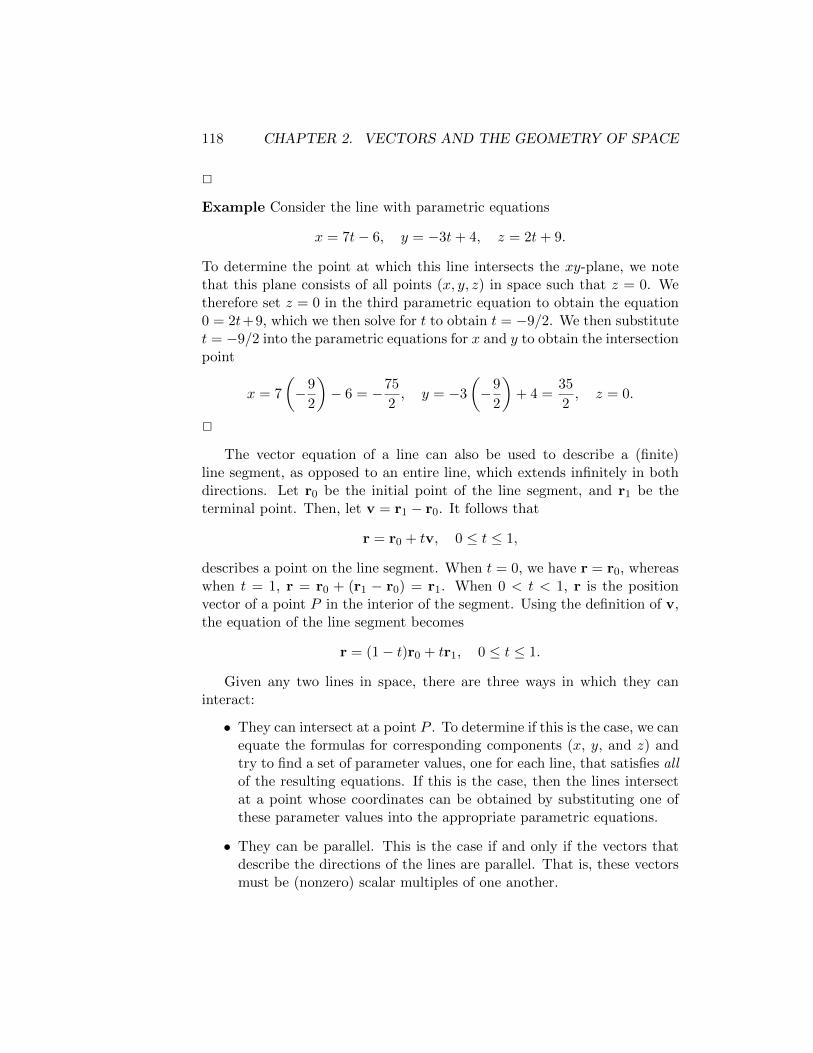
118 CHAPTER 2. VECTORS AND THE GEOMETRY OF SPACE
2
Example Consider the line with parametric equations
x = 7t− 6, y = −3t+ 4, z = 2t+ 9.
To determine the point at which this line intersects the xy-plane, we notethat this plane consists of all points (x, y, z) in space such that z = 0. Wetherefore set z = 0 in the third parametric equation to obtain the equation0 = 2t+9, which we then solve for t to obtain t = −9/2. We then substitutet = −9/2 into the parametric equations for x and y to obtain the intersectionpoint
x = 7
(−9
2
)− 6 = −75
2, y = −3
(−9
2
)+ 4 =
35
2, z = 0.
2
The vector equation of a line can also be used to describe a (finite)line segment, as opposed to an entire line, which extends infinitely in bothdirections. Let r0 be the initial point of the line segment, and r1 be theterminal point. Then, let v = r1 − r0. It follows that
r = r0 + tv, 0 ≤ t ≤ 1,
describes a point on the line segment. When t = 0, we have r = r0, whereaswhen t = 1, r = r0 + (r1 − r0) = r1. When 0 < t < 1, r is the positionvector of a point P in the interior of the segment. Using the definition of v,the equation of the line segment becomes
r = (1− t)r0 + tr1, 0 ≤ t ≤ 1.
Given any two lines in space, there are three ways in which they caninteract:
• They can intersect at a point P . To determine if this is the case, we canequate the formulas for corresponding components (x, y, and z) andtry to find a set of parameter values, one for each line, that satisfies allof the resulting equations. If this is the case, then the lines intersectat a point whose coordinates can be obtained by substituting one ofthese parameter values into the appropriate parametric equations.
• They can be parallel. This is the case if and only if the vectors thatdescribe the directions of the lines are parallel. That is, these vectorsmust be (nonzero) scalar multiples of one another.
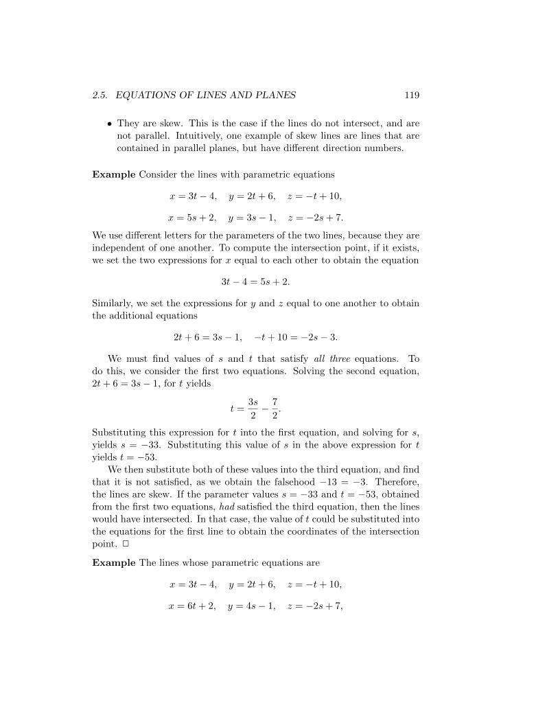
2.5. EQUATIONS OF LINES AND PLANES 119
• They are skew. This is the case if the lines do not intersect, and arenot parallel. Intuitively, one example of skew lines are lines that arecontained in parallel planes, but have different direction numbers.
Example Consider the lines with parametric equations
x = 3t− 4, y = 2t+ 6, z = −t+ 10,
x = 5s+ 2, y = 3s− 1, z = −2s+ 7.
We use different letters for the parameters of the two lines, because they areindependent of one another. To compute the intersection point, if it exists,we set the two expressions for x equal to each other to obtain the equation
3t− 4 = 5s+ 2.
Similarly, we set the expressions for y and z equal to one another to obtainthe additional equations
2t+ 6 = 3s− 1, −t+ 10 = −2s− 3.
We must find values of s and t that satisfy all three equations. Todo this, we consider the first two equations. Solving the second equation,2t+ 6 = 3s− 1, for t yields
t =3s
2− 7
2.
Substituting this expression for t into the first equation, and solving for s,yields s = −33. Substituting this value of s in the above expression for tyields t = −53.
We then substitute both of these values into the third equation, and findthat it is not satisfied, as we obtain the falsehood −13 = −3. Therefore,the lines are skew. If the parameter values s = −33 and t = −53, obtainedfrom the first two equations, had satisfied the third equation, then the lineswould have intersected. In that case, the value of t could be substituted intothe equations for the first line to obtain the coordinates of the intersectionpoint. 2
Example The lines whose parametric equations are
x = 3t− 4, y = 2t+ 6, z = −t+ 10,
x = 6t+ 2, y = 4s− 1, z = −2s+ 7,
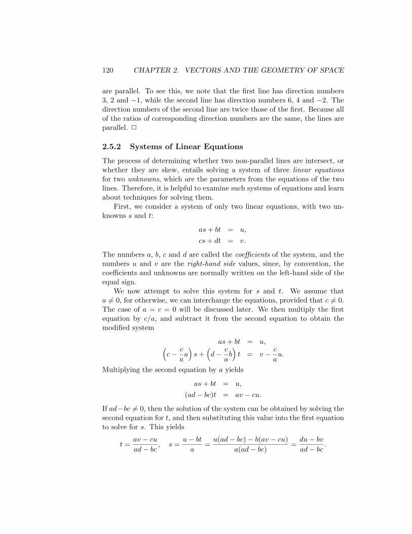
120 CHAPTER 2. VECTORS AND THE GEOMETRY OF SPACE
are parallel. To see this, we note that the first line has direction numbers3, 2 and −1, while the second line has direction numbers 6, 4 and −2. Thedirection numbers of the second line are twice those of the first. Because allof the ratios of corresponding direction numbers are the same, the lines areparallel. 2
2.5.2 Systems of Linear Equations
The process of determining whether two non-parallel lines are intersect, orwhether they are skew, entails solving a system of three linear equationsfor two unknowns, which are the parameters from the equations of the twolines. Therefore, it is helpful to examine such systems of equations and learnabout techniques for solving them.
First, we consider a system of only two linear equations, with two un-knowns s and t:
as+ bt = u,
cs+ dt = v.
The numbers a, b, c and d are called the coefficients of the system, and thenumbers u and v are the right-hand side values, since, by convention, thecoefficients and unknowns are normally written on the left-hand side of theequal sign.
We now attempt to solve this system for s and t. We assume thata 6= 0, for otherwise, we can interchange the equations, provided that c 6= 0.The case of a = c = 0 will be discussed later. We then multiply the firstequation by c/a, and subtract it from the second equation to obtain themodified system
as+ bt = u,(c− c
aa)s+
(d− c
ab)t = v − c
au.
Multiplying the second equation by a yields
as+ bt = u,
(ad− bc)t = av − cu.
If ad−bc 6= 0, then the solution of the system can be obtained by solving thesecond equation for t, and then substituting this value into the first equationto solve for s. This yields
t =av − cuad− bc
, s =u− bta
=u(ad− bc)− b(av − cu)
a(ad− bc)=du− bvad− bc
.
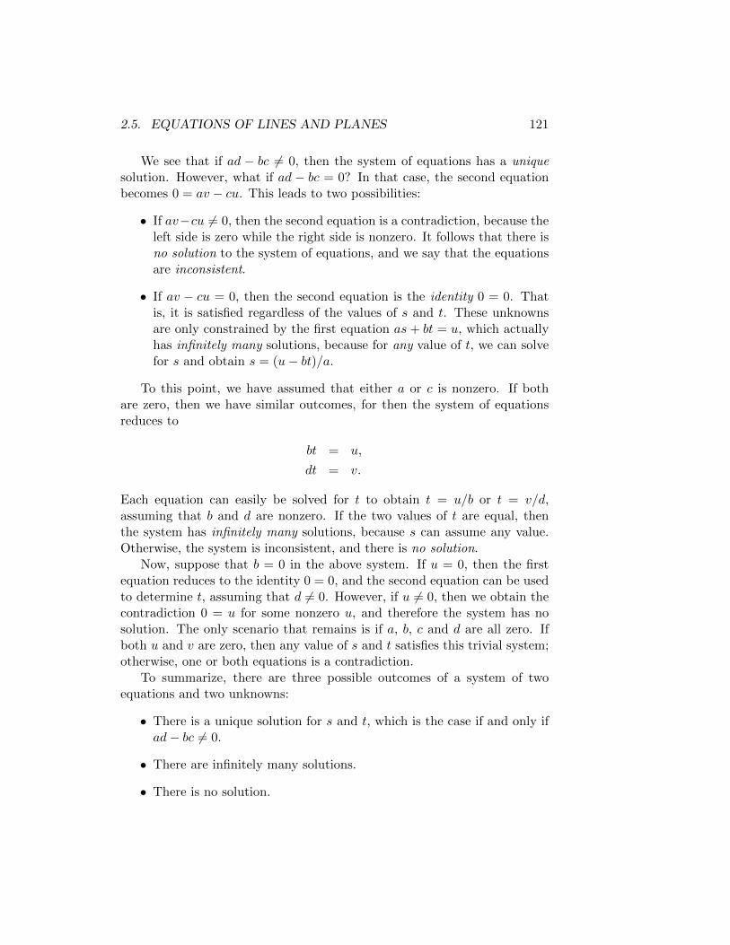
2.5. EQUATIONS OF LINES AND PLANES 121
We see that if ad − bc 6= 0, then the system of equations has a uniquesolution. However, what if ad − bc = 0? In that case, the second equationbecomes 0 = av − cu. This leads to two possibilities:
• If av−cu 6= 0, then the second equation is a contradiction, because theleft side is zero while the right side is nonzero. It follows that there isno solution to the system of equations, and we say that the equationsare inconsistent.
• If av − cu = 0, then the second equation is the identity 0 = 0. Thatis, it is satisfied regardless of the values of s and t. These unknownsare only constrained by the first equation as+ bt = u, which actuallyhas infinitely many solutions, because for any value of t, we can solvefor s and obtain s = (u− bt)/a.
To this point, we have assumed that either a or c is nonzero. If bothare zero, then we have similar outcomes, for then the system of equationsreduces to
bt = u,
dt = v.
Each equation can easily be solved for t to obtain t = u/b or t = v/d,assuming that b and d are nonzero. If the two values of t are equal, thenthe system has infinitely many solutions, because s can assume any value.Otherwise, the system is inconsistent, and there is no solution.
Now, suppose that b = 0 in the above system. If u = 0, then the firstequation reduces to the identity 0 = 0, and the second equation can be usedto determine t, assuming that d 6= 0. However, if u 6= 0, then we obtain thecontradiction 0 = u for some nonzero u, and therefore the system has nosolution. The only scenario that remains is if a, b, c and d are all zero. Ifboth u and v are zero, then any value of s and t satisfies this trivial system;otherwise, one or both equations is a contradiction.
To summarize, there are three possible outcomes of a system of twoequations and two unknowns:
• There is a unique solution for s and t, which is the case if and only ifad− bc 6= 0.
• There are infinitely many solutions.
• There is no solution.
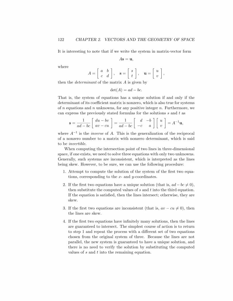
122 CHAPTER 2. VECTORS AND THE GEOMETRY OF SPACE
It is interesting to note that if we write the system in matrix-vector form
As = u,
where
A =
[a bc d
], s =
[st
], u =
[uv
],
then the determinant of the matrix A is given by
det(A) = ad− bc.
That is, the system of equations has a unique solution if and only if thedeterminant of its coefficient matrix is nonzero, which is also true for systemsof n equations and n unknowns, for any positive integer n. Furthermore, wecan express the previously stated formulas for the solutions s and t as
s =1
ad− bc
[du− bvav − cu
]=
1
ad− bc
[d −b−c a
] [uv
]= A−1u,
where A−1 is the inverse of A. This is the generalization of the reciprocalof a nonzero number to a matrix with nonzero determinant, which is saidto be invertible.
When computing the intersection point of two lines in three-dimensionalspace, if one exists, we need to solve three equations with only two unknowns.Generally, such systems are inconsistent, which is interpreted as the linesbeing skew. However, to be sure, we can use the following procedure:
1. Attempt to compute the solution of the system of the first two equa-tions, corresponding to the x- and y-coordinates.
2. If the first two equations have a unique solution (that is, ad− bc 6= 0),then substitute the computed values of s and t into the third equation.If the equation is satisfied, then the lines intersect; otherwise, they areskew.
3. If the first two equations are inconsistent (that is, av − cu 6= 0), thenthe lines are skew.
4. If the first two equations have infinitely many solutions, then the linesare guaranteed to intersect. The simplest course of action is to returnto step 1 and repeat the process with a different set of two equationschosen from the original system of three. Because the lines are notparallel, the new system is guaranteed to have a unique solution, andthere is no need to verify the solution by substituting the computedvalues of s and t into the remaining equation.
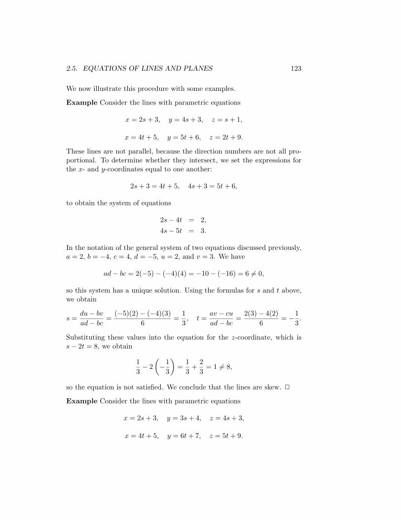
2.5. EQUATIONS OF LINES AND PLANES 123
We now illustrate this procedure with some examples.
Example Consider the lines with parametric equations
x = 2s+ 3, y = 4s+ 3, z = s+ 1,
x = 4t+ 5, y = 5t+ 6, z = 2t+ 9.
These lines are not parallel, because the direction numbers are not all pro-portional. To determine whether they intersect, we set the expressions forthe x- and y-coordinates equal to one another:
2s+ 3 = 4t+ 5, 4s+ 3 = 5t+ 6,
to obtain the system of equations
2s− 4t = 2,
4s− 5t = 3.
In the notation of the general system of two equations discussed previously,a = 2, b = −4, c = 4, d = −5, u = 2, and v = 3. We have
ad− bc = 2(−5)− (−4)(4) = −10− (−16) = 6 6= 0,
so this system has a unique solution. Using the formulas for s and t above,we obtain
s =du− bvad− bc
=(−5)(2)− (−4)(3)
6=
1
3, t =
av − cuad− bc
=2(3)− 4(2)
6= −1
3.
Substituting these values into the equation for the z-coordinate, which iss− 2t = 8, we obtain
1
3− 2
(−1
3
)=
1
3+
2
3= 1 6= 8,
so the equation is not satisfied. We conclude that the lines are skew. 2
Example Consider the lines with parametric equations
x = 2s+ 3, y = 3s+ 4, z = 4s+ 3,
x = 4t+ 5, y = 6t+ 7, z = 5t+ 9.
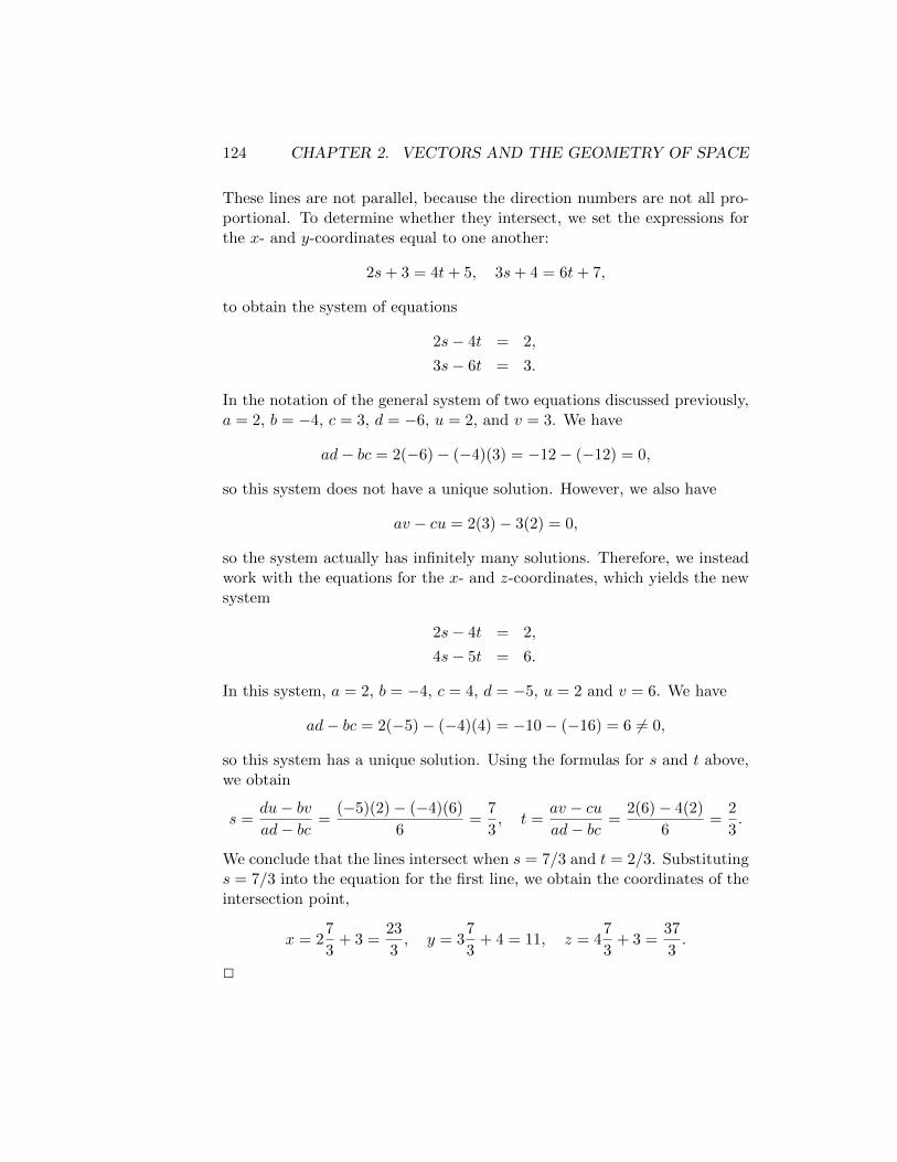
124 CHAPTER 2. VECTORS AND THE GEOMETRY OF SPACE
These lines are not parallel, because the direction numbers are not all pro-portional. To determine whether they intersect, we set the expressions forthe x- and y-coordinates equal to one another:
2s+ 3 = 4t+ 5, 3s+ 4 = 6t+ 7,
to obtain the system of equations
2s− 4t = 2,
3s− 6t = 3.
In the notation of the general system of two equations discussed previously,a = 2, b = −4, c = 3, d = −6, u = 2, and v = 3. We have
ad− bc = 2(−6)− (−4)(3) = −12− (−12) = 0,
so this system does not have a unique solution. However, we also have
av − cu = 2(3)− 3(2) = 0,
so the system actually has infinitely many solutions. Therefore, we insteadwork with the equations for the x- and z-coordinates, which yields the newsystem
2s− 4t = 2,
4s− 5t = 6.
In this system, a = 2, b = −4, c = 4, d = −5, u = 2 and v = 6. We have
ad− bc = 2(−5)− (−4)(4) = −10− (−16) = 6 6= 0,
so this system has a unique solution. Using the formulas for s and t above,we obtain
s =du− bvad− bc
=(−5)(2)− (−4)(6)
6=
7
3, t =
av − cuad− bc
=2(6)− 4(2)
6=
2
3.
We conclude that the lines intersect when s = 7/3 and t = 2/3. Substitutings = 7/3 into the equation for the first line, we obtain the coordinates of theintersection point,
x = 27
3+ 3 =
23
3, y = 3
7
3+ 4 = 11, z = 4
7
3+ 3 =
37
3.
2
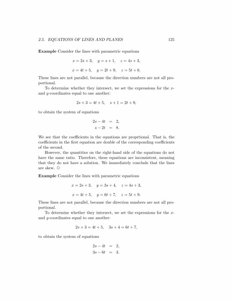
2.5. EQUATIONS OF LINES AND PLANES 125
Example Consider the lines with parametric equations
x = 2s+ 3, y = s+ 1, z = 4s+ 3,
x = 4t+ 5, y = 2t+ 9, z = 5t+ 6.
These lines are not parallel, because the direction numbers are not all pro-portional.
To determine whether they intersect, we set the expressions for the x-and y-coordinates equal to one another:
2s+ 3 = 4t+ 5, s+ 1 = 2t+ 9,
to obtain the system of equations
2s− 4t = 2,
s− 2t = 8.
We see that the coefficients in the equations are proprtional. That is, thecoefficients in the first equation are double of the corresponding coefficientsof the second.
However, the quantities on the right-hand side of the equations do nothave the same ratio. Therefore, these equations are inconsistent, meaningthat they do not have a solution. We immediately conclude that the linesare skew. 2
Example Consider the lines with parametric equations
x = 2s+ 3, y = 3s+ 4, z = 4s+ 3,
x = 4t+ 5, y = 6t+ 7, z = 5t+ 9.
These lines are not parallel, because the direction numbers are not all pro-portional.
To determine whether they intersect, we set the expressions for the x-and y-coordinates equal to one another:
2s+ 3 = 4t+ 5, 3s+ 4 = 6t+ 7,
to obtain the system of equations
2s− 4t = 2,
3s− 6t = 3.
126 CHAPTER 2. VECTORS AND THE GEOMETRY OF SPACE
The coefficients, and right-hand side quantities, of these equations are allproportional. That is, we can obtain the second equation by multiplying thefirst by 3/2. In other words, these equations are dependent on one another,and therefore do not have a unique solution. In fact, they have infinitelymany solutions.
We instead work with the equations for the x- and z-coordinates, whichyields the new system
2s− 4t = 2,
4s− 5t = 6.
These equations are guaranteed to be independent, and thus have a uniquesolution, since the lines are already known to not be parallel.
By doubling the first equation, which yields 4s−8t = 4, and subtractingit from the second, we obtain 3t = 2, and therefore t = 2/3. Substitutingthis value into the first equation yields the equation 2s− 4(2/3) = 2, whichhas the solution s = 7/3.
We conclude that the lines intersect when s = 7/3 and t = 2/3. Substi-tuting s = 7/3 into the equation for the first line, we obtain the coordinatesof the intersection point,
x = 27
3+ 3 =
23
3, y = 3
7
3+ 4 = 11, z = 4
7
3+ 3 =
37
3.
2
2.5.3 Equations of Planes
Previously, we learned how to describe lines using various types of equations.Now, we will do the same with planes. Suppose that we are given three pointsr0, r1 and r2 that are not co-linear. Then, these points define a plane, andthe vectors v1 = r1 − r0 and v2 = r2 − r0 are vectors contained within theplane, that are also not parallel to one another.
A plane consists of all vectors that are orthogonal to a given directionn, which is said to be normal to the plane, and passes through a given pointr0. The normal vector n can be obtained by computing
n = v1 × v2.
Let r be any point in the plane. Then the vector u = r − r0 is orthogonalto n. That is,
n · u = n · (r− r0) = 0.
2.5. EQUATIONS OF LINES AND PLANES 127
This equation is called the vector equation of the plane.
If we write
n = 〈a, b, c〉, r = 〈x, y, z〉, r0 = 〈x0, y0, z0〉,
then the vector equation can be rewritten as
ax+ by + cz + d = 0,
where d = −n · r0 = −(ax0 + by0 + cz0). This is a linear equation in theunknowns x, y, and z.
Example Consider the plane containing the points P0 = (1, 4, 1), P1 =(5, 1,−1) and P2 = (4, 4, 4), which we identify with the position vectors
r0 = 〈1, 4, 1〉, r1 = 〈5, 1,−1〉, r2 = 〈4, 4, 4〉.
We wish to find a linear equation that describes this plane. First, we needto compute a vector n that is normal to the plane, which can be obtainedby computing the cross product of two vectors v1 and v2 that are containedwithin the plane. We have
n = v1 × v2
= (r1 − r0)× (r2 − r0)
= 〈4,−3,−2〉 × 〈3, 0, 3〉= 〈−3(3)− (−2)0,−2(3)− 4(3), 4(0)− (−3)(3)〉= 〈−9,−18, 9〉.
It follows that the vector equation of the plane is
n · (r− r0) = 〈−9,−18, 9〉 · (〈x, y, z〉 − 〈1, 4, 1〉 = 0,
which can also be written as
−9x− 18y + 9z + 72 = 0,
since
n · r0 = −72.
2
128 CHAPTER 2. VECTORS AND THE GEOMETRY OF SPACE
2.5.4 Intersecting Planes
The angle between planes is defined to be the angle between their normalvectors. If this angle is either 0 or π, then the normal vectors are parallel,and we say that the planes are parallel. Otherwise, the planes intersect, andthis intersection is a line.
To determine the line formed by this intersection, we need to solve thesystem of equations consisting of the equations of the two planes. Becausethis system of equations has three unknowns, but there are only two equa-tions, there will be infinitely many points that satisfy the system, and theset of all such solutions constitutes a line.
Let the equations of two planes be given by
a1x+ b1y + c1z + d1 = 0, a2x+ b2y + c2z + d2 = 0,
and let the corresponding normal vectors be
n1 = 〈a1, b1, c1〉, n2 = 〈a2, b2, c2〉.
To solve this system of equations, we first check whether the equations areindependent if we were to set z = 0. That is, we must check whether
a1b2 − b1a2 = 0,
or, equivalently, whether a1 and b1 are proportional to a2 and b2. If they arenot proportional, then we can set z = 0 to obtain the system of equations
a1x+ b1y = −d1,
a2x+ b2y = −d2,
which is now guaranteed to have a unique solution. This gives us a point onthe line that is common to both planes. If a1b2 − b1a2 = 0, then we cannotnecessarily substitute z = 0, for the resulting system of equations might beinconsistent. Instead, we can set y = 0, in which case the resulting systemof equations, for the unknowns x and z, will have a unique solution.
To determine the direction of the line of intersection, we note that anyvector in a plane is orthogonal to its normal vector. Because this line belongsto both planes, a vector in the direction of the line is orthogonal to bothnormal vectors n1 and n2. It follows that a vector v in the direction of theline of intersection can be found by computing
v = n1 × n2.
2.5. EQUATIONS OF LINES AND PLANES 129
This direction, and the previously computed point on the line, can be usedto obtain the parametric or symmetric equations of the line.
Example Consider two planes defined by the equations
x+ 3y − 2z + 10 = 0, 2x− 4y + 3z − 5 = 0.
These planes are not parallel, because their normal vectors n1 = 〈1, 3,−2〉and n2 = 〈2,−4, 3〉 are not parallel. Their intersection is a line that isparallel to the vector
v = n1×n2 = 〈1, 3,−2〉×〈2,−4, 3〉 = 〈3(3)−(−2)(−4), (−2)(2)−1(3), 1(−4)−3(2)〉 = 〈1,−7,−10〉.
To write down the equation of the line of intersection, we need to computethe coordinates of a point on the line. Substituting z = 0 into the equationsof the plane yields the system
x+ 3y = −10,
2x− 4y = 5.
This system has a unique solution, because the coefficients of the equationsare not proportional. Subtracting twice the first equation from the secondyields the simpler equation −10y = 25, so y = −5/2. Substituting this valueinto the first equation yields x = −10− 3(−5/2) = −5/2. We conclude thatthe line can be described using the parametric equations
x = −5/2 + t, y = −5/2− 7t, z = −10t.
We can also describe the line using the symmetric equations
x+ 5/2
1=y + 5/2
−7=
z
−10.
2
2.5.5 Distance from a Point to a Plane
Let p1 = 〈x1, y1, z1〉 be a position vector corresponding to a point P =(x1, y1, z1). Let (r − r0) · n = 0 be the equation of a plane, where r0 =〈x0, y0, z0〉 is the position vector for a point R0 = 〈x0, y0, z0〉 in the plane,and n is the plane’s normal vector. We consider the problem of computingthe distance D between the point P1 and this plane.
Intuitively, it makes sense to define this distance as the distance fromP1 to some point P2 contained within the plane. However, we need to
130 CHAPTER 2. VECTORS AND THE GEOMETRY OF SPACE
determine what a suitable point P2 would be. We choose P2 to be the bestapproximation of P1 by a point in the plane, just as the vector projection of avector v onto a vector u was previously defined to be the best approximationof v by a vector that is parallel to u.
The key characteristic of the best approximation of the point P1 by apoint P2 in the plane is that the error in this approximation, that is, thevector between P1 and P2, should be orthogonal to the plane. That is, thisvector should be parallel to n, the normal to the plane. To determine thelength of this vector, we form a triangle with the points p1, p2 and r0, wherep2 is the position vector for the point P2.
Because p1 − p2 is parallel to n, which is orthogonal to p2 − r0, thistriangle is a right triangle, with the hypotenuse defined by p1−r0. Therefore,we can use right triangle trigonometry to determine that the distance D isgiven by
D = |v1| cos θ
where v1 = p1 − r0 and θ is the angle between v1 and n, with n chosen sothat 0 ≤ θ < π/2. It follows that
D =|v1 · n||n|
.
It is interesting to note that from this formula, we can see that D is alsothe absolute value of the scalar projection of v1 onto n, or, equivalently, themagnitude of the vector projection of v1 onto n.
If n = 〈a, b, c〉, and we write the equation of the plane in the formax+ by + cz + d = 0, then we can express this distance as
D =|a(x1 − x0) + b(y1 − y0) + c(z1 − z0)|√
a2 + b2 + c2=|ax1 + by1 + cz1 + d|√
a2 + b2 + c2,
because the equations of the plane, (r− r0) ·n = 0 and ax+ by+ cz+d = 0,are related by d = −r0 · n = −(ax0 + by0 + cz0).
Example We wish to compute the distance D between the point P1 =(4, 5, 6) and the plane described by the linear equation
2x+ 3y − 4z + 15 = 0.
The normal vector for this plane is n = 〈a, b, c〉 = 〈2, 3,−4〉. It follows thatthe distance D is given by
D =|2(4) + 3(5)− 4(6) + 15|√
22 + 32 + (−4)2=
14√29≈ 2.6.
2.5. EQUATIONS OF LINES AND PLANES 131
2
The formula for the distance between a point and a plane can be usedto compute the distance between two parallel planes. The idea is to identifyone point in the first plane, and then compute the distance between thispoint and the second plane. Because the planes are parallel, this distancewill be the same, regardless of which point from the first plane is chosen.
2.5.6 Summary
• The vector equation of a line is of the form r = r0 + tv, where r0
is the position vector of a particular point on the line, t is a scalarparameter, v is a vector that describes the direction of the line, andr is the position vector of the point on the line corresponding to thevalue of t.• The parametric equations of the line are the components of the vector
equation, and have the form x = x0 + at, y = y0 + bt, and z = z0 + ct.The components a, b and c of v are called the direction numbers ofthe line.• The symmetric equations of a line are obtained by eliminating the
parameter t from the parametric equations. The expressions (x −x0)/a, (y − y0)/b, and (z − z0)/b, for which the direction numbers arenonzero, are equated.
• The line segment between r0 and r1 can be described by the equationr = (1− t)r0 + tr1, where 0 ≤ t ≤ 1.
• If the expressions for x, y and z in the parametric equations of twolines are equal for the same values of the parameters, then the linesintersect at the point obtained by substituting the common parametersinto the appropriate parametric equations.
• If two lines have direction vectors that are parallel, then the lines arealso parallel.
• If two lines do not intersect, and are not parallel, then they are skew.
• A system of two linear equations with two unknowns can have a uniquesolution, no solution, or infinitely many solutions. It has a uniquesolution if the determinant of the system is nonzero.
• To determine whether two non-parallel lines intersect, one can tryto find a solution to a system of three equations in two unknowns,
132 CHAPTER 2. VECTORS AND THE GEOMETRY OF SPACE
obtained by equating the parametric equations of corresponding com-ponents. The unknowns correspond to the parameters of the two lines.
• If the system of any two of the three equations is inconsistent, thenthe lines are skew.
• If the system of any two of the three equations has a unique solution,then the lines intersect if that solution satisfies the remaining equation,and the lines are skew if it does not.
• If the system of any two of the three equations has infinitely many so-lutions, then the lines intersect, and the parameters of the intersectionpoint can be obtained by computing the solution of any other pair ofequations, which is guaranteed to be unique.
• The vector equation of a plane is n · (r− r0) = 0, where n is a vectorthat is normal to the plane, r is any position vector in the plane, andr0 is a given position vector in the plane. The normal vector n canbe obtained by computing the cross product of any two non-parallelvectors in the plane.
• Two planes are parallel if and only if their normal vectors are parallel.
• If two planes are not parallel, their intersection is a line. The directionof the line is a vector that is orthogonal to the planes’ normal vectors.A point on the line can be found by finding a solution of the systemof equations consisting of the equations of the planes, which can beaccomplished by setting one of the coordinates equal to zero.
• The distance between a point p and a plane n · (r − r0) = 0 is theabsolute value of the dot product of the unit (normalized) normalvector n/|n| and the vector between p and r0.
2.6 Review
You should now be able to complete the following types of problems:
• Determining the center and radius of a sphere, given the equation ofthe sphere, by completing the square.
• Using inequalities to describe a region in three-dimensional space,given a verbal description of the region.
2.6. REVIEW 133
• Normalizing and scaling vectors in order to obtain a vector of a spec-ified length and direction.
• Computing the resultant of given velocity vectors by vector addition,and computing the actual speed of an object, which is the magnitude ofthe resultant, as well as the actual direction. This involves computingthe components of a vector v in the xy-plane from its magnitude anddirection, using the formula
v = 〈r cos θ, r sin θ〉,
where r = |v| and θ is the angle that v makes with the positive x-axis.To compute the angle of a vector v = 〈x, y〉 from its components, usethe relationship
tan θ =y
x, x 6= 0,
keeping in mind that if x < 0, it is necessary to add π to the angleobtained by computing tan−1(y/x) on your calculator. If x = 0 andy > 0, the angle is π/2, whereas if x = 0 and y < 0, the angle is −π/2.
• Computing the angle θ between two vectors u and v, using the relationu · v = |u||v| cos θ.
• Computing the scalar projection of u onto v, defined by
compvu =v · u|v|
,
and the vector projection of u onto v, defined by
projvu =v · u|v|2
v.
Note that if we first compute the unit vector w in the direction of v,
w =v
|v|,
then these projections can be defined using the simpler formulas
compvu = w · u, projvu = (w · u)w.
• Computing the work done by a force F applied to an object to moveit along a displacement vector D, which can be defined in terms of itsinitial and terminal points. The work is given by
W = F ·D = |F||D| cos θ,
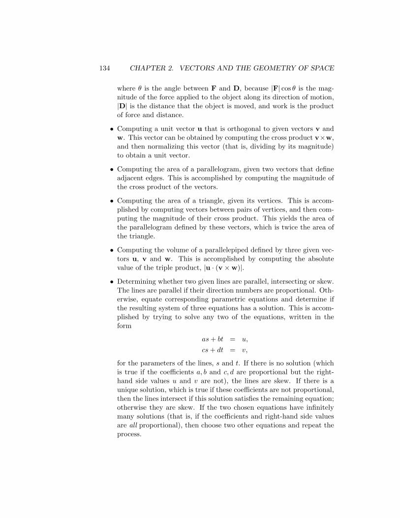
134 CHAPTER 2. VECTORS AND THE GEOMETRY OF SPACE
where θ is the angle between F and D, because |F| cos θ is the mag-nitude of the force applied to the object along its direction of motion,|D| is the distance that the object is moved, and work is the productof force and distance.
• Computing a unit vector u that is orthogonal to given vectors v andw. This vector can be obtained by computing the cross product v×w,and then normalizing this vector (that is, dividing by its magnitude)to obtain a unit vector.
• Computing the area of a parallelogram, given two vectors that defineadjacent edges. This is accomplished by computing the magnitude ofthe cross product of the vectors.
• Computing the area of a triangle, given its vertices. This is accom-plished by computing vectors between pairs of vertices, and then com-puting the magnitude of their cross product. This yields the area ofthe parallelogram defined by these vectors, which is twice the area ofthe triangle.
• Computing the volume of a parallelepiped defined by three given vec-tors u, v and w. This is accomplished by computing the absolutevalue of the triple product, |u · (v ×w)|.
• Determining whether two given lines are parallel, intersecting or skew.The lines are parallel if their direction numbers are proportional. Oth-erwise, equate corresponding parametric equations and determine ifthe resulting system of three equations has a solution. This is accom-plished by trying to solve any two of the equations, written in theform
as+ bt = u,
cs+ dt = v,
for the parameters of the lines, s and t. If there is no solution (whichis true if the coefficients a, b and c, d are proportional but the right-hand side values u and v are not), the lines are skew. If there is aunique solution, which is true if these coefficients are not proportional,then the lines intersect if this solution satisfies the remaining equation;otherwise they are skew. If the two chosen equations have infinitelymany solutions (that is, if the coefficients and right-hand side valuesare all proportional), then choose two other equations and repeat theprocess.
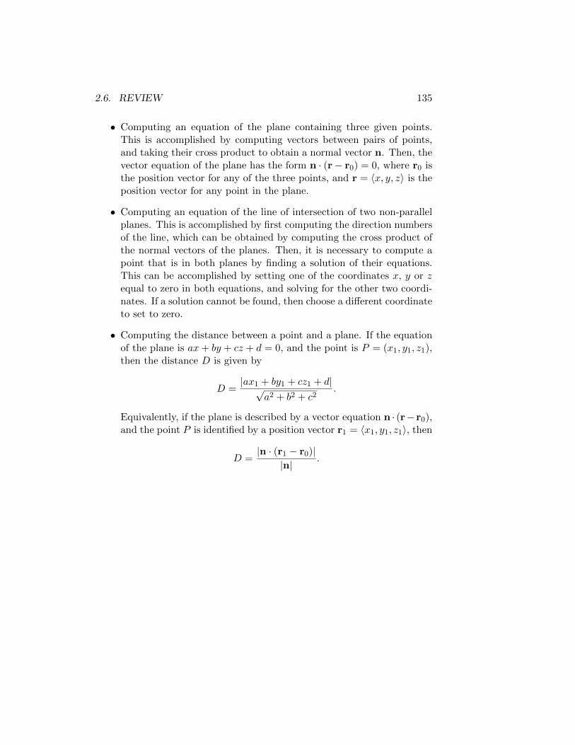
2.6. REVIEW 135
• Computing an equation of the plane containing three given points.This is accomplished by computing vectors between pairs of points,and taking their cross product to obtain a normal vector n. Then, thevector equation of the plane has the form n · (r− r0) = 0, where r0 isthe position vector for any of the three points, and r = 〈x, y, z〉 is theposition vector for any point in the plane.
• Computing an equation of the line of intersection of two non-parallelplanes. This is accomplished by first computing the direction numbersof the line, which can be obtained by computing the cross product ofthe normal vectors of the planes. Then, it is necessary to compute apoint that is in both planes by finding a solution of their equations.This can be accomplished by setting one of the coordinates x, y or zequal to zero in both equations, and solving for the other two coordi-nates. If a solution cannot be found, then choose a different coordinateto set to zero.
• Computing the distance between a point and a plane. If the equationof the plane is ax+ by + cz + d = 0, and the point is P = (x1, y1, z1),then the distance D is given by
D =|ax1 + by1 + cz1 + d|√
a2 + b2 + c2.
Equivalently, if the plane is described by a vector equation n · (r− r0),and the point P is identified by a position vector r1 = 〈x1, y1, z1〉, then
D =|n · (r1 − r0)|
|n|.
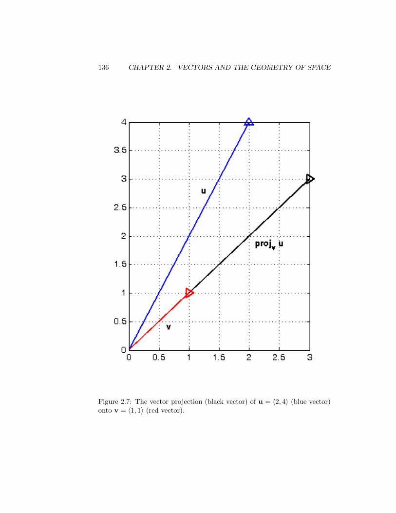
136 CHAPTER 2. VECTORS AND THE GEOMETRY OF SPACE
Figure 2.7: The vector projection (black vector) of u = 〈2, 4〉 (blue vector)onto v = 〈1, 1〉 (red vector).
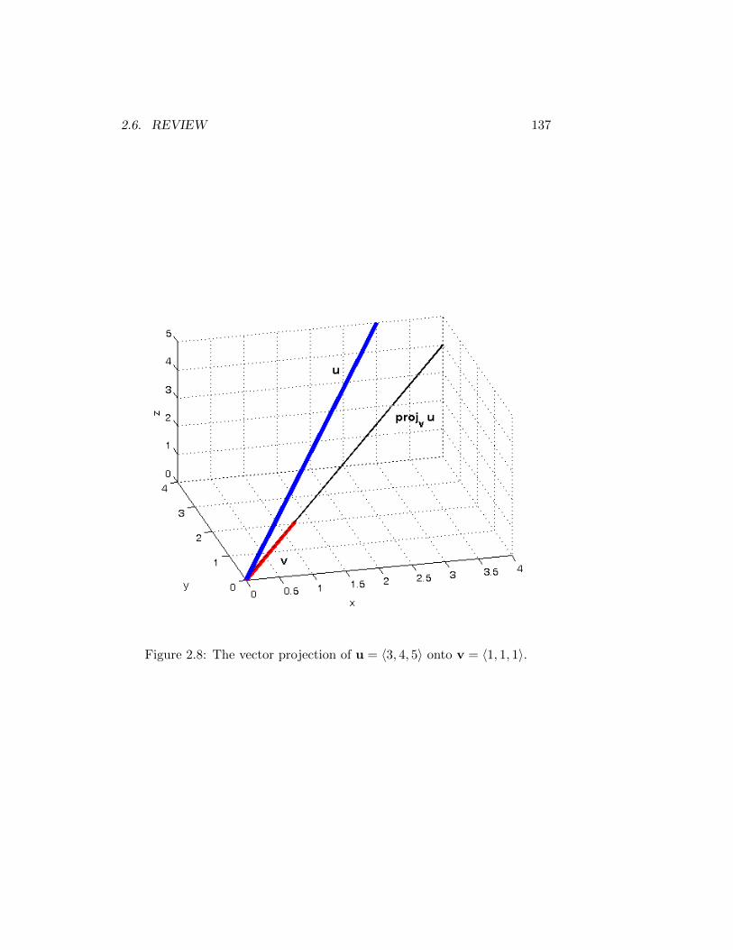
2.6. REVIEW 137
Figure 2.8: The vector projection of u = 〈3, 4, 5〉 onto v = 〈1, 1, 1〉.
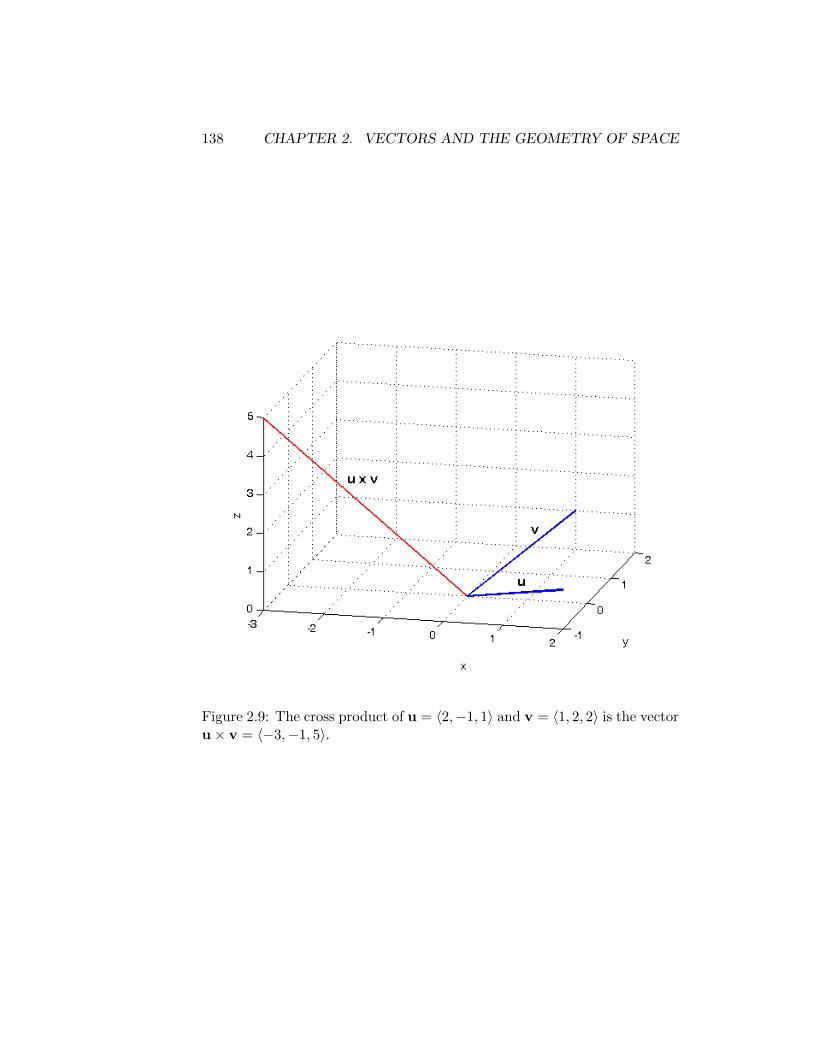
138 CHAPTER 2. VECTORS AND THE GEOMETRY OF SPACE
Figure 2.9: The cross product of u = 〈2,−1, 1〉 and v = 〈1, 2, 2〉 is the vectoru× v = 〈−3,−1, 5〉.
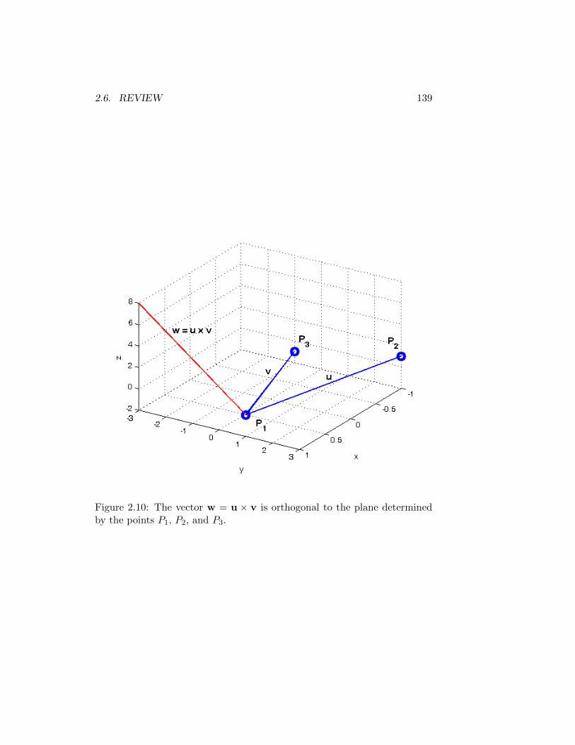
2.6. REVIEW 139
Figure 2.10: The vector w = u × v is orthogonal to the plane determinedby the points P1, P2, and P3.
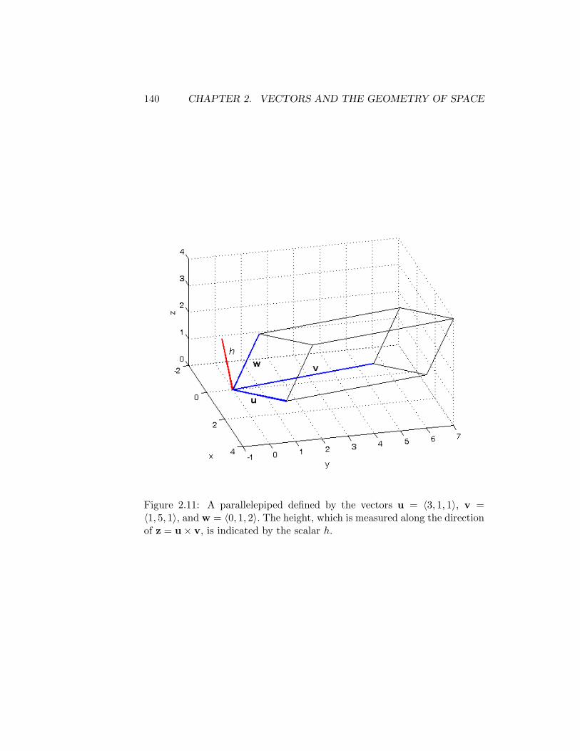
140 CHAPTER 2. VECTORS AND THE GEOMETRY OF SPACE
Figure 2.11: A parallelepiped defined by the vectors u = 〈3, 1, 1〉, v =〈1, 5, 1〉, and w = 〈0, 1, 2〉. The height, which is measured along the directionof z = u× v, is indicated by the scalar h.
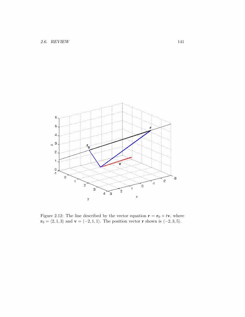
2.6. REVIEW 141
Figure 2.12: The line described by the vector equation r = r0 + tv, wherer0 = 〈2, 1, 3〉 and v = 〈−2, 1, 1〉. The position vector r shown is 〈−2, 3, 5〉.
142 CHAPTER 2. VECTORS AND THE GEOMETRY OF SPACE
Chapter 3
Parametric Curves and PolarCoordinates
3.1 Parametric Curves
There are many useful curves that cannot be described by an equation of theform y = f(x), because f is a function and therefore requires that only oney-value be associated with every x-value. For example, a complete circlecannot be described by such an equation. In such cases, we can insteaddescribe the curve by parametric equations
x = f(t), y = g(t),
where the variable t is called a parameter, and the curve defined by theseequations is called a parametric curve. For example, a circle of radius r canbe defined by the parametric equations
x = r cos t, y = r sin t.
The parameter t is typically restricted to some interval [a, b]. The pointx = f(a), y = g(a) is then called the initial point of the curve, and the pointx = f(b), y = g(b) is called the terminal point of the curve.
Because any functions f(t) and g(t) can be chosen to define the x-coordinates and y-coordinates, respectively, of points on the curve, thereis no requirement that each x-value is associated with only y-value, as witha curve defined by the equation y = f(x). It follows that any curve in theplane can be defined using parametric equations.
Example Construct parametric equations of the form
x = f(t), y = g(t)
143
144CHAPTER 3. PARAMETRIC CURVES AND POLAR COORDINATES
that describe the unit circle.
Solution The unit circle is a circle of radius 1 with center at the origin(0, 0). It is described by the equation
x2 + y2 = 1.
Choosing f(t) = cos t and g(t) = sin t, where 0 ≤ t ≤ 2π, we find that x andy satisfy this equation and describe the entire circle. If we let t denote time,and let (x, y) = (f(t), g(t)) denote the position of a particle at time t, thenthe particle begins at the point (1, 0) (corresponding to t = 0) and movesonce around the circle in the counterclockwise direction, at constant speed.
An alternative description of this circle is given by the parametric equa-tions
x = sin et, y = cos et, lnπ ≤ t ≤ ln 3π.
In this case, a particle whose motion is described by these equations startsat the point (0,−1) and travels once around the circle in the clockwisedirection, at steadily increasing speed. 2
Example Describe the differences between the following sets of parametricequations that represent the curve y = x3, where −∞ < t <∞:
1. x = t, y = t3
2. x = t2, y = t6
3. x = sin t, y = sin3 t.
Solution
1. These equations describe the entire curve y = x3. A particle whosemotion is described by these equations traces the curve from left toright, at constant speed in the x-direction.
2. These equations describe the portion of the curve in the right-halfplane x ≥ 0. A particle whose motion is described by these equationstraces the curve from right to left as t increases from −∞, until t = 0,at which point the particle turns around and retraces the curve fromleft to right, at constant speed in the x-direction.
3. These equations describe the portion of the curve for which−1 ≤ x ≤ 1and −1 ≤ y ≤ 1. A particle whose motion is described by theseequations traces the curve from left to right until reaching the point(1, 1), at which point it turns around and retraces the curve from rightto left until reaching the point (−1,−1). This process continues foreveras t increases.
3.1. PARAMETRIC CURVES 145
2
Example Find parametric equations for the astroid x2/3 + y2/3 = 1.
Solution Writing the equation for the astroid as
(x1/3)2 + (y1/3)2 = 1,
we see that x1/3 and y1/3 can only assume values between −1 and 1. There-fore, we can use the identity sin2 θ + cos2 θ = 1 and let x1/3 = cos t andy1/3 = sin t, which yields the equations
x = cos3 t, y = sin3 t,
where 0 ≤ t ≤ 2π. 2
Example Find parametric equations for the ellipse
4x2 + 9y2 = 36.
Solution Rewriting the equation as
(2x)2 + (3y)2 = 62,
we see that 2x and 3y can only assume values between −6 and 6. Equating2x = 6 cos t and 3y = 6 sin t yields the equations
x = 3 cos t, y = 2 sin t,
where 0 ≤ t < 2π. 2
Example Sketch the curve described by the parametric equations
x = sin t, y = sin 2t,
where 0 ≤ t ≤ 2π.
Solution The curve can be sketched by choosing several values of t in theinterval [0, 2π] and computing the corresponding values of x and y for eachvalue of t. In Figure 3.1, the curve is plotted by using MatlabTM to computex and y for t = 0, 0.01, 0.02, . . . all the way up to 2π, plotting the resultingpoints, and then connecting the points to obtain a smooth curve. 2
Example Given a curve defined by the parametric equations
x = 3t+ 2, y = t− 1,
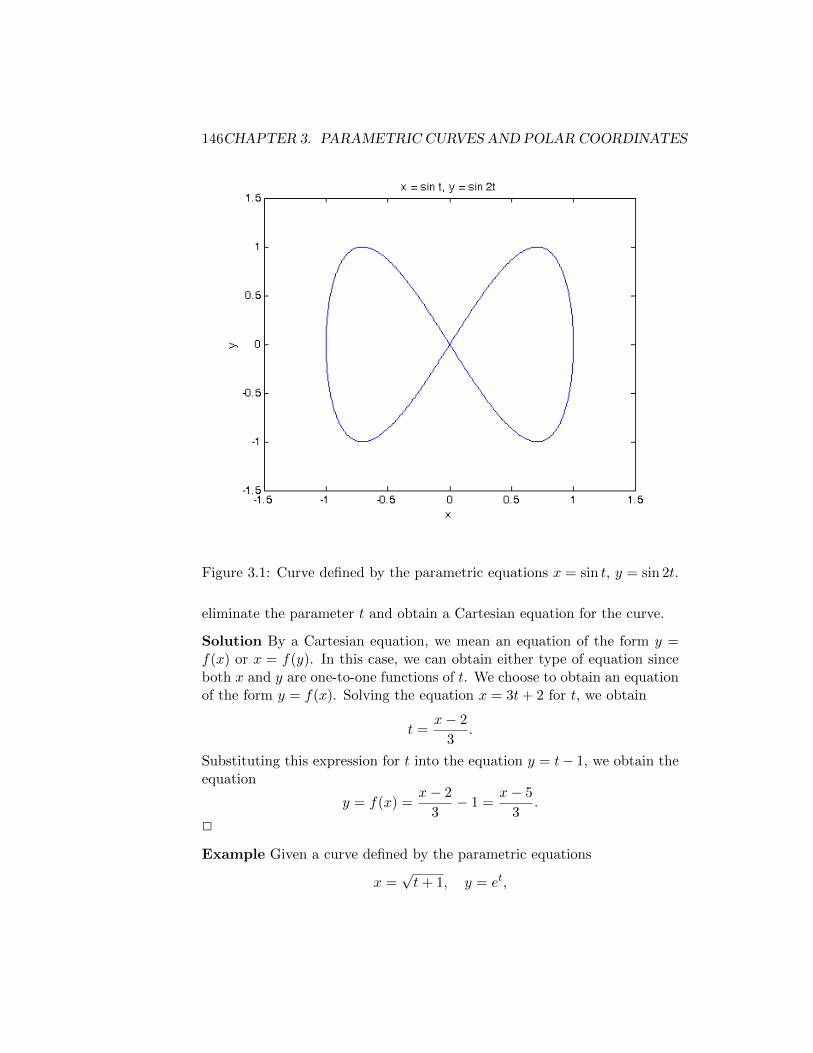
146CHAPTER 3. PARAMETRIC CURVES AND POLAR COORDINATES
Figure 3.1: Curve defined by the parametric equations x = sin t, y = sin 2t.
eliminate the parameter t and obtain a Cartesian equation for the curve.
Solution By a Cartesian equation, we mean an equation of the form y =f(x) or x = f(y). In this case, we can obtain either type of equation sinceboth x and y are one-to-one functions of t. We choose to obtain an equationof the form y = f(x). Solving the equation x = 3t+ 2 for t, we obtain
t =x− 2
3.
Substituting this expression for t into the equation y = t− 1, we obtain theequation
y = f(x) =x− 2
3− 1 =
x− 5
3.
2
Example Given a curve defined by the parametric equations
x =√t+ 1, y = et,
3.1. PARAMETRIC CURVES 147
where t ≥ 0, eliminate the parameter t and obtain a Cartesian equation forthe curve.
Solution Since x is a one-to-one function of t, we can solve the equationx =√t+ 1 for t and obtain
t = x2 − 1,
where x ≥ 1. Substituting this relation into the equation y = et, we obtainthe Cartesian equation
y = ex2−1.
Since y is also a one-to-one function of t, we have the relation
t = ln y,
where y ≥ 1. We can substitute this relation into the equation x =√t+ 1
to obtain the alternative representation of the curve,
x =√
ln y + 1.
2
3.1.1 Summary
• A parametric curve in the xy-plane is a curve that is described byparametric equations x = f(t) and y = g(t), which define the x- andy-coordinates of each point on the curve as functions of a parametert, where t belongs to an interval [a, b].
• The initial point of the curve is (f(a), g(a)), and the terminal point is(f(b), g(b)).
• Any curve can be described by parametric equations, because para-metric equations do not require that each x-value is associated withonly one y-value, unlike an equation of the form y = f(x).
• A curve defined by an equation of the form [f(x)]2 + [g(y)]2 = r2 canbe converted to parametric equations by equating f(x) = r cos t andg(y) = r sin t, and solving for x and y.
• Parametric equations x = f(t), y = g(t) can be converted to an equa-tion of the form y = f(x) by solving x = f(t) for t, if possible, andsubstituting the resulting expression for t into the equation y = g(t).
148CHAPTER 3. PARAMETRIC CURVES AND POLAR COORDINATES
3.2 Calculus with Parametric Curves
3.2.1 Arc Length
In this section, we will learn how to use calculus to compute the length of acurve that is described by an equation of the form y = f(x), for some givenfunction f(x). Just as we learned how to compute the area under such acurve as the limit of a sum of areas of simpler regions (namely, rectangles),we can compute the length of the curve by interpreting the length as a limitof a sum of lengths of the simplest curves known, which are line segments.
Suppose that we wish to compute the length of the curve y = f(x)between x = a and x = b. We can approximate this length by dividingthe interval [a, b] into subintervals of length ∆x = (b − a)/n, just as wedid when we were trying to compute the approximate area under y = f(x).Consider any subinterval [xi−1, xi]. Then, if ∆x is chosen to be sufficientlysmall, the length of the curve y = f(x) between x = xi−1 and x = xi canbe well approximated by the length of the line segment between the points(xi−1, f(xi−1)) and (xi, f(xi)). This line segment is the hypotenuse of a righttriangle with legs of length ∆x and |f(xi)−f(xi−1)|, and therefore the lengthLi of the curve y = f(x) between x = xi−1 and x = xi is approximately
Li ≈√
∆x2 + (f(xi)− f(xi−1))2 = ∆x
√1 +
(f(xi)− f(xi−1)
∆x
)2
. (3.1)
It follows that the length L of the curve between x = a and x = b isapproximated by
L ≈n∑i=1
Li =
n∑i=1
√1 +
(f(xi)− f(xi−1)
∆x
)2
∆x =
n∑i=1
√1 +
(f(xi)− f(xi−1)
xi − xi−1
)2
∆x.
(3.2)As n, the number of line segments, approaches ∞, ∆x approaches zero,
so the length of each subinterval [xi−1, xi] tends to zero. It follows from thedefinition of the derivative that
lim∆x→0
f(xi)− f(xi−1)
xi − xi−1= lim
∆x→0
f(xi−1 + ∆x)− f(xi−1)
∆x= f ′(xi−1) (3.3)
and therefore the sum converges to the definite integral
L = limn→∞
n∑i=1
Li =
∫ b
a
√1 + [f ′(x)]2 dx. (3.4)
3.2. CALCULUS WITH PARAMETRIC CURVES 149
The value of this integral is called the arc length of the curve y = f(x) fromx = a to x = b. Similarly, if a curve is defined by the equation x = f(y)from y = c to y = d, the arc length of the curve is given by the definiteintegral ∫ d
c
√1 + [f ′(y)]2 dy. (3.5)
Example 1 Compute the arc length of the curve y = 2x + 3, where 0 ≤x ≤ 2.
Solution Since the curve is just a line segment, we can simply use thedistance formula to compute the arc length, since the arc length is thedistance between the endpoints of the segment. The endpoints are (0, 3)and (2, 7), and therefore the arc length is√
(2− 0)2 + (7− 3)2 =√
22 + 42 =√
20 = 2√
5. (3.6)
Using the arc length formula, we have y′ = 2, and therefore the arc lengthis given by the integral∫ 2
0
√1 + 22 dx =
∫ 2
0
√5 dx =
√5x∣∣∣20
= 2√
5. (3.7)
2
Example 2 Compute the arc length of the curve y = sinx from x = 0 tox = π.
Solution Since y′ = cosx, the arc length is given by the integral∫ π
0
√1 + cos2 x dx. (3.8)
Unfortunately, this integral cannot be evaluated using the Fundamental The-orem of Calculus. Using an approximation method such as the CompositeSimpson’s Rule, the value of the integral is seen to be approximately 3.8202.2
Example 3 Compute the arc length of the astroid described by the equa-tion x2/3 + y2/3 = 1.
Solution We consider only the portion of the astroid in the upper quadrantx ≥ 0, y ≥ 0, which has endpoints (0, 1) and (1, 0). In this quadrant, theastroid can be described by the equation
y = (1− x2/3)3/2. (3.9)
150CHAPTER 3. PARAMETRIC CURVES AND POLAR COORDINATES
It follows that the arc length L of this segment of the astroid is given by theintegral
L =
∫ 1
0
√1 + (y′)2 dx
=
∫ 1
0
√1 + ((3/2)(1− x2/3)1/2(−(2/3)x−1/3)2 dx
=
∫ 1
0
√1 + (−(1− x2/3)1/2x−1/3)2 dx
=
∫ 1
0
√1 + (1− x2/3)x−2/3 dx
=
∫ 1
0
√1 + (x−2/3 − 1) dx
=
∫ 1
0
√x−2/3 dx
=
∫ 1
0x−1/3 dx
=3
2x2/3
∣∣∣∣10
=3
2. (3.10)
2
Example 4 Prove that the shortest distance between two given points is astraight line.
Solution For simplicity, we assume that the two points lie on the samehorizontal line; specifically, the points are (a, k) and (b, k). Let y = f(x)describe a curve connecting the two points. Then, the arc length of thecurve is given by ∫ b
a
√1 + [f ′(x)]2 dx. (3.11)
Since the integrand√
1 + [f ′(x)]2 is always positive, we can minimize thearc length by choosing f(x) so that the integrand itself is minimized. Thisis the case when f ′(x) = 0; i.e., f(x) is constant. Therefore the arc lengthis minimized when f(x) = k and the corresponding curve is a straight lineconnecting the two points. 2

3.2. CALCULUS WITH PARAMETRIC CURVES 151
In some cases, it is desirable to compute the arc length of a curve y =f(x) as a function of its endpoints. For example, if the left endpoint of thecurve is fixed at the point (a, f(a)) and we wish to know the arc length alongthis curve from the left endpoint to any other point (x, f(x)), then we canobtain this length as a function of x from the integral
s(x) =
∫ x
a
√1 + [f ′(t)]2 dt. (3.12)
The function s(x) is known as the arc length function.
3.2.2 Arc Length of Parametrically Defined Curves
We have learned how to compute the arc length of a curve described by anequation of the form y = f(x), where a ≤ x ≤ b. The arc length L of sucha curve is given by the definite integral
L =
∫ b
a
√1 + [f ′(x)]2 dx.
Now, suppose that this curve can also be defined by parametric equations
x = g(t), y = h(t), (3.13)
where c ≤ t ≤ d. It follows that
y = h(t) = f(g(t)),
and therefore, by the Chain Rule,
dy
dt= h′(t) = f ′(g(t))g′(t) = f ′(g(t))
dx
dt= f ′(x)
dx
dt.
In the integral defining the arc length of the curve, we make the substi-tution x = g(t) and obtain
L =
∫ b
a
√1 + [f ′(x)]2 dx
=
∫ d
c
√1 + [f ′(g(t))]2 g′(t) dt
=
∫ d
c
√[g′(t)]2 + [f ′(g(t))g′(t)]2 dt
=
∫ d
c
√[g′(t)]2 + [h′(t)]2 dt
=
∫ d
c
√(dx
dt
)2
+
(dy
dt
)2
dt.
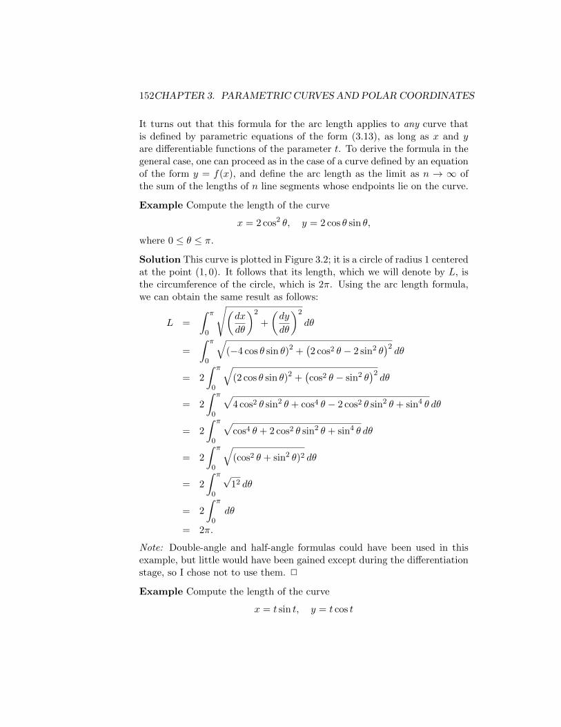
152CHAPTER 3. PARAMETRIC CURVES AND POLAR COORDINATES
It turns out that this formula for the arc length applies to any curve thatis defined by parametric equations of the form (3.13), as long as x and yare differentiable functions of the parameter t. To derive the formula in thegeneral case, one can proceed as in the case of a curve defined by an equationof the form y = f(x), and define the arc length as the limit as n → ∞ ofthe sum of the lengths of n line segments whose endpoints lie on the curve.
Example Compute the length of the curve
x = 2 cos2 θ, y = 2 cos θ sin θ,
where 0 ≤ θ ≤ π.
Solution This curve is plotted in Figure 3.2; it is a circle of radius 1 centeredat the point (1, 0). It follows that its length, which we will denote by L, isthe circumference of the circle, which is 2π. Using the arc length formula,we can obtain the same result as follows:
L =
∫ π
0
√(dx
dθ
)2
+
(dy
dθ
)2
dθ
=
∫ π
0
√(−4 cos θ sin θ)2 +
(2 cos2 θ − 2 sin2 θ
)2dθ
= 2
∫ π
0
√(2 cos θ sin θ)2 +
(cos2 θ − sin2 θ
)2dθ
= 2
∫ π
0
√4 cos2 θ sin2 θ + cos4 θ − 2 cos2 θ sin2 θ + sin4 θ dθ
= 2
∫ π
0
√cos4 θ + 2 cos2 θ sin2 θ + sin4 θ dθ
= 2
∫ π
0
√(cos2 θ + sin2 θ)2 dθ
= 2
∫ π
0
√12 dθ
= 2
∫ π
0dθ
= 2π.
Note: Double-angle and half-angle formulas could have been used in thisexample, but little would have been gained except during the differentiationstage, so I chose not to use them. 2
Example Compute the length of the curve
x = t sin t, y = t cos t
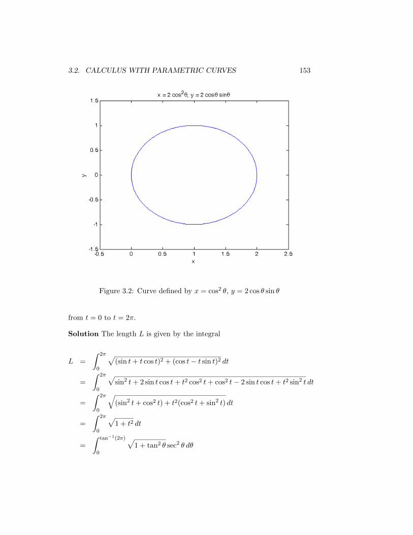
3.2. CALCULUS WITH PARAMETRIC CURVES 153
Figure 3.2: Curve defined by x = cos2 θ, y = 2 cos θ sin θ
from t = 0 to t = 2π.
Solution The length L is given by the integral
L =
∫ 2π
0
√(sin t+ t cos t)2 + (cos t− t sin t)2 dt
=
∫ 2π
0
√sin2 t+ 2 sin t cos t+ t2 cos2 t+ cos2 t− 2 sin t cos t+ t2 sin2 t dt
=
∫ 2π
0
√(sin2 t+ cos2 t) + t2(cos2 t+ sin2 t) dt
=
∫ 2π
0
√1 + t2 dt
=
∫ tan−1(2π)
0
√1 + tan2 θ sec2 θ dθ
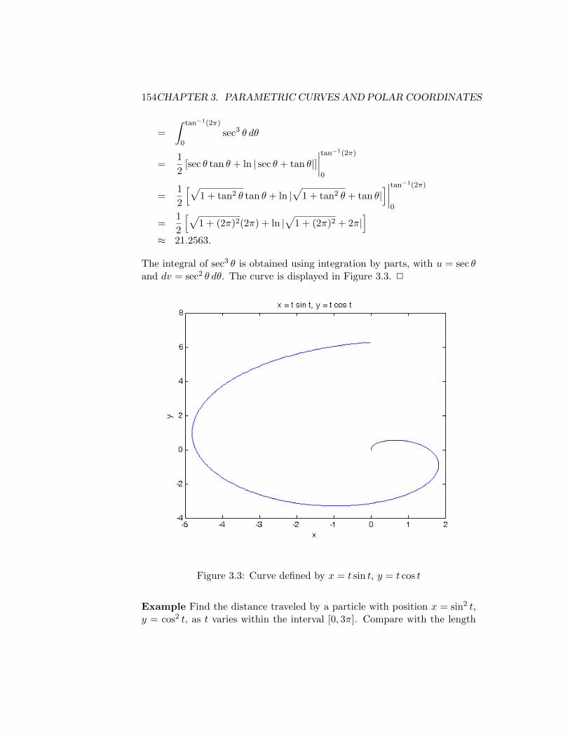
154CHAPTER 3. PARAMETRIC CURVES AND POLAR COORDINATES
=
∫ tan−1(2π)
0sec3 θ dθ
=1
2[sec θ tan θ + ln | sec θ + tan θ|]
∣∣∣∣tan−1(2π)
0
=1
2
[√1 + tan2 θ tan θ + ln |
√1 + tan2 θ + tan θ|
]∣∣∣∣tan−1(2π)
0
=1
2
[√1 + (2π)2(2π) + ln |
√1 + (2π)2 + 2π|
]≈ 21.2563.
The integral of sec3 θ is obtained using integration by parts, with u = sec θand dv = sec2 θ dθ. The curve is displayed in Figure 3.3. 2
Figure 3.3: Curve defined by x = t sin t, y = t cos t
Example Find the distance traveled by a particle with position x = sin2 t,y = cos2 t, as t varies within the interval [0, 3π]. Compare with the length
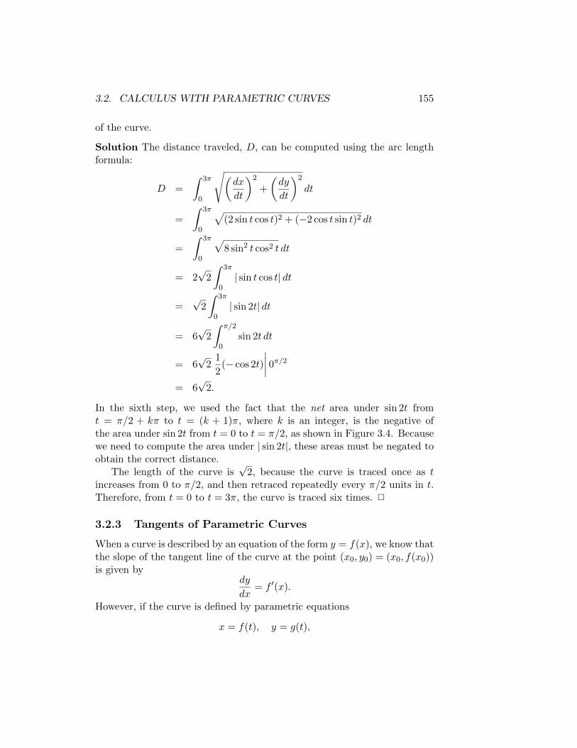
3.2. CALCULUS WITH PARAMETRIC CURVES 155
of the curve.
Solution The distance traveled, D, can be computed using the arc lengthformula:
D =
∫ 3π
0
√(dx
dt
)2
+
(dy
dt
)2
dt
=
∫ 3π
0
√(2 sin t cos t)2 + (−2 cos t sin t)2 dt
=
∫ 3π
0
√8 sin2 t cos2 t dt
= 2√
2
∫ 3π
0| sin t cos t| dt
=√
2
∫ 3π
0| sin 2t| dt
= 6√
2
∫ π/2
0sin 2t dt
= 6√
21
2(− cos 2t)
∣∣∣∣ 0π/2= 6
√2.
In the sixth step, we used the fact that the net area under sin 2t fromt = π/2 + kπ to t = (k + 1)π, where k is an integer, is the negative ofthe area under sin 2t from t = 0 to t = π/2, as shown in Figure 3.4. Becausewe need to compute the area under | sin 2t|, these areas must be negated toobtain the correct distance.
The length of the curve is√
2, because the curve is traced once as tincreases from 0 to π/2, and then retraced repeatedly every π/2 units in t.Therefore, from t = 0 to t = 3π, the curve is traced six times. 2
3.2.3 Tangents of Parametric Curves
When a curve is described by an equation of the form y = f(x), we know thatthe slope of the tangent line of the curve at the point (x0, y0) = (x0, f(x0))is given by
dy
dx= f ′(x).
However, if the curve is defined by parametric equations
x = f(t), y = g(t),
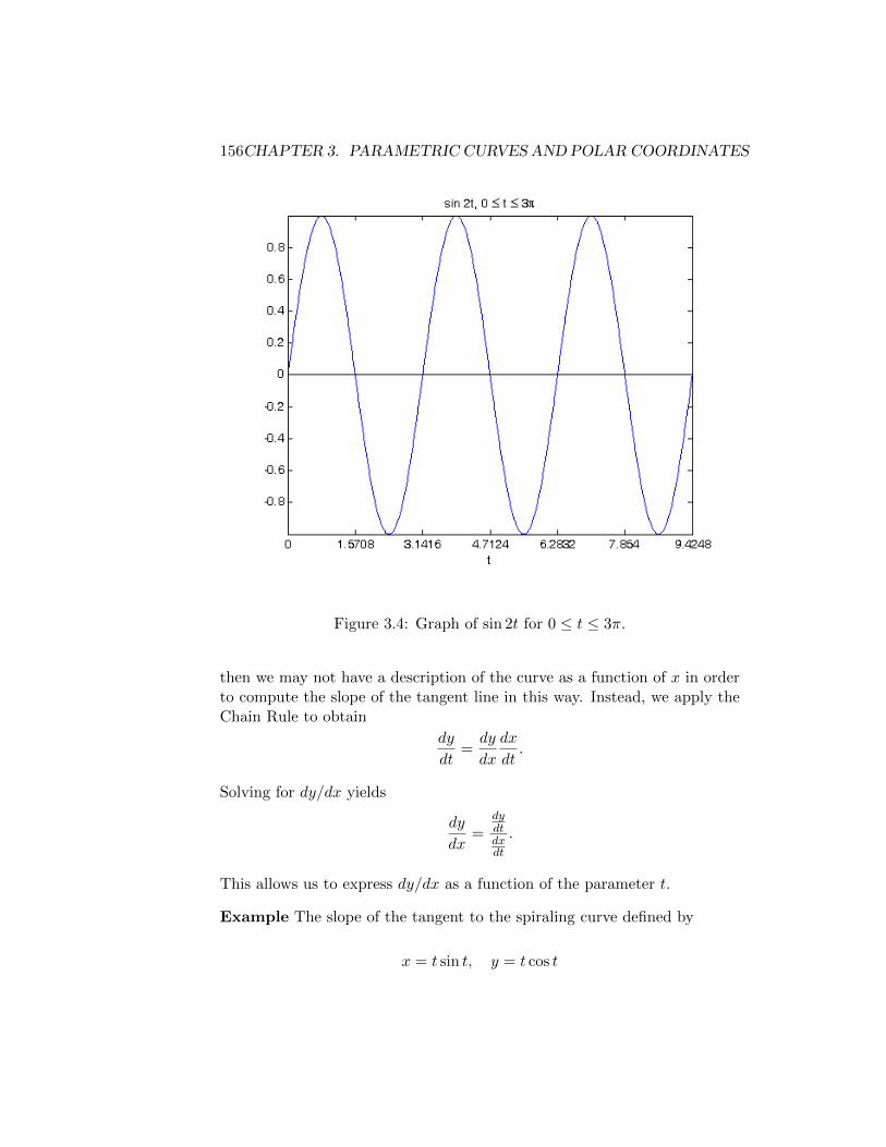
156CHAPTER 3. PARAMETRIC CURVES AND POLAR COORDINATES
Figure 3.4: Graph of sin 2t for 0 ≤ t ≤ 3π.
then we may not have a description of the curve as a function of x in orderto compute the slope of the tangent line in this way. Instead, we apply theChain Rule to obtain
dy
dt=dy
dx
dx
dt.
Solving for dy/dx yields
dy
dx=
dydtdxdt
.
This allows us to express dy/dx as a function of the parameter t.
Example The slope of the tangent to the spiraling curve defined by
x = t sin t, y = t cos t
3.2. CALCULUS WITH PARAMETRIC CURVES 157
which is shown in Figure 3.3, is given by
dy
dx=
dydtdxdt
=cos t− t sin t
sin t+ t cos t.
At the point (π/2, 0), which corresponds to t = π/2, the slope of the tangentis
m =cos π2 −
π2 sin π
2
sin π2 + π
2 cos π2=
0− π2 · 1
1 + π2 · 0
= −π2.
From the point-slope form of the equation of a line, we see the equation ofthe tangent line of the curve at this point is given by
y − 0 = −π2
(x− π
2
).
2
We know that a curve defined by the equation y = f(x) has a horizontaltangent if dy/dx = 0, and a vertical tangent if f ′(x) has a vertical asymptote.For parametric curves, we also can identify a horizontal tangent by deter-mining where dy/dx = 0. This is the case whenever dy/dt 6= 0, providedthat dx/dt = 0, thus excluding the case where dy/dx is the indeterminateform 0/0. Similarly, the tangent line is vertical whenever dx/dt = 0, butdy/dt 6= 0.
Example Consider the unit circle, which can be parametrized by the equa-tions
x = cos t, y = sin t, 0 ≤ t < 2π.
The slope of the tangent at any point on the circle is given by
dy
dx=
dydtdxdt
=cos t
− sin t= − cot t.
A horizontal tangent occurs whenever cos t = 0, and sin t 6= 0. This isthe case whenever t = π/2 or t = 3π/2. Substituting these parameter valuesinto the parametric equations, we see that the circle has two horizontaltangents, at the points (0, 1) and (0,−1).
A vertical tangent occurs whenever sin t = 0, and cos t 6= 0. This is thecase whenever t = 0 or t = π. Substituting these parameter values into theparametric equations, we see that the circle has two vertical tangents, at thepoints (1, 0) and (−1, 0). 2
158CHAPTER 3. PARAMETRIC CURVES AND POLAR COORDINATES
It is important to note that unlike a curve defined by y = f(x), a pointon the curve may have more than one tangent line, because a parametriccurve is allowed to intersect itself.
Example Consider the curve defined by the parametric equations
x = t2, y = (t2 − 4) sin t.
This curve has two tangents at the point (π2, 0). To see this, we first notethat x = t2 = π when t = ±
√π. Substituting these values into the equation
for y, we obtain y = 0, since sin t = 0 when t = ±π. Therefore, there aretwo distinct parameter values corresponding to this point on the curve.
Next, we must compute dy/dx for both values of t. We have
dy
dx=
dydtdxdt
=(t2 − 4) cos t+ 2t sin t
2t= sin t+
t2 − 4
tcos t.
Substituting t = −π yields
dy
dx= sin(−π) +
(−π)2 − 4
−πcos(−π) =
π2 − 4
π≈ 1.8684.
On the other hand, substituting t = π yields
dy
dx= sinπ +
π2 − 4
πcosπ = −π
2 − 4
π≈ −1.8684.
The curve is illustrated in Figure 3.5. 2
In order to graph curves, it is helpful to know where the curve is concaveup or concave down. For a curve defined by y = f(x), this is determined bycomputing its second derivative d2y/dx2 = f ′′(x) and checking its sign. Fora parametric curve, we can compute d2y/dx2 in the same way as dy/dx, byusing the Chain Rule. First, we note that
d2y
dx2=
d
dx
(dy
dx
).
Then, from the Chain Rule,
d
dt
(dy
dx
)=
d
dx
(dy
dx
)dx
dt=d2y
dx2
dx
dt.
Solving for d2y/dx2 yields
d2y
dx2=
ddt
(dydx
)dxdt
.
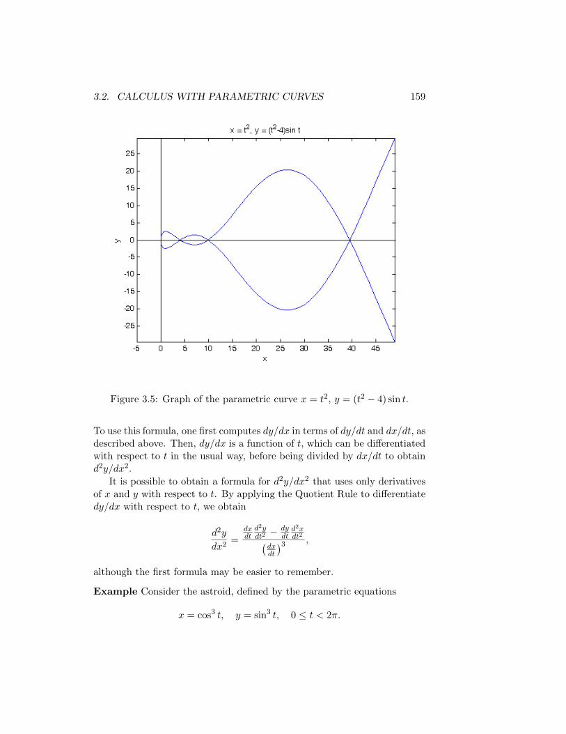
3.2. CALCULUS WITH PARAMETRIC CURVES 159
Figure 3.5: Graph of the parametric curve x = t2, y = (t2 − 4) sin t.
To use this formula, one first computes dy/dx in terms of dy/dt and dx/dt, asdescribed above. Then, dy/dx is a function of t, which can be differentiatedwith respect to t in the usual way, before being divided by dx/dt to obtaind2y/dx2.
It is possible to obtain a formula for d2y/dx2 that uses only derivativesof x and y with respect to t. By applying the Quotient Rule to differentiatedy/dx with respect to t, we obtain
d2y
dx2=
dxdtd2ydt2− dy
dtd2xdt2(
dxdt
)3 ,
although the first formula may be easier to remember.
Example Consider the astroid, defined by the parametric equations
x = cos3 t, y = sin3 t, 0 ≤ t < 2π.
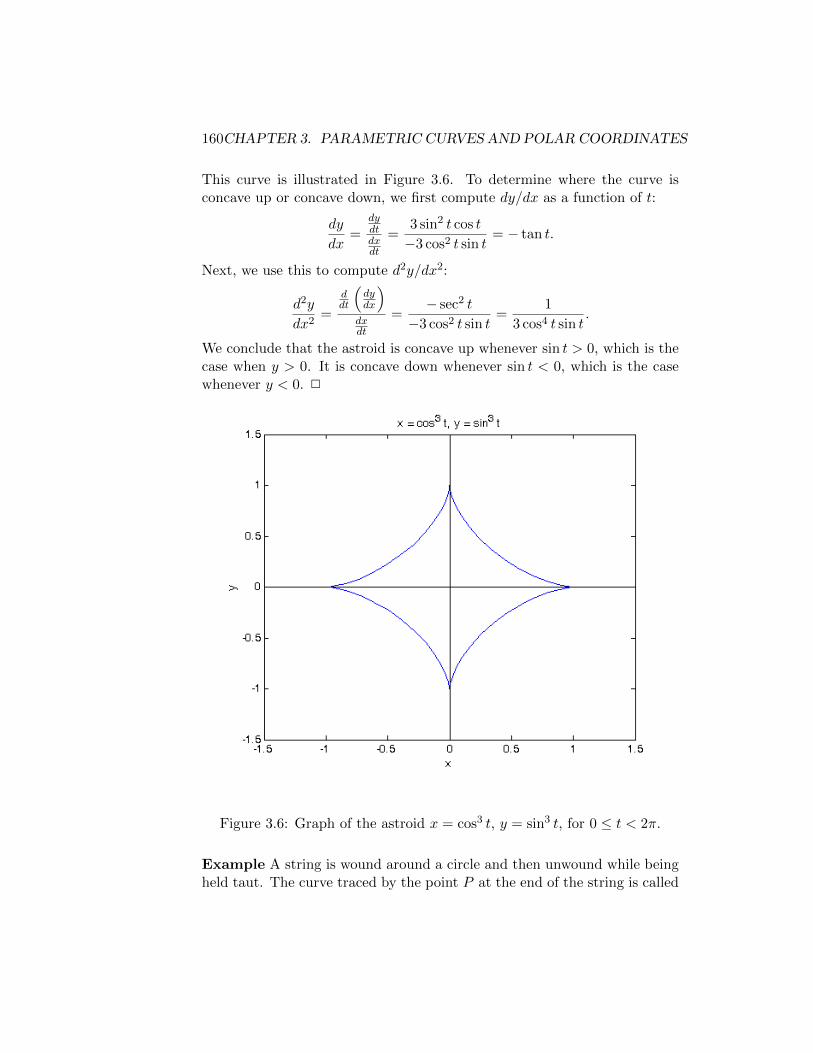
160CHAPTER 3. PARAMETRIC CURVES AND POLAR COORDINATES
This curve is illustrated in Figure 3.6. To determine where the curve isconcave up or concave down, we first compute dy/dx as a function of t:
dy
dx=
dydtdxdt
=3 sin2 t cos t
−3 cos2 t sin t= − tan t.
Next, we use this to compute d2y/dx2:
d2y
dx2=
ddt
(dydx
)dxdt
=− sec2 t
−3 cos2 t sin t=
1
3 cos4 t sin t.
We conclude that the astroid is concave up whenever sin t > 0, which is thecase when y > 0. It is concave down whenever sin t < 0, which is the casewhenever y < 0. 2
Figure 3.6: Graph of the astroid x = cos3 t, y = sin3 t, for 0 ≤ t < 2π.
Example A string is wound around a circle and then unwound while beingheld taut. The curve traced by the point P at the end of the string is called
3.2. CALCULUS WITH PARAMETRIC CURVES 161
the involute of the circle. If the circle has radius r and center O and theinitial position of P is (r, 0), and if the parameter θ is chosen as in the figure(see page 495 of the text), show that parametric equations of the involuteare
x = r(cos θ + θ sin θ), y = r(sin θ − θ cos θ).
Solution For any angle θ, the position vector for the point P is the sum oftwo vectors u and v, where u is the position vector u for the point T on thecircle corresponding to θ, and v is the vector from T to P . The magnitudeof u is r, the radius of the circle, so its components are u = 〈r cos θ, r sin θ〉.
The magnitude of v is the length of the portion of the string that hasbeen unwound, which is the length of the arc of the circle that begins atthe point (r, 0) and ends after sweeping counterclockwise (for increasing θ)through θ radians; this length is rθ.
Because the string is held taut, it is tangent to the circle at T , so v andu are perpendicular; in fact, the angle made by v with the positive x-axis,when v is translated so that its initial point is at the origin, is always 90degrees, or π/2 radians, less than that of u. That is,
v =⟨rθ cos
(θ − π
2
), rθ sin
(θ − π
2
)⟩.
Using the identities
cos(A−B) = cosA cosB+sinA sinB, sin(A−B) = sinA cosB−cosA sinB,
with A = θ and B = π/2, we obtain cos(θ − π/2) = sin θ and sin(θ −π/2) = − cos θ. By adding the components of u and v, we obtain thedesired parametric equations for the involute. 2
3.2.4 Areas Under Parametric Curves
Recall that the area A of the region bounded by the curve y = F (x), thevertical lines x = a and x = b, and the x-axis is given by the integral
A =
∫ b
aF (x) dx.
Now, suppose that the curve y = F (x) is also defined by the parametricequations x = f(t), y = g(t), for α ≤ t ≤ β. Furthermore, suppose thatf(α) = a and f(α) = b. If the curve is traversed only once as t increases
162CHAPTER 3. PARAMETRIC CURVES AND POLAR COORDINATES
from α to β, then the area can also be computed by integrating with respectto t as follows:
A =
∫ b
aF (x) dx =
∫ β
αg(t)f ′(t) dt.
On the other hand, if t = α corresponds to the right endpoint of the curve,and t = β corresponds to the left endpoint, then limits of integration mustbe reversed:
A =
∫ α
βg(t)f ′(t) dt = −
∫ β
αg(t)f ′(t) dt.
Example The upper half-circle with center (0, 0) and radius 1 can be definedby the parametric equations x = cos t, y = sin t, for 0 ≤ t ≤ π. Becauset = 0 corresponds to the right endpoint of this curve, and t = π correspondsto the left endpoint, the area bounded by the upper half-circle and the x-axisis given by
A =
∫ 0
πsin t(− sin t) dt =
∫ 0
π− sin2 t dt =
∫ π
0sin2 t dt =
∫ π
0
1− cos 2t
2dt =
t
2− sin 2t
4
∣∣∣∣π0
=π
2,
which, as expected, is half of the area of the circle. 2
Example Use the parametric equations of an ellipse, x = a cos θ, y = b sin θ,0 ≤ θ ≤ 2π, to find the area that it encloses.
Solution Because of the symmetry of the ellipse, we can compute the areaby first computing the are of the region bounded by the given curve, for0 ≤ θ ≤ π/2, and the lines x = 0 and y = 0, and then multiply the resultby 4. The area A of this region is given by the integral
A =
∫ a
0y dx.
Substituting x = a cos θ, which yields dx = −a sin θ, and substituting y =b sin θ, we obtain an integral for the area in terms of θ,
A =
∫ 0
π/2(b sin θ)(−a sin θ) dθ = ab
∫ π/2
0sin2 θ dθ.
The limits θ = 0 and θ = π/2 arise from the fact that when θ = 0, x =a cos 0 = a, and when θ = π/2, x = a cos π2 = 0. In the last step, weinterchanged the limits of integration, which changed the sign of the integral.Using the identity sin2 θ = (1− cos 2θ)/2, we obtain
A = ab
∫ π/2
0
[1
2− 1
2cos 2θ
]dθ = ab
[θ
2− 1
4sin 2θ
]∣∣∣∣π/20
=π
4ab.
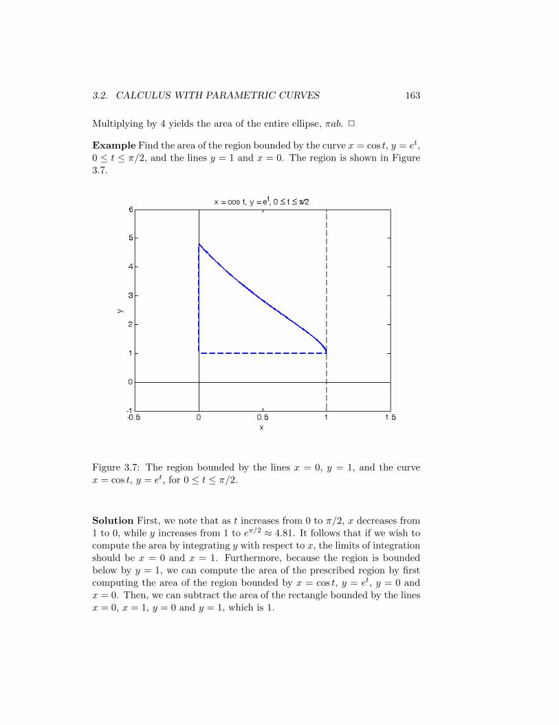
3.2. CALCULUS WITH PARAMETRIC CURVES 163
Multiplying by 4 yields the area of the entire ellipse, πab. 2
Example Find the area of the region bounded by the curve x = cos t, y = et,0 ≤ t ≤ π/2, and the lines y = 1 and x = 0. The region is shown in Figure3.7.
Figure 3.7: The region bounded by the lines x = 0, y = 1, and the curvex = cos t, y = et, for 0 ≤ t ≤ π/2.
Solution First, we note that as t increases from 0 to π/2, x decreases from1 to 0, while y increases from 1 to eπ/2 ≈ 4.81. It follows that if we wish tocompute the area by integrating y with respect to x, the limits of integrationshould be x = 0 and x = 1. Furthermore, because the region is boundedbelow by y = 1, we can compute the area of the prescribed region by firstcomputing the area of the region bounded by x = cos t, y = et, y = 0 andx = 0. Then, we can subtract the area of the rectangle bounded by the linesx = 0, x = 1, y = 0 and y = 1, which is 1.
164CHAPTER 3. PARAMETRIC CURVES AND POLAR COORDINATES
We then have
A =
∫ 1
0y dx− 1 =
∫ 0
π/2et(− sin t) dt− 1 =
∫ π/2
0et sin t dt.
Using integration by parts with u = et and dv = sin t dt, and a second timewith u = et, dv = cos t dt, yields∫ π/2
0et sin t dt = −et cos t dt
∣∣π/20
+
∫ π/2
0et cos t dt
= 1 + et sin t∣∣π/20−∫ π/2
0et sin t dt
=1
2+
1
2eπ/2.
In the last step, we moved the integral on the right side to the left side,because they are the same except for their sign, and then we divided by 2to obtain the result. Subtracting 1 from this integral yields A = 1
2eπ/2 − 1
2for the area of the region.
Another way to compute the area is to integrate x with respect to y. Inthis case, the limits of integration are y = 1 and y = eπ/2. We then have
A =
∫ exp(π/2)
1x dy =
∫ π/2
0et cos t dt.
Using integration by parts as before yields the area. 2
3.2.5 Summary
• The arc length of a curve defined by the equation y = f(x), for a ≤x ≤ b, is the integral of
√1 + [f ′(x)]2 from a to b.
• Often, this integral cannot be computed analytically using known in-tegration rules, so the arc length must instead be approximated nu-merically using a technique such as the Composite Simpson’s Rule.
• If a curve is defined by parametric equations x = g(t), y = h(t) for c ≤t ≤ d, the arc length of the curve is the integral of
√(dx/dt)2 + (dy/dt)2 =√
[g′(t)]2 + [h′(t)]2 from c to d.
• The slope of the tangent line of a parametric curve defined by paramet-ric equations x = f(t), y = g(t) is given by dy/dx = (dy/dt)/(dx/dt).
3.3. POLAR COORDINATES 165
• A parametric curve has a horizontal tangent wherever dy/dt = 0 anddx/dt 6= 0. It has a vertical tangent wherever dx/dt = 0 and dy/dt 6= 0.
• The concavity of a parametric curve at a point can be determinedby computing d2y/dx2 = d(dy/dx)/dt/(dx/dt), where dy/dt is bestrepresented as a function of t, not x. The curve is concave up whend2y/dx2 is positive, and concave down if it is negative.
• A parametric curve x = f(t), y = g(t) can have two tangents at a point(x0, y0) on its graph, if there are two distinct values of the parametert, t1 and t2, such that f(t1) = f(t2) = x0 and g(t1) = g(t2) = y0.
• The area of the region bounded by the parametric curve x = f(t),y = g(t), the x-axis, the line x = a, and the line x = b, where f(α) = aand g(β) = b, is the integral from α to β of g(t)f ′(t) dt, provided thatthe curve is only traversed once as t increases from α to β.
3.3 Polar Coordinates
Throughout this course, we have denoted a point in the plane by an orderedpair (x, y), where the numbers x and y denote the directed (i.e., signedpositive or negative) distance between the point and each of two perpen-dicular lines, the x-axis and the y-axis. The elements of this ordered pairare called coordinates, and the coordinates used in this particular methodof identifying points in the plane are called Cartesian coordinates.
In this section, we introduce an alternative coordinate system known asthe polar coordinate system. In this system, a point in the plane is identifiedby an ordered pair (r, θ), where:
• r is the directed distance from a point designated as the pole, and
• θ is the angle, in radians, that a ray between the pole and the pointmakes with a ray designated as the polar axis.
The coordinates r and θ are called polar coodinates.The pole is the point (0, 0) in Cartesian coordinates, and has polar coor-
dinates (0, θ) for any value of θ. The polar axis corresponds to the positivex-axis. An angle θ is considered positive if measured in the counterclock-wise direction from the polar axis, and negative if measured in the clockwisedirection.
Example Sketch the region in the plane consisting of points whose polarcoordinates satisfy 2 < r < 3, 5π/3 ≤ θ ≤ 7π/3.
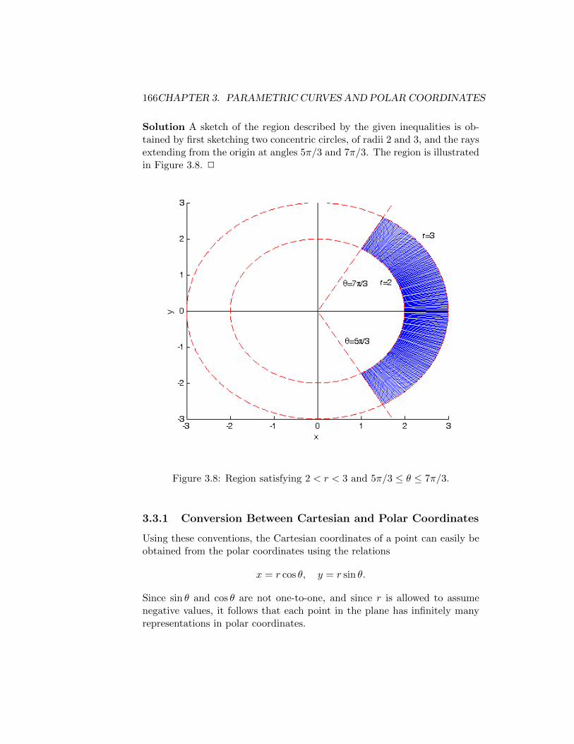
166CHAPTER 3. PARAMETRIC CURVES AND POLAR COORDINATES
Solution A sketch of the region described by the given inequalities is ob-tained by first sketching two concentric circles, of radii 2 and 3, and the raysextending from the origin at angles 5π/3 and 7π/3. The region is illustratedin Figure 3.8. 2
Figure 3.8: Region satisfying 2 < r < 3 and 5π/3 ≤ θ ≤ 7π/3.
3.3.1 Conversion Between Cartesian and Polar Coordinates
Using these conventions, the Cartesian coordinates of a point can easily beobtained from the polar coordinates using the relations
x = r cos θ, y = r sin θ.
Since sin θ and cos θ are not one-to-one, and since r is allowed to assumenegative values, it follows that each point in the plane has infinitely manyrepresentations in polar coordinates.
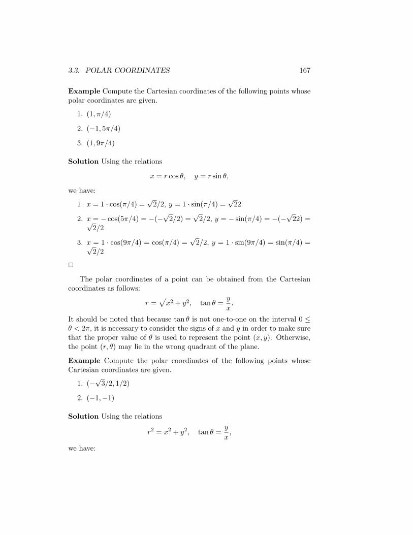
3.3. POLAR COORDINATES 167
Example Compute the Cartesian coordinates of the following points whosepolar coordinates are given.
1. (1, π/4)
2. (−1, 5π/4)
3. (1, 9π/4)
Solution Using the relations
x = r cos θ, y = r sin θ,
we have:
1. x = 1 · cos(π/4) =√
2/2, y = 1 · sin(π/4) =√
22
2. x = − cos(5π/4) = −(−√
2/2) =√
2/2, y = − sin(π/4) = −(−√
22) =√2/2
3. x = 1 · cos(9π/4) = cos(π/4) =√
2/2, y = 1 · sin(9π/4) = sin(π/4) =√2/2
2
The polar coordinates of a point can be obtained from the Cartesiancoordinates as follows:
r =√x2 + y2, tan θ =
y
x.
It should be noted that because tan θ is not one-to-one on the interval 0 ≤θ < 2π, it is necessary to consider the signs of x and y in order to make surethat the proper value of θ is used to represent the point (x, y). Otherwise,the point (r, θ) may lie in the wrong quadrant of the plane.
Example Compute the polar coordinates of the following points whoseCartesian coordinates are given.
1. (−√
3/2, 1/2)
2. (−1,−1)
Solution Using the relations
r2 = x2 + y2, tan θ =y
x,
we have:
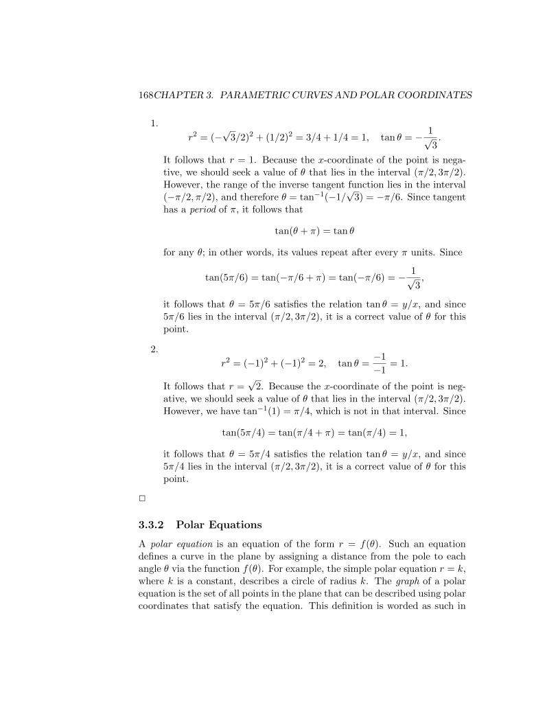
168CHAPTER 3. PARAMETRIC CURVES AND POLAR COORDINATES
1.
r2 = (−√
3/2)2 + (1/2)2 = 3/4 + 1/4 = 1, tan θ = − 1√3.
It follows that r = 1. Because the x-coordinate of the point is nega-tive, we should seek a value of θ that lies in the interval (π/2, 3π/2).However, the range of the inverse tangent function lies in the interval(−π/2, π/2), and therefore θ = tan−1(−1/
√3) = −π/6. Since tangent
has a period of π, it follows that
tan(θ + π) = tan θ
for any θ; in other words, its values repeat after every π units. Since
tan(5π/6) = tan(−π/6 + π) = tan(−π/6) = − 1√3,
it follows that θ = 5π/6 satisfies the relation tan θ = y/x, and since5π/6 lies in the interval (π/2, 3π/2), it is a correct value of θ for thispoint.
2.
r2 = (−1)2 + (−1)2 = 2, tan θ =−1
−1= 1.
It follows that r =√
2. Because the x-coordinate of the point is neg-ative, we should seek a value of θ that lies in the interval (π/2, 3π/2).However, we have tan−1(1) = π/4, which is not in that interval. Since
tan(5π/4) = tan(π/4 + π) = tan(π/4) = 1,
it follows that θ = 5π/4 satisfies the relation tan θ = y/x, and since5π/4 lies in the interval (π/2, 3π/2), it is a correct value of θ for thispoint.
2
3.3.2 Polar Equations
A polar equation is an equation of the form r = f(θ). Such an equationdefines a curve in the plane by assigning a distance from the pole to eachangle θ via the function f(θ). For example, the simple polar equation r = k,where k is a constant, describes a circle of radius k. The graph of a polarequation is the set of all points in the plane that can be described using polarcoordinates that satisfy the equation. This definition is worded as such in
3.3. POLAR COORDINATES 169
order to take into account that each point in the plane can have infinitelymany representations in polar coordinates.
Example Sketch the curve described by the polar equation
r = cos 2θ, 0 ≤ θ ≤ 2π.
Solution This curve can be sketched by evaluating r = cos 2θ at severalvalues of θ. For each such value, the point (r, θ) = (cos 2θ, θ) can be plottedby traversing r units along the ray that makes the angle θ with the polar axis(which is the x-axis), if r is positive; otherwise, use the ray that makes theangle θ+π with the polar axis. The curve r = cos 2θ is illustrated in Figure3.9. The circles indicate the points corresponding to θ = 0, π/4, π/2, 3π/4,π, 5π/4, 3π/2, 7π/4, and 2π. 2
Figure 3.9: Curve described by the polar equation r = cos 2θ, where 0 ≤θ ≤ 2π.
170CHAPTER 3. PARAMETRIC CURVES AND POLAR COORDINATES
Example Sketch the curve described by the polar equation
r = sin θ, 0 ≤ θ ≤ 2π.
Solution Figure 3.10 displays the curve, which can be plotted using thesame approach as in the previous example. The circles indicate the pointscorresponding to θ = 0, π/4, π/2, 3π/4, π, 5π/4, 3π/2, 7π/4, and 2π. Thecircle is traced twice, once for 0 ≤ θ ≤ π, and again for π ≤ θ ≤ 2π. 2
Figure 3.10: Curve described by the polar equation r = sin θ, where 0 ≤θ ≤ 2π.
Example Identify the curve r = 3 sin θ by finding a Cartesian equation forthe curve.
Solution Multiplying both sides by r yields r2 = 3r sin θ. Using the rela-tions y = r sin θ and x2 + y2 = r2, we obtain the Cartesian equation
x2 + y2 = 3y.
3.3. POLAR COORDINATES 171
Moving the 3y to the left side and completing the square yields
x2 + y3 − 3y +9
4=
9
4,
which, upon factoring, becomes
x2 +
(y − 3
2
)2
=
(3
2
)2
.
This is the equation of a circle with center (0, 3/2) and radius 3/2. 2
Example Identify the curve r = csc θ by finding a Cartesian equation forthe curve.
Solution Applying csc θ = 1/ sin θ and multiplying both sides by sin θ yieldsr sin θ = 1, which, in Cartesian coordinates, becomes y = 1. This curve is ahorizontal line that lies one unit above the x-axis. 2
Example Find a polar equation for the curve represented by the Cartesianequation x2 + y2 = 2cx.
Solution Using the relations x2 + y2 = r2 and x = r cos θ, we obtain thepolar equation r2 = 2cr cos θ, which can then be divided through by r toobtain a polar equation in standard form, r = 2c cos θ. This curve is a circlewith center (c, 0) with radius c. 2
3.3.3 Tangents to Polar Curves
We now determine the slope of a tangent line of a polar curve. If the curvecan be described by an equation of the form y = F (x) for some differentiablefunction F , then, by the Chain Rule,
dy
dθ= F ′(x)
dx
dθ,
but since F ′(x) = dy/dx, it follows that
dy
dx=dy/dθ
dx/dθ.
Expressing x and y in polar coordinates and applying the Product Ruleyields
dy
dx=
dydθdxdθ
=drdθ sin θ + r cos θdrdθ cos θ − r sin θ
.
172CHAPTER 3. PARAMETRIC CURVES AND POLAR COORDINATES
It can be shown that this result also holds for curves that cannot be describedby an equation of the form y = F (x).
We make the following observations about tangents to polar curves,based on the above expression for their slope:
• Horizontal tangents occur when dy/dθ = 0, provided that dx/dθ 6= 0.
• Vertical tangents occur when dx/dθ = 0, provided that dy/dθ 6= 0.
• At the pole, when r = 0, the slope of the tangent is given by
dy
dx=
drdθ sin θdrdθ cos θ
= tan θ
provided dr/dθ 6= 0.
Example Given the curve defined by the polar equation r = sin θ, where0 ≤ θ ≤ π, determine the values of θ at which the tangent to the curve iseither horizontal or vertical.
Solution As we learned in the previous example, this curve is a circle withcenter (0, 1/2) and radius 1/2. The curve is displayed in Figure 3.10. Usingthe formula for the slope of the tangent, we have, by double-angle formulas,
dy
dx=
dydθdxdθ
=drdθ sin θ + r cos θdrdθ cos θ − r sin θ
=(cos θ) sin θ + (sin θ) cos θ
(cos θ) cos θ − (sin θ) sin θ
=2 sin θ cos θ
cos2 θ − sin2 θ
=sin 2θ
cos 2θ= tan 2θ.
Alternatively, we can use the relations
x = r cos θ, y = r sin θ
to compute dy/dθ and dx/dθ directly. In this case, we have
x = sin θ cos θ, y = sin2 θ
3.3. POLAR COORDINATES 173
or, from double-angle and half-angle formulas,
x =sin 2θ
2, y =
1− cos 2θ
2
and thereforedy
dθ= sin 2θ,
dx
dθ= cos 2θ,
which yields dy/dx = tan 2θ as before.
The tangent is horizontal when dy/dθ = 0 and dx/dθ 6= 0. This occurswhen θ = 0, π/2, or π. The tangent is vertical when dx/dθ = 0 and dy/dθ 6=0. This occurs when θ = π/4 and θ = 3π/4. 2
Example Let P be any point (except the origin) on the curve r = f(θ). Ifψ is the angle between the tangent line at P and the radial line OP , showthat
tanψ =r
dr/dθ
[Hint: Observe that ψ = φ− θ in the figure on page 504 in the text.]
Solution We have
tanψ = tan(φ− θ) =tanφ− tan θ
1 + tanφ tan θ.
Because φ is the angle that the tangent line makes with the positive x-axis,
tanφ =dy
dx=
drdθ sin θ + r cos θdrdθ cos θ − r sin θ
.
It follows that if we write r′ = dr/dθ, then
tanψ =r′ sin θ+r cos θr′ cos θ−r sin θ −
sin θcos θ
1 + r′ sin θ+r cos θr′ cos θ−r sin θ
sin θcos θ
,
we can simplify by putting all fractions over a common denominator. Be-cause the common denominators are both equal to cos θ(r′ cos θ − r sin θ),they cancel, and we obtain
tanψ =(r′ sin θ + r cos θ) cos θ − (r′ cos θ − r sin θ) sin θ
(r′ cos θ − r sin θ) cos θ + (r′ sin θ + r cos θ) sin θ.
Expanding, and using sin2 θ + cos2 θ = 1, we obtain tanψ = r/r′. 2
174CHAPTER 3. PARAMETRIC CURVES AND POLAR COORDINATES
3.3.4 Summary
• A point can be represented by polar coordinates (r, θ), where r is thedistance between the point and the origin, or pole, and θ is the anglethat a line segment from the pole to the point makes with the positivex-axis.
• To convert from polar coordinates to Cartesian coordinates (x, y), onecan use the formulas x = r cos θ and y = r sin θ.
• To convert from Cartesian coordinates to polar coordinates, one canuse r =
√x2 + y2, and θ = tan−1(y/x) if x > 0. If x < 0, then
θ = tan−1(y/x) + π. If x = 0, θ = π/2 if y > 0, and −π/2 if y < 0.
• To graph a curve defined by a polar equation of the form r = f(θ),one can compute r for various values of θ, and use polar coordinatesto plot the corresponding points on the curve.
• To compute the slope of the tangent to a polar curve r = f(θ), onecan differentiate x = f(θ) cos θ and y = f(θ) sin θ with respect to θ,and then use the relation dy/dx = (dy/dθ)/(dx/dθ).
3.4 Areas and Lengths in Polar Coordinates
In this section, we learn how to compute areas of regions and lengths ofcurves, for regions and curves that are most easily described using polarequations instead of Cartesian equations.
3.4.1 Area
Consider a region bounded by a curve with polar equation r = f(θ) andthe rays θ = a and θ = b. The area of such a region would be difficult tocompute if working in Cartesian coordinates, but can be obtained in polarcoordinates using the formula for the area of a sector of a circle of radius rand central angle θ,
A =1
2r2θ.
To compute the area of such a region, we can divide the interval [a, b] intosubintervals of uniform width ∆θ = (b − a)/n. Then, we can approximatethe region with n circular sectors. The subinterval has endpoints [θi−1, θi],where θi = a+ i∆θ, and the corresponding sector has central angle ∆θ andradius f(θ∗i ), where θi−1 ≤ θai st ≤ θi.
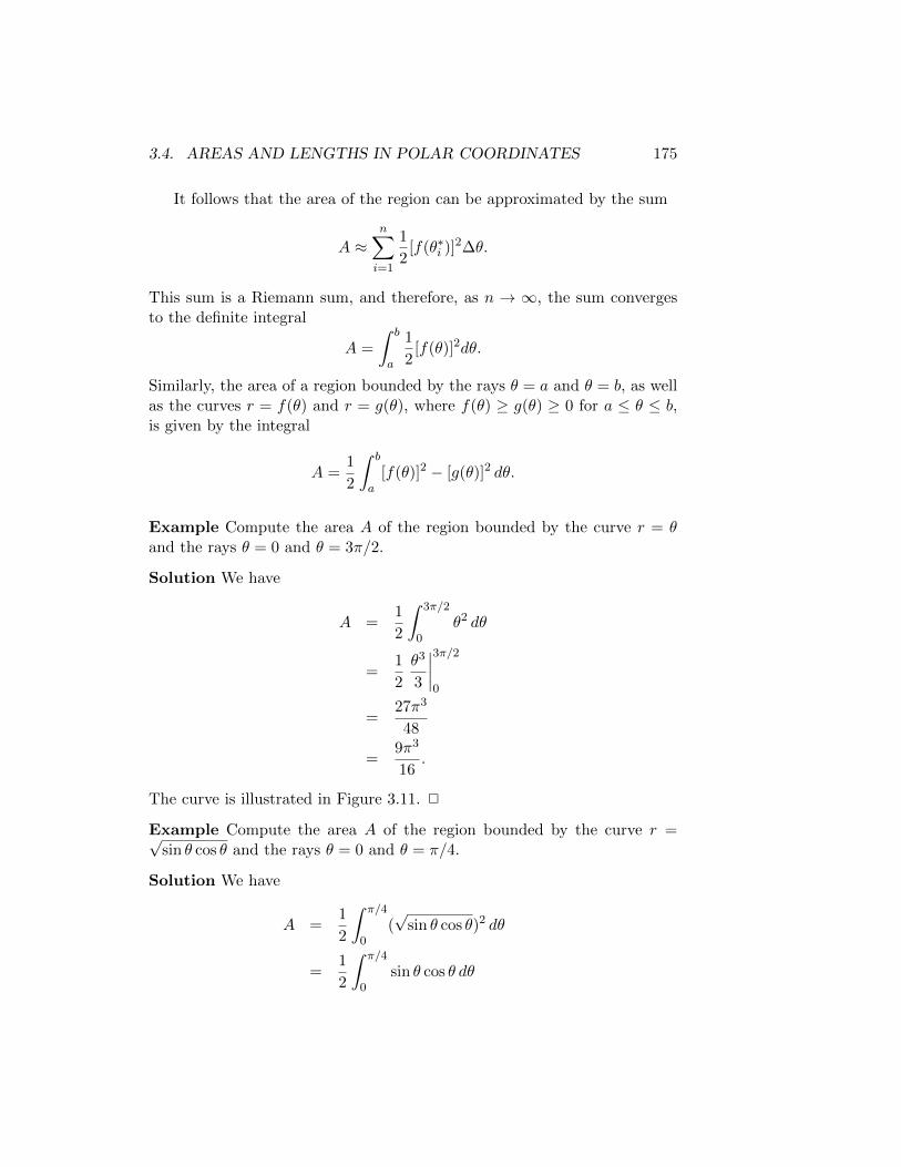
3.4. AREAS AND LENGTHS IN POLAR COORDINATES 175
It follows that the area of the region can be approximated by the sum
A ≈n∑i=1
1
2[f(θ∗i )]
2∆θ.
This sum is a Riemann sum, and therefore, as n → ∞, the sum convergesto the definite integral
A =
∫ b
a
1
2[f(θ)]2dθ.
Similarly, the area of a region bounded by the rays θ = a and θ = b, as wellas the curves r = f(θ) and r = g(θ), where f(θ) ≥ g(θ) ≥ 0 for a ≤ θ ≤ b,is given by the integral
A =1
2
∫ b
a[f(θ)]2 − [g(θ)]2 dθ.
Example Compute the area A of the region bounded by the curve r = θand the rays θ = 0 and θ = 3π/2.
Solution We have
A =1
2
∫ 3π/2
0θ2 dθ
=1
2
θ3
3
∣∣∣∣3π/20
=27π3
48
=9π3
16.
The curve is illustrated in Figure 3.11. 2
Example Compute the area A of the region bounded by the curve r =√sin θ cos θ and the rays θ = 0 and θ = π/4.
Solution We have
A =1
2
∫ π/4
0(√
sin θ cos θ)2 dθ
=1
2
∫ π/4
0sin θ cos θ dθ
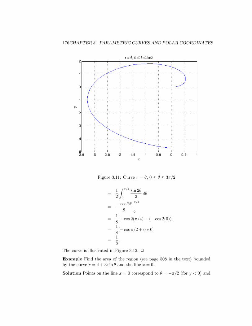
176CHAPTER 3. PARAMETRIC CURVES AND POLAR COORDINATES
Figure 3.11: Curve r = θ, 0 ≤ θ ≤ 3π/2
=1
2
∫ π/4
0
sin 2θ
2dθ
=− cos 2θ
8
∣∣∣∣π/40
=1
8[− cos 2(π/4)− (− cos 2(0))]
=1
8[− cosπ/2 + cos 0]
=1
8.
The curve is illustrated in Figure 3.12. 2
Example Find the area of the region (see page 508 in the text) boundedby the curve r = 4 + 3 sin θ and the line x = 0.
Solution Points on the line x = 0 correspond to θ = −π/2 (for y < 0) and
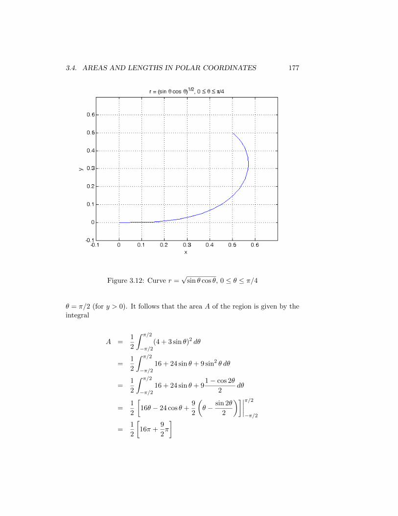
3.4. AREAS AND LENGTHS IN POLAR COORDINATES 177
Figure 3.12: Curve r =√
sin θ cos θ, 0 ≤ θ ≤ π/4
θ = π/2 (for y > 0). It follows that the area A of the region is given by theintegral
A =1
2
∫ π/2
−π/2(4 + 3 sin θ)2 dθ
=1
2
∫ π/2
−π/216 + 24 sin θ + 9 sin2 θ dθ
=1
2
∫ π/2
−π/216 + 24 sin θ + 9
1− cos 2θ
2dθ
=1
2
[16θ − 24 cos θ +
9
2
(θ − sin 2θ
2
)]∣∣∣∣π/2−π/2
=1
2
[16π +
9
2π
]
178CHAPTER 3. PARAMETRIC CURVES AND POLAR COORDINATES
=41π
4.
2
Example Find the area of the region enclosed by one loop of the curver = sin 2θ.
Solution We have r = 0 when θ = 0 and θ = π/2, so the interval 0 ≤ θ ≤π/2 corresponds to one loop of the curve. Therefore, the area of the regionenclosed by this loop is
1
2
∫ π/2
0sin2 2θ dθ =
1
2
∫ π/2
0
1− cos 4θ
2dθ =
1
4
[θ − sin 4θ
4
]∣∣∣∣π/20
=π
8,
where a double-angle identity was used to rewrite sin2 2θ in such a way thatit can be integrated. 2
Example Find the area of the region that lies inside the curve r = 3 cos θand outside the curve r = 1 + cos θ.
Solution These curves intersect when 3 cos θ = 1 + cos θ, or cos θ = 1/2,which is the case when θ = ±π/3. Therefore, the area A of the regionbetween them is given by
A =1
2
∫ π/3
−π/3[3 cos θ]2 − [1 + cos θ]2 dθ
=1
2
∫ π/3
−π/39 cos2 θ − (1 + 2 cos θ + cos2 θ) dθ
=1
2
∫ π/3
−π/38 cos2 θ − 1− 2 cos θ dθ
=1
2
∫ π/3
−π/38
1 + cos 2θ
2− 1− 2 cos θ dθ
=1
2
∫ π/3
−π/33 + 4 cos 2θ − 2 cos θ dθ
=1
2
[3θ + 4
sin 2θ
2− 2 sin θ
]∣∣∣∣π/3−π/3
= π.
2
3.4. AREAS AND LENGTHS IN POLAR COORDINATES 179
Example Find the area of the region that lies inside both of the curvesr = sin θ and r = cos θ.
Solution These curves intersect when θ = π/4. Therefore, if we divide theregion that lies inside both curves with the ray θ = π/4, we can obtain itsarea A by computing
A =1
2
∫ π/4
0sin2 θ dθ +
1
2
∫ π/2
π/4cos2θ dθ
=1
2
∫ π/4
0
1− cos 2θ
2dθ +
1
2
∫ π/2
π/4
1 + cos 2θ
2dθ
=
[θ
2− sin 2θ
4
]∣∣∣∣π/40
+
[θ
2+
sin 2θ
4
]∣∣∣∣π/2π/4
=π
8− 1
4+π
8− 1
4
=1
8(π − 2).
2
3.4.2 Arc Length
Recall that the arc length of a curve represented by parametric equations
x = f(θ), y = g(θ)
is given by
L =
∫ b
a
√(dx
dθ
)2
+
(dy
dθ
)2
dθ,
where θ is the parameter, and the curve is defined for a ≤ θ ≤ b. Ideally wewould like to be able to compute the arc length of a curve directly from itspolar equation, instead of always having to convert to Cartesian coordinates.
Since Cartesian coordinates and polar coordinates are related by theequations x = r cos θ, y = r sin θ, it follows from the Product Rule that
dx
dθ=dr
dθcos θ − r sin θ,
dy
dθ=dr
dθsin θ + r cos θ.
We then have(dx
dθ
)2
+
(dy
dθ
)2
=
(dr
dθcos θ − r sin θ
)2
+
(dr
dθsin θ + r cos θ
)2
180CHAPTER 3. PARAMETRIC CURVES AND POLAR COORDINATES
=
(dr
dθ
)2
cos2 θ − 2rdr
dθsin θ cos θ + r2 sin2 θ +(
dr
dθ
)2
sin2 θ + 2rdr
dθsin θ cos θ + r2 cos2 θ
=
(dr
dθ
)2
cos2 θ +
(dr
dθ
)2
sin2 θ + r2 sin2 θ + r2 cos2 θ
=
(dr
dθ
)2
+ r2.
It follows that the arc length of a curve can be obtained directly from itspolar equation, using the formula
L =
∫ b
a
√r2 +
(dr
dθ
)2
dθ.
Example Compute the arc length L of the curve r = cos θ, where 0 ≤ θ ≤π/2.
Solution We have dr/dθ = − sin θ, and therefore
L =
∫ π/2
0
√r2 +
(dr
dθ
)2
dθ
=
∫ π/2
0
√cos2 θ + (− sin θ)2 dθ
=
∫ π/2
0
√cos2 θ + sin2 θ dθ
=
∫ π/2
01 dθ
=π
2.
The curve is illustrated in Figure 3.13. 2
3.4.3 Summary
• The area of the region bounded by the polar curve r = f(θ), the rayθ = a, and the ray θ = b is half of the integral of r2 from a to b.
• The arc length of a polar curve r = f(θ), where a ≤ θ ≤ b, is theintegral of
√r2 + (dr/dθ)2 from a to b.
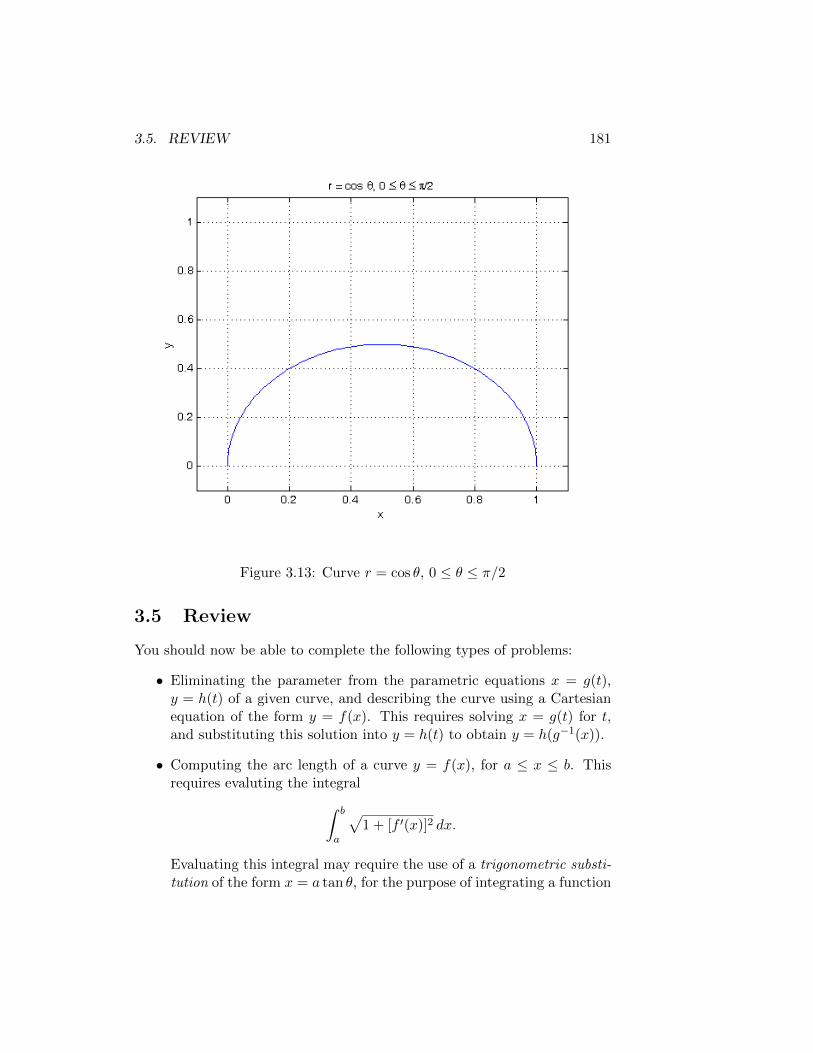
3.5. REVIEW 181
Figure 3.13: Curve r = cos θ, 0 ≤ θ ≤ π/2
3.5 Review
You should now be able to complete the following types of problems:
• Eliminating the parameter from the parametric equations x = g(t),y = h(t) of a given curve, and describing the curve using a Cartesianequation of the form y = f(x). This requires solving x = g(t) for t,and substituting this solution into y = h(t) to obtain y = h(g−1(x)).
• Computing the arc length of a curve y = f(x), for a ≤ x ≤ b. Thisrequires evaluting the integral∫ b
a
√1 + [f ′(x)]2 dx.
Evaluating this integral may require the use of a trigonometric substi-tution of the form x = a tan θ, for the purpose of integrating a function
182CHAPTER 3. PARAMETRIC CURVES AND POLAR COORDINATES
involving√a2 + x2. This substitution uses the identity tan2 θ + 1 =
sec2 θ. Alternatively, evaluating the integral may require recognizingperfect squares of the form (a − b)2 = a2 − 2ab + b2 or (a + b)2 =a2 + 2ab+ b2.
• Computing the arc length of a curve x = f(t), y = g(t), for a ≤ t ≤ b.This requires evaluating the integral∫ b
a
√[f ′(t)]2 + [g′(t)]2 dt.
See the comments above for tips on how to evaluate such an integral.
• Computing the equation of the tangent line at a point on a parametriccurve. This requires computing the slope dy/dx = (dy/dt)/(dx/dt),and then using the point-slope form y − y0 = m(x − x0), where m isthe slope and (x0, y0) is a point on the line. It will also be necessary todetermine the value of the parameter t that corresponds to the givenpoint.
• Determining whether a given parametric curve is concave up or con-cave down at a given point. This involves computing
d2y
dx2=
ddt
(dydx
)dxdt
,
where dy/dx = (dy/dt)/(dx/dt) is computed as a function of t, so thatit can readily be differentiated with respect to t.
• Computing the area of a region bounded by a parametric curve, aswell as horizontal and vertical lines. This requires using one of theformulas∫ b
ay dx =
∫ β
αg(t)f ′(t) dt,
∫ d
cx dy =
∫ β
αf(t)g′(t) dt,
where x = f(t), y = g(t), α ≤ t ≤ β describes the curve, and f(α) = a,f(β) = b, g(α) = c, and g(β) = d, with a ≤ b and c ≤ d. The choiceof formula depends on whether the region is bounded by two verticallines, in which case the first formula should be used, or two horizontallines, in which case the second formula should be used.
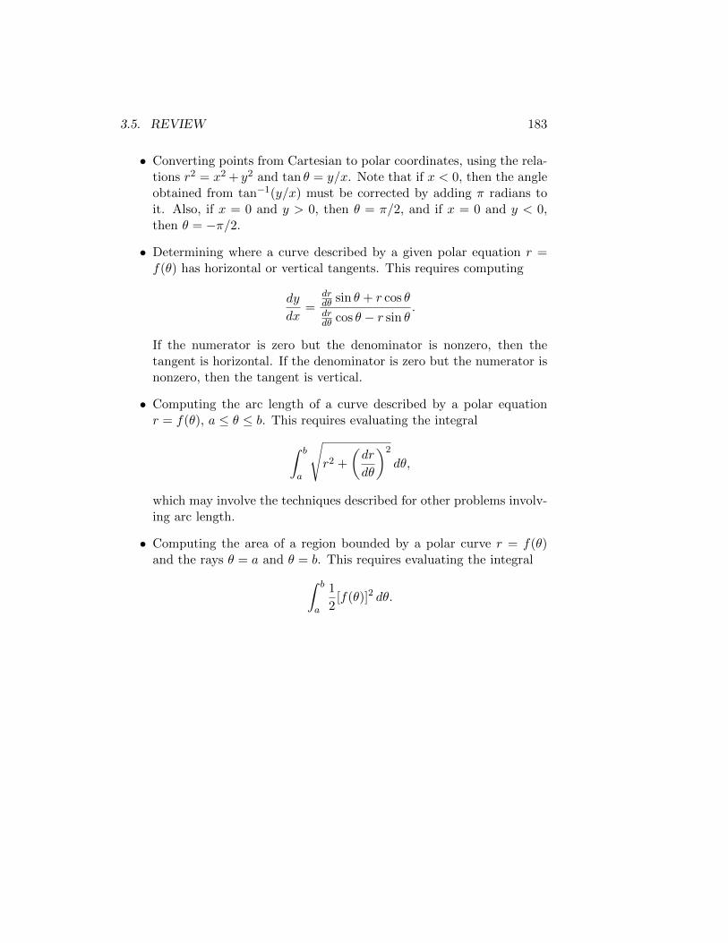
3.5. REVIEW 183
• Converting points from Cartesian to polar coordinates, using the rela-tions r2 = x2 + y2 and tan θ = y/x. Note that if x < 0, then the angleobtained from tan−1(y/x) must be corrected by adding π radians toit. Also, if x = 0 and y > 0, then θ = π/2, and if x = 0 and y < 0,then θ = −π/2.
• Determining where a curve described by a given polar equation r =f(θ) has horizontal or vertical tangents. This requires computing
dy
dx=
drdθ sin θ + r cos θdrdθ cos θ − r sin θ
.
If the numerator is zero but the denominator is nonzero, then thetangent is horizontal. If the denominator is zero but the numerator isnonzero, then the tangent is vertical.
• Computing the arc length of a curve described by a polar equationr = f(θ), a ≤ θ ≤ b. This requires evaluating the integral
∫ b
a
√r2 +
(dr
dθ
)2
dθ,
which may involve the techniques described for other problems involv-ing arc length.
• Computing the area of a region bounded by a polar curve r = f(θ)and the rays θ = a and θ = b. This requires evaluating the integral∫ b
a
1
2[f(θ)]2 dθ.
Index
Absolute Convergence Test, 57
alternating sequence, 28
Alternating Series Estimation Theo-rem, 56
Alternating Series Test, 55
angle between planes, 128
arc length, 149
arc length, function, 151
astroid, 149
basis, 99
basis, standard, 98
binomial coefficient, 77
binomial series, 76
center, power series, 61
closed form, 23
common ratio, 40
commutativity, 94
Comparison Test, 52
conjugate, 28
contrapositive, 45
convergence, 25
convergence, absolute, 57
convergence, conditional, 58
convergence, interval of, 63
convergence, radius of, 63
convergence, series, 39
converse, 45, 58
coordinate, 165
coordinate axis, 87
coordinates, Cartesian, 165
coordinates, polar, 165cross product, 111
determinant, 122direction number, 117divergence, 25, 26divergence, series, 39dot product, 105
Fibonacci sequence, 22floor function, 33
geometric sequence, 30geometric series, 40
harmonic series, 58
indeterminate form, 28index, 21infinite series, 37infinum, 31inner product, 105Integral Test, 49integral, definite, 14integrand, 14integration, 14involute, 161
l’Hospital’s Rule, 28limit, 10, 25Limit Comparison Test, 53limit laws, 26limit of integration, 14linear combination, 110
184
INDEX 185
linear equation, 127linear equations, 120
Maclaurin polynomial, 19Maclaurin series, 69Monotonic Sequence Theorem, 31
natural numbers, 21
octant, 89octant, first, 89ordered triple, 87
p-series, 50Parallelogram Law, 94parameter, 116, 143parametric curve, 143parametric curve, initial point, 143parametric curve, terminal point, 143parametric equation, 117parametric equations, 143partial fraction decomposition, 43partial sum, 38polar axis, 165polar equation, 168pole, 165power series, 42, 61projection, 89projection, scalar, 107projection, vector, 107
Ratio Test, 58recurrence relation, 22Riemann sum, 14right-hand rule, 113Root Test, 59
scalar, 94scalar multiple, 94scalar multiplication, 94sequence, 21
sequence, bounded, 31sequence, decreasing, 31sequence, increasing, 31sequence, monotonic, 31sequence, non-decreasing, 31sequence, non-increasing, 31series, alternating, 54series, Fourier, 57series, harmonic, 44series, telescoping, 43sigma notation, 37Squeeze Theorem, 26step function, 33sum, series, 39supremum, 31symmetric equations, 117
Taylor polynomial, 19, 70Taylor remainder, 19, 70Taylor series, 69term, 22term, series, 37Triangle Law, 94triple product, 115
unit sphere, 90
vector, 93vector equation, line, 116vector equation, plane, 127vector space, 98vector space, closure, 98vector, component, 95vector, displacement, 108vector, equal, 94vector, initial point, 93vector, length, 96vector, magnitude, 96vector, negative, 94vector, normal, 127vector, normalization, 100
186 INDEX
vector, orthogonal, 106vector, perpendicular, 106vector, position, 96vector, resultant, 101vector, subtraction, 94vector, sum, 94vector, terminal point, 93vector, zero, 94