master’s programme in embedded and intelligent...
TRANSCRIPT

MASTER
THESIS
Master’s Programme in Embedded and Intelligent Systems, 120 credits
Modelling the Level of Trust in a CooperativeAutomated Vehicle Control System
Thomas Rosenstatter
Embedded and Intelligent Systems, 30 credits
Halmstad University, September 18, 2016

Thomas Rosenstatter: Modelling the Level of Trust in a Cooperative Auto-mated Vehicle Control System, c© September 18, 2016
supervisor:Cristofer Englund
examiners:Antanas VerikasSlawomir Nowaczyk
location:Halmstad, Sweden

A B S T R A C T
Vehicle-to-Vehicle communication is the key technology for achievingincreased perception for automated vehicles where the communica-tion allows virtual sensing with the use of sensors placed in othervehicles. In addition, this technology also allows recognising objectsthat are out-of-sight. This thesis presents a Trust System that allowsa vehicle to make more reliable and robust decisions. The systemevaluates the current situation and generates a Trust Index indicatingthe level of trust in the environment, the ego vehicle, and the othervehicles. Current research focuses on securing the communication be-tween the vehicles themselves, but does not verify the content of thereceived data on a system level. The proposed Trust System evaluatesthe received data according to sensor accuracy, behaviour of other ve-hicles, and the perception of the local environment. The results showthat the proposed method is capable of correctly identifying varioussituations and discusses how the Trust Index can be used to makemore robust decisions.
iii


Nobody should start to undertake a large project. You start with a smalltrivial project, and you should never expect it to get large. If you do, you’lljust overdesign and generally think it is more important than it likely is at
that stage. Or worse, you might be scared away by the sheer size of thework you envision. So start small, and think about the details. Don’t think
about some big picture and fancy design. If it doesn’t solve some fairlyimmediate need, it’s almost certainly over-designed. And don’t expect
people to jump in and help you. That’s not how these things work. You needto get something half-way useful first, and then others will say "hey, that
almost works for me", and they’ll get involved in the project.
— Linus B. Torvalds [1]
A C K N O W L E D G E M E N T S
I would like to thank my thesis supervisor Cristofer Englund fromthe Halmstad University for giving me his advice and providing mewith ideas from other perspectives.
As this thesis was strongly related to the Grand Cooperative Driv-ing Challenge 2016, I would also like to thank the entire team Halm-stad and our team leaders Wojciech Mostowski and Maytheewat Aram-rattana for their support. I also want to thank all the companies whosponsored us with equipment or software.
Thank you.
Thomas Rosenstatter
v


Contents
List of Figures ixList of Tables xiListings xiiAcronyms xiii1 introduction 1
1.1 Goal and Approach . . . . . . . . . . . . . . . . . . . . . 2
1.2 Contribution . . . . . . . . . . . . . . . . . . . . . . . . . 4
1.3 Thesis Outline . . . . . . . . . . . . . . . . . . . . . . . . 4
2 related work 7
2.1 Sensor Fusion . . . . . . . . . . . . . . . . . . . . . . . . 8
2.1.1 Kalman Filter . . . . . . . . . . . . . . . . . . . . 9
2.1.2 Extended Kalman Filter . . . . . . . . . . . . . . 11
2.1.3 Particle Filter . . . . . . . . . . . . . . . . . . . . 13
2.1.4 Rèsumè . . . . . . . . . . . . . . . . . . . . . . . . 14
2.2 Trust in Vehicular Ad-Hoc Networks . . . . . . . . . . . 15
2.2.1 Security Challenges . . . . . . . . . . . . . . . . 15
2.2.2 Trust Establishment . . . . . . . . . . . . . . . . 16
2.2.3 Trust and Reputation Models . . . . . . . . . . . 17
2.3 Situation Awareness . . . . . . . . . . . . . . . . . . . . 21
2.4 Summary . . . . . . . . . . . . . . . . . . . . . . . . . . . 21
3 data acquisition 23
3.1 Linear Model . . . . . . . . . . . . . . . . . . . . . . . . 25
3.2 Non-linear Model . . . . . . . . . . . . . . . . . . . . . . 27
3.3 Summary . . . . . . . . . . . . . . . . . . . . . . . . . . . 31
4 concept 33
4.1 Trust System . . . . . . . . . . . . . . . . . . . . . . . . . 35
4.1.1 Trust Index . . . . . . . . . . . . . . . . . . . . . 36
4.1.2 Trust Index TIego . . . . . . . . . . . . . . . . . 37
4.1.3 Trust Index TImio . . . . . . . . . . . . . . . . . 40
4.1.4 Trust Index TIenv . . . . . . . . . . . . . . . . . 43
4.1.5 Trust Index TIvi . . . . . . . . . . . . . . . . . . 45
4.2 V2V Perception . . . . . . . . . . . . . . . . . . . . . . . 46
4.3 Decision Making . . . . . . . . . . . . . . . . . . . . . . 47
4.4 Summary . . . . . . . . . . . . . . . . . . . . . . . . . . . 48
5 implementation 49
5.1 Architecture . . . . . . . . . . . . . . . . . . . . . . . . . 50
5.1.1 Sensor Fusion . . . . . . . . . . . . . . . . . . . . 50
5.1.2 Trust System . . . . . . . . . . . . . . . . . . . . . 52
vii

viii contents
5.1.3 V2V Perception . . . . . . . . . . . . . . . . . . . 56
5.1.4 Decision Making . . . . . . . . . . . . . . . . . . 58
5.2 Information Flow . . . . . . . . . . . . . . . . . . . . . . 59
5.3 Summary . . . . . . . . . . . . . . . . . . . . . . . . . . . 60
6 experiments 61
6.1 Scenarios . . . . . . . . . . . . . . . . . . . . . . . . . . . 61
6.2 Accomplishment . . . . . . . . . . . . . . . . . . . . . . 63
6.3 Results . . . . . . . . . . . . . . . . . . . . . . . . . . . . 64
6.3.1 Left Lane . . . . . . . . . . . . . . . . . . . . . . . 64
6.3.2 Right Lane . . . . . . . . . . . . . . . . . . . . . . 66
6.3.3 Unreliable Geographical Position . . . . . . . . . 67
6.3.4 Comparison of the Behaviour Identifier . . . . . 68
7 conclusion and future work 71
7.1 Future Work . . . . . . . . . . . . . . . . . . . . . . . . . 72
a linearised kalman filter equations 73
b architecture 75
b.1 State Machine . . . . . . . . . . . . . . . . . . . . . . . . 77
bibliography 81

List of Figures
Figure 2.1 Technique of centralised and decentralised fil-tering. . . . . . . . . . . . . . . . . . . . . . . . . 9
Figure 2.2 Operation cycle of a Kalman Filter. . . . . . . . 11
Figure 2.3 Operation cycle of an Extended Kalman Filter. 13
Figure 2.4 Categorisation of trust establishment techniques. 16
Figure 2.5 Entity-based trust management. . . . . . . . . . 19
Figure 3.1 Sensor Environment with Vehicle-to-Vehicle com-munication. . . . . . . . . . . . . . . . . . . . . . 23
Figure 3.2 Linear Sensor Fusion model. . . . . . . . . . . . 25
Figure 3.3 Activity Diagram for the linear model. . . . . . 27
Figure 3.4 Distance fusion with a Kalman Filter. . . . . . 28
Figure 3.5 Activity Diagram for the non-linear model. . . 31
Figure 4.1 Factors influencing the awareness of a vehicle. 34
Figure 4.2 Composition of the Data Acquisition module. 35
Figure 4.3 Data calculated by the Trust System. . . . . . . 36
Figure 4.4 Composition of TIego . . . . . . . . . . . . . . . 39
Figure 4.5 Factors describing the behaviour of a vehicle. . 40
Figure 4.6 Composition of TImio. . . . . . . . . . . . . . . 44
Figure 4.7 Types of environment in which a vehicle is driv-ing. . . . . . . . . . . . . . . . . . . . . . . . . . 45
Figure 4.8 Illustration of the map and the classification ofthe surrounding vehicles. . . . . . . . . . . . . 47
Figure 5.1 The GCDC competition car from team Halmstad. 49
Figure 5.2 The trunk of the competition car with its devices. 50
Figure 5.3 Class diagram of the KF. . . . . . . . . . . . . . 51
Figure 5.4 Class diagram of the non-linear model. . . . . 52
Figure 5.5 Class diagram of trust indices. . . . . . . . . . 53
Figure 5.6 Observed interaction between the Most Impor-tant Object and other vehicles. . . . . . . . . . . 54
Figure 5.7 Illustration of the dynamic angle range calcu-lation. . . . . . . . . . . . . . . . . . . . . . . . . 57
Figure 5.8 System Architecture of the GCDC car. . . . . . . 60
Figure 6.1 Phases of the GCDC highway scenario. . . . . . 62
Figure 6.2 Map where the highway scenario took place. . 63
Figure 6.3 Experiment I: Highway scenario starting fromthe left lane. . . . . . . . . . . . . . . . . . . . . 65
Figure 6.4 Experiment II: Highway scenario starting fromright lane. . . . . . . . . . . . . . . . . . . . . . . 67
ix

x List of Figures
Figure 6.5 Unreliable/Inaccurate geographical position. . 68
Figure 6.6 Approaches to detect speed fluctuation. . . . . 69
Figure B.1 The overall system architecture of the GCDC carincluding LCM message names. . . . . . . . . . 75
Figure B.2 Class diagram of the Trust System. . . . . . . . 76
Figure B.3 State machine for the GCDC scenario 1. . . . . . 77
Figure B.4 State machine for the GCDC scenario 2. . . . . . 78
Figure B.5 State machine for the GCDC scenario 3. . . . . . 79
Figure B.6 State machine for going back to manual mode. 79

List of Tables
Table 3.1 Relevant measurements in a Vehicular Ad-HocNetwork environment. . . . . . . . . . . . . . . 24
Table 4.1 Listing of the proposed trust indices. . . . . . . 38
Table 4.2 Description of certain trust levels. . . . . . . . . 38
xi

Listings
Listing 1 Pseudo statement for the pairing index i . . . . 54
Listing 2 Pseudo statement for the pairing index ii . . . 55
xii

A C R O N Y M S
ACC Adaptive Cruise Control
AI Artificial Intelligence
CACC Cooperative Adaptive Cruise Control
CAM Cooperative Awareness Message
CAN Controller Area Network
CC Cruise Control
DA Data Acquisition
DENM Decentralised Environmental Notification Message
DOP Dilution of Precision
ECU Electronic Control Unit
EKF Extended Kalman Filter
ENU East, North, and Up
ETSI European Telecommunications Standards Institute
GCDC Grand Cooperative Driving Challenge
GPS Global Positioning System
HDOP Horizontal DOP
HLC High-Level Control
HMI Human Machine Interface
iCLCM i-GAME Cooperative Lane Change message
i-GAME Interoperable GCDC AutoMation Experience
KF Kalman Filter
LCM Lightweight Communications and Marshalling
LLA Longitude, Latitude, and Altitude
LLC Low-Level Control
MAS Multi-Agent System
MIO Most Important Object
MLC Mid-Level Control
OPC Organisation Pace Car
PDOP Position DOP
PF Particle Filter
xiii

xiv acronyms
RSU Road Side Unit
SF Sensor Fusion
STOM Safe-To-Merge
TI Trust Index
TS Trust System
VANET Vehicular Ad-Hoc Network
VDOP Vertival DOP
V2I Vehicle-to-Infrastructure
V2V Vehicle-to-Vehicle
V2X Vehicle-to-Everything

1I N T R O D U C T I O N
Yearly more than 1.2 million people die in road accidents, making itto the globally leading cause of death [2]. The increasing number ofvehicles on public roads and the goal to reduce the environmentalpollution combined with the technological progress leads to researchand development in the area of autonomous and cooperative driving.Davila et al. [3] published a paper in context of the SATRE projectwhere they investigate the benefits of platooning systems. Their con-clusion is that platooning is safer and for the reason that the vehiclecontrol system is fully autonomous, vehicle dynamics are optimisedas well. Autonomous vehicles also increase the comfort for the pas-sengers. This thesis is introducing a Trust System (TS) that evaluatesthe current situation and thus supports the vehicle control system indecision making. Software has also become the major area of innova-tion within a vehicle, more than 80 percent of the novelty is achievedby computer systems and their software [4]. The telematic systemsof Daimler and Kia use the Internet for exchanging vehicle status in-formation and automatic calls to the emergency service number incase an accident occurred [5]. Publicly known projects, such as theSelf-Driving Car Project1 from Google, demonstrate the technologicalprogress over the past years.
Autonomous driving aims to perceive the environment with theown sensors of the vehicle, e. g. Global Positioning System (GPS), radar,lidar, and camera. Due to the high price of long range and wide anglesensors, and the limitation of proximity sensors to only detect line-of-sight objects, cooperative driving turned out to be a reasonable al-ternative to expensive sensors with the advantage of perceiving alsoout-of-sight objects via wireless exchange of local information [6]. Fur-ther, cooperative driving can be a key technology to increase trafficsafety and efficiency [7].
One vital application for Vehicle-to-Vehicle (V2V) communication isplatooning or Cooperative Adaptive Cruise Control (CACC). However,following only the vehicle in front by measuring the speed of the ve-hicle and distance to the ego vehicle does not significantly increasethe efficiency of the entire platoon. With the use of wireless commu-nication to exchange sensor information, time gaps of less than onesecond can be achieved [8]. Another field of application is a coopera-tive interaction to safely cross an intersection.
1 See: https://www.google.com/selfdrivingcar/ (2016/06/12)
1

2 introduction
The proposed system described in this thesis has been designedfor the Grand Cooperative Driving Challenge (GCDC)2
2016 and hasbeen tested and evaluated in the course of this competition. TheGCDC is the result of the Interoperable GCDC AutoMation Experience(i-GAME)3 project, supported by the European Commission. i-GAME
combines research and demonstration for an interoperable exchangeof messages between vehicles and infrastructure.
The GCDC describes three scenarios that are performed in a cooper-ative and automated manner. These scenarios are performed with thesupport of V2V communication. Scenario 1 describes a cooperative ap-proach for automated merging on a two lane highway, when one lanebecomes closed because of a roadwork. In the second scenario threevehicles enter a T-intersection at the same time and with the samevelocity. The two vehicles on the main road allow the vehicle comingfrom the perpendicular road to enter the main street in a collabora-tive way, so that none of the vehicles needs to stop. In Scenario 3, theemergency scenario, an emergency vehicle informs the traffic partici-pants about its appearance and the other vehicles cooperatively createspace for the emergency vehicle [9, 10].
1.1 goal and approach
The goal of this project is to design, develop and test a framework fora cooperative and automated vehicular system that allows the con-trol system of the vehicle to perform more robust decisions based ona Trust Index (TI) of other vehicles according to their behaviour anddata provided via V2V and Vehicle-to-Infrastructure (V2I) communica-tion. For safety reasons, a robust system should be developed to beable to handle situations even though the received data is wrong orinaccurate [5].
V2V communication offers new ways of designing the system ofa vehicle, but how can one ensure that the data accuracy is suffi-cient? Or that the behaviour of the other vehicles is perfect or goodenough? Many researches consider the hardware layer for securingthe communication between vehicles. Securing the communicationwith methods, e. g. use of certificates, are described in [11]. Thesemethods assure that the messages have not been modified duringthe transmission, they do not guarantee the accuracy of the data andproper handling of errors made by other vehicles.
The overall topic of this thesis is to:
Investigate how to design a framework for a cooperative and automated vehi-cle that can perform more robust decisions based on trust and awareness?
2 See: http://gcdc.net/en/ (2016/06/12)3 See: http://gcdc.net/en/i-game (2016/06/12)

1.1 goal and approach 3
and it is split into two more specific research questions:
• Can Artificial Intelligence (AI) be used to create trust between vehiclesbased on their current and historical performance?
• Can trust improve the situation awareness in order to perform morerobust decisions?
To design a framework that performs more robust decisions basedon trust and awareness, the system of the ego vehicle needs to analysethe data provided by the other vehicles, their driving behaviour andtheir reaction to misbehaving vehicles on the road. Further, it is neces-sary to analyse the vehicle’s own performance to make it comparableto the others. Evaluating the vehicles according to their reliability isnot enough for making more robust decisions. It is inevitable to keeptrack of the environment and adapt to it. For instance is the GPS posi-tion on rural streets more accurate than in cities due to the reflectionof the electromagnetic waves. The TI can be designed as an absolutevalue with a certain range, but it is also possible to plan a TI that de-scribes the performance of the other vehicle relative to the ego vehicle.Besides the driving behaviour, the TI can consider the current packetloss of V2V messages and the environment, as well.
The first subquestion about applicability of AI to create a trust mea-surement is answered within this thesis. AI offers a large variety ofalgorithms that can be used for this purpose. The two relevant ma-jor fields are Probabilistic Reasoning over Time and Learning Algorithms,such as classification with the use of a Support Vector Machine orNeural Networks. The Kalman Filter (KF) is an algorithm belongingto the first mentioned area. This filter tries to estimate the new statesof a given model by taking the observations over time into account.Models used with this filter are required to follow a linear Gaus-sian distribution. In case that the model cannot be assumed to belinear Gaussian distributed, the Extended Kalman Filter (EKF) can beused [12]. One notable benefit of using one of the above mentionedfilter techniques is the possibility to fuse the received sensor data inorder to create a better estimation of the vehicle’s position [13].
Creating a reliable TI of the surrounding vehicles and the ego vehi-cle to make more robust decisions is the goal of this thesis. To solvethis issue, the first step is to investigate the applicability of filters thatare based on Probabilistic Reasoning over Time. Using this results asbasis allows the further investigation of how the TI can be assigned.The following design and implementation of the system is going tobe tested and evaluated in this thesis.

4 introduction
1.2 contribution
So far, many publications focus on how to establish trust betweenagents or vehicles within a Vehicular Ad-Hoc Network (VANET). Theauthentication of nodes is essential for Vehicle-to-Everything (V2X)communication as to be ready to counter attacks and other maliciousactions. The set up of a trustworthy connection between the nodesat the communication level is the base for further security related ap-plications, such as a TS that evaluates the sensor accuracy and thebehaviour of the vehicles. The different types of trust establishingtechniques are explained in [11]. Further, Zhang explains in [14] cur-rent techniques to model trust. None of these methods deal with thesensor quality nor the behaviour of the vehicles or nodes. They areonly evaluating if the node sends the correct events, e. g. slipperyroad or traffic jam.
Considering the V2V information as a new virtual sensor and esti-mating a better accuracy using Sensor Fusion (SF) has been describedin [15]. The result of this publication has been verified within a simu-lation environment.
This thesis’ contribution is the design of a TS that creates a TI byconsidering the quality of the sensor information provided by theother traffic participants, their behaviour, and the environment itself.The use of this TS allows the decision-making controller to make morerobust decisions when interacting with a specific vehicle. Further, thisTS has been tested in a Volvo S60 during the GCDC 2016 in Helmond,the Netherlands.
1.3 thesis outline
Chapter 2 describes the existing research in the area of SF, trust inVANETs, and situation awareness. The SF algorithms, such as the KF,EKF, and Particle Filter (PF) are briefly described in Section 2.1. Cur-rent research in the area of establishing trust in VANETs, and methodsto model trust are summarised in Section 2.2. Section 2.3 discussesthe impact of automation on situation awareness.
Chapter 3 gives details about the sensor data used for generatingthe Trust Index, and the linear and non-linear relation between thesemeasurements. The linear model, presented in Section 3.1, is usinga KF that fuses the distance measured by the radar and the distancecalculated with the use of the geographical position of both vehicles.Section 3.2 explains the EKF for improving the position accuracy ofthe vehicle by considering the measurements of inertial sensors.
The concept of the developed TS, the representation of the V2V per-ception, and the decision making algorithm are shown in Chapter 4.Section 4.1 provides detailed information of the generated TI. Further,Section 4.2 explains the algorithm for identifying the surrounding

1.3 thesis outline 5
vehicles. The decision making, described in Section 4.3, has been im-plemented as a state machine.
The overall architecture of the vehicle’s system is presented in Chap-ter 5. Section 5.1 focuses on the implementation of the proposed TS,the SF, and the perception of the surrounding vehicles. The flow of theinformation exchanged between the software modules is explained inSection 5.2.
Chapter 6 presents the behaviour of the TS when performing theGCDC highway scenario. The possible impacts on the decision makingare further discussed in this chapter. Chapter 7 concludes the thesisand points out future research based on the introduced TS.


2R E L AT E D W O R K
This chapter defines the problem that is being solved by this thesisand the current studies in this area in order to clarify this thesis’ inno-vation. The novelty of this project is about how to create trust betweenvehicles based on the information gathered via V2V communicationand the on-board sensors of the vehicle. It is important to point outthat this thesis does not consider security mechanisms on the physi-cal layer. The focus is on the verification of the provided data by usingAI in combination with the observations of the ego vehicle.
Trust to the other vehicles is an important component of inter-vehicle communication. Knowing about how much trust you can putin the others data is an essential task for building a robust systemthat relies on V2V communication. The problem of considering theother vehicle’s data for making decisions is that one cannot trust allvehicles to the same extent. Due to different GPS devices, different ac-curacies of the provided sensor data, and different control systems, itis important to distinguish between various levels of trust.
There are already message sets for V2V communication that ex-change the basic information between vehicles and infrastructure. TheCooperative Awareness Message (CAM) is providing information suchas the vehicle type, geographical position, lane number, yaw rate, ve-locity, and acceleration [16, 17]. This message set is essential for inter-vehicular communication and it already provides information aboutthe accuracy of the measurement. However, relying only on the pro-vided accuracy details does not ensure that the given data followsthat accuracy, for the reason that the precision is highly dependent onthe current environment. Decentralised Environmental NotificationMessage (DENM) is a message set focussing on V2I communication.This message set is mostly used for Cooperative Road Hazard Warn-ing applications to warn vehicles using event codes, e. g. road workwarning, emergency vehicle approaching, and slippery road [17, 18].The i-GAME specific protocol that has been developed and tested at theGCDC is named i-GAME Cooperative Lane Change message (iCLCM).This message contains scenario-specific fields and additional informa-tion for cooperative driving, e. g. time headway, bearing, range rate, The time headway is
the time gap to thevehicle in front [19].
and target longitudinal acceleration [19].
Section 2.1 describes the SF and filtering methods that have beenconsidered for this thesis. A comparison of the introduced methodscan be taken from Section 2.1.4. The subsections about the different
7

8 related work
filters functions as a short explanation, a detailed description can betaken from the sources used in these subsections. Current research,concerning trust and awareness, is covered in Section 2.2. The secu-rity challenges in VANETs is described in Section 2.2.1. The next stepafter identifying the challenges in V2V communication, is authenti-cation. Section 2.2.2 lists the different methods to establish trust onthe system level with the focus on authentication. Current researchconcerning trust models for VANETs and other areas is given in Sec-tion 2.2.3. Situation awareness becomes more important the higherthe level of automation of a vehicle is. Current methods on how toincrease situation awareness can be taken from Section 2.3. A briefsummary can be taken from Section 2.4.
2.1 sensor fusion
The aim of SF is to combine the sensor information of independentobservations to achieve a better estimation compared to the value ofonly one sensor. Hall and Llinas compare in [20] the use of multi-sensor data fusion with the human ability to combine several senses.For instance are human beings and animals capable of combiningthe visual and acoustic perception to see around a corner or throughvegetation [20].
The SF can be categorised according to [21] in three different tech-niques: the centralised fusion, the autonomous/distributed fusion,and the hybrid fusion. These techniques have different approachesof where the filtering of the raw sensor data is going to be performed.The first step in all cases is the preprocessing of the data, which meansthe conversion “from sensor-based units and coordinates to convenient co-ordinates and units for central processing” [20, p. 15]. Figure 2.1a illus-trates the concept of centralised fusion, which means that the filteringof the raw data and the fusion is performed within the same module.The distributed fusion, illustrated in Figure 2.1b, performs the filter-ing and the fusion in two different locations. The filter is applied toeach observation variable independently and thus, the fusion processhas only access to the estimates and their covariance. This techniquehas the advantage of a reduced information load that is transmitted tothe core fusion process. When extracting features from an image, thetransmission of the raw data uses more resources than the transmis-sion of the estimates. The distributed fusion is for this kind of sensordata more suitable than the centralised fusion. The drawback of thistechnique is that the fusion process does only have access to the es-timates and therefore, the result is typically less accurate comparedto the centralised fusion. The third technique, the hybrid fusion, com-bines the aforementioned techniques and applies the fusion of thesensor data and the estimates dynamically [20, 21].
The result of SF is the state xi and the covariance estimation Pi. Fig-ure 2.1 illustrates a filter with the observations y1 and y2 as inputs

2.1 sensor fusion 9
and the outputs x and P. The centralised filter in Figure 2.1a receivesthe raw data of both sensors as input and computes also the SF. Fig-ure 2.1b shows two independent filter systems for each observation.The output of these filters is the estimated state and the covariance es-timation based on its source data. The fusion unit computes the finalestimation based on all its xi and Pi received by the filters [21].
(a) Centralised filtering (b) Decentralised filtering
Figure 2.1: Technique of centralised and decentralised filtering.(reproduced from [21, p. 172])
Section 2.1.1 describes the concept of the KF. Moreover, Section 2.1.2gives details about the EKF, which allows filtering of systems with anon-linear behaviour.
2.1.1 Kalman Filter
The KF was first introduced in the year 1960 by Rudolph E. Kalman [22].This recursive filter offers an efficient way to estimate past, presentand future states by minimizing the mean of the squared error. Thesmall computational requirements and the use of recursion are thereason for the great success of the KF [23, 24].
A linear discrete-time controlled process with state x ∈ <n can beexpressed by the linear stochastic difference equation
xk = Axk−1 +Buk−1 +wk−1, (2.1)
whereA is a n×n matrix describing the relation between the previ-
ous time step k− 1 and the current time step k,
B is a n× l matrix relating to the control input u ∈ <l,
u is the optional control input, and
w represents the process noise [13, 23].

10 related work
The measurement z ∈ Rm is expressed as
zk = Hxk + vk, (2.2)
whereH is a m×m matrix relating from the state x to the measure-
ment z and often called measurement model, and
vk is the measurement noise [13, 23].
The two variables wk and vk standing for the process and measure-ment noise are independent from each other and have a normal prob-ability distribution
p(w) ∼ N(0,Q) and
p(v) ∼ N(0,R),(2.3)
whereQ is the process noise covariance matrix, and
R is the measurement noise covariance matrix [23].
The KF is split into two parts, the time update and the measurementupdate. The time update is used to calculate the a priori estimatesof the state and the error covariance. In order to give feedback tothe filter, the measurement update equations are used to achieve abetter a posteriori estimate by combining new observations with the apriori estimate. A prediction of the state is performed during the timeupdate and a correction is done with the use of the measurementupdate equations [23].
The time update equations can be taken from Equation 2.4. As pre-viously stated, the time update predicts the a priori estimate based onthe previous state information at time step k − 1. P−k is the a prioriestimate error covariance and x−k is the a priori estimate of state x attime k with having the knowledge before time step k [23].
x−k = Axk−1 +Buk−1
P−k = APk−1AT +Q
(2.4a)
(2.4b)
The measurement update equations are depicted in Equation 2.5. Thefirst step in the measurement update is the calculation of the Kalmangain K, or blending factor. The Kalman gain is an n×m matrix thatminimises the a posteriori error covariance. xk and Pk are the a poste-

2.1 sensor fusion 11
riori estimates calculated using new observations - the measurementzk. The matrix H is called the measurement model [23].
Kk = P−kHT (HP−kH
T + R)−1
xk = x−k +Kk(zk −Hx−k )
Pk = (I−KkH)P−k
(2.5a)
(2.5b)
(2.5c)
Figure 2.2 illustrates the operation cycle of the KF. The time updateis performed using the previous a posteriori estimates at time stepk − 1. The a posteriori estimates are calculated in the measurementupdate and act as a feedback for the time update in the next step.
Time Update (Prediction)
1. Project the state ahead
2. Project the error covariance ahead
11
kkk BuxAx
QAAPP T
kk
1
Initial estimates for
and 1kx
1kP
Measurement Update (Correction)
1. Compute the Kalman gain
2. Update estimate with measurement
3. Update the error covariance
1)( RHHPHPK T
k
T
kK
)( kkkkk xHzKxx
kkk PHKIP )(
Figure 2.2: Operation cycle of a Kalman Filter (reproduced from [23, p. 6]).
2.1.2 Extended Kalman Filter
The EKF, which is described in Section 2.1.1, solves the problem ofhaving a non-linear measurement relationship. This non-linearity iscaused by the relation between the position and the velocity, and ac-celeration over time. A linear system can be estimated with the use ofthe KF. The solution provided by the EKF is linearising the estimation.The partial derivatives of the process and measurement functions arethe key to estimate also non-linear connections [23].
The state xk can be described as a function, the state-transition func-tion, depending on the previous state xk−1, the previous control inputuk−1, and the previous process noise wk−1 [23]. Equation 2.6 illus-trates this change. The same applies for the measurement zk shown

12 related work
in Equation 2.2, what is described as a function h depending on xkand vk.
xk = f(xk−1,uk−1,wk−1) (2.6)
For the reason that the noise wk and vk are in practice unknown,they can be set to 0. The EKF can be split as the KF into two groups.Equation 2.7 shows the equations representing the time update [23].
x−k = f(xk−1,uk−1, 0)
P−k = AkPk−1ATk +WkQk−1W
Tk
(2.7a)
(2.7b)
Ak and Wk are the process Jacobians at time k and Qk−1 is the pro-cess noise covariance at the time k − 1. A Jacobian is a matrix con-taining the partial derivatives of a function, in this case the functionf.
A is the process Jacobian matrix with respect to x
A[i,j] =∂f[i]
∂x[j](xk−1,uk−1, 0), and (2.8)
W is the process Jacobian matrix with respect to w
W[i,j] =∂f[i]
∂w[j](xk−1,uk−1, 0). (2.9)
For the reason that all Jacobian matrices are time varying, they arewritten with the subscript k. Moreover, Equation 2.10 contains themeasurement update equations of the EKF. To highlight that the EKF
is a Bayes filter, one can write the estimated a priori error covarianceP−k as Pk|k−1 and the a posteriori error covariance Pk as Pk|k [23].
Kk = P−kHTk(HkP
−kH
Tk + VkRkV
Tk )
−1
xk = x−k +Kk[zk − h(x−k , 0)]
Pk = (I−KkHk)P−k
(2.10a)
(2.10b)
(2.10c)

2.1 sensor fusion 13
H is the measurement Jacobian matrix with respect to x
H[i,j] =∂h[i]
∂x[j](x−k , 0), and (2.11)
V is the measurement Jacobian matrix with respect to v
V[i,j] =∂h[i]
∂v[j](x−k , 0). (2.12)
Figure 2.3 illustrates the operation cycle of the EKF. The equationsin this figure have been simplified for the reason of readability. TheJacobian matrices A,W,H and V are still time varying. Furthermore,the control input uk−1 has been ignored.
Time Update (Prediction)
1. Project the state ahead
2. Project the error covariance ahead
)0,( 1
kk xfx
TT
kk WQWAAPP
1
Initial estimates for
and 1kx
1kP
Measurement Update (Correction)
1. Compute the Kalman gain
2. Update estimate with measurement
3. Update the error covariance
1)( TT
k
T
kK VRVHHPHPK
))0,(( kkkkk xhzKxx
kkk PHKIP )(
Figure 2.3: Operation cycle of an Extended Kalman Filter.(reproduced from [23, p. 11])
2.1.3 Particle Filter
The PF is another solution for estimating the state of a non-linearsystem. A popular application for the PF is the position estimation ofunderwater vessels, ships, cars, and aircraft. The PF as well as the EKF
belong to the field of non-linear/non-Gaussian Bayesian tracking. [21,25].
14 related work
The three steps of the PF algorithm are
1. Measurement update,
2. Resampling, and
3. Time update [21].
Choosing the distribution and the number of particles is the initialstep when using a PF. The next step is to generate N particles follow-ing the chosen distribution with equal weights. In the measurementupdate, the weights are adjusted in relation to the variation of thepredicted and observed measurements. Resampling is about generat-ing N new samples depending on the new weights of the particles.The time update is comparable to the prediction in the KF, the newposition of the particles is estimated with the use of a dynamic modelthat describes the action. A continuous execution of these three stepsleads to closer particles and thus to a better estimate of the currentstate [21, 26].
Gustafsson describes in [26] several ways to tune the PF. One wayis to adapt the resampling process. Resampling is necessary in orderto avoid having only a few particles with a significant weight. On theother hand, resampling at every iteration increases the uncertainty.A possible solution for this problem is to perform the resamplingonly when it is necessary, for instance when the number of significantsamples reaches a certain limit [26].
2.1.4 Rèsumè
A KF is the most common approach to filter a system that has a linearGaussian distribution. When it comes to estimating a system statethat does not follow a linear Gaussian distribution, more filters canbe considered. The EKF and PF are the most commonly used filtersfor this kind of application. Both algorithms have their benefits anddisadvantages that will be discussed in this section.
Systems with non-Gaussian densities, such as the bimodal distri-bution, may not be suitable for the EKF for the reason that the EKF
linearises around the current mean and covariance. One major ben-efit of the EKF is the computational requirement. At each time stepthe EKF has to evaluate the function f(x) and h(x). In comparison, thePF needs to evaluate every particle, which results in N evaluations.Gustafsson describes that the PF is by a factor of Nnx more demandingthan the EKF concerting the computation. The former described factorcontains N, the number of particles, and nx the number of size of thestate [25, 26].
The computational savings of the EKF compared to the PF are impor-tant when it comes to real time measurements. In a VANET, messagesare exchanged in a frequency of 10Hz or even higher such as theiCLCM message set, which is sent out every 40ms respectively with a
2.2 trust in vehicular ad-hoc networks 15
frequency of 25Hz (see [19]). Having only 10 other vehicles aroundleads to (10+ 1) · 25 messages or position estimations per second.
2.2 trust in vehicular ad-hoc networks
Improving the situation awareness of automated vehicles is a highlyinteresting research area. With the increasing number of electroniccomponents, called Electronic Control Units (ECUs), it becomes nec-essary to broaden the research in the area of situation awarenessin order to develop safer and more reliable vehicles regarding self-driving functionalities. The vehicles are taking over more and moretasks from the driver, e. g. anti-lock braking and lane keeping assis-tance, in order to improve safety or to increase the comfortability forthe passengers.
Miller et al. distinguish in [27] between six different levels of au-tomation. In L0, the driver has full control over the vehicle and isthus able to control the brake, steering, throttle, and motive power.Vehicles with features such as anti-lock braking are classified as L1. Isthe vehicle able to control two of the aforementioned functions, suchas steering and braking, it falls into the category L2. It is necessaryto point out, that a L2 vehicle only performs the automated action incertain situations and always with a driver that oversees the vehicle.L3 vehicles have more responsibilities for perceiving the environmentand are in charge of alerting the driver when a change to manualcontrol is necessary. Is a vehicle driving autonomously to a certaindestination without any further input of the driver, it is a L4 vehicle.The last level, L5, is a fully autonomous vehicle that can drive withouta driver [27].
This section briefly lists the security challenges and the current re-search about trust and awareness in an V2X environment. V2X commu-nication expresses the ability of vehicles to communicate with theirenvironment, by creating a VANET. The vehicle is not only able tocommunicate with other vehicles, it is also able to receive messagesfrom Road Side Units (RSUs) about emergencies, road conditions andother safety related information.
2.2.1 Security Challenges
threats . As pointed out by Bijlsma et al. in [5], the safety and secu-rity threats in VANETs and inter-vehicular systems have become veryimportant due to revealed security gaps in these systems. The motiva-tion for attackers is identical to attacks on smartphones and personalcomputers. The two noticeable incentives for attacking a system areprofit, and the urge for destruction and amusement. Espionage is notvisible and thus it is not possible to give detailed information aboutthe dissemination within IT [5].

16 related work
separation. Software within a vehicle is used to enhance function-alities in two domains: technical improvements such as CACC, andinfotainment services. Vehicle manufacturers have to separate thesedomains in order to ensure a safe system at any point of time, even ifthe system has been compromised [5].
rapid change . Vehicles are moving with different speed and maythus be visible only for a few seconds. This highly dynamic environ-ment causes topology changes in a high frequency. A RSU is stationaryand has for that reason a velocity of 0 km/h. A car may drive witha speed of 200 km/h. These two extrema highlight the fast change ofa VANET topology. Additionally, it is necessary to have a scalable ve-hicle communication system because the vehicles will receive a highamount of data in congested areas [14, 28].
data integrity. Data may be securely transmitted, but this doesnot guarantee the integrity of the received information. Applications,such as CACC, rely on the integrity of the data. A comparison of thereceived information with local sensors can help to identify incorrectdata [5, 29].
2.2.2 Trust Establishment
Creating a trust relationship between vehicles is a prerequisite for V2V
communication. Given the base of having the other vehicle identifiedor verified, allows a higher level verification of the vehicle’s data andits behaviour. Patel et al. evaluate different approaches based on trustfor secure routing in a VANET in [30]. The different concepts for estab-lishing trust known from fixed networks are provided by Wex et al.in [11]. Wex et al. assess these approaches for their usability in VANETs.The two basic methods on how to set up trust are infrastructure-basedand self-organising trust establishment. An illustration of the differ-ent techniques can be found in Figure 2.4 [11].
Trust Establishment Techniques
Infrastructure-based Self-organising
centralised distributed
online offline online offline
direct hybrid indirect
Figure 2.4: Categorisation of trust establishment techniques.(reproduced from [11, p. 2])

2.2 trust in vehicular ad-hoc networks 17
infrastructure-based trust. This techniques mostly make useof certificates for authentication. The X.509 standard, see [31], is usedfor authentication of companies or private persons within the internet.Approaches exist that try to apply this standard to VANETs. Each en-tity is identified by a unique name that is certified by a trusted author-ity. An approach that does not require a globally unique name is Sim-ple Distributed Security Infrastructure. Kerberos is another method toperform infrastructure based authentication. The major drawback ofKerberos is the required online certification procedure, which makesthis method not suitable for VANETs. Other techniques for infrastructure-based trust, e. g. use of pseudonyms, digital credentials, and groupsignatures, are discussed in [11] and [32].
self-organising trust. This technique does not need a trustedthird party and is further more independent from the need of a globalknowledge. Trust between the vehicles or nodes is therefore dynamicand dependent on the timespan in which a vehicle is connected. Thisentails that a vehicle, which is longer connected, may have a highertrust than a vehicle that is only known for a short period of time. Adirect self-organising trust establishment considers just the communi-cation and interaction with the other nodes, while vehicles using theindirect method exchange their trust information about other nodeswith each other (second hand information). A combination of theformer mentioned methods is the hybrid technique. [11] provides adescription and evaluation of self-organising methods, such as CON-FIDENT, Terminodes, SPRITE, and LLSC [11, 32].
privacy-preserving trust establishment. There exist severalapproaches to provide a privacy-preserving authentication in VANETs.The Situation-Aware Trust Architecture (SAT) is proposed in [33]. Thecryptographic-based approach uses attributes for encryption. Thismethod has the advantage that it also allows to create group policiesthat describe a group with certain attributes. Tajeddine et al. suggestin [34] a group-based model, that allows other nodes to evaluate trustof the entire group [33, 34].
2.2.3 Trust and Reputation Models
An authentication of the other participants like other vehicles or RSUs
is the basis for V2V communication. The next step is the identificationof faulty data caused by sensor errors or nodes sending malicious in-formation. Due to safety requirements in vehicles, it is inevitable torecognise the previously mentioned cases and react properly. Exist-ing methods from other areas, such as trust management in a Multi-Agent System (MAS), may be suitable for VANETs, as well. So far the fo-cus was set on the integrity and confidentiality of messages within ve-hicular networks, the evaluation about the quality of the informationhas played a minor role. Section 2.2.1 lists the challenges in a VANET.

18 related work
Because of the high velocity of the vehicles, the topology changesquickly and the time to react is short. Thus, it is important to be ableto verify the received data in real-time [14].
Trust is a common measure in decentralised systems, such as aMAS. Aras et al. discuss in [35] the relation between trust and un-certainty. The identified sources for uncertainty in a MAS are amongothers the uncertainty in the observation, and the uncertainty whenusing second-hand information. The authors propose that the trustrepresentation has to reflect the uncertainty [35].
multi-agent systems . Agents are designed to cooperate with eachother to achieve a common goal. This also applies to cooperative driv-ing. The intersection scenario described in Chapter 1 requires a col-laboration between all involved vehicles. As there are selfish driverson the roads, there might be also selfish agents. For that reason it isnecessary to create a trust metric that considers the interaction overa certain period of time. The more the agents performed a task witheach other the more accurate is the trust model. A higher value oftrust will result in a higher chance for a prospective interaction withthis agent [14, 36].
TRAVOS (Trust and reputation in the context of inaccurate informa-tion sources) is shown in [36]. This proposed model counts the num-ber of successful and unsuccessful interactions with a certain node(trustee). Based on this information the truster, the node which evalu-ates the trustee, generates a beta distributed probability density func-tion with α = # of successful outcomes +1 and β = # of unsuccessfuloutcomes +1. A detailed description of this method to manage trustcan be taken from [36].
Zhang refers in [14] to several trust management methods suitablefor MAS, but the problem of limited knowledge about the environ-ment still exists. Many of the models shown by Zhang assume com-plete knowledge about the other agents. VANETs are highly dynamicand it might be the case that a vehicle never “meets” the other vehicleagain, or knows the vehicle only for a few seconds [14].
Zhang differentiates between three categories of trust managementframeworks in VANETs: entity-oriented, data-oriented, and combinedtrust models [14].
entity-oriented trust model . These frameworks focus on thetrustworthiness of the vehicles. Minhas’ et al. approach proposedin [37] distinguishes between role-based, experience-based, priority-based trust, and majority-opinion. The key properties of VANETs areshown in Figure 2.5. In VANETs one has to cope with the sparsity ofdata, which is caused by the dynamic network topology, and the factthat communication can be event-triggered. It is important to high-light, that the reports mentioned by Minhas et al. contain informa-

2.2 trust in vehicular ad-hoc networks 19
tion about the road conditions or events, e. g. slippery road or trafficjam [14, 37].
Scalable DecentralisedCoping with
Sparsity
Sensitive to
Privacy
Event/Task
Specific
System-level
Security
Location, Time
Specific
Majority-opinion
Priority-
based
Role-based
Experience-based
Aggregated
FeedbackAssociated
Confidence
Figure 2.5: Entity-based trust management. (reproduced from [37, p. 3])
Role-based trust assigns a certain level of trust according to theidentity of the node. A police car or an emergency vehicle have ahigher trust level compared to an ordinary car. As in every approachfor trust management, the trust in a certain vehicle is dependent on itsexperience with it. Minhas et al. combine these two trust models andcreate a priority-based matrix based on these results. The majority-opinion model considers the reports of all nodes and generates avalue by considering also the experience and role of the vehicles [37].
Experienced-based trust values are in an interval of (−1, 1). 1 en-tails fully trust in the vehicle, while −1 implicates absolute distrust.Minhas et al. propose the following scheme for updating a nodesexperience-based trust value. TA(B) ∈ (−1, 1) describes the trust ofvehicle A in node B within the given interval. Equation 2.13 showsthe update procedure if node B’s information has been proven as be-ing reliable [37].
T ←
{T +α · (1− T) if T > 0
T +α · (1+ T) otherwise, (2.13)
whereT Experience-based trust value (TA(B))
0 < α < 1 Positive increment factor

20 related work
In case that node B’s information has been evaluated as wrong,Equation 2.14 is used to update the trust value of B.
T ←
{T +β · (1− T) if T > 0
T +β · (1+ T) otherwise, (2.14)
whereT Experience-based trust value (TA(B))
−1 < β < 0 Negative decrement factor
Minhas et al. further propose a forgetting factor λ(0 < λ < 1) thatassigns a lower weight to the previous trust value respectively thepast interactions. The time difference between the previous and thecurrent interaction is expressed in t. Equation 2.15 shows the updatedformula for calculating the experience-based trust value when the in-formation is evaluated as reliable. The updated formula when the B’sinformation is considered as wrong, is shown in Equation 2.16 [37].
T ←
{λt · (1−α) · T +α if T > 0
λ−t · (1+α) · T +α otherwise(2.15)
T ←
{λt · (1−β) · T +β if T > 0
λ−t · (1+β) · T +β otherwise(2.16)
The framework of Minhas et al. provides an entity-based trustmodel that considers the role of the vehicle and the past experiencewith the vehicles. Moreover, the authors have proposed a priority-based trust value that takes the afore mentioned values into account.The method based on experience of Minhas et al. has been describedin more detail due to the relevance for this work. A complete expla-nation of the author’s suggested framework can be taken from [37].
data-oriented trust model . The analysis of the received datais in the focus of this kind of models. The data-centric approach ofRaya et al. in [38] bases its trust on reports received from multiple de-vices. These reports contain information about events such as ice onthe road or traffic jam. Each vehicle is from a certain type, whichis the basis for the calculation of the default trustworthiness. Theevent- or task-specific trust is depending on a so-called trustworthi-ness function f. Dynamic factors are considered with a security statusfunction and dynamic trust metric functions for each attribute of thereport. Additionally, the method considers the distance between thereporter’s location and the event location. Raya et al. calculates thetrust value based on these factors. The authors compare different eval-uation techniques to this method, such as weighted voting, Bayesianinterference, and Dempster-Shafer theory. The Bayesian interference

2.3 situation awareness 21
is used to calculate the probability of a certain task given the newevidence [14, 38].
combined trust model . The distributed reputation model sug-gested in [39] is a representative of this class. The node generates itsown opinion about the message content by also considering the for-warding node’s direct or indirect reputation and appends it to themessage before forwarding it to the other participants. The authorscall this method Opinion Piggybacking [14, 39].
2.3 situation awareness
The environment is shifting from systems fully controlled by humanbeings to partly or fully automated systems. This change from a staticto a dynamic environment causes a new way of situation awareness.In the area of modern work settings the out-of-the-loop performanceproblem has been identified. When working with fully automatedsystems, the operators tend to react much slower in case of an au-tomation failure due to the passive monitoring of the system. Onesolution is to use varying levels of automation in order to keep theoperators in the decision-making loop. This phenomenon can also beapplied to the automated driving, a driver that just monitors the sys-tem will most probably react slower. For that reason it is essential toincrease the situation awareness of the vehicle [40].
Kurmis et al. describe in [41] a system that increases the situa-tion awareness of a vehicle based on the ego vehicle’s on-board sen-sors, other vehicle’s safety warning or road information messages,and road and government information gathered from V2I communi-cation. The evaluation of the received data and the own vehicle’s datais hereby performed using a utility function. The resulting utility isused by the Decision Support System which determines if the mes-sage is forwarded to the other traffic participants or not [41].
Röckl’s work in [42] shows a design approach of a situation awarevehicle system that uses inference. The author supports his choicewith a comparison of alternative situation models, such as formallogics, neural networks and data mining. Röckl describes the use ofa PF in [15] that fuses the information received from other vehicles. Asimulation of the designed CACC that relies on the proposed systemfor decision-making and perception is the result of Röckl’s thesis [42].
2.4 summary
This section provides the status of research concerning fusion of sen-sor data and trust in VANETs. The three most commonly used filtersfor SF have been described and compared according to their area ofapplication.
A system designed for V2V communication needs to address certainchallenges that are listed in Section 2.2.1. The fast changing topology

22 related work
of the VANET is one of the major issues that need to be addressedin the system architecture. It will happen that a vehicle “meets” theother vehicle only once in its lifetime. Moreover, it is possible that thedata exchange lasts for only a few seconds for the reason that the ve-hicles are driving in the opposite direction. The way how to establishtrust in such a highly dynamic environment has been also discussed.This thesis assumes the existence of an implemented method pro-viding secure communication with authenticated vehicles at systemlevel.
Section 2.2.3 presents different models of how to create trust. Itgives details of how trust can be designed in a MAS and the cur-rent approaches for VANETs. The methods proposed for V2V environ-ments only consider the information about events received from theother vehicles, they do not take the sensor accuracy and behaviour ofthe traffic participants into account. The experience-based algorithmshown by [37] provides the calculation of a TI including a forgettingfactor that gives new information a higher weight. Trust has been cho-sen as a measure for the current situation because trust is consideringvarious factors including the uncertainty of the observed information.
Situation awareness of autonomous vehicles is very important forthe safety of the passengers. V2V communication enables the vehiclesto perceive out-of-sight objects and to receive warnings about danger-ous situations earlier. Röckl proposes in [42] the use of inference toincrease the situation awareness of the vehicle.
Further, Röckl presents the use of a PF to fuse the information ofthe other traffic participants. The developed PF is used for a CACC
within a simulation environment. Röckl’s approach does not generatea TI that gives information about the behaviour and sensor accuracyof the vehicle as proposed in this thesis. The PF is only used to geta better estimation of the other vehicle’s position. However, Röcklconsiders the uncertainty given by the PF to increase the situationawareness [15, 42].

3D ATA A C Q U I S I T I O N
To offer new functionalities and safety features, today’s cars use sen-sors, such as radar, ultrasonic, and camera. These sensors allow thevehicle to detect lanes, speed regulation signs, and even assist whileparking. Vehicles designed for autonomous driving, such as the Googlecar1, use laser, radar and cameras to provide a 360
◦ object identifica-tion.
The results of the TS proposed in this thesis are evaluated using atest vehicle that provides data from the radar, built-in sensors, and The built-in sensors
of the car are themeasurements, suchas velocity,acceleration, angle ofthe steering wheel,and yaw rate.
V2X communication for perceiving the environment. Figure 3.1 il-lustrates the communication with the other vehicles. The GeoNet-working network architecture defined by the European Telecommu-nications Standards Institute (ETSI) in [43] is used for communica-tion. The transmission on the physical layer is established using IEEE802.11p [44], a standard for wireless vehicular communication.
The radar in combination with the geographic position of the egoand the preceding vehicle is used to achieve a more accurate estima-tion of the distance to the car in front and also to evaluate the dataaccuracy of the preceding vehicle.
V2V Communication
Radar
Figure 3.1: Sensor Environment with V2V communication.
1 See: https://www.google.com/selfdrivingcar/how/ (2016/06/12)
23

24 data acquisition
The on-board sensors of the vehicle build the basis for knowing thestatus of the ego vehicle. To be able to calculate a relative position toother vehicles, it is necessary to use a positioning via satellites suchas GPS or Galileo. Many GPS devices provide additional informationabout the accuracy of the position, the dimensionless Dilution of Pre-cisions (DOPs) values. Horizontal DOP (HDOP) and Vertival DOP (VDOP)characterise the accuracy of the horizontal or vertical position solu-tion [45, 46].
Table 3.1 lists the the measurements including their resolution rel-evant for this thesis. For more detailed information about the ex-changed information see the ETSI and the i-GAME specifications [17,19]. HDOP and VDOP values are the only measurements in Table 3.1that are not being exchanged with the other vehicles. Furthermore,the preceding vehicle will be named Most Important Object (MIO)according to [19]. Giving the other vehicles more information aboutoneself enables the design of more efficient manoeuvres, like a CACC
that reacts smoother to speed changes using the desired accelerationof the MIO.
type measurement unit/resolution
on-board speed over ground 0.01 m/slongitudinal acceleration 0.1 m/s2
desired long. acceleration 0.01 m/s2
lateral acceleration 0.1 m/s2
yaw rate 0.01 deg /s
Geographical latitude 0.1 µdegposition longitude 0.1 µdeg
heading 0.1 degHDOP −
VDOP −
with respect bearing 0.002 radto preced- range 0.01 ming vehicle range rate 0.01 m/s
time headway 0.01 s
Table 3.1: Relevant measurements in a VANET environment.
Section 3.1 describes how the KF is used. The SF of the distance tothe preceding vehicle can be obtained by two sensors, the vehicle’sfront radar and the distance between two geographic positions. Dueto the fact that this relation is linear Gaussian distributed, a KF can beused for fusing this data.
The relation between speed, acceleration, yaw rate, heading, and

3.1 linear model 25
position is non-linear. For that reason it is necessary to create a modelthat represents the relation between these measurements. The de-signed model used for SF is based on a EKF. A description of themodel and the specific EKF for this thesis can be taken from Sec-tion 3.2.
3.1 linear model
Roads are curvy and therefore the radar might not detect the MIO
while driving in a curve. It may also be the case that the geographi-cal position is not precise enough and thus a second sensor to verifythe distance is necessary. Moreover, a fusion of both distances cansignify the accuracy of the other participant’s position. These two ap-plications are useful in order to increase traffic safety and to detectmeasurement errors or inaccuracies caused by the ego or the othervehicle. The evaluation of the position quality of the MIO can be addi-tionally considered by the TS described in Section 4.1.
Moreover, this model includes security mechanisms to provide cor-rect or at least safe information to the vehicle’s system. Figure 3.2illustrates the model for fusing the distance to the vehicle in frontgiven two different sources. The geographical position can be the rawdata provided by the GPS device or already a fused dataset. The Dis-tance Calculation block calculates the ellipsoidal distance using the ge-ographical positions of both vehicles and their length. The position ofthe vehicle is throughout this thesis defined as the geometrical centreof the vehicle.
For the reason that the data of both sensors might not be availableat the same time due to environment changes, such as driving in atunnel or on a curvy road, it is important to choose a proper variancefor the data and select the data in respect to these circumstances. Thisprocedure is done by the Data Selection shown in Figure 3.2.
The Kalman Filter module performs the SF considering the adaptedstandard deviation provided by the Data Selection. A more detaileddescription about the KF is shown in Section 2.1.1.
Conversion
Conversion
Distance
Calculation
Ego Vehicle Length
MIO Length
(V2V: CAM)
Geographical Position
of Ego Vehicle
(SF)
Geographical Position
of Preceding Car
(V2V: CAM)
Data
SelectionKalman Filter
Radar
(CAN Bus)
Sensor Fusion
Figure 3.2: Linear SF model.

26 data acquisition
The Data Selection module will provide the KF with the necessarysensor data including their variances σ2. Simplifying Equation 2.5bthe following allows a state estimation given two sensors and theirstandard deviation. The first step to obtain such a filter is to assumethat the transformation matrix H is 1, which results in Equation 3.1.
xk = x−k +Kk(zk − x−k ) (3.1)
In case of having two sensors that provide their measurement in thesame unit, the predicted value x−k can be replaced with the secondmeasurement. The outcome of this one-dimensional filter is a staticSF of both sensors considering their variance [24].
xfused = z1 +K · (z2 − z1), (3.2)
wherez1 measurement of sensor 1
z2 measurement of sensor 2
K Kalman gain
The Kalman gain K is calculated using the variances σ2 describedin Equation 3.3.
K =σ21
σ21 + σ22
(3.3)
The variance of the fused measurement can be calculated accordingto Equation 3.4.
σ2 = (1−K) · σ21 (3.4)
When fusing the sensor measurements, it is important to highlightthat the position of z1 and z2 in Equation 3.2 influences the result. Incase that the measurement of sensor 1 is more accurate (σ1 << σ2), ithas to replace the estimate x−k in Equation 3.1.
Using the proposed filter allows to adapt the variance σ2i of the sen-sors according to the current needs. Further, the Data Selection moduledecides whether to fuse the sensor data or to rely on only one sensorin case that one measurement is not available or the measurement isnot accurate enough. Thus, use cases like driving in a tunnel or los-ing the radar target on a curve are safely considered. Assuming thatthe distance calculated using the geographical position is above orbelow a certain threshold compared to the radar information, the sys-tem will consider only the radar distance dr. This proceeding ensuresthat the vehicle does not crash with the car in front when receiving awrong position from the MIO.
A comparison of both distances over time can be used to classifythe control behaviour of the preceding vehicle. It provides not only in-

3.2 non-linear model 27
formation about the position accuracy, it also shows the accelerationprofile of the vehicle.
The activity diagram for the linear model is illustrated in Figure 3.3.It is going to be executed every time a geographical position updatevia CAM is received. Additionally, a map that is part of the perceptionof the TS described in Section 4.2 identifies the vehicle in front.
Figure 3.3: Activity Diagram for the linear model.
Figure 3.4 shows a simulated result of the proposed KF. The sim-ulation has been performed with PreScan2. The system has a highly PreScan2 has been
provided by TASSInternational.
accurate position and therefore a low variance. To force sensor er-rors, the ego vehicle was equipped with only one radar sensor, whichcauses a narrow view of the preceding vehicle and thus it is not ableto detect a target on curves. Figure 3.4 illustrates that the proposed fil-ter is able to compensate wrong sensor information, such as a loss ofradar information. The former mentioned Data Selection module hasnot been used for this simulation. An evaluation of more complexexperiments can be found in Chapter 6.
3.2 non-linear model
Table 3.1 shows that the received information about the ego and theother vehicles have a certain relation with each other. For instanceis the position of a vehicle dependent on its velocity, heading andyaw rate. Combining these sensor measurements in order to achievea more accurate estimation of the position, a non-linear model basedon the kinematic relations is needed. Section 2.1.2 describes the theo-
2 See: https://www.tassinternational.com/

28 data acquisition
0 200 400 600 800 1000 1200 1400 1600 1800Sample
0
50
100
150
200
Dis
tanc
e [m
]
Distance to MIO
Distance GPS
Distance Radar
0 200 400 600 800 1000 1200 1400 1600 1800
Sample
0
50
100
150
200
Dis
tanc
e [m
]
Kalman Filter estimation
Figure 3.4: Distance fusion with a KF.
retical background for the EKF implemented for this thesis. Moreover,[13, 47] provide the EKF for vehicles using the position, acceleration,heading, yaw rate, and velocity of the vehicle.
The state vector x in Equation 3.5 is taken from [47] and shows theinput for the EKF at time k.
xk =
Ek[m]
Nk[m]
ϕk[rad]
vk[m/s]
ϕk[rad/s]
ak[m/s2]
, (3.5)
where Ek and Nk are the east and north coordinates within a relativecoordinate system in metre, ϕk is the heading to the north, vk is thevelocity, ϕk is the yaw rate, and ak is the acceleration of the vehicle.
The GPS device provides the position in Longitude, Latitude, andAltitude (LLA) form. To use the position with the process model shownin Equations 3.6, 3.7, 3.8, 3.9, 3.10, and 3.11, it is necessary to trans-form the LLA coordinates into a local coordinate system, such as East,North, and Up (ENU). [13] shows the transformation steps that arenecessary for converting the coordinates from LLA to ENU and back-

3.2 non-linear model 29
wards. MATLAB’s function geodetic2enu has been used for this con-version throughout this thesis.
The heading needs to be preprocessed as well. The GPS device pro-vides the heading in compass format and thus, it has to be trans-formed to unit circle format in order to work with sine and cosinefunctions, and with the process model. Inaccuracies when drivingwith low speed have been directly corrected in the Data Acquisitionmodule. The third manipulation is the correction of jumps from 0 degto 360 deg. The other measurements, such as the velocity, accelera-tion, and the yaw rate, are provided by the internal sensors of thevehicle via the Controller Area Network (CAN) bus [13].
The motion model is the link from the previous state xk−1 to thecurrent state xk. The kinematic model taken from [13, 47] describesthis relation between the previous and the next state. Equations 3.6,3.7, 3.8, 3.9, 3.10, and 3.11 express this non-linear kinematic relation,the state-transition function f. The variable T in these equations is thesampling time, the time difference between time k− 1 and k.
Ek =Ek−1 + cos(ϕk−1)(vk−1T + ak−1T2
2+ ak−1
T3
3) − . . .
sin(ϕk−1)(vk−1ϕk−1T2
2+ (vk−1ϕk−1 + 2ak−1ϕk−1)
T3
6+ . . .
(ak−1ϕk−1 + ak−1ϕk−1)T4
8+ ak−1ϕk−1
T5
20)
(3.6)
Nk =Nk−1 + sin(ϕk−1)(vk−1T + ak−1T2
2+ ak−1
T3
3) + . . .
cos(ϕk−1)(vk−1ϕk−1T2
2+ (vk−1ϕk−1 + 2ak−1ϕk−1)
T3
6+ . . .
(ak−1ϕk−1 + ak−1ϕk−1)T4
8+ ak−1ϕk−1
T5
20)
(3.7)
ϕk = ϕk−1 + sign(vk−1)(ϕk−1T + ϕk−1T2
2) (3.8)
vk = vk−1 + ak−1T + ak−1T2
2(3.9)
ϕ = ϕk−1 + ϕk−1T (3.10)
ak = ak−1 + ak−1T (3.11)

30 data acquisition
The process model A is the Jacobian of the state-transition functionf, it can be taken from the Appendix A in Equation A.1. The mea-surement model H describes the relation between the state and themeasurement. H can be an identity matrix, which means that themapping of the state to the measurement zk is linear. In case that anelement of the state is a combination of two measurements, the mea-surement model is no longer an identity matrix. The model used forthis thesis has a linear relation between the state and the measure-ments. For that reason, H is an identity matrix and can be seen inEquation A.3.
The filter parameters, such as the measurement noise covariancematrix R, and the process noise covariance matrix Q, define the devi-ation of the measured data and the states. A heuristic analysis showedthat Q, shown in Equation A.4, is similar to the measurement noisecovariance R. Due to the fact that the implemented EKF has to adaptto the environment changes, such as low accuracy of the GPS positionor loss of the satellite connection, two measurement noise covariancematrices are used depending on the situation.
Equation 3.12 and Equation 3.13 show the measurement noise co-variance matrix for the former described two cases. It can be easilyseen that only the variance of the first three measurements, the eastand north position, and the heading, change due to the fact that thevariance of the vehicle’s on-board sensors are independent of the ge-ographical position of the vehicle. Equation 3.12 presents a low vari-ance of the geographical position, which indicates that this matrix isused when the GPS position is sufficiently accurate. In case the preci-sion of the position and the heading decreases, Equation 3.13 is beingused. The chosen variances have been determined by considering theprecision information of the manufacturer and heuristic tests.
R1 =
0.12 0 0 0 0 0
0 0.12 0 0 0 0
0 0 (2 π180)2 0 0 0
0 0 0 10−4 0 0
0 0 0 0 (0.1 pi180)2 0
0 0 0 0 0 1
(3.12)

3.3 summary 31
R2 =
1 0 0 0 0 0
0 1 0 0 0 0
0 0 (10 π180)2 0 0 0
0 0 0 10−4 0 0
0 0 0 0 (0.1 pi180)2 0
0 0 0 0 0 1
(3.13)
Figure 3.5 illustrates the processing chain, when receiving new posi-tion information. The EKF is applied to both, the data of the ego vehi-cle and the other vehicles. The time difference between two time stepscan be found by considering the timestamp of the CAM or by usingthe internal timestamp of the measurement data. Furthermore, theKalman gain K as well as the error covariance matrix P can be usedfor consideration of the accuracy of the data. An increasing Kalmangain indicates that the filter “trusts” the measurements to a widerextent than before [23] .
Figure 3.5: Activity Diagram for the non-linear model.
3.3 summary
The data relevant for this thesis is listed in Table 3.1. The introductionof a virtual sensor, the sensor information of the other vehicles, can

32 data acquisition
be used to improve road safety and efficiency with the use of coop-erative platooning. Knowing the geographical position of the othervehicle without perceiving it with the own vehicle’s sensors helps toincrease situation awareness. This chapter described modelling thedistance to the preceding vehicle with the use of the radar and theV2V data in Section 3.1. The SF of the V2V data in order to have abetter position estimation of the other vehicles has been described inSection 3.2 by using a non-linear model. The data of the ego vehiclecan also be applied to this model. Moreover, this non-linear modelimproves the efficiency of platooning and other cooperative interac-tion applications for the reason that this data is more reliable than theraw information received by the ego vehicle.
The non-linear model can be further used to observe the accuracyof the received sensor information by taking the Kalman gain intoaccount. Knowing and observing the other vehicles, especially thepreceding vehicle, is essential for increasing the awareness about thequality of the provided data. Both models rely on a KF which is brieflydescribed in Section 2.1.

4C O N C E P T
Many factors can influence the driving behaviour of a human driver.When it comes to highly automated vehicles, the vehicle needs to per-ceive the environment on its own. The higher the level of automation,the more important is the perception of the environment. Perceptioncan be increased by using more and different types of sensors, butthey do not enable the detection of out-of-sight objects or support aninteraction framework with other vehicles. For that reason and thelow cost, wireless communication between vehicles is considered asa promising addition to automated vehicles.
Automated and cooperative vehicles are introduced due to the needfor traffic safety and efficiency [3], and reduction of air pollution. V2V
communication is used to increase the line-of-sight with the goal toimprove the vehicle performance. However, using other vehicles’ in-formation also brings safety and security concerns with it. As listedin Section 2.2, there are already proposed mechanisms to establishtrust between each other. An evaluation of the other vehicle’s sensorquality/precision or of its behaviour has not been in the focus yet. Inan operational environment, the vehicle’s might not provide equallyreliable information and thus, a system that evaluates the receivedinformation is necessary.
The system of the vehicle needs to adapt to changing situations. Itneeds to take certain factors into consideration that require changesin the controller of the system. Therefore it is necessary that the sys-tem can rely on the information provided by the other vehicles, inorder to make more robust decisions. The factors that may influencethe vehicle’s driving behaviour or decision making are illustrated inFigure 4.1.
sensor quality. The knowledge about the precision/accuracy ofthe vehicles is important to make profound decisions based on thisinformation. Sensor quality is essential when it comes to the data ofother vehicles because the ego vehicle may not be able to verify theinformation with its own sensors. The CAM contains fields describingthe accuracy of the measurements, but it might be the case that thesensor, for instance the position via GPS or Galileo, is highly depen-dent on the environment and thus the message field might not getsufficiently updated.
static environment. Most of our environment on the road doesnot change frequently, e. g. tunnels, bridges are also considered as
33

34 concept
Ego vehicle s
sensor qualityPreceding vehicle
(sensor quality, behaviour)
Other vehicles
(sensor quality, behaviour)
Weather / road condition
(wet, icy, foggy, ...)
Warnings
(accident,
Static environment
(rural road, city)
Static temporary environment
changes
(tunnels, bridges)
Ego vehicle
dynamics
Figure 4.1: Factors influencing the awareness of a vehicle.
static. The environment has a strong impact on our sensors. For in-stance, the satellite connection of the GPS device is dependent on theenvironment, due to the reflection of electromagnetic waves withincities.
dynamic environment. Loss of messages can be an indicator ofan environment change. During tests with a vehicle able to use V2X
communication, it was experienced that trucks can block the commu-nication between the preceding vehicle of the truck and the vehiclein the back, due to the physical properties of a truck. A research byLarsson [48] covers this topic of forwarding messages within a pla-toon of heavy duty vehicles. Identifying that there is a temporarycommunication loss caused by another vehicle is necessary in orderto be aware of the current situation. Roadwork messages or otherimportant warnings might be received late due to the lack of commu-nication with vehicles or infrastructure in front of the truck.
behaviour . The longitudinal and lateral controller design is de-pending on the manufacturer or even on the model of the vehicle.For that reason it has to be considered how the vehicle behaves orreacts to certain events. For example, a vehicle following another ve-hicle, that has a high fluctuation of the velocity, should be able tocompensate the fluctuating speed to maintain string stability. A fur-ther indicator of the behaviour is the observation of the vehicles whilethey are interacting with each other.
Section 4.1 describes the TS in more detail. The composition of theTI and how it can be used for decision making is explained in Sec-tion 4.1.1. Perception is needed for increasing the situation awarenessof the automated vehicle. The way of how the proposed system sensesits environment is explained in Section 4.2. The process of decisionmaking and the chosen architecture is described in Section 4.3.

4.1 trust system 35
4.1 trust system
The introduction of this chapter illustrated the factors influencing avehicle’s driving behaviour in Figure 4.1. These factors should be con-sidered for an autonomous vehicle using V2X communication in orderto perform robust decisions and increase safety. The tasks of the TS
are the perception of the environment, and the creation of a TI that in-dicates the trustworthiness of other vehicles, the trust in the environ-ment and the trust in its own sensors. Verifying also the performanceof the ego vehicle is an essential part of the TS in order to make theown performance comparable to the other vehicles.
The aim of using a TS is to have an entity in the software archi-tecture of the vehicle that is responsible for the perception and eval-uation of the current situation and traffic participants. This moduleoffers the other components of the vehicle’s system more detailed in-formation about the performance of other vehicles to make their de-cision based on that information. The perception is not only the taskof the TS, it complements the SF by creating a map of the vehicles thatare surrounding the ego vehicle. Figure 4.2 illustrates the communi-cation flow between the SF and the TS. The TS receives so-called trustinformation from the ego and cooperative SF in order to evaluate theother participants. The position accuracy values, HDOP and VDOP, aregathered from the GPS device and provided by the Data Acquisitionfor other modules.
Figure 4.2: Composition of the Data Acquisition module.
The TS receives the information illustrated in Figure 4.1. The mostsignificant output of the TS is the TI and a map that shows the sur-rounding vehicles. Since the TS already generates the map, it alsocalculates the measurements with respect to the MIO. The identifica-tion of the MIO is necessary for the TS in order to evaluate the trust inthe preceding vehicle. This vehicle is the most important one for thereason that the behaviour of this vehicle is directly influencing thesafety of the ego, and all other vehicles close to it.

36 concept
Additional data generated by the TS is the trust in the environ-ment, the trust in the other vehicles, and the trust in the ego vehicleitself. The evaluation of the ego vehicle is necessary in order to makeit comparable to the other traffic participants. Figure 4.3 depicts thedata produced by the TS.
Trust in
environment
MIO
identification
Data relative to MIO
Trust in other vehicles
Trust in ego vehicle
Trust IndexMap
Figure 4.3: Data calculated by the TS.
trust index . The TI is the major product of the TS, it indicates theoverall trust level at the current point of time. Additionally, the TS
calculates a separate TI for the environment, the ego vehicle, and theother vehicle. A more detailed description of the proposed TI can betaken from Section 4.1.1.
map. The map is essential to increase the perception of the vehicle.It tells the TS, as well as the other modules, about the vehicles it issurrounded of. To increase situation awareness, all vehicles in frontFor instance, the
identification of thevehicle behind on the
right lane isnecessary for the
GCDC 2016 highwayscenario.
of the ego vehicle are vital, but for interacting with other vehiclesin order to achieve a common goal, it is also necessary to know thevehicles on the other lanes and those behind. The identification of theMIO and the data relative to the preceding vehicle are a side productof the TS. The data calculated with respect to the MIO is listed inTable 3.1 in Chapter 3.
4.1.1 Trust Index
The TI has to be designed as a value within a certain interval that indi-cates the current overall trust combining the trust in the environment,in the vehicle itself, and the trust in the other vehicles.
An absolute TI has been chosen for the reason that such an index iseasier to exchange with other vehicles in case of using a distributeddatabase providing TIs of other vehicles. Sharing a TI that is relative tothe behaviour of the ego vehicle makes it difficult to share with othervehicles, since the index is subjective.

4.1 trust system 37
In order to combine the different TIs to have one index that de-scribes the overall trust in the environment and the vehicles, a weightedaverage is proposed. The formula for the weighted average TI can betaken from Equation 4.1.
TI =
N∑n=0
wn · TIn
N∑n=0
wn
, (4.1)
whereTI is the combined TI ,
N is the total number of TIs,
wn is the weight for that specific TI , and
TIn is the index of a certain TI .
The weights for each of the TIs will be defined in Chapter 5. Thedefined TIs are listed in Table 4.1 and will be further named by theirassociated shorthand symbol.
All indices throughout this thesis are set to be in an interval of (0, 1).Table 4.2 provides a literal description of a few TI values.
Having an index that contains information about the current envi-ronment, the ego vehicle, and the other vehicles can be used by thedecision making algorithm to adapt its speed according to this infor-mation or to alert the driver that it is not safe to drive in automatedmode. The driver needs to be aware of the situation as long as thevehicle is L3 on the scale for automated vehicles. L4 vehicles wouldbenefit from this index by having one index that describes the overallsituation. It has to be said that the system cannot only rely on oneindex, but it can be used as a basis to make a decision and considerthe details in further steps.
4.1.2 Trust Index TIego
This TI indicates the trust of the ego vehicle in its own sensor data.Validating the own trust in the sensor quality is essential in order toprovide information about the awareness. If the system is not able totrust its own sensor data to a certain extent, the system will not beable to perceive its environment correctly and thus the passenger’ssafety of the ego and the surrounding vehicles would be at risk. The An increasing Kk
indicates more“trust” in themeasurement (seeSection 3.2).
EKF provides the Kalman gain Kk at each time step and reflects howmuch “trust” it puts into the predicted state x−k , respectively the newmeasurement zk. The HDOP and VDOP values provided by the GPS de-vice indicate the position accuracy.
Figure 4.4 illustrates the process of computing the TIego. The firststep is to compute a partial TI that contains the GPS precision ac-

38 concept
symbol description
TIego The trust in the ego vehicle according to sensor quality.The HDOP and VDOP values, and the EKF results can beconsidered for this index.
TImio The trust in the preceding vehicle combining sensorquality and behaviour. The linear model explainedin Section 3.1 provides additional knowledge aboutthe sensor quality of a vehicle by comparing and fus-ing the radar distance dr with the geographical dis-tance. Moreover, a monitoring of the difference be-tween these two distance values can lead to the evalu-ation of the controller behaviour.
TIenv The trust in the environment, e. g. urban, rural,bridges, or tunnels. The HDOP and VDOP values canbe integrated in this TI as well. Mapping these valuesto the geographical position, where they have been ex-perienced, is one way to predict signal loss.
TIvi The trust in vehicle vi combining sensor quality andbehaviour. This TI does not have a strong influence,for the reason that the verification of the measurementquality cannot be directly verified with a sensor of theego vehicle.
Table 4.1: Listing of the proposed TIs.
trust level description
0 Do not trust the system at all.0.5 Neutral, the system does not have enough evidence to
trust or distrust the system.1 Fully trust, the system trusts the provided information
entirely.
Table 4.2: Description of certain trust levels.
cording to the former mentioned DOP values. These values can beinfinitely large [49]. For that reason, it is necessary to set a limit thatindicates a highly inaccurate measurement. This limit is set to 25, as aprecise geographical position is an requirement for cooperative driv-ing. The limit has been gained by heuristic analysis of the DOP valueswhile driving under different conditions. The VDOP value is usuallyhigher than the HDOP value because the signals received from thesatellites are coming from above and not from all sides as with thehorizontal coordinates. This is also the reason, why the vertical posi-

4.1 trust system 39
tion is more inaccurate. The Position DOP (PDOP) value is a combina-tion of the former DOP values and used for further computation [49].
The PDOP value is calculated according to [49]. Equation 4.2 pro-
GPS device
HDOP
VDOP
EKF
Kalman Gain
Covariance
Matrix
Normalisation
Compute
value
Weighted
Average egoTI
Calculate
PDOP
Figure 4.4: Composition of TIego .
vides the formulas for calculating TIego. The first step is to computethe PDOP value and normalise it with a maximum value of 25. Next,the Kalman gain has to be evaluated. This is done by calculating themean of the diagonal of Kk, which contains the factor of “trust” foreach measurement. The overall TI of the ego vehicle representing thequality of the sensors is achieved by applying a weighted average ofthe indices describing the EKF and the GPS accuracy.
Each measurement described in zk has an equal weight for calculat-ing TIekf described in Equation 4.2c. A higher weight for the positionaccuracy is not necessary for the reason that the quality of the GPS po-sition itself is already considered in the TIgps. Indeed, the position isalso located within the EKF, but this position is estimated using themotion model described in Section 3.2.
PDOP =√
HDOP2 + VDOP2
TIgps =
{1 if PDOP > 25
PDOP25 otherwise
TIekf =
N∑i=1
Kk(i, i)
N
TIego =wgps · TIgps +wekf · TIekf
wgps +wekf
(4.2a)
(4.2b)
(4.2c)
(4.2d)

40 concept
4.1.3 Trust Index TImio
TImio and TIvi are both combining trust in the measurement qualityand trust in the behaviour of the other vehicle. A definition of cor-rect behaviour or wrong behaviour is highly complex, since one canconsider many factors that help to define behaviour itself. A surveyof the factors expressing the behaviour of a vehicle is shown in thisSection.
behaviour . The general behaviour of vehicles can be describedthrough observation and past experiences with the vehicle. Figure 4.5illustrates the identified factors that can be used to conclude aboutthe behaviour of a vehicle. The current velocity itself provides infor-mation about the cautiousness of the driver or automated system. Anautonomous system should have the ability to perceive the environ-ment to a certain extent to make correct decision about the speed. Forinstance should the system or the driver adapt its or his speed whenit is raining heavily or if the road is slippery. Speed limits have to beobeyed, as well.
Speed according to road
limit and condition
Reaction to
misbehaving vehicles
Speed fluctuation
(controller design)
Performance of scenarios
(interaction, cooperation)
Figure 4.5: Factors describing the behaviour of a vehicle.
The system of other vehicles might do something wrong or unex-pected due to a lack of perception. Vehicles have to react properlyeven if other traffic participants make a mistake. Observing misbe-having vehicles and the response to this actions by other vehicleshelps to identify the robustness of the system of a vehicle.
The interaction with the surrounding vehicles is important for co-operative driving. The main requirement for cooperative driving isusing a common interaction protocol. Especially the GCDC 2016 hasshown that the implementation of the interaction protocol may dif-fer. It may be also the case that vehicles have problems with the in-teroperability and interpret the received data wrongly. Vehicles notperforming according to the interaction protocol have to be identifiedand properly treated when executing a scenario together.
Additionally, the velocity profile of the vehicles can be observed.Are the vehicles driving continuously or is the speed fluctuating when

4.1 trust system 41
driving on a straight road. This fluctuation is an indicator for the im-plemented speed controller.
The MIO is identified via the map generated by the TS. An explana-tion of how the map is designed can be taken from Section 4.2. Sincethe MIO is important for road safety and the sensor data can be com-pared to one of the ego vehicle’s sensor, it offers a more distinct TI
compared to TIvi .
distance . As described in Section 3.1, a method to verify the trans-mitted position of the preceding car is to compare the distance mea-sured by the radar with the distance calculated by using the geo-graphical position of both vehicles. Monitoring the error of these twodistances as shown in Equation 4.3 over time allows one to figure outhow the error is distributed. The knowledge of the mean and its de-viation infer with the fluctuation of the speed and thus used as anindicator of the precision of a sensor.
ed =√
(dr − dgps)2 (4.3)
time headway. The proposed observation of the distance error overtime has the drawback that the distance is not constant, but varieswith speed. The distance to the vehicle in front can be measured withthe time headway h. The desired distance required for the participa-tion at the GCDC 2016 is shown in Equation 4.4 [50].
ddes = r+ h · v, (4.4)
whereddes is the desired distance,
r is the standstill distance (typically 6 metres),
h is the time headway, and
v is the current velocity.
The time headway used in Equation 4.4 is within the range of 0.6 to 1second [50]. Caused by the fact, that the time headway indicates thetime gap to the vehicle in front, one can calculate the current timeheadway and monitor this value over time. This method considersthe speed of the vehicle and thus does not change abruptly whenchanging the velocity. Equation 4.5 shows the calculation of the timeheadway.
h =d
v, (4.5)
whered is the distance to the vehicle in front, and
v is the current velocity of the ego vehicle.

42 concept
Monitoring the time headway takes also the velocity of the MIO intoaccount. A problem using this method is that the time headway mightnot change significantly due to the reaction of the ego vehicle’s con-troller. The controller of the test vehicle reacts for safety reasons todeceleration much faster than to accelerations.
speed. The stability of the speed of the MIO can also be considered byanalysing the speed profile. A condition for using the velocity profileThe velocity of the
vehicle is sent viaCAM to the
surroundingvehicles.
of the MIO is a second sensor that is able to measure the speed of thepreceding vehicle. A front radar is able to detect the distance to anobstacle in front and the range rate. The range rate is defined in [51]as the rate of the change of the distance to the obstacle as defined inEquation 4.6a.
R =dR
dt(4.6a)
vmio = vego + R, (4.6b)
whereR is range or distance to the detected obstacle,
R is range rate, and
v is the velocity of the MIO or ego vehicle.
Equation 4.6b shows the calculation of the preceding vehicle’s speedconsidering the speed of the ego vehicle and the range rate R of theMIO. The range rate in m/s provides information about the change ofthe distance in metre. The formula is only valid if the preceding ve-hicle is moving in the same direction as the ego vehicle. This require-ment is fulfilled when driving on a straight road. The calculation isnot valid when driving in curves.
interaction. The communication between the vehicles during ascenario can be observed as long as they are within the range of theego vehicle. The highway scenario, scenario 1, of GCDC 2016 relies onthe correct pairing of the vehicles in order to perform a safe mergefrom one lane to the other. The pairing procedure is described in thei-GAME deliverable 3.2 [19]. Observing a wrong pairing of the MIO, oranother vehicle around the ego vehicle, can be used for considerationin both, the TImio and the TIvi . Prospective scenarios for cooperativedriving may have better measures to be considered in a TI.
Another measure to validate the correct implementation of theThe interactionduring a scenario is
described in thei-GAME
proposal [19].
interaction protocol is the observation of the Safe-To-Merge (STOM)message. Vehicles that have paired up correctly are making a gaprelative to their pairing partner. As soon as the vehicle making the

4.1 trust system 43
gap for the merging vehicle decides that the gap is large enough tomerge, it sends out a STOM message to tell the merging vehicle that itcan safely merge. Observing the created gap when the STOM messageis sent, can be used to verify the trust in the vehicle when interactingwith each other.
recommended speed. The speed of the preceding vehicle indicateshow safe it is driving. Considering the weather and the road condi-tions in combination with the knowledge about the current speedlimit allows to conclude a recommended speed that should be driven.The information about the road condition can be measured with theown vehicle or by using the received road information from a RSU
that warns vehicles about dangerous situations. With regards to AI,an inference engine can be implemented to make a decision aboutthe recommended speed that should be driven.
reaction to misbehaving vehicles . The robustness of the ve-hicle’s control system is important and should be considered in theTI computation for each vehicle. Is the vehicle not able to react to mis-behaving vehicles properly, the life of the passengers in the vehicleitself and the surrounding vehicles might be at risk. Analysing the be-haviour of all vehicles and evaluating the reaction of the surroundingvehicles needs significant computational power and different types ofsensors are necessary.
Figure 4.6 illustrates the measures that can be considered for theTImio. The partial TI representing the interaction experience with theMIO evaluates the correct pairing and sending of STOM. Both resultsare summarized as one index using weighted averaging. The degreeof the speed fluctuation is mapped to a predefined value. Taking intoaccount the factors weather, the road condition, and the current speedlimit allows the computation of the recommended speed using infer-ence. A comparison of the recommended speed and the speed of thepreceding vehicle is mapped to a partial TI. The forth partial TI isthe reaction to misbehaving vehicles. A weighted average is used tocombine these four indices to calculate the TImio.
The factors illustrated in Figure 4.5 have been identified as potentialinfluences of this TI. Further, Figure 4.6 shows the composition ofTImio. For the reason that the test vehicle was not able to perceiveall the mentioned measures, such as the detection of the speed limit,road condition, and the observation of the reaction to misbehavingvehicles, this work focuses on the following three factors: EKF resultof the non-linear model, the speed fluctuation, and the performancewhen interacting with other vehicles.
4.1.4 Trust Index TIenv
The environment is categorised into static and dynamic. The staticenvironment does not change frequently, such as in urban or rural

44 concept
Correct
pairing when
merging
Vehicle sent
STOM
correctly
Speed
monitoring
Range to TI
mapping
Weather and
road condition
Current speed
limit
i
ii
w
TIw
Inference Engine
Recommended
speed
Speed of MIO
Reaction to
misbehaving
vehicles
mioTI
Mapping to TI
TI - Interaction
TI – Speed Fluctuation
TI - Speed
Radar/GPS
Comparison
Distances
Match
(true,false)
TI – Linear Model
TI – Non-linear
Model
Figure 4.6: Composition of TImio.
areas, bridges, or tunnels. Dynamic environment changes are for in-stance the lack of communication to vehicles that are in front of aheavy duty vehicle. Due to the physical properties of trucks, they areblocking the wireless communication to the vehicles in front or be-hind of the truck. Research about algorithms deciding what shouldbe forwarded by the truck in order to enable the communication forall vehicles within a certain range is ongoing. Larsson proposes in [48]a performance centric forwarding algorithm.
There are methods on how to decide whether the vehicle is cur-rently in a city or on a rural road. An approach to achieve this task isthe matching with a street map that evaluates the environment andinforms the system about the current environment of the vehicle. Fur-ther, it is possible to learn about the environment by monitoring thePDOP value provided by the GPS device. A combination of both ap-proaches integrates learned experience about the environment withpreexisting knowledge.
Figure 4.7 shows the different types of environments that have beenidentified. High buildings close to each other such as in a city cause

4.1 trust system 45
reflections of the electromagnetic waves from the satellites and thusthe GPS position becomes inaccurate. Tunnels or bridges cause a tem-porary position loss. When driving on rural roads the position is ac-curate as long as the signals are not disturbed by large trees thatsurround the road. The index describing the environment according
Figure 4.7: Types of environment in which a vehicle is driving.
to a street map and the index providing information about the expe-rienced position accuracy can be combined with a weighted average.The TIenv presented in this thesis uses the experienced PDOP value.The mapping of the learned accuracy is done with circles of a certainsize, e. g. 5 metre. Further, it has to be highlighted, that the TIenvmaps the experienced PDOP value to a certain level between 0 and 1which refers to the expected accuracy of the position for the reason,that the precision of the position is in relation to the environment.
Another approach of computing the TIenv is to create a scale thatconsiders also other dangerous situations or situations where an in-creased awareness is necessary. Such a situation is city traffic. Withina city, the vehicle has to drive more carefully because of the reduceddistance to the other vehicles and the presence of pedestrians on thepavement.
4.1.5 Trust Index TIviThis TI is quite similar to TImio. A system with enough resourcesfor computation can observe and evaluate the interaction of the sur-rounding vehicles with each other. Moreover, more sensors and dif-ferent types of sensors are needed in order to evaluate the precisionof the other vehicle’s information.
Another challenge is the calculation of a TI considering observa-tions made by other vehicles. More sensors can increase the percep-tion of the ego vehicle, but they can only be used to a certain extent.When it comes to the evaluation of vehicles that are not surroundingthe ego vehicle, the system has to rely on the measurements from

46 concept
other vehicles. The position of a vehicle can be compared with thedistance to the MIO transmitted from the vehicle behind. For the rea-son that the ego vehicle cannot fully trust this measurement, the TI
of the vehicle behind has to be considered in the TI calculation of thetarget vehicle.
4.2 v2v perception
The knowledge of the vehicle is strongly dependent on its level of au-tomation. If it is a fully autonomous vehicle, the system needs to de-The different levels
of automation aredescribed inSection 2.2.
tect the lanes, obstacles and other vehicles, pedestrians, traffic lights,speed limits, and road conditions. The system used to evaluate theconcept of this thesis has a longitudinal controller, the lateral interac-tion with the car has to be done manually. This restriction decreasesthe number of sensors needed in order to be able to drive automat-ically. The perception of the test vehicle provides the data gatheredfrom the built-in radar, and the data from the other vehicles receivedvia V2V communication.
A map of the surrounding vehicles is essential for fulfilling theinteraction of the scenarios described in [19]. The system needs toidentify the vehicle on the front right/left and also the vehicle behindit on the right lane. To generate a map that fulfils this requirementwith the available sensors, the system has to rely on the vehicles posi-tion to a certain extent, because the vehicle itself is only able to detecta vehicle in front by using the built-in radar.
The identification of the surrounding vehicle’s position can be de-termined by considering the lane in which the vehicle is currentlydriving or by computing the relative angles to the vehicles with theshortest distance. Both approaches are computed and further on com-bined with each other in order to achieve a more robust identificationof the vehicle’s relative position.
lane .The CAM as well as the iCLCM message set contain a field de-scribing the lane in which the vehicle is currently driving. The CAM
lane is an integer in the range of −1 to 14. −1 refers to a position out-side of the road, 0 is the hard shoulder and 1 is the outermost drivinglane [17]. By taking the lane position of the vehicle into account, thealgorithm is more robust against misidentified vehicles for the reasonthat this algorithm is also applicable in curves.
angles .Considering only the relative angles of the vehicles and theirdistance provides a more robust identification of vehicles that aresending a wrong or no lane ID. The downside of only using this algo-rithm for identifying the relative position of the surrounding vehiclesis the wrong classification of vehicles when driving in a curve.

4.3 decision making 47
A method that combines both of the proposed algorithms takesadvantage of both. For the reason that the vehicles experienced inthe GCDC 2016 mostly sent the correct lane ID, this algorithm is usedas a basis. In case a vehicle is identified at another position by themap that considers only the angles and the distance, this field is alsoupdated in the overall map. This approach makes it possible that onevehicle is identified at two places, for instance front-left and front. Thefault tolerance of this method will be further discussed in Chapter 6.
Figure 4.8 illustrates the ego vehicle and the relative position de-scription of the surrounding vehicles. The first letter contains the in-formation if the car is in the front of the vehicle or behind it, whilethe other letter indicates left or right. The blue areas indicate the an-gle range that is used for classifying the position of the vehicles. Amore detailed description of both algorithms and the integration inthe system is shown in Chapter 5.
FRFFL
RL
BL B BR
Lane 1Lane 2Lane 3
B
Figure 4.8: Illustration of the map and the classification of the surroundingvehicles.
4.3 decision making
The high-level decisions, such as following a certain vehicle, pairingwith a vehicle, or merging, are realised as states of a finite state ma-chine. The system itself will be manually triggered with a HumanMachine Interface (HMI) to start automated driving or it automaticallytriggers new states in case of an interaction between the vehicles. Itneeds to be highlighted that the HMI is asking the driver for confir-

48 concept
mation when it comes to decisions such as lane changing. The confir-mations are for safety reasons and were required by the GCDC 2016.Moreover, this kind of confirmations increase the situation awarenessof the driver, because the system is not a L4 or L5 autonomous vehicle.
The states have conditions that need to be fulfilled in order to trig-ger a new state. The conditions to make a transition to a new stateare to some extent defined by the GCDC 2016 interaction protocol.Additionally, the conditions contain checks that consider the trust-worthiness of the information provided by the vehicle, as well as itsbehaviour.
A more robust decision can be achieved by taking the proposed TI
into account. This index tells the decision making module the relia-bility of the current information by considering the described factors.The TI has a bigger influence to the decision of the vehicle with ahigher level of automation due to the ability to perceive the environ-ment to a greater extent and the increased control of the vehicle.
4.4 summary
This Chapter provided the design concept for a system that is ableto make more robust decisions based on trust in the own vehicle, thesurrounding vehicles, and the environment. Factors that are influenc-ing the awareness of the system of a vehicle have been identified.
Further, the desired output of the TS has been determined. A combi-nation of the trust in the environment, the own sensors of the vehicle,and the vehicle in front are described as the TI to increase situationawareness of the system. A detailed explanation of the different typesof TI, as well as their calculation can be taken from Section 4.1.1. Thefourth partial TI, the TIvi , expressing the other vehicles visible to thesystem of the vehicle, has been described but will not be implementeddue to missing computation resources and the lack of sensors that ver-ify their transmitted data.
Additionally, the concept of how to perceive the surrounding ve-hicles has been described in Section 4.2. The use of two different ap-proaches of how to identify the relative position of the surroundingvehicles has been chosen in order to increase the robustness of wrongtransmitted lane IDs, but also to withstand curves where the identifi-cation using only the angles most probably fails.
The decisions are made according to a state machine that buildsup on the interaction protocol for the three GCDC 2016 scenarios. Inaddition, the triggers for making a transition to a new state are con-sidering the TI provided by the TS.

5I M P L E M E N TAT I O N
This chapter describes the architecture of the designed system for cre-ating a TI that can be used to make more robust decisions based ontrust. The following paragraphs briefly describe the setup of teamHalmstad’s GCDC car in order to comprehend design choices. Sec-tion 5.1 provides a detailed explanation of the implemented SF, TS
and decision making module. Additionally, Section 5.2 describes theoverall architecture of the GCDC 2016 system as well as the internalcommunication between the different modules in more detail.
Java1 has been chosen as the primary programming language forthe system of the GCDC competition car of team Halmstad. For thatreason, also the trust modules have been implemented in this pro-gramming language. The communication between the modules ofthe system has been achieved with Lightweight Communications andMarshalling (LCM)2. The benefit of using LCM is the ease of replayinglog data and the real time observation of the exchanged data.
The competition car, a Volvo S60, has been provided by Volvo CarCorporation. Figure 5.1 shows the competition car with its variousantennas for the differential GPS and the wireless communication onthe roof. Additionally to the antennas, there are two lights indicatingwhether the vehicle is in automated (green light) or manual (red light)mode.
Figure 5.1: The GCDC competition car from team Halmstad (photo taken atthe RDW Lelystad, the Netherlands).
The components of the car are shown in Figure 5.2. The power isprovided via a 12V to 220V power converter which is attached to
1 See: https://java.com/en/ (2016/07/01)2 See: https://lcm-proj.github.io/ (2016/07/01)
49

50 implementation
an uninterruptible power supply that is further connected to all de-vices. The communication between the devices is established with awireless router. The V2X communication with the other vehicles andinfrastructure is provided by the Alix System Board alix2d3
3. In orderto have a certain accuracy of the geographical position in the rangeof +/− 10cm, a differential GPS device is needed. The dSPACE Mi-The MicroAutoBox
has been provided byFengco Real Time
Control AB.
croAutoBox4 is used as the interface between the system and the car.Furthermore, the MicroAutoBox executes the low-level longitudinalcontroller. The system of the competition vehicle is executed on acomputer, which is located in the front passenger seat.
Trimble differential GPS
Wireless Router
Alix System Board
Power SupplydSPACE MicroAutoBox
Figure 5.2: The trunk of the competition car with its devices.
5.1 architecture
This Section describes the architecture of each module in more detail.An overview of the communication between the modules and theoverall GCDC system architecture is shown in Section 5.2. Segmentsof the class diagram of the TS are provided within the text below. Adetailed class diagram of the TS can be taken from Appendix B inFigure B.2.
5.1.1 Sensor Fusion
The SF is split into the linear and non-linear model. The linear modelis integrated in the TS because this model requires both, the measure-ments from the ego vehicle and the preceding vehicle. The Coopera-tive SF applies the non-linear model to the V2V data from the othervehicles and the Ego SF applies this model to the measurements fromthe ego vehicle.
The class Kalman Filter is designed to have an option for adaptingthe variance of the two sensors in order to be able to perform theSF when having an inaccurate geographical position. For that reason,
3 See: http://pcengines.ch/alix2d3.htm (2016/07/02)4 See: https://www.dspace.com/en/pub/home.cfm (2016/07/02)

5.1 architecture 51
the method feedSensorData of the filter has four parameters, wheretwo are the measurements and the other two parameters are logicalvalues that indicate whether the measurement is accurate or impre-cise.
The linear model is converged within the TS that executes the feed-SensorData method from the KF. It updates the distance estimationevery time it receives a new measurement from the radar. The sametrigger applies for the measurements with respect to the precedingvehicle. The Distance Calculation and the Data Selection blocks, shownin Figure 3.2, are implemented within the TS and the Kalman Filterblock is realised as a separate class. The setter for the variance havebeen implemented in order to be able to change the variance of thesensors during runtime. Figure 5.3 shows the class diagram of the KF
and the TS. A more detailed explanation of the TS can be found in Sec-tion 5.1.2. The functionality of the superclass LCMService is describedin Section 5.2.
Figure 5.3: Class diagram of the KF.
The Cooperative and Ego SF are two separate classes running as in-dividual threads on the system of the competition car. Both SF classeshave an object of type Filter, which acts as a wrapper for the imple-mented EKF. This EKF class provides the corresponding functions tothe equations described in Section 2.1.2 and Section 3.2. Addition-ally, the EKF class is able to switch the measurement noise covariancematrix R to emphasise the accuracy of the GPS. The change of the Rmatrix is necessary because the sensor data of the GPS device is pro-vided in a lower rate and the measurement is thus more inaccurate.
The method to perform the SF is named feedSensorData as in thelinear model. This method not only returns the fused sensor data, italso returns the calculated Kalman gain, which is necessary for cal-culating the TI of the vehicles. In addition, the wrapper class Filter

52 implementation
performs the conversion of the geographical position and the correc-tion of the heading as described in Section 3.2. The class diagram ofthe afore mentioned classes can be taken from Figure 5.4. The reasonfor having two constructors of the Cooperative and Ego SF is that anadditional configuration is necessary for simulating the entire systemof the car.
Figure 5.4: Class diagram of the non-linear model.
An explanation of how the sensor measurements are received bythe SF and TS modules is provided in Section 5.2.
5.1.2 Trust System
The TS consists of one service class that is receiving and sending in-formation to the entire system. It generates the map of the surround-ing vehicles as shown in Section 4.2. Moreover, the TS is responsiblefor updating the TI by considering the received measurement data,such as the distance to the preceding vehicle, the geographical po-sition of the ego vehicle including the HDOP and VDOP values, thedata received via V2V communication, and the trust information sentby other modules of the vehicle’s system. This trust information pro-vides details about correct pairing according to the interaction proto-col and the Kalman gain calculated by the Ego SF.
First, the generation of the TIs will be described in more detail.Then, the generation of the map including the two algorithms for

5.1 architecture 53
identifying the surrounding vehicles is explained. At the end of thissection an overview of the TS is shown.
The TI is split into three separate TIs that are explained in Section 4.1.Each of the sub-TIs provides methods to update the information andto compute the TI of the partial index. The class TI is a wrapper classthat contains objects of all three sub-indices and provides methodsto calculate the overall TI of the system. Figure 5.5 shows the classdiagram of the TI classes. Their functionality is described below.
Figure 5.5: Class diagram of the TIs.
T Iego . This TI considers the DOP values that give information aboutthe position accuracy, received by the GPS device and the Kalman gainof the non-linear model. This data is produced by the Ego SF and sentas trust information to the TS. The TS updates the T Iego accordingto this information and computes the overall TI when receiving trustinformation updates.
T Imio . The calculation of the TI about the preceding car considers
• the Kalman gain of the non-linear model of the MIO,
• the interaction with other vehicles,
• the radar matching according to the linear model, and
• the speed fluctuation of the vehicle.
The index representing the Kalman gain is using the average of thesensor’s Kalman gain value. The interaction index of the T Imio canhave three different values, tiint = {0 , 0 .5 , 1}. The value 0 .5 showsthat only one method to verify the pairing had a positive result. The

54 implementation
verification of the pairing is performed on the left lane, the merginglane. Correct behaviour, as defined in the interaction protocol, is iden-tified on the right lane by observing the MIO when sending the STOM
message. Figure 5.6 illustrates the two cases, where the ego vehicle ison the left or on the right lane.
MIO
C
Assign
forward
vehicle
Acknowledge
backward pair
Assign
forward
vehicle
Assign fwd
vehicle
A
Lane A Lane B
(a) Pairing for vehiclesmerging to the rightlane.
B
MIO
D
A
d
Lane A Lane B
(b) Preceding vehicle issending STOM mes-sage as soon as thegap is large enough.
Figure 5.6: Observed interaction between the MIO and other vehicles.
Figure 5.6a illustrates two ways of verifying the pairing of the MIO.The red arrows illustrate the first approach. The MIO has to acknowl-edge its backward pair. The literal description of this statement canbe written as follows: The forward partner of the ego vehicle has set theMIO of the ego vehicle as its forward pair and the MIO of the ego vehicle hasset the forward pair of the ego vehicle as its backward pair. Listing 1 showsa pseudo statement where the second term is used to make sure thatthe forward partner of the ego vehicle (vehicle C) has initiated thecorrect pairing with the MIO of the ego vehicle.
Listing 1: Pseudo statement for the pairing index i

5.1 architecture 55
Ego.fwd == Ego.mio.fwd && Ego.fwd.fwd == Ego.mio.bwd;
The second pairing index is illustrated with the green arrow. Thischeck is comparing the pairing to vehicle A in Figure 5.6a. Literallythe check can be described as: The mio of the forward partner of the egovehicle is the forward partner of the mio of the ego vehicle. Listing 2 showsthe pseudo statement for this check.
Listing 2: Pseudo statement for the pairing index ii
Ego.fwd.mio == Ego.mio.fwd;
Figure 5.6b shows the verification of the interaction, when the egovehicle is in lane B and the MIO is sending a STOM message for vehicleB. The calculation for the minimum distance is shown in Equation 5.1and predefined by the GCDC organisation. The STOM message shouldbe sent to the forward partner of this vehicle as soon as this distancehas been reached. The distance between the MIO and the precedingvehicle of the MIO (its MIO) is calculated with the use of the geograph-ical position provided by both vehicles via V2V communication.
d > (2 · f · (r+ h · v) + L), (5.1)
whered is the distance to the car in front,
f is the scaling factor (set to 0.7),
r is the standstill distance,
h is the time headway, and
L is the length of the merging vehicle (vehicle B in Fig-ure 5.6b).
The radar match is a binary value that indicates whether the dis-tance calculated with the use of the geographical position of both carsand the radar matches or the difference of the two distances is abovea certain limit.
Section 4.1.3 describes three different approaches to detect a speedfluctuation of the vehicle in front by considering the information pro-vided by the radar and the V2V communication. The implementedalgorithm uses the range rate R and the velocity of the ego vehicle.Further, the other two approaches will be compared to this methodin Chapter 6.
The class, MioStatsitics, is designed for providing the necessary sta-tistical information and has been implemented in a way that it savesthe last 1000 values which have a time difference of 500ms. The classoffers methods to add new values and to compute the mean and stan-dard deviation. Monitoring the speed with a rate of 2Hz and storing

56 implementation
the last 1000 observations gives statistical information about the past8.3 minutes.
The mapping follows according to the level of the calculated stan-dard deviation of the velocity of the observed vehicle. The method ofusing R is only possible when the vehicle is in front of the ego vehiclefor the reason that the range rate can only be observed with the radarwhen the vehicle is in front of it.
T Ienv . The environment can be evaluated by considering the weather,road condition, and the position accuracy. As pointed out in Sec-tion 4.1.4, the competition car does not have the sensors for evaluatingthe two first mentioned factors. For that reason, the T Ienv relies onthe DOP values.
Since the system saves the observations of the corresponding area,it is able to learn about its environment. If the system has alreadyinformation about the environment, it uses this data to generate thetrust index of the environment by looking at the prospective areasand the corresponding TI.
T Ivi . As pointed out in Section 4.1.1, the computational power re-quirement and the lack of various different types of sensors to per-ceive the other vehicles with a second sensor is restricting the calcu-lation of T Ivi tremendously for the system of the test vehicle.
For that reason, the T Ivi has been restricted in this work by com-puting the TI of the non-linear model described in Section 3.2 of theforward pair within the GCDC senario 1.
The class TS has a has-a relationship to TI and the MioStatistics class.Moreover, the Statistics class serves as a superclass for MioStatisticsand provides the basic functions for calculating the mean and stan-dard deviation out of a list of values or measurements.
5.1.3 V2V Perception
Next to the computation of the TI, the TS is also computing a map ofthe surrounding vehicles and performs the calculation of measure-ments with respect to the preceding vehicle. As discussed in Sec-tion 4.2, the map uses two different approaches in order to makea more robust identification of the surrounding vehicles, the neigh-bours.
map angles . A list of all vehicles around the ego vehicle is receivedby the TS. The first step is to filter out all vehicles that are not goinginto the same direction. The information about the direction is gath-ered via the CAMs that contain the heading. Next, all vehicles that aremore than 100 metres away from the ego vehicle are sorted out be-cause they are too far away for interacting with them. The calculatedrelative angle to the vehicles is used to identify the relative position ofthe vehicles. The vehicle with the shortest distance to the ego vehicleof each group, e. g. front-left, is chosen as a surrounding vehicle.

5.1 architecture 57
The range for the angles is calculated dynamically by consideringthe distance to the vehicle and the length or width of the vehicle itself.This dynamic angle range is calculated with the use of Equation 5.2.Furthermore, Figure 5.7 illustrates the parameters for calculating thedynamic angle range. For vehicles in front or behind, the algorithmuses the lane width as parameter. The remaining angle ranges areused to identify the other vehicles, e. g. on the front-right.
α = arctanview width/2
d= arctan
L/2
d, (5.2)
whereα is half of the angle range,
view width is the length of the object that should be detected,and
d is the distance to the object.
R
B
Lane BLane A
B
d L
α
Figure 5.7: Illustration of the dynamic angle range calculation.
map lanes . The vehicles are filtered by direction and distance to theego vehicle, such as in the map that uses only the relative angles. Thenext step is to put the vehicles into a list of vehicles correspondingto their lane. The relative position of the vehicles is calculated byusing a predefined angle range for each position. Vehicles with theshortest distance to the ego vehicle within their category, e. g. front-left (see Figure 4.8), are chosen for the map.

58 implementation
neighbours .The Neighbours class is combining both map types inorder to have a robust identification of the vehicles. For the reasonthat it was experienced in the GCDC 2016 that some vehicles did nottransmit the correct lane, the map considering only the relative anglesneeds to be taken into account. Neighbours takes the map that uses thelanes as base and adds vehicles from the map considering the anglesonly in case that the system did not identify a vehicle at this locationyet. A detailed class diagram of the TS can be found in Figure B.2.
5.1.4 Decision Making
A state machine has been designed for making decisions based onthe interaction protocol defined in [19]. The communication with thedriver is performed via a HMI that provides necessary informationabout the location of the vehicle, the surrounding vehicles and thecurrent state of the state machine. Furthermore, the driver is able tointeract with the HMI in order to set parameters, e. g. lane ID, thelocation of the centre of the intersection, the radius, and the timewhen the vehicle has to enter the competition zone, or to confirmactions. The confirmation of actions is required by the GCDC 2016. Itis used for safety reasons and to increase the situation awareness ofthe driver.
The TI generated by the TS is sent to the High-Level Control (HLC),which represents the decision making module. The HLC uses this in-formation about the TI in order to make the driver aware of problems,such as the pairing cannot be performed due to a misbehaving vehicleor a vehicle with faulty sensor data.
Section B.1 depicts the state diagrams for each scenario as well asthe state flow for going from automated mode back to manual driv-ing. Figure B.3 illustrates the states for scenario 1, the highway sce-nario. Goal of this scenario is the automated merging of the vehicleson the left lane to the right lane. Each scenario starts in STANDBYand goes over to the scenario specific states as soon as a scenario hasbeen chosen. The state machine splits into two branches due to thedifferent interaction when being in lane A or B.
The state machine of scenario 2, the intersection scenario, is shownin Figure B.4. A more detailed description of the scenarios can befound in [19]. Entering all this information is only for test purposesat the GCDC, this information is planned to be broadcasted by theRSUs.
The emergency vehicle scenario, scenario 3, informs the driver assoon as a CAM or DENM containing the emergency notification is re-ceived and makes a smooth transition to manual driving with thedriver’s consent. The corresponding state diagram can be taken fromFigure B.5.
Changing from automated to manual mode is performed in a safe

5.2 information flow 59
way. The vehicle increases the gap to the vehicle in front, to corre-spond to the reaction time of a human driver. Figure B.6 illustratesthis state flow.
5.2 information flow
Figure 5.8 illustrates the entire system of the test vehicle including thecommunication between the different devices. The HLC represents thedecision making algorithm and the Mid-Level Control (MLC) convertsthe high level commands, such as follow vehicle with ID 120 with a dis-tance of 10 metres, into commands for the Low-Level Control (LLC).The LLC is executed on a separate real time device, the MicroAutoBoxthat performs the longitudinal control of the vehicle and provides theinterface to the CAN bus of the car. Further, the roof lights, see Fig-ure 5.8, indicating autonomous or manual mode and an emergencybutton to cut off the connection to the CAN bus of the vehicle, are con-trolled by the MicroAutoBox and a custom-built circuit board. TheHMI, a tablet, is communicating via wireless LAN to the system ofthe vehicle and enables the interaction with the driver. V2V communi-cation is established by the Alix cards that forward the packets to thecommunication module of the system and sends the encoded mes-sages from the system to the other vehicles. The GPS device is directlycommunicating with the Data Acquisition module via UDP. If the com-munication is not further defined, such as LAN - UDP, information isexchanged via LCM messages.
All classes that are exchanging LCM messages have the class LCM-Service as superclass. This class provides the basic functionality tosend and receive LCM messages on predefined channels. Addition-ally, this class offers a heartbeat function in order to identify a crashedmodule. Due to the fact that LCM uses UDP as transport protocol, thesystem had to be designed to be resistant against packet loss.
The Cooperative SF receives all CAMs and iCLCMs from the othervehicles from the Communication module as dirty messages. The sys- The platoon ID field
starts counting fromthe most left lane,while the lane IDstarts on theoutermost rightlane.
tem classifies the unmodified data received by other vehicles as dirty.It manipulates the lane information in case it contradicts to the pla-toon ID field, which is located in the iCLCM. Additionally, the Coop-erative SF executes the EKF for the preceding vehicle and the forwardpartner, and sends the Kalman gain via a trust info message to theTS. All other modules of the system are listening to the clean CAM andiCLCM sent by this module. The Ego SF executes the non-linear modelof the ego vehicle and generates the CAM.
The HLC module is running the state machine. It receives the cleandata of the other vehicles, the interaction messages from the HMI, andthe TI from the TS. The information used for the calculation of theinteraction index for the TImio is generated by this module. Controlmessages sent to the MLC are dependent on the current state and theenvironment.

60 implementation
Figure 5.8: System Architecture of the GCDC car.
The TS updates the TI according to the received trust information,the observations about the environment, and the MIO. The map isgenerated in a separate thread and published as a map LCM message.
5.3 summary
The functionality of the competition car has been taken into consid-eration when developing the system. The car provided mechanismsto control the acceleration of the vehicle but no mechanism to controlthe lateral steering. Furthermore, the vehicle provided the distance tothe vehicle in front with the use of the built-in radar.
The decision making is mostly based on the interaction with theother vehicles and the distance to the preceding vehicle. The TI hasbeen used for verifying the current situation and to alert the driver incase that the system would not be able to perform properly.
The implemented SF, and TS offer the basis for creating a TI thatis distributed to the other components of the system of the vehicle.The algorithms proposed for computing each individual TI , such asthe TImio, and TIego, can be extended by adding a new different TI.The proposed algorithms can be extended to estimate trust for othersensors if available.

6E X P E R I M E N T S
The GCDC 2016 was judged based on the three scenarios: the high-way scenario, the intersection scenario, and the emergency vehiclescenario. The developed TS is evaluated with data from the first men-tioned scenario, because this scenario relies the most on V2V commu-nication of different vehicles. The intersection scenario only requiresthe data provided by the Organisation Pace Car (OPC), and the thirdscenario is basically listening to emergency messages.
6.1 scenarios
The highway scenario took place on the highway A270 in the Nether-lands. The vehicles in the right lane, lane B, were driving with a speedof 60 km/h and the vehicles on the left lane, lane A, were driving at80 km/h. Due to speed limitations of some participating vehicles, thisscenario was split into two heats. The former described velocities areused for the high-speed heat. The low-speed heats have a speed of45 km/h on lane A and 40 km/h on lane B.
The highway scenario is split into four phases, the pace making,the parallel pairing, the sequential pairing, and the merging phase.Figure 6.1 illustrates the former mentioned steps of the highway sce-nario [19].
i : pace making . At the beginning, the OPCs are bringing the ve-hicles into the right position. As soon as the vehicles are correctlypositioned, a roadwork message is sent to all participants. A road-work message implicates a roadwork on a certain lane (lane A) andthe reduction of all vehicles’ speed to 40 km/h.
ii : parallel pairing . A merge request triggers the so-called B2Apairing, which means that the vehicles on the right lane are settingtheir forward pair, the vehicle on the front-left, in the iCLCM mes-sage. This pairing is performed in parallel by all vehicles. Addition-ally, their forward partner acknowledges the pairing by setting themas its backward pair. When the B2A pairing is done, the vehicles inlane B create a gap so that their forward partner can merge in frontof it.
iii : sequential pairing . After a certain time, the lead vehicle onthe left lane pairs up with the vehicle on the front-right and creates agap. The front-right vehicle is identified as the MIO of the backwardpair. As soon as the gap is large enough (see Equation 5.1), the back-
61

62 experiments
ward pair of the lead vehicle sends out a STOM message indicatingthat the gap is large enough for the lead vehicle to merge.
iv : merging done . After merging, the lead vehicle adapts its pa-rameters to the right platoon and the new lead vehicle on the leftlane can start with the A2B pairing.
1
0
3
2
Lane A Lane B
1
0
3
2
Lane A Lane B
OPC
B
OPC
A
OPC
AOPC
B
1
0
3
2
Lane A Lane B
OPC
A
OPC
B
1
0
3
2
Lane A Lane B
OPC
B
I: Pace MakingII: Parallel Pairing
(B2A)
III: Sequential Pairing
(A2B)IV: Merging done
Figure 6.1: Phases of the GCDC highway scenario(reproduced from [19, p. 8]).
A heavy duty vehicle in front of the ego vehicle may cause a lackof communication with the vehicles in front of the truck. A researchdescribing message forward algorithms for trucks is shown in [48].During the competition, one case has been experienced, where thecommunication to all vehicles in front of two trucks on both lanes wasblocked. The only available information about the vehicles in front isthe MIO information transmitted by the trucks. With this information,the system of the vehicle has the knowledge that another vehicle is infront of its MIO with a certain distance. Other information, such as thepreceding vehicle of the MIO of the truck cannot be gathered and thus

6.2 accomplishment 63
an increased situation awareness is necessary for a correct evaluationof the situation.
6.2 accomplishment
The highway scenario of the GCDC is the focus of this thesis for gen-erating a TI and thus making a robust system by considering the TI indecision making. The competition took place in Helmond, the Nether-lands, in May 2016. The data gathered during this competition hasbeen logged according to the requirements of the competition shownin [50] and with the use of lcm-log. The generated LCM logs can beplayed with the lcm-logplayer. Moreover, the logs have been createdfor each module individually as a separate file containing only the re-ceived or transmitted data. For that reason, one is able to run the logof the TS containing all information the TS received. Figure 6.2 showsthe track on Google Maps1 of the highway A270 between Eindhovenand Helmond that has been used for the highway scenario of theGCDC.
Start
End
Figure 6.2: Map where the highway scenario took place(adapted from Google Maps1).
The algorithm of the TS, as well as the methods of the other modulesdepicted in Figure 5.8, can be changed and afterwards fed with thesame data from the competition, due to the use of LCM. Thus, theresults presented in this thesis contain real data of vehicles drivingin a platoon and interacting with each other. This approach offers themodification and verification of the implemented algorithms with thecommunication and interaction data from the competition.
The use of logged data and not simulated data for evaluating thesystem has been chosen for several reasons. First, the competition
1 https://www.google.at/maps/

64 experiments
data offers a big variety of different devices with different accuraciesor functionalities. Second, the implemented control system of the ve-hicle is unique for each vehicle and thus closer to reality. Third, thesensor data is already noisy and does not need to be manipulated aswithin a simulation. Additionally, the recorded data also includes theV2V communication delay due to reflections of the signal.
6.3 results
The results of this thesis are shown as graphs illustrating the be-haviour of the TI during different heats and different placements ofthe vehicle within the two platoons. The partial TIs are depicted in thesame figure to show the composition and highlight the influences ofthe partial TIs. The generation of the TI has been simplified due to thelimited performance of the system of the competition car. For reasonsof presentability, the TIs have been filtered with a moving averagefilter from the previous twelve seconds.
6.3.1 Left Lane
The vehicles starting in the left lane have the task to acknowledge thebackward partner during the parallel pairing. As soon as the vehicleis in the first place and the forward partner has been identified, thevehicle has to create a gap with respect to this vehicle. When receivingthe STOM message from the backward pair, the gap is large enoughand the vehicle can perform the merging. After the merge, the vehiclehas to adapt to the new platoon and set its new MIO.
Figure 6.3 illustrates the TI and the speed profile of the test vehi-cle during a low-speed heat. The speed profile is shown for the sakeof completeness and omitted in further figures. The behaviour of theTIego is stable with a value at around 0.84 until the vehicle merges.The TIego decreases as soon as the TS has more information about theaccuracy of the geographic position, which is shown by the appear-ance of the TIenv that considers also the PDOP value gathered fromthe GPS device. The late appearance of the PDOP value is caused bythe GPS device that did not provide this information before.
Comparing the TImio before and after the merge shows that thereare different vehicles in front of the ego vehicle. It also indicates thatthe MIO after the merge is more reliable compared to the precedingvehicle before the merge. The vertical blue line indicates the momentwhen the merge to the right lane has been finished. It can be alsoseen that the TImio is decreasing while the merge is being performedbecause the system cannot detect the correct MIO during that phaseand thus the radar match is also negative.
The forward partner is only set within the B2A and merging phase.TIfwd describes the trust in the forward partner and is for that reasononly calculated within these phases.
The appearance of the TIenv after the merge in Figure 6.3a shows

6.3 results 65
the influence of knowledge about the environment on the TI. TheTIenv is calculated by using the current PDOP value or an experiencedTI from the area close to the vehicle.
100 200 300 400 500time t [s]
0.7
0.8
0.9
TI (
0,1)
Trust IndicesTITIegoTImioTIenvTIfwdfinished merge
50 100 150 200 250 300 350 400 450 500time t/[s]
0
5
10
15
spee
d [m
/s]
Velocity Profile
(a) TI and speed profile.
280 300 320 340 360 380time t [s]
0.7
0.75
0.8
0.85
0.9
0.95
TI (
0,1)
Trust Indices
TITIegoTImioTIenvTIfwdfinished merge
(b) TI during the merge.
Figure 6.3: Experiment I: Highway scenario starting from the left lane.
A detailed graph of the TI during the merge can be taken from Fig-ure 6.3b. It shows the TIfwd in more detail and also illustrates thebehaviour of the TImio during the merge.
The decreased TI during the merge can be used to tell the decisionmaking module that it has to increase its situation awareness. How-ever, the lane change has to be treated as a special case, since the carhas to keep its speed in order not to interfere with the interactionprotocol. Furthermore, the trust in the new preceding vehicle is sta-

66 experiments
ble with a value of around 0.9. This information can be used by thedecision making algorithm to decrease the time headway or the dis-tance to the preceding vehicle for the reason that this vehicle provideshighly reliable data.
6.3.2 Right Lane
In the highway scenario, when the vehicle starts in the right lane, itdoes not need to change the lane. It creates a gap with respect to itsforward partner on the left lane and sends out a STOM message assoon as the gap is large enough for the forward partner to merge.
Figure 6.4 depicts the composition and behaviour of the TI and theTImio. The TIego shown in Figure 6.4a is also stable and changingwhen the PDOP value occurs. The behaviour of the TIfwd behaves sim-ilarly to the one presented in Figure 6.3a. First, the TIfwd is lower andincreases with the experience gathered about the vehicle. It showsalso the same behaviour during the merge. As soon as the vehicle, inthis case the forward partner, changes the lane, the TImio is decreas-ing significantly due to the change of the ego vehicle’s precedingcar. Further, the new MIO has a lower TI compared to the previousone. This is caused by a continuous misidentification of the MIO. Dueto this misidentification, the observed values with the radar and thereported data via V2V communication does not match and the TI de-creases. The reason for this continuous misidentification is a low ac-curacy of the received geographical position. It has been experiencedthat the new preceding vehicle has provided delayed position dataand thus the system could not identify it correctly.
Figure 6.4b depicts the partial TIs used to calculate the TImio. For abetter illustration of the TIs, the same moving average filter has beenapplied. This filter also causes the effect that the TI of the radar is notbinary. The forward partner is getting the new MIO in the highway sce-nario. For the reason that the TIfwd only uses the non-linear modelfor calculating this index, the TImio does not necessarily match withthe TIfwd. The behaviour of the TImio is strongly influenced by theresult of the radar match. During the merge and afterwards, the mea-sured radar distance differs from the distance using the geographicalposition. The evaluation of the radar match is performed within thelinear model of the system of the car as described in Section 3.1.
The identification of measurement mismatches by comparing theown sensor data of the ego vehicle with the reported data is impor-tant for situation awareness. The implemented controller did not haveany problems with following this vehicle in a platoon because the sys-tem relies, for safety reasons, on the radar information. The decreasedTImio tells the other modules of the system that the reported data cannot be fully trusted.

6.3 results 67
50 100 150 200 250 300 350 400 450 500 550time t [s]
0.4
0.5
0.6
0.7
0.8
0.9
1T
I (0,
1)
Trust Indices
TITIegoTImioTIenvTIfwdfinished lane change
(a) Behaviour of the TI
150 200 250 300 350 400 450 500 550time t [s]
0
0.2
0.4
0.6
0.8
1
1.2
TI (
0,1)
Trust Index MIO
TImiointeractionradarKgain
(b) Composition of TImio.
Figure 6.4: Experiment II: Highway scenario starting from right lane.
The graph shows that the trust in the new MIO after the mergeis about 0.6. Comparing the overall TI of the system highlights thatthe situation awareness has to be increased. A possible reaction tothis behaviour can be an increased time headway or distance to thepreceding vehicle.
6.3.3 Unreliable Geographical Position
The proposed system has to rely to a certain extent on the geographi-cal position provided by the other vehicles because the system is onlyable to verify the position of the preceding vehicle and the non-linearmodel is not able to improve the position of highly inaccurate posi-

68 experiments
tion data or unreliable data. One case was experienced in the courseof the GCDC where the intended forward partner provided unreliableposition information.
The introduced TS is able to improve the geographical position ofa vehicle by considering the inertial sensor information, but it cannotimprove the position of highly inaccurate measurements that providechanges in the position from +/ − 80 metres. Figure 6.5 illustratessuch a situation. The position of the competition car is plotted inblue as a reference to the correct position. The red curve shows theposition of the forward partner.
5.53 5.54 5.55 5.56 5.57 5.58 5.59 5.6 5.61 5.62Longitude [deg]
51.455
51.46
51.465
51.47
Latit
ude
[deg
]
Geographical Position
ego vehicleother vehicle
Figure 6.5: Unreliable/Inaccurate geographical position
With the current setup of the proposed TS, vehicles that provide un-reliable position, cannot be correctly identified. For computationalreasons only vehicles that behave accurately are monitored, i.e. vehi-cles with large fluctuations in position can not be followed with theuse of the linear model.
6.3.4 Comparison of the Behaviour Identifier
Section 4.1.3 describes three approaches that can be used to detectspeed fluctuation of the MIO. These three approaches, the distance,time headway, and the speed, have been statistically evaluated usingthe MioStatistics class described in Section 5.1.2.
Figure 6.6 shows the standard deviation of the monitored measure-ments and the velocity of the observed vehicle. It is shown that themonitoring of the distance to the preceding vehicle is not a goodmeasure to identify the speed fluctuation of the MIO. As pointed outin Section 4.1.3, the variation of the time headway is not significantenough, for the reason that the controller of the competition car reacts

6.3 results 69
to the speed changes immediately in case that the safety distance isviolated.
110 120 130 140 150 160 170 180 190 200Time [s]
0
2
4
6st
dDifferent Approaches for Speed Fluctuation of the MIO
Distance [m]Time Headway [s]Speed[m/s]
110 120 130 140 150 160 170 180 190 200Time [s]
10
15
Vel
ocity
[m/s
]
Velocity Profile
Figure 6.6: Approaches to detect speed fluctuation.
The speed of the MIO has been monitored by using the speed ofthe competition car and the rate of change of the distance to the pre-ceding vehicle. This measurement does not rely on the V2V communi-cation, it uses the competition car’s sensors. The graph in Figure 6.6illustrates that the standard deviation is low at the beginning and in-creases with the decrease of the speed. The behaviour around second170 shows that the standard deviation decreases until second 170 dueto a constant speed, but increases again, due to an additional increaseof the speed.


7C O N C L U S I O N A N D F U T U R E W O R K
Automated situation awareness is a fundamental functionality thatenables decision making for automated and cooperative vehicles. Un-reliable V2V communication makes it necessary to evaluate the pro-vided information according to integrity, authenticity, accuracy of thereceived data, and reliability of the information. Current state-of-the-art researches focus on the establishment of trust between road usersto provide integrity of the data, and authenticity. This thesis focuseson a model for evaluating the reliability of the provided data receivedvia V2V communication from other vehicles. The introduced TS per-ceives its environment and generates a TI indicating the systems’ levelof trust in the sensor readings and their reliability at any given timeinstant. The TI is within a range of 0 and 1, and takes several factorsinto account. These factors are the environment itself, the ego vehicle,and the other vehicles, especially the preceding vehicle.
The evaluation of the sensor accuracy of the ego vehicle and theother vehicles is performed with a linear and non-linear model. Thelinear model describes the relation between the distance measuredwith a radar and the distance based on the provided geographicalposition. A kinematic model of the vehicle in combination with anEKF has been implemented in the non-linear model. The TS generatesthe TI based on various factors that can influence the situation.
The results of the TS are illustrated and discussed. The behaviourof the TI in various situations shows the correct identification of situa-tions, where the preceding vehicle has a lower reliability. A discussionabout the possible influences of the proposed TS in decision makingis also given.
This thesis investigates how to design a framework for a cooperative andautomated vehicle that can perform more robust decisions based on trust andawareness. The thesis describes the identified factors that influence avehicle’s decision making. These factors have been combined in orderto provide a TI that can be used to support the vehicle’s decisionmaking system.
The first research question this thesis attempts to answer: Can AIbe used to create trust between vehicles based on their current and historicalperformance? has been investigated in this thesis. It is shown how anEKF, of the category Probabilistic Reasoning over Time, can be used forestimating the reliability of the other vehicle’s measurements.
71

72 conclusion and future work
The second research question: Can trust improve the situation aware-ness in order to perform more robust decisions? is only answered to acertain extent in this thesis. The introduced TS and its TI estimate thetrust in the current situation and the results show that the TI reactsproperly to situation changes.
7.1 future work
The results based on the GCDC 2016 highway scenario show that theTS correctly reacts to situation changes. The factors used to evaluatethe current situation can be extended by adding more different typesof sensors in order to increase the perception of the ego vehicle. Anincreased perception of the ego vehicle enables the TS to verify thereceived data of the surrounding vehicles in more ways in order togenerate a more precise TI. The ego vehicle used to evaluate the pro-posed system only provided access to the measured radar distance tothe vehicle in front, since the system needs two sources of informa-tion (V2V and e.g. radar) to verify the accuracy, the system was notable to estimate a TI of the surrounding vehicles.
Future research should include experiments with an automated ve-hicle that has a higher level of automation and more proximity sen-sors. This would give a more complete TI of the situation awarenessand it would also give an indication of the computational complexityof the TS.
This thesis presents the behaviour of the TI and the partial TIs. Ithighlights that the importance of each of the partial TIs changes invarious situations, e.g. during the merging. To adapt to such situa-tions, a neural network can be used to adapt the weights for each TI
dynamically. A neural network that has the partial TIs as input can betrained to weigh the inputs depending on the different situations.
Overall, the weighing of the partial TIs has to be further investi-gated. Performing more tests in an environment with cooperative andautomated vehicles combined with an enhanced decision making al-gorithm can lead to a better insight on how the TIs have to affect thevehicle’s decision making.
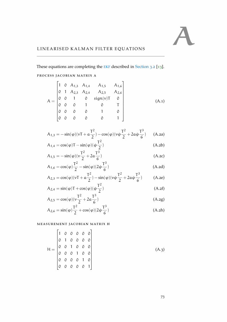
AL I N E A R I S E D K A L M A N F I LT E R E Q U AT I O N S
These equations are completing the EKF described in Section 3.2 [13].
process jacobian matrix a
A =
1 0 A1,3 A1,4 A1,5 A1,6
0 1 A2,3 A2,4 A2,5 A2,6
0 0 1 0 sign(v)T 0
0 0 0 1 0 T
0 0 0 0 1 0
0 0 0 0 0 1
(A.1)
A1,3 = − sin(ϕ)(vT + aT2
2) − cos(ϕ)(vϕ
T2
2+ 2aϕ
T3
6) (A.2a)
A1,4 = cos(ϕ)T − sin(ϕ)(ϕT2
2) (A.2b)
A1,5 = − sin(ϕ)(vT2
2+ 2a
T3
6) (A.2c)
A1,6 = cos(ϕ)T2
2− sin(ϕ)(2ϕ
T3
6) (A.2d)
A2,3 = cos(ϕ)(vT + aT2
2) − sin(ϕ)(vϕ
T2
2+ 2aϕ
T3
6) (A.2e)
A2,4 = sin(ϕ)T + cos(ϕ)(ϕT2
2) (A.2f)
A2,5 = cos(ϕ)(vT2
2+ 2a
T3
6) (A.2g)
A2,6 = sin(ϕ)T2
2+ cos(ϕ)(2ϕ
T3
6) (A.2h)
measurement jacobian matrix h
H =
1 0 0 0 0 0
0 1 0 0 0 0
0 0 1 0 0 0
0 0 0 1 0 0
0 0 0 0 1 0
0 0 0 0 0 1
(A.3)
73

74 linearised kalman filter equations
process noise covariance matrix q
Q =
0.12 0 0 0 0 0
0 0.12 0 0 0 0
0 0 (10 π180)2 0 0 0
0 0 0 10−4 0 0
0 0 0 0 (0.1 pi180)2 0
0 0 0 0 0 1
(A.4)

BA R C H I T E C T U R E
Figure B.1: The overall system architecture of the GCDC car including LCMmessage names.
75

76 architecture
FigureB.
2:Class
diagramof
theTrust
System.

B.1 state machine 77
b.1 state machine
STANDBY
WAITING_FOR_SCENARIO
choose_scenario
S1_HIGHWAY_PREPARATION
scenario1
S1_HIGHWAY_CHOOSE_HEAT
headway_time_selected
S1_CHOOSE_LANE
slow_speed_selected fast_speed_selected
S1_PA_WAIT_PARTICIPANTS_READY
lane_a
S1_PB_WAIT_PARTICIPANTS_READY
lane_b
S1_PA_CONF_PARTICIPANTS_READY
s1_participants_ready_received
S1_PB_CONF_PARTICIPANTS_READY
s1_participants_ready_received
S1_PA_WAIT_START
confirmed
S1_PB_WAIT_START
confirmed
S1_PA_CONF_START
start_a
S1_PB_CONF_START
start_b
S1_PA_PLATOON_80
confirmed_start_pa
S1_PB_PLATOON_60
confirmed_start_pb
S1_PA_CONF_SYNC_SPEED
received_roadwork_message
S1_PA_SYNC_SPEED_PB
confirmed_sync_speed
S1_PB_REDUCING_SPEED
received_roadwork_message
S1_PB_CONF_PAIRING_ZONE
merge_request_received
S1_PA_CONF_PAIRING_ZONE
recv_merging_request
S1_PA_WAIT_FOR_B2A_PAIRING
confirmed_pairing_zone
S1_PA_WAIT_FOR_BEING_FIRST_VEHICLE
paired_with_MIO_BWD_R
S1_PA_MAKE_GAP
is_first_vehicle
S1_PA_CONF_MERGING_ZONE
stom_received
S1_PA_CONF_MERGING_FINISHED
confirmed_merging_zone
S1_PA_ADAPT_PLATOON
finished_merging
FINISH
eos
S1_PB_PAIR_FWD
confirmed_pairing_zone
S1_PB_CONF_MAKE_GAP
pairing_found
S1_PB_MAKE_GAP
confirmed_make_gap
S1_PB_SEND_STOM
gap_ready gap_not_safe
S1_PB_CONF_MERGING_FINISHED
fwd_merged
S1_PB_VOID_PAIR
confirmed_finished_merging
eos
Figure B.3: State machine for the GCDC scenario 1.

78 architecture
STANDBY
WAITING_FOR_SCENARIO
choose_scenario
S2_CROSSING
scenario2
S2_INPUT_LANE
s2_cam_received
S2_INPUT_RADIUS
s2_get_cz_radius
S2_INPUT_LATITUDE
s2_get_cz_latitude
S2_INPUT_LONGITUDE
s2_get_cz_longitude
S2_INPUT_TIME
s2_get_cz_time
S2_CONTROLLER_ON
s2_switch_controller_on
S2_WAIT_START
s2_conf_ok
S2_DRIVE_TO_CZ
s2_start_received
S2_IN_CZ
s2_cz_reached
FINISH
s2_eos
Figure B.4: State machine for the GCDC scenario 2.

B.1 state machine 79
STANDBY
WAITING_FOR_SCENARIO
choose_scenario
S3_EMERGENCY_VEHICLE
scenario3
S3_DRIVING
right_laneleft_lane
S3_EMERGENCY_APPROACHING
emergency_detected
S3_CONTINUE_DRIVING
emergency_passed
Figure B.5: State machine for the GCDC scenario 3.
GO_MANUAL
TAKE_OVER
start_take_over
Figure B.6: State machine for going back to manual mode.


B I B L I O G R A P H Y
[1] L. B. Torvalds, “Desktop Market has already started, PrestonSt. Pierre of Linux Times interviews Linus Torvalds.” Anonline version is available at http://web.archive.org/web/
20050404020308/http://www.linuxtimes.net/modules.php?
name=News&file=article&sid=145 (18.06.2016), 2004.
[2] World Health Organization (WHO), Global Status Report on RoadSafety 2015. Geneva: WHO Press, 2015.
[3] A. Davila and M. Nombela, “Platooning - safe and eco-friendlymobility.,” SAE Technical Paper 2012-01-0488, 2012.
[4] R. N. Charette, “This Car Runs on Code.” An online versionis available at http://spectrum.ieee.org/transportation/
systems/this-car-runs-on-code (18.06.2016), 2009.
[5] T. Bijlsma, S. de Kievit, J. van de Sluis, E. van Nunen, I. Passchier,and E. Luiijf, Security Challenges for Cooperative and InterconnectedMobility Systems, pp. 1–15. Cham: Springer International Pub-lishing, 2013.
[6] S.-W. Kim, Z. J. Chong, B. Qin, X. Shen, Z. Cheng, W. Liu, andM. H. Ang, “Cooperative perception for autonomous vehicle con-trol on the road: Motivation and experimental results,” IEEE In-ternational Conference on Intelligent Robots and Systems, pp. 5059–5066, 2013.
[7] S. W. Kim, B. Qin, Z. J. Chong, X. Shen, W. Liu, M. H. Ang,E. Frazzoli, and D. Rus, “Multivehicle Cooperative DrivingUsing Cooperative Perception: Design and Experimental Vali-dation,” IEEE Transactions on Intelligent Transportation Systems,vol. 16, no. 2, pp. 663–680, 2015.
[8] J. Ploeg, B. T. Scheepers, E. van Nunen, N. van de Wouw, andH. Nijmeijer, “Design and experimental evaluation of coopera-tive adaptive cruise control,” 2011 14th International IEEE Con-ference on Intelligent Transportation Systems (ITSC), no. June 2016,pp. 260–265, 2011.
[9] E. Semsar-Kazerooni, A. Morales Medina, and H. H. Bengts-son, “DEL150330 i-GAME D2.1 Interaction Protocol,” tech. rep.,i-game gcdc, 2015.
81

82 bibliography
[10] C. Englund, L. Chen, J. Ploeg, E. Semsar-Kazerooni, A. Voronov,H. H. Bengtsson, and J. Didoff, “The grand cooperative drivingchallenge 2016: boosting the introduction of cooperative auto-mated vehicles,” IEEE Wireless Communications, vol. 23, pp. 146–152, August 2016.
[11] P. Wex, J. Breuer, A. Held, T. Leinmuller, and L. Delgrossi, “TrustIssues for Vehicular Ad Hoc Networks,” VTC Spring 2008 - IEEEVehicular Technology Conference, pp. 2800–2804, 2008.
[12] S. J. Russell and P. Norvig, Artificial Intelligence: A Modern Ap-proach. Pearson Education, 2 ed., 2003.
[13] N. Magnusson and T. Odenman, “Improving absolute positionestimates of an automotive vehicle using GPS in sensor fusion,”Master’s thesis, Chalmers University of Technology, 2012.
[14] J. Zhang, “A survey on trust management for VANETs,” Proceed-ings - International Conference on Advanced Information Networkingand Applications, AINA, pp. 105–112, 2011.
[15] M. Röckl, J. Gacnik, and J. Schomerus, “Integration of Car-2-CarCommunication as a Virtual Sensor in Automotive Sensor Fu-sion for Advanced Driver Assistance Systems,” in Proceedings.FISITA, no. 1, (Munich, Germany), pp. 2008–2008, Springer Au-tomotive Media, 2008.
[16] ETSI (European Telecommunications Standards Institute), “Ve-hicular Communications ; Basic Set of Applications ; Part 2 :Specification of Cooperative,” ETSI TS 102 637-2, vol. 1, pp. 1–18, 2011.
[17] ETSI (European Telecommunications Standards Institute), “Intel-ligent Transport Systems (ITS); Users and applications require-ments; Part 2: Applications and facilities layer common data dic-tionary,” ETSI TS 102 894-2, vol. 1, pp. 1–78, 2013.
[18] ETSI (European Telecommunications Standards Institute), “Intel-ligent Transport Systems (ITS); Vehicular Communications; BasicSet of Applications; Part 3: Specifications of Decentralized Envi-ronmental Notification Basic Service,” ETSI TS 102 637-3, vol. 1,no. 1, pp. 637–3, 2010.
[19] J. van de Sluis, L. Chen, and L. Garcia-Sol, “DEL_i-GAME_D3.2Proposal for extended message set for supervised automateddriving,” tech. rep., i-game gcdc, 2015.
[20] D. L. Hall and J. Llinas, “An introduction to multisensor datafusion,” Proceedings of the IEEE, vol. 85, no. 1, pp. 6–23, 1997.
[21] F. Gustafsson, Statistical Sensor Fusion. Studentlitteratur, 2 ed.,2010.

bibliography 83
[22] R. E. Kalman, “A New Approach to Linear Filtering and Predic-tion Problems,” Journal of Basic Engineering, vol. 82, no. 1, p. 35,1960.
[23] G. Welch and G. Bishop, “An Introduction to the Kalman Filter,”In Practice, vol. 7, no. 1, pp. 1–16, 2006.
[24] R. Faragher, “Understanding the basis of the kalman filter viaa simple and intuitive derivation [lecture notes],” IEEE SignalProcessing Magazine, vol. 29, no. 5, pp. 128–132, 2012.
[25] M. S. Arulampalam, S. Maskell, N. Gordon, and T. Clapp, “Atutorial on particle filters for online nonlinear/non-GaussianBayesian tracking,” IEEE Transactions on Signal Processing, vol. 50,no. 2, pp. 174–188, 2002.
[26] F. Gustafsson, “Particle Filter Theory and Practice with Position-ing Applications,” IEEE A&E Systems Magazine, vol. 25, no. 7,pp. 53–81, 2010.
[27] D. Miller, A. Sun, and W. Ju, “Situation Awareness with Differ-ent Levels of Automation,” 2014 IEEE International Conference onSystems, Man, and Cybernetics, pp. 688–693, 2014.
[28] E. Schoch, F. Kargl, and M. Weber, “Communication patternsin vanets,” IEEE Communications Magazine, vol. 46, pp. 119–125,November 2008.
[29] F. Kargl, P. Papadimitratos, L. Buttyan, M. Müter, E. Schoch,B. Wiedersheim, T. V. Thong, G. Calandriello, A. Held, A. Kung,and J. P. Hubaux, “Secure vehicular communication systems: im-plementation, performance, and research challenges,” IEEE Com-munications Magazine, vol. 46, pp. 110–118, November 2008.
[30] H. Vasudevan, A. R. Joshi, N. M. Shekokar, N. J. Patel, andR. H. Jhaveri, “International conference on advanced comput-ing technologies and applications (icacta) trust based approachesfor secure routing in vanet: A survey,” Procedia Computer Science,vol. 45, pp. 592 – 601, 2015.
[31] International Telecommunication Union: Telecom Standardiza-tion Sector, “International Standard ISO/IEC 9594-8 Recommen-dation ITU-T X.509,” 2012.
[32] S. Soni, “Reliable Trust Computation model in Vehicular ad-hocNetwork,” American Journal of Advanced Computing, vol. II, no. 1,pp. 7–11, 2015.
[33] X. Hong, D. Huang, M. Gerla, and Z. Cao, “SAT: Situation-awaretrust architecture for vehicular networks,” IEEE CommunicationsMagazine, no. November, pp. 31–36, 2008.

84 bibliography
[34] A. Tajeddine, A. Kayssi, and A. Chehab, “A privacy-preservingtrust model for vanets,” in Computer and Information Technology(CIT), 2010 IEEE 10th International Conference on, pp. 832–837,June 2010.
[35] H. Aras, C. Beckstein, S. Buchegger, P. Dittrich, T. Hubauer,F. Klan, B. Knig-Ries, and O. Wolfson, “Uncertainty and trust,”in Univ. of Illinois, Dagstuhl Seminar Proceedings, vol. 8421, 2009.
[36] W. T. L. Teacy, J. Patel, N. R. Jennings, and M. Luck, “TRAVOS:Trust and reputation in the context of inaccurate informationsources,” Autonomous Agents and Multi-Agent Systems, vol. 12,no. 2, pp. 183–198, 2006.
[37] U. F. Minhas, J. Zhang, T. Tran, and R. Cohen, “Towards ex-panded trust management for agents in vehicular ad-hoc net-works,” International Journal of Computational Intelligence Theoryand Practice (IJCITP), vol. 5, no. 1, 2010.
[38] M. Raya, P. Papadimitratos, V. D. Gligor, and J. P. Hubaux, “OnData-Centric Trust Establishment in Ephemeral Ad Hoc Net-works,” IEEE INFOCOM 2008, pp. 1912–1920, 2008.
[39] F. Dötzer, L. Fischer, and P. Magiera, “VARS: A vehicle ad-hocnetwork reputation system,” Proceedings - 6th IEEE InternationalSymposium on a World of Wireless Mobile and Multimedia Networks,WoWMoM 2005, pp. 454–456, 2005.
[40] F. Durso and A. Sethumadhavan, “Situation awareness: Under-standing dynamic environments,” Human Factors: The Journal ofthe . . . , vol. 50, no. 3, pp. 442–448, 2008.
[41] M. Kurmis, A. Andziulis, D. Dzemydiene, S. Jakovlev, M. Voz-nak, and G. Gricius, “Cooperative Context Data Acquisition andDissemination for Situation Identification in Vehicular Commu-nication Networks,” Wireless Personal Communications, vol. 85,no. 1, pp. 49–62, 2015.
[42] M. Röckl, Cooperative Situation Awareness in Transportation. PhDthesis, Leopold-Franzens-University Innsbruck, 2009.
[43] ETSI (European Telecommunications Standards Institute), “In-telligent Transport Systems (ITS); Vehicular Communications;GeoNetworking; Part 3: Network architecture,” ETSI TS 102 636-3, vol. 1, pp. 1–23, 2010.

bibliography 85
[44] IEEE, “Ieee standard for information technology – telecommuni-cations and information exchange between systems – local andmetropolitan area networks – specific requirements – part 11:Wireless lan medium access control (mac) and physical layer(phy) specifications – amendment 6: Wireless access in vehicu-lar environments,” IEEE Std 802.11p-2010 (Amendment to IEEEStd 802.11-2007 as amended by IEEE Std 802.11k-2008, IEEE Std802.11r-2008, IEEE Std 802.11y-2008, IEEE Std 802.11n-2009, andIEEE Std 802.11w-2009), pp. 1–51, Jul 2010.
[45] E. Kaplan and C. Hegarty, Understanding GPS: Principles and Ap-plications. Artech House, 2005.
[46] R. Yarlagadda, I. Ali, N. Al-Dhahir, and J. Hershey, “Gps gdopmetric,” IEE Proceedings - Radar, Sonar and Navigation, vol. 147,pp. 259–264, Oct 2000.
[47] L. Danielsson, Tracking and radar sensor modelling for automotivesafety systems. PhD thesis, Chalmers University of Technology,2010.
[48] M. Larsson, Methods to Improve V2V Communications in Platoonsof Heavy Duty Vehicles. No. 17, Lund: Halmstad University Press,2016.
[49] R. B. Langley, “Dilution of Precision,” GPS World, vol. 10,no. May, pp. 52–59, 1999.
[50] H. Salunkhe, H. H. van Huysduynen, B. Nijssen, and J. Terken,“DEL_i-GAME_D7.1 GCDC judging criteria and their evaluation(Final),” tech. rep., i-game gcdc, 2016.
[51] B. S. Bourgeois, “Using Range and Range Rate for Relative Nav-igation,” tech. rep., Naval Research Laboratory Marine, Missis-sippi, 2007.


colophon
This document was typeset using the typographical look-and-feelclassicthesis developed by André Miede. The style was inspiredby Robert Bringhurst’s seminal book on typography “The Elements ofTypographic Style”. classicthesis is available for both LATEX and LYX:
http://code.google.com/p/classicthesis/
Happy users of classicthesis usually send a real postcard to theauthor, a collection of postcards received so far is featured here:
http://postcards.miede.de/
Final Version as of September 18, 2016 (classicthesis ).