master thesis - universiteit twenteessay.utwente.nl/61807/1/thesis_definite.pdf2012 enterprise risk...
TRANSCRIPT

2012
ENTERPRISE RISK
MANAGEMENT AND BANK
PERFORMANCE DURING A
FINANCIAL CRISIS
Lisette Geessink
July 2012
MASTER THESIS

ENTERPRISE RISK MANAGEMENT AND
BANK PERFORMANCE DURING A
FINANCIAL CRISIS
MASTER THESIS
Date Enschede, July 14, 2012
Author
Name: Lisette Geessink
Student number: 0192597
Faculty: Management and Governance
Programme: Master of Business Administration (MSc. BA)
Specialization: Financial Management (FM)
Supervision
Name: dr. Xiaohong Huang
Company: University of Twente
Function: Assistant professor
Faculty: Management and Governance
Department: Finance and Accounting
Name: dr. Berend Roorda
Company: University of Twente
Function: Associate professor
Faculty: Management and Governance
Department: Finance and Accounting
Source of front page image: www.blauwgestreept.nl

iii
SUMMARY
Since the last financial crisis, risk management at banks has received much attention. It is
assumed that banks fell into problems because they took too much risk. Therefore, there is more
pressure for regulations towards risk management at banks. However, there is no clear consensus
about whether the implementation of more risk management leads to better performance. In other
words, it is not proven that more risk management is effective in helping banks survive a
financial crisis. This leads to the following research question:
How does ERM implementation affect bank’s performance before, during and after a
financial crisis?
Risk management tries to decrease the negative outcomes of uncertainty, and this could be
done in different approaches. First, there is traditional risk management, which handles risk in
different separate classes. Further, there is enterprise risk management (ERM), which uses a
holistic approach. This approach bundles all the risks and only hedges or insures the residual
risks. ERM also focuses on non-financial risks, whereas traditional risk management only
focuses on financial risks.
ERM could still be beneficial for banks, although they do not face much non-financial risk.
However, by taking a holistic approach, different risks could better be managed and the
knowledge of these risks becomes more sophisticated. An important ERM model is developed by
COSO. This framework helps to achieve an organization’s objectives in a risk-adjusted way.
Several researches have been conducted towards the relation between ERM and firm
performance. Under normal conditions, it is assumed that ERM is valuable for banks, since it
enhances performance (Baxter et al., 2011) and increases value (Liebenberg & Hoyt, 2011;
McShane et al., 2011). However, this depends on the quality of the ERM programs and it is
suggested that ERM is only valuable up until a certain level (McShane et al., 2011).
During a financial crisis, risk management lowers risk (Ellul & Yerramilli, 2010), and leads
to better performance McShane et al. (2011), it could be argued that it will be valuable for
stakeholders, if the company has a further extent of ERM implemented during a financial crisis.
From these propositions, several hypotheses were developed.
These hypotheses assumed that ERM implementation will lead to an improve in performance,
in both normal conditions and during a financial crisis. However, this improvement in
performance will only hold up until a certain extent. This means that when a banks implement
ERM above that level, it will no longer contribute to better performance.
In determining the effect of ERM on performance, also several control variables are taken
into account. These are efficiency, leverage, diversification, tier 1 capital ratio and credit quality.
These control variables are expected to have a positive effect on performance.

iv
Measurement took place in the years 2005-2010, and the banking crisis is defined in the years
2007 and 2008. This means that all the periods, before, during and after, are two years. A sample
was selected from Dutch banks which have an individual annual report, which led to a sample of
38 banks.
The regression that was used to test the hypothesis, did not show support for the hypotheses.
The effect of the ERM indices is ambiguous, which means that different results are found. It
indicates that ERM implementation does not automatically lead to better firm performance.
For validity, the model has to be improved. At this moment, only a small part of the variation
of the performance measures is explained by the variables used. Further, the residuals are not
normally distributed. Since this is one of the assumptions of a regression, the estimates of these
regression are not valid and cannot be used to draw conclusions.
These results are contradicting most of the previous research, which argued that ERM
positively affects performance. The fact that the results for this research are different, could be
because of another measure for ERM implementation, that was used in the previous researches.
When looking at the results for Aebi et al. (2011), who developed the ERM index that was used
in this research, it could be found that the effects of their ERM index also did not find significant
results. Therefore, it still remains an unsolved issue whether ERM implementation actually leads
to better performance.
All taken together, it could be stated that this research is contradicting most of the previous
research. It did not find a significant effect for ERM implementation and firm performance. This
means that more regulations on risk management and ERM specifically do not automatically
help banks to survive a next financial crisis.

v
FOREWORD
In order to prove that I have acquired the exit qualifications of the MSc-programme of
Business Administration, this thesis was written. My purpose was to write a relevant thesis,
about a topic that receives attention at this moment. I think I achieved this personal goal very
well, when writing on the financial crisis that has just past and the assumed origination of that
crisis.
Now that my thesis is finished, I would like to thank some people. First, I would like to thank
KPMG Enschede, for offering the opportunity to write this thesis at their organization. Further,
the advices, comments and support of my coach Rick ten Elzen during my thesis helped me to
improve this thesis and be more critical about my own work. Many thanks also go to my
University supervisors, mrs. Huang and mr. Roorda. Thanks to their critical view and support, I
was able to finish this thesis in time.
Finally, I would like to thank the people in my private environment. I would like to thank my
family and friends, by offering support when I needed it. Without them, I would have never been
able to succeed my studies.
Many thanks to you all.
Lisette Geessink
Beltrum, July 14, 2012

TABLE OF CONTENTS
SUMMARY ................................................................................................................................ iii
FOREWORD ............................................................................................................................... v
1. INTRODUCTION ............................................................................................................... 4
1.1 Research purpose .................................................................................................................... 4
1.2 Research problem .................................................................................................................... 4
2. RESEARCH QUESTIONS ................................................................................................... 6
3. LITERATURE REVIEW ..................................................................................................... 8
3.1 Definition of risk and risk management .................................................................................. 8
3.1.1 Benefits of risk management ........................................................................................... 9
3.2 Traditional risk management and enterprise risk management ............................................. 10
3.2.1 COSO ERM – Integrated Framework .......................................................................... 11
3.3 Enterprise risk management implementation ........................................................................ 12
3.4 Enterprise risk management and performance ...................................................................... 13
3.5 Enterprise risk management and performance during a financial crisis ................................ 15
3.6 Factors affecting firm performance ....................................................................................... 17
3.6.1 Size and efficiency ........................................................................................................ 17
3.6.2 Leverage ....................................................................................................................... 17
3.6.3 Diversification .............................................................................................................. 18
3.6.4 Bank specific variables ................................................................................................. 18
4. CONCEPTUAL MODEL ................................................................................................... 20
5. METHODOLOGY............................................................................................................ 22
5.1 Methodological classification ............................................................................................... 22
5.2 Description of work ............................................................................................................... 22
5.2.1 Variables....................................................................................................................... 22

5.2.2 Measurement period ..................................................................................................... 26
5.2.3 Sample selection ........................................................................................................... 26
5.2.4 Data collection ............................................................................................................. 27
5.3 Methodology ......................................................................................................................... 27
5.3.1 ERM index .................................................................................................................... 27
5.3.2 Descriptive statistics ..................................................................................................... 28
5.3.3 Correlation matrix ........................................................................................................ 28
5.3.4 Multivariate regression ................................................................................................ 28
5.3.5 Validity ......................................................................................................................... 30
6. RESULTS ....................................................................................................................... 31
6.1 ERM index ............................................................................................................................ 31
6.2 Descriptive statistics .............................................................................................................. 34
6.3 Correlation matrix ................................................................................................................. 36
6.3.1 Correlations before the financial crisis ........................................................................ 39
6.3.2 Correlations during the financial crisis ....................................................................... 40
6.3.3 Correlations after the financial crisis .......................................................................... 40
6.4 Initial conclusions ................................................................................................................. 41
7. ANALYSIS ...................................................................................................................... 42
7.1 Multivariate regression .......................................................................................................... 42
7.1.1 Performance under normal conditions ......................................................................... 43
7.1.2 Performance during a financial crisis .......................................................................... 45
7.1.3 Control variables .......................................................................................................... 45
7.2 Validity .................................................................................................................................. 46
7.2.1 R2 .................................................................................................................................. 46
7.2.2 Normality of residuals .................................................................................................. 47
7.3 Outliers .................................................................................................................................. 48
7.3.1 Regression results ......................................................................................................... 49
7.3.2 Validity ......................................................................................................................... 52

8. CONCLUSIONS ............................................................................................................... 55
8.1 Conclusions ........................................................................................................................... 55
8.1.1 Performance under normal conditions ......................................................................... 55
8.1.1 Performance during a financial crisis .......................................................................... 56
8.2 Answer to research question ................................................................................................. 57
9. FURTHER RESEARCH .................................................................................................... 60
9.1 Research contributions .......................................................................................................... 60
9.2 Research limitations .............................................................................................................. 60
9.3 Directions for future research ................................................................................................ 61
10. PERSONAL REFLECTION ............................................................................................... 63
REFERENCES ........................................................................................................................... 64
APPENDICES ............................................................................................................................... I
Appendix I: Overview of measurements ........................................................................................... II
Appendix II: Sample of organizational chart ................................................................................... IV
Appendix III: Sample ........................................................................................................................ V
Appendix IV: Research design ......................................................................................................... VI
Appendix V: Initial principal component analysis ......................................................................... VII
Appendix VI: Scree plot ................................................................................................................ VIII
Appendix VII: Histogram BOARDINDEP ...................................................................................... IX
Appendix VIII: Correlation matrices ................................................................................................. X
Appendix IV: Normal P-P Plots .................................................................................................... XIII
Appendix V: Normal P-P Plots sample excluding outliers ........................................................... XVI

Enterprise risk management and bank performance Introduction | 4
1. INTRODUCTION
1.1 RESEARCH PURPOSE
The purpose of this research is to define the relationship between ERM implementation and
firm performance of Dutch banks during a financial crisis.
1.2 RESEARCH PROBLEM
As a result of the global credit crisis and the role banks had in the origination of that crisis,
the Dutch Bankers Association (NVB) developed a code to regulate themselves in terms of
corporate governance, risk management, audit and remuneration policy (Nederlandse Vereniging
van Banken, 2009). This code was made effective since 2010, and will be incorporated into law
to be more effective. This is only one example of the attention risk management receives the last
couple of years at the banking and insurance industry, especially after the global credit crisis, in
order to help banks survive another crisis.
Traditional risk management consists of insurance and hedging every risk class. However,
this leads to inefficiencies, because sometimes, risks could be double counted and thus double
insured or hedged. To that problem, enterprise risk management (ERM) offers a solution. This
approach handles risk in a holistic approach, which can create natural hedges. Natural hedges
exist when a company invests in two different financial instruments, whose performance tends to
cancel each other out. Further, it leads to a better understanding of risk, which enhances growth
opportunities. This better risk insight enhances growth opportunities by risk responses that are
better aligned with the corporate strategy (Abrams, von Känel, Müller, Pfitzmann, & Ruschka-
Taylor, 2007), which could lead to better performance.
This holistic approach was developed into a framework, the COSO1 integrated framework for
risk management (2004). This framework has been adopted by companies throughout the world.
According to COSO, enterprise risk management could best be defined by ‘a process, effected by
an entity’s board of directors, management and other personnel, applied in strategy setting across
the enterprise, designed to identify potential events that may affect the entity, and manage risk to
be within its risk appetite, to provide reasonable assurance regarding the achievement of entity
objectives’ (p. 2). The purpose of risk management in general is to effectively deal with
uncertainty and enhance the capacity to build value for stakeholders (COSO, 2004).
There are several researches that try to find a relationship between the adoption and
implementation of ERM and firm performance and value (for example Baxter, Bedard, Hoitash
& Yezegel, 2011; Beasley, Pagach & Warr, 2008; Gordon, Loeb & Tseng, 2008). Another part
of research focuses on risk management-related corporate governance mechanisms and board
1 Committee of Sponsoring Organizations of the Treadway Commission

Enterprise risk management and bank performance Introduction | 5
characteristics, and the effects on performance during a financial crisis (Minton, Taillard &
Williamson, 2010; Aebi, Sabato & Schmid, 2011).
However, these researches used data only up until 2008. Now that data is available for the
years after the banking crisis, a more precise answer could be given to the question how ERM
implementation affects firm performance. Furthermore, this research could prove the
effectiveness of ERM implementation, since this is seen as one of the solutions to help banks
survive a next financial crisis.
Problem statement. Since the last financial crisis, there is more pressure for regulation
towards risk management at financial companies in the Netherlands, just as in other countries, in
order to decrease the consequences of a future crisis. However, there is still no clear consensus
about whether the implementation of ERM leads to better performance in general and also during
a financial crisis. In other words, it is not proven that more regulations on risk management are
effective in helping banks survive a financial crisis. Therefore, research is needed to address the
relationship between ERM adoption and performance during a financial crisis.

Enterprise risk management and bank performance Research questions | 6
2. RESEARCH QUESTIONS
Based on this problem statement and the theoretical framework, the following research
question could be defined:
How does ERM implementation affect bank’s performance before, during and after a
financial crisis?
Several steps need to be taken to answer this research question. First of all, the definition of
risk needs to be given and the risks that occur at (financial) companies should be defined, to have
a better understanding of what risk management is and why firms should use it. Then, enterprise
risk management needs to be discussed and the differences it has with traditional risk
management. This will be done based on the foundations and goals of the both types of risk
management. This is needed to create a fuller understanding of the topic ‘enterprise risk
management’, and leads to the following sub questions:
1. What is risk and how could this be managed?
2. What is the difference between traditional risk management and enterprise risk
management?
Based on this description of ERM, it is discussed how in theory ERM could enhance firm
performance, both during an inter-crisis period and during a financial crisis. This analysis will
provide a possible solution to the research question and has to be empirically tested, and will be
based on the following question:
3. How could enterprise risk management enhance performance?
Finally, it needs to be researched how banks perform outside a financial crisis, and whether
ERM affects that performance. This than can be compared with the performance of the same
banks during a financial crisis, to show differences between further ERM implementation and
ERM implementation in a less extent, and performance during a financial crisis and outside a
financial crisis. Together, this will lead to an answer to the question whether ERM adoption will
lead to better firm performance of banks during a financial crisis. This leads to the following
questions, which provide the final step in answering the research question:
4. Is there a relationship between ERM implementation and overall firm performance?
5. Is there a difference in performance of banks that have further implemented ERM,
compared to those banks who have a less implemented ERM program, under normal
conditions?
6. Is there a difference in performance of banks that have further implemented ERM,
compared to those banks who have a less implemented ERM program, during a financial
crisis?

Enterprise risk management and bank performance Research questions | 7
In answering these sub questions and the research questions, several control variables need to
be taken into account. These factors could also affect firm performance, and therefore could give
an alternative explanation for changes in firm performance.
This research is further structured as follows. Next, previous literature on risk and risk
management will be discussed, and enterprise risk management is introduced. Further, this
literature review will also provide previous research on the influence of enterprise risk
management and performance. From that literature review, several hypotheses are developed,
that will be tested during this research. After the financial research, the conceptual model is
introduced. This model will show which relations are expected and will be tested. How this
conceptual model will be tested, is discussed in the methodology part. In that part, the
methodological classification is discussed, from which the steps that need to be taken can be
derived. Further, the variables are operationalized and research boundaries are set up. Also the
data collection techniques are discussed. Following is the execution of the methodology and a
presentation of the results. With these results, the hypotheses will be tested. The validity of these
results is discussed afterwards. This research will end with conclusions and the answer to the
research question, research limitations and directions for further research, and a personal
reflection.

Enterprise risk management and bank performance Literature review | 8
3. LITERATURE REVIEW
In this literature review, several issues are discussed concerning risk management and firm
performance. First, a definition of risk is given and the relevance of managing risks is discussed.
Then, two different approaches towards risk management are discussed: traditional risk
management and enterprise risk management. Further, a theoretical explanation is given about
how enterprise risk management could enhance performance. Then prior research on ERM
implementation and firm performance is discussed, and in this part, hypotheses are being
developed. The final part of this theoretical framework consists of discussing several control
variables.
At the end of this theoretical framework, it should be clear what enterprise risk management
is, how this could add value and which empirical results support these theoretical explanations.
Furthermore, the developed hypotheses will show what actually is expected on the influence of
ERM implementation on firm performance, under normal conditions and during a financial
crisis.
3.1 DEFINITION OF RISK AND RISK MANAGEMENT
First, it needs to be defined what risk exactly is and what role risk management could play
here. According to the dictionary Van Dale, risk could be defined as ‘danger of damage or loss’.
Lhabitant & Tinguely (2001) define risk as the exposure to uncertainty, where uncertainty is
defined as the possibility of occurrence of one or several events. This definition could be
broadened by Kaplan & Garrick (1981), who argue that risk is not only uncertainty, but that the
consequences this uncertainty could have, should also be taken into account.
Although these consequences could also be beneficial, it is more important for companies to
take the possible negative outcomes into account. When these uncertainties become reality, the
outcomes could harm the company. There are different sources of uncertainty and risk, which
will be explained now.
In general, banks face two risk categories: financial and non-financial risk (Ai & Brockett,
2008). First, the financial risks are discussed, followed by a description of non-financial risk.
According to McNeil, Frey & Embrechts (2005), market risk and credit risk are the most
common financial risks at banks. Market risk is ‘the risk of change in the value of a financial
position due to a change in the value of the underlying components of which that position
depends’ (McNeil et al., 2005, p. 3), like for example commodity prices and interest rates.
Further, credit risk is ‘the risk of not receiving the promised repayments on outstanding
investments, because of default of the borrower’ (McNeil et al., 2005, p. 3). Another financial
risks at banks are liquidity risk, which is caused by a lack of marketability of an investment, in
order to prevent or minimize a loss. In general, these risks are managed using financial
instruments, like derivatives.

Enterprise risk management and bank performance Literature review | 9
Non-financial risk could also be further separated into hazard risk, operational risk and
strategic risk (Ai & Brockett, 2008). Hazard risk are external risks, like for example natural
disasters, theft and liability claims. These risks could best be managed by buying insurances.
Operational risks are caused by failing of internal processes, people and systems. Strategic risks
are directly related to the bank’s overall strategy and includes among others reputation risk.
These risks are difficult to insure or hedge, and should be minimized using qualitative
information.
In order to prevent these risks to give negative outcomes, banks engage into risk
management. The general purpose of risk management is to reduce the volatility of firm value
(Nance, Smith, & Smithson, 1993) and to eliminate the lower-tail outcomes (Stulz, 1996). This
means that it should reduce the expected costs of financial distress, but it should still enable
companies to gain a competitive advantage in risk-bearing. There are two basic approaches to
risk management, traditional risk management (TRM) and enterprise risk management (ERM).
These approaches will be discussed in the next part, after discussing the overall benefits of risk
management.
3.1.1 BENEFITS OF RISK MANAGEMENT
According to the modern portfolio theory, risk management is irrelevant for value, since
shareholders can easily diversify and thereby decrease the risk they have (Markowitz, 1952).
This means that for shareholders, risk management would destroy value. However, since
shareholders are not the only stakeholders for a company, it could be beneficial for a company to
use risk management. Another factor could be that markets are not as efficient as the modern
portfolio theory assumes.
This latter part is discussed by Nance, Smith & Smithson (1993). They argue that because of
tax regulations, lower expected costs of financial distress and the underinvestment problem,
hedging can be beneficial for companies.
Hedging could be beneficial in convex tax regulations. In such regulations, a higher tax
percentage is paid by firms with a higher profit. If hedging reduces the variability of the pre-tax
firm value, then the expected corporate tax liability is reduced. This reduction comes from the
fact that a lower percentage needs to be paid and there is more certainty about firm value.
Therefore, also the expected post-tax value of the firm is increased, as long as the costs of the
hedge are lower than the increase of value (Smith & Stulz, 1985).
The underinvestment problem exists when shareholders have incentives to forego a net
positive value project. This could happen when the wealth that is created by that project, is going
to the debt holders, who require a fixed payment every period. Therefore, wealth is being
decreased or even destroyed, when the debt payments are higher than the wealth created. This

Enterprise risk management and bank performance Literature review | 10
problem could be solved when companies use hedging to restrict the states in which the firm
would default on bond payments. In that case, less wealth is being decreased by debt payments.
Furthermore, since hedging reduces the probability of financial distress by reducing the
variance of earnings and firm value (Nance et al., 1993), the expected costs of financial distress
are also reduced. This is because financial distress could lead to bankruptcy, reorganizations or
liquidation, which all cause direct legal costs. It is less likely that these costs occur when hedging
is used.
Now that it is clear why risk management could be beneficial, two different approaches are
discussed.
3.2 TRADITIONAL RISK MANAGEMENT AND ENTERPRISE RISK MANAGEMENT
Traditionally, risk management happened in a silo-based way, where each risk was hedged or
insured separately. Also, it only focused on financial risks, such as credit, market and liquidity
risks (McShane et al., 2011). This kind of approach leads to inefficiencies when relations
between risks are not seen. Although banks’ main concern are the financial risks, it is still
relevant for them to adopt enterprise risk management. This will be discussed later, after a short
introduction to this risk management approach.
Enterprise risk management offers a solution to the problems traditional risk management
faces. This approach handles risks in a coordinated way, in which risks are taken together in a
portfolio, where the residual risk is hedged. This portfolio approach will decrease risk, when the
modern portfolio theory is used. This theory assumes that a portfolio with different assets is able
to absorb extreme directions. This means that it is assumed that when one assets moves in a
negative direction, this will be absorbed by an assets which moves in a positive direction. This
decreases the risk of a portfolio. It also increases efficiency, by only hedging the real risk.
Another difference between traditional risk management and ERM is that ERM also focuses on
operational and strategic risks.
Furthermore, since the different risks are aggregated into a portfolio, it is possible to see
interdependencies between risks, which leads to a better comprehension of risk (Nocco & Stulz,
2006). Therefore, management is better able to objectively allocate resources because there is a
higher risk-adjusted rate (Meulbroek, 2002), which enhances capital efficiency and return on
equity (Liebenberg & Hoyt, 2003).
According to the Committee of the Sponsoring Organizations of the Treadway Commission
(COSO), ERM could best be defined as follows (COSO, 2004, p. 2):
‘Enterprise risk management is a process, effected by an entity’s board of directors,
management and other personnel, applied in strategy setting and across the enterprise, designed

Enterprise risk management and bank performance Literature review | 11
to identify potential events that may affect the entity, and manage risk to be within its risk
appetite, to provide reasonable assurance regarding the achievement of entity objectives’.
This framework is often used by companies and is used as a guideline for regulations, like the
Dutch Corporate Governance Code (Code Tabaksblat) and the Code Banken, which was
developed by the Dutch Banking Association. The purpose of this code was to regulate banks in
terms of corporate governance, risk management, audit and remuneration policy (NVB, 2009).
Therefore, this framework will be discussed now.
3.2.1 COSO ERM – INTEGRATED FRAMEWORK
To provide companies a guideline in how to implement ERM, COSO developed a
framework, the Enterprise Risk Management – Integrated Framework in 2004. This framework
is an extension of the initial framework of 1994 and is shown in Figure 3.1.
The ultimate goal of ERM is to help to achieve an organization’s objectives (COSO, 2004).
These objectives are listed at the top of the cube: strategic, operations, reporting and compliance.
The strategic objectives should help the company to achieve its mission. These objectives should
be achieved using resources effectively and efficiently, in order to enhance the company’s value,
which is shown by the operational objectives. Further, every company should have reliable
reporting and comply with applicable laws and regulations, to also prove its value to the outside
stakeholders. These four objectives are overlapping, which shows the holistic approach of risks
by this framework. The four levels on the right-hand side of the cube show the levels in which
ERM should be present. The eight ERM components, as are listed at the front of the cube, show
what is needed to achieve these objectives.
As was argued before, the ultimate goal of ERM is to help achieve an organization’s
objectives. This is done by handling all the risks in a holistic approach. This offers opportunities
Figure 3.1: COSO ERM - Integrated Framework (COSO, 2004)

Enterprise risk management and bank performance Literature review | 12
for companies to respond to their risks in alignment with their corporate strategy. Although
banks face mainly financial risks, it could help them by integrating all these risks into one
portfolio, instead of hedging each different class. This could help to solve possible inefficiencies
in risk management.
3.3 ENTERPRISE RISK MANAGEMENT IMPLEMENTATION
There are several signals that show that companies are implementing ERM. Earlier research
on ERM and firm performance use the appointment of a Chief Risk Officer (CRO) as an
indicator that ERM is implemented (Liebenberg & Hoyt, 2003; 2011; Beasley et al., 2008). They
argue that a CRO is responsible for the management of all the risks and the oversight over these
risks. A weakness of this measure is however, that the news of an appointment of a CRO might
not be the initial appointment of a CRO. Further, an even greater weakness is that the
appointment does not say anything about the extent to which ERM is implemented.
Further, the presence of a risk committee that oversees all the company’s risk is a signal that
a bank is engaged in ERM. This is acknowledged by Aebi et al. (2011), who argue that such a
committee indicates a stronger risk management. These authors also argue that more information
about a risk committee is needed to draw relevant conclusions.
In the recent years, three measures for ERM implementation in banks have been developed.
These three measures, by Aebi et al. (2011), Ellul & Yerramili (2010), and Baxter et al. (2011)
will be discussed now.
First, Baxter et al. (2011) developed an index for ERM quality at banks, to find which factors
are related with a high S&P’s ERM quality rating. Therefore, they use factors to define
complexity, financial risk/resources and corporate governance, which are argued to have an
effect on the ERM quality rating given by S&P’s. However, it is not this research’s purpose to
find factors that cause ERM implementation, but factors that measure implementation.
Therefore, this index is not usable.
Further, Ellul & Yerramili (2010) also defined a ERM implementation index for banks. This
index is focused on the aspects of the organization structure of the risk management function. It
is composed of factors concerning the position of the CRO, the experience of the supervisory
board and the risk committee. An advantage of this measure is that it uses many different aspects
of the risk management organization. A disadvantage is the payments of the CRO and the CEO.
This is not always easy to find for Dutch banks, when the CRO is not in the executive board.
What makes it even more disadvantageous, is that these measures show to be the most important
components in the index. However, the parts that are applicable could still be used.
Finally, Aebi et al. (2011) decided to extend the ERM implementation measure by Ellul &
Yerramili (2010), in order to measure the effect of corporate governance on risk management
practices. These authors base their index on the best practices for risk management, defined by
Enterprise risk management and bank performance Literature review | 13
Mongiardino & Plath (2010). They argue that each bank should have a dedicated board-level risk
committee, of which a majority is independent, and that the CRO should be in the executive
board. Further, they use the common recommendation to ‘put risk high on the agenda’ and the
different sources that have give an indicator for that. These indicators are also used in measuring
ERM implementation.
However, these authors do not compose an index out of the different variables. This makes it
difficult to draw conclusions on the effects of the whole measure on firm performance. Right
now, it is only possible to draw conclusions on the effect of a single measure. Also the
collinearity between the different measures is not taken into account, which could also change
the results. These disadvantages could be solved, when the different measures are put into an
index in this research.
Since the measurements of Aebi et al. (2011) are derived from the index developed by Ellul
& Yerramili, and all the information that is needed for the first measurements is readily
available, it is decided to use the measurements of Aebi et al. (2011). In a later stadium from this
research, it is shown how the different factors are formed into a single variable, to develop an
ERM index.
Aebi et al. (2011) use ten different indicators for their risk management measure, which will
be briefly discussed now. First, the presence of a CRO in the executive board, and the presence
of a risk committee on the board level are taken into account. It is argued that the presence of
these factors defines whether banks implemented ERM. As was stated before, a CRO is
responsible for managing all the business risk and this should lead to a holistic approach. A risk
committee on the board level is responsible to oversee all the risks, and this makes it possible to
see interdependencies. Further, it is argued that board size, board independence and financial
expertise have an influence on ERM implementation. Third, several characteristics of the risk
committee are taken into account. These are the number of risk meetings, the number of directors
and the independence of these directors. Finally, the reporting lines are taken into account. These
consist of the reporting from the CRO to the supervisory board, and the direct reporting from the
CRO to the CEO.
A more complete overview of the different variables and how they are measured, will be
given in the part on variables, which starts at page 22.
3.4 ENTERPRISE RISK MANAGEMENT AND PERFORMANCE
In the next part, empirical results on ERM and firm performance and value are discussed, to
give an hypothesis about the effect of ERM on bank performance outside a financial crisis. As
discussed before, ERM can add value or enhance companies’ performance.

Enterprise risk management and bank performance Literature review | 14
Several authors have empirically tested this relation for financial companies. They used
different proxies for ERM adoption and implementation, and firm performance and value. These
researches will briefly be discussed, from which a hypothesis will be defined.
Based on the modern portfolio theory from Markowitz (1952), risk management is not
valuable for shareholders. This is because shareholders can easily diversify their own risk, and
therefore only the systematic risk is important. In that case, every risk management practice is a
negative net present value project and should not be undertaken. This argument is agreed by
Aebi et al. (2010), who argue that risk management could lower the risk, but that this is paid for
with lower returns for shareholders.
Beasley et al. (2008) empirically investigated this argument. They related ERM
implementation and share prices during the announcement period for both financial and non-
financial firms. ERM implementation is measured as the appointment of a Chief Risk Officer
(CRO), and the market reaction to it as the accumulative abnormal return. The authors only find
an insignificant negative relation between the accumulative abnormal returns and the
appointment of a CRO. Therefore, it could be concluded that the implementation of ERM is not
valued by shareholders, which supports the argument of the modern portfolio theory.
Further, Pagach & Warr (2010) measured the effect of ERM implementation on different
firm factors which are argued to be affected by ERM implementation. These factors are risk,
financial, asset and market characteristics of the firm. It is argued that ERM implementation,
measured as the appointment of a CRO, should lower the risk. For financial characteristics,
leverage, cash availability and profitability are taken into account, whereas asset characteristics
should tell something about the firm’s assets are likely to be impaired in financial distress.
Finally, equity markets should react on a firm’s decrease in expected costs of financial distress,
when it has implemented ERM. The authors found no significant relationship for these variables,
which leads to the conclusion that ERM implementation has no influence on performance, for
both non-financial and financial firms.
However, there are findings that suggest that ERM implementation enhances firm
performance of financial companies in general. An example is the paper by Liebenberg & Hoyt
(2011), who investigate the relation between ERM adoption and firm value at insurance
companies. These authors also use CRO appointment as indicator for ERM implementation, but
use firm value as dependent variable. Firm value is measured as Tobin’s Q. This measure defines
value as the ratio between market and book value of equity and liabilities. Their results show that
ERM significantly enhances firm value in general, however this effect is rather small. The
authors also find a difference in Tobin’s Q for firms that have implemented ERM and those who
have not, and also this relationship is significant. This indicates that ERM does enhance firm
value in general.

Enterprise risk management and bank performance Literature review | 15
When using another measure for ERM implementation, namely the Standard & Poor’s risk
management rating, as was done by McShane, Nair & Rustambekov (2011), a more accurate
answer could be given to the question whether ERM leads to better firm value for banks. The
S&P’s rating does not only indicate if ERM is adopted, but also to what extent. It could therefore
be derived if more sophisticated ERM leads to even higher firm value. In this research, firm
value is measured by Tobin’s Q. The results show that ERM is significantly positively related to
firm value, controlled for other factors. There is also a significant relationship between poor
ERM quality and firm value. However, there is no significant relations between high ERM
quality and firm value, which suggests that ERM is valued only up until a certain level of
sophistication.
Baxter, Bedard, Hoitash & Yezegel (2011) further extend this relation by relating high
quality ERM programs, firm performance and market reactions towards revisions of ERM
quality by the rating agency. They find, contradicting to McShane et al. (2011) that high ERM
program quality is positively associated with firm performance and value. For value, they also
use Tobin’s Q, whereas performance is measured by return on assets (ROA). These authors also
examine whether ERM quality ratings lead to market reactions. They measure market reactions
as accumulative average abnormal returns, and only find partial support. This suggests that
markets do value ERM quality, but that this is already incorporated in the share price. However,
market reactions are positively associated with ERM quality rating revisions.
It could be argued that the adoption of ERM is valuable for banks, since it enhances
performance (Baxter et al., 2011) and increases value (Liebenberg & Hoyt, 2011; McShane et
al., 2011). However, this depends on the quality of the ERM programs and it is suggested that
ERM is only valuable up until a certain level (McShane et al., 2011). Based on these results, the
following hypotheses could be developed:
H1a. Under normal conditions, ERM implementation increases firm performance.
H1b. ERM implementation only increases firm performance under normal conditions, up
until a certain extent.
3.5 ENTERPRISE RISK MANAGEMENT AND PERFORMANCE DURING A FINANCIAL
CRISIS
The purpose of more regulation on risk management is to help banks survive a financial crisis
of the size that emerged in 2007. Therefore, it could be assumed that banks that have higher
ERM quality programs perform better during a financial crisis, than banks that have lower ERM
quality programs, because ERM should lower the risk.
Ellul & Yerramilli (2010) tested whether the latter is the case. Although this research is not
focused on ERM, this research and its outcomes are still applicable. This is because the authors
focus on corporate governance, which is also a part of ERM. They found that risk management

Enterprise risk management and bank performance Literature review | 16
lowers enterprise risk, which is also assumed by regulators. However, risk management also
claims to be valuable for stakeholders. Ellul & Yerramilli (2010) do not find a relation between
lower enterprise risk and stock market valuations.
However, according to the results of Baxter et al. (2008), after the financial crisis, the stock
market started to value ERM implementation. They did not find significant higher market returns
for high ERM quality programs prior and during the crisis. Only after the crisis, it shows that
ERM quality is positively related to market returns. This suggests that high ERM quality
programs enabled firms to respond to the crisis, which leads to easier regain of market value
afterwards.
Since ERM should not only deliver value to shareholders, also value and performance in
general need to be discussed, so that the added value for other stakeholders could be described.
Aebi et al. (2011), Beltratti & Stulz (2010) and Minton et al., (2010) focus on the effect of risk
management structure, when measuring the effect on bank performance during a financial crisis.
The results they find are mixed. For example, Beltratti & Stulz (2010) focus on excessive risk
taking and share-holder friendliness of the bank’s board. They did not find any significant
results. Minton et al. (2010) focus on board independence and financial expertise, since these
factors are usually mentioned when improvements of risk regulations are discussed. It is argued
that independent board members are less likely to engage in excessive risk taking, since they do
not have incentives to do so. Minton et al. (2010) find that board independence does not
influence stock performance during the crisis. Board independence was also measured by Aebi et
al. (2011), and they find a significant negative association with performance, which is different
from Minton et al. (2010). Minton et al. (2010) found a significant negative association between
financial expertise and firm value, which suggests that financial experts tend to take more risk
which leads to lower firm value.
A research that completely focuses on ERM quality and bank performance during a financial
crisis, is the article of McShane et al. (2011). They focus their research on 2008, the year in
which the credit crisis was at its highest. This is supported by other researches, who also use
2007 and 2008 as crisis period (Beltratti & Stulz, 2010; Fahlenbrach & Stulz, 2011; Aebi, Sabato
& Schmid, 2011). As mentioned before, McShane et al. (2011) find that high quality ERM is
associated with better performance and value. This provides evidence that firms that adopt high
quality ERM perform better during a financial crisis.
Since it was measured that risk management lowers risk (Ellul & Yerramilli, 2010), and that
it leads to better performance (McShane et al. (2011). According to these authors, it could be
argued that it will be valuable for stakeholders, if the company has implemented ERM during a
financial crisis. Therefore, the following hypothesis could be defined:

Enterprise risk management and bank performance Literature review | 17
H2a. ERM implementation improves firm performance during a financial crisis.
H2b. ERM implementation only increases firm performance during a financial crisis, up until
a certain extent.
Since also other variables could affect firm performance, these factors are discussed in the
next part.
3.6 FACTORS AFFECTING FIRM PERFORMANCE
Besides ERM implementation, firm performance could be affected by several other variables,
the so called control variables. These factors need to be taken into account in this research,
because it is likely that they also explain differences in firm performance. Since this research will
focus on banks in one country, industry-specific and country-specific determinants of firm
performance do not have to be taken into account, since they are the same for all the banks in this
sample. The firm-specific control variables, who are thought to be different for the sample, will
be discussed now.
3.6.1 SIZE AND EFFICIENCY
In 1959, Baumol developed a hypothesis about the effect of firm size on profitability. He
argues that large firms have all the options like small firms, but have certain investment
possibilities because of their scale. These economies of scale increase the earnings per dollar
invested. This argument is tested a lot of times (Weis & Hall, 1967; Marcus, 1969; Staikouras et
al., 2007; McShane et al., 2011), but in general, no significant relationship could be found. For
banks, some evidence for Baumol’s hypothesis was found by Goddard, Molyneux & Wilson
(2004). These authors argue that this effect is caused by more efficiency at large banks, and that
not the size itself creates better performance.
This is also found by Athanasoglou, Brissimis & Delis (2008), who focus on determinants of
banking profitability, and they find that efficiency is an important factor. In that same research, it
was found that size is not significantly related to firm performance. These authors used operating
expenses to total assets as efficiency measure, which gives a negative relationship. This means
that when the ratio goes up, efficiency goes down and so should performance.
3.6.2 LEVERAGE
Another factor that is found significantly affecting performance positively, is leverage
(Athanasoglou et al., 2008). Different explanations could be given for this factor. On the one
hand, leverage could lead to a decrease in the agency costs, which means that managers cannot
invest in sub-optimal projects. This argument is supported by Hoyt & Liebenberg (2011) and
Staikouras et al. (2007), and is tested by Berger & Bonaccorsi di Patti (2006), who found
empirical support for this argument.

Enterprise risk management and bank performance Literature review | 18
Although more leverage could also lead to higher costs of financial distress (Staikouras et al.,
2007; Hoyt & Liebenberg, 2011), it was also found that those firms respond faster to financial
distress (Jensen, 1989). This could be explained by the fact that there is more at risk at higher
leveraged firms. Therefore, it could be concluded that higher leveraged firms might have higher
costs of financial distress, but that these companies are able to manage these risks better than
lower leveraged firms.
This empirical evidence means that it could be expected that higher leveraged firms perform
better, both outside and during a financial crisis.
3.6.3 DIVERSIFICATION
Diversification takes place when the firm expands to make and sell products or a product line
having no market interaction with each of the firm’s other products (Rumelt, 1982). According to
Liebenberg & Hoyt (2011), diversification could lead to higher agency costs when conflicts are
not resolved, and also find empirical evidence for this argument. They found that diversification
is negatively related to firm value.
The contrary argument is that diversification will lead to higher performance, but only when
it is related to the core business. This argument is extensively empirically supported (Palepu,
1985; Grant et al., 1988; Palich et al., 2000; Li & Greenwood, 2004).
One way to measure diversification, is to measure the functional diversification (Baele, De
Jonghe, & Vennet, 2007). In this measure, the non-interest incomes as a part of the total
operating income are used to indicate diversification. These authors argue that a bank’s main
source of income should be interest, since these institutions should offer possibilities to save and
borrow. Nowadays, banks also engage in other functions, like securitization and insurances,
which provide other types of income, like provisions.
For this measure, a negative relationship is expected, which means that if a bank has a large
part of revenues from non-interest, it is non-related diversifying from its core business, which is
negatively related to firm performance.
3.6.4 BANK SPECIFIC VARIABLES
TIER-1 CAPITAL RATIO
Aebi et al. (2011) argue that tier-1 capital ratio is a core measure of bank’s financial strength,
from a regulator’s point of view. Tier-1 capital is defined as ‘going-concern capital’, and exists
of common equity and additional capital (Bank for International Settlements, 2011). This ratio
measures the capital buffer and therefore, banks with a higher Tier-1 capital ratio would suffer
less from the debt shortage problem that develops during a financial crisis, and would be able to
respond more flexible to adverse shocks. The debt shortage problem exists when it is difficult for

Enterprise risk management and bank performance Literature review | 19
a company, in this case banks, to extract additional money from the market. In that case, tier 1
capital should offer a solution.
CREDIT QUALITY
Besides tier-1 capital, credit quality also provides an indicator for a bank’s ability to survive a
crisis. When the quality is high, it is less likely that the credit will decrease in value. This is also
argued and empirically tested by Athansoglou et al. (2008), who find that there is a significant
negative relationship, and further extended Dietrich & Wanzenried (2011), who find no
significant relation before the crisis, but this turns into significantly negative during the crisis,
which implies that credit quality especially becomes important in a crisis.
Since other possible factors could be ruled out or are also used to explain differences in firm
performance, a more precise answer could be given to what extent ERM implementation affects
firm performance. Otherwise, it could be given a wrong explanatory power.
In this theoretical framework, a theoretical basis is given for this research. In general, it could
be expected that a positive relation exists between ERM implementation and firm performance,
under normal conditions and during a financial crisis. These expectations are shown in a
conceptual model, which is discussed in the next part.

Enterprise risk management and bank performance Conceptual model | 20
4. CONCEPTUAL MODEL
In this conceptual model, the relations defined in the theoretical framework will be shown.
Based on this conceptual model, the research method will be developed and the data collection
will be discussed.
From this conceptual model, the following equation (1) could be developed.
(1) Firm performancei =
β1 ERMi lagged + β2 ERMi2lagged + β3 EFFICIENCYi + β4 LEVERAGEi +
β5 DIVERSIFICATIONi + β6 TIER-1 CAPITAL RATIOi + β7 CREDIT
QUALITYi + β8 CRISISdummy + β9 AFTERCRISISdummy + β10 (ERMi *
CRISISdummy)+ β11 (ERMi2 * CRISISdummy) + β12 (ERMi *
AFTERCRISISdummy)+ β13 (ERMi2 * AFTERCRISISdummy) * εi
From the previous parts, estimations about the forms of β could be given. Since it is argued
that ERM could increase capital efficiency, return on equity and return on assets, it is expected
that β1 and β2 are positive. In this model, the lagged measurements are used. This is to improve
the conclusions about causality. When measuring cause and effect at the same moment, causality
is more difficult to find.
Figure 4.1: Conceptual model
/ -

Enterprise risk management and bank performance Conceptual model | 21
Efficiency is likely to have a positive effect on banking performance, and therefore β3 is
expected to be positive. For leverage, the expectation is also positive, which gives a positive β4.
This expectation also goes for β5 for diversification. Further, tier-1 capital ratio is seen as a
buffer against financial distress and this leads to the expectation that β6 is positive. Credit quality
is measured as the ratio of bad loans to total loans. This means that if this ratio goes up, credit
quality decreases. Therefore, β7 is expected to have a negative influence on firm performance.
The crisis is expected to have a negative influence on performance, which leads to a negative
β8. After the crisis, performance is expected to recover, which leads to a positive expectation for
β9. As was discussed before, ERM implementation is expected to have a positive effect on
performance during the financial crisis. This is measured in β10 and β11, and is therefore expected
to be positive. After the crisis, firms that have implemented ERM, are thought to recover faster,
and the effect for β12 and β13 will therefore be positive.
Before these expectations could be tested, several steps have to be taken. First, a
methodological classification has to be chosen, from which the different methodological steps
could be derived. Further, the different variables have to be operationalized and discussed. This
will be discussed in the next part.

Enterprise risk management and bank performance Methodology | 22
5. METHODOLOGY
In this part, it is discussed how the conceptual model will be tested. This will start with a
choice for a methodological classification. Based on that classification, the empirical steps could
be described. Furthermore, the different steps will be elaborated, so that at the end of this part, it
is clear what and how will be measured to give an answer to the research question.
5.1 METHODOLOGICAL CLASSIFICATION
For measuring the effect of ERM implementation on firm performance, a cross-sectional
research method is most suitable. Using such a research method, the relation between different
variables is tested over time, and could be controlled for other variables.
In a cross-sectional research, the causal relationship between two variables is measured.
Therefore, the relationship first needs to be defined. In this case, this is done by developing the
hypotheses in the literature review, which argue that ERM implementation has a positive but
nonlinear relationship with firm performance under normal conditions. In a financial crisis, it is
argued that ERM implementation will also have a positive relationship with performance. As
could be seen, these hypotheses also show the form of the relationship and the economic
conditions under which the relationship holds. The relation between ERM implementation and
firm performance is also being controlled for several control variables, as was discussed before.
5.2 DESCRIPTION OF WORK
Now the conceptual framework and the methodological classification are discussed, the next
step is to define what work needs to be done to answer the research question. In overall, it is
assumed that ERM implementation has a positive effect on firm performance. However, also
other factors have an effect on firm performance, which are defined as control variables and the
financial crisis. The predictions made in the literature review and the conceptual model, lead to
the following steps.
First, the variables need to be operationalized, so that they can be measured. These
measurements need to be done in a certain time period, which will then be described, followed
by the sample selection method and the requirements used. Then, the collection of the data is
described, and a short description is given from each data source. In the methodology part, the
different methods that are used to relate the different measurements, are discussed. It is also
shown how the hypotheses will be tested and what criteria need to be met to accept or reject a
hypothesis. Finally, the validity of the results needs to be discussed, in order to draw relevant
conclusions on this research and its results.
5.2.1 VARIABLES
First, the different variables need to be defined and operationalized. This will be done in the
next part. A complete overview of these measures could be found in Appendix I: Overview of
measurements.

Enterprise risk management and bank performance Methodology | 23
This part will start by discussing the dependent variable, firm performance. Then the
independent variable is discussed, which is ERM implementation. Finally, the different control
variables are operationalized.
DEPENDENT VARIABLE: FIRM PERFORMANCE
Before firm performance can be measured, it needs to be defined what performance is.
According to the Business Dictionary, performance is ‘the accomplishment of a given task
measured against preset known standards of accuracy, completeness, costs, and speed’. This
could be measured in different ways, like for example shareholder value, Tobin’s Q and return
on assets.
Since not all banks in our sample, which will be discussed later, are stock-listed, it is not
possible to use shareholder value as performance measure. Therefore, also Tobin’s Q is not
applicable, since that also takes into account the market value of equity. This is only known for
stock-listed companies. This leaves this research with the accountancy-based measures, which
can be drawn from the financial statements.
It was argued that ERM could affect firm performance in terms of capital efficiency and
return on equity (Liebenberg & Hoyt, 2003). However, according to Bonin, Hasan & Wachtel
(2003), return on equity is non-comparable for banks, because it is sensitive for writing off bad
loans. This is also measured by credit quality, which is used as a control variable in this research.
Therefore, these factors should be correlated and the sensitivity should be shown. According to
the IMF (2002), an analysis of ROE omits the greater risks associated with high leverage. Since
leverage is used as a control variable for performance, these risks are incorporated into the
model.
Therefore, return on assets (ROA) and return on equity (ROE) are used to determine firm
performance. This is in accordance with among others Bonin et al. (2003), Aebi et al. (2011) and
Baxter et al. (2011). From the latter two, the measures for ROA are also used in this research.
Aebi et al. (2011) also defined a measure for ROE, which is shown in Appendix I: Overview of
measurements.
This variable is expected to be influenced by ERM implementation, whereas other variables
also influence this. First, the ERM implementation variable is now shown, followed by the
control variables.
INDEPENDENT VARIABLE: ERM IMPLEMENTATION
As was discussed before, different authors developed a measure for risk management
implementation at banks. The measures used by Aebi et al. (2011) are used to develop the ERM
index in this research. This is based on the fact that they have extended the measure from Ellul &
Yerramili (2010) and build upon the best practices developed by Mongiardino & Plath (2010).
Originally, there is no index developed by Aebi et al. (2011), and therefore, this needs to be done

Enterprise risk management and bank performance Methodology | 24
later, using a principal component analysis. This analysis is more fully described in part 5.3.1, on
page 27. This analysis makes it possible to weigh the different variables.
In the next part, the different measures are more fully described.
MEASUREMENT OF ERM IMPLEMENTATION INDICATORS
All indicators for ERM implementation are measured at the supervisory board, unless
otherwise stated. To clarify the distinction between the supervisory board and the executive
board, a sample of an organization chart is given in Appendix II: . In that figure, it is shown that
the supervisory board is at the top of the organization chart. This board has the final say in the
company and monitors the executive board. This board is shown with CEO, CFO and CRO. The
reason that CRO is in parantheses, is because this shows the possible places a CRO could have.
In the figure, also the different indicators are shown.
When a bank has a CRO in its executive board, the dummy variable CROBOARD will be set
to 1. When there is a risk committee on the board level, RISKCOMMITTEE will be set to 1. For
this research, it does not matter whether the risk committee is called Risk Committee or Audit
and Risk Committee. This is derived from Aebi et al. (2011). Further, for board size, the natural
logarithm is used. To specify the board independence, the percentage of outside directors on the
supervisory board is measured. A director is seen as independent when it has no relation with the
company except the board seat. Also for the financial expertise, a percentage is used. A director
is considered financial experienced when it has experience (present or past) as executive in a
bank or insurance company. The number of risk meetings and risk directors are taken from the
annual report, without changes. Risk committee independence is also defined as a percentage.
When the CRO reports directly to the supervisory board, or to the CEO, these dummy variables
will be set to 1.
The different measures for ERM implementation will be found in the annual reports.
However, banks were not obliged to mention their risk management process until ‘Basel II’ was
implemented into Dutch regulations, in 2008. Besides the capital requirements, this guideline
requires a transparent disclosure of the bank’s risk management. This means that in the years
before that, banks could choose to omit their risk management practices in their annual report.
In order to solve this problem, it is assumed that when a bank does not provide information
about the different ERM measures that are used in this research, this measure does not exist. This
is based on the argument of Standard & Poor’s, who argue that companies with a strong risk
management culture will have a very transparent risk management process within the company
and with other interested parties through their public communications (Standard & Poor's, 2007).
Since the presence of a risk committee is a condition for the measures for risk meetings, risk
directors and independency, it is important to mention what happens if there is no risk

Enterprise risk management and bank performance Methodology | 25
committee. In that case, the research of Aebi et al. (2011) is followed. They set these measures to
0, if the measure for risk committee is also 0. In that case, there are no missing values.
CONTROL VARIABLES
The relation between ERM implementation and firm performance will be controlled for by
several other factors, who are believed to also affect firm performance. As discussed before,
these variables are efficiency, leverage, diversification, tier-1 capital ratio and credit quality. The
measures for these variables are now being discussed.
EFFICIENCY
As was discussed before, Athanasoglou et al. (2008) use operating expenses management as
an indicator for banking efficiency. This measure is also used in this research and could be
defined as the total operating expenses over total assets. Operating costs could be defined as the
costs that incur directly from business operations, like personnel costs.
LEVERAGE
McShane et al. and Staikouras et al. differ in their measure for leverage. They both use the
same variables, assets and equity, but there is a small difference. McShane et al. use the return
on those variables as the measure. However, since return on assets and equity are also the
performance measure, it is not possible to use the same measure in one of the other variables.
Therefore, a standard measure for leverage is used, which is also defined by Leach & Melicher
(2012).
DIVERSIFICATION
According to Baele, De Jonghe & Vennet (2007), a bank’s functional diversification could
best be measured by the ratio of non-interest income to total operating income. This information
could be drawn from annual reports. When the non-interest income or the total income is
negative, this ratio will turn into negative. A percentage above 100% could occur when the non-
interest income is higher than the total income.
TIER-1 CAPITAL RATIO
Aebi et al. (2011) define tier-1 capital ratio as the ratio of tier-1 capital to total risk-weighted
assets. This measure is also used by the Bank of International Settlements (BIS) and most of the
regulatory supervisors. This measure is given in annual reports.
CREDIT QUALITY
Athanasoglou et al. (2008) and Dietrich & Wanzenried (2011) define credit quality as the
ratio of loan loss provisions to the total loans. This is given in the notes to the financial
statements. Since the loan loss provisions should be as low as possible to enhance performance,
the expected sign is negative.
Enterprise risk management and bank performance Methodology | 26
FINANCIAL CRISIS
In this research, a distinction is made between three periods: before, during and after the
financial crisis. The years 2005 and 2006 are defined as the period before the crisis, and 2007
and 2008 are the crisis-years. Finally, 2009 en 2010 are the after-crisis period. In the total
sample, these different periods are measured as subsamples. To define the variables for the
measurement periods, the average is computed. This means that for each period, each bank has
one measure for each variable.
5.2.2 MEASUREMENT PERIOD
Further, the measurement period needs to be defined, to bound this research. Following
Beltratti & Stulz (2010), Fahlenbrach & Stulz (2011) and Aebi, Sabato & Schmid (2011), the
crisis period is defined to last from July 1, 2007, to the ending of 2008. However, data is only
available on a yearly basis, and therefore the whole of 2007 will be defined as ‘financial crisis’.
Before a conclusion can be drawn about the effect of ERM implementation on performance,
it needs to be defined whether the performance is actually different for different extents of
implementation and outside a financial crisis. Therefore, also measurements need to take place
outside a financial crisis. It could be argued that ERM implementation during the years prior to
the crisis could explain performance during the crisis and that there could be differences in
recovery from the financial crisis.
This leads to a measurement period from 2005-2010, which means that there are two prior-
crisis years, two crisis years and two post-crisis years. By also adding the period after the crisis,
it could be concluded whether ERM implementation leads to faster recovery after the crisis. This
is also an indicator of performance enhancement by ERM implementation.
Observations during these periods are then averaged and this will lead to one bank measure
for each period. This means that the observations during 2005 and 2006 will averaged, and
together, these will form the pre-crisis period. The same will happen with the observations
during the other periods.
5.2.3 SAMPLE SELECTION
Third, a sample needs to be selected. As was mentioned before, this research will focus on
Dutch banks. To select the sample, it is observed which companies have got a banking license
and are considered ‘banks’ by the Financial Supervision Act in the Netherlands. From these
banks, only the banks that are under direct supervision of the Dutch National Bank (DNB) are
taken into account.
This led to an original sample of 64 banks, which are considered Dutch banks. However, some of
these banks do not have their own annual report, since they are part of another bank. Therefore,
these banks could not be taken into account. These requirements lead to a sample of 38 banks,
for which all the information needed is available. For the full sample, see Appendix III: Sample.
Enterprise risk management and bank performance Methodology | 27
5.2.4 DATA COLLECTION
Now that the different variables are explained, and the measurement period is determined and
the sample is selected, the data collection can start. During the data collection, the different
variables are measured for the sample during the measurement period. This is done with use of
several sources. Most of the information that is needed for the measurements could be drawn
from annual reports that are provided by the banks. These annual reports could be found at the
company website, company.info, and the Company Profiling and Selection Tool (CPST),
provided by KPMG. The CPST tool provides further information about annual reports. Further,
for information about the board structure, the BoardEx database is used.
Based on the measurement specifications and the data collection, the hypotheses will be
tested using the sample. This will be done by using Pearson’s correlation, followed by a
multivariate regression (McShane et al., 2011). These methods will be explained in the next part.
5.3 METHODOLOGY
In this part, the different methods that are used to measure the relation between ERM
implementation and firm performance are discussed. First, the ERM index needs to be
developed, since it is a composite variable. Then, descriptive statistics need to be shown, which
will be briefly discussed. These descriptive statistics will give an overview of the sample. When
this is completed, the different measures could be related to each other. This will be done using
Pearson’s correlation, followed by a multivariate regression. This is based on McShane et al.
(2011). From this multivariate regression, the hypotheses could be tested and conclusions could
be drawn. Finally, before final conclusions could be drawn about the research questions, the
validity needs to be tested and discussed. How this is done, will be discussed in the final part of
this section.
5.3.1 ERM INDEX
The ERM index is a so-called composite variable, which is a variable that is build up from
different measures. To be able to compute such a composite variable, the method of Ellul &
Yerramili (2010) is used. These authors use a principal component analysis to determine the
ERM index. This analysis is done with use of SPSS, a statistical program.
However, first the measures need to be standardized. This is because at this moment, these
outcomes cannot be compared because of the difference in scales. For example, CROBOARD is
a dummy variable, with 0 and 1 as the only possible scores. BOARDINDEP is a percentage,
which means that the scores vary between 0 and 1. Further, BOARDSIZE is a natural logarithm,
which could have different scores, and even higher than 1. This means that the different
measurements need to be standardized in order to be compared. By transforming all the
observations on ERM implementation into standardized z-scores, every measure is on the same
scale and this makes it possible to compare the different measures. This enables a principal
component analysis, which will be discussed now.

Enterprise risk management and bank performance Methodology | 28
Following Ellul & Yerramili (2010), a principal component analysis will be conducted. In
SPSS, several tables are shown when conducting a principal component analysis. First, a rotated
component matrix is shown. This table shows the correlation between the variables and the
component. This table shows the importance of each variable for that component. The
component score will then be computed by taking the weightings of the relevant variables, and
multiply these by the observations.
To simplify interpretation, a rotation technique is used. Since the component which explains
most of the variation will be used to develop the ERM index, this component should be
independent of the other components. Therefore, the varimax rotation technique is appropriate.
5.3.2 DESCRIPTIVE STATISTICS
To give an overview of the sample, descriptive statistics will be given. First, the total number
of bank observations in each period will be given, and the total number of observations in the
sample. Then, the overall average and standard deviations of the different measures will be given
for the entire period. Further, these numbers will also be given for each measurement period.
5.3.3 CORRELATION MATRIX
A first step in measuring the relation between ERM implementation and firm performance, is
to determine the correlation between these two variables. Based on McShane et al. (2011),
Pearson’s correlation coefficient will be used in this research, which is used for normally
distributed samples.
The correlation measures to what extent there is a relationship between two variables, which
in this case will be ERM implementation and firm performance, and firm performance and the
control variables. Also the correlations between the control variables will be measured, to count
for multicollinearity, which could affect the conclusions about the effects of those measures and
variables. Furthermore, since some of the control variables could also affect ERM
implementation (Liebenberg & Hoyt, 2003; 2011), the control variables also need to be related to
the ERM index.
Since correlations do not tell anything about causality and cannot tell whether the relation is
non-linear, another test should be done to measure this.
5.3.4 MULTIVARIATE REGRESSION
Following McShane et al. (2011), a multivariate regression is used to determine the causality.
A regression describes the dependency of the dependent variable, in this case firm performance,
to the independent variable, ERM implementation (Moore & McCabe, 2008). In this research,
we use more variables to explain firm performance, and therefore, a multivariate regression is
needed.

Enterprise risk management and bank performance Methodology | 29
This regression will take place for the three measurement periods, as was described
previously. In that case, the relation between ERM implementation, firm performance and the
different control variables could be defined for every period, and a answer could be given to the
research questions. Following McShane et al. (2011), who also measured the nonlinear effect of
ERM on performance, both the original measure and the squared term measure will be used in
the model.
This multivariate regression will be conducted using SPSS. The regression analysis will give
the β as defined in the previous section. These β show to what extent variable i has an influence
at firm performance. When the β is high, the variable has more impact on firm performance than
when the β is low. Also the form of β is important; when it is positive, performance enhances
with the increase of that variable and vice versa. However, when β is negative, performance
decreases with the increase of that variable.
HYPOTHESES TESTING
In statistics, two types of hypotheses are developed. First, a null hypothesis is developed, in
which the effect of the independent variable on the dependent variable is stated 0. In this case,
this would mean that the null hypothesis would be that ERM implementation would not affect
firm performance. Then, as alternative hypothesis, it is argued that the effect of the independent
variable and the dependent variable is not 0. In this research, this alternative hypothesis is
defined as an effect that is larger than 0, which means that ERM implementation is expected to
have a positive effect on firm performance.
When testing these hypotheses, the null hypothesis is being supported, until it is significantly
rejected (Moore & McCabe, 2005). This means that until the alternative hypothesis could be
supported, the null hypothesis cannot be rejected. For this research, this means that the
hypotheses are only supported, when there is significant evidence for that. In the case that the
results are not significant, the null hypothesis is supported. For this research, this means that if
there is no significant evidence for a positive effect of ERM implementation on firm
performance, the null hypothesis is supported that it does not have an effect.
With the results of the regression models, the hypotheses could be tested. The test used to
determine whether the hypotheses are accepted or not, is called the t-test. In such a test, it is
determined whether the sample mean is significantly different from the hypothesized mean, in
this case > 0, based on a certain confidence level. A confidence level gives an indication about
how much of the total population will fall into that sample. When a confidence interval of 5% is
used, 95% of all observations that are done within that population will find the same conclusion.
In this case, a confidence interval of 5% is used, based on other researches (e.g. Liebenberg
& Hoyt, 2003; McShane et al., 2011). In this case, the first hypothesis in this research will be
accepted when the β for ERM and performance is > 0, within the confidence interval of 5%.

Enterprise risk management and bank performance Methodology | 30
Further, the hypothesis for the nonlinearity will be accepted when the β for ERM2 and
performance is > 0, within the confidence interval of 5%. The same goes for the influence of the
financial crisis on ERM and performance, which is accepted when β is > 0 between ERM and
performance, when the financial crisis dummy counts 1. This hypothesis testing will be done
using SPSS.
5.3.5 VALIDITY
Before a final conclusion could be drawn about the results from the correlations and the
regressions, the validity must be tested. According to Shadish, Cook & Campbell (2002, p. 34),
something is valid when there is sufficient evidence that supports the proposition. There are three
types of validity, which will briefly be discussed now. After the research, a more elaborated
discussion of this research’s validity will be given.
R2
The R2 measures whether the independent variable and the control variables count for
variations in the dependent variable. With this test, it could be concluded whether the model is
able to explain differences in performance. Further, when the R2 is high enough, the conclusions
drawn from this model and its results are more reliable.
NORMALITY OF ERROR TERM
In the conceptual model, an error term is taken into account. This error term is shown by εi.
This error term measures all other factors that influence the dependent variable, other than the
independent variables used in the model. An assumption of a regression model, is that the
residuals are independent and normally distributed with a mean of 0. When this is not the case,
the estimates of the model are not valid.
The normality of the residuals could be tested using a normal p-plot. This plots the observed
cumulative probability against the expected cumulative probability. In the case the residuals are
normal, this expected and observed cumulative probability should be equal to each other. When
this is not the case, the residuals are not normally distributed.
Further, the normality of the residuals could also be numerically tested. In SPSS, the Shapiro-
Wilk and the Kolmogorov-Smirnov tests for normality could be used. When the sample is larger
than 50, the Shapiro-Wilk test is less appropriate and the Kolmogorov-Smirnov test needs to be
used. Since this research consists of 38 firms that are observed during 6 years, this sample is
larger than 50. Therefore, the Kolmogorov-Smirnov test is most appropriate. When the value for
this test is significant at 0.05, this provides good evidence that the dependent variable is not
normally distributed.
In Appendix IV: Research design, an overview of the description of work is given. In the
next part, the results of the data collection will be discussed. This will be followed by an analysis
of these results, in which the hypotheses will be tested.

Enterprise risk management and bank performance Results | 31
6. RESULTS
In this part, the results of the data collection will be given. This will start with the
development of the ERM index, and the descriptive statistics. Further, a correlation matrix will
be given, in order to give some information about the different relations between the variables.
6.1 ERM INDEX
Since the ERM index is composed out of different measures, it is needed to develop this
index before the sample could be described or analyzed. As was discussed before, this is done
using a principal component analysis (PCA) in SPSS. This has several outputs.
First, descriptive statistics are shown for each variable taken into account the PCA. These
descriptives are shown in Appendix V: Initial principal component analysis. In order to be able
to explain some variance in the data, the standard deviation should high. When the standard
deviation is small, this means that there are little differences among the observations. When this
is the case, it could be that that variable should be removed, in order to explain more variance in
the data.
From Table A.2, it could be found that for FINBACK, the standard deviation is very small,
comparing this to the mean. The mean of this indicator is 0,77, with a standard deviation of only
0,22. This means that all 106 observations are very close to the mean. This clustering could then
lead to a small explanation of total variance for that variable.
Before the interpretation of the PCA could start, the Kaiser-Meyer-Olkin (KMO) measure for
sampling adequacy should be interpreted. This test measures whether the variables used in the
principal component analysis have enough in common, to find relevant components. Values
could vary from 0 to 1. In the initial test, a value of 0,769 is found. This is sufficient, and the test
will continue.
Further, a table ‘total variance explained’ is shown in Table 6.1 below. On the left, the total
components are shown. In this case, this is 10. This side of the table shows the eigenvalues, the
percentage variance explained and the cumulative percentage explained. As could be seen, in
total this is 100%, which it should be. This percentage is highlighted in the table.
In the right-hand side of the table, the rotation sums of squared loadings are shown. These are
the eigenvalues after rotation, which simplifies interpretation, and three principal components are
found. Together, these components explain 74,22% of total variance in the data. This is less than
Ellul & Yerramili (2010) found in their PCA. These authors find a first principal component,
which already explains 88% of the variance in the data. However, this is because these authors
only use five indicators to measure ERM. When using less indicators, it is more likely to find
principal components who explain a larger part of the variance.

Enterprise risk management and bank performance Results | 32
Explained variance PCA, SPSS
Component Initial eigenvalues Rotation sums of squared loadings
Total % of variance Cumulative % Total % of variance Cumulative %
1 4,34 43,42 43,42 3,55 35,48 35,48
2 1,76 17,60 61,03 2,43 24,30 59,78
3 1,16 11,56 72,59 1,28 12,81 72,59
4 ,83 8,28 80,86
5 ,73 7,31 88,17
6 ,50 5,02 93,19
7 ,25 2,54 95,73
8 ,23 2,31 98,03
9 ,15 1,50 99,54
10 ,05 ,46 100,00
Table 6.1: Explained variance, SPSS
Further, a scree plot is presented, which could be seen in Figure A.3 in Appendix VI: Scree
plot. In a scree plot, all the different components and their eigenvalues are plotted in descending
order. This makes that the plot has a steep line, followed by an almost horizontal line. The point
at which this reversal takes place, the number of components that should be taken into account is
shown. In this case, this should be two.
Although these results are contradicting, this does not influence this research. This could be
explained by the fact that the third component has an eigenvalue just above 1. Further, it shows
in the rotated component matrix that the third component only has two variables loaded on to it.
This rotated component matrix is also shown in Appendix V: Initial principal component
analysis. For a component to be relevant, this should be minimal 3. Therefore, this leads to the
conclusion that there are only two relevant principal components.
Therefore, the PCA is conducted again, and only two principle components are conducted.
This leads to a change in Table 6.1. The two principle components explain more of the variance
now. For the first principal component, this becomes 37,13% and for the second one, this
becomes 23,89%. Together, these principle components explain 61,02% of total variance in the
data. This principle component analysis will now continue with the outputs for this second PCA.
After the table with the total explained variance, SPSS shows the rotated component matrix,
which shows the correlations between the different variables and the component. When these
correlations are higher than 0,30, this is considered as a sufficient loading and this means that the
variable will be taken into account in that component. In this table, the scores above 0,30 are
highlighted. The rotated component matrix is shown in Table 6.2 below. From this table, it could
be seen which variables are correlating with that component and are taking in to account for the
components.
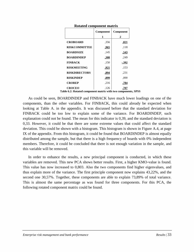
Enterprise risk management and bank performance Results | 33
Rotated component matrix
Component Component
1 2
CROBOARD ,356 ,821
RISKCOMMITTEE ,965 ,118
BOARDSIZE ,145 ,543
BOARDINDEP ,308 ,249
FINBACK ,150 -,392
RISKMEETING ,921 ,153
RISKDIRECTORS ,894 ,231
RISKINDEP ,899 ,000
CROREP ,216 ,784
CROCEO ,126 ,707
Table 6.2: Rotated component matrix with two components, SPSS
As could be seen, BOARDINDEP and FINBACK have much lower loadings on one of the
components, than the other variables. For FINBACK, this could already be expected when
looking at Table A. in the appendix. It was discussed before that the standard deviation for
FINBACK could be too low to explain some of the variance. For BOARDINDEP, such
explanation could not be found. The mean for this indicator is 0,39, and the standard deviation is
0,33. However, it could be that there are some extreme values that could affect the standard
deviation. This could be shown with a histogram. This histogram is shown in Figure A.4, at page
IX of the appendix. From this histogram, it could be found that BOARDINDEP is almost equally
distributed among the sample, but that there is a high frequency of boards with 0% independent
members. Therefore, it could be concluded that there is not enough variation in the sample, and
this variable will be removed.
In order to enhance the results, a new principal component is conducted, in which these
variables are removed. This new PCA shows better results. First, a higher KMO-value is found.
This value has now increased to 0,803. Also the two components find higher eigenvalues, and
thus explain more of the variance. The first principle component now explains 43,22%, and the
second one 30,57%. Together, these components are able to explain 73,89% of total variance.
This is almost the same percentage as was found for three components. For this PCA, the
following rotated component matrix could be found.

Enterprise risk management and bank performance Results | 34
Rotated component matrix
Component Component
1 2
CROBOARD ,315 ,854
RISKCOMMITTEE ,957 ,210
BOARDSIZE ,192 ,525
RISKMEETING ,914 ,255
RISKDIRECTORS ,865 ,375
RISKINDEP ,912 ,036
CROREP ,158 ,814
CROCEO ,027 ,781
Table 6.3: Rotated component matrix excl. BOARDINDEP and FINBACK, SPSS
As could be seen, the loadings have larger differences now and the higher scores have
increased. CROBOARD and RISKDIRECTORS are loaded onto both components. In this case,
it is decided to put the variable into the component in which the loading is higher. Since the
lower loadings for these variables are close to 0,30, these are not as relevant for that component,
as for the other. This means that CROBOARD will be taken into component 2, while
RISKDIRECOTRS is used in component 1. When looking at the variable itself, this also makes
more sense. One could see that component 1 mainly considers the existence and characteristics
of the risk committee, while component 2 mainly considers the place of the CRO in the
organization. Therefore, component 1 will now be called ERMRC, and component 2 will now be
called ERMBOARD.
These correlations are then used to weigh the different scores for the variables. The
component scores are now computed by taking the highlighted weightings and multiply these by
the standardized observation values. Because of this standardization, the components of ERM
implementation could also be negative. This means that for that observation, the implementation
is lower than for the total sample. A positive value for ERM implementation means that the
extent of implementation is higher than the total sample average.
Now that the ERM index is developed, the overall sample could be described. This is needed
to give an overview of the sample.
6.2 DESCRIPTIVE STATISTICS
The general purpose of descriptive statistics is to give the reader an overview of the sample.
These statistics show the mean and standard deviation of all the measures for the overall sample,
Also the total sample size is given. This is shown in Table 6.4, on the next page.
As was discussed before, 38 banks were taken into the sample. However, not all banks
existed throughout all the periods. For example, the Anadolubank was founded in the

Enterprise risk management and bank performance Results | 35
Netherlands in 2008. This means that for the period before the crisis, no data is available.
Further, some banks were incorporated into their mother company, like for example Bank
Insinger de Beaufort and Kempen & Co, who respectively formed into BNP Paribas and Van
Lanschot Bankiers. This leads to the fact that not 228 observations are taken into account, but
164.
Further, the benchmark period is defined as the period before the crisis. Since the effect of
ERM is measured as a lagged variable, the observations of 2005 on ERM will be used in 2006,
and so on. Therefore, no observations are used in 2005. This leads that the benchmark period
only consists of the observations in 2006. This explains the lower number of observations in this
benchmark period.
Since the ERM index is based on standardized measures, the mean is 0 and the standard
deviation is 1 (Moore & McCabe, 2008). The total sample standardized average does not say
anything about the extent of ERM implementation for the total population, but it makes it easier
to compare the different observations within this sample. A negative value on ERM
implementation does not automatically mean that ERM is not implemented, but that this is less
than the total sample.
Descriptive statistics
Total sample Benchmark* Crisis = 1 After crisis = 1
N = 164 34 67 62
Mean Std. Dev. Mean Std. Dev. Mean Std. Dev. Mean Std. Dev.
ROA 1,10 4,10 1,67 2,74 1,01 2,34 ,89 5,87
ROA2 ,84 3,12 1,76 3,56 ,74 1,98 ,43 3,75
ROE 5,45 64,59 15,05 13,91 11,29 20,05 -6,27 101,85
ERM RC ,05 1,50 -,22 1,27 -,05 1,39 ,32 1,71
ERMBOARD ,06 ,74 -,13 ,60 ,08 ,75 ,15 ,80
ERMRC2 2,24 3,96 1,61 3,41 1,89 3,52 2,98 4,59
ERMBOARD2 ,55 ,83 ,36 ,71 ,56 ,79 ,65 ,91
EFFICIENCY 2,39 4,97 3,22 8,01 -,05 1,39 2,01 2,78
LEVERAGE 91,17 9,81 91,56 9,47 2,30 4,51 90,71 10,26
DIVERSIFICATION 47,53 113,75 44,94 31,22 91,39 9,70 44,19 33,32
TIER-1 CAPITAL RATIO 25,20 32,55 31,16 48,76 51,97 174,34 22,67 18,32
CREDIT QUALITY ,56 1,63 ,47 1,33 24,42 32,50 ,57 1,43
* Benchmark period is the period before the crisis, where both the crisis and after crisis dummies are 0.
Table 6.4: Descriptive statistics, SPSS
Since the ERM index is based on standardized measures, the mean is 0 and the standard
deviation is 1 (Moore & McCabe, 2008). The total sample standardized average does not say
anything about the extent of ERM implementation for the total population, but it makes it easier

Enterprise risk management and bank performance Results | 36
to compare the different observations within this sample. A negative value on ERM
implementation does not automatically mean that ERM is not implemented, but that this is less
than the total sample.
As can be seen, return on assets is declining during the financial crisis, as was expected.
However, recovery does not show after the financial crisis. It also shows that the standard
deviation after the crisis is much larger than before the crisis, and that it declines during the
financial crisis. This indicates that most banks face bad performance during the crisis, but that
some banks recover from that crisis faster than others, who face even worse performance during
the crisis.
Return on equity is also declining during the different periods, with also an increasing
standard deviation. This means that the differences between banks are increasing, which was also
indicated by the scores an return on assets. In the period after the crisis, it could be seen that the
standard deviation is much larger than before. This could also indicate several outliers.
The variables for ERM implementation shows an increase over the periods. Before and
during the crisis, it shows that these are below the total sample average on ERM, which
automatically leads to a positive value afterwards. This increase of the ERM index indicates that
banks are further implementing ERM over time. During the financial crisis, the differences
among the sample are increasing compared to the period before the crisis. This could indicate
that during the crisis, some banks start seeing the importance of risk management and rapidly
implement it. Other banks do not use risk management to survive the crisis, maybe because they
do not really suffer from the crisis. The variables for ERM implementation are still increasing
after the crisis, and also show a higher standard deviation. This means that the differences
between banks are further increasing.
Efficiency and tier-1 capital show the same change as performance during the periods.
Leverage increases over time, while the ratio for bad credit increases during the financial crisis
and stays at approximately the same level afterwards, but with a smaller standard deviation. This
means that the credit quality is increasing, and that the differences among banks are decreasing.
Since there are several measures that show the same or an opposite change during the
measurement periods, this could indicate a relation between these variables. This will be further
investigated with a correlation matrix, which will be discussed during the next part.
6.3 CORRELATION MATRIX
In a histogram made with use of SPSS, it is shown that the sample is normally distributed,
which means that Pearson’s correlation could be used to determine the correlations between the
variables. These correlations will be determined for the entire measurement period and the three
subsamples. In the correlation matrices, all the variables are correlated to each other, including
ERM2. The correlations show whether the variables are related to each other, which is a first step

Enterprise risk management and bank performance Results | 37
in determining whether ERM implementation affects firm performance. When a significant
correlation is found between variables, several explanations could be given. First, it could be that
variable A is causing variable B, or the other way around. The final explanation is that both
variables are explained by third variable, C.
Because of the size of the tables, only the correlation matrix for the total sample is shown
here, in Table 6.5. The other tables could be found in Appendix VIII: Correlation matrices.
From Table 6.5, at the next page, it could be seen that both measurements of return on assets
(ROA1 and ROA2) are highly correlated, as could be expected. This is caused by the fact that
they use approximately the same variables. The measures for return on assets and return on
equity do not correlate with each other, which could be expected. These measures define
different parts of performance.
Since the ERM indices are lagged variables, it is possible to tell more about causation from
these correlation tables. Lagged variables are observed before the other variables. This means
that for the year 2006, ERM implementation was observed in 2005. It is therefore possible to tell
what effect ERM has on performance, based on the correlation matrix. Since ERM
implementation was there before performance, it is not possible for performance to affect ERM
implementation. It shows that ERMRC and ERMRC2 have little negative correlations with the
performance measures, and these are insignificant. This indicates that implementing ERM as a
risk committee decreases performance.
ERMBOARD does not show significant correlations with any performance measure.
However, the coefficients are also negative, which provides a further indication that ERM is not
enhancing performance, but could actually decrease it. For ERMBOARD2, the same directions
are found, although the coefficients are more close to 0. This means that there is no correlation
between these variables. This indicates that it does not matter for performance if a bank has high
or low values on ERM board characteristics.
Further, the control variables do not correlate with performance, except for leverage. This
control variable is negative correlating with return on assets. This could indicate that leverage
leads to lower performance, or higher performance leads to lower leverage. However, it could
also be that some other variable causes this effect.
The effects for the other control variables are not only insignificant, but also very small. The
correlation between return on equity and tier 1 capital is 0, which indicates that there is no
relation between these variables.

Enterprise risk management and bank performance Results | 38
Corr
elati
on
matr
ix,
n =
164
CR
ED
1
**
. C
orr
elat
ion
is
sig
nif
ican
t at
the
0.0
1 l
evel
(2
-tai
led
).
To
tal
ob
serv
atio
ns
in s
amp
le:
10
6.
Per
form
ance
is
mea
sure
d b
y r
etu
rn o
n a
sset
s (R
OA
, R
OA
2)
and
ret
urn
on
equ
ity
(R
OE
). E
RM
RC
is
ind
icat
ed a
s R
C,
ER
MB
OA
RD
is
ind
icat
ed a
s B
OA
RD
. E
ffic
ien
cy,
lev
erag
e, d
iver
sifi
cati
on,
tier
-1 c
apit
al r
atio
an
d c
red
it q
ual
ity
are
men
tion
ed a
s E
FF
, L
EV
, D
IV,
TIE
R1
an
d C
RE
D.
T
ab
le 6
.5:
Co
rrel
ati
on
ma
trix
to
tal
sam
ple
, S
PS
S
TIE
R1
1
-,0
99
DIV
1
-,0
93
,081
LE
V
1
-,0
15
-,5
78
**
,118
EF
F
1
-,2
51
**
,146
,046
,008
BO
AR
D2
2
1
-,0
92
,050
,020
-,0
82
,024
RC
2
1
,233
**
-,1
32
,106
-,0
96
,106
-,0
74
BO
AR
D
1
,346
**
,841
**
-,1
21
,110
,093
-,1
20
,126
RC
1
,360
**
,979
**
,239
**
-,1
30
,101
-,0
85
,106
-,0
84
RO
E
1
,017
,043
,013
,000
-,0
65
-,0
61
-,0
84
,000
,038
RO
A2
1
,700
**
-,0
63
-,0
27
-,0
65
-,0
66
,136
-,4
16
**
-,0
11
,085
-,0
39
RO
A 1
,882
**
,565
**
-,0
68
-,0
54
-,0
66
-,0
73
,161
*
-,4
37
**
-,0
12
,096
-,0
55
RO
A
RO
A2
RO
E
RC
BO
AR
D
RC
2
BO
AR
D
2 EF
F
LE
V
DIV
TIE
R1
CR
ED

Enterprise risk management and bank performance Results | 39
The control variables also show some correlations with each other. This goes for leverage and
efficiency, and leverage and tier 1 capital. Since leverage is also affecting performance, it could
be that this is caused by the effect of efficiency or tier 1 capital. However, this cannot be
concluded from the correlation matrix. The fact that some control variables are also correlating,
is an indication for multicollinearity. This does not affect the direction of the effect, but could
affect the size found. Therefore, it could affect the conclusions.
In the next part, the most important results for the different periods are discussed. These
tables are due to space considerations not included in the text, but are presented in Appendix
VIII: Correlation matrices, which starts at page VII of the appendix.
6.3.1 CORRELATIONS BEFORE THE FINANCIAL CRISIS
The complete correlation matrix could be found in Table A.4, in Appendix VIII: Correlation
matrices. The most important results will be discussed now. In this period, it shows that both
ERM indices do not correlate with each other. This could mean that the implementation of these
indicators happens randomly at banks. This could be explained by the fact that banks are
performing well in this period, and do not consider ERM as necessary. ERM implementation
could be seen as additional, and will be implemented when banks have superfluous resources.
It shows that the presence and the characteristics of a risk committee, do not significantly
affect performance. Although the effects are negative, these are very small. This also counts for
the squared term of this measure. For that measure, the effects are even becoming smaller,
although they are still negative. The ERM indicator for the board, ERMBOARD, also shows
negative but insignificant correlations. These correlations show a comparable coefficient.
It shows that tier 1 capital is positively correlating with ERMRC and ERMRC2. This could be
explained by the fact that tier 1 capital ratio is seen as a buffer against negative outcomes. Since
risk management is implemented with the same idea, it explains why these variables correlate.
However, it does not say which variable causes the other, or about the existence of a possible
third variable.
Further, several control variables find significant correlations. First, it was found that
leverage is negatively correlating with return on assets. This is in line with the total sample
results. Also diversification is significantly correlating with return on assets. It was found that
return on equity and credit quality are positively correlated.
Also some of the control variables is significantly correlating. These are diversification and
efficiency (positive) and leverage and tier 1 capital (negative). This leads to an indication of
multicollinearity between these variables. This means that since the control variables affect each
other, the effect of these variables on performance could be changed. Multicollinearity does not
change the direction of the effect, but it could change the size of the effect.

Enterprise risk management and bank performance Results | 40
Concluding, the ERM implementation indices do not correlate significantly with
performance. Further, some other correlations are found which could be further extended.
However, this is out of the scope of this research and therefore, this extension should be done in
future research.
6.3.2 CORRELATIONS DURING THE FINANCIAL CRISIS
The complete matrix could be found in Table A.5, in Appendix VIII: Correlation matrices.
Below, the most important outcomes are discussed.
Also during the financial crisis, it shows that both ERM indicators are not significantly
correlating. The coefficients in the correlation matrix during the crisis, are almost the same as
before, when looking at the ERM indicators and performance. ERMRC shows very little effects,
which are mostly negative for the standard ERMRC measure, but turn into positive for ERMRC2.
However, these effects are negligible.
It shows that diversification and return on equity are negatively correlating, which is also
found for leverage and return on assets. This are the only significant correlations between the
control variables and the performance measures. Tier 1 capital ratio and leverage are negatively
correlating, which indicates multicollinearity.
Also during this period, the control variables do not find significant relations with each other
or performance. This leads to an indication that the variables do not explain firm performance.
When this is confirmed, this means that no real conclusions could be drawn.
6.3.3 CORRELATIONS AFTER THE FINANCIAL CRISIS
In this part, the results of Table A.6 in Appendix VIII: Correlation matrices are being
discussed.
In this period, it could be seen that the ERM indicators are positively correlated. This
indicates that ERM implementation happens more completely now. When a risk committee is
settled, also the board characteristics change, or the other way around. This could be due to more
regulations, or better awareness.
The ERM indicators still do not significantly correlate with any performance measure. It
further shows that leverage and ERMRC are positively correlating, while diversification and the
same ERM indicator are negatively correlated. Further, it shows that tier 1 capital is negatively
correlating with leverage and diversification. This could explain the existence of a third variable
in the relation between ERMRC and leverage and diversification. However, extending this
relationship is not in the scope of this research.

Enterprise risk management and bank performance Results | 41
6.4 INITIAL CONCLUSIONS
With these descriptive statistics, an overview of the sample is given and a first indication for
the results from the regression are shown. In general, performance declined over the periods,
with also an increasing standard deviation. This indicates that the differences between banks are
increasing. Some banks recover from the crisis, whereas other banks even perform worse during
the crisis. ERM implementation increases over the different periods. This could be expected,
because of more regulations and better awareness of the relevance of risk management.
However, also the standard deviation increases. This indicates that the differences in
implementation are increasing. One would expect, because of the better awareness and more
regulations, that these differences would decline and there would be an overall increase.
However, it seems that this is not the case.
The correlation matrices showed a first indication of the relations between the different
variables. Several control variables correlate significantly with each other, which means that they
could affect the conclusions. This happens before the financial crisis, when diversification and
efficiency and leverage and tier 1 capital are significantly correlating, and afterwards, when
leverage and diversification correlate with efficiency. Further, in that period, tier 1 capital is also
correlating with leverage and diversification. Further, before the crisis, leverage and
diversification correlate with return on assets. During the financial crisis, leverage and
diversification are correlating with different measurements of performance.
For the overall sample, no significant correlations are found the ERM indices and the
performance measures. However, this will further show in the regression results. These
regressions will be discussed in the next part. With these results, the hypotheses will be tested.
The validity of these results happens afterwards. Based on this validity discussion, final
conclusions could be drawn about the effect of ERM implementation and performance.

Enterprise risk management and bank performance Analysis | 42
7. ANALYSIS
In this part, the relations found in the correlation matrices will be further extended by a
regression. This should show whether performance is affected by the different variables, and to
what extent. With the outcomes of the regressions, the hypotheses will be tested and initial
conclusions will be drawn. However, before these conclusions could be definite, the validity of
the results needs to bested. The validity will show whether the results are sufficiently supported.
After this analysis, final conclusions will be drawn. These conclusions will be incorporated with
research limitations and directions for further research.
7.1 MULTIVARIATE REGRESSION
In a regression, it is possible to define the relation between a dependent variable and several
independent variables. For this research, the regression is used to determine the effect of ERM
implementation and efficiency, leverage, diversification, tier 1 capital and credit quality on bank
performance. ERM implementation is measured as ERMRC and ERMBOARD, as the PCA has
shown. To see the effect of the crisis on the relation between ERM implementation and
performance, an interaction variable is introduced. For an overview of all the variables taken into
account, see the conceptual model at page 20.
To test the first hypothesis, whether ERM implementation leads to better performance under
normal conditions, one should look at the variables ERMRC and ERMBOARD. Further, also the
interaction variable for the period after the crisis needs to be taken into account. The hypothesis
that ERM implementation is only valued up until a certain extent, is tested by the variables
ERMRC2 and ERMBOARD
2, and the interaction variables for the after-crisis period.
The hypothesis about the crisis period, which state that ERM implementation will lead to
better firm performance during the crisis, are determined by the interaction variables for the
crisis period. The hypothesis that ERM implementation only leads to better performance up until
a certain extent of implementation, is tested by the squared term of the ERM implementation
indices.
In the regression tables, the effects of the different variables on firm performance are shown.
In the upper row, the performance measure is mentioned, and the different results are shown. In
the first two rows under each performance measure, the effect of ERM is measured. In the most
left column, which is in plain text, the β is shown. For this research, these should be positive to
support the hypotheses. In italics, in the column on the right, the significance is shown. This
should be lower than 0,05 in order to be significant for the hypotheses formulated in this
research. The meaning of the intercept is in this case the estimation of performance, when all the
other variables are 0.
The coefficients in the regression tables should be interpreted as follows. When, for example,
an effect of 0,800 is found between an independent variable and the dependent variable, this

Enterprise risk management and bank performance Analysis | 43
means that if the independent variables increases with one standard deviation, the dependent
variable increases with 0,800. In the following table, the results of the regressions are shown.
Regression results, SPSS
Firm performance
ROA1 ROA2 ROE
β t β t β t
Intercept 25,566 ** ,000 20,215 ** ,000 139,384 ,077
ERMRC -1,672 ,535 -1,762 ,386 -16,641 ,727
ERMBOARD 1,088 ,625 1,296 ,439 7,334 ,852
ERMRC2 ,594 ,551 ,571 ,445 5,463 ,756
ERMBOARD2 -,953 ,594 -1,298 ,335 -8,627 ,785
ERMRC_CRISIS 1,318 ,671 2,039 ,383 17,995 ,743
ERMBOARD_CRISIS -,782 ,753 -,540 ,772 3,682 ,933
ERMRC2_CRISIS -,461 ,692 -,696 ,427 -6,824 ,740
ERMBOARD2_CRISIS ,354 ,864 ,518 ,739 -1,501 ,967
ERMRC_AFTERCRISIS 1,739 ,544 2,016 ,350 28,552 ,573
ERMBOARD_AFTERCRISIS ,170 ,946 -,384 ,840 10,981 ,806
ERMRC2_AFTERCRISIS -,561 ,593 -,595 ,450 -8,240 ,656
ERMBOARD2_AFTERCRISIS -,181 ,929 ,602 ,696 -1,719 ,962
Efficiency ,016 ,800 -,010 ,835 -1,324 ,238
Leverage -,258 ** ,000 -,198 ** ,000 -1,303 ,070
Diversification -,002 ,542 -,002 ,455 -,055 ,257
Tier 1 capital -,034 ** ,006 -,027 ** ,005 -,224 ,306
Credit quality -,034 ,859 -,016 ,912 1,703 ,613
CRISISdummy -,079 ,977 ,019 ,993 8,721 ,857
AFTER CRISISdummy -,088 ,972 -,835 ,659 -10,071 ,820
**. Significant at the 0.01 level (two-tailed).
*. Significant at the 0.05 level (two-tailed).
Total number of observations = 164.
Table 7.1: Regression results, SPSS
7.1.1 PERFORMANCE UNDER NORMAL CONDITIONS
This research tries to answer the question how ERM implementation affects firm
performance of banks before, during and after a financial crisis. From there, hypotheses are
developed, who define this relationship under normal conditions and during a financial crisis.
These normal conditions are best described by the periods before and after the financial crisis.
For testing these hypotheses, one should look at the normal ERM indicators, and the interaction
variables for after the crisis. In this part, the results for these variables are discussed.

Enterprise risk management and bank performance Analysis | 44
When looking at the after crisis dummy variable, it could be seen what effect the period after
the crisis has on firm performance. It shows that for all performance measures, negative effects
are found. However, these effects are not significant. This means that the effects found, are not
found in 95 or 99% of the observations.
It shows that the ERM indices find mixed results, but that these results are insignificant. For
the first measure for return on assets, it is found that ERMRC and ERMBOARD show
contradicting results. ERMRC shows a negative effect, whereas ERMBOARD is positive. This
indicates that ERM implementation is not always positive for performance, but that this depends
on the parts of ERM that are implemented. It shows that characteristics as board independence
are positively affecting performance, whereas the presence of a risk committee decreases
performance. For the interaction variables for the period after the crisis, it shows that there are
positive effects. This means that ERM implementation after the crisis leads to better results for
return on assets.
The second measure for return on assets finds similar results for the original ERM indices,
compared to the first measure for return on assets. However, some differences appear in the after
crisis variables. For the RC index, it shows positive effects, contradicting the BOARD index.
This index finds a negative effect. This means that the presence of a risk committee and its
characteristics have a positive effect on return on assets, whereas the direct reporting lines of the
CRO to the CEO and the board have a negative effect.
Return on equity finds the same directions in the effects of ERM implementation as the first
measure for return on assets. However, these effects are much larger, although they are still
insignificant. Since the t-statistic for these effects are close to 1, it indicates that this model is not
valid. This is because it seems if the variables used are not able to explain return on equity.
Also for the nonlinearity of the effect between ERM implementation and firm performance,
no significance is found. This indicates that it does not matter for the extent of implementation,
which effect on performance is found. However, also for these quadratic terms, mixed results are
found. What needs to be noticed, is that these results are opposing the effects found for the
original ERM indices. For the squared terms, ERMRC is positive, and ERMBOARD is negative
for the first measure for return on assets. In the after-crisis period, both indices are now negative
instead of positive. The second measure for return on assets finds the same results as the first
measure in the period before the crisis, and also finds opposite results in the period afterwards.
This means that ERMRC2 is positive, whereas ERMBOARD
2 is negative. For return on equity,
ERMRC2 is now positive instead of negative, and ERMBOARD
2 shows the opposite. In the
period after the crisis, two negative signs are found.
Enterprise risk management and bank performance Analysis | 45
7.1.2 PERFORMANCE DURING A FINANCIAL CRISIS
As was discussed before, it is argued that ERM implementation will lead to better
performance during a financial crisis. This was formulated into a hypothesis and this hypothesis
will now be tested. This will be done when looking at the interaction variables for the financial
crisis. In this part, these results are being discussed.
The crisis dummy shows what effect the crisis has on performance. It shows that the first
measure on return on assets find negative effects, as was expected. However, these effects are
positive for the other return on assets measure and return on equity. Although these effects are
not significant, they indicate a contradiction in the expectation. With the effects found for the
after crisis dummy, it could be that the crisis is not over yet, and banks are recovering or even
face worse performance now, after the banking crisis is over.
When looking at the ERM indices, no significant results could be found. Further, the results
found are also contradicting each other. ERMRC finds positive effects on both return on assets
measures, whereas ERMBOARD finds negative ones. This means that during a financial crisis,
the presence of a risk committee leads to better performance, whereas board independence and
the reporting lines of the CRO could negatively affect performance. For return on equity, both
indices are positive.
The squared terms of the ERM indices, which would count for a possible nonlinear effect of
ERM implementation, find opposing results when comparing these with the original ERM
indices. ERMRC2 now turns negative for the return on assets measures, whereas ERMBOARD
2
turns positive. For return on equity, both the squared indices are negative. However, also those
signs are not significant.
7.1.3 CONTROL VARIABLES
When looking at the effect of the control variables on performance, it could be seen that all
these effects are negative, when looking at return on assets. For leverage and tier 1 capital, these
effects become significant. This is contradicting the expectations. It was argued that leverage
would improve performance, because of the agency problem. Further, tier 1 capital is seen as a
buffer against adverse shocks, and would therefore be positive. However, it shows that these are
both significantly negative for return on assets. Since the other control variables are not
significant, it could only be indicated that the expectations for these control variables are not
met, except for credit quality.
For return on equity, different effects are found for credit quality. This was negative for
return on assets, which is in line with the expectations. However, for return on equity, this
becomes positive. This indicates that when a bank has more bad loans, it performs worse, which
is hard to believe. These effects are also not significant, so that no real conclusions could be
drawn.

Enterprise risk management and bank performance Analysis | 46
Before definite conclusions could be drawn on the effects of ERM implementation on
performance, the validity needs to be tested. This will be done using R2 and testing the normality
of the residuals, using a normal probability plot and the Kolmogorov-Smirnov test.
7.2 VALIDITY
As was discussed before, the final conclusions could only be drawn, after the validity has
been tested. The results are valid when there is sufficient evidence that supports the propositions
from those results (Shadish et al., 2002). In this part, the different tests that have been discussed
in part 0, on page 30, will be executed and discussed. After these tests have been executed, it
could be determined whether the results found are valid. Based on the conclusions from this part,
the final conclusions can be drawn.
7.2.1 R2
The R2 measures whether the independent variable and the control variables count for
variations in the dependent variable. SPSS determines R2 for each regression model, and gives in
that case two types of R2. The first one is the original R
2, the second one is the adjusted R
2. The
adjusted R2 takes into account the number of variables. One could understand that if more
variables are taken into account, more variance could be explained. Therefore, to be able to have
comparable R2s, the adjusted R
2 is used.
R2 could have values between 0 and 1, in which 0 in this case means that 0% of the variation
of firm performance is explained by the independent and control variables. When R2 is 1, this
means that 100% of the variation of firm performance is explained by the independent and
control variables. It is therefore needed to have a R2 that is as high as possible. In Table 7.2, the
scores on R2 are shown for all the regression models. These scores will be discussed now, and
will also be compared with the R2 of previous studies.
Results for R2
Performance measure R2
ROA1 ,163
ROA2 ,185
ROE -,051
Table 7.2: R2 for all regression models, SPSS
As could be seen, these values are very close to 0. In the case of ROE, R2 is even negative.
This is because the adjusted R2 tries to allow for the fact that two variables that are completely
unrelated, show some relationship here just by luck. Therefore, the adjusted R2 reduces the
original R2 by this luck. In this case, the original R
2 is smaller than the relationship found that is
caused by luck. This indicates that the variables are not related to return on equity.
Further, for the return on assets, the values for R2 are very low. The variation in the first
measure is only for 16,5% explained by the variables used. For the second measure this increases

Enterprise risk management and bank performance Analysis | 47
to 18,5%, but this still is very low. These low values indicate that these models are not valid.
This means that the conclusions drawn from these models are not truthful enough. However, this
has to be also confirmed by the lack of normality of residuals. This will happen in the next part.
7.2.2 NORMALITY OF RESIDUALS
A residual is a point in the regression plot that is off the regression line. These residuals
should be normally distributed around the regression line, in order for the regression line to be
valid. This normal distribution is one of the assumptions of a regression.
The normality of the residuals could be graphically tested, and using mathematical tests.
First, the graphical test is explained. A normal P-P plot plots the observed cumulative probability
against the expected cumulative probability. In the case the residuals are normal, this expected
and observed probability should be equal to each other and show a straight line. When this is not
the case, the residuals are not normally distributed.
Further, the normality of the residuals could also be numerically tested. In SPSS, the Shapiro-
Wilk and the Kolmogorov-Smirnov tests for normality could be used. When the sample is larger
than 50, the Shapiro-Wilk test is less appropriate and the Kolmogorov-Smirnov test needs to be
used. Since this research consists of 164 observations, this sample is larger than 50. Therefore,
the Kolmogorov-Smirnov test is most appropriate.
When the value for this test is significant at 0.05, this provides good evidence that the
dependent variable is not normally distributed.
NORMAL P-P PLOT
Due to space considerations, the normal P-P plots are shown in Appendix IV: Normal P-P
Plots, which starts at page XIII of the appendix. As could be seen from these plots, these do not
follow the straight line that it should. This straight line is also shown in the plots. For these
variables, the residuals show a S-shaped line. This means that first, the observed cumulative
probability is lower than the expected one, while at some point, this becomes the other way
around. In this latter part, the observed cumulative probability is higher than the expected one.
This means that the residuals are not normally distributed, which means the model is not valid.
With these models, the estimates shown in Table 7.1 are not correct.
This graphical test needs to be further enhanced by a mathematical test. In this research, the
Kolmogorov-Smirnov test is used. This test will be explained and interpreted in the following
part.
KOLMOGOROV-SMIRNOV TEST
A Kolmogorov-Smirnov test tests whether the distribution of the sample is different from a
normal distribution. It tests the null hypothesis that these are equal. When the test finds a
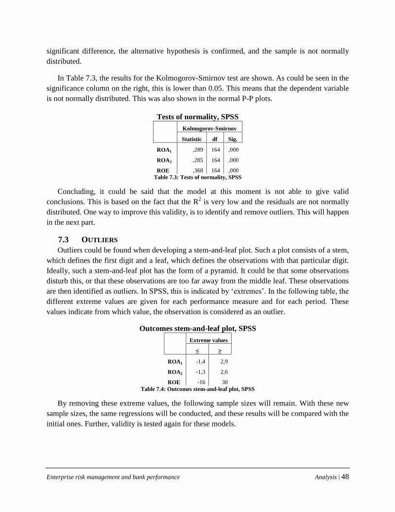
Enterprise risk management and bank performance Analysis | 48
significant difference, the alternative hypothesis is confirmed, and the sample is not normally
distributed.
In Table 7.3, the results for the Kolmogorov-Smirnov test are shown. As could be seen in the
significance column on the right, this is lower than 0.05. This means that the dependent variable
is not normally distributed. This was also shown in the normal P-P plots.
Tests of normality, SPSS
Kolmogorov-Smirnov
Statistic df Sig.
ROA1 ,289 164 ,000
ROA2 ,285 164 ,000
ROE ,368 164 ,000
Table 7.3: Tests of normality, SPSS
Concluding, it could be said that the model at this moment is not able to give valid
conclusions. This is based on the fact that the R2 is very low and the residuals are not normally
distributed. One way to improve this validity, is to identify and remove outliers. This will happen
in the next part.
7.3 OUTLIERS
Outliers could be found when developing a stem-and-leaf plot. Such a plot consists of a stem,
which defines the first digit and a leaf, which defines the observations with that particular digit.
Ideally, such a stem-and-leaf plot has the form of a pyramid. It could be that some observations
disturb this, or that these observations are too far away from the middle leaf. These observations
are then identified as outliers. In SPSS, this is indicated by ‘extremes’. In the following table, the
different extreme values are given for each performance measure and for each period. These
values indicate from which value, the observation is considered as an outlier.
Outcomes stem-and-leaf plot, SPSS
Extreme values
≤ ≥
ROA1 -1,4 2,9
ROA2 -1,3 2,6
ROE -16 30
Table 7.4: Outcomes stem-and-leaf plot, SPSS
By removing these extreme values, the following sample sizes will remain. With these new
sample sizes, the same regressions will be conducted, and these results will be compared with the
initial ones. Further, validity is tested again for these models.

Enterprise risk management and bank performance Analysis | 49
Sample sizes excl. outliers
Sample size
ROA1 151
ROA2 148
ROE 143
Table 7.5: Sample sizes excl. outliers
7.3.1 REGRESSION RESULTS
In this part, the regression results for the samples without the outliers are being discussed.
The regression results could be found in Table 7.6 below. These results will be discussed below,
and this will happen in the same way as for the original sample.
Before this discussion will start, a general comparison is made between these results and the
results for the original sample. In general, the sizes of the effects found are much smaller in this
regression, than in the original sample. This could be caused by the fact that outliers caused these
large effects, which are now removed.
Further, some variables have changed in the direction of their effect on performance. These
are highlighted in the table. Further, ERMRC_CRISIS on ROA2 does not show a change in the
direction of the effect, but in the size. In the original sample, this effect was 2,039. This has
dropped to only 0,062 in this sample. An even greater differences appears in ERMRC_CRISIS
and ROE. In the original sample, this effect was 3,682. Now, when the outliers are excluded, this
has turned into -3,026.
In the original sample, tier 1 capital was significantly negatively affecting return on assets. In
this sample, the effect is no longer significant, but also turned into almost 0. Since tier 1 capital
could be seen as some form of risk management, since it is a buffer against adverse shocks, this
could indicate that there is no effect of risk management on performance.
The crisis shows now a negative effect on performance, as could be expected. This was not
found in the original sample, but it is now. This could mean that this sample is better reflecting
reality than the original sample did.
Now that some comparison is made between the original sample results and these results, the
results for this sample could be discussed more in detail. This will happen from the next page.

Enterprise risk management and bank performance Analysis | 50
Regression results excl. outliers, SPSS
Firm performance
ROA1 ROA2 ROE
β t β t β t
Intercept 10,319 ** ,000 9,573 ** ,000 3,996 ,667
ERMRC -,784 ,231 -,378 ,506 -2,095 ,669
ERMBOARD ,397 ,452 ,274 ,502 -,789 ,851
ERMRC2 ,207 ,385 ,090 ,658 ,496 ,783
ERMBOARD2 -,453 ,288 -,314 ,336 -,322 ,925
ERMRC_CRISIS ,569 ,445 ,062 ,924 -3,026 ,602
ERMBOARD_CRISIS -,331 ,577 -,207 ,652 ,161 ,973
ERMRC2_CRISIS -,147 ,595 ,008 ,974 ,919 ,674
ERMBOARD2_CRISIS ,295 ,549 ,137 ,715 ,512 ,897
ERMRC_AFTERCRISIS ,725 ,299 ,471 ,416 ,039 ,994
ERMBOARD_AFTERCRISIS -,351 ,560 -,188 ,688 3,354 ,482
ERMRC2_AFTERCRISIS -,176 ,485 -,119 ,562 ,172 ,928
ERMBOARD2_AFTERCRISIS ,392 ,422 ,224 ,550 -1,793 ,645
Efficiency -,022 ,184 -,022 ,217 -,232 ,057
Leverage -,100 ** ,000 -,093 ** ,000 ,052 ,544
Diversification ,001 ,668 ,000 ,126 ,025 ,071
Tier 1 capital -,002 ,539 ,000 ,960 ,008 ,735
Credit quality -,011 ,810 ,007 ,845 ,060 ,874
CRISISdummy -,259 ,692 -,368 ,511 -2,448 ,637
AFTER CRISISdummy -,475 ,431 -,364 ,455 -2,718 ,556
**. Significant at the 0.01 level (two-tailed).
*. Significant at the 0.05 level (two-tailed).
Total number of observations ROA1 = 151, ROA2 = 148, ROE = 143.
Table 7.6: Regression results excl. outliers, SPSS
PERFORMANCE UNDER NORMAL CONDITIONS
When looking at the after crisis dummy, it shows that this effect is now almost as large and
negative as for the crisis dummy. This indicates that in the period after the banking crisis, banks
still are not fully recovered and suffer losses. However, these effects are not significant.
For performance under normal conditions, one should look again at the original ERM indices
and the squared terms, and the interaction variables for the period after the crisis. These variables
do not show significant effects on the performance measures. Further, the results found are
mixed. ERMRC is negatively affecting performance, while ERMBOARD is positively affecting
performance before the crisis, when looking at return on assets. Return on equity finds negative
signs for both measures. For the period after the crisis, these signs show the opposite. This

Enterprise risk management and bank performance Analysis | 51
indicates that there is not one answer to whether ERM implementation leads to better
performance under normal conditions.
For the variables to measure whether the valuation of ERM implementation only holds up
until a certain extent, again mixed results are found. These results show the opposite signs, when
comparing these with the original measures. However, also these effects are not significant.
Concluding, it could be said that there is no indication that ERM implementation leads to
better performance under normal conditions. Therefore, no support is found for the first
hypotheses. However, since the insignificant effects that are found are mixed, it also indicates
that there is not one answer to whether ERM implementation leads to better firm performance.
The fact that the signs are different for the different periods, it could also depend on economic
circumstances.
PERFORMANCE DURING A FINANCIAL CRISIS
To test the hypotheses that concern the effect of ERM implementation during a financial
crisis, one should look at the interaction variables for the financial crisis. These are indicated
with _CRISIS in the regression table.
Again, no significant effects for ERM implementation and performance could be found.
Further, these effects are also mixed. For return on assets, ERMRC is positive, while
ERMBOARD is negative. For return on equity, the opposite signs are found. This means that for
return on assets during a financial crisis, it is better to have a risk committee since this improves
performance. Board independence and direct reporting lines between the CRO and the CEO and
the board are decreasing performance, and should therefore not be implemented. However, for
return on equity, this should be the other way around.
The squared terms for ERM implementation, more unambiguous effects are found. For the
first measure for return on assets, the results are still mixed. However, for the other two
measures, these effects are positive. This means that when ERM is implemented to a further
extent, performance will increase to a less extent. This indicates that ERM implementation only
leads to better performance up until a certain extent. However, since these effects are not
significant, this cannot be concluded with a sufficient level of certainty.
CONTROL VARIABLES
When looking at the effects of the control variables on performance, it could be seen that
only little effects could be found. Only leverage finds significant effects for return on assets,
which are negative. This is contradicting the expectations formulated before. Diversification, tier
1 capital and credit quality only find very small effects on performance. This indicates that it
does not matter for performance what values these variables have, which was not suggested in
previous literature.

Enterprise risk management and bank performance Analysis | 52
Based on these results, it could be concluded that there is no support for the hypotheses
formulated in this research. However, before this could be definite conclusions, the validity has
to be tested. This is done using the R2 and testing the normality of the residuals. This has also
been done for the regression for the original sample. The R2 measures the part of the variation in
the dependent variable, that is explained by the independent variables. In this case, this measures
the part of variation in firm performance, that is caused by ERM implementation and the control
variables.
The normality of the residuals has to be tested, in order to test one of the assumptions of a
regression. These residuals have to be normally distributed around the regression line, in order
for the regression line to be valid. Just as in the original sample, this will be done using a
graphical test, the P-P plot, and a mathematical test, the Kolmogorov-Smirnov test.
Based on this discussion on validity, final conclusions will be drawn and an answer to the
research question will be formulated.
7.3.2 VALIDITY
Validity will be tested using R2 and the normality of the residuals. The results on these tests
will be shown and discussed below. In the following table, the R2 for these regressions are
compared to the R2s of the original sample. Again, the adjusted R
2 is used.
Results for R2, compared to original sample
Performance measure R2 R2 original sample
ROA1 ,284 ,163
ROA2 ,257 ,185
ROE ,026 -,051
Table 7.7: Results for R2, SPSS
When these values are compared, it could be seen that R2 is increased for the sample where
the outliers are excluded. At this moment, ROA1 is now explained for 28,4% by the other
variables, whereas ROA2 is explained for 25,7%. Return on equity was not explained by the
variables in the original sample, but now is explained for 2,6%. This is very low, and it could
therefore be concluded that the model for return on equity is not valid. However, since also the
values for return on assets are still very low, these models are not valid too.
To finalize the discussion on the validity of the results, the normality of the residuals was
tested. This is done using the normal P-P plot and the Kolmogorov-Smirnov test. First, the P-P
plot will be discussed, and the discussion on the normality of the residuals will end with the
mathematical Kolmogorov-Smirnov test.
Due to space considerations, the normal P-P plots are shown in Appendix V: Normal P-P
Plots sample excluding outliers, which starts at page XVI of the appendix. It shows that the S-

Enterprise risk management and bank performance Analysis | 53
shaped line becomes less clear for ROA1, but the line still does not follow the straight line it
should. Therefore, the residuals for the first measure for return on assets are still not normally
distributed. This means that the model for ROA1 is not valid, when looking at the distribution of
the residuals. Further, ROA2 shows a better line, but this still is not sufficient to be considered as
a normal distribution. Looking at the normal P-P plot for return on equity, it could be seen that
the observed cumulative probability is almost equal to the expected cumulative probability. It is
therefore concluded that this distribution could be considered as normal.
Looking at the normal P-P plots, it could be concluded that the models for return on assets
are not valid. This is because the residuals are not normally distributed around the regression
line. This means that the estimates given in Table 7.6 for ROA1 and ROA2 are not valid. For
return on equity, the normal P-P plot shows a normal distribution, and this means that the
estimates for return on equity are valid.
These conclusions for the normal P-P plots will be mathematically tested, using a
Kolmogorov-Smirnov test. The results for this test are shown in the following table, table …, and
these are also compared with the original values.
Tests of normality, SPSS
Kolmogorov-Smirnov
Sample excl. outliers Original sample
Statistic df Sig. Statistic df Sig.
ROA1 ,146 151 ,000 ,289 164 ,000
ROA2 ,127 148 ,000 ,285 164 ,000
ROE ,101 143 ,001 ,368 164 ,000
Table 7.8: Tests of normality, SPSS
As could be seen, all significance levels are still under 0.05, which means that the residuals in
the samples in which the outliers have been excluded, are still not normally distributed. This
means that the models are not valid, and no real conclusions could be drawn for the effect of
ERM implementation and performance.
Combining the results for the validity tests, it could be concluded that the models for return
on assets are not valid. This has shown in the graphical test in the normal P-P plots, and the
mathematical test in the Kolmogorov-Smirnov test. The plot shows a S-shaped curve, whereas
the mathematical test also shows that the distribution in this sample is significantly different
from a normal distribution.
However, for return on equity, it was concluded based on the graphical test, that the residuals
could be seen as normally distributed. In the Kolmogorov-Smirnov test, no further evidence is
provided for this conclusion. It is therefore concluded that the graphical test does not provide

Enterprise risk management and bank performance Analysis | 54
sufficient evidence on its own to conclude normality of the residuals. This makes also the model
for return on equity not valid.
In the following part, the conclusions are drawn. These conclusions are based on the results
of the regressions on the samples in which the outliers have been removed. It has shown that for
these samples, the results are more valid than for the original samples. In these conclusions, the
result for the hypotheses will be presented. However, it needs to be noticed that these results are
not valid, and therefore not representative for the total population. After the conclusions, the
answer to the research question will be given. Finally, contributions, limitations and directions
for further research will be given.

Enterprise risk management and bank performance Conclusions | 55
8. CONCLUSIONS
The final conclusions will incorporate the discussions on validity. Further, the research
question and its sub questions will be answered. In the next part, this research’ contributions and
limitations are discussed, and directions for further research are proposed.
8.1 CONCLUSIONS
In this part, a conclusion for the hypotheses and the answer to the research question will be
given. The conclusions will start with the rejection or support of the hypotheses. The discussion
of the hypotheses will be based on the periods the hypotheses concern. First, the hypotheses for
normal conditions are discussed. These normal conditions are in the periods before and after a
financial crisis. The second part is based on performance during a financial crisis. Based on these
conclusions, an answer to the research question is formulated.
8.1.1 PERFORMANCE UNDER NORMAL CONDITIONS
Performance under normal conditions was argued to be improved by the implementation of
ERM. Further, it was argued that this improvement of performance only holds up until a certain
extent. These arguments are formulated in the following hypotheses:
H1a. Under normal conditions, ERM implementation increases firm performance.
H1b. ERM implementation only increases firm performance under normal conditions, up
until a certain extent.
These hypotheses were tested using regression models for two measures for return on assets
and one measure for return on equity. In these regression models, two ERM indices were used,
ERMRC and ERMBOARD. These indices measure ERM implementation. To test for the second
hypothesis, these indices were transformed into squared terms. Further, to also see the effect of
the period after the crisis, a interaction variable was introduced. This interaction variable
multiplies the indices with the dummy variable for the period after the crisis.
From the results on these regression models, it could be seen that ERM implementation does
not significantly affect performance before and after a financial crisis. Further, the effects found
are mixed. It shows that ERMRC is negatively affecting return on assets, while ERMBOARD is
positively affecting return on assets. For return on equity, both indices have negative signs. For
the period after the crisis, the opposite signs are found.
The squared terms of these indices also find mixed results. These results show the opposite
signs, when looking at the original indices. However, also these effects are not significant.
Since no significant effects are found, there is not sufficient evidence to reject the null
hypothesis. This null hypothesis assumes that there is no effect of the independent variable on
the dependent variable. The alternative hypothesis is formulated in this research, and indicates

Enterprise risk management and bank performance Conclusions | 56
that there is a positive effect between these variable. However, since there is no support for this
alternative hypothesis, the null hypothesis needs to be supported. Further, since the models are
not significant, it cannot be said what effect ERM implementation has on firm performance, and
in that case, also the null hypothesis remains supported.
This leads to the final conclusion that ERM implementation does not increase firm
performance under normal conditions. Further, there is also no support for the hypothesis that
there is a quadratic relation between ERM implementation and firm performance.
H1a. Under normal conditions, ERM implementation increases firm performance.
Not supported.
H1b. ERM implementation only increases firm performance under normal conditions, up
until a certain extent.
Not supported.
8.1.1 PERFORMANCE DURING A FINANCIAL CRISIS
It was found in previous literature that ERM implementation tends to have a positive effect
on firm performance during a financial crisis. Further, it was also found that this effect only
holds up until a certain extent of implementation. This was formulated as follows:
H2a. ERM implementation leads to better firm performance during a financial crisis.
H2b. ERM implementation only increases firm performance during a financial crisis, up until
a certain extent.
These hypotheses were tested using the same regression models for two measures for return
on assets and one measure for return on equity. To test for the hypotheses for the financial crisis,
one should look to the interaction variables for the financial crisis. In this variable, the ERM
indices are multiplied with the dummy variable for the crisis period. With these interaction
variables, it is possible to see the effect of the financial crisis on the effect of ERM
implementation on firm performance.
From the results from Table 7.6, it could be seen that also in this period, the effect of ERM
implementation on performance is insignificant. Further, these effects are also mixed. For the
measures for return on assets, ERMRC is positive, while ERMBOARD is negative. For return on
equity, the opposite signs are found. This indicates that the effect of ERM implementation is
ambiguous.
For the squared terms for the ERM indices, the results are less ambiguous. For the second
measure for return on assets and return on equity, the effects of the squared terms are positive.
This means that when ERM is implemented to a further extent, performance will increase to a

Enterprise risk management and bank performance Conclusions | 57
less extent. However, since these effects are not significant, this cannot be used to support the
second hypotheses.
The insignificant effects found for all ERM indices and the lack of validity, means that also
in this case, the null hypotheses cannot be rejected. There is not enough support for the
alternative hypotheses, and this means that the null hypotheses remain supported.
This leads to the final conclusion that ERM implementation does not lead to better
performance during a financial crisis. There is also no support for a quadratic effect of ERM
implementation.
H2a. ERM implementation leads to better firm performance during a financial crisis.
Not supported.
H2b. ERM implementation only increases firm performance during a financial crisis, up until
a certain extent.
Not supported.
Now that the hypotheses are tested and conclusions are drawn, the research question can be
answered. This will happen in the next part.
8.2 ANSWER TO RESEARCH QUESTION
Since the last financial crisis, risk management at banks has received much attention. It is
assumed that banks fell into problems because they took too much risk. Therefore, there is more
pressure for regulations towards risk management at banks. However, there is no clear consensus
about whether the implementation of more risk management leads to better performance. In other
words, it is not proven that more risk management is effective in helping banks survive a
financial crisis. This leads to the following research question:
How does ERM implementation affect bank’s performance before, during and after a
financial crisis?
Risk management tries to decrease the negative outcomes of uncertainty, and this could be
done in different approaches. First, there is traditional risk management, which handles risk in
different separate classes. Further, there is enterprise risk management (ERM), which uses a
holistic approach. This approach bundles all the risks and only hedges or insures the residual
risks. ERM also focuses on non-financial risks, whereas traditional risk management only
focuses on financial risks.
ERM could still be beneficial for banks, although they do not face much non-financial risk.
However, by taking a holistic approach, different risks could better be managed and a better
understanding of these risks could be achieved. An important ERM model is developed by
COSO. This framework helps to achieve an organization’s objectives in a risk-adjusted way.

Enterprise risk management and bank performance Conclusions | 58
Several researches have been conducted towards the relation between ERM and firm
performance. Under normal conditions, it is assumed that ERM is valuable for banks, since it
enhances performance (Baxter et al., 2011) and increases value (Liebenberg & Hoyt, 2011;
McShane et al., 2011). However, this depends on the quality of the ERM programs and it is
suggested that ERM is only valuable up until a certain level (McShane et al., 2011).
During a financial crisis, risk management lowers risk (Ellul & Yerramilli, 2010), and leads
to better performance McShane et al. (2011), it could be argued that it will be valuable for
stakeholders, if the company has a further extent of ERM implemented during a financial crisis.
From these propositions, several hypotheses were developed.
These hypotheses assumed that ERM implementation will lead to an improve in performance,
in both normal conditions and during a financial crisis. However, this improvement in
performance will only hold up until a certain extent. This means that when a banks implement
ERM above that level, it will no longer contribute to better performance.
In determining the effect of ERM on performance, also several control variables are taken
into account. These are efficiency, leverage, diversification, tier 1 capital ratio and credit quality.
These control variables are expected to have a positive effect on performance.
Measurement took place in the years 2005-2010, and the financial crisis is defined in the
years 2007 and 2008. This means that all the periods, before, during and after, are two years. A
sample was selected from Dutch banks which have an individual annual report, which led to a
sample of 38 banks.
The regression that was used to test the hypothesis, did not show support for the hypotheses.
The effect of the ERM indices is ambiguous, which means that different results are found. It
indicates that ERM implementation does not automatically lead to better firm performance.
For validity, the model has to be improved. At this moment, only a small part of the variation
of the performance measures is explained by the variables used. Further, the residuals are not
normally distributed. Since this is one of the assumptions of a regression, the estimates of these
regression are not valid and cannot be used to draw conclusions.
These results are contradicting most of the previous research, which argued that ERM
positively affects performance. The fact that the results for this research are different, could be
because of another measure for ERM implementation, that was used in the previous researches.
When looking at the results for Aebi et al. (2011), who developed the ERM index that was used
in this research, it could be found that the effects of their ERM index also did not find significant
results. Therefore, it still remains an unsolved issue whether ERM implementation actually leads
to better performance.

Enterprise risk management and bank performance Conclusions | 59
All taken together, it could be stated that this research is contradicting most of the previous
research. It did not find a significant effect for ERM implementation and firm performance. This
means that in extreme, more regulations on risk management and ERM specifically do not
automatically help banks to survive a next financial crisis.
This research will be completed by giving research contributions, limitations and directions
for further research. This will happen in the next part.

Enterprise risk management and bank performance Remarks and further research | 60
9. REMARKS AND FURTHER RESEARCH
This research will end by discussing the specific contributions of this research to the existing
research on ERM in banks. Further, the research limitations of this particular research are
outlined and the consequences these limitations have. Further, several directions for further
research are given.
9.1 RESEARCH CONTRIBUTIONS
This research has contributed to existing literature in several ways. First, since this research
was able to use more recent data, also the period after the crisis could be taken into account when
measuring the effect of ERM implementation on performance. It is important to also take this
period into account, because it was argued that ERM implementation could help companies to
recover from the crisis faster (Baxter et al., 2008).
Second, this research showed that performance is determined by different factors over time. It
was suggested by the results of this research that it depends on perhaps the economic situation,
which determinants are most important. These findings could add to the current literature,
because it could help in defining determinants of banks’ performance. It was found in this
research, that there is no clear consensus of what determines performance.
Finally, this research’ purpose was to conclude whether ERM implementation could help a
bank survive a financial crisis. It was shown that this does not significantly matter. Therefore, it
also could be concluded that more regulations on risk management are not necessary to avoid a
next financial crisis. However, since the results from this research are contradicting previous
researches, it does not help in finding consensus about the effect of ERM implementation.
9.2 RESEARCH LIMITATIONS
Except for these contributions, also several research limitations need to be mentioned. First,
this was the fact that the model developed was not valid. Therefore, no clear conclusions could
be given on the effect of ERM implementation.
One explanation of the lack of validity is the performance measure. In this research, return on
assets and return on equity are used as performance measures. This was derived from previous
researches, like Baxter et al. (2011). However, banks would then be penalized for taking less
risk. Lower risk leads to lower returns, and this could noise the outcomes. Therefore, it could be
beneficial to take a risk adjusted rate of return for banks. Such measure takes into account the
risk taken, and the return that is made after adjusting for that risk. In such a measure, it is better
possible to compare bank’s performance.
Further, it was difficult to find a clear measure for ERM implementation. It was found that
different authors use very different measures. Therefore, a clear consideration was needed in

Enterprise risk management and bank performance Remarks and further research | 61
determining a good measure. Most ideally, different measures were taken into account, but
because of the time considerations, this was not possible.
Due to company boundaries, data was collected from annual reports. In these annual reports,
only information was given on the corporate governance side of ERM. This made the index used
in this research very general. Most ideally, one should look into a particular organization, to see
what really happens on ERM. With use of annual reports and other outsider data, it is difficult to
get a close look on how risk is actually managed within a company, especially in a short time
period.
Finally, this research only used Dutch banks with have an individual annual report, which
lead to a sample of 38 banks. However, this is a rather small number to explain the entire
population of banks. To enhance the robustness of the results, one should expand this sample.
With a larger sample, the results found are more representative for the entire population of
banks.
Together, these contributions and limitations lead to directions for further research.
9.3 DIRECTIONS FOR FUTURE RESEARCH
The results found, this research’ contributions and limitations provide directions for future
research, which will be proposed now.
First, since no significant results for ERM implementation could be found in this research, it
could be that the effect of ERM implementation is long term. Since Liebenberg & Hoyt (2011)
use information on the appointment of CRO between 1995 and 2005, and the effects of
performance for a longer period. These authors are able to find a significant effect of ERM
implementation on firm performance. Although lagged variables are used for ERM
implementation in this research, it could be that the effect is even more long-term.
Second, it was often found that both ERM indices have opposite effects on performance.
Although these effects are not significant, it could be that these different indices have a different
effect on performance. This would be difficult to interpret, since it is expected that these indices
are both measuring ERM implementation, and are enhancing performance.
Further, it is needed to find a valid research model to measure the effect of ERM
implementation on firm performance. In that case, a more complete answer could be given to the
research question formulated in this research.
One limitation of this research was the lack of a clear ERM measure. A more in-depth
research would be needed to determine how ERM implementation could be measured. One way
to do so is to look into companies, to see what actually happens on ERM and compare that to

Enterprise risk management and bank performance Remarks and further research | 62
some kind of ideal-type. This ideal-type could be the COSO framework, or the index developed
by Standard & Poor’s.
Standard & Poor’s only have an ERM index for insurers at this moment, but this is extended
to other companies at the moment. This index incorporates several parts of ERM at companies,
and looks at the policies, infrastructure and methodology of ERM. With policies, one looks at
role and structure of the ERM function, quality and compensation of the function, risk tolerance
and the control process. Further, S&P’s looks at the disclosure of these companies. For
infrastructure, the agency looks at risk technologies and back-office operations. For
methodology, one looks at the valuation techniques and risk metrics. Standard & Poor’s develop
best practices for these areas, and give a number to the sophistication of each area. Together,
these numbers form an index. By using this index, also the extent of implementation could be
taken into account. However, this should be more elaborated in future research.
The final part of this research is a personal reflection, which is written in the next part. In this
reflection, the process of writing the thesis is reflected.

Enterprise risk management and bank performance Personal reflection | 63
10. PERSONAL REFLECTION
In this personal reflection, I will look back on the process of writing this thesis. This
reflection will contain of the personal learning goals and an overall progress.
Before I wrote this thesis, I developed some personal learning goals. These contained
planning, self-criticism and accepting help. In this reflection, I will reflect on the achievement of
these goals, and the overall progress and execution of this research.
Previously, I often found myself hurrying for a deadline, because I did not stay with my own
planning. However, during this thesis, I always kept this planning in the back of my mind and
tried to keep this planning. Thanks to thinking ahead and the fact that I didn’t offer myself the
opportunity to lack the planning, I was able to finish this thesis in the time that I planned it for.
Another learning goal was to be more critical about the work I did. During this research, I
tried to be critical about what I did and what the results of these actions were. Therefore, I tried
to link my own actions to those of others. This could be in terms of results I found, or when
correcting what one of my supervisors did. By doing so, I found that it was easier to improve my
work. By comparing my own actions and thought with those of others, it was easier to find
possible improvements. However, I often find that I only start critically thinking after I did
something, instead of making clear considerations before. This could still be improved.
This also connects to the last personal learning goal, which was accepting help. During this
research, I often searched for contact with one of my supervisors, so that they could give their
opinion. This made writing this easier a lot easier.
Next to these learning goals, something is now said about the overall progress of execution of
this research. In general, this went smoothly. Sometimes it was difficult to find the information I
needed, but this was always solved. However, I found that after writing my literature review, I
got stuck in my believes that the hypotheses I developed were true. It was therefore a bit
frustrating when I found that these hypotheses were not supported.
However, in general I dare to say that writing this thesis was not that bad. I certainly learned
how to implement my research skills and refreshed my memory on statistics. The topic still
interests me, and I am satisfied that this research has contributed to this research field.

64
REFERENCES
Abrams, C., von Känel, J., Müller, S., Pfitzmann, B., & Ruschka-Taylor, S. (2007).
Optimized Enterprise Risk Management. IBM Systems Journal , 46 (2), 219-234.
Aebi, V., Sabato, G., & Schmid, M. (2011). Risk management, corporate governance, and
bank performance in the financial crisis. Journal of Banking and Finance , forthcoming.
Ai, J., & Brockett, L. (2008). Enterprise risk management. In B. Everitt, & E. Melnick,
Encyclopedia of quantitative risk assessment (2 Ausg.). Hoboken: John Wiley.
Andersen, T. (2008). Risk management, capital structure, and performance: a real options
perspective. Global Business and Economics Anthology , 9, 187-199.
Athanasoglou, P., Brissimis, S., & Delis, M. (2008). Bank-specific, industry-specific, and
macro-economic determinants of bank profitability. Journal of Financial Markets, Institutions
and Money , 18 (2), 121-136.
Babbie, E. (2007). The Practice of Social Research. Belmont: Thomson Learning.
Baele, L., De Jonghe, O., & Vennet, R. (2007). Does the stock market value bank
diversification? Journal of Banking and Finance , 31 (7), 1999-2023.
Bank for International Settlements. (2011). Basel III: A global regulatory framework for
more resilient banks and banking systems.
Baxter, R., Bedard, J., Hoitash, R., & Yezegel, A. (2011). Enterprise risk quality,
determinants, value relevance and the financial crisis. Bentley University Working Paper .
Beasley, M., Clune, R., & Hermanson, D. (2005). Enterprise risk management: an empirical
analysis of factors associated with the extent of implementation. Journal of Accounting and
Public Policy , 24 (6), 521-531.
Beasley, P., Pagach, D., & Warr, R. (2008). Information conveyed in hiring announcement of
senior executives overseeing enterprise-wide risk management process. Journal of Accounting,
Auditing and Finance , forthcoming.
Beltratti, A., & Stulz, R. (2010). The credit crisis around the globe: why did some banks
perform better during the credit crisis? Ohio State University , Working paper.
Berger, A., & Bonaccorsi di Patti, E. (2006). Capital structure and firm performance: A new
approach to testing agency theory and an application to the banking industry. The Journal of
Banking and Finance , 30 (4), 1065-1102.

65
BMOOO. (kein Datum). Samengestelde variabele. Abgerufen am 5. April 2012 von
Woordenboek onderzoek, methodologie en statistiek: http://www.bmooo.nl/samengestelde-
variabele
Commission of Committee of Sponsoring Organizations of the Treadway. (2004). Enterprise
risk management - An integrated framework. Executive summary .
Dietrich, A., & Wanzenried, G. (2011). Determinants of bank profitability before and during
the crisis: Evidence from Switzerland. Journal of International Financial Markets, Institutions
and Money , 21 (3), 307-327.
Ellul, A., & Yerramilli, V. (2010). Strong risk controls, lower risk: evidence from U.S. bank
holding companies. Indiana University , Working Paper.
Goddard, J., Molyneux, P., & Wilson, J. (2004). The profitability of European banks: a cross-
sectional and dynamic panel analysis. The Manchester School , 72 (3), 363-381.
Gordon, L., Loeb, M., & Tseng, C. (2009). Enterprise risk management and firm
performance: a contingency perspective. Journal of Accounting and Public Policy , 28, 301-327.
Graham, J., & Smith Jr., C. (1999). Tax incentives to hedge. The Journal of Finance , 54 (6),
2241-2262.
Grant, R., Jammine, A., & Thomas, H. (1988). Diversity, diversification, and profitability
among British manufacturing companies, 1972-84. The Academy of Management Journal , 31
(4), 771-801.
Hou, K., & van Dijk, M. (2010). Profitability shocks and the size effect in the cross-section
of expected stock returns. Ohio State University and Erasmus University working paper .
Hoyt, R., & Liebenberg, A. (2011). The value of enterprise risk management. Journal of Risk
and Insurance , 78 (4), 795-822.
International Monetary Fund. (2002). Financial soundness indicators: analytical aspects and
country practices. Occasional paper 212, Washington.
Jensen, M. (1989). Active investors, LBO's and privatization of bankruptcy. Journal of
Applied Corporate Finance , 2 (1), 35-44.
Kaplan, S., & Garrick, J. (1981). On the quantitative definition of risk. Risk Analysis , 1 (1),
11-27.
Kleffner, A., Lee, R., & McGannon, B. (2003). The effect of corporate governance on the use
of enterprise risk management: evidence from Canada. Risk Management and Insurance Review ,
6 (1), 53-73.

66
Leach, J., & Melicher, R. (2012). Entrepreneurial Finance. Mason: South-Western.
Lhabitant, F., & Tinguely, O. (2001). Financial risk management: an introduction.
Thunderbird International Business Review , 43 (3), 343-363.
Li, S., & Greenwood, R. (2004). The effect of within-industry diversification on firm
performance: synergy creation, multi-market contact and market structuration. Strategic
Management Journal , 25 (12), 1131-1153.
Liebenberg, A., & Hoyt, R. (2003). The determinants of enterprise risk management:
evidence from the appointment of chief risk officers. Risk Management and Insurance Review , 6
(1), 37-52.
Markowitz, H. (1952). Portfolio Selection. The Journal of Finance , 7 (1), 77 - 91.
McShane, M., Nair, A., & Rustambekov, E. (2011). Does enterprise risk management
increase firm value? The Journal of Accounting, Auditing and Finance , 26 (4), 641-658.
Meulbroek, L. (2002). Integrated risk management for the firm: a senior manager's guide.
The Journal of Applied Corporate Finance , 14 (4), 56-70.
Minton, B., Taillard, J., & Williamson, R. (2010). Do independence and financial expertise of
the board matter for risk taking and performance? Fisher College of Business Working Paper .
Moore, D., & McCabe, G. (2008). Statistiek in de praktijk (5 Ausg.). Den Haag: Sdu
Uitgevers.
Nance, D., Smith, C., & Smithson, C. (1993). On the determinants of corporate hedging. The
Journal of Finance , 48 (1), 267-284.
Nederlandse Vereniging van Banken. (2009). Code Banken, september 2009.
Nocco, B., & Stulz, R. (2006). Enterprise risk management: theory and practice. The Journal
of Applied Corporate Finance , 18 (4), 8-20.
Pagach, D., & Warr, R. (2011). The characteristics of firms that hire chief risk officers. The
Journal of Risk and Insurance , 78 (1), 185-211.
Palepu, K. (1985). Diversification strategy, profit performance and the entropy measure.
Strategic Management Journal , 6 (3), 239-255.
Palich, L., Cardinal, L., & Miller, C. (2000). Curvilinearity in the diversification-performance
linkage: an examination of over three decades of research. Strategic Management Journal , 21
(2), 155-174.

67
Porter, M. (2008). The five competitive forces that shape strategy. Harvard Business Review ,
86 (1), 78-96.
Reinhart, C., & Rogoff, K. (2008). Is the 2007 sub-prime financial crisis so different? An
international historical comparison. American Economic Review , 98 (2), 339-344.
Rumelt, R. (1982). Diversification strategy and profitability. Strategic Management Journal ,
3 (4), 359-369.
Saunders, A., Strock, E., & Travlos, N. (1990). Ownership structure, deregulation, and bank
risk taking. The Journal of Finance , 45 (2), 643-654.
Shadish, W., Cook, T., & Campbell, D. (2002). Experimental and quasi-experimental designs
for generalized causal inference. Boston, New York: Houghton Mifflin Company.
Sharpe, W. (1964). Capital asset prices: a theory of market equilibrium under conditions of
risk. The Journal of Finance , 19 (3), 425-442.
Smith, C., & Stulz, R. (1985). The determinants of firm's hedging policies. The Journal of
Financial and Quantitative Analysis , 20 (4), 391-405.
Staikouras, P., Staikouras, C., & Agoraki, M. (2007). The effect of board size and
composition on European bank performance. European Journal of Law and Economics , 23 (1),
1-27.
Standard & Poor's. (2010). Refined methodology for assessin an insurer's risk appetite.
Standard & Poor's. (2007). Summary of Standard & Poor's enterprise risk management
evaluation process for insurers.
Stulz, R. (1996). Rethinking risk management. The Journal of Applied Corporate Finance , 9
(3), 8-25.

I
APPENDICES
Appendix I: Overview of measurements ........................................................................................... II
Appendix II: Sample of organizational chart ................................................................................... IV
Appendix III: Sample ........................................................................................................................ V
Appendix IV: Research design ......................................................................................................... VI
Appendix V: Initial principal component analysis ......................................................................... VII
Appendix VI: Scree plot ................................................................................................................ VIII
Appendix VII: Histogram BOARDINDEP ...................................................................................... IX
Appendix VIII: Correlation matrices ................................................................................................. X
Appendix IV: Normal P-P Plots .................................................................................................... XIII
Appendix V: Normal P-P Plots sample excluding outliers ........................................................... XVI

II
APPENDIX I: OVERVIEW OF MEASUREMENTS
Dependent variable: firm performance
RETURN ON
ASSETS
Baxter et al. (2011) EBIT
total assets
Aebi et al. (2011) Net income t total assets t
RETURN ON
EQUITY Aebi et al. (2011)
Net income t
total equity t 1
Independent variable: ERM implementation
CROBOARD Aebi et al. (2011) Dummy variable, 1 if there is a CRO on the
executive board, 0 if not
RISKCOMMITTEE
Dummy variable, 1 if there is a risk committee, 0 if
there is none or if the audit committee is seen as
the risk committee
BOARDSIZE Natural logarithm of number of directors on the
board
BOARDINDEP % of independent outside directors
FINBACK % of directors with a financial background in
banking or insurance
RISKMEETING Number of meetings by risk committee
RISKDIRECTORS Number of directors in risk committee
RISKINDEP % of independent directors on risk committee
CROREP Dummy variable, 1 if the CRO reports directly to
the board of directors
CROCEO Dummy variable, 1 if the CRO reports directly to
the CEO
Control variables
SIZE Athanasoglou et al.
(2008)
total operating expenses
total assets
LEVERAGE Leach & Melicher (2012) total debt
assets
DIVERSIFICATION Baele et al. (2007) non interest income
total operating income

III
TIER-1 CAPITAL
RATIO Aebi et al. (2011)
tier 1 capital
total risk weighted assets
CREDIT QUALITY
Athanasoglou et al.
(2008); Dietrich &
Wanzenried (2011)
loan loss privisions
total loans
BEFORE Dummy variable, set to 1 if measurements take
place in 2005-2006
DURING Dummy variable, set to 1 if measurements take
place in 2007-2008
AFTER Dummy variable, set to 1 if measurements take
place in 2009-2010
Table A.1: Overview of measurements

IV
APPENDIX II: SAMPLE OF ORGANIZATIONAL CHART
Supervisory board (CRO)
- CROBOARD
- BOARDSIZE
- BOARDINDEP
- FINBACK
CEO
(CRO)
- CROCEO
CFO (CRO)
- CROREP
Risk committee
- RISKCOMMITTEE
- RISKMEETING
- RISKDIRECTORS
- RISKINDEP
Figure A.1: Sample of organization chart

V
APPENDIX III: SAMPLE
ABN AMRO Bank N.V.
Achmea Bank Holding N.V.
AEGON Bank N.V.
Akbank N.V.
Allianz Nederland Asset Management B.V.
Amsterdam Trade Bank N.V.
Anadolubank Nederland N.V.
ASN Bank N.V.
Financieringsmaatschappij Welstand B.V.
Bank Insinger de Beaufort N.V.
Bank Mendes Gans N.V.
Bank of Tokyo-Mitsubishi UFJ N.V.
Bank Ten Cate & Cie. N.V.
Bank voor de Bouwnijverheid, N.V.
Banque Artesia Nederland N.V.
BinckBank N.V.
Citco Bank Nederland N.V.
Coöp. Rabobank B.A.
Credit Europe Bank N.V.
Demir-Halk Bank (Nederland) N.V.
The Economy Bank N.V.
Friesland Bank N.V.
GarantiBank International N.V.
Hof Hoorneman Bankiers N.V.
ING Bank N.V.
KAS BANK N.V.
Kempen & Co N.V.
Lombard Odier & Cie (Nederland) N.V.
Mizuho Corporate Bank Nederland N.V.
Bank Nederlandse Gemeenten N.V.
Nederlandse Waterschapsbank N.V.
NIBC Bank N.V.
SNS Bank N.V.
Société Générale Bank Nederland N.V.
Staalbankiers N.V.
TD Bank N.V.
Triodos Bank N.V.
Yapi Kredi Bank Nederland N.V.

VI
APPENDIX IV: RESEARCH DESIGN
Figure A.2: Research design
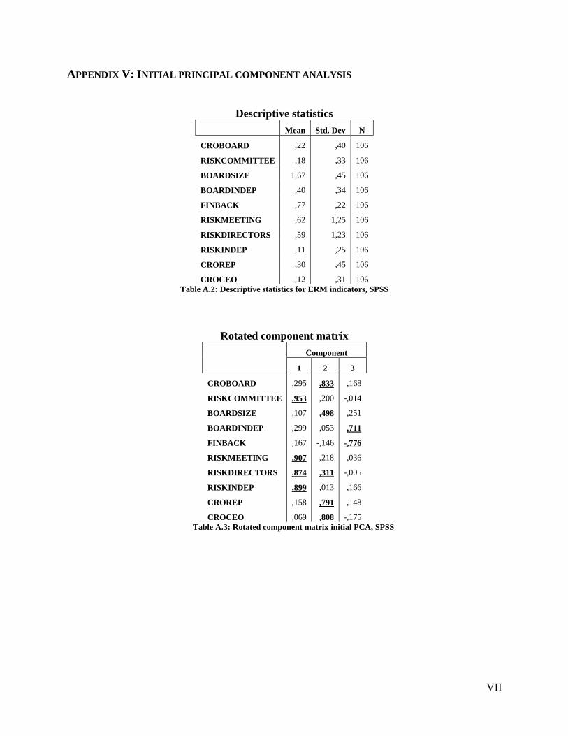
VII
APPENDIX V: INITIAL PRINCIPAL COMPONENT ANALYSIS
Descriptive statistics
Mean Std. Dev N
CROBOARD ,22 ,40 106
RISKCOMMITTEE ,18 ,33 106
BOARDSIZE 1,67 ,45 106
BOARDINDEP ,40 ,34 106
FINBACK ,77 ,22 106
RISKMEETING ,62 1,25 106
RISKDIRECTORS ,59 1,23 106
RISKINDEP ,11 ,25 106
CROREP ,30 ,45 106
CROCEO ,12 ,31 106
Table A.2: Descriptive statistics for ERM indicators, SPSS
Rotated component matrix
Component
1 2 3
CROBOARD ,295 ,833 ,168
RISKCOMMITTEE ,953 ,200 -,014
BOARDSIZE ,107 ,498 ,251
BOARDINDEP ,299 ,053 ,711
FINBACK ,167 -,146 -,776
RISKMEETING ,907 ,218 ,036
RISKDIRECTORS ,874 ,311 -,005
RISKINDEP ,899 ,013 ,166
CROREP ,158 ,791 ,148
CROCEO ,069 ,808 -,175
Table A.3: Rotated component matrix initial PCA, SPSS

VIII
APPENDIX VI: SCREE PLOT
Figure A.3: Scree plot, SPSS

IX
APPENDIX VII: HISTOGRAM BOARDINDEP
Figure A.4: Histogram BOARDINDEP, SPSS

X
APPENDIX VIII: CORRELATION MATRICES C
orr
ela
tion
ma
trix
bef
ore
th
e cri
sis,
n =
34
CR
ED
1
**
. C
orr
elat
ion
is
sig
nif
ican
t at
the
0.0
1 l
evel
(2
-tai
led
).
To
tal
ob
serv
atio
ns
in s
amp
le:
36
. M
easu
rem
ent
per
iod i
s 20
05
-20
06
.
Per
form
ance
is
mea
sure
d b
y r
etu
rn o
n a
sset
s (R
OA
, R
OA
2)
and
ret
urn
on
eq
uit
y (
RO
E).
ER
MR
C i
s in
dic
ated
as
RC
, E
RM
BO
AR
D i
s in
dic
ated
as
BO
AR
D.
Eff
icie
ncy
, le
ver
age,
div
ersi
fica
tio
n, ti
er-1
cap
ital
rat
io a
nd
cre
dit
qu
alit
y a
re m
enti
on
ed a
s E
FF
, L
EV
, D
IV,
TIE
R1 a
nd C
RE
D.
T
ab
le A
.4:
Co
rrel
ati
on
ma
trix
bef
ore
th
e fi
nan
cia
l cr
isis
, S
PS
S
TIE
R1
1
-.0
45
DIV
1
-.1
09
.198
LE
V
1
-.1
50
-.6
79
**
.150
EF
F
1
-.3
28
.503
**
.078
-.0
10
BO
AR
D2
1
-.1
12
.137
-.2
84
-.0
09
-.1
45
RC
2
1
.133
-.1
20
-.2
11
-.2
25
.465
**
-.1
15
BO
AR
D
1
.337
.846
**
-.1
30
.048
-.1
87
.072
.008
RC
1
.325
.987
**
.120
-.1
22
-.2
87
-.2
29
.498
**
-.1
19
RO
E
1
-.1
94
-.0
87
-.1
87
-.1
96
.006
-.0
81
.294
-.1
56
.428
*
RO
A2
1
.737
**
-.0
77
-.0
71
-.0
85
-.1
39
.208
-.4
41
**
.377
*
-.0
25
-.0
60
RO
A 1
.973
**
.755
**
-.0
55
-.0
73
-.0
69
-.1
53
.171
-.4
86
**
.341
*
.045
-.0
62
RO
A
RO
A2
RO
E
RC
BO
AR
D
RC
2
BO
AR
D2
EF
F
LE
V
DIV
TIE
R1
CR
ED

XI
Corr
elati
on
ma
trix
du
rin
g t
he
cris
is, n
= 6
7
CR
ED
1
**
. C
orr
elat
ion
is
sig
nif
ican
t at
the
0.0
1 l
evel
(2
-tai
led
).
To
tal
ob
serv
atio
ns
in s
amp
le:
36
. M
easu
rem
ent
per
iod i
s 20
07
-20
08
.
Per
form
ance
is
mea
sure
d b
y r
etu
rn o
n a
sset
s (R
OA
, R
OA
2)
and
ret
urn
on
eq
uit
y (
RO
E).
ER
MR
C i
s in
dic
ated
as
RC
, E
RM
BO
AR
D i
s in
dic
ated
as
BO
AR
D.
Eff
icie
ncy
, le
ver
age,
div
ersi
fica
tio
n,
tier
-1 c
apit
al r
atio
an
d c
redit
qu
alit
y a
re m
enti
on
ed a
s E
FF
, L
EV
, D
IV,
TIE
R1 a
nd C
RE
D.
T
ab
le A
.5:
Co
rrel
ati
on
ma
trix
du
rin
g t
he
fin
an
cial
cris
is,
SP
SS
TIE
R1
1
-.0
90
DIV
1
-.1
09
.067
LE
V
1
.006
-.6
32
**
.130
EF
F
1
-.2
31
.109
.001
.011
BO
AR
D2
1
-.0
82
.003
.063
-.0
63
-.0
30
RC
2
1
.300
3 *
-.1
10
.111
-.0
66
-.0
94
-.0
90
BO
AR
D
1
-3.0
2 *
.828
**
-.0
88
.060
.185
-.1
64
.127
RC
1
.315
**
.976
**
.294
*
-.1
05
.103
-.0
56
-.0
86
-.1
05
RO
E
1
-.1
21
.017
-.1
31
-.0
95
-.0
91
-.0
29
-.2
99
*
-.1
00
.090
RO
A2
1
.567
**
-.0
75
.009
-.0
95
-.0
68
.080
-.5
96
**
-.0
79
.194
-.0
23
RO
A 1
.792
**
.353
**
-.1
06
-.0
92
-.1
04
-.1
06
.175
-.6
66
**
-.1
00
.228
-.0
56
RO
A
RO
A2
RO
E
RC
BO
AR
D
RC
2
BO
AR
D2
EF
F
LE
V
DIV
TIE
R1
CR
ED

XII
Corr
elati
on
ma
trix
aft
er
the
cris
is, n
= 6
2
CR
ED
1
**
. C
orr
elat
ion
is
sig
nif
ican
t at
the
0.0
1 l
evel
(2
-tai
led
).
To
tal
ob
serv
atio
ns
in s
amp
le:
36
. M
easu
rem
ent
per
iod i
s 20
09
-20
10
.
Per
form
ance
is
mea
sure
d b
y r
etu
rn o
n a
sset
s (R
OA
, R
OA
2)
and
ret
urn
on
eq
uit
y (
RO
E).
ER
MR
C i
s in
dic
ated
as
RC
, E
RM
BO
AR
D i
s in
dic
ated
as
BO
AR
D.
Eff
icie
ncy
, le
ver
age,
div
ersi
fica
tio
n, ti
er-1
cap
ital
rat
io a
nd
cre
dit
qu
alit
y a
re m
enti
on
ed a
s E
FF
, L
EV
, D
IV,
TIE
R1 a
nd C
RE
D.
T
ab
le A
.6:
Co
rrel
ati
on
ma
trix
aft
er t
he
fin
an
cia
l cr
isis
, S
PS
S
TIE
R1
1
-.2
26
DIV
1
-.2
66
*
.218
LE
V
1
-.0
97
-.5
66
**
.093
EF
F
1
-.2
95
*
.623
**
-.0
37
.041
BO
AR
D2
1
-.0
81
.067
-.0
27
-.1
81
.155
RC
2
1
.196
-.2
08
.239
-.3
49
**
.107
-.0
49
BO
AR
D
1
.371
**
.848
**
-.1
79
.194
-.1
15
-.2
49
*
.172
RC
1
.392
**
.980
**
.213
-.2
03
.263
*
-.3
08
*
.080
-.0
56
RO
E
1
.086
.092
.080
.050
-.1
99
-.0
97
-.1
90
.033
.018
RO
A2
1
.845
**
-.0
22
.012
-.0
18
-.0
03
.086
-.3
59
**
-.0
35
.109
-.0
45
RO
A 1
.929
**
.603
**
-.0
51
-.0
25
-.0
46
-.0
38
.263
*
-.3
95
**
.066
.088
-.0
66
RO
A
RO
A2
RO
E
RC
BO
AR
D
RC
2
BO
AR
D2
EF
F
LE
V
DIV
TIE
R1
CR
ED

XIII
APPENDIX IV: NORMAL P-P PLOTS
Figure A.5: Normal P-P plot ROA1, SPSS
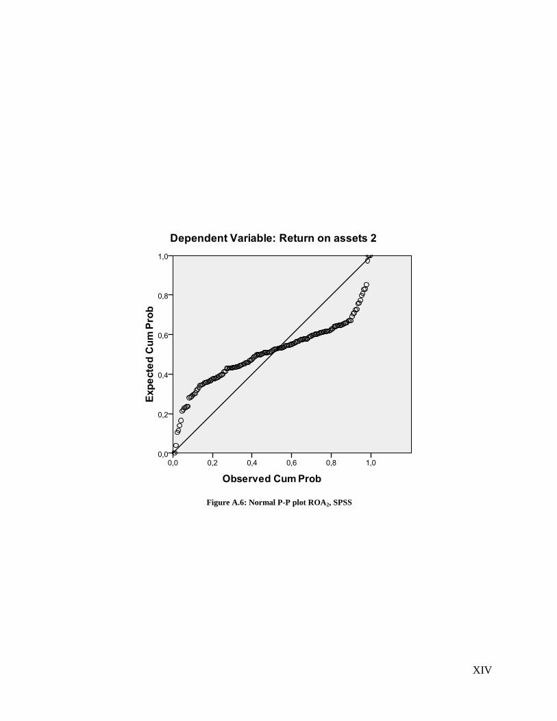
XIV
Figure A.6: Normal P-P plot ROA2, SPSS

XV
Figure A.7: Normal P-P plot ROE, SPSS

XVI
APPENDIX V: NORMAL P-P PLOTS SAMPLE EXCLUDING OUTLIERS
Figure A.8: Normal P-P plot ROA1 excl. outliers, SPSS
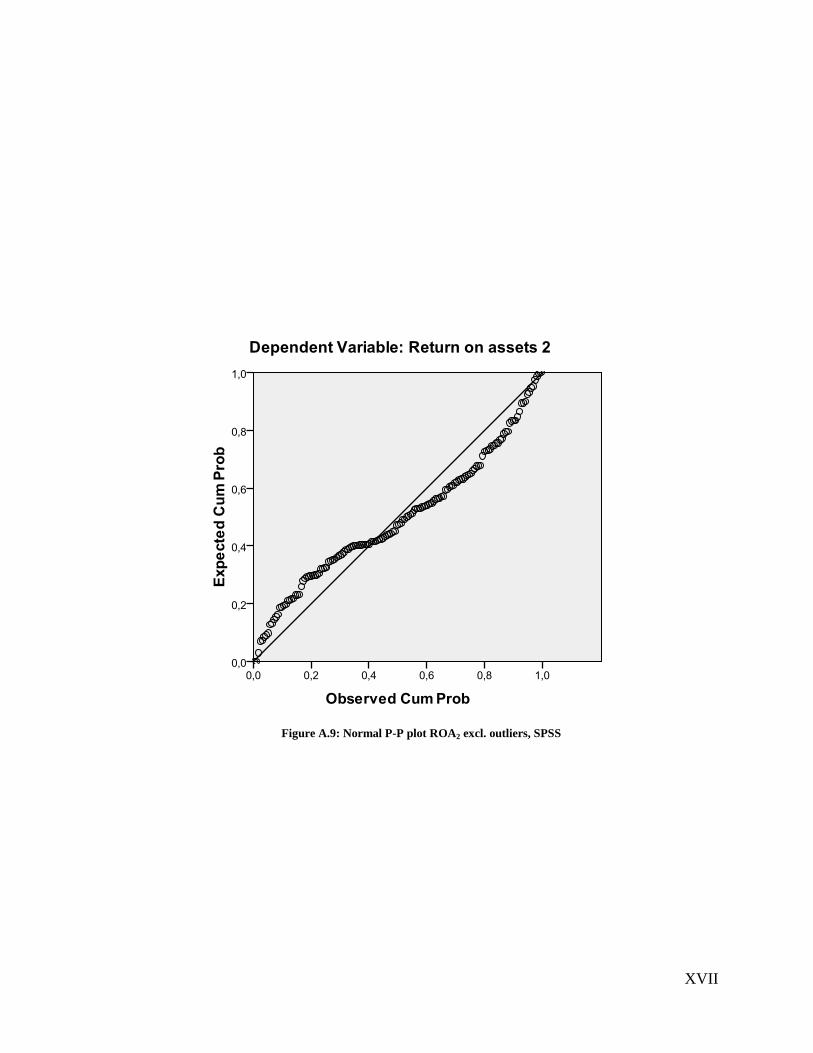
XVII
Figure A.9: Normal P-P plot ROA2 excl. outliers, SPSS

XVIII
Figure A.10: Normal P-P plot ROE excl. outliers, SPSS