master thesis in mathematics /applied...

Institutionen för Matematik och Fysik Code: MdH.IMa.Mat.0061-(2006)10p-AF

MASTER THESIS IN MATHEMATICS /APPLIED MATHEMATICS

Java Applet for the Pricing of Exotic Options by Monte-Carlo Simulations in a Lèvy market with Stochastic Volatility

by

Isaac Acheampong

Magisterarbete i matematik / tillämpad matematik

DEPARTMENT OF MATHEMATICS AND PHYSICS MÄLARDALEN UNIVERSITY

SE-721 23 VÄSTERÅS, SWEDEN

Pricing of Exotic Options by Monte-Carlo Simulations in a Lévy Market with Stochastic Volatility

DEPARTEMENT OF MATHEMATICS AND PHYSICS ___________________________________________________________________________ Master thesis in mathematics / applied mathematics Date: 2006-02-24 Projectname: Java Applet for the Pricing of Exotic Options by Monte-carlo simulations in a Lèvy market with Stochastic Volatility Author: Isaac Acheampong Supervisor: Dr. Anatoliy Malyarenko Examiner: Prof. Dmitrii Silvestrov Comprising: 10 points ___________________________________________________________________________

“We must accept finite disappointment, but we must never lose infinite hope”. --Dr. Martin Luther King Jr

by Isaac Acheampong Mälardalen University

1


Acknowledgement

Lots of thanks to God for his blessing with life. My thanks go to my supervisor Dr. Anatoliy

Malyarenko for his guidance and advise in this thesis, Dr Wim Shoutens for his suggestions

and advice I also thank Dr Henrik Jönsson and all lecturers and professors in the Analytical

Finance programme for their inspiration and patience whiles training me in this interesting

field. Lot of thanks to my wife Pernilla and my family for their support. To all my friends and

colleagues I say thanks.


2


Abstract Most financial models including the famous Black & Scholes model assumes constant

volatility. However in recent times modellers at major financial institutions are modelling

stock prices based on stochastic volatility models. One such way is when stock prices are

assumed to undergo Lévy processes with stochastic volatility.

Based on this, exotic options like the barrier and look back options are priced using Monte-

Carlo simulations. The sampling of the processes is based on time changed technique of the

Lévy processes involved. A Java applet is developed to price this options and to calculate the

standard errors.


3


Executive summary

In the last couple of years, the size of world’s exotic options market has grown considerably.

Today a large diversity of such instruments is accessible to investors and they can be used for

numerous purposes. Numerous factors can provide a clarification for the recent success of

these instruments. One likelihood is their almost boundless flexibility in the sense that they

can be personalized to meet the precise needs of any investor. Hence them being sometimes

referred to as customer-tailored options or special-purpose options.

These options also play an important hedging role and, thus, they meet the hedgers’ needs in

gainful ways. Corporations have left buying some form of general protection to designing

strategies to meet precise exposures to risk at a given point in time. These strategies can be

based on exotic options which are less expensive and much more efficient than standard

instruments. Many exotic options have been priced either numerically or analytically.

The approach we adopt for pricing is based on Monte Carlo simulations and it is

implemented in Java.


4


Table of Content

1.0 Inroduction……………………………………………………………….……….…..6 2.0 Derivatives pricing………..………………………………………………………….….9 2.1 Vanilla Options………………………………………………………………….9 2.2 Exotic Options…………………………………………………………….……10 2.2.1 Barrier and Lookback options………………………………………10 2.2.1.1 Down-Out-Barrier Options…………………………..…...10 2.2.1.2 Down-In-Barrier Options………………………………….10 2.2.1.3 Up-In-Barrier Options……………………………………...11 2.2.1.4 Up-Out-Barrier Options………………………………..11-12 3.0 Lévy Processes……………………………………………………………………….13-14 3.1 Examples of Lévy processes…………………………………………………....15 3.1.1 Normal Inverse Guassian Processes………………………………....15 3.1.2 Variance gamma processes…………………………………….…15-16 4.0 Lévy Stochastic Volatility Modelling………………………………………….…...16-17 5.0 Monte Carlo Simulation Of Stochastic Volatility Lévy Processes…………….....18-20 6.0 The LSVP Jave Applet…………………………………………………………………21 6.1 The Concept……………………………………………………………………..21 6.2 The Structure and Recommendation on How to Run………………………..21 6.3 User manual……………………………………………………………………..22 6.3.1 Start of the Program………………………………………………….22 6.3.2 Overview of LSVP’s User interface………………………………….22 6.3.3 Description of Components………………………………...………...23 6.3.3.1 Graphics panel……………………………………………...23 6.3.3.2 Process Panel………………………………………………..23 6.3.3.3 Simulations Panel…………………………………………...24 6.3.3.4 Action Pane……………………………………………….....25 6.3.3.5 Option Type panel………………………………………25-26 6.3.3.6 Parameter panel…………………………………………….26 6.3.3.7 Output Panel………………………………………………...27 6.2 Some Pricing Results…..................................................................................27-32 7.0 Conclusion……………………………………………………………………………….33 8.0 References………………………………………………………………………….34-35 9.0 Appendix……………………………………………………………………………..36-94 by Isaac Acheampong Mälardalen University

5


Introduction

The revolution of financial instruments pricing was escalated with the introduction of the

famous continuous time Black-Scholes model. It prices stocks or indices with the assumption

that their returns undergo log normal distribution. The price process of the underlying is given

by the geometric Brownian motion

,2

exp2

0 ⎟⎟⎠

⎞⎜⎜⎝

⎛+⎟⎟

⎠

⎞⎜⎜⎝

⎛−= tt WtSS σσμ

where { is a standard Brownian motion .With this formula various options can be

developed, mainly the plain vanilla options and the exotic options , one of particular interest

for this thesis is the pricing of the exotic options(so called path dependent options) of

European nature.

}0, ≥tWt

The plain vanilla products have standard well-defined properties and trade actively. Their

prices or implied volatilities are quoted by exchanges or by brokers on a regular basis. One of

the exciting aspects of over-the-counter derivatives market is the number of non-standard (or

exotic) products that have been created by financial engineers. Even though the usually make

up a very small percentage of a portfolio they are usually much more profitable than the plain

vanilla products. Exotic options are created for a number of reasons. Sometimes they meet a

genuine hedging need in the market; there could be tax, accounting, legal or regulatory

reasons why corporate treasurers find exotic option attractive. They could also be designed

to reflect a corporate treasurers perceptions about the future movement of a market variable.

However because of its flexible nature they can be made to seem more attractive than it is for

an unwary corporate treasurer.

In this paper interest is focused on the so called barrier options and the lookback options to

investigate the pricing procedures. Since there exist traditional pricing procedures a method

by way of the principles of Lévy processes is adopted. It is also investigated into detailed the

idea of stochastic volatility which is incorporated, this is a drawback in the Black-Scholes

model which assumes a constant volatility. Hence for any pricing the value is dependent

heavily on the choice of the constant volatility estimate. The relaxation of these strong

assumption in the Black-Schole world makes modelling much more realistic.

Analytical formulas are available in the BS-world however numerical procedures need

incoporated if the Lévy stochastic volatility modelling is to be used. Path-dependent options


6


are now very popular in the OTC market in these last decades. Examples of exotic type path-

dependent options are lookback options and barrier options. The lookback option gives its

holder the right but not the obligation to buy (call type lookback) or sell (put type look back)

the stock at the minimum or maximum respectively it has attained over the life of the option.

The value of barrier option depends on whether the price of the underlying asset crosses a

given threshold (the barrier) before maturity. The simplest barrier options are “knock in”

options which become alive when the price of the underlying asset touches the barrier and

“knock-out” options which goes out of existence (become dead) in the case. E.g. an up-and-

out call or put has the same payoff as a regular plain vanilla call or put whiles the price of the

underlying assets stays below the barrier during the life of the option but becomes valueless

as soon as the price of the underlying asset crosses the barrier. The Black-Scholes framework

gives a closed-form option pricing formulae for the above types of barrier and lookback

options ([2]). It has been established that the log-returns of most financial assets are

asymmetrically distributed and have an actual kurtosis that is higher than that of the Normal

distribution. The Black-Scholes model is thus a very poor model for describing stock price

dynamics. In real life traders aware that the future probability distribution of an underlying

asset may not always be log normal hence they use a volatility smile adjustment. The

volatility smile-effect is diminishing with time to maturity. To price a set of European vanilla

options, one uses for every strike K and for each maturity T a chosen volatility parameter

which is basically wrong since this implies that only one underlying stock/index is modeled

by a number of utterly different stochastic processes. What is more,one cannot guarantee that

the choice of volatility parameters can be used to price exotic options.

To handle the non-Gaussian nature of the log-returns, in the last two decades

several other models, based on more complicated distributions, were proposed. In these

models the stock price process where considered to be an exponential of a so-called Lèvy

process. As for a Brownian motion, the Lèvy process has stationary and independent

increments; however the distribution of the increments must now belong to the class of

infinitely divisible laws. Choosing this law is crucial in the modeling and it should reflect the

stochastic behavior of the log-returns of the asset.

In [3] (Madan and Seneta) and in [4] (Barndorff-Nielsen) proposed a Lèvy process with

Variance Gamma and Normal Inverse Gaussian (NIG) distributions respectively. These

models are better at calibration of model prices to market prices than the BS-models, even

though this will not be investigated in this paper it is worth mentioning. The models are better


7


fit to historical data as well. Even with a significant improvement in accuracy with respect to

the BS-model by financial modelers, there is still is a discrepancy between model prices and

market prices. In using these Lèvy models one need to note the main feature which these

models are missing, i.e. the fact that the volatility or more general the environment is varying

stochastically over time. Stochastic volatility is a stylized feature of financial time series of

log-returns of asset prices.

To deal with this problem, one begins with the Black-Scholes setting and makes the

volatility parameter itself stochastic. A variety of choices can be made to describe the

stochastic behavior of the volatility. The Cox-Ingersoll-Ross (CIR) square root process was

mentioned and used in this case as proposed in [6].

The focus was on the introduction of the stochastic situation through the stochastic time

change as proposed in [6]. This technique is not necessarily used starting from the BS-model,

but could be used with Lèvy models as well. In these stochastic volatility models the business

time (of the Lèvy process) is made stochastic, i.e. in periods with high volatility time is

running fast, and in periods with low volatility the time is running slow. For this rate of time

process, leads to the choice of the proposal in [6] a classical example of a mean-reverting

positive process: the CIR process. Based on these models and the idea of Monte-Carlo

simulations a Java applet was developed to price barrier and look back options. Finding

explicit formulae for exotic options is very difficult if not impossible in these models.

However, once the model is calibrated to a basic set of options, it is easy to price other

(exotic) options using Monte-Carlo simulations. With the choice of the time-changing process

(ie.in my case CIR) the complexity of the simulation is not made any more difficult than the

Lèvy process.

In section 5.0 I performed a number of simulations to compute option prices for

both the VG and NIG models. I also did simulations to compute the standard error of the

models option prices. It is shown in [1] that the standard error of the simulations can be

reduced if the technique of control variates is used however this was not investigated in this

paper.

Derivatives pricing

All the way through the text I denote the daily interest rate with r and the dividend yield per

year with q unless otherwise stated. Assumption of a fixed forecasting horizon T and a market


8


with a single riskless asset (one bond) with a price process given by { }TteBB rtt ≤≤== 0,

and one risky asset (the stock) with price process { }.0, TtSS t ≤≤= Focus is on the European-

type derivatives, hence no exercise prior to expiration is possible. For the market model, let

represent the payoff of the derivative at its time of expiry T. {( TuSG u ≤≤0, })

]

According to the fundamental theorem of asset pricing [15] the arbitrage free price of

the derivative at time

tP

[ Tt ,0∈ is given by ( ) { }( )[ ],0, tutTrQ

t fTuSGeEP ≤≤= −− where the

expectation is taken with respect to an equivalent martingale measure Q and

is the natural filtration of the price process { Ttff t ≤≤= 0, } { }.0, TtSS t ≤≤= An

equivalent martingale measure is a probability measure which is equivalent (.i.e. has the same

null-sets) to the given (historical) probability measure and under which the discounted process ( ){ }ttTr Se −− is a martingale. Models with only one equivalent measures are said to be complete

and those with more than one equivalent measures are said to be incomplete.

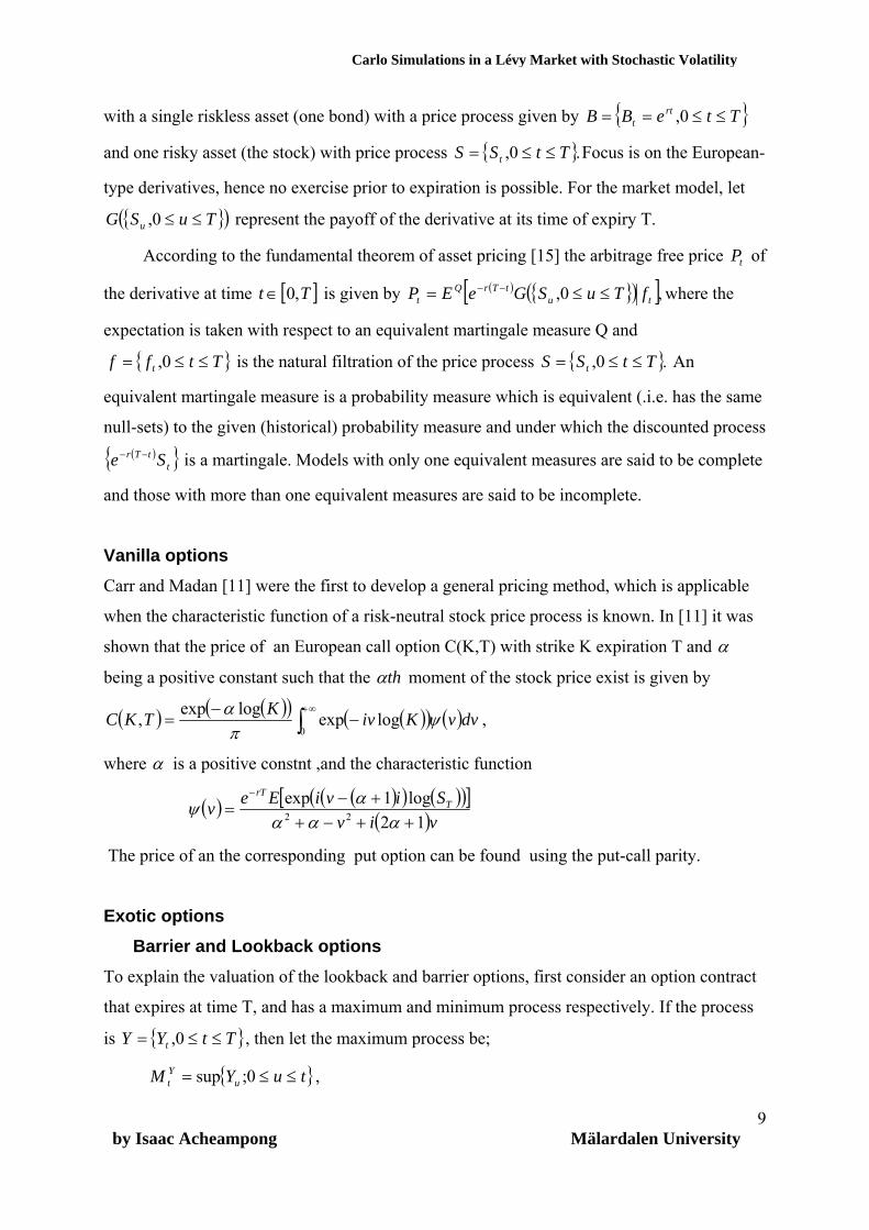
Vanilla options Carr and Madan [11] were the first to develop a general pricing method, which is applicable

when the characteristic function of a risk-neutral stock price process is known. In [11] it was

shown that the price of an European call option C(K,T) with strike K expiration T and α

being a positive constant such that the thα moment of the stock price exist is given by

( ) ( )( ) ( )( ) (∫∞+

−−

=0

logexplogexp, dvvKivKTKC ψπ

)α ,

where α is a positive constnt ,and the characteristic function

( ) ( )( ) ( )( )[ ]( )viv

SiviEev TrT

12log1exp

22 ++−++−

=−

ααααψ

The price of an the corresponding put option can be found using the put-call parity.

Exotic options Barrier and Lookback options To explain the valuation of the lookback and barrier options, first consider an option contract

that expires at time T, and has a maximum and minimum process respectively. If the process

is , then let the maximum process be; { TtYY t ≤≤= 0, }

, { }tuYM uYt ≤≤= 0;sup


9


and the minimum process being { },0;inf tuYm uYt ≤≤= Tt ≤≤0 . Then using the risk-

neutral pricing, the price of a lookback call option is given by

, ⎥⎦

⎤⎢⎣

⎡−= − s

TTQrT mSEeLC

and that of a lookback put option is given by

. ⎥⎦

⎤⎢⎣

⎡−= −

TST

QrT SMEeLP

For barrier options, specifically the single barrier type options, the following are considered.

Down-and-out barrier option:

This type of barrier option is worthless except if its minimum remains above some level H.

Usually this level H is initially set below the initial value of the underlying (stock). If it

remains above the barrier H until maturity then it retains the structure of an European call or

put with strike K.The initial price at t =0 is

( ) ( ) ⎥⎦

⎤⎢⎣

⎡>−= +− HmKSEeDOB S

TTQrT

call 1

and

( ) ( ) ⎥⎦

⎤⎢⎣

⎡>−= +− HmSKEeDOB S

TTQrT

put 1

for a Call and Put ,respectively.

Down-and-in barrier option:

This type of barrier option is worthless except if its minimum went below some level H.

Usually this level H is initially set below the initial value of the underlying asset (stock). If it

remains above the barrier H until maturity then it is worthless. However if its minimum goes

below the barrier H then it retains the structure of an European call or put with initial price i.e.

at t =0, given by;

( ) ( ⎥⎦

⎤⎢⎣

⎡≤−= +− HmKSEeDIB S

TTQrT

call 1 ) for a call contract and


10



11

)

)

)

)

)

( ) ( ⎥⎦

⎤⎢⎣

⎡≤−= +− HmSKEeDIB S

TTQrT

put 1 for a put contract

Up-and-in barrier option:

This type of barrier option is worthless except if its maximum goes above some level H.

Usually this level H is initially set above the initial value of the underlying (stock). If this

barrier is crossed during the life of the contract; it retains the structure of an European call or

put with strike K. The initial price is therefore given by

( ) ( ⎥⎦

⎤⎢⎣

⎡≥−= +− HMKSEeUIB S

TTQrT

call 1 for a call contract and

( ) ( ⎥⎦

⎤⎢⎣

⎡≥−= +− HMSKEeUIB S

TTQrT

put 1 for a put contract.

Up-and-out barrier option

This type of barrier option is worthless except if its maximum remains below some level H.

Usually this level H is initially set above the initial value of the underlying (stock). If this

barrier is never crossed during the life of the contract, then it retains the structure of an

European call or put with strike K. The initial price, t =0, is therefore given by

( ) ( ⎥⎦

⎤⎢⎣

⎡<−= +− HMKSEeUOB S

TTQrT

call 1 for a call contract and

( ) ( ⎥⎦

⎤⎢⎣

⎡<−= +− HMSKEeUOB S

TTQrT

put 1 for a put contract .

It can be easily observed that a vanilla option with strike K can be constructed from either a

combination of a DIB and DOB options with barrier H and strike K.Likewise a combination

of UIB and UOB with same strike K and barrier H will give a corresponding vanilla with

strike K. Letting C and P denote call and Put price respectively, then


( ) ( ) ( ) ( )( ) ⎥⎦

⎤⎢⎣

⎡>+≤−−=+ + HmHmKSErTDOBDIB S

TSTT

Qcallcall 11exp

( ) ( )

);,(

exp

TKC

KSErT TQ

=

⎥⎦⎤

⎢⎣⎡ −−= +

( ) ( ) ( ) ( )( ) ⎥⎦

⎤⎢⎣

⎡>+≤−−=+ + HmHmSKErTDOBDIB S

TSTT

Qputput 11exp

( ) ( )

);,(

exp

TKP

SKErT TQ

=

⎥⎦⎤

⎢⎣⎡ −−= +

For the up and in barrier options the illustration is as follows;

( ) ( ) ( ) ( )( ) ⎥⎦

⎤⎢⎣

⎡<+≥−−=+ + HMHmKSErTUOBUIB S

TSTT

Qcallcall 11exp

( ) ( )

);,(

exp

TKC

KSErT TQ

=

⎥⎦⎤

⎢⎣⎡ −−= +

( ) ( ) ( ) ( )( ) ⎥⎦

⎤⎢⎣

⎡<+≥−−=+ + HMHmSKErTUOBUIB S

TSTT

Qputput 11exp

( ) ( )

);,(

exp

TKP

SKErT TQ

=

⎥⎦⎤

⎢⎣⎡ −−= +

Hence it can be concluded that the price of a plain vanilla option is related with that of a

corresponding barrier option. The price process of the underlying are in practice usually

observed at a close of a trading day to check if a barrier has been crossed, for the above

formulation however, observations are assumed to be on a continuous basis. [7] and [8]

proposes a ways of adjusting the Black-Scholes setting for the case of discrete observations

for a lookback options and barrier options respectively. For barrier H is replaced with

⎟⎠⎞⎜

⎝⎛

mTH σ582.0exp for an up-and-in or up-and-out and ⎟

⎠⎞⎜

⎝⎛− m

TH σ582.0exp for the

DIB and DOB options.where m is the number of observations and mT is the time between


12


observations.In this paper a year is assumed to be 250 days and observations are assumed to

be made at the end of a trading day.

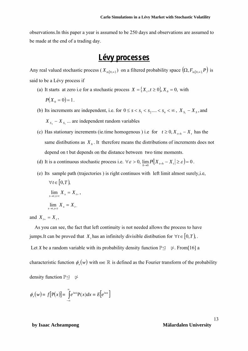
Lévy processes

Any real valued stochastic process ( ) on a filtered probability space [ )∞∈ ,0tX [ )( )PFt ,,0, ∞∈Ω is

said to be a Lévy process if

(a) It starts at zero i.e for a stochastic process { } ,0,0, 0 =≥= XtXX t with

. ( ) 100 ==XP

(b) Its increments are independent, i.e. for ∞<<<<≤ nssss ....0 21 , and

... are independent random variables

,1 SS XX −

12 SS XX −

(c) Has stationary increments (ie.time homogenous ) i.e for as the

same distibutions as . It therefore means the distributions of increments does not

depend on t but depends on the distance between two time moments.

tht XXt −≥ +,0 h

hX

(d) It is a continuous stochastic process i.e. ,0>∀ε ( ) 0lim0

=≥−+→εthth

XXP .

(e) Its sample path (trajectories ) is right continuos with left limit almost surely,i.e,

[ ),,0 Tt ∈∀

, +>→= tststs

XX,

lim

−<→= tststs

XX,

lim

and , tt XX =+

As you can see, the fact that left continuity is not needed allows the process to have

jumps.It can be proved that has an infinitely divisible distibution for tX [ ),,0 Tt ∈∀ .

Let X be a random variable with its probability density function P . From[16] a

characteristic function ( )wxφ with ω∈R is defined as the Fourier transform of the probability

density function P

( ) ( )[ ] [ ]∫∞

∞−

≡Ρ≡Ρ≡ iwxiwxx eEdxxexfw )(φ


13


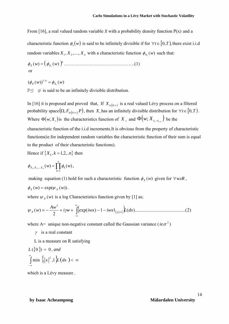
From [16], a real valued random variable X with a probability density function P(x) and a

characteristic function ( )wxφ is said to be infinitely divisible if for [ ),,0 Tt ∈∀ there exist i.i.d

random variables with a characteristic function nXXX ,....,, 21 )(wiXφ such that:

( nXX ww

i )( )( φφ = ) ……………………………………….(1)

or

)())(( /1 wwiX

nX φφ =

P is said to be an infinitely divisible distribution. In [16] it is proposed and proved that, If is a real valued Lévy process on a filtered probability space

[ )∞∈ ,0tX

[ )( )PFt ,,0, ∞∈Ω , then has an infinitely divisible distribution for . tX [ )Tt ,0∈∀

Where is the characteristics function of and ( tXw;Φ ) tX ( )1

;−−Φ

ii ttXw be the

characteristic function of the i.i.d increments.It is obvious from the property of characteristic

functions(ie.for independent random variables the characteristic function of their sum is equal

to the product of their characteristic functions).

Hence if then { }nkX k ,..2,1, =

∏=

=n

kkXXX ww

n1

,..., )()(21

φφ ,

making equation (1) hold for such a characteristic function )(wXφ given for Rwε∀ ,

))(exp()( ww XX ψφ = .

where )(wXψ is a log Characteristics function given by [1] as;

{ }{ } )2...(..............................).........(11)exp(2

)( 1

2

dxLiwxiwxwiAww xX ∫∞

∞−≤−−++−= γψ

where A= unique non-negative constant called the Gaussian variance ( ) 2.σie

γ is a real constant

L is a measure on R satisfying

{ }

{ } ( ) ∞<

=

∫∞

∞−

dxLx

andL

1,.min

,0)0(

2

which is a Lévy measure .


14


From (2), it can be seen that Lévy processes consist of three parts: linear deterministic

parts(drift) i.e (iγ w),brownian part (.ie. 2

2Aw− ) and the pure jump part. This triplets are

written as (γ ,A,L(dx)).The Lévy measure dictates how the jumps occur. For A=0,

{ } ∞<∫∞

∞−

Ldxx 1,2 , then from the theory of standard Lévy processes, the process has finite

variation. However for A=0, { } ∞=∫∞

∞−

Ldxx 1,2 , and the process has infinite variation.

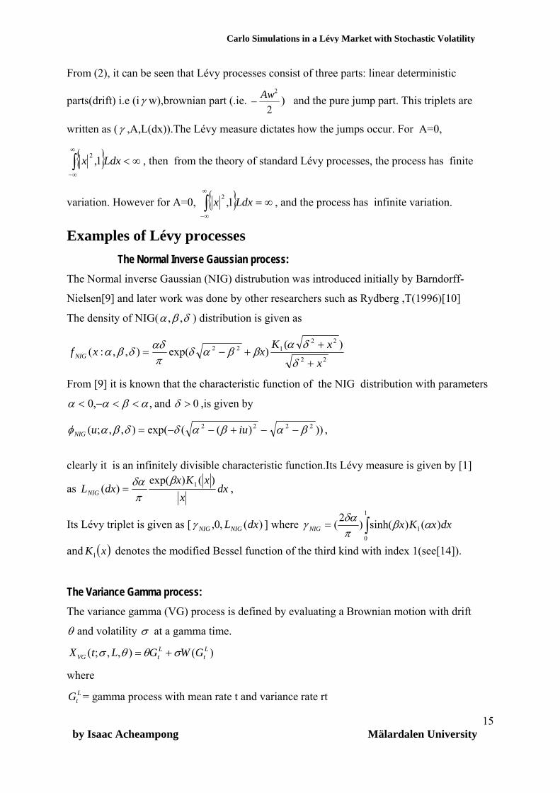
Examples of Lévy processes The Normal Inverse Gaussian process: The Normal inverse Gaussian (NIG) distrubution was introduced initially by Barndorff-

Nielsen[9] and later work was done by other researchers such as Rydberg ,T(1996)[10]

The density of NIG( δβα ,, ) distribution is given as

22

22122 )()exp(),,:(

x

xKxxf NIG+

++−=

δ

δαββαδ

παδδβα

From [9] it is known that the characteristic function of the NIG distribution with parameters

,,0 αβαα <<−< and 0>δ ,is given by

)))((exp(),,;( 2222 βαβαδδβαφ −−+−−= iuuNIG ,

clearly it is an infinitely divisible characteristic function.Its Lévy measure is given by [1]

as dxx

xKxdxLNIG

)()exp()( 1β

πδα

= ,

Its Lévy triplet is given as [ )(,0, dxLNIGNIGγ ] where ∫=1

01 )()sinh()2( dxxKxNIG αβ

πδαγ

and denotes the modified Bessel function of the third kind with index 1(see[14]). ( )xK1

The Variance Gamma process: The variance gamma (VG) process is defined by evaluating a Brownian motion with drift

θ and volatility σ at a gamma time.

)(),,;( Lt

LtVG GWGLtX σθθσ +=

where LtG = gamma process with mean rate t and variance rate rt


15


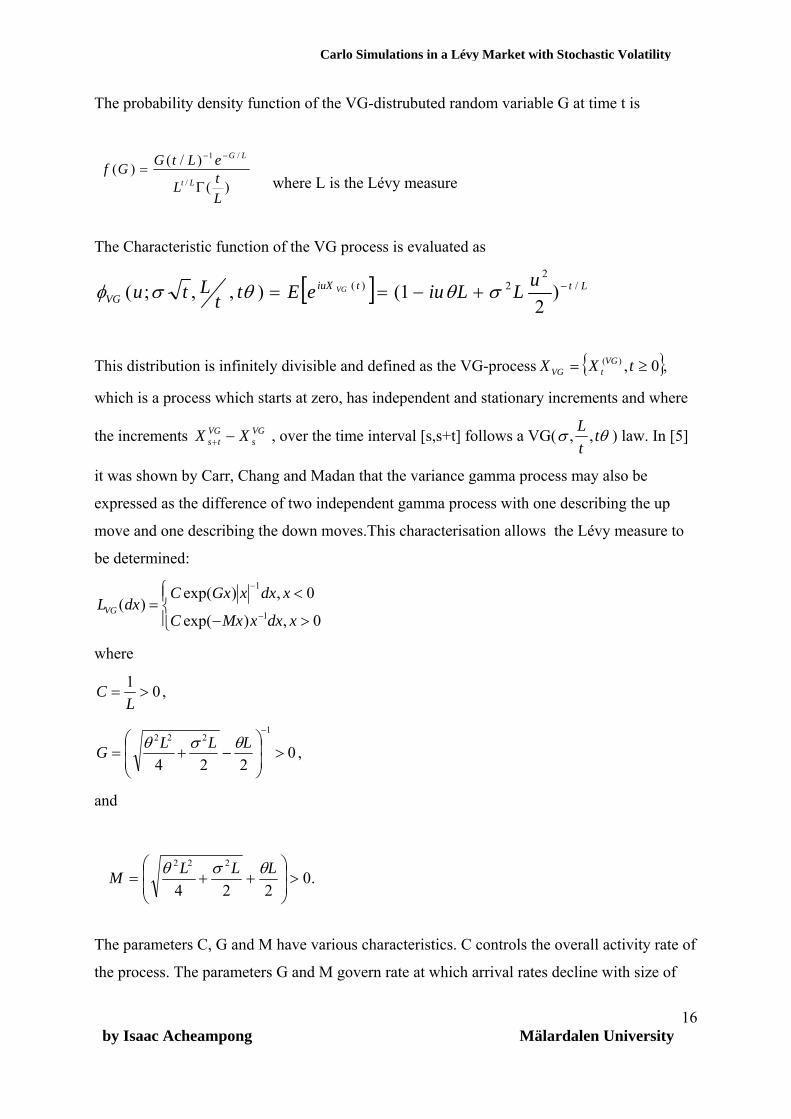
The probability density function of the VG-distrubuted random variable G at time t is

)(

)/()(/

/1

LtL

eLtGGfLt

LG

Γ=

−−

where L is the Lévy measure

The Characteristic function of the VG process is evaluated as

[ ] LttiuXVG

uLLiueEttLtu VG /

22)( )

21(),,;( −+−== σθθσφ

This distribution is infinitely divisible and defined as the VG-process { },0,)( ≥= tXX VGtVG

which is a process which starts at zero, has independent and stationary increments and where

the increments , over the time interval [s,s+t] follows a VG(VGs

VGts XX −+ θσ t

tL ,, ) law. In [5]

it was shown by Carr, Chang and Madan that the variance gamma process may also be

expressed as the difference of two independent gamma process with one describing the up

move and one describing the down moves.This characterisation allows the Lévy measure to

be determined:

⎪⎩

⎪⎨⎧

>−

<=

−

−

0,)exp(

0,)exp()(

1

1

xdxxMxC

xdxxGxCdxLVG

where

01>=

LC ,

0224

1222

>⎟⎟⎠

⎞⎜⎜⎝

⎛−+=

−

LLLG θσθ ,

and

.0224

222

>⎟⎟⎠

⎞⎜⎜⎝

⎛++=

LLLM θσθ

The parameters C, G and M have various characteristics. C controls the overall activity rate of

the process. The parameters G and M govern rate at which arrival rates decline with size of


16


the move. The average of G and M can be regarded as the measure of the size premium.The

difference between G and M is also regarded as directional premium .

Since { } ∞<∫∞

∞−

Ldxx 1,2 , a VG-process has infinetely many jumps in any finite time interval.

The VG-process has no Brownian component and its Lévy triplet is given [ ])(,0, dxLVGγ .

The Lévy-stochastic Volatility Modelling In [4] Carr, Madan, Geman and Yor proposed that one can increase or decrease the level of

uncertainty by speeding up or slowing down the rate at which time passes. They also

suggested that in order to keep time changes going forward one need to employ a mean

reverting positive process as a measure of the local rate of time change. The classical example

of a mean reverting positive process is the square root process of Cox, Ingersoll, and

Ross(CIR). Hence we define y(t) as the solution to the stochastic differential equation

tdWydtykdy λη +−= )( ………………………………(3)

where

tW is a Brownian motion independent of any process,

λ is the volatility of time change(uncertainty of time change),

k is the rate of mean reversion and

η is the long run mean

The process y(t) is the instantaneous rate of time change and so the new clock is given by its

integral ,

∫=t

duuytY0

)()( ……………………………………………………(4)

The (risk neutral ) price process of the stock { }TtSS t ≤≤= 0, is now modelled as follows

[ ] )exp()exp(

))exp((0 t

tt Z

ZEtqrSS −

=

by letting =X(Y(t)) , tZ

and where { TtXX t ≤ }≤= 0, is a Lévy process with [ ] ))(exp()exp( utiuXE xt ψ= .


17


By deduction it can easily be derived that

⎥⎦

⎤⎢⎣

⎡−−+−= )(.)(exp )(0 iYXtqrSS xttYt ψ ,

where for the VG process

⎥⎦

⎤⎢⎣

⎡−−−=− VG

VG

VGx LL

Li θσψ

21log1)(

2

and for the NIG process

NIGNIGNIGNIG

x LLLL

i θσψ 2111)( 2 −−−=−

Monte Carlo simulation of stochastic volatility Lévy processes:

The fundamental principle is to first simulate some number of paths, lets say n paths, of our

stock price process and then calculate for every single path the payoff function , i=1,....n. iV

Then by Monte-Carlo the expected payoff is estimated as the mean of all the payoffs from all

the paths as the sample mean

∑=

=n

iiV

nV

1

1 ................................................................(5)

The present value of the payoff is given by discounting the sample mean(5) with the annual

risk free rate r from expiration time in T years as VrT )exp(− .

The standard error of the estimate is found as:

∑=

−−

n

iiVV

n 1

2)()1(

1

It can be observed that the standard error decreases with the square root of the number of

number of sample paths. Hence one can reduce the standard error by half if four times as

many sample paths are generated.

Now the question is how do we even simulate the stock price process as a Lévy process?


18


First the length of business year is chosen as 250 days.

1. Simulate the rate of time change process using the (3) , the discretize version of the CIR(3)

is as follows;

{ }Ttyy t ≤≤= 0,

( ) tttt Wytyky Δ+Δ−=Δ λη

2. From 1 above the time change { }TtYY t ≤≤= 0, is calculated, where , Y is the

stochastic business time.

00 =Y

3. The Lévy process { }TtY YYYXXt

≤≤= 0, is then simulated. This is done over the

period [ ]. TY,0

4. Then the time changed Lévy process , for tYX [ ]Tt ,0∈ is calculated.

5. Calculate the stock price process { }TtSS t ≤≤= 0, .

6. Calculate a significant number n of paths for the stock price { }TtSS it

i ≤≤= 0, and for

each path i the payoff g: i.e. { }( )TtSGg iti ≤≤= 0, ,where { }( )TtSG i

t ≤≤0, is the payoff

function for an European exotic option expiring at time T.

7. Calculate the estimation of the expected payoff by

⎟⎠

⎞⎜⎝

⎛= ∑

=

n

iig

ng

1

1

8. Then finally calculate the price today,

grTprice )exp(−=

In simulating a variance Gamma process on our fixed time grid, the following algorithm was

used from [12].

Firstly we generate Gamma variables using the algorithms below:

Let

vYYa tt 1−−

= , ⎟⎠⎞

⎜⎝⎛ +=

GMC 11θ ,

GMC2

=σ

Then generate i.i.d uniform [0,1] random variables U,V.

Then set )1/(1/1 , aa VyUx −==

Until 1≤+ yx


19


Secondly generate an exponential random variable E

Return G =yx

xE+

Now we simulate the variance Gamma process on a fixed time grid with parameter

vYY

a tt 1−−=

Set for all i ii GvG Δ=Δ

Then simulate n i.i.d. N(0,1) random variables .,....1 nNN

Set iiit GGNX Δ+Δ=Δ θσ for all i,

The discretized trajectory is ∑=

Δ=i

ttY XX

t1

In simulating a Normal inverse Gaussian process on our fixed time grid, the following

alorithm was used from [12];

First generate an inverse Gaussian variable.

Generate a normal random variable N,

Set , and 2NY = 222

422

YYYx μμλλμ

λμμ +−+=

Generate a uniform [0,1] random variable U. If μ

μ+

≤x

U ,

Return x, else return x

2μ .

Now we simulate the normal inverse Gaussian process on our fixed time grid with parameter

( )vYY tt

i

21−−

=λ and 1−−= tti YYμ .

Then simulate n i.i.d N(0,1) random variables nNNN ..., 21

Set iiii xxNX Δ+Δ=Δ θσ for all i

The discretised trajectory is ∑=

Δ=i

kiY XX

t1

5.0 The LSVP Java Applet : This Java aplet is called LSVP that is Lèvy Stochastic Volatility Pricing.


20


The Concept The naming was made from the fact that the software price barrier and lookback options

under Lèvy process with stochastic volatility. This concept is combined with the notion of

Monte-Carlo simulation to arrive at this. The idea was to realise this in Java and to make it

applicable as much as possible and user friendly.

Users Manual: Start of the program: The following user graphical interface appears when the applet is started.

Figure. 1. Overview of LSVP’s user interface The applet was designed using Java to price Lookback and barrier options. It has the

capabilities to evaluate all the standard errors for any chosen number of simulations. It consist

mainly of four sections ; The two blank parts which is for graphical illustration of price


21


changes with increase in number of simulation the other blank part is for a plot of standard

deviation with number of simulations.

The right part of the applet is for input of parameters for VG and NIG processes

generation. At the bottom of this part is the choice for input of the number of simulations and

the choice of intervals for plotting.There are also choices of check boxes for every exotic

type option considered,i.e DIB,DOB,UIB,UOB and LB which are down-in- barrier ,down-

out-barrier,up-in-barrier ,up-out-barrier and lookback options respectively.The GUI is

interactive in such a way as to make it highly user friendly. Then there is the bottom part of

the GUI which basically gives the input parameters needed for valuation of the option. The

barrier must be chosen appropriately depending on the choice of exotic option under

consideration

Description of components This description does not necessarilly correspond to the panel names used in writing the

source codes. These are descriptions for the user on the features on the graphical user

interface.

Graphics panel The figure below is the graphics panel which is where the graph of standard error of the prices

are plotted with a corresponding number of simulations (i.e. the left part).The right part of it is

where option prices are plotted against the corresponding number of simulations.


22


Figure. 2. process panel: That is where the normal inverse Gaussian and the variance gamma parameters are input .

Figure. 3. The Variance gamma and the NI-gaussian radiobuttons belong to one radio buttons group

i.e. when one is clicked the other is subsequently unclicked. When the variance gamma button

is clicked as is in Figure 3 the text fields for the parameters C,G,M,kappa,eta and lambda are

enabled.This textfields are however enabled by default. If the NI-Gaussian radio button is

chosen then alpha,beta,gamma,kappa,eta and lambda text fields for input of the parameters for

Normal inverse gaussian are enabled .


23


The parameters C,G and M should be non-zero positive numbers. Eta ,kappa and lambda are

the CIR parameters for both NI-Gaussian and variance gamma which are use for in the Lèvy

stochastic volatility modelling as described in the previous sections. In the case of the NI-

Gaussian the alpha should be non-zero positive number,beta should be in the range of

plus and minus alpha then the gamma which is a non-zero positive number.

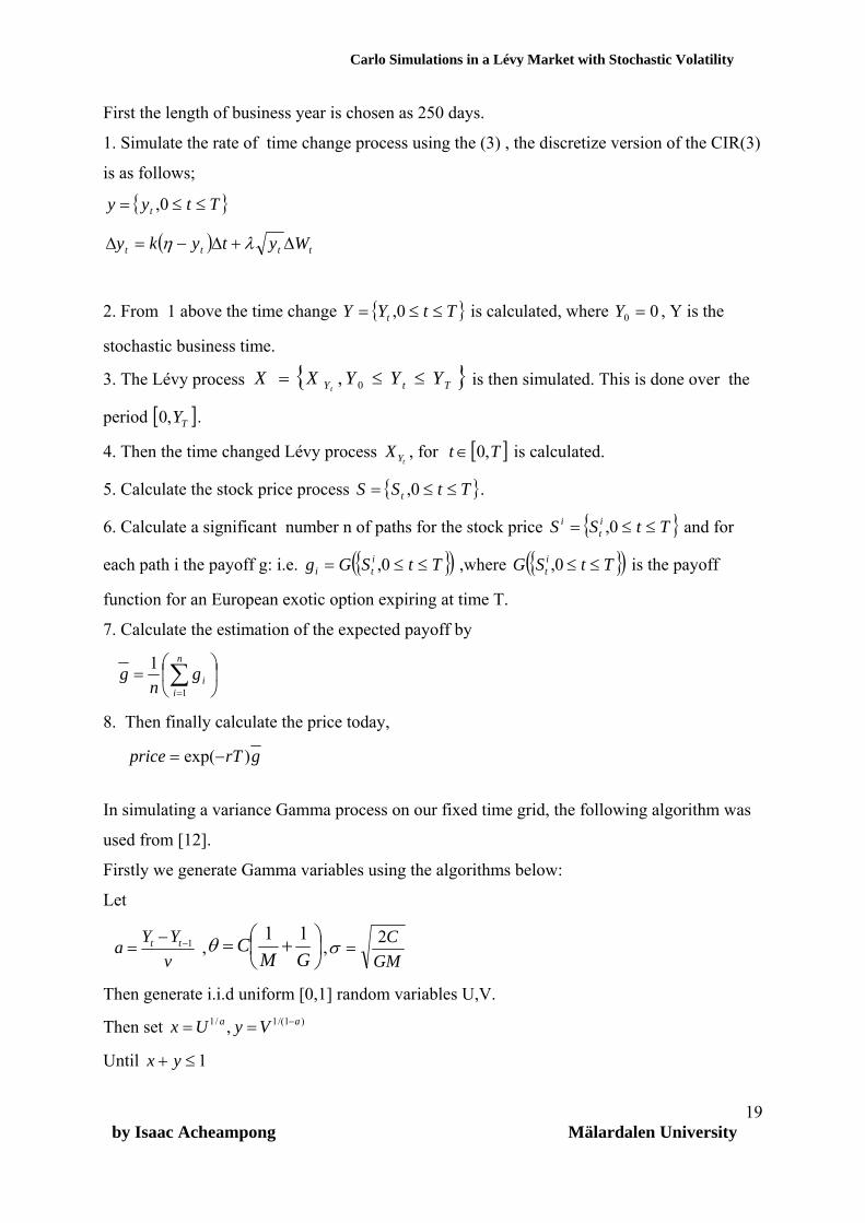
Simulations panel This panel has two text fields ; the number of simulations ,which corresponds to the

simulations for calculating the prices and the ”interval plot for simulations”which shows the

number of intervals of simulations the user wants prices to be calculated and plotted . If the

calculate radio button is clicked then the text field correspnding to the ”number of

simulations” is enabled whiles that of ”intervals plots for simulations” is not enabled likewise

the vice versa when the graphics illustration button is clicked.

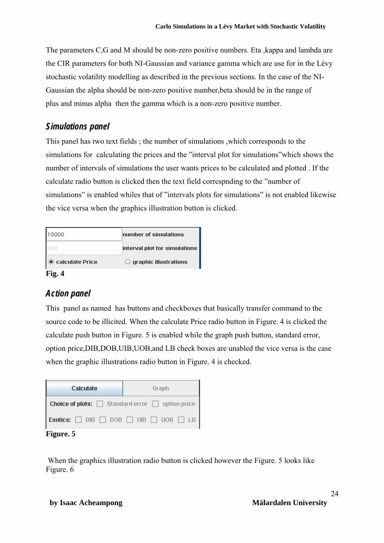
Fig. 4 Action panel This panel as named has buttons and checkboxes that basically transfer command to the

source code to be illicited. When the calculate Price radio button in Figure. 4 is clicked the

calculate push button in Figure. 5 is enabled while the graph push button, standard error,

option price,DIB,DOB,UIB,UOB,and LB check boxes are unabled the vice versa is the case

when the graphic illustrations radio button in Figure. 4 is checked.

Figure. 5 When the graphics illustration radio button is clicked however the Figure. 5 looks like Figure. 6


24


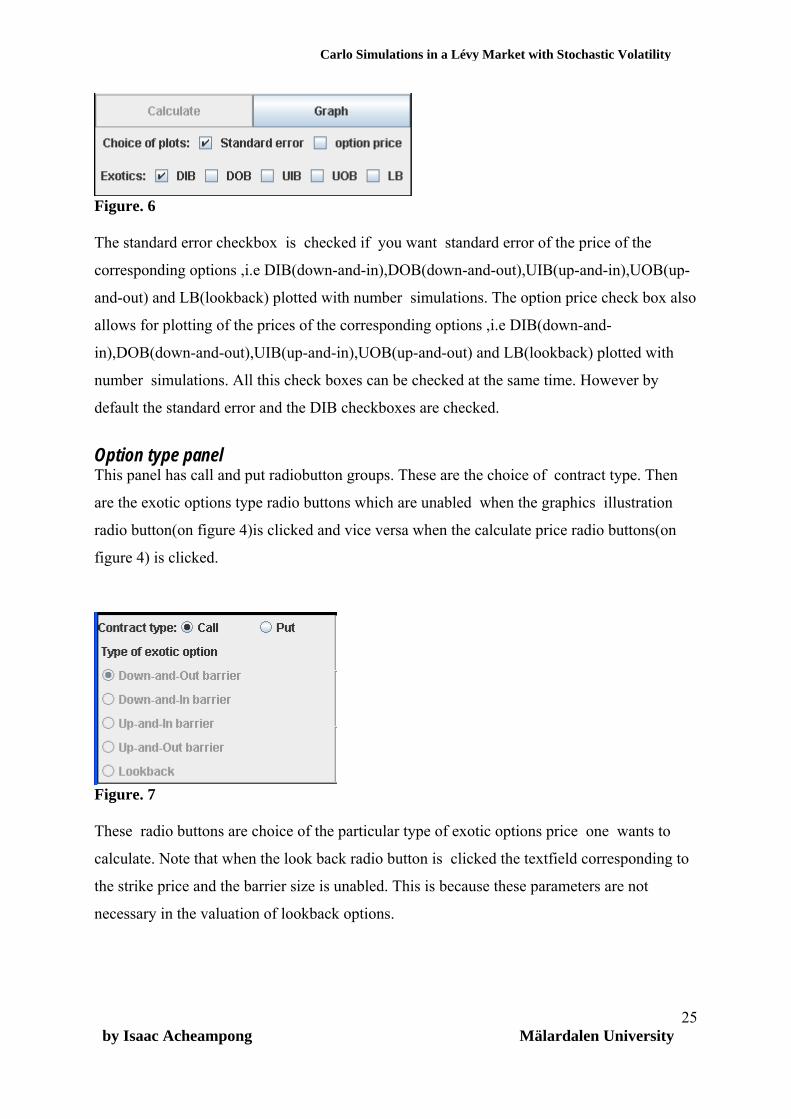
Figure. 6 The standard error checkbox is checked if you want standard error of the price of the

corresponding options ,i.e DIB(down-and-in),DOB(down-and-out),UIB(up-and-in),UOB(up-

and-out) and LB(lookback) plotted with number simulations. The option price check box also

allows for plotting of the prices of the corresponding options ,i.e DIB(down-and-

in),DOB(down-and-out),UIB(up-and-in),UOB(up-and-out) and LB(lookback) plotted with

number simulations. All this check boxes can be checked at the same time. However by

default the standard error and the DIB checkboxes are checked.

Option type panel This panel has call and put radiobutton groups. These are the choice of contract type. Then

are the exotic options type radio buttons which are unabled when the graphics illustration

radio button(on figure 4)is clicked and vice versa when the calculate price radio buttons(on

figure 4) is clicked.

Figure. 7 These radio buttons are choice of the particular type of exotic options price one wants to

calculate. Note that when the look back radio button is clicked the textfield corresponding to

the strike price and the barrier size is unabled. This is because these parameters are not

necessary in the valuation of lookback options.


25


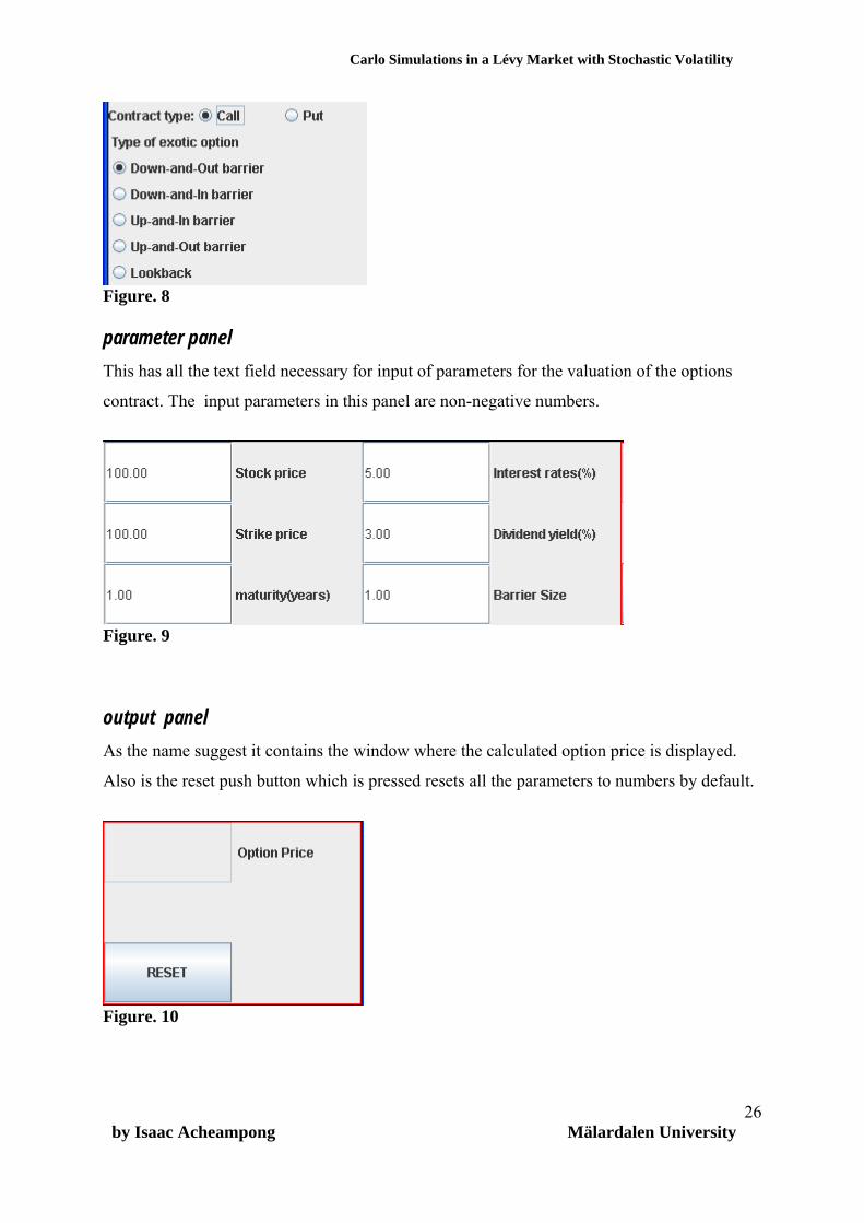
Figure. 8 parameter panel This has all the text field necessary for input of parameters for the valuation of the options

contract. The input parameters in this panel are non-negative numbers.

Figure. 9 output panel As the name suggest it contains the window where the calculated option price is displayed.

Also is the reset push button which is pressed resets all the parameters to numbers by default.

Figure. 10


26


Some pricing results For the parameters in table 1 for both the normal inverse gaussian and the variance gamma

the applet gave the corresponding results in table 2; The parameters are chosen acording to[1]

and used to calculate the prices as inddicated below.

Table 1. Parameter estimates for Lévy SV models

VG-CIR

C

=11.9896

G

=25.8523

M

=35.5344

Kappa

=0.6020

Eta

=1.5560

Lambda

=1.9992

NIG-CIR

Alpha

=18.4815

Beta

=-4.8412

Gamma

=0.4685

Kappa

=0.5391

Eta

=1.5746

Lambda

1.8772

And the initial time %,5),250(1,100,100,0 00 ===== rdaysyearTSKy and the dividend

yield . %3=q

In calculating the barrier options the strike K= (initial stock price),time to maturity

T=1(250days) and the barrier H as

0S

,*1.1 0SHUIB = ,*3.1 0SHUOB = ,*95.0 0SH DIB ==

. 0*8.0 SH DOB =

n=10000 simulations of paths covering a one year period for all the options. The time is

discretised in 250 equally small time steps for the one year period.

The values in table 2 are option prices whiles those in brackets are the standard errors.

Table 2. Exotic Option prices for Call contract Model DIB DOB UIB UOB LB VG-CIR

0.036667

(0.080530)

7.655239

(0.145755)

5.708092

(0.130512)

5.558471

(0.087452)

7.488693

(0.119967)

NIG-CIR

0.014966

(0.080798)

7.685273

(0.120522)

4.682093

(0.118225)

5.919467

(0.094543)

7.533582

(0.117828)


27


Table 3. Exotic Option prices for Put contract Model DIB DOB UIB UOB LB VG-CIR

3.051537

(0.075803)

4.290505

(0.080138)

0.003938

(0.032185)

5.728151

(0.108042)

5.737173

(0.089964)

NIG-CIR

3.639459

(0.081047)

4.09589

(0.073529)

0.000865

(0.000909)

5.93288

(0.112388)

5.739952

(0.0913711)

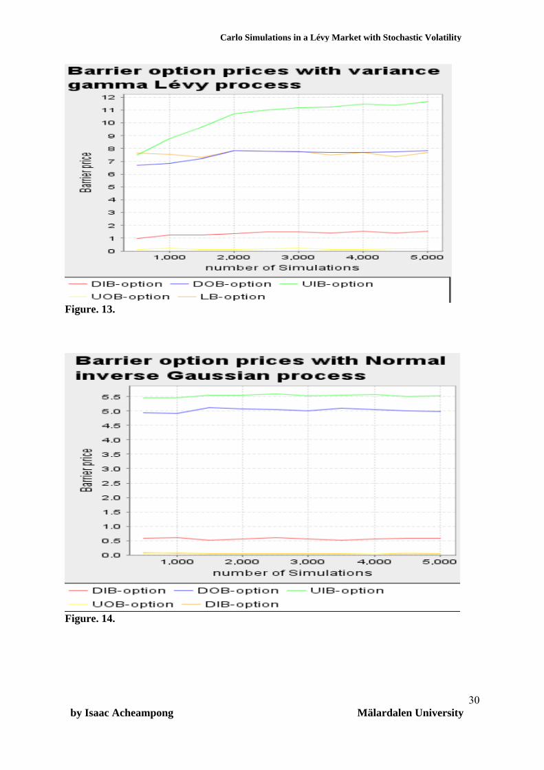
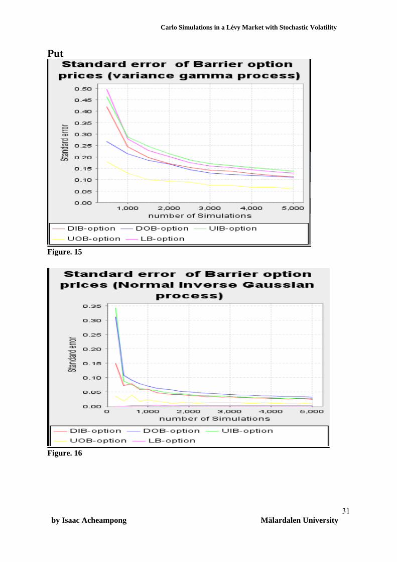
Very nice observations can be seen from the graphical results which shows the effect of

simulations on the prices and standard errors. The maximum simulations chosen was 5000

with 500 simulations as intervals for the plots. From Figure 11 ,Figure 12 ,Figure 15 and

Figure 16 it can observed that the standard error decreases with an increase in simulations.

Likewise the prices flactuations decrease as the number of simulations increase as can be seen

in Figure 13, Figure 14,Figure 17 and Figure 18. The option prices are much more stable as

the number of simulations increase, hence the larger the simulations at which the prices are

being calculated the more exact the results.


28


Call

Figure. 11.

Figure. 12.


29


Figure. 13.

Figure. 14.


30


Put

Figure. 15

Figure. 16


31


Figure. 17

Figure. 18 by Isaac Acheampong Mälardalen University

32


Conclusion: From the tables above it is easy to see that this procedure for pricing gives consistent prices

with reasonable standard errors. The choice of volatility parameters is not a problem as the

model assumes stochastic volatility. These gives it advantage over the Black-Scholes as

shown in [1],and other models which demands choice of volatility parameters which poses a

problem of what choice is most appropraite. In [1] one can easily see that prices under the

Black-Scholes depend heavily on the choice of the volatility parameter making Lèvy-SV

models most better for pricing exotic options.In real life we know volatility is stochastic

hence the idea of making volatility stochastic fits real life scenarios and there is evidence that

the Lévy-SV models are much more reliable;they give much better indication than the BS-

model.

“We are what we repeatedly do. Excellence, then, is not an act but a habit”. --Aristotle


33


REFERENCES [1] Wim Schoutens and Stijn Symens(2002), The pricing of Options by Monte Carlo

simulations in a Lèvy Market with Stochastic Volatility.International journal for

theoretical and Applied Finance,6(8),839-864.

[2] John C. Hull (2003) Options,Futures and Other Derivatives(5th Edition). Prentice Hall.

[3] Madan, D.B. and Seneta, E. (1990) The V.G. model for share market returns.

Journal of Business 63, 511–524.

[4] Barndorff-Nielsen, O.E. (1995) Normal inverse Gaussian distributions and

the modeling of stock returns. Research Report No. 300, Department of

Theoretical Statistics, Aarhus University.

[5] Asmussen, S. and Rosinski, J. (2001) Approximations of small jumps of

Lèvy processes with a view towards simulation. J. Appl. Probab. 38 (2),

482–493.

[6] Carr, P., Geman, H., Madan, D.H. and Yor, M. (2001) Stochastic Volatil-

ity for Lévy Processes. Prépublications du Laboratoire de Probabilités et

Modèles Aléatoires 645, Universités de Paris 6& Paris 7, Paris.

[7] Broadie, M., Glasserman, P. and and Kou, S.G. (1999) Connecting discrete

and continuous path-dependent options. Finance and Stochastics 3, 55–82.

[8] Broadie, M., Glasserman, P. and and Kou, S.G. (1997) A continuity correction

for discrete barrier options. Math. Finance 7 (4), 325–349.

[9] Barndorff-Nielsen, O.E. and Shephard, N. (2000) Modelling by Lévy

Processes for Financial Econometrics. In: O.E. Barndorff-Nielsen, T.

Mikosch and S. Resnick (Eds.): Lévy Processes - Theory and Applications,

Birkhäuser, Boston, 283–318.


34


[10] Rydberg, T. (1996) The Normal Inverse Gaussian L´evy Process: Simu-

lations and Approximation. Research Report 344, Dept. Theor. Statistics,

Aarhus University.

[11] Carr, P. and Madan, D. (1998) Option Valuation using the Fast FourierTransform.

Journal of Computational Finance 2, 61–73.

[12] Cont Rama and Tankov Peter (2000), Financial Modelling With Jump Processes,

Chapman & Hall/CRC Financial Mathematics Series.

[13] Madan D. and Yor M. (2005) CGMY and Meixner Subordinators are Absolutely

continuous with respect to One Sided Stable Subordinators

[14] Abramowitz, M. and Stegun, I.A. (1968) Handbook of Mathematical Functions.Dover Publ., New York. [15] Delbaen, F. and Schachermayer, W. (1994) A general version of the fundamental theorem of asset pricing. Math. Ann. 300, 463–520. [16] Sato, K., 1999, Lévy process and Infinitely Divisible Distributions, Cambridge University Press.


35


APPENDIX /** * @(#) LSVP.java 1.0 05/12/01 * * Copyright (c) 2005 Mälardalen University * Högskoleplan Box 883, 721 23 Västerås, Sweden. * All Rights Reserved. * * The copyright to the computer program(s) herein * is the property of Isaac Acheampong. * The program(s) may be used and/or copied only with * the written permission of Isaac Acheampong * or in accordance with the terms and conditions * stipulated in the agreement/contract under which * the program(s) have been supplied. * Description: Java Applet for pricing of Barrier and Lookback Oprions * using Monte-Carlo Simulations * @version 1.0 1 Dec 2005 * @author Isaac Acheampong * Mail: [email protected] */ import java.awt.*;

import java.awt.event.*;

import javax.swing.*;

import java.text.*;

import java.util.*;

import java.lang.*;

import org.jfree.chart.*;

import org.jfree.chart.axis.*;

import org.jfree.chart.plot.*;

import org.jfree.chart.renderer.category.*;

import org.jfree.data.category.*;

import org.jfree.ui.*;

import org.jfree.data.time.*;

import org.jfree.data.xy.*;

public class LSVP extends JApplet implements //ItemListener,

ActionListener {

private DecimalFormat numberFormatter=new DecimalFormat("###.######");

private Container contentPane =null;

// Panels

private JPanel titlePanel = null;

private JPanel converterPanel = null;


36


private JPanel variance_gammaPanel=null;

private JPanel nigPanel=null;

private JPanel vg_miniPanel=null;

private JPanel nig_miniPanel=null;

private JPanel process_Panel=null;

private JPanel process_miniPanel=null;

private JPanel process_1Panel=null;

private JPanel process_2Panel=null;

private JPanel barrier_inputPanel=null;

private JPanel barriermini_Panel=null;

private ChartPanel graphics1_Panel=null;

private ChartPanel graphics2_Panel=null;

private JPanel center_Panel=null;

private JPanel process_lilminiPanel=null;

// Group Buttons

private ButtonGroup processTypeGroup = null;

private ButtonGroup barrierTypesGroup= null;

private ButtonGroup callPutTypeGroup=null;

private ButtonGroup numberofpricesGroup =null;

private ButtonGroup graph_choiceGroup = null;

// Radio buttons

private JRadioButton[] processTypeButtons = null;

private JRadioButton[] barrierTypesButtons=null;

private JRadioButton[] callPutTypeButtons=null;

private JRadioButton[] numberofpricesButtons=null;

private JRadioButton[] graph_choiceButtons = null;

// Strings

private final String EMPTY = " ";

private final String CALCULATE = "Calculate";

private final String NOT_A_NUMBER = "Enter a number";

private final String NON_POSITIVE = "Enter a positive number";

private final String NON_ZERO_POSITIVE = "Enter non-zero positive number";

private final String SAMEOFINPUT_OUTPUT = "The input and output argument are

same";

private final String NOT_INRANGE ="-3.1416(pi)< beta < 3.1416(pi)";

private final String HEADER = " LÉVY STOCHASTIC VOLATILITY PRICING (LSVP) ";

private final String VARIANCE_GAMMA = "VARIANCE GAMMA ";

private final String NIG = "NORMAL INVERSE GAUSSIAN PROCESS";

private final String[] PROCESS_LABEL = {"Variance gamma ","NI-Gaussian" };

private final String[] GRAPH_CHOICELABEL = {"standard error","option prices " };

private final String[] BARRIER_TYPE=


37


{"Down-and-Out barrier","Down-and-In barrier","Up-and-In barrier","Up-and-Out

barrier","Lookback"};

private final String[] NUMBER_OF_PRICEBUTTON={"calculate Price ","graphic

illustrations"};

private final String PARAMETER_C = " C ";

private final String PARAMETER_G = " G ";

private final String PARAMETER_M = " M ";

private final String PARAMETER_KAPPA = " kappa ";

private final String PARAMETER_ETA = " eta ";

private final String PARAMETER_LAMBDA = " lambda ";

private final String PARAMETER_ALPHA = " alpha ";

private final String PARAMETER_BETA = " beta ";

private final String PARAMETER_GAMMA = " gamma ";

private final String PARAMETER_NUMBEROF_STEPS ="time Steps ";

private final String PARAMETER_ALPHACV = "alpha ";

private final String PARAMETER_K = " k ";

private final String NUMBER_OFSIMULATIONS_1 = "number of simulations";

private final String INTERVAL= "interval plot for simulations";

private final String STRIKE_PRICE = " Strike price ";

private final String STOCK_PRICE = " Stock price ";

private final String INTERESTRATE = " Interest rates(%) ";

private final String DIVIDEND = " Dividend yield(%) ";

private final String TIME_TO_MATURITY = " maturity(years) ";

private final String BARRIER_SIZE = " Barrier Size ";

private final String TYPE_OF_EXOTIC_OPTION = " Type of exotic option ";

private final String GRAPH = " Graph ";

private final String BARRIER_OPTIONPRICE=" Option Price";

private final String VG_C_ERROR=" INERSE OF LÉVY MEASURE";

private final String VG_G_ERROR="VARIANCE GAMMA G-Parameter";

private final String VG_M_ERROR="VARIANCE GAMMA M Parameter";

private final String VG_KAPPA_ERROR="VARIANCE GAMMA KAPPA Parameter";

private final String VG_ETA_ERROR="VARIANCE GAMMA ETA Parameter";

private final String VG_LAMBDA_ERROR="VARIANCE GAMMA LAMBDA Parameter";

private final String NIG_ALPHA_ERROR="Normal inverse gaussian alpha Parameter";

private final String NIG_BETA_ERROR="Normal inverse gaussian BETA Parameter";

private final String NIG_GAMMA_ERROR="Normal inverse gaussian GAMMA Parameter";

private final String NIG_KAPPA_ERROR="Normal inverse gaussian KAPPA Parameter";

private final String NIG_ETA_ERROR="Normal inverse gaussian ETA Parameter";

private final String NIG_LAMBDA_ERROR="Normal inverse gaussian LAMBDA

Parameter";

private final String SIMULATIONS_ERROR="NUMBER OF SIMULATIONS";

private final String RESET=" RESET ";

private final String NUMBER_LESS_THANMINIMUM =" Number should be Greater than

minimum";


38


private final String NUMBER_MORE_THANMAXIMUM =" Number should be Less than

maximum";

private final String STANDARD_ERROR="Standard error";

private final String OPTIONPRICE="option price";

private final String DIB="DIB";

private final String DOB="DOB";

private final String UOB="UOB";

private final String UIB="UIB";

private final String LB="LB";

private final String PLOTS="Choice of plots:";

private final String OPTCONSIDERED="Exotics:";

private final String TYPE_OF_OPTION="Contract type:";

private final String[] CALL_PUT ={"Call ","Put "};

// Labels

private JLabel emptyLabel = null;

private JLabel standardErrorLabel=null;

private JLabel optionPriceLabel=null;

private JLabel headerLabel = null;

private JLabel variance_gammaLabel = null;

private JLabel control_variatesLabel = null;

private JLabel graph_choiceLabel = null;

private JLabel optionType_Label =null;

private JLabel nigLabel = null;

private JLabel C_Label = null;

private JLabel G_Label = null;

private JLabel M_Label = null;

private JLabel kappa_Label = null;

private JLabel eta_Label = null;

private JLabel lambda_Label = null;

private JLabel alpha_Label = null;

private JLabel beta_Label = null;

private JLabel gamma_Label = null;

private JLabel numberofsimulationsLabel = null;

private JLabel numberofrunsLabel = null;

private JLabel stockprice_Label = null;

private JLabel interestrate_Label = null;

private JLabel dividentrate_Label = null;

private JLabel maturity_Label = null;

private JLabel strikeprice_Label = null;

private JLabel barriersize_Label = null;

private JLabel barrier_Label = null;

private JLabel outputprice_Label = null;


39 private JLabel numberof_Label=null;


private JLabel dibLabel=null;

private JLabel dobLabel=null;

private JLabel uibLabel=null;

private JLabel uobLabel=null;

private JLabel LbLabel=null;

private JLabel plotsLabel=null;

private JLabel optconsideredLabel=null;

// Text fields

private JTextField vg_1Field = null;






private JTextField variates1Field = null;

private JTextField variates2Field =null;

private JTextField nig_1Field = null;






private JTextField barrier1Field =null;






private JTextField barrierpriceField =null;

private JTextField interestrate_Field = null;

private JTextField dividentrate_Field = null;

private JTextField maturity_Field = null;

private JTextField strikeprice_Field = null;

private JTextField barriersize_Field = null;

// Check box(es)

private JCheckBox standardErrorBox=null;

private JCheckBox optionPriceBox=null;

private JCheckBox dibBox=null;

private JCheckBox dobBox=null;

private JCheckBox uibBox=null;

private JCheckBox uobBox=null;


40 private JCheckBox LbBox=null;


private JCheckBox variance_gammaBox = null;

// Tool tips

private final String RUNS = " number of runs for estimation of b for control

variates";

private final String K = "number of partitions for compound-Poisson

approximations";

private final String ALPHA = "constant for estimation of boundaries";

private final String KAPPA = "Rate of mean reversion ";

private final String ETA ="Long run rate of time change ";

private final String LAMBDA="Volatility of time change";

// Buttons

private JButton calculateButton = null;

private JButton graphButton = null;

private JButton resetButton =null;

// Progress bar

//private JProgressBar progressBar = null;

// ´Numerical variables

public int i=0;

public int j=0;

private final int NUMBER_OF_STEPS =250;

int simulations ;

int interval;

private double[] y = null;

private double[] Y = null;

private double[] X = null;

private double[] Xg = null;

private double[] Stockprice=null;

private double[] ExpX=null;

private double[] M=null;

private double[] payout=null;

private double[] payout1=null;





private double[] payoutS1=null;





41 private double c =11.9896;


private double g =25.8523;

private double m =35.5344;

private double vgkappa=0.6020;

private double vgeta=1.5560;

private double vglambda=1.9992;

private double deltaTime=0.004 ;

private double interestRate=0.05;

private double dividend=0.03;

private double timetoMaturity=1;

private double nigalpha=18.4815;

private double nigbeta=-4.8412;

private double niggamma=0.4685;

private double nigkappa=0.5391;

private double nigeta=1.5746;

private double niglambda=1.8772;

double mean;

double stddev;

double v;

double w;

double theta;

double sigma;

double initialstockprice;

double ExpectationX;

double Min;

double Max;

double barrier;

double strikeprice;

double b1;

double OptionPrice;

double []OptionPrice1;





double Avpayout;

double Avpayout1;

double Avpayout2;

double Avpayout3;

double Avpayout4;

double Avpayout5;

double AvpayoutS1;


42 double AvpayoutS2;


double AvpayoutS3;

double AvpayoutS4;

double C_sum;

double Y_sum;

double PayoutSum;

double PayoutSum1;

double PayoutSum2;

double PayoutSum3;

double PayoutSum4;

double PayoutSum5;

double PayoutSumS1;

double PayoutSumS2;

double PayoutSumS3;

double PayoutSumS4;

double StandardError;

double []StandardError1;





double variance;

double variance1;

double variance2;

double variance3;

double variance4;

double variance5;

// Generate Random numbers

private final static Random random = new Random();

// booleans

private boolean processtypebuttons = false;

private boolean variateschoicebuttons = false;

private boolean variateschoice0buttons = false;

private boolean variateschoice1buttons = false;

private boolean processtype0buttons = false;

private boolean processtype1buttons = false;

private boolean numberofpricesbuttons = false;


43


// Methods

public void init() {

// Get content pane

contentPane = getContentPane();

contentPane.setLayout(new BorderLayout());

//-----------------------TITLE---------------------

// Add title panel

titlePanel = new JPanel();

titlePanel.setBorder(BorderFactory.createLineBorder(

Color.BLACK, 1));

contentPane.add(titlePanel,BorderLayout.NORTH);

// Add title

headerLabel = new JLabel(HEADER);

titlePanel.add(headerLabel);

//---------------Add center_Panel to Left and Right--------------------

// Add center_Panel to Lévy Monte Carlo

center_Panel= new JPanel(new GridLayout(1,3));

center_Panel.setBorder(BorderFactory.createLineBorder(

Color.BLACK, 1));

contentPane.add( center_Panel,BorderLayout.CENTER);

// Add graphics1_Panel to center_Panel

graphics1_Panel= new ChartPanel(null);

graphics1_Panel.setBorder(BorderFactory.createLineBorder(

Color.BLACK, 1));

center_Panel.add(graphics1_Panel);

// Add graphics2_Panel to center Panel

graphics2_Panel= new ChartPanel(null);

graphics2_Panel.setBorder(BorderFactory.createLineBorder(

Color.BLACK, 1));

center_Panel.add(graphics2_Panel);

//-------Process Panel to center panel---------------------------------------

---

// Add process Panel

process_Panel=new JPanel(new GridLayout(2,1));

center_Panel.add(process_Panel);


44


//------ Add Process_1Panel to upper half of process panel--------------

process_1Panel=new JPanel(new GridLayout(7,2));

process_1Panel.setBorder(BorderFactory.createLineBorder(

Color.BLACK, 1));

process_Panel.add(process_1Panel);

//Add VG and NIG Radio buttons

process_miniPanel=new JPanel(new GridLayout(1,2));

process_1Panel.add(process_miniPanel);

processTypeGroup=new ButtonGroup();

processTypeButtons=new JRadioButton[2];

for (int i=0; i<2; i++) {

processTypeButtons[i] = new JRadioButton(PROCESS_LABEL[i]);

processTypeGroup.add(processTypeButtons[i]);

process_miniPanel.add(processTypeButtons[i]);

processTypeButtons[i].addActionListener(this);

}

processTypeButtons[0].setSelected(true);

// Add fields for VG and NIG

//1


vg_1Field = new JTextField();

vg_1Field .setText("11.9896");

C_Label= new JLabel(PARAMETER_C);

process_miniPanel.add(vg_1Field);

process_miniPanel.add(C_Label);


vg_1Field.setEnabled(true);

nig_1Field =new JTextField();

nig_1Field .setText("18.4815");

process_miniPanel.add(nig_1Field);

alpha_Label=new JLabel(PARAMETER_ALPHA);


process_miniPanel.add(alpha_Label);


nig_1Field.setEnabled(false);

//2




G_Label= new JLabel(PARAMETER_G);



45 process_miniPanel.add(G_Label);




nig_2Field = new JTextField();

nig_2Field .setText("-4.8412");


beta_Label=new JLabel(PARAMETER_BETA);


process_miniPanel.add(beta_Label);



//3




M_Label= new JLabel(PARAMETER_M);


process_miniPanel.add(M_Label);






gamma_Label=new JLabel(PARAMETER_GAMMA);


process_miniPanel.add(gamma_Label);



//4




kappa_Label= new JLabel(PARAMETER_KAPPA);


process_miniPanel.add(kappa_Label);



vg_4Field.setToolTipText(KAPPA);




kappa_Label=new JLabel(PARAMETER_KAPPA);


46 process_miniPanel.add(nig_4Field);


process_miniPanel.add(kappa_Label);



nig_4Field.setToolTipText(KAPPA);

//5




eta_Label= new JLabel(PARAMETER_ETA);


process_miniPanel.add(eta_Label);



vg_5Field.setToolTipText(ETA);




eta_Label=new JLabel(PARAMETER_ETA);


process_miniPanel.add(eta_Label);



nig_5Field.setToolTipText(ETA);

//6




lambda_Label= new JLabel(PARAMETER_LAMBDA);


process_miniPanel.add(lambda_Label);



vg_6Field.setToolTipText(LAMBDA);




lambda_Label=new JLabel(PARAMETER_LAMBDA);


process_miniPanel.add(lambda_Label);



47 nig_6Field.setEnabled(false);


nig_6Field.setToolTipText(LAMBDA);

//---Add Process_2Panel to lower part of Process Panel------

process_2Panel=new JPanel(new GridLayout(6,2));

process_1Panel.setBorder(BorderFactory.createLineBorder(

Color.BLACK, 1));

process_Panel.add(process_2Panel);


variates1Field =new JTextField();

variates1Field .setText("10000");

process_miniPanel.add(variates1Field);

numberofsimulationsLabel=new JLabel(NUMBER_OFSIMULATIONS_1);

emptyLabel = new JLabel(EMPTY);


process_miniPanel.add(numberofsimulationsLabel);


variates1Field.setEnabled(true);


variates2Field =new JTextField();



numberofsimulationsLabel=new JLabel(INTERVAL);

process_miniPanel.add(numberofsimulationsLabel);


variates2Field.setEnabled(false);

//Add calculate price or graphic illustration radio buttons



numberofpricesGroup= new ButtonGroup();

numberofpricesButtons=new JRadioButton[2];

for (int i=0; i<2; i++) {

numberofpricesButtons[i] = new

JRadioButton(NUMBER_OF_PRICEBUTTON[i]);

numberofpricesGroup.add(numberofpricesButtons[i]);

process_miniPanel.add(numberofpricesButtons[i]);

numberofpricesButtons[i].addActionListener(this);

}

numberofpricesButtons[0].setSelected(true);


48 // Add calculate and graph button



emptyLabel = new JLabel(EMPTY);

calculateButton = new JButton(CALCULATE);

graphButton = new JButton(GRAPH);

process_miniPanel.add(calculateButton);

process_miniPanel.add(emptyLabel);

process_miniPanel.add(graphButton);


graphButton.setEnabled(false);

//Add checkboxes for type of graph to plot

process_miniPanel=new JPanel();


plotsLabel=new JLabel(PLOTS);

process_miniPanel.add(plotsLabel);

standardErrorBox=new JCheckBox();

process_miniPanel.add(standardErrorBox);

standardErrorLabel = new JLabel(STANDARD_ERROR);

process_miniPanel.add(standardErrorLabel);

standardErrorBox.setEnabled(false);

standardErrorLabel.setEnabled(false);

optionPriceBox=new JCheckBox();

process_miniPanel.add(optionPriceBox);

optionPriceLabel = new JLabel(OPTIONPRICE);

process_miniPanel.add(optionPriceLabel);

optionPriceBox.setEnabled(false);

optionPriceLabel.setEnabled(false);

// Adding check boxes for type of

process_miniPanel=new JPanel();


optconsideredLabel=new JLabel(OPTCONSIDERED);

process_miniPanel.add(optconsideredLabel);

dibBox= new JCheckBox();

process_miniPanel.add(dibBox);

dibLabel=new JLabel(DIB);

process_miniPanel.add(dibLabel);

dibLabel.setEnabled(false);

dibBox.setEnabled(false);

dobBox= new JCheckBox();


49 process_miniPanel.add(dobBox);


dobLabel=new JLabel(DOB);

process_miniPanel.add(dobLabel);

dobLabel.setEnabled(false);

dobBox.setEnabled(false);

uibBox= new JCheckBox();

process_miniPanel.add(uibBox);

uibLabel=new JLabel(UIB);

process_miniPanel.add(uibLabel);

uibLabel.setEnabled(false);

uibBox.setEnabled(false);

uobBox= new JCheckBox();

process_miniPanel.add(uobBox);

uobLabel=new JLabel(UOB);

process_miniPanel.add(uobLabel);

uobLabel.setEnabled(false);

uobBox.setEnabled(false);

LbBox= new JCheckBox();

process_miniPanel.add(LbBox);

LbLabel=new JLabel(LB);

process_miniPanel.add(LbLabel);

LbLabel.setEnabled(false);

LbBox.setEnabled(false);

//------------------------------------------------------------------

//------------Add converter panel(south of Lévy monte carlo)-----------

converterPanel=new JPanel(new GridLayout(1,4));

converterPanel.setBorder(BorderFactory.createLineBorder(

Color.BLACK, 1));

contentPane.add(converterPanel,BorderLayout.SOUTH);

//-------------barrier inputPanel----------------------

//Add barrier inputPanel converter Panel

barrier_inputPanel = new JPanel(new GridLayout(7,1));

converterPanel.add(barrier_inputPanel);

optionType_Label=new JLabel(TYPE_OF_OPTION);

//barrier_inputPanel.add(optionType_Label);

barriermini_Panel=new JPanel(new GridLayout(1,3));

barriermini_Panel.add(optionType_Label);

callPutTypeGroup=new ButtonGroup();

callPutTypeButtons=new JRadioButton[2];


50 for(int i=0;i<2;i++) {


callPutTypeButtons[i]=new JRadioButton(CALL_PUT[i]);

callPutTypeGroup.add(callPutTypeButtons[i]);

barriermini_Panel.add(callPutTypeButtons[i]);

barrier_inputPanel.add(barriermini_Panel);

callPutTypeButtons[i].addActionListener(this);

}

callPutTypeButtons[0].setSelected(true);

barrier_Label= new JLabel(TYPE_OF_EXOTIC_OPTION);

barrier_inputPanel.add(barrier_Label);

barrierTypesGroup=new ButtonGroup();

barrierTypesButtons =new JRadioButton[5];

for (int i=0; i<5; i++) {

barrierTypesButtons[i] = new JRadioButton(BARRIER_TYPE[i]);

barrierTypesGroup.add(barrierTypesButtons [i]);

barrier_inputPanel.add( barrierTypesButtons [i]);

barrierTypesButtons [i].addActionListener(this);

}

barrierTypesButtons[0].setSelected(true);

// Add fields for Options price calculation



//Adding field for stockprice and label

barriermini_Panel= new JPanel(new GridLayout(1,2));

barrier1Field = new JTextField();

barrier1Field.setText("100.00");

stockprice_Label= new JLabel(STOCK_PRICE);

barriermini_Panel.add(barrier1Field );

barriermini_Panel.add(stockprice_Label);

barrier_inputPanel.add( barriermini_Panel);

//Adding field for strikeprice and label




strikeprice_Label= new JLabel(STRIKE_PRICE);


barriermini_Panel.add(strikeprice_Label);


//Adding field for maturity field and label




51 barrier3Field.setText("1.00");


maturity_Label= new JLabel(TIME_TO_MATURITY);


barriermini_Panel.add(maturity_Label);


//Adding field for INTEREST RATE and label






interestrate_Label= new JLabel(INTERESTRATE);


barriermini_Panel.add(interestrate_Label);


//Adding field for DIVIDEND and label




dividentrate_Label= new JLabel(DIVIDEND);


barriermini_Panel.add(dividentrate_Label);


//Adding field for BARRIER SIZE and label




barriersize_Label= new JLabel(BARRIER_SIZE);


barriermini_Panel.add(barriersize_Label);


// Add fields for Options price output(display of results)


barrier_inputPanel.setBorder(BorderFactory.createLineBorder(

Color.RED, 1));



barrierpriceField= new JTextField(" ");

barrierpriceField.setEditable(false);


52 outputprice_Label= new JLabel(BARRIER_OPTIONPRICE);


barriermini_Panel.add(barrierpriceField );

barriermini_Panel.add(outputprice_Label);


//Add empty position

for (int i=0; i<1; i++) {


//progressBar = new JProgressBar(JProgressBar.HORIZONTAL);

//progressBar.setStringPainted(true);

//progressBar.setForeground(Color.red);

//progressBar.setIndeterminate(true);

//barriermini_Panel.add(progressBar);


}

// Add Reset Button


resetButton = new JButton(RESET);

barriermini_Panel.add(resetButton);

barriermini_Panel.add(emptyLabel);


//--------ADD LISTENERS----------------

calculateButton.addActionListener(this);

processTypeButtons[i].addActionListener(this);

graphButton.addActionListener(this);

nig_1Field.addActionListener(this);






vg_1Field.addActionListener(this);






variates1Field.addActionListener(this);

variates2Field.addActionListener(this);

barrier1Field.addActionListener(this);






53 barrier6Field.addActionListener(this);


resetButton.addActionListener(this);

}

public void actionPerformed (ActionEvent event) {

double tempValue = 1;

Object source = event.getSource();

if (source == vg_1Field){

try {

tempValue = Double.parseDouble(vg_1Field.getText());

}

catch (NumberFormatException e) {

JOptionPane.showMessageDialog(null,

NOT_A_NUMBER,

VG_C_ERROR,

JOptionPane.ERROR_MESSAGE);


}

if (tempValue <= 0) {


NON_POSITIVE,

VG_C_ERROR,



return ;

}

}


try {


}



NOT_A_NUMBER,

VG_G_ERROR,



}



NON_POSITIVE,

VG_G_ERROR,


54 JOptionPane.ERROR_MESSAGE);



return ;

}

}


try {


}



NOT_A_NUMBER,

VG_M_ERROR,



}



NON_POSITIVE,

VG_M_ERROR,



return ;

}

}


try {


}



NOT_A_NUMBER,

VG_KAPPA_ERROR,



}



NON_POSITIVE,

VG_KAPPA_ERROR,



return ;

}


55


}


try {


}



NOT_A_NUMBER,

VG_ETA_ERROR,



}



NON_POSITIVE,

VG_ETA_ERROR,



return ;

}

}


try {


}



NOT_A_NUMBER,

VG_LAMBDA_ERROR,



}



NON_POSITIVE,

VG_LAMBDA_ERROR,



return ;

}

}

if (source == nig_1Field) {


56 try {


tempValue = Double.parseDouble(nig_1Field.getText());

}



NOT_A_NUMBER,

NIG_ALPHA_ERROR,



}



NON_POSITIVE,

NIG_ALPHA_ERROR,



return;

}

}

if (source == nig_2Field)

{

try {


}



NOT_INRANGE,

NIG_BETA_ERROR,



}

if (tempValue < -3.1416) {


NOT_INRANGE,

NIG_BETA_ERROR,



}

if (tempValue >3.1416) {


57 JOptionPane.showMessageDialog(null,


NOT_INRANGE,

NIG_BETA_ERROR,



return;

}

}


try {


}



NOT_A_NUMBER,

NIG_GAMMA_ERROR,



}



NON_POSITIVE,

NIG_GAMMA_ERROR,



return;

}

}


try {


}



NOT_A_NUMBER,

NIG_KAPPA_ERROR,



}




58 NON_POSITIVE,


NIG_KAPPA_ERROR,



return;

}

}


try {


}



NOT_A_NUMBER,

NIG_ETA_ERROR,



}



NON_POSITIVE,

NIG_ETA_ERROR,



return;

}

}


try {


}



NOT_A_NUMBER,

NIG_LAMBDA_ERROR,



}



NON_POSITIVE,


59 NIG_LAMBDA_ERROR,




return;

}

}

// Adding numbers to control variates

if (source == variates1Field) {

try {

tempValue = Double.parseDouble(variates1Field.getText());

}



NOT_A_NUMBER,

SIMULATIONS_ERROR,



}

if (tempValue <=0) {


NON_POSITIVE,

SIMULATIONS_ERROR,



}

if ( numberofpricesButtons[1].isSelected()) {

numberofpricesbuttons = false;

if (tempValue <=

Double.parseDouble(variates2Field.getText())) {


NUMBER_MORE_THANMAXIMUM,

SIMULATIONS_ERROR,




return;

}

}

}

if (source == variates2Field) {

try {


60 tempValue = Double.parseDouble(variates2Field.getText());


}



NOT_A_NUMBER,

SIMULATIONS_ERROR,



}



NON_POSITIVE,

SIMULATIONS_ERROR,



}

if (tempValue >= Double.parseDouble(variates1Field.getText())){


NUMBER_LESS_THANMINIMUM,

SIMULATIONS_ERROR,




return;

}

}

if (source == barrier1Field) {

try {

tempValue = Double.parseDouble(barrier1Field.getText());

}



NOT_A_NUMBER,

STOCK_PRICE,



//return;

}



NON_POSITIVE,

STOCK_PRICE,


61 JOptionPane.ERROR_MESSAGE);



return;

}

}


try {


}



NOT_A_NUMBER,

STRIKE_PRICE,



}

if (tempValue < 0) {


NON_POSITIVE,

STRIKE_PRICE,



return;

}

}


try {


}



NOT_A_NUMBER,

TIME_TO_MATURITY,



}



NON_POSITIVE,

TIME_TO_MATURITY,




62 return;


}

}


try {


}



NOT_A_NUMBER,

INTERESTRATE,



}



NON_POSITIVE,

INTERESTRATE,



return;

}

}


try {


}



NOT_A_NUMBER,

DIVIDEND,



}



NON_POSITIVE,

DIVIDEND,



return;

}

}


63 if (source == barrier6Field) {


try {


}



NOT_A_NUMBER,

BARRIER_SIZE,



}



NON_POSITIVE,

BARRIER_SIZE,



return;

}

}

// If Reset Button is Pressed

if (source == resetButton){






















64 barrierpriceField.setText(" ");


barrierTypesButtons[0].setSelected(true);

standardErrorBox.setSelected(true);

optionPriceBox.setSelected(false);

dibBox.setSelected(true);

dobBox.setSelected(false);

uibBox.setSelected(false);

uobBox.setSelected(false);

LbBox.setSelected(false);

}

//Add default barrier sizes to choice of barrier

if (source == barrierTypesButtons[0]) {

if ( barrierTypesButtons[0].isSelected()) {


}

}




}

}




}

}




}

}


//barrier6Field.setText(" ");

barrier2Field.setEnabled(false);

barrier6Field.setEnabled(false);

}

else{

barrier2Field.setEnabled(true);

barrier6Field.setEnabled(true);

}


65


if(source == calculateButton){

simulations=(int)(Double.parseDouble(variates1Field.getText()));

int yLength = (int)(NUMBER_OF_STEPS*timetoMaturity)+1;

initialstockprice=(double)(Double.parseDouble(barrier1Field.getText()));

interestRate=((double)(Double.parseDouble(barrier4Field.getText())))/100;

dividend =((double)(Double.parseDouble(barrier5Field.getText())))/100;

double barrier=(double)(Double.parseDouble(barrier6Field.getText()));

strikeprice=(double)(Double.parseDouble(barrier2Field.getText()));

b1= barrier*initialstockprice;

timetoMaturity=(double)(Double.parseDouble(barrier3Field.getText()));

nigalpha=(double)(Double.parseDouble(nig_1Field.getText()));

nigbeta=(double)(Double.parseDouble(nig_2Field.getText()));

niggamma=(double)(Double.parseDouble(nig_3Field.getText()));

nigkappa=(double)(Double.parseDouble(nig_4Field.getText()));

nigeta=(double)(Double.parseDouble(nig_5Field.getText()));

niglambda=(double)(Double.parseDouble(nig_6Field.getText()));

double kap=1/(niggamma*Math.sqrt(Math.pow(nigalpha,2)-

Math.pow(nigbeta,2)));

double sig=1/Math.sqrt(kap*(Math.pow(nigalpha,2)-Math.pow(nigbeta,2)));

//1/Math.sqrt(nigkappa*(Math.pow(nigalpha,2)-Math.pow(nigbeta,2)));

double thet=Math.pow(sig,2)*nigbeta;//Math.pow(niggamma,2)*nigbeta;

double nigX1;

y = new double[yLength];

Y = new double[yLength];

X = new double[yLength];

Stockprice= new double[yLength];

payout=new double[simulations];

variance=0;

PayoutSum =0;

y[0]=1;

Y[0]=0;

X[0]=0;

deltaTime = 0.004;

if(processTypeButtons[0].isSelected()){

Xg =new double[yLength];

//Xg[0]=0;

mean=0;

stddev=1/(NUMBER_OF_STEPS*timetoMaturity);


66 c =(double)(Double.parseDouble(vg_1Field.getText()));


g =(double)((Double.parseDouble(vg_2Field.getText())));

m =(double)((Double.parseDouble(vg_3Field.getText())));

theta=c*((1/m)-(1/g));

sigma=Math.sqrt((2*c)/(g*m));

vgkappa=(double)((Double.parseDouble(vg_4Field.getText())));

vgeta=(double)((Double.parseDouble(vg_5Field.getText())));

vglambda=(double)((Double.parseDouble(vg_6Field.getText())));

v=1/c;

double d=1-(sigma*sigma*v)/2-theta*v;

//progressBar.setMaximum(simulations);

//progressBar.setValue(0);

//progressBar.setIndeterminate(false);

for(int i=0;i<simulations;i++){

//progressBar.setValue(i+1);

// Simulate y and Y, i.e. time grid

for(int j=1;j<yLength;j++){

y[j]=y[j-1]+vgkappa*(vgeta-y[j-1])*deltaTime

+vglambda*Math.sqrt(y[j-1])

*((random.nextGaussian())*stddev);

//-(2)--calculate from (1)the rate of time change Y

Y[j]=Y[j-1]+y[j]*deltaTime;

}

//-simulate the Lévy process X(.ie.the Variance Gamma Process)-

//X[0] = 0;


double p = (Y[j]-Y[j-1])/v;

//u1 = Math.pow(random.nextDouble(),1/p);

//u2 = Math.pow(random.nextDouble(),1/(1-p));

double u1 = 1;

double u2 = 1;

while ((u1+u2)>1) {

u1 = Math.pow(random.nextDouble(),1/p);

u2 = Math.pow(random.nextDouble(),1/(1-p));

}

//--generate an exponential random variable z

double z = -Math.log(random.nextDouble());

double G=(z*u1)/(u1+u2) ;

//- multiply by kappa

G = G*v;

w=random.nextGaussian();

//--generating Xt as by wim


67 double Xg;


Xg=theta*G+sigma*Math.sqrt(G)*w;

// Generating Xyt as in wims paper

X[j] = X[j-1]+Xg;

// Generating of stock prices

Stockprice[j]=initialstockprice

*Math.exp((interestRate-

dividend)*j*deltaTime+X[j])*Math.pow(d,Y[j]/v);

}

// Calculating Barrier prices--

Min=Stockprice[1];

Max=Stockprice[1];


if(Stockprice[j]>Max){

Max=Stockprice[j];

}

else{

Max=Stockprice[1];

}

}


if(Stockprice[j]<Min){

Min=Stockprice[j];

}

else{

Min=Stockprice[1];

}

}

if(callPutTypeButtons[0].isSelected()){

//---Calculating DOB Options price for a VG-process-

if (barrierTypesButtons[0].isSelected()) {

if(Min>b1){

if(Stockprice[yLength-1]>strikeprice){

payout[i]=(Stockprice[yLength-1]-strikeprice);

}

}

else{

payout[i]=0;

}

}

//---Calculating DIB Options price for a VG-process-


if(Min<=b1){



68 payout[i]=(Stockprice[yLength-1]-strikeprice);


}

}

else{

payout[i]=0;

}

}

//---Calculating UIB Options price for a VG-process-


if(Max>=b1){



}

}

else{

payout[i]=0;

}

}

//---Calculating UOB Options price for a VG-process-


if(Max<b1){



}

}

else{

payout[i]=0;

}

}

//---Calculating LookBack Options price for a VG-process-


if(Stockprice[yLength-1]>Min){

payout[i]=(Stockprice[yLength-1]-Min);

}

else{

payout[i]=0;

}

}

}

else{



if(Min>b1){

if(strikeprice>Stockprice[yLength-1]){


69 payout[i]=(strikeprice-Stockprice[yLength-1]);


}

}

else{

payout[i]=0;

}

}



if(Min<=b1){


payout[i]=(strikeprice-Stockprice[yLength-1]);

}

}

else{

payout[i]=0;

}

}



if(Max>=b1){



}

}

else{

payout[i]=0;

}

}



if(Max<b1){



}

}

else{

payout[i]=0;

}

}



if(Max>Stockprice[yLength-1]){

payout[i]=(Max-Stockprice[yLength-1]);

}


70 else{


payout[i]=0;

}

}

}

PayoutSum +=payout[i];

variance+=Math.pow((Avpayout-payout[i]),2);


} //end of i simulation loop

}// end of process[0] loop

//----------NORMAL INVERSE GAUSSIAN PROCESSS ---------


//progressBar.setMaximum(simulations);

for(int i=0;i<simulations;i++){








}

//-simulate the Lévy process X(.ie.the Normal inverse Gaussian Process)-


// Generate a standard normal random variable


double u = (Y[j]-Y[j-1]);

double nigY=Math.pow(w,2);

double niglamb=Math.pow((Y[j]-Y[j-1]),2)/kap;

// double b=

// simulation of ylength number of independent standard normal random variable

double nigX=u+(u*u*nigY)/(2*niglamb)-((u/(2*niglamb))*

Math.sqrt((4*u*niglamb*nigY)+u*u*nigY*nigY));

//Generate a uniform random variable

double nigU=random.nextDouble();


71


if(nigU<=(u/(nigX+u))){

nigX1=nigX;

}

else{

nigX1=(u*u)/nigX;

}

// Simulate normal inverse Gaussian random variable..

double w1=random.nextGaussian();

double Xn=sig*w1*Math.sqrt(nigX1)+thet*nigX1;

X[j]=X[j-1]+Xn;


Stockprice[j]=initialstockprice*Math.exp((interestRate-dividend)*j*deltaTime+X[j]

-(Y[j]/kap)+(Y[j]/kap)*Math.sqrt(1-(sig*sig*kap)-(2*thet*kap)));

}


Min=Stockprice[1];

Max=Stockprice[1];



Max=Stockprice[j];

}

else{

Max=Stockprice[1];

}

}



Min=Stockprice[j];

}

else{

Min=Stockprice[1];

}

}


//---Calculating DOB Options price for a NIG-process-


if(Min>b1){



}


72 }


else{

payout[i]=0;

}

}

//---Calculating DIB Options price for a NIG-process-


if(Min<=b1){



}

}

else{

payout[i]=0;

}

}

//---Calculating UIB Options price for a NIG-process-


if(Max>=b1){



}

}

else{

payout[i]=0;

}

}

//---Calculating UOB Options price for a NIG-process-


if(Max<b1){



}

}

else{

payout[i]=0;

}

}

//---Calculating LookBack Options price for a NIG-process-



payout[i]=(Stockprice[yLength-1]-Min);

}

else{

payout[i]=0;


73 }


}

}

else{



if(Min>b1){



}

}

else{

payout[i]=0;

}

}



if(Min<=b1){



}

}

else{

payout[i]=0;

}

}



if(Max>=b1){



}

}

else{

payout[i]=0;

}

}



if(Max<b1){



}

}


74 else{


payout[i]=0;

}

}




payout[i]=(Max-Stockprice[yLength-1]);

}

else{

payout[i]=0;

}

}

}

// adding up all the payouts for i simulations

PayoutSum +=payout[i];

// adding up vaiance for i number of simulations

variance+=Math.pow((Avpayout-payout[i]),2);


} // end of i loop

//progressBar.setValue(0);

} // end of process[1] loop

//finding average for all i simulations

Avpayout =PayoutSum/simulations;

//standard error calculation for i simulations

StandardError=Math.sqrt((1/Math.pow(simulations-1,2))

*variance);

System.out.println(" StandardError="+StandardError);

// option price calculation

OptionPrice=Avpayout*Math.exp(-(interestRate*timetoMaturity));

// setting text field to price (to show on gui)

barrierpriceField.setText(numberFormatter.format(OptionPrice));

}

//-------------GRAPHIC ILLUSTRATIONS--------------

if(source==graphButton){

simulations=(int)(Double.parseDouble(variates1Field.getText()));

interval=(int)(Double.parseDouble(variates2Field.getText()));

int s=simulations/100;

int yLength = (int)(NUMBER_OF_STEPS*timetoMaturity)+1;


75


initialstockprice=(double)(Double.parseDouble(barrier1Field.getText()));

interestRate=((double)(Double.parseDouble(barrier4Field.getText())))/100;

dividend =((double)(Double.parseDouble(barrier5Field.getText())))/100;

double

barrier=(double)(Double.parseDouble(barrier6Field.getText()));

b1= barrier*initialstockprice;

timetoMaturity=(double)(Double.parseDouble(barrier3Field.getText()));

nigalpha=(double)(Double.parseDouble(nig_1Field.getText()));

nigbeta=(double)(Double.parseDouble(nig_2Field.getText()));

niggamma=(double)(Double.parseDouble(nig_3Field.getText()));

nigkappa=(double)(Double.parseDouble(nig_4Field.getText()));

nigeta=(double)(Double.parseDouble(nig_5Field.getText()));

niglambda=(double)(Double.parseDouble(nig_6Field.getText()));

strikeprice=(double)(Double.parseDouble(barrier2Field.getText()));

double kap=1/(niggamma*Math.sqrt(Math.pow(nigalpha,2)-


double sig=1/Math.sqrt(kap*(Math.pow(nigalpha,2)-


//1/Math.sqrt(nigkappa*(Math.pow(nigalpha,2)-


double thet=Math.pow(sig,2)*nigbeta;

//Math.pow(niggamma,2)*nigbeta;

double nigX1;

y = new double[yLength];

Y = new double[yLength];

X = new double[yLength];

Stockprice= new double[yLength];

payout1=new double[simulations];





payoutS1=new double[simulations];





76 variance=0;


variance1=0;

variance2=0;

variance3=0;

variance4=0;

variance5=0;

PayoutSum1 =0;

PayoutSum2=0;

PayoutSum3=0;

PayoutSum4=0;

PayoutSum5=0;

StandardError1=new double[simulations];





OptionPrice1=new double[simulations];





XYSeriesCollection dataset = new XYSeriesCollection();

XYSeries series1 = new XYSeries("DIB-option");

XYSeries series2 = new XYSeries("DOB-option");

XYSeries series3 = new XYSeries("UIB-option");

XYSeries series4 = new XYSeries("UOB-option");

XYSeries series4L = new XYSeries("LB-option");

XYSeriesCollection dataset1 = new XYSeriesCollection();

XYSeries series5 = new XYSeries("DIB-option");

XYSeries series6 = new XYSeries("DOB-option");

XYSeries series7 = new XYSeries("UIB-option");

XYSeries series8 = new XYSeries("UOB-option");

XYSeries series8L = new XYSeries("LB-option");

y[0]=1;

Y[0]=0;

X[0]=0;

deltaTime = 0.004; //unit of bussiness time in years



77 Xg =new double[yLength];


mean=0;

stddev=1/(NUMBER_OF_STEPS*timetoMaturity);

c =(double)(Double.parseDouble(vg_1Field.getText()));

g =(double)((Double.parseDouble(vg_2Field.getText())));

m =(double)((Double.parseDouble(vg_3Field.getText())));

theta=c*((1/m)-(1/g));

sigma=Math.sqrt((2*c)/(g*m));

vgkappa=(double)((Double.parseDouble(vg_4Field.getText())));

vgeta=(double)((Double.parseDouble(vg_5Field.getText())));

vglambda=(double)((Double.parseDouble(vg_6Field.getText())));

v=1/c;

double d=1-(sigma*sigma*v)/2-theta*v;

//for (s=(simulations/interval);s>0;s--){

for (s=1;s<(simulations/interval)+1;s++){

variance1=0;

variance2=0;

variance3=0;

variance4=0;

variance5=0;

PayoutSum1 =0;

PayoutSum2=0;

PayoutSum3=0;

PayoutSum4=0;

PayoutSum5=0;

StandardError1[s]=0;





for(int i=0;i<(s*interval);i++){








}

//-simulate the Lévy process X(.ie.the Variance Gamma Process)-

//X[0] = 0;



78 double p = (Y[j]-Y[j-1])/v;


//u1 = Math.pow(random.nextDouble(),1/p);

//u2 = Math.pow(random.nextDouble(),1/(1-p));

double u1 = 1;

double u2 = 1;

while ((u1+u2)>1) {

u1 = Math.pow(random.nextDouble(),1/p);

u2 = Math.pow(random.nextDouble(),1/(1-p));

}

//--generate an exponential random variable z

double z = -Math.log(random.nextDouble());

double G=(z*u1)/(u1+u2) ;

//- multiply by kappa

G = G*v;


//--generating Xt as by wim

double Xg;

Xg=theta*G+sigma*Math.sqrt(G)*w;

// Generating Xyt as in wims paper

X[j] = X[j-1]+Xg;


Stockprice[j]=initialstockprice*Math.exp((interestRate-

dividend)*j*deltaTime+X[j])*Math.pow(d,Y[j]/v);

}


Min=Stockprice[1];

Max=Stockprice[1];



Max=Stockprice[j];

}

else{

Max=Stockprice[1];

}

}



Min=Stockprice[j];

}

else{

Min=Stockprice[1];

}

}



79 //---Calculating DIB Options price for a VG-process-


if (dibBox.isSelected()) {

if(Min<=b1){


payout1[i]=(Stockprice[yLength-1]-strikeprice);

}

}

else{

payout1[i]=0;

}

}


if (dobBox.isSelected()) {

if(Min>b1){



}

}

else{

payout2[i]=0;

}

}


if (uibBox.isSelected()) {

if(Max>=b1){



}

}

else{

payout3[i]=0;

}

}


if (uobBox.isSelected()) {

if(Max<b1){



}

}

else{

payout4[i]=0;

}

}


80 //---Calculating LookBack Options price for a VG-process-


if (LbBox.isSelected()) {


payout5[i]=(Stockprice[yLength-1]-Min);

}

else{

payout5[i]=0;

}

}

}// end of if callPutTypeButtons[0].isSelected()

else{ // ie. if callPutTypeButtons[1].isSelected()



if(Min<=b1){


payout1[i]=(strikeprice-Stockprice[yLength-1]);

}

}

else{

payout1[i]=0;

}

}



if(Min>b1){



}

}

else{

payout2[i]=0;

}

}



if(Max>=b1){



}

}

else{

payout3[i]=0;

}

}


81 //---Calculating UOB Options price for a VG-process-



if(Max<b1){



}

}

else{

payout4[i]=0;

}

}




payout5[i]=(Max-Stockprice[yLength-1]);

}

else{

payout5[i]=0;

}

}

} // end of else callPutTypeButtons[1].isSelected()


PayoutSum1 +=payout1[i];





variance1+=Math.pow((Avpayout1-payout1[i]),2);





} //end of i loop

// average payout for s*intervals independent simulations

Avpayout1 =PayoutSum1/(s*interval);






82 // Creating array of Standard Error of DIB,DOB,UIB AND UOB


StandardError1[s]=Math.sqrt((1/Math.pow(((s*interval)-1),2))

*variance1);


*variance2);


*variance3);


*variance4);


*variance5);

// Creating array of Option prices

OptionPrice1[s]=(Avpayout1)*Math.exp(-(interestRate*timetoMaturity));





// creating series for graphs

if(optionPriceBox.isSelected()){ //optionPrice series

series1.add((s*interval),OptionPrice1[s]);




series4L.add((s*interval),OptionPrice5[s]);

}

if(standardErrorBox.isSelected()){ //standardError series

series5.add((s*interval),StandardError1[s]);




series8L.add((s*interval),StandardError5[s]);

}

}// end of s loop

// creating data for plot of Option prices against number of simulations graphs

if(optionPriceBox.isSelected()){

dataset.addSeries(series1); // data series for dib option pricess

dataset.addSeries(series2);// data series for dob option prices

dataset.addSeries(series3);// data series for uib option prices


83 dataset.addSeries(series4);// data series for uob option prices


dataset.addSeries(series4L);// data series for Lb option prices

JFreeChart chart = ChartFactory.createXYLineChart(

"Barrier option prices with variance gamma Lévy process", // chart title

"number of Simulations", // x axis label

"Barrier price", // y axis label

dataset, // data

PlotOrientation.VERTICAL,

true, // include legend

true, // tooltips

false // urls

);

graphics1_Panel.setChart(chart);

graphics1_Panel.setVisible(true);

//return;

}

//Creating data for plot of standard error with number of simulations graphs

if(standardErrorBox.isSelected()){

dataset1.addSeries(series5);// data series for standard error dib option prices

dataset1.addSeries(series6);// data series for standard error dob option prices

dataset1.addSeries(series7);// data series for standard error uib option prices

dataset1.addSeries(series8);// data series for standard error uob option prices

dataset1.addSeries(series8L);// data series for standard error Lb option prices

JFreeChart chart = ChartFactory.createXYLineChart("Standard error of Barrier

option prices (variance gamma process)", // chart title


"Standard error", // y axis label

dataset1, // data



true, // tooltips

false // urls

);



return;

}

}// end of processType[0] loop

else{

//for (s=(simulations/interval);s>0;s--){

for (s=1;s<(simulations/interval)+1;s++){


84 variance1=0;


variance2=0;

variance3=0;

variance4=0;

variance5=0;

PayoutSum1 =0;

PayoutSum2=0;

PayoutSum3=0;

PayoutSum4=0;

PayoutSum5=0;






for(int i=0;i<(s*interval);i++){








}

//-simulate the Lévy process X(.ie.the Normal inverse Gaussian Process)-


// Generate a standard normal random variable


double u = (Y[j]-Y[j-1]);

double nigY=Math.pow(w,2);

double niglamb=Math.pow((Y[j]-Y[j-1]),2)/kap;

// simulation of ylength number of independent standard normal random variable

double nigX=u+(u*u*nigY)/(2*niglamb)-((u/(2*niglamb))*

Math.sqrt((4*u*niglamb*nigY)+(u*u)*nigY*nigY)) ;

//Generate a uniform random variable

double nigU=random.nextDouble();

if(nigU<=(u/(nigX+u))){

nigX1=nigX;

}

else{


85


nigX1=(u*u)/nigX;

}

// Simulate normal inverse Gaussian random variable..

double w1=random.nextGaussian();

double Xn=sig*nigX1*Math.sqrt(nigX1)+thet*nigX1;

X[j]=X[j-1]+Xn;


Stockprice[j]=initialstockprice*Math.exp((interestRate-dividend)*j*deltaTime+X[j]

-(Y[j]/kap)+(Y[j]/kap)*Math.sqrt(1-sig*sig*kap-2*thet*kap));

}


Min=Stockprice[1];

Max=Stockprice[1];



Max=Stockprice[j];

}

else{

Max=Stockprice[1];

}

}



Min=Stockprice[j];

}

else{

Min=Stockprice[1];

}

}




if(Min<=b1){



}

}

else{

payout1[i]=0;

}

}



86 if (dobBox.isSelected()) {


if(Min>b1){



}

}

else{

payout2[i]=0;

}

}



if(Max>=b1){



}

}

else{

payout3[i]=0;

}

}



if(Max<b1){



}

}

else{

payout4[i]=0;

}

}




payout5[i]=(Stockprice[yLength-1]-Min);

}

else{

payout5[i]=0;

}

}

}// end of if callPutTypeButtons[0].isSelected()

else{ // ie. if callPutTypeButtons[1].isSelected()


87 //---Calculating DIB Options price for a NIG-process-



if(Min<=b1){



}

}

else{

payout1[i]=0;

}

}



if(Min>b1){



}

}

else{

payout2[i]=0;

}

}



if(Max>=b1){



}

}

else{

payout3[i]=0;

}

}



if(Max<b1){



}

}

else{

payout4[i]=0;

}

}



88 if (LbBox.isSelected()) {



payout5[i]=(Max-Stockprice[yLength-1]);

}

else{

payout5[i]=0;

}

}

} // end of else callPutTypeButtons[1].isSelected()












} //end of i loop

// average payout for s+1 independent simulations






// calculating of standard error


*variance1);


*variance2);


*variance3);


*variance4);


*variance5);


89


// discounting of expected value of prices to present

OptionPrice1[s]=Avpayout1*Math.exp(-(interestRate*timetoMaturity));





// choice for which series to create for data plotting






series4L.add((s*interval),OptionPrice5[s]);

}






series8L.add((s*interval),StandardError5[s]);

}

}// end of s loop

// creating data for plot of Option prices against number of simulations graphs


dataset.addSeries(series1);





JFreeChart chart = ChartFactory.createXYLineChart(

"Barrier option prices with Normal inverse Gaussian process", // chart title


"Barrier price", // y axis label

dataset, // data



true, // tooltips

false // urls


90 );




//return;

}

//Creating data for plot of standard error with number of simulations graphs


dataset1.addSeries(series5);




dataset1.addSeries(series8L);

JFreeChart chart = ChartFactory.createXYLineChart("Standard error of Barrier

option prices (Normal inverse Gaussian process)",// chart title


"Standard error", // y axis label

dataset1, // data



true, // tooltips

false// urls

);



return;

}

}// end of else

}

// Add choice for single or several price calculations

if (source == numberofpricesButtons[0]) {


numberofpricesbuttons = true;

graphButton.setEnabled(false);

variates2Field .setEnabled(false);

calculateButton.setEnabled(true);

standardErrorBox.setEnabled(false);

standardErrorLabel.setEnabled(false);

optionPriceBox.setEnabled(false);

optionPriceLabel.setEnabled(false);

standardErrorBox.setSelected(false);

optionPriceBox.setSelected(false);

dibLabel.setEnabled(false);

dobLabel.setEnabled(false);

uibLabel.setEnabled(false);


91 uobLabel.setEnabled(false);


LbLabel.setEnabled(false);

dibBox.setEnabled(false);

dobBox.setEnabled(false);

uibBox.setEnabled(false);

uobBox.setEnabled(false);

LbBox.setEnabled(false);

dibBox.setSelected(false);

dobBox.setSelected(false);

uibBox.setSelected(false);

uobBox.setSelected(false);

LbBox.setSelected(false);

barrierTypesButtons[0].setEnabled(true);





}

}

if (source == numberofpricesButtons[1]) {


numberofpricesbuttons = false;

graphButton.setEnabled(true);

variates2Field .setEnabled(true);

numberofsimulationsLabel.setEnabled(true);

calculateButton.setEnabled(false);

standardErrorBox.setEnabled(true);

standardErrorLabel.setEnabled(true);

optionPriceBox.setEnabled(true);

optionPriceLabel.setEnabled(true);

dibLabel.setEnabled(true);

dobLabel.setEnabled(true);

uibLabel.setEnabled(true);

uobLabel.setEnabled(true);

LbLabel.setEnabled(true);

dibBox.setEnabled(true);

dobBox.setEnabled(true);

uibBox.setEnabled(true);

uobBox.setEnabled(true);

LbBox.setEnabled(true);


92 barrierTypesButtons[0].setEnabled(false);


barrierTypesButtons[1].setEnabled(false);




standardErrorBox.setSelected(true);

dibBox.setSelected(true);


}

}

//--Making process parameter fields editable depending on choice---

if (source == processTypeButtons[0]) {

if (processTypeButtons[0].isSelected()) {

processtypebuttons = true;













}

}

if (source == processTypeButtons[1]) {

if (processTypeButtons[1].isSelected()) {

processtypebuttons = false;

nig_1Field.setEnabled(true);






vg_1Field.setEnabled(false);







93 }


}

}

}


94

master thesis in mathematics /applied...

Documents