master thesis hide and seek games - maastricht university

Master Thesis

Hide and seek games

P.G.A.M.G Uyttendaele

Master Thesis DKE 09-16

Thesis submitted in partial fulfillementof the requirements for the degree of Master of Science

of Operations Research at the Department of KnowledgeEngineering of the Maastricht University

Thesis Committee:

Dr. F. ThuijsmanDr. J. Derks

Dr. ir. J. Uiterwijk

Maastricht UniversityFaculty of Humanities and Sciences

Department of Knowledge EngineeringMaster Operations Research

June 23, 2009

Contents

I Setting up a model 4

1 Introduction to the model 51.1 Original set up . . . . . . . . . . . . . . . . . . . . . . . . . . 51.2 Assumptions . . . . . . . . . . . . . . . . . . . . . . . . . . . 61.3 Goal . . . . . . . . . . . . . . . . . . . . . . . . . . . . . . . . 6

2 Circle Approach 72.1 Simulation . . . . . . . . . . . . . . . . . . . . . . . . . . . . . 72.2 Markov Chain . . . . . . . . . . . . . . . . . . . . . . . . . . . 82.3 Choice of an approach . . . . . . . . . . . . . . . . . . . . . . 11

3 2-dimensional Board 123.1 Extension of the set up . . . . . . . . . . . . . . . . . . . . . . 123.2 Assumptions . . . . . . . . . . . . . . . . . . . . . . . . . . . 133.3 Approaches . . . . . . . . . . . . . . . . . . . . . . . . . . . . 143.4 Choice of an approach . . . . . . . . . . . . . . . . . . . . . . 14

4 Results 154.1 Circle Approach . . . . . . . . . . . . . . . . . . . . . . . . . 15

4.1.1 Average number of steps . . . . . . . . . . . . . . . . . 154.1.2 Limited time search . . . . . . . . . . . . . . . . . . . 154.1.3 Reliability of the simulation approach . . . . . . . . . 16

4.2 2-dimensional Board Game . . . . . . . . . . . . . . . . . . . 234.2.1 Average number of steps . . . . . . . . . . . . . . . . . 234.2.2 Limited time search . . . . . . . . . . . . . . . . . . . 234.2.3 Reliability of the simulation approach . . . . . . . . . 24

5 Discussion 305.1 Beliefs update . . . . . . . . . . . . . . . . . . . . . . . . . . . 305.2 Past action and observed environment . . . . . . . . . . . . . 30

1

5.3 Hit probabilities . . . . . . . . . . . . . . . . . . . . . . . . . 315.4 Random walk for the 2-dimensional model . . . . . . . . . . . 315.5 Size of the board . . . . . . . . . . . . . . . . . . . . . . . . . 32

6 Analysis 336.1 Perpendicular movement . . . . . . . . . . . . . . . . . . . . . 336.2 Diagonal movement handling . . . . . . . . . . . . . . . . . . 336.3 Vision . . . . . . . . . . . . . . . . . . . . . . . . . . . . . . . 346.4 Energy cost function . . . . . . . . . . . . . . . . . . . . . . . 34

7 Conclusion 40

II Comparing the model with related literature 41

8 Verification 428.1 Introduction . . . . . . . . . . . . . . . . . . . . . . . . . . . . 428.2 Speed Impact and Vision . . . . . . . . . . . . . . . . . . . . 428.3 Discussion . . . . . . . . . . . . . . . . . . . . . . . . . . . . . 42

8.3.1 Speed . . . . . . . . . . . . . . . . . . . . . . . . . . . 448.3.2 Vision . . . . . . . . . . . . . . . . . . . . . . . . . . . 44

9 Experiments 459.1 Vision and speed . . . . . . . . . . . . . . . . . . . . . . . . . 45

10 Conclusion 50

2

Preface

In this article we are interested in finding a way to model a classical Hideand Seek Game. Two main approaches will be presented, a simulation basedapproach and a theoretical one based on a Markov chain procedure. Themodel will be built in two parts, the first one where the board is a cycleboard represented as a sequence of rooms where the last one is connectedto the first one. The second part will be a 2-dimensional board where onecan imagine that a number of these cyclic games are on top of each otherand they are all connected to the one above and the one below. Afterthe evaluation of the performance of the models, they will be compared torelated literature. Indeed, one major application of the Hide and Seek Gameare predator/prey models. In terms of predator prey models, several studiesare based on simulating the interaction of predator and prey, but also aremade to understand their behavior. To some extend, we are going to explorethe best strategy that a predator could adopt, but also argue some modelingchoices.

This article is divided into two parts. The first one is the creation of amodel to play a Hide and Seek game, and the second one is comparing thecreated model with the model of I. Scharf et al. [6].

Numerous thanks for the support in the development of this article needsto be made: thanks to Frank Thuijsman for the collaboration and the guid-ance on the subject, thanks to Jean Derks for the preliminary work doneon the field [3] as well as the collaboration and the guidance on the subject,thanks to A. Bouskila for the article and the explanation on the subject,and finally, thanks to I. Scharf for the source code and the explanation onthe previous work done.

3

Part I

Setting up a model

4

Chapter 1

Introduction to the model

1.1 Original set up

We are going to use a board that has a cyclic graph shape as a set of therooms where the Searcher (S) and the Hider (H) are going to play a Hideand Seek game. The board on which the game is played will be referencedas B. B is represented as a set of rooms 1, 2, ..., n where each room i isconnected to the next i + 1 and the previous one i − 1. Also, to close thecircle, room n is connected to room 1 therefore room n + 1 = 1 and room1− 1 = n. This to avoid the problem of being in an endpoint, and to allowboth players to get to any point on the board in at most n

2 steps. A similarapproach has been used by Zollner and Lima [10], in previous studies.

We assume that H will hide in a random room as starting point, andthat at every moment t = 1, 2, ... he will do one of the following: move tothe next room (go to room i + 1), move to the previous room (go to roomi − 1), or stay in the current room with some positive probability. Thesethree choices will be made with respective probabilities p, q, and (1−p− q).

The same movement procedure applies to S. He may only move to roomi + 1, i− 1 or stay in room i for his next search. However, for the searcher,the movement procedure is not probabilistic, he can select his strategy theway he wants and eventually change during the game.

If S searches in room i and H is hidden in that room, he will find Hwith probability hi.S has, at every moment t, the possibility to search one room. He can

only search the room he is visiting in t, which depends on his movementstrategy. His starting point at t = 1 can be selected the way he wants.

5

1.2 Assumptions

In order to have a well defined model, many assumptions are made. Hitprobabilities have been introduced in [8], as the probability for S to find Hwhen both players are in the same room. Hit probabilities can change de-pending of the room. The first assumption is that all room hit probabilitieswill be hi = 1.

Also, we assume that the moving probabilities p and q are known by S,where H has no knowledge about the strategy of S.

Our last assumption is that S has limited information on the room whereH is hidden. At every t, after his search, if S has searched the room whereH was hidden or one of the adjacent rooms, he will be informed of theroom where H was hidden, otherwise he will not get any information. Thestrategies will be referenced as a triple (previous, next, unknown). Each ofthe values of that triple consists of the move to perform (i+?) when in oneof the three situations. previous is the situation where H is in the adjacentroom i− 1 (or n if i = 1), next when H is in the adjacent room i + 1 (or 1if i = n) and unknown when the position of H is unknown (not in i− 1 ori + 1). An example of triple is : (1,−1, 0) [read go i + 1 when H is in theprevious room, go to i− 1 when H is in the next, else stay in room i].

1.3 Goal

There can be many goals for S but we limited ourselves to these two:

• Find H as fast as possible

• Find H in a limited amount of time. We are not interested how fastit is found as long as it is within the given period

Boards containing 2 or 3 rooms will not be explored because these are lessinteresting. Indeed, in every step, each room can be reached and also S willalways have full information about the position of H.

6

Chapter 2

Circle Approach

Several ways to solve a hide and seek game can be seen. This articletreats two different approaches and compares them. These two differentapproaches are a simulation based model and an analytical model repre-sented as a Markov chain.

Both models will be compared on two bases:

• The average time needed by S to find H with a given set up andstrategy;

• The probability for S to find H within a given time period.

2.1 Simulation

The simulation based approach is used because it is a way to see the behaviorof many strategies and its accuracy can be verified very easily.

The simulation is a straight forward process. A number of rooms isentered with the different parameters for the players and then the simulationis launched. At first a random room is selected as starting point for the twoplayers and then the game starts. As the strategy for S is determined whenin one of the three different situations (H in previous, next or unknownroom), it is just an application of this movement. For H it is just a randomchoice distributed according to p and q to know in what room to go next.Once both players are in the same room, the process is stopped and thenumber of steps needed to reach that situation is computed.

Given this procedure, one can easily derive the average number of stepsas well as the average number of steps within a given time period. A slightwarning can be given to the user that is trying to find the best strategy and

7

tries all the strategies: if S has as strategy (1,-1,0), then the time to findH is unlimited if both players are not in the same room as starting point.Indeed S is fleeing H. Every time S sees H, he is going to a room that isunreachable by H and when he does not see H, he waits until he sees himcoming and starts fleeing him again.

2.2 Markov Chain

The hide and seek game with the rules and assumptions explained in section1.1 and 1.2 can be explained and solved in terms of a Markov chain.

A Markov chain is a stochastic process {Xn, n = 0, 1, 2, ...} that takes ona finite or countable number of possible values. If Xn = i, then the processis said to be in state i at time n. We suppose that whenever the process is instate i there is a fixed probability Pij that it will be next in state j. Theseprobabilities are assumed not to change over time. A matrix containing allthe Pij can be made. It is called the transition matrix and is referenced asP. [5]

P =

P00 P01 P02 · · ·P10 P11 P12 · · ·

......

...Pi0 Pi1 Pi2 · · ·...

......

. . .

The Chapman-Kolmogorov Equation [4] provides a method to compute

the n-step transition probabilities. These equations are

Pn+mij =

∞∑k=0

PnikP

mkj ∀n, m ≥ 0,∀i, j (2.1)

From these equations, it can be generalized that Pn gives the n-steptransition probabilities for all the states. Each entry Pn

ij represents theprobability to be in state j after n steps starting in i.

In matrix P some of the states are said to be transient. A state i is saidto be transient if, given that we start in state i, there is a positive probabilitythat we will never return to i. If a state i is not transient, then it is calledrecurrent or persistent. The matrix consisting of those rows and columnsthat corresponds to the transient states is called PT [2]. With the help ofthis matrix PT the mean time spent in each of the states can be computedwith the equation

8

S = (I − PT )−1

If one leaves a persistent state or a recurrent set in the matrix PT , theinversion of the matrix (I − PT ) will be impossible to compute as the matrixwill be singular. A singular matrix is a matrix from which the determinantis 0.

Each entry Sij shows the average number of time that state j is visitedwhen starting in state i before being absorbed in a recurrent state. Similarly,∑

Sij , j ∈ T

is the average number of visits before absorption when starting in a transientstate i. To get the average number of visits before absorption when startingin an arbitrary state (including the non-transient states) where the startingprobability distribution among all states is 1

n for all the room, we need tocalculate

1n

∑∑Sij , i, j ∈ T , and n the number of states in P

We need to divide by n because in this game, both players are placed in oneof the states randomly, including the absorbing states. Also, the averagenumber of visits when we start in an absorbing state is 0. This small pa-rameter needs to be taken into account when computing the average numberof steps before absorption.

The matrix PT is a modified matrix P as the recurrent states are notpresent. Indeed, it gives the average number of visits before absorption whenstarting in state i, but when we start in a state that is already absorbing,the average number of steps before absorption is 0. For the next step weneed to have all the states, therefore we modify all absorbing states fromthe matrix S. Instead of having a value Pkl = 1 for the absorbing states, wechange them to Pkl = 0. We will call this new matrix with modified valuesPM .

By combining our knowledge of the Chapman-Kolmogorov equation 2.1and the transformed matrix PM we can easily compute the probability ofabsorption within t steps. Still according to the Chapman-Kolmogorov equa-tion, taking the t power of the matrix P will give the probability distributionof being in any state after t steps for each possible initial state. In our PM

matrix, the absorbing states have been modified, which means that after tsteps the probability to be in one of these states will be 0. Thus, taking the t

9

probability distribution P tM will give us the probabilities to be in a transient

state after t steps. As we want to know the probability to be absorbed aftert steps, we will compute 1 - (Probability of still being in a transient state).Also, each row of P t

M will give us the probability of still being in the systemafter t steps starting in room i. As we select our starting point randomlywith probability 1

n for both players, we compute

1−

1n

∑i

∑j

P tM

i, j ∈ PM

If the selection of the room in which the players starts was not uniformlydistributed we would compute

1−

∑i

Pr (start in i)

∑j

P tM

i, j ∈ PM

Also we can easily compute the probability of absorption in exactly tsteps by computing

1−

1n

∑i

∑j

(P t

M − P t−1M

) i, j ∈ PM

As explained before, the hide and seek game can be written into a Markovchain. Each state is referenced as (i, j) where j is the room whereH is hiddenand i the room where S is searching. The probability matrix P depends onthe values of p and q but also on the search strategies of S.

Let’s assume that we are in the case of a 3 room game, that H has forprobabilities p = 1

6 and q = 13 and that the strategy for S is (-1,1,0) then

P =

(1, 1) (1, 2) (1, 3) (2, 1) (2, 2) (2, 3) (3, 1) (3, 2) (3, 3)(1, 1) 1 0 0 0 0 0 0 0 0(1, 2) 0 0 1

2 0 0 16 0 0 1

3(1, 3) 0 1

2 0 0 16 0 0 1

3 0(2, 1) 0 0 1

3 0 0 12 0 0 1

6(2, 2) 0 0 0 0 1 0 0 0 0(2, 3) 1

3 0 0 12 0 0 1

6 0 0(3, 1) 0 1

6 0 0 13 0 0 1

2 0(3, 2) 1

6 0 0 13 0 0 1

2 0 0(3, 3) 0 0 0 0 0 0 0 0 1

Keeping only the transient states will give us the matrix

10

PT =

(1, 2) (1, 3) (2, 1) (2, 3) (3, 1) (3, 2)(1, 2) 0 1

2 0 16 0 0

(1, 3) 12 0 0 0 0 1

3(2, 1) 0 1

3 0 12 0 0

(2, 3) 0 0 12 0 1

6 0(3, 1) 1

6 0 0 0 0 12

(3, 2) 0 0 13 0 1

2 0

2.3 Choice of an approach

The simulation approach and the Markov approach give similar results.However, they both have their strengths and weaknesses. The Markov ap-proach gives an answer in a very short time. However, it uses n4 entries togenerate the matrix P , which means that if we have 100 rooms, the matrixis so big that it requires too much memory to generate it and compute Pn.The simulation approach is a fast process for a single game. However, a lotof games needs to be played in order to have a reliable average. When wehave a lot of rooms, it also needs lots of time but much less memory for thecomputation than for the matrix computation. The choice of the method isjust a trade off between time and memory.

11

Chapter 3

2-dimensional Board

The 2-dimensional board game is an extension of the circle game presentedin Chapter 2. One can see the board as a series of circle games with thesame number of rooms placed on top of each other.

3.1 Extension of the set up

The original set up for the 2-Dimensional board is similar to the one givenin 1.1.

The board (B) consists of a number of rows (y = 1, ...,m) and columns(x = 1, ..., n). Each room will be referenced as B(x, y). We consider thatthere is no ”end” in the board, therefore each room is connected to itscorresponding adjacent: the room at x − 1 when x = 1 is x = n, and theroom at x + 1 when x = n is x = 1. The same identities hold for y. Onecan now see B as a torus.

We assume that H will hide in a random room as starting point, andthat at every moment t = 1, 2, ... he will move to one of the adjacent roomsor stay in his room. The probabilities with which he will move will bereferenced as: (p, q, r, s) where p and q are the movements on x, r and s arethe movements on y. Here p will be the probability to go in B(x − 1, y), qto go in B(x + 1, y), r to go in B(x, y − 1), s to go in B(x, y + 1) and finally(1− p− q − r − s) is the probability to stay in B(x, y).

The same movement procedure applies to S. He may only move to roomB(x− 1, y), B(x + 1, y), B(x, y − 1), B(x, y + 1) or stay in room B(x, y) forhis next search. However, the movement procedure is not probabilistic, hecan select his strategy the way he wants and eventually change during thegame.

12

If S searches in room (x, y) and H is hidden in that room, he will findH with probability hx,y.S has, at every moment t, the possibility to search precisely one room.

He can only search the room he is visiting at time t, which depends on hismovement strategy. His starting point at t = 1 can be selected the way hewants.

3.2 Assumptions

The same assumptions as in 1.2 are made, with the adaptation that it fitsthe board game.

The first assumption is that all room hit probabilities will be hx,y = 1.Hit probabilities have been introduced in [8], they are the probabilities for Sto find H when both players are in the same room. Hit probabilities dependon the room number.

Also, we assume that the movement probabilities p, q, r and s are knownby S, where H has no knowledge about the strategy of S.

Our last assumption is that S has limited information on the room whereH is hidden. At every t, after his search, if S has searched the room whereH was hidden, or in one of the adjacent rooms, he will be informed of theroom where H was hidden, otherwise he will not get any information.

The strategies for S will be referenced as two vectors. One, as a quadru-ple searcher = [previous, next, above, below] and the other as a quintu-ple unknown = [previous, next, above, below, stay]. These two vectors ex-presses the actions that S will take. The vector searcher express the moveto perform: (x+?) when H is in B(x − 1, y) (previous) or in B(x + 1, y)(next), and (y+?) when H is in B(x, y−1) (above) or in B(x, y +1) (below).The vector unknown is a set of probabilities of going to the adjacent roomsB(x − 1, y) (previous), B(x + 1, y) (next), B(x, y − 1) (above), B(x, y + 1)(below), or B(x, y) (stay) that is taken into account when the position of His not known by S.

The probability vector unknown is used because when the position of His not known, S should be able to make a random walk. However if one ofthe parameters is set to 1 and the others to 0 it will not be a random walkanymore, S will always do the corresponding movement when the positionof H is unknown.

The starting point for S will be chosen randomly because each of thehx,y = 1 and because the board is infinite. Thus, there is no advantagein starting in any of the room as they are all subject to exactly the same

13

conditions. Therefore a random starting point for S is the best choice thathe can make.

3.3 Approaches

Here again, two approaches have been exploited: a simulation based ap-proach and a Markovian model approach.

The two approaches are the same as for the Circle model, therefore onecan directly derive the application from section 2.1 and 2.2.

However, with this 2-Dimensional board, it has been realized that thenumber of entries for creating the matrix for the Markov chain was gettingincredibly large. Indeed, as each combination of position for S and H wasmade to create the matrix P , with n the number of rooms, a matrix con-taining n2 × n2 entries was created. As soon as the board starts to get over100 rooms, which is a board with dimension for example 10× 10 the matrixwould have incredibly many entries (over 100 000 000 to be exact). There-fore an adaptation needed to be made. Instead of considering all positionsof S and H, a relative distance to S was made. As B is a never ending board(each border is connected to the other side) any position can be translatedto another perspective. It has been decided to take the perspective of S.This means that we placed S in the center of the board and computed forevery possible relative position of H to S, considering both players move-ments. For example if H moves one room right and S moves one room left,according to S’s vision of the board, H will have moved two rooms right.This little change has reduced the number of possible combinations of posi-tions for the players as, relatively only H is now moving. With this changethe matrix complexity has dropped from n2 × n2 to n× n entries.

3.4 Choice of an approach

Both approaches give similar results. However, they both have their strengthsand weaknesses. The Markov approach gives an answer in a very short time.However, it uses n2 entries to generate the matrix P .

The simulation approach is a fast process for a single game. However, alot of games need to be played in order to have a reliable average. When wehave a lot of rooms, it also needs lots of time, but much less memory for thecomputation than for the matrix computation. The choice of the method isjust a trade off between time and memory.

14

Chapter 4

Results

4.1 Circle Approach

In this section are presented a number of results for the circle approach.They are included in this article as an example because each set up givesdifferent results. The set up used for the different figures is n = 10, p = 1

3and q = 1

2 .

4.1.1 Average number of steps

The average number of steps needed by S to find H with the given set upand all the possible strategies for S can be computed with the help of thetwo methods given in Chapter 2. The comparison of the two approaches canbe seen in Table 4.1. The simulation is based on 100, 000 runs.

As one can observe in the table, the best strategy with the given set upis the one where S applies the strategy (−1, 0, +1). Which can be read aswhen H is in room (i− 1), go to that room, if H is in room (i + 1), wait inthe current room, and if the position of H is unknown, go to room (i + 1).

Also one can see that one of the value is infinity, this relates to thewarning that was given in Section 2.1.

Finally, one can see that there is a relation between the strategies: theones that performs the worst are the ones that have strategies (?,−1, 0) andthe ones that performs the best are the one that have strategies (?, 0, +1).

4.1.2 Limited time search

When we limit the time search, we calculate the probability to find H withinn steps. Figure 4.1 shows the difference between the theoretical and the

15

simulated approach of one strategy for S on the same graph. In figures4.2, 4.3, and 4.4, all strategies for S are tried based on the Markov chainapproach. In all these graphs, the vertical axis expresses the probabilityto find H, and the horizontal axis expresses the limited time frame. Theoutput are based on 100, 000 simulations.

When analyzing these figures, one can notice a few things. In Figure4.2, there is a strategy that always has a probability to catch H of 0.1. Thisis explained by the fact that it is the strategy on which the note has beenmade in section 2.1. However, as S and H are placed randomly in the rooms,there is a probability that they are placed in the same room as a startingpoint. (As the board consists of 10 rooms, there is a probability of 1

10 thatthey are placed in the same room right at the beginning.

In Figure 4.3, one can see the curves that stands out and that performsthe best are actually the ones that have been shown to performs the best inaverage when analyzing Table 4.1.

Finally, one can observe with the help of Figure 4.2 and the two otherFigures 4.3 and 4.4, that applying a strategy (?, ?, 0) (meaning that whenthe position of H is unknown S should wait) is the worst strategy to applywhen trying to maximize the probability to find H in a limited amount ofsteps.

4.1.3 Reliability of the simulation approach

In order to see how reliable the simulation approach is, a statistical test hasbeen performed. As in Table 4.1, the strategy that gives the biggest differ-ence between the simulated value and the Markov value is (+1,0,0); it wasused to perform the tests. The mean and the standard deviation of 5000samples over respectively 10, 100, 1000, 10 000 and 100 000 simulations hasbeen computed. Table 4.2 shows these results. The reduction of the stan-dard deviation follows the general rule that in order to reduce the standarddeviation by a factor 2, you need 4 times as many runs [9], it is indeed thecase: there is a reduction of about

√10 = 3.16 times when we multiply the

number of challenges by 10. As an additional piece of information the timeto compute the n simulations has been added. As one can see, the time tocompute the simulation is linear to the number of simulations.

16

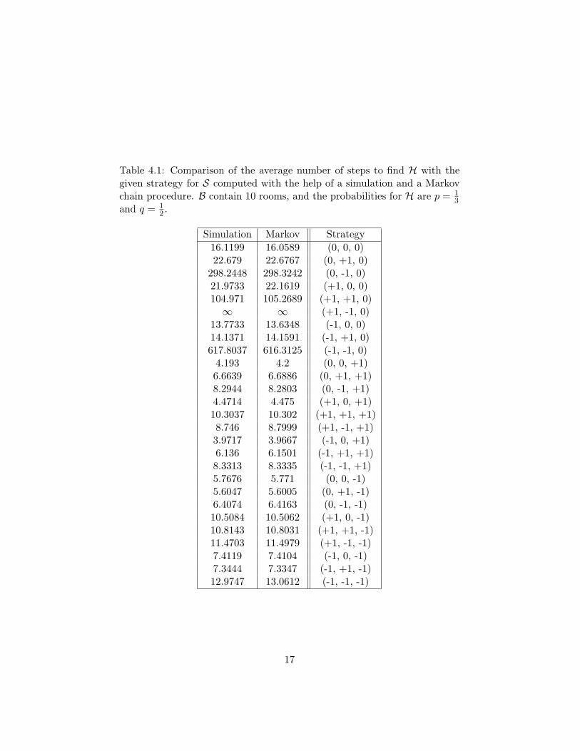
Table 4.1: Comparison of the average number of steps to find H with thegiven strategy for S computed with the help of a simulation and a Markovchain procedure. B contain 10 rooms, and the probabilities for H are p = 1

3and q = 1

2 .

Simulation Markov Strategy16.1199 16.0589 (0, 0, 0)22.679 22.6767 (0, +1, 0)

298.2448 298.3242 (0, -1, 0)21.9733 22.1619 (+1, 0, 0)104.971 105.2689 (+1, +1, 0)∞ ∞ (+1, -1, 0)

13.7733 13.6348 (-1, 0, 0)14.1371 14.1591 (-1, +1, 0)617.8037 616.3125 (-1, -1, 0)

4.193 4.2 (0, 0, +1)6.6639 6.6886 (0, +1, +1)8.2944 8.2803 (0, -1, +1)4.4714 4.475 (+1, 0, +1)10.3037 10.302 (+1, +1, +1)8.746 8.7999 (+1, -1, +1)3.9717 3.9667 (-1, 0, +1)6.136 6.1501 (-1, +1, +1)8.3313 8.3335 (-1, -1, +1)5.7676 5.771 (0, 0, -1)5.6047 5.6005 (0, +1, -1)6.4074 6.4163 (0, -1, -1)10.5084 10.5062 (+1, 0, -1)10.8143 10.8031 (+1, +1, -1)11.4703 11.4979 (+1, -1, -1)7.4119 7.4104 (-1, 0, -1)7.3444 7.3347 (-1, +1, -1)12.9747 13.0612 (-1, -1, -1)

17

0 1 2 3 4 5 6 7 8 9 10 11 12 13 14 150

0.1

0.2

0.3

0.4

0.5

0.6

0.7

0.8

0.9

1

Markov generatedSimulation generated

Figure 4.1: Comparison of a simulated limited time search and the theoret-ical limited time search. S strategy is (+1,-1,+1)

18

0 1 2 3 4 5 6 7 8 9 10 11 12 13 14 150

0.1

0.2

0.3

0.4

0.5

0.6

0.7

0.8

0.9

110 rooms. Hider probabilities: previous = 0.5, stay = 0.16667, next = 0.33333

0, 0, 00, +1, 00, −1, 0+1, 0, 0+1, +1, 0+1, −1, 0−1, 0, 0−1, +1, 0−1, −1, 0

Figure 4.2: Limited time search computed with the help of the Markov chainmodel.

19

0 1 2 3 4 5 6 7 8 9 10 11 12 13 14 150

0.1

0.2

0.3

0.4

0.5

0.6

0.7

0.8

0.9


0, 0, +10, +1, +10, −1, +1+1, 0, +1+1, +1, +1+1, −1, +1−1, 0, +1−1, +1, +1−1, −1, +1


20

0 1 2 3 4 5 6 7 8 9 10 11 12 13 14 150

0.1

0.2

0.3

0.4

0.5

0.6

0.7

0.8

0.9


0, 0, −10, +1, −10, −1, −1+1, 0, −1+1, +1, −1+1, −1, −1−1, 0, −1−1, +1, −1−1, −1, −1


21

Table 4.2: Statistical test over the reliability of the number of experiments.The test is performed with 5000 samples of completed experiments, thenumber of rooms is 10, p = 1

3 , q = 12 , and the strategy for S is (+1, 0, 0)

Number of experiments Mean Standard deviation Time to compute10 22.0948 7.1513 0.005 s100 22.0703 2.2515 0.057 s1,000 22.1548 0.7146 0.374 s10,000 22.1672 0.2271 4.980 s100,000 22.1628 0.0714 46.173 s

22

4.2 2-dimensional Board Game

Here are presented a number of results for the 2-Dimensional game. Thesame remark as the one made in the previous section is made. All the resultsare included in this article as an example, because each set up gives differentresults. The set up used for the different figures will be a 4× 4 board with,p = 0, q = 1

2 , r = 0, s = 13 . The vector searcher will be analyzed and the

vector unknown = [0.2, 0.2, 0.2, 0.2, 0.2].

4.2.1 Average number of steps

The average number of steps needed by S to find H with the given set upand all the possible strategies for S can be computed with the help of thetwo methods given in Chapter 3. The comparison of the two approaches canbe seen in Tables 4.4 and 4.5. The simulation is based on 100, 000 runs. Inthe table, no values are infinity. This is explained because the random walkallows the two players to meet each other by chance, where in the set up ofthe circle game there was not such a randomized walk for S.

As one can see in the tables, there is no values that are as big as theone that can be observed in the table of values of the circle game (Table4.1). The reason for this is that when the position of H is unknown for S, Suses its random walk procedure. This allows him to find H by pure chance.Also, unlike in the circle game, there is not a strategy that stands out of theresults as a general best strategy, the best conclusion that could be madewas that using a strategy (1, ?, ?, ?) was not a suitable choice.

Still in the table one can see that the best strategy for S is to do(0, 1,−1, 1) but that some other strategies are close to this one for example(0, 1, 0, 1).

4.2.2 Limited time search

When we limit the time search, we calculate the probability to find H withinn steps. Figure 4.5 shows the difference between the theoretical and thesimulated approach of one strategy for S on the same graph. In figures 4.6,4.7, and 4.8, some interesting strategies for S are tried. These figures havebeen chosen because some of the strategies perform better when n is lowand get worse when n gets larger. Indeed, when analyzing the Figure 4.6,one can see that the strategy (−1, 1, 1, 1) do not performs well when thenumber of steps are limited to 1 or 2, but is quite good when the number ofsteps is limited to 10.

23

One may also realize that the starting value for all these figures is thesame for all the strategies. Indeed when the time is limited to 0, it meansthat they are taken into account only when both players are in the sameroom as a starting point . As the board contains 4 × 4 rooms then theprobability that both players are in the same room at the beginning of thegame is 1

16 which is indeed the value that we observe in the figures.In all these graphs, the vertical axis expresses the probability to find H,

and the horizontal axis expresses the limited time frame. The outputs arebased on 100, 000 simulations.

4.2.3 Reliability of the simulation approach

In order to see how reliable the simulation approach is, a statistical testhas been performed. The set up used will be the same as the one usedfor Figure 4.5: strategy = (+1,−1, +1,−1). The mean and the standarddeviation of 5000 samples over respectively 10, 100, 1000, 10 000 and 100000 simulations has been computed. Table 4.3 show these results. Thereduction of the standard deviation follows the general rule that in orderto reduce the standard deviation by a factor 2, you need 4 times as manyruns [9], it is indeed the case: there is a reduction of about

√10 = 3.16

times when we multiply the number of challenges by 10. In here also, wehave included, as an additional piece of information, the time to computethe n simulations has been added. As one can see, the time to compute thesimulation is linear to the number of simulations.

24

0 1 2 3 4 5 6 7 8 9 10 11 12 13 14 150

0.1

0.2

0.3

0.4

0.5

0.6

0.7

0.8

0.9

1

Markov generatedSimulation generated

Figure 4.5: Comparison of a simulated limited time search and the the-oretical limited time search. The parameters for S are strategy =(+1,−1, +1,−1) and unknown = [0.2, 0.2, 0.2, 0.2, 0.2]

Table 4.3: Statistical test over the reliability of the number of experiments.The test is performed with 5000 samples of completed experiments.

Number of experiments Mean Standard deviation Time to compute10 7.7153 2.0523 0.008 s100 7.7931 0.66208 0.065 s1,000 7.7884 0.2071 0.827 s10,000 7.7885 0.0656 7.426 s100,000 7.7885 0.0208 78.391 s

25

0 1 2 3 4 5 6 7 8 9 10 11 12 13 14 150

0.1

0.2

0.3

0.4

0.5

0.6

0.7

0.8

0.9

1

Board of 4x4 rooms.Hider probabilities: previous = 0, next = 0.5, up = 0, down = 0.33333, stay = 0.16667

Searcher probabilities when unknown : previous = 0.2, next = 0.2, up = 0.2, down = 0.2, stay = 0.2

0, 0, 1, 10, 1, 1, 10, −1, 1, 11, 0, 1, 11, 1, 1, 11, −1, 1, 1−1, 0, 1, 1−1, 1, 1, 1−1, −1, 1, 1


0 1 2 3 4 5 6 7 8 9 10 11 12 13 14 150

0.1

0.2

0.3

0.4

0.5

0.6

0.7

0.8

0.9

1



0, 0, −1, 10, 1, −1, 10, −1, −1, 11, 0, −1, 11, 1, −1, 11, −1, −1, 1−1, 0, −1, 1−1, 1, −1, 1−1, −1, −1, 1


26

0 1 2 3 4 5 6 7 8 9 10 11 12 13 14 150

0.1

0.2

0.3

0.4

0.5

0.6

0.7

0.8

0.9

1



0, 0, 1, −10, 1, 1, −10, −1, 1, −11, 0, 1, −11, 1, 1, −11, −1, 1, −1−1, 0, 1, −1−1, 1, 1, −1−1, −1, 1, −1


27

Table 4.4: Comparison of the average number of steps to find H with thegiven strategy for S, computed with the help of a simulation and a Markovchain procedure.Simulation Markov Strategy

10.6445 10.6196 (0, 0, 0, 0)10.1683 10.1805 (0, 1, 0, 0)9.8285 9.8144 (0, -1, 0, 0)17.179 17.1687 (1, 0, 0, 0)15.6128 15.518 (1, 1, 0, 0)17.8421 17.8413 (1, -1, 0, 0)14.6483 14.6695 (-1, 0, 0, 0)12.7284 12.7627 (-1, 1, 0, 0)14.6717 14.5632 (-1, -1, 0, 0)14.966 14.9666 (0, 0, 1, 0)14.1064 14.1855 (0, 1, 1, 0)13.6563 13.6448 (0, -1, 1, 0)27.5912 27.5286 (1, 0, 1, 0)23.8101 23.9136 (1, 1, 1, 0)29.1073 28.9974 (1, -1, 1, 0)22.2174 22.2373 (-1, 0, 1, 0)18.5968 18.5084 (-1, 1, 1, 0)21.8923 21.9438 (-1, -1, 1, 0)12.8138 12.8673 (0, 0, -1, 0)11.8899 11.8628 (0, 1, -1, 0)11.1087 11.1301 (0, -1, -1, 0)22.1575 22.1972 (1, 0, -1, 0)18.1854 18.1368 (1, 1, -1, 0)24.1452 24.0167 (1, -1, -1, 0)18.4664 18.4462 (-1, 0, -1, 0)14.8041 14.8422 (-1, 1, -1, 0)18.3171 18.1865 (-1, -1, -1, 0)

Simulation Markov Strategy9.6675 9.6923 (0, 0, 0, 1)7.5853 7.5743 (0, 1, 0, 1)8.4006 8.3874 (0, -1, 0, 1)15.3406 15.3395 (1, 0, 0, 1)10.1528 10.1531 (1, 1, 0, 1)16.3391 16.3413 (1, -1, 0, 1)12.7076 12.7387 (-1, 0, 0, 1)7.9411 7.9467 (-1, 1, 0, 1)11.9369 11.8735 (-1, -1, 0, 1)13.0713 13.0514 (0, 0, 1, 1)9.472 9.4541 (0, 1, 1, 1)

11.0491 11.0577 (0, -1, 1, 1)22.6473 22.6506 (1, 0, 1, 1)13.0763 13.0219 (1, 1, 1, 1)24.4394 24.478 (1, -1, 1, 1)17.629 17.7063 (-1, 0, 1, 1)9.6631 9.6899 (-1, 1, 1, 1)15.907 15.8798 (-1, -1, 1, 1)10.8899 10.9386 (0, 0, -1, 1)7.4506 7.458 (0, 1, -1, 1)8.6399 8.6893 (0, -1, -1, 1)17.8829 17.9693 (1, 0, -1, 1)

9.58 9.5698 (1, 1, -1, 1)19.8888 19.9643 (1, -1, -1, 1)14.4663 14.572 (-1, 0, -1, 1)7.8197 7.7885 (-1, 1, -1, 1)13.0932 13.077 (-1, -1, -1, 1)

28

Table 4.5: Comparison of the average number of steps to find H with thegiven strategy for S, computed with the help of a simulation and a Markovchain procedure.

Simulation Markov Strategy9.9839 10.0029 (0, 0, 0, -1)9.3171 9.2929 (0, 1, 0, -1)9.2615 9.2164 (0, -1, 0, -1)16.0278 15.9311 (1, 0, 0, -1)13.9267 13.9075 (1, 1, 0, -1)16.6087 16.511 (1, -1, 0, -1)13.4448 13.3621 (-1, 0, 0, -1)11.0101 11.0534 (-1, 1, 0, -1)13.0131 12.9855 (-1, -1, 0, -1)15.2384 15.2614 (0, 0, 1, -1)14.5742 14.5454 (0, 1, 1, -1)13.9654 13.8512 (0, -1, 1, -1)28.6501 28.6085 (1, 0, 1, -1)24.9997 24.933 (1, 1, 1, -1)30.3144 30.3046 (1, -1, 1, -1)23.1295 23.1805 (-1, 0, 1, -1)19.4804 19.4065 (-1, 1, 1, -1)23.0605 23.0748 (-1, -1, 1, -1)12.4961 12.4912 (0, 0, -1, -1)10.9856 10.9692 (0, 1, -1, -1)10.5094 10.4927 (0, -1, -1, -1)21.4708 21.5121 (1, 0, -1, -1)16.1873 16.1543 (1, 1, -1, -1)23.5547 23.6349 (1, -1, -1, -1)17.7245 17.7607 (-1, 0, -1, -1)13.1785 13.1627 (-1, 1, -1, -1)17.25 17.2784 (-1, -1, -1, -1)

29

Chapter 5

Discussion

5.1 Beliefs update

In this article, the strategy for the searcher is determined at the beginningof the game. However after analysis, we have discovered that in some ofthe cases it is possible for S to know exactly the position of H. Indeed ifwe keep the example discussed for the 2-dimensional board, the hider hasonly three moves, he either stays with probability 1

6 , goes to the adjacentroom to the right with probability 1

2 or goes to the adjacent room belowwith probability 1

3 . There will be a case where the searcher is, at time t− 1,searching in the adjacent room to the right of H. If the strategy for S inthis particular case is to wait so that H might come to his room at time t,then no matter what happens S will know the position of H. If H stays, Swill still see him and we will be back to the same situation. If H moves tothe room where S is, the game will be over, and if H goes below, he becomesout of sight for S. However S will know with probability 1 that H is in theroom below the one he was at t−1 as he knows the strategy of H. With theset up analyzed in this article, when S does not see where H is, he makesa random movement. This means that in the situation explained here, evenif one can derive the position of H and the corresponding best reply, we donot use the information to have a sustainable advantage to find H. Somesimilar issues on beliefs have been analyzed in a previous article [8].

5.2 Past action and observed environment

Another weakness of this model, that can also be related to beliefs updating,is that S does not remember the past actions and observed environment. To

30

illustrate this statement, one can think about a hider that always moves withprobability 1 in the same direction and S always missing him by one room.As both players have the same speed, it will be a never ending game. Asboth players move simultaneously, if S is in room n− 1 and H is in room n,at the next time moment, S will move to room n and H will move to roomn + 1. The problem in this small example is that S has a limited view, thusif he does not chase H, he will lose its trace and return in the state wherethe position of H is unknown. If S had the ability to remember that he hadseen H the best reply would be to move in the opposite direction takingadvantage of the infinite universe by catching him in the opposite direction.However as there is no memory of past actions and observed environmentthis is not possible in our model.

5.3 Hit probabilities

We made the assumption that each room has a hit probability hi = 1. Thisleads to a big simplification of the model. Indeed, with this assumptionthere is no probability that a room that is searched still contains H. Ifthe ki were not all equal to 1, we could have had a best starting point forS on the board, but also a different searching strategy depending on thedistribution of these hi. We did not looked in these situations but they havebeen discussed and analyzed in [8].

5.4 Random walk for the 2-dimensional model

As one might have noticed, a random walk procedure has been introducedin the 2-dimensional board. It is not present in the circle game becausethe board contains only one dimension and one can find a best reply to thewalk made by H. In the case of a 2-dimensional board, the procedure isnot as easy as the one for the circle game, therefore the random walk wasintroduced to allow a more realistic behavior. One can imagine randomwalk that is be biased towards a particular direction or simply has the sameprobabilities for each of the possible directions. In this article we did notfocused on the different possibilities of these random walks and which onewould perform better than other depending on the movement procedure ofH. A simple test has been performed in section 6.1 to see if some walks wereperforming better than other but it is the only one that has been made.

31

5.5 Size of the board

This article did not discuss the impact of different size of board on the re-sults. As one can imagine, it has an impact on the results in terms of averagenumber of steps to find a prey, but not in any of the other parameters. Thisfeature has been discussed and analyzed in the article by Scharf et al. [6].

32

Chapter 6

Analysis

6.1 Perpendicular movement

In this study, when S does not see H, he uses a random walk strategy.However, we wanted to see if there was a better alternative than just arandom walk. As we assume that the strategy of H is known, one can thinkof a better alternative. We performed a simple test: we decided to make Hmove in one direction only (always move in the room above) and comparewith the different strategies that S could perform. As Figure 6.1 shows, theresults are significantly different when we include a perpendicular movementbehavior (meaning that S moves in a perpendicular direction from the onemade by H). It is important to note that we need to have a shift in adirection for both players, but it does not need to be a probability 1 thatthe players move in the desired direction. However, it still needs to havea general tendency to drift in the desired direction. This warning is givenbecause if both players move in perpendicular direction with probability1, as their speed are the same, they might always miss each other. Thisperpendicular movement is also taking advantage of the infinite universe.

6.2 Diagonal movement handling

In the original set up, diagonal movement was not allowed. The designof the model has been made this way because in a traditional grid board,diagonal movement makes some path faster than other especially when aplayer moves only horizontally and vertically. As a solution one can modifythe board by shifting every second row by only a half tile to allow 6 directneighbors instead of only 4. This gives a hex-grid board looking like Figure

33

6.2. In order to have an infinite universe with such a configuration, thenumber of rows must be even, otherwise the top and bottom of the boarddon’t match.

A comparison between the hex-grid board and the regular 2D boardhas been performed to see if in similar conditions similar results could beobserved. Indeed one can conclude that in similar conditions the resultsmatch. The test to see if the two boards match, has been performed on a8 × 8 board with H having equal probability to go in any adjacent roomand stay in the current, and S going in the room where H was seen andotherwise going in a random adjacent room. Another test to see how well ahex-grid board matches a traditional 2-D board, will be made in Chapter 9.

6.3 Vision

Instead of using a vision of only the neighboring rooms, we have extendedthe vision to see the impact that it would have on the process. This featurehas been implemented in a way that implies that any room seen is reachablein the number of steps that extends the vision. If S sees 3 rooms ahead,then any room that is reachable in three steps is seen, not the other ones. Inthe case of a circle or a Hex-grid model, it is a straight forward application.However, in a normal 2D board, depending whether the diagonal movementis allowed or not, the visible region will be different. In the article by Scharfet al. [6] the diagonal movement is allowing a square vision while in ourmodel diagonal movement is not allowed, creating a diamond shape visiblearea. This feature can be easily applied on a hex-grid because all directneighboring rooms are seen and reachable.

6.4 Energy cost function

An application of the hide and seek game is a predator prey model. Apredator needs to feed in order to survive. He can either go and search forfood, or wait until a prey passes by. As one can imagine, waiting is lessenergy consuming than actively searching. Thus we decided to include anenergy cost function to see the impact that it would have on the differentstrategies and on the optimal one. We allowed an initial amount of energywhere not moving for one turn consumes some amount of energy and movingconsumes more energy. The speed, or in our case the number of rooms thatS can search in one time step, consumes some energy, but this energy is notdivided in the number of sub-move: either the predator moves and consumes

34

Table 6.1: Amount k for which a moving predator is willing to pay in terms ofenergy per time step while still having an advantage on an ambush predatorthat consumes only one unit of energy. The amount has been tested on anarena containing 4 preys and of size 20× 20

Vision Affordable amount1 k < 12 k < 23 k < 44 k < 55 k < 76 k < 77 k < 78 k < 99 k < 9

the amount of energy to move or he stays and consumes the amount of energywhen not moving. We wanted to compare the probability of finding a preyby a predator being ambushed, and therefore waiting, and by a predatorbeing active and searching for the preys. We decided to see if there was athreshold that could connect the number of prey and the cost of moving.We used an observable region that corresponds to the speed of the predator.If a predator can move n tiles away, then he will be able to see all therooms reachable in n steps. By moving m steps, the predator will make hisobserved area bigger, even if he has only n −m move left, he will still seen tiles away from this new position. It has been realized that the amountof prey is not the important factor (as one can see in Figure 6.3), but theamount of energy that the predator would consume for a given speed wasthe one that matters (as one can see in Figure 6.4). Table 6.1 has been madeto get some insight about the result of the introduction of the cost functionand understand a bit about the underlying dynamics. In this table the valuek is the amount of energy that the moving predator can consume while stillhaving an bigger probability to find a prey than an ambush predator. Thetable shows some thresholds that are based on a series of graph as the onethat is display in Figure 6.4. As one can understand the accuracy and theconfidence intervals haven’t been tested, the table is just there to show thatthere is indeed different thresholds for the different speeds.

35

random perpendicular350

400

450

500

550

600

650

Ave

rage

num

ber

of s

teps

Arena size : 20 by 20. 1 Hider. Speed and vision 1

Figure 6.1: Comparison of a pure random strategy for the searcher to aperpendicular movement strategy.

36

Figure 6.2: Hex-grid example

37

1|5 2|5 3|5 4|5 5|5 6|5 7|5 8|5 9|5 10|50

0.1

0.2

0.3

0.4

0.5

0.6

0.7

0.8

0.9

Number of preys on the field | Energy consumed to move

Pro

babi

lity

to fi

nd a

pre

y

Arena of 20 by 20, Vision 3

Moving predatorEmbush predator

Figure 6.3: Probability to find a prey with an original amount of energy of20 units, depending on the number of preys

38

7|1 7|2 7|3 7|4 7|5 7|6 7|7 7|8 7|9 7|100

0.1

0.2

0.3

0.4

0.5

0.6

0.7

0.8

0.9

1

Number of preys on the field | Energy consumed to move

Pro

babi

lity

to fi

nd a

pre

y

Arena of 20 by 20, Vision 3

Moving predatorEmbush predator

Figure 6.4: Probability to find a prey with an original amount of energy of20 units, depending on the number of the amount paid for a movement.

39

Chapter 7

Conclusion

In conclusion, the theoretical model described here is a good alternative tothe simulation model. The Markov chain model is a really good and reliablemodel but is really hard to modify due to the explosion of the complexity ofthe created matrix. The modification of the Markov model is complicatedbecause any introduction of new parameters changes the way the matrix isbuilt, and if there are multiple predators or preys, the complexity is growing.The complexity grows very fast with multiple preys and this makes it hard touse in an easy way. As an alternative, one can use the Simulation model. Itis a model that is more flexible and that does not grow as fast in complexity,but that takes much more time to run and compute to have a reliable output.The different studies that have been made were not deeply analyzed becausethey were mainly out of the scope of this research but can lead to interestingresults and applications in terms of real life simulation.

40

Part II

Comparing the model withrelated literature

41

Chapter 8

Verification

8.1 Introduction

As mentioned in the Preface, a similar study has been performed by Scharfet al. [6]. As a verification to our work, it has been decided to run testsunder similar conditions and see if the models could match their results. Asthe diagonal movement is not handled in our situation, we have modifiedthe moving condition of Scharf et al. to have a better match between themodels. Also, we have allowed our model to handle multiple H (preys). Itis to the attention of the reader that a review of the article has been madeby Avgar et al. [1] which have been replied by Scharf et al. [7].

8.2 Speed Impact and Vision

In the article [6], the impact of the speed of the hider and the searcher hasbeen studied. We have run experiments under similar conditions to see ifour model could give similar results. Figures 8.1 and 8.2 show the resultsobtained with the help the simulation explained in this article. The resultsshow similar behavior when the velocity changes. It also means that onecould model the problem in terms of Markov chain.

8.3 Discussion

While running tests to see if both our model and the model by Scharf et al.could match, a few questions were raised. In this section we are going todiscuss the interpretation they have made about the speed and the vision of

42

1:1 1:3 1:5 1:7 1:10

−120

−100

−80

−60

−40

−20

0

20

40

60

80

100

predator:prey velocity ratio

∆t(a

ctiv

e −

am

bush

)

Figure 8.1: Impact of the Velocity on the time to capture a prey. Arena size:20x20. Diamond : result by Scharf et al. Squares : results by our method.

6:1 4:1 2:1 1:1

−300

−250

−200

−150

−100

−50

0

50

100


∆t(a

ctiv

e −

am

bush

)

Figure 8.2: Impact of the Velocity on the time to capture a prey. Arena size:20x20. Diamond : result by Scharf et al. Squares : results by our method.

43

the predator and how the choices influence the outcome while they will beanalyzed in Chapter 9.

8.3.1 Speed

It has been realized after a few tests that an important factor to couplewith speed was the vision. Indeed, if S has the ability to move two timesfaster than H, it is important that he sees at least two rooms ahead ineach direction otherwise he makes a random move in a direction while beingblind for its second move thus he does not anticipate its next move. Onecan imagine that if H is at only two rooms distance, S could catch H in oneturn if he can anticipate its second move. This feature is not of importancewhen talking about H because, in the assumption made by Scharf et al. andin our model, H does not try to avoid S. Thus even if he could see far away,he would not use this advantage.

8.3.2 Vision

In terms of vision, the interpretation that Scharf et al. made was foundvery restrictive. Indeed, as soon as a prey is seen, it is assumed to be caughtwhile being only capable of moving one tile at the time. This raised a bigquestion, if a predator can see, and move instantly n tiles away, why notmake these n steps to extend the observed area if no prey is in sight. Stillin their interpretation there is no coupling between speed and vision. Apredator can eat instantly a prey that is n tiles away but is not able to movethere under normal conditions. This feature also makes the active searcherperforming worse than if he was moving more than one tile away and ableto observe the neighborhood. In our view, a plausible interpretation wouldbe to make the observable area depending on the speed of the predator.This way if a predator sees a prey in the limit of its observable region, hecan catch it, but at the same time, if he sees nothing, he can still use theenergy he would have used to catch the prey to look around and maybe takeadvantage for the next moving sequence by spotting the prey.

44

Chapter 9

Experiments

9.1 Vision and speed

A few experiments have been made to see the impact of the interpretationof the vision. The figures 9.1 and 9.3 show the combination of the speedand vision. This means that when a predator is moving 6 times faster thanthe prey, he can move and see 6 tiles away. In these graphs, seeing is notcatching. In order to give more insight about the meaning of the graph,two additional graphs have been added, Figure 9.2 and 9.4. They show theaverage number of steps needed by an ambush predator to capture the prey.

As one can see in the results that an ambush predator that can see 6tiles away and can go in one move all the way to the prey performs muchbetter than a predator that can move 6 tiles but that cannot see one tileaway. This can be derived with the help of Figure 9.3 and 9.4: the firstone shows that the difference in time, when the predator is ambush to whenthe predator is moving, is much lower and the second one shows that theaverage is lower when the vision is extended.

The results are of course not unexpected, therefore, a comparison be-tween the see is catch and the combination of move and see has been per-formed. In the first case, the predator sees 6 tiles away and catches theprey instantaneously if he sees any, but moves only one tile per turn. Inthe second case, the predator can move and see 6 tiles away, but he stillneeds to make all the moves to get to the prey, so the catch is not instan-taneous. Figure 9.5 shows that there is indeed a big difference in these twoapproaches.

In Figure 9.6 and 9.7, we have tried to see if there was a possibility tocompare the model by Scharf et al. allowing diagonal movement and the

45

Hex-grid model. One can see that these models are comparable. It meansthat it could be a good alternative to remove different path lengths in atraditional grid board.

1:1 1:3 1:5 1:7 1:10

−200

−150

−100

−50

0

50

100


∆t(a

ctiv

e −

am

bush

)

Figure 9.1: Impact of the vision on the time to capture a prey. Arena size:20x20. Diamond: Vision is always 0. Square: Speed and Vision combined.

46

1:1 1:3 1:5 1:7 1:100

50

100

150

200

250

300

350

400


Ave

rage

num

ber

of s

teps

for

an a

mbu

sh p

reda

tor


6:1 4:1 2:1 1:1

−300

−250

−200

−150

−100

−50

0

50

100


∆t(a

ctiv

e −

am

bush

)


47

6:1 4:1 2:1 1:10

50

100

150

200

250

300

350


Ave

rage

num

ber

of s

teps

for

an a

mbu

sh p

reda

tor


6 4 2 10

50

100

150

200

250

Vision in number of tiles seen

Ave

rage

num

ber

of s

teps

for

a m

ovin

g pr

edat

or

Figure 9.5: Impact of the vision on the time to capture a prey. Arena size:20x20. Diamond: The speed is always 1, but see is catch. Square: Speedand Vision are combined but see is not catch.

48

1:1 1:3 1:5 1:7 1:10

−150

−100

−50

0

50

100


∆t(a

ctiv

e −

am

bush

)

Figure 9.6: Comparison of the Scharf implementation (squares) and theHex-Grid implementation (diamonds)

6:1 4:1 2:1 1:1

−300

−250

−200

−150

−100

−50

0

50

100


∆t(a

ctiv

e −

am

bush

)

Figure 9.7: Comparison of the Scharf implementation (squares) and theHex-Grid implementation (diamonds)

49

Chapter 10

Conclusion

In conclusion the choices of the interpretation of the speed, the vision, andany other parameter have to be made with great care. Indeed, they willinfluence the entire simulation, the results and, as one may understand,the reliability of this simulation. During our research it has been realizedthat even the order of update between the movements makes a difference andgives different results. It is important to know that a choice of an implemen-tation should be made to simulate a behavior in a particular environmentand that it might not be applicable for a slightly different one. One shouldask the help of a biologist or another relevant expert in the desired field tosimulate the appropriate behavior and get a more reliable simulation.

50

Bibliography

[1] T. Avgar, N. Hovitz, L. Broitman, and R. Nathan. Notes and com-ments. how movement properties affect prey encounter rates of ambushversus active predators : A comment on Scharf et al. The AmericanNaturalist, 172(4), 2008.

[2] V. Chvatal. Linear Programming. W.H. Freeman and Company, 1983.

[3] J. Derks. A note on hide-and-seek games: some first investigations andmodel building, 2008.

[4] I. Gikhman and A. Skorohod. The theory of stochastic processes 1.Springer, 2004.

[5] S. Ross. Introduction to Probability Models. Academic Press, 9-th edi-tion, 2007.

[6] I. Scharf, E. Nulman, O. Ovidia, and A. Bouskila. Efficiency evalua-tion of two competing foarging modes under different conditions. TheAmerican Naturalist, 168(3), 2006.

[7] I. Scharf, O. Ovidia, and A. Bouskila. Prey encounter rate by preda-tors: Discussing the realism of grid-based models and how to modelthe predator’s foarging mode: A reply to Avgar et al. The AmericanNaturalist, 172(4), 2008.

[8] P. Uyttendaele. Hide and seek games. Bachelor Thesis UniversiteitMaastricht, 2008.

[9] R. Walpole, R. Meyers, S. Meyers, and K. Ye. Probability & Statis-tics for Engeneers & Scientists. Pearson Education International, 8-thedition, 2007.

[10] P. Zollner and S. Lima. Search strategies for landscape-level interpatchmovements. Ecology, 1999.

51

master thesis hide and seek games - maastricht university

Documents