master thesis
DESCRIPTION
This is my master thesisTRANSCRIPT

Inequality measurement re-reexamined
Stephan Kampelmann
November 7, 2007
Master Thesis in Applied Econometrics
Faculté des Sciences Economiques et SocialesUniversité des Sciences et Technologies de Lille59655 Villeneuve d’Ascq Cedex
Directeur de mémoire
Florence Jany-Catrice
Responsable de formation
Nicolas Vaneecloo
i

Contents
1 Introduction and methodology 11.1 Why inequality measurement is still relevant . . . . . . . . . . . . . . . . . 11.2 Discussing the undiscussable: inequality as convention . . . . . . . . . . . . 61.3 Some basic terminology . . . . . . . . . . . . . . . . . . . . . . . . . . . . . 13
2 An internal history of the academic discourse 152.1 From constant inequality to complex inequalities . . . . . . . . . . . . . . . 162.2 Recent developments: generalisation of methods . . . . . . . . . . . . . . . 592.3 Closer to ‘truth’ or away from ‘normal communication’? . . . . . . . . . . 61
3 Revision of inequality in the IEWB 633.1 Introduction to the Index of Economic Well-Being . . . . . . . . . . . . . . 633.2 Four dimensions, three inequalities . . . . . . . . . . . . . . . . . . . . . . 683.3 Alternative proposals to measure inequality . . . . . . . . . . . . . . . . . 70
4 Empirical application 834.1 Data treatment . . . . . . . . . . . . . . . . . . . . . . . . . . . . . . . . . 834.2 Results for alternative inequality statistics . . . . . . . . . . . . . . . . . . 894.3 IEWB with modified equality dimension . . . . . . . . . . . . . . . . . . . 92
Compte rendu du mémoire en français 102
ii

Chapter 1
Introduction and methodology
1.1 Why inequality measurement is still relevant:the case of the IEWB
Inequalities, and more generally the distribution of resources, are fundamental problemsin economics. We believe it is important and helpful to analyse if and to what extentoutcomes can be characterised as unequal. We may even agree with R.H. Tawney whenhe argues that “inequality is perhaps what economics should be all about” (Tawney, 1964).Economic inequalities impact on a wide range of societal issues so that they can be dealtwith in many different ways. Depending on which angle one chooses to shed light on thetopic, the analysis tends to be more philosophical (the question of equity and justice),economic (the problems of incentives and resource allocation), or sociological (the functionand role of socio-economic inequalities). It is arguably difficult to discuss all these fieldssimultaneously and we will not attempt to do so.
Instead, the question of inequalities will be approached in this text from a very specificviewpoint: the discussion will take the Index of Economic Well-Being (IEWB), developedby Osberg & Sharpe (2005), as point of departure. This index was developed to pro-vide an easily communicable heuristic, allowing users with different backgrounds to makejudgements about ‘the big picture’ of economic well-being. It compiles statistical informa-tion concerning four dimensions that are thought to be relevant: 1) effective consumption;2) accumulation of productive assets; 3) equality and poverty; and 4) economic security.We believe that the IEWB is a useful tool for economic analysis, while the last term shouldbe understood as including not only a purely economic discussion, but also the analysisof economic outcomes in political, ethical or sociological terms. This implies that the ‘ex-perts’ of the economic discipline (statisticians, welfare economists etc.) are not the onlyusers of the IEWB. In order to be a useful heuristic for other actors, their conceptions andrepresentations have to be integrated in the IEWB.
However, in the context of an earlier application of the IEWB to France (cf. Jany-Catrice & Kampelmann, 2007), we noted that the position of economic inequalities withinthe architecture of the IEWB is not entirely satisfying. Only one aspect of inequalities
1

2 CHAPTER 1. INTRODUCTION AND METHODOLOGY
appears in the index: in its current state, the IEWB only includes inequality in the distri-bution of disposable income. However, Osberg and Sharpe consider the various dimensionsmentioned above to be relevant to make judgements about the development of economicwell-being. If one accepts these dimensions of economic well-being, then, we argue, in-equalities should be evaluated according to exactly these aspects, i.e. according to effectiveconsumption, wealth accumulation and economic security. This inconsistency inspired thepresent text and its basic research questions: are inequalities correctly taken into accountin the index of economic well-being? And if not, how can we improve the index withoutlosing its transparency and intuitive appeal?
Inequality being a complex and somewhat blurry concept, these research questionscontain more caveats than one might at first expect. For passing from the abstract concept‘inequality’ to a concrete empirical measure applicable to income or wealth data is not aneutral technical process. It involves many steps and decisions, and the imminent dangeris that some of the content of the original concept ‘inequality’ may be lost along the way.For a start, we cannot even define easily the very concept we are talking about. Hence,the question of how economic inequalities should appear in the framework of the IEWBleads us to a more general question: how should economic inequalities be measured in thefirst place?
Is this question worth debating? Why don’t we simply rely on the well-known andwidely-used measures of inequality such as the Gini concentration coefficient, like Osbergand Sharpe have chosen to? After all, these measures are readily available and are fre-quently referred to as objective and legitimate references in public debates on inequality.We argue that at least three points indicate that there is a strong case for discussing theconventionally used inequality measures:
1. There are not one, but many different indices, coefficients or other statistical instru-ments which supposedly measure inequalities. Since these tools frequently contradicteach other, the choice of any specific measure is not neutral and should be based onplausible and legitimate arguments (we will come back to the contradictions betweenalternative measures at several times in the text). Of course, the choice of a statisticshould correspond directly to the purpose at hand (in our case the application of theIEWB). Therefore, we need to verify if available inequality measures correspond tothis purpose. In order to do so, we need to understand what distinguishes the differ-ent measures, which judgements are embedded in their set-up and which conventionsare integrated in their usage.
2. Like in the case of poverty measurement, the empirical analysis of inequalities con-tains many controversial issues. For example, in the debates on poverty the questionof relative versus absolute poverty frequently incites vivid controversies (cf. Raval-lion, 2003). Among other things, this shows that sometimes the very basic questionof ‘what is poverty?’ does not allow for any obvious answer. As will be seen below,we think that similar controversies are involved in the measurement of inequalities,although they may be less debated and perhaps less obvious. The fact that these

1.1. WHY INEQUALITY MEASUREMENT IS STILL RELEVANT 3
controversies have not (yet) penetrated the non-expert debate is perhaps partly dueto the technical complexities involved in inequality metrics. The discussion on in-equality statistics tends to be dominated by ‘experts’, whose background and interestrender the conversation somewhat inaccessible to non-experts (we will give examplesof this phenomenon later). Given the imperative of transparency and the rather‘democratic’ purpose of the IEWB, we submit that the controversial issues in in-equality measurement should not be hidden behind the statistical technicalities. Onthe contrary, they should be subject to open argumentation like the one we attemptto provide in this text.
3. We already argued that if we accept that economic well-being has multiple dimen-sions, it follows that inequalities should be evaluated in these multiple spaces. How-ever, statistics like the Gini concentration coefficient are not directly applicable tomulti-dimensional problems. This creates the practical problem of measuring in-equalities in different spaces and the subsequent aggregation. Again, a solution tothis problem should be coherent with the overall purpose as defined by the frameworkof the index of economic well-being.
These arguments directly imply why we cannot fully rely on other reviews of inequalitymeasures that are available in the literature. While these accounts are numerous anda precious source for our endeavour, they do not explicitly address many problems thatare specific to the IEWB. In fact, many reviews of inequality measures focus on technicalissues (e.g. the problem of decomposability) or only make sense within a certain framework(e.g. the utilitarian approach). For our problem, it is of primordial importance to ensurethat the measure of inequality corresponds to the representations and conceptions of itsusers, i.e. those held by policy makers, average citizens or other individuals wishing tomake judgements on economic well-being. We therefore have to find a way to take theseconceptions into account. In fact, much of the present text is devoted to establishing acoherence between the usage of the concept of inequalities in “normal communication”, onthe one hand, and the process of its statistical operationalisation, on the other.
The specific context in which we discuss inequalities — i.e. as one of the dimensionsof the IEWB — does not only determine the criteria we have to use to evaluate differentinequality measures. Accepting the general IEWB framework also excludes from our anal-ysis some of the questions which have been largely debated in the literature on inequalitymeasurement. Due to the nature of the problem at hand, this text will not deal with thefollowing important, but for us irrelevant questions:
1. We will not elaborate on the more fundamental question which has been much de-bated since Sen made it the central issue of his book Inequality Re-Examined, namelythe question ‘inequality of what?’. In fact, the choice of the dimensions of economicwell-being already answers the question in which space inequalities should be evalu-ated (the alternative spaces that have been proposed in the literature include individ-ual income, household income, capabilities, ‘functionings’, primary goods etc.). Due

4 CHAPTER 1. INTRODUCTION AND METHODOLOGY
to the nature of the focus of this text, we are exclusively interested in the inequalitiesas regards the different dimensions of the IEWB. As a consequence, whenever theterms equality or inequality appear in the text, they are implicitly referred to asbeing evaluated in the space of the IEWB dimensions. This allows to skip exten-sive branches of the literature on inequality, including the ethical questions raised byRawls (1971) or Sen (1992), unless these contributions touch on other issues closer tothe purpose at hand. The question of ‘equity vs. equality’ is assumed to be subsumedby the philosophical debate excluded from the discussion.
2. We are not directly concerned with issues involved in the measurement of welfareas such. The IEWB is above all a pragmatic and rather descriptive approach toeconomic well-being. The index is interpreted as a positive, descriptive measureof the state of economic reality. The widely discussed problems in welfare-basedinequality analysis such as interpersonal comparability or the dichotomy of ordinalversus cardinal welfare will therefore be ignored.
3. The question of the causes of inequalities will not be discussed in this text. TheIEWB is an instrument allowing to evaluate economic outcomes over time and wasnot explicitly conceived for the analysis of causalities. Consequently, we will focus onthe question of the extent of inequalities and not on their origin. In addition, it maybe argued that the issues of empirical measurement and conceptual clarity shouldideally precede the question of their origin. However, that this is not always the casecan be seen in the controversy on poverty measurement where certain definitionsof what counts as ‘being poor’ are often determined by the alternative causes ofsocial deprivation: being poor due to an unfavourable socio-economic climate duringchildhood is not the same as being poor due to consecutive losses in risky stockmarket speculations. Even if this problem is certainly important in the context ofinequality measurement, it will be excluded from the discussion.
These exclusions restrict the scope of the analysis somewhat. On the other hand,the relationship between non-scientific conceptions and empirical measurement may be ofrelevance for research not directly concerned with inequalities. In a sense, the researchquestions at hand touch on the foundation of statistics and empirical representations ofconcepts referring to social objects. The complex interplay between scientific work and theusage of concepts, for instance in policy evaluations, is very visible in the case of empiricalmeasurement. Our analysis is hopefully a good illustration of the underlying difficultiesand relationships.
The present text is structured in four chapters. The first chapter starts with an ex-amination of the nature of concepts like inequality. This will be done with loose referenceto theories borrowed from the sociology of knowledge, the conventionalist approach ineconomics and Alain Desrosières’ history of statistics. We will sketch our methodologicalframework and end the chapter with a terminology of concepts frequently re-appearing inthe text.

1.1. WHY INEQUALITY MEASUREMENT IS STILL RELEVANT 5
The second chapter applies the methodology presented in the first chapter to the academicdiscourse on inequality measurement in economics. In an attempt to assemble elements ofan internal history of inequality statistics, understood as conventions, the scientific con-tributions in this field judged to be most relevant will be presented: these are the worksof Vilfredo Pareto, Max O. Lorenz, Corrado Gini, Hugh Dalton, Henri Theil, Anthony B.Atkinson and Amartya Sen. We will also give an overview on more recent developmentsin the literature on inequality measurement. This internal history is not to be understoodas a synthesis of the theoretical genesis, nor as a comprehensive overview on all existinginequality measures. It is an attempt to illustrate some crucial changes in the commonbody of knowledge on empirical inequality analysis. The historical perspective will notonly allow us to trace the evolution of relevant conventions chronologically, but also willserve to shed light on the process of legitimation of these measures. Since legitimacy andconventions are closely related, it is important to understand why and when certain con-ventions have evolved.In chapter three, two alternative ways of measuring inequalities in the framework of theIEWB are proposed. The legitimacy of these measures is based on a mix of acceptableconventions and a remise en question of conventions judged to be less plausible given thepurpose of the IEWB. The text argues that it is essential for the given research ques-tion to confront the internal history of the academic discourse with the use of inequalitymeasurement in the IEWB. The latter introduces the representations and usages of theterm ‘inequality’ by actors external to the academic discourse and the argumentation willbe structured around the confrontation between external and internal considerations. Forreaders not familiar with the IEWB, a brief overview of its methodology is provided in thebeginning of the chapter.The final chapter presents an empirical application of the IEWB to the case of France.The effect and the sensitivity of the alternative inequality measures proposed in chapter 3will be tested. This chapter will draw on an earlier application of the IEWB (op. cit.) anduse data from the French household survey Budget de Familles.
As to conclude this introduction, some words of a more personal nature may not beentirely misplaced. My interest in inequalities is embedded in a wider personal project andit has been for me an intriguing field of research for some considerable time now. I first hadthe opportunity to work on the empirical measurement of well-being during an internshipat the Centre Lillois d’Etudes et de Recherches Sociologiques et Economiques (Clersé)early 2006 under the inspiring guidance of Florence Jany-Catrice. Further appointmentsin 2006 and 2007 allowed me to gather some experience in field applications of syntheticsocio-economic indicators in the French region Nord-Pas de Calais and the Brazilian stateAcre. This Master thesis hopefully represents a junction between my past work and someideas I would like to develop in a later Ph.D. During the latter I intent to explore theissue of inequalities in a comparative European perspective based on the EU-SILC data,on the one hand, and the theories of socio-economic systems, on the other. In order tobuild a solid epistemological and conceptual base for my future empirical work, I wantedto dedicate my Master thesis to the more fundamental questions associated with the topic:

6 CHAPTER 1. INTRODUCTION AND METHODOLOGY
where do today’s standard measures of inequalities come from? On what theories andjustifications rests their legitimacy? And, above all, do they correspond to the concept ofinequalities as it is used in “normal communication”, in the sense that Sen (1973) employsthe term1?
1.2 Discussing the undiscussable:the concept ‘inequality’ as a convention
We already mentioned the vast body of research that has developed around the concept ofinequalities in political economy, welfare economics, political science, sociology and otherrelated fields. At first sight, adding an additional account to the panoply of contributions— including dozens which employ the same strategy we are about to use of arranging thedifferent inequality measures side by side so as to gauge their similarities and differences— seems to be a futile endeavour. And yet, we submit that some serious issues related tothe discussion of inequalities have been missed or not sufficiently treated by most writings.These issues arise from two interlinked observations, the first being related to the conceptof inequalities itself, and the second to its use in the academic discourse:
1. The nature of the concept ‘inequality’ gives rise to serious epistemological questionsthat cannot be ignored if the discussion is to be useful and scientific. Is there a ‘true’definition of income inequality2? And if this is not the case, how do definitions ofthe concept emerge?
2. There is an unavoidable and important relationship between the scientific discussionon inequalities and the use of the same concept in ‘normal communication’. Doesthe usage of the term inequality in the academic discourse correspond to the way inwhich it is employed outside the scientific arena? Would a discrepancy of meaningsbe a serious problem or only a minor inconvenience?
Sen (1973, 1997) has noted in the context of his inequality discussion some of thecomplexities we want to evoke: he frequently refers to the “usage of the term inequalities innormal communication” as some kind of constraint for the scientific discussion. However,the lack of a systematic analysis calls for a more explicit treatment of the two issues
1Cf. our discussion of Sen’s contribution and his use of “normal communication” as extra-academicconstraint in Section 2.1.7 on page 55.
2As stated above, we excluded the question “inequality of what?” from our research problems. In ourtext, the term ‘inequality’ refers implicitly to economic inequality ‘in the sense of the IEWB dimensions’.Since this expression is rather long and some of our results apply also to the discussion of inequalityoutside the IEWB, we will often use ‘income inequality’ as a generic term to say ‘quantifiable economicinequalities’. Similarly, we will not use quotation marks around the term ‘inequality’ every time it appearsin the text, although this would probably make sense in the context of our approach. To make the readingeasier, we will drop the quotation marks in most passages. This is similar to Luckmann & Berger’s (1966)strategy of not putting the term ‘reality’ systematically in quotation marks: they note that “this would bestylistically awkward”.

1.2. DISCUSSING THE UNDISCUSSABLE: INEQUALITY AS CONVENTION 7
cited above. We argue that such a ‘head-on’ approach will benefit immensely from anattempt to incorporate results obtained in fields like the history of statistics, the sociologyof quantification and the sociology of knowledge. Indeed, since we are dealing with ‘socialfacts’, it appears quite obvious to turn to the works of disciplines which precisely analyseimportant aspects of these ‘facts’, such as their genesis, their nature and the proceduresinvolved when they are discussed. While we do not pretend to offer a sociological analysisof the concept ‘inequality’, we merely want to clarify some of its key features and theirimplications for our research questions.
The nature of the concept ‘inequality’
First, and perhaps most importantly, the concept ‘inequality’ is not a fact. Objects likestones, trees and rivers, however, are facts. In the theory of the American philosopherJ.R. Searle (1995), the latter class of objects is referred to as brute facts, which existindependently from human opinions about them. However, these objects are not the onlythings qualified as facts. Searle holds that other things such as money, a screwdriver or acar share important characteristics with brute facts, since in general any given five euronote is money and any given Renault is a car, independent from one’s particular opinion onthe matter. Searle calls this second class institutional facts. The point is that in contrastto brute facts the latter do not exist unless they are constructed by some sort of processinvolving human interaction. And yet, they are normally considered to be real. It is truethat a five euro note is money, even if without humans the same object would cease to bemoney.
A whole branch of sociology has committed itself to analyse the process during whichsocial reality is constructed. The illuminating contribution of Berger & Luckmann (1966),building on the classic theories of Marx, Nietzsche, Durckheim and Weber, showed thatsocial objects we commonly consider to be real and true are in fact constructed throughconversations between humans, who are a priori capable of assigning a completely differentmeaning to the same object. The tremendous implications of the theory of the construc-tion of social reality can best be understood by contrasting it with the Platonian viewaccording to which ‘ideas’ such as truth, beauty and inequality exist independently fromhuman interference. Putnam (1981) summarised the idea that there exists no single truedescription of the world by coining the phrase “there is no God’s eye point of view”. Fromthis observation it is not far to see the main argument of what is referred to as the ‘rela-tivist’ position in epistemology, according to which any opinion on how things are is just astrue as any other. We immediately feel, however, that there must exist some very strongarguments against the radical relativist viewpoint, otherwise sensible authors such as NoblePrize Winner Amartya Sen would not dedicate much of their time to the question of howwe can measure the true extent of inequalities in the world. We have already mentionedSearle’s ‘institutional facts’, and it turns out that it is reasonable to believe that for manysocial objects we are fairly limited in the way we decide what is real and what is not real.As Putnam (ibid.) clearly points out, the theory that social reality is constructed does notlead to the relativist attitude of ‘anything goes’ since this construction is constrained by

8 CHAPTER 1. INTRODUCTION AND METHODOLOGY
several factors: 1) our experience tells us that certain things are true and others are not.It is impossible to believe that the fact ‘humans can jump out of the window and fly’ istrue (at least not after trying); and 2) our view of what we regard as true depends on thecomplex structure of conceptions that we carry with us at all times. According to Putnam,what makes a phrase or a theory rationally acceptable is its adequation and coherence withinternal and mutual beliefs which can be “theoretic” and “experimental”.
While this reduces the space of possible descriptions of reality somewhat, the puzzlethat different people may have different conceptions remains, and the problem of relativismis hence not really solved. The classic exit from this impasse put forward by sociologistslies in the processes that construct the social objects we believe to be true. Analogue toa language which is shared by the people that rely on it to communicate, humans tend toform communities in which — given a certain shared context, culture and beliefs — it isagain possible to speak of ‘objectivity’, since all speakers use a similar set of conceptions(Prieto, 1975; Putnam, ibid.).
This brief overview on the theory of the social construction of reality aimed to clarifythe nature of the concept ‘inequality’. It is obvious that the social sciences — as opposedto the natural sciences — do not deal with what we have called ‘brute facts’, but withaspects of social reality, whose elements are not objective per se but constructed througha process of objectivation. Due to the nature of social reality, the process of ‘objectivation’is carried out by social groups of some form or another and not by isolated individuals.
The concept of inequality that we are dealing with clearly is one that enables us toconceive social facts. It is, as we have seen, necessarily part of the constructed socialreality. However, we generally refer to these concepts as objects when we discuss the stateof economic well-being. An example might help to illustrate this point. In a debate on theeffects of accelerating GNP growth in an emerging country, say Brazil, an advocate of themarket might make the following statement: “The increase of GNP ultimately makes allBrazilians better off, I therefore anticipate that inequalities in this country will decrease.”A possible counterargument could sound like this: “The economic growth of the Brazilianeconomy tends to be concentrated in sectors that are not accessible to the rural populationor those who live in the favelas around the urban agglomerations. Since these people areexcluded from the increasing standard of living, inequalities will increase.” In this exampleboth sides have a different opinion about the effect of growth on inequalities. Nevertheless,they both use the term ‘inequalities’ as if it was referring to an object whose nature itselfis not discussed. If the discussion was set in a federal ministry, the two sides might tryto prove the correctness of their reasoning by pointing at the evolution of some statisticalseries reflecting a decrease or an increase of inequalities. This, too, is only possible if bothsides treat inequality measures as valid: the statistics have become autonomous from theprocess of objectivation.
The fact that we tend to treat social constructs as objects is of course vital for anycommunication. If we considered all social objects simultaneously as constructs, we couldnot engage in any sensible argument with anyone else. And yet, A. Desrosières (1993) hasshown in his history of statistical reason how highly relevant it is to engage in this activityhe calls “discuter l’indiscutable”, and we wish to apply some of his lessons to the case of the

1.2. DISCUSSING THE UNDISCUSSABLE: INEQUALITY AS CONVENTION 9
measurement of inequalities. By linking the histories of the State, statistics and economicthought, Desrosières illustrates how some of the ‘objective’ references such as the annuallypublished statistics are in fact the result of conventions.
What is a convention? The term forms the centrepiece of the so-called Economic theoryof conventions which holds that conventions are an alternative mechanism of coordinationand decision-making in economic situations. In a classic article, Favereau defined con-ventions as a “dispositif cognitif collectif ” (1989, p. 295) and underlined the functionalcharacter of conventions. For our purpose it is not necessary to go beyond the surface ofthe theory of conventions: the concept of a “dispositif cognitif collectif ” does not require acomplex theoretical underpinning and we will use the term ‘convention’ only to underlinethe general idea of social construction of empirical measures.3 However, we should mentionthat a convention typically contains an arbitrary element (i.e. the choice between equallyvalid alternatives), and a more intentional element. Sometimes the latter becomes morevisible, for instance when the legitimacy of a particular convention is contested. Gadrey &Jany-Catrice (2007) provided a discussion of conventions in a context close to our problem.They analyse the different approaches to measurement of economic well-being (among oth-ers they discuss the IEWB) and distinguish between two types of conventions. On the onehand, there are statistical conventions resulting from the necessity to make choices betweendifferent nomenclatures, data treatment methods, evaluation methods etc. On the otherhand, the authors identify conventions that directly relate to wealth and well-being. Thelatter group of conventions “concernent la représentation globale de ce qui compte et de cequi devrait être compté au titre de la richesse d’une nation, et de la contribution de diversesactivités ou patrimoines” (p. 103). According to Gadrey and Jany-Catrice both types ofconventions are interrelated. In an interesting application of the concept of conventions tothe current debate on economic well-being, they argue that it is the second, non-technicalset of conventions that has lost some of its legitimacy since more and more actors stepup to question whether the conventions currently in use actually represent what these ac-tors consider to be wealth, progress or well-being. By doing so, they reverse the processof ‘objectivation’ of the traditional methods (e.g. judgements about well-being based onGNP growth) and attempt to replace them with new and in their view more legitimateones (e.g. judgements about well-being based on the IEWB). In the context of our prob-lem of analysing inequalities within the Index of Economic Well-Being, the conventionsrelative to the question of what should count are mostly already answered by the choice ofdimensions. We are therefore more concerned with the technical conventions and whetherthey are legitimate and coherent with respect to the overall representation of well-beingin the Index. In other words, in this text we want to analyse how inequalities can beempirically measured given the constraint that the technical conventions should reflect therepresentations of inequalities held by its users.
The concept of conventions necessarily shifts the focus away from scientific ‘truth’ andunderlines strikingly clear the differences between the invariants in natural sciences and
3For our purpose it is also not relevant that the term ‘convention’ tends to be used with a slightlydifferent meaning in sociology and economics.

10 CHAPTER 1. INTRODUCTION AND METHODOLOGY
the arbitrary elements of conventions and cognitive constructs in social sciences. However,Desrosières in his analysis goes much further than simply pointing at the arbitrary characterof the conventions involved in the process of ‘objectivation’ which transforms the socialfacts into ‘real’ objects. In his history of the raison statistique, he lays out some of theingredients that have the power — given specified context, culture and beliefs — to turncertain concepts (such as averages, probabilities, unemployment or national accounts) andtheir empirical expressions into the references that consequently become indiscutable. Sincewe are ultimately interested in constructing an inequality dimension in the IEWB that restson a solid basis, we can use some of Desrosières lessons. We will rely on his approach intwo ways, one related to the method he employs, and the other to some of his results.
First, in contrast to most other accounts on inequality measures, a considerable partof this text will be in form of a chronological account. Just as in Desrosières’ work, thisapproach allows to trace the moments in which conventions have been modified or newones appeared. Highlighting the turning points in their historical order is arguably notonly didactically useful. It also allows to show why and when important conventionalchoices were made and, ultimately, whether these choices are legitimate and coherent inlight of the purpose of the IEWB. However, the account will take a different form as regardsat least one crucial point: Desrosières, a trained sociologist and civil servant for the Frenchstatistical authorities, could rely on his extensive experience to sketch what he calls aninternal and an external history of statistical reason. The former refers to the history ofthe knowledge itself, together with the instruments, results, theorems and demonstrations.The latter, linked to the work of the French sociologist Michel Callon, analyses the practicaloperations involved in the scientific process such as the laboratories, their financing, thescientific careers, and the networks of actors. Being aware of the tremendous knowledgerequired for an external history of the measurement of inequalities, we restrict ourselves tothe hope of providing some insights into its internal history. Some elements of the interplaybetween internal and external actors in the context of inequality measurement can be foundin Desrosières (1993) and Nivière (2005), although their examples refer mostly to the caseof poverty statistics. A more complete discussion of external factors on the analysis ofinequality can be found in Jenkins & Micklewright (2007). In their summary of recentdevelopments in this field they include an account of the major changes in the policyenvironment in both industrialised and developing countries. Although more indirectly,Jenkins and Micklewright’s text is also revealing in terms of personal trajectories of someof the involved actors, especially the one of Atkinson. The latter’s activity had an enormousimpact not only on the internal history of inequality analysis, but through his numerouscollaborations and research supervisions also on the external side (ibid, p.20). While wewill not attempt to trace the external history of inequality measurement, we will leave theinternal discourse in Chapter 3 and confront it with the requirements of the IEWB, whoseusers are thought to be economists and external actors.
Second, the analysis will rely on some of Desrosières’ results in a way that was probablynot intended by their author. In fact, and perhaps due to his methodological backgroundas sociologist, Desrosières mainly describes the transformation of social facts into ‘real’objects. By contrast, this text will adopt a more normative point of view and re-interpret

1.2. DISCUSSING THE UNDISCUSSABLE: INEQUALITY AS CONVENTION 11
some of his results for the purpose of argumentation: if, as Desrosières has shown, the legiti-macy of statistical measures relies on the coherence between the scientific and non-scientificspheres, a measure of inequality should take non-scientific conceptions of inequalities intoaccount. This leads to the second important issue related to inequality measurement,namely the importance of the relationship between the scientific discourse and the use ofthe concept by other actors.
The relationship between the scientific discourse on inequalities and ‘normalcommunication’
When talking about inequalities, one has to clarify the position with respect to a vastbody of epistemological questions. We have chosen our camp by accepting the importanceof conventions and the idea that the concept inequality is a social construction, whoseobjectivity relies in fine on processes of inter-subject communication. Not taking this intoaccount leads necessarily to the danger of acting as if the object at hand did not belongto the canon of the social sciences. The second issue which appears to be another cornerstone of any sensible discussion on the measurement of inequalities is the unavoidable andimportant relation between the scientific discourse and the use of the concept in normalcommunication.
In the literature on economic inequality, Sen (1975) is probably most aware of this issue:“In a trivial sense it is, of course, the case that one can define ‘inequality’ precisely as onelikes, and as long as one is explicit and consistent one may think one is above criticism.But the force of the expression ‘inequality’, and indeed our interest in the concept, derivefrom the meaning that is associated with the term, and we are not really free to defineit purely arbitrarily” (pp. 47-78). An example of this problem frequently appears withapproaches that define income inequality not in terms of income, but in terms of anotherspace like welfare or utility. As Sen (1997) has shown, it is possible that the same alterationof an income distribution can yield simultaneously decreasing utility inequality, unchangingincome inequality and increasing inequality as evaluated by an Atkinson-type index (cf.our discussion on p. 118). The meaning of the term inequality varies from one approachto the next, and some authors seem to be less concerned with this concept-stretching thanothers.
We submit that Sen’s qualification “not really free” could be worded much strongerwhen one scrutinizes the origin of the “meaning” that Sen has in mind. The meaning ofthe term ‘inequality’ is, as has been seen above, not something that can be proven by anisolated individual without any reference to the common body of social constructs. In orderto make sense, and in fact for any concept in economics to make sense, this ‘meaning’ hasto relate to the representations and conceptions of the users of the particular measurementinstrument, in our case the potential users of the IEWB. When discussing inequality,economists frequently justify the relevance of their work with its usefulness as some sortof policy instrument (evaluation, decision making, advice etc.). Now, both relevance andusefulness of academic inequality measurement are severely limited if the academic meaningdeviates from the one held collectively by the users of the policy instruments like public

12 CHAPTER 1. INTRODUCTION AND METHODOLOGY
administration staff, elected officials and others. Obviously, due to its character as socialconstruct, it is impossible that two actors at any point in time will attach an identicalmeaning to the term inequality. This is a result obtained by Rogers & Kincaid (1981) inthe context of communication theory and based on the imperfect and indefinite characterof the language we have to rely on in normal communication. But, according to the sameauthors, it is possible for the meaning to converge during the conversation via continuousfeedback loops. In other words, concepts are co-constructed trough communication.
This is the point where some of Desrosières’ results are re-interpreted. Taking hisdescriptive account of the history of statistics as an argument, it can be argued that itshould matter who participates in the co-construction of the concept and measurement ofinequality. A technical monologue held exclusively in scientific language can at best wina ‘pseudo-legitimacy’. To gain full legitimacy, it is necessary to verify whether the ideasembedded in characteristics like “first, second and third order stochastic dominance” or“partial quasi-orderings” effectively correspond to the representations of the users of thoseinequality statistics based on these technical constructs. The process of ‘objectivation’should be a co-construction, and not a monologue-like construction carried out exclusivelyby technical specialists. Desrosières’ descriptions of the link between the scientific repre-sentations and other linguistic spaces seem to point in this direction:
“Fondant son originalité sur son autonomie par rapport à d’autres langues,religieux, juridique, philosophique ou politique, le langage scientifique a unerelation contradictoire avec ces derniers. D’une part, il revendique une objec-tivité et, par là, une universalité qui, en cas de réussite de cette revendica-tion, fournissant des points d’appui et des référents communs aux débats desautres espaces: c’est l’aspect ‘science incontestable’. Mais cette autorité, quitrouve sa justification dans le processus d’objectivation lui-même et dans sesexigences strictes d’universalité, ne peut s’exercer que pour autant qu’elle par-ticipe à l’univers de l’action, de la décision, de la transformation du monde.”(ibid., p. 14)
“L’espace de représentativité des descriptions statistiques n’est rendu possibleque par un espace de représentations mentales communes, portées par un lan-gage commun, balisé notamment par l’État et par le droit.” (ibid., p. 397)
While in our case the State and the law referred to in the last sentence should probablybe replaced with ‘the different users of the IEWB’, the general message of these quotationsis the following: without interaction and a reasonable degree of semantic coherence, thescientific output on inequality measures can neither serve as common reference for publicdebate nor have representative value of social facts. If a measure of inequality is notsemantically coherent with the representations of its users, one should speak of ‘pseudo-legitimacy’ which could result from the absence of an efficient dialogue between technicalspecialists and users. In contrast to the perhaps more intuitive concept of poverty, thetechnical complexities involved in inequality metrics may create obstacles for an efficientco-construction of empirical measurement of inequalities. However, in the absence of an

1.3. SOME BASIC TERMINOLOGY 13
efficient co-construction the meaning attached to the term inequality might not converge(in the sense of Rogers & Kincaid mentioned above) — it might even diverge. In thelatter case the academic output is stripped of its relevance and, for that matter, also of itsscientificness (Wissenschaftlichkeit).
1.3 Some basic terminology
After what has been said in the preceding section, it would be somewhat incoherent tostart our discussion with a clear-cut definition of inequality. We argued that the concept isconstructed over time and by different actors, and it is precisely this process which will bethe object of our analysis in Chapter 2. However, some preliminary remarks about termsrelated to the concept of inequality may be useful.
Although the literature makes frequent use of analogies and equivalences correspondingto the term ‘inequality’, a distinction between related, but nevertheless distinct conceptsshould be made. As a matter of fact, inequality has been expressed in terms of conceptslike ‘concentration’, ‘diffusion’, ‘dispersion’, ‘entropy’, ‘variation’, ‘range’, and many others.While inequality is obviously related to these concepts, it has nevertheless an independentsemantic content and is thus not identical to concentration nor to dispersion. Our approachof examining inequality as a convention allows to see the difference between “inequalityas concentration” and “inequality as difference”, or “inequality as dispersion”. Thinkingof inequality as identical to any of these alternative concepts clearly misses importantelements of the debate on inequality measurement.
Next, we should be cautious never to confuse the related, but nevertheless distinctnotions of inequality and poverty. In public debate, poverty and inequality tend to beused as an almost inseparable pair. This is due to the fact that both are conventionallyplaced within a wider category of socio-economic problems in which we could also includethe theme of social cohesion. However, it should be borne in mind that inequality refersto questions regarding different parts of the distribution of economic assets, while povertyis concerned with the fate of those at the lower end of the distribution. The distinctionbetween poverty and inequality is of course clearer if we stick to a concept of absolute —as opposed to relative — poverty. With absolute poverty, a poor is thought to be poorregardless of the socio-economic position of other individuals. In this case, it is possibleto imagine a population with inequality but without poverty, and vice versa. On the otherhand, if poverty is defined as something related to the position of others, there can be nopoverty without at least some inequality. In recent decades, the measurement of poverty hastended toward a more relative approach and thus made the distinction between inequalityand poverty somewhat less clear. However, as we proposed for concepts like concentration,we should not think of the two as being identical.
The last item of terminology refers to the different types of descriptive devices whichcan be found in the literature. It is useful to divide these alternative ways of representingempirical inequalities into two categories, each of which has special implications. Rosen-bluth has divided the descriptive devices into the following two types (1951, p. 935):

14 CHAPTER 1. INTRODUCTION AND METHODOLOGY
1. A table or chart by means of which different parts of a distribution may be compared.
2. An over-all index for comparing different distributions as a whole.
The best-known examples of the first type is the Lorenz curve or the cumulative frequencydistribution. The Gini concentration ratio is the most frequently used exponent of thesecond type of descriptive device. Each type has advantages and differences. According toRosenbluth, it “can be said of any summary measure, such as an index number, average,or higher moment of the frequency distribution, that there is an infinity of changes inthe data to which the measure does not respond” (ibid., p. 936). The use of any one-for-all summary measure therefore implies disregarding certain variations in the incomedistribution that are judged to be negligible. On the other hand, a chart depicting theentire income distribution is more responsive to almost all changes in the distribution.However, it is often hard to draw a conclusion on the overall development of inequalitieson the basis of a ‘type one’ device. This is why both methods of representing empiricaldistributions have their merit.

Chapter 2
An internal history of the academicdiscourse since 1895
The literature on inequality measurement in economics is a vast field. Even the more re-stricted subject of income and wealth inequality has probably grown beyond the possibilityof coherent synthesis. An illustration of the sheer quantity of key readings is the lengthof the bibliography in Sen’s “On Economic Inequality” which stretches over 31 (!) pages.Mastering the relevant literature clearly is the work of a lifetime and the present author isaware of his limitations in this respect.
Since it has been argued in the first chapter that a chronological perspective on theinternal academic discourse might be useful to highlight the conventions involved in in-equality measurement, the tough choice of selection arises. However, this choice is lessdifficult than it appears at first sight. The approach of analysing inequality as a conven-tion naturally leads to selecting contributions according to their impact on conventions.And, as can easily be verified, few contributions in the field do not refer explicitly to Paretodistributions, the Lorenz curve and the Gini ratio. These devices have become commonknowledge and are arguably among the key descriptive instruments in inequality measure-ment. We therefore decided to have a closer look at the argumentations put forward byPareto, Lorenz and Gini before these measures became conventional and apparently legit-imate representations of inequalities. A second set of contributions with strong influenceon the way inequality is apprehended in economics consists of the welfare-based statisticsdeveloped by Dalton, Atkinson and Sen. As a matter of fact, it would be difficult to findan article on the welfare implications of inequality which does not draw on the ideas ofat least one of these three authors. Finally, it would be very restrictive to ignore Theil’simpact on the internal discussion on inequality statistics. Not only his own measure hasbecome a frequently used tool, but also the general theme of ‘decomposability’ continues tohave a significant impact on the scientific literature. We felt it to be preferable to discussthese seven measures in some depth — without any illusion that we have come at any pointclose to comprehensive accounts of all relevant aspects — than to include other importantauthors like Shorrocks, Bourguignon, Anand or Foster.
For each of the seven authors discussed separately in this chapter we have tried to
15

16 CHAPTER 2. AN INTERNAL HISTORY OF THE ACADEMIC DISCOURSE
acquire as broad an overview as possible on their respective articles and books. While thisis a relatively uncomplicated undertaking for Pareto1, Theil, Atkinson and Sen, it is moredifficult to access original texts by Dalton and Gini. The discussion of Dalton’s measure istherefore almost exclusively based on his article from 1920 published by the Royal EconomicSociety. Some of Gini’s texts are to the present day only available in Italian language anddifficult to obtain. It seems that the Internet Age has not yet overcome the remotenessfrom English-speaking circles of Gini’s “Variabilità e Mutabilità” that Dalton noted backin 1920.
In short, the added value of the internal history of the discourse on economic inequalitybelow is neither completeness nor technical discussion. Its purpose is to emphasise therelationship between theoretical definitions, empirical representations and their impact onconventions. Given the prominent role of the measures we discuss, this approach will allowto develop a critical stance as to the legitimacy of inequality measurement in the contextof the IEWB.
2.1 From constant inequality to complex inequalities
2.1.1 Pareto’s Law: constant or decreasing inequality?
Vilfredo Pareto (*1848, †1923) is well known as a precursor of the quantitative analysis ofincome distributions. According to our knowledge, Pareto is the inventor of the first quanti-tative assessment of inequalities. Yet, the fact that he also proposed an inequality statisticwhich he derived independently from the famous ‘Pareto Law’ is hardly ever discussed:Pareto’s inequality measure is all but absent from today’s debates on inequality. This maybe due to his decision to combine his measure of inequality and his “loi de la répartion dela richesse”. In fact, Pareto combined the two ideas and showed how inequalities could bemeasured in terms of this law. Consequently, his measure of inequality was discredited assoon as the Law had become subject of controversy. We are primarily interested in theformer, i.e. in the way Pareto defined inequalities and how he proposed to measure themempirically, independently from his law. To separate the two issues, it is useful to firstbriefly discuss Pareto’s Law and afterwards analyse how the measure of inequality fits intothis framework.
The discovery of constants in the income distribution
Before Pareto used inductive methods to identify general patterns in income distributions,classical economics focused almost exclusively on the question of production. If inequalitywas treated, it was in terms of categorical differences as in Marx’ focus on class distinctions.Probably the only quantitative study on the distribution of incomes prior to Pareto’s first
1We could draw on the compilation in French of the Pareto’s writings on income distribution by GiovanniBusino from 1965.

2.1. FROM CONSTANT INEQUALITY TO COMPLEX INEQUALITIES 17
article on the topic in 1895 was Otto Ammon’sDie Gesellschaftsordung und ihre natürlichenGrundlagen (Jena, 1895), which Pareto had read.
Pareto repeatedly expressed his preference for political economics as ‘hard science’ (cf.his Cours, published in 1896), and therefore treated the income distribution as a quan-titative phenomenon. He was inspired by the French liberal Paul Leroy-Beaulieu, whowrote fourteen years before Pareto’s first article on income distribution and fourteen yearsafter Marx published his Kapital : “L’influence des lois économiques sur la répartition desrichesses est un sujet beaucoup moins exploré que l’influence des mêmes lois sur la circu-lation. [...] Sans doute les volumes sur ce qu’on appelle les questions ouvrières abondent,mais la plupart sont absolument vides, sans rien de précis, de positif et de scientifique.”(quoted in Busino, 1964)
The essence of Pareto’s Law is simple. After having observed a strikingly similar distri-bution pattern in all his data sets, Pareto proposes the following formula supposedly validat all times and in all places:
logN≥y = logA− α log y (2.1)
Where “y is an amount of [individual] income, N≥y is the number of persons in receipt ofthat or a higher income, A and α are constants, the former varying with the total numberof incomes considered, the latter a constant indeed since it proves to be nearly the samefor different countries, about 1.5” (Edgeworth, 1926, pp. 712-713; annotation harmonisedwith our text).
The parameter α in this formula is referred to as the ‘Pareto-coefficient’ (we will comeback to its interpretation in terms of inequalities below). The Pareto-coefficient is theslope of a straight line linking the logarithms of y and N≥y and lies according to Pareto’sempirical evidence around 1.5 in all stable economies. Hans Staehle, writing in 1942,summarised Pareto’s enthusiastic reaction to the apparent constancy of this coefficient asfollows: “In 1895, Pareto presented his discovery as ‘a simple empirical law’; in 1896, hespoke of it as a ‘loi naturelle’ ; and in 1897, he made it the main basis for the third bookof his Cours” (ibid, p.78). Hence, Pareto decided to raise his statistical observation to therank of a natural law: the apparent constancy of α could not be the result of chance, andtherefore a law must govern the shape of distributions.
A concept of inequalities based on relative poverty
Until this point, only Pareto’s discovery of an apparent constancy of the slope parameter αhave been presented. This is the centrepiece of Pareto’s discussion of income distribution.His interpretation of higher and lower values of this parameter has been discussed, nor hisview on inequalities. Pareto himself hesitated several years to discuss the matter. In apaper published two years after his first article on income distribution, he still refused togive any definition of the notion ‘decrease of inequalities’: “Il vaut mieux éviter ce termeambigu” was his crisp statement in 1897. Yet, in the second volume of his Cours, heeventually gives in and asks himself: ‘‘Mais quelle est la vraie signification des termes :moindre inégalités des revenus [...] ?’ ’(ibid, p. 318).

18 CHAPTER 2. AN INTERNAL HISTORY OF THE ACADEMIC DISCOURSE
In light of his postulate of a ‘natural law’, Pareto walks on shaky ground when hediscusses changes in inequalities. Still, he makes his diagnosis clear: “Actuellement, dansnos sociétés, il parait bien que c’est ce dernier cas [a decrease in inequalities] qui se vérifie,et un grand nombre d’observations nous font connaitre que le bien-être du peuple s’est, engénéral, accru dans les pays civilisés” (ibid, p. 323). This is of course somewhat inconsistentwith the idea of stable distribution shapes, as will be seen below in more detail.
Pareto’s definition is again influenced by Leroy-Beaulieu’s ideas, who proposed a con-cept of relative poverty and a somewhat blurry notion of social progress: “Les progrésdu bien-être de la classe inférieure de la population sont [...] plus rapides que ceux de laclasse moyenne et de la classe élevée. Sans arriver à un nivellement des conditions qui estimpossible [...] le mouvement économique actuel conduit à une moindre inégalité entre lesfortunes."And Pareto adds: "La diminution de cette inégalité sera donc définie par le fait que lenombre de pauvres va en diminuant par rapport au nombre des riches. [...] En général,lorsque le nombre des personnes ayant un revenu inférieur à x augmente par rapport aunombre des personnes ayant un revenu supérieur à x, nous dirons que l’inégalité des revenusaugmente.” (ibid., p. 320)
To see the implications of this definition, Pareto defines an inequality measure in math-ematical form. Keeping the notation of equation (2.1) with the total population N , adecrease of inequality occurs when the following expression increases:
uy =N≥yN
(2.2)
To examine inequalities, it is thus necessary to evaluate uy at all levels of income. It isimportant to notice that the definition of inequality and the statistic in equation (2.2) arederived independently from Pareto’s Law. Whether or not the latter holds empirically doestherefore not affect the validity of the former. However, being a true believer in the con-stancy of the observed regularities, Pareto proceeds to combine the two ideas and showedhow his law (as expressed by equation (2.1) above) fits into the definition of inequality andformulates the following property:
A higher value for the coefficient α indicates higher inequalities, and vice versa.
Instead of having to apply equation (2.2), this property allows to take a short cut andlook directly at the coefficient α to see whether inequalities increased or decreased. Toprove this relation between α and uy, Pareto defines h as the minimum income in the dataset (which is not to be confused with any kind of legal minimum wage). It follows thatN≥h is equal to the total population N and that the measure of inequality (2.2) is confinedin the interval [0, 1]. The lowest value is attained at y = k, the maximum income, and thehighest value at y = h. Combining equations (2.2) and (2.1), Pareto shows that:
uy =N≥yN≥h
=
Ayα
Ahα
=
(h
y
)α(2.3)

2.1. FROM CONSTANT INEQUALITY TO COMPLEX INEQUALITIES 19
From equation (2.3) it can be seen that if a distribution is described by Pareto’s Law,then inequalities are lower for all levels of y if the value of α is higher (since it is assumedthat y > 1 and α > 0). A change in inequality would thus be an obvious departure fromthe idea of a fixed value of α. An example will illustrate the relationship between thecoefficient α and the measure of inequalities we just derived. Fig. 2.1 below comparesthree distributions D1, D2 and D3 that all satisfy Pareto’s Law. They all have the sameminimum income (we have chosen h = 1, so that log h = 0), the same maximum income,and the same parameter A. Hence, they differ only with respect to the slope coefficientα. The distribution D1 is characterised by α1 = 1.5, D2 has α2 = 0.7, and D3 α3 = 0.05.We can see from Fig. 2.1 that for any level of y above one, N≥y is highest for D3, second
log y
logN≥y
D3
D2D1
Figure 2.1: Pareto curves for different levels of the coefficient α.
highest for D2, and lowest for D1. Since N is the same for all three distributions, it followsthat:
uy(D1) < uy(D2) < uy(D3) ∀y > 0
This result is of course due to the linear relation between the logarithms of y and N≥ypostulated by Pareto’s Law. In general, we can say that for two distributions Du(αu) andDe(αe) it is true that:
uy(Du) ≤ uy(De) if αu ≥ αe (2.4)
This means that the distribution Du is at least as unequal as De for all levels of y. Ifdistributions can be described by Pareto’s Law, the slope coefficient α is indeed a summarystatistic for inequality defined in the sense of uy.
However, this result applies of course only to distributions for which equation (2.1) —Pareto’s Law — presents a reasonably good fit. In other cases, we might not observe alogarithmic distribution or anything close to Pareto’s Law, and then we obviously cannotuse the coefficient α to judge whether inequalities increased or decreased. It is this problemthat led Dalton (1920) to the conclusion that Pareto’s measure of inequality “evades anyjudgement” (ibid., p. 354) since it presupposes a unique determination of the distributionalshape. However, it is important to see the relationship between three elements involved inPareto’s argument: he argues that his measure of inequality as expressed in equation (2.2)

20 CHAPTER 2. AN INTERNAL HISTORY OF THE ACADEMIC DISCOURSE
leads to the conclusion that the coefficient α indicates a rise or a fall in inequality, giventhat the distribution can be described by the equation (2.1). Clearly, this line of reasoningcontains a contradiction if one interprets Pareto’s Law as a stable relationship similar toa natural law, which excludes by definition changes in inequalities. However, what Daltonprobably missed is that equation (2.2) as a measure of inequalities can be applied even ifa distribution displays a different shape, i.e. without insisting on Pareto’s Law. In otherwords, Pareto’s measure of inequality is not the coefficient α, but the measure uy. Only ifPareto’s Law holds we can use α as a short cut to evaluate uy.
Pareto’s definition and his measure of inequality were derived separately from his allegedlaw, although Pareto himself presented a summary measure of inequality in terms of thislaw. Equation (2.4) summarizes this relationship. However, in our analysis of the internalhistory of the academic discourse on inequality measurement, we are more interested inthe alternative definitions and measures of inequalities. Distribution theory (i.e. questionsof how shapes of distributions can be described or explained) is less important for ourpurpose. Therefore, we will now discuss some properties of Pareto’s measure of inequalitythat are true independent from his Law. Three points are of interest for us:
First, the definition of inequality and the empirical instrument of equation (2.2) Paretoproposed cannot be used directly as a summary measure of inequality: this is why he hasto take a detour via his Law to obtain a summary measure. Referring to the terminologyintroduced in Section 1.3, Pareto is the first to base a ‘type two’ measure (his α) on a ‘typeone’ measure (uy at different levels of y). The statistic uy gives an impression of the extent ofinequalities at different points in the distribution. A change in the shape of the distributionmight lead to increasing inequality at some levels of income, and decreasing inequalityfor others. An unambiguous answer to the question whether inequalities diminished orincreased over a certain period can only be given if uy rises or falls for all levels of y.
Second, if one accepts the definition of equation (2.2), inequality is sensitive to changesin the average income: both equal and proportionate additions to incomes result in lessinequality. We speak of equal additions to incomes when all incomes are raised by the sameamount. A proportionate addition raises all incomes but leaves their relative share in thetotal income unchanged. A simple example will illustrate this property — in the literaturereferred to as ‘mean sensitivity’ or ‘mean dependence’ — in the case of Pareto’s measureof inequality. Imagine the income distribution DA = (1, 2, 3, 4, 5, 6) among six individuals.We now add two money units to each income. The new distribution will be called DA′ , andits values are (3, 4, 5, 6, 7, 8). Next, we transform the distribution DA by multiplying eachindividual’s income by the factor 4 to arrive at the distribution DA′′ = (4, 8, 12, 16, 20, 24).Obviously, the distribution DA′ corresponds to the case of equal additions to DA, and DA′′
to proportionate additions to DA. Fig. 2.2 graphs Pareto’s inequality measure for the threedistributions DA, DA′ and DA′′ for the relevant range of income levels.
Without being a formal proof, it can be seen immediately from Fig. 2.2 that DA′
and DA′′ have equal or higher levels of uy than DA for all incomes. Hence, according toPareto’s definition of inequalities, (strictly positive) equal or proportionate additions toincomes decrease inequality for at least some income levels. This illustrates that uy is notmean independent.

2.1. FROM CONSTANT INEQUALITY TO COMPLEX INEQUALITIES 21
uy
yuy(DA)
uy(DA′)uy(DA′′)
1
Figure 2.2: Pareto’s inequality measure for different income distributions.
Although Pareto is not entirely clear on this point2, the analysis should not be ex-trapolated to comparisons across different income distributions, but only to variations ofthe same distribution. In fact, if a distribution has a higher minimum income than themaximum income of another distribution, it is not necessarily more unequal. Imagine, forexample, the distributions DA′′ with the higher mean represents the richest country in theworld, say Luxembourg, and the distributions DA with the lower mean corresponds to asmall island in the Caribbean with an economy based on barter. In this case, we could notimmediately say which of the two distributions is more equal, even if uy evaluated for Lux-embourg would probably be higher for all levels of y than the uy of the Caribbean island.The notions of ‘the rich’ and ‘the poor’ referred to in Pareto’s definition of inequality makemore sense for a given population than for cross-country comparisons. It does not containthe notions of ‘absolute poor’ or ‘absolute rich’ and Pareto clearly stresses the differencebetween pauperism and inequality in his Cours. The mean independence should thereforebe interpreted only for a given population.
Third, Pareto’s definition can be interpreted as making a distinction between concen-tration and inequality. The author reasons in terms of relative numbers of rich and poor,and not in terms of income shares. Unlike later approaches to inequality, the aggregateincome does not enter the picture. Instead of income concentration, the measure is similarto what is referred to as relative poverty in today’s literature on deprivation and socialexclusion. The standard formula used today to calculate relative poverty K is:
K ≡ N<PL
N
where N is the total population, and N<PL is the number of people below the poverty2In fact, he provides an illustration in his Cours in which two populations with very distinct shapes
are compared (ibid., p. 318). His judgement on inequalities in this case leads us to think that Paretodid not apply his measure of inequalities for comparison across different distributions, but only to gaugeinequalities of any particular distributions. In the context of the measure presented in the text, Paretodoes not speak of higher or lower inequalities, but only whether they increase or decrease.

22 CHAPTER 2. AN INTERNAL HISTORY OF THE ACADEMIC DISCOURSE
line PL. This measure is relative because the poverty line is conventionally defined asa proportion of the median income and therefore reflects poverty relative to the mostfrequently observed income in the distribution. Pareto’s measure of inequality is equivalentto a relative poverty rate evaluated not only at the poverty line, but at all income levels. Infact, the relative poverty rate is simply a particular point of Pareto’s inequality measure,namely y = PL so that K = 1 − uPL = 1 − N≥PL
N. The intuition for this measure of
inequality is therefore based on relative poverty and not on concentration.
Impact on conventions
The reason why we are interested in Pareto’s measure is that his work was one of the firstto analyse income inequalities with quantitative methods. In many ways he influenced theearly research on income distribution and initiated several lines of inquiry. Consequently,much could be said about the impact of his ‘discovery’ of constants in income distribution.Since we are more interested in the impact of his measure of inequality — and less in hiscontribution to distribution theory in general — we will try to be as brief as possible asregards the reception of his Law.
It is interesting to note that several decades after Pareto first presented the hypothesisof a constant slope many authors still adhered to his propositions. 35 years after Pareto’soriginal article Davis (1941) writes: “No one, however, has yet exhibited a stable social or-der, ancient or modern, which has not followed the Pareto pattern at least approximately”(ibid, p. 395).3 Still in the late 1960’s some authors like Aigner and Heins felt it necessaryto remark that “our results suggest that the Pareto notion of a fixed α (1.50) should bere-evaluated” (1967, p. 16).Despite the fact that Pareto’s Law still attracted sporadic support until the second halfof the last century, it had soon become subject of critique for various reasons. Edgeworthhad criticized that Pareto’s specification “does not fit the phenomena at its lower extrem-ity”. This means that the functional form specified in Pareto’s Law fitted later empiricaldata only for incomes above a certain threshold and not for the entire distribution. Inlater applications, the range over which equation (2.1) holds was therefore open to discus-sion and a serious defect for a ‘natural law’. In 1933, Yntema presented a comparison ofseveral inequality indicators with respect to their performance in empirical applications.He qualified Pareto’s coefficient as “unstable” (and hence not constant as Pareto had as-sumed) and “insensitive” (since other measures capture more of the differences betweenalternative distributions). In 1936, Gini proposed an alternative specification for incomedistributions with a more sensitive slope coefficient and showed that the range of 1.1 to 1.9Pareto had found for his coefficient actually presented a considerable difference in termsof concentration.4
3Davis went further than Pareto in his conclusions. He argued that attempts to move away from thenatural values embodied in Pareto’s Law would create inevitably economic and political distortions, andinterpreted the French Revolution, the Spanish Civil War or the weakness of the French military in thewake of the German invasion during WWII as deviations from the natural level of α (ibid., p. 435).
4For a discussion of the reception of Pareto’s Law until the 1940’s, see Bowman (1945).

2.1. FROM CONSTANT INEQUALITY TO COMPLEX INEQUALITIES 23
The fiercer the stability of his Law was questioned, the more Pareto’s inductive frame-work became inconvenient for research on inequalities. Contrary to Pareto’s quest forconstants, the comparison between the degrees of inequality across distributions and theensuing welfare implications became soon the main research questions in this field (Pigou(1912, 1920), Dalton (1920)). Since Pareto’s theory was “based upon a supposed law,according to which, if the total income and the number of income-receivers are known,the distribution is uniquely determined” (Dalton, 1920, p. 354), the analysis of differingshapes and their determinants called for other tools, which were soon found in the works ofMax O. Lorenz and Corrado Gini (see Sections 2.1.2 and 2.1.3). When we add to this thecontradiction between Pareto’s belief in constant distribution patterns and his observationof diminishing inequalities, it becomes clearer why his measure of inequalities uy all butdisappeared from the academic discourse. However, we should keep in mind that Paretoderived his definition of inequalities independently from his analysis of distributions andon the grounds of a notion of relative poverty. It had and has therefore a right on its ownand dismissing his measure of inequality due to the controversy around his ‘law’ meansthrowing out the baby with the bath water. This seems to be was has happened, sincehis intuition to imagine inequalities as a ‘poverty rate’ evaluated at all levels of incomewas not directly criticized – only the fact that his coefficient α failed to reflect inequalitiesaccording to some other definition was reproached.
Even if his inequality measure uy as such is not used any more, Pareto influenceddirectly or indirectly the state-of-the-art measurement of inequality until the present day.His heritage includes:
1. The use of quantitative methods to analyse inequality. Pareto wanted the measure-ment in this field to be ‘scientific’, and he was a pioneer in replacing a purely qualita-tive analysis (e.g. inequalities defined as socio-economico-political positions of classeswithin the overall system) with a quantitative measurement based on empirical distri-butions. This was and is of course not the only practised approach, but it neverthelessappears to be the dominant one in economics until today.
2. By linking his measure of inequality to his Law, Pareto led the way by identifyinga summary measure of inequality. He showed that the coefficient α suffices to saywhether inequalities decreased or increased. He pioneered the method of defining an‘index’ or ‘summary measure’ that synthesises available information on inequalitiesinto a single number. This has become standard practice and has not been seriouslyquestioned until Sen’s critique of complete orderings (see Section 2.1.7 on page 55).
These two points are relevant for our problem of measuring inequality in the context ofthe Index of Economic Well-Being. We will have to employ quantitative methods since theform of an index is hardly possible in qualitative terms. Pareto’s approach was inspired bydemands of writers like Leroy-Beaulieu for inequality measurement to be more “precise”,“positive” and “scientific”. Similarly, by choosing the way of quantification, the IEWBwants to contribute ‘hard facts’ to the debate on well-being, otherwise Osberg and Sharpewould have adopted the form of a literary account.

24 CHAPTER 2. AN INTERNAL HISTORY OF THE ACADEMIC DISCOURSE
Since the IEWB works with a measure in index form — and not, for example, a purelygraphical expression of well-being — the dimension ‘inequality’ will have to come in form ofa summary measure. In this respect Pareto’s example makes aware of the caveats that thisprocedure may contain. We have seen that a summary measure risks to be decontextualised.The summary measure α in the way Pareto uses it makes only sense if one accepts hisdefinition of inequality. However, later authors (including Gini, 1915; Dalton, 1920; andLorenz, 1905) judged this summary measure in light of their (respective) definitions. Weargue that an intuitive and easily communicable measure is probably best suited to avoidthe risk of misinterpretation and erroneous conclusions inherent in any quantitative statisticthat enters the public debate. One has to go through some calculations to show that, undercertain circumstances, the coefficient α could be understood as a summary measure. Aswill be seen below, the combination of Gini coefficient and Lorenz curve was a more efficientsolution to this problem.
2.1.2 The Lorenz curve: a new focus on concentration
While Pareto’s measure of inequality we presented in the preceding section occupies arather marginal place in today’s literature on inequality measurement, the heritage of M.O. Lorenz’ (*1876; †1959) famous article published in 1905 figures rather prominently.
Although the exact details of the computation of the Lorenz curve5 can attain anastonishing degree of complexity in real-world applications, the essence of it is simple:“The method is as follows: Plot along one axis cumulated per cents. of the population frompoorest to richest, and along the other the per cent. of the total wealth held by these percents. of the population” (Lorenz, 1905, p. 217).
If every individual receives an equal amount of income, this method yields a straightline from the origin to the point (1, 1). In all other cases it will be bent in the middle sothat an area between this straight line and the empirical curve appears. Lorenz adds that“the rule of interpretation will be, as the bow is bent, concentration increases” (ibid, p.217).
We will illustrate this method with a hypothetical example. Imagine two distribu-tions of 100 e: D1(6, 7, 8, 9, 10, 12, 12, 12, 12, 12) and D2(4, 5, 6, 8, 8, 12, 12, 14, 15, 16). Thecumulated percentages corresponding to each of these distributions are given in Table 2.1.
The associated Lorenz curves are illustrated in Fig. 2.3 in which the values betweenactual incomes have been interpolated. According to the interpretation Lorenz proposes,the distribution D1 is less concentrated than distribution D2.
Lorenz’ graphical approach has immediate intuitive appeal and many advantages: thecurves can be drawn and compared for populations differing in size and total income; thegraphical interpretation is not distorted by the use of logarithms; through the proposed
5The authorship of the graphical method presented in this section is commonly attributed to Lorenzand it is his article from 1905 that has become the standard reference in this context. However, Bowman(1945) indicates that other authors could claim to have invented the Lorenz-type presentations: “The sameidea was introduced almost simultaneously by Gini, Chatelain, and Seailles” (ibid., p. 617). This is anirrelevant issue for our problem.

2.1. FROM CONSTANT INEQUALITY TO COMPLEX INEQUALITIES 25
Distribution D1 Distribution D2
Cumulated% ofpopulation
Income Cumulated% of totalincome
Income Cumulated% of totalincome
0 0 0 0 00.1 6 0.06 4 0.040.2 7 0.13 5 0.150.3 8 0.21 6 0.150.4 9 0.3 8 0.230.5 10 0.4 8 0.310.6 12 0.52 12 0.430.7 12 0.64 12 0.550.8 12 0.76 14 0.690.9 12 0.88 15 0.841 12 1 16 1
Table 2.1: Lorenz table for the distributions D1 and D2.
interpretation of the ‘bent’, the approach can easily be extended into a summary measure(although Lorenz himself does not provide one in his original article). These preciousqualities contributed to the immense success of Lorenz’ approach and to the widespreaduse of Lorenz curves to the present day.
However, it is often ignored that this success is based on more than an eloquent graph-ical method. The deepest footprint Lorenz leaves on the path of inequality discourse is notthe graph itself, but his exclusive focus on concentration that has since become conven-tional. The title of his article leaves no room for doubt: Lorenz is interested in a ‘methodof measuring the concentration of wealth’. From the beginning, he uses the term ‘equal-ity’ as the opposite of concentration, i.e. as synonym of ‘diffusion’. Lorenz is one of thefirst authors to propose a dichotomy between the extremes ‘equality on the one end, fullconcentration on the other’. Armed with this definition of inequality he easily dismissesalmost all measures that have been discussed before him: the methods proposed by Wolf,Soetbeer, Holmes and Pareto all do not pass his test because they fail to equate concentra-tion and inequality. We saw above that the Pareto defined inequalities in such a way thatproportionate increases of all incomes should be registered as a decrease in inequalities.However, since a proportionate increase leaves the relative shares in the total income ofeach individual unchanged, i.e. the degree of concentration is constant, Pareto’s measure isin contradiction with Lorenz’ definition of inequalities. Lorenz’ strong language indicatesthat he has no doubt that his focus on concentration is the only acceptable way to discussinequalities: the other measures are prone to “error” and “fallacies” instead of being simplybased on alternative definitions of inequalities that have to be refuted.
Implicitly, Lorenz assumes that when people speak about inequality they make no in-terpersonal comparisons in absolute terms like the one included in the following statement:

26 CHAPTER 2. AN INTERNAL HISTORY OF THE ACADEMIC DISCOURSE
% of income
% of pop.
Line of equality
D1
D2
1
1
(a) Without intersection
% of income
% of pop.
Line of equality
D1
D3
1
1
(b) With intersection
Figure 2.3: Lorenz curves.
‘The gap between the poorest beggar and the richest capitalist has increased from 100 eto 100000 e. Therefore inequality has increased.’ Since the concentration of the aggregateincome might have remained unchanged in this situation, inequality did not necessarilyincrease according to Lorenz’ definition. Pareto’s definition also included a relative ele-ment (the number of incomes below y relative to the number of income above y), but sincehis measure is evaluated at different levels of income, it also contains an absolute element.Lorenz, on the other hand, is probably the first to understand inequality as an entirely‘relative’ concept and presents a measure that corresponds precisely to this idea.
Lorenz also notes the problem of ambiguous decisions in case of intersecting curves.For concentration is unambiguously higher in one distribution than in another only if itsLorenz curve is always at least equal and at some point more bent than the curve ofthe competing distribution. This can easily be illustrated with a diagram. We keep thedistribution D1 of our previous example and add a new division of the 100 e accordingto D3(8, 8, 8, 9, 9, 9, 9, 10, 10, 20). The corresponding Lorenz curves are depicted in Fig. 2.3above. In this case, it is hard to judge on the comparison of overall concentration. Lorenzargues to interpret this situation as a tendency towards equality in the lower half and acontrary tendency in the upper half.
Impact on conventions
As we did for Pareto’s inequality statistic, we will now try to identify some features ofLorenz’ approach that have become part of the common body of conventions in inequalityanalysis. Two points could be mentioned:
1. Lorenz’ made a clear and unambiguous equivalence between the terms concentrationand inequality. He reasoned with reference to aggregate income: not the absolute

2.1. FROM CONSTANT INEQUALITY TO COMPLEX INEQUALITIES 27
amounts of income of each individual are important, but their share in total income.Except for some isolated contributions (see e.g. Kolm, 1976; Blackorby & Donaldson,1980), this has become the viewpoint of the mainstream inequality literature.
2. Much clearer than Pareto, Lorenz evoked the problem of ambiguous comparisonsbetween different income distributions. We have seen that if two Lorenz curves inter-sect, we cannot make an immediate judgement about which of the two distributionsis more equal. The distinction between comparisons allowing for a clear decision andthose who necessitate further analytical steps has become an important and recurringtheme in the literature ever since. Through the work of Atkinson the former case hasbecome known as Lorenz dominance.
For our purpose of finding a satisfying measure of inequalities for the IEWB framework,these two points are both relevant. As we have argued in Section 1.1, a main criterion thatour statistic should satisfy is its adequation with the representations of potential users. Isthe idea of inequality as concentration and the embedded ‘relative’ concept of inequalitiessomething that policy makers or other non-experts would intuitively agree with? It seemsthat most people — not only radical egalitarians — would give at least some importance toabsolute differences between individuals incomes. We will discuss this point in more detaillater in Chapter 3. Similarly, we will defer the discussion of the second point to a laterstage when we will have presented Atkinson’s approach, which is, in a nutshell, a solutionto the problem of intersecting Lorenz curves.
2.1.3 The Gini concentration coefficient:the ideal complement to the Lorenz curve
The Italian statistician Corrado Gini (*1884, †1965) approached empirical representationsof income distributions in several alternative ways. One of his methods was very similarto Pareto’s approach of estimating logarithmic specifications to describe the income dis-tribution. His specification was slightly different from Pareto’s Law and was preferred bysome authors because it was not charged with the postulate of constant parameters as wasthe case with Pareto’s α. In the 1920’s, and still until the 1940’s, Gini’s slope coefficientδ and Pareto’s α competed against each other for best describing the shape of incomedistributions (see for example Dalton, 1920; Davis, 1941; Bowman, 1945).6
But Gini also proposed a second summary measure of income concentration. Thismeasure, the classic ‘Gini coefficient of concentration’, possesses the valuable advantage ofbeing independent of any mathematical formula for which the empirical distributions has todisplay an acceptable fit. In fact, the computation of the Gini coefficient of concentration
6After Pareto’s death, Gini himself intervened in the debate around ‘Pareto’s α vs Gini’s δ’. In hislecture given at a research conference of the Cowles Commission in 1936 he argued in favour of thesuperiority of his δ by showing that Pareto’s coefficient was less sensitive than his own estimator. Hiscoefficient δ displayed more variations among different income distributions and cast further doubt onPareto’s alleged constancies. On this see Bowman (1945).

28 CHAPTER 2. AN INTERNAL HISTORY OF THE ACADEMIC DISCOURSE
involves no regression at all. This is the first reason why the measure was convenient formany empirical applications until today. A second reason is that it constitutes an idealcomplement to the Lorenz curve, which had become in the 1940’s, and probably evenearlier, “undoubtedly the technique most commonly used to indicate differences in thedegree of inequality of different income distributions” (Bowman, 1945, p. 617).
In 1912, Gini presents a variety of indices of variation in a book entitled Variabilitàe Mutabilità. Two of the proposed formulas are the absolute mean difference and therelative mean difference. The absolute mean difference (AMD) is defined as the arithmeticaverage of the differences, taken positively, between all possible pairs of incomes. To obtainthe relative mean difference (RMD) one simply has to divide the AMD by the arithmeticaverage of all incomes.7 In mathematical form, we can write these two measures in thefollowing way:
AMD =
∑Ni=1
∑Nj=1 |yi − yj|N2
(2.5)
RMD =AMDµ
where µ =
∑Ni=1 yiN
(2.6)
In an article — again in Italian language — published in 1914, Gini explains the re-lationship between the RMD and the Lorenz curve. This was a “remarkable relation” atthe time (Dalton, 1920, p. 354). To link the RMD and the Lorenz curve Gini defines twoareas: first, the ‘area of concentration’ which is the area between the line of equality andthe Lorenz curve; second, the ‘area of maximum concentration’ is the area that would becircumscribed by the Lorenz curve that results from the extreme case in which one indi-vidual receives all income and all others nothing. Gini shows that the ratio of the areaof concentration to the area of maximum concentration is equal to half the relative meandifference. This is Gini’s ‘concentration ratio’, also referred to as ‘Gini index’ or ‘Ginicoefficient’, and can be written as:
G ≡ area of concentrationarea of maximum concentration
=AMD
2µ=
RMD2
(2.7)
After Dalton (1920) introduced the Gini concentration ratio to economists outsideItalian-speaking circles, this measure has become the standard reference for empirical anal-ysis of income inequality and almost turned into a household name beyond the scientificsphere. The straightforward interpretation in terms of the Lorenz curve and its easy com-putation8 made it a convenient summary statistic for income inequality.
7Similar to the not completely certain authorship of the Lorenz curve, some writers have argued thatit was not Gini, but F. R. Helmert and other German writers in the 1870’s who discovered the relativemean difference. For more on this question see David, 1968
8The adjective ‘easy’ is of course to be understood relatively. Some authors like Xu (2003) haveshown that the Gini concentration ratio can be computed in many different ways, including some rathersophisticated approaches. As a matter of fact, the relative mean difference presented in the text is onlyone way to calculate the concentration ratio. Other methods include the geometric approach, i.e. direct

2.1. FROM CONSTANT INEQUALITY TO COMPLEX INEQUALITIES 29
Being a standard reference in inequality measurement, it is important to note that Giniproposed his statistic as a measure of concentration for any quantitative variable. Its useto describe income distributions is only one possible application. Gini was not concernedwith welfare considerations and hence his measure of concentration can also be appliedto other objects than income distributions, such as wealth, shoes or fleas, which arguablymakes the inequality measure appear very objective and neutral. In fact, he remindedDalton of this universal applicability in 1921 in a reply to Dalton’s article on welfare-basedinequality measurement.
Impact on conventions
In empirical applications, the use of the Gini concentration ratio itself has become a tech-nical convention. Gini’s alternative statistic, the absolute mean difference, did not havea convenient graphical counterpart like her sister, the relative mean difference, and wastherefore seldom employed. As Lorenz-type diagrams were more and more mainstreamedin the period before WWII, the concentration ratio imposed itself as the standard mea-sure. Dalton (1920) showed that — according to his list of principles derived from theutilitarian framework — Gini’s concentration ratio even fared well as a measure of inequal-ity in terms of welfare. Criticism set in much later with Atkinson’s article in 1970, whodiscussed some of the implicit normative judgements contained in the Gini measure thatmight be objectionable (see our discussion in Section 2.1.6 on page 45). Still a bit later,Paglin (1975) argued that the Gini concentration ratio (together with the Lorenz curve)mistakenly confuses intra-family and inter -family inequality and sought to remedy thisproblem by replacing Lorenz’ line of perfect equality with a curve that allows to distin-guish between intra- and inter-family income. Even if Atkinson’s and Paglin’s criticismsreceived much attention in the specialised literature (the former more than the latter), theGini concentration ratio remains by far the most widely used statistic for inequality mea-surement. Two of its features that have had a particularly strong impact on conventionscan be singled out:
1. Gini’s contribution led to a further focus on summary statistics that synthesise therelevant information on inequality into a single index. Gini’s relative mean differ-ence — as an ideal complement to the Lorenz curve — provided a summary statisticthat allowed for a straight-forward graphical interpretation. Other index numbers,like Pareto’s slope coefficient α or Gini’s own regression parameter δ, could also berepresented graphically, but had the inconvenience of not being universally applica-ble: only distributions with a reasonably good fit to a given specification could beordered with respect to the regression coefficient δ. Gini’s concentration ratio over-came this problem. Being an all-round summary statistic, the concentration ratiothereby fostered the idea that judgements in terms of inequality are possible betweenall possible pairs of distributions. It was a solution to the problem noted by Lorenzthat intersecting concentration curves do not allow for an immediate decision on
calculation of the areas in the Lorenz diagram, the matrix approach, the covariance approach...

30 CHAPTER 2. AN INTERNAL HISTORY OF THE ACADEMIC DISCOURSE
which distribution is more unequal or more concentrated. Gini’s ratio is a way toweigh increases of concentration against the decreases in other parts and allows torank all thinkable distributions with respect to their concentration without losing itsgraphical interpretation.
2. The second important impact of Gini’s relative mean difference is that it further con-solidated the view that inequality and concentration are essentially the same concepts.Since the Lorenz curve is a tool for depicting concentration, the Gini ratio is also ameasure of concentration. The fact that Gini’s contribution helped blurring the dis-tinction between inequality and concentration is all the more interesting given that inhis book Variabilità e Mutabilità he also presented measures for absolute dispersion,namely the absolute mean difference. We should be careful not to overestimate thepower of graphical representation. Yet, it seems not completely aberrant to formulatethe hypothesis that the reason why it was the relative mean difference and not itsabsolute sister that has become the standard reference in inequality metrics may bemore the result of graphical representations than of conceptual arguments.
Both these points are relevant for our discussion of inequality in the context of theIEWB. As mentioned earlier, the well-being measure we want to implement has the formof an index, and inequality eventually has entered it as a synthetic one-for-all statistic. Bymeasuring inequalities in this way, we follow Gini in the idea that it is possible to capturethe essence of an income distribution’s inequality in a single number.
A second conclusion from the success of the couple Gini/Lorenz tells us something aboutthe process of reception and penetration of inequality measures. Perhaps just as importantas conceptual purity or mathematical correctness is the communicability and intuitivenessfor a given inequality statistic in order to be accepted. It seems that communicabilityis the key feature for successful penetration, especially in empirical applications that aimat a public of scientific and non-scientific actors. One of the IEWB’s intellectual fathers,Lars Osberg, has noted this point as far back as 1985. We will cite the relevant passagefrom the paper which also set the intellectual base for what had later become the IEWB.Osberg’s observations also contains a possible explanation for the continued success of theGini measure despite several proposals to amend it:
“[...]the Theil index is the only appropriate measure to use to disaggregateeconomic inequality, but this measure is not used all that often in empiricalwork, largely because it is extremely hard to communicate in anything other thanalgebraic terminology. On the other hand, the continued appeal of measures ofinequality based on the Gini index is no doubt due largely to their easy graphicalinterpretation. The importance of easy interpretation is illustrated by the fate oftwo proposed amendments to the Gini index. The Donaldson-Weymark (1980)proposals are technically correct, but they are complex and have received littleattention. The “Paglin-Gini” (Paglin, 1975) is a technically incorrect methodof inequality decomposition, but it can be presented easily in graphical form and

2.1. FROM CONSTANT INEQUALITY TO COMPLEX INEQUALITIES 31
soon became rather popular (e.g. Armstrong et al., 1977). The moral of thestory appears to be that information will not be used in public debate, whetherthe debate of the general public or the debate of technical specialists, unless itis easily communicable” (1985, p. 84).
Since we want the IEWB to continue its increasing penetration of public and expertdebates, the ‘Gini/Lorenz’ combination is at the same time a reminder of the limits oftechnical sophistication and a good example of efficient communicability. This issue is oneof the recurring themes in this text and we will discuss it in more detail in Chapter 3. How-ever, despite all its convenience, we have to analyse whether we agree on the assumptionembedded in the Gini index that concentration is essentially the same concept as inequal-ity. For if we disagree with this equivalence, we should not use Gini’s statistic since it isnothing more and nothing less than a measure of concentration. Gini himself proposedand discussed alternative measures of variability that place more importance on absoluteincome differentials: the absolute mean difference is the best example of a statistic thatreflects income differentials. Again, the implications of the difference between concentra-tion and inequality — a second recurring theme of this text — will be further examined inChapter 3.
2.1.4 Dalton’s measure of ‘distributional badness’
The influential paper by Dalton (*1887, †1967) on inequality measurement from 1920 isfrequently referred to as a pioneering contribution because it inspired an approach con-tinued by welfare theorists such as Atkinson (1970), Kolm (1976), Sen (1973) and manyothers. In contrast to earlier attempts in measuring inequality as such, Dalton proposednot to describe economic inequality as an object but instead to directly evaluate its impacton welfare.
The rupture introduced by this new approach is visible in Gini’s reply to Dalton from1921 in which the Italian reminds that the traditional methods of inequality measurementalso allowed for applications “to all other quantitative characteristics” (Gini, 1921, p. 124).By contrast, Dalton’s approach can not be disentangled from the cognitive framework ofwelfare economics. While the particular welfare function Dalton used was subsequentlycriticized (see the discussion of the Atkinson’s measure in Section 2.1.6), the shift of theevaluation space persisted and inspired a new catalogue of research questions.
The motivation for Dalton to evaluate inequality in the space of welfare lies in a purpose-oriented argument: “For the economist is primarily interested, not in the distribution ofincome as such, but in the effects of the distribution of income upon the distributionand total amount of economic welfare which may be derived from income” (Dalton, 1920,p. 348). Having identified the purpose of inequality measurement correspondingly, onestill has to introduce an important relationship in order to understand what rendered thetransition to the new evaluation space so natural and smooth. After all, if economic welfareis regarded as the only relevant object for the economist, the analysis should focus on therelation between income and welfare, without any particular interest in inequality.

32 CHAPTER 2. AN INTERNAL HISTORY OF THE ACADEMIC DISCOURSE
However, Dalton is perhaps the first to formalize the view that, ceteris paribus, aclear link exists between unequal incomes and economic welfare, namely a strictly negativerelation. By defining inequality in terms of welfare, Dalton makes use of this negative re-lationship. He equates a particular arithmetic characteristic encountered in his expressionof economic welfare with a concept that exists under the same name in normal commu-nication. Dalton’s argument starts with expressing welfare in algebraic language. Thisleads to the conclusion that “it is evident that economic welfare will be a maximum whenall incomes are equal” (ibid, p. 349). Inequality is thus a phenomenon that coincidentallyhappens to maximise economic welfare. However, from an obvious and profane observationlike ‘welfare is maximised when there is equality’ it still takes a bold move to a definitionof inequality in terms of welfare. We thus note the absence of any semantic safeguardscontained in Sen’s observation we cited earlier stating that economists are not really free todefine the term inequality arbitrarily. Hence, from now on (and this holds for all welfaristmeasures), we have to bear in mind that we are not dealing with a bottom-up definitionbased on the concept of inequality and normal communication, but with a top-down defini-tion originating from particular welfare definitions or other more sophisticated approaches.The welfarist measures of inequality are genuinely concerned with the functional form thatlinks incomes to economic (Dalton) or social (Atkinson) welfare, and their use of the term‘income inequality’ can only be understood within this particular terminology. In Dalton’scase, inequality (in a normative sense) is defined as the welfare effect of inequality (in adescriptive sense).
We now turn to the specific form Dalton gives to economic welfare and, by extension,to what he calls inequality. He applies the utilitarian framework of representing economicwelfare as the simple sum-total of individual welfare. The negative relation between in-equality and welfare inherent in the utilitarian system stems from two key assumptions (inaddition to the one that individual welfares are additive): 1) all members of the group havethe same welfare function w(y) (welfare is symmetric); 2) this function has the propertyof decreasing marginal welfare to income. Maximising economic welfare in this frameworkleads to the “very special coincidence” (Sen, 1973, p. 16) that associates an efficiency lossin terms of economic welfare with unequally distributed incomes. Inequality is hence notan independent concern, but enters the analysis only because welfare is not maximisedwhen incomes are unequally distributed. The inefficiency inherent in unequally distributedincomes is illustrated in Fig. 2.4 which represents total economic welfare in a two-personsociety. The curves are indifference curves of group welfare, which simply means that totaleconomic welfare is the same on all points of the same curve. The closer the curves are tothe upper right corner of the diagram, the higher is total welfare. The line Y Y ′ is the lineof all possible divisions of the total income Y = Y ′ between the two individuals. We cansee immediately that the point A is a rather unequal distribution since person 1 receives aconsiderably higher share of Y than person 2. The crucial point is that by moving alongthe line Y Y ′ from point A towards the line of equi-distribution EE ′, the iso-welfare curvesindicate higher and higher levels of total welfare. Maximum welfare, given Y , is attainedat point B, where both individuals receive the same share and the indifference curve istangent to the line Y Y ′. The further the actual allocation of the income Y is away from

2.1. FROM CONSTANT INEQUALITY TO COMPLEX INEQUALITIES 33
point B, the greater the extent of welfare inefficiency.
income indiv. 2
income indiv. 1E
E ′
Y
Y ′45˚
B
A
µ
I1
I2
Figure 2.4: Economic welfare in the simple utilitarian framework.
The intuitive reasoning of this two-person example can easily be extended to the caseof N individuals, given that the assumptions of an additive total welfare function (addi-tivity), identical individual welfare functions (symmetry) and decreasing marginal welfare(concavity) are retained. In this framework, the criterion used to evaluate ‘distributionalbadness’ of income distributions is the inefficiency that it creates in not generating thebiggest sum-total of welfare. Dalton formalises this idea and proposes the following mea-sure of inequality:
D ≡ maximal total welfareactual total welfare
=nw(µ)∑ni=1w(yi)
where µ =1
n
n∑i=1
yi (2.8)
It can be seen from Fig. 2.4 that D takes its minimum value of 1 when all incomes areequal. In this case, actual total welfare is already at a maximum for a given amount oftotal income. If all income shares are not equal, D increases the more total income isconcentrated. This is Dalton’s “measure of inequality” in its abstract form. However, foran empirical application one needs to spell out the individual welfare function w(y) (theaggregate simply being the sum-total of these individual functions) to compute numericalvalues for actual and potential welfare.
In order to specify the function w(y), further hypotheses on the relation between incomeand economic welfare on the individual-level are necessary. Dalton argues that the followinghypotheses are plausible: a) the higher the level of y, the lower the effect on w(y) should befor a given proportional increase; b) total individual welfare should tend to a finite limit;and c) welfare for incomes below a certain threshold should be negative.This leads Dalton to the following specification of the relation between individual incomeand individual welfare:

34 CHAPTER 2. AN INTERNAL HISTORY OF THE ACADEMIC DISCOURSE
dw =dy
y2
All three additional requirements plus decreasing marginal welfare are satisfied by thisspecification as can be easily verified. We thus obtain an infinite class of individual welfarefunctions:
w(y) = c− 1
y(2.9)
Combining equations (2.8) and (2.9), we obtain an expression for the inequality measurethat depends on the parameter c:
Dc =nw(µ)∑n
i=1
(c− 1
yi
) =nc− n
µ
nc−∑n
i=11yi
(2.10)
The denominator of this expression can be simplified by applying the definition of theharmonic mean yh to the incomes yi:
yh =n∑ni=1
1yi
Using this in equation (2.10), we can write:
Dc =c− 1
µ
c− 1yh
Dalton therefore proposes this form of D to evaluate inequality as he defines the term.However, we note the uncomfortable presence of a free parameter c which has to be specifiedfor an empirical application to an observed income distribution. In other words, by placingthe problem of inequality measurement in the framework of economic welfare, Daltoncreates the necessity to agree on an additional convention: what value should be assignedto c, the reciprocal of the minimum income that yields positive individual welfare? Withoutconvening on a way of imaging the cut-off point of positive welfare, an empirical evaluationof inequalities becomes impossible in the Dalton approach.
Apart from this problem, for Dalton the preceding expression of D provides a satisfyingdegree of acceptability given his definition of inequality in terms of welfare (and given hisdefinition of welfare). However, we have to bear in mind that the paper was published inSeptember 1920, and that in this context “the corresponding calculations for the geometricand harmonic means are very laborious, when the number of individual incomes is large,and the corresponding approximations, especially for the harmonic mean, are practicallyimpossible, where the statistics show more than a small degree of imperfection.” (ibid,p. 351). This practical impossibility — paired with the problematic choice for the parame-ter c — forces Dalton to consider an alternative method for inequality measurement. Thissecond option consists in assessing other “plausible measures of inequalities” with the help

2.1. FROM CONSTANT INEQUALITY TO COMPLEX INEQUALITIES 35
of criteria derived from Dalton’s utilitarian framework of welfare assessment.These criteria are presented in the form of “principles” and reflect certain consequences ofthe utilitarian assumptions. Dalton’s strategy consists in testing whether other practicallymore appealing measures satisfy these principles. By sticking to a particular definition ofinequality and evaluating the conformity of available measures according to a test derivedfrom this definition, we meet here another important piece of Dalton’s legacy for inequalitymeasurement. This indirect approach of testing the acceptability of measures in light oftheir conformity to a list of features has, in fact, become a standard method. It reflectsthe difficulty to transpose a definition of inequality to the space of empirical evaluations— even if the definition is relatively clear-cut and almost unambiguous as in Dalton’s case.
Dalton’s list of principles — each based on the idea of a hypothetical variation to incomedistributions — includes four items. It is important to note that these principles are notderived from ‘intuition’, or any other argument except the particular form of the welfarefunction. Each of these principles can be proven mathematically in terms of Dalton’sassumptions as regards the form of this function. The four principles are:
1. The principle of transfers;
2. The principle of proportionate additions to incomes;
3. The principle of equal additions to incomes;
4. The principle of proportionate additions to persons.
The first principle on this list has entered the literature as the Pigou-Dalton principle oftransfers since Dalton reformulates a rationale proposed by Pigou.9 In a nutshell, it holdsthat any transfer from a richer to a poorer person — provided that this transfer doesnot alter the relative position of the two persons involved in it — will diminish economicinequality and should therefore lead to a strict decrease of a plausible statistical measure.The second principle holds that if all incomes were multiplied by a scalar, then the statis-tical measure should reflect a corresponding decrease in inequality. This result is a directconsequence from the assumption of diminishing returns to income in the welfare function.From this assumption it follows intuitively that if incomes were multiplied by a scalar,then an individual with a higher income will gain less welfare from this operation than onewith a lower income. While the recipient of the higher income will still have a higher levelof welfare than his poorer neighbour, the difference in welfare levels will diminish from aproportional addition to all incomes and hence inequality in terms of welfare decreases.Third, if an equal sum is added (subtracted) to (from) all incomes, inequality diminishes(augments). This is the principle of equal additions to incomes and the reasoning is thesame as for the preceding principle. It follows from the principles of equal and proportionaladditions to income that Dalton’s measure of inequality is — like Pareto’s definition — notmean independent: increases through equal or proportional additions lead to a reductionin inequalities.
9See Pigou (1912). The transfer principle is formally discussed by Pigou on p. 44.

36 CHAPTER 2. AN INTERNAL HISTORY OF THE ACADEMIC DISCOURSE
The fourth principle of proportionate additions to persons holds that if the numbers ofpersons at each level of incomes is inflated by their proportion in the total population,inequality remains unchanged. This means that if a given population and its income dis-tribution are merely duplicated, inequality stays constant. As an example, imagine twocountries which have the same mean income and the same inequality. According to Dal-ton’s measure, inequality stays the same whether we calculate the statistic D for eachof the two countries separately or one D for both countries combined. As for the threepreceding ones, this principle is directly derived from the definition of inequality and theparticular assumptions in Dalton’s welfare arithmetic.
Armed with these principles, Dalton can evaluate different statistics as to their co-herence with his utilitarian welfare function. The measures Dalton discusses are Gini’srelative and absolute mean differences; the relative and absolute standard deviation; aninter-quartile measure proposed by Bowley (1901)10; and the relative and absolute meandeviation. All relative measures in this list are obtained by dividing their absolute sisterby the average income.It is Gini’s concentration ratio (the relative mean difference) and the relative standarddeviation that fare best in the comparison. They are both sensitive to transfers from richto poor at all levels of income (Principle 1). And they both indicate ‘correctly’ diminishinginequalities in case of equal additions to incomes (Principle 3). They also ‘correctly’ re-main unchanged in case of equal additions to persons (Principle 4). The Gini concentrationratio and the relative standard deviation fail to reflect diminishing inequalities in case ofproportional additions to incomes if all incomes are multiplied by a scalar λ (Principle 2).Since such a multiplication does not modify the concentration of income, the relative meandifference remains unchanged if incomes are inflated by λ. The relative standard devia-tion also remains unchanged: the absolute standard deviation increases by λ, but so doesthe mean. Since the relative standard deviation is the ratio of the two, the proportionalincrease of all incomes has no effect. However, all the other inequality measures Daltonreviews also contradict Principle 2. The top place in this ranking surely helped to build upthe reputation of Gini’s relative mean difference as a practical and theoretically acceptablemeasure of economic inequality.
Impact on conventions
In an immediate reply to Dalton’s article, Gini (1921) can be seen to “admire the simplicityand ease of the method which he suggests for measuring the inequality of economic welfare,on the hypothesis that the economic welfare of different persons is additive” (ibid., p. 124),and then goes on to cite a list of Italian writers or articles in Italian journals related to thetopic and which — due to the remoteness from the English-speaking audience — have notyet received the attention they deserved in the eyes of Gini.For our questions, two features of the Daltonian heritage are important:
1. Dalton’s main contribution was probably to successfully shift the purpose of inequality10The formula of Bowley’s quartile measure is B = Q3−Q1
Q3+Q1.

2.1. FROM CONSTANT INEQUALITY TO COMPLEX INEQUALITIES 37
measurement : it should not describe income inequality as such or attempt to answerquestions like “are inequalities in this country on the rise?”. Dalton’s followers im-plicitly detached this descriptive element and took the normative judging firmly intotheir own hands: according to the welfare approach, describing inequality could bebypassed by directly evaluating the income distribution in terms of welfare. On thegrounds of this precursor, a bulk of the literature on economic inequality actuallymeasures welfare instead of describing inequality as such.
2. Dalton’s method to use a list of principle-based tests has become conventional in theliterature (see among others Theil, 1967; Atkinson, 1970; Sen, 1972; and Kolm, 1976,who uses it as an axiomatic). We already mentioned that the suitability of sucha strategy may be attributed to the difficulty of transforming the concept inequal-ity into an empirical measure. Interestingly, not only the method of testing a list offeatures, but also some of the items themselves found their way into the body of mea-surement conventions. This holds notably for the Pigou-Dalton principle of transfers.This is a remarkable phenomenon since the principle of transfers used by Pigou andDalton is not derived from intuitive views on inequality but from their particulardefinition of welfare. Dalton derives it within the utilitarian framework, with itsspecial assumptions, and it makes as such only sense if one sticks to his definition ofinequality in terms of welfare. Atkinson (1970) and Kolm (1976), who do not explic-itly use a framework of additive individual utility functions, stick to the principle oftransfers by referring to Dalton’s proposition; Theil (1967) uses it as an argument fora measure not even based on welfare. The Pigou-Dalton-Theil-Atkinson-Kolm-Senprinciple of transfer, through its use in various approaches to inequality, appears tobe a good example in the inequality literature of what Favereau has called a “dispositifcognitif collectif ”. In other words, it has become a convention.
Given our problem of inequality in a context of an economic well-being index, it seemsthat the research programme Dalton initiated, with its emphasis on welfare-effects of in-equality — as opposed to describing inequalities —, makes us aware of the limits of welfaremeasurement. We submit that Dalton’s definition in terms of economic welfare led toa clear divergence in meanings of the term ‘economic inequality’ between the Daltonianapproach and non-scientific communication. Inequality is often thought of as evoking dif-ferent normative judgements, and the IEWB can only assist in these judgements if a)either preferences are accurately communicated or b) the normative judgements are left asmuch as possible open so that the users can form their own opinion on the evolution ofwell-being. By imposing a welfare criterion instead of attempting to describe as neutrallyas possible the evolution of inequalities, we risk to integrate a set of normative views eitherunknowingly or without being able to communicate it efficiently to the potential users.For our problem of empirical measurement of the concept of inequality that should rely oncommon language, we should be aware that Dalton’s approach might be a starting pointfor a separation between the internal (i.e. within the economic science) debate and othercommunicational spheres.

38 CHAPTER 2. AN INTERNAL HISTORY OF THE ACADEMIC DISCOURSE
As for the second conventional feature mentioned above, it seems that the blurrinessof the concept of inequality calls for an approach based on an indirect list of desirablefeatures. Such a method has the advantage of imposing some transparency since thedifferent “principles”, “properties” or “axioms” have to be clearly and explicitly stated.Potential differences in meanings or conceptions can therefore be detected more easily oncesuch a list is spelt out and open to debate. In the context of the IEWB, we nevertheless haveto be aware that an over-specified list might divert the focus on less important technicalities.An example of a mathematically elegant, but hardly communicable (and consequently lessused) list is the axiomatic developed by Kolm (1976). Furthermore, Dalton’s list-basedtest contains an additional choice for the investigator. The approximate character of sucha test allows to define acceptability either rather loosely (say, conformity to one principlesuffices), or extremely accurately (with a very long list of principles candidate measureshave to pass). Dalton identifies and tests four principles, and a list of roughly this lengthseems to have become a convention ever since.
2.1.5 Theil’s analogy and decomposability
The Dutch econometrician Henri Theil (*1924, †2000) applied methods of informationtheory to the problem of inequality measurement and thereby gave new impetus to theanalysis of alternative statistics for income distributions. The origin of the methodologi-cal apparatus that Theil (1967) transposed to inequality questions lies in the analysis ofinformation by Shannon (1948), who in turn applied an analogy between the notions ofinformation content and physical entropy in thermo-dynamical statistics. It appears thatde Jongh (1952) was the first to exploit the analogies between information concepts andthe partitioning problems typical for economics, but Theil is credited for transformingthese correspondences into concrete statistical tools and discussing their properties. Theseanalogies between the problems in thermo-dynamics and other research fields are of courseresponsible for the persistence of the term “entropy”, which is stripped of any sense in bothinformation theory and economics.11
While it is futile to discuss thermo-dynamics in our context, it may be useful to presentsome basic elements of information theory in order to foster our understanding of Theil’sinequality statistic and its relevance for our purpose. We begin by presenting the twobasic concepts ‘information content’ and ‘expected information content’ used in Theil’sprogramme.
According to information theory, messages differ with respect to their information con-tent. Broadly speaking, information content captures how useful a message is, in the sensethat the message changes our knowledge about certain aspects of reality. If we are alreadyfamiliar with the content of the message or if we anticipated the information it contains, theinformation content of the message is rather small. Now, assume that we ignore whether acertain event in the past has happened or not. Assume further that the message in questioncontains the information that this event has occurred. Then it is intuitively clear that the
11“Entropia” appears to be based on the Greek en- (in) + trope (a turning).
2.1. FROM CONSTANT INEQUALITY TO COMPLEX INEQUALITIES 39
information content of this message depends on the probability of the event to happen.If it was absolutely certain that the event occurred (i.e. the probability of the event’s oc-currence equals unity), the information content of the message is nil. On any Sunday, themessage ‘yesterday was a Saturday’ contains therefore only very limited information. Onthe other hand, a message stating that an event occurred which had an infinitesimal smallchance of occurring (a message like ‘the NASA discovered alien living forms on the moon’)has a very high information content.
It is therefore intuitive to postulate a negative relation between, on the one hand, theinformation content, denoted h(x), of this type of message and, on the other hand, theprobability x of the event . While infinitely many functional forms for h(x) could satisfya negative relation, information theory uses one particular function, namely the logarithmof the inverse of the probability x:
h(x) = log1
x(2.11)
Since this expression will reappear below in Theil’s inequality measure, it is importantto note that the choice of this functional form is by no means arbitrary. As Theil shows,the logarithmic definition of information content is the only form that corresponds to aset of five “natural axioms” (ibid, p. 6) defining the properties of h(). For us, it is notthe exact content of these axioms — the reader with an interest in information theory isreferred to the first chapter of Theil (1967) — that is relevant. What is more importantis the fact that the relationship in equation (2.11) is not arbitrary in the sense that it isthe only functional form of h() that corresponds to the axiomatic of information theory.12
From equation (2.11) we conclude that the information content of a message telling usthat two independent events E1 and E2 occurred simultaneously is additive. Denoting therespective probabilities of E1 and E2 with x1 and x2, we can see this additivity when weremember that the probability of both independent events occurring equals x1x2. Thenthe additive information content becomes:
h(x1x2) = h(x1) + h(x2)
If the information content is defined as in equation (2.11), additivity can be written asfollows:
h(x1x2) = log1
x1x2
= log1
x1
log1
x2
+ h(x1) + h(x2)
We can now move on to the next concept on which Theil’s inequality measure is built:the expected information content. Suppose that we have a complete system of N indepen-dent events E1, . . . , EN , of which exactly one event will occur. The probabilities of theseevents are:
xi, i = (1, ..., N) withN∑i=1
xi = 1 and xi ≥ 0 (2.12)
12It does not, however, follow from these axioms which base we should take for the logarithm.

40 CHAPTER 2. AN INTERNAL HISTORY OF THE ACADEMIC DISCOURSE
We now define a special kind of message: after one of these n events occurred, a definiteand reliable message will be received stating which Ei actually happened. However, it ispossible to form an opinion on the expected information content of this message before itis received. It is clear that this depends again on the probabilities with which the eventsoccur: if there is certainty that one specific event occurred (‘yesterday was a Saturday’),the expected information content is zero. This reasoning is formalised when the expectedinformation content is defined as the sum of all possible h(xi), weighted for the probabilitiesxi. Before the message comes in and tells us which of the n events occurred, its expectedinformation content, denoted H, is therefore:
H(x) =N∑i=1
xih(xi) =N∑i=1
xi log1
xi(2.13)
where x on the left stands for the vector of the n probabilities. The lowest possible valuefor the expected information content H(x) is zero. This corresponds to the case when oneprobability is unity and all others zero.13 The maximum value for the expected informationcontent can be calculated by maximising H(x) with respect to x, given the constraint ofequation (2.12). The result of this maximization is that the message has the highestexpected information content when all events have the same chance of occurring, i.e. all Nevents have probability 1/N . The value of equation (2.13) in this case is logN , so that wehave:
0 ≤ H(x) ≤ logN (2.14)
The crucial step in deriving Theil’s measure of inequality14 is to see the formal similaritybetween probabilities and income shares: they are both non-negative, and they both add upto one. It is thus technically possible to calculate a value for equation (2.13) by substitutingthe vector of probabilities with a vector of income shares. The income shares are of coursederived from a distribution of income among the N income receiving units i. By applyingthis analogy, the minimum of (2.13) is interpreted as the value that corresponds to completeinequality, and the maximum as complete equality. Theil defined his measure of inequalityas the difference between (2.13) and its maximum level logN . Replacing the vector ofprobabilities x by the vector of income shares s, the statistic is thus defined as:
T ≡ logN −H(s) = logN −N∑i=1
si log1
si(2.15)
13Note that the product x ∗ log(1/x) is in general not defined for x = 0. However, here it is defined tobe zero.
14In most of the literature on information theory, the notions ‘expected information’ and ‘entropy’ areused interchangeably. Hence, we could say ‘Theil’s entropy measure’ or ‘Theil’s expected informationmeasure’ and refer to the same thing. However, since entropy refers etymologically to a distinct concept,which is furthermore still used with a different meaning and a different calculation method in other sciences,we should try to avoid the term where possible.

2.1. FROM CONSTANT INEQUALITY TO COMPLEX INEQUALITIES 41
The measure T — Theil’s measure of inequality — varies between zero (complete equal-ity) and logN (complete inequality).
Decomposition of T
The measure T allows identifying two additive components of total inequality: a) theinequality within population groups and b) the inequality between these groups. How manyand which groups are identified does not alter total inequality and may be adapted to theinvestigator’s interest. Since this decomposability is arguably the key added value of Theil’smeasure, we will briefly illustrate the decomposition mechanism. The decomposition willalso help to shed light on a notion Theil called “aggregation consistency” (ibid, p. 95) inthe context of inequality measurement.
We divide the population N in k groups G1, . . . , Gk, each group containing Ng individ-uals, so that
k∑g=1
Ng = N. (2.16)
It is straightforward to rewrite equation (2.13) in order to make the k groups visible.We simply lump some of the summands together according to the criteria which allocatesthe income receiving units i into one of the k groups. Since H(s) is a sum of N elements, wecan rewrite it as a sum of k elements with each forming a sum of Ng elements. Hence, (2.13)becomes:
T = logN −k∑g=1
∑i∈Gg
si log1
si
(2.17)
We define Sg as the share of group g in total income, so that
Sg =∑i∈Gg
si g = 1, . . . , k.
We can multiply the sum over the income receivers i and the denominator of the logarithmsin equation (2.17) by (Sg/Sg). This yields:
T = logN−k∑g=1
(SgSg
∑i=1
si log1
si(Sg/Sg)
)= logN−
k∑g=1
[Sg∑i=1
siSg
(log
1
si/Sg+ log
1
Sg
)]
= logN −k∑g=1
[Sg∑i=1
(siSg
log1
si/Sg
)+ Sg log
1
Sg
]
= logN −k∑g=1
[Sg∑i=1
(siSg
log1
si/Sg
)]−
k∑g=1
Sg log1
Sg

42 CHAPTER 2. AN INTERNAL HISTORY OF THE ACADEMIC DISCOURSE
Next, we add and subtract the sum∑k
g=1 Sg logNg from the preceding equation.
logN −k∑g=1
Sg logNg −k∑g=1
[Sg∑i=1
(siSg
log1
si/Sg
)]+
k∑g=1
Sg logNg −k∑g=1
Sg log1
Sg
= logN +k∑g=1
Sg1
Ng
+k∑g=1
Sg logSg −k∑g=1
[Sg∑i=1
(siSg
log1
(si/Sg)− logNg
)]By rearranging the terms we obtain a decomposable expression for T :
T = logN −∑i=1
si1
si= B +W (2.18)
in which:
B = logN −k∑g=1
Sg log1
Sg/Ng
(Between-group inequality)
W =k∑g=1
Sg
[logNg −
∑i=1
(siSg
log1
si/Sg
)](Within-group inequality)
It is easy to see that B has the form of equation (2.15) — the basic inequality measure —,the difference being that the income shares of the individuals i are replaced by the ratio(Sg/Ng). This ratio captures the differences of per capita income between the k groups.B is therefore interpreted as between-group inequality. Note that if all group incomeshares Sg are exactly equal to the share of the different groups in the total populationthen Sg = Ng/N , for all g = 1, . . . , k. In this case B = 0 and each group’s weight in totalincome is equal to the group’s weight in the total population. In other words, there is nobetween-group inequality.
Theil proposes to interpretW as total within-group inequality. The difference in squarebrackets in the expression for W also has the form of (2.15), only that here the incomeshares of the individual i in the total income are replaced with the respective shares in thegroup income. In general, the higher the concentration of income among the members of agroup, the higher the expression in square brackets will be, and vice versa. This expressioncan therefore be interpreted as within-group inequality of group g. Total within-groupinequality is then given byW , which is the sum of the k within-group inequalities, weightedfor the income share Sg of each group.15
We have seen that Theil’s inequality measure T is derived from an analogy betweenprobabilities in the framework of information theory and income shares in the analysis ofincome distributions: since income shares are formally similar in that they are non-negativeand sum up to one, the concept of ‘expected information’ could be transformed into an
15Some authors noted an analogy between the decomposition of the Theil measure of inequality andthe well-known decomposition in the Analysis of Variation (ANOVA). In the latter, the total variation isdecomposed in explained and unexplained variation. On this point see Anand (1983) and Sen (1997).

2.1. FROM CONSTANT INEQUALITY TO COMPLEX INEQUALITIES 43
inequality measure. But does T really measure inequality? Beyond the formal similarities,income shares are not really probabilities and some prudence calls for further tests. Toovercome this problem, Theil sets up a list of features to check whether T is indeed a validinequality measure. The method to verify the acceptability of inequality statistics is thusvery similar to Dalton’s list of principles (see p. 37). However, the different items of thislist, i.e. the content of the definition, is derived completely differently by Theil comparedto Dalton. Theil, without explicit references to the utilitarian, or even a social welfareapproach, derives the items of this list partly from conventional usage, partly from his ownadditional arguments. This can be seen by discussing briefly the desirable features that heidentifies and advocates for an inequality statistic to be acceptable:16
1. The measure should be at its minimum value when the distribution is characterisedby complete equality, defined as the situation when everybody receives the same shareof total income (ibid., p. 91). This is an obvious requirement.
2. The measure should take its maximum value when the distribution is characterisedby complete inequality, defined as the situation when one person receives all incomeand all others nothing (ibid., p. 91). This requirement is more interesting (and lessobvious) than the preceding one. We note that by the time Theil was writing, Lorenz’argument of defining complete inequality as complete concentration had become aconvention that did not need any further discussion. Theil mentions it without justi-fication, perhaps assuming it to be a dispositif cognitif collectif. The proof that Theiltreats concentration and inequality as equivalents is that later in his book, in a chap-ter on industries and allocation problems, he employs essentially the same statisticT to measure concentration. For him, “concentration and inequality are essentiallythe same concepts, this index [the Herfindahl index of industrial concentration] mayin principle also be used as a measure of income inequality” (ibid., p. 128).
3. The measure should indicate decreasing inequality if income is transferred from aricher to a poorer person up to the point where the two incomes are equal (ibid.,p. 93). This, of course, is the Pigou-Dalton principle of transfers (see p. 37). It isinteresting to see that for Theil this requirement is simply an “obvious test”, whileDalton and Pigou still had to go through substantial mathematical proofs. Evenmore interesting is perhaps that Theil does not even refer to a utilitarian, or evenwelfare-based evaluation criterion. Again, he seems to rely on the dispositif cognitifcollectif, where ‘collective’ is probably restricted to the academic community.
4. The maximum extent of inequality in a situation of complete inequality should in-crease with total population size N (ibid., p. 92). In fact, Theil does not specify afixed maximum level an inequality measure may take; only the distribution of income
16Although we present these features here in list form, Theil spreads them throughout his text. Some ofthem are presented parallel to the derivation of T , others in his discussion of the “traditional” inequalitystatistics. This, however, is not an important difference for our problem. To find the passages in whichthese features are mentioned in Theil (1967), we have indicated the corresponding page numbers.
44 CHAPTER 2. AN INTERNAL HISTORY OF THE ACADEMIC DISCOURSE
that corresponds to complete inequality is defined. As we have seen above, the high-est possible value of T (which is logN) depends on the population size N . For Theil,the bigger the population, the higher is the potential inequality. The intuition behindthis theoretically unlimited maximum extent of inequality is that adding people to apopulation means also adding potential recipients of an income share equal to zero.According to Theil, a N -person economy in which one person has all income containsless inequality than a N + k-person economy (k being a positive integer), in whichone individual owns everything.
5. A proportional change of all incomes (holding income shares constant) does not alterinequalities. This is a corollary of item 2 on this list and therefore a feature inheritedfrom Lorenz (cf. our discussion p. 26).
6. The measure should easily be decomposable in within-group and between-group in-equalities (ibid., p. 123). This means the overall inequality measure should be inde-pendent from the different groups in which we might divide the population and thatoverall inequality is a sum of the different group-inequalities. The decomposabilityof T is and was its key added value over alternative measures and arguably the mostgenuine contribution of Theil to inequality measurement. Both ‘decomposability’ and‘subgroup consistency’ were regarded by later authors as axioms for the acceptabilityof inequality measures (on this see Sen, 1997, p. 149).
As one might have expected, the Theil measure passes all of these tests and is thereforeaccording to this list an acceptable measure of inequality.
Impact on conventions
Theil raised the bar that inequality measures have to pass in order to be acceptable. Headded to the other conventional requirements the feature of decomposability. The mainrationale to add this property is of practical, and not necessarily of conceptual nature.Being able to decompose an inequality measure for skin colour, gender or region is in manyempirical applications a convenient feature. Consequently, many authors have includeddecomposability as an axiom to test whether a certain inequality measure is acceptable ornot. In our discussion of the recent developments of the academic discourse (Section 2.2on p. 59), we will see that decomposability engendered a whole new branch of problems ininequality literature.
For our problem related to the IEWB we must, however, decide on at least two issuesbefore we accept some of the conventions embedded in Theil’s approach. First: is decom-posability useful for our purposes? Second: is the Theil measure an acceptable statisticfor inequality?17
17Sen (1973) went a step further. While not criticising the usefulness of decomposability, he questionedits plausibility. He noted that “if there is even a modest amount of interdependence between groups insociety, an exact separation into between-group and within-group terms may not be attainable. A residualterm [...] or some other modification to additivity may be needed to account for overflow or undercounting

2.1. FROM CONSTANT INEQUALITY TO COMPLEX INEQUALITIES 45
Concerning the first question, our answer will depend on the way in which we choose toaggregate the different inequalities in the three different dimensions (consumption, wealthand economic security). We will come back to this point in Chapter 3 in more detail whenwe discuss different alternatives to inequality measurement in the IEWB framework.
Even if we decided that decomposability is a desirable feature for our purpose, we wouldstill have to verify whether we think Theil’s measure corresponds to the usage of ‘inequality’in normal communication. After all, inequality and concentration may often be correlated,but the concepts are not identical. Item 4 on the above list of Theil’s features also callsfor some prudence. We think it is not obvious that a completely concentrated two-personeconomy is necessarily less unequal than a completely concentrated three-person economyor even a completely concentrated thousand-person economy. After all, when one personreceives all income and the rest of the people nothing, it is true that all individuals exceptone are completely equal with respect to their income. The more individuals we add to acompletely concentrated distribution, the more people are completely equal. While poverty,justice or other considerations might clearly indicate a profound malaise in a completelyconcentrated distribution, it seems odd to define complete inequality as a situation in whicheverybody except one is completely equal.
2.1.6 The Atkinson index: refining the analytical apparatus
Anthony B. Atkinson’s article “On the Measurement of Inequality”, published in 1970,updated many of Dalton’s ideas we presented in Section 2.1.4. In fact, to people withoutsome background in welfare economics, the difference between the respective measures ofAtkinson and Dalton may not be obvious. Both define inequality in terms of welfare andmeasure them in terms of incomes, i.e. they both start by defining a welfare function andthen derive an inequality statistic from this specification. Both use the additive frameworkin which individuals enter the relation between income and welfare symmetrically. Finally,both authors use a benchmark measure to gauge the ‘distributional badness’ of the actualincome distribution. And yet, despite these similarities, Atkinson — whose professionalcareer seems to be inextricably intertwined with almost all important research on inequalitysince 1970, as Jenkins & Micklewright (2007) recently noted — is rightly credited for aconsiderable improvement of the analytical apparatus of inequality measurement.
Atkinson argues that “any measure of inequality involves judgements about social wel-fare” (1970, p. 257). In order to make sure that these normative judgements correspond toaccepted values, he proposes to spell them out explicitly via the welfare function. Atkin-son’s specification of a ‘social welfare function’ includes like Dalton’s ‘economic welfarefunction’ the assumptions of additivity and symmetry. Both are classic properties of theutilitarian framework: the former simply states that group welfare can be expressed as the
inherent in the problem.” (ibid, p.156). The problem of interdependence is raised by a ‘separatist’ elementof Theil’s measure, which means that if population and average incomes rest the same and inequality risesin any subgroup without changing the within-inequality of all other groups, then total inequality mustnecessarily increase. Hence, if inequalities are interdependent between individuals of different groups, thendecomposability and subgroup consistency might not be plausible.

46 CHAPTER 2. AN INTERNAL HISTORY OF THE ACADEMIC DISCOURSE
unweighed sum-total of individual welfare; the latter implies that permutations of individ-uals leave total welfare unchanged as all individuals are supposed to be equal with respectto their welfare function (i.e. the welfare function adopts an impartial point of view in thatall individuals are treated equally). This group welfare function is defined as:
W ≡N∑i=1
U(yi) with 0 ≤ yi ≤ k and i = 1, ..., N (2.19)
where the constraint on individual incomes excludes negative incomes and those above themaximum income k. The form of the function U(y) is characterised by:18
dU(y)
dy> 0 and
d2U
dy2≤ 0 (2.20)
While this welfare specification in itself is nothing new, Atkinson’s innovation consist inlinking it to the Lorenz curve — like Gini related his concentration ratio to the Lorenzianframework (cf. Section 2.1.3). In what has become known as the Atkinson Theorem, heshows that income distributions can be ranked unambiguously according to the welfarefunction in equation (2.19) if, and only if, the Lorenz curves do not intersect. In otherwords, non-intersecting Lorenz curves allow for a complete ordering of distributions interms of welfare. In this case, any specification of the function U(y) satisfying (2.20) willlead to an identical ordering, so that further assumptions on the relation between incomeand welfare are not necessary.19 The Atkinson Theorem therefore specifies the minimumamount of information about the welfare function necessary to make unambiguous decisionswhen comparing inequality across different distributions. At the same time, it shows thata more precise specification of the function U(y) is necessary to rank distributions whoseLorenz curves do intersect. In a certain sense, the Theorem is an ex post explanationof why it is so difficult to compare inequalities when two concentration curves are notconsistently higher or lower to each other. While Lorenz provided this explanation in termsof his definition of concentration (“higher concentration in one part, lower concentration inanother”), Atkinson derived the explanation from a welfare argument: if the Lorenz curvesintersect, we need further knowledge on W and U to be able to rank them in terms of totalwelfare.
18Sen (1973) pointed out that strict concavity might be a more reasonable assumption that Atkinson’sweak concavity. In fact, if d
2Udy2 = 0, which Atkinson does not exclude, the maximisation of total welfare is
unconcerned with inequality (ibid., pp. 38-39). In this case, the distributions (0,10) and (5,5) would yieldthe same value for the Atkinson measure of inequality. This is, however, an extreme case which we canneglect without losing generality.
19The proof of this Theorem can be found in Atkinson (1970), pp. 245-248, and earlier in Kolm (1969).Like Theil, Atkinson draws strongly on an analogy between probabilities in the theory of choice under un-certainty and income shares. Due to these analogies with probabilities, the theorem of Lorenz-dominancegave rise to the term ‘stochastic dominance’ (cf. Jenkins & Micklewright, 2007, p. 13). Since no probabil-ities are involved in the case of inequality measurement, this is — like the term ‘entropy’ — arguably anunfortunate and confusing name, which is nevertheless frequently employed.

2.1. FROM CONSTANT INEQUALITY TO COMPLEX INEQUALITIES 47
Gini’s concentration ratio and Dalton’s measure of inequality are of course two answersto the same question: how can we rank intersecting Lorenz curves? But in contrast to Giniand his relative mean difference, Atkinson argues that we should directly specify W andU in order to obtain clear orderings. This approach, goes the argument, ensures that thenormative elements in inequality comparisons are explicitly spelt out and — at least intheory, we may add — open to debate. And Dalton’s measure allowed for infinitely manyspecifications due to the free parameter c as we have noted earlier (cf. p. 34). While thefree parameter in Dalton’s measure of inequality does not alter the order of distributions,different values of c make the levels of his statistic completely arbitrary, which is accordingto Atkinson a very inconvenient feature. If, for example, inequality in France accordingto Dalton’s measure is, say, 1.30, this value would have no meaning. It only gives us anidea about the extent of inequality in France if we compare it to a second numerical valuecalculated at the same level of the parameter c. In this respect, the Gini coefficient is moreconvenient since a value for France of 0.3, for instance, would contain some informationindependent from the Gini coefficient of other countries. Both the Gini coefficient and theDalton measure therefore have disadvantages which Atkinson attempts to avoid.
How then does he narrow down the possible specifications of the function U(y) to onethat allows to make judgements in case of intersecting Lorenz curves? Before discussingAtkinson’s specification, we need to introduce his notion of “equally distributed equivalentincome”. This can perhaps be explained best with the example of a hypothetical two-personeconomy. Fig. 2.5 below shows the welfare indifference curves that correspond to the totalwelfare for different divisions of total income Y between the two individuals. Again, thecloser the curves are to the upper-right corner, the higher the total welfare. If the initialdistribution is the (unequal) point A, the level of welfare generated by this distributionis the one that corresponds to the welfare indifference curve Iw. Now, it is clear that thesame level of welfare could be generated with a lower amount of total income than Y dueto the distributional inefficiency of point A. As can be seen from this figure, the lowestamount of total income that could still generate the same level of total welfare is 2× yede.In fact, if each of the two individuals receives exactly yede as in the distribution C, totalwelfare would be unchanged compared to point A. In this case, yede is called the equallydistributed equivalent income of the distribution A.
On Fig. 2.5 we see that the average income µ of the distribution A is higher than theequally distributed equivalent income that corresponds to this distribution. On the otherhand, if the distribution was the completely equal distribution of point C, the averageincome and the equally distributed equivalent income would coincide. This means that theaverage can never be smaller than the equally distributed equivalent income, which is aresult from the concavity assumption in equation (2.20). Given this relationship, Atkinsondefines his measure of inequality as a function of the ratio between average and equallydistributed equivalent income:
A ≡ 1− yedeµ
(2.21)
If, and only if, the average and the equally distributed equivalent income are identical, theindex A equals zero. In this case, the distribution is completely equal. Complete inequality

48 CHAPTER 2. AN INTERNAL HISTORY OF THE ACADEMIC DISCOURSE
income indiv. 2
income indiv. 10
Y
Y ′
yede
µ
45˚
CB
AIw
Figure 2.5: Illustration of Atkinson’s ‘equally distributed equivalent income’.
corresponds to A = 1. For intermediate values it holds that the further the average incomeµ is from yede, the more unequal is the distribution and the higher the value of the index A.With the notion of an equally distributed equivalent income comes “an intuitive appeal”:“If A = 0.3, for example, it allows us to say that if incomes were equally distributed, thenwe should need only 70 per cent of the present national income to achieve the same levelof social welfare [...]” (ibid, p. 250; notation harmonised with the text).
So far, the measure A only replaces Dalton’s “welfare if the current income was equallydistributed” with Atkinson’s notion of “the equally distributed income that would generatean equivalent level of welfare”. The former defines the benchmark against which inequalityis measured as the highest level of welfare attainable given the actual total income. Thelatter uses the lowest level of total income that yields a given level of welfare as a bench-mark. These benchmarks are very similar, and they do not give an answer to the crucialissue: how do we compute the exact values of maximum attainable welfare or equally dis-tributed equivalent income? This leads us to the specific form that Atkinson assumes forthe function U(y).
The function U(y) enters the inequality measure A via the equally distributed equivalentincome yede. The latter is defined as the income which, if equally distributed, would yieldthe same level of welfare than the actual distribution. Given the definition of total welfarein equation (2.19), this relation can be written as:
NU(yede) =N∑i=1
U(yi)
U(yede) =1
N
N∑i=1
U(yi)

2.1. FROM CONSTANT INEQUALITY TO COMPLEX INEQUALITIES 49
Inverting the function U(y) gives us an expression for yede as a function of y:
yede(y) = U−1
(1
N
N∑i=1
U(yi)
)(2.22)
So that the inequality index becomes:
A = 1− yede(y)
µ= 1−
U−1(
1N
∑Ni=1 U(yi)
)µ
(2.23)
If U(y) is specified and invertible, we can directly calculate the value of the inequalityindex. Besides the constraints on U(y) given in (2.20), Atkinson argues to opt for afunctional form of U(y) which would make A insensitive to proportional shifts of the incomedistribution. In other words, if all incomes are multiplied by the same scalar λ, yede(y)should also increase by the factor λ. Since the mean of all incomes in this case wouldas well be multiplied by the same factor, A would remain unchanged. This is preciselythe property of mean independence from proportional additions advocated by Lorenz (cf.p. 25) and later by Theil (cf. p. 44). We have argued that this restriction is by nomeans innocuous given the intuitive feeling shared by many people that if absolute incomedifferentials increase, inequality can rarely be constant. What is Atkinson’s rationale toimpose this restriction? His answer to this question is unambiguous and he does not needextensive argumentation to justify the assumption of mean independence: “Now we haveseen that nearly all the conventional measures are defined relative to the mean of thedistribution, so that they are invariant with respect to proportional shifts. If we want theequally distributed measure to have this property, then [...]” (ibid, p. 257). The rationalefor specifying U(y) so that A is insensitive to proportional shifts is thus entirely the productof conventions. Once this convention employed by Lorenz, Gini, Theil and now Atkinsonis accepted, the possible specifications of U(y) are surprisingly limited. Atkinson arguesthat this narrows U(y) down to the Arrow-Pratt class of functions with constant relativerisk-aversion. In the context of inequality measurement, this is analogous to requiring“constant relative inequality-aversion”, which implies that U(y) has the form:20
U(y) =
{y1−ε
1−ε if ε 6= 1 and ε ≥ 0
log y if ε = 1(2.24)
To illustrate that this specification of U(y) yields an inequality index which is insensitive toproportional shifts, we can insert equation (2.24) into A (we stick to the case of ε 6= 1). Todo so, we first have to insert equation (2.24) into yede as we derived it in (2.22). InvertingU(y) yields:
U−1(y) = [y(1− ε)]1
1−ε
20In technical terms, other specifications of U(y) that render equation (2.22) homothetic would alsohave the desired property of making A mean independent. An example of such a function is U(y) = yε,(0 < ε ≤ 1) used by Sen (1997, p. 128). However, the Arrow-Pratt class of functions with constant degreeof relative risk aversion ε allows Atkinson to use the analogy between ‘constant relative risk-aversion’ andconstant relative inequality-aversion’ we will explain below.

50 CHAPTER 2. AN INTERNAL HISTORY OF THE ACADEMIC DISCOURSE
The equally distributed equivalent income can therefore be written as:
yede(y) = U−1
(1
N
N∑i=1
U(yi)
)=
(1− εN
N∑i=1
y1−εi
1− ε
) 11−ε
=
(1
N
N∑i=1
y1−εi
) 11−ε
And the index A becomes:
A = 1− yede(y)
µ= 1−
(1N
∑Ni=1 y
1−εi
) 11−ε
µ, ε 6= 1 (2.25)
An equiproportional shift means multiplying all income by the same factor. If we multiplyall yi by the factor λ, the preceding equation becomes:
1−
(1N
∑Ni=1(λyi)
1−ε) 1
1−ε
λµ= 1−
(1N
∑Ni=1 λ
1−εy1−εi
) 11−ε
λµ
= 1−
(λ1−ε
N
∑Ni=1 y
1−εi
) 11−ε
λµ= 1−
(1N
∑Ni=1 y
1−εi
) 11−ε
λ1−ε1−ε
λµ
= 1−
(1N
∑Ni=1 y
1−εi
) 11−ε
µ(2.26)
Since (2.25) and (2.26) are identical, the multiplication by λ has no effect on the value ofA. This is the proof that inequality as measured by the Atkinson index is insensitive toproportional shifts. A similar calculation leads to the specification of A in the case thatε = 1. We will skip the intermediate steps and give directly the corresponding expressionfor A. The index A for all positive values of ε is:
A =
1− ( 1N
∑y1−εi )
11−ε
µif ε 6= 1 and ε ≥ 0
1− exp ( 1N
∑log yi)
µif ε = 1
(2.27)
The advantage of Atkinson’s approach is that it narrows down with relatively fewassumptions all the possible specifications of A to the class defined by equation (2.27).Yet, as was the case with Dalton’s specification, again a free parameter appears in theindex. In order to apply A empirically, the parameter ε has to be specified. To make thechoice of ε less arbitrary, Atkinson proposes the following interpretation:
“In this case, the question is narrowed to one of choosing ε, which is clearlya measure of the degree of inequality-aversion — or the relative sensitivity totransfers at different income levels. As ε rises, we attach more weight to trans-fers at the lower end of the distribution and less weight to transfers at the top.

2.1. FROM CONSTANT INEQUALITY TO COMPLEX INEQUALITIES 51
The limiting case at one extreme is ε→∞ giving the function mini{yi} whichonly takes account of transfers to the very lowest income group (and is thereforenot strictly concave); at the other extreme we have ε = 0 giving the linear util-ity function which ranks distributions solely according to total income” (1970,p. 257).
This interpretation of the parameter ε is based on the analogy between risk aversion andinequality aversion that Atkinson introduces. In risk theory, the ε in the Arrow-Prattfunction (2.24) is the ‘degree of risk-aversion’ and indicates someone’s preference for certain— as opposed to uncertain — outcomes. The degree of risk aversion determines how mucha certainty equivalent is preferred to a risky gamble. An example of such a choice wouldbe an option between ‘getting 100 e for sure’ and ‘getting 200 e or 0 e with 50% chanceeach’. If the degree of risk-aversion is zero, i.e. ε = 0, these two alternatives yield thesame level of utility. For positive levels of ε the certainty equivalent yields higher levelsof utility than the risky gamble. The analogy between the ‘certainty equivalent’ in risktheory and the ‘equally distributed equivalent income’ in Atkinson’s inequality measuretransforms a preference for certainty into a preference for equality. Consequently, theparameter ε becomes the degree of this preference for equality or, in other words, thedegree of inequality-aversion.The relationship between the parameter ε and the level of A can be illustrated graphically.In Fig. 2.6 below we have drawn welfare indifference curves for different values of ε. Ascan be seen, the indifference curve for ε = 0 is simply a straight line. For values above zerothe indifference curves are convex, and the degree of convexity increases with the value weassign to ε. We have drawn several indifference curves in such a way that they cross thepoint A, which represents an unequal distribution of income between two individuals. Asin our example above, this distribution A has the average income µ (the average incomeequals the distance between 0 and point B). In Fig. 2.6 we see that the higher the degreeof inequality-aversion ε, the greater the distance between point B and the intersection ofthe indifference curves with the 45˚-line. Since it is this very intersection which indicatesfor each value of ε the equally distributed equivalent income, we see that the ratio betweenyede and µ will be greater the higher the value of ε.
The Atkinson measure is therefore a welfare-based statistic of inequality derived fromexplicit and transparent assumptions (e.g. insensitivity to proportional increases) that pro-vides a less arbitrary specification of the remaining free parameter ε (to be understood as‘degree of inequality-aversion’). Atkinson argues that the possibility to allow for differentvalues of ε is a key advantage of A over the Gini concentration ratio, since the latter alsocontains some preference for equality, but the extent of inequality-aversion in the Ginimeasure is not obvious and implicit in its formula. To illustrate these implicit preferences,Atkinson evaluates the degree of inequality-aversion of the Gini ratio by calculating its sen-sitivity to transfers from rich to poor. The remarkable result is that for the Gini ratio this“suggests that for typical distributions more weight would be attached to transfers in thecentre of the distribution than at the tails [...]. It is not clear that such a weighting wouldnecessarily accord with social values” (ibid, p. 256). In a nutshell, Atkinson challenges the
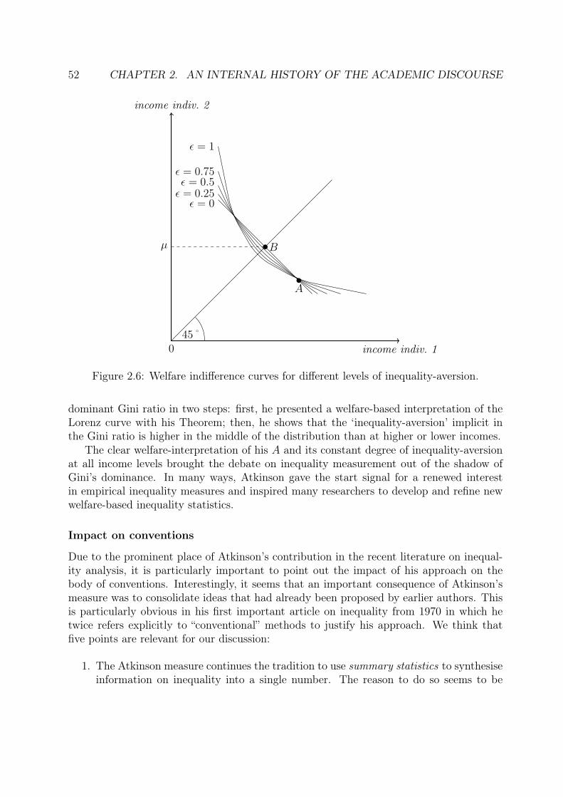
52 CHAPTER 2. AN INTERNAL HISTORY OF THE ACADEMIC DISCOURSE
income indiv. 2
income indiv. 10
ε = 0ε = 0.25ε = 0.5
45˚
B
A
µ
ε = 0.75
ε = 1
Figure 2.6: Welfare indifference curves for different levels of inequality-aversion.
dominant Gini ratio in two steps: first, he presented a welfare-based interpretation of theLorenz curve with his Theorem; then, he shows that the ‘inequality-aversion’ implicit inthe Gini ratio is higher in the middle of the distribution than at higher or lower incomes.
The clear welfare-interpretation of his A and its constant degree of inequality-aversionat all income levels brought the debate on inequality measurement out of the shadow ofGini’s dominance. In many ways, Atkinson gave the start signal for a renewed interestin empirical inequality measures and inspired many researchers to develop and refine newwelfare-based inequality statistics.
Impact on conventions
Due to the prominent place of Atkinson’s contribution in the recent literature on inequal-ity analysis, it is particularly important to point out the impact of his approach on thebody of conventions. Interestingly, it seems that an important consequence of Atkinson’smeasure was to consolidate ideas that had already been proposed by earlier authors. Thisis particularly obvious in his first important article on inequality from 1970 in which hetwice refers explicitly to “conventional” methods to justify his approach. We think thatfive points are relevant for our discussion:
1. The Atkinson measure continues the tradition to use summary statistics to synthesiseinformation on inequality into a single number. The reason to do so seems to be

2.1. FROM CONSTANT INEQUALITY TO COMPLEX INEQUALITIES 53
purely conventional: “The conventional approach in nearly all empirical work is toadopt some summary statistic of inequality such as [...]” (ibid., p. 244).
2. Again with explicit reference to conventions, Atkinson explains why he assumes thatproportional increases of incomes should leave inequality unchanged : “Now we haveseen that nearly all the conventional measures are defined relative to the mean [...]”(ibid., p. 257). With respect to this key assumption, he appropriates the legitimacythat comes with conventional usage and positions his index A in line with Lorenz,Gini, Theil and others. This is a very relevant point since the assumption of meanindependence allows Atkinson to narrow down the possible functional forms of hismeasure to the specific expression of A with a single free parameter ε we exposedabove. Without mean independence, it would be considerably less obvious how toobtain numerical values for A (cf. Kolm, 1976).
3. By placing his approach in the Daltonian welfare framework, Atkinson could presenthis measure as a continuity to an older — almost classic — contribution in inequalitymeasurement. Atkinson consolidated a convention that inequality should be definedand evaluated in terms of welfare: “it seems more reasonable to approach the questiondirectly by considering the social welfare function that we would like to employrather than indirectly through the summary statistical measures” (ibid., p. 257).Through this stance, Atkinson directed the academic discourse further away fromdirect descriptive approaches to inequality measurement and toward the more indirectmethod of evaluating ‘distributional badness’.
4. All of the three preceding points illustrate that it is safe to say that Atkinson pro-longed several pre-existing conventions in inequality measurement. However, he alsoadded a new requirement to the list of desirable features that summary statisticsof inequality should have. He argued that a measure’s sensitivity to transfers fromrich to poor should vary according to the place in the income distribution: transfersat the lower end should decrease inequality more than transfers between two indi-viduals that are already rich. The situation of a millionaire who passes a sum d toanother slightly less well-off millionaire should decrease inequality by less than if dis transferred at subsistence level. The rationale for this additional requirement wasAtkinson’s intuition that constant relative transfer sensitivity “is unlikely to com-mand wide support” (ibid., p. 58). This was an important extension of Dalton’ssimpler ‘principle of transfer’ and has since become a conventional requirement forinequality measure to be acceptable (cf. Kolm, 1976).
5. Related to the two preceding points on this list is the observation that Atkinson’sapproach led to a complexification of the analytical tools of inequality measurement.This complexification can easily be felt if one attempts to lay out the conceptualfoundation of the index A to a non-specialist: not only is it necessary to explainthe framework of utilitarian welfare maximisation. For complete comprehension,

54 CHAPTER 2. AN INTERNAL HISTORY OF THE ACADEMIC DISCOURSE
also the notions ‘equally distributed equivalent income’ and ‘constant relative risk-aversion’ have to be exposed in order to make the core features of A clear to the non-specialist. Probably the explanation would have to involve a detour via the theory ofchoice under uncertainty that we have chosen above. Complexification is obviouslynot objectionable per se, but it reveals that Atkinson prioritizes theoretical overpractical issues as the following quote from his article illustrates: “Much of the earlyliterature was in fact concerned with the problem of choosing between the differentsummary measures, and such properties were discussed as ease of computation, easeof interpretation, the range of variation, and whether they required information aboutthe entire distribution. However, [...] the central issue clearly concerns the underlyingassumption about the form of the social welfare function that is implicit in the choiceof a particular summary measure” (ibid., p. 253). We cannot state more eloquentlythat in Atkinson’s list of priorities ‘ease of interpretation’ clearly ranks behind otherconsiderations of more theoretical nature.
All these points touch core issues of our problem of measuring inequality within theIEWB. We already mentioned repeatedly our intuition that insensitivity to proportionalincreases of all incomes (or ‘constant relative risk-aversion’ as Atkinson calls it) mightnot be an innocuous assumption. We have argued that Atkinson relies without explicitargumentation on several conventional methods and we will have to analyse in Chapter 3whether we are as willing as he was to adopt these conventions at our turn.Next, Atkinson’s impact brings up an important arbitrage between theoretical completenessand internal coherence, on the one hand, and ‘ease of interpretation’ and communicability,on the other. Of course, this arbitrage is not a necessary evil of scientific work sinceinternal coherence and external communicability are not per se opposed. But the natureof the progress in analytical methods that resulted from Atkinson’s contribution — andespecially the cross-fertilization between risk theory and inequality analysis — seems toindicate that this arbitrage might be an important obstacle for a transparent debate oninequality measures. In a way, Atkinson’s approach contains a profound dilemma: he wantsto make normative values more explicit and transparent because “this approach allows usto reject at once those that attract no supporters” (ibid., p. 257); but this very strategycomplexifies his measure to such an extent that potential supporters might not be able tostep up and defend their normative values. The parameter of risk-aversion εmight be a casein point since few people could actively participate in a debate on the degree of concavityof the social welfare function. Hence, more and more actors might be excluded from adebate increasingly dominated by technical specialists. As with any dilemma, we mighthave to chose the smaller evil; in our discussion of inequality measures for the purposeof being a heuristic tool in public debate, we might argue that communicability is moreimportant than technical completeness.

2.1. FROM CONSTANT INEQUALITY TO COMPLEX INEQUALITIES 55
2.1.7 Sen’s conceptual tour de force
The influential book On Economic Inequality synthesised almost all important issues con-cerning the empirical measurement of inequality and proposed an important methodologicalcritique. Jenkins and Micklewright refer to it as “Amartya Sen’s conceptual tour de force”(2007, p. 1). Many of Sen’s ideas found their way into mainstream debates. The UNDPHuman Development Index, first published in 1990, is a prominent example of Sen’s in-fluence since it contains elements of Sen’s approach. Perhaps the deepest impact of Sen’scritique was the tabula rasa question “Inequality of what?”, which was further developedin Sen (1992). However, from the outset of the present text we excluded this very ques-tion from our analysis. Since we have chosen to operate within a predefined frameworkwhich already answers the question of what should be counted — the Index of EconomicWell-Being — Sen’s more general investigation around the question “Inequality of what?”is arguably less relevant for our current purpose. Nevertheless, On Economic Inequality,combined with the revised and extended edition Sen published with J. E. Forster in 1997,contains an array of conceptual interrogations that touch directly on our preoccupations.We will therefore present only some of the features of Sen’s approach on the measurementof inequality, and remind ourselves that this necessarily amputates many important results.We incite the reader to compare or complement our account with the complete texts ofSen (1973, 1992, 1997).
For us, perhaps the most decisive characteristic of Sen’s approach lies in his intermedi-ate position between descriptive or “objective” inequality measurement, on the one hand,and normative or welfare-based assessments, on the other. Sen argues that the conceptinequality has a dual character, blending a descriptive element (‘a cake eaten by two indi-viduals is divided into two equal parts’) and ethical judgements (‘this division is good sinceit yields equal welfare’). When discussing issues like income inequality, the argument goes,the objective and the ethical elements are intertwined: “[...] in some complex problems[...], it becomes very difficult to speak of inequality in a purely objective way, and themeasurement of the inequality level could be intractable without bringing in some ethicalconcepts” (Sen, 1973, p. 3). Sen’s intermediate position between descriptive and normativemeasurement leads to a dual constraint on statistical representations. Inequality statisticsdo not only have to take ‘ethical concepts’ and people’s values into account, they also haveto correspond to what is thought to be an ‘objective’ way to describe the factual state ofeconomic inequality. This is a more restrictive requirement than a purely normative ap-proach based on the evaluation of total welfare, which does not explicitly require objectivedescription. In fact, a welfare approach on inequality does not necessarily correspond toan ‘objective’ description of reality: a perfectly equal fifty-fifty division of a cake may notcorrespond to equal welfare: it suffices to chose different individual welfare functions. Inthis case, equality in the normative sense would correspond to inequality in the descrip-tive sense. In other words, equality of utility from cake consumption does not necessarilymean equality of cake slices. Sen argued that inequality measures must integrate both ofthese elements if they are to be relevant. A statistic that defines equality contrary to the‘objective’ or descriptive notion of equality is according to Sen not usable: “In one way

56 CHAPTER 2. AN INTERNAL HISTORY OF THE ACADEMIC DISCOURSE
or another, usable measures of inequality must combine factual features with normativeones” (ibid., p. 3). The dual constraint that Sen poses on equality metrics introduces anelement to the academic discussion that hitherto had been ignored by most writers: thenew element is “normal communication”, which we have already borrowed for our purposesin the introduction. Sen repeatedly refers to the importance to match academic and nor-mal communication, i.e. the non-expert language used outside technical models on welfareinequality. Consequently, his text is coloured with allusions to a ‘common sense idea ofinequality’ of which we will cite only some examples: “our conception of inequality” (p. 3);“the sense in which the word is used in normal communication” (p. 39); “the meaning asso-ciated with the term” (p. 47); “in terms of definitions corresponding closely to the normalusage of the term inequality” (p. 62); “in normal communication both the normative andthe positive aspect can be observed in the use of the concept of inequality” (p. 63); “sucha measure seems also to be reasonably close to the non-technical concept of inequality asemployed in normal communication” (p. 72); “our standard descriptive understanding ofinequality may conflict sharply with the ‘normative measurement’ of inequality” (p. 119).These quotations illustrate that Sen believes in a relatively clearly defined ‘normal meaning’of the concept inequality, and makes frequent use of this ‘normal meaning’ as an argumentin favour or against features of inequality statistics. In fact, he advocates that the statis-tics should be “reasonably close” to the conception of inequality in normal communication.We will argue below in Chapter 3 that this issue may be less obvious than Sen’s usage ofthe term ‘normal communication’ suggests. It may be worthwhile to analyse if what Senrefers to as ‘normal’, ‘standard’, or ‘non-technical’ corresponds indeed to widely-acceptedconceptions of inequality or if it is limited to the internal academic discourse.
Besides this insistence on a descriptive and common sense approach, Sen’s method ofevaluating inequality rests thoroughly welfarist. Like Dalton and Atkinson, Sen definesinequality in terms of a welfare function, so that much of the discussion is centered aroundthe question which functional specification of welfare is most convenient and reflects bestnormative values. In this context, Sen calls for a radical departure from the utilitarianframework of maximising the simple sum-total of identical individual utilities. In ourdiscussion of Dalton’s measure, we already indicated that a “very special coincidence”leads to the fact that equality is associated with maximum welfare (see Section 2.1.4 onp. 32). Since inequality is not a genuine concern but rather a coincidental byproduct ofthe simple utilitarian framework, Sen proposes to reject it altogether and replace it with arelation between individual incomes and total welfare that directly and explicitly integratesthe preference for equality.
A second mise en question is Sen’s stance toward economic inequality as a relativeconcept, i.e. the idea that inequality measures should remain unchanged if all incomesare multiplied by the same number. This point is somewhat blurred in On Economic In-equality since the argument is structured around the term ‘mean independence’, withoutdistinguishing between proportional and equal additions to income like Dalton had pro-posed in his list of principles (see p. 35). However, it is quite clear that Sen recognizesthe difficulties involved in the assumption of mean independence: “We are caught in a bitof a dilemma here. Making inequality measures independent of the mean income seems

2.1. FROM CONSTANT INEQUALITY TO COMPLEX INEQUALITIES 57
objectionable, but no alternative general assumption about the relationship of the meanincome to these measures seems to be acceptable at all” (ibid., p. 71). However, in theexpanded edition of his book in 1997, Sen seems to have chosen his camp with respect tomean independence from proportional increases: “What happens if welfare is not homo-thetic? We lose the property of mean independence in the normative inequality measure,and this can introduce an ‘absolutist’ element in what is standardly thought of as being arelative concept (that of inequality)” (Sen, 1997, p. 128).21
Finally, another relevant element of Sen’s theoretical observations is that completenessmay not be a reasonable characteristic of inequality measures. This means that a statisticthat generates an unambiguous and complete ranking of all possible income distributionsmay not accurately reflect the concept of inequality: “[...] inequality as a notion does nothave any innate property of ‘completeness’ ” (ibid., p. 47), and measures which generatecomplete rankings of all distributions display more precision than the notion of inequalityitself. If inequality is a ‘fuzzy’ or ‘incomplete’ concept, we may often be faced with compar-isons not allowing for a clear judgement — perhaps not even the clear judgement that twodistributions are equally unequal. This is an important point since all summary measureswe have discussed in this text share the feature of generating complete orderings of distri-butions in terms of their extent of inequality. If the concept inequality is ‘incomplete’, thesemeasures contain some artificial precision and fill in the evaluative void with arbitrariness.By the same token, it follows that if two summary measures, say the Gini and the Theilstatistics, contradict each other in their assessment of the same distributions, this is notnecessarily in discord with the concept of inequality. It could merely be a signal that theunderlying comparison does not allow for a clear decision given the fuzzy character of theinequality notion itself. The hypothesis of incompleteness of inequality gives rise to Sen’smeta-measure which he calls “intersection quasi-orderings” (ibid., pp. 72-74). In a nut-shell, this meta-measure tries to turn the cacophony of partially contradicting inequalitystatistics into a polyphony in which only the harmonic and corroborative elements obtaina voice. The more the different measures included conflict among each other, the morethe meta-ordering is incomplete and indicates the existence of arbitrary decisions if eachof the measures was to be relied upon in isolation. In technical terms, one first defines aset of a priori plausible inequality orderings Cj, for j = 1, ..., k. The intersection of thesek complete orderings is denoted Q and can be written as:
yQx if and only if ∀j = 1, ..., k : yCjx (2.28)
In words, the distribution y is ordered higher than the distribution x if this ordering holdsfor all Cj. If, for instance, we define an intersection quasi-ordering by limiting the plausiblemeasures to the Gini concentration ratio and the interdecile ratio D9/D1, the ordering Qwould only allow us to rank distributions if the ordering CG of the Gini measures does notcontradict the ordering CID of the interdecile ratio. While the intersection quasi-orderingcannot entirely eliminate the arbitrariness — the choice of the measures to be included in
21Sen’s remark cited above refers to the Atkinson measure in which homotheticity of the equally dis-tributed equivalent income function implies mean independence; cf. the footnote on page 49.

58 CHAPTER 2. AN INTERNAL HISTORY OF THE ACADEMIC DISCOURSE
Q is obviously a partially arbitrary one — it has the merit of indicating the situations inwhich simple summary statistics may be misleading. However, the ordering Q is in someways simply a sophisticated version of a much older incomplete ordering which we discussedearlier on. We have seen that the Lorenz curve only generates complete orderings if theconcentration curves do not intersect. Intersecting curves may consequently be interpretedas a sign for ‘blanks’ in our decision-making ability. In light of this similarity between Qand Lorenz comparisons and the remaining arbitrariness of the choice of the orderings Cj,it is unclear whether Q adds much practical value over the more intuitive Lorenz curve.However, if one disagrees with the concept of inequality embedded in the latter, then Sen’sintersection quasi-orderings are indeed an attractive alternative.
Impact on conventions
We already noted that some of the main results of Sen’s treatment of inequality are derivedfrom his interrogations around the question “inequality of what?” which led to the focuson individual capabilities instead of incomes. These results are beyond the reach of ourresearch questions and have therefore a negligible impact on our discussion. Nevertheless,Sen’ contribution to the measurement of inequality remains highly relevant for us. Wewant to stress two points:
1. Sen introduced the notion of normal communication and the common sense defini-tion of inequality to the academic discourse. He insisted on the requirement thatthe scientific measurement of inequality should be “reasonably close” to normal con-ceptions and thereby imposed a constraint that had hitherto been neglected or onlylaxly taken into account. However, while Sen refers to ‘normal communication’ as ifit is something obvious and easily definable, it seems to be less clear how to interpretwhat normal usage constitutes and how the coherence between scientific and ‘normal’language can be verified. Kolm (1976) picked up this point and quotes from personalconversations with friends, Sen himself quotes what he “has heard” in non-technicaldiscussions (ibid., p. 70).
2. The notion of ‘incompleteness’ is an important hypothesis. It calls for prudence notto fully rely on any single summary measure of inequality, no matter how preciseor convenient this statistic may be. For if the concept itself is too fuzzy to allowfor clear-cut decisions, an empirical measure derived from this very concept canhardly attain a higher degree of accuracy than the concept itself. However, even ifthe hypothesis of incompleteness is widely discussed in the theoretic literature, theconventional approach in empirical measurement still illustrates that many authorschose precision in preference to partial orderings.
Since communicability is one of the key concerns for a heuristic tool like the IEWB, Sen’sfrequent allusions to normal communication are close to our research question. However,the insight that economists ‘are not really free to define inequality arbitrarily’ is for usonly a necessary first step. We also need to analyse more precisely how to decide when

2.2. RECENT DEVELOPMENTS: GENERALISATION OF METHODS 59
a scientific definition of inequality is “reasonably close” to normal communication. And,most importantly, we need a more systematic way to ‘read’ and interpret the normal usageof inequality if our measure of inequality within the IEWB is to be useful for public debate.We have argued that Sen uses allusions to normal communication merely as a constraint tothe rather sophisticated usage of the term inequality in the welfare evaluations he discussesor develops. Considering common sense usage as something obvious and given, he doesnot see the necessity of an efficient dialogue between the two spheres. Implicitly, for Senit is rather the economist who casually observes normal conversations who creates thelink between academic and non-academic discourse. We submit that this vision ignoresthe problem of missing feedback loops due to the technical complexity of the analyticaltools involved in the state-of-the-art in inequality measurement. Again, we observe thatinequality statistics are mostly constructed by technical specialists — who assign a centralplace to notions like ‘third order stochastic dominance’ or ‘quasi-concavity’ in their highlydeveloped cognitive apparatus — rather than being co-constructed between experts andusers. In light of these observations, we may argue that Sen’s intersection quasi-orderingQ is an analytically attractive innovation, but it is less clear whether it enhances thetransparency of inequality measurement as a heuristic for public debate.
2.2 Recent developments:generalisation of conventional methods
Sen’s “conceptual tour de force” will be the last contribution we discuss in detail. Toconclude from this that the internal history of empirical inequality measurement has cometo an end after the publication of the extended edition of On Economic Inequality in 1997,or even after the first edition in 1973, would be wrong. In the past four decades, inequalitymeasurement underwent considerable mainstreaming effects, with many new and importantresearch fields entering the literature. However, we argue that the most important parts ofthe standardly used conceptual framework — i.e. the basis of conventional methods — inthe field of income and wealth inequality has probably been shaped in the period betweenPareto’s La courbe de la répartition de la richesse and Sen’s On Economic Inequality. Morerecent contributions have, by and large, focused on extensions, refinements or improvementsof existing approaches. This does of course not mean that these contributions are lessuseful or less innovative. But for our question of measuring inequality in the frameworkof the IEWB, it was more important to analyse the foundations of today’s state-of-the-art measurement than the current form of the methods. The impressive development ofanalytical methods in the last decades was only possible because they could refer to a moreor less coherent body of conventions, and it was the genesis of this body of conventionsthat we have tried to sketch in the present chapter.
Before we continue, we should stress that what we said in the preceding paragraphholds only for our research problem of measuring inequalities within the IEWB framework,and not for inequality analysis in general. In fact, in the wider field of inequality analysis

60 CHAPTER 2. AN INTERNAL HISTORY OF THE ACADEMIC DISCOURSE
important conceptual changes occurred so that the conventional methods have been alteredsignificantly in many ways. The increasing use of multi-dimensional inequality measuresis perhaps the most influential development and modified our perception of inequalityin general. Different influences — many of which emanating from very diverse actorsincluding civil society, governmental agencies and researchers — have led to an expansionof the uni-dimensional monetary view on economic inequality and toward a perspectivein which differences in other spheres like social status, education, working conditions,access to health services or other utilities etc. are also taken into account. In France, theRéseau d’Alerte sur les Inégalités regularly voices concerns regarding the predominanceof monetary measures and presented an alternative inequality measurement called theBaromètre des inégalités et de la pauvreté, or BIP40. To a certain extent the HumanDevelopment Index developed by the UNDP is a result of similar interrogations. LarsOsberg and Andrew Sharpe’s Index of Economic Well-Being, which we used as point ofdeparture for the present text is another example of multidimensional approaches. Ourresearch questions are thus a result from this shift toward an extension of the evaluationspace and the use of multi-dimensional measurement.
However, within the more restricted field of income and wealth measurement, a processof consolidation and improvement of conventional approaches seems to have marked therecent decades. This can be seen in the extremely useful overview on inequality analysis byJenkins & Micklewright (2007). While these authors underline the importance of the abovementioned tendency toward multidimensional approaches to inequality, most of the recentcontributions to the field of income and wealth inequality they discuss have been of moretechnical than conceptual. In terms of their conceptual frameworks, recent contributionsare all more or less based on the ideas developed by Lorenz, Gini, Theil, Atkinson and Sen.
1. The Lorenz curve and Atkinson’s Theorem have been extended into generalisedLorenz dominance and stochastic dominance by Shorrocks (1983), Foster and Shorrocks(1987) and others.
2. Atkinson’s measure has been generalised and gave birth to the “Atkinson familiy”(Jenkins & Micklewright, 2007, p. 13). The derivation of classes of parametric sum-mary indices with explicit normative characteristics that Atkinson proposed was sys-tematized and extended.
3. Theil’s decomposable index has inspired the generalized entropy class of inequalitymeasures, developed by Bourguignon (1979) and others.
4. Other developments, such as the systematic treatment of sampling errors and thederivation of confidence intervals for inequality measures proposed by Beach andDavidson (1983), were also directly based on Lorenz and generalized Lorenz curves.
5. Paglin’s (1975) critique not to confuse intra-family and inter -famliy inequality wasessentially an extension of the Gini concentration ratio and the Lorenz approach.

2.3. CLOSER TO ‘TRUTH’ OR AWAY FROM ‘NORMAL COMMUNICATION’? 61
This list suggests that the recent developments in empirical inequality measurement ofwealth and income have focused on the improvement of analytical methods. This progress isa consequence of the fact that older contributions, above all the Lorenz-Gini concentrationmeasure and the Dalton-Atkinson welfare approach, have become accepted and legitimateconventions. Due to the generalisations and extensions that occurred in recent decades, itis safe to say that the exercise of inequality measurement today is a much more complexand technical undertaking than it has ever been before.
2.3 Closer to the ‘truth’ or further away from ‘normalcommunication’?
In this chapter we have presented the scientific contributions that share the property ofhaving influenced significantly the way in which inequality is traditionally measured ineconomics. We have tried to assess their impact by naming explicitly the conventionsthat appear to be most relevant for our purpose of measuring inequality in the frameworkof the IEWB. The nature of the IEWB implies necessarily to leave the internal debatewithin the scientific community and bring in more external considerations such as ‘whoare the users of inequality measures?’ and ‘how do these users think about inequalities?’.For if the IEWB in general, and its inequality dimension in specific, is to be useful andlegitimate, the output of the internal debate on inequality measurement has to correspondto its external usage. From the elements we have presented in this chapter we can alreadyidentify some general problems that arise from the confrontation between internal scientificdiscourse and external usage.
The arbitrage between communicability and analytical completeness
There is an important arbitrage between the purity and completeness of the scientific treat-ment of economic inequality, on the one hand, and the communicability and transparency ofthe resulting statistics, on the other. Due to the analytical progress over the past hundredyears this arbitrage has become more and more uncomfortable and it is difficult to verifythe coherence of the scientific discourse with normal communication. The shift from purelydescriptive inequality analysis to welfare-based representations — initiated by Dalton andcontinued by Atkinson, Sen and others — has largely contributed to this complexification.In order to communicate welfare measures, the underlying welfare framework has to be ex-plained in more or less detail. This is particularly obvious in the case of parametric indicessuch as the Atkinson measure since the notion of inequality-aversion it contains can hardlybe understood without some insights into the theory of welfare functions, including thedegree of concavity of indifference curves at different levels of welfare. The Atkinson mea-sure is also a good example of the paradox involved in the process of improving inequalitymeasurement in economics. As a matter of fact, the rationale of the systematic derivationof parametric welfare functions is to produce inequality statistics that correspond closelyto normative values of society. In a way, the objective of improvements in the analytical
62 CHAPTER 2. AN INTERNAL HISTORY OF THE ACADEMIC DISCOURSE
apparatus has been to come closer to the ‘true’ concept of inequality given societal repre-sentations. However, we note that this very objective has led to the exclusion of more andmore actors from the debate on inequality and the construction of inequality indicators.For example, it is hard to verify whether the idea that welfare indifference curves displaya constant degree of convexity and are all radial copies of each other actually correspondsto inequality in the common-sense usage of the term. Osberg phrased the general problemfaced by economists very eloquently: “Public debate might well be improved if we couldconsider explicitly some of the aspects of economic well-being [...], but public debate willnot be assisted by an incomprehensible deluge of esoteric statistics” (1985, p. 73). To makeit clear: we do not cast any doubt on the sincerity or even the accuracy of the scientificresults we have discussed in this chapter. But economics arguably stands to gain by raisingawareness of the arbitrage we mentioned above.
The advantage of a descriptive approach
In light of this arbitrage, the distinction between descriptive and normative measures ofinequality becomes more relevant again. The explicit inclusion of normative values almostmechanically increases complexity and decreases communicability. The more we want toemphasise the interaction between internal and external spheres, the stronger will be thecase for employing purely descriptive measures — even if these include some implicit valuejudgements. These implicit values could be the kind of sacrifice we have to make by movingaway from analytical completeness toward external communicability.
Is inequality a relative or an absolute concept?
Given the difficulty to verify whether the complex scientific ‘truth’ corresponds to normalcommunication, we are ipso facto in an uncomfortable position when we want to analyseif current academic conventions are acceptable for the purpose of the IEWB. However, weintuitively feel that some of the more fundamental conventions require further attention.The convention contained in the Lorenz curve, the Gini concentration, the Theil measureand the Atkinson index of assuming that only the ratios of incomes, and not absolutedifferences, are ‘inequalities’ seems questionable. As a matter of fact, the emphasis onabsolute income differences is nothing new. Kolm (1976) and Blackorby & Donaldson(1980) have already stressed the plausibility of this alternative point of view. Interestingly,these contributions are extremely technical — Kolm employs a mathematically elegantapproach with a rigorous axiomatic — and did not significantly alter the standard body ofconventions (which is also why we excluded them from a detailed analysis in this chapter).We will present further arguments in favour of an absolute element in inequality statisticsin the next chapter.

Chapter 3
Inequality measurement within theIEWB framework
3.1 A brief introduction to Osberg and Sharpe’s Indexof Economic Well-Being
The Index of Economic Well-Being was above all conceived as an instrument for publicdebate. In his first article on the topic from 1985, Lars Osberg explicitly mentions theRoyal Commission on Economic Prospects, a Canadian body charged with the assessmentof economic policies of the government, as an institution that is concerned with evaluationsof overall economic well-being and therefore a potential user of the IEWB. In anotherexample, Osberg derives the necessity of a synthetic indicator from the need to evaluatethe performance of politicians (he mentions Ronald Reagan, who asked his electorate in1980 the question ‘Are you better off today than you were four years ago?’; ibid., p. 49).
An explicit objective of the IEWB is to present an alternative to Gross Domestic Prod-uct (GDP) as measure of economic welfare, mainly because “national income accountingmeasures may sometimes not agree with popular perceptions of trends in economic well-being” (Osberg & Sharpe, 2005, p. 311-312). As a matter of fact, the correspondancebetween normal communication and statistical representations appears repeatedly in thecontributions of the two Canadian authors. In fact, the IEWB is presented as a measurecloser to “popular perceptions”.
Furthermore, Osberg and Sharpe stress that the IEWB is not a single objective num-ber: “It is more accurate, in our view, to think of each individual in society as makinga subjective evaluation of objective data in coming to a personal conclusion about soci-ety’s well-being” (ibid., p. 313). The authors conceive their statistical tool to be useful forboth public administration staff and common people. They argue that the IEWB can helpindividuals to make informed choices:
“Citizens are interested in evaluating the well-being of their country, partly be-cause all adults are occasionally called upon, in a democracy, to exercise choices
63

64 CHAPTER 3. REVISION OF INEQUALITY IN THE IEWB
(e.g. in voting) on issues that affect the collectivity (and some individuals, suchas civil servants, have to make such decisions on a daily basis). [...] Hence,although self-interest may play some role in each individual’s evaluation of so-cietal outcomes, citizens have a number of reasons to ask questions of the form:‘Is my country better off’?” (ibid., p. 313).
The authors clearly point out that “the purpose of index construction should be to assistindividuals — e.g. as voters in elections and as bureaucrats in policy making — in thinkingsystematically about national outcomes and public policy” (ibid., p. 314). The user of theIEWB should therefore not be thought of as a technical specialist using well-being statisticsas material for sophisticated scientific analysis, but rather as a non-expert (the “citizen”)looking for an informed vision on overall well-being.
Genesis of the IEWB
The founding-stone of the house that was to become today’s index of economic well-beingwas already laid by Lars Osberg in 1985. This article contained a concrete frameworkof variables divided into four categories, although no empirical application was includedat the time. The variables retained on a preliminary list were selected in terms of dataavailability and contextual fit. In the last twenty years, this framework underwent onlyminor modifications and is hence to a large extent identical with the presentation in thenext section.
Despite the concreteness and applicability of Osberg’s measurement tool, which includesno formal model but a weighted index of components assumed to represent societal well-being, no implementation was published for 13 years. Osberg & Sharpe (1998) eventuallypresented the first index of economic well-being for Canada, covering the period from1971 to 1997. Two years later, Osberg & Sharpe (2001) tabled an index for the UnitedStates. Osberg & Sharpe (2002) extended the framework to allow for a comparison ofseven countries: Australia, Canada, Germany, Norway, Sweden, UK, and the USA for theperiod from 1981 to 1996. An updated and slightly modified version for this set of countriescan be found in Osberg & Sharpe (2005). This last version recommends the use of theIEWB as substitute of per capita GDP in the UNDP’s Human Development Index (HDI).To this end, the authors slightly modify their scaling technique and apply a logarithmicconversion to all sub-indicators. In addition to these societal IEWB, Osberg and Sharpeproposed applications of the general four dimensional framework to the labour market forNorth America (Osberg & Sharpe, 2001) and 16 OECD countries (Osberg & Sharpe, 2003).The IEWB has received international attention in debates on social well-being (cf. OECD,2002).

3.1. INTRODUCTION TO THE INDEX OF ECONOMIC WELL-BEING 65
Overview of the IEWB methodology
The IEWB consists of four main dimensions which in turn are set up by a varying numberof variables.1 In all, the full fledged indicator as in the seven-country version requires 38different variables . The four dimensions, as stated in Osberg & Sharpe (2005), are:
“(1) Effective per capita consumption flows — which differ from the consump-tion of marketed goods and services included in GDP by including the value ofgovernment services and adjusting effective per capita consumption flows to ac-count for household production, changing household economies of scale, leisureand life expectancy.(2) Net national accumulation of stocks of productive resources — which addsnet changes in the value of natural resources stocks, environmental costs, netchange in level of foreign indebtedness, net accumulation of human capital andR&D investment to the net investment in tangible capital and housing stocksnow measured in GDP.(3) Income distribution — the intensity of poverty (incidence and depth) andthe inequality of income.(4) Economic security — from the financial implications of job loss, illness,family break-up and from poverty in old age.”
The different components of the IEWB often blend very distinct concepts. For instance,the index includes such different variables as average household size and the level of netforeign indebtedness. Few people would argue that these variables are direcetly compara-ble. Nevertheless, Osberg and Sharpe put forward the proposition that economic decisionmaking and policy evaluation necessarily boils down to “ ‘adding it all up’-across domainsthat are conceptually dissimilar”. This procedure of “adding it all up” does not mean thatwe leave the grounds of an economic, material analysis of well-being. In Table 3.1, as welltaken from Osberg & Sharpe (2005), each of the four IEWB dimensions is linked to a timeperiod and a conceptual view.
Time periodConcept Present Future‘Typical citizen’ or‘representative agent’
Average flow of current in-come
Aggregate accumulation ofproductive stocks
Heterogeneous citi-zens
Distribution — income in-equality and poverty
Insecurity of future income
Table 3.1: Concepts in the IEWB — Source: Osberg & Sharpe (2005).
There is no homogeneous method of compiling the variables inside each dimension. Insome cases multiplicative indices are used, in others weighted averages or simply sums of
1The description of the IEWB methodology in this section is necessarily superficial. For more detailedexplications the interested reader is referred to Osberg & Sharpe, 2005.

66 CHAPTER 3. REVISION OF INEQUALITY IN THE IEWB
the underlying variables. In addition, each variable has its own definition. In most casesthe conventional nature of this definition does not require a detailed description (e.g. thevariable personal consumption per capita simply uses the definition specified by the nationalaccountancy). However, other variables were introduced by Osberg and Sharpe and theirinterpretation requires more information (e.g. the computation of the value of leisureinvolves information such as average wages, average numbers worked, national hours ofunemployment etc.). In order to provide a transparent view on the overall indicator and tooffer a glimpse at its complexity, the following figures illustrate how the four sub-indicatorsare created. The graphs are only horizontally exhaustive, in the sense that more verticallevels could be included to depict in more detail the construction of all variables.
Real totalconsumption
p.c.=
Index of lifeexpectancy*
Govern.spending(goods &services)
+Value ofleisure
+Index ofhousehold
size*
Personalconsumption
p.c.
Figure 3.1: Component 1 — consumption flows.
The first IEWB component is a measure of effective per capita consumption, whereasadjustments are made to take into account household economies of scale, the value ofleisure, individual consumption of government spending and life expectancy.
The second component — real stocks of wealth per capita — includes a monetarisedvariable measuring the negative externality of economic activity on the environment. Os-berg & Sharpe (2005) proposed to estimate the social cost of greenhouse gas emissions inwealth by multiplying total emission with a fixed cost per ton.
Component 3 (equality and poverty) is constructed exclusively with three variables andis itself a synthetic indicator of monetary equality and poverty. The product of povertyrate and poverty gap ratio is referred to as ‘poverty intensity’. It should be noted thatthis measure could be replaced by the modified Sen-Shorrocks-Thon index as discussed byOsberg & Xu (2000), thus integrating besides the poverty rate and the (average) povertygap ratio also the inequality of poverty gaps .
Component 4 (economic security) includes as well certain poverty rates and gaps(Fig. 3.4). However, it does not serve the purpose of measuring the poverty itself, butrather the risk to economic security borne by economic agents. The IEWB proposes to

3.1. INTRODUCTION TO THE INDEX OF ECONOMIC WELL-BEING 67
Stocks ofwealth
=
Real socialcost of CO2
p.c.+
Real netforeign debt
p.c.+
Humancapital stock
p.c.+
Real R&Dstock p.c.
+Real capitalstock p.c.
Figure 3.2: Component 2 — stocks of wealth.
Equality andpoverty
=
Ginicoefficient of
incomes0.25*+
Povertyintensity0.75*
Figure 3.3: Component 3 — equality and poverty.
identify only some relevant economic risks and trace their evolution, instead of measur-ing and compiling all conceivable risks. It should be noted that this notion of security is— analogous to the monetary poverty rate — not the ‘true’ security that agents enjoy.It is merely a proxy of the material risks that arise from uncertain factors like illness,unemployment or divorce.
Once the evolution of the four basic components is known, a weighting scheme allowsaggregating them into a single number: the index of economic well-being. The weightsattached to each dimension are ex natura rei arbitrary. Osberg and Sharpe have argued thata transparent aggregation is essential so that each user can modify the weights according toher preferences and to help consensus-building on societal preferences. The two weightingschemes currently in discussion are 1) equal weights for all sub-components, and 2) a moreprominent impact of consumption, namely 0.4×consumption flows+0.1×wealth stocks+0.25× equality + 0.25× security.

68 CHAPTER 3. REVISION OF INEQUALITY IN THE IEWB
EconomicSecurity
=
(Risk frompoverty in oldage)*(P4/P )
+
(Risk fromsingle
parenthoodpoverty)*(P3/P )
+
(Risk tofinancial
security fromillness)*(P2/P )
+
(Risk fromunemploy-ment)
*(P1/P )
Figure 3.4: Component 4 — economic security. Legend: P1 = Population aged 15-64;P2 = all persons; P3 = married woman with children; P4 = population aged 45-64. P =P1 + P2 + P3 + P4.
3.2 Four dimensions, three inequalities
In the preceding section we have presented the IEWB in its original form proposed byOsberg and Sharpe. We emphasised our opinion that the Index is a useful tool for publicpolicy analysis, which motivated our application of the IEWB to French data in an earliercommunication (op. cit.). Nevertheless, we noted an inconsistency in its internal structurethat arises from the way in which the IEWB accounts for economic inequality. As amatter of fact, the current version of the Index only measures income inequality, therebyneglecting the distribution of wealth and economic risk. However, the choice of the fourdimensions we presented in the preceding section is based on the assumption that not onlyincome, but also wealth and economic risk have a significant impact on economic well-being.Consequently, not only the level of consumption, wealth and economic risk should enter theIEWB, but also the inequalities in exactly these dimensions. In other words, if we believethat economic well-being is composed of multiple dimensions, economic inequality shouldalso consist of these multiple elements. We argue that most people think of inequalitiesof wealth or economic risk as being important. Measuring inequalities in the three IEWBdimensions would render the overall Index more consistent and provides a more accuratevision on economic well-being.
Fig. 3.5 illustrates our proposal to analyse three aspects of economic inequality. Thethree IEWB components effective consumption per capita, accumulated stocks of wealthper capita and economic security give rise to three spaces of inequalities: the distribution ofper capita consumption; the distribution of accumulated wealth per capita; and inequalityof exposure to economic risks. The modified third IEWB component that results from ourproposal is presented in Fig. 3.6.
On a conceptual level, we think that this amendment is consistent with the idea ofeconomic well-being contained in the IEWB and relatively easy to communicate. However,it is considerably more difficult to measure economic inequality in various dimensionssimultaneously, and hence to operationalise the logic of Fig. 3.5. Translating our conceptualmodification into a quantitative measure is a difficult endeavour given the incomplete

3.2. FOUR DIMENSIONS, THREE INEQUALITIES 69
Real totalconsumption
Distributionof p.c. con-sumption
Distributionof
accumulatedwealth p.c.
Stocks ofwealth
Inequalitiesof risk
exposure
Economicsecurity
Economicequality
Figure 3.5: Proposal for inequality measurement in the IEWB.
Equality andpoverty
=
Economicequality0.25*+
Povertyintensity0.75*
Figure 3.6: Modified Component 3 — equality and poverty.
nature of the data. To be entirely consistent with the definitions presented in the precedingsection, a measure of the inequality of effective consumption per capita would have to takeinto account the differences in household sizes, leisure consumption, consumption of goodsand services provided by the government and, finally, the differences in life expectancyamong the households. The second IEWB dimension, accumulated stocks of wealth, is evenmore problematic: next to household differences in per capita capital stocks, we would haveto account for differences in the level of human capital stock between households. Andit is unclear how to measure the distribution of R&D capital and the incidence of thenational foreign debt or of the environmental liabilities on particular households. Alsoin the third dimension, economic security, inequality between households is problematic.In fact, some risks are by definition not borne by all households since they are restrictedto a particular socio-demographic profile (e.g. old age and single mother poverty). Thisrenders comparisons of economic security, for instance between a single mother householdand a household of retirees, very delicate. We will discuss these problems in more detailin Section 4.1.

70 CHAPTER 3. REVISION OF INEQUALITY IN THE IEWB
3.3 Alternative proposals to measure inequality
In the preceding section we treated the question which inequalities we would like to mea-sure: our empirical measurement should reflect inequalities in the IEWB dimensions effec-tive consumption, accumulated wealth and economic risk. We now need to operationalisethe inequality measurement.
In Chapter 2 the most important inequality statistics have been discussed. We havepaid particular attention to point out in how far these measures modified the often implicitconventions in today’s analysis of economic inequality by scientific experts. To summarisethe most relevant points, it is safe to say that the internal, i.e. academic, discourse ineconomics can be characterised by a large consensus on several conventional methods:a) if theoretical correctness and simplicity conflict with each other, it seems that technicalcompleteness is frequently given priority over ease of interpretation and communicability(cf. Atkinson, 1970, p. 253); b) quantitative analysis is undoubtedly the dominant approachto economic inequality; c) the acceptability of alternative inequality statistics is convention-ally tested indirectly with the help of a list of desirable features; d) despite Sen’s critiqueon the arbitrary element in complete orderings, most authors continue to employ summarystatistics to compare the degree of inequality of different distributions; e) concentrationand inequality are widely regarded as “essentially the same concept” (Theil, 1964, p. 128).
We have argued in Section 3.1 that the IEWB user should not be thought of as atechnical expert, but rather as the average citizen looking for comprehensive informationon the ‘big picture’ of economic well-being. The radius of actors thus extended beyondacademic circles and we therefore have to confront the scientific representations with a moreexternal viewpoint. Clearly, inequality measurement in the IEWB should be as close aspossible to what Sen referred to as “normal communication”, and what Osberg and Sharpecall “popular perceptions”. At the same time, we have to be aware that these notions will notallow us to identify a precise definition of inequality. This is due to the fact that there is notone ‘typical citizen’, but a heterogeneous mass of different perceptions, representations andvalues as regards inequality. In other words, it is impossible to prove the correctness of anydefinition if our only criteria is the blurry notion of normal communication. Nevertheless,we argue that the legitimacy of the IEWB depends on the degree in which its inequalitymeasure is co-constructed and takes into account internal and external considerations. Wetherefore examine to what extent the conventions listed above are legitimate in light of thespecific purpose and the potential users of the IEWB.
First, it is obvious that the arbitrage between theoretical completeness and communica-bility has to be re-considered. Not only the final result, but also details of the computationof inequality measures have to be transparent and easily communicable. Otherwise theimportant feedback from external actors on these statistics is very difficult and measuresrisk to be constructed by experts rather than being co-constructed.Second, a quantitative approach to the measurement of inequality remains useful. If
individuals seek to compare different aspects of well-being, eventually the inherent diver-sity has to be reduced in order to evaluate the overall development. The index approachproposed by Osberg and Sharpe is a transparent and useful way to aggregate the compo-

3.3. ALTERNATIVE PROPOSALS TO MEASURE INEQUALITY 71
nents of economic well-being and preserves the possibility for individuals to attach differentweights to each of these components.Third, the convention to spell our different features of inequality measures and test theiracceptability can be an efficient way to stimulate feedback from external actors as it ren-ders underlying assumptions and characteristics more explicit. The fuzzy character of theconcept inequality contributes to the attractiveness of such an indirect approach to theconstruction of inequality measures. However, special attention has to be paid to renderthe list of desirable features accessible and avoid unnecessary technical complexity.Fourth, the completeness of summary measures is both an advantage and a problem forinequality measurement in the framework of the IEWB. Although Sen’s intersection order-ings probably reduce effectively the extent of arbitrary information, at the same time theymay increase the amount of redundant or unnecessary information. The advantage of anintersection ordering is that it allows to identify situations in which comparisons betweendistributions are difficult. But to construct a particular intersection ordering, an agreementhas to be achieved as to which summary measures should be included in the ordering. Andeventually, all included statistics have to be computed and their results compared. This in-flates the complexity of inequality measurement, as users are confronted with a panoply ofdifferent measures based on a variety of concepts. By contrast, the use of a single approachdiminishes considerably the amount of unnecessary information contained in the well-beingindex. With respect to what we said about the arbitrage between theoretical completenessand communicability, we argue in favour of a single approach which nevertheless shouldallow for different normative opinions.Fifth, it is doubtful whether inequality is always thought of as concentration and as beingindependent to proportional increases. This point merits to be discussed in some detail.
We are here confronted with two different normative views on the concept inequality:on the one hand, we have relative inequality, which is insensitive to proportional increasesof all incomes, and absolute inequality on the other. Of course, both views are a priorivalid and it seems that both are able to generate support from many people. However, aswe have seen in our discussion, mainstream academic literature in economics tends to takerelative inequality for granted, which is why we focus here on the arguments indicatingthat popular perceptions may at least in part regard inequality as containing an absoluteelement.
Arguably the most frequently used expression in normal communication to describeinequality is the “gap between rich and poor”. We think that few people would seriouslyargue that inequality is not at all related to the gap between rich and poor. While theterms ‘poor’ and ‘rich’ are both problematic and difficult to operationalise in statisticalterms, the point is that a gap does not exclude a difference in absolute terms and thereforedoes not systematically refer to ratios rather than differences of monetary amounts. It isnot aberrant to believe that most people are unconscious whether they refer to an absoluteor a relative concept when they speak of the gap between rich and poor. Nevertheless, weshould note that this frequently used expression for inequality can hardly be interpretedas a clear indicator for the relative point of view.
In line with the idea of inequality as gap, it can often be observed in public debate on

72 CHAPTER 3. REVISION OF INEQUALITY IN THE IEWB
economic inequality that people tend to oppose the fate of the lower classes with the numberof the proverbial ‘millionaires’. Sometimes even governmental reports have to include thenumber of millionaires in their assessment of economic inequality. This can be seen inthe two reports on poverty and wealth published by the German Ministry for Labour andSocial Affairs (BMAS) in 2001 and 2005. Both reports contain warnings to interpret thenumber of millionaires as a sign for increasing wealth or inequality. Nevertheless, in achapter under the plain title “Millionäre”, the interested citizen finds information aboutthe evolution of the number of inflation-corrected millionaires in Germany. The reason issimple: “In the general discussion the notion of the millionaire is often used as a synonym forproperty wealth” (BMAS, p. 47) and, combined with the number of non-millionaires, partof the common perception of inequality. Hence, although one million is an absolute amountmoney, many people tend to think that an information on the number of millionaires isuseful to evaluate economic inequality. When in the process of economic growth the numberof millionaires increases, while at the same time the low-skilled worker only notes a mereplus of 20 eon his payroll, he may very well be ignorant enough to contradict mainstreameconomics and interpret this development as an increase in inequality — although incomeratios might have remained the same.
It should be noted that the notion of ‘absolute’ inequality is not completely absent fromthe academic debate. A precursor in this field is Kolm (1976), who cites from personalconversations to come to the conclusion that it is “no less legitimate to attach the inequalitybetween two incomes to their difference than to their ratio” (ibid., p. 419). Unsurprisingly,Kolm brings in non-scientific actors to illustrate his point:
“In May 1968 in France, radical students triggered a student upheaval whichinduced a workers’ general strike. All this was ended by the Grenelle agreementswhich decreed a 13 % increase in all payrolls. Thus, labourers earning 80 poundsa month received 10 pounds more, whereas executives who already earned 800pounds a month received 100 pounds more. The Radicals felt bitter and cheated;in their view, this widely increased incomes inequality. But this would have leftunchanged an inequality index Ir [the Atkinson index] computed according tothe above formula. [...] In other countries (I have been quoted examples fromEngland and The Netherlands), trade unions are more clever and often insist onequal absolute, rather than relative, increases in remuneration, so as to avoidthe above effect. And I have found many people who feel that it is an equalabsolute increase in all incomes which does not augment inequality, whereas anequiproportional increase makes income distribution less equal or more unequal— and these were people of moderate views.” (ibid., p. 419)
Kolm translates this reasoning into a class of absolute measures of inequality and dis-cusses some of its properties. However, with some exceptions like the extension of Blackorby& Donaldson (1980), the absolute statistic introduced by Kolm has not significantly alteredthe academic focus on relative measures of inequality. This may be due to the fact that histext is extremely technical, without easy graphical interpretation and rather inaccessible

3.3. ALTERNATIVE PROPOSALS TO MEASURE INEQUALITY 73
to most lay readers. Nevertheless, Kolm should be credited for pointing out that the di-chotomy of absolute versus relative measures contains a political dimension. As a matterof fact, the letter ‘r’ with which Kolm indexes the Atkinson measure in the above quotestands for “right”. Kolm’s own measure based on inequality of differences (instead of ratios)is indexed with “l” for “left”. While this division into political camps should not be takentoo literally, Kolm uses it to interpret the many scientific contributions in economics infavour of relative measures: they “tend to support Abba Lerner’s contention that economicscience tends to shift its servants to the right” (ibid., p. 420).
Thirty years after Kolm’s introduction of ‘absolute’ inequality, the proponents of thisview still tend to be associated with a ‘left-wing’ political stance. Mostly individuals whoare critical of market capitalism and economic globalisation tend to emphasise growingdifferences in absolute income levels between inhabitants of the same country or betweendifferent economies. Martin Ravallion, in an examination into the reasons why globalisationoften tends to provoke diametrically opposed opinions, points out that relative inequalityis not the only defensible concept. Ravallion underlines that ‘anti-globalisation’ protestersdo not necessarily get the numbers wrong when they criticize free trade and the faith ineconomic growth. Perhaps they simply do not have relative, but absolute differences inmind: “Perceptions on the ground that ‘inequality is rising’ appear often to be referring tothis concept of inequality” (2003, p. 742).
In one of the few experiments on the question carried out by Amiel & Cowell (1999) withstudents from Israel and the UK, the results show that 40 % of the participants thoughtabout inequality in absolute terms. However, we have reason to believe that BehaviouralEconomics can hardy be expected to solve the problem of agreeing on a relative or absolutemeasure of inequality. If we follow Kolm and Ravallion and interpret the alternative viewson inequality as reflecting political attitudes, democratic elections are probably bettersuited to answer this question than scientific experiments.
Together, the five points we have discussed in this section indicate what type of in-equality measure we should employ for the IEWB. We have expressed our opinion thatcommunicability is one of the key features in our context and should be preferred overmore theoretically complete instruments such as intersection orderings. Furthermore, wewant to keep the index form of the IEWB and therefore look for a quantitative summarymeasure. The opposition between absolute and relative measures of inequality cannot bedecided upon since it may reflect political or ethical opinions which tend to co-exist in mostdemocratic societies. The citizen should be able to form an opinion about economic well-being according to her opinions and we should not impose either of the two alternatives.This is consistent with Osberg and Sharpe’s stance to leave the weights of the dimensionsopen to discuss so as to match the user’s values. In the next section we will illustrate whywe think that the following two alternative measures for the three-dimensional inequalityin the IEWB satisfy these considerations:
1. An easily communicable and intuitive measure of inequality is a three-dimensionalmean difference. When we think of each dimension of inequality as a dimension of aspace, each household can be treated as a point in this space. The inequality between

74 CHAPTER 3. REVISION OF INEQUALITY IN THE IEWB
two households is then the gap — or distance — between their respective points andthe total inequality is the average gap between all household. This is an absolutemeasure of inequality.
2. All distances of first measure can be divided by the mean of the different dimensions.This yields a three-dimensional relative mean difference. While this sacrifices someof the intuitive appeal of distances between points in a space, it has the advantageof being very similar to the Gini ratio. It is a relative measure of inequality.
These two measures are far less sophisticated than the state-of-the-art statistics derivedfrom welfare functions and thus subject to their criticism. However, they are also lesscomplicated than welfare-based measures and therefore better suited for the IEWB. Theyshould be thought of as a compromise in the arbitrage between theoretical purity andcommunicability: both are based on the same concept of inequality as gap, but neverthelessallow for two alternative value judgements.
3.3.1 Measuring differences: a geometric approach
The two measures we presented in the preceding section have the advantage of allowing fora relatively easy graphical representation. Since the dimensions of inequality we want toanalyse form an Euclidean space, the absolute differences between households can simplybe calculated as Euclidean distances. The Euclidean distance between two points Pi =(pi,1, pi,2, . . . , pi,n) and Pj = (pj,1, pj,2, . . . , pj,n), in a Euclidean n-space, is defined as:
PiPj =√
(pi,1 − pj,1)2 + · · ·+ (pi,n − pj,n)2 =
√√√√ n∑d=1
(pi,d − pj,d)2
In a one dimensional space, which we will denote d, the Euclidean distance between twopoints is equal to the absolute difference between their coordinates. If we write the twopoints as Pi = (pi,d) and Pj = (pj,d), their Euclidean distance is equal to:
PiPjd
=√
(pi,d − pj,d)2 = |pi,d − pj,d|
It is easy to see that Gini’s absolute differences we presented in Section 2.1.3 can beexpressed as one-dimensional Euclidean distances. We recall the formula for the absolutemean difference (AMD):
AMD =
∑Ni=1
∑Nj=1 |yi − yj|N2
Gini’s AMD is thus the average Euclidean distance between all possible pairs of the Npoints Pi, i = 1, · · · , N in a one-dimensional Euclidean space. Interpreting the incomes asone-dimensional vectors, the AMD can thus be written as:
AMDd =
∑Ni=1
∑Nj=1
√(pi,d − pj,d)2
N2(3.1)

3.3. ALTERNATIVE PROPOSALS TO MEASURE INEQUALITY 75
To obtain an expression for the relative mean difference in Euclidean space, we replace theaverage income µ by the average length λ of the income vectors:
RMDd =AMDd
λwhere λ =
∑Ni=1
√p2i,d
N
The advantage of using the Euclidean space is the possibility to increase the number ofdimensions for which we want to evaluate inequalities. If we want to measure inequalityin n dimensions, the absolute and relative mean differences become:
AMD =
∑Ni=1
∑Nj=1
√∑nd=1(pi,d − pj,d)2
N2(3.2)
RMD =AMDλ
where λ =
∑Ni=1
√∑nd=1 p
2i,d
N
For up to three dimensions the inequalities can be easily represented graphically. We willillustrate this with an example of three households and a three-dimensional space (thesedimensions could represent different dimensions for which we want to measure inequality).Each household is characterised by one value for each of the three dimensions. These threevalues are interpreted as a vector in the three-dimensional space (we can think of them as apoint in this space). In our example, we assign the respective values of P1 = (0.5, 0.5, 0.5),P2 = (0.5, 0.5, 0) and P3 = (0, 1, 1) to the three households. Their distances are illustratedin Fig. 3.7. We can also compute the AMD for the three points in our example. From the
dimension 2
dimension 1
dimension 3
P1
P2
P3 P1P2
P2P3
P1P3
Figure 3.7: Illustration of three-dimensional inequality as geometric distances.
formula 3.2 we see that there are nine possible pairs between the three points:
AMD =P1P1 + P1P2 + P1P3 + P2P1 + P2P2 + P2P3 + P3P1 + P3P2 + P3P3
32

76 CHAPTER 3. REVISION OF INEQUALITY IN THE IEWB
The numerical values for these distances are:
P1P2 = P2P1 =√
02 + 02 + 0.52 = 1/2; P1P3 = P3P1 =√
0.52 + 0.52 + 0.52 =√
3/4
P2P3 = P3P2 =√
0.52 + 0.52 + 12 =√
1 1/2; P1P1 = P2P2 = P3P3 = 0
The AMD is therefore:
AMD =2(1/2 +
√3/4 +
√1 1/2)
9= 0.576
This means that, in our example, the AMD for the three households is 0.576. We can alsocompute a multi-dimensional RMD for the three households. For this we need the averagelength λ of the household vectors:
λ =
√0.52 + 0.52 + 0.52 +
√0.52 + 0.52 + 02 +
√02 + 12 + 12
3= 0.996
And hence:RMD =
AMDλ
=0.576
0.996= 0.578
From uni-dimensional mean distances...
The geometric interpretation of Gini’s absolute and relative mean difference has a straight-forward interpretation in terms of inequalities: the further two points are away from eachother, the more the households represented by these points are unequal. However, thereare three serious problems with using multi-dimensional versions of the AMD or the RMDwhich we will have to solve if we want to use them as measures for multi-dimensionalinequality.
First, there is the problem of normalising the dimensions. In fact, if the three dimen-sions in our example differ significantly with respect to their range, mean or standarddeviation, the overall mean distance might be highly distorted. Imagine, for instance, thefirst dimension represents income (with values ranging from 1000 e to 1000000 e), thesecond dimension represents wealth (with values between 0 e to 5000000 e), and the thirddimension a coefficient of economic security (with values between 0 and 1). The contribu-tion of the third dimension to the mean difference would all but disappear compared toincome and wealth. Since we are interested in the inequality in all three dimensions, this isclearly a problem. A possible solution would be to normalise all dimensions. We could, forinstance, create an index and apply the transformation T = (xi − xmin)/(xmin − xmax) toall values (xmin and xmax could be the highest and lowest value in each dimension). Thiswould normalise all dimensions to the interval [0, 1]. However, this normalisation wouldautomatically eliminate all absolute differences: the highest absolute distance in each di-mension would always be equal to one, no matter how big the absolute difference in incomeor wealth between the rich and the poor. The fact that the dimensions are likely to havedifferent scales is thus a serious problem and cannot be easily solved by normalisation ifwe are interested in absolute differences between economic positions.

3.3. ALTERNATIVE PROPOSALS TO MEASURE INEQUALITY 77
Second, the multi-dimensional versions of the AMD and the RMD we presented abovehave the disadvantage that they do not allow to analyse directly the contribution of eachdimension to total inequality. For instance, it is unclear how much of the value for the AMDof 0.576 in our example above is due to the first, second or third dimension. However, in thecontext of the IEWB it might be highly desirable to know which of the three dimensionsis the main driver of total inequality. Furthermore, in certain cases the absolute meandifference might remain constant even if inequality changed in all three dimensions sincethese variations could cancel each other out (e.g. a 10 % increase in income inequality anda 10 % decrease in wealth inequalities could offset each other to a certain extent). Wetherefore need to look for an alternative measure of multidimensional inequality, withoutsacrificing the straighforward graphical interpretation contained in Fig. 3.7.
Third, the fact that the AMD computes N2 differences is not intuitive. In fact, we seein Fig. 3.7 that in the case of N = 3 all relevant information can be obtained from onlythree differences. The trivial differences P1P1 = P2P2 = P3P3 = 0 could be left out. Thesame holds for the redundant differences that appear twice: if we accounted already forP1P2, including P2P1 seems unnecessary. If N = 3, the mean distance should be based onthree distances, if N = 4 we should compute six differences, for N = 5 ten differences. Ingeneral, for N points we should thus compute only (N2 −N)/2 instead of N2 differences.This would make the measure intuitively more appealing and corresponds better to thegeometric representation: in the end, we are interested in the average gap between differenthouseholds, and not in the average gap between all possible combinations.
We argue that a slight modification to the AMD could solve all of these problems. Ifwe compute the average of the distances between household vectors for each dimensionseparately, we can define an index of multidimensional inequality that is a) decomposableinto the different dimensions; b) insensitive to scale differences; and c) based only on therelevant information. Consider the following measure of uni-dimensional inequality:
ADd ≡∑N−1
i=1
∑Nj>i
√(pi,d − pj,d)2
(N2 −N)/2(3.3)
Although this expression looks very similar to AMDd in equation (3.1), we argue that ADd
is more attractive as an inequality measure. It is simply the average of all differencesbetween N points in the dimension d. Sticking to our above example, we will illustrate thecomputation of ADd. For the three points in Fig. 3.7 the measure is:
ADd =P1P2
d+ P1P3
d+ P2P3
d
3
This is simply the average of three distances Fig. 3.7 in the dimension d and thus a quiteintuitive measure for the inequality between the three households. In our example, thevalues of the average distance ADd for the three dimensions are:
AD1 =1
3
(√(p1,1 − p2,1)2 +
√(p1,1 − p3,1)2 +
√(p2,1 − p3,1)2
)= 1/3

78 CHAPTER 3. REVISION OF INEQUALITY IN THE IEWB
AD2 =1
3
(√(p1,2 − p2,2)2 +
√(p1,2 − p3,2)2 +
√(p2,2 − p3,2)2
)= 1/3
AD3 =1
3
(√(p1,3 − p2,3)2 +
√(p1,3 − p3,3)2 +
√(p2,3 − p3,3)2
)= 2/3
We can show without much difficulty the effect of an equiproportional increase of valuesin one or more dimensions. If we compare two points Pi and Pj with the respective vectorsof (p1,1, p1,2, . . . , p1,n) and (p2,1, p2,2, . . . , p2,n), the distance between these two points indimension d is:
PiPjd
=√
(p1,d − p2,d)2
If we multiply both vectors by a scalar a to obtain the points P ′i and P ′j , then the distancein dimension d between them becomes:
P ′iP′j
d=√
(ap1,d − ap2,d)2 =√a2(p1,d − p2,d)2 = aPiPj
d
Hence, the effect of an equiproportional increase of all values in one dimension would bean increase of the average distance ADd by the factor a. If we inflate several dimensionsby the scalar a, then all the average distances ADd will increase by a.
What about an equal absolute increases in the values of each dimension? We can addthe amount b to our points Pi and Pj to obtain P ′′i and P ′′j . The distance between thembecomes:
P ′′i P′′j
d=
√((p1,d + b)− (p2,d + b))2 =
√(p1,d − p2,d)2 = PiPj
d
We see that equal additions to all household vectors do not alter the level of ADd since alldistances remain unchanged. Of course, this result holds also if we add equal amounts toall values of several dimensions. The insensitivity to equal additions and the sensitivity toproportional additions confirm that ADd is indeed an absolute measure.
If we want to obtain a relative measure, we have to bring back in the average lengths ofall household vectors in dimension d, which we will denote λd. The average vector lengthcan be written as:
λd =1
N
N∑i=1
√p2i,d
In our example above, the values for the average vector lengths for the different dimensionsare:
λ1 =1
3
(√0.52 +
√0.52 +
√02)
= 1/3; λ2 =1
3
(√0.52 +
√0.52 +
√12)
= 2/3
λ3 =1
3
(√0.52 +
√02 +
√12)
= 1/2
Passing from ADd to a relative measure is similar to dividing the AMD by the meanincome µ to obtain the RMD. A relative version of ADd is the measure RDd. We define a

3.3. ALTERNATIVE PROPOSALS TO MEASURE INEQUALITY 79
relative measure for each dimension by dividing the average distance by the average vectorlength:
RDd ≡Adλd
We thus obtain for each dimensions d the average distance relative to the average vectorlength. In our example, inserting the values for the average distances and the averagevector lengths yields the following RDd:
RD1 =1/3
1/3= 1; RD2 =
1/3
2/3= 1/2; RD3 =
2/3
1/2= 1 1/3
It can easily be verified that RDd is insensitive to equiproportional increases. A multipli-cation by the factor a of all values would raise all ADd and λd by this factor so that RDd
would remain unchanged.We have now derived two uni-dimensional measures, AD and RD, and it may be useful
to sum up the similarities and differences between them. The common features are:
• Both AD and RD correspond closely to the idea of representing inequalities as geo-metric distances like we have done in Fig. 3.7. They are based only on the relevantdistances in that they neglect the trivial and redundant distances that the AMD andthe RMD take into account.
• The two measures reach their minimum value of zero when all households are equal,i.e. the distances between all household points are zero.
• They both allow for analysing inequalities in many different aspects simultaneouslysince the Euclidean space can be extended to n dimensions.
By contrast, the two measures also differ in several important ways:
• The higher the average distance in a dimension, the higher will be the value ofAD. It is an absolute measure of inequality since it rises when absolute differencesbetween households increase. Furthermore, AD remains constant when the valuesof a dimension are increased by the same amount for all households. Therefore, themeasure retains the most characteristic features of absolute measures of inequalitylike the AMD or Kolm’s index of absolute inequality (cf. Kolm, 1976).
• RD is a relative measure of inequality since it is insensitive to proportional increases:it has the kind of mean independence that characterises measures like the Gini concen-tration coefficient, the Theil measure or Atkinson’s index of inequality. The measureRD increases only if the average distance rises more than the average vector length.
• The use of absolute distances in the AD implies that economic data has to be adjustedfor differences in inflation or purchasing power. This introduces a problem absent inrelative measures: inflation would increase both the average distance between pointsand the average length of household vectors, thereby leaving the ratio RD unchanged.This is, of course, only a technical and not a conceptual difference between AD andRD.

80 CHAPTER 3. REVISION OF INEQUALITY IN THE IEWB
...to an index of multi-dimensional inequality
We have argued that AD and RD are more attractive than the similar pair AMD andRMD since our measures correspond closer to the graphical representation of distances.Nevertheless, we are left with the problem of scale differences between the dimensions.Since the IEWB is an index and hence only meaningful if we trace its evolution over time,we would like to obtain an index that reflects the evolution of the ADd and RDd over time.The scaling problem can be solved by converting the two measures into indices:
I tA =1
n
ADt1
ADt−m1
+ · · ·+ 1
n
ADtn
ADt−mn
(3.4)
I tR =1
n
RDt1
RDt−m1
+ · · ·+ 1
n
RDtn
RDt−mn
(3.5)
We can interpret these two indices as averages of the inequality changes in the differentdimensions. Since the average distance in each dimension in year t, ADd
t , is compared toa base-line value in period (t −m) of the same dimension, the different scales disappear.Only the evolution in per cent over time of each dimension enters the index. Each ratio(ADt
d/ADt−md ) captures the percentage change of the average distance in the dimension
d. The overall index is simply the average of these percentage changes over time. I tA isthe index that corresponds to the evolution of absolute inequality over time, while I tR is arelative index since average distances in period t are adjusted for the average vector lengthduring the same period. Hence, I tA and I tR retain the characteristic features of AD and RD,but solve the problem of different scales since the indices are based on changes measuredin percentages.
An example will illustrate the logic behind equations (3.4) and (3.5). We take the threepoints P1 = (0.5, 0.5, 0.5), P2 = (0.5, 0.5, 0) and P3 = (0, 1, 1) from our example above asstarting points. Imagine that during period t the position of the household points in thethree-dimensional space is modified in several ways: 1) all values in the first dimensiongrow by 10%; 2) we add the amount 2 to all values in the second dimension; 3) the thirdhousehold obtains an absolute increase of 0.5 in the third dimension. We leave it up to thereader’s imagination what these modifications might represent (e.g. the equiproportionalincrease in the second dimension could represent economic growth; the absolute increasesa higher business profit or a rise in real estate values etc.). The combined result of thesemodifications defines a new set of household vectors P ′1 = (0.55, 2.5, 0.5), P ′2 = (0.55, 2.5, 0)and P ′3 = (0, 3, 0.5) which is illustrated alongside the original points in Fig. 3.8. We willdenote the values of ADd, RDd and λd etc. with a superscript t− 1 if they correspond tothe original points P1, P2 and P3. We have seen above that ADt−m
1 = 1/3, ADt−m2 = 1/3
and ADt−m3 = 2/3. The relative measures were equal to RDt−m
1 = 1, RDt−m2 = 1/3 and
RDt−m3 = 1 1/3. The values that correspond to P ′1, P ′2 and P ′3 are marked with t. The
average distances in period t are:
ADt1 =
1
3
(√02 +
√0.552 +
√0.552
)=
11
30; ADt
2 =1
3
(√02 +
√0.52 +
√0.52
)=
1
3

3.3. ALTERNATIVE PROPOSALS TO MEASURE INEQUALITY 81
dimension 2
dimension 1
dimension 3
P1
P2
P3
P ′1
P ′2
P ′3
Figure 3.8: Combined effect of modifications in the household vectors.
ADt3 =
1
3
(√0.52 +
√12 +
√1.52
)= 1
The ratios (ADtd/AD
t−md ) in our example are equal to:
ADt1
ADt−m1
= 1.1;ADt
2
ADt−m2
= 1;ADt
3
ADt−m3
= 1.5
These numbers tell us that inequality, interpreted as geometric distances, in the first di-mension increased by 10 %. This is in line with the result derived above that proportionalincreases by the factor a increase the average distance by the same factor. In our examplewe multiplied all values in the first dimension with 1.1, so as to increase them by 10%.Consequently, the average distance in the first dimension increased by the same factor. Theaverage distance in the second dimension remained the same. This, too, is not surprisingsince we added an equal amount of 2 to all values in this dimension. Since all distancesare insensitive to this addition, the average distance did not change. The third dimensiondisplays an increase of the average squared distance by 50%. The addition of 0.5 to thethird dimension of only one household had thus a big impact on the inequality in thisdimension, since it increases two of the three distances in our example. To get the overallpicture of the evolution of absolute inequality, we simply insert the three changes into theformula for I tA, which yields:
I tA =1
3(1.1 + 1 + 1.5) = 1.2
This means that the overall effect of the three hypothetical changes in our example in-creased absolute inequality by 20% .
In order to compute our relative measure of inequality, we have to calculate the newaverage vector lengths in period t:
λt1 =1
3
(√0.552 +
√0.552 +
√02)
= 11/30; λt2 =1
3
(√2.52 +
√2.52 +
√32)
= 8/3

82 CHAPTER 3. REVISION OF INEQUALITY IN THE IEWB
λt3 =1
3
(√0.52 +
√02 +
√1.52
)= 2/3
We obtain the relative distances by dividing the ADd by the corresponding λd:
RDt1 =
11/30
11/30= 1; RDt
2 =1/3
8/3= 1/8; RDt
3 =1
2/3= 1 1/2
Next, we compute the evolution of the Rd over time:
RDt1
RDt−m1
=1
1= 1;
RDt2
RDt−m2
=1/8
1/3= 3/8;
RDt3
RDt−m3
=1 1/2
1 1/3= 1 1/8
These figures illustrate the main differences between the absolute measure ADd and therelative measure RDd. The proportional increase of 10% we affected to the first dimensionleaves RD1 unchanged since the average vector length also increased proportionnally. Therelative measure of the second dimension, RD2, in which we added an equal amount of 2to the values of each houshold, indicates a decrease of inequality of 62.5%. While this is instark contrast to the constant value of AD2 we computed above, it is the expected effectof an equal absolute increase on a relative inequality measure. To see why, we simply haveto think of the second dimension in terms of concentration. In period t −m, the sum ofall values in this dimension was 0.5 + 0.5 + 1 = 2, of which 50% was concentrated in thehands of the third household (households one and two each holding 25%). In period t, thesum of all values is 2.5 + 2.5 + 3 = 8, of which the third household holds only 37.5% (withhouseholds one and two each holding 31.25%). The second dimension is thus considerablyless concentrated in period t than in period t − m, even though all distances remainedcompletely the same. The third dimension, in which we added 0.5 to the third household,shows a relative increase of inequality of 12.5%. This is the only dimension for which theabsolute and the relative measure point in the same direction, although the increae inRD3 is less pronounced than the 50% increase of AD3. The overall evolution of relativeinequality is the weighted sum of the three dimensions. The index I tR in our example istherefore equal to:
I tR =1
3(1 + 3/8 + 1 1/8) = 5/6
Relative multi-dimensional inequality decreased by 16.7%. Comparing this figure to the20% increase of the absolute index I tA, we see that our two alternative measures often yieldrather contradictory results. If our interest was merely to order the different distributions,we could use Sen’s instrument of intersection quasi-orderings (see our discussion in Sec-tion 2.1.7 on p. 55). In this case, the non-conflicting orderings are isolated from those thatdo not allow for an unambigous decision. If we think that AD and RD are both acceptablemeasures of inequality, we have seen that the only unambigous judgement we can make isthat inequality in the third dimension increased. Hence, if we cannot decide whether wethink of inequality in a relative or an absolute way, the changes in the two other dimensionscannot be judged upon.

Chapter 4
Empirical application
4.1 Data treatment
The data source we employed to evaluate economic inequalities is the household surveyBudget des Familles, or BdF, which is compiled roughly every five years since 1956 by theFrench National Institute for Statistics and Economic Studies (INSEE). The most recentyears covered by the survey have been 1979, 1984/1985, 1989, 1994/1995, 2000-2001.1The survey covers all civilian non institutional households in metropolitan France andoverseas departments, thus excluding the population living in prisons, the armed forcesetc. Overseas territories are not in the scope of the survey. The metropolitan sampleis obtained using as a sample frame the 1990 Census housing files, completed by a filecontaining new dwellings. The data collection unit is the household. No group or categoryis over-represented in the sample, since the main objective is to draw a global picture ofthe budget of all households living in France. Only the main residences are surveyed asother residences (vacant, secondary or occasional) are excluded from the survey scope.
Although the BdF is the most comprehensive data source covering our research ques-tions available for researchers not attached to the INSEE, the survey bears some seriousdisadvantages. First of all, its primary purpose is not to evaluate wealth or risk inequali-ties, but includes similar variables only as complementary information. According to theINSEE, the main objective of the BdF “is to measure with utmost accuracy expenditures,consumption and income of French households” (INSEE, 2000, p. 6). The information onwealth and economic risk are thus not very detailed since they are not the prime focus ofthe survey. The standard technique of oversampling the few but extremely rich householdsin order to obtain an accurate picture of overall wealth distribution is thus not employedin the BdF. Second, we already mentioned that the population living in institutions is notcovered. In addition, the most deprived stratum of the society is also excluded from thesample: since the interviewees are selected from housing files, the population of homelessmen and women does by definition not enter the BdF. A third drawback is related to thecalculation of taxes. To establish a series of disposable income, the annual amount of tax
1The results for 2006/2007 are expected in autumn 2007 and could unfortunately not yet be analysed.
83

84 CHAPTER 4. EMPIRICAL APPLICATION
paid by the household has to be known. However, taxes are imperfectly captured by thissurvey. In fact, the survey records the income of year t and the taxes of year t− 1. In thesurveys before 1995 the time lag between income and taxes was even two years. Fourth,income from property is systematically underestimated in the BdF, a feature that the sur-vey shares with other data sources like the Enquête Revenus Fiscaux (cf. Legendre, 2004).In an earlier application of the IBEE (op. cit.), we have developed a correction methodto overcome this bias which we will employ again in this work. Other inconveniencesof the household survey are all statistical errors common to this type of data collection:non-response bias, sample errors and (voluntary or involuntary) false responses.
Data on all three dimensions of inequality under analysis is only contained in the lasttwo editions of the BdF, namely the 1994/1995 and the 2000/2001 survey. We thereforedecided to evaluate the inequality statistics we presented in Chapter 3 for these two pointsin time. We hope to extent the series a soon as the 2006/2007 edition of the survey becomesavailable. In the remainder of this section, we explain for each of the three dimensionsidentified earlier how the underlying aspect of economic inequalities can be assessed viaproxies from the household survey. As we anticipated in Section 3.2, none of the three datavectors we compute corresponds exactly to the definitions of the IEWB dimensions, butmerely represents best estimates given the available information. Nevertheless, for eachdimension we have tried to remain as close as possible to the well-being aspect as definedby the respective IEWB dimension.
4.1.1 Inequality of effective consumption per capita
From the definition of the first IEWB dimension we presented in Section 3.1 (p. 66), it canbe seen that to accurately measure the inequality of effective consumption per capita wewould have to estimate the differences between leisure consumption and the utilisation ofgovernmental goods and services. Ideally, we should also take into account the inequalityin life expectancy enjoyed by different people. Unfortunately, the available data does notallow for an analysis in such detail. Furthermore, serious conceptual issues would have tobe clarified in order to measure the consumption of governmental production like militaryprotection and others. However, we argue that a satisfactory proxy for inequality in the firstIEWB dimension are adjusted disposable incomes per consumption unit, as this variableincludes several of the relevant aspects as will be seen below.
In order to obtain this variable, we employ the same correction procedure presented inJany-Catrice & Kampelmann (2007). The data correction addresses two problems: first,it includes information on an important — but unfortunately often absent — item ofconsumption, namely the housing services enjoyed by owners who reside in their property.Based on a hedonistic pricing model, an econometric estimation is used to generate theimputed rent for all households of owner-occupiers (see Driant & Jacquot, 2005, for furtherdiscussion of this technique). The second problem addressed by our correction procedureis the underestimation of income from property in the household survey. Compared to theaggregate values in the national accountancy, it is safe to say that the household survey doesnot capture more than 50 % of this income category. We correct this underestimation with

4.1. DATA TREATMENT 85
the help of a somewhat restrictive hypothesis: we assume that the underestimation of eachhousehold is proportional to the household’s financial wealth as declared in the survey. Thishypothesis allows us to ‘inflate’ the levels of property income in the household survey by aspecific factor so as to make the total amount of this income type in the BdF correspondto the values observed in the national accountancy. By substracting the amount of taxesdeclared by each household, we thus obtain an estimate for the adjusted disposable income.
Next, we would like to retain the idea that household sizes have an important effect onscale economies in consumption enjoyed by their inhabitants. As can be seen in Fig. 3.1,Osberg and Sharpe proposed to multiply the values of per capita consumption by anindex of household size to take the economies of scale in consumption into account. Wecan achieve a similar adjustment by dividing the disposable income per household bythe corresponding number of consumption units. Technically, each household income isdivided by the Oxford equivalence scale which assigns a value of 1 to the first householdmember, of 0.7 to each additional adult and of 0.5 to each child. This yields a vector ofadjusted disposable incomes per consumption unit which we will evaluate below in termsof inequality. The distribution of this vector is illustrated in Table 4.1 for the two years inour data set.
1994/1995 2000/2001100% Max 290599.33 480455.6199% 63654.08 67657.1995% 36309.79 39964.4090% 28027.12 30818.1775% Q3 19484.61 21011.0350% Median 13591.35 14499.4925% Q1 9733.18 10298.7210% 7142.20 7594.075% 5866.64 6187.831% 3811.23 4133.220% Min 0.00 0.00Std Deviation 597122 647890
Table 4.1: Percentile distribution and standard deviation of adjusted disposable incomeper consumption unit (all values in 1995 euros) — Data source: BdF.
4.1.2 Inequality of accumulation of productive resources per capita
The second IEWB dimension, stocks of wealth, also poses not only data, but also conceptualproblems for the evaluation of inequality. All of the five components we listed in Fig. 3.2are not easily assessed: the amount of human capital per capita is difficult to measure anddata insufficient in the household survey; the stock of investment in R & D can hardly be

86 CHAPTER 4. EMPIRICAL APPLICATION
linked to individual ownership and differences therefore difficult to evaluate; the foreigndebt is owed to a large extent by institutional or public investors and can also not beevaluated in terms of household or individual inequality; and the cost of environmentaldegradation are perhaps not caused by all consumers, but in the end borne by the societyas a whole.
However, a first picture on wealth inequality can be drawn by analysing the differencesin per capita assets. This indicates the wealth levels which can relatively easily be linkedto households. The household survey, although this source is not designed to be the mostaccurate description of wealth differences as we mentioned above, includes several questionson the composition and level of household wealth. For us, the most interesting question isthe assessment of the financial value of all assets. In fact, both surveys contain the variable“total value of everything that the household owns”. This is not identical to the “stocks ofproductive assets” that the second IEWB dimension assesses as it does not only includeproductive assets that could produce future consumption, but also assets that could beexchanged for future consumption: diamonds or rare paintings are obviously included in“everything the household owns”, but they do not constitute ‘capital’ in the sense thatthey cannot be used for the production of other consumption goods. We argue, however,that this departure from productive assets would be more problematic on a societal levelthan in our case of interpersonal comparisons. As a matter of fact, the second dimensionmeasures the consumption that will be available in the future for the society as a whole.By contrast, the individual consumption in the future may very well be determined bythe individually owned stocks of productive and unproductive assets, since in general bothcan be turned into future consumption. The financial value of households can therefore beregarded as a satisfactory proxy for wealth inequality.
In order to use the data of the household survey in this sense, two modifications haveto be made. First, the worth of household assets is indicated in brackets so that they cannot be directly evaluated in terms of differences. In 1994/1995 and 2000/2001 the overallvalue of assets is split up in eight brackets as can be seen in Table 4.2.
Value in brackets (in euros) 1994/1995 (% of hhlds.) 2000/2001 (% of hhlds.)0 - 3,049 7.69 7.11
3,049 - 7,622 10.45 9.237,622 - 15,245 9.41 9.7115,245 - 30,490 8.27 8.7130,490 - 76,225 16.64 14.0476,225 - 152,450 26.69 24.76152,450 - 304,898 15.21 19.07304,898 and more 5.65 7.37
100 100
Table 4.2: Financial value of all household assets — Data source: BdF.
We therefore worked with the assumption that all households in a given bracket possess

4.1. DATA TREATMENT 87
the value corresponding to the centre of the bracket. If the true values are roughly normallydistributed within the brackets, this assumption does not distort significantly the averagedifferences between households as positive and negative deviations from the centre of thebracket would cancel each other out. The upper limit of the highest bracket was fixed atFRF 4,000,000 (or e 609,796).
Contrary to the definition of the first IEWB dimension, Osberg and Sharpe did notpropose an adjustment for changes in household size in the wealth dimension but insteadcompute all values on a simple per capita basis. We therefore divided the value of all assetsof each household by the number of persons living in it to obtain a corresponding estimateof per capita wealth of households.
4.1.3 Inequality of exposure to economic risks
The third dimension of inequality, differences in risk exposure, can only be evaluated forunemployment risks given the data at our disposal. The poverty risks for single mothersand the elderly are difficult to compare between people with different socio-demographicprofiles. The risk of uncovered health expenditures can be evaluated ex post for the societyas a whole with the help of total amounts from the national accounts. At the individuallevel, however, health risk is difficult to measure. In general, we face the problem of mea-suring retrospectively a risk at time t that was by definition uncertain at t. Uncertainty is aconstituent element of any economic risk and makes its evaluation cumbersome, especiallyat the individual level as personal circumstances differ widely and influence the individualrisk exposure.
And yet, we argue that the household survey contains a proxy that allows us to es-timate the inequality in the risk exposure to unemployment. In fact, the BdF containsseveral variables concerning the subjective assessment of unemployment risk, notably thequestion of the likelihood of getting (or remaining) unemployed in the 12 months followingthe interview. Since this information is available both for the reference person and, whereapplicable, the partner of the reference person, we can thus construct an estimator for theindividual risk exposure based on the subjective assessments communicated by the inter-viewees. We think that the reliance on this subjective risk estimation suits our purposesince it is easily communicable and does not require complex computations. An alternativeestimation of unemployment risk would be to specify a maximum likelihood function tomeasure the probability of being unemployment given certain household or individual char-acteristics. However, this method is probably not only more difficult to communicate, butit is also uncertain whether we could thereby establish a better estimate of the situation atthe individual level than the subjective opinions expressed by the interviewees. While thesubjective risk assessment obviously opens the door to potential differences in ‘real’ andperceived unemployment risk, we argue that it may reflect satisfactorily the inequalities ineconomic well-being from unequal exposure to unemployment risk. Table 4.3 presents theseven modalities of the relevant variable.
Before we can evaluate the inequalitiy in unemployment risk, we have to formulate ahypothesis of how to aggregate the individual risks borne by the different members of the

88 CHAPTER 4. EMPIRICAL APPLICATION
Degree of unemployment risk Grade 1994/1995 (in %) 2000/2001 (in %)Not active - 8.4 10.86No, there is no risk at all 1 38.87 43.61Possible, but the risk is low 2 30.25 25.65Possible, and the risk is intermediate 3 14.37 10.70Possible, and the risk is high 4 4.96 4.27Yes, and it is almost inevitable 5 3.14 4.73Refusal to answer the question - 0 0.18
100 100
Table 4.3: Distribution of subjective household unemployment risk in the 12 months fol-lowing the survey — Data source: BdF.
household. This is particularly difficult since households vary in their composition: somehouseholds consist of two income-earners, some of only one, others are single householdsand include only the reference person. For instance, a husband with high individual unem-ployment risk may still be better off than a single with the same risk if his wife has a verysafe job. We argue that in the majority of cases the most obvious estimate for the house-hold risk is probably the unemployment risk of the reference person (the statistics showthat the reference person is by far the one who earns a higher income, is more active on thelabour market and thus the highest risk driver for the household). We therefore evaluateinequality in unemployment risk for the reference person; only if the reference person isnot active or refused to answer the question, we replaced it with the unemployment riskof the partner.
In both years, the data shows many inactive households: in 1995, 32 % of all referencepersons were not active and in 2001 this proportion grew to 35 %. These housholds con-sist mainly of retirees without exposure to unemployment risk. In the fourth dimensionof the IEWB, Osberg and Sharpe proposed to weigh the risk from unemployment by theproportion of the population between 15 and 64 years. We applied the same reasoningand excluded all household for which the age of the reference person does not fall withinthis interval. This eliminates most of the not active households in our data set and bringsthe inactive households down to 8.4 and 10.86 % for 1995 and 2001, respectively. Weinterpreted the remaining not active households as mostly reflecting early retirement, wid-owhood, handicapped persons or other parts of the population not directly exposed torisk from unemployment. Consequently, the inequality statistics we present in the nextsection are based on the porportion of households for which we could compute a grade ofunemployment risk from 1 (no risk at all) to 5 (certainty that job will be lost).
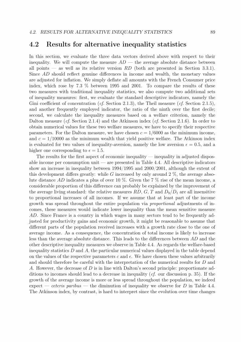
4.2. RESULTS FOR ALTERNATIVE INEQUALITY STATISTICS 89
4.2 Results for alternative inequality statistics
In this section, we evaluate the three data vectors derived above with respect to theirinequality. We will compute the measure AD — the average absolute distance betweenall points — as well as its relative version RD (both are presented in Section 3.3.1).Since AD should reflect genuine differences in income and wealth, the monetary valuesare adjusted for inflation. We simply deflate all amounts with the French Consumer priceindex, which rose by 7.3 % between 1995 and 2001. To compare the results of thesetwo measures with traditional inequality statistics, we also compute two additional setsof inequality measures: first, we evaluate the standard descriptive indicators, namely theGini coefficient of concentration (cf. Section 2.1.3), the Theil measure (cf. Section 2.1.5),and another frequently employed indicator, the ratio of the ninth over the first decile;second, we calculate the inequality measures based on a welfare criterion, namely theDalton measure (cf. Section 2.1.4) and the Atkinson index (cf. Section 2.1.6). In order toobtain numerical values for these two welfare measures, we have to specify their respectiveparameters. For the Dalton measure, we have chosen c = 1/6000 as the minimum income,and c = 1/10000 as the minimum wealth that yield positive welfare. The Atkinson indexis evaluated for two values of inequality-aversion, namely the low aversion ε = 0.5, and ahigher one corresponding to ε = 1.5.
The results for the first aspect of economic inequality — inequality in adjusted dispos-able income per consumption unit — are presented in Table 4.4. All descriptive indicatorsshow an increase in inequality between 1994/1995 and 2000/2001, although the extent ofthis development differs greatly: while G increased by only around 2 %, the average abso-lute distance AD indicates a plus of over 10 %. Given the 7 % rise of the mean income, aconsiderable proportion of this difference can probably be explained by the improvement ofthe average living standard: the relative measures RD, G, T and D9/D1 are all insensitiveto proportional increases of all incomes. If we assume that at least part of the incomegrowth was spread throughout the entire population via proportional adjustments of in-comes, these measures would indicate lower inequality than the mean sensitive measureAD. Since France is a country in which wages in many sectors tend to be frequently ad-justed for productivity gains and economic growth, it might be reasonable to assume thatdifferent parts of the population received increases with a growth rate close to the one ofaverage income. As a consequence, the concentration of total income is likely to increaseless than the average absolute distance. This leads to the differences between AD and theother descriptive inequality measures we observe in Table 4.4. As regards the welfare-basedinequality statistics D and A, the particular numerical values displayed in the table dependon the values of the respective parameters c and ε. We have chosen these values arbitrarilyand should therefore be careful with the interpretation of the numerical results for D andA. However, the decrease of D is in line with Dalton’s second principle: proportionate ad-ditions to incomes should lead to a decrease in inequality (cf. our discussion p. 35). If thegrowth of the average income is more or less spread throughout the population, we indeedexpect — ceteris paribus — the diminution of inequality we observe for D in Table 4.4.The Atkinson index, by contrast, is hard to interpret since the evolution over time changes

90 CHAPTER 4. EMPIRICAL APPLICATION
sign as we go from a low level of inequality aversion (ε = 0.5) to a higher one (ε = 1.5). Itis arguably unclear what degree of inequality aversion should be applied in our case sinceit is hard to measure the convexity of the indifference curves of the social welfare function.
1994/1995 2000/2001 change in %Sample size N 11294 10305 −8.8Mean income (in 1995 euros) 16619.66 17784.29 +7.0AD (in 1995 euros) 10808.34 11913.62 +10.2RD 0.65 0.67 +3.0G (Gini coefficient) 0.32 0.33 +1.9T (Theil measure) 0.19 0.20 +3.4D9/D1 3.92 4.06 +3.6D (Dalton measure, c = 1/6000) 1.34 1.24 −5.4A (Atkinson index, ε = 0.5) 0.08 0.09 +11.3A (ε = 1.5) 0.46 0.23 −49.4
Table 4.4: Statistics for income inequality — Data source: BdF.
The second aspect, inequality in wealth per capita, displays an even stronger oppositionbetween absolute and relative descriptive measures. Here, AD even points in the oppositedirection as it shows a 7.5 % increase in inequality, while all relative measures decreaseover time (see Table 4.5). The average wealth per capita grew by 8.5 %, partly a result ofthe prolonged investment boom referred to as the ‘internet bubble’.2 The remarkable rangebetween AD and the lowest descriptive measure, the ratio D9/D1, of over 14 percentagepoints underlines that the choice of inequality statistics is far from being neutral. As canbe seen in Table 4.5, it modifies completely our vision on the empirical observations: if wethink of it as concentration, wealth inequality decreased by around 3-7 %. By contrast, ifwe believe inequality is the average difference per capita, it increased by over 7 %. As forthe welfare-based measures, D again moves in the expected direction if we assume that atleast part of the increase in average wealth can be interpreted as a proportional increaseof the assets of many households. In that case, Dalton’s second principle again holds andinequality should, ceteris paribus, decrease. Once more the Atkinson measure is difficultto interpret as the evolution changes sign with different degrees of risk aversion.
Finally, we evaluate the inequality in the subjective assessment of unemployment riskin the two years. Since this risk is measured in grades from 1 to 5, the inequality indicatorsbased on the concept of concentration, i.e. the Gini coefficient and the Theil measure, donot make sense in this case. Also the concepts of “equally distributed equivalent income”(Atkinson) and “welfare if the current income was equally distributed” (Dalton) cannot beapplied to the distribution of unemployment risk. We therefore only compute the absoluteand relative average distance and the interdecile ratio, which give indications about how
2Since our sample was collected in 2000/20001, the ensuing stock market bust is not yet reflected inour data.

4.2. RESULTS FOR ALTERNATIVE INEQUALITY STATISTICS 91
1994/1995 2000/2001 change in %Sample size N 11294 10305 −8.8Mean wealth (in 1995 euros) 48965.10 53110.30 +8.5AD (in 1995 euros) 57059.21 61327.73 +7.5RD 1.17 1.15 −0.9G (Gini coefficient) 0.58 0.56 −3.0T (Theil measure) 0.59 0.56 −6.4D9/D1 64.29 59.99 −6.7D (Dalton measure, c = 1/10000) 1.20 1.16 −2.3A (Atkinson index, ε = 0.5) 0.29 0.28 −4.4A (ε = 1.5) 0.77 0.78 +0.2
Table 4.5: Statistics for wealth inequality per capita — Data source: BdF.
the unemployment risk is spread throughout the population. Before we interpret theevolution of these measures, we note that the average risk actually decreased by 3 %between 1994/1995 and 2000/2001. This result seems to confirm the sumultaneous drop inunemployment rates from 11.4 % in 1995 to 8.7 % in 2001 communicated by the INSEE.Interestingly, this decrease in the average unemployment risk did not translate into asmaller average distance between households. The average difference increased during thesame period from a gap in grades of 1.09 to 1.13. Since the measure RD is the ratio of theabsolute average risk difference and the average risk, it rose by even more than AD, namelyby 7 %. The considerable increase of the interdecile ratio (+33.3 %) should note be takento seriously. The jump is due to the fact that there are no intermediate values between therisk grades: all values are integers from 1 to 5 and the interdecile ratio can thus only changein rather big steps. During the obervation period, the ninth decile moved from grade 3 tograde 4, while the first decile remained unchanged at grade 1. This automatically led to aconsiderable increase in the interdecile ratio.
1994/1995 2000/2001 change in %Sample size N 11294 10305 −8.8Average risk 1.94 1.89 −3.0AD 1.09 1.13 +3.7RD 0.56 0.60 +7.0D9/D1 3 4 +33.3
Table 4.6: Statistics for inequality of exposure to economic risk — Data source: BdF.
The ranking of partial intersections orderings proposed by Sen (cf. Section 2.1.7) iseasily applied to the results in the three inequality dimensions we just presented. Wecan define the partial ordering Q as the the non-conflicting ordering of all descriptive

92 CHAPTER 4. EMPIRICAL APPLICATION
measures AD, RD, G, T and D9/D1. In this case, we see that Q ranks income inequalityin 2001/2000 higher than five years earlier. However, wealth inequality cannot be ordereddue to the opposed evaluation of absolute and relative measures. A partial ordering ofinequality from unemployment risk can only be based on AD, RD and D9/D1: in thiscase, the intersection ordering indicates an increase in inequality of risk exposure.
We can now compute the aggregate development of economic risk. To do so, we employthe indices I tA and I tR we defined in Section 3.3.1. The first index is the weighted averageof the changes in the absolute measure AD in each of the three dimensions of economicinequality. It is therefore equal to:
I2001A =
1
3(1.102 + 1.075 + 1.037) = 1.071 (4.1)
Overall economic inequality as measured by I tA therefore increased by roughly 7 % duringthe period from 1994/1995 to 2000/2001. Similarly, we can evaluate the relative index:
I2001R =
1
3(1.03 + 0.991 + 1.07) = 1.03 (4.2)
The multidimensional inequality based on the evolution of RD thus increased by only 3%during the same period. In the following section we insert these results into the IEWB inorder to analyse the impact of inequality on overall economic well-being.
4.3 Evolution of the IEWB including the modified equal-ity dimension
In the final step of our analysis we evaluate the IEWB for the alternative inequality mea-sures we computed in the preceding section. The indices IA and IR will be combined withdata already presented and discussed in an earlier application of the IEWB to the caseof France for the period 1980 to 2003 (op. cit.). Since we had to restrict the analysis ofthree-dimensional inequality to the years 1994/1995 and 2000/2001, the IEWB will alsobe evaluated for this shorter period. We hope to extend our analysis of three-dimensionalinequality to a more recent date with the 2006/2007 edition of the BdF.
For the time being, multi-dimensional inequality measurement is thus restricted to thetwo years in our dataset and a linear interpolation for the years between them. The IEWBdimension ‘equality and poverty’ is a weighted average of two items: an equality index(weighted with 0.25) and a measure poverty intensity (weighted with 0.75). According tothe data presented in our earlier version of the French IEWB, poverty intensity decreasedbetween 1994 and 2000 by 2.3 %. This is the combined result of two factors: first, wenoted a decrease in the relative monetary poverty rate from 9.4 to 9.1 % (ibid., figure 11);second, the poverty gap increased slightly from 22.1 to 22.31 %. The poverty gap indicatesthe ‘depth’ of poverty and gives an additional information on the extent of poverty: whenµPL is the average income of the poor population, the poverty gap is defined as PG =

4.3. IEWB WITH MODIFIED EQUALITY DIMENSION 93
(µPL − PL)/PL. It thus measures the overall distance of the poor to the poverty line.In our sample, this distance remained almost constant between 1994 and 2000 in France.Table 4.7 shows the combined effect of this 2.3 % decrease in poverty intensity and threealternative equality indices. Since a higher value of the IEWB indicates an improvementin well-being, the 2.3 % decrease of poverty intensity enters the ‘poverty and equality’dimension as an increase of 2.3 %. The same holds for the inequality indices which areturned into equality indices.
Evolution from 1994 to 2000 (in %) Equalityindex
IEWB dimension ‘equal-ity & poverty’
Original version (Osberg & Sharpe)Standard income equality (Gini coefficient) +0.7 0.75×2.3+0.25×(+0.7) = +1.9Alternative three-dimensional measure
Economic equality (absolute index IA) −7.1 0.75×2.3+0.25×(−7.1) = −0.1Economic equality (relative index IR) −3.0 0.75×2.3+0.25×(−3.0) = +1.0
Table 4.7: Impact of alternative inequality measurement on equality and poverty dimension— Data source: INSEE, Enquête Revenus Fiscaux; BdF.
In our earlier application, we have used the standard Gini concentration coefficient asa measure of inequality. This corresponds to the original IEWB definition proposed byOsberg and Sharpe. The Gini coefficient we used is the series published by the INSEEand thus based on standard income inequality as observed in the Enquête Revenus Fiscaux(ERF), an administrative source of French employers’ fiscal declarations and the INSEE’spreferred source for calculations of the Gini coefficient.3. According to the INSEE, theGini coefficient decreased between 1994 and 2000 slightly by 0.7% (i.e. a 0.7% increaseof income equality). Together with the 2.3 % decrease of poverty intensity this amountsto a 1.9% improvement of the IEWB dimension ‘poverty and equality’ as can be seen inTable 4.7.
The multi-dimensional indices we have derived in this text show a slightly differentpicture. If the relative index IR is included in the equality and poverty dimension, theimprovement is only 1 %. If we think of inequality as average absolute distances, theIEWB dimension displays stagnation is this aspect of economic well-being (−0.1 %).
It is obvious that the process of aggregation in the IEWB will make the impact ofalternative inequality measures less visible. The weight of the inequality index in the thirdIEWB dimension is 25 %: consequently, the deterioration of 7.1 % of equality translates intoa decrease of the corresponding dimension of only 0.25×7.1% = 1.775 %. If we employ thestandard weighting sheme in which all four dimensions of well-being are weighted equally,the impact on the overall IEWB is of course even smaller, namely only 0.25×0.25×7.1% =0.44%. The effect of aggregation can be seen in the evolution of the IEWB for the three
3Similarly to the BdF, the ERF is also object of vivid debate: see, for instance, the discussion in Conseild’analyse économique (2001).

94 CHAPTER 4. EMPIRICAL APPLICATION
different inequality indices from 1994 until 2000 (Table 4.8 and Fig. 4.1). Not surprisingly,the overall indicator of economic well-being is relatively insensitive to the choice of theequality index: the change during our observation period is 9.7 % if we include the standardincome Gini coefficient, 9.2 % for the index IA, and 9.4 % for the index IR. Although the‘big picture’ undergoes only slight modification if we move from one concept of inequalityto another, this does not mean that our reflections are unimportant cosmetics.
1994 1995 1996 1997 1998 1999 2000Consumption Flows 100 100.8 101.1 100.7 102.9 105.2 107.6Wealth Stocks 100 103.3 105.5 109.6 110.9 111.8 115.7Poverty intensity index 100 100.4 100.8 101.1 101.5 101.9 102.3Gini index (Source: INSEE, ERF) 100 100.5 101.1 101.5 102.2 101.8 100.7Multidim. equal. (based on IA) 100 98.8 97.6 96.5 95.3 94.1 92.9Multidim. equal. (based on IR) 100 99.5 99.0 98.5 98.0 97.5 97.0Poverty & Equality (incl. Gini) 100 100.4 100.8 101.2 101.7 101.9 101.9Poverty & Equality (incl. IA) 100 100.0 100.0 100.0 99.9 99.9 99.9Poverty & Equality (incl. IR) 100 100.2 100.3 100.5 100.6 100.8 101.0Economic Security 100 99.0 95.6 99.5 105.0 107.1 113.5IEWB (incl. income Gini) 100 100.9 100.8 102.8 105.1 106.5 109.7IEWB (incl. IA) 100 100.8 100.5 102.5 104.7 106.0 109.2IEWB (incl. IR) 100 100.8 100.6 102.6 104.8 106.2 109.4
Table 4.8: Evolution of the French IEWB and its components 1994-2000.
First of all, we have to bear in mind that we are unfortunately restricted to an extremelyshort observation period. If the trend in our data continues, the impact of alternativeinequality measures would become more and more visible through time. We have somereason to believe that the gap we observed between relative and absolute measures is notonly temporary, but might reflect forces which are deeply embedded in the economic systemof progressive societies. If average real monetary values grow, and if different parts of thepopulation benefit from this growth via proportional increases of income and wealth, weexpect a systematic divergence between measures based on concentration on the one hand,and absolute differences on the other. The longer the observation period, the strongerwould be the impact on the overall IEWB — a hypothesis we have to test as more recent(or more reliable past) data becomes available.
Second, even if the overall impact is small, the IEWB provides not only the generalvision, but also the draws some details of the the ‘big picture’ of economic development.Hence, even if alternative inequality measures hardly modify the synthetic well-being indi-cator, it is a useful heuristic in its own right that inequality actually increased if we adoptthe concept of average absolute differences. The decomposability is an important featureof the IEWB as it allows to contrast positive and negative developments side by side inthe same methodological framework. For instance, we can compare the evolution of the

4.3. IEWB WITH MODIFIED EQUALITY DIMENSION 95
value of index
time1994 1995 1996 1997 1998 1999 2000
102
104
106
108
Standard IEWB IEWB incl. IA
Figure 4.1: Evolution of standard IEWB and the alternative IEWB with multidimensionalinequality measurement based on average absolute distances.
two dimensions which employ the concept of typical citizens and heterogeneous citizenswe presented in Tab. 3.1. The former corresponds to the dimensions ‘effective consump-tion’ and ‘accumulation of wealth’, while the latter groups together ‘equality and poverty’and ‘economic risk’. Figure 4.2 illustrates the evolution of the ‘typical’ and ‘heterogeneous’well-being in our sample: the dimensions based on average values grew strongly and almostlinearly. By contrast, once we take the heterogeneity of the French society into account,the development is more volatile and less positive. If we substitute the standard incomeGini coefficient with our index IA, the difference is even more pronounced. This exam-ple illustrates the usefulness of the IEWB’s decomposability, since the contrast between‘typical’ and ‘heterogeneous’ citizens would have been less visible in the overall IEWB.Similarly, despite the fact that the global development is less sensitive to the changes weproposed in this text, we argue that they contain relevant information for the interpretationof economic well-being.
Concluding remarks
Inequality measurement has come a long way. The apparent constants in Pareto’s répar-tition de la richesse were replaced by different concepts used to measure changes in thedistribution of economic resources. The analytical methods were improved significantly,not least thanks to a cross-fertilization between the theory of choice under uncertainty,information theory and inequality analysis. In this text, it has been argued that the so-
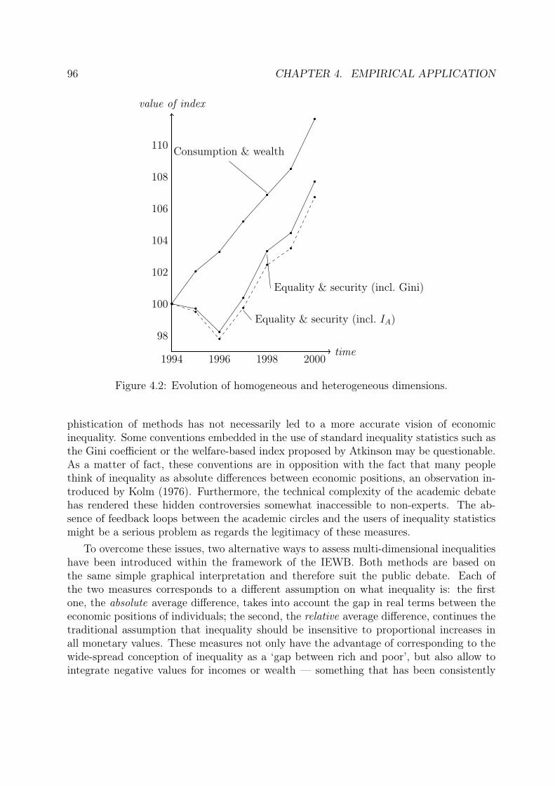
96 CHAPTER 4. EMPIRICAL APPLICATION
value of index
time1994 1996 1998 2000
98
100
102
104
106
108
110 Consumption & wealth
Equality & security (incl. Gini)
Equality & security (incl. IA)
Figure 4.2: Evolution of homogeneous and heterogeneous dimensions.
phistication of methods has not necessarily led to a more accurate vision of economicinequality. Some conventions embedded in the use of standard inequality statistics such asthe Gini coefficient or the welfare-based index proposed by Atkinson may be questionable.As a matter of fact, these conventions are in opposition with the fact that many peoplethink of inequality as absolute differences between economic positions, an observation in-troduced by Kolm (1976). Furthermore, the technical complexity of the academic debatehas rendered these hidden controversies somewhat inaccessible to non-experts. The ab-sence of feedback loops between the academic circles and the users of inequality statisticsmight be a serious problem as regards the legitimacy of these measures.
To overcome these issues, two alternative ways to assess multi-dimensional inequalitieshave been introduced within the framework of the IEWB. Both methods are based onthe same simple graphical interpretation and therefore suit the public debate. Each ofthe two measures corresponds to a different assumption on what inequality is: the firstone, the absolute average difference, takes into account the gap in real terms between theeconomic positions of individuals; the second, the relative average difference, continues thetraditional assumption that inequality should be insensitive to proportional increases inall monetary values. These measures not only have the advantage of corresponding to thewide-spread conception of inequality as a ‘gap between rich and poor’, but also allow tointegrate negative values for incomes or wealth — something that has been consistently

4.3. IEWB WITH MODIFIED EQUALITY DIMENSION 97
ignored by measures based on the concept of concentration.In our data set the impact on the overall economic well-being of these alternative
measures is rather limited. However, the question whether inequality is regarded as anabsolute or a relative concept has profound consequences of great importance. The mostobvious consequence is probably the ambiguous impact of economic growth. Traditionally,it has been assumed that economic growth — as long as it is spread throughout thepopulation via wage adjustments and other mechanisms — has no effect whatsoever oneconomic inequality. The reason for the insensitivity of inequality to economic growthis that the former has been regarded as identical to the notion of concentration. Oncethis identity is questioned, as was done with the concept of the average absolute gap,economic growth might actually lead to increasing inequality. In progressive societies thisis obviously a problematic issue calling for a re-assessment of the focus on economic growthas a means to overcome societal problems. In fact, if people think of inequality as absolutegaps, economic growth itself might be the cause of a societal problem, and not its solution.
The results presented in this text could be extended in at least two directions: first,the empirical findings could be tested as new data becomes available (a new edition ofthe BdF is currently in preparation). This would allow to test our hypothesis that inprogressive societies such as France, an increasing difference between relative and absolutemeasures of inequality should be observed. In addition, we noted that the BdF is notthe most reliable source to evaluate variables such as wealth and unemployment. Othersources focussing on theses issues (e.g. the ERF) could help to test the robustness of ourempirical results, possibly allowing to bring the analysis from the household down to theindividual level. We believe that the concepts developed in this text can easily be appliedto other sources and variables. A second extension could focus on inequality and theanalysis of the BdF data. In our empirical discussion we looked at the average gap betweenhouseholds in different dimension. However, the BdF data also allows to analyse the samehousehold in all three identified dimensions of inequality. It is therefore possible to verifyto what extent unfavourable or favourable positions in one dimension are correlated withthe other dimensions. This would lead to an even finer picture of the extent of economicinequalities — beyond the IEWB framework — and answer the question whether gapsbetween households in the different dimensions either reinforce or offset each other. Again,the concepts developed in this text could be useful for such an extension.

Bibliography
[1] Aigner, D. J. & Heins, A. J. (1967). A Social Welfare View of the Measurement ofIncome Inequality. Review of Income & Wealth, Vol. 13, Issue 1, pp. 12-25.
[2] Amiel, Y. & Cowell, F. (1999). Thinking About Inequality: Personal Judgements andIncome Distributions. Cambrigde: Cambridge University Press.
[3] Atkinson, A.B. (1970). On the Measurement of Inequality. Journal of Economic The-ory, Vol. 2, pp. 244-263.
[4] Atkinson, A.B. (dir.) (1980). Wealth, income and inequality. 2sd ed., Oxford: OxfordUniversity Press.
[5] Beach, C. M. and Davidson, R. (1983). Distribution-free Statistical Inference withLorenz Curves and Income Shares. Review of Economic Studies, 50, pp. 723-35.
[6] Benn, E.J.P. (1926). The confessions of a capitalist.
[7] Berger, P.L. & Luckmann,T. (1966). The Social Construction of Reality: A Treatisein the Sociology of Knowledge. Garden City, New York: Anchor Books.
[8] Blackorby, C. & Donaldson, D. (1980). A Theoretical Treatment of Indices of AbsoluteInequality. Econometrica, Vol. 48.
[9] Bourguignon, F. (1979). Decomposable Inequality Measures. Econometrica, Vol. 47,No. 4, pp. 901-20.
[10] Bowley, A.L. (1901). Elements of Statistic. London: P.S. King & Son.
[11] Bowman, M.-J. (1945). A Graphical Analysis of Personal Income Distribution in theUnited States. American Economic Review, Vol. 35. Issue 4, pp. 607-29.
[12] Busino, G. (ed.) (1964). Presentation of the ‘Ecrits sur la courbe de repartition de larichesse de V. Pareto’. Geneva: Librairie Droz.
[13] Conseil d’analyse économique (2001). Inégalités Economiques. Paris: La Documenta-tion Française.
98

BIBLIOGRAPHY 99
[14] Dalton, H. (1920). The measurement of the inequality of incomes. The EconomicJournal, 30, pp. 348-361.
[15] Davis, H. T. (1941). The Analysis of economic time series. Cowles Commission forresearch in Economics, Monog No 6, Bloomington, Principia Press.
[16] Desrosières, A. (2000). La politique des grands nombres: histoire de la raison statis-tique. First edition in 1993. Paris: La Découverte.
[17] Edgeworth, F.J. (1896). The Pareto Law. Journal of the Royal Statistical Society,pp. 533-34.
[18] Edgeworth, F.J. (1926). The Pareto Law. In: Palgrave’s dictionary of Political Econ-omy. London: McMillan, pp. 712-13.
[19] Favereau, O. (1989). Marchés internes, marchés externes. Revue Economique, Vol. 40,No 2, pp. 273-328.
[20] Foster, J.E. & Shorrocks, A.F. (1987). Transfer Sensitive Inequality Measures. Reviewof Economic Studies, 54, pp. 485-97.
[21] Foster, J.E. & Shorrocks, A.F. (1988). Inequality and poverty orderings. EuropeanEconomic Review, Vol. 32, No 2-3, pp. 654-661.
[22] Gadrey, J. & Jany-Catrice, F. (2007). Les nouveaux indicateurs de richesse. Firstedition in 2005. Paris: La Découverte.
[23] Gini, C. (1912). Variabilità e Mutabilità. Contributo allo studio delle distribuzioni edelle relazioni statistiche. Bologna. 8vo.
[24] Gini, C (1913). Sulla misura della concentrazione e della variabilità dei caratteri. Atti,Serie VIII, Tomo XVI, Parte II, pp. 1203-48.
[25] Gini, C. (1921). Measurement of Inequality of Incomes. Economic Journal, pp. 124-26.
[26] Gini, C. (1936). On the Measure of Concentration with Especial Reference to Incomeand Wealth. Report to the Cowles Commission on Research in Economics.
[27] Jany-Catrice, F. & Kampelmann, S. (2007). L’indicateur de bien-être économique :une application à la France. Revue Française d’économie, Vol. ?, No ?.
[28] Jenkins, S.P. & Micklewright, J. (2007). New Directions in the Analysis of Inequalityand Poverty. ISER Working Paper 2007-11. Colchester: University of Essex.
[29] Kolm, S.C. (1969). The Optimal Production of Social Justice. In: Margolis, J. &Guitton, H. (eds.), Public Economics. London: Macmillan.
[30] Kolm, S.C. (1976). Unequal Inequalities I. Journal of Economic Theory, Vol. 12.

100 BIBLIOGRAPHY
[31] Leroy-Beaulieu, P. (1881). Essai sur la répartition de richesse et sur la tendance à unemoindre inégalité des conditions. Paris: Guillaumin.
[32] Lorenz, M.O. (1905). Methods of Measuring the Concentration of Wealth. Publicationsof the American Statistical Association, 9, pp. 209-19.
[33] Nivière, D. (2005). Négocier une statistique européenne: le cas de la pauvreté.Genèses, No 58, pp. 28-47.
[34] OECD (2002). The Well-being of Nations: The Role of Human and Social Capital.Paris: Organization for Economic Cooperation and Development.
[35] Osberg, L. (1985). The Measurement of Economic Well-Being. In: Laidler, D. (ed).Approaches to Economic Well-Being, Vol. 26, (pp. 49-89). Toronto: University ofToronto Press.
[36] Osberg, L. & Sharpe, A. (1998). An Index of Economic Well-Being for Canada. Re-search Paper R-99-3E, Applied Research Branch, Strategic Policy, Human ResourceDevelopment Canada.
[37] Osberg, L. & Sharpe, A. (2002). International Comparisons of Trends in EconomicWell-Being. Social Indicators Research, Vol. 58, Nos 1-3, pp. 349-82.
[38] Osberg, L. & Sharpe, A. (2005). How Should We Measure the Economic Aspects ofWell-Being ? The Review of Income and Wealth, Series 51, Number 2, pp. 311-336.
[39] Paglin, M.(1975). The Measurement and Trend of Inequality: A Basic Revision. Amer-ican Economic Review, Vol. 65, Issue 4, pp. 598-609.
[40] Pareto, V. (1896). La courbe de la répartition de la richesse. Recueil publié par laFaculté de Droit à l’occasion de l’Exposition nationale suisse, Geneva 1896, Lausannce,Ch. Viret-Genton Impr. pp. 372-87. Reprinted in: Busino, G. (dir.) (1965). Oeuvrescomplètes de Vilfredo Pareto. Geneva: Librarie Droz.
[41] Pareto, V. (1897). La répartition des revenus. Le monde économique, pp. 259-61.Reprinted in: Busino, G. (dir.) (1965). Oeuvres complètes de Vilfredo Pareto. Geneva:Librarie Droz.
[42] Pareto, V. (1900). Un applicazione di teorie sociologiche. Revista Italiana di sociologia,pp. 401-56.
[43] Pareto, V. (1964). Cours d’économie politique. First edition in 1897. Geneva: LibrarieDroz.
[44] Pigou, A.C. (1929). Economics of Welfare. London: Macmillan.
[45] Prieto, J.-L. (1975). Pertinence et pratique. Paris: Editions de Minuit.

BIBLIOGRAPHY 101
[46] Putnam, R. (1981). Reason, Truth, and History. Cambridge: Cambridge UniversityPress.
[47] Ravallion, M. (2003). The Debate on Globalization, Poverty and Inequality: WhyMeasurement Matters. International Affairs, 79 (4), pp. 739-753.
[48] Rawls, J. (1971). A Theory of Justice. Cambridge, Mass.: Belknap Press of HarvardUniversity Press.
[49] Rosenbluth, G. (1951). Note on Mr. Schutz’s Measure of Income Inequality. AmericanEconomic Review, Vol. 41, No. 5, pp. 935-37.
[50] Searle, J.R. (1995). The Construction of Social Reality. New York: Free Press Editions.
[51] Sen, A.K. (1973). On Economic Inequality. Oxford: Clarendon Press.
[52] Sen, A.K. (1992). Inequality Re-examined. Oxford: Clarendon Press.
[53] Sen, A.K. (1997). On Economic Inequality. Expanded Edition with a Substantial An-nexe by J. E. Foster and A.K. Sen. Oxford: Oxford University Press. First edition in1973.
[54] Shorrocks, A. F. (1980). The Class of Additively Decomposable Inequality Measures.Econometrica, vol 48, pp. 613-25.
[55] Shorrocks, A. F. (1983). Ranking Income Distributions. Economica, 50, pp. 3-17.
[56] Staehle, H. (1943). Ability, Wages, and Income. The Review of Economic Statistics,Vol. 25, No. 1. pp. 77-87.
[57] Tawney, R.H. (1964). The religion of Inequality. In: Atkinson, A.B. (dir.) (1980).Wealth, income and inequality, 2sd ed. - Oxford: Oxford University Press.
[58] Theil, H. (1967). Economics and Information Theory. Amsterdam: North-HollandPublishing Company.
[59] Wedgwood, J. (1939).The Economics of Inheritance, Penguin.
[60] Yntema, D. (1933). Measures of the Inequality in Personal Distributions of Wealth orIncome. Journal of the American Statistical Association, Vol 28, p. 423.

Compte rendu du mémoire en français
Avant proposLe choix de rédiger le mémoire en langue anglaise est entièrement le résultat de consi-
dérations pratiques. A l’exception des travaux de Vilfredo Pareto et d’Alain Desrosières,l’ensemble des textes sur lesquels nous avons pris appui est issu de la littérature anglo-phone. Nous voudrions donc éviter des confusions créées par des traductions incorrectes oumaladroites d’une langue étrangère (l’anglais) à une autre (le français). De plus, la plupartdes interlocuteurs de l’auteur de ces lignes n’a que des connaissances de base du français.Les nombreuses discussions amicales et/ou professionnelles — pourtant extrêmement utilespour l’achèvement du texte final — n’auraient donc pas pu s’effectuer si le mémoire étaitréservé à un public purement francophone.
Cependant, il nous semble être utile de présenter un compte rendu en français du texteentier. Dans les pages qui suivent, nous tentons de retenir non seulement les conclusions,mais aussi une partie des raisonnements qui en étaient à l’origine. Ainsi, est proposé pourchacun des quatre chapitres de la version anglaise un compte rendu de plusieurs pages.D’une part, nous espérons que ceci sert à raccourcir la lecture pour ceux qui ne retrouventleurs intérêts que dans une ou plusieurs parties. Ils pourraient alors compléter la lecturede ces chapitres avec les comptes rendus fournis ci-dessous. D’autre part, les lecteurs fran-cophones peuvent s’y procurer une vision générale de notre approche méthodologique, denos objets d’étude et des résultats de notre recherche.
Avant de commencer par le compte rendu par chapitre quelques remarques d’ordrepratique : toutes les références aux numéros de pages, à un certain passage du texte ou à unchapitre particulier renvoient au document complet en anglais. Une partie des graphiques etdes formules a été reproduite dans les comptes rendus afin d’éviter des allers et retours nonnécessaires entre les deux documents. Par ailleurs, dans la version en Portable DocumentFormat (.pdf) toutes les références chiffrées peuvent être utilisées comme des liens encliquant sur le numéro de la page, de la section ou du chapitre de la référence (les référencesdans la version anglaise qui renvoient à d’autres passages du même document peuventd’ailleurs être utilisées de la même façon). Nous espérons que ceci facilite la lecture ainsique les comparaisons des deux documents.
102

Chapitre 1Introduction et méthodologie
Pourquoi la mesure des inégalités est toujours pertinente
Les inégalités, et de manière générale la distribution des ressources, représentent desproblèmes fondamentaux en économie. Nous sommes d’avis qu’il est important et utiled’analyser si et à quel degré des configurations économiques peuvent être caractériséescomme « inégales ». On peut même suivre R.H. Tawney dans son opinion que « la scienceéconomique devrait surtout traiter l’inégalité » (Tawney, 1964). Les inégalités économiquesont une influence importante sur un large éventail de préoccupations sociales et peuventêtre analysées sous un angle philosophique (les questions d’équité et de justice), écono-mique (les problèmes d’incitations et de l’allocation des ressources), ou bien sociologique(la fonction et le rôle des inégalités socio-économiques). Le mémoire se limite à une questiontrès spécifique : comment mesurer les inégalités économiques dans le cadre de l’indicateurde bien-être économique (IBEE), un instrument proposé par les chercheurs canadiens LarsOsberg et Andrew Sharpe. Cet indicateur a été conçu comme une heuristique permettant àses divers utilisateurs de faire des jugements sur plusieurs aspects du bien-être économique.Il contient des informations statistiques concernant quatre dimensions : 1) la consomma-tion effective ; 2) l’accumulation des stocks de richesses ; 3) les inégalités et la pauvreté ; et4) la sécurité économique.
L’IBEE est désormais reconnu comme un instrument utile pour l’analyse économique.Par ce dernier terme, nous désignons non seulement une activité exercée par des spécialistesde la science économique, mais aussi des analyses effectuées par d’autres acteurs qui s’in-téressent aux aspects politiques, éthiques ou sociologiques liés aux résultats économiques.Les usagers de l’IBEE dépassent donc le cercle des « experts » économiques (comme lesstatisticiens, les théoriciens de l’économie du bien-être etc.), et l’IBEE doit prendre enconsidération les conceptions et les représentations des autres acteurs qui en font usage.
Cependant, nous avons remarqué dans une application antérieure de l’IBEE aux don-nées françaises (cf. Jany-Catrice & Kampelmann, 2007) que la place des inégalités éco-nomiques à l’intérieur de l’architecture de l’IBEE n’est pas entièrement satisfaisante. Eneffet, Osberg et Sharpe ont retenu les quatre dimensions du bien-être économique que nousvenons de citer. Et pourtant, les inégalités n’y sont évaluées qu’en termes des revenus dis-ponibles. Ceci ne correspond pas à l’idée que le bien-être repose sur l’ensemble des quatre
103

104 COMPTE RENDU DU MÉMOIRE EN FRANÇAIS
dimensions. Autrement dit, si nous décidons que le bien-être économique est lié à la consom-mation, aux stocks de richesses et à la sécurité économique, nous devrions considérer lesinégalités dans l’ensemble de ces dimensions et non seulement l’inégalité des revenus. Cetteinconsistance dans la structure interne de l’IBEE a inspiré le thème du mémoire ainsi queles principales questions de recherche : sont les inégalités correctement prises en comptedans l’indicateur de bien-être économique ? Et si cela n’est pas le cas, comment l’indicateurpeut-il être amélioré sans perdre sa transparence et son approche intuitive ?
A partir de ces questions sur la place des inégalités au sein de l’IBEE, le premier chapitredéveloppe des réflexions sur le concept des inégalités en général. Ceci nous amène à uneinterrogation plus fondamentale et à poser une question encore plus importante : commentles inégalités économiques devraient-elles être mesurées ?
Etant donné la disponibilité d’une large gamme de mesures d’inégalités — y compris desindicateurs apparemment très légitimes tel que le coefficient de concentration de Gini — onpourrait penser que cette question ne mérite pas l’attention que nous sommes disponibles àlui prêter. En fin de compte, Osberg et Sharpe ont également opté pour la simple utilisationdu coefficient de Gini pour rendre compte des inégalités de revenus dans la version originalede l’IBEE. Nous présentons trois arguments pour souligner la pertinence de la questioncomment les inégalités économiques devraient être mesurées :
1. Il n’existe pas un seul, mais une panoplie d’indices, de coefficients ou d’autres instru-ments statistiques qui visent à rendre compte des inégalités. Comme ces indicateurssont souvent en contradiction les uns avec les autres, le choix d’une mesure spécifiquen’est pas neutre et devrait être basé sur des arguments légitimes et plausibles (noustraitons les contradictions entre les différentes mesures disponibles dans le chapitre 2).Evidemment, le choix d’une statistique doit correspondre directement à la probléma-tique donnée (dans notre cas celle d’une application de l’IBEE). Par conséquent, ilnous semble être nécessaire de vérifier si les mesures traditionnelles d’inégalités cor-respondent effectivement à l’usage que nous en voulons faire au sein de l’IBEE. Pourune telle analyse, nous devons regarder de plus près les différences entre les mesuresalternatives, ainsi que les jugements et conventions encastrés dans leurs usages.
2. Le texte argumente que la mesure des inégalités contient des questions controversesqu’on retrouve de manière similaire dans les débats autour de la mesure de la pau-vreté. A titre d’exemple, le point de vue que la pauvreté est un phénomène absoluest souvent contrasté à celui qu’il s’agit là essentiellement d’une position défavoriséed’une partie de la population relative à la situation du gros de la société. La ques-tion « qu’est-ce la pauvreté ? » ne semble pas permettre une réponse claire. Le texteargumente que la mesure des inégalités contient de façon pareille plusieurs aspectscontroverses qui sont analysés tout au long du mémoire. Par ailleurs, nous formulonsl’hypothèse selon laquelle l’absence de ces controverses des débats peut être expliquéeen partie par la complexité technique qui caractérise désormais cette mesure. Le débatsemble être dominé par des spécialistes qui mobilisent des outils inaccessibles à unepartie importante des usagers. Ceci pose des problèmes pour le propos transparentet plutôt démocratique d’un instrument comme l’IBEE. Par conséquent, le mémoire

105
vise à faire de la lumière dans les controverses liées à la mesure des inégalités et veutproposer des issues plausibles et bien fondés.
3. La troisième raison pour laquelle une discussion plus fondamentale sur la mesure desinégalités est pertinente est de nature pragmatique. Si l’idée d’une multidimension-nalité de l’inégalité est acceptée — comme le cadre d’analyse de l’IBEE le suggère— ceci introduit la difficulté de rendre compte des inégalités dans plusieurs espacesen même temps et d’agréger ces multiples espaces dans une mesure globale. Les sta-tistiques traditionnelles tel que le coefficient de concentration de Gini ne sont pasdirectement applicables à des problèmes à plusieurs dimensions. De nouveau, la so-lution de cette difficulté doit correspondre à l’objectif général qui est défini par lesusages qu’on peut faire de l’IBEE.
Au centre de notre approche est donc le souci de joindre la logique générale de l’IBEE,d’un coté, et la mesure statistique des inégalités au sein de l’IBEE de l’autre. Par consé-quent, les revues d’indicateurs d’inégalités disponibles dans la littérature ne nous peuventservir que partiellement traitant souvent des interrogations plus techniques (comme lethème de la décomposabilité) ou font référence à des cadres d’analyse distincts (commel’approche utilitariste). En revanche, notre réflexion est d’avantage axée sur la cohérenceentre l’usage du concept de l’inégalité dans la communication normale et son opérationna-lisation statistique.
A la suite du choix de problématique l’analyse exclut certaines interrogations impor-tantes. Dans le texte anglais, nous fournissons les explications pourquoi les questions sui-vantes ne sont pas traitées explicitement dans le mémoire : 1) le problème général « Inégalitéde quoi ? » inspiré par le livre Inequality Re-Examined de Sen ; 2) les interrogations spécifi-quement lié à la mesure du bien-être, comme celui de la dichotomie entre l’utilité cardinaleet ordinale ou la comparabilité interpersonnelle ; 3) les multiples causes des inégalités neseront non plus analysées de manière explicite.
Le plan du mémoire est divisé en quatre chapitres. Le premier chapitre propose uneanalyse de la nature du concept de l’inégalité. L’analyse mobilise des éléments de réflexionissus de la sociologie de la connaissance, de l’approche conventionnaliste, ainsi que de lahistoire de la raison statistique d’Alain Desrosières. Le chapitre vise à expliciter le cadreméthodologique du mémoire en fournissant en même temps une terminologie des conceptsqui réapparaissent à plusieurs reprises dans le texte.Le deuxième chapitre applique la méthodologie introduite dans le premier chapitre audiscours académique sur la mesure des inégalités en sciences économiques. Dans un essai derassembler des éléments d’une histoire interne des statistiques de l’inégalité, interprétéescomme des conventions, nous discutons les contributions scientifiques dans ce domainejugées comme les plus pertinentes pour notre propos : ce sont les travaux de VilfredoPareto, Max O. Lorenz, Corrado Gini, Hugh Dalton, Henri Theil, Anthony B. Atkinson etd’Amartya Sen. Le chapitre donne à part cela une revue des développements plus récentsde la littérature. Cette histoire interne vise à mettre en relief l’évolution chronologique desconventions les plus importantes et montre de cette façon aussi le processus de légitimation

106 COMPTE RENDU DU MÉMOIRE EN FRANÇAIS
des mesures les plus utilisées. Comme les conventions et leur légitimation sont souventliées, une compréhension de l’établissement de certaines conventions au profit d’autres estimportante pour notre question de recherche.Le troisième chapitre propose deux manières alternatives de mesurer l’inégalité économiquedans le cadre de l’IBEE. L’argumentation s’appuie sur l’acceptation des conventions quinous semblent être légitimes et une remise en question des conventions qui sont moinsplausibles étant donné le propos de l’IBEE. Cette argumentation confronte l’histoire internedu discours académique avec l’usage de l’IBEE. Ce dernier introduit alors dans la discussiond’une part les représentations et les usages du concept de l’inégalité par des acteurs externesau discours académique et d’autre part la logique interne de l’IBEE. Pour ceux qui ne sontpas familiers avec l’IBEE, le troisième chapitre donne au début une brève introduction àsa méthodologie.Le dernier chapitre contient une application empirique des résultats du chapitre précèdentau cas de la France. La sensibilité des mesures alternatives de l’inégalité y est testée etdiscutée. Ce chapitre utilise une application antérieure de l’IBEE (cf. op. cit.) et mobilisedes données issues de l’enquête Budgets de Familles.
Dans le texte anglais, l’introduction se termine par une description de la place de cemémoire dans le projet personnel de l’auteur.
Discuter l’indiscutable : l’inégalité comme une conventionCette section situe le concept d’inégalité dans le cadre de plusieurs approches théo-
riques complémentaires, à savoir celle de la sociologie de la connaissance, celle de la théoriede conventions, ainsi que celle de l’approche historique d’Alain Desrosières. Ces théoriessont mobilisées puisque les inégalités sont considérées comme des faits sociaux et qu’ellesrentrent donc étroitement dans le champs d’analyse de ces théories. Loin de proposer uneréflexion sociologique approfondie, le texte fait recours à ces approches pour éclaircir deuxpoints importants qui sont liés à la discussion des inégalités :
1. La nature du concept « inégalité » provoque des questions épistémologiques que nousne pouvons pas ignorer dans une discussion scientifique. Existe-t-il une « vraie » dé-finition des inégalités économiques ? Et dans le cas contraire, comment émergent desdéfinitions de ce concept ?
2. Il y a une relation importante entre la discussion scientifique à propos de l’inéga-lité et l’usage de ce même concept dans le langage courant. L’utilisation du terme« inégalité » au sein du discours académique correspond-elle à la manière telle qu’ilest employé à l’extérieur du monde scientifique ? Un écart sémantique poserait-il desproblèmes sérieux ou simplement une inconvenance négligeable ?
La nature du concept de l’inégalité
Dans l’interrogation sur la nature du concept de l’inégalité un certain nombre de résul-tats de la sociologie de la connaissance est utilisé. Notamment le principe de la construction

107
sociale développé par Berger & Luckmann (1966) sert à souligner que les objets sociauxtels que les inégalités ne peuvent pas être classifiés comme des faits qui sont « vrais » indé-pendamment de toute communication interpersonnelle. A tout moment, plusieurs pointsde vue alternatifs sur un même objet peuvent concourir pour le statut d’être la vraie repré-sentation de la réalité sociale. Ceci fournit des arguments à une position épistémologique,à savoir la position d’un relativisme selon lequel toutes les opinions ont la même validité.L’issue classique d’une épistémologie relativiste est celui adoptée dans le texte : toutes lesopinions ne sont pas valables, car, les conceptions partagées par une communauté donnéede personnes représentent une forte contrainte à ce qui peut compter comme des repré-sentations correctes des objets sociaux. A l’intérieur de cette communauté de personnesla réalité sociale est créée par une co-construction entre les différents participants de lacommunication interpersonnelle. Ceci est un résultat important de notre discussion car leconcept de l’inégalité rentre clairement dans la catégorie des constructions sociales. Parconséquent, il est impossible de vérifier la validité d’une définition quelconque des inégali-tés économiques sans tenir compte de la co-construction du terme au niveau de la société.Pour s’assurer de la scientificité de notre propos, la nature du concept de l’inégalité nousforce à analyser notre problème du point de vue d’une co-construction. Ceci constitue unepartielle remise en question de l’approche traditionnelle qui domine la littérature spéciali-sée, qui a plutôt tendance à construire des mesures statistiques des inégalités de manière« unilatérale », c’est-à-dire sans l’intervention des acteurs externes au débat scientifique.
Un regard inspirateur sur le processus de construction sociale est celui développé parDesrosières (1993) dans son histoire de la raison statistique. En analysant les mécanismesde l’objectivation dans le domaine statistique, Desrosières met l’accent sur les élémentsconstruits — et in fine arbitraires — de ces références apparemment indiscutables commepar exemple les statistiques officielles. Il montre que le processus d’objectivation des faitssociaux repose avant tout sur des conventions, une vision ici adoptée pour la discussion desinégalités.
En sciences économiques, des interrogations autour du thème des conventions ont donnénaissance aux théories économiques de conventions. Le texte ne retient que quelques élé-ments de base de ces théories comme par exemple celui de l’interprétation des conventionscomme un dispositif cognitif collectif, proposée par O. Favereau (1989, p. 295). Cette in-terprétation des conventions nous permet d’analyser la construction sociale des représen-tations statistiques (l’aspect cognitif ) ainsi que le processus de co-construction (l’aspectcollectif ). Dans ce contexte nous citons l’étude de Gadrey & Jany-Catrice (2007), qui ap-plique le concept de conventions au débat sur la mesure de richesse. En effet, ces auteursmontrent que dans la discussion des mesures alternatives au PIB, certains acteurs prennentconscience du caractère conventionnel des mesures traditionnelles et mettent en questionla légitimité du PIB pour des évaluations du bien-être. Selon Gadrey et Jany-Catrice lesconventions qui perdent en légitimité sont ceux qui « concernent la représentation globalede ce qui compte et de ce qui devrait être compté au titre de la richesse d’une nation, et dela contribution de diverses activités ou patrimoines » (ibid., p. 103). Dans le contexte d’unediscussion des inégalités au sein de l’IBEE, les conventions sur ce qui devrait être comptésont déjà encastrées dans l’architecture même de l’indicateur, notamment dans le choix des

108 COMPTE RENDU DU MÉMOIRE EN FRANÇAIS
variables et des dimensions. Par conséquent, le mémoire se concentre sur les conventionsplutôt d’ordre technique : ces derniers doivent correspondre aux représentations et l’usagedu concept des inégalités partagés par les utilisateurs de l’IBEE.
Pour analyser la correspondance entre conventions techniques de mesure et conceptionsdes utilisateurs il nous semble être utile de nous approprier l’approche historique de Des-rosières. Ceci permet de comprendre à quel moment et pour quelles raisons les conventionsles plus importantes ont émergé dans la littérature. Cependant, la méthodologie plus am-bitieuse de Desrosières est modifiée. En effet, ce dernier pouvait s’appuyer sur son ampleexpérience comme chercheur-sociologue et fonctionnaire-statisticien pour présenter à la foisune histoire interne (des méthodes, théorèmes etc.) et une histoire externe (des acteurs,des laboratoires, des processus opératoires etc.). Bien que cette double vision nous sembleêtre très instructrice, il nous n’est pas possible d’en fournir l’équivalent pour la genèsedes mesures d’inégalité, notamment à cause d’un manque d’expérience et de temps. Parconséquent, le texte ne rassemble dans un premier temps que des éléments d’une histoireinterne du discours scientifique sur la mesure statistique des inégalités économiques. Ce-pendant, nous confrontons dans le troisième chapitre cette vision interne des inégalités avecles représentations des acteurs externes et la logique de l’IBEE.
Après avoir présenté des arguments en faveur d’une vision du concept de l’inégalitécomme une convention, le texte prolonge le raisonnement en y introduisant un aspect nor-matif. En effet, nous sommes d’avis que pour être légitime, le processus d’objectivation doitreposer sur une co-construction des mesures d’inégalité plutôt que sur un monologue desspécialistes techniques. Ceci nous mène à penser qu’une absence de communication entreles usagers des résultats statistiques et les experts techniques est susceptible d’aboutir danscertains cas à une pseudo-légitimité des mesures des inégalités. La co-construction des sta-tistiques qui s’appuie sur des allers et retours entre les différentes sphères d’acteurs (feedbackloops), est nécessaire pour établir la légitimité des mesures et une cohérence sémantiqueentre l’utilisation scientifique et non scientifique. Dans ce contexte nous introduisons leterme de la communication normale employé par Sen (1975), qui a été le premier à insistersur le fait que la science économique n’est pas complètement libre de définir le terme de l’in-égalité de manière arbitraire (ibid., pp. 47-78). En effet, Sen indique qu’il est problématiqueque les différentes définitions d’inégalité qui ont émergé dans la littérature puissent aboutirà des résultats contradictoires. A titre d’exemple, il est possible que la même modificationd’une distribution de revenus soit interprétée simultanément comme une diminution del’inégalité en terme d’utilité, une stagnation de l’inégalité en terme de revenus et une aug-mentation de l’inégalité évaluée par l’indice d’Atkinson (cf. la discussion p. 45). Le constatde ces contradictions possibles conduit Sen à traiter la communication normale commeune contrainte au débat scientifique, qui doit rester « raisonnablement proche » au lan-gage courant. En nous appuyant sur les résultats de Desrosières, le texte argumente qu’unetelle contrainte ne rend pas suffisamment compte du principe de co-construction car elleimpose uniquement que le monde de la science observe la communication normale sansqu’il y ait une communication bilatérale (absence de feedbacks). L’importance d’une tellecommunication pour la légitimité du processus d’objectivation est très claire dans l’analysede Desrosières, comme le montrent ses observations citées en p. 12. Nous interprétons ces

109
remarques de Desrosières comme des arguments indiquant que le langage scientifique doitcorrespondre au langage commun pour obtenir sa légitimité. Dans notre contexte, ce lan-gage commun peut être délimité par celui des usagers de l’IBEE décrit dans le chapitre 3.En somme, notre interrogation sur la nature du concept de l’inégalité et sur la relationentre le discours scientifique et la communication normale nous conduit à traiter la me-sure de l’inégalité comme une convention. Tandis que dans le deuxième chapitre le texteexamine la genèse des conventions dans le domaine scientifique, ce dernier est confrontéà d’autres considérations plus externes dans le chapitre 3. Ceci aboutit à deux mesuresalternatives qui visent non seulement à être plus consistantes vis-à-vis la logique internede l’IBEE, mais aussi à mieux correspondre aux emplois du terme « inégalité » dans lacommunication normale.
Etant donné les conclusions du paragraphe précédent, il serait incohérent de commencerla discussion par une définition précise de l’inégalité. Le concept a été construit au fil dutemps et par des acteurs différents et c’est justement ce processus qui est analysé dans lechapitre 2. A la fin, le premier chapitre donne encore quelques remarques sur des termesliés au concept de l’inégalité qui réapparaissent à plusieurs reprises dans le texte.
Premièrement, une distinction est faite entre les concepts tels que la concentration, ladiffusion, la dispersion, l’entropie, la variation d’une part et celui de l’inégalité d’autrepart. Bien que la littérature utilise de manière récurrente des analogies entre ces différentstermes qui sont d’ailleurs certainement liés, nous pensons que le terme de l’inégalité possèdeun contenu sémantique indépendant et qu’il n’est donc pas identique à la concentrationou encore à la dispersion. L’usage synonyme de ces termes risque d’ignorer des élémentsimportants du débat à propos de la mesure de l’inégalité.
Une autre distinction soulignée dans cette section est celle entre la pauvreté et l’inéga-lité. Bien que la tendance vers une vision de la pauvreté comme un phénomène relatif plutôtqu’absolu ait vraisemblablement rapproché les significations respectives, une différence sé-mantique entre les deux concepts persiste. Tandis que la pauvreté reste une description dela situation de ceux qui se retrouvent en bas de la distribution des ressources, l’inégalitéest concernée par des questions relatives à différentes parties de cette distribution.
Enfin, le texte rappelle une terminologie introduite par Rosenbluth, qui distingue entredeux types d’instruments descriptifs utilisés dans le contexte de la mesure de l’inégalitééconomique : 1) un tableau ou graphique, qui permet à analyser différentes parties de ladistribution et 2) un indice qui compare des distributions entières (1951, p. 935). Nousrappelons également que chacune de ces deux formes offre à la fois des avantages et desinconvénients. En effet, tout indice est insensible à un nombre infini de modification de ladistribution et ignore donc des variations jugées comme négligeables. En revanche, les ins-truments graphiques sont sensibles à un nombre plus élevé de modifications mais souvent,ils ne permettent pas d’en tirer des conclusions en ce qui concerne le développement globalde l’inégalité.

Chapitre 2Une histoire interne du discoursacadémique sur la mesure des inégalités
Ce deuxième chapitre applique l’analyse en termes de conventions au discours acadé-mique sur les inégalités économiques pour en fournir des éléments d’une histoire interne.
Ceci dit, il est évident que la littérature en sciences économiques qui traite la mesured’inégalités est un vaste champ. Même si on restreint le sujet à celui de l’inégalité derevenus ou de capital, la littérature concernée a désormais rendu impossible toute tentativede synthèse cohérente. Une illustration de l’énorme quantité de textes fondateurs est lalongueur de la biographie retenue dans On Economic Inequality d’A. Sen qui s’étend sur31 ( !) pages. La maîtrise de cette littérature est clairement l’œuvre d’une vie entière etl’auteur de ces lignes est conscient de ses limitations à cet égard.
Le premier chapitre contient la proposition d’adopter une perspective chronologiquepour discerner les conventions importantes dans la mesure des inégalités. Pour effectuer unetelle analyse chronologique une sélection des textes s’impose. Par conséquent, le deuxièmechapitre commence avec la présentation du critère de choix appliqué à la sélection. Lecritère retenu est l’impact sur les conventions des différentes contributions scientifiques.A l’aide de ce critère sont sélectionnés, dans un premier temps, les textes fondateurs deV. Pareto, C. Gini et M. O. Lorenz. En effet, la spécification mathématique des distributionsproposée par Pareto, le coefficient de concentration de Gini, ainsi que la courbe de Lorenzsont devenus des dispositifs standard pour représenter des distributions empiriques et desréférents communs dans l’analyse des inégalités. Dans un deuxième temps, sont retenues lescontributions qui ont le plus marqué la mesure des inégalités en terme de bien-être (welfare),une approche qui est également devenue standard dans la littérature académique : ce sontles textes de H. Dalton, A. B. Atkinson et A. Sen. Une autre contribution qui a fortementinfluencé les méthodes scientifiques de la mesure de l’inégalité est celle de H. Theil, quia mis en avant le thème de décomposition, et par là inspiré des nombreuses recherchesthéoriques et empiriques sur des questions liées au problème de rendre les statistiquesd’inégalités décomposables.
Ces sept contributions sont donc analysées en vue de leur impact sur les conventionsde mesure. Par conséquent, le deuxième chapitre est loin d’être une histoire complète etn’apporte peu d’information technique au lecteur déjà familier avec les auteurs sélectionnés.
110

111
En revanche, le chapitre vise à rendre visible quelques conventions cruciales encastréesdans les mesures apparemment légitimes et fréquemment utilisées. Il est argumenté quececi permettra une analyse critique de la légitimité de ces derniers dans le chapitre 3.
La Loi de Pareto : l’inégalité constante ou décroissante ?
La première contribution discutée est celle de Pareto. Tout d’abord, une distinction estfaite entre, d’une part, l’analyse parétienne de la répartition de la richesse et, d’autre part,la définition et la mesure des inégalités de revenus de Pareto. Bien que ces deux élémentssoient entremêlés dans l’analyse de Pareto, nous constatons que la définition des inégalitésproposée par Pareto mérite une attention à part entière. Notamment le contraste avec lesmesures d’inégalités proposées plus tard par Lorenz et Gini montre clairement l’évolutiondes conventions dans cette première période de l’analyse quantitative de l’inégalité, dontPareto est le précurseur.
Avant Pareto, le problème de l’inégalité avait été traité presque exclusivement sous unangle qualitatif, notamment par K. Marx, qui contraste la situation économique des diffé-rentes classes. Ceci inspira les remarques suivantes du libéral français P. Leroy-Beaulieu :« L’influence des lois économiques sur la répartition des richesses est un sujet beaucoupmoins exploré que l’influence des mêmes lois sur la circulation. [...] Sans doute les volumessur ce qu’on appelle les questions ouvrières abondent, mais la plupart sont absolumentvides, sans rien de précis, de positif et de scientifique » (citation dans Busino, 1964).
Pareto s’approprie cette critique de Leroy-Beaulieu et l’accorde avec sa propre préfé-rence pour l’économie politique comme une « science dure » (cf. son Cours, publié en 1896).Par conséquent, il analyse la répartition de la richesse comme un phénomène quantitatifet avec une approche inductive. Le résultat le plus connu de l’analyse parétienne est sansdoute sa Loi de Répartition, qui peut être résumée de manière relativement simple. Aprèsavoir observé des formes de répartition remarquablement semblables pour toutes les sériesde données dont il dispose, Pareto propose la formule suivante qu’il proclame valide pourtoutes les économies et à tout temps :
logN≥y = logA− α log y
où « y est un montant de revenu [individuel], N≥y est le nombre de personnes qui reçoiventun revenu de ce montant ou plus élevé, A et α sont constants, le premier variant avecle nombre total de revenus considérés, le dernier une vraie constante puisqu’elle apparaîtd’être presque la même pour des pays différents, autour de 1.5 » (Edgeworth, 1926, pp. 712-713 ; notation harmonisée avec le texte).
En plus de la Loi de Répartition, le texte discute la définition particulière d’inégalitésde Pareto. Cette dernière est dérivée par Pareto indépendamment de sa Loi. Avant de laprésenter, il est rappelé que Pareto avait longtemps refusé de formuler une définition dela notion « diminution des inégalités » : « Il vaut mieux éviter ce terme ambigu » étaitencore sa position en 1897. Puis, dans le deuxième volume de son Cours, il s’interroge enfinsur la question du mémoire : « Mais quelle est la vraie signification des termes : moindreinégalités des revenus [...] ? » (ibid, p. 318).

112 COMPTE RENDU DU MÉMOIRE EN FRANÇAIS
Etant donné son postulat d’une « loi naturelle » de la répartition de la richesse, nousargumentons que la discussion de Pareto des changements d’inégalités peut sembler contra-dictoire. En effet, en opposition avec la constance des paramètres de sa spécification, Paretoconstate : « Actuellement, dans nos sociétés, il parait bien que c’est ce dernier cas [une dimi-nution des inégalités] qui se vérifie, et un grand nombre d’observations nous font connaîtreque le bien-être du peuple s’est, en général, accru dans les pays civilisés » (ibid, p. 323).Quelle est la définition d’inégalités sur laquelle est basée cette observation ? La définitionformulée par Pareto est influencée par les idées de Leroy-Beaulieu, qui avait proposé unconcept proche à celui de la pauvreté relative : « Les progrès du bien-être de la classe infé-rieure de la population sont [...] plus rapides que ceux de la classe moyenne et de la classeélevée. Sans arriver à un nivellement des conditions qui est impossible [...] le mouvementéconomique actuel conduit à une moindre inégalité entre les fortunes. »A ceci Pareto rajout : « La diminution de cette inégalité sera donc définie par le fait quele nombre de pauvres va en diminuant par rapport au nombre des riches. [...] En général,lorsque le nombre des personnes ayant un revenu inférieur à x augmente par rapport aunombre des personnes ayant un revenu supérieur à x, nous dirons que l’inégalité des revenusaugmente » (ibid., p. 320).
Cette définition est exprimée mathématiquement comme suivant :
uy =N≥yN
où N est la population totale. Lorsque uy augmente, l’inégalité au niveau y diminue. Il estdonc nécessaire d’évaluer uy à tous les niveaux de revenu pour mesurer l’inégalité totale.
A partir de cette expression mathématique, le texte illustre le lien que Pareto établitentre sa Loi et sa définition d’inégalité. En effet, il montre qu’une valeur plus élevée ducoefficient α indique une inégalité plus élevée, et vice versa. Dans ce contexte, il est observéque la mesure uy — un instrument du type 1 dans la terminologie de Rosenbluth présentéedans la section 1.3 — est ainsi transformé en indicateur synthétique. En d’autres termes,le coefficient α peut être utilisé comme un raccourci pour évaluer uy à tous les niveauxde y. Cependant, ce résultat ne peut être exploité que si la distribution en question suitla forme spécifiée par la Loi de Pareto. Si cela n’est pas le cas, le coefficient α n’a pas lamême signification et ne peut pas être interprété comme un indice synthétique d’inégalité.Néanmoins, la mesure uy reste a priori valide pour représenter les inégalités même si laLoi de Pareto n’est pas vérifiée.
Ceci nous conduit à identifier deux propriétés supplémentaires de la mesure uy :
1. Premièrement, cette mesure est sensible aux changements du revenu moyen : uneaugmentation de tous les revenus par une somme égale et une multiplication de tousles revenus par un scalaire positive conduisent à une moindre inégalité en termes deuy.
2. Deuxièmement, la définition de Pareto peut être interprétée comme faisant une dis-tinction entre concentration et inégalité.

113
Le texte rappelle que le revenu total n’apparaît pas dans le calcul et que ce sont des nombresrelatifs de personnes qui y sont analysés. De plus, notons la ressemblance entre uy et laformule standard utilisée aujourd’hui pour rendre compte de la pauvreté relative :
K ≡ N<PL
N
où N<PL est le nombre de personnes qui vivent avec un revenu en dessous du seuil depauvreté PL. En effet, la mesure K est un point particulier de uy, à savoir y = PL tel queK = 1 − uPL = 1 − N≥PL
N. L’intuition pour cette mesure de l’inégalité est donc basée sur
une notion de pauvreté relative au lieu de concentration.Après la présentation de l’analyse parétienne de la répartition et de l’inégalité de la
richesse, le mémoire résume l’impact de Pareto sur les conventions dans le domaine enquestion. Pour ceci, un bref compte rendu de la réception de la Loi de Pareto est fourni.Il semble que la disparition de la mesure d’inégalité uy de la littérature est vraisemblable-ment dû au fait que de nombreux auteurs postérieurs à Pareto ne font pas de distinctionentre la définition du concept d’inégalité et la Loi de Répartition. La stratégie de Paretod’interpréter le coefficient α en termes d’inégalité semble avoir largement contribué à cetteconfusion. Même si la définition particulière d’inégalité de Pareto n’a pas marqué long-temps le discours scientifique, nous rappelons trois points qui illustrent l’impact de Paretosur les conventions :
1. Pareto, dans un objectif de rendre l’analyse des inégalités plus scientifique, était unprécurseur des méthodes quantitatives dans ce domaine. Bien que ceci ne soit pasla seule approche à la question d’inégalités, elle semble être dominante en scienceséconomiques jusqu’à nos jours.
2. En liant sa mesure d’inégalité et sa Loi, Pareto a été un pionner dans l’identificationde mesures sommaires ou synthétiques (summary measures) d’inégalité : si la Loi dePareto est valide, le coefficient α synthétise toute l’information sur l’inégalité en unseul chiffre. Ceci est devenu la méthode standard et n’a pas été sérieusement mise enquestion jusqu’à la critique de Sen des classements complets (voir notre discussiondans la section 2.1.7, p. 55).
Ces deux points sont pertinents pour le problème de mesurer l’inégalité dans le contextede l’IBEE. Pareto était inspiré par les demandes de Leroy-Beaulieu que la mesure desinégalités devrait être plus « précise », plus « positive » et plus « scientifique ». En optantpour une approche de quantification, l’IBEE vise également à contribuer des « chiffressolides » au débat sur le bien-être, sinon Osberg et Sharpe auraient adopté la forme d’unrésumé littéraire sur le même sujet.
Par ailleurs, le mémoire travaille avec une mesure en forme d’indice au lieu d’une repré-sentation graphique du bien-être car la dimension égalité et pauvreté de l’IBEE contient unemesure synthétique. La mesure α de Pareto nous avertit des dangers d’une telle procédure.En effet, les mesures synthétiques risquent d’être décontextualisées et ont souvent tendanceà s’autonomiser lors d’une utilisation par d’autres acteurs. La mesure synthétique α de Pa-reto n’a du sens que si on accepte aussi sa définition de l’inégalité. Cependant, des auteurs

114 COMPTE RENDU DU MÉMOIRE EN FRANÇAIS
postérieurs (y compris Gini, 1915 ; Dalton, 1920 ; et Lorenz, 1905) ont jugé cette mesuresynthétique sous l’angle de leurs définitions (respectives). Nous évoquons dans ce contextel’importance d’une communicabilité et d’une intuitivité élevées des mesures d’inégalités.
La courbe de Lorenz : l’inégalité comme concentration
La discussion de l’apport de Lorenz débute sur une brève présentation de la propositionrelativement simple de cet auteur d’évaluer la concentration d’une distribution de revenus :« La méthode est la suivante : tracez selon une axe le pourcentage cumulé de la populationdu plus pauvre au plus riche, et selon l’autre le pourcentage de la richesse totale détenuepar ces pourcentages de la population » (Lorenz, 1905, p. 217). Les courbes qui résultentde cette méthode peuvent être évaluées facilement en termes de concentration : « la règled’interprétation sera que plus le courbe est coudée, plus la concentration est élevée » (ibid.,p. 217).
Le texte illustre cette approche à l’aide des exemples et des graphiques pour les casdes courbes avec et sans intersection. Sont également évoqués les avantages de la méthodeproposée par Lorenz : elle peut être appliquée à des distributions de tailles et de valeurstotales différentes ; les graphiques ne font pas recours aux logarithmes et sont donc plusintuitives ; les courbes peuvent facilement être transformées en mesure synthétique.
Cependant, est souligné que le succès qui connut la courbe de Lorenz est non seulementle résultat de l’éloquence d’une méthode graphique. Lorenz marque la discussion des inéga-lités surtout en déclarant que la concentration et l’inégalité devraient être vues comme dessynonymes. Le titre de sa communication originale indique clairement que son auteur estintéressé par une « méthode de mesurer la concentration de la richesse ». Lorenz utilise leterme de l’égalité comme étant l’opposé de la concentration, c’est-à-dire comme synonymede « diffusion ». Il est alors un de premiers auteurs à proposer une dichotomie entre lesextrêmes de l’égalité d’un coté, et la concentration complète, de l’autre.
A l’aide de cette définition de l’inégalité, il réfute facilement presque toutes les mesuresqui avaient été discutées avant : les méthodes proposées par Wolf, Soetbeer, Holmes etPareto ne passent pas son test puisqu’elle ne font pas l’égalisation entre la concentration etl’inégalité, qui semble être la seule vision possible pour Lorenz. Au lieu d’argumenter contreles définitions alternatives de l’inégalité, il y voit des « erreurs » et des « raisonnementsfallacieuses » étant donné sa vision que l’inégalité est identique à la concentration.
En ce qui concerne l’impact de la méthode de Lorenz sur les conventions, deux pointsimportants sont discutés :
1. Lorenz est à l’origine d’une équivalence entre les termes de la concentration et del’inégalité. Son raisonnement est basé sur l’agrégat de revenus : ce ne sont pas lesmontants absolus de revenu de chaque individu qui entrent dans le calcul, mais queleurs parts dans le revenu total. En remplissant la notion de l’« inégalité de reve-nus »avec le contenu du concept de la « diffusion du revenu total », Lorenz exprimeplus ou moins explicitement que les différences de revenus entre individus en valeursabsolues ne sont pas importantes : seules les différences de leurs revenus relatifs se-

115
raient pertinentes. A l’exception de quelques contributions isolées (voir Kolm, 1976 ;Blackorby & Donaldson, 1980), ceci est devenu l’approche standard dans la littéra-ture.
2. Plus clairement que Pareto, Lorenz évoque le problème des comparaisons ambiguësentre distributions différentes. Lorsque les courbes de concentrations affichent uneintersection, un jugement immédiat quant à leurs degrés d’inégalité est très difficile.La distinction entre les comparaisons qui permettent des décisions claires et cellesqui nécessitent une analyse plus extensive est devenue un thème récurrent dans lalittérature.
En vue du problème d’identifier une mesure des inégalités satisfaisante dans le cadrede l’IBEE, ces deux points doivent être pris en compte. Comme il est souligné dans la sec-tion 1.1, un critère important qu’une telle statistique devrait satisfaire est son adéquationavec les représentations de ses usagers potentiels. L’idée de l’inégalité économique commeconcentration est-elle représentative pour les conceptions de non experts ? Il semble que laplupart de personnes — et pas seulement les égalitaristes radicaux — assignerait au moinsune importance faible aux différences absolues entre les revenus individuels. Ce point estapprofondi dans la section 2.3 et dans le chapitre 3.
Le coefficient de Gini : un complément à la courbe de Lorenz
Dans cette section le double apport de Corrado Gini dans le domaine de l’analyse desinégalités est résumé. D’une part, il utilise comme Pareto des spécifications logarithmiquespour approximer la distribution des revenus. Mais sa contribution la plus importante pournous est un catalogue de mesures de la variabilité, de la concentration et de la mutabilitéqui est résumé dans son livre Variabilità e Mutabilità, publié en 1921. Nous discutons deuxde ses mesures synthétiques : la différence moyenne absolue (DMA) et la différence moyennerelative (DMR), qui peuvent être écrites mathématiquement comme suivant :
DMA =
∑Ni=1
∑Nj=1 |yi − yj|N2
DMR =DMAµ
où µ =
∑Ni=1 yiN
La DMR est devenue la méthode standard dans la mesure empirique de l’inégalité,notamment grâce au lien avec la courbe de Lorenz. Le lien est l’indice de Gini, qui estdéfini comme le ratio entre l’aire de concentration (l’aire entre la droite d’équi-répartitionet la courbe de concentration) et l’aire de concentration maximale (qui correspond au casou le revenu total est concentré dans une seule main) :
G ≡ aire de concentrationaire de concentration maximale
=DMR
2Le coefficient de Gini peut être appliqué à des distributions de toutes sortes de variables
quantitatives, comme le souligne son auteur dans une réponse à Dalton (1920). La mesure

116 COMPTE RENDU DU MÉMOIRE EN FRANÇAIS
de concentration de Gini n’est pas le résultat d’un raisonnement en termes de bien-être oud’utilité et peut être employé pour l’analyse de la distribution de revenu, de chaussures oude puces. Cette universalité de l’indice de Gini contribue sans doute à sa réputation d’êtreune mesure objective et neutre.
Au fur et à mesure que la courbe de Lorenz est devenue la méthode standard pourla représentation graphique des distributions de valeurs monétaires, le coefficient de Giniapparaît comme la mesure synthétique la plus utilisée. Ceci a eu un impact considérablesur les conventions dans le domaine de l’analyse des inégalités. Deux points sont discutés :
1. Le coefficient de Gini a renforcé la pratique de résumer toute l’information sur unedistribution dans un seul chiffre. L’avantage de la statistique de Gini consiste dansle fait qu’elle ne nécessite pas d’estimation d’une spécification mathématique de laforme de la distribution (comme le faisait le coefficient α de Pareto). Le coefficientde Gini permettait donc de décider sans ambiguïté laquelle de deux distributionsest la plus inégale et était donc une solution au problème d’intersections entre deuxcourbes de concentration.
2. L’utilisation répandue de la DMR a consolidé le point de vue qu’inégalité et concen-tration sont essentiellement les mêmes concepts. Puisque la courbe de Lorenz est uninstrument pour représenter graphiquement la concentration d’une distribution, lecoefficient de Gini est aussi une mesure de concentration. La dominance de la DMRdans le débat scientifique est d’autant plus intéressante que Gini présentait dans sonlivre Variabilità e Mutabilità aussi des mesures de dispersion absolue, notamment laDMA.
Implicitement, l’IBEE prolonge la tradition de Gini dans la mesure où l’indicateurd’Osberg et Sharpe vise à résumer toute information sur le bien-être économique (ou sesdifférentes composantes) dans un seul chiffre. La validité de cette approche est analyséedans la section 2.1.7 (p. 55).
Une autre conclusion du succès du couple Gini/Lorenz concerne le processus de récep-tion et pénétration des mesures d’inégalités. Il semble que la communicabilité et intuitivitésont aussi importantes pour qu’une mesure soit acceptée que la pureté conceptuelle et l’élé-gance mathématique. Dans ce contexte Lars Osberg est cité, qui dans un article de 1985rappelle que ce ne sont pas forcément les statistiques les plus « correctes » qui s’imposentau débat publique.
Dalton et l’effet de l’inégalité sur le bien-être
Nous présentons ici la rupture épistémologique introduite par Hugh Dalton en 1920.Cet auteur a été le premier à insister sur une évaluation directe de l’effet de l’inégalité desrevenus sur le bien-être (welfare). Selon Dalton, l’économiste est avant tout concerné par lesconséquences de la répartition des revenus. Dans son approche, la description de l’inégalitén’est donc plus un objectif de la recherche : Dalton passe directement à l’évaluation à l’aidedu critère d’une fonction de bien-être à maximiser. L’inégalité économique entre dans cette

117
maximisation par la « coïncidence très spéciale » (Sen, 1973, p. 16) que la fonction de bien-être utilisée par Dalton atteint sa valeur maximale lorsque tous les individus sont dotésavec le même montant de la variable analysée.
Les hypothèses sur la fonction de bien-être et le raisonnement de Dalton sont illustrésdans le graphique ci-contre qui représente le bien-être économique d’une société composéede deux individus. Les courbes regroupent les points pour lesquelles le bien-être de la sociétéest au même niveau. La droite Y Y ′ représente toutes les repartions possibles du revenutotal Y = Y ′ entre les deux individus. Par conséquent, le point A est une distributioninégale puisque individu 1 reçoit une part plus importante de Y qu’individu 2. Il est ànoter que plus on s’approche sur la droite Y Y ′ du point A vers la droite d’équi-répartitionEE ′, plus les courbes d’indifférence indiquent des niveaux de bien-être plus élevés. Le bien-être maximal pour un niveau de Y donné est atteint dans le point B, où les deux individusreçoivent la même part de Y . Plus la distribution observée de Y s’éloigne du point B, plusl’inefficience en termes de bien-être est importante.
revenu indiv. 2
revenu indiv. 1E
E ′
Y
Y ′45˚
B
A
µ
I1
I2
Fig. 3 – Bien-être économique dans le cadre utilitariste simple.
Le raisonnement de cet exemple peut être aisément généralisé à des sociétés de taillesplus élevées. Ceci conduit Dalton à définir l’inégalité en termes de l’inefficience distribu-tionnelle qu’elle entraîne :
D ≡ Bien-être total maximalBien-être total observé
=nw(µ)∑ni=1w(yi)
où µ =1
n
n∑i=1
yi
Cette mesure d’inégalité requiert une spécification plus précise de la fonction de bien-être pour permettre une application empirique. Le texte présente la spécification proposéepar Dalton et montre que l’approche de Dalton pose le problème d’un paramètre libre quidoit également être spécifié pour obtenir des valeurs numériques pour D.
Un autre apport important de Dalton a été sa méthode de tester l’acceptabilité desmesures alternatives d’inégalités à l’aide d’une liste de « principes ». Tous ces principes

118 COMPTE RENDU DU MÉMOIRE EN FRANÇAIS
sont des conséquences du cadre utilitariste et résultent donc directement des hypothèsessur la forme de la fonction de bien-être. Nous nous contentons ici de nommer les principesretenus par Dalton et reportons le lecteur aux explications dans le texte (p. 35). Lesquatre principes de Dalton sont : 1) le principe de transferts ; 2) le principe d’additionsproportionnelles aux revenus ; 3) le principe d’additions égales aux revenus ; 4) le principed’additions proportionnelles aux personnes.
Cette liste définit comment une mesure acceptable d’inégalité devrait réagir aux mo-difications contenues dans les différents principes. Appliquée à une batterie d’indicateursalternatifs d’inégalité, cette approche conduit Dalton à classer le coefficient de Gini commela mesure la plus acceptable en vue du critère de maximisation du bien-être.
Par ailleurs, le texte souligne deux aspects de l’héritage de Dalton :
1. L’apport le plus important de Dalton est sa modification réussie de l’objectif de lamesure d’inégalité : selon Dalton, elle ne devrait pas décrire les inégalités observéesou essayer de répondre à des questions comme « les inégalités dans ce pays croissent-elles ? ». La tradition initiée par Dalton exclut l’élément descriptif de la discussion etpasse directement au jugement normatif des distributions. Suivant ce précurseur, unepartie importante de la littérature sur les inégalités économiques discute des formesalternatives de la fonction de bien-être au lieu de décrire les inégalités.
2. La méthode de Dalton d’employer un test sous forme d’une liste de principes estdevenue une convention dans la littérature (cf. Theil, 1967 ; Atkinson, 1970 ; Sen,1972 ; et Kolm, 1976, qui l’utilise comme un ensemble d’axiomes). Il est souligné quecette approche est une conséquence du caractère flou du concept inégalité et permetd’énoncer de manière transparente les desiderata utilisées pour décider sur l’accepta-bilité des mesures. Il est à noter que non seulement la méthode de lister les différentescaractéristiques d’une mesure acceptable est devenue conventionnelle. Aussi certainsdes éléments de la liste de Dalton se sont autonomisés du cadre utilitariste et appa-raissent dans les desiderata d’autres auteurs. Ceci est certainement le cas du principede transferts utilisé par Atkinson (1970), Kolm (1976) et Theil (1967), ce qui montreque ce principe est perçu comme un dispositif cognitif collectif par les spécialistes del’analyse d’inégalité.
L’analogie de Theil et le thème de décomposabilité
La statistique d’inégalité proposée par Henri Theil est fondée sur une analogie entreprobabilités et la distribution d’un montant d’argent. Cette section contient une explicationde cette analogie en exposant les principaux concepts de la théorie d’information utilisésdans le programme de Theil. Ensuite, l’impact de l’apport de Theil est identifié et discuté.
Selon la théorie d’information, on distingue différents messages par rapport à leurcontenu en information. De manière générale, ce dernier dépend de l’utilité et de la nou-veauté de l’information du message, dans le sens que le message peut modifier la connais-sance du récipient de la réalité. Si le message est déjà connu, son contenu en informationest faible. Supposons que nous ignorons si un certain évènement a eu lieu. Puis, suppo-

119
sons que le message en question contient l’information que cet évènement a effectivementeu lieu. Il est clair que le contenu informationnel de ce message dépend de la probabilitéd’occurrence de l’évènement. Lorsqu’il est absolument certain que l’évènement a été réalisé(i.e. la probabilité d’occurrence est égale à 1), le contenu en information du message estzéro. En revanche, un message qui nous dit qu’un évènement avec une faible probabilité aeu lieu contient un haut degré d’information.
Dans la théorie d’information cette relation négative entre probabilité (x) et contenuinformationnel (h(x)) est formalisée de manière particulière :
h(x) = log1
xUn autre concept nécessaire pour la compréhension de la statistique de Theil est le
contenu informationnel espéré. Supposons que nous observons un système complet quiconsiste de N évènements indépendants E1, · · · , EN , et qu’un seul parmi ces évènementsaura lieu. Les probabilités de ces évènements sont :
xi, i = (1, ..., N) avecN∑i=1
xi = 1 et xi ≥ 0
Nous définissons maintenant un message particulier : après un de ces N évènements alieu, un message définitif et fiable sera reçu contenant l’information quel Ei a effectivementété réalisé. Il est possible de former une opinion sur le contenu informationnel espéréde ce message avant qu’il ne soit reçu. De nouveau la valeur de ce contenu dépend desprobabilités des évènements : si l’occurrence d’un évènement du système est certaine, lecontenu informationnel espéré du message est zéro. Ce raisonnement est formalisé dansla théorie d’information en définissant le contenu espéré comme la somme pondérée del’ensemble des h(xi). Les pondérations sont simplement les probabilités xi. Avant que lemessage soit transmis et qu’il nous informe lequel des N évènement a eu lieu, sa valeurinformationnelle espérée H est alors :
H(x) =N∑i=1
xih(xi) =N∑i=1
xi log1
xi
où x à gauche est le vecteur des N probabilités. La valeur minimale de H(x) est zéro, sonmaximum est atteint dans le cas où tous les évènements ont la même probabilité, i.e. lesN événements ont la probabilité 1/N . Dans ce cas, la valeur de H(x) est logN .
Le passage du contenu informationnel espéré à la mesure d’inégalité de Theil est lasimilitude formelle entre probabilités et les parts dans une distribution de revenus : lesdeux sont toujours positifs, et leur somme est égale à 1. Il est donc techniquement possiblede calculer une valeur numérique pour H(x) en remplaçant le vecteur des probabilités parun vecteur des parts dans le revenu total. Ceci aboutit à la mesure d’inégalité de Theil,qui est définie comme la différence entre H(x) et sa valeur maximale logN :
T ≡ logN −H(s) = logN −N∑i=1
si log1
si

120 COMPTE RENDU DU MÉMOIRE EN FRANÇAIS
Cette mesure d’inégalité T varie entre zéro (égalité complète) et logN (inégalité complète).L’apport original de Theil consiste dans la décomposabilité de l’inégalité globale me-
surée par T en inégalité entre différents groupes et inégalité au sein de ces groupes. Dansle texte l’arithmétique de cette décomposition est récapitulée pour arriver à l’expressionsuivante :
T = logN −∑i=1
si1
si= B +W
où
B = logN −k∑g=1
Sg log1
Sg/Ng
(inégalité entre groupes)
W =k∑g=1
Sg
[logNg −
∑i=1
(siSg
log1
si/Sg
)](inégalité au sein des groupes)
On peut observer que B a la même forme que T — la mesure globale d’inégalité —, avec ladifférence que les parts dans le revenus des individus sont remplacées par le ratio (Sg/Ng).Ce ratio reflète les différences du revenu par tête entre les k groupes. B est donc interprétéepar Theil comme l’inégalité entre les groupes.
Theil proposeW comme mesure d’inégalité totale à l’intérieur des groupes. La différenceentre crochets dans l’expressionW est également de la forme de H(x), sauf que cette fois-cisont remplacées les parts des individus dans le revenu total par les parts respectives dansle revenu du groupe. L’expression entre crochets est donc interprétée comme l’inégalitéà l’intérieur du groupe g. L’inégalité intra-groupe est alors W , la somme pondérée des kinégalités. Les pondérations sont les parts respectives des groupes dans le revenu total Sg.
La mesure T repose sur la ressemblance formelle de probabilités et parts dans le revenutotal. Mais rien n’assure que le remplacement du vecteur de probabilités dans la valeur ducontenu informationnel espéré par le vecteur de parts individuelles dans le revenu abou-tisse effectivement à une mesure d’inégalité. Pour argumenter que ceci est le cas, Theilmobilise — à l’image de Dalton — une liste de caractéristiques qu’une mesure d’inégalitédoit posséder pour qu’elle soit une statistique acceptable. Cette liste contient les élémentssuivants :
1. La mesure doit atteindre sa valeur minimale lorsque la distribution est caractériséepar une égalité complète, définie comme la situation dans laquelle tous les individusreçoivent la même proportion du revenu total.
2. Le maximum de la mesure d’inégalité correspond à l’inégalité complète, définie commela situation dans laquelle une personne reçoit l’intégralité du revenu global et le restede la population ne touche rien. Cette exigence est moins évidente que la première.Elle indique que pour Theil, l’argument de Lorenz de définir l’inégalité complètecomme concentration complète peut être traité comme un dispositif cognitif collec-tif. En effet, Theil ne fournit aucune justification élaborée concernant cette vision

121
d’inégalité complète sauf le simple constat que « concentration et inégalité sont es-sentiellement les mêmes concepts » (ibid., p. 128).
3. La mesure doit indiquer une diminution des inégalités si une somme est transféréed’une personne plus riche à une personne plus pauvre jusqu’au point où les deuxrevenus sont égaux. Ceci est équivalent au Pigou-Dalton principe de transferts (cf.p. 37). De nouveau ce principe est « un test évident » pour Theil, tandis que Daltonet Pigou avaient encore fait recours aux mathématiques pour prouver la validité decette exigence.
4. Le degré maximal d’inégalité dans une situation d’inégalité complète dépend de lataille de la population N . En effet, la mesure T n’a pas de borne supérieure fixe et lavaleur maximale logN dépend clairement de N . Selon Theil, plus une population estimportante, plus l’inégalité potentielle est grande : une économie de N membres danslaquelle une personnes possède toutes les richesses contient moins d’inégalité qu’uneéconomie avec N + k membres (k étant un nombre entier positif) dans laquelle unepersonne possède tout.
5. Une modification proportionnelle de tous les revenus (qui donc n’affecte pas les partsdans le revenu total) ne change pas la valeur de la mesure d’inégalité. Ceci est uncorollaire du point deux sur cette liste et une propriété héritée de Lorenz (voir ladiscussion p. 26).
6. La mesure doit être facilement décomposable en inégalités inter- et intra-groupes.Ceci veut dire que la statistique doit être indépendante des choix alternatifs pourdiviser la population en groupes. La somme des inégalités des groupes doit toujoursêtre égale à l’inégalité total.
Theil montre que sa mesure d’inégalité T passe tous ces tests et qu’elle apparaît donccomme une mesure acceptable.
L’introduction du thème de décomposition élargit les exigences posées aux mesuresd’inégalités. Theil rajoute une demande supplémentaire que les statistiques candidatesdoivent satisfaire pour être acceptables. Cependant, il est à noter que la justification pourajouter cette propriété est d’ordre pratique, et pas nécessairement de nature conceptuel.Il peut être utile dans le cadre de différentes études de pouvoir décomposer une mesure,par exemple en fonction des groupes sociodémographiques. Par conséquent, la propriétéde décomposabilité a inspiré une multitude de contributions dans la littérature spécialisée(voir la partie 2.2, p. 59).
Pour le problème lié à l’IBEE, la réflexion doit se positionner par rapport à aux moinsdeux questions qui seront traitées dans le chaptre 3. Premièrement, la décomposabilité est-elle utile pour notre propos ? Et deuxièmement, la mesure de Theil est-elle une statistiqueacceptable dans le contexte de l’IBEE ?
Ensuite, le texte note que point 4 sur la liste ci-dessus ne va pas de soi. Il n’est pasévident qu’une économie complètement concentrée de deux personnes soit moins inégalequ’une économie complètement concentrée de trois, quatre ou N personnes. Car lorsqueune personne monopolise le revenu total, il est vrai que tous les individus sauf un sont

122 COMPTE RENDU DU MÉMOIRE EN FRANÇAIS
complètement égaux par rapport à leurs revenus. Plus nous rajoutons des personnes à unedistribution complètement concentrée, plus le nombre de personnes complètement égalesaugmente. Bien qu’une telle distribution soit vraisemblablement caractérisée par une pro-fonde malaise en termes de pauvreté, de justice ou d’autres considérations, il semble inadé-quat de définir l’inégalité complète comme une situation dans laquelle tous les individussauf un sont complètement égaux.
L’indice d’Atkinson : une focalisation sur les méthodes analytiques
Dans cette section l’indice d’inégalité développé par Anthony B. Atkinson en 1970 estdiscuté. Par la proximité de l’analyse d’Atkinson aux idées de Dalton (voir section 2.1.4),une comparaison de ces deux contributions s’impose et leurs similitudes et différences sontanalysées.
Comme Dalton, Atkinson part de l’hypothèse d’une fonction de bien-être sociétal de laforme suivante :
W ≡N∑i=1
U(yi) avec 0 ≤ yi ≤ k et i = 1, ..., N
La forme de la fonction U(y) est caractérisée par deux inégalités :
dU(y)
dy> 0 avec
d2U
dy2≤ 0
Est discuté par la suite comment le Théorème d’Atkinson résulte de ces définitions. Eneffet, Atkinson montre qu’avec les spécifications ci-dessus, il existe un lien entre l’informa-tion contenue dans la courbe de Lorenz et les comparaisons entre distribution en termesde W . Le Théorème d’Atkinson dit que si, et seulement si, des courbes de Lorenz n’ontpas d’intersection la question de l’inégalité des différentes distributions peut être tranchéesans ambiguïté. Sans intersection des courbes de Lorenz, toutes fonctions qui vérifientla spécification ci-dessus résultent dans le même rangement des distributions en termesd’inégalité.
Une conséquence importante de ce théorème est que lorsqu’on observe une intersectiondes courbes de Lorenz, il est nécessaire de spécifier la fonction U avec plus de précision pourpouvoir décider quelle distribution est la plus inégale. La solution proposée par Atkinson auproblème de spécification de U introduit la notion du revenu équivalent distribué également.Nous exposons cette notion à l’aide d’un exemple d’une économie hypothétique de deuxpersonnes.
Le diagramme ci-contre montre les courbes d’indifférences qui correspondent au bien-être total de différentes distributions alternatives du revenu total Y entre deux individus.Si la distribution initiale est le point A, le niveau de bien-être généré par cette distributionest celui qui correspond au bien-être de la courbe d’indifférence Iw. Il est clair que ce niveaude bien-être peut être atteint avec un revenu total plus faible si sa répartition est modifiée.Le graphique montre que le montant le plus faible qui génère le même niveau de bien-être

123
que la distribution A est égal à 2 × yede. En effet, si chacun des deux individus reçoitexactement yede, comme c’est le cas de la distribution C, le niveau du bien-être total seraitidentique à celui du point A. Dans ce cas, yede est appelé le revenu équivalent distribuéégalement de la distribution A. Il est à noter que le revenu moyen µ de la distribution A
revenu indiv. 2
revenu indiv. 10
Y
Y ′
yede
µ
45˚
CB
AIw
Fig. 4 – Illustration du revenu équivalent distribué également.
est plus élevé que yede. Seul au point C µ et yede coïncident. Ceci conduit Atkinson à définirsa mesure d’inégalité comme suit :
A ≡ 1− yedeµ
En fonction de la différence entre µ et yede, cette mesure est 0 (égalité complète), 1 (inégalitécomplète), ou prend des valeurs intermédiaires. Suite à cette définition d’inégalité, Atkinsonpeut préciser directement la forme fonctionnelle de yede. Ceci rend une comparaison detoutes distributions possible (même en cas d’intersection des courbes de Lorenz), et aboutità des valeurs numériques pour la mesure A. En effet, yede peut être exprimé en fonction deU(y) :
NU(yede) =N∑i=1
U(yi)
U(yede) =1
N
N∑i=1
U(yi)
L’inverse de la fonction U(y) donne une expression pour yede en fonction de y :
yede(y) = U−1
(1
N
N∑i=1
U(yi)
)
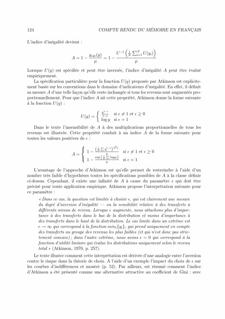
124 COMPTE RENDU DU MÉMOIRE EN FRANÇAIS
L’indice d’inégalité devient :
A = 1− yede(y)
µ= 1−
U−1(
1N
∑Ni=1 U(yi)
)µ
Lorsque U(y) est spécifiée et peut être inversée, l’indice d’inégalité A peut être évaluéempiriquement.
La spécification particulière pour la fonction U(y) proposée par Atkinson est explicite-ment basée sur les conventions dans le domaine d’indicateurs d’inégalité. En effet, il définitsa mesure A d’une telle façon qu’elle reste inchangée si tous les revenus sont augmentés pro-portionnellement. Pour que l’indice A ait cette propriété, Atkinson donne la forme suivanteà la fonction U(y) :
U(y) =
{y1−ε
1−ε si ε 6= 1 et ε ≥ 0
log y si ε = 1
Dans le texte l’insensibilité de A à des multiplications proportionnelles de tous lesrevenus est illustrée. Cette propriété conduit à un indice A de la forme suivante pourtoutes les valeurs positives de ε :
A =
1− ( 1N
∑y1−εi )
11−ε
µsi ε 6= 1 et ε ≥ 0
1− exp ( 1N
∑logyi)
µsi ε = 1
L’avantage de l’approche d’Atkinson est qu’elle permet de restreindre à l’aide d’unnombre très faible d’hypothèses toutes les spécifications possibles de A à la classe définieci-dessus. Cependant, il existe une infinité de A à cause du paramètre ε qui doit êtreprécisé pour toute application empirique. Atkinson propose l’interprétation suivante pource paramètre :
« Dans ce cas, la question est limitée à choisir ε, qui est clairement une mesuredu degré d’aversion d’inégalité — ou la sensibilité relative à des transferts àdifférents niveau de revenu. Lorsque ε augmente, nous attachons plus d’impor-tance à des transferts dans le bas de la distribution et moins d’importance àdes transferts dans le haut de la distribution. Le cas limite dans un extrême estε→∞ qui correspond à la fonction mini{yi}, qui prend uniquement en comptedes transferts au groupe des revenus les plus faibles (et qui n’est donc pas stric-tement concave) ; dans l’autre extrême, nous avons ε = 0 qui correspond à lafonction d’utilité linéaire qui évalue les distributions uniquement selon le revenutotal » (Atkinson, 1970, p. 257).
Le texte illustre comment cette interprétation est dérivée d’une analogie entre l’aversioncontre le risque dans la théorie de choix. A l’aide d’un exemple l’impact du choix de ε surles courbes d’indifférences et montré (p. 52). Par ailleurs, est résumé comment l’indiced’Atkinson a été présenté comme une alternative attractive au coefficient de Gini : avec

125
son théorème, Atkinson a d’abord établi une relation avec la courbe de Lorenz ; ensuite, ilintroduit le concept d’aversion contre l’inégalité et montre que le coefficient de Gini contientun degré d’aversion plus élevé au milieu de la distribution qu’aux franges. L’interprétationclaire de A en termes de bien-être et son paramètre d’aversion contre l’inégalité ont permisde mettre en cause la position dominante du coefficient de Gini dans le débat académique.
En ce qui concerne l’impact sur les conventions d’Atkinson dans le domaine de la mesured’inégalité, les points suivants sont analysés :
1. L’indice d’Atkinson continue la tradition d’employer des mesures sommaires poursynthétiser toute l’information sur l’inégalité dans un seul chiffre. La raison pouropter pour une mesure sommaire semble être purement conventionnelle : « L’approcheconventionnelle dans presque tous les travaux empiriques est d’adopter une statistiquesommaire d’inégalité comme [...] » (ibid., p. 244).
2. La décision de retenir la propriété d’insensibilité de A à une augmentation proportion-nelle est également basée sur une référence explicite aux conventions : « Maintenant,nous avons vu que presque toutes les mesures conventionnelles sont définies relativeà la moyenne [...] » (ibid., p. 257). Ceci est un point très important car sans cettepropriété il serait considérablement moins évident d’obtenir des valeurs numériquespour A (cf. Kolm, 1976).
3. En plaçant son approche dans le cadre d’analyse de Dalton, Atkinson pouvait présen-ter sa mesure comme étant en continuité à une contribution plus ancienne et presqueclassique. En enrichissant le raisonnement en terme de bien-être, Atkinson a éloigné lediscours académique des indicateurs purement descriptifs et renforcé l’idée d’évaluerdirectement les conséquences des inégalités au lieu de leur ampleur.
4. Atkinson a modifié le principe de transferts de Dalton en exigeant qu’une mesureacceptable d’inégalité soit plus sensible en bas de la distribution. L’argument enfaveur de cette modification est l’intuition d’Atkinson qu’une sensibilité constanteaux transferts ne serait pas acceptée par la plupart des gens.
5. Avec son refus de l’approche descriptive, son raisonnement approfondi en terme defonction de bien-être et son exigence d’une sensibilité aux transferts variable, Atkin-son a sans doute contribué à la complexification des instruments analytiques. Nousrappelons d’ailleurs qu’Atkinson a exprimé explicitement ses préférences pour desconsidérations théoriques au profit de la communicabilité des mesures d’inégalité.
Le tour de force conceptuel de Sen
Après un bref commentaire sur l’apport global de Sen au débat sur l’inégalité écono-mique, le texte discute quatre points qui sont importants pour la présente discussion.
Tout d’abord, il est rappelé que Sen préconise une position intermédiaire entre d’un coté,l’approche descriptive ou « objective » à la mesure de l’inégalité et, de l’autre coté, les éva-luations normatives en terme de bien-être. Sen propose que le concept d’inégalité possèdeun caractère dual qui mélange ces deux éléments. Ceci attribut une place plus importante à

126 COMPTE RENDU DU MÉMOIRE EN FRANÇAIS
la description d’inégalité et, par là, à la correspondance des mesures d’inégalité à la « com-munication normale ». Pour Sen, un indicateur acceptable doit non seulement satisfairedes considérations d’ordre technique, mais également être « raisonnablement proche » àl’usage normale du concept d’inégalité. Dans ce contexte, le texte montre comment Senutilise le concept de « communication normale » à plusieurs reprises comme une contrainteà la validité des mesures alternatives d’inégalité (p. 56). Il semble que Sen emploie ce termecomme étant un objet que l’économiste peut identifier de manière relativement simple.
Malgré ce rappel en faveur de l’intégration d’éléments descriptifs, la méthode de Senreste encastrée dans l’évaluation de l’inégalité en termes du bien-être. Cependant, il argu-mente que l’approche utilitariste n’est pas adaptée à l’analyse de l’inégalité car elle associele maximum de la fonction de bien-être à la notion de l’égalité qu’à cause d’une « coïn-cidence très spéciale » . Sen propose d’introduire la préférence pour l’égalité directementpar des axiomes explicites.
Le problème de décider si l’inégalité est un concept relatif est également abordé parSen, mais apparemment sans une décision claire en faveur ou contre l’insensibilité des me-sures d’inégalité à une multiplication proportionnelle. Sen juge que la question si l’inégalitéest un concept absolu ou relatif est un dilemme conceptuel. Cependant, dans la versionélargie et mise à jour de On economic inequality, publiée en 1997, Sen souligne que « tra-ditionnellement on pense de l’inégalité comme un concept relatif » et rejette l’introductiond’un « élément absolutiste » dans les statistiques d’inégalité.
Enfin, un autre élément pertinent de la réflexion théorique de Sen est l’observation quela complétude des mesures statistiques est problématique. En effet, Sen remarque que leconcept d’inégalité n’est pas suffisamment clair pour toujours permettre des jugements sansambiguïté. Pour décider laquelle de deux distributions est la plus inégale, il serait nécessairequ’un contraste relativement marqué entre elles soit observable. Cette réflexion conduit Senà proposer l’instrument de rangement par intersection, qui vise à identifier les situationsplus faciles à évaluer. Le principe d’un rangement par intersection est d’évaluer toute unebatterie de statistiques d’inégalités pour isoler les cas conflictuels de ceux où toutes lesstatistiques conduisent au même rangement des distributions. En termes techniques, ondéfinit d’abord un ensemble de k rangements, Cj, for j = 1, ..., k, qui sont tous a prioriplausibles. L’intersection de ces k rangements complets est annotée Q et peut être écritecomme :
yQx si, et seulement si ∀j = 1, ..., k : yCjx
Ceci veut dire que la distribution y obtient une place plus élevée dans le rangement Q quela distribution x si le même rangement est observé pour toutes les mesures d’inégalité Cj.Par exemple, si le rangement par intersection est défini comme l’intersection du coefficientde concentration de Gini et le ratio interdécile D9/D1, le rangement Q permet d’ordonnerles distributions si le rangement CG du coefficient de Gini ne contredit pas le rangementCID du ratio interdécile. Cependant, force est de constater que l’approche de rangementspar intersection contient toujours un élément arbitraire à cause de la sélection nécessairede mesures qui y sont intégrées.
Ensuite, le texte approfondie la réflexion sur les deux apports de Sen les plus importants

127
pour nos questions : la position particulière de la communication normale dans l’œuvre deSen et l’hypothèse de l’incomplétude du concept d’inégalité.
En effet, l’utilisation de la communication normale comme une contrainte ne rend passuffisamment compte du fait que les conceptions sont les résultats d’une co-construction :elles ne peuvent pas être construites de manière unilatérale par la science. Il semble quele problème de rester « raisonnablement proche » à la communication normale est plusdifficile à résoudre que l’approche de Sen ne le laisse penser.
L’hypothèse d’incomplétude du concept d’inégalité introduit un problème central desmesures sommaires. Les rangements complets issus des statistiques synthétiques pourraienten effet être plus précises que le concept d’inégalité lui-même. Par conséquent, la précisiondes statistiques introduit forcément un élément arbitraire dans l’analyse. Néanmoins, unesolution à cette ‘sur-précision’ des mesures sommaires doit rester communicable et trans-parente. La panoplie d’indicateurs contenue dans un rangement par intersection risqued’introduire une multitude de concepts différents dans une seule mesure et accroître lacomplexité informationnelle et l’opacité des statistiques.
Les généralisations récentes des méthodes
Malgré le fait que le tour de force conceptuel de Sen soit la dernière contribution discu-tée en détail dans ce chapitre, l’analyse scientifique de l’inégalité économique a connu desévolutions importantes depuis la première édition de On economic inequality de 1973, etmême après la version actualisée de 1997. Une exemple de développements récents est latendance d’insister sur des approches multidimensionnelles, dont l’IBEE est indirectementle résultat. D’autres innovations conceptuelles et théoriques peuvent être identifiées. Cepen-dant, il est argumenté que la littérature académique sur la mesure empirique des inégalitéséconomiques fait d’avantage preuve d’un approfondissement des méthodes conventionnellesdéjà en place à partir des années 1970. Le résumé de développements récents par Jenkins &Micklewright (2007) indique également que nous sommes en présence d’un procès de conso-lidation et d’amélioration des approches conventionnelles. Cinq axes de recherche peuventêtre cités pour illustrer la plausibilité de cette hypothèse :
1. La courbe de Lorenz et le théorème d’Atkinson ont été les bases pour les concepts dedominance généralisée de Lorenz et de dominance stochastique de Shorrocks (1983),Foster & Shorrocks (1987) et d’autres.
2. L’indice d’Atkinson a été généralisé et a donné naissance à la « famille d’Atkin-son » (Jenkins & Micklewright, 2007, p. 13). La dérivation de classes d’indices pa-ramétriques avec des caractéristiques normatives explicites a été systématisée et ap-profondie.
3. L’indice décomposable de Theil a inspiré une classe d’entropie généralisée de mesured’inégalité développée par Bourguignon (1979) et d’autres.
4. D’autres développements, comme le traitement systématique des erreurs d’échan-tillonnage et la dérivation des intervalles de confiance pour les mesures d’inégalités

128 COMPTE RENDU DU MÉMOIRE EN FRANÇAIS
proposés par Beach and Davidson (1983) sont directement basés sur la méthode deLorenz et les courbes généralisées de Lorenz.
5. La critique de Paglin (1975) de ne pas confondre l’inégalité entre et à l’intérieur defamilles est essentiellement une extension du coefficient de concentration de Gini etde l’approche de Lorenz.
Cette section termine avec la conclusion que la focalisation sur la concentration— initiéepar Lorenz et Gini — et l’approche basée sur la fonction de bien-être par Dalton et Atkinsonsont devenues des conventions acceptées dans ce domaine. Suite à des généralisations etextensions de ces concepts, la mesure de l’inégalité semble aujourd’hui d’être plus complexeet technique qu’auparavant.
Proche de la ‘vérité’ ou du citoyen ?Pour terminer ce chapitre sur l’histoire interne du discours académique sur la mesure
de l’inégalité, trois aspects sont discutés qui semblent indiquer que le progrès scientifiquedans ce domaine ne se traduit pas forcément par un rapprochement aux conceptions de lacommunication normale.
Premièrement, la présence gênante d’un arbitrage entre communicabilité et complétudeanalytique de la discussion scientifique est rappelée. Cet arbitrage n’a pas été suffisammentpris en compte et a rendu les mesures plus difficilement communicables. Par conséquent,un nombre élevé d’acteur est désormais exclu du débat ; leurs conceptions risquent d’êtreignorées ou au moins sous-représentées. Or, une mesure avec l’objectif d’assister au débatpublic comme l’IBEE doit confronter ce problème et s’assurer d’une communicabilité ac-ceptable afin de permettre l’intégration des conceptions des usagers dans la constructiondes mesures statistiques.
Deuxièmement, l’arbitrage entre communicabilité et complétude théorique crée uneconséquence directe pour la distinction entre d’une part, les mesures descriptives et, d’autrepart, les approches plus normatives basées sur l’évaluation d’une fonction de bien-être. Ilsemble que ces dernières augmentent le degré de complexité de la mesure empirique etrisquent de la rendre plus opaque pour les utilisateurs non spécialistes.
Enfin, malgré le progrès méthodologique considérable, ils restent des problèmes concep-tuels qui sont loin d’être résolus de manière satisfaisante. La focalisation de la littératurescientifique sur les mesures relatives n’est pas suffisamment balancée et ignore les pointsde vue alternatives observables dans la communication normale.

Chapitre 3La mesure des inégalités dans l’IBEE
Une brève introduction à l’IBEE d’Osberg et SharpeCe chapitre contient des éléments de contexte sur l’indicateur de bien-être économique
proposé par L. Osberg et A. Sharpe. Tout d’abord, nous présentons les objectifs et lesusagers de cet instrument, ensuite la genèse de l’IBEE est esquissée.
Quant aux objectifs, l’IBEE a été conçu comme un outil d’évaluation de la perfor-mance économique des politiques gouvernementales et, de manière générale, comme uneheuristique sur l’état économique d’une société. En analysant les explications des auteurscanadiens dans leurs articles sur l’IBEE, le texte montre que l’usager ciblé n’est pas l’ex-pert technique qui base une recherche sophistiquée sur les résultats de l’indicateur. L’IBEEassiste plutôt le « citoyen », qui dans l’exercice de ses devoirs démocratiques nécessite unevision globale et informée sur la réalité (socio-) économique. L’objectif de l’IBEE est doncd’assister le débat public en fournissant un outil d’évaluation au citoyen. Il vise à résumerl’information pertinente dans un format compréhensible. Une conséquence de cet objectifest que les « perceptions populaires » jouent un rôle important dans l’analyse d’Osberg etSharpe et que l’indicateur devrait permettre aux usagers d’y retrouver leurs systèmes devaleurs.
Les bases théoriques de l’IBEE ont déjà été établies en 1985 dans un article de LarsOsberg. Cependant, la première application empirique n’a été effectuée qu’en 1998 pourl’économie canadienne. Le texte cite les applications qui ont suivi ce premier exemple etnote que l’IBEE possède désormais une place dans le débat international autour de lamesure du bien-être économique (p. 64).
La méthodologie de l’IBEE
Sont présentés dans cette section l’architecture générale de l’indicateur ainsi que lesconcepts qui y sont intégrés. Les quatre grandes dimensions du bien-être identifiées parOsberg & Sharpe (2005) sont les suivantes :
« (1) Flux effectifs de consommation par tête (valeur monétaire à prix constants)— affectée d’un indice de progression de l’espérance de vie, et ajustée pour te-nir compte des variations du temps de travail annuel par personne. A cette
129

130 COMPTE RENDU DU MÉMOIRE EN FRANÇAIS
consommation s’ajoutent les dépenses gouvernementales par tête, hors servicede la dette4, ainsi que le travail domestique non rémunéré et bénévolat5.(2) Stock de capital national physique net par tête (valeur monétaire)6 — auquelsont ajoutés les stocks de R&D par tête (valeur monétaire7), les variations dansla valeur du patrimoine de ressources naturelles par tête (valeur monétaire)8,les variations de stocks de capital humain9. De ces stocks sont déduits la detteextérieure nette par tête, ainsi que les coûts des émissions polluantes10.(3) Indicateur synthétique de pauvreté combinant le taux de pauvreté monétaireet une mesure de l’intensité de cette pauvreté. Un indicateur d’inégalité de ladistribution des revenus compose également une partie de cette dimension.(4) Sécurité économique — des risques économiques liés au chômage, à la mala-die, aux risques de rupture familiale (familles monoparentales) et à la pauvretédes personnes âgées. »
Osberg et Sharpe sont conscients du fait que le bien-être économique n’est pas unobjet homogène. Cependant, ils argumentent qu’il est nécessaire de « faire la somme deschoses qui sont conceptuellement distinctes » afin d’aboutir à des évaluations du bien-être économique global. Le tableau ci-dessous résume les différents concepts contenus dansl’IBEE.
TempsConcept Présent Futur« Citoyen typique » ou« agent représenta-tif »
Flux moyens de revenuscourants
Accumulation de stocksproductifs
« Citoyens hétéro-gènes »
Distribution — inégalité desrevenus et pauvreté
Insécurité des revenus fu-turs
Tab. 9 – Concepts dans l’IBEE. Source : Osberg & Sharpe, 2005.
Le caractère hybride de la compilation de données et de leur synthèse statistique estune des forces de l’indicateur : plutôt que d’imposer une vision hégémonique en termes
4 Il n’y a pas ici de soustraction de dépenses jugées « défensives » comme cela était le cas dans lestravaux initiaux de Nordhaus et Tobin.
5L’estimation de la valeur de l’heure de travail domestique est effectuée sur la base d’un salaire horairede personnel domestique.
6Méthode dite d’inventaire permanent, appliquée à tous les stocks mesurables d’équipement productifprivé ou public, locaux d’habitation, infrastructures...
7Comptabilisé par attribution d’un taux d’amortissement de 20 % aux séries de flux.8En fonction des données nationales ou internationales existantes, on peut tenter d’inclure des valeurs
estimées pour les ressources en minéraux principaux, forêts, et réserves d’énergie (ce que font les auteurspour le cas du Canada).
9Coûts de l’éducation de l’ensemble de la population, estimés sur la base des coûts par niveau d’étudeset de la répartition de la population par niveau.
10Limité dans cet indicateur au coût social estimé des émissions de CO2.

131
méthodologiques, il insiste sur les variables qui constituent l’indicateur, recourant ensuiteà la méthode jugée la plus appropriée : monétarisation pour les dimensions consommationet accumulation de stocks productifs, moyennes normalisées à partir d’indices connus (uneversion simplifiée du Sen-Shorrocks-Thon Index et le coefficient de Gini) pour les inégalitéset la pauvreté, méthode originale de calcul de risques économiques pour la dimensionsécurité économique.
Pour chacune des quatre dimensions de l’IBEE sont présentées la structure générale etles pondérations des différentes variables qu’elles contiennent.
Premier pilier de l’indicateur synthétique, la consommation ajustée repose sur l’hypo-thèse que le bien-être économique est directement corrélé aux volumes de biens et servicesconsommés. Les ajustements procédés tiennent compte de la taille des ménages, par le biaisde l’utilisation des échelles d’équivalence, des dépenses publiques, de l’espérance de vie, etde la valeur du loisir. Le graphique suivant présente le contenu ainsi que le mécanismed’agrégation de la dimension consommation effective.
Consommationréelle totalepar tête
=
Indiced’espérance
de vie*
Dépensespubliques(biens &services)
+Valeur duloisir
+Indice derevenu
équivalent*
Consommationpersonnellepar tête
Fig. 5 – Dimension 1 : consommation.
La deuxième dimension — l’accumulation des stocks de richesse productive— , considé-rée comme une estimation des flux de consommations futures, est susceptible d’influencerle bien-être pour deux raisons. D’une part, les individus sont soucieux de leur propre condi-tion matérielle dans le futur. D’autre part, il est raisonnable de supposer que la plupartdes individus est sensible à la situation matérielle des générations futures. La dimensioncontient les principales catégories de facteurs productifs, à savoir le capital fixe, le stockdes investissements en matière de recherche et développement, ainsi qu’une estimation dela valeur du capital humain de la population. Tandis que la mesure des deux premiers fac-teurs repose sur des conventions statistiques traditionnelles, la valeur monétaire du capitalhumain est estimée sur la base des coûts par niveau d’études et de la répartition de lapopulation par niveau.
Les individus sont concernés par un certain niveau de redistribution des richesses :quelle part leur sera-t-elle attribuée ? Quelle part sera attribuée aux autres ? Osberg et
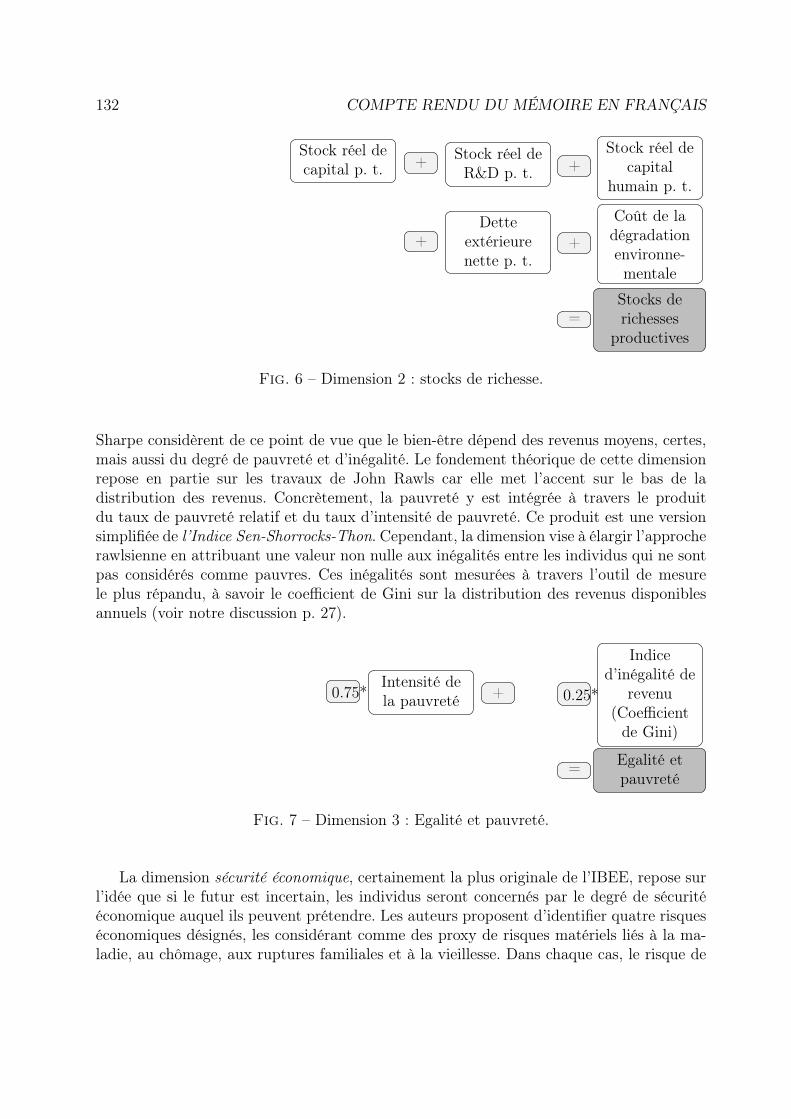
132 COMPTE RENDU DU MÉMOIRE EN FRANÇAIS
Stocks derichesses
productives=
Coût de ladégradationenvironne-mentale
+Dette
extérieurenette p. t.
+
Stock réel decapital
humain p. t.+
Stock réel deR&D p. t.
+Stock réel decapital p. t.
Fig. 6 – Dimension 2 : stocks de richesse.
Sharpe considèrent de ce point de vue que le bien-être dépend des revenus moyens, certes,mais aussi du degré de pauvreté et d’inégalité. Le fondement théorique de cette dimensionrepose en partie sur les travaux de John Rawls car elle met l’accent sur le bas de ladistribution des revenus. Concrètement, la pauvreté y est intégrée à travers le produitdu taux de pauvreté relatif et du taux d’intensité de pauvreté. Ce produit est une versionsimplifiée de l’Indice Sen-Shorrocks-Thon. Cependant, la dimension vise à élargir l’approcherawlsienne en attribuant une valeur non nulle aux inégalités entre les individus qui ne sontpas considérés comme pauvres. Ces inégalités sont mesurées à travers l’outil de mesurele plus répandu, à savoir le coefficient de Gini sur la distribution des revenus disponiblesannuels (voir notre discussion p. 27).
Egalité etpauvreté
=
Indiced’inégalité de
revenu(Coefficientde Gini)
0.25*+Intensité dela pauvreté0.75*
Fig. 7 – Dimension 3 : Egalité et pauvreté.
La dimension sécurité économique, certainement la plus originale de l’IBEE, repose surl’idée que si le futur est incertain, les individus seront concernés par le degré de sécuritééconomique auquel ils peuvent prétendre. Les auteurs proposent d’identifier quatre risqueséconomiques désignés, les considérant comme des proxy de risques matériels liés à la ma-ladie, au chômage, aux ruptures familiales et à la vieillesse. Dans chaque cas, le risque de

133
perte économique lié à l’événement en question est évalué comme une probabilité condi-tionnelle, elle-même représentée comme le produit de diverses circonstances. La potentialitéde chaque risque est pondérée par la part de la population concernée. L’hypothèse fonda-mentale est que les variations du niveau subjectif d’anxiété qui résulte d’une insécurité(variations de bien-être subjectif ) sont proportionnelles aux variations du risque objectif.
Sécuritééconomique
=
(Risque écon.de pauvreté(personnes
agées))*(P4/P )
+
(Risqueéconomique
lié à lapauvreté mo-noparentale)*(P3/P )
+
(Risquefinancier lié àla maladie)*(P2/P )
+
(Risqueéconomique
lié auchômage)*(P1/P )
Fig. 8 – Dimension 4 : sécurité économique. Légende : P1 = Population entre 15-64 ; P2
= population entière ; P3 = population de femmes mariées avec enfants ; P4 = populationentre 45-64. P = P1 + P2 + P3 + P4.
Les pondérations utilisées pour permettre l’agrégation des dimensions sont ex naturarei arbitraires mais transparentes, permettant d’une part d’évaluer la sensibilité du choixde ces pondérations, d’autre part de les modifier en fonction de systèmes de préférencescollectives, qu’il reste à construire. Dans la partie applicative suivante, nous utiliseronsla pondération la plus fréquemment suggérée par les auteurs, à savoir des poids égauxattribués à l’ensemble des dimensions.
Quatre dimensions, trois inégalités
Après avoir présenté l’IBEE dans sa forme originale, une proposition de modification dela dimension égalité et pauvreté est proposée. En effet, nous notons une inconsistance dans lastructure interne de l’IBEE qui résulte de la manière avec laquelle l’indicateur rend comptede l’inégalité. D’un coté, l’IBEE identifie quatre dimensions comme étant pertinentes pourl’évaluation du bien-être économique. De l’autre coté, l’inégalité est évaluée pour une seulevariable, à savoir pour le revenu par tête à travers le coefficient de Gini. Nous constatonsque si nous admettons que le bien-être économique est composé de multiples dimensions,l’inégalité économique devrait aussi consister de ces éléments multiples. Le graphique ci-contre illustre la proposition d’analyser trois aspects de l’inégalité économique. Les troisdimensions consommation par tête, stocks de richesses par tête et sécurité économiqueengendrent trois espaces d’inégalités.
Cette proposition nous conduit à la modification de la dimension égalité et pauvretéillustrée sur le graphique suivant.

134 COMPTE RENDU DU MÉMOIRE EN FRANÇAIS
Consommationréelle totale
Distributionde la consom-
mation
Distributiondes stocks de
richesse
Stocks derichesses
Inégalitésface auxrisques
économiques
Sécuritééconomique
Egalitééconomique
Fig. 9 – Proposition de mesurer l’égalité au sein de l’IBEE.
Egalité etpauvreté
=
Egalitééconomique0.25*+
Intensité dela pauvreté0.75*
Fig. 10 – Dimension 3 modifée : égalité et pauvreté.
Propositions alternatives de mesurer l’égalité dans l’IBEE
Après avoir énoncées les dimensions des inégalités économiques à évaluer, cette sectiontraite l’opérationnalisation de la mesure. Afin de pouvoir mesurer les inégalités relativesà la consommation, aux stocks de richesse et à la sécurité économique, il est nécessairede choisir une statistique qui reflète de manière satisfaisante l’objectif de l’IBEE. Lesprincipales conventions identifiées dans le chapitre 2 sont donc discutées dans le contextespécifique de cette question. Ceci conduit à une confrontation des considérations internesissues du discours académique avec les conceptions des acteurs externes (les usagers del’IBEE).
Lors de la discussion des contributions les plus importantes dans le domaine de lamesure empirique des inégalités, un consensus assez large sur les points suivants a étéidentifié : a) dans le cas d’un conflit entre complétude théorique et simplicité des mesures,l’approche conventionnelle semble donner la priorité aux considérations théoriques (cf. At-kinson, 1970, p. 253) ; b) l’analyse quantitative est sans doute l’approche dominante à lamesure des inégalités économiques ; c) l’acceptabilité des statistiques d’inégalité est testée

135
conventionnellement de manière indirecte à l’aide d’une liste de caractéristiques désirées ;d) malgré la critique de Sen que les rangements complètes aboutissent à une précisionen partie arbitraire, la plupart des analyses continuent à employer des statistiques som-maires pour comparer le degré d’inégalités de différentes distributions ; e) concentration etinégalité sont souvent regardées comme « essentiellement le même concept » (Theil, 1964,p. 128).
La légitimité de chacun de ces cinq aspects est discutée dans le contexte de la mesuremultidimensionnelle des inégalités au sein de l’IBEE. Etant donné que l’objectif de cetindicateur consiste à représenter les conceptions du « citoyen », nous argumentons queplusieurs de ces méthodes conventionnelles doivent être mise en question. Il est à noterqu’il est impossible de définir avec exactitude le concept d’inégalité à l’aide du critère de la« communication normale ». Cependant, il semble la légitimité de l’IBEE dépend du degréavec lequel la mesure est co-construite et prend en compte des considérations internes etexternes.
Ceci nous conduit à identifier la communicabilité des mesures comme une conditio sinequa non de la co-construction des statistiques (p. 70). Si la technicité des statistiquesdépasse un certain seuil de complexité, le « citoyen » ne sera pas en mesure de vérifier sises valeurs sont effectivement reflétées par les instruments empiriques.
Un aspect normatif qui n’a pas été suffisamment pris en compte par les méthodesconventionnelles est la distinction entre les concepts relatif et absolu d’inégalité qui a étéremarqué à plusieurs reprises tout au long du texte. Si l’inégalité est perçue comme étantrelative, alors les augmentations proportionnelles ne modifient pas l’ampleur de l’inégalité.Toutes les mesures basées sur la notion de concentration possèdent cette caractéristiqued’être insensible à des augmentations proportionnelles car elle prennent uniquement encompte les ratios entre les différents revenus. En revanche, si l’inégalité est perçue commeun concept absolue, l’écart absolu entre les positions des individus est un facteur d’inégalité.Bien que la relation entre différences absolues et la notion d’inégalités soit traitée par descontributions isolées (notamment par Kolm, 1976), l’approche orthodoxe est de considérerl’inégalité comme un concept relatif.
Selon notre analyse, il n’est pas légitime de donner préférence à un de ces deux visionsalternatives des inégalités (p. 73). Le texte présente des arguments en faveur de l’hypothèseque l’inégalité est souvent associée avec les différences en termes absolues et cite les travauxde Kolm (1976) et Ravallion (2003). Ces auteurs indiquent que l’opposition en questionpeut être pensée comme des positionnements politiques alternatives. En effet, Kolm associeune attitude « de gauche » aux mesures absolues d’inégalité et réserve la vision relativeaux attitudes « de droite ». Selon Ravallion, une partie du débat autour de la globalisationdes marchés reflète la différence entre une vision absolue et relative des inégalités.
En conclusion, deux façons alternatives de penser les inégalités sont présentés. Ellessont moins sophistiquées que les statistiques qui intègrent directement une quelconquefonction de bien-être, mais ont l’avantage d’être plus faciles à communiquer et à représentergraphiquement. Comme l’opposition entre inégalité absolue et inégalité relative semblerefléter des opinions politiques divergentes, nous proposons deux concepts alternatifs afinde laisser le choix au citoyen d’évaluer le bien-être en fonction de son système de valeurs.

136 COMPTE RENDU DU MÉMOIRE EN FRANÇAIS
Les deux concepts alternatifs proposés pour représenter les inégalités multidimension-nelles sont les suivants :
1. Un concept facilement communicable et intuitive est de penser des inégalités commedes écarts moyens. Si nous imaginons chaque dimension des inégalités comme étantune dimension d’un espace, chaque ménage peut être traité comme un point danscet espace. L’inégalité entre deux ménages est simplement l’écart entre leurs pointsrespectifs. L’inégalité totale est alors l’écart moyen entre tous les ménages. Ceci estun concept absolu d’inégalité.
2. Si on divise toutes les écarts par la moyenne de différentes dimensions, nous obtenonsun écart moyen relatif, qui reste cependant multidimensionnel. Ceci est donc similaireà un coefficient de concentration de Gini à plusieurs dimensions.
Mesurer les écarts : une approche géométrique
Les deux concepts issus de la réflexion sur la légitimité des méthodes conventionnellesoffrent l’avantage de permettre une représentation graphique simple. Cette section montreque les écarts moyens peuvent être pensés comme des distances moyennes dans un espaceEuclidien. Ceci permet de préciser les formules à appliquer aux données empiriques etfranchir la dernière étape de l’opérationnalisation de la mesure des inégalités dans l’IBEE.
La première partie de cette section est dédiée à un rappel sur les distances Euclidienneset montre comment les DMA et DMR proposées par Gini (voir section 2.1.3) peuventêtre représentées comme des distances dans l’espace. Cependant, nous argumentons queles versions multidimensionnelles des mesures de Gini nous confrontent à des problèmessérieux quant à leur utilisation comme des indicateurs d’inégalité multidimensionnelle. Cesproblèmes sont, premièrement, les différences d’échelles entre les trois dimensions à évaluer.L’écart moyen entre plusieurs points sera forcément plus sensible aux écarts dans unedimension qui varient entre 1000 e et 1000000 e qu’aux écarts dans une autre dimensionpour laquelle les valeurs ne varient qu’entre 0 et 1. Une normalisation simple comme latransformation T = (xi − xmin)/(xmin − xmax), appliquée à toutes les valeurs, ne peut pasrésoudre ce problème (xmin et xmax pourraient être les montants maximaux et minimauxde chaque dimension). En effet, une telle transformation normalise toutes les dimensions àun intervalle [0, 1] et élimine une partie importante des écarts absolue entre les points.La deuxième difficulté est qu’une version multidimensionnelle de la DMA ou de la DMR nenous permet pas d’analyser les contributions des différentes dimensions à l’égalité totale.Enfin, les mesures de Gini sont basées sur toutes les différences possibles entre tous lespoints, c’est-à-dire y compris les différences de tous les ménages avec eux-mêmes. De plus,chaque écart entre deux ménages différents apparaît deux fois dans le calcul. Nous pensonsqu’il serait plus intuitif de baser la mesure d’inégalité que sur les différences entre despoints différents et de réduire leur nombre de N2 à (N2 −N)/2.
A cause de ces trois aspects problématiques une modification de DMA est proposée. Lastratégie est de formuler une mesure d’inégalité unidimensionnelle basée sur (N2 − N)/2différences et de la transformer en indice pour surmonter la difficulté lié aux différentes

137
échelles des dimensions. La mesure unidimensionnelle proposée est définie comme :
ADd ≡∑N−1
i=1
∑Nj>i
√(pi,d − pj,d)2
(N2 −N)/2
La computation de ADd est illustrée à l’aide d’un exemple qui montre qu’il s’agiteffectivement d’une mesure absolue dans le sens définie ci-dessus (p. 78). Pour obtenir unemesure relative d’inégalité, nous introduisons la notion de la longueur moyenne des vecteursdans la dimension d, qui sera annotée λd et qui peut être écrite comme suivant :
λd =1
N
N∑i=1
√p2i,d
Passer de la mesure ADd à un indicateur relatif est semblable à diviser la DMA par lerevenu moyen pour obtenir la DMR. Une version relative de ADd est donc la mesure RDd,qui est définie comme :
RDd ≡Adλd
De nouveau le calcul de la mesure est illustrée à l’aide des exemples et les différences etsimilitudes entre les deux statistiques sont discutées (p. 79).
Enfin, pour synthétiser les ADd et RDd de chaque dimension d dans une mesure del’évolution globale des inégalités, nous proposons les indices suivants :
I tA =1
n
ADt1
ADt−m1
+ · · ·+ 1
n
ADtn
ADt−mn
I tR =1
n
RDt1
RDt−m1
+ · · ·+ 1
n
RDtn
RDt−mn
Nous pouvons interpréter ces deux indices comme la moyenne des changements d’inégalitésdans les différentes dimensions. Puisque la distance moyenne de chaque dimension à la datet, ADd
t , est comparée à la valeur de base de la même dimension, les différences d’échellesentre les dimensions disparaissent. Seules les évolutions temporelles en pourcentage dechaque dimension sont retenues dans l’indice. La logique de ces indices est illustrée à l’aided’un exemple (p. 80).

Chapitre 4Application empirique
Traitement de données
Avant de passer à l’application des mesures d’inégalité, la source utilisée pour la partieempirique est décrite en début de ce chapitre : l’enquête Budget des Familles, BdF. Leslimites de cette source sont également discutées. Notamment le champ restreint, la faiblefréquence et le fait que les questions de sécurité économique et du patrimoine économique nesont pas des objectifs principaux de l’enquête sont identifiés comme des limites importantes.
Des données sur l’ensemble des trois dimensions d’inégalités de l’IBEE ne sont mal-heureusement disponibles que pour les deux éditions les plus récentes de l’enquête BdF, àsavoir les éditions des années 1994/1995 et 2000/2001. Pour chacune des trois dimensionsnous expliquons comment les définitions contenues dans l’IBEE peuvent être approximéespar des variables issues de l’enquête BdF.
Le constat s’impose qu’il est impossible d’évaluer les trois dimensions en termes d’inéga-lité si nous retenons les définitions exactes de ces dimensions. Ceci est dû à deux facteurs :d’une part, notre source (le BdF) ne contient pas de renseignements sur l’ensemble de fac-teurs qui font partie des dimensions du bien-être, comme par exemple l’espérance de vieau sein de chaque ménage. D’autre part, nous sommes confrontés à des problèmes d’ordreconceptuel car un certain nombre de variables (comme par exemple la consommation desbiens et services produits par le gouvernement) ne sont pas facilement individualisable. Letexte présente pour chaque composante des trois dimensions les raisons de soit retenir lavariable et de l’approximer à l’aide de l’enquête BdF, soit de ne pas l’intégrer. Ceci aboutità des proxies des trois dimensions qui sont ensuite évalués en termes d’inégalité.
Inégalité de la consommation effective par tête
Nous argumentons qu’un proxy satisfaisant pour l’inégalité en termes de consomma-tion effective par tête est le revenu disponible ajusté par unité de consommation. Pourobtenir cette variable, nous mettons en œuvre la même procédure de correction que nousavons présentée dans Jany-Catrice & Kampelmann (op. cit.). La correction de donnéesadressent deux problèmes : premièrement, nous incluions des informations sur une compo-sante importante de la consommation privée, à savoir les loyers fictifs dont bénéficient les
138

139
propriétaires qui habitent dans leurs propres logements. Deuxièmement, nous corrigeonsla sous-estimation des revenus issus du patrimoine des ménages. La sous-estimation desrevenus de patrimoine est un problème bien connu et apparaît non seulement dans l’en-quête BdF, mais aussi dans d’autres sources. Notre approche consiste à ‘gonfler’ les valeursdes revenus de patrimoine pour que leur montant total coïncide avec le montant issu de lacomptabilité nationale, une source jugée comme plus fiable.
Comme Osberg et Sharpe insistent sur l’importance des économies d’échelle associées àla taille de ménages, nous divisons le revenu disponible par le nombre d’unité de consom-mation (défini par l’échelle d’équivalence d’Oxford). La distribution par percentiles quirésulte de ces traitements est illustrée dans le tableau ci-dessous.
1994/1995 2000/2001100% Max 290599.33 480455.6199% 63654.08 67657.1995% 36309.79 39964.4090% 28027.12 30818.1775% Q3 19484.61 21011.0350% Median 13591.35 14499.4925% Q1 9733.18 10298.7210% 7142.20 7594.075% 5866.64 6187.831% 3811.23 4133.220% Min 0.00 0.00Std Deviation 597122 647890
Tab. 10 – Distribution par percentiles et écart type du revenu disponible ajusté par unitéde consommation (toutes les valeurs en 1995 euros) — Source de données : BdF.
Inégalité de stocks de richesses par tête
A cause de problèmes conceptuels qui rendent une évaluation exacte de l’inégalité destocks de richesses impossible, nous présentons un proxy : la valeur totale de tous ce quepossède le ménage, exprimé en montant par tête.
L’enquête BdF contient une question de ce type, qui n’est cependant renseignée qu’entranches au lieu de valeurs « exactes ». Mais comme les huit tranches sont les mêmes pourles années 1994/1995 et 2000/2001, il est possible d’obtenir une approximation de la valeurde tout ce que possède le ménage à l’aide des hypothèses relativement peu restrictives(p. 86). Les montants par ménage sont ensuite divisés par le nombre de personnes vivantdans le ménage pour pouvoir évaluer les inégalités par tête entre les ménages. Le tableauci-dessous montre la proportion de ménages dans les différentes tranches pour les deuxenquêtes de 1994/1995 et 2000/2001.

140 COMPTE RENDU DU MÉMOIRE EN FRANÇAIS
Valeurs en tranches (en euros) 1994/1995 (% de mén.) 2000/2001 (% de mén.)0 - 3,049 7.69 7.11
3,049 - 7,622 10.45 9.237,622 - 15,245 9.41 9.7115,245 - 30,490 8.27 8.7130,490 - 76,225 16.64 14.0476,225 - 152,450 26.69 24.76152,450 - 304,898 15.21 19.07304,898 et plus 5.65 7.37
100 100
Tab. 11 – Valeur monétaire de tout ce que possède le ménage — Source de données : BdF.
Inégalité face aux risques économiques
L’enquête BdF permet d’approximer un des risques désignés par Osberg et Sharpe,à savoir l’inégalité face au risque de chômage. Dans le cadre du BdF, chaque ménageenquêté est demandé d’évaluer le risque de chômage dans les prochains 12 mois pourles différentes personnes qui constituent le ménage. Ceci permet de calculer l’écart entreles risques subjectifs des ménages et d’analyser la distribution du risque au sein de lapopulation.
Il est nécessaire de formuler une hypothèse comment les risques des différents membresdu ménage peuvent être agrégés. Nous avons décidé de retenir que le risque de la personnede référence, sauf si cette personne n’est pas active ou si elle a refusé de répondre à laquestion. Que dans ces cas le risque de chômage du conjoint est utilisé comme approxi-mation du risque économique du ménage. Le tableau ci-dessous présente la proportion desdifférents degrés de risque.
Degré de risque de chômage Score 1994/1995 (en %) 2000/2001 (en %)Non active - 8.4 10.86Non, il n’y a aucun risque 1 38.87 43.61C’est possible, mais le risque est faible 2 30.25 25.65C’est possible, et le risque est moyen 3 14.37 10.70C’est possible, et le risque est élevé 4 4.96 4.27Oui, c’est quasiment inévitable 5 3.14 4.73Refus - 0 0.18
100 100
Tab. 12 – Distribution du risque subjectif de chômage dans le 12 mois qui suivent l’enquête— Source de données : BdF.

141
Résultats pour les statistiques alternatives d’inégalité
Cette partie présente l’évaluation des trois vecteurs de données — qui décrivent res-pectivement le revenu disponible, le patrimoine et le risque de chômage — par rapportà leur inégalité. Est calculée la mesure AD (la distance moyenne absolue entre tous lespoints) ainsi que la version relative de cette mesure RD (les deux sont présentées dansla section 3.3.1). Pour comparer les résultats avec les statistiques traditionnelles d’inéga-lité sont également calculés : le coefficient de Gini (cf. Section 2.1.3), la mesure de Theil(cf. Section 2.1.5), le ratio interdécile, la mesure de Dalton (cf. Section 2.1.4) et l’indiced’Atkinson (cf. Section 2.1.6). La mesure de Dalton est évaluée pour une valeur du revenuminimum de c = 1/6000 et pour une valeur du patrimoine minimal c = 1/10000. L’indicede Atkinson est calculé pour deux niveaux d’aversion contre l’inégalité : une aversion faiblede ε = 0.5, et une aversion forte de ε = 1.5.
Les résultats pour le premier aspect d’inégalité économique sont présentés dans le ta-bleau ci-dessous. Tous les indicateurs descriptifs indiquent une augmentation de l’égalitéentre 1994/1995 et 2000/2001. Cependant, la taille de cette augmentation varie significati-vement : tandis que G n’augmente que par 2 %, la distance moyenne absolue AD indiqueun changement de plus de 10 %. Etant donné l’augmentation de 7 % du revenu moyen,une proportion considérable de cette différence peut vraisemblablement être expliquée parl’amélioration du niveau de vie moyen. Les mesures relatives RD, G, T et D9/D1 sonttoutes insensibles à des augmentations proportionnelles de tous les revenus. Si nous sup-posons qu’au moins une partie de la croissance du revenu moyen est distribuée parmi lesdifférentes couches de la société, ces mesures indiceraient une inégalité plus faible que lastatistique absolue AD. Concernant le développement des mesures basées sur l’évaluationd’une fonction de bien-être, les valeurs numériques observées dépendent des paramètres res-pectifs c et ε. Nous avons choisi ces valeurs de manière arbitraire et devons être prudentsavec leur interprétation. Cependant, la diminution de D est en accord avec le deuxièmeprincipe proposé par Dalton : une addition proportionnelle à tous les revenus devrait abou-tir à une diminution de l’inégalité (cf. notre discussion p. 35). Si la croissance du revenumoyen affecte plusieurs parties de la distribution, nous anticipons — ceteris paribus — ladiminution de l’inégalité que nous observons pour D. En ce qui concerne la statistique A,nous observons qu’une interprétation est difficile. Ceci ne vaut pas seulement pour l’inéga-lité en termes de revenu, mais aussi pour la dimension suivante, les stocks de richesses.La raison pour cette difficulté d’interprétation est que l’évolution de l’indice A change designe lorsque nous passons d’un degré d’aversion contre l’inégalité faible à un degré plusélevé. Comme il est problématique de connaître le degré d’aversion d’une société (ou mêmed’une personne), il est difficile d’interpréter ces chiffres.
La deuxième dimension, l’inégalité de richesses par tête, affiche une opposition encoreplus forte entre les mesures descriptives absolues et relatives. Ici, AD pointe même dans ladirection opposée avec une augmentation de 7.5 %, tandis que toutes les mesures relativesdiminuent entre les deux dates (voir le tableau ci-dessous). En même temps, le patrimoinemoyen a augmenté par 8.5 %, et une partie de la différence entre mesures relatives etabsolues peuvent être expliquée analogue à la première dimension. La mesure D évolue de

142 COMPTE RENDU DU MÉMOIRE EN FRANÇAIS
1994/1995 2000/2001 change en %Taille de l’échantillon N 11294 10305 −8.8Revenu moyen (en 1995 euros) 16619.66 17784.29 +7.0AD (en 1995 euros) 10808.34 11913.62 +10.2RD 0.65 0.67 +3.0G (Coefficient de Gini) 0.32 0.33 +1.9T (Mesure de Theil) 0.19 0.20 +3.4D9/D1 3.92 4.06 +3.6D (Mesure de Dalton, c = 1/6000) 1.34 1.24 −5.4A (Indice d’Atkinson, ε = 0.5) 0.08 0.09 +11.3A (ε = 1.5) 0.46 0.23 −49.4
Tab. 13 – Statistiques de l’inégalité de revenu — Source de données : BdF.
nouveau en accord avec le deuxième principe de Dalton.
1994/1995 2000/2001 change en %Taille de l’échantillon N 11294 10305 −8.8Patrimoine moyen (en 1995 euros) 48965.10 53110.30 +8.5AD (en 1995 euros) 57059.21 61327.73 +7.5RD 1.17 1.15 −0.9G (Coefficient de Gini) 0.58 0.56 −3.0T (Mesure de Theil) 0.59 0.56 −6.4D9/D1 64.29 59.99 −6.7D (Mesure de Dalton, c = 1/10000) 1.20 1.16 −2.3A (Indice d’Atkinson, ε = 0.5) 0.29 0.28 −4.4A (ε = 1.5) 0.77 0.78 +0.2
Tab. 14 – Statistiques de l’inégalité de richesse — Source de données : BdF.
Enfin, nous évaluons l’inégalité en termes du risque subjective d’être au chômage dansles 12 prochains mois. Puisque ce risque est mesuré à l’aide d’un score entre 1 et 5, lesindicateurs d’inégalité basés sur le concept de concentration, à savoir le coefficient de Giniet la mesure de Theil, n’ont pas de sens dans ce cas. Aussi les concepts du « revenuéquivalent également distribué » (Atkinson) et du « bien-être si le revenu actuel seraitdistribué également » (Dalton) ne peuvent pas être appliqués à la distribution du risquede chômage. Par conséquent, que les distances moyennes absolues et relatives ainsi que leratio interdéciles sont évalués. Avant d’interpréter l’évolution de ces mesures, nous notonsque le risque moyen a diminué par 3 % entre 1994/1995 et 2000/2001. Ce résultat sembleconfirmer la chute simultané du taux de chômage de 11.4 % en 1995 à 8.7 % en 2001communiquée par l’INSEE. Il est intéressant à observer que cette diminution du risque de

143
chômage n’a pas conduit à une distance moyenne plus faible entre les ménages. La différencemoyenne a augmenté durant la même période d’un écart de 1.09 à 1.13. Puisque la mesureRD est le ratio entre la différence moyenne absolue des risques et le risque moyen, cettefois-ci RD a augmenté plus que AD, à savoir par 7 %. L’augmentation considérable duratio interdécile (+33.3 %) ne doit pas être pris trop sérieux. Le bond de cette mesure estdue au fait qu’il y n’a pas de valeurs intermédiaires entre les scores du risque : les scoresétant des nombres entiers de 1 à 5, le ratio peut uniquement changer en étapes relativementlarges. Durant la période d’observation, le neuvième décile a changé d’un score de 3 à unscore de 4, tandis que le premier décile reste inchangé. Ceci a conduit automatiquement àl’augmentation considérable du ratio.
1994/1995 2000/2001 change en %Taille de l’échantillon N 11294 10305 −8.8Risque moyen 1.94 1.89 −3.0AD 1.09 1.13 +3.7RD 0.56 0.60 +7.0D9/D1 3 4 +33.3
Tab. 15 – Statistiques de l’inégalité face au risque économique — Source de données : BdF.
Les résultats présentés ci-dessus peuvent facilement être insérés dans les deux indicesI tA et I tR, définis dans la section 3.3.1. Le premier indice est égale à :
I2000A =
1
3(1.102 + 1.075 + 1.037) = 1.071
L’inégalité globale mesurée par I tA a donc augmenté par environ 7 % pendant la périodede 1994/1995 à 2000/2001. L’indice relatif est égal à :
I2000R =
1
3(1.03 + 0.991 + 1.07) = 1.03
L’inégalité multidimensionnelle basée sur l’évaluation de RD a augmenté par 3 % durantla même période.
Evolution de l’IBEE modifiéDans l’étape finale de l’analyse, l’IBEE est évalué pour les mesures alternatives d’in-
égalités que nous avons calculé dans la section précédente.Jusqu’à la publication de l’édition 2005/2005 de l’enquête BdF, nous sommes obligés
de restreindre notre analyse aux deux dates pour lesquelles nous disposons de données.L’évolution de l’inégalité a été estimée par une interpolation linéaire et est ici combinéeavec les résultats d’une application antérieure de l’IBEE (op. cit).

144 COMPTE RENDU DU MÉMOIRE EN FRANÇAIS
Nous rappelons la structure de la dimension égalité et pauvreté, qui est une sommepondérée de deux éléments : un indice d’égalité (avec le poids 0.25) et une mesure del’intensité de la pauvreté (avec le poids 0.75). Cette dernière a diminué par 2.3 % entre 1994et 2000 (ibid., figure 11). Le tableau ci-dessous montre l’effet combiné de cette diminution etl’évolution de trois indices alternatives d’inégalité. Puisqu’une valeur plus élevée de l’IBEEindique une amélioration du bien-être, la diminution de l’intensité de la pauvreté de 2.3% est transformée en une augmentation de 2.3 %. La même transformation est appliquéeaux indices d’inégalité qui sont modifiés pour devenir des indices d’égalité.
Evolution entre 1994 et 2000 (en %) Indiced’égalité
Dimension de l’IBEE ‘égalité etpauvreté’
Version originale (Osberg & Sharpe)Egalité de revenu standard (Gini) +0.7 0.75×2.3+0.25×(+0.7) = +1.9Mesures trois-dimensionnelles
Egalité économique (Indice absolu IA) −7.1 0.75×2.3+0.25×(−7.1) = −0.1Egalité économique (Indice relatif IR) −3.0 0.75×2.3+0.25×(−3.0) = +1.0
Tab. 16 – Impact de différentes mesures d’inégalités sur la dimension égalité et pauvreté— Sources de données : INSEE, Enquête Revenus Fiscaux ; BdF.
Lors de notre application antérieure, le coefficient de Gini a été utilisé comme mesured’inégalité. Ceci correspond à la définition initiale de l’IBEE proposée par Osberg et Sharpe.Le coefficient de Gini est issu de la série publiée par l’INSEE et donc basé sur l’inégalitéstandard en terme de revenu mesuré par l’Enquête Revenus Fiscaux (ERF), une sourceadministrative. Selon l’INSEE, le coefficient de Gini a légèrement diminué entre 1994 et2000 par 0.7 % (ce qui signifie une augmentation de 0.7 % de l’égalité). Ensemble avec ladiminution de 2.3 % de l’intensité de la pauvreté ceci résulte à une amélioration de 1.9 %de la dimension égalité et pauvreté, comme le montre le tableau ci-dessus.
Or, les indices multidimensionnels montrent une évolution différente. Si l’indice relatifIR est intégré dans la dimension égalité et pauvreté, l’amélioration est réduite à 1 %. Sinous pensons de l’inégalité comme une distance absolue moyenne, la dimension de l’IBEEstagne.
Il est évident que le processus d’agrégation de l’IBEE rend l’impact des mesures alterna-tives d’inégalités moins visible. Le poids de l’indice d’inégalité dans la troisième dimensionde l’IBEE est 25 % : par conséquent, la détérioration de 7.1 % de l’égalité se traduit par unediminution de la dimension par seulement 0.25× 7.1% = 1.775 %. Si nous utilisons le sys-tème de pondération standard qui associe le même poids aux quatre dimensions, l’impactsur l’IBEE global est encore plus faible, à savoir seulement 0.25×0.25×7.1% = 0.44%. Ceteffet est visible dans les trois versions de l’IBEE associées aux différentes mesures d’inéga-lités (voir le tableau ci-dessous). Il n’est pas surprenant que l’indicateur global de bien-êtreéconomique est relativement insensible au choix de l’indice d’inégalité : le changement du-rant la période d’observation est 9.7 % si nous incluions le coefficient de concentration de

145
Gini, 9.2 % pour l’indice IA, et 9.4 % pour l’indice IR. Malgré le fait que la vision globalesur le bien-être n’est pas significativement modifiée en passant d’un concept d’inégalité àl’autre, ceci ne signifie pas que nos réflexions ne sont que des détails cosmétiques.
1994 1995 1996 1997 1998 1999 2000Flux de consommation 100 100.8 101.1 100.7 102.9 105.2 107.6Stocks de richesses 100 103.3 105.5 109.6 110.9 111.8 115.7Indice d’intensité de la pauvreté 100 100.4 100.8 101.1 101.5 101.9 102.3Indice de Gini (INSEE, ERF) 100 100.5 101.1 101.5 102.2 101.8 100.7Egal. Multidim. (basée sur IA) 100 98.8 97.6 96.5 95.3 94.1 92.9Egal. Multidim. (basée sur IR) 100 99.5 99.0 98.5 98.0 97.5 97.0Egalité & pauvreté (y.c. Gini) 100 100.4 100.8 101.2 101.7 101.9 101.9Egalité & pauvreté (y.c. IA) 100 100.0 100.0 100.0 99.9 99.9 99.9Egalité & pauvreté (y.c. IR) 100 100.2 100.3 100.5 100.6 100.8 101.0Sécurité économique 100 99.0 95.6 99.5 105.0 107.1 113.5IBEE (y.c. Gini de revenu) 100 100.9 100.8 102.8 105.1 106.5 109.7IBEE (y.c. IA) 100 100.8 100.5 102.5 104.7 106.0 109.2IBEE (y.c. IR) 100 100.8 100.6 102.6 104.8 106.2 109.4
Tab. 17 – Evolution de l’IBEE français et de ses composantes 1994-2000.
Tout d’abord, il est à noter que nous sommes malheureusement restreints à une périoded’observation extrêmement courte. Si la tendance observée dans les données continue, l’im-pact des mesures alternatives d’inégalité va devenir de plus en plus visible au cours dutemps. Plusieurs raisons nous laissent croire que l’écart observé entre les mesures relativeset absolues n’est pas seulement temporaire, mais reflète des forces profondément encastréesdans les systèmes économiques des sociétés progressives. Si les valeurs monétaires réellescroissent, et si différentes parties de la population profitent de cette croissance via desaugmentations proportionnelles des revenus et de la richesse, alors nous anticipons unedivergence systématique entre les mesures basées sur la concentration d’un coté, et lesdifférences absolues de l’autre.
Deuxièmement, même si l’impact net est faible, l’IBEE offre non seulement une visionglobale, mais informe également sur les différents aspects du développement économique.Par conséquent, même si les mesures alternatives d’inégalité ne modifient que légèrementl’indicateur synthétique, l’information que les inégalités économiques ont augmentées sinous adoptons le concept des différences moyennes contient une valeur à part entière. Ladécomposabilité de l’IBEE est une caractéristique importante car elle permet de contrasterles développements positifs et négatifs dans le même cadre analytique. A titre d’exemple,nous pouvons comparer l’évolution des deux dimensions qui emploient le concept du citoyentypique et citoyen hétérogène que nous avons présentés dans le tableau 3.1 (p. 65). Lepremier correspond aux dimensions consommation effective et stocks de richesses, tandisque le dernier regroupe égalité et pauvreté et risque économique. Le graphique 4.2 en p. 96

146 COMPTE RENDU DU MÉMOIRE EN FRANÇAIS
montre le contraste entre ces deux groupes et illustre l’utilité de la décomposabilité del’IBEE.
Remarques conclusives
Depuis les constantes dans la répartition de la richesse de Pareto, la mesure des inéga-lités a connu une longe évolution. Les méthodes analytiques ont été améliorées de manièresignificative, notamment grâce à un échange fructueux entre la théorie de choix, la théoried’information et l’analyse d’inégalité.
Ce mémoire montre que la sophistication des méthodes n’a pas forcément conduit àune vision plus claire sur les inégalités économiques. Plusieurs conventions encastrées dansl’usage des statistiques standard de l’inégalité — comme le coefficient de Gini ou l’indicede Atkinson — restent (au moins) discutables. En effet, ces conventions sont en oppo-sitions avec l’idée qu’une partie de la population pense des inégalités comme étant desdifférences absolues entre les positions économiques, une idée déjà introduite au débat parKolm (1976). Nous avons argumenté que la complexité technique du discours académiquea éloigné ces controverses du citoyen non expert. Par ailleurs, l’absence d’une communica-tion effective entre les cercles académiques et les usagers potentiels des statistiques pourraitcauser un problème sérieux en vue de la légitimité des mesures de l’inégalité.
Pour surmonter ces lacunes, nous avons introduit — dans le cadre de l’IBEE — deuxmesures alternatives pour évaluer des inégalités économiques multidimensionnelles. Lesdeux méthodes sont basées sur une interprétation graphique simple et sont donc adaptéesau débat public. Chacune de ces deux mesures correspond à une hypothèse différente sur lanature des inégalités : la première, la différence absolue moyenne, prend en compte l’écarten termes réelles entre les positions économiques des individus ; la deuxième, la différencerelative moyenne, continue l’hypothèse traditionnelle que l’inégalité devrait être insensibleaux augmentations proportionnelles des valeurs monétaires.
Selon les données à notre disposition, l’impact sur le bien-être économique de ces me-sures alternatives est limité. Cependant, la question si nous pensons de l’inégalité commeun concept absolu ou relatif entraîne des conséquences profondes d’une grande importance.La conséquence la plus évidente est vraisemblablement l’effet ambigu de la croissance éco-nomique. Traditionnellement, la proposition dominante est que la croissance économique— si elle est répartie sur l’ensemble de la population via des ajustements des salaireset d’autres mécanismes similaires — n’a aucun effet sur l’inégalité économique. La raisonpour cette insensibilité de l’inégalité à la croissance est que la première a été pensée commeidentique à la notion de concentration. Une fois cette identité est mise en question, commenous l’avons fait avec le concept de l’écart absolu moyen, la croissance économique est fac-teur des inégalités croissantes. Dans nos sociétés progressives, ceci est évidemment un effetproblématique et met en question la focalisation sur la croissance économique comme unmoyen d’attaquer un certain nombre de défis sociétaux. En effet, si une partie de la sociétépense de l’inégalité comme des différences absolues, la croissance économique pourrait êtrela cause d’un problème sociétal au lieu de sa solution.