master production scheduling under uncertainty … · master production scheduling under...
TRANSCRIPT

MASTER PRODUCTION SCHEDULINGUNDER UNCERTAINTY WITH
CONTROLLABLE PROCESSING TIMES
a thesis
submitted to the department of industrial engineering
and the institute of engineering and science
of bilkent university
in partial fulfillment of the requirements
for the degree of
master of science
By
Ersin Korpeoglu
July, 2009
I certify that I have read this thesis and that in my opinion it is fully adequate,
in scope and in quality, as a thesis for the degree of Master of Science.
Prof. Dr. M. Selim Akturk (Supervisor)
I certify that I have read this thesis and that in my opinion it is fully adequate,
in scope and in quality, as a thesis for the degree of Master of Science.
Assoc. Prof. Dr. Hande Yaman
I certify that I have read this thesis and that in my opinion it is fully adequate,
in scope and in quality, as a thesis for the degree of Master of Science.
Asst. Prof. Dr. Aysegul Altın
Approved for the Institute of Engineering and Science:
Prof. Dr. Mehmet B. BarayDirector of the Institute Engineering and Science
ii
ABSTRACT
MASTER PRODUCTION SCHEDULING UNDERUNCERTAINTY WITH CONTROLLABLE
PROCESSING TIMES
Ersin Korpeoglu
M.S. in Industrial Engineering
Supervisor: Prof. Dr. M. Selim Akturk
July, 2009
Master Production Schedules (MPS) are widely used in industry especially within
Enterprise Resource Planning (ERP) Software. MPS assumes infinite capacity,
fixed processing times and a single scenario for demand forecasts. In this thesis,
we questioned these assumptions and considered a problem with finite capacity,
controllable processing times and finally and most importantly, several demand
scenarios instead of just one. We used a multi-stage stochastic programming ap-
proach in order to come up with maximum expected profit given the demand
scenarios. We used controllable processing times, which are feasible in most of
the scheduling practice in industry, to achieve a flexibility in capacity usage. We
provided a non-linear mixed integer programming formulation for our problem.
Afterwards, we analyzed two sub-problems to simplify the structure of the objec-
tive function and suggested alternative linearizations. We considered easier cases
of our problem, proposed sufficient conditions for optimality and established the
computational complexity status for two special cases. We conducted three ex-
periments, to test computational performance of the formulations, to analyze
the profit performance of the multi-stage solutions and finally, to analyze the
effect of controllability on profit. Our computational studies show that one of
the proposed formulations solves large instances in a very small amount of time.
The second experiment suggests that the performance of multi-stage solutions
is significantly better than the one of solutions obtained using single scenario
strategies in terms of relative regret. Finally, the third experiment shows that
controllability significantly increases the performance of multi-stage solutions.
Keywords: Master Production Scheduling, Multi-stage stochastic programming,
Controllable processing times.
iii
OZET
BELIRSIZLIK ALTINDA KONTROL EDILEBILIRISLEM SURELERIYLE TEMEL URETIM
CIZELGELEMESI
Ersin Korpeoglu
Endustri Muhendisligi, Yuksek Lisans
Tez Yoneticisi: Prof. Dr. M. Selim Akturk
Temmuz, 2009
Ana uretim cizelgelemeleri (MPS) endustride ozellikle Kurumsal Kaynak Plan-
laması (ERP) yazılımlarında sıklıkla kullanılmaktadır. MPS sınırsız kapasite,
sabit islem sureleri ve tek senaryoya dayalı talep tahminleri varsayımında bu-
lunmaktadır. Bu tezde, bu varsayımları sorguladık ve sınırlı kapasite, kon-
trol edilebilir islem sureleri, son ve en onemli olarak da bir yerine birden cok
senaryoya dayalı talep tahminlerini iceren bir problemi ele aldık. Cesitli talep
senaryoları verildiginde en yuksek beklenen karı elde etmek amacıyla cok asamalı
olasılıksal programlama yaklasımı kullandık. Pek cok endustri uygulamasının
olanak sagladıgı kontrol edilebilir islem surelerini kapasite kullanımında esnek-
lik saglamak amacıyla kullandık. Degerlendirdigimiz problem icin dogrusal ol-
mayan karısık tamsayılı programlama gosterimi onerdik. Daha sonrasında iki
tane alt problem inceleyerek hedef fonksiyonunun yapısını ortaya cıkarttık ve
onerdigimiz ilk gosterim icin iki alternatif dogrusallastırma onerdik. Ana prob-
lemin daha basit hallerini inceleyerek, bazı yeterli kosullar ortaya cıkardık ve iki
ozel durumun hesaplama karmasıklıgını gosterdik. Onerdigimiz modellerin zaman
performansını, cok asamalı olasılıksal programlama cozum performansını ve son
olarak kontrol edilebilirligin katkısını olctugumuz uc tane deneysel calısma yaptık.
Deneysel calısmalar, onerdigimiz modellerden birinin buyuk problem icin bile
cok hızlı calıstıgını, cok asamalı olasılıksal programlama cozum performansının
tekli senaryo stratejilerine oranla cok daha iyi oldugunu ve son olarak kontrol
edilebilirligin cok asamalı olasılıksal programlama cozum performansını belirgin
bir sekilde yukselttigini gosterdi.
Anahtar sozcukler : Ana uretim cizelgelemesi, Kontrol edilebilir islem sureleri,
Cok asamalı olasılıksal programlama.
iv

Dedicated to
Gizem
Mustafa and Gulhayat ...
v

Acknowledgement
I would like to sincerely thank to my thesis supervisor and advisor Prof.
M. Selim Akturk for his precious and perpetual guidance and encouragement
throughout this study and my M.S. studies. His unconditional belief in me, his
patience and interest made this thesis possible.
I would also like to thank to Prof. Hande Yaman for kindly guiding me
in preparation of this dissertation and giving me the upmost analytical support
during my studies. I am also grateful for her patience while answering my endless
questions and her time.
I gratefully acknowledge Prof. Aysegul Altın who have given her time to read
this manuscript and offered valuable advice.
I am especially indebted to my fiancee Gizem for her love, encouragement and
endless support which made this thesis possible. I can never thank her enough for
being there for me anytime I needed. I also am grateful to my father Mustafa and
mother Gulhayat for all the spiritual and financial support that they perpetually
provided during and before my M.S. studies.
I would like to thank to TUBITAK for providing the financial support for my
M.S. study.
vi
Contents
1 Introduction 1
2 Problem Definition and Literature Review 4
2.1 Problem Description . . . . . . . . . . . . . . . . . . . . . . . . . 4
2.2 Controllable Processing Times . . . . . . . . . . . . . . . . . . . . 5
2.3 Multi-stage Stochastic Programming . . . . . . . . . . . . . . . . 6
2.3.1 Robust Optimization and Multi-stage Stochastic Program-
ming . . . . . . . . . . . . . . . . . . . . . . . . . . . . . . 7
2.3.2 Multi-stage Stochastic Model and Scenario Tree . . . . . . 9
2.4 Master Production Scheduling and Available to Promise . . . . . 12
3 The Stochastic Model 14
3.1 The Multi-Stage Stochastic Programming Formulation . . . . . . 14
3.2 Two Sub-problems . . . . . . . . . . . . . . . . . . . . . . . . . . 17
3.2.1 The Single Period Capacitated Deterministic Scheduling
Problem with Cost Minimization Objective . . . . . . . . . 17
vii
CONTENTS viii
3.2.2 The Single Period Capacitated Deterministic Problem with
Profit Maximization Objective . . . . . . . . . . . . . . . . 19
3.3 The Formulation with a Reduced Size . . . . . . . . . . . . . . . . 23
3.4 An Alternative Linearization of the Stochastic Formulation (SF) . 23
4 On Easy Cases and Complexity 27
4.1 Sufficient Conditions for Optimality . . . . . . . . . . . . . . . . . 27
4.2 Stochastic Problem with no Postponement Cost . . . . . . . . . . 29
4.3 The Deterministic Problem . . . . . . . . . . . . . . . . . . . . . . 30
4.4 The Structure of Stochastic Formulation SF . . . . . . . . . . . . 31
5 Computational Results 36
5.1 The Design of Experiments and the Environment Generated . . . 37
5.2 Tests on CPU Performance . . . . . . . . . . . . . . . . . . . . . . 39
5.3 Experiments on Comparison of Multi-stage to Single Scenario
Strategies . . . . . . . . . . . . . . . . . . . . . . . . . . . . . . . 41
5.3.1 T Period Frozen Policy . . . . . . . . . . . . . . . . . . . . 47
5.3.2 One Period Frozen Myopic Adjustment Policy . . . . . . . 52
5.3.3 One Period Frozen Scenario Tree Based Demand Selection
Policy . . . . . . . . . . . . . . . . . . . . . . . . . . . . . 58
5.3.4 Effects of Shortage and Excess Production . . . . . . . . . 64
5.4 Experiments on the Effect of Controllability . . . . . . . . . . . . 68
5.5 Concluding Remarks on Computational Results . . . . . . . . . . 69
CONTENTS ix
6 Conclusion 71
6.1 Summary . . . . . . . . . . . . . . . . . . . . . . . . . . . . . . . 71
6.2 Contribution . . . . . . . . . . . . . . . . . . . . . . . . . . . . . . 72
6.3 Future Research Directions . . . . . . . . . . . . . . . . . . . . . . 73
A Nomenclature 79
List of Figures
2.1 A Scenario Tree . . . . . . . . . . . . . . . . . . . . . . . . . . . . 9
3.1 Profit charts in different cases . . . . . . . . . . . . . . . . . . . . 22
4.1 A counter example for totally unimodularity of constraint matrix
of SF . . . . . . . . . . . . . . . . . . . . . . . . . . . . . . . . . . 32
4.2 A counter example for structure in Hemmecke et al. [19] . . . . . 34
5.1 Average regrets of strategy policy combinations and multi-stage
for combinations of factors C, D, F, and G. . . . . . . . . . . . . . 47
5.2 Cross section of regret function as shortage factor is fixed. . . . . 66
5.3 Cross section of regret function as excess factor is fixed. . . . . . . 67
5.4 Cross section of regret function where shortage and excess are equal. 67
x
List of Tables
2.1 The profit of several strategies in different cases . . . . . . . . . . 11
2.2 Relative regret of several strategies in different scenarios . . . . . 11
4.1 Constraint coefficient matrix for stochastic formulation of Figure 4.1 32
4.2 Constraint coefficient matrix for stochastic formulation of Figure 4.2 34
5.1 Experimental design factors and their settings. . . . . . . . . . . . 38
5.2 Average, maximum, and number of times max values of each factor. 40
5.3 Factors used in the experiments. . . . . . . . . . . . . . . . . . . . 45
5.4 Average relative regret and number of times minimum values of
each scenario selection strategy. . . . . . . . . . . . . . . . . . . . 45
5.5 Pairwise statistics of differences between regrets for all data. . . . 48
5.6 ANOVA table for compression cost exponent a/b. . . . . . . . . 48
5.7 Pairwise statistics of differences between regrets for cases where
a/b = 2 and a/b = 3. . . . . . . . . . . . . . . . . . . . . . . . . . 49
5.8 ANOVA tables for capacity factor. . . . . . . . . . . . . . . . . . 50
xi
LIST OF TABLES xii
5.9 Pairwise statistics of differences between regrets for capacity factor
0.2 and 0.4. . . . . . . . . . . . . . . . . . . . . . . . . . . . . . . 51
5.10 Pairwise statistics of differences between regrets for capacity factor
0.6 and 0.8. . . . . . . . . . . . . . . . . . . . . . . . . . . . . . . 51
5.11 ANOVA tables for business factor. . . . . . . . . . . . . . . . . . 52
5.12 Pairwise statistics of differences between regrets for [0,20] and
[0,40]. . . . . . . . . . . . . . . . . . . . . . . . . . . . . . . . . . 52
5.13 Pairwise statistics of differences between regrets for [10,30]. . . . . 52
5.14 Pairwise statistics of differences between regrets for all data. . . . 53
5.15 ANOVA tables for compression cost exponent a/b. . . . . . . . . 54
5.16 Pairwise statistics of differences between regrets of strategies for
cases where a/b = 2 and a/b = 3. . . . . . . . . . . . . . . . . . . 55
5.17 ANOVA tables for capacity factor. . . . . . . . . . . . . . . . . . 56
5.18 Pairwise statistics of differences between regrets for capacity factor
0.2 and 0.4. . . . . . . . . . . . . . . . . . . . . . . . . . . . . . . 56
5.19 Pairwise statistics of differences between regrets for capacity factor
0.6 and 0.8. . . . . . . . . . . . . . . . . . . . . . . . . . . . . . . 57
5.20 ANOVA tables for business factor. . . . . . . . . . . . . . . . . . 57
5.21 Pairwise statistics of differences of regrets for [0,20] and [0,40]. . 58
5.22 Pairwise statistics of differences between regrets for [10,30]. . . . . 58
5.23 Pairwise statistics of differences between regrets of strategies for
all data. . . . . . . . . . . . . . . . . . . . . . . . . . . . . . . . . 60
5.24 ANOVA tables for compression cost exponent a/b. . . . . . . . . 60
LIST OF TABLES xiii
5.25 Pairwise statistics of differences between regrets of strategies for
cases where a/b = 2 and a/b = 3. . . . . . . . . . . . . . . . . . . 61
5.26 ANOVA tables for capacity factor. . . . . . . . . . . . . . . . . . 62
5.27 Pairwise statistics of differences between regrets of strategies for
capacity factor 0.2 and 0.4. . . . . . . . . . . . . . . . . . . . . . 62
5.28 Pairwise statistics of differences between regrets of strategies for
capacity factor 0.6 and 0.8. . . . . . . . . . . . . . . . . . . . . . 63
5.29 ANOVA tables for business factor. . . . . . . . . . . . . . . . . . 63
5.30 Pairwise statistics of differences between regrets of strategies for
[0,20] and [0,40]. . . . . . . . . . . . . . . . . . . . . . . . . . . . 64
5.31 Pairwise statistics of differences between regrets of strategies for
[10,30]. . . . . . . . . . . . . . . . . . . . . . . . . . . . . . . . . . 64
5.32 Comparison of multi stage solution with and without controllability. 68
Chapter 1
Introduction
Master production schedules (MPS) are widely used by manufacturing facilities to
handle the production and scheduling decisions. In the current industry practice,
MPS produces the production schedules in a finite planning horizon assuming
infinite capacity, fixed processing times and fixed demand.
The largest auto manufacturer in Turkey recently introduced a new multi
purpose vehicle to the market. They installed a new single production line with
a limited production capacity which is dedicated to this particular model. Since
they have flexible production facilities, the processing times can be altered or
controlled (albeit at higher manufacturing cost) by changing the machining con-
ditions in response to the demand changes. This is a new model, therefore they
could only generate different demand scenarios in each time period. One of the
important planning problems is to develop a master production schedule to de-
cide on how many units of this new model will be produced in each time period
along with the desired cycle time (i.e., equivalently the optimum processing times
to satisfy the demand and available capacity constraints) to maximize the total
profit. This plan will be used in their ERP system as an important input to the
materials management module to explode the component requirements and to
generate the required purchase and shop floor orders for the lower level compo-
nents.
1
CHAPTER 1. INTRODUCTION 2
In this thesis, we propose a new master production scheduling approach in
which we can control the processing times of jobs, have a finite capacity, and
finally and most importantly, consider several scenarios for demand realizations
in each time period instead of relying on an unrealistic fixed demand assumption.
We have a single work center which can control the processing times of jobs albeit
at a compression cost. The work center produces a single product type and it
has a finite production capacity. The demand is uncertain but the probability
distribution of the demand is known with certainty. Each job has a due date at the
end of the period that they are ordered but the due dates can be extended albeit
at a postponement cost. The objective is to maximize total profit by deciding
on the number of jobs to produce, the period in which each job will be produced
and the required processing times.
We formulated a non-linear mixed integer formulation to solve the problem of
finding the optimal number of jobs to produce and their corresponding production
periods given the profit function. Afterwards, making use of two sub-problems, we
first obtained some results to immediately come up with the optimal processing
times and also to obtain the structure of the objective function of the main
formulation. Using the analysis of sub-problems, we proposed a linearization of
the main formulation which is very effective in terms of CPU time performance.
Then, we analyzed some special cases and discuss the complexity of the special
cases and the main problem. Finally, we demonstrate the results of the heavy
computational study that we conducted using the effective linear formulation that
we proposed.
In Chapter 2, we first give a brief definition of the problem at hand and explain
the concepts that we use in this thesis while referring to the related literature.
We first review the related literature on controllable processing times. We then
give an extensive review on stochastic programming and briefly mention robust
optimization. We add an explanation of scenario tree and use a small numerical
example to go through the concepts that we introduce and to motivate our study.
Chapter 2 ends with a review of studies regarding MPS and Available-to-promise
(ATP) problems which try to handle decisions similar to the ones of our problem.
CHAPTER 1. INTRODUCTION 3
In Chapter 3, we first give a generic non-linear mixed integer programming
formulation for the problem assuming that the profit function is available. Af-
terwards, we propose an immediate linearized version for this formulation. We
analyze two sub-problems to derive the profit function for the particular type of
manufacturing costs that is of interest to us and also to decrease the problem
size by introducing new concepts. Finally, using the results that we obtained,
we propose an alternative linear formulation which proved very efficient in our
experimental results.
In Chapter 4, we first suggest some sufficient conditions for optimality for
special cases of our problem. Then, we analyze two special cases and show that
these are polynomially solvable. Finally, we show that the arguments used to
prove for polynomially solvability of the special cases are not valid in the general
case.
In Chapter 5, we conduct and analyze three experiments. In the first experi-
ment, we test the CPU time performance of our formulations and give insights on
how the solution times are affected by the changes in certain parameters. Then,
in the second experiment, we compare the solution performance of multi-stage to
several single scenario strategies assuming that all these strategies use controllable
processing times. Finally, in the last experiment, we compared the performance
of multi-stage solution when the processing times are controllable versus the case
where they are fixed.
Throughout this thesis, we use a wide range of notations and parameters. We
introduce most of these in Chapters 2 and 3. All the notation used throughout
the thesis is given in Appendix A.
Chapter 2
Problem Definition and
Literature Review
In this chapter, we first give a description of the problem. Then, we explain
controllability of the processing times and its related literature. After that, we
briefly review robust optimization and introduce stochastic programming while
giving the literature on two stage and multi stage stochastic programming. We
clarify the concepts with a numerical example. Finally, we review the literature
on MPS and Available-to-promise (ATP) concepts.
2.1 Problem Description
We have a single work center with controllable processing times. The work center
produces a single product type which has a given price, manufacturing cost func-
tion, processing time upper bound (i.e., processing time with minimum cost) and
maximum compressibility value. As in the case of MPS, we have a finite planning
horizon and each job has a due date at the end of the period it is ordered but
can be postponed at an additional cost. Each demand has a deadline that is at
the end of the planning horizon after which the unsatisfied demand is lost. The
demand arrives at the beginning of each period and the products are replenished
4
CHAPTER 2. PROBLEM DEFINITION AND LITERATURE REVIEW 5
at the end of the period. Thus, the demand of the first period is assumed to be
known with certainty prior to scheduling at the beginning of the planning hori-
zon. However, the demand of the other periods are uncertain but there are some
possible scenarios for demand realizations with known probabilities.
The objective in the problem is to maximize the total expected profit by
deciding how many units to produce, when to produce, and how to produce them
(i.e., the required processing times).
The problem has many application areas. For instance, the production line of
a factory in which a single product type is produced, may constitute a probable
environment for our problem as discussed above. The plant does not have to
produce a single type, even if it produces in large batches, planning of a single
batch on the production line can still be modeled as a single work center with a
single product type.
We will use some concepts interchangeably in the thesis. In the MPS calcu-
lations, the number of units will be defined in terms of the multiples of a base
unit and each base unit could be viewed as a job. Therefore, the total demand
in a period will be equal to the number of jobs in the same period multiplied by
the base unit. Consequently, a product and a job will be used interchangeably,
demand will be used for number of jobs and producing or processing a job will
be used in the same meaning. We will use realization of a demand and arrival of
a job interchangeably.
2.2 Controllable Processing Times
There are several instruments that can be used to control the processing times.
For example, in CNC machining operations, the processing time can be controlled
by changing the feed rate and the cutting speed. In a turning operation, as you
increase the cutting speed and the feed rate, the processing time of the operation
is compressed at an additional cost that arises due to increased tooling costs [18].
This would imply a strictly convex cost function for compression. We will thus
CHAPTER 2. PROBLEM DEFINITION AND LITERATURE REVIEW 6
define the nonlinear cost function as f(y) = κ · ya/b where y is the amount of
compression, a and b are two positive integers such that a > b > 0, and κ is a
positive real number as discussed in Kayan and Akturk [23].
A review of scheduling with controllable processing times can be found in
Shabtay and Steiner [30]. Another survey paper which reviews the results
achieved until 1990 is Nowicki and Zdrzalka [27]. Akturk et al. [4] study unrelated
parallel machine environment with controllable processing times and proposed a
conic quadratic reformulation which can be used both to form an initial machine
job assignment with optimal processing times and to reschedule the initial sched-
ule in case of a disruption. Akturk et al. [3] consider match-up time minimization
and cost minimization problems for a parallel machine environment with control-
lable processing times and analyzed the trade-off between the two objectives.
As far as our problem is concerned, controllable processing times may con-
stitute a flexibility in capacity since the number of jobs that can be produced
is no longer fixed but it can be increased by compressing the processing times
of the jobs with, of course, an additional amount of cost. Thus, it brings up
the trade-off between the additional revenue gained by satisfying an additional
demand and the additional amount of compression cost that would be incurred
if the corresponding job is added to the current schedule.
2.3 Multi-stage Stochastic Programming
In this section, we briefly review literature on robust optimization. Afterwards,
we describe stochastic programming and give the related literature. Finally, we
explain the scenario tree and related concepts in a numerical example.
CHAPTER 2. PROBLEM DEFINITION AND LITERATURE REVIEW 7
2.3.1 Robust Optimization and Multi-stage Stochastic
Programming
Stochastic programming uses mathematical programming to handle uncertainty.
Although deterministic optimization problems are formulated with parameters
that are known with certainty, in real life, it is difficult to know every parame-
ter exactly during planning. When parameters are known to be within certain
bounds, one approach to tackling such problems is called robust optimization.
There is a fairly wide literature covering several different approaches on robust
optimization. See for instance, Kouvelis and Yu [24], Ben-Tal and Nemirovski [6]
or Bertsimas and Sim [8]. All these papers study single stage robust optimiza-
tion problems. There are several recent papers on two stage robust optimization.
Ben-Tal et al. [7] studies two stage robust linear programming under the name
adjustable robust linear programming. One can refer to the example given in
Atamturk and Zhang [5] in order to understand the benefit that two-stage robust
optimization brings compared to single stage.
Stochastic programming is similar in style to robust optimization as it also
tries to handle uncertainty but assumes that probability distributions governing
the data are known or can be estimated. The goal here is to maximize the
expectation of some function of the decisions and the random variables. Such
models are formulated, analytically or numerically, solved and then analyzed in
order to provide useful information to a decision-maker.
Stochastic programming consists of several decision stages by which it achieves
to exploit the data available at the beginning and data that become available in
consequent decision stages. This way, it postpones some decisions to future stages
where more data will be available. Stochastic programming is applied to a wide
range of problems. As far as production planning is concerned, Karabuk and Wu
[22] apply stochastic programming to semiconductor industry, Maatman et al.
[26] to agricultural planning, Eppen et al. [13] to capacity planning. Ahmed and
Sahinidis [1] propose approximation schemes for stochastic programs arising in
capacity expansion, Lulli and Sen [25] suggests a branch and price algorithm ap-
plicable to batch-sizing problems and Escudero et al. [14] elaborate on stochastic
CHAPTER 2. PROBLEM DEFINITION AND LITERATURE REVIEW 8
programming approaches for production planning problems.
Two stage stochastic programs are the most widely used versions of stochastic
programs. Here the decision maker takes some action in the first stage, after
which a random event occurs affecting the outcome of the first-stage decision. A
recourse decision can then be made in the second stage that compensates for any
bad effect that might have been experienced as a result of the first-stage decision.
The optimal policy from such a model is a single first-stage policy and a collection
of recourse decisions (a decision rule) defining which second-stage action should be
taken in response to each random outcome. A detailed explanation of stochastic
programming, its applications and solution techniques can be found in Birge and
Louveaux [9] and a survey of two stage stochastic programming is given in Schultz
et al. [29]. As examples for papers which use two-stage stochastic programming,
Engell et al. [12] applied two-stage stochastic programming to chemistry industry,
Shmoys and Sozio [31] applied 2-stage stochastic programming on single machine
scheduling and came up with approximation algorithms to solve the problems.
In multi-stage stochastic programming, several decision stages instead of one
is used. At each stage a different decision is made or recourse action is taken.
Multi-stage gives better results than two-stage because it uses more of known
data and less uncertain data. On the other hand, they are generally more diffi-
cult to solve than their two-stage counterparts. Therefore, multi-stage stochastic
programming applications are rare compared to 2-stage. There are several areas
that multi-stage stochastic programming is applied to. Dantzig and Infanger [10],
for example, applied multi-stage stochastic programming to finance, Pereira and
Pinto [28] applied it to energy planning using a solution approach, called stochas-
tic dual dynamic programming. Karabuk [21] applied stochastic programming to
production planning in textile manufacturing. He proposed a formulation and a
two-step preprocessing algorithm in order to improve the computational require-
ments of the proposed model. Guan et al. [17] studied un-capacitated lot-sizing
problem and Ahmed et al. [2] studied capacity expansion problem with uncertain
demand and cost parameters. To the best of our knowledge, there is no study in
the literature which applies multi-stage stochastic programming to master pro-
duction scheduling.
CHAPTER 2. PROBLEM DEFINITION AND LITERATURE REVIEW 9
Stochastic programming problems are generally considered to be difficult
problems [11]. However, in this thesis, we provide a formulation which is solved
in a very short amount of time.
2.3.2 Multi-stage Stochastic Model and Scenario Tree
321
(1 , 1 , 5)
(2 , 0.7 , 4)
(4 , 0.21, 2)
(5 , 0.28, 3)
(6, 0.21, 4)
(3 , 0.3 , 7)
(7 , 0.12, 5)
(8 , 0.18, 1)
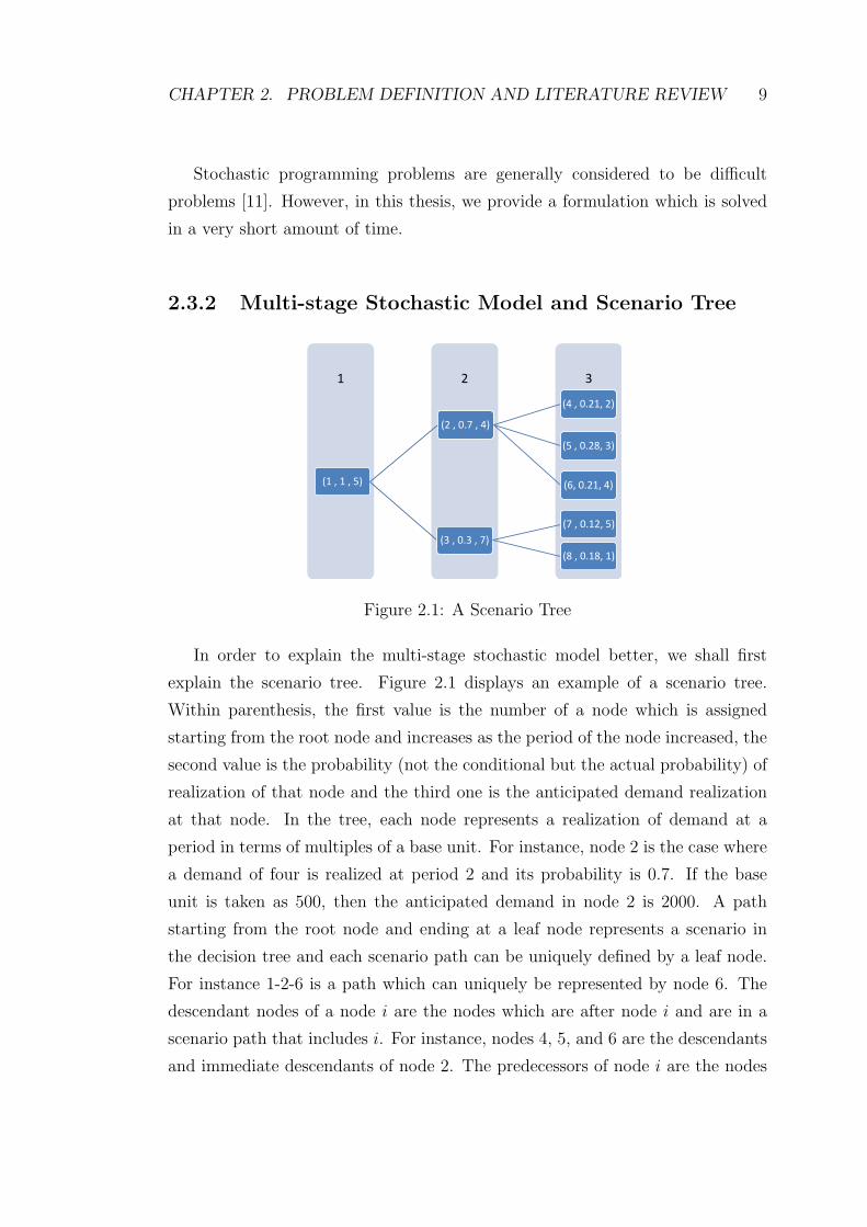
Figure 2.1: A Scenario Tree
In order to explain the multi-stage stochastic model better, we shall first
explain the scenario tree. Figure 2.1 displays an example of a scenario tree.
Within parenthesis, the first value is the number of a node which is assigned
starting from the root node and increases as the period of the node increased, the
second value is the probability (not the conditional but the actual probability) of
realization of that node and the third one is the anticipated demand realization
at that node. In the tree, each node represents a realization of demand at a
period in terms of multiples of a base unit. For instance, node 2 is the case where
a demand of four is realized at period 2 and its probability is 0.7. If the base
unit is taken as 500, then the anticipated demand in node 2 is 2000. A path
starting from the root node and ending at a leaf node represents a scenario in
the decision tree and each scenario path can be uniquely defined by a leaf node.
For instance 1-2-6 is a path which can uniquely be represented by node 6. The
descendant nodes of a node i are the nodes which are after node i and are in a
scenario path that includes i. For instance, nodes 4, 5, and 6 are the descendants
and immediate descendants of node 2. The predecessors of node i are the nodes
CHAPTER 2. PROBLEM DEFINITION AND LITERATURE REVIEW 10
that are in the same scenario path with i and that are before i. For example, 1
and 2 are the predecessors of node 4 whereas 2 is the immediate predecessor of
node 4.
We use a multi-stage stochastic programming approach and a scenario tree
in order to handle the uncertainty in demand. We use multiple stages since
we need to decide on how much of the anticipated demand will be satisfied at
each period and how will the production be distributed among periods, thus
we have multiple decision points. The benefits of using a multi-stage stochastic
programming approach instead of using fixed values as in the case of classical
MPS can be illustrated in the following example:
Example 1. Consider the scenario tree illustrated in Figure 2.1. In classical
MPS, the planner needs to define fixed values for demand realizations. There are
several strategies available to choose this single scenario:
1) Choosing the most likely scenario, which is 1-2-5,
2) Choosing the most optimistic scenario, which is 1-3-7,
3) Choosing the most pessimistic scenario, which is 1-2-4, and
4) Calculating the expected demand at each period and using the nearest integer
to these expected demand values which are 5 in the first period, 5 in the second
one and 3 in the third one.
The fifth option is using multi-stage stochastic programming. Suppose we
have a compression cost function of f(y) = y32 , a unit profit excluding the com-
pression and postponement cost given as h = 60, a minimum cost processing
time of p = 10, maximum compression amount of u = 4, and the limited capacity
of a node given as C = 36. For the simplicity of the example, we assume that
the postponement cost is 0. Assuming that in all cases, the allocation and com-
pression decisions are optimally made, the resulting profits of each strategy with
different scenario realizations are given in Table 2.1 (the cost that is incurred
due to excess production is ξ per item. We did not give it a value at this point
since we did not want this assumption to effect the overall results. For simplicity
of the example, suppose that shortage cost is 0).
As it can be observed from Table 2.1, using fixed scenarios provides good
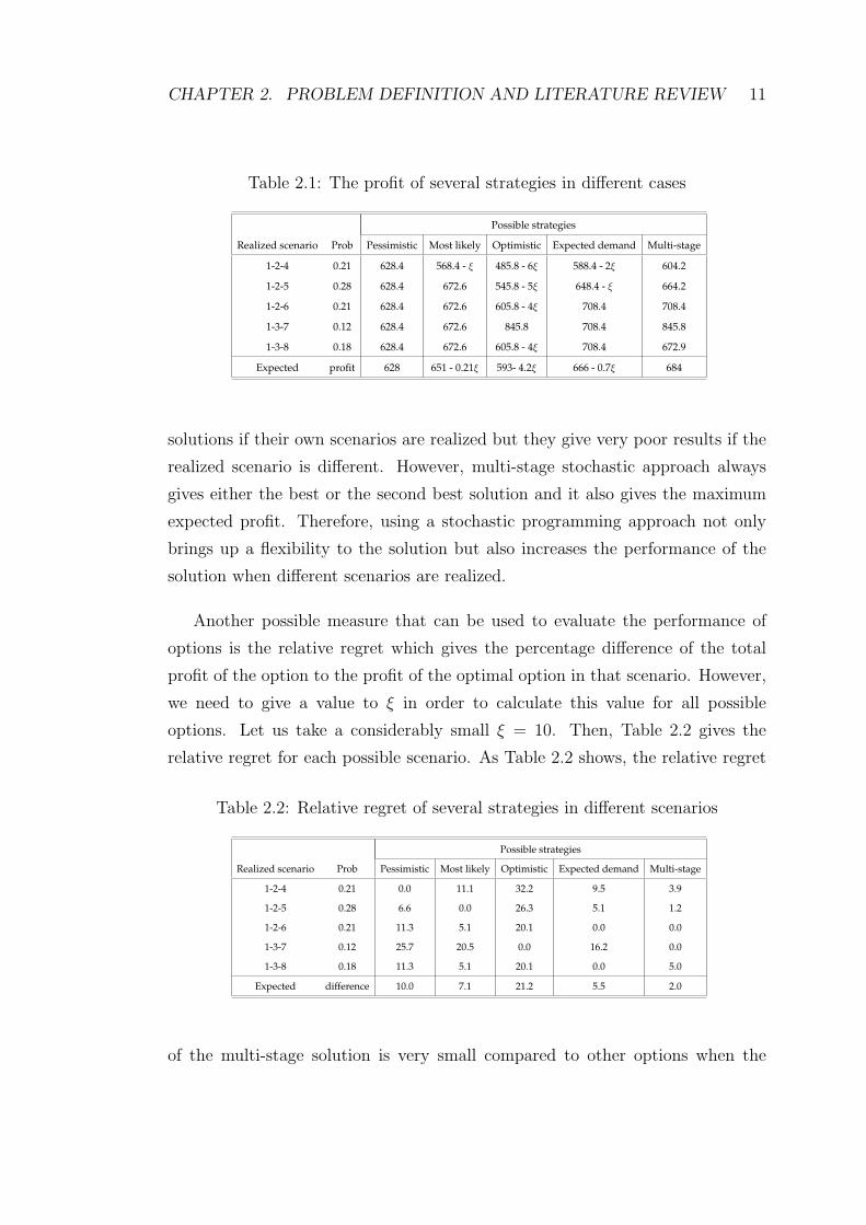
CHAPTER 2. PROBLEM DEFINITION AND LITERATURE REVIEW 11
Table 2.1: The profit of several strategies in different cases
Possible strategies
Realized scenario Prob Pessimistic Most likely Optimistic Expected demand Multi-stage
1-2-4 0.21 628.4 568.4 - ξ 485.8 - 6ξ 588.4 - 2ξ 604.2
1-2-5 0.28 628.4 672.6 545.8 - 5ξ 648.4 - ξ 664.2
1-2-6 0.21 628.4 672.6 605.8 - 4ξ 708.4 708.4
1-3-7 0.12 628.4 672.6 845.8 708.4 845.8
1-3-8 0.18 628.4 672.6 605.8 - 4ξ 708.4 672.9
Expected profit 628 651 - 0.21ξ 593- 4.2ξ 666 - 0.7ξ 684
solutions if their own scenarios are realized but they give very poor results if the
realized scenario is different. However, multi-stage stochastic approach always
gives either the best or the second best solution and it also gives the maximum
expected profit. Therefore, using a stochastic programming approach not only
brings up a flexibility to the solution but also increases the performance of the
solution when different scenarios are realized.
Another possible measure that can be used to evaluate the performance of
options is the relative regret which gives the percentage difference of the total
profit of the option to the profit of the optimal option in that scenario. However,
we need to give a value to ξ in order to calculate this value for all possible
options. Let us take a considerably small ξ = 10. Then, Table 2.2 gives the
relative regret for each possible scenario. As Table 2.2 shows, the relative regret
Table 2.2: Relative regret of several strategies in different scenarios
Possible strategies
Realized scenario Prob Pessimistic Most likely Optimistic Expected demand Multi-stage
1-2-4 0.21 0.0 11.1 32.2 9.5 3.9
1-2-5 0.28 6.6 0.0 26.3 5.1 1.2
1-2-6 0.21 11.3 5.1 20.1 0.0 0.0
1-3-7 0.12 25.7 20.5 0.0 16.2 0.0
1-3-8 0.18 11.3 5.1 20.1 0.0 5.0
Expected difference 10.0 7.1 21.2 5.5 2.0
of the multi-stage solution is very small compared to other options when the
CHAPTER 2. PROBLEM DEFINITION AND LITERATURE REVIEW 12
option does not coincide with the scenario that it expects to happen. Moreover,
in all cases multi-stage approach gives a profit value which is within 5% of the
actual optimum profit while others may deviate up to 32%. Therefore, using
a multi-stage approach instead of using fixed demand values may significantly
improve the achieved results.
In addition to using multi-stage approach, using controllable processing times
also increases the solution quality. For instance, for the given problem parameters,
the multi-stage stochastic profit would decrease to 540 for every scenario if the
processing times were fixed. This clearly indicates that the controllable processing
times would enlarge the solution space such that we could utilize the limited
capacity of the production resources more effectively.
2.4 Master Production Scheduling and Avail-
able to Promise
Master Production Schedules (MPS) assume infinite capacity and fixed processing
times. The literature of MPS generally focuses on the length of frozen period, i.e.
the number of periods in which the production scheduling decisions will not be
altered even though there is a change in inputs, on stability issues of the MPS,
and demand uncertainty. Sridharan et al. [33] consider the effect of the length of
the frozen zone on production and inventory costs and also suggest that an order
based freezing method is superior to a period based freezing method. Sridharan
et al. [32] investigate the effects of several decision variables such as the freezing
method, length of the frozen zone, and the length of the planning horizon. Tang
and Grubbstrom [34] also study the effects of the length of the frozen period.
ATP problems consider decisions similar to our problem such as determining
the amount of demand that will be satisfied, setting the due dates and planning
resources which our problem also considers. A review of ATP problems can be
found in Framinan and Leisten [15]. According to the classification of Framinan
and Leisten [15], our problem has a similar structure with ATP problems using
CHAPTER 2. PROBLEM DEFINITION AND LITERATURE REVIEW 13
flexible due dates with a postponement penalty and flexible resources (we have
flexible production capacity due to controllable processing times).
In this chapter, we defined the problem and explained the related literature,
in the next chapter, we will give the formulations that we proposed and the
sub-problems that we analyzed.
Chapter 3
The Stochastic Model
As we explained in the problem definition, we have a capacitated version of the
MPS where the demand is uncertain and the processing times are controllable.
Thus, the necessary decisions in the problem are how much to produce, when
to produce, and the processing times during production. In this chapter, we
give the main formulation that decides on when to produce and how much to
produce assuming that the structure of the objective function is given. After
that we introduce an equivalent linear version of the main formulation. Then,
we introduce two subproblems: The first one is used to decide on the optimal
processing times and to define the objective function of the main formulation
whereas the second one reduces the size of the formulation. Finally, we give
an alternative linearization of the main formulation using the results we have
obtained.
3.1 The Multi-Stage Stochastic Programming
Formulation
We begin with defining the parameters of the problem. Let T be the number of
periods in the planning horizon. Let N be the set of nodes of the scenario tree and
14
CHAPTER 3. THE STOCHASTIC MODEL 15
Nt be the set of the nodes of period t = 1, 2, ..., T . Suppose that the anticipated
demand at node i in N is denoted as di and the total demand (∑
i∈N di) is denoted
as d. For node i in N , let Di be the set of descendants of i including i, Bi be
the set of predecessors of i including i and finally, let γi denote the probability of
realization of node i (γ1 = 1). For i ∈ N and j ∈ Di, let Pij be the set of nodes
on the path from i to j in the scenario tree. Let si be the period of node i.
In addition to the parameters that are defined above, we will refresh some
parameters that are already defined in Chapter 2 and will be used in the model.
Let h be the unit profit excluding the compression and postponement costs, p be
the processing time of a job with minimum compression cost, u be the maximum
compression amount, and C be the capacity. We assume that h, p and C are
positive and u is non-negative. Let kmax be the maximum number of jobs that
can be produced without violating the capacity constraint, i.e., kmax =⌊
Cp−u
⌋.
Let Π(k) be the total profit when k jobs are produced at a node excluding the
cost of postponement. Let b(t) be the cost of postponing one job for t periods.
We assume that b(t) is a convex function with b(0) = 0. For the time being,
we will assume that Π(k) is given for all possible values of k but later, we will
explain how this value is calculated. The decision variables of the model are:
yj = Amount of production in j, j ∈ N ,
xij = Amount of dj that is processed in i, i ∈ N , j ∈ Bi,
zj = Amount of dj that will be satisfied, j ∈ N .
Then, the formulation for the stochastic problem (named as SF) is as follows:
Max∑i∈N
γi · (Π(yi)−∑j∈Bi
b(si − sj)xij)
s.t.∑j∈Bi
xij = yi ∀i ∈ N (3.1.1)
(SF )∑i∈Pjm
xij = zj ∀m ∈ NT ∩Dj, j ∈ N (3.1.2)
zj ≤ dj ∀j ∈ N (3.1.3)
yj ≤ kmax ∀j ∈ N (3.1.4)
CHAPTER 3. THE STOCHASTIC MODEL 16
xij ∈ Z+ ∀ i ∈ N, j ∈ Bi
yi ∈ Z+ ∀i ∈ N
zi ∈ Z+ ∀i ∈ N.
The objective of SF is to maximize the total expected profit. Constraint
(3.1.1) links xij and yi. It sums up the demand of j that is produced in node
i for all possible j values, i.e., all predecessors of node i including node i. This
value is equal to the production amount in node i. Constraint (3.1.2) ensures
that for each possible path that starts from node j and end at a descendant leaf
node, the amount of j’s demand that is satisfied is the same as the amount of
j’s demand that is produced along the path. Finally, Constraint (3.1.3) is the
demand constraint and (3.1.4) is the capacity constraint.
As we will prove later, the objective function of SF is concave so it is a non-
linear mixed integer formulation which necessitates a non-linear mixed integer
solver. A directly linearized version of SF (SFL1) is as follows:
wik =
{1 if k jobs are produced in node i
0 otherwise,i ∈ N, k ∈ {0, 1, ..., kmax}.
Suppose that xij and zj are defined as before.
Max∑i∈N
γi · (kmax∑k=0
Π(k) · wik −∑j∈Bi
b(si − sj)xij)
s.t.kmax∑k=0
wik = 1 ∀i ∈ N (3.1.5)
(SFL1)∑j∈Bi
xij =kmax∑k=0
k · wik ∀i ∈ N (3.1.6)∑i∈Pjm
xij = zj ∀m ∈ NT ∩Dj, j ∈ N (3.1.7)
zj ≤ dj ∀j ∈ N (3.1.8)
xij ∈ Z+ ∀ i ∈ N, j ∈ Bi
zi ∈ Z+ ∀i ∈ N
wik ∈ {0, 1} ∀i ∈ N, k ∈ {0, 1, ..., kmax}.
CHAPTER 3. THE STOCHASTIC MODEL 17
The only difference between SF and SFL1 is formulating the integer variables
as weighted sum of binaries. Constraint (3.1.5) guarantees that a node can have a
single production amount. Since wik values are defined among feasible production
amounts, there is no need for constraint (3.1.4) of SF in SFL1.
At this point, we take the possible number of jobs that will be produced at a
node as 0 to kmax which is the maximum number of jobs that can be produced
without violating the capacity of that node. Moreover, the compression amounts
cannot be directly determined from the output of the model. In the following
section, we will introduce two sub-problems which will be used to reduce the
possible number of jobs and to calculate the optimal compression amounts.
3.2 Two Sub-problems
In this section, we introduce two sub-problems; the first sub-problem is the sin-
gle period capacitated deterministic scheduling problem with cost minimization
objective. The results that we obtain from this problem will be used to define
the optimal compression costs and the Π(k) values.
3.2.1 The Single Period Capacitated Deterministic Schedul-
ing Problem with Cost Minimization Objective
This problem corresponds to a single machine (or work center), single product
type problem where the machine has a finite capacity of C. Suppose that the
processing time of a job which has the minimum compression cost is p and the
maximum compressibility of the job is u. Let n be a positive integer such that
n ≤ kmax. Suppose that there are n jobs in the work center. Let cj be the
compression amount of job j in {1, ..., n}. Recall that f is the compression cost
function that is defined in Chapter 2. Then, the formulation of this subproblem
CHAPTER 3. THE STOCHASTIC MODEL 18
is:
Minn∑j=1
f(cj)
s.t. cj ≤ u ∀j ∈ {1, ..., n} (3.2.1)n∑j=1
(p− cj) ≤ C (3.2.2)
cj ∈ R+ ∀ j ∈ {1, ..., n}.
The objective is to find the compression amounts for the jobs so that the total
compression cost is minimized. (3.2.1) is the maximum compressibility constraint.
(3.2.2) is the capacity constraint. Proposition 3.1 characterizes the optimal solu-
tion of this problem.
Proposition 3.1. Let n be a positive integer with n · (p− u) ≤ C. If n jobs are
to be processed in a work center, then the optimal compression amount of all the
jobs is equal to max{p− Cn, 0}.
Proof. First, we show that the compression amount is equal for all the jobs in
the work center. Let c be an optimal solution. Suppose to the contrary that
there exist jobs i and j such that ci > cj. Let c be the same as c except ci =
cj =ci+cj
2. The solution c is feasible and by strict convexity of the cost function,
f(ci)+f(cj) < f(ci)+f(cj). This contradicts the optimality of the initial solution
c. Now it follows immediately that cj = max{p − Cn, 0} for all j = 1, ..., n is an
optimal solution.
The Proposition 3.1 is intuitive. In a strict convex function, the more a
compression amount is, the more the marginal compression cost that will be
incurred. Thus, in order to minimize the compression cost, the necessary com-
pression amount (n · p − C) will be evenly distributed among all jobs. Using
Proposition 3.1, it is possible to find the optimal compression amounts for jobs
given the optimal allocation of jobs to the nodes. Thus, given the solution of SF,
it is possible to find the compression amounts of jobs using this proposition.
As stated before, Π(k) function was considered as given when the main for-
mulation is explained. Using Corollary 3.1, which makes use of Proposition 3.1,
CHAPTER 3. THE STOCHASTIC MODEL 19
we come up with the total cost and total profit functions of a node given the
number of allocated jobs. As a remark, one should consider that each node can
be modeled as a single work center once the allocation is available. For x ∈ R+,
let Π(x) = x · h− Φ(x) where Φ(x) =
{x · κ · (p− C
x)
ab if x > C
p,
0 otherwise.
Corollary 3.1. Let n be a positive integer that satisfies n · (p − u) ≤ C. If n
jobs are to be processed at a work center, then the total profit at the work center
is Π(n) and the total compression cost when n jobs are processed in the work
center is Φ(n).
Using Corollary 3.1, the profit function is calculated for all possible values of
job numbers at a node and hence given as an input to the main formulation. The
following sub-section will be used to define the threshold value.
3.2.2 The Single Period Capacitated Deterministic Prob-
lem with Profit Maximization Objective
In this problem, we have a single machine (or work center) with finite capacity C
and a single period with infinite demand. The objective is to maximize the total
profit. Let the threshold value, denoted by τ , be the optimal number of jobs that
will be produced at the work center so that the total profit is maximized. Then,
the formulation of the problem is:
max Π(n)
s.t. n ≤ kmax
n ∈ Z+.
The value of τ depends on both the available capacity and relative profit gain
of producing one more job. One should note that there is a trade-off between the
revenue gained by increasing the number of jobs at a work center and the increase
in the compression costs incurred in order to produce all these jobs. Thus, the
CHAPTER 3. THE STOCHASTIC MODEL 20
threshold value is the optimum production amount given the capacity of the work
center.
We can simply use enumeration to come up with τ in O(kmax) time. However,
Lemma 3.1 gives the structure of the Π function when the compression amount
of jobs are non-zero and Proposition 3.2, which gives the necessary and sufficient
condition for the threshold value, can also be used to compute τ immediately.
Lemma 3.1. Let Π : (0,+∞)→ R be the profit function. The following proper-
ties hold:
1) Π(x) is continuously differentiable at all points,
2) Π(x) is concave,
3) If h < κ · pab , there exists x in (C
p,+∞) such that dΠ(x)
dx= 0.
Proof. Let Πc : (Cp,+∞)→ R be such that Πc(x) = x ·h− x ·κ · (p− C
x)
ab . Then,
Π(x) =
{Πc(x) if x > C
p,
x · h otherwise.
When x < Cp
, Π(x) is linear and when x > Cp
, Πc(x) is a smooth function since
x 6= 0. Therefore, the only point that needs consideration is x = Cp
. The first
derivative of the Πc function with respect to x is:
dΠc(x)
dx= h− κ · (p− C
x)
ab − a
b· κ · (p− C
x)
ab−1 · C
x.
The right derivative of Π(x) at x = Cp
is h and the left derivative of Π(x) at
x = Cp
is also h. Therefore Π(x) is continuously differentiable at all points.
The second derivative of Πc(x) with respect to x is:
d2Πc(x)
dx2= −a
b·κ·(p−C
x)
ab−1· C
x2−ab·(ab−1)·κ·(p−C
x)
ab−2·C
2
x3+a
b·κ·(p−C
x)
ab−1· C
x2
= −ab· (ab− 1) · κ · (p− C
x)
ab−2 · C
2
x3≤ 0
since a > b and x ≥ Cp
, dΠc(x)dx
is decreasing. Moreover, hx is non-increasing. In
addition to those, the derivative function of Π(x) is continuous. Hence, dΠ(x)dx
is
monotonically non-increasing and continuous which means Π(x) is concave.
CHAPTER 3. THE STOCHASTIC MODEL 21
Now suppose that h < κ · pab . When x tends to C
p, dΠc(x)
dx> 0 and when x
tends to infinity, dΠc(x)dx
< 0 since h < κ · pab . In addition to that, the derivative
function is continuous. Then, by the intermediate value theorem, there exists x∗
in (Cp,+∞) such that dΠc(x∗)
dx= 0. Since Π(x) has the same values as Πc(x) on
the domain (Cp,+∞), then dΠ(x∗)
dx= 0.
Lemma 3.1 shows that the profit function is concave. It also shows that it
always has a critical point within its domain if h < κ ·pab . Thus, one can find this
critical point and by concavity this critical point is the maximizing point within
a continuous domain if h < κ ·pab . Obviously, this does not immediately tell what
the τ value is since τ is the maximum value defined among only integer points.
Moreover, it does not consider the capacity constraint. However, Proposition 3.2
uses Lemma 3.1 to come up with the actual threshold value. Let kmin =⌊Cp
⌋.
Proposition 3.2. Suppose that h < κ · pab . Let x∗ be the critical point of Πc(x).
Then,
τ =
kmax if x∗ > kmax
Πdx∗e if x∗ ≤ kmax and Π(dx∗e) > Π(bx∗c)Πbx∗c otherwise
On the other hand, if h ≥ κ · pab , then τ = kmax.
Proof. While explaining the cases of the proof, we will refer to the charts in Figure
3.1. Consider first the case where h < κ · pab . The first condition immediately
follows from the concavity of the function. If x∗ > kmax, then the function is
increasing until kmax which is the largest feasible number of jobs that can be
produced. Thus in this case, τ = kmax.
The second case is where the critical point is within the domain of Proposition
3.1 and it is feasible (smaller than or equal to kmax). If x∗ < kmin + 1, this case
corresponds to charts c and d in Figure 3.1. As it can be also seen from the figures,
the function is decreasing after kmin + 1 and increasing before kmin. Thus, either
τ = kmin + 1 = dx∗e as illustrated in chart c or τ = kmin = bx∗c as illustrated
in chart d. Therefore, we need to check each one and take the one with higher
profit as the threshold value. Similarly, if kmax ≥ x∗ ≥ kmin+ 1, the critical point
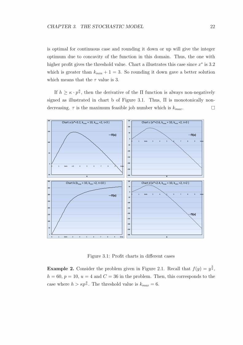
CHAPTER 3. THE STOCHASTIC MODEL 22
is optimal for continuous case and rounding it down or up will give the integer
optimum due to concavity of the function in this domain. Thus, the one with
higher profit gives the threshold value. Chart a illustrates this case since x∗ is 3.2
which is greater than kmin + 1 = 3. So rounding it down gave a better solution
which means that the τ value is 3.
If h ≥ κ · pab , then the derivative of the Π function is always non-negatively
signed as illustrated in chart b of Figure 3.1. Thus, Π is monotonically non-
decreasing. τ is the maximum feasible job number which is kmax.
-50
0
50
100
150
200
0 1 kmin τ=3 4 5 6 7 8 9 kmax
x
Chart a (x*=3.2, kmax = 10, kmin =2, τ=3 )
Π(x)
0
50
100
150
200
250
300
350
400
0 1 kmin 3 4 5 6 7 8 9 kmax
Chart b (kmax = 10, kmin =2, τ=10 )
Π(x)
-300
-250
-200
-150
-100
-50
0
50
100
150
0 1 kmin 3 4 5 6 7 8 9 kmax
x
Chart c (x*=2.6, kmax = 10, kmin =2, τ=3 )
Π(x)
-400
-350
-300
-250
-200
-150
-100
-50
0
50
100
0 1 kmin 3 4 5 6 7 8 9 kmax
x
Chart d (x*=2.4, kmax = 10, kmin =2, τ=2 )
Π(x)
Figure 3.1: Profit charts in different cases
Example 2. Consider the problem given in Figure 2.1. Recall that f(y) = y32 ,
h = 60, p = 10, u = 4 and C = 36 in the problem. Then, this corresponds to the
case where h > κpab . The threshold value is kmax = 6.
CHAPTER 3. THE STOCHASTIC MODEL 23
3.3 The Formulation with a Reduced Size
Using the threshold value, it is possible to reduce the size of the main formulation.
Proposition 3.3 gives a necessary condition for the optimality of the main problem
which will be used to reduce the formulation size.
Proposition 3.3. At an optimal solution to SF, the production amounts of all
nodes are less than or equal to the threshold value, τ .
Proof. If τ = kmax, then it is infeasible to produce more than τ . If not, suppose
that there exists an optimal solution in which the production amount at a node
is greater than τ . Then, we can simply improve the solution by decreasing the
production amount to τ and reach a contradiction.
According to Proposition 3.3, the number of jobs that will be produced will
be less than the threshold value at all nodes in the optimal solution. Thus, the
maximum number of jobs that will be produced at a node decreases from kmax
to τ . Therefore, kmax in the main formulation is replaced by τ .
After explaining the main formulation and two sub-problems which are used
to reduce problem size of the main formulation, to calculate Π(n) values as well
as optimum compression amounts, we will introduce an alternative linearization
to SF.
3.4 An Alternative Linearization of the Stochas-
tic Formulation (SF)
In this section, we give an alternative linearized version of SF. In this formula-
tion, we write the integer variable yj as the sum of binary variables vik. Then,
the decision variables of the alternative formulation are:
CHAPTER 3. THE STOCHASTIC MODEL 24
vik =
{1 if at least k jobs are produced in i
0 otherwise,i ∈ N, k ∈ {1, ..., τ},
xij = Amount of dj processed in i, i ∈ N , j ∈ Bi,
zj = Amount of dj that will be satisfied, j ∈ N .
Consequently, the alternative linear formulation (named as SFL2) is as follows:
Max∑i∈N
γi · (τ∑k=1
(Π(k)− Π(k − 1)) · vik −∑j∈Bi
b(si − sj) · xij)
s.t. vik ≥ vi(k+1) ∀i ∈ N, k ∈ {1, ..., τ − 1} (3.4.1)
(SFL2)∑j∈Bi
xij =τ∑k=1
vik ∀i ∈ N (3.4.2)∑i∈Pjm
xij = zj ∀m ∈ NT ∩Dj, j ∈ N (3.4.3)
zj ≤ dj ∀j ∈ N (3.4.4)
xij ∈ Z+ ∀ i ∈ N, j ∈ Bi
zi ∈ Z+ ∀i ∈ N
vik ∈ {0, 1} ∀i ∈ N, k ∈ {1, ..., τ}.
Constraint (3.4.1) of SFL2 handles the fact that if at least k+1 jobs are processed
at a node, then clearly at least k jobs will be processed. Constraint (3.4.2) has
the same task as Constraint (3.1.1) but in it, the integer variable yi is written as
the sum of binary variables vik. The other constraints are the same as Constraint
(3.1.7) and (3.1.8) in SFL1.
SFL2 linearizes SF albeit at a cost of increased number of variables due to
addition of vik’s and increased number of constraints due to addition of Constraint
(3.4.1). However, it is easy to get rid of Constraint (3.4.1) due to concavity of
Π(x) and convexity of b(k). Let SFL3 be the same formulation as SFL2 without
Constraint (3.4.1). Proposition 3.4 formalizes this idea.
Proposition 3.4. Let SFL2 and SFL3 be defined as above. Then, there exists
an optimal solution for SFL3 which is also optimal for SFL2.
Proof. Let x∗ij, v∗ik, and z∗j be an optimal solution for SFL3. Since SFL3 is a
relaxation of SFL2, if there is an optimal solution for SFL3 which is feasible

CHAPTER 3. THE STOCHASTIC MODEL 25
for SFL2, then it is also optimal for SFL2. Now clearly x∗ij, v∗ik, and z∗j satisfy
constraints 3.4.2, 3.4.3,3.4.4 since SFL3 also includes these constraints. Then, if
v∗ik satisfies 3.4.1, we are done. If not, suppose that∑τ
k=1 v∗ik = n∗ and let kin be
defined as:
ki1 = min{k ∈ {1, ..., τ} : vik = 1}ki2 = min{k ∈ {1, ..., τ} : vik = 1; k > ki1}...
kin∗ = min{k ∈ {1, ..., τ} : vik = 1; k > ki(n∗−1)}Now consider the solution xij = x∗ij, zj = z∗j and
vin =
{vikin
if n ≤ n∗
0 if n > n∗i ∈ N, k ∈ {1, ..., τ}
Now by definition,∑τ
k=1 vik = n∗ thus this solution satisfies 3.4.2. Moreover,
this solution satisfies 3.4.1 since vik = 0 implies vi(k+1) = 0 (otherwise leads to a
contradiction). Moreover, vi(k+1) = 1 means vik = 1 by definition of kin. Thus,
this new solution is feasible for SFL2 and clearly for SFL3. Now to show that
it is optimal for SFL3, we need to consider the objective function value of it.
The difference between the objective function of the old and new formulation is∑i∈N γi · (
∑τk=1(Π(k)− Π(k − 1)) · (v∗ik − vik)
= γi · (∑n∗
n=1((Π(kin)− Π(kin − 1))− (Π(n)− Π(n− 1))).
As Lemma 3.1 suggests, Π(k) is a concave function, hence the first derivative is
always non-increasing. Therefore, ((Π(kin) − Π(kin − 1)) ≤ (Π(n) − Π(n − 1)))
since by definition kin ≥ n. Thus, this solution is also optimal for SFL3 and
feasible for SFL2, hence it is optimal for SFL2.
SFL2 is always feasible since setting all variables to zero gives a feasible so-
lution for it. Therefore, according to Proposition 3.4, there exists an optimal
solution of SFL3 which is also optimal for SFL2. Thus, one can solve SFL3, find
an optimal solution and convert the solution so that it is feasible for SFL2 via
procedure (kin) that is proposed in the proof. Hence, the the solution obtained
is optimal for SFL2.
In this chapter, we first proposed a stochastic formulation and a linearized
version of it. Afterwards, we analyzed two sub-problems to come up with the
optimal processing times and profit function Π(k) and the threshold value. We

CHAPTER 3. THE STOCHASTIC MODEL 26
also obtained the result that Π(k) is concave which is used while forming SFL3.
We also came up with τ value and reduced the size of the formulations that we
propose. In the next chapter, we will introduce sufficient conditions for optimality
and two special cases of the main problem which are polynomially solvable. Then
we will discuss the complexity of our problem.
Chapter 4
On Easy Cases and Complexity
In this chapter, we first give some instances of the problem which are easily
solvable. Then we introduce the case where there is no postponement cost and
the case where the demands are deterministic. We prove the polynomiality of
both cases. Finally, we have a negative result: The techniques that we used to
determine the complexity of the easy cases is not applicable to the main problem.
4.1 Sufficient Conditions for Optimality
In this section, we will introduce some easy cases where the optimal solution can
be found easily. Suppose that the demand at each node is less than the threshold
value and equal to each other. Then by Proposition 4.1, the solution where each
job is produced at its own node (the node in which the demand of the job is
realized) is optimal.
Proposition 4.1. Suppose that, di < τ for all i in set N . If di = dj for all i and
j, then the solution where all the demand is satisfied and each job is produced at
its own node is optimal.
Proof. Suppose that di = dj = n for all i and j in N but the solution is not
optimal. Then, there exists a better solution. Firstly, it is not possible to improve
27
CHAPTER 4. ON EASY CASES AND COMPLEXITY 28
the solution by decreasing the production amount because di < τ for all i in N .
Then there exists i and set M ⊂ Di such that adding a job to i from the nodes in
set M or adding a job from i to the nodes in set M improves the solution. Note
that by definition, γi =∑
k∈M γk.
Case 1: An improvement is achieved by adding a job to i from the nodes in set M .
Then, the change in cost for i is Φ(n+1)−Φ(n) and the cost change for all nodes in
M is Φ(n)−Φ(n−1). Thus the total change in cost is ∆f = γi ·(Φ(n+1)−Φ(n))−∑k∈M γk ·(Φ(n)−Φ(n−1)) = γi ·(Φ(n+1)−Φ(n))−(Φ(n)−Φ(n−1))·
∑k∈M γk =
γi ·((Φ(n+1)−Φ(n))−(Φ(n)−Φ(n−1))) = γi ·((Φ(n+1)+Φ(n−1)−2Φ(n))) > 0
by strict convexity of the cost function. However, this contradicts with the fact
that this case improves the solution.
Case 2: An improvement is achieved by adding a job from i to the nodes in set
M . A similar contradiction is reached for this case just as case 1.
Therefore, there does not exist such i and set M . Hence, the solution is optimal.
Another easy to solve case is where the demand exceeds the threshold value
at all of the nodes. A sufficient condition for optimality in this case is given in
Proposition 4.2.
Proposition 4.2. Suppose that, the demand exceeds the threshold value for all
nodes in the scenario tree. Then, the solution where τ jobs are produced at all
nodes is optimal.
Proof. In the solution proposed, τ jobs will be produced in all nodes. For any
node, the optimal number to produce is τ by definition. Thus, adding a job to
or subtracting a job from a node will worsen the objective function value. Thus,
the solution is optimal.
Using Propositions 4.1 and 4.2, one can immediately find the optimal solution
when the corresponding easy cases are encountered.
CHAPTER 4. ON EASY CASES AND COMPLEXITY 29
4.2 Stochastic Problem with no Postponement
Cost
We propose a special formulation for the stochastic problem without any post-
ponement cost. This special formulation comes out with a simple observation:
the number of jobs that will be produced along a path starting from the root
node will be less than or equal to the total demand along the path. Having this
observation in mind, one can define the necessary decision variable as the amount
of production at a node without considering where the demands of this produc-
tion are realized once the postponement is no longer costly. Let yi denote the
production at node i in N . Then the alternative formulation is as follows:
Max∑i∈N
γi · Π(yi)
s.t.∑j∈P1i
yj ≤∑j∈P1i
dj ∀i ∈ N (4.2.1)
(SF2) yi ≤ τ ∀i ∈ N (4.2.2)
yi ∈ Z+ ∀i ∈ N
The objective is to maximize the total expected profit and Constraint (4.2.1)
guarantees that the production amount along a path does not exceed the total
demand. Constraint (4.2.2) is the capacity constraint.
SF2 cannot be solved in a commercial solver for reasonable input sizes since it
is a non-linear mixed integer problem. However, this formulation will be used to
show the complexity of the stochastic problem without postponement cost since
it has a special structure. Lemma 4.1 shows the special structure of its constraint
matrix.
Lemma 4.1. Constraint matrix of SF2 is totally unimodular.
Proof. The constraint matrix consists of two parts, one (sub-matrix 1) is identity
matrix and the other(sub-matrix 2) is due to Constraint (4.2.1). If we sort the
CHAPTER 4. ON EASY CASES AND COMPLEXITY 30
rows of sub-matrix 2 in a depth-first search basis, then this sub-matrix satisfies
consecutive 1’s property and thus is totally unimodular [16]. Moreover, sub-
matrix 1 is an identity matrix. Thus, the constraint matrix is totally unimodular.
Theorem 4.1. Stochastic problem with no postponement cost is polynomially
solvable.
Proof. In the objective function, for i in N , γi · Π(yi) is concave so multiplying
it by -1, we obtain a convex function. Their summation generates a convex
separable objective function (with minimization objective or concave separable
objective function with maximization). Moreover, by Lemma 4.1, the constraint
matrix is totally unimodular. Thus according to Hochbaum and Shantikumar
[20], stochastic problem is polynomially solvable.
4.3 The Deterministic Problem
In this section, we consider the problem with deterministic demand realizations. If
we adjust SF for the deterministic case, we obtain the following decision variables:
yj = Amount of production in period j
xij = Amount of demand of j that is processed in i, i ∈ {1, ..., T}, j ∈ {1, ..., i}.
Then, the formulation for the deterministic case (named as DF) is as follows:
Max
T∑i=1
(Π(yi)−i∑
j=1
b(si − sj)xij)
s.t.i∑
j=1
xij = yi ∀i ∈ {1, ..., T} (4.3.1)
(DF )T∑i=j
xij ≤ dj ∀j ∈ {1, ..., T} (4.3.2)

CHAPTER 4. ON EASY CASES AND COMPLEXITY 31
yj ≤ τ ∀j ∈ {1, ..., T} (4.3.3)
xij ∈ Z+ ∀i ∈ {1, ..., T}, j ∈ {1, ..., i}
yi ∈ Z+ ∀i ∈ {1, ..., T}
Constraints have the same tasks as SF but the only difference is that instead of
different scenarios, there is a single scenario, i.e., the scenario tree is a path.
Lemma 4.2. Constraint matrix of DF is totally unimodular.
Proof. Firstly, the constraint matrix clearly consists of 1’s -1’s and 0’s. Given a
set of rows of the constraint matrix, put the rows of Constraint Set (4.3.1) into
partition 1 and the rows of Constraint Sets (4.3.2) and (4.3.3) into partition 2.
Then the difference of the sums of rows of partition 1 and 2 has entries that are
equal to either 1, 0 or -1. Therefore, the matrix is totally unimodular [35].
Theorem 4.2. The deterministic problem is polynomially solvable.
Proof. In the objective function, for i in {1, ..., T}, Π(yi) is concave and b(x) is
convex which leads to -b(x) being concave. Therefore, the objective function is
concave separable and so multiplying it by -1, we obtain minimization of sum of
convex separable functions. Moreover, by Lemma 4.2, the constraint matrix is
totally unimodular. Thus, according to Hochbaum and Shantikumar [20], deter-
ministic version of the problem is also polynomially solvable.
4.4 The Structure of Stochastic Formulation SF
In the previous sections, we proved that some special cases of the problem are
polynomially solvable. We achieved this by suggesting formulations with totally
unimodular constraint matrices and concave separable objective functions. In
this section, we first show that this approach cannot be applied to the general
problem because the constraint matrix of SF may not be totally unimodular.
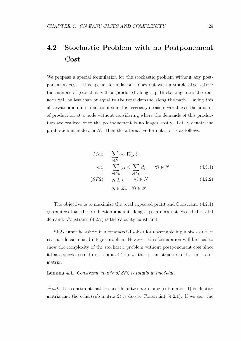
Example 3. Consider the very simple scenario tree given in Figure 4.1. The co-
efficient matrix of the corresponding stochastic formulation of this scenario tree
CHAPTER 4. ON EASY CASES AND COMPLEXITY 32
4321
(1,1,1) (2,1,1) (3,1,1)
(4,0.3,1)
(5,0.2,2)
(6,0,5,3)
Figure 4.1: A counter example for totally unimodularity of constraint matrix ofSF
is given in Table 4.1:
Table 4.1: Constraint coefficient matrix for stochastic formulation of Figure 4.1
Ctr x11 x21 x22 x31 x32 x33 x41 x42 x43 x44 x51 x52 x53 x55 x61 x62 x63 x66 y1 y2 y3 y4 y5 y6 z1 z2 z3 z4 z5 z6
1 1 0 0 0 0 0 0 0 0 0 0 0 0 0 0 0 0 0 -1 0 0 0 0 0 0 0 0 0 0 0
2 0 1 1 0 0 0 0 0 0 0 0 0 0 0 0 0 0 0 0 -1 0 0 0 0 0 0 0 0 0 0
3 0 0 0 1 1 1 0 0 0 0 0 0 0 0 0 0 0 0 0 0 -1 0 0 0 0 0 0 0 0 0
4 0 0 0 0 0 0 1 1 1 1 0 0 0 0 0 0 0 0 0 0 0 -1 0 0 0 0 0 0 0 0
5 0 0 0 0 0 0 0 0 0 0 1 1 1 1 0 0 0 0 0 0 0 0 -1 0 0 0 0 0 0 0
6 0 0 0 0 0 0 0 0 0 0 0 0 0 0 1 1 1 1 0 0 0 0 0 - 1 0 0 0 0 0 0
7 1 1 0 1 0 0 1 0 0 0 0 0 0 0 0 0 0 0 0 0 0 0 0 0 -1 0 0 0 0 0
8 1 1 0 1 0 0 0 0 0 0 1 0 0 0 0 0 0 0 0 0 0 0 0 0 -1 0 0 0 0 0
9 1 1 0 1 0 0 0 0 0 0 0 0 0 0 1 0 0 0 0 0 0 0 0 0 -1 0 0 0 0 0
10 0 0 1 0 1 0 0 1 0 0 0 0 0 0 0 0 0 0 0 0 0 0 0 0 0 -1 0 0 0 0
11 0 0 1 0 1 0 0 0 0 0 0 1 0 0 0 0 0 0 0 0 0 0 0 0 0 -1 0 0 0 0
12 0 0 1 0 1 0 0 0 0 0 0 0 0 0 0 1 0 0 0 0 0 0 0 0 0 -1 0 0 0 0
13 0 0 0 0 0 1 0 0 1 0 0 0 0 0 0 0 0 0 0 0 0 0 0 0 0 0 -1 0 0 0
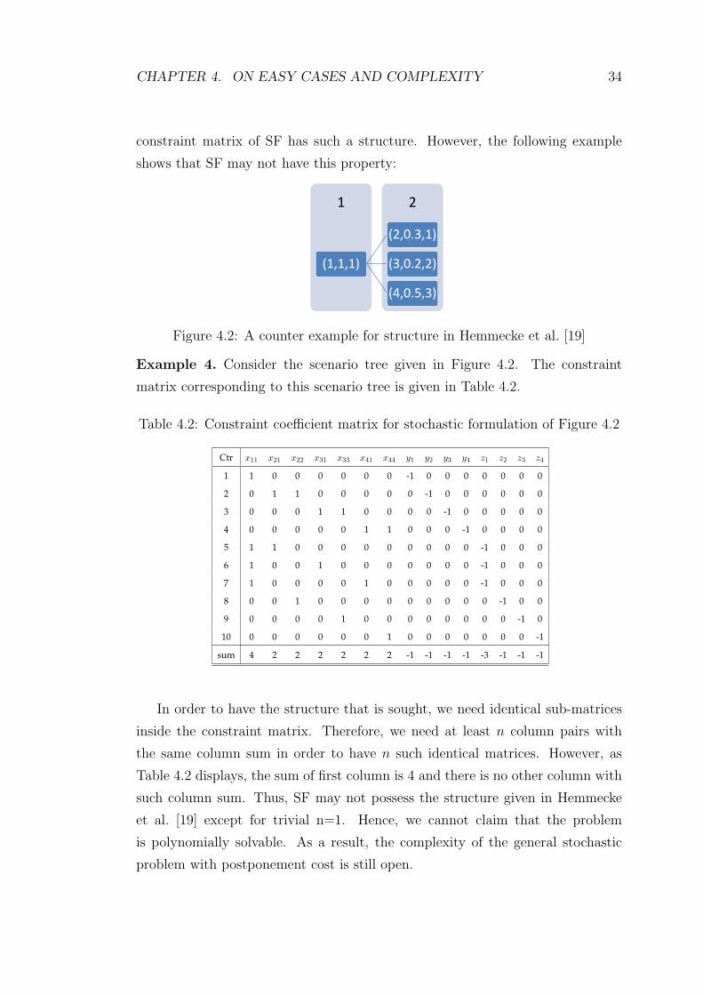
14 0 0 0 0 0 1 0 0 0 0 0 0 1 0 0 0 0 0 0 0 0 0 0 0 0 0 -1 0 0 0
15 0 0 0 0 0 1 0 0 0 0 0 0 0 0 0 0 1 0 0 0 0 0 0 0 0 0 -1 0 0 0
16 0 0 0 0 0 0 0 0 0 1 0 0 0 0 0 0 0 0 0 0 0 0 0 0 0 0 0 -1 0 0
17 0 0 0 0 0 0 0 0 0 0 0 0 0 1 0 0 0 0 0 0 0 0 0 0 0 0 0 0 -1 0
18 0 0 0 0 0 0 0 0 0 0 0 0 0 0 0 0 0 1 0 0 0 0 0 0 0 0 0 0 0 -1
For this constraint matrix to be totally unimodular, we need to have all sub-
matrices to have determinant -1,0 or 1. However, the following sub-matrix of this
coefficient matrix has determinant 2:
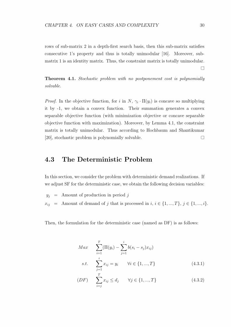
CHAPTER 4. ON EASY CASES AND COMPLEXITY 33
0 0 0 1 1 0 0 0 0
0 0 0 0 0 1 1 0 0
0 0 0 0 0 0 0 1 1
1 0 0 1 0 0 0 0 0
1 0 0 0 0 0 0 1 0
0 1 0 0 0 1 0 0 0
0 1 0 0 0 0 0 0 1
0 0 1 0 1 0 0 0 0
0 0 1 0 0 0 1 0 0
Therefore, the constraint matrix of SF may not be totally unimodular. This
directly implies that the constraint matrix of SFL3 may not be TU, either because
the same sub-matrix exists in the coefficient matrix of SFL3 for the problem given
in Figure 4.1.
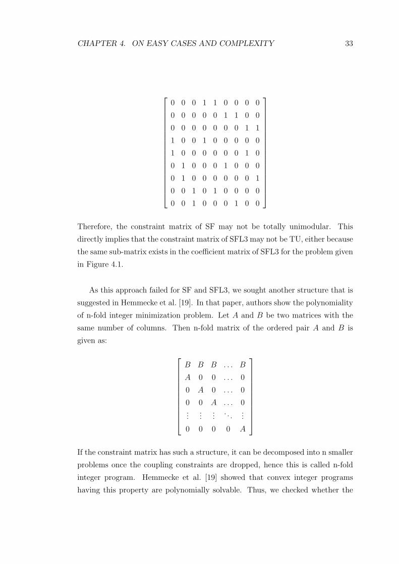
As this approach failed for SF and SFL3, we sought another structure that is
suggested in Hemmecke et al. [19]. In that paper, authors show the polynomiality
of n-fold integer minimization problem. Let A and B be two matrices with the
same number of columns. Then n-fold matrix of the ordered pair A and B is
given as:
B B B . . . B
A 0 0 . . . 0
0 A 0 . . . 0
0 0 A . . . 0...
......
. . ....
0 0 0 0 A
If the constraint matrix has such a structure, it can be decomposed into n smaller
problems once the coupling constraints are dropped, hence this is called n-fold
integer program. Hemmecke et al. [19] showed that convex integer programs
having this property are polynomially solvable. Thus, we checked whether the
CHAPTER 4. ON EASY CASES AND COMPLEXITY 34
constraint matrix of SF has such a structure. However, the following example
shows that SF may not have this property:
21
(1,1,1)
(2,0.3,1)
(3,0.2,2)
(4,0.5,3)
Figure 4.2: A counter example for structure in Hemmecke et al. [19]
Example 4. Consider the scenario tree given in Figure 4.2. The constraint
matrix corresponding to this scenario tree is given in Table 4.2.
Table 4.2: Constraint coefficient matrix for stochastic formulation of Figure 4.2
Ctr x11 x21 x22 x31 x33 x41 x44 y1 y2 y3 y4 z1 z2 z3 z4
1 1 0 0 0 0 0 0 -1 0 0 0 0 0 0 0
2 0 1 1 0 0 0 0 0 -1 0 0 0 0 0 0
3 0 0 0 1 1 0 0 0 0 -1 0 0 0 0 0
4 0 0 0 0 0 1 1 0 0 0 -1 0 0 0 0
5 1 1 0 0 0 0 0 0 0 0 0 -1 0 0 0
6 1 0 0 1 0 0 0 0 0 0 0 -1 0 0 0
7 1 0 0 0 0 1 0 0 0 0 0 -1 0 0 0
8 0 0 1 0 0 0 0 0 0 0 0 0 -1 0 0
9 0 0 0 0 1 0 0 0 0 0 0 0 0 -1 0
10 0 0 0 0 0 0 1 0 0 0 0 0 0 0 -1
sum 4 2 2 2 2 2 2 -1 -1 -1 -1 -3 -1 -1 -1
In order to have the structure that is sought, we need identical sub-matrices
inside the constraint matrix. Therefore, we need at least n column pairs with
the same column sum in order to have n such identical matrices. However, as
Table 4.2 displays, the sum of first column is 4 and there is no other column with
such column sum. Thus, SF may not possess the structure given in Hemmecke
et al. [19] except for trivial n=1. Hence, we cannot claim that the problem
is polynomially solvable. As a result, the complexity of the general stochastic
problem with postponement cost is still open.
CHAPTER 4. ON EASY CASES AND COMPLEXITY 35
In this chapter, we introduced some sufficient conditions and proved the poly-
nomiality of two special cases of the problem. In the next chapter, we will give
the results of our computational study.
Chapter 5
Computational Results
The computational study consists of three stages. In stage one, we test the CPU
time performance of the linearized versions of the main formulation which are
SFL1 and SFL3 and then consider the effects of several factors on CPU time per-
formance in order to have some insights on how the solution time of a multi-stage
stochastic programming formulation is affected from changes in certain param-
eters. Then, in the second stage, we compare several single scenario strategies
having different production adjustment policies to multi-stage solution in terms
of relative regret assuming that these strategies also use controllable processing
times. While comparing these strategies, we investigate the effects of several fac-
tors on their relationship. Finally in the third stage, we investigate the effect of
controllability on the solution quality of multi-stage stochastic programming. We
compare the profit values of multi-stage solutions with and without controllabil-
ity. We start with explaining experimental factors and their selected levels.
36
CHAPTER 5. COMPUTATIONAL RESULTS 37
5.1 The Design of Experiments and the Envi-
ronment Generated
In our test problems, the number of periods is T = 4, the coefficient of the
compression cost function κ = 1, and the profit excluding the compression and
postponement cost h = 200. We generated processing time upper bound p from
Uniform[10,15]. In practice, one can expect a correlation between processing
time upper bound and the maximum compressibility at least due to the fact that
processing time upper bound is an upper bound for the maximum compressibility.
Thus, we generated the compression bound u from p× Uniform [0.5, 0.9].
In order to define the scenario tree, we needed to generate node numbers,
probabilities, and demand realizations. To determine the number of immediate
descendants of a node, we used the concept of node factor. We generated the num-
ber of nodes descending a node from either Uniform[0,14] or Uniform[7,14]. We
generated the demand realizations at the nodes and the probabilities of the nodes
as follows: We created the number of job alternatives (we use the term business
factor throughout the thesis) by rounding the random variate with distribution
Uniform[blow, bhigh] where blow ∈ {0, 10, 0} and bhigh ∈ {20, 30, 40} respectively.
Afterwards, we assigned probabilities to these alternatives either according to
normal distribution with mean µ =blow+bhigh
2and standard deviation 0.5 ∗ µ or
with equal probabilities. While generating the immediate descendants of a node,
each immediate descendant received a different job number alternative and a
conditional probability which was proportional to the probability that the job
number alternative had. Afterwards, this conditional probability was multiplied
by the probability of the parent node to come up with the actual probability.
We set the capacity of the machine as below (ζ is the capacity scaling factor
which is an input for the problem):
C = ζ × p · blow + bhigh2
The factors used in the experiments, their descriptions, and combinations are
given in Table 5.1.
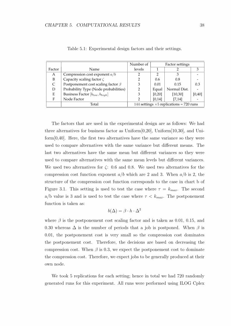
CHAPTER 5. COMPUTATIONAL RESULTS 38
Table 5.1: Experimental design factors and their settings.
Number of Factor settingsFactor Name levels 1 2 3
A Compression cost exponent a/b 2 2 3 -B Capacity scaling factor ζ 2 0.6 0.8 -C Postponement cost scaling factor β 3 0.01 0.15 0.3D Probability Type (Node probabilities) 2 Equal Normal Dist. -E Business Factor [blow, bhigh] 3 [0,20] [10,30] [0,40]F Node Factor 2 [0,14] [7,14] -
Total 144 settings ×5 replications = 720 runs
The factors that are used in the experimental design are as follows: We had
three alternatives for business factor as Uniform[0,20], Uniform[10,30], and Uni-
form[0,40]. Here, the first two alternatives have the same variance so they were
used to compare alternatives with the same variance but different means. The
last two alternatives have the same mean but different variances so they were
used to compare alternatives with the same mean levels but different variances.
We used two alternatives for ζ: 0.6 and 0.8. We used two alternatives for the
compression cost function exponent a/b which are 2 and 3. When a/b is 2, the
structure of the compression cost function corresponds to the case in chart b of
Figure 3.1. This setting is used to test the case where τ = kmax. The second
a/b value is 3 and is used to test the case where τ < kmax. The postponement
function is taken as:
b(∆) = β · h ·∆2
where β is the postponement cost scaling factor and is taken as 0.01, 0.15, and
0.30 whereas ∆ is the number of periods that a job is postponed. When β is
0.01, the postponement cost is very small so the compression cost dominates
the postponement cost. Therefore, the decisions are based on decreasing the
compression cost. When β is 0.3, we expect the postponement cost to dominate
the compression cost. Therefore, we expect jobs to be generally produced at their
own node.
We took 5 replications for each setting; hence in total we had 720 randomly
generated runs for this experiment. All runs were performed using ILOG Cplex
CHAPTER 5. COMPUTATIONAL RESULTS 39
Version 11.2 on a 2×2.83 Ghz Intel Xeon CPU and 8GB memory workstation HP
with the operating system Ubuntu 8.04.
5.2 Tests on CPU Performance
In the computational study, we first tested the performance of our formulations
SFL1 and SFL3 in terms of CPU times on different input parameters.
For 144 different settings and 5 replications, SFL3 solved all of the problems
within at most 4 seconds. Moreover, SFL3 LP relaxation always gave an integer
solution in all our randomly generated runs and preliminary studies. This is a
very interesting result because in section 4.4, we showed that SFL3 may not be
TU.
During 720 randomly generated runs, SFL3 always gave a better result in
terms of CPU time than SFL1. SFL1 took up to 36 minutes to solve the problem
in 142 settings and could not find a solution up to an hour and gave out of memory
result in 2 settings (i.e., 10 randomly generated runs). In the settings which SFL1
could not solve, A = 2, B = 0.8, C = Normal, E = [0,40], and F = [7,14]. Factor
D was 0.01 for the first unsolvable setting and 0.15 for the second one. This
corresponds to the case where kmax is very high due to high capacity, job number
alternatives and the number of descendants have high mean and variability, and
tree is unbalanced in terms of the probability distributions of nodes.
In order to suggest some insights about the effects of changes in factors on the
multi-stage stochastic programming solution time, we made comparative statics
analysis on the factors. However, SFL3 solved the problems in a very short
time so it was not possible to clearly observe the affect of each factor on its
solution time. Therefore, we tested the effects of factors on SFL1 because it was
affected significantly from the changes in factor values. We believe that the results
may give some insight about the sensitivity of the CPU time of the multi-stage
stochastic programming solution to several factors.
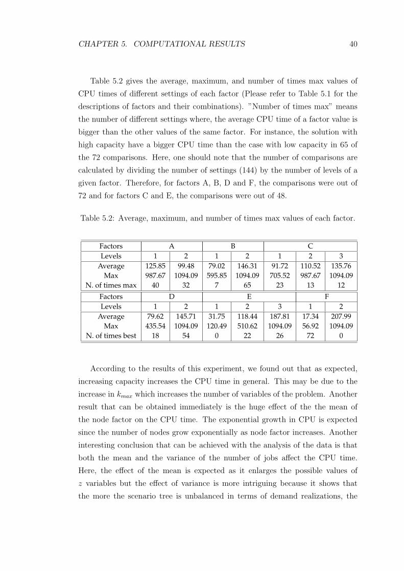
CHAPTER 5. COMPUTATIONAL RESULTS 40
Table 5.2 gives the average, maximum, and number of times max values of
CPU times of different settings of each factor (Please refer to Table 5.1 for the
descriptions of factors and their combinations). ”Number of times max” means
the number of different settings where, the average CPU time of a factor value is
bigger than the other values of the same factor. For instance, the solution with
high capacity have a bigger CPU time than the case with low capacity in 65 of
the 72 comparisons. Here, one should note that the number of comparisons are
calculated by dividing the number of settings (144) by the number of levels of a
given factor. Therefore, for factors A, B, D and F, the comparisons were out of
72 and for factors C and E, the comparisons were out of 48.
Table 5.2: Average, maximum, and number of times max values of each factor.
Factors A B CLevels 1 2 1 2 1 2 3
Average 125.85 99.48 79.02 146.31 91.72 110.52 135.76Max 987.67 1094.09 595.85 1094.09 705.52 987.67 1094.09
N. of times max 40 32 7 65 23 13 12
Factors D E FLevels 1 2 1 2 3 1 2
Average 79.62 145.71 31.75 118.44 187.81 17.34 207.99Max 435.54 1094.09 120.49 510.62 1094.09 56.92 1094.09
N. of times best 18 54 0 22 26 72 0
According to the results of this experiment, we found out that as expected,
increasing capacity increases the CPU time in general. This may be due to the
increase in kmax which increases the number of variables of the problem. Another
result that can be obtained immediately is the huge effect of the the mean of
the node factor on the CPU time. The exponential growth in CPU is expected
since the number of nodes grow exponentially as node factor increases. Another
interesting conclusion that can be achieved with the analysis of the data is that
both the mean and the variance of the number of jobs affect the CPU time.
Here, the effect of the mean is expected as it enlarges the possible values of
z variables but the effect of variance is more intriguing because it shows that
the more the scenario tree is unbalanced in terms of demand realizations, the
CHAPTER 5. COMPUTATIONAL RESULTS 41
harder finding an optimal solution becomes. Finally and most intriguingly, the
probability distribution of the nodes strongly affects the CPU time. As the tree
becomes more unbalanced in terms of the probabilities of the nodes and as the
domination of several nodes exists, the solution time increases significantly.
5.3 Experiments on Comparison of Multi-stage
to Single Scenario Strategies
In the second experiment, we compare the performance of the multi-stage stochas-
tic programming solution with the solution of several single scenario strategies.
The single scenario strategies that we consider are:
1) Using the most likely scenario (ML),
2) Using the most optimistic scenario (OPT),
3) Using the most pessimistic scenario (PES),
4) Using the rounded version of expected demand of each period (EXP).
We compare the performance of single scenario strategies that use three different
production policies (A total of 12 different strategy - policy combinations) with
the solution of multi-stage stochastic programming solution (MST). In order to
do so, we first generate 10 randomly selected scenarios among all possible sce-
narios (i.e., select 10 nodes from the leaf nodes of the scenario tree). Then for
each scenario, we come up with the nodes corresponding to the scenario and use
the demand values of these nodes as the demand realizations of that particular
scenario. We obtain the production values for each strategy using three different
policies (the policies will be explained in detail later):
1) T periods frozen policy (TPF)
2) One period frozen myopic adjustments policy (1PF)
3) One period frozen scenario tree based demand selection policy (STB)
Using Algorithm 5.1, we come up with the total profit of a strategy given its
production values at each period and the demand realizations of the randomly
generated scenario.
Suppose that per unit per period inventory holding cost is denoted as I, and
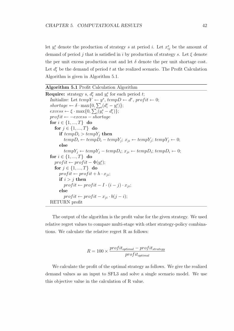
CHAPTER 5. COMPUTATIONAL RESULTS 42
let ysi denote the production of strategy s at period i. Let xsij be the amount of
demand of period j that is satisfied in i by production of strategy s. Let ξ denote
the per unit excess production cost and let δ denote the per unit shortage cost.
Let drt be the demand of period t at the realized scenario. The Profit Calculation
Algorithm is given in Algorithm 5.1.
Algorithm 5.1 Profit Calculation Algorithm
Require: strategy s, drt and yst for each period t;Initialize: Let tempY ← ys, tempD ← dr, profit← 0;shortage← δ ·max{0,
∑i(d
ri − ysi )};
excess← ξ ·max{0,∑
i(ysi − dri )};
profit← −excess− shortagefor i ∈ {1, ..., T} do
for j ∈ {1, ..., T} doif tempDi > tempYj thentempDi ← tempDi − tempYj; xji ← tempYj; tempYj ← 0;
elsetempYj ← tempYj − tempDi; xji ← tempDi; tempDi ← 0;
for i ∈ {1, ..., T} doprofit← profit− Φ(ysi );for j ∈ {1, ..., T} doprofit← profit+ h · xji;if i > j thenprofit← profit− I · (i− j) · xji;
elseprofit← profit− xji · b(j − i);
RETURN profit
The output of the algorithm is the profit value for the given strategy. We used
relative regret values to compare multi-stage with other strategy-policy combina-
tions. We calculate the relative regret R as follows:
R = 100× profitoptimal − profitstrategyprofitoptimal
We calculate the profit of the optimal strategy as follows. We give the realized
demand values as an input to SFL3 and solve a single scenario model. We use
this objective value in the calculation of R value.
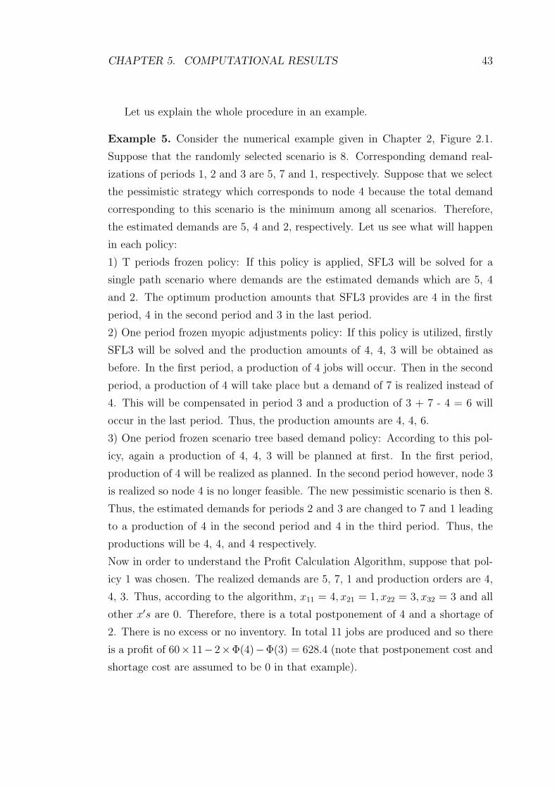
CHAPTER 5. COMPUTATIONAL RESULTS 43
Let us explain the whole procedure in an example.
Example 5. Consider the numerical example given in Chapter 2, Figure 2.1.
Suppose that the randomly selected scenario is 8. Corresponding demand real-
izations of periods 1, 2 and 3 are 5, 7 and 1, respectively. Suppose that we select
the pessimistic strategy which corresponds to node 4 because the total demand
corresponding to this scenario is the minimum among all scenarios. Therefore,
the estimated demands are 5, 4 and 2, respectively. Let us see what will happen
in each policy:
1) T periods frozen policy: If this policy is applied, SFL3 will be solved for a
single path scenario where demands are the estimated demands which are 5, 4
and 2. The optimum production amounts that SFL3 provides are 4 in the first
period, 4 in the second period and 3 in the last period.
2) One period frozen myopic adjustments policy: If this policy is utilized, firstly
SFL3 will be solved and the production amounts of 4, 4, 3 will be obtained as
before. In the first period, a production of 4 jobs will occur. Then in the second
period, a production of 4 will take place but a demand of 7 is realized instead of
4. This will be compensated in period 3 and a production of 3 + 7 - 4 = 6 will
occur in the last period. Thus, the production amounts are 4, 4, 6.
3) One period frozen scenario tree based demand policy: According to this pol-
icy, again a production of 4, 4, 3 will be planned at first. In the first period,
production of 4 will be realized as planned. In the second period however, node 3
is realized so node 4 is no longer feasible. The new pessimistic scenario is then 8.
Thus, the estimated demands for periods 2 and 3 are changed to 7 and 1 leading
to a production of 4 in the second period and 4 in the third period. Thus, the
productions will be 4, 4, and 4 respectively.
Now in order to understand the Profit Calculation Algorithm, suppose that pol-
icy 1 was chosen. The realized demands are 5, 7, 1 and production orders are 4,
4, 3. Thus, according to the algorithm, x11 = 4, x21 = 1, x22 = 3, x32 = 3 and all
other x′s are 0. Therefore, there is a total postponement of 4 and a shortage of
2. There is no excess or no inventory. In total 11 jobs are produced and so there
is a profit of 60×11−2×Φ(4)−Φ(3) = 628.4 (note that postponement cost and
shortage cost are assumed to be 0 in that example).
CHAPTER 5. COMPUTATIONAL RESULTS 44
The optimal policy in this case is to produce 5, 4, 4 which yields a profit
of 728.4. Thus the relative regret is 11.3% for the PES strategy - TPF policy
combination.
While calculating the postponement cost, we use the β parameter as explained
in the previous section. Here we take two values for β in order to avoid bias in
our analysis. These values are 0.15 and 0.3. In the problem we consider, holding
inventory is undesirable so we do not allow it in our model. However, if a single
scenario is used to estimate the demand, inventory is inevitable when the scenario
estimated is not realized. Thus, in order to have a comparison, we assign inventory
holding cost a specific value. In practice, the inventory holding cost is generally
lower than the postponement cost thus we take the inventory holding cost per
unit per period as 80% and 20% of postponement cost coefficient (we assume
linear inventory holding cost function). We consider two types of probability
distributions and one in which probabilities of nodes are equally distributed, the
other one is determined due to normal distribution. The probabilities of nodes are
determined as explained in Section 5.2. The standard deviation factor is taken
as 0.4 in this case. In our preliminary studies, we found out that the solution is
very sensitive to capacity. Therefore, in addition to 0.6 and 0.8 values that are
used in Section 5.2, we also use 0.2 and 0.4. Finally, we increased h value from
200 to 1000 in order to balance the effects of compression cost and postponement
cost. The factors used in the experiments are summarized in Table 5.3. As the
table suggests, we have 19200 runs for 12 policy - strategy combinations and
multi-stage solutions so we took 19200 × 13 = 249600 runs in total, for this
experiment.
Similar to inventory, some excess production or shortage may occur within
the planning horizon if the total demand of the realized (randomly generated)
scenario is strictly less or more than the demand of the estimated scenario. In
practice, having excess production or shortage results in some cost but assigning
some values to these costs may affect the output of the analysis. Thus, we first
conducted the analysis assuming that these values are zero and then in a separate
subsection, we investigated the effects of these cost factors on the comparison of
single scenario strategies to multi-stage.
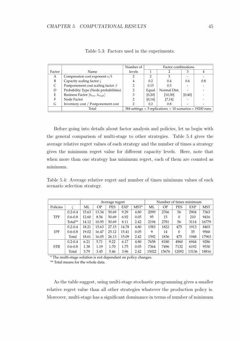
CHAPTER 5. COMPUTATIONAL RESULTS 45
Table 5.3: Factors used in the experiments.
Number of Factor combinationsFactor Name levels 1 2 3 4
A Compression cost exponent a/b 2 2 3 - -B Capacity scaling factor ζ 4 0.2 0.4 0.6 0.8C Postponement cost scaling factor β 2 0.15 0.3 - -D Probability Type (Node probabilities) 2 Equal Normal Dist. - -E Business Factor [blow, bhigh] 3 [0,20] [10,30] [0,40] -F Node Factor 2 [0,14] [7,14] - -G Inventory cost / Postponement cost 2 0.2 0.8 - -
Total 384 settings × 5 replications × 10 scenarios = 19200 runs
Before going into details about factor analysis and policies, let us begin with
the general comparison of multi-stage to other strategies. Table 5.4 gives the
average relative regret values of each strategy and the number of times a strategy
gives the minimum regret value for different capacity levels. Here, note that
when more than one strategy has minimum regret, each of them are counted as
minimum.
Table 5.4: Average relative regret and number of times minimum values of eachscenario selection strategy.
Average regret Number of times minimumPolicies ζ ML OP PES EXP MST* ML OP PES EXP MST
0.2-0.4 15.63 13.34 50.69 9.29 4.80 2099 2766 56 2904 7363TPF 0.6-0.8 12.60 8.56 50.69 6.92 0.05 95 15 0 210 9416
Total** 14.12 10.95 50.69 8.11 2.42 2194 2781 56 3114 167790.2-0.4 18.21 15.63 27.15 14.78 4.80 1583 1822 475 1913 8403
1PF 0.6-0.8 19.02 16.47 25.12 15.41 0.05 9 14 0 35 9560Total 18.61 16.05 26.13 15.09 2.42 1592 1836 475 1948 17963
0.2-0.4 6.21 5.71 9.22 6.17 4.80 7658 8180 4960 6944 9286STB 0.6-0.8 1.38 1.19 1.70 1.75 0.05 7364 7496 7132 6192 9530
Total 3.79 3.45 5.46 3.96 2.42 15022 15676 12092 13136 18816
* The multi-stage solution is not dependant on policy changes.** Total means for the whole data.
As the table suggest, using multi-stage stochastic programming gives a smaller
relative regret value than all other strategies whatever the production policy is.
Moreover, multi-stage has a significant dominance in terms of number of minimum

CHAPTER 5. COMPUTATIONAL RESULTS 46
regret values. In the first two policies, the difference between the regret of multi-
stage and other strategies is significantly high (going up to 50%) whereas in the
third policy the difference reduces. On the other hand, the number of times multi-
stage gives the minimum regret value increases as the policy changes from TPF
to STB. This might be due to the fact that STB uses scenario tree as multi-stage
but it only considers a single scenario. Therefore, on conditions where multi-stage
performs badly, strategies utilizing STB performs even worse. On the other hand,
other policies are not as related to MST as STB so may outperform MST in more
cases. It is especially interesting that among 19200 randomly generated runs,
multi-stage gives one of the minimum values 98% of the time when compared
to strategies that utilize STB. Another interesting conclusion is that capacity
significantly effects the solution of all strategies. This actually points out that
assuming infinite capacity in master production scheduling is quite unreasonable
since solutions are very sensitive to changes in capacity.
We will give detailed statistics for factors A, B, and E later in this section
when we further discuss alternative production policies. Figure 5.1 illustrates the
average relative regret values for each strategy - policy combination and multi-
stage solution for the remaining factor settings which are C, D, F, and G, i.e.,
24 = 16 different settings. For example, in Setting 1, all of the factors are set
to their level 1 values, whereas in Setting 16, all of them are at their level 2
values. The pessimistic strategy with TPF policy is not illustrated in the graph
since it is way out of scale (its regret values are around 80%). In the graph,
each strategy is given a number according to the policy it is used with. ML1
for instance represents the ML strategy used with TPF policy, EXP2 is the EXP
strategy used with 1PF policy and OPT3 is the OPT strategy used with STB
policy. All of these combinations are compared with the multi-stage approach,
denoted as MST. As the figure displays, the average regret performance of multi-
stage is significantly better than other strategy - policy combinations in all of the
settings.
After having a look at the general view of the data, we focus on the production
policy specific results.
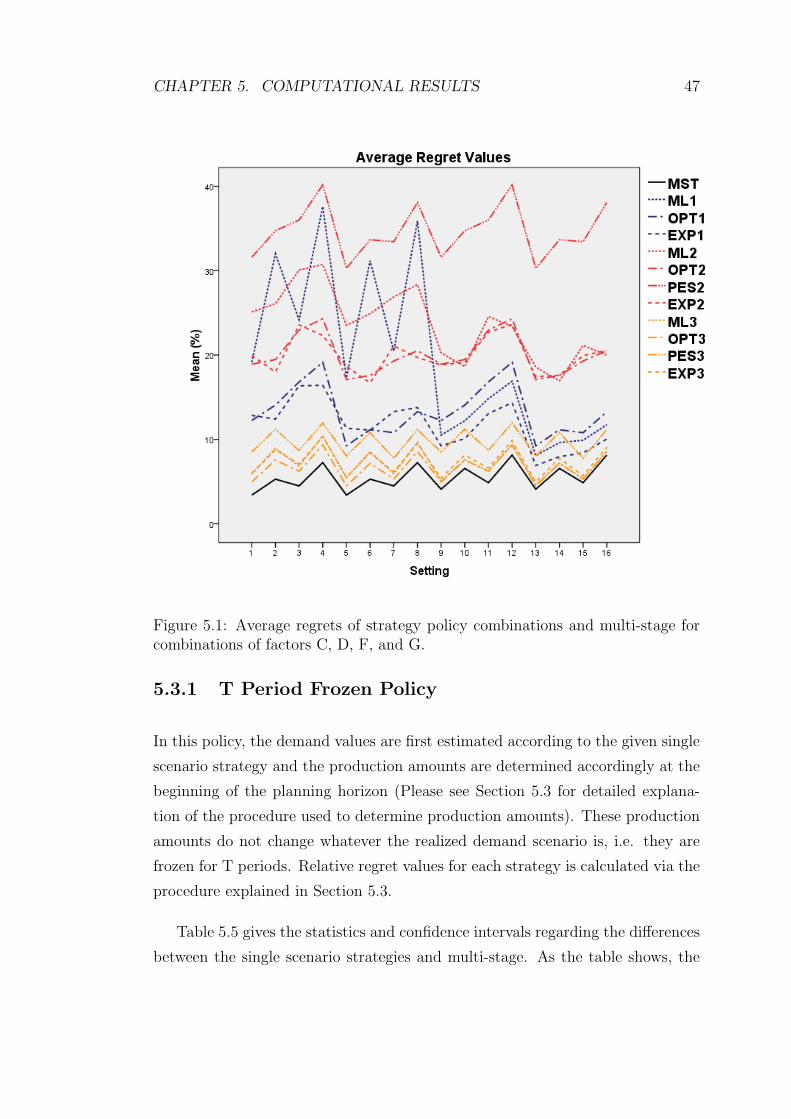
CHAPTER 5. COMPUTATIONAL RESULTS 47
Figure 5.1: Average regrets of strategy policy combinations and multi-stage forcombinations of factors C, D, F, and G.
5.3.1 T Period Frozen Policy
In this policy, the demand values are first estimated according to the given single
scenario strategy and the production amounts are determined accordingly at the
beginning of the planning horizon (Please see Section 5.3 for detailed explana-
tion of the procedure used to determine production amounts). These production
amounts do not change whatever the realized demand scenario is, i.e. they are
frozen for T periods. Relative regret values for each strategy is calculated via the
procedure explained in Section 5.3.
Table 5.5 gives the statistics and confidence intervals regarding the differences
between the single scenario strategies and multi-stage. As the table shows, the
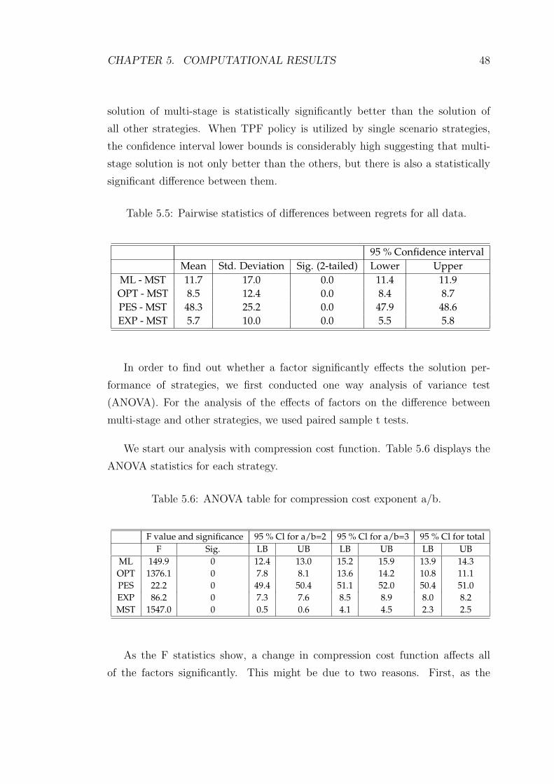
CHAPTER 5. COMPUTATIONAL RESULTS 48
solution of multi-stage is statistically significantly better than the solution of
all other strategies. When TPF policy is utilized by single scenario strategies,
the confidence interval lower bounds is considerably high suggesting that multi-
stage solution is not only better than the others, but there is also a statistically
significant difference between them.
Table 5.5: Pairwise statistics of differences between regrets for all data.
95 % Confidence intervalMean Std. Deviation Sig. (2-tailed) Lower Upper
ML - MST 11.7 17.0 0.0 11.4 11.9OPT - MST 8.5 12.4 0.0 8.4 8.7PES - MST 48.3 25.2 0.0 47.9 48.6EXP - MST 5.7 10.0 0.0 5.5 5.8
In order to find out whether a factor significantly effects the solution per-
formance of strategies, we first conducted one way analysis of variance test
(ANOVA). For the analysis of the effects of factors on the difference between
multi-stage and other strategies, we used paired sample t tests.
We start our analysis with compression cost function. Table 5.6 displays the
ANOVA statistics for each strategy.
Table 5.6: ANOVA table for compression cost exponent a/b.
F value and significance 95 % Cl for a/b=2 95 % Cl for a/b=3 95 % Cl for totalF Sig. LB UB LB UB LB UB
ML 149.9 0 12.4 13.0 15.2 15.9 13.9 14.3OPT 1376.1 0 7.8 8.1 13.6 14.2 10.8 11.1PES 22.2 0 49.4 50.4 51.1 52.0 50.4 51.0EXP 86.2 0 7.3 7.6 8.5 8.9 8.0 8.2MST 1547.0 0 0.5 0.6 4.1 4.5 2.3 2.5
As the F statistics show, a change in compression cost function affects all
of the factors significantly. This might be due to two reasons. First, as the
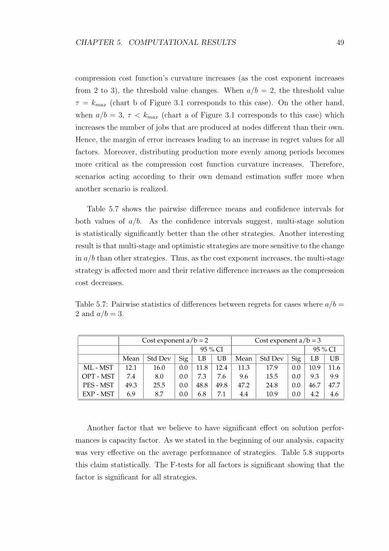
CHAPTER 5. COMPUTATIONAL RESULTS 49
compression cost function’s curvature increases (as the cost exponent increases
from 2 to 3), the threshold value changes. When a/b = 2, the threshold value
τ = kmax (chart b of Figure 3.1 corresponds to this case). On the other hand,
when a/b = 3, τ < kmax (chart a of Figure 3.1 corresponds to this case) which
increases the number of jobs that are produced at nodes different than their own.
Hence, the margin of error increases leading to an increase in regret values for all
factors. Moreover, distributing production more evenly among periods becomes
more critical as the compression cost function curvature increases. Therefore,
scenarios acting according to their own demand estimation suffer more when
another scenario is realized.
Table 5.7 shows the pairwise difference means and confidence intervals for
both values of a/b. As the confidence intervals suggest, multi-stage solution
is statistically significantly better than the other strategies. Another interesting
result is that multi-stage and optimistic strategies are more sensitive to the change
in a/b than other strategies. Thus, as the cost exponent increases, the multi-stage
strategy is affected more and their relative difference increases as the compression
cost decreases.
Table 5.7: Pairwise statistics of differences between regrets for cases where a/b =2 and a/b = 3.
Cost exponent a/b = 2 Cost exponent a/b = 395 % CI 95 % CI
Mean Std Dev Sig LB UB Mean Std Dev Sig LB UBML - MST 12.1 16.0 0.0 11.8 12.4 11.3 17.9 0.0 10.9 11.6OPT - MST 7.4 8.0 0.0 7.3 7.6 9.6 15.5 0.0 9.3 9.9PES - MST 49.3 25.5 0.0 48.8 49.8 47.2 24.8 0.0 46.7 47.7EXP - MST 6.9 8.7 0.0 6.8 7.1 4.4 10.9 0.0 4.2 4.6
Another factor that we believe to have significant effect on solution perfor-
mances is capacity factor. As we stated in the beginning of our analysis, capacity
was very effective on the average performance of strategies. Table 5.8 supports
this claim statistically. The F-tests for all factors is significant showing that the
factor is significant for all strategies.
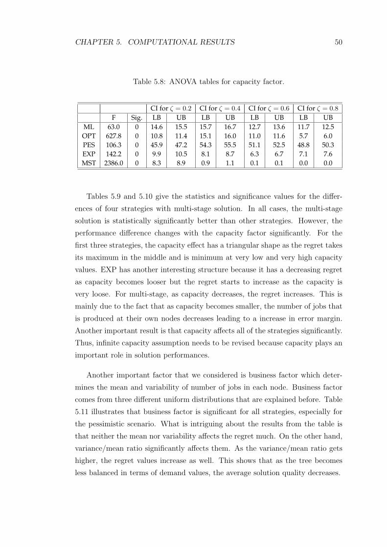
CHAPTER 5. COMPUTATIONAL RESULTS 50
Table 5.8: ANOVA tables for capacity factor.
CI for ζ = 0.2 CI for ζ = 0.4 CI for ζ = 0.6 CI for ζ = 0.8F Sig. LB UB LB UB LB UB LB UB
ML 63.0 0 14.6 15.5 15.7 16.7 12.7 13.6 11.7 12.5OPT 627.8 0 10.8 11.4 15.1 16.0 11.0 11.6 5.7 6.0PES 106.3 0 45.9 47.2 54.3 55.5 51.1 52.5 48.8 50.3EXP 142.2 0 9.9 10.5 8.1 8.7 6.3 6.7 7.1 7.6MST 2386.0 0 8.3 8.9 0.9 1.1 0.1 0.1 0.0 0.0
Tables 5.9 and 5.10 give the statistics and significance values for the differ-
ences of four strategies with multi-stage solution. In all cases, the multi-stage
solution is statistically significantly better than other strategies. However, the
performance difference changes with the capacity factor significantly. For the
first three strategies, the capacity effect has a triangular shape as the regret takes
its maximum in the middle and is minimum at very low and very high capacity
values. EXP has another interesting structure because it has a decreasing regret
as capacity becomes looser but the regret starts to increase as the capacity is
very loose. For multi-stage, as capacity decreases, the regret increases. This is
mainly due to the fact that as capacity becomes smaller, the number of jobs that
is produced at their own nodes decreases leading to a increase in error margin.
Another important result is that capacity affects all of the strategies significantly.
Thus, infinite capacity assumption needs to be revised because capacity plays an
important role in solution performances.
Another important factor that we considered is business factor which deter-
mines the mean and variability of number of jobs in each node. Business factor
comes from three different uniform distributions that are explained before. Table
5.11 illustrates that business factor is significant for all strategies, especially for
the pessimistic scenario. What is intriguing about the results from the table is
that neither the mean nor variability affects the regret much. On the other hand,
variance/mean ratio significantly affects them. As the variance/mean ratio gets
higher, the regret values increase as well. This shows that as the tree becomes
less balanced in terms of demand values, the average solution quality decreases.
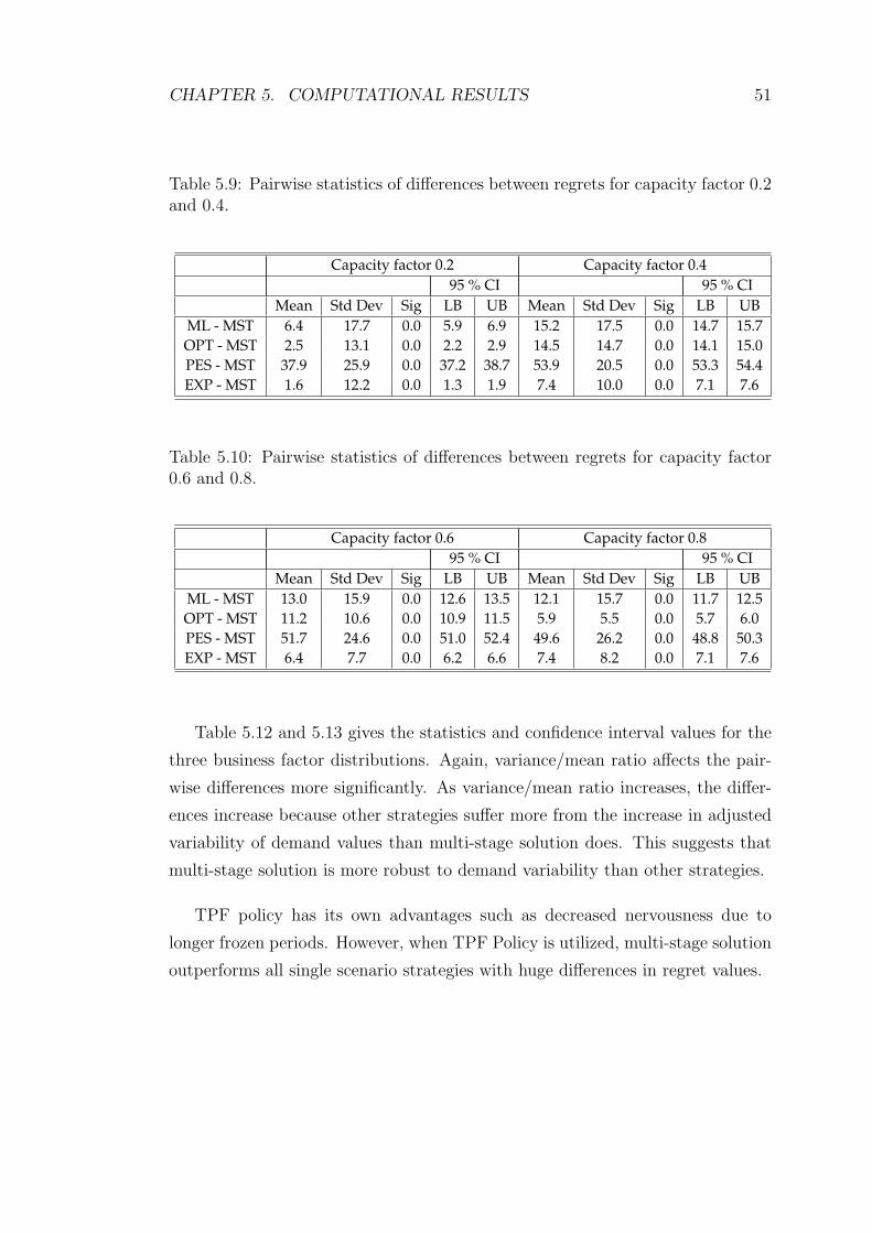
CHAPTER 5. COMPUTATIONAL RESULTS 51
Table 5.9: Pairwise statistics of differences between regrets for capacity factor 0.2and 0.4.
Capacity factor 0.2 Capacity factor 0.495 % CI 95 % CI
Mean Std Dev Sig LB UB Mean Std Dev Sig LB UBML - MST 6.4 17.7 0.0 5.9 6.9 15.2 17.5 0.0 14.7 15.7OPT - MST 2.5 13.1 0.0 2.2 2.9 14.5 14.7 0.0 14.1 15.0PES - MST 37.9 25.9 0.0 37.2 38.7 53.9 20.5 0.0 53.3 54.4EXP - MST 1.6 12.2 0.0 1.3 1.9 7.4 10.0 0.0 7.1 7.6
Table 5.10: Pairwise statistics of differences between regrets for capacity factor0.6 and 0.8.
Capacity factor 0.6 Capacity factor 0.895 % CI 95 % CI
Mean Std Dev Sig LB UB Mean Std Dev Sig LB UBML - MST 13.0 15.9 0.0 12.6 13.5 12.1 15.7 0.0 11.7 12.5OPT - MST 11.2 10.6 0.0 10.9 11.5 5.9 5.5 0.0 5.7 6.0PES - MST 51.7 24.6 0.0 51.0 52.4 49.6 26.2 0.0 48.8 50.3EXP - MST 6.4 7.7 0.0 6.2 6.6 7.4 8.2 0.0 7.1 7.6
Table 5.12 and 5.13 gives the statistics and confidence interval values for the
three business factor distributions. Again, variance/mean ratio affects the pair-
wise differences more significantly. As variance/mean ratio increases, the differ-
ences increase because other strategies suffer more from the increase in adjusted
variability of demand values than multi-stage solution does. This suggests that
multi-stage solution is more robust to demand variability than other strategies.
TPF policy has its own advantages such as decreased nervousness due to
longer frozen periods. However, when TPF Policy is utilized, multi-stage solution
outperforms all single scenario strategies with huge differences in regret values.
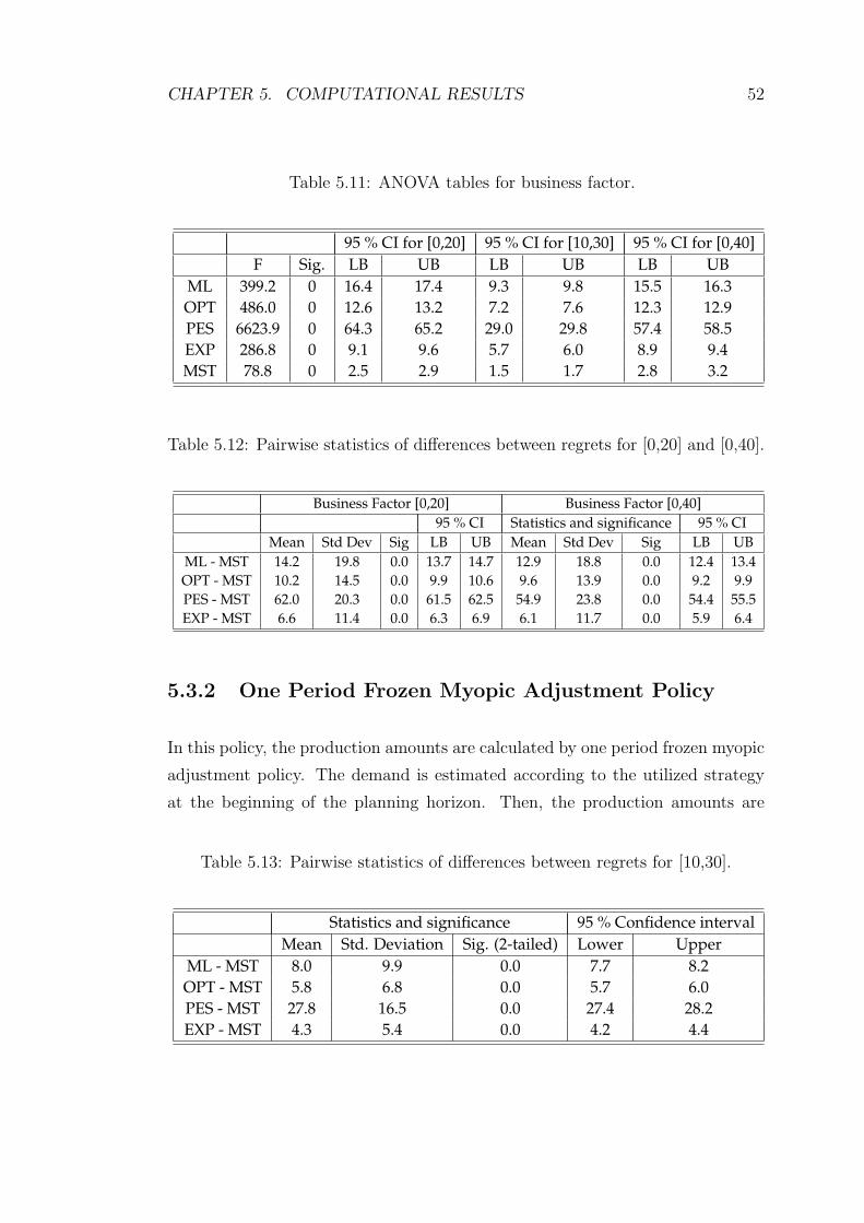
CHAPTER 5. COMPUTATIONAL RESULTS 52
Table 5.11: ANOVA tables for business factor.
95 % CI for [0,20] 95 % CI for [10,30] 95 % CI for [0,40]F Sig. LB UB LB UB LB UB
ML 399.2 0 16.4 17.4 9.3 9.8 15.5 16.3OPT 486.0 0 12.6 13.2 7.2 7.6 12.3 12.9PES 6623.9 0 64.3 65.2 29.0 29.8 57.4 58.5EXP 286.8 0 9.1 9.6 5.7 6.0 8.9 9.4MST 78.8 0 2.5 2.9 1.5 1.7 2.8 3.2
Table 5.12: Pairwise statistics of differences between regrets for [0,20] and [0,40].
Business Factor [0,20] Business Factor [0,40]95 % CI Statistics and significance 95 % CI
Mean Std Dev Sig LB UB Mean Std Dev Sig LB UBML - MST 14.2 19.8 0.0 13.7 14.7 12.9 18.8 0.0 12.4 13.4OPT - MST 10.2 14.5 0.0 9.9 10.6 9.6 13.9 0.0 9.2 9.9PES - MST 62.0 20.3 0.0 61.5 62.5 54.9 23.8 0.0 54.4 55.5EXP - MST 6.6 11.4 0.0 6.3 6.9 6.1 11.7 0.0 5.9 6.4
5.3.2 One Period Frozen Myopic Adjustment Policy
In this policy, the production amounts are calculated by one period frozen myopic
adjustment policy. The demand is estimated according to the utilized strategy
at the beginning of the planning horizon. Then, the production amounts are
Table 5.13: Pairwise statistics of differences between regrets for [10,30].
Statistics and significance 95 % Confidence intervalMean Std. Deviation Sig. (2-tailed) Lower Upper
ML - MST 8.0 9.9 0.0 7.7 8.2OPT - MST 5.8 6.8 0.0 5.7 6.0PES - MST 27.8 16.5 0.0 27.4 28.2EXP - MST 4.3 5.4 0.0 4.2 4.4
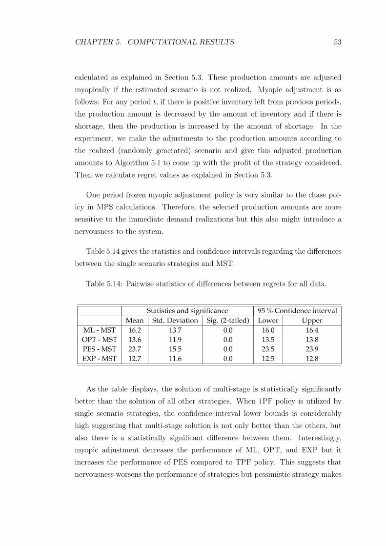
CHAPTER 5. COMPUTATIONAL RESULTS 53
calculated as explained in Section 5.3. These production amounts are adjusted
myopically if the estimated scenario is not realized. Myopic adjustment is as
follows: For any period t, if there is positive inventory left from previous periods,
the production amount is decreased by the amount of inventory and if there is
shortage, then the production is increased by the amount of shortage. In the
experiment, we make the adjustments to the production amounts according to
the realized (randomly generated) scenario and give this adjusted production
amounts to Algorithm 5.1 to come up with the profit of the strategy considered.
Then we calculate regret values as explained in Section 5.3.
One period frozen myopic adjustment policy is very similar to the chase pol-
icy in MPS calculations. Therefore, the selected production amounts are more
sensitive to the immediate demand realizations but this also might introduce a
nervousness to the system.
Table 5.14 gives the statistics and confidence intervals regarding the differences
between the single scenario strategies and MST.
Table 5.14: Pairwise statistics of differences between regrets for all data.
Statistics and significance 95 % Confidence intervalMean Std. Deviation Sig. (2-tailed) Lower Upper
ML - MST 16.2 13.7 0.0 16.0 16.4OPT - MST 13.6 11.9 0.0 13.5 13.8PES - MST 23.7 15.5 0.0 23.5 23.9EXP - MST 12.7 11.6 0.0 12.5 12.8
As the table displays, the solution of multi-stage is statistically significantly
better than the solution of all other strategies. When 1PF policy is utilized by
single scenario strategies, the confidence interval lower bounds is considerably
high suggesting that multi-stage solution is not only better than the others, but
also there is a statistically significant difference between them. Interestingly,
myopic adjustment decreases the performance of ML, OPT, and EXP but it
increases the performance of PES compared to TPF policy. This suggests that
nervousness worsens the performance of strategies but pessimistic strategy makes
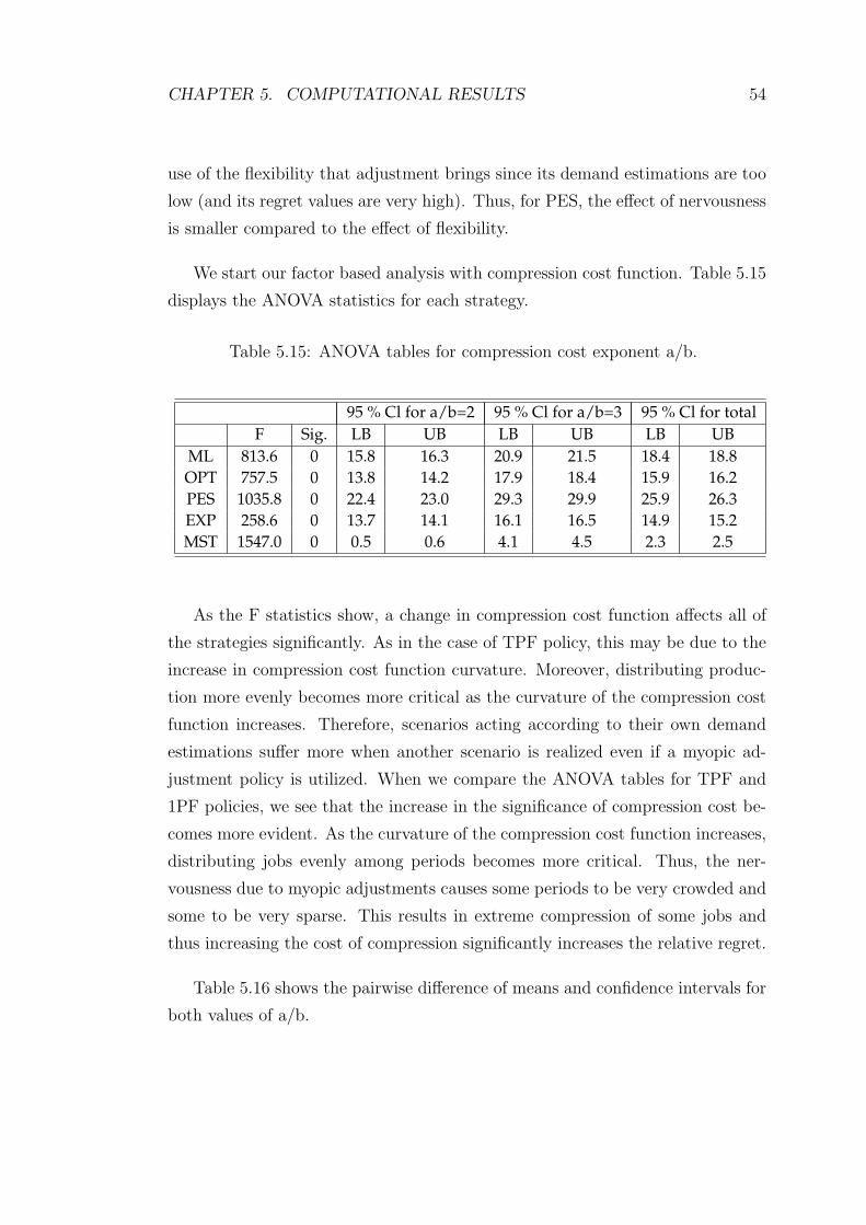
CHAPTER 5. COMPUTATIONAL RESULTS 54
use of the flexibility that adjustment brings since its demand estimations are too
low (and its regret values are very high). Thus, for PES, the effect of nervousness
is smaller compared to the effect of flexibility.
We start our factor based analysis with compression cost function. Table 5.15
displays the ANOVA statistics for each strategy.
Table 5.15: ANOVA tables for compression cost exponent a/b.
95 % Cl for a/b=2 95 % Cl for a/b=3 95 % Cl for totalF Sig. LB UB LB UB LB UB
ML 813.6 0 15.8 16.3 20.9 21.5 18.4 18.8OPT 757.5 0 13.8 14.2 17.9 18.4 15.9 16.2PES 1035.8 0 22.4 23.0 29.3 29.9 25.9 26.3EXP 258.6 0 13.7 14.1 16.1 16.5 14.9 15.2MST 1547.0 0 0.5 0.6 4.1 4.5 2.3 2.5
As the F statistics show, a change in compression cost function affects all of
the strategies significantly. As in the case of TPF policy, this may be due to the
increase in compression cost function curvature. Moreover, distributing produc-
tion more evenly becomes more critical as the curvature of the compression cost
function increases. Therefore, scenarios acting according to their own demand
estimations suffer more when another scenario is realized even if a myopic ad-
justment policy is utilized. When we compare the ANOVA tables for TPF and
1PF policies, we see that the increase in the significance of compression cost be-
comes more evident. As the curvature of the compression cost function increases,
distributing jobs evenly among periods becomes more critical. Thus, the ner-
vousness due to myopic adjustments causes some periods to be very crowded and
some to be very sparse. This results in extreme compression of some jobs and
thus increasing the cost of compression significantly increases the relative regret.
Table 5.16 shows the pairwise difference of means and confidence intervals for
both values of a/b.
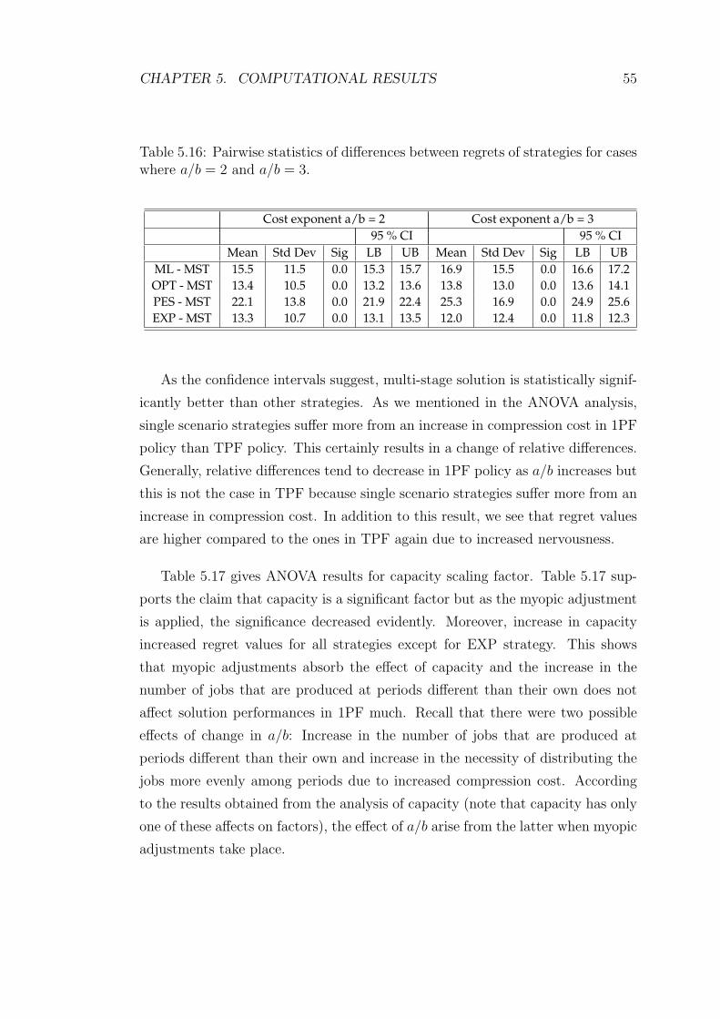
CHAPTER 5. COMPUTATIONAL RESULTS 55
Table 5.16: Pairwise statistics of differences between regrets of strategies for caseswhere a/b = 2 and a/b = 3.
Cost exponent a/b = 2 Cost exponent a/b = 395 % CI 95 % CI
Mean Std Dev Sig LB UB Mean Std Dev Sig LB UBML - MST 15.5 11.5 0.0 15.3 15.7 16.9 15.5 0.0 16.6 17.2OPT - MST 13.4 10.5 0.0 13.2 13.6 13.8 13.0 0.0 13.6 14.1PES - MST 22.1 13.8 0.0 21.9 22.4 25.3 16.9 0.0 24.9 25.6EXP - MST 13.3 10.7 0.0 13.1 13.5 12.0 12.4 0.0 11.8 12.3
As the confidence intervals suggest, multi-stage solution is statistically signif-
icantly better than other strategies. As we mentioned in the ANOVA analysis,
single scenario strategies suffer more from an increase in compression cost in 1PF
policy than TPF policy. This certainly results in a change of relative differences.
Generally, relative differences tend to decrease in 1PF policy as a/b increases but
this is not the case in TPF because single scenario strategies suffer more from an
increase in compression cost. In addition to this result, we see that regret values
are higher compared to the ones in TPF again due to increased nervousness.
Table 5.17 gives ANOVA results for capacity scaling factor. Table 5.17 sup-
ports the claim that capacity is a significant factor but as the myopic adjustment
is applied, the significance decreased evidently. Moreover, increase in capacity
increased regret values for all strategies except for EXP strategy. This shows
that myopic adjustments absorb the effect of capacity and the increase in the
number of jobs that are produced at periods different than their own does not
affect solution performances in 1PF much. Recall that there were two possible
effects of change in a/b: Increase in the number of jobs that are produced at
periods different than their own and increase in the necessity of distributing the
jobs more evenly among periods due to increased compression cost. According
to the results obtained from the analysis of capacity (note that capacity has only
one of these affects on factors), the effect of a/b arise from the latter when myopic
adjustments take place.
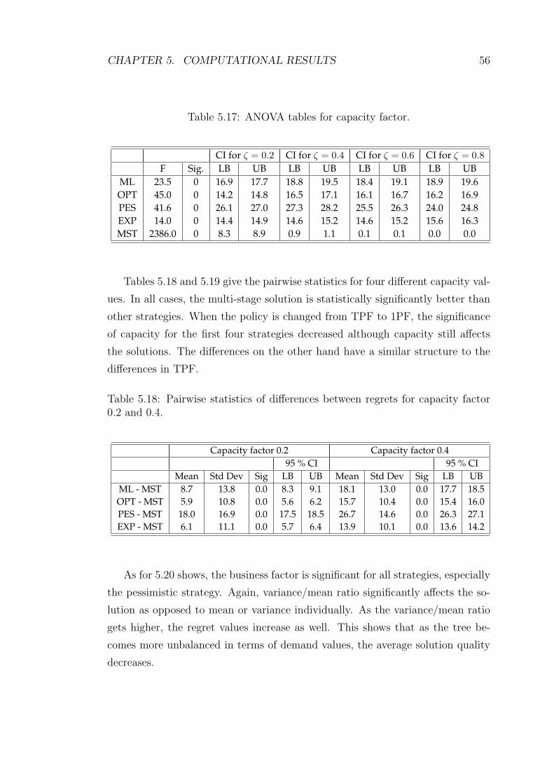
CHAPTER 5. COMPUTATIONAL RESULTS 56
Table 5.17: ANOVA tables for capacity factor.
CI for ζ = 0.2 CI for ζ = 0.4 CI for ζ = 0.6 CI for ζ = 0.8F Sig. LB UB LB UB LB UB LB UB
ML 23.5 0 16.9 17.7 18.8 19.5 18.4 19.1 18.9 19.6OPT 45.0 0 14.2 14.8 16.5 17.1 16.1 16.7 16.2 16.9PES 41.6 0 26.1 27.0 27.3 28.2 25.5 26.3 24.0 24.8EXP 14.0 0 14.4 14.9 14.6 15.2 14.6 15.2 15.6 16.3MST 2386.0 0 8.3 8.9 0.9 1.1 0.1 0.1 0.0 0.0
Tables 5.18 and 5.19 give the pairwise statistics for four different capacity val-
ues. In all cases, the multi-stage solution is statistically significantly better than
other strategies. When the policy is changed from TPF to 1PF, the significance
of capacity for the first four strategies decreased although capacity still affects
the solutions. The differences on the other hand have a similar structure to the
differences in TPF.
Table 5.18: Pairwise statistics of differences between regrets for capacity factor0.2 and 0.4.
Capacity factor 0.2 Capacity factor 0.495 % CI 95 % CI
Mean Std Dev Sig LB UB Mean Std Dev Sig LB UBML - MST 8.7 13.8 0.0 8.3 9.1 18.1 13.0 0.0 17.7 18.5OPT - MST 5.9 10.8 0.0 5.6 6.2 15.7 10.4 0.0 15.4 16.0PES - MST 18.0 16.9 0.0 17.5 18.5 26.7 14.6 0.0 26.3 27.1EXP - MST 6.1 11.1 0.0 5.7 6.4 13.9 10.1 0.0 13.6 14.2
As for 5.20 shows, the business factor is significant for all strategies, especially
the pessimistic strategy. Again, variance/mean ratio significantly affects the so-
lution as opposed to mean or variance individually. As the variance/mean ratio
gets higher, the regret values increase as well. This shows that as the tree be-
comes more unbalanced in terms of demand values, the average solution quality
decreases.
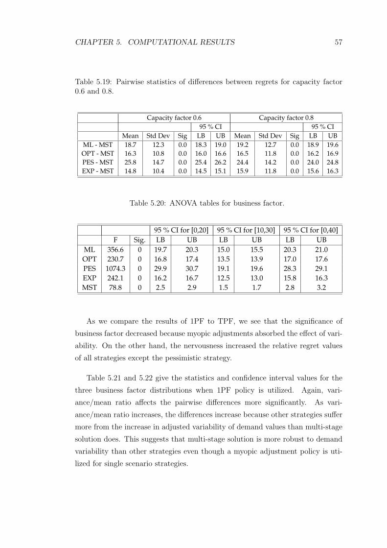
CHAPTER 5. COMPUTATIONAL RESULTS 57
Table 5.19: Pairwise statistics of differences between regrets for capacity factor0.6 and 0.8.
Capacity factor 0.6 Capacity factor 0.895 % CI 95 % CI
Mean Std Dev Sig LB UB Mean Std Dev Sig LB UBML - MST 18.7 12.3 0.0 18.3 19.0 19.2 12.7 0.0 18.9 19.6OPT - MST 16.3 10.8 0.0 16.0 16.6 16.5 11.8 0.0 16.2 16.9PES - MST 25.8 14.7 0.0 25.4 26.2 24.4 14.2 0.0 24.0 24.8EXP - MST 14.8 10.4 0.0 14.5 15.1 15.9 11.8 0.0 15.6 16.3
Table 5.20: ANOVA tables for business factor.
95 % CI for [0,20] 95 % CI for [10,30] 95 % CI for [0,40]F Sig. LB UB LB UB LB UB
ML 356.6 0 19.7 20.3 15.0 15.5 20.3 21.0OPT 230.7 0 16.8 17.4 13.5 13.9 17.0 17.6PES 1074.3 0 29.9 30.7 19.1 19.6 28.3 29.1EXP 242.1 0 16.2 16.7 12.5 13.0 15.8 16.3MST 78.8 0 2.5 2.9 1.5 1.7 2.8 3.2
As we compare the results of 1PF to TPF, we see that the significance of
business factor decreased because myopic adjustments absorbed the effect of vari-
ability. On the other hand, the nervousness increased the relative regret values
of all strategies except the pessimistic strategy.
Table 5.21 and 5.22 give the statistics and confidence interval values for the
three business factor distributions when 1PF policy is utilized. Again, vari-
ance/mean ratio affects the pairwise differences more significantly. As vari-
ance/mean ratio increases, the differences increase because other strategies suffer
more from the increase in adjusted variability of demand values than multi-stage
solution does. This suggests that multi-stage solution is more robust to demand
variability than other strategies even though a myopic adjustment policy is uti-
lized for single scenario strategies.
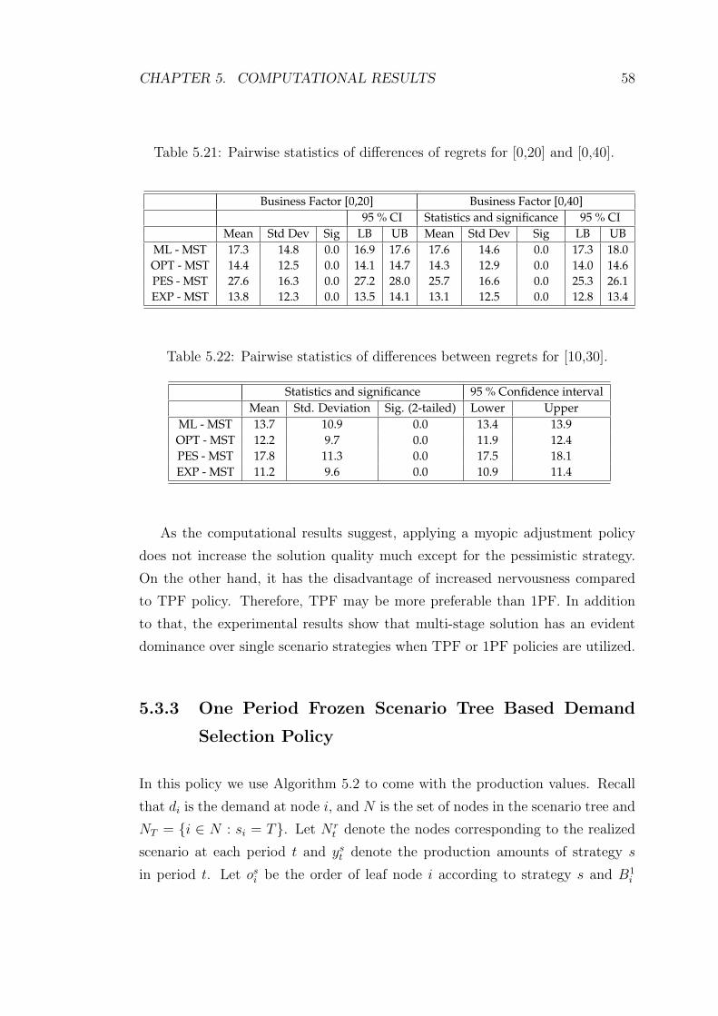
CHAPTER 5. COMPUTATIONAL RESULTS 58
Table 5.21: Pairwise statistics of differences of regrets for [0,20] and [0,40].
Business Factor [0,20] Business Factor [0,40]95 % CI Statistics and significance 95 % CI
Mean Std Dev Sig LB UB Mean Std Dev Sig LB UBML - MST 17.3 14.8 0.0 16.9 17.6 17.6 14.6 0.0 17.3 18.0OPT - MST 14.4 12.5 0.0 14.1 14.7 14.3 12.9 0.0 14.0 14.6PES - MST 27.6 16.3 0.0 27.2 28.0 25.7 16.6 0.0 25.3 26.1EXP - MST 13.8 12.3 0.0 13.5 14.1 13.1 12.5 0.0 12.8 13.4
Table 5.22: Pairwise statistics of differences between regrets for [10,30].
Statistics and significance 95 % Confidence intervalMean Std. Deviation Sig. (2-tailed) Lower Upper
ML - MST 13.7 10.9 0.0 13.4 13.9OPT - MST 12.2 9.7 0.0 11.9 12.4PES - MST 17.8 11.3 0.0 17.5 18.1EXP - MST 11.2 9.6 0.0 10.9 11.4
As the computational results suggest, applying a myopic adjustment policy
does not increase the solution quality much except for the pessimistic strategy.
On the other hand, it has the disadvantage of increased nervousness compared
to TPF policy. Therefore, TPF may be more preferable than 1PF. In addition
to that, the experimental results show that multi-stage solution has an evident
dominance over single scenario strategies when TPF or 1PF policies are utilized.
5.3.3 One Period Frozen Scenario Tree Based Demand
Selection Policy
In this policy we use Algorithm 5.2 to come with the production values. Recall
that di is the demand at node i, and N is the set of nodes in the scenario tree and
NT = {i ∈ N : si = T}. Let N rt denote the nodes corresponding to the realized
scenario at each period t and yst denote the production amounts of strategy s
in period t. Let osi be the order of leaf node i according to strategy s and B1i
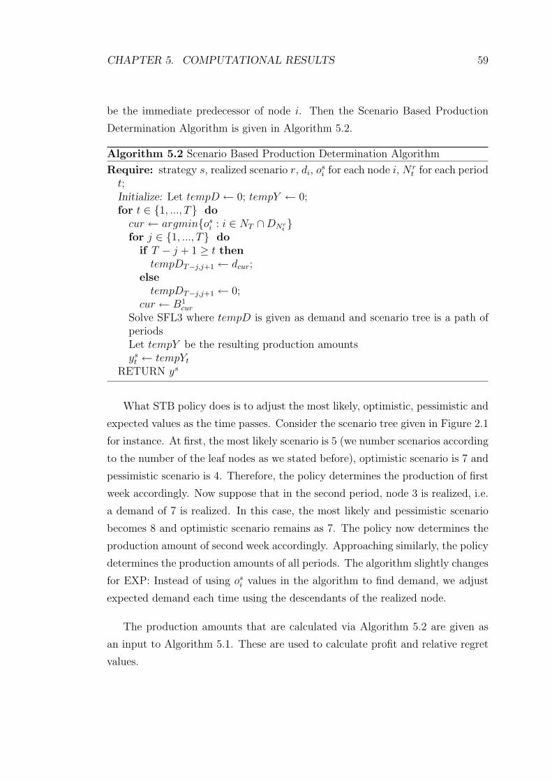
CHAPTER 5. COMPUTATIONAL RESULTS 59
be the immediate predecessor of node i. Then the Scenario Based Production
Determination Algorithm is given in Algorithm 5.2.
Algorithm 5.2 Scenario Based Production Determination Algorithm
Require: strategy s, realized scenario r, di, osi for each node i, N r
t for each periodt;Initialize: Let tempD ← 0; tempY ← 0;for t ∈ {1, ..., T} docur ← argmin{osi : i ∈ NT ∩DNr
t}
for j ∈ {1, ..., T} doif T − j + 1 ≥ t thentempDT−j,j+1 ← dcur;
elsetempDT−j,j+1 ← 0;
cur ← B1cur
Solve SFL3 where tempD is given as demand and scenario tree is a path ofperiodsLet tempY be the resulting production amountsyst ← tempYt
RETURN ys
What STB policy does is to adjust the most likely, optimistic, pessimistic and
expected values as the time passes. Consider the scenario tree given in Figure 2.1
for instance. At first, the most likely scenario is 5 (we number scenarios according
to the number of the leaf nodes as we stated before), optimistic scenario is 7 and
pessimistic scenario is 4. Therefore, the policy determines the production of first
week accordingly. Now suppose that in the second period, node 3 is realized, i.e.
a demand of 7 is realized. In this case, the most likely and pessimistic scenario
becomes 8 and optimistic scenario remains as 7. The policy now determines the
production amount of second week accordingly. Approaching similarly, the policy
determines the production amounts of all periods. The algorithm slightly changes
for EXP: Instead of using osi values in the algorithm to find demand, we adjust
expected demand each time using the descendants of the realized node.
The production amounts that are calculated via Algorithm 5.2 are given as
an input to Algorithm 5.1. These are used to calculate profit and relative regret
values.
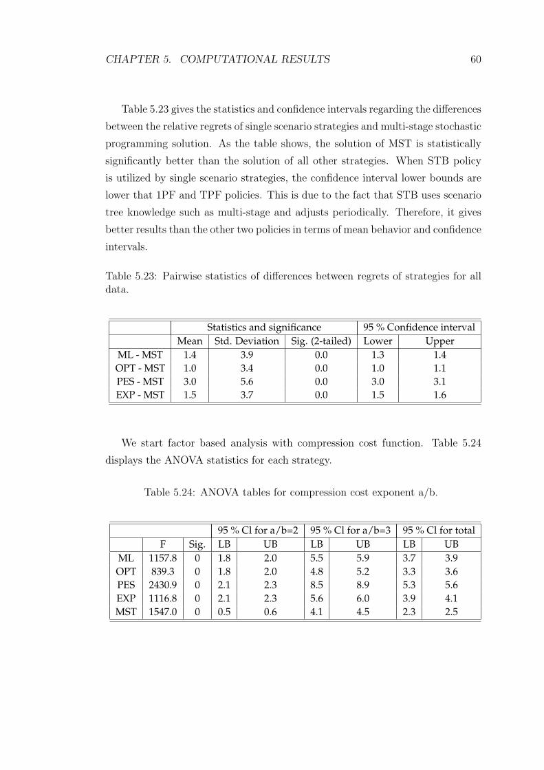
CHAPTER 5. COMPUTATIONAL RESULTS 60
Table 5.23 gives the statistics and confidence intervals regarding the differences
between the relative regrets of single scenario strategies and multi-stage stochastic
programming solution. As the table shows, the solution of MST is statistically
significantly better than the solution of all other strategies. When STB policy
is utilized by single scenario strategies, the confidence interval lower bounds are
lower that 1PF and TPF policies. This is due to the fact that STB uses scenario
tree knowledge such as multi-stage and adjusts periodically. Therefore, it gives
better results than the other two policies in terms of mean behavior and confidence
intervals.
Table 5.23: Pairwise statistics of differences between regrets of strategies for alldata.
Statistics and significance 95 % Confidence intervalMean Std. Deviation Sig. (2-tailed) Lower Upper
ML - MST 1.4 3.9 0.0 1.3 1.4OPT - MST 1.0 3.4 0.0 1.0 1.1PES - MST 3.0 5.6 0.0 3.0 3.1EXP - MST 1.5 3.7 0.0 1.5 1.6
We start factor based analysis with compression cost function. Table 5.24
displays the ANOVA statistics for each strategy.
Table 5.24: ANOVA tables for compression cost exponent a/b.
95 % Cl for a/b=2 95 % Cl for a/b=3 95 % Cl for totalF Sig. LB UB LB UB LB UB
ML 1157.8 0 1.8 2.0 5.5 5.9 3.7 3.9OPT 839.3 0 1.8 2.0 4.8 5.2 3.3 3.6PES 2430.9 0 2.1 2.3 8.5 8.9 5.3 5.6EXP 1116.8 0 2.1 2.3 5.6 6.0 3.9 4.1MST 1547.0 0 0.5 0.6 4.1 4.5 2.3 2.5
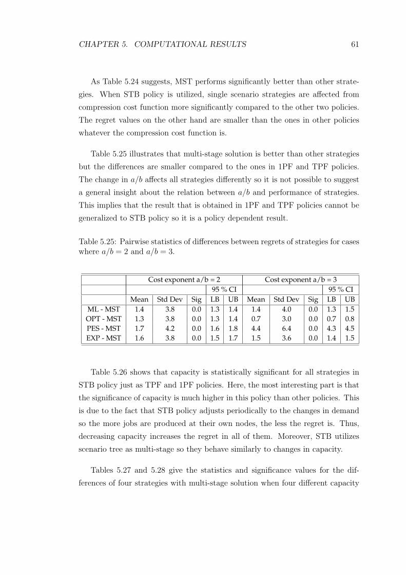
CHAPTER 5. COMPUTATIONAL RESULTS 61
As Table 5.24 suggests, MST performs significantly better than other strate-
gies. When STB policy is utilized, single scenario strategies are affected from
compression cost function more significantly compared to the other two policies.
The regret values on the other hand are smaller than the ones in other policies
whatever the compression cost function is.
Table 5.25 illustrates that multi-stage solution is better than other strategies
but the differences are smaller compared to the ones in 1PF and TPF policies.
The change in a/b affects all strategies differently so it is not possible to suggest
a general insight about the relation between a/b and performance of strategies.
This implies that the result that is obtained in 1PF and TPF policies cannot be
generalized to STB policy so it is a policy dependent result.
Table 5.25: Pairwise statistics of differences between regrets of strategies for caseswhere a/b = 2 and a/b = 3.
Cost exponent a/b = 2 Cost exponent a/b = 395 % CI 95 % CI
Mean Std Dev Sig LB UB Mean Std Dev Sig LB UBML - MST 1.4 3.8 0.0 1.3 1.4 1.4 4.0 0.0 1.3 1.5OPT - MST 1.3 3.8 0.0 1.3 1.4 0.7 3.0 0.0 0.7 0.8PES - MST 1.7 4.2 0.0 1.6 1.8 4.4 6.4 0.0 4.3 4.5EXP - MST 1.6 3.8 0.0 1.5 1.7 1.5 3.6 0.0 1.4 1.5
Table 5.26 shows that capacity is statistically significant for all strategies in
STB policy just as TPF and 1PF policies. Here, the most interesting part is that
the significance of capacity is much higher in this policy than other policies. This
is due to the fact that STB policy adjusts periodically to the changes in demand
so the more jobs are produced at their own nodes, the less the regret is. Thus,
decreasing capacity increases the regret in all of them. Moreover, STB utilizes
scenario tree as multi-stage so they behave similarly to changes in capacity.
Tables 5.27 and 5.28 give the statistics and significance values for the dif-
ferences of four strategies with multi-stage solution when four different capacity
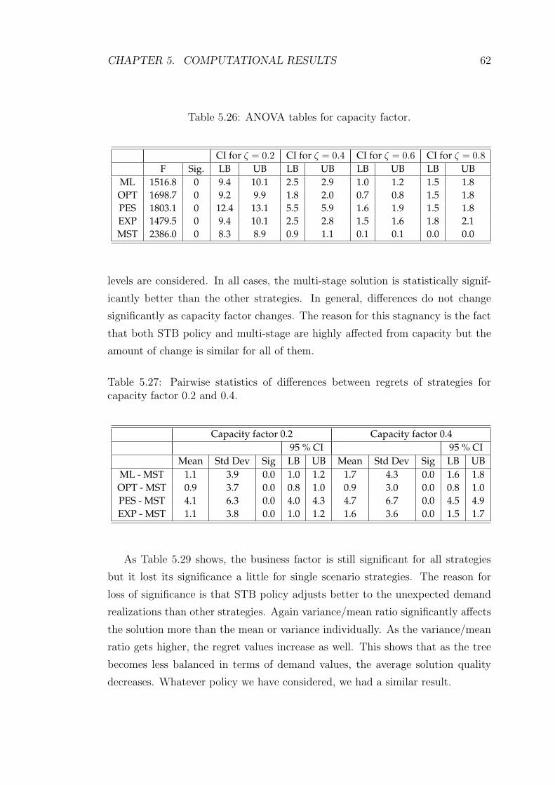
CHAPTER 5. COMPUTATIONAL RESULTS 62
Table 5.26: ANOVA tables for capacity factor.
CI for ζ = 0.2 CI for ζ = 0.4 CI for ζ = 0.6 CI for ζ = 0.8F Sig. LB UB LB UB LB UB LB UB
ML 1516.8 0 9.4 10.1 2.5 2.9 1.0 1.2 1.5 1.8OPT 1698.7 0 9.2 9.9 1.8 2.0 0.7 0.8 1.5 1.8PES 1803.1 0 12.4 13.1 5.5 5.9 1.6 1.9 1.5 1.8EXP 1479.5 0 9.4 10.1 2.5 2.8 1.5 1.6 1.8 2.1MST 2386.0 0 8.3 8.9 0.9 1.1 0.1 0.1 0.0 0.0
levels are considered. In all cases, the multi-stage solution is statistically signif-
icantly better than the other strategies. In general, differences do not change
significantly as capacity factor changes. The reason for this stagnancy is the fact
that both STB policy and multi-stage are highly affected from capacity but the
amount of change is similar for all of them.
Table 5.27: Pairwise statistics of differences between regrets of strategies forcapacity factor 0.2 and 0.4.
Capacity factor 0.2 Capacity factor 0.495 % CI 95 % CI
Mean Std Dev Sig LB UB Mean Std Dev Sig LB UBML - MST 1.1 3.9 0.0 1.0 1.2 1.7 4.3 0.0 1.6 1.8OPT - MST 0.9 3.7 0.0 0.8 1.0 0.9 3.0 0.0 0.8 1.0PES - MST 4.1 6.3 0.0 4.0 4.3 4.7 6.7 0.0 4.5 4.9EXP - MST 1.1 3.8 0.0 1.0 1.2 1.6 3.6 0.0 1.5 1.7
As Table 5.29 shows, the business factor is still significant for all strategies
but it lost its significance a little for single scenario strategies. The reason for
loss of significance is that STB policy adjusts better to the unexpected demand
realizations than other strategies. Again variance/mean ratio significantly affects
the solution more than the mean or variance individually. As the variance/mean
ratio gets higher, the regret values increase as well. This shows that as the tree
becomes less balanced in terms of demand values, the average solution quality
decreases. Whatever policy we have considered, we had a similar result.
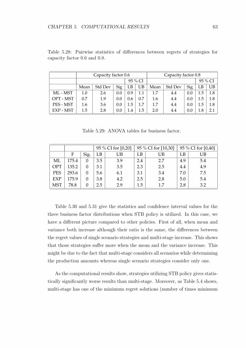
CHAPTER 5. COMPUTATIONAL RESULTS 63
Table 5.28: Pairwise statistics of differences between regrets of strategies forcapacity factor 0.6 and 0.8.
Capacity factor 0.6 Capacity factor 0.895 % CI 95 % CI
Mean Std Dev Sig LB UB Mean Std Dev Sig LB UBML - MST 1.0 2.6 0.0 0.9 1.1 1.7 4.4 0.0 1.5 1.8OPT - MST 0.7 1.9 0.0 0.6 0.7 1.6 4.4 0.0 1.5 1.8PES - MST 1.6 3.6 0.0 1.5 1.7 1.7 4.4 0.0 1.5 1.8EXP - MST 1.5 2.8 0.0 1.4 1.5 2.0 4.4 0.0 1.8 2.1
Table 5.29: ANOVA tables for business factor.
95 % CI for [0,20] 95 % CI for [10,30] 95 % CI for [0,40]F Sig. LB UB LB UB LB UB
ML 175.4 0 3.5 3.9 2.4 2.7 4.9 5.4OPT 135.2 0 3.1 3.5 2.3 2.5 4.4 4.9PES 293.6 0 5.6 6.1 3.1 3.4 7.0 7.5EXP 175.9 0 3.8 4.2 2.5 2.8 5.0 5.4MST 78.8 0 2.5 2.9 1.5 1.7 2.8 3.2
Table 5.30 and 5.31 give the statistics and confidence interval values for the
three business factor distributions when STB policy is utilized. In this case, we
have a different picture compared to other policies. First of all, when mean and
variance both increase although their ratio is the same, the differences between
the regret values of single scenario strategies and multi-stage increase. This shows
that those strategies suffer more when the mean and the variance increase. This
might be due to the fact that multi-stage considers all scenarios while determining
the production amounts whereas single scenario strategies consider only one.
As the computational results show, strategies utilizing STB policy gives statis-
tically significantly worse results than multi-stage. Moreover, as Table 5.4 shows,
multi-stage has one of the minimum regret solutions (number of times minimum
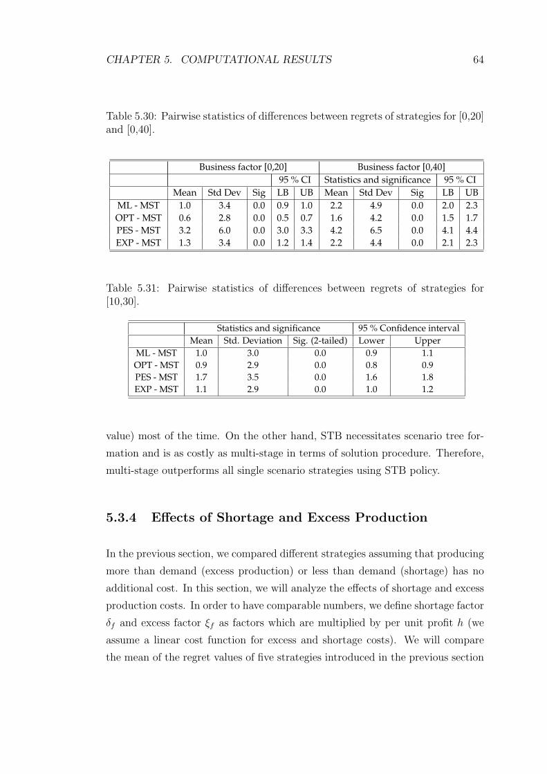
CHAPTER 5. COMPUTATIONAL RESULTS 64
Table 5.30: Pairwise statistics of differences between regrets of strategies for [0,20]and [0,40].
Business factor [0,20] Business factor [0,40]95 % CI Statistics and significance 95 % CI
Mean Std Dev Sig LB UB Mean Std Dev Sig LB UBML - MST 1.0 3.4 0.0 0.9 1.0 2.2 4.9 0.0 2.0 2.3OPT - MST 0.6 2.8 0.0 0.5 0.7 1.6 4.2 0.0 1.5 1.7PES - MST 3.2 6.0 0.0 3.0 3.3 4.2 6.5 0.0 4.1 4.4EXP - MST 1.3 3.4 0.0 1.2 1.4 2.2 4.4 0.0 2.1 2.3
Table 5.31: Pairwise statistics of differences between regrets of strategies for[10,30].
Statistics and significance 95 % Confidence intervalMean Std. Deviation Sig. (2-tailed) Lower Upper
ML - MST 1.0 3.0 0.0 0.9 1.1OPT - MST 0.9 2.9 0.0 0.8 0.9PES - MST 1.7 3.5 0.0 1.6 1.8EXP - MST 1.1 2.9 0.0 1.0 1.2
value) most of the time. On the other hand, STB necessitates scenario tree for-
mation and is as costly as multi-stage in terms of solution procedure. Therefore,
multi-stage outperforms all single scenario strategies using STB policy.
5.3.4 Effects of Shortage and Excess Production
In the previous section, we compared different strategies assuming that producing
more than demand (excess production) or less than demand (shortage) has no
additional cost. In this section, we will analyze the effects of shortage and excess
production costs. In order to have comparable numbers, we define shortage factor
δf and excess factor ξf as factors which are multiplied by per unit profit h (we
assume a linear cost function for excess and shortage costs). We will compare
the mean of the regret values of five strategies introduced in the previous section
CHAPTER 5. COMPUTATIONAL RESULTS 65
for different shortage and excess factor values. We considered each factor ranging
from 0 to 2 meaning that shortage and excess costs range from 0 to 2 ·h which is
a reasonably big range because we expect these costs to be less than h and more
than 0 in practice.
If we consider ξf and δf as exogenous variables, we have a three dimensional
profit function. Figures 5.2, 5.3, and 5.4 display three cross-sections from this
three dimensional profit function of all strategies with all possible policies. The
lines of each policy has a different style to distinguish between strategies. As
the graphs suggest, multi-stage solution is always better than other strategies
regardless of the values of excess and shortage factors. The closest strategy is the
optimistic strategy using the STB policy.
Figure 5.2 displays the cross section of mean regret values of strategy - policy
combinations and multi-stage when excess cost is fixed. As the graph in Figure
5.2 displays, increase in shortage factor increases the regret value of multi-stage.
However, the relative differences increase since the regret of other strategies grow
faster than multi-stage.
Figure 5.3 displays the cross section of mean regret values of strategy - policy
combinations and multi-stage when shortage cost is fixed. PES policy utiliz-
ing TPF policy could not be displayed in the graph since it is way out of scale
(Around 100%). As the graph in Figure 5.3 suggests, when cost of excess produc-
tion increases, single scenario strategies suffer significantly while the multi-stage
solution is not affected as much. This indicates that multi-stage solution incurs
less shortage or excess although it does not directly consider such an objective.
Another intriguing result is that optimistic strategy suffers significantly from the
increase of excess cost when 1PF and TPF policies are utilized whereas the effect
decreases evidently when it utilizes STB policy. This shows that the flexibility
that STB policy provides decreases the excess production significantly.
Figure 5.4 displays the cross-section where the shortage and excess factors
are equal. Some strategy - policy combinations exceed 100% regret (their profit
drops to negative) and becomes out of scale. As the graph in Figure 5.4 suggests,
when shortage and excess costs equally increase, the relative difference between
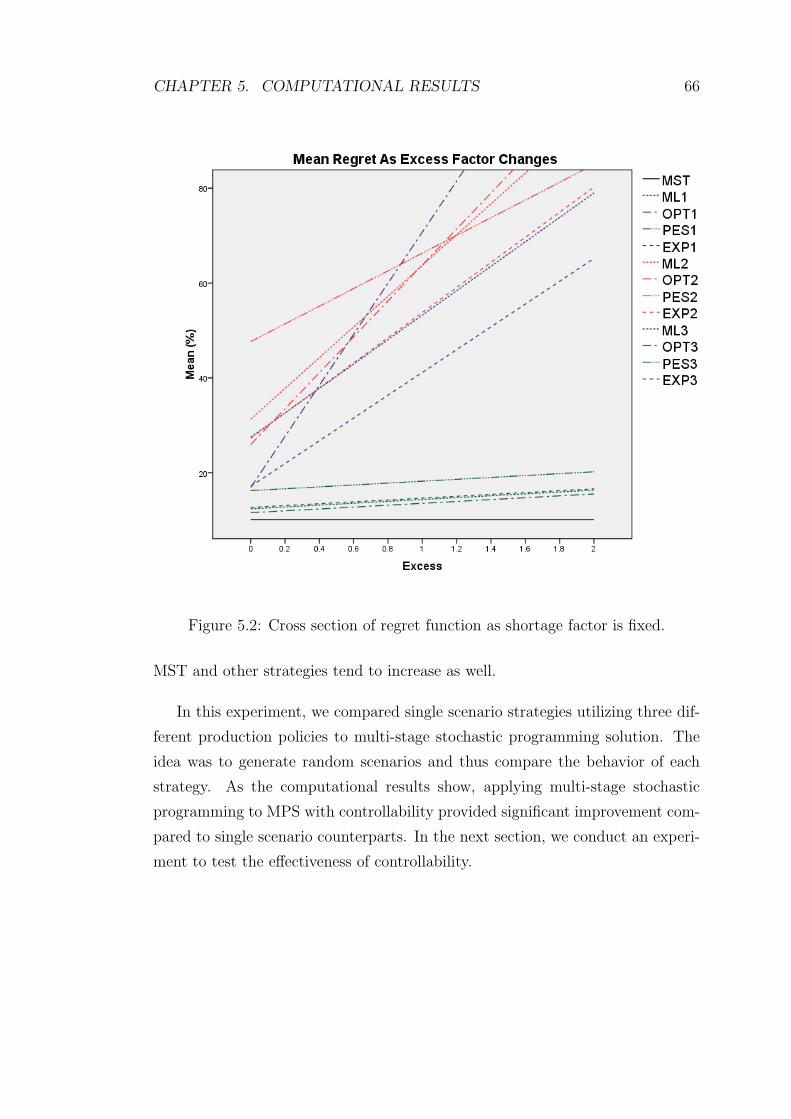
CHAPTER 5. COMPUTATIONAL RESULTS 66
Figure 5.2: Cross section of regret function as shortage factor is fixed.
MST and other strategies tend to increase as well.
In this experiment, we compared single scenario strategies utilizing three dif-
ferent production policies to multi-stage stochastic programming solution. The
idea was to generate random scenarios and thus compare the behavior of each
strategy. As the computational results show, applying multi-stage stochastic
programming to MPS with controllability provided significant improvement com-
pared to single scenario counterparts. In the next section, we conduct an experi-
ment to test the effectiveness of controllability.
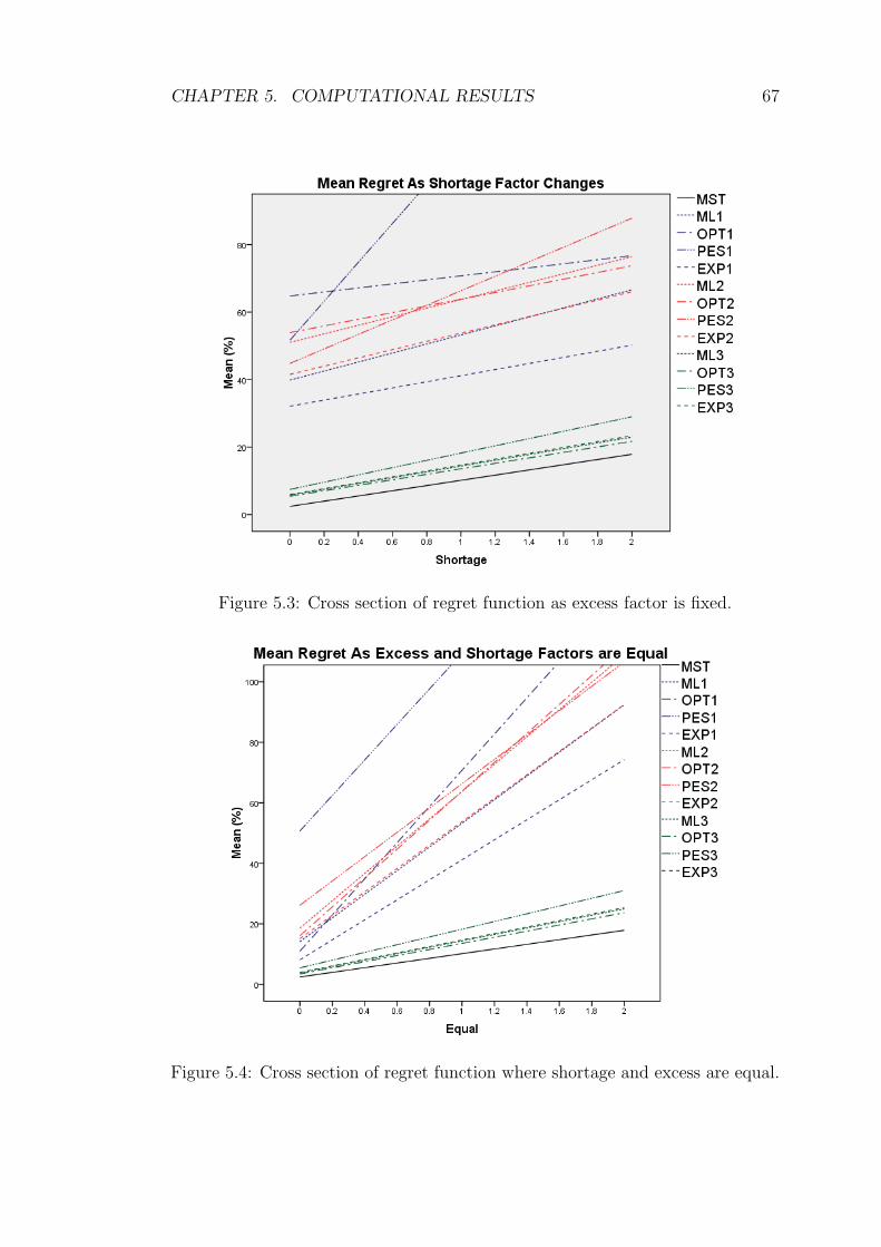
CHAPTER 5. COMPUTATIONAL RESULTS 67
Figure 5.3: Cross section of regret function as excess factor is fixed.
Figure 5.4: Cross section of regret function where shortage and excess are equal.
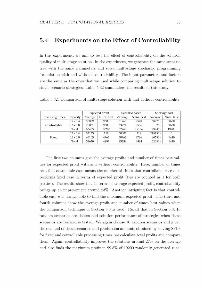
CHAPTER 5. COMPUTATIONAL RESULTS 68
5.4 Experiments on the Effect of Controllability
In this experiment, we aim to test the effect of controllability on the solution
quality of multi-stage solution. In the experiment, we generate the same scenario
tree with the same parameters and solve multi-stage stochastic programming
formulation with and without controllability. The input parameters and factors
are the same as the ones that we used while comparing multi-stage solution to
single scenario strategies. Table 5.32 summarizes the results of this study.
Table 5.32: Comparison of multi stage solution with and without controllability.
Expected profit Scenario based Shortage costProcessing times Capacity Average Num. best Average Num. best Average Num. best
0.2 - 0.4 56869 9600 51765 9578 5847δf 9600Controllable 0.6 - 0.8 70061 9600 63771 9586 2δf 9600
Total 63465 19200 57768 19164 2924δf 192000.2 - 0.4 37135 118 30002 118 27878δf 0
Fixed 0.6 - 0.8 66105 4766 60766 4766 2658δf 1440Total 51620 4884 45384 4884 15268δf 1440
The first two columns give the average profits and number of times best val-
ues for expected profit with and without controllability. Here, number of times
best for controllable case means the number of times that controllable case out-
performs fixed case in terms of expected profit (ties are counted as 1 for both
parties). The results show that in terms of average expected profit, controllability
brings up an improvement around 23%. Another intriguing fact is that control-
lable case was always able to find the maximum expected profit. The third and
fourth columns show the average profit and number of times best values when
the comparison technique of Section 5.3 is used. Recall that in Section 5.3, 10
random scenarios are chosen and solution performance of strategies when these
scenarios are realized is tested. We again choose 10 random scenarios and given
the demand of these scenarios and production amounts obtained by solving SFL3
for fixed and controllable processing times, we calculate total profits and compare
them. Again, controllability improves the solutions around 27% on the average
and also finds the maximum profit in 99.8% of 19200 randomly generated runs.
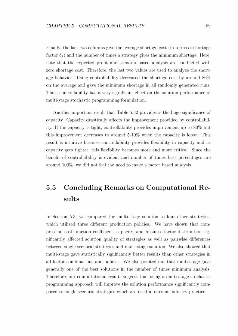
CHAPTER 5. COMPUTATIONAL RESULTS 69
Finally, the last two columns give the average shortage cost (in terms of shortage
factor δf ) and the number of times a strategy gives the minimum shortage. Here,
note that the expected profit and scenario based analysis are conducted with
zero shortage cost. Therefore, the last two values are used to analyze the short-
age behavior. Using controllability decreased the shortage cost by around 80%
on the average and gave the minimum shortage in all randomly generated runs.
Thus, controllability has a very significant effect on the solution performance of
multi-stage stochastic programming formulation.
Another important result that Table 5.32 provides is the huge significance of
capacity. Capacity drastically affects the improvement provided by controllabil-
ity. If the capacity is tight, controllability provides improvement up to 80% but
this improvement decreases to around 5-10% when the capacity is loose. This
result is intuitive because controllability provides flexibility in capacity and as
capacity gets tighter, this flexibility becomes more and more critical. Since the
benefit of controllability is evident and number of times best percentages are
around 100%, we did not feel the need to make a factor based analysis.
5.5 Concluding Remarks on Computational Re-
sults
In Section 5.3, we compared the multi-stage solution to four other strategies,
which utilized three different production policies. We have shown that com-
pression cost function coefficient, capacity, and business factor distribution sig-
nificantly affected solution quality of strategies as well as pairwise differences
between single scenario strategies and multi-stage solution. We also showed that
multi-stage gave statistically significantly better results than other strategies in
all factor combinations and policies. We also pointed out that multi-stage gave
generally one of the best solutions in the number of times minimum analysis.
Therefore, our computational results suggest that using a multi-stage stochastic
programming approach will improve the solution performance significantly com-
pared to single scenario strategies which are used in current industry practice.
CHAPTER 5. COMPUTATIONAL RESULTS 70
In Section 5.4, we tested the effect of controllability on the profit performance
of multi-stage. The computational results showed that controllability provided
a huge improvement which was evident due to three different criteria: Expected
profit, expected profit performance when the comparison technique of Section 5.3
is utilized and finally shortage values. Also, capacity is found to be a signifi-
cant factor which critically affects the improvement that controllability provided.
Therefore, our computational results suggest that utilizing finite capacity and
controllability will significantly improve solution performances especially in envi-
ronments with tight capacity.
In Section 5.2, we tested the performance of our formulations and one of the
formulations named SFL3 proved very efficient in terms of CPU performance.
We exploited this fact during our experiments in Sections 5.3 and 5.4 taking
approximately 250,000 runs in the experiment of Section 5.3 and 40,000 runs in
the experiment of Section 5.4. To have a small illustration of the importance of
this result, suppose that the formulation took 4 minutes (which is a considerably
small number) on the average instead of 1 seconds. Then, 290,000 runs would
take 2 years 2 months. On the other hand, it takes only around 3 days to have
that number of runs using SFL3.
The results obtained in Sections 5.3 and 5.4 suggest that using a capacitated
version of MPS with controllability and considering several scenarios for demand
realization provides drastic improvements in the solution performance of MPS.
Moreover, the fact that SFL3 solves even large instances in a few seconds opens
up limitless application possibilities of our approach such as establishing it in
ERP software or conducting what if and sensitivity analysis. It is also possible
to extend the analysis that we made in the computational study by adding new
factors or considering new strategies and policies, even firm based strategies and
policies.
Chapter 6
Conclusion
In this chapter, we first summarize this thesis and explain our contribution. Then,
we state possible further research directions.
6.1 Summary
In this thesis, we have questioned three critical assumptions of master production
scheduling which are infinite capacity, fixed processing times and fixed known
demand. In Chapter 2, we gave the problem definition and a review of the
related literature. In Chapter 3, we proposed formulations and related results. In
Chapter 4, we analyzed some easy cases and made complexity analysis. Finally,
in Chapter 5, we conducted and analyzed three computational studies.
In Chapter 3, we first proposed a non-linear mixed integer programming for-
mulation using the multi-stage stochastic programming approach assuming that
the objective function is given. After that, we proposed a linearized version of the
problem. Then, we analyzed two sub-problems and proposed some results sug-
gesting the structure of the objective function of the main formulation, optimal
compression amounts, and introduced threshold value. Finally, we proposed an
alternative linearized version of the main formulation making use of our previous
71
CHAPTER 6. CONCLUSION 72
results.
In Chapter 4, we first proposed some sufficient conditions for optimality that
can be used to solve problems with specific structure immediately. Afterwards,
we introduced two special cases, the deterministic version and the version with
no postponement cost, proved that these special cases are polynomially solvable.
Then, we had a negative result: The technique that we used to prove the poly-
nomiality of the easy cases is not applicable to the main formulation.
In Chapter 5, we performed three different experiments. In the first one, we
tested CPU performances of SFL1 and SFL3. We observed that SFL3 proved
very efficient solving large instances in only a few seconds. Then, we compared
multi-stage solution to single scenario strategies that utilize different production
policies and showed that using a multi-stage stochastic programming approach
provided statistically significant improvement in relative regret values. We also
showed that the dominance of multi-stage solution did not decrease even when
we introduce shortage and excess costs. Finally, in the third experiment, we have
shown that controllability significantly improved the performance of multi-stage
solution.
6.2 Contribution
In the current industry, MPS assumes finite capacity, fixed processing times and
known demand realizations. In this thesis, we questioned these assumptions and
came up with a model with finite capacity, controllable processing times and
finally and most importantly uncertain demand values. We used multi-stage
stochastic programming to handle this uncertainty and proposed a very effective
formulation which solves large instances in a very short time. The fact that the
formulation solves considerably large instances at a maximum of four seconds,
enabled us to conduct an extensive computational study. Our computational
results showed that using multi-stage stochastic programming instead of single
CHAPTER 6. CONCLUSION 73
scenario strategies significantly improved the solution quality when a random sce-
nario (generally different than the estimated one by the single scenario strategy)
is realized. Moreover, using controllability provided improvements up to 80% in
total profit gained. Finally, capacity was very effective on solution performances
of both single scenario strategies and multi-stage. Therefore, our computational
results suggest that changing these three unrealistic assumptions of MPS provides
huge improvement with a very little computational cost. The efficiency of our
formulation enables further analysis with various different factors, strategies and
policies. Moreover, it provides the time flexibility to conduct sensitivity and what
if analysis. Being aware of the severe limitations of the MPS algorithms in the
current ERP software, firms are making significant investments in new advanced
planning and scheduling (APS) software. Unfortunately, these new APS systems
rely on relatively simple heuristic methods (such as capable-to-promise, etc.) to
solve the MPS problems. Our computational results clearly indicate that MPS
problems could be solved to optimality using multi-stage stochastic programming
approach in a very short computation time.
6.3 Future Research Directions
In this thesis, we have proposed a new MPS approach which uses controllable
processing times, finite capacity, and multi-stage stochastic programming to han-
dle several scenarios instead of a single demand forecast. We considered a single
work center and a single product type. Two direct extensions of this problem
are considering multiple work centers or parallel machines along with multiple
product types. This would of course require extensive work on solution proce-
dures since the formulations on this paper cannot be directly applied to multiple
product case.
Although the formulation that we proposed works very efficiently, the com-
plexity of the stochastic problem with postponement cost is still open. Thus, as a
future research, the complexity of the problem can be studied. The fact that the
LP relaxation of SFL3 always gave integer results though its constraint matrix is
CHAPTER 6. CONCLUSION 74
not totally unimodular makes this problem more interesting.
Controllability and multi-stage stochastic programming proved very useful in
MPS according to our computational results. Therefore, a possible future research
direction would be to apply these to ATP problems which have similar objectives
as the problem that we considered in this thesis.
In this problem, we did not give any specific value to shortage or excess costs.
We also did not allow holding inventory in our solution method as the problem
environments that we consider generally work with zero inventory policies. A
possible future research direction would be to apply this problem into different
industries by considering these costs while formulating the problem.
While studying MPS, we assumed that each period is a frozen zone. There-
fore, we did not question issues such as the length of frozen zones and freezing
strategies. The related literature on MPS on the other hand focuses on frozen
zones. As a future direction, the length of the frozen zone can also be considered
along with controllability and stochastic programming. Therefore, it would be
interesting to question freezing on the MPS that we proposed with finite capacity,
controllability, and multi-stage solution procedure.
Bibliography
[1] S. Ahmed and N. V. Sahinidis. Approximation scheme for stochastic integer
programs arising in capacity expansion. Operations Research, 51(3):461–471,
2003.
[2] S. Ahmed, A. J. King, and P. Gyana. A multi-stage stochastic integer pro-
gramming approach for capacity expansion under uncertainty. Journal of
Global Optimization, 26(1):3–24, 2003.
[3] M.S. Akturk, A. Atamturk, and S. Gurel. Parallel machine match-up
scheduling with manufacturing cost considerations. Journal of Scheduling.
to appear.
[4] M.S. Akturk, A. Atamturk, and S. Gurel. A strong conic quadratic re-
formulation for machine-job assignment with controllable processing times.
Operations Research Letters, 37:187 – 191, 2009.
[5] A. Atamturk and M. Zhang. Two-stage robust network flow and design
under demand uncertainty. Operations Research, 55:662–673, 2007.
[6] A. Ben-Tal and A. Nemirovski. Robust solutions of linear programming
problems contaminated with uncertain data. Mathematical Programming,
88:411–424, 2000.
[7] A. Ben-Tal, A. Goryashko, E. Guslitzer, and A. Nemirovski. Adjustable
robust solutions of uncertain linear programs. Mathematical Programming,
99:351–376, 2004.
[8] D. Bertsimas and M. Sim. The price of robustness. Operations Research, 52:
35–53, 2004.
75
BIBLIOGRAPHY 76
[9] J. R. Birge and J. Louveaux. Introduction to Stochastic Programming.
Springer, 1997.
[10] G. B. Dantzig and G. Infanger. Multi-stage stochastic linear programs for
portfolio optimization. Annals of Operations Research, 45:59–76, 1993.
[11] M. Dyer and S. Leen. Computational complexity of stochastic programming
problems. Mathematical Programming, 106:423–432, 2006.
[12] S. Engell, A Markert, G. Sand, and R. Schultz. Aggregated scheduling of
a multiproduct batch plant by two-stage stochastic integer programming.
Optimization and Engineering, 5:335–359, 2004.
[13] G. Eppen, R. Martin, and L. Schrage. A scenario approach to capacity
planning. Operations Research, 37(4):517 – 527, 1989.
[14] L.F. Escudero, P.V. Kamesam, A.J. King, and R. J-B. Wets. Production
planning via scenario modeling. Annals of Operations Research, 43:311 –
335, 1993.
[15] J. M. Framinan and R. Leisten. Available-to-promise (ATP) systems: a clas-
sification and framework for analysis. International Journal of Production
Research. to appear.
[16] D.R. Fulkerson and O.A. Gross. Incidence matrices and interval graphs.
Pasific Journal of Mathematics, 15(3):835–865, 1965.
[17] Y. Guan, S. Ahmed, G. L. Nemhauser, and A. J. Miller. A branch-and-cut
algorithm for the stochastic uncapacitated lot-sizing problem. Mathematical
Programming, 105(1):55–84, 2006.
[18] S. Gurel and M.S. Akturk. Optimal allocation and processing time decisions
on non-identical parallel CNC machines: ε-constraint approach. European
Journal of Operational Research, 183:591–607, 2007.
[19] R. Hemmecke, S. Onn, and R. Weismantel. A polynomial oracle-time al-
gorithm for convex integer minimization. Mathematical Programming. to
appear.
BIBLIOGRAPHY 77
[20] D. S. Hochbaum and J. G. Shantikumar. Convex optimization is not much
harder than linear optimization. Journal of the Association for Computing
Machinery, 37(4):843–862, 1990.
[21] S Karabuk. Production planning under uncertainty in textile manufacturing.
Journal of the Operations Research Society, 59:510–520, 2008.
[22] S. Karabuk and S. D. Wu. Coordinating strategic capacity planning in the
semiconductor industry. Operations Research, 51(6):839 – 849, 2003.
[23] R.K. Kayan and M.S. Akturk. A new bounding mechanism for the CNC
machine scheduling problems with controllable processing times. European
Journal of Operational Research, 167:624–643, 2005.
[24] P. Kouvelis and G. Yu. Robust Discrete Optimization and Its applications.
Kluwer Academic Publishers, 1997.
[25] G Lulli and S. Sen. A branch-and-price algorithm for multistage stochastic
integer programming with application to stochastic batch-sizing problems.
Management Science, 50(6):786–796, 2004.
[26] A. Maatman, C. Schweigman, A. Ruijs, and M. H. van der Vlerk. Mod-
eling farmers response to uncertain rainfall in burkina faso: A stochastic
programming approach. Operations Research, 50(3):399 – 414, 2002.
[27] E. Nowicki and S. Zdrzalka. A survey of results for sequencing problems
with controllable processing times. Discrete Applied Mathematics, 26:271–
287, 1990.
[28] M. V. F. Pereira and L. M. V. G. Pinto. Multi-stage stochastic optimization
applied to energy planning. Mathematical Programming, 52:359–375, 1991.
[29] R. Schultz, L. Stougie, and M. H. Vlerk. Two-stage stochastic integer pro-
gramming: A survey. Statistica Neerlandica, 50:404–416, 1996.
[30] D. Shabtay and G. Steiner. A survey of scheduling with controllable pro-
cessing times. Discrete Applied Mathematics, 155(13):1643–1666, 2007.
BIBLIOGRAPHY 78
[31] D. B. Shmoys and M. Sozio. Approximation algorithms for 2-stage stochastic
scheduling problems. In Integer Programming and Combinatorial Optimiza-
tion. Springer Berlin / Heidelberg, 2007.
[32] V. Sridharan, William L. Barry, and V. Udayabhanu. Measuring master pro-
duction schedule stability under rolling planning horizons. Decision Sciences,
19(1):147–166, 1986.
[33] V. Sridharan, William L. Barry, and V. Udayabhanu. Freezing the master
production schedule under rolling planning horizons. Management Science,
33(9):1137–1149, 1987.
[34] O. Tang and R. W. Grubbstrom. Planning and replanning the master pro-
duction schedule under demand uncertainty. International Journal of Pro-
duction Economics, 78:323–334, 2002.
[35] L. A. Wolsey. Integer Programming. Wiley-Interscience, 1998.
Appendix A
Nomenclature
Decision Variables:
yj = Amount of production in j, j ∈ N ,
xij = Amount of demand of j that is processed in i, i ∈ N , j ∈ Bi,
zj = Amount of demand of j that will be satisfied, j ∈ N .
cj = the compression amount of job j in {1, ..., n}wij = if k jobs are produced in i and 0 otherwise i ∈ N, k ∈ {0, 1, ..., kmax}vij = if at least k jobs are produced in i and 0 otherwise i ∈ N, k ∈ {1, ..., τ}
Parameters:
T : The number of periods in the planning horizon.
N : The set of nodes of the scenario tree.
Nt : The set of nodes of period t = 1, 2, ..., T .
di : The anticipated demand at node i in N .
d : The total demand (∑
i∈N di).
γi : The probability of realization of node i (γ1 = 1).
Di : The set of descendants of node i and node i.
Bi : The set of predecessors of node i and node i.
B1i : The immediate predecessor of node i.
79
APPENDIX A. NOMENCLATURE 80
Pij : The set of nodes on the path from i ∈ N to j in Di.
si : The period of node i.
h : Per unit profit excluding compression and backlogging costs.
p : The processing time of a job with minimum compression cost.
u : Maximum compressibility of a job.
C : The time capacity of a period (and a node).
kmin : The maximum production without compression (⌊Cp
⌋).
kmax : Production capacity in terms of number (⌊
Cp−u
⌋).
τ : The threshold value.
ξf : Excess cost scaling factor.
δf : Shortage cost scaling factor.
ζ : Capacity scaling factor.
β : Postponement cost scaling factor.
κ : Compression cost coefficient.
a/b : Compression cost exponent.
f(y) : Comression cost function (f(y) = κ · ya/b a, b ∈ Z+ : a > b > 0, κ > 0.)
b(∆) : Cost of postponing a job for ∆ periods.
I : Per unit per period inventory holding cost.
ξ : Per unit excess production cost.
δ : Per unit shortage cost.
Φ(n) : Total compression cost at a node with n jobs.
Π(n) : h · n− Φ(n)
ysi : The production of strategy s at period i.
osi : The order of leaf node i according to strategy s.
drt : The demand of period t at the realized scenario r.
APPENDIX A. NOMENCLATURE 81
Abbreviations
MPS : Master Production Scheduling.
ERP : Enterprise Resource Planning.
R : Relative Regret.
SF : The main non-linear mixed integer programming formulation.
SFL1 : The first linearization of SF using wik variables.
SFL2 : The second linearization of SF using vik variables.
SFL3 : SFL2 without contraint 3.4.1, the formulation used in the experiments.
SF2 : The formulation of stochastic case without postponement cost.
DF : The formulation of the deterministic case.
TPF : T periods frozen solution policy.
1PF : One period frozen myopic adjustment policy.
STB : One period frozen scenario tree based demand selection policy.
ML : The most likely scenario strategy.
OPT : The most optimistic scenario strategy.
PES : The most pessimistic scenario strategy.
EXP : The rounded version of expected demand of each period strategy.
MST : Multi-stage stochastic programming solution strategy.
Experimental Factors
A : Compression cost exponent a/b.
B : Capacity scaling factor ζ.
C : Postponement cost scaling factor β.
D : Probability type, (either normally distributed or equal node probabilities).
E : Business factor which determines the distribution of number of jobs
F : Node factor which determines the number of immediate descendants of nodes.
G : Inventory holding cost / postponement cost ratio.
VITA
Ersin Korpeoglu was born on February 13, 1985 in Bolu, Turkey. He attended
middle school and high school in Ankara Ataturk Anadolu Lisesi and graduated
in 2003 summa cum laude. He graduated from Bilkent University Industrial
Engineering Department cum laude in 2007. In 2007, he attended Industrial
Engineering Department of Bilkent University as a Research Assistant. Since
then, he has been working with Prof. M. Selim Akturk on his graduate study.
He had been on the grant 2210 awarded by TUBITAK during his M.S. study.
82