master production scheduling system under a gt cell
TRANSCRIPT

Retrospective Theses and Dissertations Iowa State University Capstones, Theses andDissertations
1984
Master production scheduling system under a GTcellSeung-Ryeol KimIowa State University
Follow this and additional works at: https://lib.dr.iastate.edu/rtd
Part of the Industrial Engineering Commons
This Dissertation is brought to you for free and open access by the Iowa State University Capstones, Theses and Dissertations at Iowa State UniversityDigital Repository. It has been accepted for inclusion in Retrospective Theses and Dissertations by an authorized administrator of Iowa State UniversityDigital Repository. For more information, please contact [email protected].
Recommended CitationKim, Seung-Ryeol, "Master production scheduling system under a GT cell " (1984). Retrospective Theses and Dissertations. 9000.https://lib.dr.iastate.edu/rtd/9000

INFORMATION TO USERS
This reproduction was made from a copy of a document sent to us for microfilming. While the most advanced technology has been used to photograph and reproduce this document, the quality of the reproduction is heavily dependent upon the quality of the material submitted.
The following explanation of techniques is provided to help clarify markings or notations which may appear on this reproduction.
1. The sign or "target" for pages apparently lacking from the document photographed is "Missing Page(s)". If it was possible to obtain the missing page(s) or section, they are spliced into the film along with adjacent pages. This may have necessitated cutting through an image and duplicating adjacent pages to assure complete continuity.
2. When an image on the film is obliterated with a round black mark, it is an indication of either blurred copy because of movement during exposure, duplicate copy, or copyrighted materials that should not have been filmed. For blurred pages, a good image of the page can be found in the adjacent frame. If copyrighted materials were deleted, a target note will appear listing the pages in the adjacent frame.
3. When a map, drawing or chart, etc., is part of the material being photographed, a definite method of "sectioning" the material has been followed. It is customary to begin filming at the upper left hand comer of a large sheet and to continue from left to right in equal sections with small overlaps. If necessary, sectioning is continued again—beginning below the first row and continuing on until complete.
4. For illustrations that cannot be satisfactorily reproduced by xerographic means, photographic prints can be purchased at additional cost and inserted into your xerographic copy. These prints are available upon request from the Dissertations Customer Services Department.
5. Some pages in any document may have indistinct print. In all cases the best available copy has been filmed.
UniversiV MicrOTims
International 300 N. Zeeb Road Ann Arbor, Ml 48106


8423645
Kim, Seung-Ryeol
MASTER PRODUCTION SCHEDULING SYSTEM UNDER A GT CELL
Iowa State University PH.D. 1984
University IVIicrofilms
I ntern&tionsl SOO N. zeeb Road, Ann Arbor, Ml 48106
Copyright 1984
by
Kim, Seung-Ryeol
All Rights Reserved


Master production scheduling system
under a GT cell
by
Seung-Ryeol Kim
A Dissertation Submitted to the
Graduate Faculty in Partial Fulfillment of the
Requirements for the Degree of
DOCTOR OF PHILOSOPHY
Department: Industrial Engineering
Major: Engineering Valuation
For the Graduate College
Iowa State University •Ames, Iowa
1984
Copyright (c) Seung-Ryeol Kim, 1984. All rights reserved.
Members of the Committee
Charge of^ajor Work
Signature was redacted for privacy.
Signature was redacted for privacy.
Signature was redacted for privacy.
Signature was redacted for privacy.

(c)1984 Seung-Ryeol Kim
All Rights Reserved

ii
TABLE OF CONTENTS
PAGE
CHAPTER 1. INTRODUCTION 1
Preface . 1
Background 3 Production planning process 3
A formal planning system 3 Aggregate production plan 5 Master production schedule 6 Rough Cut Capacity Plan (RCCP) 9
MRP and GT 10 MRP 10 Group technology 12 A GT based MRP system 12
Need for the Study 14
Research Scope and Objectives 17 Research objectives 18
Uniqueness of the MPS under a GT Based MRP System . . 20
CHAPTER 2. LITERATURE REVIEW 22
Aggregate Production Plan 22
Master Production Schedule 25 Classification 25 Special topics 27 Interface with other functions 29
GT Based MRP System 29
Capacitated Lot Sizing for Multi-Items 30
Evaluation Method of the Heuristic Solution 31
Summary 33
CHAPTER 3. PROBLEM DEFINITION 35
Characteristics and Assumptions 35
Aggregate Production Plan 38
Master Production Schedule ,42

iii
CHAPTER 4. THE APPROACHES 47
Preliminary Work 47 Input data 47 Load profile 50
Aggregate Production Plan 52
Heuristics to Develop a TMPS 54 Method A: period-by-period method 56 Method B: shortest path method 61 Method C: tree search method 52
Sampling procedure 55 Tree search method 57
Characteristics of the Methods 68
CHAPTER 5, EXPERIMENTAL TEST 72
Aggregate Production Plan 72 Illustrative example 72 Discussion of the model 74
Master Production Schedule .......; 77 Test problem generation 77 Evaluation measure 86 Discussion of the experimental tests 88
CHAPTER 6. SUMMARY AND CONCLUSION 98
BIBLIOGRAPHY 108
ACKNOWLEDGEMENTS 118
APPENDIX A: AGGREGATE PRODUCTION PLANNING SUBSYSTEM . 119
Program List 119
Input of MPSX 120
APPENDIX B: MASTER PRODUCTION SCHEDULING SUBSYSTEM . . 123
System Flow of Experimental Test 123
Program list 124 Method A 124 Method B 141 Method C 153 Solution standard 165

iv
APPENDIX C: SHORTEST PATH ALGORITHM

LIST OF TABLES
PAGE
TABLE 1. I/O and managerial variables for APP .... 7
TABLE 2. The method to determine a production requirement 19
TABLE 3. Contrasts of the research with other works . 36
TABLE 4. Input data summary 49
TABLE 5. Demand requirements for APP problem .... 72
TABLE 6. Weighting factors of each goal 73
TABLE 7. Values of cost parameters 73
TABLE 8. Production plan 74
TABLE 9. Required and planned load 75
TABLE 10. Budgeted and planned expenditure 75
TABLE 11. A pool of all test items 79
TABLE 12. Two cases of average demand for small size problem 80
TABLE 13. Two cases of demand pattern for small size problem 80
TABLE 14. Summary of test data 31
TABLE 15. Cost structure 84
TABLE 16. Setup cost summary 85
TABLE 17. S/H summary 85
TABLE 18. R for constant and seasonal demand patterns 90
TABLE 19. Summary of evaluation measures 91

vi
TABLE 20. Distribution of evaluation measures 92
TABLE 21. Evaluation measures by cost structure .... 93
TABLE 22. Characteristics of solution standard (Frequency) 94
TABLE 23. Characteristics of solution standard (Ratio) 95
TABLE 24. A Wilcoxon's signed-rank test for cost factors 96
vii
LIST OF FIGURES
PAGE
FIGURE 1. A formal planning system 4
FIGURE 2. A system flow for load profile 51
FIGURE 3. Flow diagram of Method A 58
FIGURE 4. A shortest path representation of a MPS . 63
FIGURE 5. Flow diagram of Method B 64
FIGURE 6. Tree search method 59
FIGURE 7. Flow diagram of Method C 70
FIGURE 8. Experimental procedure 89

1
CHAPTER 1. INTRODUCTION
Preface
A production system operates most effectively when the
input and the output of the production system flow smoothly.
But there are frequently overstocks or shortages in the
inventory and unbalanced loads in the shop flow. Therefore,
a system plan must consider the variation in the product
quantity, place, and time. A planning system should be
carefully designed to improve the efficiency of the total
production system.
The following points indicate that the importance of
the Master Production Schedule (MPS) is increasing.
1. In the hierarchy of production planning
processes, the MPS should be the basis of all
operational level schedules. Therefore, the
impact of the MPS on the efficiency of the total
production system is tremendous.
2. Material Requirement Planning (MRP), where the
MPS is the primary input, is replacing the
traditional ordering point system in the
requirement planning of materials.
3. The MPS is frequently used as an essential part
to observe an overall effectiveness for the
organization in the decision making of strategic

2
level which is the final phase of development of
management information systems.
Group technology (GT) has the promise of meeting the
following challenges in modern manufacturing (19).
1. 75% of manufactured parts will be small lot sizes
in coming years. This compares with 25% to 35%
now.
2. Customized products require special options and
are composed of components with high reliability
and closer tolerances.
3. The need to integrate the activities of design
and manufacturing is increasing.
This research is to propose an aggregate production
planning model and methodologies deriving a Tentative Master
Production Schedule (TMPS) for a GT cell where MRP is the
production planning and control system. Since the MPS
interacts with several functions in the planning system,
this research deals with planning subsystems including the
Aggregate Production Plan (APP) and MPS. A production plan
presents a general outline of the manufacturing activity
during the planning horizon. This outline should agree with
the objective of the work force, the production capacity,
and the customer service level in the aggregate level. The
APP has been developed for this purpose. The MPS is derived
from the production plan or all demand sources while

3
minimizing the total production cost.
The objective of the research is to find a more formal,
responsible method to develop a TMPS which would have the
ability to plan the future work load under the available and
the authorized capacity limits.
Background
Production planning process
A formal planning system In the hierarchy of the
production planning processes, the MPS is the basis for the
lower level plans such as the material and the capacity
requirement plan. It is constrained by higher level plans
such as the marketing plan and the production plan. Robert
McCormick (41) described a formal planning system (Figure
1). He pointed out that the MPS is the planning keystone
for a manufacturing company utilizing a formal planning and
execution system.
The business plan is the long-term objective of the
business and the guideline for the marketing plan, the
production plan, and the resource allocation plan for the
mid-term period. The marketing plan is developed to meet
the income level of the business and the existing and
potential customer demand. The production capacity works as
a constraint for this marketing plan. The production plan
is the time phased statement of the production rate, and it

4
I Business Plan |
Marketing I Production I Resource
Plan Plan Plan
Rough Master
Production Cut
Schedule Capacity
Plan
Material/
Capacity
Plan
I Execution System
FIGURE 1. A formal planning system
defines the boundary for the future production process. The
resource plan functions for all key resources in the company
during the production planning horizon. Resources range
from drafting-room personnel to cash to capital equipment

5
and plant square footage (47). The resource plan is
prepared to follow up the production plan.
If the MPS is feasible, the material/capacity
requirement planning is derived to expedite the MPS. If the
material or the capacity cannot be prepared on time, the MPS
may be changed. An MRP method can be used for the
requirement planning of the material. A load profile which
is derived from the Bill of Material (BOM) and the routing
file are the bases for the Rough Cut Capacity Plan (RCCP).
This research is concerned with the Production Plan and
the MPS, which will be respectively described in the
following sections. The MPS is derived from the production
plan and is evaluated by the RCCP which calculates the
impact of the MPS on the key resources. If there is no
production planning function, the MPS is derived from all
the demand sources.
Aggregate production plan The production plan may
be defined as the time phased statement of the production
rate required to meet the customer demand with the minimum
total cost. The production plan establishes the manpower
requirement, the equipment requirement, and the level of the
anticipated inventories. At this point, managers are
required to make many decisions such as smoothing the plant
production load, adjusting the capacity target and
coordinating with production support functions. The

6
production plan works interactively with the marketing
function, the manufacturing function and other supporting
functions such as the financing function and the material
procurement function.
When there are constraints in the company resources,
the production plan is not consistent with the customer
demand. Therefore, the company needs the production plan to
satisfy the fluctuating customer demand. This suggests that
the production plan ought to consider the sales volume, the
production volume, and the inventory level in the aggregate
level. A production plan is developed to minimize the total
production cost constituting the facility, the inventory,
the overload and delay penalty cost, etc. The APP has been
developed and used for this purpose.
This research considers the APP where the planning
horizon is from one month to one year. Buff a and Taubert
(5) described the inputs required, the nature of the plans
which are the outputs, and the variables which are under
managerial control for the aggregate plan (Table 1). This
research addresses the aggregate production planning problem
where there are conflicting, multiple objectives. The
production plan becomes not only the guideline but also the
constraint on the MPS.
Master production schedule An MPS, which may be
derived from the production plan, is the expected

7
TABLE 1. I/O and managerial variables for APP
1. Inputs: Forecasts of:
Amount and timing of sales
Costs
Supply
Policies and constraints on:
Overtime
Hiring and firing
Inventories
Capital
Long-range plans
2. Outputs: Aggregate plans and schedules for the use
of various sources of capacity
3. Variables under managerial control:
Size of work force
Production rate
Inventory
Subcontracting
manufacturing schedule for the major assemblies or the
shippable end items. There are several factors affecting
the development of the MPS such as the product level to be

8
scheduled, the planning horizon, and the time bucket. The
master scheduled items are identified by the part number in
the BOM. McCormick (41) gives some guidelines for the
product level to be scheduled in the BOM, He suggested that
the BOM level which minimizes the number of potential master
scheduled items should meet two criteria.
1. The master scheduled items must be forecastable
by marketing.
2. They must represent the bulk of the capacity
resources required to manufacture the shippable
end items.
The planning horizon of the MPS is larger than the lead
time of the master scheduled items. The lead time is
constituted of component manufacturing, subassembly and
final assembly, etc. Orlicky (47) stated that one week is
the suitable time bucket for a MPS, when MRP is implemented.
There are many variations of the MPS among companies.
However, the development procedure for the majority of the
MPSs can be stated in the following way.
1. The marketing plan and the production plan which
are at a higher level than the MPS are built up.
The marketing plan is developed by the customer
demand or the forecast. The production plan is
coordinated with the marketing plan.
2. A TMPS is derived from the production plan and
9
the marketing plan.
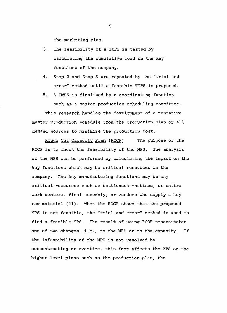
3. The feasibility of a TMPS is tested by
calculating the cumulative load on the key
functions of the company.
4. Step 2 and Step 3 are repeated by the "trial and
error" method until a feasible TMPS is proposed.
5. A TMPS is finalized by a coordinating function
such as a master production scheduling committee.
This research handles the development of a tentative
master production schedule from the production plan or all
demand sources to minimize the production cost.
Rough Cut Capacity Plan (RCCP) The purpose of the
RCCP is to check the feasibility of the MPS. The analysis
of the MPS can be performed by calculating the impact on the
key functions which may be critical resources in the
company. The key manufacturing functions may be any
critical resources such as bottleneck machines, or entire
work centers, final assembly, or vendors who supply a key
raw material (41). When the RCCP shows that the proposed
MPS is not feasible, the "trial and error" method is used to
find a feasible MPS. The result of using RCCP necessitates
one of two changes, i.e., to the MPS or to the capacity. If
the infeasibility of the MPS is not resolved by
subcontracting or overtime, this fact affects the MPS or the
higher level plans such as the production plan, the

10
marketing plan, and the resource plan.
The cumulative load which is derived by the proposed
TMPS is compared with the available capacity limit to
evaluate the feasibility of the proposed MPS. The load
profile is used instead of the BOM and the routing file to
calculate the time-phased cumulative load. The load profile
is the planning data representing the time-phased load on
each resource to produce one end item. The success of the
RCCP depends on the load profile which should be carefully
designed and prepared. The logic of the RCCP is just simple
calculation to get the cumulative load via the MPS and the
load profile. Therefore, the critical factor is the load
profile and not the logic of the RCCP.
MRP and GT
MRP The basic principle of MRP is that the quantity
and timing of the raw materials/components are determined by
the known or forecasted requirements for the end product.
Using MRP keeps the inventory balance at the minimum level
by supplying the raw materials/components just prior to the
date of need, and makes up for the drawbacks of the
traditional order point system where shortage and over-stock
occur by considering only the past requirements. Wight and
Plossl (59) pointed out that "the number of items in
inventory that can best be controlled by MRP outnumbers
those that can be controlled effectively by the order point

11
by about 100 to 1".
The advantages of MRP are well-known, but successful
implementation of an MRP system has not been easy. A great
many of MRP systems are still "order launching systems
coupled with computer aided dispatching and there have been
a number of failures" (56). One U.S. consultant has
commented that only about one in a hundred MRP systems might
be regarded as "successful" (45).
There may be many factors affecting the successful
implementation of an MRP system, but this low rate of
success does reflect the inherent problems of the MRP
system. Colin New (45) described the drawbacks of MRP:
1. Load input variability is significantly greater
than master schedule levels because of the random
initiation of orders and their phasing.
2. It is inevitable that component sets will not
"match" assembly requirements, because the lot
sizes are set in relation to the individual
component rather than to a production cycle.
This increases inventories and may cause
allocation problems when shortages occur.
3. Groups of components with the same setup
requirements will rarely be ordered at the same
time because of independent component batching.
Thus, the scope for setup savings is severely

12
limited.
All these problems are caused by the complex routings of
components and complex interactions among jobs based on the
functional layout.
Group technology A GT cell is the production cell
which is determined by the component similarity rather than
the machine similarity. The production cell is composed of
a small group of humans and machines which produce a
component set from the raw material. A coding and
classification scheme is used to classify similar components
and the product families.
A GT cell offers some distinct advantages compared to
the functional layout. Reduced throughput time, decreased
Work In Process (WIP) and finished goods inventory,
increased flexibility to handle forecast errors, and reduced
paperwork are some advantages mentioned by actual users
( 2 1 ) .
The components must be produced with the right quantity
at the right time to meet the final assembly. Correct
components should be produced on the scheduled time to get
the advantage of GT. This requires a production planning
and control system which is suitable for GT cells.
A GT based MRP system Several authors (21, 45, 56)
proposed that MRP can be used as a production planning and
inventory control system on a group layout producing small
13
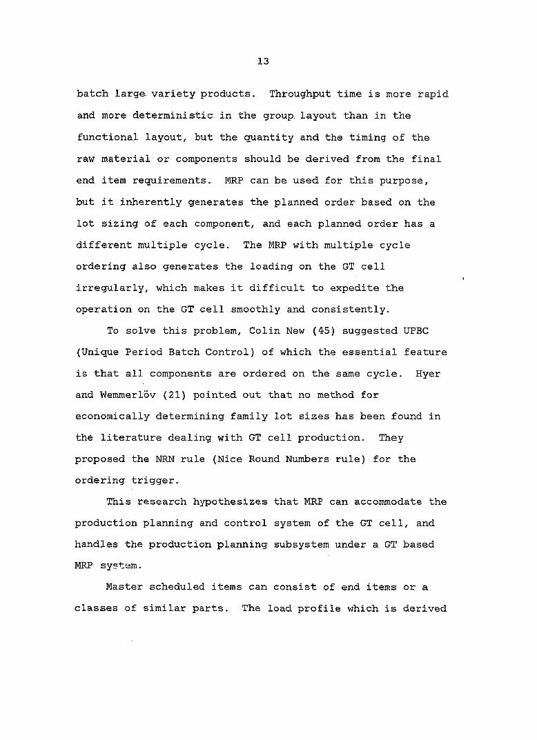
batch large, variety products. Throughput time is more rapid
and more deterministic in the group, layout than in the
functional layout, but the quantity and the timing of the
raw material or components should be derived from the final
end item requirements. MRP can be used for this purpose,
but it inherently generates the planned order based on the
lot sizing of each component, and each planned order has a
different multiple cycle. The MRP with multiple cycle
ordering also generates the loading on the GT cell
irregularly, which makes it difficult to expedite the
operation on the GT cell smoothly and consistently.
To solve this problem, Colin New (45) suggested UPBC
(Unique Period Batch Control) of which the essential feature
is that all components are ordered on the same cycle. Hyer
and Wemmerlov (21) pointed out that no method for
economically determining family lot sizes has been found in
the literature dealing with GT cell production. They
proposed the NRN rule (Nice Round Numbers rule) for the
ordering trigger.
This research hypothesizes that MRP can accommodate the
production planning and control system of the GT cell, and
handles the production planning subsystem under a GT based
MRP system.
Master scheduled items can consist of end items or a
classes of similar parts. The load profile which is derived

14
from the BOM and routing file is used as a tool of master
production scheduling. Therefore, the process stages of the
master production scheduled items are considered in
developing the load profile. This research handles only one
level of the production process and does not consider the
process stages of the master production scheduled items or
interrelationships of the parts. Further, the application
of this research is in a GT environment as described by
short lead times, small volumes, and,requirement of a load
profile. While parts classification may be included in
developing the load profile, the existence of a
classification system is not mandatory to this research. As
such the application to a GT cell or a small shop are
equally effective.
Need for the Study
The traditional method for master production scheduling
is as follows. The master production scheduler develops a
TMPS, based on experience, intuition and business sense. It
is not known, however, whether a TMPS is reasonable or not
until the RCCP of the proposed TMPS is developed.
Therefore, the "trial and error" method must be used to get
a better TMPS. Even though there is an integrated
production planning and inventory control system, the master
production scheduling logic usually does not include the

15
resource constraints. It does include netting logic to
derive the production requirement from the gross requirement
and on-hand inventory. There are also many designed logic
structures to minimize the sum of production and inventory
holding cost in order to find the optimal MPS, but the
feasibility of the MPS with respect to capacity is also
evaluated by the RCCP. A trial and error method is also
used to get a better TMPS.
In the traditional "trial and error" method, if
multiple items and resources are involved it is almost
impossible to balance the work-load on the resources in one
iteration. Even several retrials cannot assure the
balancing of the work-load. The "trial and error" method
has been used because the capacity limit is not considered
in developing the TMPS.
There are several reasons why the traditional approach
does not include the capacity as a criterion to get the
optimal MPS.
1. It is not easy to determine the capacity target/
capacity limit because there are so many control
variables and elements. The capacity
target/capacity limit is derived by compromising
available capacity and required capacity.
Required capacity is derived from the authorized
production plan or the production requirements.
15
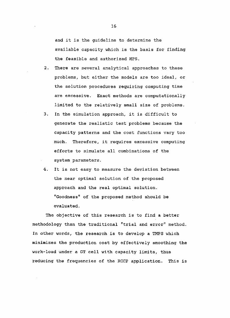
and it is the guideline to determine the
available capacity which is the basis for finding
the feasible and authorized MPS.
2. There are several analytical approaches to these
problems, but either the models are too ideal, or
the solution procedures requiring computing time
are excessive. Exact methods are computationally
limited to the relatively small size of problems.
3. In the simulation approach, it is difficult to
generate the realistic test problems because the
capacity patterns and the cost functions vary too
much. Therefore, it requires excessive computing
efforts to simulate all combinations of the
system parameters.
4. It is not easy to measure the deviation between
the near optimal solution of the proposed
approach and the real optimal solution.
"Goodness" of the proposed method should be
evaluated.
The objective of this research is to find a better
methodology than the traditional "trial and error" method.
In other words, the research is to develop a TMPS which
minimizes the production cost by effectively smoothing the
work-load under a GT cell with capacity limits, thus
reducing the frequencies of the RCCP application. This is
17
possible by including a critical capacity limit in the
master production scheduling logic as a constraint.
Research Scope and Objectives
This research deals with the case where the business
type is make-to-stock under a GT cell. An MRP system
accommodates the production planning and control function
for this GT cell. The demand pattern of the end items is
seasonal, and the capacity limit during the scheduling
period is constant. The proposed master production
scheduling system is a decision support system, therefore,
the TMPS which is the output of the proposed system will be
finalized by coordinating functions such as the master
production scheduling committee. That is, the process to
generate the finalized MPS is not included, but only the
process to get the TMPS.
There are several ways to derive the production
requirements. They may be derived from the on-hand
inventory and all demand sources, which are composed of
actual demand (order on the book) and potential order
(forecast demand). There may be two categories in deriving
a production requirement. First, if there is a production
planning function, a TMPS is guidelined by the production
plan. A weekly production requirement is derived from the
monthly production plan and the customer order entries.

18
Second, if there is no production planning function, then a
weekly production requirement is determined by all demand
sources such as customer order, interplant requirements,
warehouse requirements, etc. The methods to derive a
production requirement depend on their source and the level
of the MPS. The combination of the methods to obtain the
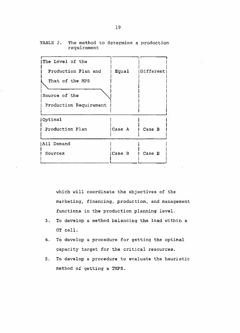
production requirements is given in Table 2. In this
research, only case B is handled, and the interaction
between the production plan and the MPS is excluded. When a
heuristic procedure is proposed for the combinatorial
problems, the number of test problems may be so large that
it is highly impractical to test all the combinations of the
system parameters. Therefore, this research will only
evaluate the proposed procedure for a family of the specific
test problems.
Research objectives The purpose of this research is
to develop the following objectives in a GT based MRP
System:
1. To develop a master production scheduling
procedure deriving a TMPS which minimizes the
total production cost when there is a constraint
of capacity limit. The total production cost is
composed of setup, holding, overload and delay
penalty cost.
2. To develop an aggregate production planning model
19
TABLE 2. The method to determine a production requirement
1 |The Level of the
1 Production Plan and
I^That of the MPS
1 1 1 1 Equal 1 1 1
1 1 1 1 1 1 1 Different| 1 1 1 1 1 1
1 Source of the
1 Production Requirement 1 1
1 1 1 1 1 1 1 1 1 1
1 Optimal
1 Production Plan
1 1 [Case A
1
1 1 1 1 1 Case B | 1 1
[All Demand
1 Sources
1
1 1 [Case B
1 1
1 1 1 1 1 Case B |
1 1
which will coordinate the objectives of the
marketing, financing, production, and management
functions in the production planning level.
3. To develop a method balancing the load within a
GT cell.
4. To develop a procedure for getting the optimal
capacity target for the critical resources.
5. To develop a procedure to evaluate the heuristic
method of getting a TMPS.

20
Uniqueness of the MPS under a GT Based MRP System
When a functional layout is changed into a GT layout,
there are several advantages in master production
scheduling. Several characteristics of the MPS under a GT
based MRP system and the reasons for them are described
below (5). These characteristics will justify the approach
to develop the optimal TMPS.
1. The lead time of an end item which includes setup
time, queuing time, and transporting time can be
reduced.
a. The total setup time can be reduced because
similar parts are ordered together, therefore,
changeover is decreased
b. The queuing time and WIP can be reduced, because
the material flow and the routings of components and
the interactions among the jobs are simplified.
c. Transportation time can be reduced. Because
machines in a group are close together, continuous
transfer is possible.
2. The MPS has the capability to accommodate the market
changes quickly because of the reduction in the lead
time of the production. This also makes it possible
to promise quick delivery to the customer, resulting
in increasing the customer service level and
potential orders. This implies that the MPS is

21
elastic to the other external variables; then, the
firm planned period in the planning horizon is not
mandatory.
The feasibility of the proposed TMPS can be
evaluated interactively. Similar parts are
classified by the coding and classification scheme
and they are planned in one family. That is, the
scheduling approach is based on the tooling and the
material families; therefore, the complexity of the
master production scheduling is reduced and the
implementation of the interactive MPS system is
easier than the other MPS systems under a different
environment.
Expediting the MPS over the GT cell is simple
because the workers have common aims and know their
contribution to the company. They understand all
operations on a part instead of one operation and
work together well because of the minimal external
control and the reduction in co-ordination with the
other functions.
The scheme developing a load profile is different
from that of the other environments. A coding and
classification scheme and the MRP logic with the
single cycle and single phase ordering are used to
develop the load profile.

22
CHAPTER 2. LITERATURE REVIEW
Aggregate Production Plan
There are four widely recognized traditional approaches
such as the linear decision rule, management coefficient
model, parametic production planning approach, and search
decision rule in the aggregate production planning problem.
The pioneering research of the aggregate planning meth
ods was made by Modigliani et al. (43). They developed the
linear decision rule as a means of making aggregate employ
ment and production rate decisions. The objective function
of the linear decision rule model is to minimize a quadratic
total cost function. The total cost is composed of the
costs caused by regular work force level, hiring/firing,
overtime/idle time, and inventory holding.
Bowman (2) developed the management coefficient model on
the premise that the managers are aware of and sensitive to
the variables which are important in the aggregate planning
decisions, but they are inconsistent in using their knowl
edge. He proposed to establish the form of decision rules
for aggregate planning through rigorous analysis. On the
contrary, the coefficients for these decision rules were
setup through the multiple regression analysis of the man
agement's past decisions.
The parametic production planning approach developed by
23
Jones (24) is a heuristic approach to discover the decision
rules for work force and production. This approach is to
evaluate all of the possible combinations of parameters for
these rules and to find a parameter set minimizing the cost
function. The selected parameters are incorporated with the
work force rule and the production rule.
The search decision rule developed by Taubert (57) can
cover more realistic problems. The more realistic the model
is, the more difficult the analysis is. The search decision
rule uses the heuristic optimum-seeking procedures to reach
the optimum of an objective function.
Elwood S. Buffa and William H. Taubert (5) classified
the decision rule approaches to the aggregate planning prob
lem into mathematically optimal decision rule approach, heu
ristic decision rule approach and search decision rule
approach.
This research is devoted to the mathematically optimal
decision rule approach to solve the problem where there are
conflicting multiple objectives. The mathematical decision
rule approach contains the linear decision rule, linear
programming, dynamic programming, goal programming, etc.
Several authors cited below extended the linear decision
rule (5). Hanssman and Hess attempted to formulate an
approximating linear model to the original non-linear cost
terms. Hanssman-Hess linear programming model is equivalent

24
to the linear decision rule model in terms of general struc
ture. The decision variables and the cost criterion function
are the same, but there is a difference that in the Hanssman-
Hess linear programming model the cost criterion function is
linear, but in the linear decision rule model it is qua
dratic. Sypkens identifies plant capacity as a decision
variable in addition to the work force and production rate.
Chang and Jones generalized the linear decision rule method
ology to yield both aggregate and disaggregate planning in a
multi-product environment. Bergstrom and Smith have devel
oped the basic linear decision rule model to one involving
both multi-products and the inclusion of a revenue term.
Some authors described below tried to solve the aggre
gate production planning problem by applying linear program
ming (5). Bowman proposed the use of the distribution model
of linear programming for aggregate planning. McGarrah
developed a basic simplex model of aggregate planning for
one period where change and inventory cost functions have
the general forms. The specific applications of the simplex
model in the industrial aggregate planning situations are
reported by Eisemann and Young in the study of a textile mill
and by Greene, Chatto, Hicks and Cox in the packing industry.
Several authors tried to solve the problem where there
are multiple objectives by applying goal programming.
Veikko Jaâskëlainen (23) used three separate and incompatible

25
goals, the levels of production, employment and inventories.
He defined the preemptive priority factors associated with
goals so that goals in a lower rank are satisfied only after
those in a higher rank are satisfied or reach points beyond
which no improvements are possible under the given con
straints. Lee (30) and Kornbluth (26) suggested that goal
programming can provide an improved model for the aggregate
scheduling problem. Lee (30) pointed out that one advantage
of goal programming is that it can be solved by a modified
version of the familiar simplex method. Goodman (18) devel
oped a goal programming approach to the problem of scheduling
aggregate production and work force. He demonstrated that
the effectiveness of such an approach is highly dependent
upon the degree of nonlinearity which the goal programming
model must approximate. The results indicate that, for rel
atively low degree models, goal programming may provide an
efficient and effective solution approach, while for higher
degree models the approach may be inappropriate. Lawrence
and Burbridge (29) presented a multiple goal linear program
ming model for coordinating production and logistics plan
ning. S. M. Lee, R. L. Morris and L. Franz (31) presented an
integer goal programming approach to the problem involving
fixed costs and multiple goals. A. G. Lockett and A. P.
Muhlemann (34) handled the problem achieving a balance be
tween a smooth work-load on the factory and matching
production with promised delivery dates.
25
Master Production Schedule
Classification
Each company may have its own master production sched
uling procedure. This can be shown from the fact that most
literature of the master production scheduling procedure
published from the industry has its own uniqueness. Some
authors tried to classify the Master Production Schedule
types. Mather and Plossl (38) reviewed ten different types
of the master schedule. Paul Maranka (36) discussed the
classification of Mather and Plossl and pointed out that a
number of combinations of the ten master schedule types
under one roof can be encountered and this required the
master schedule process to be defined general enough so that
any of the types or the combination, thereof, could be in
corporated into one planning group. He identified the
master schedule type with one of three basic business types—
continuous process; production lots made-to-stock and/or
option-to-order; and make-to-order. David I. Leo (33) made
the abstracts of the COPICS (Conversational Oriented Produc
tion and Inventory Control System), where the master pro
duction schedule planning flow is classified into—make-to-
stock, assemble-to-order, and make-to-order. A. L. Steven
(55) suggested three criteria; make-to-stock, make-to-order,
and the completely engineered product for the MPS classifi
cation.

2 7
Special topics
Many authors have concentrated on conceptualizing the
development of Master Production Schedules within the hier
archy of production plans.
A. L. Steven (55) described the closed loop MRP system
where the relationships among production plan, master sched
ule and RCCP are represented. David 0. Nellemann (44)
explained the production planning and the master scheduling
as the management's game plan. Robert McCormick (40) dis
cussed the interdependence of the master schedule to the
other planning functions including production plan, fore
casting, rough cut capacity planning, and planning BOM, plus
its interface with downstream modules of material require
ments planning and the final assembly schedule. Richard W.
Malko (35) stressed that the master scheduling System is the
key sub-system for the successful manufacturing control
systems and needs the help of other sub-systems to generate
the final results. He also wrote about how the raw data can
be acquired at the beginning and what techniques are used to
remain consistent. John F. Proud (48) introduced the twelve
principles of good MPS.
Several companies announced the master production sched
uling system in specific business types. Robert W.
Kohankie II, Waterbury Farrell and Richard R. Morency (25)
implemented a system for preparing a master schedule in a

2 8
consumer goods company. They developed the master schedule
to convert the production forecast into specific product code
level demands that can then be used to schedule each produc
tion line against current capacities. W. H. Gaw (17) showed
the "team approach" can be used to develop and maintain the
master scheduling in a "make-to-order" manufacturing firm.
In the process industrials, John Burt (7) discussed the
appropriate levels of MPS, techniques for integrating multi
ple levels, use of planning, inverted BOM, and the relation
ships with forecasting, production planning and scheduling
design. Romeyn C. Everdell and Woodrow W. Chamberlain (16)
discussed master scheduling in a multi-plant environment.
Several authors discussed one aspect of MPS. Darnton
and Garton (11) described the factors that lead to the
changes in the company's planning and control systems, and
described the means used to monitor effectiveness of the
system. James R. Schwendinger (50) stressed that order
promising is a by-product of the MPS process which makes it
feasible to make significant improvements in dealing with
customers. Ernest C. Huge (20) stressed that lead time
management is the key to successful master scheduling and
proposed a method to establish a successful lead time man
agement program. Scott R. Miller (42) showed that the Master
Production Schedule can compromise the objectives of market
ing and production and inventory control. John. J. Bruggeman

29
and Kathleen T. Merkin (4) described how the master sched
uling project is responsible for coordinating the efforts of
the other organizational specialists to insure the develop
ment of a comprehensive, feasible master production plan.
Hal Mather (37) pointed out the importance of the BOM for a
successful MPS and excessive protectionism within the various
organizations that use the BOM prevents the development of
its improvements.
Interface with other functions
J. Gaylord May (40) stressed that an accurate forecast
of customer demand is, perhaps, the most important ingredient
to establish a good master schedule. So, he focused on the
concepts which are designed to improve customer demand fore
casts in front of manufacturing lead-times. Russel Copeman
(9) covered a specific approach used to integrate product
line forecasts with actual orders and actual satellite
assembly plant requirements into a single master schedule,
where it includes the make-to-stock and make-to-order type of
customer orders together. Linda M. Smith (51) stressed that
order factors have an effect on the success of any MRP-master
schedule coordination.
GT Based MRP System
As far as the literature survey is concerned, only four
papers have dealt with MRP and GT in combination. Colin New

30
(45) said that the combination of MRP and GT is the new
strategy for the component production. The SCRAGOP (Short
Cycle Requirements and Group Organized Production) system
works well for the component production if the production
order trigger is UPBC (Unique Period Batch Control). Nallan
C. Suresh (56) pointed out that the optimal production system
in a small batch/large variety situation, where the condi
tions are appropriate for the GT, consists of the following:
A group layout; a "short cycle-flow control" approach for
direct materials planning and ordering; and a scheduling
approach based on tooling, and material families in addition
to the other relevant factors. He explained the short cycle-
flow control approach which is required in a GT situation
can be met by an MRP system. Hyer and Wemmerlov (21)
explained that MRP and GT are a viable combination in a gen
eral framework for production planning and control. They
discussed the drawback of the period batch control and pro
posed NRN (Nice Round Numbers) rule to find the order quan
tity. Spencer (52) explored the scheduling components for
the GT lines producing diesel engines in a company.
Capacitated Lot Sizing for Multi-Items
Lot sizing is used to determine the timing and sizing of
production to minimize the setup and the holding cost. The
first effort to develop the lot sizing technique for multi

31
items with the capacity limit was made by Eisenhut (15). He
defined a priority index from a modified Silver-Meal heuris
tic for a single product without capacity constraints. Then
the production lots are assigned to the current scheduling
period until either the capacity constraint is violated or
all marginal cost reductions become negative. But this
method may generate an underload in an earlier period; there
fore, it will result in an infeasible solution. Lambrecht
and Vanderveken (28) proposed a backtrack routine to solve
this problem by extending the Eisenhut heuristic. Dixon and
Silver (13) presented an alternative modified heuristic which
guarantees the generation of a feasible solution (if one
exists) to avoid the above situation. Ali Dogramaci et al.
(14) developed four-step algorithm which improves the feasi
ble solutions obtained to get a better solution. Reuven
Kami and Yaakov Roll (49) also developed a lower bound solu
tion by improving the feasible solution so obtained until no
further improvement can be made. The above heuristics can be
described as period-by-period methods. Newson (46) devel
oped another technique by using a modified Wagner-Whitin
algorithm. Newson's heuristic is based upon a series of the
shortest path calculations for a network representing the
uncapacitated problem.

32
Evaluation Method of the Heuristic Solution
When a heuristic solution is developed for the large
combinatorial problems, a solution standard is necessary to
evaluate the proposed solution or procedure. An optimal
solution can be used for the solution standard, but it is
almost impractical to find the optimal solution for the
combinatorial problems in most cases. Therefore, a near
optimal solution can be used for the solution standard.
Several researchers developed inference procedures to get an
estimation of the minimum using small order statistics of a
large sample. Lauren de Hann (12) constructed a procedure
to derive a confidence interval for the minimum of a function
using asymptotic theory. Weissman (58) constructed a pro
cedure to develop confidence intervals based on the lower
extreme values of a large sample for the threshold parameter
(unknown minimum-life) of a life distribution.
After getting the solution standard, a question is
raised, "How does one use the solution standard to evaluate
the heuristic solution and procedure?" Dannenbring (10)
classified the measurement of a solution goodness as follows;
1. Comparative measure
2. Achievement measure
3. Distributional measure
Comparative measure determines the magnitude of the dif
ference between the solution standard and the value of the

33
heuristic solution. Achievement measure determines whether
the heuristic solution value is equal to the solution stan
dard or not. Distributional measure is aimed at finding the
chances that a solution could have been obtained with a value
better than that for the heuristic solution being evaluated.
Achievement measure gives a simple yes or no statement for
an individual problem; therefore, this measure is useful
when it is used together with other measures. Distributional
measure requires the generation of the possible solution set
to determine the distribuiton pattern of the solution.
Summary
1. An aggregate production planning problem with
multiple objectives has been developed to coordinate
the conflicting objectives of each function in an
organization. This type of an APP problem is solved
by goal programming technique.
2. Considerable research has been devoted to the con
ceptual aspect of master production scheduling, but
there is little research in the methodology of master
production scheduling.
3. Several researches have been handled concerning
operational level scheduling in a GT cell, but not
much concerning managerial level scheduling.

34
Little research has been made in master production
scheduling with the time phasing effect of the load
and the capacity limit.
Little research has been done in multi-item lot
sizing rules, and these lot sizing rules may be used
for the master production scheduling tool. But,
there are more managerial factors to be considered
in master production scheduling; therefore, these
multi-item lot sizing rules cannot be directly used
for master production scheduling.
Little research has been done under the environment
where MRP is used as the production planning and
control system on a GT cell.
Comparative measures other than distributional
measures and prélèvement measures have been mostly
used to evaluate the heuristics for the combinatorial
optimization problems.

35
CHAPTER 3. PROBLEM DEFINITION
Characteristics and Assumptions
Contrasts between this research and the papers of
Eisenhut and Newson are shown in Table 3. The characteris
tics of this research can be described as follows. The time
phasing effect of load, overload cost, and delay penalty cost
are considered in the process of scheduling. The methods in
the research include the traditional period-by-period method
and the shortest path algorithm. A tree search scheme is
also included as a heuristic search method for the optimal
solution. A left threshold parameter of an unknown distribu
tion is used as a solution standard instead of a solution
from the Wagner-Whitin (W-W) algorithm. The need for produc
tion smoothing is reduced because available capacity is
compromised in the process of master production scheduling.
Multi-resource cases are also allowed in this research.
This research deals with two subsystems of the
production planning and control system for a GT based MRP
system. These subsystems include the aggregate production
planning and the master production scheduling systems. The
APP, the output of the aggregate production planning system,
is the basis for the production plan which may be the
primary input to the master production scheduling system.
If there is no APP function in the production planning

35
TABLE 3. Contrasts of the research with other works
1 1 1
1 1 1Eisenhut(15)| Newson(46) 1 Kim
1 Time Phasing.
1 of Load No 1 No Yes
1 Backlog &
1 Overload No 1 No Yes
1 Cost Factor Setup 1
Holding |
Setup
Holding
Overload
Setup
Holding
Overload
Penalty
1 Approach
1 Method
Period-by- |
Period j
Shortest Path Period-by-period
Shortest Path
Tree Search
1 Solution
1 Standard
W-W 1
Algorithm j
W-W
Algorithm
Threshold Parameter
Estimation
1 Need for
1 Production
j Smoothing
More 1 More Less
1 Multi-Resource
1 Problem
1
No 1
1
No
1
Yes
1

37
system, then the production requirements are determined from
all demand sources. The following assumptions are made in
the development of the aggregate production planning and the
master production planning systems.
1. The marketing plan and the APP are represented on
a per month basis, and the MPS is on a per week
basis.
2. A company has a controllable number of end items
made from multiple component parts.
3. A structured BOM exists and end items in the TMPS
are identified by part numbers in the BOM. The
business type is make-to-stock.
4. The demand pattern is seasonal. All production
lead times of end items are known and
deterministic.
5. The relative importances among conflicting goals
can be quantified.
6. Every end item has a load profile which
represents the measurable load on the critical
resources.
7. Capacity limitations of critical resources can be
defined and constant during the scheduling
period.
8. There is a one to one correspondence between a
TMPS and a total cost which is composed of set

38
up, holding, overload, and delay penalty cost.
Aggregate Production Plan
The APP is the plan of production, inventories and work
force at an aggregate level to respond to fluctuating
demands on a production system (32). The function of the
aggregate production planning system is to keep a balance of
work-load and to match production with the promised delivery
dates and the expenditure plan. For work-load smoothing,
load profiles and capacity limitations are used. Therefore,
load profiles, capacity limitation of the critical
resources, and the marketing and financing plans are
prepared in advance.
Load profile refers to the estimated capacity
requirements of the item in the MPS on a limited number of
the key departments (41). For every manufacturing end item
in a TMPS, the standard load on each machine for a GT cell
should be defined. In the production planning level, only
the capacity limitations of several critical resources are
considered, instead of considering all resources. The
marketing plan is a guideline for the monthly APP. The
marketing department develops the marketing plan on a per
month basis. The financing plan is prepared in the same
way.
The aggregate production planning system must consider

the balance between external demand and internal supply in a
production system. The objective function in the aggregate
production planning system is to minimize the weighted
deviations from the desired goals. These goals are defined
as follows;
1. Satisfy the requirement that the production cost
is consistent with the production budget.
2. Satisfy all of the forecast requirements of the
marketing department during the planning horizon.
3. Satisfy the sales requirements for each period.
4. Insure that the actual production load is equal
to the average capacity limit of the GT cell for
each period.
5. Insure that the total amount of inventory during
the planning horizon is less than a given value.
6. Insure that the actual workload is equal to the
regular workload in the supporting departments
for each period.
The production planner uses the output of the aggregate
production planning system to build up the monthly
production plan which may be translated into a weekly TMPS.
The aggregate production planning problem can be represented
in the following goal programming model:
1) Variable Definitions
The variables in the model are defined as follows:

40
X it
it
B.
it
^i jkt'
production quantity of end item i in month t
sales requirement of end item i in month t
available budget for the production in month t
on hand inventory level of end item i at the end
of month t
load of end item i assigned to machine K in the
jth group at the period t, t=l,2,...,T where T is
the total lead time
L. * * *
a set which is composed of L. , L. . , L. ijk. 1] 'i.k. '
jk.
where is the weighting factor for machines
total load of end item i assigned to machine K
in the jth group =
sum of the weighted load of each machine in
group j = ^i jk.
^i.k.
L. 1,
total load of end item i on machine K = E.L.
total load of end item i on the shop floor
L " j^ij = Zk^k i.k.
A **
A. 3
. k
a set which is composed of A, A. , A, A ] jc ^ * «Je ••
: average load of machine K in the jth group
: average load of the jth group = (1/T)Z^Z^X^^
j • •
: average load of machine K = (1/T)Z.Z X.. • L. , 1. u It X • JC <
: average load of total shop floor = (1/T)Z^Z^X^^
1.. .

41
load of end item i assigned to jth key department
at period t, t=l,2,...,T where T is the total lead
time.
L..* : total load of end item i assigned to the jth key
department =
: regular available capacity of key department in
month t
L : maximum accumulated dollar amount of the inventory
item during the planning horizon
: inventory holding cost per unit per period for the
end item i
CMj^ : manufacturing cost per unit for the end item i
CV^ : dollar amount of the end item i
W : vector of weighting factors for the deviation
variables
D ; transposed vector of the deviation variable
2) Model Formulation
The objective function and the constraints of the
model are defined as follows;
(1) Objective Function: Minimize the total weighted
deviation derived from the gap between the desired
goal and the achieved goal. Several goals are
developed by financing, marketing, manufacturing,
management, and other major supporting functions.
Minimize Z = W D

42
(2) Constraints: Several goals described above are
transformed into the following constraints. All
variables and constraints need not be considered simul
taneously. Critical variables and constraints are
included in the model. The deviation variables with
subscript n and p are, respectively, under achieving
and over achieving for each goal.
1. Financing;
£.(C. . (I.^) + CM. . X.^) + = B^,
for all t
2. Marketing;
C t ^ i t = ^
3. Shop Floor:
^n**t ~ p**t ~ ^
4. Management ;
ZiZ^CV. . (I.^) + - Dp = L
5. Others:
°nj»t " "pj't " t
- ®it = :it'
A small size problem for a GT cell is illustrated in
Chapter 5.
Master Production Schedule
The purpose of the master production scheduling system
is to derive a TMPS which satisfies the objective function

43
from the demand requirements. The quantity of end items in
a period of the MPS may represent a gross requirement, a
production requirement, or a planned order. This research
presupposes that the quantity of end items in the MPS
implies production requirements or planned order. If the
quantity is the gross requirement, it can be changed into
the production requirement by considering the on-hand
inventory. The demand requirements of end items can be
determined from all demand sources or derived from the
production plan. If the capacity target can be derived from
capacity planning, it can be used, if not, the capacity
limit is used instead of the capacity target. Tne problem
is to derive a TMPS from the demand requirements which is
derived from the production plan or all demand sources. The
objective function to be minimized is the sum of setup,
carrying, overload, and shortage penalty cost. There is a
per end item setup cost parameter for each product group and
a per unit carrying cost parameter for each product group
in one week period. There is also machine-hour or man-hour
cost for overload for each critical resource. It is not
easy to determine the shortage penalty cost, which is
determined for each product group in a one week period. In
general, the shortage penalty cost includes loss of goodwill
and business, loss of revenue, etc. In this research, the
shortage penalty cost only includes the shut down cost of
the assembly department when an order misses a due date.
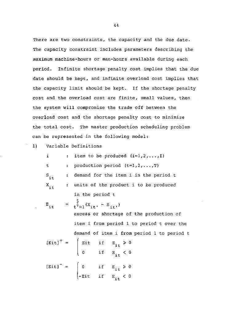
44
There are two constraints, the capacity and the due date.
The capacity constraint includes parameters describing the
maximum machine-hours or man-hours available during each
period. Infinite shortage penalty cost implies that the due
date should be kept, and infinite overload cost implies that
the capacity limit should be kept. If the shortage penalty
cost and the overload cost are finite, small values, then
the system will compromise the trade off between the
overload cost and the shortage penalty cost to minimize
the total cost. The master production scheduling problem
can be represented in the following model:
1) Variable Definitions
i : item to be produced (i=l,2,...,I)
t : production period (t=l,2,...,T)
: demand for the item i in the period t
: units of the product i to be produced
in the period t
^ i t " t + = i ( X i t ' - S i t ' )
excess or shortage of the production of
item i from period 1 to period t over the
demand of item i from period 1 to period t
Eit if E.^ > 0 It
0 if E.^ < 0 It
[Eit]"*" =
[Eit] = 0 if E.^ > 0
-Eit if E.^ < 0 it

d(Xi^) =
1
[00^]+ =
45
0 if = 0
1 if X > 0 it
RC^ : capacity limit during the period t
S. ; setup cost of the item i
C. : carrying cost per unit of the item i
per period carried
: penalty cost per unit of the item i
per period delayed
0^ : cost per man-hour or machine-hour of labor or
machine which is overdriven in the period t
L.. : load of the end item i in the period j, 1 ]
where j=l,2,...,J and the total lead time(J)
is less than three in the test problems.
L . : l o a d o f t h e e n d i t e m i i n t h e p e r i o d k c a u s e d
by the production X^^
^ijk ^i,k-j+l ^ij
OC^ : the total required load minus the available
load in period t
OC^ if OC^ > 0 t t
0 if OC^ < 0

4 6
Model Formulation
(1) Objective Function
Minimize Z = Z.E.d(X,.) • S, + Z.Z.[E • C,
+ • Pi + ZJOC^]-^ . 0^
(2) Constraints
+ °^t' all
If the value of subscript is non-positive, the
corresponding load is zero.

47
CHAPTER 4. THE APPROACHES
Preliminary Work
Input data
The time bucket in the aggregate production planning
level is one month but at the master production scheduling
level is one week. All input variables discussed in Chapter
3 can be summarized as follows. The related function and
the necessities of each variable are summarized in Table 4:
(1) Load Profile
L. ^; load of end item i assigned to machine k in i]kt
the jth group at period t, t=l,2,...,T where
T is the total lead time.
load of end item i assigned to the jth key
department at period t, t=l,2,3,...,T where
T is the total lead time.
; load of end item i in the period j,
j=l,2,...,J where J is the total lead time.
In the master production planning level, only
one resource is observed. This load profile
can be derived from L.and L. i]kt i]*t
(2) Policy Variables
; sales requirement of end item i at month t.
: available budget for the production at
month t.

48
L : maximum accumulated dollar amount of the
total inventory for all items during the
planning horizon.
: regular workforce level of the jth key
department at month t.
RC^ : production capacity limit on the shop floor
which is defined by each critical resource.
(3) Cost Parameters
: setup cost of end item i.
: penalty cost per unit of end item i per
period delayed.
: inventory holding cost per unit per period
for the end item i.
0^ : the cost of overload for the critical
resources.
(4) System Output
PP ; production plan determined by the APP which
is the output of the aggregate production
planning system.
TMPS : tentative master production schedule which
is the output of the master production
scheduling system.
(5) Others
CM^ : manufacturing unit cost for the end item i.
CV^ : market price of an end item i.
W : set of weighing factors for the

49
TABLE 4. Input data summary^
1 1 Input Data |
1
Var 1 1 1 Related Function|
1 1
1 APP|
1
1 MPSj
1 1 .Load Profile] 1 Production |
1 1
M*|
1 M* 1
1 2 .Policy Var. | 1 Sit 1 Marketing |
1 1 0 1
1 • 1
1 1 1 Bt
1 1 1 Financing | 1 1
1 0 1
1 • 1
1 1 1 L
1 1 1 Management | 1 1
1 0 1 • 1
1 1 1 ^j*t
1 1 1 Supporting | 1 1
M*| 1
• 1 1 1 1 RCt
1 1 1 Production | 1 1
1
1 M* 1
1 3 .cost Para. | 1 S. 1
1 Accounting | 1 1
0 1 1
M 1 1 1 1 ^i
1 1 1 Accounting | 1 1
1 0 1
1 M 1
1 1 ^i
1 1 1 Accounting | 1 1
1 0 1
1 M 1
1 1 °t
1 1 1 Accounting | 1 1
1
1 M* 1
1 4 .System Output 1 PP 1 APP 1
1 0 1
1 1 1
TMPS 1 MPS 1 1 1
1
1 ^ 1
1 5 .Others | 1 CM^ 1 Accounting |
1 1 0 1
1 • 1
1 1 1 CVj
1 1 1 Accounting | 1 1
1 0 1 • 1
1 1 1 W
1 1 1 Planning |
1 1
M 1 1 1 1
M: mandatory input data 0: optional input data *: system needs only the value of critical
resources • : not necessary .
50
deviation variables.
Load profile
The most important prerequisite for the analysis is the
existence of the load profile for each end item. The element
of the load profile of the end item i is defined for the shop
floor and the key departments. Key departments include sub
assembly, final assembly, and other critical supporting
departments. To get the load profile, an explosion simulator
and a detail operation scheduling and loading system are
used. The general system flow of these two functions is
given in Figure 2.
The BOM (Bill of Material) specifies the composition
and the process stages of the end item in the MPS. An MRP
system and a coding and classification system are used for
the explosion simulator which generates the planned order
schedule for all manufactured components by exploding the
end item in the BOM through all levels. The Bill of Labor
(or Capacity) provides the standard hours of labor (or
Capacity) requirements for each operation. The planned
order schedule and the Bill of Labor (or Capacity) are the
inputs for the operation scheduling system which determines
the sequence of the planned order for the made parts. The
loading system determines the standard hours representing
the estimated labor (or capacity) requirements of an end
item on each key resource in a company. These standard data

51
BOM
i Explosion i I Simulator |
Planned
Order
Scedule
7
^ Bill of Labor/
Bill of Capacity
I
Operation Scheduling j
& Loading System |
^ Bill of Labor/
Bill of Capacity
I I
Operation Scheduling j
& Loading System |
Load
Profile
FIGURE 2. A system flow for load profile
52
are the load profile which represents the time phased load
on each key resource to produce one unit of end item.
Aggregate Production Plan
The given aggregate production planning problem is a
typical multi-goal optimization problem. All variables and
constraints need not be handled simultaneously. The
critical resources and the constraints are selected by the
user. A matrix generator program creating the input of the
aggregate production planning system is necessary to make
the system more flexible. In this research, several
critical resources and constraints are selected for an
illustrative example. The goal programming model is con
verted into the linear programming model in the following
ways. The machine K in the Jth group and Lth supporting
department are only critical resources. The other cases can
be handled in the same way.
The objective is to minimize WD, i.e. ,
Min " ^nt + ^pt ' +
* °njkt ^pjkt * ^pjkt^ •*"
(W • D + W • D ) + n n p p
• D.lt Vt • "pit"
All deviation variables with subscript n should have

53
positive values, therefore constraints are changed in the
following way:
°„t = - Zi'Ci • :it + • XitI > 0
therefore
Ei(C, • I., + CM. • X.^) - Opt
In the similar manner,
o.ikt- Ej. Wit • > 0
Zi'Xit ' - Dpikt < Ajk "I
D. = + Dp - • lit' > °
î,I^(CVi • I.^) - Dp < L (4)
o.it = + "pit - Zi'Xit • \ l } > °
~ °plt ^ It
The number in parentheses is the constraint number in
Chapter 3. If we substitute all deviation variables with
subscript n into the objective function and drop the
constant term, we can get the following objective function:
Objective Function
MIN[Xt((W„t + Npt> • °pt - "nt • Ci'Ci ' it + ' it'
+ CjCk("nikt + "pjkt' • "pjkt - ".jkt • (ZiXit • ^Ijk."
+ + "pi • °p - • ZiCt'cVi • lit'
+ ElCt"Dpltl • ("nit + "pit' - "nit • El'Xit • 'il."l

54
A small size illustrative example for a GT cell will
be shown in Chapter 5.
Heuristics to Develop a TMPS
The following functions are defined to explain the
heuristics developing a TMPS.
AVA(t) : available capacity in the time period t. When
the production quantity t+l-j scheduled,
AVA(t) is updated. If AVA(t) is a negative
value, this means that there is overload in
the time period t. AVA(t) = [AVA(t) - Z^(L^^
*1,t+l-j)^' 3=lf2,3
OC(i,t,q) : the amount by which the cumulative capacity
exceeds the capacity limit when the requirement
q of the item i is scheduled in the period t.
OC(i,t,q) = • q) - AVA(t-l+i)+] +
A(i,t,q) ; overload cost which is caused by scheduling
the demand requirement q of the item i in the
period t. A(i,t,q) = 0^ • OC(i,t,q) where 0^
is the overload cost per unit resource.
B(i,t,q) ; penalty cost caused by delaying the requirement
q of the item i in the period t by one period.

55
B(i,t,q) = • q + • (S^)
where a( S . = ° " Si,t+l = "
1 " Si,t+1 > 0
C(i,j,t) ; penalty cost when the requirement t-j+l'
S. ^ ,S. . are scheduled in the i,t-]+2 x,t
period t+1. The value of J is the difference
between the current period t and the earliest
period t where Sit is not scheduled at period t. J
C(i,j,t) = ,2 • J •
D--'-
p . ) + s .
Ul(i,t) ; Eisenhut Formula: Expected cost reduction by
including S^^ in the present lot.
S^-I(i,t)
t.fSit
U2(i,t) : Lambrecht and Vanderveken Formula: Expected
cost reduction by including S^^ in the present
lot.
S^+I(i,t-1)-C^-(t-1)• (t-1)"S.^
I(i,T) : inventory cost of the item i when the order
cycle is length T.
I(i,T) = h(i)E^(t-l) -S.^

56
subtraction of I(i,T) from based on the
shortest path from the first period to the period
j •
N(i,j,k): total cost composed of setup, holding and overload
cost for producing the demand of item i for the
period j+1 to k at the very end of the period j.
Method A: period-by-period method
The basic principle of this approach is to increase the
lot size with the demand requirement where the marginal cost
reduction is positive until there is an overload. If there
is an overload at the current requirement, backtracking and
delaying are also considered together, and a decision with
minimum cost is made to minimize the total cost. Scheduling
is performed in the following way from the beginning month
to the end month of the planning horizon (See Figure 3).
Step 0. Preliminary Analysis: Determine the supply and the
demand, i.e., the allowable capacity and the
required capacity during the scheduling horizon. If
the average overload is not acceptable, the master
production scheduler should appeal to the upper
production planning level or revise the production
requirements. The allowable overload should be
determined by the master production scheduler. This
analysis is performed in the lump.

57
Step 1. Initialize all system parameters: System parameters
include cost and resource parameters. There are
four cost elements, i.e., setup, holding, overload
and shortage penalty cost. Resource parameter
implies the capacity limit or the capacity target.
The net production requirement and the load profile
are also determined. In the net production
requirement matrix, the element of the matrix
represents the requirements for the product i in the
period t where i = 1,2,...,I and t = 1,2,...,T.
Find T. = 3 - k where L. = MAX(L ,L ,L ). i 2 i jC 1 J. 16 ZL j
step 2. If there are waiting requirements in the waiting
list, schedule the requirements with the penalty
cost C(i,j,t) as a priority. The value of j is
recalled by the system. The higher penalty cost
will have the higher priority. After calculating
positive and finite Ul(i,t) for the current period,
schedule current requirement with the priority of
high Ul(i,t). If the waiting and current
requirements cannot be scheduled without
overloading, go to Step 5. Otherwise, calculate the
positive U2(i,t) for all i and t if Sit is not zero.
Step 3. Search the highest U2(i,t) in the coming periods.
If the corresponding S _ ^ does not generate an
overload, add the S to the production quantity of

5 8
Start
Stop
Yes
Scheduling
All Items?
Yes
No No
/Schedules^ Waiting & Current
Requirement
Yes Back
tracking
No
/waiting Requirement V Exist? y
Yes Yes
No
Increase Lot Size With The
Priority U2(i,t)
Schedule
Waiting
Requirement
Backtracking
is Performed
Schedule
Current
Requirement
Move to Next
Scheduling
Period
FIGURE 3. Flow diagram of Method A

59
the current scheduling period. This step is
repeated until there is an overload. If there is
an overload, get the next item which does not
generate an overload.
Step 4. Update the requirements matrix by subtracting the
scheduled amount from the corresponding requirements
of the matrix, and make the next scheduling period
number one. Repeat Step 2, Step 3 and Step 4 until
the end of the scheduling horizon.
Step 5. Check to determine whether backtracking is possible.
Calculate TAVA. and TL. where 1 1
TAVA^ = AVA(t-T^) + AVA(t-T^+l) + + AVA(t-T^2)
TLi = (L.^ + L,, + L.;, .
The value of T^ equals min(t,AA/((C^)•(S^^))) where
AA = min(A(i,t,S^^),B(i,t,S^^)).
If the condition of backtracking is satisfied,
i.e., TAVA^ is larger than TL^ and there is no
waiting requirement at the beginning of scheduling
in the current period, go to Step 7. If not, go
to Step 6.
Step 6. Calculate overloading and penalty cost, then follow
the policy which has the minimum cost.
1) If overloading occurs in the waiting list of
schedules in the current period.
Calculate A(i,t,WA^^) and C(i,j,t) for the
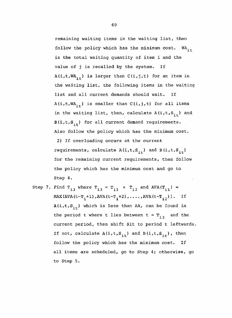
6 0
remaining waiting items in the waiting list, then
follow the policy which has the minimum cost.
is the total waiting quantity of item i and the
value of j is recalled by the system. If
A(i,t,WA^^) is larger than C(i,j,t) for an item in
the waiting list, the following items in the waiting
list and all current demands should wait. If
A(i,t,WA^^) is smaller than C(i,j,t) for all items
in the waiting list, then, calculate A(i,t,S^^) and
B(i,t,S^^) for all current demand requirements.
Also follow the policy which has the minimum cost.
2) If overloading occurs at the current
requirements, calculate A(i,t,S^^) and B(i,t,S^^)
for the remaining current requirements, then follow
the policy which has the minimum cost and go to
Step 4.
Step 7. Find T. where T = T. + T and AVA(T ) = 1 j 1 j 1 JL 1 6 1 -L
MAX(AVA(t-T^+l) ,AVA(t-T^+2) ,AVA(t-Tj^^) ) . If
A(i,t,S^^) which is less than AA, can be found in
the period t where t lies between t = and the
current period, then shift Sit to period t leftwards.
If not, calculate A(i,t,S^^) and B(i,t,S^^), then
follow the policy which has the minimum cost. If
all items are scheduled, go to Step 4; otherwise, go
to Step 5.

6 1
Method B; shortest path method
There is always a one to one correspondence between the
path from the node 0 to the node t and a TMPS. For example,
in a single product (Figure 4), if the path is composed of
two arcs, 02 and 2_4, then this path corresponds to a TMPS
which will produce the the beginning of the
period 1 and at the beginning of the period 3.
The addition of the node 0 is used for the graphical
representation of the lot sizing problem (46) . If the
planning horizon is T, then the total number of possible
T — 1 paths from the period 1 to the period T is 2 , and the
total number of arcs is T*(T+l)/2. In the above example
where T equals 4, the total number of paths is 2^ = 8, and
the total number of arcs is 4*5/2 =10. The basic principle
of Method B is to get the shortest path from the node 0 to
the node T while allocating the required capacity for each
item. Scheduling is performed in the following way item-
by-item (see Figure 5).
Step 0. Same as Method A except that the priorities among
all items should be defined.
Step 1. Same as Method A except that backlogging is not
allowed. Set i=l,j=l,k=l. The value of i is the
item number which implies the priority sequence
among all items. An arc is made of the node j and
the node k, i.e., j is the beginning node number and

62
k is the ending node number.
Step 2. If all items are scheduled, stop the process.
Calculate the positive M(i,j-l,k). If the net
requirement of the current period is zero, then the
product i is disregarded, and if the net requirement
of the future period is zero, then M(i,j-l,k) will
have a very large value. If M(i,j-l,k) is positive,
then go to Step 5, otherwise go to Step 3.
Step 3. If j equals T-1, then go to Step 6. If not, go to
Step 4.
Step 4. Find the shortest path from the node 0 to the node j
and update the resource in the work area based on
this shortest path. Increase j and k by 1
respectively, then go to Step 2.
Step 5. Calculate the value of N(i,j-l,k), and put this
value into the corresponding position of the matrix
N(i,T-l,T). Increase k by 1 and go to Step 2.
Step 6. Find the shortest path from the node 0 to the node
T. The corresponding TMPS is the proposed TMPS of
item i. Update the resource and get next item
number and set j at 1 and k at 1, then go to Step 2.
Method C: tree search method
Method C is proposed when splitting of the production
quantity is allowed. The splitting of the quantity is
usually constrained by several restrictions such as batching
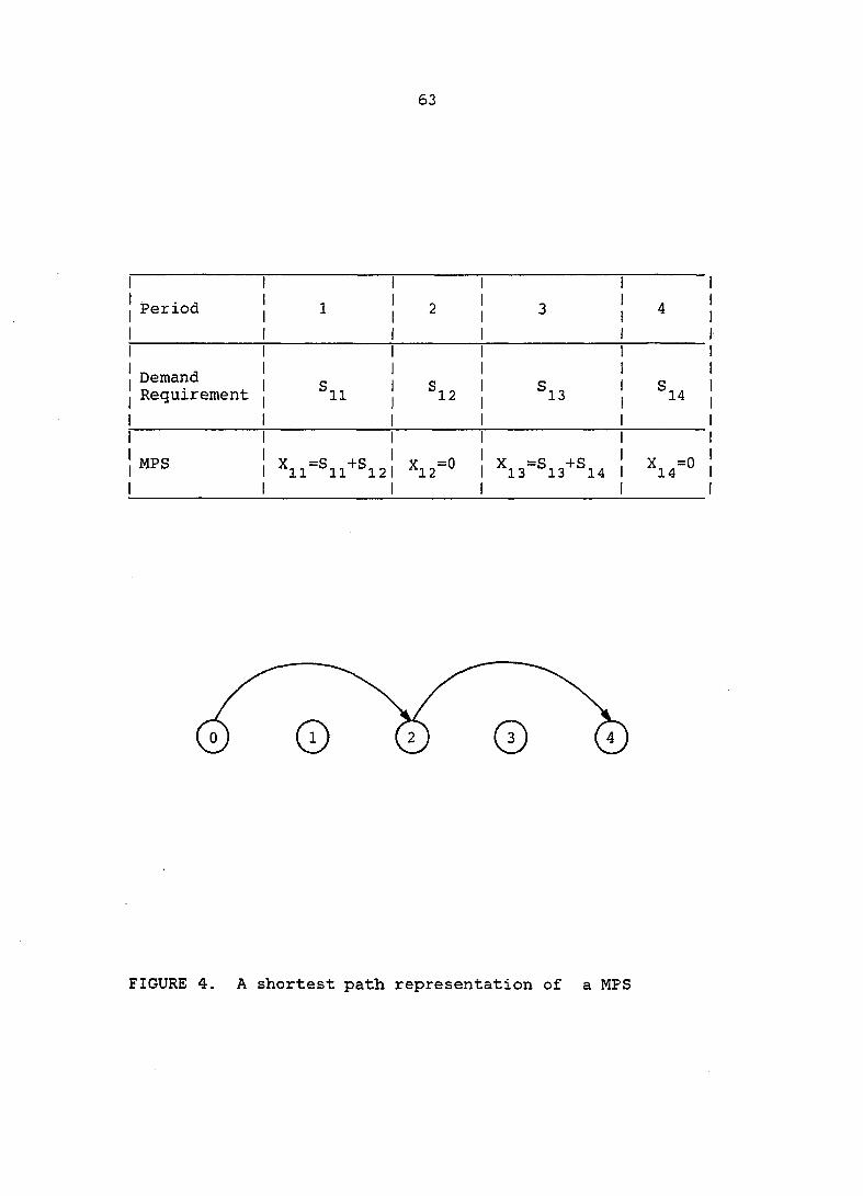
53
1 Period
1
1 1
1
2
1 1
1 ^ 1 1 1
4
1 Demand
1 1
1 1 1 1
c . Requirement ^11 j
1
®12 1 ^13 1
1 1
14
MPS
1
1
Xl2=0
1 1
1 Xl3=Si3+Si4 1
1 1
*14=0
FIGURE 4. A shortest path representation of a MPS
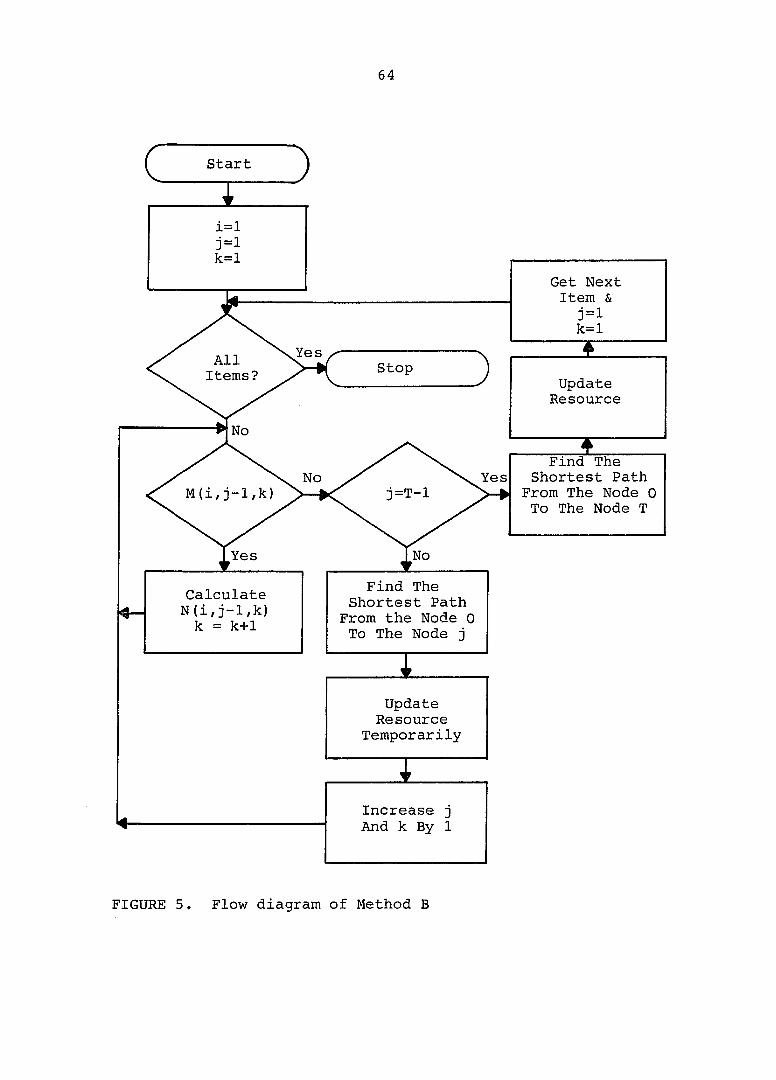
6 4
Start
Yes All
Items? Stop
No
Yes No j=T-l
No Yes
Get Next Item &
j = l k=l
Find The Shortest Path
From The Node 0 To The Node T
Update Resource
Calculate N(i, j-l,k) k = k+1
Increase j And k By 1
Update Resource
Temporarily
Find The Shortest Path
From the Node 0 To The Node j
i=l j=l k=l
FIGURE 5. Flow diagram of Method B

55
rules. But there is no restriction for splitting in method
C to simplify the problem. Method C is incorporated with
the TMPS which is derived from Method A or Method B. A
mechanism to derive a random sampling TMPS is defined as
follows to describe Method C.
Sampling procedure Available capacity in each
period is determined from the capacity limit and the
required capacity, which is calculated from the load profile
of each end item and the proposed TMPS. The process to
generate a TMPS is performed in the following ways:
Case A. When there is overload
The total cost of a TMPS can be primarily decreased by
reducing overload cost, but there is a trade-off between
overload cost and holding cost. When production quantity
shifts leftwards, the overload cost may be reduced, but
inventory holding cost is increased. The sampling process
is performed as follows.
1. Determine the period spans where there is
overload or underload during the scheduling
period. If there are several underload and
overload spans, the selection of a consecutive
underload and overload span is determined
randomly.
2. An Origin Period (t=OP) during the overload
period span is determined randomly.

66
3. A Destination Period (t=DP) during the underload
period span which is the previous span of the
above overload period span is determined
randomly. Item number (i) is also determined
randomly. When the corresponding production
quantity is zero, all items and periods during
the overload period span are scanned to search a
positive production quantity. If the search
fails, repeat 1, 2, and 3 until the predetermined
counter number is reached.
4. A production quantity is determined by dividing
the available capacity at period DP by Lij
(j=l,2,3) where the value j is determined
randomly. The Left Shift Quantity (LSQ) is the
smaller quantity between this production quantity
and corresponding scheduling quantity
5. Shift the amount of LSQ in the period OP to the
period DP leftwards.
5. Modify the previous TMPS and calculate the total
cost of the new generated TMPS.
Case B. When there is no overload
The total cost of a TMPS can be decreased by reducing
the inventory holding cost and the setup cost. The
inventory holding cost only can be decreased by shifting the
production quantity rightwards, but right shifting should

67
not be allowed to generate a penalty cost. The sampling
procedure is performed as follows.
1. For every end item and scheduling period, find
positive Bit.
2. For each above case, find the maximum right shift
period which does not generate delay penalty
cost.
3. Select the item number (i) and the Origin Period
(t=OP) randomly. Right Shift Quantity (RSQ) is
the smaller quantity between Eit and Xit.
4. Modify the previous TMPS and calculate the total
cost of the new proposed TMPS.
Tree search method Method C is a myopic search
method to get a better TMPS from a good W-W type TMPS. An
improved TMPS is selected among random TMPSs of size n.
Random sampling is performed from the above improved TMPS
until predetermined number of levels is reached (See Figure
6). Method C is described as follows (Figure 7).
Step 1. Start from a good W-W type TMPS. Method A or Method
B can be used to determine a good W-W type TMPS.
Step 2. If the search level is a predetermined number, then
stop the process. The best schedule which is found
so far, is the proposed TMPS of Method C.
Step 3. Generate random TMPSs of size n by using the above
random sampling procedure.

58
Step 4. Choose the best TMPS among random TMPSs of size n.
Step 5. Update the schedule and all the related statistics,
i.e., the available capacity and all cost
statistics.
Step 6. Branch from the best TMPS and increase the search
level by 1. Then, go to Step 2.
Four independent random samples of the TMPS are
selected and the predetermined number for the search level
is also four in the experimental test of this research.
Characteristics of the Methods
Several characteristics of the methods to develop a
TMPS can be described as follows:
1. Capacity target/capacity limit is considered in
order to develop the best MPS.
2. The total cost function includes setup, holding,
overload and shortage penalty cost. The trade
off between the capacity and the due date is
considered.
3. The load profile is used as a tool for the master
production scheduling. This is possible because
the lead time of each end item is short. The
firm planning period need not be included,
because of a quick response to customer orders.
Manual intervention is possible where there is a

6 9
W-W Type Schedule
Non W-W Type Schedule
Non W-W Type Schedule
Non W-W Type Schedule
FIGURE 6. Tree search method

7 0
Start
Yes Stop
No
yT Pre-determined
Level Number
n Samples
From
W-W Type TMPS
n Samples From The Selected Best TMPS
Select The Best TMPS Among n Samples
FIGURE 7. Flow diagram of Method C

71
trade off between the capacity and the due date;
therefore interactive programming is favorable to
implement this approach. The master production
scheduling system under a GT based MRP system can
be interactive.
4. This approach can be used even though there is no
total production planning and inventory control
system. That is, an MPS alone system is
possible, if the load profile and other auxiliary
system parameters are determined manually.
5. The use of a RCCP function is not necessary
because the capacity target /capacity limit is
already considered in order to develop the MPS.
6. If the lead time and queuing time are short, this
approach can be used for the master production
scheduling system of the other environments.
7. The scheduling procedure considers the time
phasing effect of the production load.
8. This approach is capacity-sensitive in developing
the TMPS, therefore it will make up for the
capacity-insensitivity of MRP.

72
CHAPTER 5. EXPERIMENTAL TEST
Aggregate Production Plan
Illustrative example
An illustrative example, where the total number of
items is 2 and the planning horizon is 6, is given as
follows. The critical resources are a machine in a GT cell
and a supporting department. The sales requirements which
are given in Table 5 are generated from the equation (5.1)
where o = 67 and a = 125, and the average demand is 300 for
item 1 and 400 for item 2.
TABLE 5. Demand requirements for APP problem
KPERIOD 1 ITEM
1 1 1 N
1 1 2 . 1
1 1 3 1
1 1 4 1
1 1 5 1
1 1 1 6 1 1 1
1 1 1 111 1
|302
1 1226 1
|393
1
|413
1 |445 1 1 1
1 2 1274 1 1
|410
1 "
|405
1 I
|384
1 1
1452 1 1
1532 1 1 1 I 1
All weighting factors which are presented in Table 5
are independent of the time period, and the highest
weighting is given to the over utilization of a machine.
The corresponding deviation variable can be found from the
corresponding index of the weighting factors. The choice of

73
these values can be best determined by the management
function based on the relative importance of the goals.
TABLE 6. Weighting factors of each goal
Variable
Weighting Factor I 0.3|0.110.8 |0.1 |0.7|0.2|0.5 |0.1 |
I I I I I I I I I I I I I I I I I I
TABLE 7. Values of cost parameters
Kitem 1 1 Variable\|
1 1 1 1 2 1 1 1
1 1 1 1 1 1
1 1
1 CM. I X }
2 1 4 1 1 1
1 CV. 1 1
1 1
5 1 10 1 1 1
The value of C^, CM^, and CVfor each item are given
in Table 7. The maximum inventory amount (L) is 16500 and
the regular available capacity of the critical department is
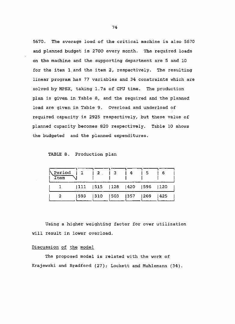
74
5570. The average load of the critical machine is also 5570
and planned budget is 2700 every month. The required loads
on the machine and the supporting department are 5 and 10
for the item 1 and the item 2, respectively. The resulting
linear program has 77 variables and 34 constraints which are
solved by MPSX, taking 1.7s of CPU time. The production
plan is given in Table 8, and the required and the planned
load are given in Table 9. Overload and underload of
required capacity is 2925 respectively, but these value of
planned capacity becomes 820 respectively. Table 10 shows
the budgeted and the planned expenditures.
TABLE 8. Production plan
Period 1 Item 1
.. 1 1 1
\l
1 1 2 . 1
1 1 3 1
1 1 4 1
1 1 5 1
1 1 1 6 1 1 1
1 1 1
1111 |515 1 128 1420 |595 1120 1
1 2 1
1593 1
|310 1
|503 1
|357 |269 1
|425 1 ( 1
Using a higher weighting factor for over utilization
will result in lower overload.
Discussion of the model
The proposed model is related with the work of
Krajewski and Bradford (27); Lockett and Muhlemann (34).

75
TABLE 9. Required and planned load
j Load 1 1 1
1 ! 2
1 1 3
1 -• 1 4
1 1 5
1 1 1 6 1
1 Required 13295 15610 15180 15805 16585 17545 1
1 Planned 16485 15675 15670 1
15670 1
15670 1 r
00 o
TABLE 10. Budgeted and planned expenditure
j Cost 1 1 1
1 1 2
1 1 3
1 1 4
1 1 5
1 1 1 6 1
1 Budgeted 12700 12700 12700 12700 12700 12700 1
1 Planned 12913 1
12698 1
12702 1
12700 1
12700 1
11940 1 1 1
The variables and the system parameters are defined for a GT
environment. There are several differences between this
research and the other works. Even though the solution
method is that of Lockett, the environment of the problem
and the flexibility of the model are quite different. The
proposed model includes a large number of managerial factors
for decision making and can handle many critical resources.
Therefore, the proposed model is more practical and
realistic than the other models. This model is formulated
for a GT environment, but can be easily revised for other
environments.

76
Existing software, MPSX, can be used to solve this
model. The above example of the small size problem included
77 variables and 34 constraints. The total number of the
variables and the constraints in the proposed model is not
small, but the program logic of MPSX provides for a maximum
of 16,383 rows (and virtually an unlimited number of
columns) on a 1024 K system (22), Therefore, the capacity
of MPSX releases the restriction of the problem size under
the real environment.
A small problem was given and encoded manually for the
example. Yet the encoding task for the input of MPSX for a
larger problem would be a tremendous task, and the
interpretation of the output of MPSX would require much time
if the number of constraints and variables is large.
Therefore, a matrix generator and report writing program are
desirable to implement this model for a real situation.
Critical resources are included in the model instead of all
resources. It is shown that MPSX can be used to solve the
proposed problem. The model does not allow the backlogging
case, but backlogging is possible, if the balance equation
of the constraints is changed.
How is it possible to get the input data for the matrix
generator or MPSX? The prerequisite of implementation of
this model is the existence of the standard performance data
such as load profiles and cost parameters. The decision

77
variables can be determined by a decision maker, but the
standard performance data which can be derived from the
accumulated historical data are not easy to determine.
These standard data should be accumulated systematically or
given by another related system.
The relative importances of the conflicting goals are
not easy to determine. The most suitable decision maker to
determine the weighting factor is the manager who can
control and compromise the conflicting objectives in each
function. There are many ways to determine these weighting
factors. For example, when they are trying to determine the
weighting factors for overload and over-expenditure, and if
the cost of overload is expensive, then they may give higher
weighting for overload. The amount of the weighting factor
depends on the overload cost and the expenditure caused by
loaning. If this model is incorporated with qualitative
managerial factors, this model is a very dynamic approach to
the production planning problem where there are conflicting
objectives.
Master Production Schedule
Test problem generation
A number of test problems are generated to test the
proposed methods. The test problem parameters include the
pattern of demand, the pattern of capacities and the setup
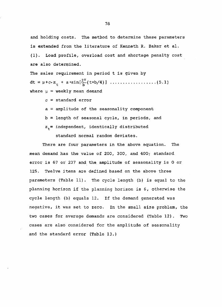
78
and holding costs. The method to determine these parameters
is extended from the literature of Kenneth R. Baker et al.
(1). Load profile, overload cost and shortage penalty cost
are also determined.
The sales requirement in period t is given by
dt = y+a«z^ + a •sin[-^(t+b/4) ] (5.1)
where y = weekly mean demand
a = standard error
a = amplitude of the seasonality component
b = length of seasonal cycle, in periods, and
z^= independent, identically distributed
standard normal random deviates.
There are four parameters in the above equation. The
mean demand has the value of 200, 300, and 400; standard
error is 57 or 237 and the. amplitude of seasonality is 0 or
125. Twelve items are defined based on the above three
parameters (Table 11). The cycle length (b) is equal to the
planning horizon if the planning horizon is 6, otherwise the
cycle length (b) equals 12. If the demand generated was
negative, it was set to zero. In the small size problem, the
two cases for average demands are considered (Table 12). Two
cases are also considered for the amplitude of seasonality
and the standard error (Table 13.)

79
TABLE 11. A pool of all test items
1 ITEM
1 NO y
1 1
1 ^ 1
1 1
a 1
1 1 200 1 0 1
671
1 2 200 1 0 1
237 1
1 3 200 1125 1
671
1 4 200 1125 1
2371
1 5 300 1 0 1
671
1 6 300 i 0 1
2371
1 7 300 1125 1
67 1
1 8 300 1125 1
237 1
1 9 400 1 0 1
671
1 10 400 1 0 1
237 1
1 11 400 1125 1
671
1 12
1
400 1125
1
237|
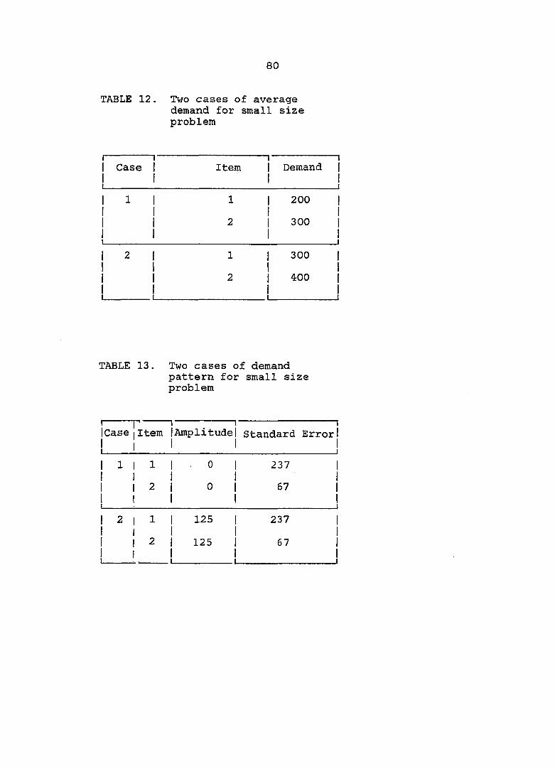
80
TABLE 12. Two cases of average demand for small size problem
1 1 1 Case 1 1 1
Item "1 ' " 1
1 Demand | 1 1
1 1 1 1 1
1 1 200 1 1 1 1 1
1 1 1 1
2 1 1 1 300 1 1 1
1 2 1 I {
1 1 300 1 1 i 1 1
1 1 1 1 1 1
2 1 1 1 400 1 i 1 1 1
TABLE 13. Two cases of demand pattern for small size problem
1 lease Item
1 1 1Amplitude! 1 1
1 Standard Error 1
1 1 1 1 . 0 1 1 1
237 1
2 1 1 1 0 1 1 1
57 1
1 2 1 1 125 1 1 1
237 1
I
2 1 1
1 125 1
1 1
67 1
1

81
TABLE 14. Summary of test data
1 1 Problem
|Size(N)
1
Small Medium
1 1
Large j
1 Group of
1 Items
2,5
4,7
6,9
8,11
1
4
7
,2,3,4,5,6
,5,6,7,8,9
,8,9,10,11,12
1,2,...,12 1
jScheduling
iPeriod(T) 6,12 18 24 1
ICost
j Structure 3 Cases 3 Cases 3 Cases j
1 Capacity
1 Limit 3 Cases 3 Cases 3 Cases j
1 Problem
1 Set 72 27 9 1
1 Replication 5 5 5 1
[Total
[Number of
1 Problem Set
L
360 135
...
45 1
1

82
In the medium size problem, 6 items are selected. The
selection is made to represent the all possible combinations
of all demand varieties. The large size problem includes
all 12 items. .Table 14 shows the summary of the test
problem sets.
Five replications were made for each problem by
changing the seed of random number generator for the demand
pattern and the load profile. Only the case of constant
capacity, which represents a stable status of a company, was
studied. The required capacity is calculated from the load
profile and the demand requirements. The capacity limit is
represented in terms of the ratio of allowable capacity to
required capacity. The ratio 1.1, 1.2, and 1.3, which are
used as the capacity limit, corresponds to a capacity
utilization of 90.9%, 83.3%, and 75.9% respectively. There
are four cost parameters, that is, setup, holding, overload,
and penalty cost. The last three costs are referenced from
real data in industry (52, 53, 54)^, and the setup cost is
determined systematically. The holding, overload, and
penalty cost are 1.38/item*period, 15/unit*period, and
695/item*period respectively. For testing purposes, it was
assumed that the setup cost is independent of time period.
^ The cost ratios are arbitrarily defined and set by the author following personal communication with a master scheduler in industry.

83
Instead of the ratio of the setup cost to the holding cost,
both setup and holding costs are related with the optimal
solution. EOQ time supply of each product has been used to
represent the set of setup and holding costs (1). The
selected EOQ time supply is one, three, and six periods.
Three cases were considered for each problem size to
represent the various cases of the problem. Table 15 shows
the number of items in the problem size and the EOQ time
supply. Setup costs are determined from the selected
holding cost and the EOQ time supply (Table 15). Table 17
shows the ratio of the setup cost to the holding cost. The
spectrum of the ratios covers the band of the ratios which
are used in industry and that used by other author (8).
The load profile is determined from the uniform random
number generator which gives an integer between 0 and 9.
The selected sample problems will be diverse and a represen
tative problem set to evaluate the proposed methods.
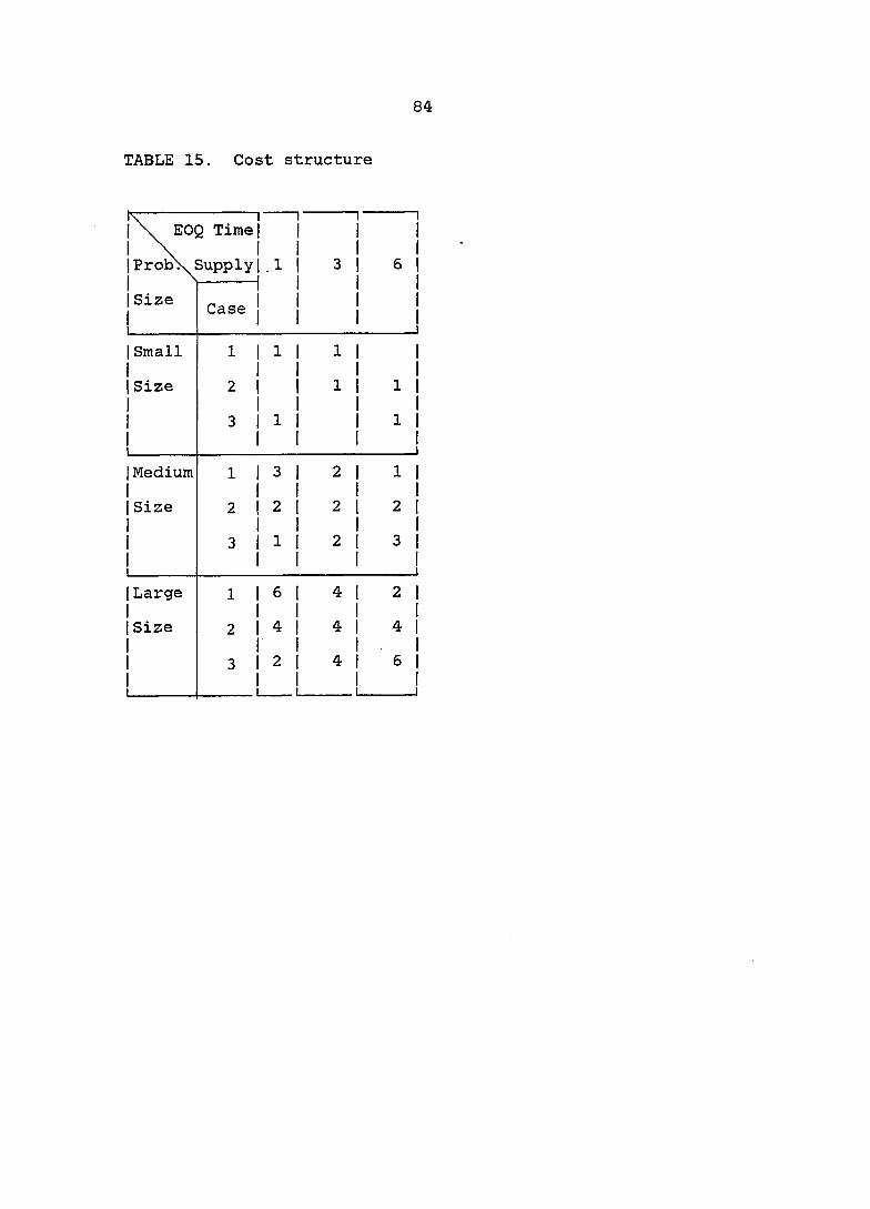
TABLE 15. Cost structure
IV Il 1 1 1\ EOQ Time| | | |
1ProbV Supply 1.1 | 3 | 6 |
1 Size Il 1 1
Case
1 Small
iSize
1 1 1 1 1 1 1 1 1 1 1
2 1 1 11 11 1 1 1 1
3 1 1 1 1 11 1 1 1 1
1 Medium
1 Size
1 1 3 1 2 1 11 I I I !
2 12 1 2 1 2 1 1 1 1 1
3 1 1 1 2 1 3 1 1 1 1 1
1 Large
1 Size
1
1 1 6 1 4 1 2 1 1 1 1 1
2 1 4 1 4 1 4 1
3 1 2 1 4 1 6 1
Il 1 1

85
TABLE 16. Setup cost summary
1 \ EOQ Time 1 1 1 1 1 1
1 AvrXSupply Small 1 1 1Medium| 1 1
Large j
1 Demand \. 1 1 1 1 1 1
1 200 138 1 1242 1 1 1
49681
1 300 207 1 1863 1 1 1
7452 1
1 400
1 1
276 1 2484 1 1 1 1 1
99361
TABLE 17. S/H summary
EOQ Time
AvrXSupply Small Medium Large
Demand
17.3 69.0 200
29.5 103.5 300
34.5 138.0 400 3.8

86
Evaluation measure
The ratio (R) of the total cost which is calculated
from the proposed TMPS to the solution standard is used as
an evaluation measure. The total cost includes setup,
inventory, overload, and penalty cost. Solution standard is
the near optimal cost which is derived from the small order
statistics by using the method of Weissman (58). When there
is a large sample, then small order statistics can be used
to derive the left threshold of the population distribution.
Suppose a distribution function (df) F has a finite left
threshold y. A confidence interval can be derived by using
the order statistics T^<T2<...<T^ from a sample whose df is
F. The pivotal ratio
T -y / k-1 T -y
"k = TTZf /// .Z, log (k>3) 1 / 1=1 1
is the basis for the confidence interval for y. Given a
confidence level r and a lower error-probability
P (0<r+P <1), determine W = W (P ) and W = W (r+P ). • L J . J . J . ^ j \ A .
k- 1 W (p) is the quantiles of W = Y / j Y., where the Y. are •K jc K""l J T i i
i—x
the order statistics from an exponential sample of size k-1. Put
G(y) = log ^k , H{y) = log '^k ^ (y<T ) , i=2 T^-y T^-y

87
and = W^/(l-W^) (i=l,2). Then the set
{jj: VI^<VI^<V}^} = {y; U^G (y) <H (y) <U2G (y) } is an asymptotically
exact (as n ->• 0° and k/n 0) confidence set for y with
confidence level r for df F which satisfies
lim fr^ = '°>°»
xf 0
for every C>0. Unfortunately, this does not guarantee the
solution, i.e., there may be null set for this equation.
"Median-unbiased" estimator of y (i.e., estimators which
are too large with 50% probability and too small with 50%
probability) when r is .50 is used as a solution standard.
The df F near the left threshold is assumed to satisfy the
regularity condition. Three hundred random total costs of
TMPS is generated from a good W-W type schedule which is
derived from Method A or Method B and the smallest 10 total
costs among 300 are used as the small order statistics.
A quick estimate of a, suggested by Weiss, was
used (58) .
® S / / ml
where k=10, m=4. As the value of a increases beyond 1,
it is known that the approach of Weissman becomes less
reliable. When the value of a is larger than 1.1, the

88
smallest value among all samples is used as the evaluation
criteria.
Discussion of the experimental tests
Experimental procedure is shown in Figure 8. Method A
and Method B are applied to each test problem and develop
TMPS A and TMPS B respectively. Method C uses a good W-W
type TMPS which is better between TMPS A and TMPS B and
generates TMPS C. Each TMPS is associated with a cost which
will be compared with a near optimal cost.
The evaluation measure, when the total number of end
item is 2 and the amplitude of seasonality is 0 or 125, is
shown in Table 18. The measures in the Tables represent the
values of R multiplied by 100. Method B is superior to
Method A when there is seasonality in demand. The
evaluation measures for all types of the test problem sets
are given in Figure 19. The results show that Method B is
better than Method A for the small size problem set, but
Method A is better than Method B for the medium and large
size problem sets. The average cost ratios are 1.25, 1.55,
and 1.05 for Method A, Method B, and Method C, respectively.
As the number of items is increased. Method B becomes less
reliable. The defect of Method B is that scheduling is
performed item-by-item. Therefore, all items can not be
considered simultaneously in each scheduling period. An MPS
which is derived from Method B depends on the priority of
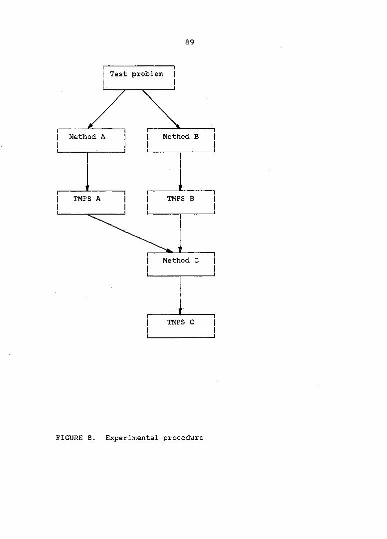
89
I Test problem |
Method B I Method A
I I TMPS A I I TMPS B
Method C
I I
' •
1 TMPS C I
FIGURE 8. Experimental procedure

90
TABLE 18. R for constant and seasonal demand patterns
1 1 1 1 N i T 1 1 1 1
1 Method 1
1 Capacity Ratio
1
1 1 1 1 1 1 1 1 1
1
1 1 .1 1.2 1 3 Average j
1 1 1 1 1 1
a 1 1
0 125 0 125 0 125 0 125 1
1 2 1 6 1 1 1
A 1 1
121 184 129 142 145 116 132 147 1 1 1 1 1 1 1 1
1 B 1
1 127 133 145 118 125 110 134 120 1
1 1 1 1 1 1 1 1
1 c 1
1
108 108 105 107 108 106 107 107 1
1
1 2 1 12 1 1 1
A 1 1
155 157 118 205 112 154 128 172 1 1 1
1 1 1 1 1
1 B 1
1 171 154 147 141 139 119 153 142 1
1 1
1 1 1
1 1 1 1 1
C 1
1
114 120 103 124 103 102 107 115 1
1 Average| 1 1
A 1 1
138 170 123 173 128 135 130 159 1 1 1 1 1 1 1
1 B 1
1 149 .148 145 129 132 114 143 131 1
1 1 1 1 1 1 1 1
1 C 1
1 109 106 103 109 104 104 105 105 1
1
end items. Therefore, Method B becomes less reliable as the
total number of end items increases. As the capacity ratio
decreases, i.e., the utilization of capacity increases, all
methods become less effective. It is interesting that these
phenomena are similar to that of other heuristics under
different environments (49).

91
TABLE 19. Summary of evaluation measures
1 1 1 Number|Scheduling 1 1
Scheduling 1
Capacity Ratio |
i 1 1 of 1 Period 1 1
Method
1 1 1 Items 1 1 1
1.1 1.2 1.3 Avr. i
1 2 1 6 1 ]
A 152 135 130 1391 I I 1 1 1 1
B 130 132 118 126 1 1 1 1 1 ! 1
C 108 106 107 1071
1 2 1 12 1 1
A 156 161 133 1501 1 1 1 1 1 1
B 167 144 129 1461 1 1 1 1 1 1
C 117 113 102 1111
1 6 1 18 1 1
A 110 113 107 1101 1 1 1 1 B 180 162 146 163 1 1 1 1 1 1 1
C 106 102 101 103 i
1 12 1 24 1 1
A 104 104 101 1031 1 1 1 1 1 1
B 253 226 201 2271 1 1 1 1 1 i 1 1
C 103 103 100 102 1
A 130 128 117 1251
1 Average B 182 166 148 1651
1 1
C 108 106 102 1051
1

92
TABLE 20. Distribution of evaluation measures
r 1 |N |T
1 1
\R 1.0 1.1 1.2 1.3 1.4 1.5
VO t—1
1.7 1.8 1.9 2.0 < 1
Total 1
1 1 1
A 72 28 16 7 6 6 5 5 2 3 4 26 180 1
|2 1 6 1 1
B 74 34 15 11 11 6 6 3 5 3 1 11 180 1 1 1 1 1 1 1
C 140 19 11 3 1 180 1
1 1 1 1
A 38 46 19 7 9 7 6 10 7 3 2 26 180 1
|2 112 1 1
B 26 28 29 20 17 12 5 9 9 3 4 18 180 1 1 1 1 1 1 1
C 71 65 20 6 7 3 180 1
1 1 1 1
A 42 53 20 7 4 5 1 1 1 1 135 1
|6 118 I 1
B 11 19 16 19 14 8 11 4 2 4 1 26 135 1 1 1 1 1 1 1
C 63 58 12 2 135 1
1 1 1 1
A 20 22 3 45 1
112|24 1 1
B 1 6 1 6 3 5 2 21 45 1 1 1 1 1 i 1
C
, . 1
25 18 2
1
45 1
1
The distributions of R for each category are given in
Table 20 When the number of items is 2 and scheduling period
is 6, frequencies between 1.1 and 1.2 are 16 for Method A.
Table 21 classified evaluation measures by cost structure.
It is difficult to conclude in the lump which cost structure

93
TABLE 21. Evaluation measures by cost structure
1 1 Number 1 of 1 Items
Scheduling
Period
Scheduling
Method
1 Cost Structure]
Case 1
1 2 3 1
1 2 6 A 155 138 125 1
B 115 147 116 1
C 100 121 100 1
1 2 12 A 183 129 138 1
B 190 123 128 1
C 118 107 107 1
1 6 18 A 117 110 103 1
B 165 132 192 1
C 103 104 102 1
1 12 24 A 105 101 102 1
B 235 215 230 1
1. 1 1
C 104 101 101 1

94
TABLE 22. Characteristics of solution standard (Frequency)
1 1 Number 1 of 1 Items
1 Scheduling 1
1 Period |
1 X
1 Improved |
1 a>l.l a<l.l|
1 X
Unimproved
a>l.l a<l.1
Total
1 2 6 1 1
0 12 44 1 1
49 75 0 180
1 2 12 1 1
13 58 78 1 1
10
CO CO
180
1 6 18 1 1
4 45 71 1 1
5 5 . 3 135
1 12
1 1
24 1 1
0 22 23 1 0 0 0 45
1 Total 1 1 1 1 1
17 138 216 1
1 1
55 98 5
1
540
gives a good or bad solution. When the total number of
items is 12 and scheduling period is 24, it can be said
that, if the portion of small EOQ time supplies is large,
then the result is poor. Table 22 and Table 23 show the
frequencies of the lower bound and the ratios of each case.
"Improved" implies that the lower bound is improved from a
good W-W type MPS. "Unimproved" implies that the lower
bound is the smaller value between the total costs of Method
A and that of Method B. To find the lower bound, 40% of al]
problems used Weissman's approach and 28.8% of all problems
used the smallest value among all samples. Among the test

95
TABLE 23. Characteristics of solution standard (Ratio)
1 1 Number 1 of 1 Items
Scheduling
Period X
Improved
a>l.l a<l.l
1 Unimproved |
X a>l.l a<l.l
Total!
1 2 6 0 6.7 24.4 27.2 41.7 0 1 100 1
1 2 12 7 .2 32.2 43.4 5.6 10.0 1.7 1 100 I
1 6 18 3 .0 34.0 52.6 4.4 3.7 2.2 1 100 j
1 12
1 1
24 0 48.9 51.1 0 0 0 1 100 j
1 Total
1
3 .2 25.6 40.0 12.0 18.1 1.1 1
1
100 {
problems, 31.2% have not improved the lower bound from a
good W-W type TMPS. This portion may be caused by poor
estimation procedure of the lower bound or good heuristics
of master production scheduling. X implies that a can not
be calculated because of insufficient number of sample data.
When the lower bound is not improved and a is less than 1.1,
this implies that there is a null set of solutions in the
interval estimation of Weissman. These figures show that
the frequencies of application of Weissman's approach for
large size problem is more than that for the small and
medium size problems.

96
TABLE 24. A Wilcoxon's signed-rank test for cost factors
1 [Number 1 of 1 Items
1 Scheduling]
Period j
Setup
Cost
1 1 Holding
1 1 Cost 1
1 1 1 Overload | 1 1 1 Cost 1
A ; B 1 1 A ; B 1
1 A : B 1 1 1
1 2 6 1 < 1 > 1
1 > 1 1 1
1 2 12 1 < 1 > 1 1 1
1 6 18 1 < 1 > 1 1 1
1 12
1 1
24 1 < 1 > 1
1 < 1 1 1
1 Total 1
1 1
< 1 > 1 1 1 1 1 1
Setup cost, holding cost, and overload cost are
observed separately. Method A and Method B give a paired
data of setup, holding, and overload cost for each test
problem. The Wilcoxon's signed-rank test is performed for
the paired data of three costs to test the different effect
of Method A and Method B. The null hypothesis is Ma=Mb
and the alternate hypothesis is MafMb where Ma is the
median of the cost distribution from Method A and Mb is the
median of the cost distribution from Method B. Equality in
Figure 24 shows that the null hypothesis H is accepted and
97
inequality means that the alternate hypothesis H is
accepted at 0.05 level of significance respectively.
Average setup cost from Method A is less than that from
Method B and holding cost from Method A is larger than that
of Method B in any case. When the total number of items is
2 and the scheduling period is 6, the average overload cost
from Method A is larger than that from Method B, but when
the problem size is the largest, the results are reversed.
The other problem sets show that there is no significant
difference between the overload cost from Method A and that
from Method B. In the overall sense, there is strong
evidence that the setup cost from Method A is less than that
from Method B and holding cost from Method A is larger than
that from Method B. There is no significant difference
between Method A and Method B for overload cost.

98
CHAPTER 6. SUMMARY AND CONCLUSION
There are several evidences that the importance of
master production scheduling is increasing and GT is the
future oriented manufacturing concept. A master production
scheduling system is discussed under a GT cell where MRP can
be used as a production planning and inventory control
system. An aggregate production planning problem where
there are multiple conflicting objectives is considered, and
a practical model is proposed. Traditional lot sizing
problems do not consider the capacity limit or can not
violate capacity limit. Three heuristics for master
production scheduling are discussed when the capacity limit
can be violated, i.e., overloading and subcontracting are
allowed.
In Chapter 2, it was shown that goal programming can be
used to coordinate the conflicting objectives in the
aggregate production planning problem under a GT cell. The
master production scheduling problem is important, but
little attention is given to this area for following
reasons. '
1. Master production scheduling problems are diverse
in industry.
2. Master production scheduling system is complex
because of interrelation with other systems.
3. It is difficult to verify the proposed heuristics

99
for combinatorial optimization problems.
In Chapter 3 , the aggregate production problem is
characterized by the goal programming model. The master
production scheduling problem is formulated, but linear
programming or mixed integer programming are both
inefficient methods when there are many end items and the
scheduling period is long. This will justify the necessity
of heuristics for master production scheduling.
In Chapter 4, the goal programming model for the APP
problem is converted into a linear programming model and
three heuristics for master production scheduling are
discussed. Method A and Method B consider only a W-W type
schedule, i.e., demand requirement can not be split for the
production requirement. Method C allows splitting the
demand requirement in the production scheduling requirement.
Method A is the traditional period-by-period method and
Eisenhut's marginal cost reduction is used as a priority for
scheduling. Method B uses the shortest path algorithm and
tries to find a TMPS item-by-item. Method C uses a good W-W
type schedule which may be derived from Method A or Method B
and searches a TMPS by shifting the production quantity
leftwards or rightwards. The search pattern is similar to a
tree search scheme.
In Chapter 5, an APP problem where the total number of
end items is 2 and the planning horizon is 5 is selected as

100
an illustrative example. All input data are encoded
manually and the output of MPSX is discussed. Diverse sets
of the test problems are generated to verify the three
proposed heuristics for master production scheduling. There
are several system parameters of the test problem sets: the
demand pattern, the type of load profile, the capacity
limit, and cost parameters. These parameters are determined
systematically or referenced from the data of the industry.
Five hundred and forty test problems are generated and
Method A, Method B, and Method C are applied to each problem
respectively. The evaluation measure is the ratio of the
total cost from the proposed method to the near optimal
total cost which is derived from small order statistics.
The left threshold parameter of the distribution of the
population is determined by the method of Weissman. When
the Weissman's method can not be applied, the smallest value
among 300 random costs from sampled TMPSs is used as the
near optimal cost.
In Chapter 6, it is shown that Method B dominates
Method A where the problem size is small and the pattern of
demand requirement is seasonal. Method A is better than
Method B for the other cases. Method C can be only applied
for a hypothetical situation, i.e., there is no restriction
in splitting of the demand requirement for the production
quantity. There should be many variations for Method C but

101
a typical splitting scheme is shown in this research. All
heuristics become less reliable as the capacity utilization
is increasing. The average cost ratios of Method A, Method
B, and Method Ç are 1.25, 1.55, and 1.05 respectively. A
Wilcoxon's signed-rank test is performed to check the effect
of Method A and Method B for setup, holding, and overload
cost respectively.
The following areas are categorized as areas for
further research:
1. It is not surprising that Method B becomes less
reliable as the total number of items increases.
The defect of Method B is that scheduling is
performed item-by-item, therefore, all end items
can not be observed simultaneously in every
scheduling period. Therefore, TMPS from Method B
depends on the priority of end items and
investigation of the effect of the priority of
end items will compensate for the defects of
Method B. This research determines the priority
among end items randomly. The priority can be
determined based on average load of each end item
or lead time, etc.
2. The quality of the solution depends on the
quality of the lower bound, therefore, the
solution standard is important in the evaluation

102
process for a proposed heuristic. An optimal
solution is characterized by solution space which
depends on the restriction of production size in
the real situation. This research assumes that
there should be corresponding MPS for the near
optimal total cost which is derived from the
approach of Weissman. The analytical approach
for the optimal solution is ineffective when the
problem size is large, but it may be effective
when the problem size is small. When the lower
bound is determined based on small order
statistics, the quality of the lower bound
depends on the quality of sampling and estimation
procedure. Test results show that sampling
procedure and Weissman's approach are useful when
the problem size is large, but poor when the
problem size is small. The investigation of the
procedure to develop the lower bound is valuable
for the evaluation of heuristics for general
combinatorial problems. Among the total test
problems, 31.2% show no improvement of the total
cost of the W-W type MPS in this research. This
research does not verify whether the lack of
improvement comes from the lower quality of the
evaluation procedure or from the higher quality

103
of the proposed heuristics. There should be many
variations in the splitting scheme of production
requirement, but the research to derive W-W type
optimal MPS is required for the case where the
production requirement can not be split. The
analytical approach to get the optimal schedule
is possible for small problems, but the
analytical approach is ineffective for medium and
large size problem, therefore, this research only
used small order statistics to estimate the lower
bound to keep consistency for all size problem
sets.
3. The ratio of the calculated total cost to the
near optimal cost is used as an evaluation
measure. A "50%-unbiased median" estimator is
used as a lower bound. When the inference of the
lower bound is interval estimation instead of
point estimation, new evaluation measure should
be defined, and the evaluation scheme should be
different.
4. Even though the proposed heuristics allow for
cases of multi-resource problems, test problems
only handled the cases of single resource
problems. Therefore, it would be interesting to
test the proposed heuristics for the multi-
104
resource problems. The quality of the heuristics
for the master production scheduling system
depends on the input data structure of the
system, therefore, it is necessary to test the
proposed heuristics for other input data
structures to verify the proposed heuristics for
general cases.
5. There are several factors affecting the value of
R. Factors include demand pattern and cost
structures, capacity ratio, type of load profile,
etc. The contribution of these factors to the
value of R is not investigated, because it is not
easy to quantify the several factors.
Finally, several conclusions reached are as follows;
1. The aggregate production planning problem where
there are multiple objectives can be formulated
as a goal programming model. The proposed
aggregate production planning model can be used
effectively with a matrix generating and report
writing program for input and output of MPSX. If
the model is incorporated with the qualititive
managerial factors, the proposed model is dynamic
in the sense that any critical factors varying
with time can be included in the model.
2. Method B dominates the traditional period-by-

105
period Method A in the small size problem where
there is seasonality. But, Method A is better
than Method B in the other cases. Method C
dominates both Method A and Method B in all
cases, but there should be many variations and
restrictions in Method C. The average cost
ratios are 1.25, 1.65, and 1.05 for Method A,
Method B, and Method C, respectively. There are
defects in Method B which can be solved by
considering the effect of priorities among end
items. Method A allows delay penalty, but there
are no cases of delay for the selected test data.
Method A and Method B are used to find a global
optima, but Method C is used to search local
optima from a good W-W type schedule.
3. The aggregate production planning model and the
heuristics for master production scheduling are
proposed for a GT cell, but the APP model can be
easily revised for other environments, and the
heuristics for master production scheduling can
be used if the production lead time is short
under other environments.
4. The efficiency of the evaluation procedure
depends on the quality of the sampling procedure
and the estimation procedure. The solution

106
standard is determined from the Weissman's
approach or the smallest sample value among all
observations. The portion of Weissman's approach
is 40,0% and that of the other case is 28.8%.
Among the test problems, 31.2% show no
improvement from a good W-W type TMPS.
The expected value and the contributions of this
research are as follows;
1. Many decision factors and critical resources can
be included in the APP model for a GT cell.
2. A better methodology is presented to develop a
TMPS than the traditional "trial and error"
method; therefore, reduces the turn around time
for a master production scheduler to find the
best TMPS.
3. The possibility of eliminating the traditional
RCCP evaluation method is raised because the
available capacity can be negotiable during the
process of master production scheduling.
4. The frequency of running the MRP explosion logic
is decreased by providing a practical MPS.
Therefore, MRP can be well incorporated in the
production planning and inventory control system.
5. A communication tool for finalizing MPS is
proposed and the effectiveness of the total

107
production system is increased by improving the
procedure to develop a MPS which is the trigger
for the planning of the production support
function.
5. An optimization procedure for combinatorial
problems is shown and an evaluation procedure for
heuristics of combinatorial problems is proposed.

108
BIBLIOGRAPHY
1. Baker, Kenneth R., Dixon, Paul, Magazine, M. J., and
Silver, E. A. "An algorithm for the dynamic lot-size
problem with time-varying production capacity
constraints." Management Science 24, No. 16 (1978),
1710-1720.
2. Bowman, E.H. "Consistency and Optimality in Managerial
Decision Making." Management Science, 9, No. 2
(January 1953), 310-321.
3. Bradly, James V. Distribution-Free Statistical Tests.
Englewood Cliffs, New Jersey: Prentice Hall, Inc.,
1968.
4. Bruggeman, John T., and Merkin, Kathleen T. "Should
the Master Scheduler Consider Manpower a Constraint or
a Decision Variable ?" Annual Conference Proceedings
of APICS, (1979), 206-208.
5. Buffa, Elwood S. and Taubert, William H. "Production
Inventory Systems: Planning and Control. Rev.ed.
Homewood, Illinois: Richard D. Irwin, Inc., 1972
6. Burbidge, J. L. The Introduction of Group Technology.
New York: John Wiley & Sons, 1975.
109
7. Burt, John, "Master Production Scheduling
considerations for process industries." Annual
Conference Proceedings of APICS, (1980), 417-418.
8. Collier, David A. "The interaction of single-stage lot
size models in a material requirements planning
system." Production and Inventory Management 21, No. 4
(1980), 11-20.
9. Copeman, Russell. "The Master Schedule in Relation To
Customer Orders and Replenishment in a Distribution I
Environment." Annual Conference Proceedings of APICS,
(1977), 115-120.
10. Dannenbring, David Gareld. "The evaluation of heuristic
solution procedures for large combinatorial problems."
Unpublished Ph.D. Dissertation. Columbia University,
New York, 1973.
11. Darnton, William T. & Carton, James B. "Integration
Firm Orders and Product Forecast into the Production
Plan." Annual Conference Proceedings of APICS, (1976),
192-201.
12. de Hann, L. "Estimation of the minimum of a function
using order statistics." Journal of the American
Statistical Association, 76, No. 374 (1981), 457-469.
110
13. Dixon, P. S. and Silver, A. S. "A Heuristic Solution
Procedure For the Multi-Item, Single-Level, Limited
Capacity, Lot-Sizing Problem." Journal of Operations
Management, 2, No. 1 (1981), 23-39.
14. Dogramaci, A., Panayiotopolous, J. C., and Adam, N. R.
"The Dynamic Lot-Sizing Problem for Multi Items under
Limited Capacity." AIIE TRANSACTIONS, 13, No. 4
(1981), 295-303.
15. Eisenhut, P. S. "A dynamic lot-sizing algorithm with
capacity constraints." AIIE TRANSACTIONS, 7, No. 2
(1975) 170-175.
15. Everdell, Romeyn C., and Chamberlain, Woodrow W.
"Master scheduling in a multi-plant environment, master
scheduling The state of the art." Annual
Conference Proceedings of APICS, (1980), 421-429.
17. Caw, W. H. "The master schedule -- A key to
controlling the manufacturing environment" Annual
Conference Proceedings of APICS, (1979), 155-158.
18. Goodman, D.A. "A Goal Programming Approach to
aggregate planning of production and Work Force."
Management Science, 20, No. 12 (August 1974),
1559-1575.

Ill
19. Groover, Mikell P. Automation, Production Systems, and
Computer-Aided Manufacturing. Englewood Cliffs, New
Jersey: Prentice-Hall, Inc, 1980.
20. Huge, Ernest C. "Lead Time Management: Your Key to
Successful Master Scheduling." Annual Conference
Proceedings of APICS, (1978), 269-281.
21. Hyer, Nancy L. and Wemmerlov, Urban. "MRP/GT: A
Framework for Production Planning and Control of
Cellular Manufacturing." 13th annual meeting of AIDS,
2 (1981), 92-94.
22. "Introduction to Mathematical Programming System -
Extended(MPSX), Mixed Integer Programming(MIP), and
Generalized Upper Bounding(GUB)" ,Form No. GH
20-0849-3. White Plains, N.Y., International Business
Machines Corp., 1973.
23. Jââskëlainen V. "A Goal Programming Model of Aggregate
Production Planning." Swedish Journal of Economics,
71, No. 1 (1969) 21-29.
24. Jones, C. H. "Parametric Production Planning."
Management Science, 13, No. 11 (July 1967), 843-866.
25. Kohankie II, Robert W., Farrell, Waterbury and Morency,
Richard R. "Master Scheduling: An On-Going, Analytical

112
Process." Annual Conference Proceedings of APICS,
(1976), 202-213.
26. Kornbluth, J.S.H. "A survey of goal programming."
Omega, 1 , 'NO. 2 (1973 ) , 193 -205 .
27. Krajewski, L. and Bradford, J. W. "Resolving Multiple
Objectives in Master Production Scheduling."
Proceedings of AIDS Meeting Chicago, (October 1977),
372-374.
28. Lambrecht, M. and Vanderveken, H. "Heuristic
Procedures for the Single Operation, Multi-Item Loading
Problem." AIIE TRANSACTIONS, 11, No. 4 (1979),
319-326.
29. Lawrence, K. D., and Burbridge, J. J. "A multiple goal
linear programming model for coordinated production and
logistics planning." International Journal of
Production Research, 14, No. 2 (1976), 215-222.
30. Lee, S. M. Goal Programming for Decision Analysis.
Philadelphia: Auerbach Publishers, 1972.
31. Lee, S. M., Morris, R. L. and Franz, L. "Optimization
of the Fixed-Charged Problem with Multiple Objectives."
Proceedings of AIDS, Meeting Chicago, (October 1977),
584.

113
32. Lee, William B. and Khumawala, Basheer M. "Simulation
Testing of Aggregate Production Planning Models in an
Implementation Methodology," Management Science, 20,
No. 6 (February 1974), 903-911.
33. Leo, David I. "The Preparation and Maintenance of a
Valic and Realistic Master Production Schedule."
Annual Conference Proceedings of APICS, (1955) 103-141.
34. Lockett, A. G. and Muhlemann, A. P. "A problem of
aggregate scheduling; An application of goal
programming." International Journal of Production
Research, 16, No. 2 (1978), 127-135.
35. Malko, Richard W. "Master Scheduling; A Key to
results." Annual Conference Proceedings of APICS,
(1980), 408-412.
36. Maranka, Paul. "Master Schedule -- A user applies the
theory." Annual Conference Proceedings of APICS,
(1976), 162-179.
37. Mather, Hal. "Which Comes First, the Bill of Materials
or the Master Productioan Schedule ?" Annual
Conference Proceedings of APICS, (1982), 404-407.
38. Mather, Hal F., and Plossl, G.W. The MPS Management's
handle on the business. Decatur, Ga: G.W. Plossl &
114
Co., Inc., 1975,
39. Maurer, Herman H. Data Structures and Programming
Techniques. Englewood Cliffs, N.J.: Prentice-Hall,
Inc., 1977.
40. May, J. Gaylord. "The Master Schedule in Relation to
the Sales Forecast and Marketing." Annual Conference
Proceedings of APICS, (1977), 105-114.
41. McCormick, Robert. "Master Production Scheduling --
The fundamental Concepts." Annual Conference
Proceedings of APICS, (1980), 400-403.
42. Miller, Scott R. "Master Schedule — The Link between
Marketing and P.& IC." Annual Conference Proceedings
of APICS, (1979), 233.
43. Modigliani, F., Holt, C. C. and Muth, J. F.
"Derivation of a Linear Decision Rule for Production
and Employment." Management Science, 2, No. 2 (January
1955), 159-177.
44. Nellemann, David 0. "Production Planning and Master
Scheduling: Management's Game Plan." Annual Conference
Proceedings of APICS, (1979), 166-168.
45. New, Colin. "M.R.P. & G.T., A new strategy for
component production." Production and Inventory

115
Management 18, No. 3 (1977), 50-63.
46. Newson, E.F.P. "Multi-item Lot size Scheduling by
Heuristic, Part 1: With Fixed Resources." Management
Science, 21, No. 10 (1975), 1186-1193.
47. Orlicky, Joseph. Material Requirement Planning, The
new way of life in production and inventory management.
New York: McGraw-Hill Book Company, 1974.
48. Proud, John F. "Controlling the master schedule."
Production and Inventory Management 22, No. 2 (1981),
78-90.
49. Roll, Yaakov and Kami, Reuven. "A Heuristic Algorithm
for the Multi-Item Lot-Sizing Problem with Capacity
Constraints." IIE Transactions, 14, No. 4 (1982)
249-256.
50. Schwendinger James R. "Master Production Scheduling's
available to Promise Marketing's Key to Rational Order
Promising." Annual Conference Proceedings of APICS,
(1978), 316-330.
51. Smith, Linda M. "MRP-master schedule coordination."
Annual Conference Proceedings of APICS, (1978),
290-298.
52. Spencer, Michael S. "Scheduling Components for Group

116
Technology Lines (A New Application for MRP)."
Production and Inventory Management 21, No. 4 (1980),
43-49.
53. Spencer, Michael S. "Scheduling Group Technology Lines
for Optimum Productivity." MS81-982, Group Technology
User's Workshop, Dearborn, Michigan: Society of
Manufacturing Engineers(SME), 1981.
54. Spencer, Michael S. "Planning Applications of Capacity
Adjusted Run Size Calculations on Group Technology
Lines.", MS81-985, Group Technology user's workshop.
Dearborn, Michigan: Society of Manufacturing
Engineers(SME), 1981.
55. Steven, A.L. "The Material Manager's Role in Master
Scheduling in a Material Requirements Planning
Environment." Annual Conference Proceedings of APICS,
(1977), 121-132.
56. Suresh, Nallan C. "Optimizing intermittent production
systems through Group Technology and an MRP system."
Production and Inventory Management 20, No. 4 (1979),
76-83.
57. Taubert, William H. "A search rule for the aggregate
scheduling problem." Management Science, 14, No. 6
(February 1968), B343-B359.

117
58. Weissman, I. "Confidence intervals for the threshold
parameter. Part II: Unknown shape parameter." Commun.
Stat., 11, No. 21 (1982), 2451-2474.
59. Wight, Oliver W., and Plossl, G. "Designing and
implementing a MRP system." Annual Conference
Proceedings of APICS, (1970), 206-227.

118
ACKNOWLEDGEMENTS
I would like to express my gratitude to those people
who were instrumental in the completion of this
dissertation,
I wish to thank the members of my dissertation
committee, professors Eric M. Malstrom, John C. Even, and
Vincent A. Sposito for their thoughtful criticisms and
suggestions. I am indebted to professor Herbert T. David
for his valuable discussions in the estimation of unknown
shape parameters. I am extremely thankful to professor
Keith L. McRoberts, my committee chairman, for his guidance
and assistance in the research and his support throughout my
graduate study.
I am also indebted to many others who have helped in
this study. The brief discussions with professor William Q.
Meeker and Dorea C. Y. Chang were valuable in accomplishing
this dissertation. Several letters answering my questions
from Michael S. Spencer, William L. Berry, and Colin New
were also helpful for this research.
I am grateful to my parents and parents-in-law who have
faith in me. Finally, I am grateful for the patience and
continuous support of my wife, and to two beautiful
daughters who understood my absence when they wanted my
attention.

119
APPENDIX A: AGGREGATE PRODUCTION PLANNING SUBSYSTEM
Program List
PROGRAM INITIALZ MOVE(XDATA,'APP2') MOVE(XPBNAME,'GTMRP') CONVERT BCDOUT SETUP MOVE(XOBJ,'COST') MOVE(XRHS,'ZZ2') PRIMAL SOLUTION EXIT PEND

120
Input of MPSX
NAME APP2 ROWS N COST L R1 L R2 L R3 L R4 L R5 L R5 E R7 E R8 L R9 L RIO L Rll L R12 L R13 L R14 L R15 L R16 L R17 L R18 L R19 L R20 L R21 E R22 E R23 E R24 E R25 E R25 E R27 E R28 E R29 E R30 E R31 E R32 E R33
COLUMNS DPI COST .40000 R1 - 1.00000 DP2 COST .40000 R2 - 1.00000 DP3 COST .40000 R3 - 1.00000 DP4 COST .40000 R4 - 1.00000 DPS COST .40000 R5 - 1.00000 DP5 COST . 40000 R6 - 1.00000 DPll COST .90000 R9 - 1.00000 DP12 COST .90000 RIO - 1.00000 DP13 COST .90000 Rll - 1.00000 DP14 COST .90000 R12 - 1.00000

DP DPI: DPI: DPI] DPI: DPI: DPI: 111 111 111 112 112 112 113 113 113 114 114 114 115 115 115 116 116 121 121 121 122 122 122 123 123 123 124 124 124 125 125 125 126 126 Xll Xll Xll X12 X12 X12 X13
121
COST COST COST COST COST COST COST COST COST COST R15 R23 COST R15 R24 COST R15 R25 COST R15 R26 COST R15 R27 COST R15 COST R15 R29 COST R15 R30 COST R15 R31 COST R15 R32 COST R15 R33 COST R15 COST R7 R16 COST R7 • R17 COST
.90000 R13
.90000 R14
.90000 R15
.60000 R16
.50000 R17
.60000 R18
.50000 R19
.50000 R20
.50000 R21
.80000 R1
.00000 R22
.00000
.80000 R2
.00000 R23
.00000
.80000 R3
.00000 R24
.00000
.80000 R4
.00000 R25
.00000
.80000 RS
.00000 R26
.00000
.80000 R6
.00000 R27
.30000 R1
.00000 R28
.00000
.30000 R2
.00000 R29
.00000
.30000 R3
.00000 R30
.00000
.30000 R4
.00000 R31
.00000
.30000 R5
.00000 R32
.00000
.30000 R6
.00000 R33
.10000 R1
.00000 R9
.00000 R22
.10000 R2
.00000 RIO
.00000 R23
.10000 R3
3 5 1 3 5 1 3 5 1 3 5 1 3 5 1 3 5 7
10 1 7
10 1 7
10 1 7 10 1 7
10 1 7
10 5 1 5 5 1 5 5

122
X13 X13 X14 X14 X14 X15 X15 X15 X16 X16 X15 X21 X21 X21 X22 X22 X22 X23 X23 X23 X24 X24 X24 X25 X25 X25 X26 X26 X26
RHS ZZ2 ZZ2 ZZ2 ZZ2 ZZ2 ZZ2 ZZ2 ZZ2 ZZ2 ZZ2 ZZ2 ZZ2 ZZ2 ZZ2 ZZ2 ZZ2 ZZ2
ENDATA
R7 R18 COST R7 R19 COST R7 R20 COST R7 R21 COST RB R16 COST RB R17 COST RB RIB COST RB R19 COST RB R20 COST RB R21
R1 R3 R5 R7 R9 Rll R13 R15 R17 R19 R21 R23 R25 R27 R29 R31 R33
1.00000 5.00000 5.10000 1.00000 5.00000 5.10000 1.00000 5.00000 5.10000 1.00000 5.00000 10.20000 1.00000 10.00000 10.20000 1.00000 10.00000 10.20000 1.00000 10.00000 10.20000 1.00000 10.00000 10.20000 1.00000 10.00000 10.20000 1.00000 10.00000
2700. 2700. 2700. 1B90. 5670. 5670. 5570. 16500. 5670. 5670, 5670, 302, 393. 445. 410. 384. 532.
00000 00000 00000 00000 00000 00000 00000 00000 00000 00000 00000 00000 00000 00000 00000 00000 00000
Rll R24 R4 R12 R25 R5 R13 R25 R6 R14 R27 R1 R9 R28 R2 RIO R29 R3 Rll R30 R4 R12 R31 R5 R13 R32 R6 R14 R33
R2 R4 R6 RB RIO R12 R14 R15 RIB R20 R22 R24 R26 R28 R30 R32
5.00000 1.00000 2.00000 5.00000 1.00000 2.00000 5.00000 1.00000 2.00000 5.00000 1.00000 4.00000
10.00000 1.00000 4.00000
10.00000 1.00000 4.00000
10.00000 1.00000 4.00000
10.00000 1.00000 4.00000
10.00000 1.00000 4.00000
10.00000 1.00000
2700, 2700, 2700, 2457, 5570, 5570, 5570, 5570. 5570, 5670, 111, 225, 413, 274, 405, 452,
00000 00000 00000 00000 00000 00000 00000 00000 00000 00000 00000 00000 00000 00000 00000 00000
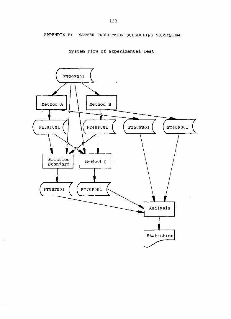
123
APPENDIX B: MASTER PRODUCTION SCHEDULING SUBSYSTEM
System Flow of Experimental Test
FT20F001
Method A Method B
FT30F001 FT40F001 FT50F001 FT60F001
Solution Standard
Method C
FT90F001 FT70F001
Analysis
Statistics

124
Program list
Method A
$JOB 'KIM',TIME=(2,03),PAGES=200 C C234567890 C C * I/O FILE SUMMARY **************************************** C C DD NAME DSN C C 1. INPUT FT20F001 K.I6467.DATA C C 2. OUTPUT FT30F001 K.I6467.RESA C C FT50F001 K.16467.MINA C Q ********* FILE DESCRIPTION ******************************** C C 1. K.16467.DATA C C 1) INO: TOTAL NUMBER OF END-ITEM C C TNO: TOTAL NUMBER OF PERIOD C C DSEED: SEED FOR LOAD PROFILE C C OCOST: OVERLOAD COST PER UNIT RESOURCE C C 2) IX: SEED FOR DEMAND REQUIREMENT C C 3) MEAN: AVERAGE DEMAND C C MVAR: STANDARD ERROR C C MAMP: SEASONAL AMPLITUDE C C 4) RATIO: CAPACITY RATIO (START) C C NCT: NUMBER OF CASES OF CAPACITY RATIO C (INCREMENT IS 0.1) C C 5) P(I), S(I), H(I) C C 2. K.16467.RESA C C 1) SUMTC: TOTAL COST FROM METHOD A C

125
C 2) WDT(I,T): C C 3) SKD(I,T): C C 4) AVARES(J,T): C C 3. K.16467.MINA C C 1) SUMTC: SUMS+SUMH+SUMP+SUMOC C C SUMS: TOTAL SETUP COST C C SUMH: TOTAL HOLDING COST C C SUMP: TOTAL PENALTY COST C C SUMOC: TOTAL OVERLOAD COST C C ******************* ARRAY DESCRIPTION ******************** C C ITEM(T): PRODUCTION REQUIREMENT AT TIME T, T=L, 2,..., TNO C C DT(I,T): WDT(I,T): PRODUCTION REQUIREMENT OF END ITEM I c AT TIME T C 1=1, 2,..., INO T=L, 2, TNO C C RESLIM(J,T): CAPACITY LIMIT, J=1 T=L, 2,...., TNO C C LP(I,1,K): LOAD PROFILE, 1=1,2,...,INO J=1 K=L,2,3 C C P(I): PENALTY COST PER UNIT OF THE ITEM I C PER PERIOD CARRIED. C C S(I): SET UP COST OF THE ITEM I C C H(I): CARRYING COST PER UNIT OF THE ITEM I C PER PERIOD CARRIED. C C WAIT(I,T): WAITING AREA FOR SCHEDULING, C 1=1, 2,..., INO; T=L, 2,..., TNO C C RQRES(J,T): REQUIRED RESOURCE, J=1 T=L,2,3 C C AVARES(J,T): AVAILABLE RESOURCE, J=1 T=1,2 ,26 C C W0RK(I,1): WAITING COST C C WORK(1,2): WAITING AMOUNT C C W0RK(I,3): MAX WAITING PERIOD FROM CURRENT PERIOD. C

125
C SWDT(I,2): SORTED ARRAY OF WAITING COST. C C SWDT(I,1): WAITING COST/COST INDEX C C SWDT(I,2): CORRESPONDING ITEM NUMBER. C C SKD(I,T): SCHEDULE OF END ITEM I AT PERIOD T,
1 = 1 , 2 , I N O T = l , 2 , . . . , T N O C CCCCCCCCCCCCCCCCCCCCCCCCCCCCCCCCCCCCCCCCCCCCCCCCCCCCCCCCCCCCCC c C VARIABLE DECLARATION C
INTEGER SW, CT,T,TNO,TO,TT,T1,T2(12),T3,TA,CTMT2,SI,SIMl INTEGER WORK,TEMP1,CHECK,TN02 REAL GGNQF,Y,LP REAL ITEM(24),OCOST,MTAVA,MTLI,MAB REAL RQRES(1,3),TEMP(12,1,3),E(12,26) DOUBLEPRECISION DSEED,NDSEED COMMON /ONE/ P(12),S(12) COMMON /TWO/ DT(12,24),H(12),U(12,24),SWDT(12,3) COMMON /THREE/ LP(12,1,3),SKD(12,24),AVARES(1,26) COMMON/FOUR/WORK(12,3),WAIT(12,2 4) COMMON/FIVE/CHECK(12) COMMON/SIX/WDT(12,24),DSEED,NDSEED,SUMD COMMON/SEVEN/OCOST
C DO 12345 IJKL=1,5 C INITIALIZATION
CALL CLOCK(IC) J=1 JN0=1 KN0=3 READ(20,10) INO,TNO,DSEED,OCOST
10 FORMAT(2I2,F20.7,F7.2) IF (TN0.GE.12) THEN
NTN0=12 ELSE
NTN0=TN0 ENDIF TN02=TN0+2 NDSEED=DSEED WRITE(6,30) INO,TNO,DSEED,OCOST
30 FORMAT(' INO,TNO,DSEED,OCOST',213,F20.7,F7.2) C GENERATE LOAD PROFILE
READ(20,50) IX 50 FORMAT(I12)
WRITE(6,70) IX 70 FORMAT(' OLD SEED FOR LP',118)
DO 90 111=1,INO CALL RANDU(IX,IY,R)
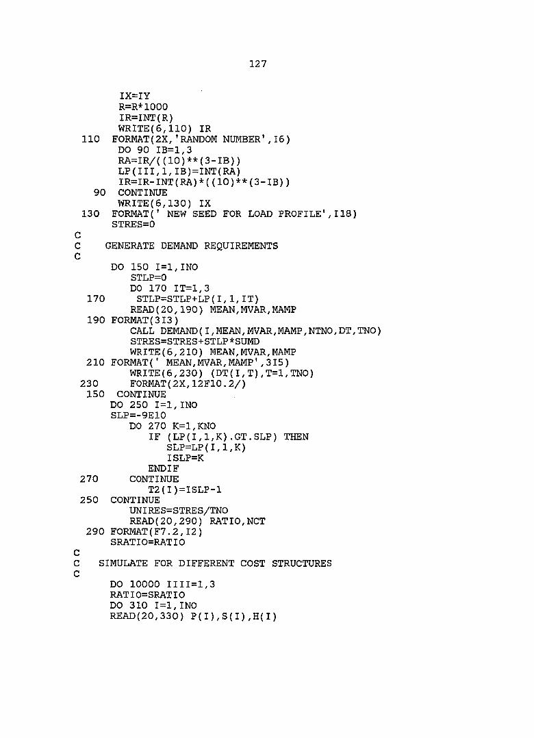
127
IX=IY R=R*1000 IR=INT(R) WRITE(6,110) IR
110 F0RMAT(2X,'RANDOM NUMBER',16) DO 90 IB=1,3 RA=IR/((10)**(3-IB)) LP(III,1,IB)=INT(RA) IR=IR-INT(RA)*((10)**(3-IB))
90 CONTINUE WRITE(6,130) IX
130 FORMAT(' NEW SEED FOR LOAD PROFILE',118) STRES=0
C C GENERATE DEMAND REQUIREMENTS C
DO 150 1=1,INO STLP=0 DO 170 IT=1,3
170 STLP=STLP+LP(I,1,IT) READ(20,190) MEAN,MVAR,MAMP
190 FORMAT(3I3) CALL DEMAND(I,MEAN,MVAR,MAMP,NTNO,DT,TNO) STRES=STRES+STLP * SUMD WRITE(6,210) MEAN,MVAR,MAMP
210 FORMAT(' MEAN,MVAR,MAMP',315) WRITE(6,230) (DT(I,T),T=1,TNO)
230 FORMAT(2X,12F10.2/) 150 CONTINUE
DO 250 1=1,INO SLP=-9E10
DO 270 K=1,KN0 IF (LP(I,1,K).GT.SLP) THEN
SLP=LP(I,1,K) ISLP=K
ENDIF 270 CONTINUE
T2(I)=ISLP-1 250 CONTINUE
UNIRES=STRES/TNO READ(20,290) RATIO,NOT
290 FORMAT(F7.2,12) SRATIO=RATIO
C C SIMULATE FOR DIFFERENT COST STRUCTURES C
DO 10000 1111=1,3 RATIO=SRATIO DO 310 1=1,INO READ(20,330) P(I),S(I),H(I)
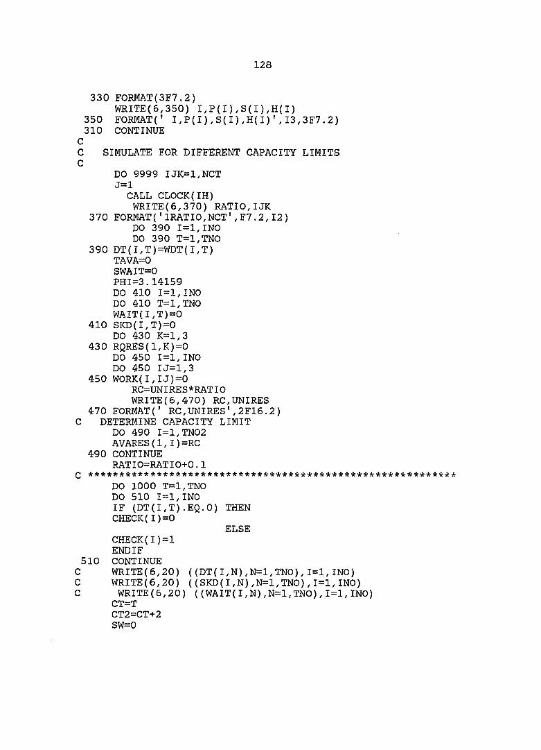
128
330 FORMAT(3F7.2) WRITE(5,350) I,P(I),S(I),H(I)
350 FORMAT(' I,P(I),S(I),H(I)',13,3F7.2) 310 CONTINUE
C C SIMULATE FOR DIFFERENT CAPACITY LIMITS C
DO 9999 IJK=1,NCT J=1
CALL CLOCK(IH) WRITE(6,370) RATIO,IJK
370 FORMAT('1RATI0,NCT',F7.2,12) DO 390 1=1,INO DO 390 T=1,TN0
390 DT(I,T)=WDT(I,T) TAVA=0 SWAIT=0 PHI=3.14159 DO 410 1=1,INO DO 410 T=1,TN0 WAIT(I,T)=0
410 SKD(I,T)=0 DO 430 K=L,3
430 RQRES(1,K)=0 DO 450 1=1,INO DO 450 IJ=1,3
450 WORK(I,IJ)=0 RC=UNIRES*RATIO WRITE(6,470) RC,UNIRES
470 FORMAT(' RC,UNIRES',2F16.2) C DETERMINE CAPACITY LIMIT
DO 490 I=1,TN02 AVARES(1,I)=RC
490 CONTINUE RATIO=RATIO+0.1
Q *********************************************************** DO 1000 T=1,TN0 DO 510 1=1,INO IF (DT(I,T).EQ.O) THEN CHECK(I)=0
ELSE CHECK(I)=1 END IF
510 CONTINUE C WRITE(6,20) ((DT(I,N),N=1,TN0),1=1, INO) C WRITE(6,20) ((SKD(I,N),N=1,TN0),I=1,IN0) C WRITE(6,20) ((WAIT(I,N),N=1,TN0),1=1,INO)
CT=T CT2=CT+2 SW=0

129
C SORT W0RK(I,1) IN SWDT(I,2) C PRIORITY OF SCHEDULING IS DETERMINED
IF (SWAIT.EQ.l) THEN DO 550 1=1,INO SWDT(I,1)=W0RK(I,1) SWDT(I,2)=I
550 CONTINUE C
CALL SRT(SWDT,INO,1) ENDIF
C IF (SWAIT.EQ.l) THEN
DO 570 11=1,INO I=SWDT(II,2)
IF (WORK(I,1).EQ.O) GO TO 570 DO 590 K=1,KN0
RQRES(J,K)=LP(I,1,K)*W0RK(I,2) T1=T+K-1 TEMP1=AVARES(J,T1)-RQRES(J, K) IF (TEMPI.LT.O) THEN
SW=1 SI=II
GO TO 600 ENDIF
590 CONTINUE DO 510 K=1,KN0
T1=T+K-1 AVARES(J,T1)=AVARES(J,T1)-RQRES(J,K)
610 CONTINUE C THE REQUIREMENTS IN WAITING AREA IS SCHEDULED
SKD(I,T)=SKD(I,T)+W0RK(I,2) CALL CLEARW(I,CT)
WRITE(6,901) 570 CONTINUE
SWAIT=0 ENDIF
630 CONTINUE DO 550 11=1,INO IF (DT(II,T).NE.O) THEN
GO TO 670 ENDIF
650 CONTINUE GO TO 1000
670 CONTINUE DO 590 1=1,INO
IF ((DT(I,CT).EQ.O)) THEN SWDT(I,1)=9E10
ELSE SWDT(I,1)=S(I)/DT(I,CT)
ENDIF

130
SWDT{I,2)=I 690 CONTINUE
C CALL SRT(SWDT,IN0,1) DO 710 11=1,INO I=SWDT(II,2) IF (CHECK(I).EQ.O) GO TO 710
DO 730 K=1,KN0 RQRES(J,K)=LP(I,1,K)*DT(I,T) T1=T+K-1 TEMP1=AVARES(J,T1)-RQRES(J,K) IF (TEMPI.LT.O) THEN
SW=2 SI=II GO TO 500 ENDIF
730 CONTINUE DO 770 K=1,KN0
T1=T+K-1 AVARES(J,T1)=AVARES(J,T1)-RQRES(J,K)
770 CONTINUE SKD(I,T)=SKD(I,T)+DT(I,T) WRITE(6,902)
DT(I,T)=0 710 CONTINUE
C SW=1,2 IMPLIES SKD IS NOT POSSIBLE WITHOUT OVERLOADING IF (CT.LT.TNO) THEN CALL UNI(CT,INO,TNO) ENDIF GO TO 1000
600 CONTINUE IF ((SWAIT.EQ.L).OR.(SW.EQ.L).OR.(T.EQ.L)) GO TO 870
C CHECK WHETHER THE BACKTRACKING IS POSSIBLE OR NOT C *************** BACK TRACKING ROUTINE START ***************
DO 790 II=SI,INO I=SWDT(II,2)
SAVA=-9E10 IF (CT.GT.3) THEN DO 810 T0=3,CT IF (AVARES(1,T0).GT.SAVA) THEN
SAVA=AVARES(1,TO) T1=T0
ENDIF 810 CONTINUE
C T IMPLIES THE TIME OF MAXIMUM AVA(T) T3=T1-T2(I)
ELSE T3=L ENDIF TAVA=0

131
DO 830 T0=T3,CT TAVA=TAVA+AVARE S(J,TO)
830 CONTINUE MTAVA=TAVA/(CT-T3+1) TLI=(LP(I,1,1)+LP(I,1,2)+LP(I,1,3))*DT(I,CT) MTLI=TLI/3 IF ((MTAVA.GT.MTLI).AND.(SWAIT.EQ.O)) THEN
GO TO 850 ELSE I=II GO TO 870
ENDIF C FIND MAX AVA 850 Q=DT(I,T)
A1=A(I,T,Q,LP,AVARES) B1=B(I,T,DT,TN0) IF (Al.LT.BI) THEN
MAB=A1 ELSE
MAB=B1 ENDIF
C DO 890 TA=T3,CT HCOST=(CT-TA)*H(I)*Q AWORK=A(I,TA,Q,LP,AVARES)+HCOST
C IF (SKD(I,TA).EQ.O) THEN
DEL=1 ELSE
DEL=0 ENDIF AWORK=AWORK+DEL*S(I)
C IF (AWORK.LT.MAB) THEN
QTY=DT(I,T) CALL SKDING(SKD,I,TA,DT,QTY,AVARES,RQRES,LP,1) DT(I,T)=0 WRITE{6,903) GO TO 910
ENDIF 890 CONTINUE
C C
IF (Al.LT.BI) THEN QTY=DT(I,T) CALL SKDING(SKD,I,T,DT,QTY,AVARES,RQRES,LP,0) WRITE(6,904)
ELSE WAIT(I,T)=DT(I,T) W0RK(I,2)=W0RK(I,2)+DT(I,T)

132
WORK(I,3)=WORK(I,3)+L W0RK(I,1)=C(I,W0RK(I,3),T,WAIT,DT) DT(I,T)=0 SWAIT=1 WRITE(6,907)
ENDIF 910 TAVA=0 790 CONTINUE
C *************** BACK TRACKING ROUTINE END ************** GO TO 1000
870 SI=II IF (SW.EQ.L) THEN
DO 930 II=SI,INO I=SWDT(II,2) IF (W0RK(I,2).EQ.O) GO TO 930 TEMP5=WORK(I,2) AWORK=A(I,CT,TEMPS,LP,AVARES)+WORK(1,1) ITEMP=W0RK(I,3)+1 WAIT(I,CT)=DT(I,CT) CWORK=C(I,ITEMP,CT,WAIT,DT) WAIT(I,CT)=0
IF (AWORK.LT.CWORK) THEN QTY=W0RK(I,2) CALL SKDING(SKD,I,T,DT,QTY,AVARES,RQRES,LP,1) CALL CLEARW(I,CT) WRITE(5,905) SWAIT=0
ELSE C UPDATE WORK AND WAIT AREA
DO 950 1=1,INO WAIT(I,CT)=DT(I,CT) TEMP1=W0RK(I,3)+1 W0RK(I,1)=C(I,TEMP1,CT,WAIT,DT) W0RK(I,2)=W0RK(I,2)+DT(I,T) W0RK(I,3)=TEMP1 DT(I,CT)=0 SWAIT=1
950 CONTINUE WRITE(6,908)
901 FORMAT(' CHECK POINT 1' ) 902 FORMAT(' CHECK POINT 2' ) 903 FORMAT(' CHECK POINT 3' ) 904 FORMAT(' CHECK POINT 4' ) 905 FORMAT(' CHECK POINT 5' ) 905 FORMAT(' CHECK POINT 6' ) 907 FORMAT(' CHECK POINT 7' ) 908 FORMAT(' CHECK POINT 8' )
GO TO 1000 ENDIF
C

133
C 930 CONTINUE
ENDIF IF (SW.EQ.L) THEN
SI=1 DO 990 1=1,INO
IF ((DT(I,CT).EQ.O)) THEN SWDT(I,1)=9E10
ELSE SWDT(I,1)=S(I)/DT(I,CT)
ENDIF SWDT(I,2)=I
990 CONTINUE C
CALL SRT(SWDT,INO, 1) ENDIF DO 1010 II=SI,INO I=SWDT(II,2) IF (CHECK(I).EQ.O) GO TO 1010
AWORK=A(I, CT, DT(I, T), LP,AVARES) BWORK=B(I,CT,DT,TNO)
C IF (AWORK.LT.BWORK) THEN
QTY=DT(I,T) CALL SKDING(SKD,I,CT,DT,QTY,AVARES,RQRES,LP, 0) WRITE(6,905)
ELSE C
WAIT(I,CT)=DT(I,CT) TEMP1=W0RK(I,3)+1 W0RK(I,3)=TEMP1 WORK(I,2)=WORK(1,2)+DT(I,CT) WORK(I,1)=C(I,TEMPI,CT,WAIT,DT) DT(I,CT)=0
C WRITE(6,1030) (W0RK(I,JJ),JJ=1,3),I,CT,WAIT(I,CT) 1030 F0RMAT(2X,'WORK123, I,CT,WAIT(I.CT)',5I5,F16.2)
SWAIT=1 C
ENDIF C 1010 CONTINUE 1000 CONTINUE
WRITE(6,20) ((SKD(I,T),T=1,TN0),I=1,INO) C WRITE(6,20) ((WAIT(I,N),N=1,TN0),I=1,IN0) 20 FORMAT(2(4X,6F10.2/))
C TOTAL SETUP COST C
SETN=0 SUMS=0 DO 4020 1=1,INO
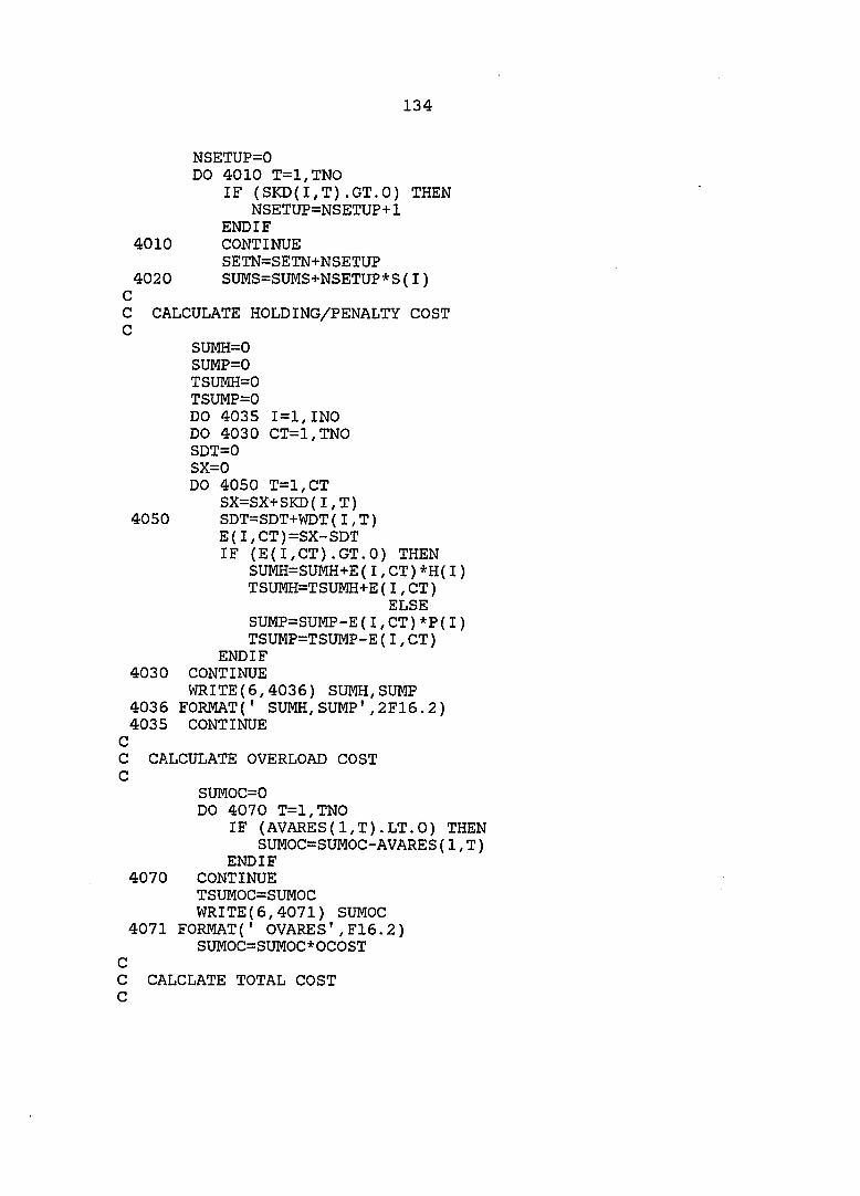
134
NSETUP=0 DO 4010 T=1,TN0
IF (SKD(I,T).GT.O) THEN NSETUP=NSETUP+1
ENDIF 4010 CONTINUE
SETN=SETN+NSETUP 4020 SUMS=SUMS+NSETUP*S(I) C C CALCULATE HOLDING/PENALTY COST C
SUMH=0 SUMP=0 TSUMH=0 TSUMP=0 DO 4035 1=1,INO DO 4030 CT=1,TN0 SDT=0 SX=0 DO 4050 T=1,CT
SX=SX+SKD(I,T) 4050 SDT=SDT+WDT(I,T)
E(I,CT)=SX-SDT IF (E(I,CT).GT.O) THEN
SU]yiH=SUMH+E ( I, CT ) *H ( I ) TSUMH=TSUMH+E(I,CT)
ELSE SUMP=SUMP-E(I,CT)*P(I) TSUMP=TSUMP-E(I,CT)
ENDIF 4030 CONTINUE
WRITE(5,4036) SUMH,SUMP 4036 FORMAT(' SUMH,SUMP',2F16.2) 4035 CONTINUE C C CALCULATE OVERLOAD COST C
SUM0C=0 DO 4070 T=1,TN0
IF (AVARES(l,T).LT.O) THEN SUMOC=SUMOC-AVARES(1,T)
ENDIF 4070 CONTINUE
TSUMOC=SUMOC WRITE(6,4071) SUMOC
4071 FORMAT(' OVARES',F16.2) SUMOC=SUMOC*OCOST
C C CALCLATE TOTAL COST C

135
SUMTC=SUMS+SUMH+SUMP+SUMOC C
WRITE(50,4077) SUMTC,SUMS,SUMH,SUMP,SUMOC C WRITE(50,4077) SUMTC,SETN,TSUMH,TSUMP,TSUMOC 4077 FORMAT(5F16.2)
WRITE(6,4093) SUMTC,SUMS,SUMH,SUMP,SUMOC 4093 FORMAT(2X,'SUMTC,SUMS,SUMH,SUMP,SUMOC',5F16.2)
WRITE(30,4097) SUMTC 4097 FORMAT(F16.2)
WRITE(30,4098) ((WDT(I,T),T=1,TNO),1=1,INO) WRITE(30,4098) ((SKD(I,T),T=L, TNO),1=1,INO)
4098 FORMAT(FIO.2) WRITE(30,4099) (AVARES(1,LT), LT=1,TN02)
4099 FORMAT(F16.2) WRITE(6,4100) (AVARES(1,LT), LT=1,TN02)
4100 FORMAT(2(2X,7F16.2/)) CALL CLOCK(IG) IHPU=IH-IG WRITE(6,4092) IH,IG,IHPU
4092 FORMAT(' IH,IG,IHPU',315) 9999 CONTINUE 10000 CONTINUE
CALL CLOCK(ID) ICPU=IC-ID WRITE(6,4091) IC,ID,ICPU
4091 FORMAT(' IC,ID,ICPU',315) C2345 CONTINUE
STOP END
Q ********************************************************* REAL FUNCTION A(I,T,Q,LP,AVARES) REAL TEMP(12,1,3),LP(12,1,3),AVARES(1,26) INTEGER T
COMMON/SEVEN/OCOST SUM=0 J=1 DO 5000 K=L,3 TEMP(I,J,K)=LP(I,1,K)*Q T1=T+K-1 IF (AVARES(J,T1).LT.0) THEN
SUM=SUM+TEMP(I,J,K) ELSE
WK=TEMP(I,J,K)-AVARES(J,T1) IF (WK.GT.O) THEN
SUM=SUM+WK ENDIF
ENDIF 5000 CONTINUE
A=SUM*OCOST RETURN

136
END C Q ****************************************************** C
REAL FUNCTION B(I,T,DT,TNO) REAL DT(12,24) COMMON /ONE/ P(12),S(12) INTEGER TyTNO IF (T.EQ.TNO) THEN
DEL=0 GO TO 5100
ENDIF IF (DT(I,T+1).EQ.O) THEN
DEL=1 ELSE
DEL—0 ENDIF
5100 B=P(I)*DT(I,T)+DEL*S(I) RETURN
END C Q ****************************************************** C
REAL FUNCTION C(I,JD,T,WAIT,DT) COMMON /ONE/ P(12),S(12) REAL WAIT(12,24),DT(12,24) INTEGER T,TMIAl SUM=0 DO 5200 IA=1,JD
TMIA1=T-IA+1 C WRITE(5,5300) T,IA,JD 5300 F0RMAT(2X,'T,IA,JD',315)
SUM=SUM+WAIT(I,TMIAl)*IA*P(I) 5200 CONTINUE
IF (DT(I,T).GT.O) THEN ELSE SUM=SUM+S(I)
END IF C=SUM RETURN
END C Q ******************************************************
SUBROUTINE DEMAND (IC,MIYOU,SIGMA,AA,BB,DT,TNO) INTEGER TNO,SIGMA,AA,BB DOUBLEPRECISION DSEED,NDSEED COMMON/SIX/WDT(12,24),DSEED,NDSEED,SUMD REAL DT(12,24),ITEM(24) DSEED = NDSEED SUMD=0 PHI=3.14159
137
DO 5400 1=1,TNO Y=GGNQF(DSEED) W1=SIGMA*Y W2=(2 *PHI/BB)*(I+BB/4.) ITEM(I)=MIYOU + W1 +AA*SIN(W2) IF (ITEM(I).LT.O) THEN ITEM(I)=0 ENDIF
C CALCULATE THE RATIO OF ZERO DT(IC,I)=ITEM(I) WDT(IC,I)=ITEM(I) SUMD=SUMD+DT(IC,I)
5400 CONTINUE NDSEED=DSEED WRITE(5,5500) NDSEED
5500 FORMAT(' NEW SEED FOR DEMAND',F20.7) RETURN END
0 ******************************************************** SUBROUTINE UNI(CT,INO,TNO) REAL LP,RQRES(1,3) INTEGER T,T1,CT,CT1,TN0,TT,TM1 COMMON /ONE/ P(12),S(12) COMMON /TWO/ DT(12,24),H(12),U(12,24),SWDT(12,3) COMMON /THREE/ LP(12,1,3),SKD(12,24),AVARES(1,26) COMMON/FIVE/CHECK(12) CALL CLOCK(IE) KN0=3 J=1
DO 6010 LL=CT,TNO DO 6010 11=1,INO
6010 U(II,LL)=-9E10 C WRITE(6,6030) CT,INO,TNO 6030 F0RMAT(2X,'CT,INO,TNO',315) C WRITE{6,20) ((DT(I,T),T=1,TN0),1=1,INO) 20 FORMAT(2(4X,6F10.2/))
C WRITE(6,20) ({SKD(I,T),T=1,TN0),1=1,INO) DO 6070 1=1,INO
C WRITE(6,6090) DT(I,CT) 6090 F0RMAT(2X,'DT(I,CT)',F16.2)
IF (CHECK(I).EQ.O) GO TO 6070 CT1=CT+1
DO 6110 T1=CT1,TN0 SUM=0 TM1=T1-CT DO 6130 TT=1,TM1 ITT1=CT+TT-1 SUM=SUM+{TT-1)*DT(I,ITT1)*H(I) WRITE(6,6150) SUM,DT(I,ITTL),H(I)
6150 F0RMAT(2X,3F16.2)

138
6130 CONTINUE A1=S(I)+SUM -H(I)*((TMl+1-1)**2)*DT(I, T1) WRITE(6,6170) Al,SUM,DT(I,T1),I,T1,T1
IF (Al.LE.O) GO TO 6070 B1=(TM1+1)*(TM1+1-1)*DT(I,T1)
IF (Bl.EQ.O) THEN U(I,T1)=9E10
ELSE U(I,T1)=A1/B1
ENDIF WRITE(6,6210) CT,I,T1,U(I,T1)
6210 FORMAT(2X,'CT,I,T1,U(I,T1)',315,F16.8) 6110 CONTINUE 6070 CONTINUE
DO 6230 1=1,INO SWDT(I,1)=U(I,CT1) SWDT(I,2)=I SWDT(I,3)=CT1
6230 CONTINUE 6270 CALL SRT(SWDT,INO,2)
DO 6250 11=1,INO I=SWDT(II,2) J0=SWDT(II,3)
IF (CHECK(I).EQ.O) GO TO 6250 IF ((U(I,J0)+9E10).LT.O.00001) GO TO 6250
DST=DT{I,JO) DO 6280 K=1,KN0
RQRES(J,K)=LP(I,1,K)*DST T1=CT+K-1 TEMP1=AVARES(J,T1)-RQRES(J, K) IF (TEMPI.LT.O) THEN
RETURN ENDIF
SKD(I,CT)=SKD(I,CT)+DST DT(I,J0)=0
DO 6290 K=1,KN0 T1=CT+K-1 AVARES(J,T1)=AVARES(J,T1)-RQRES(J,K)
6290 CONTINUE IF (JO.EQ.TNO) THEN
GO TO 6250
6170 FORMAT(2X,3F16.2,3I6)
6280 CONTINUE
ENDIF SWDT(II,1)=U(I,J0+1) SWDT(II,3)=SWDT(II,3)+1
IF (SWDT(II,1).GT.O) THEN GO TO 6270
ELSE GO TO 6250

139
ENDIF 6250 CONTINUE
RETURN END
Q ****************************************************** SUBROUTINE CLEARW(I,CT) INTEGER TT,CT,CTT INTEGER WORK COMMON/FOUR/WORK(12,3),WAIT(12,24)
CTT=CT-W0RK(I,3) DO 7010 TT=CTT,CT WAIT(I,TT)=0 SWAIT=0
7010 CONTINUE C
W0RK(I,1)=0 W0RK(I,2)=0 W0RK(I,3)=0 SWAIT=0 RETURN
END C C Q ****************************************************** c
SUBROUTINE SRT(SWDT,INO,CHK) C
INTEGER CHK REAL SWDT(12,3) IN0M1=IN0-1 DO 7030 NPASS=1,INOMl
INOMN=INO-NPASS DO 7050 I=l,INOMN
IF (SWDT(I,1).LT.SWDT{I+1,1)) THEN TEMP0=SWDT(I,1) SWDT(I,1)=SWDT(I+1,1) SWDT(I+1,1)=TEMP0
C C
TEMP0=SWDT(I,2) SWDT(I,2)=SWDT(I+1,2) SWDT(I+1,2)=TEMP0
C IF (CHK.EQ.2) THEN
TEMP0=SWDT(I,3) SWDT(I,3)=SWDT(I+1,3) SWDT(I+1,3)=TEMP0 ENDIF
ENDIF 7050 CONTINUE

140
7030 CONTINUE RETURN END
Q *********************************************************** c
SUBROUTINE SKDING(SKD,I,T,DT,QTY,AVARES,RQRES,LP,CHK) INTEGER T,CHK REAL SKD(12,24),DT(12,24),RQRES(1,3),AVARES(1,25) REAL LP(12,1,3) J=1 KN0=3 SKD(I,T)=SKD(I,T)+QTY
IF (CHK.EQ.O) THEN DT(I,T)=0
ENDIF DO 7070 K=1,KN0 T1=T+K-1 RQRES(J,K)=LP{I,1,K)*QTY AVARES(J,T1)=AVARES(J,T1)-RQRES(J,K)
7070 CONTINUE RETURN END
C$ENTRY

141
Method B
$JOB 'KIM',TIME=(2,00),PAGES=100 C C234557890 C C * I/O FILE SUMMARY ***************************************** C C DD NAME DSN C C 1. INPUT FT20F001 K.I6467.DATA C C 2. OUTPUT FT40F001 K.16467.RESB C C FT60F001 K.I6467.MINE C C C ********* FILE DESCRIPTION ********************************* C C 1. K.16467.DATA C C REFER TO METHODA C C 2. K.16467.RESB C C SAME AS K.I6467.RESA C C 3. K.16467.MINB C C SAME AS K.I6467.MINA C C ** ARRAY DESCRIPTION ************************************** C C ITEM(T); PRODUCTION REQUIREMENT AT TIME T, T=1,2,...,TNO C C DT(I,T): PRODUCTION REQUIREMENT OF END ITEM I AT TIME T, C 1=1,2,...,INO T=l,2, ,TNO C C RESLIM(J,T): CAPACITY LIMIT, J=1 T=l,2, ,TN0+2 C C LP(I,J,K): LOAD PROFILE, 1=1,2,...,INO J=1 K=l,2,3 C C P(I): PENALTY COST PER UNIT OF THE ITEM I C PER PERIOD CARRIED. C C S(I): SET UP COST OF THE ITEM I C C H(I): CARRYING COST PER UNIT OF THE ITEM I C PER PERIOD CARRIED. C
142
C OCOST: COST PER MAN PERIOD OR MACHINE PERIOD C OF OVER TIME LABOR OR MACHINE. C C RQRES(J,T): REQUIRED RESOURCE, J=1 T=l,2,3 C C AVARES(J,T): AVAILABLE RESOURCE, J=1 T=l,2, ,TN0+2 C C SKD(I,T): SCHEDULE OF END ITEM I, 1=1,2,...,INO C T=l,2,...,TN0 CCCCCCCCCCCCCCCCCCCCCCCCCCCCCCCCCCCCCCCCCCCCCCCCCCCCCCCCCCCCC C C VARIABLE DECLARATION C
INTEGER INO,CT,T,TNO,TNOl,TT,T1,T2,T3,TA,CTMT2 INTEGER TEMP1,TEMP2,TFROM,TFROMl,TTO,TN02 INTEGER SIGMA,A,B,IPRD(12),MEAN(12) INTEGER ST,TN0M1 INTEGER SWA,STFROM,STTO,COUNT REAL IRA(5),E(12,26),VAL(12),H,MINVAL,MAXVAL REAL GGNQF,Y,LP,LSQ,LSQl,LSQ2,MAABB REAL ITEM(24),RESLIM(l,25),SKD(12,24),EOQ(12) REAL P(12),COST(24,24),OCOST,HCOST,AVADMD(12),TALP(12) REAL RQRES(1,3),AVARES(1,25),SWDT(12,2),TEMP(12,1,3) DOUBLEPRECISION DSEED,NDSEED COMMON /ONE/ H(12),DT(12,24),LP(12,1,3),S(12) COMMON /TWO/ TARES(1,25),ELSN(25),PRED(25) COMMON /THREE/ DSEED,NDSEED,SUMD COMMON /FOUR/ TN0,TN02
C DO 12345 IJKL=1,5 . C INITIALIZATION
CALL CLOCK(IC) STRES=0 1=1 J=1 K=1 READ(20,10) INO,TNO,DSEED,OCOST
10 FORMAT(2I2,F20.7,F7.2) IF (TN0.GE.12) THEN
NTN0=12 ELSE
NTNO=TNO END IF
C GENERATE LOAD PROFILE READ(20,30) IX
30 FORMAT(112) WRITE(6,50) IX
50 FORMAT(' OLD SEED FOR LP',112) DO 70 111=1,INO CALL RANDU(IX,IY,R) IX=IY

143
R=R*1000 IR=INT(R) WRITE(5,90) IR
90 FORMAT(2X,'RANDOM NUMBER',16) DO 70 IB=1,3 RA=IR/((10)**(3-IB)) LP(III,1,IB)=INT(RA) IR=IR-INT(RA)*((10)**(3-IB))
70 CONTINUE WRITE(6,110) IX
110 FORMAT(' NEW SEED FOR LOAD PROFILE',112) DO 130 11=1,INO
SUM=0 DO 150 12=1,3
SUM=SUM+LP(I1,1,12) 150 CONTINUE
TALP(I1)=SUM 130 CONTINUE
NDSEED=DSEED WRITE(6,170) INO,TNO,DSEED,OCOST
170 FORMAT(' INO,TNO,DSEED,OCOST',212,F20.7,F7.2) KN0=3
C WRITE(6,190) NF,NTEMPl,NTEMP2,TEMPO 190 FORMAT(2X,'NF,NTEMPl,2,TEMPO',3I5,F15.2)
TN01=TN0+1 TN02=TN0+2 JP1=J+1 DO 210 1=1,INO
STLP=0 DO 230 IT=1,3
230 STLP=STLP+LP(I,1,IT) READ(20,250) MEAN(I),MVAR,MAMP
250 FORMAT(3I3) CALL DEMAND(I,MEAN(I),MVAR,MAMP,NTNO,DT,TNO) AVADMD(I)=SUMD/TNO WRITE(6,270) SUMD,AVADMD(I)
270 FORMAT(' TOTAL SUM& AVA DMD',2F15.2) STRE S=STRE S+STLP * SUMD WRITE(6,290) MEAN(I),MVAR,MAMP
290 FORMAT(' MEAN(I),MVAR,MAMP',315) WRITE(6,310) (DT(I,T),T=1,TN0)
310 FORMAT{2X,12F10.2/) 210 CONTINUE
UNIRES=STRES/TNO READ(20,330) RATIO,NCT
330 FORMAT(F7.2,12) SRATIO=RATIO DO 10000 1111=1,3 RATIO=SRATIO DO 350 1=1,INO
144
READ(20,370) P(I),S(I),H(I) 370 FORMAT(3F7.2)
EOQ(I)=SQRT(2*MEAN(I)*S(I)/H(I)) TMP=EOQ(I)/MEAN(I) IPRD{I)=INT(TMP)
WRITE(5,390) I,P(I),S(I),H(I) 390 FORMAT(' I,P(I),S(I),H(I)',13,3F10.2)
350 CONTINUE DO 9999 IJK=1,NCT
1=1 J=1 K=1
DO 410 1=1,INO DO 410 T=1,TN0
410 SKD(I,T)=0 PHI=3.14159
C WRITE(6,430) INO 430 FORMAT(IX,15)
DO 450 1=1,INO DO 450 T=1,TN0
450 SKD(I,T)=0 DO 470 K=l,3
470 RQRES(1,K)=0 DO 490 J=1,TN0 DO 490 K=J,TNO COST(J,K)=9E10
490 CONTINUE WRITE(6,510) RATIO, UK
510 FORMAT('1RATI0,NCT',F7.2,12) RC=UNIRES*RATIO
WRITE(6,530) RC,UNIRES 530 FORMAT(' RC,UNIRES',2F15.2) C CAPACITY LIMIT
DO 550 I=1,TN02 AVARES(1,I)=RC
550 CONTINUE RATIO=RATIO+0.1
DO 1000 1=1,INO IF (I.LT.INO) THEN
RCC=AVADMD(I)*TALP ( I) DO 570 T=1,TN02
570 TARES(1,T)=RCC ELSE
DO 590 T=1,TN02 590 TARES(1,T)=AVARES(1,T)
END IF DO 510 J=1,TN0 JP1=J+1 DO 530 K=JP1,TN01 SUM=0
145
DO 550 T=JP1,K SUM=SUiyi+H ( I ) * ( T-JPl ) *DT ( I, T-1 )
650 CONTINUE TEMP1=S(I)-SUM IF (TEMPI.GT.O) THEN KM1=K-1
COST(J,KMl)=CALC(I,J,KMl,AVARES,TARES,OCOST) ELSE
GO TO 670 ENDIF
630 CONTINUE 670 CONTINUE
IF (J.EQ.TNO) THEN GO TO 690
ELSE GO TO 710
ENDIF 710 CONTINUE
IF (J.GE.2) THEN CALL SPATH(JP1,ELSN,C0ST)
ENDIF CALL UPRES(I,JP1,1,DT,LP,AVARES,SKD,COST)
WRITE(6,3 70) (TARES(1,LT),LT=1,TN02) 100 CONTINUE 690 CALL SPATH(TNOl,ELSN,COST)
CALL UPRES(I,TNOl,2,DT,LP,AVARES,SKD,COST) 1000 CONTINUE
CALL CLOCK(ID) ICPU=IC-ID WRITE(6,730) IC,ID,ICPU
730 FORMAT(' IC,ID,ICPU',3 IS) C
WRITE(6,310) ((SKD(I,T),T=1,TN0),I=1,INO) WRITE(6,750) (AVARES(1,LT),LT=1,TN02)
750 FORMAT(2X,8F16.2) CALL CCOST(INO,TNO,SKD,AVARES,OCOST,RC,1) WRITE(40,770) ((DT(I,T),T=1,TN0),1=1,INO) WRITE(40,770) ((SKD(I,T),T=1,TN0),1=1,INO)
770 FORMAT(FIO.2) WRITE(40,790) (AVARES(1,LT),LT=1,TN02)
790 F0RMAT(F16.2) 9999 CONTINUE 10000 CONTINUE C2345 CONTINUE
STOP END
Q *********************************************************** SUBROUTINE DEMAND (IC,MIYOU,SIGMA,A,B,DT,TNO) INTEGER TNO,SIGMA,A,B REAL DT(12,24),ITEM(24),PHI

146
DOUBLEPRECISION DSEED,NDSEED COMMON /THREE/ DSEED,NDSEED,SUMD SUMD=0 PHI=3.14159 DSEED = NDSEED DO 1500 1=1,TNO Y=GGNQF(DSEED) W1=SIGMA*Y W2=(2 *PHI/B)*(I+B/4.) ITEM(I)=MIYOU + W1 + A*SIN(W2) IF (ITEM(I).LT.O) THEN
ITEM(I)=0 ENDIF
C CALCULATE THE RATIO OF ZERO DT(IC,I)=ITEM(I) SUMD=SUMD+DT(IC,I)
1500 CONTINUE NDSEED=DSEED WRITE(6,1510) DSEED
1510 FORMAT(2X,'NEW DSEED',F20.7) RETURN END
0 ********************************************************** SUBROUTINE SPATH(J,ELSN,COST) REAL COST(24,24),TCOST(25),TEST(25) REAL ELSN(25) WRITE(6,1530) ((COST(JJ,KK),KK=1,6),JJ=1, 6)
1530 F0RMAT(6(2X,6F16.1/)) DO 1550 1=1,J
TCOST(I)=9E10 TEST(I)=0 ELSN(I)=0
1550 CONTINUE TCOST(1)=0 TEST(1)=1
1590 CONTINUE DO 1600 1=1,J
IF {TEST(I).EQ.l) THEN JM1=J-1 NUM=0
DO 1610 JJ=1,JM1 DO 1620 KK=JJ,JM1
NUM=NUM+1 SERN=NUM KKP1=KK+1 IF (JJ.EQ.I) THEN IF ((TCOST(I)+COST(JJ,KK)).LT.TCOST(KKPl))
THEN TCOST(KKPl)=TCbST(I)+COST(JJ, KK) ELSN(KKPl)=SERN TEST(KKPl)=1

147
1620 1610
1600
1650
1661 1660
C ****
1665
1670
1690
ENDIF ENDIF
CONTINUE CONTINUE
TEST(I)=0 ENDIF
CONTINUE DO 1650 1=1,J
IF (TEST(I).EQ.l) GO TO 1590 CONTINUE IF (J.EQ.5) THEN
DO 1660 M=1,J WRITE(6,1661) M,TCOST(M),ELSN(M),TEST(M)
FORMAT(2X,I4,3F15.2) CONTINUE ENDIF RETURN
END ************************************************
SUBROUTINE UPRES(I,JNO,CHK,DT,LP,AVARES,SKD,COST) COMMON /TWO/ TARES(1,26)^ELSN(25),PRED(25) COMMON /FOUR/ TN0,TN02 REAL RQRES(1,3),AVARES(1,26),LP(12,1,3),DT(12,24) REAL C0ST(24,24),SKD(12,24) INTEGER S,S1,F,T,TN0,TN02,CHK IF (JN0.EQ.2) THEN
TDMD=DT(I,1) DO 1670 K=l,3
WRITE(6,1665) TDMD,LP(I,1,K) FORMAT(2X,2F10.3)
RQRES(1,K)=TDMD* LP(1,1,K) TARES(1,K)=TARES(1,K)-RQRES(1,K)
CONTINUE RETURN
ENDIF PRED(1)=JN0 J=1 N=1 WHILE(PRED(N).NE.1)
WRITE(6,1690) N,PRED(N) FORMAT(5X,'PRED',15,'=',F10.3)
N=N+1 SERN=ELSN(PRED(N-1)) JTEMP=JN0-1 JNOM1=JNO-1 DO 1750 L=1,JTEMP
T=SERW-JN0M1 IF (T.LE.O) THEN
PRED(N)=L GO TO 1770

148
ELSE SERN=SERN-JN0M1 JN0M1=JN0M1-1
ENDIF 1750 CONTINUE 1770 CONTINUE
WRITE(6,1690) N,PRED(N) END WHILE
IF (CHK.EQ.2) GO TO 2000 JN01=JN0 NM1=N-1 DO 1800 KA=1,NM1
TDMD=0 F=JN01
C PRED(l) IS THE DESTINATION KA1=KA+1
S=PRED(KA1)+1 S1=S-1
DO 1850 K1=S,F TDMD=TDMD+DT(I,Kl-1)
1850 CONTINUE DO 1900 K=l,3
RQRES(J,K)=TDMD*LP(I,J,K) T1=S1-1+K TARES(J,T1)=TARES(J,T1)-RQRES(J,K)
1900 CONTINUE JN01=PRED(KA1)
WRITE(5,1950) JN01,KA 1950 FORMAT(2X,215/) . 1800 CONTINUE
RETURN 2000 CONTINUE
JN01=JNO WRITE(5,2040) N
2040 FORMAT(2X,15/) NM1=N-1
DO 2050 KA=1,NM1 TDMD=0 F=JN01 KA1=KA+1 S=PRED(KA1)+1 S1=S-1
DO 2100 K1=S,F TDMD=TDMD+DT(I,Kl-1)
2100 CONTINUE SKD(I,S1)=TDMD
WRITE(6,1950) S,F DO 2200 K=l,3
T1=S1-1+K RQRES(J,K)=TDMD*LP(I,J,K)

149
AVARES(J,T1)=AVARES(J,T1)-RQRES(J, K) CONTINUE
JN01=PRED(KA1) CONTINUE
WRITE(6,370) (TARES(1,LT),LT=1,TN02) F0RMAT(2X,8F16.2)
DO 2270 KKK=1,TN0 DO 2270 JJJ=KKK,TNO COST(JJJ,KKK)=9E10 CONTINUE RETURN END
Q ***************************************************** SUBROUTINE CCOST(INO,TNO,SKD,AVARES,OCOST,RC,III) REAL LP COMMON /ONE/ H(12),DT(12,24),LP(12,1,3),S(12) REAL E(12,26),AVARES(1,26),SKD(12,24),P(12) REAL RQRES(1,3) INTEGER TN0,T,T1,CT,TN02 WRITE(6,4000) ((SKD(I,T),T=1,TNO),1=1,INO)
4000 FORMAT(2X,12F10.2/) C C TOTAL SETUP COST C
TN02=TN0+2 DO 4005 11=1,12
4005 P(II)=0 SETN=0 SUMS=0 DO 4020 1=1,INO NSETUP=0 DO 4010 T=1,TN0
IF (SKD(I,T).GT.O) THEN NSETUP=NSETUP+1
ENDIF 4010 CONTINUE
SETN=SETN+NSETUP 4020 SUMS=SUMS+NSETUP * S(I) C C CALCULATE HOLDING/PENALTY COST C
SUMH=0 SUMP=0 TSUMH=0 TSUMP=0 DO 4035 1=1,INO DO 4030 CT=1,TN0 SDT=0 SX=0 DO 4050 T=1,CT
2200
2050
370
2270

150
SX=SX+SKD(I,T) 4050 SDT=SDT+DT(I,T)
E(I,CT)=SX-SDT IF (E(I,CT).GT.O) THEN
SUMH=SUMH+E(I,CT)*H(I) TSUMH=TSUMH+E(I,CT)
ELSE SUMP=SUMP-E(I,CT)*P(I) TSUMP=TSUMP-E(I,CT)
ENDIF 4030 CONTINUE
WRITE(6,4036) SUMH,SUMP 4035 FORMAT(' SUMH,SHMP',2F16.2) 4035 CONTINUE C C CALCULATE OVERLOAD COST C
SUMOC=0 DO 5000 11=1,TN02
5000 AVARES(1,II)=RC DO 5010 1=1,INO DO 5010 IT=1,TN0 DO 5010 K=l,3
T1=IT+K-1 RQRES(1,K)=LP(I,1,K)*SKD(I, IT) AVARES(1,T1)=AVARES(1,T1)-RQRES(1,K)
5010 CONTINUE WRITE(5,5020) (AVARES(1,LT),LT=1,TN02)
5020 F0RMAT(2X,2(7F15.2/).) DO 4070 T=1,TN0
IF (AVARES(1,T).LT.O) THEN SUMOC=SUMOC-AVARES(1,T)
ENDIF 4070 CONTINUE
TSUM0C=SUM0C WRITE(5,4071) SUMOC
4071 FORMAT(' OVARES',F15.2) SUMOC=SUMOC*OCOST
C C CALCLATE TOTAL COST C
SUMTC=SUMS+SUMH+SUMP+SUMOC C
WRITE(50,4077) SUMTC,SUMS,SUMH,SUMP,SUMOC C WRITE(50,4077) SUMTC,SETN,TSUMH,TSUMP,TSUMOC 40570 FORMAT(5F16.2)
WRITE(5,5090) SUMTC,SUMS,SUMH,SUMP,SUMOC 5090 FORMAT(2X,'SUMTC,SUMS,SUMH,SUMP,SUMOC' ,5F15.2)
IF (III.EQ.l) THEN WRITE(40,5093) SUMTC

151
5093 FORMAT(FI6.2) END IF RETURN END
0 ******************************************************** REAL FUNCTION AMIN(AM,BM)
REAL AM,BM IF (AM.LT.BM) THEN
AMIN=AM ELSE
AMIN=BM ENDIF
RETURN END
0 ******************************************************** REAL FUNCTION CALC(I,JN,KN,AVARES,TARES,OC) REAL AVARES(1,25),TARES(1,26),TEMP(12,1,3),LP INTEGER T,TNO J=1 COMMON /ONE/ H(12),DT(12,24),LP(12,1,3),S(12) COMMON /FOUR/ TN0,TN02
C SET UP COST A=S(I)
C HOLDING COST/PRODUCTION QUANTITY B=0 PQ=0 DO 5000 T=JN,KN
B=B+H(I)*(T-JN)*DT(I,T) PQ=PQ+DT(I/T)
6000 CONTINUE C OVERLOAD COST
SUM=0 DO 5010 K=l,3 TEMP(I,J,K)=LP(I,J,K)*PQ T1=JN+K-1 IF (Tl.GT.TNO) GO TO 5010 IF (TARES(J,T1).LT.O) THEN
SUM=SUM+TEMP(I,J,K) ELSE
WK=TEMP(I,J,K)-TARES(J,T1) IF (WK.GT.O) THEN
SUM=SUM+WK ENDIF
WRITE(5,5030) K,TARES(1,T1),PQ,TEMP(1, 1,K) 5030 FORMAT(2X,'K,TARES,PQ,TEMP',I3,3F15.2)
ENDIF 5010 CONTINUE
WRITE(5,5050) SUM 5050 FORMAT(2X,'SUM=',F16.2)
C=SUM*0C

152
IF (JN.EQ.3) THEN WRITE(6,6070) A,B,C
6070 F0RMAT(2X,'A,B,C=',3F12.2) ENDIF CALC=A+B+C RETURN END
C$ENTRY

153
Method C
$JOB 'KIM',TIME=(2,30),PAGES=100,NOWARN C C * I/O FILE SUMMARY **************************************** C C DD NAME DSN C C 1. INPUT FT20F001 K.I6467.DATA C C FT30F001 K.16467.RESA C C FT40F001 K.I6467.RESB C C 2. OUTPUT FT70F001 K.I6467.MING C C Q ********* FILE DESCRIPTION ********************************* C C 1. K.16467.DATA C C REFER TO METHODA C C 2. K.16467.RESA C C REFER TO METHODA C C 3. K.16467.RESB C C REFER TO METHODB C C 4. K.16467.MING C C 1) BOUNDL: COST C FROM METHOD C (TREE SEARCH METHOD) C C VARIABLE DEFINITION *************************************** C
INTEGER INO,CT,T,TNO,TNOl,TT,T1,T2,T3,TA,CTMT2 INTEGER TEMP1,TEMP2, TFROM,TFROMl,TTO,TN02 INTEGER ST,TNOMl,CTl,KSAVE(12),TABLE(20,4) INTEGER SWA,STFROM,STTO,COUNT,ITBL(300,4) REAL TEMP(12,1,3),LP(12,1,3),E(12,24) REAL SIGN(20,3),IRA(5),TARES(1,26) REAL S(12),P(12),H(12),VAL(10) REAL LSQ,LSQ1,LSQ2,MAABB REAL MINVAL,MAXVAL DOUBLEPRECISION DENOM,DNUMER COMMON/ONE/DT(12,24),SKD(12,24),AVARES(1,26) COMMON/TWO/VALIO(10),UVAL
C DO 12345 IJKL=1,5

154
KN0=3 READ(20,50) INO,TNO,DSEED,OCOST
50 FORMAT(2I2,F20.7,F7.2) WRITE(6,100) INO,TNO,DSEED,OCOST
100 FORMAT(' INO,TNO,DSEED,OCOST',212,F20.7,F7.2) TN02=TN0+2
C GENERATE LOAD PROFILE READ(20,150) IX,ICT
150 F0RMAT(I12,I4) WRITE(6,200) IX,ICT
200 FORMAT(' OLD SEED FOR LP & TOTAL COUNT',112,14) DO 250 111=1,INO CALL RANDU(IX,IY,R) IX=IY R=R*1000 IR=INT(R) WRITE(6,300) IR
300 FORMAT(2X,'RANDOM NUMBER',15) DO 250 IB=1,3 RA=IR/((10)**(3-IB)) LP(III,1,IB)=INT(RA) IR=IR-INT(RA)*((10)**(3-IB))
250 CONTINUE WRITE{5,350) IX
350 FORMAT(' NEW SEED FOR LOAD PROFILE',112) DO 400 11=1,INO
READ(20,450) MEAN,MVAR,MAMP 450 FORMAT(3I3) 400 CONTINUE
READ(20,500) RATIO,NCT 500 FORMAT(F7.2,12)
SRATIO=RATIO DO 550 INUM=1,INO SLP=0 DO 500 K=l,3
IF (LP(INUM,1,K).GT.SLP) THEN SLP=LP(INUM,1,K) KSAVE(INUM)=K
ENDIF 500 CONTINUE 550 CONTINUE
DO 10000 1111=1,3 RATI0=SRATI0 DO 650 1=1,INO READ(20,700) P(I),S(I),H(I)
700 FORMAT(3F7.2) WRITE(5,750) P(I),S(I),H(I)
750 FORMAT(' P(I),S(I),H(I)',3F7.2) 550 CONTINUE
DO 9999 IJK=1,NCT

155
IBRCH=0 C0UNT=0 B0UNDL=9E11 ILEVEL=1 CALL CLOCK(IC) SWA=0 STFROM=0. STTO=0 WRITE(6,800) RATIO, UK
800 FORMAT( ' IRATIO, UK',F16.2, 13) RATIO=RATIO+0.1 READ(30,850) STCA
850 FORMAT(F16.2) WRITE(6,900) STCA
900 FORMAT(' ORIGINAL TOTAL COST OF RESA',F15.2) READ(40,850) STCB WRITE(5,900) STCB
900 FORMAT(' ORIGINAL TOTAL COST OF RESB',F16.2) IF (STCA.LE.STCB) THEN
IUNIT=30 SUMTC=STCA
ELSE IUNIT=40 SUMTC=STCB
END IF VAL(1)=SUMTC SMALLV=SUMTC NC0L=2 CALL READ(IUNIT,INO,TNO)
950 CONTINUE DO 1050 LT=1,TN02
1050 TARES(1,LT)=AVARES(1,LT) IF (SMALLV.LT.BOUNDL) THEN
BOUNDL=SMALLV ENDIF IF (ILEVEL.GT.4) THEN
GO TO 1100 ENDIF DO 3010 T=1,TN0
IF (AVARES(1,T).GT.O) THEN ST=T GO TO 3030
ENDIF 3010 CONTINUE
WRITE(6,3015) 3015 FORMAT(2X,'ALL AVARES IS NEGA')
GO TO 3950 0 ****************************************************** 3030 TN0M1=TN0-1
N=1

156
SIGN(N,1)=ST TAVA=0 DO 3050 T=ST,TN0M1 IF (((AVARES(1,T).LT.O).AND.(AVARES(1,T+1) . GT. 0 ) ) .OR.
1 ((AVARES(l,T).GT.O).AND.(AVARES(1,T+1).LT.O))) THEN SIGN(N,2)=T SIGN(N,3)=TAVA+AVARES(1,T) TAVA=0 N=N+1 SIGN(N,1)=T+1
IF (T.EQ.TNOMl) THEN SIGN(N,2)=T+1 SIGN(N, 3)=TAVA+AVARE S(1,T+1)
ENDIF ELSE
TAVA=TAVA+AVARES(1,T) IF (T.EQ.TNOMl) THEN
SIGN(N,2)=TN0 SIGN(N,3)=TAVA+AVARES(1,T+1)
ENDIF ENDIF
3050 CONTINUE NT=M0D(N,2) IF (NT.EQ.O) THEN
NT=N ELSE
NT=N-1 ENDIF
C WRITE(6,3070) NT 3070 FORMAT(2X, 15)
IF (NT.LT.2) THEN WRITE(6,3075) NT
3075 FORMAT(2X,15,'NT IS LESS THAN 2') GO TO 3950
ENDIF C NT IS THE TOTAL NUMBER OF ROWS Q *******************************************************
IX=12357 3800 CONTINUE
C0UNT=C0UNT+1 IF (COUNT.GT.ICT) THEN
WRITE(6,3701) 3701 F0RMAT(2X, 'INCREASE COUNT')
GO TO 1100 ENDIF CALL RANDU(IX,IY,R) IX=IY R=R*100000 IR=INT(R)

157
C WRITE(5,3090) IR 3090 FORMAT(2X,'RANDOM NUMBER',16)
DO 3110 IB=1,5 RA=IR/((10)**(5-IB)) IRA(IB)=INT(RA)/10. IR=IR-INT(RA)*((10)**(5-IB))
3110 CONTINUE C WRITE(6,3000) (IRA(IB),IB=1,5) 3000 FORMAT(2X,5F10.2)
TEMP0=NT*IRA(1) NTEMP1=INT(TEMPO+01.000) NTEMP2=M0D(NTEMPl,2) IF (NTEMP2.EQ.0) THEN
NF=NTEMP1 ELSE
NF=NTEMP1+1 ENDIF
C FIND ITEM NUMBER TEMPO=INO*IRA(2) INUM=INT(TEMPO+01.000)
C FIND THE ORIGIN PERIOD TEMP1=SIGN(NF,1) TEMP2=SIGN(NF,2) TEMPO=(TEMP2-TEMP1)* IRA(3) IF (TEMPO.EQ.O) THEN
TEMP0=-0.001 ENDIF TFROM=INT(TEMP0+01.000)+TEMP1
C WRITE(6,3145) NF,TEMPI,TEMP2,TFROM,TEMPO 3145 FORMAT(2X,'NF,TEMPI,2,TFROM,TEMPO',415,F16.2)
IF (SKD(INUM,TFROM).EQ.O) THEN DO 3150 II=TEMP1,TEMP2
IF (SKD(INUM,II).GT.O) THEN TFROM=II GO TO 3156
ENDIF 3150 CONTINUE C ORIGIN PERIOD IS EMPTY
DO 3175 III=TEMP1,TEMP2 DO 3175 JJJ=1,IN0
IF (SKD(JJJ,III).GT.O) THEN TFROM=III INUM=JJJ LSQ=IRA(5)*SKD(JJJ, III)
C FIND THE TO PERIOD NFM1=NF-1 TMP1=SIGN(NFM1,1) TMP2=SIGN(NFM1,2) TMP0=(TMP2-TMP1)*IRA(4) IF (TMPO.EQ.O) THEN

158
TMPO=-0.001 ENDIF TTO=INT(TMPO+Ol.000)+TMP1
GO TO 3180 ENDIF
3175 CONTINUE GO TO 3800
ELSE GO TO 3155
ENDIF C C C FIND THE DESTINATION PERIOD C 3156 NFM1=NF-1
TEMP1=SIGN(NFMl,1) TEMP2=SIGN(NFM1,2) TEMP 0=(TEMP2-TEMP1)* IRA(4) IF (TEMPO.Eg.0) THEN
TEMP0=-0.001 ENDIF TTO=INT(TEMP0+01.000)+TEMP1
C FIND LSQ TEMP0=3*IRA(5) JJJ=INT(TEMPO+1.000)
TLP=LP(INUM,1,JJJ) IF (TLP.EQ.O) THEN
TLP=1. ENDIF LSQ1=AVARES(1,TTO)/TLP LSQ2=SKD(INUM,TFROM) LSQ=AMIN(LSQl,LSQ2) WRITE(5,3157) AVARES(1,TTO),LSQl,LSQ2,TTC
3157 FORMAT(2X,'AVA,LSQl,2,TTO',3F16.2,15) 3180 CONTINUE C C MINUS OCOST C
SUM=0 DO 3200 K=l,3 TEMP(INUM,1,K)=LSQ*LP(INUM,1,K) T1=TFR0M+K-1 IF (TARES(1,T1).LT.O) THEN
AAA=(-1)*TARES(1,T1) BBB=TEMP(INUM,1,K) WRITE(6,3205) AAA,EBB,TARES(1,T1),T1
3205 FORMAT(2X,'AAA,EBB,AVA,T1',3F15.2,15) IF (AAA.LT.BBB) THEN
MAABB=AAA ELSE

159
MAABB=BBB ENDIF SUM=SUM+MAABB
ENDIF TARES(1,T1)=TARES(1,T1)-TEMP(INUM,1,K)
3200 CONTINUE OTCOST=SUM*OCOST
C WRITE(6,3210) OTCOST,SUM,OCOST 3210 FORMAT(2X,'OTCOST,SUM,OCOST',3F16.2) C C C PLUS OCOST C C OVERLOAD COST
J=1 SUM1=0 DO 3300 K=L,3 TEMP(INUM,J,K)=LP(INUM,J,K)*LSQ T1=TT0+K-1 IF (TARES(J,T1).LT.O) THEN
SUM1=SUM1+TEMP(INUM,J,K) ELSE
WK=TEMP(INUM,J,K)-TARES(J, T1 ) IF (WK.GT.O) THEN
SUM1=SUM1+WK ENDIF
C WRITE(6,3350) K,TARES(1,TL),PQ,TEMP(INUM,1,K) 3350 FORMAT(2X,'K,TARES,PQ,TEMP',I3,3F16.2)
ENDIF 3300 CONTINUE C WRITE(5,3400) SUML 3400 F0RMAT(2X,'SUM1=',F16.2)
0MC0ST=SUM1*OCOST DO 3450 LT=1,TN02 TARES(1,LT)=AVARES(1,LT) SETUP COST
TEMPO=SKD(INUM,TTO) IF (TEMPO.EQ.O.) THEN
SCOST=S(INUM) ELSE
SC0ST=0 ENDIF
HOLDING COST HCOST=(TFROM-TTO)*H(INUM)*LSQ
WRITE(6,3500) HCOST,H(INUM),TFROM TTO F0RMAT(2X,2F16.2,2I6) WRITE(6,3550) HCOST
3450 C ADD C
C C ADD
C C 3500 C

160
3550 F0RiyiAT(2X,'HCOST',F16.2) C ADD ALL ADDITIONAL COST C
TOTCOST=-OTCOST+OMCOST+SCOST+HCOST C 3600 CONTINUE
IF (NCOL.LT.IO) THEN ENDIF VAL(NCOL)=T0TC0ST+B0UNDL TABLE(NCOL,1)=TT0 TABLE(NCOL,2)=TFR0M TABLE(NCOL,3)=INUM IF (IBRCH.EQ.O) THEN TABLE{NCOL,4)=INT(LSQ)
ELSE TABLE(NCOL,4)=INT(RSQ) ENDIF NC0L=NC0L+1
C IF (NC0L.GE.5) THEN
SMALLV=9E10 DO 3650 1=1,4
IF (SMALLV.GT.VAL(I)) THEN ISAVE=I SMALLV=VAL(I)
ENDIF 3650 CONTINUE
IF (IBRCH.EQ.l) THEN WRITE(6,3700) (VAL{II),I1=1,4)
3700 FORMAT(' **VAL10**',9F10.2/) ENDIF VAL(1)=VAL(ISAVE)
IF (ISAVE.EQ.l) THEN NC0L=2
ILEVEL=ILEVEL+1 GO TO 950
ENDIF INUM=TABLE(ISAVE,3) TTO=TABLE(ISAVE,1) TFROM=TABLE(ISAVE,2) LSQT=TABLE(ISAVE,4) RLSQ=FLOAT(LSQT) DO 3750 K=l,3
TEMP(INUM,1,K)=RLSQ*LP(INUM,1,K) K1=TFR0M+K-1 K2=TT0+K-1
AVARES(1,Kl)=AVARES(1,Kl)+TEMP(INUM,1,K) AVARES(1,K2)=AVARES(1,K2)-TEMP(INUM,1,K)
3750 CONTINUE C UPDATE SCHEDULE

161
SKD(INUM,TFROM)=SKD(INUM,TFROM)-RLSQ SKD(INUM,TTO)=SKD(INUM,TTO)+RLSQ ILEVEL=ILEVEL+1 NC0L=2 GO TO 950
ELSE IF (IBRCH.EQ.O)
GO TO 3800 THEN
ELSE GO
ENDIF TO 3900
ENDIF 3950 CONTINUE
IBRCH=1 ISER=1 DO 4035 DO
1=1,INO CT=1,TNO 4030
SDT=0 SX=0
DO 4050 T=1,CT SX=SX+SKD(I,T)
4050 SDT=SDT+DT(I,T) E(I,CT)=SX-SDT IF (E(I,CT).GT.O) THEN
ITBL(ISER,1)=I ITBL(ISER,2)=CT ITBL(ISER,3)=INT(E(I,CT)) SUME=E(I,CT) IF (CT.EQ.TNO) THEN
ITBL(ISER,4)=0 ELSE
CT1=CT+1 DO 4055 T=CT,TNO
SUME=SUME-DT(I,T) IF (SUME.LE.O) THEN
ITBL(ISER,4)=T-CT-1 GO TO 4055
ENDIF CONTINUE ITBL(ISER,4)=0 CONTINUE ENDIF ISER=ISER+1
ENDIF CONTINUE CONTINUE
3900 CONTINUE C GENERATE RANDOM VARIABLE AND INUM AND TFROM
CALL RANDU(IX,IY,R) IX=IY
4055
4056
4030 4035

162
R=R*100 IR=INT(R)
C WRITE(6,3090) IR DO 4100 IB=1,2 RA=IR/((10)**(2-IB)) IRA(IB)=INT(RA)/10. IR=IR-INT(RA)*( (10)**(2-IB'))
4100 CONTINUE TEMP0=(ISER-1)* IRA(1) ISERC=INT(TEMP0+1.0) TE]yiP0=ITBL(ISERC,4)*IRA(2) IRSP=INT(TEMP0+1.0) INUM=ITBL(ISERC,1) TFROM=ITBL(ISERC,2) TTO=ITBL(ISERC,2)+IRSP IF (TTO.GT.TNO) THEN TT0=TN0 ENDIF ITEMP=ITBL(ISERC,3) TEMP11=FL0AT(ITEMP) RSQ1=AMIN(SKD(INUM,TFROM),TEMPI1) TTOS=TTO+KSAVE(INUM)-1 TLP=LP(INUM,1,KSAVE(INUM)) IF (TLP.EQ.O) THEN
TLP=1. ENDIF RSQ2=AVARES(1,TTOS)/TLP RSQ=AMIN{RSQl,RSQ2)
C DECREASE THE HOLDING COST DHC0ST=H(INUM)*(TTO-TFROM)*RSQ
C ADD THE SET UP COST IF (SKD(INUM,TT0).EQ.O) THEN
ASCOST=S(INUM) ELSE
ASC0ST=0 ENDIF TOTCOST=-DHCOST+ASCOST GO TO 3600
1100 CONTINUE WRITE(70,4250) BOUNDL
4250 FORMAT(F16.2) WRITE(6,4300) NCOL,ILEVEL,BOUNDL
4300 FORr^AT('NCOL, I LEVEL, * BOUNDL * ' , 2 IS, F15. 2 ) CALL CLOCK(ID) ICPU=IC-ID WRITE(6,4350) IC,ID,ICPU
4350 FORMAT(' IC,ID,ICPU',3 IS) WRITE(6,4400) ((SKD(11,IT),IT=1,TNO),11=1, INO)
4400 FORMAT(6(2X,6F10.2/)) WRITE(6,4450) (AVARES(1,IT),IT=1,TN02)

153
4450 FORMAT{2(2X,7F15.2/)) 9999 CONTINUE 10000 CONTINUE C2345 CONTINUE
STOP END
Q ********************************************************** SUBROUTINE READ(IUNIT,INO,TNO)
INTEGER TN0,T,TN02 COMMON/ONE/DT(12,24),SKD(12,24),AVARES(1,26) TN02=TN0+2 DO 5000 1=1,INO DO 5000 T=1,TN0 READ(IUNIT,70) DT(I,T)
5000 CONTINUE WRITE(6,6050) ((DT(11, IT),IT=1,TNO),11=1,INO)
6050 FORMAT(5(2X,5F10.2/)) DO 5100 1=1,INO DO 6100 T=1,TN0 READ(lUNIT,6125) SKD(I,T)
6125 FORMAT(FIO.2) 6100 CONTINUE
WRITE(6,6150) ((SKD(II,IT),IT=1,TNO),I1=1,INO) 6150 FORMAT(6(2X,6F10.2/))
DO 6200 T=1,TN02 READ(lUNIT,5250) AVARES(1,T)
6250 FORMAT(F16.2) 6200 CONTINUE
WRITE(6,6300) (AVARES(1, IT),IT=1,TN02) 6300 FORMAT(2(2X,7F16.2/))
IF (IUNIT.EQ.30) THEN IDUM=40
ELSE IDUM=30
ENDIF IT=2*IN0*TN0+TN0+2 DO 5350 11=1,IT
READ(IDUM,5400) DUMMY 6400 FORMAT(F16.2) 6350 CONTINUE
RETURN END
0 ********************************************************** REAL FUNCTION AMIN(AM,BM)
REAL AM,BM IF (AM.LT.BM) THEN
AMIN=AM ELSE
AMIN=BM ENDIF

164
RETURN END
Q ******************************************************** SUBROUTINE SORT(VAL,INO)
C REAL VAL(100) IN0M1=IN0-1 DO 6450 NPASS=1,INOMl
INOMN=INO-NPASS DO 5500 1=1,INOMN
IF (VAL(I).Gt.VAL(I+l)) THEN TEMPO=VAL(I) VAL(I)=VAL(I+1) VAL(I+1)=TEMP0
C C
ENDIF 6500 CONTINUE 5450 CONTINUE
RETURN END
C$ENTRY

155
Solution standard
$JOB 'KIM',TIME=(2,00),PAGES=100 C C * I/O FILE SUMMARY ************************************** C C DD NAME DSN C C 1. INPUT FT20F001 K.16457.DATA C C FT30F001 K.16467.RESA C C FT40F001 K.I5457.RESB C C 2. OUTPUT FT90F001 K.16467.EXT C C C ********* FILE DESCRIPTION ****************************** C C 1. K.15457.DATA C C REFER TO METHODA C C 2. K.15457.RESA C C REFER TO METHODA C C 3. K.15457.RESB C C REFER TO METHODS C C 4. K.15457.EXT C C 1) VAL(l): VALlO(l): BOUNDL: SOLUTION STANDARD C C *** VARIABLE DEFINITION ******************************** C
INTEGER INO,CT,T,TNO,TNOl,TT,T1,T2,T3,TA,CTMT2 INTEGER TEMP1,TEMP2,TFROM,TFROMl,TTO,TN02 INTEGER ST,TN0M1,CT1,KSAVE(12) INTEGER SWA,STFROM,STTO,COUNT,ITBL(300,4) REAL TEMP(12,1,3),LP(12,1,3),E(12,24) REAL SIGN(20,3),IRA(5),TARES(1,26) REAL S(12),P(12),H(12),VAL(300) REAL LSQ,LSQ1,LSQ2,MAABB REAL MINVAL,MAXVAL DOUBLEPREC ISI ON DENOM, DNUMER, DB, ALPm COMMON/ONE/DT(12,24),SKD(12,24),AVARES(1,26) COMMON/TWO/VALIO (10), UVAL
C DO 12345 IJKL=1,5
166
KN0=3 READ(20,50) INO,TNO,DSEED,OCOST
50 FORMAT(2I2,F20.7,F7.2) WRITE(6,100) INO,TNO,DSEED,OCOST
100 FORMAT(' INO,TNO,DSEED,OCOST',212,F20.7,F7.2) TN02=TN0+2
C GENERATE LOAD PROFILE READ(20,150) IX,ICT
150 F0RMAT(I12,I4) WRITE(6,200) IX,ICT
200 FORMAT(' OLD SEED FOR LP & TOTAL COUNT',112,14) DO 250 111=1,INO CALL RANDU(IX,IY,R) IX=IY R=R*1000 IR=INT(R) WRITE(6,300) IR
300 FORMAT(2X,'RANDOM NUMBER',16) DO 250 IB=1,3 RA=IR/((10)**(3-IB)) LP(III,1,IB)=INT(RA) IR=IR-INT(RA)*{(10)**(3-IB))
250 CONTINUE WRITE(6,400) IX
400 FORMAT(' NEW SEED FOR LOAD PROFILE',112) DO 450 11=1,INO READ(20,500) MEAN,MVAR,MAMP
500 FORMAT(313) 450 CONTINUE
READ(20,550) RATIO,NCT 550 FORMAT(F7.2, 12)
SRATIO=RATIO DO 600 INUM=1,INO SLP=0 DO 650 K=l,3
IF (LP(INUM,1,K).GT.SLP) THEN SLP=LP(INUM,1,K) KSAVE(INUM)=K
ENDIF 650 CONTINUE 600 CONTINUE
DO 10000 1111=1,3 RATIO=SRATIO DO 700 1=1,INO READ(20,750) P(I),S(I),H(I)
750 FORMAT{3F7.2) WRITE(6,800) P(I),S(I),H(I)
800 FORMAT(' P(I),S(I),H(I)',3F7.2) 700 CONTINUE
DO 9999 IJK=1,NCT

167
IBRCH=0 COUNT=0
CALL CLOCK(IC) SWA=0 STFROM=0 STTO=0
WRITE(6,850) RATIO, UK 850 FORMAT('1RATI0,IJK',F16.2,I3)
RATIO=RATIO+0.1 READ(30,900) STCA
900 FORMAT(F16.2) WRITE(6,950) STCA
950 FORMAT(' ORIGINAL TOTAL COST OF RESA',F16.2) READ(40,900) STCB WRITE(6,1050) STCB
1050 FORMAT(' ORIGINAL TOTAL COST OF RESB',F16.2) IF (STCA.LE.STCB) THEN
IUNIT=30 SUMTC=STCA
ELSE IUNIT=40 SUMTC=STCB
ENDIF VAL(1)=SUMTC NC0L=2 CALL READ(IUNIT,INO,TNO) DO 1100 LT=1,TN02
1100 TARES(1,LT)=AVARES(1,LT) DO 1150 T=1,TN0
IF (AVARES(1,T).GT.O) THEN ST=T GO TO 3030
ENDIF 1150 CONTINUE
WRITE(6,1200) 1200 FORMAT(2X,'ALL AVARES IS NEGA')
GO TO 9997 0 ****************************************************** 3030 TNOM1=TNO-1
N=1 SIGN(N,1)=ST TAVA=0 DO 3050 T=ST,TN0M1 IF (((AVARES(1,T).LT.O).AND.(AVARES(1,T+1).GT.0)).OR.
1 ((AVARES(1,T).GT.O).AND.(AVARES(1,T+1).LT.O))) THEN SIGN(N,2)=T SIGN ( N, 3 ) =TAVA+AVARES ( 1, T ) TAVA=0 N=N+1 SIGN(N,1)=T+1

168
IF (T.EQ.TNOMl) THEN SIGN(N,2)=T+1 SIGN(N,3)=TAVA+AVARES(1,T+1)
ENDIF ELSE
TAVA=TAVA+AVARES(1,T) IF (T.EQ.TNOMl) THEN
SIGN(N,2)=TN0 SIGN(N,3)=TAVA+AVARES{1,T+1)
ENDIF ENDIF
3050 CONTINUE C WRITE(6,3020) T,N,((SIGN(N,JJ),JJ=1,3), N=1, 4) 3020 FORMAT(2X,'T,N,SIGN123',215,4(3F16.2/))
NT=M0D(N,2) IF (NT.EQ.O) THEN
NT=N ELSE
NT=N-1 ENDIF
C WRITE(6,3070) NT 3070 F0RMAT(2X,15)
IF (NT.LT.2) THEN WRITE(6,3075) NT
3075 FORMAT(2X,15,'NT IS LESS THAN 2') GO TO 9997
ENDIF C NT IS THE TOTAL NUMBER OF ROWS Q *******************************************************
IX=12357 3700 CONTINUE
C0UNT=C0UNT+1 IF (COUNT.GT.ICT) THEN
WRITE(6,3701) 3701 FORMAT(2X,' INCREASE COUNT')
NC0LM1=NC0L-1 IF (NCOLMl.GT.l) THEN CALL S0RT(VAL,NC0LM1)
ENDIF C WRITE(80,4450) VAL(l)
WRITE(90,4450) VAL(l) WRITE(6,3778) VAL(l)
3778 FORMAT(' VAL(1)',F16.2) GO TO 9999
ENDIF CALL RANDU(IX,IY,R) IX=IY R=R*100000 IR=INT(R)

159
3110
3000
: WRITE(5,3090) IR 3090 FORMAT(2X,'RANDOM NUMBER',!5)
DO 3110 IB=1,5 RA=IR/((10)**(5-IB)) IRA(IB)=INT(RA)/10. IR=IR-INT(RA)*((10)**(5-IB)) CONTINUE WRITE(5,3000) (IRA(IB),IB=1,5) FORMAT(2X,5F10.2) TEMP0=NT*IRA(1) NTEMP1=INT(TEMPO+01.000) NTEMP2=M0D(NTEMPl,2) IF (NTEMP2.EQ.0) THEN
NF=NTEMP1 ELSE
NF=NTEMP1+1 END IF
C FIND ITEM NUMBER TEMPO=INO*IRA(2) INUM=INT(TEMP0+01.000)
C FIND THE FROM PERIOD TEMP1=SIGN(NF, 1) TEMP2=SIGN(NF,2) TEMP 0=(TEMP2-TEMP1)* IRA(3) IF (TEMPO.EQ.O) THEN
TEMPO=-0.001 END IF TFROM=INT(TEMPO+01.000)+TEMP1
C WRITE(6,3145) NF,TEMPI,TEMP2,TFROM,TEMPO 3145 F0RMAT(2X,'NF,TEMPI,2,TFROM,TEMPO',415,F16.
IF (SKD{INUM,TFROM).EQ.O) THEN DO 3150 II=TEMP1,TEMP2
IF (SKD(INUM,II).GT.O) THEN TFROM=II GO TO 3156
END IF 3150 CONTINUE C FROM PERIOD IS EMPTY
DO 3175 III=TEMP1,TEMP2 DO 3175 JJJ=1,IN0
IF (SKD(JJJ,III).GT.O) THEN TFROM=III INUM=JJJ LSQ=IRA(5)*SKD(JJJ,III)
C FIND THE TO PERIOD NFM1=NF-1 TMP1=SIGN(NFM1,1) TMP2=SIGN(NFM1,2) TMP0=(TMP2-TMP1)*IRA(4) IF (TMPO.EQ.O) THEN
2 )
170
TMP0=-0.001 ENDIF TTO=INT(TiyiP0+01.000)+TMPl
GO TO 3180 ENDIF
3175 CONTINUE GO TO 3700
ELSE GO TO 3155
ENDIF C C C FIND THE DESTINATION PERIOD C 3155 NFM1=NF-1
TEMP1=SIGN(NFM1,1) TEMP2=SIGN(NFML,2) TEMPO=(TEMP2-TEMP1)*IRA(4) IF (TEMPO.EQ.O) THEN
TEMPO=-0.001 ENDIF TTO=INT(TEMPO+Ol.000)+TEMP1
C FIND LSQ TEMP0=3*IRA(5) JJJ=INT(TEMP0+1.000) TLP=LP(INUM,1,JJJ) IF (TLP.EQ.O) THEN
TLP=1 ENDIF LSQ1=AVARES(1,TTO)/TLP LSQ2=SKD(INUM,TFROM) LSQ=AMIN(LSQl, LSQ2)
C WRITE(5,3157) AVARES(1,TTO),LSQL,LSQ2,TTO 3157 F0RMAT(2X,'AVA,LSQL,2,TTO',3F16.2,15) 3180 CONTINUE C C MINUS OCOST C
SUM=0 DO 3200 K=l,3 TEMP(INUM,1,K)=LSQ*LP(INUM, 1,K) T1=TFR0M+K-1 IF (TARES(1,T1).LT.O) THEN
AAA=(-1)*TARES(1,T1) BBB=TEMP(INUM,1,K)
C WRITE(5,3205) AAA,BBB,TARES(1,T1), T1 3205 FORMAT(2X,'AAA,BBB,AVA,T1' ,3F15.2, 15)
IF (AAA.LT.BBB) THEN MAABB=AAA
ELSE

171
MAABB=BBB ENDIF SUM=SUM+MAABB
ENDIF TARES(1,T1)=TARES(1,T1)-TEMP(INUM,1,K)
3200 CONTINUE OTCOST=SUM*OCOST
C WRITE(6,3210) OTCOST,SUM,OCOST 3210 FORMAT(2X,'OTCOST,SUM,OCOST',3F15.2) C C C PLUS OCOST C C OVERLOAD COST
J=1 SUM1=0 DO 3300 K=l,3 TEMP(INUM,J,K)=LP(INUM,J,K)*LSQ T1=TT0+K-1 IF (TARES(J,T1).LT.0) THEN
SUM1=SUM1+TEMP(INUM,J,K) ELSE
WK=TEMP(INUM,J,K)-TARES(J,T1) IF (WK.GT.O) THEN
SUM1=SUM1+WK ENDIF
C WRITE(6,3350) K,TARES(1,T1),PQ,TEMP(INUM,1,K) 3350 F0RMAT(2X,'K,TARES,PQ,TEMP',I3,3F16.2)
ENDIF 3300 CONTINUE C WRITE(5,3400) SUMl 3400 FORMAT(2X,'SUM1=',F16.2)
OMCOST=SUM1*OCOST DO 3450 LT=1,TN02 TARES(1,LT)=AVARES(1,LT) SETUP COST
TEMPO=SKD(INUM,TTO) IF (TEMPO.EQ.O.) THEN
SCOST=S(INUM) ELSE
SCOST=0 ENDIF
HOLDING COST HCOST=(TFROM-TTO)*H(INUM)*LSQ
WRITE(6,3500) HCOST,H(INUM),TFROM TTO FORMAT(2X,2F16.2,2I6) WRITE(6,3550) HCOST
3450 C ADD C
C C ADD
C C 3500 C

172
3550 F0RMAT(2X,'HCOST',F16.2) C ADD ALL ADDITIONAL COST C
TOTCOST=-OTCOST+OMCOST+SCOST+HCOST C
IF (NCOL.LT.IO) THEN END IF
3500 VAL(NCOL)=TOTCOST+SUMTC NC0L=NC0L+1
C IF (NCOL.GT.300) THEN
CALL SORT(VAL,100) 11=1
SVAL=0.00 DO 3650 1=1,100
IF (SVAL.NE.VAL(I)) THEN IF (II.LE.10) THEN
VAL10(II)=VAL(I) 11=11+1
ELSE GO TO 124
END IF END IF
SVAL=VAL(I) 3550 CONTINUE
IF (II.LT.IO) THEN IIM1=II-1 DO 3800 111=11,10
3800 VALIO(III)=VAL10(IIMl) ENDIF
124 WRITE(5,3850) (VALIO(II),I1=1,10) 3850 FORMAT(' VALIO',lOFlO.1/)
DBN=VAL10(4)-VALIO(1) IF (DEN.NE.O) THEN DB=(VALIO(10)-VAL10(l))/DBN .
ELSE WRITE(5,3900)
GO TO 3960 ENDIF IF (DL0G(DABS(DB)).NE.O) THEN ALPHA=DL0G(DFL0AT(3))/DLOG(DABS(DB)) WRITE(5,3950) ALPHA
3950 FORMAT(' ALPHA',D16.7/) ELSE
WRITE(5,3900) 3900 FORMAT(' ALPHA CAN NOT BE CALCULATED')
GO TO 3960 ENDIF
ELSE IF (IBRCH.EQ.O) THEN

173
GO TO 3700 ELSE
GO TO 3970 END IF
END IF IF (ALPHA.GT.(DFLOAT(11)/DFLOAT(10))) THEN
WRITE(6,4150) 4150 FORMAT(' ALPHA IS LARGER THAN 1.1')
GO TO 3950 ENDIF UVAL=0.4266 B=VAL10(1)-1 IF (VALlO(l).GT.3000) THEN
DICRT=1000 ELSE
DICRT=100 ENDIF A=B-1000. DO 4200 1=1,40 IF (A.LT.O) THEN
GO TO 4250 ENDIF
CALC=F(A)*F(B) IF (CALC.LE.O) THEN
GO TO 4560 ELSE
A=B-1000.*(I+1) ENDIF
4200 CONTINUE 4250 WRITE(6,4300) 4300 FORMAT(' F(A)*F(B) IS POSITIVE')
WRITE(6,4350) 4350 FORMAT(' BOUNDL:: : : : :zNULL')
C3960 WRITE(80,4450) VALlO(l) WRITE(90,4450) VALlO(l) WRITE(6,4500) VALlO(l)
4500 FORMAT(' SMALLEST VALUE AMONG SAMPLE',F16. GO TO 9999
4560 CONTINUE ICOUNT=50 CALL ZBRENT(F,0.0,3,A,B,ICOUNT,1ER) B0UNDL=(A+B)/2 IBRCH=0 GO TO 4570
9997 CONTINUE IBRCH=1 ISER=1 DO 4035 1=1,INO DO 4030 CT=1,TN0
SDT=0

174
SX=0 DO 4050 T=1,CT
SX=SX+SKD(I,T) SDT=SDT+DT(I,T) E(I,CT)=SX-SDT IF (E(I,CT).GT.O) THEN
ITBL(ISER,1)=I ITBL(ISER,2)=CT ITBL(ISER,3)=INT(E(I,CT)) SUME=E(I,CT) IF (CT.EQ.TNO) THEN
ITBL(ISER,4)=0 ELSE
CT1=CT+1 DO 4055 T=CT1,TN0
SUME=SUME-DT(I,T) IF (SUME.LE.O) THEN
ITBL(ISER,4)=T-CT-1 GO TO 4056
ENDIF CONTINUE ITBL(ISER,4)=0 CONTINUE ENDIF ISER=ISER+1
ENDIF 4030 CONTINUE 4035 CONTINUE 3970 CONTINUE C GENERATE RANDOM VARIABLE AND INUM AND TFROM
CALL RANDU(IX,IY,R) IX=IY R=R*100 IR=INT(R)
C WRITE(6,3090) IR DO 4600 IB=1,2 RA=IR/((10)**(2-IB)) IRA(IB)=INT(RA)/10. IR=IR-INT(RA)*({10)**(2-IB))
4600 CONTINUE TEMPO={ISER-1)* IRA(1) ISERC=INT(TEMP0+1.0) TEMPO=ITBL(ISERC,4)*IRA(2) IRSP=INT(TEMPO+1.0) INUM=ITBL(ISERC,1) TFROM=ITBL(ISERC,2) TTO=ITBL(ISERC,2)+IRSP IF (TTO.GT.TNO) THEN
TTO=TNO ENDIF
4050
4055
4056

175
ITEMP=ITBL(ISERC,3) TEMPI1=FL0AT(ITEMP) RSQ1=AMIN(SKD(INUM,TFR0M),TEMP11) TTOS=TTO+KSAVE(INUM)-1 TLP=LP(INUM,1,KSAVE(INUM)) IF (TLP.EQ.O) THEN
TLP=1 ENDIF RSQ2=AVARES(1,TTOS)/TLP RSQ=AMIN(RSQl,RSQ2)
C DECREASE THE HOLDING COST DHCOST=H(INUM)*(TTO-TFROM)*RSQ
C ADD THE SET UP COST IF (SKD(INUM,TTO).EQ.O) THEN
ASCOST=S(INUM) ELSE
ASCOST=0 ENDIF TOTCOST=-DHCOST+ASCOST GO TO 3600
4570 CONTINUE WRITE(90,4450) BOUNDL
4450 FORMAT(F16.2) WRITE(6,4750) BOUNDL
4750 FORMAT(' * BOUNDL *',F16.2) CALL CLOCK(ID) ICPU=IC-ID WRITE(6,4800) IC,ID,ICPU
4800 FORMAT(' IC,ID,ICPU',315) C WRITE(80,4450) VALlO(l) 9999 CONTINUE 10000 CONTINUE C2345 CONTINUE
STOP END
0 ************************************************* SUBROUTINE READ(lUNIT,INO,TNO)
INTEGER TN0,T,TN02 COMMON/ONE/DT(12,24),SKD(12,24),AVARES(1,26) TN02=TN0+2 DO 6000 1=1,INO DO 6000 T=1,TN0 READ(IUNIT,6150) DT(I,T)
6000 CONTINUE C WRITE(6,6050) ((DT(II,IT),IT=1,TNO),I1=1,INO) 6050 FORMAT(6(2X,6F10.2/))
DO 6160 1=1,INO DO 6160 T=1,TN0 READ(lUNIT,6150) SKD(I,T)
6150 FORMAT(FIO.2)

176
6160 CONTINUE WRITE(6,6200) ((SKD(II,IT),IT=1,TN0),11=1,INC)
6200 FORMAT(6(2X,6F10.2/)) DO 6250 T=1,TN02 READ(lUNIT,6300) AVARES(1,T)
6300 FORMAT(F16.2) 6250 CONTINUE C WRITE(6,6350) (AVARES(1,IT),IT=1,TN02) 6350 FORMAT{2(2X,7F16.2/))
IF (IUNIT.EQ.30) THEN IDUM=40
ELSE IDUM=30
ENDIF IT=2*INO*TNO+TNO+2 DO 6500 11=1,IT
READ(IDUM,6400) DUMMY 6400 FORMAT(FI6.2) 6500 CONTINUE
RETURN END
Q ******************************************************** REAL FUNCTION AMIN(AM,BM)
REAL AM,BM IF (AM.LT.BM) THEN
AMIN=AM ELSE
AMIN=BM ENDIF
RETURN END
Q ******************************************************** SUBROUTINE SORT(VAL,INO)
C REAL VAL(300) IN0M1=IN0-1 DO 6600 NPASS=1,INOMl
INOMN=INO-NPASS DO 6700 1=1,INOMN
IF (VAL(I).GT.VAL(I+1)) THEN TEMPO=VAL(I) VAL(I)=VAL(I+1) VAL(I+1)=TEMP0
C C
ENDIF 6700 CONTINUE 6600 CONTINUE
RETURN END

177
Q **********************************************************
REAL FUNCTION F(U) COMMON/TWO/VALIO(10),UVAL DOUBLEPRECISION DENOM,DNUMER
DENOM=(VAL10(2)-U)*(VAL10(3)-U)*(VAL10(4)-U)* 1 (VAL10(5)-U)*(VAL10(5)-U)*(VAL10(7)-U)* 2 (VAL10(8)-U)*(VAL10(9)-U)
DNUMER=(VAL10(10)-U)**8 F=(DNUMER/DENOM)* *UVAL-(VAL10(10)-U)/(VALIO(1) -U )
RETURN END
C$ENTRY

178
APPENDIX C; SHORTEST PATH ALGORITHM
The shortest path algorithm (39) which is applied to
the Method B can be described as follows;
Definition 1(Data structure); A data structure B is a pair
B=(K,R), where K is a finite set of nodes and R is a finite
set of relations on K. The value of a node k e K is
denoted by Wk.
Definition 2(Linear List); A linear list (of length n) is a
data structure B=(K,R), where K consists of n nodes and R
consists of exactly one relation N and where the nodes of K
can be ordered so that N = {(K. _,K.) I 2<i<n} . 1-1 1 '
Definition 3(Queue); A queue is a linear list in which
nodes can be removed only at the beginning and nodes can
be inserted only at the end of the list.
The problem is to find the shortest connection from
node g to node j. There is a linear array E of length n
with nodes e^, a queue S, and a number U much
larger than any possible distance occurring in the problem.
The shortest path algorithm is processed as follows:
1. The value We^ assigns at each point in time the
shortest connection from g to i yet found. Thus,
We^=u means that so far no connection from g to i
has been found and We.=0 indicates that i is the 1

179
given city, i.e., that i=g. So at the beginning
We.=u for i=g and We ^0. 1 g
If a value i occurs in the queue S, then i can be
reached from g by way of a connection of length
Wei; it is then to be determined whether there are
possibly shorter connections than any yet found,
from g via node i to other nodes j. The queue
S initially consists of exactly one node with
value g.
If a connection of length h, where 0<h<Wej, from
g to j is found, then We^ is replaced by this value
h and j is added to the queue S, as long as j does
not already appear in S.
For finding new or shorter connections to nodes
from g, the value i of the first node of the queue
S is always used: since i appears in S, there
is a connection from g to i; each j that can be
reached directly from i is considered. Let
h=We^+direct distance from i to j; if h<Wej, then
proceed according to Step 3. After considering
all direct connections from i, i is removed from
S.
The process terminated as soon as the queue S is
empty. Each ei with 0<We^<u means that at this

180
point in time the shortest distance from g to
i is We^.