Massive Stars in the Arches Cluster 12

Donald F. Figer3,4, Francisco Najarro5, Diane Gilmore3,

Mark Morris6, Sungsoo S. Kim6, Eugene Serabyn7,

Ian S. McLean6, Andrea M. Gilbert8, James R. Graham8,

James E. Larkin6, N. A. Levenson4, Harry I. Teplitz9,10

figer@stsci.edu

ABSTRACT

We present and use new spectra and narrow-band images, along with pre-

viously published broad-band images, of stars in the Arches cluster to extract

photometry, astrometry, equivalent width, and velocity information. The data

are interpreted with a wind/atmosphere code to determine stellar temperatures,

luminosities, mass-loss rates, and abundances. We have doubled the number of

known emission-line stars, and we have also made the first spectroscopic iden-

tification of the main sequence for any population in the Galactic Center. We

conclude that the most massive stars are bona-fide Wolf-Rayet (WR) stars and

are some of the most massive stars known, having Minitial >100 M�, and prodi-

gious winds, M >10−5 M� yr−1, that are enriched with helium and nitrogen;

with these identifications, the Arches cluster contains about 5% of all known

WR stars in the Galaxy. We find an upper limit to the velocity dispersion of

22 km s−1, implying an upper limit to the cluster mass of 7(104) M� within a

radius of 0.23 pc; we also estimate the bulk heliocentric velocity of the cluster

3Space Telescope Science Institute, 3700 San Martin Drive, Baltimore, MD 21218; figer@stsci.edu

4Department of Physics and Astronomy, Johns Hopkins University, Baltimore, MD 21218

5Instituto de Estructura de la Materia, CSIC, Serrano 121, 29006 Madrid, Spain

6Department of Physics and Astronomy, University of California, Los Angeles, Division of Astronomy,Los Angeles, CA, 90095-1562

7Caltech, 320-47, Pasadena, CA 91125; eserabyn@huey.jpl.nasa.gov

8Department of Astronomy, University of California, Berkeley, 601 Campbell Hall, Berkeley, CA, 94720-3411

9Laboratory for Astronomy and Solar Physics, Code 681, Goddard Space Flight Center, Greenbelt MD20771

10NOAO Research Associate

– 2 –

to be vcluster,� ≈ +95 km s−1. Taken together, these results suggest that the

Arches cluster was formed in a short, but massive, burst of star formation about

2.5±0.5 Myr ago, from a molecular cloud which is no longer present. The cluster

happens to be approaching and ionizing the surface of a background molecular

cloud, thus producing the Thermal Arched Filaments. We estimate that the clus-

ter produces 4(1051) ionizing photons s−1, more than enough to account for the

observed thermal radio flux from the nearby cloud, 3(1049) ionizing photons s−1.

Commensurately, it produces 107.8 L� in total luminosity, providing the heating

source for the nearby molecular cloud, Lcloud ≈ 107 L�. These interactions be-

tween a cluster of hot stars and a wayward molecular cloud are similar to those

seen in the “Quintuplet/Sickle” region. The small spread of formation times

for the known young clusters in the Galactic Center, and the relative lack of

intermediate-age stars (τage=107.0 to 107.3 yrs), suggest that the Galactic Center

has recently been host to a burst of star formation. Finally, we have made new

identifications of near-infrared sources that are counterparts to recently identified

x-ray and radio sources.

Subject headings: Galaxy: center — techniques: spectroscopic — infrared: stars

1. Introduction

The Arches cluster is an extraordinarily massive and dense young cluster of stars near

the Galactic Center. First discovered about 10 years ago as a compact collection of a dozen or

so emission-line stars (Cotera et al. 1992; Nagata et al. 1995; Figer 1995; Cotera 1995; Cotera

et al. 1996), the cluster contains thousands of stars, including at least 160 O stars (Serabyn

et al. 1998; Figer et al. 1999a). Figer et al. (1999a) used HST/NICMOS observations to

estimate a total cluster mass (&104 M�) and radius (0.2 pc) to arrive at an average mass

density of 3(105) M� pc−3 in stars, suggesting that the Arches cluster is the densest, and one

of the most massive, young clusters in the Galaxy. They further used these data to estimate

1Based on observations with the NASA/ESA Hubble Space Telescope, obtained at the Space TelescopeScience Institute, which is operated by the Association of Universities for Research in Astronomy, Inc. underNASA contract No. NAS5-26555.

2Data presented herein were obtained at the W.M. Keck Observatory, which is operated as a scientificpartnership among the California Institute of Technology, the University of California and the NationalAeronautics and Space Administration. The Observatory was made possible by the generous financialsupport of the W.M. Keck Foundation.

– 3 –

an initial mass function (IMF) which is very flat (Γ ∼ −0.6±0.1) with respect to what has

been found for the solar neighborhood (Salpeter 1955, Γ∼ −1.35) and other Galactic clusters

(Scalo 1998). They also estimated an age of 2±1 Myr, based on the magnitudes, colors, and

mix of spectral types, which makes the cluster ideal for testing massive stellar-evolution

models.

Given its extraordinary nature, the Arches cluster has been a target for many new

observations. Stolte et al. (2002) recently verified a flat IMF slope for the Arches cluster,

finding Γ = −0.8, using both adaptive optics imaging with the Gemini North telescope and

the HST/NICMOS data presented in Figer et al. (1999a). Blum et al. (2001) used adaptive

optics imaging at the CFHT and HST/NICMOS data (also presented in this paper) to

identify several new emission-line stars and estimate an age for the cluster of 2−4.5 Myr.

Lang, Goss, & Rodriguez (2001a) detected eight radio sources, seven of which have thermal

spectral indices and stellar counterparts, within 10′′ of the center of the cluster. They

suggest that the stellar winds from the counterparts produce the radio emission via free-free

emission, consistent with earlier indications from near-infrared narrow-band imaging (Nagata

et al. 1995) and spectroscopy (Cotera et al. 1996). In a related study, Lang, Goss, & Morris

(2001b) argued that the hot stars in the Arches cluster are responsible for ionizing the

surface of a nearby molecular cloud to produce the arches filaments, as originally suggested

by Cotera et al. (1996) and Serabyn et al. (1998), but in contrast to earlier suggestions

(Morris & Yusef-Zadeh 1989; Davidson et al. 1994; Colgan et al. 1996). Yusef-Zadeh et al.

(2001) used the Chandra telescope to detect three x-ray components that they associate

with the cluster, claiming that hot (107 K) x-ray emitting gas is produced by an interaction

between material expelled by the massive stellar winds and the local interstellar medium.

The Arches cluster has also been the target of several theoretical studies regarding

dynamical evolution of compact young clusters. Kim, Morris, & Lee (1999) used Fokker-

Planck models and Kim et al. (2000) used N-body models to simulate the Arches cluster,

assuming the presence of the gravitational field of the Galactic Center. They found that such

a cluster will disperse through two-body interactions over a 10 Myr timescale. Portegies-

Zwart et al. (2001) performed a similar study and found a similar result, although they

note the possibility that the Arches cluster is located in front of the plane containing the

Galactic Center. Finally, Gerhard (2001) considered the possibility that compact clusters

formed outside the central parsec will plunge into the Galactic center as a result of dynamical

friction, eventually becoming similar in appearance to the young cluster currently residing

there; Kim & Morris (2002) further consider this possibility.

In this paper, we use new and existing observations to determine the stellar properties

of the most massive stars in the Arches cluster. We present astrometry and photometry of

– 4 –

stars with estimated initial masses greater than 20 M� (the theoretical minimum mass of O

stars), based upon HST/NICMOS narrow-band and broad-band imaging. We also present

K-band high-resolution spectra of the emission-line stars, based upon Keck/NIRSPEC ob-

servations. We couple these data with previously-reported radio and x-ray data to infer

stellar wind/atmosphere properties using a modeling code. Finally, we compare our results

to those reported in recent observational and theoretical papers.

2. Observations

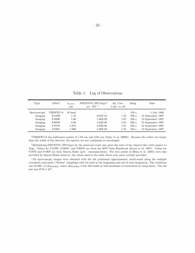
A log of our observations obtained using HST and KECK is given in Table 1.

2.1. HST

The HST data were obtained as part of GO-7364 (PI Figer), a program designed to

measure the IMF’s in the Arches and Quintuplet clusters (Figer et al. 1999a), determine

the star-formation history of the Galactic Center (Serabyn et al. 2002), and determine the

nature of the “Pistol Star” (Figer et al. 1999b).

Broad-band images were obtained using HST/NICMOS on UT 1997 September 13/14,

in a 2×2 mosaic pattern in the NIC2 aperture (19.′′2 on a side). Four nearby fields, separated

from the center of the mosaic by 59′′ in a symmetric cross-pattern, were imaged in order to

sample the background population. All fields were imaged in F110W (λcenter = 1.10 µm),

F160W (λcenter = 1.60 µm), and F205W (λcenter = 2.05 µm). The STEP256 sequence was

used in the MULTIACCUM read mode with 11 reads, giving an exposure time of ≈256

seconds per image. The plate scale was 0.′′076 pixel−1 (x) by 0.′′075 pixel−1 (y), in detector

coordinates. The mosaic was centered on RA 17h45m50.s35, DEC −28◦49′21.′′82 (J2000), and

the pattern orientation was −134.◦6. The spectacular F205W image is shown in Figure 1a,

after first being processed with the standard STScI pipeline procedures.

The narrow-band images were obtained at roughly the same time as the broad-band

images. One image was obtained in each of the F187N (λcenter = 1.87 µm) and F190N

(λcenter = 1.90 µm) filters in the NIC2 aperture. The filters widths are 0.0194 µm for F187N

and 0.0177 µm for F190N. We used the same exposure parameters for these images as those

used for the broad-band images. The difference image, F187N minus F190N, is shown in

Figure 2.

– 5 –

2.2. Keck

The spectroscopic observations were obtained on July 4, 1999, using NIRSPEC, the

facility near-infrared spectrometer, on the Keck II telescope (McLean et al. 1998, 2002), in

high resolution mode, covering K-band wavelengths (1.98 µm to 2.28 µm). The long slit

(24′′) was positioned in a north-south orientation on the sky, and a slit scan covering a

24′′×14′′ rectangular region was made by offsetting the telescope by a fraction of a slit width

to the west between successive exposures. The slit-viewing camera (SCAM) was used to

obtain images simultaneously with the spectroscopic exposures, making it easy to determine

the slit orientation on the sky when the spectra were obtained. From SCAM images, we

estimate seeing (FWHM) of 0.′′6. The plate scales for both spectrometer and SCAM were

taken from Figer et al. (2000a). We chose to use the 3-pixel-wide slit (0.′′43) in order to

match the FWHM of the seeing disk. The corresponding resolving power was R∼23,300

(=λ/∆λFWHM), as measured from unresolved arc lamp lines.

The NIRSPEC cross-disperser and the NIRSPEC-6 filter were used to image six echelle

orders onto the 10242-pixel InSb detector. The approximate spectral range covered in these

orders is listed in Table 2. Coverage includes He I (2.058 µm), He I (2.112/113 µm), Brγ/He I(2.166 µm), He II (2.189 µm), N III (2.24/25 µm), and the CO bandhead, starting at

2.294 µm and extending to longer wavelengths beyond the range of the observations.

Quintuplet Star #3 (hereafter “Q3”), which is featureless in this spectral region (Figer

et al. 1998, Figure 1), was observed as a telluric standard (Moneti et al. 1994). Arc lamps

containing Ar, Ne, Kr, and Xe, were observed to set the wavelength scale. In addition, a

continuum lamp was observed through a vacuum gap etalon filter in order to produce an

accurate wavelength scale between arc lamp lines and sky lines (predominantly from OH).

A field relatively devoid of stars (RA 17h 44m 49.s8, DEC −28◦

54′

6.′′8 , J2000) was observed

to provide a dark current plus bias plus background image; this image was subtracted from

each target image. A quartz-tungsten-halogen (QTH) lamp was observed to provide a “flat”

image which was divided into the background-subtracted target images.

3. Data Reduction

3.1. Photometry

The NICMOS data were reduced as described in Figer et al. (1999a) using STScI pipeline

routines, calnica and calnicb, and the most up-to-date reference files. Star-finding, PSF-

building, and PSF-fitting procedures were performed using the DAOPHOT package (Stetson

– 6 –

et al. 1987) within the Image Reduction and Analysis Facility (IRAF)10. For the narrow-

band photometry, PSF standard stars were identified in the field and used in ALLSTAR. We

used these stars to construct a model PSF with a radius of 15 pixels (1.125′′). This model

was then fitted stars found throughout the image using DAOFIND. Aperture corrections

were estimated by comparing the magnitudes of the PSF stars with those from an aperture

of radius 7.5 pixels (0.563′′), and then adding −2.5 log(1.159) in order to extrapolate to an

infinite aperture (M. Rieke, priv. comm.). Table 1 gives the net aperture corrections to

correct the aperture from a 3 pixel radius to infinity.

3.2. Source Identification and Astrometry

We culled the list produced by the process above by excluding stars with AK<2.8 or

AK>4.2, or equivalently, stars with mF160W−mF205W<1.4 or mF160W−mF205W>2.1. These

choices are motivated by the fact that the majority of stars in the Arches cluster have

values within these limits, as can be seen in Figure 4 of Figer et al. (1999a); stars with

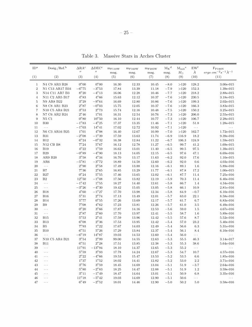
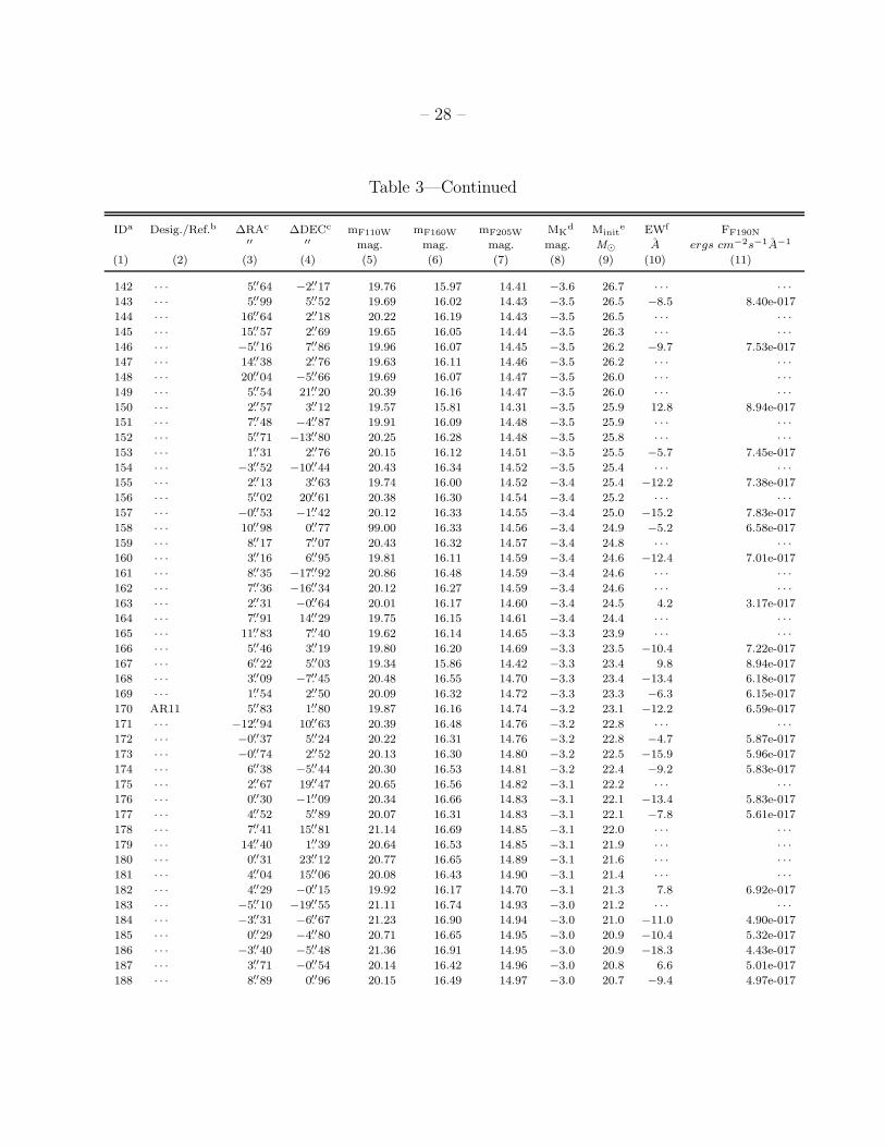
values outside of these limits are likely to be foreground or background stars. The resultant

star list is shown in Table 3. Objects are sorted according to inferred absolute K-band

magnitudes, in order of decreasing brightness. K-band absolute magnitudes were calculated

using AK = EH−K/(AH/AK−1), where EH−K = (H−K)−(H−K)0, and Aλ ∝ λ−1.53 (Rieke

et al. 1989). We estimated intrinsic colors by convolving filter profiles with our best-matched

model spectra. In cases where spectra were not available, i.e. for faint stars, AK = 3.1, a value

that is supported by Figer et al. (1999a). This absolute magnitude was then translated into

an initial mass according to the procedure in Figer et al. (1999a), except that we assumed

solar metallicity, a decision supported by our quantitative spectroscopic analysis described

later. Alternate identifications were taken from the following: Nagata et al. (1995), Cotera

et al. (1996), Lang, Goss, & Rodriguez (2001a), and Blum et al. (2001). We had to allow as

much as a 1′′ offset in some cases so that the correct objects coincided in the various data

sets. The position offsets in the table are in right ascension (RA) and declination (Dec)

and with respect to the star with the brightest inferred absolute magnitude at K. These

offsets were calculated by applying the anamorphic plate scale at the time of observation

and rotating x- and y- pixel offsets in the focal plane in to RA and Dec offsets in the sky.

The stars are plotted and numbered in Figure 1b. Note that the masses in this table apply

only in the case that the stars satisfy our model assumptions. This is not the case for some of

10IRAF is distributed by the National Optical Astronomy Observatories, which are operated by the As-sociation of Universities for Research in Astronomy, Inc., under cooperative agreement with the NationalScience Foundation.

– 7 –

the stars, especially the faint ones, given that they are likely to be field stars in the Galactic

Center, but otherwise unassociated with the Arches cluster.

3.3. Narrow-band Imaging

The narrow-band filters cover wavelength regions that include several potentially rele-

vant atomic transitions. There are potential contributions to the total observed flux through

the F187N and F190N filters from 8 and 2 transitions (H I Paschen−α, He I, and He II),respectively. It is clear from the broad feature near 2.166 µm that He I lines are strong in

the spectra of the emission-line stars, while the relatively weak 2.189 µm line indicates that

the He II lines falling in the F187N filter are minor contributors to FF187N. We estimate that

the flux in the two lines falling in the F190N filter is negligible.

3.4. Narrow-band equivalent-widths

The equivalent-widths in Table 3 were computed according to the following equation:

EW1.87 µm =(FF187N − FF190N)

FF190N×∆λ, (1)

where the fluxes are in W cm−2 µm−1 and ∆λ is the FWHM of the F187N filter; this equation

assumes that the emission line(s) lie completely within the filter bandwidth, and that there is

no contamination of FF190N by emission or absorption lines. We increased FF187N to account

for the difference in reddening for the two wavelengths, assuming the extinction law of Rieke

et al. (1989); this correction is approximately 8.0% and depends slightly on the estimated

extinction. In addition, we reduced FF187N by 9.4% to account for the fact that the F187N

filter has a shorter wavelength than the F190N filter and thus FF187N will be greater by this

amount than FF190N for normal stars due to increasing flux toward shorter wavelengths on

the Rayleigh-Jeans tail of the flux distributions at these wavelengths. Apparently, these two

effects nearly cancel each other.

The difference image (F187N−F190N) in Figure 2 contains about two dozen emission-

line stars with significant flux excesses in the F187N filter, as listed in Table 3. The narrow-

band equivalent-widths increase with apparent brightness, as seen in Figure 3. In addition,

the colors are redder as a function of increasing brightness (Figer et al. 1999a, Figure 4).

Both effects are consistent with the notion that the winds are radiatively driven, so that

higher luminosity stars will have stronger winds, and thus stronger emission lines, with

commensurately stronger free-free emission which has a relatively flat (red) spectrum. In

– 8 –

addition, the emission lines themselves contribute to a redder appearance. These effects are

borne out in our models which show that a zero-age O star will have mF160W−mF205W =−0.07,

while a late-type nitrogen-rich WR (WNL) star will have mF160W−mF205W =+0.07 from the

continuum alone, and mF160W−mF205W =+0.13 from the emission-lines and continuum. So,

a WNL star will have a color that is about +0.20 magnitudes redder than a zero-age O

star. This agrees very well with the color trend seen in Figure 4, after one removes the stars

with mF160W−mF205W>1.85; these stars are subject to extraordinary reddening, consistent

with their location far from the cluster center and the behavior of reddening as a function

of increasing distance from the center of the cluster (Stolte et al. 2002).

3.5. Spectroscopy

The spectra were reduced using IDL and IRAF routines. All target and calibration

images were bias and background subtracted, flat fielded, and corrected for bad pixels. The

target images were then transformed onto a rectified grid of data points spanning linear scales

in the spatial and wavelength directions using the locations of stellar continuum sources and

wavelength fiducials extracted from arc line images and continuum lamp plus etalon images.

The rectified images were then used as inputs to the aperture extraction procedure. Finally,

all 1D spectra were coadded and divided by the spectrum of a telluric standard to produce

final spectra. The following gives a detailed description of this data reduction procedure.

A bias plus background image was produced from several images of a dark area of sky,

observed with the same instrument and detector parameters as the targets. Because the sky

level was changing while these images were being obtained, we scaled the sky components

before combining them with a median filter. The combined image was scaled in order to

match the varying sky emission level in the target images and then added to the bias image

formed by taking the median of several bias images. The resultant image was then subtracted

from target images, thus subtracting properly scaled bias structure and background. This

operation also removes dark current, although the subtraction will be perfect only in the

case that the scaling factor for the varying sky level is exactly one. In other cases, a small

residual in dark current will remain, although the amount of this residual will typically be

less than 1 count (5 e−).

Target images were divided by a normalized flat image, with bias structure and dark

current first removed. We then removed deviant pixels from these images with a two-pass

procedure. First, the median in a 5-by-5 pixel box surrounding each pixel was subtracted

from every pixel in order to form an image with the low-spatial-frequency information re-

moved. If the absolute value of a pixel in this difference image was larger than five times

– 9 –

the deviation in the nearby pixels, then its value was replaced by the median data value in

the box. The deviation in nearby pixels is defined as the median of the absolute values of

those pixels in the difference image. On the second pass, isolated bad pixels were flagged

and replaced if both the following were true: they were higher or lower than both immediate

neighbors in the dispersion direction, and their value deviated by more than 10 times the

square root of the average of those two neighbors. Isolated bad pixel values are replaced by

the average values of their neighbors.

We rectified the target images by mapping a set of continuum traces and wavelength

fiducials in the reduced images onto a set of grid points. This dewarping in both spatial

and spectral directions is done simultaneously and requires knowledge of the wavelengths

and positions of several spectral and spatial features; this information was extracted using

arc, sky, or etalon lines. Typically, we identified 15 to 20 lines in each echelle order for this

purpose. Two stellar continuum spectra and two flat-field edges traced across the length

of the dispersion direction were used to define spatial warping. Rectification was done

separately for each echelle order.

Unfortunately, there is a lack of naturally occurring, and regularly spaced, wavelength

fiducials (absorption or emission lines) produced by the night sky or arc lamps. Because of

this, we had to use a three-stage process for determining the relationship between column

number and wavelength: rectify the images using the arc and sky lines, measure the etalon

line wavelengths in the rectified version of the etalon image and obtain a solution to the etalon

equation, and use the analytically determined wavelengths to produce a better rectification

matrix. This approach gave results that were repeatable (to within an rms of ∼1 km s−1)

(Figer et al. 2002). This three-stage process is described in detail below.

In the first stage, we chose an order containing many (15 to 20) arc and sky lines

so that wavelengths in the rectified images would be fairly well determined. The last few

significant figures of some of the arc-line wavelengths, and all of the OH lines, out to seven

significant figures, were derived from lists available from the National Institute of Standards

and Technology (NIST) Atomic Spectra Database11.

The process for fitting spectral lines was as follows. Each arc or sky line was divided into

10 to 20 sections along the length of the line. Rows from each section were averaged together,

and the location of the peak was found by centroiding. Points along the line obtained from

the centroiding were typically fitted with a 3rd-order polynomial. Outliers were clipped, and

a new fit performed. We used a similar approach to fit the stellar and flat-field edge spatial

traces.

11http://physics.nist.gov/PhysRefData/ASD1/nist-atomic-spectra.html

– 10 –

We then used the arrays of coefficients from spatial and spectral fits to produce a

mapping between points along the spectral features in the warped frame, and points in the

dewarped frame. A two-dimensional second or third order polynomial was then fitted to

these points, resulting in a list of transformation coefficients, the “rectification matrix.”

In the second stage, after dewarping the etalon image with the rectification matrix

produced from the arc and sky lines, we measured the wavelength of each etalon line using

SPLOT in IRAF. This provided preliminary estimated wavelengths for each etalon line.

Exact etalon wavelengths were given by the etalon equation. Solutions to the etalon equation

were found using the constraint that features must have integer order numbers that decrease

sequentially toward longer wavelengths. The estimated wavelengths of the 14 to 16 lines were

used to produce a series of etalon equations that we simultaneously solved by finding the

thickness and order numbers giving the least overall variance from the measured wavelengths.

Once these parameters were determined, exact wavelengths could be calculated for each

etalon line.

In stage three, the exact etalon wavelengths were used to determine a new rectification

matrix by tracing these features in the rectified etalon image. Together with the same spatial

information used to produce the first stage rectification matrix, a new rectification matrix

was produced. The improved quality of the etalon lines allowed for a higher order (fourth

or fifth order) polynomial fit to the etalon mapping between warped and dewarped points.

The new matrices were applied to the appropriate spectral orders of target images.

Three images of the telluric standard (“Q3”) were taken using the same setup as was

used to obtain the target images. We moved the telescope along the slit length direction

between exposures so that the spectra were imaged onto different rows of the detector. We

reduced these images using the sames procedures used for reducing the target images.

Finally, APALL (IRAF) was used to extract spectra in manually chosen apertures. The

resultant 1D spectra were then coadded in the case that a single object was observed in

multiple slit positionings. Before coadding, we shifted all spectra to a common slit position

by cross-correlating the telluric absorption features and shifting the spectra. The coadded

spectra of all the stars in Table 3 for which we have spectra are shown in Figure 5; note that

these spectra have been smoothed using an 11-pixel (44 km s−1) square boxcar function for

display purposes. The fluxes were not reddening-corrected, so the spectral shape (roughly

flat) is indicative of a hot star observed through a large amount of extinction.

– 11 –

4. Results

We use the data in this paper to form a census of stellar types for massive stars in

the cluster, estimate physical properties of the stars, determine the dynamical state of the

cluster members, and assess the impact of the cluster on its environment.

4.1. Spectral Types

The spectra for the most massive stars in our data set are relatively similar, although

the features have smaller equivalent-widths for fainter stars. The brightest stars generally

have spectra with a weak feature near 2.058 µm (He I), weak emission near 2.104 µm (N III)and 2.112/113 µm (He I), broad and strong emission near 2.166 µm (He I, H I), a weak line

near 2.189 µm in P-Cygni profile (He II) in some cases, and weak lines at 2.115/2.24/2.25 µm

(N III), where the primary contributors to the emission line fluxes are due to transitions of

species listed in parentheses. There are indications of absorption at 2.058 µm in most of

the first ten stars, and in some cases, it is strongly in a P-cygni profile (#3 and #8). In

both these cases, the absorption appears to have a “double-bottom.” This line and the

2.112/113 µm blend are narrow in the spectra of #10, #13, #15, and #29.

From these spectra alone, we might assign spectral types of WNL (WN7−WN9) (Figer,

McLean, & Najarro 1997) or O If+ (Hanson et al. 1996) for the brightest stars, just as

have been assigned in Nagata et al. (1995) and Cotera et al. (1996); the degeneracy in the

classification of stars of these spectral types was noted by Conti et al. (1995). Figure 6

compares an average spectrum of the Arches stars with those of WNL stars (Figer, McLean,

& Najarro 1997) and O If+ stars (Hanson et al. 1996). We can see that the Arches stars

have N III emission at 2.104 µm, 2.24 µm, and 2.25 µm, just like that seen in the spectra of

WN7−8 stars, while the spectra of the O If+ stars do not have those lines in emission (or

they are very weak). Figer, McLean, & Najarro (1997) argued that N III lines in the K-band

might be used to distinguish Wolf-Rayet (WR) from O If+ stars on both observational and

theoretical grounds. In addition, Figer, McLean, & Najarro (1997) showed that WN stars

separate by subtype as a function of the relative line strengths in certain lines of their K-

band spectra, i.e. W2.189 µm/W2.166µm or W2.189 µm/W2.11µm. The relevant values for spectra

of the most massive Arches stars are consistent with classifications of WNL. In addition,

the equivalent-widths measured for the emission lines are in the range of those measured for

WNL stars in Figer, McLean, & Najarro (1997), but not for O If+ stars. From all these

measures, we conclude that the Arches stars are WN9 types, with an uncertainty of ± one

subtype. Later in this paper, we use wind/atmosphere models to show that the estimated

nitrogen, carbon, and helium abundances verify WNL classifications.

– 12 –

One objection to the WNL classification might be that it is improbable that all the

WR stars in the cluster be in the exact same evolutionary phase, i.e. WNL. Actually, such a

situation is predicted by Meynet (1995). Indeed, our new observations show that there are no

WR stars in the cluster other than the WNL types, given that our narrow-band observations

would easily detect the strong emission lines from all WR stars, such as the WNE star in

the Quintuplet cluster (Figer, McLean, & Morris 1995), or the carbon-rich WR (WC) stars

seen near the Pistol Star (Figer et al. 1999b). The lack of WC stars suggests an age less

than 3.5 Myr (Meynet 1995), consistent with the WNL classification for brightest stars in

the Arches cluster.

We have identified two groups among the most massive stars with spectral types dis-

tinctly different than the WN9 spectral type. The group of stars from #10 to #30 are O If+

types, and fainter stars are O main sequence stars.

4.2. Identification of the Main Sequence in the Galactic Center

The fainter stars in Table 3 (ID>30) appear to have little to no excess emission at

1.87 µm, consistent with the fact that their spectra appear to be relatively flat. Indeed, some

even show absorption at 2.058 µm, 2.112 µm, and 2.166 µm, of a few angstroms equivalent

width. In the case of star #68, the spectrum (Brγ absorption), apparent magnitude, and

extinction, suggest a luminosity and temperature consistent with an initial mass of about

60 M�, and its presence on the main sequence, given an age of 2.5 Myr and the Geneva

models. The star is likely to be a late-O giant or supergiant, albeit still burning hydrogen

in its core, and thus its classification on the main sequence; note that it is too bright to

be a dwarf. There are several other similar stars that have relatively featureless spectra,

consistent with the spectra of O main sequence stars. This result is a significant spectroscopic

verification of the claim in Figer et al. (1999a) that the main sequence is clearly visible in the

broadband NICMOS data; also, note that Serabyn, Shupe, & Figer (1999) identified likely

O stars with spectra that appeared to be featureless at the resolution of their observations.

While a possible identification of the main sequence in the Galactic Center has previously

been claimed (Eckart et al. 1999; Figer et al. 2000a), the result in this paper is the first

spectroscopic identification of single stars that are unambiguously on the main sequence, as

observed by their narrow absorption lines.

– 13 –

4.3. Wind/atmosphere Modelling

To model the massive Arches stars and estimate their physical parameters, we have used

the iterative, non-LTE line blanketing method presented by Hillier & Miller (1998). The code

solves the radiative transfer equation in the co-moving frame for the expanding atmospheres

of early-type stars in spherical geometry, subject to the constraints of statistical and radiative

equilibrium. Steady state is assumed, and the density structure is set by the mass-loss rate

and the velocity field via the equation of continuity. We allow for the presence of clumping

via a clumping law characterized by a volume filling factor f(r), so that the “smooth” mass-

loss rate, MS, is related to the “clumped” mass-loss rate, MC , through MS=MC/f1/2. The

velocity law (Hillier 1989) is characterized by an isothermal effective scale height in the

inner atmosphere, and becomes a β law in the wind. The model is then prescribed by the

stellar radius, R∗, the stellar luminosity, L∗, the mass-loss rate M , the velocity field, v(r),

the volume filling factor, f, and the abundances of the elements considered. Hillier & Miller

(1998, 1999) present a detailed discussion of the code. For the present analysis we have

assumed the atmosphere to be composed of H, He, C, N, Mg, Si and Fe.

We created a grid of models within the parameter domain of interest. It was bounded

by 4.4<log(Teff)<4.6, 5.0≤log(L∗/L�)≤6.5, −5.7≤log(M/M� yr−1)≤−3.8 , 0.25≤H/He≤10,

and 1≤Z/Z�≤2. This grid was used as a starting point to perform detailed analyses of the

objects, for which the grid parameters were fine tuned, and other stellar properties such as

the velocity field and clumping law were relaxed. The observational constraints were set by

the NIRSPEC K-band spectra, and the NICMOS F187W equivalent-width and continuum

(F110W, F160W and F205W) values.

We present preliminary results for stars #8 and #10. A complete, detailed analysis

of the whole sample will be discussed in Najarro et al. (2002). Table 4 shows the stellar

parameters derived for stars #8 and #10, while Figures 7a,b show the excellent fits of the

models to the observed spectra. All stellar parameters for the strong-line-emission object

(#8) displayed in Table 4 should be regarded as rather firm with the exception of the

carbon abundance which should be considered as an upper limit. For star #10, however, no

information can be obtained about its terminal velocity and clumping factor. Further, only

upper limits are found again for the carbon abundance, while the uncertainty in the nitrogen

abundance is rather high, up to a factor of 3, due to the extreme sensitivity of the N III lines

to the transition region between photosphere and wind in this parameter domain. Therefore

we have assumed the star to have a terminal velocity of 1000 km s−1, which is representative

of this class of objects, and a filling factor of f = 0.1 as derived for object #8. To illustrate

how the assumption of different clumping factor or v∞values can affect the derived stellar

parameters, we also show in Table 4 two additional models which match as well the observed

– 14 –

spectra with modified f (f=1, #10b) and terminal velocity (v∞=1600 km s−1, #10c). Note

that there is no simple MC1/f11/2 = MC2/f2

1/2 scaling (Herald, Hillier, & Schulte-Ladbeck

2001) nor M 1/v∞1 =M 2/v∞2 scaling between the models, and that other stellar parameters

require readjustment.

Table 4 reveals that objects #8 and #10 have very similar luminosities, temperatures,

and ionizing-photon rates. However, their wind densities (M) and abundances reveal differ-

ent evolutionary phases for these two objects. Object #8 fits well with a WNL evolutionary

stage. Its wind density and helium abundance are very similar to those derived by Bohannan

& Crowther (1999) for WN9h stars. On the other hand, object #10 can be placed into a

O If+ phase as its wind density is roughly an order of magnitude lower than that of object #8

and the derived He abundance and upper limits for nitrogen enrichment indicate an earlier

evolutionary phase. Indeed, its K-band spectrum is nearly identical to that of the O8 If+

star HD151804 (Hanson et al. 1996). Interestingly, both Arches objects have luminosities

about one magnitude larger than their counterparts in Bohannan & Crowther (1999).

4.4. Ionizing Flux

Containing so many massive stars, the Arches cluster produces a large ionizing flux. We

estimate the total ionizing flux emitted by the cluster to be 4(1051) photons s−1, based on

our wind/atmosphere model fits for the two emission-line stars in Table 4. To estimate the

total flux, we multiplied the estimated ionizing flux from #8 by 10, that from #10 by 20,

and determined those of the remaining stars in Table 3 by applying equation 3 in Crowther

& Dessart (1998); these factors reflect our choice of #8 and #10 as representatives of the

first 30 stars in the table. The ionizing flux estimate is a bit higher than that in Serabyn et

al. (1998), ≈ a few 1051 photons s−1, after scaling that number for the fact that the cluster

contains 50% more O stars than originally thought (Figer et al. 1999a). This amount of

ionizing flux is consistent with the Arches cluster being the ionizing source for the Thermal

Arches Filaments (Lang, Goss, & Morris 2001b).

4.5. Luminosity

Using the same process as applied to estimate the cluster ionizing flux, we estimate

a total cluster luminosity of 107.8 L�, or one of the most luminous clusters in the Galaxy.

About 40% of the total luminosity is contributed by the 30 brightest stars in Table 3.

– 15 –

4.6. Age

As described in Figer et al. (1999b), the absolute magnitudes and mix of spectral types

are consistent with a cluster age of 2±1 Myr. This was estimated using the colors and

magnitudes of the stars, i.e. the colors give the extinction value, and the apparent magnitudes

lead to absolute K-band magnitudes, which are then compared to isochrones from the Geneva

models (Meynet et al. 1994). It is possible for older stars to attain magnitudes as bright as

the brightest stars in the cluster, but only at relatively cool temperatures, i.e. Teff < 25kK.

A new age constraint from the data in this paper is given by the absence of WC or WNE

stars in the cluster. This observational constraint, when combined with the models of Meynet

(1995), gives τage < 3.0 Myr for the least limiting case (2×M , Z=0.040) and τage < 2.5 Myr

for the most limiting case (1×M , Z=0.040). In addition, the presence of WNL stars requires

τage > 1.5 Myr from these models. Finally, we note the lack of relatively cool (B-type)

supergiant emission-line stars, such as those found in the central parsec (Krabbe et al.

1995) and the Quintuplet cluster (Figer et al. 1999b). The lack of such stars in the Arches

cluster implies τage < 4.0 Myr. Finally, the detailed model for star #8 suggests an age

of 2.5 Myr, at least for that star. We combine all this evidence to suggest that the cluster

age is 2.5 ±0.5 Myr, where the error is dominated by our lack of information concerning

metallicity.

4.7. Velocities

A velocity determination for the emission-line stars is complicated by several facts. First,

the strongest spectral features are blended emission lines, making it impractical to simply

compare the measured wavelength centroid of a “line” to the expected vacuum wavelength.

Because of this, one must cross-correlate the target spectra with respect to a template

spectrum composed of features that accurately represent relative strengths of the blended

lines. Second, the emission lines are broad, so that small wavelength shifts will produce little

change in the cross-correlated power when compared to a template spectrum. Third, there

are slight differences in the shapes of the emission lines between spectra of the various stars,

so a model blend for one spectrum might not faithfully reproduce the features in another

spectrum, at least not to the fidelity required for high precision velocity measurements.

Because of these difficulties, we approached the velocity estimates using two techniques. We

smoothed the spectra using a box-car filter with varying widths between 1 and 31 pixels (4

and 120 km s−1), finding little difference in the velocities as a function of these widths.

First, we estimated an absolute velocity for star #8 by cross-correlating its spectrum

with that of our model spectrum. This method gave a velocity of +54 km s−1 (redshifted),

– 16 –

in the heliocentric frame, for the blend near 2.166 µm. Our estimates using other lines are

somewhat less than this value, as low as +20 km s−1, but those lines are weaker than the

blend at 2.166 µm, and thus produce larger velocity errors.

In the second method, we cross-correlated all the spectra against each other. The cross-

correlations were performed separately on three wavelength regions, the first containing the

2.104 µm and 2.115 µm features, the second containing the 2.166 µm and 2.189 µm features,

and the third containing the doublet at 2.25 µm. This method was used to compute the

standard deviation of relative velocities, allowing us to infer the mass enclosed within some

orbital radius that represents an average of the emission-line stars’ orbital radii. Given that

small differences in intrinsic blend morphology can affect the location of the maximum point

of the cross-correlated power, we also repeated this approach using line centroids to compute

velocity differences. Using both approaches, we found a standard deviation of ≈22 km s−1

for a sample containing eight emission-line stars. This value represents an upper limit on

the intrinsic dispersion, given that the effects described above would tend to increase the

estimated value over the intrinsic velocity dispersion. We also found that the stars were

redshifted by +41 km s−1 with respect to star #8. We therefore estimate a heliocentric

“cluster” velocity of +95±8 km s−1, where the error is simply the standard deviation divided

by the square root of eight; note that this error neglects the systematic effects described

above, so the true velocity might differ from the estimate by significantly larger than the

quoted error.

For a gravitationally bound and spherically symmetric cluster of mass Mcluster, the virial

theorem gives Mcluster = 3σ2R/G (Ho and Filippenko 1996), where σ is the one-dimensional

velocity dispersion, R is the appropriate radius, G is the gravitational constant, the ve-

locities are assumed to be isotropic, and all stars have equal mass. This simple formula

can be compared to the more general case where the cluster can be resolved into individ-

ual stars (Illingworth 1976). Using R = 0.23 pc for the sample in question, we calculate

Mcluster < 7(104) M�, or about five times greater than what would be expected from direct

integration of the mass function in Figer et al. (1999a) over the area sampled by the stars

used in the analysis. This high mass limit results from the systematic effects inherent in our

radial velocity determinations, as described above.

5. Discussion

In this section, we compare our measurements to those in previous papers and use

measurements at other wavelengths to determine the physical parameters of the observed

stars. Finally, we discuss how the Arches cluster interacts with its local environment to

– 17 –

create heating and ionization of a nearby cloud.

5.1. Comparison to Previous Near-infrared Measurements

Table 3 lists over 30 probable emission-line stars, albeit the faintest having relatively

weak emission lines; Figure 3a confirms that there are roughly this number of stars with

reliable emission-line excesses. This list contains over a factor of two increase in the number

of emission-line stars previously identified in the cluster (Blum et al. 2001; Nagata et al. 1995;

Cotera et al. 1996). The line and continuum fluxes presented here largely agree with earlier

results (Nagata et al. 1995; Cotera et al. 1996). The FF187N and FF190N fluxes reported in

this paper are similar to those reported in Blum et al. (2001), after correcting for differences

in the assumed zero points, the fact that we corrected for the difference in extinction at

the two narrow-band wavelengths, and that we also corrected for the intrinsic shape of the

stellar continuum; in addition, our extinction estimates are higher in many cases than those

used in Blum et al. (2001).

The spectra in this paper are consistent with the narrow-band photometry in Nagata

et al. (1995) and Blum et al. (2001) and the spectra in Cotera et al. (1996), although our

high-resolution spectroscopy shows that the photometry is significantly affected by blending

of absorption and emission features in P-Cygni profiles.

We confirm the discovery of a new bright emission-line star (#5, B22, N9) near the

southern edge of the cluster, reported in Blum et al. (2001), and note that it is a counterpart

of the x-ray source, “AR8,” in Lang, Goss, & Rodriguez (2001a). We also confirm that star

#16 (B19) is an emission-line star, as suspected by Blum et al. (2001). Blum et al. (2001)

listed some additional candidate emission-line stars. We confirm that the following stars

from that list are, indeed, emission-line stars (their designations in parentheses): #15 (B8),

#27 (B16), #17 (B29), #10 (B30), #10 (B20), #13 (B31).

5.2. Comparison to X-ray Flux Measurements

Yusef-Zadeh et al. (2001) reported Chandra X-ray observations of a region including

the Arches cluster. They detected three extended sources, one (A1) near the center of the

Arches cluster, another (A2) located to the North and West of the center by about 7′′ and

a third weaker source (A3) about 90′′ × 60′′ in size underlying the first two. The centroid

of source A2 coincides within 1 arcsecond with an emission-line star, #9 in Table 3. The

apparent spatial coincidence of the X-ray sources and Arches cluster strongly suggests that

– 18 –

the X-ray sources are physically associated with the cluster. Yusef-Zadeh et al. estimate the

total X-ray luminosity between 0.2 and 10 keV to be 3.3, 0.8 and 0.16 (1035) ergs s−1 for A1,

A2 and A3, respectively. They attribute the emission from A1 and A2 to either colliding

winds in binary systems or to the winds from single stars interacting with the collective

wind from the entire cluster. The coincidence of source A2 with an emission-line source is

very interesting in the context of the latter scenario. A3, on the other hand, has roughly

the characteristics expected from shock-heated gas created by the collisions of the multitude

of 1000-km s−1 stellar winds emanating from the stars in the rich, dense cluster (Ozernoy,

Genzel, & Usov 1997; Canto, Raga, & Rodriguez 2000). Because the X-ray sources are

extended, it is unlikely that they can be attributed to single X-ray binary systems. However,

the rough coincidence of source A1 with the core of the cluster raises the possibility that it

may be comprised of many relatively weak stellar X-ray sources, binary or single, residing

in the cluster core, and unresolved spatially from each other.

5.3. Comparison to Radio Flux Measurements

From Table 3 we see that one of the objects analysed in this work, #8, has also been de-

tected at 8.5 GHz (Lang, Goss, & Rodriguez 2001a). Our derived mass-loss rate is consistent

with the observed radio flux (0.23 mJy) only if the outer wind regions are unclumped. Such

a behavior for the clumping law has been suggested by Nugis, Crowther, & Willis (1998)

from analysis of galactic WR stars. They found that the observed infrared to radio fluxes

of WR stars are well reproduced by a clumping law where the filling factor is unity close

to the stellar surface, increasing to a minimum at 5 to 10 R∗ and returning again to unity

in the outer wind where the radio flux forms. Note, however, that the line fluxes of the

weaker lines like Brγ or He I remain unaltered with this new description of the clumping

law, but the line fluxes of the strongest lines, such as Paα, formed in the outer wind can

be significantly reduced. From Table 4 we see that our models are fully consistent with the

observed equivalent-width of Paα.

We consider now the possible correlation between line fluxes and radio-continuum flux

analogous to the one discussed above for K-band fluxes (see Figure 3a). In principle, we also

expect the near-infrared emission line strengths to scale with the free-free emission detected

at radio wavelengths (Nugis, Crowther, & Willis 1998; Leitherer, Chapman, & Koribalski

1997). However, we do not find such a correlation, as can be seen in Figures 8a,b. A similar

result was obtained by Bieging, Abbott, & Churchwell (1982) for a sample of eight WR stars.

We believe this apparent absence of correlation between Paα line-strength and radio flux is

caused by both observational and physical effects. The observational effect is related to the

– 19 –

fact that the radio measurements are picking up only the tip of the iceberg, i.e., those stars

with the densest winds of the cluster. The physical effect is related to the fact that all three

components contributing to EW1.87µm (H I, He I, and He II) are very sensitive to changes in

temperature in the parameter domain appropriate to these objects. Further, both the line

and continuum fluxes depend strongly not only on the mass-loss rate but also on the shape

of the velocity field and the clumping law. Therefore, such strong dependence of the Paα

line flux on several stellar parameters introduces a large scatter in the expected line-strength

vs radio-flux relationship.

The radio fluxes of the most massive Arches stars are comparable to those of WNL

stars, but not to those of O If+ stars. The WN8 star WR105 (van der Hucht 2001) would

emit 0.14 mJy at the distance of the Arches cluster, comfortably within the range of fluxes

measured for the Arches stars. Similar values are reported for WR stars in Bieging, Abbott,

& Churchwell (1982). On the other hand, HD 16691 (O4 If+) emits 0.3 mJy at 4.9 GHz,

according to Wendker (1995), implying an expected flux of 1.7 µJy at the distance of the

Arches cluster, assuming that the star has a parallax of 1.7 mas (Perryman et al. 1997).

The expected flux is two orders of magnitude below the flux levels of the brightest Arches

stars (Lang, Goss, & Rodriguez 2001a). No doubt, this difference is due to the relatively low

mass-loss rate for HD 16691, about 1/20 of that of the bright Arches stars. A similar trend

can be seen in Figure 6 where the emission lines in the spectra of HD 16691 are shown to be

much weaker than those in the spectra of the Arches emission-line stars. Again, weak winds

produce weak emission lines and weak free-free emission.

Finally, we report several additional radio sources having emission-line star counterparts.

They were found by comparing the radio continuum contour plot in Lang, Goss, & Rodriguez

(2001a) with the difference image in Figure 2; they are marked by squares in this figure. We

have designated the four near-infrared counterparts to these newly identified radio sources

in Table 3.

5.4. Evolutionary Status of the Massive Stars in the Arches Cluster

The emission-line stars appear to contain significant amounts of hydrogen, while also

exhibiting considerable helium content. We believe that this can be explained by the most

massive stellar models in Meynet et al. (1994). For the brightest 10 or so stars in Table 3, the

observations can be fit by these models for Minitial&120 M� stars that have evolved to cool

temperatures while retaining hydrogen. In particular, star #8 can be fit by a Minitial∼120 M�star with solar abundance, standard mass-loss rates, age of 2.4 Myr to 2.5 Myr, and present-

day mass of 72 M� to 76 M� (Schaller, Schaerer, Meynet, & Maeder 1992).

– 20 –

5.5. Relation to the Nearby Molecular Cloud (M0.10+0.03)

It appears that the Arches cluster heats and ionizes the surface of M0.10+0.03, the

nearby molecular cloud (Serabyn & Guesten 1987; Brown & Liszt 1984), given that the cluster

can easily provide the necessary flux to account for the infrared emission and recombination-

line flux from the cloud.

The relative heliocentric velocity between the cluster stars (+95±8 km s−1) and the

ionized gas on the surface of the cloud (−20 to −50 km s−1) suggests that the physical

association is accidental and that the cluster stars are ionizing the surface of the cloud. This

difference in velocity is reminiscient of that observed between the Quintuplet (+130 km s−1)

(Figer 1995; Figer et al. 1999a) and the Sickle cloud, M0.10+0.03 (+30 km s−1) (Lang, Goss,

& Wood 1997). In both cases, it appears that young clusters happen to lie near molecular

clouds whose surfaces are ionized by the photons from the hot stars in the clusters. The

following shows that the ionizing flux and energy required to heat the cloud can be provided

by the Arches cluster. Note that a differential velocity of 100 km s−1 would produce a relative

drift of 100 pc in 1 Myr, a distance that would bring a cluster within the vicinity of a few

clouds, given the spatial distribution of clouds in the central few hundred parsecs.

5.5.1. Ionization and Heating

Even before the discovery of the Arches cluster, Serabyn & Guesten (1987), Genzel

et al. (1990), and Mizutani et al. (1994) suggested that the Thermal Arched Filaments

are photoionized by nearby hot stars. After the discovery of the cluster, many authors

considered the possibility that the cluster is ionizing the cloud. One problem with this idea

is the fact that the filaments are very large, and have roughly constant surface brightness and

excitation conditions (Erickson et al. 1991; Colgan et al. 1996), indicating that the ionizing

source is either evenly distributed over many parsecs or is relatively far away. Given the new

ionizing flux estimates in this paper and in (Serabyn et al. 1998), the cluster would produce

enough flux to account for the filaments, even if 20 pc away, far enough to allow for the even

illumination that is observed. Indeed, Timmermann et al. (1996) predicted this result, and

Lang, Goss, & Morris (2001b) present a detailed analysis that confirms it.

Cotera et al. (1996) give estimates for the total ionizing flux of 2−5(1050) photons s−1,

depending on whether one models the spectral energy distributions for the emission-line stars

with Kurucz (1979) atmospheres or blackbody functions; however, this estimate includes only

flux from the dozen or so emission-line stars that were known at the time. Nonetheless, the

results of this paper suggest that the cluster ionizes the cloud.

– 21 –

The heating in the cloud produces an infrared luminosity of 107 L� (Morris, Davidson,

& Werner 1995). Assuming a covering fraction of ≈10%, we find that the Arches cluster can

deliver about this much luminosity, within a factor of two.

5.5.2. Location along the line of sight

Given the Brγ flux from the filaments measured by Figer (1995), we know that the line

emission is extincted by about AK∼3. This implies that the filaments are on the near side of

the cloud, since such an extinction corresponds only to the typical foreground extinction to

the Galactic Center, and precludes any substantial additonal extinction. This information

leads to the conclusion that the Arches cluster is on the near side of, and is approaching,

the wayward molecular cloud that is moving in opposition to the bulk motion of stars and

gas around the Galactic Center (McGinn, Sellgren, Becklin, & Hall 1989), consistent with

the geometry described in Lang, Goss, & Morris (2001b).

5.6. Dynamical Evolution and Uniqueness of the Arches and Quintuplet

Clusters

The temporal coincidence of the star formation events that produced the massive clusters

in the Galactic Center, and the lack of older red supergiants, suggest that the Galactic Center

has been host to a recent burst of star formation. Kim, Morris, & Lee (1999) and Kim et

al. (2000) predicted that compact young clusters in the Galactic Center would evaporate

on short timescales, i.e. a few Myr. Portegies-Zwart et al. (2001) argue that other clusters

similar to, yet somewhat older than, the Arches and Quintuplet clusters exist in the central

100 pc. This argument is based upon a dynamical analysis which predicts that such clusters

evaporate after 55 Myr, and further that the clusters’ projected surface number density in

stars drops below the limit of detectability in a few Myr. The statement that members

of dispersed clusters could have gone undetected is incorrect. Such stars would easily be

detectable for their extreme brightness, i.e. there would be hundreds of stars as bright as

IRS 7 (in the central parsec) strewn about the central 100 pc for each Arches/Quintuplet-like

cluster between the age of 5 and 30 Myr. Given the claim in Portegies-Zwart et al. about

the expected number of “hidden” young clusters in the central hundred parsecs, we would

expect to see of order ten thousand red supergiants in this region. Only a few are seen, as

demonstrated by surveys for such stars (Figer 1995; Cotera 1995).

Portegies-Zwart et al. suggest that clusters could be “hiding” near bright stars due to

– 22 –

limitations in dynamic range, but these arguments are specious, since the dynamic range

of array-based detections are obviously not limited by the digitization of a single read if

multiple coadds are used (e.g. Figer et al. (1999a) reach a dynamic range of over 105). Thus

in agreement with Kim et al., we conclude that the clusters must disperse rapidly

5.7. Comparison to NGC 3603 and R136 in 30 Dor

The Arches cluster is similar in age and content to NGC 3603 and R136 in 30 Dor, and

is surrounded by a giant H II region as is R136. In contrast to these clusters, we do not

see WN5h or WN6h stars (Crowther & Dessart 1998), suggesting that the Arches cluster is

older. This is consistent with our age determination, as suggested by other means described

earlier.

While our spectra exhibit no primary diagnostic lines to estimate metallicity, we may

use our estimates for the helium and nitrogen abundances in object #8 in conjunction with

the evolutionary model for 120 M� to infer metallicity. For Z(He)=0.7, the models predict

the star to have already reached its maximum nitrogen surface mass fraction. Hence, we

may compare our derived nitrogen mass fraction, Z(N)=0.016, with the evolutionary models

values at different metallicities (Schaller, Schaerer, Meynet, & Maeder 1992). We see that

this value is met for solar metallicity. A more detailed analysis of the metallicity of the

Arches stars will be presented in Najarro et al. (2002).

We thank Nolan Walborn and Nino Panagia for critical readings of the paper. We

thank John Hillier for providing his code. F. N. acknowledges DGYCIT grants ESP98-

1351 and PANAYA2000-1784. We acknowledge the work of: Maryanne Angliongto, Oddvar

Bendiksen, George Brims, Leah Buchholz, John Canfield, Kim Chin, Jonah Hare, Fred

Lacayanga, Samuel B. Larson, Tim Liu, Nick Magnone, Gunnar Skulason, Michael Spencer,

Jason Weiss and Woon Wong.

– 23 –

Table 1. Log of Observations

Type Filtera λcenter PHOTFNU/ZP(Vega)b Ap. Corr. Integ. Date

µm sec. DN−1 3 pix. to inf

Spectroscopyc NIRSPEC-6 K-band · · · · · · 150 s. 3 July 1999

Imaging F110W 1.10 9.61E-10 1.35 256 s. 13 September 1997

Imaging F160W 1.60 1.86E-09 1.67 256 s. 13 September 1997

Imaging F205W 2.05 1.64E-09 1.81 256 s. 13 September 1997

Imaging F187N 1.874 4.95E-08 1.75 256 s. 13 September 1997

Imaging F190N 1.900 5.36E-08 1.76 256 s. 13 September 1997

aNIRSPEC-6 has half-power points of 1.85 µm and 2.62 µm (Figer et al. 2000b). Because the orders are longer

than the width of the detector, the spectra are not contiguous in wavelength.

bMultiplying PHOTFNU/ZP(Vega) by the observed count rate gives the ratio of the object’s flux with respect to

Vega. Values for F110W, F160W, and F205W are from the HST Data Handbook (Keyes et al. 1997). Values for

F187N and F190N are from Marcia Rieke (priv. communication). The zero points in Blum et al. (2001) were also

provided by Marcia Rieke; however, the values used in the table above were more recently provided.

cAll spectroscopy images were obtained with the slit positioned approximately north-south using the multiple

correlated read mode (“Fowler” sampling) with 16 reads at the beginning and end of each integration. The resolution

was 23,300, (λ/∆λFWHM, where ∆λFWHM is the full-width at half maximum of unresolved arc lamp lines). The slit

size was 0.′′43× 24′′.

– 24 –

Table 2. Wavelength Coverage in Spectra

Echelle λmin λmax

Order µm µm

33 2.281 2.315

34 2.214 2.248

35 2.152 2.184

36 2.092 2.124

37 2.036 2.067

38 1.983 2.013

– 25 –

Table 3. Massive Stars in Arches Cluster

IDa Desig./Ref.b ∆RAc ∆DECc mF110W mF160W mF205W MKd Minit

e EWf FF190N′′ ′′ mag. mag. mag. mag. M� A ergs cm−2s−1A−1

(1) (2) (3) (4) (5) (6) (7) (8) (9) (10) (11)

1 N4 C9 AR3 B28 0.′′00 0.′′00 16.30 12.33 10.45 −8.0 >120 128.2 3.00e-015

2 N1 C13 AR17 B34 −6.′′75 −3.′′53 17.84 13.39 11.18 −7.9 >120 152.3 1.39e-015

3 N14 C11 AR7 B3 8.′′20 −4.′′13 16.06 12.28 10.46 −7.7 >120 218.2 2.88e-015

4 N11 C2 AR5 B17 4.′′83 4.′′66 15.63 12.12 10.37 −7.6 >120 230.5 3.18e-015

5 N9 AR8 B22 3.′′29 −9.′′64 16.69 12.80 10.86 −7.6 >120 199.3 2.02e-015

6 N8 C8 AR1 B23 2.′′87 −0.′′03 15.75 12.05 10.37 −7.6 >120 166.3 3.83e-015

7 N10 C5 AR4 B21 3.′′53 2.′′73 15.74 12.16 10.48 −7.5 >120 150.2 3.25e-015

8 N7 C6 AR2 B24 2.′′46 1.′′01 16.31 12.54 10.76 −7.3 >120 206.0 2.55e-015

9 N5 C1 0.′′80 10.′′50 16.10 12.44 10.77 −7.3 >120 106.7 2.28e-015

10 B30 −1.′′83 −4.′′25 17.37 13.35 11.46 −7.1 >120 51.8 1.28e-015

11 · · · −1.′′03 14.′′41 17.02 12.72 10.92 −7.1 >120 · · · · · ·12 N6 C3 AR16 B25 1.′′01 4.′′98 16.40 12.67 10.99 −7.0 >120 162.7 1.72e-015

13 B31 −2.′′08 −1.′′39 17.59 13.63 11.74 −6.9 116.9 18.2 9.39e-016

14 B12 6.′′24 −0.′′32 16.38 12.84 11.22 −6.7 106.3 124.9 1.59e-015

15 N12 CB B8 7.′′24 5.′′67 16.12 12.78 11.27 −6.5 99.7 41.2 1.69e-015

16 B19 4.′′22 1.′′59 16.62 13.01 11.40 −6.5 99.5 97.5 1.39e-015

17 B29 −0.′′89 −4.′′90 18.13 14.05 12.15 −6.5 97.6 47.1 6.69e-016

18 AR9 B20 3.′′58 4.′′34 16.70 13.17 11.63 −6.2 92.0 17.6 1.10e-015

19 AR6 −5.′′81 −3.′′72 18.89 14.58 12.60 −6.2 92.0 0.6 4.03e-016

20 · · · 2.′′90 2.′′58 17.49 13.88 12.16 −6.1 89.1 1.6 5.89e-016

21 B7 7.′′36 2.′′65 16.85 13.29 11.77 −6.1 87.8 17.2 1.00e-015

22 B27 0.′′24 5.′′55 17.46 13.65 12.02 −6.1 87.7 11.4 7.25e-016

23 B2 12.′′50 −1.′′08 17.56 13.82 12.19 −5.9 70.3 11.4 6.40e-016

24 · · · −1.′′42 1.′′55 18.27 14.40 12.61 −5.8 66.7 1.4 4.34e-016

25 · · · −3.′′26 −4.′′30 19.42 15.05 13.05 −5.8 66.1 10.9 2.81e-016

26 B18 4.′′60 −1.′′27 17.70 13.98 12.34 −5.8 64.9 −0.7 6.10e-016

27 B16 5.′′31 2.′′74 17.13 13.49 12.01 −5.7 63.0 22.1 8.58e-016

28 B14 5.′′77 0.′′55 17.26 13.69 12.17 −5.7 61.7 6.7 6.83e-016

29 B9 7.′′08 4.′′62 17.23 13.81 12.26 −5.7 61.0 3.5 6.49e-016

30 · · · 0.′′20 3.′′66 17.87 14.16 12.53 −5.6 59.0 1.5 4.67e-016

31 · · · 2.′′87 2.′′60 17.70 13.97 12.41 −5.5 58.7 1.6 5.89e-016

32 B15 5.′′53 2.′′41 17.59 13.96 12.42 −5.5 57.6 8.7 5.52e-016

33 B13 6.′′08 2.′′36 17.53 13.95 12.42 −5.4 57.0 23.2 5.40e-016

34 B5 7.′′93 1.′′22 17.67 14.03 12.49 −5.4 56.6 6.3 5.31e-016

35 B10 6.′′51 5.′′26 17.29 13.84 12.37 −5.4 56.1 8.4 6.10e-016

36 · · · −6.′′19 14.′′87 19.03 14.53 12.60 −5.4 56.0 · · · · · ·37 N10 C5 AR4 B21 3.′′54 2.′′99 99.00 14.55 12.63 −5.3 55.5 46.3 3.14e-017

38 B11 6.′′51 2.′′28 17.51 13.85 12.38 −5.3 55.3 38.6 5.64e-016

39 · · · 11.′′91 −13.′′94 18.10 14.37 12.65 −5.3 55.2 · · · · · ·40 · · · 5.′′59 3.′′93 17.78 14.24 12.67 −5.3 54.7 10.7 4.57e-016

41 · · · 2.′′22 −4.′′66 19.53 15.47 13.53 −5.2 53.5 6.6 1.85e-016

42 · · · 1.′′37 1.′′52 18.02 14.41 12.82 −5.2 53.0 2.2 3.71e-016

43 · · · 3.′′76 3.′′59 18.45 14.69 13.04 −5.1 51.9 −3.7 2.64e-016

44 · · · 5.′′80 −2.′′83 18.25 14.47 12.88 −5.1 51.9 1.2 3.59e-016

45 · · · 3.′′11 −1.′′49 18.47 14.64 13.01 −5.1 50.9 6.8 3.35e-016

46 · · · 11.′′18 −5.′′42 19.03 14.69 12.90 −5.1 50.6 · · · · · ·47 · · · 6.′′49 −2.′′52 18.01 14.46 12.90 −5.0 50.2 5.0 3.58e-016

– 26 –

Table 3—Continued

IDa Desig./Ref.b ∆RAc ∆DECc mF110W mF160W mF205W MKd Minit

e EWf FF190N′′ ′′ mag. mag. mag. mag. M� A ergs cm−2s−1A−1

(1) (2) (3) (4) (5) (6) (7) (8) (9) (10) (11)

48 · · · 4.′′77 −4.′′20 18.73 15.00 13.28 −5.0 50.2 −3.2 2.39e-016

49 · · · −1.′′74 14.′′97 18.36 14.59 12.94 −5.0 49.9 · · · · · ·50 · · · −1.′′65 −3.′′41 19.57 15.38 13.53 −5.0 49.9 2.1 2.01e-016

51 · · · 10.′′80 −1.′′62 19.82 14.99 12.94 −5.0 49.9 −7.8 2.94e-016

52 · · · 12.′′43 −10.′′55 18.59 14.67 12.94 −5.0 49.9 · · · · · ·53 · · · 5.′′96 −2.′′25 18.25 14.51 12.94 −5.0 49.7 6.4 3.53e-016

54 · · · 0.′′14 6.′′95 18.77 14.78 13.02 −5.0 48.4 −5.4 2.75e-016

55 · · · 6.′′93 0.′′15 18.13 14.57 13.03 −4.9 48.1 −10.4 3.13e-016

56 · · · 4.′′35 0.′′57 18.15 14.54 13.03 −4.9 48.1 −11.4 3.33e-016

57 B11 6.′′67 2.′′45 18.01 14.53 13.04 −4.9 47.9 · · · · · ·58 · · · −3.′′84 3.′′16 18.87 14.90 13.05 −4.9 47.8 −8.7 2.78e-016

59 · · · 11.′′54 8.′′42 18.27 14.63 13.05 −4.9 47.8 · · · · · ·60 · · · 7.′′08 0.′′58 18.32 14.56 13.02 −4.9 47.0 7.0 3.06e-016

61 · · · −1.′′53 23.′′67 18.56 14.69 13.09 −4.9 47.0 · · · · · ·62 · · · 2.′′20 6.′′15 18.10 14.57 13.04 −4.8 46.4 −0.5 2.90e-016

63 · · · 7.′′60 −2.′′92 18.21 14.64 13.15 −4.8 46.0 −22.0 2.74e-016

64 · · · 2.′′91 6.′′05 18.25 14.69 13.13 −4.8 45.9 0.7 2.62e-016

65 · · · −2.′′34 1.′′23 18.67 14.90 13.16 −4.8 45.7 −5.6 2.61e-016

66 · · · 3.′′57 2.′′34 18.32 14.63 13.11 −4.8 44.9 −1.4 2.98e-016

67 · · · 2.′′82 7.′′66 18.68 14.94 13.35 −4.7 43.8 −4.2 2.16e-016

68 · · · 7.′′82 4.′′61 17.74 14.33 12.93 −4.7 43.7 −5.1 3.53e-016

69 · · · 7.′′72 2.′′44 18.10 14.52 13.06 −4.7 43.5 −0.4 3.13e-016

70 · · · −0.′′10 −0.′′63 18.89 14.94 13.30 −4.7 43.2 −9.4 2.34e-016

71 · · · −2.′′63 6.′′33 19.28 15.32 13.62 −4.7 43.1 −3.7 1.72e-016

72 · · · 6.′′88 2.′′49 18.21 14.62 13.13 −4.6 42.5 32.1 2.89e-016

73 · · · 5.′′50 −2.′′82 18.81 14.96 13.35 −4.6 42.3 −12.4 2.37e-016

74 · · · 9.′′63 −4.′′73 18.73 14.98 13.36 −4.6 42.2 · · · · · ·75 · · · 7.′′42 11.′′51 19.83 15.32 13.36 −4.6 42.2 · · · · · ·76 · · · 1.′′07 5.′′70 18.81 14.98 13.38 −4.6 41.9 −14.2 2.04e-016

77 · · · 6.′′71 2.′′93 18.40 14.74 13.25 −4.6 41.3 −1.4 2.61e-016

78 · · · 22.′′07 −1.′′95 19.03 15.08 13.44 −4.5 40.8 · · · · · ·79 · · · −2.′′45 4.′′65 19.91 15.41 13.46 −4.5 40.5 −9.4 1.98e-016

80 · · · 4.′′33 3.′′30 18.45 14.92 13.47 −4.5 40.3 −5.2 2.25e-016

81 · · · 5.′′95 −1.′′48 18.74 15.02 13.48 −4.5 40.1 −10.9 2.00e-016

82 · · · 6.′′26 3.′′63 18.35 14.93 13.40 −4.5 40.1 −2.2 2.24e-016

83 · · · −2.′′62 2.′′09 19.21 15.34 13.53 −4.4 39.3 −9.4 1.80e-016

84 · · · 3.′′50 6.′′48 18.70 15.08 13.54 −4.4 39.1 −13.6 1.95e-016

85 · · · 2.′′94 4.′′16 18.50 15.03 13.54 −4.4 39.1 −8.8 1.85e-016

86 · · · 9.′′53 −10.′′83 18.33 15.00 13.56 −4.4 38.7 · · · · · ·87 · · · 3.′′39 6.′′18 18.71 15.10 13.60 −4.4 38.1 −5.4 1.74e-016

88 · · · −7.′′98 5.′′53 20.11 15.55 13.62 −4.3 37.8 · · · · · ·89 · · · 9.′′14 5.′′61 18.48 15.07 13.65 −4.3 37.3 −7.1 1.84e-016

90 · · · 4.′′08 −10.′′21 19.37 15.38 13.68 −4.3 36.9 −20.6 1.47e-016

91 · · · −3.′′70 5.′′24 19.36 15.52 13.69 −4.3 36.8 −6.8 1.39e-016

92 · · · 3.′′39 1.′′31 18.59 14.95 13.48 −4.3 36.8 −2.9 2.18e-016

93 · · · 1.′′52 −0.′′02 19.18 15.43 13.81 −4.3 36.5 0.4 1.57e-016

94 · · · 5.′′22 −5.′′27 19.81 15.91 14.14 −4.3 36.5 −1.1 1.06e-016

– 27 –

Table 3—Continued

IDa Desig./Ref.b ∆RAc ∆DECc mF110W mF160W mF205W MKd Minit

e EWf FF190N′′ ′′ mag. mag. mag. mag. M� A ergs cm−2s−1A−1

(1) (2) (3) (4) (5) (6) (7) (8) (9) (10) (11)

95 · · · 4.′′18 0.′′76 18.73 15.18 13.71 −4.3 36.4 −8.5 1.67e-016

96 · · · 6.′′10 3.′′03 18.47 15.01 13.54 −4.3 36.3 −5.3 2.03e-016

97 · · · 14.′′78 6.′′19 19.02 15.33 13.73 −4.2 36.2 · · · · · ·98 · · · 11.′′74 −14.′′30 19.16 15.36 13.75 −4.2 35.8 · · · · · ·99 · · · 4.′′01 5.′′67 19.42 15.35 13.76 −4.2 35.6 −47.3 1.44e-016

100 · · · 10.′′53 5.′′15 18.71 15.21 13.77 −4.2 35.6 · · · · · ·101 · · · 8.′′59 4.′′39 18.69 15.28 13.78 −4.2 35.4 −10.0 1.63e-016

102 · · · 8.′′09 −6.′′04 19.19 15.35 13.78 −4.2 35.4 −9.7 1.51e-016

103 · · · −7.′′64 0.′′18 21.30 16.45 14.53 −4.2 35.3 3.0 6.98e-017

104 · · · 4.′′17 −21.′′01 19.13 15.39 13.79 −4.2 35.3 · · · · · ·105 · · · 4.′′41 −16.′′84 20.07 15.71 13.81 −4.2 34.9 · · · · · ·106 · · · −4.′′92 −0.′′47 99.00 15.47 13.82 −4.1 34.8 −169.5 1.41e-016

107 · · · −5.′′10 −8.′′23 19.11 15.39 13.87 −4.1 34.1 · · · · · ·108 · · · 7.′′22 11.′′83 19.29 15.54 13.89 −4.1 33.7 · · · · · ·109 · · · 3.′′42 2.′′06 19.19 15.44 13.91 −4.1 33.5 −10.2 1.42e-016

110 · · · 4.′′13 6.′′41 19.04 15.44 13.93 −4.0 33.2 −11.2 1.25e-016

111 · · · 0.′′65 18.′′90 19.47 15.67 13.94 −4.0 33.1 · · · · · ·112 · · · 3.′′25 6.′′40 18.94 15.40 13.87 −4.0 32.9 −0.3 1.31e-016

113 · · · −3.′′19 5.′′29 19.80 15.70 13.97 −4.0 32.7 −8.0 1.14e-016

114 · · · 7.′′15 3.′′69 18.97 15.46 13.99 −4.0 32.3 −6.3 1.27e-016

115 · · · 2.′′32 2.′′72 19.27 15.32 13.83 −4.0 32.3 2.9 1.42e-016

116 · · · 3.′′64 16.′′48 19.53 15.71 14.01 −4.0 32.1 · · · · · ·117 · · · 6.′′51 3.′′32 19.14 15.54 14.06 −3.9 31.4 −8.0 1.25e-016

118 · · · 2.′′54 −3.′′21 19.66 15.82 14.08 −3.9 31.1 −8.0 1.16e-016

119 · · · 7.′′65 0.′′01 19.29 15.62 14.06 −3.9 31.1 0.2 1.13e-016

120 · · · 5.′′68 −7.′′20 19.82 15.86 14.09 −3.9 31.1 −14.9 1.10e-016

121 · · · −0.′′73 3.′′12 19.51 15.66 14.09 −3.9 31.0 −11.4 1.06e-016

122 · · · 1.′′29 5.′′48 19.24 15.58 14.09 −3.9 30.9 −13.6 1.17e-016

123 B14 5.′′58 0.′′41 99.00 15.96 14.11 −3.9 30.8 −16.8 1.04e-016

124 · · · 6.′′02 5.′′50 19.49 15.66 14.11 −3.9 30.7 −8.5 8.40e-017

125 · · · 16.′′14 1.′′01 20.41 16.03 14.15 −3.8 30.1 · · · · · ·126 · · · 8.′′80 19.′′13 19.12 15.73 14.16 −3.8 30.0 · · · · · ·127 · · · 12.′′14 −8.′′76 20.41 15.98 14.16 −3.8 30.0 · · · · · ·128 · · · 12.′′56 −13.′′77 19.69 15.86 14.18 −3.8 29.8 · · · · · ·129 · · · −9.′′61 10.′′04 20.61 16.16 14.20 −3.8 29.4 · · · · · ·130 · · · 4.′′53 −4.′′74 19.94 15.97 14.21 −3.8 29.3 −12.9 1.01e-016

131 B29 −1.′′28 −4.′′70 20.04 16.01 14.23 −3.7 29.1 −17.2 8.29e-017

132 · · · 7.′′04 20.′′08 19.61 15.90 14.27 −3.7 28.5 · · · · · ·133 · · · 6.′′72 7.′′79 19.25 15.90 14.27 −3.7 28.5 −14.2 1.03e-016

134 · · · 3.′′14 −13.′′78 20.15 16.18 14.28 −3.7 28.4 · · · · · ·135 · · · 1.′′35 −2.′′97 19.91 16.06 14.29 −3.7 28.3 −13.2 9.86e-017

136 · · · −2.′′41 −5.′′08 20.53 16.21 14.30 −3.7 28.1 −6.4 8.96e-017

137 · · · 16.′′11 1.′′50 20.92 16.32 14.32 −3.7 27.9 · · · · · ·138 · · · −0.′′63 −16.′′45 20.61 16.37 14.35 −3.6 27.5 · · · · · ·139 · · · 12.′′45 −0.′′65 19.75 15.96 14.36 −3.6 27.3 −10.7 8.77e-017

140 · · · 3.′′99 4.′′28 19.19 15.83 14.38 −3.6 27.2 −9.9 7.72e-017

141 · · · −18.′′83 3.′′95 20.93 16.41 14.39 −3.6 26.9 · · · · · ·

– 28 –

Table 3—Continued

IDa Desig./Ref.b ∆RAc ∆DECc mF110W mF160W mF205W MKd Minit

e EWf FF190N′′ ′′ mag. mag. mag. mag. M� A ergs cm−2s−1A−1

(1) (2) (3) (4) (5) (6) (7) (8) (9) (10) (11)

142 · · · 5.′′64 −2.′′17 19.76 15.97 14.41 −3.6 26.7 · · · · · ·143 · · · 5.′′99 5.′′52 19.69 16.02 14.43 −3.5 26.5 −8.5 8.40e-017

144 · · · 16.′′64 2.′′18 20.22 16.19 14.43 −3.5 26.5 · · · · · ·145 · · · 15.′′57 2.′′69 19.65 16.05 14.44 −3.5 26.3 · · · · · ·146 · · · −5.′′16 7.′′86 19.96 16.07 14.45 −3.5 26.2 −9.7 7.53e-017

147 · · · 14.′′38 2.′′76 19.63 16.11 14.46 −3.5 26.2 · · · · · ·148 · · · 20.′′04 −5.′′66 19.69 16.07 14.47 −3.5 26.0 · · · · · ·149 · · · 5.′′54 21.′′20 20.39 16.16 14.47 −3.5 26.0 · · · · · ·150 · · · 2.′′57 3.′′12 19.57 15.81 14.31 −3.5 25.9 12.8 8.94e-017

151 · · · 7.′′48 −4.′′87 19.91 16.09 14.48 −3.5 25.9 · · · · · ·152 · · · 5.′′71 −13.′′80 20.25 16.28 14.48 −3.5 25.8 · · · · · ·153 · · · 1.′′31 2.′′76 20.15 16.12 14.51 −3.5 25.5 −5.7 7.45e-017

154 · · · −3.′′52 −10.′′44 20.43 16.34 14.52 −3.5 25.4 · · · · · ·155 · · · 2.′′13 3.′′63 19.74 16.00 14.52 −3.4 25.4 −12.2 7.38e-017

156 · · · 5.′′02 20.′′61 20.38 16.30 14.54 −3.4 25.2 · · · · · ·157 · · · −0.′′53 −1.′′42 20.12 16.33 14.55 −3.4 25.0 −15.2 7.83e-017

158 · · · 10.′′98 0.′′77 99.00 16.33 14.56 −3.4 24.9 −5.2 6.58e-017

159 · · · 8.′′17 7.′′07 20.43 16.32 14.57 −3.4 24.8 · · · · · ·160 · · · 3.′′16 6.′′95 19.81 16.11 14.59 −3.4 24.6 −12.4 7.01e-017

161 · · · 8.′′35 −17.′′92 20.86 16.48 14.59 −3.4 24.6 · · · · · ·162 · · · 7.′′36 −16.′′34 20.12 16.27 14.59 −3.4 24.6 · · · · · ·163 · · · 2.′′31 −0.′′64 20.01 16.17 14.60 −3.4 24.5 4.2 3.17e-017

164 · · · 7.′′91 14.′′29 19.75 16.15 14.61 −3.4 24.4 · · · · · ·165 · · · 11.′′83 7.′′40 19.62 16.14 14.65 −3.3 23.9 · · · · · ·166 · · · 5.′′46 3.′′19 19.80 16.20 14.69 −3.3 23.5 −10.4 7.22e-017

167 · · · 6.′′22 5.′′03 19.34 15.86 14.42 −3.3 23.4 9.8 8.94e-017

168 · · · 3.′′09 −7.′′45 20.48 16.55 14.70 −3.3 23.4 −13.4 6.18e-017

169 · · · 1.′′54 2.′′50 20.09 16.32 14.72 −3.3 23.3 −6.3 6.15e-017

170 AR11 5.′′83 1.′′80 19.87 16.16 14.74 −3.2 23.1 −12.2 6.59e-017

171 · · · −12.′′94 10.′′63 20.39 16.48 14.76 −3.2 22.8 · · · · · ·172 · · · −0.′′37 5.′′24 20.22 16.31 14.76 −3.2 22.8 −4.7 5.87e-017

173 · · · −0.′′74 2.′′52 20.13 16.30 14.80 −3.2 22.5 −15.9 5.96e-017

174 · · · 6.′′38 −5.′′44 20.30 16.53 14.81 −3.2 22.4 −9.2 5.83e-017

175 · · · 2.′′67 19.′′47 20.65 16.56 14.82 −3.1 22.2 · · · · · ·176 · · · 0.′′30 −1.′′09 20.34 16.66 14.83 −3.1 22.1 −13.4 5.83e-017

177 · · · 4.′′52 5.′′89 20.07 16.31 14.83 −3.1 22.1 −7.8 5.61e-017

178 · · · 7.′′41 15.′′81 21.14 16.69 14.85 −3.1 22.0 · · · · · ·179 · · · 14.′′40 1.′′39 20.64 16.53 14.85 −3.1 21.9 · · · · · ·180 · · · 0.′′31 23.′′12 20.77 16.65 14.89 −3.1 21.6 · · · · · ·181 · · · 4.′′04 15.′′06 20.08 16.43 14.90 −3.1 21.4 · · · · · ·182 · · · 4.′′29 −0.′′15 19.92 16.17 14.70 −3.1 21.3 7.8 6.92e-017

183 · · · −5.′′10 −19.′′55 21.11 16.74 14.93 −3.0 21.2 · · · · · ·184 · · · −3.′′31 −6.′′67 21.23 16.90 14.94 −3.0 21.0 −11.0 4.90e-017

185 · · · 0.′′29 −4.′′80 20.71 16.65 14.95 −3.0 20.9 −10.4 5.32e-017

186 · · · −3.′′40 −5.′′48 21.36 16.91 14.95 −3.0 20.9 −18.3 4.43e-017

187 · · · 3.′′71 −0.′′54 20.14 16.42 14.96 −3.0 20.8 6.6 5.01e-017

188 · · · 8.′′89 0.′′96 20.15 16.49 14.97 −3.0 20.7 −9.4 4.97e-017

– 29 –

Table 3—Continued

IDa Desig./Ref.b ∆RAc ∆DECc mF110W mF160W mF205W MKd Minit

e EWf FF190N′′ ′′ mag. mag. mag. mag. M� A ergs cm−2s−1A−1

(1) (2) (3) (4) (5) (6) (7) (8) (9) (10) (11)

189 · · · 4.′′40 −0.′′76 19.90 16.24 14.77 −3.0 20.7 4.0 5.87e-017

190 · · · −6.′′58 3.′′00 20.61 16.72 14.99 −3.0 20.6 −18.3 4.81e-017

191 · · · 11.′′56 4.′′59 20.03 16.51 15.00 −3.0 20.5 · · · · · ·192 · · · −2.′′78 17.′′82 20.57 16.66 15.00 −3.0 20.4 · · · · · ·193 · · · 1.′′61 13.′′20 20.32 16.60 15.00 −3.0 20.4 −4.7 4.17e-017

194 · · · 3.′′56 14.′′83 21.41 16.96 15.01 −3.0 20.3 · · · · · ·195 · · · 3.′′55 7.′′46 20.13 16.48 15.03 −2.9 20.1 −8.0 4.44e-017

196 · · · 2.′′67 15.′′02 20.54 16.69 15.03 −2.9 20.1 · · · · · ·

aID numbers were assigned by sorting the data in order of increasing MK (decreasing luminosity), and rejecting stars outside

the range 1.4 < m160 - m205 < 2.1

bDesignations are taken from the following, in order of preference: (1) Nagata et al. (1995) (N#), (2) Cotera et al. (1996) (C#),

(3) Lang et al. (2001) (AR#), and (4) Blum et al. (2001) (B#). Radio sources AR9-17 are newly identified in this paper, and

their coordinates have been extracted from Figure 2 of Lang et al. (2001).

cPositions are with respect to RA(J2000) 17h 45m 50.26s DEC(J2000) −28◦ 49′ 22.′′76 and have a relative error of ±0.008′′.

dMK assumes (m205-K)0=0, d=8000 pc (Reid 1993), (m160 - m205)0=−0.05 and AK = 1.95 × E(H − K).

eMinitial assumes the relation between mass and magnitude for τ=2.5 Myr from the Geneva models with solar metallicity and

enhanced mass-loss rates.

fEquivalent is calculated as EW = [(FF187N − FF190N)/FF190N ] ∗∆λF187N, where FF187N is corrected for extinction and the

intrinsic shape of the spectral energy distribution.

– 30 –

Table 4. Model Parameters

star# #8 #10a #10b #10c

log L∗/L� 6.26 6.27 6.15 6.24

R∗/R� 43.5 46.8 46.8 46.8

T∗ kK 32.2 31.1 29.1 30.7

Rτ=2/3/R� 47.5 48.2 48.6 48.2

Teff kK 30.9 30.7 28.5 30.3

v∞km s−1 1100 1000: 1000: 1600:

log M/M� yr−1 −4.35 −5.37 −4.79 −5.21

β 1.25 2.25 1.50 2.25

f 0.1 0.1 1.0 .1

mF205W 10.71 11.44 11.45 11.43

mF160W 12.50 13.33 13.35 13.32

mF110W 16.27 17.41 17.43 17.40

EWPα A 242. 54.0 63.3 54.9

Ak 3.34 3.80 3.75 3.75

Ha 0.27 0.42 0.42 0.42

Hea 0.71 0.56 0.56 0.56

Ca 0.0002: 0.0008: 0.0008: 0.0008:

Na 0.016 0.006: 0.006: 0.006:

log Q(H+) 49.9 49.8 49.5 49.7

log Q(He+) 48.5 48.4 47.6 48.2

aMass fraction

Note. — Quantities followed by a colon are upper

limits.

– 31 –

REFERENCES

Bieging, J. H., Abbott, D. C., & Churchwell, E. B. 1982, ApJ, 263, 207

Blum, R. D., Schaerer, D., Pasquali, A., Heydari-Malayeri, M., Conti, P. S., Schmutz, W. 2001,AJ, accepted

Bohannan, B., & Crowther, P.A., 1999, ApJ, 511, 374

Brown, R. L. & Liszt, H. S. 1984, ARA&A, 22, 223

Canto, J., Raga, A. C., & Rodriguez, L. F. 2000, ApJ, 536, 896

Colgan, S. W. J., Erickson, E. F., Simpson, J. P., Haas, M. R., & Morris, M. 1996, ApJ, 470, 882

Conti, P. S., Hanson, M. M., Morris, P. W., Willis, A. J., & Fossey, S. J. 1995, ApJ, 445, L35

Cotera, A. S., Erickson, E. F., Simpson, J. P., Colgan, S. W. J., Allen, D. A., & Burton, M. G.1992, American Astronomical Society Meeting, 181, 8702

Cotera, A. S. 1995, Ph.D. Thesis, Stanford University

Cotera, A. S., Erickson, E. F., Colgan, S. W. J., Simpson, J. P., Allen, D. A., & Burton, M. G.1996, ApJ, 461, 750

Crowther, P. A. & Dessart, L. 1998, MNRAS, 296, 622

Davidson, J. A., Morris, M., Harvey, P. M., Lester, D. F., Smith, B., & Werner, M. W. 1994, NATOASIC Proc. 445: The Nuclei of Normal Galaxies: Lessons from the Galactic Center, 231

Eckart, A., Ott, T., & Genzel, R. 1999, A&A, submitted

Erickson, E. F., Colgan, S. W. J., Simpson, J. P., Rubin, R. H., Morris, M., & Haas, M. R. 1991,ApJ, 370, L69

Figer, D. F., Najarro, F., Morris, M., McLean, I. S., Geballe, T. R., Ghez, A. M., & Langer, N.1998, ApJ, 506, 384

Figer, D. F. et al. 2000a, ApJ, 533, L49

Figer, D. F., McLean, I. S., Becklin, E. E., Graham, J. R., Larkin, J. E., Levenson, N. A., & Teplitz,H. I. 2000b, Proc. SPIE, 4005, 104

Figer, D. F., McLean, I. S., & Najarro, F. 1997, ApJ, 486, 420

Figer, D. F., McLean, I. S., & Morris, M. 1995, ApJ, 447, L29

Figer, D. F. 1995, Ph.D. Thesis, University of California, LosAngeles

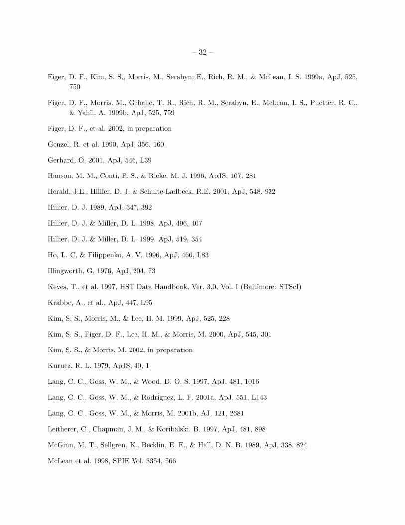
– 32 –

Figer, D. F., Kim, S. S., Morris, M., Serabyn, E., Rich, R. M., & McLean, I. S. 1999a, ApJ, 525,750

Figer, D. F., Morris, M., Geballe, T. R., Rich, R. M., Serabyn, E., McLean, I. S., Puetter, R. C.,& Yahil, A. 1999b, ApJ, 525, 759

Figer, D. F., et al. 2002, in preparation

Genzel, R. et al. 1990, ApJ, 356, 160

Gerhard, O. 2001, ApJ, 546, L39

Hanson, M. M., Conti, P. S., & Rieke, M. J. 1996, ApJS, 107, 281

Herald, J.E., Hillier, D. J. & Schulte-Ladbeck, R.E. 2001, ApJ, 548, 932

Hillier, D. J. 1989, ApJ, 347, 392

Hillier, D. J. & Miller, D. L. 1998, ApJ, 496, 407

Hillier, D. J. & Miller, D. L. 1999, ApJ, 519, 354

Ho, L. C. & Filippenko, A. V. 1996, ApJ, 466, L83

Illingworth, G. 1976, ApJ, 204, 73

Keyes, T., et al. 1997, HST Data Handbook, Ver. 3.0, Vol. I (Baltimore: STScI)

Krabbe, A., et al., ApJ, 447, L95

Kim, S. S., Morris, M., & Lee, H. M. 1999, ApJ, 525, 228

Kim, S. S., Figer, D. F., Lee, H. M., & Morris, M. 2000, ApJ, 545, 301

Kim, S. S., & Morris, M. 2002, in preparation

Kurucz, R. L. 1979, ApJS, 40, 1

Lang, C. C., Goss, W. M., & Wood, D. O. S. 1997, ApJ, 481, 1016

Lang, C. C., Goss, W. M., & Rodriguez, L. F. 2001a, ApJ, 551, L143

Lang, C. C., Goss, W. M., & Morris, M. 2001b, AJ, 121, 2681

Leitherer, C., Chapman, J. M., & Koribalski, B. 1997, ApJ, 481, 898

McGinn, M. T., Sellgren, K., Becklin, E. E., & Hall, D. N. B. 1989, ApJ, 338, 824

McLean et al. 1998, SPIE Vol. 3354, 566

– 33 –

McLean et al. 2002, PASP, in preparation

Meynet, G., Maeder, A., Schaller, G., Schaerer, D., & Charbonnel, C. 1994, A&A Supp., 103, 97

Meynet, G. 1995, A&A, 298, 767

Mizutani, K. et al. 1994, ApJS, 91, 613

Moneti, A., Glass, I. S. & Moorwood, A. F. M. 1994, MNRAS, 268, 194

Morris, M. & Yusef-Zadeh, F. 1989, ApJ, 343, 703

Morris, M., Davidson, J. A., & Werner, M. W. 1995, ASP Conf. Ser. 73: From Gas to Stars toDust, 477

Najarro, F. et al. 2002, in preparation

Nagata, T., Woodward, C. E., Shure, M., & Kobayashi, N. 1995, AJ, 109, 1676

Nugis, T., Crowther, P. A., & Willis, A. J. 1998, A&A, 333, 956

Ozernoy, L. M., Genzel, R., & Usov, V. V. 1997, MNRAS, 288, 237

Perryman, M. A. C. et al. 1997, A&A, 323, L49

Portegies-Zwart, S. F., Makino, J., McMillan, S. L. W., & Hut, P. 2001, ApJ, 546, L101

Reid, M. J. 1993, ARA&A, 31, 345

Rieke, G. H., Rieke, M. J., & Paul, A. E. 1989, ApJ, 336, 752

Salpeter, E. E. 1955, ApJ, 121, 161

Scalo, J. 1998, in The Stellar Initial Mass Function, G. Gilmore and D. Howell (eds.), vol. 142 of38th Herstmonceux Conference, San Francisco, ASP Conference Series, p. 201

Schaller, G., Schaerer, D., Meynet, G., & Maeder, A. 1992, A&AS, 96, 269

Serabyn, E. & Guesten, R. 1987, A&A, 184, 133

Serabyn, E., Shupe, D., & Figer, D. F. 1998, Nature, 394, 448

Serabyn, E., Shupe, D., & Figer, D. F. 1999, ASP Conf. Ser. 186: The Central Parsecs of theGalaxy, 320

Serabyn, E., Figer, D. F., Kim, S. S., Morris, M., & Rich, R. M. 2002, ApJ, in preparation

Stetson, P. 1987, PASP, 99, 191

Stolte, A., Grebel, E. K., Brandner, W., & Figer, D. F. 2002, a, submitted

– 34 –

Timmermann, R., Genzel, R., Poglitsch, A., Lutz, D., Madden, S. C., Nikola, T., Geis, N., &Townes, C. H. 1996, ApJ, 466, 242

van der Hucht, K. A. 2001, New Astronomy Review, 45, 135

Wendker, H. J. 1995, A&AS, 109, 177

Yusef-Zadeh, F., Cotera, A., Fruscione, A., Lang, C., Law, C., Wang, D., & Wardle, M. 2001,American Astronomical Society Meeting, 198, 8709

Yusef-Zadeh, F., Law, C., Wardle, M., Wang, Q. D., Fruscione, A., Lang, C. C., & Cotera, A. 2002,in preparation

This preprint was prepared with the AAS LATEX macros v5.0.

– 35 –

Fig. 1a.— (a) F205W image, after processing by calnica and calnicb.

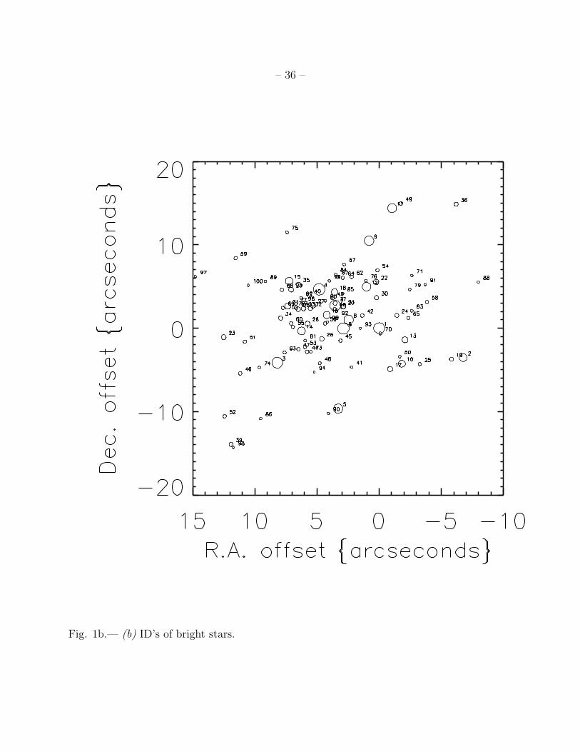
– 36 –

Fig. 1b.— (b) ID’s of bright stars.

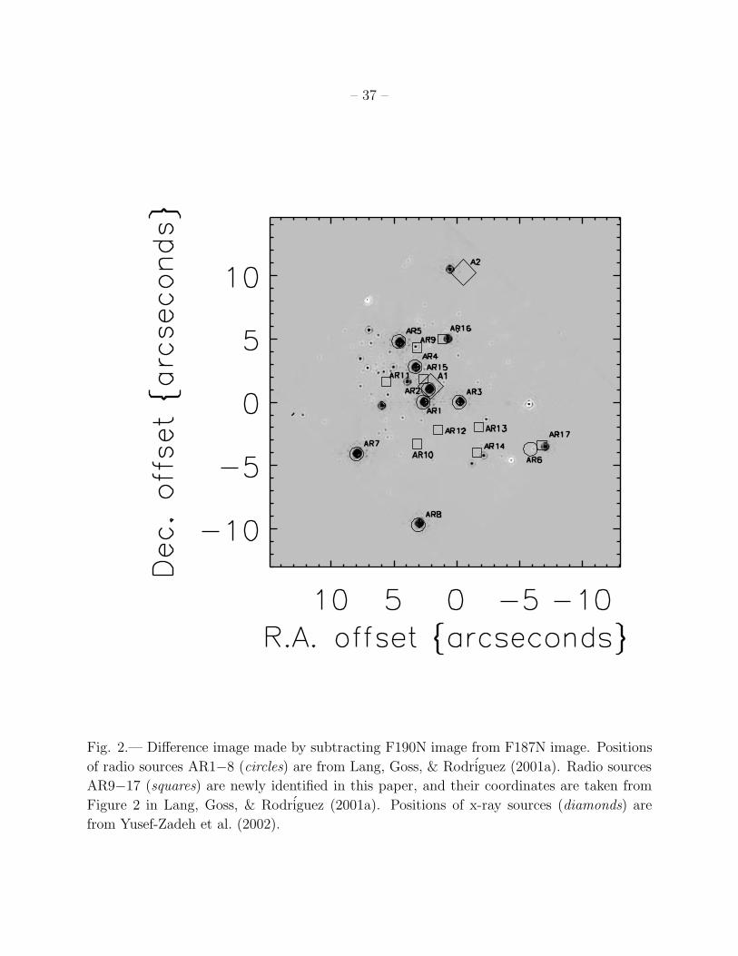
– 37 –

Fig. 2.— Difference image made by subtracting F190N image from F187N image. Positions

of radio sources AR1−8 (circles) are from Lang, Goss, & Rodriguez (2001a). Radio sources

AR9−17 (squares) are newly identified in this paper, and their coordinates are taken from

Figure 2 in Lang, Goss, & Rodriguez (2001a). Positions of x-ray sources (diamonds) are

from Yusef-Zadeh et al. (2002).

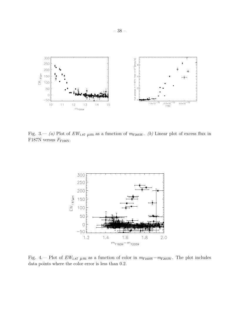
– 38 –

Fig. 3.— (a) Plot of EW1.87 µm as a function of mF205W. (b) Linear plot of excess flux in

F187N versus FF190N.

Fig. 4.— Plot of EW1.87 µm as a function of color in mF160W−mF205W. The plot includes

data points where the color error is less than 0.2.

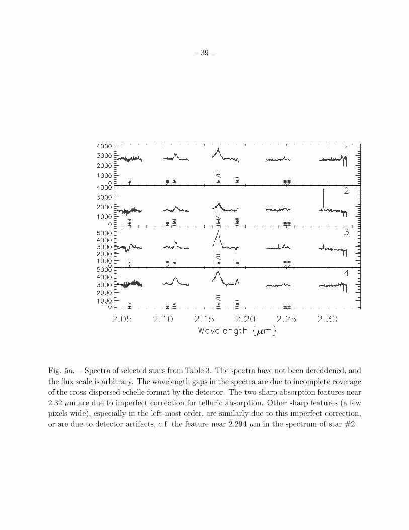
– 39 –

Fig. 5a.— Spectra of selected stars from Table 3. The spectra have not been dereddened, and

the flux scale is arbitrary. The wavelength gaps in the spectra are due to incomplete coverage

of the cross-dispersed echelle format by the detector. The two sharp absorption features near

2.32 µm are due to imperfect correction for telluric absorption. Other sharp features (a few

pixels wide), especially in the left-most order, are similarly due to this imperfect correction,

or are due to detector artifacts, c.f. the feature near 2.294 µm in the spectrum of star #2.

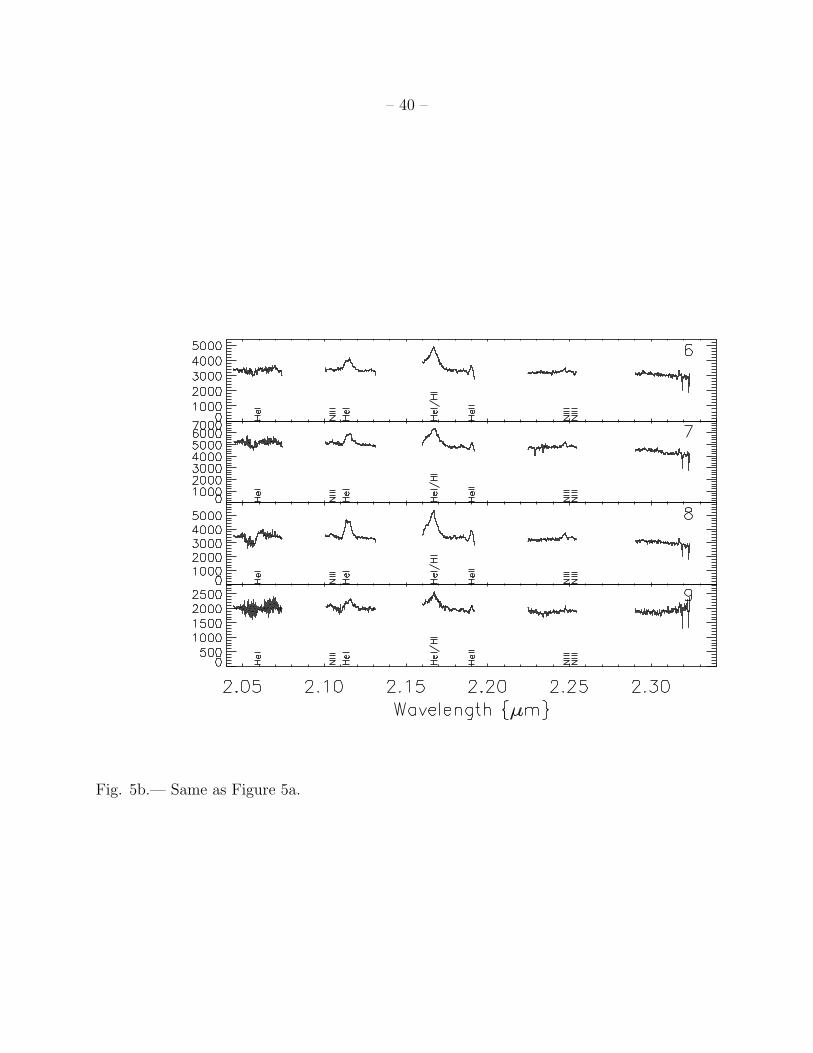
– 40 –

Fig. 5b.— Same as Figure 5a.

– 41 –

Fig. 5c.— Same as Figure 5a. The sharp features near 2.294 µm in the spectra of star #10

and #14 are due to detector artifacts.

– 42 –

Fig. 5d.— Same as Figure 5a.

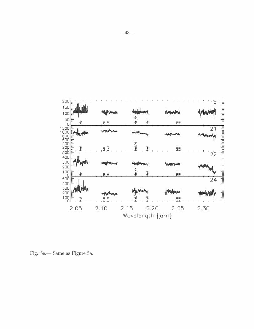
– 43 –

Fig. 5e.— Same as Figure 5a.

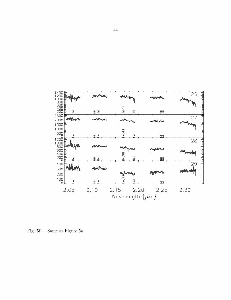
– 44 –

Fig. 5f.— Same as Figure 5a.

– 45 –

Fig. 5g.— Same as Figure 5a.

– 46 –

Fig. 5h.— Same as Figure 5a.

– 47 –

Fig. 5i.— Same as Figure 5a.

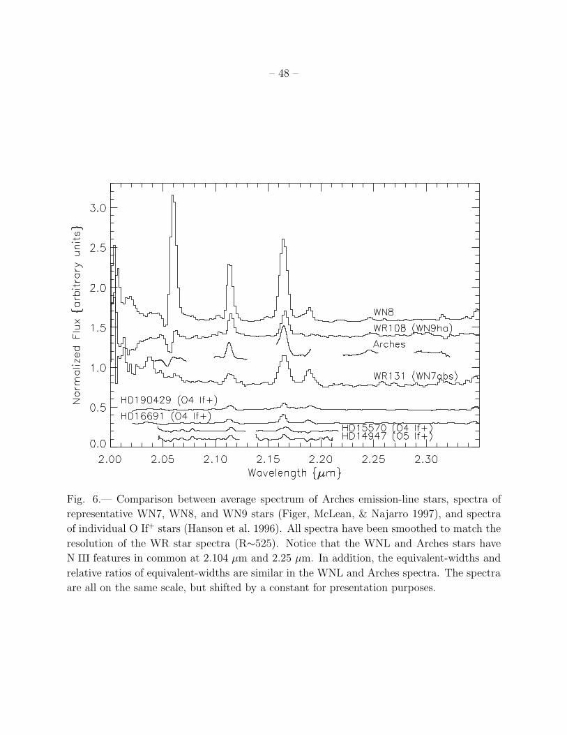
– 48 –

Fig. 6.— Comparison between average spectrum of Arches emission-line stars, spectra of

representative WN7, WN8, and WN9 stars (Figer, McLean, & Najarro 1997), and spectra

of individual O If+ stars (Hanson et al. 1996). All spectra have been smoothed to match the

resolution of the WR star spectra (R∼525). Notice that the WNL and Arches stars have

N III features in common at 2.104 µm and 2.25 µm. In addition, the equivalent-widths and

relative ratios of equivalent-widths are similar in the WNL and Arches spectra. The spectra

are all on the same scale, but shifted by a constant for presentation purposes.

– 49 –

Fig. 7a.— Observed (dots) and modelled (line) spectrum of star #8.

– 50 –

Fig. 7b.— Observed (dots) and modelled (line) spectrum of star #10.

– 51 –

Fig. 8a.— Plot of (FF187N−FF190N)×∆λ versus F8.5 GHz.

Fig. 8b.— Plot of (FF187N−FF190N)×∆λ versus F4.9 GHz.

– 52 –

Fig. 9.— Histogram of massive star separations from cluster center. Data are taken from

Table 3.