1

Massive MIMO Performance—TDD Versus FDD:What Do Measurements Say?

Jose Flordelis, Student Member, IEEE, Fredrik Rusek, Member, IEEE, Fredrik Tufvesson, Fellow, IEEE,Erik G. Larsson, Fellow, IEEE, and Ove Edfors, Senior Member, IEEE

Abstract—Downlink beamforming in Massive MIMO eitherrelies on uplink pilot measurements—exploiting reciprocity andTDD operation, or on the use of a predetermined grid of beamswith user equipments reporting their preferred beams, mostlyin FDD operation. Massive MIMO in its originally conceivedform uses the first strategy, with uplink pilots, whereas there iscurrently significant commercial interest in the second, grid-of-beams. It has been analytically shown that in isotropic scattering(independent Rayleigh fading) the first approach outperformsthe second. Nevertheless there remains controversy regardingtheir relative performance in practice. In this contribution,the performances of these two strategies are compared usingmeasured channel data at 2.6 GHz.

Index Terms—Massive MIMO, FDD, TDD, performance, chan-nel measurements.

I. INTRODUCTION

THE idea behind Massive MIMO is to equip base stations(BS) in wireless networks with large arrays of phase-

coherently cooperating antennas. The use of such arrays facil-itates spatial multiplexing of many user equipments (UEs) inthe same time-frequency resource, and yields a coherent beam-forming gain that translates directly into reduced interferenceand improved cell-edge coverage.

The original Massive MIMO concept [1]–[4] assumes time-division duplexing (TDD) and exploits reciprocity for theacquisition of channel state information (CSI) at the BS. UEssend pilots on the uplink (UL); all UE-to-BS channels areestimated, and each antenna has its own RF electronics. Theconcept has, since its introduction a decade ago [1], [3],matured significantly: rigorous information-theoretic analysesare available [2], field-trials have demonstrated its performancein high-mobility scenarios [5]–[7], and circuit prototypes haveshown the true practicality of implementations [8].

Concurrently, motivated by spectrum regulation issues, thereis significant interest in developing frequency-division duplex-ing (FDD) versions of Massive MIMO [9]–[13]. There isalso interest in hybrid beamforming architectures that rely on

This work was supported by the Seventh Framework Programme (FP7)of the European Union under grant agreement no. 619086 (MAMMOET),ELLIIT—an Excellence Center at Linkoping-Lund in Information Technology,the Swedish Research Council (VR), and the Swedish Foundation for StrategicResearch (SSF).

Jose Flordelis, Fredrik Rusek, Fredrik Tufvesson, and Ove Edfors arewith the Department of Electrical and Information Technology, LundUniversity, SE-221 00 Lund, Sweden (e-mail: jose.flordelis@eit.lth.se;fredrik.rusek@eit.lth.se; fredrik.tufvesson@eit.lth.se; ove.edfors@eit.lth.se).

E. G. Larsson is with the Department of Electrical Engineering(ISY), Linkoping University, SE-581 83 Linkoping, Sweden (e-mail:erik.g.larsson@liu.se).

the use of analog phase shifters and signal combiners [14]–[17], somewhat reminiscent of phased-arrays implementationsof radar. With hybrid beamforming, the number of actualantennas may substantially exceed the number of RF chains.

FDD operation and hybrid beamforming solutions bothbring the same difficulty – albeit for different reasons: sig-nificant assumptions on the structure of propagation must bemade for the techniques to work efficiently. Specifically:• FDD operation requires CSI feedback from the UEs to the

BS. Efficient encoding of this CSI is only possible if sideinformation on the propagation is exploited. The resultingtechniques are often called “grid-of-beams”, and havesimilarities to existing forms of multiuser (MU) MIMOin LTE [18].

• Hybrid-beamforming architectures inherently rely onbeamforming into predetermined spatial directions, asdefined by the angle-of-arrival or angle-of-departure, seenfrom the array. Such directions only have a well-definedoperational meaning when the propagation environmentoffers strong direct or specular paths [19].

There has been a long-standing debate on the relative per-formance between reciprocity-based (TDD) Massive MIMOand that of solutions based on grid-of-beams or hybrid-beamforming architectures. The matter was, for example, thesubject of a heated debate in the 2015 Globecom industrypanel “Massive MIMO vs FD-MIMO: Defining the next gener-ation of MIMO in 5G” where on the one hand, the commercialarguments for grid-of-beams solutions were clear, but on theother hand, their real potential for high-performance spatialmultiplexing was strongly contested [20]. It is known that grid-of-beams solutions perform poorly in isotropic scattering [21],but no prior experimental results are known to the authors.

The object of this paper is to conclusively answer thisperformance question through the analysis of real MassiveMIMO channel measurement data obtained at the 2.6 GHzband. The conclusion, summarized in detail in Sec. VI, isthat except for in certain line-of-sight (LOS) environments,the original reciprocity-based TDD Massive MIMO of [1], [3]represents the only feasible implementation of Massive MIMOat the frequency bands under consideration.

A. Notation

We use the following notation throughout the paper: Bold-face lowercase letters represent column vectors, and boldfaceuppercase letters represent matrices. Also, I is the identitymatrix, ‖a‖ the Euclidean norm of vector a, tr (A) the trace

arX

iv:1

704.

0062

3v1

[cs

.IT

] 3

Apr

201

7

2

of matrix A, span(A) its column space, AT denotes thetranspose, AH the Hermitian transpose, |A| stands for thedeterminant, and A � 0 means that A is positive semidefinite.diag(a) builds a matrix having a along its diagonal and allother elements set to zero,

[A | b

]denotes the matrix resulting

from appending b toA, and [A]I is the submatrix ofA formedby choosing the columns of the index set I. The imaginaryunit is denoted by , CN (µ,Λ) denotes the complex Gaussiandistribution with mean µ and covariance matrix Λ, E[·] is theexpectation operator, and |I| denotes the number of elementsin the set I.

II. SYSTEM MODEL

We consider the downlink (DL) of a single-cell MassiveMIMO system in which an M -antenna BS communicates withK single-antenna UEs in the same time-frequency resource.Orthogonal Frequency Division Multiplexing (OFDM) withL subcarriers is assumed [22]. Let hk(`) ∈ CM×1, for k =1, . . . ,K, and ` = 1, . . . , L, denote the channel vector betweenthe BS and the kth UE at the `th subcarrier, and let

H(`) =[h1(`) · · · hK(`)

]T(1)

denote the corresponding K ×M channel matrix. Then, thenormalized input-output relation of the channel can be writtenas

y(`) =√ρH(`) s(`) + n(`), (2)

where y(`) ∈ CK×1 is the vector containing the receivedsignals of all the UEs, s(`) ∈ CM×1 the vector of precodedtransmit signals satisfying

E{sH(`)s(`)

}= 1, (3)

ρ the signal-to-noise ratio (SNR), and n(`) is a vector ofCN (0, 1) receiver noise at the UEs.

III. TRANSMISSION TECHNIQUES

This section outlines the beamforming techniques includedin the comparison—first, fully-digital reciprocity-based (TDD)beamforming in Sec. III-A, and then, four flavors of FDDbeamforming based on feedback of CSI in Sec. III-B.

A. Fully-Digital Reciprocity-Based (TDD) Beamforming

With fully-digital beamforming, no a priori assumptions aremade on the propagation environment. There are no predeter-mined beams, but CSI is measured at the BS by observingUL pilots transmitted by the UEs. By virtue of TDD operationand reciprocity of propagation, the so-obtained UL CSI is alsovalid for the DL, assuming proper reciprocity calibration [23].All signal processing takes place in the digital domain. A TDDbeamforming system is schematically depicted in Fig. 1 forK = 2 UEs.

With full CSI at the BS, TDD performs optimally andcan achieve the DL sum-capacity by dirty-paper coding(DPC) [24]. For given ρ, the sum-capacity of the `th subcarrier,

UE 1

UE 2

...K...

...M...

Base Station

DigitalPrecoder

RF Chain

RF Chain

HDL = HULT

.

.

.

Fig. 1: Fully-digital reciprocity-based (TDD) beamformingwith K = 2 single-antenna UEs.

CTDD(H(`), ρ), is given by the solution to the followingoptimization problem [25]–[28]:

maximizeΛ(`)

log2

∣∣∣I +HH(`)Λ(`)H(`)∣∣∣

subject to tr (Λ(`)) ≤ ρ, Λ(`) � 0,(4)

where Λ(`) = diag(λ1(`), . . . , λK(`)) is a diagonal powerallocation matrix. The sum-capacity averaged over all thesubcarriers is then

CTDD(ρ) =1

L

L∑`=1

CTDD(H(`), ρ). (5)

Problem (4) is convex and can be efficiently solved by asimple gradient search, or via a technique known as sum-power iterative waterfilling [29], [30].

B. Feedback-Based FDD Beamforming with PredeterminedBeams

Feedback-based beamforming relies on the reporting ofquantized CSI from the UEs to the BS. Typically, CSIquantization is obtained by using a predetermined codebookconsisting of M ′ beams, which imposes a certain structure onthe precoded signals s(`). These techniques may be appliedwhen reliance on reciprocity is undesirable or impossible,notably in FDD operation.

We represent the M ′ beams through the set of M -vectors{ci}M

′

i=1. Throughout this article, we assume that these beamsare given by Vandermonde vectors comprising the array re-sponse in M ′ directions uniformly spaced in the sine-angledomain. More precisely, we define

ci =1√M

[1 eπψi · · · eπψi(M−1)

]T, (6)

where ψi = −1 + 2i−1M ′ , for i = 1, . . . ,M ′. We also define the

M ×M ′ codebook matrix

C =[c1 · · · cM ′

]. (7)

A special case of the codebook is when M ′ = M and thebeams are orthonormal; then CHC = I . In this case, thevectors ci are the columns of an M ×M IDFT matrix, up toa constant shift of the origin of the phase angle ψi.

3

The UEs report their preferred beams to the BS. There areseveral ways that this may be done, and we consider two cases:

1) Each UE individually reports the indices and complexgains of a predetermined number, N ≤M ′, of beams.

2) The BS, possibly based on interaction with the UEs,decides on a common set of N beams that are simul-taneously used for all the UEs. Then, each UE reportsthe complex gains of these N beams.

The structure imposed by the predetermined codebook ofbeams may be implemented either in the digital domain, or inthe analog domain:(a) If implemented in the digital domain, the selection of the

beams may be performed individually for each subcarrier.(b) In contrast, if implemented in the analog domain, the

same set of beams must be used for the entire band.The combination of 1 and 2, respectively (a) and (b) above,

yields four cases of interest, illustrated in Fig. 2 for K = 2single-antenna UEs and N = 2 reported beams. These fourcases are described in detail in the next four subsections.Throughout this article, we assume that for every subcarriereach UE can acquire its vector of complex gains perfectly. Wefurther assume that feedback channels are delay- and error-free.

Digital Grid-of-Beams (D-GOB): Each UE individuallyreports the indices and complex gains of a number, N , ofbeams. The selection and reporting of the beams is done inde-pendently for each subcarrier. This corresponds to combination1a above.

Let us compute the achievable sum-rate of D-GOB,CD-GOB(ρ), averaged over all the subcarriers. Each UE learnsthe vector of complex gains

gk(`) = CThk(`). (8)

of the M ′ predetermined beams. It then selects N beams,according to some criterion that will be shortly explained,and forms the set Qk(`) of selected beam indices. Then, eachUE reports Qk(`) and the vector gk(`) of associated complexgains to the BS. By construction, we have that

gk(`) = BTk (`) gk(`), (9)

where the M ×N matrix Bk(`) is obtained by extracting therelevant beams from C, as dictated by Qk(`). Accordingly,the BS may produce a quantized version hk(`) of hk(`), asgiven by the expression

hk(`) = arg minv∈span(Bk(`))

‖BTk (`)v − gk(`)‖2. (10)

With D-GOB, multiuser interference is only partiallyknown. Given i 6= j, the sets Qi(`) and Qj(`) producedby UEs i and j may be different, but the BS can only dealwith interference in Qi(`)∩Qj(`). It follows that DPC is notfeasible in this setting. Instead, zero-forcing (ZF) based on thequantized channels hk(`) is commonly used as the multiusertransmission strategy [31], [32]. To apply ZF, one can definethe quantized channel matrix

H(`) =[h1(`) · · · hK(`)

]T. (11)

Then, from [33], the columns of the ZF precoding ma-trix, P (`) in Fig. 2, can be computed as

pk(`) = zk(`)/‖zk(`)‖,

where zk(`) are the columns of the Moore-Penrose pseudoin-verse H

†(`) of H(`). If equal power ρ/K is allocated to each

UE, the receive SINR of the kth UE can be written as

SINRk (H(`), ρ) =

ρK

∣∣∣hTk (`)pk(`)

∣∣∣21 + ρ

K

∑i 6=k

∣∣∣hTk (`)pi(`)

∣∣∣2 , (12)

from which the achievable sum-rate is computed as [33]

CD-GOB(H(`), ρ) =

K∑k=1

log2

(1 + SINRk (H(`), ρ)

). (13)

The sum-rate averaged over all the subcarriers, CD-GOB(ρ),is then defined similar to (5). Note that even though theprecoders P (`) are designed according to the ZF principle,

the multiuser cross-talk terms∣∣∣hTk (`)pi(`)

∣∣∣2, i 6= k, in thedenominator of (12) do not vanish in general. In fact, pre-coding that completely suppresses interference is impossiblehere since complete CSI cannot be obtained at the BS, unlessN = min(M ′,M).

Next, we briefly discuss the problem of beam selection bythe UEs, which we formulate as the solution to the followingoptimization problem [16], [29], [32]:

arg minQk(`)

‖hk(`)− hk(`)‖2

subject to Qk(`) ⊂ {1, . . . ,M ′}, |Qk(`)| = N,(14)

where hk(`) depends on Qk(`) through Bk(`) as givenby (10). Generally, (14) is a hard combinatorial problem,and can be solved exactly only for fairly small values ofN . (A special case is when CHC = I , in which case onesimply needs to pick the N strongest entries in the vectorgk(`) defined by (8).) Because of this, a heuristic rather thanoptimal algorithm to solve (14) is favored in this work. Forthe particulars on the algorithm, the reader is referred toAppendix A.

Digital Subspace Beamforming (D-SUB): The BS, possi-bly based on interaction with the UEs, decides on a commonset of N beams that are used for all the UEs. Beams areselected independently for each subcarrier. Thus, we havecombination 2a.

We seek to find a beamfoming matrix B(`), formed fromthe columns of C, such that the resulting channel H(`)B(`)maximizes the sum-rate for given ρ. Let CD-SUB(H(`), ρ)denote the optimal sum-rate. The structure of D-SUB beam-forming is shown in Fig. 2. Clearly, the precoder P (`) needs tobe designed jointly with B(`). For this, we adopt a two-stepapproach. First, we address the problem of designing P (`)when B(`) and ρ are given. Then, we return to the originalproblem of jointly designing P (`) and B(`) for given ρ, andapply the results of the first step.

4

Individual set of N beams for each UE Common subspace, spanned by N beams, for all UEs

Per-subcarrier

UE 1

UE 2

a

b

d

c

...K...

...N’ = M

...

Base Station

ZF Precoder

P(l)

RF Chain

RF Chain

HDL

a, b + complex gains

b, c + complex gains

Digital grid-of-beams (D-GOB)

UE 1

UE 2

a, b complex gains

a

b

d

c

RF Chain

RF Chain

...K...

...N’ = M

...

Base Station

...N...

Digital Beam-formerB(l)

Digital Precoder

P(l)

HDL

a, b complex gains

Digital subspace beamforming (D-SUB)

Wholeband

c1

ZF Precoder

P(l)

RF Chain

RF Chain

...K...

...N’ ≥ N

...

Analog Phase

ShiftersB

...M...

Base Station

a

b

d

c

UE 1

UE 2

... +

... +

HDL

a, b + complex gains

b, c + complex gains

Hybrid grid-of-beams (H-GOB)

c1

c2Digital

Precoder P(l)

RF Chain

RF Chain

...K...

...N’ = N

...

Analog Phase

ShiftersB

...M...

Base Station

a

b

d

c

... +

... +

UE 2

UE 1HDL

a, b complex gains

a, b complex gains

Hybrid subspace beamforming (H-SUB)

Fig. 2: The four considered cases of feedback-based FDD beamforming. A Massive MIMO BS communicates with K = 2single-antenna UEs, each reporting on N = 2 beams picked from a codebook of size M ′ = 4. N ′ is the number of RF chains.In this example, with D-GOB and H-GOB, UE 1 selects beams a and b, and UE 2 selects beams b and c; with D-SUB andH-SUB, UE 1 and UE 2 report on the common subspace spanned by both beams a and b.

For given B(`) and ρ, let CBC(H(`)B(`), ρ) denote themaximum sum-rate over H(`)B(`). It is shown in Ap-pendix B that CBC(H(`)B(`), ρ) can be found as the solutionto the optimization problem

maximizeΛ(`)

log2

∣∣∣I +UH(`)HH(`)Λ(`)H(`)U(`)∣∣∣

subject to Λ(`) � 0, tr (Λ(`)) ≤ ρ,(15)

where Λ(`) = diag (λ1(`), . . . , λK(`)) is a diagonal powerallocation matrix, and U(`) is an M × N matrix such thatB(`) = U(`)L(`) with UH(`)U(`) = I , and L(`) aninvertible matrix. If one defines the effective channel matrixH(`) = H(`)U(`), problem (15) is formally identical to(4), and hence can be solved efficiently. The optimal pre-coder P (`) for given B(`) and ρ is defined by the set ofcovariance matrices {Qi}

Ki=1, which are found by (i) obtaining

the effective covariance matrices {Qi(`)}Ki=1 from the powerallocations {λi(`)}Ki=1 in (15) via the so-called “MAC-to-BC” transformation (described in, e.g., [26], [29]); and (ii)

computing Qi(`) = L−1(`)Qi(`)(LH(`)

)−1, i = 1, . . . ,K.

Returning to our original problem, we can now expressCD-SUB(H(`), ρ) as the solution to the optimization problem

maximizeB(`)=[C]Q(`)

CBC(H(`)B(`), ρ)

subject to Q(`) ⊂ {1, . . . ,M ′}, |Q(`)| = N.(16)

Put in words, for each subcarrier, the sum-rate as given by (15)is maximized over all M×N beamformers B(`) generated bycodebook C. The sum-rate averaged over all the subcarriers,CD-SUB(ρ), is then defined similar to (5).

Although, in principle, one could attempt the maximizationin (16) by exhaustive search, solving (15) at each step, thenumber of beamformers B(`) that needs to be checked withthis approach is

(M ′

N

). Thus, for values of M ′ in the hundreds

or larger, the above direct approach appears intractable, exceptfor very small N . Therefore, alternative methods for solv-ing (16) are needed. An efficient algorithm for approximatesolution of (16) is presented in Appendix C.

Hybrid Subspace Beamforming (H-SUB): The BS, pos-sibly based on interaction with the UEs, decides on a commonset of N beams to service all the UEs. In contrast to D-SUB,this choice is applied across all subcarriers, thereby facilitatingthe implementation of the beamforming in analog hardware.This corresponds to combination 2b above.

The hybrid beamforming architecture is shown in Fig. 2.The vector of precoded transmit signals, s(`), has the form

s(`) = BP (`)x(`), ` = 1, . . . , L,

where x(`) is a vector containing the information bits from theUEs satisfying E

{x(`)x(`)

H}

= I . Importantly, the precoderP (`) is frequency-selective, but the beamforming matrix B isnot. Hence, B can be realized entirely by analog hardware.

5

An important consequence is that the number of required RFchains at the BS can be reduced from M (i.e., one RF chainper antenna element) to N (i.e., one RF chain per selectedbeam).

To obtain a cost-effective analog beamforming network, acertain structure is typically enforced on the matrix B. In thiswork, we require that B be formed from the columns of thecodebook matrix C defined by (7). Under this constraint, theanalog beamforming network defined by B can be realizedby using N phase shifters, and M N -input signal combiners,as depicted in Fig. 2. Other constraints on B leading tosimplifications of the analog hardware are possible; the readerif referred to [19], [34] for a comprehensive survey of thefield.

Optimal beam selection for H-SUB is analogous to D-SUB,except that beams are reused for all subcarriers. For given ρ,the sum-capacity averaged over all subcarriers, CH-SUB (ρ), canbe found as the solution to the optimization problem

maximizeB=[C]Q

CH-SUB({H(`)B}L`=1, ρ

)subject to Q ⊂ {1, . . . ,M ′}, |Q| = N.

(17)

where CH-SUB({H(`)B}L`=1, ρ

)is in turn defined as the

solution to

maximize{Λ(`)}L`=1

1

L

L∑`=1

log2

∣∣∣I +UHHH(`)Λ(`)H(`)U∣∣∣

subject to Λ(`) � 0, tr (Λ(`)) ≤ ρ,(18)

where, as usual, Λ(`) = diag(λ1(`), . . . , λK(`)) are powerallocation matrices, and B = UL with UHU = I , and L aninvertible matrix. Again, the efficient algorithm proposed inAppendix C can be used to solve (17).

Hybrid Grid-of-Beams (H-GOB): Last, we have combi-nation 1b, wherein similar to D-GOB, each UE individuallyreports the indices and complex gains of N beams, but whereinthe choice of the beams is applied across all subcarriers. Thisstrategy enables the implementation of the beamforming inanalog hardware, as illustrated in Fig. 2. A special case iswhen N = 1, and additionally one dispenses with all thedigital signal processing. This case is sometimes referred toas analog-only beamforming, and is used in communicationstandards such as IEEE 802.11ad [35]. The problem of beamselection can be posed as the following optimization problem:

arg minQk

1

L

L∑`=1

‖hk(`)− hk(`)‖2

subject to Qk ⊂ {1, . . . ,M ′}, |Qk| = N,

(19)

where hk(`) is given by (10). The heuristic algorithm inAppendix A (with minor modifications) is proposed for solv-ing (19).

IV. MEASURED CHANNELS

The measured channels were obtained in two different mea-surement campaigns conducted at the Faculty of Engineering(LTH) of Lund University, Lund, Sweden. At the BS side,a virtual uniform linear array (ULA) with 128 elements was

used. The ULA spans 7 meters, and uses vertically-polarized,omnidirectional-in-azimuth antenna elements [36]. At the UEside, vertically-polarized omnidirectional antennas of the sametype were used. The measurements were acquired at a carrierfrequency of 2.6 GHz, and a bandwith of 50 MHz. A briefdescription of the two campaigns and the scenarios follows:• Campaign A. The UEs were located at the parking place

outside the E-building of LTH, with the ULA mountedon top of the E-building, three floors above ground level.We consider five UE sites, denoted MS 1, . . . , MS 5.Sites MS 1 to MS 4 have mainly LOS propagationconditions to the BS, while site MS 5 experiences NLOS.At each site, several UE locations are measured. In thiswork, we consider three propagation scenarios, which aresummarized in Table I as scenarios 1, 2, and 3. For furtherdetails on Campaign A, the reader is referred to [5].

• Campaign B. The UEs were located in a courtyard ofthe E-building. The ULA was on a roof two floors aboveground, while the 16 UEs were spread out at variouspositions in the courtyard. In this environment, the UEsexperience LOS propagation conditions to the array,along with a number of strong scattered componentscaused by interactions with the walls, outdoor furniture,and vegetation. (The Ricean K-factor [37], [38] is lowcompared to scenarios 1 and 3.) In this work, we considerthree propagation scenarios, which are summarized inTable I as scenarios 4, 5, and 6. For further details onCampaign B, the reader is referred to [39].

We should also mention that, prior to applying DL beam-forming as described in Sec. III, the measured channels arenormalized to have unit average gain. This normalization stepremoves differences in path loss among UEs, while preservingvariations across frequencies and antenna positions.

V. RESULTS AND DISCUSION

Based on the measured channels obtained from Campaign Aand Campaign B, we compare the performance of the fivebeamforming techniques described in Sec. III, namely, TDDbeamforming, and four flavors of FDD beamforming: D-GOB, H-GOB, D-SUB, and H-SUB. Because TDD performsoptimally, it serves as baseline. First, in Sec. V-A, we studyhow much one can reduce the number, N , of reported beamsin FDD beamforming while still retaining a prescribed fractionof the sum-capacity. Next, in Sec. V-B, we fix the FDD sum-rate to a desired value and address the following question:“Given N , what is the average SNR loss relative to optimalTDD?” Then, in Sec. V-C, we investigate the tradeoff betweenRF chains and BS antennas in FDD beamforming, subject toa sum-rate constraint. In Sec. V-D, we reevaluate the findingsof Sec. V-A, but now including the overhead of DL training.Last, in Sec. V-E, we make a remark about analog-onlybeamforming.

In the preparation of the results reported below, the follow-ing parameter settings were used. There are M = 128 antennasat the BS, which communicate with K = 4, 8, and 16 single-antenna UEs, depending on the particular scenario. Evaluationsare done based on L = 71 subcarriers equispaced over a

6

TABLE I: Summary of measured scenarios.

Campaign A

MS 1

MS 2

MS 3MS 4MS 5

ULA...

LOS

LOSLOS

LOSMS 1

MS 2

MS 3MS 4MS 5

ULA...

NLOS MS 1

MS 2

MS 3MS 4MS 5

ULA

...

LOS

Scenario 1. K = 4 well-separatedUEs in LOS, in which one UE fromeach of the sites MS 1 to MS 4 isselected. The minimum UE separationis 10 m.

Scenario 2. K = 4 co-located UEs inNLOS, in which four UEs are selectedfrom site MS 5. The minimum UEseparation is 0.5 m.

Scenario 3. K = 4 co-located UEs inLOS, in which four UEs are selectedfrom site MS 2. The minimum UEseparation is 0.5 m.

Campaign B

ULA... ULA... ULA...

Scenario 4. K = 4 separated UEs inLOS and strong scattered components.We considered four sets of UEs (indifferent colors). The minimum UEseparation is 3 m.

Scenario 5. K = 8 separated UEs inLOS and strong scattered components.We considered four sets of UEs (indifferent colors). The minimum UEseparation is 3 m.

Scenario 6. K = 16 separated UEs inLOS and strong scattered components.The minimum UE separation is 3 m.

50 MHz bandwidth, for which flat-frequency fading can beassumed. For each of the four considered FDD beamformingschemes, the “best” N beams (in the sense described inSec. III-B) are selected from a codebook of size M ′ = 512,with N in the range from K to 128. In Sec. V-A andSec. V-D, we choose ρ = 0 dB. With this choice the per-UEspectral efficiencies are in the range 0.5–5.0 bits/s/Hz, whichis representative of several wireless standards [18], [40]. Ad-ditionally for Sec. V-C, m-antenna subarrays, K ≤ m ≤ M ,are considered. For each m, several m-antenna subarrays areselected so as to span the full length of the original M -antennaarray.

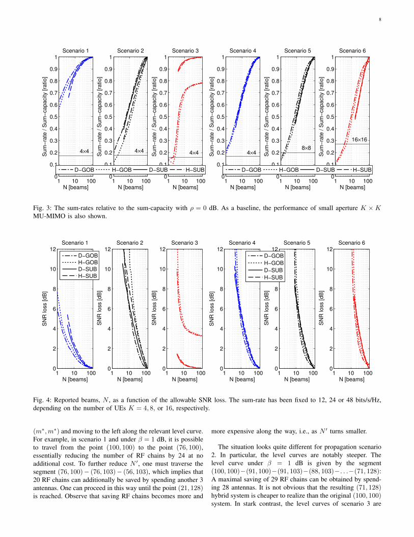
A. Relative Sum-rate as a Function of NFirst, we examine scenarios 1, 2, and 3, for which

K = 4 UEs. Fig. 3 (left half) shows the relative sum-rates cA(ρ,N) = CA(ρ,N)/CTDD(ρ), where A is one of“D-GOB”, “H-GOB”, “D-SUB”, and “H-SUB”. The sum-capacities CTDD(ρ) are given in Table II. For fixed N , we saythat A outperforms B if cA(ρ,N) > cB(ρ,N), where A andB may be applied to different scenarios.

TABLE II: Sum-capacity (in bits/s/Hz) for TDD at ρ = 0 dB.

Scenario 1 2 3 4 5 6

Number of UEs 4 4 4 4 8 16Sum-capacity 19.9 20.0 16.7 20.0 32.2 49.0

With one exception1, the relative sum-rates cA(ρ,N) in-crease with increasing values of N . At N = 128, D-SUB

1In scenario 3, the relative sum-rate of H-GOB decreases slightly when Ngoes from 1 to 2. This can happen because ZF is used based on partial CSI.

and H-SUB reach the sum-capacity, and D-GOB and H-GOBattain the sum-rate of ZF with perfect CSI. In general, D-GOB extracts a larger share of the sum-capacity than H-GOB,and D-SUB extracts a larger share than H-SUB. This mustbe so since with D-GOB and D-SUB, beams are selectedindividually for each subcarrier, while with H-GOB and H-SUB, the same set of beams is used for the entire band. Thehorizontal gap between the curves of D-GOB and H-GOB, andbetween those of D-SUB and H-SUB, represents the penaltydue to the frequency selectivity of the channel, in terms ofthe number of additional beams needed. At 70% of the sum-capacity, this penalty is at most one beam for scenarios 1 and3, and between 4 to 17 beams for scenario 2. These penaltiesare significantly larger for NLOS scenarios than for LOS ones,which can be explained by the larger frequency selectivity ofNLOS channels [41].

Looking at scenarios 1 and 2, we note that D-GOB outper-forms D-SUB. With N = 4, D-GOB can reach 82% of thesum-capacity, but D-SUB can only reach 72%; with N = 10,the relative sum-rates are 90% and 86%, respectively. Infact, this holds for all N , although the gap closes as Nincreases. This is somewhat surprising as one would expectthat DPC should outperform ZF. The explanation is as follows.With D-GOB, beams are individually selected by each UE,with the goal of maximizing the channel gain. With D-SUB,however, channel beamforming gains are traded off againstlower multiuser interference. When the channel propagationconditions are somewhat favorable (e.g., distinct LOS direc-tions as in scenario 1, or NLOS propagation as in scenario2), maximizing the channel beamforming gain is the betterstrategy. The relative performance of D-GOB and D-SUB

7

depends in general on ρ: For all N , cD-SUB(ρ,N) goes to 1in the limit ρ→∞, with the difference between CTDD(ρ) andCD-SUB(ρ,N) constant [42], [43]. Meanwhile, for interference-limited D-GOB we have that cD-GOB(ρ,N) must go to 0 asρ→∞, if N < 128, and to 1, if N = 128.

The situation is more involved with regards to H-GOB andH-SUB: H-GOB beats H-SUB in scenario 1, and the oppositeis true in scenario 2. This hints to a larger sensitivity tofrequency selectivity of ZF compared to DPC. Turning toscenario 3, we observe that D-SUB and H-SUB vastly outper-form D-GOB and H-GOB. Addressing multiuser interferenceis crucial in this case, where the UEs are co-located and haveLOS, and failure to do so leads to large performance losses.An interesting conclusion thus far is that there is no singleFDD beamforming technique, D-GOB or D-SUB, H-GOB orH-SUB, that is “best” in all cases, but which technique that ismost appropriate depends largely on the propagation scenario.We also make the obvious remark that if one desires to operatewith N < K beams, then D-GOB and H-GOB are the onlyavailable choices.

We now move on to scenarios 4, 5, and 6, with K = 4, 8,and 16 UEs, respectively, facing LOS propagation conditionswith strong scattered components. Shown in Fig. 3 (righthalf) are the relative sum-rates cA(ρ,N). The sum-capacitiesCTDD(ρ) are given in Table II.

An important observation is that the presence of significantscatterers in the propagation environment has a notable impacton the performance of D-GOB, H-GOB, D-SUB, and H-SUB.To see this, compare in Fig 3 the reported values of N forscenario 1 with those of scenario 4. In addition to the LOScomponent, a substantial part of the received power in scenario4 originates from scattered components, and more beams areneeded to achieve a prescribed fraction of the sum-capacity.

We also note that the required number of beams, N ,increases with the number of active UEs, K. That N shouldgrow with K is consistent with the conventional MassiveMIMO wisdom that the number of BS antennas (here, beams)should grow proportional to K [44]—this is also necessaryfor D-SUB and H-SUB, for which N ≥ K must hold. Thescalability of FDD Massive MIMO as K grows is ultimatelylimited by the number of beams that can be learnt and reported,regardless of how many antennas are added to the system. Inpractical systems, where this number is typically small, theusefulness of FDD beamforming is limited to serving a smallnumber of UEs.

From the above discussion, it should be clear that theperformance of D-GOB, H-GOB, H-SUB and D-SUB isgreatly influenced by the characteristics of the propagationscenario. In particular, LOS propagation conditions with largeRicean factors seem necessary to achieve reasonably goodperformance for small N . By contrast, TDD Massive MIMOoffers high performance across a variety of propagation scenar-ios. In particular, LOS propagation is not required. This distin-guishing feature of TDD beamforming underlines the value offully-digital precoding and reciprocity-based CSI acquisition:With measured channels and no structural limitations on theprecoded signals, NLOS channels are as good as LOS channels(cf. scenarios 1 and 2 in Table II).

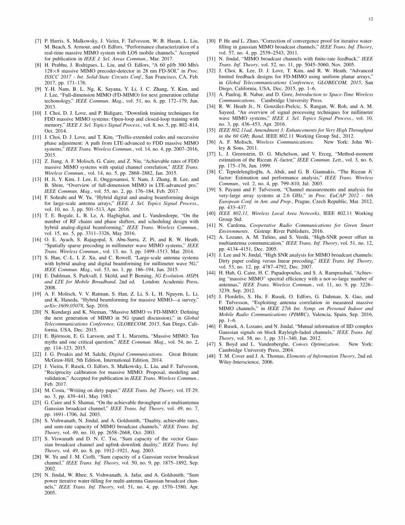
B. Required N for a Maximum SNR Loss

To obtain additional insights, we fix the sum-rate to adesired value, C∗, and investigate the impact of varying N ,the number of reported beams. The required N will depend onC∗, and on the system SNR, ρ. Given C∗ > 0 and N ≤ 128,it is immediate that one must use ρ ≥ ρ∗, with ρ∗ being therequired SNR of TDD at C∗. We define the SNR loss δρ bythe expression

δρ := ρ∗/ρ. (20)

Shown in Fig. 4 (left half) is the required number of beams,N , as a function of the maximum allowable SNR loss, forC∗ = 12 bits/s/Hz, and for scenarios 1, 2 and 3. In general,N increases sharply with decreasing SNR loss. In scenario 1,D-GOB is more efficient than D-SUB, and H-GOB is moreefficient than H-SUB. At 3 dB SNR loss, D-GOB, H-GOB,D-SUB and H-SUB require 3, 4, 6, and 7 beams, respectively.If 6 dB SNR loss is allowed, D-GOB can operate with N = 1beam, and similarly for H-GOB. On the other hand, in scenario3, D-SUB and H-SUB greatly outperfom D-GOB and H-GOB.In fact, neither D-GOB nor H-GOB can operate at less than3 dB SNR loss, regardless of N . In scenario 2, none of thefour investigated techniques can operate at low SNR loss withsmall N : At 3 dB SNR loss, all of them require N > 20.

Shown in Fig. 4 (right half) is N versus the allowable SNRloss, for C∗ = 12, 24 and 48 bits/s/Hz and K = 4, 8, and16 UEs as obtained from scenarios 4, 5 and 6, respectively.The required N increases rapidly with K. For a large rangeof the SNR loss, D-GOB outperforms D-SUB, and H-GOBoutperforms H-SUB.

C. Tradeoff of Antennas versus RF Chains

We next address the following question: Given a systemwith N ′ RF chains and M antennas, M ≥ N ′, to which extentcan one compensate for a reduction of N ′ by increasing M?For that, we consider the level curves Γβ of the SNR lossfunction δρ for some fixed sum-rate C∗ given by (20). Theparameter β represents the maximum allowable SNR loss.More explicitly, we define

Γβ = {(r(m),m) : K ≤ m ≤M} , (21)

with the mapping

r(m) = arg minn:K≤n≤m, δρ(n,m)≥β

δρ(n,m). (22)

Here, δρ(n,m) is the SNR loss, as defined by (20), of a systemwith n RF chains and m antennas with respect to TDD with128 antennas.

Let β ∈ {1, 3, 6, 9, 12} dB. Fig. 5 shows the correspondinglevel curves for H-SUB, C∗ = 12 bits/s/Hz and scenarios 1,2 and 3. For each β, there exists a fully-digital system ofminimal size m∗ (thus fulfilling N ′ = m = m∗). The systemis minimal in the sense that m cannot be further reducedwithout violating the SNR loss requirement, β. For example, inscenario 1, if β = 1 dB, then m∗ = 100; but if β = 3 dB, thenm∗ = 69. From Fig. 5, there exists a multiplicity of hybridsystems for which β is upheld (thus fulfilling N ′ < m∗ ≤ m).Furthermore, all those systems can be reached by starting from

8

1 10 1000

0.1

0.2

0.3

0.4

0.5

0.6

0.7

0.8

0.9

1

4×4

Scenario 1S

um

−ra

te /

Su

m−

ca

pa

city [

ratio

]

N [beams]1 10 100

0

0.1

0.2

0.3

0.4

0.5

0.6

0.7

0.8

0.9

1

4×4

Scenario 3

Su

m−

rate

/ S

um

−ca

pa

city [

ratio

]

N [beams]1 10 100

0

0.1

0.2

0.3

0.4

0.5

0.6

0.7

0.8

0.9

1

4×4

Scenario 2

Su

m−

rate

/ S

um

−ca

pa

city [

ratio

]

N [beams]

D−GOB H−GOB D−SUB H−SUB

1 10 1000

0.1

0.2

0.3

0.4

0.5

0.6

0.7

0.8

0.9

1

4×4

Scenario 4

Su

m−

rate

/ S

um

−ca

pa

city [

ratio

]

N [beams]1 10 100

0

0.1

0.2

0.3

0.4

0.5

0.6

0.7

0.8

0.9

1

16×16

Scenario 6

Su

m−

rate

/ S

um

−ca

pa

city [

ratio

]

N [beams]1 10 100

0

0.1

0.2

0.3

0.4

0.5

0.6

0.7

0.8

0.9

1

8×8

Scenario 5

Su

m−

rate

/ S

um

−ca

pa

city [

ratio

]

N [beams]

D−GOB H−GOB D−SUB H−SUB

Fig. 3: The sum-rates relative to the sum-capacity with ρ = 0 dB. As a baseline, the performance of small aperture K ×KMU-MIMO is also shown.

1 10 1000

2

4

6

8

10

12Scenario 1

SN

R lo

ss [

dB

]

N [beams]

1 10 1000

2

4

6

8

10

12Scenario 2

SN

R lo

ss [

dB

]

N [beams]1 10 100

0

2

4

6

8

10

12Scenario 3

SN

R lo

ss [

dB

]

N [beams]

D−GOB

H−GOB

D−SUB

H−SUB

1 10 1000

2

4

6

8

10

12Scenario 4

SN

R lo

ss [

dB

]

N [beams]1 10 100

0

2

4

6

8

10

12Scenario 5

SN

R lo

ss [

dB

]

N [beams]1 10 100

0

2

4

6

8

10

12Scenario 6

SN

R lo

ss [

dB

]

N [beams]

D−GOB

H−GOB

D−SUB

H−SUB

Fig. 4: Reported beams, N , as a function of the allowable SNR loss. The sum-rate has been fixed to 12, 24 or 48 bits/s/Hz,depending on the number of UEs K = 4, 8, or 16, respectively.

(m∗,m∗) and moving to the left along the relevant level curve.For example, in scenario 1 and under β = 1 dB, it is possibleto travel from the point (100, 100) to the point (76, 100),essentially reducing the number of RF chains by 24 at noadditional cost. To further reduce N ′, one must traverse thesegment (76, 100)− (76, 103)− (56, 103), which implies that20 RF chains can additionally be saved by spending another 3antennas. One can proceed in this way until the point (21, 128)is reached. Observe that saving RF chains becomes more and

more expensive along the way, i.e., as N ′ turns smaller.

The situation looks quite different for propagation scenario2. In particular, the level curves are notably steeper. Thelevel curve under β = 1 dB is given by the segment(100, 100)−(91, 100)−(91, 103)−(88, 103)−. . .−(71, 128):A maximal saving of 29 RF chains can be obtained by spend-ing 28 antennas. It is not obvious that the resulting (71, 128)hybrid system is cheaper to realize than the original (100, 100)system. In stark contrast, the level curves of scenario 3 are

9

4 16 6410

30

50

70

90

110

m [

an

ten

na

s]

N’ [RF chains]

1 dB

3 dB

6 dB

9 dB

12 dB

Scenario 1

4 16 6410

30

50

70

90

110

N’ [RF chains]

1 dB

3 dB

6 dB

9 dB

12 dB

Scenario 2

4 16 6410

30

50

70

90

110

N’ [RF chains]

1 dB

3 dB

6 dB

9 dB

12 dB

Scenario 3

Fig. 5: Required number of BS antennas, m, versus RFchains, N ′, for H-SUB transmission with K = 4 UEs, and12 bits/s/Hz. The curve N ′ = m for fully-digital has beenhighlighted as reference.

close to horizontal, suggesting that drastic reductions in thenumber of RF chains are possible. For example, the level curveunder β = 1 dB starts at (116, 116) and ends at (6, 128). Inother words, 110 RF chains can be saved by merely adding12 antennas.

D. The Impact of DL Training Overhead

We next illustrate the performances of the different trans-mission schemes when the training overhead is taken intoaccount. We assume a simple block-fading model, wherethe channel is constant for Tc samples. Typically, Tc is thelength (time-bandwidth product) of the coherence intervalof the channel, and ranges from just above one to a fewhundred, depending on the carrier frequency, the richnessof the channel (multipath), and the relative motion of theBS, UEs, and scatterers (Doppler). As an illustrative value,Tc = 200 corresponds to, e.g., a coherence time of 1 ms and acoherence bandwidth of 200 kHz. We assume that Np DL pilotsymbols are inserted within each coherence interval, leavingTc −Np symbols available for data. For D-SUB and H-SUB,Np ≥ N pilot symbols are needed to learn the channel.2 ForD-GOB and H-GOB, we have that Np ≥ αN , where α rangesfrom α = 1, if all the UEs report the same beams, to α = K,if the UEs report distinct beams. Here, we consider the worstcase α = K. Thus, we let

Np(N) =

{KN for D-GOB, H-GOBN for D-SUB, H-SUB,

(23)

2This is true after the N beams have been selected. Optimal beam selectionrequires that the entire “beam space” is observed, implying Np = 128.Nonetheless, Np = N holds approximately if one assumes that the structureof the beam space changes much more slowly than the particular coefficientsof the beams. That is, if one assumes that the length of the stationarity regionsof the channel is much larger than the length of the coherence interval [45].

0 100 2000

0.1

0.2

0.3

0.4

0.5

0.6

0.7

0.8

0.9

1

Su

m−

rate

/ S

um

−ca

pa

city [

tim

es]

Tc [times]

4×4

Scenario 1

0 100 2000

0.1

0.2

0.3

0.4

0.5

0.6

0.7

0.8

0.9

1

Su

m−

rate

/ S

um

−ca

pa

city [

tim

es]

Tc [times]

4×4

Scenario 2

0 100 2000

0.1

0.2

0.3

0.4

0.5

0.6

0.7

0.8

0.9

1

Su

m−

rate

/ S

um

−ca

pa

city [

tim

es]

Tc [times]

4×4

Scenario 3

D−GOB D−SUB

Fig. 6: Sum-rate relative to optimal TDD as a function of Tcwith K = 4 UEs, and ρ = 0 dB.

and compute the sum-rate CA(ρ, Tc) achievable over a largenumber of fading blocks (see [46]) by the formula

CA(ρ, Tc) =

(1−

Np(N∗)

Tc

)CA(ρ,N∗), (24)

where the average sum-rates CA(ρ,N) can be inferred fromFig. 3, and the quantity N∗ is defined by

N∗ = arg max1≤N≤128

(1−

Np(N)

Tc

)CA(ρ,N). (25)

From (25), N∗ is the optimal number of beams to be activated:If N < N∗, the degrees of freedom of the channel areunderused, whereas if N > N∗, too few symbols are leftavailable for data.

The following example demonstrates that when the over-head of DL training is properly accounted for, D-GOB andD-SUB can nevertheless extract a sizable share of the sum-capacity of LOS channels. In NLOS conditions, however, thesetechniques do not work as well.

Example 1: Let ρ = 0 dB, and let Tc = 1, 2, . . . , 200. Fig. 6shows CA(ρ, Tc) relative to optimal TDD, and the sum-rate of4× 4 MU-MIMO. D-GOB and D-SUB perform several timesbetter than conventional MU-MIMO, with D-SUB consistentlyoutperforming D-GOB. D-GOB performs poorly if UEs areco-located with LOS, and none of them works well in NLOS.The associated values of N∗ are shown in Fig. 7. Observe thatas Tc increases, more beams should be activated. As the UEsmay report distinct beams, DL training with D-GOB is moreexpensive, and N∗ is thus pushed towards zero.

In the next example, we examine the optimal number ofactive beams, N∗, with H-GOB and H-SUB. It is shown that,in LOS conditions, H-GOB and especially H-SUB performreasonably well when operated with a small excess of RFchains, i.e., N = K + 2, or so.

10

0 100 2000

5

10

15

20

25

30

35

N* [

be

am

s]

Tc [times]

Scenario 1

0 100 2000

5

10

15

20

25

30

35

N* [

be

am

s]

Tc [times]

Scenario 2

0 100 2000

5

10

15

20

25

30

35

N* [

be

am

s]

Tc [times]

Scenario 3

D−GOB D−SUB

Fig. 7: Optimal number of active beams, N∗, as a function ofTc with K = 4 UEs, and ρ = 0 dB.

1 32 64 96 1280

0.1

0.2

0.3

0.4

0.5

0.6

0.7

0.8

0.9

1

Sum

−ra

te / S

um

−capacity [tim

es]

N [beams]

H−GOB

Tc = 200

Scenario 1

Scenario 2

Scenario 3

1 32 64 96 1280

0.1

0.2

0.3

0.4

0.5

0.6

0.7

0.8

0.9

1

Sum

−ra

te / S

um

−capacity [tim

es]

N [beams]

H−SUB

Tc = 200

Scenario 1

Scenario 2

Scenario 3

Fig. 8: The estimated sum-rate relative to optimal TDD as afunction of N with K = 4 UEs, ρ = 0 dB, and Tc = 200.

Example 2: Let ρ = 0 dB, and let Tc = 200. Fig. 8 shows(1− Np(N)

Tc

)CA(ρ,N) relative to optimal TDD as a function

of N . For H-GOB, it is optimal to activate 4, 15, and 9 beamsin scenarios 1, 2 and 3, respectively. For H-SUB, the numbersare 18, 38, and 10. In fact, in LOS scenarios activating K+2 =6 beams results in losses smaller than 10% of the relative sum-rate at N∗. In NLOS scenarios, losses at K + 2 beams surgeto 20–40% of an already much diminished peak relative sum-rate.

E. On the Performance of Analog-Only Beamforming

The main remark we shall make here is that analog-only beamforming does not offer a sum-rate advantage over

conventional, small aperture MU-MIMO systems, except forthe very special case of well-separated UEs with LOS. Forthat, recall that analog-only beamforming is the same as H-GOB with N = 1, but wherein baseband processing has beensuppressed. In fact, analysis of the measured channels showsthat the sum-rates of analog-only beamforming, and thoseof regular H-GOB (thus with baseband processing) differ byless than 1%, in all scenarios. The claim follows by directinspection of Fig. 3, in Sec. V-B.

VI. CONCLUSIONS

Using measured channels at 2.6 GHz, we have comparedthe performance of five techniques for DL beamforming inMassive MIMO, namely, fully-digital reciprocity-based (TDD)beamforming, and four flavors of FDD beamforming based onfeedback of CSI (D-GOB, H-GOB, D-SUB, and H-SUB). Thecentral result is that, while FDD beamforming with predeter-mined beams may achieve a hefty share of the DL sum-rate ofTDD beamforming, performance depends critically on the ex-istence of advantageous propagation conditions, namely, LOSwith high Ricean factors. In other considered scenarios, theperformance loss is significant for the non reciprocity-basedbeamforming solutions. Therefore, if robust operation across awide variety of propagation conditions is required, reciprocity-based TDD beamforming is the only feasible alternative.

APPENDIX

A. Efficient Algorithm for Approximate Solution of (14)As noted in Sec. III-B, solving problem (14) exactly be-

comes computationally intractable for moderately large valuesof M ′. Instead, we present an algorithmic solution based onthe concept of greedy pursuit. The algorithm is summarizedin Alg. 1. (Note that, for simplicity of notation, the indices` and k have been omitted.) In short, the procedure starts byobtaining (steps 3 and 4) the index j∗ such that h has thelargest projection along cj∗ . It then stores cj∗ and j∗ in steps 5and 6 to formB(1) andQ(1), respectively. In the next iteration,a new beam cj∗ is selected such as to maximize the projectionon the subspace spanned by the columns of

[B(1) | cj∗

]of h.

(Note that the desired projection is given as the result ofthe multiplication

[B(i−1) | cj

]†[B(i−1) | cj

]Hh in step 4.)

It then repeats steps 5 and 6. The algorithm continues untilsteps 3 to 6 have been executed exactly N times, at whichpoint B(N) would contain the N selected beams, and Q(N)

their indices. Computationally, Alg. 1 can be efficiently im-plemented by sequential Gram-Schmidt orthogonalization ofthe beamforming matrices B(1), . . . ,B(N).

B. The Sum-Capacity of the MIMO-BC with BeamformingFor ease of notation, we will drop the index `. For given B

and ρ, CBC(HB, ρ) is the sum-rate of the MIMO broadcastchannel (BC) HB, and is given by the solution to [26], [27]:

maximize{Qi}Ki=1

K∑i=1

log2

1 + hTi B

(∑ij=1Qj

)BHh∗i

1 + hTi B

(∑i−1j=1Qj

)BHh∗i

subject to Qi � 0,

K∑i=1

tr(BQiB

H)≤ ρ,

(26)

11

Algorithm 1 UE-side Greedy Beam Selection

Require: h, C, N1: Q(0) = ∅, B(0) =

[ ]2: for i = 1 to N do3: S(i) = {1, . . . ,M ′} \ Q(i−1)

4: j∗ = arg maxj∈S(i)‖[B(i−1) | cj

]†[B(i−1) | cj

]Hh‖2

5: B(i) =[B(i−1) | cj∗

]6: Q(i) = Q(i−1) ∪ {j∗}7: end for8: return Q = Q(N), B = B(N).

where Q1, . . . ,QK are covariance matrices. The objectivefunction of (26) is nonconcave in Q1, . . . ,QK , and hencefinding the maximum is a nontrivial problem. One wouldlike to apply the BC-multiple access channel (MAC) dualitytheorem [26] so as to transform the nonconcave problem (26)into an equivalent, concave one, for which efficient solversare known to exist [47]. However, the presence of B inthe constraint

∑Ki=1 tr

(BQiB

H)≤ ρ prevents us from

invoking the BC-MAC duality theorem. Fortunately, we havethe following useful result.

Lemma 1: For given B = UL with UHU = I , and L aninvertible matrix, and for given ρ, we have that

CBC (HB, ρ) = CMAC

(UHHH, ρ

), (27)

where CMAC

(UHHH, ρ

)is the sum-capacity of the MIMO-

MAC UHHH [48].Proof: By inserting B = UL into equation (26), we

obtain the optimization problem

maximize{Qi}Ki=1

K∑i=1

log2

1 + hTi UL

(∑ij=1Qj

)LHUHh∗i

1 + hTi UL

(∑i−1j=1Qj

)LHUHh∗i

(28)

subject to Qi � 0,

K∑i=1

tr(LQiL

H)≤ ρ,

where we have used that tr(ULQiL

HUH)

= tr(LQiL

H)

by the cyclic property of the trace operator and the fact thatUHU = I , by assumption.

Define the effective covariance matrices Qi = LQiLH,

i = 1, . . . ,K, and the effective channel H = HU . Usingthese definitions, and the fact that L is invertible, (28) can berewritten as

maximize{Qi}Ki=1

K∑i=1

log2

1 + hT

i

(∑ij=1 Qj

)h∗i

1 + hT

i

(∑i−1j=1 Qj

)h∗i

subject to Qi � 0,

K∑i=1

tr(Qi

)≤ ρ.

(29)

Crucially, because L is invertible, Qi = LQiLH is an iso-

morphism. Thus, for every {Qi}Ki=1 satisfying the constraintsin (29) we can find {Qi}Ki=1 fulfilling the constraints in (28),

Algorithm 2 BS-side Multiuser Greedy Beam Selection

Require: H , C, N , ρ1: Q(0) = ∅, B(0) =

[ ], Λ = ρ

K I2: for i = 1 to N do3: S(i) = {1, . . . ,M ′} \ Q(i−1)

4: j∗ = arg maxj∈S(i) log2

∣∣∣I +U jTHHΛHU j

∗∣∣∣,

where U j =[B(i−1) | cj

]†[B(i−1) | cj

]H.

5: B(i) =[B(i−1) | cj∗

]6: Q(i) = Q(i−1) ∪ {j∗}7: end for8: return Q = Q(N), B = B(N).

and the converse is also true. We may now apply the BC-MAC duality theorem [26] to (29), from which the desiredresult follows.

C. Efficient Algorithm for Approximate Solution of (16)

An algorithmic solution for beam selection in multiuserMIMO systems is presented in Alg. 2. For ease of notation,the index ` has been omitted. Alg. 2 is again based on theconcept of greedy pursuit, and proceeds analogously to Alg. 1,although with a different objective function. In particular,the objective function in Alg. 2 needs to depend on thechannel matrix H , rather than on a single channel vector hk.Also, the selection of the beams depends now on the systemSNR ρ. Once the N beams (that is, the columns of the beam-former B) have been selected, the optimal covariance matricesQ1, . . . ,QK may be comptuted by first solving (15), and thenapplying the MAC-to-BC transformation—see, e.g., [26], [27],[29]. The selection of the beams along with the computationof the MIMO-BC covariance matrices is done independentlyfor each subcarrier.

ACKNOWLEDGMENT

The presented investigations are based on data obtained inmeasurement campaigns performed by Xiang Gao, FredrikTufvesson, Ove Edfors, Tommy Hult, and Meifang Zhu, aswell as Sohail Payami, and Fredrik Tufvesson.

REFERENCES

[1] T. L. Marzetta, “Noncooperative cellular wireless with unlimited numberof base station antennas,” IEEE Trans. Wireless Commun., vol. 9, no. 11,pp. 3590–3600, Nov. 2010.

[2] T. L. Marzetta, E. G. Larsson, H. Yang, and H. Q. Ngo, Fundamentalsof Massive MIMO. Cambridge: Cambridge University Press, 2016.

[3] T. L. Marzetta, “How much training is required for multiuser MIMO?” inProc. ASILOMAR 2006 - 40th Conf. on Sig., Syst. and Comput. (ACSSC),Pacific Grove, CA, USA, Nov.–Dec. 2006, pp. 359–363.

[4] F. Rusek, D. Persson, B. K. Lau, E. G. Larsson, T. L. Marzetta,O. Edfors, and F. Tufvesson, “Scaling up MIMO: Opportunities andchallenges with very large arrays,” IEEE Signal Process. Mag., vol. 30,no. 1, pp. 40–60, Jan. 2013.

[5] X. Gao, O. Edfors, F. Rusek, and F. Tufvesson, “Massive MIMOperformance evaluation based on measured propagation data,” IEEETrans. Wireless Commun., vol. 14, no. 7, pp. 3899–3911, 2015.

[6] J. Flordelis, X. Gao, G. Dahman, F. Rusek, O. Edfors, and F. Tufvesson,“Spatial separation of closely-spaced users in measured massive multi-user MIMO channels,” in Proc. ICC 2015 - IEEE Int. Conf. Commun.,London, UK, Jun. 2015, pp. 1441–1446.

12

[7] P. Harris, S. Malkowsky, J. Vieira, F. Tufvesson, W. B. Hasan, L. Liu,M. Beach, S. Armour, and O. Edfors, “Performance characterization of areal-time massive MIMO system with LOS mobile channels,” Acceptedfor publication in IEEE J. Sel. Areas Commun., Mar. 2017.

[8] H. Prabhu, J. Rodrigues, L. Liu, and O. Edfors, “A 60 pJ/b 300 Mb/s128×8 massive MIMO precoder-detector in 28 nm FD-SOI,” in Proc.ISSCC 2017 - Int. Solid-State Circuits Conf., San Francisco, CA, Feb.2017, pp. 171–176.

[9] Y.-H. Nam, B. L. Ng, K. Sayana, Y. Li, J. C. Zhang, Y. Kim, andJ. Lee, “Full-dimension MIMO (FD-MIMO) for next generation cellulartechonology,” IEEE Commun. Mag., vol. 51, no. 6, pp. 172–179, Jun.2013.

[10] J. Choi, D. J. Love, and P. Bidigare, “Downlink training techniques forFDD massive MIMO systems: Open-loop and closed-loop training withmemory,” IEEE J. Sel. Topics Signal Process., vol. 8, no. 5, pp. 802–814,Oct. 2014.

[11] J. Choi, D. J. Love, and T. Kim, “Trellis-extended codes and successivephase adjustment: A path from LTE-advanced to FDD massive MIMOsystems,” IEEE Trans. Wireless Commun., vol. 14, no. 4, pp. 2007–2016,2015.

[12] Z. Jiang, A. F. Molisch, G. Caire, and Z. Niu, “Achievable rates of FDDmassive MIMO systems with spatial channel correlation,” IEEE Trans.Wireless Commun., vol. 14, no. 5, pp. 2868–2882, Jan. 2015.

[13] H. Ji, Y. Kim, J. Lee, E. Onggosanusi, Y. Nam, J. Zhang, B. Lee, andB. Shim, “Overview of full-dimension MIMO in LTE-advanced pro,”IEEE Commun. Mag., vol. 55, no. 2, pp. 176–184, Feb. 2017.

[14] F. Sohrabi and W. Yu, “Hybrid digital and analog beamforming designfor large-scale antenna arrays,” IEEE J. Sel. Topics Signal Process.,vol. 10, no. 3, pp. 501–513, Apr. 2016.

[15] T. E. Bogale, L. B. Le, A. Haghighat, and L. Vandendorpe, “On thenumber of RF chains and phase shifters, and scheduling design withhybrid analog-digital beamforming,” IEEE Trans. Wireless Commun.,vol. 15, no. 5, pp. 3311–3326, May 2016.

[16] O. E. Ayach, S. Rajagopal, S. Abu-Surra, Z. Pi, and R. W. Heath,“Spatially sparse precoding in millimeter wave MIMO systems,” IEEETrans. Wireless Commun., vol. 13, no. 3, pp. 1499–1513, Mar. 2014.

[17] S. Han, C.-L. I, Z. Xu, and C. Rowell, “Large-scale antenna systemswith hybrid analog and digital beamforming for millimeter wave 5G,”IEEE Commun. Mag., vol. 53, no. 1, pp. 186–194, Jan. 2015.

[18] E. Dahlman, S. Parkvall, J. Skold, and P. Beming, 3G Evolution. HSPAand LTE for Mobile Broadband, 2nd ed. London: Academic Press,2008.

[19] A. F. Molisch, V. V. Ratman, S. Han, Z. Li, S. L. H. Nguyen, L. Li,and K. Haneda, “Hybrid beamforming for massive MIMO—a survey,”arXiv:1609.05078, Sep. 2016.

[20] N. Kundargi and K. Nieman, “Massive MIMO vs FD-MIMO: Definingthe next generation of MIMO in 5G (panel discussion),” in GlobalTelecommunications Conference, GLOBECOM, 2015, San Diego, Cali-fornia, USA, Dec. 2015.

[21] E. Bjornson, E. G. Larsson, and T. L. Marzetta, “Massive MIMO: Tenmyths and one critical question,” IEEE Commun. Mag., vol. 54, no. 2,pp. 114–123, 2015.

[22] J. G. Proakis and M. Salehi, Digital Communications. Great Britain:McGraw-Hill, 5th Edition, International Edition, 2014.

[23] J. Vieira, F. Rusek, O. Edfors, S. Malkowsky, L. Liu, and F. Tufvesson,“Reciprocity calibration for massive MIMO: Proposal, modeling andvalidation,” Accepted for publication in IEEE Trans. Wireless Commun.,Feb. 2017.

[24] M. Costa, “Writing on dirty paper,” IEEE Trans. Inf. Theory, vol. IT-29,no. 3, pp. 439–441, May 1983.

[25] G. Caire and S. Shamai, “On the achievable throughput of a multiantennaGaussian broadcast channel,” IEEE Trans. Inf. Theory, vol. 49, no. 7,pp. 1691–1706, Jul. 2003.

[26] S. Vishwanath, N. Jindal, and A. Goldsmith, “Duality, achievable rates,and sum-rate capacity of MIMO broadcast channels,” IEEE Trans. Inf.Theory, vol. 49, no. 10, pp. 2658–2668, Oct. 2003.

[27] S. Viswanath and D. N. C. Tse, “Sum capacity of the vector Gaus-sian broadcast channel and uplink-downlink duality,” IEEE Trans. Inf.Theory, vol. 49, no. 8, pp. 1912–1921, Aug. 2003.

[28] W. Yu and J. M. Cioffi, “Sum capacity of a Gaussian vector broadcastchannel,” IEEE Trans. Inf. Theory, vol. 50, no. 9, pp. 1875–1892, Sep.2002.

[29] N. Jindal, W. Rhee, S. Vishwanath, A. Jafar, and A. Goldsmith, “Sumpower iterative water-filling for multi-antenna Gaussian broadcast chan-nels,” IEEE Trans. Inf. Theory, vol. 51, no. 4, pp. 1570–1580, Apr.2005.

[30] P. He and L. Zhao, “Correction of convergence proof for iterative water-filling in gaussian MIMO broadcast channels,” IEEE Trans. Inf. Theory,vol. 57, no. 4, pp. 2539–2543, 2011.

[31] N. Jindal, “MIMO broadcast channels with finite-rate feedback,” IEEETrans. Inf. Theory, vol. 52, no. 11, pp. 5045–5060, Nov. 2005.

[32] J. Choi, K. Lee, D. J. Love, T. Kim, and R. W. Heath, “Advancedlimited feedback designs for FD-MIMO using uniform planar arrays,”in Global Telecommunications Conference, GLOBECOM, 2015, SanDiego, California, USA, Dec. 2015, pp. 1–6.

[33] A. Paulraj, R. Nabar, and D. Gore, Introduction to Space-Time WirelessCommunications. Cambridge University Press.

[34] R. W. Heath Jr., N. Gonzalez-Prelcic, S. Rangan, W. Roh, and A. M.Sayeed, “An overview of signal processing techniques for millimeterwave MIMO systems,” IEEE J. Sel. Topics Signal Process., vol. 10,no. 3, pp. 436–453, Apr. 2016.

[35] IEEE 802.11ad, Amendment 3: Enhancements for Very High Throughputin the 60 GHz Band, IEEE 802.11 Working Group Std., 2012.

[36] A. F. Molisch, Wireless Communications. New York: John Wi-ley & Sons, 2011.

[37] L. J. Greenstein, D. G. Michelson, and V. Erceg, “Method-momentestimation of the Ricean K-factor,” IEEE Commun. Lett., vol. 3, no. 6,pp. 175–176, Jun. 1999.

[38] C. Tepedelenglioglu, A. Abdi, and G. B. Giannakis, “The Ricean Kfactor: Estimation and performance analysis,” IEEE Trans. WirelessCommun., vol. 2, no. 4, pp. 799–810, Jul. 2003.

[39] S. Payami and F. Tufvesson, “Channel measurements and analysis forvery-large array systems at 2.6 GHz,” in Proc. EuCAP 2012 - 6thEuropean Conf. in Ant. and Prop., Prague, Czech Republic, Mar. 2012,pp. 433–437.

[40] IEEE 802.11, Wireless Local Area Networks, IEEE 802.11 WorkingGroup Std.

[41] N. Cardona, Cooperative Radio Communications for Green SmartEnvironments. Gistrup: River Publishers, 2016.

[42] A. Lozano, A. M. Tulino, and S. Verdu, “High-SNR power offset inmultiantenna communication,” IEEE Trans. Inf. Theory, vol. 51, no. 12,pp. 4134–4151, Dec. 2005.

[43] J. Lee and N. Jindal, “High SNR analysis for MIMO broadcast channels:Dirty paper coding versus linear precoding,” IEEE Trans. Inf. Theory,vol. 53, no. 12, pp. 4787–4792, Dec. 2007.

[44] H. Huh, G. Caire, H. C. Papadopoulus, and S. A. Ramprashad, “Achiev-ing “massive MIMO” spectral efficiency with a not-so-large number ofantennas,” IEEE Trans. Wireless Commun., vol. 11, no. 9, pp. 3226–3239, Sep. 2012.

[45] J. Flordelis, S. Hu, F. Rusek, O. Edfors, G. Dahman, X. Gao, andF. Tufvesson, “Exploiting antenna correlation in measured massiveMIMO channels,” in IEEE 27th Int. Symp. on Personal Indoor andMobile Radio Communications (PIMRC), Valencia, Spain, Sep. 2016,pp. 1–6.

[46] F. Rusek, A. Lozano, and N. Jindal, “Mutual information of IID complexGaussian signals on block Rayleigh-faded channels,” IEEE Trans. Inf.Theory, vol. 58, no. 1, pp. 331–340, Jan. 2012.

[47] S. Boyd and L. Vandenberghe, Convex Optimization. New York:Cambridge University Press, 2004.

[48] T. M. Cover and J. A. Thomas, Elements of Information Theory, 2nd ed.Wiley-Interscience, 2006.