massachusetts institute of technology lincoln laboratory · massachusetts institute of technology...

ESC-TR-97-119

MASSACHUSETTS INSTITUTE OF TECHNOLOGY

LINCOLN LABORATORY

GENERIC CHANNEL SIMULATOR SOFTWARE

LINCOLN MANUAL 200

7 JANUARY 1998

(Revised 10 July 1998)

Prepared for the Department of Defense under Air Force Contract F19628-95-C-0002.

Approved for public release; distribution is unlimited.

MASSACHUSETTS INSTITUTE OF TECHNOLOGY LINCOLN LABORATORY

GENERIC CHANNEL SIMULATOR SOFTWARE

CATHERINE M. KELLER

Group 44

LINCOLN MANUAL 200

7 JANUARY 1998

(Revised 10 July 1998)


19980721 002 _ a

LEXINGTON MASSACHUSETTS

This work is based on studies performed at Lincoln Laboratory, a center for research operated by Massachusetts Institute of Technology. This work was sponsored by the Department of Defense under Air Force Contract F19628-95-0002.

This report may be reproduced to satisfy needs of U.S. Government agencies.

The ESC Public Affairs Office has reviewed this report, and it is releasable to the National Technical Information Service, where it will be available to the general public, including foreign nationals.

This technical report has been reviewed and is approved for publication.

FOR THE COMMANDER

Gai-y/IJutungian / Administrative Contracting Officer Contracted Support Management

Non-Lincoln Recipients

PLEASE DO NOT RETURN

Permission is given to destroy this document when it is no longer needed.

ACKNOWLEDGMENTS

Many thanks go to Linda B. Riehl who provided extensive help in under- standing the existing software, installing the software on our computer system, and making and testing most of the software enhancements in the first year, especially concerning the GUI's. Thanks go to Marcia S. Ruklic who offered many suggestions on how to make this report more understandable to a potential software user. Thanks also go to Patricia M. Meadows and Loretta M. Wesley who helped with the publication of this report. Finally, many thanks go to Phillip A. Bello who offered advice and feedback to ensure that the software successfully agrees with the theoretical models in his reports.

in

ABSTRACT

This report serves as a user's manual for version LLO.O of the Generic Chan- nel Simulator (GCS) software developed for UNIX systems. The GCS allows users to simulate HF, land-mobile cellular and personal communications services (PCS), VHF/UHF land-mobile, VHF/UHF air-to-ground and air-to-air, and land-mobile satellite propagation channels. The GCS software was originated by BELLO, Inc. and the Mitre Corporation and was extensively enhanced by the MIT Lincoln Lab- oratory using material generated by BELLO, Inc.

TABLE OF CONTENTS

Acknowledgments in Abstract v List of Illustrations List of Tables

IX

xi

1. INTRODUCTION 1

2. SOFTWARE IMPLEMENTATION 3

2.1 Directory Structure 3 2.2 Program Enhancements 9 2.3 New Channel Models 13 2.4 New Default Scenarios 25 2.5 Software Setup 37 2.6 Benchmarks for Simulation Run Time 41

3. VALIDATION TESTS 43

3.1 Mixed Discrete/Scatter Model Enhancements 43 3.2 VHF/UHF Mobile-to-Mobile Model 44 3.3 Air-to-Air Model 47 3.4 Land-Mobile Satellite Models 55 3.5 VHF/UHF Ignition Noise Simulator 62

4. SUMMARY 65

REFERENCES 67

Vll

LIST OF ILLUSTRATIONS

Figure No. Page

1 The directory structure of the GCS software. 4

2 Motif window for the cellular mixed channel model with the data options selected. 12

3 Motif window for the cellular JTC channel model with the data option selected. 14

4 Motif window for the VHF/UHF mobile-to-mobile channel model. 16

5 Motif window for the VHF/UHF air-to-air channel model. 18

6 Motif window for the VHF/UHF air-to-ground channel model. 20

7 Motif window for the Lutz land-mobile satellite channel model. 21

8 Motif window for the Lin land-mobile satellite channel model. 23

9 Motif window for the ignition noise additive disturbance model. 24

10 Example output of the VHF/UHF ignition noise simulator. 25

11 Motif window for the VHF/UHF mobile-to-mobile channel with default scenario parameters from microscen7f. 31

12 Motif window for the tool "signal" set up to generate an impulse with samples out to 10 fis. 32

13 Motif window for the VHF/UHF mobile-to-mobile channel with default scenario parameters from "microscen7f' and with user entered selections. 33

14 A possible impulse response of the VHF/UHF mobile-to-mobile channel defined in "microscen7f." 35

15 IIR filter design compared with desired shape for a = 0.0. 44





20 IIR filter design for the VHF/UHF air-to-air channel. 48

21 Impulse response for the default scenario in Cmdline script file "landmed9." 49

22 Impulse response shown in dB for the default scenario in Cmdline script file "landmed9." 50

IX

LIST OF ILLUSTRATIONS (Continued)

Figure No. Page

23 Three example impulse responses for the default scenario in Cmdline script file "seaneard3v." 51

24 One example magnitude-squared channel impulse response for the modified default scenario "landmed9." 52

25 The scatter-path portion of the magnitude-squared channel impulse response as a function of time (256 trials of the simulation). 52

26 The averaged scatter-path portion of the magnitude-squared channel impulse response compared to the theoretical delay power spectral density. 53

27 The averaged scatter-path portion of the magnitude-squared channel impulse response in dB, compared to the theoretical delay power spectral density. 53

28 A simulation run output for scatter-path Doppler power spectral density validation. 54

29 One magnitude-squared frequency response for scatter-path Doppler power spectral density validation. 54

30 The averaged scatter-path magnitude-squared frequency response of the channel compared to the theoretical Doppler power spectral density. 55

31 Histogrammed outputs of 201og10 of the lognormal distribution subroutine with mean 3 and standard deviation 0.2. 56

32 Example output from a run of the Lutz land-mobile satellite channel simulator. 58

33 Example output from a run of the Lin land-mobile satellite channel simulator with open-area input parameters. 59

34 Example output from a run of the Lin land-mobile satellite channel simulator with open-area input parameters. 60

35 Comparison of the VHF/UHF ignition noise amplitude statistics with the theoretical Weibull probability density function. 63

36 Comparison of the VHF/UHF ignition noise interarrival time statistics with the theoretical exponential probability density function. 63

37 Validation of the VHF/UHF ignition noise impulse phase statistics. 64

LIST OF TABLES

Table No. Page

1 GCS Directory Description 5

2 SUN SPARCstation 2 GCS Benchmarks 42

3 Validation of Lognormal Parameter Calculations 57

XI

1. INTRODUCTION

The software described in this report was written to implement the Generic Channel Simulator (GCS) as described in [1] and [2]. The goal of this project was to enhance and expand already existing simulation software originated by BELLO, Inc. and the Mitre Cor- poration [3]. The final "tool box" of GCS software programs are to allow users to simulate conditions on numerous types of channels. Originally, software enhancements were made on the mixed discrete/scatter path model for signal distortion caused by the land-mobile cellular propagation channel. This software was then expanded to cover a broader range of channels: land-mobile satellite, VHF/UHF land-mobile, VHF/UHF air-to-ground, and VHF/UHF air-to-air propagation channels. For each of these channels, a set of computer- command files containing pre-determined values for the channel model parameters (default scenarios) were constructed to aid the simulator user. In addition, an additive disturbance model for vehicle ignition noise is included in the "tool box."

The original software and the software enhancements were developed on workstations running UNIX.

2. SOFTWARE IMPLEMENTATION

This section describes the GCS software enhancements and provides information necessary to install and use this software.

The enhancements are actually an extensive expansion of Revision 3.0 of the GCS, including plans for numerous new channel models. A new organized directory structure containing the channel model programs was necessary. Section 2.1 describes the new directory structure. Section 2.2 describes the enhancements that were made to existing cellular and Personal Communications Services (PCS) channel model software. Section 2.3 describes the new channel models that have been implemented. With each channel model, there is a set of default scenarios available; their use is described in Section 2.4. Section 2.5 describes some general usage. Finally, Section 2.6 describes some timing benchmarks for running the simulator software.

2.1 Directory Structure

The original version, Revision 3.0, of the GCS software, written by The Mitre Corpora- tion and described in [3], consisted of a set of ionospheric HF channel simulation programs, two different cellular channel models, and some tools including "signal" and "fileconv." The top level directory was called "HF." Under this directory, a subdirectory called "mobilechan" contained the cellular channel model software. There were two executable programs in the "mobilechan" subdirectory called "mobilechan," for the JTC cellular channel model, and "macromobilechan," for the mixed-path channel model. In the original version, it wasn't unreasonable to have this simple directory structure, since the cellular models used a lot of the same program structure as the original HF channel simulator programs.

However, the enhanced version of the GCS software described here, Revision LL0.0, includes additional channel models for VHF/UHF and several land-mobile satellite channel models. A new directory structure that logically organizes all of the channel models was constructed.

The diagram in Figure 1 shows the new directory structure with major executable programs shown in parentheses. Note that some programs have not been developed, so there are empty directories, denoted with an asterisk. Table 1 provides a brief description of each subdirectory and the programs it contains.

The new directory paths, though logical, can be cumbersome due to their length. There- fore, a list of UNIX aliases are defined in each of two files in the "GenChanSim" directory that provides the user easy access to the executable programs and allows the user to move easily into the subdirectories. These two files are called "MOTIF.alias" and "NO-MOTIF.alias." The user must edit a few lines of these files to set up the paths to libraries and to Motif as they exist on their own system.

GenChanSim ' HF (hfc)

' AddDist | ' atmosphere (atmosphere) I I ' calibrate (atmoscal) I ' gaussnoise (gaussnoise) I ' narrowband (narrowband) ' PathLoss * ' PropChan (propchan)

' scenarios (whichhf) < src

MobileChan ' AddDist I ' cochannel * I ' gaussnoise (gaussnoise) I ' ignition (ignition) ' PathLoss (cost231hata, cost231walike, hata, nlosbelrfblk, ...) ' PropChan SatMobile (lin, lutz, flatfade)

' scenarios AirMobile

« airtoair (airairchan) ' scenarios (whichscen)

' airtoground (airgroundchan) ' scenarios (whichscen)

LandMobile ' cellular I ' JTCmod (JTCchan) I I ' scenarios I ' mixedmod (mixedchan) | ' scenarios I ' indoor (whichscen) I ' macro (whichscen) I ' micro (whichscen) ' VHFUHF (vhfuhfmixedchan)

' scenarios ' mobiletobase (whichscen)

-Sat ' mobiletomobile (whichscen) ' AddDist * ' PathLoss * ' PropChan *

' Tools (fileconv, filesum, linkbud) I ' signal (signal) ' cmdline ' matlab ' misc ' xapplres

Figure 1. The directory structure of the GCS software.

4

DIRECTORY

GenChanSim

• HF

o AddDist

-atmosphere

-gaussnoise

-narrowband

o Path Loss

o PropChan

TABLE 1

GCS Directory Description

DESCRIPTION

o src

Base directory containing all the required software (excluding standard

UNIX1 libraries) to compile and run the GCS code.

Base directory for all HF channel simulator software.

Also contains a top-level GUI program "hfc" with a menu of HF programs.

Additive disturbance simulators.

Contains the atmospheric interference simulator "atmosphere."

Subdirectory "calibrate" contains software "atmoscal" for calibrating

values of Vd and a.

Contains the additive Gaussian noise generator "gaussnoise."

Contains the narrowband interference simulator "narrowband."

To contain path-loss models for HF.

Contains the HF propagation channel simulator "propchan"

and the subdirectory "scenarios" with script files to run specific models, and

the program "whichhf" to help the user select one of the scenarios.

A subdirectory "tapwgts" contains software used in generating the

tap weight coefficients.

Contains the source code for the Motif2 front end that selects

channel modeling software. NOTE: not used for path-loss or

received SNR programs.

TABLE 1 (Continued)


DIRECTORY DESCRIPTION

• MobileChan

o AddDist

-cochannel

-gaussnoise

-ignition

o Path Loss

o PropChan

-SatMobile

-AirMobile

* airtoair

* airtoground

-LandMobile

* cellular

JTCmod

mixed mod

*VHFUHF

Base directory for all mobile channel simulator software.

Additive disturbance simulators.

Will contain the cochannel interference simulator.

Contains the Gaussian noise generator "gaussnoise."

Contains the ignition noise simulator "ignition."

Contains path-loss models for the mobile channel, "cost231hata,"

"cost231walike," "hata," "nlosbelrfblk," "ploss.jtc," "qkarea,"

"snr2loss," and "unobdirurbhf." To also contain

satellite-to-ground path-loss models.

The base directory for the mobile propagation channel simulators.

Contains the satellite-to-ground propagation

channel simulators "lin," "lutz," "flatfade," and the subdirectory

"scenarios" with script files to run specific models.

The base directory for the VHF/UHF air mobile propagation

channel simulators.

Contains the air-to-air channel simulator "airairchan"


the program "whichscen" to help the user select one of the scenarios.

Contains the air-to-ground channel simulator "airgroundchan"


the program "whichscen" to help the user select one of the scenarios.

The base directory for the mobile communication channel simulators.

Contains the cellular and PCS channel simulators.

Contains the JTC channel simulator "JTCchan" and a subdirectory

"scenarios" with script files to run specific default models.

Contains the mixed discrete/scatter path channel simulator

"mixedchan" and subdirectories "scenarios/indoor", "scenarios/macro" and

"scenarios/micro" with script files to run specific models, and the

program "whichscen" to help the user select one of the scenarios.

Contains the VHF/UHF mobile-to-mobile program

"vhfuhfmixedchan" and the subdirectories "scenarios/mobiletobase"

and "scenarios/mobiletomobile" with script files to run specific

models, and the program "whichscen" to help the user select one

of the scenarios.

TABLE 1 (Continued)


DIRECTORY DESCRIPTION

• Sat The base directory for the conventional (non-land-mobile) satellite

channel simulators.

• Tools Contains tools used with any type of simulator including a link

budget program "linkbud" that calculates receiver SNR, the program

to convert a simulator output file to MATLAB3 format "fileconv,"

and the program to add simulator output files, "filesum."

o signal Contains a complex signal generator for steps and impulses "signal"

that can be used for simulator input signals.

• cmdline Contains software routines used in the development of the Motif

interfaces.

• matlab Contains scripts for data reduction.

• misc Contains miscellaneous software and common support software for

many of the simulator routines.

• xapplres Contains resource files for the Motif interface, "cmdline" is the

default resource file.

Once the ".alias" files are edited to contain the proper paths, the user must define the aliases in the UNIX window by using the UNIX "source" command. If the user has Motif available, the user should type "source pathtoGenChanSim/MOTIF.alias" at the UNIX prompt, where "pathtoGenChanSim" is the directory path to the location of the "GenChanSim" directory. If Motif is not available on the system, the user must type "source pathtoGenChanSim/NO .MOTIF. alias."

Frequent users of the GCS software should define a single alias in his/her ".cshrc" file that, when called, will in turn "source" the appropriate alias file. The alias is called "simstart" in this document, but can be called anything the user chooses. The procedure to set up such an alias is discussed further in Section 2.5.1.

JUNIX is a trademark of American Telephone and Telegraph Company. 2Motif is a trademark of the Open Software Foundation, Inc. 3MATLAB is a trademark of The MathWorks, Inc.

The use of the defined aliases makes it possible to call the programs from any working directory so that the directory structure is transparent to the user. The following aliases are defined to run the GCS "tools" and simulations:

signal

fileconv

filesum

propchan

atmosphere

atmoscal

narrowband

hfnoise

hfc

ignition

thermnoise

mixedchan

vhfuhfmixedchan

JTCchan

airairchan

airgroundchan

flatfade

lutz

lin

cost*231hata

cost'231walike

hata

nlosbelrfblk

nlosbelrfint

ploss_jtc

qkarea

snrloss'2

unobdirurbhr

generates a periodic train of pulses or impulses for a test signal

does file format conversion

merges simulator outputs

HF propagation channel simulator

HF atmospheric noise simulator

find HF atmosphere parameters

HF narrowband interference simulator

background Gaussian noise simulator

selectable menu of HF and cellular simulator programs and tools

VHF/UHF ignition additive disturbances simulator

background Gaussian noise simulator

cellular mixed discrete/scatter path model simulator

VHF/UHF mixed discrete/scatter path model simulator

JTC cellular simulator

VHF/UHF air-to-air channel simulator

VHF/UHF air-to-ground channel simulator

flat fading channel simulator

Lutz land-mobile satellite channel simulator

Lin land-mobile satellite channel simulator

wireless path loss calculator






illustrates the use of the Longley-Rice area prediction mode



At the same time, an experienced user who plans to modify a routine may find the many-branched and deep directory structure helpful because it separates the routines out that are specific to a channel model. The following aliases are set up in the "MOTIF.alias" and "NOJMOTIF.alias" files to allow the user to move to a directory in the GCS software tree:

cdsim GenChanSim directory

cdhf HF directory

cdmob GenChanSim/MobileChan directory

cdtools tools directory

cdjtc cellular JTC directory

cdmixed cellular mixed discrete/scatter path model directory

cdvhf VHF/UHF mixed discrete/scatter path model directory

cdairair VHF/UHF air-to-air directory

cdairground VHF/UHF air-to-ground directory

cdpathloss pathloss calculator directory

cdsat land-mobile satellite directory

cdignition ignition noise additive disturbances directory

New aliases can be defined if the user desires.

One consequence of setting up the new directory structure was that all of the GCS routines were affected, whether or not they were edited with enhancements. Thus, all of the routines were recompiled and tested to ensure that there were not any directory path problems.

2.2 Program Enhancements

2.2.1 Mixed Discrete/Scatter Model for Cellular

Revision 3.0 of the GCS software included a general model for cellular and PCS mobile communications channels utilizing both discrete and scatter paths. The program name in this original version was "macromobilechan."

In Revision LLO.O of this program, enhancements were added that make the simulator even more general. The new program is called "mixedchan," and it is in the subdirectory

/GenChaiiSim/MobileChan/PropChan/LandMobile/cellular/mixedmod.

The Motif window is invoked by typing "mixedchan -win" at the UNIX prompt.

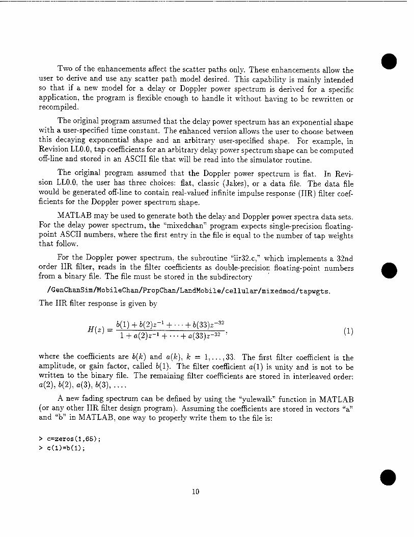
Two of the enhancements affect the scatter paths only. These enhancements allow the user to derive and use any scatter path model desired. This capability is mainly intended so that if a new model for a delay or Doppler power spectrum is derived for a specific application, the program is flexible enough to handle it without having to be rewritten or recompiled.

The original program assumed that the delay power spectrum has an exponential shape with a user-specified time constant. The enhanced version allows the user to choose between this decaying exponential shape and an arbitrary user-specified shape. For example, in Revision LLO.O, tap coefficients for an arbitrary delay power spectrum shape can be computed off-line and stored in an ASCII file that will be read into the simulator routine.

The original program assumed that the Doppler power spectrum is flat. In Revi- sion LLO.O, the user has three choices: fiat, classic (Jakes), or a data file. The data file would be generated off-line to contain real-valued infinite impulse response (IIR) filter coefficients for the Doppler power spectrum shape.

MATLAB may be used to generate both the delay and Doppler power spectra data sets. For the delay power spectrum, the "mixedchan" program expects single-precision floating- point ASCII numbers, where the first entry in the file is equal to the number of tap weights that follow.

For the Doppler power spectrum, the subroutine "iir32.c," which implements a 32nd order IIR filter, reads in the filter coefficients as double-precision floating-point numbers from a binary file. The file must be stored in the subdirectory

/GGnChanSim/MobileChan/PropChan/LandMobile/cellular/mixedmod/tapwgts.

The IIR filter response is given by

b(l) + b(2)z-i + ... + b(Z3)z-™ W l + a(2)£-i + ... + a(33)z-32 ' {i>

where the coefficients are b(k) and a(fc), k = 1,...,33. The first filter coefficient is the amplitude, or gain factor, called 6(1). The filter coefficient G(1) is unity and is not to be written to the binary file. The remaining filter coefficients are stored in interleaved order: a(2), 6(2), a(3), 6(3), ....

A new fading spectrum can be defined by using the "yulewalk" function in MATLAB (or any other IIR filter design program). Assuming the coefficients are stored in vectors "a" and "b" in MATLAB, one way to properly write them to the file is:

> c=zeros(l,65); > c(l)=b(l);

10

> c(2:2:length(c))=a(2:l:length(a)); > c(3:2:length(c))=b(2:l:lengtb(b)); > fid=fopen('dopp_filt.coef,'w') > fwrite(fid,c,'double')

If the data entry option is selected for either delay power spectrum or Doppler power spectrum, the filename is entered as a program parameter.

A third modification made to the cellular mixed-model program affects the discrete paths. The program in Revision 3.0 asked for the user to enter a Doppler angle for each discrete path. The Doppler shift was then calculated by taking the cosine of this angle and multiplying it by the maximum Doppler shift, where the maximum Doppler shift is directly proportional to the vehicle speed and indirectly proportional to the wavelength. In Revision LL0.0, the user enters the fractional Doppler shift for each discrete path, as a number between —1 and 1. Then, the Doppler shift for the path is calculated by multiplying the fractional Doppler shift by the maximum Doppler shift.

This third change provides consistency with the new mobile-to-mobile VHF/UHF communication channel model. In this channel model, it is more convenient to enter one fractional Doppler shift per discrete path rather than two Doppler angles per discrete path, one for each mobile station.

The graphical user interface Motif window was redesigned to accommodate the enhancements. Figure 2 shows the Revision LLO.O window as it appears on the screen after the data options are selected for both the delay and Doppler power spectra for one scatter path. Note that the user can only enter values in fields with bold labels; the fields with light-gray labels depend on entries made in other fields to become bold and enabled.

Other enhancements to the cellular programs are updated help files with appropriate terminology applicable to the mixed channel model and better formatted pages with carriage returns. There is a "README" file in the "mixedmod" subdirectory that explains the enhancements.

2.2.2 JTC Model for Cellular

The original JTC model program, Revision 3.0, only allowed a choice between a flat Doppler power spectrum and the classic (Jakes) Doppler power spectrum. Revision LLO.O has additional flexibility, allowing the user to input a binary data file containing IIR filter coefficients generated off-line for the Doppler power spectrum. The Revision LLO.O program resides in the subdirectory

/GenChanSim/MobileChan/PropChan/LandMobile/cellular/JTCmod

11

Sample

Vehicle

Carrier Frequ

Wan

Number ofDi

%r&ziir8£d D??*

Rei Bii ■&■■«* Fet

Number vfS

Scat Path Samp

Fractional Dop i

Sei Scatter Paii

Scatter BuB

Doppier Powe

DopPt

Delay Pove

Del Pi.

Scatter I

mixedchan Input File] 1

reiterate Vfarmup Filter Files

Rate (MHz) \\

Output Fuel

Speed (m/s)' 1

ency(MHz) 1I

tutpFuters: _] none

_l C

icrete Paths: i|

—

-Aflat

\h

n +

:}? +

|]i +

! < dassic

£<?<?:« f<£?}jj|

:ö*&syrÄSj!l§

caOer Paths f

r Spectrum: FT Aöc

>w Spec Fäe: \

r Spectrum: W data

>w Spec Fäe; 1

1 exp

BrpTVnitKs;:] - Ji +

KJVX7.S#4:!j

w CANCEL OK

Script 132? ijcmdScript

HELP j

. —1

Figure 2. Motif window for the cellular mixed channel model with the data options selected.

12

and is invoked by typing "JTCchan -win" at the UNIX prompt. For the Doppler power spectrum, the IIR filter coefficients should be generated as instructed in Section 2.2.1, and stored in the subdirectory

/GenChanSim/MobileChan/PropChan/LaiidMobile/cellular/JTCmod/tapwgts.

If the data entry option is selected for the Doppler power spectrum, the filename is entered as a program parameter.

The graphical user interface Motif window was redesigned to accommodate the en- hancement. Figure 3 shows the Revision LLO.O window as it appears on the screen after the data option is selected for the Doppler power spectrum.

2.3 New Channel Models

Several new channel models have been implemented for Revision LLO.O of the GCS: VHF/UHF mobile-to-mobile channel model, VHF/UHF air-to-air channel model, VHF/UHF air-to-ground channel model, the Lutz and Lin land-mobile satellite channel models, and an ignition noise additive disturbances model. The VHF/UHF mobile-to-mobile channel simulator retained most of the original mixed-model software. The VHF/UHF air-to-air channel simulator required extensive modification, but once modified, the VHF/UHF air-to- ground channel model followed with little changes. The Lutz and Lin models for the satellite channels were developed by first simplifying the mixed-model software to the flat fading case and then building up a Markov channel state model, one state at a time. The ignition noise additive disturbance model is a new program.

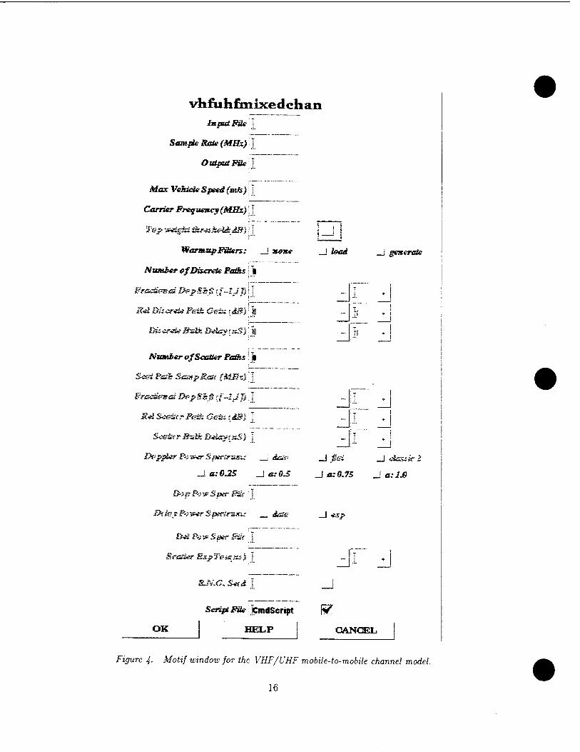
2.3.1 VHF/UHF Mobile-to-Mobile Model

The VHF/UHF mobile-to-mobile channel simulator is invoked in a UNIX window by typing "vhf uhf mixedchan -win" and resides in the subdirectory

/GenChanSim/MobileChan/PropClian/LandMobile/VHFUHF.

The modifications to the mixed-model software required for this application included the off-line computation of four new IIR filters for the four new choices of Doppler power spectra shown in Figure 10.1 of [2]. These filter coefficients were generated in MATLAB using the "yulewalk" function and are stored in the files "class25Jilt.coef," "class50Jilt.coef," "class75_filt.coef," and "classlOOJilt.coef" in the subdirectory

/GenChanSim/MobileChan/PropChan/LandMobile/VHFUHF/tapwgts.

The new set of Doppler power spectra are denoted as "classic2" spectra in the program. Once the "classic2" Doppler power spectrum option is chosen, the value of "a," the ratio of the smallest to largest vehicle speed, determines which of the four filter coefficient files is used. This velocity ratio, along with the maximum vehicle velocity, is used to compute discrete-path Doppler shifts as well. Although the "classic2" Doppler power spectrum is the

13

JTGchan Input Füe:

Simple Sate (MHz)

Output Fite

Vehicle Speed (m/s)

Carrier Frequency (MHz) j

DepPow Spec Füe I

Number ofJTC Paths

SxieiivePeih Ceia ;ßB)

gJ%\C.S*td: !

W. data

I flat doppier spectrum

_1 classic doppler spectrum

_J

I waroiup fitters

I load filter warmupfiles

I generate fitter warmup files

OK

Script Fäe j JCmdScript

HELP CANCEL

Figure 3. Motif window for the cellular JTC channel model with the data option selected.

14

analytical model derived for the mobile-to-mobile channel, the user has two other choices for the Doppler power spectrum. The other choices are a flat Doppler power spectrum or a data file; the data file choice requires the name of the file containing user-specified off-line calculated IIR filter coefficients as given in (1).

For the scatter paths, the user can also choose between an exponential delay power spectrum or a data file containing off-line computed tap weights.

The graphical user interface Motif window was redesigned to accommodate the new Doppler power spectrum choice "classic2" and the new parameter "a." The Revision LLO.O window is shown in Figure 4 as it appears on the screen.

Note that if at least one of the vehicle speeds is zero, the communications channel is identical to a mobile-to-base channel. The user must use the "mixedchan" program in this situation, entering the appropriate VHF/UHF center frequency.

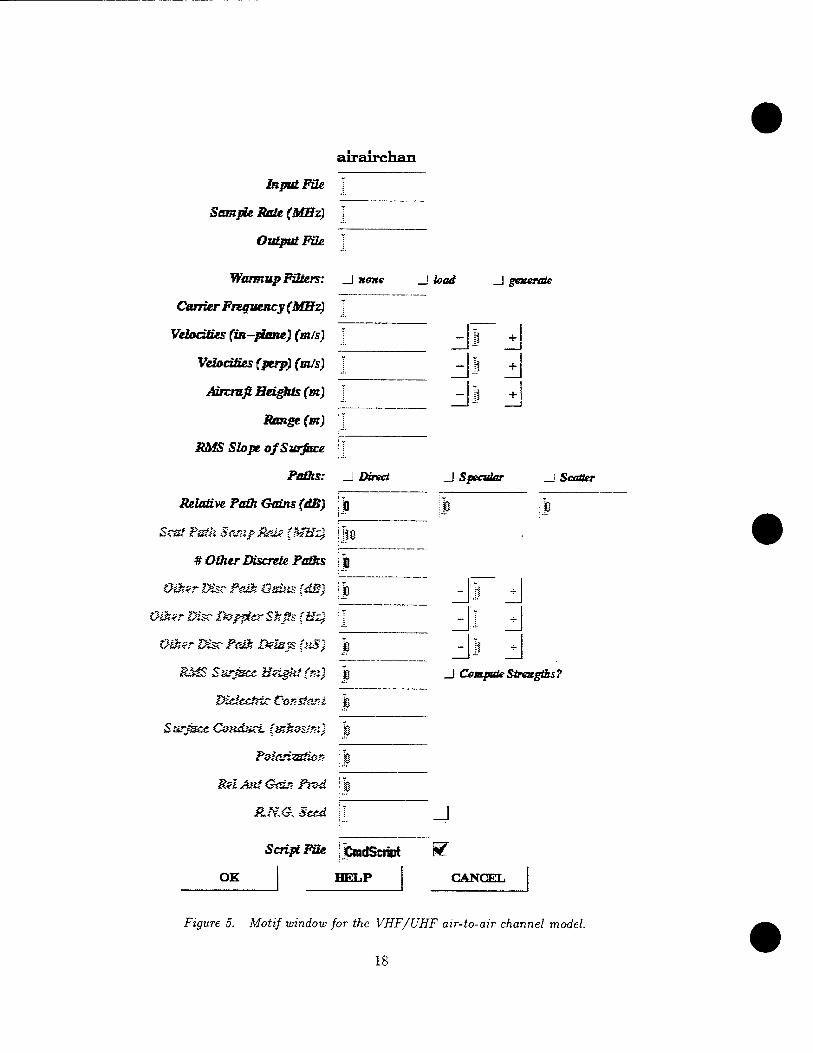
2.3.2 VHF/UHF Air-to-Air Model

The VHF/UHF air-to-air channel simulator program is invoked by typing "airairchan -win" in a UNIX window and resides in the subdirectory

/GenChanSim/MobileChan/PropChan/AirMobile/airtoair.

Numerous modifications were made to the mixed-model program to accommodate a large number of new user-input parameters and additional options for the air-to-air channel model. Also, new scatter path Doppler and delay power spectra were designed for the program.

The scatter path Doppler power spectrum has a Gaussian shape and is given in (8.1) of [2]. The filter coefficients were computed using the "yulewalk" function in MATLAB and saved according to the method outlined in Section 2.2.1. The computed coefficients for the filter, normalized to unit variance, are stored in the file "gaussian_filt.coef in the subdirectory

/GenChanSim/MobileChan/PropChan/AirMobile/airtoair/tapwgts.

The Doppler power spectrum width depends on the parameter a„, defined in (8.2) of [2], which is applied in the simulator program.

The delay power spectrum, defined in (8.5) of [2], is a decaying exponential function multiplying the 0-th order modified Bessel function of the first kind. To compute the tap weights for such a power spectrum, a new program was added that implements some numerical computation techniques. The 0-th order modified Bessel function grows quickly with increasing positive arguments, while the multiplicative exponential term decays to zero. The decaying exponential dominates; the program was implemented to ensure that this was the numerical result. The polynomial approximation in [4] for the 0-th order modified Bessel

15

vhfuhfmixedchan input Fiie I

Simple Rate (MHz) I

Output File 1

Carrier Frequency (MHz) \ ]

Warm-up Fitters: _J none

Number ef Discrete Pains \ i

Frocst'ita; I>e?Sbp t.J-lJJ} \ I

R<£ &iicr<ä* Psih Ceix :<£Bi'j§

Bis er*w &zlk DeLsv r «S ) |g

Number of Scatter Paths : |

Scsi P&h StzzpRsit (MIH'; \ T

Fradkmai DepShß -J-lJJi ■ I

SceinrB~£k Sv&syrjsS} I

D(=?}£*T &>v**r Sptcirxnx; _J <&£&

_1 c:«L25 _| ß.-ö^

!>;# P-;is Se*jr Irfe

Asia

Scalier SspTeism't }

OK

Script File l JcmdScript

HELP

_J had generate

JF J

_J ßei

_! a:Q.7S

_J cbzaic l

_! o.-i.ö

Sf CANCEL

Figure ^. Mofti/ window for the VHF/UHF mobile-to-mobile channel model.

16

function was implemented in the program with the decaying exponential multiplier applied term by term to achieve the desired result.

The air-to-air channel program is quite different from the other mixed models. In this model, the Doppler shifts and delays for one direct, one specular, and one scatter path are calculated in the program from the scenario geometry parameters rather than from explicit entry by the user. The user selects whether or not a direct, specular, and/or scatter path exists in any combination. Whether or not a specular path exists, the user is allowed to specify additional discrete paths. However, if the user enters additional discrete paths, then the Doppler shifts and delays for each additional path must be entered explicitly. In all cases, at most one direct path and at most one scatter path are allowed in the model.

In addition to the usual mixed-model program input parameters such as input file, sample rate, output file, carrier frequency, and warmup filter option, the user must specify two aircraft velocities in two dimensions, the range of the aircraft, the aircraft heights, and the RMS slope of the surface.

The user has two choices for how to specify the relative powers of the paths. In the case in which the user wants maximum control over the path structure, the user enters all of the relative powers explicitly. This is similar to the way paths are entered in the mixed-model programs "mixedchan" and "vhfuhfmixedchan." The alternative is to allow the program to compute the relative powers of the paths. The user chooses this alternative by turning on the "Compute Strengths?" flag. This selection forces a channel model with one direct path, one specular path, and one scatter path. The user must specify values for a set of physical parameters that the program needs for the relative power computation. These parameters are the root-mean-squared (RMS) surface height, the dielectric constant, the surface conductivity, the polarization, and the relative antenna gain product. Any entered relative path gains and any additional discrete paths entered are ignored when the user chooses the "Compute Strengths?" option.

The graphical user interface Motif window was redesigned to accommodate these new parameters and options. Figure 5 shows the Revision LLO.O window as it appears on the screen.

2.3.3 VHF/UHF Air-to-Ground Model

The VHF/UHF air-to-ground channel simulator is invoked in a UNIX window by typing "airgroundchan -win" and resides in the subdirectory

/GenChanSim/MobileChan/PropChan/AirMobile/airtoground.

Figure 6 shows the air-to-ground channel model window as it appears on the screen. The difference between the air-to-air and air-to-ground inputs are due to the fact that there is only one aircraft; hence, there is only one aircraft in-plane velocity, one aircraft perpendicular velocity, and one aircraft height. The height of the ground station is an input parameter.

17

airairchan

Input FüR

Sample Rate (MHz)

Output FüR

Warmup Füters: _J xexe

Carrier Frequency (MHz)

Velocities (in-plane) (m/s)

Velocities (perp) (m/s)

Aircrafi Heights (m)

Range(m)

RMS Slope of Surface \

Paths: _J Direct

_! load _] generate

Relative Path Gains (dB) jb

Scsf Pstk 5&-ip 8ai* iMU^ \ \%

# Other Discrete Paths J

O^r Disc Paßt Qsdas (dB) jjp

0&trDisc£k>ppterSJißs{H3 ||

*?££«■ Disc PcJ$ Ikrisvs (öS) |

SMS Surjsce Hfigkt (*i> \ \

Diciccfric Cozstard

Surßsct Cviid&cL (ssfios/rzi)

Poiarizstiof- ; $

R<1 AH? Giss- Prod i r$

&/£<?.. Seed \ I

_| Specular _J Scatter

_i Compote Strengths?

Script Fäe jCmdScriirt

OK HELP

w. CANCEL

Figure 5. Motif window for the VHF/UHF air-to-air channel model.

18

Several computations within the program are simplified versions of the air-to-air channel model computations.

2.3.4 Land-Mobile Satellite Models

There are two land-mobile satellite models available in the GCS based on two different Markov models in the literature: the Lutz and the Lin models. All states of both channel models exhibit fiat fading; there is only one tap per scatter or discrete path in these models. The next two subsections discuss the software for the models in more detail.

2.3.5 Lutz Land-Mobile Satellite Model

The Lutz land-mobile satellite channel simulator is invoked in a UNIX window by typing "lutz -win" and resides in the subdirectory

/GenChanSim/MobileChan/PropChan/SatMobile.

Figure 7 shows the Lutz land-mobile satellite channel model window as it appears on the screen. Since the channel can be in one of two states, "clear" or "blocked," the probability of being in one of the states has to be specified. To determine the initial channel state, a random number generator is used to choose a number from a uniform [0,1] distribution. If the random number is smaller than the specified probability of being in the "blocked" state, the channel starts out in the "blocked" state; otherwise, the channel starts out in the "clear" state. The inputs for the number of meters traveled in the "blocked" and "clear" states determine the duration of the channel states.

Because the channel can be in either of two states, each with a different path structure, the path gain normalization has to be handled differently than in the other mixed channel models. Rather than assuring that output power equals input power, the path powers are all relative to the direct path of the "clear" state for this simulation. Section 3.4 provides an example of running the Lutz land-mobile satellite model.

2.3.6 Lin Land-Mobile Satellite Model

The Lin land-mobile satellite channel simulator is invoked in a UNIX window by typing "lin -win" and resides in the subdirectory

/GenChanSim/MobileChan/PropChan/SatMobile.

Figure 8 shows the Lin land-mobile satellite channel model window as it appears on the screen. Since the channel can be in one of three states, "clear," "shadowed," or "blocked," the probability of being in each of the states has to be specified. They are entered into the simulation in the order (1) "clear," (2) "shadowed," and (3) "blocked" states. Three mutually exclusive intervals are then set up in [0,1] with lengths equal to the corresponding state probabilities. To determine the initial channel state, a random number generator is

19

airgroundctian

Input FüR

Sample Rate (MHz)

Output File

Warmup Filters: _l »one

Carrier Frequency (MHz)

Velocity (in-plane) (m/s)

Velocity (perp) (mis)

Aircmfi Height (m)

Ground Height (m)

Range (m)

RMS Slope of Surface

Paths:

Relative Path Gains (dB)

Scsf Pstk SasipRrj* (MHz)

# Other Discrete Paths

0&?r Disc ?<& Gsms (dB)

Oik ?r Disc DopplerShßs (Hz)

Ö&zr Disc Fmk Deists (HS)

RMS Sarßzx. Hzlght (zi) jß

Di£f££ffic Cozstar-i ! jo

_iioad _l generate

Direct Specular Scatter

ID

ID

iü

Compote Strengths?

Sarßtce Conduct (mhos-xi) jg

Poi&izsHa. 9

R<1 Ant Gitzrr Prod j jg

R.N.G,Seed _l

Script File jlCmdSeriDt W.

OK HELP CANCEL

Figure 6. Motif window for the VHF/UHF air-to-ground channel model.

20

lutz Input FüR

Sample Rate (MHz) \

Output FHR\

Warmup Filters:

Carrier Frequency (MHz) \

Vehicle Speed (mis) \

_! none

# of Clear-State Discrete Paths ! jj

Fractional Dop Shfi ([-1,1]) \ I

Rel Discrete Path Gain (dB) \ ]

Discrete Bulk Delay (nS) \ I

Rel Scatter Path Gain (dB) \

Scatter Bulk Delay (nS)

Doppier Poiver Spectrum:

lead _J generate

RMS si&pc &fsur$zce \}

SsteiHtc E0& fc AH«, ideg) \ T

Dap Fw Spec File \ T

Probability of Blocked State \

Avg Distance Clear State (m) ;

Avg Distance Blocked State (m) \

Lognormal m (dB) \

Lognormal Sigma (dB) \

&.&& secdW

fiat _] Gaussian _] data

_J

OK

Script File jJCmdScrin*

HELP CANCEL

Figure 7. Motif window for the Lutz land-mobile satellite channel model.

21

used to choose a number from a uniform [0,1] distribution and checked against the intervals.

The duration of the state is determined using (12.25) and (12.27) in [2] from the state transition probability matrix and the state transition distance provided as simulator inputs. The next state is also determined by using the state transition probability matrix. The nine element state transition probability matrix is entered in the following order: (1) "clear" to "clear" state; (2) "clear" to "shadowed" state: (3) "clear" to "blocked" state: (4) "shadowed" to "clear" state; (5) "shadowed" to "shadowed" state; (6) "shadowed" to "blocked" state: (7) "blocked" to "clear" state; (8) "blocked" to "shadowed" state: and (9) "blocked" to "blocked" state.

Each state has a set of specified lognormal parameters and relative path gains. Because the channel can be in one of three states, each with a different path structure, the path gain normalization is handled differently than in the other mixed channel models, and similarly to the Lutz land-mobile satellite model. Rather than assuring that output power equals input power, the path powers are all relative to the direct path of the "clear" state for this simulation. Section 3.4 provides two examples of running the Lin land-mobile satellite model.

2.3.7 Ignition Noise Additive Disturbance Model

The ignition noise additive disturbance channel simulator is invoked in a UNIX window by typing "ignition -win" and resides in the subdirectory

/GenChanSim/MobileChan/AddDist/ignition.

No input signal is required for this simulator. The signal duration and sample rate should match those for the output of a propagation channel simulator; the output of the ignition noise model can then be added to the output of the propagation channel simulator using the "filesum" tool.

Figure 9 shows the ignition noise additive disturbance model window as it appears on the screen. Figure 10 shows an example of one run of the simulator using the following script file:

#

# script file written by Cmdline #

# list of available args: # -t Total_Time_(seconds) (float) # -s Sample_Rate_(MHz) (float) optional (default = 1) # -lam Pulses_Per_Second (float)

22

lin Input File

Sample Rate (MHz)

Output FüR

Warmup Filters: _j none

Carrier Frequency (MHz) \\

Vehicle Speed (mis) \

Number of Discrete Paths j jj

Fractional DopShfi (1-lf.J)

Bel Discrete Path Gain (dB)

Discrete Bulk Delay (nS)

State RMS Scatter Path Gain (dB) \

Scatter PaOt Bulk Delay (nS) \

Doppter Power Spectrum: _j ßat

H^JS -Steps o/S&r&c?

SsteftSfc m*\r. Axg. (dfg) I

Do? ?&* Spec File \

State Probs.

State Transition Probs.

State Lognormal m (dB)

State Lognormal Sigma (dB)

State Transition Distance (m)

R.N.G. Seed

_] load _l generate

_J Gaussian _] date

— jft _+

ft +

ft +

J 1-

1 +

_l

Script File \ CmdSeript

OK HELP CANCEL

Figure 8. Motif window for the Lin land-mobile satellite channel model.

23

ignition Teid Time (seconds) 1

Sm?kRtite(MBx)$

Fakes Per Second 1

B

Center Frequency (täBz)

&N£.S*d J

Osi&äFik:.!.

J J

SOT^Kfe;]PmdScriP't |?

OK FTRT.P CANCEL

Figure 9. Motif window for the ignition noise additive disturbance model.

-Wm Weibull_parameter_m (float) -freq Center_Frequency (MHz) (float) -S R.N.G._Seed (int) optional -o Dutput_File (file) optional -win (int flag) optional

# # # # # # # '$*' at the bottom of the file allows for additional # command-line arguments to be added when running this # script (e.g., the '-win' flag to invoke the window) #

pathtoGenChanSim/GenChanSim/MobileChan/AddDist/ignition/ignition \ -t 0.05 \ -s 1 \ -lam 1000 \ -Wm 2.5 \

24

.Q

UJ o 3

-80

-82

-84

-86

-88

-90

-92

-94

-96

-98

-100

<fc

c°°° 0 °° o o o Cfc

O 0

o o

# o

o o

c 0

o o °0°

1000 pulses/s Weibull m = 2.5 Fc = 400 MHz

10 20 30 TIME (ms)

40

o o

0 § oo

0.

50

Figure 10. Example output of the VHF/UHF ignition noise simulator.

-freq 400 \ -o example.bin \ -Script.File $0 \ $*

where the "pathtoGenChanSim" would be replaced with the actual path to the "GenChan- Sim" directory.

2.4 New Default Scenarios

A set of default scenarios that use the "cmdline" script format is available for each of the programs enhanced in Revision LLO.O of the GCS. These default scenarios are contained in a subdirectory of the particular program to which they apply called "scenarios.'" For example, the subdirectory

25

/GenChanSim/MobileChan/PropChan/LaiidMobile/cellular/mixedmod/scenarios

contains three subdirectories, "indoor," "micro," and "macro'* which, in turn, contain numerous default scenario "cmdline" script files. These sets of default scenarios call the cellular "mixedchan" channel simulator. The "indoor" subdirectory contains 280 script files named "inscenlFa" through "inscenl6Nj." The "micro" subdirectory contains 144 script files named "microscenla" through "microscenl6i." The "macro" subdirectory contains 144 script files named "scenla" through "scenl6i," as well as nine additional script files named "coxleckl" through "coxleck9." "o-1

The "indoor," "macro," and "micro" default scenarios were specified according to Sec- tion 13.2.2 of [2] and Section 3.2 of [1]. Because of the large number of scenarios, an interactive C-program was written for each of the sets of default scenarios. In each subdirectory with the scenarios, the program is called "whichscen" that queries the user on the type of scenario desired. The queries are in the form of multiple choice menus. Based on the user's responses, the program prints out which default scenario file to use. For example, the program "whichscen" in the "macro" subdirectory has the following queries:

Enter environment: 0=Urban High-Rise l=Urban/Suburban Low-Rise 2=Residential

Enter amount of delay spread: 0=small l=medium 2=large

Enter channel structure: 0=scatter only l=scatter + direct 2=scatter + discrete (no direct) 3=scatter + direct + discrete

If the user selects options 1, 2, or 3 in the last query, then the program also asks the user to select relative powers of the paths:

Enter power level of SCATTER path relative to total path power:

26

0=small l=medium 2=large

Enter power level of DIRECT path relative to total discrete-path power: 0=small l=medium 2=large

Aliases are set up in the files "MOTIF.alias" and "NO-MOTIF.alias" that call the desired version of "whichscen" and help the user copy the selected scenario into his/her working directory. The current set of aliases and their descriptions are:

mixedmacro

dirmacro

cpmacro

mixedmicro

dirmicro

cpmicro

mixedindoor

dirindoor

cpindoor

mobiletobase

dirmobiletobase

cpmobiletobase

mobiletomobile

dirmobiletomobile

cpmobiletomobile

Select a cellular macro default scenario.

List the possible cellular macro default scenarios.

Copy a selected cellular macro default scenario to

the current directory.

Select a cellular micro default scenario.

List the possible cellular micro default scenarios.

Copy a selected cellular micro default scenario to


Select a cellular indoor default scenario.

List the possible cellular indoor default scenarios.

Copy a selected cellular indoor default scenrio to


Select a VHF/UHF mobile-to-base station default scenario.

List the possible VHF/UHF mobile to base default scenarios.

Copy a selected VHF/UHF mobile-to-base default scenario to


Select a VHF/UHF mobile-to-mobile default scenario.

List the possible VHF/UHF mobile-to-mobile default scenarios.

Copy a selected VHF/UHF mobile-to-mobile default scenario to


27

airtoair

dirairtoair

cpairtoair

airtoground

dirairtoground

cpairtoground

dirsat

cpsat

dirJTC

cpJTC

whichhf

dirhf

cphf

Select a VHF/UHF air-to-air default scenario.

List the possible VHF/UHF air-to-air default scenarios.

Copy a selected VHF/UHF air-to-air default scenario to


Select a VHF/UHF air-to-ground default scenario.

List the possible VHF/UHF air-to-ground default scenarios.

Copy a selected VHF/UHF air-to-ground default scenario to


List the possible land-mobile satellite default scenarios.

Copy a selected land-mobile satellite default scenario to


List the possible JTC cellular default scenarios.

Copy a selected JTC cellular default scenario to


Select a wideband HF default scenario.

List the possible wideband HF default scenarios.

Copy a selected wideband HF default scenario to


The following subsection gives an example for a typical sequence of steps that the user might go through to run one of the VHF/UHF mobile-to-mobile default scenarios.

2.4.1 Example

The user has set up the GCS software and all the necessary paths and aliases a week ago. Today, the user logs into his UNIX workstation, which automatically puts him into a window environment. The user brings up a window and gets into his working directory that happens to be called "/h°me/me/vhf.'" Also, in that window, the user types the alias"

simstart

which sets up all of the aliases that make the GCS easy to use from any directory. The user now wishes to run a simulation to find the impulse response of a VHF/UHF mobile- to-mobile channel in a suburban area. The user first invokes the mobile-to-mobile default scenario selection program in a UNIX window by typing

28

mobiletomobile

The user answers the queries at the "?" prompt with integer responses and obtains the

following result:

1996 MIT Lincoln Laboratory, Lexington MA

DEFAULT SCENARIO SELECTION

Enter environment:

0=Urban High-Rise

l=Urban/Suburban Low-Rise

2=Residential

? 1

Environment = URBAN/SUBURBAN LOW RISE

Enter amount of delay spread:

0=small

l=medium

2=large

? 2

Delay spread = LARGE

Enter channel structure:

0=scatter only

l=scatter + direct

2=scatter + discrete (no direct)

3=scatter + direct + discrete

? 2

Channel structure = SCATTER + DISCRETE

Enter power level of SCATTER path relative to total path power:

0=small

l=medium

2=large

? 2

SCATTER path power level = LARGE

THE DEFAULT SCENARIO FILE TO USE IS microscen7f

29

The user copies the suggested default scenario "microscenTf" to his current working directory by typing

cpmobiletomobile microscen7f

The user notices that the file "microscenTf" is "write-protected" in the original directory, so that he would not inadvertently change the original default scenario. However, the copy of "microscenTf" was automatically made "writable" after it was copied into his own work directory so that he can edit the file. The user then types

microscen7f -win

which results in the Motif window shown in Figure 11.

To perform a run of the program, the user must fill in values for "Input File," "Sample Rate (MHz)," "Output File," "Maximum Vehicle Speed," "Carrier Frequency," "Fractional Doppler Shift([-l,l])" (for 4 paths) and select a value for the parameter "a." The user has not generated the input file yet, so he clicks on the "CANCEL" button to get out of the "vhfuhfmixedchan" program.

To generate the input data file that contains an impulse, the user calls up the tool "signal" by typing

signal -win

at the UNIX prompt. Figure 12 shows the window that results after the user makes his desired entries. The user clicks on the "OK" button to run the signal generator which results in the following output in the UNIX window:

script file 'Cmdimpulse' written writing 100 samples to 'impulse.bin'...done

Now the user reenters the "microscenTf" default scenario window

microscen7f -win

and enters the desired variables to obtain the window shown in Figure 13. After clicking the "OK" button, the following information is printed in the UNIX window:

30

vhfuhfmixedchan Input Fäe \ jnputfile jda

Sample Rate (MHz) jjp

Output Fäe!Jputputfilejd

Max Vehicle Speed (m/s) \ J

Carrier Frequency (MHz) \ %

Tap v&igki i&r*z£n$d;d&i \ \

War map Filters: W none

Number of Discrete Paths \ Ü

Fractional DopShfi({-2,2^ \ J

Rel Discrete Path Gain (dB) \ J-13 JS51

Discrete Bläk Delay (nS) ■ fISIl

Number of Scatter Paths \ fl

Scat Path Samp Sate (MHz) \ _p|

Fractional DopShfl ([-2,1]) 11

Ret Scatter Path Gam (dB) \ §

Scatter Bu& Delay (nS)! jl

Doppier Power Spectrum: _J data

_i a:0J2S _J 0.-0.5

&■>& B'>v; Spec £?ik |j_

Delay Power Spectrum: _] dtric

Sector ExpTaufns) \ j215

OK

Script JR&? ; jmicroscen

HELP !

_J _l food _J generate

J*~ J JS _ J

fT

if^

ii ri

_i Jtet F? classic 2

_i or 0.7? _] c-1.0

ST «rp

JF

CANCEL.

Figure 11. Motif window for the VHF/UHF mobile-to-mobile channel with default scenario parameters from microscenlf.

31

signal Sample Rate (MHz) 1$.

Time (seconds) 1^-5

Output FÜ* impulse.bitj

W Impulse

_] Pulse

_J Gaussian

_J SiBeWcw

Fn q-zi iwgz ih.)

Script File

_J

OK

JCmdScrip-t

HELP

W. CANCEL

Figure 12. Motif window for the tool "signal" set up to generate an impulse with samples out to 10 fis.

32

vhfuhfinixedchan Input Fäe j impulse J>ir

Sample Sate (MHz) \ hi

Output Fäe i ioutput Jtin

Max Vehicle Speed (m/s) \ jll

Carrier Frequency (MHz) \ J3M

WarmupFüters: £? son«

Number of Discrete Paths i 4

Fractional Dop Shfi (1-1,1 J) \ h St

Rei Discrete Path Gain (dB) \ J-13 JS51

Discrete Bulk Delay(nS) \ fl5M

Number of Scatter Paths \ H

Scat Path Samp Sate (MHz) \ fit

FractionalDopSkß([-JJJ)\ l^f

JW ScvsUer JFtaft Gear fd»;: l|

Sooter Bulk Delay (nS) \ §

Doppier Power Spectrum: I ^o&z

_1 a:G-25 W c-0.5

Delay Power Spectrum: | dkdte

!><*? P-^w S&tr I?ik ; J

Scwtfer J&cp TVEBCKS^ ; JZ15

&JV,<7, -S*f- ^! I

OK

Script Fäe \ gnicroseen'

HELP

_l food _| generate

- I* J _

Üb +

_J JJIoi F? classic 2

_l c-0.75 _J c-f.«l

SF «cp

J _j

CANCEL

Figure 13. Motif window for the VHF/UHF mobile-to-mobile channel with default scenario parameters from "microscen7f" and with user entered selections.

33

script file 'microscen7f' written

Using filter file: pathtoGenChanSim/GenChanSim/MobileChan/PropChan/LandMobile/

VHFUHF/tapwgts/dopp_filt.coef

Sample Rate (Hz): 10000000.000

Scat Samp Rate (Hz): 10000000.000

Number of paths: 5

Vehicle Speed (m/s): 20.00000

Carrier Freq. (MHz): 300.000

path 1 2 3 4 5

mode Discrete Discrete Discrete Discrete Scatter

Exp. Tau(ns) N/A N/A N/A N/A 215.000

number of taps 1 1 1 1 11

snapshot (Hz) 1500.000 1500.000 1500.000 1500.000 1920.000

Dpi shift(Hz) 9.000 6.000 -27.000 29.400 6.900

Bulk Delay (ns) 1500.000 3000.000 5000.000 9000.000 0.000

Rel. Gain (dB) -13.651 -15.663 -21.717 -14.674 0.000

Writing output file 'output.bin'... 1000 samples per tick: done. 100 samples written to output.bin

where the "pathtoGenChanSim" would be replaced with the actual path to the "GenChan- Sim" directory.

The user converts the binary output file to MATLAB by typing

fileconv -i output.bin -o output.mat -m

at the UNIX prompt. Then, using MATLAB. the samples in "output.mat" are loaded and the magnitude of the samples are plotted resulting in Figure 14.

Note that the user can run the default scenario "microscenTP again without the "-win" option if he does not care to change any of the parameters. The results will all be different unless the random number generator "seed" parameter is explicitly set to be the same for each run. (If the user wants to set the random seed to a fixed number, he should select the button to the right of the "R.N.G. Seed" field and then type the desired seed inside that field. This is useful for validation runs, for example.) Also, the file "microscen7f" is in ASCII format and can be pulled into an editor for entering new parameters. For example, the ASCII file that corresponds to the Motif window shown in Figure 13 is:

34

20 40 60 SAMPLE NUMBER

80 100

Figure 14. A possible impulse response of the VHF/UHF mobile-to-mobile channel defined in "microscen7f."

#

# script file written by Cmdline #

# list of available args:

# -i InputJFile (file)

# -s Sample_Rate_(MHz) (float)

# -o OutputJFile (file)

# -vs Max Vehicle_Speed (m/s) (float)

# -fc Carrier Frequency (MHz) (float)

# -tl Tap_weight_threshold(dB) (float) optional

# -w none (int flag) optional

# -wld load (int flag) optional

# -wgen generate (int flag) optional

# -norm Number_of_Discrete_Paths (int) optional (default = 4)

35

# -nd Fractional_Dop_Shft_([-l,l]) (float array)

# -nx Rel_Discrete_Path_Gain_(dB) (float array) optional (default = -13.7)

# -nb Discrete_Bulk_Delay_(nS) (float array) optional (default = 1.5e+03)

# -dist Number_of_Scatter_Paths (int) optional (default = 1)

# -ds Scat_Path_Samp_Rate_(MHz) (float)

# -dd Fractional_Dop_Shft_([-l,l]) (float array)

# -dx Rel_Scatter_Path_Gain_(dB) (float array)

# -db Scatter_Bulk_Delay_(nS) (float array)

# -datadopp data (int flag) optional

# -flat flat (int flag) optional

# -classic classic_2 (int flag) optional

# -al a:_0.25 (int flag) optional

# -a2 a:_0.5 (int flag) optional



# -dopfile Dop_Pow_Spec_File (file)

# -datapow data (int flag) optional

# -exppow exp (int flag) optional

# -powfile Del_Pow_Spec_File (file)

# -et Scatter_Exp_Tau(ns) (float array)

# -seed R.N.G._Seed (int) optional

# -win (int flag) optional

#

# '$*' at the bottom of the file allows for additional # command-line arguments to be added when running this

# script (e.g., the '-win' flag to invoke the window)

#

pathtoGenChanSim/GenChanSim/MobileChan/PropChan/LandMobile/VHFUHF/vhfuhfmixedchan \

-i impulse.bin \

-s 10 \

-o output.bin \

-vs 20 \

-fc 300 \

-w \

-norm 4 \

-nd 0.3 0.2 -0.9 0.98 \

-nx -13.651 -15.663 -21.717 -14.674 \

-nb 1500 3000 5000 9000 \

-dist 1 \

-ds 10 \

36

dd 0.23 dx 0 \ db 0 \ classic \ a2 \ exppow \ et 215 \

-ScriptJFile $0 \

where "pathtoGenChanSim" would be replaced by the actual path that leads to where the user installed the GCS software. The cmdline script file is overwritten with the current parameter values when the program is run.

2.5 Software Setup

2.5.1 Getting Started

The top directory of the simulator software is called "GenChanSim," and the user needs to set aside a location on his/her disk to install this software. The software currently needs about 15.8 Mbytes of disk space including the executable programs. For example, the user may put "GenChanSim" directly in his/her "home" directory or may decide to put it under a subdirectory constructed to keep it separate from other projects. Another alternative is to locate the "GenChanSim" directory (with all of its subdirectories) in a location on a disk shared by a group of users. Whatever the user installing the software does decide, he/she must then make a note of the full path to the "GenChanSim" directory.

Once the location for "GenChanSim" is decided upon, and the software is copied into it using the UNIX "tar" command, the user should enter one alias in his/her UNIX shell (usually the ".cshrc" file in the "home" directory). The alias takes one of two forms, de- pending upon whether or not the user has Motif available on the system. If the user does have Motif, the alias should be defined as

alias simstart 'source pathtoGenChanSim/GenChanSim/MOTIF.alias'

where "pathtoGenChanSim" is replaced with the actual path to the "GenChanSim" directory. The file MOTIF.alias in the "GenChanSim" directory must also be edited to set the proper path to the Motif "include" and "lib" directories.

If the user does not have Motif, the alias must be defined as

37

alias simstart 'source pathtoGenChanSim/GenChanSim/NO_MOTIF.alias'

in the UNIX shell.

This "simstart" alias, once invoked in a window, defines logical parameters for the directory paths required when "making'1 the GCS C programs. It also defines a large set of aliases that help the user move around the GenChanSim subdirectories as well as execute any of the GCS routines from any desired work directory. These aliases are extremely useful, because it is recommended that the user do actual simulation runs and store results in a work directory separate from the software source-file directories.

Once the desired "MOTIF" or "NO-MOTIF", ".alias" file is edited to contain all of the correct paths to libraries and to the "GenChanSim" directory, the simulator programs must be installed by invoking the "Makefile" in the "GenChanSim" directory. This is done by getting into the "GenChanSim" directory and typing "make" at the UNIX prompt.

2.5.2 Example

Here is an example of how the user might set up the GCS software:

A group of users shares a workstation network and all plan to use the GCS software. The group has access to a disk drive on their system called "/sysname." The leader of the research group, with user name "userl" installs the GCS software by using the UNIX "tar" command to copy it from tape onto the top level of this disk, thus creating a "/sysname/GenChanSim" directory with all of its subdirectories. Userl also double checks that the Motif directory is set properly in the "/sysname/GenChanSim/MOTIF.alias" file. Then, userl instructs all of the group members to add the line

alias simstart 'source /sysname/GenChanSim/MOTIF.alias'

to their own ".cshrc" files. Then, the next time the users log in or refresh their ".cshrc" file, the simstart alias will work. Userl refreshes her ".cshrc" file using the UNIX "source" command.

Userl completes the installation of the software with the following commands, each at the UNIX prompt:

simstart

cdsim

make

38

The "simstart" command makes a large set of aliases available to userl and the "cdsim" command (one of those aliases) changes the current directory to "/sysname/GenChanSim."

The "make" command creates executables for all of the existing GCS programs. The "making" process stops with an error message if there is a problem. If there is a problem, the user should check that the paths to libraries and to the "GenChanSim" directory are set up properly in the "MOTIF.alias" and the "NO_MOTIF.alias" files. Userl "makes" the programs with no problems.

Userl tries out the simulator program by opening up a UNIX window and creating a working directory in her own "home" directory called "/home/user 1/sim." She then changes to that directory by typing "cd /home/userl/sim" at the UNIX prompt and executes the mixed-model program by typing

mixedchan -win

so that the Motif window with all of the input parameter fields appears on the screen.

2.5.3 Arbitrary User Specified Scenarios

Revision LLO.O of the GCS software includes the following executable programs that use "cmdline" Motif windows:

signal

fileconv

filesum

propchan

atmosphere

atmoscal

narrowband

hfnoise

mixedchan

vhfuhfmixedchan

ignition

JTCchan

airairchan

airgroundchan

lutz

lin

39

Any of these programs can be invoked at the UNIX prompt with the "-win" option to obtain the Motif window or by entering the command followed by a long string of input parameters. Usually, one does not do the latter, but instead takes an existing "cmdline" script file and edits it to contain the desired parameters. There are numerous existing "cmdline" script files in the scenario subdirectories that may be used as examples.

If the user desires to enter data for a scatter path delay power spectrum, the data file must be placed in the user's work directory, the directory in which the simulation programs are being run. If the user defines a new IIR filter for a scatter path Doppler power spectrum, the filter coefficient file must be placed in the appropriate "tapwgts" subdirectory in the GCS software. This is one time that the user must be able to move within the GCS directory structure. There is a set of aliases defined to allow the user to easily find the "GenChanSim" subdirectories:

cdsim cd ${SIMDIR} cdhf cd ${SIMDIR}/HF cdmob cd ${SIMDIR}/MobileChan cdtools cd ${SIMDIR}/Tools

cdjtc cd ${SIMDIR}/MobileChan/PropChan/LandMobile/cellular/JTCmod cdmixed cd ${SIMDIR}/MobileChan/PropChan/LandMobile/cellular/mixedmod cdvhf cd ${SIMDIR}/MobileChan/PropChan/LandMobile/VHFUHF cdairair cd ${SIMDIR}/MobileChan/PropChan/AirMobile/airtoair cdairground cd ${SIMDIR}/MobileChan/PropChan/AirMobile/airtoground cdpathloss cd ${SIMDIR}/MobileChan/PathLoss cdsat cd ${SIMDIR}/MobileChan/PropChan/SatMobile cdignition cd ${SIMDIR}/MobileChan/AddDist/ignition

There is a set of programs existing from Mitre's Revision 3.0 of the software that does not use "cmdline." Most of these are interactive, querying the user for inputs and then calculating a result. Aliases are set up for these programs so that they can be invoked from any work directory. The following aliases are for programs that compute path-loss for various cellular communications channels:

cost231hata

cost231walike

hata

nlosbelrfblk

nlosbelrfint

ploss_jtc

qkarea

snr21oss

40

unobdirurbhr

The aliases that are defined for selecting default scenarios, copying them over into the user's work directory, and getting a listing of the contents of the existing default scenario directories are listed in Section 2.4.

2.5.4 Editing the Source Files

Most of the source code for the GCS is written in "C" and compiled using "gcc." Under the Mitre copyright, any user may edit a GCS program, and all of the source code is included in the directories. It is suggested that the original program be copied into a ".sav" file before editing. To make it easy to recompile the software, there are files called "Makefile" in every appropriate directory. If all of the variables and paths are set properly in the "MOTIF.alias" and the "NO-MOTIF.alias" files in the "GenChanSim" directory, then these programs should be readily compiled by typing "make" in the directory in which source code has been changed. The "GenChanSim" directory has a top level "Makefile" that will create executables for all of the GCS software.

2.5.5 Other Information

For additional information, the user should look at the "README" files and help files (files that have a ".hip" extension in the filename) in the "GenChanSim" subdirectories.

2.6 Benchmarks for Simulation Run Time

The mixedchan simulator program was run on a SUN4 SPARCstation0 2 system with little other loading to determine the elapsed time users should expect to encounter. Sinusoids with 10 MHz sampling rate and with various durations were first constructed using the program "signal." Then, these various length signals were used as inputs to "mixedchan." For the first set of simulation runs, warmup filters were generated during execution, assuming no warmup filter files. For the second set of simulation runs, pre-existing warmup filter files were loaded. A fiat Doppler power spectrum and an exponential delay power spectrum were assumed. Elapsed run times were recorded for each length of the input signal.

The scenario chosen was macro-channel default scenario "scen7c." This scenario has 4 discrete paths and 1 scatter path with an exponential tau of 2200 ns; the model requires a total number of 115 taps. The elapsed times for the channel simulation are shown in Table 2.

4SUN is a trademark of SUN Microsystems. Inc.

°SPARC is a trademark of SPARC International. Inc.

41

All other cellular default scenarios require fewer taps, so the elapsed times would be shorter than those shown in the table. The table shows that the use of pre-existing warmup filter files saves 30-38 seconds of elapsed time.

TABLE 2

SUN SPARCstation 2 GCS Benchmarks ELAPSED TIME

NUMBER OF INPUT

SIGNAL SAMPLES

SIMULATION TIME ASSUMING

10 MHz SAMPLING RATE

min:sec

NO WARMUP FILES WARMUP FILES

2e2 2 us 1:18 0:40

le3 10 us 1:18 0:40

le4 100 us 1:20 0:42

5e4 5 ms 1:32 0:55

le5 10 ms 1:48 1:09

le6 100 ms 6:07 5:32

le7 1 s 52:00 51:30

42

3. VALIDATION TESTS

This section describes the ways in which the software enhancements and new programs were tested. Section 3.1 describes the testing procedure for the "mixedchan" and "JTCchan" simulation programs. Section 3.2 describes the procedure for testing the "vhfuhfmixedchan" program and provides plots of the IIR filters for the Doppler power spectrum. Section 3.3 describes the procedure for testing the VHF/UHF air-to-air channel program including a description of the delay and Doppler power spectra. Section 3.4 describes how the land- mobile satellite models were built up from existing software and how each building block was tested. Section 3.5 describes how the VHF/UHF ignition noise simulator was validated. Within these sections, there are examples given that demonstrate the parameters calculated for several default scenarios that can be compared to values computed analytically.

3.1 Mixed Discrete/Scatter Model Enhancements

The enhancements to the programs "mixedchan" and "JTCchan" were easily validated.

To validate a data file entry for the IIR filter coefficients for each of these programs, one of the existing filter coefficient files was copied into another file with a unique name. For example, the filter coefficient file "flatült.coef" was copied into the file "data_filt.coef" in the appropriate tapwgts subdirectory. Then each program was run two times, with the random seed set to a known number and everything except the Doppler power spectrum type the same. One run was made with the data entry for the Doppler'power spectrum selected and the data file "data_filt.coef typed into the "filename" field. The other run was with the "fiat" Doppler power spectrum selected.

The programs provide feedback in the UNIX window including the name of the Doppler power spectrum filter file. This output was checked to be sure that it was the chosen file. Then, the program outputs were compared and seen to be identical, as they should be.

To validate a data file entry for the delay power spectrum shape, one run of the "mixedchan" program was made with the random seed set to a known number and with an impulse input signal; the values for the exponential delay power spectrum tap weights were typed out and the output impulse response file was saved. Then MATLAB was used to generate a file with tap weight coefficients that matched the printed out weights; these weights were saved in ASCII format with the first entry equal to the total number of taps. Finally, another run of "mixedchan" was made with the same seed and the same input signal, but with the data file entry for delay power spectral density chosen and the saved ASCII tap weight file selected. The output impulse response was identical to the previously calculated impulse response.

The Doppler shifts were validated by printing out the values computed by the program and comparing them with analytical calculations for the data entered.

43

o

HI (O, c J O o. (O UJ ~ a=0.0 CE 2 - CE DESIRED SHAPE: SOLID LU DESIGNED FILTER: DASHED _J E1.5 i u. ^^^^ i

O -^^^ i i UJ

Q 1 . i

=> i

1- i

z 1

a i

<0.5 - i

s i i

n ■ 0.2 0.4 0.6

NORMALIZED FREQUENCY 0.8

Figure 15. IIR filter design compared with desired shape for a — 0.0.

3.2 VHF/UHF Mobile-to-Mobile Model

The VHF/UHF mobile-to-mobile simulation program was adapted from the "mixed- chart" simulation program. The new program "vhfuhfmixedchan" required the generation of four new Doppler power spectra as shown plotted in Figure 10.1 of [2]. These were generated in MATLAB using the "yulewalk" function and saved according to Section 2.2.1. Figures 15 through 19 show the desired filter shapes plotted with the "yulewalk" generated filters for the classic Jakes spectrum (a = 0.0) and the four new filters. The classic Jakes spectrum design is shown here to demonstrate that the "yulewalk" design matches the desired shape well. This match in Figure 15 was achieved without difficulty.

Note that the four new filter designs are not matched well to the theoretical models at frequencies near the cutoff frequency after employing the MATLAB "yulewalk" function. In addition, the numerator filter coefficients were uniformly scaled to insure that input power equals output power, which accounts for the mismatch at other frequencies. Further attempts to design filters that match the theoretical designs more closely are deferred to an interested user and/or a future implementation of the software for two reasons. One reason is that there were simplifying assumptions made in order to derive the new theoretical filter shapes, and their relationship to a physical channel is not proven. A second reason is that using a

44

Ill »,,.1

O Q. CO

tr 2 cr LU _i

u. O tu 9 1

a <0.5

1

I

I

1

1 - —T" " - '

a=.25

DESIRED SHAPE: SOLID

DESIGNED FILTER: DASHED

-

1 1

■ ■ ■

0.2 0.4 0.6 NORMALIZED FREQUENCY

0.8

Figure 16. IIR filter design compared with desired shape for a — 0.25.

UJ z2.5 O Q. CO

0C 2 cr ai

IE 1.5

a=.50



» 0.2 0.4 0.6 0.8

NORMALIZED FREQUENCY

Figure 17. IIR filter design compared with desired shape for a = 0.50.

45

C0OC 2 2.5 O O. CO

cc 2 DC tu

a=.75



0 0.2 0.4 0.6 0.8 1 NORMALIZED FREQUENCY

Figure 18. HR filter design compared with desired shape for a = 0.75.

UJ

2 2.5 O Q. CO

cc 2 CC 111

a=1.0



0.2 0.4 0.6 0.8 NORMALIZED FREQUENCY

Figure 19. HR filter design compared with desired shape for a = 1.0.

46

fiat Doppler power spectrum may be quite satisfactory for simulation runs, and that option is available to the user in this program.

The current VHF/UHF mobile-to-mobile channel implements the designs shown in Figures 16 through 19. The filter coefficients were stored in files as specified in Section 2.3.1. The "vhfuhfmixedchan" program was run four times, each time with a different value for "a" selected. The Doppler power spectrum file, printed out as feedback in the UNIX window, was checked to see if it was as expected for the run. The Doppler shifts were printed to the UNIX window and compared to values calculated analytically using the value of "a" and the "fractional Doppler shift" value inputted for the run.

Note that the Doppler power spectrum for the Revision 3.0 version of the "mixedchan" program, the parent to the "vhfuhfmixedchan7' program, had been statistically validated by running over 16,000 trials of the program and comparing the average simulated power spectral shape with the shape obtained by using the IIR filter coefficients in the ".coef" file. The portion of the program that implements the Doppler power spectrum was not touched to form the Revision LLO.O program. The only change was to allow different files containing new filter coefficients to be used. Therefore, the validation techniques described in the previous paragraph are sufficient to insure that the simulation program runs properly.

3.3 Air-to-Air Model

The VHF/UHF air-to-air channel simulator was validated on numerous levels. The shapes of the scatter-path Doppler and delay power spectra were checked by examining plots and by comparing program-computed values to those computed analytically. The discrete and scatter-path delays and Doppler shifts were checked against analytically computed values. Intermediate parameter values from a simulation run were compared to values calculated analytically. Specular/scatter-path power ratios were computed in the program and printed to the screen to compare with values in Tables 8.3 and 8.4 in [2]. Finally, channel impulse responses for numerous default scenarios were computed and plotted to check if the relative path delays, relative path powers, and scatter-path delay power spectrum shape were as expected.

The IIR filter for the scatter-path Doppler power spectrum was designed to have a Gaussian shape as in (8.1) in [2] with width dependent on ov, given in (8.2) in [2]. The IIR filter is shown as a function of normalized frequency in Figure 20. The filter is designed so that the magnitude of its response is down 30 dB at a normalized frequency of 0.5. This results in a normalized Doppler power spectrum with au = 0.1445. This is the same design technique used for the cellular IIR filters. Knowing this value for the normalized filter width, the air-to-air channel program scales the filter width according to the value for uv calculated for the simulation run.

The scatter-path delay power spectrum was designed according to (8.5) in [2]. A discussion on how the tap-weights are computed is given in Section 2.2.1.

47

0.2 0.4 0.6 0.8 NORMALIZED FREQUENCY

Figure 20. IIR filter design for the VHF/UHF air-to-air channel.

To demonstrate some of the methods used to validate the VHF/UHF air-to-air channel program, first two example default scenarios will be shown with parameters that agree with those computed theoretically. Then, the scatter path delay power spectrum is validated by showing the agreement of the average of 256 simulation runs with the theoretical power spectrum shape. Finally, the scatter path Gaussian-shaped Doppler power spectrum is validated by performing 200 simulation runs, where each run provides 4096 delay power spectra that can be used in a 4096 FFT with respect to time. The average Doppler power spectrum is then compared to the ideal IIR filter shape.

First, the default scenario called "landmed9" is examined; the scenario has the aircraft flying over land at medium range. Thus, the aircraft are both at heights of 7620 m (25,000 ft) and are at a range of 15.24 km (50,000 ft). The scenario is for aircraft flying over rough terrain (so that there is no specular path and the RMS slope of the surface is 0.5), and with a scatter path that is 20 dB down from the direct path. The in-plane aircraft velocities are 168 m/s and 201 m/s, while the aircraft velocities perpendicular to this plane are both 0 m/s. The center frequency is set at 300 MHz and both the simulation and scatter path sample rates are set at 10 MHz. After performing a simulation, intermediate values of hi = h2 = 0.5, k = 0.125, and b = 2 are obtained. The direct path Doppler shift is 33 Hz, and the scatter path Doppler shift is -9.7 Hz with respect to the direct-path Doppler shift. The scatter path is delayed 21.1 /xs after the direct path. The scatter-path delay power spectrum requires 69 taps to contain 99% of the power in that path.

48

1.5

£ 1 o Q. UJ >

!0.5

DEFAULT SCENARIO Iandmed9

DIRECT PATH POWER = 0 dB SCATTER PATH POWER = -20 dB

i*M*— 50 100 150 200

SAMPLE NUMBER 250 300

Figure 21. Impulse response for the default scenario in Cmdline script file "landmed9."

Figures 21 and 22 show the impulse response for this default scenario. Note that the impulse response is shown delayed by 5 samples, because the program is using fractional delay filters. At a 10 MHz sampling rate, a delay of 21.1 /^s corresponds to 211 samples. The plot shows the scatter-path responses beginning at sample 217, which is exactly 211 samples after the direct path response at 6 samples. The direct path gain is 0 dB and the scatter path gain is 20 dB down from this. The input signal (a complex impulse) 1 + j, where j, has power 2 and the output signal has power 2, with most of it in the direct path.

Figure 23 shows the overlaid impulse responses for the channel of default scenario "seaneard3v" for three different runs. In this scenario, the aircraft are flying over the sea at a range of 1.524 km (5000 ft). One aircraft is at an altitude of 7620 m (25,000 ft) and the second aircraft is at an altitude of 1524 m (5,000 ft). The aircraft velocities are the same as in the previous example. The RMS slope of the surface is 0.25. The RMS surface height is 0.61 m. Other parameters set in the program run are a dielectric constant of 25, a surface conductivity of 5 mhos/m, vertical polarization, and a relative antenna gain product of 0.9 (-0.46 dB). The center frequency is set at 250 MHz and both the simulation and scatter path sample rates are set at 10 MHz. The program calculates the relative path strengths. The aircraft heights relative to their range are hi = 5 and A2 = 1. The program calculates the parameters k = 0.0225 and b = 1332. The scatter path requires 9 taps for the delay power spectrum and has a power relative to the direct path of —9.0 dB. The specular path power is negligible. The scatter path has a Doppler shift relative to the direct path of —2.1 Hz.

49

10

5

0

2, -5 CC ^-10 o 0--15h

1- Eu-25

-30

-35

-40

DEFAULT SCENARIO Iandmed9

DIRECT PATH POWER = 0 dB

SCATTER PATH POWER = -20 dB

50 100 150 200 250 300 SAMPLE NUMBER

Figure 22. Impulse response shown in dB for the default scenario in Cmdline script file alandmed9."

Note again that the impulse response is shown delayed by 5 samples, because the program is using fractional delay filters. At a 10 MHz sampling rate, a delay of 9.96 fis corresponds to 99 samples. The plot shows the scatter-path responses beginning at sample 105, which is exactly 99 samples after the direct path response at 6 samples.

The scenario ulandmed9" is now modified and used further to demonstrate that the scatter path delay power spectrum calculated in the program agrees with the analytical form given in (8.5) of [2]. The default scenario was modified to emphasize the scatter path. The relative gain of the direct path was changed to —5 dB and the relative gain of the scatter path was changed to 0 dB, but all of the other default scenario parameters remained unchanged. Figure 24 shows the magnitude-squared channel impulse response for one simulation run. Figure 25 shows a plot of the scatter path portion of the magnitude-squared channel impulse response for 256 consecutive simulation runs. Figure 26 shows the average of the the 256 slices in Figure 25 compared with the theoretical calculation of (8.5) in [2] for the simulation inputs. Note how well the average of a moderate number of simulation runs already fits the theoretical curve. In both Figures 26 and 27, the simulated delay power spectrum is truncated to use only as many taps necessary so that 99% of the power is contained in the portion shown, while the theoretical curves continue. Another interesting thing to note is that the theoretical and simulated curves fit very well to a decaying exponential shape exp{—t/r}, in this case with r = 1.66//S.

50

1.5

DC 111

O Q. UJ

UJ 0.5

DEFAULT SCENARIO seaneard3v

DIRECT PATH: POWER = 0 dB, DELAY = 0 us

SPECULAR PATH: POWER = -354 dB, DELAY = 9.96 us SCATTER PATH: POWER = -9.0 dB, DELAY = 9.96 us

50 100 150 SAMPLE NUMBER

200

Figure 23. Three example impulse responses for the default scenario in Cmdline script file "seaneardSv."

Validation of the Gaussian-shaped Doppler power spectral density is necessary because in addition to a new filter coefficient file used as input to the program, code was added that performs scaling of the standard deviation. To do this validation, an input signal that consists of a series of 4096 complex unit impulses was constructed using the "ones" option in the program "signal." The sample frequency was set at 4096 Hz, which is equivalent to the channel snapshot update rate. Each air-to-air simulation run provides one second worth of output data, with a new frequency response for each of the 4096 input samples. Figure 28 shows the output of one simulation run. MATLAB was then used to perform a 4096-point FFT on this output. Figure 29 shows the magnitude-squared of the FFT of the time sequence shown in Figure 28. The simulation/FFT loop was performed 200 times and the magnitude-squared of the results were averaged. For all of the simulation runs, the center frequency was set at 400 MHz. The aircraft speeds were set to 100 m/s and 300 m/s. The resulting Doppler shift was 78 Hz and av = 133.43 Hz. Figure 30 shows the Gaussian shape of the averaged simulation results compared with the theoretical curve. It is clear that the simulated results follow the theoretical shape well.

51

0.5

0.45

0.4

OCO.35 ill

§ 0.3 D. £0.25

< 0.2 UJ

^O/IS

0.1

0.05

10 15 20 DELAY (us)

Figure 24- One example magnitude-squared channel impulse response for the modified default scenario "landmed9."

TIME (ms)

DELAY (us)

Figure 25. The scatter-path portion of the magnitude-squared channel impulse response as a function of time (256 trials of the simulation).

52

U. 1

0.09 -

0.08 — AVERAGE OVER 256 SIMULATIONS -

CCO.07 Ul

^0.06 a.

-

| --- THEORETICAL

-

£0.05

<0.04 i\

Ul * 0.03 -

0.02 x^^ -

0.01

n 20 22 24 26

DELAY (us) 28 30

Figure 26. The averaged scatter-path portion of the magnitude-squared channel impulse response compared to the theoretical delay power spectral density.

u

-5

1 l 1 l

— AVERAGE OVER 256 SIMULATIONS --- THEORETICAL

ST-10 • "O

g-15 ^^^^^ £ o a. -20 I ^^C Ul > 5-25 I ^*%«V^ _i Ul = -30 1 1 *"**• -35

—Aft j

—i - - ■■- ' '■

20 22 24 26 DELAY (us)

28 30

Figure 27. The averaged scatter-path portion of the magnitude-squared channel impulse response in dB, compared to the theoretical delay power spectral density.

53

0.4 0.6 TIME (s)

0.8

Figure 28. A simulation run output for scatter-path Doppler power spectral density validation.

500 DOPPLER FREQUENCY (Hz)

Figure 29. One magnitude-squared frequency response for scatter-path Doppler power spectral density validation.

54

0.01

0.009

0.008

£ 0.007

a. 0-006 O H 0.005

10.004 DC O 0.003

0.002

0.001

200 TRIALS 4096-POINT FFTs SIGMA = 133.4 Hz

0 -500

DOPPLER FREQUENCY (HZ) 500

Figure 30. The averaged scatter-path magnitude-squared frequency response of the channel compared to the theoretical Doppler power spectral density.

3.4 Land-Mobile Satellite Models

The two GCS land-mobile satellite simulators were constructed using the mixed discrete/scatter simulator as a foundation. The Lin and Lutz models were built in several stages, each validated as completed.

First, the mixed discrete/scatter program was copied and modified to allow Doppler power spectrum choices of uniform (needed for mobiles in built-up areas), Gaussian (needed for mobiles in open areas), or a general data file. These were validated in previous simulators.

Second, the program was modified to create the degenerate case of flat fading. This required a simple modification of forcing the number of taps to be one for the scatter path as well as for each discrete path. Thus, there are no choices for delay power spectrum shape. Validation simply required monitoring that only one tap was used for all paths; simple program output print statements were examined. At this stage, the simulator program "flatfade" was available for use.

Third, a subroutine that generates lognormally distributed random variables "lognorm.c" was written and tested. Figure 31 shows a normalized histogram of 201og10 of 5000

55

2.5

Z o K 2 O z LL

H1.5

z UJ o

m < m O0.5 DC 0.

5000 TRIALS MEAN 3.0 STD 0.2

20 log (LOGNORMAL SAMPLES)

Figure 31. Histogrammed outputs o/201og10 of the lognormal distribution subroutine with mean 3 and standard deviation 0.2.

outputs of the lognormal distribution subroutine when the mean is 3 and the standard deviation is 0.2. This is compared to the normal density function exp{-(x-3)2/2(0.2)2}/{\/27r(0.2)} and the data matches the theoretical curve well.

Before building the Markov models required for the Lutz and Lin models, each of the individual channel states was constructed in software. The Lutz model required "good" ("clear") and "bad" ("blocked") states with a lognormal multiplicative term applied to the scatter path of the "blocked" state only. The Lin model required "clear," "shadowed," and "blocked" states with a lognormally distributed direct path with different parameters for each state. One of the things to check was that the correct lognormal parameters were being passed to the lognormal subroutine for each state. For the Lin default scenarios specified in Tables 12.6 through 12.9 in [2], the lognormal parameters specified are md and ad. The Lin program expects these as inputs. However, the lognormal subroutine "lognorm.c" requires m2 and CT2 as inputs. The translations from m^ and ad to m2 and <72 are calculated in the

56

program using (12.12), (12.17) and (12.18) from [2] and were checked using print statements. Table 3 gives the results of the program inputs and outputs for the Lin urban default scenario.

TABLE 3

Validation of Lognormal Parameter Calculations State Clear Shadowed Blocked

Entered Mean (dB) -0.4666 -6.0519 -21.6814

Entered Standard Deviation (dB) -22.3041 -11.5910 -28.0681

Computed m<2 0.9477 0.4982 0.0824

Computed <7<f 0.0767 0.2633 0.0395

Computed mi -0.0567 -0.7314 -2.4970

Computed a\ 0.0065 0.2463 0.2068

mo sent to "lognorm.c" -0.4921 -6.353 -21.688

(72 Sent to "lognorm.c" 0.0567 2.1390 1.7970

Finally, the Markov chain software that links the states together was written. Sub- routines were written and tested that compute the initial channel state, the next state to transition into, and the duration of the state, all based on input probabilities and random number generators. The workings of the Markov chain overlays were verified by using printed output statements during runs of the programs.

Figure 32 shows a resulting outcome of one run of the Lutz model program when the input is a length 100,000 sequence of complex input samples 1+j; the sample rate is 0.1 MHz; the carrier frequency is 300 MHz; the vehicle speed is 45 m/s; there are three "clear" state discrete paths with relative gains of 0 dB, -5 dB, and -7 dB, delays of 200 ns, 400 ns, and 700 ns, and fractional Doppler shifts of 0.3, 0.4, and 0.2, respectively; the scatter path has relative gain of-2 dB and delay of 4000 ns; the Doppler power spectrum is flat; the probability of being in the "blocked" state is 0.89; the average distance traveled in the "blocked" state is 50 m; the average distance traveled in the "clear" state is 7 m; the lognormal mean is -11.5 dB; and the lognormal standard deviation is 2 dB. The reason that the vehicle speed is set so high (100.7 mph) is to make it more likely to have state transitions in the example.

In the example, the channel is in the "blocked" state for 32,351 samples, followed by the "clear" state for 24,382 samples, followed by the "blocked" state for 3 samples, followed by the "clear" state for 19,038 samples, followed by the "blocked" state for 19,356 samples,

0/

10

-50

BLOCKED STATE CLEAR STATE

4 6 SAMPLE NUMBER

8 10

x10

Figure 32. Example output from a run of the Lutz land-mobile satellite channel simulator.

followed by the "clear" state for 51,891 samples. (The simulation is over before this last state can be completed). The relative power of the signal in the "clear" state is up around 3 dB while the relative power of the signal in the "blocked" state is around -5 dB.

Figures 33 and 34 show example outputs when the Lin land-mobile satellite channel simulator is run using the following script file:

# # script file written by Cmdline # # list of available args: # -i Input_File (file) # -s Sample_Rate_(MHz) (float) # -o Output_File (file)

58

10

SHADOWED STATE

BLOCKED STATE

4 6 SAMPLE NUMBER

10

x10

Figure 33. Example output from a run of the Lin land-mobile satellite channel simulator with open-area input parameters.

# -w none (int flag) optional # -wld load (int flag) optional # -wgen generate (int flag) optional # -fc Carrier Frequency (MHz) (float) # -vs Vehicle_Speed (m/s) (float) # -norm Number_of_Discrete_Paths (int) optional (default # -nd Fractional_Dop_Shft_([-l,l]) (float array) # -nx Rel_Discrete_Path_Gain_(dB) (float array) # -nb Discrete_Bulk_Delay_(nS) (float array) # -dx State RMS Scatter Path Gain (dB) (float array) # -db Scatter_Path_Bulk_Delay_(nS) (float) # -flat flat (int flag) optional # -gaussian Gaussian (int flag) optional # -datadopp data (int flag) optional # -rms RMS Slope of Surface (float)

= 2)

59

10

m 5

ui

2 _ (3 -5 <

3 Q.

-10

3-15 O 1ö

_i ill Z-20 z < g-25

-30

SHADOWED STATE

CLEAR STATE

4 6 SAMPLE NUMBER

8 10

x10

Figure 34- Example output from a run of the Lin land-mobile satellite channel simulator with open-area input parameters.

-el Satellite Elev. Ang. (deg) (float) -dopfile Dop_Pow_Spec_File (file) -prob State Probs. (float array)' -trans State Transition Probs. (float array) -mean State Lognormal m (dB) (float array) -std State Lognormal Sigma (dB) (float array) -dis State Transition Distance (m) (float) -seed R.M.G._Seed (int) optional -win (int flag) optional

# # # # # # # # # # # '$*> at the bottom of the file allows for additional # command-line arguments to be added when running this # script (e.g., the '-win' flag to invoke the window) #

60

pathtoGenChanSim/GenChanSim/MobileChan/PropChan/SatMobile/lin \ -i ones.bin \ -s 0.02 \ -o out.bin \ -w \ -fc 200 \ -vs 45 \ -norm 2 \ -nd 0.4 -0.2 \ -nx 0 -3 \ -nb 0 0 \ -dx -3 -5 -2 \ -db 0 \ -flat \ -prob 0.7 0.2 0.1 \ -trans 0.999 0.001 0 -mean -5 -6 -8 \ -std -10 -10 -10 \ -dis 1 \ -Script. .File $0 \ $*

0.097 0.71 0.194 0.061 0.121 0.818 \

where the "pathtoGenChanSim" would be replaced with the actual path to the "GenChan- Sim" directory. Again, the vehicle speed is set high and the state probabilities are set to make state transitions more likely for an example of a simulation of 100,000 samples. In Figure 33, the system (1) starts out in the "shadowed" state for 2938 samples with a lognormal discrete path multiplier of 0.777 and an average relative power of 1.74 dB; (2) transitions into the "blocked" state for 47,862 samples with a lognormal discrete path multiplier of 0.053 and an average relative power of -20.3 dB; (3) transitions into the "shadowed" state for 18,850 samples with a lognormal discrete path multiplier of 0.431 and an average relative power of -3.7 dB; and (4) finishes in the "blocked" state with a lognormal discrete path multiplier of 0.110 and an average relative power of-15.71 dB.

Figure 34 shows an example when the same input parameters were used; the "clear" and "shadowed" channel states are featured. First, the system is in the "clear" state for 87,198 samples with a lognormal discrete path multiplier of 0.941 and an average relative power of 2.48 dB. Then the channel goes into the "shadowed" state for the rest of the simulation with a lognormal discrete path multiplier of 0.477 and an average relative power of -3.2 dB.

These examples demonstrate the workings of the Markov model for the land-mobile satellite models.

61

3.5 VHF/UHF Ignition Noise Simulator

Three aspects of the VHF/UHF ignition noise simulator needed to be validated: (1) that the amplitudes of the noise impulses follow the Weibull distribution for the k and m input parameters; (2) that the interval between occurences of the noise impulses follows the exponential distribution with the A input parameter; and (3) that the phases of the noise impulses have a uniform [0. 2TT] distribution.

To gather the statistics necessary to validate the Weibull-distributed amplitude and the exponentially distributed noise impulse interarrival time, the ignition simulator was run twelve times, each time with a one second duration and with a 1 MHz sample rate. The exponential parameter A was set to 200, the m parameter of the Weibull distribution was set to 2.5 and the center frequency was set to 400 MHz. The result of the twelve simulations produced 2276 noise impulses.

For a center frequency of 400 MHz, the parameter Fa in dB relative to thermal noise at 270°K is 3.31 according to Table 11.2 of [2]. From this, A'",, the noise power, is caculated to be Fa -144 + 3 = -137.69 dBm/kHz. Thus, N, is 1.703e-20 Watts/Hz. Then, using (11.6) in [2], the k parameter of the Weibull distribution is computed to be 3.54e27. The normalized histogram of amplitude statistics for the 2276 trials is compared with the theoretical Weibull probability density function in Figure 35. The shape of the simulation output histogram follows the shape of the Weibull probability density well.

The interarrival times of the 2276 noise impulses were compiled and the normalized histogram is shown in Figure 36. The theoretical exponential probability density curve with A = 200 is also plotted and there is obvious agreement between the ignition noise program statistics and the theoretical density function.

Finally, Figure 37 shows a histogram of the phase of 9485 noise impulses generated using a simulation with a high rate of impulse arrivals to facilitate statistics gathering. It is clear that the phase distribution of the 9485 samples is nearly uniform from —TT to IT.

62

2276 TRIALS

1 1.5 2 AMPLITUDE (volts)

2.5 x10

Figure 35. Comparison of the VHF/UHF ignition noise amplitude statistics with the theoretical Weibull probability density function.

2276 TRIALS 200

180

160

— 140

HI 120

fclOO

< 80 m g 60

20 30 40 TIME (ms)

50 60

Figure 36. Comparison of the VHF/UHF ignition noise interarrival time statistics with the theoretical exponential probability density function.

63

-1 0 1 PHASE (radians)

Figure 37. Validation of the VHF/UHF ignition noise impulse phase statistics.

64

4. SUMMARY

This report provides a description of the software enhancements made to the GCS and serves as a user's manual for software installation and usage with examples. Validation results for the program enhancements and new software are presented.

65

REFERENCES

1. P. A. Bello, Appendix B of the LPI/D Evaluation Standards (Final Report), BELLO, Inc., Technical Report BTR-104, February, 1996.

2. P. A. Bello, Generic Channel Simulator, BELLO, Inc., Technical Report BTR-103, February, 1997.

3. P. A. Bello, C. A. Nissen, and J. J. Blanchard, Generic Channel Simulator, Draft Final Report on Project 8632L, Mitre Corporation, September, 1994.

4. M. Abramowitz and I. A. Stegun, Handbook of Mathematical Functions, p. 378. New York: Dover Publications, Inc., 1972.

67

•

REPORT DOCUMENTATION PAGE Form Approved OMB No. 0704-0188

Public reporting burden for this collection of information is estimated to average 1 hour per response, including the time for reviewing instructions, searching existing data sources, gathering and maintaining the data needed, and completing and reviewing the collection of information. Send comments regarding this burden estimate or any other aspect of this collection of information, including suggestions for reducing this burden, to Washington Headquarters Services, Directorate for Information Operations and Reports. 1215 Jefferson Davis Highway, Suite 1204, Arlington. VA 22202-4302, and to the Office of Management and Budget Paperwork Reduction Project (0704-0188), Washington, DC20S03.

1. AGENCY USE ONLY (Leave blank) 2. REPORT DATE 7 Jaunuary 1998

3. REPORT TYPE AND DATES COVERED Lincoln Manual

4. TITLE AND SUBTITLE

Generic Channel Simulator Software

5. FUNDING NUMBERS

C — F19628-95-C-0002 6. AUTHOR(S)

Catherine M. Keller

7. PERFORMING ORGANIZATION NAME(S) AND ADDRESS(ES)

Lincoln Laboratory, MIT 244 Wood Street Lexington, MA 02420-9108

8. PERFORMING ORGANIZATION REPORT NUMBER

LM-200

9. SPONSORING/MONITORING AGENCY NAME(S) AND ADDRESS(ES)

Department of Defense The Pentagon Washington, DC 20301

10. SPONSORING/MONITORING AGENCY REPORT NUMBER

ESC-TR-97-119

11 .SUPPLEMENTARY NOTES

None

12a. DISTRIBUTION/AVAILABILITY STATEMENT


12b. DISTRIBUTION CODE

13. ABSTRACT (Maximum 200 words)

This report serves as a user's manual for version LLO.O of the Generic Channel Simulator (GCS)

software developed for UNIX systems. The GCS allows users to simulate HF, land-mobile cellular and

personal communications services (PCS), VHF/UHF land-mobile, VHF/UHF air-to-ground and air-to-air,

and land-mobile satellite propagation channels. The GCS software was originated by BELLO, Inc. and the

Mitre Corporation and was extensively enhanced by the MIT Lincoln Laboratory using material generated by BELLO, Inc.

14. SUBJECT TERMS Simulator Multipath Propagation

15. NUMBER OF PAGES 81

16. PRICE CODE

17. SECURITY CLASSIFICATION OF REPORT

Unclassified

18. SECURITY CLASSIFICATION OF THIS PAGE

Same as Report

19. SECURITY CLASSIFICATION OF ABSTRACT

Same as Report

20. LIMITATION OF ABSTRACT

Same as Report

NSN 7540-01-280-5500 Standard Form 298 (Rev. 2-89) Prescribed by AMSI Std. 239-18 298-102

massachusetts institute of technology lincoln laboratory · massachusetts institute of technology...

Documents