mass selective laser photoionisation spectroscopy …
TRANSCRIPT
MASS SELECTIVE LASER PHOTOIONISATION SPECTROSCOPY
OF COPPER DIMER
Peter C. Cartwright
A Thesis presented for the Degree of Doctor of Philosopy in the
Faculty of Science at the
University of Edinburgh, 1989
Abstract
An experimental apparatus for the study of naked transition metal clusters has
been constructed, consisting of three differentially pumped chambers and a
time-of-flight mass spectrometer. Clusters were generated using the technique of
laser vaporisation of a solid target within the throat of a supersonic nozzle and
were detected by mass-selective resonant two-photon ionisation. The factors
affecting the resolution of the time-of-flight mass spectrometer used for
mass-selective detection are considered and the experimental performance is
compared to the predicted performance.
High resolution spectroscopy was performed on the A-X, B-X and C-X systems of
Cu2 . Rotational constants were extracted for all three upper states. The
uncertainty regarding the electronic symmetry of the A-state has been removed
and it has conclusively been shown to be of ( O ) symmetry. The electronic
symmetry of the C-state, 1 fl (lu), and the rotational constants presented in this
thesis have not previously been reported.
Collision-free lifetimes have been measured for selected vibrational levels of the A-,
B- and C-states of Cu 2 . The lifetimes were found to be in agreement with the
literature values. An explanation of the electronic structure of Cu 2 is presented in
the light of the results presented in this work and previous experimental and
theoretical results.

Acknowledgements
There are many people who deserve my thanks and acknowledgements for their
contribution to this work. Firstly, I must thank the SERC for the award of a
postgraduate studentship and for their funding of the project. Moving away from
the abstract, I also thank my supervisor, Dr Patrick Langridge-Smith, for his
enthusiasm throughout the project, his great attention to detail and his seemingly
never-ending supply of ideas.
Running these experiments alone was not easy and I was very fortunate to work
alongside two people who made the experiments more manageable. I would like to
thank Mr Andrew Butler for providing and maintaining the computer software
that made the experiments feasible and Mr Andrew James for his great enthusiasm
in the laboratory which made the experiments tolerable.
In the construction of the experimental apparatus, we had to draw on the skills of
those employed in the departmental Mechanical and Electronic workshops. I would
like to thank them for their work and their tolerance to the occasional late change
in specification.
Latterly, I am also indebted to Dr Kenneth Lawley for his time and constructive
comments on the interpretation of the experimental results.
I would also like to thank the people who have patiently supported and encouraged
me during course of this work. I thank my parents for their generous and open
support and I thank my wife, Cielo. Not only did she type the bulk of this thesis,
her constant support, understanding and encouragement was a great inspiration
when most needed.

DECLARATION
I declare that this thesis has been composed by me and that the work described in
it is my own, except where due acknowledgement is made, and was carried out at
the University of Edinburgh.
Signed
Date : 2s"DcbI,ex j9 g9•

To Cielo,
TABLE OF CONTENTS
1 Introduction
1.1 Techniques of Cluster Generation 2 1.1.1 Sputtering 2 1.1.2 Ligand Stripping 2 1.1.3 Direct Heating 3 1.1.4 Laser Vaporisation 4
1.2 Techniques for Studying Clusters 5 1.2.1 Matrix Isolation 5 1.2.2 Gas Phase Studies 6
1.3 Experimental objective 7
References 8
2 Experimental Apparatus and Techniques
2.1 Introduction 10 2.2 Experimental Cycle 13
2.3 Molecular Beam Apparatus 15 2.3.1 Main Chamber 16
2.3.1.1 Cluster Source 17 2.3.1.2 Molecular Beam Skimmer 21
2.3.2 A-Chamber 23 2.3.2.1 TOFMS Ion Extraction Optics 23
2.3.3 B-Chamber 24
2.4 Laser Systems 0 26 2.4.1 HyperYAG HY750 26 2.4.2 Quanta-Ray System 27 2.4.3 Lumonics TE-861T-4 29 2.4.4 Lambda Physik System 30
2.5 Data Acquisition and Control Electronics 31 2.5.1 Control Modules 31
2.5.1.1 KS 3655 Pulse Generator 31 2.5.1.2 LeCroy 4222 Pulse Generator 32 2.5.1.3 Line Driver Box 33 2.5.1.4 Hytec SMC 1604 33 2.5.1.5 BiRa 5408 DAC 34
2.5.2 Data Acquisition Modules 35 2.5.2.1 DSP 2001 Transient Digitiser 35 2.5.2.2 PVA 2A50 Amplifier 36 2.5.2.3 Microchannel Plate Detector 37 2.5.2.4 BiRa 5303 ADC 38
2.6 Modes of Operation 39 2.6.1 Acquisition of Mass Spectra 39 2.6.2 Acquisition of Timing Data 41

2.6.3 Acquisition of Spectroscopic Data 44
2.7 Photoionisation Techniques 46
2.7.1 Single Photon Ionisation 46 2.7.2 Non-Resonant Two-Photon Ionisation 48
2.7.3 Resonant Two-Photon Ionisation 49
References 51
3 Time-Of-Flight Mass Spectrometry
3.1 Introduction 52
3.2 Principles of Operation of a TOFMS 55
3.3 Resolution of a TOFMS 56 3.3.1 Factors Affecting the Mass Spectral Widths 58
- 3.3.1.1 Spatial Resolution 58 3.3.1.2 Energy Resolution 58 3.3.1.3 Timing Resolution 59 3.3.1.4 Detector Response 59 3.3.1.5 Space-Charge Effects 60
3.3.2 Wiley and McLaren Condition for Optimum Spatial Resolution 61
3.3.3 Overall Resolution in TOFMS 66
3.4 Ion Transmission Function 66
3.5 Choice of an Experimental TOFMS 71
3.6 Comparison of the Experimental and Theoretical TOFMS 74 3.6.1 Experimental Performance of the TOFMS 74 3.6.2 Analytical Treatment of the TOFMS 78 3.6.3 Monte Carlo Simulation of Mass Spectral Peaks 82
3.7 Conclusions 94
References 95
4 Spectroscopic Studies of The Lower Excited Electronic States of Cu2
4.1 Introduction 97
4.2 Previous Experimental Work 98
4.3 Experimental Details of R2PI Spectroscopy 102 4.3.1 Pump Laser 102 4.3.2 Probe Laser 103 4.3.3 Alignment of the Lasers and
Molecular Beam 104 4.3.4 Adjustment of the Ratio of Laser Power 105 4.3.5 Number of Ions Generated 105 4.3.6 Spectral Calibration 106

4.4 Experimental Results 107 4.4.1 Low Resolution Spectroscopy of Cu2 107 4.4.2 High Resolution Spectroscopy of Cu2 112
4.4.2.1 A-X System 112 4.4.2.2 B-X System 120 4.4.2.3 C-X System 125
4.4.3 Simulation of Rotational Spectra 131 4.4.4 Extraction of Rotational Constants 135 4.4.5 Collision-Free Lifetimes of the Lower
Excited States of Cu2 138 4.4.6 Isotope Shifts of the Rotationless Origins 146
4.5 Conclusions 148
References 149
5 The Electronic Structure of the Lower Excited States of Copper Dimer
5.1 Introduction 151 5.2 Atomic Structure of Copper 152 5.3 Correlation of Electronic States to the
First Excited Atomic Limit 154
5.4 Molecular States of Cu2 Correlating to Higher Asymptotic Limits 165
5.4.1 2D + 2 D Atomic Limit 165 5.4.2 2S + 2 P ° Atomic Limit 165 5.4.3 - S( Cu ) + 1S( Cu ) Ion Pair Limit 168
5.5 Conclusions 177
References 180
Appendices
Appendix A: Simulation of Mass Spectral Peaks 182 Appendix B: Peak Finding Routines 190 Appendix C: Lecture Courses Attended 196
LIST OF FIGURES
2.1 Schematic Elevation of the Cluster Apparatus 11
2.2 Schematic Plan of the Experimental Apparatus 12
2.3 Schematic Plan and Elevation of the Cluster Source Faceplate 19
2.4 Illustration of the Importance of Rotation of the
Target Rod 22
2.5 Schematic Elevation of the TOFMS Ion Extraction Optics 25
2.6 Mass Spectra for Nix, Fe x and MOx Clusters 40
2.7 Illustration of the Timing Constraints on the Detection of Clusters 43
2.8 R2PI Spectra for Nb and NbO 45
2.9 Schemes for One- and Two-Photon Ionisation 47
3.1 Importance of Mass Resolution in Simplifying Spectral Structure of the 0-0 Band of the C-X system of Cu2 54
3.2 Schematic Diagram of the TOFMS Ion Extraction Optics 57
3.3 Mass Discrimination of the Deflection Plates 70
3.5 Carbon Clusters Mass Spectra illustrating Resolution of the Experimental TOFMS 75
3.6 Mass Spectra of Mo 4 and Mo 76
3.7 Expanded Mass Peak of 98 M 77
3.8 Analytical Mass Spectral Peak Shapes 80
3.9 Relaxed Potential Map with no guard rings 83
3.10 Monte Carlo Simulations on an Ideal Potential 86
3.11 Monte Carlo Simulations on an Ideal Potential with a Voltage across the Deflection Plates 87
3.12 Simulations on a Relaxed Potential 90
3.13 Simulations on a Relaxed Potential using a Finite Detector 91
3.14 Potential Map with Guard Rings 92
3.15 Simulation on a Relaxed Potential with Guard Rings 93
4.1 Vibronic Spectrum of the B-X and C-X Systems of Cu2 108
4.2 Vibronic Spectrum of the A-X System of Cu2 110
4.3 Low Resolution Scans over the ( 0-0 ) Bands of the A-X, B-X, and C-X systems of Cu2 111
4.4 Low Temperature High Resolution Spectrum of the 0-0 ) band of the A-X system of Cu2 114
4.5 High Temperature High Resolution Spectrum of the 0-0 ) band of the A-X system of Cu2 115
4.8 High Resolution Spectrum of the ( 0-0 ) band of the B-X system of Cu2 121
4.10 Low Temperature High Resolution Spectrum of the 0-0 ) band of the C-X system of Cu2 126
4.11 High Temperature High Resolution Spectrum of the 1-0 ) band of the C-X system of Cu2 127

4.13 Time resolved R2PI on the Vibrationless Origins of the A-, B-, and C-states of Cu2 140
4.15 Fitted Curves to the Lifetime Data of the A-, B-, and C-states of Cu2 142
5.1 Lowest Lying Electronic States of Cu and Cu2 153
5.3 Energy Level Diagram for the urigerade electronic excited states of Cu2 ( 2 S + 2 D ) 157
5.4 Molecular Orbital Energies of the Cu2 ground state using ab initio methods 161
5.7 Potential Curves for the Lower Excited States Of Cu2 171

LIST OF TABLES
3.4 Parameters used in the Experimental TOFMS 73
4.6 Rotational Constants of the Lower Excited Electronic States of 63Cu2 116
4.7 Rotational Line Positions for the ( 0-0 ) Band of the A-X system of Cu2 117
4.9 Rotational Line Positions for the ( 0-0 ) Band of the B-X system of Cu2 122
4.12 Rotational Line Positions for the ( 0-0 ) Band of the C-X system of Cu2 128
4.14 Collision-Free Lifetimes for selected Vibrational Levels of the A-, B-, and C-states of Cu2 141
4.16 Predicted and observed Isotope Shifts for the A-X, B-X, and C-X systems of Cu2 147
5.2 Electronic Configurations of the One-Photon Accessible Molecular States of Cu2 derived from the 2S + 2 D Atomic Limit 155
5.5 Relaxation Energies Accompanying Electronic Transitions to the 4sau molecular orbital 163
5.6 Electronic Configurations of the One-Photon Accessible Molecular States of Cu2 correlating to the 2S + 2 P ° Atomic Limit 166
Bl Errors in line positions introduced by approximate least squares 194
B2 Monitor etalon free spectral range as determined from the spectra 195

1
.3
0
z
tTj

Clusters have been described as entities containing between two or three atoms or
molecules to up to several thousand 1. As such they occupy a unique position
amongst chemical, structures, spanning the range from small isolated molecules
towards the bulk phase.
Ligand-free transition metal clusters are a class in which there is a great deal of
interest 1-41. It is thought that they may provide models of processes such as
catalysis and, more fundamentally, they offer the opportunity to study the
chemical bonding and electronic structure of metals as they change from the
molecular orbital description of small molecules to the band theory description of
the bulk phase.
Until recently, however, both theoretical and experimental studies on transition
metal clusters have been limited. They have been difficult to treat theoretically
because the presence of d-electrons increases the number of electrons which must
be considered in calculations. The d-electrons also introduce significant electron
correlation and exchange effects, further complicating the calculations 31.
Experimentally, it has been difficult to generate sufficient quantities of clusters of (
refractory ) transition metals to permit experimental investigation. The last decade
has seen a tremendous growth in studies on transition metal clusters due to the
advent of new experimental techniques and theoretical methods, concurrent with
better instrumentation and faster computers. The following section, 1.1, discusses
the techniques by which clusters can be generated. Section 1.2 describes the
techniques by which the previously generated clusters can be studied.

2
1.1 Techniques of Cluster Generation
1.1.1 Sputtering
This is a technique whereby a highly energetic beam of atoms or ions, generally of
the noble gas group, is fired at a surface causing ablation. Even though sputtering
produces mainly neutral clusters with only a small fraction charged [5], most of the
work performed on clusters generated by this technique has been on ionic clusters.
This is because sputtering produces translationally 16] and internally hot 171
clusters which are ejected with a wide angular distribution and it is much easier to
contain and direct charged species than neutrals. The high, and generally unknown,
temperature of the clusters precludes many of the experiments we wish to perform
on clusters, such as the measurement of ionisation potentials and dissociation
energies, and the study of the cluster reactivity or spectroscopy. The technique
therefore remains best suited to the study of hot, or at best thermalised [8], cluster
ions. In contrast to cluster ions, neutral clusters cannot be readily collimated,
slowed down, thermalised nor mass or energy selected without first being ionised,
an inefficient process on account of the high energy of ejection. The technique,
therefore, has limited usefulness.
1.1.2 Ligand Stripping
Ligand stripping is a technique whereby a volatile derivative of a refractory metal
is vaporised and then the ligands are removed leaving behind a bare metal core.
The various methods used to remove the ligands include the use of metastable
atoms, electron impact, multiphoton dissociation / ionisation and flash photolysis.
The major attraction of the technique is the promise it holds in being able to
produce clusters of a specific size by maintaining the metal framework of the
precursor. Indeed, Leopold et at [9] have reported the generation of FeRu from
3
Fe2 Ru(CO) 12 without any detectable generation of Fe or Ru. The technique has
been most successful in the generation of neutral and charged atomic and dimeric
species i011[11] and with the exception of the report of Duncan et a! [12], the
technique does not generate bare metal clusters significantly larger than the
number of metal atoms in the precursor. The maximum cluster size is therefore
limited by available precursors. Another problem with the technique is the presence
of the former ligands which can complicate the interpretation of results [12].
1.1.3 Direct Heating
In this technique, metal clusters are usually generated in an oven which they leave
through a small nozzle. The technique is very successful for producing clusters of
low boiling materials and clusters as large 500 atoms have readily been attained
[13]. However, it has been less useful with refractory metals since, for example,
even at a temperature of 4000 K, the vapour pressure of tungsten is still less than
1 torr. The design of an oven capable of vaporising refractory materials is critical
because, at the high temperatures required, reactions between the oven materials
and the charge can occur [14] and elaborate precautions must be taken to prevent
metal vapour supersaturating and clogging the nozzle [15]. Clusters are also
produced at approximately the same temperature as the oven and oven sources
therefore produce a very convenient sample for emission studies. A substantial
amount of spectroscopic data has been collected on metal dimers using ovens. The
large number of lines from the hot sample permits extraction of accurate constants
[16] but, on the other hand, can lead to spectral congestion and consequent
misinterpretation [17]. Techniques exist to cool the clusters [18] but,
unfortunately, cooling usually involves flow of an inert gas either through or near
to the oven, which is therefore also cooled.

4
1.1.4 Laser Vaporisation
It is the technique of laser vaporisation, coupled to a supersonic molecular beam,
that has largely been responsible for the recent growth in the number of
experimental studies on transition metal clusters. This technique solves many of
the problems associated with other techniques of cluster generation, namely, the
difficulty vaporising refractory materials, the need for intense sources and the
difficulty in obtaining cold, or at least cooled, clusters.
The species generated by laser vaporisation, like those from sputtering, suffer from
high internal and translational temperatures 1191. However, as was first
demonstrated by Smalley in 1981 1201, vaporising the metal within the throat of a
supersonic nozzle quenched the plasma generated by the laser, promoted
aggregation and clustering and, on expansion of the beam, cooled the clusters.
Other advantages of the technique are that the laser heating is localised on the
target and it is not necessary to go to elaborate lengths to maintain the whole
apparatus at a high temperature. Also, the laser vaporisation / molecular beam
source produces non-equilibrium cluster distributions which are shifted in favour of
larger clusters [21] and produces neutral, cationic and anionic clusters directly and
in sufficient numbers that all can be studied.
The major disadvantages of the technique are firstly that it generates a
distribution of clusters of different sizes over which there is only limited control
and secondly, shot-to-shot reproducibility of the cluster intensity is quite poor due
to instabilities in the lasers and molecular beams.
The technique has become universal and it is often the only way to prepare
clusters of refractory materials.
1.2 Techniques for studying clusters
1.2.1 Matrix Isolation
Clusters trapped in inert gas matrices are only amenable to spectroscopic
investigation. The major advantage of matrix isolation is its ability to keep
clusters for a relatively long time, thus permitting study with less sensitive
techniques than are required in the gas phase. For example, clusters have been
studied by ESR 22] and Raman spectroscopies 1 23] in inert gas matrices. This is
not possible in the gas phase due to the short lifetime of gas phase clusters.
The obvious objection to matrix isolation is that the clusters under study are not
naked clusters but are species subjected to interactions with the host matrix. The
interactions introduce perturbations and there have been reports where the ground
state in the matrix is different than that in the gas phase [24]. Interactions with
matrix phonons can also broaden spectral transitions and the presence of several
different trapping sites can split the transitions, further complicating spectra. It is
also not possible to obtain rotational spectra of matrix isolated clusters, with the
resultant loss of the ability to measure accurate bondlerigths and assign state
symmetries.
The other major problem associated with studies of matrix isolated clusters is the
difficulty encountered in assigning a spectral feature to a carrier. Assignment relies
heavily on control experiments to estimate the clusters present in the matrix and
to determine the effect of possible contaminants 221.
6
1.2.2 Gas Phase Studies
The major problems in studying the clusters in the gas phase are the low
concentrations and the short timescale in which experiments must be performed.
Detection of the clusters is limited to sensitive techniques such as laser-induced
fluorescence ( LIF ) and ionisation. However, once these problems have been
overcome, studies in the gas phase yield data on unperturbed clusters.
Through the use of mass-selective detection, signal can be unambiguously a particular
attributed t o /k carr i er . Many studies have been performed using mass-selective
photoionisation.
Through these new experimental techniques, several properties of clusters have
been studied. lonisation potentials [25][261, electron affinities [27] and magnetic
moments [28] have all been measured as functions of cluster size. The
photoelectron spectroscopy [29][30} and chemical reactivity 131][321 of clusters have
also been studied as a function of cluster size. The results from all these studies
suggest that the change in properties is not a smooth monotonic function of size.
Spectroscopic techniques offer the opportunity to directly study the electronic
structure of the clusters. Many such studies have been performed on transition
metal dimers [33][34] and a few on larger clusters [35]. These studies have
illustrated the difficulties, due to perturbations and predissociat ions, associated
with the electronic spectroscopy of species with dense manifolds of molecular
states.
In this respect, a spectroscopic study of the group LB metal dimers, particularly
Cu2 , should offer one of the least perturbed systems. The closed d-shell and large
separation of atomic terms make it a focus for theoretical and experimental
studies.
7
1.3 Experimental Objectives
There were two objectives to the work described in this thesis. Firstly, a molecular
beam apparatus, based round the laser vaporisation / supersonic molecular beam
cluster source with mass-selective photoionisation detection, was to be constructed
with the capability to perform several types cf experiments on transition metal
clusters. This also involved the development of suitable software for the control of
these complex experiments. Secondly, a study of the high resolution electronic
spectroscopy of Cu2 was seen as an ideal means of both testing the new apparatus
and software whilst at the same time offering the opportunity to perform new
studies on systems that were not particularly well characterised.
Chapter II describes the molecular beam apparatus, the laser vaporisation /
supersonic molecular beam cluster source and the time-of-flight mass spectrometer
used to achieve mass-selective detection. Also discussed are the laser systems, the
electronic modules, the experimental techniques used and, briefly, how the
computer controlled the experiments. More details on the latter can be found in
reference [36].
Chapter III discusses time-of-flight mass spectrometry in more detail and describes
the important factors affecting its resolution and transmission. Chapter IV
presents the results of high resolution studies on the electronic spectroscopy of the
A-X, B-X and C-X systems of Cu2 performed using the technique of resonant
two-photon ionisation ( R2PI ). Finally, chapter V discusses the electronic
structure of the excited states of Cu 2 in the light of this work and previous
experimental and theoretical studies.

REFERENCES
A.W. Castleman Jr. and R.G. Keesee, Ann. Rev. Phys. Chem., 37, 525 (1986)
W. Weitner Jr. and R.J. Van Zee, Ann. Rev. Phys. Chem., 35, 291 (1984)
M.D. Morse, Chem. Rev., 86, 1049 (1986)
G.A. Ozin and S.A. Mitchell, Angew. Chem., 22, 674 (1983)
P. Fayet, J.P. Wolf, and L. Woste, Phys. Rev. B, 33, 6792 (1986)
T.R. Lundquist, J. Vac. Sci. Technol., 15, 684 (1978)
W. Begemann, K.H. Meiwes-Broer, and H.O. Lutz, Phys. Rev. Lett., 56, 2248, (1986)
L.H. Hanley, and S.L. Anderson, Chem. Phys. Lett., 122, 410 (1985)
D.G. Leopold and V. Vaida, J. Am. Chem. Soc., 105, 6809 (1983)
Yu.M. Efremov, A.N. Samoilava, V.B. Kozhurhovsky, and L.V. Gurvich, J. Mol. Spectrosc., 73, 430 (1978)
D.G. Leopold and W.C. Lineberger, J. Chem. Phys., 85, 51 (1986)
M.A. Duncan, T.G. Dietz, and R.E. Smalley, J. Am. Chem. Soc., 103, 5245 (1981)
K. Saltier, J. Muhibach, and E. Recknagei, Phys. Rev. Lett., 45, 821 (1980)
D.S. Ginter, M.L. Ginter, and K.K. Innes, Astrophys. J., 139, 365 (1964)
D.R. Preuss, S.A. Pace, and J.L. Gole, J. Chem. Phys., 71, 3553 (1979)
N. Aslund, R.F. Barrow, W.G. Richards, and D.N. Travis, Ark. Fys., 30, 171, (1965)
D.S. Pesic, and S. Weniger, Comptes. Rendus. Ser. B 273, 602 (1971)
S.J. Riley, E.K. Parks, C.R. Mao, L.G. Pobo, and S. Wexler, J. Phys. Chem., 86, 3911 (1982)
A.W. Ehier, J. Appl. Phys., 37, 4962 (1966)
T.G. Dietz, M.A. Duncan, D.E. Powers, and R.E. Smalley, J. Chem. Phys., 74, 6511 (1981)
L.A. Heimbrook, M. Rasaneu, and V.E. Bondybey, J. Phys. Chem., 91, 2468 (1987)
R.J. Van Zee, R.F. Ferrante, K.J. Zerigue, W. Weitner, and D.W. Ewing, J. Chem. Phys., 88, 3465 (1988)
M. Moskovits, D.P. DiLella, and W. Limm, J. Chem. Phys., 80, 626 (1984)
W. Schrittenlacher, W. Schroeder, H.H. Rotermund, and D. M. Kolb, J. Phys. Lett., 109, 7 (1984)
E.A. Rohlfing, D.M. Cox, A. Kaldor, and K.H.J. Johnson, J. Chem. Phys., 81, 3846 (1984)
E.A. Rohifing, D.M. Cox, and A. Kaldor, J. Phys. Chem., 88, 4497 (1984)
L.S. Zheng, C.M. Karner, P.J. Brucat, S.M. Yang, C.L. Pettiette, M.J. Craycraft, and R.E. Smalley, J. Chem. Phys., 85, 1681 (1986)
D.M. Cox, D.J. Trevor, R.L. Whetten, E.A. Rohifing, and A. Kaldor, Phys. Rev. B, 32, 7290 (1985)
D.G. Leopold, J. Ho, and W.C. Lineberger, J. Chem. Phys., 86, 1715 (1987)
A.D. Sappey, J.E. Harrington, and J.C. Weisshaar, J. Chem. Phys., 88, 5243 (1988)
S.C. Richtsmeier, E.K. Parks, K. Lim, L.G. Pobo, and S.J. Riley, J. Chem. Phys., 82, 3659 (1985)
R.J. St. Pierre, and M.A. El-Sayed, J. .Phys. Chem., 91, 763 (1987)
S.J. Riley, E.K. Parks, L.G. Pobo, and S. Wexler, J. Chem. Phys., 79, 2577 (1983)
P.R.R. Langridge-Smith, M.D. Morse, G.P. Hansen, and R.E. Smalley, J. Chem. Phys., 80, 593 (1984)
E.A. Rohifing and J.J. Valentini, Chem. Phys. Lett., 126, 113 (1986)
A.M. Butler, Ph.D. Thesis, Edinburgh University (1989)

CHAPTER TWO
Experimental Apparatus and Techniques

10
2.1 Introduction
The previous chapter outlined the various methods used to generate clusters and
the different techniques by which they can be studied. The experiments described
in this thesis were all performed using a laser vaporisation / supersonic molecular
beam source to generate the clusters and resonantly-enhanced or non-resonant laser
photoionisation time-of-flight mass spectrometry for detection.
A schematic elevation and plan of the experimental apparatus are shown in
Figures 2.1 and 2.2 respectively. Clusters were generated within the main (M-)
chamber and were carried by the molecular beam to the A-chamber, which housed
the time-of-flight mass spectrometer ( TOFMS ). Cluster generation required a
high gas density to ensure there were sufficient collisions both to cool the plasma
produced by the vaporisation laser and to ensure efficient nucleation ill. It was
therefore not uncommon to operate with more than 8 atmospheres backing
pressure behind the nozzle and to reduce the demands placed on the pumping
system, the nozzle was operated in a pulsed mode. The opposing constraints of
high pressure for cluster generation and low pressure for collision-free detection in
the TOFMS were satisfied by differentially pumping the M- and A-chambers and
linking them only through the aperture of a small skimmer. Before describing the
apparatus in more detail, it is instructive to give a flavour of the experiment.
This is most easily done by describing an experimental cycle.

11
Figure 2.1 : Schematic elevation of the cluster apparatus
Abbreviations used in the figure
RTM Rod translation mechansism. PGV Pneumatic Gate Valves. MBA Molecular beam axis. MCP Microchannel plate detector.

Figure 2.1 : Schematic Elevation of the Experimental Apparatus
MCP PGV
TOS Drift Tube
skinned
wars
1 To CVC PBA-1 000
12
Figure 2.2 Schematic plan of the experimental apparatus

Figure 2.2 : Schematic Plan View of the Experimental Apparatus
Molecular
i Beam Axis
Vaporisation Loser
Molecular
Beam Valve
Molecular
Beam Skimmer
Photoionisation Laser Spectroscopic Laser

13
2.2 Experimental Cycle
The heart, or rather brain, of the experimental system was an IBM PC-AT
computer. Through a CA-MAC interface, it controlled the experiment and acquired
the data. The computer performed these two tasks by running a program which
toggled, at a rate of 20 Hz, between routines for controlling the experimental
apparatus, known as the "tic" routines, and routines for storing and processing the
data, known as the "toc" routines. The overall repetition rate for the experiments
was therefore 10 Hz. The computer software was developed in-house and more
details may be found in reference [2].
On a "tic", the computer sent data to the CAMAC crate to prime the transient
digitiser and the two pulse generators. The pulse generators delivered pulses in
the time sequence appropriate for the items of equipment in use. The first item of
equipment triggered was the pulsed molecular beam valve. After an
experimentally determined delay, the Nd:YAG laser used for vaporisation was
triggered. This time delay was chosen empirically to maximise the number of
clusters generated and, in practice, it meant that the Q-switch of the laser was
triggered at the time the maximum gas density delivered by the molecular valve
was above the target rod [3]. After another experimentally determined time delay
to allow the plug of gas containing the clusters to traverse the distance between
the nozzle and the ion extraction optics of the TOFMS, the interrogation lasers
were triggered to photoionise the clusters.
The photoion signal was detected and amplified at the end of the TOFMS drift
tube by a microchannel plate ( MCP ) detector. At an appropriate time, chosen to
allow for the mass dependent ion flight times within the TOFMS, the transient
digitiser received a stop pulse. It continued to digitise the signal from the MCP
detector one last time before scanning was ceased. This completed the work of the

14
"tic" routines.
On a "toc", the data from the transient digitiser together with signals from
monitor photodiodes acquired through an analogue-to-digital converter ( ADC )
unit were transferred to the computer. The computer was able to process the data
until the next "tic" pulse when the experimental cycle was repeated.
All the experiments described in this thesis have been based around this cycle. A
detailed description of the experimental apparatus is given in the following section
which should be read in conjunction with Figures 2.1 and 2.2
15
2.3 Molecular Beam Apparatus
The whole vacuum system, with the exception of aluminium side flanges on the
main-chamber, was constructed from 304 stainless steel. Vacuum sealing between
flanges was achieved with viton 0-rings. The apparatus consisted principally of
three chambers, each pumped by independent, baffled diffusion pumps. Pressures in
the main-chamber were measured by an Edwards Pirani gauge PRL 010 covering
the range 10 to 10 mbar and an Edwards Penning gauge CP25-K for the range
10-2 to 10 mbar. In the A- and B-chambers, Baizers Pirani gauge TPR 010
range 100 to 5.6 x 10 mbar ) and Balzers cold cathode ionisation gauge IKR 020
( range 5 x 10⁻³to 4 x 10⁻¹⁰ mbar ) were used. The cold cathode ionisation
gauges were factory calibrated for operation with nitrogen. A reasonable
assumption was that the major background gases in the chambers were helium
from the molecular beam and hydrogen liberated from the breakdown of the
diffusion pump fluids. The pressures registered by the gauges therefore had to be
corrected to give accurate pressure readings. Using the correction factors supplied
with the gauges [4], the ultimate pressures obtained with no gas load in the M-, A-
and B-chambers were 5.0 x 10 mbar, 5.0 x 10⁻⁸ mbar and 3.0 x 10⁻⁸ mbar
respectively. Typically, during operation, these pressures rose to the values 2.0 x
10 mbar, 2.0 x 10⁻⁶ mbar and 1.0 x 10⁻⁶ mbar respectively. The pressure in the
A-chamber was low enough to ensure that the ions formed in the extraction region
of the TOFMS experienced collision-free conditions during their flight along the
1.32 in drift tube.
16
2.3.1 The Main Chamber
The main-chamber had a capacity of 68 1 and was pumped by a 16" diameter
diffusion pump ( CVC PBA-1000 ) with an unbaffled pumping speed for air of
5300 1 s_ i up to a pressure of 1 x 10⁻³ mbar. The diffusion pump was charged
with Convoil-20 pump fluid and was baffled with a water-cooled, half-chevron, 12"
diameter baffle, which reduced the pumping speed to 2690 1 s i .
It is possible to estimate the molecular beam valve throughput from the
equilibrium pressure in the chamber and the speed of the pump. The pressure was
measured as 2 x 10 mbar and since the loss of gas through the skimmer was
insignificant, the valve throughput can therefore be estimated as 0.53 mbar I s.
The M-chamber had to handle high gas loads since its function was to couple a
high pressure cluster source to a TOFMS, the latter device requiring as low a
pressure as possible to prevent collisions within the drift tube. To cope with the
high throughput , the diffusion pump was backed by a mechanical booster / rotary
pump combination ( Edwards EH250 / E2M40 ) capable of handling up to 8.5
mbar I s 1 at the typical foreline pressure of 0.1 mbar.
Since it was often necessary to work on equipment housed within the M-chamber,
the ability to isolate this chamber from the A-chamber and from the the diffusion
pump was essential. This was accomplished using pneumatic gate valves. The gate
valves were interlocked to the pressure gauges in the A-chamber to prevent
malfunctioning of the molecular beam valve choking the pumps or contaminating
the microchannel plate detector.
The main chamber housed the cluster source and the molecular beam skimmer

17
2.3.1.1 Cluster Source
Molecular Beam Valve
The molecular beam valve was mounted on an xyz-translator. Flexibility of
movement was essential for the alignment of the molecular beam with respect to
the skimmer and for the alignment of the vaporisatiorl laser on to the target rod.
Two pulsed molecular beam valves were used during the course of this work
either an NRC BV-100 or a General Valves Series 9. Generation of clusters
required a high density of buffer gas and both nozzles were designed for operation
at high pressures.
The NRC BV-100 was a double solenoid pulsed valve with a soft iron actuator
with a viton tip which sealed against a 0.5 mm diameter orifice. It followed the
design reported by Adams et al [5J. One solenoid, the "close" coil, was used to hold
the actuator firmly against the orifice sealing the nozzle. The second solenoid, the
"open" coil, was used to pull the actuator away from the orifice, opening the valve
and permitting gas flow. In normal operation, a continuous current flowed
through the close coil until a trigger was received to open the valve. The current
to the close coil was then removed and simultaneously an electrical pulse applied
to the open coil. The width of this electrical pulse determined the stroke of the
actuator and, approximately, the intensity of the gas pulse delivered. After a
delay corresponding to the desired time duration of the gas pulse, a second, larger
electrical pulse was sent to the close coil to shut the valve. In principle, the valve
should have been able to deliver pulses from as short as 100 is up to 1 ms in
duration, the upper limit being set by the driver unit. In practice, seldom was
successful operation achieved at high backing pressures with gas pulses shorter
than 900 j.is since, for settings shorter than this time, valve sealing became
18
extremely unreliable.
The General Valves Series 9 was a single solenoid pulsed valve with a tenon
plunger sealing against a 0.5 mm diameter orifice. Sealing of the valve was
achieved through a spring pushing the plunger against the orifice and the valve
was opened by the application of an electrical pulse to the solenoid coil which
attracted the soft iron actuator to which the tenon plunger was attached. The
valve remained open for as long as the electrical pulse was supplied. Good
operation depended on balancing the spring tension against the width of the
electrical pulse sent to the solenoid for the backing pressure in use. In principle,
the valve could deliver pulses from as short as 10 us to pulses as long as one week.
In practice, reliable operation was obtained for pulses as short as 200 - 250 us (
the upper limit was not tested ! ). Unfortunately, the gas throughput delivered by
this valve was less than that from the NRC nozzle and, although it was more
reliable, cluster generation was experimentally more difficult with this nozzle.
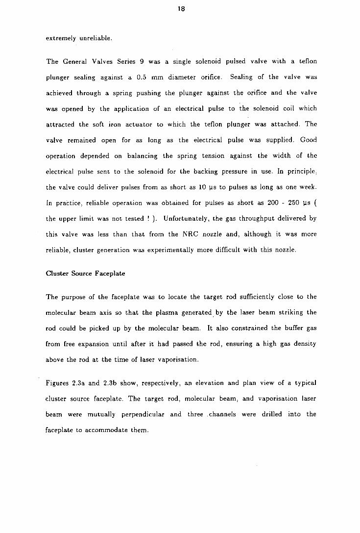
Cluster Source Faceplate
The purpose of the faceplate was to locate the target rod sufficiently close to the
molecular beam axis so that the plasma generated by the laser beam striking the
rod could be picked up by the molecular beam. It also constrained the buffer gas
from free expansion until after it had passed the rod, ensuring a high gas density
above the rod at the time of laser vaporisation.
Figures 2.3a and 2.3b show, respectively, an elevation and plan view of a typical
cluster source faceplate. The target rod, molecular beam, and vaporisation laser
beam were mutually perpendicular and three channels were drilled into the
faceplate to accommodate them.

19
Figure 2.3 : Schematic plan and elevation of the cluster source
faceplate. The scale is approximately 1:2.
Figure 2.3 : Schematic Plan and Elevation of the Cluster Source Faceplate
I $ I I I I I I
Channel
Elevation :i:i::r::::::::::::::_::::J Channel M
I S I I I I I .I
Channel R
I I Plan ::::: ::::

20
With reference to Figure 2.3, the target rods were Located in channel R. The rods
purchased were nominally 5 mm in diameter and were slightly oversized for the
channel. They were turned down until they slip-fitted into the channel and were
slack enough to permit free movement of the rod but tight enough to prevent the
escape of a significant proportion of gas from around the rod.
Channel L allowed passage of the laser beam to the target rod. To reduce the
amount of carrier gas escaping down this channel, it was desired to keep it as
narrow as possible. On the other hand, to relax the severity of the constraints on
the alignment between the vaporisation laser and the target rod, and to reduce the
sensitivity of this alignment to vibration, it was desired to use as wide a channel
as possible. A practical compromise was reached by using a 1 mm diameter
channel with the General Valves molecular beam valve, and a 2 mm diameter
channel with the more powerful NRC molecular beam valve.
Channel M, orthogonal to channels R and L, was located over the valve orifice.
By constraining the gas within the channel, a sufficiently high density of gas was
guaranteed above the rod to quench the plasma generated by laser vaporisation
and to promote clustering. The channel diameter on the valve side of the target
rod matched the valve orifice but after the target rod it increased to
approximately 1 mm.
To further increase the number of collisions occurring, and hence the degree of
clustering, a variable length extender channel, E, was located at the end of channel
M [6]. The diameter of the extender channel was approximately 2 mm and the
length used varied between 8 - 50 mm, depending on the propensity of the target
element to cluster and the cluster size distribution required. For most of the
spectroscopic work on copper dimer, an extender channel length of 33 mm was
found to be satisfactory.
21
Rod Translation Mechanism
Above the faceplate, and mounted on an xy-translator, was a mechanical vacuum
feedthrough which allowed continuous translation and rotation of the rod via a
stepper motor driven screw mechanism ( McLennan 34 HS-106 motor driving a
8-32 UNF rod ). Exposure of fresh target surface to the vaporisation laser greatly
enhanced the stability of cluster generation. This is illustrated in Figure 2.4.
Figure 2.4 shows the spectrum obtained by scanning the trigger to the Q-switch of
the Nd:YAG vaporisation laser with respect to the nozzle trigger, that is
vaporising the rod into different parts of the helium carrier gas pulse. The copper
target rod was rotated at 1 Hz. It is readily seen that the cluster signal generated
increases markedly on every tenth shot of the laser, corresponding the movement of
the target rod. The cause of the drop in intensity if the rod is not moved is
thought to be due to the laser digging a pit in the target rod from which the
plasma has difficulty escaping [7].
2.3.1.2 Molecular Beam Skimmer
Also housed in the M-chamber was a molecular beam skimmer ( Beam Dynamics,
3 mm diameter, 50° included angle ) which for the gas loads used ( 0.53 mbar 1
i ), maintained a pressure differential of approximately 100 between the M- and
A-chambers. The skimmer was mounted off the end wall of the M-chamber to
reduce the disturbance to the molecular beam caused by skimmed gas reflected
back from the wall [8].

22
Figure 2.4 Illustration of the importance of rotating the target rod.
The spectrum was taken by altering the time delay
between triggering the molecular beam valve and
triggering the vaporisation laser Q-switch. The target rod
was rotated at 1 Hz and the sharp peaks in intensity
correspond to movement of the target rod. The
underlying background in the spectrum maps the
dependence of the cluster intensity on the position within
the carrier gas pulse at which vaporisation occurred.
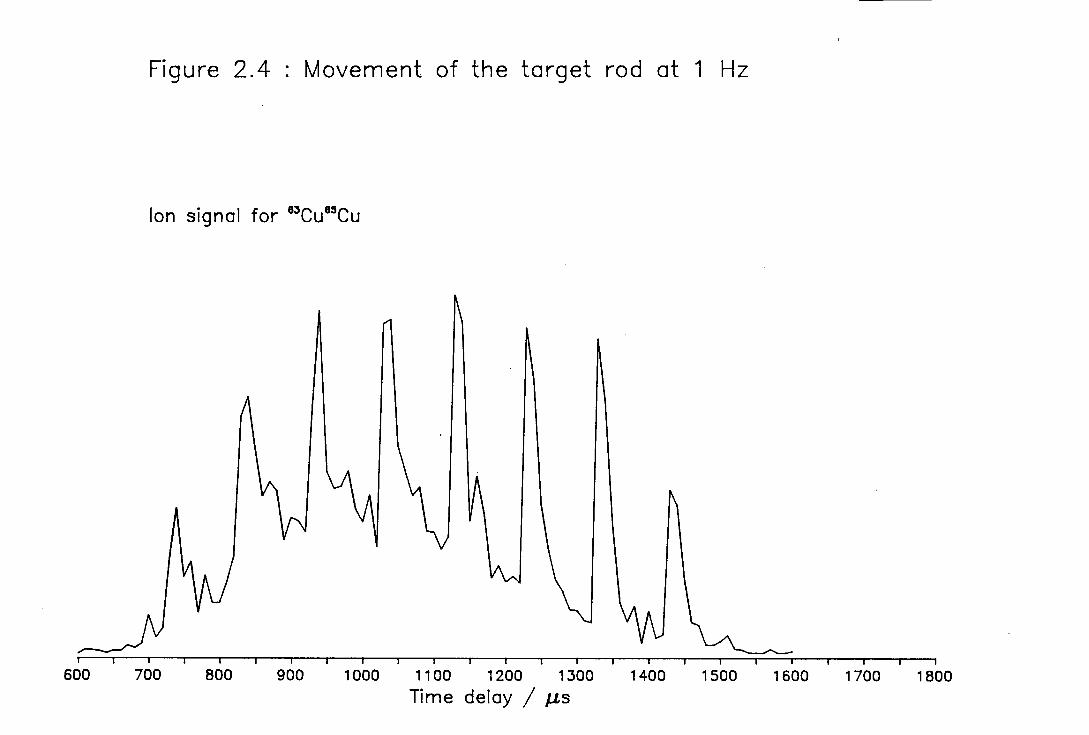
Figure 2.4 : Movement of the target rod at 1 Hz
Ion signal for °3Cu 85Cu
I I I I I I I I I I I I I I
600 700 800 900 1000 1100 1200 1300 1400 1500 1600 1700 1800
Time delay / ,as

23
2.3.2 A-Chamber
The A-chamber was a 17 1 stainless steel cube pumped by an Edwards E09
diffusion pump equipped with a water cooled, full chevron baffle. The unbaffled
pumping speed on hydrogen was quoted as 3300 1 si. The pump foreline was
connected to that of the diffusion pump on the B-chamber and the pumps were
backed by a combination of two rotary pumps ( Edwards E2M18 ) connected in
parallel. This chamber was the part of the apparatus where the clusters were
investigated and for this purpose, it was equipped with two 50 mm diameter
Spectrosil-B windows, one on each side flange, to permit the passage of the counter
propagating interrogation lasers
The drift tube of the TOFMS was mounted on the top flange of the chamber. It
was 1.32 m long with an internal diameter of 40 mm. The MCP detector was
located at the top of the drift tube, separated from the main vacuum system by a
pneumatic gate valve. The lower 66 cm of the drift tube was surrounded by a
liquid nitrogen dewar, the bottom of which penetrated into the vacuum chamber to
a depth of 2.5 inches. The ion extraction optics were supported from the bottom
of the dewar and were surrounded by a copper box which was in good thermal
contact with the dewar and which was completely closed except for four 40 mm
diameter apertures, one on each side, to permit the passage of the molecular beam
and the interrogation laser beams. The cryopumping was effective in reducing the
base pressure within the A-chamber by an order of magnitude.
2.3.2.1 TOFM.S Ion Extraction Optics
A diagram of the ion extraction optics for the TOFMS is shown in Figure 2.5.
The design followed that first described by Wiley and McLaren in 1955 [9] and
consisted of two electric fields defined, in Figure 2.5, by grids R and D, and by D
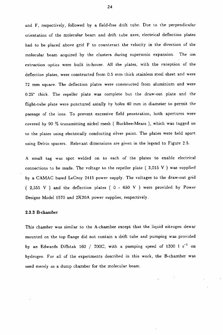
24
and F, respectively, followed by a field-free drift tube. Due to the perpendicular
orientation of the molecular beam and drift tube axes, electrical deflection plates
had to be placed above grid F to counteract the velocity in the direction of the
molecular beam acquired by the clusters during supersonic expansion. The ion
extraction optics were built in-house. All the plates, with the exception of the
deflection plates, were constructed from 0.5 mm thick stainless steel sheet and were
72 mm square. The deflection plates were constructed from aluminium and were
0.25" thick. The repeller plate was complete but the draw-out plate and the
flight-tube plate were punctured axially by holes 40 mm in diameter to permit the
passage of the ions. To prevent excessive field penetration, both apertures were
covered by 90 % transmitting nickel mesh ( Buckbee-Mears ), which was tagged on
to the plates using electrically conducting silver paint. The plates were held apart
using Delrin spacers. Relevant dimensions are given in the legend to Figure 2.5.
A small tag was spot welded on to each of the plates to enable electrical
connections to be made. The voltage to the repeller plate ( 3,015 V ) was supplied
by a CAMAC based LeCroy 2415 power supply. The voltages to the draw-out grid
( 2,555 V ) and the deflection plates ( 0 - 650 V ) were provided by Power
Designs Model 1570 and 2K20A power supplies, respectively.
2.3.3 B-chamber
This chamber was similar to the A-chamber except that the liquid nitrogen dewar
mounted on the top flange did not contain a drift tube and pumping was provided
by an Edwards Diffstak 160 / 700C, with a pumping speed of 1300 1 s_ i on
hydrogen. For all of the experiments described in this work, the B-chamber was
used merely as a dump chamber for the molecular beam.
25
Figure 2.5 : Schematic elevation of the TOFMS ion extraction
optics. The separation between the repeller plate, R,
and the draw-out grid, D, was 32 mm. The separation
between the draw-out grid and the flight-grid, F, was 6
mm. The deflection plates were located 17 mm above the
flight grid, were 19 mm long, and were separated by 38
mm.

Clearence Channel
for Assembly Bolts
Deflection Plates
Flight Grid
Draw—out Grid
> Repeller Plate
Deli,
Spa
Molecul
Beam ,A
Figure 2.5 : Schematic Elevation of the TOFMS Ion Extraction Optics

26
2.4 Laser Systems
The experiments described in this thesis routinely required the use of three laser
systems and always required a minimum of two. The tasks required of the laser
systems were to vaporise the metal target rod and to photoionise the clusters
either resonantly or non-resonantly ( See Section 2.7 ). Non-resonant
photoionisation used only one laser, whereas resonantly-enhanced photoionisation
generally required two lasers. The first was a tunable dye laser and the second, if
required, was a fixed frequency laser. There were four laser systems available in
the laboratory.
2.4.1 HyperYAG HY750
The HY750 was an oscillator-amplifier Nd:YAG laser capable of delivering 800 mJ
per pulse at its fundamental wavelength of 1064 nm. It was designed to operate at
a repetition rate of 10 Hz and it was equipped with crystals for generation of both
the second and third harmonics of the fundamental wavelength ( crystals CD*A
and KD*P ). Specified, and achieved, output energies for the second and third
harmonics were 320 and 170 mJ per pulse, respectively. The three harmonics could
be spatially separated by passing them through a prism harmonic separator
assembly. Both Q-switched and fixed-Q output could be produced.
External control of this laser required two trigger pulses. The first pulse triggered
the flashlamps and the second pulse, delayed by approximately 180 Us from the
first pulse, triggered the Q-switch.
The laser was used to vaporise the target rod and was operated on its second
harmonic at 532 nm. The energy needed for optimum vaporisation of a target rod
depended on the material and was in the range 20 - 50 mJ per pulse. The second
harmonic output was focused on to the target rod with a 1 m focal length lens to

27
a spot roughly 0.5 mm in diameter, yielding power densities on the order of 2 - 5
108 Wcm 2
2.4.2 Quanta-Ray System
The Quanta-Ray laser system consisted of a DCR-2A Nd:YAG laser, a PDL-2 dye
laser and a unit for extending the wavelength range of the dye laser through
frequency doubling and mixing, the WEX-1c.
The DCR-2A had similar specifications to the JK HY750. It was capable of
delivering 800 mJ per pulse at 1064 nm at a repetition rate of 10 Hz. It was also
equipped with crystals for second and third harmonic generation ( KDP ), had a
prism harmonic separator assembly, the PHS-1, for spatially separating the three
harmonics and it could also deliver Q-switched and fixed-Q output.
The PDL-2 dye laser was designed to be pumped by the DCR-2A Nd:YAG laser.
It consisted of an oscillator, an optional, preamplifier and an amplifier which could
be pumped either longitudinally or transversely. The laser was also fitted with an
optional delay line which introduced a 2.5 ns delay between the oscillator pump
pulse and that of the preamplifier and amplifier. The function of the delay line was
to reduce the amount of amplified spontaneous emision ( ASE ) produced and was
used when pumping low gain dyes. Movement of the dye laser grating was
controlled by the IBM PC-AT via a stepper motor driver unit.
The WEX-1c extended the tuning range of the PDL-2 into the ultraviolet, covering
the range 432 - 217 nm. The unit consisted of two modules containing crystals.
The first set of crystals covered the wavelength range 432 - 259 nm by either
mixing the fundamental output of the Nd:YAG laser with the fundamental dye
output or by frequency doubling the dye laser output. The second set of crystals
mixed the frequency doubled dye laser output with the Nd:YAG fundamental
28
wavelength to cover the range 265 - 217 nm.
Correct angle tuning of the crystals as the dye laser wavelength was scanned was
maintained by constant monitoring of the output beam profile by a biphotodiode
linked to servo-motors. Any asymmetry in the profile of the doubled ( mixed )
output beam was detected by the biphotodiode and compensated for by angle
tuning. A prerequisite for reliable operation was the attainment of a good dye laser
beam profile. Unfortunately, this was not trivial when the amplifier was
transversely pumped.
External control of this laser system was quite complex and required a
modification to the laser trigger circuit board. Three trigger pulses were required
to operate the Nd:YAC laser and a further pulse was required if the WEX-1c
module was used. The first pulse to the Nd:YAG laser activated the relays to the
Q-switch high-voltage supply. Approximately 3 ms later, a second pulse triggered
the flashlamps. Between 140 - 210 ps later, a third pulse triggered the Q-switch
releasing the laser output. The actual time delay between the second and third
pulses was adjusted to control the energy of the laser output. A fourth pulse,
simultaneous with the third pulse, was used to refresh the logic circuits of the
photodiodes in the WEX-1c unit, if it was in use.
The Quanta Ray laser system was very versatile and had a variety of uses.
Tunable radiation from the dye laser was used for low resolution spectroscopic
investigations of metal species as, for example, with the Nb and NbO spectra
shown in Figure 2.8. If the second harmonic from the Nd:YAG laser was not
required for pumping the dye laser, then it could be frequency doubled in the
WEX-1c unit to provide an alternative lower energy photon to the ArF photon for
photionisation of the clusters. This was required for the spectroscopic investigation
on species with ionisation potentials below the 6.4 eV energy of the ArF photon.

29
For example, studies on Mo2 were performed using the 266 nm photon for
photoionisation. Finally, the Nd:YAG laser was sometimes used alone as an
alternative to the JK HY750 laser for cluster generation. When used in this mode,
it was operated to produce identical output to the JK laser.
2.4.3 Lumonics TE-861T-4
The TE-861T-4 excimer laser was capable of operating on both chloride and
fluoride gas mixes, but was passivated for the latter. It was always operated on an
argon fluoride mix producing radiation at 193 nm. It was capable of producing
approximately 100 mJ per pulse at 10 Hz with a specified pulse duration of 8 - 10
ris full-width-half-maximum ( FWHM ) [10].
The laser was operated in a "charge-on-demand" mode. In this mode, two trigger
pulses were required. The first pulse activated the circuit for charging the capacitor
banks and had to be delivered approximately 12 ms before the second trigger
pulse. The second pulse triggered the thyratron, generating the laser output.

30
2.4.4 Lambda Physik System
The Lambda Physik system consisted of an EMG 201 MSC excimer laser,
operating on a xenon chloride gas mix lasing at 308 nm, which pumped a
FL3002EC dye laser. The excimer was able to deliver 400 mJ per pulse at 1 Hz.
The excimer energy used at 10 Hz was typically 200 mJ pulse 1 .
The FL3002EC dye laser consisted of an oscillator / preamplifier cuvette followed
by two further stages of amplification. The pump beam was appropriately delayed
between each stage of amplification to reduce ASE. The dye laser could also be
fitted with an intracavity etalon to produce line-narrowed output ( the laser
spectral bandwidth was reduced from 0.4 cm -1 to less than 0.04 cm-1 ) and with a
range of frequency doubling crystals to extend the laser output into the ultraviolet.
Initial alignment and calibration of both the intracavity etalon and the frequency
doubling crystals was required. However, tracking of both the etalon and the
crystal as the dye laser grating was scanned was performed automatically by an
inbuilt microprocessor.
Control of the timing of this laser system required one pulse to trigger the excimer
laser. A further trigger pulse was required by the microprocessor in the dye laser
to initiate movement of the etalon and / or grating.
The Lambda Physik system was used exclusively for spectroscopic investigations of
the metal dimers. Due to the small rotational constants of the transition metal
dimers, all work at rotational resolution had to be performed with this system and
using the intracavity etalon.

31
2.5 Data Acquisition and Control Electronics
The electronic modules were mounted in either a CAMAC crate ( WES ) or in a
NIM bin. The CAi'vtAC modules were interfaced to the computer through a crate
controller ( DSP 6002 ) and an IBM interface card ( DSP PCO04 ). The NIM
modules were not interfaced to the computer and the function of the bin was solely
to provide the necessary power rails.
The modules either controlled the experiment or acquired data. The first group
consisted of two pulse generators ( Kinetic Systems 3655 and LeCroy 4222 ), the
digital-to-analogue converter ( DAC ) unit ( BiRa 5408DAC ) and the stepper
motor controller ( Hytec SMC 1604 ). The second group consisted of the transient
digitiser ( DSP 2001 ) and the ADC unit ( BiRa 5303ADC ).
2.5.1 Control Modules
These units were essentially triggering devices for firing the pulsed molecular beam
valve and the lasers. They were also used to control the movement of the dye laser
grating and the target rod.
2.5.1.1 Kinetic Systems 3655 Pulse Generator
This was an eight channel pulse generator capable of delivering 200 ns wide TTL
pulses with microsecond accuracy. Each channel had its own 16 bit register to
store the set time delay for the pulse with respect to an external trigger pulse.
The module compared a counter with the registers sequentially and for correct
operation, each successive channel had to be programmed with a larger time delay
than the previous one. This meant that two channels could not be triggered
simultaneously and the channels had to be used sequentially with at least 1 l.ts
between adjacent channels.
32
The pulses provided by the device were too narrow to trigger the external systems
and were sent to a NIM based line driver module which lengthened the pulses and
boosted their power.
2.5.1.2 LeCroy 4222 Pulse Generator
This was a four channel pulse generator with sub-nanosecond accuracy which could
be programmed to nanosecond precision. Pulses from this module were used to
trigger devices for which timing was critical. For example, in spectroscopic
experiments ( See Section 2.6.3 ) both lasers were triggered from this device.
Each channel had its own 24 bit register, in which was stored the time delay, and
a 21 bit counter. On receiving a trigger pulse, the counters were loaded with the
21 most significant bits from the registers and were then decremented at 125 MHz
( every 8 ns ). Nanosecond accuracy of the output was obtained by feeding the
three least significant bits from the register into a digital-to-analogue converter
which in turn generated a threshold level for a fast ECL comparator. The channels
were independent and could be used in any order or even simultaneously. The
pulses had sharp rising edges, risetime faster than 1 ns, and suffered from a jitter
of less than 600 Ps for delays as long as 10 ms. The pulses were also too narrow to
trigger the external devices ( 100 ns, 5 V into 50 S2 ) and had to be sent via the
line driver box.
In operation the unit had to be "enabled" to receive a trigger pulse and it had to
be triggered. It was enabled on each "tic" by the computer and triggered from one
of the channels of the KS-3655.
33
2.5.1.3 Line Driver Box
This was a custom-built unit, based around the dual monostable multivibrator
chip, the 74221, and its function was to take the narrow pulses from the pulse
generators, lengthen them and increase their power. The unit was capable of
delivering outputs at either 5 or 15 V. It was housed in the NIM bin.
The unit had twelve input channels and each channel could output either a 10 is
long 5 V pulse or a 50 j.is long 15 V pulse ( switch selectable ). The input was
fed into one of two parallel circuits depending on which output pulse was required.
For 5 V output, the input was directed to a 74221 chip with the appropriate
external resistor and capacitor ( 15 K2 and 0.001 pF, respectively ) to generate a
pulse of width 10 us. This 10 us pulse was sent to a 7417 driver chip to provide
a 10 us wide 5 V pulse powerful enough to drive a 50 9 load. The 50 us wide
pulse ( 3.3 K2 external resistor and 0.023 j.iF capacitor ) was sent to a CMOS
40107 driver to provide a 50 ps wide 15 V pulse capable of driving 50 E2.
2.5.1.4 Hytec SMC 1604 Stepper Motor Controller
This CAMAC based stepper motor controller was capable of controlling up to four
independent stepper motors. It was used to control the stepper motor which
translated and rotated the target rod ( McLennan 34 HS-106 ) and the motor
which stepped the grating on the PDL-2 dye laser.
The SMC 1604 was programmed to deliver single step commands at a speed of 50
steps per second. For control of the movement of the target rod, one such
command was issued on each "tic". Control of the PDL-2 grating was a little more
complicated. As described in Section 2.6.3, spectroscopic experiments involved
running "N" experimental cycles at a particular wavelength and commands had
only to be issued on every "N1h tic". Thus, on each "N 1h tic" the SMC 1604
34
delivered "p" single step commands to the grating, where "p" was the number of
single steps required to move the grating by the desired wavelength step. Scanning
of the PDL-2 grating was under full computer control.
Each channel from the SMC 1604 was linked to one of four McLennan TM162C
driver cards which were mounted in a standard 19" rack unit. The driver cards
were designed to drive up to 2 A per phase ( more than adequate for the motors
in use ) and could produce either full- or half-steps ( 1.8 0 or 0.90 )•
2.5.1.5 BiRa 5408 Digital-to-Analogue Converter ( DAC)
This was an eight channel DAC able to deliver 5 mA at between 0 and 10
V. Each channel had a 12 bit register and hence a resolution of 2.5 mV in the
output voltage. The voltage required less than 4 us to settle. In the present
work, the function of the DAC was merely to provide an external trigger pulse to
the grating on the FL3002EC dye laser. Unlike the PDL-2 laser which was only
provided with a stepper motor on the grating, the FL3002EC had its own
microprocessor for controlling the direction of motion, step-size, and speed of the
stepper motors used to drive the grating and etalon. Since the microprocessor was
also responsible for the synchronised tracking of the intracavity etalon and the
grating, it was felt best to leave the package alone. The only external input
required by the microprocessor was a trigger pulse and this was provided by the
DAC every "N 1h tic". The reason for using the DAC rather than a pulse from one
of the pulse generators was that the pulse generators produced pulses on every
"tic" whereas the spectroscopic experiments (See Section 2.6.3) required a pulse on
only every "N 1h tic". It was technically simpler to program the DAC to do this
than to send a pulse from the pulse generator to a counter which would only
transmit every Nth pulse.

35
2.5.2 Data Acquisition Modules
The data acquisition units converted the analogue voltage outputs of the various
detectors into digital form for subsequent processing by the IBM PC-AT. The
essential unit for any of the experiments was the DSP 2001 transient digitiser.
2.5.2.1 DSP 2001 Transient Digitiser
The DSP 2001 was a 100 MHz transient digitiser with 8 bit resolution and 32 K of
memory. It could digitise signals from 0 to -512 mV and was used to record the
output voltage waveform from the microchannel plate detector.
The DSP 2001 could sample at a selection of frequencies (from 100 MHz down to
1 MHz ) and only a fraction of its memory could be used if desired. The fraction
of memory used could be further divided into "pre-trigger" and "post-trigger"
samples, as described below.
The mode of operation was straightforward. The module received a "start-scanning"
signal from the computer initiating digitisation at the selected frequency. When all
of the fraction of memory in use had been written to, the digitiser started to
overwrite the memory with new samples. Overwriting started with the oldest
datum and continued until a stop trigger was received. Experimentally, this stop
pulse was usually synchronised to the trigger pulse to the laser used to photoionise
the clusters. On receipt of the stop pulse, the digitiser continued to sample until it
had overwritten the fraction of memory selected as post-trigger samples (
experimentally this was mostly 1 ). The digitiser memory thus contained the
pre-trigger fraction of samples taken before the stop-pulse, providing a baseline, if
required, and the post-trigger fraction taken afterwards.
After a short settling time ( 1.2 ps ), the data from the memory was available for
36
transfer across to the computer. Transfer occurred via the direct-memory access (
DMA ) chip. Due to the limiting speed of data transmission through the CAMAC
data bus, all the experiments used only 2 K of memory from the transient
digitiser.
To circumvent the limited time range that could be stored in 2 K of data sampled
at 100 MHz ( a range of 20 Ps ), two approaches were adopted. Firstly, if a total
mass spectrum was required and it extended over a greater range than 20 us, the
simple solution was to reduce the sampling frequency to 50, 20 or, occasionally, 10
MHz. This degraded the observed time resolution of the signal. However, if it was
desired to retain the highest resolution for a cluster with a flight time longer than
20 us, then the stop pulse was delayed with respect to the trigger to the laser used
to photoionise the clusters. The stop pulse was always provided by one of the
channels from the LeCroy 4222 for accuracy.
2.5.2.2 Pacific Instruments Video Amplifier 2A50
The signal to the digitiser did not come directly from the microchannel plate
detector but via a direct-coupled non-inverting amplifier with a gain of
approximately 100. Both input and output impedances were 50 Q, ideally suited
for linking the 50 S2 anode of the microchannel plate detector to the 50 11 input of
the transient digitiser. The amplifier operated at a constant gain to about 150
MHz. The amplifier was mounted directly above the microchannel detector and
hence the signal was amplified before picking up any noise along the cable linking
the detector to the digitiser.
37
2.5.2.3 Mlicrochannel Plate Detector ( R.M. Jordan )
Although not an electronic module, the microchannel plate detector was so
intimately involved with the electronics of data acquisition that it is now
discussed. The microchannel plate ( MCP ) detector was of a dual chevron design
[11] using two Galileo MCP-18B plates, which had an active diameter of 18 mm.
Each plate had a gain of 1000 when biased by 1 kV, resulting in a total gain of
106 .
There are two ways of coupling a MCP detector to observe ions [ll]. Firstly, the
front plate can be grounded and the anode held at a high positive potential. This
method does not interfere with the ion flight times since the earthed front plate
defines the end of the field-free drift tube. The major disadvantage of this coupling
is that signal from the anode must be capacitively coupled to remove the large
positive bias. The other way of coupling the MCP involves applying a large
negative potential to the front plate and holding the anode at earth potential. To
prevent the potential of the front plate from penetrating into the supposedly
field-free drift tube and perturbing the flight times, an earthed grid must be placed
in front of the plate with a consequent reduction in ion transmission. The presence
of the large negative potential on the front plate also precludes the detection of
negative ions. However, this form of coupling means that the anode can be directly
linked to other equipment ( i.e. amplifier and digitiser ) and it has an unexpected
bonus for the detection of positive ions in that the presence of approximately -2
kV on the front plate accelerates the positive ions which results in a greater gain
at the MCP ( the gain increases with ion impact energy ) [12].
The R.M. Jordan MCP used the second coupling scheme and had an 82 %
transmitting grounded grid in front of the first microchannel plate. The grounded
anode was impedance matched for 50 fl.
38
2.5.2.4 BiRa 5303 ADC
The ADC was used to convert signals from monitor photodiodes for storage in the
computer.
The 5303 ADC has 16 bipolar channels each with 12 bit resolution. All the
channels may be accessed sequentially or randomly, or one channel may be
repetitively sampled. This latter mode of operation was used in the present work.
The unit was set-up to convert voltages between 0 and +5 V. In operation, the
signal from a photodiode monitoring, for example, etalon fringes was sent to a
gated integrator ( Stanford Research Systems SR 250 ). The averaged output
from the gated integrator was then digitised by the ADC.
As mentioned previously, all the experiments performed on the apparatus used the
experimental cycle described in Section 2.2. Three different types of experiment
were performed and they are described in the following section.

39
2.6 Modes of Operation
2.6.1 Acquisition of Mass Spectra
This was the most basic experiment and was an essential preliminary to more
detailed experiments. The mass spectra were used to analyse the cluster species
present in the molecular beam, to aid optimisation of the generation of the desired
cluster range and to measure the relative intensity and stability of cluster
generation on a day-to-day basis. Only when cluster intensity and shot-to-shot
stability were satisfactory was it worthwhile to attempt more complex
experiments.
In these experiments, referred to as "mass scans", all of the clusters of various sizes
were photoionised in the extraction region of the TOFMS, usually with the 6.4 eV
photon from the ArF excimer laser. The experimental cycle was repeated "N" times
and at the end of each cycle, 2 K channels of digitiser memory were transferred to
the computer to form a cumulative sum of photoion signal intensity against
transient digitiser channel number. The value of "N" was programmable and was
chosen to give an acceptable signal-to-noise ratio. From the known scan rate of
the transient digitiser, the channel number could be related to the flight time of
the ions and the mass spectrum was displayed as photoion intensity against time.
Figure 2.6 illustrates the generality of the laser vaporisation technique to produce
clusters of a variety of materials with a wide range of boiling points. Clusters
could be readily generated from copper ( boiling point 2868 K ) up to molybdenum
( boiling point 5800 K ).
40
Figure 2.6 : Mass spectra for nickel, iron and molybdenum clusters.
All three spectra were acquired using the second
harmonic from the Nd:YAG laser to generate the clusters
and 193 nm ArF excimer laser output for
photoionisation.

Figure 2.6 : Mass Scans
F; clusters
Ni clusters
Mo. clusters
0 2 4 6 8 10 12 14 16 18 20 22 24
Number of atoms in cluster

41
2.6.2 Acquisition of Timing Data
These experiments are referred to as "time scans". They depended for their success
on the ability to monitor selectively the signal of interest as a function of the time
delay between two events, such as the time delay between triggering the
vaporisation laser and triggering the photoionisation laser. Selectivity was achieved
by monitoring only those channels on the transient digitiser which held the mass
resolved signal of the species under study. These channels are referred to as "mass
channels".
The computer was programmed with a start-time, a stop-time and a step size for
scanning. The programmed time delay in the selected channel of the pulse
generator, the scanned channel, was set to the start-time. An experimental cycle
was then run and the data from the mass channels was stored in the computer.
The computer then incremented the time in the scanned channel by the step size
and another experimental cycle was run. The data from the digitiser mass channels
was transferred to the next array element in the computer. The time-increment /
experimental cycle / store-in-next-element sequence was continued until the time in
the scanned channel had reached the stop-time. At this point, the programmed
time delay in the scanned channel was reset to the start-time and the whole cycle
was repeated, storing the averaged signal for successive timings in successive array
elements. Repetition of this cycle enabled an averaged spectrum of photoion
intensity against trigger delay time to be acquired for an arbitrary number of
samples.
Any channel of the pulse generators could be scanned and optimisation of the
production and detection of the clusters required scanning of the triggers to the
vaporisation and photoionisation lasers, respectively. It was also possible to
measure the lifetimes of electronically excited states of selected cluster species in
42
this mode by time resolved resonant two-photon ionisation methods ( See Section
4.4.5 ).
An example of the type of experiment that can be performed in this mode is
illustrated in Figure 2.7. Figures 2.7a and 2.7b illustrate the importance of setting
the correct timing between triggering the laser which vaporised the target rod and
the laser which ionised the clusters. Figure 2.7a was obtained by monitoring the
ion signal corresponding to the mass of helium as the trigger to the ArF excimer
laser, used to produce the ions in the TOFMS, was scanned. By scanning the
trigger to this laser, the helium pulse profile was mapped out. It can be seen that
the pulse width is approximately 1 ms.
There is a significant dip in the helium pulse intensity at t = 1860 us. This
corresponds to that part of the gas pulse which was directly above the target rod
at the time of vaporisation. The drop in intensity was caused by the laser
generated plasma displacing the helium from the molecular beam [13].
Figure 2.7b was obtained by scanning the ionisation laser as before, but in this
case the ion signal corresponds to 63 Cu. The clusters were present in only the
small plug of the helium pulse which was disturbed in Figure 2.7a and not
throughout the gas pulse.
43
Figure 2.7 : Illustration of the timing constraints on the detection of
clusters. The figures illustrate that the signal due to
63 Cu is present in only a small part of the helium gas
pulse and not throughout it. The dip in the helium pulse
is due to the cluster plume displacing helium. Larger
clusters behaved similarly to the atom.

Figure 2.7 : Example of a "Time Scan"
Helium Pulse Profile
"Cu Profile
1200 1400 1600 1800 2000 2200 2400 2600
Time Delay / ps

44
2.6.3 Acquisition of Spectroscopic Data
These experiments were used to obtain spectroscopic data on one or more clusters
and are referred to as "frequency scans". Pre-selected mass channels were again
required in order to study mass-selected signal. The experiments were performed
via a resonant photoionisation scheme. The technique of resonant photoionisation
is discussed in the following section.
The experimental cycle was repeated "N" times at a particular dye laser
wavelength and the signal from the mass channels was summed, averaged and
stored. The computer then triggered the stepper motor driving the grating of the
dye laser, altering its wavelength. The experimental cycle was repeated another "N"
times and the averaged ion signal from the mass channels was stored in the
computer. This process of stepping the laser grating, performing "N" experimental
cycles and storing the averaged signal was continued until a programmable stop
wavelength was reached, yielding an array of averaged signal intensities. The
approximate wavelength at which a particular element was acquired was contained
in its position within the array.
The computer was capable of handling up to ten sets of independent mass channels
and hence it was possible to scan the laser wavelength whilst monitoring several
different clusters together with calibration fringes provided by a monitor etalon.
Figure 2.8 illustrates some results of spectroscopic data acquired in this manner.
The spectrum of NbO was generated from a rod of niobium without addition of
oxygen to the carrier gas and was recorded simultaneously with the Nb atomic
spectrum. The spectrum did not disappear after the surface layer of the rod had
been removed by the vaporisation laser, suggesting that oxygen had penetrated
quite deeply into the rod.

45
Figure 2.8 : Illustration of spectroscopic experiments. The Nb atom
spectrum exhibits many lines from the z 6 D - a 6 1), z 6 F
4- a 6 1), and the z 4 D - a 4 F transitions. The NbO
spectrum exhibits several bands from the G-X system (
~ 4E )
transition, specifically the (
0-1 ), (
1-2 ), (
2-3),(3-4),(4-5),(0-2),(1-3),(2-4),(3-5)
bands.

Figure 2.8 : Spectroscopic Scans
(a) NbO
(b) Nb atom
486 491 496 501 506 511 516 521 526 531 536 541 Wavelength / nm

46
2.7 Photoionisation Techniques
The technique used to record the electronic spectra presented in this thesis was
resonant two-photon ionisation. In this technique, ionisation occurs stepwise via an
intermediate, resonant state. By monitoring the overall photoion yield as a
function of excitation wavelength, a spectrum of the transition to the intermediate
state can be obtained. This is illustrated by considering the three mechanisms by
which a molecule can be ionised by either a single or by two photons. These are
shown diagramatically in Figure 2.9.
2.7.1 Single Photon lonisation
This process can occur when the energy of the incident photon is greater than the
first molecular ionisation potential. It is a relatively facile process since the
density of molecular states near the ionisation potential is usually high and
selection rules are readily met. The latter factor is because the photoejected
electron is able to carry away energy and angular momentum permitting strongly
allowed transitions with good Franck-Condon factors [14]. The transition rate for
absorption can be described by the equation [15],
W =a 1 1
where,
W = transition rate in molecules per second
a 1 = single-photon absorption cross-section in cm 2
I = radiation flux in photon cm -2 s_ 1
Typically, single-photon absorption cross-sections are in the region of 10_16 to
10 22 cm2 [15].
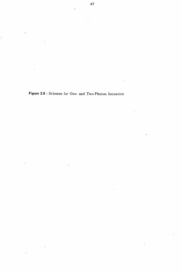
o.
Cl)
(D
tI) 1 0
(D 9 0
0
0
U)
C.
0
491, -4
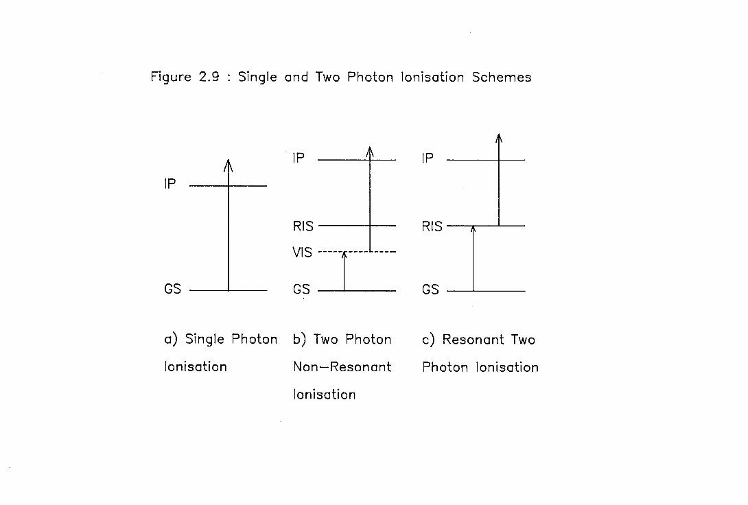
Figure 2.9 Single and Two Photon lonisation Schemes
ts
Cs
is
RI S
V'S
Cs
RIS
Cs
a) Single Photon b) Two Photon c) Resonant Two
lonisation Non—Resonant
Photon lonisation
lonisation

48
2.7.2 Non-Resonant Two-Photon lonisation
When the photon energy is less than the molecular ionisation potential, but greater
than half the value, and is also of such an energy that there are no excited states
present at the correct energy to permit one photon absorption, then ionisation can
be achieved by non-resonant two-photon ionisation. The transition rate is strongly
dependent on the radiation flux and the rate of ionisation can be described by the
equation [15],
W =a21
where,
a2 = two-photon absorption cross-section in cm4 s
The other terms are as described previously.
is The magnitude of a2 A very small compared to a 1 , typically being of the order of
10-50 crn4s [16]. This process becomes more probable as the radiation flux is
increased and most of the mass spectra described in this work were obtained using
non-resonant two-photon ionisation with an argon fluoride excimer laser. The
two-photon cross-section can be calculated from perturbation theory and - its
magnitude depends inversely on the sum of the differences between the energies of
real states, E, and the energy of the photon [17]. The closer in energy the
contributing real states E 1 , are to the energy of the photon, then the greater is
their contribution to the two-photon cross-section. It is therefore reasonable to
suppose that when there is a real resonant state, then a rapid rise in the value of
the absorption coefficient occurs. Although perturbation theory is not applicable
when the first photon is resonant with a state, the implications are and the ion
49
signal produced via resonant two-photon ionisation can be orders of magnitude
greater than the signal from non-resonant ionisation.
2.7.3 Resonant Two-Photon Ionisation
As described above, this technique applies when the first photon is in resonance
with a molecular transition and is able to excite the molecule to a real resonant
state. Transitions via real states are much stronger than non-resonant transitions,
even if the real state is dissociative. The probability that a second photon can
interact with the molecule and produce ionisation is greatly enhanced by the
presence of a state resonant with the photon energy. The equation describing the
rate of the transition can be written as [15],
where,
GA = two-photon resonant cross-section in cm 4 s
n = a number in the range 1 - 2.
It is the enhancement in ionisation observed when the first photon is resonant with
a real intermediate state that presents the possibility of studying the intermediate
state. Drawing on the terminology prevalent in optical-optical double resonance
work [181, the first laser which promotes the transition between the ground state
and the resonant state, will be referred to as the "pump" laser. The second laser
responsible for ionising the molecule in the resonant state, will be referred to as
the "probe" laser.
By scanning the wavelength of the pump laser and collecting the ion signal, it is

50
seen that the magnitude of the ion signal rises and falls dramatically as the pump
beam moves into and out of resonance. A spectrum can be generated for the
intermediate state. A distortion of the spectrum from the absorption spectrum
may be produced by the probe laser also moving into and out of resonance as the
wavelength of the pump laser is changed. However, distortions are likely to be
small if the density of states accessed by the probe laser is high, if its bandwidth is
large compared to the range in wavelength scanned with the pump laser and if the
energy of the second photon is sufficiently high to take the molecule well above its
ionisation threshold. These criteria were satisfied in the rotationally resolved
spectra reported in this work since the pump laser was scanned over a narrow
range of approximately 10 cm 1 , the probe laser was a broadband excimer laser
and it excited the molecules to at least 1 eV above the ionisation threshold.
The detail attainable about the resonant intermediate state depends on the
spectral resolution of the probe laser and the fundamental complication and
congestion of the spectrum. Successful elucidation of the electronic spectra of the
low-lying electronic states of copper dimer was only possible through the use of a
high resolution dye laser as the pump laser and through mass-selective detection of
the ion signal thereby removing isotopic congestion.

51
REFERENCES
T.G. Dietz, M.A. Duncan, and R.E. Smalley, J. Chem. Phys., 74, 6511 (1981)
A.M. Butler, Ph.D. Thesis, Edinburgh University (1989)
J.B. Hopkins, P.R.R. Langridge-Smith, M.D. Morse, and R.E. Smalley, J. Chem. Phys., 78, 1627 (1983)
A.G. Baizers, Document BG 800 105BE Liechenstein (1984)
T.E. Adams, B.H. Rockney, R.J.S. Morrison, and E.R. Grant, Rev. Sci. Instrum., 52, 1469 (1981)
E.A. Rohlfing, D.M. Cox, and A. Kaldor, Chem. Phys. Lett., 99, 161 (1983)
D.E. Powers, S.G. Hansen, M.E. Geusic, A.C. Puiu, J.B. Hopkins, T.G. Dietz, M.A. Duncan, P.R.R. Langridge-Smith, and R.E. Smalley, J. Phys. Chem., 86, 2556 (1982)
P.J. Brucat, L.S. Zheng, C.L. Pettiette, S. Yang, and R.E. Smalley, J. Chem. Phys., 84, 3078 (1986)
W.C. Wiley and I.H. McLaren, Rev. Sci. Instrum., 26, 1150 (1955)
Lumonics Inc. Series TE-860-4 Excimer Laser Instruction Manual, Kanata, Ontario, Canada (1984)
J.L. Wiza, Nuci. Instr. Methods, 162, 587 (1979)
J.L. Heilsing, L. Karrison, H.O. Andren, 'and H. Norden, J. Phys. E: Sci. Instrum. 18, 920 (1985)
P.R .R. Langridge-Smith (Private Communication)
J.M. Hollas, High Resolution Spectroscopy, p444, Butterworths, London (1982)
D.H. Parker, Ultrasensitive Laser Spectroscopy Ed. D.S. Kliger, Academic Press, New York (1983)
P.M. Johnson and C.E. Otis, Ann. Rev. Phys. Chem. 31, 139 (1981)
M. Goppert-Mayer, Ann. Phys. Leipzig, 9, 273 (1931)
D.L. Andrews, Lasers in Chemistry, p95 Springer-Verlag, Heidelberg (1986)

CHAPTER THREE
Time-of-Flight Mass Spectrometry
52
3.1 Introduction
As discussed in Chapter II, cluster generation by laser vaporisation of a solid
substrate into a molecular beam produces a soup of cluster sizes. The distribution
of cluster sizes could be crudely controlled by changing either the backing pressure
behind the nozzle or the length of extender piece in front of it. It was not possible,
however, to "fine tune" the cluster distribution to predominantly contain species of
just one size. Mass resolution of the ion signal was essential for the correct
attribution of signal to carrier in the resonant two-photon ionisation studies
reported in this thesis. This is readily illustrated in Figure 3.1.
Figures 3.1 a-c show the rotationally resolved spectrum of the 0-0 band of the C-X
system of Cu2 for all three isotopic combinations and Figure 3.1 d shows the
composite spectrum that would have been obtained in the absence of mass
resolution.
The nature of the experiments imposed severe constraints upon the type of mass
spectrometer suitable. The experiments were performed in a pulsed mode with a
duty factor less than 10. The repetition rate was limited to 10 Hz by a variety
of factors, such as the ability of the pumps to handle the high gas loads required
for cluster generation, the design of the lasers and the speed of the data acquisition
system. The low duty factor made it imperative to extract as much data as
possible on each experimental cycle, which meant, in practice, that the mass
spectrometer had to produce a complete mass spectrum on each cycle. The pulsed
nature and the need for a complete mass spectrum per cycle were matched best by
a TOFMS [1]. Precluding double-sector- and Fourier Transform mass
spectrometers on the grounds of cost alone, the only alternative to the use of a
TOFMS is the quadrupole mass filter. However, as the name implies, quadrupole
mass filters selectively transmit ions of a particular charge-to-mass ratio whilst

53
discarding all the others. Even the fastest scanning quadrupole ( approximately 6
amu per ms ) would have been unable to acquire a complete mass spectrum on
each and every cycle and its use would have resulted in an extremely inefficient
collection of signal. The unsuitability of a quadrupole mass filter is not surprising
since the instrument is designed to operate with a continuous source of ions rather
than with a pulsed source. A TOFMS, on the other hand, requires a reference
time, which is provided naturally in these experiments by the pulsed nature of the
ionisation source. This results in an ideal match between the requirements of the
experiment and the requirements of the mass spectrometer.

54
Figure 3.1 : Importance of mass resolution in simplifying spectral
structure of the 0-0 band of the C-X system of Cu 2 .
Figures 3.1 a-c show the rotationally resolved spectra for
63 Cu2 , 63 Cu65 Cu and 65 Cu2 respectively. Figures 3.1d
was generated by combining the three spectra.

Figure 3.1 : Importance of Mass Resolution in
Simplifying Spectral Structure
'Cu,
'CuCu
(c)'Cu, ( x 5 )
(d) Spectrum without
mass resolution
-4.5 -3.5 -2.5 -1.5 -0.5 0.5 1.5 2.5
Relative Frequency / cm-'
55
3.2 Principles of Operation of a TOFMS
Mass separation is achieved by the instantaneous generation of ions within the
electric fields of the ion extraction optics, their acceleration and subsequent flight
through a field-free region before their arrival at a detector. The ions traverse the
field-free region, known as the drift tube, D, with velocities dependent on their
charge-to-mass ratios ( since all ions of the same charge extract the same energy
from the electric fields in the acceleration region of the spectrometer ). Heavier
ions arrive at the detector after the faster, lighter ions. By recording the detector
output as a function of time, a mass spectrum is obtained.
The flight time of an ion is related to its mass through the equation [21,
tm = K m 112 -(1)
where,
tm = flight time of the ion of mass m.
K = proportionality constant.
The magnitude of K is determined by the parameters used in the physical design
of the TOFMS and the initial energy of the ions. For example, the strengths of the
electric fields used in the ion extraction optics and the size of the optics contribute
to the value of K.
The two most important properties of a mass spectrometer are its resolution and
its transmission. Unfortunately, a high resolution often results from a
spectrometer being highly selective on the ions transmitted to the detector. Since
TOF instruments place no filter on the transmitted ions, the resolution is generally

56
quite low and traditionally, this has been one of the major factors against their
use. In the design of a TOFMS suitable for a particular application, several factors
affecting the resolution and transmission of the instrument must be considered.
3.3 Resolution of a TOFMS
The limiting resolution can be defined as the mass at which the widths of the ion
packets are just smaller than the difference between the flight times of ions
separated in mass by 1 amu. With reference to equation (1), the difference in flight
times is given by the formula,
At = tm+ltm
= K ( (m+1) 112 - m 112 ) -(2)
Clearly as the mass increases, the separation between flight times of adjacent
species becomes smaller and even if the peak width were independent of the ion
mass, a point would be reached when the TOFMS could no longer resolve adjacent
mass peaks. The point at which resolution is lost depends on the widths of the ion
packets and the value of K. A narrow packet width and a large value of K
increase the maximum mass resolvable by the spectrometer.
The five factors affecting the resolution of a TOFMS by broadening the ion packet
width are now considered.
57
Figure 3.2 : Schematic Diagram of the TOFMS Ion Extraction
Optics.
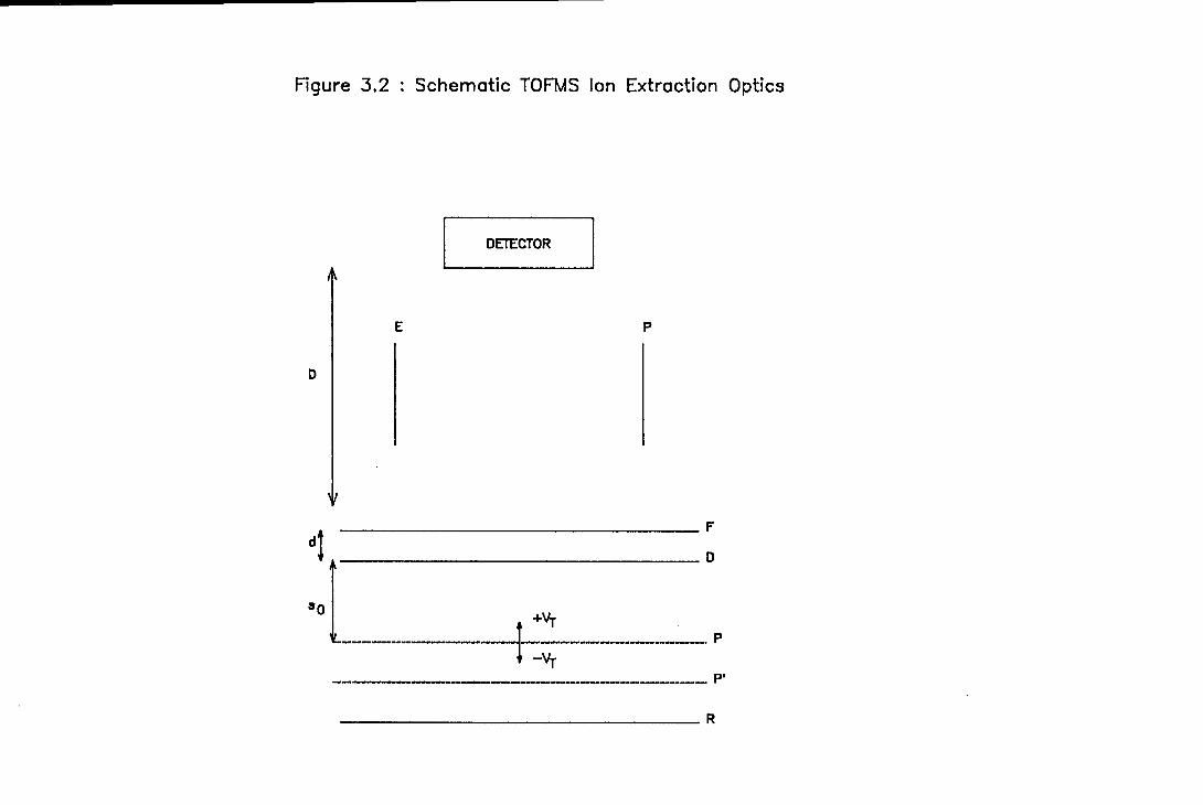
Figure 3.2 : Schematic TOFMS Ion Extraction Optics
DETECTOR 1
t +Vr
-VT P.
58
3.3.1 Factors Affecting the Mass Spectral Peak Widths in a TOFMS
3.3.1.1 The Potential at which the ion is formed - "Spatial Resolution"
With reference to Figure 3.2, all ions formed in plane P, perpendicular to the
electric field and parallel to the detector will extract the same kinetic energy from
the field. In the absence of all other peak broadening effects, all ions of the same
charge-to-mass ratio will arrive at the detector simultaneously and the ion packet
will be infinitely narrow. However, ions of the same charge-to-mass ratio formed
in a different plane, for example P', or from different points of the same plane P,
in the case of non-ideal fields, will extract varying amounts of energy from the
field depending on their position. The infinitely narrow ion packet at the detector
will acquire a finite width. Since this peak broadening is caused by the formation
of ions at positions of different potential in the extraction region, the limiting
resolution achievable with a particular mass spectrometer and caused by this effect
is known as the "spatial resolution" of the instrument.
3.3.1.2 The Initial Energy of the Ions - "Energy Resolution"
The resolution of a TOFMS is affected by the component of velocity parallel to
the spectrometer axis, the components in the plane perpendicular to the axis affect
the transmission of the instrument. The simplest way to consider the effect of the
initial ion energy is to consider the case of two ions in plane P subjected to ideal
electric fields. If the ions had no velocity component along the axis of the
TOFMS, they would arrive at the detector simultaneously. If, however, one ion
had a velocity component of +VT along the TOFMS axis ( positive towards the
detector ) whilst the other had a component -v T) they would not arrive
simultaneously. The second ion would lag the first ion by a "turn-around" time
which depends on the ion energy and the strength of the electric field. The
59
"turn-around" time is the time taken for the ion with velocity to decelerate and
to return to its initial position with velocity ±vT. The ion would then follow a
trajectory identical to that of the ion which originally had velocity +VT and would
arrive at the detector delayed by the "turn-around" time. A distribution of initial
energies will yield ion packets of finite width. By analogy to the case of spatial
resolution, this effect is known as "energy resolution".
3.3.1.3 The Lonisation Source - "Timing Resolution"
In a simple TOFMS, the temporal width of the ion packet reaching the detector
cannot be less than the temporal width of the ionisation source. Pulsed lasers
readily produce light pulses shorter than 20 ns making them ideal ionisation
sources for TOF instruments. Before the advent of pulsed lasers, timing resolution
of the ion source was a major contributor to the temporal width of the ion packet
and hence a fundamental limit on the resolution achievable with a TOFMS. For
mass spectrometers which operate in a continuous mode, the precise time of
ionisation is not so critical and electron impact ionisation is suitable. For
time-of-flight mass spectrometry, the temporal characteristics of the ionisatiori
source are vitally important to the resolution.
3.3.1.4 The Detector Response
The detector response includes the speed at which the ion signal can be
transformed into an electrical signal and the speed at which the electrical signal
can be processed. Both factors affect the observable mass resolution of a TOFMS
without affecting its intrinsic resolution. If one considers a mass spectrometer
capable of producing two adjacent mass peaks each of 5 ns temporal width and
separated in arrival time at the detector by 20 ns then the mass spectrometer can
be described as physically resolving the peaks. If the detector greatly broadens the
peaks or if the instrument which stores the time dependent output of the detector
samples at, for example, only 10 MHz, resolved peaks will not be observed even
though they were produced in the mass spectrometer. Hence, the TOFMS has to
be designed to match the broadening effects of the detector and the sampling
frequency of the instrument which monitors the detector output. No matter how
effective the mass spectrometer is in maintaining narrow peak widths, if the
detector response is not matched to the packet widths, no resolution, and possibly
no spectrum, will be obtained.
3.3.1.5 Space-Charge Effects
The repulsion between ions of like charges travelling as a packet can serve to
spread out the packet. The required ion density for such effects to become
important has been suggested to be in the range 10 6 - 108 cm-3 [3 11 4 1. It has been
calculated that the number of ions generated experimentally was in the region of
102 - 10 ( see Section 4.3.5 ) per pulse and the ions were produced in a volume of
0.05 cm3 . The ion density was therefore in the range 2 x 10 3 - 2 x 105 cm-3 and
the effects of space-charge repulsion are believed to be small. The effects of
space-charge repulsion on the resolution are therefore not considered in any greater
detail.
The forementioned factors affecting the resolution of a TOFMS have been treated
in various ways to minimise their effect. The problems of timing resolution and
detector response can be tackled in two ways. The first and simplest is to increase
the flight time of the ions as this increases the temporal separation of adjacent
mass packets. Since the temporal width of the ionisation source is constant it
becomes relatively less important as the ion flight time is increased. Similarly, the
greater difference in flight times between adjacent mass peaks places lower
demands on the detector response. The second way to reduce the problems of

61
timing resolution and detector response is to use shorter ionisation sources, such as
picosecond pulsed lasers, and faster detectors [5], [6]. Ultimately, this path offers
better performance since increased flight times result in lower transmission as the
velocity components in the plane perpendicular to the TOFMS axis become more
significant.
Energy resolution was improved by Mamyrin et a! [] in 1973. They used a
shaped TOFMS, known as a "reflectron", with the ion source at the end of one
limb of the "V" and the detector at the end of the other limb. At the apex of the
"V", they placed an electric field to reflect ions accelerated from the ion source to
the detector. Energy resolution can be improved because ions with a greater
velocity penetrate deeper into the reflecting field than the slower ions and spend
longer in this region. Conditions can be chosen such that ions are temporally
focused at the detector. This type of TOFMS was not used in the present work
and will not be discussed any further.
The problem of spatial resolution was treated in 1955 by Wiley and McLaren [8]
They developed a two-field ion acceleration region which enabled first-order
focusing of the ions such that ions from different positions in the ionisation region
would arrive at a detector placed a particular distance downstream at
approximately the same time. The TOFMS used in this work follows the design
described by Wiley and McLaren and the following treatment of spatial resolution
is after them.
3.3.2 Wiley and McLaren Condition for Optimum Spatial Resolution
Wiley and McLaren tackled the problem of spatial resolution by using a two-field
acceleration region as illustrated in Figure 3.2
Consider ions of initial energy U0 formed in a plane P which is a distance s 0 from
62
plate D. All electric fields are considered to be ideal.
The equations describing the motion of a particle of charge q and mass m are [8),
T = (2m)' 12 / qE ( ( U0 + qs0E5 )1/2 ± uj2 ) -(3)
Td = (2m) 112 / qE ( ( U1"2 - ( U0 + qs0E )1/2 ) (4)
TD = (2m) 112 ( D / 2U 112 ) -(5)
where,
U = qs 0E + qdE + U0 -(6)
and TS 7 Td, and TD are the flight times for the ion to traverse the distances from
plane P to plate D, from plate D to plate F, and from plate F to the detector,
respectively.
Defining k0 , as
k0 = ( sgE + dE d ) / soE
The total ion flight time, TT, from the point of ionisation is given by,
TT = (2m) 2 ( U 1 "2 / qE + (1 / qE - 1 / qE
x ( U0 + qs0E )1/2 + 0 / 2U 2 ± U 1 1 qE
For small displacements, As, about plane P, TT can be approximated by a Taylor
expansion,

63
TT ( WAS ) = TT(so) + 1 / n! ( 3T(s0) / as") ( s) -(9)
Wiley and McLaren obtained an expression which forced 3T / as = 0 and hence
yielded first-order spatial focusing of the ions. Equating,
aTT / as = 1 / 2 (2m) 1 '2 ( U_ 1/2 E / Ed + 0 - E 5 / Ed )
x ( U0 + qs0E5 )_1/2 - 1 / 2 qE 5 DU 3"2 ) -(10)
to zero, yields the following expression for the required length of drift tube, D,
D= 2U 312 /qE(E 5 /EU 112 +(1-E 5 /E)(U 0 +qs 0 E 5 ) 112 )-(11)
Equation (11) is a function of the initial ion energy U 0 . The sensitivity of the
required drift tube D to the initial energy U 0 can be estimated by expanding D as
a Taylor Series in U 01
Neglecting all terms greater than the first-order term,
D(U0+AU0)-D(U0) = (2/qE+2/qE 5 (1-E 5 /E)
X ( U1"2 ( U0 + qs 0 E 5 - 1 / 2 qdE ) / ( U0 + qs0E5 )312 ) AU0 -(12)
At U0 = 0 and substituting in parameter k 0 from equation (7) into (12) and (11)
respectively,
D(AU 0)-D(0)= (2IqE+ 1/qE 5 (1 - E s /Ed)
x(k/ 2(3-k0 ))) AU0 (13)
0 = 2 S0 k"2( 1 - 1 / ( k0 + k(2) d / s0 ) -(14)
Equation (14) defines the first-order focus of the ions which is independent of mass
and dependent only on the electric fields applied in the two regions of the
64
extraction optics, the position of ionisation within the first electric field and the
initial ion kinetic energy. Equation (13) shows the sensitivity of the focal position
defined in (14) to initial ion energy; it does not define a focusing condition for a
spread in initial energy. To obtain the latter, equation (8) must be expressed as a
Taylor Series in U0 and ST,. / 3U0 equated to 0.
3TT / 3UO = 1 / 2 (2m) 112 ( U_ 1/ / qE + (1 / qE 5 - 1 / qE
x ( U0 + qs0E )_1/2 - 1 / 2 DU -3/2 ± U 1 "2 / qE ) -(15)
At 3TT / au0 = 0,
D = 2U 312 ( U" / qE + (1 / qE 5 - 1 / qE
x ( U0 + qs0E5 )_1/2 ± U 1 "2 / qE 5 ) -(16)
Due to the last term, ± U1"2 / qE5 , this cannot be an exact focal position.
When U0 = 0, equation (16) simplifies to equation (14) and hence the first-order
focus for ions with initially no kinetic energy and with small spatial displacements
around s0 is the same as the focal position for ions formed at s 0 with small initial
kinetic energies. It is not possible to improve on the Wiley and McLaren first-order
focus with simple two-field ion acceleration optics [9].
The focal position has a small dependence on U 0 as shown in equation (13). For
systems used in this work, the ions have small variations of approximately 10-3 eV
about the average energy (that is, kinetic energy due to the component of velocity
parallel to the TOFMS axis ). Using the experimental values for E, Ed, and k 0 ,
D(0+1O 3 )-D(0)-2.13x 10 6 m
Thus for the likely initial ion energies in the system, the equations derived
65
assuming U0 = 0 are valid. The remainder of the treatment assumes this
condition to hold.
Equation (14) gives the first-order focal position, that is, the required drift length
such that ions formed at s o and at small displacements around s 0 arrive at the
detector at approximately the same time. How approximate depends on the
magnitude of the higher terms in the Taylor expansion, equation (9). Due to the
smallness of As, it will be assumed that the most significant of the remaining
terms is the second-order term, 1 / 2 82 T / as2 ( As )2. At U0 = 0,
92 TT / 8s 2 = 1 / 4 ( 2m / qE )1/2 1 / (s0k0 )3/2
x ( ( k"2 - 1 / ( k0 - 1) d / so - k"2 + 3D / 2s 0 k0 ) -( 17)
and substituting in the first-order value of D,
d 2TT / ds 2 = 1 / 4 ( 2m / qE5 )1/2 ( qE / U )3/2
x[2ES /E d +k(2(3-ko )(1-E S /E d )] -(18)
For constant field strength E 5 and constant total energy, U, the sign and absolute
magnitude of 92 TT / 3s2 are determined by the quantity in the square brackets. If
the term is positive, then the flight times of ions from positions slightly displaced
from s0 will be greater than the flight time of ions from s 0 ; if it is equal to zero,
the flight times of ions from positions displaced from s 0 and from s0 will be equal
to second-order and higher order terms will be responsible for differences in flight
times. Finally, if the term in square brackets is negative, the flight times of ions
formed with slight displacements from s0 will be less than the flight times of ions
formed at s0 . At first sight, a spectrometer should be chosen such that 3 2 T / as2
= 0 and the only contribution to spatial peak broadening would be third or higher
order terms. However, the resolution of the spectrometer depends on other factors

and these must be considered in determining the overall resolution of a TOFMS.
3.3.3 Overall Resolution in TOFMS
The overall resolution of a TOFMS depends on a combination of the temporal
width of the ion packets at the detector and on the time separation between
adjacent ion packets. With reference to equation (3), it is readily seen that the
separation between the peaks is proportional to the flight time and hence the
resolution is dependent on the flight time of the ions. The factors affecting the ion
packet width have been outlined above. The flight times of ions of a particular
mass can be readily calculated from equation (8). Practically, it is found that
satisfying the second-order spatial focus requires the use of a relatively short drift
tube. This results in a consequent reduction in ion flight times which outweighs
the gain in resolution achieved by the narrower ion packets at the second-order
focus.
3.4 Ion Transmission Function
There are only two requirements of the transmission function of a TOFMS it
should be as large as possible and essentially mass independent. The ion
transmission function is affected by several factors, such as the divergence of the
ion source, the flight time of the ions and the finite size of the detector. The
factors combine to give the overall transmission function and it is clear that a
source of low divergence, a short flight time and a large detector size all contribute
to a high transmission function.
The ion transmission function can be further reduced by the presence of obstacles
in the ion flight path, such as high transmission grids used to define the electric
fields of the ion source.

67
The simplest way to estimate ion transmission function is to consider ions as
originating from a point source along the TOFMS axis. The ion intensity is
attenuated at each of the grids through which the ions must pass to leave the
acceleration region of the TOFMS. If the ions pass through n grids each of equal
transmittance TR, the ion intensity after leaving the acceleration region will be,
'DT = T Is
where,
1DT = intensity of the ions at the start of the drift tube
Is = intensity of the ions at the source
The total flight time, TF, of the ions can be approximated by the equation,
TF =D(m/2U) 112
where,
D = length of the drift tube
m = mass of the ion
U = energy of the ion.
If the radius of the circular detector is r, then a limiting off ( TOFMS ) axis speed
can be defined such that ions with greater speeds move so far from the TOFMS
axis that they are not detected. The limiting speed is defined by,
Vlim =r/TF
If further, the velocity distribution of the ions is assumed to be Boltzmann with a
mean zero velocity away from the TOFMS axis, then the proportion of ions with
speeds greater than the limiting value v, can readily be calculated. Using a
two-dimensional Boltzmann distribution j10}, the proportion of ions reaching the
detector from the ion source can be approximated by,
VIi m
1detS T $ my! kT e mv/kt dv -(19) 0
Equation (19) is only an approximation to the true transmission function since the
transmission function is affected by factors neglected in the calculation. For
example, stray electric or magnetic fields, space-charge repulsions and collisions
with background gas may all further reduce the transmission function. The
calculations are also based on assumptions which are only valid at a high level of
approximation. The assumptions are discussed below.
The ion source is not strictly a point source but a line of point sources. Those
point sources off the TOFMS axis will have smaller transmission functions than
the point source located on the axis. The overall transmission function will be less
than that calculated for a single point source located on the TOFMS axis.
It has been calculated that the temperature distributions perpendicular and
parallel to a supersonic molecular beam axis are different, limiting the validity of
the assumption of a common two-dimensional velocity distribution 111.
In the configuration used in this work, the TOFMS axis was perpendicular to
the molecular beam axis and ions were generated with a large velocity along the
molecular beam axis. Deflection plates were placed above the acceleration region of

At
the TOFMS to remove the energy associated with the directed flow.
If one considers a pair of deflection plates of length d and with an electric field of
strength E between them, then an ion with energy U perpendicular to the field
and energy UPL parallel to the field will extract an energy
E = -Edq ( UPL / Up ) 1/2 + E 2q 2 d 2 / UPD
from the field. This is mass independent and the appropriate field strength and
plate length could be chosen to remove the ion kinetic energy associated with
motion parallel to the field. Unfortunately, the nature of the cluster ion source is
to produce ions which have approximately the same velocity along the molecular
beam axis irrespective of mass [12]. The heavier clusters therefore possess more
energy associated with this motion than the lighter ones. The deflection plates thus
introduce mass discrimination into the transmission function [13] and the
assumption of a Boltzmann distribution with zero mean velocity with respect to
the TOFMS axis is valid only for a small range of masses at any particular value
of the electric field between the deflection plates. This mass discrimination is
illustrated in Figure 3.3, which shows mass spectra of copper clusters taken under
identical conditions except for the voltage across the deflection plates. It is clearly
seen that the higher voltage over-compensates for the directed flow of the lighter
clusters and that the lower voltage under-compensates for the directed flow of the
heavier clusters.
The method of calculating ion transmission functions is highly approximate but
has the advantage of being quick and simple. A different method of estimating ion
transmission functions is described in Section 3.6.3

70
Figure 3.3 : Mass discrimination of the deflection plates. Figure 3.3a
was recorded with 250 V across the deflection plates.
Figure 3.3b was recorded with 450 V across the
deflection plates, significantly favouring the heavier
clusters.

Figure 3.3 : Effect of Deflection Plate Voltage on the Mass Spectrum of Copper Clusters
(b)Deflection Plate Voltage = 450 V ( Scale X 3 )
(a)Deflection Plate Voltage = 250 V
0 2 4 6 8 10 12 14 16 18 20 22 24
Number of atoms in cluster

71
3.5 Choice of an Experimental TOFMS
The analytical equations introduced earlier can be used to calculate the flight
times of ions with any displacement and any initi'al velocity parallel to the
TOFMS axis. If the TOFMS is restricted to obey the Wiley and McLareri
condition for spatial focusing, then several empirical rules can be derived by
performing calculations on ions with different displacements and velocities for a
variety of TOFMS parameters. Calculations were performed on benzene ions with
translational temperatures along the TOFMS axis of between 0.03 and 300 K,
displacements from s0 as large as s itself and for electric field strengths of
between 10 - 105 Vm' 1 . The results of the calculations were always unambiguous
and empirical rules were derived for identifying the ion which had the longest
flight time and the one which had the shortest. For a TOFMS with a focal point
that is a maximum, the ion of shortest flight time is the one closest to the
detector and with maximum velocity towards the detector. The ion with the
longest flight time is the one at s 0 and with maximum velocity away from the
detector. Similar rules could be developed for a TOFMS with a focal point at a
minimum. It was not possible to develop such simple rules for a TOFMS where
the focal point was a point of inflection.
Practical TOF instruments are invariably selected with the focal position as a
maximum since this permits longer drift tubes and better resolution. Hence using
the rules derived for a TOFMS with a maximum focal point and by tracking the
ions of longest and shortest flight time, a crude estimate of the ion packet width
can be obtained. With the inclusion of the temporal distribution of the ionisation
source, the maximum resolvable mass of the instrument can be estimated. By
making reasonable assumptions about the spatial and energy distributions, the
maximum resolvable mass could be calculated for a TOFMS with a series of
72
parameters. A further empirical rule was derived which showed that if the
maximum voltage applied to the repeller plate and the length of the drift tube are
fixed, then the highest resolving TOFMS is the one with the largest value of s.
This rule was used as guidance in selecting the parameters for an experimental
TOFMS.
There were certain physical constraints imposed on the design of the TOFMS.
The flight tube was to be between 1.2 - 1.5 m since previous studies had been
successful using flight tubes of this length. The length chosen was 1.32 m. Due to
the requirement for deflection plates above the ion acceleration region, the
combined size of ( s0 + d ) was limited to 50 mm. Finally, the maximum voltage
that could be applied to the repeller plate was limited to 3.5 kV by the available
power supplies. The experimental parameters chosen are listed in Table 3.4, along
with the estimated maximum resolvable mass. It is instructive to compare the
predicted performance of the TOFMS with that obtained experimentally.

73
Table 3.4 : Parameters used in the Experimental TOFMS
Voltage on Repeller Plate : 3015 V Voltage on Draw-out Grid : 2555 V Voltage on Flight Grid : 0 V
Repeller / Draw-out distance 32 mm Draw-out / Flight distance : 6 mm
Flight / Deflection plates : 17 mm Length of drift tube 1.32 m
Temporal width of ion packet at mass = 98 amu : 6 ns Maximum resolvable mass by simple method : 540 amu

74
3.6 Comparison of the Experimental and Theoretical TOFMS
3.6.1 Experimental Performance of the TOFMS
Figure 3.5 shows the mass spectrum of carbon clusters in the size range up to 140
atoms. The spectrum was taken by photoionising the clusters using ArF radiation
and the spectrum was recorded with 460 V on the deflection plates. It is clear
from the spectrum that the experimental performance of the TOFMS is far inferior
to that predicted with the crude model described in Section 3.5 and quoted in
Table 3.4
Figures 3.6a and 3.6b show unit mass resolved spectra for Mo and Mo
respectively. The spectrum of Mo was taken non-resonantly by photoionising with
266 nm radiation. The spectrum of Mo was taken through a resonant scheme via
the A-X system of Mo 2 [1 4]. The resolution of the instrument, defined as M / Am
where M is the mass of the species and Am is the peak width [15], is 364 and 385
for Figures 3.6a and 3.6b respectively. A similar resolving power was reported by
Riley [16].
Figure 3.7 shows the peak corresponding to 98Mo greatly expanded. The FWHM
of the peak is approximately 26 ns, compared to 6 ns from the crude model
presented in Section 3.5 . It was not possible to reduce the experimental peak
width by fine-tuning the voltages applied to the ion extraction optics, suggesting
that the observed resolution was a fundamental limit to a real TOFMS. Since the
resolution was so markedly different from that predicted, it was decided to
investigate the discrepancy further. The most likely cause for the discrepancy was
thought to be due to the crude model used to estimate peak widths. It was
therefore decided to treat the problem more rigorously.

75
Figure 3.5 : Mass spectrum of carbon clusters illustrating the high
mass resolution of the experimental TOFMS.

Figure 3.5 : Mass Spectrum of Large Carbon Clusters
40 50 60 70 80 90 100 110 120 130 140 150 160
Number of atoms in cluster
76
Figure 3.6 : Mass Spectra of Mo and Mo

Figure 3.6 : Mass Spectra of Mo and M0 2
KAn
90 92 94 96 98 100 102
Mass / amu
(b) Mo
180 184 188 192 196 200 204
Mass / amu

77
Figure 3.7 : Expanded Mass Peak of 98Mo

Figure 3.7 : Expanded 98Mo Peak
-60 -40 -20 0 20 40 60
Time / ns
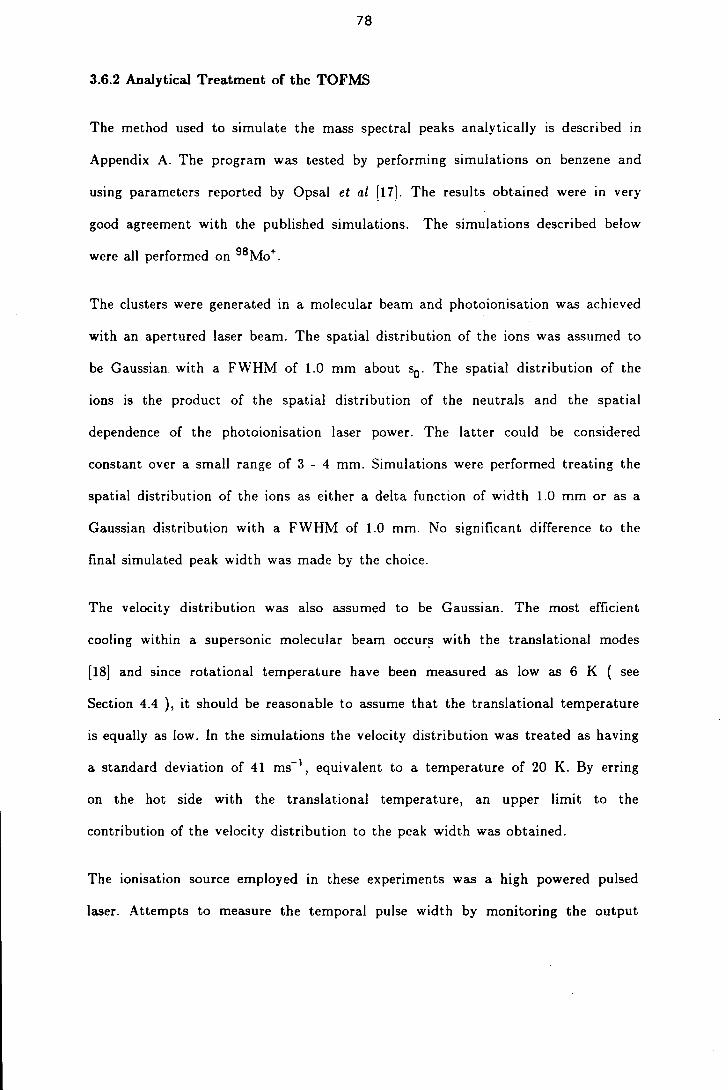
78
3.6.2 Analytical Treatment of the TOFMS
The method used to simulate the mass spectral peaks analytically is described in
Appendix A. The program was tested by performing simulations on benzene and
using parameters reported by Opsal et al [17]. The results obtained were in very
good agreement with the published simulations. The simulations described below
were all performed on 98 Mo.
The clusters were generated in a molecular beam and photoionisation was achieved
with an apertured laser beam. The spatial distribution of the ions was assumed to
be Gaussian with a FWHM of 1.0 mm about s 0 . The spatial distribution of the
ions is the product of the spatial distribution of the neutrals and the spatial
dependence of the photoionisation laser power. The latter could be considered
constant over a small range of 3 - 4 mm. Simulations were performed treating the
spatial distribution of the ions as either a delta function of width 1.0 mm or as a
Gaussian distribution with a FWHM of 1.0 mm. No significant difference to the
final simulated peak width was made by the choice.
The velocity distribution was also assumed to be Gaussian. The most efficient
cooling within a supersonic molecular beam occurs with the translational modes
[18] and since rotational temperature have been measured as low as 6 K ( see
Section 4.4 ), it should be reasonable to assume that the translational temperature
is equally as low. In the simulations the velocity distribution was treated as having
a standard deviation of 41 ms 1 , equivalent to a temperature of 20 K. By erring
on the hot side with the translational temperature, an upper limit to the
contribution of the velocity distribution to the peak width was obtained.
The ionisation source employed in these experiments was a high powered pulsed
laser. Attempts to measure the temporal pulse width by monitoring the output
79
from a fast photodiode with a 100 MHz transient digitiser or on a 125 MHz
oscilloscope suggested that the FWHM of the pulse was less than 10 ns. In the
simulations, therefore, the photoionisation source was treated as having a Gaussian
profile with a FWHM of 10 ns.
Figure 3.8a displays the mass peak for 98Mo simulated by setting all but the
spatial distribution to zero. The peak is asymmetrical with a sharp cut-off at
longer flight times and a relatively long tail to shorter flight times. The shape of
the peak is as expected since the value of k 0 was such that the TOFMS focused to
a maximum. Ions with small displacements from S had shorter flight times than
those from s0 leading to the tail to shorter flight times.
The simulation shown in Figure 3.8b was obtained by setting all but the velocity
distribution to zero. It is significantly broader than the width due to the spatial
distribution, suggesting that even in a molecular beam with a translational
temperature of 20 K, the spread of initial energies made a significant contribution
to the mass peak width. The peak width displayed in Figure 3.8b can be
considered an upper limit to the contribution from the velocity spread.
Figure 3.8c shows a simulation that was obtained by setting all but 'the time
distribution to zero. It too is significantly broader than the width due to the
spatial spread. The simulations suggest that the major contributions to the
analytical peak width are due to the velocity distribution and the temporal width
of the ionisation source.
Figure 3.8d is the simulated mass peak with none of the distributions set to zero.
Figure 3.8 : Analytical peak shapes calculated for 98 Mo using
experimental parameters for the TOFMS.

Figure 3.8
Analytical Peak Shapes
(d) Total
(c) Temporal
(b) Energy
(a) Spatial
-40 -20 0 20 40
Time / ns

81
The simulations implicitly assumed that ions with all possible values of the s, v,
and t variables would reach the detector. The only reason for this not happening is
if the velocity components perpendicular to the TOFMS axis resulted in some ions
missing the detector. This can be calculated from equation (19). Using a detector
radius of 9 mm, the limiting off TOFMS axis velocity for 98 Mo to hit the detector
is 464 ms-1 . The proportion of ions having velocities greater than this at 20 K is
negligible. Hence, irrespective of the values of s, v and t, all ions would reach the
detector. In passing through the extraction optics the ion pass through two 90 %
transmitting grids and in front of the detector there is another 82 % transmitting
grid. Hence the transmission function is reduced to 66 %. However, the attenuation
introduced by the grids is indiscriminate and the peak shapes in Figure 3.8 will
not be distorted. They can be viewed as the true analytical approximations to the
mass spectral peaks.
Comparison with the experimental peak illustrated in Figure 3.7 shows that the
experimental peak is significantly broader than the simulated one. There are
immediately two likely causes of the broadened peak width:
As stated previously, a set of deflection plates had to be applied above the
extraction optics to remove ion velocity along the molecular beam axis. These
plates introduced an electric field into what should have been a field-free region.
Ions which closer approach the positively biased plate P ( Figure 3.2 ) sample a
higher potential and are more retarded than ions which traverse the region close to
the earthed plate E. This effect introduces an additional peak broadening to those
previously considered.
The analytical equations assume perfect electric fields, which, to a greater or
lesser extent, must be approximations. Any irregularities in the fields will serve to
enhance the spatial peak-broadening factors.

82
It was decided to investigate these two peak-broadening effects with a Monte Carlo
trajectory program using a two-dimensional model of the potential within the
extraction optics and between the deflection plates.
3.6.3 Monte Carlo Simulation of Mass Spectral Peaks
The first step in simulating mass spectral peaks by a Monte Carlo method was to
generate the potential through which the ions travelled. Since the drift tube was a
field-free region, the potential had only to be calculated for the ion extraction
optics and for the part of the drift tube influenced by the deflection plates. The
potential was generated by solving the Laplace equation numerically by a
relaxation technique [19] and using as boundary conditions the copper box
surrounding the acceleration region. More details can be found in Appendix A.
Figure 3.9 shows a potential map generated by the relaxation technique for the
experimental extraction optics. It can be seen that the field between the repeller
plate and draw-out plate is far from ideal and that the field-free region around the
deflection plates is not field-free.

83
Figure 3.9 Relaxed potential map with no guard rings. The map
was generated with 250 V across the deflection plates
and the contours are spaced by 50 V intervals.
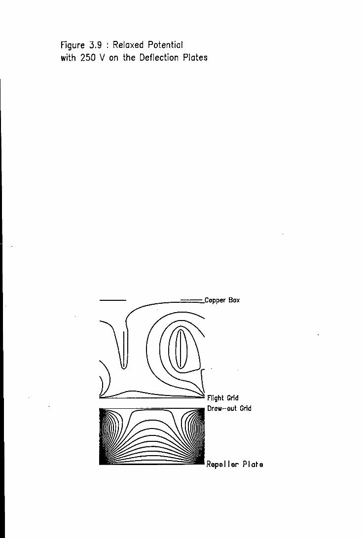
Figure 3.9 Relaxed Potential
with 250 V on the Deflection Plates
Copper Box
Flight Grid Draw—out Grid
Repeller Plate

84
Before simulating trajectories on the above potential, the Monte Carlo method was
tested on a potential with ideal electric fields and with no voltage across the
deflection plates. These conditions matched the ones used in the analytical
simulations. The spatial, velocity and temporal distributions used in all the Monte
Carlo simulations were the same as those used in the analytical case. To reiterate,
the spatial distribution was Gaussian with a FWHM of 1.0 mm, the velocities were
distributed according to a one dimensional Boltzmann velocity distribution at 20 K
and the temporal width of the photoionisation source was Gaussian with a FWHM
of 10 ns. Figure 3.10 shows the simulated mass peaks obtained using the Monte
Carlo method on the ideal potential for the spatial distribution alone, the velocity
distribution alone, the temporal ionisation distribution alone and for all three
distributions. Each peak was generated by following 40,000 ion trajectories and
collecting each ion in the plane of the detector. The mass spectral widths and
flight times calculated by the analytical and Monte Carlo methods agree to within
1 ns. The peak widths simulated for the spatial distributions alone are relatively
least in agreement. As the peak widths increase, the discrepancy between the two
methods remains constant, indicating that the discrepancy is a small correction
rather than a relative difference. The discrepancy is probably due to two factors:
The potential map is generated on a grid with a mesh length of 2 mm and
hence the plate positions can only be defined to such an accuracy. However, the
peaks show that the potential is a good approximation to the analytical one.
Flight times through each cell of the grid are calculated to an accuracy better
than 0.1 ns. Since in traversing the extraction region, ions have to pass through
about 40 cells, the flight times could accumulate errors of up to approximately 4
ns. This extreme is not the case, but errors in flight times of approximately 1 ns
could be due to this cause. Since peak width accuracy is not required to 1 ns, this

85
level of uncertainty is acceptable and is unlikely to distort any conclusion. The
Monte Carlo method on an ideal potential agrees with the results of the analytical
approach.
The power of the Monte Carlo method over the analytical approach is that it can
readily take into account perturbations introduced by non-ideal fields and by the
deflection plates. To fully define the problem, one more variable must be included,
namely the position along the molecular beam axis at which the ion is formed.
This distribution, known as the lateral distribution and given the symbol "1" was
taken to be a 10 mm long strip centred on the TOFMS axis. The probability
density function was further assumed to be a delta function of width 10 mm. In
the case of ideal fields and no deflection plates, this variable has no effect on the
peak widths.
Figure 3.11 shows the peak widths calculated on an ideal potential but with 250 V
across the deflection plates. As expected the peak width most severely affected is
the lateral peak width. However, the contribution of the broadened lateral peak to
the final peak width is quite small and is insufficient to obtain agreement between
the simulated and experimental peak widths. It appears, therefore, that the
deflection plates only have a small effect on mass spectral peak widths. Although
not shown in the figures, one effect of the deflection plates is to lengthen the ion
flight times. The flight time for 98MOI calculated analytically and on the ideal
potential with 0 V across the deflection plates was 19.399 us. The flight time on
an ideal potential with 250 V across the deflection plates was 19.409 Ps. The
deflection plates thus present a potential barrier to the ions which lengthens the
overall flight time.

[:J
Figure 3.10 : Monte Carlo simulations of the 98Mo mass peak on
an ideal potential with no voltage across the deflection
plates.
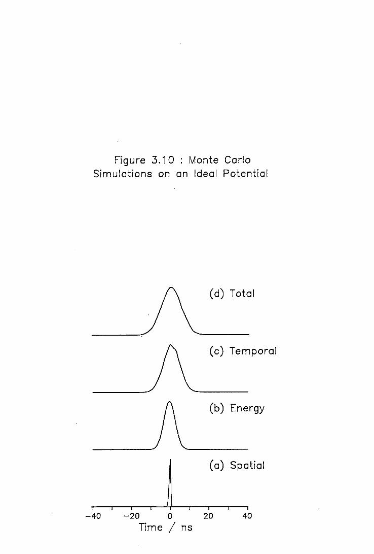
Figure 3.10 : Monte Carlo Simulations on an Ideal Potential
(d) Total
(c) Temporal
(b) Energy
(a) Spatial
-40 -20 0 20 40
Time / ns

87
Figure 3.11 : Monte Carlo simulations of 98Mo on an ideal
potential with 250 V across the deflection plates.

Figure 3.11 Monte Carlo Simulations on
an Ideal Potential with Deflection Plates
(f) Total
—A
Total ( Exc Lateral )
(d) Lateral
(c) Temporal
(b) Energy
(a) Spatial
40 —20 0 20 40
Time / ns

Figure 3.12 shows the effect of relaxing the potential and maintaining 250 V across
the deflection plates. The effect is dramatic. The peak widths that depend on the
position of the ion within the ion extraction optics - the spatial and lateral
distributions - have broadened greatly and the simulated peak width is broader
than the experimental one ( Figure 3.7 ). This is in contrast to all previous
simulations where the experimental peak was always broader. Equally important is
the significant lengthening of the flight time from approximately 19.40 j.is to 19.70
Us. From the potential map shown in Figure 3.9, the lengthened flight time and
the broadening of the mass spectral peaks, it is clear that the electric field between
the repeller and draw-out plates is not uniform and that the potential at any point
is less than would have been predicted assuming uniform fields. With the relaxed
potential, the Wiley and McLaren condition for spatial focusing is not met.
In contrast to the earlier simulations where the the peaks were simulated to a
resolution of 1 ns, the simulations in Figure 3.12 were performed with a resolution
of 10 ns. This was done to bring the simulation closer to the conditions used to
record the experimental peak.
Simulations were also performed on a relaxed potential with 0 V across the
deflection plates. There was essentially no change in the peak width or the flight
time compared to the simulation performed with 250 V across the deflection
plates. This confirmed that the distortions introduced by the deflection plates are
very small compared to those introduced by the non-uniform electric fields.
Relaxing the potential resulted in a simulated peak width greater than the
experimental peak width. However, the experimental peak width is generated by
only those ions which strike the detector whereas the simulated peak was generated
by collecting all ions in the plane of the detector. Figure 3.13 shows the simulated
peak width generated by collecting only those ions which arrive in the detector
plane within one detector radius of the TOFMS axis. Immediately obvious is the
reduction in the lateral peak width. Ions from large lateral displacements follow
trajectories which either crash into the walls of the flight tube or miss the
detector. It can also be seen that the overall peak width has decreased to a
FWHM of 28 ns, comparing very favourably with the experimental peak of FWHM
26 ns. By placing a finite size on the detector and counting only those ions that
strike the detector, the transmission function of the TOFMS can be estimated.
Although only two dimensional, it is likely to be more realistic than that estimated
by the analytical method. The percentage of ions with trajectories hitting the
detector was 12 %. By including the grids through which the ions must pass to
reach the detector, the transmission function can be estimated as approximately 8
It is clear that it is the spread, As, and the non-uniform electric fields which most
affect the peak width. The simplest way to improve the uniformity of the fields
and hence reduce the peak width is to use guard rings. Figure 3.14 shows the
potential generated using two guard rings between the repeller and draw-out
plates, and Figure 3.15 shows a simulated mass peak for 98 Mo on this potential.
The-width of the spectral peak is significantly reduced, having a FWHM of only 12
ns, close to the limit set by the temporal width of the ionisation source. This
width 'is equivalent to a resolution of approximately 810. The flight time calculated
for the ion is 19.402 us, only 3 ns longer than that calculated analytically or by
Monte Carlo simulations on an ideal potential.

011
Figure 3.12 : Simulations on a relaxed potential collecting all ions in
the plane of the detector.

Figure 3.12 Monte Carlo Simulations on
a Relaxed Potential with Deflection Plates
Total
(e) Total ( Exc Lateral )
Lateral
Temporal
Energy
tial
-
Time / ns
91
Figure 3.13 : Simulations on a relaxed potential collecting only those
ions which hit a finite detector.

Figure 3.13 : Monte Carlo Simulations on
a Relaxed Potential with a Finite Detector
(f) Total
(e) Total ( Exc Lateral )
(d) Lateral
Temporal
Energy
a!
-
Time / ns

92
Figure 3.14 : Potential map generated using two guard rings
between the repeller plate and the draw-out grid.

Figure 3.14 Relaxed Potential With Guard
Rings and 250 V across the Deflection Plates
Box
Flight Grid Draw—Out Grid
G2
Cl
Repeller Plate

93
Figure 3.15 : Simulation on a relaxed potential with guard rings.
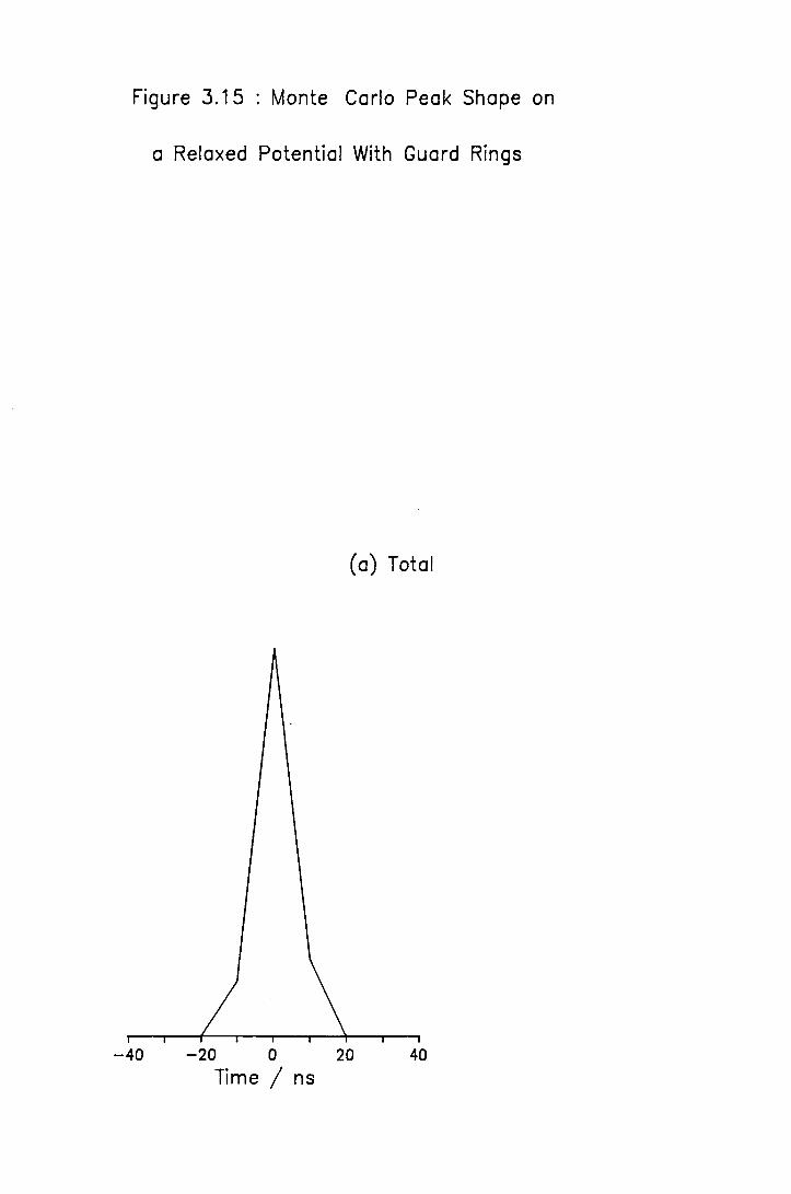
Figure 3.15 : Monte Carlo Peak Shape on
a Relaxed Potential With Guard Rings
(a) Total
-40 -20 0 20 40
Time / ns

94
3.7 Conclusions
The Monte Carlo method offers a good way of simulating peak widths in a
TOFMS and results close to experimental can be obtained. The ion transmission
function of a TOFMS can also be estimated by collecting only those ions which hit
a simulated detector. However, it has the disadvantage of being a computationally
expensive method.
The simulations have shown the importance of uniform electric fields in attaining a
high resolution. Unfortunately, one of the appeals of a TOFMS is the ease with
which its open ion extraction optics can be coupled to a supersonic molecular beam
with minimal interference to the molecular beam flow. The presence of the guard
rings required to maintain uniform electric fields will possibly result in greater
interaction between the molecular beam and the structure of the ion extraction
optics. This could lead to collisional heating, fragmentation or loss of signal
through increased collisions. The presence of the guard rings may also introduce
further transmission grids with consequent loss of transmission.
It should be noted that the potential generated is probably worse than the
experimental potential. This is because generation of the potential required
boundary conditions and assumed that the copper box surrounding the extraction
optics was complete ( See Appendix A ). This is not true as each wall in the
copper box contained a 40 mm hole for the passage of the molecular beam or the
photoionisation laser. Since the electric potential could penetrate through these
holes, the potential near the centre of the extraction optics where photoionisation
occurs would not have been dragged down as much as when calculated under
assumption of no holes.
95
REFERENCES
D. Price and C. Mimes, mt. J. Mass Spectrom. Ion Phys., 60, 61 (1984)
J.B. Farmer, Mass Spectrometry, Ed. C.A. McDowell, McGraw-Hill (1963)
M.S. Vries, N.J.A. Van Veen, T. Bailer, and A.E. de Vries. Chem. Phys., 56, 157 (1981)
D.H. Parker, Ultrasensitive Laser Spectroscopy, Ed. D.S. Kliger, Academic Press (1983)
R Larciprete and M. Stuke, J. Phys. Chem., 90, 4568 (1986)
L.Q. Huang, R.J. Conzemius, G.A. Junk, and R.S. Houk, Anal. Chem.. 60, 1490 (1988)
B.A. Mamyrin. V.A. Karataev, D.V. Schmikk, and V.A. Zagulin. Soy. Phys., JETP 37, 45 (1973)
W.C. Wiley, and I.H. McLaren, Rev. Sci. Instrum., 26, 1150 (1955)
C. Sanzone, Rev. Sci. Instrum., 41, 741 (1970)
P.W. Atkins, Physical Chemistry, Oxford University Press (1982)
J.P. Toennies and K. Winkelmann, J. Chem. Phys., 66, 3965 (1977)
E.A. Rohifing, D.M. Cox, and A. Kaldor, J. Chem. Phys. 81, 3322 (1984)
E.A. Rohifing, D.M. Cox, and A. Kaldor, J. Phys. Chem., 88, 4497 (1984)
J.B. Hopkins, P.R.R. Langridge-Smith, M.D. Morse, and R.E. Smalley, J. Chem. Phys., 78, 1627 (1983)
U. Boesi, H.J. Neusser, R. Weinkauf, and E.W. Schiag, J. Phys. Chem., 86, 4857 (1982)
S.C. Richtsmeier, E.K. Parks, K. Liu, L.G. Pobo, and S.J. Riley, J. Chem. Phys., 82, 3659 (1985)
R.B. Opsal, K.G. Owens, and J.P. Reilly, Anal. Chem., 57, 1884 (1985)
R.E. Smalley, L. Wharton, and D.H. Levy, Acc. Chem. Res., 10, 139 (1977)
W. Kaplan, Advanced Mathematics for Engineers, Addison-Wesley (1980)

CHAPTER FOUR
Spectroscopic Studies of the Lower Electronic States of Copper Dimer

M
4.1 Introduction
Copper dimer should offer the simplest example of the electronic spectroscopy of
transition metal clusters [1]. It is the lightest member of the group of dimers
formed from atoms with a closed shell of d-electrons and its spectra should be
simpler than those of the heavier members of its group which have smaller
rotational constants and, hence, more congested spectra. The closed d-shell and
the related wide separation of the atomic terms results in a density of molecular
states significantly lower than many of the other homonucleár transition metal
dimers. For example, it has been calculated that 30 molecular states of Ni 2 lie
within I eV of the ground state [2]. In contrast, no known excited electronic
molecular states lie within 1 eV of the ground state of Cu 2 .
There are also sound practical reasons for studying the low-lying excited electronic
states of copper dimer. The transitions from the ground state occur in a convenient
region for excitation with a dye laser and their spectroscopy is relatively well
documented [3-131, compared to other transition metal dimers. However, the
understanding of the electronic structure of Cu provided by the previous body of
work is not complete. A study of the electronic spectroscopy of Cu 2 therefore
provided an opportunity to test the newly constructed experimental apparatus,
described in Chapter II, with studies on well known systems and to perform new
work on the less well known systems. The following section provides a review of
previous experimental studies performed on the low-lying states of copper dimer.
4.2 Previous Experimental Work
The earliest observations of the emission spectrum of copper dimer were reported
in 1954 by Kleman and Lindkvist 1131 and Ruamps [4]. They observed vibrationally
resolved emission in the blue and green. The green emission , the A - X system
with its origin at 20,396 cm, was the more extensive, but the blue emission, the
B + X system with its origin at 21,748 cm 1 , appeared of dominating strength.
Emission was observed from a furnace filled with 500 torr of argon [3], suggesting
that the radiative process competes quite effectively against non-radiative
processes.
Rotational resolution of the B-X system was achieved in 1965 by Aslund et al [11].
They conclusively showed that the B-X system corresponded to a 1 E - 1 L
transition. By consideration of the atomic electronic configurations, the ground
state was assigned to 1 E symmetry and the upper state to 1 E symmetry.
Pesic and Weniger [12], in 1971, performed a rotational analysis of the A-X system
and assigned the A-state to 'fl U or l symmetry. In a subsequent laser-induced
fluorescence study, Lochet [13] observed only P and R branches forcing the
1 symmetry of the A-state to be Z or +
Using a dc arc source to generate copper dimer, Rao and Rao [7] observed six
band systems in the region 270 - 600 am. Two systems could be assigned as
emissions from the known A- and B-states and two matched observations reported
from studies on the spectra of flames of copper salts [14]. These latter two had
also tentatively been assigned to copper dimer. Rao and Rao vibrationally analysed
the two new systems, one of which emitted to the ground state. This emission is
now known as the E -' X system and has an electronic origin at 27,136 cm - '. The
other emission did not terminate on the ground state and is therefore either

between two excited states of copper dimer or from a different spectral carrier.
Preuss et al [151, in 1979, identified a spectral feature approximately 100 cm -1 to
the blue of the B-X origin. The authors were unable to perform a detailed study
on this new feature since it appeared with approximately one-third to one-half of
the intensity of the B-X system and, conceivably, half of the intensity could have
been due to underlying B-X structure (the 5-4 band ).
Powers et a! [5] and Gole et a! [16] simultaneously published the results of studies
of Cu2 seeded in an inert gas supersonic beam which confirmed that the spectral
feature previously observed by Preuss [15] did indeed emanate from Cu 2 . The
electronic origin of the upper state, known as the C-state, was found to lie at
21,870 cm-1 . Powers et a!, using R2PI, found the intensity of the 0-0 band of the
C-X system to be approximately two and a half times that of the B-X system, in
complete contrast to Preuss' earlier work. Powers et al also measured the lifetimes
for the B- and C-states, obtaining values of 35 ± 10 ns and 1.0 ± 0.2 Ps
respectively. The conflict in the lifetime and intensity data was accounted for by
stating that the B-state lifetime was shortened by predissociation.
Cu2 has also been investigated trapped in inert gas matrices. Ozin et a! [17]
published results which suggested that when Cu2 was trapped in argon, krypton or
xenon matrices, the matrix induced shifts of the spectral transitions to the A- and
B-states were large, approximately 5000 - 7000 cm-1 to the blue. Bondybey et a!
[6], however, found that the matrix-induced shift of the electronic transition energy
for the A-X and B-X systems in a neon matrix was small. Bondybey et al
performed a time resolved fluorescence emission study on the system excited at
26,000 cm 1 that Ozin had assigned to a strongly blue shifted A- ( or B- ) state.
The emission from this system was long-lived with an estimated lifetime of
approximately 6.5 ps. This is considerably longer than the matrix-isolated lifetimes

100
of either the A- or B-states, both of which have been measured as shorter than 10
ns (8].[181. The state excited at 26,000 cm -1 in the neon matrix is known as the
D-state. The intensity distribution of the emission from the D-state suggested
that it was considerably less strongly bound than the A- and B-states.
Studies have also revealed information on the lifetimes and photoprocesses of the
excited states. Steele [ij measured the lifetimes of several vibrational levels of the
A- and B-states at a selection of buffer-gas pressures. The B-state lifetime,
measured by monitoring laser-induced emission, was shorter than that of the
A-state and in addition to the expected decrease in lifetimes with increasing buffer
gas pressure, the B-state luminescence showed evidence at the higher pressures ( 10
torr of Ar ) of a second longer-lived decay corresponding to the lifetime of the
A-state.
In later work, Bondybey et at [20] measured the gas-phase lifetimes of the A-, B-
and C-states. The lifetimes for the lowest three vibrational levels of the A-state
were found to shorten rapidly with vibrational excitation but, in contrast to
Steele's earlier work, were independent of helium pressure in the range 0.5 to 15
torr. The emissions from v' = 3 and v' = 4 levels appeared only weakly.
The lifetime of the C-state, in agreement with Gole's [16] work on the lowest three
vibrational levels, was confirmed as being strongly dependent on pressure with an
extrapolated zero pressure lifetime of 800 ± 100 ns. At high pressures, the
Stern-Volmer plot became non-linear and at pressures above approximately 10 torr,
the lifetime was found to level off near 100 ns.
The lifetimes of the lowest three vibrational levels of the B-state were found to be
identical within experimental error, in agreement with Steele's [19] previous work.
At higher pressures, the decay curves became doubly exponential with one

101
component shortening and one lengthening with respect to the 40 ns lifetime at
lower pressures. By pressures of 10 - 12 torr, only the longer component survived.
The longer component was identical to the lifetime of the C-state at similar
pressures. Bondybey concluded that efficient collisional transfer between
vibrational levels of the B- and C-states led to a joint decay of the two coupled
levels.
Cole et al 1161 complemented their gas-phase work on the A- and B-state lifetimes
with studies on matrix-isolated dimers. In addition to fluorescence from the
directly excited state, a second much stronger and longer-lived emission was also
observed in the red and near infra red. This emission was attributed to the
predissociation of either the A- or B-states followed by a cage recombination of the
atoms to form the 3 E state correlating to the 2 S + 2 S atomic limit. Further
matrix work by Bondybey [8] on this long-lived emission in the red measured its
lifetime as 27 ms and confirmed the assignment of the state as the lowest triplet
state of Cu2 .
Work on the D + X system [6] showed that the emission was accompanied by
stronger B-X fluorescence and by phosphorescence in the near JR ( from the 3 E
a-state ). The measured lifetime of the B-state emission was long and it was clear
that the B-state was populated indirectly via the higher lying D-state. No emission
corresponding to the A-X system was observed even though B-X and a-X emissions
were present. The true radiative lifetime of the D-state was estimated to be three
or four times longer than that measured ( 6.5 Us ) due to the above-mentioned
photoprocesses shortening the measured lifetime.
There is no experimental data on the lifetime of the E-state.
102
4.3 Experimental Details of R2PI Spectroscopy
The overall description of the experimental apparatus and of cluster generation can
be found in Chapter II. The details included here are specific to the two colour
spectroscopic and lifetime studies on copper dimer.
The investigations were performed using frequency scans and time scans, both of
which have been described previously. With either technique, channels from the
transient digitiser corresponding to ions of a certain mass are selected and the ion
signal recorded in these channels is monitored as a function of the laser wavelength
( frequency scans ) or of the time delay between excitation and ionisation of the
molecule ( time scans ). A more detailed description has been presented in
Chapter II.
4.3.1 Pump Laser
The first colour was provided by an excimer pumped dye laser ( Lambda Physik ).
Two different dye solutions were required to cover the wavelength range. For the
A-X system Coumarin 102 ( range 460 - 510 nm ) was used and for the B-X and
CA systems, Coumarin 47 ( range 440 - 484 rim ) was used. Line narrowing of
the dye laser output was achieved through the use of an air spaced intracavity
etalon with a free spectral range of 1 cm - ' [21] and a finesse of at least 25. The
laser was capable of producing line narrowed tunable radiation with a bandwidth
of approximately 0.04 cm-1 . The etalon was angle-tuned as the wavelength was
scanned to maintain synchronisation between the peak of the profile transmitted
by the grating and peak transmission of the etalon. The synchronised scanning of
grating and etalon was under the control of a dedicated microprocessor and it was
only necessary to locate the normal position of the etalon and one transmitted
maximum as calibration points for the scanning program. The scan range was
103
limited to approximately 1 nm at the wavelengths used in these studies and the
direction of scanning had always to be from red to blue. The former restriction
caused no problems for spectra as compact as those generated from supersonically
cooled copper dimer. However, the latter tended to be a nuisance with systems
which formed a head at the blue end of the spectrum.
It was advantageous to pump the dye laser with a high energy excimer pump
beam energy ( 200 mJ ) and to reduce the dye laser output irradiating the Cu
sample with neutral density filters rather than to operate the dye laser with
reduced pump beam. Typically, the dye laser beam energy was below 1 mJ
pulse-1 and was then further attenuated with neutral density filters of total optical
density between 0.6 - 1.6 OD. Hence the energy of the dye beam was in the was
region 100 to 250 j.tJ pulse- '. The beam diameter Aapertured from approximately 8
mm to 3 mm and the approximate power density was 500 IA cm -2 pulse- '. No
focusing was required or used.
4.3.2 Probe Laser
The second colour was provided by the Lumonics laser operating on argon fluoride.
For temporal stability, this was operated at an energy of approximately 50 mJ
pulse-1 and was then attenuated by placing a series of metal grids between the
laser and entrance window to the cluster apparatus. The grids served to reduce
the power density from 6.4 mJ cm -2 pulse-1 to approximately 400 j.iJ cm-2
pulse-
Emission from this laser was both broadband and of sufficiently high energy ( 6.42
eV ) not to have caused any distortions of the spectrum.

104
4.3.3 Alignment of the Lasers and Molecular Beam
The two laser beams were counterpropagating and crossed the molecular beam at
right angles. To observe an R2PI signal, the problems of the spatial and temporal
alignment of the pulsed beams had to be solved.
The first step in this process was the' optimisation of cluster generation and
detection. Optimisation of cluster generation involved tuning the focus and timing
of the vaporisation laser ( See Chapter II ). The detection of the maximum
number of dimer species was obtained by operating the ArF excimer laser at high
energy and iteratively adjusting the height of the laser with respect to the
molecular beam and the trigger to the laser with respect to the trigger to the
molecular beam valve. Although cluster generation and detection are logically two
separate operations, experimentally they are coupled. Hence the steps taken to
maximise cluster generation had to be performed iteratively with the steps to
maximise cluster detection.
Once the optimum signal had been observed using non-resonant photoionisation,
the pump laser beam was introduced. The two laser beams were aligned spatially,
and then temporally. The latter was achieved by splitting off small fractions from
each beam and directing them to independent fast photodiodes whose outputs were
monitored on an oscilloscope. For excited electronic states with short lifetimes,
the constraints on temporal alignment could be quite severe. For example, to
obtain a spectrum of the B-X system of Cu 2 , the two lasers had to be aligned
temporally to within 10 ns. The final adjustment of temporal alignment was
performed iteratively whilst monitoring the signal of interest. With the spatial
and temporal alignments completed, the correct probe laser wavelength was set
and the ratio of the powers between the pump and probe lasers was adjusted to
observe 112PI.

105
4.3.4 Adjustment of the Ratio of Laser Powers
Obtaining the correct ratio of powers was an empirical operation. To observe a
spectral transition the probe laser beam power had to be attenuated so that most
of the species in the probed volume were resonantly ionised. It was desired to
operate with the maximum laser powers. The upper limit to the power of the
pump laser was set by saturation effects broadening the spectral features and
degrading the resolution. The upper limit to the power of the probe laser was set
by the need to obtain sufficient contrast between the resonantly ionised signal and
the non-resonant signal. In typical operation, the laser powers were selected such
that the ratio of resonantly ionised signal ( with the pump laser set at a
wavelength near to a rotational head ) to non-resonant signal ( where the pump
laser was set at a wavelength beyond a rotational head ) was between eight and
ten to one. Reduction of the probe laser power from this point led to particularly
noisy spectra while an increase in pump laser power resulted in line broadening.
4.3.5 Number of Ions Generated
A good signal for resonant ionisation was a pulse approximately 320 mV in
amplitude and 40 ns wide across a 50 0 load. This corresponded to a charge of
approximately 2.5 x 10⁻¹⁰ C, or 1.5 x 10 electrons. The signal was the result of
various stages of attenuation and amplification. From computer simulations ( see
Section 3.6.3 ), the transmission function of the TOFMS drift tube has been
estimated as approximately 8 %. At the end of the drift tube the ions struck the
microchannel plate detector, which provided between 10 - 10 6 amplification. The
signal was further amplified by the preamplifier with a gain of between 10 - 100.
The overall amplification of the ion signal between the point of generation and it
reaching the digitiser was between 10 5 - 107 , suggesting therefore that between 102
- 104 ions were produced by each laser pulse.
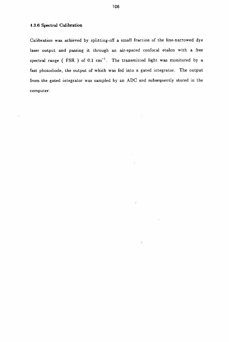
106
4.3.6 Spectral Calibration
Calibration was achieved by splitting-off a small fraction of the line-narrowed dye
laser output and passing it through an air-spaced confocal etalon with a free
spectral range ( FSR ) of 0.1 cm-1 . The transmitted light was monitored by a
fast photodiode, the output of which was fed into a gated integrator. The output
from the gated integrator was sampled by an ADC and subsequently stored in the
computer.
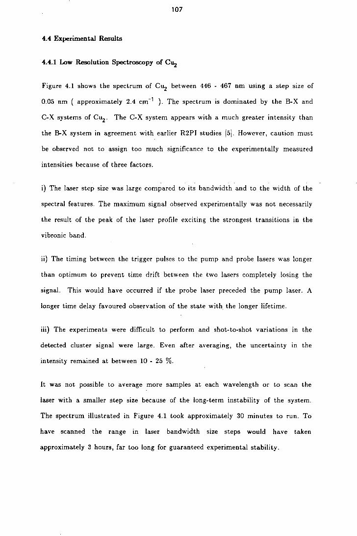
107
4.4 Experimental Results
4.4.1 Low Resolution Spectroscopy of Cu2
Figure 4.1 shows the spectrum of Cu2 between 446 - 467 nm using a step size of
0.05 nm ( approximately 2.4 cm -1 ). The spectrum is dominated by the B-X and
CA systems of Cu2 . The CA system appears with a much greater intensity than
the BA system in agreement with earlier 112PI studies [5]. However, caution must
be observed not to assign too much significance to the experimentally measured
intensities because of three factors.
The laser step size was large compared to its bandwidth and to the width of the -
spectral features. The maximum signal observed experimentally was not necessarily
the result of the peak of the laser profile exciting the strongest transitions in the
vibronic band.
The timing between the trigger pulses to the pump and probe lasers was longer
than optimum to prevent time drift between the two lasers completely losing the
signal. This would have occurred if the probe laser preceded the pump laser. A
longer time delay favoured observation of the state with the longer lifetime.
The experiments were difficult to perform and shot-to-shot variations in the
detected cluster signal were large. Even after averaging, the uncertainty in the
intensity remained at between 10 - 25 %.
It was not possible to average more samples at each wavelength or to scan the
laser with a smaller step size because of the long-term instability of the system.
The spectrum illustrated in Figure 4.1 took approximately 30 minutes to run. To
have scanned the range in laser bandwidth size steps would have taken
approximately 3 hours, far too long for guaranteed experimental stability.

108
Figure 4.1 : Vibronic spectrum of the B-X and C-X systems of Cu 2 .
The spectrum was taken by scanning the dye laser from
blue to red in 0.05 nm steps. Each point is the result of
30 laser shots. The ArF excimer laser was used to
photoionise the excited species.
Figure 4.1 Vibronically Resolved Spectrum of the B—X and C—X Systems of 6 Cu °5Cu
c-x • VA • A
448 450 452 454 456 458 460 462 464 466 468
Wavelength / nm
109
Figure 4.2 shows the spectrum of copper dimer over the range 492 - 485 nm and
exhibits only several bands of the A-X system. The laser was stepped at
approximately 1 cm-1 . A crude estimation of the vibrational temperature was
obtained by comparing the intensities of the ( 0-0 ) and ( 1-0 ) bands to those of
the ( 1-1 ) and ( 2-1 ) bands, after each band had been normalised by the
appropriate Franck-Condon factor. The vibrational temperature obtained was 312
± 160 K. The temperature illustrates the cooling effect of the supersonic
expansion [22]. The dimers condense from the laser generated plasma and although
the original vibrational temperature is unknown, it is estimated to be very high
[23]. However, the expansion serves to cool the vibrational temperature to
approximately ambient temperature. The narrowness of the bands in Figures 4.1
and 4.2 show that the rotational structure has been greatly collapsed through the
cooling achieved in the supersonic expansion.
To fully appreciate this cooling and to determine any useful information regarding
electronic state symmetries, the vibronic bands had to be investigated under
greater resolution.
Figures 4.3 a-c show the origin bands of the A-X, B-X and C-X systems
respectively obtained by scanning the dye laser without an intracavity etalon and
with a step size of 0.001 nm ( approximately 0.0045 cm -1 ). The contours for the
A-X and B-X systems appear to form heads at the blue end of the spectrum
whereas the C-X contour shows less evidence of head formation and instead shows
a relatively intense central band.
It was not possible to resolve the rotational structure lying beneath the contours
without recourse to a higher resolution excitation source. This was provided by
using the intracavity etalon in the Lambda Physik laser.

110
Figure 4.2 : Vibronic spectrum of the A-X system of Cu 2 . The
spectrum was acquired by scanning the dye laser from
red to blue in 0.02 nm steps and averaging 30 laser shots
at each point. Photoionisation of the excited species was
achieved with the ArF excimer laser.

Figure 4.2 : Vibronic Spectrum of the A—X System of "Cu,
A—X
Ill
1-1
2-1
492 491 490 489 488 487 486 485
Wavelength / nm
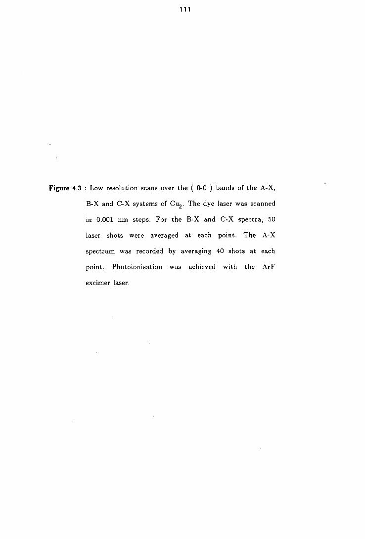
111
Figure 4.3 : Low resolution scans over the ( 0-0 ) bands of the A-X,
B-X and C-X systems of Cu 2 . The dye laser was scanned
in 0.001 nm steps. For the B-X and C-X spectra, 50
laser shots were averaged at each point. The A-X
spectrum was recorded by averaging 40 shots at each
point. Photoionisation was achieved with the ArF
excimer laser.
Figure 4.3 : Low Resolution Scans over the 0-0 bands of the A—X, B—X and C—X Systems of'Cu,
A—X System
B—X System
C—X System
8 7 6 5 4 3 2 1 Relative Frequency / cm-1

112
4.4.2 High Resolution Spectroscopy of Cu2
4.4.2.1 A-X System
Figure 4.4a shows the high resolution spectrum of the ( 0-0 ) band of the A-X
system of Cu2 recorded using line narrowed output from the FL3002EC laser. The
spectrum was obtained under the most severe expansion conditions ( 1 ms wide gas
pulses from the NRC BV-100 valve operating with 10 bar backing pressure of He
and it is readily seen from the simulated spectrum in Figure 4.4b that the
rotational structure has been strongly cooled. The details of spectral simulation
are covered in Section 4.4.3.
To obtain more extensive rotational structure for a more accurate determination of
the rotational constants, spectra were also recorded with attenuated expansion
conditions. Figure 4.5a illustrates a hotter spectrum for the A-X system. The
rotational temperature, as determined by simulation, is 18 K.
Several high resolution spectra were recorded for the ( 0-0 ) band of the A-X
system at the attenuated expansion conditions. Each one was analysed and the
rotational constants extracted. If the FSR of the etalon used to calibrate the
spectra was treated as a fixed parameter, the spectroscopic constants extracted
from one spectrum invariably differed from those extracted from another spectrum.
However, the ratio of the upper state rotational constant to the lower state
constant was, within experimental error, the same from spectrum to spectrum.
The FSR of the monitor etalon was therefore treated as constant within a
spectrum but as a variable parameter between spectra. Its value was determined
by normalising the ground state rotational constant extracted from the data to the
literature value [1]. After normalisation, the upper state constants extracted from
the various spectra all agreed within experimental error. The spectroscopic

113
constants for the ( 0-0 ) band of the A-state listed in Table 4.6 are the average of
8 normalised spectra. The constants for the ( 1-0 ) band were extracted from a
single spectrum. All isotopic combinations were fitted simultaneously and more
details of the extraction of the spectroscopic constants from the the spectra are
discussed in Section 4.4.4.
Table 4.7 shows the experimental line positions, the calculated line positions, and
the residuals for a representative ( 0-0 ) band spectrum of the A-X system.
Normalisation of the ground state spectroscopic constants in this spectrum to the
literature value required the use of a FSR of 0.09964 cm -1 .
It is clear from the spectra illustrated in Figures 4.4a and 4.5a that the A-X
system of Cu2 consists of only parallel bands and the assignment of Lochet [13) is
correct. The spectroscopic constants obtained for the upper state do not agree
within experimental error with Lochet's, but it is believed that the constants
quoted in this work are more correct than those reported by Lochet due to the
larger number of lines analysed.
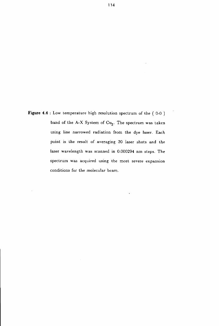
114
Figure 4.4 : Low temperature high resolution spectrum of the ( 0-0
band of the A-X System of Cu 2 , The spectrum was taken
using line narrowed radiation from the dye laser. Each
point is the result of averaging 30 laser shots and the
laser wavelength was scanned in 0.000294 nm steps. The
spectrum was acquired using the most severe expansion
conditions for the molecular beam.
Figure 4.4 : 0-0 Band of the A—X system of "Cu,
(a) Experimental Spectrum
P 1 4 1 3 1 2 1 1 1 09 1 8 17161514131211 10111
(b) Simulated Spectrum ( I = 6 K )
-1 0 1 2 3 4 5 6 7 Relative Frequency / cm-1
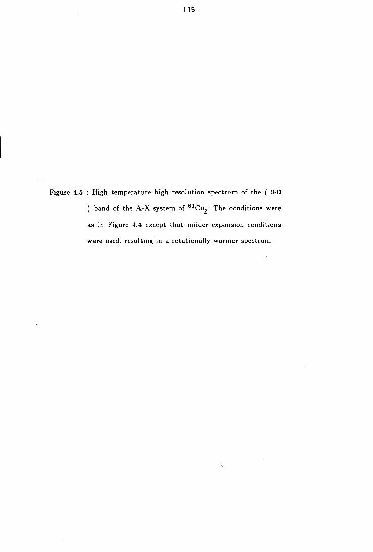
115
Figure 4.5 : High temperature high resolution spectrum of the ( 0-0
band of the A-X system of 63 Cu2 . The conditions were
as in Figure 4.4 except that milder expansion conditions
were used, resulting in a rotationally warmer spectrum.
Figure 4.5 0-0 Band of the A—X system of "Cu,
(a) Experimental Spectrum
P 1 25 1 24 123 '22 121 '20 1 19 1 18 1 17 1 16 1 15 1 14 1 13 1 12 1 11 1 10 1 9 1 8 1 7 1 6 1 5 1 4 1 3 1 2 1 1 1 01 1 1
JllIll
(b) Simulated Spectrum ( T = 18 K )
-10 -9 -8 -7 -6 -5 -4 -3 -2 -1 0 1 2 Relative Frequency / cm-'
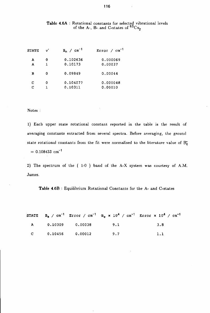
116
Table 4.6A : Rotational constants for selected vibrational levels of the A-, B-. and C-states of 63 Cu2
STATE V B, / CM-1 Error / cm-1
A 0 0.102636 0.000069 A 1 0.10173 0.00037
B 0 0.09849 0.00044
C 0 0.104077 0.000048 C 1 0.10311 0.00010
Notes
Each upper state rotational constant reported in the table is the result of
averaging constants extracted from several spectra. Before averaging, the ground
state rotational constants from the fit were normalised to the literature value of B'
= 0.108433 cm-1
The spectrum of the ( 1-0 ) band of the A-X system was courtesy of A.M.
James.
Table 4.6B : Equilibrium Rotational Constants for the A- and C-states
STATE Be / cm- 1 Error / c& 1 ae x 104 / c& 1 Error x 104 / CM-1
A 0.10309 0.00038 9.1 3.8
C 0.10456 0.00012 9.7 1.1
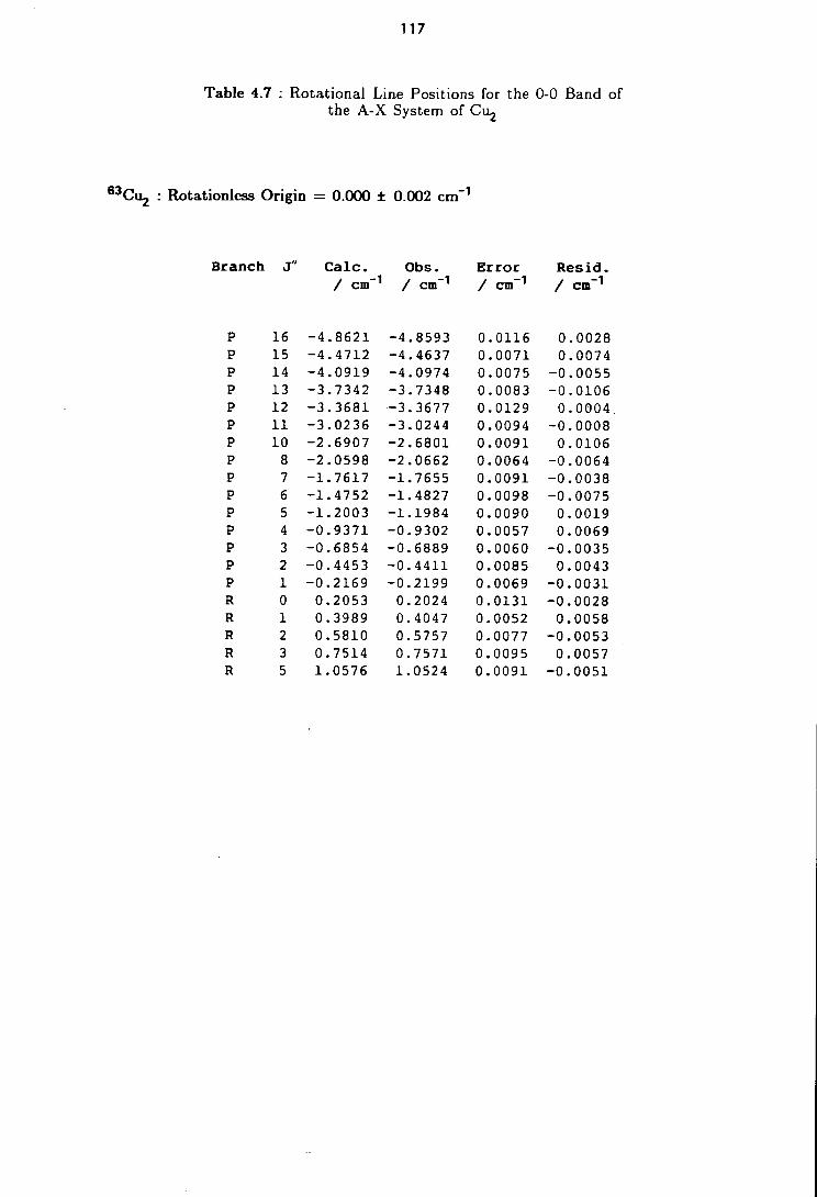
117
Table 4.7 : Rotational Line Positions for the 0-0 Band of the A-X System of Cu2
63 Cu2 : Rotationless Origin = 0.000 ± 0.002 cm-1
Branch J" Calc. Obs. error Resid. / CM-1 / CM-1 / cn( 1 / cm
p
p
p
p
p
p
p
p
p
p
p
p
p
p
p
R R R R R
16 -4.8621 -4.8593 15 -4.4712 -4.4637 14 -4.0919 -4.0974 13 -3.7342 -3.7348 12 -3.3681 -3.3677 11 -3.0236 -3.0244 10 -2.6907 -2.6801 8 -2.0598 -2.0662 7 -1.7617 -1.7655 6 -1.4752 -1.4827 5 -1.2003 -1.1984 4 -0.9371 -0.9302 3 -0.6854 -0.6889 2 -0.4453 -0.4411 1 -0.2169 -0.2199 0 0.2053 0.2024 1 0.3989 0.4047 2 0.5810 0.5757 3 0.7514 0.7571 5 1.0576 1.0524
0.0116 0.0028
0.0071 0.0074 0.0075 -0.0055 0.0083 -0.0106 0.0129 0.0004. 0.0094 -0.0008 0.0091 0.0106 0.0064 -0.0064 0.0091 -0.0038 0.0098 -0.0075
0.0090 0.0019
0.0057 0.0069 0.0060 -0.0035 0.0085 0.0043 0.0069 -0.0031 0.0131 -0.0028 0.0052 0.0058 0.0077 -0.0053 0.0095 0.0057 0.0091 -0.0051
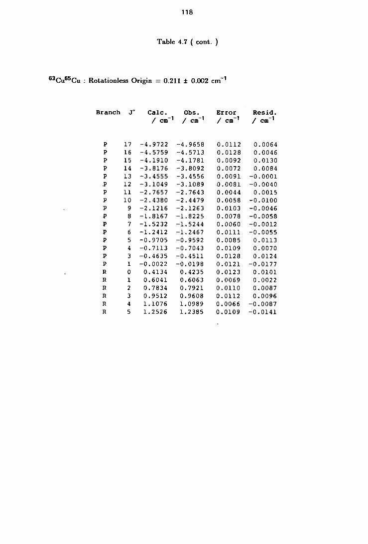
118
Table 4.7 ( cont. )
63Cu65Cu : Rotationless Origin = 0.211 ± 0.002 cm - '
Branch J" Caic. Obs. Error Resid. / cm-1 / cm-1 / cm 1 / cm 1
p
p
p
p
p
p
p
P p
p
P p
p
p
p
p
R R R R P P
17 -4.9722 -4.9658 16 -4.5759 -4.5713 15 -4.1910 -4.1781 14 -3.8176 -3.8092 13 -3.4555 -3.4556 12 -3.1049 -3.1089 11 -2.7657 -2.7643 10 -2.4380 -2.4479 9 -2.1216 -2.1263 8 -1.8167 -1.8225 7 -1.5232 -1.5244 6 -1.2412 -1.2467 5 -0.9705 -0.9592 4 -0.7113 -0.7043 3 -0.4635 -0.4511 1 -0.0022 -0.0198 0 0.4134 0.4235 1 0.6041 0.6063 2 0.7834 0.7921 3 0.9512 0.9608 4 1.1076 1.0989 5 1.2526 1.2385
0.0112 0.0064
0.0128 0.0046
0.0092 0.0130
0.0072 0.0084 0.0091 -0.0001 0.0081 -0.0040 0.0044 0.0015 0.0058 -0.0100 0.0103 -0.0046 0.0078 -0.0058 0.0060 -0.0012 0.0111 -0.0055
0.0085 0.0113
0.0109 0.0070
0.0128 0.0124 0.0121 -0.0177
0.0123 0.0101
0.0069 0.0022
0.0110 0.0087
0.0112 0.0096 0.0066 -0.0087 0.0109 -0.0141

119
Table 4.7 ( cont. )
65Cu2 : Rotationless Origin = 0.432 ± 0.002 cm -1
Branch J Calc. Obs. Error Resid. / cm-1 / cm-1 / cm-1 / cm-1
P P P P P P P P P P P P P P P R R R R R R R R
17 -4.6706 -4.6690 15 -3.9016 -3.9051 14 -3.5340 -3.5511 13 -3.1776 -3.1721 12 -2.8325 -2.8340 11 -2.4986 -2.5063 10 -2.1760 -2.1766 9 -1.8646 -1.8735 7 -1.2755 -1.2813 6 -0.9978 -0.9906 5 -0.7314 -0.7339 4 -0.4763 -0.4750 3 -0.2323 -0.2223 2 0.0003 0.0014 1 0.2218 0.2140 0 0.6309 0.5999 1 0.8186 0.8337 2 0.9951 1.0044 3 1.1603 1.1507 4 1.3143 1.3428 5 1.4570 1.4563 6 1.5885 1.5964 7 1.7087 1.7178
0.0211 0.0015 0.0106 -0.0035 0.0120 -0.0171 0.0148 0.0055 0.0132 -0.0015 0.0101 -0.0077 0.0130 -0.0007 0.0140 -0.0089 0.0181 -0.0058 0.0148 0.0073 0.0076 -0.0024
0.0079 0.0013
0.0066 0.0100
0.0140 0.0010 0.0156 -0.0078 0.0237 -0.0310
0.0106 0.0151
0.0158 0.0093 0.0111 -0.0096
0.0385 0.0285 0.0080 -0.0007
0.0686 0.0079
0.0304 0.0091
Normalised constants derived from spectrum ( 63Cu2 )
Bb = 0.10263 ± 0.00018 cm-1
B'ó = 0.10843 ± 0.00016 cm -1 ( FSR = 0.09964 cm-1
Chi-squared = 41.94 with 60 degrees of freedom
Reduced Chi-squared = 0.70

120
4.4.2.2 B-X System
Figure 4.8a illustrates a high resolution scan recorded over the ( 0-0 ) band of the
B-X system of Cu2 . Figure 4.8b illustrates a simulation of the spectrum for a
rotational temperature of 18 K. The spectroscopic constants extracted from the
data are listed in Table 4.6 and are the result of averaging the normalised
constants from two spectra.
Table 4.9 shows the experimental line positions, the calculated line positions and
the residuals for a spectrum of ( 0-0 ) band of the B-X system. Normalisation of
the ground state constant to the known literature value yielded an etalon FSR of
0.10036 cm-
The spectroscopic constants listed in Table 4.9 are in agreement with those
published by Aslund et al [11] and confirm that the electronic symmetry of the
1+ + B-state is either Z or 0.
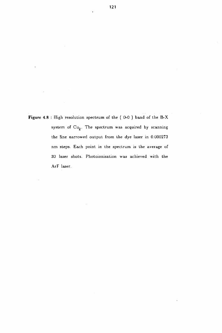
121
Figure 4.8 : High resolution spectrum of the ( 0-0 ) band of the B-X
system of Cu2 . The spectrum was acquired by scanning
the line narrowed output from the dye laser in 0.000273
nm steps. Each point in the spectrum is the average of
30 laser shots. Photoionisation was achieved with the
ArF laser.
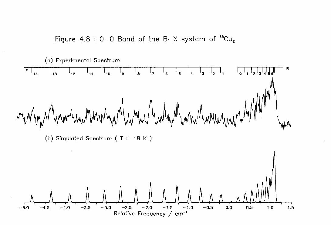
Figure 4.8 : 0-0 Band of the B—X system of "Cu,
Experimental Spectrum
I I I I I I I 111111 14 13 12 11 10 9 8 7 6 5 4 3 2 0 i I2I3I4III
R
Simulated Spectrum ( T = 18 K )
-5.0 -4.5 -4.0 -3.5 -3.0 -2.5 -2.0 -1.5 -1.0 -0.5 0.0 0.5 1.0 1.5
Relative Frequency / cm-'

122
Table 4.9 Line Positions for the 0-0 Band of the B-X System of Cu2
63Cu2 : Rotationless Origin = 0.000 ± 0.003 cm-1
Branch J" Calc. Obs. Error Resid. / CM-1 / CM-1 / CM-1 / cm
p
p
p
p
p
p
p
p
p
p
p
p
R R R R
13 -4.3741 -4.3827 12 -3.9180 -3.8947 11 -3.4818 -3.4787 9 -2.6693 -2.6610 8 -2.2929 -2.2988 7 -1.9365 -1.9411 6 -1.6000 -1.6054 5 -1.2835 -1.2783 4 -0.9869 -0.9802 3 -0.7101 -0.7174 2 -0.4534 -0.4544 1 -0.2166 -0.2038 0 0.1972 0.1951 1 0.3742 0.3759 2 0.5312 0.5605 3 0.6683 0.6782
0.0073 -0.0085
0.0199 0.0234
0.0189 0.0032
0.0106 0.0083 0.0190 -0.0059 0.0073 -0.0046 0.0079 -0.0053
0.0200 0.0052
0.0264 0.0066 0.0121 -0.0072 0.0246 -0.0009 0.0123 0.0129 0.0081 -0.0021
0.0184 0.0018
0.0141 0.0293
0.0188 0.0099
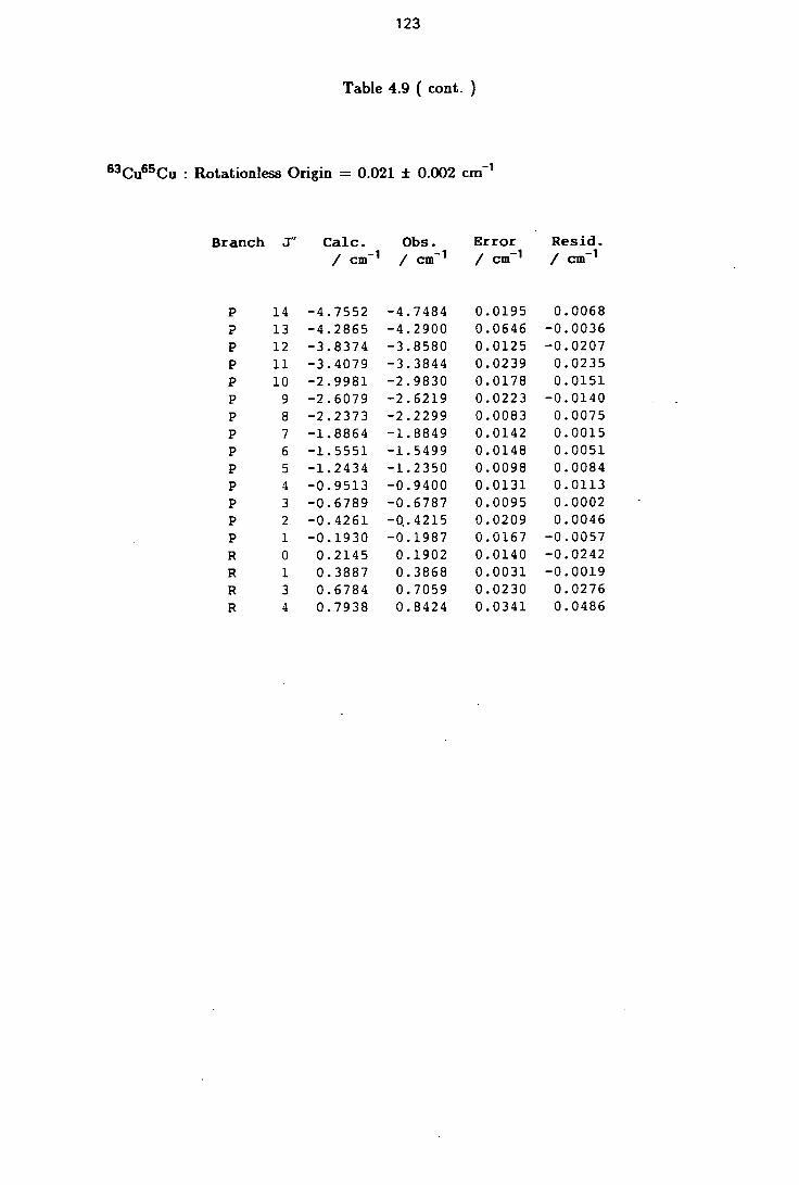
123
Table 4.9 ( cont. )
63 Cu65Cu : Rotationless Origin = 0.021 ± 0.002 cm-1
Branch J" Caic. Obs. Error Resid. / cm-1 / cm 1 / cm-1
/ cm
P 14 -4.7552 -4.7484 0.0195 0.0068 p 13 -4.2865 -4.2900 0.0646 -0.0036 P 12 -3.8374 -3.8580 0.0125 -0.0207 P 11 -3.4079 -3.3844 0.0239 0.0235 P 10 -2.9981 -2.9830 0.0178 0.0151 P 9 -2.6079 -2.6219 0.0223 -0.0140 P 8 -2.2373 -2.2299 0.0083 0.0075 P 7 -1.8864 -1.8849 0.0142 0.0015 P 6 -1.5551 -1.5499 0.0148 0.0051 P 5 -1.2434 -1.2350 0.0098 0.0084 P 4 -0.9513 -0.9400 0.0131 0.0113 p 3 -0.6789 -0.6787 0.0095 0.0002 p 2 -0.4261 -q.4215 0.0209 0.0046 p 1 -0.1930 -0.1987 0.0167 -0.0057 R 0 0.2145 0.1902 0.0140 -0.0242 R 1 0.3887 0.3868 0.0031 -0.0019 R 3 0.6784 0.7059 0.0230 0.0276 R 4 0.7938 0.8424 0.0341 0.0486
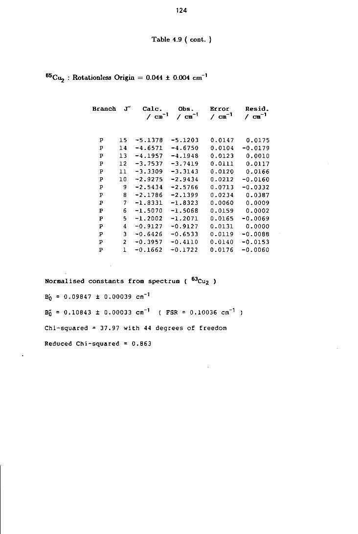
124
Table 4.9 ( cont. )
Cu2 : Rotationless Origin = 0.044 ± 0.004 cm -1
Branch J" Calc. Obs. Error Resid.
/ cm-1 / cm 1 / cm- 1 / cm
P P P P P P P P P P P P P P P
15 -5.1378 -5.1203 14 -4.6571 -4.6750 13 -4.1957 -4.1948 12 -3.7537 -3.7419 11 -3.3309 -3.3143 10 -2.9275 -2.9434 9 -2.5434 -2.5766 8 -2.1786 -2.1399 7 -1.8331 -1.8323 6 -1.5070 -1.5068 5 -1.2002 -1.2071 4 -0.9127 -0.9127 3 -0.6426 -0.6533 2 -0.3957 -0.4110 1 -0.1662 -0.1722
0.0147 0.0175 0.0104 -0.0179
0.0123 0.0010
0.0111 0.0117
0.0120 0.0166 0.0212 -0.0160 0.0713 -0.0332
0.0234 0.0387
0.0060 0.0009
0.0159 0.0002 0.0165 -0.0069 0.0131 0.0000 0.0119 -0.0088 0.0140 -0.0153 0.0176 -0.0060
Normalised constants from spectrum ( 63Cu2 )
Bb = 0.09847 ± 0.00039 cm-1
B = 0.10843 ± 0.00033 cm-1 ( FSR = 0.10036 cm-1
Chi-squared = 37.97 with 44 degrees of freedom
Reduced Chi-squared = 0.863
125
4.4.2.3 C-X System
Figure 4.10a illustrates a high resolution scan over the ( 0-0 ) band of the C-X
system of Cu2 . It is immediately obvious from the spectrum that the transition is
perpendicular, in contrast to the A-X and B-X systems. Figure 4.10b illustrates a
simulation of this spectrum using a rotational temperature of 5 K. The spectrum
in Figure 4.10a was obtained using the most severe expansion conditions.
The spectroscopic constants derived for the C-state are listed in Table 4.6. The
constants for the ( 0-0 ) band were obtained by averaging the normalised constants
from five spectra. The constants for the ( 1-0 ) band were extracted from one
spectrum.
A hot spectrum of the ( 1-0 ) band of the C-X system is shown is Figure 4.11a.
Table 4.12 shows experimental line positions, calculated line positions, and
residuals for a representative hot spectrum of the ( 0-0 ) band of the C-X system.
An etalon FSR of 0.100028 cm -1 was required to normalise the spectrum. The
C-state can be assigned either to a state of fl electronic symmetry in Hund's case
(a) or of l electronic symmetry in Hund's case (c). This is the first assignment
of the electronic symmetry of the C-state.
126
Figure 4.10 : Low temperature high resolution spectrum of the ( 0-0
band of the C-X System of Cu 2 . The spectrum was
obtained using the most extreme expansion conditions of
the molecular beam. The intracavity etalon was installed
in the dye laser to line narrow the output. Each point is
the result of 30 laser shots and the scan step size was
0.000276 nm. Photoionisation was achieved with the ArF
excimer laser.
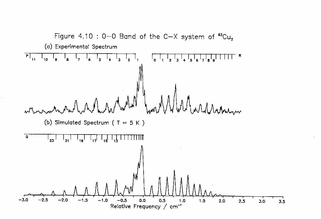
Figure 4.10 : 0-0 Band of the C—X system of 63Cu 2 Experimental Spectrum
I I I I I 11 10 9 8 7 6 5 4 3 2 1 0 1 1 1 2 1 3 1 4 1 5 1 6 1 7 1 8 1 9 11111
Simulated Spectrum ( I = 5 K )
I I I I I liii 23 21 19 17 1 I 1S 11111111111
-3.0 -2.5 -2.0 -1.5 -1.0 -0.5 0.0 0.5 1.0 1.5 2.0 2.5 3.0 3.5 Relative Frequency / cm-'
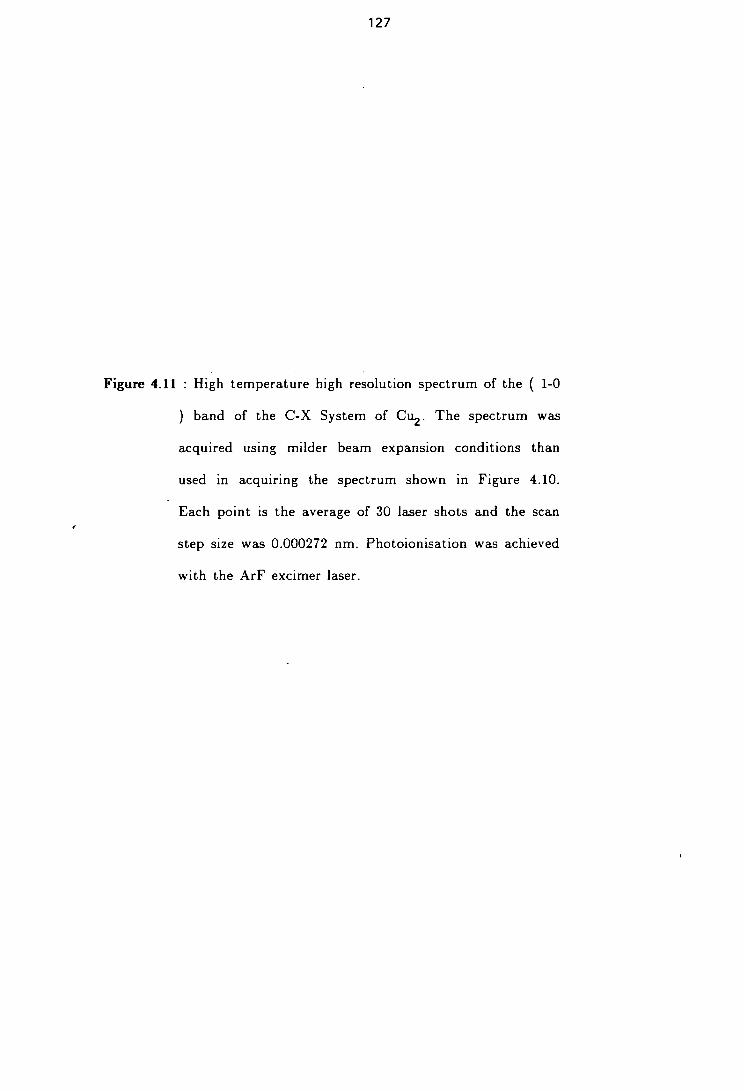
127
Figure 4.11 High temperature high resolution spectrum of the ( 1-0
band of the C-X System of Cu2 . The spectrum was
acquired using milder beam expansion conditions than
used in acquiring the spectrum shown in Figure 4.10.
Each point is the average of 30 laser shots and the scan
step size was 0.000272 nm. Photoionisation was achieved
with the ArF excimer laser.
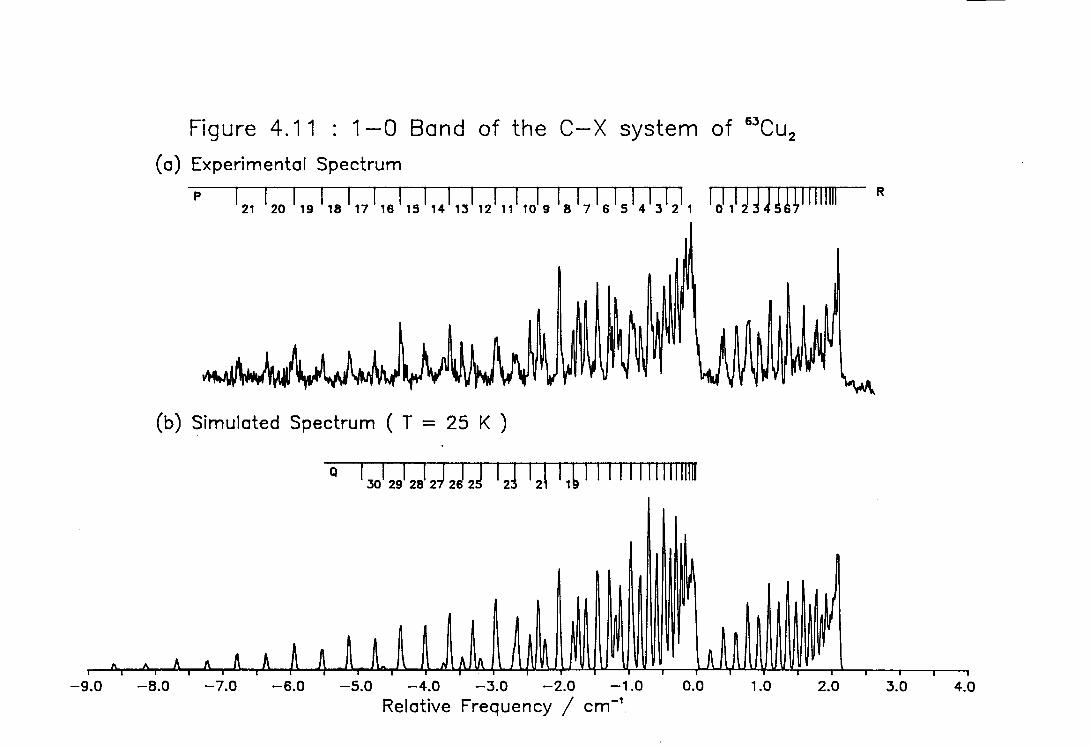
Figure 4.11 : 1-0 Band of the C—X system of "Cu,
Experimental Spectrum
P 1 21 1 20 1 19 1 1 8 1 17 1 16 1 15 1 14 1 13 1 12 1 11 1 101 9 I s 1 7 1 6 1 5 1 4 1 3 1 2 1 1 '1WW"
Simulated Spectrum ( I = 25 K )
Q I 30 29 28 I I I 27J22 121211L1111111111111111
-9.0 -8.0 -7.0 -6.0 -5.0 -4.0 -3.0 -2.0 -1.0 0.0 1.0 2.0 3.0 4.0
Relative Frequency / cm -1 .

128
Table 4.12 : Line Positions for the 0-0 Band of the C-X System of Cu
63 Cu2 : Rotationless Origin = 0.000 ± 0.002 cm-1
Branch J" Caic. Obs. Error Resid. / cn( 1 / CM-1 / CM-1 / cin
P 23 -7.2069 -7.1895 0.0078 0.0174 P 21 -6.3959 -6.3808 0.0121 0.0150 P 20 -6.0036 -5.9585 0.0234 0.0450 P 19 -5.6200 -5.6135 0.0194 0.0065 P 18 -5.2452 -5.2585 0.0244 -0.0132 P 17 -4.8792 -4.8986 0.0204 -0.0194 P 16 -4.5220 -4.5326 0.0066 -0.0106 P 15 -4.1735 -4.1766 0.0115 -0.0031 P 14 -3.8338 -3.8345 0.0160 -0.0007 P 13 -3.5029 -3.4977 0.0112 0.0052 P 12 -3.1808 -3.1646 0.0138 0.0162 P ii -2.8674 -2.8735 0.0103 -0.0061 P 10 -2.5628 -2.5708 0.0161 -0.0079 Q 23 -2.4207 -2.4138 0.0128 0.0069 P 9 -2.2670 -2.2578 0.0148 0.0092 P 8 -1.9799 -1.9796 0.0318 0.0003 P 7 -1.7016 -1.7024 0.0090 -0.0008 P 6 -1.4321 -1.4231 0.0226 0.0090 P 5 -1.1714 -1.1773 0.0115 -0.0059 Q 15 -1.0521 -1.0607 0.0047 -0.0086 P 4 -0.9194 -0.9323 0.0131 -0.0128 Q 13 -0.7977 -0.8091 0.0093 -0.0114 Q 9 -0.3941 -0.4002 0.0121 -0.0061 R 1 0.4081 0.4131 0.0113 0.0050 R 2 0.5986 0.5925 0.0091 -0.0061 R 3 0.7804 0.7860 0.0167 0.0056 R 4 0.9534 0.9617 0.0112 0.0083 R 5 1.1176 1.1218 0.0108 0.0041 R 6 1.2731 1.2771 0.0125 0.0040 R 7 1.4198 1.4298 0.0120 0.0101 R 8 1.5577 1.5574 0.0087 -0.0003 R 9 1.6868 1.6886 0.0228 0.0018 R 11 1.9188 1.9268 0.0107 0.0080 R 12 2.0216 2.0360 0.0108 0.0144 R 13 2.1156 2.1254 0.0185 0.0098

129
Table 4.12 ( cont. )
63 Cu65Cu : Rotationless Origin = 0.146 ± 0.002 cm -1
Branch .1" Caic. Obs. Error Resid. / cm-1 / cm-1 / cm- I /
P 27 -8.6513 -8.6625 0.0143 -0.0112 P 25 -7.7837 -7.7920 0.0366 -0.0083 P 24 -7.3629 -7.3685 0.0112 -0.0056 P 23 -6.9506 -6.9408 0.0153 0.0099 P 22 -6.5471 -6.5700 0.0143 -0.0229 P 21 -6.1522 -6.1511 0.0162 0.0011 P 20 -5.7659 -5.7621 0.0095 0.0038 P 19 -5.3882 -5.3760 0.0236 0.0122 P 18 -5.0192 -5.0144 0.0182 0.0048 P 17 -4.6588 -4.6552 0.0093 0.0036 P 16 -4.3071 -4.3190 .0117 -0.0119 P 15 -3.9640 -3.9573 0.0089 0.0066 P 14 -3.6295 -3.6413 0.0085 -0.0118 P 13 -3.3037 -3.3063 0.0175 -0.0026 Q 27 -3.1192 -3.1377 0.0203 -0.0195 P 12 -2.9865 -2.9703 0.0083 0.0162 P 11 -2.6780 -2.6800 0.0118 -0.0020 P 10 -2.3780 -2.3898 0.0095 -0.0117 Q 23 -2.2381 -2.2463 0.0193 -0.0082 P 9 -2.0868 -2.0814 0.0081 0.0054 P 8 -1.8041 -1.8034 0.0107 0.0007 Q 20 -1.6680 -1.6956 0.0141 -0.0276 P 7 -1.5301 -1.5399 0.0155 -0.0098 P 6 -1.2648 -1.2622 0.0186 0.0026 Q 16 -1.0288 -1.0174 0.0119 0.0114 P 4 -0.7600 -0.7671 0.0119 -0.0071 Q 13 -0.6401 -0.6384 0.0081 0.0017 Q 12 -0.5278 -0.5418 0.0133 -0.0140 R 0 0.3509 0.3662 0.0258 0.0154 R 1 0.5471 0.5527 0.0137 0.0056 R 2 0.7347 0.7349 0.0185 0.0001 R 3 0.9137 0.9218 0.0107 0.0081 R 4 1.0841 1.0818 0.0133 -0.0023 R 5 1.2458 1.2488 0.0154 0.0031 R 6 1.3988 1.4050 0.0124 0.0062 R 7 1.5432 1.5375 0.0069 -0.0057 R 8 1.6790 1.6854 0.0197 0.0064 R 9 1.8062 1.7956 0.0166 -0.0106 R 10 1.9247 1.9231 0.0129 -0.0016 R 11 2.0346 2.0408 0.0046 0.0062
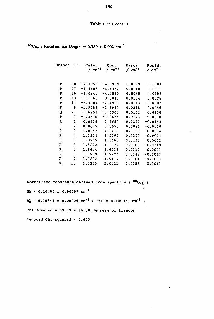
130
Table 4.12 ( cont. )
65Cu2 : Rotationless Origin = 0.289 ± 0.003 cm-1
Branch J" Caic. Obs. / cm-1 / cm-1
P
18 -4.7955 -4.7959 P
17 -4.4408 -4.4332 P
16 -4.0945 -4.0840 P
13 -3.1068 -3.1040 P
11 -2.4909 -2.4911 P
9 -1.9089 -1.9033 0
21 -1.6753 -1.6903 P
7 -1.3610 -1.3628 R
1 0.6838 0.6685 R
2 0.8685 0.8655 R
3 1.0447 1.0413 R
4 1.2124 1.2099 R
5 1.3715 1.3663 R
6 1.5222 1.5074 R
7 1.6644 1.6735 R
8 1.7980 1.7924 R
9 1.9232 1.9174 R
10 2.0399 2.0411
Error Resid. / cm- cm-1
0.0089 -0.0004 0.0148 0.0076 0.0080 0.0105 0.0134 0.0028 0.0113 -0.0002 0.0218 0.0056 0.0161 -0.0150 0.0173 -0.0018 0.0291 -0.0153 0.0096 -0.0030 0.0103 -0.0034 0.0270 -0.0024 0.0117 -0.0052 0.0189 -0.0148 0.0212 0.0091 0.0243 -0.0057 0.0181 -0.0058 0.0085 0.0013
Normalised constants derived from spectrum C 63Cu2 )
Bb = 0.10405 ± 0.00007 cm -1
B' = 0.10843 ± 0.00006 cm -1 ( FSR = 0.100028 cm-1
Chi-squared = 59.19 with 88 degrees of freedom
Reduced Chi-squared = 0.673
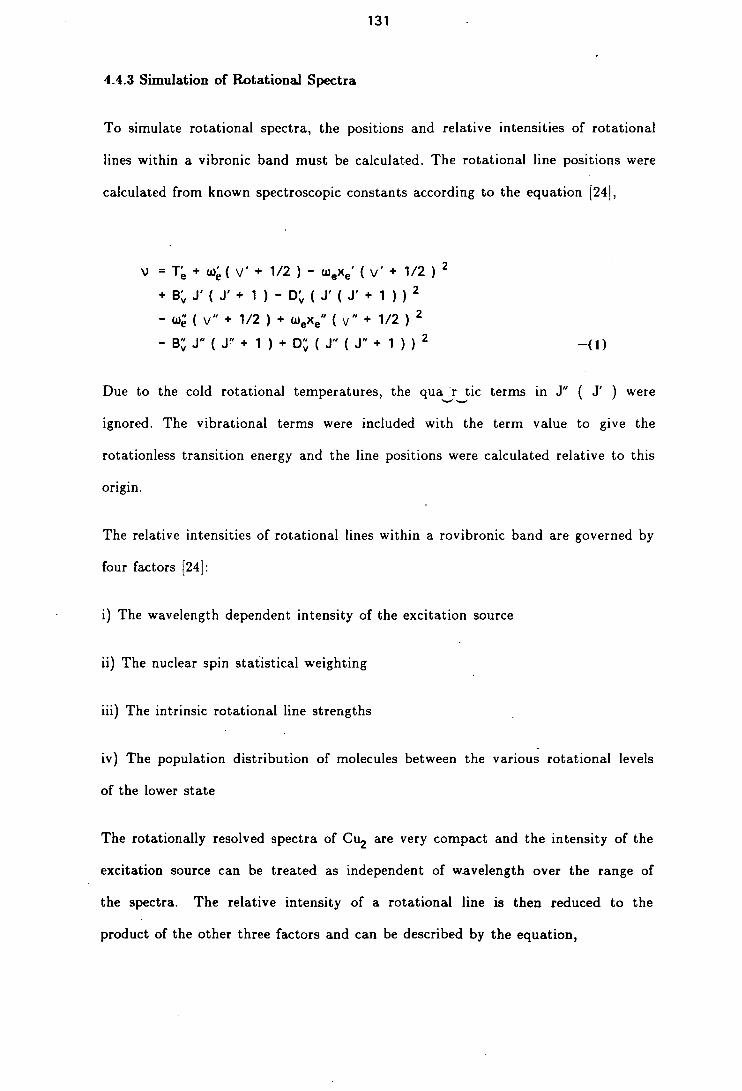
131
4.4.3 Simulation of Rotational Spectra
To simulate rotational spectra, the positions and relative intensities of rotational
lines within a vibronic band must be calculated. The rotational line positions were
calculated from known spectroscopic constants according to the equation [24],
\) = TW(V' 4 1/2)WeXe '(V' 4 1/2) 2
+B,J'(J'+ 1 )—D(J'(J'+ 1 ) ) 2
_W(V"+1/2)+W exe"(V"+1/2) 2
—(1)
Due to the cold rotational temperatures, the qua:r tic terms in J" ( J' ) were
ignored. The vibrational terms were included with the term value to give the
rotationless transition energy and the line positions were calculated relative to this
origin.
The relative intensities of rotational lines within a rovibronic band are governed by
four factors [24]:
The wavelength dependent intensity of the excitation source
The nuclear spin statistical weighting
The intrinsic rotational line strengths
The population distribution of molecules between the various rotational levels
of the lower state
The rotationally resolved spectra of Cu2 are very compact and the intensity of the
excitation source can be treated as independent of wavelength over the range of
the spectra. The relative intensity of a rotational line is then reduced to the
product of the other three factors and can be described by the equation,

132
IR = N" S j "j ' N o e- BJ"( J + 1 ) / kT —(2)
where,
IR = relative intensity of the rotational transition between J" and J'
N" = nuclear spin statistical weighting on rotational level J"
S"j' = rotational line strength for the transition from J" to J'
No e BJ"(J + 1) / kT = population of rotational level J"
Each of the three factors is readily calculated.
Nuclear Spin Statistical Weighting
The total wavefunction of a homonuclear diatomic molecule may be written as the
product of four parts, the electronic-, vibrational-, rotational-, and
nuclear-wavefunctions [24],
i.e.
= e Pr Pv 4) n —(3)
The behaviour of the total wavefunction to the exchange of nuclei depends on the
nuclear spin of the (identical) nuclei. If the nuclear spin is zero or an integral
value, then the wavefunction obeys Bose-Einstein statistics and is symmetric to
exchange of nuclei. Alternatively, if the nuclear spin is half-integral, then the
wavefunction obeys Fermi-Dirac statistics and is antisymmetric to the exchange of
nuclei. The vibrational part of the wavefunction is symmetric to the exchange of
133
nuclei and hence the overall symmetry of the wavefunction is determined by the
product of the rotational, electronic, and nuclear-spin wavefunctions.
Restricting the discussion to Cu 2 , the nuclear spin of both copper isotopes is 1.5
[25] and hence they are Fermions. The ground state of Cu 2 is 1 symmetry with
the consequence that the even rotational levels are symmetric to nuclear exchange
and the odd rotational levels are antisymmetric. To obey Fermi-Dirac statistics,
molecules possessing antisymmetric rotational wavefunctions ( odd J ) must have
nuclei with symmetric nuclear spin wavefunctions and vice-versa. The number of
molecules in the even rotational levels compared to the odd rotational levels will
be weighted by the number of nuclei with odd nuclear spin wavefunctions to the
number of nuclei with even nuclear spin wavefunctions. Since nuclear spin
splittings are very small, each nuclear spin level has almost the same population
and the number of nuclei with symmetric and antisymmetric wavefunctions is
readily calculable from the degeneracies of the symmetric and antisymmetric
nuclear spin levels.
The total nuclear spin angular momentum for Cu 2 can be calculated using a
Clebsch-Jordan series as 3, 2, 1, 0 units. The wavefunctions for the states of 3
and 1 units are symmetric and those of 2 and 0 units are antisymmetric. Allowing
for the ( 21 + 1 ) degeneracy of the states, there are 10 symmetric states to 6
antisymmetric ones. The net result is to weight the odd rotational levels 5 / 3
times the even rotational levels.
Rotational Line Strength
The strength of the individual rotational lines within a vibronic band may be
calculated using the Hönl-London formulae appropriate to the change in angular
momentum and the electronic state symmetries of the lower and upper states. The

134
line strength includes all terms dependent on either J" or J', except for the
Boltzmann factor. Hence the degeneracy of the rotational level is included within
the line strength.
The formulae for the line strengths of P, Q, and R branches for transition between
electronic states where AA = 0, ± 1 are listed in reference [24] and these were
applied in the simulation of the spectra.
Boltzmann Population
If the ensemble of molecules is in thermal equilibrium at a single temperature, then
the proportion of molecules in a given excited rotational level relative to those in
the lowest excited level can be described by the Boltzmann equation [24],
N e / No = (2 J + 1 ) e - BJ(J+1) / kT —(4)
Since the degeneracy factor, ( 2' J + 1 ) is included in the rotational line
strength, only the exponential term is included in the calculation of line intensities.
In simulating the spectra, thermal equilibrium was assumed and the temperature,
T, was treated as a variable parameter which was adjusted to obtain the best fit
between the simulated spectrum and the experimental data.
Computational Details
The spectral simulation program performed three functions. Firstly, the rotational
line positions were calculated. Once the line positions had been calculated, a "stick"
spectrum was generated by plotting at each rotational line position a line whose
height was proportional td the product of the nuclear spin statistical weighting,
the rotational line strength and the Boltzmann population of the ground state
rotational level. The "stick" spectrum was converted to the simulated spectrum by
135
running a laser beam of finite bandwidth over the spectrum. The function of this
convolution was to blend lines that experimentally were unresolvable but which
were resolved in the "stick" spectrum. This was essential to simulate realistic
intensities for bandheads where, experimentally, many rotational transitions were
excited simultaneously and each contributed to the observed ion signal. In all the
simulations performed the laser pulse was treated as Gaussian with a FWHM
bandwidth of 0.04 cm 1 .
4.4.4 Extraction of Rotational Constants
The etalon fringe calibration spectrum and the spectra for the different isotopic -
combinations of copper dimer were recorded simultaneously and stored
independently in the computer. The spectral intensity was stored sequentially in an
array ( See Section 2.6.3 ). Each element in the array was known as a "bin".
Extraction of the rotational constants involved the following steps:
1) Location of the bin numbers corresponding to the spectral peaks and etalon
fringes.
Conversion of the spectra stored as intensity against bin number to spectra of
intensity against etalon fringe number. This was necessary as the constant
frequency marker was provided by the fringes and not the bin number.
Assignment of the lines in the spectrum.
Extraction of the molecular constants by a linear least squares method.
The typical frequency step used in acquiring the spectra was approximately 0.0125
cm-1 . When examined this closely, the spectral peaks showed the intensity
fluctuations expected from the nature of cluster generation and the instabilities in
the lasers. To determine the best value for the location of the peak maximum, a

136
least squares cubic polynomial was fitted through the data and the position of
the peak maximum and its uncertainty were extracted analytically from the least
squares coefficients [26]. More details can be found in Appendix B. This method
was used to locate the peak maxima for both the etalon calibration fringes and the
experimental peaks.
The conversion of the spectrum in bin numbers to a spectrum in etalon fringe
numbers was achieved simply by counting the number of etalon fringes between
the first fringe and the spectral feature of interest. Linear interpolation between
fringes yielded the fractional displacement. Thus the line positions were measured
in free spectral ranges ( FSR's ). The FSR of the confocal etalon used to calibrate
the spectrum was quoted as 0.1 cm-1 . Since it was not possible to simultaneously
calibrate the etalon against known atomic lines, the FSR was kept as a variable
and its value determined by normalisation of the calculated ground state constant
of copper dimer to the value quoted in the literature [1]. Table B2 in Appendix B
lists the values of the FSR obtained by applying this method to the various
spectra examined in this work. The averaged value of the FSR was calculated to
be 0.10008 ± 0.00060 cnf 1 .
Assignment of the lines in the spectrum was most easily achieved by considering
the R-branches of the spectra for the 63 Cu2 isotopic combination since the
R-branch suffered no interference from the Q-branch and the homonuclear 63 Cu2
exhibited a modulation in line intensity between even and odd rotational levels
which aided assignment. The absolute numbering was confirmed from combination
differences [24],
R(J"-1)--P(J"+1)=2B"(J"+2) —(5)

137
using the known value for B' and the good estimate of the free spectral range.
The molecular sample was rotationally cold and all the spectra involved transitions
to v' = 0 or 1 in the respective upper states. Consequently, the data was fitted to
expressions involving only B' and B' and any contributions from the centrifugal
distortion coefficient were ignored. The spectra for all three isotopic combinations
were recorded simultaneously and were fitted in one expression. The data to be
fitted can be described by the following system of equations:
1 0 0 J(J'+1) J"(J"+l) 126 00
\)
128
0 1 0 pJ'(J'+1) pJ"(J"+I) 130
V n 0 0 1 pJ'(J'+1) pJ"(J"+1) B.
where,
V n = frequency of the transition from J" to J'
p 1 = ratio of the reduced masses of 63 Cu2 and 63 Cu65 Cu
P2 = ratio of the reduced masses of 63 Cu2 and 65 Cu2
rotationless transition energy for 63 Cu2
V 128= 00 rotationless transition energy for 63 Cu65 Cu
V 130= rotationless transition energy for 65 Cu2
A least squares solution [27] of this system of equations yielded the spectral origins
for all three isotopic combinations of the dimer and 9 and B". The absolute values

138
of the spectral rotationless origins are arbitrary, but the differences gave the
isotope shifts. It must be noted that this system of equations is only an
approximation to the true system since the formulae relating the rotational
constant for one isotopic combination to that for another isotopic combination
involve Be rather than B ( n = vibrational level ). Strictly, the columns relating
to B should have been replaced by two columns, one relating to Be and one to
e' for both the upper and lower states. However, the columns relating to Be and
ae are nearly linearly dependent and produced instability in the method. It is
shown in Appendix B that the magnitude of the error introduced on making this
simplification is negligibly small.
4.4.5 Collision-Free Lifetimes of the Lower Excited Electronic States of Cu 2
It is possible to measure the lifetime of a molecular state by a time-resolved R2PI
technique [28]. With this technique, a molecule is excited to a state below its
ionisation potential by a pump laser. The power of the pump laser is maintained
sufficiently low that multiphoton ionisation is negligible. After an experimentally
chosen time delay, the sample is irradiated by a second laser to generate
photoions. By monitoring the photoion signal as a function of the time delay
between the two lasers, it is possible to measure the lifetime of the excited state.
Figures 4.13 a-c show the spectra obtained for the A-, B- and C-states by scanning
the trigger to the probe laser with respect to the pump laser. The spectra were
taken by setting the wavelength of the pump laser to a rotational head. The
intracavity etalon was not used to narrow the dye laser output, and hence, many
rotational lines were excited simultaneously. Since Cu 2 was studied within a fully
expanded supersonic molecular beam, the lifetime measured is effectively the
collision-free lifetime.

139
The collision-free lifetimes extracted from the spectra are listed in Table 4.14. The 120)
measured lifetimes are in agreement with published values. The lifetime of the
13-state is seen to be the shortest, in agreement with reference [19] and with the
results of fluorescence emission studies which have found emission from the B-state
to be the most intense [3]. The lifetime of the A-state is approximately three
times longer than that of the B-state. However, both lifetimes are short compared
to that of the C-state. The lifetimes of the different vibrational levels of the
C-state are seen to agree within experimental error. There may be a shortening by
V = 2, but one can not be conclusive due to the large error bound. The lifetime
for v' = 2 is subject to greater error because it was experimentally more difficult
to take the spectrum due to the low Franck-Condon factor between it and v" = 0
in the ground state. Attempts to access the level through a hot band were
unsuccessful due to their low intensity in the cold sample. An attempt was also
made to measure the lifetime of v' = 3 in the C-state via the 3-0 band of the C-X
system. A spectrum was obtained that appeared qualitatively similar to those for
the lower vibrational levels. However, the spectrum was of insufficient quality to
yield a lifetime. -
Figure 4.15 shows the curves fitted through the data after lifetimes had been
extracted. The method of extraction of the collision-free lifetimes of the states will
now be described.

140
Figure 4.13: Lifetime scans of the vibrationless origins of the A-, B-
and C-states of Cu2 . The figure illustrates graphically
the difference in the lifetime between the vibrationless
levels of the three states.

Figure 4.13 : Lifetimes of the 0-0 Bands of the A—X. B—X and C—X systems of 'Cu,
(a) A—X System
B—X System
C—X System
—100 100 300 500 700 900 1100 1300 1500 1700 1900 2100 2300 Time Delay between Pump and Probe Lasers / ns

141
Table 4.14 : Collision-free lifetimes for selected vibrational levels of the A-, B- and C-states of Cu 2
STATE v' Lifetime / ns Error / ns
A 0 105 5
B 0 32 2 B 2 26 4
C 0 746 27 C 1 783 50 C 2 682 96
Notes
1) The errors quoted are derived purely from the numerical fit and take no
account of the finite width of the laser pulses. They should be viewed as
conservative estimates.
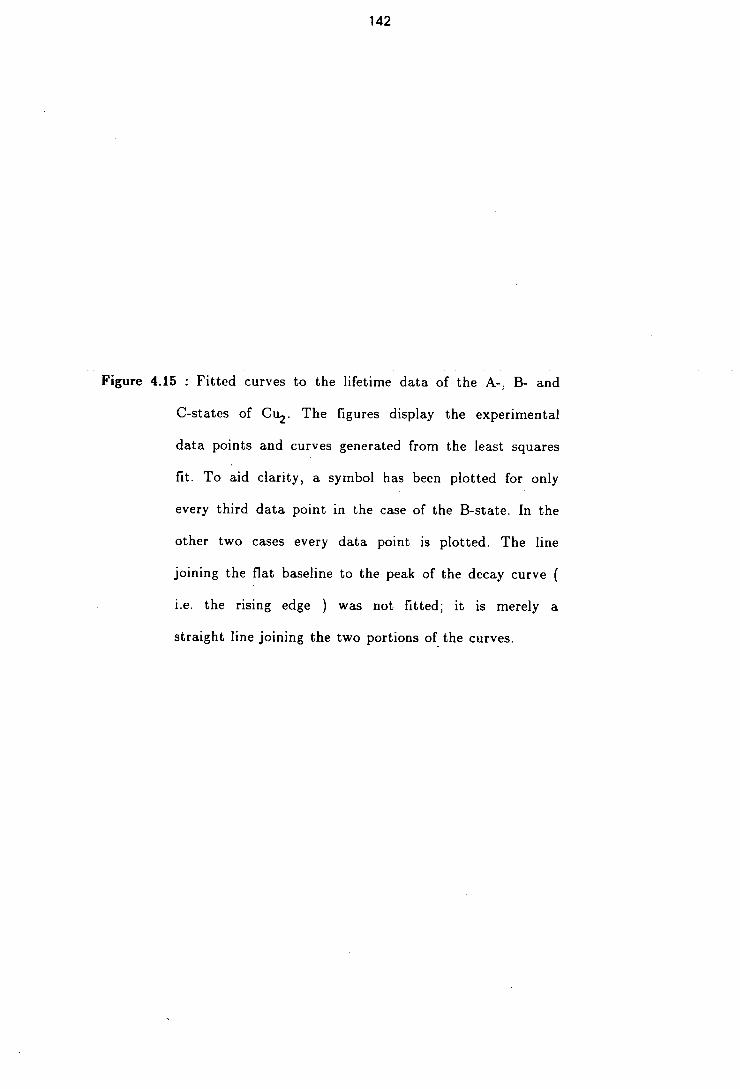
142
Figure 4.15 : Fitted curves to the lifetime data of the A-, B- and
C-states of Cu2 . The figures display the experimental
data points and curves generated from the least squares
fit. To aid clarity, a symbol has been plotted for only
every third data point in the case of the B-state. In the
other two cases every data point is plotted. The line
joining the flat baseline to the peak of the decay curve (
i.e. the rising edge ) was not fitted; it is merely a
straight line joining the two portions of the curves.

Figure 4.15 : Fitted Lifetime Data for the v' = 0
Levels of the A—, B— and C—States of ° Cu2
'tote
-100 0 100 200 300 400 500
Time Delay / ns
tote
-100 -50 0 50 100 150 200
Time Delay / ns
(c) C—State
-100 200 500 800 1100 1400 1700
Time Delay / ns

143
Extraction of Collision-Free Excited State Lifetimes
The experimentally observed ion signal can be described by the equation,
I exp(t) = I nr(t) + I r(t)
- (6)
where,
Iexp(t) = time dependent experimentally observed ion signal
m nr(t) = non-resonant ion signal
Ir(t) = resonantly enhanced ion signal
If one considers an ensemble of N molecules and a timescale with its origin when
the pump and probe lasers are triggered simultaneously, equation (6) can be
described by the equations,
I exp(t) = Knr N ( t < 0 )
- (7)
t exp(t) = Knr No + Kr N i ( t > 0 ) — (8)
where,
Knr = rate of non-resonant photoionisation
K r = rate of resonantly-enhanced photoionisation
N 0(t) = population of the ground state
N 1 (t) = population of the intermediate resonant state
If one further assumes that the excited state decays according to first-order
kinetics, then the state populations for t > 0 are given by,
144
N0(t) = N (1 - exc et )
—(.9)
N 1 (t) = N exc et — (1t
where,
Pexc = proportion excited to the resonant intermediate state
k = first-order decay constant of the excited state
Substituting (9) and (10) into (8)
I exp(t) = Knr N + N Pexc ( Kr - Knr ) — 01)
A plot of in ( Iexp (t) - Knr N ) against t will yield a straight line with a gradient
of A. The value of Knr N can be determined from the ion signal recorded at
negative times.
The above treatment implicitly assumes that the ion signal recorded at time t1 ( t
> 0 ) is due solely to molecules which were excited at time t = 0 and ionised at
time t = t1 . This is an approximation since both laser pulses had finite widths.
The extent to which the approximation holds depends on the lifetime of the
excited state compared to the temporal widths of the laser pulses and can be
estimated from the sharpness of the rising edge of the ion signal. With reference
to figures 4.15 a-c, it is readily seen that the rising edges of the timescans of the
C-state is effectively vertical whereas the rising edges of the A- and B-state spectra
show distinct curvature due to the convolution of the laser pulses with the decay
curve. To extract more accurate lifetime in such cases, the experimentally
observed decay curves should be deconvoluted from the laser pulse. However, the
quality of the experimental data did not merit any attempt at deconvolution, and

145
all the lifetimes reported in this work were obtained by plotting In ( ' exp - Knr N )
against t, for t > 0. The error bounds quoted in Table 4.14 are derived purely
from the numerical method [27] used to analyse the data. They take no account of
the finite widths of the laser pulses. They should therefore be treated as being
rather conservative.
In extracting the lifetimes from the decay curves, the data were inspected for
points which belonged to the flat baseline at the start of the curve, points which
belonged to the rising edge and for points which were part of the true decay curve.
Those points selected as belonging to the flat baseline were averaged. Those
belonging to the rising edge were ignored and the origin of the decay curve, i.e.
when there was no delay between the pump and probe lasers, was chosen by
inspection to ensure none of the points belonging to the rising edge were included
in the decay curve. Although the point chosen as the origin was not necessarily the
true origin, the choice would not have affected the value of the lifetime extracted
from the data.

146
4.4.6 Isotope Shifts of the Rotationless Origins
At a late stage in the thesis, McCaffrey et at [291 published a paper concerning the
isotope shifts of the A- and B-states of Cu2 . They noted that the isotope shifts
measured from their data differed from the values predicted from the known
vibrational constants. The values of the isotope shifts extracted from the data in
this work were re-examined. They were found to agree with the results from
McCaffrey et at. This work was also able to furnish an isotope shift for the
C-state.
Table 4.16 lists the isotope shifts in. the. rotationless origins, extracted from the
experimental data for various bands of the A-X, B-X and C-X systems. Also listed
in the Table are the isotope shifts predicted from known vibrational constants.
It can, be seen from Table 4.16 that whilst the discrepancies in the isotope shifts
for the A- and B-states are approximately equal, the discrepancy in the isotope
shift for the ( 0-0 ) band of the C-state is only approximately half of that in
the A- and B-states.
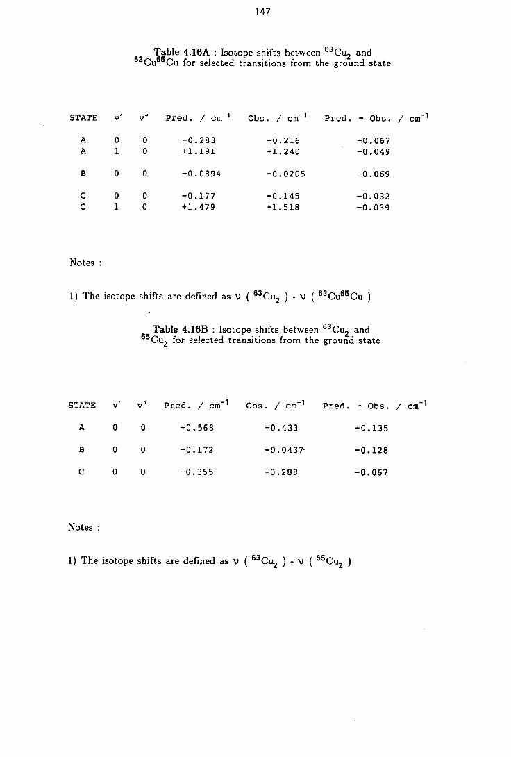
147
Table 416A Isotope shifts between 63Cu2 and 63CU65CU for selected transitions from the ground state
STATE v' v" Pred. / cm-1 Obs. / cm-1 Pred. - Cbs. / cm-1
A 0 0 -0.283 -0.216 -0.067 A 1 0 +1.191 +1.240 -0.049
B 0 0 -0.0894 -0.0205 -0.069
C 0 0 -0.177 -0.145 -0.032 C 1 0 +1.479 +1.518 -0.039
Notes
1) The isotope shifts are defined as v ( 63Cu2 ) - (
63CU65CU )
Table 4.16B : Isotope shifts between 63 Cu2 and 65Cu2 for selected transitions from the ground state
STATE v' v" Pred. / cm-1 Cbs. / cm-1 Pred. - Obs. / cm-1
A 0 0 -0.568 -0.433 -0.135
B 0 0 -0.172 -0.0437 -0.128
C 0 0 -0.355 -0.288 -0.067
Notes
1) The isotope shifts are defined as V ( 63Cu2 ) - v ( 65Cu2 )

148
4.5 Conclusions
The R2PI studies on the A-X and B-X systems of Cu 2 have confirmed the
assignments of the electronic symmetry of the B-state given by Aslund and the
assignment of the electronic symmetry of the A-state given by Lochet. Both are of
1+ (
o ) symmetry and the uncertainty regarding the A-state assignment has
thus been removed. The rotationally resolved spectrum of the C-X system has
been shown to exhibit P, Q and R branches and hence the previously unknown
electronic symmetry of the C-state can be assigned as fl ( 1 )
The collision-free lifetimes of the lowest vibrational levels of .the A-, B- and
C-states have been measured by time resolved 112PI techniques. The lifetimes of
the zero-point vibrational levels of the three states agree with previous
experimental work and the lifetime data on the C-state has been extended to
higher vibrational levels. The state lifetimes span a wide range from 32 ns for the
B-state through 105 ns for the A-state and to 750 ns for the C-state.
The following chapter discusses the electronic structure of the low lying excited
state of Cu2 in the light of the experimental results on the electronic symmetries
and lifetimes presented in this thesis and previous experimental and theoretical
work.
149
REFERENCES
M.D. Morse, Chem. Rev., 86, 1049 (1986)
J.O. Noel!, M.D. Newton, P.J. Hay, R.L. Martin, and F.W. Bobrowicz, J. Chem. Phys., 73, 2360 (1980)
B. Kieman and S. Lindkvist, Ark. Fys., 8, 333 (1954)
J.C.R. Riamps, Comptes. Rendus., 238, 1489 (1954)
D.E. Powers, S.C. Hansen, M.E. Geusic, A.C. Puiu, J.B. Hopkins, T.C. Dietz, M.A. Duncan, P.R.R. Langridge-Smith, and R.E. Smalley, J. Phys. Chem., 86, 2556 (1982)
V.E. Bondybey and J.H. English, J. Phys. Chem., 87, 4647 (1983)
S.S.S. Rao and S.V.K. Rao, Indian J. Pure App!. Phys., 16, 923 (1978)
V.E. Bondybey, J. Chem. Phys., 77 3771 (1982)
D.E. Powers, S.G. Hansen, M.E. Geusic, D.L. Michalopoulos, and R.E. Smalley, J. Chem. Phys., 78, 2866 (1983)
E.A. Rohlfing and J.J Valentini, J. Chem. Phys., 84, 6560 (1986)
N. Aslund, R.F. Barrow, W.G. Richards, and D.N. Travis, Ark. Fys., 30, 4171 (1965)
D.S. Pesic and S. Weniger, Comptes. Rendus. Ser. B, 273, 602 (1971)
J. Lochet, J. Phys. B, 11, L55 (1978)
N.L. Singh, Phys. Rev., 99, 1624 (1955)
D.R. Preuss, S.A. Pace, and J.L Gole, J. Chem. Phys., 71, 3553 (1979)
J.L Gole, J.H. English, and V.E. Bondybey, J. Phys. Chem., 86, 2560 (1982)
G.A. Ozin, S.A. Mitchell, and J. Garcia-Prieto, J. Phys. Chem., 86, 473 (1982)
H. Wiggenhauser, D.M. Kolb, H.H. Rotermund, W. Schrittenlacher, and W. Schroder, Chem. Phys. Lett., 122, 71 (1985)
R.E. Steele, J. Mo!. Spectrosc. 61, 477 (1976)
150
V.E. Bondybey, C.P. Schwartz, and J.H. English, J. Chem. Phys., 78, 11 (1983)
Lambda Physik, FL3001/2 Instruction Manual, Gottingen, FRG (1986)
D.H. Levy, Ann. Rev. Phys. Chem., 31, 197 (1980)
J.F. Ready, Effects of High Power Laser Radiation, Academic Press (1971)
C. Herzberg, Molecular Spectra and Molecular Structure I. Spectra of Diatomic Molecules, Van Nostrand Reinhold, New York (1950)
J.A. Saithouse and M.J. Ware, Point Group Character Tables and Related Data, Cambridge University Press (1972)
A. Savitzsky and M.J.E. Golay, Anal. Chem., 36, 1627
( 1964 )
P.R. Bevington, Data Reduction and Error Analysis for the Physical Sciences, McGraw-Hill, (1969)
M.A. Duncan, T.G. Dietz, M.G. Liverman, and R.E. Smalley, J. Phys. Chem., 85, 7 (1981)
J.G. McCaffrey, R.R. Bennett, M.D. Morse, and W.H. Breckenridge, J. Chem. Phys., 91, 92 (1989)
CHAPTER FIVE
The Electronic Structure of the Lower Electronic States of Copper Dimer

151
5.1 Introduction
The data on the lower excited states of Cu 2 is neither complete nor self-consistent.
There is evidence for the predissociation of the A- and B-states in matrix work and
some evidence for gas-phase predissociation. However, strong emission has been
observed from many vibrational levels of these upper states, suggesting that
fluorescence competes efficiently against any predissociation.
The relationship between the A-, B-, C- and D-states is not obvious. The lifetimes
of the states span a range from approximately 30 ns to greater than 6.5 l.is. The
short lifetimes of the A- and B-states with respect to the C- and D-states could be
indicative of either predissociation of the former two states or of fundamental
differences in electronic structure between the A- and B-states, and the C- and
D-states.
This chapter attempts to find an explanation for the observed energetic ordering of
the excited molecular states, for their symmetries and for their lifetimes. In
attempting to account for the properties of the low-lying excited states of copper
dimer, one must know the number and types of the molecular states derivable from
the appropriate atomic limits. The following section discusses the atomic structure
of Cu.
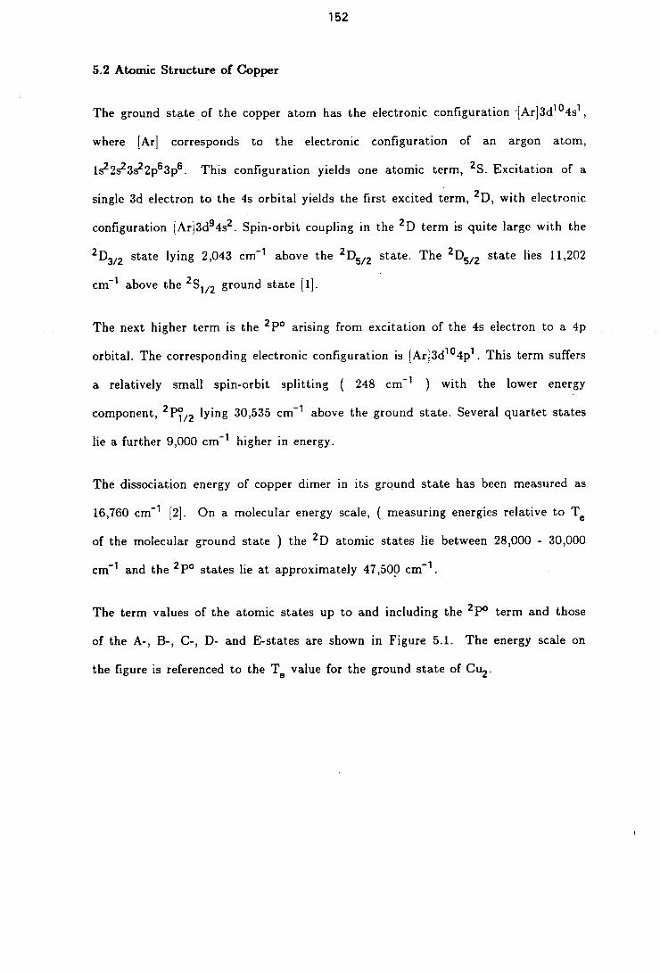
152
5.2 Atomic Structure of Copper
The ground state of the copper atom has the electronic configuration '[Ar]3d 10 4s1 ,
where [Ar] corresponds to the electronic configuration of an argon atom,
1s2s2 3s2 2p6 3p6 . This configuration yields one atomic term, 2 S. Excitation of a
single 3d electron to the 4s orbital yields the first excited term, 2 D, with electronic
configuration (Ar]3d 9 4s2 . Spin-orbit coupling in the 2 D term is quite large with the
state lying 2,043 cm-1 above the2D5/2 state. The2D5/2 state lies 11,202
cm-1 above the 2 S112 ground state [1].
The next higher term is the 2p0 arising from excitation of the 4s electron to a 4p
orbital. The corresponding electronic configuration is [Ar] 3d 10 4p1 . This term suffers
a relatively small spin-orbit splitting ( 248 cm -1 ) with the lower energy
component, 2?I2 lying 30,535 cm-1 above the ground state. Several quartet states
lie a further 9,000 cm -1 higher in energy.
The dissociation energy of copper dimer in its ground state has been measured as
16,760 cm-1 [2]. On a molecular energy scale, (
measuring energies relative to T e
of the molecular ground state )
the 2 D atomic states lie between 28,000 - 30,000
cm-1 and the 2p0 states lie at approximately 47,500 cm -1
The term values of the atomic states up to and including the 2O term and those
of the A-, B-, C-, D- and E-states are shown in Figure 5.1. The energy scale on
the figure is referenced to the Te value for the ground state of Cu2.
153
Figure 5.1: Lowest lying electronic states of Cu and Cu2

Figure 5.1 Schematic Energy Level Diagram for
the Lowest Electronic States of Cu and Cu,
50,000
40,000
2 D3/2
________________ D512
C B A
2s
r3 12
r
30,000
20,000
10,000
., x
L_0
Cu 2 Cu ENERGY/ CM
154
5.3 Correlation to the First Excited Atomic Limit, 2S +2 D
With reference to Figure 5.1, it can be seen that, on energetic grounds, the A-, B-,
C-, D- and E-states of the dimer could all correlate to an asymptotic limit
consisting of one ground state atom ( 2S ) and one excited state atom ( 2D ). A
reasonable starting point is to limit discussion of the nature of the excited
molecular states of copper dimer to those states correlating to the first excited
atomic limit ( 2 S + 2D ). These states can be considered as the " basis set " of
pure molecular states from which the real states derive their principal
characteristics. Although a highly approximate method, it is justified by extreme
difficulty in obtaining good theoretical calculations on transition metal dimers,
especially in excited electronic configurations.
The 2 S + 2 D limit can give rise to three types of states, E, II and A, each of
which can exist as singlet or triplet, and gerade or ungerade [3]. In total, there
are twelve molecular states which correlate to this limit. Only those states
optically accessible via one photon transitions from the 1 Z + ground state, i.e. only
the ungerade states, need be considered further. The electronic configurations
corresponding to these states are listed in Table 5.2.
A satisfactory description of the electronic structure of the low-lying excited states
of Cu2 must meet certain criteria. It must qualitatively account for the number of
states of each electronic symmetry and for their energetic ordering. It must also
provide qualitative agreement with the observed relative transition strengths, and
account for the observed vibrational frequencies and equilibrium bondlengths.

155
Table 5.2 : Electronic configurations of the one-photon accessible molecular states of Cu2 derived from the 2 S ± 2 D
atomic limit
State Configuration
1,3 E +[3da9 ] 1 .. . [4s] 1 U
1,311 [3drr 9 J 3 . . . [4sa]1
1.31.1A [3d6 ] 3 . . . [4saJ1 u
Note
1) All molecular orbitals up to and including the 4sa orbital that are not
explicitly listed are completely filled.
156
It is possible to derive enough states of the correct symmetry from the first excited
atomic limit. However, in order to account for the observed transitions, it is not
possible to treat the excited states in Hund's case (a) [3] coupling scheme with the
assumption that the spin-selection rule, AS = 0, is strongly obeyed. The presence
of two O states can only be accounted for by assigning one state as the 1 state
and one as the 0 component of the 311 state. The C-, D- and E-states would
then have to be assigned as either the 1fl U state or l components from either the
311, 3A
U or states. As suggested from the lifetime data in this study and
supported by the previous time-resolved fluorescence emission studies [4] [5], the
B-X transition carries most of the oscillator strength. Therefore, it is reasonable to
assume that, in this model, it should be assigned as the fully allowed transition to
'E + state, forcing the A-state to be assigned to the state.
To proceed further with the description of the states, three reasonable assumptions
must be made
The bonding due to the molecular orbitals derived from the 3d-orbitals on the
copper atoms is negligible compared to that from the molecular orbitals derived
from the atomic 4s-orbitals.
The strength of bonding due to the molecular orbitals, as expected from
elementary overlap considerations, decreases in the order, a > TT > 6
The energy associated with electronic restructuring when an electron is
promoted from a 3d-based molecular orbital to the 4sa orbital is independent of
the symmetry of the d-based molecular orbital.
With these assumptions, it is possible to qualitatively rank the molecular states
according to energy. This is shown in Figure 5.3.
157
Figure 5.3 : Schematic energy level diagram for the ungerade
electronic excited states of copper dimer correlating to
the 2 S + 2 D atomic limit. Within each manifold the
order is predicted from the three assumptions listed
previously in the text. The relative spacing of the triplet
and singlet manifolds, determined by the electron
exchange energy, is schematic.
Figure 5.3 Schematic Energy Level Diagram for
the ungerade states of Cu 2 correlating to 2S + 2D
Energy
lug
3rL
158
From Figure 5.3, it can be seen that the lowest l state is the l component from
the 311U state. Within the triplet manifold , the 3 E state lies at highest energy
and the state lies between the 3fl and states. The only other state is
the 'II U state itself. This state is known to lie higher than the 311w state, due to
the exchange energy of the latter j61. Whether it lies above or below the 3 A u and
3 E states depends on the relative magnitudes of the exchange energy and the
energy separation between the states within the triplet manifold.
The 311 U state arising from the 2 S + 2 D atomic limit is an inverted multiplet (3},
meaning that the component with zero angular momentum lies at highest energy.
Therefore the l component of the 311w state will lie below the A-state and the
assignments given to the C-, D- and E-states can therefore be limited to the 1fl
3 state and the l components from the 3,&U and E+ states.
On comparing the observed energetic ordering of the states to the predicted order
based on the assignments of the A- and B- states given previously, it is seen that
agreement is poor. The B-state, which is known experimentally to lie below the
C-, D-, and E-states, is assigned to the state of highest energy. The lifetime data
is even more conflicting. The lifetimes of the A- and C-states are markedly
different and it is difficult to reconcile a shorter lifetime, ignoring predissociation,
applying to the 311 state than to the 11I state. Therefore, the C-state would
have to be assigned to the l component of a triplet state. The D-state, which
has an even longer lifetime than that of the C-state, would then have to be
assigned to the l component of the remaining triplet state. By default, the
E-state, for which no lifetime data exists, would have to be assigned as the 1 11
state. However, this still leaves unexplained the fact that three states that are
formally components of the triplet states exhibit lifetimes ranging from 100 ns
through 750 ns to greater than 6.5 Us.

159
Even arguing that the D-X and E-X transitions have not been definitively assigned
to Cu2 , the discrepancy between the lifetimes of the A- and C-states still remains
and the energy of the B-state is still low with respect to the other states. The
state assignments possible using this simplistic model provide a poor description of
the observed spectroscopic data.
The failings of the model can be broken down into two separate factors. Firstly,
the three assumptions on which the predicted energetic ordering of the states was
based may be invalid. Secondly, the model itself may be too simple and the
assumption that the states can be considered as derived purely from the 2 + 2 D
atomic limit could be invalid due to the intrusion of states from higher asymptotic -
limits. To address these factors requires recourse to theoretical calculations.
Most of the theoretical work on copper dimer has concentrated on the ground state
[7-15]. The bonding has been shown to be predominantly through 4s orbital
interactions, with the 3d orbitals remaining essentially atomic in nature [9] [12-15].
The 3d-electrons do play a significant role in determining the bond-dissociation
energy through increased correlation in the molecule with respect to the atom.
The correlation energy increases the depth of the potential well with respect to the
value calculated by assuming that the 3d electrons are frozen in the atomic cores.
For example, Dixon and Robertson [7] calculated a dissociation energy which was
only 45 % of the experimental value when the d-electrons were treated as a frozen
core, but which rose to 85 % of the experimental value upon relaxing the
d-electrons.
Several sets of calculations have tackled the ordering of the molecular orbitals in
the ground state of copper dimer [14-15] [17.18]. Although the absolute energies
vary from one calculation to another, a clear and consistent pattern emerges as to
the ordering of the molecular energy levels: this is shown in Figure 5.4. In order

160
of decreasing energy, one finds first the 4s 9 bonding orbital, and lying a further 5
eV lower in energy the 'non-bonding' band of 3d-electrons, which is approximately
1 eV in width. The energetic ordering of the orbitals within the d-band is as
expected from basic atomic overlap considerations. Therefore, there appears to be
strong theoretical support for the first and second assumptions used in the simple
model describing the electronic structure of the excited states, at least if bonding
nature and ordering of the orbitals for the ground state can be transferred to the
excited state. It thus appears valid to treat the 3d electrons as essentially
non-bonding.

161
Figure 5.4: Molecular orbital energies of the ground state of Cu 2
calculated by ab initio methods.

Figure 5.4 : Molecular Orbital Energies of the Cu 2 Ground State
Energy
4su1 0 eV ( arbitrary origin )
3dg ca-5eV
3d,r,
3dö
306
3d;
3do, ca-6eV
162
The third assumption in the model regards the degree of electronic reorganisation
of orbitals not directly involved in the transition. Miyoshi et al [19] have
calculated the extent of reorganisation upon ionisation of Cu 2 . They obtained a
value of 0.4 eV for removal of a 4s electron and a value of 5.7 - 6.2 eV for
removal of a 3d electron. They argued that d-electron ionisation resulted in a high
degree of electronic reorganisation because the d-orbitals should be thought of as
localised on individual atoms. The creation of a hole on either atom would then in
resultA significant d-level reconstruction. With regard to electronic transitions, the
absolute magnitude of d-electron relaxation energy is not important. Rather, the
important factor is whether the energy remains constant regardless of the orbital
from which the electron has been promoted. Perhaps the most useful calculations
that provide data on which to test this assumption are those of Witko and
Beckmann [17]. These authors carried out ab initio multi-reference double
excitation configuration-interaction ( MRD Cl ) calculations on the ground and
excited states of copper dimer. They calculated the adiabatic transition energies for
the promotion of an electron from a 3d-based orbital to the 4sa molecular orbital.
They also listed the energies for the various molecular orbitals. A discrepancy in
the energy gap between the molecular orbitals involved in the transition and the
adiabatic transition energy would indicate that some electronic restructuring had
accompanied the transition. If the relaxation energy is defined by,
Relaxation Energy = Adiabatic Transition Energy - Energy Gap Between Orbitals
then the relaxation energy measures the extent of electronic reorganisation
associated with the transition. For transitions to triplet states, an "effective"
relaxation energy can be defined by the above equation, differing from the normal
relaxation energy by the inclusion of the core-valence exchange integral for the
triplet state.

163
Table 5.5 : Relaxation energies accompanying electronictransitions from the d-based Molecular orbitals on Cu 2 to the 4sa Orbital.
Relaxation Energy / hartrees Orbital Vacated Singlet State Triplet State
3da -0.3422 -0.3624 3d71 9 -0.3484 -0.3808
3d6 -0.3463 -0.3584 3d5 9 -0.3469 -0.3539
3dTr -0.3618 -0.3342 3d09 -0.3796
Notes
The above values were calculated using the expression described in the text.
Orbital and adiabatic transition energies were taken from [17].
1 hartree = 2.19462 x 10 cm-1
164
Table 5.5 lists the relaxation energy for the promotion of a single electron from a
3d derived molecular orbital into the 4s orbital. Energies for the formation of
singlet and triplet states are quoted.
It can be seen that the relaxation energies for the transitions generating singlet
states are consistent to approximately ± 700 cm -1 . Unfortunately, the energies for
the triplet states are only consistent if given an order of magnitude more latitude.
The authors do not quote the accuracy of their calculations and although the
consistency between the relaxation energies for the singlet states is ( probably )
within their accuracy, the spread for the triplet states suggests that the
assumption of equal relaxation energies is not necessarily valid.
In the light of this conclusion, the importance of the discrepancy between the
experimental energetic ordering of the states and the order predicted, based on the
three assumptions listed previously, should be relaxed.
The simplistic approach to the assignment of the lower excited states of Cu 2 as
essentially pure states correlating with the 2 S + 2 D limit, however, remains
unsatisfactory because it cannot readily account for the observed lifetimes and the
energetic ordering of the states. It is evident that a satisfactory description of
these states will only be possible by considering the likelihood of 'intruder states'
from higher atomic limits penetrating into the region of the A-, B- and C-states
and mixing with them. The next section develops this theme.

165
5.4 Molecular States of Cu2 Correlating to Higher Asymptotic Limits
5.4.1 2 D + 2D Atomic Limit
This limit gives rise to 30 molecular states in Hund's case (a) coupling scheme.
All the states possess the electronic configuration [3d]18(4sa9)2(4s(Y)2 i.e. the
molecular orbitals derived primarily from the atomic 4s orbitals are completely
filled. Any bonding in the molecule will therefore be through the d-shell and will
be essentially negligible due to the highly contracted nature of the shell [20].
Since, even in Hund's case (c) coupling, only 12 out of the 59 states derived from
the 2 D + 2 D limit are optically accessible via one-photon transitions from the
ground state, these states can be thought of as forming an essentially transparent,
non-bonding band that has little effect on the spectroscopically accessible states
lying below it.
5.4.2 2 S + 2po Atomic Limit
The electronic configurations of the states of interest in one-photon transitions
from the ground state which correlate to this atomic limit are listed in Table 5.6.
The asymptotic limit lies at approximately 47,500 cm -1 on the molecular energy
scale, suggesting that for the states to play a significant role in the spectroscopy of
the lower excited states, they would have to be very strongly bound, with
dissociation energies in the region of 25,000 - 30,000 cm -1 . This is almost double
the binding energy of the ground state. The limited theoretical calculations
available tend to suggest that transitions to the states derived from this limit lie
at higher energy than the transitions to the A-, B- and C-states.
166
Table 5.6 : Electronic configurations of the one-photon accessible molecular states of Cu 2
correlating to the 2 S + 2 P atomic limit.
State Configuration
L.0 [4sa9 ] 1 .. . [4paJ
13n fl u [4s09 ] 1 . [ 4p1T]1
Note
1) All molecular orbitals up to and including those derived from the 3d atomic
orbitals are filled. All other orbitals not explicitly listed are empty.

167
Hare et at [18] have performed an extended Mickel calculation on Cu and
predicted that electronic transitions to orbitals due to the 4p-4p interactions lie at
considerably higher energy than the experimentally observed energy of the A-, B-
and C-states. The authors suggested that mixing between the molecular orbital
derived from the 4p atomic orbitals and the 4so orbital would serve to lower the
energy of the latter.
Anderson [21], also using extended Hückel theory, has predicted the 3dir 9 + 4sa
transition to occur at 2.18 eV and the 3do 9 + 4s to occur at 2.85 eV. The
lowest lying transition involving 4p orbitals occurred at 4.24 eV. This was the
transition 4sa9 . 4r• The agreement between experiment and calculations is
quite good for the lower excited states, though this may be due to the use of
relatively accurate experimental data as part of the input required in this type of
calculation. The validity of the calculations on the higher excited states must
remain questionable due to the lack of correspondingly good experimental data on
which to base the higher state energetics.
Ozin et at [22] have also performed calculations on molecular states derived from
the 2 S + 2 PO atomic limit. They used the SCF-X-SW method and assigned the
A-X transition to the promotion 3d1T 9 - 4sa and the B-X transition as 4sa 9 -1-
4sa. The transitions from the 3d-orbitals or the 4sa orbitals 9 orbital to the 4p ff
were calculated to occur between 260 - 220 rim. It must be noted, however, that
the results of their calculations on the orbital energies are in disagreement with the
more rigorous ab initio calculations and, in contrast to the ab initio work, the
authors calculated the 4sa orbital to lie below the 3d7T 9 and Ma u orbitals.
The quality of the theoretical work on the molecular states of Cu 2 correlating to
the 2 S + 2p0 limit is not high. The methods used are semi-empirical and are
influenced by the experimental data input into the calculations. Hence, although
168
the studies tend to suggest that the states correlating to the 2 S + 2 P atomic
limit lie at too high an energy to be considered in the assignment of the lower
excited molecular states of Cu 2 , this evidence must be treated with caution.
5.4.3 'S (Cut ) + S ( Cu ) Ion Pair Limit
The final limit which deserves inclusion amongst the set that should be considered
as possible asymptotic limits for the low-lying excited states of Cu 2 is the ion pair
limit Cu ( 1S ) + Cu ( 'S ). This limit gives rise to two molecular states, one
of 'E + symmetry and one of 'Z + symmetry. Only the ungerade state need be
- considered since the gerade state will not interact with the ungerade states that
are one-photon accessible from the ground state. This ionic limit lies at 69,166
cm on the molecular energy scale, but due to the strong Coulombic attraction at
large internuclear distance, the energy of the state drops to that of the 2 S +
atomic limit when the ions are still 5.37 A apart. It appears reasonable to treat
the ion pair state as having an "effective" asymptotic limit at a considerably lower
energy than its true value.
Many theoretical calculations have assigned the B-state as arising from the
electronic promotion 4s09 + 4sa which formally correlates to the ion pair limit [7]
[19] [22]. Miyoshi et al [19] calculated a transition energy of 2.4 eV for the
electronic promotion 7a9 (4s) + 7a (4s) generating the singlet state and a
transition energy of 4.07 eV for the promotion 31t g (3d) • 7a (4s) generating the
triplet state. The first result is in good agreement with the experimental data and
supports the assignment of either the A-X or B-X systems to the 7a9 (4s) - 7a
(4s) transition. The second result, however, argues against the assignment of the
remaining state ( A or B ) to the 0 component of the 311U state. However, the
calculation was performed in D,, symmetry and the authors showed that if the
hole in the d-orbitals was localised on one atom or the other, then under the lower

169
symmetry ( C, ), the transition energy for the promotion 31T 9 (3d) + 7o (4s)
dropped to 2.4 eV, in much better agreement with experiment.
Witko and Beckmann's [17] calculations also support the hypothesis that the state
corresponding to the 7a9 (4s) -. 7a (4s) promotion lies at an energy close to the
A-, B-, and C-states. They found the 4sa 9 - 4sa transition had an adiabatic
transition energy of 23,600 cm 1 , whilst the 311 U state corresponding to the 3d7T 9 +
4sa transition had an energy of 19,600 cm -1 . Although the calculated energies do
not agree with the experimental ones, they are similar and the order matches that
observed experimentally. It is significant that the authors quote the energy of the
state correlating to the 2 S + 2 D limit substantially higher at 27,150 cm,
which is very close to the reported transition to the E-state. Although they have
not published the transition energy for excitation to the complementary 1 Z + state,
one can expect it to lie at higher energy than its 3 E counterpart. The
calculations thus support the argument against the state from the 2 S + 2 D
limit playing a major role in the A- or B-states.
Joyes and Leleyter [23] have also performed ab initio work on copper dimer. They
found the 'Z + state arising from the ion pair limit to lie approximately 6 eV above
the ground state, considerably higher than the value calculated in other studies.
The remaining theoretical work on the ion pair state is semi-empirical in nature.
Ozin's [22] SCF-Xot calculations lead him to suggest that the B-state arises from
the electronic promotion 4sa 9 + 4sa, whereas Anderson's [21] extended- Mickel
calculations suggested that the bonding - antibonding transition is dissociative in
nature. The results from the theoretical work are therefore contradictory although
the weight of evidence is in favour of the ion pair state, rather than one of the
states from the 2 S + 2p atomic limit, playing a role in the spectroscopy of the
low-lying excited states of Cu2.

170
There is also circumstantial experimental evidence to support the presence of a
deeply descending intruder state. In 1983, Powers et al [24] located five band
systems of Cu2 lying in the UV between 300 - 260 nm. One of the band systems,
named system II in their nomenclature and subsequently renamed the C-X system
[20], had a low vibrational frequency of only 116 cm -1 ( compared to the ground
state frequency of 266 cm ). This state was later studied in more detail by
Rohifing and Valentini [2] who monitored fluorescence emission. The latter
authors noted that the state had a transition dipole moment that was strongly
dependent on the internuclear separation, r, a feature that is characteristic of a
state formed by an avoided crossing. The transition dipole moment was greater at - - -
larger separations and the authors suggested one possible avoided crossing could
occur between a repulsive state from the 2 S + 2 D asymptote and a strongly bound
curve from the 2 S + 2 P' asymptote. In this case, the C-state has 2 S +
character at small internuclear separation and 2 S + 2 p*character at large
internuclear separation, with the latter carrying much more oscillator strength to
the ground state.
Figure 5.7 shows the potential curves for the lower excited electronic states of Cu 2 .
At present, the origin of the intruder state which might be involved in an avoided
crossing forming the C-state has not been investigated. The nature of the state
formed by the avoided crossing may favour the suggestion that it is the 'Z + state
from the ion pair limit rather than a state from the 2 S + 2po limit that interacts
with a state from the 2 S + 2 D limit. Both the low vibrational frequency and large
internuclear separation ( 2.73 A ) are characteristic of an ion pair state. The
other state generated from the suspected avoided crossing which forms the G-state
could descend further and intrude into the lower lying excited electronic states of
Cu2.

171
Figure 5.7 : Potential curves for the lower excited electronic states -
of Cu2

>' Im
25000 C) C Iii
20000
Figure 5.7 : RKR Potential Energy Curves
for the X—, A—, B— and C—states of Cu,
2.10 2.70 3.30 3.90 4.50 5.10 5.70 6.30 6.90
Internuclear Separation / A
35000
30000
40000
10000
55000
45000
15000
50000
5000
0 1.50
F 25 F 2S
2 Do
F'S
I. 'S
Is

172
It remains to be answered whether the inclusion of an intruder state from a higher
atomic asymptotic limit provides a better explanation of the experimental
observations on the lower excited electronic states of Cu 2 than did the simple
model presented earlier, which assumed the states correlated purely to the 2 S ± 2 D
limit. The states correlating to the 2 S + 2po or 1 S (. Cu ) + 'S ( Cu )
asymptotic limits are expected to carry more oscillator strength to the ground
state than states correlating to the 2 S + 2 D atomic limit. If the intruder state is
from one of these two higher limits, then the effect of it mixing with states from
the 2 S + 2 D limit would be to increase their transition strength to the ground
state. Since the B-X system carries the greatest oscillator strength of the lowest
excited states of Cu 2 [25], it is likely that it is the B-state that is most influenced
by the intruder state. It is therefore believed that the symmetry of the intruder
state is . The A-state, which shares the same symmetry as the B-state would
also pick up some character from the intruder state. The candidate states for the
intruder state can therefore be limited to the 'E + and the 3 fl 0 states from the 2 S
2 1 pair . . 1 + P° limit, or the from the ion pair limit. Whilst both E. states should be
strongly radiatively coupled to the ground state, transitions from the ground state
to the 3fl state are formally forbidden. Intensity may be gained through spin-orbit
coupling.
One hypothesis that may be proposed is that the A-state arises from the O
component of the 311 state correlating to the 2 + 2 D atomic limit with a little
character from the intruder state. The B-state would then arise mainly from the
intruder state, and the C-state would be the 11T U state correlating to the first
excited atomic limit. The D-state would be a l component of a triplet state
correlating to the 2 S + 2 D atomic limit. The E-state could then either be the l u
component from the remaining triplet state or the state itself, with both states
correlating to the first excited atomic limit. Since the E-state has been observed

173
in gas-phase emission, it is likely to be the singlet state since the triplet state
would probably have a similar lifetime to the D-state and would not be readily
observed in gas-phase emission.
If one uses the C-state as a model for a pure, unperturbed singlet molecular state
arising from the 2 S + 2 D limit and the D-state as a model for a triplet state, then
the energetic ordering, lifetimes and equilibrium bondlengths of the states can be
rationalised. The C-state has a relatively long lifetime which is to be expected
since the atomic transition from which it derives its oscillator strength is strongly
forbidden. It also has a longer equilibrium bondlength than the ground state, in
keeping with the assumed electronic promotion of a non-bonding / weakly
antibonding electron to a strongly antibonding orbital. The D-state has an even
longer lifetime than that of the C-state, in keeping with the spin forbidden nature
of the transition.
The shorter lifetimes and longer equilibrium bondlengths of the A- and B-states
compared to the C-state would then be due to the influence of the intruder state.
Experimentally, properties of the A-state such as its equilibrium bondlength and
its lifetime are seen to lie between those of the B- and C-states. This is expected,
since it lies between the two extremes of a state correlating to the 2 S + 2 D atomic
limit and one correlating to a higher atomic limit. The mixing-in of character
from the intruder state into the would therefore appear to lengthen the bond
and shorten the lifetime with respect to the "pure" 2 S -f- 2 D derived C-state.
The final experimental results that merit discussion are the observed
photoprocesses such as predissociation and relaxation mechanisms within matrix
cages. The 3 E state correlating to the lowest 2 S + 2 S atomic asymptote is the can
only state thatAinduce predissociation. In Hund's case (c), this state splits into l u
and O components, and from symmetry considerations [3J only the first component
174
can predissociate O states. With reference to Figure 5.7, it is very hard to
visualise a state which can simultaneously predissociate the lower vibrational levels
of both the A- and B-states. Hence, Powers et al [26], who invoked predissociation
of the B-state to explain its short lifetime, Bondybey et a! [5] who suggested
predissociation of the A-state to explain the marked vibrational dependence of its
lifetime and Gole et al 1271 who used predissociation of the C-state to explain the
observation of a curtailed vibronic progression from the ground state cannot all
have been correct.
The strongest evidence for gas-phase predissociation is that on the A-state.
Although far from conclusive, it does attempt to pin down the 3 E state as having
a perturbative effect on the low vibrational levels of A-state, though none was
observed during these studies on the zero-point vibrational level. The suggestion
that the shorter lifetime of the B-state compared to that of the C-state was
evidence of predissociation is probably then due to an error in assuming that the
B- and C-states were of the same origin. Similarly, the suggestion of
predissociation of the C-state was made before its bondlength had been established.
The low intensity of the vibronic bands from the zero point level in the ground
state to v' - 3 or higher in the C-state are in fact due to poor Franck-Condon
factors.
The matrix cage recombination data can also be addressed. Excitation of the A-
and B-states isolated within a matrix provided strong evidence for predissociation
of both states by the 3 E state. The observation of predissociation in both states
in a matrix is more easily rationalised through the perturbations introduced by the
matrix environment. Excitation of the D-state also yields emission from the
B-state, emission from the 3 E + state but none from the A-state. This suggests that
the B-state is predissociated directly by the 3 E and not through the A-state and

175
that the A-state does not interact with the D-state. The non-interaction between
the A- and D-states can be understood because the A- and B-states are of the
same symmetry and would then not cross the D-state potential curve in the same
region.
The hypothesis presented above appears to fit the experimental data. The exact
origin of the intruder state remains unclear, however. The low vibrational
frequency and large internuclear separation of the C-state can be taken as evidence
that that the ion pair state undergoes an avoided crossing with one of the states
from the 2 S + 2 D atomic limit forming the G-state. The B-state could then be the
other state generated from this avoided crossing. If this were the case, it would
agree with the results of many calculations that assign the B-X transition as the
promotion 4sa g - 4s. The electronic promotion is from a bonding to an
antibonding orbital and this would account for the observed lengthening of the
bond. However, the B-state has a high vibrational frequency and, although it has
the longest bondlength of the lowest states of Cu 2 , the bondlength is not
significantly longer than that of the ground state. Neither observation is
characteristic of a state derived from an ion pair limit.
The B-state could also be the O component of the 311U state correlating to the 2 S
+ atomic limit. However, the spin-orbit splitting in the 2po atomic state is
quite small and it might be supposed that the molecular state would tend more to
Hund's case (a) coupling. The B-X system would not then be expected to be as
strong as is experimentally observed. The electronic promotion generating the 31l
state also involves the promotion of a bonding electron to a different bonding
orbital and one would intuitively expect the bondlength of the B-state derived
from the 31I U state to be shorter than that of the C-state, which is believed to be
generated by the promotion of an electron from a non-bonding orbital to an

176
antibonding orbital. This is not observed experimentally.
A third possibility would be to assign the B-state to the 1 state correlating to
the 2 S ± 2O atomic limit. This would account for the observed bondlengths , as
the electronic promotion is from a bonding to an antibonding orbital. However, it
is difficult to justify the high dissociation energy required for the state to influence
the low-lying excited states since it is generated from a bonding - antibonding
transition.
The B-state probably takes some character from all three states and some from the
state correlating to the 2 S + 2 D limit. The major contribution probably comes
from the 1 E state correlating to the ion pair limit. Alternatively, states from
even higher atomic limits may be responsible for the intruder state. Excitation of a
3d electron in the copper atom to the 'Ip orbital yields a group of atomic quartet
states 9,000 cm higher than the 2p0 states, and a group of doublet states 4,000
cm higher than the quartet states. Although these states are energetically
further from the lower excited electronic states, theoretical calculations have
suggested that if the d-hole present in these states was localised, then the state
would be relaxed through greater molecular correlation energy. This may
compensate for the higher asymptotic limit.
177
5.5 Conclusions
When the energetic ordering, transition strengths and lifetimes of the low-lying
excited state of Cu2 are considered together, simply assigning them as pure states
correlating to the first excited atomic limit is unsatisfactory. Better agreement
with experimental data is obtained if a state of O symmetry from a higher
asymptotic limit is assumed to mix with the A- and B-states. The mixing is
thought to occur predominantly with the latter. The prime candidate for the
intruder state is the 1 Z' state correlating to the ion pair limit. The A- and
B-states will ultimately dissociate to the first excited atomic limit, however, near
to their potential minima, they may have more character from a different
configuration.
The C- and D-states are thought to represent relatively pure singlet and triplet
states correlating to the 2 S + 2 D atomic limit, respectively. The greater lifetime
of the D-state compared to the C-state may suggest that the spin selection rule,
AS = 0, is still quite valid and the molecule is not best described by Hund's case
(c) coupling scheme.
To conclude this chapter, it must be reiterated that the state assignments
presented are speculative though not, I believe, at odds with the experimental
observations or with theoretical calculations. Clearly, much more work will be
required, both theoretically and experimentally, before a full understanding of the
electronic structure of the low-lying excited states of Cu 2 is acquired.
High quality calculations are required on the molecular states correlating to atomic
limits above the 2 S + 2 D limit to obtain a better picture of any that are deeply
bound and could mix with the low-lying excited electronic states. As illustrated
by the difficulties encountered in calculations on the ground state, correlation
I

178
effects between the 3d-electrons are important and are likely to become even more
important with the excited states, many of which are formed by the promotion of
an electron out of the 3d-based molecular orbitals thus opening up the d-shell.
More experimental data is also required to put the low-lying excited states into
context. The electronic symmetry of the C-state should be determined. Since
the G-X transition is a one-photon transition, the C-state is of either of 1 or O
symmetry. If it were found to be of 1 symmetry then it could not be the resultant
state from the avoided crossing between the ion pair state and a weakly bonding /
non-bonding state from the 2 S + 2 D atomic asymptotic limit. Finding it of O
symmetry would only add circumstantial evidence to the hypothesis that the
C-state is formed by an avoided crossing involving the ion pair state.
The longer lifetime of the C-state compared to the A- and B-states is thought to
be indicative of a relatively small transition dipole moment between the ground
state and a singlet state arising from the 2 S + 2 D limit. It cannot be ruled out,
however, that the longer lifetime is due to the C-state being a l component
of a triplet state. Determination of the state symmetries and gas-phase transition
strengths to the D- and E-states from the ground state would help to clarify the
position. The D-state is known to have a much longer lifetime than the C-state
and if the transition coupling it to the ground state were shown to be typical of
that for a triplet state correlating to the 2 S + 2 D limit, then this would support
the view that the C-state is a singlet state from this limit. The E-state was
observed in gas phase emission and could possibly be the state from the 2 S +
2 D limit, or it could be the other state generated by the avoided crossing thought
to generate the C-state. If the latter were the case, then the B-state could not be
the result of the same avoided crossing. Knowledge of the electronic symmetries of
the D-, E- and C-states would help to clarify their relationship, if any, to the A-,

179
B- and C-states.
Similarly, more information on the higher electronic states ( systems I - V ) can
only help elucidate which, if any, states are intruding into the lower states. These
experiments are all to be performed and progress is being made in this laboratory.
Much remains uncertain about the electronic spectroscopy and structure of Cu 2 .
Opening the d-shell results in a large number of states in which electron
correlation is important and spin-orbit couplings can be large. It is clear that we
are a long way from theoretically understanding and experimentally characterising
the effects of open d-shells on the electronic structure of molecules.
And to think, Cu2 is probably the simplest transition metal cluster

180
REFERENCES
1. C.E. Moore, Nat!. Bur. Stand. Circ. 467 (1949)
2. E.A. Rohifing, and J.J Va!entini, J. Chem. Phys., 84, 6560 (1986)
3. G. Herzberg, Molecular Spectra and Molecular Structure I. Spectra of Diatomic Molecules, Van Nostrand Reinhold, New York (1950)
4. R.E. Steele, J. Mo!. Spectrosc., 61, 477 (1976)
5. V.E. Bondybey, G.P. Schwartz, and J.H. English, J. Chem. Phys., 78, 11 (1983)
6. J.N. Murrell, S.F.A. Kettle, and J.M. Tedder, Valence Theory, Wiley (1970)
7. R.N. Dixon and I.L. Robertson, Mo!. Phys., 36, 1099 (1978)
8. H. Tatewaki, E. Miyoshi, and T. Nakamura, J. Chem. Phys., 76, 5073 (1982)
9. C.W. Bausch!icher, S.P. Walch, and P.E.M. Siegbahn, J. Chem. Phys., 78, 3347 (1983)
10. H.J. Werner and R.L. Martin, Chem. Phys. Lett., 113, 451 (1985)
11. K. Raghavachari, K.K. Sunil, and K.D. Jordan, J. Chem. Phys., 83, 4633 (1985)
12. C.W. Bausch!icher, S.P. Walch, and P.E.M. Siegbahn, J. Chem. Phys., 76, 6015 (1982)
13. C.W. Bausch!icher, Chem. Phys. Lett., 97, 204 (1983)
14. H. Tatewaki, and S. Huzinaga, J. Chem. Phys., 72, 399 (1970)
15. I. Shim and K.A. Gingerich, J. Chem. Phys., 79, 2903 (1983)
16. M. Pelissier, J. Chem. Phys., 75, 775 (1981)
17. M. Witko and H.O. Beckmann, Mo! Phys., 47, 945 (1982)
18. C.R. Hare, T.P. Sleight, W. Cooper, and G.A. Clarke, Inorg. Chem., 7, 699 (1968)
19. E. Miyoshi, H. Tatewaki, and T. Nakamura, J. Chem. Phys., 78, 815 (1983)
20. M.D. Morse, Chem. Rev., 86, 1049 (1986)
21. A.B. Anderson, J. Chem. Phys., 68, 1744 (1978)
181
G.A. Ozin, H. Huber, D. McIntosh, S. Mitchell, J.G. Norman, and L. Noodlemann, J. Am. Chem. Soc., 101, 3504 (1979)
P. Joyes, and M. Leleyter, J. Phys. B, 6, 150 (1973)
D.E. Powers, S.G. Hansen, M.E. Geusic, D.L. Michalopoulos, and R.E. Smalley, J. Chem. Phys., 78, 2866 (1983)
B. Kieman and S. Lindkvist, Ark. Fys., 8, 333 (1954)
D.E. Powers, S.G. Hansen, M.E. Geusic, A.C. Piui, J.B. Hopkins, T.G. Dietz, M.A. Duncan, P.R.R. Langridge-Smith, and R.E. Smalley, J. Chem. Phys., 86, 2556 (1982)
J.L Gole, J.H. English, and V.E. Bondybey, J. Phys. Chem., 86, 2560 (1982)

182
Appendix A : Simulation of Mass Spectral Peaks
a) Analytical
The method applied is similar to the described by Opsal [1]. The flight time of an
ion of mass m in a TOFMS can be described by equation A.!,
Ti = g (si, v i , t i -(A,i)
where,
Ti = flight time of the ion
s1 = initial position of the ion
vi = initial velocity component parallel to the TOFMS axis
t1 = time of ionisation relative to the centre of the photoionisation pulse
If the probability of an ion occupying position s 1 with velocity v 1 and being
ionised at time t 1 is known, then the probability of an ion having flight time T i
can be calculated for that particular set of variables. However, there are many
ways in which s, -v and t can combine to give the same overall flight time T i and
the total probability of an ion having flight time T 1 must be calculated by
summing the contributions from all combinations of variables s, v and t which
yield flight time T 1 .
If the probability density functions ( pdf's ) of the three distributions, f. (s), fV(v)
and f (t), are uncorrelated, then the probability that the ion will simultaneously
take all three values is the product of the pdf's, that is,
P ( Si, Vi, t1 ) = f (si ) (vi ) ft (t 1 ) -( A.2)

183
If the variables are altered by small amounts, As, AV and At such that the flight
time changes by a small amount, AT, then the probability, F, of an ion having a
flight time between T i and AT is given by,
= fs +A fe (s) ds
j+A f (v) d f 1 t+At ft (t) dt -(A.3)
An approximation to AT can be obtained by expanding A.1 as a Taylor series,
T1 +AT=g(s1 ,v1 ,t1 )+Asag(s1 )/as+Avag(v 1 )/av+Atag
(t1) / 3t -(A.4)
that is,
AT=As3g(s1 )/as+Av3g(v 1 )/3v---Atag(t 1 )/3t -(A.5)
The method for simulating the mass peaks makes use of equations A.3 and A.5.
The total ion intensity, I, at any flight time T 1 , is given by,
f (v) ft (t) ds dv dt -(A.6) J- J-co J_ f(s) V
subject to the constraint that,
Ti = g ( 5, v, t ) -(A.7)
Computationally, the integrals were replaced by sums and the differential operators
by a finite step size. It was also simpler to systematically scan through the
variables, calculate the flight time and then put the probability for that flight time
in an appropriate "box" than to attempt to weave a path- through the variable
space maintaining a constant flight time. It is the width of the box that
determines the resolution to which a peak was simulated. At the start of the
simulation, boxes were generated with widths AT and corresponding to the
expected flight times of the ions. The process of simulation involved stepping
184
through all three variables s, v and t in small steps As, Av and At respectively,
such that the combined effect of all the changes on the flight time was less than
AT / 2. The probability of ions having flight times between T and T ± AT / 2
could then be calculated from the pdf's of the three distributions. This probability
was then added to the box corresponding to the flight time T.
Each individual contribution to AT was assigned a ceiling value for the change it
could induce in one step. The step size for the parameter was then calculated by
dividing the differential term into the ceiling value. Calculation of the step size
for the time of ionisation was the simplest since the differential multiplier is
constant and equal to unity ( that is, a 1 ns change in the time of ionisation will
be mapped to a 1 ns change in the flight time ). The temporal step size had need
only to be be calculated once and because the step size was independent of the
variables s and v, the probabilities for different times of ionisation also had only to
be calculated once. They were then stored and reused. It is because of these
properties that stepping through t occupied the inner loop of the algorithm.
The calculation of step size, As, made use of the Wiley and McLaren focusing
condition. For a TOFMS focusing to a maximum, it is known that the absolute
value of a g (s) / as approaches zero as s tends to s 0 . Hence, if As was chosen so
that s approached the small change in a g / as as s varies did not result in As
a g / as becoming greater than its ceiling. By calculating a / as at the point
furthest from s, it was ensured that As x a g / as never broke through its ceiling.
In calculating Av, it should be noted that a g / av is approximately constant and
that it can be shown numerically that when s is greater than s 0 , the a g / av
increases as v is scanned from negative to positive values and when s is less than
, a g / av decreases as v is scanned from negative to positive. The direction of
scanning of v was therefore altered to suit the value of s and Av x 3g / av could
185
be contained below its ceiling.
A little more must be said about the boxes into which the probabilities are added.
The boxes were ET wide, and except in the unlikely case that the calculated flight
time for the probability element lay exactly on the box axis, the element straddled
two boxes. In these cases the probability element was approximated by a
trapezium of width AT and with heights that were the products of the pdf's. The
probability element was then split proportionally between the two adjacent boxes.
b) Monte Carlo Simulation of Mass Spectral Peaks
Generation of a Potential Map
The equilibrium electrical potential at a point in two dimensions is given by the
Laplace equation [2],
2r / ax2 + a 2 v / 3y2 = 0
where,
V = electrical potential at a point in ( x, y ) Cartesian space.
Equation A.8 is readily solved numerically by a relaxation technique with fixed
boundary conditions [3]. Briefly, the area within the boundary was divided into
small cells by a mesh of unit length and width. Each vertex of the cells was
assigned an initial potential. The vertices were divided into two classes. The first
class consisted of those points where the potential was held constant by some
external influence. These were not relaxed. The second class consisted of those
points which were not held constant and these points were relaxed.
For each relaxable point in turn, the potential at the point was compared to the
potential calculated from the average of its four nearest neighbours. If the
186
potentials differed, the potential at the point was not fully relaxed and it was
replaced by that calculated from its neighbours. Relaxation of each point in turn
was repeated and eventually the potentials converged such that the potential at a
particular point was equal to the average potential of its four nearest neighbours.
The number of iterations required depended on the latitude given to the equality
between the potential at a point and that calculated from its neighbours and on
the initial approximate potential. The potential maps generated in this work were
taken to be fully relaxed when the difference between the potentials was less than
5 mV for all points. In general, between 200 - 800 relaxations of each point were
required for convergence, the exact number depending on the quality of the initial
potential.
Experimentally, and in the simulations, the boundary conditions were imposed by
the copper box surrounding the TOFMS acceleration region and by the plates
constituting the ion extraction optics. For the simulations the box was
approximated as being fully closed and the apertures through which the molecular
beam passed were ignored. The box was held at earth potential. The unit length of
the mesh was 2 mm with the result that the area defined by the box was mapped
with a 60 x 65 grid of points. The points lying on the copper box or along the
plates of the ion extraction optics were not relaxed as external supplies maintained
their potentials.
Calculation of Ion Trajectories
The potential within a cell of the mesh can be approximated by,
V = a0 + a1 x + a2y + a3 xy -(A.9)
If two new Cartesian coordinates are defined such that,

187
=(x+y)/I2
-(A.11)
then a separation of variables can be achieved and the potential can be described
by,
V = bo+ bfl+ b27s+ b3(n2-2 ) -(A.12)
The coefficients a can be obtained from the known potential at each of the
vertices of the cell and the coefficients b 1 can be related to them through equations
A. 10 and A.11. The equations of motion of an ion in the ( r, & ) coordinate
system can therefore be established. The actual form of the equations depends on
the sign and magnitude of b3 .
Following the trajectory of an ion involved using the equations of motion within a
cell to calculate where the ion would leave a cell and enter an adjacent one. The
equations of motion for the next cell were then derived and the ion tracked until it
left that cell. This was repeated until the ion crossed-out from one of the cells at
the boundary of the ion extraction optics.
Except in the case where b3 was equal to zero, it was not possible to invert the
equations of motion to make time a function of the coordinates. In the cases
where inversion was not possible, a time step size was selected such that the ion
would move through 0.1 of the cell if its velocity remained constant. After each
step, the position of the ion was tested to see if it lay within the cell or if a wall
had been breached. When the latter applied, the exact time at which the ion left
the particular cell and the position at which it entered the adjacent cell was
obtained using a Newton - Raphson [41 iterative method. The criterion for
convergence of the iteration was that the calculated time to exit the cell differed

188
from the time calculated on the previous iteration by less than 0.1 ns. It was
found to be computationally quicker to step through the cell in small steps than to
take one large step and iterate backwards. In the case when b 3 was equal to zero
or the cell was an equipotential plane, then the equations of motion could be
inverted and the exact time and position of the ion leaving the cell could be
calculated directly.
Simulation of Mass Spectral Peaks
The mass spectral peaks were generated by repeatedly calculating the trajectories
and total flight times of ions for different initial distributions. As in the analytical
case, boxes were set up to store the accumulating ion signal. Unlike the analytical
case, however, there was no ambiguity over where to place the ion since it had a
definite flight time and could be assigned to a specific box.
To obtain realistic mass spectral peaks, a random sample of all distributions had
to be selected as trial trajectories. This was achieved through the use of NAG
library routines for generating series of "random" numbers from specified
distributions. In addition to the spatial, velocity and temporal distributions
considered in the analytical case, a further variable was required to define the
problem with relaxed electric potentials. Relaxation of the potentials meant that
ions formed in the same plane parallel to the plates of the ion extraction optics did
not necessarily occupy equipotential positions or that they would follow similar
trajectories through the electric potential. This extra variable is referred to as the
lateral distribution of the ions and is denoted by the symbol "1°.

189
REFERENCES
R.B. Opsal, K.G. Owens, and J.P. Reilly, Anal. Chem., 57, 1884 (1985)
W. Kaplan, Advanced Mathematics for Engineers, Addison-Wesley p431, (1981)
W. Kaplan, Advanced Mathematics for Engineers, Addison-Wesley p793, (1981)
E. Kreyszig, Advanced Engineering Mathematics, p765, Wiley (1979)

190
Appendix B : Extraction of Rotational Constants
(a) Peak Finding Routines
The method for locating the bin number of a spectral peak is a modification of
that described by Savitzsky and Colay [1] and makes use of a moving origin across
the data. The method requires data equally spaced along the abscissa. If one
considers n-sequential data ( where n is an odd number ) to which the best
possible cubic function is to be fitted, then the problem can be described as finding
the best fit to the following system of equations
1 2 3 - x_,2 a0 - V-n/2
a 1
a 2
a3
1 X 4 ,2 X n/2 X n/
that is,
X a = y —(B.1)
The best linear least squares solution is obtained by left-multiplying both sides of
the equation by the transpose of X, XT, and then solving the new system of
equations,
XT X a = XT
Calling A = XTX, b = XT y, the best least squares solution can be obtained from
the following equation
191
a = A 1 b
The numerical computation required in solving this set of equations can be greatly
reduced by using a moving origin method. It is then necessary to calculate only
once the matrices X, XT, and A 1 and solution of the equations can be calculated
by the computationally cheap multiplications of A 1 and XT on to each new y
vector.
The result of the least squares fit is to represent the data by a cubic polynomial of
the form
= a 0 + a 1 n + a 2 n 2 + a 3 n 3
where n is the index of the data point relative to the moving origin.
Differentiation of equation (B.4) yields
dV, / dn = a1 + 2a 2n + 3a3n 2
Equation (B.5) was solved to determine the value of n corresponding to a
stationary point. If the modulus of n is less than 1, then the cubic polynomial had
been fitted to the data with the moving origin located near to the stationary
point. If, however, n was greater than 1 then a stationary point had been located
at the peripheral of the data used to define the polynomial. Such a stationary
point was ignored and the moving origin stepped on a further data point. Ignoring
stationary points that were further from the moving origin than one step ensured

192
that the data points through which the polynomial was fitted were the ones which
best defined the peak.
A further refinement implicit in the method is that the stationary point was
located with the moving origin on both sides of it. The two, generally different
values for the peak position were averaged.
The uncertainty in the peak position was calculated from the uncertainties in the
coefficients a 1 to a-3 using the following equation:
CYSP = ( 3 / 3a T
(b) Approximate Least Squares
The least squares method used to extract rotational constants from the data
approximated the relationships [2],
B = p2 Be -(B.7)
ai = P 3 e -(B.8)
by the relationship,
B = p 2 B -(B.9)
where n is the vibrational quantum number.
The error introduced by this approximation is given by,
Err =O.5p 2 (1-p)((n'+1)J'(J'+1)-(n"+1)"e J"(J"+1)) (B.10)
Table Bi contains the results of calculation using equation (8.10) and realistic

193
parameters for Cu2 . It can be seen from the table that all the discrepancies are
smaller than the experimental errors in the line positions and are unlikely to cause
any error.
REFERENCES
A. Savitszsky and M.J.E. Golay, Anal. Chem., 36, 1627 (1964)
G. Herzberg, Molecular Spectra and Molecular Structure I. Spectra of Diatomic Molecules

194
Table B! : Errors in lines positions caused by the approximation in isotopic relationships
R / cm -1 P / cm Q / CM -1
0 7.6 x 10 6
1 1.8 x io -4.6 x 10⁶ 3.0 x 10 6
2 3.2 x 10 -5 -6.1 x 10⁶ 9.1 x 10 6
3 4.9 x 10 -5 -4.6 X 10 -6 1.8 x 10 4 6.8 x 10 -5 0.0 3.0 x 10 5 9.1 x 10 7.6 x io 4.6 x io
10 2.5 x 10 -4 9.1 x 10 -5 1.7 x 10 15 4.9 x 10 -4 2.5 x 10 -4 3.7 x 10 20 8.0 x 10 4.9 x 10 -4 6.4 x 10 25 1.2 x 10 8.0 x 10 -4 9.9 x 10 30 1.7 x 10 1.2 x io 1.4 x 10
Notes
1) The figures were calculated using equation (13.10) and the following values were
used for the parameters
n" = 0; n' = 0
= 6.0 x 10 cm-1
= 1.0 x 10 cm-1
P = 0.992276
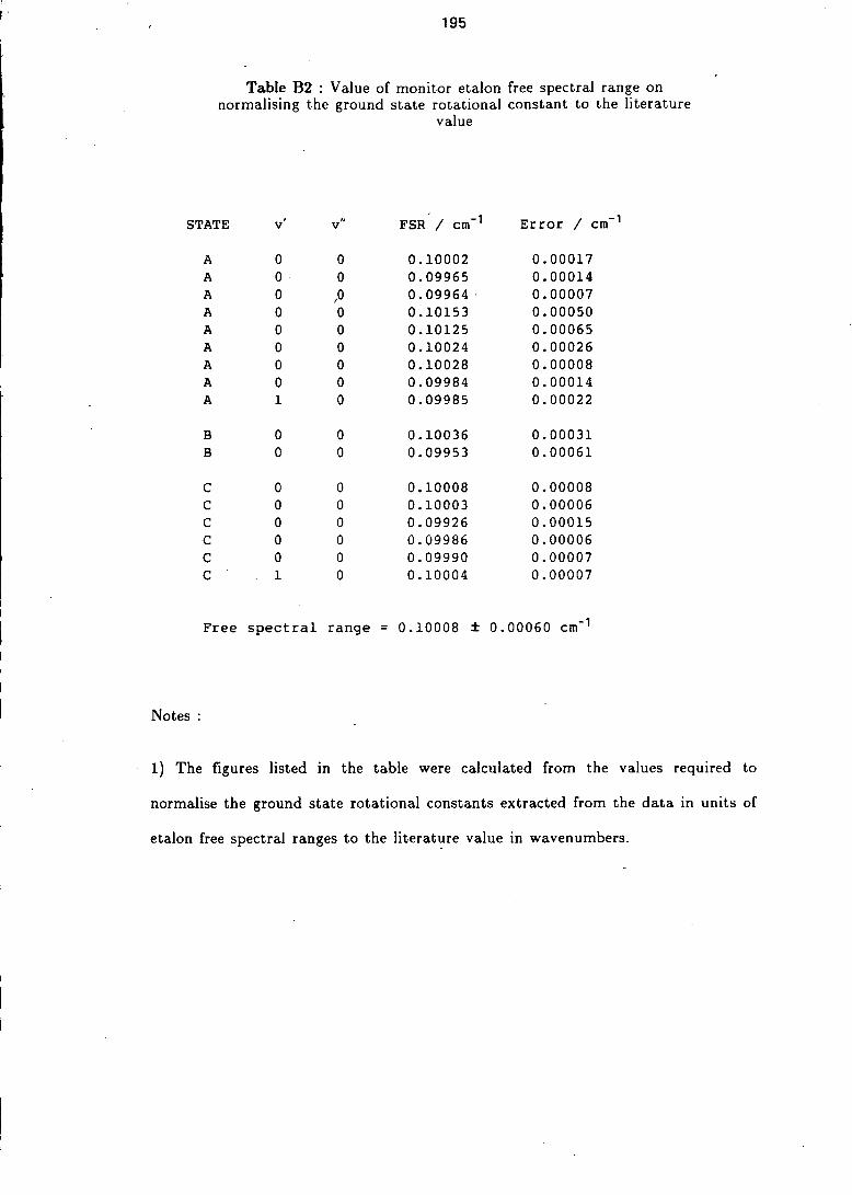
195
Table B2 Value of monitor etalon free spectral range on normalising the ground state rotational constant to the literature
value
STATE V v" FSR/ cm-1 Error / cm-1
A 0 0 0.10002 0.00017 A 0 0 0.09965 0.00014 A 0 ,0 0.09964 0.00007 A 0 0 0.10153 0.00050 A 0 0 0.10125 0.00065 A 0 0 0.10024 0.00026 A 0 0 0.10028 0.00008 A 0 0 0.09984 0.00014 A 1 0 0.09985 0.00022
B 0 0 0.10036 0.00031 B 0 0 0.09953 0.00061
C 0 0 0.10008 0.00008 C 0 0 0.10003 0.00006 C 0 0 0.09926 0.00015 C 0 0 0.09986 0.00006 C 0 0 0.09990 0.00007 C 1 0 0.10004 0.00007
Free spectral range = 0.10008 ± 0.00060 cm-1
Notes
1) The figures listed in the table were calculated from the values required to
normalise the ground state rotational constants extracted from the data in units of
etalon free spectral ranges to the literature value in wavenumbers.
196
Appendix C
In accordance with the regulations of the Department of Chemistry, University of
Edinburgh, I attended the the following lectures and courses during my period of
study:
Mass Spectroscopy
Molecular Electronics
Micro Computing
Fortran 77
Signal Processing
Laser Physics
RKR Method
Least Squares Method
Theoretical Chemistry
Scientific German
In addition, all the regular departmental seminars and research group meetings
were attended.
Conferences Attended
Faraday Division, High Resolution Spectroscopy Group, Reading, 1984
Faraday Division, High Resolution Spectroscopy Group, York, 1985
Scottish Quantum Chemistry Group, Dundee, 1985
Scottish Quantum Chemistry Group, Strathclyde, 1986
Xlth International Symposium on Molecular Beams, Edinburgh, 1987