martingale control variate methods for pricing of …s3.amazonaws.com/zanran_storage/€¦ · i...

i

Martingale control variate methods for

pricing of European and American

arithmetic average Asian options

Henan Wang,

Department of Mathematics,

Texas A&M University.

August 2011.

ii

Abstract

The pricing of arithmetic average Asian European options is problematic because there is no

Black-Scholes formula available. The pricing of American options is also problematic because

they may be exercised at any time between inception and expiration.

This article presents an analysis of the martingale control variate technique of Han and Lai (2010)

for estimating prices of European and American arithmetic Asian options. Longstaff &

Schwartz’s (2001) linear regression method is used to estimate exercise time for American

options. For European options, it was found that,

The martingale control variate technique gives estimates with the standard deviation

lower than that of the standard control variate estimate.

Only small further gains in variance reduction can be obtained using both standard and

martingale control variate methods in a two step approach.

On the other hand, for American option it was found that,

Martingale control variate technique is no better than standard control variate in variance

reduction when volatility is low, but is better when volatility is high.

No improvement in variance reduction is obtained by using both methods in two step

approach.

Quasi-Monte Carlo sampling techniques (antithetic and Sobol) do not result in any variance

reduction.

iii

Contents

Introduction ..................................................................................................................................... 1

Methods........................................................................................................................................... 4

Simulation of Stock Prices .......................................................................................................... 4

Simulation of European Option Prices ....................................................................................... 5

Black Scholes Formula for Geometric Asian Option ................................................................. 6

Control Variate Method .............................................................................................................. 7

Martingale Control Variate Method ............................................................................................ 9

Black Scholes Formula for Delta of Geometric Asian Option ................................................. 10

Black Scholes Formula for Delta of Arithmetic Asian Option ................................................. 11

Simulation of American Option Prices ..................................................................................... 11

Quasi-Monte Carlo Sampling ................................................................................................... 13

Antithetic Variates ................................................................................................................ 13

Sobol Sequence ..................................................................................................................... 13

A Two-step Algorithm .............................................................................................................. 13

Results ........................................................................................................................................... 14

Simulation of Stock Prices ........................................................................................................ 14

Simulation of European Options Prices .................................................................................... 15

Control Variate Method ............................................................................................................ 15

Martingale Control Variate Method .......................................................................................... 18

Simulation of American Option Prices ..................................................................................... 19

iv

Quasi-Monte Carlo Sampling ................................................................................................... 22

A Two-step Algorithm .............................................................................................................. 23

Conclusion .................................................................................................................................... 26

v

Table of Figures

Figure 1: Simulated stock price paths. .......................................................................................... 14

Figure 2: Scatter plot of arithmetic average Asian and geometric average Asian option prices. . 16

Figure 3: Scatter plot of control variate estimate and Monte Carlo estimate of arithmetic Asian

option prices. ..................................................................................................................... 17

Figure 4: Scatter plot of control variate estimate and arithmetic average stock price at expiration

with initial stock price S0=65. ........................................................................................... 18


with initial stock price S0=55. ........................................................................................... 18

Figure 6: Histogram of exercise time for arithmetic average Asian call with K=45, S0=65,

r=0.06,σ=0.4, sample size=30,000 with 200 time steps. ................................................. 20

Figure 7: Histogram of exercise time of arithmetic average Asian call with K=50, S0=65,




Figure 9: Scatter plot of arithmetic average Asian European call and geometric average Asian

European call prices .......................................................................................................... 24

Figure 10: Scatter plot of arithmetic average Asian American call and geometric average Asian

American call prices ......................................................................................................... 25

vi

Table of Tables

Table 9: Monte Carlo estimate of arithmetic and geometric mean stock price, with S0=65, r=0.06,

, T=1 year. Sample size N=100 and 10,000 replicates with 200 time steps. ....... 14

Table 10: Monte Carlo estimate of European call prices: arithmetic A and geometric G with

So=65, r=0.06, , T=1 year. Sample size N=100 and 10,000 replicate with 200

time steps. ......................................................................................................................... 15

Table 11: Monte Carlo A and control variate Acv estimates of arithmetic Asian European option

prices with S0=65, r=0.06, and T=1 year. Sample size N=100 and 10,000

replicates with 200 time steps. .......................................................................................... 16

Table 12: Arithmetic average Asian European call prices with =65, K=55, r=0.06, T=1 year.

Sample size N=10,000 with 200 time steps. ..................................................................... 19

Table 13: Arithmetic average Asian call prices with S0=65, r=0.06,σ=0.4,T=1 year sample

size=30,000 replicate with 200 time steps. ....................................................................... 21

Table 14: Arithmetic average Asian American call prices with K=55, S0=65, r=0.06, T=1 year.

Sample size=30,000 replicate with 200 time steps. .......................................................... 21

Table 15: Quasi Monte Carlo Estimates of Arithmetic average Asian European call prices with

S0=65, K=45,r=0.06, , T=1 year. ........................................................................ 22

Table 16: Monte Carlo Estimates of Arithmetic average Asian American call prices with S0=65,

K=45, r=0.06, , T=1 year. ................................................................................... 23

Table 17: One step and two step control variate of arithmetic average Asian European call price.

........................................................................................................................................... 24

Table 18: One step and two step control variate of arithmetic average Asian American call price

........................................................................................................................................... 25

1

Introduction

A derivative is a financial contract between two parties that has a value determined by the price

of an underlying asset. The most common underlying assets include stocks, bonds, commodities,

currencies, interest rates and market indexes. Derivatives are generally used as an instrument to

hedge risk, but can also be used for speculative purposes. For example, a Chinese investor

purchasing shares of an American company (using U.S. dollars to do so) would be exposed to

exchange-rate risk while holding that stock. To hedge this risk, the investor could purchase

currency futures to lock in a specified exchange rate for the future stock sale and currency

conversion back into RMB.

Forward contracts, futures contracts and options are the most common types of derivatives.

Forward contract: a non-standardized contract between two parties to buy or sell

a specified asset at a pre-determined price at a specified future date.

Futures contract: a standardized contract between two parties to buy or sell a

specified asset at a pre-determined price at a specified future date. Futures differ

from forward in that a forward is traded on an exchange and thus has the interim

partial payments due to marking to market.

Option: There are two main types of options: call option and put option. Unlike

future contracts, an option offers the buyer the right, but not the obligation, to buy

(call) or sell (put) a security or other financial asset.

Call option: an option contract that gives the holder the right, but not the

obligation, to buy a certain quantity of an underlying security at a specified price,

called the strike price, within a specified time, called expiration time. (If the stock

price is greater than strike price, we say this call option is in the money.)

2

Put option: an option contract that gives the holder the right, but not the

obligation, to sell a certain quantity of an underlying security at a specified price

within a specified time. (If the strike price is greater than stock price, we say this

put option is in the money.)

Options are like insurance: freedom from worry. For example, a farmer grows corn and will sell

the corn in a year. The current price of corn is $100 for a bushel. He worries that the price of

corn will drop, so he buys a put option. If the price of corn drops below $100 in one year, the

farmer could still sell the corn in $100 per bushel by exercising the option. If the price of corn is

greater than $100, the farmer would not exercise the option, but would sell the corn at current

price. Call options can also be viewed as insurance for the people who worry about a price going

up. For example, Continental Airlines needs a large amount of fuel and worry that the price of

fuel will go up. The current fuel price is $86 per barrel. The manager wisely buys a call option.

In a year, if the fuel price is greater than $86 per barrel, the manager will exercise the option and

buy the fuel at $86 per barrel. But if the price is less than $86 per barrel, manager would buy the

fuel at the market price.

There are different types of options that vary in the time the owner can exercise or in the amount

of the payoff. For example:

European: an option that can only be exercised at the end of its maturity.

American: an option that can be exercised at any time before its maturity.

Asian: An option whose payoff depends on the average price of the underlying

asset over some pre-set period of time, rather than just the price at expiration.

There are two types of averaging used in Asian options:

Arithmetic Average: It is the sum of the daily prices of the underlying asset

divided by the number of prices.

3

Geometric Average: It is obtained by multiplying underlying prices together and

then taking the nth root, where n is the number of prices of the underlying. In

other words, the natural log of the geometric mean is the arithmetic average of the

log of the prices.

Most Asian options traded are arithmetic average options and so far, there is no closed-form

formula for calculating the price of this option. However, there is a formula for the price of

geometric average option using the Black-Scholes framework. Thus, some research focuses on

how to estimate the price of an arithmetic option using the price of the geometric one.

Control variate method is a variance reduction technique used in Monte Carlo methods (Kemna

& Vorst, 1990). It exploits information about the errors in estimates of known quantities to

reduce the error of an estimate of an unknown quantity. Since there is a closed-form solution for

the price of geometric Asian option, but there is no such formula for arithmetic Asian option.

Thus, the control variate method can be applied as means of variance reduction to better estimate

the price of arithmetic Asian option. The difficulty for estimating the price of American Asian

option is to find its exercise time; Longstaff & Schwartz’s (Longstaff & Schwartz, 2001) linear

regression method can be used to solve this problem.

4

Methods

A stochastic model of stock prices St on continuous time t was first introduced by Paul

Samuelson in 1965 (Samuelson, 1965). In this model

where Zt is Brownian Motion, which means that Zt is normally distributed with mean zero,

variance t and non-overlapping intervals are independent. This type of equation is called a

stochastic differential equation since it is a differential equation with a stochastic component.

The solution for this stochastic differential equation is

( ) ( ) ((

) ( )) ( )

which is known as geometric Brownian motion (Stampfli & Goodman, 2001).

Simulation of Stock Prices

Given a stock paying continuous dividends at the rate of , and a continuously compounding

risk-free interest rate of r, paths of stock prices can be simulated using Equation (1) for the stock

price by the equation

( ) ( ) ((

) √ ) (2)

where Z has a standard normal distribution. Starting with the initial stock price S(0), we simulate

the stock price at the next time value dt=h=T/N, by taking a realization Z1 of a standard normal

random variable and evaluating the right-hand-side of the equation. This process is repeated

using the previous price as the new initial price. For example,

( ) ( ) ((

) √ )

( ) ( ) ((

) √ )

( ) ( ) ((

) √ )

5

Simulation of European Option Prices

Call options are most profitable for the buyer when the underlying asset goes above the strike

price, because the buyer can still purchase the underlying asset at strike price. However, if the

price of the underlying asset does not reach the strike price, the buyer would not exercise the

option. Thus, the payoff for call options is the maximum of either 0 or the underlying price

minus the strike price.

Similarly, put options are most profitable for the buyer when the underlying asset does not reach

the strike price, because the buyer can still sell the underlying asset at the strike price. But if the

price of the underlying asset goes up to or above the strike price, the buyer would not exercise

the option. Thus the payoff for put option is the maximum of either 0 or the strike price minus

the underlying price.

At the expiration of an Asian European option we compare strike price with average stock price

to determine the payoff. In other words,

Call option payoff=Max {0, (Average Stock Price - Strike Price)}

Put option payoff=Max {0, (Strike price – Average Stock Price)}

Once we know the payoff for Asian call option, its price can be calculated as the present value of

the payoff. Present value means the current value of a future amount payment, discounted at the

appropriate interest rate. It reflects the time value of money. For example, 1 dollar you receive

now is more valuable than 1 dollar you receive in one year, because you can invest this 1 dollar

to receive more in one year. In our case, the payoff happens at exercise and the present value of

the payoff can be obtained by taking discount of it. The appropriate interest rate is continuous

compounded risk-free interest rate, and the present value of payoff is the value of the option.

To obtain Monte Carlo estimates of an Asian call option prices, we separately simulate samples

of N=100, 1000, 5000, 10,000 paths of stock price, calculate the payoff, and take the present

value of the payoff. Thus for each stock price path, we obtain one value of the option. For a

6

sample of N paths, the Monte Carlo estimate of the option price is the average of option prices

from each path.

Black Scholes Formula for Geometric Asian Option

There exists a closed form solution for a geometric Asian option (McDonald, 2006, pp. App,

19.A, page 625). Sampling the stock price N times from time 0 to T, with distance between

samples h=T/N, the simulated stock prices are described by

( ) ( ) ((

) √ )

( ) ( ) ((

) √ )

( ) ((

) √ ( ))

so that the price at expiry satisfies

( ) ( ) ((

) √ ∑

)

Let SG(t) be the geometric average stock price at T. The natural log of the geometric average of

this price is then

( ( )) ( ( )) (

)

∑

√

∑∑

The mean of this normal random variable is

( ( ( ))) ( ( )) (

)

( )

which, as N→ , is

( ( ( ))) ( ( )) (

)

The variance of this normal random variable is

7

( ( ( ))) ( )( )

which, as N→ , is

( ( ( )))

Let √ Then find the so that

(

)

Since the geometric average price is log-normally distributed, the geometric average price can

now be expressed in a form so that the usual Black-Scholes formula can be applied. Black

Scholes formula for the option price at t=0 gives

(

) (

)

√

√

( )

( ) (3)

Control Variate Method

Let A and G be Monte Carlo estimates of arithmetic and geometric Asian option prices,

respectively. The goal of the control variate method is to obtain a better simulated estimate of the

price of arithmetic Asian option, where by better we mean less variance for the same sample size.

Define

( ) (4)

where Gbs is the geometric Asian option price calculated Black-Scholes formula. We aim to find

the value b of that minimizes the variance of Acv.

8

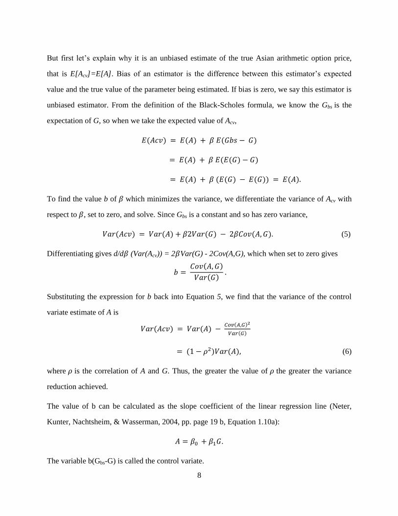
But first let’s explain why it is an unbiased estimate of the true Asian arithmetic option price,

that is E[Acv]=E[A]. Bias of an estimator is the difference between this estimator’s expected

value and the true value of the parameter being estimated. If bias is zero, we say this estimator is

unbiased estimator. From the definition of the Black-Scholes formula, we know the Gbs is the

expectation of G, so when we take the expected value of Acv,

( ) ( ) ( )

( ) ( ( ) )

( ) ( ( ) ( )) ( )

To find the value b of which minimizes the variance, we differentiate the variance of Acv with

respect to , set to zero, and solve. Since Gbs is a constant and so has zero variance,

( ) ( ) ( ) ( ) (5)

Differentiating gives d/d (Var(Acv)) = 2 Var(G) - 2Cov(A,G), which when set to zero gives

( )

( )

Substituting the expression for b back into Equation 5, we find that the variance of the control

variate estimate of A is

( ) ( ) ( )

( )

( ) ( ) (6)

where is the correlation of A and G. Thus, the greater the value of the greater the variance

reduction achieved.

The value of b can be calculated as the slope coefficient of the linear regression line (Neter,

Kunter, Nachtsheim, & Wasserman, 2004, pp. page 19 b, Equation 1.10a):

.

The variable b(Gbs-G) is called the control variate.

9

Martingale Control Variate Method

In the Black-Scholes framework, stock prices satisfy the stochastic differential equation

For any option price ( ) at t, applying Ito’s lemma (Ito, 1951) to the function

( ) gives

( ( ))

( ( ))

( ( ))

( ( ))

( ( ) ( )

)

( )

( )

( )

( ( ) ( )

)

( )

( )

( ( ) ( )

( )

( )

)

( )

( )

Integrating both sides, gives

( ) ( ) ∫ ( )

( ) ( ) ∫

( )

By using an approximate derivative for the unknown

, and approximating the integral with a

sum, we may use the integral term on the right-hand side to improve the estimate of

( ) (Han & Lai, 2010, p. Section 2.1). That is

∑

√

( )

The sum of the right hand side is called the martingale control variate.

10

Black Scholes Formula for Delta of Geometric Asian Option

In 2003, Zhang developed a Black-Scholes formula for the price at t, where 0 ≤ t ≤ T, of a

geometric average Asian European call option (Zhang, 2003, p. Equation 9):

( ) [

(

) ( )

√ ] ( ) [

(

) ( )

√ ]

where

[

( )( )]

(

)

( )

√

∫

We note that in the case where t=0, this formula agrees with Equation (3) above. We obtain

Delta for the option by applying the chain rule:

[

(

) ( )

√ ]

[

( )( )]

[

( )( )]

(

)，

[

(

) ( )

√ ] (

)， ( )

11

When implementing this formula in a simulation, we let dt=T/N and evaluate the integral

∫

as the sum ∑ ( )

Black Scholes Formula for Delta of Arithmetic Asian Option

In 2001, Zhang developed a Black-Scholes formula for the approximate price and delta at t,

where 0 ≤ t ≤ T, of an arithmetic average Asian European call option (Zhang, 2001, pp.

Equations 5, 6,12 ,13)

( )

(

√ )

√

(

) (

√ )

where

( )

( )

and to expiry. In the same paper Zhang derived the following expression for

the call option Delta:

(

√ )

√

( )

Simulation of American Option Prices

The most challenging problem for American option price is that American option can be

exercised at any time before expiration, but we don’t know when exercise it to get maximum

payoff.

There are various methods to estimate optimal exercise time for an American option in a

simulation (for example (Rogers, 2002)). One is a least-squares approach (Longstaff &

12

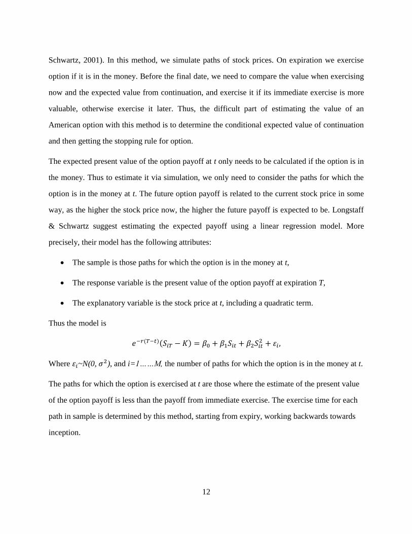
Schwartz, 2001). In this method, we simulate paths of stock prices. On expiration we exercise

option if it is in the money. Before the final date, we need to compare the value when exercising

now and the expected value from continuation, and exercise it if its immediate exercise is more

valuable, otherwise exercise it later. Thus, the difficult part of estimating the value of an

American option with this method is to determine the conditional expected value of continuation

and then getting the stopping rule for option.

The expected present value of the option payoff at t only needs to be calculated if the option is in

the money. Thus to estimate it via simulation, we only need to consider the paths for which the

option is in the money at t. The future option payoff is related to the current stock price in some

way, as the higher the stock price now, the higher the future payoff is expected to be. Longstaff

& Schwartz suggest estimating the expected payoff using a linear regression model. More

precisely, their model has the following attributes:

The sample is those paths for which the option is in the money at t,

The response variable is the present value of the option payoff at expiration T,

The explanatory variable is the stock price at t, including a quadratic term.

Thus the model is

( )( )

Where ~N(0, ), and i=1……M, the number of paths for which the option is in the money at t.

The paths for which the option is exercised at t are those where the estimate of the present value

of the option payoff is less than the payoff from immediate exercise. The exercise time for each

path in sample is determined by this method, starting from expiry, working backwards towards

inception.

13

Quasi-Monte Carlo Sampling

Another strategy frequently employed to reduce variance is to use a more sophisticated method

for obtain random numbers.

Antithetic Variates

When simulating sample paths, the random standard normal variates for the path antithetic to

Z(1), Z(2), Z(3),……,Z(N) are –Z(1), -Z(2), -Z(3),……,-Z(N). That means whenever the original

path goes up, the antithetic path goes down (Mikhail, 1972) . This is to obtain a sample of size N,

we start with N/2 paths and then add the antithetic path to the sample.

Sobol Sequence

The Sobol sequence is a set of quasi-random numbers which was introduced in 1966 (Sobol,

1966). Quasi-random numbers are frequency used in Monte Carlo simulations as they are more

uniform than uniformly distributed numbers. This can lead to estimates that are less biased and

having less variability. This sequence is calculated in MATLAB using the Bratley and Fox

Algorithm 659 (Bratley & Fox, 1988).

A Two-step Algorithm

To apply the standard control variate technique, one needs estimates of prices of two types of

option with a correlation close to one. Thus, for arithmetic Asian options, we may investigate the

possibility that arithmetic and geometric options estimated using martingale control variates are

highly correlated. If so, this opens the possibility to further variance reduction by applying the

standard control variate technique following the martingale control variate method.

14

Results

Simulation of Stock Prices

Using a current stock price of 65 and annual risk-free continuously compounding rate of 0.06,

paths of stock prices were simulated. The one year is cut into 200 time steps. Figure 1 shows five

example paths.

Figure 1: Simulated stock price paths.

The arithmetic and geometric mean stock price is the average over the path, not including the

initial price. The Monte Carlo estimate is the average of the arithmetic and geometric means over

a number of paths N, called sample size. Table 1 shows five estimates of mean stock price for

various sample sizes.

Table 1: Monte Carlo estimate of arithmetic and geometric mean stock price, with S0=65, r=0.06,

, T=1 year. Sample size N=100 and 10,000 replicates with 200 time steps.

N=100 N=10,000

Stock price Arithmetic Geometric Arithmetic Geometric

Run 1 66.0723 (3.9111) 67.0064 (3.8885) 67.1829 (3.9056) 67.1150 (3.8673)

Run 2 66.8051 (3.7753) 66.7429 (3.7512) 67.1353 (3.8558) 67.0679 (3.8191)

Run 3 66.4462 (3.8658) 66.3840 (3.8404) 67.1305 (3.8840) 67.0633 (3.8471)

Run 4 66.7777 (3.7891) 66.7197 (3.7574) 67.2080 (3.9133) 67.1401 (3.8739)

0 20 40 60 80 100 120 140 160 180 20050

55

60

65

70

75

80

time

sto

ck p

rice

15

Run 5 67.1272 (4.0715) 67.0591 (4.0345) 67.0628 (3.8531) 66.9962 (3.8178)

* mean; standard deviation in parentheses.

Simulation of European Options Prices

Recall that the payoff for an Asian call option is

Call option payoff=Max {0, (Average Stock Price - Strike Price)}

and that its price is the present value of this payoff. Using an annual risk-free continuously

compounding rate of 0.06, the price of Asian option is

Call price=exp (-0.06*1)* Max {0, (Average Stock Price - Strike Price)}.

The Monte Carlo estimate is the average of the call price over the sample. Table 2 shows ten

estimates of arithmetic and geometric Asian call option prices, for an option with strike price

K=55, volatility and T=1 year to expiry.

Table 2: Monte Carlo estimate of European call prices: arithmetic A and geometric G with So=65,

r=0.06, , T=1 year. Sample size N=100 and 10,000 replicate with 200 time steps.

N=100 N=10,000

A G A G

Run 1 11.3791 (3.6510) 11.3194 (3.6216) 11.3133 (3.6794) 11.2512 (3.6450)

Run 2 11.1176 (3.5554) 11.0591 (3.5328) 11.2639 (3.6742) 11.2013 (3.6404)

Run 3 10.7797 (3.6406) 11.7211 (3.6168) 11.2790 (3.6344) 11.2174 (3.6019)

Run 4 11.0919 (3.5685) 11.0372 (3.5385) 11.2614 (3.6535) 11.1998 (3.6207)

Run 5 11.4210 (3.8344) 11.3568 (3.7996) 11.3229 (3.6609) 11.2608 (3.6261)

Run 6 11.1176 (3.5554) 11.0591 (3.5328) 11.2302 (3.6840) 11.1682 (3.6530)

Run 7 10.7797 (3.6406) 10.7211 (3.6168) 11.2398 (3.6720) 11.1787 (3.6397)

Run 8 11.0919 (3.5685) 11.0372 (3.5385) 11.3235 (3.6989) 11.2613 (3.6645)

Run 9 11.4210 (3.8344) 11.3568 (3.7996) 11.3382 (3.6773) 11.2754 (3.6442)

Run 10 11.5661 (3.9034) 11.4959 (3.8689) 11.2898 (3.6469) 11.2278 (3.6138)


The closed form Black-Scholes solution for geometric Asian option (Equation 3), gives 11.2297

as the price of the option.

Control Variate Method

The control variate estimate is calculated using Equation (4):

Acv = A+ (Gbs - G),

16

where b is calculated as the slope coefficient of the linear regression line . Recall

from Equation (6) that the closer the correlation of A and G is to one, the smaller the variance of

Acv the control variate estimate. Figure 2 shows a scatter plot of A and G for a sample of size

N=10,000. The correlation of A and G is seen to be very close to one.

Figure 2: Scatter plot of arithmetic average Asian and geometric average Asian option prices.

Table 11 shows ten Monte Carlo on control variate estimates of arithmetic Asian call option

price.

Table 3: Monte Carlo A and control variate Acv estimates of arithmetic Asian European option

prices with S0=65, r=0.06, and T=1 year. Sample size N=100 and 10,000 replicates

with 200 time steps.

N=100 N=10,000

Stock price A ACV A ACV

Run 1 11.3791 (3.6510) 11.2887(0.0424) 11.3133 (3.6794) 11.2915 (0.0522)

Run 2 11.1176 (3.5554) 11.2892(0.0521) 11.2639 (3.6742) 11.2925 (0.0547)

Run 3 10.7797 (3.6406) 11.2916(0.0479) 11.2790 (3.6344) 11.2913 (0.0528)

Run 4 11.0919 (3.5685) 11.2859(0.0427) 11.2614 (3.6535) 11.2915 (0.0515)

Run 5 11.4210 (3.8344) 11.2926(0.0468) 11.3229 (3.6609) 11.2914 (0.0533)

Run 6 11.1176 (3.5554) 11.2892(0.0521) 11.2302 (3.6840) 11.2922 (0.0527)

Run 7 10.7797 (3.6406) 11.2916(0.0479) 11.2398 (3.6720) 11.2912 (0.0526)

Run 8 11.0919 (3.5685) 11.2859(0.0427) 11.3235 (3.6989) 11.2916 (0.0528)

Run 9 11.4210 (3.8344) 11.2926(0.0468) 11.3382 (3.6773) 11.2920 (0.0526)

Run 10 11.5661 (3.9034) 11.2975(0.0603) 11.2898 (3.6469) 11.2917 (0.0532)


0 5 10 15 20 250

5

10

15

20

25

Geometric Option price G

Arith

metic O

ption p

rice A

17

The variance reduction achieved by the control variate method is evident: a seven thousand-fold

reduction in variance. This variance reduction can be seen in Figure 3 by noticing that the spread

in the Monte Carlo estimate A is much greater than that of the control variate estimate Acv.

Figure 3: Scatter plot of control variate estimate and Monte Carlo estimate of arithmetic Asian

option prices.

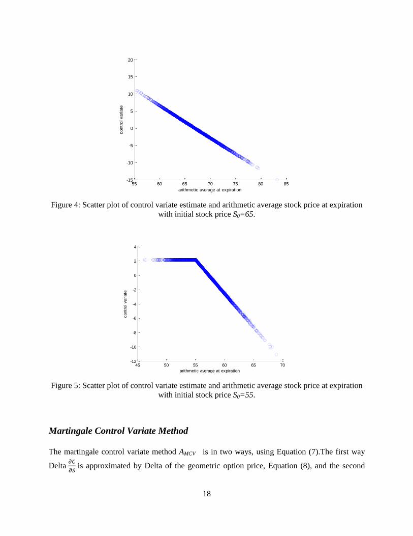
To see how the control reduces variance, we plot the control variate against the arithmetic

average at expiration (see Figure 4). The control variate is positive and large when the average

stock price is low, and negative when the average stock price is high. For best effect, instead of

using S0 =65, we use S0 =55 in Figure 5. In this example, the option price is approximated to be

2.16. When the simulated stock price happens to be large, the simulated payoff will be large, so

the control variate has to be large and negative for it to add, leaving an estimate close to mean.

When the simulated stock price happens to be small, the simulated payoff will be zero, so the

control variate has to be the positive option price, so that when it is added up, it will give an

estimate close to the option price.

0 5 10 15 20 2510

10.5

11

11.5

12

12.5

13

Arithmetic Option price A

Contr

ol V

ariate

price A

cv

18


with initial stock price S0=65.


with initial stock price S0=55.

Martingale Control Variate Method

The martingale control variate method AMCV is in two ways, using Equation (7).The first way

Delta

is approximated by Delta of the geometric option price, Equation (8), and the second

55 60 65 70 75 80 85-15

-10

-5

0

5

10

15

20

arithmetic average at expiration

contr

ol variate

45 50 55 60 65 70-12

-10

-8

-6

-4

-2

0

2

4

arithmetic average at expiration

contr

ol variate

19

way uses Zhang’s approximation of Delta for the arithmetic option price Equation (9). These are

denoted AMCV_G and AMCV_A, respectively. Table 4 shows the results of a single run of the

standard control variate method discussed above, and these two martingale control variates, for

differing price volatility levels.

Table 4: Arithmetic average Asian European call prices with =65, K=55, r=0.06, T=1 year.

Sample size N=10,000 with 200 time steps.

ACV_G AMCV_G AMCV_A

Control Variate Martingale CV

geometric Delta

Martingale CV

arithmetic Delta 0.10 11.2908 (0.0539) 11.2995 (0.0658) 11.3011 (0.0383)

0.20 11.4005 (0.1752) 11.4044 (0.2448) 11.4110 (0.1481)

0.30 11.8924 (0.3807) 11.8796 (0.5867) 11.8907 (0.3319)

0.40 12.6669 (0.6422) 12.6443 (1.0180) 12.6801 (0.5768)

0.50 13.6341 (1.0788) 13.5880 (1.7276) 13.6189 (0.8788)

0.60 14.6737 (1.5773) 14.5985 (2.5445) 14.6462 (1.2689)

0.70 15.7460 (2.0717) 15.6638 (3.4503) 15.7535 (1.7272)


The martingale control variate only out-performs the standard control variate with the Delta for

arithmetic option is used. Even then this improvement in variance is not large.

Simulation of American Option Prices

Recall that the payoff for an American call option is

Call option payoff=Max {0, (Average Stock Price - Strike Price)},

where it has been exercised the first time that the immediate payoff is greater than the expected

value of continuing to hold the option. Its price is the present value of this payoff. We use the

Longstaff and Schwartz method to estimate exercise times (Longstaff & Schwartz, 2001). Figure

6Figure 7Figure 8 show how the exercise times decrease as the strike price K decreases. Even

when K is much less than the initial stock price, it is surprising how many options are held to

expiration.

20

Figure 6: Histogram of exercise time for arithmetic average Asian call with K=45, S0=65,

r=0.06,σ=0.4, sample size=30,000 with 200 time steps.



0 0.1 0.2 0.3 0.4 0.5 0.6 0.7 0.8 0.9 10

0.5

1

1.5

2

2.5

3x 10

4

count

exercise time

0 0.1 0.2 0.3 0.4 0.5 0.6 0.7 0.8 0.9 10

0.5

1

1.5

2

2.5

3x 10

4

count

exercise time

21



Table 5 shows that the price difference between the European and American style options is not

that great, which is to be expected since the exercise times are very close to the expiry time of 1.

Table 5: Arithmetic average Asian call prices with S0=65, r=0.06,σ=0.4,T=1 year sample

size=30,000 replicate with 200 time steps.

AMCV_A AmMCV_A 25th

percentile

K European

American

of exercise time

45 20.8876 (0.4242) 22.2974 (3.0852) 0.8800

50 16.5631 (0.4846) 17.2583 (1.8796) 0.9650

55 12.6727 (0.5763) 12.8977 (0.7789) 0.9900


Table 6, column 1, shows ten estimates of arithmetic American Asian option prices, with strike

price equal to 55, and 1 year to expiry. Columns 2, 3 and 4 are obtained by using control variate

methods: standard, martingale with Delta from European geometric and martingale with Delta

from Zhang’s European arithmetic.

Table 6: Arithmetic average Asian American call prices with K=55, S0=65, r=0.06, T=1 year.

Sample size=30,000 replicate with 200 time steps.

AmA AmACV_G AmAMCV_G AmAMCV_A

0 0.1 0.2 0.3 0.4 0.5 0.6 0.7 0.8 0.9 10

0.5

1

1.5

2

2.5

3x 10

4

count

exercise time

22

Monte Carlo Control Variate Martingale CV

geometric Delta

Martingale CV

arithmetic Delta

0.10 11.3788 (3.5063) 11.4018 (0.4485) 11.4109 (0.4863) 11.4125 (0.4648)

0.20 11.7916 (6.8596) 11.7251 (0.8378) 11.7223 (0.9068) 11.7293 (0.8693)

0.30 12.1977 (10.1482) 12.1456 (0.8178) 12.1344 (0.8698) 12.1476 (0.7235)

0.40 13.0054 (13.2696) 12.8978 (0.9884) 12.8789 (1.2013) 12.8977 (0.7789)

>> 0.50 13.9380 (16.4828) 13.8716 (1.3038) 13.8308 (1.7602) 13.8717 (0.9960)

0.60 14.9655 (19.4713) 14.9143 (1.7242) 14.8568 (2.4696) 14.9101 (1.2865)

0.70 15.7699 (23.1818) 16.0861 (2.4464) 15.9738 (3.6000) 16.0638 (1.7193)


Looking at Table 6, comparing the standard deviation the control variate methods to that from

Monte Carlo, we see that there is an approximately at least sixty-fold reduction in variation. The

reduction is not quite as large as it is for European options, possibly because the Deltas are for

European options.

Quasi-Monte Carlo Sampling

Improvements in these estimates may be possible by using quasi-random numbers rather random

numbers. We use two methods: antithetic and Sobol, in various combinations, and the results are

shown in Table 7. For the martingale control variate, the Delta for the arithmetic average is used.

Also shown are the variance reduction ratios (VRR), which is the variance of the Monte-Carlo

estimate divided by the variance of the alternative estimate.

Table 7: Quasi Monte Carlo Estimates of Arithmetic average Asian European call prices with

S0=65, K=45,r=0.06, , T=1 year.

N=1000 N=8000 N=30000

Mean (sd) VRR Mean (sd) VRR Mean (sd) VRR

MC 20.598(3.730) 20.7447(3.712) 20.6651(3.691)

Antithetic 20.716(3.706) 1.01 20.716(3.674) 1.02 20.718(3.683) 1.00

Sobol 20.714(3.587) 1.08 20.705(3.699) 1.01 20.698(3.666) 1.01

CV 20.709(0.063) 3494 20.709(0.054) 4725 20.709(0.053) 4795

CV+Anti 20.706(0.045) 6779 20.707(0.052) 5018 20.709(0.054) 4552

CV+Sobol 20.705(0.050) 5455 20.708(0.053) 4850 20.708(0.053) 4741

MCV 20.716(0.038) 9533 20.718(0.037) 9593 20.718(0.037) 9483

MCV+Anti 20.718(0.037) 10110 20.718(0.037) 9746 20.718(0.038) 9384

23

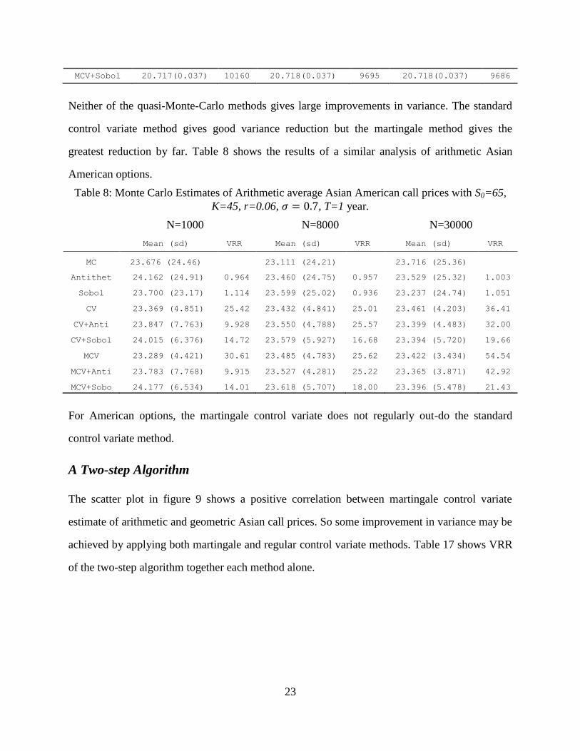
MCV+Sobol 20.717(0.037) 10160 20.718(0.037) 9695 20.718(0.037) 9686

Neither of the quasi-Monte-Carlo methods gives large improvements in variance. The standard

control variate method gives good variance reduction but the martingale method gives the

greatest reduction by far. Table 8 shows the results of a similar analysis of arithmetic Asian

American options.

Table 8: Monte Carlo Estimates of Arithmetic average Asian American call prices with S0=65,

K=45, r=0.06, , T=1 year.

N=1000 N=8000 N=30000


MC 23.676 (24.46) 23.111 (24.21) 23.716 (25.36)

Antithet

ic

24.162 (24.91) 0.964 23.460 (24.75) 0.957 23.529 (25.32) 1.003

Sobol 23.700 (23.17) 1.114 23.599 (25.02) 0.936 23.237 (24.74) 1.051

CV 23.369 (4.851) 25.42 23.432 (4.841) 25.01 23.461 (4.203) 36.41

CV+Anti 23.847 (7.763) 9.928 23.550 (4.788) 25.57 23.399 (4.483) 32.00

CV+Sobol 24.015 (6.376) 14.72 23.579 (5.927) 16.68 23.394 (5.720) 19.66

MCV 23.289 (4.421) 30.61 23.485 (4.783) 25.62 23.422 (3.434) 54.54

MCV+Anti 23.783 (7.768) 9.915 23.527 (4.281) 25.22 23.365 (3.871) 42.92

MCV+Sobo

l

24.177 (6.534) 14.01 23.618 (5.707) 18.00 23.396 (5.478) 21.43

For American options, the martingale control variate does not regularly out-do the standard

control variate method.

A Two-step Algorithm

The scatter plot in figure 9 shows a positive correlation between martingale control variate

estimate of arithmetic and geometric Asian call prices. So some improvement in variance may be

achieved by applying both martingale and regular control variate methods. Table 17 shows VRR

of the two-step algorithm together each method alone.

24

Figure 9: Scatter plot of arithmetic average Asian European call and geometric average Asian

European call prices

Table 9: One step and two step control variate of arithmetic average Asian European call price.

N=1000 N=8000 N=30000


MC 20.598(3.730) 20.746(3.688) 20.712(3.671)

CV 20.71(0.063) 3505 20.71(0.054) 4664 20.71(0.053) 4798

MCV 20.72(0.038) 9635 20.72(0.038) 9419 20.72(0.038) 9333

MCV+CV 20.71(0.033) 12776 20.71(0.032) 13283 20.71(0.032) 13160

Some reduction in variance as achieved, but it is modest by comparison the martingale control

variate. The table 18 shows the results of similar analysis of arithmetic average Asian American

option.

20.6 20.65 20.7 20.75 20.8 20.85 20.9 20.95 2120.6

20.62

20.64

20.66

20.68

20.7

20.72

20.74

Amcv

Gm

cv

25

Figure 10: Scatter plot of arithmetic average Asian American call and geometric average Asian

American call prices

Table 10: One step and two step control variate of arithmetic average Asian American call price

N=1000 N=8000 N=30000


MC 20.798(3.216) 20.849(3.362) 20.905(3.360)

CV 20.863(0.506) 40.4 20.920(0.620) 29.4 20.927(0.631) 28.4

MCV 20.879(0.552) 33.9 20.938(0.691) 23.6 20.939(0.709) 22.4

MCV+CV 20.868(0.551) 34.1 20.922(0.690) 23.7 20.924(0.708) 22.5

15 20 25 3020.6

20.62

20.64

20.66

20.68

20.7

20.72

AmAmcv

Gm

cv

26

Conclusion

In this paper we have studied Asian option pricing problem. After reviewing basic concepts for

derivatives and the simulation of stock prices, European and American option prices, we derived

Black-Scholes model for pricing geometric Asian option and deltas of geometric and arithmetic

Asian option.

The standard control variate method of Kemna & Vorst was compared to the martingale control

variate method of Han & Lai when the martingale applied to Asian European and Asian

American options. In addition, Quasi-Monte Carlo methods were investigated to determine if

they could lead to additional variance reduction when combined with control variate techniques.

Our results shows that the martingale control variate method significantly reduce the variance of

option price estimates, particularly when volatility is high.

27

References

Bratley, P., & Fox, B. (1988). Algorithm 659 Implementing Sobol's Quasirandom Sequence

Generator. ACM Transactions on Mathematical Software , 14 (1), 88-100.

Han, C., & Lai, Y. (2010). Generalized control variate methods for pricing Asian options.

Journal of Computational Finance , 14 (2), 87-118.

Ito, K. (1951). On stochastic differential equations. Memoirs, American Mathematical Society , 4,

1-51.

Kemna, A., & Vorst, A. (1990). A pricing method for options based on average asset values.

Journal of Banking and Finance , 14, 113-129.

Longstaff, F., & Schwartz, E. (2001). Valuing American Options by Simulation: A Simple

Least-Squares Approach. The review of Financial Studies , 14 (1), 113-147.

McDonald, R. (2006). Derivatives Markets. Boston MA: Addison-Wesley.

Mikhail, W. M. (1972). Simulating the Small-Sample Properties of Econometric Estimators.

Journal of the American Statistical Association , 67 (339), 620-624.

Neter, J., Kunter, M., Nachtsheim, C., & Wasserman, W. (2004). Applied Linear Regression

Models. Chicago IL: McGraw Hill.

Samuelson, P. (1965). Rational Theory of Warrant Pricing. Industrial Management Review , 6,

13-31.

Sobol, I. M. (1966). On the distribution of points in a cube and the approximate evaluation of

integrals. 7 (4), 86-112.

Stampfli, J., & Goodman, V. (2001). The Mathematics of Finance: Modeling and Hedging.

Boston, MA: Addison-Wesley.

Zhang, J. (2001). A semi-analytical method for pricing and hedging continuously sampled

arithmetic average rate options. Journal of Computational Finance , 5, 59-79.

Zhang, J. (2003). Pricing continuously sampled Asian option with perturbation method. Journal

of Futures Markets , 23 (6), 535-560.

martingale control variate methods for pricing of …s3.amazonaws.com/zanran_storage/€¦ · i...

Documents