markovian model for data-driven p2p video streaming applications · 2012-08-16 · markovian model...
TRANSCRIPT

Markovian Model for Data-Driven P2P Video Streaming
Applications
Maher Ali
A Thesis
in
The Department
of
Electrical and Computer Engineering
Presented in Partial Fulfilment of the Requirements for the degree of Master of
Applied Science (M.A.Sc) at
Concordia University
Montreal, Quebec, Canada
May, 2012
c⃝Maher Ali, 2012


Abstract
Markovian Model for Data-Driven P2P Video Streaming Applications
Maher Ali
The purpose of this study is to propose a Markovian model to evaluate general P2P
streaming applications with the assumption of chunk-delivery approach similar
to Bit-Torrent file sharing applications. The state of the system was defined as the number
of useful pieces in a peer’s buffer. The model was numerically solved to find out the proba-
bility distribution of the number of useful pieces. The central theme of this study revolved
around answering the question: what is the probability that a peer can play the stream
continuously? This is one of the most important metrics to evaluate the performance of a
streaming application. By finding the numerical solution of the Markov chain, we found that
increasing the number of neighbours enhances the continuity to a certain threshold, after
which the continuity improvement is marginal which complies with empirical results con-
ducted with DONet, a data-driven overlay network for media streaming. We also found that
increasing the buffer length increases the continuity but there is a trade-off because peers
exchange information about the buffer map, hence increasing the buffer length increases
the overhead. We discussed the continuity for both homogeneous and heterogeneous peers
regarding the uploading bandwidth. Then we discussed the case when the first chunk is
downloaded, but not played out because the playtime deadline was missed. We suggested
a general approach for freezing and skipping the playback pointer, that can be used to take
advantage of the available delay tolerance, finally given a specific configuration we measured
the probability of sliding action, that could be used to initiate peers’ adaptation process.
III

Acknowledgement
Working on the modelling problem of P2P streaming applications was challeng-
ing and joyful, the approaches used to study such dynamic systems allowed
me to sense the meaning of Richard Feynman’s sentence: ”I don’t know anything, but I do
know that everything is interesting if you go into it deeply enough”.
I owe respect and thanks to Dr. Dongyu Qiu, working with him on this problem was
a great opportunity. I thank him for his patience, generosity and encouraging me to work
hard to get consistent and justifiable approaches. His advices played the greatest role in
this work.
IV

Dedicated to my family. In spite of a year full of sufferings they were always able to give
me hope and encouraged me to pursue my dreams.
V

Contents
1 Background and literature review 2
1.1 Introduction . . . . . . . . . . . . . . . . . . . . . . . . . . . . . . . . . . . . 2
1.2 Significance and Emergence of P2P . . . . . . . . . . . . . . . . . . . . . . . 5
1.3 P2P Classification . . . . . . . . . . . . . . . . . . . . . . . . . . . . . . . . 9
1.3.1 Centralized index . . . . . . . . . . . . . . . . . . . . . . . . . . . . . 9
1.3.2 Local Index . . . . . . . . . . . . . . . . . . . . . . . . . . . . . . . . 10
1.3.3 Distributed Index . . . . . . . . . . . . . . . . . . . . . . . . . . . . . 11
1.4 Unstructured and structured overlays . . . . . . . . . . . . . . . . . . . . . . 14
1.4.1 Unstructured P2P networks . . . . . . . . . . . . . . . . . . . . . . . 14
1.4.2 Structured P2P networks . . . . . . . . . . . . . . . . . . . . . . . . 16
1.5 P2P Live streaming . . . . . . . . . . . . . . . . . . . . . . . . . . . . . . . 20
1.5.1 Tree-based approach . . . . . . . . . . . . . . . . . . . . . . . . . . . 21
1.5.2 Data-driven approach . . . . . . . . . . . . . . . . . . . . . . . . . . 22
1.5.3 Hybrid push-pull model . . . . . . . . . . . . . . . . . . . . . . . . . 24
1.6 Related work . . . . . . . . . . . . . . . . . . . . . . . . . . . . . . . . . . . 26
1.7 Thesis organization . . . . . . . . . . . . . . . . . . . . . . . . . . . . . . . . 29
2 The probability of broken relation 31
2.1 Introduction . . . . . . . . . . . . . . . . . . . . . . . . . . . . . . . . . . . . 31
2.2 Definitions . . . . . . . . . . . . . . . . . . . . . . . . . . . . . . . . . . . . . 32
2.2.1 Chunks . . . . . . . . . . . . . . . . . . . . . . . . . . . . . . . . . . 32
2.2.2 Peer Playback Pointer - PPP . . . . . . . . . . . . . . . . . . . . . . 33
VI

2.2.3 Stream Playback pointer - SPP . . . . . . . . . . . . . . . . . . . . . 33
2.2.4 Maximum Allowed Delay - T . . . . . . . . . . . . . . . . . . . . . . 34
2.2.5 Buffer . . . . . . . . . . . . . . . . . . . . . . . . . . . . . . . . . . . 36
2.2.6 Useful Pieces . . . . . . . . . . . . . . . . . . . . . . . . . . . . . . . 37
2.2.7 Old pieces . . . . . . . . . . . . . . . . . . . . . . . . . . . . . . . . . 37
2.2.8 Missing pieces . . . . . . . . . . . . . . . . . . . . . . . . . . . . . . . 38
2.2.9 Virtual Buffer . . . . . . . . . . . . . . . . . . . . . . . . . . . . . . . 38
2.2.10 Relation between T and L . . . . . . . . . . . . . . . . . . . . . . . . 39
2.3 Important events . . . . . . . . . . . . . . . . . . . . . . . . . . . . . . . . . 40
2.3.1 The probability of finding partial useful pieces - U(x, i,G) . . . . . . 42
2.3.2 The probability of Partial Broken Relation - P (i, j, G,K, x) . . . . . 43
2.4 The cases of broken relation . . . . . . . . . . . . . . . . . . . . . . . . . . . 44
2.4.1 Case1 - tB ≤ tA − L . . . . . . . . . . . . . . . . . . . . . . . . . . . 45
2.4.2 Case2 - tA − L+ 1 ≤ tB ≤ tA − 1 . . . . . . . . . . . . . . . . . . . . 45
2.4.3 Case3 - tA ≤ tB ≤ tA + L− 1 . . . . . . . . . . . . . . . . . . . . . . 46
2.4.4 Case4 - tA + L ≤ tB . . . . . . . . . . . . . . . . . . . . . . . . . . . 48
2.4.5 Case5 - tA + L ≤ tB − L . . . . . . . . . . . . . . . . . . . . . . . . . 49
2.4.6 The probability of broken relation . . . . . . . . . . . . . . . . . . . 51
2.5 Discussion . . . . . . . . . . . . . . . . . . . . . . . . . . . . . . . . . . . . . 51
2.6 Conclusion . . . . . . . . . . . . . . . . . . . . . . . . . . . . . . . . . . . . 53
3 The Probabilistic model 54
3.1 Introduction . . . . . . . . . . . . . . . . . . . . . . . . . . . . . . . . . . . . 54
3.2 User state . . . . . . . . . . . . . . . . . . . . . . . . . . . . . . . . . . . . . 56
3.3 Probability of busy slot µi . . . . . . . . . . . . . . . . . . . . . . . . . . . . 58
3.4 Max number of requests D . . . . . . . . . . . . . . . . . . . . . . . . . . . 59
3.5 ri,n . . . . . . . . . . . . . . . . . . . . . . . . . . . . . . . . . . . . . . . . . 60
3.6 Death rate βi . . . . . . . . . . . . . . . . . . . . . . . . . . . . . . . . . . . 60
3.7 Birth rate Zi,k . . . . . . . . . . . . . . . . . . . . . . . . . . . . . . . . . . 61
3.8 Markov chain . . . . . . . . . . . . . . . . . . . . . . . . . . . . . . . . . . . 61
VII

3.9 Interesting factor Ui . . . . . . . . . . . . . . . . . . . . . . . . . . . . . . . 65
3.10 F (H, i′,K) . . . . . . . . . . . . . . . . . . . . . . . . . . . . . . . . . . . . 66
3.11 Average number of requests K̄ . . . . . . . . . . . . . . . . . . . . . . . . . 69
3.12 Distribution of received requests X . . . . . . . . . . . . . . . . . . . . . . . 70
3.13 Probability of fulfilling a request Q . . . . . . . . . . . . . . . . . . . . . . . 72
3.14 ri,n . . . . . . . . . . . . . . . . . . . . . . . . . . . . . . . . . . . . . . . . . 73
3.15 Paradox of Q . . . . . . . . . . . . . . . . . . . . . . . . . . . . . . . . . . . 73
3.16 Average download rate D̄ . . . . . . . . . . . . . . . . . . . . . . . . . . . . 74
3.17 Efficiency η . . . . . . . . . . . . . . . . . . . . . . . . . . . . . . . . . . . . 75
3.18 Continuity Pc . . . . . . . . . . . . . . . . . . . . . . . . . . . . . . . . . . . 75
3.19 Discussion of Numerical results . . . . . . . . . . . . . . . . . . . . . . . . . 76
3.19.1 Continuity Pc as a function of H . . . . . . . . . . . . . . . . . . . . 76
3.19.2 Average request rate K̄ . . . . . . . . . . . . . . . . . . . . . . . . . 78
3.19.3 Comparison between DONet and our model results . . . . . . . . . . 80
3.19.4 The average number of received requests αH . . . . . . . . . . . . . 80
3.19.5 Probability of fulfilling a request Q . . . . . . . . . . . . . . . . . . . 82
3.19.6 Average download rate D̄ . . . . . . . . . . . . . . . . . . . . . . . . 82
3.19.7 Why Pc increases in the range −H? . . . . . . . . . . . . . . . . . . 84
3.19.8 The effect of buffer length L . . . . . . . . . . . . . . . . . . . . . . . 85
3.19.9 The effect of maximum allowed delay T . . . . . . . . . . . . . . . . 85
3.19.10Efficiency η . . . . . . . . . . . . . . . . . . . . . . . . . . . . . . . . 87
3.19.11Releasing upload bandwidth β . . . . . . . . . . . . . . . . . . . . . 89
3.19.12Releasing uploading bandwidth for Heterogeneous peers . . . . . . . 89
3.20 Conclusion . . . . . . . . . . . . . . . . . . . . . . . . . . . . . . . . . . . . 92
4 Problems in numerical solution 94
4.1 Introduction . . . . . . . . . . . . . . . . . . . . . . . . . . . . . . . . . . . . 94
4.2 The initial conditions tree - F (H, i′,K) . . . . . . . . . . . . . . . . . . . . 94
4.2.1 Linear recursion and iteration . . . . . . . . . . . . . . . . . . . . . . 95
4.2.2 Tree Recursion . . . . . . . . . . . . . . . . . . . . . . . . . . . . . . 97
VIII

4.2.3 Simulating the call stack . . . . . . . . . . . . . . . . . . . . . . . . . 99
4.2.4 Multilevel Cache structure . . . . . . . . . . . . . . . . . . . . . . . . 102
4.3 Method used to get the steady-state solution for the markov chain . . . . . 103
4.3.1 Iterative solution for Markov chain . . . . . . . . . . . . . . . . . . . 103
4.3.2 Numerical Solution for Our Model . . . . . . . . . . . . . . . . . . . 106
4.3.3 GUI Software to find the numerical solution . . . . . . . . . . . . . . 107
4.4 Conclusion . . . . . . . . . . . . . . . . . . . . . . . . . . . . . . . . . . . . 108
5 The First Block Problem 109
5.1 Introduction . . . . . . . . . . . . . . . . . . . . . . . . . . . . . . . . . . . . 109
5.2 Capturing the problem . . . . . . . . . . . . . . . . . . . . . . . . . . . . . . 110
5.3 Modifying the broken relation . . . . . . . . . . . . . . . . . . . . . . . . . . 112
5.3.1 Case1 - tB ≤ tA − L . . . . . . . . . . . . . . . . . . . . . . . . . . . 113
5.3.2 Case2 - tA − L+ 1 ≤ tB ≤ tA − 1 . . . . . . . . . . . . . . . . . . . . 113
5.3.3 Case3 - tA ≤ tB ≤ tA + L− 1 . . . . . . . . . . . . . . . . . . . . . . 114
5.3.4 Case4 - tA + L ≤ tB . . . . . . . . . . . . . . . . . . . . . . . . . . . 117
5.3.5 Case5 - tA + L ≤ tB − L . . . . . . . . . . . . . . . . . . . . . . . . . 119
5.3.6 Broken relation in the first chunk problem . . . . . . . . . . . . . . . 120
5.4 Numerical results . . . . . . . . . . . . . . . . . . . . . . . . . . . . . . . . . 120
5.5 Proposing a freezing and skipping method . . . . . . . . . . . . . . . . . . . 124
5.5.1 Probability of sliding action . . . . . . . . . . . . . . . . . . . . . . . 126
5.6 Conclusion . . . . . . . . . . . . . . . . . . . . . . . . . . . . . . . . . . . . 128
6 Conclusion, Limitations and Future Work 129
6.1 Concluding our work . . . . . . . . . . . . . . . . . . . . . . . . . . . . . . . 129
6.2 Limitations and future work . . . . . . . . . . . . . . . . . . . . . . . . . . . 133
IX

List of Figures
1.1 Global CDN market . . . . . . . . . . . . . . . . . . . . . . . . . . . . . . . 5
1.2 Client Server Model . . . . . . . . . . . . . . . . . . . . . . . . . . . . . . . 7
1.3 Napster Model . . . . . . . . . . . . . . . . . . . . . . . . . . . . . . . . . . 8
1.4 Freenet routing table . . . . . . . . . . . . . . . . . . . . . . . . . . . . . . . 13
1.5 Freenet searching process . . . . . . . . . . . . . . . . . . . . . . . . . . . . 14
1.6 CAN 2-dimensional space example . . . . . . . . . . . . . . . . . . . . . . . 17
1.7 CAN 2-dimensional neighbours set example . . . . . . . . . . . . . . . . . . 17
1.8 Identifier ring consisting of ten nodes storing five keys . . . . . . . . . . . . 19
1.9 Pastry: routing table example for node Id=3123, D = 4, b = 2 . . . . . . . 20
1.10 Comparison between trees and multitrees approaches . . . . . . . . . . . . . 22
1.11 Coolstreaming sub-streams . . . . . . . . . . . . . . . . . . . . . . . . . . . 25
1.12 GUI Program to find the numerical solution with first block option . . . . . 30
2.1 Peer A with 2 useful pieces with buffer length L = 5 . . . . . . . . . . . . . 38
2.2 Peer A buffer after replacing old pieces with new pieces as a notation . . . . 38
2.3 Peer A Virtual buffer . . . . . . . . . . . . . . . . . . . . . . . . . . . . . . . 39
2.4 Peer A real buffer snapshot . . . . . . . . . . . . . . . . . . . . . . . . . . . 39
2.5 T and L relation . . . . . . . . . . . . . . . . . . . . . . . . . . . . . . . . . 40
2.6 The probability of finding partial useful pieces - U(x, i,G) . . . . . . . . . . 43
2.7 The probability of Partial Broken Relation - P (i, j, G,K, x) . . . . . . . . . 44
2.8 Case1 . . . . . . . . . . . . . . . . . . . . . . . . . . . . . . . . . . . . . . . 45
2.9 Case2 . . . . . . . . . . . . . . . . . . . . . . . . . . . . . . . . . . . . . . . 46
2.10 Case3 . . . . . . . . . . . . . . . . . . . . . . . . . . . . . . . . . . . . . . . 47
X

2.11 Case4 . . . . . . . . . . . . . . . . . . . . . . . . . . . . . . . . . . . . . . . 49
2.12 Case4 - The General case . . . . . . . . . . . . . . . . . . . . . . . . . . . . 49
2.13 Case5 . . . . . . . . . . . . . . . . . . . . . . . . . . . . . . . . . . . . . . . 51
3.1 State transitions diagram . . . . . . . . . . . . . . . . . . . . . . . . . . . . 59
3.2 initial conditions tree . . . . . . . . . . . . . . . . . . . . . . . . . . . . . . . 68
3.3 The calculation of Q . . . . . . . . . . . . . . . . . . . . . . . . . . . . . . . 72
3.4 Continuity with different values of H and T, L = 40 . . . . . . . . . . . . . 77
3.5 K̄ as a function of H - and T = 35, L = 40 . . . . . . . . . . . . . . . . . . . 78
3.6 N̄ as a function of H - and T = 35, L = 40 . . . . . . . . . . . . . . . . . . . 79
3.7 M̄, K̄ as a function of H - and T = 35, L = 40 . . . . . . . . . . . . . . . . . 79
3.8 DONet results taken from [42] . . . . . . . . . . . . . . . . . . . . . . . . . . 80
3.9 Comparison between our model and DONet results . . . . . . . . . . . . . . 81
3.10 α with different values of H . . . . . . . . . . . . . . . . . . . . . . . . . . . 81
3.11 αH The Average number of received requests as a function of H . . . . . . 82
3.12 Q, 1K̄
with different values of H . . . . . . . . . . . . . . . . . . . . . . . . . 83
3.13 D̄ with different values of H . . . . . . . . . . . . . . . . . . . . . . . . . . . 83
3.14 L The Effect of Buffer length on Pc, η . . . . . . . . . . . . . . . . . . . . . 86
3.15 Effect of Delay T on Interesting factor U and Continuity Pc . . . . . . . . . 87
3.16 η with different values of H and T . . . . . . . . . . . . . . . . . . . . . . . 88
3.17 Continuity as a function of upload bandwidth β . . . . . . . . . . . . . . . . 90
3.18 η as a function of upload bandwidth β . . . . . . . . . . . . . . . . . . . . . 90
3.19 K̄ as a function of upload bandwidth β . . . . . . . . . . . . . . . . . . . . 91
3.20 The heterogeneous and homogeneous peer continuity . . . . . . . . . . . . . 92
4.1 Execution path of the factorial recursive function . . . . . . . . . . . . . . . 95
4.2 Execution path of the factorial iterative function . . . . . . . . . . . . . . . 96
4.3 Execution path of the Fibonacci . . . . . . . . . . . . . . . . . . . . . . . . 98
4.4 Execution tree of the F (5, 3, 2) . . . . . . . . . . . . . . . . . . . . . . . . . 99
4.5 GUI Program to find the numerical solution . . . . . . . . . . . . . . . . . . 108
XI

5.1 The buffer when tA = ts − T . . . . . . . . . . . . . . . . . . . . . . . . . . 111
5.2 The buffer when tA = ts − T , after downloading the first chunk . . . . . . . 111
5.3 First Chunk Problem: Case1 . . . . . . . . . . . . . . . . . . . . . . . . . . 113
5.4 First Chunk Problem: Case2 . . . . . . . . . . . . . . . . . . . . . . . . . . 114
5.5 First Chunk Problem: Case3 . . . . . . . . . . . . . . . . . . . . . . . . . . 115
5.6 First Chunk Problem: Case4 . . . . . . . . . . . . . . . . . . . . . . . . . . 118
5.7 First Chunk Problem: Case5 . . . . . . . . . . . . . . . . . . . . . . . . . . 120
5.8 GUI Program to find the numerical solution with first block option . . . . . 121
5.9 Continuity with different values of H and T = 5, L = 40, with first chunk . 122
5.10 Pc − PcFB as a function of H . . . . . . . . . . . . . . . . . . . . . . . . . . 122
5.11 Efficiency η with different values of H and T = 5, L = 40, with first chunk . 123
5.12 ηFB − η as a function of H . . . . . . . . . . . . . . . . . . . . . . . . . . . 123
5.13 Interesting factor UFB as a function of H . . . . . . . . . . . . . . . . . . . 124
5.14 sliding action scenario . . . . . . . . . . . . . . . . . . . . . . . . . . . . . . 125
5.15 Probability of sliding action as a function of H . . . . . . . . . . . . . . . . 127
5.16 continuity for L = 25, T = 20 as a function of H . . . . . . . . . . . . . . . 127
XII

1.
List of Tables
2.1 F (i, j) Table when L=8, T=2 . . . . . . . . . . . . . . . . . . . . . . . . . . 52
2.2 F (i, j) Table when L=8, T=4 . . . . . . . . . . . . . . . . . . . . . . . . . . 52
2.3 F (i, j) Table when L=8, T=8 . . . . . . . . . . . . . . . . . . . . . . . . . . 52
3.1 Results for F (H, i′, k) . . . . . . . . . . . . . . . . . . . . . . . . . . . . . . 69
3.2 Q Calculation . . . . . . . . . . . . . . . . . . . . . . . . . . . . . . . . . . . 73
4.1 Results for recursive execution of F (H, i‘,K) . . . . . . . . . . . . . . . . . 99
4.2 Results for simulated call stack algorithm . . . . . . . . . . . . . . . . . . . 101
4.3 Cache hit count . . . . . . . . . . . . . . . . . . . . . . . . . . . . . . . . . . 103

2. CHAPTER 1. BACKGROUND AND LITERATURE REVIEW
Chapter 1
Background and literature review
It left the record industry with no
choice but to gain control or shut it
down.
Randy Komisar - About Napster
1.1 Introduction
P2P Network Applications is a distributed technology used to meet the require-
ments of large scale applications, this technology gained wide interest due to
the success of file sharing applications, media streaming, and telephony applications. Dif-
ferent P2P architectures were proposed, but they share common features which include:
self-organization, decentralization, converting the system consumers to contributors just to
name a few. The research in this domain does not serve only the P2P Applications, because
other trends in network technology like the wireless networks, sensor networks and mobile
networking are benefiting from the capabilities of P2P paradigm.
Nowadays, the Internet has become the main platform to deliver the video/audio delay-
sensitive traffic, according to Cisco report [6] for the first time in 10 years, the P2P traffic
is no longer the largest internet traffic type. Internet video was 40% of consumer Internet
traffic in 2010, it will reach 50% by the year-end of 2012, and the 62% by 2015, and this
traffic doesn’t include the video content exchanged in P2P file sharing. In 2015 it is antici-

3. CHAPTER 1. BACKGROUND AND LITERATURE REVIEW
pated that in every minute, 1 million minutes of video content will cross the network, and
the sum of all forms of videos (P2P, Internet, TV) will continue to be approximately 90%
of global consumer traffic by 2015.
Considering the dominance of video traffic and the expansion of broadband technologies,
the marketing has been stimulated for the delivery of live streaming. Many frameworks
were proposed for live streaming service, we recognize two main approaches for streaming
services, the Content Delivery Networks (CDN) and Peer-to-Peer networks, and recently
the hybrid CDN-P2P architecture for live streaming [34].
Obviously distributing the media over the traditional, old-fashion client server model, is
very costly in terms of servers and bandwidth, this includes very expensive license for me-
dia streaming servers like Adobe Flash Media Server which is the most popular commercial
streaming solution, besides paying some cents per gigabytes on the top of normal costs.
CDNs were created to improve the performance by distributing the content to cache servers
close to users. Caching is also provided by Proxy servers, the proxy servers provide many
clients with shared cache location, then if requested object is found in the cache and has
not expired then the client request is fulfilled by the ISP cache. Web caching has three
benefits [37]:
• Reducing the network traffic by storing the responses in closer locations
• Reducing the latency for fulfilling the request
• Improving the reliability, when the server is down for short period of time, then cache
is used to serve clients
But Proxy cache has also drawbacks:
• the client may receive incorrect or stale data when the proxy is not updated at suitable
times
• Even with web proxies, the origin servers become bottlenecks, this happens when
large number of users access the web site simultaneously, a phenomena known as flash
crowds. Since web caches hit rate tends to be low 25-40 percent, consequently proxy
caches have limited success in improving the web sites scalability.

4. CHAPTER 1. BACKGROUND AND LITERATURE REVIEW
• Most of today websites generating dynamic content, then the HTML pages are created
on the fly and unique to specific users, because proxy can not cache the dynamic
content, the performance is improved to a certain limit.
Akamai was evolved out of MIT research effort for solving the flash crowds problem, the
approach is based on the observation that serving web content from single location can
present serious problems for site scalability. The system simply deploys surrogate servers
at different geographical locations around the globe at the network edge. Akamai name
servers map host names to IP addresses by mapping the requests to servers using criteria
like: Server load, server health (up or down), client location, content requested. In Akamai
there is DNS-based load balancing system continuously monitors the state of surrogates
servers, the content server periodically reports its load to the monitoring application, based
on these reports the DNS server determines which IP addresses to return when resolving
the DNS names, this process happens as part of DNS resolving process after the root name
servers return (NS) records for Akamai top-level name servers [10]. Interestingly, Akamai
CDN cache also overcomes the proxy caches problem of caching dynamic content by using
ESI (Edge Side Includes) technology, which breaks the dynamic page into fragments with
independent cachability properties, this allows the server to fetch only the noncachable frag-
ments from origin web site. It was found that ESI can reduce the bandwidth requirements
for dynamic content by 95-99%.
CDN are used not only for delivering web pages, but also for delivering the streaming me-
dia, the content provider sends the stream to entry-point server in the CDN network, the
stream is delivered from entry-point server to edge servers and then to end users. When
Google launched the Youtube Live service in 2011, they had many options, using their own
live service, acquire a streaming platform or simply stream the live event using CDN.
Examining the HTML code during the live event showed that, youtube did not launch any
live service and chose AKAMAI to stream the live event with custom Flash Player built by
web agency Digitaria [14].
From the previous discussion it is obvious that the CDNs started as an attempt to reduce
the server load during the flash crowds, then the provided services were expanded to include

5. CHAPTER 1. BACKGROUND AND LITERATURE REVIEW
live streaming which is recently adopted by Google. Clearly, the CDN pure solution is very
costly, currently CDNs have become a huge market generating large revenues. The Global
CDN market was a high as 1.5$ billion in 2009 because of video streaming applications as
illustrated in Fig.1.1, this is refelcted by the Akamai which handles 20% of total internet
traffic [44].
Figure 1.1: Global CDN market
Because of the cost of CDNs, this market is dedicated from medium to large scale com-
panies, that is why P2P Streaming gained more attention from researchers. Recently new
hybrid architecture was proposed to integrate both of the competing technologies to over-
come problems of both approaches. In [34] the proposed CDN-P2P architecture divides the
content delivery network into meshes, each mesh contains source node and other peers that
collaborate in the network with their upload bandwidth, in each mesh a P2P system like
Coolstreaming is used with tracker to achieve the P2P functionality. This hybrid architec-
ture befits from P2P scalability by leveraging the resources of the peers and the reliability
of CDNs, this approach reduces the server cost but does not eliminate it.
Whether live streaming is deployed using hybrid CDNs or P2P architecture, understanding
the performance of P2P system is still a challenging research topic as explained later in this
chapter.
1.2 Significance and Emergence of P2P
Definitions of P2P networks try to distinguish it from Client/Server architecture, one of
these definitions: ”A distributed network architecture may be called a Peer-to-Peer net-

6. CHAPTER 1. BACKGROUND AND LITERATURE REVIEW
work, if the participants share a part of their own hardware resources (processing power,
storage capacity, network link capacity, printers,...). These shared resources are neces-
sary to provide the Service and content offered by the network (e.g file sharing or shared
workspaces or collaboration): They are accessible by other peers directly, without passing
intermediary entities. The participants of such a network are thus resource (Service and
content) providers as well as resource (Service and content) requesters (Servent-concept)”
[33]. The emphasize of this definition is on the role of the node in P2P networks, while in
Client/Server applications the node acts as either a server or client, in P2P networks the
node is Servent, which means the node is able to play the role of both server and client at
the same time. Also P2P networks can be classified as Pure P2P networks where removing
any random node does not cause any loss in the network service, similarly there is the hybrid
P2P networks in which a central entity is necessary to provide parts of the network service
[33].
Some characteristics of P2P networks are:
• Resource sharing : The peer is not just a consumer or requester, but also it con-
tributes to the system resources by uploading information to other peers. There should
be some rules to specify how much the peer can download depending on his contribu-
tion, these rules try to solve the problem of peer downloading but not uploading to
other peers, a problem is widely known in the literature as free rider problem.
• Scalability : On the contrary of Client/Server architecture, increasing the number of
users in the overlay will increase the performance, this revolutionary concept means
the P2P networks designed to provide services for millions of concurrent users.
• Symmetry : nodes are assumed to have equal roles in the overlay, although some P2P
designs suggest the concept of superpeers.
• Decentralization : in P2P overlays the behaviour doesn’t depend on central point
of control but this concept has been changed to include servers to speed up some
operations in the overlay like the tracker server in the design of Bittorrent.
• Self-Organization : Nodes in P2P overlays appear and leave at random times, this

7. CHAPTER 1. BACKGROUND AND LITERATURE REVIEW
churn rate should be cosidered to maintain the structure of the overlay, additionally
the operations at each node should be organized based on a partial view or local
information only.
P2P applications emerged with Napster, before Napster the communication between clients
was only through server, this is the traditional Client/Server model explained in Fig.1.2,
where the user A uploads a resource (file, database record ...) to the server, and then
another user B sends the request to the server asking for that resource and if it is available
it downloads it from the server, this is the general concept of Client/Server applications.
This model changed with Napster [40], which was motivated by making it easier for music
Figure 1.2: Client Server Model
listeners to share their MP3 files. Napster is an example of hybrid P2P system, because
there is a centralized directory that describes how files are stored in the network, and also
joining peers should register in this directory. In other words the centralised directory
stores information about both nodes and files, information about nodes is table of active
connections, while information about files includes file names, creation date, size, copyright
information ...etc . The operation of Naspter [40] is illustrated in Fig.1.3:
• user A connects to server (centralized directory) and the server keeps information
about connected clients
• user B wants to download a file, it sends a request to the Napster server, and directory
service looks up for a match.
• the server sends a list of matches to B including the IP address, file name, file size ...
etc

8. CHAPTER 1. BACKGROUND AND LITERATURE REVIEW
• user B establishes the connection with A directly and downloads the file
Figure 1.3: Napster Model
The connection between clients is direct once the required information is obtained from the
Napster server, also we have to notice that the content downloaded by B is not stored on
Napster server, instead the content is found on the peers.
Once completed, Napster was a huge success and became one of the fasted growing sites in
history, reaching the 25 million users in less than a year [40]. After the wide spreading of
Napster since it was launched in 1999, many giants in the music industry like AOL, Sony
music, Warner Music ... realised that Napster posed potential threat, so they sued Napster
over violating copyright law, they sensed that Napster with simple file-sharing and with
no royalty charging mechanism will cost the music industry millions of dollars, and as a
defence Napster team said the content itself is not on our servers but it is distributed by
users themselves. The original service was shut down by court order, in [35] [40] Napster
legal issues are presented.
Obviously Napster was an attempt to solve the problems found in traditional Client/Server
applications, these issues are caused by the limitation of the server resources: CPU utiliza-
tion, network bandwidth, storage and I/O speed, solving these problems means companies
should bear high costs of additional resources. For instance, Google clusters more than
200,000 AMD servers to give successful web indexing services [29].

9. CHAPTER 1. BACKGROUND AND LITERATURE REVIEW
1.3 P2P Classification
There are many applications of P2P overlays like: file-sharing, instant messaging, media
streaming, VoIP ...but file-sharing is considered to be the most popular of these applications,
and the foundation of all later services, for instance some live streaming protocols build on
bit-torrent file sharing architecture. According to [30] File sharing P2P networks can be
categorized based on the index type, and defined the index to be the collection of terms with
pointers to places where the information about documents can be found, the structure of the
index affects the search operations. Concerning index types there are three classifications
of P2P networks:
• Centralized index
• Local index
• Decentralized index
1.3.1 Centralized index
This approach is used in the first generation of P2P networks like Napster, there is a central
server that keeps meta-information about peers and files, but it does not store the content
itself, thus searching process is very efficient, and Napster is considered the first to demon-
strate the scalability of P2P network by separating data from index.
These systems are also called the hybrid systems because elements of both client/server and
pure P2P system coexist [43]. The index is updated at different operations, for instance
when the user logs on, after a user completed the downloading process it sends an update
message to the server, or when the user drops the connection.
In hyper architecture there could be many servers, these servers can be chained, which
means if one server can’t fulfil the request then it forwards the request to another server,
hence some requests could be expensive. Or there could be full replication of index on
all servers, and obviously this imposes difficulties for maintaining the synchronization of
different copies, and servers could be independent like the one used in Napster. The real
barriers of the central index is not technical but legal and financial. Another popular P2P

10. CHAPTER 1. BACKGROUND AND LITERATURE REVIEW
file sharing system with centralized architecture is BitTorrent [9]. In BitTorrent imple-
mentation a static file with extension .torrent is uploaded to a web server. This torrent file
contains information about the file, its length, name, and hashing information (to check if
the file is corrupted during storage or transmission), and the URL of the trackers. Trackers
are responsible for helping downloaders finding each other. The protocol of tracker is very
simple layered on the top of HTTP, the downloader sends information about the required
file and port it is listening to and other information, then the tracker sends a a random list
of peers which are currently downloading the same file. then downloaders connect to each
other and upload information to each other. To make sure the file is available a peer with
complete file is called the seeder must be started in the overlay.
The file itself is divided into smaller pieces of fixed size, then each peer can report to its
partners what pieces it maintains, so that other peers can use this information to send
requests asking for pieces from different partners. In BitTorrent there is no central resource
allocation, each peer is responsible for maximizing its own downloading rate, and in BT
application the user can put limits on its upload bandwidth. Peers operate by download-
ing from whoever they can and then deciding which peers to upload to using tit-for-tat
mechanism, uploading to peers means to cooperate while not uploading means to choke.
there is well studied problem in Bittorrent system that is the fairness problem: Peers that
participate in BT file sharing are highly likely to be heterogeneous [12]. It is highly likely
they have different uploading/downloading bandwidth capabilities, then the well-designed
protocol should encourage peers to contribute using incentive mechanism: those who con-
tribute more should receive a better service, this problem is difficult and is still receiving a
lot of interest in research community.
1.3.2 Local Index
The local index designs are becoming rare, in this model the peer is responsible for indexing
only its content, hence the content and index are both distributed. Gnutella [18] uses the
local index architecture, where each node launches Gnutella program which seeks out other
Gnutella nodes in process called bootstrapping. Although Gnutella eliminates the need for
centralized index, the bootstrapping process requires well-known list of peers hosted on some

11. CHAPTER 1. BACKGROUND AND LITERATURE REVIEW
websites to be distributed by Gnutella software. There are two bootstrapping approaches
[19]:
• Peer-based: a peer tries to detect the overlay by contacting other peers directly. As
an example the peer cache, which contains a list of previously known peers. In spite
of simplicity this approach cannot guarantee a successful bootstrapping, when there
is no available peer in the cache.
• Mediator-based: also known as Well-Known Entry Point (WKEP), the mediator can
be a server provided by the operator of P2P system, it manages a list of peers that
are currently in the overlay. The challenge is to keep the list fresh, here the successful
bootstrapping depends on the availability of the mediator. Also managing the server
and financial issues should be considered.
Solving the bootstrapping issue is challenging, and full distributed solution is not yet found
to best of our knowledge, new bootstrapping processes are continuously proposed as the
approach in [19] which depends on the Dynamic DNS service. In centralized approach
finding the content is very efficient because the index information is located on centralized
servers, but in local index searching the overlay is more time consuming. In local index
approaches like Gnutella 0.4 a search request is sent to connected nodes, if these nodes do
not have the required file then they forward the request to their neighbours. To enhance
the scalability of local-index, Gnutella uses a Time-To-Live(TTL) values to minimize the
broadcast overhead by forcing a search boundary.
1.3.3 Distributed Index
FreeNet was the first proposal for distributed index, the motivation in this proposal [8]
was creating a decentralized storage and indexing system resistant to censorship, hence the
emphasis was on the anonymity of peers. In FreeNet the node inserts a file, this file is
split into smaller chunks, these parts are stored on multiple nodes in the system and this
means the file would be available even if the original node went offline which satisfies the
decentralized storage requirement. Here we have to mention that although this process looks
similar to BitTorrent, but there is huge difference, in FreeNet the node is part of the System

12. CHAPTER 1. BACKGROUND AND LITERATURE REVIEW
storage where the software will allocate few Gigabytes to be used for content in the system,
while in BT the peer is contributing in specific content, this means the node in Freenet
could receive data chunks for any content. FreeNet node also will remove the rarest used
data chunks when running out of storage space.
To insert a file the user sends a message containing the file and globally unique identifier
(GUID), which causes the file to be stored on some set of nodes [7]. Although there are
different types of keys (keys for file, keys for description information) but in general the
GUID are calculated using hashing with file content as input.
There is a difference between Gnutella and Freenet that can be explained with simple
example and using the original work published by Ian Clark in [8] and [38]. Gnutella
keeps only one copy of data in the whole overlay as we have seen but Freenet implements
”write approach” in this approach the file is stored in different nodes, also Gnutella uses the
broadcast to find the file while Freenet uses the concept of closest neighbour while searching
and inserting the file.
Assuming that we have 3 keys A,B,C the Freenet architecture requires answering this
question: is A closer to C than B?. assuming that the keys are integers then we can use
this test to define the ”closeness”:
|A− C| < |B − C|
Or if the key A is 64-bit integer, we can divide it into two 32-bit integers (Ax, Ay) and using
the distance in the Cartesian space:
(Ax − Cx)2 + (Ay − Cy)2 <
(Bx − Cx)2 + (By − Cy)2
Each node in Freenet maintains a routing table to forward the request, this routing table
includes the following minimum details:
• id : file identifier
• next hop: node that stores the file with identifier id
• file: file identified by id and is stored on the local node data store.

13. CHAPTER 1. BACKGROUND AND LITERATURE REVIEW
Example of this routing table in Fig.1.4 Searching for a file is by building a message that
Figure 1.4: Freenet routing table
contains the file id :
• if id is stored locally then stop.
• if not, search for the closest id in the table and forward the message to the corre-
sponding next hop
While in Gnutella there is broadcast, Freenet does not send the message to all neighbours,
and it uses also TTL value that is decremented each time the message is forwarded. The
node on the searching path will also search for the file in the same way, when the file is
returned to the original node it is cached along the reverse path. Example of search path
is illustrated in Fig.1.5, note that:
• node n1 chooses the closest id which is 12 to the required id=10 and hence forwarding
the request to n2
• n2 chooses the closest id which is 9 and next hop to be n3
• n3 chooses the closest id which is 14, and next hop to be n4
• n4 chooses the next hop to be n2, here n2 sends error message, because nodes keep
track of outgoing requests
• n4 then chooses the next closest node which is n5 that has the file

14. CHAPTER 1. BACKGROUND AND LITERATURE REVIEW
Figure 1.5: Freenet searching process
Inserting file with specific id in the overlay follows the same steps in retrieving a file:
• if the file is found, report a collision because ids should be unique
• if the max number of nodes is reached report failure
• if not found then insert the file
during this process the file is inserted at each node along the path.
1.4 Unstructured and structured overlays
In the previous section we categorized the P2P networks according to the location of data
and index, the previous classification is tightly bound to Unstructured networks, in which
the overlay does not impose any structure hence the topology is random. On the other
hand, Structured networks impose particular structure commonly known as the (DHT)
Distributed Hash Table.
1.4.1 Unstructured P2P networks
To understand the difference between these two classes, we consider the search process. In
the unstructured networks like Gnutella 0.4 the searching process depends on the flooding
[11], and the searching process is controlled through (TTL) value. The request is sent by a

15. CHAPTER 1. BACKGROUND AND LITERATURE REVIEW
node to all of its neighbours, the neighbours then check to see whether they can reply to this
request or not by matching it to keys in their internal database. If they find a match they
reply; otherwise, they forward the message to their neighbours. Of course this could easily
consume the network bandwidth, so TTL value is used to define a boundary for searching
process and to stop the propagation of messages. Problems with this approach are obviously
the scalability, what is the suitable TTL value, inefficiency in locating unpopular files, and
bottlenecks because of very limited capabilities of some peers. This problem is because
Gnutella-like approaches consider all peers are equal in capabilities which is practically not
true.
Unstructured network searching had been improved using the hybrid approach or the super-
peer approach [2]. KaZaa which was the predecessor of Skype is an example of this partially
centralized approach. In this approach peers with powerful resources are automatically
designated as super-peers, these super-peers can serve many clients like a centralized server,
clients send requests to their super-peers, and super-peers are connected to each other as
peers in pure P2P system are. This approach provides the missed load balancing in the
centralized approaches like (Napster) and benefits from the peers heterogeneity. At the same
time there are some issues not well understood like the good ratio of clients to super-peers,
how super-peers should connect to each other, and what operations should be conducted
between the peers and super-peers, these issues are addressed in [2]. Unstructured networks
are resilient to random behaviour in P2P networks but it has two main problems [11]:
• Content location and network topology are uncorrelated : network search is open end,
in other words it is not limited by certain number of hops, that’s why unstructured
networks use the (TTL) value to put a boundary on the search process. This (TTL)
value means unstructured networks could fail to retrieve information even if it is found
in the network.
• Network is random: the query usually traverses multiple sections of the topology in
parallel to reduce the response time, the implication is a scalability issue.
Freenet as a decentralized index approach is also unstructured network, but the search
process as we have seen is not flooding, that is why it is often called loosely structured

16. CHAPTER 1. BACKGROUND AND LITERATURE REVIEW
overlays [22] to distinguish it from strictly structured networks or simply the structured
networks as known in the literature. In loosely structured overlays the overlay structure is
not strictly defined, as an example Freenet forms a structure based on the concept of closest
nodes this is a hint used to push the overlay to evolve into some structure, but the structure
is still randomly formed. And Freenet also uses the TTL value to limit the propagation of
searching query.
1.4.2 Structured P2P networks
In structured overlays [26] there is a geometry constructed to enable the deterministic
searching process, then the lookup performance is related to how nodes are arranged and
how the geometry is maintained. Because of the geometry there is maintenance overhead
to overcome the dynamics of peers churn rate, which imposes a trade-off problem: should
we keep the routing tables small and hence the searching process would take more time, or
do we construct a relatively large routing table, which increases the maintenance overhead.
With structured overlays any existing item can be found by any node in the overlay.
Nodes in structured overlays can position themselves in the overlay using (DHT) the dis-
tributed hash table.
Content Addressable Network
A hashing table is a data structure that efficiently maps ”keys” onto ”values” and serves as
a core building block in the implementation of software systems [28], extending this concept
to distributed environment is called the DHT, and (CAN) Content Addressable Networks
[28] is one of the first proposals that provides hash table functionality.
CAN design centres around d-dimensional Cartesian coordinate space, this space is logical
not related to the physical location, the sapce is divided into zones and each node in the
system ”owns” its zone. example in Fig.1.6 a 2-dimensional [0, 1] × [0, 1] coordinate space
partitioned between 5 CAN nodes. The virtual coordinate space is used to store (key,value)
pairs as the following: to store a pair (K1,V1), key K1 is deterministically mapped onto a
point P in the coordinate space using hashing function. and the pair is then stored in the
node that owns that zone that includes the point P . Any node wants to retrieve the value

17. CHAPTER 1. BACKGROUND AND LITERATURE REVIEW
V 1 can use the same hashing function to find the corresponding point P . if the required
point P is not owned by the requesting node or its neighbours then the request should be
routed through CAN until it reaches the required node. In CAN the node should maintain a
Figure 1.6: CAN 2-dimensional space example
routing table that holds the address of neighbour and information about its zone, two nodes
in CAN are neighbours when their coordinate spans overlaps along d-1 dimensions and abut
along one dimension. in Fig.1.7 node 5 is a neighbour of node 1 because its coordinate zone
overlaps with 1 along the Y axis and abuts along the X-axis. while node 6 and 1 are not
neighbours because their coordinate zones abut along both X and Y axes. The routing
then is done simply by using this coordinate set in which the node sends the message to
the neighbour with closest coordinates to the destination coordinates. Joining the CAN
Figure 1.7: CAN 2-dimensional neighbours set example
is done by finding a CAN node through bootstrapping process, then the new node picks
a random point in the sapce, then using the CAN routing mechanism the JOIN message
reaches a node responsible for that zone, the owner would split the zone in half and assigns
one half to the new node. The new node obtains the addresses of the neighbours from the

18. CHAPTER 1. BACKGROUND AND LITERATURE REVIEW
owner which eliminates nodes that are no longer neighbours, the new and old nodes will
send update messages to neighbours to reflect the changes in the topology. in the same way
leaving the overlay results in merging the zone with other zones in the overlay.
Other DHT schemes
In general DHT maps data to keys which are m-bit identifiers using hashing function on
meta-data. Nodes in the overlay are also assigned unique IDs from the same identifier space
by hashing information specific to the node like the IP address or public key. m should be
large enough to make the probability of collision too small, with each node is responsible for
storing subset of keys in the identifier space. The value is associated with a key, this value
is stored in the node responsible for the indicated subset of addresses, this value can be the
data or the address of data depending on the implementation. The DHT scheme defines
how the overlay is structured, how node state is maintained and the routing process. All
DHT schemes support the following two operations:
• insert(k,v): inserting pair (k,v) in the DHT.
• lookup(k): get the value associated with the key (k).
By denoting Ni as the node with the id i, and Kj the key with id j we briefly present some
DHT schemes.
Chord [36] places nodes and keys in a ring as illustrated in Fig.1.8. suppose i < j < s and
Ni and Ns are existing nodes in the DHT. When Nj first joins the overlay it looks up j and
gets Ns addess, it then sets Ns as successor in the ring. Finally Ns transfers keys (i, j] to
Nj . With this ring approach the key Kj is placed on the node Ni immediately following
j in the ring. in Fig 1.8 key with K10 is stored on the successor of N10 which is the N14.
With this basic information the node can use the successor in linear approach to reach the
destination. But chord uses another table called the finger table in which the node keeps
the address of other nodes in the ring, for node n the finger table is defined by m entries:
finger[k] = first node on circle that succeeds (n+ 2k−1)mod(2m), 1 ≤ k ≤ m

19. CHAPTER 1. BACKGROUND AND LITERATURE REVIEW
In this definition the first finger is the successor.
Pastry [31] each node is assigned 128-bit node ID, which is used to indicate the position of
Figure 1.8: Identifier ring consisting of ten nodes storing five keys
the node in circular identifiers space with range [0 · · · 128], we consider the node Ids as series
of digits with base 2b. In each routing step a node forwards the message to the node whose
ID shares with key at least a prefix that is at least one digit (b− bits) longer than the prefix
that the key shares with the present node’s ID, if no node is available then it is forwarded to
a node whose nodeId shares with the key as long as the current node, but it is numerically
closer. dividing the Node ID into digits creates levels regarding the common prefix, level-0
represents a 0-digit common prefix, level-1 represents one digit common prefix. The routing
table contains rows, in the nth row there are 2b − 1 entry for each row, each entry refers to
a node whose ID shares the current node ID in the first n− digits, so nodes are placed in
the routing table according to the prefix as illustrated in Fig1.9. choosing b is a trade-off
between the table size and the max number of hops in routing process. the number of rows
in routing table is D one row for each level or digit, then the range of address space is: 2bD.
In the structured overlay, the geometry depends on the DHT scheme in use, as we have
seen Chord uses one dimensional routing table, Pastry used two dimensional routing table,
while CAN uses d-dimensional routing table. there are many approaches for DHT schemes
and structured overlays. DHT is not limited to P2P but it has many other applications in

20. CHAPTER 1. BACKGROUND AND LITERATURE REVIEW
Figure 1.9: Pastry: routing table example for node Id=3123, D = 4, b = 2
wireless networks and sensor networks.
1.5 P2P Live streaming
P2P file sharing networks has received a lot of research and improvements, the main interest
of this sort of applications is how to make the system more efficient concerning the searching
and routing processes, this framework can be used to deliver any content including the live
streaming. The traditional model for live streaming is a server that distributes streams
to viewers, obviously this approach of one stream per viewer is not scalable, when the
server bandwidth is saturated then no new viewer can be served. Overcoming the issue of
scalability is greatly achieved in the P2P networks, thus the video stream can be divided
into smaller chunks and then distributed in the overlay to the viewers, hence converting the
viewers also to streamers. With P2P streaming the streamer provides the stream to some
subscribers and then subscribers exchange stream information with each other.
As P2P live streaming builds on the top of file sharing architectures, it is expected that
live streaming would use the already developed technologies to deliver the stream with
some modifications to meet the QoS requirements, such as the start-up delay and stream
continuity. Some contrasts to P2P file sharing applications are:
• file size in file sharing P2P application is defined as a parameter while in streaming
application the stream length is not determined, thus peers should maintain a buffer
to store part of stream, and use it to serve other peers.
• in file sharing applications, segments of file are exchanged and received maybe out of

21. CHAPTER 1. BACKGROUND AND LITERATURE REVIEW
order, the order is not important, while in P2P streaming applications, this approach
is not feasible. the peer can not receive any segment in the overlay. Downloaded
segments should respect the restriction of playback deadline.
• Streaming applications demand bandwidth requirement, and delay can be tolerated
with certain threshold. While in other types of streaming like conference applica-
tions the delay and bandwidth would be stringent requirements. In on-demand video
streaming the peers could be asynchronous then only bandwidth considered a critical
requirement.
• In streaming applications the design should guarantee a smooth and continuous stream-
ing, while in P2P file sharing the system design is to minimize the downloading time.
In general P2P streaming proposals can be classified into two main categories: tree-based
and data-driven. In the following we discuss these two approaches in detail.
1.5.1 Tree-based approach
In this approach nodes are organized into tree structure, with nodes maintaining well-defined
relationships ”Parent-child” for delivering data. This approach is typically push-based, that
is, when a node receives a data block it also forwards a copy of it to all of its children.
The overhead in this model is related to maintaining the tree structure when nodes join and
leave the overlay. When node leaves the tree all of its offspring will stop receiving the video
stream, also there should be loop avoidance mechanism. Trees are natural implementation
for video streaming, though the implementation is very complicated. One concern also in
this structure is that most nodes would be leaves in the tree, hence not participating in the
overlay, In response to these problems, researchers suggested multi-tree based approaches.
One of the first proposals for tree-based overlays is ESM (End System Multicast) [15].
In ESM there is a protocol called Narada responsible for maintaining the tree structure and
group management operation in a fully distributed manner.
When the peer joins the overlay it obtains a random list of members, it then selects one
of these members as a parent. Since Narada is targeting the small groups in the tree (tens
to hundreds of members) then each member should maintain a list of all members in the

22. CHAPTER 1. BACKGROUND AND LITERATURE REVIEW
group, the peer builds this topological information with gossip-like protocol by sending a
message to randomly selected member announcing the peers known in its table.
Single tree approach suffers from many problems, such as the leaf nodes not utilized and
disruptive delivery due to failures of high-level nodes, for example for a tree with f offspring
for each node and the height is h, then the number of leaf nodes is fh and the number of
interior nodes is fh−1f−1 , which means for binary tree more than half of nodes are leaves.
More resilient approaches have been introduced, one of them is the multitree approach as il-
lustrate in Fig1.10. in this approach the source divides the stream into multiple substreams,
and each substream is disseminated along a particular tree structure. Two advantages with
multitree solution: resilience of the system is improved, since the failure of the parent does
not result in full disruption, and all nodes bandwidth is utilized as long as a node is not
a leaf in at least one tree in the forest. Splitstream [4]is also a multitree approach which
Figure 1.10: Comparison between trees and multitrees approaches
is implemented using structured peer-to-peer networks such as Pastry, by exploiting the
properties of Pastry through choosing groupId to differ in the most significant digit, this
ensures the node with id = 1 is an interior node in tree with groupId = 1 and leaf node in
other trees.
1.5.2 Data-driven approach
Some proposals were conducted to eliminate the need for trees in live streaming such as
Chainsaw [25] and Coolstreaming [42][41]. The data driven approach is inspired by Bit-
Torrent file sharing protocol which creates unstructured overlay mesh to distribute a file, as

23. CHAPTER 1. BACKGROUND AND LITERATURE REVIEW
we have seen the file is divided into discrete pieces, peers should send a request for a piece
to be downloaded, this model is referred to as pull-based approach.
the system design uses both Bit-Torrent and gossip protocol, the system has one or more
seeders or called streamers, that generate series of chunks with increasing IDs or sequence
numbers. The system can be extended to support many streams by including the Stream
ID in every chunk. As an example Coolstreaming [41] [21] [42] adopts a sliding windows
(buffer) of 120 segments, each of 1 second. Then the buffer map exchanged among peers is
120 bits each indicates the availability of the corresponding chunk, the gossip message also
contains other two bytes for the first segment ID.
Every node builds a partial view of the overlay by maintaining the state of neighbours,
this state determines a list of available pieces the neighbour has. This list is updated by
the neighbour sending periodic message about the available chunks, or using notification
message upon receiving the chunk.
In Coolstreaming there is no tracker, the membership information is disseminated in the
overlay by randomly picking one neighbour and exchanging information about members,
this is the SCAM (scalable gossip membership protocol), while in Bittorrent there is a
centralized tracker to keep track of information about available pieces and peers’ upload-
ing/downloading statistics. Pure Bittorrent solution can not be used for video streaming.
BiTos (BitTorrent Streaming) [39] is built with BitTorrent tracker concept by modifying
the piece selection algorithm, but the service was video playback, in which the video files
are uploaded to server, it is not live streaming service, because supporting the streaming
service requires proposing a new protocol.
Peers in live streaming applications maintain a buffer for downloaded pieces that can be
played out later, to utilize the available bandwidth and enhance the continuity. using this
buffer the peer generates two vectors or lists:
• availability vector : set of chunks available for uploading to other peers
• missing vector : a list of chunks in which the peer is interested to acquire in the current
time.

24. CHAPTER 1. BACKGROUND AND LITERATURE REVIEW
using these vectors peers can communicate with each other, announcing the available chunks
(gossip) and sending requests for missing pieces, choosing the gossip target could be random
to achieve high resilience to random failures, also the gossip protocol is just used to announce
the availability of chunks not pushing the chunks, because obviously this would result in
high redundancy.
Choosing the chunks to be downloaded is referred to as scheduling algorithm, which can
be as simple as randomly picking one or more missing pieces in round robin fashion, or it
can be more intelligent such as the one used in Coolstreaming. The scheduling algorithm
should meet some constraints: the playback deadline for each chunk and the heterogeneous
bandwidth from the partners. In Coolstreaming a list of potential suppliers for each chunk
is created from the gossip messages, then the chunks with fewer suppliers are picked first,
then for each chunk the supplier with higher bandwidth is chosen.
The peer keeps track of sent requests and make sure not sending more than one request per
missing piece. The peer limits the number of requests sent to each neighbour, this makes
sure that requests are spread to all neighbours and also no bandwidth is wasted because of
duplicate requests. The streamer has a streaming rate, and peers slides their buffers at the
same rate, this will be discussed more in our model.
This approach does not impose any structure, thus it is simpler and more resilient to high
churn rates. in this model the availability of data is what guides the data flow not the
structure.
There are also some drawbacks in this approach compared to tree-based, such as the high
start-up latency and transmission delays.
1.5.3 Hybrid push-pull model
Coolstreaming was developed in python in 2004, its implementation is platform independent
and supports RealPlayer and Windows Media formats. Since the first release (Coolstream-
ing v0.9) in 2004, it has attracted millions of downloads. The peak concurrent users reached
over 80,000 with an average bit rate of 400 Kbps, with users from 24 countries.
Coolstreaming has been enhanced, the first version adopts the pure pull-based approach,
this causes overhead for sending a request per chunk, and as a result there would be delay

25. CHAPTER 1. BACKGROUND AND LITERATURE REVIEW
in retrieving the content.
In the latest version, the system has been modified to adopt the hybrid push-pull model, by
implementing a novel substreams model. In the new version, when node joins the overlay,
during the bootstrapping process it obtains a list of active nodes from a server, this list is
called the mCache, then it randomly contacts few nodes to establish the partnership main-
tained by partnership module, this partnership relation specifies that nodes can exchange
the availability information.
Another relation which is the parent-children relation can be established when a node (child)
is receiving video from another node (parent). Parents are subset of Partners.
The novel design proposed the concept of substreams. The stream is divided into multiple
sub-streams and node can subscribe to sub-streams from different partners. The original
design is the same, the stream is also divided into blocks of the same size and with unique
IDs. The node would place the received blocks into synchronization buffer for each sub-
stream, and then combine these substreams in one stream sent to another buffer called
cache buffer.
Assuming the number of sub-streams isK, then substreams are created with simple rule, the
ith substream contains blocks with the following IDs: nK + i, n : 0, 1, 2 · · · ; i : 1, · · · ,K,
then K specifies the maximum number of parent nodes. Fig 1.11 shows an example of 4
substreams.
also the periodically exchanged buffer map has been changed, the buffer map is now
Figure 1.11: Coolstreaming sub-streams
2K−tuples, the firstK−tuple represents the latest received block from each substream, and

26. CHAPTER 1. BACKGROUND AND LITERATURE REVIEW
is denoted as {Hs1 , Hs2 , · · · , Hsk} for substreams {s1, s2, · · · , sk}. the second K−tuple rep-
resents the subscriptions of substreams from the partner, if node A is subscribed to the first
and second substreams from node B then it sends the following K − tuple: {1, 1, 0, · · · , 0}.
In the hyper push-pull model, the node sends a pull message for substream and then the
parent pushes the chunks to child node, which decreases the overhead in the pure pull model
in which a request is sent for each chunk.
an important process in the system is the Peer adaptation process, in which the peer
selects new parents when existing TCP connections are inadequate in satisfying the stream-
ing quality requirement, the criteria is to use two parameters {Ts, Tp}. For node A, Ts
is the threshold of the maximum sequence number deviation allowed between the latest
received blocks in any two substreams in node A, while Tp is the threshold of the maximum
sequence number deviation between partners and parents of node A. by denoting HSi,A as
the sequence number of the latest block received for substream Si at node A, for monitoring
the service of substream Sj from parent P two inequalities are used:
max{|HSi,A −HSj ,P | : i ≤ K} < Ts
max{HSi,q : i ≤ K, q ∈ partners} −HSj ,p < Tp
The first inequality when not satisfied means that the substream is delayed beyond the
threshold, this happens because of insufficient uploading bandwidth for this substream or
congestion then it triggers peer adaptation process.
The second inequality compares the buffer of parents and partners, if it does not hold, it
means the partner is lagging or insufficient, which triggers the peer adaptation process.
1.6 Related work
Recently there has been a tremendous efforts to adopt P2P technologies for video streaming.
there are two main reasons for this tendency: First it does not require a special support
from the existing network infrastructure, consequently it is cost-effective and easy to deploy.
Secondly, in such applications a node that tunes into a broadcast is not only downloading

27. CHAPTER 1. BACKGROUND AND LITERATURE REVIEW
but also uploading to other peers which means peers also contribute to the system by up-
loading the stream chunks to other peers, thus this sort of applications scales well with large
number of peers. As we have seen there are two main approaches for P2P streaming: tree
based approach in which the data is disseminated using the same structure (parent-children).
This approach is natural but there are problems, like maintaining the tree structure and
the failure of the nodes at high levels affects large number of offspring nodes. The other
approach is the data delivery approach, in this approach the node exchanges messages with
randomly selected partners using Gossip Algorithm, where the node asks for missing infor-
mation and download it from neighbours. In data-driven approach the environment is very
dynamic and achieves high resilience to random failures and provides decentralized opera-
tions [24]. DONet is presented in [42] , A data driven overlay network for media streaming,
which adopted the data-driven design, in [42] an experiment was conducted using Planet-
Lab nodes and performance evaluations were obtained like the continuity. Most research in
P2P streaming is either empirical or on particular implementation like Coolstreaming [41]
[21]. With the very dynamic nature of data-driven approach, there is a need for proposing
mathematical models to give deeper insight on the system performance, that is the main-
stream of this work. We compared the calculated continuity obtained from the Markovian
model with the one measured in [42], and numerical results were obtained to understand
the effect of buffer length, the number of neighbours, uploading bandwidth and delay on the
continuity. We also explained the dynamics of playback pointer and how to benefit from the
delay tolerance by providing simple strategy for freezing and skipping, and calculated the
probability of sliding action, that can be used by system designer for evaluation purposes.
In [32] a stochastic model was proposed for Bit-Torrent file sharing applications, then
by numerically solving the proposed model they were able to get interesting insight on how
the performance of P2P file sharing network is affected by parameters such as the number
of neighbours, and the seed departure time. Although the model is very useful for un-
derstanding the operations of file sharing networks, it is not applicable in video streaming
networks, simply because streaming imposes different performance requirements, and the
most stringent requirement is the stream delay. Also in video streaming the length of the
content is not determined like the duration of live soccer game or festival, another major

28. CHAPTER 1. BACKGROUND AND LITERATURE REVIEW
difference is that the peer in video streaming networks does not store the content on the
disk, instead the downloaded chunks are stored in a buffer in the memory, basically this
buffer works like a sliding window which is used to fulfil the requests of other peers. These
differences require a new model which was the motivation of our work.
In [23] a probability model was proposed to evaluate the efficiency of P2P streaming appli-
cations, with the help of the proposed model they were able to get a formula for the upper
bound of the efficiency for P2P streaming application. In this paper the relation between
two buffers was studied, but we believe this study is very simple and ignored lot of cases
regarding the positions of the playback pointers. This gap is closed in our work, and we
proposed an equation for the efficiency of the system that is much more complicated.
In [20] a simple stochastic fluid model is described to expose the fundamental characteristics
and limitations of P2P streaming systems. This model accounts for many essential features
of a P2P streaming system, including the peers’ real-time demand for content, peer churn
rate, peers with heterogeneous upload bandwidth, and peer buffering and playback delay.
The model is tractable, providing closed-form expressions which can be used to shed insight
on the fundamental behaviour of P2P streaming systems. This fluid model shows that large
systems have better performance than small systems since they are more resilient to band-
width fluctuations and peers churn rate, and finally it shows that buffering can dramatically
improve performance.
In [45] a simple stochastic model was described, this model was used to compare differ-
ent data-driven downloading strategies based on two performance metrics: continuity (the
probability of continuous playback) and startup latency, they studied two strategies: greedy
and rarest first then they proposed a mixed strategy, and they got closed-form formulas for
the continuity. The approach used in [45] does not capture all aspects of Data-driven model,
for example when calculating the probability a peer will be selected by 0 ≤ k peers in over-
lay with M peers, a binomial distribution is used with probability of success to be 1M−1 ,
surely this approach is not real, one simple reason is that peers obtain partial view of the
overlay, in other words peer receives requests from subset of peers in the overlay with dif-
ferent probabilities and it does not receive any request from other peers. The approach
used in this paper relates the probability p(i+1) with p(i), the buffer occupancy for the ith

29. CHAPTER 1. BACKGROUND AND LITERATURE REVIEW
buffer location, to get the differential equations, by solving these equations they derived the
closed-form formulas. In this work they proposed a mixed strategy to combine the benefits
of both rarest first and greedy approaches. In our work we assume a general data-driven ap-
proach without delving too much into the implementation details, hence providing a tool to
guide the system designer how to choose most of the key parameters for the P2P streaming
applications.
1.7 Thesis organization
The rest of the thesis is organized as following:
Chapter2 The probability of broken relation
the probability of broken relation between two buffers is calculated, this probability
is used to build the Markovian model. In this chapter we present the building blocks
of our study such as the: virtual buffer, playback pointer, maximum allowed delay,
types of chunks, and finally five cases are considered to calculate the probability of
broken relation.
Chapter3 The Probabilistic model
In this chapter we gradually built the Markovian model, starting with simple param-
eters like the probability of busy slot, maximum number of requests a peer can send,
defining our model assumptions, interesting factor ...etc then we calculated the terms
of Probability transition matrix for the Markovian model. Finally we obtained the
numerical results and discussed different evaluation parameters like the efficiency and
continuity.
Chapter4 Problems in numerical solution
In this chapter we present some difficulties we encountered in the numerical solution,
such as the method used to extract the numerical solution for our Markovian model,
and also we presented a method to simulate the stack to overcome the recursive
function limitations and poor performance.
Chapter5 The First Block Problem

30. CHAPTER 1. BACKGROUND AND LITERATURE REVIEW
In this chapter we study the dynamics of playback pointer, and we explain the first
block problem that builds on the original model, we explain how to calculate it, and
use it to suggest a very fundamental strategy for freezing and skipping the playback
pointer. The numerical solution is modified and also new results were discussed, these
results prove that ignoring the first chunk gives better continuity.
Chapter6 conclusion and Future Work
We conclude our work with future work that can be done.
Part of our work was designing a desktop application with Nokia Qt Framework with user-
friendly interface to define the simulation parameters and getting a report as CSV format
or by just copying the table and paste it in spreadsheet processing program like Libre Calc
used with Ubuntu systems. The program interface is illustrated in Fig 1.12.
Figure 1.12: GUI Program to find the numerical solution with first block option

31. CHAPTER 2. THE PROBABILITY OF BROKEN RELATION
Chapter 2
The probability of broken relation
It seems essential, in relationships and
all tasks, that we concentrate only on
what is most significant and important
Soren Kirkegaard
2.1 Introduction
In this analysis the first building block is to study the relation between two buffers,
with the overlay containing large number of peers in the steady-state, we randomly
choose two peers and then find out how these two peers are going to interact with each
other; the interaction is calculated as the probability of broken relation, this means: what
is the probability that two buffers are not interested in each other, this probability is calcu-
lated for any pair of peers, with the assumption that they are neighbours. The focus is on
the relation between two peers rather than the structure itself like the number of partners.
This parameter is an essential part in this study, based on this parameter other parameters
in the thesis are derived like the probability of interesting factor for any peer, which is used
extensively in the Markovian model.
Choosing this scheme of broken relation instead of calculating the interesting relation is
intuitive, because the problem is formed as two buffers, and then the question would be:
what are the common pieces of these two buffers. This probability can be calculated based

32. CHAPTER 2. THE PROBABILITY OF BROKEN RELATION
on many cases and simple distributions, basically the hyper-geometric distribution.
It turned out that the problem is not that simple, because there are lot of possibilities or
cases, this diversity should be captured with the minimum number of cases, one of these
difficulties for example is the fact the chunks are placed randomly in the buffer, there is no
assumption of consecutive chunks. The chunks to be played out can be anywhere in the
buffer.
Also one thing complicates the problem is the location of the playback pointers of the two
peers, because we assumed the two peers are neighbours then the playback pointers should
satisfy the delay inequality (discussed later).
We start this chapter by some definitions and notations, then we enumerate the possible
cases, and then derive the equation of broken relation. The equation is very long and com-
plicated, hence it will consume a lot of processing time in the numerical solution. The terms
in the equation include five summations operators. Also in this chapter we discussed the
effect of parameters on the broken relation which helps to understand the numerical results
for the Markovian model in the upcoming chapters.
we believe that this study of the broken relation can be the foundation of any model at-
tacking this kind of applications, that’s why it is explained in dedicated chapter.
2.2 Definitions
2.2.1 Chunks
In our study we are building a discrete model where the time is slotted, we assume that the
stream itself is divided into chunks or blocks, where the chunk length is equal to the time
slot in the model, therefore the chunk’s length is assumed to be constant.
Actually this assumption is adopted in the CoolStreaming, even in the most advanced
architecture, where the stream is divided into multiple substreams, and the whole stream is
divided into blocks with equal size. Each block is assigned a sequence number to represent
its playback order in the stream.
Since it is a live streaming and the framework is implemented using TCP protocol, then the
sequence number serves as timestamps, which can be used to combine and reorder blocks

33. CHAPTER 2. THE PROBABILITY OF BROKEN RELATION
after reception. [41]
The blocks concept in CoolStreaming is used to build the discrete model, as the time
progresses the Chunk IDs increase, then higher ID means the most recent chunk in the
stream. In the model we embedded points at the end of slots with the length equal to
chunk size, with this assumption we eliminated the chunk size as a parameter for the sake
of generality. Also in our model the assumption is of one stream, the concept of multiple
streams and substreams is out of scope of this work.
We have to mention that the number of chunks is unknown in this kind of applications, on
the contrary to file sharing applications.
2.2.2 Peer Playback Pointer - PPP
It represents the ID of the current chunk being played in the peer buffer, this would be
delayed from the real stream, because of the chunks distribution time, the playback pointer
for a peer A is denoted by tA in the equations.
2.2.3 Stream Playback pointer - SPP
As stated in DONet [42] the node can be either a receiver, supplier or both, the only
exception is the origin node that is always supplier, this node can be a dedicated video
server.
Unlike the traditional P2P file sharing applications, in the streaming application we take
into account the delay, The streamer will get chunks for distribution in the overlay from a
real time event, these chunks will be assigned unique IDs, the current ID distributed by the
streamer is referenced by the stream playback pointer ts which is an indication of the real
event’s progression .
One important thing to note is that ts and Peer Playback pointer will not match, that’s
because of the overlay operations like searching and downloading the chunks.

34. CHAPTER 2. THE PROBABILITY OF BROKEN RELATION
For example:
PPP = 40 While SPP = 60
For sure this equation holds:
PPP ≤ SPP − 1
2.2.4 Maximum Allowed Delay - T
Our model builds on the DONet (the first version of CoolStreaming)for data delivery ap-
proach with some assumptions, in the real implementation discussed in [42] the delay con-
straint is not preserved with the server playback pointer, in other words the nodes are not
all fully synchronized to the origin node playback pointer, meanwhile the nodes are said to
be semi-synchronized.
Each node has a unique ID and maintains a membership cache (mCache).
In the joining algorithm the newly joined node first contact the origin node which randomly
selects a node from the mCache called the deputy, and then redirects the new peer to the
deputy, then the new peer obtains a list of partners candidates from that deputy, after that
the peer contacts the candidates and exchange some information to establish connections
with the partners.
In this simple implementation (DONet) there is no constraint on the playback lags even
in the scheduling algorithm, while in the second version of the study basically in [21] and
[41] there are parameters accounting for delay and synchronization issue among peer and
its parents; but the second version of CoolStreaming adopted new approach based on the
concept of substreams which is out of the scope of this study.
Interestingly, in the CoolStreaming new version which adopts the Push-Pull hybrid mode,
the delay parameters are used for initiating parent reselection process, in [21] the parame-
ter Tp is defined as the threshold of the maximum sequence number deviation of the latest
received blocks between the partners and the parent nodes of the node A.
Understanding this parameter requires explaining the architecture of new version of Cool-

35. CHAPTER 2. THE PROBABILITY OF BROKEN RELATION
Streaming, which is discusses in the first chapter. We believe that the delay constraint
between the peer and its partners is very important to meet the delay sensitivity require-
ment in the video streaming applications; thus we decided to embed this parameter in our
study and defined it as the maximum allowed delay, this parameter is denoted as T in our
model equations.
In our model, the peer maintains a list of partners, these partners could be obtained from
a tracker or using gossip membership algorithm. All of these partners playback pointers
should be in a range of length T , thus for any peer A the following inequality should be
applied:
ts − T ≤ tA ≤ ts − 1 (2.1)
Achieving this inequality at the overlay scale is not easy, because it requires the communi-
cation with the server to obtain the current ts value, obviously this is not possible in this
kind of applications designed to mitigate the server overloading problems.
This inequality can be approximated in specific implementation by replacing ts with the
following value, for a peer A:
ts = tA
foreach(partner i in A partners)
if(ts ≤ ti)then ts = ti
(2.2)
In the previous algorithm we are assuming ts to be the maximum sequence number
found in all partners which is inspired by the approach used in [41]. The advantage of this
approach is the simplicity, which means a less overhead and making the decision of the
partner validity based on the partial view.
Recall that one benefit of the maximum allowed delay is to meet the service requirement of
video streaming applications, without this parameter in the model, there could be a peer
receiving the segment for the beginning of the soccer game while another peer is actually
is watching the end of the game, so defining this parameter is required in the P2P video
streaming applications. We avoid delving too much in the implementation details.
Bear in mind that our model is defining ts to be the origin streamer playback pointer not

36. CHAPTER 2. THE PROBABILITY OF BROKEN RELATION
the approximated value. Obviously small values of T is preferred not just for obtaining
synchronized view for all peers and for better continuity, but the small value of T means a
lot of peers reselection overhead.
When a partner fails to apply the 2.1 the peer is going to drop that partner and selecting
another one to catch up the original streamer, as explained in [21].
Based on the previous discussion, we define the location of tA for any peer in the proba-
bilistic model to be Uniform distribution in the range [1 · · ·T ] which means:
Pr(tA) =1
T; where tA ∈ [ts − T, ts − 1] (2.3)
2.2.5 Buffer
In our model we form the problem in a way similar to the approach used in [23], where the
notation is almost similar regarding the type of pieces that could be found in the buffer,
where [23] proposed a simple model to derive the upper limit for efficiency in terms of the
number of partners. In our work we proposed another formula to calculate the efficiency
and we believe it is more accurate and heuristic.
Some of the most significant differences between P2P file sharing applications and P2P
Video streaming applications [23]:
• Unlike P2P file sharing the total size of the content to be downloaded is not deter-
mined. In file sharing applications the peer knows how many pieces to be downloaded
such as the size of PDF file embedded in the torrent file, but in video streaming the
peer has no idea about the size of the stream or how many chunks can be downloaded.
• Unlike the file sharing applications the video streaming is highly time sensitive, chunks
should be delivered before the playback deadline.
• Unlike the file sharing, the peer in video streaming doesn’t store the content on the
disk, instead the peer stores the downloaded chunks in a memory data structure called
the buffer, then media player will read chunks from this cache buffer. The length of
this buffer is fixed and denoted as L in our model.

37. CHAPTER 2. THE PROBABILITY OF BROKEN RELATION
Because the length of the buffer is limited, the peer can’t ask for any pieces, for instance it
can’t ask for too fresh pieces and also can’t ask for old pieces, hence the length of the buffer
imposes limitation on what chunks that can be downloaded.
The buffer is used to cache some chunks in order to achieve fluency in stream playing. While
the peer is playing the current chunk, she can download some future chunks to be played out
later, thus the length of the buffer will affect this fluency represented in our model as the
probability of continuity; the numerical results derived from our model helps to understand
this effect.
There is also some operations for buffer management, which needs further explanation. The
buffer is used as we have said to cache the chunks to be played out later, this is one side
of the coin, the other side is actually using the buffer itself to provide other peers with the
useful chunks. Also chunks with IDs smaller than the current ID referenced by playback
pointer tA for peer A are not useful for this peer any more, but they can be used to fulfil
other peers requests. Chunks with IDs larger than the playback pointer are considered to be
useful chunks, also downloaded chunks will replace other chunks. The buffer itself is a cyclic
data structure, so when the playback pointer reaches the end of the buffer it rolls back to
the beginning of the buffer. In [23] the suggested definitions are a little bit confusing, there
are two pointers and extended buffer, in the following sections we provide simpler buffer
representation with one pointer that is the playback pointer.
2.2.6 Useful Pieces
A useful piece is a chunk downloaded and stored in the peer buffer, and not played out yet;
which means the useful chunks are with IDs greater than the playback pointer. Also it’s
important to note that these chunks can’t be overwritten but can be used to fulfil other
peers requests; once the useful piece has been played out then it becomes old piece and it
is safe to overwrite it with missing pieces.
2.2.7 Old pieces
Old pieces are chunks which have been played out, this means the IDs of these chunks are
less than the playback pointer, and it’s safe to remove them from the buffer. But also old

38. CHAPTER 2. THE PROBABILITY OF BROKEN RELATION
chunks can be used to fulfil other peers requests.
2.2.8 Missing pieces
The peer is always looking for new chunks to be downloaded and to overwrite the old ones,
once the new piece has been downloaded it becomes a useful piece.
2.2.9 Virtual Buffer
Here we bring the concept of the virtual buffer, it is a key concept of our model, first we
examine the content of a buffer at a specific time slot, then we can draw a picture of the
buffer by noticing that all useful pieces will be always after the peer playback pointer, so
we assume the start of the buffer to be always the PPP , similar concept is used in [23]. We
study a peer A with buffer length assumed to be L = 5. The buffer contains the useful pieces
that are waiting to be played out, and also old pieces that are waiting to be overwritten by
missing pieces, as illustrated in the Fig.2.1 In this figure the peer A has the following useful
pieces 26, 28
Figure 2.1: Peer A with 2 useful pieces with buffer length L = 5
At the same time the buffer will contain old pieces that should be replaced by missing
pieces, in our example the old pieces are: 22, 24, 25 that should be replaced with the new
pieces: 27, 29, 30; we change the structure of the buffer with small modification that doesn’t
affect the analysis because the chunks of the buffer are rearranged according to their IDs,
in the place of old chunks we write down the new pieces that are not downloaded yet to get
the buffer illustrated in the Fig.2.2.
To include the old pieces in the conceptual buffer we append L pieces to the left of tA to
Figure 2.2: Peer A buffer after replacing old pieces with new pieces as a notation

39. CHAPTER 2. THE PROBABILITY OF BROKEN RELATION
get the virtual buffer illustrated in the Fig.2.3 with lower bound is tA − L and the upper
bound is tA + L− 1.
Fig 2.3 represents the virtual buffer in our analysis, here the middle of the virtual buffer
Figure 2.3: Peer A Virtual buffer
represents the PPP (Peer playback pointer), on the right side there are the useful pieces
and the missing pieces; while on the left side we can find the range of old pieces.
This Virtual buffer that we got in Fig 2.3 can represent the real buffer illustrated in the Fig
2.4. We have simplified the representation of the buffer, while most papers will include the
write pointer and playback pointer, here we used only the playback pointer, this playback
pointer moves forward at steady speed if there is chunk it would be delivered to the media
player component or there would be an interruption, and if the playback pointer reached
the end of the buffer it rolls back to the beginning.
NOTE: on the right side of PPP in the virtual buffer there are either useful pieces or empty
cells representing the missing pieces, and on the left side there are the old pieces.
Figure 2.4: Peer A real buffer snapshot
2.2.10 Relation between T and L
In our study we don’t assume any relation between buffer length (L) and the MAD param-
eter (T ), but this relation guides our calculation.
T could be greater than L or less than L, this will influence some cases in our analysis,
because it will affect the ts and tA .
In the Fig 2.5 we can plot four graphs, to illustrate the possible pointers positions. These
four cases are obtained from the Eq (2.1), as we note in the case (A) that T > L while in
case (B) that T < L; understanding these positions is very important in the calculation

40. CHAPTER 2. THE PROBABILITY OF BROKEN RELATION
Figure 2.5: T and L relation
of Broken Relation probability. In all cases the playback pointer should respect the range
[ts − T · · · ts − 1].
2.3 Important events
In the calculation of Broken Relation we found that the relation between T and L will
cancel some cases or create additional cases, for the sake of simplicity we defined two events
that can be implemented easily in the numerical solution.
Event (e1)
Event e1 represents:
e1 = ts − T < tA − L

41. CHAPTER 2. THE PROBABILITY OF BROKEN RELATION
It can be visualized using Fig 2.5 - (A). This event will happen only when T > L as we will
see:
Pr(e1) = Pr(ts − T < tA − L)
= Pr(tA > ts + L− T )
= 1− Pr(tA ≤ ts + L− T )
= 1− Pr(ts − T ≤ tA ≤ ts + L− T )
We break this summation into two parts:
Pr(e1) = 1−tA=ts+L−TtA=ts−T
1
T
Pr(e1) =
1−tA=ts+L−TtA=ts−T
1T when : T > L
1−tA=ts−1tA=ts−T
1T when : T ≤ L
Using the distribution in Eq 2.3 we get the following probability:
Pr(e1) =
1− L+1
T when : T > L
0 when : T ≤ L
(2.4)
Event (e2)
Event e2 represents:
e2 = tA + L− 1 < ts − 1

42. CHAPTER 2. THE PROBABILITY OF BROKEN RELATION
It can be visualized using Fig 2.5 - (A - C), this event will happen only when T > L as we
will see:
Pr(e2) = Pr(tA + L− 1 < ts − 1)
= Pr(tA < ts − L)
= 1− Pr(tA ≥ ts − L)
= 1− Pr(ts − L ≤ tA ≤ ts − 1)
We break this summation into two parts:
Pr(e2) = 1−tA=ts−1tA=ts−L
1
T
Pr(e2) =
1−tA=ts−1tA=ts−L
1T when : T > L
1−tA=ts−1tA=ts−T
1T when : T ≤ L
Using the distribution in Eq 2.3 we get the following probability:
Pr(e2) =
1− L
T when : T > L
0 when : T ≤ L
(2.5)
2.3.1 The probability of finding partial useful pieces - U(x, i, G)
For a peer with i useful pieces, given the peer buffer length is L, and subset of this buffer
is x as illustrated in the Fig 2.6. Then U(x, i,G) represents the probability of finding G

43. CHAPTER 2. THE PROBABILITY OF BROKEN RELATION
useful pieces in x and it is given by the following hyper geometric distribution:
U(x, i,G) =
xG
L−xi−G
Li
(2.6)
Obviously the range of G ∈ [0, i].
Figure 2.6: The probability of finding partial useful pieces - U(x, i,G)
2.3.2 The probability of Partial Broken Relation - P (i, j, G,K, x)
This probability is very important in our calculation, and it appears in many cases. Taking
into consideration the definition of the virtual buffer, where on the right side of PPP there
are either the useful pieces or missing pieces, then this probability can be defined as the
following:
• A: peer with i useful pieces
• B: another peer with j useful pieces
• x: the number of common pieces between A, B (a common range of pieces like chunks
from 30 to 40, we mean continuous range)
• G: the number of A’s useful pieces in x
• K: the number of B’s useful pieces in x
What is P (i, j, G,K, x)? it is the probability of Broken relation between A and B, in other
words the probability that A is not interested in B.
This will happen when A has all the useful pieces of B in the common range, which means
the probability that G contains all K pieces. This can be easily found as hyper geometric
distribution.
Obviously we have the following:
• K : 0 → j

44. CHAPTER 2. THE PROBABILITY OF BROKEN RELATION
• G : 0 → i
• i and j can be of any size in the range 0 → L
The relation of buffers represented by this distribution is illustrated in the Fig 2.7
Figure 2.7: The probability of Partial Broken Relation - P (i, j, G,K, x)
Pr(K ⊆ G) =
(x−KG−K)(xG)
When K ≤ G
0 When K > G
P (i, j, G,K, x) = Pr(K ⊆ G) ∗ U(x, i,G) ∗ U(x, j,K)
By substitution the Eq 2.6:
P (i, j, G,K, x) =
x−KG−K
xG
xG
L−xi−G
Li
xK
L−xj−K
Lj
P (i, j, G,K, x) =
x−KG−K
L−xi−G
xK
L−xj−K
Li
Lj
(2.7)
2.4 The cases of broken relation
F (i, j) denotes the probability a peer with i useful pieces is not interested in a peer with
j useful pieces, the calculation of this probability is not a simple problem, that’s why we
break down the problem into multiple cases and using the events defined previously we can
find the F (i, j)

45. CHAPTER 2. THE PROBABILITY OF BROKEN RELATION
In the calculations we are assuming two reference peers, peer A with i useful pieces and
peer B with j useful pieces.
2.4.1 Case1 - tB ≤ tA − L
In this case B pieces are considered old pieces for A as illustrated in Fig 2.8, then A is not
interested in B, this happens only when event (e1) is true, because: ts − T ≤ tB ≤ tA − L
Pr(c1) = Pr(tB ≤ tA − L)P (e1)
= Pr(ts − T ≤ tB ≤ tA − L)P (e1)
=
tB=tA−LtB=ts−T
ts−1tA=ts−T
1
T 2P (e1)
Pr(C1) =
tB=tA−LtB=ts−T
ts−1tA=ts−T
1T 2 ∗ Pr(e1) when : T > L
0 when : T ≤ L
(2.8)
Figure 2.8: Case1
2.4.2 Case2 - tA − L+ 1 ≤ tB ≤ tA − 1
In this case some useful pieces of B are considered old pieces for A. But there is a common
range of chunks L−(tA−tB), in that range A has G useful pieces and B has K useful pieces,
then A is not interested in B when G contains all the useful pieces of B in the common
range. Obviously this is true because on the right side of PPP there are only useful pieces

46. CHAPTER 2. THE PROBABILITY OF BROKEN RELATION
or missing pieces.
Assuming tAB = tA − tB then from Fig 2.9 we write the probability of C2 as two parts
regarding the event (e1), noting that K ≤ G and by using the Probability of partial broken
relation defined in Eq 2.7:
Figure 2.9: Case2
Pr(C2) =
K=jK=0
G=iG=min(K,i)
tB=tA−1tB=tA−L+1
ts−1tA=ts−T
P (i, j, G,K,L− tAB)Pr(e1)1
T 2+
K=jK=0
G=iG=min(K,i)
tB=tA−1tB=ts−T
ts−1tA=ts−T
P (i, j, G,K,L− tAB)(1− Pr(e1))1
T 2(2.9)
2.4.3 Case3 - tA ≤ tB ≤ tA + L− 1
In this case some useful pieces of B and also some old pieces could be interesting to A, we
take the first part for the useful pieces of B in the common range tBA = tB − tA, where A
is assumed to have G useful pieces and B is assumed to have K useful pieces then A is not
interested in B when G contains all K. From Fig.2.10 we write the probability of C3 as
two parts regarding the event (e2):

47. CHAPTER 2. THE PROBABILITY OF BROKEN RELATION
Figure 2.10: Case3
Pr(C3) =
K=jK=0
G=iG=min(K,i)
tB=tA+L−1tB=tA
ts−1tA=ts−T
P (i, j, G,K,L− tBA)Pr(e2)1
T 2+
K=jK=0
G=iG=min(K,i)
tB=ts−1tB=tA
ts−1tA=ts−T
P (i, j, G,K,L− tBA)(1− Pr(e2))1
T 2(2.10)
But this calculation is partially true, because in the Eq 2.10 we assumed that the peer B
is going to fulfil the requests using only useful pieces, and we note that some old pieces of
B could be also interesting to A, then we extend the previous equation by using the same
probability defined in Eq 2.6 with parameter R to represent the old pieces in B as the useful
pieces for A in the range tB − tA, and assuming that the useful old pieces L − j of B are
now useful pieces in the equation, and the useful pieces of A are now i−G, then R is also
a random number, as the following:
Pr(C3) =
K=jK=0
G=iG=min(K,i)
tB=tA+L−1tB=tA
ts−1tA=ts−T
R=L−jR=0
P (i, L− j, i−G,R, tBA)P (i, j, G,K,L− tBA)Pr(e2)1
T 2+
K=jK=0
G=iG=min(K,i)
tB=ts−1tB=tA
ts−1tA=ts−T
R=L−jR=0
P (i, L− j, i−G,R, tBA)P (i, j, G,K,L− tBA)(1− Pr(e2))1
T 2
(2.11)

48. CHAPTER 2. THE PROBABILITY OF BROKEN RELATION
Eq 2.11 is consistent with the assumption that old pieces could be used in fulfilling peers
requests as long as these are in a valid range.
2.4.4 Case4 - tA + L ≤ tB
This case happens only when event (e2) is true, and that’s obvious from the Fig 2.11.
Assuming we are not going to account for old pieces of B, in other words assuming that the
peer is using the useful pieces to fulfil the requests of other peers then the the probability
of the fourth case is given as following:
Pr(C4) = Pr(tB ≥ tA + L)P (e2)
= Pr(tA + L ≤ tB ≤ ts − 1)P (e2)
=
tB=ts−1tB=tA+L
ts−1tA=ts−T
1
T 2P (e2)
Pr(C4) =
tB=ts−1tB=tA+L
ts−1tA=ts−T
1T 2P (e2) when : T > L
0 when : T ≤ L
(2.12)
The Eq 2.12 is not accurate, because the peer can also fulfil other requests using the old
pieces found in the buffer, this is illustrated in the Fig 2.12, some of the old pieces of peer
B are interesting to peer A, now the common range is:
tA + L− 1− (tB − L) + 1 = tA − tB + 2L = tAB + 2L
Then A is not interested in B when event e2 is satisfied and when G contains the R which
is the probability calculated in the Eq 2.6:
Pr(C4) =
L−jR=0
iG=min(R,i)
ts−1tB=tA+L
ts−1tA=ts−T
Pr(e2)P (i, L− j,G,R, tAB + 2L)1
T 2(2.13)

49. CHAPTER 2. THE PROBABILITY OF BROKEN RELATION
Figure 2.11: Case4
Figure 2.12: Case4 - The General case
2.4.5 Case5 - tA + L ≤ tB − L
In this case none of the pieces found in B Buffer is interesting for A because they are con-
sidered too new pieces or too fresh, and in this case we can say both peers are not interested
in each other as illustrated in the Fig 2.13
This case is equivalent to the event tA + L ≤ tB − L, the calculation is as following:
Pr(C5) = Pr(tA + L ≤ tB − L)
= Pr(tA + 2L ≤ tB)
= Pr(tA + 2L ≤ tB ≤ ts − 1)

50. CHAPTER 2. THE PROBABILITY OF BROKEN RELATION
For this probability to be possible the following condition should be true:
tA + 2L ≤ tB ≤ ts − 1
tA + 2L ≤ ts − 1
tA ≤ ts − 2L− 1
This condition as we can see is also an event, we denote it as e3 and as we will find this
event has a value when a certain condition is applied:
Pr(e3) = Pr(tA ≤ ts − 2L− 1)
= 1− Pr(tA > ts − 2L− 1)
= 1− Pr(ts − 2L ≤ tA)
= 1− Pr(ts − 2L ≤ tA ≤ ts − 1)
Now we can find the probability of this event depending on the relation between T and 2L
Pr(e3) =
1−
ts−1tA=ts−2L
1T When T > 2L
1−ts−1
tA=ts−T
1T otherwise
The final equation of event e3 is
Pr(e3) =
1− 2L
T When T > 2L
0 otherwise
(2.14)
then the fifth case can be calculated using the event e3 as the following:
Pr(C5) =
ts−1tA=ts−T
ts−1tB=tA+2L
1
T 2Pr(e3) (2.15)

51. CHAPTER 2. THE PROBABILITY OF BROKEN RELATION
Figure 2.13: Case5
2.4.6 The probability of broken relation
We wrap up this chapter with the final value of F (i, j) which is the probability a peer with
i useful pieces is not interested in downloading pieces from another peer with j useful pieces
is given by this equation:
F (i, j) = Pr(C1) + Pr(C2) + Pr(C3) + Pr(C4) + Pr(C5) (2.16)
The equation Eq 2.16 involves the following relations: Eq 2.8, Eq 2.9, Eq 2.11, Eq 2.13, Eq
2.13, Eq 2.4, Eq 2.4, Eq 2.5, Eq 2.14, Eq 2.6.
2.5 Discussion
In our implementation (Qt program) we specify the parameters T and L to find the table
of F (i, j) values that would be used in our model, here are some of the results for small
values just for illustration purposes and also the results are rounded to 3 decimals.
From tables Table 2.1, Table 2.2, Table 2.3 we have the following results:
• The previous numerical results say the probability F (i, j) is not a probability distri-
bution, and that’s obvious for instance in each of three tables when looking at the
case when the first peer has i = L useful pieces then the F (i, j) in the last row in
every table is always (1), the interpretation is simple: a peer with buffer full of useful
pieces is not interested in any other peer, which means the Broken Relation is with
probability (1); from this case we know the summation of values of F (i, j) is not

52. CHAPTER 2. THE PROBABILITY OF BROKEN RELATION
Table 2.1: F (i, j) Table when L=8, T=2
F(i,j) 0 1 2 3 4 5 6 7 8
0 0.750 0.035 0.000 0.000 0.000 0.000 0.000 0.000 0.000
1 0.754 0.128 0.010 0.000 0.000 0.000 0.000 0.000 0.000
2 0.766 0.221 0.045 0.004 0.000 0.000 0.000 0.000 0.000
3 0.785 0.320 0.106 0.025 0.003 0.000 0.000 0.000 0.000
4 0.813 0.427 0.198 0.076 0.021 0.003 0.000 0.000 0.000
5 0.848 0.545 0.324 0.173 0.078 0.026 0.004 0.000 0.000
6 0.891 0.677 0.493 0.338 0.213 0.116 0.048 0.010 0.000
7 0.941 0.828 0.715 0.602 0.488 0.375 0.262 0.148 0.035
8 1.000 1.000 1.000 1.000 1.000 1.000 1.000 1.000 1.000
Table 2.2: F (i, j) Table when L=8, T=4
F(i,j) 0 1 2 3 4 5 6 7 8
0 0.625 0.081 0.011 0.001 0.000 0.000 0.000 0.000 0.000
1 0.628 0.152 0.030 0.005 0.001 0.000 0.000 0.000 0.000
2 0.637 0.224 0.066 0.016 0.003 0.000 0.000 0.000 0.000
3 0.653 0.301 0.122 0.042 0.012 0.003 0.000 0.000 0.000
4 0.678 0.386 0.201 0.094 0.038 0.013 0.003 0.001 0.000
5 0.716 0.484 0.310 0.184 0.099 0.046 0.018 0.005 0.001
6 0.774 0.606 0.459 0.332 0.226 0.141 0.077 0.034 0.012
7 0.863 0.768 0.672 0.576 0.480 0.385 0.289 0.193 0.098
8 1.000 1.000 1.000 1.000 1.000 1.000 1.000 1.000 1.000
Table 2.3: F (i, j) Table when L=8, T=8
F(i,j) 0 1 2 3 4 5 6 7 8
0 0.563 0.166 0.070 0.035 0.019 0.010 0.005 0.002 0.000
1 0.564 0.217 0.095 0.049 0.027 0.016 0.009 0.005 0.002
2 0.569 0.269 0.131 0.069 0.040 0.024 0.015 0.010 0.006
3 0.579 0.324 0.180 0.101 0.060 0.038 0.025 0.018 0.013
4 0.595 0.385 0.244 0.153 0.096 0.063 0.044 0.032 0.024
5 0.620 0.457 0.329 0.232 0.161 0.112 0.080 0.060 0.047
6 0.664 0.549 0.446 0.356 0.279 0.214 0.163 0.124 0.098
7 0.754 0.690 0.627 0.563 0.500 0.437 0.373 0.310 0.246
8 1.000 1.000 1.000 1.000 1.000 1.000 1.000 1.000 1.000

53. CHAPTER 2. THE PROBABILITY OF BROKEN RELATION
normalized.
• When the other peer (B) has 0 useful pieces, the broken relation is not 1, the broken
relation is proportional to the number of useful pieces maintained by the first peer i.
Also it can be interpreted because although the peer has no useful pieces there are
old pieces that can be used to fulfil requests, which actually supports the integrity of
our calculations.
• Changing T will change the values of F (i, j), to visualize the change and hence the
effect on the application itself we need some other probabilities, that will be provided
in the next chapters, like the probability distribution of the useful pieces in the peer
buffer.
2.6 Conclusion
In this chapter we calculated the first building block in the Markovian model, which is
the probability of broken relation between two buffers. As we have seen there are lot of
cases and possibilities, we were able to limit the calculation to five cases with the help of
some definitions and probabilities. This parameter is used to find the interesting factor,
that is the probability a peer with i useful pieces is interested in downloading pieces from
a neighbour, which will be explained in the chapter that follows.

54. CHAPTER 3. THE PROBABILISTIC MODEL
Chapter 3
The Probabilistic model
The sciences do not try to explain,
they hardly even try to interpret, they
mainly make models. By a model is
meant a mathematical construct which,
with the addition of certain verbal
interpretations, describes observed
phenomena. The justification of such a
mathematical construct is solely and
precisely that it is expected to work.
John von Neumann
3.1 Introduction
Probabilistic models that can be used to describe the dynamics of P2P streaming
applications can be applied on the network scale or on the user scale; designing a
probabilistic model to describe all peers in the network is very general but also very difficult
concerning performance metrics. Nevertheless it gives the best insight on the nature of the
dynamic system.
Assuming the number of peers in the overlay is M , and let the buffer length be L then we
can describe the network state as a vector of length M.L, the state vector is going to record
the state of every buffer in the network, in other words it records the buffer state of all

55. CHAPTER 3. THE PROBABILISTIC MODEL
peers in the network.
The state vector is then defined as:
X = [x1, x2, ...., xM ];xi ∈ {0, 1}L
In the previous expression xi represents one buffer state which is the ith buffer in the
network; where the buffer state is also known in the literature as Buffer Map or simply as
BM is also a vector of length L where each component of the vector holds either 1 or 0
representing busy or empty buffer location.
At the end of the nth time slot we define the system state to be X(n), during the time slot
peers communicate with each other for downloading, uploading and also some peers would
play useful chunks, all of these operations would change the system state, then we define in
general the Pij to be the transition probability matrix:
P(n)ij = Pr(X(n+1) = j|X(n) = i)
j=∞j=0
Pij = 1
and noting that the state of the system depends only on the previous state, then the model
can be constructed as Markov chain.
It turns out that the previous problem is very complex, finding the transition probability
for the system to move from one state to another is very complex. For example when
the overlay contains: M = 100 peer and the buffer length is L = 20 then the number of
states is 2L.M = 22000 = 1.148130695 × 10602, hence the transition probability matrix size
is: 22000 × 22000 = 24000 = 101024, that’s considered a heavy task even if the transition
probabilities can be found.
The previous model can be reduced to simpler form by recording only the number of useful
pieces in each buffer, which eliminates the need to record the state of all buffer cells, then the
system state would be the vector X = [x1, x2, · · · , xM ] but even with this simplification the
P2P systems tends to contain very large peers. For instance the first version of CoolStream-
ing was released on May 30, 2004 contained 4000 concurrent users at some peak times [42],

56. CHAPTER 3. THE PROBABILISTIC MODEL
which will result in the modified model with 24000 states and transition matrix with 28000.
by recording the number of useful pieces in each buffer we reduce the number of states to
LM , in the previous example the number of states becomes 20100 = 1.2676506× 10130 and
the matrix size becomes 20200 = 1.606938044×10260. The network state model as we notice
is computationally very expensive even it can capture the whole system state.
3.2 User state
In P2P Streaming application we are interested in the performance metrics experienced by
each individual peer, in other words what is the peer view of the network, this leads us
to the user state model, where we choose one peer, define the state of the peer, set some
assumptions and then find the transition probabilities, this dramatically reduces the size of
our problem.
We assume the state of the peer to be the number of Useful Pieces in its buffer, the
probability Pi denotes the probability that the peer has i useful pieces in its buffer, finding
this probability would be the target of our model; clearly there are L + 1 states in the
system: P0, P1, P2, · · · , PL
To capture the state of the system, we embed points at the end of the time slot, this slot
would be either empty or busy, and the probability of slot occupancy is calculated later and
is used in the calculation of death rate in our model.
After defining the state of the system, we make some assumptions to simplify this sort of
complex and dynamic systems:
1. Each peer in the overlay would have the same number of neighbours or also known in
the literature as Partners, this number of neighbours is denoted asH. This assumption
is reasonable when we have in the steady-state very large number of peers, then for
sure every peer will get list of H neighbours that also satisfy the MAD inequality
defined in Eq 2.1. But in reality the fluctuation of the video stability would be always
affected by the number of the neighbours and also the insufficiency of the partner
where the peer would drop that partner and then choose another one, this reselection

57. CHAPTER 3. THE PROBABILISTIC MODEL
would cause instability in the overlay, this operation is known as PeerAdaptation, but
it is not captured by our model. Where we assume a perfect working peer and then
we are trying to find what is the best record for some parameters like video continuity
and efficiency.
2. The Peer exchanges information with neighbours, by asking them about the avail-
able chunks that can be downloaded, and also giving them the information about its
available chunks. These information is sent in CoolStreaming as messages containing
the Buffer Map, this approach is known as Gossip Protocol and is known to achieve
significantly higher efficiency than other traditional systems [27]
3. The timeline is slotted, and the time slot length is considered the time required to
play a single chunk
4. At the beginning of the time slot the peer with i useful pieces sends requests to
download the missing pieces which are L− i missing pieces, these requests and other
maintenance messages are assumed to take no time in our model.
5. The download bandwidth is assumed to be unlimited, which means that the time to
download those useful pieces would be negligible, and it will depend only on the upload
bandwidth of the other peer that holds the useful piece in its buffer, so downloading
the piece would depend on the upload bandwidth. This is also reasonable assumption
given that in nowadays internet connections the download bandwidth is much higher
than the upload bandwidth, like the asymmetric ADSL connections.
6. we assume the upload bandwidth is limited to one chunk per slot, and later the
upload bandwidth is released and denoted as a parameter β. We assume all peers
in the overlay have the same upload bandwidth (homogeneous peers) and later the
heterogeneous uploading bandwidth is discussed.
7. The peer can send only one request to each neighbour, and also there would be only
one request for each missing piece, this would put a limit on the number of requests
that the peer can send and is discussed later in details.

58. CHAPTER 3. THE PROBABILISTIC MODEL
8. When the peer receives more than one request it will pick one of them randomly to
be fulfilled
9. Also it is important to note that the peer can upload one piece in each time slot (or in
maximum β chunks) but it can download many useful pieces in a time slot and that
is related to the number of neighbours.
10. Very important component in data-driven approaches is the scheduling algorithm, in
our model we do not study a particular scheduling algorithm, rather than we assume a
random approach, the peer simply picks a missing piece from the list, then randomly
chooses a neighbour for sending the request. In our model we capture some basic
aspects of scheduling algorithm such as sending the request to neighbour should be
with certain probability depending on the interesting factor, the number of requests
should be limited by the number of partners and the number of missing pieces, and
finally neighbours are not independent from the peer’s point of view.
With these assumptions the system state would be updated at the end of the time slot,
because the exchanged messages would take no time then the uploading process starts at
the beginning of the time slot. It will take one time slot to be completed, thereby no
download will take effect in the middle of the time slot, as illustrated in the Fig 3.1.
From Fig 3.1 for a peer at the state i, there would be a death with probability βi and there
would be also k births with probability Zi,k.
As we can see from the Fig 3.1 the states are finite, and also the time epochs at which the
state is changed are discrete, this enables us to fully describe the system as Markov chain.
In the rest of this chapter we will derive the transitions probabilities.
3.3 Probability of busy slot µi
For a randomly selected peer with i useful pieces and the buffer length is L, we can find the
probability that a peer will have a chunk in the current time slot to be played out.
It depends on the distribution of the useful pieces in the buffer, and this will be also related
to the chunks selection policy, for example: if the useful pieces are distributed uniformly
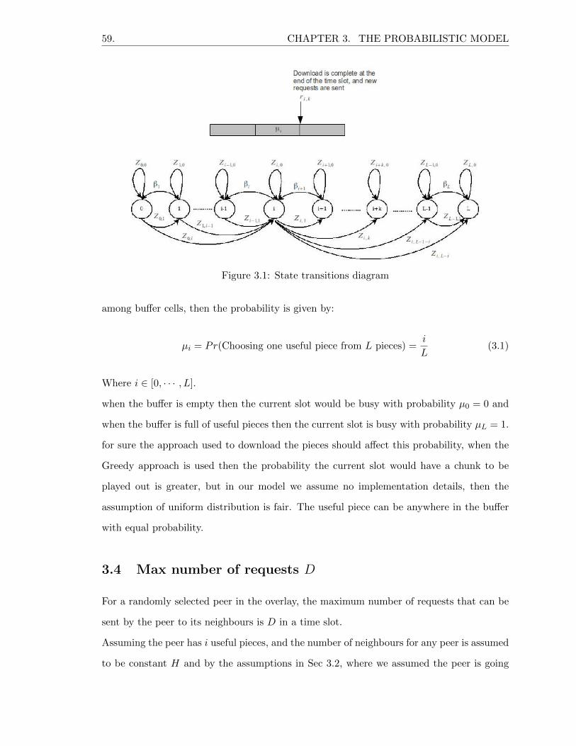
59. CHAPTER 3. THE PROBABILISTIC MODEL
Figure 3.1: State transitions diagram
among buffer cells, then the probability is given by:
µi = Pr(Choosing one useful piece from L pieces) =i
L(3.1)
Where i ∈ [0, · · · , L].
when the buffer is empty then the current slot would be busy with probability µ0 = 0 and
when the buffer is full of useful pieces then the current slot is busy with probability µL = 1.
for sure the approach used to download the pieces should affect this probability, when the
Greedy approach is used then the probability the current slot would have a chunk to be
played out is greater, but in our model we assume no implementation details, then the
assumption of uniform distribution is fair. The useful piece can be anywhere in the buffer
with equal probability.
3.4 Max number of requests D
For a randomly selected peer in the overlay, the maximum number of requests that can be
sent by the peer to its neighbours is D in a time slot.
Assuming the peer has i useful pieces, and the number of neighbours for any peer is assumed
to be constant H and by the assumptions in Sec 3.2, where we assumed the peer is going
60. CHAPTER 3. THE PROBABILISTIC MODEL
to send a request for each neighbour and only one request for each missing piece then the
maximum number of requests sent by a peer is:
D = min(H,L− i) (3.2)
3.5 ri,n
this parameter is the probability a peer with i useful pieces will download n pieces in the
current time slot. It is used to determine the birth and death rates in our model, and also
in calculating the average downloading rate.
These probability satisfies the following normalization condition:
n=Dn=0
ri,n = 1
Which means it is a probability distribution, and D is given in the Eq 3.2.
3.6 Death rate βi
The death rate in our model is the probability a peer in the state i will move at the end of
the time slot to the previous state i− 1, it happens only under these two conditions:
• The current time slot is busy with one of the useful pieces
• And no pieces have been downloaded in the current time slot
This probability is given by the following equation:
βi = µi × ri,0 (3.3)
For sure when the peer is at the state 0 then the death rate is going to be β0 = 0 because
µ0 = 0.

61. CHAPTER 3. THE PROBABILISTIC MODEL
3.7 Birth rate Zi,k
As illustrated in the Fig 3.1 the birth rate is the parameter Zi,k which means a peer with i
useful pieces will generate k births to move to another state j = i+ k.
This probability depends on the number of downloaded pieces and also whether the slot is
empty or busy:
Zi,k = µi × ri,k+1 + (1− µi)× ri,k (3.4)
In the previous equation, there would be k final downloads or births, in either case:
• The current slot is empty, and during the slot there are k downloads of useful pieces.
• The current slot is busy, and during the slot there are k+1 downloads of useful pieces.
Thereby Zi,0 means the peer has downloaded one piece during the busy slot, or the peer
has downloaded no pieces during an empty slot:
Zi,0 = µi × ri,1 + (1− µi)× ri,0
In either case the peer will stay at state i at the end of the slot, this concept of birth and
death rates gives a lot of flexibility in defining the Markov chain illustrated in Fig 3.1.
3.8 Markov chain
An integer-valued Markov random process is calledMarkov Chain [13], ifX(t) is a Markov
chain then the joint PMF for three arbitrary time instants is:
P [X(t3) = x3, X(t2) = x2, X(t1) = x1] =
P [X(t1) = x1]× P [X(t2) = x2|X(t1) = x1]× P [X(t3) = x3|X(t2) = x2]
the joint pmf of X(t) at arbitrary time instants is given by the product of the pmf of the
initial time instant and the probabilities for the subsequent transitions, clearly the state
transition probabilities determines the statistical behaviour of Markov Chain [13].

62. CHAPTER 3. THE PROBABILISTIC MODEL
letXn be a discrete-time integer-valued Markov chain, whereXn takes values on a countable
set of integers, in our model these values are the peer states defined by the number of useful
pieces in its buffer {0, · · · , L}, we say that Markov chain is finite if Xn takes values from a
finite set.
The joint pmf for the first n+ 1 values of the process is:
P [Xn = in, · · · , X0 = i0] = P [X0 = i0] · · ·P [Xn = ii|Xn−1 = in−1]
The joint pmf for a particular sequence is simply the product of the probability for the
initial state and the probabilities for the subsequent one-step state transitions.
In our model and in the steady-state we assume the transition probabilities are independent
of time, that is:
P [Xn+1 = j|Xn = i] = Pij
Then Xn is said to have a homogeneous transition probabilities [13].
By defining the probability of one death and the probability of birth(s) in a time slot we
can write the transition probability matrix for markov chain:
P =
Z0,0 Z0,1 ... ... Z0,L
β1 Z1,0 ... ... Z1,L−1
... ... ... ... ...
0 β2 Z2,0 ... Z2,L−2
0 0 ... βL ZL,0
(3.5)
the rows of the transition matrix will add to 1, since:
j
Pij = 1

63. CHAPTER 3. THE PROBABILISTIC MODEL
And P is (L+1)× (L+1) nonnegative square matrix with rows that each adds up to 1. as
an example assuming H = 1 then we have three possible transitions:
• moving to the previous state with the probability βi
• moving to the next state with probability Zi,1
• to stay in the same state with probability Zi,0
then the transition matrix for L = 2:
P =
Z0,0 Z0,1 0
β1 Z1,0 Z1,1
0 β2 Z2,0
The summation of the first row is:
Z0,0 + Z0,1 + 0 = µ0r0,1 + (1− µ0)r0,0 + (1− µ0)r0,1
= 0× r0,1 + (1− 0)r0,0 + (1− 0)r0,1
= r0,0 + r0,1
= 1
The summation of the second row is:
β1 + Z1,0 + Z1,1 = µ1r1,0 + (1− µ1)r1,0 + µ1r1,1 + (1− µ1)r1,1
= µ1r1,0 + r1,0 − µ1r1,0 + µ1r1,1 + r1,1 − µ1r1,1
= r1,0 + r1,1
= 1

64. CHAPTER 3. THE PROBABILISTIC MODEL
The summation of the third row is:
β2 + Z2,0 + 0 = µ2r2,0 + µ2r2,1 + (1− µ2)r2,0
= 1× r2,0 + 1× r2,1 + (1− 1)r2,0
= r2,0 + r2,1
= 1
The proof can be easily generalized as the following.
Proof Rows of transition matrix defined in Eq 3.5 each sums up to one.
For row i > 0 the proof is as following:
βi +
k=L−ik=0
Zi,k = βi +
k=L−ik=0
(µiri,k+1 + (1− µi)ri,k)
= µiri,0 + µi
k=L−ik=0
(ri,k+1 − ri,k) +
k=L−ik=0
ri,k
= µiri,0 + µi(ri,L−i+1 − ri,0) +k=L−ik=0
ri,k
= µiri,L−i+1 +k=L−ik=0
ri,k
= 0 +k=L−ik=0
ri,k
=k=Dk=0
ri,k = 1
For row i = 0:
k=Lk=0
Z0,k =k=Lk=0
(µ0r0,k+1 + (1− µ0)r0,k)
= µ0
k=Lk=0
(r0,k+1 − r0,k) +k=Lk=0
r0,k
= 0×k=Lk=0
(r0,k+1 − r0,k) + 1
= 1
65. CHAPTER 3. THE PROBABILISTIC MODEL
Assuming at time n the state vector is π(n) = [p(n)0 , p
(n)1 , ......, p
(n)L ] and the transition
matrix at time (n) is P (n). We have the following relation between the state-vector at time
n+ 1 and the state vector at time n:
π(n+1) = π(n)P (3.6)
The relation between the state-vector at time 0 and the state-vector at time n is given as
the following:
π(n) = π(0)P (n) = π(0)Pn
At the steady state we have the following equilibrium equation:
π = πP (3.7)
where π is the state vector in the steady state:
π = limn→∞
π(n)
The numerical solution result would be obtained by finding the steady-state vector π =
[P0, P1, · · · , PL] that describes the probability a peer would have specific number of useful
pieces in its buffer.
3.9 Interesting factor Ui
For a randomly selected peer with i useful pieces we denote Ui to be the probability that a
randomly selected peer with i useful pieces is interested in downloading pieces from a one
of its neighbours, this interesting factor is calculated based on the calculation of F (i, j) in
the previous chapter. The number of neighbours for any peer is assumed to be constant
H, and the steady-state probability for the peer is assumed to be available which is the

66. CHAPTER 3. THE PROBABILISTIC MODEL
state-vector π = [P0, · · · , PL]
Ui = Pr(peer with i useful pieces is interested
in downloading pieces from a neighbour)
Ui =
j=Lj=0
(1− F (i, j))Pj (3.8)
Where Pj is the probability a peer has j useful pieces. This factor is very important in our
model and later we will plot curves for the numerical results for this factor.
We can also define U to be the general interesting factor, which is the probability a ran-
domly selected peer is interested in any neighbour, even though it is not used widely in our
calculations:
U =i
UiPi (3.9)
3.10 F (H, i′, K)
In [32] when calculating the the probability ri,n they used a simple formula to calculate the
probability of a neighbour is sending a request to a peer B with j pieces, this probability
is qj :
qj =Nk=0
Pk(1− F (k, j))
Where F (i, j) is the probability a peer A with i pieces is not interested in peer B with j
pieces in Bittorrent file sharing application; this formula is very simple because it depends
only on the interesting factor while sending the request to a neighbour is very difficult
problem, for example: when a peer A is interested in peer B that does not mean A is going
to choose B, especially in streaming applications where we have assumed the peer is going
to send only request for each missing pieces and one request for each neighbour.
To fully describe the problem we define F (H, i′, k) to be the Probability that a peer with i

67. CHAPTER 3. THE PROBABILISTIC MODEL
useful pieces in its buffer, and is looking for i′= L− i pieces will send k requests to its H
neighbours in a time slot.
Where i′is the number of missing pieces, and k should be less than the maximum number
of requests as defined in Eq 3.2, in other words:
0 ≤ k ≤ D
To calculate this probability we need to understand the mechanism of sending a request, this
probability describes what is called in the literature the scheduling algorithm. For simplicity
we assume general random approach, the peer as we said maintains a list of neighbours, the
peer is going to choose a neighbour randomly from the list and then sending a request to that
neighbour with probability of Ui, and it chooses not to send the request with probability
1− Ui. This will be continued until the requests number is 0, the number of neighbours is
0 or there is no more missing pieces, We can use iterative algorithm to calculate it:
F (H, i′, k) = Ui × F (H − 1, i
′ − 1, k − 1) + (1− Ui)× F (H − 1, i′, k) (3.10)
As we note the iterative method contains two recursive functions on the right hand side,
computing this value is also a challenging problem discussed in the next chapter, but for
now we know that the recursive calculation ends when reaching the initial conditions, it
turns out that there are(6) initial conditions represented as a tree (the initial conditions
tree) illustrated in the Fig 3.2:
Ui the probability of sending request to one neighbour defined in Eq 3.8
H − 1 because one request is sent for each neighbour
i′ − 1 missing pieces will be now less with one after the request
k − 1 the requests are now less with one request

68. CHAPTER 3. THE PROBABILISTIC MODEL
Figure 3.2: initial conditions tree
The cases for initial conditions:
• Pr(C1) = 1 → when there is no neighbour the peer is certainly not going to send any
request
• Pr(C2) = 0 → the complement of C1
• Pr(C3) = 1 → when there are neighbours and no missing pieces that means the buffer
is full of useful pieces there would be no request
• Pr(C5) = 0 → the complement of C3
• Pr(C6) by applying the Eq 3.10 iteratively
The case C4 needs a little more explanation. This case means: the peer is connected to
some neighbours and there are some missing pieces, then what is the probability the
peer will not send any request in the current time slot?
The peer will not send any request only when the peer is not interested in any neighbour,
this can be calculated using the following equation for peer with i useful pieces:
Pr(C4) =
j=Lj=0
F (i, j)Pj
H
= (1− Ui)H

69. CHAPTER 3. THE PROBABILISTIC MODEL
By applying Eq 3.10 iteratively and using the initial conditions we obtain F (H, i′, k), as
an example we obtained a table for some numerical results. From Table 3.1 we note that
Table 3.1: Results for F (H, i′, k)
H i′
K Value Sum
1 3 0 0.00312543 1.00000043
1 3 1 0.996875
1 3 2 0
2 2 0 0.00851766 1.00662666
2 2 1 0.174174
2 2 2 0.823935
1 2 0 0.0204852 1.0000002
1 2 1 0.979515
1 2 2 0
1 1 0 0.0922911 1.0000001
1 1 1 0.907709
2 3 0 0.000419643 1.000355343
2 3 1 0.0404867
2 3 2 0.959449
the max number of requests can’t be greater than H and i′and we note the following
distribution:
k=Dk=0
F (H, i′, k) = 1
3.11 Average number of requests K̄
Let K̄i be the average number of requests sent by a peer with i useful pieces to its neighbours,
then it is given by the following equation:
K̄i = E[F (H, i‘, k)] =k=Dk=0
F (H, i‘, k)× k (3.11)

70. CHAPTER 3. THE PROBABILISTIC MODEL
From Eq 3.11 and by unconditioning over i we get K̄ the average number of requests sent
by a randomly selected peer to its neighbours.
K̄ =i=Li=0
K̄i × Pi (3.12)
We have also to note in our model and calculation of F (H, i′,K) we assumed there is at
maximum one request sent per neighbour, which results in K̄ ≤ H, this parameter is very
important as we will see in justifying the numerical results.
3.12 Distribution of received requests X
To calculate the probability of fulfilment a request as the next step in our model, we use a
similar approach as in [32], but here the problem is more complex, and also it contains a
new parameter which is F (H, i′, k). The calculation would be illustrated by the Fig 3.3.
In the Fig.3.3 a reference peer A sends requests to its neighbours with certain probability
F (H, i′, k), one of these neighbours is B we consider it as a reference neighbour, any neigh-
bour would fulfil the request with certain probability that is Q, this probability should be
calculated.
Any peer during the time slot will receive many requests from neighbours, that is B would
receive requests from neighbours including A, how the peer is going to fulfil the re-
quests?
It simply chooses one of these requests randomly to be fulfilled, or as we will see later it
chooses at maximum β requests to be fulfilled. We define a random variable X to be the
number of requests received from H neighbours, then X is a Binomial random variable with
parameters: H,α.
Where α is the probability the peer is receiving request from a neighbour. In the Fig 3.3
when referring to B, then α means the probability that B receives a request from A, and
it is the same probability that B receives a request from C.
Pr(X = i) =
H
i
αi(1− α)H−i (3.13)

71. CHAPTER 3. THE PROBABILISTIC MODEL
To calculate the probability α, we consider the peer B in the Fig.3.3, to derive α we assume
the number of requests sent by C is constant k which results in the following argument:
• If k = 1 then peer C is going to choose any neighbour with probability 1H
• If k = 2 then peer C is going to choose any neighbour for sending the request to it
with probability 2H
• · · ·
• in General when the peer sends k requests then the probability a neighbour will receive
a request is kH
This can be easily justified by remembering that a peer will choose any peer from the list
randomly and uniformly to send it a request with probability Ui, assuming the peer has i
useful pieces then:
αi =1
HF (H, i
′, 1) +
2
HF (H, i
′, 2) + · · ·+ D
HF (H, i
′, D)
=
Dk=1
kF (H, i′, k)
H
Where D is defined in Eq 3.2 and by using the definition of Ki in Eq 3.11
αi =K̄i
H(3.14)
And by unconditioning over i we get the equation of α:
α =
Li=0
αiPi =K̄
H(3.15)
From Eq 3.15 and Eq 3.13 the average number of requests received from a neighbour is:
X̄ = Hα
= HK̄
H

72. CHAPTER 3. THE PROBABILISTIC MODEL
Figure 3.3: The calculation of Q
which means the average number of received requests from neighbours is:
X̄ = K̄ (3.16)
This also means in the steady-state what the peer sends is also what it receives from
neighbours, given that the peer will choose any neighbour equally for sending the request.
We need to mention that F (H, i′,K) is to measure the probability a peer will send
number of requests to neighbours, while X measure the probability a peer receives
number of requests from neighbours. These two parameters are different, the first
one is calculated from the peer perspective, which chooses one neighbour randomly
each time and sends the request with certain probability. While the second one is
from neighbours perspective, neighbours are independent when sending requests
to a specific peer.
3.13 Probability of fulfilling a request Q
When the peer B in the Fig 3.3 receives many requests, the peer chooses one of these
requests randomly to be fulfilled, the probability of fulfilling a specific request is Q and can
be found by this table:
Where X is the random variable representing the number of requests a peer receives from

73. CHAPTER 3. THE PROBABILISTIC MODEL
Table 3.2: Q Calculation
X 1 2 · · · H
Q 1 0.5 · · · 1H
H neighbours, then we can calculate Q as in the following equation:
Q =k=Hk=1
1
kPr(X = k) (3.17)
The previous equation is derived assuming that the peer can upload only one chunk per
time slot, but When releasing the upload bandwidth then Q is calculated as the following,
given that β denotes the upload bandwidth:
Q =Hk=1
min(1,β
k)Pr(X = k) (3.18)
3.14 ri,n
After calculating Q we can find the probability a peer with i useful pieces downloads n
chunks in the current time slot, the peer will send k requests with probability F (H, i′, k),
and the probability of fulfilling a request is Q then ri,n is calculated as the following:
ri,n =
Dk=n
k
n
Qn(1−Q)k−nF (H, i‘, k) (3.19)
3.15 Paradox of Q
One may choose to calculate Q in another way which is:
Q =H−1k=0
1
k + 1Pr(X = k)
Where X is now the number of requests received from H − 1 neighbours, but we found
this approach is not correct since it gives the highest continuity always to be at H = 1,
so increasing H is actually decreasing the continuity which contradicts the common sense

74. CHAPTER 3. THE PROBABILISTIC MODEL
in these applications, the problem can be explained when we there is only one neighbour
H = 1, then the probability of fulfilling the request is Q = 1, because then Pr(X = 0) = 1
for X now represents the number of requests received from H − 1 then:
Q =1
1 + 0Pr(X = 0) = 1
and the probability of sending a request to one neighbour is very high, that will result in
the highest continuity at H = 1, also by using the lower bound of Jensen Inequality then
Q can be approximated to the following value:
Q ≈ 1
1 + H−1H K̄
the interpretation is: picking one request from (requests received from H − 1 neighbours
+ 1), this actually breaks the assumption that the peer is sending on average K̄ and
should receive on average also K̄, then to solve this paradox the best approximation for this
probability would be:
Q =
1 K̄ <= 1
1K̄
K̄ > 1
This equation imposes the fact that the average number of received requests is the same
as the average number of sent requests, which is actually used in the calculation of α, the
previous equation is an approximation for the calculation of Q used in the Eq 3.17, and
then Q can be understood by that equation: the probability a neighbour receives at least
one request and fulfilling one of these requests.
3.16 Average download rate D̄
Average download rate is also another important parameter to be calculated, this parame-
ter can be used to justify the continuity. The larger the average download rate the better
continuity the peer will experience, given that the peer has i useful pieces then the average

75. CHAPTER 3. THE PROBABILISTIC MODEL
download rate is:
Di =D
k=0
kri,k (3.20)
Then the average download rate for a peer is:
D =Li=0
DiPi (3.21)
3.17 Efficiency η
The efficiency is calculated following the same approach in [27], in this paper the efficiency
is defined as: for a given peer the efficiency is the probability the peer is now uploading
data to its neighbours, we use the parameter α to get the following expression:
η = Pr(The peer is uploading to neighbours)
= Pr(Peer receives at least one request)
= 1− Pr(X = 0)
where X is the number of received requests from H neighbours, this means the peer would
be in uploading state just when the peer receives at least one request from its neighbours,
therefore:
η = 1− (1− α)H (3.22)
3.18 Continuity Pc
Given a randomly selected peer in the network, then the probability that this peer is now
listening to or watching the live stream, is known as the probability of continuity and
denoted as Pc, this probability is actually the probability the current time slot is busy, we

76. CHAPTER 3. THE PROBABILISTIC MODEL
have seen this probability in Eq 3.1, then by unconditioning over i:
Pc =Li=0
µiPi (3.23)
As we can see this probability is actually the average number of useful pieces over the buffer
length, using Eq 3.1:
Pc =Li=0
µiPi
=Li=0
i
LPi
=N̄
L
Where N̄ denotes the average number of useful pieces in the buffer.
3.19 Discussion of Numerical results
In this section we plot some numerical results and discuss the implications.
3.19.1 Continuity Pc as a function of H
• From the Fig 3.4 it is noted that when increasing H then the continuity increases until
H reaches a threshold H̃, we call this threshold the saturation point and is denoted
as H̃.
• Values less than H̃ are denoted as −H and values greater than H̃ are denoted as +H
• It is noted also that this threshold would be in the first few values{1, 2, 3, 4, 5} and the
precise value depends on the value of delay T . Here we have to mention that in [42]
the paper that presents the DONet a data-driven overlay network for live streaming
applications, in their experiment with a prototype implementation of 200-300 nodes
and operating in PlanetLab test-bed, plotting the curve of Continuity Index the result
was: ”To Evaluate the continuity we define the continuity index which is the number of
segments that arrive before or on playback deadline over the total number of segments,

77. CHAPTER 3. THE PROBABILISTIC MODEL
Figure 3.4: Continuity with different values of H and T, L = 40
Fig.7 shows that the continuity index as a function of M , the number of partners, we
can see that the continuity increases with increasing M because each node may have
more choices of suppliers, the improvments with more than 4 partners are marginal,
using 4 partners is reasonably good even under high rates, considering that the control
overhead increases with more than 4 partners, we believe that M = 4 is good practical
choice” [42].
• the result in [42] is similar to our result in the Fig 3.4, but in our result we notice that
after H̃ the continuity decreases at very slow rate 10−5, and this is also explained later
because of our model assumptions, while in [42] it is mentioned that after 4 partners
the continuity will decrease because of the control overhead which is the real practical
reason in their experiment.Pc ↑ When H ↑ and H ∈ −H
Pc ↓ When H ↑ and H ∈ +H

78. CHAPTER 3. THE PROBABILISTIC MODEL
3.19.2 Average request rate K̄
Figure 3.5: K̄ as a function of H - and T = 35, L = 40
It is noted from the Fig 3.5 that increasing the number of neighbours H increases the
average request rate K̄, but the increment is not linear, and that is because after few number
of neighbours, the buffer would be almost full of useful pieces (in the case of tow neighbours,
there is a possibility of downloading two chunks and playing one, because of buffering). As
illustrated in Fig 3.6 the average number of useful pieces in the buffer is very high even
at small values of H, which means small number of missing pieces as illustrated in Fig 3.7
where we define the parameter M̄ as the following:
M̄ = L− N̄ (3.24)
Where N̄ is the average number of useful pieces in the buffer and is calculated as the
following:
N̄ =
Li=0
iPi = PcL (3.25)
the small number of missing pieces illustrated in the Fig 3.7 is the reason for small rate of

79. CHAPTER 3. THE PROBABILISTIC MODEL
Figure 3.6: N̄ as a function of H - and T = 35, L = 40
Figure 3.7: M̄, K̄ as a function of H - and T = 35, L = 40

80. CHAPTER 3. THE PROBABILISTIC MODEL
K̄ increment.
3.19.3 Comparison between DONet and our model results
From the Fig 3.8 (Figure. 7 in [42]),Fig 3.9 we can compare the results obtained from the
experiment in [42] and our model for the continuity as a function of the H the number of
partners, we notice that our results are very close to the practical results obtained in [42],
we used the same buffer length L = 60, we defined T = 60 in our model, and used the
same number of partners for sample points. In emperical results the continuity was around
98% while in our model the continuity is around 97%. Taking into consideration lot of
assumptions in our model we believe that the result is very encouraging.
Figure 3.8: DONet results taken from [42]
3.19.4 The average number of received requests αH
From Fig 3.10 as expected increasing the number of neighbours will decrease the probability
of receiving a request from a neighbour, obviously the reason is because the neighbour would
have more choices, but the product αH illustrated in the Fig 3.11 increases in the same
way K̄ increase in the Fig 3.5. That is also obvious because the product αH is actually
the expected value of the binomial random variable X, which means the average number of
received requests, the more neighbours maintained by a peer the more requests it receives.

81. CHAPTER 3. THE PROBABILISTIC MODEL
Continuity
0.9
0.91
0.92
0.93
0.94
0.95
0.96
0.97
0.98
0.99
H
1 2 3 4 5 6 7
Figure 3.9: Comparison between our model and DONet results
And based on our assumptions and how we calculated α it is expected that the peer will
receive on average what it sends on average, comparing the two diagrams of Fig 3.5 and
Fig 3.11 there is a match, they are the same values.
Figure 3.10: α with different values of H

82. CHAPTER 3. THE PROBABILISTIC MODEL
Figure 3.11: αH The Average number of received requests as a function of H
3.19.5 Probability of fulfilling a request Q
Increasing the number of neighbours H increases also the average number of received re-
quests αH as illustrated in the Fig 3.11, and recall that the request is fulfilled by randomly
choosing one of the received requests to be fulfilled, then the probability of fulfilling a spe-
cific request would decrease always as illustrated in the Fig 3.12, but the decrement rate
would be slower in the range +H.
This relation is illustrated as the following:
H ↑⇒ αH ↑⇒ Q ↓
3.19.6 Average download rate D̄
From the Fig 3.13 we notice that increasing H increases the average download rate D̄ in the
range −H but then it will decrease in the range +H, and this complies with the behaviour
of continuity Pc illustrated in the Fig 3.4.
From the Fig 3.13 we notice also that D̄ < 1, this can be explained mathematically,
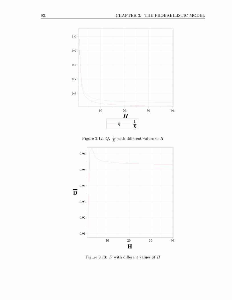
83. CHAPTER 3. THE PROBABILISTIC MODEL
Figure 3.12: Q, 1K̄
with different values of H
Figure 3.13: D̄ with different values of H

84. CHAPTER 3. THE PROBABILISTIC MODEL
from the Fig 3.12 we notice that Q < 1K̄
then:
D̄ = K̄Q
< K̄1
K̄
< 1
Also here we have to mention that, the Jensen Inequality [16][Page 1066] if it is applied it
should give the following:
E[f(X)] ≥ f(E[X])
E[1
X] ≥ f(K̄)
Q ≥ 1
K̄
Which is the opposite to our numerical results, the reason we can’t apply the Jensen In-
equality to the function 1X where X defined in the Eq 3.13, because X is not convex even
though the second derivative is positive, also it is because 1X defined as 0 when X = 0
this will make the function quasiconcave, we did not dig too much into the details of this
function, but the justification is enough to explain why we get this upper limit.
We can not apply Jensen Inequality on Q to get the lower limit, because the
function is not convex.
3.19.7 Why Pc increases in the range −H?
The behaviour of Pc is reflected by the average download rate D̄, which also increases in the
range −H. The average download rate can be justified because of the product K̄Q which
has the following behaviour:
−H QK̄ ↑
+H QK̄ ↓

85. CHAPTER 3. THE PROBABILISTIC MODEL
From the Fig 3.12 and the Fig 3.5, in the range +H it is noted that Q decreases faster than
the increment of K̄, so after H̃ there is no improvement in the system, on the contrary it
will initiate a competition because of the nature of our model.
when the peer sends a request to a neighbour it does it randomly and independently of
other neighbours, that would cause the probability of a competition with other peers to
increase.
After H̃ the choices of peer would increase because K̄ does not increase linearly,
the system is not intelligent enough to use the resources efficiently because peers
do not communicate with each other, this will result in a competition tendency in
our model.
To get a deeper insight from Fig 3.7 before H̃ there are many missing pieces and few
number of peers, for example at the first sample: {H = 1, M̄ = 3.5} then K̄ is limited by
H according to our assumption, and just after 2 peers M̄ drops under 2 which causes K̄ to
be limited by M̄ not H and the match happens at H̃.
3.19.8 The effect of buffer length L
From the Fig 3.14, increasing the buffer length would increase both the efficiency and
continuity, but there is also a trade-off because increasing L in this kind of applications
will increase the overhead of exchanging messages among neighbours because the peers will
exchange the buffer map to create the partial view of the overlay. In Coolstreaming the
buffer size is usually 120, as noted from Fig 3.14 after L = 100 the continuity is over 98%.
3.19.9 The effect of maximum allowed delay T
As defined in Sec 2.2.4 and CoolStreaming documentation it is the maximum allowed devi-
ation between the peer playback pointer and the playback pointer of other neighbours.
As stated in CoolStreaming: it is used to indicate whether the partner is sufficient or not,
it’s a measurement for the partner insufficiency. In our model: when the neighbour play-
back pointer falls behind or is far ahead the peer playback pointer that’s an indication that
the neighbour is insufficient, this insufficiency is because the neighbour upload bandwidth

86. CHAPTER 3. THE PROBABILISTIC MODEL
Figure 3.14: L The Effect of Buffer length on Pc, η
is not enough. In our model this can be interpreted in the same way, the peer should be
synchronized with other neighbours.
From the Fig 3.4 it is noted that increasing T causes the continuity to decrease, which
means smaller values of T are preferred unlike the effect of buffer length L, but there is
also a trade-off; increasing T means the peer would be more tolerant regarding the partner
selection, and it would be easier to find the suitable partner in the overly, while smaller T
means the peer would be very strict and demanding, which will lead to more reselection
rate, and instability in the overly, and more maintenance overhead.
This negative effect can not be measured in our model because the assumption is that we
have infinite number of peers in the overlay and always the peer can find H neighbours that
satisfy T inequality in the Eq 2.1. When addressing the First Chunk Problem we give a
parameter for measuring the sliding action and lack of synchronization.
The reason behind the decrement of Pc when increasing T can be easily explained by the
broken relation definition, when increasing T the common window between two peers in-
creases which means the probability of broken relation increases, this effect can be found

87. CHAPTER 3. THE PROBABILISTIC MODEL
in the Fig 3.15, by increasing T the average interesting factor U decreases which causes the
continuity to decrease as illustrated in the same figure.
Figure 3.15: Effect of Delay T on Interesting factor U and Continuity Pc
3.19.10 Efficiency η
The efficiency as calculated in the Eq 3.22 is the probability a peer is in the uploading state,
in other words it is the probability of peer contribution in the overlay, from the Fig 3.16 we
notice the following:
• Increasing T results in the decrement of the efficiency η that can be explained with
the same argument used before, increasing T increases the probability of a broken
relation.
• Increasing the number of neighbours decreases the efficiency, this behaviour does
not mean the continuity should always decrease, because although the contribution
of one peer decreases but the number of neighbours increases, the reason behind this
decrement is obvious, increasing the number of neighbours H means the probability of

88. CHAPTER 3. THE PROBABILISTIC MODEL
receiving a request from a neighbour decreases α, and the probability of not receiving
a request from a neighbour 1−α increases, and hence the probability of not receiving
a request from all neighbours increases (1 − α)H . The decreased efficiency supports
the integrity of our discussion, in which increasing the number of neighbours initiates
the competition.
• We note also the efficiency in the range −H is higher than the efficiency in the range
+H
Figure 3.16: η with different values of H and T
Here we have to mention that the contribution of the peer in the overlay would decrease by
increasing the number of the neighbours, because those neighbours would have more choices
for sending the request, and the system depends on the partial view, there is no complete
picture in the data-driven approach, but the implementation is simpler.

89. CHAPTER 3. THE PROBABILISTIC MODEL
3.19.11 Releasing upload bandwidth β
We obtained numerical results for different values of uploading bandwidth β assuming
homogeneous peers, where each peer has the same uploading capability.
It is noted from the Fig 3.17 that the Continuity Pc increases as we increase the uploading
bandwidth, but also we notice that there is a threshold, after specific value of β we notice
that increasing the uploading bandwidth does not improve the continuity. This can be easily
explained by the Fig 3.19 which represents the average request rate K̄ for different values
of upload bandwidth β, from that figure we notice that increasing the uploading bandwidth
will decrease K̄, because the peer can now download more chunks in a time slot, this will
cause the buffer to be almost full, and when K̄ is stable on a specific value then also Q will
stabilize, then the product QK̄ will also be fixed, and so do the average download rate and
hence the continuity.
The Fig 3.18 represents the effect of the uploading bandwidth β on the efficiency η, from
this figure it is noted that increasing the uploading bandwidth will decrease the efficiency,
this is easily explained by the parameter K̄, which decreases by increasing β which means
also decreasing the probability of receiving a request from neighbour α, this is the main
reason for the efficiency decrease.
3.19.12 Releasing uploading bandwidth for Heterogeneous peers
We assumed in the previous sections the homogeneous peers, which means all peers have
the same capabilities like: the number of partners H and also the uploading bandwidth β,
these parameters assumed to be constant. Now we consider the case of heterogeneous peers
regarding the uploading bandwidth.
We assume the random variable W to be the number of chunks a peer can upload in one
time slot, with the probability mass function:
Pr(W = n), with∀n
Pr(W = n) = 1

90. CHAPTER 3. THE PROBABILISTIC MODEL
Figure 3.17: Continuity as a function of upload bandwidth β
Figure 3.18: η as a function of upload bandwidth β

91. CHAPTER 3. THE PROBABILISTIC MODEL
Figure 3.19: K̄ as a function of upload bandwidth β
this random variable replaces the parameter β in the previous analysis.
Then Q the probability of fulfilling a request is given by the following expression:
Q =Hk=1
∀n
min(1,n
k)Pr(X = k)Pr(W = n) (3.26)
Assuming the random variable W is uniform with the following PMF:
Pr(W = n) =1
7, n : 1, 2, , 3, 4, 5, 6, 7
Substituting this PMF in Eq 3.27 we get the following expression for Q:
Q =1
7
Hk=1
7n=1
min(1,n
k)Pr(X = k) (3.27)
In the Fig 3.20 we plot the continuity for two cases:
• Homogeneous peers with uploading bandwidth β = 4

92. CHAPTER 3. THE PROBABILISTIC MODEL
• Heterogeneous peers with uploading bandwidth as random variable W and PMF:
Pr(W = n) = 17 , n : 1, · · · , 7 and the expected value is: W̄ = 4
Figure 3.20: The heterogeneous and homogeneous peer continuity
From Fig 3.20 It is noted that the continuity in the heterogeneous case is lower than the
continuity for the homogeneous case, this is expected due to the variability of the random
variable W .
3.20 Conclusion
In this chapter we completed the basic model for live streaming applications, using the
concept of broken relation we proposed a Markovian model, and calculated the terms of
probability transition matrix. Then we plotted the numerical results.
Using our model we got a continuity that is similar to empirical results, and we extended
the model to address the heterogeneous uploading bandwidth.
we found that increasing the number of neighbours does not necessary result in better
continuity, also increasing the buffer length gives better continuity but there is a trade-off.

93. CHAPTER 3. THE PROBABILISTIC MODEL
we discussed the effect of delay on the continuity as well as the efficiency.
We believe that this model provides the system designer with a fundamental mathematical
model to help choosing and tweaking the system parameters. In the following chapter we
discuss the problems in the numerical solution and in later chapter we show that the model
is very flexible by addressing the first chunk problem.

94. CHAPTER 4. PROBLEMS IN NUMERICAL SOLUTION
Chapter 4
Problems in numerical solution
4.1 Introduction
In this chapter we present two problems encountered in the numerical solution, the
first problem is related to the calculation of probability of sending K requests for
a peer with i useful pieces and maintaining a list of H neighbours. The second problem is
how to iteratively solve the Markovian model. We believe these two problems are important
for any researcher building on the top of this model.
4.2 The initial conditions tree - F (H, i′, K)
We used the Eq 3.10 to calculate the probability that a peer with i useful pieces sends k
requests to H neighbours, here we write down the equation again:
F (H, i′, k) = UiF (H − 1, i
′ − 1, k − 1) + (1− Ui)F (H − 1, i′, k)
This function is used extensively in the numerical solution, and finding the result of this
function is not a simple task, because this type of functions is known in the computer
science literature as tree recursive function, it will be explained next using [1] and we
suggest algorithm for more efficient computation.

95. CHAPTER 4. PROBLEMS IN NUMERICAL SOLUTION
4.2.1 Linear recursion and iteration
The simplest example of recursion is the calculation of the factorial function defined by:
n! = n× (n− 1)× (n− 2) · · · × 1
The idea of recursion is to calculate the term (n− 1)! and multiply it by n:
n! = n× [(n− 1)× (n− 2) · · · 1] = n× (n− 1)!
By adding the initial condition 1! = 1 then the recursive function can be written in simple
C++ computer program to calculate the factorial as the following:
Listing 4.1: Factorial Recursive Function
i n t f a c t o r i a l ( i n t n)
{
i f (n==1) re turn 1 ;
re turn n∗ f a c t o r i a l (n−1);
}
the execution path for 6! can be visualized in the Fig 4.1.
Also we can describe a rule for computing n! by specifying that we first multiply 1 by 2
Figure 4.1: Execution path of the factorial recursive function
and the result by 3 · · · and so on until we reach n, this implementation is known as iterative
solution, and is implemented in C++ program using a simple loop:

96. CHAPTER 4. PROBLEMS IN NUMERICAL SOLUTION
Listing 4.2: Factorial Iterative Function
i n t f a c t o r i a l ( i n t n)
{
i n t r e s =1;
f o r ( i n t i =1; i<=n ; i++)
r e s∗=i ;
re turn r e s ;
}
The execution path can be visualized as in the Fig.4.2.
Comparing the two approaches, the first process reveals a shape of expansion followed
by a contraction, this is because the process or the recursive function builds up a chain
of deferred operations, and the contraction happens when these operations are actually
performed, this process is called the recursive process. Where the execution requires to
keep track of operations to be performed later. In the recursive process for calculating the
n! grows linearly with n.
While in the second process there is no expansion in the execution path, and all we need
is to keep track of only one variable res, this process is called the iterative process, whose
state is summarized by fixed number of state variables. Hence we can conclude that the
problem with recursive computation: it consumes a lot of memory; this will be a problem
for calculating large values of n!, the stack is used to store the local variables at each call
and it is considered very small in size (few megabytes); another problem with recursive
process is the performance because function call is expensive.
Figure 4.2: Execution path of the factorial iterative function

97. CHAPTER 4. PROBLEMS IN NUMERICAL SOLUTION
4.2.2 Tree Recursion
Recursion can be also more complex, consider generating the sequence of Fibonacci numbers,
in which each number is the sum of the preceding two:
0, 1, 1, 2, 3, 5, 8, 12, 21, · · ·
The Fibonacci numbers are defined by the following rule:
Fib(n) =
0 if n = 0
1 if n = 1
Fib(n− 1) + Fib(n− 2) otherwise
this rule can be implemented by the following C++ recursive function:
Listing 4.3: Fibonacci Recursive Function
i n t f i b ( i n t n)
{
i f (n==0) re turn 0 ;
i f (n==1) re turn 1 ;
re turn f i b (n−1)+ f i b (n−2);
}
Because the function calls itself twice, the execution path will be like a tree, at each level
the branches split into two(except the bottom), the execution path is illustrated in the Fig
4.3. This way of calculating the Fibonacci numbers is inefficient for the following reasons:
• there is much of redundant calculations, for example in the Fig 4.3 the Fib(3) is
calculated twice.
• the number of steps grows exponentially with n, so the processing time is very large
Thus as stated in [1] the tree-recursive processes are useless, and the problem of calculating
F (H, i′,K) is considered tree-recursive process, that can be implemented as a recursive

98. CHAPTER 4. PROBLEMS IN NUMERICAL SOLUTION
Figure 4.3: Execution path of the Fibonacci
function using the initial conditions in Fig 3.2:
Listing 4.4: Our Problem Recursive function
double F( i n t H, i n t ip , i n t K, double Ui )
{
i f (K>ip | | K>H) return 0 ;
i f (H==0 && K==0) return 1 ;
i f (H==0 && K>0) re turn 0 ;
i f (H>0 && K>0 && ip==0) return 0 ;
i f (H>0 && K==0 && ip==0) return 1 ;
i f (H>0 && K==0 && ip>0)
{
re turn qPow(1−Ui ,H) ;
}
re turn Ui∗F(H−1, ip−1,K−1,Ui)+(1−Ui )∗F(H−1, ip ,K, Ui ) ;
}
Using this function for F (5, 3, 2, 0.5) there would be a calling tree illustrated in the Fig 4.4.
We tested the function with some values that could be encountered in P2P scenarios, and

99. CHAPTER 4. PROBLEMS IN NUMERICAL SOLUTION
Figure 4.4: Execution tree of the F (5, 3, 2)
the result was very disappointing regarding the performance, in the Table 4.1 the count
field represents how many times the function was called and reflects the number of tree
nodes, and time field is in seconds. It is obvious from the table that we can not use this
method in the numerical solution, as we increase the number of the partners the execution
times grows exponentially, for large values the stack overflow fatal error occurs.
Table 4.1: Results for recursive execution of F (H, i‘,K)
H i′
K Time Count
5 3 2 0 29
10 9 8 0 329
20 15 13 0.007 406979
25 20 18 0.032 3124549
25 20 10 0.195 10623569
30 20 10 1.548 88704329
30 20 15 6.168 601080389
35 20 15 136.575 11135805119
4.2.3 Simulating the call stack
The issue with the recursive tree process is the function calls which are very expensive and
require storing the memory frame in the stack, and also the limitation of the stack size.
These issues can be solved by building our stack in the heap, by designing a data structure
to store the nodes of the recursive tree.

100. CHAPTER 4. PROBLEMS IN NUMERICAL SOLUTION
To simulate the stack, we have used the data structure QStack in Qt framework, and also
designed a custom node class FNode and many other classes, there are lot of technical
details regarding the OOP implementation that will be avoided in this context, but we
provide the pseudo code for the algorithm:
Listing 4.5: Pseudo code for custom stack algorithm
stack . push ( root ) ;
cur r ent=root ;
whi l e ( ! root . i sVa l i d ( ) )
{
i f ( ! cu r r ent . i sVa l i d ( ) )
{
s tack . push ( cur rent . l e f t ) ;
}
i f ( cur rent . i sVa l i d ( ) && current . i s L e f t ( ) )
{
s tack . push ( cur rent . parent . r i g h t ) ;
}
i f ( cur rent . i sVa l i d ( ) && ! cur rent . i s L e f t ( ) )
{
r i g h t=stack . pop ( ) ;
l e f t=stack . pop ( ) ;
parent=stack . top ( ) ;
parent . setValue (u∗ l e f t . va lue+(1−u)∗ r i g h t . va lue ) ;
d e l e t e l e f t , r i g h t ;
}
cur rent=stack . top ;
}
The algorithm is actually the depth-first traversal that will try to go deeper in the tree
before examining the siblings; some points to explain the algorithm:

101. CHAPTER 4. PROBLEMS IN NUMERICAL SOLUTION
• current, root are actually data structure FNode where the initial conditions are im-
plemented
• in FNode there are two pointers for the left and right nodes, and parent refers to the
parent node; in the real code we eliminated the need for these pointers
• stack.push(), stack.pop(), stack.top(): operations to insert new node on the top of the
stack, remove the node at the top of the stack, and return the top of the stack without
removing it.
• isValid() indicates whether the node value has been calculated or not, and when used
with the root it indicates that the function value has been calculated
• delete operation will keep the data structure very small and it is more effective than
the recursive call
• isLeft() indicates whether the node is left for its parent or not
these points will make the previous algorithm very easy to understand, we check the current
node, if it has a valid value then we have two possibilities: it is left node, then we need to
traverse to the right node at the same level, or it is right then we have obtained the value
of the parent. When it does not have a valid value then the left node is traversed.
Table 4.2: Results for simulated call stack algorithm
H i′
K Time (msec)
5 3 2 0.3125
10 9 8 0.0439443
20 15 13 0.0739288
25 20 18 0.014326
25 20 10 0.0974166
30 20 10 0.0279816
30 20 15 0.144464
35 20 15 0.0945276
From Table 4.2 the execution time (in milliseconds) is very efficient when compared to
Table 4.1, most of the calculations takes almost 0sec, which allows us to test the numerical
results on very large value of parameters.

102. CHAPTER 4. PROBLEMS IN NUMERICAL SOLUTION
4.2.4 Multilevel Cache structure
In the Fibonacci execution path illustrated in the Fig 4.3, we mentioned that the calculation
is not that efficient for some reasons and one of them is the redundant calculations, like
calculating Fib(3) twice in the Fig 4.3.
To solve this problem we can cache the results of the function F (H, i′,K) in a data structure,
when a node is constructed, the cache is checked, either it has been already calculated so
we retrieve the value or it is new node then we calculate it and insert it in the right position
in the cache.
The most efficient cache would be a dictionary like data structure, so we used theQMap data
structure provided as template class in the Qt C++ framework, that stores < key, value >
pairs and provides a fast lookup of the value associated with a key; most programming
languages provide a similar container type.
But to fit our problem we nested many QMap templates to get a multilevel data structure
cache defined like the following:
Listing 4.6: Multilevel data structure cache
QMap<i n t , QMap <int , QMap < i n t , double > ∗ > ∗ > ∗ cache ;
Where the first level is for H, second level is for i′and the third one is for K. With this data
structure we minimize the redundant information to be stored in a table data structure.
Adding this cache saves millions of CPU cycles in the numerical solution, we defined a hit
count to be the number of matches found in the cache(the saved operations) and Items to
be the number of items maintained by the cache. The Table 4.3 lists cache statistics in the
last iteration in the numerical solution; the hit count in one cycle can be very large like in
the last row of the Table 4.3 where the hit count reached 26 millions. One last note, the
content of the Cache is cleared after each cycle in the numerical solution, because after each
cycle as we will see the values of the interesting factors Ui are changed which causes the
cache to be stale.

103. CHAPTER 4. PROBLEMS IN NUMERICAL SOLUTION
Table 4.3: Cache hit count
L T H Hits Items
25 5 3 123322 146
25 5 10 848054 1210
25 5 15 2154054 2440
25 5 20 3952024 3920
25 5 25 5978464 5525
40 10 20 13533044 7070
40 10 30 26361704 14105
4.3 Method used to get the steady-state solution for the
markov chain
4.3.1 Iterative solution for Markov chain
Markov chains concerns are about the sequence of random variables which correspond to
states of certain system, in such a way the state at one time epoch depends only on the
previous states [5]. We will present a simple example about Markov chains and explain how
to find the stationary distribution.
Example There are two companies A and B, A marketing research indicated that a cus-
tomer of A may switch to B in his next shopping with probability α > 0 while a customer
of B may switch to A in his next shopping with probability β > 0, hence the question is:
what would be the market share of the two companies in the long-run?
This example can be easily represented by two-state Markov chain with the following one-
step transition probability matrix:
P =
1− α α
β 1− β
Definition P (n) = Pn where P (n) is the nth step transition probability matrix and P is
the one-step transition probability matrix.

104. CHAPTER 4. PROBLEMS IN NUMERICAL SOLUTION
The matrix P (n) elements are: P(n)ij = Pr(X(n+1) = j|X(n) = i) and
jPij = 1 In the
marketing example assuming α = 0.3, β = 0.4 then:
P =
0.7 0.3
0.4 0.6
The n transition matrices are:
P 2 =
0.61 0.39
0.52 0.48
P 3 =
0.583 0.417
0.556 0.444
P 4 =
0.5749 0.4251
0.5668 0.4332
P 5 =
0.57247 0.42753
0.57004 0.42996
· · ·
P 8 =
0.57145669 0.42854331
0.57139108 0.42860892
We notice that the matrix power will converge to matrix with identical rows, where the
columns are multiples of the eigenvector of [1, 1]. Assuming that the state vector of the
marketing example is π = [π0, π1], with π0 the proportion of time a customer is shopping
with A and π1 is the proportion of time the customer is shopping with B, starting with the

105. CHAPTER 4. PROBLEMS IN NUMERICAL SOLUTION
initial condition π(0) = [1, 0] we get the following transitions:
π(1) = π(0)P = [1, 0]
0.7 0.3
0.4 0.6
= [0.7, 0.3]
π(2) = π(1)P = [0.7, 0.3]
0.7 0.3
0.4 0.6
= [0.61, 0.39]
· · ·
π(8) = [0.57145669, 0.42854331]
we notice that π(8) is almost identical to the rows of the matrix P (8), these primitive results
can be summarized as the following: The nth state vector can be found in two methods:
• π(n) = π(n−1)P
• π(n) = π(0)P (n)
when n → ∞ then: limn→∞ π(n) = π we call π the stationary distribution because: π(n) =
π(n−1)P and taking the limit
π = πP withi
πi = 1 (4.1)
According to [5] for any Aperiodic and Irreducible Markov chain there is a stationary
distribution. The equation 4.1 represents a system of linear equations, by solving this
system we can obtain the stationary distribution for the marketing example:
π = [β
α+ β,
α
α+ β]
With α = 0.3, β = 0.4 the stationary distribution is: π = [0.571428571, 0.42857141428]
which complies with the previous results. With large-scaled applications it is not practical
to solve the system of linear equations so iterative methods are used.

106. CHAPTER 4. PROBLEMS IN NUMERICAL SOLUTION
4.3.2 Numerical Solution for Our Model
Our model illustrated in Fig 3.1 is actually simple Markov chain, because in P2P streaming
applications the buffer is designed to accommodate only small number of chunks like 60 in
the DONet, so the number of states is very small in comparison to large scaled systems
with thousands of states.
The iterative solutions to find the stationary distribution is used not only in the Markov
chain, in [5] [17] [3] there is extensive explanation for the use of Power method to find in
general the dominant eigenvector for any square matrix, and one of the applications to this
iterative method is the PageRank algorithm used by Google to find the popularity of web
pages.
In [17] they mentioned Markov chains as one application, with a difference in the application
of the algorithm, since the transition matrix with each row sum to one then the iterative
algorithm is actually the relation we found in the previous subsection:
π(n) = π(n−1)P (4.2)
we start by initial state vector π(0) and then we find the next iteration by using Eq 4.2, but
our model is not that simple because the transition probabilities are derived depending on
the steady-state vector, hence we propose the following algorithm to find the steady state
distribution.
1. Assume the initial state distribution is the uniform distribution π(0) = [ 1L+1 , · · · ,
1L+1 ]
2. calculate the transition probability by calculating the different parameters:
Ui, F (H, i′,K), K̄, α,X,Q, ri,n, Q, µi, βi, Zi,k
3. We got a Markov chain transition probabilities then we apply the Power method for

107. CHAPTER 4. PROBLEMS IN NUMERICAL SOLUTION
this subproblem as the following:
π(n+1) = π(n)P = π(n)
Z0,0 Z0,1 ... ... Z0,L
β1 Z1,0 ... ... Z1,L−1
... ... ... ... ...
0 β2 Z2,0 ... Z2,L−2
0 0 ... βL ZL,0
4. After the previous step we got the π(1) then we use it for the first step to get π(2)
In this algorithm we use two loops: one for the π(i) and one for the power method iteration
that should be applied for each sub-problem, we end each loop when the following condition
is satisfied:
Max
|π(n+1)
i − π(n)i |
π(n)i
<= ϵ, i ∈ [0, · · · , L]
Where ϵ is error rate defined in the algorithm.
4.3.3 GUI Software to find the numerical solution
Using this algorithm we were able to design a GUI program for finding the numerical
solution of the Markov chain, this program automates running the scenarios for a range of
H values, and is represented in the Fig 4.5 The program contains four sections:
• Section for entering the parameters of the experiment H,β, L, T, ϵ
• Section for displaying the numerical results and the ability to copy these results in
CSV format to clipboard and then paste it in the OpenOffice Spreadsheet
• Section to display the F (i, j)
• Section to display the stationary distribution
This program was created with Nokia Qt C++ framework.

108. CHAPTER 4. PROBLEMS IN NUMERICAL SOLUTION
Figure 4.5: GUI Program to find the numerical solution
4.4 Conclusion
In this chapter we presented two main problems in the numerical solution, the first one is
related to the calculation of F (H, i′, k), this problem is a tree recursive, we proposed an
algorithm for simulating the stack in the heap structure, and also we suggested a multi-
level cache to speed up the calculation. The second problem is how to iteratively solve the
Markovian model, we presented the concept of Power Method and explained how it can be
used to numerically solve our model.
In next chapter we attack a problem called The First Block Problem, when the peer some-
times downloads the chunk even though it missed the playback deadline. we modify our
model and show that ignoring this chunk is beneficial to the whole system. Finally we
suggest a freezing and skipping approach for the playback pointer.

109. CHAPTER 5. THE FIRST BLOCK PROBLEM
Chapter 5
The First Block Problem
Science is a first-rate piece of furniture
for a man’s upper chamber, if he has
common sense on the ground floor.
Oliver Wendell Holmes
5.1 Introduction
In the previous chapters, we calculated the probability of broken relation F (i, j) then
we used this parameter to build the Markovian model to extract the stationary
distribution for the number of useful pieces in the buffer, but we did not explain very
important aspect of the video streaming on the peer side, which is the dynamics of the peer
playback pointer, the main focus of the study till now was on the relation between peers.
In this chapter we build on our model to show how theoretically the playback pointer
changes the position in the range of length T , by answering a fundamental question: how
long the peer should freeze the playback pointer if the first chunk is not downloaded, and
how many chunks should be skipped?. We suggest a method to change the position of the
playback pointer, and we calculate a parameter SA which is the probability of initiating a
sliding action that can be used with a counter SP , the number of sliding actions, to help
the system designer in evaluating the performance of the application.
In this chapter we use the abstract model to answer a question that could be encountered by
the system designer: should the peer download a chunk that is not going to be interesting to

110. CHAPTER 5. THE FIRST BLOCK PROBLEM
the peer but it could be used to fulfil other peers requests, in other words, which approach
is preferred in designing these systems, the selfish peer or the collaborative peer, we believe
answering this critical question with abstract model is very important for shedding the light
on very complicated details in these applications.
5.2 Capturing the problem
We mean by the dynamics of the playback pointer, how the position of the playback pointer
(tA for peer A) moves in the range [ts−T, · · · , ts−1], we just assumed this range and without
delving too much in the details we made an assumption that the playback pointer position
is a uniform distribution in that range.
Recalling that also the parameter ts is used as an abstract concept in our study, because the
range itself can not be implemented in any peer to peer streaming application, obviously
because getting the value of ts requires periodically pulling the streamer for the ts which
causes a huge load on the server. This problem is basically the one we are trying to avoid
with P2P streaming application. So we assumed this theoretical range to simplify our
model.
But this concept of delay itself is not quiet theoretical, in [21] [41] the parameter Tp is defined
to be as the threshold of the maximum sequence number deviation of the latest received
blocks between the partners and the parents of node A, while another parameter Ts is
defined to be the threshold of the maximum sequence number deviation allowed between
the latest received blocks in any two substreams in node. These two parameters {Ts, Tp}
are used in two inequalities to monitor the performance and predict problems in streaming.
They didn’t use parameter similar to ts in our study but they used the latest received block
id for each parent or partner to approximate the synchronization, and that’s because of the
technical issues and the nature of P2P application that requires minimizing the server load.
We used this concept to suggest simple algorithm to get an approximation of ts in Eq 2.2.
In our model one problem we did not address till now, the problem is related to the lower

111. CHAPTER 5. THE FIRST BLOCK PROBLEM
bound of the inequality in Eq 2.1 we write it again:
ts − T ≤ tA ≤ ts − 1
We observed the problem of the first chunk or first block when tA is at the lower bound
ts − T , if the slot at ts− T is empty then the peer will send request for that missing piece.
When the chunk is found at some partners then the chunk would be downloaded. Even in
this theoretical model the problem is that the downloading process is not instantaneous, it
takes time t > 0, this time in our model depends on the uploading bandwidth for the peer
but we did not assume this time to be zero, which reconciles with real applications.
Hence downloading the first chunk at tA = ts − T will result in chunk that is beyond the
allowed range in our model, we denote this problem as the first chunk problem or first
block problem.
the Fig 5.1 illustrates the case when tA = ts − T , here the peer will send request for the
Figure 5.1: The buffer when tA = ts − T
Figure 5.2: The buffer when tA = ts − T , after downloading the first chunk
first chunk located at tA, then the request could be fulfilled by a neighbour, and because
times progresses in the stream then ts advances with 1 slot, this causes the downloaded
chunk to be at ts − T − 1 as illustrated in the Fig 5.2, this means the downloaded chunk is
not useful piece, it is downloaded but not played out because it is beyond the range.

112. CHAPTER 5. THE FIRST BLOCK PROBLEM
For sure, this is an abstract problem because the range itself as we have explained can not
be built in this deterministic way, but investigating this problem is useful to understand
the dynamics of the playback pointer.
In the previous chapters we assumed the chunk is downloaded and would be con-
sidered an old piece, regarding the strict bounds in our model, this downloaded
piece is not going to be requested by any neighbour simply because these neigh-
bours themselves respect the range of ts. But in real applications, this downloaded
chunk could be used by other peers because peers in the overlay would be semi-
synchronized, we refer to this concept as collaborative peer. But it provides
no improvement for the peer itself, hence it is considered useless from the peer
perspective. In the next section we will repeat the calculation of F (i, j) and with
concerning the problem of the first chunk, by assuming the peer will ignore the
first chunk, we refer to this approach as the selfish peer, the goal of this study
is to answer this question: which is better, the selfish peer or collaborative peer,
concerning the continuity in the whole overlay.
5.3 Modifying the broken relation
When considering the problem of the first chunk, the model itself is not going to be changed,
to explain it we need to understand what happens in the implementation.
The peer receives the buffer maps from neighbours as periodic messages, then it checks
the buffer maps for missing pieces, at the beginning of the time slot it sends requests to
neighbours asking for these missing pieces. When considering the first chunk problem the
peer does not send a request for the first chunk when tA = ts − T , in other words, the peer
ignores the first chunk when checking for the missing pieces.
The interpretation of this approach simply suggests to modify the interesting factor Ui,
hence the broken relation should be also modified, but the Markovian model itself would be
the same, because peers would communicate in the same way, also the transition probability
matrix will be the same, but it gives different results because of different interesting factor.
We are going to use the same notations used in the first chapter, and also we are going

113. CHAPTER 5. THE FIRST BLOCK PROBLEM
to use the same probabilities U(x, i,G), P (i, j, G,K, x) defined in Eq 2.6 and Eq 2.7. We
explain the changes should be made to the five different cases.
5.3.1 Case1 - tB ≤ tA − L
Obviously in this case the First Chunk Problem can not happen, from Fig 5.3 the case:
tA = ts − T is impossible because we are assuming tB ≤ tA −L. Then we calculate it as we
did in the first chapter.
Assuming event FBC1 = tB ≤ tA − L then:
Pr(FBC1) = Pr(C1) (5.1)
Where Pr(C1) is given in Eq 2.8.
Figure 5.3: First Chunk Problem: Case1
5.3.2 Case2 - tA − L+ 1 ≤ tB ≤ tA − 1
In this case the first chunk problem can’t happen, from Fig 5.2 the most extreme case is
when: tB = ts − T and is explained in Fig 5.2-(b). It is obvious that the case: tA = ts − T
can’t happen because then the range of tB would be: tB ∈ [tA − L + 1, · · · , tA − 1] =
[ts − T −L+1, · · · , ts − T − 1] which contradicts our assumption about the range of PPP .
Then the calculation of the event FBC2 = tA −L+ 1 ≤ tB ≤ tA − 1 would be the same as
the calculation of C2 defined in Eq 2.9.
Pr(FBC2) = Pr(C2) (5.2)

114. CHAPTER 5. THE FIRST BLOCK PROBLEM
Figure 5.4: First Chunk Problem: Case2
5.3.3 Case3 - tA ≤ tB ≤ tA + L− 1
This is the first case where the First chunk Problem is observed, Fig 5.5 illustrates the
possible positions of tA, to calculate this probability we break the problem into two parts,
by solving the problem for two cases:
• The first case is denoted as FBC31, this case corresponds to the range tA > ts − T ,
it is illustrated in Fig 5.5-(a)
• The second case is denoted as FBC32, this case corresponds to the range tA = ts−T
, it is illustrated in Fig 5.5-(b)

115. CHAPTER 5. THE FIRST BLOCK PROBLEM
Figure 5.5: First Chunk Problem: Case3
To calculate FBC31 we use the same approach in the first chapter for C3, we will get the
same equation but with different range for tA then:
Pr(FBC31) =
K=jK=0
G=iG=min(K,i)
tB=tA+L−1tB=tA
ts−1tA=ts−T+1
R=L−jR=0
P (i, L− j, i−G,R, tBA)P (i, j, G,K,L− tBA)Pr(e2)1
T 2+
K=jK=0
G=iG=min(K,i)
tB=ts−1tB=tA
ts−1tA=ts−T+1
R=L−jR=0
P (i, L− j, i−G,R, tBA)P (i, j, G,K,L− tBA)(1− Pr(e2))1
T 2
(5.3)
With e2 is the same event defined in Eq 2.5. For the second range when tA = ts − T , the
problem needs a more explanation, although we are going to use the same approach but
here we encounter another problem. By ignoring the first chunk as illustrated in the Fig
5.5-(b) we will get two common ranges for the two buffers as in FBC31, the number of
useful pieces for peer A is assumed to be i then the number of useful pieces in the common
range L − tBA is a random variable denoted as G1, in the same way the number of useful

116. CHAPTER 5. THE FIRST BLOCK PROBLEM
pieces in the common range tBA − 1 is another random variable G2, with the following
relation is true: G1 +G2 + I(FB) = 1.
FB is an event that indicates the occupancy of the first chunk, this event happens with
probability µi, which is defined in Eq 3.1, and the complement event is then F̄B = 1 − µi
that corresponds to an empty first chunk, then the indicator function is defined as the
following:
I(FB) =
1 With µi
0 With 1− µi
(5.4)
depending on the indicator function we have two possibilities for the values of G1, G2
assuming the peer has i useful pieces:
• I(FB) = 1: then G1 ∈ [0, · · · , i− 1] and G2 ∈ [0, · · · , i− 1−G1]
• I(FB) = 0: then G1 ∈ [0, · · · , i] and G2 ∈ [0, · · · , i−G1]
and by using one random variable G1 = G:
• I(FB) = 1: then G ∈ [0, · · · , i− 1] and the remaining part is ∈ [0, · · · , i− 1−G]
• I(FB) = 0: then G ∈ [0, · · · , i] and the remaining part is ∈ [0, · · · , i−G]
Using the previous argument we can define these two conditional probabilities:
Pr(FBC32|I(FB) = 1) =
K=jK=0
G=i−1G=min(K,i−1)
tB=tA+L−1tB=ts−T
R=L−jR=0
P (i, L− j, i− 1−G,R, tBA − 1)P (i, j, G,K,L− tBA)Pr(e2)1
T 2+
K=jK=0
G=i−1G=min(K,i−1)
tB=ts−1tB=ts−T
R=L−jR=0
P (i, L− j, i− 1−G,R, tBA − 1)P (i, j, G,K,L− tBA)
(1− Pr(e2))1
T 2
(5.5)

117. CHAPTER 5. THE FIRST BLOCK PROBLEM
Pr(FBC32|I(FB) = 0) =
K=jK=0
G=iG=min(K,i)
tB=tA+L−1tB=ts−T
R=L−jR=0
P (i, L− j, i−G,R, tBA − 1)P (i, j, G,K,L− tBA)Pr(e2)1
T 2+
K=jK=0
G=iG=min(K,i)
tB=ts−1tB=ts−T
R=L−jR=0
P (i, L− j, i−G,R, tBA − 1)P (i, j, G,K,L− tBA)
(1− Pr(e2))1
T 2
(5.6)
Then by unconditioning over I(FB) we get the following probability:
Pr(FBC32) = µiPr(FBC32|I(FB) = 1) + (1− µi)Pr(FBC32|I(FB) = 0) (5.7)
Using Eq 5.3, and Eq 5.7 we get the probability of the third case considering the first chunk
problem:
Pr(FBC3) = Pr(FBC31) + Pr(FBC32) (5.8)
5.3.4 Case4 - tA + L ≤ tB
In this case as illustrated in Fig 5.6 there are many possibilities for the position of tB, in (c)
we notice the first chunk problem, this happens only when: tA = ts − T and tB = tA + L,
so this case should be calculated as three subproblems:
• FBC41 which corresponds to tA > ts − T
• FBC42 which corresponds to tA = ts − T and tB > tA + L
• FBC43 which corresponds to tA = ts − T and tB = tA + L

118. CHAPTER 5. THE FIRST BLOCK PROBLEM
Figure 5.6: First Chunk Problem: Case4

119. CHAPTER 5. THE FIRST BLOCK PROBLEM
For the probability of FBC41 it is calculated as in Eq 2.13 but with truncated range of tA
and e2 is given in Eq 2.5:
Pr(FBC41) =
L−jR=0
iG=min(R,i)
ts−1tB=tA+L
ts−1tA=ts−T+1
Pr(e2)P (i, L− j,G,R, tAB + 2L)1
T 2(5.9)
For the second event FBC42 we calculate it by assuming tA = ts − T and tB > tA + L:
Pr(FBC42) =
L−jR=0
iG=min(R,i)
ts−1tB=ts−T+L+1
Pr(e2)P (i, L− j,G,R, ts − T − tB + 2L)1
T 2(5.10)
The third event FBC43 represents the first block problem, here the range should be reduced
by one for ignoring the first chunk,then the common range would be:
tAB + 2L− 1 = tA − tB + 2L− 1 = tA − (tA + L) + 2L− 1 = L− 1
which is illustrated in the Fig 5.6-(c), then the calculation is as the following:
Pr(FBC43) =
L−jR=0
iG=min(R,i)
Pr(e2)P (i, L− j,G,R,L− 1)1
T 2(5.11)
From equations: Eq 5.9, Eq .5.10, Eq 5.11 the probability of the fourth case is given as:
Pr(FBC4) = Pr(FBC41) + Pr(FBC42) + Pr(FBC43) (5.12)
5.3.5 Case5 - tA + L ≤ tB − L
In the fifth case, the issue of first block is not recognized as illustrated in the Fig 5.7, hence
the probability is simply the probability calculated in Eq 2.15:
Pr(FBC5) = Pr(C5) (5.13)

120. CHAPTER 5. THE FIRST BLOCK PROBLEM
Figure 5.7: First Chunk Problem: Case5
5.3.6 Broken relation in the first chunk problem
After calculating the probabilities of broken relation in five cases, we define FB(i, j) to be
the probability of broken relation with first chunk problem is taken into consideration, then
this probability is given by the following equation:
Pr(FB) = Pr(FBC1) + Pr(FBC2) + Pr(FBC3) + Pr(FBC4) + Pr(FBC5) (5.14)
where Pr(FBC1), P r(FBC2), P r(FBC3), P r(FBC4), P r(FBC5) are given by equations:
Eq 5.1, Eq 5.2, Eq 5.8, Eq 5.12, Eq 5.13. Using this new probability we can modify our
solution and compare the results with the original model.
5.4 Numerical results
After finding the probability of the broken relation, the model itself is not going to be
changed because what is modified is just the interesting factor, then we use the same model
proposed in the second chapter. We have modified the GUI program to include the first
block option, which means instead of using the probability F (i, j), use the new broken
relation FB(i, j) as illustrated in the Fig 5.8.
Using this new option in GUI program, we run some scenarios to get the numerical results,
that allows us to make the comparison between the model for collaborative peer and the
model for selfish peer.
We run a scenario for L = 40, T = 20 twice, one without the first chunk assumption and
the second one is with first chunk option.

121. CHAPTER 5. THE FIRST BLOCK PROBLEM
Figure 5.8: GUI Program to find the numerical solution with first block option
• In Fig 5.9, PcFB represents the continuity with first chunk option, in this figure the
change is not obvious, because actually the continuity in the first chunk case is very
close to the normal continuity. To recognize the difference we plot the value PcFB−Pc
as a function of neighbours, then we notice there is an improvement on the continuity,
but this improvement is extremely small as illustrated in Fig 5.10. The improvement
is around 10−5 and it is noted in the first few values of H, in other words in the range
−H. Here we have to mention again, although this is an abstract simple model with
lot of assumptions, the continuity improved, which supports the common sense when
designing the applications. Then we can say the selfish peer design is preferred in
this sort of applications, of course this result should be supported by simulations and
empirical results, which unfortunately we did not include in our work.
• In Fig 5.11 the efficiency with first chunk option is denoted as ηFB, we notice that
also the efficiency is almost the same as the efficiency without first chunk option, but
numerical results show some deviation, so we plot this deviation ηFB−η as a function
of the number of neighbours H as illustrated in Fig 5.12, this figure shows efficiency

122. CHAPTER 5. THE FIRST BLOCK PROBLEM
Figure 5.9: Continuity with different values of H and T = 5, L = 40, with first chunk
Figure 5.10: Pc − PcFB as a function of H
with first chunk to be less than the normal efficiency calculated with F (i, j). Here
we got more continuity but less efficiency, this is due to the fact that the peers are
going to ask for fewer pieces when ignoring the the first chunk, hence the efficiency
decreases, but the continuity shows a marginal improvement.
• To get better understanding why the continuity increases with first chunk option,
we plot the interesting factor U and interesting factor with first chunk option UFB
as functions of H, the result in Fig 5.13 shows that the interesting factor UFB is
higher than U , which explains the improvement on the continuity. The increment

123. CHAPTER 5. THE FIRST BLOCK PROBLEM
Figure 5.11: Efficiency η with different values of H and T = 5, L = 40, with first chunk
Figure 5.12: ηFB − η as a function of H
in interesting factor also can be explained by the calculation of FB(i, j), in this
parameter some cases (third and fourth) by ignoring the first chunk causes the common
range between two buffers to be smaller, which means the broken relation would be
smaller.
Based on this numerical results, we say that ignoring the first chunk gives a better conti-
nuity. In spite of the marginal improvement in mathematical model, the real systems could

124. CHAPTER 5. THE FIRST BLOCK PROBLEM
Figure 5.13: Interesting factor UFB as a function of H
experience better performance.
5.5 Proposing a freezing and skipping method
Based on the first block problem, we are ready now to answer some technical questions,
how the peer playback pointer moves, and under what conditions.
This question can be answered by considering the peer playback pointer at random position
in the range [ts − T, · · · , ts − 1]. let’s investigate the following scenario:
• Peer playback pointer tA is at position x ∈]ts − T, · · · , ts − 1]
• the first chunk is missing, but the peer can freeze and benefit from the the available
time x − (ts − T ), freezing means the playback pointer is not going to be advanced
the next time slot, which means the lower bound ts − T will increase by one slot to
be closer to tA
• there is a probability that the peer will not download the missing piece at tA until

125. CHAPTER 5. THE FIRST BLOCK PROBLEM
tA = ts−T here the peer should ignore the first chunk, because downloading it will be
useless, and as we have seen, not downloading the first chunk gives better continuity.
This scenario is visualized in the Fig 5.14, in (a) the peer is ahead of lower bound ts − T
and is missing the first piece (missing pieces in black), then the peer can send request for
this chunk and freezing the playback pointer which causes the playing time to freeze with
one time slot. After some few slots the peer is still missing the first chunk, and as we note
in (b) some useful pieces were downloaded during the freezing process. In (b) the peer
should forward the playback pointer, then as we propose it should skip the missing pieces
till reaching the first busy slot, then the buffer would be visualized as in (c).
Proposition: regarding the previous scenario, when tA = ts − T then at the end of
Figure 5.14: sliding action scenario
the time slot the peer should advance the playback pointer or it will be out of the range
[ts − T, · · · , ts − 1] which violates our assumptions, here we propose that the peer should
skip all empty slots till it reaches the first busy slot. This gives three benefits:
• the first benefit is to utilize downloaded pieces while the playback pointer was in

126. CHAPTER 5. THE FIRST BLOCK PROBLEM
freezing state
• when the playback pointer reaches tA = ts−T that indicates the required pieces could
not be downloaded.
• pieces not downloaded during the consecutive freezing periods are most likely to be
rare, so skipping these pieces would avoid the peer future freezing periods.
Using the previous approach, we refer to the skipping action as sliding action, which
means to skip the empty slots and playing the first busy slot. This sliding action means the
stream suffer from lags, these lags could be a result of insufficient partners, then the peer
can initiate a new adaptation process to select new ones. The system designer can use this
concept to define a counter SAC, the sliding action counter, with every sliding action the
counter is increased, then after a certain threshold the peer should select new partners.
5.5.1 Probability of sliding action
We can calculate the probability of sliding Action, this event is denoted as SA by defining
the conditional probability SAx to be the probability of sliding action for a peer with
playback pointer at position x ∈ [1, · · · , T ], then the sliding action will happen when the
first chunk is missing for x− 1 slots and at the end of the xth slot there would be a sliding
action. The first chunk would be empty in our model with probability 1− Pc, where Pc is
the probability of continuity, then the probability is give by:
Pr(SA) =T
x=1
Pr(SAx)Pr(x)
=
Tx=1
(1− Pc)x−1 1
T(5.15)
Running simple scenario for L = 25, T = 20 we plot both the continuity in Fig 5.16 and
probability of sliding action in Fig 5.15.
the result is self explanatory, with higher continuity the probability of sliding action would
be smaller, which is the expected behaviour.

127. CHAPTER 5. THE FIRST BLOCK PROBLEM
Figure 5.15: Probability of sliding action as a function of H
Figure 5.16: continuity for L = 25, T = 20 as a function of H

128. CHAPTER 5. THE FIRST BLOCK PROBLEM
5.6 Conclusion
In this chapter we investigated the problem of First Block or First Chunk. By capturing
this problem and studding the dynamics of playback pointer in the tolerant delay range,
we were able to propose a method for freezing and skipping the playback pointer.We also
provided the system designer with probability of skipping action. We proved that ignoring
the first chunk in particular cases gives better continuity. The First chunk problem required
more sophisticated calculation than the original model, though the Markovian model was
not modified, which proves the flexibility and extensibility properties of our the model.

129. CHAPTER 6. CONCLUSION, LIMITATIONS AND FUTURE WORK
Chapter 6
Conclusion, Limitations and
Future Work
we often discover what will do by
finding out what will not do; and
probably he who never made a mistake
never made a discovery
Samuel Smiles
6.1 Concluding our work
P2P streaming emerged in recent years as compelling applications, in this sort
of applications peers play the role of both viewers and streamers, which was
previously reserved to servers. Proposals for designing P2P streaming frameworks can be
categorized into two main approaches: the tree-based approach and the data-driven ap-
proach.
In tree based approach nodes are positioned in tree starting with root as a streamer, the
structure is built by exploiting some DHT schemes like Pastry. This approach is natural
in streaming applications because it achieves the minimum delay. however, tree-based ap-
proach suffers from drawbacks, such as failure in a node located at the top of the tree would
cause service interruption for many sibling nodes. Also maintaining the tree structure is

130. CHAPTER 6. CONCLUSION, LIMITATIONS AND FUTURE WORK
overwhelming task, while nodes leave and join the overlay, the structure should respond
to these changes as quickly as possible, this results in much complicated design and lot of
overhead for control messages.
Nodes in tree could be at the bottom, then they are known as leaves. The pure tree based
approach does not benefit from the leaves bandwidth, and taking into consideration the
number of leaves in binary tree would be more than 50% of nodes, thereby this design is
not efficient. To solve these problems mutliple trees approaches were proposed. In such
models the stream is divided into many substreams, each substream is disseminated with
one specific tree structure, then the node could be leaf in one tree but interior node in
other tree, and failure of one substream does not cause service failure. But the design and
implementation would be even more complicated when dealing with forest of substream
trees.
Unlike tree-based approaches, the data-driven approaches are much simpler in design. The
overlay does not require a specific structure, because peers communicate in a manner similar
to BitTorrent protocol. Membership management could be done using centralized track-
ers or by using gossip algorithm. This model is known as pull-based model, in which the
peer sends requests for missing pieces to neighbours. The basic model has been also im-
proved with hybrid push-pull mechanism, where peer asks to subscribe to some substreams
from parent nodes, then the parent node pushes the substream to the child. Data-driven
approaches proved to be more resilient to churn rate than the tree-based approaches do.
In our thesis we proposed a Markovian model to shed the light on the data-driven P2P
streaming systems performance, and designed a desktop application using Qt Framework
to specify the system configuration and extract the system performance metrics. This work
can be described as three major phases.
First phase was analysing the relation between two buffers, by calculating the probability
of broken relation denoted as F (i, j), that is the probability a peer with i useful pieces is not
interested in downloading pieces from another peer with j useful pieces. In this calculation
we took into consideration the random location of playback pointers, and the random posi-
tions of chunks in the buffer map. We were able to limit the calculation to five cases with
the help of some definitions and probabilities like the probability of partial broken relation.

131. CHAPTER 6. CONCLUSION, LIMITATIONS AND FUTURE WORK
Second Phase was dedicated to propose the basic model, in P2P streaming applications
we are interested in the system performance experienced by a randomly selected peer, this
model is the user state model. The performance of the system is then simply the continu-
ity of live stream, which was the motivation for defining the user state to be the number
of chunks available in the buffer at any instance of time. We gradually built the Markov
chain, by defining the transition probabilities matrix, and proved that the rows of probabil-
ity transition matrix each sum up to one. We also provided some assumptions to simplify
the model, such as the peer can send only one request for each missing piece, the peer can
upload one chunk per time slot, and peers are assumed to be homogeneous.
Then we released the uploading bandwidth restriction, by assuming the peer is able to up-
load β chunks per time slot, and finally we addressed the case of heterogeneous peers with
uploading bandwidth is assumed to be a random variable W .
By numerically solving this model, we got many results which are summarized as the fol-
lowing:
1. Increasing the number of neighbours increases the continuity to a certain threshold,
after which the continuity improvement is marginal. This threshold as we found is in
the first few values 1 · · · 5, which complies with empirical results obtained in DONet.
2. Increasing the maximum allowed delay causes the continuity to drop down, hence
smaller values of delay are preferred. But we argued that smaller values of delay
makes peer more demanding when searching for partners.
3. Increasing the buffer length causes the continuity to increase, but also there is a trade-
off, because the buffer map is exchanged among peers to share information and build
partial view of overlay.
4. The efficiency of the system is defined as the proportion of time in which the peer is
uploading to other peers. We found that by increasing the number of neighbours the
efficiency decreases, we justified that with more neighbours the peer has more choices
for sending the request.
5. Increasing the uploading bandwidth results in increasing the continuity, but also for

132. CHAPTER 6. CONCLUSION, LIMITATIONS AND FUTURE WORK
a certain threshold after which the improvement is marginal.
6. Continuity for heterogeneous case is lower than the continuity in the homogeneous
case because of the variability of uploading bandwidth.
Third phase was to explain the flexibility of our model to answer more difficult ques-
tions. In this section we attacked the problem of the first chunk that is downloaded and
not played out because of missing the playback deadline. After describing the problem we
modified the calculation of broken relation to ignore the first chunk in the cases when the
playback pointer is at the lower bound of the defined range. We also discussed the relation
between the abstract model and the real applications which does not have strict and de-
terministic range for the playback pointers, so peers are not fully synchronized but we say
they are semi-synchronized. The relations are also not static, because the environment is
very dynamic, peers could periodically change the partnership relations. For these reasons
when the first chunk is downloaded, it could be used by other peers in real applications.
We referred to this concept as collaborative peer. But it provides no improvement for the
peer itself, hence it is considered useless from the peer perspective. when constructing the
model for solving the problem of the first chunk, we assumed the peer will ignore the first
chunk, and we referred to this approach as the selfish peer. By getting the numerical results
we approved that ignoring the first chunk would provide better continuity even though the
theoretical improvement is very small, we believe that real application would experience
much better performance.
Finally we proposed a very simple theoretical approach for freezing and skipping the play-
back pointer, this approach benefits from the delay tolerance, suggests to freeze the playback
pointer for the grace period allowed by the delay when the current slot is missing the re-
quired chunk, then when reaching the lower bound the peer should ignore the first chunk
for better continuity, and at the end of the time slot skip the empty slots till reaching the
first busy slot. This approach gives the following benefits:
• the first benefit is to utilize downloaded pieces while the playback pointer was in
freezing state

133. CHAPTER 6. CONCLUSION, LIMITATIONS AND FUTURE WORK
• when the playback pointer reaches the lower bound, it indicates that the required
pieces could not be downloaded.
• pieces not downloaded during the consecutive freezing periods are most likely to be
rare, so skipping this pieces would avoid the peer any possible future freezing periods.
We provided the system designer with the probability of initiating a skipping action, the
numerical results show this parameter is inversely proportional to continuity.
6.2 Limitations and future work
In spite of the promising results obtained from the Markovian model, we have to mention
that this model is simple and does not capture all aspects of P2P live streaming applications.
We fairly mention the limitations of this model to overcome them in future work:
1. The number of neighbours H is assumed to be constant and identical for all peers,
this simplified our model based on the argument of randomly selecting one peer and
finding the probability distribution of useful chunks in its buffer. The variability of
this parameter in data-driven approach has a minor effect compared to tree-based
approaches. However, this assumption and many others make the model incapable of
analysing the transient behaviour. Modelling the system using user space approach
(selecting one peer) means also the model can not consider the effect of overlay size
on the continuity.
2. We assumed that the peer randomly selects a neighbour and with the probability of
interesting factor, it sends a request for a missing piece. This is very simple approach
compared to the real implementation of the scheduler. The algorithm could select
some missing pieces with higher priority than other pieces, like in the rarest first
or greedy approach. Our model can be modified to meet these approaches in the
calculation of F (H, i′, k) that resembles the scheduler in the real implementation.
3. We assumed a theoretical deterministic range for the playback pointer with maximum
allowed delay to be constant T . We extensively justified this assumption and provided

134. CHAPTER 6. CONCLUSION, LIMITATIONS AND FUTURE WORK
some approaches to approximate it in real applications. Even though the fixed value
of T made the calculation of the probability of broken relation straightforward, it can
be modified to include an average value assumed by the system designer, such as:
all playback pointers’ deviations should be less than 10 slots. Assuming the delay to
be a random variable would make the model more consistent, and it complicates the
calculation of F (i, j) though.
4. although the basic model numerical results complied with empirical results from the
literature, the first chunk problem should be approved with simulation software. And
it can be further generalized to ignore the first γ chunks, and finding the optimal
value of chunks to be ignored. This problem can be integrated with priority analysis
for more complicated model.
We hope to fill these gaps in a future work.

135. BIBLIOGRAPHY
Bibliography
[1] Harold Abelson. Structure and Interpretation of Computer Programs. MIT Press,
Cambridge, 1996. ISBN 0262011530.
[2] B. Beverly Yang and H. Garcia-Molina. Designing a super-peer network. In Data
Engineering, 2003. Proceedings. 19th International Conference on, pages 49 – 60, march
2003. doi: 10.1109/ICDE.2003.1260781.
[3] Eric A. Carlen. The power method. http://people.math.gatech.edu/~carlen/
2605S04/Power.pdf. URL http://people.math.gatech.edu/~carlen/2605S04/
Power.pdf.
[4] Miguel Castro, Peter Druschel, Anne-Marie Kermarrec, Animesh Nandi, Antony Row-
stron, and Atul Singh. Splitstream: High-bandwidth multicast in cooperative environ-
ments. In SOSP ’03, pages 298–313, 2003.
[5] Ching. Markov chains : models, algorithms and applications. Springer, New York,
2006. ISBN 0387293353.
[6] Cisco. Cisco visual networking index: Forecast and methodology, 2010-2015. White
Paper, June 2011.
[7] I. Clarke, S.G. Miller, T.W. Hong, O. Sandberg, and B. Wiley. Protecting free expres-
sion online with freenet. Internet Computing, IEEE, 6(1):40 –49, jan/feb 2002. ISSN
1089-7801. doi: 10.1109/4236.978368.
[8] Ian Clarke. A distributed decentralised information storage and retrieval system. un-
dergraduate thesis, University Of Edinburgh, 1999.
136. BIBLIOGRAPHY
[9] Bram Cohen. Incentives build robustness in bittorrent. In 1st Workshop on Economics
of Peer-to-Peer Systems, May 2003.
[10] J. Dilley, B. Maggs, J. Parikh, H. Prokop, R. Sitaraman, and B. Weihl. Globally
distributed content delivery. Internet Computing, IEEE, 6(5):50 – 58, sep/oct 2002.
ISSN 1089-7801. doi: 10.1109/MIC.2002.1036038.
[11] D. Doval and D. O’Mahony. Overlay networks: A scalable alternative for p2p. Internet
Computing, IEEE, 7(4):79 – 82, july-aug. 2003. ISSN 1089-7801. doi: 10.1109/MIC.
2003.1215663.
[12] Bin Fan, Dah-Ming Chiu, and J.C.S. Lui. The delicate tradeoffs in bittorrent-like
file sharing protocol design. In Network Protocols, 2006. ICNP ’06. Proceedings of
the 2006 14th IEEE International Conference on, pages 239 –248, nov. 2006. doi:
10.1109/ICNP.2006.320217.
[13] Alberto Garcia. Probability, statistics, and random processes for electrical engineering.
Pearson/Prentice Hall, Upper Saddle River, NJ, 2008. ISBN 0131471228.
[14] Max Haot. Who powered youtube live? an industry comment. http://www.
livestream.com/blog/?p=756. URL http://www.livestream.com/blog/?p=756.
[15] Yang hua Chu, S.G. Rao, S. Seshan, and Hui Zhang. A case for end system multicast.
Selected Areas in Communications, IEEE Journal on, 20(8):1456 – 1471, oct 2002.
ISSN 0733-8716. doi: 10.1109/JSAC.2002.803066.
[16] Alan Jeffrey. Table of Integrals, Series and Products. Academic, San Diego, 2007.
ISBN 0123736374.
[17] Ph. D John H. Mathews. The power method for eigenvectors. http://math.
fullerton.edu/mathews/n2003/PowerMethodMod.html, 2003. URL http://math.
fullerton.edu/mathews/n2003/PowerMethodMod.html. online resource.
[18] T. Klingberg and R. Manfredi. Gnutella 0.6. Rfc, Network Working Group, June 2002.
http://rfc-gnutella.sourceforge.net/src/rfc-0_6-draft.html.

137. BIBLIOGRAPHY
[19] M. Knoll, A. Wacker, G. Schiele, and T. Weis. Bootstrapping in peer-to-peer systems.
In Parallel and Distributed Systems, 2008. ICPADS ’08. 14th IEEE International Con-
ference on, pages 271 –278, dec. 2008. doi: 10.1109/ICPADS.2008.26.
[20] R. Kumar, Yong Liu, and K. Ross. Stochastic fluid theory for p2p streaming systems. In
INFOCOM 2007. 26th IEEE International Conference on Computer Communications.
IEEE, pages 919 –927, may 2007. doi: 10.1109/INFCOM.2007.112.
[21] Bo Li, Susu Xie, G.Y. Keung, Jiangchuan Liu, I. Stoica, Hui Zhang, and Xinyan Zhang.
An empirical study of the coolstreaming+ system. Selected Areas in Communications,
IEEE Journal on, 25(9):1627 –1639, december 2007. ISSN 0733-8716. doi: 10.1109/
JSAC.2007.071203.
[22] Xiuqi Li and Jie Wu. Searching techniques in peer-to-peer networks. Aspects of Ad
Hoc Sensor and PeertoPeer Networks, pages 1–31, 2006. URL http://citeseerx.
ist.psu.edu/viewdoc/download?doi=10.1.1.84.4014&rep=rep1&type=pdf.
[23] Hao Liu and G. Riley. How efficient peer-to-peer video streaming could be? In
Consumer Communications and Networking Conference, 2009. CCNC 2009. 6th IEEE,
pages 1 –5, jan. 2009. doi: 10.1109/CCNC.2009.4784765.
[24] Jiangchuan Liu, S.G. Rao, Bo Li, and Hui Zhang. Opportunities and challenges of
peer-to-peer internet video broadcast. Proceedings of the IEEE, 96(1):11 –24, jan.
2008. ISSN 0018-9219. doi: 10.1109/JPROC.2007.909921.
[25] Vinay Pai, Kapil Kumar, Karthik Tamilmani, Vinay Sambamurthy, Alexander E.
Mohr, and Er E. Mohr. Chainsaw: Eliminating trees from overlay multicast. In
in IPTPS, pages 127–140, 2005.
[26] Hyojin Park, Jinhong Yang, Juyoung Park, Shin Gak Kang, and Jun Kyun Choi. A
survey on peer-to-peer overlay network schemes. In Advanced Communication Tech-
nology, 2008. ICACT 2008. 10th International Conference on, volume 2, pages 986
–988, feb. 2008. doi: 10.1109/ICACT.2008.4493931.

138. BIBLIOGRAPHY
[27] Dongyu Qiu and R. Srikant. Modeling and performance analysis of bittorrent-like
peer-to-peer networks. SIGCOMM Comput. Commun. Rev., 34:367–378, August 2004.
ISSN 0146-4833. doi: http://doi.acm.org/10.1145/1030194.1015508. URL http://
doi.acm.org/10.1145/1030194.1015508.
[28] Sylvia Ratnasamy, Paul Francis, Mark Handley, Richard Karp, and Scott Shenker.
A scalable content-addressable network. SIGCOMM Comput. Commun. Rev., 31(4):
161–172, August 2001. ISSN 0146-4833. doi: 10.1145/964723.383072. URL http:
//doi.acm.org/10.1145/964723.383072.
[29] The Register. Google goes gaga for optero. http://www.theregister.co.uk/2006/
03/04/goog_opteron_sun/, 2006. URL http://www.theregister.co.uk/2006/03/
04/goog_opteron_sun/. online resource.
[30] John Risson and Tim Moors. Survey of research towards robust peer-to-peer networks:
Search methods. Computer Networks, 50(17):3485 – 3521, 2006. ISSN 1389-1286.
doi: 10.1016/j.comnet.2006.02.001. URL http://www.sciencedirect.com/science/
article/pii/S1389128606000223.
[31] Antony I. T. Rowstron and Peter Druschel. Pastry: Scalable, decentralized object loca-
tion, and routing for large-scale peer-to-peer systems. In Proceedings of the IFIP/ACM
International Conference on Distributed Systems Platforms Heidelberg, Middleware ’01,
pages 329–350, London, UK, UK, 2001. Springer-Verlag. ISBN 3-540-42800-3. URL
http://dl.acm.org/citation.cfm?id=646591.697650.
[32] Weiqian Sang and Dongyu Qiu. On the efficiency of peer-to-peer file sharing. In
Multimedia and Expo, 2007 IEEE International Conference on, pages 32 –35, july
2007. doi: 10.1109/ICME.2007.4284579.
[33] R. Schollmeier. A definition of peer-to-peer networking for the classification of peer-
to-peer architectures and applications. In Peer-to-Peer Computing, 2001. Proceedings.
First International Conference on, pages 101 –102, aug 2001. doi: 10.1109/P2P.2001.
990434.

139. BIBLIOGRAPHY
[34] S.M.Y. Seyyedi and B. Akbari. Hybrid cdn-p2p architectures for live video streaming:
Comparative study of connected and unconnected meshes. In Computer Networks and
Distributed Systems (CNDS), 2011 International Symposium on, pages 175 –180, feb.
2011. doi: 10.1109/CNDS.2011.5764567.
[35] R. Stern. Napster: a walking copyright infringement? Micro, IEEE, 20(6):4 –5, 95,
nov/dec 2000. ISSN 0272-1732. doi: 10.1109/40.888696.
[36] I. Stoica, R. Morris, D. Liben-Nowell, D.R. Karger, M.F. Kaashoek, F. Dabek, and
H. Balakrishnan. Chord: a scalable peer-to-peer lookup protocol for internet appli-
cations. Networking, IEEE/ACM Transactions on, 11(1):17 – 32, feb 2003. ISSN
1063-6692. doi: 10.1109/TNET.2002.808407.
[37] Athena Vakali and George Pallis. Content delivery networks: Status and trends. IEEE
INTERNET COMPUTING, December 2003.
[38] Wamberto Vasconcelos. Cs4027. lectures, University of Aberdeen. http://www.abdn.
ac.uk/~csc232/teaching/CS4027/abdn.only/p2p-freenet.pdf.
[39] A. Vlavianos, M. Iliofotou, and M. Faloutsos. Bitos: Enhancing bittorrent for sup-
porting streaming applications. In INFOCOM 2006. 25th IEEE International Con-
ference on Computer Communications. Proceedings, pages 1 –6, april 2006. doi:
10.1109/INFOCOM.2006.43.
[40] Wikipedia. Napster. http://en.wikipedia.org/wiki/Napster. URL http://en.
wikipedia.org/wiki/Napster. online resource.
[41] Susu Xie, Bo Li, G.Y. Keung, and Xinyan Zhang. Coolstreaming: Design, theory,
and practice. Multimedia, IEEE Transactions on, 9(8):1661 –1671, dec. 2007. ISSN
1520-9210. doi: 10.1109/TMM.2007.907469.
[42] Bo Lis Xinyan Zhang, Jiangchuan Liut and Tak-Shng Peter Yum. Coolstreamingdonet:
A data-driven overlay network for peer-to-peer live media streaming. In INFOCOM
2005. 24th Annual Joint Conference of the IEEE Computer and Communications So-
cieties., 2005.

140. BIBLIOGRAPHY
[43] Beverly Yang and Hector Garcia-Molina. Comparing hybrid peer-to-peer systems (ex-
tended). Technical Report 2000-35, Stanford InfoLab, 2000. URL http://ilpubs.
stanford.edu:8090/455/.
[44] Hao Yin, Xuening Liu, Geyong Min, and Chuang Lin. Content delivery networks: a
bridge between emerging applications and future ip networks. Network, IEEE, 24(4):
52 –56, july-august 2010. ISSN 0890-8044. doi: 10.1109/MNET.2010.5510919.
[45] Yipeng Zhou, Dah Ming Chiu, and J.C.S. Lui. A simple model for analyzing p2p
streaming protocols. In Network Protocols, 2007. ICNP 2007. IEEE International
Conference on, pages 226 –235, oct. 2007. doi: 10.1109/ICNP.2007.4375853.