markov switching in disaggregate unemployment rates

Empirical Economics (2002) 27:205–232EMPIRICALECONOMICS( Springer-Verlag 2002

Markov switching in disaggregate unemployment rates*

Marcelle Chauvet1, Chinhui Juhn2, Simon Pottery3

1Department of Economics University of California, Riverside, CA 92521,[email protected] Department of Economics, Univesity of Houston, Houston, TX 77204, [email protected] Research, Federal Reserve Bank of New York, New York, NY 10045,[email protected].

First Version Received: December 2000/Final Version Received: June 2001

Abstract. We develop a dynamic factor model with Markov switching to ex-amine secular and business cycle fluctuations in the U.S. unemployment rates.We extract the common dynamics amongst unemployment rates disaggregatedfor 7 age groups. The framework allows analysis of the contribution of demo-graphic factors to secular changes in unemployment rates. In addition, it allowsexamination of the separate contribution of changes due to asymmetric busi-ness cycle fluctuations. We find strong evidence in favor of the common factorand of the switching between high and low unemployment rate regimes. Wealso find that demographic adjustments can account for a great deal of secu-lar changes in the unemployment rates, particularly the abrupt increase in the1970s and 1980s and the subsequent decrease in the last 18 years.

Key words: Markov switching, unemployment, common factor, asymmetries,business cycle, baby boom, Bayesian methods

JEL classification: C32, E32

1. Introduction

The U.S. economic performance during the 1990s expansion was in some as-pects unprecedented. Not only was this the longest expansion in U.S. history,inflation and unemployment were unusually low far into the business cycle,

* We would like to thank the editors and two referees for numerous useful comments and sug-gestions.y The views expressed in this paper are those of the authors and do not necessarily reflect theviews of the Federal Reserve Bank of New York or the Federal Reserve System.

even in the presence of the 2000–2001 slowdown. In particular, the unem-ployment rate reached its lowest levels since before the 1970 recession.

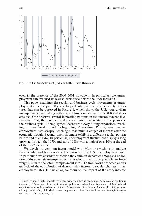
This paper examines the secular and business cycle movements in unem-ployment over the past 50 years. In particular, we focus on a variety of fea-tures that can be observed in Figure 1, which shows the U.S. total civilianunemployment rate along with shaded bands indicating the NBER-dated re-cessions. One observes several interesting patterns in the unemployment fluc-tuations. First, there is the usual cyclical movement related to the phases ofthe business cycle. Unemployment decreases slowly during expansions, reach-ing its lowest level around the beginning of recessions. During recessions un-employment rises sharply, reaching a maximum a couple of months after theeconomic trough. Second, unemployment exhibits a di¤erent secular patternbefore and after 1969. In particular, unemployment fluctuations display a longupswing through the 1970s and early 1980s, with a high of over 10% at the endof the 1982 recession.

We develop a common factor model with Markov switching to analyzethese secular and business cycle fluctuations in the U.S. unemployment rate.1In particular, we consider extracting the common dynamics amongst a collec-tion of disaggregate unemployment rates which, given appropriate labor forceweights, sum to the total unemployment rate. The framework proposed allowsanalysis of the contribution of demographic factors to secular changes in un-employment rates. In particular, we focus on the impact of the entry into the

1 Linear dynamic factor models have been widely applied in economics. A classical exposition isGeweke (1977) and one of the most popular applications is Stock and Watson’s (1989), who buildcoincident and leading indicators of the U.S. economy. Diebold and Rudebusch (1996) proposeadding Hamilton’s (1989) Markov switching model to this framework in order to capture asym-metries over the business cycle.

Fig. 1. Civilian Unemployment (SA), and NBER-Dated Recessions

206 M. Chauvet et al.

labor force and the subsequent aging of the baby-boom generation.2 In addi-tion, it allows examination of the separate contribution of changes in unem-ployment rates due to asymmetric business cycle fluctuations.

The behavior of unemployment over the business cycle has attracted a greatdeal of attention from economists using nonlinear time series models.3 With afew exceptions4 this large literature has focused on some measure of aggregateunemployment. The focus of this paper is to extend the nonlinear analysis ofunemployment rates to the disaggregate level. There are two main motivationsfor this. The first is that some of the multiple regimes that have been found inthe unemployment rate may be explained by demographic factors, particularlythe baby boom. The second motivation is that nonlinear models ask a greatdeal of a single time series in terms of identifying Markov switching regimes.For example, in Neftci’s (1984) original analysis the evidence for asymmetryin the total unemployment was marginal. If the regimes are actually present,one would expect to find a common switch in disaggregate series. This wouldincrease both the accuracy of the switch estimates as well as the evidence fortheir presence.

With respect to demographic factors, the significant increase in the num-ber of births in the 1950s and early 1960s is often acknowledged as chang-ing several aspects of the economy. As far as the overall unemployment rateis concerned, because younger labor market participants tend to have higherunemployment rates than older ones, their entry into the labor market pro-duced an increase in the unemployment rate in the 1970s and 1980s, while theirsubsequent aging induced a decrease in the 1990s.5 Our approach is to modela latent unemployment rate that captures common labor market conditionsacross groups, and then re-aggregate this latent unemployment rate using thetime-varying labor force weights of the di¤erent age groups. This allows us todecompose changes in unemployment between baby-boom type e¤ects andchanges in the overall functioning of the labor market.

We find strong statistical evidence in favor of the common factor struc-ture and of the switching between high and low unemployment rate regimes.In particular, the latent factor exhibits the stylized business cycle asymmetriesfound in unemployment. The factor displays a fast and steep growth and a slowand long decline, associated with the phases of the business cycle. In addition,the high unemployment state is less persistent and more volatile compared tothe low unemployment phase. We also find that demographic adjustments canaccount for a great deal of secular changes in the U.S. unemployment rates,particularly the abrupt increase in unemployment in the 1970s and 1980s and

2 Another potential application of our methods is to explain the skill-biased technological changein the 1970s and 1980s, and its di¤erential e¤ects on education groups (see Juhn, Murphy and Topel1991). Alternatively, one might consider unemployment grouped by sex and race to examine secularchanges in the labor market behavior of these groups, particularly the increasing participation ofwomen in the labor force.3 See for example, Neftci (1984), Rothman (1993), Boldin (1994), Franses (1995), Montgomery,Zarnowitz, Tsay, and Tiao (1998), Abbring, Berg and Ours (1999), Vredin and Warne (2000), orSkalin and Terasvirta (2001).4 Rothman (1993) and Abbring, Berg, Ours (1999).5 Some of the important studies in this subject include Perry (1970) and Gordon (1982). Morerecently, Shimer (1998) uses an accounting style analysis, which suggests that the aging babyboomer is an important cause of the reduction in unemployment in the 1990s. These results arecorroborated in Katz and Krueger (1999).

Markov switching in disaggregate unemployment rates 207

the subsequent decrease in the last 18 years. The baby boom e¤ect induces asteep increase in the unemployment rate at the beginning of recessions in the1970s and 1980s as the labor force weights of young labor market participantswere increasing at the time that these switches to the high unemployment re-gime occurred. On the other hand, the impact of age on the unemploymentrate was substantially smaller in the 1990 recession, which is related to thesubsequent aging of the baby-boom generation.

The model is estimated and analyzed using Bayesian methods. In particu-lar, the Gibbs sampling is used to simulate and estimate the model while theSavage-Dickey Generalized Density Ratio is used to calculate Bayes factors,which allow evaluation of the sample evidence in favor of the Markov switches.

The organization of the paper is as follows. Section 2 develops the statis-tical model for disaggregate unemployment rates. Section 3 describes someBayesian techniques to estimate and test the model. Section 4 discusses thefeatures of the data on unemployment rates disaggregate by age. Section 5 dis-cusses the prior used and the results. Section 6 o¤ers some concluding remarksand directions for future research. The appendix summarizes the complete setof priors and conditional distributions used in the analysis.

2. Statistical model and methods

2.1. Common factor model

Let Ut be the K � 1 vector of unemployment rates for di¤erent age groupsused to estimate the common factor, Ct. The statistical model is:

Ut ¼ lCt þ Vt; ð1Þ

where l is the K � 1 vector of factor loadings, which measures the sensitivityof group k ’s unemployment rate to the 1x1 underlying factor Ct, and the K � 1random vector Vt represents a possibly autocorrelated measurement error. Thecommon factor is given by the Markov switching model:

Ct ¼a1 þ f1pðLÞCt�1 þ s1et if st ¼ 1

a2 þ f2pðLÞCt�1 þ s2et if st ¼ 2

�; ð2Þ

with P½stþ1 ¼ 1 j st ¼ 1 ¼ r11 and P½stþ1 ¼ 2 j st ¼ 2 ¼ r22. The regime specificmeans are defined as:

hð1Þ ¼ a1

1� f11 � � � � � f1p; hð2Þ ¼ a2

1� f21 � � � � � f2p

:

We identify state 1 as the high unemployment phase and state 2 as the lowunemployment phase, that is, hð1Þ > hð2Þ. Further, we consider the observedasymmetries in unemployment of sharp increases during recessions followedby slow decreases during expansions using restrictions on the autoregressivecoe‰cients in the two regimes. These restrictions are easier to describe in thecase of a first order process. In order for unemployment to increase quicklywhen it switches from state 2 to 1, f11 needs to be relatively small so that a1 is


close in size to hð1Þ. Alternatively, when there is a switch from state 1 to state2, unemployment declines slowly if f21 is close to 1 and, therefore, a2 is verydi¤erent from hð2Þ.

The measurement error vector Vt has an autoregressive structure:

Vt ¼ Y1Vt�1 þ � � � þYqVt�q þMt; ð3Þ

where the innovations to the common factor, et @ IIDNð0; 1Þ, and the mea-surement errors,Mt @ IIDNð0;SKÞ, are independent of each other at all leadsand lags, and SK is diagonal. In addition, the autoregressive matrices are di-agonal:

Yi ¼y1i � � � 0

..

. . .. ..

.

0 � � � y1K

264

375:

2.2. Latent unemployment

Given our collection of K di¤erent age groups, we construct demographicweights for each category by:

okt ¼LktPKk¼1 Lkt

; ð4Þ

where Lkt is the total civilian labor force for age group k at time t. The over-all unemployment rate for all groups URt is given by the estimate of the totalnumber of workers unemployed, TUt, divided by the total civilian labor force,PK

k¼1 Lkt:

URt ¼TUtPKk¼1 Lkt

¼PK

k¼1 LktUktPKk¼1 Lkt

; or

URt ¼XKk¼1

oktUkt;

where Ukt is the unemployment rate for age group k. The latent aggregateunemployment rate implied by the common factor model is:

Ut ¼ Ct

XKk¼1

oktlk; ð5Þ

The average or ‘‘natural rate’’ of unemployment fluctuates between the‘‘high-mismatch’’ average,

Utð1Þ ¼ hð1ÞXKk¼1

oktlk; ð6Þ


and the ‘‘low-mismatch’’ average,

Utð2Þ ¼ hð2ÞXKk¼1

oktlk: ð7Þ

That is, Utð1Þ and Utð2Þ correspond to demographically adjusted high andlow bounds for average unemployment. In the empirical analysis, these boundsallow examination of periods in which average unemployment exceeds thehigh-mismatch and low mismatch averages in the sample.

Notice that, in contrast with an analysis of the aggregate unemploymentrate, our estimate of fCt; stg is not influenced by variations over time in thedemographic weights. In the case where the labor force weights are constantover time, we have:

Ut �Ut ¼ ðCt � CtÞXKk¼1

oklk; for t < t; ð8Þ

or, alternatively, the factor loadings are equal across groups at unity:

Ut �Ut ¼ ðCt � CtÞ: ð9Þ

In both cases, demographic changes have no e¤ect on the change in latentaggregate unemployment and there would be little advantage from examiningdisaggregate unemployment rates. This should be compared to the more gen-eral case in which the factor loadings vary across k or the demographic weightschange over time. In these cases, changes in aggregate latent unemploymentcan be split into 2 di¤erent contributions – the ones arising from changes inthe common factor and the ones from demographic changes:

Ut �Ut ¼ ðCt � CtÞXKk¼1

oktlk Factor E¤ect

þ Ct

XKk¼1

ðokt � oktÞlk Demographic E¤ect ð10Þ

2.3. State space form

The model can be written in state space form where we assume that p ¼ qþ 1for simplicity of notation. First we define the following:

1. Let U�t ¼ ðIk �YðLÞÞUt.

2. Let C�t ¼ ½Ct; . . . ;Ct�pþ1 0.

3. Define the K � ðqþ 1Þ matrix H by:

H ¼

l1 �l1y11 � � � �l1yq1

l2 �l2y12 � � � �l2yq2

..

. ... . .

. ...

lK �lKy1K � � � �lKyqK

26664

37775:


4. Define the p� p matrices Ai by:

Ai ¼

fi1 fi2 � � � fip

1 0 � � � 0

0 1 . .. ..

.

0 . ..

1 0

266664

377775:

The state space form has measurement equation:

U�t ¼ HC�

t þMt ð11Þ

and transition equation:

C�t ¼ a1 þ A1C

�t�1 þW1et if st ¼ 1

a2 þ A2C�t�1 þW2et if st ¼ 2,

�ð12Þ

where Wi ¼ ½si; 0; . . . ; 0 0 and ai ¼ ½ai; 0; . . . ; 0 0 are ðp� 1Þ vectors.

Below we will also sometimes summarize the conditional mean coe‰cientsin each regime by the p�1 vector fi ¼ ðf1i; . . . ; fpiÞ, or by the ðpþ1Þ�1 vectorbi ¼ ðai; f1i; . . . ; fpiÞ. Let j represent all the parameters of the common factormodel with Markov switching and w represent the (smaller by b2; s2; r11; r22Þset of parameters of the common factor model without Markov switching.

As is true of all single factor models there is an identification issue betweenthe factor loadings and the scaling of the innovation to the common factor (seeChauvet 1998). We normalize one of the elements of the factor loading vectorto 1. Also, unlike Stock andWatson (1989), we do not demean and standardizethe observable variables before the analysis. Thus, not only will l be estimatedfrom the joint dynamics of the observed time series it will also depend on in-formation on the relative means and variances of the unemployment rates. Inorder to capture movements between low and high unemployment regimes, itis crucial to keep the mean information in the series.

3. Bayesian methods

If the sequence fstg were known, estimation by classical or Bayesian methodswould be standard. Both methods use the Kalman filter to construct the like-lihood function.

3.1. Kalman filter

The Kalman filter iterations are given by:

1. Prediction Step: The conditional mean of the factor is,

C�tþ1 j t ¼

a1 þ A1C�tjt if st ¼ 1

a2 þ A2C�tjt if st ¼ 2

�:


The conditional variance of the factor is,

Ptþ1 j t ¼A1PtjtA

01 þW1W

01 if st ¼ 1

A2PtjtA02 þW2W

02 if st ¼ 2

�:

Using the conditional mean of the factor and the measurement equation(11), we obtain the conditional forecast error:

U�tþ1 � UU�

tþ1 j t ¼ HðC�tþ1 � C�

tþ1 j tÞ þMtþ1;

and its conditional variance:

E½ðU�tþ1 � UU�

tþ1 j tÞðU�tþ1 � UU�

tþ1 j tÞ0 ¼ HPtþ1 j tH

0 þ SK :

2. Updating Step: First, the Kalman gain matrix is constructed:

Gtþ1 ¼ Ptþ1 j tH0fE½ðU�

tþ1 � UU�tþ1 j tÞðU�

tþ1 � UU�tþ1 j tÞ

0g�1:

Then, as new information about the factor is obtained after observing U�tþ1,

the Kalman gain is used to include it in the conditional mean of the factor:

C�tþ1 j tþ1 ¼ C�

tþ1 j t þGtþ1ðU�tþ1 � UU�

tþ1 j tÞ;

and to update the conditional variance:

Ptþ1 j tþ1 ¼ ðIp �Gtþ1HÞPtþ1 j t:

3.2. Posterior draws of Markov states and common factor

The main estimation problem in the model proposed is that the switches in theMarkov chain are not observable. As is well-known, this causes a computa-tional problem for standard maximum likelihood approaches, since one has tokeep track of the 2T possible values of the Markov sequence in the sample.Kim (1994) suggests an maximum likelihood approach using an approxima-tion that truncates the exponential increasing number of terms at each iterationin the Kalman filter. On the other hand, Bayesian simulation techniques canbe used to obtain the exact likelihood function of the common factor Markovswitching model, as proposed by Albert and Chib (1993) and Shephard (1994).

In this paper our focus is on Bayesian methods to extract the sample evi-dence about the Markov sequence. In our model it is not possible to work outanalytically the properties of the posterior even if the common factor andMarkov states were directly observed. In these cases, Bayesians have increas-ingly turned to simulation methods. These methods are based on the intuitionthat, given a large enough random sample from a distribution, it is possible tofigure out the properties of that distribution (e.g. its mean, median, variance,etc.). Geweke (1999) and Chib (2001a, 2001b) provide recent surveys of themethods used for developing such posterior simulators.6 The advantage ofposterior simulators in our case is that they can also be developed to generatedraws of the unobservables, which greatly simplifies the estimation problem.

6 A textbook-type explanation of the method can also be found in Kim and Nelson (1999).


Posterior simulators for many models can be developed by successivelydrawing from a sequence of conditional posterior distributions. To motivatesuch methods, let X and Y be random variables and suppose that we are in-terested in the features of their joint distribution, pðX;YÞ. Assume that pðX;Y Þis di‰cult to simulate, but that we can easily obtain draws from the conditionaldistributions pðX jYÞ and pðY jX Þ. Consider the strategy where one selects an

initial value, Y ð0Þ, and then successively draws X ð jÞ from pðX jY ð j�1ÞÞ, and Y ð jÞ

from pðY jX ð jÞÞ. The resulting sequence, X ð jÞ;Y ð jÞ for j ¼ 1; . . . ; J will, underweak conditions, converge to a sample from pðX ;YÞ as J increases. In prac-tice, this means we can discard J initial draws to mitigate startup e¤ects. Wecan then treat X ð jÞ;Y ð jÞ for j ¼ J þ 1; . . . ; J as an approximate sample frompðX ;Y Þ, which can be used to estimate features of interest. This is a simpleexample of a Gibbs sampler, which belongs to a more general class of tech-niques known as Markov Chain Monte Carlo methods.

Many commonly-used econometric models with latent variables can beeasily estimated using Gibbs sampling algorithms. In our particular model, theGibbs sampler generates random draws of fstg, which allows analysis as if thesequence were known. However, in order to obtain inferences we also need toobtain a random draw of the common factor.

3.2.1. Common factor

The recursion to generate the random draw of the common factor is as follows(see Fruhwirth-Schnatter, 1994, Carter and Kohn, 1994, or Shephard, 1994):

1. The last iteration of the Kalman filter gives:

C�T @NðC�

T jT ;PT jTÞ:

Thus, using standard methods a realization ~CC�T can be drawn from this mul-

tivariate normal. Then, the draw of the most recent value of the commonfactor is given by:

~CCT ¼ e ~CC�T :

where e ¼ ½1; 0; . . . ; 0 is a p� 1 selection vector. In practice, one only needsto draw from the univariate normal with mean given by the first element ofC�

T jT and variance by the first diagonal element of PT jT .2. Given a draw at tþ 1 based on draws from tþ 2 to T the information from

the Kalman filter iterations is incorporated as if the filter were runningbackwards combining prior information from its initial forward run withthe ‘sample’ information generated by the random draw:

ft ¼ ~CCtþ1 �a1 þ f1pðLÞCtjt if st ¼ 1

a2 þ f2pðLÞCtjt if st ¼ 2

�;

pt ¼f 01Ptjtf1 þ s2

1 if st ¼ 1

f 02Ptjtf2 þ s2

2 if st ¼ 2

(;


gt ¼Ptjtf1=pt if st ¼ 1

Ptjtf2=pt if st ¼ 2

�;

C�tjT ¼ C�

tjt þ gt ft;

PtjT ¼ðIp � gtf

01ÞPtjt if st ¼ 1

ðIp � gtf02ÞPtjt if st ¼ 2

�:

Thus, after observing the whole sample we obtain C�t @NðC�

tjT ;PtjT Þ, andstandard methods can be used to obtain a random draw.

3. This iteration stops with C�p @NðC�

pjT ;PpjT Þ, which is used to simulta-neously draw the first p observations of the common factor.

3.2.2. Markov states

1. Given this realization of the common factor, the methods described in Chib(1996) can be directly applied to investigate the pattern of Markov statescontained in the draw of the dynamic factor. Similarly to the analysis of thecommon factor, the recursion starts by filtering the ‘‘observations’’ on thecommon factor to construct a sequence of prior and posterior distributionsfor the Markov state.

In our case, we assume that the chain starts in the low mismatch state 2.Thus, we have S1 ¼ � � � ¼ Sp ¼ 2. The prior distribution for the state at timepþ 1 is then:

P½Spþ1 ¼ 2 jS1 ¼ � � � ¼ Sp ¼ 2 ¼ bbpþ1 ¼ r22:

The relevant sample information is contained in the likelihood for ~CCpþ1, whichtakes on the value:

l1ð ~CCpþ1Þ ¼ ð2ps21 Þ

�0:5 exp½�0:5ð ~CCpþ1 � a1 � f1pðLÞ ~CCpÞ2=s21

if Spþ1 ¼ 1, and:

l2ð ~CCpþ1Þ ¼ ð2ps22 Þ

�0:5 exp½�0:5ð ~CCpþ1 � a2 � f2pðLÞ ~CCpÞ2=s22

if Spþ1¼ 2. Thus, the posterior distribution P½Spþ1¼ 2 jS1¼ � � � ¼ Sp¼ 2; ~CCpþ1is given by:

bbpþ1 ¼l2ð ~CCpþ1Þr22

l2ð ~CCpþ1Þr22 þ l1ð ~CCpþ1Þð1� r22Þ:

This posterior is used to form a prior for Spþ2 ¼ 2 from:

bbpþ2 ¼ bpþ1r22 þ ð1� bpþ1Þð1� r11Þ:

This process continues through the end of the sample and we obtain:

bT ¼ P½ST ¼ 2 jS1 ¼ � � � ¼ Sp ¼ 2; ~CCT :


Next, the posterior distribution over the last sample value of the Markovstate is used to generate a draw of ST . This draw is easy to obtain from thegeneration of a uniform random variable. If the draw is less than or equal to

the posterior probability that ST ¼ 2, then we have ~SST ¼ 2, otherwise ~SST ¼ 1.Similarly to the draw of the common factor, a sequence of draws of fStg is

also generated going backwards through the sample. From the Markov prop-erty and the exogeneity of the Markov chain, none of the future realizations ofthe observed time series f ~CCs : s > tg conditional on observing the value of to-morrow’s state, stþ1 are relevant for the estimate of today’s state. Using thisrestriction and ignoring the dependence on estimated parameters and the re-striction on the initial states, we have:

P½ST�1 ¼ 2 jST ¼ 2; ~CCT�1

¼ P½ST�1 ¼ 2;ST ¼ 2 j ~CCT�1P½ST ¼ 2 j ~CCT�1

¼ P½ST�1 ¼ 2 j ~CCT�1P½ST ¼ 2 jST�1 ¼ 2bbT

¼ bT�1r22

bbT

;

and also:

P½ST�1 ¼ 2;ST ¼ 2 j ~CCT

¼ P½ST�1 ¼ 2 jST ¼ 2; ~CCT P½ST ¼ 2 j ~CCT

¼ P½ST�1 ¼ 2 jST ¼ 2; ~CCT�1bT

¼ r22bT�1

bbT

bT :

This last expression can be used to generate a smoothed probability ~bbt byaveraging out over the values of ST :

~bbT�1 ¼ bT�1 r22

~bbT

bbT

þ ð1� r11Þ1� ~bbT

1� bbT

!:

The first expression gives a direct method for drawing ~SST�1 using a ran-dom uniform number. This iteration is repeated until the draw of ~SSPþ1 usingP½Sp ¼ 2;Spþ1 ¼ 2 j ~CCT ¼ 1 is obtained.

3.3. Estimation by Gibbs sampler

We initialize the Gibbs sampler running the Kalman filter on the observeddata with the following parameters: a Markov sequence given by the NBER


business cycle dates, factor loadings proportional to the sample means of theunemployment rates, measurement error equal to 1/4 of the observed vari-ances of the unemployment rates with autoregressive coe‰cients equal to 1/3,and the prior means used for the common factor dynamic model and loadings.The results of the Kalman filter are then used to draw a initial sequence of re-alizations for the common factor f ~CCtg. Given this sequence and the sequenceof Markov states, it is relatively simple to update the draws of the remainingparameters using the Gibbs sampler with appropriate choices of prior distri-butions.

A summary of our choices is as follows: for the parameters of Ct we use arestricted normal inverted gamma prior; for the factor loadings l we use in-dependent normal priors; for the measurement error variances, fskkg we useindependent normal inverted gamma priors; for the autoregressive coe‰cientsin the measurement error process we use restricted independent normal priors;for the transition probabilities we use a Beta distribution. Section 5.1 containsinformation of the exact prior distributions used and the appendix containsmore detailed information on the priors and the implied conditional poste-riors. Here we focus on some of the restrictions imposed on the parameters.

For both the parameters of Ct and the measurement error processes weimpose a stationarity condition. In the case of the measurement error processthe roots of the individual lag polynomials 1� ykqðLÞ all lie outside the unitcircle. For the common factor Markov switching model we use the su‰cientcondition that the roots of each lag polynomial 1� fipðLÞ lie outside the unitcircle. For both sets of restrictions we use simple rejection sampling.

In addition to the stationarity restriction, we also impose the restrictionthat hð1Þ > hð2Þ > 0. Since the regime specific means are nonlinear functionsof the underlying autoregressive parameters and the intercept, the restriction isimposed sequentially as follows. First, we draw b2 and check whether the sta-tionarity and non-negativity conditions are satisfied. If they are not we make anew draw. This process continues until a satisfactory draw is obtained. Next,we draw b1 and check whether both the stationarity and mean inequalityconditions hold. Again, we reject this draw if it does not satisfy the conditions,continuing until a statisfactory draw is obtained.

3.4. Evidence for Markov switching

We assess the observed sample evidence in favor of a Markov switching in thecommon factor model by comparing the average (often called the marginal)likelihood of the observed time series with and without switching. The ratiosof these two average likelihoods is the Bayes factor and it provides a direct‘test’ of the usefulness of the additional complexity of the Markov switchingmodel. On the other hand, classical testing of Markov switching models is asomewhat unresolved area due to various non-standard aspects of the model.We do not attempt to solve these issues here. Instead, we provide someclassical-type information by calculating F-statistics at each iteration of theGibbs sampler. Note that under the null hypothesis of no Markov switchinge¤ect and uninformative priors we would expect these statistics to be drawsfrom a F-distribution with appropriate degrees of freedom. Since we are notusing non-informative priors the exact sampling distribution of this sequence


of F-statistics is unknown.7 However, we focus on the minimum value of thisstatistic across iterations of the Gibbs sampler.

Although the calculation of marginal likelihoods involves multiple inte-gration, it can be simplified using the following tricks. The Bayes factor is themarginal likelihood of the ‘no-switching model’ divided by the marginal like-lihood of the ‘switching model’:

BNo Switching vs: Switching ¼ÐlðUjw; fCtgÞbðw; ÞdfCtg dwÐ

lðUjj; fstg; fCtgÞbðj; s1 ¼ 2Þ dfCtg dfstg dj;

if this ratio is larger than 1 the sample favors the simple model with no switch-ing. Notice that a ratio of 0.05 is not equivalent to a classical critical value. In-stead, it implies that the Markov switching model is 20 times more likely thanthe simple model, given the observed data on unemployment rates.

Using the basic likelihood identity (see Chib 1995) we have:ðlðUjj; fstg; fCtgÞbðj; s p ¼ 2Þ dfCtg dfstg dj

¼ lðUjj; fstg; fCtgÞbðj; s p ¼ 2ÞpðjjUÞ ;

for all points in the parameter space. In particular, consider the transforma-tion of the parameter space for the Markov swtiching common factor modelfrom ðb1; s1; b2; s2; r11; r22Þ to ðb1; s1; b2 � b1; s2=s1; tÞ. If we evaluate thetransformation at b2 � b1 ¼ 0; s2=s1 ¼ 1, then there is no information in thelikelihood function about fstg. As discussed in Koop and Potter (1999), onecan use this lack of identification to simplify marginal likelihood calculationsusing the Savage-Dickey Density ratio. In this case, conditional on the gen-erated sequence of f ~CCt; ~sstg we have:Ð

lðf ~CCt; ~sstg j b1; s1Þbðb1; s1Þ db1 ds1Ðlðf ~CCt; ~sstg j b1; s1; b2; s2Þbðb1; s1; b2; s2Þ db1 ds1 db2 ds2

¼ pðb2 � b1 ¼ 0; s2=s1 ¼ 1 j f ~CCt; ~sstg;U; j�Þbðb2 � b1 ¼ 0; s2=s1 ¼ 1 j j�Þ ;

where j� signifies the parameter space excluding the parameters of thecommon factor model.8 Using the methods of Koop and Potter (2000), theLHS of this expression can be directly calculated at each iteration of the Gibbssampler, for normal inverted gamma prior distributions that are independentacross regimes. If this quantity is averaged across draws of j� and f ~CCt; ~sstg fromthe Gibbs sampler we will have:

pðb2 � b1 ¼ 0; s2=s1 ¼ 1 jUÞbðb2 � b1 ¼ 0; s2=s1 ¼ 1Þ ;

7 The informative priors on the parameters of the Markov switching model used here rule outsome of the computationally based non-standard problems directly.8 In practice, we use di¤erent priors between the no switching and switching models, which re-quire a generalization of the density ratio. For simplicity, we ignore this complication here.


which is the Savage Dickey ratio for the Bayes factor of a ‘no-switching com-mon factor’ versus a ‘switching common factor model’.

Our choice of the prior distribution presents a di‰culty when implement-ing this approach, since the prior imposes some nonlinear restrictions on theparameter space. Instead of attempting to directly incorporate these restrictionsin the calculation of the conditional marginal likelihood, we calculate the con-ditional marginal likelihood for the unrestricted case. In practice, the di¤erencesin the conditional marginal likelihoods are so large that the computer is rarelyable to distinguish the conditional Bayes factor from zero. Since we find fewviolations of the nonlinear restrictions on the parameter space, an adjustmentfor the restrictions on the prior would not change the overall result of strongsupport for the Markov switching model in the data.

4. Data description

We use unemployment rates for seven age groups for the period from 1948Q1to 2000Q2.9 The age groups are 16–19, 20–24, 25–34, 35–44, 45–54, 55–64,and 65 and over. We construct the unemployment rates from the three-monthaverages of the estimated total unemployment for each group, divided by thethree-month average of the estimated labor force for each group:

URkt ¼TUkt

Lkt

:

These underlying data are not seasonally adjusted. We adjusted the age-specific unemployment rates using a seasonal factor given by the ratio of thepublished seasonally adjusted to the unadjusted total civilian unemploymentrates. We also constructed weights for each group given by equation (4). Notethat these weights are not seasonally adjusted. Our adjustment procedure pro-duces an overall unemployment rate that is virtually identical to the publishedseries. This would obviously not be the case if we also seasonally adjusted thelabor force weights.

Our focus in on the impact of demographic changes related to the entry intothe labor market and subsequent aging of the baby-boom generation, which isillustrated in Figure 2. In particular, the figure shows the time path of the ci-vilian labor force for di¤erent age groups. The aging of the baby boomers canbe observed in the pattern of changes in the age composition of the labor forceover time. The wave of young workers (age 16–19) had its peak at the endof the 1970s. Ten years later, some of these workers fell into the 25–35 agecategory that peaked in 1990. Currently, the majority of the workers is nowbetween 35–44.

What are the implications of these demographic changes in the labor mar-ket? In order to answer this question it is important to understand how the un-employment rate behaves di¤erently across di¤erent age groups. Table 1 con-tains some sample statistics on unemployment rates for di¤erent age groups,while Table 2 contains information on the relative weights of each group in the

9 This is the earliest available starting point for high frequency and disaggregate unemploymentrates in the United States. For a descriptive analysis of unemployment statistics over 120 years, seeDenman and McDonald (1996).


labor force, with the weights scaled by 100. The unemployment rate for teen-agers is much higher and more volatile than for the other age groups. In fact,the mean and variance of the unemployment rate decrease steadily as workersage. For example, teenagers have an average unemployment rate of 15.5%,workers between 35–45 have an average of 4%, while the aggregate rate is5.7% (Table 1).

As a result of these di¤erences, secular changes in the relative participa-tion of young workers in the labor force has had a significant impact on ag-gregate unemployment. In particular, as can be seen in Figures 1 and 2, thelong secular upswing in the aggregate unemployment rate coincides with theentry of young workers into the labor market. The participation of teenagersin the labor market increased substantially in the 1960s reaching a peak in themid 1970s, while the participation of workers between 35–45 fell substantiallyduring this period. The subsequent aging of the baby boom generation in the

Table 1. Statistics for unemployment rates

UktnStatistic Mean St. Dev. Min Max

16–19 15.5 3.6 6.3 25.0

20–24 9.0 2.4 3.9 16.0

25–34 5.6 1.7 2.2 10.8

35–44 4.0 1.2 1.8 8.2

45–54 3.6 1.0 1.8 6.7

55–64 3.7 1.0 1.7 6.2

65þ 3.6 0.8 1.7 6.1

Fig. 2. Civilian Labor Force by Age Groups


1980s and 1990s is associated with a reduced fraction of teenagers in the laborforce and a substantial increase in the proportion of workers between age 35and 55 (Figure 3 and Table 2).

Finally, we present the contemporaneous correlation matrix for the un-employment rates ordered from the youngest to the oldest (Table 3). It is in-teresting to notice how the unemployment rates are correlated between groupsclose in age, and much less so when comparing younger workers with olderworkers. The reason is that unemployment rates for younger workers are veryvolatile over the entire sample, and display particularly accentuated oscil-lations over the business cycle. On the other hand, the volatility of unem-ployment decreases monotonically as workers age. Table 1 shows that thestandard deviation of teenagers’ unemployment is more than 3 times higherthan the standard deviation for workers age 35 or older. In addition, the un-employment rates for older workers exhibit much smaller oscillations around

Fig. 3. Participation in the Labor Force by Age (SA)

Table 2. Statistics for labor force weights

oktnStatistic Mean St. Dev. Min Max

16–19 7.3 1.4 5.1 10.7

20–24 11.8 2.0 8.4 15.3

25–34 24.2 3.2 18.7 29.6

35–44 22.7 2.2 17.6 27.5

45–54 18.7 2.2 14.8 21.8

55–64 11.8 1.7 8.8 14.2

65þ 3.6 1.0 2.5 5.3


business cycle turning points. As argued by Shimer (1998), this may be ex-plained by the fact that although younger workers do not have trouble find-ing jobs, they are more frequently fired.10

Anticipating our empirical results, the resulting dynamic factor model isbroadly consistent with the sample moments given in Table 1 for the group ofworkers 35–44. Notice that this is not only the mid-group, but it is also the onewith the highest relative participation in the labor force. On the other hand, as itturns out to be somewhat striking, given the contemporaneous correlation be-tween unemployment rates, our measure of latent unemployment constructedfrom the factor loadings and demographic weights tracks almost exactly theoverall unemployment rate.

5. Priors and results

5.1. Properties of the prior distribution

We start by considering the choice of the hyperparameters of the normal-inverted gamma priors for the common factor parameters in each regime,under the restriction used in the estimation that the lag length is 1. These pri-ors are the most important ones for interpretation of the sample evidence. Webegin by eliciting a prior that is relatively noninformative, but accords withour subjective prior beliefs. To simplify matters, the prior covariances are as-sumed to be zero for all the conditional mean parameters in the model. As wework with one lag in each regime, this does not seem controversial. Since weare examining unemployment rates, it does not make economic sense to as-sume that the prior means are zero. Instead, we specify the prior means interms of common empirical findings regarding asymmetries in the unemploy-ment rate.

The prior is specified in two steps. First we describe the unrestricted prior,then we discuss various restrictions on the prior that are imposed as in Ge-

10 Young workers in the U.S. have a mean and median unemployment duration smaller thanolder workers.

Table 3. Correlation matrix for unemployment rates

16–19 20–24 25–34 35–44 45–54 55–64 65þ

16–19 1

20–24 0.88 1

25–34 0.84 0.96 1

35–44 0.79 0.92 0.97 1

45–54 0.68 0.86 0.91 0.95 1

55–64 0.50 0.70 0.76 0.84 0.92 1

65þ 0.28 0.43 0.39 0.45 0.53 0.64 1


weke (1986). For the low unemployment regime, we specify a mean of 0.4 forthe intercept, and of 0.8 for the autoregressive parameter. The respective vari-ances of these parameters are 1 and 0.3. For the high unemployment regime,we specify a mean of 2.5 for the intercept, and of 0.5 for the autoregressive pa-rameter. The variances of these parameters are 0.8 and 0.95, respectively. Theseare the priors used in generating candidate random draws from the conditionalposterior. These draws must satisfy stationarity as well as the restriction hð1Þ >hð2Þ > 0. Finally, the degrees of freedom for the inverted gamma priors are 3for both regimes, and the prior mean of the variance is set to 0.1.11

We simulate from this combined normal inverted gamma prior for tworegimes in order to obtain some prior features of interest. The prior means ofh are around 1% for the low unemployment regime, and around 13.5% for thehigh unemployment regime. These values are reasonable, given that the h’s areupper and lower bounds under the AR(1) assumption. About 32% of the jointpriors have hð1Þ > 6% and hð2Þ < 4%.

For the factor loadings, we use a normal prior centered at 1 with a diagonalvariance matrix, individual variance of 4 for unemployment rates of workersage 25 and over, and variance 1 for the unemployment rates of workers 16–19and 20–24. Once again, this is an uninformative choice. Naturally, we imposethe degenerate prior that the factor loading is 1 for the unemployment rates ofworkers age 35–44 in order to normalize the dynamic factor.

For the measurement error innovation variance, we use the minimally in-formative inverted gamma prior with degrees of freedom 3 and mean 1. Forthe autogressive structure of the measurement errors, we use a more infor-mative Gaussian prior. The prior mean is set to zero and the variance is a di-agonal matrix. The standard deviation of the autoregressive coe‰cient for thegroup age 25 and older is set to 0.07, while for the 16–19 and 20–24 groupsit is equal to 0.1. These priors are based on the fact that the Current Popula-tion Survey currently follows a ‘‘4 month in 8 month out, 4 month in’’ rota-tion for households. Thus, the measurement error in the survey across house-holds should not be too strong.

For the parameters of the Markov chain transition matrix, we use a com-mon beta prior. For the probability of unemployment staying in the low re-gime r22 or staying in the high regime r11, the parameters are ð9; 1Þ. This isequivalent to having observed about 10 observations of the Markov chain.Thus, it will be easily dominated by the sample information if there are re-peated switches. Using standard formula for the beta distribution, this impliesa very vague prior on the expected duration 1=ð1� r22Þ or 1=ð1� r11Þ, sincethe first moment does not exist. The median duration obtained from the sim-ulation is 13.6 quarters, with a probability equal to 0.09 that the duration islonger than 25 years, and a probability of 0.08 that it is less than 1 year.

5.2. Empirical results

The model is estimated with the order of the autogressive parameters q ¼ 1,p ¼ 1. The unemployment rate of the age group 35–44 is chosen as the vari-

11 The variance for the conditional mean parameters already takes into account the prior meanfor the variance of the errors.


able with factor loading equal to unity. The Gibbs sampler was run with aburn-in phase of 200 iterations and a further 4000 iterations. Repeated runsof the sampler with di¤erent initial conditions produced very few changes inthe posterior features suggesting that the sampler has converged.

As noted above, the di¤erence in marginal likelihoods is so large be-tween a model with switching and no switching (a Bayes factor of 1019 in favorof switching) that there is little information in the conditional Bayes factors.Figure 4 shows evidence on the F-Statistics calculated at each iteration of theGibbs sampler. Here we can see that the F-statistics are uniformly higher thana 0.1% critical value of around 7 obtained from a F-distribution.

The resulting latent unemployment is highly correlated with total unem-ployment rate (0.995). In addition, the latent factor is also centered with theactual unemployment rate. With respect to the posterior mean of the factorloadings, they show a pattern consistent with the di¤erences in meansand standard deviations reported in Table 1. In particular, young labor mar-ket participants have the highest factor loading, and the loadings decline withage.12

Figure 5 plots the actual unemployment rate with posterior means of thedemographically adjusted bounds, calculated from equations (6) and (7). Theunemployment rate fluctuates inside the high-mismatch and low mismatchaverages almost the entire sample. In two main instances the bounds are vio-lated, which correspond to periods in which the unemployment rate reachedits minimum and maximum values in the sample. One was in the early 1950s,when unemployment rates were very low (2.6%). The other was in the early1980s, when unemployment rates peaked at 10.7%. The role of the demo-graphic adjustment to the upper and lower bounds can also be seen in this fig-ure. The high and low mismatch averages display a hump in the 1970s, reflect-ing the entry and subsequent aging of the baby boom in the labor market.

Fig. 4. Approximate F-Statistics at Each Gibbs Iteration

12 Similar patterns are also found in the posterior means of the autogressive model for the indi-vidual measurement errors.


In order to further investigate the subsequent influence of the agingbaby boomers on unemployment, we compare changes in the unweighted andweighted latent unemployment factors. First, recall that the weighted latentunemployment can be decomposed into a factor e¤ect and a demographic ef-fect, as described in Section 2.2. We consider the change in unemployment for3 cases: from the earlier dates 1978, 1982, and 1992 to the present (2000). Forexample, comparing unemployment in 2000 and 1982, equation (10) becomes:

U2000 �U1982 ¼ ðC2000 � C1982ÞXKk¼1

oktlk Factor E¤ect

þ C1982

XKk¼1

ðok2000 � ok1982Þlk Demographic E¤ect

For changes in unemployment from 1978 and 1982 to the present, we find asa demographic e¤ect a reduction of 75 basis points in the latent unemploy-ment rate. This is is very close to the ones obtained in Shimer’s (1998) analy-sis of the actual unemployment rates. Since 1992, there has been a mild demo-graphic induced reduction in the latent unemployment of 10 basis points.

Second, consider the case in which demographic changes have no e¤ecton the change in latent aggregate unemployment, that is, the factor withoutdemographic or factor loading weights, as described in equations (8) and (9).Since we normalize the factor loading of the 35–44 year old group to unity,the factor without demographicnfactor loading weights is a measure of the un-derlying state of the labor market for this group. In this case, equation (8) be-comes:

Ct

XKk¼1

oktlk � 1

!;

Fig. 5. Unemployment Rate, High and Low Mismatch Averages


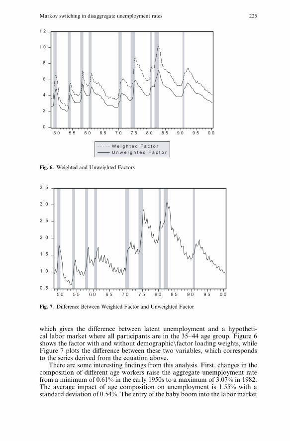
which gives the di¤erence between latent unemployment and a hypotheti-cal labor market where all participants are in the 35–44 age group. Figure 6shows the factor with and without demographicnfactor loading weights, whileFigure 7 plots the di¤erence between these two variables, which correspondsto the series derived from the equation above.

There are some interesting findings from this analysis. First, changes in thecomposition of di¤erent age workers raise the aggregate unemployment ratefrom a minimum of 0.61% in the early 1950s to a maximum of 3.07% in 1982.The average impact of age composition on unemployment is 1.55% with astandard deviation of 0.54%. The entry of the baby boom into the labor market

Fig. 6. Weighted and Unweighted Factors

Fig. 7. Di¤erence Between Weighted Factor and Unweighted Factor


in the 1960s and 1970s increased the aggregate unemployment rate by about1.8%.13 The subsequent aging of the baby boomers has decreased unemploy-ment by around 1.7%.14 These findings are also similar to the ones obtained byShimer’s (1998).

A second interesting observation is that the baby boom e¤ect induces asteep increase in the unemployment rate at the beginning of recessions in the1970s and 1980s. In particular, the values of the di¤erence between the un-weighted and weighted factors doubled during the 1970, the 1975, and 1980–82recessions. The reason is that the labor force weights of young labor marketparticipants were increasing at the time that these switches to the high unem-ployment regime occurred. One can also observe that in the 1990 recession theimpact of age on the unemployment rate was substantially smaller.

The properties of the dynamic factor stochastic model are very similar tothose expected and broadly consistent with the sample moments given in Table1 for the group of workers 35–44. Notice that this is not only the mid-group,but currently is also the one with the highest relative participation in the laborforce. If we evaluate the parameters at their posterior means, the impliedmodel is:

Ct ¼1:41þ 0:75Ct�1 þ e1t if st ¼ 1

0:16þ 0:94Ct�1 þ e2t if st ¼ 2

�;

with P½stþ1 ¼ 1 j st ¼ 1 ¼ r11 ¼ 0:81 and P½stþ1 ¼ 2 j st ¼ 2 ¼ r22 ¼ 0:93, e1t @Nð0; 0:48Þ and e2t @Nð0; 0:15Þ.

However, analysis of the posterior means can be misleading, since they ig-nore the amount of uncertainty about each parameter and their joint variation.In order to gain some insight into the importance of this, we compare the pos-terior means of hð1Þ and hð2Þ and the average duration in each regime to thoseimplied by the model evaluated at the posterior means of the parameters. Inthe high unemployment state, hð1Þ ¼ 5:81 (compared to a1=ð1� f1Þ ¼ 5:64),while hð2Þ ¼ 2:55, in state 2 (compared to a2=ð1� f2Þ ¼ 2:66). For the poste-rior mean of duration, state 2 lasts 16.9 quarters (compared to 1=ð1� r22Þ ¼14:3 quarters), while state 1 lasts 5.9 quarters (compared to 1=ð1� r11Þ ¼ 5:3Þ.Thus, the posterior means provide a reasonably accurate summary of the dif-ferences between regimes in terms of average dynamics.

Now, consider the following experiments with impact multipliers to il-lustrate the asymmetries in unemployment, which consist of sharp increasesfollowed by long slow declines as implied by the model. Assume that the dy-namic factor is in regime 1 with an unemployment rate of 5.5%, and that itswitches to the low unemployment regime (state 2) with no future shocks. Atfirst unemployment stays high (a2 þ f2 5:5 ¼ 5:33Þ and then it gradually de-clines. After 4 years, which is the typical duration of the low missmatch regime,the unemployment rate is equal to ½a2=ð1� f2Þ þ f16

2 ½5:5� a2=ð1� f2Þ ¼3:7. That is, it drops 63% of the way to the long run low unemployment level.

13 More specifically, since the baby boomers correspond to births between 1946 and 1964, herewe calculate the average di¤erence between the two factors using sample from 1962 to 1983. Thisperiod corresponds to the years in which the first and last generations of the baby boomers werebetween age 16–19.14 This is calculated using sample from 1981 on, which corresponds to the year in which the firstgeneration of the baby boomers reached the age of 35.


In contrast, if we start the dynamic factor in regime 2 with an unemploymentrate of 2%, upon a switch to regime 1 unemployment immediately jumps toða1 þ f1 2Þ ¼ 2:91. After 6 quarters, which is the average duration of thehigh mismatch regime, unemployment reaches a level of ½a1=ð1� f1Þ þ f6

1 ½2� a1=ð1� f1Þ ¼ 5:0, which corresponds to a 82% increase of the way to thelong run high unemployment level.

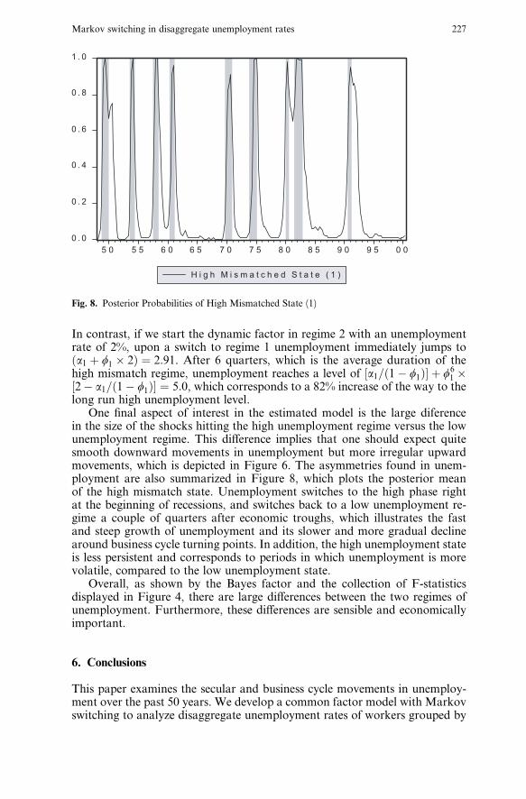
One final aspect of interest in the estimated model is the large diferencein the size of the shocks hitting the high unemployment regime versus the lowunemployment regime. This di¤erence implies that one should expect quitesmooth downward movements in unemployment but more irregular upwardmovements, which is depicted in Figure 6. The asymmetries found in unem-ployment are also summarized in Figure 8, which plots the posterior meanof the high mismatch state. Unemployment switches to the high phase rightat the beginning of recessions, and switches back to a low unemployment re-gime a couple of quarters after economic troughs, which illustrates the fastand steep growth of unemployment and its slower and more gradual declinearound business cycle turning points. In addition, the high unemployment stateis less persistent and corresponds to periods in which unemployment is morevolatile, compared to the low unemployment state.

Overall, as shown by the Bayes factor and the collection of F-statisticsdisplayed in Figure 4, there are large di¤erences between the two regimes ofunemployment. Furthermore, these di¤erences are sensible and economicallyimportant.

6. Conclusions

This paper examines the secular and business cycle movements in unemploy-ment over the past 50 years. We develop a common factor model with Markovswitching to analyze disaggregate unemployment rates of workers grouped by

Fig. 8. Posterior Probabilities of High Mismatched State (1)


age. We find a strong statistical evidence in favor of the common factor struc-ture and of the switching between high and low unemployment rate regimes. Inparticular, the latent factor exhibits the stylized asymmetries in unemploymentassociated with the phases of the business cycle. In addition, the model cap-tures the low frequency fluctuations in the U.S. unemployment rate associatedwith secular demographic changes. We find that demographic adjustments tothe unemployment rate can account for a great deal of secular changes in theU.S. unemployment rates. In particular, they explain some of the increases inunemployment in the 1970s and 1980s, and the subsequent decrease in the lasttwo decades.

The framework we have constructed is being extended in two mainways. First, we are examining the introduction of a second factor, in order tomodel short term fluctuations in disaggregate unemployment rates. In partic-ular, the factor is identified by including changes in inflation rates and in out-put amongst the observed variables to identify business cycle patterns. Themodel implies a time-varying Phillips curve associated with the phases of thebusiness cycle. Second, we are extending the framework to include a more de-tailed demographic decomposition of the total unemployment rate, using ob-servations on unemployment rates by age, sex, education, and race.

7. Appendix

This appendix gives information on the prior distributions used in the Gibbssampler and the resulting conditional posterior distributions.

1. Factor Loadings: we assume that the factor loadings are a priori normallydistributed and independent of each other with mean mðl kÞ and precisiontðl kÞ. Conditional on f ~CCtg, YðLÞ;SK we draw the K 1 vector of factorloadings l from (independent) normal distributions. For the generic load-ing lk we have the sample information:

XTt¼qþ1

C 2kt

" #�1

;XTt¼qþ1

C ktU

kt;

where C kt ¼ ~CCt � y1k ~CCt�1 � � � � � yqk ~CCt�q. Thus, the conditional posterior

is normal with mean:

tðl kÞmðl kÞ þPT

t¼qþ1 C ktU

kt=skk

tðl kÞ þPT

t¼qþ1 C 2kt =skk

and precision:

tðl kÞ þXTt¼qþ1

C 2kt =skk

" #:

For one of the elements of l we impose the prior belief that it is equal to 1.


2. Innovation Variance to Measurement Error: we assume that the innova-tion variances to the measurement errors are a priori independent invertedGamma distributions with degrees of freedom of x and scale s�2. Condi-tional on f ~CCtg, YðLÞ; l we draw the posterior of the measurement errorinnovations variances as independent gamma distributions. For the genericmeasurement error variance skk we have the sample information:

XTt¼qþ1

ðU kt � lkC

ktÞ

2; T � q;

which is combined with the prior degrees of freedom of x and ‘‘prior sumof squares’’ xs2 to obtain the posterior degrees of freedom xþ T � q and

sum of squares xs2 þPT

t¼pþ1ðU kt � lkC

ktÞ

2.3. Measurement Error Autoregressive Parameters: we assume that the mea-

surement error autoregressive parameters are truncated normal with thetruncation determined by the stationarity condition. Since we use rejec-tion sampling to implement the truncated prior, we start by describing theproposal distribution. The location and scale parameters of the truncatednormal are given by the vector mðykÞ and matrix tðykÞ�1. Thus, without thestationarity condition we would have the Gaussian prior. Conditional onf ~CCtg; l;SK we draw a proposed set of the measurement autoregressive co-e‰cients from independent multivariate Gaussian distributions. For the ge-neric measurement error autoregression k the sample information is:

½Z 0kZk�1; Z 0

kWk;

where Wk ¼ ½Ukqþ1; . . . ;UkT 0 and

Zk ¼

Ukq � � � Uk1

Ukqþ1 � � � Uk2

..

. ... ..

.

UkT�1 � � � UkT�q

266664

377775;

and Ukt ¼ Ukt � lkCt. This is combined with the unrestricted Gaussian‘‘prior’’ on the autoregressive coe‰cients in the standard way to obtain anormal distribution with variance matrix:

½tðykÞ þ Z 0kZk=skk�1

and mean:

½tðykÞ þ Z 0kZk=skk�1½tðykÞmðykÞ þ Z 0

kWk=skk:

This distribution is used to generate draws until the stationarity conditionis satisfied.

4. Bayes Factor Calculation: conditional on f ~CCtg, fstg we calculate the mar-ginal likelihood of f ~CCtg under both the Markov switching model and the noswitching model priors. As discussed in the main text this is an approximatecalculation.


5. Dynamic Factor Model Parameters: as noted in the main text, assuming thatfbi; sig are a priori distributed normal inverted gamma and independentlyof each other simplifies the calculation of Bayes factors considerably. Con-ditional on f ~CCtg; fstg we make candidate draws of the autoregressive modelparameters for the two regimes from the posterior distributions, which areinverted-gamma normal distribution. These draws are made sequentiallystarting with the low unemployment regime first as described in the maintext. Denote the prior precision matrix of bi by tðbiÞs2

i and its prior meanby mðbiÞ. Let the prior degrees of freedom of s�2

i be ni and its mean be s�2i :

The sample information is contained in the draw of the common factorand the Markov states. Let yit ¼ 1ðst ¼ iÞ ~CCt and define the vector yi ¼½yi1þp; . . . yiT 0 and the matrix:

Xi ¼1 yip � � � yi1

..

. ...

� � � ...

1 yiT�1 � � � yiT�p

2664

3775:

The posterior degrees of freedom of the variance in regime i are:

vi ¼ ni þXTt¼1

1ðst ¼ iÞ:

The posterior scale of the inverted gamma is given by:

vs2i ¼ nis2 þ vs2 þ ½mðbiÞ � bi

0X 0iXi½mðbiÞ � Xi

þ ½mðbiÞ � mðbiÞ 0tðbiÞ½mðbiÞ � mðbiÞ;

where the posterior mean of bi is:

mðbiÞ ¼ tðbiÞ½tðbiÞmðbiÞ þ X 0iyi;

the posterior precision matrix is:

tðbiÞ ¼ tðbiÞ þ X 0iXi

and sample sum of squared errors is:

vs2 ¼ ½yi � Xi bbi0½yi � Xi bbi:

In addition,

bbi ¼ ½X 0iXi�1X 0

iyi:

The candidate draws are obtained by first drawing a value of s2i from a

Gamma distribution with posterior degrees of freedom and scale givenabove. This draw is then used to obtain the posterior variance of bi ass2i tðbiÞ

�1. This variance together with the mean described above is used toobtain a candidate draw of bi. If the draw is rejected, we draw s2

i and biagain and repeat until a succesful draw is obtained.


6. Markov States: conditional on f ~CCtg; r11; r22, b1, b2; s1; s2, we draw the se-quence fstg as discussed in the main text using the methods of Chib (1996)with the restriction that S1 ¼ � � � ¼ Sp ¼ 2.

7. Transition Probabilities: we assume that the transition probabilities are apriori independent with a Beta distribution. Under the Beta distributionprior, the posterior is also in the Beta family. We focus on updating thetransition probabilities for state 1, as the case for state 2 follows anala-gously. The Beta density is proportional to:

rd11�111 ð1� r11Þ

d12�1; d11 > 0; d12 > 0:

The updating of the parameters of the Beta distribution is direct with:

d11 ¼ d11 þXTt¼pþ1

P½St ¼ 1;St�1 ¼ 1 j ~CCT ;

d12 ¼ d12 þXTt¼pþ1

P½St ¼ 2;St�1 ¼ 1 j ~CCT :

8. Common Factor: conditional on YðLÞ; l;SK , b1, b2; s1; s2, the Kalman fil-ter is run on the observed data. The Kalman filter is initialized at the sta-tionary distribution for fCtg implied by b2; s2. Then, using the recursionsdescribed above, a draw of f ~CCtg is obtained and we return to step 1 above.We also calculate various features of the latent unemployment rate usingthe draw of the common factor and factor loading.

References

Abbring JH, Berg GJVD, Ours JCV (1999) Business cycles and compositional variation in U.S.unemployment. Tinbergen Institute Working Paper 97-050/3

Albert J, Chib S (1993) Bayes inference via Gibbs sampling of autoregressive time series subject tomarkov mean and variance shifts. Journal of Business and Economic Statistics 11:1–15

Boldin M (1994) Dating turning points in the business cycle. Journal of Business 1:97–131Carter C, Kohn P (1994) On Gibbs sampling for state space models. Biometrika 81:541–553Chauvet M (1998) An econometric characterization of business cycle dynamics with factor struc-

ture and regime switches. International Economic Review 39(4):969–96Chib S (1995) Marginal likelihood from Gibbs output. Journal of American Statistical Associa-

tion 90:1313–1321Chib S (1996) Calculating posterior distributions and modal estimates in Markov mixture models.

Journal of Econometrics 75:79–97Chib S (2001a) Monte Carlo methods and Bayesian computation: Overview. In: Fienberg SE,

Kadane JB (eds) International Encyclopedia of the Social and Behavioral Sciences: Statistics,Amsterdam: Elsevier Science, in press

Chib S (2001b) Markov Chain Monte Carlo methods: Computation and inference. In: HeckmanJJ, Leamer E (eds) Handbook of Econometrics, vol. 5, Amsterdam: North Holland, in press

De Jong P, Shephard N (1995) The simulation smoother for time series models. Biometrika82:339–350

Denman J, McDonald P (1996) Unemployment statistics from 1881 to the present day. LabourMarket Trends 5–18

Diebold FX, Rudebusch GD (1996) Measuring business cycles: A modern perspective. Review ofEconomics and Statistics 78:67–77


Franses PH (1995) Quarterly U.S. unemployment: Cycles, seasons and asymmetries. EmpiricalEconomics 20:717–725

Fruhwirth-Schnatter S (1994) Data augmentation and dynamic linear models. Journal of TimeSeries Analysis 15:183–202

Geweke J (1977) The dynamic factor analysis of economics time series model. In: Aigner D,Goldberg A (eds) Latent Variables in Socioeconomic Models, 365–383. Amsterdam: North-Holland

Geweke J (1986) Exact inference in the inequality contrained normal linear regression model.Journal of Applied Econometrics 1:127–142

Geweke J (1999) Using simulation methods for Bayesian econometric models: Inference, devel-opment and communication. Econometric Reviews 18:1–126

Gordon R (1982) Inflation, flexible exchange rates and the natural rate of unemployment. In:Martin Baily edited Workers, Jobs and Inflation Brookings 89–152

Hamilton J (1989) A new approach to the economic analysis of nonstationary time series and thebusiness cycle. Econometrica 57:357–384

Juhn CK, Murphy M, Topel R (1991) Why has the natural rate of unemployment increased overtime? Brookings Papers On Economic Activity 75–126

Katz LF, Krueger AB (1999) New trend in unemployment? Brookings Review 4:4–8Kim CJ (1994) Dynamic linear models with Markov-switching. Journal of Econometrics 60:1–22Kim C-J, Nelson C (1999) State space models with regime switching: Classical and Gibbs-sampling

approaches with applications. Cambridge: MIT PressKoop G, Potter SM (1999) Bayes factors and nonlinearity: Evidence from economic time series.

Journal of Econometrics 88:251–281Koop G, Potter SM (2000) Nonlinearity, structural breaks or outliers in economic time series? In:

Nonlinear Econometric Modeling in Time Series Analysis, William Barnett (ed) Cambridge:Cambridge University Press 61–78

Montgomery AL, Zarnowitz V, Tsay RS, Tiao GC (1998) Forecasting the U.S. unemploymentrate. Journal of the American Statistical Association 442:478–493

Neftci S (1984) Are economic time series asymmetric over the business cycle. Journal of PolticalEconomy 92:307–328

Rothman P (1993) Further evidence on the asymmetric behavior of unemployment rates over thecycle. Journal of Macroeconomics 13:291–298

Shephard N (1994) Partial non-gaussian state space. Biometrika 81:115–131Shimer R (1998) Why is the unemployment rate so much lower? In: Bernanke B, Rotemberg JJ

(eds) NBER Macroeconomics Annual, Cambridge, MIT Press 11–61Skalin J, Terasvirta T (2001) Modelling asymmetries and moving equilibria in unemployment

rates. Forthcoming in Macroeconomic DynamicsStock JH, Watson MW (1989) New indices of coincident and leading indicators. In: Blanchard O,

Fischer S (eds) NBER Macroeconomics Annual, Cambridge, MIT PressVredin A, Warne A (2000) Unemployment and inflation regimes. Mimeo, Research Department,

Sveriges Riksbank


markov switching in disaggregate unemployment rates

Documents