Markov-Perfect Network Formation∗

Robin S. Lee† and Kyna Fong‡

July 12, 2010

PRELIMINARY AND INCOMPLETE

PLEASE DO NOT CIRCULATE OR CITE WITHOUT PERMISSION

Abstract

We develop a dynamic model of network formation with transfers, and detail the specificationand computation of a Markov-Perfect equilibrium whereby agents only condition on the currentnetwork state. Applications include the study of buyer-seller networks, bilateral oligopoly, anddynamic mergers. The framework takes as primitives each agent’s static profits as a function ofeach network state, and can compute both the recurrent class of equilibrium network structuresthat are realized and the contracted prices or rents captured by each agent. In an example drawnfrom healthcare, we model the negotiations between insurance firms and medical providers.Simulations reveal the efficient network may not always be realized in equilibrium, and thatstatic Nash equilibrium conditions leveraged in previous applied work may not hold in dynamicenvironments, leading to different predicted determinants of negotiated payments. We alsodemonstrate how agents’ “bargaining power” and associated transfers between agents can bepartially identified from observing realized equilibrium network structures.

1 Introduction

Network formation, or the creation of relationships, trading partnerships, or links, is a generalphenomenon underlying many areas of economic exchange and interaction. Capturing the notionthat the value of a relationship between two parties can be influenced by relationships involvingother parties is crucial in understanding common economic settings such as buyer-seller networksand bilateral oligopoly. Justifiably, given their importance, networks have attracted a great dealof interest and research; however, there have been few models that explicitly yield sharp predic-tions about equilibrium network structures and the rents that accrue to agents when there areexternalities and transfers. The complexity of network formation, especially when relationships areconstantly renegotiated in a dynamic setting, have so far limited previous approaches.∗We thank John Asker, Adam Brandenburger, Allan Collard-Wexler, Ignacio Esponda, Rachel Kranton and

seminar participants at Duke, NYU Stern, UCLA, U. Toronto, and U. Warwick for helpful comments. All errors areour own.†Stern School of Business, New York University. Contact: rslee@stern.nyu.edu.‡Department of Economics, Stanford University. Contact: kyna.fong@stanford.edu.

1

This paper offers a new dynamic model of network formation with endogenous transfers. Inlight of the complexity of the problem, the primary emphasis lies on tractability and computability.Our goal is to provide an applied framework for the analysis and computation of both equilibriumsurplus division and network composition when agents engage in repeated interaction. Applicationsinclude bilateral contracting among firms (e.g., negotiations between: suppliers and manufacturersor manufacturers and retailers; insurers and medical providers in healthcare; and content providersand distributors or hardware and software providers in platform markets) as well as merger analysis.By providing predictions as to who contracts with whom, the model is also useful for counterfactualanalysis in these applied settings and can be used to predict how trading or contracting relationshipsbetween firms might change as a result of a policy intervention or industry shock. Furthermore, wealso show how the dynamics introduced in our model can (partially) identify agents’ “bargainingpower” and contracted payments simply by observing equilibrium network structures, which isuseful as both are often unknown or unobserved in applied work.

We consider an infinite horizon, discrete time network formation game between n agents, withoutlimits on the set of feasible networks that may arise. In each period, there is a current networkstructure or state reflecting the current set of relationships between agents; additionally, at mostone agent is randomly selected to be a “proposer,” who may offer to form new links or maintainan existing link with other agents. Associated with these offers may be lump-sum transfers, andthe proposer may also be required to pay a cost to break existing links. Through this process, thenetwork evolves over time.

Within each period, there is a separate subgame where agents’ receive period payoffs as afunction of the current network structure. The subgame in which payoffs are determined areassumed to be primitives of the analysis; since these payoffs are a function of the entire network,the formulation admits any general form of externalities across agents. Within the subgame, allagents that are linked engage in bilateral Nash bargaining to determine period contracts.1 Our modelthus admits two sources of what may be interpreted as asymmetric “bargaining power.” First, theprobability with which an agent is selected to be a proposer determines how often he may proposenew links or open up negotiation with other agents; a higher probability of being selected gives theagent the ability to move towards more “desirable” network structures. Second, each agent has anexplicit Nash bargaining parameter which is used when negotiating period contracts, which mayreflect her individual “negotiating ability” in capturing a larger share of potential gains from trade.

As a solution concept, we restrict attention to Markov-Perfect equilibria (MPE) (Maskin andTirole, 1988) in which agents’ strategies are a function of the current network state only. Doingso allows us to capture the importance of dynamics with forward-looking agents and endogenousoutside options while also maintaining tractability. One conceptual issue often discussed in thenetwork formation and bilateral contracting literatures is the question of which equilibrium conceptor refinement is most appropriate, particularly governing beliefs of opponents’ actions in out-of-equilibrium play. Commonly used approaches include relying upon static Nash conditions, “passive

1E.g, these may represent wholesale prices between firms or patient capitation rates between insurers and providers.

2

beliefs,” and pairwise stability, all of which are inherently static concepts that do not allow forfurther deviations by others (c.f. Jackson and Wolinsky (1996); McAfee and Schwartz (1994)).2

Such assumptions are not innocuous, as they determine outside options and disagreement pointsof bargaining, which in turn affect surplus division and equilibrium play. One of the key featuresof our model is that we endogenize agents’ disagreement points for each bilateral bargain, and setthem equal to their continuation values of being in a network state without such a bilateral linkwhich derives from the complete infinite horizon game. We thus ensure that our model is internallyconsistent without ad hoc assumptions, and aim to capture the fact that in reality, agents repeatedlyrenegotiate (albeit perhaps with some delay) and anticipate future network structure changes.

We provide assumptions which guarantee the existence of an MPE in this game, and detaila means of computation. It is important to note that due to the dynamic nature of the game,multiple networks may be visited in equilibrium; however, a single network may be still observedwith probability close to one. The ability to compute the equilibrium network distribution – i.e., whocontracts with whom over time – and the associated division of surplus given static period profitsis the first step towards predicting counterfactual network structures in dynamic applied settings.3

Furthermore, as static Nash conditions may fail to hold once dynamics are incorporated, utilizingthem may result in inaccurate predictions regarding transfers and other underlying fundamentalsof interest. Consequently, there may be significant value that can be derived from an applicabledynamic framework.

One key observation we make is that the dynamic nature of our model introduces an additionalsource of identification that is not present in many static settings. Specifically, in our model theparameterizations of bargaining power directly affects agents’ outside options and value functions,and therefore impacts both which networks are sustainable in equilibrium and the steady statedistribution over those networks. Thus, our dynamic framework can also be leveraged to estimatea notion of bargaining power and transfers purely as a function of observed network structures, staticprofits, and discount factors. This is in contrast to previous empirical work in bilateral contractingthat has either required assuming bargaining power (e.g., Ho (2009)) or observing transfers (e.g.,Crawford and Yurukoglu (2010)) to estimate parameters of interest, since static Nash conditionsoften utilized do not allow for primitives such as bargaining power to affect outside options.4

We explore the implications of our model for applied analysis through a stylized simulated exam-ple. In particular, we study a bilateral contracting game between hospitals and health maintenanceorganizations (HMOs) where period payoffs are generated from an underlying demand system andpricing stage game, and explicitly compute MPE networks and transfers. Simulations indicate

2There also exist extensive form games where all agents may re-contract immediately following any breakdown(e.g., Stole and Zweibel (1996)).

3Lee (2010) computes an equilibrium of a dynamic network formation game without transfers in which links canbe made unilaterally but not dropped; Crawford and Yurukoglu (2010) computes the equilibrium reallocation of acontracting game in a static environment.

4This is not strictly a function of dynamics, per se; utilizing a model such as Stole and Zweibel (1996) whereagents’ outside options include the renegotiation of all other links also would allow the set of equilibrium networksto be a function of bargaining power.

3

that the complete or efficient network need not be visited (frequently) in equilibrium, and that thetotal number of equilibrium network structures remains small even as the number of agents andpotential network states increase. Finally, using the same market-level primitives, we compare theequilibrium predictions of our dynamic model with those of a static bargaining model; we show thespecification of bargaining power between agents matters greatly, and that incorporating dynamicsyield different predicted equilibrium transfers than a static model.

Although this paper aims to provide a tractable dynamic foundation for the empirical studyof network formation, we recognize that it is a highly stylized model and provide the explicitcaveat that certain applications may be ruled out given our modeling assumptions. Furthermore,our reliance on simulation is a result of the complexity/intractability of these network formationgames, particularly in a dynamic context. In this light, our approach can be seen as in the spiritof the literature on industry dynamics (c.f. Doraszelski and Pakes (2007)) and the estimation ofdynamic games (e.g., Benkard, Bajari, and Levin (2007); Hotz and Miller (1993); Pakes, Ostrovsky,and Berry (2007)). In particular, we build off the results in Aguirregabiria and Mira (2007) for thecomputation and estimation of our model.

Our paper contributes to the general theoretical literature on network formation and bilateralcontracting. Several papers focus on static, one-shot settings and study the existence of stable andefficient networks (Bloch and Jackson, 2007; Jackson and Wolinsky, 1996; Kranton and Minehart,2001; Prat and Rustichini, 2003) and surplus division via bargaining or contracting (Cremer andRiordan, 1987; de Fontenay and Gans, 2007; Horn and Wolinsky, 1988). Exceptions include Manea(2009) and Abreu and Manea (2009), which analyze surplus division in a repeated game on networksbut restrict how the network can change, and papers on dynamic coalition formation games.5 Dutta,Ghosal, and Ray (2005) provides a model of dynamic network formation without transfers, andprovides conditions under which the efficient network will be realized.

The application of our paper to insurer-medical provider negotiations is similar to Dranove,Satterthwaite, and Sfekas (2008), which compares predictions from a “naive” static bargainingmodel and a more sophisticated bargaining model motivated by Stole and Zweibel (1996) in whichagents anticipate the future reactions of other agents. Our work is complementary in that it doesnot allow all agents to immediately renegotiate upon a network change, and attempts to endogenizethe equilibrium networks that arise in equilibrium in a fully dynamic game.

2 Model

We study an infinite horizon, discrete time, dynamic network formation game between a set of nagents denoted by N = {1, 2, . . . , n}. At any point in time, agents may be linked to one another,thereby defining the current network structure. Let G ⊂ {0, 1}n×(n−1) represent the set of all“feasible” networks: it may include all possible networks, or only bi-partite networks that admit

5E.g., Gomes (2005) studies the MPE of a coalition formation game with transfers permits which only allowsagents to join one coalition (but never break off), and focuses primarily on efficiency and on circumstances in whichthe grand coalition of all agents forms.

4

only links between two subsets of agents (e.g., as in buyer-seller networks). We focus only onnetworks which are undirected graphs, so that if i is linked to j in network g ∈ G, j is linked to i ing as well; we denote this by ij ∈ g. Let Ni(g) denote the set of agents i is connected to in networkstructure g. Let gi denote the set of links in network g that contain agent i, and g−i denote thenetwork that remains if all links containing agent i are removed.6 Every agent i discounts futurepayoffs at constant rate βi ∈ (0, 1).

Associated with any given network structure g are per-period payoffs π(g, ·) ≡ {πi(g, ·)}i∈N .Such payoffs are also a function of per-period contracts tg ≡ {tij;g}ij∈g, which represent negotiatedpayments between all linked agents in each period.7 We will assume per-period payoffs are prim-itives of the analysis which arise from some exogenously specified subgame, and that payoffs toeach agent are uniquely determined for any network structure and set of per-period contracts. Inaddition, we assume that the payoffs πi(g, ·) are continuous in per-period contracts tg for any givennetwork g. 8

Timing. Assume at the beginning of period k the current network structure is gk. We firstprovide a brief overview of the timing for each period before detailing specifics:

1. Agents engage in bilateral Nash bargaining to determine period contracts and period payoffs:

(a) First, each pair ij ∈ gk observes a publicly observable pair-specific shock ηij ∈ η, whereη is drawn from continuous density fη and ηij represents the additional period profit iand j realize if they reach an agreement and maintain their link in the current period.

(b) Any pair ij ∈ gk for which there exists no Nash bargaining solution (i.e., no gainsfrom trade conditional on their expectations of whether other pairs will maintain theiragreements) is unstable and immediately dissolves, generating a new network g̃. If g̃ thenhas links that are unstable, those dissolve as well. This repeats until a stable networkg ⊆ g̃ ⊆ gk (i.e., every pair ij ∈ g has gains from trade) is reached.

(c) Per-period contracts tg are determined via bilateral Nash bargaining, and each agent iobtains per-period profits πi(g, η, tg).

2. Subsequent to the distribution of per-period payoffs, at most one agent is randomly chosento be a “proposer” according to the state-dependent probability distribution λ(·) : G→ ∆n.Denote this current proposer by i, where i ∈ N ∪ {0} and i = 0 means that no proposer waschosen.

6In this regards, we abuse notation slightly for expositional clarity and interpret g ∈ G as both a network as wellas a set of links.

7E.g., in a buyer-seller setting, period payoffs may arise from a price competition game among downstream buyersfor consumers given wholesale prices tg. Note these payoffs also contain any per-period costs of maintaining links topotential trading partners.

8In applied work, these payoff functions π(·) (even for states never observed) can be recovered from separateanalysis (c.f. Ackerberg, Benkard, Berry, and Pakes (2007)); e.g., in a manufacturer-retailer setting, they can beobtained from a structural model of consumer demand for products and retailer pricing.

5

(a) If i 6= 0 is chosen to be a proposer, i can “propose” to move from the current networkstructure g to a new network g′ ∈ χi(g), where χi(g) denotes i’s set of reachable networksfrom network g. We assume χi(g) ≡ {g′ : g′−i = g−i} – i.e., χi(g) contains only networksthat differ from g by which agents i is linked to.9

(b) When an agent is selected to be a proposer, he also privately observes a vector of randomproposer-payoff shocks εi ≡ {εi,1, . . . , εi,|G|} drawn independently from a continuousdensity f εi (εi) with finite first moments, and obtains additional payoffs εi,g′ if he proposesnetwork g′.10

(c) In proposing network g′, i offers to pay lump-sum transfers T (·)(g′|g) ≡ {T (·)i,j (g′|g)} to

each agent j ∈ Ni(g′) if j accepts link ij, where T (·)i,j (·) is assumed to be exogenously

given for now and will be defined later. As penalties (potentially zero) for breaking links,agent i also may be required to pay lump-sum transfers T (·)

i,k (g′|g) to all agents k suchthat k ∈ Ni(g) and k /∈ Ni(g′).

3. All agents j ∈ Ni(g′) simultaneously choose whether or not to accept lump-sum transfers; ifj accepts, link ij is formed (or maintained). This results in the creation of a new networkg′′, where g′′−i = g′−i, and ij ∈ g′′ if and only if j has accepted i’s offer. Transfers {T (·)

i,j (g′|g)}are exchanged between i and all j ∈ Ni(g′′), and i realizes additional profits εi,g′ . gk+1 = g′′

is the starting network structure for the next period.

Strategies and Value Functions We first focus on the strategies faced by agents when chosenas a proposer or when proposed to, which we call being a “proposee.”11 We restrict attention toMarkov strategies denoted by σ = {σi(g, εi), σ̃i(g′|g)}, where σi : G × R|G| → G are proposerstrategies, σ̃i : G ×G × N → {0, 1} are proposee strategies, and the space of all strategies σ isgiven by Σ. In other words, proposers only condition on the current network state and their drawof payoff shocks when determining their actions, whereas proposees condition on the current andproposed network state as well as who is proposing.

For exposition, we will focus on cases where σ̃j(g′|g; i) = 1 ∀ i, j, g, g′, and will in the nextsubsection provide conditions on the underlying lump-sum transfers such that it will always be anequilibrium in the subgame for all proposees to always accept any proposed network.

Following related literature on dynamic discrete games (c.f., Hotz and Miller (1993), Hotz,Miller, Sanders, and Smith (1994)), given a vector of strategies σ, we define P σi (g′|g) to be theconditional choice probabilities of state g′ from state g given that agent i ∈ N is chosen as aproposer:

P σi (g′|g) = Pr(σi(g, εi) = g′) =∫I{σi(g, εi) = g′}fi(εi)dεi. (1)

Given the current network structure is g and i is the current proposer who utilizes strategy σi,9The definition of χi(g) can vary depending on the application; we provide other examples of χi(g) later.

10|G| represents the dimensionality of G.11I.e., if i proposes g′, all j ∈ Ni(g′) are proposees.

6

P σi (g′|g) is the probability an opponent that does not observe εi assigns to the event that the nextperiod network will be g′. For convenience, if no one is selected as a proposer such that i = 0, wedefine P σ0 (g′|g) = 1 if g′ = g and P σ0 (g′|g) = 0 otherwise.

Let V σi (g) represent agent i’s expected value function at the beginning of a period before any

agent is selected as a proposer and before any payoff shocks ε and η are realized:

V σi (g) =Eη

[πi(g′, η, tσg′) + V̂ σ

i (g′) : g′ = Γg(·)], (2)

The value function takes expectations over the per-period contracting shocks η, and g′ = Γg(·)represents the stable network which arises from g as unstable links dissolve. V̂ σ

i (g) represents thevalue function after unstable links have dissolved and per-period payoffs and contracts have beenrealized, and is given by:

V̂ σi (g) =

∑j∈N∪{0},j 6=i

λj(g)∑

g′∈χj(g)

P σj (g′|g)(T σj,i(g

′|g) + βiVσi (g′)

)(3)

+ λi(g)∫ [

maxg′∈χi(g)

(εi,g′ −

(∑j 6=i

T σi,j(g′|g))

+ βiVσi (g′)

)]fi(εi)dεi.

The first line in (3) represents i’s expected future profits if agent j 6= i is selected to be a proposer:j chooses to propose network g′ with the transition probabilities given by P σj (g′|·), which provides iwith potential lump sum transfers and the future value function from transitioning to state g′. Thesecond line, by Bellman’s principle of optimality, is agent i’s portion of the value function when i isselected as proposer. Again given our restriction on proposee strategies, we are implicitly assumingthat an agent i can induce any network g′ ∈ χi(g) through the appropriate transfers. Although allvalue functions in this section are functions of period contracts t, in the next subsection we definet endogenously as a function of strategies and value functions.

Note that for a given vector of πi, the right hand side of (2) is a contraction mapping (c.f.Aguirregabiria and Mira (2002)), and thus there is a unique V σ

i which solves (2) for any given σ.

Lump-sum Transfers. As mentioned, we assume that lump-sum transfers are pre-defined forour game, and T ·i,j(·) : G×G× Σ→ R. We will assume that ∀i 6= j and g, g′ ∈ G×G:

T σi,j(g′|g) =

max{βj

(V σj (g′ − ij)− V σ

j (g′)), 0} if j ∈ Ni(g′),

ci,j(g′|g) ≥ 0 if j ∈ Ni(g) and j /∈ Ni(g′),

0 otherwise,

(4)

where T σi,i(g′|g) = −

∑j 6=i T

σi,j(g

′|g), and g′ − ij denotes the network realized by subtracting link ijfrom g′.12

12Formally, transfers will only depend on strategy profiles σ in prescribing play for all agents in the future; i.e.,what agent i does at time t does not enter into the determination of transfers at time t. This is important, since eventhough σi may place 0 probability on g′ given the network is g, it will be the case that Tσi,j(g

′|g) is well defined.

7

What this means is that j is worse off accepting an offer from i to form a link given j believesall other agents j′ ∈ Ni(g′) will accept, i offers to pay j the minimum required to induce j to accept(i.e., make him indifferent between accepting and rejecting).13 Consequently, it will be a subgameNash equilibrium for all proposees to accept: i.e., σ̃j(g′|g; i) = 1.14 Thus, given our definition oftransfers, i essentially chooses a new network whenever he proposes g′. Note we do not allow i asa proposer to offer negative transfers (i.e., demand a lump-sum payment in order to accept).

The second line in the definition of T σi,j allows for the possibility that i may need to pay anyj whom he previously was linked to in g but will no longer be linked to in g′ a termination feeci,j(g′|g) ≥ 0 to break that link; i.e., although links can be broken unilaterally, it might only bepossible to do so with some penalty. Depending on the application, this fee can be interpretedas a breach of contract penalty (e.g. legal costs, damages), the cost of redirecting downstreamconsumers, or of dissolving a merger. Note that this termination fee can depend on the specificpair i, j as well as the specific networks g and g′.

We define the transfer functions to be exogenous for several reasons. If in fact transfers were ineach agent’s strategy space (either instead of or in addition to networks), then we would need todetermine whether such transfer offers were private or public. If transfer offers were private, thenwe would need to specify an agent’s beliefs upon observing an out-of-equilibrium transfer offer overwhat transfers the proposer offered to all the other agents; this would potentially admit deviationsby a proposer by proposing one network but potentially “tricking” agents into transitioning into adifferent network.15 Given our motivation to model settings where agents interact repeatedly overtime, it does not seem reasonable to believe agents can consistently trick other agents by proposingone network but inducing another; consequently, we wish to rule out these types of deviations.

On the other hand, if transfers offers were publicly observable, then there would be potentialsubgame equilibrium multiplicity and pure-strategy existence issues in determining whether ornot agents would accept or reject links whenever i proposes a new network for any given set oftransfer offers. To determine the equilibrium responses of all agents for any potential menu oftransfers would require resolving these issues in some fashion (e.g., proposing a consistent selection

13Note any proposee j ∈ Ni(g′) will always accept i’s proposal as long as Tσi,j(g′|g) + βV σj (g′) ≥ βV σj (g′′), where

g′′ is what j believes next-period’s network would be if j rejected.14In the case that there are multiple equilibria in the subgame, we assume that this is the particular one that is

selected.15E.g., imagine a candidate equilibrium where proposer i would propose g′ whenever in state g that would be

supported with a set of transfers {Ti,j}j . Consider the case where transfer offers were contained in i’s strategy space,Ti,j was privately observed by each agent j, and we utilized the notion of passive beliefs introduced in McAfee andSchwartz (1994) – where if a proposer changes his transfer offers to one agent from equilibrium offers, that agent’sbeliefs over the proposer’s other transfer offers does not change. Furthermore, imagine i would prefer to reach networkg′′ ≡ {g′ + ij + ij′} (where g + ij denotes adding link ij to network g), but the transfers to induce such a networkif all agent’s knew g′′ was to be realized would make this a less profitable choice. In this setting, a proposer couldpotentially get to a network g′′ “more cheaply” by proposing network g′, but changing his transfer offers to j and j′

from the candidate equilibrium: under passive beliefs, j does not believe j′’s transfer offers have changed, and thusdoesn’t believe j′ will link with i leading j to potentially accept because he believes the new network will be {g′+ ij};however, j′, believing that the new network will be {g′ + ij′}, may accept i’s offer as well. Indeed, i thus can induceg′′ by tricking j and j′, and possibly pay less than he otherwise would have needed to had j and j′ known that thenew network would have been g′′.

8

mechanism in the case of multiplicity), thus making it difficult to evaluate all potential deviationson the part of a proposer when transfers are contained within the strategy space.

Per-period Contracts To close the model, we define the process by which per-period contractsare determined. In turn, this allows us to define the function Γg(·), which finds the stable networkwhich arises if g is unstable.

We denote the space of feasible per-period contracts as τ , which is determined by the particularapplication being modeled; e.g., τ ≡ R if contracts can only be simple linear fees, or τ ≡ Rn forn-part tariffs. As with transfers, these contracts will also be pre-defined for our game, and be afunction of agent strategies.

We assume the set of all period contracts tσ(η) ≡ {tσg (η)} are determined endogenously viaNash bargaining. Assume g is stable (which we will define shortly); in this case, every contracttij;g(η) ∈ tσg (η) satisfies the following:

tij;g(η) ∈ arg maxt̃

[ [πi(g, η, {t̃, tσ−ij;g}) + V̂ σ

i (g)]︸ ︷︷ ︸

Sσi,j(g;η)

−[πi(g′, η, tσg′) + V̂ σ

i (g′)]︸ ︷︷ ︸

Sσi,j(g−ij;η)

]bij

×[ [πj(g, η, {t̃, tσ−ij;g}) + V̂ σ

j (g)]︸ ︷︷ ︸

Sσj,i(g;η)

−[πj(g′, η, tσg′) + V̂ σ

j (g′)]︸ ︷︷ ︸

Sσj,i(g−ij;η)

]bji(5)

where g′ ≡ Γg−ij(·), tσ−ij;g ≡ {tσg \tσij;g}, and bij , bji represent agent i and j’s Nash relative bargainingparameters (which are primitives of the analysis). Thus, each tij;g(η) maximizes the (weighted)Nash product of i and j’s gains from trade (represented by ∆Sσi,j(g; η) = Sσi,j(g; η)− Sσi,j(g − ij; η)and ∆Sσj,i(g; η) = Sσj,i(g; η) − Sσj,i(g − ij; η)), given the contracts of all other linked pairs of agentsand the strategies of agents employed in the larger network formation game. This is a variant ofthe static bilateral bargaining equilibria between an upstream supplier and downstream firms usedin Cremer and Riordan (1987) and Horn and Wolinsky (1988), and later adapted by Crawfordand Yurukoglu (2010) in applied work to model negotiations between multiple upstream contentproviders and multiple downstream multichannel video distributors.

Importantly, in a significant departure from these papers and other previous literature, wedo not assume the disagreement point if i and j fail to contract to be fixed nor a function ofone particular network structure, but rather simply the continuation value from moving to a newnetwork structure in which i and j do not contract.16 Indeed, our notion of a disagreement point isinternally consistent with the larger dynamic network formation game that we propose: when twoagents fail to come to an agreement, we assume that they simply move to a new network structurein which they are not linked and anticipate subsequent changes to the network (e.g., that they mayeven contract again in the future).

There may, however, be instances in which for a certain pairs of linked agents {ij ∈ g}, draws of16E.g., many have assumed the disagreement point to be simply each agent’s static profits given the pair do not

contract.

9

η, perceived continuation values V and per-period contracts in alternative network structures, thereis no value of tg in which both ∆Sσi,j(g; η) and ∆Sσj,i(g; η) are positive; i.e., there are no potentialgains from trade. In this case, the Nash bargaining solution is undefined. One reason this mayoccur is due to the presence of general externalities (i.e., no restrictions on π): e.g., an agent i byforming a new link or dissolving an existing link may cause a link between agents j and k, whichpreviously exhibited gains from trade, to no longer be profitable to maintain.17

Consequently, we assume that any network g for which there are no gains from trade betweenat least one pair of agents ij ∈ g for any set of period-contracts tg is unstable. Similarly, if tg existssuch that there are gains from trade between all connected agents, g is considered stable. Since∆Si,j and ∆Sj,i may depend on contracts t−ij;g (again, due to general externalities embedded inπ), we assume any link ij ∈ g in which there exists some t−ij;g such that ∆Si,j < 0 or ∆Sj,i < 0for all ti,j;g is an unstable link, and immediately is broken. This will yield a new network, whichwill either be stable or unstable; if unstable, the process by which unstable links dissolve continues.Eventually, a stable network is reached, which is given by the function Γg(η, V, t) and is definedrecursively as:

Γg(η, V, t) =

g if ∃tg s.t. ∀ ij ∈ g, ∆Sij(g; η) ≥ 0,

Γg′(η, V, t) otherwise, where g′ = g \ {ij ∈ g : ∃t−ij;gs.t. ∀ti,j;g, ∆Sij(g; η) < 0}.(6)

Note that Γg(η, V, t) may also be the empty network.

Markov Perfect Network Formation Game We can parametrize our model by the tuple(N,G, χ, π, λ,b, β, f , c), where χ = {χi}, π = {πi}, b = {bij}, β = {βi}, f = {fη, {f εi }}, c = {ci,j},and G and λ are as defined before.

2.1 Equilibrium

A (pure-strategy) Markov-Perfect equilibrium (MPE) of this game is a set of strategies σ∗ suchthat for any proposer i, network g, and payoff shocks εi:

σ∗i (g, εi) = arg maxg′∈χi(g)

[εi,g′ + T σ

∗i,i (g′|g) + βiV

σ∗i (g′)

].18 (7)

where lump-sum transfers T σ∗

i,j (g′|g) are given by (4), and given V σ∗ for any η, period contracts tσ∗

g

satisfy (5) for all stable g and Γg satisfies (6) for all g ∈ G.

Existence Following Milgrom and Weber (1985) and Aguirregabiria and Mira (2007), we findthat an MPE of this game can be re-expressed in probability space. Let σ∗ be an MPE, and P σ

∗be

17This is why when defining the disagreement point in (5), agents anticipate moving to g′ ≡ Γg−ij(·) as opposedto simply g − ij.

18As discussed before, we choose the equilibrium in which proposees always accept.

10

the associated conditional choice probabilities. Note that P σ∗

is a fixed point of the the followingbest response probability function function Λ(P ) = {Λi(g′|g;P−i)}, where

Λi(g′|g;P−i) =∫I(g′ = arg max

g′′∈χi(g)εi,g′′ + TPi,i(g

′′|g) + βiVPi (g′′))f εi (εi)dεi (8)

where TP and V P are transfers and value functions defined for a given vector of conditional choiceprobabilities P .

To prove there exists at least one fixed point of Λ and hence at least one MPE, it is sufficient toprove that Λ is well-defined and continuous in the compact space P ; the existence of at least onefixed point will then follow from Browser’s theorem. We proceed by showing V P is continuous in P ,or equivalently that V σ is continuous in σ. From equations (2) and (3), we see that the continuityof V σ is guaranteed if the expression Eη

[πi(g, η, tσg )

]is continuous in σ for a fixed network g. This

in turn will follow given the density function fη is assumed to be continuous and from the followingassumption:

Assumption 2.1. Fix η, σ, a stable network g, and a matrix of continuation values {V̂ σi (·)}. We

can select a unique set of per period contracts tσg (η) that solves (5). In addition, each contract intσg (η) is continuous in σ for a fixed η.

Finally, since f εi is assumed to be continuous and the continuity of V P implies continuity of TP

(see (4)), the existence claim follows.Whether or not the assumption used to guarantee existence holds depends on the specification

of π, and will be application dependent. In our applied example discussed in the next section, wewere always able to compute and find an MPE of the game.

2.2 Computation

Although finite per-period payoff shocks η are necessary for existence, we detail computation ofthe equilibrium assuming the support of fη is arbitrarily small so that η essentially does not affectcomputation.

Let σ∗ be an equilibrium, P ∗ be the associated transition probabilities, and {V P ∗i } the equilib-

rium value functions for all agents. Note that in equilibrium, we can rewrite any agent i’s valuefunction as:

V P ∗i (g) = πi(g̃, tP

∗) +

∑j∈N∪{0}

λj(g̃)∑

g′∈χj(g̃)

[P ∗j (g′|g̃)

(TP∗

j,i (g′|g̃) + βiVP ∗i (g′) + eP

∗j,i (g′, g̃)

)], (9)

where g̃ = ΓP∗

g , and eP∗

j,i (g′, g̃) = 0 if j 6= i, and

eP∗

i,i (g′, g̃) = E[εi|σ∗i (g̃, εi) = g′] =∫εiI{σ∗i (g̃, εi) = g′}fi(εi)dεi, (10)

which is the expected choice-specific payoff shock to agent i when he is chosen as a proposer, the

11

network is g̃ and he proposes g′. Even though σ∗ is referenced in (10), eP∗

i,i is a function only ofP ∗ and choice specific value functions vP

∗i (·|g) ≡ TP ∗i,i (·|g) +βiV

P ∗i (·) (c.f. Aguirregabiria and Mira

(2007); Hotz and Miller (1993)).19 Consequently for any equilibrium, the computation of valuefunctions in (9) can be obtained via matrix algebra and rewritten in matrix notation as:

VP ∗i =

(I− βi

∑j

[λj ⊗ 1T|G|] ∗P∗j

)−1(πi +

∑j

λj ∗∑g′

P∗j (g′) ∗ [TP ∗

j,i (g′) + eP∗

i,j (g′)])

(11)

where I is the identity matrix, 1|G| a vector of ones of length |G|, Pσ∗j is the matrix of j’s perceived

transition probabilities; Vσ∗i , λj , Pσ∗

j (g′), πi Tσ∗j,i (g

′), and eσ∗i,j (g

′) are vectors across all networkstates g (given equilibrium strategies σ∗, where applicable); and ⊗ is the Kronecker product and ∗denotes the Hadamard, or element-by-element product. Importantly, values at any state g 6= ΓP

∗g

which are unstable are replaced with those at state ΓP∗

g .Define Υ(P ) ≡ {Υi(P )} to be the solution to (11) for an arbitrary set of probabilities P ;

i.e., Υ(P ) is the vector of value functions for all agents which is consistent with the transitionprobabilities given by P . We can follow the same procedure in Aguirregabiria and Mira (2007) toshow that any fixed point of the mapping Ψ(P ) ≡ {Ψi(g′|g;P )}, where:

Ψi(g′|g;P ) =∫I(g′ = arg max

g′′∈χi(g)εi,g′′ + TPi,i(g

′′|g) + βiΥi(g′′;P ))fi(εi)dεi

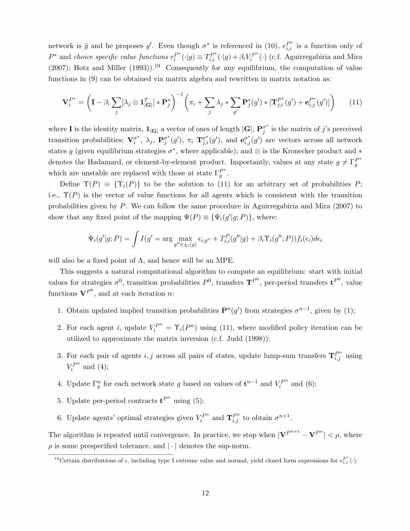
will also be a fixed point of Λ, and hence will be an MPE.This suggests a natural computational algorithm to compute an equilibrium: start with initial

values for strategies σ0, transition probabilities P 0, transfers TP 0, per-period transfers tP

0, value

functions VP 0, and at each iteration n:

1. Obtain updated implied transition probabilities Pn(g′) from strategies σn−1, given by (1);

2. For each agent i, update V Pni = Υi(Pn) using (11), where modified policy iteration can be

utilized to approximate the matrix inversion (c.f. Judd (1998));

3. For each pair of agents i, j across all pairs of states, update lump-sum transfers TPni,j using

V Pni and (4);

4. Update Γng for each network state g based on values of tn−1 and V Pni and (6);

5. Update per-period contracts tPn

using (5);

6. Update agents’ optimal strategies given V Pni and TPn

i,j to obtain σn+1.

The algorithm is repeated until convergence. In practice, we stop when |VPn+1 −VPn | < ρ, whereρ is some prespecified tolerance, and | · | denotes the sup-norm.

19Certain distributions of ε, including type I extreme value and normal, yield closed form expressions for eP∗

i,i (·).

12

On the “curse of dimensionality” One issue with using the entire network structure as thestate space is that the size of the space grows exponentially: the dimensionality is 2n×(n−1) ingeneral network formation games; in bi-partite network formation games, the dimensionality is2B×S where one side has B agents and the other S. For small n, computation is not problematic,as the entire state space can be traversed rapidly. Further aiding computation is the fact that thedimensionality of χi(·) grows much slower than |G|. For larger games, we are exploring the use ofother approaches including reinforcement learning algorithms (c.f. Pakes and McGuire (2001)).

2.3 Extensions to the Model

Mergers The model can be extended to allow for the possibility that certain agents can “merge”with other agents, where merging implies that the two agents are permanently linked (ignoring thepossibility for dissolving a merger), and that they jointly propose new links and bargain over allfuture contracts. To simplify exposition, we focus on settings in which the set of agents who canmerge is exogenously given, and that if these agents link, they can only merge. For example, in thecase of buyer-seller networks, although buyers can link and engage in trade with sellers, buyers areonly allowed to merge with other buyers (and sellers with other sellers).

Exogenously we assume that for any pair ij that can only merge, one agent (say i) will alwaysbe deemed the “acquirer” and the other agent the “target.” If ij merge, j no longer retains anystrategic actions: the probability that j is ever selected to be a proposer becomes 0, and all futureprofits that would otherwise accrue to j are captured by i. Additionally, i and j will have the sameset of links upon merging: i.e., for any network g where ij ∈ g, Ni(g) = Nj(g).

We maintain the timing and structure of the main model, but assume when an agent is selectedas a proposer, he may propose at most one merger in addition to offering new links or droppingexisting links as before. E.g., if i is the proposer, who for the sake of discussion is a buyer, his set ofreachable networks χi(g) includes the possibility of linking with other sellers as well as linking withat most one additional buyer. Instead of offering a lump-sum or per-period contracts, a proposerwho offers a merger negotiates the purchase price TMij which satisfies the following Nash bargainingproblem:

TMij (g) ∈ arg maxT̃

[V̂ σi (g)− T̃ − V̂ σ

i (g − ij)]bij×[V̂ σj (g) + T̃ − V̂ σ

j (g − ij)]bji

(12)

Consequently, a merger is only feasible if for the network g that is proposed, V̂ σi (g) + V̂ σ

j (g) ≥V̂ σi (g − ij) + V̂ σ

i (g − ij).Assumptions on how λ, bargaining parameters, or profit functions change upon merging will

depend on the application.

Exclusive Contracts In certain applications, an agent may be able to propose an exclusivecontract in which he demands another agent contract only with him. We can extend our model toincorporate this possibility by expanding an agent’s set of reachable networks when he is chosen as

13

a proposer. Let χei (g) denote agent i’s set of reachable networks from g when exclusive contractsare permitted, where:

χei (g) ≡ χi(g) ∪{g′ : ∀j ∈ Ni(g′), (g′−i ∩ g′−j = g−i ∩ g−j) ∧ Nj(g′) = {i}

}.

In words, agent i can propose to form a link with any set of agents, and in addition, he has theoption of proposing to any of those agents that she drop all her other links, i.e. form an exclusivecontract. For any proposed network g′ ∈ χei (g), let ki(g′) denote the set of agents to whom i offersan exclusive contract.

To accommodate exclusivity, we also modify the transfers that accompany proposals. Specifi-cally, we let T e,σi,j (g′|g) denote the new transfers and define it as follows:

T e,σi,j (g′|g) =

max{βj

(V σj (g′)− V σ

j (g′′)), 0} if j ∈ Ni(g′),

ci,j(g, g′) if j ∈ Ni(g) and j /∈ Ni(g′),

0 otherwise,

where g′′ = (g′ ∪ gj)− ij. As before, T e,σi,i (g′|g) = −∑

j 6=i Te,σi,j (g′|g).

If an agent j is offered an exclusive contract, she has two options: she can either accept, therebyforming link ij, receiving transfer T e,σi,j and dropping all of her other links, or she can reject so thatij is not formed, no transfer is made, and she keeps her existing links.

Notice that our model does not support imposing specific penalties to agents for breaking anexclusive contract. The reason is that in any given state, the model cannot distinguish betweenan agent who has voluntarily chosen to contract with only one other agent, and an agent who hasaccepted an exclusive contract in a previous period.

Strategic transfers In the appendix, we present a variant of our model in which transfer offersare within each agents’ strategy space, but links that can be negotiated arise randomly. We showthat the equilibrium transfers proposed will be similar to those prescribed before.

2.4 Estimation of Nash Bargaining Parameters

Assume there are m = 1 . . .M markets, each with primitives (Nm,Gm, χm, πm, βm, fm, cm, λm)which are either observed, assumed, or can be separately estimated. Assume Nash bargainingparameters b ≡ {bij} can be parameterized as a function of observable market characteristics zm,t

and parameters to be estimated θ.The econometrician observes network structures {gm,t} for markets m = 1 . . .M and t = 1 . . . T .

We assume the econometrician observes changes to the network structure; furthermore, althoughthe econometrician does not observe who a “proposer” is, she knows (or can make an assumptionabout) when a network does not change as a result of an agent actively choosing to keep the samenetwork (i.e., whenever gm,t = gm,t−1).

14

Define the pseudo-likelihood:

QM (θ, P ) =M∑m=1

T∑t=2

ln Υ(gm,t|gm,t−1; θ, P,b(θ, zm,t)), (13)

where Υ(gm,t|gm,t−1; θ, P ) =∑

j∈Nm λj(gm,t−1)Ψj(g′|g;P,b(θ, zm,t)).Since there is the possibility of multiple equilibria, define the MLE as:

θ̂MLE = arg maxθ

[sup

P∈(0,1)N×|G|QM (θ, P ) subject to P = Ψ(θ, P )

](14)

If all equilibira P can be computed for every θ and compared, then the estimator will be consistent,asymptotically normal, and efficient. For small n, this computation may be plausible; nonetheless,it is an extremely strong assumption, and it remains to be seen how feasible this estimator is.

3 Application: Insurer-Provider Negotiations

We analyze a stylized network formation game between health insurers (e.g., HMOs) and medi-cal providers (e.g., hospitals), where insurers negotiate with providers over reimbursement ratesfor serving patients. Health insurers typically offer potential customers access to a “network” ofproviders: if an insurer and a provider are able to agree on a payment scheme under which theprovider is willing to treat the insurer’s members, then the provider becomes part of the insurer’s“network.” In general, little is known about how payments between insurers and providers are ne-gotiated in the private insurance sector, yet those determine over 40% of healthcare spending, i.e.approximately $1 trillion. Previous empirical work on these negotiations include Capps, Dranove,and Satterthwaite (2003); Dranove, Satterthwaite, and Sfekas (2008); Ho (2009); Sorensen (2003);Town and Vistnes (2001). We analyze simulated markets to understand the networks and negoti-ated payments that arise in a dynamic equilbria; importantly, we allow for forward looking agentsand allow the link structure between insurers and hospitals to change over time.

We first detail the stylized stage game which is used to provide the underlying period-profitfunctions π accruing to each agent for any given network structure. We then examine simulatedequilibria across several markets as bargaining power and the number of agents change, examinethe relationship between observable market characteristics and negotiated per-patient transfers, anddetail how the variation in equilibrium network structures across markets can be used to identifybargaining power (and hence transfers) if they are unobserved.

3.1 Stage Game Timing

For a given network structure g, the basic timing every period is as follows:

1. HMOs compete Nash-in-prices and choose premiums to charge consumers;

15

2. Each consumer in a market chooses to join at most one HMO and pays the premium for thatinsurer;

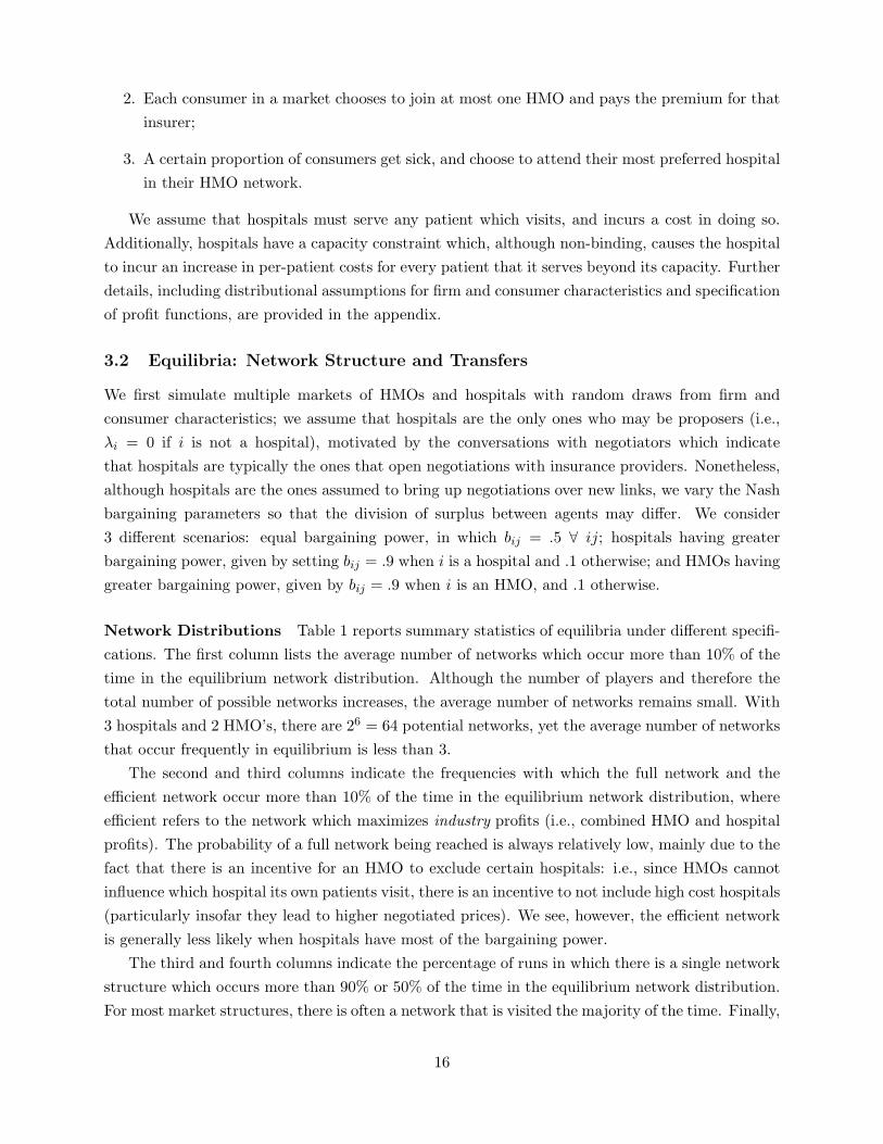
3. A certain proportion of consumers get sick, and choose to attend their most preferred hospitalin their HMO network.

We assume that hospitals must serve any patient which visits, and incurs a cost in doing so.Additionally, hospitals have a capacity constraint which, although non-binding, causes the hospitalto incur an increase in per-patient costs for every patient that it serves beyond its capacity. Furtherdetails, including distributional assumptions for firm and consumer characteristics and specificationof profit functions, are provided in the appendix.

3.2 Equilibria: Network Structure and Transfers

We first simulate multiple markets of HMOs and hospitals with random draws from firm andconsumer characteristics; we assume that hospitals are the only ones who may be proposers (i.e.,λi = 0 if i is not a hospital), motivated by the conversations with negotiators which indicatethat hospitals are typically the ones that open negotiations with insurance providers. Nonetheless,although hospitals are the ones assumed to bring up negotiations over new links, we vary the Nashbargaining parameters so that the division of surplus between agents may differ. We consider3 different scenarios: equal bargaining power, in which bij = .5 ∀ ij; hospitals having greaterbargaining power, given by setting bij = .9 when i is a hospital and .1 otherwise; and HMOs havinggreater bargaining power, given by bij = .9 when i is an HMO, and .1 otherwise.

Network Distributions Table 1 reports summary statistics of equilibria under different specifi-cations. The first column lists the average number of networks which occur more than 10% of thetime in the equilibrium network distribution. Although the number of players and therefore thetotal number of possible networks increases, the average number of networks remains small. With3 hospitals and 2 HMO’s, there are 26 = 64 potential networks, yet the average number of networksthat occur frequently in equilibrium is less than 3.

The second and third columns indicate the frequencies with which the full network and theefficient network occur more than 10% of the time in the equilibrium network distribution, whereefficient refers to the network which maximizes industry profits (i.e., combined HMO and hospitalprofits). The probability of a full network being reached is always relatively low, mainly due to thefact that there is an incentive for an HMO to exclude certain hospitals: i.e., since HMOs cannotinfluence which hospital its own patients visit, there is an incentive to not include high cost hospitals(particularly insofar they lead to higher negotiated prices). We see, however, the efficient networkis generally less likely when hospitals have most of the bargaining power.

The third and fourth columns indicate the percentage of runs in which there is a single networkstructure which occurs more than 90% or 50% of the time in the equilibrium network distribution.For most market structures, there is often a network that is visited the majority of the time. Finally,

16

Table 1: Simulated Equilibrium Network Distributions

“B-Power” # Eq. Full Efficient Single Single Single Single &Networks Network Network (90%) (50%) & Full Efficient

1 Hosp Equal 2.14 0.07 0.24 0.25 0.65 0.00 0.182 HMOs Hospitals 1.96 0.00 0.24 0.35 0.71 0.00 0.18

HMOs 2.46 0.11 0.28 0.18 0.40 0.00 0.18

2 Hosp Equal 2.33 0.11 0.79 0.26 0.69 0.01 0.262 HMOs Hospitals 2.45 0.03 0.36 0.20 0.61 0.00 0.08

HMOs 2.84 0.04 0.84 0.14 0.42 0.00 0.14

3 Hosp Equal 2.34 0.00 0.68 0.18 0.52 0.00 0.152 HMOs Hospitals 2.59 0.00 0.27 0.10 0.42 0.00 0.01

HMOs 2.51 0.00 0.69 0.20 0.47 0.00 0.18

Notes: 100 market draws. B-Power (λ): Equal - bij = .5 ∀ ij; Hospitals - bij = .9 when i is a hospital, .1 otherwise;

HMOs - bij = .9 when i is an HMO, .1 otherwise. # Eq Networks: Average number of networks that occur more than

10% in the equilibrium network distribution (E.N.D.). Full / Efficient: % of runs in which full / efficient network

occurs more than 10% in E.N.D. Single (x%): % of runs in which a single network occurs more than x% in E.N.D.

Single & Full / Efficient: % of runs in which a single network occurs more than 90% in E.N.D., and that network is

full / efficient

the last two columns indicate the percentage of time there is a single network occurring more than90% of the time, and that network is either the full network or the efficient network.

Predicted Transfers We examine equilibrium hospital per-patient margins computed acrossdifferent specifications, and project them on market characteristics, where margins are defined asper-patient transfers from HMOs to hospitals minus hospital costs for serving a patient. Thisexercise is in the spirit Ho (2009) and Pakes (2009) to examine the role of various factors indetermining negotiated per-patient transfers between hospitals and insurers.

In our dynamic model, we focus on the expected values of per-patient margins averaged acrossthe different network structures visited in equilibrium, weighting by the equilibrium network dis-tributions; we only analyze negotiated transfers for hospitals that serve patients in equilibrium(as some hospitals may be excluded in all equilibrium network states). We also examine a staticspecification (β = 0) where two agents negotiate assuming disagreement points are given by staticprofits in the the stable network (i.e., a network in which there exist gains to trade between allcontracting agents) which arises if they fail to contract; hence, they do not account for any subse-quent play (and continuation values are 0). A static model, importantly, cannot determine whichnetwork arises in equilibrium, and only can determine which networks are stable; as a result, weexamine transfers in all stable networks which maximize the number of connected agents.

Table 2 reports results. We first focus on the results from the dynamic specification. Asexpected, hospitals receive a higher per-patient transfer (on average) when they have higher bar-gaining power, partly evident through the higher constant coefficients. The most significant impacton hospital margins come from both having a lower average cost within a market and having alower than average cost, and this is more pronounced the greater a hospital’s bargaining power.

17

Table 2: Regression of Hospital Margins on Observables / Characteristics

Timing: Static Dynamic

Equal Hospital HMO Equal Hospital HMOCoeff S.e. Coeff S.e. Coeff S.e. Coeff S.e. Coeff S.e. Coeff S.e.

Const. 7.85 0.84 18.94 3.66 0.98 0.46 5.71 0.51 12.51 1.56 0.06 0.24Cap Con 1.15 0.25 -0.41 1.18 1.03 0.17 0.33 0.16 -0.13 0.55 0.86 0.09Av. Cost -0.30 0.02 -0.76 0.09 -0.05 0.01 -0.42 0.01 -0.80 0.04 -0.10 0.01Cost-AC -0.35 0.02 -0.36 0.07 -0.09 0.02 -0.50 0.01 -0.65 0.03 -0.13 0.01Pop/Bed -0.02 0.01 -0.01 0.05 0.01 0.01 0.01 0.01 0.07 0.03 0.02 0.01

# Patient 0.15 0.02 0.32 0.10 0.03 0.01 0.04 0.01 -0.15 0.04 0.01 0.01HMO Marg -1.04 0.29 -2.17 1.18 -0.02 0.18 0.31 0.20 0.38 0.52 0.55 0.11

Extra Hospital - - - -0.09 0.08 0.74 0.25 0.03 0.05

R2 0.73 0.31 0.32 0.85 0.57 0.64

Notes: Projection of simulated equilibrium per-patient markups onto market observables as bargaining power varies.

Static results use 2x2 markets; dynamic pools across 2x2 and 3x2 settings. Cap Con: if hospital is capacity constrained

in full network setting; Av. Cost: average hospital marginal cost in the market; Cost-AC: difference between hospital’s

cost and average cost; Pop/Bed: Total market population divided by total hospital capacity; # Patient: expected

number of patients served by hospital in equilibrium; HMO Marg: expected HMO margins (premiums minus marginal

cost; Extra Hospital: indicator for whether there are 3 hospitals (instead of 2) in the market).

Generally, being capacity constrained yields higher margins as well (though this is not statisticallysignificant when hospitals have greater bargaining power), and a higher HMO margin is also associ-ated with higher negotiated hospital margins. The number of patients served by a hospital reducesmargins when hospitals have greater bargaining power. Finally, only when hospitals have greaterbargaining power does the addition of a third hospital increase average hospital margins.

The static specification, in contrast, tends to overestimate implied hospital margins. Thiswould be consistent with the idea that by anticipating future renegotiation and continuation values,hospitals’ outside options are slightly weaker and HMO outside options are slightly stronger ina dynamic setting. For certain market observables, coefficients have different magnitudes (e.g.,for whether or not a hospital is capacity constrained, hospital costs); for others, including HMOmargins, signs are reversed. Thus, not only does a static model fail to provide guidance as towhich (stable) networks are actually played in equilibrium, but also yields economically differentpredictions as to the magnitudes and determinants of underlying negotiated payments betweenagents.

3.3 Estimation, Monte Carlo

One important takeaway from the simulated equilibrium network distributions is that the allocationof bargaining power through the choice of Nash bargaining parameters has a significant impact onwhich networks are reached in equilibrium, and hence the determinants of equilibrium transfers.We explore how this variation in observed network structure can be used to identify and estimateNash bargaining parameters used to generate the data, which would then allow us to computetransfers between agents if they were unobserved.

18

Table 3: Monte Carlo Estimates of bH

True bH 1 Markets / Sample 5 Markets / Sample 10 Markets / SampleAvg. Estimate: 0.50 0.57 0.52 0.48

95% C.I.: [0.00,0.95] [0.30,0.70] [0.35,0.70]

Avg. Estimate: 0.90 0.76 0.86 0.8695% C.I.: [0.00,1.00] [0.70,0.95] [0.75,0.95]

Avg. Estimate: 0.10 0.30 0.10 0.1195% C.I.: [0.00,0.95] [0.00,0.25] [0.00,0.25]

Notes: Estimated values of hospital bargaining power bH for 40 samples of either 1, 10, or 25 markets in 2x2 settings

where a sequence of 10 networks were observed. Grid search conducted over bH in increments of .05.

We initially focus on 2x2 markets where we observe a sequence of 10 networks {gm,1, . . . , gm,10}for each market m, where the initial network drawn from the equilibrium steady state distribu-tion, and subsequent networks are drawn according to the equilibrium transition probabilities. Weassume Nash bargaining parameters are constant across markets in each sample, and are parame-terized by θ = bH ∈ [0, 1], where we assume bij = bH if i is a hospital and bij = (1− bH) otherwise.For all other parameters used to generate the data, we assume them to be known. We choose thevalue of bH which maximizes the probability of observing the sequence of networks in the datagiven by the likelihood in (14). In the absence of a proof of uniqueness, we are relying on a strongassumption of either the uniqueness of the equilibrium network distribution across all equilibria,or the ability to select the same equilibrium in the presence of multiplicity during the estimationroutine. Since the estimation routine utilizes the same computational algorithm as the data gener-ating process, this will not likely be a problem in our current setup given the latter interpretation.However, the degree to which this is problematic will depend on the application.

Table 3 summarizes the estimation results as we vary the size of the sample from 1, 5, and10 different markets; for computational convenience, we conduct a grid search over [0, 1] where weallow bH to vary by .05. With only a single market per sample, the 95% confidence interval is notinformative; this partly occurs because there are some markets in which a single network exists,which is consistent with a wide range of values for bH . However, once the sample size increasesto include 5 markets, fewer values of bH are consistent with generating the observed sequence ofnetworks in the data. As a result, the average estimates become extremely close to the true valueof bH , and the confidence intervals are within .2 of the true value.

4 Concluding Remarks

//Forthcoming.//

19

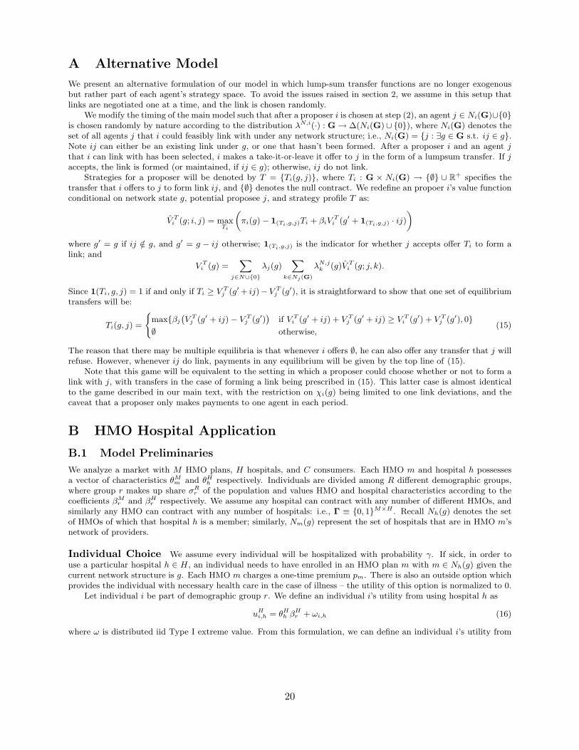
A Alternative Model

We present an alternative formulation of our model in which lump-sum transfer functions are no longer exogenousbut rather part of each agent’s strategy space. To avoid the issues raised in section 2, we assume in this setup thatlinks are negotiated one at a time, and the link is chosen randomly.

We modify the timing of the main model such that after a proposer i is chosen at step (2), an agent j ∈ Ni(G)∪{0}is chosen randomly by nature according to the distribution λN,i(·) : G→ ∆(Ni(G)∪ {0}), where Ni(G) denotes theset of all agents j that i could feasibly link with under any network structure; i.e., Ni(G) = {j : ∃g ∈ G s.t. ij ∈ g}.Note ij can either be an existing link under g, or one that hasn’t been formed. After a proposer i and an agent jthat i can link with has been selected, i makes a take-it-or-leave it offer to j in the form of a lumpsum transfer. If jaccepts, the link is formed (or maintained, if ij ∈ g); otherwise, ij do not link.

Strategies for a proposer will be denoted by T = {Ti(g, j)}, where Ti : G × Ni(G) → {∅} ∪ R+ specifies thetransfer that i offers to j to form link ij, and {∅} denotes the null contract. We redefine an propoer i’s value functionconditional on network state g, potential proposee j, and strategy profile T as:

V̂ Ti (g; i, j) = maxTi

„πi(g)− 1(Ti,g,j)Ti + βiV

Ti (g′ + 1(Ti,g,j) · ij)

«where g′ = g if ij /∈ g, and g′ = g − ij otherwise; 1(Ti,g,j) is the indicator for whether j accepts offer Ti to form alink; and

V Ti (g) =X

j∈N∪{0}

λj(g)X

k∈Nj(G)

λN,jk (g)V̂ Ti (g; j, k).

Since 1(Ti, g, j) = 1 if and only if Ti ≥ V Tj (g′+ ij)−V Tj (g′), it is straightforward to show that one set of equilibriumtransfers will be:

Ti(g, j) =

(max{βj

`V Tj (g′ + ij)− V Tj (g′)

´if V Ti (g′ + ij) + V Tj (g′ + ij) ≥ V Ti (g′) + V Tj (g′), 0}

∅ otherwise,(15)

The reason that there may be multiple equilibria is that whenever i offers ∅, he can also offer any transfer that j willrefuse. However, whenever ij do link, payments in any equilibrium will be given by the top line of (15).

Note that this game will be equivalent to the setting in which a proposer could choose whether or not to form alink with j, with transfers in the case of forming a link being prescribed in (15). This latter case is almost identicalto the game described in our main text, with the restriction on χi(g) being limited to one link deviations, and thecaveat that a proposer only makes payments to one agent in each period.

B HMO Hospital Application

B.1 Model Preliminaries

We analyze a market with M HMO plans, H hospitals, and C consumers. Each HMO m and hospital h possessesa vector of characteristics θMm and θHh respectively. Individuals are divided among R different demographic groups,where group r makes up share σRr of the population and values HMO and hospital characteristics according to thecoefficients βMr and βHr respectively. We assume any hospital can contract with any number of different HMOs, andsimilarly any HMO can contract with any number of hospitals: i.e., Γ ≡ {0, 1}M×H . Recall Nh(g) denotes the setof HMOs of which that hospital h is a member; similarly, Nm(g) represent the set of hospitals that are in HMO m’snetwork of providers.

Individual Choice We assume every individual will be hospitalized with probability γ. If sick, in order touse a particular hospital h ∈ H, an individual needs to have enrolled in an HMO plan m with m ∈ Nh(g) given thecurrent network structure is g. Each HMO m charges a one-time premium pm. There is also an outside option whichprovides the individual with necessary health care in the case of illness – the utility of this option is normalized to 0.

Let individual i be part of demographic group r. We define an individual i’s utility from using hospital h as

uHi,h = θHh βHr + ωi,h (16)

where ω is distributed iid Type I extreme value. From this formulation, we can define an individual i’s utility from

20

enrolling in a given HMO m that has a set of hospitals Nm(g):20

uMi,m(g) = θMm βMr − αpm + γ

0@ln(X

h∈Nm(g)

exp(θHh βHr ))

1A+ εi,m (17)

where ε is also distributed iid Type I extreme value.With this linear utility function and distribution on error terms, we can calculate the the (expected) share of the

population that chooses HMO m given any particular network structure g as follows:

σMm (g) =Xr∈R

σRrexp(θMm β

Mr − αpm + γ ln(

Ph∈Nm(g) exp(θHh β

Hr )))

1 +Pl∈M (exp(θMl β

Mr − pl + γ ln(

Ph∈Nl(g)

exp(θHh βHr ))))

=Xr∈R

σRr σ̃Mm,r(g)

We use σ̃Mm,r(g) to represent the share of demographic group r that chooses HMO plan m.Define the demographic distribution of individuals within each HMO plan (i.e., the share of people who use HMO

plan m who are part of demographic group r) as follows:

σ̃Rr,m(g) =σRr σ̃

Mm,r(g)P

s∈R σRs σ̃Mm,s(g)

Thus, the share of HMO plan m’s customers who actually will be sick and need to use hospital h ∈ Nm(g) can bewritten as:

σHh,m(g) = γXr∈R

σ̃Rr,m(g)exp(θHh β

Hr )P

l∈Nm(g) exp(θHl βHr )

Note that although σMm is a function of the entire network structure g and premiums charged by all HMOs, σHm willjust be a function of HMO m’s own hospital network Nm(g).

Hospital and HMO Per-Period Profits For expositional convenience, let σMm and σHm will denote valuesfor a given network structure g unless otherwise specified. Let thm be the negotiated per-patient transfers betweenhospital h and m in network structure g. For hospital h, profits for a given network structure g are given by theequation

πHh (g) = (thm − cHj )(X

m∈Nh(g)

NσMm σHh,m) +

Xm∈Nh(g)

ηh,m

cHh represents the average cost of serving each patient at hospital h. Each hospital h has a “capacity constraint” Γh,and will face increasing costs if it serves more than Γh patients. We assume that if hospital h serves x patients, itsaverage costs per patient will be given by cHh = c̄Hh + (x− Γh)φ1x>Γh , where c̄Hh is an hospital specific constant, andφ represents the exponential parameter through which overflow patients affect average costs if the hospital is overcapacity (denoted by the indicator function 1x>Γh).

For any HMO m, its profits are calculated as follows:

πMm (g) = NσMm (pm − cMm −X

h∈Nm(g)

σHh,mthm) +X

h∈Nm(g)

ηh,m

Timing The timing in each period, given a network structure g, is as follows:

1. Each HMO m chooses a premium pm ∈ R+ that it will charge each consumer that chooses to join its plan.

2. Each individual i chooses to enroll in an HMO plan, with the utility from choosing HMO m being uMi,m definedin (17), or chooses to utilize the outside option, thereby deriving a utility of 0.

3. γ proportion of the population becomes sick. Each individual i that is sick chooses the best hospital on theHMO they enrolled in to attend according to their utility given by (16).

4. HMO payoffs (πM ) and hospital payoffs (πH) are realized.

B.2 Parameters

Units, unless otherwise specified, are in thousands.

20Note Eω(maxh∈Nm(g)(uHi,h)) = ln(

Ph∈Nm(g) exp(θHh β

Hr ))

21

Demographic Characteristics People are hospitalized with probability γ = .075. We assume that marketsshould be, in expectation over the aggregate, not over-capacity. Market size is distributed normally with a mean of600, standard deviation 300, and a minimum value of 100; thus, if the mean number of people enroll in an HMO plan,40 patients will need to be served. In the current specification, we do not assume there are different demographicgroups, and assume βr = 1 for all agents.

HMO Characteristics HMO per-patient costs cMm are normally distributed with mean .75 and standarddeviation .25. HMO quality θMm is distributed normally with mean 2.5 and standard deviation .25. It is correlatedwith costs by a value of ρM = .5.

Hospital Characteristics Hospital quality θHh for each hospital are normals with mean µθH = 25 andstandard deviation σθH = .5. Hospital constant marginal costs c̄Hj are gaussian normals with mean µc̄H = 12 andstandard deviation µc̄H = 9, with a minimum of 1. Costs and hospital quality index for a particular hospital h arecorrelated by a value of ρH = .5. For each pair, these variables are generated first by creating two correlated standardnormal random variables, and then appropriately transforming them with the correct mean and standard deviation.We assume that hospital capacity Γh is i.i.d. normal, with mean µΓ = 25 and standard deviation σΓ = 10, with aminimum value of 1. Marginal costs increase exponentially in the number over capacity by the value φ = 1.5.

Parameters of the Dynamic Game We assume proposer shocks εi are distributed iid Type I extremevalue with variance 10π2/6. We assume away profit shocks η; i.e., ηi,j = 0. We set discount factors βi = .9 ∀ i, andset termination fees ci,j = 0.

References

Abreu, D., and M. Manea (2009): “Bargaining and Efficieny in Networks,” mimeo.

Ackerberg, D., C. L. Benkard, S. Berry, and A. Pakes (2007): “Econometric Tools forAnalyzing Market Outcomes,” in Handbook of Econometrics, ed. by J. J. Heckman, and E. E.Leamer, vol. 6a, chap. 63. North-Holland, Amsterdam.

Aguirregabiria, V., and P. Mira (2002): “Swapping the Nested Fixed Point Algorithm: AClass of Estimators for Discrete Markov Decision Models,” Econometrica, 70(4), 1519–1543.

(2007): “Sequential Estimation of Dynamic Discrete Games,” Econometrica, 75(1), 1–53.

Benkard, C. L., P. Bajari, and J. Levin (2007): “Estimating Dynamic Models of ImperfectCompetition,” Econometrica, 75(5), 1331–1370.

Bloch, F., and M. O. Jackson (2007): “The Formation of Networks with Transfers amongPlayers,” Journal of Economic Theory, 127(1), 83–110.

Capps, C., D. Dranove, and M. Satterthwaite (2003): “Competiton and Market Power inOption Demand Markets,” RAND Journal of Economics, 34(4), 737–763.

Crawford, G. S., and A. Yurukoglu (2010): “The Welfare Effects of Bundling in MultichannelTelevision,” mimeo.

Cremer, J., and M. H. Riordan (1987): “On Governing Multilateral Transactions with BilateralContracts,” RAND Journal of Economics, 18(3), 436–451.

de Fontenay, C. C., and J. S. Gans (2007): “Bilateral Bargaining with Externalities,” mimeo.

Doraszelski, U., and A. Pakes (2007): “A Framework for Applied Dynamic Analysis in IO,” inHandbook of Industrial Organization, ed. by M. Armstrong, and R. Porter, vol. 3, pp. 1887–1966.North-Holland, Amsterdam.

22

Dranove, D., M. Satterthwaite, and A. Sfekas (2008): “Boundedly Rational Bargaining inOption Demand Markets: An Empirical Application,” mimeo.

Dutta, B., S. Ghosal, and D. Ray (2005): “Farsighted Network Formation,” Journal of Eco-nomic Theory, 122, 143–164.

Gomes, A. (2005): “Multilateral Contracting with Externalities,” Econometrica, 73(4), 1329–1350.

Ho, K. (2009): “Insurer-Provider Networks in the Medical Care Market,” American EconomicReview, 99(1), 393–430.

Horn, H., and A. Wolinsky (1988): “Bilateral Monopolies and Incentives for Merger,” RANDJournal of Economics, 19(3), 408–419.

Hotz, V. J., and R. A. Miller (1993): “Conditional Choice Probabilities and the Estimationof Dynamic Models,” Review of Economic Studies, 60(3), 497–529.

Hotz, V. J., R. A. Miller, S. Sanders, and J. Smith (1994): “A Simulation Estimator forDynamic Models of Discrete Choice,” Review of Economic Studies, 61(3), 265–289.

Jackson, M. O., and A. Wolinsky (1996): “A Strategic Model of Social and Economic Net-works,” Journal of Economic Theory, 71(1), 44–74.

Judd, K. L. (1998): Numerical Methods in Economics. MIT Press, Cambridge, MA.

Kranton, R. E., and D. F. Minehart (2001): “A Theory of Buyer-Seller Networks,” AmericanEconomic Review, 91(3), 485–508.

Lee, R. S. (2010): “Vertical Integration and Exclusivity in Platform and Two-Sided Markets,”mimeo, http://pages.stern.nyu.edu/ rslee/papers/VIExclusivity.pdf.

Manea, M. (2009): “Bargaining in Stationary Networks,” mimeo.

Maskin, E., and J. Tirole (1988): “A Theory of Dynamic Oligopoly: I & II,” Econometrica,56(3), 549–600.

McAfee, R. P., and M. Schwartz (1994): “Opportunism in Multilateral Vertical Contracting:Nondiscrimination, Exclusivity, and Uniformity,” American Economic Review, 84(1), 210–230.

Milgrom, P., and R. Weber (1985): “Distributional Strategies for Games with IncompleteInformation,” Mathematics of Operations Research, 10, 619–32.

Pakes, A. (2009): “Alternative Models for Moment Inequalities,” mimeo.

Pakes, A., and P. McGuire (2001): “Stochastic Algorithms, Symmetric Markov Perfect Equili-brum, and the ‘curse’ of dimensionality,” Econometrica, 69(5), 1261–1281.

Pakes, A., M. Ostrovsky, and S. Berry (2007): “Simple Estimators for the Parameters ofDiscrete Dynamic Games, with Entry/Exit Examples,” RAND Journal of Economics, 38(2),373–399.

Prat, A., and A. Rustichini (2003): “Games Played Through Agents,” Econometrica, 71(4),989–1026.

23

Sorensen, A. T. (2003): “Insurer-Hospital Bargaining: Negotiated Discounts in Post-Deregulation Connecticut,” Journal of Industrial Economics, 51(4), 469–490.

Stole, L. A., and J. Zweibel (1996): “Intra-Firm Bargaining under Non-Binding Contracts,”Review of Economic Studies, 63(3), 375–410.

Town, R. J., and G. Vistnes (2001): “Hospital Competition in HMO Networks,” Journal ofHealth Economics, 20, 733–753.

24