/k

12

1/25

MARKOV MODEL WITH COSTS

In Markov models we are often interested in cost calculations.

• inventory model: storage costs

• manpower planning model: salary costs

• machine reliability model: repair costs

We will look at 3 types of cost calculations:

1. Expected total costs over a finite horizon

2. Long-run expected costs per period

3. Expected total costs over an infinite horizon

(possible if you only have costs in the transient states)

/k

12

2/25

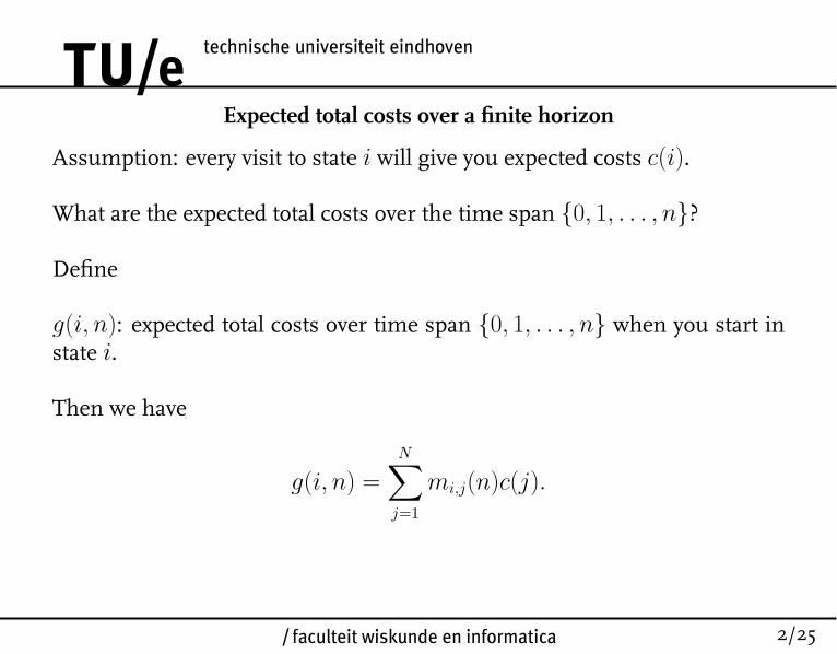
Expected total costs over a finite horizon

Assumption: every visit to state i will give you expected costs c(i).

What are the expected total costs over the time span {0, 1, . . . , n}?

Define

g(i, n): expected total costs over time span {0, 1, . . . , n} when you start instate i.

Then we have

g(i, n) =

N∑j=1

mi,j(n)c(j).

/k

12

3/25

Using the notation

g(n) =

g(1, n)g(2, n)

...g(N, n)

, c =

c(1)c(2)

...c(N)

we have

g(n) = M(n) ∗ c.

Conclusion: If we know the matrix of occupancy times M(n) and the costvector c, we can calculate the expected total costs over a finite horizon.

/k

12

4/25

Example: Inventory system (see Example 5.6)

State space: S = {2, 3, 4, 5}

Transition matrix:

P =

0.0498 0 0 0.95020.1494 0.0498 0 0.80080.2240 0.1494 0.0498 0.57680.2240 0.2240 0.1494 0.4026

Assume storage costs in state i: 50 ∗ i.

Then expected total storage costs over time span {0, 1, 2, . . . , 10}

g(10) =

2161219722292270

,

/k

12

5/25

Long-run expected costs per period

If n → ∞, then often the total expected costs over the time span{0, 1, . . . , n} also tend to infinity. Hence, usually in long-run cost calcu-lations we look at the expected costs per period:

g(i) = limn→∞

g(i, n)

n + 1.

Theorem:

For an irreducible Markov chain with occupancy distribution π̂ we have

g(i) = g =

N∑j=1

π̂jc(j).

Remark that for an irreducible Markov chain the long-run expected costs perperiod do not depend on the initial state.

/k

12

6/25

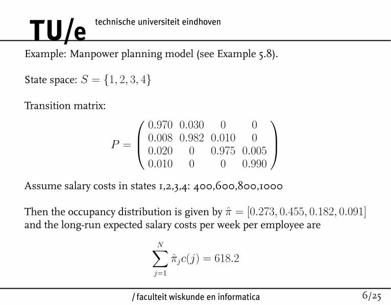
Example: Manpower planning model (see Example 5.8).

State space: S = {1, 2, 3, 4}

Transition matrix:

P =

0.970 0.030 0 00.008 0.982 0.010 00.020 0 0.975 0.0050.010 0 0 0.990

Assume salary costs in states 1,2,3,4: 400,600,800,1000

Then the occupancy distribution is given by π̂ = [0.273, 0.455, 0.182, 0.091]and the long-run expected salary costs per week per employee are

N∑j=1

π̂jc(j) = 618.2

/k

12

7/25

Expected total costs over an infinite horizon

If there are only costs in transient states, then the expected total costs will nottend to infinity when n→∞.

How do we calculate in this case g̃(i) = limn→∞ g(i, n)?

Let A be the set of states in the end classes and hence S \ A the set oftransient states.

By using a first-step analysis we can show that

g̃(i) = c(i) +∑

j∈S\A

pi,jg̃(j), i ∈ S \ A.

This system of equations has a unique solution.

/k

12

8/25

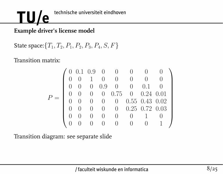
Example driver’s license model

State space:{T1, T2, P1, P2, P3, P4, S, F}

Transition matrix:

P =

0 0.1 0.9 0 0 0 0 00 0 1 0 0 0 0 00 0 0 0.9 0 0 0.1 00 0 0 0 0.75 0 0.24 0.010 0 0 0 0 0.55 0.43 0.020 0 0 0 0 0.25 0.72 0.030 0 0 0 0 0 1 00 0 0 0 0 0 0 1

Transition diagram: see separate slide

/k

12

9/25

What is the meaning of the different states?

T1, T2: theoretical exam (first + second time)

P1, P2, P3, P4: practical exam (1st,2nd,3rd,≥ 4th time)

S: Leaving with driver’s license (Success)

F : Leaving without driver’s license (Failure)

costs theoretical exam: 45 euro each time,costs practical exam: 90 euro each time.

Question: What are the expected total costs over an infinite horizon?

/k

12

10/25

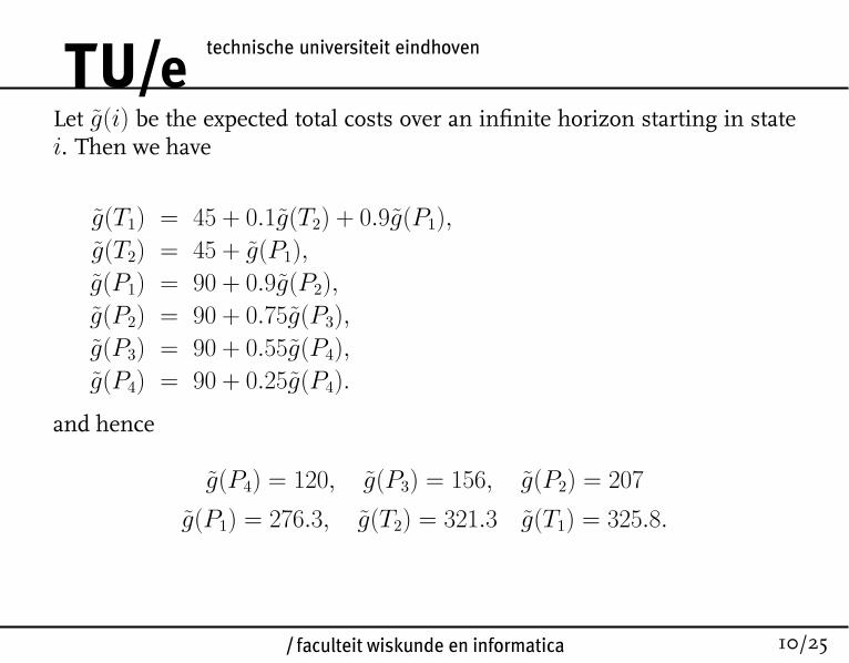
Let g̃(i) be the expected total costs over an infinite horizon starting in statei. Then we have

g̃(T1) = 45 + 0.1g̃(T2) + 0.9g̃(P1),

g̃(T2) = 45 + g̃(P1),

g̃(P1) = 90 + 0.9g̃(P2),

g̃(P2) = 90 + 0.75g̃(P3),

g̃(P3) = 90 + 0.55g̃(P4),

g̃(P4) = 90 + 0.25g̃(P4).

and hence

g̃(P4) = 120, g̃(P3) = 156, g̃(P2) = 207

g̃(P1) = 276.3, g̃(T2) = 321.3 g̃(T1) = 325.8.

/k

12

11/25

First passage times(Time until the Markov chain first enters a certain set of states)

In the preceding slides we have seen twice that you can calculate a certainquantity by doing a so-called "first-step analysis": derive a system of equa-tions by considering what can happen in the first period with the Markovchain.

• Calculation of the probability that a reducible Markov chain will end ina certain end class.

• Calculation of the expected total costs over an infinite horizon for a re-ducible Markov chain with only costs in the transient states.

The same technique can be used to calculate expected first passage times ofa Markov chain.

/k

12

12/25

Let A be a subset of the state space S and define mi(A) as the expectedtime until the Markov chain first enters the subsetA when it starts in state i.

Then of course we have mi(A) = 0 if i ∈ A and furthermore

mi(A) = 1 +∑

j∈S\A

pi,jmj(A), i /∈ A.

This, again, gives a system of equations from which we can obtain the quan-tities mi(A) for i /∈ A.

/k

12

13/25

Example: Manpower planning model

Calculate the expected time an employee is working in the company.Markov model for 1 specific employee:

State space S = {1, 2, 3, 4, left company}

Transition matrix

P =

0.95 0.03 0 0 0.020 0.982 0.01 0 0.0080 0 0.975 0.005 0.020 0 0 0.99 0.010 0 0 0 1

.

/k

12

14/25

Let A = {left company} and hence S \ A = {1, 2, 3, 4}.

The quantities mi(A) satisfy the equations

m1(A) = 1 + 0.95m1(A) + 0.03m2(A)

m2(A) = 1 + 0.982m2(A) + 0.01m3(A)

m3(A) = 1 + 0.975m3(A) + 0.005m4(A)

m4(A) = 1 + 0.99m4(A)

The solution of this system of equations is given by

m4(A) = 100, m3(A) = 60, m2(A) = 88.89, m1(A) = 73.33

Hence, the expected time an employee is working in the company is equalto 73.33 weeks (approximately 1.4 years).

/k

12

15/25

COHORT MODELS

Discrete time Markov chains are often used in the study of the behaviour ofa group of persons or objects. These systems are often called Cohort models.An example of a cohort model is the manpower planning model.

In the manpower planning model we assumed so far that the total numberof employees is constant. Each time an employee leaves the company, he orshe is instantaneously replaced by a new employee.

Using the theory of Markov chains we were able to determine the short-term and long-term behaviour of the number of employees in the differentcategories.

/k

12

16/25

Example: Manpower planning model

Transition matrix

P =

0.97 0.03 0 00.008 0.982 0.01 00.02 0 0.975 0.0050.01 0 0 0.99

.

Assume we have 100 employees and in the beginning of week 1 we havethat 50 employees belong to category 1, 25 to category 2, 15 to category 3 and10 to category 4.

How many employees do you expect in the different categories in the begin-ning of week 5, 11 and 100?

How many employees do you expect in the different categories in the long-run?

/k

12

17/25

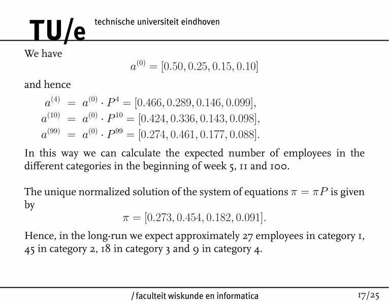
We havea(0) = [0.50, 0.25, 0.15, 0.10]

and hence

a(4) = a(0) · P 4 = [0.466, 0.289, 0.146, 0.099],

a(10) = a(0) · P 10 = [0.424, 0.336, 0.143, 0.098],

a(99) = a(0) · P 99 = [0.274, 0.461, 0.177, 0.088].

In this way we can calculate the expected number of employees in thedifferent categories in the beginning of week 5, 11 and 100.

The unique normalized solution of the system of equations π = πP is givenby

π = [0.273, 0.454, 0.182, 0.091].

Hence, in the long-run we expect approximately 27 employees in category 1,45 in category 2, 18 in category 3 and 9 in category 4.

/k

12

18/25

However, in many applications it is not realistic to assume that the numberof persons in the group is constant over time. The departures of personsfrom the group on the one hand and the arrivals of new persons into thegroup can be independent processes.

Example: The number of persons having a car insurance at a certain insu-rance company. (The different categories here represent the different levelsin the no-claims bonus system).

How do we calculate in such cases quantities like

• the expected number of persons in the group at a certain time instantand the division of the persons within the group over the different levels(short-term behaviour)?

• the expected number of persons in the group in the long-run and thedivision of the persons within the group over the different levels (long-term behaviour)?

/k

12

19/25

Assume we have a group of persons, where the behaviour of each personcan be described by a Markov chain with state space S = {0, 1, 2, . . . , N}and transition matrix P .

State 0 represents the situation that the person has left the system.

Q is the part of the transition matrix corresponding to transitions fromstates {1, 2, . . . , N} to states {1, 2, . . . , N}.

Here, Q is a sub-stochastic matrix, i.e., a matrix with qi,j ≥ 0 for all i and jand

∑Nj=1 qi,j ≤ 1 for all i.

/k

12

20/25

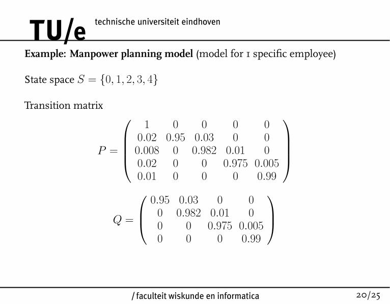
Example: Manpower planning model (model for 1 specific employee)

State space S = {0, 1, 2, 3, 4}

Transition matrix

P =

1 0 0 0 0

0.02 0.95 0.03 0 00.008 0 0.982 0.01 00.02 0 0 0.975 0.0050.01 0 0 0 0.99

Q =

0.95 0.03 0 00 0.982 0.01 00 0 0.975 0.0050 0 0 0.99

/k

12

21/25

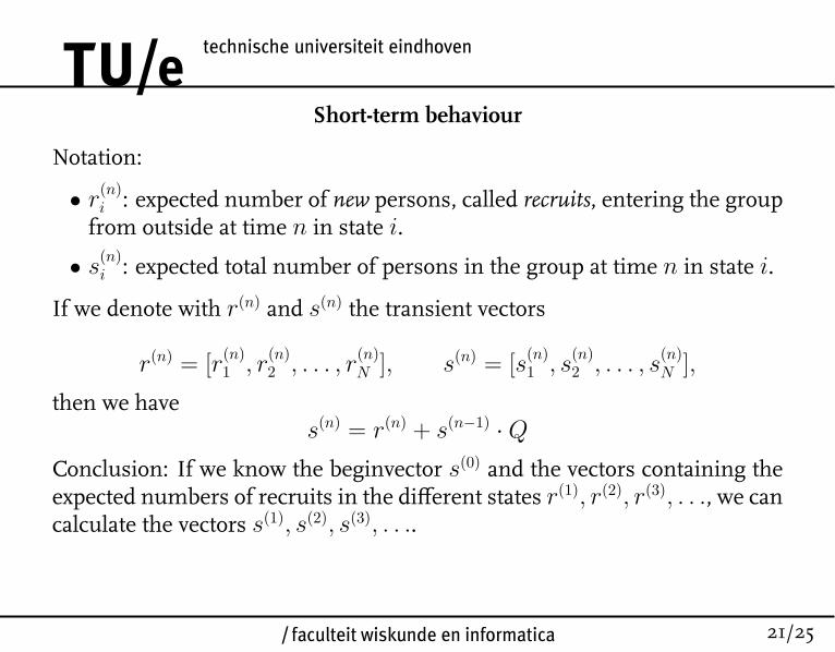
Short-term behaviour

Notation:

• r(n)i : expected number of new persons, called recruits, entering the group

from outside at time n in state i.

• s(n)i : expected total number of persons in the group at time n in state i.

If we denote with r(n) and s(n) the transient vectors

r(n) = [r(n)1 , r

(n)2 , . . . , r

(n)N ], s(n) = [s

(n)1 , s

(n)2 , . . . , s

(n)N ],

then we haves(n) = r(n) + s(n−1) ·Q

Conclusion: If we know the beginvector s(0) and the vectors containing theexpected numbers of recruits in the different states r(1), r(2), r(3), . . ., we cancalculate the vectors s(1), s(2), s(3), . . ..

/k

12

22/25

Example:Markov chain with state space S = {0, 1, 2, 3, 4} and transition matrix

P =

1 0 0 0 0

0.2 0.6 0.2 0 00.05 0 0.7 0.25 00.1 0 0 0.7 0.20.10 0 0 0 0.9

.

Furthermore assume that s(0) = [10, 10, 10, 10] and r(n) = [10, 0, 0, 0] for alln.

s(1) = [10, 0, 0, 0] + [10, 10, 10, 10] ·

0.6 0.2 0 00 0.7 0.25 00 0 0.7 0.20 0 0 0.9

= [16, 9, 9.5, 11].

/k

12

23/25

s(2) = [10, 0, 0, 0] + [16, 9, 9.5, 11] ·

0.6 0.2 0 00 0.7 0.25 00 0 0.7 0.20 0 0 0.9

= [19.6, 9.5, 8.9, 11.8].

s(3) = [10, 0, 0, 0] + [19.6, 9.5, 8.9, 11.8] ·

0.6 0.2 0 00 0.7 0.25 00 0 0.7 0.20 0 0 0.9

= [21.76, 10.57, 8.61, 12.40].

and so on ....

/k

12

24/25

Long-term behaviour

In the case that the expected number of recruits is constant over time, i.e.,r(n) = r for all n, we can also determine the long-run expected number ofpersons in the group in the different states.

In this case we have that s = limn→∞ s(n) satisfies

s = r + s ·Q,

and hence

s = r · (I −Q)−1

where I is the identity matrix.

Remark: The existence of the inverse of the matrix I − Q follows form thefact that the matrix Q is sub-stochastic.

/k

12

25/25

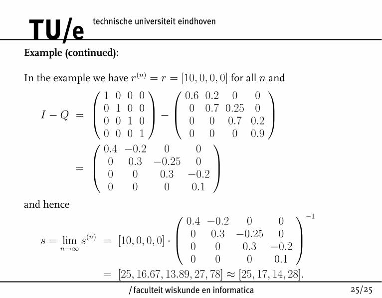
Example (continued):

In the example we have r(n) = r = [10, 0, 0, 0] for all n and

I −Q =

1 0 0 00 1 0 00 0 1 00 0 0 1

− 0.6 0.2 0 0

0 0.7 0.25 00 0 0.7 0.20 0 0 0.9

=

0.4 −0.2 0 00 0.3 −0.25 00 0 0.3 −0.20 0 0 0.1

and hence

s = limn→∞

s(n) = [10, 0, 0, 0] ·

0.4 −0.2 0 00 0.3 −0.25 00 0 0.3 −0.20 0 0 0.1

−1

= [25, 16.67, 13.89, 27, 78] ≈ [25, 17, 14, 28].