Market Transparency and Pricing Efficiency: Evidencefrom Corporate Bond Market∗

Jia Chenchen.1002@gmail.com

Guanghua School of ManagementPeking University

Ruichang Luruichanglu@gsm.pku.edu.cn

Guanghua School of ManagementPeking University

September 1, 2016

Abstract

This paper investigates how mandatory post-trade market transparency affectspricing efficiency in the corporate bond market. Using the phase implementation ofTRACE and a differences-in-differences research design, we find that higher trans-parency leads to a shorter return drift and a lower price delay. These effects are similarbetween bonds with low and high liquidity and between bonds with low and hightrading activity. In addition, the increase in market transparency leads to a higherco-movement between individual bond return and bond market return. These resultshighlight the importance of market transparency on the information efficiency in fi-nancial markets.

∗We thank Bing Han, Laura Liu, Qiao Liu, Xiong Wei, Lucy White, Liyan Yang, and Haoxiang Zhu andbrown bag participants at the Guanghua School of Management and the Five-star workshop at TsinghuaPBC School of Finance.

1

1 Introduction

Transparency is a fundamental issue in the functioning of financial markets to which

financial economics have paid substantial attention. Researchers write down models to study

how transparency induced by different market structure impacts welfare, trading activity,

and liquidity (Biais, 1993; Naik, Neuberger, and Viswanathan, 1999; Madhavan, 1995, 1996;

Pagano and Roell, 1996). Empirical studies examine how transparency changes caused by

regulatory changes in equity and bond markets affect trading and liquidity (Boehmer, Saar,

and Yu, 2005; Gemmill, 1996; Bessembinder, Maxwell, and Venkataraman, 2006; Madhavan,

Porter, and Weaver, 2005; Edwards, Harris, and Piwowar, 2007; Goldstein, Hotchkiss, and

Sirri, 2007; Asquith, Covert, and Pathak, 2013). Laboratory experiments are used to help

determine the effects of transparency changes (Bloomfield and O’Hara, 1999, 2000).

There have been disagreements on what effects market transparency has on pricing effi-

ciency between regulators and researchers. On the one hand, a positive, beneficial view is

often held by U.S regulators: transparency improves the price discovery, fairness, competi-

tiveness, and attractiveness of U.S. markets (SEC, 1994). A number of studies support this

view using different contexts: market fragmentation versus consolidation (Madhavan, 1995),

auction versus dealer markets (Pagano and Roell, 1996), and experiments (Bloomfield and

O’Hara, 1999). The intuition of this view is simple. Transparency helps pricing efficiency be-

cause patterns in trades allow investors to better learn information from trades and thereby

set their prices more efficiently.

On the other hand, UK regulators have had concerns that increased market transparency

may reduce liquidity and/or market efficiency (Franks and Schaefer, 1995). Several recent

papers argue that transparency may have adverse impacts on market efficiency in the con-

texts of correlated asset values (Asriyan, Fuchs, and Green, 2015), investors with or without

immediate liquidity needs (Bhattacharya, 2016), and liquidity traders’ learning about fun-

damentals (Banerjee, Davis, and Gondhi, 2016). In these models, investors’ incentives of

collecting fundamental information can be lowered by transparency, leading to less informa-

tive prices and lower pricing efficiency.

Despite the research importance and attention, the empirical research on this topic is

relatively little, partially due to the lack of data and the rarity of the regulation change event.

In this paper, we offer empirical evidence on how a specific form of transparency, post-trade

transparency, causally impacts pricing efficiency. Specifically, we use the implementation

phases of Trade Reporting and Compliance Engine (TRACE) to examine whether disclosing

trading price and volume information after the trade affects pricing efficiency. We focus

on the impacts of transparency on pricing efficiency because pricing efficiency is critical for

2

financial markets to provide accurate information for resource allocation (Fama, 1970).

TRACE implementation provides a unique setting for understanding the impacts of mar-

ket transparency on pricing discovery. From 1940s to July 2002, there was no public disclo-

sure of transaction details in the corporate bond market, where transactions happened over

the counter with private negotiations.1 In July 2002, the prices and volume information of

transactions became publicly disclosed after the transactions were completed. FINRA (then

NASD) required all transactions of U.S. corporate bonds by regulated market participants

be reported to TRACE shortly after transaction completion. TRACE then publicly release

the prices and volume information, which is known as dissemination.

The implementation of TRACE is not applied to all bonds at the same time. Although

TRACE began collecting all price and volume information for all corporate bonds in July

2002, it began on that day dissemination of this information for a subset of bonds. Three

other primary TRACE implementation phases (Phases 2, 3A, and 3B) followed, each includ-

ing more bonds into the dissemination. FINRA assigned bonds into each phase according

to bond issue size, credit quality, and previous levels of trading activity. In February 2005,

all corporate bonds’ price and volume information was publicly disseminated shortly after

trade completion.

We take advantage of these implementation phases to conduct a difference-in-difference

analysis that compares the price discovery speed of bonds subject to a change in transparency

and that of the bonds that are not. This research design helps control for the confounding

effects of unobserved shocks to the corporate bond markets.

We consider two primary pricing efficiency measures: bond return drift after a bond

analysts’ report or credit rating change and the delay with which a bond’s price responds to

information. We follow Gleason and Lee (2003) to define the return drift measure as 8-week

sum of the absolute abnormal return (∑8

n=1 |ARn|) after a bond analyst report or rating

change. We follow Hou and Moskowitz (2005) to define the price delay measure. Both

these measures rely on an intuitive principle: a security price that is slow to incorporate

information in market events or market index movements is less efficient than a security

price that instantaneously incorporates the information. Both these measures decrease with

pricing efficiency.

We find that post-trade transparency of price and volume leads to a significant increase

in pricing efficiency. According to our difference-in-difference regression analysis, drift af-

ter bond analyst’s reports decreases by about 50% after phase implementation in all three

phases compared to pre-phase levels. Drift after credit rating change decreases by about

1See Biais and Green (2007) and Piwowar (2011) for detailed account of evolution of the transparencyregulations in the bond market.

3

30% after phase implementation in phase 3A and 3B and 5% in phase 2 compared to pre-

phase implementation levels . Delay decreases by about 16% for in one year after phase

implementation for Phase 2 bonds, 25% for Phase 3A bonds, and 24% for Phase 3B bonds.

These results are robust to using different ways of measuring delay and logarithm and logistic

transformations of the drift and delay measures. These findings suggest that with higher

transparency information is more quickly incorporated into bond prices, which is consistent

with the conclusions of Madhavan (1995), Pagano and Roell (1996), and Bloomfield and

O’Hara (1999).

Because recent papers suggest transparency can potentially lower investors’ information

collection incentive and reduce price informativeness (Asriyan et al., 2015; Bhattacharya,

2016; Banerjee et al., 2016), we consider the R-squared of the regression of individual bond

returns on bond and stock market returns and bond portfolio returns. Previous literature

suggests that this variable is negatively related to the informativeness of bond prices (Morck,

Yeung, and Yu, 2000; Durnev, Morck, Yeung, and Zarowin, 2003; Durnev, Morck, and

Yeung, 2004; Chun, Kim, Morck, and Yeung, 2008). We find that post-trade transparency

significantly increases R-squared. A treated bond’s R-squared increases by 59.6% relative

to the mean of treated bonds’ R-squared before phase implementation. These findings are

consistent with the conjecture that transparency can lead to lower price informativeness.

Using TRACE implementation, previous studies show that higher market transparency

can lead to higher liquidity (Bessembinder et al., 2006; Edwards et al., 2007; Goldstein

et al., 2007) and lower trading activity (Asquith et al., 2013). These studies, however, do

not examine the impact of market transparency on pricing efficiency. To understand whether

the improvement of pricing efficiency can vary depending on the liquidity and trading activity

characteristics of the bonds, we conduct the difference-in-difference analysis for different bond

groups sorted by illiquidity and trading activity. Using Amihud as the illiquidity measure

and the ratio of volume divided by issue amount as the trading activity measure, we find

that the difference-in-difference estimates do not significantly differ between bonds with high

and low illiquidity or bonds with high and low trading activity. Therefore, the impact of

market transparency on pricing efficiency is relatively uniform across bonds with different

liquidity and trading activity.

We study how higher bond market post-trade transparency impacts pricing efficiency and

price informativeness of the stock market. We repeat the difference-in-difference regression

analysis using the stocks corresponding to the treated bonds and the stocks corresponding

to the control bonds and use as the dependent variable the delay measure and R-squared

measure based on the stock prices. We find no significant improvements of pricing efficiency

or price informativeness of stocks matched with the treated bonds relative to that of the

4

stocks matched with the control bonds.

Our paper is closely related to and contributes to two strands of literature. First, it adds

new empirical evidence to the literature that studies market transparency. This literature

studies the effect of market transparency on pricing efficiency in a setting of laboratory

experiment (Bloomfield and O’Hara, 1999, 2000) but is lack of empirical analysis using real

market data. Our paper fills that void. Our paper is related to the literature that studies

how implementation of TRACE impacts liquidity (Bessembinder et al., 2006; Edwards et al.,

2007; Goldstein et al., 2007) and price dispersion and trading (Asquith et al., 2013). We

consider pricing efficiency that this literature has not addressed.

Not only does our analysis contribute to the above literature, it is also relevant to the

ongoing regulatory changes. During and after the Global Financial Crisis, the issues relating

to the trading and the valuation of over-the-counter instruments during the crisis has made

many people to promote greater transparency in such markets. As a result, regulatory

agenda has considered implementing for these instruments trade reporting systems similar

to TRACE and Transaction Reporting System (TRS). Such a system became effective for

OTC swap trades in January 2013, and TRACE has expanded its coverage to including

agency debentures, mortgage-backed securities, 144-A private placement, and asset backed

securities in recent years. Our paper can help understand the potential impacts of these

regulatory changes.

The rest of this paper is organized as follows. Section 2 reviews the related literature.

Section 3 provides information on TRACE and discusses key empirical variables and the

research design. Section 4 describes the data source and presents descriptive statistics.

Section 5 shows the main difference-in-difference results. Section 6 concludes.

2 Related literature

Market transparency has received significant attention from researchers. A number of

papers point out the positive effects of market transparency on the functioning of mar-

kets. Madhavan (1995) argues that fragmented markets will not become consolidated by

themselves unless transparency of trade price information is required. Madhavan (1996)

demonstrates that an increase in transparency of order flow information can lead to higher

price informativeness but can potentially lead to higher price volatility and lower liquidity.

Pagano and Roell (1996) define transparency as the extent to which market makers can

observe the size and direction of the current order flow and find that greater transparency

generates lower trading costs for uninformed traders on average, although not necessarily for

every size of trade. Using laboratory experiments, Bloomfield and O’Hara (1999) find that

5

trade disclosure significantly improves the informational efficiency of the markets but can

cause spread to widen. They also find that quote disclosure has little effects.

A few recent theory papers discuss how market transparency might negatively impact

efficiency. Asriyan, Fuchs, and Green (2015) argue that when asset values are correlated,

higher market transparency does not necessarily lead to higher welfare. In a multi-period

auction model, Bhattacharya (2016) shows that potential counterparties may delay their

trades when there is transparency because they can monitor transaction prices and learn

more before participating. As a result, investors with immediate liquidity needs suffer in

terms of revenue. Banerjee, Davis, and Gondhi (2016) find that an increase in transparency

can lower liquidity traders’ incentives for learning about fundamentals and hence lead to

lower informativeness. Goldstein and Yang (2016) and Han, Tang, and Yang (2016) both

discuss the potential negative effects of public information transparency on real efficiency.

Four empirical studies have examined the change in market transparency due to TRACE

phase implementation, each of which focuses on either the liquidity or trading costs. Bessem-

binder, Maxwell, and Venkataraman (2006) study the bonds in phase 1 using transaction

data from the National Association of Insurance Commissioners. They find that the trans-

action costs reduce after the implementation of the phase 1 of TRACE. Edwards, Harris,

and Piwowar (2007) exam the imputed transaction cost for phase 2 bonds. They find that

transparent bonds have lower transaction costs. Goldstein, Hotchkiss, and Sirri (2007) use a

controlled experiment of 120 BBB phase 2 bonds. Using a matching sample, they find that

the transaction costs for all but the group with the smallest trade size experience a reduc-

tion. Asquith, Covert, and Pathak (2013) use the phase 1, 2, 3A, 3B of TRACE setting and

find that the transparency causes a significant decrease in price dispersion for all bonds and

a significant decrease in trading activity for some categories of bonds. They conclude that

the mandated transparency may help some investors and dealers though a decline in price

dispersion, while harming others through a reduction in trading activity.

3 Research design

3.1 TRACE

In this section, we first introduce the historical background of Trade Reporting and

Compliance Engine (TRACE) and discuss why it provides an ideal setting for this research.

6

3.1.1 History and implementation of TRACE

The prices and volume of completed transactions became publicly disclosed when FINRA2

launched TRACE in 2002.3 All transactions in U.S. corporate bonds by regulated market

participants were required to be reported to TRACE on a timely basis. FINRA then made

this information transparent by publicly releasing it. FINRA called this disclosing process

“disseminating”. TRACE covers any US dollar-denominated debt security that is depository-

eligible and registered with SEC, or issued pursuant to Section 4(2) of Securities Act of 1933

and purchased or sold pursuant to Rule 144a.

When FINRA implemented TRACE on 1 July 2002, it required all transactions on

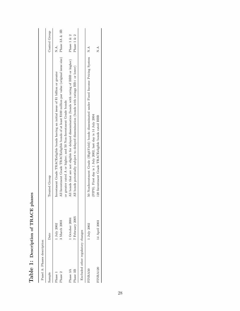
TRACE-eligible securities to be reported within 75 minutes of trading. As described in Table

1, FINRA began disseminating price and volume data for trades in selected investment-grade

bonds with initial issue of $1 billion or greater. We call these bonds Phase 1 bonds. The

dissemination occurred immediately upon reporting for these bonds. Additionally, the 50

high-yield securities previously disseminated under FIPS were transferred to TRACE, whose

trades were disseminated. We denote these bonds the FINRA50. About 520 securities had

their information disseminated by the end of 2002.

After FINRA and SEC approved the expansion of TRACE beyond Phase 1, Phase 2 of

TRACE was implemented on 3 March 2003, and it expanded dissemination to include smaller

investment grade issues. The securities added into dissemination include those with at least

$100 million par value or greater and rating of A- or higher. In addition, dissemination

began on 14 April 2003 for a group of 120 investment-grade securities rated BBB. We denote

these BBB bonds FINRA120. After Phase 2 was implemented, the number of disseminated

bonds increased to approximatively 4,650 bonds. Meanwhile, the FINRA50 subset did not

remain constant over the time period. On July 13, 2003, the FINRA50 list was updated,

and the list was then updated quarterly for the next 5 quarters. We exclude FINRA50 and

FINRA120 bonds from our analysis.

Finally, on 22 April 2004, after TRACE had been in effect for some bonds for almost

two years, FINRA approved the expansion of TRACE to almost all bonds. The last Phase

came in two parts, which FINRA designates as Phase 3A and Phase 3B. The distinction

between Phase 3A and 3B is that Phase 3B bonds are eligible for delayed dissemination.

Dissemination is delayed if a transaction is over $1 million and occurs in a bond that trades

infrequently and is rated BB or below. In addition, dissemination is delayed for trades

immediately following the offering of TRACE-eligible securities rated BBB or below. In

2The National Association of Security Dealers (NASD) changed its name to the FINRA in 2007.3Price and volume information of corporate bonds were publicly available in 1930s and 1940s when

corporate bonds were primarily traded on exchanges.

7

Phase 3A, effective on 1 October 2004, 9,558 new bonds started having their information

about trades disseminated. In Phase 3B, effective on 7 February 2005, an additional 3016

bonds started dissemination, though sometimes with delay. According to FINRA at that

point, there was “real-time dissemination of transaction and price data for 99 percent of

corporate bond trades.”

In an effort parallel to increase the number of bonds with disseminated trade information,

FINRA reduced the time delay for reporting a transaction from 75 minutes on 1 July 2002,

to 45 minutes on 1 October 2003, to 30 minutes on 1 October 2004, and to 15 minutes on 1

July 2005. On 9 January 2006, the time delay for dissemination was eliminated. Since most

bond trades infrequently, our analysis uses one week as the basic unit of time. Therefore,

we do not focus on changes in time to dissemination, but instead on new dissemination.

3.2 Measuring pricing efficiency in bond market

3.2.1 Individual bond, bond market, and bond portfolio returns

In this section, we discuss two different measures for the information efficiency. Our first

measure is return drift after bond analysts’ reports, and the second measure is a price delay

measure.

Both these measures rely on bond returns, which we calculate at the weekly frequency

as follows. For a bond in week t, we take all trades within the week and calculate the clean

price for the week as the transaction size-weighted average of these trades. Returns are then

calculated as

Reti,t = ln

(Pi,t + AIi,t + Ci,tPi,t−1 + AIi,t−1

), (1)

where Pi,t is the transaction size-weighted clean price4, AIi,t is the accrued interest, and Ci,t

is the coupon paid in week t. Coupon rates and maturities are obtained from FISD.

The construction of the return drift and price delay measures needs bond market re-

turn and bond portfolio returns. We define corporate bond market return as the amount-

outstanding weighted average of bond returns for all bonds from TRACE.5 We follow Bessem-

binder, Kahle, Maxwell, and Xu (2009) to create portfolios segmented by both bond rating

and time-to-maturity and calculate amount-outstanding weighted bond portfolio return. We

segment bonds by Moody’s six major rating categories (Aaa, Aa, A, Baa, Ba, below Ba)

and three time-to-maturity categories. For investment grade bonds, the time to-maturity

4Bessembinder, Kahle, Maxwell, and Xu (2009) recommend calculating prices as the transaction size-weighted averages of prices because it minimizes the effects of bid-ask spread in prices. Bao and Pan (2013)and Bao, Pan, and Wang (2011) also use transaction size-weighted averages of prices.

5According to NASD (2005), TRACE covers 99% of corporate bonds.

8

cutoffs are 0 to 5 years, +5 to 10 years, and +10 years. For non-investment grade bonds,

the cutoffs are 0 to 6 years, +6 to 9 years, and +9 years. These cutoffs are designed to

ensure roughly equivalent terciles. Because the Aaa sample size is too small to split into

three subsets based on maturity, we follow Bessembinder, Kahle, Maxwell, and Xu (2009) to

split the Aaa sample into two maturity categories, 0 to 7 years and +7 years. The procedure

above provides a total of seventeen matching portfolios. The portfolio return is amount-

outstanding weighted return of the portfolio. We martch each bond with a portfolio by the

above rating and time-to-maturity categories and follow Bessembinder, Kahle, Maxwell, and

Xu (2009) to abnormal return (AR) as the difference between a bond’s observed return and

the matching portfolio return.

3.2.2 Return drift

Following Gleason and Lee (2003), we consider return drift after bond analyst report as

measures of pricing efficiency. We use bond analyst report as the events for return drift

calculation for following reasons. First, bond investors are almost exclusively institutions.

The average level of investor sophistication is higher than in the equity market. Institutional

investors likely have access to multiple sources of information and better understand how

to utilize the bond analyst’s report. Therefore, the post bond analyst report drift would

be good measure of pricing of information incorporation rather than a measure of noise

trading. Second, unlike quarterly earning announcement and quarterly report, the fixed

income reports are issued throughout the quarter. Because of their frequency and timeliness,

these reports have become a vital source of information for many users of corporate financial

reports. According to Bond Market Association (BMA 2004), fixed income research analysts

play an important role in informing the marketplace about particular issues or securities.

These bond reports are critical in promoting market efficiency in the fixed income price

discovery process. De Franco, Vasvari, and Regina (2009) find that bond analysts issue more

negative reports than equity analysts and provide more information about low credit quality

bonds as a result of the asymmetric demand for negative information by bond investors.

In an alternative specification, we use return drift after rating change to measure the

information efficiency. Rating agencies have preferential access to information that are not

public available. Because rating agencies are alternative information intermediaries with

extensive reputational capital at stake, their disclosures provide potentially relevant infor-

mation that can serve as an independent check on the results of bond analyst reports.

Specifically, we use 8-week window after bond analyst report or rating change to measure

return drift. We choose the 8-week window for two reasons. First, bond market liquidity is

low. Therefore it may take time to incorporate information. Second, too short time window

9

may mainly capture the initial reaction to the events. To better capture information diffusion

instead of over- or under- reaction, we use a long enough window. Since we do not care about

the direction of reaction, we do not classify the news in bond analyst report or rating change

into good news or bad news. We define the Drift variable as 8-week sum of the absolute

abnormal return (∑8

n=1 |ARn|) after the events (bond analyst report or rating change). In

the robustness tests, we alternatively use the sum of the absolute values of weekly abnormal

return as a drift measure, and the results are similar.

3.2.3 Price delay

We adopt Hou and Moskowitz’s (2005 price delay measure as the second pricing efficiency

measure. This measure is an estimate of how quickly prices incorporate public information

in market and/or portfolio return movements. Same as for the drift measure, we calculate

the price delay measure each week. Although calculation at a higher frequency, such as daily,

provide more precision and perhaps more dispersion in delay, they may also introduce more

confounding microstructure influences such as bid-ask bounce and non-synchronous trading.

We consider bond market portfolio return, stock market return6, and bond portfolio

return as the relevant market information to which bonds respond. Using the dissemination

date as the cut-off point, we divide the sample into two parts, 1 year before dissemination

and 1 year after dissemination. We then estimate a regression of each bond’s weekly returns

on contemporaneous and four weeks of lagged returns on the bond market, stock market,

and bond portfolio before and after dissemination.

RetBi,t = αi+βBMi RetBM,t +

4∑n=1

δBM,(−n)i RetBM,t−n+

βSMi RetSM,t +4∑

n=1

δSM,(−n)i RetSM,t−n+

βBPi RetBP,t +4∑

n=1

δBP,(−n)i RetBP,t−n + εi,t (2)

where RetBi,t is the return on bond i, RetBM,t is the return on the value-weighted bond market

return in week t, RetSM,t is value-weighted stock market return in week t, and RetBP,t is the

value-weighted bond portfolio return in week t. If the bond responds immediately to market

news, then βi will be significantly different from zero, but none of the δ(−n)i will differ from

zero. Otherwise, δ(−n)i will differ significantly from zero. This regression identifies the delay

with which a bond responds to market-wide information if expected returns are relatively

6Stock market return is the value-weighted CRSP market index return.

10

constant over weekly horizons. Our delay measure is one minus the ratio of the R2 from

above regression restricting δ(−n)i = 0 for all n, over the R2 from above regression without

restriction.

Delay1 = 1−R2δ(−n)=0, ∀n∈[1,4]

R2. (3)

The higher this number, the more return variation is captured by lagged returns, and hence

the stronger is the delay in response to new information. Because Delay1 does not distin-

guish between shorter and longer lags or the precision of the estimates, we follow Hou and

Moskowitz (2005) to consider two alternative measures of price delay: Delay2 and Delay3.

Delay2 =

∑4n=1

(n∣∣δBM,(−n)

∣∣+ n∣∣δSM,(−n)

∣∣+ n∣∣δBP,(−n)

∣∣)|βBM |+ |βSM |+ |βBP |+

∑4n=1 (|δBM,(−n)|+ |δSM,(−n)|+ |δBP,(−n)|)

(4)

Delay3 = ∑4n=1

(n

∣∣∣∣ δBM,(−n)

se(δBM,(−n))

∣∣∣∣+ n

∣∣∣∣ δSM,(−n)

se(δSM,(−n))

∣∣∣∣+ n

∣∣∣∣ δBP,(−n)

se(δBP,(−n))

∣∣∣∣)∣∣∣ βBM

se(βBM )

∣∣∣+∣∣∣ βSM

se(βSM )

∣∣∣+∣∣∣ βBP

se(βBP )

∣∣∣+∑4

n=1

(∣∣∣∣ δBM,(−n)

se(δBM,(−n))

∣∣∣∣+

∣∣∣∣ δSM,(−n)

se(δSM,(−n))

∣∣∣∣+

∣∣∣∣ δBP,(−n)

se(δBP,(−n))

∣∣∣∣) ,(5)

where se(.) is the standard error of the coefficient estimate. When Delay2 or Delay3 is

higher, the current bond’s return has a stronger relation to the distant past public market

information relative to the current public market information.

3.2.4 R-squared

In addition to price delay measures, we also consider R-squareds from regressions in

Equation 2 with or without the restriction that δ(−n)i = 0. We label the R-squared with the

restriction R-squared1 and the one without the restriction R-squared2. R-squared1 captures

how much variation in bond return can be explained by the contemporaneous bond market

returns, and R-squared2 captures how much the variation in bond return can be explained

by the contemporaneous and past four-week public information. These two R-squareds can

measure how much bond-specific information that the bond prices contain (Morck et al.,

2000; Durnev et al., 2003, 2004; Chun et al., 2008). The higher the two R-squared numbers,

the less bond-specific information in the bond prices.

11

3.3 Difference-in-difference method

We esitmate a difference-in-difference regression to empirically test and quantify the

impact of market transparency on information efficiency in bond market.

yi,t = b0 + b1Treatedi + b2Postt + b3Treatedi × Postt + εi,t, (6)

where yi,t is the measure of information efficiency for bond i in week t, Treatedi is an indicator

for whether the bond changes its dissemination status and Postt is a dummy variable which

equals to one in the period after the dissemination starts and zero otherwise. The coefficient

b3 on interaction term, Treatedi × Postt, captures the difference-in-difference effect. This

parameter measures how the difference in information efficiency between treated bonds and

control bonds changes before and after the public dissemination status of the bond changes.

The detail variable description is in Appendix A.

Since the phase implementation is directly related to the rating and issue size of the

bond, we define the control groups as follows in order to get a better match. We use the

phase 1 bonds as the control group for the phase 2 bonds (phase 3A and 3B bonds as control

group is reported in the robust test). Phase 2 bonds are used as the control group for the

phase 3A and 3B bonds.7 We do not utilize the phase 1 shock because there was no return

data available before TRACE implemented. Therefore, we can not compare the pre- and

post- return drift for phase 1 bonds.

4 Data and Summary Statistics

4.1 Data source

TRACE is available starting from July 1, 2002. Approximately 500 corporate bond

transactions data was made public since then. To obtain information on the characteristics

of each traded bond, including maturity date and bond rating, we use the Fixed Income

Security Database (FISD).

The source of sell-side bond analyst report data is Investext, a provider of full-text analyst

reports. In our sample, the sell-side debt report data covers the period from 2001 to 2006.

The intersection of the bond pricing and debt report data is the period from July 1, 2001

(i.e. 1 year before the implementation of TRACE) to February 7, 2006 (i.e. 1 year after the

dissemination of the Phase 3B bonds), because this period aligns with the implementation

7Although 3A bonds and 3B bonds are more comparable to each other, we do not use phase 3A bondsas the control for phase 3B bonds, because phase 3A and 3B are only 4 months apart and our test windowis 1-year surround the phase start date.

12

of phases of TRACE. We manually collect the bond analysts’ reports and code the name

of the analyst and brokerage firm who issues the report, report date, name of the company

the report is about, and the analysts’ recommendation. We exclude reports about industry,

geographic, investing/economics, and reports that are aggregated either by industry or time,

which often repeat previously published information (e.g. Stickel 1995). More details on the

collection of bond analyst report can be found in Appendix B.

Financial and accounting data is obtained from Compustat. Equity return data is ob-

tained from CRSP.

4.2 Summary statistics of pricing efficiency measures

Table 2 reports the summary statistics of efficiency measures for each phase implementa-

tion. The total sample size differs across measures of information efficiency. The treatment

and control groups of bonds are defined in Panel A of Table 1. There is a trade-off in choos-

ing the time window surrounding dissemination. On the one hand, to focus on immediate

effect of dissemination, we should use the short time window which is really relevant to the

event; on the other hand, to have enough observation for credit report or rating change, we

should use the longer time window. Generally, we use the time period between phase change

as our investigation period. Details could be found in Panel B of Table 1.

Panel A of Table 2 provides summary statistics of bond report drift based on phases

and treatment. The difference in bond report drift provides an independent and intuitive

justification for the market transparency shocks. Three patterns emerge from this panel.

First, the bonds with smaller issue size and lower rating will have larger drift in all phases.

For example, drift is 0.027 for the Phase 2 bonds (treated) whereas it is 0.075 for the phase

3A and phase 3B bonds (control). This is consistent with our intuition that bonds with

large issue size and high rating have better information environment and the market more

quickly incorporates information into their prices. Second, bonds experience a decrease in

drift after the dissemination of trading price. For example, drift is 0.028 for phase 3A treated

bonds before the dissemination and is 0.015 after the dissemination. Third, the difference in

pre- and post-dissemination period is relative large for treated group and small for control

group. The difference for control group is roughly 0 for phase 3A and 3B. This provides some

confirmation of the validity of our research design. The diff-in-diff numbers are capturing the

net effect of dissemination and they are negative in phase 3A and 3B. These results indicate

an beneficial impact of market transparency on pricing efficiency.

One exception is the phase 2 control group, which has significant decrease in drift after

the dissemination and the diff-in-diff number is positive in phase 2. One possible explanation

13

is that there is strong spill-over effect from phase 2 bonds to phase 3A and 3B bonds during

the phase 2 shock. We do not observe similar spill-over effect in phase 3A and 3B, because at

that time the control group bonds are already subject to disclosure of trading information. In

contrast, in phase 2 the control group bonds are not subject to dissemination requirement.

Panel B provides the summary statistics for post-credit rating change drift and we find

similar patterns as that in Panel A.

Panel C reports the summary statistics of price delay. 919 (866), 1959 (1778), and 311

(300) treated bonds have Delay1 available before (after) the phase implementation for Phases

2, 3A, and 3B, respectively. The mean values of treated bonds’ Delay1 decrease for all three

phases. Specifically, the mean of treated bonds’ Delay1 decreases by 0.156 (from 0.658 to

0.501) for Phase 2, by 0.062 (from 0.579 to 0.518) for Phase 3A, and by 0.071 (from 0.616 to

0.545) for Phase 3B. The mean of control bonds’ Delay1 decreases by 0.049 (from 0.608 to

0.560) for Phase 2 and increases by 0.084 (from 0.364 to 0.449) for Phase 3A and increases by

0.077 (from 0.377 to 0.454) for Phase 3B. These numbers show that information inefficiency

measured by Delay1 decreases for all three phases in the treated bonds, but the control

bonds show more mixed results.

After examining the change in price delay for treated and control bond seperately, we

calculate the difference between the treated and control bonds. These differences are -0.108

(-0.156 - (-0.049)) for Phase 2, -0.146 (-0.062 - 0.084) for Phase 3A, and -0.148 (-0.071 -

0.077) for Phase 3B. These numbers show that after phase implementation Delay1 decreases

more for the treated bonds than for the control bonds. Comparing these difference numbers

to the mean price delay measures before phase implementation, we find that these numbers’

economic magnitudes are large. For example, for Phase 2, -0.108 is -16.4% (-0.108/0.658)

relative to the mean Delay1 of treated bonds (0.658) and -21.6% (-0.108/0.501) relative to

the mean Delay1 of control bonds (0.501). These results indicate that the treated bonds’

information efficiency improves relative to that of the control bonds.

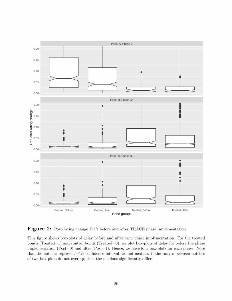
We make boxplots of the efficiency measures in Figures 1, 2, and 3. In these boxplots,

the bottom and top of the box are the first and third quartiles of the distribution, and the

band inside the box is the median. The width of notches on the box represents the 95%

confidence interval around the median. Hence, if notches of two boxes do not overlap with

each other, then the medians significantly differ. The upper whisker extends from the top

of the box to the highest value that is within 1.5 times the interquartile range of the box

top, and the lower whisker is similarly defined. Observations outside of upper and lower

whiskers are plotted as points, and such observations may or may not exist depending on

the distribution.

We distinguish between four groups of bonds: treated bonds before and after phase

14

implementation and control bonds before and after phase implementation. We compare the

boxplots between these four groups of bonds for each phase implementation. Figure 1 shows

the boxplots for drift after bond report. The median drift significantly decreases for the

treated bonds after the phase implementation for all three phase implementation stages.

The median drift for the control bonds decreases for Phase 2 and stays relatively the same

for Phase 3A and 3B. This evidence suggests that the treated bonds’ drift decreases relative

to the control bonds for Phase 3A and 3B but not necessarily decreases for Phase 2.

Note that the treated bonds’ interquartile range is lower than that of control bonds for

Phase 2 and that the opposite is true for Phase 3A and 3B. This is because the treated bonds

of Phase 2 are large, high credit rating bonds (Phase 2 bonds), and the control bonds are

primarily smaller, non-investment grade bonds (Phase 3A and 3B bonds). In comparison,

treated bonds of Phase 3A and 3B is smaller and have lower credit rating than the control

bonds of these two phases. Figure 2 reports the boxplots for drift after credit rating change.

The evidence is similar to that of Figure 1.

Figure 3 shows the boxplots for delay. The median delay significantly decreases for the

treated bonds after the phase implementation for all three phase implementation stages. The

median drift for the control bonds decreases for Phase 2 and increases for Phase 3A and 3B.

These results suggest that the treated bonds’ delay significantly decreases relative to the

control bonds for all three phase implementation stages. In summary, evidence in Figures 1,

2, and 3 suggests that pricing efficiency for the treated bonds relative to control bonds after

phase implementation, which is consistent with evidence in Table 2.

5 Difference-in-difference regression analysis

5.1 Return drift after bond analyst report

Table 3 presents a difference-in-difference regression result for post-bond report drift.

Drift is the absolute value of the sum of weekly abnormal return after announcement week

of bond report. Treated is a dummy variable equal to 1 if the bond is subject to disclosure

requirement. Post is a dummy variable equal to 1 if it is after the phase implementation.

Treated × Post is an interaction term between Treated and Post. Columns 1 to 3 reports

the result for Phase 2, 3A, and 3B, respectively. We cluster the standard errors at firm level

for all regressions. We are interested in the coefficient on Treated × Post, which captures

the impact of the market transparency on return drift.

Three key results emerge from Table 3. First, the interaction term in first column is

insignificant (0.018 with a t-statistic 1.14), which means that there is no effect on return

15

drift after the phase 2. Phase 2 bonds are those bonds with at least $100 million par

value or greater and ratings of A- or higher. These bonds are typically issued by compa-

nies with strong cash flows and good information environment. A potential explanation for

the insignificant result is that these bonds are already very transparent, so the post-trade

transparency increase has little impact on these bonds. Another explanation is the strong

spill-over effect to the control group bonds as suggested in Table 2. The control groups bonds

are not subject to disclosure requirement before and after the phase 2 shocks. However, due

to the distinct feature of bond payoff function, bonds with similar cash flows and credit risk

can be substitutes for bonds covered in the treatment group, and thus can serve as pricing

benchmarks. Therefore, the control bonds will experience an improvement in information

environment as well and lead to insignificant results in the interaction term.8 This explana-

tion is supported by the evidence that the Post is very significant and negative in phase 2

regression but insignificant in phase 3A and 3B regressions.

Second, the return drift is significantly smaller after the trading information disclosure

for phase 3A bonds. It shows that, after the shock, the average return drift after bond

analyst report reduces by 1.2%, comparing to that the average drift is 2.7% for phase 3A

bonds before shock. Therefore, the effect on return drift of Phase 3A is both statistically

significant and economically significant.

Third, the return drift reduction is even stronger for low credit rating bonds. Third

column reports the results for phase 3B bonds. These bonds are the lowest rated bonds

comparing to phase 1, 2, and 3A. The treatment effect is -1.9% and it is significantly larger

than that in second column. The result suggests that those bond with worse information

environment may benefit more from the disclosure of trading information.

To summarize, the evidence above supports the view that the better market transparency

leads to quicker price discovery.

5.2 Return drift after rating changes

Table 4 presents a difference-in-difference regression result for post-bond report drift.

Dependent variable is the absolute value of sum of (+1, +8) week abnormal return after

announcement week of rating change. To be consistent with the test using fixed income

report, we do not distinguish between upgrades and downgrades, since we care about only

the magnitude of the drift. The results in Table 4 confirm our previous finding in Table

3. The price adjustment process has not changed for the phase 2 bonds, but significantly

8The spill-over effect would be minimal in Phase 3A and 3B, because the respective control groups arebonds already subject to dissemination of trading information before the shocks.

16

changed for phase 3A and 3B bonds. These evidence further supports the view that the

better market transparency leads to better information efficiency.

5.3 Price delay

We report difference-in-difference regression results for price delay in Table 5. We use

price delay measures as the dependent variables and cluster standard errors by firm. Panel

A of this table shows results for Delay1. The coefficients on Treated × Post are -0.1076,

-0.1461, and -0.1478, showing that price delay decreases more for the treated bonds than

for the control bonds. These results confirm those in Table 2 and Figure 3 that price delay

reduces after the phase change. These coefficient estimates are economically significant. The

-0.1076 coefficient on Treated × Post of Phase 2 is -16.4% of the mean delay of treated bonds

before phase implementation.9 The decreases of Delay1 for Phase 3A and 3B are 25.2% and

24.0% of the means of treated bonds’ delay for the corresponding phase.

In Panel B and C, we report difference-in-difference regression results for two alternative

measures of price delay: Delay2 and Delay3. When the values of these two measures are

higher, price delay is more severe, and information efficiency is lower. Compared to Delay1,

Delay2 and Delay3 increase in value more if current bond return are more sensitive to

distant lag public information. Panel B shows that the coefficients on Treated × Post are

negative for Phase 2 and Phase 3A and positive for Phase 3B, and only the coefficient for

Phase 3A is statistically significant. Panel C shows that the coefficient on Treated × Post

are negative and statistically significant for all three phases. The results in Panel C support

that dissemination has a negative effect on Delay3, while the results in Panel B are more

mixed than those in Panel C.

To alleviate the concern that the distribution of Delay1 is bounded between 0 and 1 and

that extremely large values of Delay2 and Delay3 may affect the results, we replace raw

Delay1 with the logistic transformation of Delay1 and replace Delay2 and Delay3 with log

of Delay2 and Delay3 and repeat the analysis in Table 5. The results are similar. Overall,

the results in Table 5 demonstrate that pricing efficiency improves after TRACE phase

implementation.

5.4 Return R-squared

As we summarize in Section 2, theories suggest that the improvement of market trans-

parency can decrease the price informativeness (Asriyan et al., 2015; Bhattacharya, 2016;

9Based on Table 2, the mean of Delay1 is 0.658 for the treated Phase 2 bonds before the phase imple-mentation.

17

Banerjee et al., 2016). The previous literature suggests that R-squareds from a regression

of individual bond returns on market stock and bond returns and bond portfolio returns

can be related to how much bond-specific information the bond prices contain. We consider

two R-squared measures (R-squared1 and R-squared2) based on Equation 2. R-squared1

is based on the regression with restriction that δ(−n)i = 0, and R-squared2 is based on the

regression without the restriction. According to previous literature, both these R-squareds

can be negatively related to the amount of bond-specific information in bond prices (Morck

et al., 2000; Durnev et al., 2003, 2004; Chun et al., 2008). In this section, we study how

these two R-squareds change around phase implementation and whether the treated bonds

behave differently than the control bonds.

Table 6 reports difference-in-difference regression estimates for R-squareds for all three

phases. We use raw R-squareds as the dependent variable in the difference-in-difference

regressions, and standard errors are clustered by firm.10 Panel A reports the difference-in-

difference regression results for R-squared1. The coefficients on Treated× Post are 0.0983,

0.1280, and 0.1051 for Phase 2, Phase 3A, and Phase 3B, respectively, and these estimates

are statistically significant. Hence, R-squared1 increases more for treated bonds than for

control bonds for all three phases.

The economic magnitudes of these estimates are large. For instance, the 0.0983 coefficient

on Treated × Post of Phase 2 is 42.8% of the mean of R-squared1 (0.2298) for the treated

Phase 2 bonds before the phase implementation. The coefficients on Treated×Post of Phase

3A and 3B are 59.6% and 45.2% of the corresponding means of R-squared1 for treated bonds

before the phase implementation. Panel B shows similar results for R-squared2 with those

in Panel A.

In summary, results in Table 6 suggests that after phase implementation individual bonds’

prices comove more with market bond prices and are consistent with the interpretation that

less bond specific information is contained in bond prices after phase implementation.

5.5 Difference-in-difference regression estimates by ex-ante bond

characteristics

We study whether the difference-in-difference estimates differ between different groups

of treated bonds grouped by ex-ante bond characteristics. We assign treated bonds into

groups according to illiquidity and trading activity. Specifically, we calculate medians of

bond characteristics across treated bonds before phase implementation and consider treated

bonds above the median and those below the median. We use Amihud as the illiquidity

10The results are robust to using logistic transformation of R-squared as the dependent variable.

18

measure and the ratio of volume divided by issue amount as the trading activity measure.

For the bond report drift and rating change drift, we measure illiquidity and trading activity

using the average of daily illiquidity and trading activity during the week before the bond

report or the rating change. For the delay measure, we measure illiquidity and trading

activity using the average of daily illiquidity and trading activity one year before the phase

implementation. We then estimate a regression as follows.

yi,t =b0 + b1Treatedi + b2Postt + b3HighGroupi + b4Treatedi × Postt+

b3Treatedi × Postt ×HighGroupi + εi,t, (7)

where the dependent variable yi,t is the measure of information efficiency for bond i in

week t, Treatedi is an indicator for whether the bond changes its dissemination status and

Postt is a dummy variable that equals to one in the period after the dissemination starts

and zero otherwise. HighGroupi is a dummy variable that is one for treated bonds with

high characteristics values and zero for treated bonds with low characteristics values. The

coefficient b3 on interaction term Treatedi×Postt captures the difference-in-difference effect

for treated bonds with low characteristics, and the coefficient b4 on the triple interaction

term Treatedi × Postt ×HighGroupi captures the difference in the difference-in-difference

effect between treated bonds with high and low characteristics values.11

Table 7 reports difference-in-difference regression results for bond groups. We highlight

coefficients on Treatedi × Postt and Treatedi × Postt × HighGroupi. In Panel A, the co-

efficients on Treatedi × Postt show that the difference-in-difference effects on drift after

bond reports for treated bonds with low Amihud values are positive for Phase 2 and neg-

ative for Phase 3A and 3B. These results are similar to those in Table 3. The coefficients

on Treatedi × Postt × HighGroupi demonstrate that for Phase 2 bonds the difference-in-

difference effect is higher for treated bonds with high Amihud values than treated bonds

with low Amihud values, while for Phase 3A and 3B the difference-in-difference effects are

lower for the former group of bonds than the latter group. These coefficients, however, are

not statistically significant. Hence, we conclude that the difference-in-difference effects are

similar between treated bonds with high and low Amihud values. The results in Panel A

show that the difference-in-difference effects are similar between treated bonds with high

trading activity and low trading activity.

Panel B shows that the results for drift after rating change are similar to those in Panel

A. We do not find significant difference between liquidity subgroups (trading activity sub-

11We omit second-order interaction term Treatedi×HighGroupi because it is colinear with HighGroupiand omit Postt ×HighGroupi because it is colinear with Treatedi × Postt ×HighGroupi.

19

groups). Instead of overall insignificant result in Table 4, there is some evidence that the

impact of dissemination on phase 2 bonds only show up in liquid bonds.

Panel C demonstrates the results for the Delay measure. The coefficient estimates for

Amihud show that the coefficients on Treatedi × Postt are negative and significant for all

three phases, which is consistent with the results in Table 5. The coefficients on Treatedi ×Postt×HighGroupi are negative for all three phases but are not statistically significant. The

coefficients estimates for trading activity again show that the coefficients on Treatedi×Posttare negative and significant but the coefficients on Treatedi × Postt ×HighGroupi are not

significantly different from zero.

5.6 Spillover to stock market

In this section, we test whether there is spillover effect of increased market transparency

from bond market to stock market. If market transparency changes the pricing efficiency in

bond market, it is possible that the corresponding stocks will be affected by it as well because

investors can observe the price in bond market and adjust their valuation accordingly. To

capture the potential impact of bond market transparency in the stock market, we consider

delay measure and R-squared measure based on stock prices.

Specifically, we regress individual stock return on contemporaneous stock market return

and lagged stock market returns up to four weeks. Similar to the definition in Equation 3,

the stock delay measure is defined as one minue the ratio of R-squared from the regression

without lagged market returns and the R-squared from the regression with lagged market

returns. The R-squared measure is the R-squared from the regression with lagged market

returns.

First and second column report the result for the treated stocks in phase 1. Third and

fourth column report the result for the treated stocks in phase 2. Fifth and sixth column

report the result for the treated stocks in phase 3A. Seventh and eighth column report the

result for the treated stocks in phase 3B. In all specifications, we do not find any significant

impact of bond market transparency on stock market. An potential explanation for this

finding is that the stock market is much more liquid and transparent than bond market,

and hence the impact of the increased post-trade transparency will have little impact on the

stock market.

20

6 Conclusion

Issues related to market transparency are hotly debated by researchers and policy makers.

Although previous literature has shown the potential benefits and drawbacks of increased

market transparency in general, few empirical studies specifically focus on the impact of

market transparency on pricing efficiency. This paper examines the causal effects of post-

trade market transparency on pricing efficiency using the implementation of TRACE and

a difference-in-difference research design. We find that mandated post-trade market trans-

parency in the corporate bond market increases the pricing efficiency of individual bonds.

No sample of bonds in any phases experience an decrease in pricing efficiency and phase 3A

and 3B bonds experience a large and significant increase. This finding is robust across dif-

ferent measures of pricing efficiency. Subgroup analysis indicates that there is little variation

between groups of bonds with different levels of liquidity and trading activity before phase

implementation. Also, the increase in market transparency may lead to higher co-movement

between bond return and market return. The results suggest the important impact of in-

creasing post-trade market transparency on information efficiency and lend some support to

the recent reform in derivative markets.

21

References

Asquith, P., T. R. Covert, and P. A. Pathak (2013). The effects of mandatory transparency

in financial market design: Evidence from the corporate bond market. working paper .

Asriyan, V., W. Fuchs, and B. Green (2015). Information spillovers in asset markets with

correlated values. working paper.

Banerjee, S., J. Davis, and N. Gondhi (2016). When transparency improves, must prices

reflect fundamentals better? working paper.

Bao, J. and J. Pan (2013). Bond illiquidity and excess volatility. Review of Financial

Studies 26 (12), 3068–3103.

Bao, J., J. Pan, and J. Wang (2011). The illiquidity of corporate bonds. Journal of Fi-

nance 66 (3), 911–946.

Bessembinder, H., K. M. Kahle, W. F. Maxwell, and D. Xu (2009). Measuring Abnormal

Bond Performance. Review of Financial Studies 22 (10).

Bessembinder, H., W. Maxwell, and K. Venkataraman (2006). Market transparency, liquidity

externalities, and institutional trading costs in corporate bonds. Journal of Financial

Economics 82, 251–288.

Bhattacharya, A. (2016). Can transparency hurt investors in over-the-counter markets?

working paper.

Biais, B. (1993). Price Formation and Equilibrium Liquidity in Fragmented and Centralized

Markets. Journal of Finance 48 (1), 157–185.

Biais, B. and R. C. Green (2007). The Microstructure of the Bond Market in the 20th

Century. IDEI Working Papers 482 .

Bloomfield, R. and M. O’Hara (1999). Market transparency: Who wins and who loses?

Review of Financial Studies 12 (1), 5–35.

Bloomfield, R. and M. O’Hara (2000). Can Transparent Markets Survive? Journal of

Financial Economics 55 (3), 425–459.

Boehmer, E., G. Saar, and L. Yu (2005). Lifting the Veil: An Analysis of Pre-trade Trans-

parency at the NYSE. Journal of Finance 60 (2), 783815.

22

Chun, H., J. Kim, R. Morck, and B. Yeung (2008). Creative Destruction and Firm-specific

Performance Heterogeneity. Journal of Financial Economics 89 (1), 109–135.

De Franco, G., F. P. Vasvari, and W.-M. Regina (2009). The Informational Role of Bond

Analysts. Journal of Accounting Research 47 (5), 1201–1248.

Dick-Nielsen, J., P. Feldhutter, and D. Lando (2012). Corporate bond liquidity before and

after the onset of the subprime crisis. Journal of Financial Economics 103, 471–492.

Durnev, A., R. Morck, and B. Yeung (2004). Value-enhancing Capital Budgeting and Firm-

specific Stock Return Variation. Journal of Finance 59 (1), 65–105.

Durnev, A., R. Morck, B. Yeung, and P. Zarowin (2003). Does Greater Firm-specific Re-

turn Variation Mean More or Less Informed Stock Pricing? Journal of Accounting Re-

search 41 (5), 797–836.

Edwards, A. K., L. E. Harris, and M. S. Piwowar (2007). Corporate bond market transaction

costs and transparency. Journal of Finance 62, 1421–1451.

Fama, E. F. (1970). Efficient Capital Markets: A Review of Theory and Empirical Work.

Journal of Finance 25 (2), 383–417.

Franks, J. and S. Schaefer (1995). Equity Market Transparency on the London Stock Ex-

change. Journal of Applied Corporate Finance 8 (1), 70–78.

Gemmill, G. (1996). Transparency and Liquidity: A Study of Block Trades on the London

Stock Exchange under Different Publication Rules. Journal of Finance 51 (5), 1765–1790.

Gleason, C. A. and C. M. C. Lee (2003). Analyst forecast revisions and market price dis-

covery. Accounting Review 78, 193–225.

Goldstein, I. and L. Yang (2016). Good disclosure, bad disclosure. working paper.

Goldstein, M. A., E. S. Hotchkiss, and E. R. Sirri (2007). Transparency and liquidity: A

controlled experiment on corporate bonds. Review of Financial Studies 20, 235–273.

Han, B., Y. Tang, and L. Yang (2016). Public information and uninformed trading: Im-

plications for market liquidity and price efficiency. Journal of Economic Theory 163 (5),

604–643.

Hou, K. and T. J. Moskowitz (2005). Market frictions, price delay, and the cross-section of

expected returns. Review of Financial Studies 18 (3), 981.

23

Madhavan, A. (1995). Consolidation, fragmentation, and the disclosure of trading informa-

tion. Review of Financial Studies 8 (3), 579–603.

Madhavan, A. (1996). Security prices and market transparency. Journal of Financial Inter-

mediation 5 (3), 255–283.

Madhavan, A., D. Porter, and D. Weaver (2005). Should securities markets be transparent?

Journal of Financial Markets 8 (3), 265–287.

Morck, R., B. Yeung, and W. Yu (2000). The Information Content of Stock Markets: Why

Do Emerging Markets Have Synchronous Stock Price Movements? Journal of Financial

Economics 58 (1-2), 215–260.

Naik, N. Y., A. Neuberger, and S. Viswanathan (1999). Trade Disclosure Regulation in

Markets with Negotiated Trades. Review of Financial Studies 12 (4), 873–900.

NASD (2005). NASD’s Fully Implemented ”TRACE” Brings Unprece-

dented Transparency to Corporate Bond Market. February 7. Available

at http://www.finra.org/newsroom/2005/nasds-fully-implemented-trace-brings-

unprecedented-transparency-corporate-bond-market, Last accessed: 28 August 2016.

Pagano, M. and A. Roell (1996). Transparency and liquidity: A comparison between auction

and dealer markets with informed trading. Journal of Finance 51 (2), 579–611.

Piwowar, M. S. (2011). Corporate and Municipal Bond Market Microstructure in the US. In

R. A. Meyers (Ed.), Complex Systems in Finance and Econometrics, pp. 93–115. Springer.

SEC (1994). Market 2000: An Examination of Current Market Developments. Available at

https://www.sec.gov/divisions/marketreg/market2000.pdf.

24

●

●

●

●●●

●

●●

●●

●

●

●

●●

●

●

●

●●

●

●●

●

●

●

●

●

●

●

●●

●

●

●

●●

●

●●

●

●

●

●

●

●

●

●

●

●

●

●●

●

●

●

●●

●

●

●

●

●

●

●

●

●●

●●

●

●

●●

●

●

●

●

●

●

●

●

●

●●

●●

●

●

●

●

●

●

●●●

●

●

●

●●

●

●

●

●

●●

●

●

●

●●

●

●

●

●

●

●●

●

●

●

●●●

●

●

●●

●

●

●

●

●

●

●

●

●

●

●

●

●

●

●

●

●

●

●

●

●

●

●

●

●

●

●●

●

●

●

●

●

●

●

●●

●●

Panel A: Phase 2

Panel B: Phase 3A

Panel C: Phase 3B

0.00

0.04

0.08

0.12

0.00

0.04

0.08

0.12

0.00

0.04

0.08

0.12

Control, Before Control, After Treated, Before Treated, AfterBond groups

Drif

t afte

r bo

nd r

epor

t

n

Figure 1: Post-bond report Drift before and after TRACE phase implementation

This figure shows box-plots of delay before and after each phase implementation. For the treatedbonds (Treated=1) and control bonds (Treated=0), we plot box-plots of delay for before the phaseimplementation (Post=0) and after (Post=1). Hence, we have four box-plots for each phase. Notethat the notches represent 95% confidence interval around median. If the ranges between notchesof two box-plots do not overlap, then the medians significantly differ.

25

●

●●

●●●●

●●

●

●●●

●●●

●●

●●

●

●●

●

●

●

●●●

●

●●

●

●

●

●

●●●

●

●●

●●

●●

●

●

●

●

●

●

●

●

●

●

●●

●

●●

●

●●

●

●

●

●

●

●●

●

●

●

●

●●●●

●

●

●●●

●

●

●

●

●

●

●●●●

●

●

●●●

●

●

●

●●

●

●

●●

●

●

●

●●●●

●●

●

●●●

●●●

●●

●

●

●

●

●

●

●

●●●

●

●

●

●●

●

●

●

●

●

●

●

●

●●●

●

●

●

●

●

●

●

●

●

●

●

●

●

●

●

●

●

●

●

●

●

●

●

●

●

●●

Panel A: Phase 2

Panel B: Phase 3A

Panel C: Phase 3B

0.00

0.05

0.10

0.15

0.20

0.00

0.05

0.10

0.15

0.20

0.00

0.05

0.10

0.15

0.20

Control, Before Control, After Treated, Before Treated, AfterBond groups

Drif

t afte

r ra

ting

chan

ge

Figure 2: Post-rating change Drift before and after TRACE phase implementation

This figure shows box-plots of delay before and after each phase implementation. For the treatedbonds (Treated=1) and control bonds (Treated=0), we plot box-plots of delay for before the phaseimplementation (Post=0) and after (Post=1). Hence, we have four box-plots for each phase. Notethat the notches represent 95% confidence interval around median. If the ranges between notchesof two box-plots do not overlap, then the medians significantly differ.

26

Panel A: Phase 2

Panel B: Phase 3A

Panel C: Phase 3B

0.00

0.25

0.50

0.75

1.00

0.00

0.25

0.50

0.75

1.00

0.00

0.25

0.50

0.75

1.00

Control, Before Control, After Treated, Before Treated, AfterBond groups

Del

ay

Figure 3: Delay before and after TRACE phase implementation

This figure shows box-plots of delay before and after each phase implementation. For the treatedbonds (Treated=1) and control bonds (Treated=0), we plot box-plots of delay for before the phaseimplementation (Post=0) and after (Post=1). Hence, we have four box-plots for each phase. Notethat the notches represent 95% confidence interval around median. If the ranges between notchesof two box-plots do not overlap, then the medians significantly differ.

27

Tab

le1:

Desc

rip

tion

of

TR

AC

Ep

hase

s

Pan

elA

:P

hase

sd

escr

ipti

on

Sam

ple

Date

Tre

ate

dG

rou

pC

ontr

ol

Gro

up

Ph

ase

11

Ju

ly2002

Inves

tmen

tG

rad

eT

RA

CE

elig

ible

bon

ds

havin

gan

init

ial

issu

eof

$1

billion

or

gre

ate

rN

.A.

Ph

ase

23

Marc

h2003

All

Inves

tmen

tG

rad

eT

RA

CE

elig

ible

bon

ds

of

at

least

$100

million

par

valu

e(o

rigin

al

issu

esi

ze)

or

gre

ate

rra

ted

Aor

hig

her

;an

d50

Non

-Inves

tmen

tG

rad

eb

on

ds

Ph

ase

3A

&3B

Ph

ase

3A

1O

ctob

er2004

All

bon

ds

that

are

not

elig

ible

for

del

ayed

dis

sem

inati

on

(bon

ds

wit

hra

tin

gof

BB

Bor

hig

her

)P

hase

1&

2

Ph

ase

3B

7F

ebru

ary

2005

All

bon

ds

pote

nti

ally

sub

ject

tod

elayed

dis

sem

inati

on

(bon

ds

wit

hra

tin

gs

BB

+or

low

er)

Ph

ase

1&

2

Excl

ud

edoth

erre

gu

lato

rych

an

ges

FIN

RA

50

1Ju

ly2002

50

Non

Inves

tmen

tG

rad

e(H

igh

Yie

ld)

bon

ds

dis

sem

inate

du

nd

erF

ixed

Inco

me

Pri

cin

gS

yst

em

(FIP

S).

Fir

std

ay

is1

Ju

ly2002,

last

day

is14

Ju

ly2004

N.A

FIN

RA

120

14

Ap

ril

2003

120

Inves

tmen

tG

rad

eT

RA

CE

elig

ible

bon

ds

rate

dB

BB

N.A

28

Table 2: Summary statistics

Panel A: Drift after credit report

Treated Control

Num. obs. Mean Num. obs. Mean Diff. in Diff

Phase 2 Before 36 0.027 160 0.075

Phase 2 After 35 0.012 271 0.043

Difference -0.015 -0.032 0.017

Phase 3A Before 210 0.028 107 0.010

Phase 3A After 315 0.015 166 0.010

Difference -0.013 -0.000 -0.013

Phase 3B Before 173 0.036 135 0.011

Phase 3B After 107 0.016 138 0.010

Difference -0.020 -0.001 -0.019

Panel B: Drift after credit rating change

Treated Control

Num. obs. Mean Num. obs. Mean Diff. in Diff

Phase 2 Before 32 0.020 399 0.110

Phase 2 After 66 0.019 296 0.086

Difference -0.001 -0.024 0.023

Phase 3A Before 227 0.074 123 0.016

Phase 3A After 1110 0.046 119 0.022

Difference -0.028 0.006 -0.034

Phase 3B Before 227 0.075 145 0.016

Phase 3B After 155 0.048 97 0.024

Difference -0.027 -0.005 -0.022

Panel C: Key statistics of Delay

Treated Control

Num. obs. Mean Num. obs. Mean Diff. in Diff

Phase 2 Before 919 0.658 1441 0.608

Phase 2 After 866 0.501 1769 0.560

Difference -0.156 -0.049 -0.108

Phase 3A Before 1959 0.579 1178 0.364

Phase 3A After 1778 0.518 923 0.449

Difference -0.062 0.084 -0.146

Phase 3B Before 311 0.616 1118 0.377

Phase 3B After 300 0.545 863 0.454

Difference -0.071 0.077 -0.148

29

Table 3: Drift after bond credit report

Phase 2 Phase 3A Phase 3B

Dependent variable: Drift Drift Drift

Post -0.033 -0.00025 -0.0012

(-4.77) (-0.16) (-0.80)

Treated -0.048 0.017 0.026

(-5.00) (5.55) (5.87)

Treated × Post 0.018 -0.012 -0.019

(1.77) (-4.06) (-4.14)

Constant 0.075 0.010 0.011

(11.3) (7.60) (8.55)

Num. obs. 502 798 553

Adj. R-squared 0.089 0.070 0.118

This table reports the difference-in-difference estimates for the post bond report drift. Drift

is the absolute value of sum of (+1, +8) week abnormal return after announcement week of

bond report. Post is a dummy variable equal to 1 if it is after the phase implementation.

Treated is a dummy variable equal to 1 if the bond is subject to disclosure requirement.Treated

x Post is the interaction term between Post and Treated. The details on phases change can be

found in Table 1. The numbers in parentheses are t-statistics. Standard errors are clustered

at firm level.

30

Table 4: Drift after rating change

Phase 2 Phase 3A Phase 3B

Dependent variable: Drift Drift Drift

Post -0.022 0.0062 0.0076

(-1.81) (1.31) (1.43)

Treated -0.091 0.058 0.059

(-9.13) (5.67) (6.66)

Treated × Post 0.022 -0.035 -0.035

(1.63) (-2.98) (-2.15)

Constant 0.11 0.016 0.016

(12.5) (8.08) (8.94)

Num. obs. 783 1579 624

Adj. R-squared 0.067 0.053 0.088

This table reports the difference-in-difference estimates for the post rating change (Moody’s)

drift. Drift is the absolute value of sum of (+1, +8) week abnormal return after announce-

ment week of bond report. Post is a dummy variable equal to 1 if it is after the phase

implementation. Treated is a dummy variable equal to 1 if the bond is subject to disclosure

requirement.Treated x Post is the interaction term between Post and Treated. The details

on phases change can be found in Table 1. The numbers in parentheses are t-statistics.

Standard errors are clustered at firm level.

31

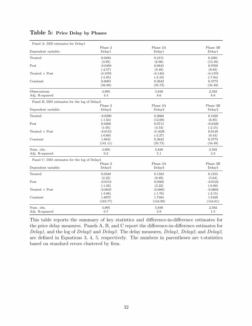
Table 5: Price Delay by Phases

Panel A: DID estimates for Delay1Phase 2 Phase 3A Phase 3B

Dependent variable: Delay1 Delay1 Delay1

Treated 0.0494 0.2151 0.2391(3.92) (6.96) (13.49)

Post -0.0488 0.0845 0.0769(-2.57) (9.48) (8.63)

Treated × Post -0.1076 -0.1461 -0.1478(-5.05) (-3.10) (-7.94)

Constant 0.6083 0.3642 0.3773(56.88) (35.73) (34.49)

Observations 4,995 5,838 2,592Adj. R-squared 4.4 8.6 8.8

Panel B: DID estimates for the log of Delay2Phase 2 Phase 3A Phase 3B

Dependent variable: Delay2 Delay2 Delay2

Treated -0.0290 0.2660 0.1829(-1.64) (12.00) (6.85)

Post 0.0200 0.0714 -0.0420(1.05) (4.53) (-2.15)

Treated × Post -0.0153 -0.1628 0.0149(-0.60) (-3.27) (0.43)

Constant 1.8831 0.3642 0.3773(141.11) (35.73) (34.49)

Num. obs. 4,995 5,838 2,592Adj. R-squared 0.2 5.1 3.3

Panel C: DID estimates for the log of Delay3Phase 2 Phase 3A Phase 3B

Dependent variable: Delay3 Delay3 Delay3

Treated 0.0349 0.1583 0.1255(2.22) (6.89) (5.64)

Post -0.0154 0.0302 -0.0122(-1.02) (2.22) (-0.80)

Treated × Post -0.0845 -0.0865 -0.0604(-3.96) (-1.76) (-2.15)

Constant 1.8975 1.7484 1.8168(163.77) (144.99) (144.61)

Num. obs. 4,995 5,838 2,592Adj. R-squared 0.7 2.9 1.5

This table reports the summary of key statistics and difference-in-difference estimates forthe price delay measures. Panels A, B, and C report the difference-in-difference estimates forDelay1, and the log of Delay2 and Delay3. The delay measures, Delay1, Delay2, and Delay3,are defined in Equations 3, 4, 5, respectively. The numbers in parentheses are t-statisticsbased on standard errors clustered by firm.

32

Table 6: Difference-in-difference estimates: R-squareds

Panel A: DID estimates for R-squared1Phase 2 Phase 3A Phase 3B

Treated -0.0540 -0.1799 -0.1515(-5.45) (-7.44) (-10.11)

Post 0.0341 -0.0827 -0.0691(2.07) (-12.18) (-9.43)

Treated × Post 0.0983 0.1280 0.1051(5.40) (3.44) (7.47)

Constant 0.2838 0.4213 0.4015(34.73) (41.45) (38.74)

Num. obs. 5,167 5,972 2,668Adj. R-squared 4.3 8.9 5.5

Panel B: DID estimates for R-squared2Phase 2 Phase 3A Phase 3B

Treated -0.0552 -0.0827 0.0158(-6.44) (-6.93) (1.18)

Post -0.0146 -0.0516 -0.0391(-1.30) (-8.22) (-5.53)

Treated × Post 0.0638 0.0751 0.0216(5.55) (3.25) (1.34)

Constant 0.7086 0.6268 0.6089(89.78) (85.53) (83.25)

Num. obs. 4,995 5,838 2,592Adj. R-squared 1.9 2.3 1.1

This table reports the summary of key statistics and difference-in-difference estimates forR-squared1 and R-squared2. Panel A and B report the difference-in-difference estimates forthe logistic transformation of R-squared1 and R-squared1. R-squared1 is based on Equation2 without the restriction that δ

(−n)i = 0 and R-squared2 is based on the Equation 2 with the

restriction. The numbers in parentheses in Panels C and D are t-statistics based on standarderrors clustered by firm.

33

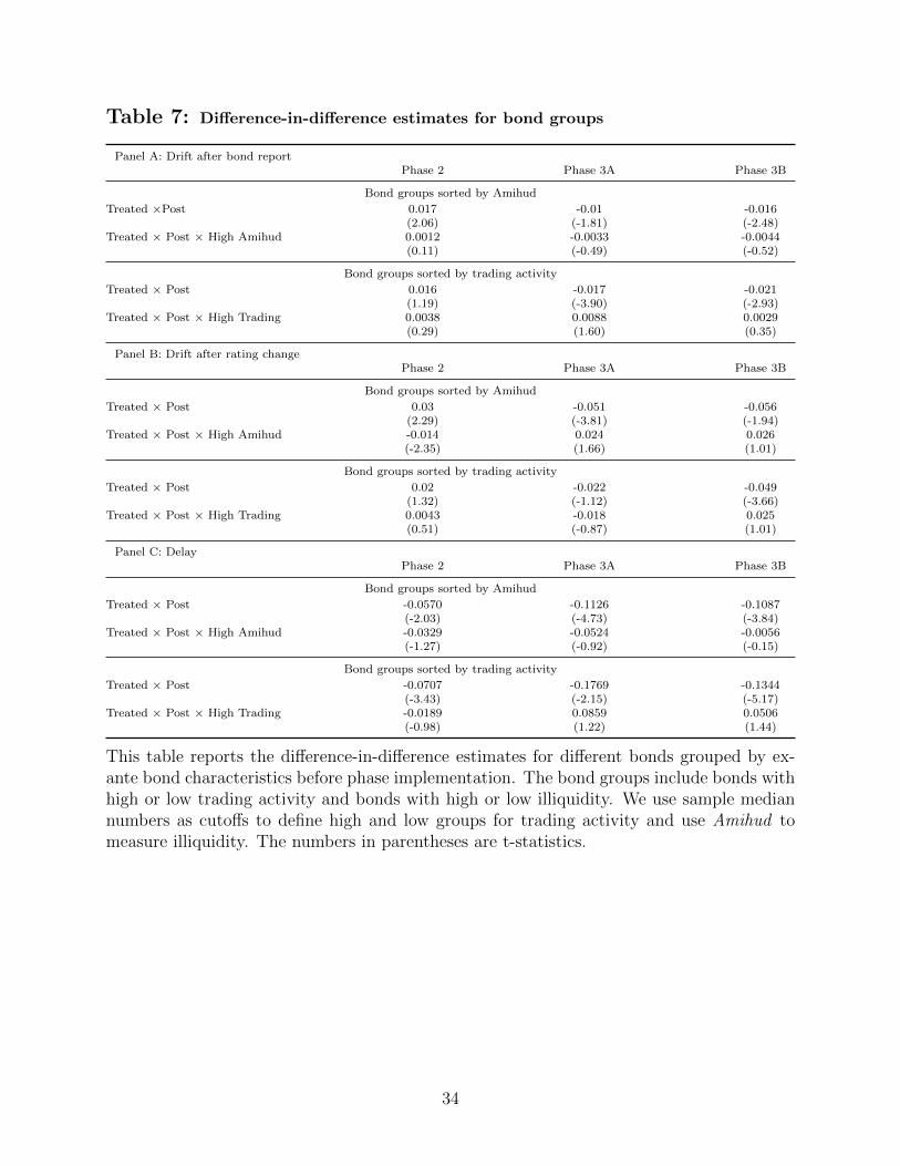
Table 7: Difference-in-difference estimates for bond groups

Panel A: Drift after bond reportPhase 2 Phase 3A Phase 3B

Bond groups sorted by Amihud

Treated ×Post 0.017 -0.01 -0.016(2.06) (-1.81) (-2.48)

Treated × Post × High Amihud 0.0012 -0.0033 -0.0044(0.11) (-0.49) (-0.52)

Bond groups sorted by trading activity

Treated × Post 0.016 -0.017 -0.021(1.19) (-3.90) (-2.93)

Treated × Post × High Trading 0.0038 0.0088 0.0029(0.29) (1.60) (0.35)

Panel B: Drift after rating changePhase 2 Phase 3A Phase 3B

Bond groups sorted by Amihud

Treated × Post 0.03 -0.051 -0.056(2.29) (-3.81) (-1.94)

Treated × Post × High Amihud -0.014 0.024 0.026(-2.35) (1.66) (1.01)

Bond groups sorted by trading activity

Treated × Post 0.02 -0.022 -0.049(1.32) (-1.12) (-3.66)

Treated × Post × High Trading 0.0043 -0.018 0.025(0.51) (-0.87) (1.01)

Panel C: DelayPhase 2 Phase 3A Phase 3B

Bond groups sorted by Amihud

Treated × Post -0.0570 -0.1126 -0.1087(-2.03) (-4.73) (-3.84)

Treated × Post × High Amihud -0.0329 -0.0524 -0.0056(-1.27) (-0.92) (-0.15)

Bond groups sorted by trading activity

Treated × Post -0.0707 -0.1769 -0.1344(-3.43) (-2.15) (-5.17)

Treated × Post × High Trading -0.0189 0.0859 0.0506(-0.98) (1.22) (1.44)

This table reports the difference-in-difference estimates for different bonds grouped by ex-ante bond characteristics before phase implementation. The bond groups include bonds withhigh or low trading activity and bonds with high or low illiquidity. We use sample mediannumbers as cutoffs to define high and low groups for trading activity and use Amihud tomeasure illiquidity. The numbers in parentheses are t-statistics.

34

Table 8: Test of spill-over effect to stock market

Phase 1 Phase 2 Phase 3A Phase 3B

Delay1 R-squared Delay1 R-squared Delay1 R-squared Delay1 R-squared

Treated -0.21 -1.50 -0.21 -1.32 0.086 0.71 0.19 1.29(-5.76) (-6.43) (-9.07) (-8.85) (4.81) (5.51) (8.56) (9.32)

Post -0.046 -0.28 -0.13 0.15 0.014 -0.37 0.090 0.081(-3.49) (-3.29) (-10.2) (1.86) (0.68) (-2.45) (3.74) (0.54)

Treated × Post -0.010 -0.25 0.080 0.31 0.020 0.13 -0.018 -0.17(-0.20) (-0.77) (2.50) (1.49) (0.77) (0.72) (-0.59) (-0.86)

Constant 0.40 0.71 0.37 0.51 0.15 -0.24 0.17 -0.67(43.4) (12.1) (42.0) (8.90) (9.96) (-2.22) (10.2) (-6.33)

Num. obs. 1869 1861 1804 1800 1196 1193 860 856Adj. R-squared 0.041 0.055 0.104 0.066 0.048 0.063 0.153 0.148

This table reports the difference-in-difference estimates for the spill-over effect to stockmarket. The sample is the companies whose bonds are subject to disclosure requirementin different phases. Delay1 is the delay measure based on stock prices. R-squared is theR-squared from a regression of individual stock returns on contemporaneous and lag stockmarket returns and industry returns. Post is a dummy variable equal to 1 if it is after thephase implementation. Treated is a dummy variable equal to 1 if the bond of the companyis subject to disclosure requirement. Treated×Post is the interaction term between Treatedand Post. The details of phases change can be found in Table 1. The details of delay mea-sure and R-squared measure can be found in Appendix. The numbers in parentheses aret-statistics.

35

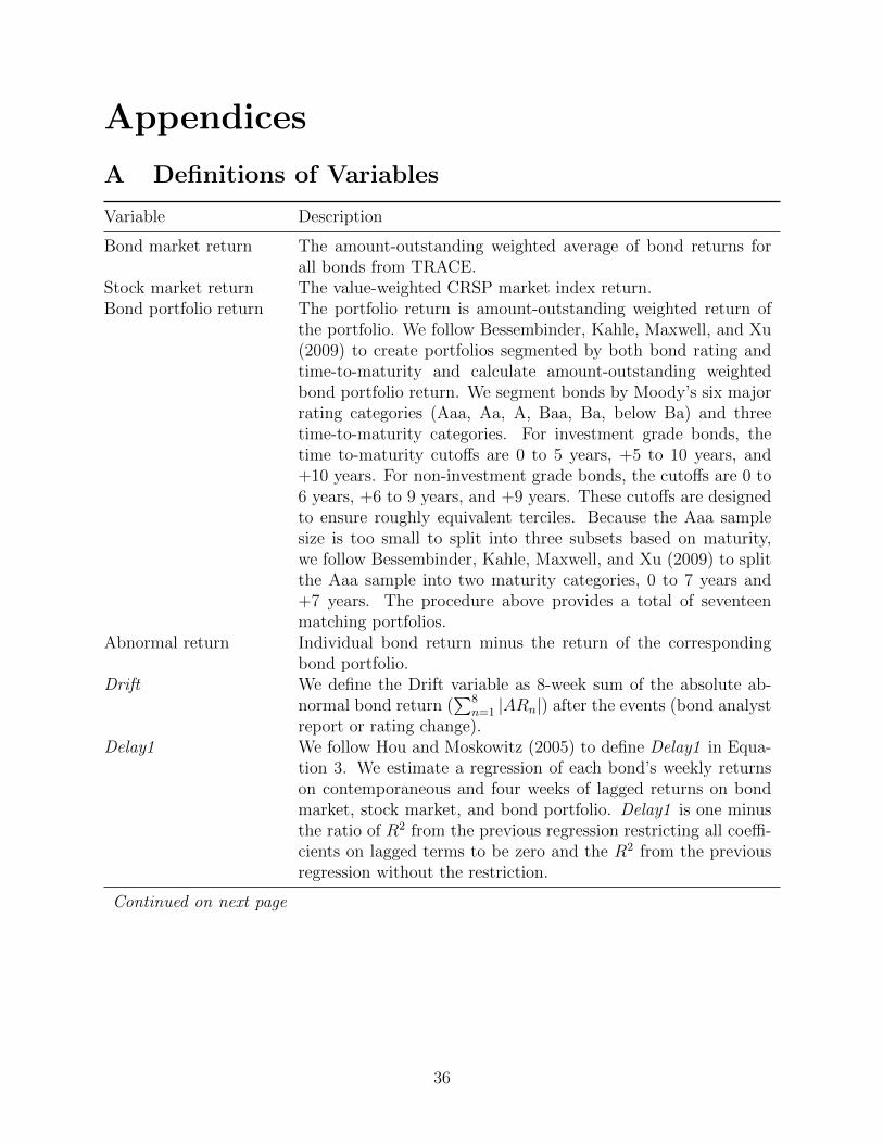
Appendices

A Definitions of Variables

Variable Description

Bond market return The amount-outstanding weighted average of bond returns forall bonds from TRACE.

Stock market return The value-weighted CRSP market index return.Bond portfolio return The portfolio return is amount-outstanding weighted return of

the portfolio. We follow Bessembinder, Kahle, Maxwell, and Xu(2009) to create portfolios segmented by both bond rating andtime-to-maturity and calculate amount-outstanding weightedbond portfolio return. We segment bonds by Moody’s six majorrating categories (Aaa, Aa, A, Baa, Ba, below Ba) and threetime-to-maturity categories. For investment grade bonds, thetime to-maturity cutoffs are 0 to 5 years, +5 to 10 years, and+10 years. For non-investment grade bonds, the cutoffs are 0 to6 years, +6 to 9 years, and +9 years. These cutoffs are designedto ensure roughly equivalent terciles. Because the Aaa samplesize is too small to split into three subsets based on maturity,we follow Bessembinder, Kahle, Maxwell, and Xu (2009) to splitthe Aaa sample into two maturity categories, 0 to 7 years and+7 years. The procedure above provides a total of seventeenmatching portfolios.

Abnormal return Individual bond return minus the return of the correspondingbond portfolio.

Drift We define the Drift variable as 8-week sum of the absolute ab-normal bond return (

∑8n=1 |ARn|) after the events (bond analyst

report or rating change).Delay1 We follow Hou and Moskowitz (2005) to define Delay1 in Equa-

tion 3. We estimate a regression of each bond’s weekly returnson contemporaneous and four weeks of lagged returns on bondmarket, stock market, and bond portfolio. Delay1 is one minusthe ratio of R2 from the previous regression restricting all coeffi-cients on lagged terms to be zero and the R2 from the previousregression without the restriction.

Continued on next page

36

Variable Description

Delay2 We follow Hou and Moskowitz (2005) to define Delay1 in Equa-tion 4. We estimate a regression of each bond’s weekly returnson contemporaneous and four weeks of lagged returns on bondmarket, stock market, and bond portfolio. Delay2 is the ratioof the sum of scaled absolute coefficients from the previous re-gression restricting all coefficients on lagged terms to be zero andsum of absolute coefficients from the previous regression withoutthe restriction.

Delay3 We follow Hou and Moskowitz (2005) to define Delay1 in Equa-tion 5. We estimate a regression of each bond’s weekly returnson contemporaneous and four weeks of lagged returns on bondmarket, stock market, and bond portfolio. Delay3 is the ratioof the sum of scaled absolute t-stat from the previous regressionrestricting all coefficients on lagged terms to be zero and thesum of absolute t-stat from the previous regression without therestriction.

Bond return We define bond return according to Equation 1RetBM Bond market return is the amount-outstanding weighted average

of all bond returns from TRACE.RetSM Stock market return is the value-weighted stock index return

from CRSP.RetBP Bond portfolio return is the amount-outstanding weighted aver-

age of all bond returns in a portfolio. We follow Bessembinder,Kahle, Maxwell, and Xu (2009) to create portfolios segmentedby both bond rating and time-to-maturity. We segment bondsby Moody’s six major rating categories (Aaa, Aa, A, Baa, Ba,below Ba) and three time-to-maturity categories. For investmentgrade bonds, the time to-maturity cutoffs are 0 to 5 years, +5 to10 years, and +10 years. For non-investment grade bonds, thecutoffs are 0 to 6 years, +6 to 9 years, and +9 years. We splitthe Aaa sample into two maturity categories, 0 to 7 years and+7 years. These cutoffs are designed to ensure roughly equiva-lent terciles. The procedure above provides a total of seventeenmatching portfolios.

Continued on next page

37

Variable Description

Amihud The price impact of a trade per unit traded. We first calculate thedaily price impact using transactions within each day and thenuse the mean of daily values over a certain period of time. It issimilarly defined and calculated as in Dick-Nielsen, Feldhutter,and Lando (2012)

Trading activity Volume divided by issue amount. We first calculate the dailytrading activity using transactions within each day and then usethe mean of trading activity over a certain period of time.

38

B Bond Analyst Report

We code a company list from the Compustat-CRSP database, then search and downloadall their fixed income reports and its summary containing information of title, page, and dateaccording to their company name from the Thomson One Investext database manually. Afew company names cannot be found in the database and we recognize it by adding a variableof report id1=0. These company probably have not had any records in the database. Inaddition, many firms may not have any fixed income reports although they can be matchedwith the database, which we identify by report id1=1. We then identify those firms whichhave fixed income reports by report id1=2. We have a few problems when searching thecompany name in the database since the company name in the Compustat-CRSP list cannotbe exactly same with the name recorded by Thomson one database:

The first problem is that when we type in a specific company name, there may be morethan one result coming out from the database. In this case, we download all of these resultsand identified them by report id1=M, report id2=N, report id3=P,report id4=N. Becausethe number of these firms is very small, we first delete these firms and then check therobustness by adding them again.

The second problem is that we can have two firm names that are nearly the same butslightly differ (probably because a firm changes its name, and the database identifies it byadding phases like old into the old name). In this case, we download both names and thenseparate them by the date of report, or manually clean the records by searching on theinternet.

The third problem is that some company name in our list may not be exactly same asthose in Thomsonone Database, Many firms in both list may use some abbreviations astheir name like “INC”, “CORP”, “LTD” which may mean “incorporated”, “corporation”,“limited”, accordingly. In this case, we match these abbreviations as much as possible.Sometimes we confirm this matching by looking at those reports title listed in the searchingscreening after we submit the searching command.

Finally, according to the firm list which contains 17,882 firms (gvkeys), we find 50,175fixed income reports. All these reports can be recognized by unique gvkey report id, report idis a unique id for each report given by Thomsonone Database. However, there might be manyduplicate reports among these 50,175 reports for some reason.

39