Market Power and Price Movements over the Business Cycle*

by

Bart J. Wilson Stanley S. Reynolds Interdisciplinary Center for Economic Science Department of Economics

George Mason University University of Arizona 4400 University Boulevard, MSN 1B2 P.O. Box 210108, McClelland Hall 401

Fairfax, VA 22030 Tucson, AZ 85721 bwilson3@gmu.edu reynolds@eller.arizona.edu

August 2003

JEL Classification: L1, E3 Abstract: This paper develops and tests implications of an oligopoly-pricing model. The model predicts that during a demand expansion the short run competitive price is a pure strategy Nash equilibrium, but in a recession firms set prices above the competitive price. Thus, price markups over the competitive price are countercyclical. Prices set during a recession are more variable than prices set in expansions, because firms employ mixed strategy pricing in recessions. The empirical analysis utilizes Hamilton’s time series switching regime filter to test the predictions of the model. Fourteen out of fifteen industries have fluctuations consistent with this oligopoly-pricing model. *Wilson acknowledges research support from the John M. Olin Foundation and the National Science Foundation. We thank the Editor and an anonymous referee for comments that have improved the paper. Doc Ghose, James Hamilton, Joe Harrington, Mark Walker, and John Wooders also provided helpful suggestions, as have seminar participants at the University of Arizona, the University of Houston, Johns Hopkins University, the University of Kansas, the University of Toronto, and Virginia Polytechnic Institute and State University.

1

I. Introduction

In this paper we examine price variation in manufacturing industries over the business

cycle. This study is motivated by the hypothesis that firms with market power may have

incentives to exercise this power differentially over the business cycle. Such differential exercise

of market power could exacerbate business cycle fluctuations relative to what would occur in the

absence of market power.

Our point of departure is a model of oligopoly investment and pricing that has

implications for variations in prices and industry efficiency over the business cycle. This model

emphasizes the role of long run production capacity investments that must be made before

demand conditions are known. After capacity investments are made, firms learn about the level

of product demand and choose prices. The pricing incentives for firms differ depending on the

level of demand. If demand is high, then the short run competitive (market clearing) price is a

pure strategy Nash equilibrium. However, if demand is low, then capacity constrained firms

have an incentive to deviate from the short run competitive price; the typical result is that firms

adopt mixed strategies that yield prices above the short run competitive price and that generate

excess production capacity. These results are developed in detail in Reynolds and Wilson (2000).

We refer to this as a non-collusive oligopoly model to distinguish it from collusive theories of

oligopoly behavior over the business cycle.

This non-collusive model predicts that output prices are procyclical, as do many other

theories. The key prediction that we empirically examine is that output price changes will have

greater variance during low demand periods than during high demand periods.1 We search for

this differential variance of price changes over the business cycle using a version of time series

switching regime filter developed by Hamilton (1989). We estimate this model for each of

seventeen manufacturing industries at the two- and three-digit Standard Industrial Classification

(SIC) level.

This prediction on business cycle price variation is not unique to this non-collusive

model. Staiger and Wolak (1992) formulate a model with demand uncertainty in which firms

invest in production capacity and set output prices, as we do. They examine optimal collusion in

infinitely repeated games. Staiger and Wolak point out that price-cutting and market-share

instability can emerge during demand downturns in their optimal collusion model when the

industry is relatively ineffective in maintaining collusion. If we find differential variance of price

changes over the business cycle in the data then this could be accounted for by an optimal

2

collusion model such as Staiger and Wolak (1992) or by a non-collusive model similar to ours.

In either case, a model that provides this variance prediction has the following features: there is

demand uncertainty, firms have market power, firms have production capacity constraints, and

firms set prices. We might add that if non-collusive models of market power are capable of

explaining key empirical regularities, then analysts may not need to turn to relatively more

complicated optimal collusion models of behavior over the business cycle.

The paper is organized as follows. Section II provides background on the exercise of

market power over the business cycle. In Section III we formulate and analyze a dynamic model

in which demand alternates stochastically between expansionary and contractionary phases. We

show that ex ante capacity investments coupled with ex post price setting lead to price variation

over the business cycle. This formulation provides the structure for our empirical tests. In

Section IV we explain the estimation approach, the time series data, and the empirical results.

Concluding remarks appear in Section V.

II. Background on Market Power over the Business Cycle

Studies by Greenwald et al. (1984), Gottfries (1991), Klemperer (1995), and Chevalier

and Scharfstein (1996) have emphasized the role of capital-market imperfections in price

fluctuations over the business cycle. When capital-market imperfections exist, the incentives for

firms to make investments may be reduced because firms may not reap the profits associated

with the investment. One form of investment is a low price that builds a firm’s market share by

attracting more customers in the future. During a recession, firms may raise prices, forgoing any

attempt to raise future market share, because the probability of default is high. Chevalier and

Scharfstein (1996) find support for this hypothesis in data drawn from the supermarket industry.

Another strand of the literature has emphasized the role of collusion. Rotemberg and

Saloner (1986), Rotemberg and Woodford (1991, 1992) and Bagwell and Staiger (1997) show

that a firm participating in a collusive group may have more incentive to defect during a boom

period, because the short-term gains from defection are relatively large. Thus, an optimal

collusive mechanism may involve lower prices (or markups over marginal cost) during booms

than during recessions, in order to eliminate the incentive to defect. Bagwell and Staiger (1997)

show that this pattern of countercyclical pricing (or markups) becomes less likely as demand

shocks become more positively correlated.2

Domowitz, Hubbard, and Petersen (1987) examine the empirical evidence on cyclical

3

responses of prices and price-cost margins. With a panel data set of industries at the four-digit

SIC level spanning 1958-1981, they find that more concentrated industries have more procyclical

margins. As they note, these estimates may be biased upward (downward) if marginal cost is

greater (less) than measured average variable cost. Consistent with the Rotemberg and Saloner

predictions, Domowitz et al. further find that industries with high price-cost margins have more

countercyclical price movements. However, Domowitz et al. use industry-level changes in

capacity utilization as a proxy for business cycle movements. Low capacity utilization at the

industry level may simply be a result of high prices, rather than the result of a downward shift in

demand. Bresnahan (1989) also points out the limitations of cross-industry comparisons of

competition when assessing cyclical variations of margins and prices.

To avoid the problems of using accounting data for estimating the price-cost margin,

Domowitz (1992) takes an approach that examines total factor productivity. He adjusts the

Solow residual to allow firms to price above marginal cost and then permits the price-cost

margin to vary with the level of aggregate demand as measured by capacity utilization in

manufacturing. Domowitz’s point estimates indicate that there is a negative correlation between

the margin and aggregate demand movements; however, the standard errors are large enough so

that the null hypothesis of acyclicality cannot be rejected.

Bresnahan and Suslow (1989) study the aluminum industry and do not find any evidence

of oligopoly market power. They develop an econometric model of short run supply, capacity

constraints, and long-lived capital. Employing a switching regression model, they find evidence

of two regimes in their reduced form quantity-produced and quantity-shipped equations. The

implication is that in the high demand regime, prices are competitive (determined by the vertical

portion of the supply curve) when production is constrained at capacity. Output is unconstrained

in the second regime, output falls well short of capacity, and prices are determined by linear

average variable costs. The aluminum industry is part of one of the industry groups considered

in our empirical analysis. Our empirical results for this industry are largely consistent with

theirs; we find no evidence of price markups above the competitive price in recessions for this

industry. However, this industry is the exception rather than the rule among the industries that

we examine.

Wilson (1998) reports evidence from laboratory experiments on oligopoly pricing. The

experiments are similar to the posted offer pricing experiments of Davis and Holt (1994) except

that Wilson considers the effects of a demand shift rather than the effects of a supply/capacity

4

change. The results are broadly consistent with the model’s predictions. When demand is high,

prices are near the short run competitive level. When demand is low, prices remain above the

short run competitive level and prices are more variable than when demand is high. When

demand is low prices fail to conform precisely to the equilibrium mixed strategy predictions but

appear to follow a disequilibrium process similar to an Edgeworth cycle process.

III. Theoretical Model We develop a dynamic duopoly model of capacity investment and pricing. Each firm

makes a sequence of investment and price decisions over an infinite horizon. Each time period is

divided into two stages. In stage one firms simultaneously invest in production capacity. In stage

two firms simultaneously choose prices, having observed capacity choices from stage one. The

level of demand is uncertain when firms make investment decisions but is known before firms

make pricing decisions.3

We utilize a simple “step demand” formulation. All consumers are assumed to have a

common value, v, for one unit of the product. Let at denote the market size (number of

consumers) in period t. For any price less than or equal to v, the quantity demanded in period t is

at .

Market size evolves probabilistically. st is the “state” at date t and takes on the value of

one or two. The evolution of the state variable is governed by a Markov chain process with,

2,1,],|Prob[ 1 ∈=== − jiisjs ttijφ . The size of the market follows a state dependent trend

a at s tt+ =+1 1

τ where τ τ1 2 0> > . In percentage terms, demand growth between t and t + 1 is,

ln a at t st( ) ( ) ( )+ − =

+1 1ln ln τ . This Markov model of demand growth is utilized in Bagwell and

Staiger’s (1997) theoretical analysis of collusive pricing over the business cycle (they assume a

downward sloping demand, rather than a step demand). The same type of Markov model is also

used in Hamilton’s (1989) econometric analysis of aggregate U.S. business cycle fluctuations.

His formulation involves an unobserved (for the econometrician) state variable that indicates

whether the economy is in a low-growth or a high-growth state. Hamilton develops an estimation

procedure for this model and finds that it provides a good characterization of aggregate business

cycle fluctuations.4 We adopt a similar approach in our empirical analysis, where we permit

values of the state variable over time to be determined endogenously by the data.

Capacities are chosen in the first stage of each period. In stage one of period t, 1ta − and

5

1ts − are known, but at is unknown. If 1ts i− = , then φi2 is the probability of low growth (or

contraction if τ2 < 1) from t-1 to t. Firms choose prices in stage two of period t after observing

the level of demand, at. Another interpretation is that firms are producing to a stock each period,

but it is after production occurs that the firms learn the actual level of demand (market size) and

choose prices. For industries with large irreversible capacity investments (e.g., chemicals), this

must be the interpretation.

The marginal cost of capacity in the first stage is c. Firm one chooses capacity xt and

firm two, capacity yt, in period t. The marginal cost of production is constant in stage 2, and is

normalized to zero. The parameter v can be interpreted as the value of the good minus the short

run marginal production cost. We assume that both firms know v and c, with v > c > 0.

We first seek a characterization of noncooperative Nash equilibrium investment and

pricing strategies for the two-stage game within a single time period. Later in this section we

explain how single period equilibria may be linked together to form an equilibrium for the

infinite horizon game. The level of demand is observed before firms set prices in stage two. A

subgame in stage two of period t is defined by the triple, ( , , )t t tx y a . There are three cases to

consider. First, suppose that t t tx y a+ ≤ . This is region A in the graph of capacity pairs in Figure

1. If capacities are in region A, then a price equal to v is a dominant strategy for each firm. Note

that v is also the short run competitive price when capacities are in A.5 A firm’s subgame payoff

(revenue) is simply v times its capacity. Second, suppose that t tx a≥ and t ty a≥ . Each firm has

enough capacity to serve the market by itself and the pricing subgame corresponds to a situation

of Bertrand price competition. This is region B in Figure 1. The unique subgame Nash

equilibrium (NE) has each firm setting price equal to zero (the short run competitive price) and

earning zero in the subgame. The final case is represented by region C in Figure 1. Total

capacity exceeds the size of the market, but at least one firm is too small to serve all consumers

by itself. In this case there is no pure strategy equilibrium for the pricing subgame (except for

the trivial case in which one firm’s capacity is zero). A subgame Nash equilibrium involves

mixed strategies for prices. Subgame equilibrium price distributions and expected revenues for

region C may be derived using an approach similar to Kreps and Scheinkman (1983). The

expected revenue for firm one in the stage two subgame equilibrium of period t is given by the

following function:

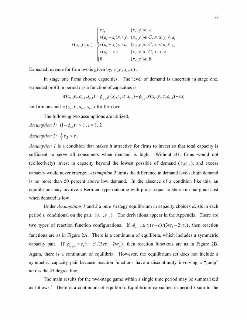
6

( , )( ) / ( , ) ,

( , , ) ( ) / ( , ) ,( ) ( , ) ,

0 ( , )

t t t

t t t t t t t t t

t t t t t t t t t t t t

t t t t t t

t t

vx x y Av a x x y x y C x y a

r x y a v a x x a x y C x a yv a y x y C x y

x y B

∈ − ∈ ≤ <= − ∈ < ≤ − ∈ >

∈

Expected revenue for firm two is given by, ( , , )t t tr y x a .

In stage one firms choose capacities. The level of demand is uncertain in stage one.

Expected profit in period t as a function of capacities is

1 11 1 ,1 1 1 ,2 2 1( , , , ) ( , , ) ( , , )t tt t t t s t t t s t t t tx y a s r x y a r x y a cxπ φ τ φ τ− −− − − −= + −

for firm one and 1 1( , , , )t t t ty x a sπ − − for firm two.

The following two assumptions are utilized.

Assumption 1: cvi >− )1( 2φ , i = 1, 2

Assumption 2: 32 2 1τ τ>

Assumption 1 is a condition that makes it attractive for firms to invest so that total capacity is

sufficient to serve all consumers when demand is high. Without A1, firms would not

(collectively) invest in capacity beyond the lowest possible of demand ( 2 1taτ − ), and excess

capacity would never emerge. Assumption 2 limits the difference in demand levels; high demand

is no more than 50 percent above low demand. In the absence of a condition like this, an

equilibrium may involve a Bertrand-type outcome with prices equal to short run marginal cost

when demand is low.

Under Assumptions 1 and 2 a pure strategy equilibrium in capacity choices exists in each

period t, conditional on the pair, 1 1( , )t ta s− − . The derivations appear in the Appendix. There are

two types of reaction function configurations. If 1 ,2 1 1 2( ) /(3 2 )

ts v c v vφ τ τ τ−

≤ − − , then reaction

functions are as in Figure 2A. There is a continuum of equilibria, which includes a symmetric

capacity pair. If 1 ,2 1 1 2( ) /(3 2 )

ts v c v vφ τ τ τ−

> − − , then reaction functions are as in Figure 2B.

Again, there is a continuum of equilibria. However, the equilibrium set does not include a

symmetric capacity pair because reaction functions have a discontinuity involving a “jump”

across the 45 degree line.

The main results for the two-stage game within a single time period may be summarized

as follows.6 There is a continuum of equilibria. Equilibrium capacities in period t sum to the

7

level of high demand, 1 1taτ − . If demand is high, then in stage two both firms set price v, which is

the upper bound of the set of short run market clearing prices. There is no excess capacity. If

demand is low, then in stage two both firms adopt mixed strategies for prices, with prices above

the short run market-clearing price of zero. Prices have positive variance and excess capacity

emerges. An illustration of equilibrium price distributions for a low demand realization is

provided in Figure 3. The figure illustrates the skewness of pricing distributions that is a feature

of equilibrium mixed strategies in Bertrand-Edgeworth models.

We use the term price markup to indicate the difference between a firm’s price and the

(maximum) short run competitive price. Equilibrium prices are procyclical while equilibrium

price markups are countercyclical in the simple two-stage game. The term “markup” is often

used to indicate the difference between the price and short run marginal cost. In our setting,

when demand is low, the conventional definition of a markup coincides with ours. However,

short run marginal cost is not defined for output equal to capacity when demand is high, and

hence we use the short run competitive price as the benchmark in that state.

Now consider the infinite horizon game beginning in period one, given initial conditions,

( , )a s0 0 . Let δ be a common discount factor, where we assume that τ δ1 1< so that payoffs are

bounded. We focus on equilibria that have two features:7 (1) firms use strategies that constitute

an equilibrium for the two-stage game in each period t, conditional on ( , )a st t− −1 1 , and (2) the

market shares of capacities are the same whenever the previous period state is the same.

Equilibria with these features yield a stationary Markov process for price and quantity changes.

Note that other, more complex, equilibria may exist. For example, Bagwell and Staiger (1997)

consider collusive mechanisms that can be supported as noncooperative Nash equilibria in a

dynamic pricing game (without capacity constraints) with essentially the same probabilistic

demand growth model that we use.

Suppose that ( , ) ( ,2)s st t− =1 1 ; i.e., there is high growth in t-1 and low growth in t. Then

in period t firms utilize mixed strategy distributions of prices. As long as st-1 = 1, this distribution

is the same, regardless of the value of at-1, given the features of the equilibrium we consider. Let

m1t be a random variable representing the average of the two firms’ prices, based on their mixed

strategies, with m v m m vt t1 1 10∈ = <( , ], ( ) , E and ( ) Var m t m12

1= σ .

Suppose instead that ( , ) ( ,2)s st t− =1 2 ; i.e., there is low growth in periods t-1 and t.

Firms utilize mixed strategy distributions of prices and, as long as st-1 = 2, this distribution is the

8

same, regardless of the value of at-1. Let m2t be a random variable representing the average of the

two firms’ prices, based on their mixed strategies, with 2 2 2(0, ], ( ) ,t tm v E m m v∈ = < and

2

22( )t mVar m σ= .

Up to this point our analysis has dealt with levels of prices. However, as we document in

the last part of Section IV, industry time series of price levels are non-stationary. Therefore we

utilize data on price changes rather than price levels in our empirical analysis. With two states

the model makes four predictions for price and quantity changes. Let pt and qt represent the

percentage change in prices and quantity, respectively. The results are derived in the last section

of the Appendix and summarized in Table I. The testable implications of the model are twofold.

First, during recessions ( )st = 2 the model predicts that changes in price will have a larger

variance than during booms.8 Second, the form of the distribution of price changes will be

different in recessions than in booms. In our theoretical model, there is price variation arising

from mixed strategy pricing during recessions and no price variation in boom periods. In a more

general formulation, price variation due to mixing during recessions would be in addition to

other possible sources of price variation that might occur in both booms and recessions. For

example, prices in booms may be normally distributed, while prices in recessions consist of a

normally distributed component plus a non-normally distributed component due to mixed

strategy pricing. This would generate price changes in recessions that have a distribution that is

not Gaussian.

IV. Estimation Approach, Data and Empirical Analysis

The business cycle formulation of the previous section generates a specific time series

model of price and quantity changes. However, some features of the model are too restrictive.

For example, due to our “step demand” formulation, the predicted variance of quantity changes

is zero in each state; only two different quantity-change amounts are predicted to appear. A more

general model with downward sloping demand would generate non-zero quantity change

variances.9 In what follows we specify an empirical model that is more general than what is laid

out in Table I. This specification permits a nonzero covariance between price and quantity

changes and a positive variance for quantity change is permitted in each state. Since the state

variable is not observable, the observed path of price and quantity changes must be used to make

inferences about the values of the state variable (as with the Kalman filter). The unobserved

9

state is assumed to be one of two growth rates, “high” or “low,” and the probabilistic switch

from one state to another is assumed to follow a Markov process. This approach to the issue of

cyclical pricing is appealing because the data will determine when an industry switches regimes

and whether relative price changes are more variable or not in recessions.

Time Series Model

The model we use is of the type formulated by Engel and Hamilton (1990) to test the

hypothesis of uncovered interest parity. Let y t t tq p= ′[ , ] be a two-dimensional vector at date t

where qt is the percentage change in production and pt is the percentage change in price for a

particular industry. There is an unobservable variable, st, which characterizes the “state” at date t

and takes on the value of one or two. In Engel and Hamilton (1990), y t is drawn from one

bivariate distribution if the state in t is equal to one and a second bivariate distribution if the state

in t is equal to two. Our setting is somewhat more complex, in that we have predictions on the

distribution governing y t draws conditional on both the current and the prior state (recall Table

I). Depending on the current and prior states, the contemporaneous changes in the growth rates

of production and real prices are drawn from a N s s s st t t t( , ), ,µ Ω

− −1 1 distribution. Thus, there are

four different bivariate distributions governing y t draws, since the pair ( , )s st t−1 can take on

four different values.

The state variable follows the Markov chain process specified in Section I. Only through

st-1 do past realizations of y and s affect the unobservable state variable. Note that the draws of

yt are not independent draws from a mixture of normal distributions. The inferred probability

that yt is drawn from one distribution depends on all the realizations of y prior to time t. This

approach differs from the Bresnahan and Suslow (1989) switching regime regression in that all

prior information is used to infer the current probability that yt is drawn from a particular

distribution.

The bivariate model of stochastic segmented trends permits a wide variety of behavior for

the series. First, the industry mean production growth rates may pick up slow or fast growth

rates of production for an industry. The production growth rates could also be the same in both

regimes, or one state may reflect recessionary periods and the other expansionary periods.

Likewise, these combinations are possible for the contemporaneous real price regimes.

The model described above is the basis for estimation of a parameter vector,

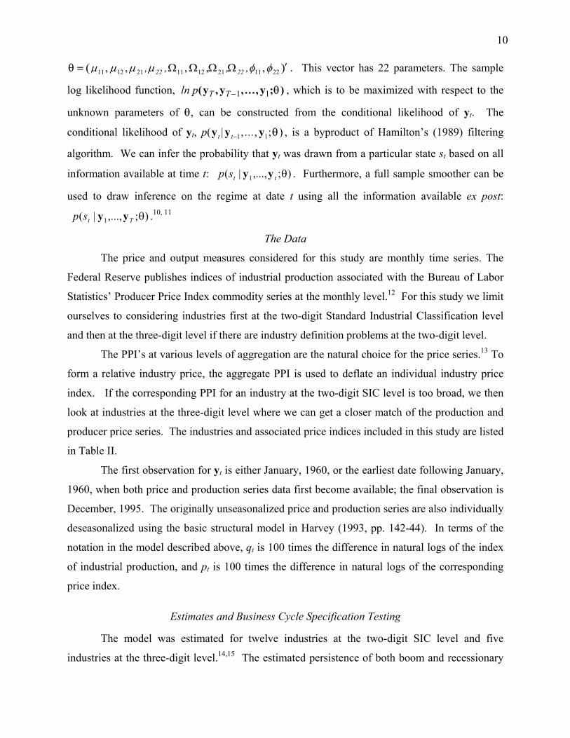
10

)(=θ ′ΩΩΩΩ 2211211211211211 ,,,,, φφµµµµ ,, ,, 2222 . This vector has 22 parameters. The sample

log likelihood function, ln p( , , .. ., ; )y y yT T −1 1 θ , which is to be maximized with respect to the

unknown parameters of θ, can be constructed from the conditional likelihood of yt. The

conditional likelihood of yt, p t t( | , ..., ; )y y y−1 1 θ , is a byproduct of Hamilton’s (1989) filtering

algorithm. We can infer the probability that yt was drawn from a particular state st based on all

information available at time t: );,...,|( 1 θttsp yy . Furthermore, a full sample smoother can be

used to draw inference on the regime at date t using all the information available ex post:

);,...,|( 1 θTtsp yy .10, 11

The Data

The price and output measures considered for this study are monthly time series. The

Federal Reserve publishes indices of industrial production associated with the Bureau of Labor

Statistics’ Producer Price Index commodity series at the monthly level.12 For this study we limit

ourselves to considering industries first at the two-digit Standard Industrial Classification level

and then at the three-digit level if there are industry definition problems at the two-digit level.

The PPI’s at various levels of aggregation are the natural choice for the price series.13 To

form a relative industry price, the aggregate PPI is used to deflate an individual industry price

index. If the corresponding PPI for an industry at the two-digit SIC level is too broad, we then

look at industries at the three-digit level where we can get a closer match of the production and

producer price series. The industries and associated price indices included in this study are listed

in Table II.

The first observation for yt is either January, 1960, or the earliest date following January,

1960, when both price and production series data first become available; the final observation is

December, 1995. The originally unseasonalized price and production series are also individually

deseasonalized using the basic structural model in Harvey (1993, pp. 142-44). In terms of the

notation in the model described above, qt is 100 times the difference in natural logs of the index

of industrial production, and pt is 100 times the difference in natural logs of the corresponding

price index.

Estimates and Business Cycle Specification Testing The model was estimated for twelve industries at the two-digit SIC level and five

industries at the three-digit level.14,15 The estimated persistence of both boom and recessionary

11

states is high for all industries, so there are only a small number of months representing

transitions from one state to another. Because of this, the standard errors associated with

estimates of 21122112 and ,,, ΩΩµµ are large. Therefore, in Table III we report parameter

estimates for the persistent states and the estimated state transition probabilities for each of the

seventeen industries.

It is clear from the estimates that the filter is capturing the dynamics of business cycles as

opposed to structural changes in positive growth rates. For fourteen of the seventeen industries,

the production mean growth rate is statistically different from zero in state 1. The mean change

in production for state 2 is also negative for these fourteen industries, but not always statistically

different from zero.16

The production growth rates for the newspaper (SIC 271) and metalworking machinery

(SIC 354) industries are not statistically different from zero in state 1 or 2. Leather (SIC 31)

production is trending down for the entire sample, and the mean growth rate in production in the

food (SIC 20) industry is constant.

An alternative empirical approach is to estimate a model in which price and quantity

changes depend on the current state ( st ∈ 1 2, ) but not on the previous state. Such a model has

two bivariate distributions for p and q, rather than four. Ex post we find that there are very few

month with transition states and so for ease of exposition and computation the statistical tests

below that compare means and variances in different states are based on estimates from this two

state model. The point estimates and the standard errors from estimating such a two-state model

differ only slightly from those presented in Table III.

A Wald statistic for testing whether the means for one of the component series, µst, are

different across states is given by

( $ $ )

v$ar( $ ) v$ar( $ ) c$ov( $ , $ )µ µ

µ µ µ µ1 2

2

1 2 1 22−

+ −,

which is asymptotically distributed χ12 . The asymptotic variance and covariance of the

parameters, denoted by v$ar( $ )µst and c$ov( $ , $ )µ µ1 2 , are estimated from the inverse of the negative

of the matrix of second derivatives. These statistics for the production and price series are

reported in Table IV. Superscripts on the means denote the series: production (q) and price (p).

The growth rates of production for the two states are significantly different for eight industries at

the α =.05 level of significance and ten industries at α = .10.

12

Figure 4 reports the estimated smoothed probability, p st T( | , ..., ; $ )y y1 θ , that the industry

is in the recessionary regime (state 2) at date t.17 A reasonable criteria for inferring that the

recessionary regime is more likely is p st T( | ,..., ; $ )= 2 1y y θ > .5. The smoothed inferences on

state 2 indicate that the dates of the business cycle at the industry level are similar to the

traditional NBER dates of business cycles. This first month of the recession in the mid 1970’s is

nearly uniform among these 17 industries, indicating that the filter is capturing the dynamics of

the business cycle. For the chemical (SIC 28) industry, the filter dates the beginning of the

1973-75 recession as December, 1972, nearly a whole year earlier than the NBER date of

1973:IV. The turning point in April, 1975, however, is identical to the conventional NBER date,

1975:II. The chemical industry also experiences contractions conforming to the traditional

recessions of 1980, 1981-82, and 1990-91. These, too, are present in the other industries but

with more variation in the starting and ending dates. At the monthly and industry level the

algorithm also indicates the common feature across industries of contractions in the early months

of 1986 and in the latter half of 1994, but these rarely last more than three months.

Note that the filter typically permits a clear classification of months into regimes. The

smoothed probabilities are usually very close to 0% or to 100%. There are only 6 inferences

between 40% and 60% for the chemical industry. The lumber (SIC 24) industry is an exception

with frequent regime switches and more months with less conclusive inferences on the state.

The estimated switching probabilities can be used to calculate the expected duration of a

regime. A regime i is expected to last (1 - φii)-1 months. The postwar historical average

recession according to NBER dating is 4.7 quarters which would imply that the probability of

remaining in the production contraction regime is 92.01%. Many of the industries have smaller

probabilities suggesting shorter recessionary periods at the industry level.

Columns 3 and 4 in Table IV report the results of Wald tests of the null hypothesis that

the growth rate of real prices is identical for both regimes. The chemical (SIC 28) industry is the

only industry with countercyclical pricing trends, and the nonferrous metals industry (SIC 33:3-

6, 9) is the only industry with strong procyclical trends in real prices.

Estimates of the Price Variance

The primary testable implication of our non-collusive oligopoly model is that the

variance of the price changes, σ s pt ,2 , is greater in the recessionary regime than during times of

13

production growth. Using a likelihood ratio test, the null hypothesis that we now test is

H 0 : σ σ12

22

p p= .

The results from these tests are reported in Table V.

For every industry, save one, we can reject the null hypotheses of equal price change

variance draws across regimes. As the estimates in Table III show, the recessionary variance for

price changes is anywhere from 6 to 17 times the expansionary variance. For these sixteen

industries, the average ratio of the state 2 price variance to the state 1 price variance is 11.69.

Because the inferred probabilities of being in either state are usually close to 0% or to 100%, we

are confident that the prices are much more variable in a recession than in an expansion.

The lone exception is the nonferrous metals industry (SIC 33:3-6, 9) for which the point

estimates of the price variance are nearly identical. This classification includes the aluminum

industry. Notice from Tables III and IV that the nonferrous metals industry is the only industry

that has different mean price growth rates across regimes and which has negative price changes

in recessions and positive price changes in expansions. Using p st T( | ,..., ; $ )= 2 1y y θ > .5 as the

criteria for dating a recession, the levels of the real price by state are shown in Figure 5 for the

nonferrous metals industry. Prices almost uniformly rise during expansions and fall during

recessions, and as mentioned earlier, these price changes have equal variances. The sharp rise in

the level of real prices as the industry reaches the peak of the business cycle is consistent with

the Bresnahan and Suslow (1989) model in which firms are producing at the vertical portion of

the short run supply curve during expansions. During contractions, however, the industry

produces at short run marginal cost with considerable excess capacity such that equilibrium is in

pure strategies. Bresnahan and Suslow document how competition increased in the aluminum

market by observing that the Herfindahl index and concentration ratios fell for the U.S.

aluminum industry from 1957-1982. It appears that there was too much competition and excess

capacity in the Aluminum Industry for firms to set a price above the short run competitive price

when demand was low.18

In addition to our theory, another source of increased price variation during contractions

may be more variable input prices. However, the estimates from the machinery industry (SIC

35) seem to indicate that input costs are not likely responsible for the increase in the price change

variance. All three-digit machinery industries plausibly have related mixes of the same inputs. If

input cost variation is responsible for the price variation in both recessions and expansions, then

14

a testable prediction is that the price change variance is the same in recessions and expansions

for the three-digit machinery industries. As Table III indicates, the point estimates for the

expansionary price change variance are identical (.168) for the agricultural machinery (SIC 352)

and metalworking machinery (SIC 354) industries, but they differ in recessions, 1.620 and 2.341,

respectively. This suggests that these two industries with similar inputs have different oligopoly

pricing in recessions.

The food (SIC 20) industry may also provide some insight into how much of the increase

in the price variance may be due to economy-wide reasons other than oligopoly pricing

incentives. Our theory of oligopoly pricing may not be applicable to this industry because

production in the food industry is growing at a constant rate throughout the sample (see Table

III). Nevertheless, the filter estimates two empirically distinct regimes. Figure 4a illustrates that

food industry is in regime 2 from 1973-1981 and from 1990-91. The former time period was a

period of high inflation and general economic stagnation and the latter was the 1990-91

recession. As Table V reports, the two regimes for the food industry have statistically different

price change variances, apparently for reasons not due to oligopoly pricing incentives. If this is a

macroeconomic phenomenon, it may be a component of the state 2 price variances for the other

industries which do experience expansions and contractions. However, the food industry’s price

change variance only increases by a factor of six, the smallest of all the significantly different

variances (see Table V). For the fourteen industries that have distinct expansionary and

recessionary states, the average ratio of the state 2 price change variance to the state 1 price

change variance is 12.20. This suggests that if there is a macroeconomic source for a higher

price change variance in recessions, it is not responsible for all of the increased variance.

Moreover, as the next subsection discusses, for the fourteen industries with expansions and

contractions we find support for the additional prediction on the change in the form of the price

change distribution.

Capacity Utilization and Price Variance Ratios

Capacity constraints play a crucial role in developing the theoretical predictions in

Section III--the tighter the capacity constraints, the lower the variance of prices. With

considerable excess capacity, the variance is also low. However, in the intermediate range of

capacity constraints, the variance is higher. This suggests a quadratic relationship between

capacity utilization and the ratio of the variances in Table V. Figure 6 plots average capacity

utilization during recessions, as dated by the switching regime filter, against the ratio of price

15

variances in Table V for thirteen of the fifteen industries that experience business cycles.19

Figure 6 also plots the fitted values from an OLS regression of the price variance ratio on

capacity utilization, capacity utilization squared, and a constant. This regression is consistent

with the prediction that the variance of recessionary prices is greatest for intermediate levels of

capacity utilization, but the quadratic relationship is sensitive to single observations.

Distribution of Price Draws

We have assumed that yt has bivariate normal distributions in all states. Assuming that

expansionary price changes come from a normal distribution, the model predicts that

recessionary price changes come from a non-normal distribution because firms use non-normal

mixed strategy distributions for prices during recessions.20 Following the work of Newey (1985)

and Hamilton (1996), we make use of the score statistics in tests that certain moment restrictions

of the normal distribution hold for the data for both regimes. In particular, we will take the

standard approach and examine the third and fourth moments, jointly and individually for each

series. The null hypothesis then implies the following expectations hold for the joint test:

E p s S

E p s S

t t Ts

t s

t t Ts

t ss q

s p

tt

tt

t

t

( | , , ; )( )

( | , , ; ) ( ),

,

= −

=

= ⋅ − −

=

=

=

∑

∑

y y y

y y y

11

23

11

24

4

4

0

3 0

K

K

θ µ

θ µ

and

σ

σ

Hamilton (1996) provides the scores for the univariate case, which can be naturally extended to

the bivariate model. The sample counterparts to the above moment restrictions are

r =

= −

= ⋅ − −

=

=

=

∑

∑∑1

3

11

23

11

24

4

4

1T

p s S

p s S

t t Ts

t s

t t Ts

t s

s q

s p

t

T tt

tt

t

t

( | , , ; $ )( $ )

( | , , ; $ ) ( $ )$

$

,

,

y y y

y y y

K

K

θ µ

θ µσ

σ

.

Let M be the T × 4 matrix whose t th row is given by

p s S p s St t Ts

t s t t Ts

t ss q

s ptt

tt

t

t

( | , , ; )( ) , ( | , , ; ) ( ),

,

= −

′= ⋅ − −

′

= =∑ ∑y y y y y y1

1

23

11

24

4

43K Kθ µ θ µ σ

σ,

and let the matrix D be the T × 12 matrix of scores. ForS M M M D D D D M= ′ − ′ ′ ′−1 1

T( ( ) ) , the

16

Wald statistic, T ′ −r S r1 , is asymptotically distributed as a χ42 and tests whether qt and pt are

jointly normally distributed. For only testing one restriction (column) of M, the test statistic is

asymptotically χ12 .

The results of the joint and individual tests for skewness and kurtosis are reported in

Table VI. Column 2 reports the statistic for the joint test of normality for both regimes. There

are clear rejections for all industries except food (SIC 20). Most of the individual series reject

the null hypotheses of no skewness and/or kurtosis equal to 3. Recall that the moments being

tested include both states.

Histograms of the price draws by state are shown in Figure 7. A price change is

considered to be in state j ( j = 1, 2) if p s jt T( | ,..., ; $ ) .= >y y1 5θ . These histograms for the price

draws in state 1, the expansionary state, appear to be consistent with a normal distribution

whereas the state 2 draws clearly are not. The variances of these draws are larger as our tests

above indicate, and the skewness and non-normal kurtosis detected in the conditional moment

tests is apparently coming from the recessionary price draws. Many of the industries have state 2

price draws with means shifted to the left, but with longer tails to the right.21 Other industries

like electrical machinery (SIC 36) and metalworking machinery (SIC 353) appear to have bi-

modal price distributions during recessions.

Price Levels over the Business Cycle

Our simple theoretical model yields a prediction regarding price levels as well as

predictions about price changes. Specifically, the model predicts that price levels are pro-

cyclical. Our empirical analysis has focused on the pattern of (percentage) price changes, rather

than price levels, over the business cycle. The main reason for this focus is the non-stationarity

our of real price level data. One cannot reject the hypothesis of a unit root for the (log of) real

price data, using Dickey-Fuller critical values, for each of the 17 industry price series. A direct

comparison of average price levels in expansions with average price levels in contractions can be

misleading when the price series is non-stationary.

In what follows we examine the prediction that price levels are procyclical, taking into

account the non-stationarity of prices. Rather than using a binary classification of expansions and

recessions (either our endogenous classification, or the NBER dating), we use monthly data on

capacity utilization in the manufacturing sector as a measure of the “state of demand” for

17

manufacturing as a whole.22 Let zt be capacity utilization in manufacturing in month t. Consider

the following two alternative relationships between the (log of) real price in industry j in month t

and capacity utilization, zt:

ln jt j j t jtP t zα γ β ε= + + +

, 1ln lnjt j j t j t jtP t z Pα γ β θ µ−= + + + +

In both relationships, the level of (log) real price is related to the “state of demand” via the

coefficient β. A positive β would indicate procyclical price levels, a negative β would indicate

counter-cyclical price levels, and a zero β would indicate acyclical price levels. Differencing

these two equations yields, respectively:

(1) , 1ln lnjt j t jt j t jtP P p z eγ β−− ≡ = + ∆ +

(2) jttjtjjttjjt upzpPP ++∆+=≡− −− 1,1,lnln θβγ

Equation (2) is very similar to (9.12), estimated in Domowitz (1992). Domowitz uses the same

change in capacity utilization variable for manufacturing as a whole, though he uses yearly rather

than monthly data.23

OLS estimates for these 2 specifications are reported in Table VII. Specification (2) is

clearly better in terms of goodness of fit. Both models yield positive, significant coefficients for

β, which is consistent with procyclical real price levels for our data sample. The estimated

economic significance of changes in capacity utilization is fairly small. An increase in capacity

utilization of 10 percent (a large increase) yields about a one-half percent real price increase,

based on estimation of (1) and (2). Domowitz’s estimates for β tend to negative. They are

significant for some subsamples (e.g., for what he calls the trigger-strategy sample of industries)

but his estimate is not significant for the entire sample. So he cannot reject the hypothesis of

acyclical price levels for the entire sample.

V. Concluding Remarks Our theoretical analysis predicts that output price changes exhibit higher variance during

recessions than during boom periods and that the form of the distribution of price changes

differs across recession and boom periods. The analysis also predicts that the markup of output

price over the short run competitive price (conditional on demand and capacity levels) is higher

in recessions than in booms. Evidence from U.S. manufacturing industries is consistent with the

hypothesis that price changes have higher variance in recessions than in booms. In fact, price

18

changes are much more variable in recessions than in booms for almost all industries studied. In

addition, the frequency distributions of these price changes in recessions are distinctly unlike

their expansionary counterparts.

While we do not provide any direct evidence regarding price markups, the evidence

presented here is consistent with the view that oligopoly firms charge prices involving a higher

markup over the short run competitive price during recessions than during boom periods. This

pattern of markups may amplify the effects of demand shocks on output. This in turn may

provide a mechanism through which oligopoly market power exacerbates the effects of aggregate

demand shocks on the macroeconomy.

The variation in price changes over the business cycle that we identify could be

accounted for by an optimal collusion model such as Staiger and Wolak (1992) or by a non-

collusive model similar to ours.24 Each of these models has the following features: there is

demand uncertainty, firms have market power, firms have production capacity constraints, and

firms set prices. We might add that if non-collusive models of market power are capable of

explaining key empirical regularities, then analysts may not need to turn to relatively more

complicated optimal collusion models of behavior over the business cycle.

Future research may focus on how industry concentration is related to the variance of

price changes at a more disaggregated industry level and how nature of costs affects oligopoly

pricing incentives. Forming larger systems by grouping industries together may also improve

estimation efficiency and increase the number of significant parameters. Since the empirical

results suggest that the form of the distribution of price changes differs across recessionary and

boom regimes, it would also seem worthwhile to develop a more sophisticated econometric

model of the recessionary regime. Extending our model to include product differentiation and

semi-flexible capacity constraints, along the lines of the work by Maggi (1996), would likewise

be a productive avenue of research.

19

Appendix

Analysis of Two-Stage Game

In stage one, firm one’s expected profit is,

1 11 1 ,1 1 1 ,2 2 1( , , , ) ( , , ) ( , , )t tt t t t s t t t s t t t tx y a s r x y a r x y a cxπ φ τ φ τ− −− − − −= + − ,

where r( )⋅ is the expected subgame revenue, defined in Section III. π is continuous in ( , )t tx y

since r( )⋅ is continuous in these arguments. However, π is not differentiable in x for all

capacity levels, so one cannot rely exclusively on first-order conditions to characterize best

responses. In order to simplify the exposition we drop the time subscripts from capacity

variables, and we define 2,1−≡

tsφθ , 2 1ta aτ −≡ , and 1 1ta aτ −≡ . Using this notation, firm one’s

expected profit as a function of capacities is,

( , ) (1 ) ( , , ) ( , , )x y r x y a r x y a cxπ θ θ= − + −% .

Consider the investment incentives for firm one, conditional on firm one being the larger

firm (x > y). In this case Assumption 1 implies that expected profit is strictly increasing in x for

x y a+ < ; ( , ) ( ( ) )x y v E a y cxπ = − −% for x y a+ > , so that π% is strictly decreasing when total

capacity exceeds the high demand level; and π% is continuous in x at x a y= − . Therefore, if

y a< 12 then π% reaches a local maximum at x a y= − . This may not be a global maximum

since π% may attain a higher value for some x < y.

The payoffs for firm one are more complex when it is the smaller firm (x < y). Consider

first the best response to y a a∈[ , ] . Any best response will be less than a , since Assumption 2

implies that π% is strictly decreasing in x for x > a . Given y a a∈[ , ] , π% is strictly increasing in

x for 0 ≤ ≤ −x a y by Assumption 2. π% is strictly concave in x for a y x a− ≤ ≤ . In addition π%

is continuous in x at x a y= − with a left derivative that exceeds the right derivative So, there is

a unique best response to each y a a∈[ , ] , which lies in a y x a− ≤ ≤ . This best response is,

(A1) b y a y v c ay vaavy va

( ) , ( ) ( )( ( ) )

= −− + −

+ −

max θ θ

θ θ1

2 1.

Suppose that y a a∈[ , ]12 . If x a y≤ − then ( , )x y vx cxπ = −% , which is strictly

increasing in x. If x y≥ then ( , ) ( ( ) )x y v E a y cxπ = − −% , which is strictly decreasing in x. So

any best response must be in [ , ]a y y− . Firm one’s expected profit function is not differentiable

20

at x a y= − ; expected profit is strictly concave in x for x a y y∈ −[ , ] . This implies that there

is a unique best response to y a a∈[ , ]12 that lies in [ , ]a y y− .

If the condition,

(A2) ( )3 2a v cva va

θ −≤

−,

holds then the best response to y a a∈[ , ]12 is,

(A3) b y E a cy v( ) ( ( ) / )= −max a - y, 12 .

Condition (A2) is equivalent to the condition, 1,2 1 1 2( ) /(3 2 )

ts v c v vφ τ τ τ−

≤ − − , in the main text.

From (A3) it follows that b a a( )12

12= and b y a y( ) = − for some interval of y-values extending

above y a= 12 . Inequality (A2) also implies that a y− is a best response to y a∈[ , )0 1

2 ; i.e.,

the local best response for firm one as a large firm is also a global best response to y a∈[ , )0 12 .

So, inequality (A2) yields a reaction function for firm one that is as depicted by R1 in Figure 2A.

The reaction function for firm two is defined symmetrically. The set of equilibria is the set of

capacity pairs that sum to a such that neither x nor y exceed some critical value. This critical

value is the lowest value of y such that b(y) in (A1) or (A3) exceeds a y− .

If (A2) does not hold then a best response to y a a∈[ , ]12 may be less than a y− . For

some values of y a a∈[ , ]12 , expected profit for firm one is maximized by choosing capacity,

~( ) [ ( / ) / ]x y a c v y≡ + − −12 1 θ θ .

This capacity choice is optimal for firm one when ~( )x y a y< − , which is possible only when

(A2) does not hold. If (A2) does not hold then ~( )x a a12

12< and ~( )x y a y< − for an interval of

y-values exceeding 12 a . The best response to y a a∈[ , ]1

2 is,

(A4) b y x y E a cy v( ) ~( ), ( ( ) / )= −min max a - y, 12 .

If (A2) does not hold there is also an interval of y-values below 12 a for which the best response

is ~( )x y a y< − . In such cases, there is a local maximum that involves firm one being the large

firm and choosing capacity, a y− ; however, the global maximum is for firm one to respond as a

small firm, choosing ~( )x y y< . Once y becomes sufficiently small, firm one’s best response

21

“jumps” up to a y− . The reaction correspondence for firm one is depicted as R1 in Figure 2B.

The set of equilibria is the set of capacity pairs that sum to a such that, (1) neither x nor y

exceed a critical value defined in the previous paragraph and, (2) an interval of capacity pairs

around x y= is excluded (when firm two is the large firm, the excluded set involves y-values

such that ~( )x y a y< − ).

Illustration of the Derivations in Table 1

We define p P Pt t t≡ − −ln ln 1 and q Q Qt t t≡ − −ln ln 1 where Pt is the average price for

sellers and Qt is total industry production in period t. The approximations of pt use a first order

Taylor expansion:

( )ln( ) ln( ( ))( )

x E xx E xE x−

≈ + .

A derivation for the case, st-1 = 1 and st = 2, is provided here. Derivations for the other

three cases in Table I are similar to this. The period t price is the random variable, m1t , where

m v m m v mt t t m1 1 1 120

1∈ = < =( , ], ( ) , ( ) . E and Var σ The price in t − 1 is, v . Thus we have,

1 111

1

ln( ) ln( ) ln tt t

m mmp m vv m

− = − ≈ +

,

and

-1 2ln - ln ln( )t t tq a a τ= = .

The first and second moments are:

1( ) ln 0tmE pv

= <

, 1

22 21 11

21 1

( )= ln mtt t

m mmVar p E p Ev m m

σ − − = = ,

2( ) ln( )tE q τ= , and Var(qt) = 0.

22

References

Bagwell, K. and R. Staiger, “Collusion over the Business Cycle,” Rand Journal of Economics, Spring 1997, 28, 82-106. Bresnahan, T. F., “Empirical Studies of Industries with Market Power,” in R. Schmalensee and R. Willig, eds., Handbook of Industrial Organization, 1989, 2, New York: North-Holland, 1011-57. Bresnahan, T. F., and V. Y. Suslow, “Short run Supply with Capacity Constraints,” Journal of Law and Economics, 1989, 32, S11-S41. Chevalier, J., and D. Scharfstein, “Capital-Market Imperfections and Countercyclical Markups: Theory and Evidence,” American Economic Review, September 1996, 86, 703-725. Davis, D. and C. Holt, “Market Power and Mergers in Laboratory Markets with Posted Prices,” Rand Journal of Economics, Autumn 1994, 25, 467-487. Dempster, A., N. Laird, and D. Rubin, “Maximum Likelihood from Incomplete Data via the EM Algorithm, Journal of the Royal Statistical Society, 1977, B 39, 1-38. Domowitz, I., “Oligopoly Pricing: Time-Varying Conduct and the Influence of Product Durability as an Element of Market Structure,” in The New Industrial Economics, eds. G. Norman and M. La Manna, Brookfield, VT: Elgar Publishing, 1992, 214-235. Domowitz, I., R. G. Hubbard, and B. Petersen, “Oligopoly Supergames: Some Empirical Evidence on Prices and Margins,” in T. Bresnahan and R. Schmalensee, eds., The Empirical Renaissance in Industrial Organization: An Overview, Oxford: Blackwell, 1987, p. 9-28. Engel, C., and J. D. Hamilton, “Long Swings in the Dollar: Are They in the Data and Do Markets Know It?” American Economic Review, 1990, 80, 689-713. Gottfries, N. “Customer Markets, Credit Market Imperfections, and Real Price Rigidity,” Economica, 1991, 58(3), 317-23. Greenwald, B., J. Stiglitz, and A. Weiss, “Informational Imperfections in the Capital Market and Macroeconomic Fluctuations,” American Economic Review (Papers and Proceedings, 1984, 74(2), 194-99. Hamilton, J. D. “A New Approach to the Economic Analysis of Nonstationary Time Series and the Business Cycle,” Econometrica, 1989, 57(2), 357-384. Hamilton, J. D. “Analysis of Time Series Subject to Changes in Regime,” Journal of Econometrics, 1990 45, 39-70. Hamilton, J. D. “A Quasi-Bayesian Approach to Estimating Parameters for Mixtures of Normal Distributions,” Journal of Business and Economic Statistics, 1991, 9, 27-39.

23

Hamilton, J. D. “Specification Testing in Markov-Switching Time-Series Models, Journal of Econometrics, 1996, 70, 127-157. Harvey, A. C. Time Series Models. Cambridge, MA: MIT Press, 1993. Klemperer, P. “Competition When Consumers Have Switching Costs: An Overview with Applications to Industrial Organization, Macroeconomics, and International Trade,” Review of Economic Studies, 1995, 62, 515-39. Kreps, D. M., and J. A. Scheinkman, “Quantity Precommitment and Bertrand Competition Yield Cournot Outcomes,” Bell Journal of Economics, 1983, 14, 326-337. Maggi, G. “Strategic Trade Policies with Endogenous Mode of Competition,” American Economic Review, 86(1), 237-258. Newey, W. “Maximum Likelihood Specification Testing and Conditional Moment Tests,” Econometrica, 1985, 53, 1047-70. Reynolds, S. and B.J. Wilson, “Bertrand-Edgeworth Competition, Demand Uncertainty, and Asymmetric Outcomes,” Journal of Economic Theory, 2000, 92, 122-141. Rotemberg, J. J., and G. Saloner, “A Supergame-Theoretic Model of Price Wars during Booms,” American Economic Review, 1986, 76, 390-407. Rotemberg, J. J., and M. Woodford, “Oligopolistic Pricing and the Effects of Aggregate Demand on Economic Activity,” Journal of Political Economy, 1992, 100(6), 1153-207. Rotemberg, J. J., and M. Woodford, “Markups and the Business Cycle,” Macroeconomics Annual, 1991, 6, 63-129. Staiger, R.W., and F. Wolak, “Collusive pricing with Capacity Constraints in the Presence of Demand Uncertainty”, Rand Journal of Economics, Summer 1992, 23, 203-220. Stiglitz, J. “Price Rigidities and Market Structure,” American Economic Review (Papers and Proceedings, 1984, 74(2), 350-55. White, H. “Maximum Likelihood Estimation of Misspecified Models,” Econometrica, 1982, 50, 1-25. Wilson, B. J., “What Collusion? Unilateral Market Power as a Catalyst for Countercyclical Pricing,” Experimental Economics, 1998, 1(2), 133-145.

24

1 Two other implications of this non-collusive oligopoly model are noteworthy. First, price adjustments are

sluggish in the downward direction, relative to competitive prices. If demand changes from high to low then

oligopoly firms reduce prices by an amount less than the change in the competitive price, since oligopoly firms

charge a markup over the short run competitive price when demand is low. A second (and related) implication is

that existing capacity is utilized efficiently when demand is high but may be utilized inefficiently when demand is

low. Oligopoly price markups above the short run competitive price can lead to less output and employment than is

efficient when demand is low. 2 The model in Bagwell and Staiger (1997) does not predict that the variance of price changes will be greater in

recessions than in expansions. Their unique prediction is that a high transitory demand shock within a recessionary

or expansionary regime is associated with a lower most-collusive price. This would generate a negative covariance

between price changes and quantity changes within recessions and expansions. 3 Reynolds and Wilson (2000) analyze more general two-stage models, including formulations with a downward

sloping demand. However, the simple formulation of the present paper yields the principal empirical implications

that we search for in the data. 4 The business cycle dates from Hamilton’s filter closely correspond to the traditional NBER dates. It is also worth

noting that the unobservable state is only one of many influences on the growth rate so that output could be falling

even though the economy is in the “high” growth rate state. 5 If total capacity is less than a then v is the unique competitive price. If total capacity equals a then v is the upper

bound on the interval of competitive prices. 6 The two-stage model is formulated as a duopoly. However, the basic results on markups and price variability

continue to hold for markets with more than two firms, as long as the market does not become too competitive. For

example, suppose that there are n ≥2 equal sized firms, with total capacity equal to the maximum possible demand.

If 1 1 21 /( )n ττ τ −+ < , then when demand is low, equilibrium prices are draws from a mixed strategy distribution;

prices involve a positive markup over short run marginal cost and prices have positive variance. 7 A sequence of equilibria for single period games constitute an equilibrium for the infinite horizon game because

the choices that a firm makes in period t have no effect on the payoffs of either firm in period t+1. We are assuming

that capacity choices are reversible from one period to the next, so that period t capacity choices have no impact on

period t+1 capacities or payoffs. The market size in period t+1 is related to market size in period t, but the

probabilistic transition of market size from one period to the next is unaffected by firms’ decisions. 8 If firms are mixing across periods during recessionary periods, then an index of these prices will vary over time. If

the equilibrium during a boom is in pure strategies, then there is no source of variation due to mixing. 9 We should emphasize that the main predictions of the model regarding differential variances of price changes

over the business cycle are not sensitive to our “step demand” assumption. In Reynolds and Wilson (2000) we show

that the same pattern of price variances emerges in a model with downward sloping demand.

10 Two issues arise when attempting to find the maximum likelihood estimate θ . Both involve the process of

finding the global maximum of the sample log likelihood function. From the filter we can determine the sample log

25

likelihood function as the sum of the conditional log likelihoods:

∑= −=−T

t ttpTTp1

)1,...,1|()1,...,1,( yyyyyy lnln . As in Hamilton (1989) the sample log likelihood can be

maximized using numeric hill-climbing methods, but systems with a large number of parameters (e.g., twenty-two)

often have many local maxima and require lengthy computing time. Hamilton (1990) shows how the switching

regime filter can be estimated using the EM (expected maximum likelihood) algorithm developed by Dempster,

Laird, and Rubin (1977). With the EM algorithm, analytic derivatives are easily calculated from smoothed

inferences. Furthermore, systems with a larger number of parameters, as in the bivariate model employed here, do

not require additional iterations or computing time because the analytic derivatives are calculated from the smoothed

probabilities. In addition to choosing the method for maximizing the likelihood function, another problem arises

when the mean of the first state is set exactly equal to the first observation and the variance of the first state is

allowed to vanish. In such a case the likelihood function blows up to infinity. Hamilton (1991) offers Bayesian

priors as a solution to this problem. These positive Bayesian priors imply that one is now maximizing a generalized

objective function that is not subject to these singularities. The first order conditions from maximizing the log

likelihood function with and without the Bayesian priors are given in Hamilton (1990) and Engel and Hamilton

(1990). In practice we find that this potential singularity in the likelihood function is not a problem with our data. 11 The smoothed probability, );,...,1| ,1( θ==− Tjtsitsp yy , is calculated as part of the filter for the two-state

model employed by Engel and Hamilton. In a two-state model, the transition observations from state i in period t-1

to state j in period t are incorporated into the estimate of µ st j= and Ωst j= . In practice we estimate a two-state

model and use );,...,1| ,1( θ==− Tjtsitsp yy to estimate the parameters from a four-state version of the EM

equations in Hamilton (1990) (p.54). 12 The results are similar if capacity utilization rates are used instead of industrial production. 13 The PPI data were downloaded from the BLS World Wide Web site http://stats.bls.gov/. We use price and

quantity data with a monthly frequency. The model that we analyzed in Section III assumed that firms were able to

choose both prices and capacity in each period. If firms could in fact adjust their capacities on a monthly basis then

they might choose to reduce their production capacities significantly during recessionary regimes.

However, this kind of significant capacity reduction is not observed in most recessions. Our Assumption 1 insures

that value and cost parameters are such that even though firms could reduce capacity in anticipation of continued

weak demand, that they would prefer to maintain enough capacity to meet a higher demand level. 14 We thank James Hamilton for kindly distributing his Gauss code with which we replicated his results. Additional

code was added for the likelihood ratio tests and bivariate conditional moment tests. 15 The following industries are not included: Tobacco (SIC 21), Textiles (SIC 22), Apparel SIC (23), and

Instruments (SIC 38). The real price of tobacco was fairly constant from January, 1960, to August, 1982, after

which it began a nearly deterministic climb from 102 in September, 1983, to 234 in July, 1993. Then the real price

fell 24% in August, 1993, and does not change much for the rest of the sample. Clearly a more complicated model

explaining these events is necessary before the switching regime model is applied. The BLS does not publish a

26

price index solely for textiles, but one for Textiles and Apparel. It did publish a separate series for Apparel, but it

ends in 1977. There is also no price index that adequately captures the general industry, Instruments (SIC 38). The

five industries at the three-digit level represent three industries for which good measures of the price could not be

found at the two-digit level. 16 Furthermore, following Engel and Hamilton (1990) we use a general null hypothesis to test whether a series

follows a random walk against the alternative of the two-state regime model. The Markov switching probabilities

are not identified in the model when µ µ Ω Ω1 2 1 2= and = , but asymptotically valid tests of the following null

hypothesis do exist- 21 and ,21 ,22111 :0H ΩΩµµ ≠≠−= φφ . As in Engel and Hamilton, we test the null

hypothesis of a random walk with both a Wald and likelihood ratio statistic. The Wald statistic is given by

21)22

ˆ,11ˆv(oc2)22

ˆr(av)11ˆr(av

2)]22ˆ1(11

ˆ[χ

φφφφ

φφ≈

++

−−. The likelihood ratio test compares the unconstrained log likelihood

to the largest log likelihood when φ11 = 1 - φ22 and is asymptotically distributed as χ12 . These test statistics are not

reported here. The Wald test statistics are all larger (in some cases much larger) than the likelihood ratio test

statistics, but the even the latter soundly rejects the null hypothesis of a random walk in favor of the two regime

model. (The smallest LR statistic is greater than 68.) In sum, the switching regime model is capturing the dynamics

of the business cycle for these industries. 17 The evolving probabilities are similar to the smoothed inferences. Using all the information in the sample reduces

the “noise” in the some of probabilities within a recession. For example, six months into the 1973-75 recession, the

probability of being in the recessionary state falls from 99% to 70%, but using all the information in the sample

revises that estimate back to 99%. 18 cf ft. 5. 19 We could not find data on capacity utilization for nonferrous metals (SIC 33:3-6, 9) and newspapers (SIC 271)

that is consistent with the data used for prices and production, though we already discuss the former explicitly in the

previous subsection. 20 Even though the recessionary price changes may not be Gaussian, the estimates in Table III are consistent quasi-

maximum likelihood estimates (see White (1982)). 21 These conditional moments tests are influenced, but not overwhelmingly so, by a common outlier in August,

1973. Food prices jumped 9% that month causing the overall PPI to rise abruptly. For many industries, this real

price draw around -5% is the lone outlying negative real price change. 22 Utilization is measured in percentage units. This data is available from the Federal Reserve Board web site,

http://www.federalreserve.gov/releases/g17/download.htm. 23 The main differences between (2) and (9.12) in Domowitz are that we have an industry-specific dummy rather

than a fixed constant, and Domowitz includes a cost change variable on the RHS. He uses instrumental variables for

this cost change variable. We do not have data to serve as proxies for unit cost, as in Domowitz. However, our

deflation of nominal prices by the producer price index will account for at least some of the effects of cost shocks.

27

Domowitz uses changes in nominal prices rather than changes in real prices, as the dependent variable. 24 Our results also indicate that there are as many positive as negative covariances (see the off diagonal results for

Ω11 and Ω22 in Table III). Hence, the evidence does not support the Bagwell and Staiger prediction regarding

transitory demand shocks in an optimal collusion mechanism (cf ft. 2).

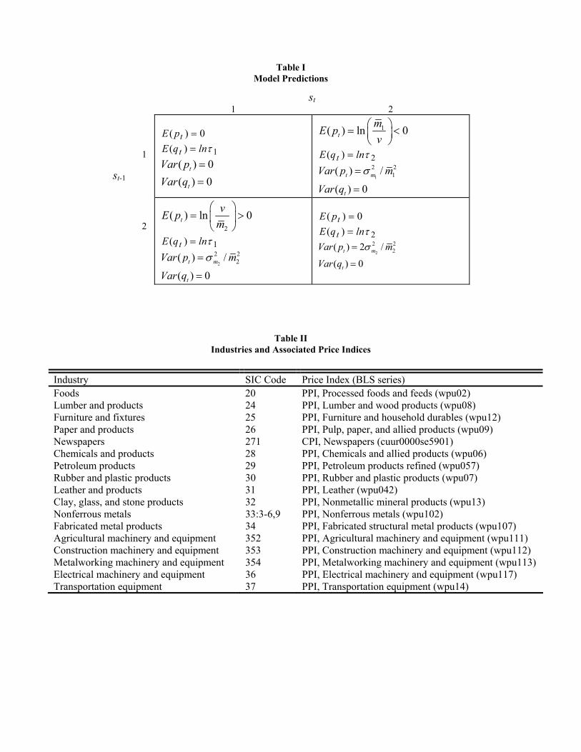
Table I Model Predictions

Table II Industries and Associated Price Indices

st 1 2

st-1

1

E pt( ) = 0 E qt( ) = lnτ 1

( ) 0( ) 0

t

t

Var pVar q

==

1( ) ln 0tmE pv

= <

E qt( ) = lnτ 2

1

2 21( ) /

( ) 0t m

t

Var p m

Var q

σ=

=

2 2

( ) ln 0tvE p

m

= >

E qt( ) = lnτ 1

2

2 22( ) /

( ) 0t m

t

Var p m

Var q

σ=

=

E pt( ) = 0 E qt( ) = lnτ 2

2

2 22( ) 2 /

( ) 0t m

t

Var p m

Var q

σ=

=

Industry SIC Code Price Index (BLS series) Foods 20 PPI, Processed foods and feeds (wpu02) Lumber and products 24 PPI, Lumber and wood products (wpu08) Furniture and fixtures 25 PPI, Furniture and household durables (wpu12) Paper and products 26 PPI, Pulp, paper, and allied products (wpu09) Newspapers 271 CPI, Newspapers (cuur0000se5901) Chemicals and products 28 PPI, Chemicals and allied products (wpu06) Petroleum products 29 PPI, Petroleum products refined (wpu057) Rubber and plastic products 30 PPI, Rubber and plastic products (wpu07) Leather and products 31 PPI, Leather (wpu042) Clay, glass, and stone products 32 PPI, Nonmetallic mineral products (wpu13) Nonferrous metals 33:3-6,9 PPI, Nonferrous metals (wpu102) Fabricated metal products 34 PPI, Fabricated structural metal products (wpu107) Agricultural machinery and equipment 352 PPI, Agricultural machinery and equipment (wpu111) Construction machinery and equipment 353 PPI, Construction machinery and equipment (wpu112) Metalworking machinery and equipment 354 PPI, Metalworking machinery and equipment (wpu113) Electrical machinery and equipment 36 PPI, Electrical machinery and equipment (wpu117) Transportation equipment 37 PPI, Transportation equipment (wpu14)

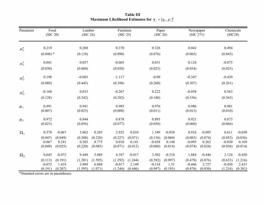
Table III Maximum Likelihood Estimates for y t t tq p= ′[ , ]

Parameter Food

(SIC 20) Lumber

(SIC 24) Furniture

(SIC 25)

Paper (SIC 26)

Newspaper (SIC 271)

Chemicals (SIC28)

µ11

q 0.219 0.260 0.370 0.326 0.042 0.494 (0.048) * (0.118) (0.090) (0.076) (0.065) (0.043) µ11

p 0.041 0.057 -0.065 0.031 0.124 -0.075 (0.030) (0.060) (0.020) (0.023) (0.034) (0.023) µ22

q 0.198 -0.083 -1.117 -0.09 -0.347 -0.439 (0.089) (0.445) (0.398) (0.260) (0.307) (0.261) µ22

p -0.168 0.033 -0.267 0.222 -0.058 0.563 (0.128) (0.342) (0.282) (0.180) (0.336) (0.365) φ11 0.991 0.941 0.985 0.976 0.986 0.981 (0.007) (0.025) (0.008) (0.011) (0.013) (0.010) φ22 0.972 0.844 0.878 0.893 0.921 0.873 (0.023) (0.056) (0.077) (0.058) (0.060) (0.066) Ω11 0.578 -0.067 3.062 0.203 2.852 0.010 1.549 -0.038 0.916 -0.095 0.611 -0.030 (0.047) (0.049) (0.308) (0.220) (0.227) (0.071) (0.136) (0.060) (0.083) (0.074) (0.052) (0.036) -0.067 0.241 0.203 0.775 0.010 0.141 -0.038 0.148 -0.095 0.262 -0.030 0.169 (0.049) (0.025) (0.220) (0.085) (0.071) (0.012) (0.060) (0.014) (0.074) (0.024) (0.036) (0.014) Ω22 0.645 -0.072 9.449 3.889 4.397 -0.017 3.502 -0.318 1.884 -0.446 2.124 -0.450 (0.113) (0.191) (1.201) (1.595) (1.292) (1.244) (0.592) (0.997) (0.478) (0.876) (0.633) (1.216) -0.072 1.418 3.889 6.888 -0.017 2.149 -0.318 1.51 -0.446 2.727 -0.450 2.431 (0.191) (0.207) (1.595) (1.071) (1.244) (0.446) (0.997) (0.193) (0.876) (0.830) (1.216) (0.381) *Standard errors are in parentheses.

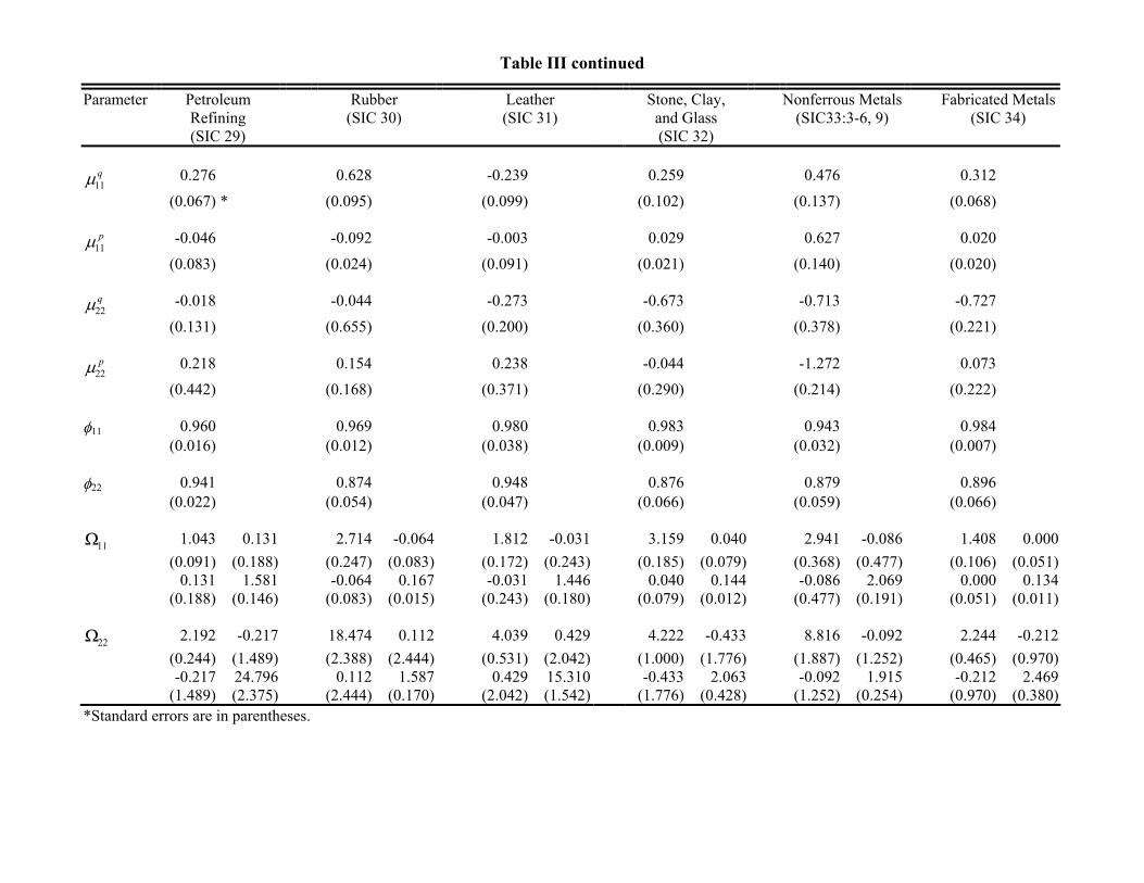
Table III continued

Parameter Petroleum Refining (SIC 29)

Rubber (SIC 30)

Leather (SIC 31)

Stone, Clay, and Glass (SIC 32)

Nonferrous Metals(SIC33:3-6, 9)

Fabricated Metals(SIC 34)

µ11

q 0.276 0.628 -0.239 0.259 0.476 0.312 (0.067) * (0.095) (0.099) (0.102) (0.137) (0.068) µ11

p -0.046 -0.092 -0.003 0.029 0.627 0.020 (0.083) (0.024) (0.091) (0.021) (0.140) (0.020) µ22

q -0.018 -0.044 -0.273 -0.673 -0.713 -0.727 (0.131) (0.655) (0.200) (0.360) (0.378) (0.221) µ22

p 0.218 0.154 0.238 -0.044 -1.272 0.073 (0.442) (0.168) (0.371) (0.290) (0.214) (0.222) φ11 0.960 0.969 0.980 0.983 0.943 0.984 (0.016) (0.012) (0.038) (0.009) (0.032) (0.007) φ22 0.941 0.874 0.948 0.876 0.879 0.896 (0.022) (0.054) (0.047) (0.066) (0.059) (0.066) Ω11 1.043 0.131 2.714 -0.064 1.812 -0.031 3.159 0.040 2.941 -0.086 1.408 0.000 (0.091) (0.188) (0.247) (0.083) (0.172) (0.243) (0.185) (0.079) (0.368) (0.477) (0.106) (0.051) 0.131 1.581 -0.064 0.167 -0.031 1.446 0.040 0.144 -0.086 2.069 0.000 0.134 (0.188) (0.146) (0.083) (0.015) (0.243) (0.180) (0.079) (0.012) (0.477) (0.191) (0.051) (0.011) Ω22 2.192 -0.217 18.474 0.112 4.039 0.429 4.222 -0.433 8.816 -0.092 2.244 -0.212 (0.244) (1.489) (2.388) (2.444) (0.531) (2.042) (1.000) (1.776) (1.887) (1.252) (0.465) (0.970) -0.217 24.796 0.112 1.587 0.429 15.310 -0.433 2.063 -0.092 1.915 -0.212 2.469 (1.489) (2.375) (2.444) (0.170) (2.042) (1.542) (1.776) (0.428) (1.252) (0.254) (0.970) (0.380)*Standard errors are in parentheses.

Table III continued

Parameter Agricultural Machinery (SIC 352)

Construction Machinery (SIC 353)

Metalworking Machinery (SIC 354)

Electrical Machinery (SIC 36)

Transportation Equipment (SIC 37)

µ11

q 0.490 0.400 0.125 0.604 0.329 (0.192) * (0.092) (0.133) (0.080) (0.173) µ11

p 0.036 0.051 0.053 -0.071 0.036 (0.034) (0.029) (0.036) (0.021) (0.028) µ22

q -1.088 -1.369 -0.641 -0.297 -0.393 (0.543) (0.364) (0.347) (0.336) (0.980) µ22

p 0.084 0.156 0.121 -0.122 -0.176 (0.199) (0.293) (0.277) (0.307) (0.213) φ11 0.962 0.976 0.988 0.987 0.965 (0.019) (0.014) (0.050) (0.007) (0.018) φ22 0.893 0.897 0.913 0.89 0.87 (0.063) (0.060) (0.042) (0.080) (0.070) Ω11 5.629 0.066 1.964 -0.024 3.737 -0.062 1.892 -0.027 5.291 -0.033 (0.640) (0.167) (0.170) (0.086) (0.373) (0.131) (0.153) (0.059) (0.528) (0.130) 0.066 0.168 -0.024 0.204 -0.062 0.168 -0.027 0.146 -0.033 0.16 (0.167) (0.023) (0.086) (0.018) (0.131) (0.021) (0.059) (0.012) (0.130) (0.016) Ω22 14.529 -0.439 5.957 -0.746 4.723 -1.290 3.507 -0.416 23.141 0.026 (3.347) (1.802) (0.969) (1.796) (1.099) (0.968) (0.915) (1.173) (3.587) (3.024) -0.439 1.620 -0.746 2.481 -1.290 2.341 -0.416 2.321 0.026 1.736 (1.802) (0.216) (1.796) (0.330) (0.968) (0.479) (1.173) (0.459) (3.024) (0.388)*Standard errors are in parentheses.

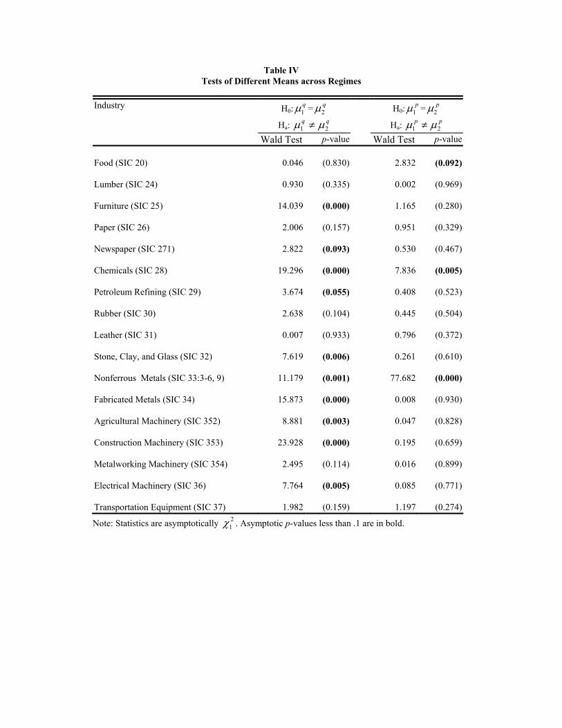
Table IV

Tests of Different Means across Regimes

Note: Statistics are asymptotically χ12 . Asymptotic p-values less than .1 are in bold.

Industry H0:µ1q =µ2

q

Ha: µ µ1 2q q≠

H0:µ1p =µ2

p

Ha: µ µ1 2p p≠

Wald Test p-value Wald Test p-value Food (SIC 20)

0.046 (0.830)

2.832 (0.092)

Lumber (SIC 24)

0.930 (0.335) 0.002 (0.969)

Furniture (SIC 25)

14.039 (0.000) 1.165 (0.280)

Paper (SIC 26)

2.006 (0.157) 0.951 (0.329)

Newspaper (SIC 271)

2.822 (0.093) 0.530 (0.467)

Chemicals (SIC 28)

19.296 (0.000) 7.836 (0.005)

Petroleum Refining (SIC 29)

3.674 (0.055) 0.408 (0.523)

Rubber (SIC 30)

2.638 (0.104) 0.445 (0.504)

Leather (SIC 31)

0.007 (0.933) 0.796 (0.372)

Stone, Clay, and Glass (SIC 32)

7.619 (0.006) 0.261 (0.610)

Nonferrous Metals (SIC 33:3-6, 9)

11.179 (0.001) 77.682 (0.000)

Fabricated Metals (SIC 34)

15.873 (0.000) 0.008 (0.930)

Agricultural Machinery (SIC 352)

8.881 (0.003) 0.047 (0.828)

Construction Machinery (SIC 353)

23.928 (0.000) 0.195 (0.659)

Metalworking Machinery (SIC 354)

2.495 (0.114) 0.016 (0.899)

Electrical Machinery (SIC 36)

7.764 (0.005) 0.085 (0.771)

Transportation Equipment (SIC 37) 1.982 (0.159) 1.197 (0.274)

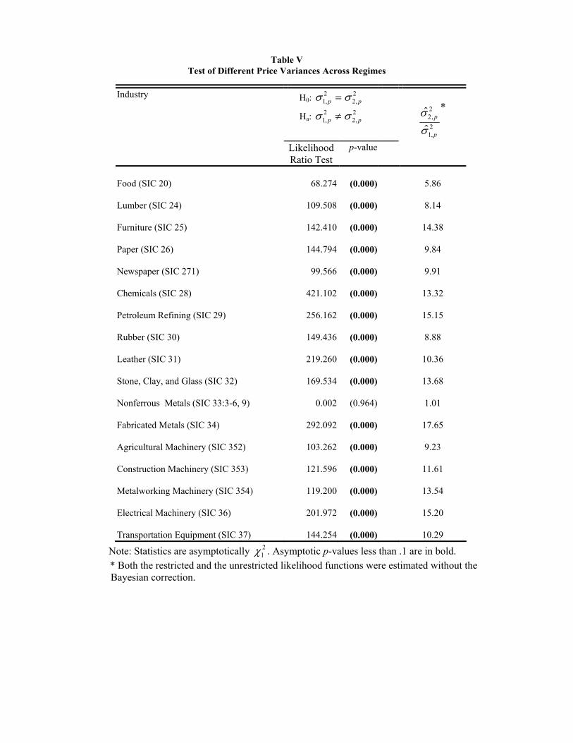
Table V Test of Different Price Variances Across Regimes

Note: Statistics are asymptotically χ12 . Asymptotic p-values less than .1 are in bold.

* Both the restricted and the unrestricted likelihood functions were estimated without the Bayesian correction.

Industry H0: σ σ12

22

, ,p p=

Ha: σ σ12

22

, ,p p≠

$

$

*,

,

σσ

22

12

p

p

Likelihood Ratio Test

p-value

Food (SIC 20)

68.274 (0.000)

5.86

Lumber (SIC 24)

109.508 (0.000) 8.14

Furniture (SIC 25)

142.410 (0.000) 14.38

Paper (SIC 26)

144.794 (0.000) 9.84

Newspaper (SIC 271)

99.566 (0.000) 9.91

Chemicals (SIC 28)

421.102 (0.000) 13.32

Petroleum Refining (SIC 29)

256.162 (0.000) 15.15

Rubber (SIC 30)

149.436 (0.000) 8.88

Leather (SIC 31)

219.260 (0.000) 10.36

Stone, Clay, and Glass (SIC 32)

169.534 (0.000) 13.68

Nonferrous Metals (SIC 33:3-6, 9)

0.002 (0.964) 1.01

Fabricated Metals (SIC 34)

292.092 (0.000) 17.65

Agricultural Machinery (SIC 352)

103.262 (0.000) 9.23

Construction Machinery (SIC 353)

121.596 (0.000) 11.61

Metalworking Machinery (SIC 354)

119.200 (0.000) 13.54

Electrical Machinery (SIC 36)

201.972 (0.000) 15.20

Transportation Equipment (SIC 37) 144.254 (0.000) 10.29

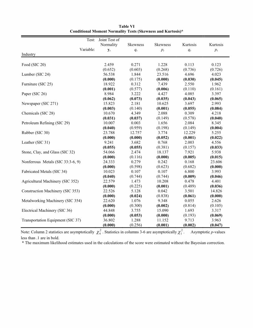
Table VI Conditional Moment Normality Tests (Skewness and Kurtosis)*

Note: Column 2 statistics are asymptotically χ42 . Statistics in columns 3-6 are asymptotically χ1

2 . Asymptotic p-values less than .1 are in bold. * The maximum likelihood estimates used in the calculations of the score were estimated without the Bayesian correction.

Test:

Variable: Industry

Joint Test of Normality

yt

Skewness

qt

Skewness

pt

Kurtosis

qt

Kurtosis

pt

Food (SIC 20)

2.459

(0.652)

0.271

(0.603)

1.228

(0.268)

0.113

(0.736)

0.123

(0.726) Lumber (SIC 24)

56.538 (0.000)

1.844 (0.175)

23.516 (0.000)

4.696 (0.030)

4.023 (0.045)

Furniture (SIC 25)

18.922 (0.001)

0.312 (0.577)

7.439 (0.006)

2.550 (0.110)

1.962 (0.161)

Paper (SIC 26)

8.984 (0.062)

3.222 (0.073)

4.427 (0.035)

4.085 (0.043)

3.397 (0.065)

Newspaper (SIC 271)

15.823 (0.003)

2.181 (0.140)

10.625 (0.001)

3.697 (0.055)

2.993 (0.084)

Chemicals (SIC 28)

10.670 (0.031)

4.349 (0.037)

2.088 (0.149)

0.309 (0.578)

4.218 (0.040)

Petroleum Refining (SIC 29)

10.007 (0.040)

0.003 (0.959)

1.656 (0.198)

2.084 (0.149)

8.345 (0.004)

Rubber (SIC 30)

23.788 (0.000)

12.757 (0.000)

3.774 (0.052)

12.229 (0.001)

5.255 (0.022)

Leather (SIC 31)

9.241 (0.055)

3.682 (0.055)

0.768 (0.381)

2.003 (0.157)

4.556 (0.033)

Stone, Clay, and Glass (SIC 32)

54.066 (0.000)

2.474 (0.116)

18.137 (0.000)

7.921 (0.005)

5.938 (0.015)

Nonferrous Metals (SIC 33:3-6, 9)

24.333 (0.000)

0.279 (0.598)

0.242 (0.623)

0.168 (0.682)

23.606 (0.000)

Fabricated Metals (SIC 34)

10.023 (0.040)

0.107 (0.744)

0.107 (0.744)

6.800 (0.009)

3.993 (0.046)

Agricultural Machinery (SIC 352)

22.579 (0.000)

1.473 (0.225)

10.208 (0.001)

0.478 (0.489)

4.401 (0.036)

Construction Machinery (SIC 353)

22.526 (0.000)

5.128 (0.024)

0.042 (0.838)

3.501 (0.061)

14.826 (0.000)

Metalworking Machinery (SIC 354)

22.620 (0.000)

1.076 (0.300)

9.348 (0.002)

0.055 (0.814)

2.626 (0.105)

Electrical Machinery (SIC 36)

44.848 (0.000)

3.755 (0.053)

15.090 (0.000)

1.693 (0.193)

3.317 (0.069)

Transportation Equipment (SIC 37) 36.802 (0.000)

1.288 (0.256)

11.152 (0.001)

9.713 (0.002)

3.963 (0.047)

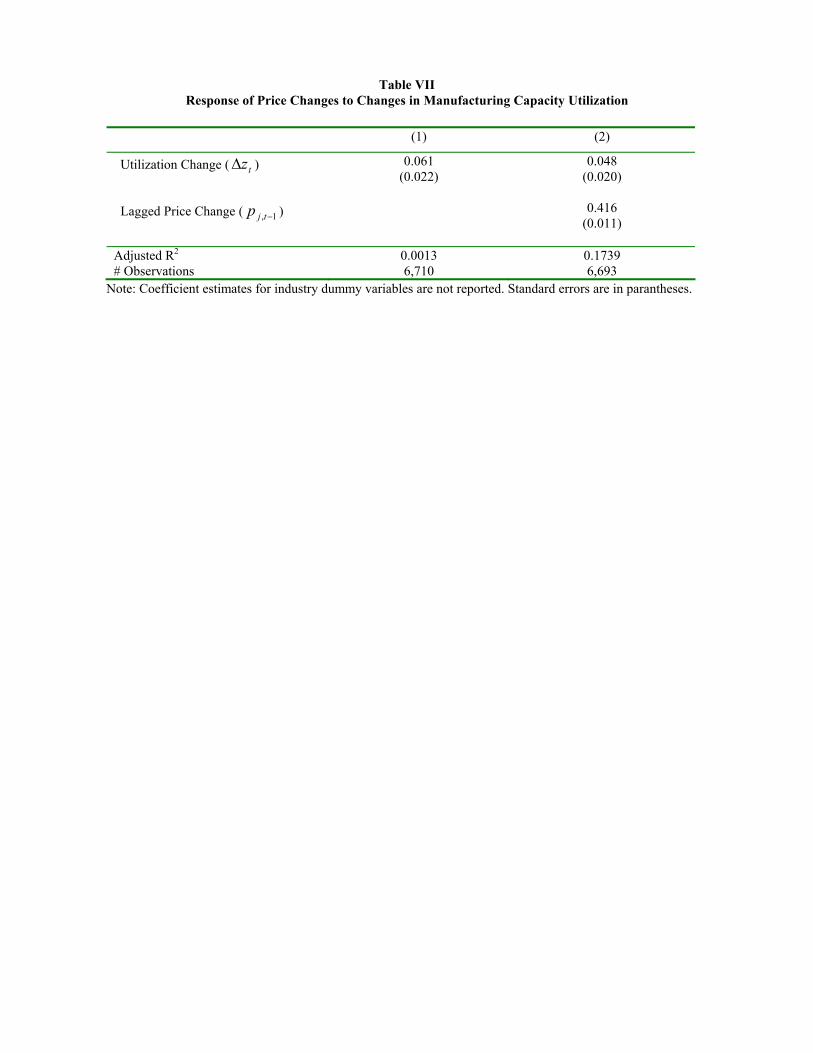
Table VII Response of Price Changes to Changes in Manufacturing Capacity Utilization

(1) (2)

Utilization Change ( tz∆ ) 0.061 (0.022)

0.048 (0.020)

Lagged Price Change ( 1, −tjp ) 0.416

(0.011)

Adjusted R2 # Observations

0.0013 6,710

0.1739 6,693

Note: Coefficient estimates for industry dummy variables are not reported. Standard errors are in parantheses.

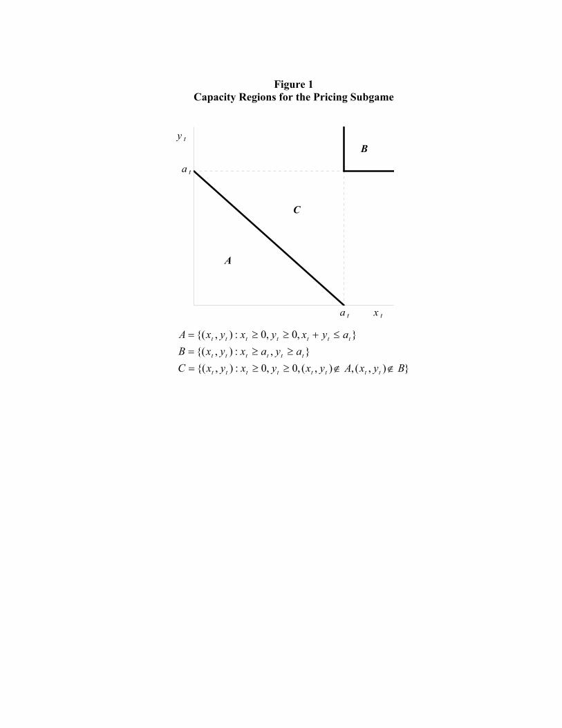
Figure 1 Capacity Regions for the Pricing Subgame

a t

a t

y t

x t

A

C

B

),(,),(,0,0:),(,:),(

,0,0:),(

ByxAyxyxyxCayaxyxB

ayxyxyxA

tttttttt

tttttt

ttttttt

∉∉≥≥=≥≥=

≤+≥≥=

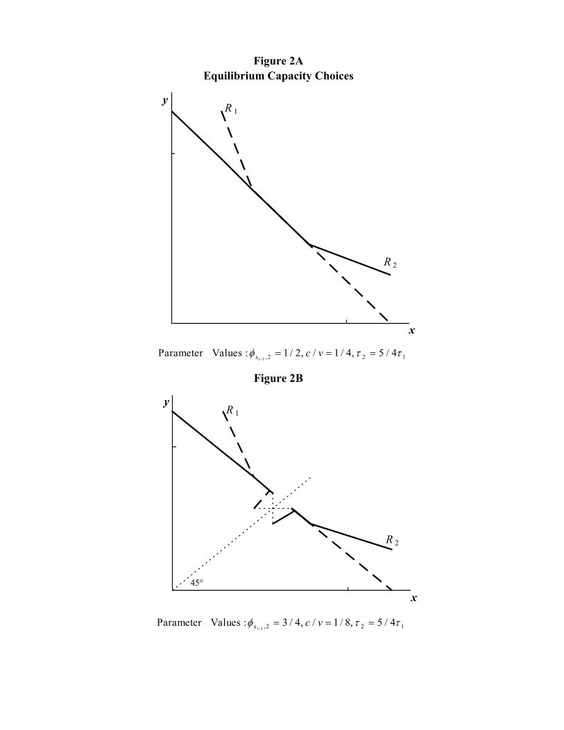
Figure 2AEquilibrium Capacity Choices

Figure 2B

x

yR 1

R 2

x

yR 1

R 2

45°

122,s 4/5 ,8/1/ ,4/3 :Values Parameter 1-t

ττφ === vc

122,s 4/5 ,4/1/ ,2/1 :Values Parameter 1-t

ττφ === vc

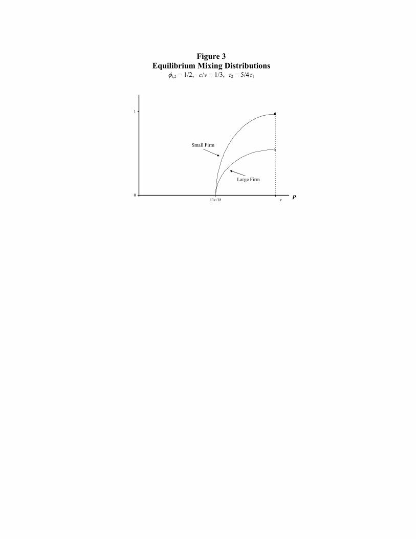
Figure 3 Equilibrium Mixing Distributions

φi,2 = 1/2, c/v = 1/3, τ2 = 5/4τ1

0

1

Pv

Large Firm

Small Firm

13v /18

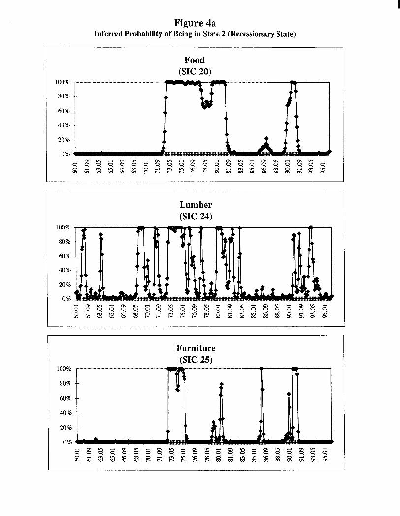
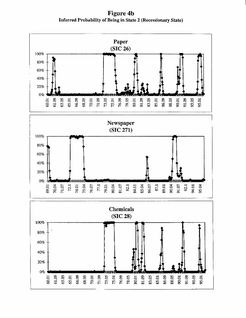
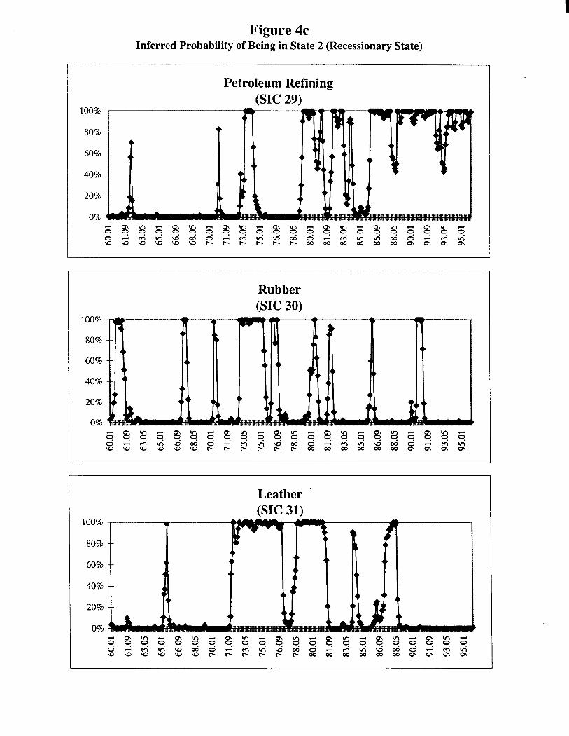
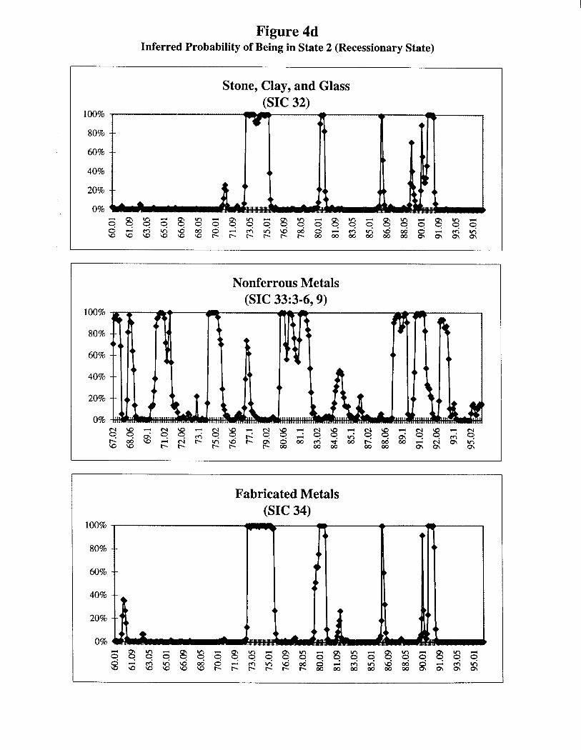
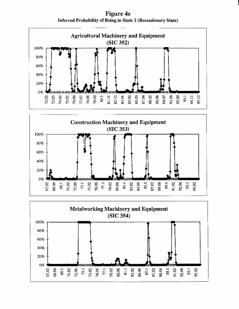
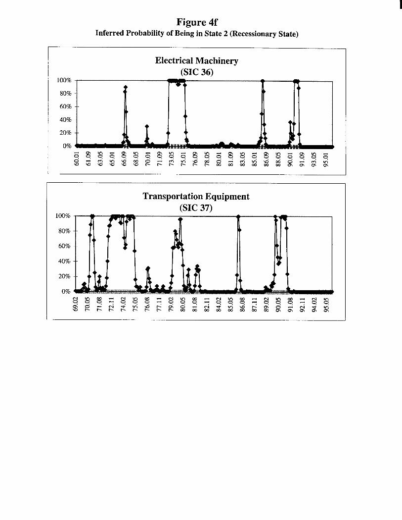
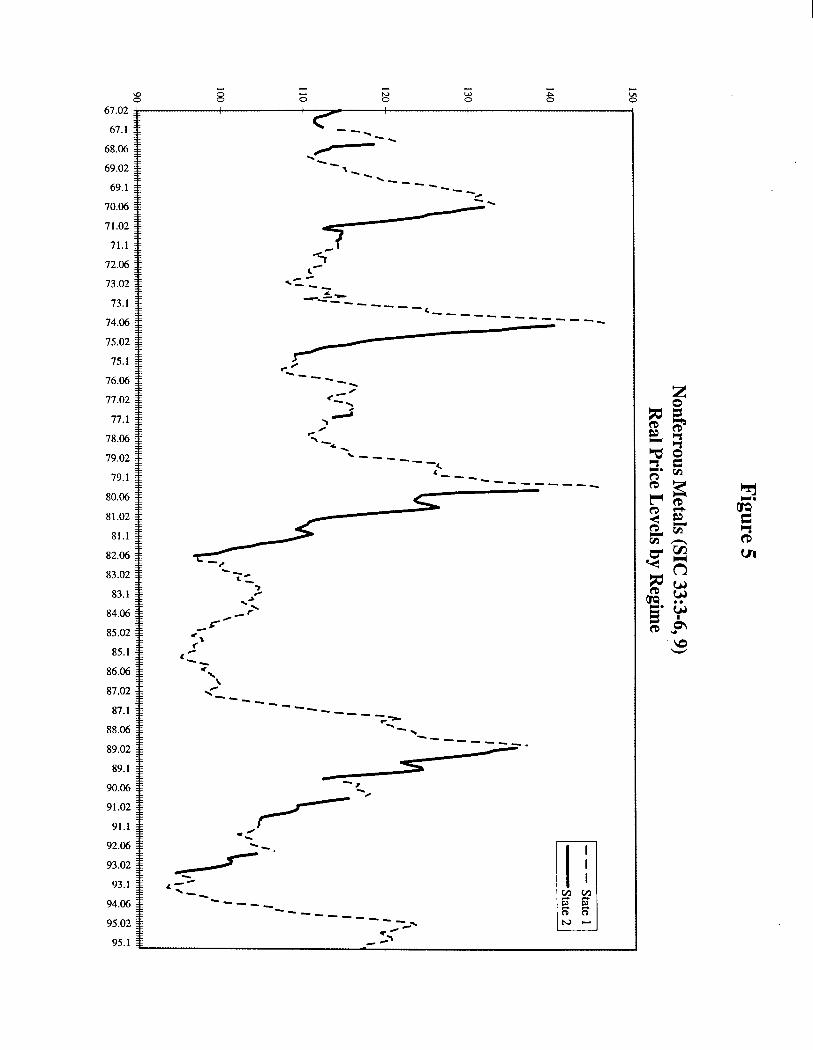
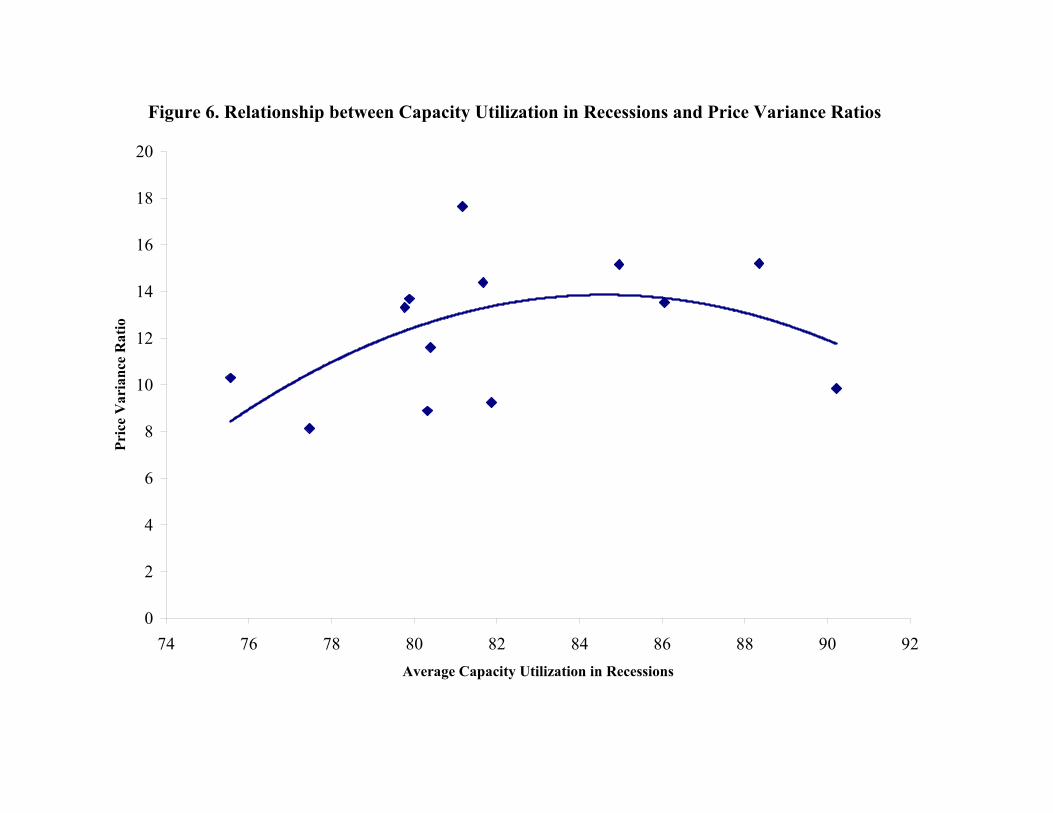
Figure 6. Relationship between Capacity Utilization in Recessions and Price Variance Ratios

0

2

4

6

8

10

12

14

16

18

20

74 76 78 80 82 84 86 88 90 92Average Capacity Utilization in Recessions

Pric

e V

aria

nce

Rat

io

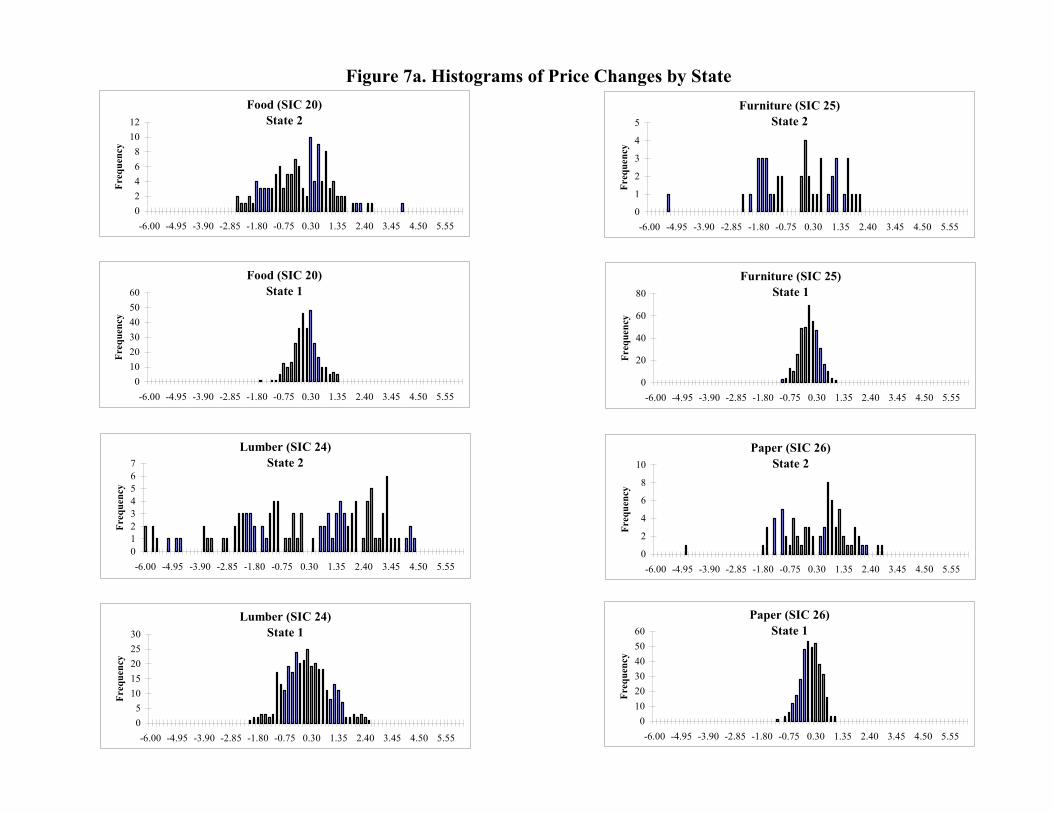
Figure 7a. Histograms of Price Changes by State

Lumber (SIC 24)State 1

05

1015202530

-6.00 -4.95 -3.90 -2.85 -1.80 -0.75 0.30 1.35 2.40 3.45 4.50 5.55

Freq

uenc

y

Lumber (SIC 24)State 2

01234567

-6.00 -4.95 -3.90 -2.85 -1.80 -0.75 0.30 1.35 2.40 3.45 4.50 5.55

Freq

uenc

yFurniture (SIC 25)

State 2

0

1

2

3

4

5

-6.00 -4.95 -3.90 -2.85 -1.80 -0.75 0.30 1.35 2.40 3.45 4.50 5.55

Freq

uenc

y

Furniture (SIC 25)State 1

0

20

40

60

80

-6.00 -4.95 -3.90 -2.85 -1.80 -0.75 0.30 1.35 2.40 3.45 4.50 5.55

Freq

uenc

y

Paper (SIC 26)State 2

0

2

4

6

8

10

-6.00 -4.95 -3.90 -2.85 -1.80 -0.75 0.30 1.35 2.40 3.45 4.50 5.55

Freq

uenc

yPaper (SIC 26)

State 1

0102030405060

-6.00 -4.95 -3.90 -2.85 -1.80 -0.75 0.30 1.35 2.40 3.45 4.50 5.55

Freq

uenc

y

Food (SIC 20)State 2

02468

1012

-6.00 -4.95 -3.90 -2.85 -1.80 -0.75 0.30 1.35 2.40 3.45 4.50 5.55

Freq

uenc

y

Food (SIC 20)State 1

0102030405060

-6.00 -4.95 -3.90 -2.85 -1.80 -0.75 0.30 1.35 2.40 3.45 4.50 5.55

Freq

uenc

y

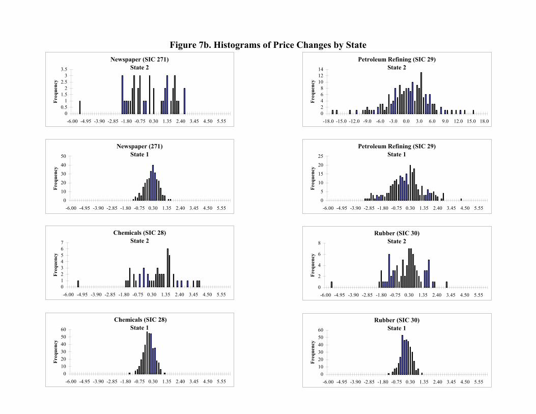
Figure 7b. Histograms of Price Changes by State Newspaper (SIC 271)

State 2

00.5

11.5

22.5

33.5

-6.00 -4.95 -3.90 -2.85 -1.80 -0.75 0.30 1.35 2.40 3.45 4.50 5.55

Freq

uenc

y

Newspaper (271)State 1

0

10

20

30

40

50

-6.00 -4.95 -3.90 -2.85 -1.80 -0.75 0.30 1.35 2.40 3.45 4.50 5.55

Freq

uenc

y

Chemicals (SIC 28)State 2

01234567

-6.00 -4.95 -3.90 -2.85 -1.80 -0.75 0.30 1.35 2.40 3.45 4.50 5.55

Freq

uenc

y

Chemicals (SIC 28)State 1

0102030405060

-6.00 -4.95 -3.90 -2.85 -1.80 -0.75 0.30 1.35 2.40 3.45 4.50 5.55

Freq

uenc

yPetroleum Refining (SIC 29)

State 2

02468

101214

-18.0 -15.0 -12.0 -9.0 -6.0 -3.0 0.0 3.0 6.0 9.0 12.0 15.0 18.0

Freq

uenc

y

Petroleum Refining (SIC 29)State 1

0

5

10

15

20

25

-6.00 -4.95 -3.90 -2.85 -1.80 -0.75 0.30 1.35 2.40 3.45 4.50 5.55

Freq

uenc

y

Rubber (SIC 30)State 2

0

2

4

6

8

-6.00 -4.95 -3.90 -2.85 -1.80 -0.75 0.30 1.35 2.40 3.45 4.50 5.55

Freq

uenc

yRubber (SIC 30)

State 1

0102030405060

-6.00 -4.95 -3.90 -2.85 -1.80 -0.75 0.30 1.35 2.40 3.45 4.50 5.55

Freq

uenc

y

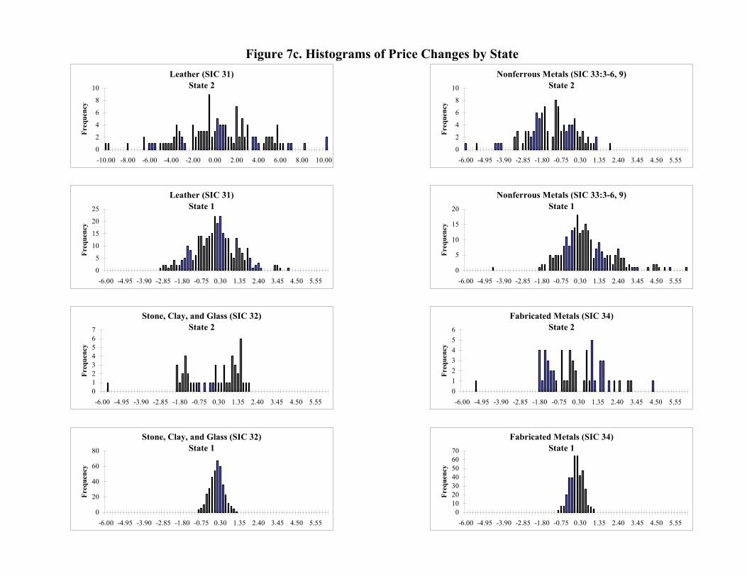
Figure 7c. Histograms of Price Changes by State Leather (SIC 31)

State 2

0

2

4

6

8

10

-10.00 -8.00 -6.00 -4.00 -2.00 0.00 2.00 4.00 6.00 8.00 10.00

Freq

uenc

y

Leather (SIC 31)State 1

0

5

10

15

20

25

-6.00 -4.95 -3.90 -2.85 -1.80 -0.75 0.30 1.35 2.40 3.45 4.50 5.55

Freq

uenc

y

Stone, Clay, and Glass (SIC 32)State 2

01234567

-6.00 -4.95 -3.90 -2.85 -1.80 -0.75 0.30 1.35 2.40 3.45 4.50 5.55

Freq

uenc

y

Stone, Clay, and Glass (SIC 32)State 1

0

20

40

60

80

-6.00 -4.95 -3.90 -2.85 -1.80 -0.75 0.30 1.35 2.40 3.45 4.50 5.55

Freq

uenc

yNonferrous Metals (SIC 33:3-6, 9)

State 2

0

2

4

6

8

10

-6.00 -4.95 -3.90 -2.85 -1.80 -0.75 0.30 1.35 2.40 3.45 4.50 5.55

Freq

uenc

y

Nonferrous Metals (SIC 33:3-6, 9)State 1

0

5

10

15

20

-6.00 -4.95 -3.90 -2.85 -1.80 -0.75 0.30 1.35 2.40 3.45 4.50 5.55

Freq

uenc

y

Fabricated Metals (SIC 34)State 2

0123456

-6.00 -4.95 -3.90 -2.85 -1.80 -0.75 0.30 1.35 2.40 3.45 4.50 5.55

Freq

uenc

yFabricated Metals (SIC 34)

State 1

010203040506070

-6.00 -4.95 -3.90 -2.85 -1.80 -0.75 0.30 1.35 2.40 3.45 4.50 5.55

Freq

uenc

y

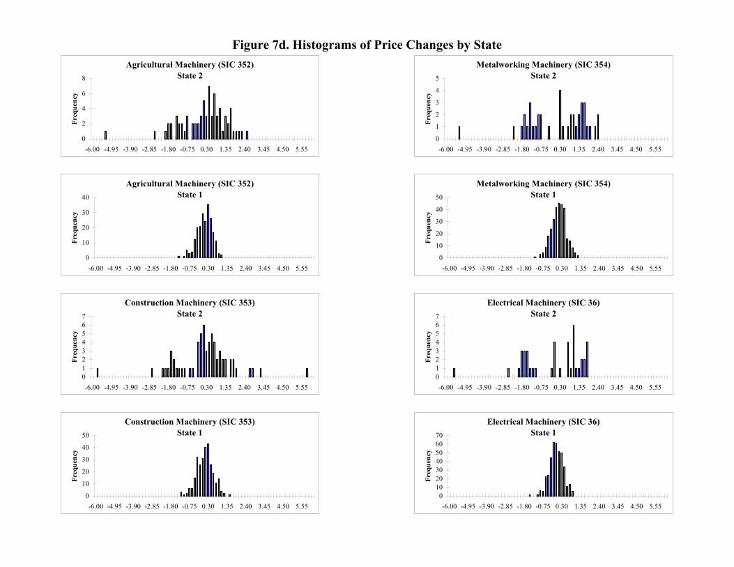
Figure 7d. Histograms of Price Changes by State Agricultural Machinery (SIC 352)

State 2

0

2

4

6

8

-6.00 -4.95 -3.90 -2.85 -1.80 -0.75 0.30 1.35 2.40 3.45 4.50 5.55

Freq

uenc

y

Agricultural Machinery (SIC 352)State 1

0

10

20

30

40

-6.00 -4.95 -3.90 -2.85 -1.80 -0.75 0.30 1.35 2.40 3.45 4.50 5.55

Freq

uenc

y

Construction Machinery (SIC 353)State 2

01234567

-6.00 -4.95 -3.90 -2.85 -1.80 -0.75 0.30 1.35 2.40 3.45 4.50 5.55

Freq

uenc

y

Construction Machinery (SIC 353)State 1

0

10

20

30

40

50

-6.00 -4.95 -3.90 -2.85 -1.80 -0.75 0.30 1.35 2.40 3.45 4.50 5.55

Freq

uenc

yMetalworking Machinery (SIC 354)

State 2

0

1

2

3

4

5

-6.00 -4.95 -3.90 -2.85 -1.80 -0.75 0.30 1.35 2.40 3.45 4.50 5.55

Freq

uenc

y

Metalworking Machinery (SIC 354)State 1

0

10

20

30

40

50

-6.00 -4.95 -3.90 -2.85 -1.80 -0.75 0.30 1.35 2.40 3.45 4.50 5.55

Freq

uenc

y

Electrical Machinery (SIC 36)State 2

01234567

-6.00 -4.95 -3.90 -2.85 -1.80 -0.75 0.30 1.35 2.40 3.45 4.50 5.55

Freq

uenc

yElectrical Machinery (SIC 36)

State 1

010203040506070

-6.00 -4.95 -3.90 -2.85 -1.80 -0.75 0.30 1.35 2.40 3.45 4.50 5.55

Freq

uenc

y

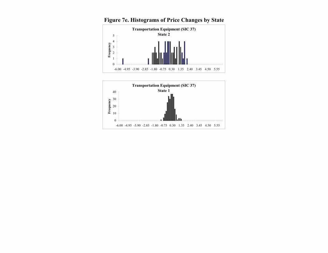
Figure 7e. Histograms of Price Changes by State Transportation Equipment (SIC 37)

State 2

0

1

2

3

4

5

-6.00 -4.95 -3.90 -2.85 -1.80 -0.75 0.30 1.35 2.40 3.45 4.50 5.55

Freq

uenc

y

Transportation Equipment (SIC 37)State 1

0

10

20

30

40

-6.00 -4.95 -3.90 -2.85 -1.80 -0.75 0.30 1.35 2.40 3.45 4.50 5.55

Freq

uenc

y