mark trew ct1 2002. halfway down halfway down the stairs is a stair where i sit. there isn't...
TRANSCRIPT

Mark Trew CT1 2002

Mark Trew CT1 2002
Halfway Down Halfway down the stairsIs a stair Where I sit.There isn't any Other stairQuite likeIt.I'm not at the bottom,I'm not at the top;So this is the stairWhere I alwaysStop.
Halfway up the stairs Isn't up,And isn't down.It isn't in the nursery,It isn't in the town.And all sorts of funny thoughtsRun round my head:"It isn't really Anywhere!It's somewhere else instead!"
A.A. Milne

Mark Trew CT1 2002
Interpolation – the ups and Interpolation – the ups and downsdowns

Mark Trew CT1 2002
Interpolation and FittingInterpolation and Fitting
• Discrete datum points obtained by some process
• Provide basis for a description of behaviour at any point
• Description usually in some function form:
• Function can have some physical form based on theoretical behaviour or can be a more general form
• Use interpolation every day, e.g. measurements, weights, solving ODEs etc.
)f(xy or 1,f iii xxxxy

Mark Trew CT1 2002
Interpolation and FittingInterpolation and Fitting•Interpolation vs Fitting – in general:
-Interpolation reproduces datum values at the datum locations
-Fitting seeks to provide the best overall description
• Interpolation vs Extrapolation-Interpolation: unknown value bracketed by known values-Extrapolation: unknown value has known value on one side only
x
y
x
y
Mark Trew CT1 2002
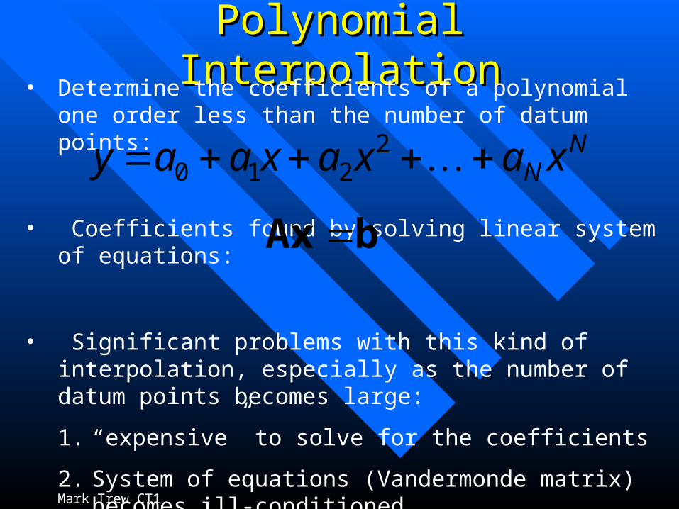
Polynomial InterpolationPolynomial Interpolation• Determine the coefficients of a polynomial one order less than
the number of datum points:
• Coefficients found by solving linear system of equations:
• Significant problems with this kind of interpolation, especially as the number of datum points becomes large:
1. “expensive” to solve for the coefficients
2. System of equations (Vandermonde matrix) becomes ill-conditioned
3. High order polynomials oscillate between points
NN xaxaxaay 2
210
bAx

Mark Trew CT1 2002
Polynomial (and other) FittingPolynomial (and other) Fitting• Polynomials useful for small number of points – at least 3 for a
quadratic
• Can be useful for fitting rather than datum interpolation
• Given polynomial to “reasonable” order, find coefficients such that function is a good representation of data, e.g. minimise the sum of the squared difference between function and datum values (called Least Squares Fit):
• If we have N data points and our polynomial is of order m, how can we solve? The problem is overdetermined.
2
1
2210
N
i
mimiii xaxaxaay
know
don’t know

Mark Trew CT1 2002
Polynomial (and other) FittingPolynomial (and other) Fitting• Problem looks like:
• Two options:
1. Solve the normal equations: ATAa = ATb. Solved by standard LU decomposition, but tend to be badly conditioned and prone to roundoff error.
2. Do a singular value decomposition on A. Naturally finds the solution which is the best least squares approximation.
A= a= b=Aa=b
Mark Trew CT1 2002
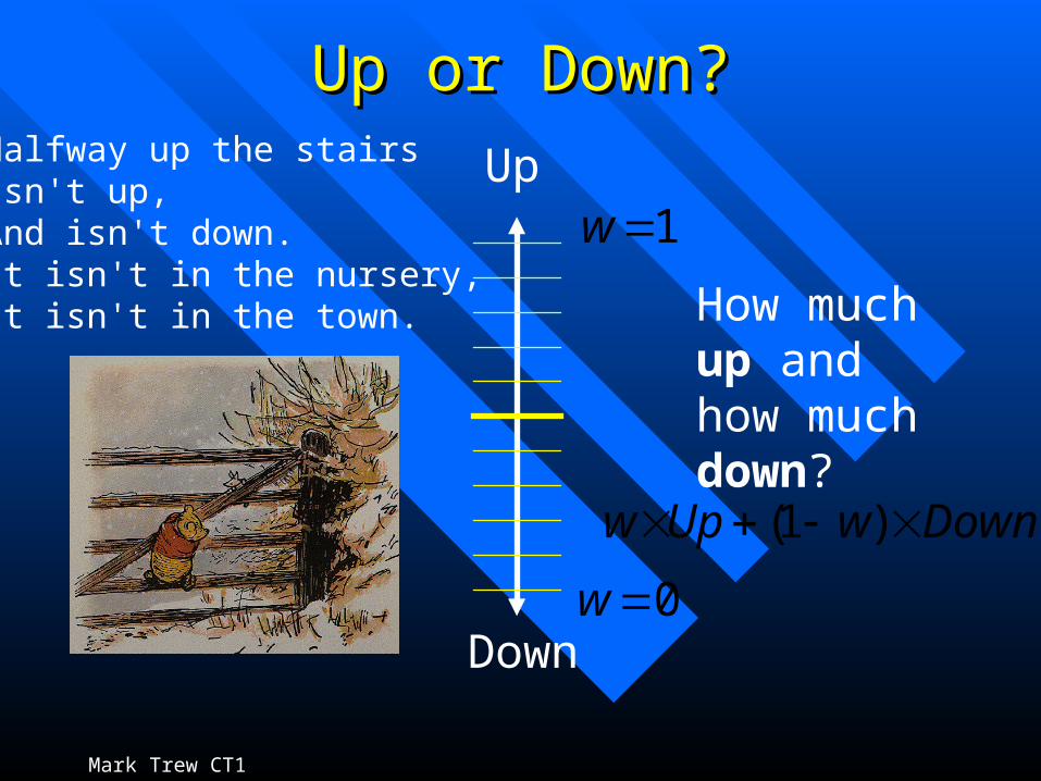
Up or Down?Up or Down?
Up
Down
Halfway up the stairs Isn't up,And isn't down.It isn't in the nursery,It isn't in the town. How much
up and how much down?
DownwUpw )1(
1w
0w

Mark Trew CT1 2002
Lagrangian InterpolationLagrangian Interpolation
• Used for large number of datum points
• Break whole interpolation range into smaller intervals
• Use low order polynomial to interpolate over sub-interval only
• Overcomes problems with high-order polynomial interpolation
x
yentire range
sub-interval

Mark Trew CT1 2002
Linear Lagrange InterpolationLinear Lagrange Interpolation
x
y
sub-interval
• Put a straight line between each pair of points
(xj,yj) (xj+1,yj+1)
yj(x)
11
111
1)(
jjjj
jjj
jj
jj
jj
yLyL
yxx
xxy
xx
xxxy
What form do Lj and Lj+1 take?

Mark Trew CT1 2002
Linear Lagrange InterpolationLinear Lagrange Interpolation
x
x
y
sub-interval
• Put a straight line between each pair of points
(xj,yj) (xj+1,yj+1)
yj(x)
Lj+1
1
xjxj+1
11
111
1)(
jjjj
jjj
jj
jj
jj
yLyL
yxx
xxy
xx
xxxy
11 jj LLImportant!! L act as weighting functions: some of yj and some of yj+1

Mark Trew CT1 2002
Quadratic Lagrange InterpolationQuadratic Lagrange Interpolation
x
y
sub-interval
• Put a quadratic between each triplet of points
(xj-1,yj-1) (xj,yj)
yj(x)
1
1
1111)(j
jiii
jjjjjjj
yL
yLyLyLxy
(xj+1,yj+1)

Mark Trew CT1 2002
Quadratic Lagrange InterpolationQuadratic Lagrange InterpolationLj-1
1
xj-1 xj+1xj
Lj
1
xj-1 xj+1xj
Lj+1
1
xj-1 xj+1xj
?
))((
))((
))((
))((
1
11
11
111
11
j
jjjj
jjj
jjjj
jjj
L
xxxx
xxxxL
xxxx
xxxxL

Mark Trew CT1 2002
Quadratic Lagrange InterpolationQuadratic Lagrange Interpolation
11
1
j
jiiL
Still true?
))((
))((
))((
))((
))((
))((
111
11
11
11
111
11
jjjj
jjj
jjjj
jjj
jjjj
jjj
xxxx
xxxxL
xxxx
xxxxL
xxxx
xxxxL
Check!
L continue to act as weighting functions: some of yj-1, some of yj, and some of yj+1
Mark Trew CT1 2002
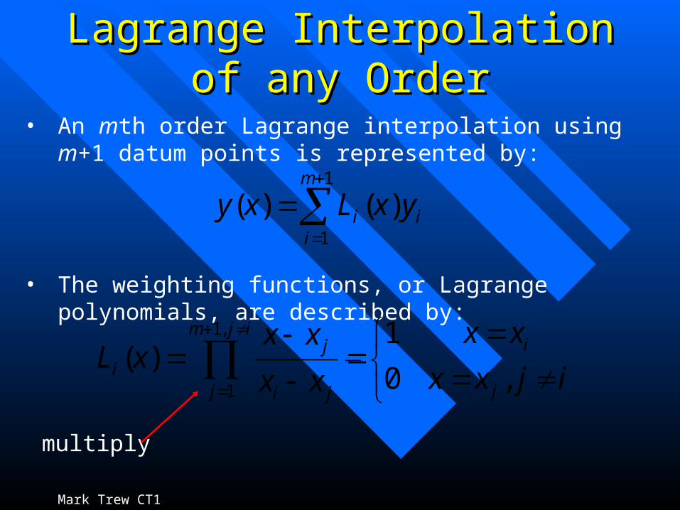
Lagrange Interpolation of any Lagrange Interpolation of any OrderOrder
• An mth order Lagrange interpolation using m+1 datum points is represented by:
• The weighting functions, or Lagrange polynomials, are described by:
1
1
)()(m
iii yxLxy
ijxx
xx
xx
xxxL
j
iijm
j ji
ji ,0
1)(
,1
1
multiply

Mark Trew CT1 2002
Lagrange Interpolation of any Lagrange Interpolation of any OrderOrder
• Always true that:
• A problem with Lagrange interpolation is the lack of slope continuity between the sub-interval (element) boundaries.
1)(1
1
m
ii xL
x
ysub-interval
(xj-1,yj-1) (xj,yj)(xj+1,yj+1)
slope discontinuousNot always important

Mark Trew CT1 2002
Next time…Next time…
Function Function continuity and continuity and Cubic SplinesCubic Splines

Mark Trew CT1 2002
The story The story continues…continues…
Function Function continuity and continuity and Cubic SplinesCubic Splines

Mark Trew CT1 2002
Function ContinuityFunction Continuity
Continuity for Quadratic Function
-10
-5
0
5
10
15
20
25
-5 -3 -1 1 3 5
x
f(x)
, f'(
x),
f''(x
)
f(x)=x^2
f'(x)=2x
f''(x)=2
Continuity for Cubic Function
-125
-75
-25
25
75
125
-5 -3 -1 1 3 5
x
f(x)
, f'(
x),
f''(x
)
f(x)=x^3
f'(x)=3x^2
f''(x)=6x

Mark Trew CT1 2002
Function ContinuityFunction Continuity
Continuity for Quadratic/Cubic Function
-2
-1
0
1
2
3
4
5
6
-1 -0.5 0 0.5 1
x
f(x)
, f'(
x),
f''(x
)
f(x)
f'(x)
f''(x) • C0 continuity – value continuous
• C1 continuity – gradient or slope continuous
• C2 continuity – curvature (2nd derivative) continuous

Mark Trew CT1 2002
Interpolation with Slope Interpolation with Slope ContinuityContinuity
• Four “degrees of freedom” over interval: pj(xj), pj(xj+1), p’j(xj)=kj and p’j(xj+1 )=kj+1
• Four dof can be fitted by a cubic polynomial.
• Gradients may be known at x0 and xN.
• May be reasonable to set p’’=0 at x0 and xN.
x
y sub-interval: j
xj xj+1
yj(x)
• Definitions:kj kj+1
p’’ 0
p’’=0

Mark Trew CT1 2002
Cubic Spline PolynomialCubic Spline Polynomial• General form:
• Spline – from thin rods used by engineers to fit smooth curves through a number of points.
• pj(x) must satisfy: pj(xj)=yj, pj(xj+1)=yj+1, p’j(xj)=kj and p’j(xj+1 )=kj+1
• Two steps to make pj(x) useful. (1) Determine a0 to a3. (2) Determine k values. Two sets of equations necessary.
33
22
210
)(
)()()(
j
jjj
xxa
xxaxxaaxp

Mark Trew CT1 2002
Step 1: Spline CoefficientsStep 1: Spline Coefficients• To satisfy: pj(xj)=yj, p’j(xj)=kj , pj(xj+1)=yj+1 and p’j(xj+1 )=kj+1
1232
133
22
1
0
32
jjj
j
jjjj
jj
j
j
kc
a
c
ak
yc
a
c
a
c
ky
ka
ya
jjj xx
c
1
1

Mark Trew CT1 2002
……some algebra some algebra later…later…

Mark Trew CT1 2002
Step 1: Spline CoefficientsStep 1: Spline Coefficients• Solving for a2 and a3:
• Once the kj values are known, the spline function is determined.
)()(2
)2()(3
12
13
3
112
2
1
0
jjjjjj
jjjjjj
j
j
kkcyyca
kkcyyca
ka
ya

Mark Trew CT1 2002
Step 2: Unknown GradientsStep 2: Unknown Gradients
x
y’’sub-interval: j
xj
p’’j-1(x)
sub-interval: j-1
p’’j(x)
• For cubic in each interval:
• Evaluating the second derivatives:
• Equating the second derivatives:
)2(2)(6)(''
)2(2)(6)(''
112
1112
11
jjjjjjjj
jjjjjjjj
kkcyycxp
kkcyycxp
)('')('' 1 jjjj xpxp
)]()([3
)(2
12
112
1111
jjjjjj
jjjjjjj
yycyyc
kckcckc

Mark Trew CT1 2002
Step 2: Unknown GradientsStep 2: Unknown Gradients• Known or assumed information:
• If k0 and kN are known, there are N-1 points, N-1 unknown k values and N-1 equations.
• Equal number of equations and unknowns.
)]()([3
)(2
12
112
1111
jjjjjj
jjjjjjj
yycyyc
kckcckc
x
y
x0 xN
k0
kN
y’’N-1(xN)=0y’’0(x0)=0N-1 internal points

Mark Trew CT1 2002
Step 2: Unknown GradientsStep 2: Unknown Gradients• If k0 and kN are not known, there are N+1 points, N+1 unknown k values and N-1 equations of the type:
and two equations:
from the condition of zero curvature (p’’=0) at the end-points.
•Still equal number of equations and unknowns.
)]()([3
)(2
12
112
1111
jjjjjj
jjjjjjj
yycyyc
kckcckc
)(642
)(624
12
1111
01201000
NNNNNNN yyckckc
yyckckc

Mark Trew CT1 2002
Step 2: Unknown GradientsStep 2: Unknown Gradients• In both cases, equations are put together into a matrix of linear equations in the unknown k values.
• The system of equations is solved.
• Each row has only 3 non-zero terms – one on either side of the diagonal. Very efficient to solve.
=k

Mark Trew CT1 2002
SummarySummary• Gradient continuous interpolations can be produced using cubic splines.
• Gradients must be known at the extremum points – or assumption of zero curvature can be used.
• System of linear equations solved to give gradients at each discrete point. (Step 2)
• Gradients used to determine coefficents of cubic spline interpolation for each sub-interval. (Step 1)
• Cubic splines can be used to interpolate to x points lying between known discrete points.

Mark Trew CT1 2002
The end…The end…