Complexity change under conformal transformations in AdS3/CFT2

Mario Flory†1, Nina Miekley♦2

†Institute of Physics, Jagiellonian University, Lojasiewicza 11, 30-348 Krakow, Poland

♦Lehrstuhl fur Theoretische Physik III, Institut fur Theoretische Physik und Astrophysik,Julius-Maximilians-Universitat Wurzburg, Am Hubland, D-97074 Wurzburg, Germany

Abstract

Using the volume proposal, we compute the change of complexity of holographic states caused by a smallconformal transformation in AdS3/CFT2. This computation is done perturbatively to second order. We givea general result and discuss some of its properties. As operators generating such conformal transformationscan be explicitly constructed in CFT terms, these results allow for a comparison between holographic methodsof defining and computing computational complexity and purely field-theoretic proposals. A comparison ofour results to one such proposal is given.

1mflory@th.if.uj.edu.pl2nina.miekley@physik.uni-wuerzburg.de

arX

iv:1

806.

0837

6v2

[he

p-th

] 2

2 O

ct 2

018

Contents

1 Introduction 1

2 Gravity setup 3

3 Complexity = Volume 6

4 Examples 9

5 Comparison to field theory ansatz 12

6 Conclusion and outlook 14

A Unitary operator for conformal transformations 16

1 Introduction

Suppose that a scientist in possession of a quantum computer is given a specific task like, for example, applyinga certain operator U to an initial reference state |R〉 in order to obtain the resulting state

|ψU 〉 = U |R〉 . (1)

In [1,2] it was proposed to define the quantum computational complexity (short complexity from here on) of theoperator U by geometric methods, defining a distance measure on the space of unitary operators and equatingthe complexity of U , C(U), as the (minimal) distance between U and the identity operator 1 according to thisdistance function. Equivalently, the complexity of |ψU 〉 with respect to |R〉, C(|ψU 〉 , |R〉), could be definedto be the minimal complexity of any operator U ′ such that |ψU 〉 = U ′ |R〉.3 The idea behind this is that inorder to implement the operation, the programmer of the quantum computer would have to subdivide U intoa product of allowed universal gates that implement the operation step by step, until the end-state agrees withthe desired outcome |ψU 〉 at least within a certain error tolerance. This notion of complexity is meant to countthe minimal number of gates that the programmer would have to utilise even when using an optimal program.This definition of the complexity would hence neccessarily depend on the following explicit or implicit choices(see also [3, 4]):

• A choice of the reference state |R〉, which often is assumed to be a simple product state, without spacialentanglement. This should not be confused with the groundstate |0〉 of a given physical system.

• A choice of the set of allowed gates {µi}, such that the operation can be decomposed as U ≈ µ1µ2µ3...

• ...within a specified error tolerance (in some distance measure between U and µ1µ2µ3).

Starting with [5–7], the idea of computational complexity has begun to see rising interest from the AdS/CFTcommunity. A tentative entry to the holographic dictionary called the volume proposal was proposed andmotivated in [6–10]. According to this, the complexity C of a field theory state with a smooth holographicdual geometry should be measured by the volumes V of certain spacelike extremal co-dimension one bulk

3 U ′ might be equal to U , or it may be a more efficient operator in terms of complexity. Hence C(U) ≥ C(U |ψ〉 , |ψ〉) in general.

hypersurfaces, i.e.

C ∝ VLGN

, (2)

wherein a length scale L has to be introduced into equation (2) for dimensional reasons which is usually pickedto be the AdS scale [9–12].

Interestingly, computational complexity is not the only field theory quantity that has been proposed to beholographically dual to the volumes of extremal co-dimension one hypersurfaces in the bulk. In [13], it wasargued that the volume V of an extremal spacelike co-dimension one hypersurface is approximately dual to aquantity Gλλ called fidelity susceptibility [14, 15] according to the formula

Gλλ = ndVLd, (3)

where nd is an order one factor, L is the AdS radius and d determines the dimension such that the AdS spaceis d+ 1 dimensional. Given two normalised states |ψ(λ)〉 and |ψ(λ+ δλ)〉 depending on one parameter λ, Gλλis defined as4

| 〈ψ(λ)|ψ(λ+ δλ)〉 | = 1−Gλλδλ2 +O(δλ3) (4)

and measures the distance between the two states in a sense, hence it may also be referred to as the quantuminformation metric [16]. The derivation of (3) in [13] (see also [17, 18]) assumed that two states |ψ(λ)〉 and|ψ(λ+ δλ)〉 are the ground states of a theory allowing for a holographic dual, and that the difference δλ isthe result of a perturbation of the Hamiltonian by δλ · O with an exactly marginal operator O. The bulkspacetime dual to this field theory problem is a Janus solution [19, 20], but as shown in [13] this geometrycan be approximated by a simpler spacetime with a probe defect brane embedded into it, leading to (3). Thisproposal has been utilised for holographic calculations in [21–24], and our results concerning changes δV inducedby infinitesimal conformal transformations, to be derived in section 3, may also have an interesting physicalinterpretation from the perspective of fidelity susceptibility, however in this paper we will focus on bulk volumesas a holographic dual to computational complexity.

The necessity to include a lengthscale in the definition (2) of holographic complexity was considered unsat-isfactory by some, and so [11,12] proposed the competing action proposal

C =Aπ~

(5)

wherein A is the bulk action over a certain (co-dimension zero) bulk region, the Wheeler-DeWitt patch.

Both the volume- and action proposals for holographic complexity where subsequently used for a numberof holographic investigations. Specific topics of interest where the boundary terms required to calculate theaction A in (5) correctly [25], the time dependence of complexity [26–31] (especially with respect to the socalled Lloyd’s bound, see however [32,33]), generalisations of holographic complexity to mixed states [4,34–37],RG-flows [24,38], three-dimensional gravity models [39,40] and many others. Interesting connections have beenmade between holographic complexity and kinematic space approaches [37,41] as well as Liouville theory in twodimensions [42–45].5

This amount of progress on the holographic side has also led to increased efforts to provide better and moreconcrete definitions of quantum computational complexity in quantum mechanical or even quantum field theorycontexts [3, 30, 42, 43, 46–52]. However, in the proposals (2) and (5) for holographic complexity calculations itis not clear what the relevant reference state, gate set and error tolerance are to be. If one or both of these

4The name fidelity susceptibility derives from the fact that | 〈ψ(λ)|ψ(λ+ δλ)〉 | is called the fidelity.5Although a comparably young topic, the literature on holographic complexity has indeed grown to a considerable size by know.

We apologize to everyone who feels they where unjustly left out above.

2

proposals for holographic complexity are to be correct, then these choices need to be somehow implicit in theholographic dictionary.

This is the main motivation of our present work: We will, focusing on the volume proposal (2) for now,calculate how the complexity of a given state of a two dimensional conformal field theory (CFT2) with smoothholographic dual changes under a conformal transformation. Such conformal transformations can of course beapplied to any two dimensional CFT, irrespectively of whether the central charge is large or not, or whether theCFT satisfies any other requirement for having a holographic dual. Hence we believe these results will be usefulin the future for comparisons between the holographic and field theory proposals for complexity, and this mayhelp to elucidate the choices of gateset, reference state and error tolerance that are implicit in the holographicproposals.6

The structure of our paper is as follows: In section 2, we will review how to implement a (small) conformaltransformation in AdS3/CFT2. This will provide the general setup of our work and fix the notation. Then,based on the volume proposal (2), we will calculate in section 3 how holographic complexity changes undersmall conformal transformations. A few illustrative examples will be discussed in section 4, and in section 5 wewill investigate which constraints our results imply on the reference state |R〉 in the framework of a field theoryproposal for complexity made in [47]. We close in section 6 with a conclusion and outlook. Some technicaldetails about the implementation of conformal transformations on the field theory side will be presented inappendix A.

Note: While in the final stages of preparing this draft, we became aware of the upcoming paper [54] thatseems to share some common ideas with ours, however approaching the topic from the field theory side.

2 Gravity setup

We consider the vacuum state of a two-dimensional CFT with a classical holographic dual. The bulk geometryis given by AdS3 space which in the Poincare-patch is written as

ds2 =dλ2

4λ2− λdx+ · dx−, (6)

where λ is our radial coordinate and x± = t± x (−∞ < t, x < +∞) are the light-cone coordinates of the fieldtheory. In these coordinates, the boundary of AdS is at λ = ∞ and the Poincare horizon at λ = 0. Placinga cutoff at λ = 1/ε2 (ε → 0), it is possible to holographically calculate the expectation value of the energy-momentum tensor of the boundary CFT by the method of [55], which gives a vanishing result as expected.

Although Einstein-Hilbert gravity in three dimensions is trivial in the sense of having no propoagatingdegrees of freedom, there is a surprising number of vacuum solutions which were derived in [56] (see also [57]).The reason is that these solutions, called Banados geometries, can be derived from (6) by diffeomorphisms whichare global in the sense that they act nontrivially near the boundary, such that while the resulting metric is stillasymptotically AdS in the appropriate sense, the holographic energy-momentum tensor has changed. Despiteall being locally isometric to AdS3 in the bulk, these geometries are hence dual to different states of the dualfield theory.7 In [57], these transformations were hence termed solution generating diffeomorphisms (SGDs),and in this section we will explain these transformations in detail, following the outline and notation of [57].

6 See also [49,53] for recent papers comparing results from the action- and volume-proposal and discussing what they may implyfor a possible field theory definition of complexity.

7These states are generically time dependent, and can for example be used for studies of thermalisation or equilibration processes[58,59]. See also [60–62] for more detailed studies of such Banados geometries.

3

In order to apply a SGD to the geometry described by (6), we perform a coordinate transformation8

λ =λ

G′+(x+)G′−(x−), (7a)

x+ = G+(x+), (7b)

x− = G−(x−). (7c)

The metric in the tilted coordinates is [57]

ds2 =1

4λ2dλ2 − λ dx+ · dx− +

(A+dx

+ +A−dx−)2 +

1

λdλ ·

(A+dx

+ +A−dx−) , (8a)

A± = −1

2

G±′′(x±)

G±′(x±). (8b)

In principle, general relativity is invariant under coordinate transformations. However, these SGDs fall off slowlyat the boundary and are asymptotically non-trivial gauge transformation. The new cutoff is at

λ =1

ε2⇔ λ =

1

ε2G+′(x+)G−′(x−)

, (9)

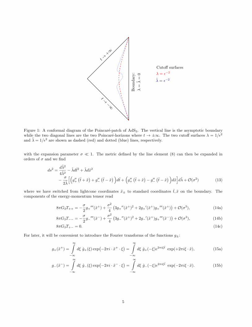
with the field theory UV-cutoff ε. This shows the non-triviality of the coordinate transformation: in terms ofthe old coordinates, the cutoff surface is wrapped and different to the one which describes the vacuum state(i.e. λ = 1/ε2). This is shown in Figure 1.

We started with a CFT state with vanishing energy-momentum tensor. In the deformed state, with thecutoff defined as in (9), we have [57]

8πG3T++ =1

4G+′(x+)2

(3G+

′′(x+)2 − 2G+′(x+)G+

′′′(x+)), (10a)

8πG3T−− =1

4G−′(x−)2(3G−

′′(x−)2 − 2G−′(x−)G−

′′′(x−)), (10b)

8πG3T+− = 0, (10c)

which is precisely what we expect for the change of the energy-momentum tensor after applying a conformaltransformation to the groundstate, see appendix A. The SGDs hence implement conformal transformations onthe boundary theory, which is also evident from the change of the induced metric of the cutoff surface underthese transformations. In field theory terms, the conformal transformation with functions G± hence maps theground state |0〉 to a new state

|ψ(G+, G−)〉 = U(G+)U(G−) |0〉 (11)

with known (commuting) unitary operators U(G+) and U(G−), see [57] and appendix A for an explicit con-struction in the case of a small conformal transformation.

In the following, we consider a small SGD, i.e.

x+ = G+(x+) = x+ + σ g+(x+), (12a)

x− = G−(x−) = x− + σ g−(x−), (12b)

8One virtue of the SGDs formulated in [56] was that they preserved a specific form of the metric tensor. As can be seen fromequation (8), this is not the case for the SGDs as used in [57] and herein. As can be read-off from the holographic energy-momentumtensor (10), both types of SGD implement conformal transformations on the CFT-state. The apparent difference between the SGDscomes merely from the fact that the SGDs of [56] and the corresponding SGDs of [57] differ by a bulk-diffeomorphism that actstrivially at the boundary. We mostly follow the convention and notation of [57] as therein the authors also explicitly discuss how toimplement such SGDs on two-sided black holes and thereby construct an infinite family of purifications of, e.g., the thermal state.We hope to investigate this class of solutions from the viewpoint of holographic complexity in the future.

4

t→+∞

λ = ε−2

t→−∞

λ = ε−2

Bou

nd

ary

:

λ=λ

=0

Cutoff surfaces

Figure 1: A conformal diagram of the Poincare-patch of AdS3. The vertical line is the asymptotic boundarywhile the two diagonal lines are the two Poincare-horizons where t → ±∞. The two cutoff surfaces λ = 1/ε2

and λ = 1/ε2 are shown as dashed (red) and dotted (blue) lines, respectively.

with the expansion parameter σ � 1. The metric defined by the line element (8) can then be expanded inorders of σ and we find

ds2 =dλ2

4λ2− λdt2 + λdx2

− σ

2λ

[(g′′+(t+ x

)+ g′′−

(t− x

) )dt+

(g′′+(t+ x

)− g′′−

(t− x

) )dx]dλ+O(σ2) (13)

where we have switched from lightcone coordinates x± to standard coordinates t, x on the boundary. Thecomponents of the energy-momentum tensor read

8πG3T++ = −σ2g+′′′(x+) +

σ2

4

(3g+

′′(x+)2 + 2g+′(x+)g+

′′′(x+))

+O(σ3), (14a)

8πG3T−− = −σ2g−′′′(x−) +

σ2

4

(3g−

′′(x+)2 + 2g−′(x+)g+

′′′(x−))

+O(σ3), (14b)

8πG3T+− = 0. (14c)

For later, it will be convenient to introduce the Fourier transforms of the functions g±:

g+(x+) =

∞∫−∞

dξ g+(ξ) exp(−2πi · x+ · ξ

)=

∞∫−∞

dξ g+(−ξ)e2πiξt exp(+2πiξ · x), (15a)

g−(x−) =

∞∫−∞

dξ g−(ξ) exp(−2πi · x− · ξ

)=

∞∫−∞

dξ g−(−ξ)e2πiξt exp(−2πiξ · x). (15b)

5

3 Complexity = Volume

In this section we calculate the complexity of states (11) for small conformal transformations (12) using theComplexity=Volume (CV) proposal (2). For this, we have to calculate the maximal volume of a co-dimensionone spacelike slice with fixed boundary conditions, i.e. we have to maximize

V =

∫dλdx

√γ (16)

with the determinant of the induced metric√γ depending on the embedding function t(x, λ). This spacelike

slice is anchored at the boundary at a constant time slice of the coordinates x± = t± x. For a small conformaltransformation, we can expand the embedding9

t(x, λ) =t0 + σt1(x, λ) + σ2t2(x, λ) + ... . (17)

Just as the metric functions (15), we can write the embedding function t1 as an (inverse) Fourier transform

t1(x, λ) =

∞∫−∞

dξ t(ξ, λ) exp(2πiξx). (18)

With (17), we can now expand the integrand of (16) in orders of σ, and the lowest nontrivial order leads toequations of motion for t1(x, λ) of the form

8λ3t1(0,2)

(x, λ

)+ 20λ2t1

(0,1)(x, λ

)+ 2t1

(2,0)(x, λ

)= −g′′+ (x+ t0)− g′′− (t0 − x) , (19a)

8λ3t(0,2)(ξ, λ)

+ 20λ2t(0,1)(ξ, λ)− 8π2ξ2t

(ξ, λ)

= 4π2ξ2(g+(−ξ)e2iπξt0 + g−(ξ)e−2iπξt0

). (19b)

Therefore, we have a second order partial differential equation for the Fourier coefficients t. The boundaryconditions are the fixed behaviour at the asymptotic boundary (i.e. limλ→∞ t1 = 0) and at the Poincare-horizon

at λ = 0 we demand that t1 does not diverge to keep the perturbative expansion meaningful. This wouldmean that the embedding function t1 does not leave the Poincare-patch through one of the null-segments of thePoincare-horizon in figure 1, but instead goes into the corner on the left hand side of the figure.10

Using these conditions to solve (19b), we obtain a piece-wise smooth result11

t(ξ, λ) =

(1

2

(e−2π|ξ|√

λ − 1

)+π|ξ|√λe−2π|ξ|√

λ

)(g−(ξ)e−2iπξt0 + g+(−ξ)e2iπξt0

). (20)

Now, let us turn to the volume. Expanding (16) up to second order in σ, we obtain 12

V = V|σ=0 + σ2V(2) +O(σ3) (21)

9For σ = 0, the metric (13) is just the Poincare metric, and the appropriate embedding for a maximal volume slice anchored toa constant time-slice on the boundary is just given by t = t0.

10One can avoid the problem of having to specify boundary conditions at the Poincare-horizon altogether by mapping the problemto global AdS and solving the equations for the embedding there. Then, it would suffice to give Dirichlet boundary conditions atthe full boundary circle of global AdS.

11In all our calculations, we implicitly assume that integrals are sufficiently well behaved to interchange integration order orintegration and differentiation where necessary, and that the functions g± fall off to zero towards infinity. Note that for all thespecific examples to be discussed in section 4, it is possible to analytically calculate the embedding t1(x, λ) and confirm that theequation (19a) as well as the boundary conditions are satisfied.

12 The first-order term is

V(1) =δVδt

∣∣∣∣σ=0︸ ︷︷ ︸0

·t1 +δVδg±

∣∣∣∣σ=0︸ ︷︷ ︸

0

·g± = 0,

where the first term vanishes because of extremality of the 0th-order embedding in the Poincare-metric. It directly follows fromthis that the second-order term V(2) only depends on the first order terms in the changes of embedding and metric.

6

with

V(2) =

∞∫0

dλ

∞∫−∞

dx

[−

√λ

2t1

(0,1)(x, λ

) (g′′−(t0 − x

)+ g′′+

(t0 + x

))− λ5/2t1(0,1)

(x, λ

)2 −

t1(1,0)

(x, λ

)2

4√λ

], (22a)

=π3

∞∫−∞

dξ |ξ|3(g+(ξ)e−2iπξt0 + g−(−ξ)e2iπξt0

) (g−(ξ)e−2iπξt0 + g+(−ξ)e2iπξt0

), (22b)

=π3

∞∫−∞

dξ |ξ|3∣∣g−(ξ)e−2iπξt0 + g+(−ξ)e2iπξt0

∣∣2 ≥ 0. (22c)

We can already point out the following observations: First of all, we see that the change in complexity ∝ V(2)(see (2)) due to the operators U being applied to the groundstate is always independent of the cutoff ε, i.e. UVfinite.13 Secondly, we find

C(U(g+)U(g−) |0〉 , |R〉) ≥ C(|0〉 , |R〉) (23)

for any g±. So any U(g±) (with small σ) applied on the groundstate |0〉 (described by the Poincare-metric) willonly increase the complexity with respect to the reference state. We hence see that among the geometries (13)in a neighbourhood around the groundstate, the groundstate is the least complex with respect to the referencestate |R〉. This result has an interesting physical interpretation: The operators U only map states with smoothdual geometry to other states with smooth dual geometry. However, it is commonly assumed that the referencestate |R〉 will be a state without spatial entanglement, and such states cannot have a smooth dual geometry [64].So in the total space of states, the states of the form U(g+)U(g−) |0〉 in a neighbourhood of |0〉 form a set inwhich |0〉 locally minimises the complexity with respect to the reference state. See figure 2 for an illustrativesketch of the space of states.

|ψU 〉

|R〉

|0〉U

C(|ψU 〉 , |R〉)

C(|0〉 , |R〉)

Figure 2: The space of states with the reference state |R〉, the groundstate |0〉 and the state |ψU 〉 ≡ U |0〉 forthe generator U of a small conformal transformation. The red dashed lines signify the complexities of the states|ψU 〉 and |0〉 with respect to the reference state |R〉.

The way in which complexity is defined as a distance measure between states can be very abstract and doesnot need to employ a Riemannian metric, for example it may also be based on Finslerian geometry [1, 2]. Infact, although one would commonly assume that for a distance measure D between states φ and ψ the symmetryproperty D(φ, ψ) = D(ψ, φ) has to be satisfied [10], it was suggested in [50] this requirement might have tobe abandoned for definitions of complexity. E.g. one could imagine defining the complexity with respect toa gate-set that includes a given gate, but not its inverse. Then, operators will in general not have the same

13In the terms of [63], the complexity of formation is finite.

7

complexity as their inverse operators. However, from the result (22) it is evident that V(2) is invariant under

g± → −g±, which to first order in σ corresponds to U(g±) → U†(g±), see appendix A. So when applied tothe vacuum state |0〉, the two operators U(g±) and U†(g±) lead (at least to leading order in σ) to a change ofcomplexity by the same amount. This is not true when these operators are applied to generic states.

One of the few kinds of geometric intuition that we can likely rely on when dealing with complexities is thetriangle inequality [1, 2]

C(U(g+)U(g−) |0〉 , |R〉) ≤ C(U(g+)U(g−) |0〉 , |0〉) + C(|0〉 , |R〉), (24)

hence

C(U(g+)U(g−)) ≥ C(U(g+)U(g−) |0〉 , |0〉) ≥ C(U(g+)U(g−) |0〉 , |R〉)− C(|0〉 , |R〉) ∝σ2V(2)LGN

. (25)

So if the proportionality factor in equation (2) could be fixed, our results would lead to quantitative lowerbounds on the complexities of the field theory operators U . However, as we see from (21), the righthand-side ofthe above bound will be of order σ2, while for small σ the change of the state due to the action of U(g±) willbe of order σ, and hence we would intuitively assume that C(U(g+)U(g−)) and C(U(g+)U(g−) |0〉 , |0〉) will beof order σ also. If this is true, the bound of (25) is not very strict. It would be interesting to extend our studiesto operators U being applied to general Banados geometries without the need of taking σ small, however weleave this for the future.

The result (22) can be rewritten suggestively as two time-independent pieces, which only depend on g+ org−, and a time-dependent mixed term

V(2) = V(2),pure(g+) + V(2),pure(g−) + V(2),mixed(g+, g−), (26a)

V(2),pure(g) = π3

∞∫−∞

dξ |ξ|3 · g(−ξ)g(ξ), (26b)

V(2),mixed(g+, g−) = 2π3

∞∫−∞

dξ |ξ|3 · g+(ξ)g−(ξ)e−4iπξt0 . (26c)

The reason why this is interesting is that the energy-momentum tensor of the two-dimensional CFT can beunderstood in terms of left- and right-moving modes. Setting either g+ = 0 or g− = 0 will hence result ina configuration with translational invariance in one of the light-cone coordinates x±. As we integrate overthe spatial direction x to obtain the holographic complexity, the result for the change in complexity will thenbe time-independent and given by either V(2),pure(g+) or V(2),pure(g−) in (26a). If both g± 6= 0, we get atime-dependent result.

The result (26) allows for some general insights into the behaviour of V(2) under simple manipulations of the

functions g±. For example, we find that under rescalings of arguments, g±(x)→ g±(λx)⇔ g±(ξ)→ 1|λ| g±(ξ/λ),

Vpure →λ2Vpure (27a)

Vmixed →λ2Vmixed|t0→λt0 . (27b)

Another interesting thing to look at is what happens under addition of functions g±, as at first order in σthis corresponds to carrying out two small conformal transformations after each other (see appendix A.3). We

8

obtain

V(2),pure(g + f) = V(2),pure(g) + V(2),pure(f) + 2π3

∫dξ|ξ|3g(−ξ)f(ξ) (28a)

V(2),mixed(g+ + f+, g− + f−) = V(2),mixed(g+, g−) + V(2),mixed(f+, f−)

+ V(2),mixed(f+, g−) + V(2),mixed(g+, f−). (28b)

In the next section, we will proceed to pick some illustrative examples of g± which allow for particularlysimple analytical expressions to be derived for t1(x, λ) and V(2).

4 Examples

Example 1

To begin, let us choose14

g+(x+)

=a+c+

a2+ + (x+)2 ⇔ g+(ξ)=c+e

−2a+π|ξ|π (29a)

g−(x−)

=a−c−

a2− + (x−)2 ⇔ g−(ξ)=c−e

−2a−π|ξ|π. (29b)

These functions have the virtue of allowing for comparably simple analytic expressions. Furthermore, they falloff towards infinity like a power law and hence describe wavepackets which are approximately localised, seefigure 3.

-2 -1 0 1 2-2

-1

0

1

2

-4

-2

0

2

4

Figure 3: First order term in σ (as in (14)) of the energy density E(t, x) = T++(t+x) +T−−(t−x) for example1 with a± = c± = 1. This picture can be interpreted in terms of two wavepackets, one moving to the left andone moving to the right at the speed of light.

14For simplicity of notation, we will drop the tildes over the coordinates in this section.

9

For the first order correction to the embedding in (17), we find

t1(x, λ) =c−2√λ((t0 − x)2 − a2−

)− λa−

(a2− − 3(t0 − x)2

)− a−

2(a2− + (t0 − x)2

) (2a−√λ+ λ

(a2− + (t0 − x)2

)+ 1)

2

+ c+2√λ((t0 + x)2 − a2+

)− λa+

(a2+ − 3(t0 + x)2

)− a+

2(a2+ + (t0 + x)2

) (2a+√λ+ λ

(a2+ + (t0 + x)2

)+ 1)

2(30)

and the correction to the volume is given by

V(2) =c2+ ·3π

64a4++ c2− ·

3π

64a4−+

c−c+(a+ + a−)4

·3π(16t4a − 24t2a + 1

)2 (4t2a + 1) 4

with ta =t0

a+ + a−, (31)

which nicely displays the structure derived in (26a). The mixed term V(2),mixed is shown in figure 4.

Example 2

Using instead

g+(x+)

= − c+x+

a2+ + (x+)2 ⇔ g+(ξ)=− ic+e−2a+π|ξ|πsgn(ξ) (32a)

g−(x−)

= − c−x−

a2− + (x−)2 ⇔ g−(ξ)=− ic−e−2a−π|ξ|πsgn(ξ), (32b)

we obtain the embedding

t1(x, λ) =− c−(t0 − x)

(−4a−

√λ+ λ

(−3a2− + (t0 − x)2

)− 1)

2(a2− + (t0 − x)2

) (2a−√λ+ λ

(a2− + (t0 − x)2

)+ 1)

2

− c+(t0 + x)

(−4a+

√λ+ λ

(−3a2+ + (t0 + x)2

)− 1)

2(a2+ + (t0 + x)2

) (2a+√λ+ λ

(a2+ + (t0 + x)2

)+ 1)

2(33)

and the volume change

V(2) =c2+ ·3π

64a4++ c2− ·

3π

64a4−− c−c+

(a+ + a−)4·

3π(16t4a − 24t2a + 1

)2 (4t2a + 1) 4

with ta =t0

a+ + a−. (34)

Interestingly, this is identical to the result (31) up to a sign change in the term V(2),mixed(g+, g−). See figure 4for a plot of this quantity.

Interestingly, we see that V(2),mixed(g+, g−) → 0 as t0 → ±∞. The physical reason for this appears to bethat the wavepackages of left and right moving modes propagate away from each other in this limit and haveincreasingly little overlap due to the falloff of the functions g±(x±) on a constant time slice. The larger theseparation of these wavepackages, the less they influence each other, and in the limit t0 → ±∞ the change incomplexity V(2) becomes the sum of the complexity changes due to each individual wavepackage:

limt0→±∞

V(2) → V(2),pure(g+) + V(2),pure(g−). (35)

Another noteworthy feature of the time-dependent contribution is that+∞∫−∞V(2),mixed(g+, g−)dt0 = 0, which is a

generic consequence of (26c) for sufficiently well-behaved g±. This means that the time-average of V(2) is alsogiven by the sum on the right-hand side of (35).

10

-1.0 -0.5 0.5 1.0

-2

-1

1

2

3

4

5

Figure 4: Plot of the term V(2),mixed(g+, g−) for example 1, respectively −V(2),mixed(g+, g−) for example 2. Fort0 → ±∞, V(2),mixed(g+, g−)→ 0.

These additivity properties are interesting in the light of the axiom G3 proposed in [47], which qualitativelystates that the sum of the complexity of two independent tasks should be the sum of the complexities of eachindividual task. For non-zero functions g±, the conformal transformation on the CFT state is implemented bythe two commuting operators U(g+) ≡ UL and U(g−) ≡ UR, as there are two copies of the Virasoro algebra.By G3 of [47], we would hence expect

C(ULUR) = C(UL) + C(UR). (36)

However, due to the triangle inequality (24) and the inequality explained in footnote 3, this does not translatedirectly into a statement about the complexities of the states ULUR |0〉, so the fact that the additivity of (35)does not hold for finite times is not inconsistent.

Example 3

As a final example, we may look at

g+(x+)

=c+x

+

a2+ + (x+)2 ⇔ g+(ξ)=ic+e

−2a+π|ξ|πsgn(ξ) (37a)

g−(x−)

=a−c−

a2− + (x−)2 ⇔ g−(ξ)=c−e

−2a−π|ξ|π, (37b)

which yields

V(2) =c2+ ·3π

64a4++ c2− ·

3π

64a4−− c−c+

(a+ + a−)4·

12πta(1− 4t2a

)(4t2a + 1) 4

with ta =t0

a+ + a−(38)

The time-dependent part V(2),mixed(g+, g−) of this expression is plotted in figure 5. As before, this quantityvanishes in the limit t0 → ±∞.

11

-1.0 -0.5 0.5 1.0

-4

-2

2

4

Figure 5: V(2),mixed(g+, g−) for example 3.

5 Comparison to field theory ansatz

In this section, we will compare our results to a field-theory complexity proposal made in ArXiv version 1 of [47]and [65]. There, it was proposed that axiomatic complexity between two pure states |ψ1〉 and |ψ2〉 could bedefined via their fidelity as

C (ψ1, ψ2) = −2 ln(| 〈ψ1|ψ2〉 |). (39)

Irrespectively of whether this proposal is the correct result for the field theory dual of holographic complexity(see the discussion in [47, 65]), we will use (39) as an easy to work with model for field theory complexity, andwe will derive the non-trivial constraints on the reference state |R〉 that our results of section 3 imply whentaken together with (39).

First of all, for small σ, we expand the operator generating a conformal transformation as

U(σ) ≈ 1 + σU1 + σ2U2 + ... (40)

with15,

σU1 = L, σ2U2 =1

2L2 + B. (41)

We are implicitly still making the assumption that the functions g±(x±) on which these operators will dependare smooth and well behaved enough to allow for all the manipulations performed in the earlier sections ofthe paper, i.e. for all integrals to converge etc. The operators U1, U2,L and B hence stand for a large familyof operators which are dependent on a choice of functions g±(x±) which is arbitrary to a degree within these

15Where, from appendix A, specifically section A.4, we take

L = σi

2π

∫dx g+(x) · T++(x),

B = −σ2 i

8π

∫∫dx1dx2 g

′+(x1)g+(x2) · T++(x1 + x2).

For these, we have L† = −L, B† = −B.

12

limitations. We can now expand16

〈R|U(σ)|0〉 ≈ 〈R|0〉+ σ 〈R|U1|0〉+ σ2 〈R|U2|0〉 .... (42)

For the fidelity, this then yields

| 〈R|U(σ)|0〉 |2 = 〈R|U(σ)|0〉⟨0|U†(σ)|R

⟩= A0 + σA1 + σ2A2 (43)

with

A0 ≡ 〈R|0〉 〈0|R〉 , (44)

A1 ≡ 〈R|0〉⟨

0|U†1 |R⟩

+ 〈0|R〉 〈R|U1|0〉 , (45)

A2 ≡ 〈R|0〉⟨

0|U†2 |R⟩

+ 〈0|R〉 〈R|U2|0〉+⟨

0|U†1 |R⟩〈R|U1|0〉 . (46)

Plugging this into (39), we find

C (U(σ) |0〉 , |R〉) = − log(| 〈R|U(σ)|0〉 |2

)≈ − log

(A0 + σA1 + σ2A2

)≈ − log(A0)− σA1

A0+ σ2

(1

2

(A1

A0

)2

− A2

A0

)(47)

.

We are now in a position to compare (47) to our results obtained in the earlier sections assuming theholographic volume proposal (2). Most importantly, (21) seems to show that the first order term −σ 2B1

B0should

vanish in (47). However, if (39) is to hold in the case of a continuum field theory, we have to be careful aboutthe appearance of the UV cutoff ε� 1. Holography shows [36]

C (|0〉 , |R〉) ∼ 1

ε� 1. (48)

We argued that complex phases should not affect the value of complexity, and this is certainly true in theproposal (39). So without loss of generality, we can choose the complex phase of |R〉 such that

| 〈R|0〉 | = 〈R|0〉 = 〈0|R〉 = e−12C(|0〉,|R〉) ∼ e

−12ε . (49)

Due to the exponentiation in the last step, it is conceivable that some of the terms in (47) might not vanish,but still be nonperturbatively small, and might hence not be captured by a holographic calculation as done inthe previous sections. However, the vanishing of the first order term in (47) is not only implied by (21), butalso by the general expectation that the complexity change due to U or the inverse U† being applied to theground state |0〉 should be identical, at least up to second order (see section 3 and also [47]). We hence obtain

A1

A0≡ 0⇔ Re

(〈0|R〉 〈R|U1|0〉〈0|R〉 〈R|0〉

)≡ 0 (50)

This is the first and most important condition on the reference state |R〉 that we derive in this section. It shouldhold for any sufficiently well behaved choice of g±(x±), and hence represents an entire class of restrictions onthe reference state.

16Here we explicitly assume that the reference state |R〉 is a pure state. This might not be necessarily true, we thank Keun-Young Kim for discussions on this issue, see also [47]. In the main results of this section, such as (50) for example, we can howeverre-generalise to a mixed reference state by making the replacement |R〉 〈R| → ρR.

13

We now turn our attention to the second order term in (47):

A21

2A20

− A2

A0(51)

Assuming (50), this simplifies to

−A2

A0= −2 Re

(〈0|R〉 〈R|U2|0〉〈0|R〉 〈R|0〉

)+

⟨0|U†1 |R

⟩〈R|U1|0〉

〈0|R〉 〈R|0〉

=−2 Re (〈0|R〉 〈R|U2|0〉) + | 〈R|U1|0〉 |2

〈0|R〉 〈R|0〉(52)

As argued above, we expect the complexity change induced by acting on the groundstate with

U ≈ 1 + L︸︷︷︸≡σU1

+B +1

2L2︸ ︷︷ ︸

≡σ2U2

+... (53)

to be identical to the complexity change induced by acting on the groundstate with

U† ≈ 1 −L︸︷︷︸≡σU1

−B +1

2L2︸ ︷︷ ︸

≡σ2U2

+... . (54)

This implies

2 Re

(〈0|R〉

⟨R|B + 1

2L2|0⟩

〈0|R〉 〈R|0〉

)+| 〈R|L|0〉 |2

〈0|R〉 〈R|0〉≡ 2 Re

(〈0|R〉

⟨R| − B + 1

2L2|0⟩

〈0|R〉 〈R|0〉

)+| 〈R| − L|0〉 |2

〈0|R〉 〈R|0〉(55)

⇔ Re

(〈0|R〉 〈R|B|0〉〈0|R〉 〈R|0〉

)≡ 0 (56)

As the condition (50) is supposed to hold for any reasonable choice of function g±, and as otherwise thetwo operators L and B have a similar structure (see appendix A), (56) actually follows from (50). Reversingthe above reasoning, (55) is hence implied by (50), too. Consequently, the second order term in the complexitychange only depends on the term ∼ L2 in the expansion of the operator to second order, and not the term ∼ B,as may have been anticipated from the discussion in section 3.

Consequently, in (52), the positivity of our result (22) and its independence of the UV cutoff imply

−2 Re

(〈0|R〉

⟨R|1

2L2|0

⟩)≥ | 〈R|L|0〉 |2, (57)

2 Re

(〈0|R〉

⟨R|1

2L2|0

⟩)+ | 〈R|L|0〉 |2 ∼ −e−C(|0〉,|R〉). (58)

These appear to be non-trivial conditions on the reference state |R〉. We leave it for future research toinvestigate these conditions and the possible reference states that satisfy them in more detail.

6 Conclusion and outlook

To summarise: Based on the volume proposal (2) for holographic complexity, and the solution generatingdiffeomorphisms explained in section 2 for small σ, we have calculated explicit and general formulas (22), (26)

14

for how holographic complexity changes when such transformations are applied to the ground state in section 3.We have also pointed out a number of nontrivial analytic properties of these expressions, such as the formulasfor scaling (27) and the addition (28). In section 4, we studied a couple of explicit and analytically solvableexamples which exemplify the generic results of section 3. Also, in (35) we pointed out the interesting propertyof additivity of both the late time results and the time-average of the change in complexity when using conformaltransformations that make use of both copies of the Virasoro group.

The motivation behind our investigations was the idea that if holographic complexity is really a measure ofa field theoretic concept of complexity along the lines explained in section 1, then there have to be some implicitchoices of e.g. gateset or reference state associated with it. When comparing our results to how complexitychanges under small conformal transformations in field theory proposals for complexity, this might help to shedlight on the choices that are implicit in the holographic proposal. We started with some preliminary work in thisdirection in section 5. In this context it is important that, of course, conformal transformations are somethingthat can be studied in any CFT, not only strongly coupled or large c ones with a classical gravity dual. Thisshould make a comparison with field theory results easier in general.

Let us close with an outlook on interesting investigations that may now follow. Firstly, it would obviouslybe of great interest to study how complexity changes under conformal transformations according to the fieldtheory prescriptions of e.g. of [3, 42, 43, 46, 48–50] and compare the results to the ones presented in this paper,as well as continue the work on the proposal of [47,65] started in section 5. Similarly, it would be interesting tocompare these results to similar results that could be gained from the holographic action proposal (5). This isalready work in progress.

Secondly, another worthwhile direction may be to study the effect of (infinitesimal) conformal transforma-tions on subregions of the dual CFT2. When acting with such a transformation on the groundstate, the resultingenergy-momentum tensor (10) will necessarily violate the null energy condition (NEC) somewhere. This is notproblematic, as in holography the dual field theory is a quantum field theory, and it is well known that quantumeffects can lead to a violation of the NEC. In fact holography has been used as a tool to study such NECviolations on the boundary in the past. Now, out of phyiscal intuition, it might be interesting to ask whethersubregions in which the NEC is violated have a larger or lower complexity than similarly sized and shaped onesin which the average energy is positive.

Thirdly, one could holographically calculate the complexities of the states corresponding to the two sidedblack holes studied in [57], i.e. BTZ black holes to which a solution generating diffeomorphism was applied onone or both of its sides. This way one generates an infinite set of purifications of the thermal state, of whichthe well known thermofield-double state is only one example. One might then ask: Which of these states isthe optimal purification of the thermal state in the sense of having minimal complexity, and what makes thispurification special?

We leave these interesting questions, as well as many others, for future research.

Acknowledgements

We would like to thank the following people for useful discussions: Dmitry Ageev, Martin Ammon, AndreyBagrov, Ralph Blumenhagen, Pawel Caputa, Johanna Erdmenger, Federico Galli, Haye Hinrichsen, RomualdJanik, Keun-Young Kim, Javier Magan, Charles Melby-Thompson, Rene Meyer, Max Riegler, Alvaro Veliz-Osorio and Runqiu Yang.

MF was supported by the Polish National Science Centre (NCN) grant 2017/24/C/ST2/00469. We wouldalso like to thank the Max Planck Institute for Physics and the Galileo Galilei Institute for Theoretical Physicsfor the hospitality and the INFN for partial support during the completion of this work.

15

A Unitary operator for conformal transformations

In this appendix we will review how the unitary operators implementing conformal transformations in equation(11) can be explicitly constructed in terms of field theory operators, specifically in terms of the Virasorogenerators Ln. For this, we will follow the perturbative approach of appendix E of [57] and extend it to secondorder.

A.1 Conformal maps

Let us start by considering a compact spatial direction, i.e. x ∈ [0, `]. The usual coordinates for radial quanti-sation are

w = exp

(i2π

`· x+

), (59a)

w = exp

(i2π

`· x−

). (59b)

In the following, we demand |w| = 1 ⇔ w† = w−1 to ensure x± ∈ R. The energy-momentum tensor in theseradial coordinates is17

T (w) =∑n

Lnw−n−2, (60a)

and in the light-cone coordinates18

T++ = −4π2

`2(w2T (w) + const.

). (60b)

This expression has to be real, yielding the condition L†n = L−n for the Virasoro generators Ln, which satisfythe well known algebra

[Lm, Ln] = (m− n)Lm+n +c

12(m3 −m)δm+n,0 (61a)

[Ln, c] = 0 (61b)

where c is the central charge. A small conformal transformation in radial coordinates is

w → w′ = w + ε(w). (62)

and similarly for w. The function ε can be written as Fourier decomposition

ε =∑n

εnw−n+1. (63)

Since x′+ has to be real as well, we need to demand

ε∗n = −ε−n +

∞∑n1=−∞

ε−n1· εn1−n +O(ε)3 (64)

which is the extension of the result of [57] to second order.

17Of course, this is only the chiral part of the energy-momentum tensor, similar relations hold for the anti-chiral part T (w).18The const. is related to the Casimir energy on the cylinder. Note however that later we will send `→∞.

16

A.2 Conformal transformations

Under a conformal transformation, the energy-momentum tensor transforms as

T (w′) =

(∂w′

∂w

)−2 (T (w)− c

12S(w′, w)

), (65)

where S(w′, w) is the Schwarzian derivative

S(w′, w) =

(∂3w′

∂w3

)(∂w′

∂w

)−1− 3

2

(∂2w′

∂w2

)2(∂w′

∂w

)−2. (66)

Our goal is to explicitly construct an operator U(ε) that generates this transformation to second order in ε. Inorder to do this, we calculate the change of the energy-momentum tensor to be

δT (w) ≡T (w)− T (w) (67a)

=− ε(w)T ′(w)− 2T (w)ε′(w)− 1

12cε(3)(w)

+1

12cε(4)(w)ε(w) +

1

8cε′′(w)2 +

1

4cε(3)(w)ε′(w) +

1

2ε(w)2T ′′(w)

+ 3ε(w)T ′(w)ε′(w) + 2T (w)ε(w)ε′′(w) + 3T (w)ε′(w)2, (67b)

where the second line is the first order result also found in [57]. At the same time, we have δT (w) ≡∑n δLnw

−n−2 and consequently

δLk =∑n

εn [Lk, L−n] +1

2

∑m,n

εnεm [L−n, [L−m, Lk]] +∑m,n

n+m− 2

4εnεm [Lk, L−n−m] +O(ε)3, (68a)

!= U†LkU − Lk. (68b)

Defining L ≡∑n εnL−n, the first order result of [57] was U(ε) = eL up to terms of order O(ε2). The

second term we obtain in (68a) also arises from this form of U as is obvious from the formula eXY e−X =Y + [X,Y ] + 1

2 [X, [X,Y ]] + ... . However, we have to include a correction which produces the third term. So forthe form of U(ε) including terms of order O(ε2), we make the ansatz

U(ε) = eL+B (69)

where B is an operator of O(ε2). Examining (68) yields

B =∑m,n

m+ n− 2

4εmεnL−n−m. (70)

Let us perform some consistency checks. For U to be unitary, B has to satisfy

(L+ B)†

= −L− B +O(ε)3, (71)

which (70) does, using (64). Furthermore, we require that the inverse conformal transformation yields theinverse unitary operator. Calculating the inverse transformation yields

w = w′ + εinv.(w′), εinv.n = −εn +1

2

∑n1

εn1εn−n1(2− n) +O(ε)3. (72)

The subleading terms arise since εinv. is expanded with respect to w′ and not w. This resulting condition is

U(εinv.) = U(ε)† = e−L−B. (73)

17

B is quadratic in ε and hence identical up to second order for ε and εinv.. Therefore, this consistency conditioncan also be used to determine B, yielding the same result as obtained in (70).

This determines U(ε) in (69) up to terms of orderO(ε3)19 and up to a possible complex phase shift B → B+iβ(β ∈ R), as equation (68a) only depends on commutators of B. This will play a role in the next section.

A.3 Products

What happens if we do two conformal transformations ε(1,2) after each other? It should be possible to writethis as one conformal transformation

w′ = w + ε(1)(w) (74a)

w′′ = w′ + ε(2)(w′) ≡ w + ε(3)(w) (74b)

ε(3)(w) = ε(1)(w) + ε(2)(w + ε(1)(w))

= ε(1)(w) + ε(2)(w) + ε(2)′(w)ε(1)(w) +O(ε3). (74c)

Consequently, we obtain

ε(3)m = ε(1)m + ε(2)m +∑n

(1− n)ε(1)m−nε

(2)n . (75)

Using the Baker-Campbell-Hausdorff formula

eXeY = eZ , Z = X + Y +1

2[X,Y ] +

1

12[X, [X,Y ]] + ... (76)

it is possible to show that indeed

U(ε(3)) ≈ U(ε(2))U(ε(1)) (77)

up to terms of order O(ε3) and up to an ε-dependent complex phase that is proportional to the central chargec and stems from the commutator [L(ε(1)),L(ε(2))].

There are a few comments about this in order. First of all, in the previous subsection we noted that therequirement that the operators U(ε) in (69) generate conformal transformations (67a) does not fix an overallcomplex phase of these operators, so we might define an entire equivalence class of operators (all equal upto a complex phase) and say that each such equivalence class generates the same conformal transformation.This means that the operators U(ε) form a projective representation of the Virasoro group. Acting withsuch operators on a state like |0〉 would then determine the resulting state only up to a complex phase. Forour purposes, this is sufficient, as we assume that states that differ only by a complex phase have the samecomplexity [10].20 Upon inspecting equation (4), the reader will also notice that fidelity susceptibility wouldnot depend on an overall complex phase of one of the states either.

A more formal treatment of the operators U(ε), taking care of the extra phases introduced by the centralcharge c 6= 0 would have to take into account the Bott-cocycle as outlined in [66].

19We see that for a small SGD these operators are simple in the sense of [32].20I.e. we assume physical states to be defined modulo overall phase. From the holographic perspective, this also makes sense as

we could try to take a state with a holographic dual and reconstruct its bulk geometry from data about entanglement entropiesof subregions. This reconstruction will not depend on the overall phase, so neither should other geometrical probes that can becalculated from the reconstructed bulk.

18

A.4 Real space

Let us return to our previous notation. The conformal transformation induced by the SGD is

x+ = G+(x+) = x+ + σ g+(x+) (78)

Comparison with (59a) and (62) yields the identification

exp

(−σ 2πi

`· g+

)= 1 +

ε

w. (79)

The Fourier decomposition of g+ is

g+ =∑n

g+,nw′−n, (80a)

g∗+,n = g+,−n. (80b)

Here we have to be careful: The Fourier decomposition of ε is with respect to w, whereas the Fourier decom-position of g+ is with respect to w′. This produces an additional contribution when expressing εn in terms ofg+,n. Up to second order in g+, we obtain

ε

w≈ −σ 2πi

`· g+ − σ2 2π2

`2· g2+, (81a)

εn ≈ −σ2πi

`g+,n + σ2 2(n− 1)π2

`2

∑n1

g+,n1g+,n−n1

. (81b)

Expressing the previous results in terms of g+ yields

δLm = −σ 2πi

`

∑n

g+,n[Lm, L−n]− σ2 2π2

`2

∑ni

g+,n1g+,n2

[L−n1, [L−n2

, Lm]]

+ σ2 π2

`2

∑ni

(n1 + n2)g+,n1g+,n2 [Lm, L−n1−n2 ] +O(σ)3 (82a)

U(g+) = 1− σ 2πi

`

∑n

g+,nL−n − σ2 2π2

`2

∑ni

g+,n1g+,n2L−n1L−n2

+ σ2 π2

`2

∑ni

(n1 + n2)g+,n1g+,n2L−n1−n2 +O(σ)3. (82b)

This operator is unitary, keeping in mind that g∗+,n = g+,−n. Now, let us carefully take the limit of an infinitespatial cycle, i.e. `→∞. For that, we define

ξ =n

`, dξ =

1

`. (83)

The expansions in w are Fourier transformations in this limit21

g+(x+) =

∫dξ ` · g+,`ξ︸ ︷︷ ︸

g+(ξ)

exp(−2πi · x+ · ξ

), (84a)

T++(x+) =− 4π2

∫dξ

1

`2` · L`ξ︸ ︷︷ ︸L(ξ)

exp(−2πi · x+ · ξ

). (84b)

21We see that in this limit, the εn are not suitable any more, as they go as g+/` = g+/`2 → 0.

19

The operator we look at consequently is

U(g+) = 1− σ 2πi

∫dξ g+(ξ)L(−ξ)− σ2 2π2

∫∫dξ1dξ2 g+(ξ1)g+(ξ2)L(−ξ1)L(−ξ2)

+ σ2 π2

∫∫dξ1dξ2 (ξ1 + ξ2)g+(ξ1)g+(ξ2)L(−ξ1 − ξ2) +O(σ)3, (85a)

= 1 + σi

2π

∫dx g+(x) · T++(x)− σ2 1

8π2

∫∫dx1dx2 g+(x1)g+(x2) · T++(x1)T++(x2)

− σ2 i

8π

∫∫dx1dx2 g

′+(x1)g+(x2) · T++(x1 + x2) +O(σ)3 (85b)

and similarly for U(g−).

References

[1] M. A. Nielsen, “A geometric approach to quantum circuit lower bounds,” eprint arXiv:quant-ph/0502070(Feb., 2005) , quant-ph/0502070.

[2] M. A. Nielsen, M. R. Dowling, M. Gu, and A. C. Doherty, “Quantum Computation as Geometry,”Science 311 (Feb., 2006) 1133–1135, quant-ph/0603161.

[3] S. Chapman, M. P. Heller, H. Marrochio, and F. Pastawski, “Toward a Definition of Complexity forQuantum Field Theory States,” Phys. Rev. Lett. 120 no. 12, (2018) 121602, arXiv:1707.08582[hep-th].

[4] C. A. Agon, M. Headrick, and B. Swingle, “Subsystem Complexity and Holography,” arXiv:1804.01561

[hep-th].

[5] D. Harlow and P. Hayden, “Quantum Computation vs. Firewalls,” JHEP 06 (2013) 085,arXiv:1301.4504 [hep-th].

[6] L. Susskind, “Butterflies on the Stretched Horizon,” arXiv:1311.7379 [hep-th].

[7] L. Susskind, “Computational Complexity and Black Hole Horizons,” Fortsch. Phys. 64 (2016) 44–48,arXiv:1403.5695 [hep-th]. [Fortsch. Phys.64,24(2016)].

[8] L. Susskind, “Entanglement is not enough,” Fortsch. Phys. 64 (2016) 49–71, arXiv:1411.0690[hep-th].

[9] D. Stanford and L. Susskind, “Complexity and Shock Wave Geometries,” Phys. Rev. D90 no. 12, (2014)126007, arXiv:1406.2678 [hep-th].

[10] L. Susskind and Y. Zhao, “Switchbacks and the Bridge to Nowhere,” arXiv:1408.2823 [hep-th].

[11] A. R. Brown, D. A. Roberts, L. Susskind, B. Swingle, and Y. Zhao, “Holographic Complexity EqualsBulk Action?,” Phys. Rev. Lett. 116 no. 19, (2016) 191301, arXiv:1509.07876 [hep-th].

[12] A. R. Brown, D. A. Roberts, L. Susskind, B. Swingle, and Y. Zhao, “Complexity, action, and blackholes,” Phys. Rev. D93 no. 8, (2016) 086006, arXiv:1512.04993 [hep-th].

[13] M. Miyaji, T. Numasawa, N. Shiba, T. Takayanagi, and K. Watanabe, “Distance between QuantumStates and Gauge-Gravity Duality,” Phys. Rev. Lett. 115 no. 26, (2015) 261602, arXiv:1507.07555[hep-th].

[14] W.-L. You, Y.-W. Li, and S.-J. Gu, “Fidelity, dynamic structure factor, and susceptibility in criticalphenomena,” Phys. Rev. E 76 no. 2, (Aug., 2007) 022101, quant-ph/0701077.

20

[15] W.-L. You and L. He, “Generalized fidelity susceptibility at phase transitions,” Journal of PhysicsCondensed Matter 27 no. 20, (May, 2015) 205601, arXiv:1504.00447 [cond-mat.str-el].

[16] S. L. Braunstein and C. M. Caves, “Statistical distance and the geometry of quantum states,” Phys. Rev.Lett. 72 (1994) 3439–3443.

[17] D. Bak, “Information metric and Euclidean Janus correspondence,” Phys. Lett. B756 (2016) 200–204,arXiv:1512.04735 [hep-th].

[18] A. Trivella, “Holographic Computations of the Quantum Information Metric,” Class. Quant. Grav. 34no. 10, (2017) 105003, arXiv:1607.06519 [hep-th].

[19] D. Bak, M. Gutperle, and S. Hirano, “A Dilatonic deformation of AdS(5) and its field theory dual,”JHEP 05 (2003) 072, arXiv:hep-th/0304129 [hep-th].

[20] D. Bak, M. Gutperle, and S. Hirano, “Three dimensional Janus and time-dependent black holes,” JHEP02 (2007) 068, arXiv:hep-th/0701108 [hep-th].

[21] D. Momeni, M. Faizal, K. Myrzakulov, and R. Myrzakulov, “Fidelity Susceptibility as HolographicPV-Criticality,” Phys. Lett. B765 (2017) 154–158, arXiv:1604.06909 [hep-th].

[22] M. Sinamuli and R. B. Mann, “Geons and the Quantum Information Metric,” Phys. Rev. D96 no. 2,(2017) 026014, arXiv:1612.06880 [hep-th].

[23] S. Banerjee, J. Erdmenger, and D. Sarkar, “Connecting Fisher information to bulk entanglement inholography,” JHEP 08 (2018) 001, arXiv:1701.02319 [hep-th].

[24] M. Flory, “A complexity/fidelity susceptibility g-theorem for AdS3/BCFT2,” JHEP 06 (2017) 131,arXiv:1702.06386 [hep-th].

[25] L. Lehner, R. C. Myers, E. Poisson, and R. D. Sorkin, “Gravitational action with null boundaries,” Phys.Rev. D94 no. 8, (2016) 084046, arXiv:1609.00207 [hep-th].

[26] R.-Q. Yang, “Strong energy condition and complexity growth bound in holography,” Phys. Rev. D95no. 8, (2017) 086017, arXiv:1610.05090 [gr-qc].

[27] A. R. Brown and L. Susskind, “Second law of quantum complexity,” Phys. Rev. D97 no. 8, (2018)086015, arXiv:1701.01107 [hep-th].

[28] D. Carmi, S. Chapman, H. Marrochio, R. C. Myers, and S. Sugishita, “On the Time Dependence ofHolographic Complexity,” JHEP 11 (2017) 188, arXiv:1709.10184 [hep-th].

[29] M. Moosa, “Evolution of Complexity Following a Global Quench,” JHEP 03 (2018) 031,arXiv:1711.02668 [hep-th].

[30] R.-Q. Yang, C. Niu, C.-Y. Zhang, and K.-Y. Kim, “Comparison of holographic and field theoreticcomplexities for time dependent thermofield double states,” JHEP 02 (2018) 082, arXiv:1710.00600[hep-th].

[31] D. S. Ageev, I. Ya. Aref’eva, A. A. Bagrov, and M. I. Katsnelson, “Holographic local quench and effectivecomplexity,” JHEP 08 (2018) 071, arXiv:1803.11162 [hep-th].

[32] W. Cottrell and M. Montero, “Complexity is simple!,” JHEP 02 (2018) 039, arXiv:1710.01175[hep-th].

[33] M. Moosa, “Divergences in the rate of complexification,” Phys. Rev. D97 no. 10, (2018) 106016,arXiv:1712.07137 [hep-th].

21

[34] M. Alishahiha, “Holographic Complexity,” Phys. Rev. D92 no. 12, (2015) 126009, arXiv:1509.06614[hep-th].

[35] O. Ben-Ami and D. Carmi, “On Volumes of Subregions in Holography and Complexity,” JHEP 11 (2016)129, arXiv:1609.02514 [hep-th].

[36] D. Carmi, R. C. Myers, and P. Rath, “Comments on Holographic Complexity,” JHEP 03 (2017) 118,arXiv:1612.00433 [hep-th].

[37] R. Abt, J. Erdmenger, M. Gerbershagen, C. M. Melby-Thompson, and C. Northe, “HolographicSubregion Complexity from Kinematic Space,” arXiv:1805.10298 [hep-th].

[38] P. Roy and T. Sarkar, “Subregion holographic complexity and renormalization group flows,” Phys. Rev.D97 no. 8, (2018) 086018, arXiv:1708.05313 [hep-th].

[39] M. Ghodrati, “Complexity growth in massive gravity theories, the effects of chirality, and more,” Phys.Rev. D96 no. 10, (2017) 106020, arXiv:1708.07981 [hep-th].

[40] M. M. Qaemmaqami, “Complexity growth in minimal massive 3D gravity,” Phys. Rev. D97 no. 2, (2018)026006, arXiv:1709.05894 [hep-th].

[41] R. Abt, J. Erdmenger, H. Hinrichsen, C. M. Melby-Thompson, R. Meyer, C. Northe, and I. A. Reyes,“Topological Complexity in AdS3/CFT2,” Fortsch. Phys. 66 no. 6, (2018) 1800034, arXiv:1710.01327[hep-th].

[42] P. Caputa, N. Kundu, M. Miyaji, T. Takayanagi, and K. Watanabe, “Anti-de Sitter Space fromOptimization of Path Integrals in Conformal Field Theories,” Phys. Rev. Lett. 119 no. 7, (2017) 071602,arXiv:1703.00456 [hep-th].

[43] P. Caputa, N. Kundu, M. Miyaji, T. Takayanagi, and K. Watanabe, “Liouville Action as Path-IntegralComplexity: From Continuous Tensor Networks to AdS/CFT,” JHEP 11 (2017) 097, arXiv:1706.07056[hep-th].

[44] B. Czech, “Einstein Equations from Varying Complexity,” Phys. Rev. Lett. 120 no. 3, (2018) 031601,arXiv:1706.00965 [hep-th].

[45] A. Bhattacharyya, P. Caputa, S. R. Das, N. Kundu, M. Miyaji, and T. Takayanagi, “Path-IntegralComplexity for Perturbed CFTs,” JHEP 07 (2018) 086, arXiv:1804.01999 [hep-th].

[46] R. Jefferson and R. C. Myers, “Circuit complexity in quantum field theory,” JHEP 10 (2017) 107,arXiv:1707.08570 [hep-th].

[47] R.-Q. Yang, Y.-S. An, C. Niu, C.-Y. Zhang, and K.-Y. Kim, “Principles and symmetries of complexity inquantum field theory,” arXiv:1803.01797 [hep-th].

[48] K. Hashimoto, N. Iizuka, and S. Sugishita, “Thoughts on Holographic Complexity and itsBasis-dependence,” Phys. Rev. D98 no. 4, (2018) 046002, arXiv:1805.04226 [hep-th].

[49] A. P. Reynolds and S. F. Ross, “Complexity of the AdS Soliton,” Class. Quant. Grav. 35 no. 9, (2018)095006, arXiv:1712.03732 [hep-th].

[50] R.-Q. Yang, “Complexity for quantum field theory states and applications to thermofield double states,”Phys. Rev. D97 no. 6, (2018) 066004, arXiv:1709.00921 [hep-th].

[51] J. M. MagA¡n, “Black holes, complexity and quantum chaos,” JHEP 09 (2018) 043, arXiv:1805.05839[hep-th].

[52] R. Khan, C. Krishnan, and S. Sharma, “Circuit Complexity in Fermionic Field Theory,”arXiv:1801.07620 [hep-th].

22

[53] Z. Fu, A. Maloney, D. Marolf, H. Maxfield, and Z. Wang, “Holographic complexity is nonlocal,” JHEP 02(2018) 072, arXiv:1801.01137 [hep-th].

[54] P. Caputa and J. M. Magan, “Quantum Computation as Gravity,” arXiv:1807.04422 [hep-th].

[55] V. Balasubramanian and P. Kraus, “A Stress tensor for Anti-de Sitter gravity,” Commun. Math. Phys.208 (1999) 413–428, arXiv:hep-th/9902121 [hep-th].

[56] M. Banados, “Three-dimensional quantum geometry and black holes,” AIP Conf. Proc. 484 no. 1, (1999)147–169, arXiv:hep-th/9901148 [hep-th].

[57] G. Mandal, R. Sinha, and N. Sorokhaibam, “The inside outs of AdS3/CFT2: exact AdS wormholes withentangled CFT duals,” JHEP 01 (2015) 036, arXiv:1405.6695 [hep-th].

[58] M. J. Bhaseen, B. Doyon, A. Lucas, and K. Schalm, “Far from equilibrium energy flow in quantumcritical systems,” arXiv:1311.3655 [hep-th]. [Nature Phys.11,5(2015)].

[59] J. Erdmenger, D. Fernandez, M. Flory, E. Megias, A.-K. Straub, and P. Witkowski, “Time evolution ofentanglement for holographic steady state formation,” JHEP 10 (2017) 034, arXiv:1705.04696[hep-th].

[60] M. M. Sheikh-Jabbari and H. Yavartanoo, “On quantization of AdS3 gravity I: semi-classical analysis,”JHEP 07 (2014) 104, arXiv:1404.4472 [hep-th].

[61] M. M. Sheikh-Jabbari and H. Yavartanoo, “On 3d bulk geometry of Virasoro coadjoint orbits: orbitinvariant charges and Virasoro hair on locally AdS3 geometries,” Eur. Phys. J. C76 no. 9, (2016) 493,arXiv:1603.05272 [hep-th].

[62] M. M. Sheikh-Jabbari and H. Yavartanoo, “Excitation entanglement entropy in two dimensionalconformal field theories,” Phys. Rev. D94 no. 12, (2016) 126006, arXiv:1605.00341 [hep-th].

[63] S. Chapman, H. Marrochio, and R. C. Myers, “Complexity of Formation in Holography,” JHEP 01(2017) 062, arXiv:1610.08063 [hep-th].

[64] N. Bao and G. N. Remmen, “Bulk Connectedness and Boundary Entanglement,” EPL 121 no. 6, (2018)60007, arXiv:1703.00018 [hep-th].

[65] R.-Q. Yang, Y.-S. An, C. Niu, C.-Y. Zhang, and K.-Y. Kim, “Complexity between quantum states inquantum field theory and its applicatons,” to appear; see also ArXiv version 1 of [47] (2018) .

[66] B. Oblak, “Berry Phases on Virasoro Orbits,” JHEP 10 (2017) 114, arXiv:1703.06142 [hep-th].

23