march 2011; revised september 2011 rff dp 11-19 … de...1616 p st. nw washington, dc 20036...
TRANSCRIPT
1616 P St. NW Washington, DC 20036 202-328-5000 www.rff.org
March 2011; revised September 2011 RFF DP 11-19-REV
Fat-Tailed Distributions: Data, Diagnostics, and Dependence
Roger M. Cooke and Daan Nieboer , w i th
Jo lanta Mi s iew icz
DIS
CU
SS
ION
PA
PE
R
Resources for the FutureDepartment of Mathematics, Delft University of Technology
Fat-Tailed Distributions:Data, Diagnostics and Dependence
Roger M. Cooke and Daan Nieboer with a chapter by Jolanta Misiewicz
September 2011Support from US National Science Foundation grant no. 0960865 and comments from
Prof. J. Misiewicz are gratefully acknowledged
2
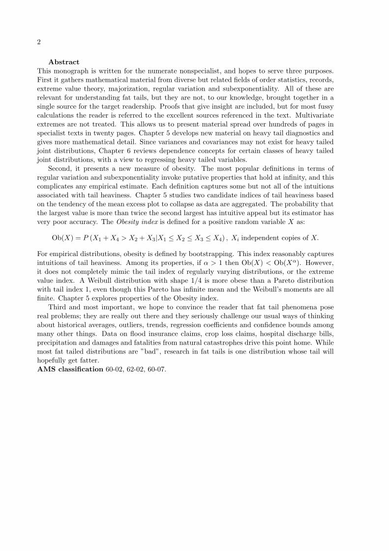
AbstractThis monograph is written for the numerate nonspecialist, and hopes to serve three purposes.First it gathers mathematical material from diverse but related fields of order statistics, records,extreme value theory, majorization, regular variation and subexponentiality. All of these arerelevant for understanding fat tails, but they are not, to our knowledge, brought together in asingle source for the target readership. Proofs that give insight are included, but for most fussycalculations the reader is referred to the excellent sources referenced in the text. Multivariateextremes are not treated. This allows us to present material spread over hundreds of pages inspecialist texts in twenty pages. Chapter 5 develops new material on heavy tail diagnostics andgives more mathematical detail. Since variances and covariances may not exist for heavy tailedjoint distributions, Chapter 6 reviews dependence concepts for certain classes of heavy tailedjoint distributions, with a view to regressing heavy tailed variables.
Second, it presents a new measure of obesity. The most popular definitions in terms ofregular variation and subexponentiality invoke putative properties that hold at infinity, and thiscomplicates any empirical estimate. Each definition captures some but not all of the intuitionsassociated with tail heaviness. Chapter 5 studies two candidate indices of tail heaviness basedon the tendency of the mean excess plot to collapse as data are aggregated. The probability thatthe largest value is more than twice the second largest has intuitive appeal but its estimator hasvery poor accuracy. The Obesity index is defined for a positive random variable X as:
Ob(X) = P (X1 +X4 > X2 +X3|X1 ≤ X2 ≤ X3 ≤ X4) , Xi independent copies of X.
For empirical distributions, obesity is defined by bootstrapping. This index reasonably capturesintuitions of tail heaviness. Among its properties, if α > 1 then Ob(X) < Ob(Xα). However,it does not completely mimic the tail index of regularly varying distributions, or the extremevalue index. A Weibull distribution with shape 1/4 is more obese than a Pareto distributionwith tail index 1, even though this Pareto has infinite mean and the Weibull’s moments are allfinite. Chapter 5 explores properties of the Obesity index.
Third and most important, we hope to convince the reader that fat tail phenomena posereal problems; they are really out there and they seriously challenge our usual ways of thinkingabout historical averages, outliers, trends, regression coefficients and confidence bounds amongmany other things. Data on flood insurance claims, crop loss claims, hospital discharge bills,precipitation and damages and fatalities from natural catastrophes drive this point home. Whilemost fat tailed distributions are ”bad”, research in fat tails is one distribution whose tail willhopefully get fatter.AMS classification 60-02, 62-02, 60-07.
Contents
1 Fatness of Tail 1
1.1 Fat tail heuristics . . . . . . . . . . . . . . . . . . . . . . . . . . . . . . . . . . . . 1
1.2 History and Data . . . . . . . . . . . . . . . . . . . . . . . . . . . . . . . . . . . . 2
1.2.1 US Flood Insurance Claims . . . . . . . . . . . . . . . . . . . . . . . . . . 2
1.2.2 US Crop Loss . . . . . . . . . . . . . . . . . . . . . . . . . . . . . . . . . . 3
1.2.3 US Damages and Fatalities from Natural Disasters . . . . . . . . . . . . . 3
1.2.4 US Hospital Discharge Bills . . . . . . . . . . . . . . . . . . . . . . . . . . 3
1.2.5 G-Econ data . . . . . . . . . . . . . . . . . . . . . . . . . . . . . . . . . . 3
1.3 Diagnostics for Heavy Tailed Phenomena . . . . . . . . . . . . . . . . . . . . . . 3
1.3.1 Historical Averages . . . . . . . . . . . . . . . . . . . . . . . . . . . . . . . 4
1.3.2 Records . . . . . . . . . . . . . . . . . . . . . . . . . . . . . . . . . . . . . 6
1.3.3 Mean Excess . . . . . . . . . . . . . . . . . . . . . . . . . . . . . . . . . . 7
1.3.4 Sum convergence: Self-similar or Normal . . . . . . . . . . . . . . . . . . . 7
1.3.5 Estimating the Tail Index . . . . . . . . . . . . . . . . . . . . . . . . . . . 9
1.3.6 The Obesity Index . . . . . . . . . . . . . . . . . . . . . . . . . . . . . . . 11
1.4 Conclusion and Overview of the Technical Chapters . . . . . . . . . . . . . . . . 15
2 Order Statistics 17
2.1 Distribution of order statistics . . . . . . . . . . . . . . . . . . . . . . . . . . . . . 17
2.2 Conditional distribution . . . . . . . . . . . . . . . . . . . . . . . . . . . . . . . . 19
2.3 Representations for order statistics . . . . . . . . . . . . . . . . . . . . . . . . . . 21
2.4 Functions of order statistics . . . . . . . . . . . . . . . . . . . . . . . . . . . . . . 22
2.4.1 Partial sums . . . . . . . . . . . . . . . . . . . . . . . . . . . . . . . . . . 22
2.4.2 Ratio between order statistics . . . . . . . . . . . . . . . . . . . . . . . . . 23
3 Records 25
3.1 Standard record value processes . . . . . . . . . . . . . . . . . . . . . . . . . . . . 25
3.2 Distribution of record values . . . . . . . . . . . . . . . . . . . . . . . . . . . . . . 25
3.3 Record times and related statistics . . . . . . . . . . . . . . . . . . . . . . . . . . 26
3.4 k-records . . . . . . . . . . . . . . . . . . . . . . . . . . . . . . . . . . . . . . . . 28
4 Regularly Varying and Subexponential Distributions 29
4.0.1 Regularly varying distribution functions . . . . . . . . . . . . . . . . . . . 29
4.0.2 Subexponential distribution functions . . . . . . . . . . . . . . . . . . . . 33
4.0.3 Related classes of heavy-tailed distributions . . . . . . . . . . . . . . . . . 35
4.1 Mean excess function . . . . . . . . . . . . . . . . . . . . . . . . . . . . . . . . . . 35
4.1.1 Properties of the mean excess function . . . . . . . . . . . . . . . . . . . . 35
3
4 CONTENTS
5 Indices and Diagnostics of Tail Heaviness 395.1 Self-similarity . . . . . . . . . . . . . . . . . . . . . . . . . . . . . . . . . . . . . . 39
5.1.1 Distribution of the ratio between order statistics . . . . . . . . . . . . . . 425.2 The ratio as index . . . . . . . . . . . . . . . . . . . . . . . . . . . . . . . . . . . 465.3 The Obesity Index . . . . . . . . . . . . . . . . . . . . . . . . . . . . . . . . . . . 48
5.3.1 Theory of Majorization . . . . . . . . . . . . . . . . . . . . . . . . . . . . 515.3.2 The Obesity Index of selected Datasets . . . . . . . . . . . . . . . . . . . 55
6 Dependence 596.1 Definition and main properties . . . . . . . . . . . . . . . . . . . . . . . . . . . . 596.2 Isotropic distributions . . . . . . . . . . . . . . . . . . . . . . . . . . . . . . . . . 596.3 Pseudo-isotropic distributions . . . . . . . . . . . . . . . . . . . . . . . . . . . . . 62
6.3.1 Covariation as a measure of dependence for essentially heavy tail jointlypseudo-isotropic variables . . . . . . . . . . . . . . . . . . . . . . . . . . . 64
6.3.2 Codifference . . . . . . . . . . . . . . . . . . . . . . . . . . . . . . . . . . . 676.3.3 The linear regression model for essentially heavy tail distribution . . . . . 67
7 Conclusions and Future Research 71
Chapter 1
Fatness of Tail
1.1 Fat tail heuristics
Suppose the tallest person you have ever seen was 2 meters (6 feet 8 inches); someday you maymeet a taller person, how tall do you think that person will be, 2.1 meters (7 feet)? What is theprobability that the first person you meet taller than 2 meters will be more than twice as tall,13 feet 4 inches? Surely that probability is infinitesimal. The tallest person in the world, BaoXishun of Inner Mongolia,China is 2.36 m or 7 ft 9 in. Prior to 2005 the most costly Hurricanein the US was Hurricane Andrew (1992) at $41.5 billion USD(2011). Hurricane Katrina wasthe next record hurricane, weighing in at $91 billion USD(2011)1. People’s height is a ”thintailed” distribution, whereas hurricane damage is ”fat tailed” or ”heavy tailed”. The ways inwhich we reason from historical data and the ways we think about the future are - or shouldbe - very different depending on whether we are dealing with thin or fat tailed phenomena.This monograph gives an intuitive introduction to fat tailed phenomena, followed by a rigorousmathematical treatment of many of these intuitive features. A major goal is to provide adefinition of Obesity that applies equally to finite data sets and to parametric distributionfunctions.
Fat tails have entered popular discourse largely thanks to Nassim Taleb’s book The BlackSwan, the impact of the highly improbable (Taleb [2007]). The black swan is the paradigm shat-tering, game changing incursion from ”extremistan” which confounds the unsuspecting public,the experts, and especially the professional statisticians, all of whom inhabit ”mediocristan”.
Mathematicians have used at least three main definitions of tail obesity. Older texts some-time speak of ”leptokurtic distributions”, that is, distributions whose extreme values are ”moreprobable than normal”. These are distributions with kurtosis greater than zero2, and whosetails go to zero slower than the normal distribution.
Another definition is based on the theory of regularly varying functions and characterizesthe rate at which the probability of values greater than x goes to zero as x → ∞. For alarge class of distributions this rate is polynomial. Unless otherwise indicated, we will alwaysconsider non-negative random variables. Letting F denote the distribution function of randomvariable X, such that F (x) = 1 − F (x) = ProbX > x, we write F (x) ∼ x−α, x → ∞ to
mean F (x)x−α → 1, x → ∞. F (x) is called the survivor function of X. A survivor function with
polynomial decay rate −α, or as we shall say tail index α, has infinite κth moments for allκ > α. The Pareto distribution is a special case of a regularly varying distribution whereF (x) = x−α, x > 1. In many cases, like the Pareto distribution, the κth moments are infinte for
1http://en.wikipedia.org/wiki/Hurricane Katrina, accessed January 28, 20112Kurtosis is defined as the (µ4/σ
4)−3 where µ4 is the fourth central moment, and σ is the standard deviation.Subtracting 3 arranges that the kurtosis of the normal distribution is zero
1
2 CHAPTER 1. FATNESS OF TAIL
all κ ≥ α. Chapter 4 unravels these issues, and shows distributions for which all moments areinfinite. If we are ”sufficiently close” to infinity to estimate the tail indices of two distributions,then we can meaningfully compare their tail heaviness by comparing their tail indices, and manyintuitive features of fat tailed phenomena fall neatly into place.
A third definition is based on the idea that the sum of independent copies X1 +X2+, . . . Xn
behaves like the maximum of X1, X2, . . . Xn. Distributions satisfying
ProbX1 +X2+, · · ·+Xn > x ∼ ProbMaxX1, X2, . . . Xn > x, x → ∞
are called subexponential. Like regular variation, subexponality is a phenomenon that is definedin terms of limiting behavior as the underlying variable goes to infinity. Unlike regular variation,there is no such thing as an ”index of subexponality” that would tell us whether one distributionis ”more subexponential” than another. The set of regularly varying distributions is a strictsubclass of the set of subexponential distributions. Other more exotic definitions are given inchapter 4.
There is a swarm of intuitive notions regarding heavy tailed phenomena that are capturedto varying degree in the different formal definitions. The main intuitions are:
• The historical averages are unreliable for prediction
• Differences between successively larger observations increases
• The ratio of successive record values does not decrease;
• The expected excess above a threshold, given that the threshold is exceeded, increases asthe threshold increases
• The uncertainty in the average of n independent variables does not converge to a normalwith vanishing spread as n → ∞; rather, the average is similar to the original variables.
• Regression coefficients which putatively explain heavy tailed variables in terms of covaritesmay behave erratically.
1.2 History and Data
A colorful history of fat tailed distributions is found in (Mandelbrot and Hudson [2008]). Man-delbrot himself introduced fat tails into finance by showing that the change in cotton priceswas heavy-tailed (Mandelbrot [1963]). Since then many other examples of heavy-tailed distri-butions are found, among these are data file traffic on the internet (Crovella and Bestavros[1997]), returns on financial markets (Rachev [2003], Embrechts et al. [1997]) and magnitudesof earthquakes and floods (Latchman et al. [2008], Malamud and Turcotte [2006]). The web-site http://www.er.ethz.ch/presentations/Powerlaw mechanisms 13July07.pdf gives examples ofearthquake number per 5x5 km grid,wildfires, solar flares, rain events, financial returns, moviesales, health car costs, size of wars, etc etc.
Data for this monograph were developed in the NSF project 0960865, and are availablefrom http : //www.rff.org/Events/Pages/Introduction − Climate − Change − Extreme −Events.aspx, or at public cites indicated below.
1.2.1 US Flood Insurance Claims
US flood insurance claims data from the National Flood Insurance Program (NFIP) are aggre-gated by county and year for the years 1980 to 2008. The data are in 2000 US dollars. Over this
1.3. DIAGNOSTICS FOR HEAVY TAILED PHENOMENA 3
time period there has been substantial growth in exosure to flood risk, particularly in coastalcounties. To remove the effect of growing exposure, the claims are divided by personal incomeestimates per county per year from the Bureau of Economic Accounts (BEA). Thus, we studyflood claims per dollar income, by county and year3.
1.2.2 US Crop Loss
US crop insurance indemnities paid from the US Department of Agriculture’s Risk ManagementAgency are aggregated by county and year for the years 1980 to 2008. The data are in 2000 USdollars. The crop loss claims are not exposure adjusted, as a proxy for exposure is not obvious,and exposure growth is less of a concern.4
1.2.3 US Damages and Fatalities from Natural Disasters
The SHELDUS database, maintained by the Hazards and Vulnerability Research Group at theUniversity of South Carolina, has county-level damages and fatalities from weather events. Infor-mation on SHELDUS is available online: http://webra.cas.sc.edu/hvri/products/SHELDUS.aspx.The damage and fatality estimates in SHELDUS are minimum estimates as the approach to com-piling the data always takes the most conservative estimates. Moreover, when a disaster affectedmany counties, the total damages and fatalities were apportioned equally over the affected coun-ties, regardless of population or infrastructure. These data should therefore be seen as indicativerather than as precise.
1.2.4 US Hospital Discharge Bills
Billing data for hospital discharges for a northeastern US state were collected over the years2000 - 2008. The data is in 2000 USD.
1.2.5 G-Econ data
This uses the G-Econ database (Nordhaus et al. [2006]) showing the dependence of Gross CellProduct (GCP) on geographic variables measured on a spatial scale of one degree. At 45 latitude,a one by one degree grid cell is [45mi]2 or [68km]2. The size varies substantially from equator topole. The population per grid cell varies from 0.31411 to 26,443,000. The Gross Cell Product isfor 1990, non-mineral, 1995 USD, converted at market exchange rates. It varies from 0.000103to 1,155,800 USD(1995), the units are $106. The GCP per person varies from 0.00000354 to0.905, which scales from $3.54 to $905,000. There are 27,445 grid cells. Throwing out zero andempty cells for population and GCP leaves 17,722; excluding cells with empty temperature dataleaves 17,015 cells.
The data are publicly available at http : //gecon.yale.edu/world big.html.
1.3 Diagnostics for Heavy Tailed Phenomena
Once we start looking, we can find heavy tailed phenomena all around us. Loss distributions area very good place to look for tail obesity, but something as mundane as hospital discharge billingdata can also produce surprising evidence. Many of the features of heavy tailed phenomena wouldrender our traditional statistical tools useless at best, dangerous at worst. Prognosticators basepredictions on historical averages. Of course, on a finite sample the average and standard
3Help from Ed Pasterick and Tim Scoville in securing and analysing this data is gratefully acknowledged.4Help from Barbara Carter in securing and analysing this data is gratefully acknowledged.
4 CHAPTER 1. FATNESS OF TAIL
deviation are always finite; but these may not be converging to anything and their value forprediction might be nihil. Or again, if we feed a data set into a statistical regression package, theregression coefficients will be estimated as ”covariance over the variance”. The sample versionsof these quantities always exist, but if they aren’t converging, their ratio could whiplash wildly,taking our predictions with them. In this section, simple diagnostic tools for detecting tailobesity are illustrated on mathematical distributions and on real data.
1.3.1 Historical Averages
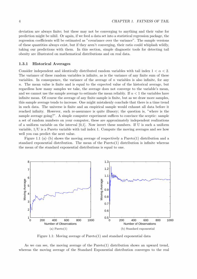
Consider independent and identically distributed random variables with tail index 1 < α < 2.The variance of these random variables is infinite, as is the variance of any finite sum of thesevariables. In consequence, the variance of the average of n variables is also infinite, for anyn. The mean value is finite and is equal to the expected value of the historical average, butregardless how many samples we take, the average does not converge to the variable’s mean,and we cannot use the sample average to estimate the mean reliably. If α < 1 the variables haveinfinite mean. Of course the average of any finite sample is finite, but as we draw more samples,this sample average tends to increase. One might mistakenly conclude that there is a time trendin such data. The universe is finite and an empirical sample would exhaust all data before itreached infinity. However, such re-assurance is quite illusory; the question is, ”where is thesample average going?”. A simple computer experiment suffices to convince the sceptic: samplea set of random numbers on your computer, these are approximately independent realizationsof a uniform variable on the interval [0,1]. Now invert these numbers. If U is such a uniformvariable, 1/U is a Pareto variable with tail index 1. Compute the moving averages and see howwell you can predict the next value.
Figure 1.1 (a)–(b) shows the moving average of respectively a Pareto(1) distribution and astandard exponential distribution. The mean of the Pareto(1) distribution is infinite whereasthe mean of the standard exponential distributions is equal to one.
0 200 400 600 800 10001
2
3
4
5
6
7
8
Number of Observations
Mov
ing
Ave
rage
(a) Pareto(1)
0 200 400 600 800 10000.5
0.6
0.7
0.8
0.9
1
1.1
1.2
1.3
Number of Observations
Mov
ing
Ave
rage
(b) Standard exponential
Figure 1.1: Moving average of Pareto(1) and standard exponential data
As we can see, the moving average of the Pareto(1) distribution shows an upward trend,whereas the moving average of the Standard Exponential distribution converges to the real
1.3. DIAGNOSTICS FOR HEAVY TAILED PHENOMENA 5
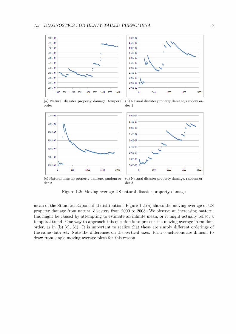
(a) Natural disaster property damage, temporalorder
(b) Natural disaster property damage, random or-der 1
(c) Natural disaster property damage, random or-der 2
(d) Natural disaster property damage, random or-der 3
Figure 1.2: Moving average US natural disaster property damage
mean of the Standard Exponential distribution. Figure 1.2 (a) shows the moving average of USproperty damage from natural disasters from 2000 to 2008. We observe an increasing pattern;this might be caused by attempting to estimate an infinite mean, or it might actually reflect atemporal trend. One way to approach this question is to present the moving average in randomorder, as in (b),(c), (d). It is important to realize that these are simply different orderings ofthe same data set. Note the differences on the vertical axes. Firm conclusions are difficult todraw from single moving average plots for this reason.
6 CHAPTER 1. FATNESS OF TAIL
1.3.2 Records
One characteristic of heavy-tailed distributions is that there are usually a few very large valuescompared to the other values of the data set. In the insurance business this is called the Paretolaw or the 20-80 rule-of-thumb: 20% of the claims account for 80% of the total claim amountin an insurance portfolio. This suggests that the largest values in a heavy tailed data set tendto be further apart than smaller values. For regularly varying distributions the ratio betweenthe two largest values in a data set has a non-degenerate limiting distribution, whereas fordistributions like the normal and exponential distribution this ratio tends to zero as we increasethe number of observations. If we order a data set from a Pareto distribution, then the ratiobetween two consecutive observations also has a Pareto distribution. In Table 1.1 we see the
Number of observations standard normal distribution Pareto(1) distribution
10 0.2343 12
50 0.0102 12
100 0.0020 12
Table 1.1: Probability that the next record value is at least twice as large as the previous recordvalue for different size data sets
probability that the largest value in the data set is twice as large as the second largest value forthe standard normal distribution and the Pareto(1) distribution. The probability stays constantfor the Pareto distribution, but it tends to zero for the standard normal distribution as thenumber of observations increases.
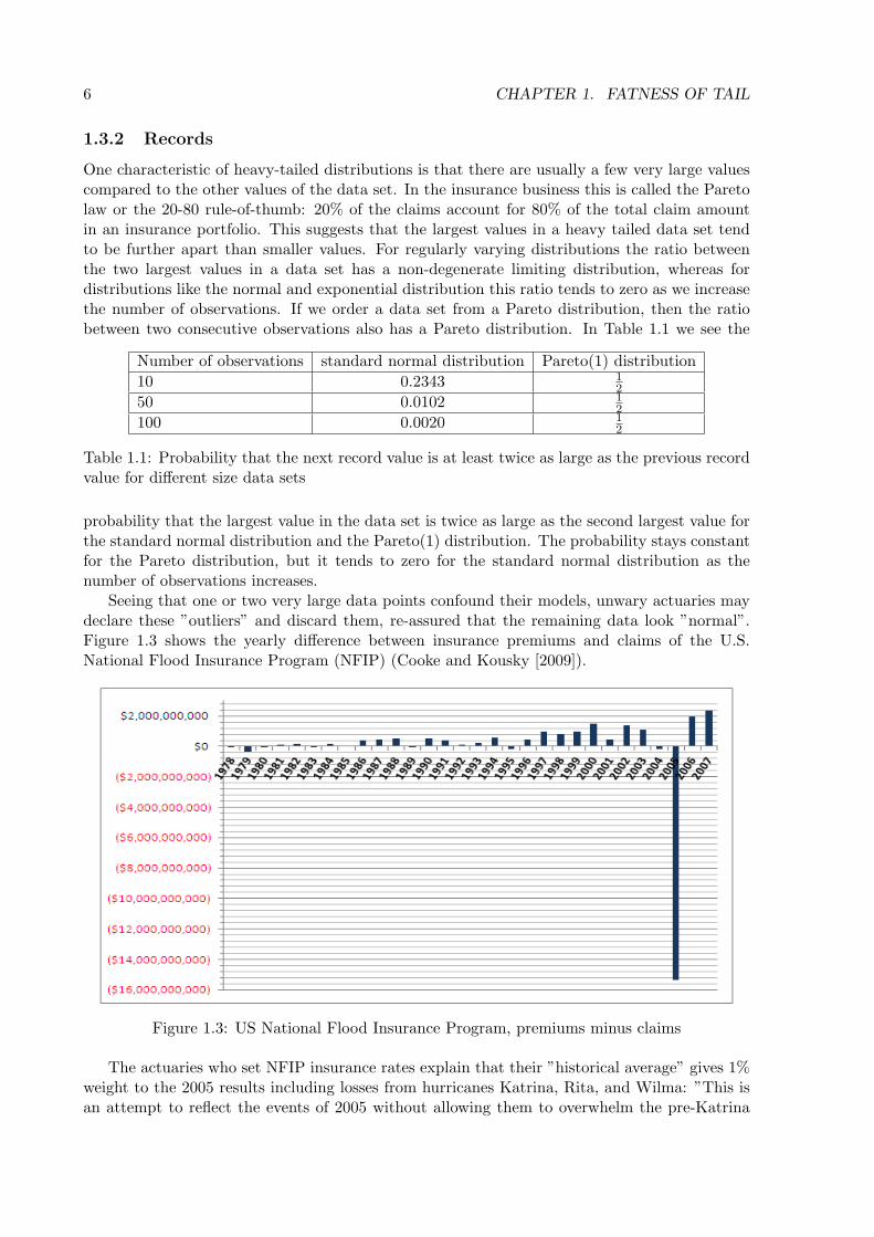
Seeing that one or two very large data points confound their models, unwary actuaries maydeclare these ”outliers” and discard them, re-assured that the remaining data look ”normal”.Figure 1.3 shows the yearly difference between insurance premiums and claims of the U.S.National Flood Insurance Program (NFIP) (Cooke and Kousky [2009]).
Figure 1.3: US National Flood Insurance Program, premiums minus claims
The actuaries who set NFIP insurance rates explain that their ”historical average” gives 1%weight to the 2005 results including losses from hurricanes Katrina, Rita, and Wilma: ”This isan attempt to reflect the events of 2005 without allowing them to overwhelm the pre-Katrina
1.3. DIAGNOSTICS FOR HEAVY TAILED PHENOMENA 7
experience of the Program” (Hayes and Neal [2011] p.6)
1.3.3 Mean Excess
The mean excess function of a random variable X is defined as:
e(u) = E [X − u|X > u] (1.1)
The mean excess function gives the expected excess of a random variable over a certain thresholdgiven that this random variable is larger than the threshold. It is shown in chapter 4 thatsubexponential distributions’ mean excess function tends to infinity as u tends to infinity. Ifwe know that an observation from a subexponential distribution is above a very high thresholdthen we expect that this observation is much larger than the threshold. More intuitively, weshould expect the next worst case to be much worse than the current worst case. It is also shownthat regularly varying distributions with tail index α > 1, have a mean excess function which isultimately linear with slope 1
α−1 . If α < 1, then the slope is infinite and (1.1) is not useful. Ifwe order a sample of n independent realizations of X, we can construct a mean excess plot asin (1.2). Such a plot will not show an infinite slope, rendering the interpretation of such plotsproblematic for very heavy tailed phenomena.
e(xi) =
∑j>i xj − xi
n− i; i < n, e(xn) = 0; x1 < x2 < . . . xn. (1.2)
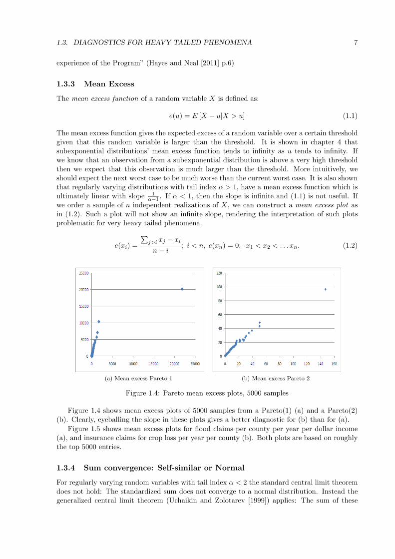
(a) Mean excess Pareto 1 (b) Mean excess Pareto 2
Figure 1.4: Pareto mean excess plots, 5000 samples
Figure 1.4 shows mean excess plots of 5000 samples from a Pareto(1) (a) and a Pareto(2)(b). Clearly, eyeballing the slope in these plots gives a better diagnostic for (b) than for (a).
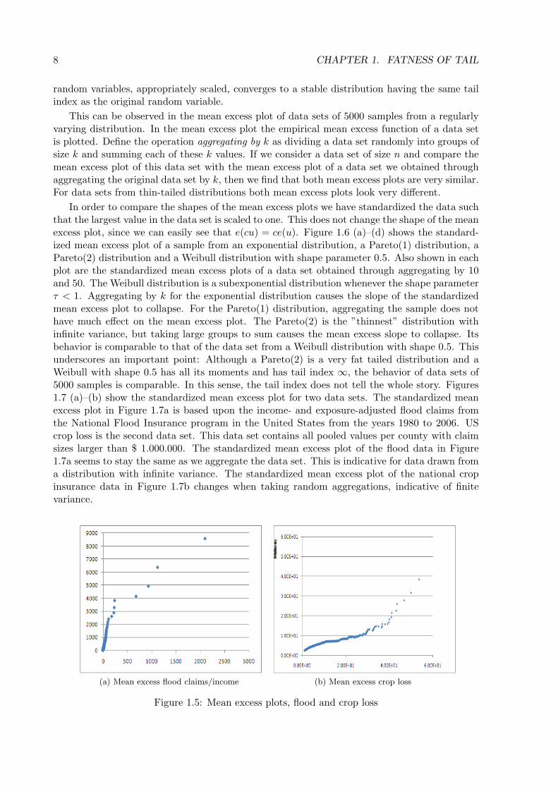
Figure 1.5 shows mean excess plots for flood claims per county per year per dollar income(a), and insurance claims for crop loss per year per county (b). Both plots are based on roughlythe top 5000 entries.
1.3.4 Sum convergence: Self-similar or Normal
For regularly varying random variables with tail index α < 2 the standard central limit theoremdoes not hold: The standardized sum does not converge to a normal distribution. Instead thegeneralized central limit theorem (Uchaikin and Zolotarev [1999]) applies: The sum of these
8 CHAPTER 1. FATNESS OF TAIL
random variables, appropriately scaled, converges to a stable distribution having the same tailindex as the original random variable.
This can be observed in the mean excess plot of data sets of 5000 samples from a regularlyvarying distribution. In the mean excess plot the empirical mean excess function of a data setis plotted. Define the operation aggregating by k as dividing a data set randomly into groups ofsize k and summing each of these k values. If we consider a data set of size n and compare themean excess plot of this data set with the mean excess plot of a data set we obtained throughaggregating the original data set by k, then we find that both mean excess plots are very similar.For data sets from thin-tailed distributions both mean excess plots look very different.
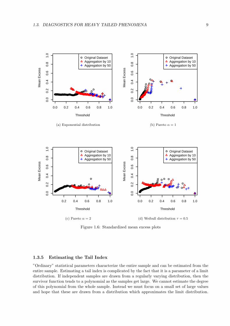
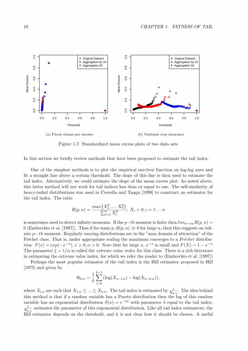
In order to compare the shapes of the mean excess plots we have standardized the data suchthat the largest value in the data set is scaled to one. This does not change the shape of the meanexcess plot, since we can easily see that e(cu) = ce(u). Figure 1.6 (a)–(d) shows the standard-ized mean excess plot of a sample from an exponential distribution, a Pareto(1) distribution, aPareto(2) distribution and a Weibull distribution with shape parameter 0.5. Also shown in eachplot are the standardized mean excess plots of a data set obtained through aggregating by 10and 50. The Weibull distribution is a subexponential distribution whenever the shape parameterτ < 1. Aggregating by k for the exponential distribution causes the slope of the standardizedmean excess plot to collapse. For the Pareto(1) distribution, aggregating the sample does nothave much effect on the mean excess plot. The Pareto(2) is the ”thinnest” distribution withinfinite variance, but taking large groups to sum causes the mean excess slope to collapse. Itsbehavior is comparable to that of the data set from a Weibull distribution with shape 0.5. Thisunderscores an important point: Although a Pareto(2) is a very fat tailed distribution and aWeibull with shape 0.5 has all its moments and has tail index ∞, the behavior of data sets of5000 samples is comparable. In this sense, the tail index does not tell the whole story. Figures1.7 (a)–(b) show the standardized mean excess plot for two data sets. The standardized meanexcess plot in Figure 1.7a is based upon the income- and exposure-adjusted flood claims fromthe National Flood Insurance program in the United States from the years 1980 to 2006. UScrop loss is the second data set. This data set contains all pooled values per county with claimsizes larger than $ 1.000.000. The standardized mean excess plot of the flood data in Figure1.7a seems to stay the same as we aggregate the data set. This is indicative for data drawn froma distribution with infinite variance. The standardized mean excess plot of the national cropinsurance data in Figure 1.7b changes when taking random aggregations, indicative of finitevariance.
(a) Mean excess flood claims/income (b) Mean excess crop loss
Figure 1.5: Mean excess plots, flood and crop loss
1.3. DIAGNOSTICS FOR HEAVY TAILED PHENOMENA 9
0.0 0.2 0.4 0.6 0.8 1.0
0.0
0.2
0.4
0.6
0.8
1.0
Threshold
Mea
n E
xces
s
Original DatasetAggregation by 10Aggregation by 50
(a) Exponential distribution
0.0 0.2 0.4 0.6 0.8 1.0
0.0
0.2
0.4
0.6
0.8
1.0
Threshold
Mea
n E
xces
s
Original DatasetAggregation by 10Aggregation by 50
(b) Pareto α = 1
0.2 0.4 0.6 0.8 1.0
0.0
0.2
0.4
0.6
0.8
1.0
Threshold
Mea
n E
xces
s
Original DatasetAggregation by 10Aggregation by 50
(c) Pareto α = 2
0.0 0.2 0.4 0.6 0.8 1.0
0.0
0.2
0.4
0.6
0.8
1.0
Threshold
Mea
n E
xces
s
Original DatasetAggregation by 10Aggregation by 50
(d) Weibull distribution τ = 0.5
Figure 1.6: Standardized mean excess plots
1.3.5 Estimating the Tail Index
”Ordinary” statistical parameters characterize the entire sample and can be estimated from theentire sample. Estimating a tail index is complicated by the fact that it is a parameter of a limitdistribution. If independent samples are drawn from a regularly varying distribution, then thesurvivor function tends to a polynomial as the samples get large. We cannot estimate the degreeof this polynomial from the whole sample. Instead we must focus on a small set of large valuesand hope that these are drawn from a distribution which approximates the limit distribution.
10 CHAPTER 1. FATNESS OF TAIL
0.0 0.2 0.4 0.6 0.8 1.0
0.0
0.2
0.4
0.6
0.8
1.0
Threshold
Mea
n E
xces
s
Original DatasetAggregation by 10Aggregation 50
(a) Flood claims per income
0.0 0.2 0.4 0.6 0.8 1.0
0.0
0.2
0.4
0.6
0.8
1.0
Threshold
Mea
n E
xces
s
Original DatasetAggregation by 10Aggregation 50
(b) National crop insurance
Figure 1.7: Standardized mean excess plots of two data sets
In this section we briefly review methods that have been proposed to estimate the tail index.
One of the simplest methods is to plot the empirical survivor function on log-log axes andfit a straight line above a certain threshold. The slope of this line is then used to estimate thetail index. Alternatively, we could estimate the slope of the mean excess plot. As noted above,this latter method will not work for tail indices less than or equal to one. The self-similarity ofheavy-tailed distributions was used in Crovella and Taqqu [1999] to construct an estimator forthe tail index. The ratio
R(p, n) =maxXp
1 , . . . Xpn∑n
i=1Xpi
; Xi > 0, i = 1 . . . n
is sometimes used to detect infinite moments. If the p−thmoment is finite then limn→∞R(p, n) =0 (Embrechts et al. [1997]). Thus if for some p,R(p, n) ≫ 0 for large n, then this suggests an infi-nite p−th moment. Regularly varying distributions are in the ”max domain of attraction” of theFrechet class. That is, under appropriate scaling the maximum converges to a Frechet distribu-tion: F (x) = exp(−x−α), x > 0, α > 0. Note that for large x, x−α is small and F (X) ∼ 1− x−α
The parameter ξ = 1/α is called the extreme value index for this class. There is a rich literaturein estimating the extreme value index, for which we refer the reader to (Embrechts et al. [1997])
Perhaps the most popular estimator of the tail index is the Hill estimator proposed in Hill[1975] and given by
Hk,n =1
k
k−1∑i=0
(log(Xn−i,n)− log(Xn−k,n)) ,
where Xi,n are such that X1,n ≤ ... ≤ Xn,n. The tail index is estimated by 1Hk,n
. The idea behind
this method is that if a random variable has a Pareto distribution then the log of this randomvariable has an exponential distribution S(x) = e−λx with parameter λ equal to the tail index.
1Hk,n
estimates the parameter of this exponential distribution. Like all tail index estimators, the
Hill estimator depends on the threshold, and it is not clear how it should be chosen. A useful
1.3. DIAGNOSTICS FOR HEAVY TAILED PHENOMENA 11
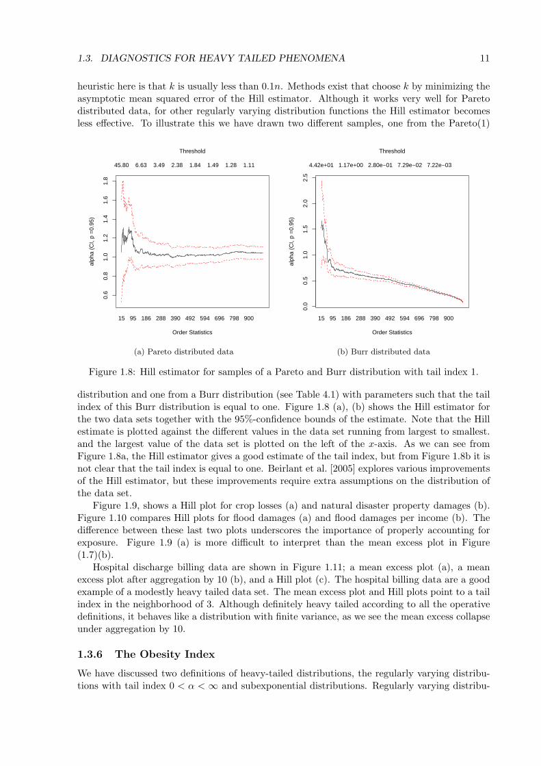
heuristic here is that k is usually less than 0.1n. Methods exist that choose k by minimizing theasymptotic mean squared error of the Hill estimator. Although it works very well for Paretodistributed data, for other regularly varying distribution functions the Hill estimator becomesless effective. To illustrate this we have drawn two different samples, one from the Pareto(1)
15 95 186 288 390 492 594 696 798 900
0.6
0.8
1.0
1.2
1.4
1.6
1.8
45.80 6.63 3.49 2.38 1.84 1.49 1.28 1.11
Order Statistics
alph
a (C
I, p
=0.
95)
Threshold
(a) Pareto distributed data
15 95 186 288 390 492 594 696 798 900
0.0
0.5
1.0
1.5
2.0
2.5
4.42e+01 1.17e+00 2.80e−01 7.29e−02 7.22e−03
Order Statistics
alph
a (C
I, p
=0.
95)
Threshold
(b) Burr distributed data
Figure 1.8: Hill estimator for samples of a Pareto and Burr distribution with tail index 1.
distribution and one from a Burr distribution (see Table 4.1) with parameters such that the tailindex of this Burr distribution is equal to one. Figure 1.8 (a), (b) shows the Hill estimator forthe two data sets together with the 95%-confidence bounds of the estimate. Note that the Hillestimate is plotted against the different values in the data set running from largest to smallest.and the largest value of the data set is plotted on the left of the x-axis. As we can see fromFigure 1.8a, the Hill estimator gives a good estimate of the tail index, but from Figure 1.8b it isnot clear that the tail index is equal to one. Beirlant et al. [2005] explores various improvementsof the Hill estimator, but these improvements require extra assumptions on the distribution ofthe data set.
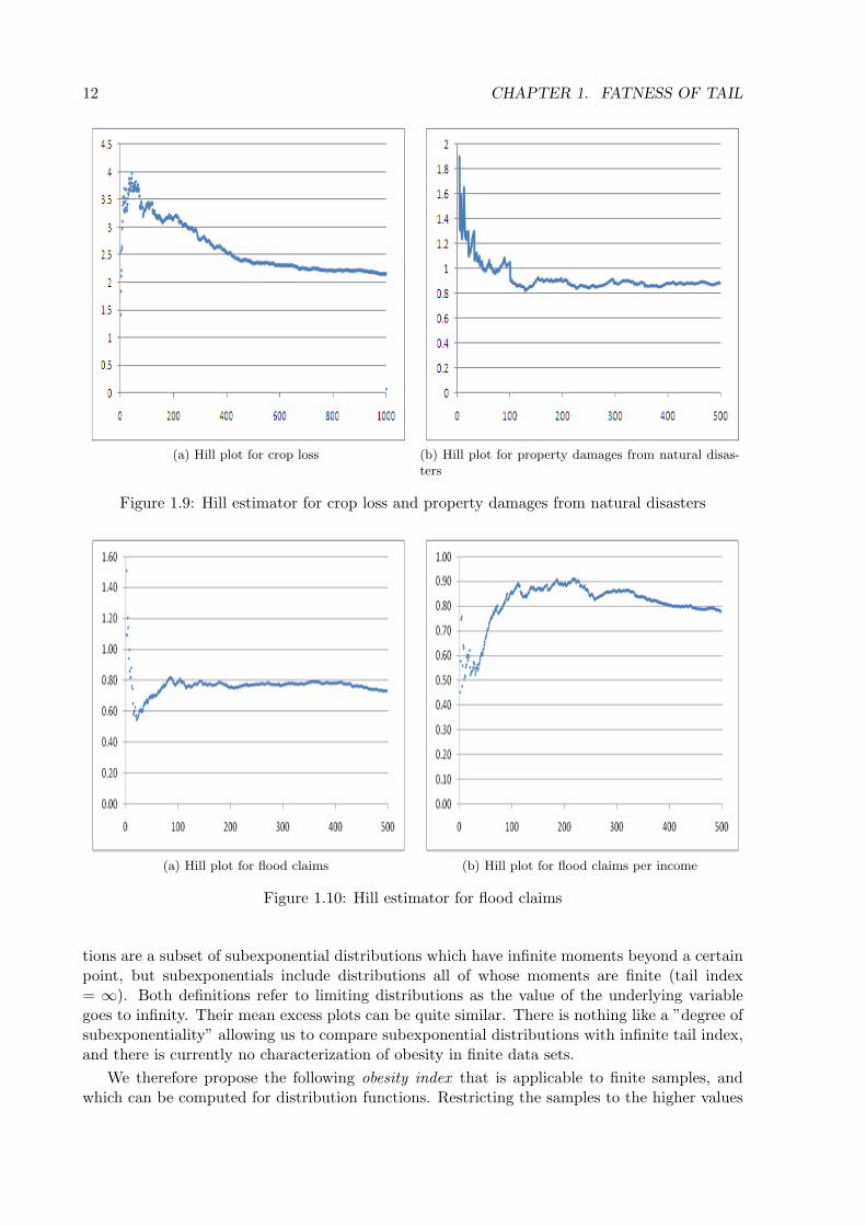
Figure 1.9, shows a Hill plot for crop losses (a) and natural disaster property damages (b).Figure 1.10 compares Hill plots for flood damages (a) and flood damages per income (b). Thedifference between these last two plots underscores the importance of properly accounting forexposure. Figure 1.9 (a) is more difficult to interpret than the mean excess plot in Figure(1.7)(b).
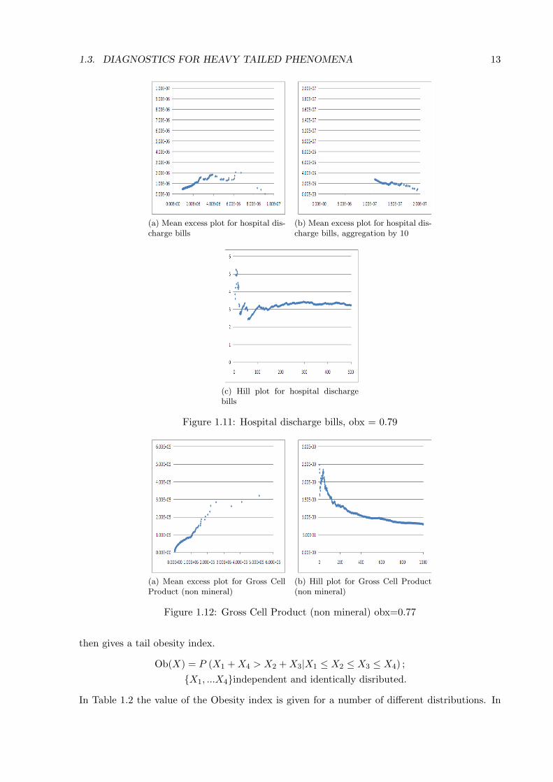
Hospital discharge billing data are shown in Figure 1.11; a mean excess plot (a), a meanexcess plot after aggregation by 10 (b), and a Hill plot (c). The hospital billing data are a goodexample of a modestly heavy tailed data set. The mean excess plot and Hill plots point to a tailindex in the neighborhood of 3. Although definitely heavy tailed according to all the operativedefinitions, it behaves like a distribution with finite variance, as we see the mean excess collapseunder aggregation by 10.
1.3.6 The Obesity Index
We have discussed two definitions of heavy-tailed distributions, the regularly varying distribu-tions with tail index 0 < α < ∞ and subexponential distributions. Regularly varying distribu-
12 CHAPTER 1. FATNESS OF TAIL
(a) Hill plot for crop loss (b) Hill plot for property damages from natural disas-ters
Figure 1.9: Hill estimator for crop loss and property damages from natural disasters
(a) Hill plot for flood claims (b) Hill plot for flood claims per income
Figure 1.10: Hill estimator for flood claims
tions are a subset of subexponential distributions which have infinite moments beyond a certainpoint, but subexponentials include distributions all of whose moments are finite (tail index= ∞). Both definitions refer to limiting distributions as the value of the underlying variablegoes to infinity. Their mean excess plots can be quite similar. There is nothing like a ”degree ofsubexponentiality” allowing us to compare subexponential distributions with infinite tail index,and there is currently no characterization of obesity in finite data sets.
We therefore propose the following obesity index that is applicable to finite samples, andwhich can be computed for distribution functions. Restricting the samples to the higher values
1.3. DIAGNOSTICS FOR HEAVY TAILED PHENOMENA 13
(a) Mean excess plot for hospital dis-charge bills
(b) Mean excess plot for hospital dis-charge bills, aggregation by 10
(c) Hill plot for hospital dischargebills
Figure 1.11: Hospital discharge bills, obx = 0.79
(a) Mean excess plot for Gross CellProduct (non mineral)
(b) Hill plot for Gross Cell Product(non mineral)
Figure 1.12: Gross Cell Product (non mineral) obx=0.77
then gives a tail obesity index.
Ob(X) = P (X1 +X4 > X2 +X3|X1 ≤ X2 ≤ X3 ≤ X4) ;
X1, ...X4independent and identically disributed.
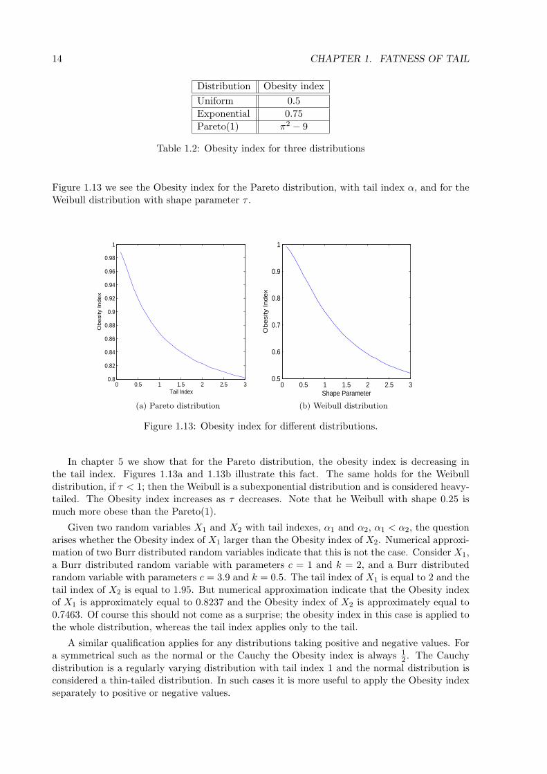
In Table 1.2 the value of the Obesity index is given for a number of different distributions. In
14 CHAPTER 1. FATNESS OF TAIL
Distribution Obesity index
Uniform 0.5
Exponential 0.75
Pareto(1) π2 − 9
Table 1.2: Obesity index for three distributions
Figure 1.13 we see the Obesity index for the Pareto distribution, with tail index α, and for theWeibull distribution with shape parameter τ .
0 0.5 1 1.5 2 2.5 30.8
0.82
0.84
0.86
0.88
0.9
0.92
0.94
0.96
0.98
1
Tail Index
Obesi
ty Index
(a) Pareto distribution
0 0.5 1 1.5 2 2.5 30.5
0.6
0.7
0.8
0.9
1
Shape Parameter
Ob
esi
ty I
nd
ex
(b) Weibull distribution
Figure 1.13: Obesity index for different distributions.
In chapter 5 we show that for the Pareto distribution, the obesity index is decreasing inthe tail index. Figures 1.13a and 1.13b illustrate this fact. The same holds for the Weibulldistribution, if τ < 1; then the Weibull is a subexponential distribution and is considered heavy-tailed. The Obesity index increases as τ decreases. Note that he Weibull with shape 0.25 ismuch more obese than the Pareto(1).
Given two random variables X1 and X2 with tail indexes, α1 and α2, α1 < α2, the questionarises whether the Obesity index of X1 larger than the Obesity index of X2. Numerical approxi-mation of two Burr distributed random variables indicate that this is not the case. Consider X1,a Burr distributed random variable with parameters c = 1 and k = 2, and a Burr distributedrandom variable with parameters c = 3.9 and k = 0.5. The tail index of X1 is equal to 2 and thetail index of X2 is equal to 1.95. But numerical approximation indicate that the Obesity indexof X1 is approximately equal to 0.8237 and the Obesity index of X2 is approximately equal to0.7463. Of course this should not come as a surprise; the obesity index in this case is applied tothe whole distribution, whereas the tail index applies only to the tail.
A similar qualification applies for any distributions taking positive and negative values. Fora symmetrical such as the normal or the Cauchy the Obesity index is always 1
2 . The Cauchydistribution is a regularly varying distribution with tail index 1 and the normal distribution isconsidered a thin-tailed distribution. In such cases it is more useful to apply the Obesity indexseparately to positive or negative values.
1.4. CONCLUSION AND OVERVIEW OF THE TECHNICAL CHAPTERS 15
1.4 Conclusion and Overview of the Technical Chapters
Fat tailed phenomena are not rare or exotic, they occur rather frequently in loss data. Asattested in hospital billing data and Gross Cell Product data, they are encountered in mundaneeconomic data as well. Customary definitions in terms of limiting distributions, such as regularvariation or subexponentiality, may have contributed to the belief that fat tails are mathematicalfreaks of no real importance to practitioners concerned with finite data sets. Good diagnosticshelp dispel this incautious belief, and sensitize us to the dangers of uncritically applying thintailed statistical tools to fat tailed data: Historical averages, even in the absence of time trendsmay may be poor predictors, regardless of sample size. Aggregation may not reduce variationrelative to the aggregate mean, and regression coefficients are based on ratios of quantities thatfluctuate wildly.
The various diagnostics discussed here and illustrated with data each have their strengthsand weaknesses. Running historical averages have strong intuitive appeal but may easily beconfounded by real or imagined time trends in the data. For heavy tailed data, the overallimpression may be strongly affected by the ordering. Plotting different moving averages fordifferent random orderings can be helpful. Mean excess plots provide a very useful diagnostic.Since these are based on ordered data, the problems of ordering do not arise. On the downside,they can be misleading for regular varying distributions with tail indices less than or equal toone, as the theoretical slope is infinite. Hill plots, though very popular, are often difficult tointerpret. The Hill estimator is designed for regularly varying distributions, not for the widerclass of subexponential distributions; but even for regularly varying distributions, it may beimpossible to infer the tail index from the Hill plot.
In view of the jumble of diagnostics, each with their own strengths and weaknesses, it isuseful to have an intuitive scalar measure of obesity, and the obesity index is proposed herefor this purpose. The obesity index captures the idea that larger values are further apart, orthat the sum of two samples is driven by the larger of the two, or again that the sum tendsto behave like the max. This index does not require estimating a parameter of a hypotheticaldistribution; in can be computed for data sets and computed, in most cases numerically, fordistribution functions.
In Chapter 2 and 3 we discuss different properties of order statistics and present some resultsfrom the theory of records. These results are used in Chapter 5 to derive different properties ofthe index we propose. Chapter 4 discusses and compares regularly varying and subexponentialdistributions, and develops properties of the mean excess function. Chapter 6 opens a salienttoward fat tail regression by surveying dependence concepts.
16 CHAPTER 1. FATNESS OF TAIL
Chapter 2
Order Statistics
This chapter discusses some properties of order statistic that are used later to derive propertiesof the Obesity index. Most of these properties can be found in David [1981] or Nezvorov [2001].Another useful source is Balakrishnan and Stepanov [2007] We consider only order statistics froman i.i.d. sequence of continuous random variables. Suppose we have a sequence of n independentand identically distributed continuous random variables X1, ..., Xn ; if we order this sequence inascending order we obtain the order statistics
X1,n ≤ ... ≤ Xn,n.
Order statistics are used in Chapter 5 to prove properties of the Obesity index; we thereforestep through some fussy proofs. Readers less interested in the proofs of new results may surfthis and the following chapters.
2.1 Distribution of order statistics
The distribution function of the r-th order statistic Xr,n, from a sample of a random variableX with distribution function F , is given by
Fr,n(x) = P (Xr,n ≤ x)
= P (at least r of the Xi are less than or equal to x)
=n∑
m=r
P ( exactly m variables among X1, ..., Xn ≤ x)
=n∑
m=r
(n
m
)F (x)m (1− F (x))n−m
Using the following relationship for the regularized incomplete Beta function1
n∑m=k
(n
m
)ym(1− y)n−m =
∫ y
0
n!
(k − 1)!(n− k)!tk−1(1− t)n−kdt, 0 ≤ y ≤ 1,
we get the following resultFr,n(x) = IF (x) (r, n− r + 1) , (2.1)
where Ix(p, q) is the regularized incomplete beta function
Ix (p, q) =1
B (p, q)
∫ x
0tp−1(1− t)q−1dt,
1http://en.wikipedia.org/wiki/Beta function, accessed Feb.7 2011
17
18 CHAPTER 2. ORDER STATISTICS
and B(p, q) is the beta function
B(p, q) =
∫ 1
0tp−1(1− t)q−1dt.
Now assume that the random variable Xi has a probability density function f(x) = ddxF (x).
Denote the density function of Xr,n as fr,n. Using (2.1) we get the following result.
fr,n(x) =1
B(r, n− r + 1)
d
dx
∫ F (x)
0tr−1(1− t)n−rdt,
=1
B(r, n− r + 1)F (x)r−1 (1− F (x))n−r f(x) (2.2)
If k(1), ..., k(r) is a subset of the numbers 1, 2, 3, ..., n, k(0) = 0, k(r+1) = n+1 and 1 ≤ r ≤ n,the joint density of Xk(1),n, ..., Xk(r),n is given by
fk(1),...,k(n);n(x1, ..., xr) =n!∏r+1
s=1(k(s)− k(s− 1)− 1)!r+1∏s=1
(F (xs)− F (xs−1))k(s)−k(s−1)−1
r∏s=1
f(xs), (2.3)
where −∞ = x0 < x1 < ... < xr < xr+1 = ∞. We prove this for r = 2 and assume forsimplicity that f is continuous at the points x1 and x2 under consideration. Consider thefollowing probability
P (δ,∆) = P(x1 ≤ Xk(1),n < x1 + δ < x2 ≤ Xk(2),n < x2 +∆
).
We show that as δ → 0 and ∆ → 0 the following limit holds.
f(x1, x2) = limP (δ,∆)
δ∆
Now define the following events
A = x1 ≤ Xk(1),n < x1 + δ < x2 ≤ Xk(2),n < x2 +∆ and the intervals
[x1, x1 + δ) and [x2, x2 +∆) each contain exactly one order statistic,B = x1 ≤ Xk(1),n < x1 + δ < x2 ≤ Xk(2),n < x2 +∆ and
[x1, x1 + δ) ∪ [x2, x2 +∆) contains at least three order statistics.
We have that P (δ,∆) = P (A) + P (B). Also define the following events
C = at least two out of n variables X1, ..., Xn fall into [x1, x1 + δ)D = at least two out of n variables X1, ..., Xn fall into [x2, x2 +∆).
Now we have that P (B) ≤ P (C) + P (D). We find that
P (C) =
n∑k=2
(n
k
)(F (x1 + δ)− F (x1))
k (1− F (x1 + δ) + F (x1))n−k
≤ (F (x1 + δ)− F (x1))2
n∑k=2
(n
k
)≤ 2n (F (x1 + δ)− F (x1))
2
= O(δ2), δ → 0,
2.2. CONDITIONAL DISTRIBUTION 19
and similarly we obtain that
P (D) =
n∑k=2
(n
k
)(F (x2 +∆)− F (x2))
k (1− F (x2 +∆) + F (x2))n−k
≤ (F (x2 +∆))n∑
k=2
(n
k
)≤ 2n (F (x2 +∆)− F (x2))
2
= O(∆2), ∆ → 0.
This yields
limP (δ,∆)− P (A)
δ∆= 0 as δ → 0, ∆ → 0.
It remains to note that
P (A) =n!
(k(1)− 1)!(k(2)− k(1)− 1)!(n− k(2))!F (x1)
k(1)−1 (F (x1 + δ)− F (x1))
(F (x2)− F (x1 + δ))k(2)−k(1)−1 (F (x2 +∆)− F (x2)) (1− F (x2))n−k(2) .
From this equality we see that the limit exists and that
f(x1, x2) =n!
(k(1)− 1)!(k(2)− k(1)− 1)!(n− k(2))!F (x1)
k(1)−1 (F (x2)− F (x1))k(2)−k(1)−1
(1− F (x2))n−k(2)f(x1)f(x2),
which is the same as equation (2.3). Note that we have only found the right limit of f(x1+0, x2+0), but since f is continuous we can obtain the other limits f(x1 + 0, x2 − 0), f(x1 − 0, x2 + 0)and f(x1 − 0, x2 − 0) in a similar way.
Also note that when r = n in (2.3) we get the joint density of all order statistics and thatthis joint density is given by
f1,...,n;n(x1, ..., xn) =
n!∏n
s=1 f(xs) if, −∞ < x1 < ... < xn < ∞0, otherwise.
(2.4)
2.2 Conditional distribution
When we pass from the original random variables X1, ..., Xn to the order statistics, we loseindependence among these variables. Now suppose we have a sequence of n order statisticsX1,n, ..., Xn,n, and let 1 < k < n. In this section we derive the distribution of an order statisticXk+1,n given the previous order statisticXk = xk, ..., X1 = x1. Let the density of this conditionalrandom variable be denoted by f(u|x1, .., xk). We show that this density coincides with the
20 CHAPTER 2. ORDER STATISTICS
distribution of Xk+1,n given that Xk,n = xk, denoted by f(u|xk)
f(u|x1, ..., xk) =f1,...,k+1;n(x1, ..., xk, u)
f1,...,k;n(x1, ..., xk)
=
n!(n−k−1)! [1− F (u)]n−k−1∏k
s=1 f(xs)f(u)
n!(n−k)! [1− F (xk)]
n−k∏ks=1 f(xs)
=
n!(k−1)!(n−k−1)! [1− F (u)]n−k−1 F (xk)
k−1f(xk)f(u)
n!(k−1)!(n−k)! [1− F (xk)]
n−k F (xk)k−1f(xk)
=fk,k+1;n(xk, u)
fk,n(xk)= f(u|xk).
From this we see that the order statistics form a Markov chain. The following theorem is usefulfor finding the distribution of functions of order statistics.
Theorem 2.2.1. Let X1,n ≤ ... ≤ Xn,n be order statistics corresponding to a continuous distri-bution function F . Then for any 1 < k < n the random vectors
X(1) = (X1,n, ..., Xk−1,n) and X(2) = (Xk+1,n, ..., Xn,n)
are conditionally independent given any fixed value of the order statistic Xk,n. Furthermore,the conditional distribution of the vector X(1) given that Xk,n = u coincides with the uncondi-tional distribution of order statistics Y1,k−1, ..., Yk−1,k−1 corresponding to i.i.d. random variablesY1, ..., Yk−1 with distribution function
F (u)(x) =F (x)
F (u)x < u.
Similarly, the conditional distribution of the vector X(2) given Xk,n = u coincides with the uncon-ditional distribution of order statistics W1,n−k, ...,Wn−k;n−k related to the distribution function
F(u)(x) =F (x)− F (u)
1− F (u)x > u.
Proof. To simplify the proof we assume that the underlying random variables X1, ..., Xn havedensity f . The conditional density is given by
f(x1, ..., xk−1, xk+1, ..., xn|Xk,n = u) =f1,...,n;n(x1, ..., xk−1, xk+1,n, ..., xn)
fk;n(u)
=
[(k − 1)!
k−1∏s=1
f(xs)
F (u)
][(n− k)!
n∏r=k+1
f(xr)
1− F (u)
].
As we can see the first part of the conditional density is the joint density of the order statisticsfrom a sample size k− 1 where the random variables have a density f(x)
F (u) for x < u. The secondpart in the density is the joint density of the order statistics from a sample of size n− k wherethe random variables have a distribution F (x)−F (u)
1−F (u) for x > u.
2.3. REPRESENTATIONS FOR ORDER STATISTICS 21
2.3 Representations for order statistics
We noted that one of the drawbacks of using the order statistics is losing the independenceproperty among the random variables. If we consider order statistics from the exponentialdistribution or the uniform distribution the following properties can be used to study linearcombinations of the order statistics. The first is obvious.
Lemma 2.3.1. Let X1,n ≤ ... ≤ Xn,n, n = 1, 2, ..., be order statistics related to independent andidentically distributed random variables with distribution function F , and let
U1,n ≤ ... ≤ Un,n,
be order statistics related to a sample from the uniform distribution on [0, 1]. Then for anyn = 1, 2, ... the vectors (F (X1,n), ..., F (Xn,n)) and (U1,n, ..., Un,n) are equally distributed.
Theorem 2.3.2. Consider exponential order statistics
Z1,n ≤ ... ≤ Zn,n,
related to a sequence of independent and identically distributed random variables Z1, Z2, ... withdistribution function
H(x) = max(0, 1− e−x
).
Then for any n = 1, 2, ... we have
(Z1,n, ..., Zn,n)d=
(v1n,v1n
+v2
n− 1, ...,
v1n
+ ...+ vn
), (2.5)
where v1, v2, ... is a sequence of independent and identically distributed random variables withdistribution function H(x).
Proof. In order to prove Theorem 2.3.2 it suffices to show that the densities of both vectors in(2.5) are equal. Putting
f(x) =
e−x, if x > 0,
0 otherwise,(2.6)
and substituting equation (2.6) into the joint density of the n order statistics given by
f1,2,...,n;n (x1, ..., xn) =
n!∏n
i=1 f(xi), x1 < ... < xn,
0, otherwise,
we find that the joint density of the vector on the LHS of equation (2.5) is given by
f1,2,...,n;n(x1, ..., xn) =
n! exp−
∑ns=1 xs, if 0 < x1 < ... < xn < ∞,
0, otherwise.(2.7)
The joint density of n i.i.d. standard exponential random variables v1, ..., vn is given by
g(y1, ..., yn) =
exp−
∑ns=1 ys, if y1 > 0, ..., yn > 0,
0, otherwise.(2.8)
The linear change of variables
(v1, ..., vn) = (y1n,y1n
+y2
n− 1,y1n
+y2
n− 1+
y3n− 2
, ...,y1n
+ ...+ yn)
22 CHAPTER 2. ORDER STATISTICS
with Jacobian 1n! which corresponds to the passage to random variables
V1 =v1n, V2 =
v1n
+v2
n− 1, ..., Vn =
v1n
+ ...+ vn,
has the property thatv1 + v2 + ...+ vn = y1 + ...+ yn
and maps the domain ys > 0s = 1, ..., n into the domain 0 < v1 < v2 < ... < vn < ∞. Equa-tion (2.8) implies that V1, ..., Vn have the joint density
f(v1, ..., vn) =
n! exp −
∑ns=1 vs , if 0 < v1 < ... < vn,
0, otherwise.(2.9)
Comparing equation (2.7) with equation (2.9) we find that both vectors in (2.5) have the samedensity and this proves the theorem.
Using Theorem 2.3.2 it is possible to find the distribution of any linear combination of orderstatistics from an exponential distribution, since we can express this linear combination as asum of independent exponential distributed random variables.
Theorem 2.3.3. Let U1,n ≤ ... ≤ Un,n, n = 1, 2, ... be order statistics from an uniform sample.Then for any n = 1, 2, ...
(U1,n, ..., Un,n)d=
(S1
Sn+1, ...,
Sn
Sn+1
),
whereSm = v1 + ...+ vm, m = 1, 2, ...,
and where v1, ..., vm are independent standard exponential random variables.
2.4 Functions of order statistics
In this section we discuss different techniques that can be used to obtain the distribution ofdifferent functions of order statistics.
2.4.1 Partial sums
Using Theorem 2.2.1 we can obtain the distribution of sums of consecutive order statistics,∑s−1i=r+1Xi,n. The distribution of the order statistics Xr+1,n, ..., Xs−1,n given that Xr,n = y
and Xs,n = z coincides with the unconditional distribution of order statistics V1,n, ..., Vs−r−1
corresponding to an i.i.d. sequence V1, ..., Vs−r−1 where the distribution function of Vi is givenby
Vy,z(x) =F (x)− F (y)
F (z)− F (y), y < x < z. (2.10)
From Theorem 2.2.1 we can write the distribution function of the partial sum in the followingway
P (Xr+1 + ...+Xs−1 < x) =
∫−∞<y<z<∞
P (Xr+1 + ...+Xs−1 < x|Xr,n = y,Xs,n = z) fr,s;n(y, z)dydz
=
∫−∞<y<z<∞
V (s−r−1)∗y,z (x)fr,s;n(y, z)dydz,
where V(s−r−1)∗y,z (x) denotes the s− r − 1-th convolution of the distribution given by (2.10).
2.4. FUNCTIONS OF ORDER STATISTICS 23
2.4.2 Ratio between order statistics
Now we look at the distribution of the ratio between two order statistics.
Theorem 2.4.1. For r < s and 0 ≤ x ≤ 1
P
(Xr,n
Xs,n≤ x
)=
1
B(s, n− s+ 1)
∫ 1
0IQx(t)(r, s− r)ts−1(1− t)n−sdt, (2.11)
where
Qx(t) =F(xF−1(t)
)t
.
Proof.
P
(Xr,n
Xs,n≤ x
)=
∫ ∞
−∞P
(y
Xs,n≤ x|Xr,n = y
)fXr,n(y)dy,
=
∫ ∞
−∞P(Xs,n >
y
x|Xr,n = y
)fXr,n(y)dy,
=
∫ ∞
−∞
∫ ∞
yx
fXs,n|Xr,n=y(z)dzfXr,n(y)dy,
=
∫ ∞
−∞
∫ zx
−∞fXr,n(y)fXs,n|Xr,n=y(z)dydz,
= C
∫ ∞
−∞
∫ zx
−∞F (y)r−1 [1− F (y)]n−r f(y)
[F (z)− F (y)]s−r−1 [1− F (z)]n−s f(z)
[1− F (y)]n−r dydz,
where C = 1B(r,n−r+1)B(s−r,n−s+1) . We apply the transformation t = F (z) from which we get
the following
P
(Xr,n
Xs,n≤ x
)= C
∫ 1
0
∫ xF−1(t)
−∞F (y)r−1f(y) [t− F (y)]s−r−1 dy (1− t)n−s dt.
Next we use the transformation F (y)t = u.
P
(Xr,n
Xs,n≤ x
)= C
∫ 1
0
∫ F (xF−1(t))t
0tr−1ur−1 (t− tu)s−r−1 tdu (1− t)n−s dt,
= C
∫ 1
0
∫ F (xF−1(t))t
0ur−1 (1− u)s−r−1 duts−1 (1− t)n−s dt
We can rewrite the constant C in the following way
C =1
B(r, n− r + 1)B(s− r, n− s+ 1)
=n!
(r − 1)!(n− r)!
(n− r)!
(s− r − 1)!(n− s)!
=1
(s− r − 1)!(r − 1)!
n!
(n− s)!
=(s− 1)!
(s− r − 1)!(r − 1)!
n!
(n− s)!(s− 1)!
=1
B(r, s− r)B(s, n− s+ 1).
24 CHAPTER 2. ORDER STATISTICS
If we substitute this in our integral, and define Qx(t) =F (xF−1(t))
t , we get the following
P
(Xr,n
Xs,n≤ x
)=
1
B(s, n− s+ 1)
∫ 1
0
∫ Qx(t)0 ur−1 (1− u)s−r−1 du
B(s, s− r)ts−1 (1− t)n−s dt
=1
B(s, n− s+ 1)
∫ 1
0IQx(t)(r, s− r)ts−1 (1− t)n−s dt.
This chapter derived properties of order statistics which are used in chapter 5 to deriveproperties of the obesity index and the distribution of the ratio between order statistics. Becausethe ratio of order statistics has intuitive appeal in characterizing fat tails, the next chapterreviews the theory of records.
Chapter 3
Records
Records are used in Chapter 5 to explore possible measures of tail obesity. Records are closelyrelated to order statistics. This brief chapter discusses the theory of records and summarizes themain results. For a more detailed discussion see Arnold [1983],Arnold et al. [1998] or Nezvorov[2001], where most of the results we present here can be found. Records are closely related toextreme values and related material can be found in A.J. McNeil and Embrechts [2005], Coles[2001]and Beirlant et al. [2005].
3.1 Standard record value processes
Let X1, X2, ... be an infinite sequence of independent and identically distributed random vari-ables. Denote the cumulative distribution function of these random variables by F and assumeit is continuous. An observation is called an upper record value if its value exceeds all previousobservations. So Xj is an upper record if Xj > Xi for all i < j. We are also interested in thetimes at which the record values occur. For convenience assume that we observe Xj at time j.The record time sequence Tn, n ≥ 0 is defined as
T0 = 1 with probability 1
and for n ≥ 1,Tn = min
j : Xj > XTn−1
.
The record value sequence Rn is then defined by
Rn = XTn , n = 0, 1, 2, ...
The number of records observed at time n is called the record counting process Nn, n ≥ 1where
Nn = number of records among X1, ..., Xn.
We have that N1 = 1 since X1 is always a record.
3.2 Distribution of record values
Let the record increment process be defined by
Jn = Rn −Rn−1, n > 1,
with J0 = R0. It can easily be shown that if we consider the record increment process from asequence of i.i.d. standard exponential random variables then all the Jn are independent and
25
26 CHAPTER 3. RECORDS
Jn has a standard exponential distribution. Using the record increment process we are ableto derive the distribution of the n-th record from a sequence of i.i.d. standard exponentialdistributed variables.
P (Rn < x) = P (Rn −Rn−1 +Rn−1 −Rn−2 +Rn−2 − ...+R1 −R0 +R0 < x)
= P (Jn + Jn−1 + ...+ J0 < x)
Since∑n
i=0 J + i is the sum of n+1 standard exponential distributed random variables we findthat the record values from a sequence of standard exponential distributed random variableshas the gamma distribution with parameters n+ 1 and 1.
Rn ∼ Gamma(n+ 1, 1), n = 0, 1, 2, ...
A Gamma(n, λ) distributed random variable X has density function
fX(x) =
λ(λx)n−1e−λx
Γ(n) , x ≥ 0
0, otherwise
We can use the result above to find the distribution of the n-th record corresponding to asequence Xi of i.i.d. random variables with continuous distribution function F . If X hasdistribution function F then
H(X) ≡ − log(1− F (X))
has a standard exponential distribution function. We also have that Xd= F−1(1− e−X∗
) whereX∗ is a standard exponential random variable. Since X is a monotone function of X∗ we canexpress the n-th record of the sequence Xj as a simple function of the n-th record of thesequence X∗. This can be done in the following way
Rnd= F−1(1− e−R∗
n), n = 0, 1, 2, ...
Using the following expression of the distribution of the n-th record from a standard exponentialsequence
P (R∗n > r∗) = e−r∗
n∑k=0
(r∗)k
k!, r∗ > 0,
the survival function of the record from an arbitrary sequence of i.i.d. random variables withdistribution function F is given by
P (Rn > r) = [1− F (r)]n∑
k=0
− [log(1− F (r))]k
k!.
3.3 Record times and related statistics
The definition of the record time sequence Tn, n ≥ 0 was given by
T0 = 1, with probability 1,
and for n ≥ 1Tn = minj : Xj > XTn−1.
In order to find the distribution of the first n non-trivial record times T1, T2, ..., Tn we firstconsider the sequence of record time indicator random variables:
I1 = 1 with probability 1,
3.3. RECORD TIMES AND RELATED STATISTICS 27
and for n > 1
In = 1Xn>maxX1,...,Xn−1
So In = 1 if and only if Xn is a record value. We assume that the distribution function F iscontinuous. It is easily verified that the random variables In have a Bernoulli distribution withparameter 1
n and are mutually independent. The joint distribution for the first m record timescan be obtained using the record indicators. For integers 1 < n1 < ... < nm we have that
P (T1 = n1, ..., Tm = nm) = P (I2 = 0, ..., In1−1 = 0, In1 = 1, In1+1 = 0, ..., Inm = 0)
= [(n1 − 1)(n2 − 1)...(nm − 1)nm]−1 .
In order to find the marginal distribution of Tk we first review some properties of the recordcounting process Nn, n ≥ 1 defined by
Nn = number of records among X1, ...Xn
=
n∑j=1
Ij .
Since the record indicators are independent we can immediately write down the mean and thevariance for Nn.
E [Nn] =
n∑j=1
1
j,
Var(Nn) =
n∑j=1
1
j
(1− 1
j
).
We obtain the exact distribution of Nn using the probability generating function. We have thefollowing result.
E[sNn
]=
n∏j=1
E[sIj]
=
n∏j=1
(1 +
s− 1
j
)
From this we find that
P (Nn = k) =Skn
n!
where Skn is a Stirling number of the first kind:
(x)n =
n∑k=0
Sknx
k,
where (x)n = x(x − 1)(x − 2)...(x − n + 1). The record counting process Nn obeys the centrallimit theorem.
Nn − log(n)√log(n)
d→ N(0, 1)
28 CHAPTER 3. RECORDS
We can use the information about the record counting process to obtain the distribution of Tk.Note that the events Tk = n and Nn = k+1, Nn−1 = k are equivalent. From this we obtain:
P (Tk = n) = P (Nn = k + 1, Nn−1 = k)
= P (In = 1, Nn−1 = k)
=1
n
Skn−1
(n− 1)!
=Skn−1
n!.
We also have asymptotic log-normality for Tk.
log(Tk)− k√k
d→ N(0, 1)
3.4 k-records
There are two different sequences that are called k-record values in the literature. We discussboth definitions here. First define the sequence of initial ranks ρn given by
ρn = #j : j ≤ n and Xn ≤ Xj, n ≥ 1.
We callXn a Type 1 k-record value if ρn = k, when n ≥ k. Denote the sequence that is generated
through this process byR
(k)n
. The Type 2 k-record sequence is defined in the following way,
let T0(k) = k, R0(k) = Xn−k+1,k and
Tn(k) = minj : j > T(n−1)(k), Xj > XT(n−1)(k)−k+1,T(n−1)(k)
,
and define Rn(k) = XTn(k)−k+1as the n-th k-record. Here a k record is established whenever
ρn ≥ k. Although the corresponding Xn does not need to be a Type 2 k-record, unless k = 1, theobservation eventually becomes a Type 2 k-record value. The sequence
Rn(k), n ≥ 0
from a
distribution F is identical in distribution to a record sequence Rn, n ≥ 0 from the distributionfunction F1,k(x) = 1− (1− F (x))k. So all the distributional properties of the record values andrecord counting statistics do extend to the corresponding k-record sequences.
The difference between the Type 1 and Type 2 k-records can also be explained in the fol-lowing way. We only observe a new Type 1 k-record whenever an observation is exactly the k-thlargest seen yet. We observe a new Type 2 k-record whenever we observe a new value that islarger than the previous k-th largest.
Chapter 4
Regularly Varying andSubexponential Distributions
This chapter develops properties of the two most important classes of heavy tailed distributions,namely the regularly varying and the subexponential distributions, introduced informally inChapter 1. Regularly varying distributions have tails with polynomial decay; all sufficientlyhigh moments are infinite. Moments of subexponential distributions may be all finite, and yetthey may exhibit very fat tail behavior. The goal is to derive diagnostic properties for theseclasses, the most important of which are related to their mean excess functions. In a nutshell,the mean excess function of a light tailed distribution is non increasing, for subexponentialdistributions the mean excess function goes to infinity and for regularly varying functions withfinite expectation the function is asymptotically linear with slope determined by the polynomialdecay rate.
The following notation is used throughout: if X1, ..., Xn is an iid sample, then Sn = X1 +... + Xn is the partial sum with distribution function Fn∗, and Mn = max X1, ..., Xn is themaximum with distribution function Fn. This material is found in Embrechts et al. [1997],Bingham et al. [1987], Rachev [2003]and Resnick [2005].
4.0.1 Regularly varying distribution functions
An important class of heavy-tailed distributions is the class of regularly varying distributionfunctions.
Definition 4.0.1. A distribution function F is called regularly varying at infinity with tail indexα if:
limx→∞
F (tx)
F (x)= t−α, α ∈ (0,∞) (4.1)
where the survivor function F (x) = 1 − F (x). If equation (4.1) holds with α = ∞, then F israpidly varying. In either case we write F ∈ R−α, and if F is the distribution function of X,X ∈ R−α.
The definition of regular variation implies that if α ∈ (0,∞) then for every ϵ > 1; there
is an xϵ(t) depending on t, such that for all x ≥ xϵ, ϵt−αF (x) > F (tx) > t−α
ϵ F (x). However,for survivor functions proposition (4.0.1) gives uniform convergence in t for xϵ sufficiently large.We first present properties of regularly varying functions, and then develop some properties ofregularly varying distributions.
29
30 CHAPTER 4. REGULARLY VARYING AND SUBEXPONENTIAL DISTRIBUTIONS
Regularly varying functions
The following results concern regularly varying functions, for details see Bingham et al. [1987].
Definition 4.0.2. A positive measurable function h on (0,∞) is regularly varying at infinitywith index α ∈ R if:
limx→∞
h(tx)
h(x)= tα, t > 1. (4.2)
We write h(x) ∈ Rα. If α = 0 , h(x) is slowly varying at infinity; if α = −∞, h(x) is rapidlyvarying at infinity.
If h(x) ∈ Rα then we can rewrite the function h(x) as:
h(x) = xαL(x), (4.3)
where L(x) is slowly varying. In the case of polynomial decay, convergence is uniform in thefollowing sense:
Proposition 4.0.1. For α > 0, and h(x) ∈ R−α, limx→∞h(t,x)h(x) = t−α, uniformly in t for
x ∈ [b,∞), b > 0, t > 1.
Karamata’s theorem is an important tool for studying the behavior of regularly varyingfunctions, the ’direct half’ is important for this chapter; the converse is omitted.
Theorem 4.0.2. Suppose h ∈ Rα , for α ∈ R, and that h is locally bounded in [x0,∞) for somex0 ≥ 0. Then
1. for α > −1,
limx→∞
∫ xx0
h(t)dt
xh(x)=
1
1 + α,
2. for α < −1
limx→∞
∫∞x h(t)dt
xh(x)= − 1
1 + α,
Properties of regularly varying distribution functions
The regularly varying distributions have attractive properties. This class is closed under convolu-tions as can be found in Applebaum [2005], where the result was attributed to G. Samorodnitsky.
Theorem 4.0.3. If X and Y are independent real-valued random variables with FX ∈ R−α andF Y ∈ R−β, where α, β > 0, then FX+Y ∈ Rρ, where ρ = minα, β.
The same theorem, but with the assumption that α = β can be found in Feller [1971].
Proposition 4.0.4. If F1 and F2 are two distribution functions such that as x → ∞
1− Fi(x) ∼ x−αLi(x) (4.4)
with Li slowly varying, then the convolution G = F1 ∗ F2 satisfies, as x → ∞:
1−G(x) ∼ x−α (L1(x) + L2(x)) . (4.5)
From Proposition 4.0.4 we obtain the following result using induction on n.

31
Corollary 4.0.1. If F (x) = x−αL(x) for α ≥ 0 and L ∈ R0, then for all n ≥ 1,
Fn∗(x) ∼ nF (x), as x → ∞, (4.6)
P (Sn > x) ∼ P (Mn > x) as x → ∞. (4.7)
Proof (Embrechts et al. [1997]) (4.6) follows directly from Proposition 4.0.4. To prove (4.7),for all n ≥ 2 we have:
P (Sn > x) = Fn∗(x)
P (Mn > x) = Fn(x) = 1− F (x)n
= F (x)
n−1∑k=0
F k(x)
∼ nF (x), x → ∞.
Thus, we have
P (Sn > x) ∼ P (Mn > x) as x → ∞.
To establish moment properties of regularly varying distributions, we first need:
Lemma 4.0.5. Let X be a positive random variable, and let g be an increasing differentiablefunction with g(0) = 0 such that ∞ > E(g(X)); then
1. limx→∞g(x)F (x) = 0
2. E(g(X)) =∫∞0 (dg/dx)F (x)dx.
Proof
1.∫∞0 g(x)dF (x) −
∫ xo
0 g(x)dF (x) ≥ g(xo)F (xo) ≥ 0, since g is increasing from zero. TheLHS goes to zero as xo → ∞.
2. Using the above and integrating by parts, 0 = g(x)F (x)|∞0 =∫∞0 (dg/dx)F (x)dx−
∫∞0 g(x)dF (x).
Since E(g(X)) < ∞, the terms on the RHS are finite and equal.
Proposition 4.0.6. Let X ∈ R−1, and β > 0:
1. if β < 1 then E(Xβ) < ∞
2. if β > 1 then E(Xβ) = ∞
Proof: It is easy to check that Y = Xβ ∈ R−1/β.
1. For Y , we are in case (2) of Theorem (4.0.2). Using proposition (4.0.1), for any ϵ > 0, t > 1and yo sufficiently large:
(tyo)F Y (tyo) < yot(β−1)/βF Y (yo)(1 + ϵ).
It follows that limy→∞yF Y (y) = 0, and by Theorem (4.0.2), limy→∞∫∞y F ydy → 0. Since
F Y ≤ 1, E(Y ) = ∞ only if∫∞yo
F ydy = ∞ for all yo; therefore E(Y ) < ∞.
32 CHAPTER 4. REGULARLY VARYING AND SUBEXPONENTIAL DISTRIBUTIONS
2. If β > 1 then, by a similar argument
∞ = limt→∞yot(β−1)/βF Y (yo)(1− ϵ) ≤ limt→∞(tyo)F Y (tyo).
With lemma(4.0.5)(1), this contradicts E(Y ) < ∞.
If X ∈ R−1 then E(X) can be either finite or infinite, depending on the slowly varying functionL in equation (4.3).
Remark 4.0.1. The following facts are easily checked:
• If X ∈ R−α then E(Xβ) < (=)∞ if β < (>)α. If β = α, then E(Xβ) can be either finiteor infinite.
• For α = 1 the Pareto(1) is an example with infinite mean.
• For an example of X ∈ R−α with E(Xα) < ∞, consider the distribution function F on(e,∞) with the density f(t) = Ct−α−1(ln(t))−s−1, α > 0, s > 0, where C is the appropriate
constant. By L’Hopital’s rule, F (tx)
F (x)∼ tf(xt)
f(x) → t−α as x → ∞. On the other hand∫∞e tαf(t)dt =
[−1
s (ln(t))−s]∞e
= 1s < ∞. 1
• if α = 0, s > 0 in the above example then the corresponding random variable X ∈R0. F (x) = (C/s)(ln(x))−s. For all b > 0, E(Xb) = ∞.
• if α = 0, s = 0 then f(x) = c(xln(x))−1, x ≥ e is not a density, as its integral ln(ln(x)) isinfinite on this domain.
• F (x) = e(xln(x))−1, x ≥ e, is a survivor function for X ∈ R−1; limx→∞xF (x) = 0, but∫∞e F (x)dx = eln(ln(x))|∞e = ∞. This shows that the converse of lemma 4.0.5(1) is false.
• If X is exponential, then 1/X ∈ R−1.
• If X is normal with mean µ and variance σ2 then 1/X R−1; if µ = 0, E(1/X) = 0.
Other distribution functions in the class of regularly varying distributions are given in Table4.1.
Distribution F (x) or f(x) Index of regular variation
Pareto F (x) = x−α −α
Burr F (x) =(
1xτ+1
)α−τα
Log-Gamma f(x) = αβ
Γ(β) (ln(x))β−1 x−α−1 −α
Table 4.1: Regularly varying distribution functions
The tail index of a regularly varying distribution gives a convenient characterization of thedegree of tail heaviness; if X ∈ R−α and Y ∈ R−β with β < α then Y is heavier tailed than X.
1We are grateful to Prof. Misiewicz for these examples.
33
4.0.2 Subexponential distribution functions
The class of subexponential distribution functions contains the class of regularly varying dis-tribution functions and captures the feature that ’the sum behaves like the max’. This sectiondevelops several properties of distributions with subexponential tails.
Definition 4.0.3. A distribution function F with support (0,∞) is a subexponential distribution,written F ∈ S, if for all n ≥ 2,
limx→∞
Fn∗(x)
F (x)= n. (4.8)
Note that, by definition, F ∈ S entails that F is supported on (0,∞). Whereas regular vari-ation entails that the sum of independent copies is asymptotically disributed as the maximum,from equation (4.8) we see that this fact characterizes the subexponential distributions:
P (Sn > x) ∼ P (Mn > x) as x → ∞ ⇒ F ∈ S.
Noting that t−α ∼ F (ln(tx))
F (ln(x))if and only if F (ln(t)+ln(x))
F (ln(x))∼ e−αln(t), we find the following is a useful
property:
Lemma 4.0.7. A distribution function F with support (0,∞) satisfies
F (z + x)
F (z)∼ e−αx, as z → ∞, α ∈ [0,∞] (4.9)
if and only ifF ln ∈ R−α (4.10)
.
The first equation is equivalent to F (x−y)
F (x)∼ eαy, as x → ∞.
In order to check if a distribution function is a subexponential distribution we do not need tocheck equation (4.8) for all n ≥ 2. Lemma 4.0.8 gives a sufficient condition for subexponentiality.
Lemma 4.0.8. If
lim supx→∞
F 2∗(x)
F (x)= 2,
then F ∈ S.
Lemma 4.0.9 gives a few important properties of subexponential distributions, (Embrechtset al. [1997]).
Lemma 4.0.9. 1. If F ∈ S, then uniformly in compact y-sets of (0,∞),
limx→∞
F (x− y)
F (x)= 1. (4.11)
2. If (4.11) holds then, for all ε > 0,
eεxF (x) → ∞, x → ∞
3. If F ∈ S then, given ε > 0, there exists a finite constant K such that for all n ≥ 2,
Fn∗(x)
F (x)≤ K(1 + ε)n, x ≥ 0. (4.12)
34 CHAPTER 4. REGULARLY VARYING AND SUBEXPONENTIAL DISTRIBUTIONS
Proof. The proof of the first statement involves an interesting technique. If X1, . . . Xn+1 arepositive i.i.d. variables, then
Fn+1(x)− F (n+1)∗(x) = P∪t≤x
ω|Xn+1(ω) = t ;
n∑i=1
Xi(ω) > x− t
=
∫ x
0Fn∗(x− t)dF (t).
F 2∗(x)
F (x)=
1− F 2∗(x)
F (x)
=F (x) + F (x)− F 2∗(x)
F (x)
= 1 +
∫ x0 F (x− t)dF (t)
F (x)
= 1 +
∫ y0 F (x− t)dF (t)
F (x)+
∫ xy F (x− t)dF (t)
F (x).
Since F (x−t)
F (x)> 1 and F (x−t)
F (x)> F (x−y)
F (x)we have
F 2∗(x)
F (x)≥ 1 + F (y) +
F (x− y)
F (x)(F (x)− F (y)).
Re-arranging gives
F 2∗(x)
F (x)− 1− F (y)
F (x)− F (y)≥ F (x− y)
F (x)≥ 1.
The proof of the first statement concludes by using (4.0.8) to show that the left hand sideconverges to 1 as x → ∞. Uniformity follows from monotonicity in y. For the second statement,note that by lemma (4.0.7) F ln ∈ R0, which implies that xεF (ln(x)) → ∞. The thirdstatement is a fussy calculation for which we refer the reader to (Embrechts et al. [1997] p.42).
Note that if F ∈ S, then α = 0 in lemma (4.0.7).
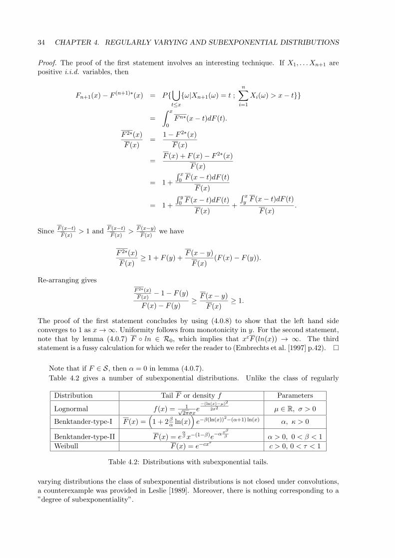
Table 4.2 gives a number of subexponential distributions. Unlike the class of regularly
Distribution Tail F or density f Parameters
Lognormal f(x) = 1√2πσx
e−(ln(x)−µ)2
2σ2 µ ∈ R, σ > 0
Benktander-type-I F (x) =(1 + 2β
α ln(x))e−β(ln(x))2−(α+1) ln(x) α, κ > 0
Benktander-type-II F (x) = eαβ x−(1−β)e
−αxβ
β α > 0, 0 < β < 1
Weibull F (x) = e−cxτc > 0, 0 < τ < 1
Table 4.2: Distributions with subexponential tails.
varying distributions the class of subexponential distributions is not closed under convolutions,a counterexample was provided in Leslie [1989]. Moreover, there is nothing corresponding to a”degree of subexponentiality”.
4.1. MEAN EXCESS FUNCTION 35
4.0.3 Related classes of heavy-tailed distributions
For the sake of completeness, this section introduces two other classes of heavy tailed distribu-tions, the dominatedly varying denoted by D and the long tailed denoted by L
D =
F d.f. on (0,∞) : lim sup
x→∞
F(x2
)F (x)
< ∞
L =
F d.f. on (0,∞) : lim
x→∞
F (x− y)
F (x)= 1 for all y > 0
The relations between these, the regularly varying distribution functions (R) and the subexpo-nential distribution functions (S) are as follows:
1. R ⊂ S ⊂ L and R ⊂ D,
2. L ∩ D ⊂ S,
3. D * S and S * D.
4.1 Mean excess function
The mean excess function is a popular diagnostic tool. For subexponential distribution functionsthe mean excess function tends to infinity. For regularly varying distributions with tail indexα > 1 it tends to a straight line with slope 1/(α − 1). For the exponential distribution themean excess function is a constant and for the normal distribution it tends to zero. In insurancee(u) is called the mean excess loss function where it is interpreted as the expected claim sizeover some threshold u. In reliability theory or in the medical field e(u) is often called the meanresidual life function. An accessible discussion is found in Beirlant and Vynckier.
The mean excess function of a random variable X with finite expectation is defined as:
Definition 4.1.1. Let X be a random variable with right endpoint xF ∈ (0,∞] and E(X) < ∞,then
e(u) = E [X − u|X > u] , 0 ≤ u ≤ xF ,
is the mean excess function of X.
In data analysis one uses the empirical counterpart of the mean excess function which isgiven by
en(u) =
∑ni=1Xi,n1Xi,n>u∑n
i=1 1Xi,n>u− u.
The empirical version is usually plotted against the values u = xi,n for k = 1, ..., n− 1.
4.1.1 Properties of the mean excess function
For positive random variables the mean excess function can be calculated using the followingproposition:
Proposition 4.1.1. The mean excess function of a positive random variable with survivor func-tion F can be calculated as:
e(u) =
∫ xF
u F (x)dx
F (u), 0 < u < xF ≤ ∞,
where xF is the endpoint of the distribution function F .
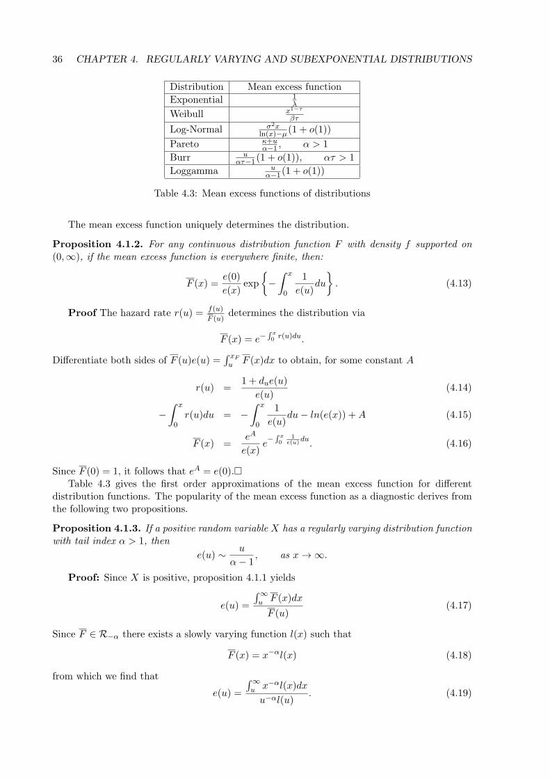
36 CHAPTER 4. REGULARLY VARYING AND SUBEXPONENTIAL DISTRIBUTIONS
Distribution Mean excess function
Exponential 1λ
Weibull x1−τ
βτ
Log-Normal σ2xln(x)−µ(1 + o(1))
Pareto κ+uα−1 , α > 1
Burr uατ−1(1 + o(1)), ατ > 1
Loggamma uα−1(1 + o(1))
Table 4.3: Mean excess functions of distributions
The mean excess function uniquely determines the distribution.
Proposition 4.1.2. For any continuous distribution function F with density f supported on(0,∞), if the mean excess function is everywhere finite, then:
F (x) =e(0)
e(x)exp
−∫ x
0
1
e(u)du
. (4.13)
Proof The hazard rate r(u) = f(u)
F (u)determines the distribution via
F (x) = e−∫ x0 r(u)du.
Differentiate both sides of F (u)e(u) =∫ xF
u F (x)dx to obtain, for some constant A
r(u) =1 + due(u)
e(u)(4.14)
−∫ x
0r(u)du = −
∫ x
0
1
e(u)du− ln(e(x)) +A (4.15)
F (x) =eA
e(x)e−
∫ x0
1e(u)
du. (4.16)
Since F (0) = 1, it follows that eA = e(0).Table 4.3 gives the first order approximations of the mean excess function for different
distribution functions. The popularity of the mean excess function as a diagnostic derives fromthe following two propositions.
Proposition 4.1.3. If a positive random variable X has a regularly varying distribution functionwith tail index α > 1, then
e(u) ∼ u
α− 1, as x → ∞.
Proof: Since X is positive, proposition 4.1.1 yields
e(u) =
∫∞u F (x)dx
F (u)(4.17)
Since F ∈ R−α there exists a slowly varying function l(x) such that
F (x) = x−αl(x) (4.18)
from which we find that
e(u) =
∫∞u x−αl(x)dx
u−αl(u). (4.19)
4.1. MEAN EXCESS FUNCTION 37
From theorem 4.0.2: ∫∞u x−αl(x)dx
u−αl(u)∼ u
α− 1, u → ∞
Remark 4.1.1. A direct calculation with the survivor function of a Pareto distribution withfinite mean, F (x) = ( k
k+x)α; α > 1, shows that e(u) = k+u
α−1 . In other words, e(u) is linear with
intercept kα−1 and slope 1
α−1
Proposition 4.1.4. Let F be the distribution function of a positive unbounded continuous ran-dom variable X with finite mean. If for all y ∈ R
limx→∞
F (x− y)
F (x)= eγy, (4.20)
for some γ ∈ [0,∞], then
limu→∞
e(u) =1
γ.
Proof. By lemma (4.0.7) and (??), F ln ∈ R−γ which implies F (x) ∼ x−γL(x); L(tx)L(x) ∼ 1. Wehave
e(u) =
∫∞u F (x)dx
F (u)
=
∫ ∞
eu
z−1F (ln(z))dz
F (ln(eu))
∼∫ ∞
eu
z−(1+γ)L(z)dz
e−γuL(eu).
By (4.0.2.2) this is equal to 1/γ
Remark 4.1.2. If F ∈ S, then equation (4.20) is satisfied with γ = 0. If a distribution functionis subexponential, the mean excess function e(u) tends to infinity as u → ∞. If a distributionfunction is regularly varying with a tail index α > 1 then we know that the mean excess functionof this distribution is eventually linear with slope 1
α−1 .
One drawback of the mean excess function as a diagnostic is that it does not exist for regularlyvarying distributions with tail index α < 1. Since the empirical mean excess function alwayshas finite slope, the plots can be misleading in such cases. Using Remark (??) we could searchfor 1 > β > 0 such that E(Xβ) < ∞. If the mean excess function of Xβ tends to a straightline with slope 1/(γ − 1), then we could infer that X ∈ R−γ/β . In Chapter 5 a new diagnosticapplicable to all distributions will be proposed.
38 CHAPTER 4. REGULARLY VARYING AND SUBEXPONENTIAL DISTRIBUTIONS
Chapter 5
Indices and Diagnostics of TailHeaviness
This chapter studies diagnostics for tail obesity using the self-similarity - or lack thereof - of themean excess plot. We examine how the mean excess plot changes when we aggregate a data setby k. From this we define two new diagnostics; the first is the ratio of the largest to the secondlargest observation in a data set. The second, termed the Obesity index, is the probabilitythat the sum of the largest and the smallest of four observations is larger than the sum ofthe other two observations. A note on terminology: heuristic suggests a (possibly inaccurate)shortcut, a diagnostic is a way of identifying something already defined, a measure entails adefinition, but not necessarily a method of estimation. Index is less precise but suggests allof these. Tail index is already preempted, moreover we seek a characterization which appliesequally to selected data, eg the largest values, as well as to entire distributions, heavy tailed orotherwise. The term Obesity index is enlisted for this purpose. It defines a property of empiricalor theoretical distributions and in this sense includes a method of estimation. For the rest, theterms ”heuristic” and ”diagnostic” are used indiscriminately.
5.1 Self-similarity
One of the heuristics discussed in Chapter 1 was the self-similarity under aggregation of heavy-tailed distributions and how this could be seen in the mean excess plot of a distribution. Considera data set of size n and create a new data set by dividing the original data set randomly intogroups of size k and summing each of the k members of each group. We call this operation”aggregation by k”. If we compare the mean excess plots of regularly varying distributionfunction with tail index α < 2, then the mean excess plot of the original data set and the dataset obtained through aggregating by k look very similar. For distributions with a finite variancethe mean excess plots of the original sample and the aggregated sample look very different.
39
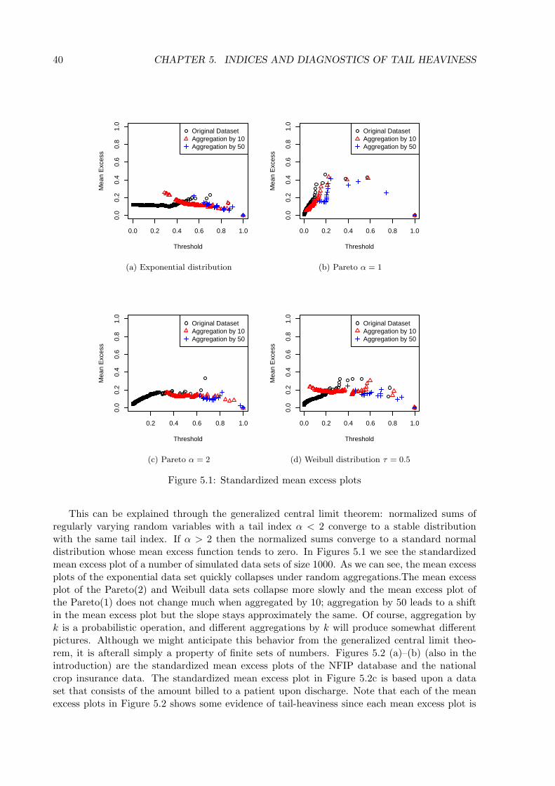
40 CHAPTER 5. INDICES AND DIAGNOSTICS OF TAIL HEAVINESS
0.0 0.2 0.4 0.6 0.8 1.0
0.0
0.2
0.4
0.6
0.8
1.0
Threshold
Mea
n E
xces
s
Original DatasetAggregation by 10Aggregation by 50
(a) Exponential distribution
0.0 0.2 0.4 0.6 0.8 1.0
0.0
0.2
0.4
0.6
0.8
1.0
Threshold
Mea
n E
xces
s
Original DatasetAggregation by 10Aggregation by 50
(b) Pareto α = 1
0.2 0.4 0.6 0.8 1.0
0.0
0.2
0.4
0.6
0.8
1.0
Threshold
Mea
n E
xces
s
Original DatasetAggregation by 10Aggregation by 50
(c) Pareto α = 2
0.0 0.2 0.4 0.6 0.8 1.0
0.0
0.2
0.4
0.6
0.8
1.0
Threshold
Mea
n E
xces
s
Original DatasetAggregation by 10Aggregation by 50
(d) Weibull distribution τ = 0.5
Figure 5.1: Standardized mean excess plots
This can be explained through the generalized central limit theorem: normalized sums ofregularly varying random variables with a tail index α < 2 converge to a stable distributionwith the same tail index. If α > 2 then the normalized sums converge to a standard normaldistribution whose mean excess function tends to zero. In Figures 5.1 we see the standardizedmean excess plot of a number of simulated data sets of size 1000. As we can see, the mean excessplots of the exponential data set quickly collapses under random aggregations.The mean excessplot of the Pareto(2) and Weibull data sets collapse more slowly and the mean excess plot ofthe Pareto(1) does not change much when aggregated by 10; aggregation by 50 leads to a shiftin the mean excess plot but the slope stays approximately the same. Of course, aggregation byk is a probabilistic operation, and different aggregations by k will produce somewhat differentpictures. Although we might anticipate this behavior from the generalized central limit theo-rem, it is afterall simply a property of finite sets of numbers. Figures 5.2 (a)–(b) (also in theintroduction) are the standardized mean excess plots of the NFIP database and the nationalcrop insurance data. The standardized mean excess plot in Figure 5.2c is based upon a dataset that consists of the amount billed to a patient upon discharge. Note that each of the meanexcess plots in Figure 5.2 shows some evidence of tail-heaviness since each mean excess plot is
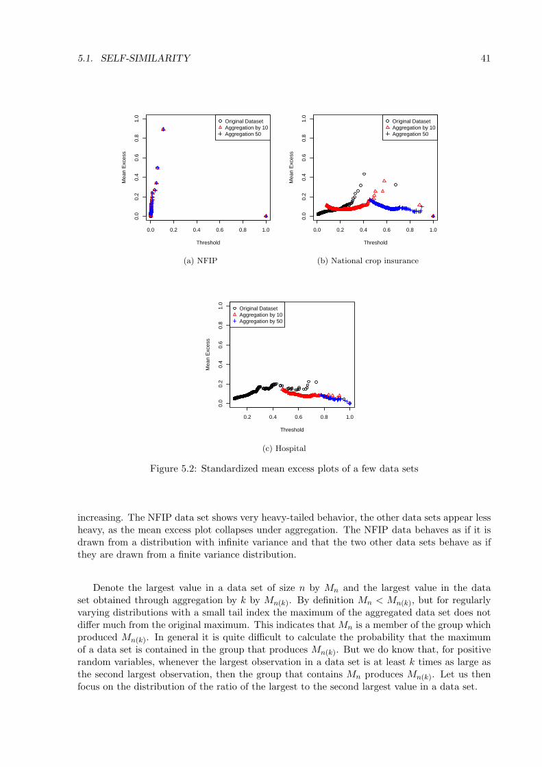
5.1. SELF-SIMILARITY 41
0.0 0.2 0.4 0.6 0.8 1.0
0.0
0.2
0.4
0.6
0.8
1.0
Threshold
Mea
n E
xces
sOriginal DatasetAggregation by 10Aggregation 50
(a) NFIP
0.0 0.2 0.4 0.6 0.8 1.0
0.0
0.2
0.4
0.6
0.8
1.0
Threshold
Mea
n E
xces
s
Original DatasetAggregation by 10Aggregation 50
(b) National crop insurance
0.2 0.4 0.6 0.8 1.0
0.0
0.2
0.4
0.6
0.8
1.0
Threshold
Mea
n E
xces
s
Original DatasetAggregation by 10Aggregation by 50
(c) Hospital
Figure 5.2: Standardized mean excess plots of a few data sets
increasing. The NFIP data set shows very heavy-tailed behavior, the other data sets appear lessheavy, as the mean excess plot collapses under aggregation. The NFIP data behaves as if it isdrawn from a distribution with infinite variance and that the two other data sets behave as ifthey are drawn from a finite variance distribution.
Denote the largest value in a data set of size n by Mn and the largest value in the dataset obtained through aggregation by k by Mn(k). By definition Mn < Mn(k), but for regularlyvarying distributions with a small tail index the maximum of the aggregated data set does notdiffer much from the original maximum. This indicates that Mn is a member of the group whichproduced Mn(k). In general it is quite difficult to calculate the probability that the maximumof a data set is contained in the group that produces Mn(k). But we do know that, for positiverandom variables, whenever the largest observation in a data set is at least k times as large asthe second largest observation, then the group that contains Mn produces Mn(k). Let us thenfocus on the distribution of the ratio of the largest to the second largest value in a data set.
42 CHAPTER 5. INDICES AND DIAGNOSTICS OF TAIL HEAVINESS
5.1.1 Distribution of the ratio between order statistics
In Theorem 2.4.1 we derived the distribution of the ratio between two order statistics in thegeneral case given by
P
(Xr,n
Xs,n≤ x
)=
1
B(s, n− s+ 1)
∫ 1
0IQx(t)(r, s− r)ts−1(1− t)n−sdt, (r < s) (5.1)
where B(x, y) is the beta function, Ix(r, s) the incomplete beta function and Qx(t) =F (tF−1(x)
t .We are interested in the case that r = n− 1 and s = n so the distribution function in equation(5.1) simplifies to
P
(Xn−1,n
Xn,n≤ x
)= n(n− 1)
∫ 1
0IQx(t)(n− 1, 1)tn−1dt.
It turns out there is a much simpler form for the distribution function of the ratio of successiveorder statistics from a Pareto distribution.
Proposition 5.1.1. When X1,n, ..., Xn,n are order statistics from a Pareto distribution then
the ratio between two consecutive order statistics,Xi+1,n
Xi,n, also has a Pareto distribution with
parameter (n− i)α.
Proof. The distribution function ofXi+1,n
Xi,ncan be found by conditionalizing on Xi,n and using
Theorem 2.2.1 to find the distribution of Xi+1,n|Xi,n = x.
P
(Xi+1,n
Xi,n> z
)=
∫ ∞
1P (Xi+1,n > zx|Xi+1,n = x) fXi,n(x)dx
=
∫ ∞
1
(1− F (zx)
1− F (x)
)n−i 1
B(i, n− i+ 1)F (x)i−1 (1− F (x))n−i f(x)dx
=1
B(i, n− i+ 1)
∫ ∞
1(1− F (zx))n−iF (x)i−1f(x)dx
=1
B(i, n− i+ 1)z−(n−i)α
∫ ∞
1x−(n−i)α(1− x−α)i−1αx−α−1dx
= z−(n−i)α 1
B(i, n− i+ 1)
∫ 1
0un−i(1− u)i−1du (u = x−α)
= z−(n−i)α 1
B(i, n− i+ 1)B(i, n− i+ 1)
= z−(n−i)α.
One might ask whether the converse of proposition 5.1.1 also holds, i.e. if for some k andn the ratio
Xk+1,n
Xk,nhas a Pareto distribution, is the parent distribution of the order statistics
also a Pareto distribution? That this is not the case is shown by a counter-example of Arnold[1983]: Let Z1 and Z2 be two independent Γ(12 , 1) random variables, and let X = eZ1−Z2 . If oneconsiders a sample of size 2, then we find that X1 and X2 are not Pareto distributed, but thatthe ratio
X2,2
X1,2does have a Pareto distribution.
One needs to make additional assumptions, for example, that the ratio of two successiveorder statistics have a Pareto distribution for all n, as was shown in H.J.Rossberg [1972]. Herewe will give a different proof of this result. The following lemma is needed to prove the result1.
1Result was found on 1 February 2010 at http://at.yorku.ca/cgi-bin/bbqa?forum=ask an analyst 2006;task=show msg;msg=1091.0001
5.1. SELF-SIMILARITY 43
Lemma 5.1.2. If f(x) is a continuous function on [0, 1], and if for all n ≥ 0∫ 1
0f(x)xndx = 0, (5.2)
then f(x) is equal to zero.
Proof. Since equation (5.2) holds, we know that for any polynomial p(x) the following equationholds ∫ 1
0f(x)p(x)dx = 0.
From this we find that for any polynomial p(x)∫ 1
0f(x)2dx =
∫ 1
0([f(x)− p(x)] f(x) + f(x)p(x))dx
=
∫ 1
0[f(x)− p(x)] f(x)dx.
Since f(x) is a continuous function on [0, 1] we find by the Weierstrass theorem that for anyε > 0 there exists a polynomial P (x) such that
supx∈[0,1]
|f(x)− P (x)| < ε.
By the Min-Max theorem there exists a constant M such that |f(x)| ≤ M for all 0 ≤ x ≤ 1.From this we find that for any ε > 0 there exists a polynomial P (x) such that
|∫ 1
0f(x)2dx| = |
∫ 1
0[f(x)− P (x)] f(x)dx|,
≤∫ 1
0|f(x)− P (x)||f(x)|dx,
≤ εM. (5.3)
But since equation (5.3) holds for all ε > 0 we find that∫ 1
0f(x)2dx = 0. (5.4)
Since f is continuous on [1, 0], it follows that f(x) = 0, x ∈ [0, 1]
Theorem 5.1.3. For positive continuous random variable X with invertible distribution functionF , if there exists α > 0 such that for all n ≥ 2 and all x > 1:
P
(Xn,n
Xn−1,n> x
)= x−α, (5.5)
then for some κ > 0
F (x) = 1−(κx
)α,
for x > κ.
44 CHAPTER 5. INDICES AND DIAGNOSTICS OF TAIL HEAVINESS
Proof. The two largest of n values can be chosen in n(n− 1) ways, thus
P (Xn,n > Xn−1,nx) = n(n− 1)
∫ ∞
0(1− F (zx))F (z)n−2f(z)dz = x−α. (5.6)
Since n(n− 1)(1−F (z))F (z)n−2f(z) is the density of the n− 1-th order statistic from a sampleof n:
n(n− 1)
∫ ∞
0(1− F (z))F (z)n−2f(z)dz = 1, (5.7)
Divide (5.6) by x−α and subtract from (5.7) to find:
n(n− 1)
∫ ∞
0
(xαF (xz)− F (z)
)F (z)n−2f(z)dz = 0, (5.8)
Since equation (5.8) holds for all n ≥ 2 we can apply lemma 5.1.2 and find that
xαF (xz) = F (z).
This is a variant of the Cauchy equation, whose solution may be written as F (x) = καx−α,x > κ.
As in the above proof, the distribution of the ratio between two upper order statistics canbe obtained by evaluating the following integral:
P
(Xn,n
Xn−1,n> x
)= n(n− 1)
∫ ∞
−∞(1− F (zx))F (z)n−2f(z)dz (5.9)
For the Weibull distribution an analytic expression for the integral in equation (5.9 ) is:
P
(Xn,n
Xn−1,n> x
)= n(n− 1)
∫ ∞
0(1− F (zx))F (z)n−2f(z)dz
= n(n− 1)
∫ ∞
0
(e−(λxz)τ
)(1− e−(λz)τ
)n−2τλτzτ−1e−(λz)τdz
= n(n− 1)
∫ 1
0ux
τ(1− u)n−2du
= n(n− 1)B(xτ + 1, n− 1).
Figures 5.3 (a)–(b) show the approximation of the probability in equation (5.9), with x = 2,for the Burr distribution with parameters c = 1 and k = 1 and the Cauchy distribution. ThisBurr distribution and the Cauchy distribution both have tail index one. The probability thatthe largest order statistic is at least twice as large as the second largest order statistic seems toconverge to a half. This is exactly the probability that the the ratio of the largest to the secondlargest order statistic from a Pareto(1) is at least one half, suggesting that the distribution ofthe ratio of the two largest order statistics of a regularly varying distribution converges to thedistribution of that ratio from a Pareto distribution with the same tail index. The next theoremproves this statement. We first recall some results from the theory of regular variation. If thefollowing limit exists for z > 1
limx→∞
F (zx)
F (x)= β(z) ∈ [0, 1] , z > 1
then the three following cases are possible:
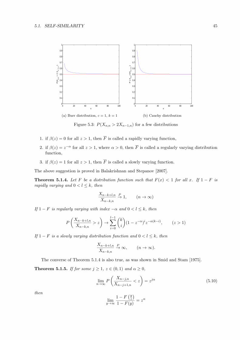
5.1. SELF-SIMILARITY 45
0 20 40 60 80 1000
0.1
0.2
0.3
0.4
0.5
0.6
0.7
0.8
0.9
1
n
P(X
n,n
> 2
Xn
−1
,n )
(a) Burr distribution, c = 1, k = 1
0 20 40 60 80 1000
0.1
0.2
0.3
0.4
0.5
0.6
0.7
0.8
0.9
1
n
P (
Xn
,n>
2X
n−
1,n
)
(b) Cauchy distribution
Figure 5.3: P (Xn,n > 2Xn−1,n) for a few distributions
1. if β(z) = 0 for all z > 1, then F is called a rapidly varying function,
2. if β(z) = z−α for all z > 1, where α > 0, then F is called a regularly varying distributionfunction,
3. if β(z) = 1 for all z > 1, then F is called a slowly varying function.
The above suggestion is proved in Balakrishnan and Stepanov [2007].
Theorem 5.1.4. Let F be a distribution function such that F (x) < 1 for all x. If 1 − F israpidly varying and 0 < l ≤ k, then
Xn−k+l,n
Xn−k,n
P→ 1, (n → ∞)
If 1− F is regularly varying with index −α and 0 < l ≤ k, then
P
(Xn−k+l,n
Xn−k,n> z
)→
l−1∑i=0
(k
i
)(1− z−α)iz−α(k−i), (z > 1)
If 1− F is a slowly varying distribution function and 0 < l ≤ k, then
Xn−k+l,n
Xn−k,n
P→ ∞, (n → ∞).
The converse of Theorem 5.1.4 is also true, as was shown in Smid and Stam [1975].
Theorem 5.1.5. If for some j ≥ 1, z ∈ (0, 1) and α ≥ 0,
limn→∞
P
(Xn−j,n
Xn−j+1,n< z
)= zjα (5.10)
then
limy→∞
1− F(yz
)1− F (y)
= zα
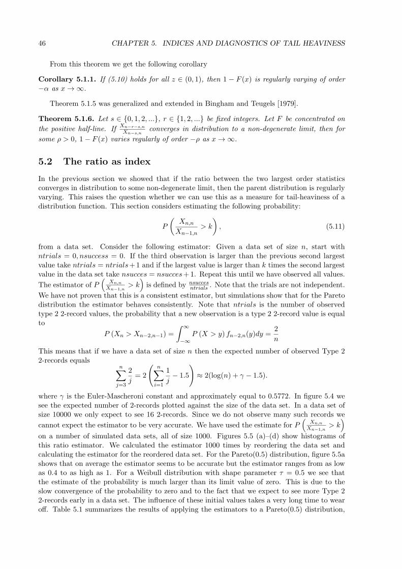
46 CHAPTER 5. INDICES AND DIAGNOSTICS OF TAIL HEAVINESS
From this theorem we get the following corollary
Corollary 5.1.1. If (5.10) holds for all z ∈ (0, 1), then 1 − F (x) is regularly varying of order−α as x → ∞.
Theorem 5.1.5 was generalized and extended in Bingham and Teugels [1979].
Theorem 5.1.6. Let s ∈ 0, 1, 2, ..., r ∈ 1, 2, ... be fixed integers. Let F be concentrated on
the positive half-line. IfXn−r−s,n
Xn−s,nconverges in distribution to a non-degenerate limit, then for
some ρ > 0, 1− F (x) varies regularly of order −ρ as x → ∞.
5.2 The ratio as index
In the previous section we showed that if the ratio between the two largest order statisticsconverges in distribution to some non-degenerate limit, then the parent distribution is regularlyvarying. This raises the question whether we can use this as a measure for tail-heaviness of adistribution function. This section considers estimating the following probability:
P
(Xn,n
Xn−1,n> k
), (5.11)
from a data set. Consider the following estimator: Given a data set of size n, start withntrials = 0, nsuccess = 0. If the third observation is larger than the previous second largestvalue take ntrials = ntrials+1 and if the largest value is larger than k times the second largestvalue in the data set take nsucces = nsucces+1. Repeat this until we have observed all values.
The estimator of P(
Xn,n
Xn−1,n> k
)is defined by nsucces
ntrials . Note that the trials are not independent.
We have not proven that this is a consistent estimator, but simulations show that for the Paretodistribution the estimator behaves consistently. Note that ntrials is the number of observedtype 2 2-record values, the probability that a new observation is a type 2 2-record value is equalto
P (Xn > Xn−2,n−1) =
∫ ∞
−∞P (X > y) fn−2,n(y)dy =
2
n
This means that if we have a data set of size n then the expected number of observed Type 22-records equals
n∑j=3
2
j= 2
(n∑
i=1
1
j− 1.5
)≈ 2(log(n) + γ − 1.5).
where γ is the Euler-Mascheroni constant and approximately equal to 0.5772. In figure 5.4 wesee the expected number of 2-records plotted against the size of the data set. In a data set ofsize 10000 we only expect to see 16 2-records. Since we do not observe many such records we
cannot expect the estimator to be very accurate. We have used the estimate for P(
Xn,n
Xn−1,n> k
)on a number of simulated data sets, all of size 1000. Figures 5.5 (a)–(d) show histograms ofthis ratio estimator. We calculated the estimator 1000 times by reordering the data set andcalculating the estimator for the reordered data set. For the Pareto(0.5) distribution, figure 5.5ashows that on average the estimator seems to be accurate but the estimator ranges from as lowas 0.4 to as high as 1. For a Weibull distribution with shape parameter τ = 0.5 we see thatthe estimate of the probability is much larger than its limit value of zero. This is due to theslow convergence of the probability to zero and to the fact that we expect to see more Type 22-records early in a data set. The influence of these initial values takes a very long time to wearoff. Table 5.1 summarizes the results of applying the estimators to a Pareto(0.5) distribution,
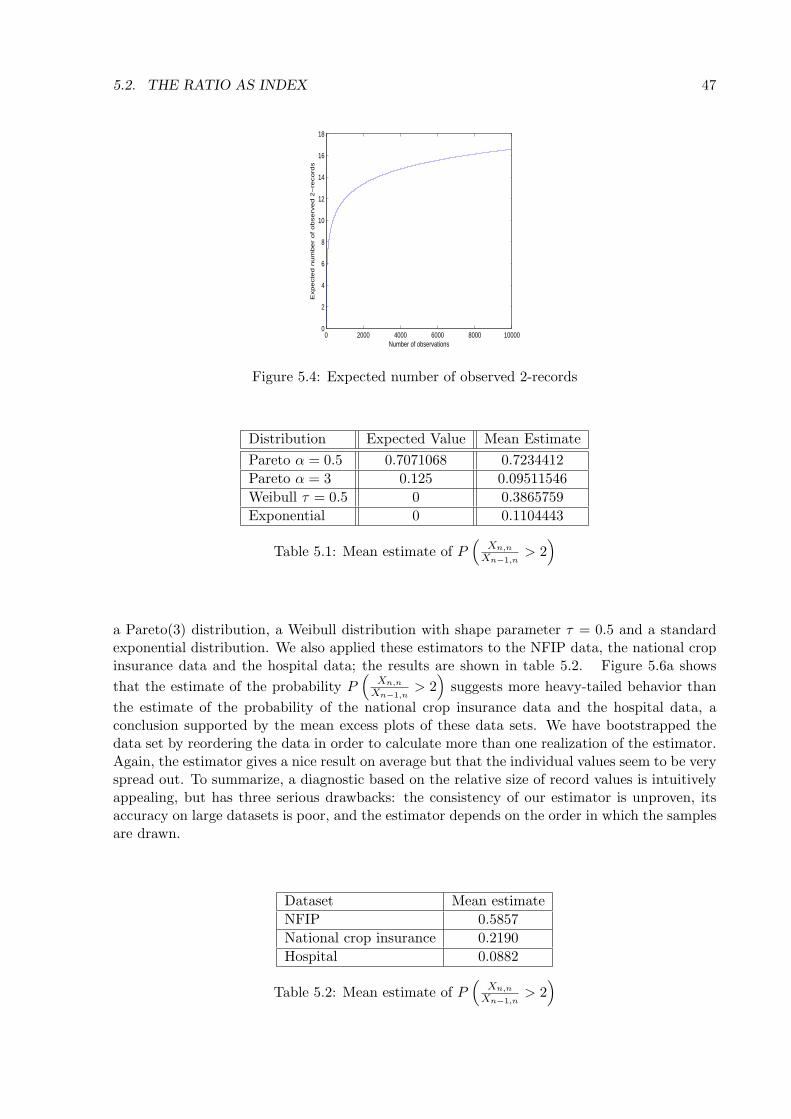
5.2. THE RATIO AS INDEX 47
0 2000 4000 6000 8000 100000
2
4
6
8
10
12
14
16
18
Number of observations
Exp
ecte
d n
um
be
r o
f o
bse
rve
d 2
−re
co
rds
Figure 5.4: Expected number of observed 2-records
Distribution Expected Value Mean Estimate
Pareto α = 0.5 0.7071068 0.7234412
Pareto α = 3 0.125 0.09511546
Weibull τ = 0.5 0 0.3865759
Exponential 0 0.1104443
Table 5.1: Mean estimate of P(
Xn,n
Xn−1,n> 2)
a Pareto(3) distribution, a Weibull distribution with shape parameter τ = 0.5 and a standardexponential distribution. We also applied these estimators to the NFIP data, the national cropinsurance data and the hospital data; the results are shown in table 5.2. Figure 5.6a shows
that the estimate of the probability P(
Xn,n
Xn−1,n> 2)suggests more heavy-tailed behavior than
the estimate of the probability of the national crop insurance data and the hospital data, aconclusion supported by the mean excess plots of these data sets. We have bootstrapped thedata set by reordering the data in order to calculate more than one realization of the estimator.Again, the estimator gives a nice result on average but that the individual values seem to be veryspread out. To summarize, a diagnostic based on the relative size of record values is intuitivelyappealing, but has three serious drawbacks: the consistency of our estimator is unproven, itsaccuracy on large datasets is poor, and the estimator depends on the order in which the samplesare drawn.
Dataset Mean estimate
NFIP 0.5857
National crop insurance 0.2190
Hospital 0.0882
Table 5.2: Mean estimate of P(
Xn,n
Xn−1,n> 2)
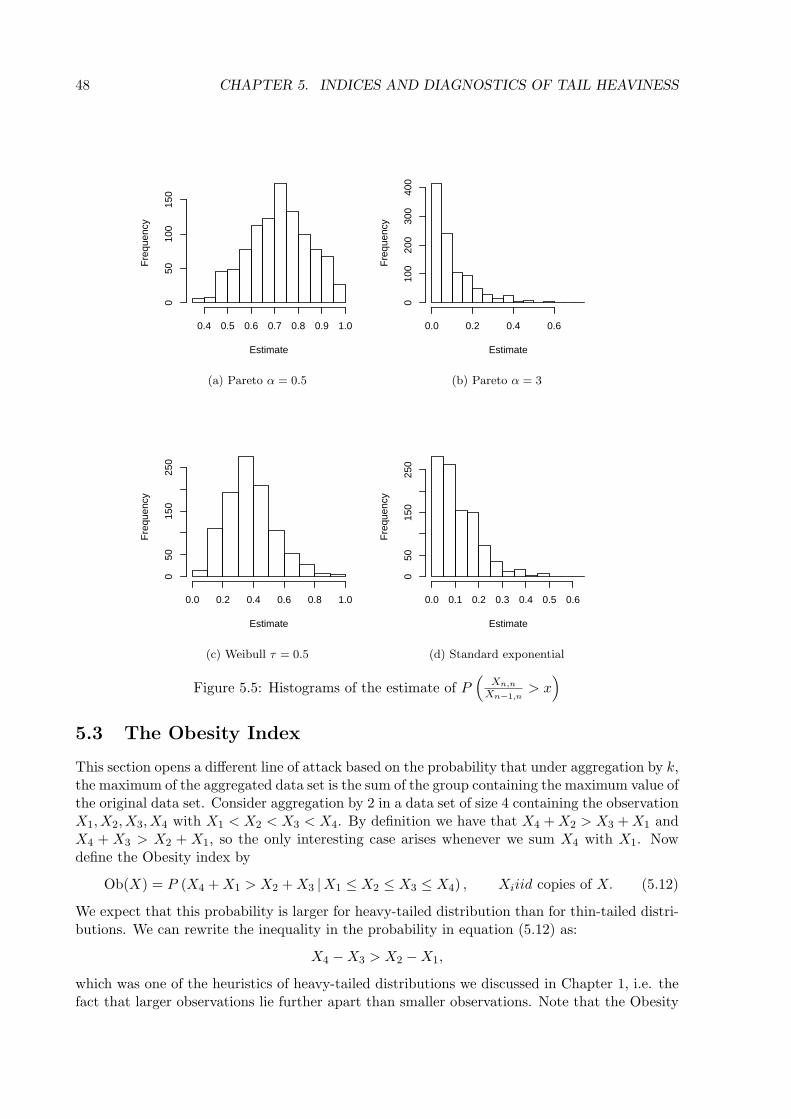
48 CHAPTER 5. INDICES AND DIAGNOSTICS OF TAIL HEAVINESS
Estimate
Fre
quen
cy
0.4 0.5 0.6 0.7 0.8 0.9 1.0
050
100
150
(a) Pareto α = 0.5
Estimate
Fre
quen
cy
0.0 0.2 0.4 0.6
010
020
030
040
0
(b) Pareto α = 3
Estimate
Fre
quen
cy
0.0 0.2 0.4 0.6 0.8 1.0
050
150
250
(c) Weibull τ = 0.5
Estimate
Fre
quen
cy
0.0 0.1 0.2 0.3 0.4 0.5 0.6
050
150
250
(d) Standard exponential
Figure 5.5: Histograms of the estimate of P(
Xn,n
Xn−1,n> x
)5.3 The Obesity Index
This section opens a different line of attack based on the probability that under aggregation by k,the maximum of the aggregated data set is the sum of the group containing the maximum value ofthe original data set. Consider aggregation by 2 in a data set of size 4 containing the observationX1, X2, X3, X4 with X1 < X2 < X3 < X4. By definition we have that X4 +X2 > X3 +X1 andX4 + X3 > X2 + X1, so the only interesting case arises whenever we sum X4 with X1. Nowdefine the Obesity index by
Ob(X) = P (X4 +X1 > X2 +X3 |X1 ≤ X2 ≤ X3 ≤ X4) , Xiiid copies of X. (5.12)
We expect that this probability is larger for heavy-tailed distribution than for thin-tailed distri-butions. We can rewrite the inequality in the probability in equation (5.12) as:
X4 −X3 > X2 −X1,
which was one of the heuristics of heavy-tailed distributions we discussed in Chapter 1, i.e. thefact that larger observations lie further apart than smaller observations. Note that the Obesity
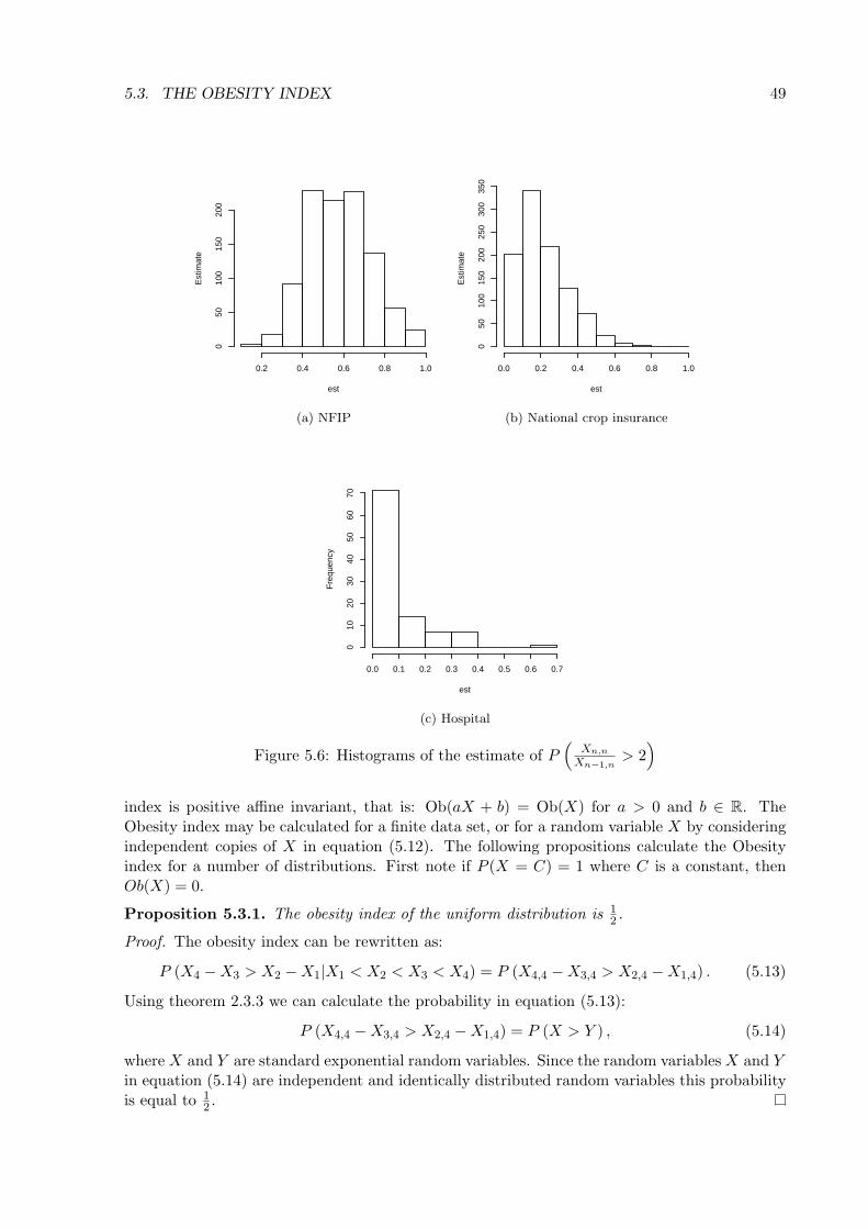
5.3. THE OBESITY INDEX 49
est
Est
imat
e
0.2 0.4 0.6 0.8 1.0
050
100
150
200
(a) NFIP
est
Est
imat
e
0.0 0.2 0.4 0.6 0.8 1.0
050
100
150
200
250
300
350
(b) National crop insurance
est
Fre
quen
cy
0.0 0.1 0.2 0.3 0.4 0.5 0.6 0.7
010
2030
4050
6070
(c) Hospital
Figure 5.6: Histograms of the estimate of P(
Xn,n
Xn−1,n> 2)
index is positive affine invariant, that is: Ob(aX + b) = Ob(X) for a > 0 and b ∈ R. TheObesity index may be calculated for a finite data set, or for a random variable X by consideringindependent copies of X in equation (5.12). The following propositions calculate the Obesityindex for a number of distributions. First note if P (X = C) = 1 where C is a constant, thenOb(X) = 0.
Proposition 5.3.1. The obesity index of the uniform distribution is 12 .
Proof. The obesity index can be rewritten as:
P (X4 −X3 > X2 −X1|X1 < X2 < X3 < X4) = P (X4,4 −X3,4 > X2,4 −X1,4) . (5.13)
Using theorem 2.3.3 we can calculate the probability in equation (5.13):
P (X4,4 −X3,4 > X2,4 −X1,4) = P (X > Y ) , (5.14)
where X and Y are standard exponential random variables. Since the random variablesX and Yin equation (5.14) are independent and identically distributed random variables this probabilityis equal to 1
2 .
50 CHAPTER 5. INDICES AND DIAGNOSTICS OF TAIL HEAVINESS
Proposition 5.3.2. The obesity index of the exponential distribution is 34 .
Proof. Again we rewrite the obesity index:
P (X4 −X3 > X2 −X1|X1 < X2 < X3 < X4) = P (X4,4 −X3,4 > X2,4 −X1,4) . (5.15)
Using theorem 2.3.2:
P (X4,4 −X3,4 > X2,4 −X1,4) = P
(X >
Y
3
), (5.16)
where X and Y are independent standard exponential random variables. We can calculate theprobability on the RHS in equation (5.16):
P
(X >
Y
3
)=
∫ ∞
0P (X > y) fY
3(y)dy
=
∫ ∞
0e−y3e−3ydy
=3
4.
Proposition 5.3.3. If X is a symmetrical random variable with respect to zero, Xd= −X, then
the obesity index is equal to 12 .
Proof. If Xd= −X, then FX(x) = 1− FX(−x), and fX(x) = fX(−x). The joint density of X3,4
and X4,4 is now given by
f3,4;4(x3, x4) =24
2F (x3)
2f(x3)f(x4), x3 < x4
=24
2(1− F (−x3))
2f(−x3)f(−x4), −x4 < −x3
= f1,2;4(−x4,−x3)
This is equal to the joint density of −X1,4 and −X2,4, and from this we find that
X4,4 −X3,4d= X2,4 −X1,4.
Hence the obesity index 12 .
From proposition 5.3.3 we find that for a distribution which is symmetric with respect tosome constant µ, the Obesity index is 1
2 . Indeed, if X is symmetric about µ, X−µ is symmetricabout zero and with positive affine invariance, Ob(X) = Ob(X − µ). This means that theObesity index of both the Cauchy and the Normal distribution is 1
2 . The Cauchy distributionhas a regularly varying distribution function with tail index 1, and the Normal distribution isthin-tailed distribution on any definition. Evidently the Obesity index must be restricted topositive random variables.
Theorem 5.3.4. The Obesity index of a random variable X with distribution function F anddensity f can be calculated by evaluating the following integral,
24
∫ ∞
−∞
∫ ∞
x1
∫ ∞
x2
F (x2 + x3 − x1)f(x1)f(x2)f(x3)dx3dx2dx1.
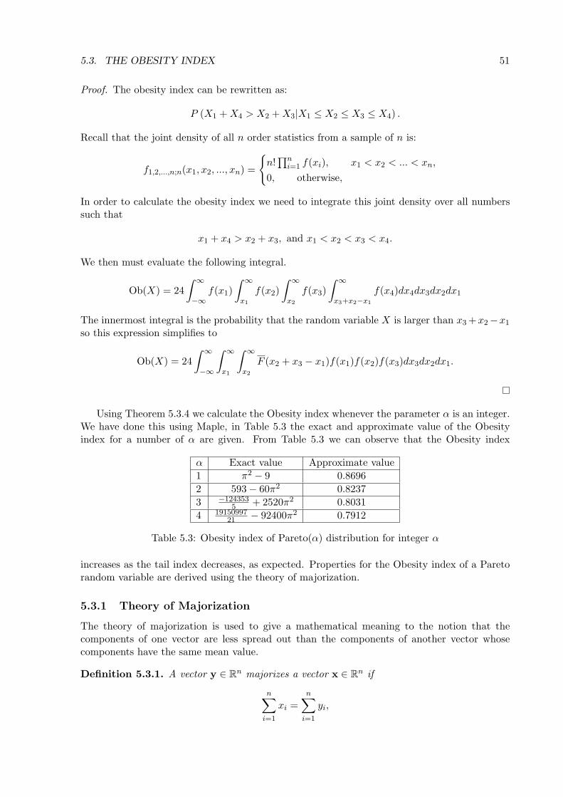
5.3. THE OBESITY INDEX 51
Proof. The obesity index can be rewritten as:
P (X1 +X4 > X2 +X3|X1 ≤ X2 ≤ X3 ≤ X4) .
Recall that the joint density of all n order statistics from a sample of n is:
f1,2,...,n;n(x1, x2, ..., xn) =
n!∏n
i=1 f(xi), x1 < x2 < ... < xn,
0, otherwise,
In order to calculate the obesity index we need to integrate this joint density over all numberssuch that
x1 + x4 > x2 + x3, and x1 < x2 < x3 < x4.
We then must evaluate the following integral.
Ob(X) = 24
∫ ∞
−∞f(x1)
∫ ∞
x1
f(x2)
∫ ∞
x2
f(x3)
∫ ∞
x3+x2−x1
f(x4)dx4dx3dx2dx1
The innermost integral is the probability that the random variable X is larger than x3+x2−x1so this expression simplifies to
Ob(X) = 24
∫ ∞
−∞
∫ ∞
x1
∫ ∞
x2
F (x2 + x3 − x1)f(x1)f(x2)f(x3)dx3dx2dx1.
Using Theorem 5.3.4 we calculate the Obesity index whenever the parameter α is an integer.We have done this using Maple, in Table 5.3 the exact and approximate value of the Obesityindex for a number of α are given. From Table 5.3 we can observe that the Obesity index
α Exact value Approximate value
1 π2 − 9 0.8696
2 593− 60π2 0.8237
3 −1243535 + 2520π2 0.8031
4 1915099721 − 92400π2 0.7912
Table 5.3: Obesity index of Pareto(α) distribution for integer α
increases as the tail index decreases, as expected. Properties for the Obesity index of a Paretorandom variable are derived using the theory of majorization.
5.3.1 Theory of Majorization
The theory of majorization is used to give a mathematical meaning to the notion that thecomponents of one vector are less spread out than the components of another vector whosecomponents have the same mean value.
Definition 5.3.1. A vector y ∈ Rn majorizes a vector x ∈ Rn if
n∑i=1
xi =
n∑i=1
yi,
52 CHAPTER 5. INDICES AND DIAGNOSTICS OF TAIL HEAVINESS
andk∑
i=1
x[i] ≤k∑
i=1
y[i], k = 1, ..., n
where x[1] . . . x[n] is the decreasing arrangement of the vector x such that
x[1] ≥ ... ≥ x[n].
We denote this by x ≺ y.
Schur-convex functions preserve the majorization ordering.
Definition 5.3.2. A function ϕ : A → R, where A ⊂ Rn, is called Schur-convex (-concave) onA if
x ≺ y on A ⇒ ϕ(x) ≤ (≥)ϕ(y) (5.17)
The following proposition gives sufficient conditions for a function ϕ to be Schur-convex(concave).
Proposition 5.3.5. If I ⊂ R is an interval and g : I → R is convex (concave), then
ϕ(x) =n∑
i=1
g(xi),
is Schur-convex (-concave)on In.
We prove two theorems about the inequality in the obesity index.
Theorem 5.3.6. Let Xα be Pareto(α) distributed, for α > 0. Then limα→0Ob(Xα) = 1.
Proof. X(α) has the same distribution as U−1/α From Hardy et al. [1934] we know that
limp→∞
(n∑
i=1
upi
) 1p
= max u1, ..., un .
Suppose that u1 < u2 < u3 < u4, we have
limα→0
(u−1/α1 + u
−1/α4
)= max
u−11 , u−1
4
1α = max
u− 1
α1 , u
− 1α
4
.
This means that as α tends to 0, u−1/α1 + u
−1/α4 tends to max
u−1/α1 , u
−1/α4
, which is u
−1/α1 .
The same limit holds for u−1/α2 + u
−1/α3 , where the maximum of these two by definition is equal
to u−1/α2 . The proof concludes by substituting X = U−α.
There is no comparable result for general regularly varying distributions since obesity de-pends on the whole distribution, not just the tail. For example, let X be uniform on [0, 1] withprobability (1/2)1/4 and be Pareto(1) with probability 1−(1/2)1/4. Clearly X ∈ R−1. However,with probability 1/2 four independent copies of X are all drawn from the uniform distributionwith obesity 1/2. Hence the obesity of X cannot exceed 0.75. The second result shows thatobesity is increased by applying a convex increasing function.
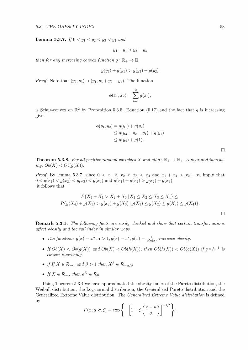
5.3. THE OBESITY INDEX 53
Lemma 5.3.7. If 0 < y1 < y2 < y3 < y4 and
y4 + y1 > y2 + y3
then for any increasing convex function g : R+ → R
g(y4) + g(y1) > g(y3) + g(y2)
Proof. Note that (y2, y3) ≺ (y1, y3 + y2 − y1). The function
ϕ(x1, x2) =
2∑i=1
g(xi),
is Schur-convex on R2 by Proposition 5.3.5. Equation (5.17) and the fact that g is increasinggive:
ϕ(y1, y2) = g(y1) + g(y2)
≤ g(y3 + y2 − y1) + g(y1)
≤ g(y4) + g(1).
Theorem 5.3.8. For all positive random variables X and all g : R+ → R+, convex and increas-ing, Ob(X) < Ob(g(X)).
Proof. By lemma 5.3.7, since 0 < x1 < x2 < x3 < x4 and x1 + x4 > x2 + x3 imply that0 < g(x1) < g(x2) < g(x3) < g(x4) and g(x1) + g(x4) > g(x2) + g(x3);it follows that
PX4 +X1 > X2 +X3 |X1 ≤ X2 ≤ X3 ≤ X4 ≤Pg(X4) + g(X1) > g(x2) + g(X3) | g(X1) ≤ g(X2) ≤ g(X3) ≤ g(X4).
Remark 5.3.1. The following facts are easily checked and show that certain transformationsaffect obesity and the tail index in similar ways.
• The functions g(x) = xα;α > 1, g(x) = ex, g(x) = 1xln(x) increase obesity.
• If Ob(X) < Ob(g(X)) and Ob(X) < Ob(h(X)), then Ob(h(X)) < Ob(g(X)) if g h−1 isconvex increasing.
• if If X ∈ R−α and β > 1 then Xβ ∈ R−α/β
• If X ∈ R−α then eX ∈ R0
Using Theorem 5.3.4 we have approximated the obesity index of the Pareto distribution, theWeibull distribution, the Log-normal distribution, the Generalized Pareto distribution and theGeneralized Extreme Value distribution. The Generalized Extreme Value distribution is definedby
F (x;µ, σ, ξ) = exp
−[1 + ξ
(x− µ
σ
)]−1/ξ,
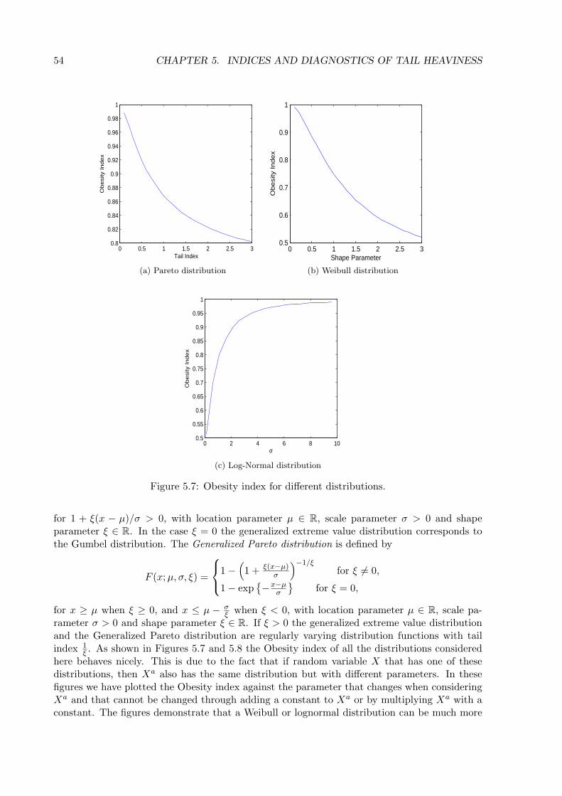
54 CHAPTER 5. INDICES AND DIAGNOSTICS OF TAIL HEAVINESS
0 0.5 1 1.5 2 2.5 30.8
0.82
0.84
0.86
0.88
0.9
0.92
0.94
0.96
0.98
1
Tail Index
Obesi
ty Index
(a) Pareto distribution
0 0.5 1 1.5 2 2.5 30.5
0.6
0.7
0.8
0.9
1
Shape Parameter
Ob
esi
ty I
nd
ex
(b) Weibull distribution
0 2 4 6 8 100.5
0.55
0.6
0.65
0.7
0.75
0.8
0.85
0.9
0.95
1
σ
Obesi
ty Index
(c) Log-Normal distribution
Figure 5.7: Obesity index for different distributions.
for 1 + ξ(x − µ)/σ > 0, with location parameter µ ∈ R, scale parameter σ > 0 and shapeparameter ξ ∈ R. In the case ξ = 0 the generalized extreme value distribution corresponds tothe Gumbel distribution. The Generalized Pareto distribution is defined by
F (x;µ, σ, ξ) =
1−(1 + ξ(x−µ)
σ
)−1/ξfor ξ = 0,
1− exp−x−µ
σ
for ξ = 0,
for x ≥ µ when ξ ≥ 0, and x ≤ µ − σξ when ξ < 0, with location parameter µ ∈ R, scale pa-
rameter σ > 0 and shape parameter ξ ∈ R. If ξ > 0 the generalized extreme value distributionand the Generalized Pareto distribution are regularly varying distribution functions with tailindex 1
ξ . As shown in Figures 5.7 and 5.8 the Obesity index of all the distributions consideredhere behaves nicely. This is due to the fact that if random variable X that has one of thesedistributions, then Xa also has the same distribution but with different parameters. In thesefigures we have plotted the Obesity index against the parameter that changes when consideringXa and that cannot be changed through adding a constant to Xa or by multiplying Xa with aconstant. The figures demonstrate that a Weibull or lognormal distribution can be much more
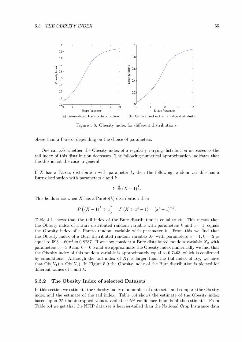
5.3. THE OBESITY INDEX 55
−3 −2 −1 0 1 2 30.1
0.2
0.3
0.4
0.5
0.6
0.7
0.8
0.9
1
Shape Parameter
Ob
esi
ty I
nd
ex
(a) Generalized Pareto distribution
−2 −1 0 1 20
0.2
0.4
0.6
0.8
1
Shape Parameter
Ob
esi
ty I
nd
ex
(b) Generalized extreme value distribution
Figure 5.8: Obesity index for different distributions.
obese than a Pareto, depending on the choice of parameters.
One can ask whether the Obesity index of a regularly varying distribution increases as thetail index of this distribution decreases. The following numerical approximation indicates thatthe this is not the case in general.
If X has a Pareto distribution with parameter k, then the following random variable has aBurr distribution with parameters c and k
Yd= (X − 1)
1c .
This holds since when X has a Pareto(k) distribution then
P((X − 1)
1c > x
)= P (X > xc + 1) = (xc + 1)−k .
Table 4.1 shows that the tail index of the Burr distribution is equal to ck. This means thatthe Obesity index of a Burr distributed random variable with parameters k and c = 1, equalsthe Obesity index of a Pareto random variable with parameter k. From this we find thatthe Obesity index of a Burr distributed random variable X1 with parameters c = 1, k = 2 isequal to 593 − 60π2 ≈ 0.8237. If we now consider a Burr distributed random variable X2 withparameters c = 3.9 and k = 0.5 and we approximate the Obesity index numerically we find thatthe Obesity index of this random variable is approximately equal to 0.7463, which is confirmedby simulations. Although the tail index of X1 is larger than the tail index of X2, we havethat Ob(X1) > Ob(X2). In Figure 5.9 the Obesity index of the Burr distribution is plotted fordifferent values of c and k.
5.3.2 The Obesity Index of selected Datasets
In this section we estimate the Obesity index of a number of data sets, and compare the Obesityindex and the estimate of the tail index. Table 5.4 shows the estimate of the Obesity indexbased upon 250 bootstrapped values, and the 95%-confidence bounds of the estimate. FromTable 5.4 we get that the NFIP data set is heavier-tailed than the National Crop Insurance data
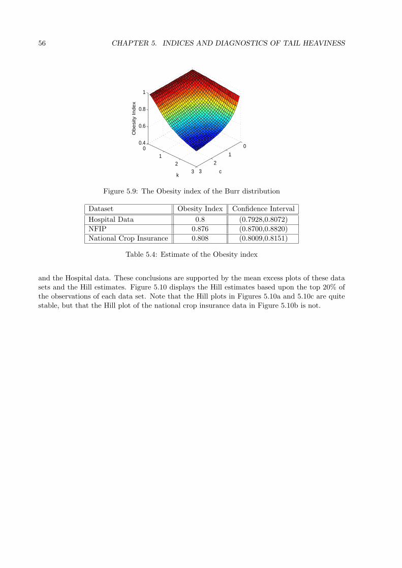
56 CHAPTER 5. INDICES AND DIAGNOSTICS OF TAIL HEAVINESS
0
1
2
3
01
23
0.4
0.6
0.8
1
ck
Ob
esi
ty I
nd
ex
Figure 5.9: The Obesity index of the Burr distribution
Dataset Obesity Index Confidence Interval
Hospital Data 0.8 (0.7928,0.8072)
NFIP 0.876 (0.8700,0.8820)
National Crop Insurance 0.808 (0.8009,0.8151)
Table 5.4: Estimate of the Obesity index
and the Hospital data. These conclusions are supported by the mean excess plots of these datasets and the Hill estimates. Figure 5.10 displays the Hill estimates based upon the top 20% ofthe observations of each data set. Note that the Hill plots in Figures 5.10a and 5.10c are quitestable, but that the Hill plot of the national crop insurance data in Figure 5.10b is not.
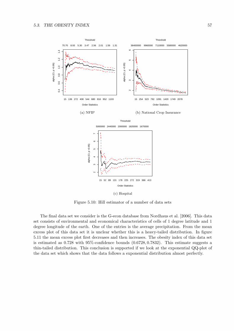
5.3. THE OBESITY INDEX 57
15 136 272 408 544 680 816 952 1103
0.4
0.6
0.8
1.0
1.2
1.4
70.70 8.93 5.30 3.47 2.56 2.01 1.59 1.31
Order Statistics
alph
a (C
I, p
=0.
95)
Threshold
(a) NFIP
15 254 523 792 1091 1420 1749 2078
23
45
6
36400000 9960000 7110000 5580000 4620000
Order Statistics
alph
a (C
I, p
=0.
95)
Threshold
(b) National Crop Insurance
15 52 89 131 178 225 272 319 366 413
23
45
67
5000000 2440000 2000000 1820000 1670000
Order Statistics
alph
a (C
I, p
=0.
95)
Threshold
(c) Hospital
Figure 5.10: Hill estimator of a number of data sets
The final data set we consider is the G-econ database from Nordhaus et al. [2006]. This dataset consists of environmental and economical characteristics of cells of 1 degree latitude and 1degree longitude of the earth. One of the entries is the average precipitation. From the meanexcess plot of this data set it is unclear whether this is a heavy-tailed distribution. In figure5.11 the mean excess plot first decreases and then increases. The obesity index of this data setis estimated as 0.728 with 95%-confidence bounds (0.6728, 0.7832). This estimate suggests athin-tailed distribution. This conclusion is supported if we look at the exponential QQ-plot ofthe data set which shows that the data follows a exponential distribution almost perfectly.
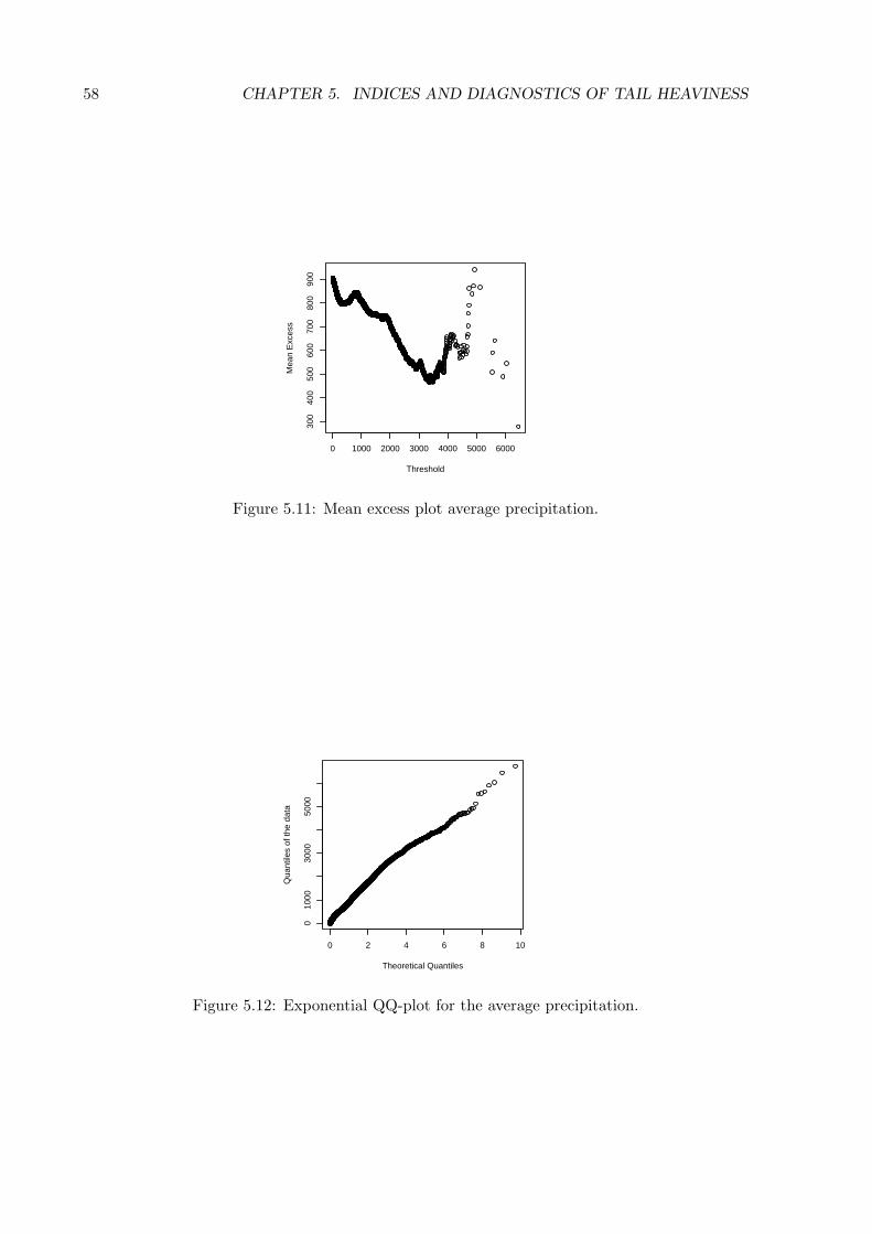
58 CHAPTER 5. INDICES AND DIAGNOSTICS OF TAIL HEAVINESS
0 1000 2000 3000 4000 5000 6000
300
400
500
600
700
800
900
Threshold
Mea
n E
xces
s
Figure 5.11: Mean excess plot average precipitation.
0 2 4 6 8 10
010
0030
0050
00
Theoretical Quantiles
Qua
ntile
s of
the
data
Figure 5.12: Exponential QQ-plot for the average precipitation.
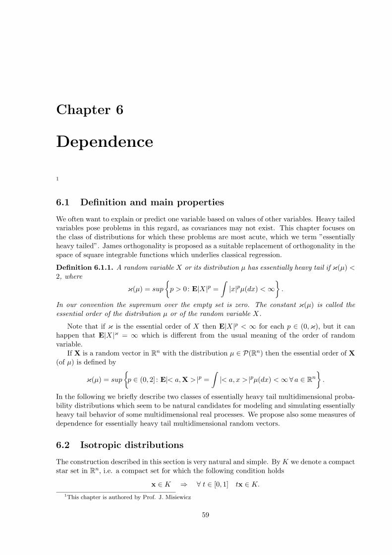
Chapter 6
Dependence
1
6.1 Definition and main properties
We often want to explain or predict one variable based on values of other variables. Heavy tailedvariables pose problems in this regard, as covariances may not exist. This chapter focuses onthe class of distributions for which these problems are most acute, which we term ”essentiallyheavy tailed”. James orthogonality is proposed as a suitable replacement of orthogonality in thespace of square integrable functions which underlies classical regression.
Definition 6.1.1. A random variable X or its distribution µ has essentially heavy tail if κ(µ) <2, where
κ(µ) = sup
p > 0: E|X|p =
∫|x|pµ(dx) < ∞
.
In our convention the supremum over the empty set is zero. The constant κ(µ) is called theessential order of the distribution µ or of the random variable X.
Note that if κ is the essential order of X then E|X|p < ∞ for each p ∈ (0,κ), but it canhappen that E|X|κ = ∞ which is different from the usual meaning of the order of randomvariable.
If X is a random vector in Rn with the distribution µ ∈ P(Rn) then the essential order of X(of µ) is defined by
κ(µ) = sup
p ∈ (0, 2] : E|< a,X > |p =
∫|< a, x > |pµ(dx) < ∞∀ a ∈ Rn
.
In the following we briefly describe two classes of essentially heavy tail multidimensional proba-bility distributions which seem to be natural candidates for modeling and simulating essentiallyheavy tail behavior of some multidimensional real processes. We propose also some measures ofdependence for essentially heavy tail multidimensional random vectors.
6.2 Isotropic distributions
The construction described in this section is very natural and simple. ByK we denote a compactstar set in Rn, i.e. a compact set for which the following condition holds
x ∈ K ⇒ ∀ t ∈ [0, 1] tx ∈ K.
1This chapter is authored by Prof. J. Misiewicz
59
60 CHAPTER 6. DEPENDENCE
To avoid the situation that the set K is in fact contained in some linear subspace of Rn weassume also that K contains an open neighborhood of zero. By ∂K we denote the boundary ofthe set K. Sometimes it is more convenient to define first a quasi-norm q on Rn and then thestar set K = x ∈ Rn : q(x) 6 1.
Definition 6.2.1. A random vector X is isotropic if it can be written in the following form
Xd= Z · θ,
where θ is a non-negative random variable independent of the random vector Z with the uniformdistribution on the boundary ∂K of a compact star subset K of Rn.
Notice that if X has a density, then this density has level curves of the form
c · ∂K, c > 0.
It is also easy to see that for every choice of half-lines starting at zero ℓ1, ℓ2 ∈ Rn the distributionsof the following conditional random variables
R1 :=(∥X∥2
∣∣X ∈ ℓ1), R2 :=
(∥X∥2
∣∣X ∈ ℓ2)
are equal up to a scale parameter, i.e. there exists c(ℓ1, ℓ2) such that
R1d= c(ℓ1, ℓ2)R− 2.
Moreover the essential order of the random vector X is equal to the essential order of the variableθ since the random vector Z has the strong second moment finite (E∥Z∥2 < ∞).
The construction of isotropic random vectors is maybe the simplest (except vectors withindependent coordinates) construction of multidimensional distributions. Assuming for simplic-ity that the distribution of X is symmetric it is natural to define in this case the correlationcoefficient
ϱ (X1, X2)def= ϱ(Z1, Z2) =
Cov(Z1, Z2)√Var(Z1)Var(Z2)
.
This coincides with the usual correlation coefficient if Eθ2 < ∞; i.e. in this case we have
ϱ (X1, X2) ≡ ϱ (X1, X2).
Pareto distributions. The most convenient in precise calculations example of essentiallyheavy tail distributions are Pareto distributions πα with densities given by
fα(x) =α
xα+11[1,∞)(x).
In this case we have κ(πα) = α. The n-dimensional version of Pareto distribution has thedensity function given by
fα(x) =C(q, α)
q(x)α+n1[1,∞)(q(x)).
where q : Rn 7→ [0,∞) is a quasi-norm on Rn and C(q, α) is the normalizing constant. Noticethat the level curves of n-dimensional version of Pareto distribution are of the form
x ∈ Rn : q(x) = c , c > 0.
6.2. ISOTROPIC DISTRIBUTIONS 61
Here we have K = x ∈ Rn : q(x) 6 1 and the random vector Z is uniformly distributed onthe set ∂K = x ∈ Rn : q(x) = and the random variable θ has Pareto distribution πα with thedensity fα. In the case
q(x)p =
n∑k=1
|xk|p
for some p > 0 we have
C(q, α) = 2−n+1pn−1Γ (n/p) .
Elliptically contoured distributions The best known isotropic distributions are spheri-cally invariant (rotationally invariant) distributions with
q(x)2 =n∑
k=1
x2k = ∥x∥2, ∂K = x ∈ Rn : ∥x∥2 = 1 ,
and elliptically contoured distributions with
q(x)2 = xΣ−1xT , ∂K =x ∈ Rn : xΣ−1xT = 1
,
for some positive definite symmetric n × n-matrix Σ. The elliptically contoured distributionsare playing a very important role in multidimensional probability, stochastic processes, statisticsand stochastic modeling.
Dirichlet and Liouville-type distributions. The classical Dirichlet random vector takesvalues in a positive rectangle of Rn, however here we consider sign-symmetric Dirichlet distri-bution, where
Definition 6.2.2. A random vector U = (U1, . . . , Un) has a sign-symmetric Dirichlet-type dis-tribution with parameters α1, . . . , αn and β1, . . . , βn (notation U ∼ SD(α1, . . . , αn;β1, . . . , βn))if the following conditions hold
(i) Un is a symmetric random variable;
(ii)∑n
i=1 |Ui|αi = 1 almost surely;
(iii) the joint density function of (U1, . . . , Un−1) is
Γ(pn)
Γ(βn/αn)
n−1∏i=1
αi
2Γ(βi/αi)|ui|βi−1
(1−
n−1∑i=1
|ui|αi
)(βn/αn)−1
+
,
where pi =∑i
j=1 βj/αj for i = 1, . . . , n.
The sign symmetric Dirichlet random vector can be obtained by the following construction:Let Γ1, . . . ,Γn be mutually independent real random variables where the probability densityfunction of Γi is
αi
2Γ(βi/αi)|zi|βi−1 exp−|zi|αi
for zi ∈ R. Then
(U1, . . . , Un)d=
(Γ1(∑n
j=1 |Γj |αj)1/αi
, . . . ,Γn(∑n
j=1 |Γj |αj)1/αi
).
62 CHAPTER 6. DEPENDENCE
Since
Var(Ui) =Γ(pn)Γ(βi/αi + 2/αi)
Γ(pn + 2/αi)Γ(βi/αi)
we see that
Cov
(n∑
i=1
xiUi,
n∑i=1
yiUi
)= Γ(pn)
n∑i=1
xiyiΓ(βi/αi + 2/αi)
Γ(pn + 2/αi)Γ(βi/αi).
Of course the Dirichlet distributions are supported on a compact subset of Rn and thus theydo not have essentially heavy tails. In order to get essentially heavy-tail distribution based onDirichlet random vector we shall consider the following:
Definition 6.2.3. A random vector X = (X1, . . . , Xn) is said to have a sign-symmetric Liouville-type distribution if there exists a sign-symmetric Dirichlet-type random vector U ∼ SD(α1, . . . , αn;β1, . . . , βn)and a non-negative random variable θ such that
(X1, . . . , Xn)d=(U1θ
1/α1 , . . . , Unθ1/αn
).
Notation: X ∼ SL(α1, . . . , αn;β1, . . . , βn; θ).
The random vector X ∼ SL(α1, . . . , αn;β1, . . . , βn; θ) has essentially heavy tail if and onlyif the corresponding variable θ has essentially heavy tail, however the dependence structure ofcoordinates of X and corresponding U are the same up to scale mixture. More about sign-symmetric Dirichlet type and Liouville type distributions one can find e.g. in R.D. Gupta andRichards [1996].
6.3 Pseudo-isotropic distributions
Another class of handy in calculations essentially heavy tail distributions are symmetric multi-dimensional distributions having all one-dimensional projections (not only projections onto theaxis) the same up to a scale parameter. A wide description of such distributions one can find inJ. K. Misiewicz and Scheffer. [1990] and J. K. Misiewicz.
The main example of such distributions are symmetric stable distributions and ellipticallycontoured distributions.
Stable distributions. For a long time applicability of stable distributions was rather the-oretical, since there are only three cases α = 2, 1, 12 in which the density of α-stable randomvariable is given in an explicit formula. Now we can deal with most of difficulties with the help ofcomputer calculations and the role of stable distributions and processes in stochastic modelingis growing.
In the following we assume that the considered random vectors are living in Rn, however infull generality we could assume that they are taking values in any separable Banach space E.
Definition 6.3.1. A random vector Y ∈ Rn is stable if for every a, b > 0 there exist c =c(a, b) > 0 and d = d(a, b) ∈ Rn such that
aY + bY′ d= cY + d,
where Y′ is an independent copy of Y andd= denotes equality of distributions.
6.3. PSEUDO-ISOTROPIC DISTRIBUTIONS 63
If d(a, b) = 0 for each choice of a, b > 0 then the random vector Y is called strictly stable.
Every symmetric stable random vector, i.e. such vector that Yd= −Y, is strictly stable.
It is known that if Y is stable then there exists a constant α ∈ (0, 2] such that c(a, b)α =aα + bα. The constant α is called the characteristic exponent and it coincides with the essentialorder κ(µ) for µ = L(Y), the distribution of Y. A stable random vector Y with the essentialorder α is called α-stable. A symmetric α-stable vector we denote by SαS.
If Y ∈ Rn, n > 2, is SαS then there exists a symmetric finite measure Γ on the unit sphereSn−1 ⊂ Rn such that
Eei<ξ,Y> = exp
−∫
· · ·∫
Sn−1|< ξ,u > |α Γ(du)
. (∗)
The measure Γ is called the spectral measure for SαS random vector. This measure is uniquelydetermined if only α < 2. For α = 2 we do not have uniqueness, but this is just the Gaussiancase and we have many other methods of dealing with this distribution.
By Yα we denote the canonical SαS random variable with the characteristic function exp−|t|α.By (∗) we see that if Y is SαS random vector in Rn then for each ξ ∈ Rn we have
< ξ,Y >=
n∑k=1
ξkYkd= C(ξ)Yα,
where the constant C(ξ) is given by
C(ξ)α =
∫· · ·∫
Sn−1|< ξ,u > |α Γ(du).
Pseudo-isotropic distributions. The SαS distributions are the main examples of pseudo-isotropic distributions, where
Definition 6.3.2. A symmetric random vector X taking values in Rn is pseudo-isotropic if allits one-dimensional projections have the same distributions up to a scale parameter, i.e.
∀ ξ ∈ Rn ∃C(ξ) > 0 < ξ,X >=n∑
k=1
ξkXkd= C(ξ)X1.
The function C : Rn → [0,∞) defines a quasi-norm on Rn.
It is known that if µ denotes the distribution of a pseudo-isotropic random vector X withthe quasi-norm C and κ(µ) > 0 then κ(µ) 6 α(µ), where
α(µ)def= sup
p ∈ (0, 2] : exp −C(ξ)p is positive definite on Rn
.
The constant α(µ) is called the index of stability for pseudo-isotropic distribution µ. Theformulation: exp −C(ξ)p is positive definite on Rn means simply that exp −C(ξ)p is acharacteristic function of some random vector, which (it is easy to check) is Sp S. By the Levy-Cramer theorem we have that exp
−C(ξ)α(µ)
is also a characteristic function of some Sα(µ)S
random vector Y. Of course Y is also pseudo-isotropic and < ξ,Y > has the same distributionas C(ξ)Yα. Consequently for each 1 < p < α(µ) we have
E∣∣< ξ,Y >
∣∣p = C(ξ)p E|Yα|p.
64 CHAPTER 6. DEPENDENCE
If the pseudo-isotropic random vector X = (X1, . . . , Xn) with distribution µ and the quasi-normC is such that 1 < κ(µ) 6 α(µ) then for each ξ ∈ Rn and each 1 < p < κ(µ)
E∣∣< ξ,X >
∣∣p = C(ξ)pE|X1|p.
Consequently for all 1 < p < κ(µ) 6 α(µ) we have
E∣∣< ξ,Y >
∣∣pE|Yα|p
=E∣∣< ξ,X >
∣∣pE|X1|p
.
We see also that if a pseudo-isotropic random vector X ∼ µ is such that κ(µ) > 0 then thereexists a symmetric finite measure Γ on the unit sphere Sn−1 ⊂ Rn such that
C(ξ)α(µ) =
∫· · ·∫
Sn−1|< ξ,u > |α(µ) Γ(du).
The measure Γ we shall call the spectral measure of pseudo-isotropic distribution of positiveessential order.Remak. It is known (see Misiewicz and Tabisz) that the distribution which is both isotropicand pseudo-isotropic must be elliptically contoured.
6.3.1 Covariation as a measure of dependence for essentially heavy tail jointlypseudo-isotropic variables
The covariation of random variables was originally defined for jointly stable variables. We candefine it also for jointly pseudo-isotropic variables.
Definition 6.3.3. Let (X1, X2) be pseudo-isotropic with parameter α > 1 and let Γ be thespectral measure of the corresponding SαS random vector (Y1, Y2). The covariation of X1 on X2
is the real number
[X1, X2]α ≡ [Y1, Y2]αdef=
∫S1
u1u<α−1>2 Γ(du),
where a<p> = |a|p sign(a).
Equivalently we can say that
[X1, X2]α ≡ [Y1, Y2]α =1
α
∂
∂r
∫S1
|ru1 + su2|α Γ(du)∣∣∣r=0,s=1
=1
α
∂
∂rC((r, s))α
∣∣∣r=0,s=1
,
where C is the quasi-norm C for (X1, X2).
Lemma 6.3.1. If the random vector (X1, X2) is pseudo-isotropic and 1 < p < κ 6 α then
[X1, X2]αC(0, 1)α
=EX1X
<p−1>2
E|Y2|p. (∗∗)
Proof. Let (Y1, Y2) be the corresponding SαS random vector. Since E|rY1 + sY2|p =C(r, s)pE|Yα|p for p < α and E|rX1 + sX2|p = C(r, s)pE|X1|p for p < κ then for each p < κwe have
∂
∂rE|rX1 + sX2|p =
∂
∂rC(r, s)pE|X1|p = pE|X1|pC(r, s)p−α 1
α
∂
∂rC(r, s)α.
6.3. PSEUDO-ISOTROPIC DISTRIBUTIONS 65
Consequently, for each 1 < p < κ we have
[X1, X2]α =
[C(r, s)α−p
pE|X1|p∂
∂rE|rX1 + sX2|p
]r=0,s=1
=C(0, 1)α−p
E|X1|pEX1X
<p−1>2 .
Now it is enough to notice that E|X2|p = C(0, 1)pE|X1|p.
Example 1. Consider an rotationally invariant random vector (Y1, Y2) = (U1, U2)θ, where(U1, U2) has uniform distribution on the unit sphere S1 ⊂ R2, θ is a random variable withthe Pareto distribution with parameter α ∈ (1, 2) independent of (U1, U2). Denote by µ thedistribution of (Y1, Y2). It is easy to check that the quasi-norm C is given by C(r, s)2 = r2 + s2,thus α(µ) = 2 and the corresponding symmetric stable vector is Gaussian with independentincrements. On the other hand
E|rY1 + sY2|p = E|rU1 + sU2|pEθp,
thus κ(µ) = supp ∈ (0, 2] : Eθp < ∞ = α and (Y1, Y2) has essentially heavy tail distribution.Evidently [Y1, Y2]2 = 0 in spite of the fact that Y1 and Y2 are not independent.
Remark. Of course the covariation [Z1, Z2]p, p ∈ (1, 2), can be defined for any symmetricrandom vector (Z1, Z2) with the property E|rZ1 + sZ2|p < ∞ for all r, s ∈ R. However thechosen parameter p does not have to be the maximal with this property. Moreover if κ is theessential order of (Z1, Z2) then it may happen that E|Z1|κ = ∞. This makes a difference becausewithout pseudo-isotropy we do not have equality
(E|rZ1 + sZ2|p)1/p = c(p, q) (E|rZ1 + sZ2|q)1/q
for every p, q < κ and a suitable constant c(p, q). Consequently the substitutes of inner product[Z1, Z2]p and [Z1, Z2]q are different for the same random vector (Z1, Z2). In particular, be-tween two-dimensional Pareto distributions only Bessel–Pareto (rotationally invariant Pareto)distribution is pseudo-isotropic.
In the case of non pseudo-isotropic random vector (Z1, Z2) of essential order κ ∈ (1, 2) wecould use the following construction: It is known that for each p ∈ (1,κ)
φp(r, s) = exp −E|rZ1 + sZ2|p
is the characteristic function of some symmetric p-stable random vector. If we assume thatE|Z1|p = E|Z2|p =: mp (e.g. if Z1 and Z2 have the same distribution) then
φp
((r, s)
mp
)= exp
−E
∣∣∣∣rZ1 + sZ2
mp
∣∣∣∣pconverges for p κ to the characteristic function of some symmetric κ-stable random vector(Y1, Y2) since(
E
∣∣∣∣rZ1 + sZ2
mp
∣∣∣∣p)1/p
6(E
∣∣∣∣rZ1
mp
∣∣∣∣p)1/p
+
(E
∣∣∣∣sZ2
mp
∣∣∣∣p)1/p
6 |r|+ |s|.
Then we can define uniquely the covariation of Z1 on Z2 by
[Z1, Z2]κ := [Y1, Y2]κ,
66 CHAPTER 6. DEPENDENCE
however in practice it is difficult to approximate this parameter from data.
The following lemma was proven in Samorodnitsky and Taqqu [1994] only in the case of SαSrandom vectors. The proof in the case of pseudo-isotropic vectors is almost the same and willbe omitted.
Lemma 6.3.2. Let (X1, . . . , Xn) be a pseudo-isotropic random vector with the characteristicexponent α > 1 and spectral measure Γn. If
W =n∑
k=1
akXk and Z =n∑
k=1
bkXk,
then
[W,Z]α =
∫Sn−1
( n∑k=1
akuk
)( n∑k=1
bkuk
)<α−1>Γn(du).
Now we are able to define an analog of the covariance coefficient for essentially heavy tailpseudo-isotropic variables.
Definition 6.3.4. Let X = (X1, X2) be a pseudo-isotropic random vector with α > 1 and thequasi-norm C. Then the covariation norm of the random variable X = rX1 + sX2 is defined by
∥X∥ααdef= [X,X]α = C(r, s)α.
The covariation coefficient of X1 on X2 is
ρα(X1, X2) :=[X1, X2]α
∥X1∥α∥X2∥α−1α
=[X1, X2]αC(0, 1)α−1
Notice that by our definition C(1, 0) = 1.
Example 2. Consider Y0, Y1, . . . independent identically distributed SαS random variables withα > 1. First we will discuss the covariation of Z1 = Y1±εY0 on Z2 = Y2+εY0. The random vector(Y0, Y1, Y2) has the spectral measure Γ3 with 6 atoms (u1, u2, u3) = (±1, 0, 0), (0,±1, 0), (0, 0,±1)of the weight 1/2 each. Thus
[Z1, Z2]α =
∫S2
(u1 ± εu3) (u2 + εu3)<α−1> Γ3(du)
= ±1
2
(ε · (ε)<α−1> − ε · (−ε)<α−1>
)= ±εα.
The covariation norms of these variables are as follows
∥Z1∥αα = ∥Z2∥αα = 1 + εα,
thus
ρα(Z1, Z2) =±εα
1 + εα.
We see that it can be taken really small. Consider now the following:
Z(n)1 = n−1/α
n∑k=1
(Yk ± εY0) and Z(n)2 = n−1/α
2n∑k=n+1
(Yk + εY0) .
6.3. PSEUDO-ISOTROPIC DISTRIBUTIONS 67
It is well known that
(Z(n)1 , Z
(n)2 )
d=(Y1 ± n1−1/αεY0, Y2 + n1−1/αεY0
),
thus the covariation Z(n)1 on Z
(n)2 is given by
[Z(n)1 , Z
(n)2 ]α = ±nα−1εα.
The covariation norm∥Z(n)
1 ∥αα = 1 + nα−1εα,
thus
ρ(Z(n)1 , Z
(n)2 ) =
±nα−1εα
1 + nα−1εα→ 1 when n → ∞.
However if we put ε = εn = cn1/α−1 then for each n ∈ N
[Z(n)1 , Z
(n)2 ]α = ± cα, ∥Z(n)
1 ∥αα = 1 + cα, ρ(Z(n)1 , Z
(n)2 ) =
± cα
1 + cα,
and it can attain every value from the interval (−1, 1).
6.3.2 Codifference
Unfortunately for α 6 1 the idea of covariation and the corresponding covariation norm do nothave required properties since the triangular inequality does not hold. In such case we shall usecodifference:
τ(X1, X2) = ∥X1∥αα + ∥X2∥αα − ∥X1 −X2∥αα
= C(1, 0)α + C(0, 1)α − C(1,−1)α.
Notice that for the variables described in the previous example (for α < 1) we have
τ(Z(n)1 , Z
(n)2 ) = 2
(1 + nα−1εα
)− 2−
(1 + (−1)±1
)αnα−1εα
=(2−
(1 + (−1)±1
)α)nα−1εα → 0 for n → ∞,
and for εn = cn1/α−1
τ(Z(n)1 , Z
(n)2 ) =
(2−
(1 + (−1)±1
)α)cα.
6.3.3 The linear regression model for essentially heavy tail distribution
In many classical problems of statistics we want to approximate value of variable Y by the valueaX with the best possible constant a in the sense of minimizing the following function
E (Y − aX)2 .
Let L20(Ω,F ,P) be the space of all random variables on (Ω,F) with mean zero and finite second
moment. The space L20(Ω,F ,P) is a Hilbert space with the scalar product
(X,Y ) := Cov(X,Y ) = EXY.
If X,Y ∈ L20(Ω,F ,P) then minimizing the value of E(Y −aX)2 is the same as finding the value
a ∈ R such that X is orthogonal to (Y − aX), thus
a =(Y,X)
∥X∥22.
68 CHAPTER 6. DEPENDENCE
This construction is not possible if EX2 = EY 2 = ∞. However in the space Lp0(Ω,F ,P) of the
variables with the finite pth moment, p ∈ (1, 2), equipped with the norm
∥X∥pp := E|X|p
(see James [1947]) it is possible to consider James orthogonality in the following way:X is James orthogonal to Y (notation X⊥JY ) if for every real λ
∥X + λY ∥p > ∥X∥p.
The next proposition was proven in Samorodnitsky and Taqqu [1994] for jointly SαS randomvectors.
Proposition 6.3.3. Let (X,Y ) be pseudo-isotropic with the essential order κ ∈ (1, 2) and indexof stability α ∈ [κ, 2). Then
[X,Y ]α = 0
if and only if Y is James orthogonal to X in Lp0(Ω,F ,P) for each p ∈ (1,κ).
Proof. Let (Z1, Z2) be the corresponding SαS random vector with the same as (X,Y ) quasi-norm c. It was shown in Samorodnitsky and Taqqu [1994] that
[Z1, Z2]α = 0 iff ∥λZ1 + Z2∥α > ∥Z2∥α
for every real λ. Now it is enough to notice that
∥λX + Y ∥pp = E|λX + Y |p = c(λ, 1)pE|X|p = ∥λX + Y ∥pαE|X|p
for each real λ and that by definition
[X,Y ]α = [Z1, Z2]α.
Coming back to the linear regression problem for essentially heavy tail distributions assumethat (X,Y ) is pseudo-isotropic with pseudo-norm c, distribution µ of the essential order κ(µ) ∈(1, 2) and the corresponding index of stability α(µ) < 2. We want to find a ∈ R such that
X ⊥α (Y − aX).
Then the random vector (Y − aX,X) is also pseudo-isotropic with the quasi-norm c1(r, s) =c(s− ar, s) since
r(Y − aX) + sX = (s− ar)X + rYd= c(s− ar, s)X.
By Lemma 1 we have that
0 = [Y − aX,X]α =c1(0, 1)
α−p
E|X|p(EY X<p−1> − aE|X|p
),
for each 1 < p 6 κ(µ). Consequently
a =EY X<p−1>
E|X|p.
The next proposition describes the consistent statistics for linear regression in this case.
6.3. PSEUDO-ISOTROPIC DISTRIBUTIONS 69
Proposition 6.3.4. Let (X,Y ) be pseudo-isotropic with pseudo-norm c, distribution µ of theessential order κ(µ) ∈ (1, 2) and the corresponding index of stability α(µ) < 2 and let p ∈(1,κ(µ)). If X⊥J(Y − aX), i.e.
E|Y − aX|p = inf E|Y + λX|p : λ ∈ R
then
Qn =
∑nk=1 YkX
<p−1>k∑n
k=1 |Xk|p
is a consistent estimator of a.
Proof. Let mp = E|X|p = c(1, 0)p and µ(Y,X) = EY X<p−1>. Take γ, ε, δ > 0, δ ≪ mp andsuch that
δ(µ(Y,X) +mp)
mp(mp − δ)< γ.
We define
An =
ω : mp − δ <
1
n
n∑k=1
|Xk|p < mp + δ
,
Bn =
ω : µ(Y,X)− δ <
1
n
n∑k=1
YkX<p−1>k < µ(Y,X) + δ
.
By the Weak Law of Large Numbers there exists n0 ∈ N such that for each n > n0 we haveP(An) > 1−ε/2 and P(Bn) > 1−ε/2 and consequently P(An∩Bn) > 1−P(Ac
n)−P(Bcn) > 1−ε.
On the set An ∩Bn we have that
µ(Y,X)
mp− δ(µ(Y,X) +mp)
mp(mp + δ)6 Qn 6 µ(Y,X)
mp+
δ(µ(Y,X) +mp)
mp(mp − δ).
Consequently for each n > n0 = n0(γ, ε) we have
P
ω :
∣∣∣∣Qn − µ(Y,X)
mp
∣∣∣∣ > γ
6 ε.
Now it is enough to take ε = εn → 0 for n → ∞.
70 CHAPTER 6. DEPENDENCE
Chapter 7
Conclusions and Future Research
The data sets discussed in chapter 1 hopefully persuade the reader that heavy tail phenomenaare not incomprehensible bolts from ”extremistan”, but arise in many commonplace data sets.They are not incomprehensible, but they cannot be understood with traditional statistical tools.Using the wrong tools is incomprehensible. This monograph reviewed various notions, intuitionsand definitions of tail heaviness. The most popular definitions in terms of regular variation andsubexponentiality invoke putative properties that hold at infinity, and this complicates anyempirical estimate. Each definition captures some but not all of the intuitions associated withtail heaviness.
Chapter 5 studied two different candidates to characterize the tail-heaviness of a data setbased upon the behavior of the mean excess plot under aggregations by k. We first consideredthe ratio of the largest to the second largest observations. It turned out this ratio has a non-degenerate limit if and only if the distribution is regularly varying. An estimate of the probabilitythat this ratio exceeds 2 based on the observed Type 2 2-records in a data set was very inaccurate:the expected number of Type 2 2-records in a data set of size 10000 is 16.58. For thin-taileddistributions the estimator is biased, since the probability in question decreases to zero butthe estimator is non-negative on initial segments. This is due to the fact that most 2-recordswill be observed early in the data set, and then relative frequency of the largest observationexceeding twice the second largest is still quite large. This motivated the search for for anothercharacterization of heavy-tailedness. The Obesity index of a random variable was defined as:
Ob(X) = P (X1 +X4 > X2 +X3|X1 ≤ X2 ≤ X3 ≤ X4) , Xii.i.d. copies of X.
This index reasonably captures intuitions on tail heaviness and can be calculated for distributionsand computed for data sets. However, it does not completely mimic the tail index. We saw thatthe obesity index of two Burr distributions could reverse the order of their tail indices. Whenapplied to various data sets we saw that the Obesity index and the Hill estimator both gaveroughly similar results, in those cases where the Hill estimator gave a clear signal.
As with any new notion, it is easy to think of interesting research questions. We mentiontwo. The notion of a multivariate Obesity index immediately suggests itself by considering ajoint probability
Ob(X,Y )Ob(X)Ob(Y ) =
P (X1 +X4 > X2 +X3 ∩ Y1 + Y4 > Y2 + Y3 |X1 ≤ X2 ≤ X3 ≤ X4 ∩ Y1 ≤ Y2 ≤ Y3 ≤ Y4) ,
Xi i.i.d. copies of X, Yi i.i.d. copies of Y.
The second question concerns covariates. We might like to explain tail heaviness in terms ofindependent variables. An obvious idea is to regress the rank of the dependent variable on the
71
72 CHAPTER 7. CONCLUSIONS AND FUTURE RESEARCH
independent variables; that might get at ”tail” but not ”tail heaviness”. The problem is todefine an appropriate notion of orthogonality, and James orthogonality is is proposed in chapter6. We may safely speculate that research in fat tails is itself a fat tailed phenomenon.
Bibliography
R. Frey A.J. McNeil and P. Embrechts. Quantitative Risk Management. Princeton UniversityPress, 2005.
D. Applebaum. Levy-type stochastic integrals with regurlary varying tails. Stochastic Analysisand Applications, 2005.
B.C. Arnold. Pareto Distributions. Fairland International Co-operative Publishing, 1983.
B.C. Arnold, N. Balakrishnan, and H.N. Nagaraja. Records. John Wiley Sons, 1998.
N. Balakrishnan and A. Stepanov. Asymptotic properties of the ratio of order statistics. Statisticsand Probability letters, 78:301–310, 2007.
J. Beirlant, G. Dierckx, and A. Guillou. Estimation of the extreme-value index and generalizedquantle plots. Bernoulli, 11:949–970, 2005.
J.L. Beirlant, J. Teugels and title = Practical Analysis of Extreme Values publisher = LeuvenUniversity Press year = 1996 Vynckier, P.
N.H. Bingham and J.L. Teugels. Conditions implying domains of attraction. In Proceedings ofthe Sixth conference on Probability Theory, pages 23–24, 1979.
N.H. Bingham, C.M. Goldie, and J.L. Teugels. Regular Variation. Cambridge University Press,1987.
S. Coles. An Introduction to Statistical Modelling of Extreme Values. Springer-Verlag, 2001.
R.M. Cooke and C. Kousky. Are catgastrophes insurable? Resources, 172:18–23, 2009.
M.E. Crovella and A. Bestavros. Self-similarity in world wide web traffic: Evidence and possiblecauses. IEEE/ACM Transactions on Networking, 1997.
M.E. Crovella and M.S. Taqqu. Estimating the heavy tail index from scaling properties. Method-ology and Computing in Applied Probability, 1:55–79, 1999.
Herbert A. David. Order Statistics. John Wiley Sons, 2nd edition edition, 1981.
P. Embrechts, C. Kluppelberg, and T. Mikosch. Modelling Extremeal Events for Insurance andFinance. Springer, 1997.
W. Feller. An Introduction to Probability Theory and Its Applications, volume II. John WileySons, 2nd edition edition, 1971.
G.H. Hardy, J.E. Littlewood, and G. Polya. Inequalities. Cambridge University Press, 1934.
73
74 BIBLIOGRAPHY
T.L. Hayes and D.A. Neal. Actuarial Rate Review In Support of the Recommended October 1,2010, Rate and Rule Changes. FEMA, 2011.
B.M. Hill. A simple general approach to inference about the tail of a distribution. Annals OfStatistics, 3, 1975.
H.J.Rossberg. Charcterization of distribution functions by the independence of certain functionsof order statistics. Saknhya Ser A, 134, pages = 111-120, 1972.
R.C. James. Orthogonality and linear functionals in normed linear spaces. Trans. Amer. Math.Soc., 61:265–292, 1947.
J.L. Latchman, F.D.O. Morgan, and W.P. Aspinall. Temporal changes in the cumulative piece-wise gradient of a variant of the gutenbergrichter relationship, and the imminence of extremeevents. Earth-Science Reviews, 87:94–112, 2008.
J.R. Leslie. On the non-closure under convolution of the subexponential family. Journal ofApplied Probability, 1989.
B.D. Malamud and D.L. Turcotte. The applicability of power-law frequency statistics to floods.Journal of Hydrology, 322:168–180, 2006.
B. Mandelbrot. The variation of certain speculative prices. The Journal of Business, 36:394–419,1963.
B.B. Mandelbrot and R.L. Hudson. The (Mis)behaviour of Markets. Profile Books Ltd, 2008.
J. K. Misiewicz and K. Tabisz. When an isotropic random vector is pseudo-isotropic? In HighDimensional Probability II (Seatle, WA.1999). Birkhauser Boston, Boston, MA.
Valery B. Nezvorov. Records: Mathematical Theory. American Mathematical Society, 2001.
W. Nordhaus, Q. Azam, D. Corderi, K. Hood, N. Makarova Victor, Mukhtar Mohammed,Alexandra Miltner, and Jyldyz Weiss. The g-econ database on gridded output: Methods anddata. Yale university, 2006.
S.T. Rachev. Handbook of heavy-tailed distributions in finance. Elsevier, 2003.
J.K. Misiewicz R.D. Gupta and D.St.P. Richards. Infinite sequences with sign-symmetric liouvilledistributions. Probab. and Math. Statist., 16:29–44, 1996.
S.I. Resnick. Heavy-tail phenomena : probabilistic and statistical modeling. Springer series inoperations research and financial engineering. Springer, 2005.
G. Samorodnitsky and M.S. Taqqu. Stable non-Gaussian Random Processes; Stochastic Modelswith Infinite Variance. Chapman & Hall, 1994.
J. K. Misiewicz. Sub-stable and pseudo-isotropic processes. connections with thegeometry of sub-spaces of lα-spaces. Dissertationes Mathematicae, CCCLVIII.
J. K. Misiewicz and C. L. Scheffer. Pseudo-isotropic measures. Nieuw Archief voorWiskunde, 8:111–152, 1990.
B. Smid and A.J. Stam. Convergence in distribution of quotients of order statis-tics. Stochastic Processes and their Applications, 1975.
BIBLIOGRAPHY 75
N.N. Taleb. The Black Swan, the impact of the highly improbable. Random House, 2007.
V.V. Uchaikin and V.M. Zolotarev. Chance and stability: stable distributions and theirapplications. VSP International Science Publishers, 1999.