march 2009 women’s pay · report to congressional ... opportunity commission 93 ... you asked us...
TRANSCRIPT
GAO United States Government Accountability Office
Report to Congressional Requesters
WOMEN’S PAY
Gender Pay Gap in the Federal Workforce Narrows as Differences in Occupation, Education, and Experience Diminish
March 2009
GAO-09-279
Page i GAO-09-279 Women’s Pay
Contents
Letter 1
Appendix I Briefing Slides 5
Appendix II Summary of Methods and Data 39
Appendix III Cross-sectional Analysis 46
Appendix IV Cohort Analysis 68
Appendix V Crosswalk between the Statistics Presented in the
Briefing Slides and Those Presented in
Appendices III and IV 81
Appendix VI Comments from the U.S. Office of Personnel
Management 91
Appendix VII Comments from the U.S. Equal Employment
Opportunity Commission 93
Appendix VIII GAO Contact and Staff Acknowledgments 100
Bibliography 101

Tables
Table 1: Descriptive Statistics for Selected CPDF Variables Used in Our Cross-sectional Analysis 50
Table 2: Description and Definition of the Alternate Models 53 Table 3: Main Regression Results 57 Table 4: Female Coefficient under Alternate Specifications of the
Model 59 Table 5: Estimated Female Coefficient within Subgroups Using
Main Specification 60 Table 6: Decomposition Results Using Main Specification (with
contributions of key factors) 63 Table 7: Decomposition Results Using Alternate Specifications 64 Table 8: Estimated Total, Unexplained, and Explained Pay Gaps for
Different Subgroups (using main specification of the model) 67
Table 9: Number of Federal Employees from the 1988 Entry Cohort Remaining over 2 Decades in the Status and Dynamic Files 69
Table 10: Cohort Differences between Men and Women in Occupational Categories in 1988 and 2007 72
Table 11: Cohort Differences between Men and Women in Education Levels in 1988 and 2007 73
Table 12: Descriptive Statistics for Men and Women in 1988 Entering Cohort 73
Table 13: Trends in the Female Coefficient for the 1988 Entering Cohort before and after Controlling for Differences between Men and Women in Measurable Factors 75
Table 14: Results of the Decomposition: Amount of Gender Pay Gap Resulting from Differences between Men’s and Women’s Characteristics from 1988 to 2007 77
Table 15: Summary of Breaks in Services Use among Cohort, Fiscal Years 1988 and 2007 79
Table 16: Example of Precision of Log Difference 82 Table 17: Crosswalk between Cross-sectional Estimates of the
Total Pay Gap 83 Table 18: Crosswalk between Cohort Estimates of the Total Gap in
Appendix IV and the Briefing Slides 83 Table 19: Crosswalk between Cross-sectional Estimates of
Unexplained Gap and the Portions of the Gap Resulting from Differences between Men and Women in Measurable Factors in Appendix III and the Briefing Slides 84
Page ii GAO-09-279 Women’s Pay

Table 20: Crosswalk between Cohort Estimates of Explained Gap Resulting from Differences between Men and Women in Measurable Factors in Appendix IV and the Briefing Slides 86
Figures
Figure 1: Distribution of Occupational Categories in the Entering Class of 1988 over 20-year Period 71
Figure 2: Cost of Taking Unpaid Leave on Pay for Men and Women 79 Abbreviations
CPDF Central Personnel Data File CPS Current Population Survey EEOC Equal Opportunity Employment Commission LWOP leave without pay OPM Office of Personnel Management PATCOB Professional, Administrative, Technical, Clerical, Other
White-Collar and Blue-Collar
This is a work of the U.S. government and is not subject to copyright protection in the United States. The published product may be reproduced and distributed in its entirety without further permission from GAO. However, because this work may contain copyrighted images or other material, permission from the copyright holder may be necessary if you wish to reproduce this material separately.
Page iii GAO-09-279 Women’s Pay
Page 1 GAO-09-279 Women’s Pay
United States Government Accountability Office
Washington, DC 20548
March 17, 2009
The Honorable Edward M. Kennedy Chairman Committee on Health, Education, Labor and Pensions United States Senate
The Honorable Tom Harkin Chairman Subcommittee on Labor, Health and Human Services, Education, and Related Agencies Committee on Appropriations United States Senate
The Honorable Carolyn B. Maloney Chair Joint Economic Committee House of Representatives
Although the pay gap between men and women in the U.S. workforce has narrowed since the 1980s, numerous studies have found that a disparity still exists. In 2003, we found that women in the general workforce earned, on average, 20 cents less for every dollar earned by men in 2000 when differences in work patterns, industry, occupation, marital status, and other factors were taken into account.1 Other research indicates that this disparity existed for federal workers as well. For example, a 1998 study showed that the pay gap between men and women in the federal workforce decreased significantly between 1976 and 1995, but in 1995 white women still earned 14 cents less for every dollar earned by white men and African-American women earned 8 cents less for every dollar earned by African-American men after available factors related to pay were taken into account.2
1GAO, Women’s Earnings: Work Patterns Partially Explain Difference between Men’s and
Women’s Earnings, GAO-04-35 (Washington, D.C.: Oct. 31, 2003).
2Gregory B. Lewis, “Continuing Progress toward Racial and Gender Pay Equality in the Federal Service: An Update,” Review of Public Personnel Administration, vol. 18, no. 2 (Spring 1998) 23-40.

21B
In light of concerns that a pay gap may continue to exist between men and women in the workplace, you asked us to examine pay disparity issues and the role the federal government has played in enforcing anti-discrimination laws. In agreement with your staff, we addressed these questions in two separate, consecutive reports, the first of which focused on enforcement and outreach efforts in the private sector and among federal contractors.3 This second report addresses the following question: To what extent has the pay gap between men and women in the federal workforce changed over the past 20 years and what factors account for the gap?
To answer this question, we used two approaches to analyze data from the Central Personnel Data File (CPDF)—maintained by the Office of Personnel Management (OPM)—covering a 20-year period. First, we looked at “snapshots” of the federal workforce at three points in time (1988, 1998, and 2007) to show changes in the federal workforce over a 20-year period.4 Second, we examined the cohort (or group) of employees who joined the federal workforce in 1988 and tracked their careers over the course of 20 years to look for differences in the pay gap in this group. We used CPDF data to generate summary statistics on the federal workforce and to perform multivariate analyses, which we used to identify the amount of the gender pay gap attributable to differences in measurable factors—such as work-related and demographic characteristics of men and women. To further inform our analyses, we reviewed existing literature and reports on gender and pay and interviewed officials at the Office of Personnel Management and the Equal Employment Opportunity Commission (EEOC).
We conducted our work from March 2008 to March 2009 in accordance with all sections of GAO’s Quality Assurance Framework that are relevant to our objectives. The framework requires that we plan and perform the engagement to obtain sufficient and appropriate evidence to meet our stated objectives and to discuss any limitations in our work. We believe
3GAO, Women’s Earnings: Federal Agencies Should Better Monitor Their Performance in
Enforcing Anti-Discrimination Laws,” GAO-08-799 (Washington, D.C.: Aug. 11, 2008).
4The CPDF contain personnel data for most of the executive branch departments and agencies as well as a few agencies in the legislative branch. For the purposes of this report, we refer to workers covered by the CPDF data as the federal workforce. Our “snapshot” findings are based on an analysis of a 20 percent random sample of federal employees in the CPDF for each of the three points in time. See appendix II for further details on the agencies not covered by the CPDF.
Page 2 GAO-09-279 Women’s Pay

21B
that the information and data obtained, and the analysis conducted, provide a reasonable basis for our findings and conclusions.
On January 26, 2009, we briefed your staff on the results of our work. This report formally conveys the information provided during that briefing (see app. I). In summary, we found:
• From 1988 to 2007, the gender pay gap—the difference between men’s and women’s average annual salary in the federal workforce—declined from 28 cents to 11 cents on the dollar. For each year we examined, all but about 7 cents of the gap can be accounted for by differences in measurable factors such as the occupations of men and women and, to a lesser extent, other factors such as years of federal experience and level of education. The pay gap narrowed as men and women in the federal workforce increasingly shared similar characteristics in terms of the jobs they held, their levels of experience, and educational attainment. Factors for which we lacked data or are difficult to measure, such as work experience outside the federal government and discrimination, may account for some or all of the remaining 7 cent gap.
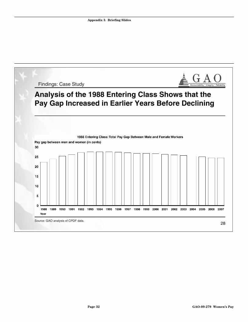
• Our case study analysis of workers who entered the federal workforce in 1988 showed that their pay gap grew from 22 cents in 1988 to a maximum of 28 cents in 1993 through 1996 and then declined to 25 cents in 2007. As with the federal workforce, differences between men and women that can affect pay, especially occupation, accounted for a significant portion of the pay gap over the 20-year period. In addition, our analysis found that differences in the use of leave without pay and breaks in federal service accounts for little of the pay gap for this group. The portion of the gap that we could not explain increased over time from 2 cents in 1988 to 9 cents in 2007. However, the results of the 1988 cohort are not necessarily representative of other cohorts
Ultimately, the gender pay gap for the entire federal workforce has declined primarily because the men and women in the federal workforce are more alike in characteristics related to pay than in past years. We cannot be sure why a persistent unexplained pay gap remains for both our analyses, but this may be due to the inability to account for certain factors that cannot effectively be measured or for which data are not available.
We received written comments on a draft of this report from OPM, which manages the CPDF data that were used in our analysis, and from EEOC. OPM reviewed our methodology and found our use of the CPDF data to be appropriate. They had two suggestions regarding variables in our analysis, which we considered carefully. As a result of their comments, we clarified
Page 3 GAO-09-279 Women’s Pay
21B
our discussion of the empirical results in the appendices, but did not alter the main findings of our report. OPM’s full comments and our responses to them are presented in appendix VI.
EEOC stated that our study has a solid research design and modeling analysis and will serve as an important source of information to the federal sector. In addition, EEOC suggested that we expand our report to show how the gender pay gap evolved for different protected groups. We acknowledge that the difference in wages between men and women may vary further by race, age, disability status, and other factors that we analyzed. However, to appropriately report on the influence of factors related to other protected groups would require substantial analysis that is beyond the scope of our study’s objective. EEOC also provided technical comments for our consideration. Their full comments and our responses to them are presented in appendix VII.
As agreed with your offices, unless you publicly announce the contents of this report earlier, we plan no further distribution of this report until 30 days from the report date. At that time, we will provide copies to the Chair of EEOC, the Director of OPM, relevant congressional committees, and other interested parties. We will make copies available to others upon request. In addition, the report will be available at no charge on GAO’s Website at http://www.gao.gov.
If you or your staff have any questions about this report, please contact me at (202) 512-7215 or [email protected]. Contacts for our Offices of Congressional Relations and Public Affairs may be found on the last page of this report. GAO staff who made major contributions to this report are
Andrew Sherrill
listed in appendix VIII.
Director, Education, Workforce, curity Issues
and Income Se
Page 4 GAO-09-279 Women’s Pay
A
ppendix I: Briefing Slides
Page 5 GAO-09-279 Women’s Pay
Appendix I: Briefing Slides
WOMEN’S PAY: Gender Pay Gap in the Federal Workforce Narrows as Differences in Occupation, Education, and Experience Diminish
Briefing for Congressional RequestersJanuary 26, 2009
*The briefing slides were subsequently updated to reflect comments that EEOC provided on our draft report. See appendix VII for EEOC’s comments and our response.
Appendix I: Briefing Slides
2
Overview
• Key Question• Scope and Methodology• Summary of Results• Background• Findings
• Entire Federal Workforce• Case Study
• Concluding Observations
Page 6 GAO-09-279 Women’s Pay
Appendix I: Briefing Slides
3
Key Question
In response to your request, we answered this question::
• To what extent has the pay gap between men and women in the federal workforce changed over the past 20 years and what factors account for the gap?
Page 7 GAO-09-279 Women’s Pay
Appendix I: Briefing Slides
4
Scope and Methodology
• To answer our key question, we looked at data covering the last 20 years in two different ways:
1. We examined the federal workforce at 3 points in time (1988, 1998, and 2007) to show changes in the pay gap within the federal workforce as a whole over a 20-year perioda
2. We examined a cohort (group) of federal workers, i.e., those who entered the federal workforce in 1988, to look for differences in the pay gap for this group over timeb
aFor this analysis, we used a 20 percent random sample of federal employees in the CPDF for each of the 3 years.bWe followed the careers of workers in this group, including those who left the federal workforce and later returned.
Page 8 GAO-09-279 Women’s Pay
Appendix I: Briefing Slides
5
Scope and Methodology (cont.)
• Our data came from the Central Personnel Data File (CPDF), which:
• Is maintained by the Office of Personnel Management.
• Contains information on gender, annual salary, and other demographic and occupational factors for federal workers.
• Covers federal employees within most of the executive branch as well as a few agencies in the legislative branch, but does not cover employees in the judicial branch and federal contractors.a
• We used CPDF data to compute the overall pay gap between men andwomen. We then performed multivariate analysis to estimate how much of the overall pay gap could be explained by demographic, occupational, and other measurable factors for which we have data.
aFor the purposes of this briefing, we refer to workers covered by the CPDF data as the federal workforce. See appendix II for further details on our data and data reliability analyses, as well as the employees excluded from the CPDF.
Page 9 GAO-09-279 Women’s Pay

Appendix I: Briefing Slides
6
Scope and Methods (cont.)
• To inform our analyses, we:• Reviewed existing literature and reports on gender and pay• Consulted officials at the Office of Personnel Management and
the Equal Employment Opportunity Commission—agencies that are in part responsible for overseeing the employment practices of federal agencies
Page 10 GAO-09-279 Women’s Pay
Appendix I: Briefing Slides
7
Summary of Results
• Our analysis of the federal workforce shows that:
• From 1988 to 2007, the gender pay gap—the difference between men’s and women’s average paya before controlling for other factors—narrowed from 28 cents to 11 cents on the dollar.
• For each year we analyzed, all but about 7 cents of the gap was accounted for by differences in measurable factors—predominantly the occupations of men and women and, to a lesser extent, other factors such as experience and education.
• Factors that we could not measure may have accounted for some orall of the unexplained 7 cent gap.
aPay refers to annual salary.
Page 11 GAO-09-279 Women’s Pay
Appendix I: Briefing Slides
8
Summary of Results (cont.)
• Our case study analysis of one cohort of employees, i.e., those who entered the federal workforce in 1988, showed that between 1988 and 2007:
• The gender pay gap grew from 22 cents in 1988 to a maximum of 28cents in 1993 and then declined to 25 cents in 2007.
• After controlling for differences between men and women, all but 2 to 9 cents (depending on the year) of the pay gap over this period was accounted for by differences in measurable factors. Occupation is the measurable factor that contributed most to the gap.
• Differences in usage of unpaid leave and breaks in federal service accounted for less than 1 cent of this pay gap.
• These results are not necessarily representative of other cohorts.
Page 12 GAO-09-279 Women’s Pay

Appendix I: Briefing Slides
9
Background: Previous Studies Have Sought to Measure the Pay Gap between Men and Women
• For the entire U.S. workforce:• Previously, GAO found that after accounting for certain measurable
differences such as years of experience and part-time work status, women earned about 20 cents less for every dollar earned by men in 2000a
• For the federal workforce:• Research shows that the gap dropped significantly between 1976 and
1995, but in 1995 white women still earned 14 cents less for every dollar earned by white men, and African-American women earned 8 cents less for every dollar earned by African-American men after accounting for differences in measurable factors between men andwomen
a GAO, Women’s Earnings: Work Patterns Partially Explain Difference between Men’s and Women’s Earnings, GAO-04-35 (Washington, D.C.: Oct. 31, 2003).
Page 13 GAO-09-279 Women’s Pay

Appendix I: Briefing Slides
10
Background: Federal Workers Are Classified in Six General Categories
Occupations comprising the crafts, trades, and manual labor, including foremen.Blue-collar
Includes positions that do not fall into other white-collar groups. Most of these positions are related to law enforcement or protective services.
Other white-collar
Involves structured work in support of office, business, or fiscal operations. Examples include typists, dispatchers, and clerks.
Clerical
Occupations typically associated with and supportive of a professional or administrative field. Includes medical technicians, safety technicians, and food inspectors.
Technical
Does not have a specific educational requirement, but involves skills typically gained through general college education. Examples include human resources management and budget analysis.
Administrative
Requires knowledge in a specific discipline, typically acquired through a bachelor’s or higher degree in a specialized field. Examples include accounting and engineering.
Professional
DescriptionOccupational category
Source: OPM.
Page 14 GAO-09-279 Women’s Pay

Appendix I: Briefing Slides
11
Background: Federal Employees are Increasingly Concentrated in Professional and Administrative Jobs
• However, the proportion of clerical and blue-collar jobs decreased significantly
Source: GAO analysis of CPDF data.
Page 15 GAO-09-279 Women’s Pay
Appendix I: Briefing Slides
12
Background: Federal Employees Are Increasingly Concentrated in Professional and Administrative Jobs (cont.)
• The decline in clerical and blue-collar employment may be due to the following trends:
• Many defense-related jobs being phased out following the end of the Cold War
• Government efforts to increase efficiency through automation and by contracting out jobs
Page 16 GAO-09-279 Women’s Pay

Appendix I: Briefing Slides
13
Background: The Federal Workforce Has Increasingly More Education
Source: GAO analysis of CPDF data.
• The proportion of federal workers with a bachelor’s degree or higher increased from 33% in 1988 to 44% in 2007
Page 17 GAO-09-279 Women’s Pay
Appendix I: Briefing Slides
Page 18 GAO-09-279 Women’s Pay
14
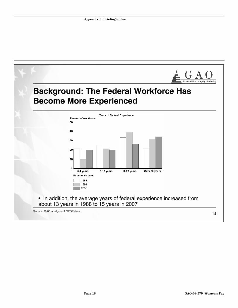
Background: The Federal Workforce Has Become More Experienced
Source: GAO analysis of CPDF data.
• In addition, the average years of federal experience increased from about 13 years in 1988 to 15 years in 2007

Appendix I: Briefing Slides
Page 19 GAO-09-279 Women’s Pay
15
The Pay Gap—before Accounting for Differences between Men and Women in Factors Related to Pay—Has Decreased Significantly Since 1988
Source: GAO analysis of CPDF data.
Findings: Federal Workforce

Appendix I: Briefing Slides
16
The Pay Gap Does Not Take into Account Differences in Measurable Factors between Men and Women
• The gap is a measure of the differences in pay for all men and all women in the federal workforce before accounting for any factors, such as differences in occupation or education
• We found that some of the gap can be accounted for by differences in measurable factors
Findings : Federal Workforce
Page 20 GAO-09-279 Women’s Pay

Appendix I: Briefing Slides
17
We Used Multivariate Analysis to Account for the Following Factors:
• Work characteristics including occupational category,agency, and state
• Worker characteristics including education level, federal experience, bargaining unit status, part-time work status, and veteran status
• Demographic characteristics including gender, age, race and ethnicity, and disability status
Findings: Federal Workforce
Page 21 GAO-09-279 Women’s Pay

Appendix I: Briefing Slides
18
Measurable Factors Account for a Significant Portion of the Gap
Source: GAO analysis of CPDF data.
Findings: Federal Workforce
Page 22 GAO-09-279 Women’s Pay
Appendix I: Briefing Slides
19
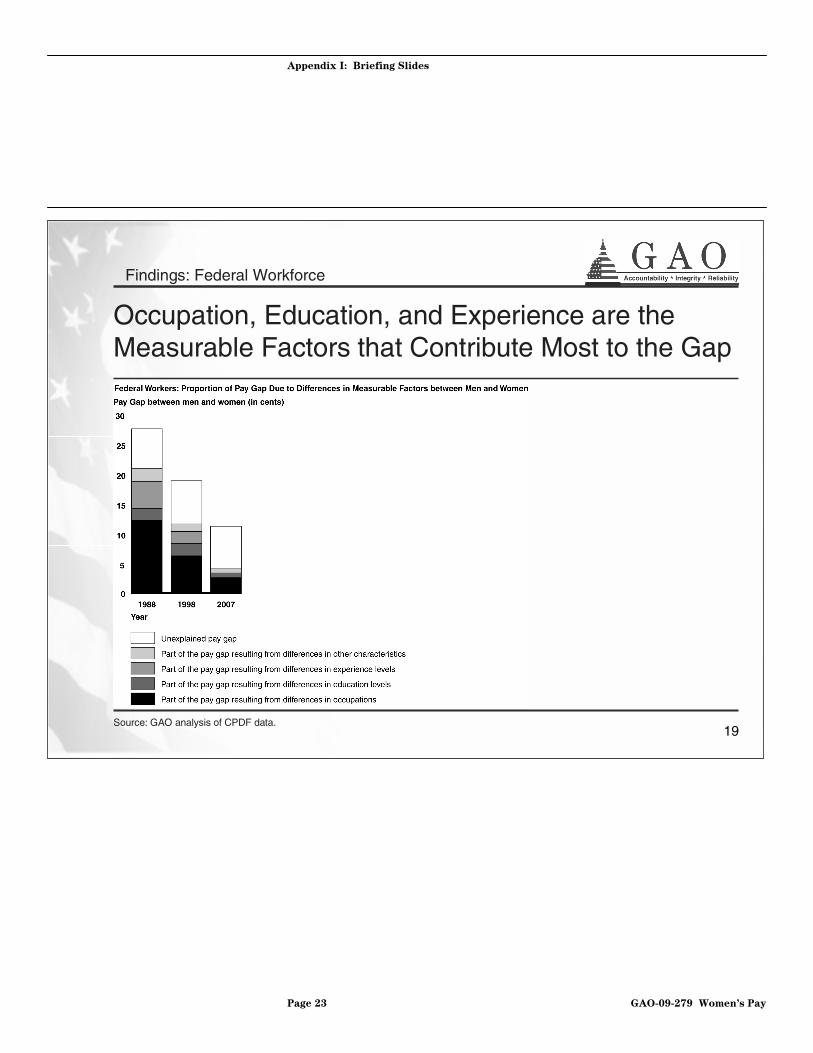
Occupation, Education, and Experience are the Measurable Factors that Contribute Most to the Gap
Source: GAO analysis of CPDF data.
Findings: Federal Workforce
Page 23 GAO-09-279 Women’s Pay

Appendix I: Briefing Slides
20
Other Factors That We Could Not Measure May Account for the Persistent Unexplained 7 Cent Gapa
• Factors for which we lacked data or are difficult to measure, such as work experience outside the federal government and discriminatory practices, could account for some of the unexplained gap
• Our analysis neither confirms nor refutes the presence of discriminatory practices
Findings: Federal Workforce
aThe size of the unexplained gap varies slightly depending on the number of occupational categories used in the analysis. See appendix III for further details.
Page 24 GAO-09-279 Women’s Pay
Appendix I: Briefing Slides
21
Converging Characteristics of Men and Women in the Workplace Help Explain the Narrowing Gap
• Men and women in the federal workforce became more alike in several characteristics, especially in:
• The occupations they hold,• Their educational attainment, and• Their years of federal work experience
Findings: Federal Workforce
Page 25 GAO-09-279 Women’s Pay

Appendix I: Briefing Slides
22
Some Federal Occupational Categories Have Become More Integrated by Gender
Findings: Federal Workforce
• Professional, administrative, and clerical occupations—which accounted for 68 percent of federal jobs in 2007—have becomemore integrated by gender since 1988. For example, between 1988 and 2007, the proportion of females in professional positions rose from 30 to 43 percent and in administrative positions rose from 38 to 45 percent
• Other occupations—accounting for 32 percent of the workforce in 2007—have become or remained less integrated. Between 1988 and 2007, the proportion of females in technical occupations rose from 52 to 60 percent, in blue collar occupations ranged between9 to 10 percent, and in other white-collar occupations rose slightly from 12 to 13 percent.
Page 26 GAO-09-279 Women’s Pay
Appendix I: Briefing Slides
23
The Decline of the Clerical Workforce Accounts for a Large Reduction in the Gap
• In 1988, there were 312,000 female clerical workers in the federal workforce, accounting for 38% of all women in the government
• By 2007, this number dropped to 97,000, with female clerical workers accounting for only 13% of all female federal employees
• Clerical workers are primarily female (85% in 1988 and 69% in 2007)
• Clerical workers are among the lowest paid group in the federal government
Findings: Federal Workforce
Page 27 GAO-09-279 Women’s Pay
Appendix I: Briefing Slides
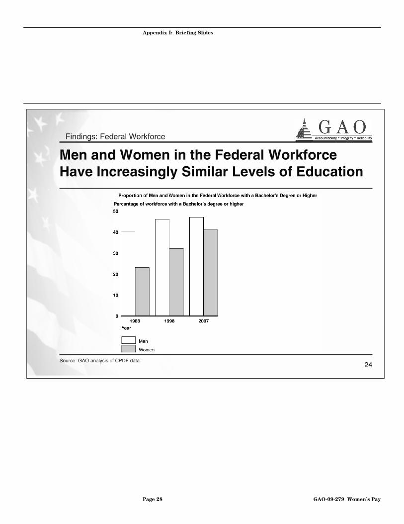
24
Men and Women in the Federal Workforce Have Increasingly Similar Levels of Education
Source: GAO analysis of CPDF data.
Findings: Federal Workforce
Page 28 GAO-09-279 Women’s Pay

Appendix I: Briefing Slides
25
Men and Women in the Federal Workforce Have Increasingly Similar Levels of Federal Experience
Source: GAO analysis of CPDF data.
Findings: Federal Workforce
Page 29 GAO-09-279 Women’s Pay
Appendix I: Briefing Slides
26
Analysis of Pay Gap among the Employees Who Began Working for the Federal Government in 1988
• To better understand changes in the gender pay gap over time, we compiled a data set on the people who began working for the federal government in 1988, which allowed us to track their federal pay and leave patterns over a 20-year perioda
• We accounted for differences between men and women in leave patterns (unpaid leave and breaks in serviceb) as well as occupation, agency, region, education level, bargaining unit status, part-time work status, veteran status, gender, age, race and ethnicity, disability status
Findings: Case Study
aData on work patterns came from the CPDF dynamics file.bA break in service happens when an employee leaves the federal government and later returns.
Page 30 GAO-09-279 Women’s Pay
Appendix I: Briefing Slides
27
The 1988 Cohort Is Different from Our Analysis of the Entire Government in Important Ways
• The cohort only includes individuals who started working for the federal government in 1988, and as a result:
• This group became much smaller over time due to workers leaving the government, declining from about 90,000 in 1988 to about 29,000 in 2007
• By definition, new workers did not enter this group over the study period
• Additionally, this cohort is not necessarily representative of other cohorts
Findings: Case Study
Page 31 GAO-09-279 Women’s Pay
Appendix I: Briefing Slides
28
Analysis of the 1988 Entering Class Shows that the Pay Gap Increased in Earlier Years Before Declining
Findings: Case Study
Source: GAO analysis of CPDF data.
Page 32 GAO-09-279 Women’s Pay
Appendix I: Briefing Slides
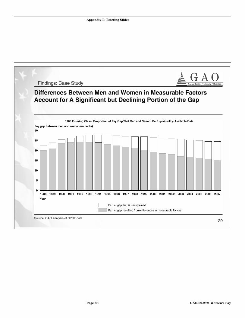
29
Differences Between Men and Women in Measurable Factors Account for A Significant but Declining Portion of the Gap
Findings: Case Study
Source: GAO analysis of CPDF data.
Page 33 GAO-09-279 Women’s Pay
Appendix I: Briefing Slides
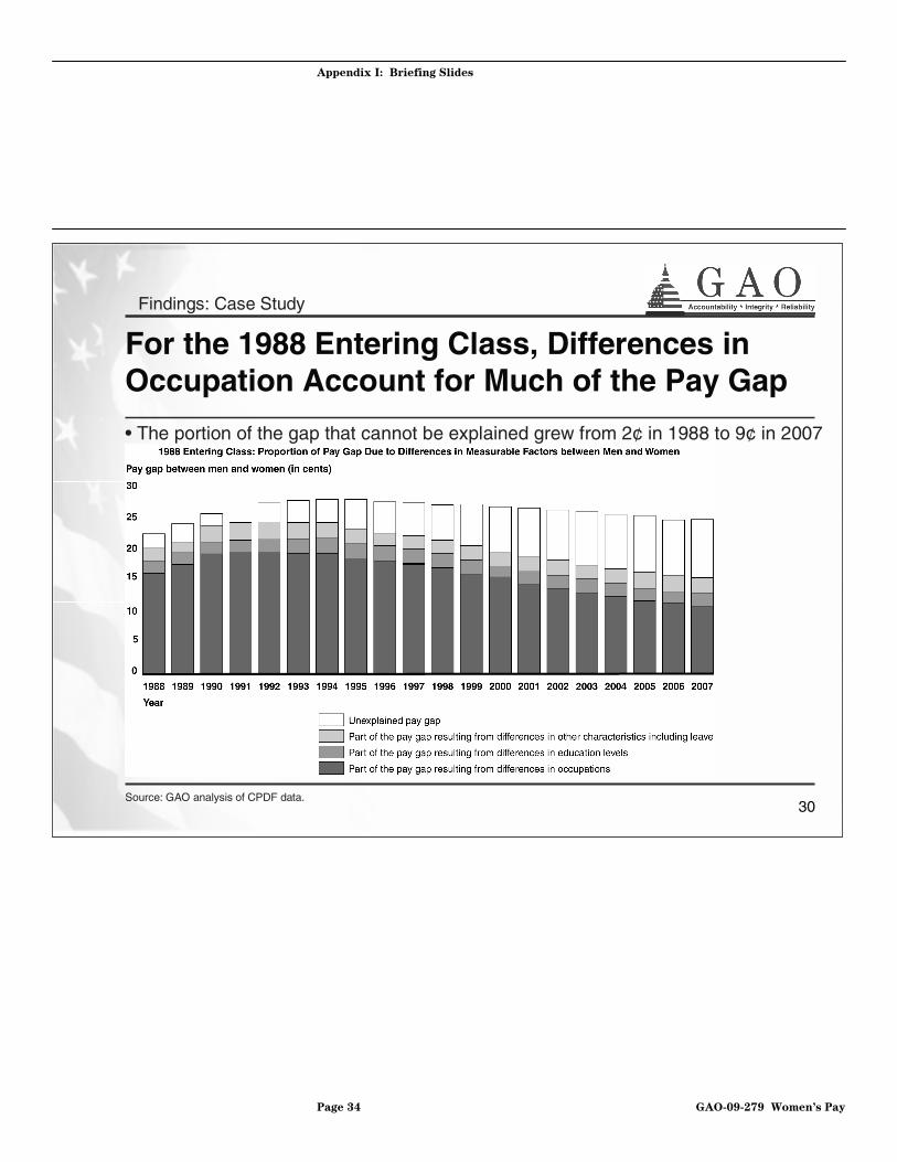
30
For the 1988 Entering Class, Differences in Occupation Account for Much of the Pay Gap
Findings: Case Study
Source: GAO analysis of CPDF data.
• The portion of the gap that cannot be explained grew from 2¢ in 1988 to 9¢ in 2007
Page 34 GAO-09-279 Women’s Pay

Appendix I: Briefing Slides
31
For Women in the Entering Cohort of 1988, the Decrease in the Clerical Workforce Was also Significant
Findings: Case Study
Source: GAO analysis of CPDF data.
• Over the same period, the number of female administrative workers increased
Page 35 GAO-09-279 Women’s Pay
Appendix I: Briefing Slides
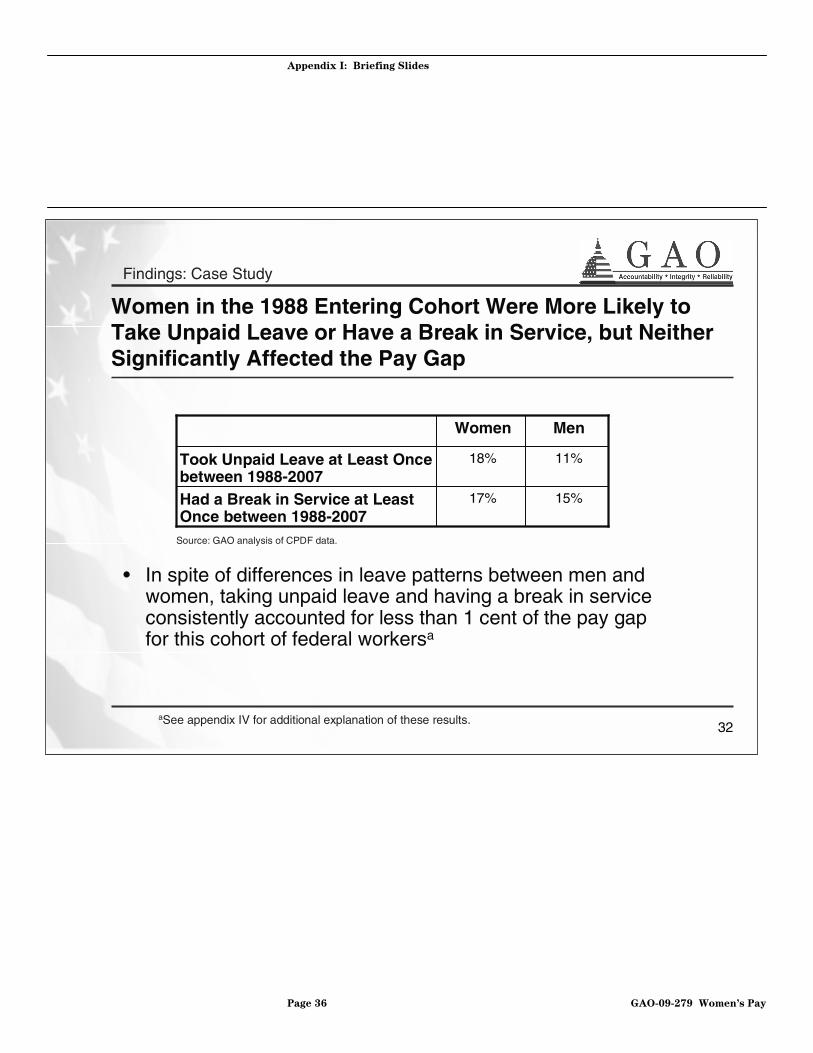
32
Women in the 1988 Entering Cohort Were More Likely to Take Unpaid Leave or Have a Break in Service, but Neither Significantly Affected the Pay Gap
• In spite of differences in leave patterns between men and women, taking unpaid leave and having a break in service consistently accounted for less than 1 cent of the pay gap for this cohort of federal workersa
17%
18%
Women
Had a Break in Service at Least Once between 1988-2007
Took Unpaid Leave at Least Once between 1988-2007
15%
11%
Men
Source: GAO analysis of CPDF data.
Findings: Case Study
aSee appendix IV for additional explanation of these results.
Page 36 GAO-09-279 Women’s Pay
Appendix I: Briefing Slides
33
Our Data Do Not Allow Us to Describe Why the Unexplained Pay Gap Grew
• As with our analysis of the federal workforce, other factors not captured by our data, such as experience outside the federal government and discrimination, could account for some of the unexplained pay gap
• Our analysis neither confirms nor refutes the presence of discriminatory practices
• We could not accurately measure the duration of instances of unpaid leave or determine why it was taken
Findings: Case Study
Page 37 GAO-09-279 Women’s Pay
Appendix I: Briefing Slides
34
Concluding Observations
• The decline in the pay gap for the federal workforce is primarily due to men and women in the federal workforce becoming more alike in characteristics related to pay
• We cannot be sure why a persistent unexplained pay gap remains for both analyses, but this may be due to the inability to account for certain factors that cannot effectively be measured or for which data are not available
Page 38 GAO-09-279 Women’s Pay
Appendix II: Summary of Methods and Data
Appendix II: Summary of Methods and Data
To determine the extent to which the pay gap between men and women in the federal workforce changed over the past 20 years and the factors that accounted for the gap, we developed several models to estimate gender differences in annual salaries before and after controlling for other factors that affect pay. These models employed multivariate regression and decomposition1 methods. The factors that affect the pay gap and are used in our models include: (1) work characteristics (i.e., the occupation men and women worked in, and the agency and state in which they worked); (2) worker characteristics (i.e., their education level, years of federal experience, bargaining unit status, full-time or part-time work status, and veteran status); and (3) additional demographic or background characteristics of federal employees (i.e., their gender, age, race/ethnicity, and disability status). We conducted a literature review of relevant research to inform these analyses and collaborated with GAO methodologists and consulted with OPM officials at various stages in doing this work.2
For our analysis, we examined federal personnel data covering a 20-year period—using both multivariate regression and decomposition methods—in the following ways:
1. We computed background statistics on the federal government for 1988, 1998, and 2007 using information on every federal worker in our data.
2. We then conducted a cross sectional analysis of gender differences in salaries for workers in the federal workforce at three points in time (September of 1988, 1998, and 2007) using a 20 percent sample of the federal workers in our data.
3. Finally, we analyzed gender differences in salaries for a cohort of federal workers who entered the federal workforce in 1988. We examined these workers annually for a 20-year period to examine how the pay gap evolved over the course of their careers and whether it was produced by differences in work patterns (i.e., unpaid leave and breaks in service).
1Decomposition allowed us to analyze men’s and women’s salaries in separate regressions and provided an additional tool for determining which attributes were the key explanations of the differences between men’s and women’s salaries.
2See the bibliography for a list of relevant articles and reports.
Page 39 GAO-09-279 Women’s Pay

Appendix II: Summary of Methods and Data
Appendix III provides a detailed discussion of our cross sectional analysis for the federal workforce, and appendix IV provides a detailed discussion of the cohort analysis. Appendix V presents the conversion of statistical output in appendices III and IV into the estimates of the pay gap that are presented in the briefing slides. In this appendix, we describe the data we used for our analyses, excluded data, our assessment of the reliability of the data, and the limitations of our analysis.
The data we analyzed came from the Central Personnel Data File (CPDF). The CPDF is maintained by the Office of Personnel Management, and represents the primary government source of information on federal employees. We used two separate sets of files contained in the CPDF—the annual status files and the annual dynamics files. The status files consist of data elements describing all employees who were present in the federal workforce in September of each year, with some notable exclusions described below. These elements include information on the federal employee’s adjusted basic pay, agency, age, education level, disability status, occupation, race or national origin, gender, veteran’s preference and status, bargaining unit status, and work schedule as of a certain date each year. We used these elements from the status files for 1988, 1998, and 2007 to construct the data for the cross sectional analysis.
Data
The annual dynamics files consist of data elements describing each personnel action taken by an agency for the time period covered by the file. Personnel actions are the official records of events that occur over the course of employees’ careers, and the dynamics file includes indicators and dates of hires, unpaid leaves of over 30 days, promotions, reassignments, pay changes, resignations, and retirements. We used some of these elements from the annual dynamics files, in combination with elements described above from the status files, for each year from 1988 to 2007 to construct the data for the cohort analysis.
While the CPDF is considered to be the most comprehensive, authoritative, and up-to-date database of federal executive branch employees, it does not include information for: (1) certain executive branch agencies, such as the intelligence services; (2) agencies in the
Exclusions
Page 40 GAO-09-279 Women’s Pay
Appendix II: Summary of Methods and Data
judicial branch; and (3) most agencies in the legislative branch.3 Ultimately, of the approximately 2.7 million federal employees, the CPDF covers roughly 1.6 million of them. The CPDF also does not include information on an estimated 10.5 million federal contractors and grantees, 1.4 million members of the armed forces, and 1 million reservists.
In addition to those exclusions, for purposes of consistency we performed some fairly routine data cleaning by systematically excluding certain observations from our analysis that were missing important information.4
We assessed the reliability of the CPDF data elements that were critical to our analyses and determined that, despite the limitations outlined below, they were sufficiently reliable for the purposes of our analyses. Specifically, we:
Data Reliability
• Reviewed documentation on the data elements included in the CPDF and past GAO analyses of the reliability of the CPDF data;
• Interviewed OPM officials knowledgeable about the CPDF data and consulted these officials periodically throughout the course of our study;
3Specifically, CPDF coverage of the executive branch currently includes all agencies except the Board of Governors of the Federal Reserve, the Central Intelligence Agency, the Defense Intelligence Agency, Foreign Service personnel at the State Department, the National Geospatial-Intelligence Agency, the National Security Agency, the Office of the Director of National Intelligence, the Office of the Vice President, the Postal Rate Commission, the Tennessee Valley Authority, the U.S. Postal Service, and the White House Office. Also excluded are the Public Health Service’s Commissioned Officer Corps, non-appropriated fund employees, and foreign nationals overseas. CPDF coverage of the legislative branch is limited to the Government Printing Office, the U.S. Tax Court, and selected commissions.
4Specifically, in both analyses, we excluded individuals for whom we had no wage data (less than one-half of 1 percent of the individuals in the cross-section analysis). For the cohort analysis, when wage data were not available from the status file, we were able to use wage data from the dynamics file. For individuals in the status file with more than one record in a given year and for whom the wage data on those records differed, we selected the higher of the two wages. For those individuals in the dynamics file with more than one personnel action in a given year and for whom the wage data on the different actions differed, we selected the last reported personnel action with data on wages. In the cross sectional analysis we excluded individuals that had missing data on federal experience, race, veteran’s preference, and disability status (totaling less than 1 percent of the observations). For the cohort analysis, we were able to impute values for missing variables using data from other years.
Page 41 GAO-09-279 Women’s Pay
Appendix II: Summary of Methods and Data
• Conducted our own electronic data testing to assess the accuracy and completeness of the data used in our analyses; and
• Consulted with GAO staff knowledgeable about these data sets.
As a result of these efforts, we identified the following limitations with our data:
• Education data. A GAO report issued in 1998 found that the CPDF data for education level were both inaccurate and, in many cases, understated. OPM officials we consulted reported that education was sometimes understated because employee information was not updated after the time of hiring. Therefore, the education data do not always reflect additional education acquired during federal service. They also noted that the education data and the degree major data were self-reported and therefore subject to error. OPM officials stated that no changes have been made to enhance the accuracy of the education variable in response to GAO’s 1998 finding. However, in a 1996 CPDF accuracy survey, OPM noted that “education level values appear reliable for determining general education groups (e.g., less than high school, high school graduate, some college), but less reliable when used to determine the precise education level.” As a result, in our analysis, we did not use information on the employee’s precise education level, but instead used broad categories to distinguish education groups.5
• Duration of Leave without Pay Period. For approximately one-quarter of the personnel actions for the employees we analyzed to determine whether they took leave without pay (LWOP), there was no corresponding personnel action indicating that the employee returned to duty. While we attempted to use various proxies in lieu of return to duty actions, we could not be certain that these proxies were accurate. Ultimately, we decided that it would not be possible for us to reliably measure the impact of the duration of LWOP on salaries, and we opted instead to look more simply at the effect of taking LWOP, regardless of its duration. Appendix IV provides a detailed discussion of our analyses of LWOP.
5Despite this assurance, however, we undertook an additional analysis to determine whether the underreporting of the education variable might affect our results. We used data from the Census Bureau’s Current Population Survey (CPS), whose reliability we did not assess, to run a similar model with more recent self-reported education data, for a sample of self-reported federal workers. The results of the CPS and CPDF analyses were similar enough to provide us with considerable confidence that the broad education variable was accurate for the purposes of our report.
Page 42 GAO-09-279 Women’s Pay

Appendix II: Summary of Methods and Data
This analysis was not intended to be used to determine whether or not discrimination exists in the federal workforce, and the existence of a persistent unexplained pay gap in both our cross-sectional and cohort analyses after we controlled for as many factors as our data allowed means that we can neither rule out nor confirm the possibility that women are being treated unequally. A few limitations, some of which are common to almost all multivariate analyses, prevent us from definitively determining whether unexplained differences in pay by sex are due to discrimination or to other factors. First, discrimination is not usually overt, and as such direct measures of it generally do not exist. Second, we lack data on several factors that may legitimately influence wages, such as experience outside of the federal workforce and individual priorities. Third, certain variables that were included in our model—such as occupation, education level, and part-time status—may have been imprecisely measured or reported. Although there is no way to fully address these limitations with the data we were using, we took various steps to explore the latter two.
Limitations of the Analysis
With respect to the second set of limitations described above, we conducted two sets of cross-sectional analyses to further explore the impact of individual priorities on the pay gap, such as personal obligations outside of work, and found they had only a minor impact. The CPDF data do not contain information on marital status and number of children, variables that are commonly regarded as proxies for personal obligations and have been included in wage models in some literature.6 To address this potential shortcoming, we used data from the Current Population Survey (CPS) to run a similar model with additional variables for marital status and number of children. We found that including these variables in the model had only a slight effect on the unexplained pay gap (i.e., it was reduced by less than 1 percent). We also analyzed a variable in the CPDF that indicates whether a federal employee is enrolled in a federal health benefit plan for single or family benefits. The health plan variable is a rough proxy of whether an individual has a family because individuals may receive family health benefits through a spouse. The results of this analysis corroborate our analysis of the variables for martial status and number of
6See, for example, June O’Neill, “The Gender Gap in Wages, circa 2000,” The American
Economic Review. Vol. 93, No .2, Papers and Proceedings of the One Hundred Fifteenth Annual Meeting of the American Economic Association, Washington, D.C.: January 3-5, 2003 (May 2003), pp. 309-314, and Audrey Light and Manuelita Ureta, “Early-Career Work Experience and Gender Way Differentials,” Journal of Labor Economics, Vol. 13, No. 1. (January 1995), pp. 121-154.
Page 43 GAO-09-279 Women’s Pay
Appendix II: Summary of Methods and Data
children in the CPS data. Including the health care variable in the model reduced the unexplained pay gap by less than 1 percent. In contrast to the above analyses, we did not have proxies for motivation and work performance that were independent from the process used to determine an individual’s salary; therefore, we could not test the effect of these factors on the pay gap.7
Also with respect to the second limitation, some of the wage gap may be affected by the possibility that women, or certain women and men, may be more or less likely to enter the federal government. However, because our scope was limited to effects for men and women already employed by the federal government, we did not attempt to explain the impact that propensity to enter the workforce may have had on the gap.
With respect to the third limitation, we conducted additional cross-sectional analyses of the CPDF data to better understand the degree to which different measures of key variables might impact our results. For example, we tested several different specifications of the occupation variable. We found, using the most detailed occupation data, that the unexplained pay gap declined from 7 percent to 5 percent for all 3 years of analysis. Although more precise measures of occupation reduced the pay gap more than broad measures, we opted to use a broader specification because the occupation category variable itself may reflect discriminatory practices. Specifically, the fact that men and women are hired into or remain in (albeit decreasingly) different occupations may itself reflect some level of discrimination associated with hiring, promotion, or other employer practices.8 As such, using a more precise measure of occupation in the model might hide the contribution of any such discrimination to the pay gap, and thereby understate the unexplained gap. To shed light on this, we estimated our model with no control for occupation, which would represent an upper-bound on the unexplained pay gap. We found that, with
7While the CPDF include data on performance ratings and grade information, which reflect promotions, these decisions feed directly into determining (and are therefore nearly synonymous with) salary. Therefore, it is more appropriate to evaluate these variables as dependent variables (in the same way that we are evaluating salary). However, such an analysis was beyond the scope of our report.
8For discussions of sex discrimination in hiring, see Claudia Goldin and Cecilia Rouse, “Orchestrating Impartiality: The Impact of ‘Blind’ Auditions on Female Musicians,” American Economic Review, vol. 90, no. 4 (2000); and David M. Neumark, “Sex Discrimination in Restaurant Hiring: An Audit Study,” Quarterly Journal of Economics, vol. 111, no. 3 (1996).
Page 44 GAO-09-279 Women’s Pay
Appendix II: Summary of Methods and Data
no control for occupation, the unexplained pay gap was 20 percent in 1988, 14 percent in 1998, and 11 percent in 2007. (See app. III, table 7, for further details on these results.) Ultimately, in an effort to strike a balance between the two extremes—either no control for occupation or the most detailed control for occupation—we used the occupational category variable in our model. This occupation variable was also relatively simple to interpret because it had significantly fewer categories than the most detailed occupation variable.9
We also tested whether additional information on education and geography reduced the pay gap. Specifically, we included in the model a variable for an individual’s educational major, which was only available for our 2007 cross-sectional analysis. For that year, we found that educational major reduced the unexplained gap by less than 1 percent. (See app. III, table 7, for further details on these results.) We also included a more detailed measure of geography—the county in which an employee works. We found that the more specific control for geography had no impact on the pay gap.
In addition, certain variables in our model reflect personal decisions that may be correlated with salary, such as whether an employee chooses to work part-time. Including such variables in the model has the potential to lead to biased estimates.10 Although we ultimately decided to keep these variables in the main model used in our briefing slides, we ran different versions of the model without these variables. (See app. III, table 7, for these results.)
9OPM categorizes occupations into one of six occupational categories: Professional, Administrative, Technical, Clerical, Other White-Collar and Blue-Collar (PATCOB). In applying decomposition methods, the occupation variable with fewer categories also had advantages. Specifically, any category that contains only men or women is excluded when computing the decomposition. Using more disaggregated occupation data therefore results in the exclusion of individuals that are in an all-female or all-male occupation category.
10Because of this bias, the academic literature sometimes does not include controls for marital status and family size in analyses of the pay gap. See, for example, Francine D. Blau and Lawrence M. Kahn, “The U.S. Gender Pay Gap in the 1990’s: Slowing Convergence,” Industrial and Labor Relations Review, Vol. 60, No. 1 (October 2006).
Page 45 GAO-09-279 Women’s Pay
Appendix III: Cross-sec
tional Analysis
Page 46 GAO-09-279 Women’s Pay
Appendix III: Cross-sectional Analysis
In order to perform our cross-sectional analysis of differences in salaries between men and women in the federal government as a whole over a 20-year period, and the extent those differences can be explained by other factors, we employed two separate techniques. Both techniques involved multivariate regression, and controlled for many factors that might affect pay, such as level of education or occupation. The data used for both techniques come from the status file of the Central Personnel Data File (CPDF), as described in appendix II.
The first technique involved regression analysis on a data set which included men and women. In this analysis, we used a variable for gender to measure the average difference between men and women’s salaries. Then by adding additional variables to the regression, we controlled for other characteristics of men and women to determine the extent to which the difference is (or is not) explained by the addition of those variables. The second technique, called a decomposition, analyzed men’s and women’s salaries in separate regressions. This method provides an additional tool for determining which attributes were the key explanations of the differences between men and women’s salaries, and also what percentage of men and women’s salary remains unexplained by the characteristics measured in our data.
The data for the analysis come from the status file of the CPDF. As described in appendix II, this data set is produced by the Office of Personnel Management as a central source of information regarding the federal workforce.1 For the cross-sectional analysis, we selected a 20 percent random sample of federal employees in the CPDF for each of the 3 years of the analysis.2
Data Used in the Cross-Sectional Analysis and Descriptive Statistics
Table 1 shows descriptive statistics for men and women in our sample, for the 3 years we used in our analysis. As the table shows, there has been a significant narrowing in the gap between the characteristics of men and women in the federal workforce in almost all categories, although gaps remain. Specifically:
1For more information regarding the CPDF, exclusions, and the steps we took to ascertain whether it was sufficiently reliable for our purposes, see appendix II.
2Due to computational limitations associated with conducting sophisticated econometric analyses with a large dataset, we selected a 20 percent sample using the random generator function in SAS.
Appendix III: Cross-sectional Analysis
• Average salary: We performed our analysis using adjusted basic pay as recorded in the CPDF, which takes into account various differences in pay based on locality and special rates and takes into account existing pay caps. This figure reflects that amount an individual would have earned had he or she worked a complete year. It does not reflect their actual earnings, which are not available in the CPDF data. We deflated the salary using the consumer price index.
• There has been a narrowing of the gap in average salary between men and women in the federal workforce. The difference in the average log earnings of men and women was about 0.33 in 1988, 0.21 in 1998, and 0.12 in 2007.
• The standard interpretation of the log difference is that it is equivalent to the percent difference; however, at larger values this value will differ somewhat from the precise percent difference. As presented in the briefing slides, the percent difference was negative 28 percent in 1988, negative 19 percent in 1998, and negative 11 percent in 2007.3
• Age: We computed age using the month and year of birth, and the date the data were drawn (September of each year).
• There has been a narrowing of the difference in the average age between men and women. In 1988 it was more than 3 years—by 2007, it was less than a year.
• Federal experience: We measured federal experience by the months between the service computation date and the date the data were drawn (September of each year).
• As table 1 shows, there has been a narrowing of the difference in years of federal experience between men and women. Specifically, the average years of experience for a man was almost 3-1/2 years greater than a woman in 1988, about 2 years in 1998, and by 2007 there was no appreciable difference.
• Race and ethnicity: We measured race and ethnicity using the CPDF definitions. These definitions do not allow for multiple races. Unlike many data sets, they do not record Hispanic status distinctly from race.
• There appears to be less change in differences in racial composition between men and women in the federal workforce. In general, there appears to be a decline in the percentage that is white with an increase
3To transform the coefficient to more exactly equal the percent difference, we applied the following formula: exp(difference in logarithms)-1.
Page 47 GAO-09-279 Women’s Pay

Appendix III: Cross-sectional Analysis
in the percentage that is Hispanic and Asian/Pacific Islander. This holds for both men and women.
• Education: We used the CPDF definition of the highest degree obtained by the employee.
• There has been a narrowing of the difference in degree attained between men and women over the past 20 years. For example, in 1988, almost twice as many men in the federal workforce had bachelor’s, master’s, professional, or doctoral degrees (40 percent versus 23 percent). By 2007, the difference was less than 10 percentage points (46 versus 40 percent). In some specifications, we included educational major within each degree type. However, this measure was only available in 2007.
• Rates of disability: We defined disability by whether the employee did or did not have a CPDF code for a disability condition and whether that condition indicated a targeted disability as defined by EEOC’s Management Directive 715. Only targeted disabilities were counted as disabled.
• There has been a slight narrowing of the difference in the rates of disability, as slightly more men and slightly fewer women are classified as having no condition.
• Work schedule: Employees were classified by whether they worked full-time, part-time or held a flexible schedule (such as seasonal, intermittent, on-call, etc.).
• There has been a slight narrowing of the difference in the work schedule of employees, as men are classified as 4 percentage points more likely to work full-time in 2007, and about 6 percentage points in 1988.
• Occupation: Our main analysis defined occupation using occupational category in the CPDF, which groups occupations into six categories: Professional, Administrative, Technical, Clerical, Other White-collar, and Blue-collar. For the purposes of our analysis, we called this categorical variable PATCOB.
• One of the most striking changes in the composition of the federal workforce has been the narrowing of the difference between occupations held by men and by women. Much of the narrowing is the result of a diminishing clerical sector in the federal workforce. In 1988, about 38 percent of women in the federal workforce were in a clerical occupation. By 2007, that number was 13 percent. Similarly, in 1988
Page 48 GAO-09-279 Women’s Pay

Appendix III: Cross-sectional Analysis
almost 28 percent of men in the federal workforce were in the “Blue-Collar” field; by 2007, that number was 17 percent.4
• While PATCOB is a rough measure of occupation, with six categories, we also experimented with more disaggregated measures. For example, we created “job family level”—a categorical variable that had about 50 different occupation categories—and “job series”—another categorical variable with more than 700 occupation categories.5 In other specifications, we included the percentage of occupation that was female as an additional covariate.
• Marital status and number of children: A variable containing information on the family of the employee was not available. However, as a proxy, in some specifications we included a measure of whether that individual had registered for health insurance for their family or themselves or had declined health insurance coverage. Declined coverage may imply that the employee receives coverage through a spouse.
• In all the years, men are much more likely than women to participate in a family plan. In 1988, women were more than twice as likely to have declined coverage, although this gap has closed in the most recent year.
• Percentage female: We used the CPDF classification of the gender of the employee.
• The percentage of the federal workforce that is female has risen from 42 percent to 44 percent over the past 20 years.
Additionally the following variables were included in the analysis but do not appear in the descriptive statistics table:
4An index of dissimilarity is an alternate way to demonstrate the convergence of the occupational structure. The index of dissimilarity is defined as the fraction of either men or women that would have to switch occupations to make the distributions identical. The range of values are 1 (meaning that the 100 percent of men or women would have to switch) to 0 (meaning that the distributions are identical). Using PATCOB, the dissimilarity index fell from 40 percent in 1988 to 30 percent in 1998 to almost 20 percent in 2007, indicating that the distributions are much closer today.
5“Job family level” was constructed by combining PATCOB with the “occupational group” variable in the CPDF data, and collapsing blue-collar occupations into a single category. An occupational group is a set of occupations in a related field such as engineering or health care. In addition, those occupations that individually represented 0.35 percent of the population were combined into an “other” category. The number of categories included in a regression depended on whether that category had any individuals in a particular year.
Page 49 GAO-09-279 Women’s Pay

Appendix III: Cross-sectional Analysis
• Veteran status: Veteran status was categorized into three types defined by whether or not the employee was a veteran, and whether or not the employee qualified for a veteran’s preference in CPDF data.
• Geography: An employee’s geographic location, such as state, was defined using the location of the employment, which may or may not be the location of residence.
Table 1: Descriptive Statistics for Selected CPDF Variables Used in Our Cross-sectional Analysis
1988 1998 2007
Men Women Men Women Men Women
Annual adjusted salary 55,862 39,750 62,595 50,540 70,109 62,021
Log of salary 10.847 10.520 10.957 10.745 11.059 10.938
Age 42.980 39.772 45.707 43.823 46.707 46.148
Federal experience 14.035 10.469 16.143 14.260 14.901 14.995
Race/ethnicity
African-American .115 .232 .113 .232 .122 .238
Asian Pacific Islander .035 .030 .047 .043 .053 .055
Hispanic .055 .048 .066 .060 .080 .072
Native American .016 .021 .018 .025 .016 .026
White .779 .668 .756 .639 .726 .606
Other .000 .001 .0005 .000 .003 .003
Education
Less than high school .042 .031 .017 .016 .011 .011
High school diploma .265 .350 .251 .315 .283 .276
Trade degree .047 .076 .030 .052 .023 .041
Some college .236 .300 .231 .287 .194 .239
Bachelor degree .258 .168 .279 .207 .272 .243
Masters degree .082 .044 .102 .070 .124 .114
Professional degree .038 .015 .050 .029 .032 .025
Doctorate degree .023 .006 .029 .011 .031 .020
Other education .010 .010 .011 .013 .031 .030
Occupation (PATCOB)
Administrative .257 .213 .305 .284 .349 .354
Blue-collar .283 .046 .215 .031 .173 .026
Clerical .048 .381 .035 .202 .045 .126
Other white-collar .029 .002 .040 .004 .051 .006
Professional .234 .143 .266 .214 .244 .242
Technical .148 .216 .139 .264 .138 .246
Page 50 GAO-09-279 Women’s Pay

Appendix III: Cross-sectional Analysis
1988 1998 2007
Men Women Men Women Men Women
Work schedule
Full time .938 .886 .932 .885 .939 .900
Part time .019 .056 .017 .048 .020 .048
Another type .043 .058 .051 .067 .040 .051
Disability status
None .927 .951 .930 .945 .936 .946
Disabled not targeted .060 .038 .058 .044 .054 .044
Disabled .012 .010 .012 .011 .010 .010
Health plan
Family plan .600 .317 .598 .364 .524 .357
Self plan .194 .326 .222 .347 .235 .371
Declined coverage .105 .230 .104 .203 .161 .186
Pending .031 .045 .020 .022 .030 .033
Not eligible .070 .082 .056 .063 .045 .052
Percentage female 42% 44% 44%
Number of observations 241,611 175,776 199,153 158,460 205,767 162,822
Source: GAO analysis of CPDF data.
Regression Analysis
Approach and Results
Description of Econometric Method
In order to determine the extent to which gender differences persist when characteristics of men and women are taken into account, we performed a multivariate regression analysis for 3 years of data: 1988, 1998, and 2007. Consistent with the usual practice in studies of the determinants of earnings, we attempted to explain the differences by predicting the logarithm of annual adjusted pay on characteristics of federal workers.
Equation 1:
Ln(annual pay) = α + β*(female) + δ1*(set of work characteristics) + δ2*(set of worker characteristics) + δ3*(set of demographic characteristics)
Page 51 GAO-09-279 Women’s Pay

Appendix III: Cross-sectional Analysis
The standard interpretation of β, the coefficient on female, is that it represents the average percent difference in earnings between men and women, after controlling for the other variables in the model. However, similar to the descriptive statistics above, the coefficient in a model such as this will differ somewhat from the precise percent change at larger values. Consequently, for discussion purposes, as in the briefing slides, we perform a transformation on the coefficients to accurately present percent changes.6 This transformation is described in detail in appendix V.
The following variables were included as controls:
1. “Work characteristics”: These were characteristics of the individual that were dependent on the specific position held, including occupation, the agency, and the state in which they worked.
2. “Worker characteristics”: These were characteristics of the individual, rather than the position held, and included years of federal experience, educational degree attained, bargaining unit, part-time status, and veterans status.
3. “Demographic characteristics”: These were characteristics of the individual that were associated with demography and included race/ethnicity, disability status, and age.7
In choosing the variables included in our model, we had to balance two competing ideas. As described by Blau and Kahn (2000)8, the difference between male and female wages can be decomposed into two categories: what is explained by measured characteristics and what is unexplained by those characteristics that may be due to discrimination. However, if a study estimates that a portion is unexplained, that finding can be challenged if some important explanatory variable has been excluded from the analysis, such as occupation. Conversely, including a variable that is itself a result of discrimination would cause the unexplained portion to be understated. For example, if women are denied access to certain
6To transform the coefficient to more exactly equal the percent difference, we applied the following formula: exp(β)-1.
7Although age is a demographic variable, it could have been classified as a worker characteristic. This is because our measure of experience only includes experience in the federal government. Therefore, the age variable could likely be a proxy for other experience.
8See Francine Blau and Lawrence Kahn, 2000, “Gender Differences in Pay,” The Journal of Economic Perspectives 14 (4): pp.75-99.
Page 52 GAO-09-279 Women’s Pay
Appendix III: Cross-sectional Analysis
occupations, controlling for occupation might be explaining away the effect of discrimination. In our main analysis, we chose a broad category of occupation, PATCOB, in order to balance these competing ideas. Alternate definitions of occupation or of other variables could yield different results. For example, it may be that defining education using educational major in addition to degree reduces the unexplained pay gap.
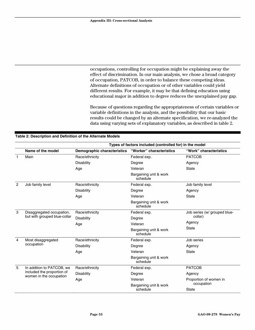
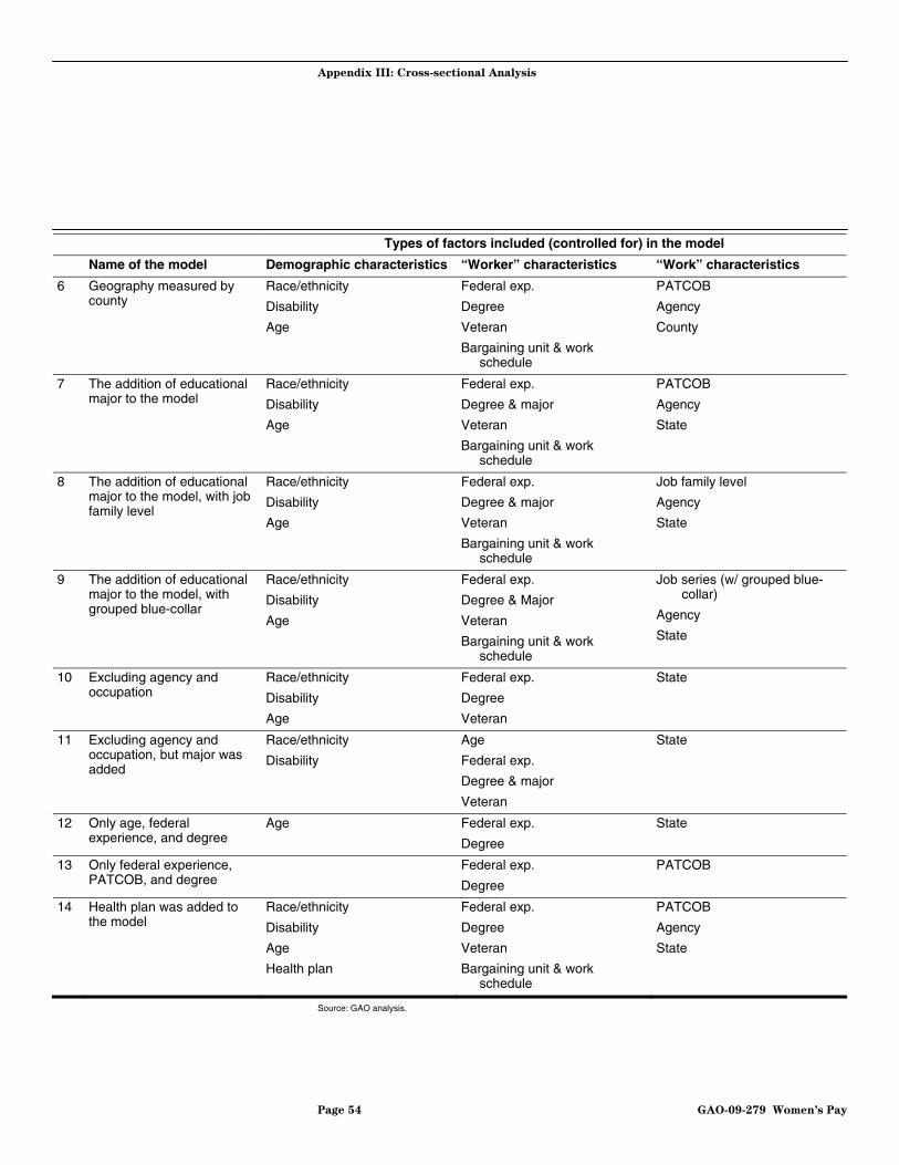
Because of questions regarding the appropriateness of certain variables or variable definitions in the analysis, and the possibility that our basic results could be changed by an alternate specification, we re-analyzed the data using varying sets of explanatory variables, as described in table 2.
Table 2: Description and Definition of the Alternate Models
Types of factors included (controlled for) in the model
Name of the model Demographic characteristics “Worker” characteristics “Work” characteristics
1 Main Race/ethnicity
Disability
Age
Federal exp.
Degree
Veteran
Bargaining unit & work schedule
PATCOB
Agency
State
2 Job family level Race/ethnicity
Disability
Age
Federal exp.
Degree
Veteran
Bargaining unit & work schedule
Job family level
Agency
State
3 Disaggregated occupation, but with grouped blue-collar
Race/ethnicity
Disability
Age
Federal exp.
Degree
Veteran
Bargaining unit & work schedule
Job series (w/ grouped blue-collar)
Agency
State
4 Most disaggregated occupation
Race/ethnicity
Disability
Age
Federal exp.
Degree
Veteran
Bargaining unit & work schedule
Job series
Agency
State
5 In addition to PATCOB, we included the proportion of women in the occupation
Race/ethnicity
Disability
Age
Federal exp.
Degree
Veteran
Bargaining unit & work schedule
PATCOB
Agency
Proportion of women in occupation
State
Page 53 GAO-09-279 Women’s Pay
Appendix III: Cross-sectional Analysis
Types of factors included (controlled for) in the model
Name of the model Demographic characteristics “Worker” characteristics “Work” characteristics
6 Geography measured by county
Race/ethnicity
Disability
Age
Federal exp.
Degree
Veteran
Bargaining unit & work schedule
PATCOB
Agency
County
7 The addition of educational major to the model
Race/ethnicity
Disability
Age
Federal exp.
Degree & major
Veteran
Bargaining unit & work schedule
PATCOB
Agency
State
8 The addition of educational major to the model, with job family level
Race/ethnicity
Disability
Age
Federal exp.
Degree & major
Veteran
Bargaining unit & work schedule
Job family level
Agency
State
9 The addition of educational major to the model, with grouped blue-collar
Race/ethnicity
Disability
Age
Federal exp.
Degree & Major
Veteran
Bargaining unit & work schedule
Job series (w/ grouped blue-collar)
Agency
State
10 Excluding agency and occupation
Race/ethnicity
Disability
Age
Federal exp.
Degree
Veteran
State
11 Excluding agency and occupation, but major was added
Race/ethnicity
Disability
Age
Federal exp.
Degree & major
Veteran
State
12 Only age, federal experience, and degree
Age
Federal exp.
Degree
State
13 Only federal experience, PATCOB, and degree
Federal exp.
Degree
PATCOB
14 Health plan was added to the model
Race/ethnicity
Disability
Age
Health plan
Federal exp.
Degree
Veteran
Bargaining unit & work schedule
PATCOB
Agency
State
Source: GAO analysis.
Page 54 GAO-09-279 Women’s Pay

Appendix III: Cross-sectional Analysis
As noted in model 5, table 2, we estimated a model that contained a variable to measure the proportion of women in each occupation.9 This variable allowed us to measure the degree to which the proportion of women in an occupation accounted for some of the wage gap. There is some debate about the appropriateness of including this variable in addition to the variable that controls for being female in the model because it can be interpreted as double-counting the impact of being female.10 Because of this, we chose to exclude it from our main model that we discuss in the briefing slides.
Finally, in addition to the alternate models described above, we also examined the gap in salaries within subgroups of the federal workforce. Specifically, we examined the gender gap by race and ethnicity, occupation, agency, and employees in the federal workforce with less than a year of federal work experience. The results of this, as well as the main and alternative regression analyses, are provided below.
Regression Analysis Results
Main Specification of the Model
Table 3 presents the coefficients and standard errors for the main regression results from estimating equation 1. As described above, the coefficient on female can be interpreted as the percent difference between women’s and men’s annual salary, after accounting for all of the measurable characteristics of men and women that we controlled for in the model. Additionally, table 3 presents values and standard errors of the coefficients associated with all of the other characteristics in the main specification model.
9The occupation category that was used to measure the proportion of women in each occupation was “job series,” which was more disaggregated than PATCOB.
10The inclusion of this variable makes the coefficient on female difficult to interpret. As others have noted, the share of women in a particular occupation may be correlated with some unobserved characteristics of workers that also influences pay. Since these unobserved characteristics may also be captured by the coefficient on the variable for female—and since by definition women will tend to be in occupations with more women—we may be simply introducing two measures of the same thing. This could result in a lower measured effect of the female variable and therefore could be misleading. See Altonji, J. G., and R. M. Blank, “Race and Gender in the Labor Market,” in Handbook of Labor Economics, Volume 3C, O. Ashenfelter and D. Card, eds. (Amsterdam: North-Holland, 1999), p. 3222.
Page 55 GAO-09-279 Women’s Pay

Appendix III: Cross-sectional Analysis
• As the table shows, the percent difference between women’s and men’s salary, controlling for the factors in the main specification, has fallen over the past 20 years. A negative value indicates that women’s salary was less than men’s. Specifically, the coefficient on female changed from approximately negative 10.9 percent in 1988, to negative 8.8 in 1998, and negative 8.3 in 2007. It is important to note that these results differ slightly from our Oaxaca decomposition results, which are discussed in the briefing slides. We chose to highlight the results of the Oaxaca decomposition in the briefing slides because, unlike with the simple regression analysis presented here, the decomposition allows us to quantify the amount that each factor in our model contributes to the pay gap.
• Many of the other parameters associated with the control variables are in the expected direction. Higher education levels are associated with higher levels of salary. For example, after controlling for the other factors in the model, in 2007 a federal worker with a BA had a salary that was 18 percent higher than the salary of a person who did not complete high school. A person with an MA, in 2007, had a salary that was 25 percent higher than the salary of a person who did not complete high school. Salary increases at higher levels of federal experience and age, but the marginal effect of an additional year decreases as the years increase (as indicated by the negative sign of the estimate for the squared terms for age and experience).
• As would be expected, there were differences in pay between occupations, even after the controls were introduced. For example, clerical workers tend to be paid significantly less in the 3 years analyzed. Specifically, clerical workers were paid 15.6 percent less than technical workers in 1988, 16.3 percent less in 1998 and 20.4 percent less in 2007. On the other hand, in 1988, professional workers were paid 37.0 percent more than technical workers, 39.7 percent more in 1998 and 43.2 more in 2007, after controlling for the other factors.
• Similar to gender, there are disparities by racial and ethnic groups, as well as by disability status. For example, in 2007, the salary for an African-American employee was 7.4 percent lower than the salary of a white person, after controlling for the other factors in the model.
Page 56 GAO-09-279 Women’s Pay

Appendix III: Cross-sectional Analysis
Table 3: Main Regression Results
1988 1998 2007
Estimate Standard error Estimate Standard error Estimate Standard error
Female -.109 .001 -.088 .001 -.083 .001
Experience and age
Age .018 .001 .041 .001 .050 .001
Age squared -.0002 .00002 -.0007 .00002 -.0008 .00002
Age cubed 6.46E-7 1.53E-7 3.64E-7 1.73E-7 4.31E-6 1.59E-7
Federal experience .035 .0002 .031 .0003 .029 .0003
Federal exp. squared -.001 .00002 -.001 .00002 .001 1.6E-6
Federal exp. cubed .00001 2.60E-7 .00001 2.82E-7 .00001 2.62E-7
Race/Ethnicity (white is omitted)
African-American -.079 .001 -.074 .001 -.074 .001
Asian Pacific Islander -.015 .002 -.022 .002 -.005 .002
Hispanic -.045 .001 -.042 .001 -.028 .001
Native American -.033 .002 -.042 .002 -.055 .003
Other -.043 .014 -.057 .016 -.037 .007
Education (less than high school is omitted)
High school .078 .002 .074 .003 .076 .003
Trade degree .112 .002 .112 .003 .112 .004
Some college .110 .002 .112 .003 .114 .004
Bachelor degree .182 .002 .193 .003 .182 .004
Masters degree .258 .002 .272 .003 .247 .004
Professional degree .456 .003 .442 .003 .561 .004
Doctorate degree .411 .003 .418 .004 .398 .004
Other education .035 .004 .058 .004 .091 .004
Occupation (technical is omitted)
Administrative .260 .001 .318 .001 .363 .001
Blue-collar .095 .001 .053 .001 .036 .001
Clerical -.156 .001 -.163 .001 -.204 .002
Other white-collar -.124 .002 .006 .002 .097 .002
Professional .370 .001 .397 .001 .432 .001
Work schedule (part time is omitted)
Full time .040 .002 .023 .002 .040 .002
Another type -.097 .002 -.171 .002 -.085 .003
Disability status (targeted disability is omitted)
None .085 .003 .102 .003 .090 .004
Page 57 GAO-09-279 Women’s Pay
Appendix III: Cross-sectional Analysis
1988 1998 2007
Estimate Standard error Estimate Standard error Estimate Standard error
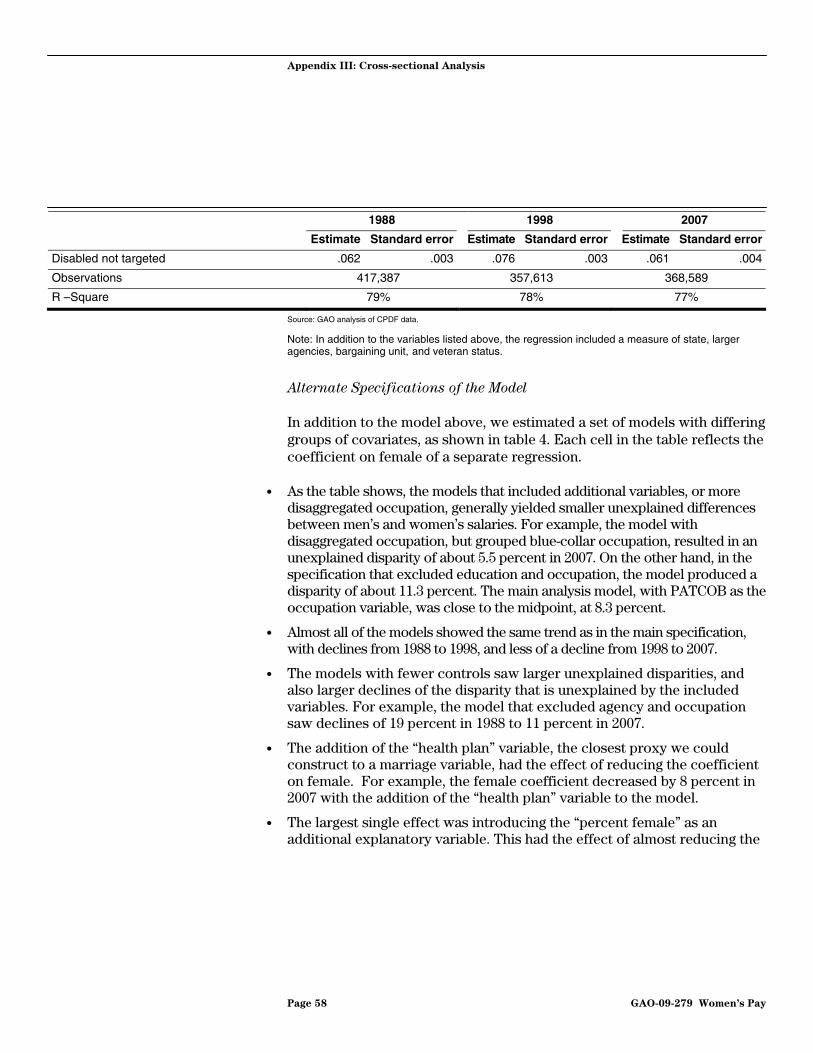
Disabled not targeted .062 .003 .076 .003 .061 .004
Observations 417,387 357,613 368,589
R –Square 79% 78% 77%
Source: GAO analysis of CPDF data.
Note: In addition to the variables listed above, the regression included a measure of state, larger agencies, bargaining unit, and veteran status.
Alternate Specifications of the Model
In addition to the model above, we estimated a set of models with differing groups of covariates, as shown in table 4. Each cell in the table reflects the coefficient on female of a separate regression.
• As the table shows, the models that included additional variables, or more disaggregated occupation, generally yielded smaller unexplained differences between men’s and women’s salaries. For example, the model with disaggregated occupation, but grouped blue-collar occupation, resulted in an unexplained disparity of about 5.5 percent in 2007. On the other hand, in the specification that excluded education and occupation, the model produced a disparity of about 11.3 percent. The main analysis model, with PATCOB as the occupation variable, was close to the midpoint, at 8.3 percent.
• Almost all of the models showed the same trend as in the main specification, with declines from 1988 to 1998, and less of a decline from 1998 to 2007.
• The models with fewer controls saw larger unexplained disparities, and also larger declines of the disparity that is unexplained by the included variables. For example, the model that excluded agency and occupation saw declines of 19 percent in 1988 to 11 percent in 2007.
• The addition of the “health plan” variable, the closest proxy we could construct to a marriage variable, had the effect of reducing the coefficient on female. For example, the female coefficient decreased by 8 percent in 2007 with the addition of the “health plan” variable to the model.
• The largest single effect was introducing the “percent female” as an additional explanatory variable. This had the effect of almost reducing the
Page 58 GAO-09-279 Women’s Pay
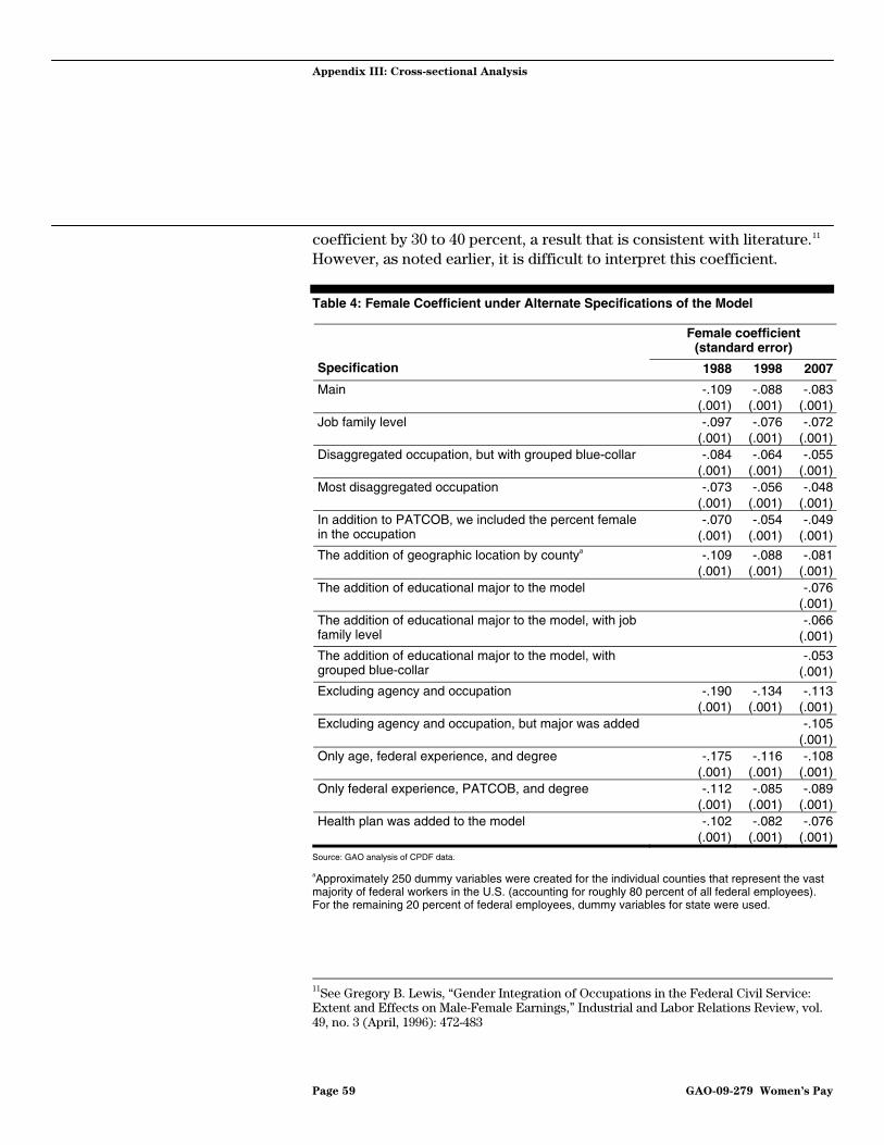
Appendix III: Cross-sectional Analysis
coefficient by 30 to 40 percent, a result that is consistent with literature.11 However, as noted earlier, it is difficult to interpret this coefficient.
Table 4: Female Coefficient under Alternate Specifications of the Model
Female coefficient (standard error)
Specification 1988 1998 2007
Main -.109(.001)
-.088(.001)
-.083(.001)
Job family level -.097(.001)
-.076(.001)
-.072(.001)
Disaggregated occupation, but with grouped blue-collar -.084(.001)
-.064(.001)
-.055(.001)
Most disaggregated occupation -.073(.001)
-.056(.001)
-.048(.001)
In addition to PATCOB, we included the percent female in the occupation
-.070(.001)
-.054(.001)
-.049(.001)
The addition of geographic location by countya -.109(.001)
-.088(.001)
-.081(.001)
The addition of educational major to the model -.076(.001)
The addition of educational major to the model, with job family level
-.066(.001)
The addition of educational major to the model, with grouped blue-collar
-.053(.001)
Excluding agency and occupation -.190(.001)
-.134(.001)
-.113(.001)
Excluding agency and occupation, but major was added -.105(.001)
Only age, federal experience, and degree -.175(.001)
-.116(.001)
-.108(.001)
Only federal experience, PATCOB, and degree -.112(.001)
-.085(.001)
-.089(.001)
Health plan was added to the model -.102(.001)
-.082(.001)
-.076(.001)
Source: GAO analysis of CPDF data.
aApproximately 250 dummy variables were created for the individual counties that represent the vast majority of federal workers in the U.S. (accounting for roughly 80 percent of all federal employees). For the remaining 20 percent of federal employees, dummy variables for state were used.
11See Gregory B. Lewis, “Gender Integration of Occupations in the Federal Civil Service: Extent and Effects on Male-Female Earnings,” Industrial and Labor Relations Review, vol. 49, no. 3 (April, 1996): 472-483
Page 59 GAO-09-279 Women’s Pay
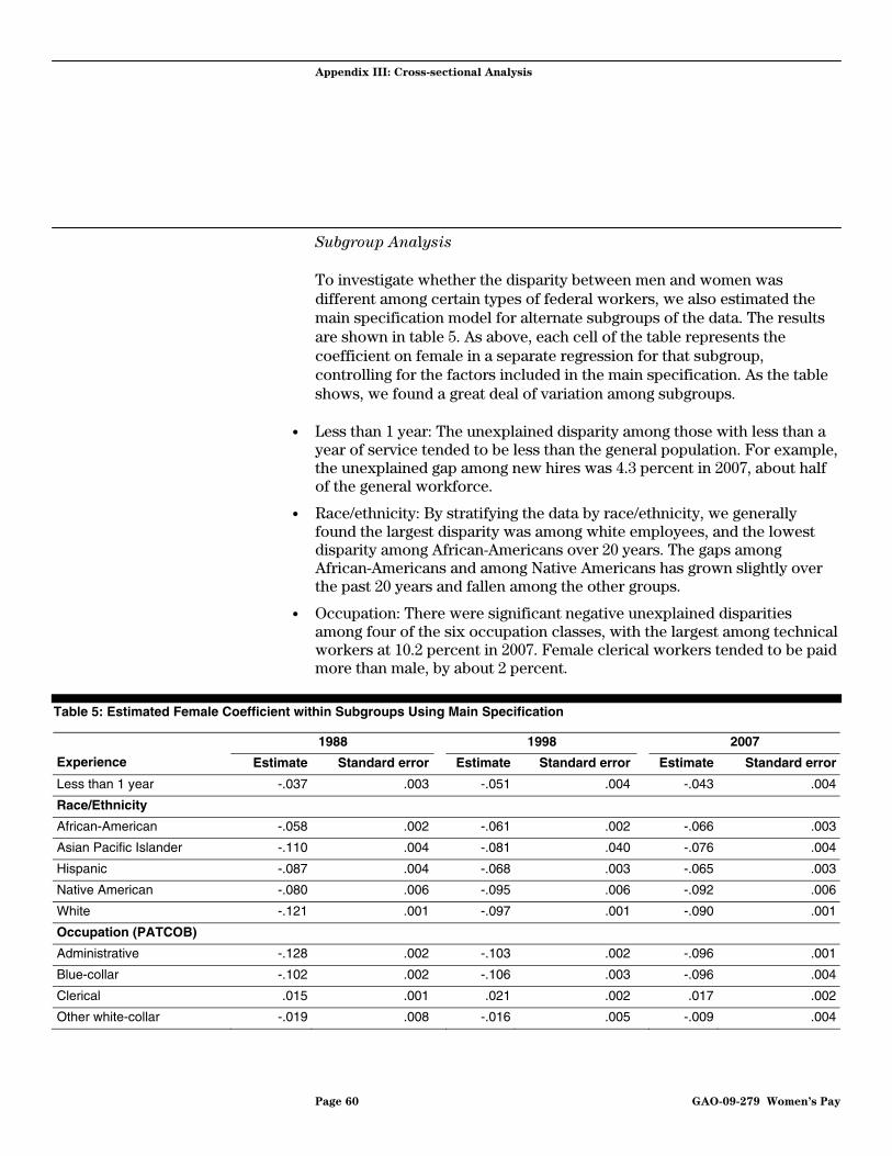
Appendix III: Cross-sectional Analysis
Subgroup Analysis
To investigate whether the disparity between men and women was different among certain types of federal workers, we also estimated the main specification model for alternate subgroups of the data. The results are shown in table 5. As above, each cell of the table represents the coefficient on female in a separate regression for that subgroup, controlling for the factors included in the main specification. As the table shows, we found a great deal of variation among subgroups.
• Less than 1 year: The unexplained disparity among those with less than a year of service tended to be less than the general population. For example, the unexplained gap among new hires was 4.3 percent in 2007, about half of the general workforce.
• Race/ethnicity: By stratifying the data by race/ethnicity, we generally found the largest disparity was among white employees, and the lowest disparity among African-Americans over 20 years. The gaps among African-Americans and among Native Americans has grown slightly over the past 20 years and fallen among the other groups.
• Occupation: There were significant negative unexplained disparities among four of the six occupation classes, with the largest among technical workers at 10.2 percent in 2007. Female clerical workers tended to be paid more than male, by about 2 percent.
Table 5: Estimated Female Coefficient within Subgroups Using Main Specification
1988 1998 2007
Experience Estimate Standard error Estimate Standard error Estimate Standard error
Less than 1 year -.037 .003 -.051 .004 -.043 .004
Race/Ethnicity
African-American -.058 .002 -.061 .002 -.066 .003
Asian Pacific Islander -.110 .004 -.081 .040 -.076 .004
Hispanic -.087 .004 -.068 .003 -.065 .003
Native American -.080 .006 -.095 .006 -.092 .006
White -.121 .001 -.097 .001 -.090 .001
Occupation (PATCOB)
Administrative -.128 .002 -.103 .002 -.096 .001
Blue-collar -.102 .002 -.106 .003 -.096 .004
Clerical .015 .001 .021 .002 .017 .002
Other white-collar -.019 .008 -.016 .005 -.009 .004
Page 60 GAO-09-279 Women’s Pay

Appendix III: Cross-sectional Analysis
1988 1998 2007
Experience Estimate Standard error Estimate Standard error Estimate Standard error
Professional -.099 .002 -.070 .002 -.074 .002
Technical -.127 .002 -.116 .002 -.102 .002
Source: GAO analysis of CPDF data. In addition to the subgroups described above, we also performed subgroup analysis on the larger agencies.
Decomposition Approach and Results
Description of our econometric method
One possible explanation for the gap could be that women have different levels of important attributes, like years of experience, than men. Alternatively, women could have the same level of attributes, but women’s attributes were treated differently. For example, the effect of an additional year of experience might be different for a woman than a man. In order to determine whether the difference between men’s and women’s pay is a function of men and women having different levels of characteristics, or different effects of those characteristics, we asked the following questions:
• What would the difference in wages be if we took women’s average level of characteristics, assigned them men’s effects of those characteristics and calculated the difference with women’s average wages? This is referred to as the parameter, or unexplained difference.
• What would the difference in wages be if we took women’s average level of characteristics, assigned them men’s effects of those characteristics and calculated the difference with men’s average wages? This is referred to as the characteristic, or explained difference.
This methodology, widely used in the discrimination literature, is often referred to as “Oaxaca decomposition.”12 In order to apply the “Oaxaca decomposition,” we followed these steps:
• First, we estimated two versions of equation (1), one on women in our sample and one on men in our sample. This provided us with two sets of regression coefficients, one for men and one for women.
• Second, we applied the regression coefficients for men to the average values of characteristics for men. This gave us the average wages of men.
12For details on this technique see “Male-Female Wage Differentials in Urban Labor Markets,” Ronald Oaxaca, International Economic Review, Volume 14, Issue 3 (October 1973), pp. 693-709.
Page 61 GAO-09-279 Women’s Pay

Appendix III: Cross-sectional Analysis
We repeated this analysis for women, producing the average wages for women.
• Third, we then applied the coefficients for men to the average values for the characteristics for women. This gave us a new predicted wage—the predicted wage for women if they had the same effects of characteristics as men.
With these three values, we were able to decompose the total difference between the average of male and female wages into two parts:
Equation 2:
(Average Female Wages) – (Male returns with female characteristics)
= “Unexplained” or due to parameter differences between women and men
+ (Male returns with female characteristics) – (Male Average Wages)
= + “Explained” or due to characteristics difference between men and women
(Average Female Wages) – (Average Male Wages)
= Total
Similar to the regression case above, the standard interpretation of this analysis is that it represents a decomposition of the percent change in earnings between men and women. However, at larger values, this value will differ somewhat from the precise percent difference. Consequently, for discussion purposes in the briefing slides, we scaled the decomposition to be proportional to the actual percent difference.
We performed the decomposition using the same specifications as outlined in table 2. In addition, we performed the analysis on the same subgroups.
Results of Decomposition Approach
Main Specification
Table 6 reports on the results of applying the decomposition methodology as outlined in equation 2. As the table shows, the overall conclusions drawn from both approaches were similar. Under both the regression and the decomposition approaches, differences remain between men and women’s salaries, even after correcting for a wide range of characteristics, as a negative value indicates that the salary of women was less than men. The first row details the total difference, the unexplained or parameter difference, and the explained or characteristic difference in each year. The other rows indicate the contribution of each of the factors.
Page 62 GAO-09-279 Women’s Pay

Appendix III: Cross-sectional Analysis
• As the table shows, using the decomposition methodology, the unexplained percentage has been remarkably constant over the past 20 years. Specifically, it was 7.8 percent in 1988, 8.1 percent in 1998, and 7.5 percent in 2007. After scaling these numbers to be proportional to the actual percent difference (as described in detail in app. V), this gap was 6.7, 7.3, and 7.1, respectively.
• Consequently, because the pay gap has been falling, the percentage of the gap explained by measurable characteristics has been decreasing. For example, the percentage explained by measurable characteristics was 76 percent (-.249/-.327) in 1988 and 37 percent (-.045/-.121) in 2007.
• The contribution of occupation is the largest component of any of the explanatory variables, accounting for over half of the explained difference in the gender pay gap in each year. Specifically, the contribution of occupation was 14.5 percentage points in 1988, 7.1 percentage points in 1998 and 2.9 percentage points in 2007.
• The geographic location of employment (as measured by the state in which the federal worker was employed) had a minimal contribution in explaining the gender pay gap for all 3 years.
Table 6: Decomposition Results Using Main Specification (with contributions of key factors)
1988 1998 2007
Total gap Unexplained
gap Explained
gap Total gapUnexplained
gap Explained
gap Total gap Unexplained
gap Explained
gap
Total -.327 -.078 -.249 -.211 -.081 -.13 -.121 -.075 -.045
Detailed factors
Intercept -.106 -.106 0 .0622 .0622 0 -.04 -.04 0
Age -.162 -.143 -.019 -.236 -.227 -.009 -.096 -.096 4E-7a
Federal experience
-.06 -.006 -.054 -.001 .024 -.022 .015 .014 .001
Race/ ethnicity
.004 .016 -.012 -3E-6 .011 -.011 -.002 .009 -.011
Education -.034 -.01 -.024 -.039 -.016 -.023 -.013 -.005 -.008
Occupation -.06 .085 -.145 -.01 .060 -.071 .0168 .0456 -.029
Work schedule
.024 .027 -.003 .0258 .029 -.004 -.024 -.021 -.003
Disability status
-.015 -.015 .001 -.041 -.042 .001 -.032 -.032 .0003
State .0129 .0106 .002 -.017 -.019 .002 .0332 .030 .0031
Page 63 GAO-09-279 Women’s Pay

Appendix III: Cross-sectional Analysis
1988 1998 2007
Total gap Unexplained
gap Explained
gap Total gapUnexplained
gap Explained
gap Total gap Unexplained
gap Explained
gap
Veteran status
.028 .002 .027 .011 -.015 .026 -.008 -.028 .019
Bargaining unit
.029 .040 -.012 .028 .035 -.007 .019 .024 -.005
Agency .013 .023 -.011 .005 .018 -.013 .01 .023 -.013
Source: GAO analysis of CPDF data.
aE reflects multiplication by 10 to that power. For example, “-3E-6” refers to -3 multiplied by 10 to the negative 6th power.
Alternate Specifications
As with the main regression, we also performed the decomposition using alternate models. The results—which are consistent with those using the main specification regression model—are shown in table 7.
• While the size of the unexplained gap varied, in almost all of the specifications that included agency and occupation, the size of the unexplained gap remained roughly constant over time. However, because the percentage explained by characteristics has decreased, the total gap has been falling.
• In the models without agency and occupation, the unexplained gap has fallen over the past 20 years. For example, in the model without agency or occupation, the size of the unexplained gap has fallen from about 20 percent to about 11 percent. However, the percentage explained by characteristics has fallen at a faster rate. Consequently, the explained portion of the gap was almost 40 percent in 1988, and less than 10 percent in 2007.
Table 7: Decomposition Results Using Alternate Specifications
Specification Total gap Unexplained gap Explained gapPercentage
explained
Main
1988 -.327 -.078 -.249 .761
1998 -.211 -.081 -.130 .616
2007 -.121 -.075 -.045 .372
Job family level
1988 -.327 -.064 -.263 .803
1998 -.211 -.066 -.145 .688
Page 64 GAO-09-279 Women’s Pay
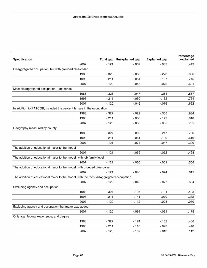
Appendix III: Cross-sectional Analysis
Specification Total gap Unexplained gap Explained gapPercentage
explained
2007 -.121 -.067 -.053 .443
Disaggregated occupation, but with grouped blue-collar
1988 -.326 -.053 -.273 .836
1998 -.211 -.054 -.157 .745
2007 -.120 -.048 -.072 .601
Most disaggregated occupation—job series
1988 -.328 -.047 -.281 .857
1998 -.211 -.050 -.162 .764
2007 -.120 -.046 -.076 .622
In addition to PATCOB, included the percent female in the occupation
1988 -.327 -.022 -.305 .934
1998 -.211 -.038 -.173 .818
2007 -.120 -.035 -.085 .705
Geography measured by county
1988 -.327 -.080 -.247 .756
1998 -.211 -.081 -.130 .616
2007 -.121 -.074 -.047 .390
The addition of educational major to the model
2007 -.121 -.069 -.052 .428
The addition of educational major to the model, with job family level
2007 -.121 -.060 -.061 .504
The addition of educational major to the model, with grouped blue-collar
2007 -.121 -.046 -.074 .615
The addition of educational major to the model, with the most disaggregated occupation
2007 -.122 -.045 -.077 .634
Excluding agency and occupation
1988 -.327 -.195 -.131 .403
1998 -.211 -.141 -.070 .332
2007 -.120 -.112 -.008 .070
Excluding agency and occupation, but major was added
2007 -.120 -.099 -.021 .175
Only age, federal experience, and degree
1988 -.327 -.174 -.152 .466
1998 -.211 -.118 -.093 .440
2007 -.120 -.107 -.013 .112
Page 65 GAO-09-279 Women’s Pay
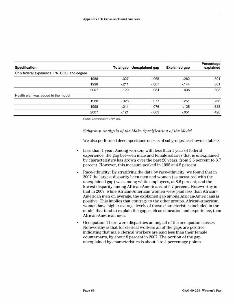
Appendix III: Cross-sectional Analysis
Specification Total gap Unexplained gap Explained gapPercentage
explained
Only federal experience, PATCOB, and degree
1988 -.327 -.065 -.262 .801
1998 -.211 -.067 -.144 .681
2007 -.120 -.084 -.036 .303
Health plan was added to the model
1988 -.328 -.077 -.251 .766
1998 -.211 -.076 -.135 .638
2007 -.121 -.069 -.051 .428
Source: GAO analysis of CPDF data.
Subgroup Analysis of the Main Specification of the Model
We also performed decompositions on sets of subgroups, as shown in table 8.
• Less than 1 year: Among workers with less than 1 year of federal experience, the gap between male and female salaries that is unexplained by characteristics has grown over the past 20 years, from 2.5 percent to 3.7 percent. However, this measure peaked in 1998 at 4.8 percent.
• Race/ethnicity: By stratifying the data by race/ethnicity, we found that in 2007 the largest disparity been men and women (as measured with the unexplained gap) was among white employees, at 8.6 percent, and the lowest disparity among African-Americans, at 5.7 percent. Noteworthy is that in 2007, while African-American women were paid less than African-American men on average, the explained gap among African-Americans is positive. This implies that contrary to the other groups, African-American women have higher average levels of those characteristics included in the model that tend to explain the gap, such as education and experience, than African-American men.
• Occupation: There were disparities among all of the occupation classes. Noteworthy is that for clerical workers all of the gaps are positive, indicating that male clerical workers are paid less than their female counterparts, by about 8 percent in 2007. The portion of the gap unexplained by characteristics is about 2 to 4 percentage points.
Page 66 GAO-09-279 Women’s Pay
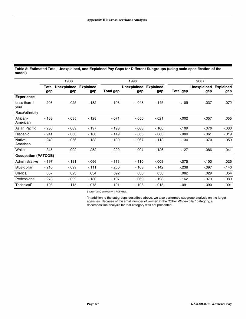
Appendix III: Cross-sectional Analysis
Table 8: Estimated Total, Unexplained, and Explained Pay Gaps for Different Subgroups (using main specification of the model)
1988 1998 2007
Total
gap Unexplained
gap Explained
gap Total gapUnexplained
gapExplained
gap Total gap Unexplained
gapExplained
gap
Experience
Less than 1 year
-.208 -.025 -.182 -.193 -.048 -.145 -.109 -.037 -.072
Race/ethnicity
African-American
-.163 -.035 -.128 -.071 -.050 -.021 -.002 -.057 .055
Asian Pacific -.286 -.089 -.197 -.193 -.088 -.106 -.109 -.076 -.033
Hispanic -.241 -.063 -.180 -.149 -.065 -.083 -.080 -.061 -.019
Native American
-.240 -.056 -.183 -.180 -.067 -.113 -.130 -.070 -.059
White -.345 -.092 -.252 -.220 -.094 -.126 -.127 -.086 -.041
Occupation (PATCOB)
Administrative -.197 -.131 -.066 -.118 -.110 -.008 -.075 -.100 .025
Blue-collar -.210 -.099 -.111 -.250 -.108 -.142 -.238 -.097 -.140
Clerical .057 .023 .034 .092 .036 .056 .082 .029 .054
Professional -.273 -.092 -.180 -.197 -.069 -.128 -.162 -.073 -.089
Technicala -.193 -.115 -.078 -.121 -.103 -.018 -.091 -.090 -.001
Source: GAO analysis of CPDF data.
aIn addition to the subgroups described above, we also performed subgroup analysis on the larger agencies. Because of the small number of women in the “Other White-collar” category, a decomposition analysis for that category was not presented.
Page 67 GAO-09-279 Women’s Pay

ohort Analysis
Page 68 GAO-09-279 Women’s Pay
Appendix IV: C
Appendix IV: Cohort Analysis
To examine the effect of leave patterns on the pay gap between men and women and to further understand changes in the pay gap, we constructed and analyzed a dataset on a cohort of workers who entered the federal workforce for the first time in 1988. In addition to the variables included in our cross sectional analysis, this dataset included controls for leave patterns, i.e., unpaid leave and breaks in service. As with the cross sectional analysis, we employed linear regression models and decomposition methods. In contrast to the cross sectional analysis, the cohort analysis used data for each fiscal year from 1988 to 2007, rather than at three points in time.
We used data from the CPDF status and dynamics files to construct a longitudinal dataset containing information on the same federal workers over a 20-year period. (See app. II for a description of the CPDF data.) Specifically, we selected a cohort1 of 89,356 federal employees hired in 1988 and tracked their annual salary and leave patterns through the end of fiscal year 2007. The dataset contains information on the same individuals for each fiscal year that they worked for the federal government. The data do not contain information on individuals during fiscal years when they did not work in the federal government, including periods following retirement or separation and during breaks in service (i.e., when a worker separates then returns to the federal workforce). Table 9 shows the number of workers remaining in the data over time. By 2007, only 29,009 of the employees who joined the federal workforce in 1988 remained.
Data used in Cohort Analysis and Descriptive Statistics
1We define this cohort as the group of people who entered the federal workforce in the same period. The characteristics of the 1988 federal hiring cohort might not be representative of other hiring cohorts, especially those after 2000 because of the change in the occupational structure of the federal workforce. This cohort also may not be representative of the federal workforce as a whole in any given year.

Appendix IV: Cohort Analysis
Table 9: Number of Federal Employees from the 1988 Entry Cohort Remaining over 2 Decades in the Status and Dynamic Files
Fiscal year Male Female Total
1988 38,687 50,669 89,356
1989 32,996 41,812 74,808
1990 28,351 34,212 62,563
1991 25,541 29,973 55,514
1992 23,483 27,133 50,616
1993 22,149 25,389 47,538
1994 21,013 23,995 45,008
1995 19,928 22,790 42,718
1996 19,052 21,649 40,701
1997 18,195 20,597 38,792
1998 17,485 19,586 37,071
1999 16,816 18,774 35,590
2000 16,329 18,088 34,417
2001 15,872 17,571 33,443
2002 15,558 17,074 32,632
2003 15,247 16,715 31,962
2004 14,957 16,374 31,331
2005 14,612 15,987 30,599
2006 14,233 15,605 29,838
2007 13,828 15,181 29,009
Source: GAO analysis of CPDF data.
Note: In our data, unpaid leave was indicated with a Leave-Without-Pay personnel action.
The cohort analysis included two variables on leave patterns, which were not available in the data used for our cross sectional analyses:
• Unpaid leave: We measured the use of unpaid leave (e.g., when an individual was absent from work for over 30 consecutive workdays without receiving pay) with an indicator that represented whether the individual had taken unpaid leave in either the current or any previous fiscal year.2
2In our data, unpaid leave was indicated with a Leave-Without-Pay personnel action.
Page 69 GAO-09-279 Women’s Pay
Appendix IV: Cohort Analysis
• Break in service: We measured the cumulative duration of breaks in federal service over the 20-year period. We define a break in service to be when a federal worker separates from the federal government and is appointed back into federal service at some later date. Transfers between agencies do not represent breaks in service.3
In comparison with the cross sectional analysis, we estimated a slightly more parsimonious model for the cohort because the number of observations in the cohort decreases by more than 65 percent over the study period. The remaining variables in the cohort analysis were identical to those used in the cross sectional analysis, with the following exceptions:
• Geography was measured by region (rather than state) of duty station, in order to reduce the number of variables in the model. The regions were: Northeast, South, Midwest, West, and other.
• Agency was measured by a dummy variable that had the value of 1 if the agency was large and 0 if the agency was not large, again to reduce the number of variables in the model.4
• Because the members of the cohort all began their federal service in the same fiscal year, we did not include a control for federal experience because we assume that the federal experience would increase by the same amount for each person. Differences in federal experience caused by extended periods of unpaid leave or breaks in service were accounted for in our analyses directly with the variables that control for unpaid leave and breaks in service.
The overall characteristics of the study population changed over time because, as noted earlier, the cohort analysis only included individuals as long as they remained in the federal workforce and about two-thirds of the people left over the period. In particular, the study population changed with respect to occupation and education characteristics.
The distribution of occupational categories (PATCOB) for the cohort changed dramatically over the period as a result of both individuals leaving the federal workforce and changing occupations within it. Figure 1
3The duration of a break in service was computed using the effective date of the separation action as the start of the break and the effective date of the subsequent appointment action as the end of the break.
4The size of the agency was determined by the relative number of federal workers in that agency in 1988.
Page 70 GAO-09-279 Women’s Pay

Appendix IV: Cohort Analysis
shows the number of people in each occupational category over the period. The number of employees declined in five of the six categories. The largest decline was within the clerical category in which more than 90 percent of the workers who began in 1988 separated from the government or changed occupational category over the period. The administrative category received a net gain of about 10 percent through workers, and primarily women switching from the technical and clerical categories.
Figure 1: Distribution of Occupational Categories in the Entering Class of 1988 over 20-year Period
Number of employees (in thousands)
Year
Technical
Professional
Other white-collar
Clerical
Blue-collar
Administrative
0
10
20
30
40
50
60
70
80
90
100
20072006200520042003200220012000199919981997199619951994199319921991199019891988
Source: GAO analysis of CPDF data.
Table 10 shows the proportions of men and women working in each occupational category in 1988 and 2007. In comparison to the men and women that were in the cohort in 1988, the percentages of men and women who remained in the cohort in 2007 were more similar in five out of six categories they occupied, especially in the clerical and administrative categories.
Page 71 GAO-09-279 Women’s Pay

Appendix IV: Cohort Analysis
Table 10: Cohort Differences between Men and Women in Occupational Categories in 1988 and 2007
1988 2007
Men WomenDifference between
men and women Men Women Difference between
men and women
Occupational Category (PATCOB)
Professional 34% 17% 17% 35% 23% 12%
Administrative 18% 7% 11% 42% 38% 4%
Technical 10% 11% -1% 9% 26% -17%
Clerical 18% 59% -41% 2% 11% -9%
Other white-collar 10% 3% 7% 5% 0% 5%
Blue-collar 10% 4% 6% 7% 1% 6%
Source: GAO analysis of CPDF data.
Note: Figures may not sum to 100 percent due to rounding.
Table 11 shows the education levels of men and women in the 1988 entry cohort in 1988 and 2007. In comparison to the men and women that were in the cohort in 1988, the men and women who remained in the cohort in 2007 had higher levels of education.5 For example, in 1988, 30 percent of women in the 1988 entering cohort had a bachelor’s degree or higher, while 53 percent of men had a bachelor’s degree or higher. By 2007, of those remaining in the federal workforce, 41 percent of women and 63 percent of men had a bachelor’s degree or higher.
5The shift in the educational distribution among the cohort members over the 20-year period is due to two factors. People with higher levels of education, particularly with bachelor’s degrees, stayed in the federal workforce while those with lower levels of education were more likely to leave the federal workforce. In addition, people who stayed in the federal workforce over the entire period gained advanced degrees over their careers. The exception to the trend toward a more educated workforce is that men and women with professional degrees were more likely to leave the federal workforce.
Page 72 GAO-09-279 Women’s Pay

Appendix IV: Cohort Analysis
Table 11: Cohort Differences between Men and Women in Education Levels in 1988 and 2007
1988 2007
Education level Men Women Difference between
men and women Men Women Difference between
men and women
Less than high school 1% 3% -2% 0% 1% -1%
High school graduate 21% 40% -19% 18% 32% -14%
Some college 24% 28% -4% 20% 26% -6%
Bachelor’s degree 30% 21% 9% 42% 28% 14%
Master’s degree 6% 4% 2% 12% 9% 3%
Doctorate degree 2% 1% 1% 4% 1% 3%
Professional degree 15% 4% 11% 5% 3% 2%
Bachelor’s degree or higher 53% 30% 23% 63% 41% 22%
Source: GAO analysis of CPDF data.
Note: Figures may not sum to 100 percent due to rounding.
Table 12 shows the remaining characteristics of the men and women in the cohort at the beginning and end of the study period. As the table shows, the relative characteristics of men and women varied in any given year and over time.
Table 12: Descriptive Statistics for Men and Women in 1988 Entering Cohort
1988 2007
Men Women Men Women
Number of observations 38,687 50,669 13,828 15,181
Annual salary 37,320 28,154 89,364 68,468
Age 31 30 48 48
Race/ethnicity
Nonhispanic White 75% 62% 77% 59%
Nonhispanic African-American 11% 26% 9% 28%
Native American 1% 2% 1% 2%
Asian/Pacific Islander 6% 4% 6% 5%
Hispanic 6% 6% 7% 7%
Other Race/Ethnicity 1% 1% 0% 0%
Large agency 74% 76% 75% 75%
Region
Northeast 19% 20% 13% 15%
South 42% 40% 49% 50%
Page 73 GAO-09-279 Women’s Pay

Appendix IV: Cohort Analysis
1988 2007
Men Women Men Women
Midwest 16% 14% 15% 15%
West 21% 18% 21% 18%
Other 2% 7% 2% 2%
Bargaining Unit Status 63% 72% 52% 63%
Veteran Status 15% 1% 19% 3%
Disability Status 1% 1% 1% 1%
Part-Time Work Schedule 11% 12% 1% 4%
Ever Used Unpaid Leave 4% 3% 11% 21%
Source: GAO analysis of CPDF data.
Regression Analysis
Approach and Results
Empirical Methods To determine the extent to which gender pay disparities existed among the
1988 entering cohort of federal employees and to examine the effect of leave patterns on the pay gap, we performed the following analyses for each year between 1988 and 2007.
• First we computed the pay gap before controlling for other factors.
• Then, as described in detail in appendix III, we estimated Equation 1 using multivariate regression, with two additional variables included to capture (1) whether or not an individual took unpaid leave that year or in previous years and (2) the cumulative duration of breaks in service over the course of an individual’s career. (See app. III for details on the factors that we controlled for.)
• Finally, to determine how much each measurable factor in our econometric model accounted for the pay gap, we performed the Oaxaca decomposition, as described in detail in appendix III.
Trends in Pay Gap and Contributing Factors
Table 13 shows the regression coefficient on the dummy variable for being female (i.e., the female coefficient) for the 1988 entering cohort after controlling for differences between men and women in measurable factors for each year of the analysis. As explained in appendix III, the female coefficient can be interpreted as the percent difference between women’s
Page 74 GAO-09-279 Women’s Pay
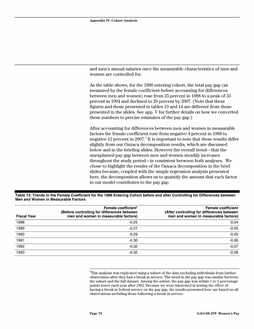
Appendix IV: Cohort Analysis
and men’s annual salaries once the measurable characteristics of men and women are controlled for.
As the table shows, for the 1988 entering cohort, the total pay gap (as measured by the female coefficient before accounting for differences between men and women) rose from 25 percent in 1988 to a peak of 33 percent in 1994 and declined to 28 percent by 2007. (Note that these figures and those presented in tables 13 and 14 are different from those presented in the slides. See app. V for further details on how we converted these numbers to precise estimates of the pay gap.)
After accounting for differences between men and women in measurable factors the female coefficient rose from negative 4 percent in 1988 to negative 12 percent in 2007.6 It is important to note that these results differ slightly from our Oaxaca decomposition results, which are discussed below and in the briefing slides. However the overall trend—that the unexplained pay gap between men and women steadily increases throughout the study period—is consistent between both analyses. We chose to highlight the results of the Oaxaca decomposition in the brief slides because, coupled with the simple regression analysis presented here, the decomposition allows us to quantify the amount that each factor in our model contributes to the pay gap.
Table 13: Trends in the Female Coefficient for the 1988 Entering Cohort before and after Controlling for Differences between Men and Women in Measurable Factors
Fiscal Year
Female coefficienta
(Before controlling for differences between men and women in measurable factors)
Female coefficient (After controlling for differences between
men and women in measurable factors)
1988 -0.25 -0.04
1989 -0.27 -0.05
1990 -0.29 -0.05
1991 -0.30 -0.06
1992 -0.32 -0.07
1993 -0.32 -0.08
6This analysis was replicated using a subset of the data excluding individuals from further observation after they had a break in service. The trend in the pay gap was similar between the subset and the full dataset. Among the subset, the pay gap was within 1 to 2 percentage points lower each year after 1992. Because we were interested in testing the effect of having a break in federal service on the pay gap, the results presented here are based on all observations including those following a break in service.
Page 75 GAO-09-279 Women’s Pay

Appendix IV: Cohort Analysis
Fiscal Year
Female coefficienta
(Before controlling for differences between men and women in measurable factors)
Female coefficient (After controlling for differences between
men and women in measurable factors)
1994 -0.33 -0.08
1995 -0.32 -0.09
1996 -0.32 -0.09
1997 -0.32 -0.09
1998 -0.31 -0.09
1999 -0.31 -0.10
2000 -0.31 -0.11
2001 -0.31 -0.11
2002 -0.30 -0.11
2003 -0.30 -0.12
2004 -0.29 -0.12
2005 -0.29 -0.12
2006 -0.28 -0.11
2007 -0.28 -0.12
Source: GAO analysis of CPDF data.
aAll the figures presented in this table are statistically significant at the 0.01 alpha-level.
To determine the extent to which specific factors account for differences between the salaries of men and women in the federal workforce, table 14 shows the results of the decomposition analysis for individuals in the 1988 entering cohort.7 Similar to the regression results above, the standard interpretation of this analysis is that it represents a decomposition of the percent change in earnings between men and women. However, at larger values, this value will differ somewhat from the precise percent difference. Consequently, for discussion purposes in the briefing slides, we scaled the decomposition to be proportional to the actual percent difference. See appendix V for further details.
Notably, the data show that:
• The unexplained percentage—i.e., that which could not be explained by differences between men and women in measurable factors—rose from 3 percentage points in 1988 to 11 percentage points in 2007.
7These data are presented in graphic format on slide 30.
Page 76 GAO-09-279 Women’s Pay

Appendix IV: Cohort Analysis
• Differences between men’s and women’s occupations accounted for most of the pay gap. The effect of occupation differences declined over this period as the distribution of men and women within occupational categories became more similar.
• After occupation, differences in education contributed to almost as much of the gap as all other remaining factors.
• The use of unpaid leave and breaks in service, which is included under “all other characteristics” in table 14, in fact contributed a very small amount to the pay gap among men and women in this cohort of federal workers.
Table 14: Results of the Decomposition: Amount of Gender Pay Gap Resulting from Differences between Men’s and Women’s Characteristics from 1988 to 2007
Total pay gap Unexplained pay gap Occupation Education All other
characteristics
1988 -0.25 -0.03 -0.18 -0.02 -0.02
1989 -0.27 -0.03 -0.20 -0.02 -0.02
1990 -0.29 -0.02 -0.22 -0.02 -0.03
1991 -0.31 -0.03 -0.22 -0.02 -0.03
1992 -0.32 -0.04 -0.23 -0.03 -0.03
1993 -0.32 -0.04 -0.23 -0.03 -0.03
1994 -0.33 -0.04 -0.23 -0.03 -0.03
1995 -0.33 -0.06 -0.22 -0.03 -0.03
1996 -0.32 -0.06 -0.21 -0.03 -0.02
1997 -0.32 -0.06 -0.21 -0.03 -0.02
1998 -0.31 -0.07 -0.20 -0.03 -0.03
1999 -0.31 -0.08 -0.19 -0.03 -0.03
2000 -0.31 -0.09 -0.18 -0.02 -0.03
2001 -0.31 -0.09 -0.17 -0.02 -0.03
2002 -0.30 -0.09 -0.16 -0.02 -0.03
2003 -0.30 -0.10 -0.15 -0.03 -0.03
2004 -0.29 -0.10 -0.14 -0.02 -0.03
2005 -0.29 -0.10 -0.13 -0.02 -0.03
2006 -0.28 -0.10 -0.13 -0.02 -0.03
2007 -0.28 -0.11 -0.12 -0.02 -0.03
Source: GAO analysis of CPDF data.
Page 77 GAO-09-279 Women’s Pay
Appendix IV: Cohort Analysis
One reason why unpaid leave may not have impacted the overall pay gap is that the differences between men’s and women’s propensity to use unpaid leave and the cost of unpaid leave for men and women may have cancelled each other out. As shown in slide 32, 18 percent of women took unpaid leave at least once between 1988 and 2007 while only 11 percent of men took unpaid leave over this period, a difference that one would expect to contribute to the pay gap. However, the cost of taking unpaid leave was higher for men than women as shown in figure 2. The y-axis of figure 2 represents the cost of taking unpaid leave (i.e., the difference between the average salaries of those who took leave versus those who did not, after controlling for other factors). Figure 2 shows that, in the first year of federal service, the salaries of men who took unpaid leave were about 9 percent lower than the salaries of men who did not take unpaid leave that year.8 In contrast, in the first year of federal service, the salaries for women who took unpaid leave were about 4 percent lower than those of women who did not take unpaid leave that year. We also were not able to identify the reason for using unpaid leave in most cases.9 Because using unpaid leave had a larger negative effect on men’s pay than women’s pay, it likely cancelled out the effect of men’s lower propensity to take it.
Exploring the Use and Cost of Unpaid Leave for Men and Women
8The cost of unpaid leave is represented by the coefficient for ever using unpaid leave on pay after controlling for all other factors in the model. The coefficient in 1988 cannot fully be attributed to the effect of unpaid leave on pay because pay for that year might have been determined before the leave was taken.
9The CPDF data contain information on the legal authorities for LWOP personnel actions. For more than 80 percent of the LWOP actions among the cohort, the legal authority did not provide any information on the reason for the LWOP or indication of how the employee would be using the time on unpaid leave.
Page 78 GAO-09-279 Women’s Pay

Appendix IV: Cohort Analysis
Figure 2: Cost of Taking Unpaid Leave on Pay for Men and Women
0
2
4
6
8
10
12
14
16
20072006200520042003200220012000199919981997199619951994199319921991199019891988
Cents
Source: GAO analysis of CPDF data.
Fiscal yearMen
Women
Similarly, we also explored the effect of having a break in federal service on pay for men and women. With the exception of the first year, the effect of a month of break in service on pay is similar for men and women. Furthermore, similar percentages of men and women had breaks in service. As a result, less than one percent of the pay gap can be attributed to differences between men and women in their propensity to take breaks in service. While women’s breaks were longer than men’s breaks on average as shown in table 15, this did not have an effect on the pay gap between them.
Table 15: Summary of Breaks in Services Use among Cohort, Fiscal Years 1988 and 2007
Number of people who had a
break in serviceAverage cumulative duration
of break in months
1988 330
Male 111 2.02
Female 219 2.21
2007 427
Male 146 86.4
Female 281 97.8
Source: GAO analysis of CPDF data.
Page 79 GAO-09-279 Women’s Pay

Appendix IV: Cohort Analysis
Our findings on the effect of leave patterns on the pay gap differ from those of the 2003 GAO report, which showed work patterns contributing significantly to the differences in men and women’s pay in the general population. This could be due to the fact that our data differed from the 2003 data in three ways. First, our data only follow people through their federal careers and do not account for time they spend in other employment sectors. Second, unlike the 2003 report, we could not differentiate periods of unemployment from time out of the workforce for other reasons. Third, the dependent variable for this analysis is annual salary while the dependent variable for the 2003 report was earnings.
The Effects of Workforce Attrition and Job Switching
As noted earlier, the number of employees in 5 of the 6 occupational categories declined while the administrative category received a net gain of more than 1,000 employees—largely as a result of employees switching their jobs from the technical and clerical categories. Further, we found that, on average, men and women who switched to the administrative category earned a lower salary than those who were originally hired into the category. This may be due in part to differences in education levels between the individuals who switched and the individuals who were originally hired into the category. Among people who switched, men also had more education than women. Specifically, about 50 percent of the men who switched to the administrative category had at least a bachelor’s degree compared with 36 percent of the women.
To determine whether changing jobs or leaving the workforce had an effect on the pay gap, we tested two alternative specifications of our model. We included (1) an indicator for whether a person changed occupational categories in the current fiscal year and (2) an indicator for whether a person left the federal workforce through a separation action in the current fiscal year. The latter indicator is an attempt to measure the effect of the propensity to leave the workforce on the pay gap, i.e., whether those who leave the workforce may have some unobservable characteristic that affects the pay gap. Although we cannot measure the unobservable characteristic, we can control for the fact that the individual is about to leave the workforce, thereby isolating the effect of their imminent departure on the pay gap. We found that the inclusion of each of these two indicator variables explained less than 1 percentage point of the pay gap.10
10Both variables for changing jobs and leaving the workforce were statistically significant predictors of annual salary.
Page 80 GAO-09-279 Women’s Pay

Appendix V: Crosswalk between the Statistics
Presented in the Briefing Slides and Those
Presented in Appendices III and IV
Appendix V: Crosswalk between the Statistics Presented in the Briefing Slides and Those Presented in Appendices III and IV
This appendix presents the conversion of statistical output in appendices III and IV into the estimates of the pay gap that are presented in the briefing slides.
In using regression analysis to understand variation in pay among a group of people, it is common to express the dependent variable (e.g., salary) in log form (i.e., the log of salary). An advantage of expressing a dependent variable like salary in log form is that it allows the coefficients of the explanatory variables to be interpreted in a consistent way regardless of the value of the variable, e.g., as a percent rather than dollar difference. In any regression where the dependent variable is in log form (e.g., the log of salary), economists often interpret the coefficient on a particular explanatory (or independent) variable as the average percent change in the dependent variable that results from a one-unit change in the explanatory variable. As such, in our regression analysis—where log of salary is the dependent variable and gender is an explanatory variable with two possible values (0 for male, 1 for female)—the coefficient on the variable for gender represents the percent difference in salary between men and women.1
However, this interpretation of the coefficient—i.e., as a percent difference when the dependent variable is in log form—loses its precision in certain cases. In cases where the difference in average log salary between two comparison groups (in our case men and women) is small, the size of the coefficient accurately reflects the percent difference in salary. However, as the difference in average log salary becomes larger, the coefficient will increasingly differ from the precise percent difference that would result from a one-unit change in the explanatory variable. When the dependent variable in log form takes on large values, a formula can be used to convert the coefficient of the explanatory variable (β) into a more precise estimate of the percentage difference in the actual salaries caused by a one-unit change in the explanatory variable:
(exp(β)-1)
1If the dependent variable were not expressed in log form, the coefficient on the variable for gender would represent the dollar difference in salary that results when gender is female (1) instead of male (0). The dollar difference is less informative because it does not convey the relative magnitude of the salary difference. For example, it might indicate that there was a $10 difference in salary between two groups, but it would not indicate whether $10 represented a small or large proportion of the salary (1 percent or 10 percent, for example).
Page 81 GAO-09-279 Women’s Pay

Appendix V: Crosswalk between the Statistics
Presented in the Briefing Slides and Those
Presented in Appendices III and IV
where exp is the base of the natural logarithm (commonly known as e) and β is the coefficient of the explanatory variable. (Note: all logarithms in this paper are natural logarithms, i.e., to the base e.)
Table 16 illustrates how the above conversion formula allows us to precisely report the pay gap (salary differences) using two hypothetical examples: one involving small (10 percent) salary differences between two persons; the other large (50 percent). In example 1, where the salary difference is small, the difference in log salary (.10) precisely reflects the actual percent change in actual salary (10 percent)—such that the two can be used interchangeably. In example 2, where the salary difference is large, the difference in log salary (.41) does not precisely reflect the percent change (50 percent). When the conversion formula is applied to both examples, the result precisely reflects the actual change in salary (10 percent=.10 and 50 percent=.50).
Table 16: Example of Precision of Log Difference
Person 1 Person 2Difference in log
salary
Percentage difference in
$ salary Converted difference
Example 1: 10% Difference in salaries
Salary $11,000 $10,000 10%
Log salary 9.31 9.21 0.10 0.10
Example 2: 50% Difference in salaries
Salary $15,000 $10,000 50%
Log salary 9.62 9.21 0.41 0.50
Source: GAO.
Note: Figures presented above may be rounded.
For our cross-sectional analysis, we applied the conversion formula to the coefficient associated with the total pay gap for the 3 years: 1988, 1998, and 2007. Table 17 shows the crosswalk between the results from appendix III to the results in slides 15 and 18 for which we used the conversion formula.
Page 82 GAO-09-279 Women’s Pay

Appendix V: Crosswalk between the Statistics
Presented in the Briefing Slides and Those
Presented in Appendices III and IV
Table 17: Crosswalk between Cross-sectional Estimates of the Total Pay Gap
Log gap (as presented in table 6 of app. III, under
“Total Gap”) Converted log gap (as presented in slides 15 and 18 as the “Pay Gap”)
Fiscal year Converted log gap=exp(Log gap)-1
1988 -0.327 -0.279
1998 -0.211 -0.190
2007 -0.121 -0.114
Source: GAO analysis of CPDF data.
Note: In the briefing slides, we present the pay gap as a positive number. Figures presented above may be rounded.
As with the cross-sectional analysis above, for the cohort analysis, we used the formula to convert the estimates of the total pay gap for each year between 1988 and 2007. The crosswalk between the results in appendix IV and our slides are presented in table 18.
Table 18: Crosswalk between Cohort Estimates of the Total Gap in Appendix IV and the Briefing Slides
Log gap (as presented in table 14 of app. IV)
Converted log gap (as presented in slides 28 and 29)
Fiscal year Converted log gap=exp(Log gap)-1
1988 -0.25 -0.22
1989 -0.27 -0.24
1990 -0.29 -0.25
1991 -0.31 -0.26
1992 -0.32 -0.27
1993 -0.32 -0.28
1994 -0.33 -0.28
1995 -0.33 -0.28
1996 -0.32 -0.28
1997 -0.32 -0.27
1998 -0.31 -0.27
1999 -0.31 -0.27
2000 -0.31 -0.27
2001 -0.31 -0.26
2002 -0.30 -0.26
2003 -0.30 -0.26
Page 83 GAO-09-279 Women’s Pay
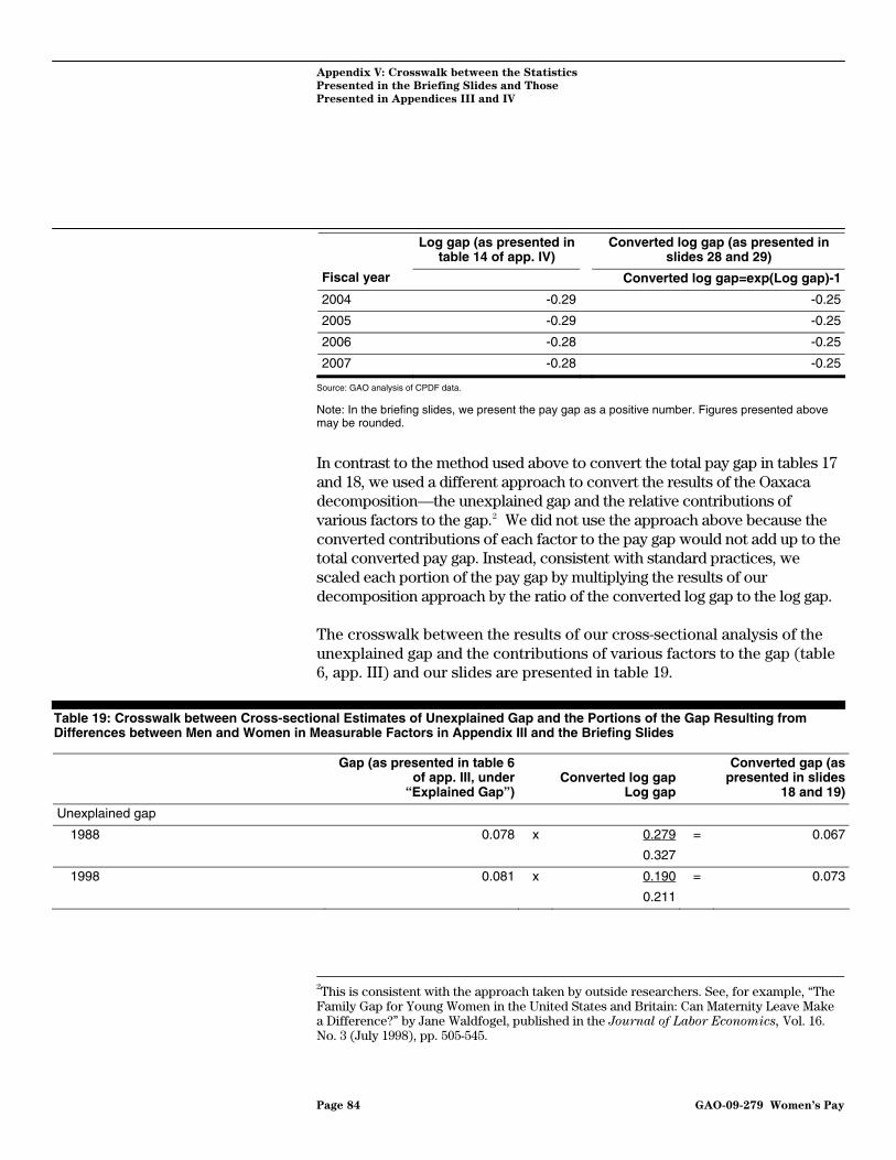
Appendix V: Crosswalk between the Statistics
Presented in the Briefing Slides and Those
Presented in Appendices III and IV
Log gap (as presented in table 14 of app. IV)
Converted log gap (as presented in slides 28 and 29)
Fiscal year Converted log gap=exp(Log gap)-1
2004 -0.29 -0.25
2005 -0.29 -0.25
2006 -0.28 -0.25
2007 -0.28 -0.25
Source: GAO analysis of CPDF data.
Note: In the briefing slides, we present the pay gap as a positive number. Figures presented above may be rounded.
In contrast to the method used above to convert the total pay gap in tables 17 and 18, we used a different approach to convert the results of the Oaxaca decomposition—the unexplained gap and the relative contributions of various factors to the gap.2 We did not use the approach above because the converted contributions of each factor to the pay gap would not add up to the total converted pay gap. Instead, consistent with standard practices, we scaled each portion of the pay gap by multiplying the results of our decomposition approach by the ratio of the converted log gap to the log gap.
The crosswalk between the results of our cross-sectional analysis of the unexplained gap and the contributions of various factors to the gap (table 6, app. III) and our slides are presented in table 19.
Table 19: Crosswalk between Cross-sectional Estimates of Unexplained Gap and the Portions of the Gap Resulting from Differences between Men and Women in Measurable Factors in Appendix III and the Briefing Slides
Gap (as presented in table 6 of app. III, under
“Explained Gap”)Converted log gap
Log gap
Converted gap (as presented in slides
18 and 19)
Unexplained gap
1988 0.078 x 0.279
0.327
= 0.067
1998 0.081 x 0.190
0.211
= 0.073
2This is consistent with the approach taken by outside researchers. See, for example, “The Family Gap for Young Women in the United States and Britain: Can Maternity Leave Make a Difference?” by Jane Waldfogel, published in the Journal of Labor Economics, Vol. 16. No. 3 (July 1998), pp. 505-545.
Page 84 GAO-09-279 Women’s Pay

Appendix V: Crosswalk between the Statistics
Presented in the Briefing Slides and Those
Presented in Appendices III and IV
Gap (as presented in table 6 of app. III, under
“Explained Gap”)Converted log gap
Log gap
Converted gap (as presented in slides
18 and 19)
2007 0.075 x 0.114
0.121
= 0.071
Part of the Gap Resulting from Differences in Occupations
1988 0.145 x 0.279
0.327
= 0.124
1998 0.071 x 0.190
0.211
= 0.064
2007 0.029 x 0.114
0.121
= 0.027
Part of the Gap Resulting from Differences in Education Levels
1988 0.024 x 0.279
0.327
= 0.020
1998 0.023 x 0.190
0.211
= 0.021
2007 0.008 x 0.114
0.121
= 0.008
Part of the Gap Resulting from Differences in Experience Levels
1988 0.054 x 0.279
0.327
= 0.046
1998 0.022 x 0.190
0.211
= 0.020
2007 0.000 x 0.114
0.121
= 0.000
Part of the Gap Resulting from Differences in Other Characteristics
1988 0.026 x 0.279
0.327
= 0.022
1998 0.014 x 0.190
0.211
= 0.013
2007 0.008 x 0.114
0.121
= 0.008
Source: GAO analysis of CPDF data.
Note: Figures presented above may be rounded.
As with the cross-sectional analysis, for the cohort analysis, we computed the unexplained gap and the contributions of each factor to the pay gap by scaling the results of the decomposition approach by the ratio of the
Page 85 GAO-09-279 Women’s Pay

Appendix V: Crosswalk between the Statistics
Presented in the Briefing Slides and Those
Presented in Appendices III and IV
converted log gap to the log gap. The crosswalk between the results of our cohort analysis (table 14 of app. IV) and the slides are presented in table 20.
Table 20: Crosswalk between Cohort Estimates of Explained Gap Resulting from Differences between Men and Women in Measurable Factors in Appendix IV and the Briefing Slides
Portion of gap (as
presented in table 14 of app. IV)
Converted log gap Log gap
(from table 18)
Converted portion of gap
(as presented in slide 30)
Unexplained gap
1988 0.03 x 0.22
0.25
= 0.02
1989 0.03 x 0.24
0.27
= 0.03
1990 0.02 x 0.25
0.29
= 0.02
1991 0.03 x 0.26
0.31
= 0.02
1992 0.04 x 0.27
0.32
= 0.03
1993 0.04 x 0.28
0.32
= 0.04
1994 0.04 x 0.28
0.33
= 0.04
1995 0.06 x 0.28
0.33
= 0.05
1996 0.06 x 0.28
0.32
= 0.05
1997 0.06 x 0.27
0.32
= 0.05
1998 0.07 x 0.27
0.31
= 0.06
1999 0.08 x 0.27
0.31
= 0.07
2000 0.09 x 0.27
0.31
= 0.07
2001 0.09 x 0.26
0.31
= 0.08
Page 86 GAO-09-279 Women’s Pay
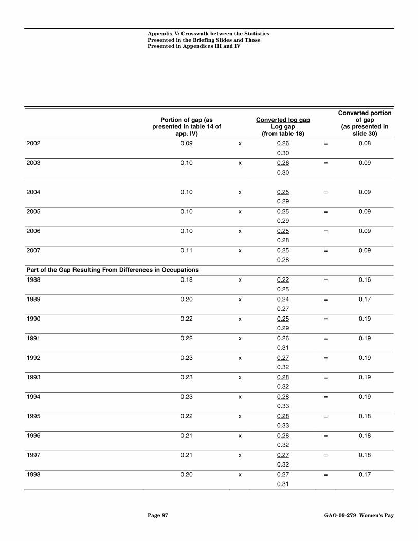
Appendix V: Crosswalk between the Statistics
Presented in the Briefing Slides and Those
Presented in Appendices III and IV
Portion of gap (as
presented in table 14 of app. IV)
Converted log gap Log gap
(from table 18)
Converted portion of gap
(as presented in slide 30)
2002 0.09 x 0.26
0.30
= 0.08
2003 0.10 x 0.26
0.30
= 0.09
2004 0.10 x 0.25
0.29
= 0.09
2005 0.10 x 0.25
0.29
= 0.09
2006 0.10 x 0.25
0.28
= 0.09
2007 0.11 x 0.25
0.28
= 0.09
Part of the Gap Resulting From Differences in Occupations
1988 0.18 x 0.22
0.25
= 0.16
1989 0.20 x 0.24
0.27
= 0.17
1990 0.22 x 0.25
0.29
= 0.19
1991 0.22 x 0.26
0.31
= 0.19
1992 0.23 x 0.27
0.32
= 0.19
1993 0.23 x 0.28
0.32
= 0.19
1994 0.23 x 0.28
0.33
= 0.19
1995 0.22 x 0.28
0.33
= 0.18
1996 0.21 x 0.28
0.32
= 0.18
1997 0.21 x 0.27
0.32
= 0.18
1998 0.20 x 0.27
0.31
= 0.17
Page 87 GAO-09-279 Women’s Pay
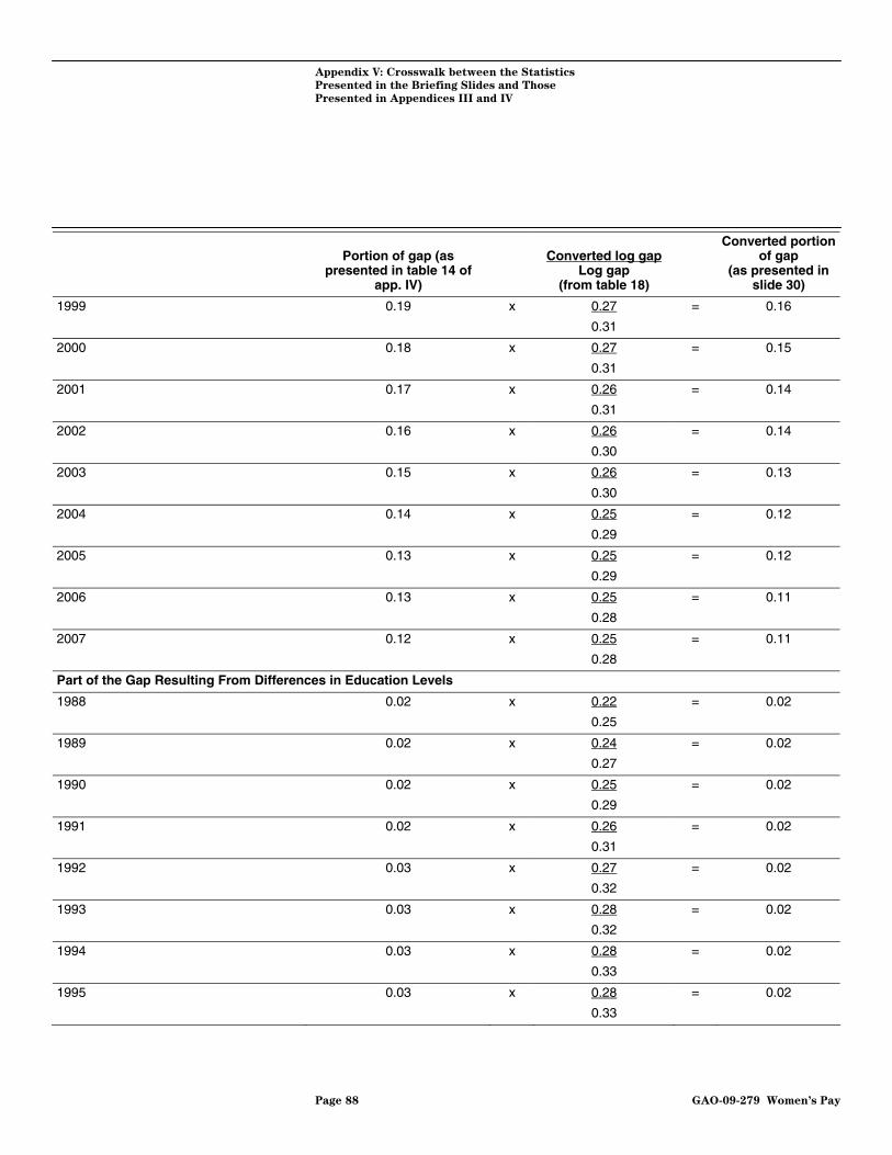
Appendix V: Crosswalk between the Statistics
Presented in the Briefing Slides and Those
Presented in Appendices III and IV
Portion of gap (as
presented in table 14 of app. IV)
Converted log gap Log gap
(from table 18)
Converted portion of gap
(as presented in slide 30)
1999 0.19 x 0.27
0.31
= 0.16
2000 0.18 x 0.27
0.31
= 0.15
2001 0.17 x 0.26
0.31
= 0.14
2002 0.16 x 0.26
0.30
= 0.14
2003 0.15 x 0.26
0.30
= 0.13
2004 0.14 x 0.25
0.29
= 0.12
2005 0.13 x 0.25
0.29
= 0.12
2006 0.13 x 0.25
0.28
= 0.11
2007 0.12 x 0.25
0.28
= 0.11
Part of the Gap Resulting From Differences in Education Levels
1988 0.02 x 0.22
0.25
= 0.02
1989 0.02 x 0.24
0.27
= 0.02
1990 0.02 x 0.25
0.29
= 0.02
1991 0.02 x 0.26
0.31
= 0.02
1992 0.03 x 0.27
0.32
= 0.02
1993 0.03 x 0.28
0.32
= 0.02
1994 0.03 x 0.28
0.33
= 0.02
1995 0.03 x 0.28
0.33
= 0.02
Page 88 GAO-09-279 Women’s Pay

Appendix V: Crosswalk between the Statistics
Presented in the Briefing Slides and Those
Presented in Appendices III and IV
Portion of gap (as
presented in table 14 of app. IV)
Converted log gap Log gap
(from table 18)
Converted portion of gap
(as presented in slide 30)
1996 0.03 x 0.28
0.32
= 0.02
1997 0.03 x 0.27
0.32
= 0.02
1998 0.03 x 0.27
0.31
= 0.02
1999 0.03 x 0.27
0.31
= 0.02
2000 0.02 x 0.27
0.31
= 0.02
2001 0.02 x 0.26
0.31
= 0.02
2002 0.02 x 0.26
0.30
= 0.02
2003 0.03 x 0.26
0.30
= 0.02
2004 0.02 x 0.25
0.29
= 0.02
2005 0.02 x 0.25
0.29
= 0.02
2006 0.02 x 0.25
0.28
= 0.02
2007 0.02 x 0.25
0.28
= 0.02
Part of the Gap Resulting From Differences in Other Characteristics
1988 0.02 x 0.22
0.25
= 0.02
1989 0.02 x 0.24
0.27
= 0.02
1990 0.03 x 0.25
0.29
= 0.03
1991 0.03 x 0.26
0.31
= 0.03
1992 0.03 x 0.27
0.32
= 0.03
Page 89 GAO-09-279 Women’s Pay
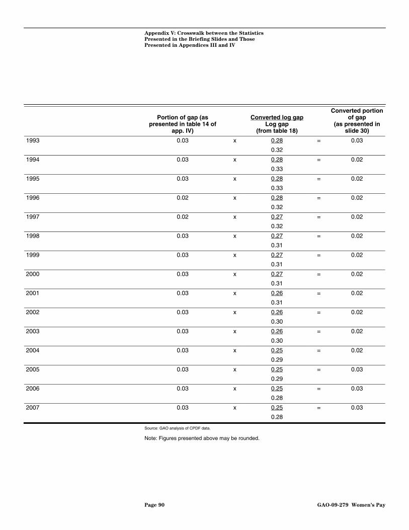
Appendix V: Crosswalk between the Statistics
Presented in the Briefing Slides and Those
Presented in Appendices III and IV
Portion of gap (as
presented in table 14 of app. IV)
Converted log gap Log gap
(from table 18)
Converted portion of gap
(as presented in slide 30)
1993 0.03 x 0.28
0.32
= 0.03
1994 0.03 x 0.28
0.33
= 0.02
1995 0.03 x 0.28
0.33
= 0.02
1996 0.02 x 0.28
0.32
= 0.02
1997 0.02 x 0.27
0.32
= 0.02
1998 0.03 x 0.27
0.31
= 0.02
1999 0.03 x 0.27
0.31
= 0.02
2000 0.03 x 0.27
0.31
= 0.02
2001 0.03 x 0.26
0.31
= 0.02
2002 0.03 x 0.26
0.30
= 0.02
2003 0.03 x 0.26
0.30
= 0.02
2004 0.03 x 0.25
0.29
= 0.02
2005 0.03 x 0.25
0.29
= 0.03
2006 0.03 x 0.25
0.28
= 0.03
2007 0.03 x 0.25
0.28
= 0.03
Source: GAO analysis of CPDF data.
Note: Figures presented above may be rounded.
Page 90 GAO-09-279 Women’s Pay

Appendix VI: Comments from the U.S. Office
of Personnel Management
Appendix VI: Comments from the U.S. Office of Personnel Management
Note: GAO comments supplementing those in the report text appear at the end of this appendix.
See comment 1.
See comment 2.
Page 91 GAO-09-279 Women’s Pay
Appendix VI: Comments from the U.S. Office
of Personnel Management
The following are GAO’s comments to the Office of Personnel Management’s letter dated February 23, 2009.
1. OPM suggested that it may be useful to examine whether certain pay
plans that provide higher pay are populated by a greater percentage of males vs. females. We agree that such an analysis would be useful in understanding gender disparities within the federal government, particularly with regard to promotions of women and men into careers with higher pay structures. However, as we explain in appendix II, an analysis of promotion was beyond the scope of this review. We also considered incorporating the pay plan variable into our statistical model of pay, but ultimately decided that we could control more directly for the underlying sources of variation in pay plans by using variables for occupation, geographic location, and agency.
GAO Comments
2. OPM also expressed the concern that we provided too little information on the role of geographical location in explaining gender pay disparities in the federal government. In our main cross-sectional analysis, we tested two controls for geographical location—state of employment and county of employment—in different models. These controls had only a minimal effect on the pay gap. We have clarified our definition of the county-level control and added a discussion of the state results in appendix III.
Page 92 GAO-09-279 Women’s Pay
Appendix VII: Comments from the U.S.
Equal Employment Opportunity
Commission
Appendix VII: Comments from the U.S. Equal Employment Opportunity Commission
Note: GAO comments supplementing those in the report text appear at the end of this appendix.
See comment 1.
Page 93 GAO-09-279 Women’s Pay

Appendix VII: Comments from the U.S.
Equal Employment Opportunity
Commission
Page 94 GAO-09-279 Women’s Pay

Appendix VII: Comments from the U.S.
Equal Employment Opportunity
Commission
See comment 2.
See comment 3.
See comment 4.
See comment 5.
Page 95 GAO-09-279 Women’s Pay

Appendix VII: Comments from the U.S.
Equal Employment Opportunity
Commission
See comment 6.
See comment 7.
See comment 8.
See comment 9.
See comment 10.
See comment 11.
See comment 12.
Page 96 GAO-09-279 Women’s Pay

Appendix VII: Comments from the U.S.
Equal Employment Opportunity
Commission
The following are GAO’s comments to the Equal Employment Opportunity Commission’s letter dated February 25, 2009.
1. As we stated in our letter, we acknowledge that the difference in wages
between men and women may vary further by race, age, disability status, and other factors that we analyzed. However, to appropriately report on the influence of factors related to other protected groups would require substantial analysis that is beyond the scope of our study’s objective.
GAO Comments
2. We agree that it would be useful to include additional explanation of our regression results pertaining to occupational categories and have done so in appendix III.
3. We agree that graphical depictions of the converging characteristics of men and women are generally useful. In fact, slides 24 and 25 contain figures depicting the education and experience levels of men and women in the federal government over the study period. For occupational categories, however, the trends were mixed depending on the occupation, and therefore we chose to describe these trends with text. As we point out in slides 22 and 23, the professional, administrative, and clerical occupations became more integrated by gender since 1988, and blue and other white-collar occupations remained less integrated. In response to EEOC’s comments, we added information to slide 22 on changes in the proportion of women working in technical and administrative occupations.
4. We agree with EEOC’s interpretation of the coefficients on the female variable in table 13 of appendix IV (the fifth table in app. IV as stated in EEOC’s comments), i.e., that for the 1988 entering cohort, the unexplained pay gap steadily increased over the study period. This finding was consistent for the main regression analysis and the Oaxaca decomposition analysis pertaining to the cohort, as depicted in slide 29. We have clarified this consistency in appendix IV.
5. We agree with EEOC’s interpretation of our graphical depiction of the explained and unexplained pay gap over the study period. However, after experimenting with several graphical depictions of the pay gap, we believe our depictions of the pay gap in slides 18, 19, 29, and 30 appropriately convey both the actual magnitude of the gap and the rising share of the unexplained gap. As to EEOC’s question regarding whether “unexplained differences” included uncontrolled differences such as non-federal work experience, we believe that it may, as we
Page 97 GAO-09-279 Women’s Pay

Appendix VII: Comments from the U.S.
Equal Employment Opportunity
Commission
point out in slide 20 (for the cross-sectional analyses) and 33 (for the cohort analysis).
6. In designing our study, we considered including interaction terms in our models, but ultimately decided to restrict our attention and our presentation of results to “main-effects” models, which omit interactions, for several reasons. In addition to being consistent with the central objective of our study, the main effects models explained a very large portion of the variation in wages without resorting to complex interaction terms. Further, our simpler models have the advantage of providing easily interpretable estimates of the average difference in wages between men and women across all races and occupational categories and agencies, after the separate effects of all of these other characteristics on wages are controlled for.
7. We agree that the growing unexplained gap for the 1988 entering cohort is perplexing. In slide 34, we listed factors that cannot effectively be measured or for which data were not available, that may account for this trend. Further, in appendix II, we discussed our inability to sufficiently control for personal priorities, as measured by number of children and marital status. If men and women differ in their personal priorities and these priorities have a cumulative impact on pay over the course of a career, it is possible that the growing unexplained pay gap that we observe among the cohort is an artifact of our inability to control for these unmeasured factors. However we were unable to test this hypothesis with the CPDF data.
8. Due to significant computational limitations associated with conducting sophisticated econometric analyses with an enormous dataset, we used a 20 percent sample. As a result of EEOC’s comment, we expanded the second footnote in appendix III to include more information on our sampling technique.
9. We agree that for future research examining gender differences in drop-out rates may provide useful insights into the gender pay gap.
10. Regarding EEOC’s suggestion that we test how the exclusion of clerical workers would impact our results, we conducted a Oaxaca decomposition separately for each occupational group. These results are presented in table 8 of appendix III. They reveal a very consistent story for non-clerical occupation groups. Specifically, for each of these groups, the unexplained pay gap fell over the study period to between 7.3 and 10 percentage points (depending on the occupational category) by 2007.
Page 98 GAO-09-279 Women’s Pay

Appendix VII: Comments from the U.S.
Equal Employment Opportunity
Commission
11. With regard to EEOC’s comment about examining other dominant job categories, it is worth noting that, in addition to the PATCOB categories, we tested three different specifications of the occupational variable. Each of these specifications was more disaggregated than PATCOB. The most detailed specification contained over 700 occupational categories. These results are presented in table 4 of appendix III.
12. We agree that future longitudinal research on the gender pay gap could benefit from examining the initial grade or step of individual workers, particularly within job categories and agencies. We did not include grade and step in our cohort analysis due to the variation in the definitions of these categories across job categories and agencies over the study period.
Page 99 GAO-09-279 Women’s Pay
Appendix VIII:
A
GAO Contact and Staff
cknowledgments
Page 100 GAO-09-279 Women’s Pay
Appendix VIII: GAO Contact and Staff Acknowledgments
Andrew Sherrill, Director (202) 512-7215 or [email protected]
Michele Grgich (Assistant Director) and Erin Godtland (Analyst-in-Charge) managed this engagement. In addition, the following people made significant contributions to this work: Daniel R. Concepcion, Anne-Marie Lasowski, Kathleen Van Gelder, and Monique B.Williams, Education, Workforce, and Income Security; and Benjamin Bolitzer, Grant Mallie, Rhiannon Patterson, Douglas Sloane, Shana Wallace, and Gregory H. Wilmoth, Applied Research and Methods. Also contributing to this work were: Jeremy Conley, Christoph Hoashi-Erhardt, Cynthia Fagnoni, and Gene Kuehneman, Education, Workforce, and Income Security; James Rebbe, Office of General Counsel; Ronald Fecso, Chief Statistician; Belva Martin, George Stalcup, and Tamara Stenzel, Strategic Issues; Carolyn Taylor, Office of Opportunity and Inclusion; Cynthia Heckmann, Human Capital Office; and Jennifer Popovic and Wayne Turowski, Applied Research and Methods.
GAO Contact
Staff Acknowledgments

Bibliography
Bibliography
Altonji, Joseph G. and Rebecca M. Blank. “Race and Gender in the Labor Market.” Handbook of Labor Economics, vol. 3 (1999): 3143-3259.
Black, Matthew, Robert Moffitt, John T. Warner. “The Dynamics of Job Separation: The Case of Federal Employees.” Journal of Applied
Econometrics, vol. 5, no. 3, (July – August, 1990): 245-262.
Blau, Francine D., and Lawrence M. Kahn. “Gender Differences in Pay.” The Journal of Economic Perspectives, vol. 14, no. 4, (Autumn 2000): 75-99.
Blau, Francine D., and Lawrence M. Kahn. “The U.S. Gender Pay Gap in the 1990’s: Slowing Convergence.” Industrial and Labor Relations
Review, vol. 60, no. 1 (October 2006): 45-66.
Borjas, George J. “The Measurement of Race and Gender Wage Differentials: Evidence from the Federal Sector.” Industrial and Labor
Relations Review, vol. 37, no. 1, (October 1983): 79-91.
Bridges, William P. “Rethinking Gender Segregation and Gender Inequality: Measures and Meanings.” Demography, vol. 40, no.3, (August 2003): 543-568.
Congressional Budget Office. Characteristics and Pay of Federal Civilian
Employees. Washington, D.C.: March 2007.
GAO. OPM’s Central Personnel Data File: Data Appear Sufficiently
Reliable to Meet Most Customer Needs. GAO/GGD-98-199. Washington, D.C.: September 30, 1998.
GAO. SSA Disability Decision Making: Additional Steps Needed to
Ensure Accuracy and Fairness of Decisions at the Hearings Level. GAO-04-14. Washington, D.C.: November 12, 2003.
GAO. Women’s Earnings: Federal Agencies Should Better Monitor Their
Performance in Enforcing Anti-Discrimination Laws. GAO-08-799. Washington, D.C.: August 11, 2008.
GAO. Women’s Earnings: Work Patterns Partially Explain Difference
between Men’s and Women’s Earnings. GAO-04-35. Washington, D.C.: October 31, 2003.
Page 101 GAO-09-279 Women’s Pay

Bibliography
Goldin, Claudia and Cecilia Rouse. “Orchestrating Impartiality: The Impact of ‘Blind’ Auditions on Female Musicians.” The American Economic Review, vol. 90, no. 4, (September 2000): 715-741.
Lewis, Gregory B. “Gender and Promotions: Promotion Chances of White Men and Women in Federal White-Collar Employment.” The Journal of
Human Resources, vol. 21, no. 3 (Summer 1986): 406-419.
Lewis, Gregory B. “Progress toward Racial and Sexual Equality in the Federal Civil Service?” Public Administration Review, vol. 48, no. 3, (May – June 1988): 700-707.
Lewis, Gregory B. “Gender Integration of Occupations in the Federal Civil Service: Extent and Effects on Male-Female Earnings.” Industrial and
Labor Relations Review, vol. 49, no. 3 (April, 1996): 472-483.
Lewis, Gregory B. “Continuing Progress toward Racial and Gender Pay Equality in the Federal Service: An Update.” Review of Public Personnel
Administration, vol. 18, no. 2 (Spring 1998): 23-40.
Light, Audrey and Manuelita Ureta, “Early-Career Work Experience and Gender Wage Differentials.” Journal of Labor Economics, vol. 13, no. 1. (January 1995): 121-154.
Neumark, David, Roy J. Bank, and Kyle D. Van Nort. “Sex Discrimination in Restaurant Hiring: An Audit Study.” The Quarterly Journal of Economics, vol. 111, no. 3, (August 1996): 915-941
Oaxaca, Ronald. “Male-Female Wage Differentials in Urban Labor Markets.” International Economic Review, vol. 14, no. 3 (October 1973): 693-709.
Olson, Craig A., Donald P. Schwab, and Barbara L. Rau. “The Effects of Local Market Conditions on Two Pay-Setting Systems in the Federal Sector.” Industrial and Labor Relations Review, vol. 53, no.2, (January 2000): 272-289.
O’Neill, June. “The Gender Gap in Wages, Circa 2000.” The American
Economic Review. vol. 93, no.2, Papers and Proceedings of the One Hundred Fifteenth Annual Meeting of the American Economic Association, Washington, D.C.: January 3-5, 2003 (May 2003): 309-314.
Page 102 GAO-09-279 Women’s Pay

Bibliography
Waldfogel, Jane. “The Family Gap for Young Women in the United States and Britain: Can Maternity Leave Make a Difference?” Journal of Labor Economics, vol. 16, no. 3, (July 1998): 505-545.
(130833) Page 103 GAO-09-279 Women’s Pay
GAO’s Mission The Government Accountability Office, the audit, evaluation, and investigative arm of Congress, exists to support Congress in meeting its constitutional responsibilities and to help improve the performance and accountability of the federal government for the American people. GAO examines the use of public funds; evaluates federal programs and policies; and provides analyses, recommendations, and other assistance to help Congress make informed oversight, policy, and funding decisions. GAO’s commitment to good government is reflected in its core values of accountability, integrity, and reliability.
The fastest and easiest way to obtain copies of GAO documents at no cost is through GAO’s Web site (www.gao.gov). Each weekday afternoon, GAO posts on its Web site newly released reports, testimony, and correspondence. To have GAO e-mail you a list of newly posted products, go to www.gao.gov and select “E-mail Updates.”
Obtaining Copies of GAO Reports and Testimony
Order by Phone The price of each GAO publication reflects GAO’s actual cost of production and distribution and depends on the number of pages in the publication and whether the publication is printed in color or black and white. Pricing and ordering information is posted on GAO’s Web site, http://www.gao.gov/ordering.htm.
Place orders by calling (202) 512-6000, toll free (866) 801-7077, or TDD (202) 512-2537.
Orders may be paid for using American Express, Discover Card, MasterCard, Visa, check, or money order. Call for additional information.
Contact:
Web site: www.gao.gov/fraudnet/fraudnet.htm E-mail: [email protected] Automated answering system: (800) 424-5454 or (202) 512-7470
Ralph Dawn, Managing Director, [email protected], (202) 512-4400 U.S. Government Accountability Office, 441 G Street NW, Room 7125 Washington, DC 20548
To Report Fraud, Waste, and Abuse in Federal Programs
Congressional Relations
Chuck Young, Managing Director, [email protected], (202) 512-4800 U.S. Government Accountability Office, 441 G Street NW, Room 7149 Washington, DC 20548
Public Affairs
Please Print on Recycled Paper