Marangoni flows during nonsolvent inducedphase separation

Douglas R. Tree,∗,† Tatsuhiro Iwama,‡ Kris T. Delaney,¶ Joshua Lee,§ andGlenn H. Fredrickson‖

†Chemical Engineering Department, Brigham Young University, Provo, UT 84602‡Asahi Kasei Corporation, 2-1 Samejima, Fuji, Shizuoka 416-8501 Japan

¶Materials Research Laboratory, University of California, Santa Barbara, CA 93106-5121§Chemical Engineering Department, University of California, Santa Barbara, CA

93106-5121‖Chemical Engineering Department, Materials Department and Materials Research

Laboratory, University of California, Santa Barbara, CA 93106-5121

E-mail: tree.doug@byu.edu

Abstract

Motivated by the much discussed, yet unexplained, presence of macrovoids in polymermembranes, we explore the impact of Marangoni flows in the process of nonsolvent inducedphase separation. Such flows have been hypothesized to be important to the formation ofmacrovoids, but little quantitative evidence has been produced to date. Using a recentlydeveloped multi-fluid phase field model, we find that roll cells indicative of a solutal Marangoniinstability are manifest during solvent/nonsolvent exchange across a stable interface. However,these flows are weak and subsequently do not produce morphological features that might leadto macrovoid formation. By contrast, initial conditions that lead to an immediate precipitationof the polymer film coincide with large Marangoni flows that disturb the interface. Thepresence of such flows suggests a new experimental and theoretical direction in the search fora macrovoid formation mechanism.

Non-solvent induced phase separation (NIPS)is a widely used process to create a porous mi-crostructure in a variety of polymer materialsincluding membranes1 and colloidal particles2.As shown in Figure 1, the NIPS process formembranes consists of either immersing or co-flowing a polymer/good solvent mixture along-side a nonsolvent, inducing the phase separa-tion of a polymer-rich phase from a polymer-lean phase. As good solvent and nonsol-vent are continuously exchanged, the polymer-rich phase eventually solidifies freezing the mi-crostructure. The resulting characteristic size,distribution and defectivity of the pore networkare the primary determinant of the commercialuses and value of the material.

One common nuisance in the NIPS process isthe appearance of relatively large “macrovoids”that introduce mechanical defects. Since atleast the early 1970s, researchers have workedto understand how macrovoids form in an at-tempt to find ways to eliminate them3,4. How-ever, because of the complexity of the pro-cess, most of our knowledge of macrovoidformation remains qualitative. Macrovoidsare much larger than the rest of the porenetwork and are roughly periodically spaced.They are observed when demixing occurs veryquickly—often accompanied by hydrodynamicflows—and their formation is sensitive to sol-vent/nonsolvent miscibility1,5,6. Researcherscontinue to debate multiple mechanisms con-

1

nonsolvent bath

substrate

polymer

solution

nonsolvent bath

polymer

solution

spinneretnonsolvent

solvent

Figure 1: A schematic showing a continuousprocess for producing flat membranes (left) orhollow-fiber membranes (right). Membranesconsist of a porous microstructure (inset)that occasionally includes unwanted, finger-likevoids.

sistent with these observations; some have ar-gued that macrovoid formation is primarily aresult of the mass-transfer driven phase sepa-ration process, while others believe mechanicalstresses at the film/bath interface are the pri-mary cause1,5–8.

We argue that a more quantitative approachis necessary to reconcile these disparate mech-anisms. To this end, we recently developeda multi-fluid phase-field model capable of de-scribing the phase-separation and hydrodynam-ics of an incompressible ternary polymer solu-tion with nearly arbitrary viscosity contrast9.The model is given by a set of coupled diffu-sion, momentum and continuity equations,

∂φi

∂t+ v · ∇φi = ∇ ·

[p,n∑j

Mij∇µj

](1)

0 = −∇p+∇ ·[η(∇v +∇vT )

]−∇ ·Π (2)

∇ · v = 0 (3)

where φp and φn are, respectively, the vol-ume fractions of the polymer and nonsolventcomponents, v is the velocity and p is thepressure. Additionally, the diffusive flux inEq. 1 contains chemical potential terms, µi, andconcentration-dependent mobility coefficients,Mij.

The chemical potential is derived from a freeenergy functional consisting of a local Flory-

Huggins expression and square gradient termswith parameters describing species molecularweight, Ni, enthalpic interactions between com-ponents, χij, and square-gradient coefficients,κi. For this work, we make the simplifyingassumptions that Np = N , Nn = Ns = 1,χpn = χ, χps = χns = 0 and κp = κn = κ. Themomentum equation, Eq. 2, contains a solutionviscosity, η, which can depend on local concen-tration, and an osmotic stress tensor, Π, thatis directly related to chemical potential gradi-ents. We solve the model numerically using acustom CUDA/C++ program on a GPU witha semi-implicit, pseudo-spectral method. Manymore details of the model and methods can befound in the Supporting Information and in ourprevious work9.

Equations 1–3 represent a non-trivial descrip-tion of phase separation, diffusion and con-vection in a ternary polymer solution. How-ever, our current model does not include elas-tic forces, and therefore cannot be used to in-vestigate macrovoid formation via mechanicalrupture10. Despite this deficiency, our modeldoes allow us to quantitatively evaluate poten-tial mechanisms for macrovoid formation drivenby thermodynamic and transport processes. Itshould also be noted that there are alternativemethods capable of simulating the hydrody-namics of phase-separating polymeric fluids in-cluding Lattice Boltzmann11,12, dissipative par-ticle dynamics13, kinetic Monte Carlo14 andmulti-particle collision dynamics15.

In this Letter we investigate the possibilitythat Marangoni flows, i.e. flows driven by aconcentration-dependent surface tension gradi-ent, play a key role in initiating macrovoid for-mation during the NIPS process. Matz, From-mer and Messalem (MFM) originally proposedthat a Marangoni instability was responsiblefor macrovoid formation in the early 1970s3,4,but like most theories, it remains controver-sial1,5,6,16. Indeed, to our knowledge, it hasnever been conclusively shown that a soluto-capillary hydrodynamic instability exists in theNIPS process, nor have details of this instabil-ity been quantified sufficiently to connect themto macrovoid formation.

The requirements for a solutal Marangoni in-

2

0 128 256x/R0

512

640

768

896

1024y/R

0

(a) nonsolvent

0.0

0.2

0.4

0.6

0.8

1.0

(b) velocity

0.0 0.5 1.0 ×10−4

φn

−0.0005

0.0000

0.0005

φn − 〈φn〉x

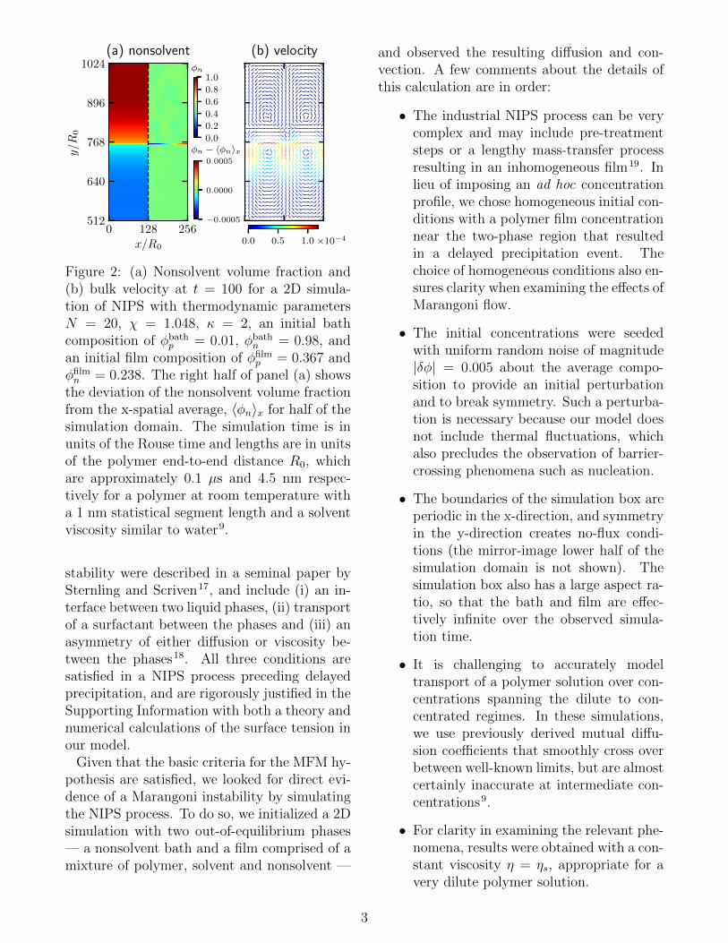
Figure 2: (a) Nonsolvent volume fraction and(b) bulk velocity at t = 100 for a 2D simula-tion of NIPS with thermodynamic parametersN = 20, χ = 1.048, κ = 2, an initial bathcomposition of φbath

p = 0.01, φbathn = 0.98, and

an initial film composition of φfilmp = 0.367 and

φfilmn = 0.238. The right half of panel (a) shows

the deviation of the nonsolvent volume fractionfrom the x-spatial average, 〈φn〉x for half of thesimulation domain. The simulation time is inunits of the Rouse time and lengths are in unitsof the polymer end-to-end distance R0, whichare approximately 0.1 µs and 4.5 nm respec-tively for a polymer at room temperature witha 1 nm statistical segment length and a solventviscosity similar to water9.

stability were described in a seminal paper bySternling and Scriven17, and include (i) an in-terface between two liquid phases, (ii) transportof a surfactant between the phases and (iii) anasymmetry of either diffusion or viscosity be-tween the phases18. All three conditions aresatisfied in a NIPS process preceding delayedprecipitation, and are rigorously justified in theSupporting Information with both a theory andnumerical calculations of the surface tension inour model.

Given that the basic criteria for the MFM hy-pothesis are satisfied, we looked for direct evi-dence of a Marangoni instability by simulatingthe NIPS process. To do so, we initialized a 2Dsimulation with two out-of-equilibrium phases— a nonsolvent bath and a film comprised of amixture of polymer, solvent and nonsolvent —

and observed the resulting diffusion and con-vection. A few comments about the details ofthis calculation are in order:

• The industrial NIPS process can be verycomplex and may include pre-treatmentsteps or a lengthy mass-transfer processresulting in an inhomogeneous film19. Inlieu of imposing an ad hoc concentrationprofile, we chose homogeneous initial con-ditions with a polymer film concentrationnear the two-phase region that resultedin a delayed precipitation event. Thechoice of homogeneous conditions also en-sures clarity when examining the effects ofMarangoni flow.

• The initial concentrations were seededwith uniform random noise of magnitude|δφ| = 0.005 about the average compo-sition to provide an initial perturbationand to break symmetry. Such a perturba-tion is necessary because our model doesnot include thermal fluctuations, whichalso precludes the observation of barrier-crossing phenomena such as nucleation.

• The boundaries of the simulation box areperiodic in the x-direction, and symmetryin the y-direction creates no-flux condi-tions (the mirror-image lower half of thesimulation domain is not shown). Thesimulation box also has a large aspect ra-tio, so that the bath and film are effec-tively infinite over the observed simula-tion time.

• It is challenging to accurately modeltransport of a polymer solution over con-centrations spanning the dilute to con-centrated regimes. In these simulations,we use previously derived mutual diffu-sion coefficients that smoothly cross overbetween well-known limits, but are almostcertainly inaccurate at intermediate con-centrations9.

• For clarity in examining the relevant phe-nomena, results were obtained with a con-stant viscosity η = ηs, appropriate for avery dilute polymer solution.

3

Figure 2 shows the results of a characteristicsimulation soon after the initiation of diffusiveexchange. The left half of Figure 2(a) showsa non-solvent concentration profile exhibitingthe beginning of solvent/nonsolvent diffusionacross an interface separating the two phases.The right half of Figure 2(a) shows the de-viation of the non-solvent concentration fromthe horizontally-averaged (x-direction) value,revealing the existence of nonsolvent-rich andnonsolvent-lean regions along the interface.The bulk velocity field in Figure 2(b) shows rollcells consistent with those of a Marangoni insta-bility (though perhaps limited by finite size ef-fects), with a flow field that corresponds to theconcentration inhomogeneities (and by implica-tion surface tension inhomogeneities) shown inpanel (a).

Despite the existence of roll cells, we findlittle evidence that a classical Marangoni in-stability leads to macrovoid formation. Fora Marangoni instability to induce macrovoids,the roll cells must be of sufficient magnitudeand duration to influence the delayed precip-itation event that the polymer film undergoesas solvent/nonsolvent exchange proceeds. How-ever, as exhibited in Figure 2, the magnitudeof the concentration inhomogeneities (|∆φ| ≈5 × 10−4) and velocity of the roll cells (|v| ≈10−4R0/τ) are small. Furthermore, we observethat the magnitude of these perturbations de-creases with time as the solvent/nonsolvent fluxdecreases. By t = 1000 (data not shown)the magnitude of the concentration inhomo-geneities have decreased nearly two orders ofmagnitude (|∆φ| ≈ 3 × 10−6) and the roll cellvelocities have shown a similar decline (|v| ≈6× 10−7R0/τ). Additional results given in theSupporting Information show that increasingthe viscosity of the polymer film further de-creases the magnitude of these flows. Thus,for a delayed precipitation event the Marangoniflows are inconsequential by the time the poly-mer film phase separates, and the resulting mi-crostructure is unaffected by their presence.

Although our simulations do not support thehypothesis that a classical Marangoni instabil-ity drives the formation of macrovoids, we dofind conditions where solutocapillary flows sig-

φp φn

φs binodal

spinodal

critical pt.

Figure 3: Initial volume fraction profiles andphase diagram for N = 20, χ = 1.048 andκ = 2. A colored dot signifies the initialcomposition of the polymer film in four differ-ent simulations, {φ(film)

p , φ(film)n }: {0.265, 0.450}

(purple), {0.214, 0.477} (green), {0.163, 0.512}(blue), {0.112, 0.559} (red). The correspond-ing colored curves give composition profiles ofthe four simulations (film, interface and bath)shortly after initiation (t = 0.1). The graycurve shows the initial composition profile ofdata in Figure 2.

nificantly perturb the surface of the polymerfilm. Using the same model as above (includ-ing constant viscosity), we vary the initial poly-mer film composition so that the delay time be-fore film precipitation is eliminated. Figure 3shows the ternary phase diagram for the rele-vant parameters, and the initial conditions offour new simulations alongside the initial con-dition of the simulation in Figure 2. The initialconcentration of the polymer film in the newsimulations are very close to (but just outsideof) the binodal line, ensuring that the polymerfilm begins to immediately demix when solventand nonsolvent are exchanged. Note also thatthe initial compositions span the polymer-richand polymer-lean sides of the critical point andinclude a nearly critical film.

Figures 4(a)-(d) shows the polymer volumefraction of the demixing film in the four newsimulations as a function of time. Panel

4

polymer velocity

0 128 256

x/R0

512

640

768

896

y/R

0

0.00.20.40.60.81.0

0.00.20.40.60.81.0

polymer

velocity

t=

100

t=

200

t=

300

(a) (b) (c) (d)

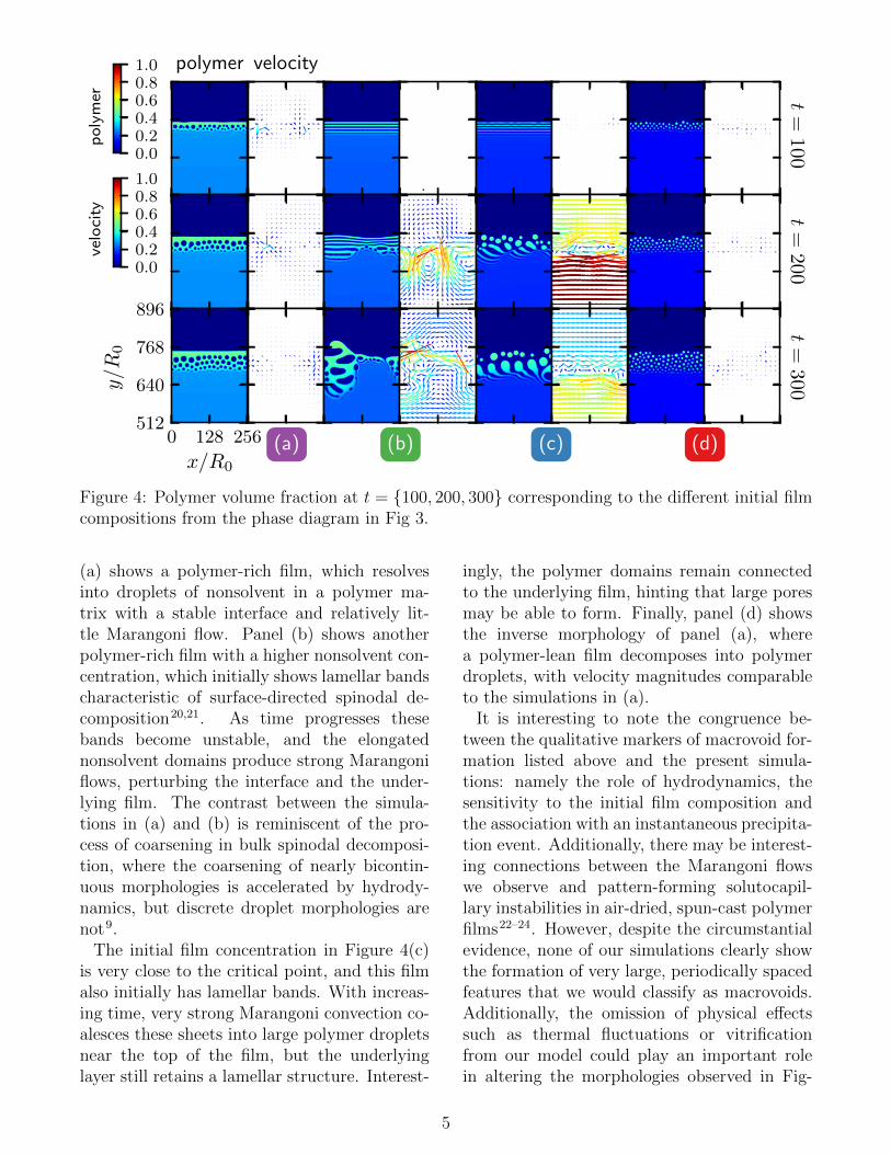
Figure 4: Polymer volume fraction at t = {100, 200, 300} corresponding to the different initial filmcompositions from the phase diagram in Fig 3.

(a) shows a polymer-rich film, which resolvesinto droplets of nonsolvent in a polymer ma-trix with a stable interface and relatively lit-tle Marangoni flow. Panel (b) shows anotherpolymer-rich film with a higher nonsolvent con-centration, which initially shows lamellar bandscharacteristic of surface-directed spinodal de-composition20,21. As time progresses thesebands become unstable, and the elongatednonsolvent domains produce strong Marangoniflows, perturbing the interface and the under-lying film. The contrast between the simula-tions in (a) and (b) is reminiscent of the pro-cess of coarsening in bulk spinodal decomposi-tion, where the coarsening of nearly bicontin-uous morphologies is accelerated by hydrody-namics, but discrete droplet morphologies arenot9.

The initial film concentration in Figure 4(c)is very close to the critical point, and this filmalso initially has lamellar bands. With increas-ing time, very strong Marangoni convection co-alesces these sheets into large polymer dropletsnear the top of the film, but the underlyinglayer still retains a lamellar structure. Interest-

ingly, the polymer domains remain connectedto the underlying film, hinting that large poresmay be able to form. Finally, panel (d) showsthe inverse morphology of panel (a), wherea polymer-lean film decomposes into polymerdroplets, with velocity magnitudes comparableto the simulations in (a).

It is interesting to note the congruence be-tween the qualitative markers of macrovoid for-mation listed above and the present simula-tions: namely the role of hydrodynamics, thesensitivity to the initial film composition andthe association with an instantaneous precipita-tion event. Additionally, there may be interest-ing connections between the Marangoni flowswe observe and pattern-forming solutocapil-lary instabilities in air-dried, spun-cast polymerfilms22–24. However, despite the circumstantialevidence, none of our simulations clearly showthe formation of very large, periodically spacedfeatures that we would classify as macrovoids.Additionally, the omission of physical effectssuch as thermal fluctuations or vitrificationfrom our model could play an important rolein altering the morphologies observed in Fig-

5

ure 4. Finally, we note that our results are con-sistent with previous simulation work on bothmultiphase capillary flow with phase-field25 andLattice Boltzmann26 models and with simula-tions of phase-separating films in liquid-liquidsystems27 and liquid-air systems11.

In summary, we have shown that roll cells in-dicative of a classical Marangoni instability oc-cur in a model of the NIPS process, but arelikely too weak to lead to macrovoid formationin a subsequent delayed precipitation process.By contrast, initial bath and film compositionswhich lead to instantaneous precipitation arecoupled to much stronger Marangoni flows thatcan significantly perturb the surface of the film,especially when the composition is nearly criti-cal. This latter process warrants further inves-tigation as a key mechanism for microstructureformation in NIPS membranes. Additionally,we anticipate that simulations in three dimen-sions with more sophisticated viscous and vis-coelastic models and a more thorough investi-gation of the role of the initial conditions in themass transfer process will yield further insight.

Supporting Information Avail-

able

• Detailed description of multi-fluid modeland methods

• Conditions necessary for a Marangoniinstability and justification that NIPSmeets these conditions

• Details of the surface tension calculationsneeded for the prior justification

• A near-critical, pseudo-binary theory ofthe surface tension

• Variable-viscosity calculations showingroll cells

Acknowledgement

We would like to acknowledge financial sup-port from Asahi Kasei Co. and computational

resources from the Center for Scientific Com-puting from the CNSI, MRL: an NSF MRSEC(DMR-1720256) and NSF CNS-0960316. Ad-ditionally we would like to thank Michael Treefor his insights on hydrodynamic stability.

References

(1) Smolders, C. A.; Reuvers, A. J.;Boom, R. M.; Wienk, I. M. Microstruc-tures in phase-inversion membranes. Part1. Formation of macrovoids. J. Membr.Sci. 1992, 73, 259–275.

(2) Watanabe, T.; Lopez, C. G.; Dou-glas, J. F.; Ono, T.; Cabral, J. T. Microflu-idic Approach to the Formation of Inter-nally Porous Polymer Particles by SolventExtraction. Langmuir 2014, 30, 2470–2479.

(3) Matz, R. The structure of cellulose acetatemembranes 1. The development of porousstructures in anisotropic membranes. De-salination 1972, 10, 1–15.

(4) Frommer, M. A.; Messalem, R. M. Mech-anism of Membrane Formation. VI. Con-vective Flows and Large Void Formationduring Membrane Precipitation. Ind. Eng.Chem. Prod. Res. Dev. 1973, 12, 328–333.

(5) Widjojo, N.; Chung, T.-S. Thickness andAir Gap Dependence of Macrovoid Evolu-tion in Phase-Inversion Asymmetric Hol-low Fiber Membranes. Ind. Eng. Chem.Res. 2006, 45, 7618–7626.

(6) Kosma, V. A.; Beltsios, K. G. Macrovoidsin solution-cast membranes: Direct prob-ing of systems exhibiting horizontalmacrovoid growth. J. Membr. Sci. 2012,407–408, 93–107.

(7) Strathmann, H.; Kock, K. The formationmechanism of phase inversion membranes.Desalination 1977, 21, 241–255.

(8) Prakash, S. S.; Francis, L. F.; Scriven, L.Microstructure evolution in dry–wet castpolysulfone membranes by cryo-SEM: A

6

hypothesis on macrovoid formation. J.Membr. Sci. 2008, 313, 135–157.

(9) Tree, D. R.; Delaney, K. T.;Ceniceros, H. D.; Iwama, T.; Fredrick-son, G. H. A multi-fluid model formicrostructure formation in polymermembranes. Soft Matter 2017, 13,3013–3030.

(10) Tanaka, H. Viscoelastic phase separation.J. Phys.-Condens. Mat. 2000, 12, R207.

(11) Martys, N. S.; Douglas, J. F. Criticalproperties and phase separation in latticeBoltzmann fluid mixtures. Phys. Rev. E2001, 63, 031205.

(12) Akthakul, A.; Scott, C. E.; Mayes, A. M.;Wagner, A. J. Lattice Boltzmann simula-tion of asymmetric membrane formationby immersion precipitation. J. Membr.Sci. 2005, 249, 213 – 226.

(13) Wang, X.-L.; Qian, H.-J.; Chen, L.-J.;Lu, Z.-Y.; Li, Z.-S. Dissipative particle dy-namics simulation on the polymer mem-brane formation by immersion precipita-tion. J. Membr. Sci. 2008, 311, 251 – 258.

(14) Termonia, Y. Monte Carlo diffusion modelof polymer coagulation. Phys. Rev. Lett.1994, 72, 3678–3681.

(15) Gompper, G.; Ihle, T.; Kroll, D. M.; Win-kler, R. G. Advanced Computer Simula-tion Approaches for Soft Matter SciencesIII ; Springer Berlin Heidelberg, 2009; pp1–87.

(16) Ray, R. J.; Krantz, W. B.; Sani, R. L. Lin-ear stability theory model for finger forma-tion in asymmetric membranes. J. Membr.Sci. 1985, 23, 155–182.

(17) Sternling, C. V.; Scriven, L. E. Interfa-cial turbulence: Hydrodynamic instabilityand the marangoni effect. AIChE Journal1959, 5, 514–523.

(18) Schwarzenberger, K.; Kllner, T.;Linde, H.; Boeck, T.; Odenbach, S.;

Eckert, K. Pattern formation andmass transfer under stationary solutalMarangoni instability. Adv. Colloid.Interfac. 2014, 206, 344–371.

(19) van de Witte, P.; Dijkstra, P.; van denBerg, J.; Feijen, J. Phase separation pro-cesses in polymer solutions in relation tomembrane formation. J. Membrane Sci.1996, 117, 1–31.

(20) Ball, R. C.; Essery, R. L. H. Spin-odal decomposition and pattern formationnear surfaces. J. Phys.: Condens. Matter1990, 2, 10303–10320.

(21) Jones, R. A. L.; Norton, L. J.;Kramer, E. J.; Bates, F. S.; Wiltzius, P.Surface-directed spinodal decomposition.Phys. Rev. Lett. 1991, 66, 1326–1329.

(22) Fowler, P. D.; Ruscher, C.; McGraw, J. D.;Forrest, J. A.; Dalnoki-Veress, K. Con-trolling Marangoni-induced instabilities inspin-cast polymer films: How to prepareuniform films. Eur. Phys. J. E 2016, 39,90.

(23) Bormashenko, E.; Pogreb, R.;Stanevsky, O.; Bormashenko, Y.;Stein, T.; Gaisin, V.-Z.; Cohen, R.;Gendelman, O. V. Mesoscopic Patterningin Thin Polymer Films Formed underthe Fast Dip-Coating Process. Macromol.Mater. Eng. 2005, 290, 114–121.

(24) de Gennes, P. Instabilities during theevaporation of a film: Non-glassy polymer+ volatile solvent. Eur. Phys. J. E 2001,6, 421–424.

(25) Wang, F.; Mukherjee, R.; Selzer, M.;Nestler, B. Numerical study on solutalMarangoni instability in finite systemswith a miscibility gap. Phys. Fluids 2014,26, 124102.

(26) Stensholt, S.; Øien, A. Lattice Boltzmannsimulations of the motion induced by vari-able surface tension. Advances in Engi-neering Software 2011, 42, 944–953.

7

(27) Zhou, B.; Powell, A. C. Phase field sim-ulations of early stage structure forma-tion during immersion precipitation ofpolymeric membranes in 2D and 3D. J.Membr. Sci. 2006, 268, 150–164.

8

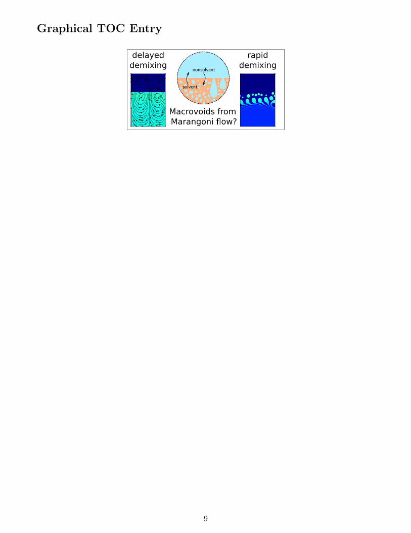
Graphical TOC Entry

nonsolvent

solvent

Macrovoids from

Marangoni �ow?

delayed

demixing

rapid

demixing

9

Supporting information for:

Marangoni flows during nonsolvent induced phase

separation

Douglas R. Tree,∗,† Tatsuhiro Iwama,‡ Kris T. Delaney,¶ Joshua Lee,§ and Glenn Fredrickson‖

†Chemical Engineering Department, Brigham Young University, Provo, UT 84602

‡Asahi Kasei Corporation, 2-1 Samejima, Fuji, Shizuoka 416-8501 Japan

¶Materials Research Laboratory, University of California, Santa Barbara, CA 93106-5121

§Chemical Engineering Department, University of California, Santa Barbara, CA 93106-5121

‖Chemical Engineering Department, Materials Department and Materials Research Laboratory, University

of California, Santa Barbara, CA 93106-5121

E-mail: tree.doug@byu.edu

S1

Description of Multi-fluid Model and Methods

The ternary multi-fluid model was derived using Doi and Onuki’s formalismS1 in a previous publication,S2

and the final transport equations can be summarized as,

∂φi∂t

+ v · ∇φi = ∇ ·

p,n∑j

Mij∇µj

(1)

0 = −∇p+∇ ·[η(∇v +∇vT )

]−∇ ·Π (2)

∇ · v = 0 (3)

where φi are the volume fractions of the polymer (p), nonsolvent (n) and solvent (s), v is the velocity, Mij

are the mobility coefficients, µi is the exchange chemical potential of species i, p is the pressure, η is the

viscosity, and Π is the osmotic stress. Due to incompressibility, the solvent volume fraction, φs, is not an

independent component and is given by,

φs = 1− φp − φn. (4)

The chemical potential, µi, is given by

µi =kBT

b3

(∂f0

∂φi− κi∇2φi

)(5)

where f0 is the homogeneous free energy, b is the monomer size, kB is Boltzmann’s constant, T is the

absolute temperature and κi are gradient coefficients. The homogeneous free energy is given by a ternary

Flory–Huggins model,

f0 =

p,n,s∑i

φiNi

lnφi +

p,n,s∑i 6=j

χijφiφj (6)

where Ni parameterize the molecular weight of the components, and χij quantify the strength of interaction

between species. As mentioned in the main text, in the present study we assume that Np = N , Nn = Ns = 1,

and χpn = χ, χps = χns = 0, giving

f0 =φpN

lnφp + φn lnφn + φs lnφs + χφpφn. (7)

The osmotic stress tensor in Eq. 2 is completely determined by the chemical potential, and its divergence

is given by

∇ ·Π = φn∇µn + φp∇µp. (8)

S2

The mobility coefficients appearing in Eq. 1 are defined as,

Mpp =b3

ζ0φp(1− φp) (9a)

Mpn = Mnp = −b3

ζ0φpφn (9b)

Mnn =b3

ζ0φn(1− φn) (9c)

where ζ0 = ηsb is the monomer friction coefficient. The viscosity in Eq. 2 is assumed to be consistent with

a Rouse model of polymer solutions,

η = ηs(1 + cφpNp) (10)

where c is a constant that is set to unity. Simulations are conducted with a constant viscosity η = ηs unless

otherwise noted.

Space is discretized in equations 1–3 using pseudo-spectral methods and periodic boundary conditions

with ∆x = ∆y = 0.5R0. A symmetric initial condition was used to obtain the effective no-flux boundary

conditions at y = 512 and y = 1024 in Figure 3. The diffusion equation (Eq. 1) was solved using a linearly-

implicit method, which stabilizes the high-order gradients in the model for large time steps. The momentum

and continuity equations (Eq. 2 and Eq. 3) were solved simultaneously using a transverse projection operator,

which is explicit in Fourier space. An iterative method is needed to solve the momentum equation when the

viscosity depends on concentration. A simple fixed-point method combined with a continuation method and

Anderson mixing, gives an efficient solution. All methods were custom-coded using C++ and CUDA for use

on a GPGPU. Many more details regarding the model and method can be found in a prior publication.S2

Conditions for Marangoni Instability

The Marangoni instability at a liquid-liquid interface was described in a seminal paper by Sternling and

ScrivenS3 and exists when (i) a surfactant is diffusing between two liquid phases, and (ii) when the transport

of the surfactant is asymmetric between the phases (e.g. there is a diffusivity or viscosity contrast between

the two phasesS4). When this is so, a perturbation gives rise to local surfactant-rich and surfactant-lean

inhomogeneities, resulting in a surface-tension gradient and subsequent Marangoni stresses along the inter-

face. These stresses lead to the development of convective roll cells, which are a classical manifestation of

the instability.

Without the explicit inclusion of a surfactant, one may dismiss the existence of a Marangoni instability

during NIPS, since surface tension gradients are a necessary condition. However this conclusion would

S3

10−2

10−1

100

101

0 0.1 0.2 0.3 0.4 0.5

γbR

0/k

BT

φs

χ = 1.05, κ = 4χ = 1.20, κ = 4χ = 1.20, κ = 8

(a)

0

0.2

0.4

0.6

0.8

1

512 640 768 896 1024

〈Dnn〉 x/D

0

y/R0

(b)

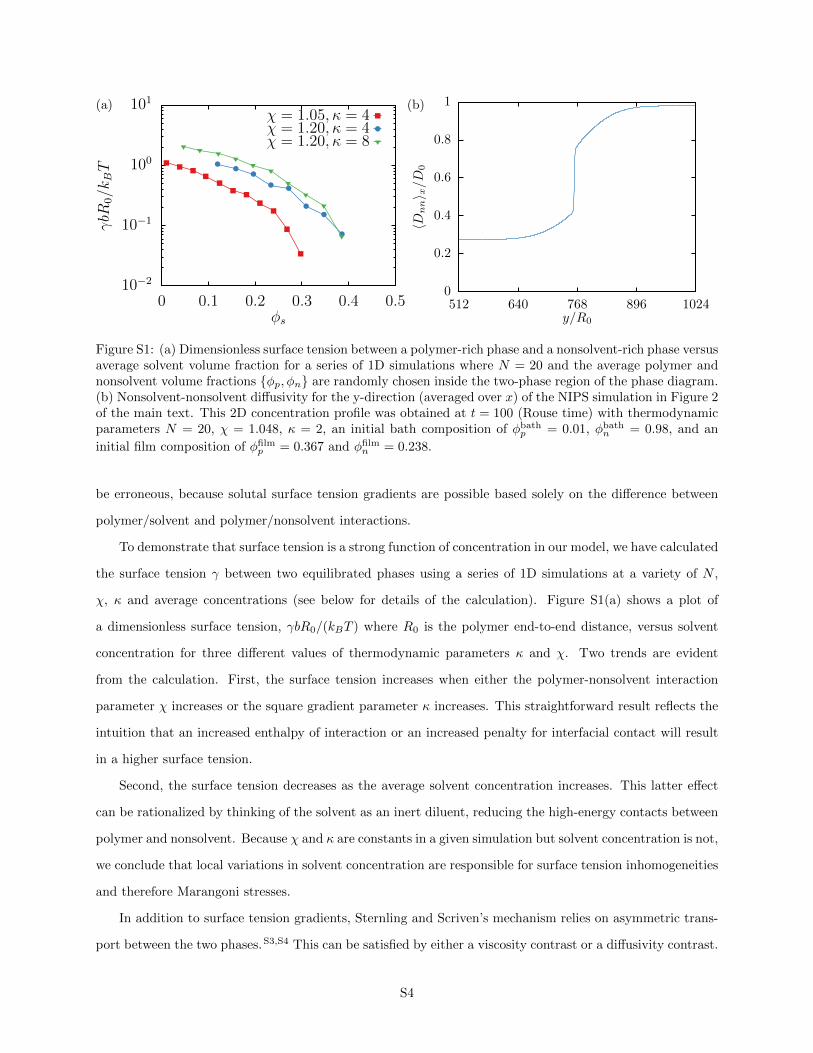
Figure S1: (a) Dimensionless surface tension between a polymer-rich phase and a nonsolvent-rich phase versusaverage solvent volume fraction for a series of 1D simulations where N = 20 and the average polymer andnonsolvent volume fractions {φp, φn} are randomly chosen inside the two-phase region of the phase diagram.(b) Nonsolvent-nonsolvent diffusivity for the y-direction (averaged over x) of the NIPS simulation in Figure 2of the main text. This 2D concentration profile was obtained at t = 100 (Rouse time) with thermodynamicparameters N = 20, χ = 1.048, κ = 2, an initial bath composition of φbath

p = 0.01, φbathn = 0.98, and an

initial film composition of φfilmp = 0.367 and φfilm

n = 0.238.

be erroneous, because solutal surface tension gradients are possible based solely on the difference between

polymer/solvent and polymer/nonsolvent interactions.

To demonstrate that surface tension is a strong function of concentration in our model, we have calculated

the surface tension γ between two equilibrated phases using a series of 1D simulations at a variety of N ,

χ, κ and average concentrations (see below for details of the calculation). Figure S1(a) shows a plot of

a dimensionless surface tension, γbR0/(kBT ) where R0 is the polymer end-to-end distance, versus solvent

concentration for three different values of thermodynamic parameters κ and χ. Two trends are evident

from the calculation. First, the surface tension increases when either the polymer-nonsolvent interaction

parameter χ increases or the square gradient parameter κ increases. This straightforward result reflects the

intuition that an increased enthalpy of interaction or an increased penalty for interfacial contact will result

in a higher surface tension.

Second, the surface tension decreases as the average solvent concentration increases. This latter effect

can be rationalized by thinking of the solvent as an inert diluent, reducing the high-energy contacts between

polymer and nonsolvent. Because χ and κ are constants in a given simulation but solvent concentration is not,

we conclude that local variations in solvent concentration are responsible for surface tension inhomogeneities

and therefore Marangoni stresses.

In addition to surface tension gradients, Sternling and Scriven’s mechanism relies on asymmetric trans-

port between the two phases.S3,S4 This can be satisfied by either a viscosity contrast or a diffusivity contrast.

S4

In our model, diffusivity is a function of concentration, and asymmetric transport is therefore guaranteed

even with constant viscosities. As an example of this, Figure S1(b) shows a plot of the horizontally-averaged

nonsolvent component of the mutual diffusion coefficient as a function of y/R0, the distance normal to the

interface between phases. The diffusivity tracks the local concentration,S2 and is smaller in the film relative

to the bath.

Surface Tension Calculations

The surface tension for the multi-fluid model is defined as,S2,S5,S6

γ =kBT

b3

∫dz

[∆f0 +

1

2

p,n∑i

κi

(dφidz

)2]

(11)

where ∆f0 is the difference between the local Flory–Huggins free energy and the equilibrium value. This

difference is defined as

∆f0 = f0 − f (e)0 − [φp − φ(e)

p ]µ(e)p − [φn − φ(e)

n ]µ(e)n (12)

where the superscript “e” denotes an evaluation of the relevant quantity at the equilibrium volume fraction.

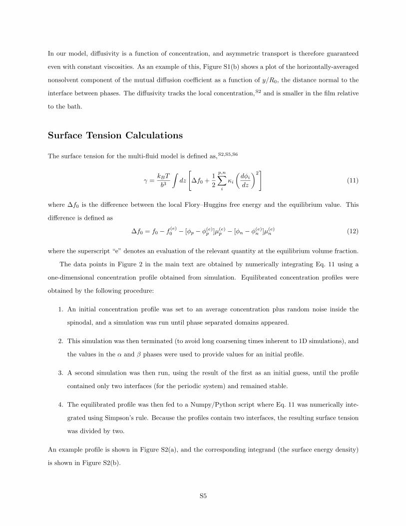
The data points in Figure 2 in the main text are obtained by numerically integrating Eq. 11 using a

one-dimensional concentration profile obtained from simulation. Equilibrated concentration profiles were

obtained by the following procedure:

1. An initial concentration profile was set to an average concentration plus random noise inside the

spinodal, and a simulation was run until phase separated domains appeared.

2. This simulation was then terminated (to avoid long coarsening times inherent to 1D simulations), and

the values in the α and β phases were used to provide values for an initial profile.

3. A second simulation was then run, using the result of the first as an initial guess, until the profile

contained only two interfaces (for the periodic system) and remained stable.

4. The equilibrated profile was then fed to a Numpy/Python script where Eq. 11 was numerically inte-

grated using Simpson’s rule. Because the profiles contain two interfaces, the resulting surface tension

was divided by two.

An example profile is shown in Figure S2(a), and the corresponding integrand (the surface energy density)

is shown in Figure S2(b).

S5

0 64 128 192 256x/R0

0.0

0.2

0.4

0.6

0.8

1.0vo

lume fra

ction

ϕpϕnϕs

(a)

0 64 128 192 256x/R0

0.0

0.1

0.2

0.3

0.4

0.5

surfa

ce ene

rgy de

nsity

(b)

Figure S2: (a) 1D concentration profile for N = 100, χ = 0.968, κ = 30, 〈φp〉 = 0.1498, 〈φn〉 = 0.5627. (b)Surface energy density for the concentration profile.

Table S1: Parameters used to obtain the data in Figure 2 in the main text. χbc = 12

(1√N

+ 1)2

, the critical

point for a binary solution of polymer and non-solvent.

N κ χ/χbc1 1 1.2, 1.4, 1.62 2 1.45 2, 4 1.410 1, 2, 4 1.420 1, 4, 8 1.2, 1.4, 1.650 10, 12, 15, 20, 30 1.4, 1.680 15, 20, 30, 40 1.2, 1.4, 1.6100 20, 30, 40 1.2, 1.4, 1.6

The profile in Figure S2 is just one of many different profiles obtained for different values of N , χ, κ

and average concentrations. A table summarizing all of the parameters used to obtain the data in Figure

2 are found in Table S1. Note that this table also appears in a previous publication,S2 where the same

concentration profiles were used to obtain interfacial widths.

A Near-Critical, Pseudo-Binary Theory of the Surface Tension

We show that the surface tension is a function of solvent concentration, providing evidence that Marangoni

flows are possible. However, we can go further and show how the surface tension depends on all of the model

parameters using a pseudo-binary approximation and scaling theory.

First, it is useful to obtain an approximation to the surface tension for a pseudo-binary solution near

the critical point. To do so, we simplify Equations 7, 11 and 12 assuming that the solvent concentration is

everywhere constant and equal to its average, φs = 〈φs〉. We label this the pseudo-binary assumption.

S6

Using this assumption to simplify Eq. 11 leads to

γ =kBT

b3

∫dz

[∆f0 + κi

(dφ

dz

)2]

(13)

where

∆f0 = f0 − f (e)0 − [φ− φ(e)]µ(e) (14)

and

f0 =φ

Nlnφ+ (1− φ− 〈φs〉) ln(1− φ− 〈φs〉) + 〈φs〉 ln〈φs〉+ χφ(1− φ− 〈φs〉) (15)

with φ = φp.

The logarithms in Eq. 15 make an analytical solution difficult. Furthermore, we showed in a prior work

that a near-critical theory did an excellent job describing the interfacial width.S2 As such, we expand ∆f0

about the critical point,

φc =1− 〈φs〉√N + 1

(16)

χc =1

2(1− 〈φs〉)

(1√N

+ 1

)2

. (17)

to fourth order giving,

∆f0 = λ[(∆φ)2 − (∆φ(e))2

]2(18)

where

∆φ = φ− φc (19)

∆φ(e) = φ(e) − φc (20)

λ =1

12(1− 〈φs〉)(1 +

√N)4

N3/2(21)

and

(∆φ(e))2 =χ− χc

2λ. (22)

Equation 13 has a Lagrangian form,S6 which implies that

(d∆φ

dz

)2

=λ

κ

[(∆φ)2 − (∆φ(e))2

]2(23)

S7

This can be used to solve for the equilibrium profile, which is a familiar hyperbolic tangent,

∆φ = ∆φ(e) tanh (−z/l) (24)

where

l =√

2κ(χ− χc)−1/2 (25)

is the interfacial width.S2

To find the surface tension, we substitute Eq. 23 into Eq. 13,

γ =kBT

b3

∫ −∆φ(e)

∆φ(e)

dφ[2√κ(∆f0)1/2

](26)

=kBT

b32√κγ

∫ −∆φ(e)

∆φ(e)

dφ[(∆φ)2 − (∆φ(e))2

](27)

and integrate. This gives,

γ = 8√

2kBT

b3(1− 〈φs〉)3κ1/2(χ− χc)3/2 N3/2

(1 +N1/2)4(28)

which is the prediction we seek. In the limit that N � 1, Eq. 28 reduces to

γ = 8√

2kBT

b3(1− 〈φs〉)3κ1/2(χ− χc)3/2N−1/2 (29)

which gives a scaling of γ ∼ N−1/2(χ − χc)3/2, which was previously reported by Widom for a mean-field

model near a critical point.S5,S7

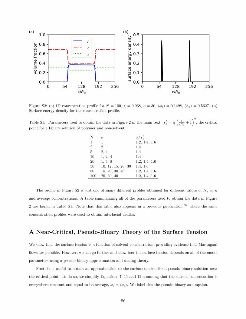
Figure S3 shows that our data is in excellent agreement with the pseudo-binary theory. Panel (a) shows

a representative spinodal, critical line for N = 20 alongside part of the data in Table S1. (The data shown

in Figure S3(a), correspond to those in Figure 2 of the main text.) Panel (b) is a plot of the normalized

surface tension, γ/γref versus the quench depth, χ− χc, where the reference surface tension

γref = 8√

2kBT

b3N3/2κ1/2(1− 〈φs〉)3

(1 +√N)4

(30)

contains all of the terms in Eq. 28, except the dependence on the χ-parameter. For completeness, panel

(c) also shows a plot of the interfacial width versus χ − χc, similar to a plot produced in a previous paper

characterizing our model.S2 The collapse and quantitative agreement of the data Eq. 28 and Eq. 25 strongly

supports the conclusion that the near-critical, pseudo-binary theory provides a satisfactory explanation of

S8

(a)

10−3

10−2

10−1

100

10−2 10−1 100γ/γ

ref

χ− χc

(b)

100

101

102

10−2 10−1 100

l/l 0

χ− χc

(c)

Figure S3: (a) Plot of the spinodal surface and critical line for N = 20. Data points at different averageconcentrations for N = 20 and {χ, κ} = {1.05, 4}[red], {1.20, 4}[green], {1.20, 8}[blue] are shown, providingan example of the scope of the data contained in the other panels. (b) Normalized surface tension versusquench depth for equilibrated 1D simulations with N = 1 (filled red squares), 5 (filled blue circles), 10 (filledgreen triangles), 20 (filled purple diamonds), 50 (open orange squares), 80 (open blue circles) and 100 (openbrown triangles), and a variety of values of κ, χ and average concentrations (see Table S1). The line is(χ− χc)3/2. Note that no fitting parameters have been used. (c) Plot of the interfacial width for the samesimulations as panel (b). The line is (χ− χc)−1/2, and again, no fitting parameters have been used.

the 1D data.

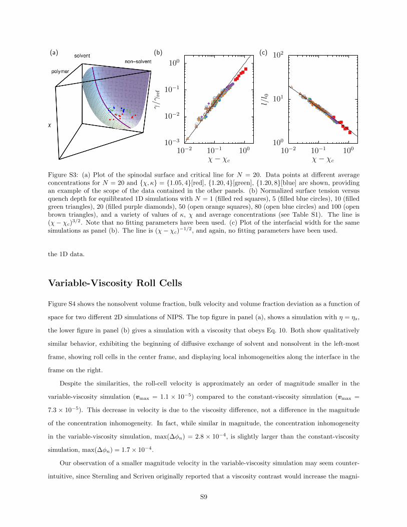
Variable-Viscosity Roll Cells

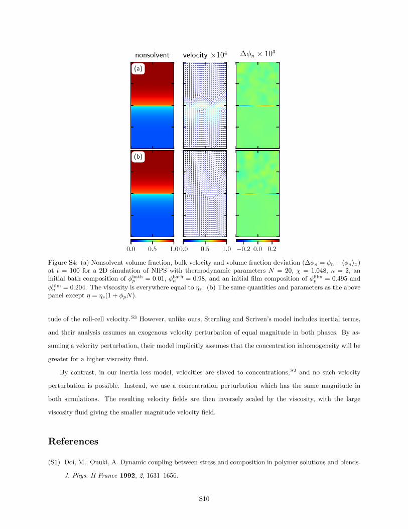
Figure S4 shows the nonsolvent volume fraction, bulk velocity and volume fraction deviation as a function of

space for two different 2D simulations of NIPS. The top figure in panel (a), shows a simulation with η = ηs,

the lower figure in panel (b) gives a simulation with a viscosity that obeys Eq. 10. Both show qualitatively

similar behavior, exhibiting the beginning of diffusive exchange of solvent and nonsolvent in the left-most

frame, showing roll cells in the center frame, and displaying local inhomogeneities along the interface in the

frame on the right.

Despite the similarities, the roll-cell velocity is approximately an order of magnitude smaller in the

variable-viscosity simulation (vmax = 1.1 × 10−5) compared to the constant-viscosity simulation (vmax =

7.3 × 10−5). This decrease in velocity is due to the viscosity difference, not a difference in the magnitude

of the concentration inhomogeneity. In fact, while similar in magnitude, the concentration inhomogeneity

in the variable-viscosity simulation, max(∆φn) = 2.8 × 10−4, is slightly larger than the constant-viscosity

simulation, max(∆φn) = 1.7× 10−4.

Our observation of a smaller magnitude velocity in the variable-viscosity simulation may seem counter-

intuitive, since Sternling and Scriven originally reported that a viscosity contrast would increase the magni-

S9

nonsolvent velocity ×104 ∆φn × 103

(a)

0.0 0.5 1.00.0 0.5 1.0 −0.2 0.0 0.2

(b)

Figure S4: (a) Nonsolvent volume fraction, bulk velocity and volume fraction deviation (∆φn = φn−〈φn〉x)at t = 100 for a 2D simulation of NIPS with thermodynamic parameters N = 20, χ = 1.048, κ = 2, aninitial bath composition of φbath

p = 0.01, φbathn = 0.98, and an initial film composition of φfilm

p = 0.495 and

φfilmn = 0.204. The viscosity is everywhere equal to ηs. (b) The same quantities and parameters as the above

panel except η = ηs(1 + φpN).

tude of the roll-cell velocity.S3 However, unlike ours, Sternling and Scriven’s model includes inertial terms,

and their analysis assumes an exogenous velocity perturbation of equal magnitude in both phases. By as-

suming a velocity perturbation, their model implicitly assumes that the concentration inhomogeneity will be

greater for a higher viscosity fluid.

By contrast, in our inertia-less model, velocities are slaved to concentrations,S2 and no such velocity

perturbation is possible. Instead, we use a concentration perturbation which has the same magnitude in

both simulations. The resulting velocity fields are then inversely scaled by the viscosity, with the large

viscosity fluid giving the smaller magnitude velocity field.

References

(S1) Doi, M.; Onuki, A. Dynamic coupling between stress and composition in polymer solutions and blends.

J. Phys. II France 1992, 2, 1631–1656.

S10

(S2) Tree, D. R.; Delaney, K. T.; Ceniceros, H. D.; Iwama, T.; Fredrickson, G. H. A multi-fluid model for

microstructure formation in polymer membranes. Soft Matter 2017, 13, 3013–3030.

(S3) Sternling, C. V.; Scriven, L. E. Interfacial turbulence: Hydrodynamic instability and the marangoni

effect. AIChE Journal 1959, 5, 514–523.

(S4) Schwarzenberger, K.; Kllner, T.; Linde, H.; Boeck, T.; Odenbach, S.; Eckert, K. Pattern formation

and mass transfer under stationary solutal Marangoni instability. Adv. Colloid. Interfac. 2014, 206,

344–371.

(S5) Cahn, J. W.; Hilliard, J. E. Free Energy of a Nonuniform System. I. Interfacial Free Energy. J. Chem.

Phys. 1958, 28, 258–267.

(S6) Broseta, D.; Fredrickson, G. H.; Helfand, E.; Leibler, L. Molecular weight and polydispersity effects at

polymer-polymer interfaces. Macromolecules 1990, 23, 132–139.

(S7) Widom, B. Scaling of the surface tension of phase-separated polymer solutions. J. Stat. Phys. 1988,

53, 523–529.

S11