mapping tree canopy cover and aboveground biomass in...
TRANSCRIPT
Remote Sens. 2015, 7, 10017-10041; doi:10.3390/rs70810017
remote sensing ISSN 2072-4292
www.mdpi.com/journal/remotesensing
Article
Mapping Tree Canopy Cover and Aboveground Biomass
in Sudano-Sahelian Woodlands Using Landsat 8 and
Random Forest
Martin Karlson 1,*, Madelene Ostwald 1,2, Heather Reese 3, Josias Sanou 4, Boalidioa Tankoano 5
and Eskil Mattsson 6
1 Centre for Climate Science and Policy Research, Department of Thematic Studies/Environmental
Change, Linköping University, Linköping 581 83, Sweden; E-Mail: [email protected] 2 Centre for Environment and Sustainability (GMV), University of Gothenburg and Chalmers
University of Technology, Gothenburg 405 30, Sweden 3 Section of Forest Remote Sensing, Department of Forest Resource Management, Swedish
University of Agricultural Sciences, Umeå 901 83, Sweden; E-Mail: [email protected] 4 Institut de l’Environnement et de Recherches Agricoles (INERA), Département Productions
Forestières, 03 BP 7047 Ouagadougou 03, Burkina Faso; E-Mail: [email protected] 5 Polytechnic University of Bobo-Dioulasso, Development Rural Institute/Department of Forestery,
BP 01 1091 Bobo-Dioulasso, Burkina Faso; E-Mail: [email protected] 6 Division of Physical Resource Theory, Department of Energy and Environment,
Chalmers University of Technology, Gothenburg 412 96, Sweden; E-Mail: [email protected]
* Author to whom correspondence should be addressed; E-Mail: [email protected];
Tel.: +46-13-282-977; Fax: +46-13-133-630.
Academic Editors: Josef Kellndorfer and Prasad S. Thenkabail
Received: 8 June 2015 / Accepted: 29 July 2015 / Published: 6 August 2015
Abstract: Accurate and timely maps of tree cover attributes are important tools for
environmental research and natural resource management. We evaluate the utility of
Landsat 8 for mapping tree canopy cover (TCC) and aboveground biomass (AGB) in a woodland
landscape in Burkina Faso. Field data and WorldView-2 imagery were used to assemble the
reference dataset. Spectral, texture, and phenology predictor variables were extracted from
Landsat 8 imagery and used as input to Random Forest (RF) models. RF models based on
multi-temporal and single date imagery were compared to determine the influence of
phenology predictor variables. The effect of reducing the number of predictor variables on
the RF predictions was also investigated. The model error was assessed using 10-fold cross
OPEN ACCESS
Remote Sens. 2015, 7 10018
validation. The most accurate models were created using multi-temporal imagery and
variable selection, for both TCC (five predictor variables) and AGB (four predictor
variables). The coefficient of determination of predicted versus observed values was 0.77 for
TCC (RMSE = 8.9%) and 0.57 for AGB (RMSE = 17.6 tons∙ha−1). This mapping approach is
based on freely available Landsat 8 data and relatively simple analytical methods, and is
therefore applicable in woodland areas where sufficient reference data are available.
Keywords: Landsat 8; woodland; Sudano-Sahel; tree canopy cover; aboveground biomass;
multi-temporal imagery; Random Forest; variable selection; phenology
1. Introduction
The Sudano-Sahelian woodlands occupy vast areas between the Saharan desert and the moist forests of
the Guinean zone [1,2]. Woodland tree cover is an essential element of the local livelihoods,
in particular through agro-forestry practices [3], fuelwood, and timber extraction, and the provision of
non-wood products (such as food, fodder, and medicine). The wide area extent also makes this landscape
type an important component in the global climate system by sequestering and storing substantial amounts
of carbon in woody biomass and soils [4–6]. At present, these woodlands are subject to increasing pressure
from intensified land use [7] and climate change [8]. Local case studies based on field assessments and
high resolution remote sensing data have shown that these factors have resulted in decreased tree density,
carbon stocks, and floristic diversity [9–11]. Yet other local case studies show that tree cover conditions
have improved substantially since the severe droughts that hit the area in the 1970s and 1980s [12]. Such
improvements are generally attributed to increased rainfall or farmer managed natural regeneration, with
notable cases found in northern Burkina Faso [13] and southern Niger [14,15]. Given these divergent
research findings and the importance of trees for local livelihoods, timely information on the extent and
conditions of woodlands, including agroforestry landscapes, is therefore of great interest to a number of
local actors, such as researchers, natural resource managers and forestry industries [2].
In this paper, we evaluate the potential of Landsat 8 imagery to map two attributes commonly used
to characterize tree cover structure and conditions, namely tree canopy cover (TCC) and aboveground
biomass (AGB). Quantifying TCC and AGB at spatial scales relevant for natural resource monitoring
(e.g., landscape scale) through field surveys is time-demanding and costly. Furthermore, the application
of robust sampling strategies in woodlands is complicated by the heterogeneous landscape composition
and the variable tree cover structure [1]. A large body of research has explored the potential of using
various satellite systems as tools for providing remote sensing based observations of TCC and AGB at
a range of spatial scales [16–19]. Optical satellite data of medium spatial resolution, such as Landsat
imagery, are favorable when the objective is to map and monitor large areas over decadal time scales
while retaining a relatively high degree of spatial detail and minimizing data acquisition costs.
Pixel size is of particular importance when remote sensing data are used in fragmented landscapes
where tree cover may alternate from open to closed canopy within short distances [20]. Several factors
contribute to the reflected radiance recorded by the sensor which poses challenges to the mapping of tree
cover in landscapes with an open canopy, such as the Sudano-Sahelian woodlands [21]. Important factors
Remote Sens. 2015, 7 10019
include the heterogeneous spectral characteristics of soil and bedrock [22], the spectral similarity
between different vegetation types [23,24] and the high seasonal and annual variability in vegetation
development, which is species dependent and related to water availability [25]. Assessments have
repeatedly shown that global tree cover products, such as the Vegetation Continuous Fields [26] derived
from the Moderate Resolution Imaging Spectroradiometer (MODIS), have significant limitations in
characterizing areas with an open tree canopy [21,27–29].
Some environmental characteristics of woodlands may represent opportunities for using optical
satellite data for mapping TCC and AGB. For example, saturation of spectral vegetation indices, such
as the Normalized Difference Vegetation Index (NDVI), is less of a problem when relating spectral data
to TCC and AGB in open tree cover conditions compared to closed forests [16]. The relatively open
canopy of woodlands does not obscure low growing trees to the same extent as in dense forests, where
these can represent 30%–50% of the AGB [30]. Previous research also suggests that the correlation
between tree cover attributes, in particular AGB, and image texture is higher in open as compared to closed
canopies [31–34]. Eckert [33] hypothesized that texture is highly correlated to AGB in open canopy
conditions due to its ability to capture shadow structures caused by large trees, which may contain up to 80%
of the AGB in woodland landscapes [35]. Lastly, trees in the seasonal tropics have contrasting phenological
traits compared to other vegetation that may be identified using multi-temporal satellite data [36,37].
The Operational Land Imager (OLI) onboard Landsat 8 has several improvements over its predecessors
the Thematic Mapper (TM; Landsat 4 and 5) and the Enhanced Thematic Mapper (ETM+; Landsat 7).
The main changes include an increased number of spectral bands, a higher radiometric resolution
(12 bits) and an improved signal-to-noise ratio resulting from the use of a push-broom sensor [38].
These improvements may enable higher accuracy in the mapping of tree cover attributes, including
AGB [39]. The continuity and open data policy of the Landsat program also enables the use of image
time series, which have shown great promise for large area mapping of tree cover attributes in boreal
forests [40,41]. Thus, Landsat 8 represents an interesting data source for remote sensing based tree cover
mapping, but its use has not yet been evaluated in the Sudano-Sahelian woodlands.
The estimation of tree cover attributes from remote sensing data involves modeling the relation
between the response variable Y (e.g., local reference measurements of TCC or AGB) [42] and the
predictor variables Xn (e.g., remotely sensed reflectance). The parametric Ordinary Least Squares (OLS)
regression has been the most common choice for fitting the equation between X and Y [43], which enables
the prediction of the tree cover attribute over the extent of the satellite imagery. An alternative to
statistical regression is provided by non-parametric machine learning techniques, or algorithmic
modeling [44]. During the last decade machine-learning techniques, such as support vector machines [45],
decision trees [46], and Random Forest [47] have been increasingly used for both classification and
relationship modeling with remote sensing data. These techniques tend to outperform the commonly
used statistical regression models (e.g., OLS regression) in terms of prediction accuracy of TCC and
AGB from remote sensing data [19,48,49]
The aim of this study was to assess the utility of Landsat 8 imagery for mapping TCC and AGB in a
Sudano-Sahelian woodland landscape. The Random Forest (RF) algorithm [47] was used for identifying
important predictor variables and for predictive modeling. Our methodology comprised three main steps:
(a) assemblage of a reference dataset from field data and WorldView-2 imagery; (b) identification of
important predictor variables from Landsat 8 data; (c) RF modeling of TCC and AGB as a function of
Remote Sens. 2015, 7 10020
the predictor variables. Three types of predictor variables were assessed for their effectiveness to capture
woodland tree cover characteristics: spectral, texture, and phenology variables. The spectral variables
included top of atmosphere (TOA) reflectance values of the Landsat 8 bands (bands 2 to 8), tasseled cap
components [50–52] and a set of vegetation indices. Texture variables were calculated using the gray
level co-occurrence matrix (GLCM) approach [53]. Phenology variables were derived from a dry season
NDVI time series [28]. The potential benefit of including phenology variables was assessed by
comparing RF models based on multi-temporal and single date imagery, respectively.
2. Materials and Methods
2.1. Study Area
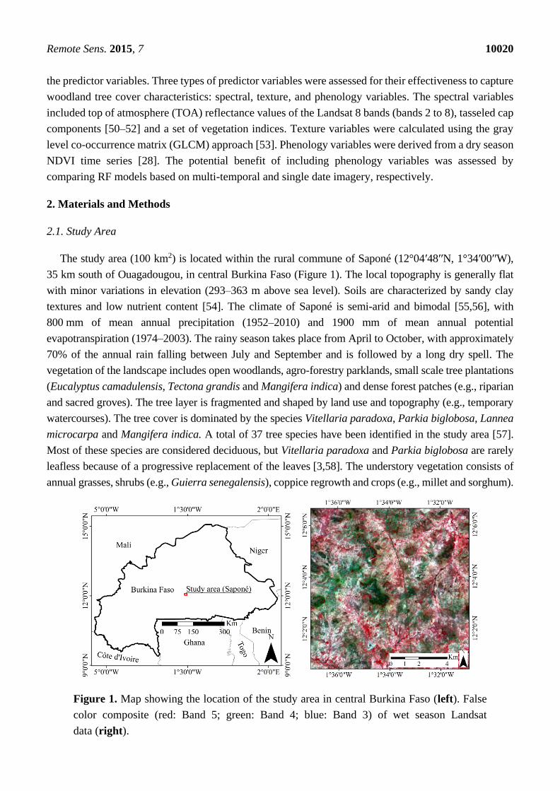
The study area (100 km2) is located within the rural commune of Saponé (12°04′48′′N, 1°34′00′′W),
35 km south of Ouagadougou, in central Burkina Faso (Figure 1). The local topography is generally flat
with minor variations in elevation (293–363 m above sea level). Soils are characterized by sandy clay
textures and low nutrient content [54]. The climate of Saponé is semi-arid and bimodal [55,56], with
800 mm of mean annual precipitation (1952–2010) and 1900 mm of mean annual potential
evapotranspiration (1974–2003). The rainy season takes place from April to October, with approximately
70% of the annual rain falling between July and September and is followed by a long dry spell. The
vegetation of the landscape includes open woodlands, agro-forestry parklands, small scale tree plantations
(Eucalyptus camadulensis, Tectona grandis and Mangifera indica) and dense forest patches (e.g., riparian
and sacred groves). The tree layer is fragmented and shaped by land use and topography (e.g., temporary
watercourses). The tree cover is dominated by the species Vitellaria paradoxa, Parkia biglobosa, Lannea
microcarpa and Mangifera indica. A total of 37 tree species have been identified in the study area [57].
Most of these species are considered deciduous, but Vitellaria paradoxa and Parkia biglobosa are rarely
leafless because of a progressive replacement of the leaves [3,58]. The understory vegetation consists of
annual grasses, shrubs (e.g., Guierra senegalensis), coppice regrowth and crops (e.g., millet and sorghum).
Figure 1. Map showing the location of the study area in central Burkina Faso (left). False
color composite (red: Band 5; green: Band 4; blue: Band 3) of wet season Landsat
data (right).
Remote Sens. 2015, 7 10021
2.2. Reference Data
Two data sources were used to assemble the reference datasets for TCC and AGB, including field
data collected during October and November 2012 and a pan-sharpened WorldView-2 image from
October 2012 [57]. TCC refers to the proportion of land area covered by tree crowns, when viewed from
above, and is a widely used variable in land-cover definitions (e.g., woodlands 10%–30% TCC) [2].
The AGB of woody vegetation (i.e., trees and shrubs) is a measure of dry matter weight per unit area
(e.g., tons∙ha−1) and represents a key indicator for ecosystem structure and functioning [2,59].
The reference datasets were used to calibrate and validate the RF regression models. There is a temporal
difference of two years between the reference dataset and the Landsat imagery. However, the cutting of
trees is prohibited in the area and potential changes in tree cover were assumed to be minor with limited
influence on the predictive modeling.
2.2.1. Field Data
The field data included 75 inventory plots (50 m × 50 m) located within the study area. The allocation
of plots followed a stratified random sampling approach where NDVI [60] from the WorldView-2 image
was used to partition the study area into three classes of vegetation density to ensure that landscape
heterogeneity was reflected in the field dataset (Table 1). Within the 75 plots, 1143 trees with diameter
at breast height (DBH) ≥ 5 cm were measured for height, DBH, crown area and species [57]. The trees
were geo-referenced individually using a global positioning system receiver (GPS; Garmin Oregon 550,
Garmin, Olathe, KS, USA). To account for the positional uncertainties in the GPS recordings, each point
was manually related to the correct tree in the pan-sharpened WorldView-2 image using information on
crown dimension, height, and species as guidance. Karlson et al. [57] provide further details regarding
the collection of field data.
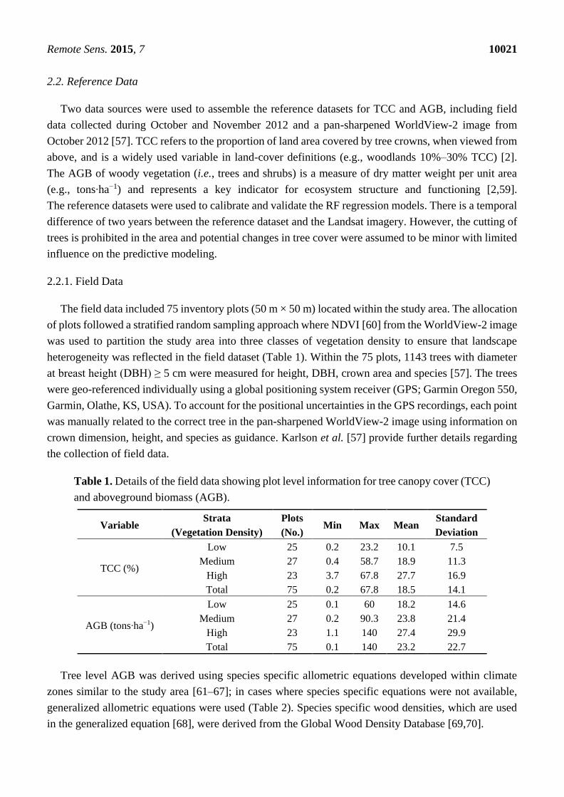
Table 1. Details of the field data showing plot level information for tree canopy cover (TCC)
and aboveground biomass (AGB).
Variable Strata
(Vegetation Density)
Plots
(No.) Min Max Mean
Standard
Deviation
TCC (%)
Low 25 0.2 23.2 10.1 7.5
Medium 27 0.4 58.7 18.9 11.3
High 23 3.7 67.8 27.7 16.9
Total 75 0.2 67.8 18.5 14.1
AGB (tons∙ha−1)
Low 25 0.1 60 18.2 14.6
Medium 27 0.2 90.3 23.8 21.4
High 23 1.1 140 27.4 29.9
Total 75 0.1 140 23.2 22.7
Tree level AGB was derived using species specific allometric equations developed within climate
zones similar to the study area [61–67]; in cases where species specific equations were not available,
generalized allometric equations were used (Table 2). Species specific wood densities, which are used
in the generalized equation [68], were derived from the Global Wood Density Database [69,70].
Remote Sens. 2015, 7 10022
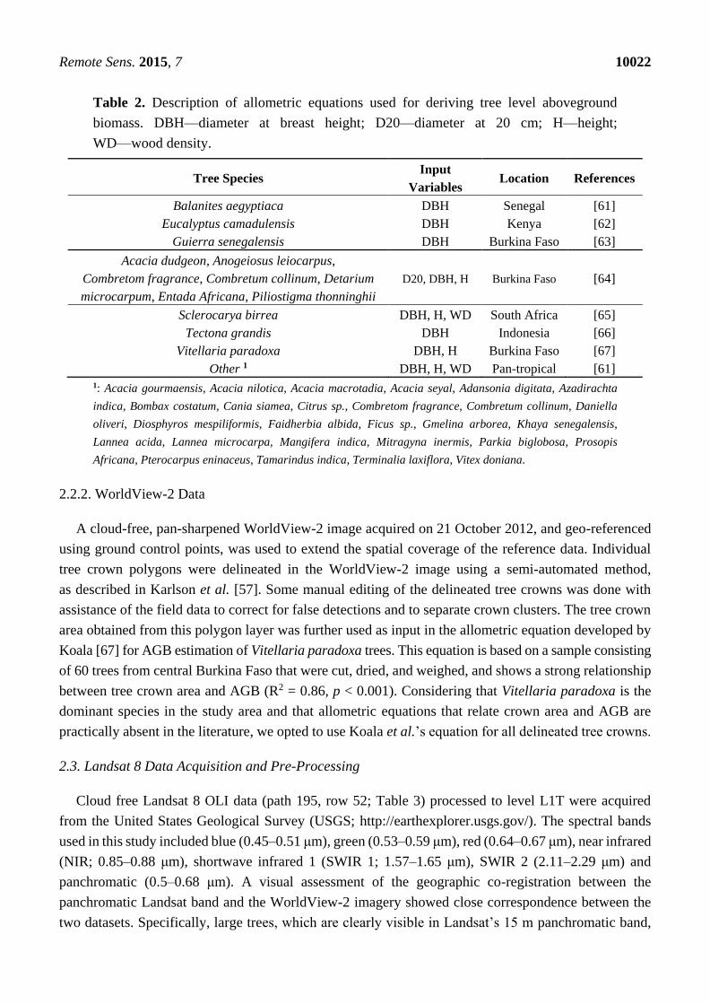
Table 2. Description of allometric equations used for deriving tree level aboveground
biomass. DBH—diameter at breast height; D20—diameter at 20 cm; H—height;
WD—wood density.
Tree Species Input
Variables Location References
Balanites aegyptiaca DBH Senegal [61]
Eucalyptus camadulensis DBH Kenya [62]
Guierra senegalensis DBH Burkina Faso [63]
Acacia dudgeon, Anogeiosus leiocarpus,
Combretom fragrance, Combretum collinum, Detarium
microcarpum, Entada Africana, Piliostigma thonninghii
D20, DBH, H Burkina Faso [64]
Sclerocarya birrea DBH, H, WD South Africa [65]
Tectona grandis DBH Indonesia [66]
Vitellaria paradoxa DBH, H Burkina Faso [67]
Other 1 DBH, H, WD Pan-tropical [61]
1: Acacia gourmaensis, Acacia nilotica, Acacia macrotadia, Acacia seyal, Adansonia digitata, Azadirachta
indica, Bombax costatum, Cania siamea, Citrus sp., Combretom fragrance, Combretum collinum, Daniella
oliveri, Diosphyros mespiliformis, Faidherbia albida, Ficus sp., Gmelina arborea, Khaya senegalensis,
Lannea acida, Lannea microcarpa, Mangifera indica, Mitragyna inermis, Parkia biglobosa, Prosopis
Africana, Pterocarpus eninaceus, Tamarindus indica, Terminalia laxiflora, Vitex doniana.
2.2.2. WorldView-2 Data
A cloud-free, pan-sharpened WorldView-2 image acquired on 21 October 2012, and geo-referenced
using ground control points, was used to extend the spatial coverage of the reference data. Individual
tree crown polygons were delineated in the WorldView-2 image using a semi-automated method,
as described in Karlson et al. [57]. Some manual editing of the delineated tree crowns was done with
assistance of the field data to correct for false detections and to separate crown clusters. The tree crown
area obtained from this polygon layer was further used as input in the allometric equation developed by
Koala [67] for AGB estimation of Vitellaria paradoxa trees. This equation is based on a sample consisting
of 60 trees from central Burkina Faso that were cut, dried, and weighed, and shows a strong relationship
between tree crown area and AGB (R2 = 0.86, p < 0.001). Considering that Vitellaria paradoxa is the
dominant species in the study area and that allometric equations that relate crown area and AGB are
practically absent in the literature, we opted to use Koala et al.’s equation for all delineated tree crowns.
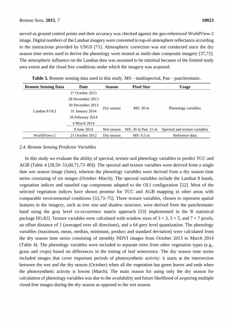
2.3. Landsat 8 Data Acquisition and Pre-Processing
Cloud free Landsat 8 OLI data (path 195, row 52; Table 3) processed to level L1T were acquired
from the United States Geological Survey (USGS; http://earthexplorer.usgs.gov/). The spectral bands
used in this study included blue (0.45–0.51 μm), green (0.53–0.59 μm), red (0.64–0.67 μm), near infrared
(NIR; 0.85–0.88 μm), shortwave infrared 1 (SWIR 1; 1.57–1.65 μm), SWIR 2 (2.11–2.29 μm) and
panchromatic (0.5–0.68 μm). A visual assessment of the geographic co-registration between the
panchromatic Landsat band and the WorldView-2 imagery showed close correspondence between the
two datasets. Specifically, large trees, which are clearly visible in Landsat’s 15 m panchromatic band,
Remote Sens. 2015, 7 10023
served as ground control points and their accuracy was checked against the geo-referenced WorldView-2
image. Digital numbers of the Landsat imagery were converted to top-of-atmosphere reflectance according
to the instructions provided by USGS [71]. Atmospheric correction was not conducted since the dry
season time series used to derive the phenology were treated as multi-date composite imagery [37,72].
The atmospheric influence on the Landsat data was assumed to be minimal because of the limited study
area extent and the cloud free conditions under which the imagery was acquired.
Table 3. Remote sensing data used in this study. MS—multispectral, Pan—panchromatic.
Remote Sensing Data Date Season Pixel Size Usage
Landsat 8 OLI
27 October 2013
Dry season MS: 30 m Phenology variables
28 November 2013
30 December 2013
31 January 2014
16 February 2014
4 March 2014
8 June 2014 Wet season MS: 30 m Pan: 15 m Spectral and texture variables
WorldView-2 21 October 2012 Dry season MS: 0.5 m Reference data
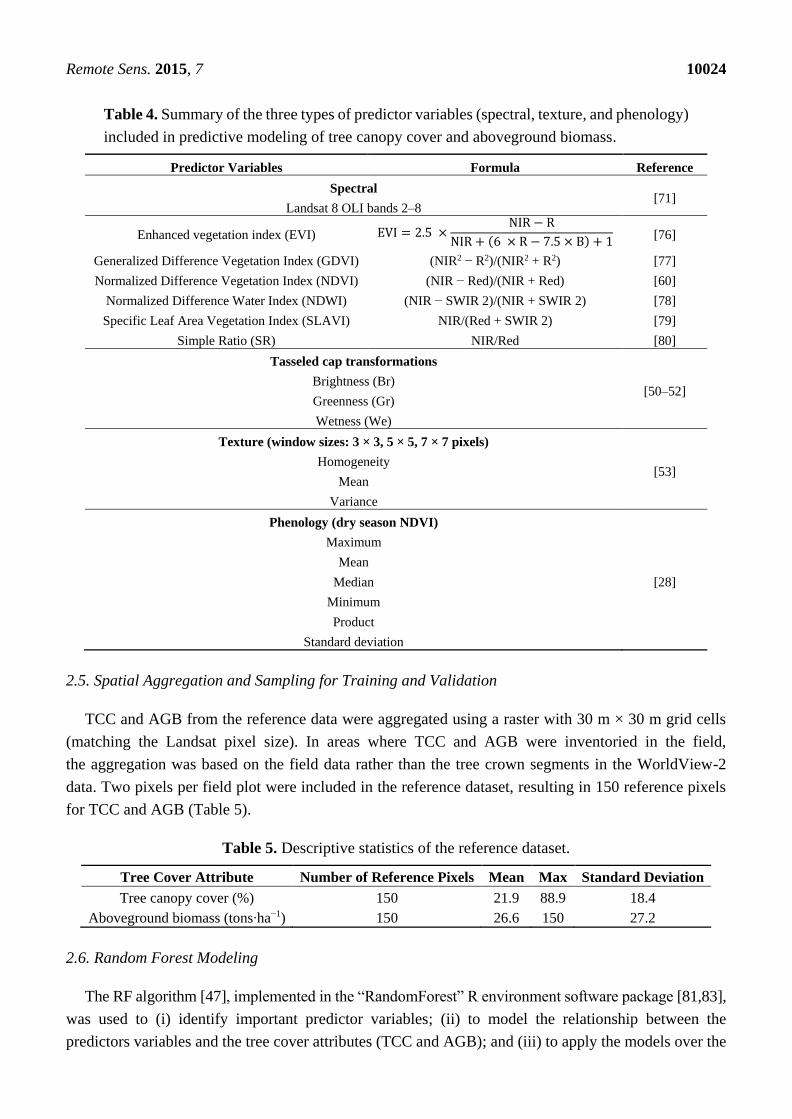
2.4. Remote Sensing Predictor Variables
In this study we evaluate the ability of spectral, texture and phenology variables to predict TCC and
AGB (Table 4 [28,50–53,60,71,73–80]). The spectral and texture variables were derived from a single
date wet season image (June), whereas the phenology variables were derived from a dry season time
series consisting of six images (October–March). The spectral variables include the Landsat 8 bands,
vegetation indices and tasseled cap components adapted to the OLI configuration [52]. Most of the
selected vegetation indices have shown promise for TCC and AGB mapping in other areas with
comparable environmental conditions [33,73–75]. Three texture variables, chosen to represent spatial
features in the imagery, such as tree size and shadow structure, were derived from the panchromatic
band using the gray level co-occurrence matrix approach [53] implemented in the R statistical
package [81,82]. Texture variables were calculated with window sizes of 3 × 3, 5 × 5, and 7 × 7 pixels,
an offset distance of 1 (averaged over all directions), and a 64 grey level quantization. The phenology
variables (maximum, mean, median, minimum, product and standard deviation) were calculated from
the dry season time series consisting of monthly NDVI images from October 2013 to March 2014
(Table 4). The phenology variables were included to separate trees from other vegetation types (e.g.,
grass and crops) based on differences in the timing of leaf senescence. The dry season time series
included images that cover important periods of photosynthetic activity: it starts at the intersection
between the wet and the dry season (October) when all the vegetation has green leaves and ends when
the photosynthetic activity is lowest (March). The main reason for using only the dry season for
calculation of phenology variables was due to the availability and future likelihood of acquiring multiple
cloud-free images during the dry season as opposed to the wet season.
Remote Sens. 2015, 7 10024
Table 4. Summary of the three types of predictor variables (spectral, texture, and phenology)
included in predictive modeling of tree canopy cover and aboveground biomass.
Predictor Variables Formula Reference
Spectral
Landsat 8 OLI bands 2–8 [71]
Enhanced vegetation index (EVI) EVI = 2.5 ×NIR − R
NIR + (6 × R − 7.5 × B) + 1 [76]
Generalized Difference Vegetation Index (GDVI) (NIR2 − R2)/(NIR2 + R2) [77]
Normalized Difference Vegetation Index (NDVI) (NIR − Red)/(NIR + Red) [60]
Normalized Difference Water Index (NDWI) (NIR − SWIR 2)/(NIR + SWIR 2) [78]
Specific Leaf Area Vegetation Index (SLAVI) NIR/(Red + SWIR 2) [79]
Simple Ratio (SR) NIR/Red [80]
Tasseled cap transformations
Brightness (Br)
Greenness (Gr)
Wetness (We)
[50–52]
Texture (window sizes: 3 × 3, 5 × 5, 7 × 7 pixels)
Homogeneity
Mean
Variance
[53]
Phenology (dry season NDVI)
Maximum
Mean
Median
Minimum
Product
Standard deviation
[28]
2.5. Spatial Aggregation and Sampling for Training and Validation
TCC and AGB from the reference data were aggregated using a raster with 30 m × 30 m grid cells
(matching the Landsat pixel size). In areas where TCC and AGB were inventoried in the field,
the aggregation was based on the field data rather than the tree crown segments in the WorldView-2
data. Two pixels per field plot were included in the reference dataset, resulting in 150 reference pixels
for TCC and AGB (Table 5).
Table 5. Descriptive statistics of the reference dataset.
Tree Cover Attribute Number of Reference Pixels Mean Max Standard Deviation
Tree canopy cover (%) 150 21.9 88.9 18.4
Aboveground biomass (tons∙ha−1) 150 26.6 150 27.2
2.6. Random Forest Modeling
The RF algorithm [47], implemented in the “RandomForest” R environment software package [81,83],
was used to (i) identify important predictor variables; (ii) to model the relationship between the
predictors variables and the tree cover attributes (TCC and AGB); and (iii) to apply the models over the
Remote Sens. 2015, 7 10025
study area for mapping TCC and AGB. RF was chosen because it has produced more accurate remote
sensing based predictions of TCC and AGB compared to other modeling techniques [19,37,48,49,84,85].
RF can also handle noisy and highly correlated predictor variables [47], which is the default situation in
remote sensing [42].
RF is an ensemble modeling technique where the forest consists of a large number of regression trees
(e.g., 500). Each tree is built from a random sample (approximately two-thirds) of the training data and
is drawn with replacements [47]. At each node in the trees, a random subset of the predictor variables is
used to identify the most efficient split. The most efficient split is defined by identifying the predictor
variable and the split point that results in the largest reduction in the residual sum of squares between
the sample observations and the node mean. All trees are grown to the maximum extent (i.e., no pruning)
that is controlled by the node size set by the user. The result is an ensemble (i.e., forest) of low bias and
high variance regression trees, where the final predictions are derived by averaging the predictions of
the individual trees [47].
In this study, 1000 trees (ntree) were used in the RF modeling. For the parameter mtry (i.e., the number
of variables to be tested at each node), the default value of the square root of the total number of predictor
variables was used [47]. The parameter nodesize was set to the default value of 1. RF modelling was
performed separately using predictor variables derived from single date and multi-temporal imagery
(including phenology variables), respectively. The separate modeling was done to assess the potential
benefit of using phenology variables, which are more problematic to acquire due to cloud contamination
compared to variables derived from single date imagery (spectral and texture variables).
2.6.1. Predictor Variable Selection
In RF, one third of the training data is used for internal model performance evaluation and for deriving
two different variable importance measures (VIM). The VIM used in this study is based on the percent
increase in mean squared prediction error (MSE) that results when an individual predictor variable is
permuted, while the others are unaltered. The resulting VIM provides means to assess the contribution
of each predictor variable to the modeling performance. This VIM is also useful for variable selection,
which may improve model performance [84,85] and facilitate the interpretability of the model by
reducing its complexity [86]. We applied a backward variable elimination method to identify the most
accurate and efficient models [85,87]. The method applied in this study starts by ranking all predictor
variables based on the MSE VIM. The least important predictor variables are then successively removed
from the model until the MSE of the prediction is minimized. The initial variable ranking (all predictor
variables) is used throughout all the iterations [88], and the smallest subset of predictor variables with
the lowest MSE is selected for constructing the final model. The models resulting from the variable
selection process were compared to the models based on the full predictor variable dataset in terms of
their abilities to predict TCC and AGB.
2.6.2. Accuracy Assessment and Statistical Analyses
RF modeling was done using the reduced and the full predictor variable datasets for (i) the single date
Landsat 8 imagery (spectral and texture variables) and (ii) the multi-temporal Landsat 8 imagery
(spectral, texture, and phenology variables). The predictive ability of all models was assessed using

Remote Sens. 2015, 7 10026
10-fold cross validation (10% of reference data). The cross-validation approach is based on the entire
reference dataset, rather than using separate training and validation data subsets, which is a useful
approach when there is limited reference data [49]. Four measures of model performance were calculated
from the 10-fold cross validation, including the coefficient of determination (R2), the root mean square
error (RMSE), relative RMSE (relRMSE) and mean bias error (MBE). Wilcoxon signed rank test was
used for assessing differences between the models’ abilities to predict TCC and AGB.
3. Results
3.1. Variable Importance
The error rate estimated from the RF out of bag (OOB) data was used to rank all of the predictor
variables by their capacity to predict TCC and AGB. Figures 2 and 3 show the rankings for both
multi-temporal and single date imagery.
Figure 2. Importance of predictor variables for estimating tree canopy cover (TCC) using
multi-temporal and single date imagery. A higher out of bag (OOB) error rate indicates
stronger importance of the predictor variables. See Table 4 for description of abbreviations
for predictor variables.
3.1.1. Tree Canopy Cover
The variable importance ranking identified the panchromatic band, homogeneity texture features
(3 × 3 and 7 × 7) and greenness (Gr) as particularly important for predicting TCC (Figure 2). Several of
the phenology variables are ranked as relatively important for predicting TCC. The product of dry season
NDVI stands out as the most important phenology variable. Individual Landsat 8 multi-spectral bands are
generally ranked low compared to vegetation indices and tasseled cap components (Br, Gr, We).
Remote Sens. 2015, 7 10027
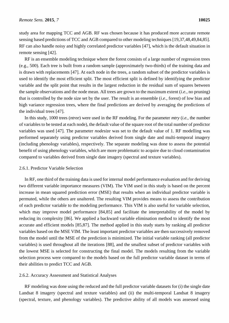
Figure 3. Importance of predictor variables for estimating aboveground biomass (AGB)
using multi-temporal and single date imagery. Higher out of bag (OOB) error rate indicates
stronger importance of the predictor variables. See Table 4 for description of abbreviations
for predictor variables.
3.1.2. Aboveground Biomass
The variables which stand out in the ranking as important for the prediction of AGB include the
panchromatic band, homogeneity texture features (3 × 3 and 5 × 5) and wetness (We; Figure 3).
This was generally true for both the single date and the multi-temporal imagery. The median of dry
season NDVI was ranked as the third most important variable for predicting AGB (median).
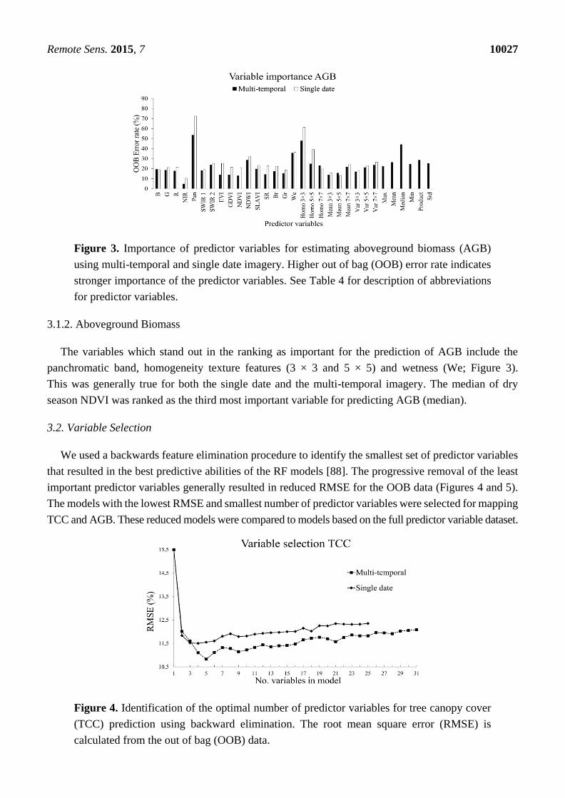
3.2. Variable Selection
We used a backwards feature elimination procedure to identify the smallest set of predictor variables
that resulted in the best predictive abilities of the RF models [88]. The progressive removal of the least
important predictor variables generally resulted in reduced RMSE for the OOB data (Figures 4 and 5).
The models with the lowest RMSE and smallest number of predictor variables were selected for mapping
TCC and AGB. These reduced models were compared to models based on the full predictor variable dataset.
Figure 4. Identification of the optimal number of predictor variables for tree canopy cover
(TCC) prediction using backward elimination. The root mean square error (RMSE) is
calculated from the out of bag (OOB) data.
Remote Sens. 2015, 7 10028
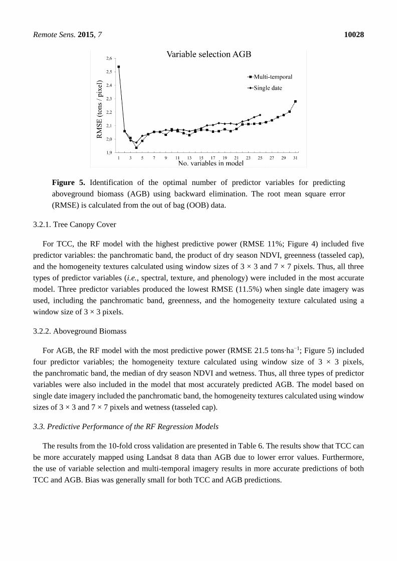
Figure 5. Identification of the optimal number of predictor variables for predicting
aboveground biomass (AGB) using backward elimination. The root mean square error
(RMSE) is calculated from the out of bag (OOB) data.
3.2.1. Tree Canopy Cover
For TCC, the RF model with the highest predictive power (RMSE 11%; Figure 4) included five
predictor variables: the panchromatic band, the product of dry season NDVI, greenness (tasseled cap),
and the homogeneity textures calculated using window sizes of 3 × 3 and 7 × 7 pixels. Thus, all three
types of predictor variables (i.e., spectral, texture, and phenology) were included in the most accurate
model. Three predictor variables produced the lowest RMSE (11.5%) when single date imagery was
used, including the panchromatic band, greenness, and the homogeneity texture calculated using a
window size of 3 × 3 pixels.
3.2.2. Aboveground Biomass
For AGB, the RF model with the most predictive power (RMSE 21.5 tons∙ha−1; Figure 5) included
four predictor variables; the homogeneity texture calculated using window size of 3 × 3 pixels,
the panchromatic band, the median of dry season NDVI and wetness. Thus, all three types of predictor
variables were also included in the model that most accurately predicted AGB. The model based on
single date imagery included the panchromatic band, the homogeneity textures calculated using window
sizes of 3 × 3 and 7 × 7 pixels and wetness (tasseled cap).
3.3. Predictive Performance of the RF Regression Models
The results from the 10-fold cross validation are presented in Table 6. The results show that TCC can
be more accurately mapped using Landsat 8 data than AGB due to lower error values. Furthermore,
the use of variable selection and multi-temporal imagery results in more accurate predictions of both
TCC and AGB. Bias was generally small for both TCC and AGB predictions.
Remote Sens. 2015, 7 10029
Table 6. Results of model performance evaluation. relRMSE—relative root mean square
error; MBE—mean bias error.
Variable Variable Selection Predictor Dataset R2 relRMSE (%) RMSE MBE
Tree canopy
cover (%)
Full Single date 0.49 60.0 13.1 0.04
Multi-temporal 0.54 57.0 12.5 0.08
Reduced Single date 0.65 49.7 10.9 0.02
Multi-temporal 0.77 40.6 8.9 0.08
Aboveground
biomass (tons ha−1)
Full Single date 0.34 83.0 22.2 0.06
Multi-temporal 0.46 75.0 20 −0.66
Reduced Single date 0.44 75.0 20 0.44
Multi-temporal 0.57 66.0 17.6 0.22
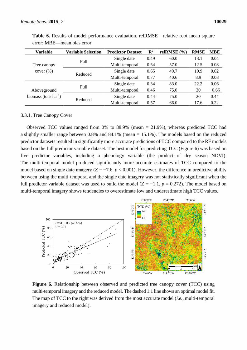
3.3.1. Tree Canopy Cover
Observed TCC values ranged from 0% to 88.9% (mean = 21.9%), whereas predicted TCC had
a slightly smaller range between 0.8% and 84.1% (mean = 15.1%). The models based on the reduced
predictor datasets resulted in significantly more accurate predictions of TCC compared to the RF models
based on the full predictor variable dataset. The best model for predicting TCC (Figure 6) was based on
five predictor variables, including a phenology variable (the product of dry season NDVI).
The multi-temporal model produced significantly more accurate estimates of TCC compared to the
model based on single date imagery (Z = −7.6, p < 0.001). However, the difference in predictive ability
between using the multi-temporal and the single date imagery was not statistically significant when the
full predictor variable dataset was used to build the model (Z = −1.1, p = 0.272). The model based on
multi-temporal imagery shows tendencies to overestimate low and underestimate high TCC values.
Figure 6. Relationship between observed and predicted tree canopy cover (TCC) using
multi-temporal imagery and the reduced model. The dashed 1:1 line shows an optimal model fit.
The map of TCC to the right was derived from the most accurate model (i.e., multi-temporal
imagery and reduced model).
Remote Sens. 2015, 7 10030
3.3.2. Aboveground Biomass
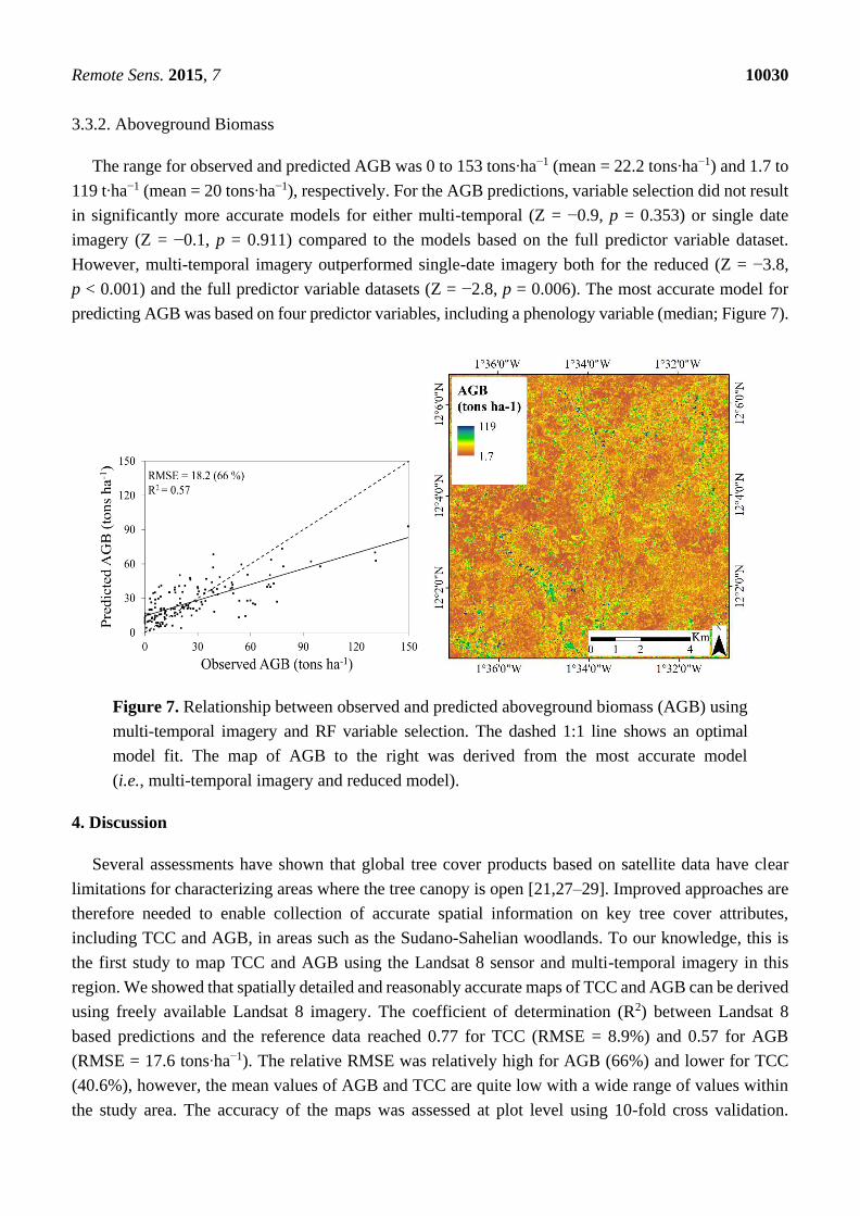
The range for observed and predicted AGB was 0 to 153 tons∙ha−1 (mean = 22.2 tons∙ha−1) and 1.7 to
119 t∙ha−1 (mean = 20 tons∙ha−1), respectively. For the AGB predictions, variable selection did not result
in significantly more accurate models for either multi-temporal (Z = −0.9, p = 0.353) or single date
imagery (Z = −0.1, p = 0.911) compared to the models based on the full predictor variable dataset.
However, multi-temporal imagery outperformed single-date imagery both for the reduced (Z = −3.8,
p < 0.001) and the full predictor variable datasets (Z = −2.8, p = 0.006). The most accurate model for
predicting AGB was based on four predictor variables, including a phenology variable (median; Figure 7).
Figure 7. Relationship between observed and predicted aboveground biomass (AGB) using
multi-temporal imagery and RF variable selection. The dashed 1:1 line shows an optimal
model fit. The map of AGB to the right was derived from the most accurate model
(i.e., multi-temporal imagery and reduced model).
4. Discussion
Several assessments have shown that global tree cover products based on satellite data have clear
limitations for characterizing areas where the tree canopy is open [21,27–29]. Improved approaches are
therefore needed to enable collection of accurate spatial information on key tree cover attributes,
including TCC and AGB, in areas such as the Sudano-Sahelian woodlands. To our knowledge, this is
the first study to map TCC and AGB using the Landsat 8 sensor and multi-temporal imagery in this
region. We showed that spatially detailed and reasonably accurate maps of TCC and AGB can be derived
using freely available Landsat 8 imagery. The coefficient of determination (R2) between Landsat 8
based predictions and the reference data reached 0.77 for TCC (RMSE = 8.9%) and 0.57 for AGB
(RMSE = 17.6 tons∙ha−1). The relative RMSE was relatively high for AGB (66%) and lower for TCC
(40.6%), however, the mean values of AGB and TCC are quite low with a wide range of values within
the study area. The accuracy of the maps was assessed at plot level using 10-fold cross validation.

Remote Sens. 2015, 7 10031
If TCC and AGB estimates from application of the models were to be aggregated over larger areas,
the errors would be lower.
The observed prediction errors highlight the uncertainties and limitations associated with mapping
tree cover attributes using optical remote sensing. A main problem of using optical imagery in areas with
an open tree canopy is that the understory vegetation and soil contributes to the spectral signal and therefore
renders the relationship between the tree cover and the remote sensing data less predictable [22].
In particular bright soil types, such as those found in the study area, have been shown to negatively affect
the prediction of tree cover attributes from optical remote sensing data [21]. An additional complicating
factor is that woodland tree cover in general, and in the study area in particular, is composed of a
relatively large number of tree species [2] which are partly characterized by variations in the spectral
properties of leaves and canopies [28].
We aimed to account for the contribution from understory vegetation by using imagery from periods
when the phenological differences between trees and grasses/crops are largest [28,37,89], including
the early wet season and the dry season. However, the understory vegetation in the study area also
includes a considerable component of shrubs and tree coppice, which contribute to the spectral signal.
The reference dataset therefore has limitations because (i) only trees with DBH ≥ 5 cm were surveyed
in the field and (ii) the tree crown delineation in the WorldView-2 imagery has a higher likelihood of
omitting small trees [57]. A complete sampling of all woody vegetation in the field plots would require
substantially more time and resources, which were not available in this study. A compromise between
limited resources and field data completeness could be to use a nested inventory design where different
types of woody vegetation are surveyed in small sub-plots [90]. A further potential limitation of the
reference dataset that may cause prediction errors is the use of allometric equations to obtain plot-level
AGB from individual tree attributes (i.e., height, DBH, and crown area). We opted to use species specific
equations developed in areas with similar environmental conditions as those of the study area to the
largest extent possible. However, the availability of species specific equations is limited in Africa [91]
and the pan-tropical allometric equation by Chave et al. [68] was therefore used for 28 of the tree species
(42% of the field data). Furthermore, our approach to estimate AGB from tree crowns delineated in
WorldView-2 imagery includes two uncertainties. Firstly, the crown delineation in the WorldView-2
image includes errors, especially for small trees [57]. Secondly, the allometric equation used for
estimating AGB from crown area was developed for Vitellaria paradoxa and may therefore not be
optimal for other tree species. The relationship between crown area and AGB is also complicated due to
the pollarding of trees, which is a common practice in the region [92,93].
In order to reduce the effect of potential spatial mis-registration between remote sensing data and
reference data, one suggestion is to average the remote sensing data within a window (e.g., 3 × 3) of
pixels [16,31,39]. However, the spatial variation in tree cover properties is extremely high in woodlands
and parklands, and such an approach was therefore not suitable for this study. Instead we extracted the
remote sensing predictor variables from individual Landsat pixels. This approach is heavily dependent
on the spatial correspondence between the remote sensing data and the reference dataset. We estimate
that the geo-location accuracy of the Landsat 8 imagery is below half a panchromatic pixel (i.e., 7.5 m),
thereby giving confidence to the approach used in this study. Similarly accurate spatial registration of
Landsat 8 was also recognized by Zandler et al. [94].
Remote Sens. 2015, 7 10032
4.1. Relationships between Predictor Variables and Tree Cover Attributes
The panchromatic band proved to be the most important variable for predicting both TCC and AGB,
ranking above all of the vegetation indices. The observed strong inverse relationship between the
panchromatic band and the tree cover attributes suggests two things. Firstly, the image acquisition date
in early June (i.e., early wet season) provided good contrast between tree cover and background
components due to low growth activity of grasses, crops, and shrubs [95]. Specifically, the foliage of
Sudan-Sahelian tree species is known to develop before the re-growth of the herbaceous vegetation [96,97].
Secondly, the size of the 15 m panchromatic pixels seemed to be better suited to capture the reflectance
contributions from trees, which may be mixed (e.g., trees and grass) in the larger 30 m Landsat
multispectral pixels when the tree canopy is open [28]. This observation was reinforced since image
texture derived from the panchromatic band also proved useful for predicting both TCC and AGB.
The relatively strong relationship between image texture, in particular the gray level co-occurrence
matrix (GLCM) homogeneity, and tree cover attributes found in this study agrees with previous research
suggesting that image texture is particularly useful in areas where the tree canopy is open [31–34,98].
In addition to the panchromatic band, tasseled cap components adapted to Landsat 8 [52] proved to be
important for predicting tree cover attributes; greenness and wetness were strongly related to TCC and
AGB, respectively. Greenness measures the amount of green vegetation by quantifying the contrast
between the NIR band and the visible bands that results from spectral properties of leaf cellular structure
and plant pigments. The better performance of greenness to predict TCC compared to the other vegetation
indices can be explained by the inclusion of a mechanism to account for soil reflectance [50,51].
Soil reflectance can be highly variable in the Sudano-Sahelian zone and has been shown to complicate
relationships between vegetation indices and vegetation properties [99]. Individual SWIR bands have
been shown to be sensitive to vegetation water content [100,101]. Wetness contrasts the SWIR bands
against the visible and NIR bands in order to isolate the reflectance contribution from water content in
leafs and soil [51]. Previous research has found wetness and SWIR bands to be among the most important
for predicting forest structure, including AGB, in various types of environments [28,102–104]. The same
pattern is seen in the present study where the importance of wetness and SWIR bands is more pronounced
when predicting AGB as compared to predicting TCC.
The inclusion of phenology variables generally improved the predictions of TCC and AGB;
the product of dry season NDVI was included in the best TCC model (Figure 6), while the median of
dry season NDVI was included in the best AGB models (Figure 7). The decreased RMSE for both TCC
(−9.1%) and AGB (−9%) predictions suggest that the dry season NDVI time series contain additional
information related to phenology and seasonal differences in soil moisture that facilitates the separation
between tree cover and background components. These results are promising, but further research will
be required to investigate the underlying mechanisms of this observation and to optimize the procedure
for the Sudano-Sahelian woodland landscape. For example, the dry season time series could be
contrasted to climate data, field observations of phenological events and temporal profiles from MODIS
in order to better understand the Landsat 8 phenology variables. We used NDVI to characterize
vegetation during the dry season, but other remote sensing variables could be used. The results from this
study suggest that tasseled cap greenness and wetness are potential candidates for the phenology
Remote Sens. 2015, 7 10033
variables due to their stronger relationship to TCC and AGB in this study. The temporal definition of
the dry season and frequency of image acquisition during this period may also merit further research.
4.2. Random Forest Regression and Variable Selection
We used the error rate calculated from the OOB data to perform variable selection with RF in order
to assess its effect on the predictive performance of the resulting models. Previous research has shown
this to be a statistically sound and efficient approach because the OOB data provide reliable internal
estimates of error rate when compared to results derived from 10-fold cross-validation [84,105,106].
The results show that variable selection did improve predictions of both TCC and AGB. This finding is
in line with previous related remote sensing research [84,86,106], and suggests that the effect of variable
selection should be evaluated when RF is used for predicting tree cover attributes from remote sensing
data. A plausible explanation to the better performance of the reduced models is that the mechanisms of
RF partly fail to block the influence of noisy predictor variables [106].
RF regression has several advantages for modeling remote sensing data [47], but also limitations.
In this study, RF appeared to consistently overestimate low values and underestimated high values,
which partly explains the absence of bias in the TCC and AGB predictions. This effect was most
pronounced for AGB predictions and is due to both properties of the algorithm and characteristics of the
reference data. The final prediction from a RF model is based on the average value of individual trees
generated from bootstrap samples [47]. If the reference dataset contains too few extreme values they
might be consistently underrepresented in the tree construction and RF predictions may therefore be
biased towards the mean value. This property of the RF algorithm needs specific attention when
reference data are collected. Specifically, the reference data need to cover the full range and represent
the variability of the variable of interest in the specific study area. A stratified sampling design is
therefore recommended for reference data collection.
The results from this study are promising, especially for the mapping of TCC. However, the approach
should be tested in a larger area, preferably a site that covers a wider tree cover gradient. We used
WorldView-2 imagery in addition to field data to derive the reference dataset. Availability of such
imagery may be restricted due to high costs, especially for large areas. However, Wu et al. [75] showed
that Google Earth is an interesting alternative source of high resolution imagery by using it to manually
derive a reference dataset of TCC for the main part of Sudan.
5. Conclusions
In this study, we assessed the utility of Landsat 8 OLI imagery for mapping tree canopy cover (TCC)
and aboveground biomass (AGB) in a Sudano-Sahelian woodland landscape. Spectral, texture, and
phenology predictor variables were extracted from multi-temporal Landsat 8 imagery and used as input
to Random Forest (RF) models. A combination of field data and WorldView-2 imagery was used to
create a reference dataset, which facilitated integration with the Landsat data at pixel level. The following
conclusions are drawn from this study:
• Landsat 8 is more suitable for mapping TCC compared to AGB in this landscape type: the best
model for TCC resulted in a coefficient of determination (R2) of 0.77 and a root mean square error
Remote Sens. 2015, 7 10034
(RMSE) of 8.9 percent and the best model for AGB resulted in an R2 of 0.57 and a RMSE of
17.6 tons∙ha−1. The weaker relationship between the Landsat 8 data and AGB was expected, and
can be explained by the difficulty of resolving information related to the three dimensional
structure in optical satellite data.
• The use of variable selection to reduce the number of predictor variables improved the
performance and interpretability of the RF models, and should therefore be considered when RF
is used for similar tasks. From the total of 31 predictor variables, five were included in the best
model for TCC and four were included for AGB.
• All three types of predictor variables (spectral, texture, and phenology), were included by the
variable selection in the best model, which suggests that they provide complementary information
to the predictions.
• The methods presented in this study are relatively simple and applicable over the Sudano-Sahelian
woodlands where sufficient reference data for calibration and validation is available. High resolution
satellite data, such as WorldView-2, represents a useful complement to field data in this context.
• The large contribution of Landsat’s 15 m panchromatic band and the phenology variables to the
prediction success suggests that the upcoming Sentinel-2 optical sensor will have spatial and
temporal features well suited for mapping tree cover attributes in Sudano-Sahelian woodlands.
Future research will focus on (i) assessing the transferability of this approach to other woodland areas
with different tree cover characteristics; and (ii) testing the capacity of Sentinel-2 data for mapping tree
cover attributes in Sudano-Sahelian woodlands.
Acknowledgments
The research work and the publication has been funded by the Swedish International Development
Cooperation Agency (Sida), the Swedish Energy Agency and the Swedish Research Council (VR/Sida).
The study was conducted in close collaboration with the Institut de l’Environnement et de Recherches
Agricoles (INERA) in Burkina Faso. Huges Bazié is thanked for arranging the practicalities of the field
campaign, and the farmers in Saponé are thanked for their permission to perform the tree inventory. We
also thank the anonymous reviewers for helping with improving the manuscript.
Author Contributions
Martin Karlson contributed to the design of the study, conducted the fieldwork, performed the image
processing and analysis, and prepared the manuscript. Madelene Ostwald initiated the work and took
part in the study design, fieldwork, discussion, and manuscript editing. Heather Reese contributed to
the design of the study, the image processing and analysis, discussion, and manuscript editing.
Eskil Mattsson contributed to the implementation of allometric equations, discussion, and manuscript
editing. Josias Sanou and Boalidioa Tankoano contributed to designing and the implementation of
the field work.
Conflicts of Interest
The authors declare no conflict of interest.

Remote Sens. 2015, 7 10035
References
1. Grainger, A. Constraints on modelling the deforestation and degradation of tropical open woodlands.
Global Ecol. Biogeogr. 1999, 8, 179–190.
2. Chidumayo, E.; Gumbo, D.J. The Dry Forests and Woodlands of Africa: Managing for Products
and Services; Earth Scan: London, UK, 2010.
3. Boffa, J.M. Agroforestry Parkland in Sub-Saharan Africa: Fao Conservation Guide 34;
United Nations-Food and Agricultural Organization: Rome, Italy, 1999.
4. Dixon, R.K.; Brown, S.; Houghton, R.A.; Solomon, A.M.; Trexler, M.C.; Wisniewski, J. Carbon
pools and flux of global forest ecosystems. Science 1994, 263, 185–190.
5. Lal, R. Carbon sequestration in dryland ecosystems. Environ. Manag. 2004, 33, 528–544.
6. Foley, J.A.; DeFries, R.; Asner, G.P.; Barford, C.; Bonan, G.; Carpenter, S.R.; Chapin, F.S.; Coe, M.T.;
Daily, G.C.; Gibbs, H.K.; et al. Global consequences of land use. Science 2005, 309, 570–574.
7. Tappan, G.G.; Sall, M.; Wood, E.C.; Cushing, M. Ecoregions and land cover trends in Senegal.
J. Arid Environ. 2004, 59, 427–462.
8. Intergovernmental Panel on Climate Change (IPCC). Climate Change 2014: Impacts, Adaptation,
and Vulnerability. Part B: Regional Aspects. Contribution of Working Group II to the Fifth
Assessment Report of the intErgovernmental Panel on Climate Change; Barros, V.R., Field, C.B.,
Dokken, D.J., Mastrandrea, M.D., Mach, K.J., Bilir, T.E., Chatterjee, M., Estrada, Y.O., Genova, R.C.,
Ebi, K.L., et al., Eds.; Cambridge University Press: New York, NY, USA, 2014.
9. Gonzalez, P. Desertification and a shift of forest species in the West African Sahel. Clim. Res 2001,
17, 217–228.
10. Maranz, S. Tree mortality in the African Sahel indicates an anthropogenic ecosystem displaced by
climate change. J. Biogeogr. 2009, 36, 1181–1193.
11. Gonzalez, P.; Tucker, C.J.; Sy, H. Tree density and species decline in the African Sahel attributable
to climate. J. Arid Environ. 2012, 78, 55–64.
12. Brandt, M.; Mbow, C.; Diouf, A.A.; Verger, A.; Samimi, C.; Fensholt, R. Ground- and satellite-based
evidence of the biophysical mechanisms behind the greening Sahel. Global Chang. Biol. 2015,
21, 1610–1620.
13. Reij, C.; Tappan, G.; Belemvire, A. Changing land management practices and vegetation on the
central plateau of Burkina Faso (1968–2002). J. Arid Environ. 2005, 63, 642–659.
14. Tougiani, A.; Guero, C.; Rinaudo, T. Community mobilisation for improved livelihoods through
tree crop management in Niger. GeoJournal 2009, 74, 377–389.
15. Sendzimir, J.; Reij, C.P.; Magnuszewski, P. Rebuilding resilience in the Sahel: Regreening in the
Maradi and Zinder regions of Niger. Ecol. Soc. 2011, 16, doi:10.5751/ES-04198-160301.
16. Lu, D.S. The potential and challenge of remote sensing-based biomass estimation. Int. J. Remote Sens.
2006, 27, 1297–1328.
17. Goetz, S.J.; Baccini, A.; Laporte, N.T.; Johns, T.; Walker, W.; Kellndorfer, J.; Houghton, R.A.;
Sun, M. Mapping and monitoring carbon stocks with satellite observations: A comparison of methods.
Carbon Balance Manag. 2009, doi:10.1186/1750-0680-4-2.
18. Eisfelder, C.; Kuenzer, C.; Dech, S. Derivation of biomass information for semi-arid areas using
remote-sensing data. Int. J. Remote Sens. 2012, 33, 2937–2984.

Remote Sens. 2015, 7 10036
19. Barbosa, J.M.; Broadbent, E.N.; Bitencourt, M.D. Remote sensing of aboveground biomass in
tropical secondary forests: A review. Int. J. For. Res. 2014, doi:10.1155/2014/715796.
20. Sexton, J.O.; Song, X.P.; Feng, M.; Noojipady, P.; Anand, A.; Huang, C.; Kim, D.H.; Collins, K.M.;
Channan, S.; DiMiceli, C.; et al. Global, 30-m resolution continuous fields of tree cover: Landsat-based
rescaling of MODIS vegetation continuous fields with lidar-based estimates of error. Int. J. Digit.
Earth 2013, 6, 427–448.
21. Hansen, M.C.; Townshend, J.R.G.; DeFries, R.S.; Carroll, M. Estimation of tree cover using
MODIS data at global, continental and regional/local scales. Int. J. Remote Sens. 2005,
26, 4359–4380.
22. Franklin, J.; Strahler, A.H. Invertible canopy reflectance modeling of vegetation structure in
semiarid woodland. IEEE Trans. Geosci. Remote Sens. 1988, 26, 809–825.
23. Franklin, J. Land cover stratification using Landsat Thematic Mapper data in Sahelian and
Sudanian woodland and wooded grassland. J. Arid Environ. 1991, 20, 141–163.
24. Cord, A.; Conrad, C.; Schmidt, M.; Dech, S. Standardized FAO-LCCS land cover mapping in
heterogeneous tree savannas of West Africa. J. Arid Environ. 2010, 74, 1083–1091.
25. Tagesson, T.; Fensholt, R.; Guiro, I.; Rasmussen, M.O.; Huber, S.; Mbow, C.; Garcia, M.; Horion, S.;
Sandholt, I.; Holm-Rasmussen, B.; et al. Ecosystem properties of semiarid savanna grassland in
West Africa and its relationship with environmental variability. Global Chang. Biol. 2015,
21, 250–264.
26. Hansen, M.C.; DeFries, R.S.; Townshend, J.R.G.; Carroll, M.; Dimiceli, C.; Sohlberg, R.A. Global
percent tree cover at a spatial resolution of 500 meters: First results of the MODIS vegetation
continuous fields algorithm. Earth Interact. 2003, 7, 1–15.
27. Heiskanen, J. Evaluation of global land cover data sets over the tundra-taiga transition zone in
northern most finland. Int. J. Remote Sens. 2008, 29, 3727–3751.
28. Gessner, U.; Machwitz, M.; Conrad, C.; Dech, S. Estimating the fractional cover of growth forms
and bare surface in savannas. A multi-resolution approach based on regression tree ensembles.
Remote Sens. Environ. 2013, 129, 90–102.
29. Herrmann, S.M.; Wickhorst, A.J.; Marsh, S.E. Estimation of tree cover in an agricultural parkland
of Senegal using rule-based regression tree modeling. Remote Sens. 2013, 5, 4900–4918.
30. Broadbent, E.N.; Asner, G.P.; Peña-Claros, M.; Palace, M.; Soriano, M. Spatial partitioning of
biomass and diversity in a lowland Bolivian forest: Linking field and remote sensing
measurements. For. Ecol. Manag. 2008, 255, 2602–2616.
31. Lu, D. Aboveground biomass estimation using Landsat TM data in the Brazilian Amazon. Int. J.
Remote Sens. 2005, 26, 2509–2525.
32. Fuchs, H.; Magdon, P.; Kleinn, C.; Flessa, H. Estimating aboveground carbon in a catchment of
the Siberian forest tundra: Combining satellite imagery and field inventory. Remote Sens. Environ.
2009, 113, 518–531.
33. Eckert, S. Improved forest biomass and carbon estimations using texture measures from
Worldview-2 satellite data. Remote Sens. 2012, 4, 810–829.
34. Kelsey, K.C.; Neff, J.C. Estimates of aboveground biomass from texture analysis of Landsat
imagery. Remote Sens. 2014, 6, 6407–6422.
35. Karlson, M. Linköping University, Linköping, Sweden; Unpublished work, 2015.

Remote Sens. 2015, 7 10037
36. Horion, S.; Fensholt, R.; Tagesson, T.; Ehammer, A. Using earth observation-based dry season
ndvi trends for assessment of changes in tree cover in the Sahel. Int. J. Remote Sens. 2014, 35,
2493–2515.
37. Kamusoko, C.; Gamba, J.; Murakami, H. Mapping woodland cover in the Miombo ecosystem:
A comparison of machine learning classifiers. Land 2014, 3, 524–540.
38. Irons, J.R.; Dwyer, J.L.; Barsi, J.A. The next Landsat satellite: The Landsat data continuity mission.
Remote Sens. Environ. 2012, 122, 11–21.
39. Dube, T.; Mutanga, O. Evaluating the utility of the medium-spatial resolution Landsat 8 multispectral
sensor in quantifying aboveground biomass in Umgeni catchment, South Africa. ISPRS J.
Photogramm. Remote Sens. 2015, 101, 36–46.
40. Pflugmacher, D.; Cohen, W.B.; Kennedy, R.E. Using Landsat-derived disturbance history
(1972–2010) to predict current forest structure. Remote Sens. Environ. 2012, 122, 146–165.
41. Frazier, R.J.; Coops, N.C.; Wulder, M.A.; Kennedy, R. Characterization of aboveground biomass
in an unmanaged boreal forest using Landsat temporal segmentation metrics. ISPRS J. Photogramm.
Remote Sens. 2014, 92, 137–146.
42. Curran, P.J.; Hay, A.M. The importance of measurement error for certain procedures in remote
sensing at optical wavelengths. Photogramm. Eng. Remote Sens. 1986, 52, 229–241.
43. Cohen, W.B.; Maiersperger, T.K.; Gower, S.T.; Turner, D.P. An improved strategy for regression
of biophysical variables and Landsat ETM+ data. Remote Sens. Environ. 2003, 84, 561–571.
44. Breiman, L. Statistical modeling: The two cultures. Stat. Sci. 2001, 16, 199–231.
45. Vapnik, V.N. An overview of statistical learning theory. IEEE Trans. Neural Netw. 1999, 10,
988–999.
46. Breiman, L.; Friedman, J.; Stone, C.J.; Olshen, R.A. Classification and Regression Trees;
Taylor & Francis: New York, NY, USA,1984; p. 368 .
47. Breiman, L. Random forests. Mach. Learn. 2001, 45, 5–32.
48. Powell, S.L.; Cohen, W.B.; Healey, S.P.; Kennedy, R.E.; Moisen, G.G.; Pierce, K.B.; Ohmann, J.L.
Quantification of live aboveground forest biomass dynamics with Landsat time-series and field
inventory data: A comparison of empirical modeling approaches. Remote Sens. Environ. 2010,
114, 1053–1068.
49. Fassnacht, F.E.; Hartig, F.; Latifi, H.; Berger, C.; Hernández, J.; Corvalán, P.; Koch, B. Importance
of sample size, data type and prediction method for remote sensing-based estimations of aboveground
forest biomass. Remote Sens. Environ. 2014, 154, 102–114.
50. Kauth, R.J.; Thomas, G.S. The Tasselled cap—A graphic description of the spectral-temporal
development of agricultural crops as seen by Landsat. In Proceedings of the Symposium on
Machine Processing of Remotely Sensed Data, West Lafayette, IN, USA, 29 June–1 July 1976;
pp. 41–51.
51. Crist, E.P.; Cicone, R.C. Physically-based transformation of Thematic Mapper data—The TM
tasseled cap. IEEE Trans. Geosci. Remote Sens. 1984, GE-22, 256–263.
52. Baig, M.H.A.; Zhang, L.; Shuai, T.; Tong, Q. Derivation of a tasselled cap transformation based
on Landsat 8 at-satellite reflectance. Remote Sens. Lett. 2014, 5, 423–431.
53. Haralick, R.M.; Shanmugam, K.; Dinstein, I. Textural features for image classification. IEEE
Trans. Syst. Man Cybern. 1973, SMC-3, 610–621.

Remote Sens. 2015, 7 10038
54. Jonsson, K.; Ong, C.K.; Odongo, J.C.W. Influence of scattered nere and karite trees on microclimate,
soil fertility and millet yield in Burkina Faso. Exp. Agric. 1999, 35, 39–53.
55. Peel, M.C.; Finlayson, B.L.; McMahon, T.A. Updated world map of the Köppen-Geiger climate
classification. Hydrol. Earth Syst. Sci. 2007, 11, 1633–1644.
56. Nicholson, S.E. A revised picture of the structure of the “monsoon” and land ITCZ over West
Africa. Clim. Dyn. 2009, 32, 1155–1171.
57. Karlson, M.; Reese, H.; Ostwald, M. Tree crown mapping in managed woodlands (parklands) of
semi-arid West Africa using Worldview-2 imagery and geographic object based image analysis.
Sens. Switz. 2014, 14, 22643–22669.
58. Arbonnier, M. Trees, Shrubs and Lianas of West African Dry Zones, 2nd ed.; Magraf Publishers
CIRAD: Paris, France, 2004; p. 573.
59. Brown, S.L.; Schroeder, P.; Kern, J.S. Spatial distribution of biomass in forests of the eastern USA.
For. Ecol. Manag. 1999, 123, 81–90.
60. Rouse, J.W.; Haas, R.H.; Schell, J.A.; Deering, D.W. Monitoring vegetation systems in the Great
Plains with ERST. NASA Spec. Publ. 1973, 351, 309–317.
61. Poupon, H. Structure et Dynamique de la Strate Ligneuse d’une Steppe Sahélienne au Nord du
Sénégal; ORSTOM: Paris, France, 1980; p. 351.
62. Kuyah, S.; Dietz, J.; Muthuri, C.; van Noordwijk, M.; Neufeldt, H. Allometry and partitioning of
above- and below-ground biomass in farmed eucalyptus species dominant in Western Kenyan
agricultural landscapes. Biomass Bioenergy 2013, 55, 276–284.
63. Neya, B.; Kaboré, C.; Kiboa, D.; Sedego, T. Production de bois, élaboration d’un tarif de cubage
dans la forêt du Nazinon Ouest (Sobaka); Rapport Annuel de Project “Recherche sur l’amelioration
et la gestion de la jachére en Afrique de l’Ouest—Project 7 ACP RPR 269; CORAF: Dakar,
Senegal, 1998.
64. Sawadogo, L.; Savadogo, P.; Tiveau, D.; Dayamba, S.D.; Zida, D.; Nouvellet, Y.; Oden, P.C.;
Guinko, S. Allometric prediction of above-ground biomass of eleven woody tree species in the
Sudanian savanna-woodland of West Africa. J. For. Res. 2010, 21, 475–481.
65. Colgan, M.S.; Asner, G.P.; Swemmer, T. Harvesting tree biomass at the stand level to assess the
accuracy of field and airborne biomass estimation in savannas. Ecol. Appl. 2013, 23, 1170–1184.
66. Siregar, C.A. Develop Forest Carbon Standard and Carbon Accounting System for Small-Scale
Plantation Based on Local Experiences; Project Technical Report RED-PD 007/09 Rev. 2 (F);
Indonesia’s Ministry of Forestry: Jakarta, Indonesia; International Tropical Timber Organization:
Yokohama, Japan, 2011.
67. Koala, J. Influence des Utilisation des Terres sur la séCuestration du Carbone dans les écosystémes
de Savane du Burkina Faso. Ph.D. Thesis, Université Polytechnique de Bobo Dioulasso, Bobo
Dioulasso, Burkina Faso, 2015.
68. Chave, J.; Réjou-Méchain, M.; Búrquez, A.; Chidumayo, E.; Colgan, M.S.; Delitti, W.B.C.;
Duque, A.; Eid, T.; Fearnside, P.M.; Goodman, R.C.; et al. Improved allometric models to estimate
the aboveground biomass of tropical trees. Global Chang. Biol. 2014, 20, 3177–3190.
69. Chave, J.; Coomes, D.; Jansen, S.; Lewis, S.L.; Swenson, N.G.; Zanne, A.E. Towards a worldwide
wood economics spectrum. Ecol. Lett. 2009, 12, 351–366.
Remote Sens. 2015, 7 10039
70. Zanne, A.E.; Lopez-Gonzalez, G.; Coomes, D.A.; Ilic, J.; Jansen, S.; Lewis, S.L.; Miller, R.B.;
Swenson, N.G.; Wiemann, M.C.; Chave, J. Data from: Towards a worldwide wood economics
spectrum. Dryad Data Repos. 2009, doi:10.5061/dryad.234.
71. Using the USGS the Landsat 8 Product. Available online: http://landsat.usgs.gov/
Landsat8_Using_Product.php (accessed on 8 June 2015).
72. Song, C.; Woodcock, C.E.; Seto, K.C.; Lenney, M.P.; Macomber, S.A. Classification and change
detection using Landsat TM data: When and how to correct atmospheric effects? Remote Sens.
Environ. 2001, 75, 230–244.
73. Larsson, H. Linear regressions for canopy cover estimation in Acacia woodlands using
Landsat-TM, -MSS and SPOT HRV XS data. Int. J. Remote Sens. 1993, 14, 2129–2136.
74. Gasparri, N.I.; Parmuchi, M.G.; Bono, J.; Karszenbaum, H.; Montenegro, C.L. Assessing
multi-temporal Landsat 7 ETM+ images for estimating above-ground biomass in subtropical dry
forests of Argentina. J. Arid Environ. 2010, 74, 1262–1270.
75. Wu, W.; de Pauw, E.; Helldén, U. Assessing woody biomass in African tropical savannahs by
multiscale remote sensing. Int. J. Remote Sens. 2013, 34, 4525–4549.
76. Huete, A.; Didan, K.; Miura, T.; Rodriguez, E.P.; Gao, X.; Ferreira, L.G. Overview of the
radiometric and biophysical performance of the MODIS vegetation indices. Remote Sens. Environ.
2002, 83, 195–213.
77. Wu, W. The generalized difference vegetation index (GDVI) for dryland characterization.
Remote Sens. 2014, 6, 1211–1233.
78. Gao, B.C. NDWI—A normalized difference water index for remote sensing of vegetation liquid
water from space. Remote Sens. Environ. 1996, 58, 257–266.
79. Lymburner, L.; Beggs, P.J.; Jacobson, C.R. Estimation of canopy-average surface-specific leaf
area using Landsat TM data. Photogramm. Eng. Remote Sens. 2000, 66, 183–191.
80. Birth, G.S.; McVey, G.R. Measuring the color of growing turf with a reflectance spectrophotometer.
Agron. J. 1968, 60, 640–643.
81. R Development Core Team. R: A Language and Environment for Statistical Computing;
R Foundation for Statistical Computing: Vienna, Austria, 2013; p. 3551.
82. Zvoleff, A. Calculate Textures from Grey-Level Co-Occurance Matrices. R Package Version 1.2.
Available online: http://cran.r-project.org/web/packages/glcm/index.html (accessed on 8 June 2015).
83. Liaw, A.; Wiener, M. Classification and regression by randomForest. R J. 2002, 2, 18–22.
84. Ismail, R.; Mutanga, O. A comparison of regression tree ensembles: Predicting Sirex noctilio
induced water stress in Pinus patula forests of Kwazulu-Natal, South Africa. Int. J. Appl. Earth
Obs. Geoinform. 2010, 12, S45–S51.
85. Mutanga, O.; Adam, E.; Cho, M.A. High density biomass estimation for wetland vegetation using
Worldview-2 imagery and random forest regression algorithm. Int. J. Appl. Earth Obs. Geoinform.
2012, 18, 399–406.
86. Beckschäfer, P.; Fehrmann, L.; Harrison, R.; Xu, J.; Kleinn, C. Mapping leaf area index in
subtropical upland ecosystems using RapidEye imagery and the randomforest algorithm. iForest
Biogeosciences For. 2014, 7, 1–11.
Remote Sens. 2015, 7 10040
87. Reese, H.; Nyström, M.; Nordkvist, K.; Olsson, H. Combining airborne laser scanning data and
optical satellite data for classification of alpine vegetation. Int. J. Appl. Earth Obs. Geoinform.
2014, 27, 81–90.
88. Díaz-Uriarte, R.; Alvarez de Andrés, S. Gene selection and classification of microarray data using
random forest. BMC Bioinform. 2006, 7, doi:10.1186/1471-2105-7-3.
89. Shoshany, M.; Svoray, T. Multidate adaptive unmixing and its application to analysis of ecosystem
transitions along a climatic gradient. Remote Sens. Environ. 2002, 82, 5–20.
90. Ravindranath, N.H.; Ostwald, M. Carbon Inventory Methods: Handbook for Greenhouse Gas
Inventory, Carbon Mitigation and Roundwood Production Projects; Springer: Heidelberg,
Germany, 2008; p. 306.
91. Henry, M.; Picard, N.; Trotta, C.; Manlay, R.J.; Valentini, R.; Bernoux, M.; Saint-André, L.
Estimating tree biomass of sub-saharan African forests: A review of available allometric equations.
Silva Fenn. 2011, 45, 477–569.
92. Sinare, H.; Gordon, L.J. Ecosystem services from woody vegetation on agricultural lands in
Sudano-Sahelian West Africa. Agric. Ecosyst. Environ. 2015, 200, 186–199.
93. Bayala, J.; Sanou, J.; Teklehaimanot, Z.; Kalinganire, A.; Ouédraogo, S.J. Parklands for buffering
climate risk and sustaining agricultural production in the Sahel of West Africa. Curr. Opin.
Environ. Sustain. 2014, 6, 28–34.
94. Zandler, H.; Brenning, A.; Samimi, C. Quantifying dwarf shrub biomass in an arid environment:
Comparing empirical methods in a high dimensional setting. Remote Sens. Environ. 2015, 158,
140–155.
95. Couteron, P.; Deshayes, M.; Roches, C. A flexible approach for woody cover assessment from
SPOT HRV XS data in Semi-Arid West Africa. Application in northern Burkina Faso. Int. J.
Remote Sens. 2001, 22, 1029–1051.
96. Seghieri, J.; Floret, C.; Pontanier, R. Plant phenology in relation to water availability: Herbaceous
and woody species in the savannas of northern Cameroon. J. Trop. Ecol. 1995, 11, 237–254.
97. Seghieri, J.; Carreau, J.; Boulain, N.; de Rosnay, P.; Arjounin, M.; Timouk, F. Is water availability
really the main environmental factor controlling the phenology of woody vegetation in the central
Sahel? Plant Ecol. 2012, 213, 861–870.
98. Sarker, L.R.; Nichol, J.E. Improved forest biomass estimates using alos AVNIR-2 texture indices.
Remote Sens. Environ. 2011, 115, 968–977.
99. Kammerud, T.A. Soil impact on satellite based vegetation monitoring in Sahelian Mali. Geogr. Ann.
Ser. A Phys. Geogr. 1996, 78, 247–259.
100. Tucker, C.J. Remote sensing of leaf water content in the near infrared. Remote Sens. Environ. 1980,
10, 23–32.
101. Fensholt, R.; Sandholt, I. Derivation of a shortwave infrared water stress index from MODIS near- and
shortwave infrared data in a semiarid environment. Remote Sens. Environ. 2003, 87, 111–121.
102. Cohen, W.B.; Spies, T.A.; Fiorella, M. Estimating the age and structure of forests in a multi-ownership
landscape of western Oregon, USA. Int. J. Remote Sens. 1995, 16, 721–746.
103. Cohen, W.B.; Maierspergers, T.K.; Spies, T.A.; Oetter, D.R. Modelling forest cover attributes as
continuous variables in a regional context with Thermatic Mapper data. Int. J. Remote Sens. 2001,
22, 2279–2310.

Remote Sens. 2015, 7 10041
104. Steininger, M.K. Satellite estimation of tropical secondary forest above-ground biomass: Data
from Brazil and Bolivia. Int. J. Remote Sens. 2000, 21, 1139–1157.
105. Lawrence, R.L.; Wood, S.D.; Sheley, R.L. Mapping invasive plants using hyperspectral imagery
and breiman cutler classifications (randomforest). Remote Sens. Environ. 2006, 100, 356–362.
106. Adam, E.; Mutanga, O.; Abdel-Rahman, E.M.; Ismail, R. Estimating standing biomass in papyrus
(Cyperus papyrus l.) swamp: Exploratory of in situ hyperspectral indices and random forest
regression. Int. J. Remote Sens. 2014, 35, 693–714.
© 2015 by the authors; licensee MDPI, Basel, Switzerland. This article is an open access article
distributed under the terms and conditions of the Creative Commons Attribution license
(http://creativecommons.org/licenses/by/4.0/).