Mapping the nano-Hertz gravitational wave sky

Neil J. CornishDepartment of Physics, Montana State University, Bozeman, MT 59717

Rutger van HaasterenJet Propulsion Laboratory, California Institute of Technology,

4800 Oak Grove Drive, Pasadena, CA 91106, USA

We describe a new method for extracting gravitational wave signals from pulsar timing data. Weshow that any gravitational wave signal can be decomposed into an orthogonal set of sky maps, withthe number of maps equal to the number of pulsars in the timing array. These maps may be used as abasis to construct gravitational wave templates for any type of source, including collections of pointsources. A variant of the standard Hellings-Downs correlation analysis is recovered for statisticallyisotropic signals. The template based approach allows us to probe potential anisotropies in thesignal and produce maps of the gravitational wave sky.

Millisecond pulsars emit pulse trains with a timing sta-bility that rivals the best atomic clocks. After taking intoaccount relative motion and propagation effects with anaccurate timing model, the best timed pulsars have tim-ing residuals of tens of nanoseconds. Gravitational waveswill impart a distinct variation in the timing residuals [1–3] that allows us to separate this signal from noise [4, 5].Here we present a radically different approach for ana-lyzing timing data from an array of pulsars based on skymaps that allows us to detect anisotropy, and offers newinsight into the geometrical underpinnings of the analy-sis.

The likelihood of observing timing residuals δt in thepresence of a gravitational wave signal h, given a tim-ing model with parameters ~ξ, and a noise model withparameters ~φ is given by [6]

p(δt|h, ~ξ, ~φ) =1√

(2π)ndetC×

exp

(−1

2(δt− Fh−M~ξ)TC−1(δt− Fh−M~ξ)

),(1)

where F is the network response operator, M is the de-sign matrix for the timing model, and C is the noisecovariance matrix. Here n is the total number of datapoints. It is convenient to introduce an upper triangularCholesky decomposition for the noise: C−1 = QTQ, andwhiten the data by replacing δt → Qδt, F → QF andM→ QM. To avoid introducing additional notation, wewill simply refer to Qδt as δt etc in what follows.

The network response s = Fh can be cast in matrixform by introducing a pixelization of the sky with Nequal-area pixels, such that the gravitational wave signalin the n direction, (h+(n), h×(n) can be represented bythe element hn = (h+n , h

×n ) of the column vector h. The

gravitational wave induced timing residuals in the jth

pulsar in array of Np pulsars can then be written as [7]

sj =

N∑n=1

F+jnh

+n + F×

jnh×n . (2)

In matrix form s = Fh, s is a Np× 1 column vector, F isthe Np×2N network response matrix, and h is a 2N ×1column vector. There is a separate copy of sj for eachtime sample, but we suppress this additional index in aneffort to keep the notation compact.

The geometrical properties of the network response op-erator are revealed by performing a singular value decom-position F = UΣVT . The 2N columns of V with non-zero singular values are the sky basis vectors v(k), and theNp rows of U with non-zero singular values are the rangevectors u(k). Here we are using notation where indices inparentheses label which vector we are referencing, whileindices without parentheses label the components of thevectors. The sky basis vectors and range vectors are re-lated via Fv(k) = σku(k), where σk is the singular value

for the kth component of the decomposition. One conve-nient method for computing these quantities is to use theHealpix sky pixelization [8]. For moderate sized arrays ofpulsars (say tens to hundreds), the solution for the singu-lar values and range vectors rapidly converges to a uniquesolution as the number of pixels is increased. We foundthat a Healpix Nside = 32, which has N = 12288 equal-area pixels, was sufficient. Note that the sky pixelizationis merely a computational convenience. Any other basiscan be used to represent the network response operatorand the same range vectors will result. This has beenconfirmed by Gair et al [9] using a spherical harmonicbasis.

Note that any gravitational sky h can be decomposedinto a portion that registers a response in the pulsar tim-ing array, hobs = γkv(k), with γk = v(k) · h, and a por-tion that lies in the null space of the response operator,hnull = h− hobs. We have s = Fh = Fhobs = γkσku(k).The Np amplitudes γk of the sky basis vectors provide anatural set of variables with which to model any gravita-tional wave signal. One significant complication is thatthe network response operator has two terms - the Earthterm and the pulsar term F = FE+FP. The Earth term isa simple matrix with components that vary slowly across

arX

iv:1

406.

4511

v2 [

gr-q

c] 1

9 Ju

n 20

14

2

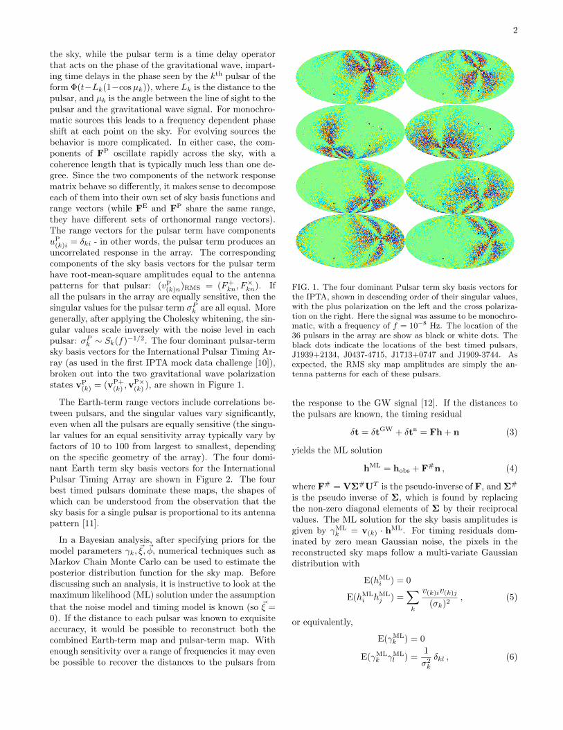
the sky, while the pulsar term is a time delay operatorthat acts on the phase of the gravitational wave, impart-ing time delays in the phase seen by the kth pulsar of theform Φ(t−Lk(1−cosµk)), where Lk is the distance to thepulsar, and µk is the angle between the line of sight to thepulsar and the gravitational wave signal. For monochro-matic sources this leads to a frequency dependent phaseshift at each point on the sky. For evolving sources thebehavior is more complicated. In either case, the com-ponents of FP oscillate rapidly across the sky, with acoherence length that is typically much less than one de-gree. Since the two components of the network responsematrix behave so differently, it makes sense to decomposeeach of them into their own set of sky basis functions andrange vectors (while FE and FP share the same range,they have different sets of orthonormal range vectors).The range vectors for the pulsar term have componentsuP(k)i = δki - in other words, the pulsar term produces anuncorrelated response in the array. The correspondingcomponents of the sky basis vectors for the pulsar termhave root-mean-square amplitudes equal to the antennapatterns for that pulsar: (vP(k)n)RMS = (F+

kn, F×kn). If

all the pulsars in the array are equally sensitive, then thesingular values for the pulsar term σP

k are all equal. Moregenerally, after applying the Cholesky whitening, the sin-gular values scale inversely with the noise level in eachpulsar: σP

k ∼ Sk(f)−1/2. The four dominant pulsar-termsky basis vectors for the International Pulsar Timing Ar-ray (as used in the first IPTA mock data challenge [10]),broken out into the two gravitational wave polarizationstates vP

(k) = (vP+(k) ,v

P×(k) ), are shown in Figure 1.

The Earth-term range vectors include correlations be-tween pulsars, and the singular values vary significantly,even when all the pulsars are equally sensitive (the singu-lar values for an equal sensitivity array typically vary byfactors of 10 to 100 from largest to smallest, dependingon the specific geometry of the array). The four domi-nant Earth term sky basis vectors for the InternationalPulsar Timing Array are shown in Figure 2. The fourbest timed pulsars dominate these maps, the shapes ofwhich can be understood from the observation that thesky basis for a single pulsar is proportional to its antennapattern [11].

In a Bayesian analysis, after specifying priors for themodel parameters γk, ~ξ, ~φ, numerical techniques such asMarkov Chain Monte Carlo can be used to estimate theposterior distribution function for the sky map. Beforediscussing such an analysis, it is instructive to look at themaximum likelihood (ML) solution under the assumption

that the noise model and timing model is known (so ~ξ =0). If the distance to each pulsar was known to exquisiteaccuracy, it would be possible to reconstruct both thecombined Earth-term map and pulsar-term map. Withenough sensitivity over a range of frequencies it may evenbe possible to recover the distances to the pulsars from

FIG. 1. The four dominant Pulsar term sky basis vectors forthe IPTA, shown in descending order of their singular values,with the plus polarization on the left and the cross polariza-tion on the right. Here the signal was assume to be monochro-matic, with a frequency of f = 10−8 Hz. The location of the36 pulsars in the array are show as black or white dots. Theblack dots indicate the locations of the best timed pulsars,J1939+2134, J0437-4715, J1713+0747 and J1909-3744. Asexpected, the RMS sky map amplitudes are simply the an-tenna patterns for each of these pulsars.

the response to the GW signal [12]. If the distances tothe pulsars are known, the timing residual

δt = δtGW + δtn = Fh + n (3)

yields the ML solution

hML = hobs + F#n , (4)

where F# = VΣ#UT is the pseudo-inverse of F, and Σ#

is the pseudo inverse of Σ, which is found by replacingthe non-zero diagonal elements of Σ by their reciprocalvalues. The ML solution for the sky basis amplitudes isgiven by γML

k = v(k) · hML. For timing residuals dom-inated by zero mean Gaussian noise, the pixels in thereconstructed sky maps follow a multi-variate Gaussiandistribution with

E(hMLi ) = 0

E(hMLi hML

j ) =∑k

v(k)iv(k)j

(σk)2, (5)

or equivalently,

E(γMLk ) = 0

E(γMLk γML

l ) =1

σ2k

δkl , (6)

3

FIG. 2. The four dominant Earth term sky basis vectorsfor the IPTA, shown in descending order of their singularvalues, with the plus polarization on the left and the crosspolarization on the right.

with no summation on k in the last expression. Thenoise in the reconstruction is dominated by sky mapswith small singular values. In a Bayesian analysis thisproblem can be avoided by using a trans-dimensionalMCMC to select the sub-set of the sky basis vectorsthat optimally balances model fidelity against modelcomplexity. In a frequentist analysis we can achievea similar result by using a low-rank approximation tothe pseudo-inverse, F#, which is found by replacingthe largest diagonal elements of Σ# by zero. Thereconstruction can be further improved by specifyingsuitable priors on the sky basis amplitudes.

In the event that the pulsar distances can not be deter-mined to sufficient accuracy, we can attempt to recoverthe Earth-term sky. To do this, we first break the timingresidual out into the contribution from the Earth-term,pulsar-term, and timing noise:

δt = δtE + δtP + δtn = FEh + FPh + n . (7)

In this case we treat the pulsar term as an additionalnoise source in the ML reconstruction. The Earth-termML solution is given by

hE,ML = hEobs + FE#FPh + FE#n , (8)

where FE# = VEΣE#UETis the pseudo-inverse of FE .

The ML solution for the Earth term sky basis ampli-tudes is given by γML

k = vE(k) · h

ML. The noise in the

FIG. 3. Sky map reconstruction of h2++h2

× for a point source.The first column uses the full 36 Earth-term sky basis vectorsfor the IPTA, while the second column uses the 10 basis func-tions with the largest singular values. The first row is for theEarth term contribution, while the second row includes pulsarand noise contributions. The whitened signal power was setequal to the whitened noise level. The white circles show thelocation of the point source, which is indicated by an arrowin the bottom left panel.

reconstruction δh = hE,ML−hEobs has contributions from

the instrument noise and the pulsar term. Figure 3 showsfull and reduced rank reconstructions of a point source.The full rank reconstruction with pulsar term and noiseis badly corrupted, while the reduced rank reconstructionis not.Statistically Isotropic Signals Since the sky template

analysis is entirely general, it can be used in place of thestandard cross-correlation analysis for isotropic stochas-tic signals. With a suitable parameterized prior on theamplitudes γk, defined below, the model shares the samedimensionality as the correlation analysis. However, thetemplate based analysis offers the distinct computationaladvantage of avoiding the inversion of large correlationmatrices when computing the likelihood.

A statistically isotropic stochastic signal is fully char-acterized by the expectation values for the sky-pixel am-plitudes:

E(hi) = 0

E(hihj) =1

2Shδij . (9)

The factor of one-half comes from averaging over the po-larization angle. If the pulsars distances were known, wecould work with the sky-basis vectors for the full responsematrix and write

δt = σk(v(k) · h)u(k) + n , (10)

from which it then follows that the timing residuals wouldbe described by a multi-variate Gaussian distributionwith

E(δti) = 0

E(δtiδtj) =1

2Shσ

2ku(k)iu(k)j + δij . (11)

4

The expression for the cross correlation can be put ina more familiar form if we recall that what we reallyhave in (11) is E((Qδt)i(Qδt)j). In the frequency do-main, under the assumption that the noise in each pulsaris uncorrelated, the noise correlation matrix is diagonal:Cij(f) = Si(f)δij , where Si(f) is the noise in the ith pul-

sar, and Qij(f) = S−1/2i (f)δij . Undoing the Cholesky

whitening we find

E(δtiδtj)Colored = Sh(f)βij + Si(f)δij , (12)

where the correlation matrix

βij =σ2k(f)

2u(k)iu(k)j(Si(f)Sj(f))1/2 (13)

is closely related to the Hellings-Downs (H&D) correla-tion matrix [4]. It differs since here we are considering theideal case where both the pulsar-term and the Earth-termcan be treated coherently. Using (4), it can be shown thatthe expectation values for the amplitudes of the ML skybasis vectors are given by

E(γMLk ) = 0

E(γMLk γML

l ) =

(Sh

2+

1

σ2k

)δkl . (14)

Equations (11) and (14) contain the same informationbut package it differently. In terms of the timing cor-relations in (11), the gravitational wave signal and theinstrument noise can be separated as they have differ-ent correlation matrices - the gravitational wave signalis correlated between pairs of pulsars while the noise isnot. In terms of the amplitude correlations in (14) thegravitational wave signal and the instrument noise canbe separated as they enter the different sky maps withdifferent strengths.

More realistically, when the pulsar distances are notknown to high accuracy we have to split the response intoEarth-term, pulsar-term and noise contributions whichleads to a multi-variate Gaussian distribution for the tim-ing residuals:

E(δti) = 0

E(δtiδtj) =Sh

(SiSj)1/2αij + δij , (15)

where αij is the H&D [4] correlation matrix

αij =1

2

((σE

k (f))2uE(k)iuE(k)j(Si(f)Sj(f))1/2 + δij

)=

1

2+

3

2κij lnκij −

1

3κij +

1

2δij (16)

with κij = (1−cos(θij))/2, where θij is the angle betweenthe line of sight to pulsars i, j. Note that the cross termE(δtEi δt

Pj ) vanishes since vE

(k) · vP(l) = 0, which is a con-

sequence of the pulsar-term sky maps oscillating rapidlyacross the sky and integrating to zero against the Earth-term sky maps which are smooth functions. Undoing the

Cholesky whitening and working in the frequency domainwe get

E(δtiδtj)Colored = Sh(f)αij + Si(f)δij , (17)

It is interesting to note that the scaled range vectors

uE(k)(i) = uE(k)(i)/(σEk S

1/2i ) diagonalize the Earth-term of

the H&D correlation matrix. The fact that the range vec-tors, which can be used to describe any GW signal, formthe H&D correlation matrix explains why this quantity,which was originally derived for isotropic skies, is alsorelevant to point sources [14].

The amplitudes of the sky basis maps for the Earth-term and pulsar-term each have the correlation structure

E(γk) = 0

E(γkγl) =Sh

2δkl . (18)

The Earth-pulsar cross terms vanish. In a Bayesian anal-ysis the correlation structure (18) serves as a prior on theγk. Analytically marginalizing over the pulsar-term con-tribution adds a diagonal component to the noise correla-tion matrix proportional to Sh/2. Analytically marginal-izing over the Earth-term contribution results in the stan-dard H&D correlation analysis. Alternatively, we cannumerically marginalize over the Earth-term GW tem-plates δtGW = γEk σkuE

(k), thereby avoiding the costlystep of inverting a large correlation matrix when com-puting the likelihood. The templates can be generatedin the Fourier domain then transformed to the time do-main and interpolated to match the un-even samplingof the data [13]. Updates to the noise model parame-

ters ~φ introduce a minor complication as they alter theCholesky whitening, which changes the sky basis vec-tors, singular values and range vectors. Since the up-dated Earth-term response matrix shares the same nullspace, column space and range as the original responsematrix the new sky basis vectors and range vectors canbe expressed as linear combinations of the original vec-tors, and the amplitudes of the sky basis amplitudes canbe mapped to the new basis. The model dimension forthe template based analysis matches that of the standardHellings-Downs cross-correlation analysis, but could offerdramatic computational savings since the only matricesthat need to be factorized or inverted are block diagonal.Anisotropic Signals The sky template approach is ide-

ally suited to studying anisotropic signals. Equation(8) provides a general maximum likelihood reconstruc-tion of any signal, but this can be improved upon in aBayesian analysis that builds in priors on the sky-basisamplitudes. The key signature of an anisotropic signal isa non-diagonal (though diagonal dominant) correlationmatrix γkγl. A variant of the isotropic search describedabove, but with a weaker prior on the correlation ma-trix, can be used to detect anisotropies in the nanoHzgravitational wave sky.

5

ACKNOWLEDGMENTS

We would like to thank Joe Romano for several infor-mative discussions. We thank Jonathan Gair, StephenTaylor, Joe Romano and Chiara Mingarelli for sharing adraft of their work using spherical harmonics to charac-terize anisotropic gravitational signals with pulsar tim-ing arrays, and for verifying several of our key resultsusing their formalism. NJC appreciates the support ofNSF grant PHY-1306702. RvH is supported by NASAEinstein Fellowship grant PF3-140116. This work waspartially carried out at the Jet Propulsion Laboratory,California Institute of Technology, under contract to theNational Aeronautics and Space Administration. Copy-right 2014.

[1] F. B. Estabrook and H. D. Wahquist, General Relativityand Gravitation 6, 439 (1975)

[2] M. V. Sazhin, Soviet Ast. 22, 36, (1978).

[3] S. L. Detweiler, Astrophys. J. 234, 1100 (1979).[4] R. w. Hellings and G. s. Downs, Astrophys. J. 265, L39

(1983).[5] R. S. Backer and D. C. Backer, ApJ 361, 300, (1990).[6] R. van Haasteren and Y. Levin, MNRAS 428, 1147

(2013). arXiv:1202.5932 [astro-ph.IM].[7] N. J. Cornish and J. D. Romano, Phys. Rev. D 87, no.

12, 122003 (2013) [arXiv:1305.2934 [gr-qc]].[8] K. M. Gorski, E. Hivon, A. J. Banday, B. D. Wandelt,

F. K. Hansen, M. Reinecke and M. Bartelman, Astro-phys. J. 622, 759 (2005)

[9] J. R. Gair, J. D. Romano, S. Taylor and C. M. F. Min-garelli, arXiv:1406.4664 [gr-qc].

[10] http:// www.ipta4gw.org/

[11] J. Romano, private communication.[12] V. Corbin and N. J. Cornish, arXiv:1008.1782 [astro-

ph.HE].[13] L. Lentati, P. Alexander, M. P. Hobson, S. Taylor,

J. Gair, S. T. Balan and R. van Haasteren, Phys. Rev.D 87, no. 10, 104021 (2013) [arXiv:1210.3578 [astro-ph.IM]].

[14] N. J. Cornish and A. Sesana, Class. Quant. Grav. 30,224005 (2013) [arXiv:1305.0326 [gr-qc]].