Mapping river bathymetries: Evaluatingtopobathymetric LiDAR surveyDaniele Tonina,1* James A. McKean,2 Rohan M. Benjankar,3 C. Wayne Wright,4 Jaime R. Goode,5 Qiuwen Chen,6

William J. Reeder,1 Richard A. Carmichael1 and Michael R. Edmondson71 Center for Ecohydraulics Research, University of Idaho, 322 E. Front Street, suite 340, Boise, Idaho 83702, USA2 US Forest Service, Rocky Mountain Research Station, 322 E. Front Street, suite 401, Boise, Idaho 83702, USA3 Civil Engineering Department, Southern Illinois University Edwardsville, Edwardsville, Illinois 620254 US Geological Survey, Remote Sensing, Florida Integrated Science Center, St. Petersburg, FL 33701, USA5 Mathematics & Physical Sciences Department and Environmental Studies, The College of Idaho, 2112 Cleveland Blvd Caldwell ID83605, USA

6 Center for Eco-Environmental Research, Nanjing Hydraulic Research Institute, Nanjing 210098, China7 Idaho Office of Species Conservation, 304 N. 8th Street, Suite 149, Boise, ID 83702, USA

Received 26 May 2018; Revised 10 September 2018; Accepted 13 September 2018

*Correspondence to: Daniele Tonina, University of Idaho, Center for Ecohydraulics Research, 322 E. Front Street, suite 340; Boise, Idaho 83702, USA. E-mail:dtonina@uidaho.edu

ABSTRACT: Advances in topobathymetric LiDARs could enable rapid surveys at sub-meter resolution over entire stream networks.This is the first step to improving our knowledge of riverine systems, both their morphology and role in ecosystems. The ExperimentalAdvanced Airborne Research LiDAR B (EAARL-B) system is one such topobathymetric sensor, capable of mapping both terrestrialand aquatic systems. Whereas the original EAARL was developed to survey littoral areas, the new version, EAARL-B, was also de-signed for riverine systems but has yet to be tested. Thus, we evaluated the ability of EAARL-B to map bathymetry and floodplaintopography at sub-meter resolution in a mid-size gravel-bed river. We coupled the EAARL-B survey with highly accurate field sur-veys (0.03m vertical accuracy and approximately 0.6 by 0.6m resolution) of three morphologically distinct reaches, approximately200m long 15m wide, of the Lemhi River (Idaho, USA). Both point-to-point and raster-to-raster comparisons between ground andEAARL-B surveyed elevations show that differences (ground minus EAARL-B surveyed elevations) over the entire submerged topog-raphy are small (root mean square error, RMSE, and median absolute error, M, of 0.11m), and large differences (RMSE, between 0.15and 0.38m and similar M) are mainly present in areas with abrupt elevation changes and covered by dense overhanging vegetation.RMSEs are as low as 0.03m over paved smooth surfaces, 0.07m in submerged, gradually varying topography, and as large as 0.24malong banks with and without dense, tall vegetation. EAARL-B performance is chiefly limited by point density in areas with strongelevation gradients and by LiDAR footprint size (0.2m) in areas with topographic features of similar size as the LiDAR footprint.© 2018 John Wiley & Sons, Ltd.

KEYWORDS: topobathymetric LiDAR; streambed bathymetry; performance of green LiDAR

Introduction

Investigations of morphology, habitat conditions and ecosys-tem function of streams depend on accurate maps of the ba-thymetry made with a resolution and extent appropriate forstudying abiotic and biotic processes (Carbonneau et al.,2012). Stream morphology is shaped by sediment transport,which in turn is a function of the local (0.1m scale) interactionbetween stream flow and streambed sediment (Wheaton et al.,2010; Maturana et al., 2013). The performance of multi-dimensional, numerical, hydrodynamic models in riverine sys-tems directly depends on bathymetric accuracy and resolution(Lane et al., 2005; Pasternack et al., 2006; Tonina and Jorde,2013), as does water and solute exchange between streamsand streambed sediments (Tonina et al., 2015; Benjankaret al., 2016). Stream habitat monitoring (White et al., 2002),

modeling (Pasternack et al., 2006; McDonald et al., 2010;Kammel et al., 2016), and management (Le Pichon et al.,2006) require a survey resolution comparable with the scaleof organism sizes, their mobility and the entire extent of theriver domain used throughout their full life cycle. Furthermore,highly mobile species, such as salmonids, may travel long dis-tances, forcing us to map not just stream reaches or sections,but whole river networks (Fausch et al., 2002; Isaak et al.,2007). Thus, to support these diverse analyses and improveour understanding of riverine systems and processes, bathyme-try surveys ideally must meet quite demanding survey criteria,including the ability to map entire stream segments (up to104m) with sub-meter spatial resolution and decimeter or evencentimeter-scale vertical accuracy.

A variety of survey methods have recently been developed tomap stream bathymetry and near-channel environments

EARTH SURFACE PROCESSES AND LANDFORMSEarth Surf. Process. Landforms 44, 507–520 (2019)© 2018 John Wiley & Sons, Ltd.Published online 4 November 2018 in Wiley Online Library(wileyonlinelibrary.com) DOI: 10.1002/esp.4513

(McKean et al., 2009c; Pasternack and Senter, 2011; Waltheret al., 2011; Carbonneau et al., 2012). Airborne near-infrared(NIR) LiDAR (Cavalli et al., 2008) has been suggested for qual-itative mapping of the main morphological features in shallowsystems (water depths less than 0.5m) because of the inabilityof the infrared beam to adequately penetrate water, such thatto map the bed topography with NIR LiDAR the channel shouldbe completely dry. Real-time kinematic (RTK) differential globalposition systems (DGPS) have been used for very high resolu-tion surveying of subaerial topography of floodplains and otherareas around streams. However, for surveying submerged to-pography, RTK DGPS is limited to wadable reaches for tradi-tional data collection with surveyors carrying the instrumentsor with instruments installed on vehicles (Brasington et al.,2000). Its application by installing it on floating devices, cou-pling with an echo-sounder can overcome the limitation to sur-vey non-wadable sections of streams (Kammel et al., 2016).Multi- and hyper-spectral image analyses (Marcus et al.,2003; Legleiter et al., 2009) have also been used to map waterdepths (rather than submerged topography), but their successdepends on accurately defining local water optical propertiesand linking those to changes in water depth and turbidity ofstream water. These passive optical surveys have generallybeen limited to short reaches (Legleiter et al., 2015). Multibeamsonar (Conner and Tonina, 2014) has been shown to be very ef-fective in large, navigable streams and rivers where sufficientflow depth is available for power boats. Standard photogram-metric techniques have also shown promising results in defin-ing submerged topography, but as with hyper-spectral imageanalysis, this approach requires site-specific, light-dependentrelationship between depth and water color, which coulddepend on water turbidity and be influenced by overhangingvegetation, substrate type, and water surface characteristics(Carbonneau et al., 2006).Following the success of near-infrared LiDAR in mapping

terrestrial systems, topobathymetric airborne LiDARs, includingthe NASA Experimental Advanced Airborne Research LiDAR(EAARL) (McKean et al., 2009b), the Optech Scanning Hydro-graphic Operational Airborne LiDAR System (SHOALS)(Hilldale and Raff, 2007), the Coastal Zone Mapping and Imag-ing Lidar (CZMIL) (Tuell et al., 2010), the Laser Airborne DepthSounder (LADS) Mk II and Mk 3 (Parker and Sinclair, 2012), theRiegl VQ-820-G (Mandlburger et al., 2011), the OptechAquarius (Fernandez-Diaz et al., 2014), the Teledyne OptechTitan TopoBathy Sensor (Fernandez-Diaz et al., 2016) andLeica Aquatic Hydrography AB (AHAB) Chiroptera II andHawkEye II and III (Quadros, 2013), have recently beenapplied to stream systems (McKean et al., 2009a). All of thesesystems use a green wavelength laser, which has very lowabsorbance in water, rather than the near-infrared to mapsubmerged topography (McKean et al., 2009a).Whereas topobathymetric LiDAR performance in littoral sys-

tems is well documented and has become an established tech-nique (Nayegandhi et al., 2006, 2009), this approach has notbeen systematically tested (McKean et al., 2009c, 2014;Mandlburger et al., 2015; Pan et al., 2015) and accepted in riv-erine systems (Kinzel et al., 2013; Legleiter et al., 2015). None-theless, recent investigations showed the advantages ofbathymetric LiDAR in ecohydraulics applications that aim tounderstand the interaction between biotic and abiotic pro-cesses in lotic systems (Tonina and McKean, 2010; Toninaet al., 2011; McKean and Tonina, 2013). Previous studies ontopobathymetric LiDAR, and specifically the original EAARLsystems (McKean et al., 2009c, 2014), highlighted the mainproblems for application in riverine systems: (1) low resolutionof the survey (0.3 points/m2); and (2) difficulty mapping deeppools and banks. A new EAARL system, EAARL-B (Wright

et al., 2016), has recently been designed and developed formapping both riverine and littoral systems to address theselimitations. Similar to EARRL, EAARL-B flies at an operatingaltitude of 300m and has a 240m swath width and covers40–80 km2/h. It uses a small 0.2-m footprint 400μJ green laser,with 30 000 pulses per second, each 1.2 ns long and a 1 ns dig-itizer. The new system splits the light beam into three beamletsthat are staggered to increase the survey resolution reaching anominal density of 1 pt/m2 with one flight line. Additionally, afourth dedicated receiver merges the three beamlets to increasethe energy of the returning waveform to improve water penetra-tion in deep pools. This allows a wide range of water depthsfrom 0 to 44m with very clear water (1.5 secchi depth). TheLiDAR is co-registered with a color-infrared (CIR) and colordigital cameras, and each camera has an 80% image overlap.The new sensor potentially could become the first of a newgeneration of topobathymetric instruments capable of mappingentire river systems at the resolution needed for mostecohydraulics studies.

Here, we systematically test the performance of the EAARL-Bsystem, which mapped the entire Lemhi River (Idaho, USAapproximately 100 km stream length) in October 2013, inmapping the bathymetry of three morphologically distinctreaches of this stream by comparing results against very accu-rate sub-meter resolution (1.67 points/m2) RTK DGPS groundsurveys. Previous studies used coarse ground survey (0.08points/m2) to compare with EAARL data (0.3 points/m2)(McKean et al., 2009b, 2009c, 2014), a resolution that is notadequate for evaluating its ability to map microhabitat. Theseprevious works also indicated that the EAARL system was notable to map banks because of the very low density in narrowareas (typically 1–2m wide) where topographical gradientsare strong (from 30 degree to vertical banks). These early worksdid not systematically analyze the performance of the LiDARsystem for each morphological feature of a stream reach. Thus,we analyze the performance of the LiDAR in each one of aseries of zones with uniform morphology and vegetation (e.g.banks, riffles, pools, runs, and tall versus short vegetation) to in-vestigate the effects of topographic complexity and vegetationon survey accuracy. Our accuracy assessment includes bothpoint measurements (which was not possible in previous work)and comparison of rasters created from point clouds.

Methodology

Study area

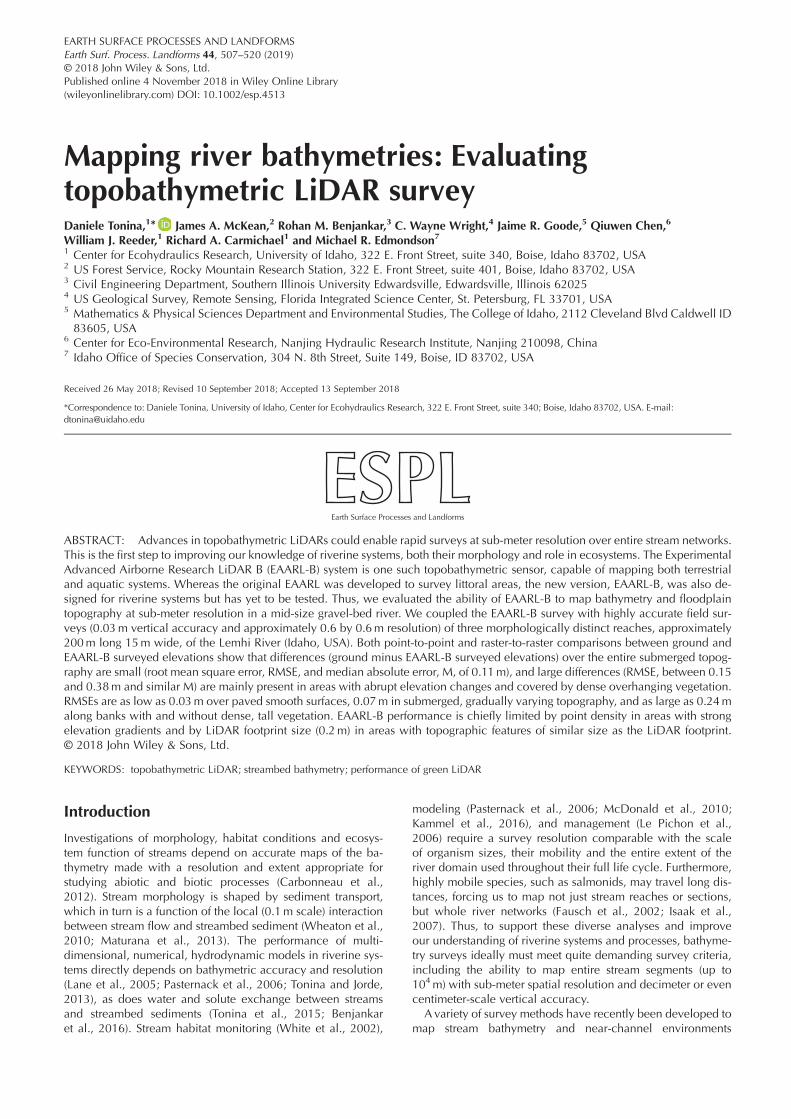
The Lemhi River Basin (3260 km2) is located near the Idaho-Montana border with an elevation range between 1585 and2745m (Figure 1). Annual precipitation ranges between 230and 1016mm and hydrology is snowmelt dominated, with70% of precipitation falling as snow during the winter monthsbetween November and April. The Lemhi River is a gravel-bed stream with a bankfull width ranging between 8 and20m. Its minimum, average, and maximum daily mean dis-charges measured at the confluence with the Salmon Riverare 0.02, 7.11, 73.91m3/s, respectively (Borden, 2014).

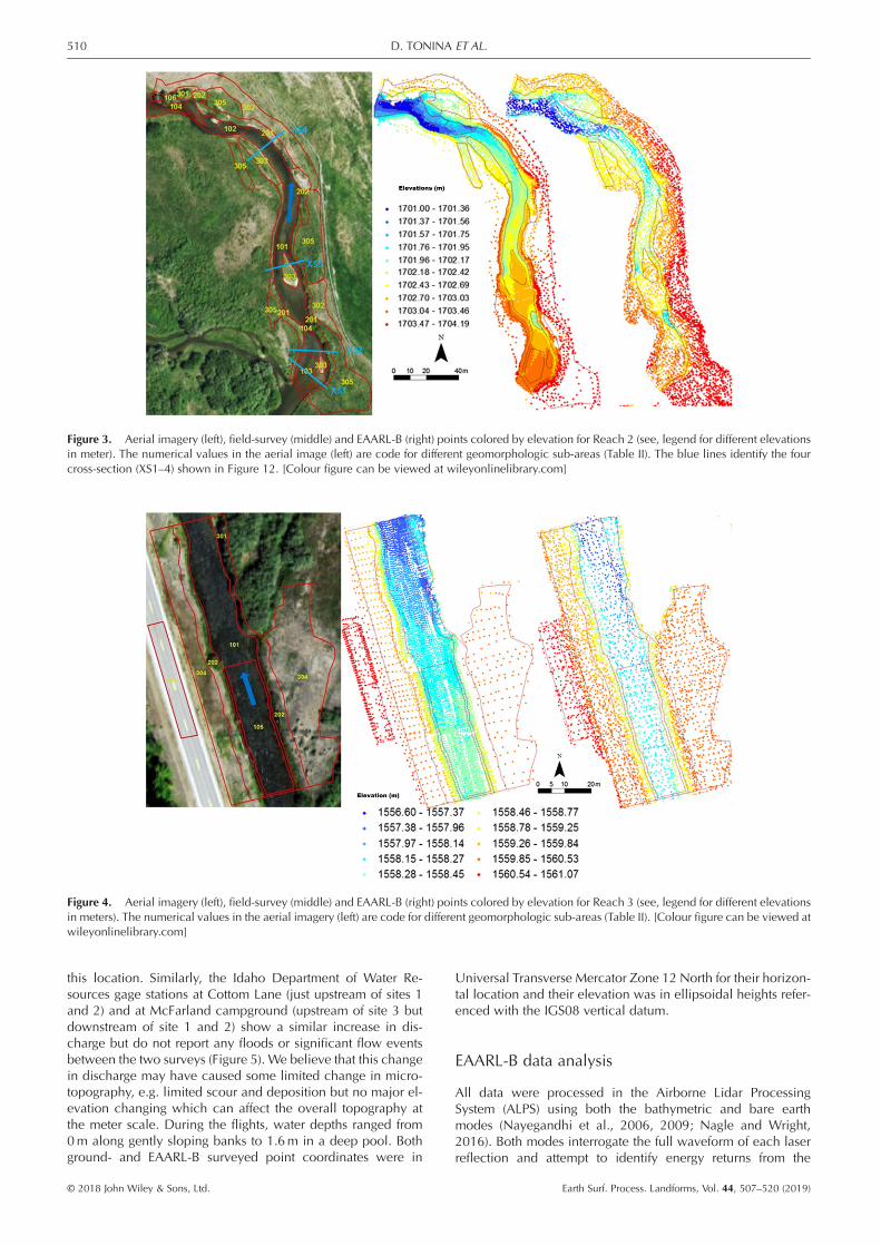
We selected three geomorphically different channel reachesas test sites for quantifying the accuracy of the EAARL-B surveyin different stream morphologies. Reach 1 has an average reachslope of 0.53% and includes a long bend with a deep pool(1.5m), riffles and runs. It is approximately 160m long and10m wide (Figure 2) with substrate dominated by gravel(2–64mm) and cobbles (64–256mm). Reach 2 is a morpholog-ically complex reach, which includes pools (~1.6m deep),riffles, runs, and vegetated point bars (Figure 3). It is

508 D. TONINA ET AL.

© 2018 John Wiley & Sons, Ltd. Earth Surf. Process. Landforms, Vol. 44, 507–520 (2019)

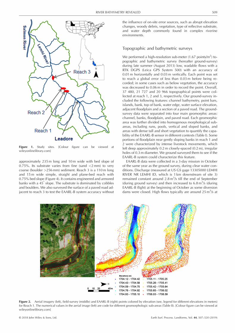
approximately 235m long and 10m wide with bed slope of0.75%. Its substrate varies from fine (sand <2mm) to verycoarse (boulder >256mm) sediment. Reach 3 is a 110m longand 15m wide simple, straight and plane-bed reach with0.75% bed slope (Figure 4). It contains engineered and armoredbanks with a 45° slope. The substrate is dominated by cobblesand boulders. We also surveyed the surface of a paved road ad-jacent to reach 3 to test the EAARL-B system accuracy without

the influence of on-site error sources, such as abrupt elevationchanges, woody debris, vegetation, type of reflective substrate,and water depth commonly found in complex riverineenvironments.

Topographic and bathymetric surveys

We performed a high-resolution sub-meter (1.67 points/m2) to-pographic and bathymetric survey (hereafter ground-survey)during late summer (August 2013) low, wadable flows with aRTK DGPS (Leica GPS System 500) with an accuracy of0.01m horizontally and 0.03m vertically. Each point was setto reach a global error of less than 0.03m before being re-corded; in some cases such as below vegetation, the accuracywas decreased to 0.06m in order to record the point. Overall,37 480, 21 727 and 20 966 topographical points were col-lected at reach 1, 2 and 3, respectively. Our ground-survey in-cluded the following features: channel bathymetry, point bars,islands, bank, top of bank, water edge, water surface elevation,adjacent floodplain and a section of a paved road. The ground-survey data were separated into four main geomorphic areas:channel, banks, floodplain, and paved road. Each geomorphicarea was further divided into homogenous morphological sub-areas, including runs, pools, vertical and sloped banks, andareas with dense tall and short vegetation to quantify the capa-bility of the EAARL-B sensor in different contexts (Table I). Someportions of floodplain near gently sloping banks in reach 1 and2 were characterized by intense livestock movements, whichleft deep approximately 0.2m closely-spaced (0.2m), irregularholes of 0.3m diameter. We ground surveyed them to see if theEAARL-B system could characterize this feature.

EAARL-B data were collected in a 3-day mission in Octoberof the same year as the ground survey, during clear water con-ditions. Discharge (measured at US GS gage 13305000 LEMHIRIVER NR LEMHI ID, which is 1 km downstream of site 3)remained constant around 2.8m3/s till the end of September(during ground survey) and then increased to 6.8m3/s (duringEAARL-B flight) at the beginning of October as some diversiondams were closed. High flows typically are around 25m3/s at

Figure 1. Study sites. [Colour figure can be viewed atwileyonlinelibrary.com]

Figure 2. Aerial imagery (left), field-survey (middle) and EAARL-B (right) points colored by elevation (see, legend for different elevations in meters)for Reach 1. The numerical values in the aerial image (left) are code for different geomorphologic sub-areas (Table II). [Colour figure can be viewed atwileyonlinelibrary.com]

509RIVER BATHYMETRY REVEALED

© 2018 John Wiley & Sons, Ltd. Earth Surf. Process. Landforms, Vol. 44, 507–520 (2019)

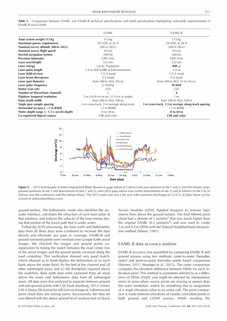
this location. Similarly, the Idaho Department of Water Re-sources gage stations at Cottom Lane (just upstream of sites 1and 2) and at McFarland campground (upstream of site 3 butdownstream of site 1 and 2) show a similar increase in dis-charge but do not report any floods or significant flow eventsbetween the two surveys (Figure 5). We believe that this changein discharge may have caused some limited change in micro-topography, e.g. limited scour and deposition but no major el-evation changing which can affect the overall topography atthe meter scale. During the flights, water depths ranged from0m along gently sloping banks to 1.6m in a deep pool. Bothground- and EAARL-B surveyed point coordinates were in

Universal Transverse Mercator Zone 12 North for their horizon-tal location and their elevation was in ellipsoidal heights refer-enced with the IGS08 vertical datum.

EAARL-B data analysis

All data were processed in the Airborne Lidar ProcessingSystem (ALPS) using both the bathymetric and bare earthmodes (Nayegandhi et al., 2006, 2009; Nagle and Wright,2016). Both modes interrogate the full waveform of each laserreflection and attempt to identify energy returns from the

Figure 3. Aerial imagery (left), field-survey (middle) and EAARL-B (right) points colored by elevation for Reach 2 (see, legend for different elevationsin meter). The numerical values in the aerial image (left) are code for different geomorphologic sub-areas (Table II). The blue lines identify the fourcross-section (XS1–4) shown in Figure 12. [Colour figure can be viewed at wileyonlinelibrary.com]

Figure 4. Aerial imagery (left), field-survey (middle) and EAARL-B (right) points colored by elevation for Reach 3 (see, legend for different elevationsin meters). The numerical values in the aerial imagery (left) are code for different geomorphologic sub-areas (Table II). [Colour figure can be viewed atwileyonlinelibrary.com]

510 D. TONINA ET AL.

© 2018 John Wiley & Sons, Ltd. Earth Surf. Process. Landforms, Vol. 44, 507–520 (2019)

ground surface. The bathymetric mode also identifies the air–water interface, calculates the refraction of each laser pulse atthat interface, and reduces the velocity of the laser energy dur-ing that portion of the travel path that is under water.Following ALPS processing, the bare earth and bathymetric

data from all three days were combined to increase the datadensity and eliminate any gaps in coverage. EAARL-B andground surveyed points were overlaid over Google Earth aerialimages. We checked the images and ground points co-registration by testing the match between the road center lineof the aerial images and the ground points surveyed along theroad centerline. This verification showed very good match,which allowed us to hand digitize the delineation of (a) eachbank above the water level, (b) the bed of the channel and allother submerged areas, and (c) the floodplain exposed abovethe waterline. Bare earth data were extracted from all areasabove the water and bathymetric data from all submergedareas. All data were first analyzed to separate between groundand non-ground points with LAS Tools (Isenburg, 2012) (whereLAS is binary file format for efficient exchange of 3-dimensionalpoint cloud data sets among users). Successively, the data setwas filtered with the above ground level analysis tool of Quick

Terrain Modeler (QTM, Applied Imagery) to remove laserreturns from above the ground surface. The final filtered pointcloud had a density of 1 point/m2 that was much higher thanthe original EAARL (0.3 points/m2) and was used to create1m and 0.5m DEMs with the Natural Neighborhood interpola-tion method (Sibson, 1981).

EAARL-B data accuracy analysis

EAARL-B accuracy was quantified by comparing EAARL-B andground surveys using two methods: raster-to-raster (hereafterraster) and point-to-point (hereafter point) based comparison(Skinner, 2011; Woodget et al., 2015). The raster comparisoncomputes the elevation difference between DEMs for each in-dividual pixel. This method is sometimes referred to as a differ-ence of DEMs (DoD), and might be affected by interpolationerrors in areas where survey points are missing or sparser thanthe raster resolution, and/or by smoothing due to assignmentof a single elevation value to an entire cell. The point compar-ison is made between elevations of closely coincident points inboth ground and LiDAR surveys. While avoiding the

Table I. Comparison between EAARL and EAARL-B technical specifications with bold specifications highlighting noticeable improvements ofEAARL-B over EAARL

EAARL EAARL-B

Total system weight 113 kg 113 kg 113 kgMaximum power requirement 28 VDC at 26 A 28 VDC at 26 ANominal survey altitude 300m (AGL) 300m (AGL) 300m (AGL)Nominal survey flight speed 50m/s 50m/sInertial navigation system 200Hz 200HzPrecision kinematic GPS 2Hz GPS 2HzLaser wavelength 532 nm 532 nmLaser energy Up to 70 μJ/pulse 400 μJLaser pulse length 1.2 ns (full width at half-maximum) 1.2 nsLaser field-of-view 1.5–2 mrad 1.5–2 mradLaser beam divergence 0.5 mrad 0.5 mradLaser spot diameter from 300m AGL 20 cm from 300m AGL 15 to 20 cmLaser pulse frequency 3–10 kHz 30 kHZRaster scan rate 25/s 25/sNumber of Waverfrom channels 1 4Digitizer temporal resolution 1 ns (14.9 cm in air, 11.3 cm in water) 1 nsData swath width from 300m AGL 240m from 300m AGL 240mSingle pass sample spacing 2m cross-track, 2m average along-track 1m cross-track, 1.5m average along-track spacingHorizontal accuracy <1m RMSE <1m RMSE <1m RMSEWater depth range (~ 1.5 x secchi depth) 0 to 28m 0 to 44mCo-registered digical camers CIR and color CIR and color

Figure 5. 2013 hydrographs at Idaho Department Water Resources gage station at Cottom Lane (just upstream of site 1 and 2) and McFarland camp-ground (upstream of site 3 and downstream of sites 1 and 2), and USGS gage station near Lemhi (downstream of site 3) and at Salmon (in the City ofSalmon near the confluence with the Salmon River). The 2013 water year was a dry year with maximum discharges at 12m3/s. [Colour figure can beviewed at wileyonlinelibrary.com]

511RIVER BATHYMETRY REVEALED

© 2018 John Wiley & Sons, Ltd. Earth Surf. Process. Landforms, Vol. 44, 507–520 (2019)

interpolation issues of the DoD method, the point-based ap-proach might include errors due to real changes in elevationwithin the distance between compared points, because pointsare never at exactly the same location in both the ground andLiDAR surveys. For example, elevations may change rapidlybetween top and bottom of a boulder or on sloped surfaces likebanks or the sides of pools. Additionally, ground-survey dataare point measurements, whereas EAARL-B data are spatiallyaveraged elevations within the footprint area, typically a circleof 0.2m diameter.In the DoD analysis, we used 0.5 (hereafter sub-meter, SMR)

and 1m (hereafter meter, MR) resolution raster to analyze accu-racy at the scale of individual DEM grid cells. These high-resolution cell sizes are typically used in hydrodynamic model-ing for quantifying aquatic habitat quality (Gard, 2009;Benjankar et al., 2014; Kammel et al., 2016). Raster surfacesare interpolated with the Natural Neighborhood interpolationmethod and comparison was restricted to the extent of theground-survey areas so the comparisons between the EAARL-B and ground-survey raster had similar spatial extents.The point-based analysis is restricted to ground points that

have at least one EAARL-B point within a 0.1m radius, whichcoincides with that of the laser footprint. We selected the clos-est EAARL-B point when more than one was available. The0.1m distance threshold minimizes the error due to elevationvariability between the two points being compared and stillpreserves a large sample of points for statistical analysis. Typi-cally, we had only a single point and rarely two points withinthe 0.1m radius, which prevented us from studying the statis-tics of point cloud elevations, such as mean and variance,within the EAARL-B footprints.The errors between the EAARL-B and ground-survey eleva-

tions are reported with their frequency distribution, median ab-solute error (M, the residual that is half way through the ordereddata set), mean error (or bias, B), root mean square error (RMSE),and the correlation coefficient (R2) for the regression of EAARL-B and ground-survey elevations for each morphologic area andsub-area. We calculated errors, residuals, Res, as ground-surveyelevations, z, minus EAARL-B-surveyed elevations,

Resi ¼ zg;i � zL;i (1)

M ¼ median jResi jð Þ ¼ j∣Resnþ 1

2

∣ if n is odd

Resn2∣þ ∣Resn

2þ 1

∣

2if n is even

8>><>>:

(2)

B ¼ 1n∑n

i¼1Resi (3)

RMSE ¼ffiffiffiffiffiffiffiffiffiffiffiffiffiffiffiffiffiffiffiffi1n∑n

i¼1Res2i

s(4)

where n is the total number of points, i is the ith point and sub-scripts L and g stand for EAARL-B and ground survey, respec-tively. Therefore, positive bias indicates a higher elevationvalue for ground-survey data than for the EAARL-B data. Lowmagnitudes of RMSE, M, and B and high values of R2 indicategood agreement between surveys. Mean error helps to identifysystematic bias between the two surveys, whereas the medianabsolute error is insensitive to the effect of large residuals (out-liers). Thus, M is more robust to outliers than RMSE, becauseRMSE squares the residuals before averaging them giving ahigher weight to large errors than M. The comparison betweenM and RMSE values helps to identify the presence of large errorswithin the residual distribution.

We report the results in three sections, one for each of threemain geomorphic features: channel, banks and floodplain. Ad-ditionally, we analyzed the accuracy of the system by surveyinga nearby paved road. The channel area covers the streambedsection and is fully submerged. The bank area is a narrow band,partially submerged, between the bottom and top of the bank,and thus is where data analysis transitions between the bathy-metric and terrestrial algorithms. The floodplain area is a terres-trial environment.

Results

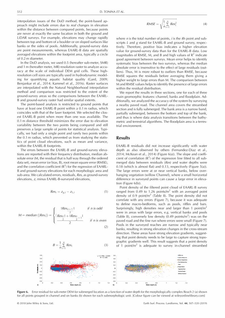
EAARL-B residuals did not increase significantly with waterdepth as also observed by others (Fernandez-Diaz et al.,2014; McKean et al., 2014) (Figure 6(a)). The slope and coeffi-cient of correlation (R2) of the regression line fitted to all sub-merged data between residuals (Res) and water depths were0.18 (which is almost flat) and 0.13, respectively (Figure 5(a)).The large errors were at or near vertical banks, below over-hanging vegetation (willow Channel), where a small horizontaldifference in surveyed points can cause a large error in eleva-tion (Figure 6(b)).

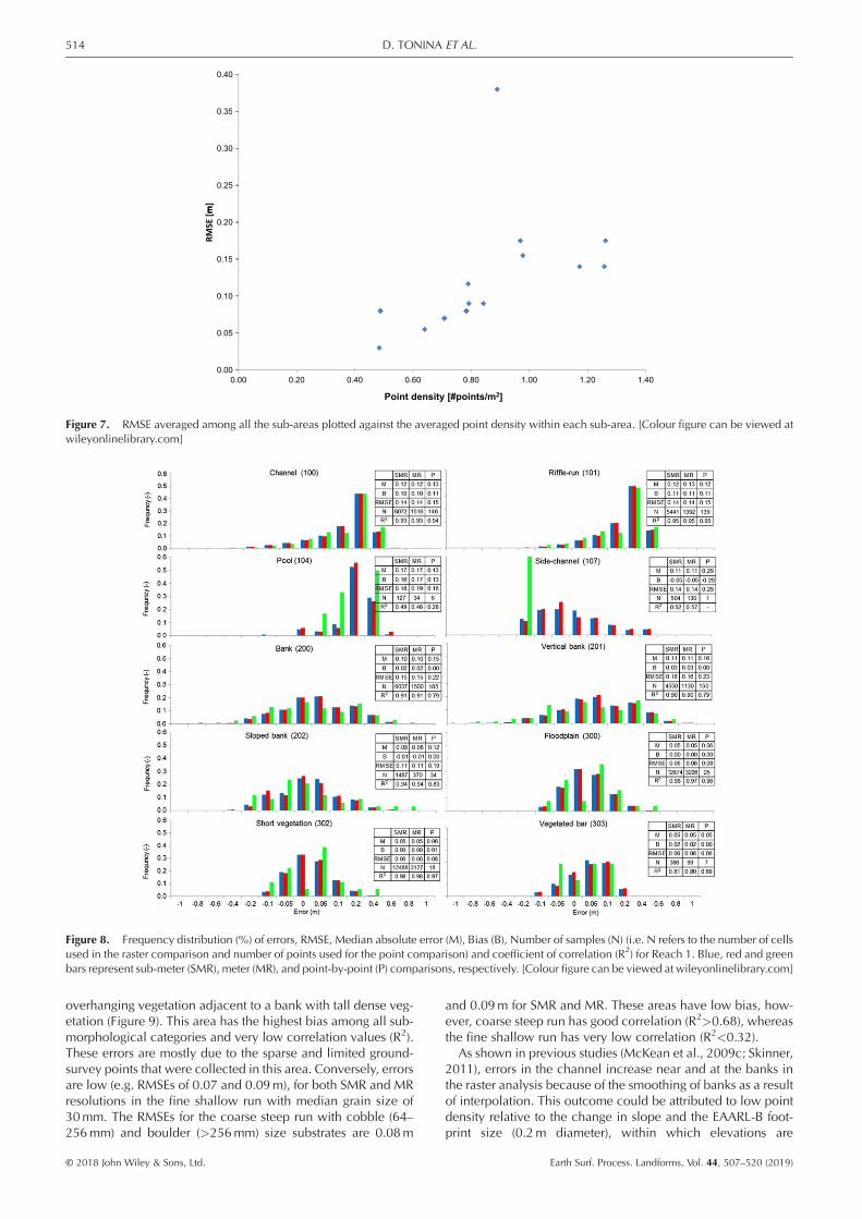
Point density of the filtered point cloud of EAARL-B surveyranged from 0.49 to 1.26 points/m2 with an averaged pointdensity of 0.9 point/m2 (Table II). The point density did notcorrelate with any errors (Figure 7), because it was adequateto define macro-bedforms, such as pools, riffles and bars.Surprisingly, high densities near and larger than 1 point/m2

were in areas with large errors, e.g. vertical banks and pools(Table II), conversely low density (0.49 points/m2) was on thepaved road and the fine run where errors were small (Figure 7).Pools in the surveyed reaches are narrow and typically nearbanks, resulting in strong elevation changes in the cross-streamdirection. These areas have strong elevation gradients, suggest-ing that point density needs to be large to capture strong topo-graphic gradients well. This result suggests that a point densityof 1 point/m2 is adequate to survey in-channel streambed

Figure 6. Error residual for sub-meter DEM for submerged location as a function of water depth for the morphologically complex Reach 2 (a) shownfor all points grouped in channel and on banks (b) shown for each submorphologic unit. [Colour figure can be viewed at wileyonlinelibrary.com]

512 D. TONINA ET AL.

© 2018 John Wiley & Sons, Ltd. Earth Surf. Process. Landforms, Vol. 44, 507–520 (2019)

features in small streams like the Lemhi. However, higher den-sity is needed in areas characterized by strong elevationchanges, like banks and steep pool sides.

Paved surface

Paved surfaces, like roads, provide an ideal area to test the min-imum expected error of EAARL-B because of their gentlechange in elevation, lack of submergence (completely dry),uniform reflectivity of the asphalt, and lack of vegetative cover.The largest errors, M (0.05m), B (–0.05m) and RMSE (0.04m),are from the point analysis (Figure 10). These large errors couldbe due to the low number of points, only four, within a 0.1mradius. Conversely, both sub-meter and meter DEM have simi-lar errors: RMSE is 0.03m, which is similar to many DGPS sur-veys, and M and B are even smaller.

Channel

The overall RMSEs for the channel vary from 0.10 to 0.15m forboth raster and point based comparisons (Figures 8, 9 and 10)regardless of substrate size (from sand to boulder, >256mm)and morphological complexity (straight featureless andmeandering pool–riffle reaches). Errors are a bit smaller forthe sub-meter than meter resolutions and for the raster thanfor the point comparison. Both bias (mean error) and medianabsolute error values are always lower than RMSEs and resid-uals do not vary systematically with depth (Fernandez-Diazet al., 2014; McKean et al., 2014) or morphological unit. Corre-lations between EAARL-B and field-survey elevations are strong(R2>0.9) regardless of comparison and raster resolution, exceptfor reach 3.

The RMSE in deep pools varies from 0.16 to 0.19m for reach2 and 1, respectively (Figures 9 and 8). The largest error (RMSEof 0.38m) is estimated in a deep pool (reach 2) below

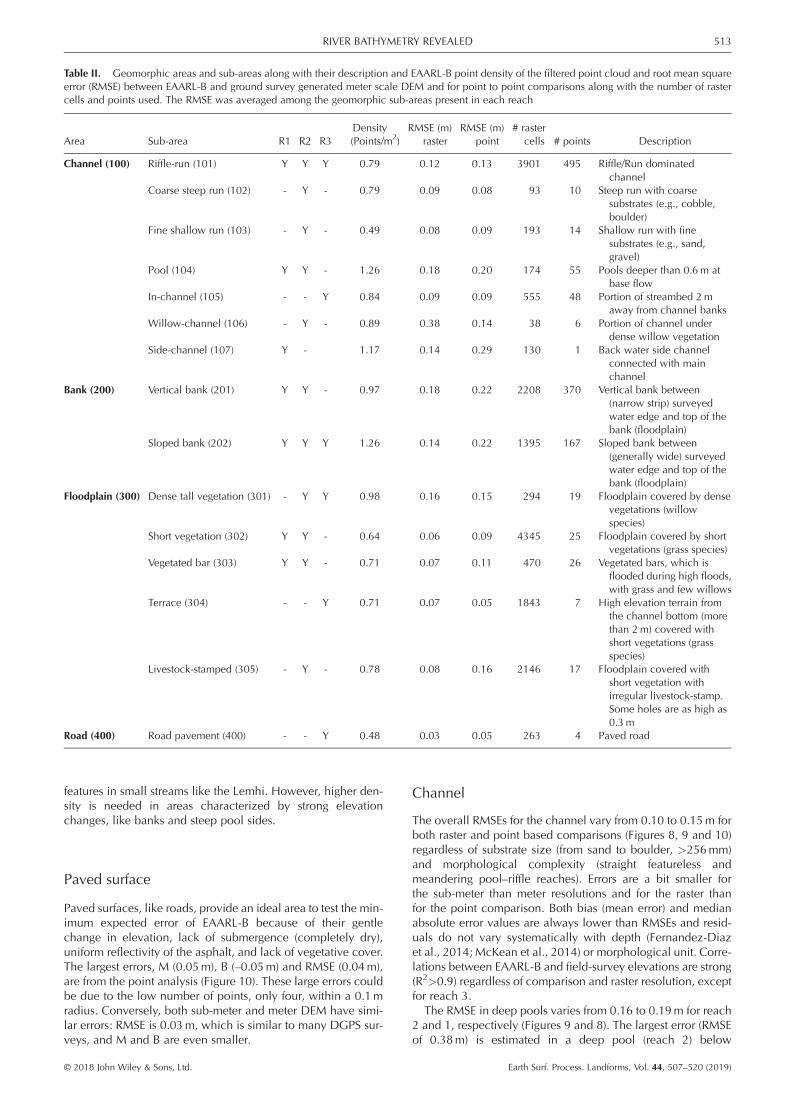
Table II. Geomorphic areas and sub-areas along with their description and EAARL-B point density of the filtered point cloud and root mean squareerror (RMSE) between EAARL-B and ground survey generated meter scale DEM and for point to point comparisons along with the number of rastercells and points used. The RMSE was averaged among the geomorphic sub-areas present in each reach

Area Sub-area R1 R2 R3Density(Points/m2)

RMSE (m)raster

RMSE (m)point

# rastercells # points Description

Channel (100) Riffle-run (101) Y Y Y 0.79 0.12 0.13 3901 495 Riffle/Run dominatedchannel

Coarse steep run (102) - Y - 0.79 0.09 0.08 93 10 Steep run with coarsesubstrates (e.g., cobble,boulder)

Fine shallow run (103) - Y - 0.49 0.08 0.09 193 14 Shallow run with finesubstrates (e.g., sand,gravel)

Pool (104) Y Y - 1.26 0.18 0.20 174 55 Pools deeper than 0.6m atbase flow

In-channel (105) - - Y 0.84 0.09 0.09 555 48 Portion of streambed 2maway from channel banks

Willow-channel (106) - Y - 0.89 0.38 0.14 38 6 Portion of channel underdense willow vegetation

Side-channel (107) Y - 1.17 0.14 0.29 130 1 Back water side channelconnected with mainchannel

Bank (200) Vertical bank (201) Y Y - 0.97 0.18 0.22 2208 370 Vertical bank between(narrow strip) surveyedwater edge and top of thebank (floodplain)

Sloped bank (202) Y Y Y 1.26 0.14 0.22 1395 167 Sloped bank between(generally wide) surveyedwater edge and top of thebank (floodplain)

Floodplain (300) Dense tall vegetation (301) - Y Y 0.98 0.16 0.15 294 19 Floodplain covered by densevegetations (willowspecies)

Short vegetation (302) Y Y - 0.64 0.06 0.09 4345 25 Floodplain covered by shortvegetations (grass species)

Vegetated bar (303) Y Y - 0.71 0.07 0.11 470 26 Vegetated bars, which isflooded during high floods,with grass and few willows

Terrace (304) - - Y 0.71 0.07 0.05 1843 7 High elevation terrain fromthe channel bottom (morethan 2m) covered withshort vegetations (grassspecies)

Livestock-stamped (305) - Y - 0.78 0.08 0.16 2146 17 Floodplain covered withshort vegetation withirregular livestock-stamp.Some holes are as high as0.3m

Road (400) Road pavement (400) - - Y 0.48 0.03 0.05 263 4 Paved road

513RIVER BATHYMETRY REVEALED

© 2018 John Wiley & Sons, Ltd. Earth Surf. Process. Landforms, Vol. 44, 507–520 (2019)

overhanging vegetation adjacent to a bank with tall dense veg-etation (Figure 9). This area has the highest bias among all sub-morphological categories and very low correlation values (R2).These errors are mostly due to the sparse and limited ground-survey points that were collected in this area. Conversely, errorsare low (e.g. RMSEs of 0.07 and 0.09m), for both SMR and MRresolutions in the fine shallow run with median grain size of30mm. The RMSEs for the coarse steep run with cobble (64–256mm) and boulder (>256mm) size substrates are 0.08m

and 0.09m for SMR and MR. These areas have low bias, how-ever, coarse steep run has good correlation (R2>0.68), whereasthe fine shallow run has very low correlation (R2<0.32).

As shown in previous studies (McKean et al., 2009c; Skinner,2011), errors in the channel increase near and at the banks inthe raster analysis because of the smoothing of banks as a resultof interpolation. This outcome could be attributed to low pointdensity relative to the change in slope and the EAARL-B foot-print size (0.2m diameter), within which elevations are

Figure 7. RMSE averaged among all the sub-areas plotted against the averaged point density within each sub-area. [Colour figure can be viewed atwileyonlinelibrary.com]

Figure 8. Frequency distribution (%) of errors, RMSE, Median absolute error (M), Bias (B), Number of samples (N) (i.e. N refers to the number of cellsused in the raster comparison and number of points used for the point comparison) and coefficient of correlation (R2) for Reach 1. Blue, red and greenbars represent sub-meter (SMR), meter (MR), and point-by-point (P) comparisons, respectively. [Colour figure can be viewed at wileyonlinelibrary.com]

514 D. TONINA ET AL.

© 2018 John Wiley & Sons, Ltd. Earth Surf. Process. Landforms, Vol. 44, 507–520 (2019)

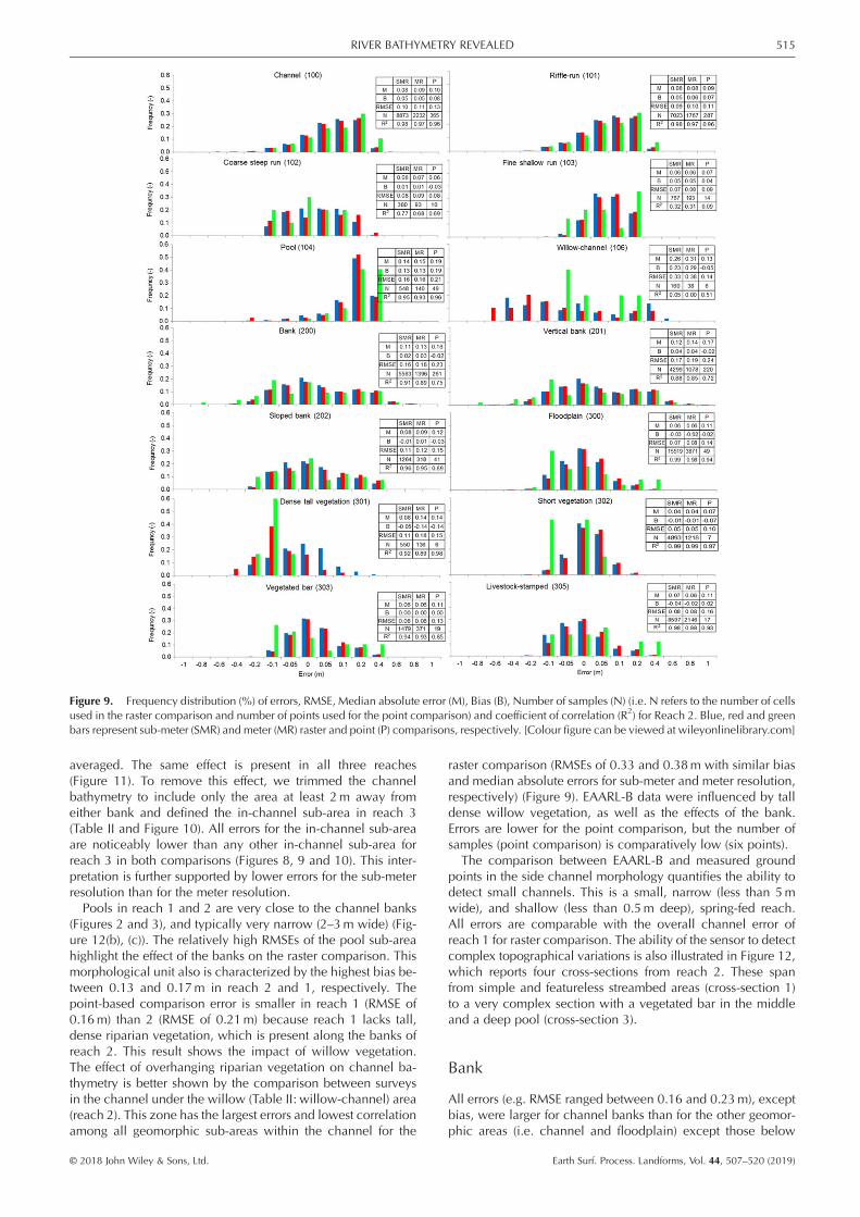
averaged. The same effect is present in all three reaches(Figure 11). To remove this effect, we trimmed the channelbathymetry to include only the area at least 2m away fromeither bank and defined the in-channel sub-area in reach 3(Table II and Figure 10). All errors for the in-channel sub-areaare noticeably lower than any other in-channel sub-area forreach 3 in both comparisons (Figures 8, 9 and 10). This inter-pretation is further supported by lower errors for the sub-meterresolution than for the meter resolution.Pools in reach 1 and 2 are very close to the channel banks

(Figures 2 and 3), and typically very narrow (2–3m wide) (Fig-ure 12(b), (c)). The relatively high RMSEs of the pool sub-areahighlight the effect of the banks on the raster comparison. Thismorphological unit also is characterized by the highest bias be-tween 0.13 and 0.17m in reach 2 and 1, respectively. Thepoint-based comparison error is smaller in reach 1 (RMSE of0.16m) than 2 (RMSE of 0.21m) because reach 1 lacks tall,dense riparian vegetation, which is present along the banks ofreach 2. This result shows the impact of willow vegetation.The effect of overhanging riparian vegetation on channel ba-thymetry is better shown by the comparison between surveysin the channel under the willow (Table II: willow-channel) area(reach 2). This zone has the largest errors and lowest correlationamong all geomorphic sub-areas within the channel for the

raster comparison (RMSEs of 0.33 and 0.38m with similar biasand median absolute errors for sub-meter and meter resolution,respectively) (Figure 9). EAARL-B data were influenced by talldense willow vegetation, as well as the effects of the bank.Errors are lower for the point comparison, but the number ofsamples (point comparison) is comparatively low (six points).

The comparison between EAARL-B and measured groundpoints in the side channel morphology quantifies the ability todetect small channels. This is a small, narrow (less than 5mwide), and shallow (less than 0.5m deep), spring-fed reach.All errors are comparable with the overall channel error ofreach 1 for raster comparison. The ability of the sensor to detectcomplex topographical variations is also illustrated in Figure 12,which reports four cross-sections from reach 2. These spanfrom simple and featureless streambed areas (cross-section 1)to a very complex section with a vegetated bar in the middleand a deep pool (cross-section 3).

Bank

All errors (e.g. RMSE ranged between 0.16 and 0.23m), exceptbias, were larger for channel banks than for the other geomor-phic areas (i.e. channel and floodplain) except those below

Figure 9. Frequency distribution (%) of errors, RMSE, Median absolute error (M), Bias (B), Number of samples (N) (i.e. N refers to the number of cellsused in the raster comparison and number of points used for the point comparison) and coefficient of correlation (R2) for Reach 2. Blue, red and greenbars represent sub-meter (SMR) and meter (MR) raster and point (P) comparisons, respectively. [Colour figure can be viewed at wileyonlinelibrary.com]

515RIVER BATHYMETRY REVEALED

© 2018 John Wiley & Sons, Ltd. Earth Surf. Process. Landforms, Vol. 44, 507–520 (2019)

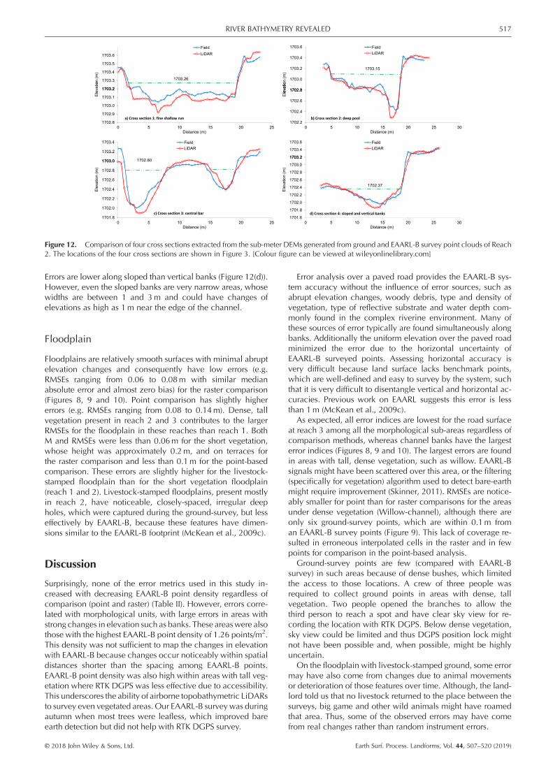
dense overhanging vegetation in all three reaches regardless ofthe type of comparison (Figures, 8, 9 and 10). Therefore, thelargest errors occurred in areas with abrupt elevation changes(Figure 11). Nevertheless, the estimated RMSEs for the channelbanks are lower than the values (0.4–0.73m) reported in previ-ous studies (McKean et al., 2009c; Skinner, 2011), which alsoobserved the smoothing or widening of channel banks. Thelarge errors at channel banks stem from the combined effectsof abrupt changes in elevation, EAARL-B geo-location errors,

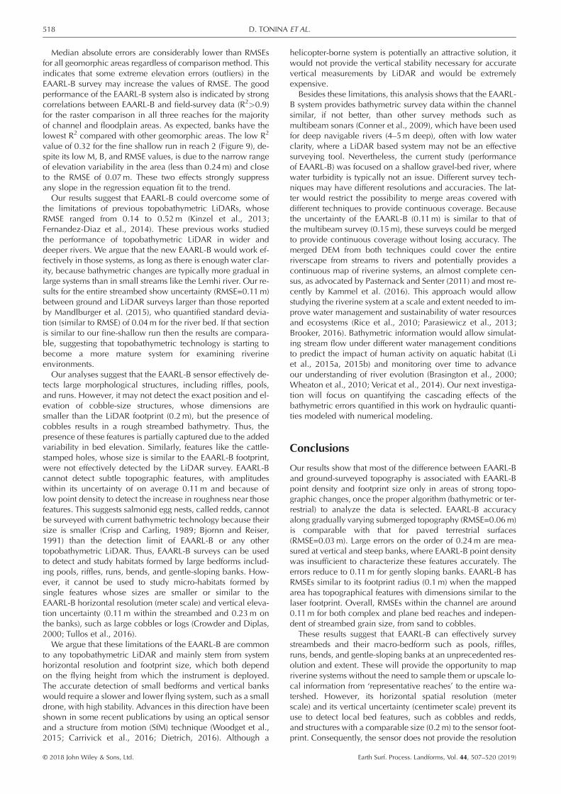
the 0.2m EAARL-B footprint size and interpolation error in gen-erating a raster from the field- and LiDAR-survey points for theraster comparison (McKean et al., 2009c). Although the pointdensity of EAARL-B points over the surface of channel bankswas higher than other locations, it was still not sufficient to cap-ture the strong gradients in the steep banks, which resulted inhigh RMSEs. Figure 12(b) and (d) show this issue, althoughthe LiDAR tracks the banks very well, because of the strongslope at the vertical bank the elevation error is around 0.2m.

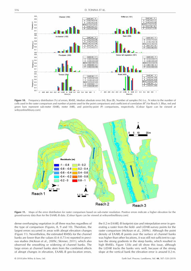
Figure 10. Frequency distribution (%) of errors, RMSE, Median absolute error (M), Bias (B), Number of samples (N) (i.e., N refers to the number ofcells used in the raster comparison and number of points used for the point comparison) and coefficient of correlation (R2) for Reach 3. Blue, red andgreen bars represent sub-meter (SMR), meter (MR), and point-by-point (P) comparisons, respectively. [Colour figure can be viewed atwileyonlinelibrary.com]

Figure 11. Maps of the error distribution for raster comparison based on sub-meter resolution. Positive errors indicate a higher elevation for theground-survey data than for the EAARL-B data. [Colour figure can be viewed at wileyonlinelibrary.com]

516 D. TONINA ET AL.

© 2018 John Wiley & Sons, Ltd. Earth Surf. Process. Landforms, Vol. 44, 507–520 (2019)

Errors are lower along sloped than vertical banks (Figure 12(d)).However, even the sloped banks are very narrow areas, whosewidths are between 1 and 3m and could have changes ofelevations as high as 1m near the edge of the channel.

Floodplain

Floodplains are relatively smooth surfaces with minimal abruptelevation changes and consequently have low errors (e.g.RMSEs ranging from 0.06 to 0.08m with similar medianabsolute error and almost zero bias) for the raster comparison(Figures 8, 9 and 10). Point comparison has slightly highererrors (e.g. RMSEs ranging from 0.08 to 0.14m). Dense, tallvegetation present in reach 2 and 3 contributes to the largerRMSEs for the floodplain in these reaches than reach 1. BothM and RMSEs were less than 0.06m for the short vegetation,whose height was approximately 0.2m, and on terraces forthe raster comparison and less than 0.1m for the point-basedcomparison. These errors are slightly higher for the livestock-stamped floodplain than for the short vegetation floodplain(reach 1 and 2). Livestock-stamped floodplains, present mostlyin reach 2, have noticeable, closely-spaced, irregular deepholes, which were captured during the ground-survey, but lesseffectively by EAARL-B, because these features have dimen-sions similar to the EAARL-B footprint (McKean et al., 2009c).

Discussion

Surprisingly, none of the error metrics used in this study in-creased with decreasing EAARL-B point density regardless ofcomparison (point and raster) (Table II). However, errors corre-lated with morphological units, with large errors in areas withstrong changes in elevation such as banks. These areaswere alsothose with the highest EAARL-B point density of 1.26 points/m2.This density was not sufficient to map the changes in elevationwith EAARL-B because changes occur noticeably within spatialdistances shorter than the spacing among EAARL-B points.EAARL-B point density was also high within areas with tall veg-etation where RTK DGPS was less effective due to accessibility.This underscores the ability of airborne topobathymetric LiDARsto survey even vegetated areas. Our EAARL-B survey was duringautumn when most trees were leafless, which improved bareearth detection but did not help with RTK DGPS survey.

Error analysis over a paved road provides the EAARL-B sys-tem accuracy without the influence of error sources, such asabrupt elevation changes, woody debris, type and density ofvegetation, type of reflective substrate and water depth com-monly found in the complex riverine environment. Many ofthese sources of error typically are found simultaneously alongbanks. Additionally the uniform elevation over the paved roadminimized the error due to the horizontal uncertainty ofEAARL-B surveyed points. Assessing horizontal accuracy isvery difficult because land surface lacks benchmark points,which are well-defined and easy to survey by the system, suchthat it is very difficult to disentangle vertical and horizontal ac-curacies. Previous work on EAARL suggests this error is lessthan 1m (McKean et al., 2009c).

As expected, all error indices are lowest for the road surfaceat reach 3 among all the morphological sub-areas regardless ofcomparison methods, whereas channel banks have the largesterror indices (Figures 8, 9 and 10). The largest errors are foundin areas with tall, dense vegetation, such as willow. EAARL-Bsignals might have been scattered over this area, or the filtering(specifically for vegetation) algorithm used to detect bare-earthmight require improvement (Skinner, 2011). RMSEs are notice-ably smaller for point than for raster comparisons for the areasunder dense vegetation (Willow-channel), although there areonly six ground-survey points, which are within 0.1m froman EAARL-B survey points (Figure 9). This lack of coverage re-sulted in erroneous interpolated cells in the raster and in fewpoints for comparison in the point-based analysis.

Ground-survey points are few (compared with EAARL-Bsurvey) in such areas because of dense bushes, which limitedthe access to those locations. A crew of three people wasrequired to collect ground points in areas with dense, tallvegetation. Two people opened the branches to allow thethird person to reach a spot and have clear sky view for re-cording the location with RTK DGPS. Below dense vegetation,sky view could be limited and thus DGPS position lock mightnot have been possible and, when possible, might be highlyuncertain.

On the floodplain with livestock-stamped ground, some errormay have also come from changes due to animal movementsor deterioration of those features over time. Although, the land-lord told us that no livestock returned to the place between thesurveys, big game and other wild animals might have roamedthat area. Thus, some of the observed errors may have comefrom real changes rather than random instrument errors.

Figure 12. Comparison of four cross sections extracted from the sub-meter DEMs generated from ground and EAARL-B survey point clouds of Reach2. The locations of the four cross sections are shown in Figure 3. [Colour figure can be viewed at wileyonlinelibrary.com]

517RIVER BATHYMETRY REVEALED

© 2018 John Wiley & Sons, Ltd. Earth Surf. Process. Landforms, Vol. 44, 507–520 (2019)

Median absolute errors are considerably lower than RMSEsfor all geomorphic areas regardless of comparison method. Thisindicates that some extreme elevation errors (outliers) in theEAARL-B survey may increase the values of RMSE. The goodperformance of the EAARL-B system also is indicated by strongcorrelations between EAARL-B and field-survey data (R2>0.9)for the raster comparison in all three reaches for the majorityof channel and floodplain areas. As expected, banks have thelowest R2 compared with other geomorphic areas. The low R2

value of 0.32 for the fine shallow run in reach 2 (Figure 9), de-spite its low M, B, and RMSE values, is due to the narrow rangeof elevation variability in the area (less than 0.24m) and closeto the RMSE of 0.07m. These two effects strongly suppressany slope in the regression equation fit to the trend.Our results suggest that EAARL-B could overcome some of

the limitations of previous topobathymetric LiDARs, whoseRMSE ranged from 0.14 to 0.52m (Kinzel et al., 2013;Fernandez-Diaz et al., 2014). These previous works studiedthe performance of topobathymetric LiDAR in wider anddeeper rivers. We argue that the new EAARL-B would work ef-fectively in those systems, as long as there is enough water clar-ity, because bathymetric changes are typically more gradual inlarge systems than in small streams like the Lemhi river. Our re-sults for the entire streambed show uncertainty (RMSE=0.11m)between ground and LiDAR surveys larger than those reportedby Mandlburger et al. (2015), who quantified standard devia-tion (similar to RMSE) of 0.04m for the river bed. If that sectionis similar to our fine-shallow run then the results are compara-ble, suggesting that topobathymetric technology is starting tobecome a more mature system for examining riverineenvironments.Our analyses suggest that the EAARL-B sensor effectively de-

tects large morphological structures, including riffles, pools,and runs. However, it may not detect the exact position and el-evation of cobble-size structures, whose dimensions aresmaller than the LiDAR footprint (0.2m), but the presence ofcobbles results in a rough streambed bathymetry. Thus, thepresence of these features is partially captured due to the addedvariability in bed elevation. Similarly, features like the cattle-stamped holes, whose size is similar to the EAARL-B footprint,were not effectively detected by the LiDAR survey. EAARL-Bcannot detect subtle topographic features, with amplitudeswithin its uncertainty of on average 0.11m and because oflow point density to detect the increase in roughness near thosefeatures. This suggests salmonid egg nests, called redds, cannotbe surveyed with current bathymetric technology because theirsize is smaller (Crisp and Carling, 1989; Bjornn and Reiser,1991) than the detection limit of EAARL-B or any othertopobathymetric LiDAR. Thus, EAARL-B surveys can be usedto detect and study habitats formed by large bedforms includ-ing pools, riffles, runs, bends, and gentle-sloping banks. How-ever, it cannot be used to study micro-habitats formed bysingle features whose sizes are smaller or similar to theEAARL-B horizontal resolution (meter scale) and vertical eleva-tion uncertainty (0.11m within the streambed and 0.23m onthe banks), such as large cobbles or logs (Crowder and Diplas,2000; Tullos et al., 2016).We argue that these limitations of the EAARL-B are common

to any topobathymetric LiDAR and mainly stem from systemhorizontal resolution and footprint size, which both dependon the flying height from which the instrument is deployed.The accurate detection of small bedforms and vertical bankswould require a slower and lower flying system, such as a smalldrone, with high stability. Advances in this direction have beenshown in some recent publications by using an optical sensorand a structure from motion (SfM) technique (Woodget et al.,2015; Carrivick et al., 2016; Dietrich, 2016). Although a

helicopter-borne system is potentially an attractive solution, itwould not provide the vertical stability necessary for accuratevertical measurements by LiDAR and would be extremelyexpensive.

Besides these limitations, this analysis shows that the EAARL-B system provides bathymetric survey data within the channelsimilar, if not better, than other survey methods such asmultibeam sonars (Conner et al., 2009), which have been usedfor deep navigable rivers (4–5m deep), often with low waterclarity, where a LiDAR based system may not be an effectivesurveying tool. Nevertheless, the current study (performanceof EAARL-B) was focused on a shallow gravel-bed river, wherewater turbidity is typically not an issue. Different survey tech-niques may have different resolutions and accuracies. The lat-ter would restrict the possibility to merge areas covered withdifferent techniques to provide continuous coverage. Becausethe uncertainty of the EAARL-B (0.11m) is similar to that ofthe multibeam survey (0.15m), these surveys could be mergedto provide continuous coverage without losing accuracy. Themerged DEM from both techniques could cover the entireriverscape from streams to rivers and potentially provides acontinuous map of riverine systems, an almost complete cen-sus, as advocated by Pasternack and Senter (2011) and most re-cently by Kammel et al. (2016). This approach would allowstudying the riverine system at a scale and extent needed to im-prove water management and sustainability of water resourcesand ecosystems (Rice et al., 2010; Parasiewicz et al., 2013;Brooker, 2016). Bathymetric information would allow simulat-ing stream flow under different water management conditionsto predict the impact of human activity on aquatic habitat (Liet al., 2015a, 2015b) and monitoring over time to advanceour understanding of river evolution (Brasington et al., 2000;Wheaton et al., 2010; Vericat et al., 2014). Our next investiga-tion will focus on quantifying the cascading effects of thebathymetric errors quantified in this work on hydraulic quanti-ties modeled with numerical modeling.

Conclusions

Our results show that most of the difference between EAARL-Band ground-surveyed topography is associated with EAARL-Bpoint density and footprint size only in areas of strong topo-graphic changes, once the proper algorithm (bathymetric or ter-restrial) to analyze the data is selected. EAARL-B accuracyalong gradually varying submerged topography (RMSE=0.06m)is comparable with that for paved terrestrial surfaces(RMSE=0.03m). Large errors on the order of 0.24m are mea-sured at vertical and steep banks, where EAARL-B point densitywas insufficient to characterize these features accurately. Theerrors reduce to 0.11m for gently sloping banks. EAARL-B hasRMSEs similar to its footprint radius (0.1m) when the mappedarea has topographical features with dimensions similar to thelaser footprint. Overall, RMSEs within the channel are around0.11m for both complex and plane bed reaches and indepen-dent of streambed grain size, from sand to cobbles.

These results suggest that EAARL-B can effectively surveystreambeds and their macro-bedform such as pools, riffles,runs, bends, and gentle-sloping banks at an unprecedented res-olution and extent. These will provide the opportunity to mapriverine systems without the need to sample them or upscale lo-cal information from ‘representative reaches’ to the entire wa-tershed. However, its horizontal spatial resolution (meterscale) and its vertical uncertainty (centimeter scale) prevent itsuse to detect local bed features, such as cobbles and redds,and structures with a comparable size (0.2m) to the sensor foot-print. Consequently, the sensor does not provide the resolution

518 D. TONINA ET AL.

© 2018 John Wiley & Sons, Ltd. Earth Surf. Process. Landforms, Vol. 44, 507–520 (2019)

needed to study micro-habitat characteristics and processes. Inour future research, we will quantify how these mapping errorsand resolution limitations propagate into numerical hydraulicmodels to predict meter scale hydraulic quantities such as flowvelocity, depth, and shear stress, which are commonly used tostudy riverine environments.

Acknowledgements—This research was partially supported by theIdaho Office of Species Conservation (grant number LEM023 16), byBonneville Power Administration (Bonneville Power Administration’sLemhi River Restoration Project, Project # 2010-072-0), by the US For-est Service (grant number 16-CR-11221634-049) and by the Universityof Idaho Office of Research (seed grant 2011). We also thank Quantita-tive Consultants Inc. for logistical support and for facilitating access toland and streams. We thank Mr Merrill Beyeler for access to his prop-erty, which made this research project possible. We thank FrankGariglio, Ryan Carnie, Roberto Marivela for helping with data collec-tion. The comments from the associate editor, two anonymous re-viewers and Dr. Lee Harrison on the earlier version improved themanuscript. Any opinions, conclusions, or recommendations expressedin this material are those of the authors and do not necessarily reflectthe views of the supporting agencies.

ReferencesBenjankar R, Tonina D, McKean J. 2014. One-dimensional and two-dimensional hydrodynamic modeling derived flow properties:Impacts on aquatic habitat quality predictions. Earth SurfaceProcesses and Landforms 40(3): 340–356.

Benjankar R, Tonina D, Marzadri A, McKean JA, Isaak DJ. 2016. Effectsof habitat quality and ambient hyporheic flows on salmon spawningsite selection. Journal of Geophysical Research: Biogeoscience121(5): 1222–1235. https://doi.org/10.1002/2015JG003079.

Bjornn TC, Reiser DW. 1991. Habitat requirements of salmonids instreams. In Influence of Forest and Rangeland Management on Sal-monid Fishes and their Habitats, Meehan WR (ed). American Fisher-ies Society Special Publication 19: Bethesda, MD; 83–138.

Borden JC. 2014. Flexible Framework for assessing water resource sus-tainability in river basins. PhD Dissertation, University of Idaho,Moscow, Idaho.

Brasington J, Rumsby BT, McVey RA. 2000. Monitoring and modellingmorphological change in a braided gravel-bed river using high reso-lution GPS-based survey. Earth Surface Processes and Landforms25(9): 973–990.

Brooker DJ. 2016. Generalized models of riverine fish hydraulic habi-tat. Journal of Ecohydraulics 1(1–2): 31–49. https://doi.org/10.1080/24705357.2016.1229141.

Carbonneau PE, Lane SN, Bergeron NE. 2006. Feature based imageprocessing methods applied to bathymetric measurements fromairborne remote sensing in fluvial environments. Earth SurfaceProcesses and Landforms 31: 1413–1423.

Carbonneau PE, Fonstad MA, Marcus WA, Dugdale SJ. 2012. Makingriverscapes real. Geomorphology 137(1): 74–86. https://doi.org/10.1016/j.geomorph.2010.09.030.

Carrivick JL, Smith MW, Quincey DJ. 2016. Structure from Motion inthe Geosciences. John Wiley & Sons: Oxford.

Cavalli M, Tarolli P, Marchi L, Dalla Fontana G. 2008. The effectivenessof airborne LiDAR data in the recognition of channel-bed morphol-ogy. Catena 73(3): 249–260.

Conner JT, Tonina D. 2014. Effect of cross-section interpolated bathym-etry on 2D hydrodynamic results in a large river. Earth Surface Pro-cesses and Landforms 39(4): 463–475. https://doi.org/10.1002/esp.3458.

Conner JT, Butler M, Welcker C, Parkinson S. 2009. Inundation analy-sis, Mid-Snake River, Idaho. Idaho Power Company: Boise, Idaho.

Crisp DT, Carling PA. 1989. Observations on siting, dimensions, andstructure of salmonid redds. Journal of Fish Biology 34: 119–134.

Crowder DW, Diplas P. 2000. Using two-dimensional hydrodynamicmodels at scales of ecological importance. Journal of Hydrology230: 172–191.

Dietrich JT. 2016. Riverscape mapping with helicopter-based Structure-from-Motion photogrammetry. Geomorphology 252: 144–157.

Fausch KD, Torgersen CE, Baxter CV, Li HW. 2002. Landscapes toriverscapes: bridging the gap between research and conservation ofstream fishes. Bioscience 52(6): 483–498.

Fernandez-Diaz JC, Glennie CL, Carter WE, Shrestha RL, Sartori MP,Singhania A, Legleiter CJ, Overstreet BT. 2014. Early results of simul-taneous terrain and shallow water bathymetry mapping using asingle-wavelength airborne LiDAR Sensor. IEEE Journal of SelectedTopics in Applied Earth Observations and Remote Sensing 7(2):623–636. https://doi.org/10.1109/JSTARS.2013.2265255.

Fernandez-Diaz JC, CarterWE, Glennie CL, Shrestha RL, Pan Z, EkhatariN, Singhania A, Hauser D, Sartori M. 2016. Capability assessmentand performance metrics for the Titan Multispectral Mapping Lidar.Remote Sensing 8(11): 936. https://doi.org/10.3390/rs8110936.

Gard M. 2009. Comparison of spawning habitat predictions ofPHABSIM and River2D models. International Journal of River BasinManagement 7(1): 55–71.

Hilldale RC, Raff D. 2007. Assessing the ability of airborne LiDAR tomap river bathymetry. Earth Surface Processes and Landforms 33(5):773–783.

Isaak DJ, Thurow RF, Rieman BE, Dunham JB. 2007. Chinook salmonuse of spawning patches: relative roles of habitat quality, size andconnectivity. Ecological Applications 17(2): 352–364.

Isenburg M. 2012. LAStools efficient tools for LiDAR processing. Avail-able at: https://rapidlasso.com/lastools/

Kammel LE, Pasternack GB, Massa DA, Bratovich PM. 2016. Near-cen-sus ecohydraulics bioverification of Oncorhynchus mykiss spawningmicrohabitat preferences. Journal of Ecohydraulics 1(1–2): 62–78.

Kinzel PJ, Legleiter CJ, Nelson JM. 2013. Mapping river bathymetrywith a small footprint green lidar: applications and challenges. Jour-nal of the American Water Resources Association 49(1): 183–204.https://doi.org/10.1111/jawr.12008.

Lane SN, Hardy RJ, Ferguson RI, Parsons DR. 2005. A framework formodel verification and validation of CFD schemes in natural openchannel flows. In Computational Fluid Dynamics: Applications in En-vironmental Hydraulics, Bates PD, Lane SN, Ferguson RI (eds). JohnWiley & Sons: Chichester.

Le Pichon C, Gorges G, Boët P, Baudry J, Goreaud F, Faure T. 2006. Aspatial explicit resource-based approach for managing stream fishesin riverscapes. Environmental Management 37(3): 322–335.

Legleiter CJ, Roberts DA, Lawrence RL. 2009. Spectrally based remotesensing of river bathymetry. Earth Surface Processes and Landforms34(8): 1039–1059. https://doi.org/10.1002/esp.1787.

Legleiter CJ, Overstreet BT, Glennie CL, Pan Z, Fernandez-Diaz JC,Singhania A. 2015. Evaluating the capabilities of the CASIhyperspectral imaging system and Aquarius bathymetric LiDAR formeasuring channel morphology in two distinct river environments.Earth Surface Processes and Landforms 41: 344–363. https://doi.org/10.1002/esp.3794.

Li R, Chen Q, Rui H, Cai D. 2015a. Determination of daily eco-hydrographs by a fish spawning habitat suitability model andapplication to reservoir eco-operation. Ecohydrology 9(6): 973–981.https://doi.org/10.1002/eco.1695.

Li R, Chen Q, Tonina D, Cai D. 2015b. Effects of upstream reservoir reg-ulation on the hydrological regimeand fish habitats of the LijiangRiver, China. Ecological Engineering 76: 75–83. https://doi.org/10.1016/j.ecoleng.2014.04.021.

Mandlburger G, Pfennigbauer M, Steinbacher F, Pfiefer N. 2011.Airborne hydrographic Lidar mapping-potential of a new techniquefor capturing shallow water bodies. In 19th International Congresson Modelling and Simulation, Chan F, Marinova D, Anderssen RS(eds). Modelling and Simulation Society of Australia andNew Zealand: Perth, Australia; 2416–2422.

Mandlburger G, Hauer C, Wieser M, Pfeifer N. 2015. Topo-bathymetricLiDAR for monitoring river morphodynamics and instream habitats –a case study at the Pielach river. Remote Sensing 7(5): 6160–6195.https://doi.org/10.3390/rs70506160.

Marcus WA, Legleiter CJ, Aspinall RJ, Boardman JW, Crabtree RL. 2003.High spatial resolution hyperspectral mapping of in-stream habitats,depths, and woody debris in mountain streams. Geomorphology55: 363–380.

Maturana O, Tonina D, Mckean JA, Buffington JM, Luce CH, CaamañoD. 2013. Modeling the effects of pulsed versus chronic sand inputson salmonid spawning habitat in a low-gradient gravel-bed river.

519RIVER BATHYMETRY REVEALED

© 2018 John Wiley & Sons, Ltd. Earth Surf. Process. Landforms, Vol. 44, 507–520 (2019)

Earth Surface Processes and Landforms 39(7): 877–889. https://doi.org/10.1002/esp.3491.

McDonald RR, Nelson JM, Paragamian V, Barton GJ. 2010. Modelingthe effect of flow and sediment transport on white Sturgeon spawninghabitat in the Kootenai River, Idaho. Journal of Hydraulic Engineering136(12): 1077–1092. https://doi.org/10.1061/(ASCE)HY.1943-7900.0000283.

McKean JA, Tonina D. 2013. Bed stability in unconfined gravel-bedmountain streams: with implications for salmon spawning viabilityin future climates. Journal of Geophysical Research: Earth Surface118: 1–14. https://doi.org/10.1002/jgrf.20092.

McKean JA, Isaak DJ, Wright CW. 2009a. Improving stream studies witha small-footprint Green Lidar. EOS, Transactions of the AmericanGeophysical Union 90(39): 341–342.

McKean JA, Isaak DJ, Wright CW. 2009b. Stream and riparian habitatanalysis and monitoring with a high-resolution terrestrial-aquatic Li-DAR. In PNAMP Special Publication: Remote Sensing Applicationsfor Aquatic Resource Monitoring, Bayer JM, Schei JL (eds). PacificNorthwest Aquatic Monitoring Partnership: Cook, WA; 7–16.

McKean JA, Nagel D, Tonina D, Bailey P, Wright CW, Bohn C,Nayegandhi A. 2009c. Remote sensing of channels and riparianzones with a narrow-beam aquatic-terrestrial LIDAR. Remote Sensing1: 1065–1096. https://doi.org/10.3390/rs1041065.

McKean JA, Tonina D, Bohn C, Wright CW. 2014. Effects of bathymet-ric lidar errors on flow properties predicted with a multi-dimensionalhydraulic model. Journal of Geophysical Research: Earth Surface119(3): 644–664. https://doi.org/10.1002/2013JF002897.

Nagle DB, Wright CW. 2016. Algorithms used in the Airborne LidarProcessing System (ALPS). US Geological Survey Open-File Report,45, US Geological Survey, Reston, Virginia.

Nayegandhi A, Brock JC, Wright CW, O’Connell MJ. 2006. Evaluating asmall footprint, waveform-resolution lidar over coastal vegetationcommunities. Photogrammetry Engineering and Remote Sensing 72:1407–1417.

Nayegandhi A, Brock JC, Wright CW. 2009. Small-footprint, waveform-resolving lidar estimation of submerged and subcanopy topographyin coastal environments. International Journal of Remote Sensing30: 861–878.

Pan Z, Glennie CL, Preston H, Fernandez-Diaz JC, Legleiter CJ,Overstreet BT. 2015. Performance assessment of high resolutionairborne full waveform LiDAR for shallow river bathymetry. RemoteSensing 7(5): 5133–5159. https://doi.org/10.3390/rs70505133.

Parasiewicz P, Rogers J, Vezza J, Gortázar J, Seager T, Pegg M,WiśniewolskiW,ComoglioC. 2013. Applications of theMesoHABSIMsimulationmodel. In Ecohydraulics: An IntegratedApproach,MaddockI,WoodPJ, HarbyA, KempP (eds).Wiley-Blackwell: NewDelhi, India;31–66.

Parker H, Sinclair M. 2012. The successful application of AirborneLiDAR Bathymetry surveys using latest technology. Oceans May21–24: 1–4.

Pasternack GB, Senter A. 2011. 21st Century instream flow assessmentframework for mountain streams. Public Interest Energy Research(PIER), California Energy Commission.

Pasternack GB, Gilbert AT, Wheaton JM, Buckland EM. 2006. Errorpropagation for velocity and shear stress prediction using 2D modelsfor environmental management. Journal of Hydrology 328: 227–241.

Quadros N. 2013. Unlocking the characteristics of bathymetric LiDARsensors. LiDAR Magazine 3(6): 62–67.

Rice SP, Little S, Wood PJ, Moir HJ, Vericat D. 2010. Special Issue:Ecohydraulics at Scales Relevant to Organisms. Selected Papers from

the British Hydrological Society National Meeting, LoughboroughUniversity, UK, June 2008. River Research and Applications 26(4):363–527.

Sibson R. 1981. A brief description of natural neighbor interpolation. InInterpreting Multivariate Data, Barnett V (ed). John Wiley: Chichester;21–36.

Skinner KD. 2011. Evaluation of LiDAR-acquired bathymetric andtopograhic data accuracy in various hydrogeomorphic settings inthe Deadwood and South Fork Boise Rivers, West-Central Idaho,2007. US Geological Survey Scientific Investigations Report 2011–5051, US Geological Survey Reston, Virginia.

Tonina D, Jorde K. 2013. Hydraulic modeling approaches forecohydraulic studies: 3D, 2D, 1D and non-numerical models. InEcohydraulics: An integrated Approach, Maddock I, Wood PJ, HarbyA, Kemp P (eds). Wiley-Blackwell: New Delhi, India; 31–66.

Tonina D, McKean JA. 2010. Climate change impact on salmonidspawning in low-land streams in Central Idaho, USA. In 9th Interna-tional Conference on Hydroinformatics 2010, Tao J, Chen Q, Liong S-Y (eds). Chemical Industry Press: Tianjin, China; 389–397.

Tonina D, McKean JA, Tang C, Goodwin P. 2011. New Tools forAquatic Habitat Modeling. 34th IAHR World Congress 2011, IAHR,Brisbane, Australia, 3137–3144.

Tonina D, Marzadri A, Bellin A. 2015. Benthic uptake rate due tohyporheic exchange: the effects of streambed morphology for con-stant and sinusoidally varying nutrient loads. Water 7(2): 398–419.https://doi.org/10.3390/w7020398.

Tuell G, Barbor K, Wozencraft J. 2010. Overview of the coastal zonemapping and imaging lidar (CZMIL): a new multisensor airbornemapping system for the US Army Corps of Engineers. In Proceedingsof SPIE 7695, Algorithms and Technologies for Multispectral,Hyperspectral, and Ultraspectral Imagery XVI, 76950Z, https://doi.org/10.1117/12.851905.

Tullos D, Walter C, Dunham JB. 2016. Does resolution of flow field ob-servation influence apparent habitat use and energy expenditure injuvenile coho salmon? Water Resources Research 52(8): 5938–5950https://doi.org/10.1002/2015WR018501.

Vericat D, Smith M, Brasington J. 2014. Patterns of topographic changein sub-humid badlands determined by high resolution multi-temporal topographic surveys. Catena 120: 164–176.

Walther SC, Marcus WA, Fonstad MA. 2011. Evaluation of high resolu-tion, true colour, aerial imagery for mapping bathymetry in a clearwater river without ground-based depth measurements. InternationalJournal of Remote Sensing 32(15): 4343–4363. https://doi.org/10.1080/01431161.2010.486418.

Wheaton JM, Brasington J, Darby SE, Sear DA. 2010. Accounting foruncertainty in DEMs from repeat topographic surveys: improved sed-iment budgets. Earth Surface Processes and Landforms 35(2):136–156. https://doi.org/10.1002/esp.1886.

White DF, Stanford JA, Kimball JS. 2002. Application of airborne multi-spectral digital imagery to quantify riverine habitats at different baseflows. River Research and Applications 18(6): 583–594. https://doi.org/10.1002/rra.695.

Woodget AS, Carbonneau PE, Visser F, Maddock IP. 2015. Quantifyingsubmerged fluvial topography using hyperspatial resolution UAS im-agery and structure from motion photogrammetry. Earth Surface Pro-cesses and Landforms 40(1): 47–64.

Wright CW, Kranenburg C, Troche RJ, Mitchell RW, Nagle DB. 2016.Depth calibration of the Experimental Advanced Airborne ResearchLidar, EAARL-B: Geological Survey Open-File Report 2016–1048.US Geological Survey: Reston, Virginia.

520 D. TONINA ET AL.

© 2018 John Wiley & Sons, Ltd. Earth Surf. Process. Landforms, Vol. 44, 507–520 (2019)